
Financial Analysis w/Microsoft Excel, 7th ed. - Dr. Nishikant Jha
546
-
Upload
khangminh22 -
Category
Documents
-
view
0 -
download
0
Transcript of Financial Analysis w/Microsoft Excel, 7th ed. - Dr. Nishikant Jha


Financial Analysis with Microsoft® Excel®
SEVENTH EDITION
Timothy R. MayesMetropolitan State College of Denver
Todd M. ShankUniversity of South Florida – St. Petersburg
Australia • Brazil • Mexico • Singapore • United Kingdom • United States
Copyright 2015 Cengage Learning. All Rights Reserved. May not be copied, scanned, or duplicated, in whole or in part. Due to electronic rights, some third party content may be suppressed from the eBook and/or eChapter(s).Editorial review has deemed that any suppressed content does not materially affect the overall learning experience. Cengage Learning reserves the right to remove additional content at any time if subsequent rights restrictions require it.

This is an electronic version of the print textbook. Due to electronic rights restrictions,some third party content may be suppressed. Editorial review has deemed that any suppressed content does not materially affect the overall learning experience. The publisher reserves the right to remove content from this title at any time if subsequent rights restrictions require it. Forvaluable information on pricing, previous editions, changes to current editions, and alternate formats, please visit www.cengage.com/highered to search by ISBN#, author, title, or keyword for materials in your areas of interest.
Copyright 2015 Cengage Learning. All Rights Reserved. May not be copied, scanned, or duplicated, in whole or in part. Due to electronic rights, some third party content may be suppressed from the eBook and/or eChapter(s).Editorial review has deemed that any suppressed content does not materially affect the overall learning experience. Cengage Learning reserves the right to remove additional content at any time if subsequent rights restrictions require it.

Financial Analysis with Microsoft® Excel®,Seventh EditionTimothy R. Mayes
VP, GM Science, Math & Quantitative Business: Balraj S. Kalsi
Product Director: Joe Sabatino
Sr. Product Manager: Mike Reynolds
Content Developer: Adele Tait Scholtz
Marketing Director: Natalie King
Marketing Manager: Heather Mooney
Content Project Manager: Jennifer Ziegler
Associate Media Developer: Mark Hopkinson
Manufacturing Planner: Kevin Kluck
Art and Cover Direction, Production Management, and Composition: Lumina Datamatics Inc.
Cover Image: Cover Screenshots are used with permission
from Microsoft Corporation, Microsoft Excel® is a registered trademark of Microsoft Corporation. © 2014 Microsoft.
Intellectual Property
Analyst: Christina Ciaramella
Project Manager: Betsy Hathaway
© 2015, 2012 Cengage Learning
ALL RIGHTS RESERVED. No part of this work covered by the copyright herein may be reproduced, transmitted, stored, or used in any form or by any means graphic, electronic, or mechanical, including but not limited to photocopying, recording, scanning, digitizing, taping, Web distribution, information networks, or information storage and retrieval systems, except as permitted under Section 107 or 108 of the 1976 United States Copyright Act, without the prior written permission of the publisher.
For product information and technology assistance, contact us atCengage Learning Customer & Sales Support, 1-800-354-9706
For permission to use material from this text or product,submit all requests online at www.cengage.com/permissions
Further permissions questions can be emailed [email protected]
Library of Congress Control Number: 2014945654ISBN: 978-1-285-43227-4
Cengage Learning20 Channel Center StreetBoston, MA 02210USA
Cengage Learning is a leading provider of customized learning solutions with office locations around the globe, including Singapore, the United Kingdom, Australia, Mexico, Brazil, and Japan. Locate your local office at: www.cengage.com/global
Cengage Learning products are represented in Canada by Nelson Education, Ltd.
To learn more about Cengage Learning Solutions, visit www.cengage.com
Purchase any of our products at your local college store or at ourpreferred online store www.cengagebrain.com
Printed in the United States of AmericaPrint Number: 01 Print Year: 2014
Copyright 2015 Cengage Learning. All Rights Reserved. May not be copied, scanned, or duplicated, in whole or in part. Due to electronic rights, some third party content may be suppressed from the eBook and/or eChapter(s).Editorial review has deemed that any suppressed content does not materially affect the overall learning experience. Cengage Learning reserves the right to remove additional content at any time if subsequent rights restrictions require it.
WCN: 02-200-203

iii
Copyright 2015 Cengage Learning. All Rights Reserved. May not be copied, scanned, or duplicated, in whole or in part. Due to electronic rights, some third party content may be suppressed from the eBook and/or eChapter(s).Editorial review has deemed that any suppressed content does not materially affect the overall learning experience. Cengage Learning reserves the right to remove additional content at any time if subsequent rights restrictions require it.

Copyright 2015 Cengage Learning. All Rights Reserved. May not be copied, scanned, or duplicated, in whole or in part. Due to electronic rights, some third party content may be suppressed from the eBook and/or eChapter(s).Editorial review has deemed that any suppressed content does not materially affect the overall learning experience. Cengage Learning reserves the right to remove additional content at any time if subsequent rights restrictions require it.

v
Preface xvPurpose of the Book xvi
Target Audience xviiA Note to Students xvii
Organization of the Book xviiOutstanding Features xviii
Pedagogical Features xixSupplements xx
Typography Conventions xxChanges from the 6th Edition xxiA Note on the Internet xxiiAcknowledgments xxii
CHAPTER 1 Introduction to Excel 2013 1Spreadsheet Uses 2
Starting Microsoft Excel 2Parts of the Excel Screen 3
The File Tab and Quick Access Toolbar 3The Home Tab 4The Formula Bar 6The Worksheet Area 6
Contents
Copyright 2015 Cengage Learning. All Rights Reserved. May not be copied, scanned, or duplicated, in whole or in part. Due to electronic rights, some third party content may be suppressed from the eBook and/or eChapter(s).Editorial review has deemed that any suppressed content does not materially affect the overall learning experience. Cengage Learning reserves the right to remove additional content at any time if subsequent rights restrictions require it.

Contents
vi
Sheet Tabs 7Status Bar 7
Navigating the Worksheet 8Selecting a Range of Cells 9Using Defined Names 9Entering Text and Numbers 11Formatting and Alignment Options 11Formatting Numbers 13Adding Borders and Shading 14
Entering Formulas 15Copying and Moving Formulas 17Mathematical Operators 19Parentheses and the Order of Operations 19
Using Excel’s Built-In Functions 20Using the Insert Function Dialog Box 22“Dot Functions” in Excel 2013 24Using User-Defined Functions 25
Creating Graphics 26Creating Charts in a Chart Sheet 27Creating Embedded Charts 28Formatting Charts 29Changing the Chart Type 30Creating Sparkline Charts 32
Printing 33Using Excel with Other Applications 35Quitting Excel 36Best Practices for Spreadsheet Models 36Summary 37Problems 38Internet Exercise 41
CHAPTER 2 The Basic Financial Statements 43The Income Statement 44
Building an Income Statement in Excel 44The Balance Sheet 49
Building a Balance Sheet in Excel 49Improving Readability: Custom Number Formats 51
Copyright 2015 Cengage Learning. All Rights Reserved. May not be copied, scanned, or duplicated, in whole or in part. Due to electronic rights, some third party content may be suppressed from the eBook and/or eChapter(s).Editorial review has deemed that any suppressed content does not materially affect the overall learning experience. Cengage Learning reserves the right to remove additional content at any time if subsequent rights restrictions require it.

vii
Contents
Creating Common-Size Income Statements 54Creating a Common-Size Balance Sheet 56
Building a Statement of Cash Flows 57Using Excel’s Outliner 62Common-Size Statement of Cash Flows 64
Summary 67Problems 68Internet Exercise 70
CHAPTER 3 The Cash Budget 71The Worksheet Area 73
Using Date Functions 73Calculating Text Strings 74Sales and Collections 75Purchases and Payments 76
Collections and Disbursements 78Calculating the Ending Cash Balance 80
Repaying Short-Term Borrowing 82Using the Cash Budget for What-If Analysis 83The Scenario Manager 85
Adding Interest and Investment of Excess Cash 89Calculating Current Borrowing 91Using the Formula Auditing Tools to Avoid Errors 92Calculating Current Investing 96Working Through the Example 97
Summary 99Problems 101
CHAPTER 4 Financial Statement Analysis Tools 107Liquidity Ratios 108
The Current Ratio 109The Quick Ratio 110
Efficiency Ratios 111Inventory Turnover Ratio 111Accounts Receivable Turnover Ratio 112Average Collection Period 112Fixed Asset Turnover Ratio 114Total Asset Turnover Ratio 114
Common-Size Financial Statements 54
Copyright 2015 Cengage Learning. All Rights Reserved. May not be copied, scanned, or duplicated, in whole or in part. Due to electronic rights, some third party content may be suppressed from the eBook and/or eChapter(s).Editorial review has deemed that any suppressed content does not materially affect the overall learning experience. Cengage Learning reserves the right to remove additional content at any time if subsequent rights restrictions require it.

Contents
viii
Leverage Ratios 115The Total Debt Ratio 116The Long-Term Debt Ratio 116The Long-Term Debt to Total Capitalization Ratio 117The Debt to Equity Ratio 117The Long-Term Debt to Equity Ratio 118
Coverage Ratios 118The Times Interest Earned Ratio 119The Cash Coverage Ratio 119
Profitability Ratios 120The Gross Profit Margin 121The Operating Profit Margin 121The Net Profit Margin 121Return on Total Assets 122Return on Equity 123Return on Common Equity 123DuPont Analysis 124Analysis of EPI’s Profitability Ratios 126
Financial Distress Prediction 127The Original Z-Score Model 127The Z-Score Model for Private Firms 128
Using Financial Ratios 129Trend Analysis 129Comparing to Industry Averages 130Company Goals and Debt Covenants 131Automating Ratio Analysis 132
Economic Profit Measures of Performance 134Summary 137Problems 140Internet Exercise 141
CHAPTER 5 Financial Forecasting 143The Percent of Sales Method 144
Forecasting the Income Statement 144Forecasting Assets on the Balance Sheet 148Forecasting Liabilities on the Balance Sheet 150Discretionary Financing Needed 151
Using Iteration to Eliminate DFN 153Other Forecasting Methods 156
Linear Trend Extrapolation 156
Copyright 2015 Cengage Learning. All Rights Reserved. May not be copied, scanned, or duplicated, in whole or in part. Due to electronic rights, some third party content may be suppressed from the eBook and/or eChapter(s).Editorial review has deemed that any suppressed content does not materially affect the overall learning experience. Cengage Learning reserves the right to remove additional content at any time if subsequent rights restrictions require it.

ix
Contents
Regression Analysis 160Statistical Significance 165
Summary 168Problems 169Internet Exercises 170
CHAPTER 6 Break-Even and Leverage Analysis 173Break-Even Points 174
Calculating Break-Even Points in Excel 176Other Break-Even Points 177
Using Goal Seek to Calculate Break-Even Points 179Leverage Analysis 180
The Degree of Operating Leverage 181The Degree of Financial Leverage 184The Degree of Combined Leverage 186Extending the Example 187
Linking Break-Even Points and Leverage Measures 188Summary 189Problems 191Internet Exercise 193
CHAPTER 7 The Time Value of Money 195Future Value 196
Using Excel to Find Future Values 197Present Value 198Annuities 200
Present Value of an Annuity 200Future Value of an Annuity 202Solving for the Annuity Payment 204Solving for the Number of Periods in an Annuity 205Solving for the Interest Rate in an Annuity 207Deferred Annuities 208
Graduated Annuities 210Present Value of a Graduated Annuity 211Future Value of a Graduated Annuity 214
Uneven Cash Flow Streams 215Solving for the Yield in an Uneven Cash Flow Stream 216
Copyright 2015 Cengage Learning. All Rights Reserved. May not be copied, scanned, or duplicated, in whole or in part. Due to electronic rights, some third party content may be suppressed from the eBook and/or eChapter(s).Editorial review has deemed that any suppressed content does not materially affect the overall learning experience. Cengage Learning reserves the right to remove additional content at any time if subsequent rights restrictions require it.

Contents
x
Continuous Compounding 221Summary 223Problems 224
CHAPTER 8 Common Stock Valuation 227What Is Value? 228Fundamentals of Valuation 229Determining the Required Rate of Return 230
A Simple Risk Premium Model 231CAPM: A More Scientific Model 231
Valuing Common Stocks 234The Constant-Growth Dividend Discount Model 235The Two-Stage Growth Model 240Three-Stage Growth Models 242
Alternative Discounted Cash Flow Models 246The Earnings Model 246The Free Cash Flow Model 250
Relative Value Models 254Preferred Stock Valuation 255Summary 257Problems 259Internet Exercise 261
CHAPTER 9 Bond Valuation 263Bond Valuation 264
Valuing Bonds Between Coupon Dates 266Using Excel’s Advanced Bond Functions 268
Bond Return Measures 271Current Yield 271Yield to Maturity 272Yield to Call 274Returns on Discounted Debt Securities 276
The U.S. Treasury Yield Curve 278Bond Price Sensitivities 280
Changes in the Required Return 281Changes in Term to Maturity 283Comparing Two Bonds with Different Maturities 285Comparing Two Bonds with Different Coupon Rates 287
Nonannual Compounding Periods 218
Copyright 2015 Cengage Learning. All Rights Reserved. May not be copied, scanned, or duplicated, in whole or in part. Due to electronic rights, some third party content may be suppressed from the eBook and/or eChapter(s).Editorial review has deemed that any suppressed content does not materially affect the overall learning experience. Cengage Learning reserves the right to remove additional content at any time if subsequent rights restrictions require it.

xi
Contents
Duration and Convexity 288Duration 289Modified Duration 291Visualizing the Predicted Price Change 292Convexity 294
Summary 296Problems 299Internet Exercise 301
CHAPTER 10 The Cost of Capital 303The Appropriate “Hurdle” Rate 304
The Weighted Average Cost of Capital 305Determining the Weights 306
WACC Calculations in Excel 307Calculating the Component Costs 308
The Cost of Common Equity 309The Cost of Preferred Equity 310The Cost of Debt 311
Using Excel to Calculate the Component Costs 312The After-Tax Cost of Debt 312The Cost of Preferred Stock 314The Cost of Common Stock 314
The Role of Flotation Costs 315Adding Flotation Costs to Our Worksheet 316The Cost of Retained Earnings 317
The Marginal WACC Curve 318Finding the Break-Points 318Creating the Marginal WACC Chart 323
Summary 324Problems 325Internet Exercise 327
CHAPTER 11 Capital Budgeting 329Estimating the Cash Flows 330
The Initial Outlay 331The Annual After-Tax Operating Cash Flows 332The Terminal Cash Flow 333Estimating the Cash Flows: An Example 334
Copyright 2015 Cengage Learning. All Rights Reserved. May not be copied, scanned, or duplicated, in whole or in part. Due to electronic rights, some third party content may be suppressed from the eBook and/or eChapter(s).Editorial review has deemed that any suppressed content does not materially affect the overall learning experience. Cengage Learning reserves the right to remove additional content at any time if subsequent rights restrictions require it.

Contents
xii
Calculating the Relevant Cash Flows 339Making the Decision 341
The Payback Method 341The Discounted Payback Period 343Net Present Value 345The Profitability Index 347The Internal Rate of Return 348Problems with the IRR 349The Modified Internal Rate of Return 351
Sensitivity and Scenario Analysis 354NPV Profile Charts 354Scenario Analysis 355
The Optimal Capital Budget 358Optimal Capital Budget Without Capital Rationing 358Optimal Capital Budget Under Capital Rationing 361Other Techniques 366
Summary 366Problems 367
CHAPTER 12 Risk and Capital Budgeting 371Review of Some Useful Statistical Concepts 372
The Expected Value 372Measures of Dispersion 374
Using Excel to Measure Risk 377The Freshly Frozen Fish Company Example 377
Introducing Uncertainty 381Sensitivity Analysis 381Scenario Analysis 386Calculating the Expected NPV from the Scenarios 388Calculating the Variance and Standard Deviation 389Calculating the Probability of a Negative NPV 391Monte Carlo Simulation 392The Risk-Adjusted Discount Rate Method 399The Certainty-Equivalent Approach 400
Summary 403Problems 405
Copyright 2015 Cengage Learning. All Rights Reserved. May not be copied, scanned, or duplicated, in whole or in part. Due to electronic rights, some third party content may be suppressed from the eBook and/or eChapter(s).Editorial review has deemed that any suppressed content does not materially affect the overall learning experience. Cengage Learning reserves the right to remove additional content at any time if subsequent rights restrictions require it.

xiii
Contents
CHAPTER 13 Portfolio Statistics and Diversification 409Portfolio Diversification Effects 410Determining Portfolio Risk and Return 412
Portfolio Standard Deviation 413Changing the Weights 416
Portfolios with More than Two Securities 418Creating a Variance/Covariance Matrix 419Calculating the Portfolio Standard Deviation 422
The Efficient Frontier 424Locating Portfolios on the Efficient Frontier in Excel 425Charting the Efficient Frontier 428
The Capital Market Line 429Charting the Capital Market Line 432Identifying the Market Portfolio 434
Utility Functions and the Optimal Portfolio 436Charting Indifference Curves 436
The Capital Asset Pricing Model 438The Security Market Line 440
Summary 441Problems 442Internet Exercise 445
CHAPTER 14 Writing User-Defined Functions with VBA 447What Is a Macro? 448
Two Types of Macros 448The Visual Basic Editor 450
The Project Explorer 451The Code Window 452
The Parts of a Function 453Writing Your First User-Defined Function 453Writing More Complicated Functions 458
Variables and Data Types 458The If-Then-Else Statement 460Looping Statements 462Using Worksheet Functions in VBA 465Using Optional Arguments 466Using ParamArray for Unlimited Arguments 467
Copyright 2015 Cengage Learning. All Rights Reserved. May not be copied, scanned, or duplicated, in whole or in part. Due to electronic rights, some third party content may be suppressed from the eBook and/or eChapter(s).Editorial review has deemed that any suppressed content does not materially affect the overall learning experience. Cengage Learning reserves the right to remove additional content at any time if subsequent rights restrictions require it.

Contents
xiv
Debugging VBA Code 468Breakpoints and Code Stepping 468The Watch Window 470The Immediate Window 471
Creating Excel Add-Ins 472Best Practices for VBA 473Summary 474Problems 475
CHAPTER 15 Analyzing Datasets with Tables and Pivot Tables 477Creating and Using an Excel Table 478
Removing Duplicate Records from the Table 480Filtering the Table 480Sorting and Filtering Numeric Fields 482Using Formulas in Tables 484
Using Pivot Tables 485Creating a Pivot Table 486Formatting the Pivot Table 488Rearranging the Pivot Table and Adding Fields 490Transforming the Data Field Presentation 491Calculations in Pivot Tables 492
Pivot Tables for Financial Statements 494Grouping Data by Date 495Using Pivot Charts to Show Trends over Time 497Displaying Multiple Subtotals 498Using Calculated Fields for Financial Ratios 499Filtering Data with Slicers and Timelines 501
Extracting Data from a Pivot Table 503Summary 504Problems 505Internet Exercise 508
APPENDIX Directory of User-Defined Functions in Famefncs.xlam 509
INDEX 513
Copyright 2015 Cengage Learning. All Rights Reserved. May not be copied, scanned, or duplicated, in whole or in part. Due to electronic rights, some third party content may be suppressed from the eBook and/or eChapter(s).Editorial review has deemed that any suppressed content does not materially affect the overall learning experience. Cengage Learning reserves the right to remove additional content at any time if subsequent rights restrictions require it.

xv
Preface
Electronic spreadsheets have been available for microcomputers since the introduction ofVisiCalc® for the Apple I in June 1979. The first version of Lotus 1-2-3® in January 1983convinced businesses that the IBM PC was a truly useful productivity-enhancing tool.Today, any student who leaves business school without at least basic spreadsheet skills istruly at a disadvantage. Much as earlier generations had to be adept at using a slide rule orfinancial calculator, today’s manager needs to be proficient in the use of a spreadsheet.International competition means that companies must be as efficient as possible. No longercan managers count on having a large staff of “number crunchers” at their disposal.
Copyright 2015 Cengage Learning. All Rights Reserved. May not be copied, scanned, or duplicated, in whole or in part. Due to electronic rights, some third party content may be suppressed from the eBook and/or eChapter(s).Editorial review has deemed that any suppressed content does not materially affect the overall learning experience. Cengage Learning reserves the right to remove additional content at any time if subsequent rights restrictions require it.

Preface
xvi
Microsoft first introduced Excel in 1985 for the Apple Macintosh and showed the world thatspreadsheets could be both powerful and easy to use, not to mention fun. Excel 2.0 wasintroduced to the PC world in 1987 for Microsoft Windows version 1.0, where it enjoyedsomething of a cult following. With the introduction of version 3.0 of Windows, sales ofExcel exploded so that today it is the leading spreadsheet on the market.
As of this writing, Excel 2013 (also known as Excel version 15) is the current version.Unlike Excel 2007, which introduced the Ribbon interface, Excel 2013 is more evolutionarythan revolutionary. The changes are mostly cosmetic, though changes to the way that chartsare created and edited are truly useful. While the book has been written with the currentversion in mind, it can be used with older versions, if allowances are made for the interfacedifferences. The user interface is even more different on the Apple Mac, but Excel for Mac2011 supports virtually all of the features discussed in this book. The only missing feature ofwhich I am aware is pivot charts.
Purpose of the BookFinancial Analysis with Microsoft Excel, 7th ed., was written to demonstrate usefulspreadsheet techniques and tools in a financial context. This allows readers to see thematerial in a way with which they are familiar. For students just beginning their education infinance, the book provides a thorough explanation of all of the concepts and equations thatare usually covered. In other words, it is a corporate finance textbook, but it uses Excelinstead of financial calculators.
Students with no prior experience with spreadsheets will find that using Excel is veryintuitive, especially if they have used other Windows applications. For these students,Financial Analysis with Microsoft Excel, 7th ed., will provide a thorough introduction to theuse of spreadsheets from basic screen navigation skills to building fairly complex financialmodels. I have found that even students with good spreadsheet skills have learned a greatdeal more about using Excel than they expected.
Finally, I feel strongly that providing pre-built spreadsheet templates for students to use is adisservice. For this reason, this book concentrates on spreadsheet building skills. I believethat students can gain valuable insights and a deeper understanding of financial analysis byactually building their own spreadsheets. By creating their own spreadsheets, students willhave to confront many issues that might otherwise be swept under the carpet. It continuallyamazes me how thankful students are when they are actually forced to think rather than justto “plug and go.” For this reason, the book concentrates on spreadsheet building skills(though all of the templates are included for instructors) so that students will be encouragedto think and truly understand the problems on which they are working.
Copyright 2015 Cengage Learning. All Rights Reserved. May not be copied, scanned, or duplicated, in whole or in part. Due to electronic rights, some third party content may be suppressed from the eBook and/or eChapter(s).Editorial review has deemed that any suppressed content does not materially affect the overall learning experience. Cengage Learning reserves the right to remove additional content at any time if subsequent rights restrictions require it.

xvii
Organization of the Book
Target AudienceFinancial Analysis with Microsoft Excel is aimed at a wide variety of students andpractitioners of finance. The topics covered generally follow those in an introductoryfinancial management course for undergraduates or first-year MBA students. Because of theemphasis on spreadsheet building skills, the book is also appropriate as a reference for case-oriented courses in which the spreadsheet is used extensively. I have been using the book inmy Financial Modeling course since 1995, and students consistently say that it is the mostuseful course they have taken. A sizable number of my former students have landed jobs inlarge part due to their superior spreadsheet skills.
I have tried to make the book complete enough that it may also be used for self-pacedlearning, and, if my e-mail is any guide, many have successfully taken this route. I assume,however, that the reader has some familiarity with the basic concepts of accounting andstatistics. Instructors will find that their students can use this book on their own time to learnExcel, thereby minimizing the amount of class time required for teaching the rudiments ofspreadsheets. Practitioners will find that the book will help them transfer skills from otherspreadsheets to Excel and, at the same time, refresh their knowledge of corporate finance.
A Note to StudentsAs I have noted, this book is designed to help you learn finance and understand spreadsheetsat the same time. Learning finance alone can be a daunting task, but I hope that learning touse Excel at the same time will make your job easier and more fun. Be sure to experimentwith the examples by changing numbers and creating charts.
You will likely find that learning the material and skills presented is more difficult if you donot work the examples presented in each chapter. While this will be somewhat timeconsuming, I encourage you to work along with, rather than just read, the book as eachexample is discussed. Further, I suggest that you try to avoid the trap of memorizing Excelformulas. Instead, try to understand the logic of the formula so that you can more easilyapply it in other, slightly different, situations in the future.
Make sure that you save your work often and keep a current backup.
Organization of the BookFinancial Analysis with Microsoft Excel, 7th ed., is organized along the lines of anintroductory financial management textbook. The book can stand alone or be used as anadjunct to a regular text, but it is not “just a spreadsheet book,” and shouldn’t be treated as acookbook with recipes. In most cases, topics are covered at the same depth as the material in
Copyright 2015 Cengage Learning. All Rights Reserved. May not be copied, scanned, or duplicated, in whole or in part. Due to electronic rights, some third party content may be suppressed from the eBook and/or eChapter(s).Editorial review has deemed that any suppressed content does not materially affect the overall learning experience. Cengage Learning reserves the right to remove additional content at any time if subsequent rights restrictions require it.

Preface
xviii
conventional textbooks; in many cases, the topics are covered in greater depth. For thisreason, I believe that Financial Analysis with Microsoft Excel, 7th ed., can be used as acomprehensive primary text. The book is organized as follows:
• Chapter 1: Introduction to Excel 2013
• Chapter 2: The Basic Financial Statements
• Chapter 3: The Cash Budget
• Chapter 4: Financial Statement Analysis Tools
• Chapter 5: Financial Forecasting
• Chapter 6: Break-Even and Leverage Analysis
• Chapter 7: The Time Value of Money
• Chapter 8: Common Stock Valuation
• Chapter 9: Bond Valuation
• Chapter 10: The Cost of Capital
• Chapter 11: Capital Budgeting
• Chapter 12: Risk and Capital Budgeting
• Chapter 13: Portfolio Statistics and Diversification
• Chapter 14: Writing User-Defined Functions with VBA
• Chapter 15: Analyzing Datasets with Tables and Pivot Tables
• Appendix: Directory of User-Defined Functions in Famefncs.xlam
Extensive use of built-in functions, charts, and other tools (e.g., Scenario Manager andSolver) throughout the book encourages a much deeper exploration of the models presentedthan do more traditional methods. Questions such as “What would happen if...” are easilyanswered with the tools and techniques taught in this book.
Outstanding FeaturesThe most outstanding feature of Financial Analysis with Microsoft Excel, 7th ed., is its useof Excel as a learning tool rather than just a fancy calculator. Students using the book will beable to demonstrate to themselves how and why things are the way they are. Once studentscreate a worksheet, they understand how it works and the assumptions behind the
Copyright 2015 Cengage Learning. All Rights Reserved. May not be copied, scanned, or duplicated, in whole or in part. Due to electronic rights, some third party content may be suppressed from the eBook and/or eChapter(s).Editorial review has deemed that any suppressed content does not materially affect the overall learning experience. Cengage Learning reserves the right to remove additional content at any time if subsequent rights restrictions require it.

xix
Outstanding Features
calculations. Thus, unlike the traditional “template” approach, students gain a deeperunderstanding of the material. In addition, the book greatly facilitates the professors’ use ofspreadsheets in their courses.
The text takes a self-teaching approach used by many other “how-to” spreadsheet books, butit provides opportunities for much more in-depth experimentation than the competition. Forexample, scenario analysis is an often recommended technique, but it is rarely demonstratedin any depth. This book uses the tools that are built into Excel to greatly simplifycomputation-intensive techniques, eliminating the boredom of tedious calculation. Otherexamples include regression analysis, linear and nonlinear programming, and Monte Carlosimulation. The book encourages students to actually use the tools that they have learnedabout in their statistics and management science classes.
Pedagogical FeaturesFinancial Analysis with Microsoft Excel, 7th ed., begins by teaching the basics of Excel.Then, the text uses Excel to build the basic financial statements that students encounter in alllevels of financial management courses. This coverage then acts as a “springboard” intomore advanced material such as performance evaluation, forecasting, valuation, capitalbudgeting, and modern portfolio theory. Each chapter builds upon the techniques learned inprior chapters so that the student becomes familiar with Excel and finance at the same time.This type of approach facilitates the professor’s incorporation of Excel into a financialmanagement course since it reduces, or eliminates, the necessity of teaching spreadsheetusage in class. It also helps students see how this vital “tool” is used to solve the financialproblems faced by practitioners.
The chapters are organized so that a problem is introduced, solved by traditional methods,and then solved using Excel. I believe that this approach relieves much of the quantitativecomplexity while enhancing student understanding through repetition and experimentation.This approach also generates interest in the subject matter that a traditional lecture cannot(especially for nonfinance business majors who are required to take a course in financialmanagement). Once they are familiar with Excel, my students typically enjoy using it andspend more time with the subject than they otherwise would. In addition, since charts areused extensively (and are created by the student), the material may be better retained.
A list of learning objectives precedes each chapter, and a summary of the major Excelfunctions discussed in the chapter is included at the end. In addition, each chapter containshomework problems, and many include Internet Exercises that introduce students to sourcesof information on the Internet.
Copyright 2015 Cengage Learning. All Rights Reserved. May not be copied, scanned, or duplicated, in whole or in part. Due to electronic rights, some third party content may be suppressed from the eBook and/or eChapter(s).Editorial review has deemed that any suppressed content does not materially affect the overall learning experience. Cengage Learning reserves the right to remove additional content at any time if subsequent rights restrictions require it.

Preface
xx
SupplementsThe Instructor’s Manual and other resources, available online, contain the following:
(These materials are available to registered instructors at the product support Web site, http://www.cengagebrain.com/).
• The completed worksheets with solutions to all problems covered in the text. Having this material on the product Web site allows the instructor to easily create transparencies or give live demonstrations via computer projections in class without having to build the spreadsheets from scratch.
• Additional Excel spreadsheet problems for each chapter that relate directly to the con-cepts covered in that chapter. Each problem requires the student to build a worksheet to solve a common financial management problem. Often the problems require solutions in a graphical format.
• Complete solutions to the in-text homework problems and those in the Instructor’s Man-ual and on the product Web site, along with clarifying notes on techniques used.
• An Excel add-in program that contains some functions that simplify complex calcula-tions such as the two-stage common stock valuation model and the payback period, among many others (see the Appendix for a complete listing of the functions). Also included is an add-in program for performing Monte-Carlo simulations discussed exten-sively in Chapter 12, and an add-in to create “live” variance/covariance matrices. These add-ins are available on the Web site.
Typography ConventionsThe main text of this book is set in the 10-point Times New Roman True Type font. Text ornumbers that readers are expected to enter are set in the 10 point Courier New True Typefont.
The names of built-in functions are set in small caps and boldface. Function arguments canbe either required or optional. Required inputs are set in small caps and are italicized andboldface. Optional inputs are set in small caps and italicized. As an example, consider the PVfunction (introduced in Chapter 7):
PV(RATE, NPER, PMT, FV, TYPE)
In this example, PV is the name of the function, and RATE, NPER, and PMT are the requiredarguments, while FV and TYPE are optional.
Copyright 2015 Cengage Learning. All Rights Reserved. May not be copied, scanned, or duplicated, in whole or in part. Due to electronic rights, some third party content may be suppressed from the eBook and/or eChapter(s).Editorial review has deemed that any suppressed content does not materially affect the overall learning experience. Cengage Learning reserves the right to remove additional content at any time if subsequent rights restrictions require it.

xxi
Changes from the 6th Edition
In equations and the text, equation variables (which are distinct from function arguments)are italicized. As an example, consider the PV equation:
I hope that these conventions will help avoid confusion due to similar terms being used indifferent contexts.
Changes from the 6th EditionThe overall organization of the book remains similar, but there have been many changesthroughout the book. All of the chapters have been updated, but the more important changesinclude:
Chapter 1—Updated for Excel 2013, including coverage of the new charting interface thatuses buttons for chart elements and panels for formatting.
Chapter 2—Added contribution analysis to the common-size statements, and new coverageof the common-size statement of cash flows. The latter motivates a new discussion of theCHOOSE function as well as the Data Validation tool.
Chapter 4—Added the extended DuPont method for decomposing the ROE into its morebasic components.
Chapter 5—Added the SLN function for calculating straight-line depreciation, as well as asection on using the SLOPE and INTERCEPT functions to get regression parameters withoutrunning a full regression analysis.
Chapter 6—Added a new section that explicitly shows the linkage between the break-evenpoint and the various measures of leverage.
Chapter 7—New coverage of the EFFECT and NOMINAL functions for converting interestrates.
Chapter 8—Added two additional multi-stage dividend growth common stock valuationmodels (the traditional three-stage model, and a three-step model).
Chapter 11—Added the new Arnold and Nixon method of calculating the MIRR based onthe profitability index. This more clearly shows the linkage between NPV and MIRR.
Chapter 13—Extensive changes were made to the methodology for calculating the efficientfrontier. Instead of using the Solver to calculate each portfolio, I am now using it to calculate
PVFVN
1 i+( )N------------------=
Copyright 2015 Cengage Learning. All Rights Reserved. May not be copied, scanned, or duplicated, in whole or in part. Due to electronic rights, some third party content may be suppressed from the eBook and/or eChapter(s).Editorial review has deemed that any suppressed content does not materially affect the overall learning experience. Cengage Learning reserves the right to remove additional content at any time if subsequent rights restrictions require it.

Preface
xxii
just two portfolios. The remaining portfolios are calculated as a weighted average of thosetwo portfolios. This significantly speeds up the process of charting the efficient frontier.Additionally, I have added a utility function and used it to chart an indifference map andshow how to find the optimal portfolio for an investor by maximizing utility in the Solver.Finally, I changed all of the calculations to use sample statistics, instead of populationparameters, because Excel now has a sample covariance function.
Chapter 14—Added coverage of Do…Loops (Do…While and Do…Until), as well as newcoverage of optional arguments and ParamArray, which allows for an unlimited number offunction arguments. I also added a section with some best practices for VBA programming.
Chapter 15—Added coverage of the new TimeLine feature for filtering pivot tables by date andtime. In addition, all of the data used in the examples has been updated, and new problems added.
A Note on the InternetI have tried to incorporate Internet Exercises into those chapters where the use of the Internetis applicable. In many cases, the necessary data simply is not available to the public or verydifficult to obtain online (e.g., cash budgeting), so some chapters do not have InternetExercises. For those chapters that do, I have tried to describe the steps necessary to obtainthe data—primarily from either MSN Money or Yahoo! Finance. It should be noted that Websites change frequently and these instructions and URLs may change in the future. I choseMSN Money and Yahoo! Finance because I believe that these sites are the least likely toundergo severe changes and/or disappear completely. In many cases, there are alternativesites from which the data can be obtained if it is no longer available from the given site. AllExcel spreadsheets for students’ and instructors’ use (as referenced in the book) are availableat the product support Web site http://www.cengagebrain.com.
AcknowledgmentsAll books are collaborative projects, with input from more than just the listed authors. Thisis true in this case as well. I wish to thank those colleagues and students who have reviewedand tested the book to this point. Any remaining errors are my sole responsibility, and theymay be reported to me by e-mail.
For this edition, I would like to thank two of my colleagues at Metro State: Juan Dempereand Su-Jane Chen were very kind to review chapters or sections of chapters. The input of theanonymous reviewers who responded to surveys is also greatly appreciated. I would alsolike to thank Debra Dalgleish, an author of several books on pivot tables, Microsoft ExcelMVP, and a blogger at http://blog.contextures.com/, for answering some technical questionsabout pivot tables.
Copyright 2015 Cengage Learning. All Rights Reserved. May not be copied, scanned, or duplicated, in whole or in part. Due to electronic rights, some third party content may be suppressed from the eBook and/or eChapter(s).Editorial review has deemed that any suppressed content does not materially affect the overall learning experience. Cengage Learning reserves the right to remove additional content at any time if subsequent rights restrictions require it.

xxiii
Acknowledgments
I would also like to thank the several reviewers who spent a great deal of time and effort readingover the previous editions. These reviewers are Tom Arnold of the University of Richmond,Denise Bloom of Viterbo University, David Suk of Rider College, Mark Holder of Kent StateUniversity, Scott Ballantyne of Alvernia College, John Stephens of Tri State University, Jong Yi ofCalifornia State University Los Angeles, and Saiyid Islam of Virginia Tech. I sincerely appreciatetheir efforts. In particular, I would like to thank Nancy Jay of Mercer University–Atlanta for herscrupulous editing of the chapters and homework problems in the first three editions.
Many people long ago provided invaluable help on the first and second editions of this text,and their assistance is still appreciated. Professional colleagues include Ezra Byler, AnthonyCrawford, Charles Haley, David Hua, Stuart Michelson, Mohammad Robbani, Gary McClure,and John Settle. In addition, several of my now former students at Metropolitan StateUniversity of Denver were helpful, most especially, Peter Ormsbee, Marjo Turkki, KevinHatch, Ron LeClere, Christine Schouten, Edson Holland, Mitch Cohen, and TheresaLewingdon.
Finally, I wish to express my gratitude to Mike Reynolds (Senior Product Manager), AdeleScholtz (Content Developer), and Heather Mooney (Marketing Manager) of the CengageLearning team. Without their help, confidence, and support, this book would never havebeen written. To anybody I have forgotten, I heartily apologize.I encourage you to send your comments and suggestions, however minor they may seem toyou, to [email protected].
Timothy R. MayesJune 2014
Copyright 2015 Cengage Learning. All Rights Reserved. May not be copied, scanned, or duplicated, in whole or in part. Due to electronic rights, some third party content may be suppressed from the eBook and/or eChapter(s).Editorial review has deemed that any suppressed content does not materially affect the overall learning experience. Cengage Learning reserves the right to remove additional content at any time if subsequent rights restrictions require it.

Copyright 2015 Cengage Learning. All Rights Reserved. May not be copied, scanned, or duplicated, in whole or in part. Due to electronic rights, some third party content may be suppressed from the eBook and/or eChapter(s).Editorial review has deemed that any suppressed content does not materially affect the overall learning experience. Cengage Learning reserves the right to remove additional content at any time if subsequent rights restrictions require it.

1
CHAPTER 1 Introduction to Excel 2013
The term “spreadsheet” covers a wide variety of elements useful for quantitative analysis ofall kinds. Essentially, a spreadsheet is a simple tool consisting of a matrix of cells that canstore numbers, text, or formulas. The spreadsheet’s power comes from its ability torecalculate results as you change the contents of other cells. No longer does the user need todo these calculations by hand or on a calculator. Instead, with a properly constructedspreadsheet, changing a single number (say, a sales forecast) can result in literally thousandsof automatic changes in the model. The freedom and productivity enhancement provided bymodern spreadsheets presents an unparalleled opportunity for learning financial analysis.
After studying this chapter, you should be able to:1. Explain the basic purpose of a spreadsheet program.2. Identify the various components of the Excel screen.3. Navigate the Excel worksheet (entering, correcting, and moving data within
the worksheet).4. Explain the purpose and usage of Excel’s built-in functions and user-defined
functions.5. Create graphics and know how to print and save files in Excel.
Copyright 2015 Cengage Learning. All Rights Reserved. May not be copied, scanned, or duplicated, in whole or in part. Due to electronic rights, some third party content may be suppressed from the eBook and/or eChapter(s).Editorial review has deemed that any suppressed content does not materially affect the overall learning experience. Cengage Learning reserves the right to remove additional content at any time if subsequent rights restrictions require it.

CHAPTER 1: Introduction to Excel 2013
2
Spreadsheet UsesSpreadsheets today contain built-in analytical capabilities previously unavailable in a singlepackage. Years ago, users often had to learn a variety of specialized software packages to doany relatively complex analysis. With the newest versions of Microsoft Excel, users canperform tasks ranging from the routine maintenance of financial statements to multivariateregression analysis to Monte Carlo simulations of various hedging strategies.
It is literally impossible to enumerate all of the possible applications for spreadsheets. Youshould keep in mind that spreadsheets are useful not only for financial analysis, but also forany type of quantitative analysis whether your specialty is in marketing, management,engineering, statistics, or economics. For that matter, a spreadsheet can also prove valuablefor personal uses. With Excel, it is a fairly simple matter to build a spreadsheet to monitoryour investment portfolio, plan for retirement, experiment with various mortgage optionswhen buying a house, create and maintain a mailing list, and so on. The possibilities arequite literally endless. The more comfortable you become with the spreadsheet, the moreuses you will find. Using a spreadsheet can help you find solutions that you never wouldhave imagined on your own. Above all, feel free to experiment and try new things as yougain more experience working with spreadsheet programs, particularly Excel.
The above is not meant to suggest that Excel is the only analytical tool you’ll ever need. Forexample, Excel is not meant to be a relational database, though it has some tools that allow itto work well for small databases (see Chapter 15). For bigger projects, however, Excel canserve as a very effective “front-end” interface to a database. It also isn’t a completereplacement for a dedicated statistics program, though it can work well for many statisticalproblems. Although Excel can be made to do just about anything, it isn’t always the best toolfor the job. Still, it may very well be the best tool that you or your colleagues know how touse.
Starting Microsoft ExcelIn Windows, you start programs like Excel by double-clicking on the program’s icon. Thelocation of the Excel icon will depend on the organization of your system. You may have theExcel icon (at left) on the desktop or in the taskbar. Otherwise, you can start Excel byclicking the Windows Start button and then choosing Microsoft Office from the AllPrograms menu and then Excel 2013. In Windows Vista or 7, you can also type Excel intothe search box at the bottom of the Start menu.
For easier access, you may wish to create a Desktop or Taskbar shortcut. To do this, right-click on the Excel icon in the All Programs menu and either choose Create Shortcut or dragthe icon to the Desktop or Taskbar. Remember that a shortcut is not the program itself, soyou can safely delete the shortcut if you later decide you don’t need it.
Excel 2013 Icon
Copyright 2015 Cengage Learning. All Rights Reserved. May not be copied, scanned, or duplicated, in whole or in part. Due to electronic rights, some third party content may be suppressed from the eBook and/or eChapter(s).Editorial review has deemed that any suppressed content does not materially affect the overall learning experience. Cengage Learning reserves the right to remove additional content at any time if subsequent rights restrictions require it.

3
Parts of the Excel Screen
Parts of the Excel ScreenIf you have used Excel 2007 or 2010, then you will be familiar with most of the userinterface in Excel 2013. Compared to Excel 2003 or earlier version, it is dramaticallydifferent. In particular, all of the old and familiar menus are gone, having been replaced bythe new Ribbon interface. However, aside from the user interface, Excel 2013 still worksvery much like previous versions.
FIGURE 1-1MICROSOFT EXCEL 2013
In Figure 1-1, note the labeled parts of the Excel screen. We will examine most of these partsseparately. Please refer to Figure 1-1 as you read through each of the sections that follow.
The File Tab and Quick Access ToolbarThe File tab in Excel 2013 is similar to the File menu in most other Windows programs. Itcan be opened either by clicking the tab or by pressing Alt-F (most of the keyboard shortcutsfrom previous versions will still work). Click the File tab when you need to open, save, print,or create a new file.
The File tab also contains additional functionality. It opens in what is known as BackstageView, which takes over the entire window. This additional space, compared to a menu,allows for much more information to be displayed. For example, if you click the Print tab on
Copyright 2015 Cengage Learning. All Rights Reserved. May not be copied, scanned, or duplicated, in whole or in part. Due to electronic rights, some third party content may be suppressed from the eBook and/or eChapter(s).Editorial review has deemed that any suppressed content does not materially affect the overall learning experience. Cengage Learning reserves the right to remove additional content at any time if subsequent rights restrictions require it.

CHAPTER 1: Introduction to Excel 2013
4
the left side you get access not only to all of the print settings, but also to print preview onthe same page. The Info tab is where you can set the document properties (author, keywords,etc.), inspect the document for hidden data that may reveal private details, encrypt thespreadsheet, and so on.
Finally, the File tab is the pathway to setting the program options. At the bottom of the tabson the left you will find a link to Options. This launches the Excel Options dialog box whereyou can set all of the available options. It is advisable to go through the Excel Options tofamiliarize yourself with some of the things that you can control. While you may notunderstand all of the choices, at least you will know where to go when you need to changesomething (e.g., the user name, macro security level, or the default file locations).
You also have the ability to customize the Ribbon interface. Click the File tab, chooseOptions, and then select Customize Ribbon in the dialog box. Here you can create new tabs,move buttons from one tab to another, remove them completely, and even export yourcustomizations so that others can use them.
The Quick Access toolbar (typically abbreviated as QAT) is located above the File tab and,by default, provides a button to save the current file as well as the Undo and Redo buttons. Ifyou regularly use commands that aren’t located on the Home tab, you can easily customizethe Quick Access toolbar to add those commands by right-clicking the QAT and choosing“Customize Quick Access Toolbar…” The dialog box is self-explanatory. You can also addor remove commands, such as Print Preview, by clicking the arrow to the right of the QAT.
The Home Tab
FIGURE 1-2EXCEL 2013 HOME TAB
Immediately below the title bar, Excel displays the various tabs in what is known as theRibbon. Tabs are the toolbars that replaced the menus of pre-2007 versions. The Home tabcontains the most commonly used commands, including the Cut, Copy, and Paste buttons,and the various cell formatting buttons. You can learn what function each button performs byplacing the mouse pointer over a button. After a few seconds, a message will appear thatinforms you of the button’s function. This message is known as a ToolTip. ToolTips are usedfrequently by Excel to help you identify the function of various items on the screen.
Note that several of the buttons (e.g., the Copy and Paste buttons) on the Ribbon have adownward-pointing arrow. This is a signal that the button has options besides the default
Copyright 2015 Cengage Learning. All Rights Reserved. May not be copied, scanned, or duplicated, in whole or in part. Due to electronic rights, some third party content may be suppressed from the eBook and/or eChapter(s).Editorial review has deemed that any suppressed content does not materially affect the overall learning experience. Cengage Learning reserves the right to remove additional content at any time if subsequent rights restrictions require it.

5
Parts of the Excel Screen
behavior. For example, by clicking the arrow on the Paste button you will find that there areseveral choices regarding what to paste (e.g., just the formula, or the value without theformula, etc.). Clicking the upper half of a split button invokes the default purpose.
The other tabs are named according to their functionality, and you will quickly learn whichone to choose in order to carry out a command. Table 1-1 shows the other tabs and a shortdescription of what they do.
Note that another set of tabs will appear when you are working on charts. The Design andFormat tabs contain all of the options that you will need for working with charts (see“Creating Graphics” on page 26). Furthermore, add-in programs may create additional tabs.
TABLE 1-1OTHER TABS IN THE EXCEL 2013 RIBBON
Tab What It DoesFile File management features (open, save, close, print, etc.)
Insert Contains buttons for inserting pivot tables, charts, pictures, shapes, text boxes, equations, and other objects.
Page LayoutHas choices that control the look of the worksheet on the screen and when printed. You can change the document theme, the page margins and orientation, and so on.
FormulasThis is where to go when you want to insert a formula, create a defined name for a cell or range, or use the formula-auditing features to find errors.
Data
Contains buttons to guide you through getting data from other sources (such as an Access database, a Web site, or a text file). Launch tools such as the Scenario Manager, Goal Seek, Solver, and the Analysis Toolpak.
Review Here you will find spell check, the thesaurus, and also commands for working with cell comments and worksheet protection.
ViewContains commands that control the worksheet views, zoom controls, and the visibility of various objects on the screen (such as gridlines and the formula bar).
DeveloperHas tools that allow you to access the VBA editor, insert controls (e.g., dropdown lists), and work with XML. This tab is not visible by default, but can be enabled in Options.
Add-Ins This is where older Excel add-ins that create custom tool bars and menus will be located. Not visible unless older add-ins are installed.
Copyright 2015 Cengage Learning. All Rights Reserved. May not be copied, scanned, or duplicated, in whole or in part. Due to electronic rights, some third party content may be suppressed from the eBook and/or eChapter(s).Editorial review has deemed that any suppressed content does not materially affect the overall learning experience. Cengage Learning reserves the right to remove additional content at any time if subsequent rights restrictions require it.

CHAPTER 1: Introduction to Excel 2013
6
The Formula BarAs you work more in Excel to create financial models, you will find that the formula bar isone of its most useful features. The formula bar displays information about the currentlyselected cell, which is referred to as the active cell. The left part of the formula bar indicatesthe name or address of the selected cell (H9 in Figure 1-3). The right part of the formula bardisplays the contents of the selected cell. If the cell contains a formula, the formula bardisplays the formula while the cell displays the result of the formula. If text or numbers havebeen entered, then the text or numbers are displayed.
FIGURE 1-3THE EXCEL 2013 FORMULA BAR
The fx button on the formula bar is used to show the Insert Function dialog box. This dialogbox helps you to find and enter functions without having to memorize them. It works thesame as the Insert Function button on the Formulas tab. See page 22 for more information.
The chevron at the right of the formula bar is used to expand the formula bar. This is usefulif you have long formulas that occupy more than one line. You can expand the formula bareven further by dragging its lower edge.
The Worksheet AreaThe worksheet area is where the real work of the spreadsheet is done. The worksheet is amatrix of cells (1,048,576 rows by 16,384 columns),1 each of which can contain text,numbers, or formulas. Each cell is referred to by a column letter and a row number. Columnletters (A, B, C, … , XFD) are listed at the top of each column, and row numbers (1, 2,3, …, 1048576) are listed to the left of each row. The cell in the upper left corner of theworksheet is therefore referred to as cell A1, the cell immediately below A1 is referred to ascell A2, the cell to the right of A1 is cell B1, and so on. This naming convention is commonto all spreadsheet programs. If not already, you will become comfortable with it once youhave gained some experience working in Excel.
The active cell can be identified by a solid black border around the cell. Note that the activecell is not always visible on the screen, but its address is always named in the leftmostportion of the formula bar.
1. This is known as the “big grid” because it is much larger than in pre-2007 versions of Excel, whichonly supported up to 65,536 rows and 256 columns.
Copyright 2015 Cengage Learning. All Rights Reserved. May not be copied, scanned, or duplicated, in whole or in part. Due to electronic rights, some third party content may be suppressed from the eBook and/or eChapter(s).Editorial review has deemed that any suppressed content does not materially affect the overall learning experience. Cengage Learning reserves the right to remove additional content at any time if subsequent rights restrictions require it.

7
Parts of the Excel Screen
Sheet Tabs
FIGURE 1-4THE SHEET TABS
Excel worksheets are stored in a format that allows you to combine multiple worksheets intoone file known as a workbook. This allows several related worksheets to be contained in onefile for easy access. The sheet tabs, near the bottom of the screen, enable you to move easilyfrom one sheet to another in a workbook. You may rename, copy, or delete any existing sheetor insert a new sheet by right-clicking a sheet tab with the mouse and making a choice fromthe resulting menu. You can easily change the order of the sheet tabs by left-clicking a taband dragging it to a new position. To insert a new worksheet, click the New Sheet button tothe right of the last worksheet.
It is easy to do any of these operations on multiple worksheets at once, except for renaming.Simply click the first sheet and then Ctrl+click each of the others. (You can select acontiguous group of sheets by selecting the first and then Shift+click the last.) Now, right-click one of the selected sheets and select the appropriate option from the pop-up menu.When sheets are grouped, anything you do to one sheet gets done to all. This feature isuseful if, for example, you need to enter identical data into multiple sheets or need toperform identical formatting on several sheets. To ungroup the sheets, either click on anynongrouped sheet or right-click a sheet tab and choose Ungroup Sheets from the pop-upmenu. Another feature in Excel 2013 allows you to choose a color for each sheet tab byright-clicking the tab and choosing a Tab Color from the pop-up menu.
The transport buttons to the left of the sheet tabs are the sheet tab control buttons; they allowyou to scroll through the list of sheet tabs. Right-clicking either of these buttons will displaya pop-up menu that allows you to quickly jump to any sheet tab in the workbook. This is anespecially helpful tool when you have too many tabs for them all to be shown.
Status BarThe status bar, located below the sheet tabs, contains information regarding the current stateof Excel, as well as certain messages. For example, most of the time the only message is“Ready” indicating that Excel is waiting for input. At other times, Excel may add“Calculate” to the status bar to indicate that it needs to recalculate the worksheet because ofchanges. You can also direct Excel to do certain calculations on the status bar. For example,in Figure 1-5, Excel is showing the average, count, and sum of the highlighted cells in theworksheet.
Copyright 2015 Cengage Learning. All Rights Reserved. May not be copied, scanned, or duplicated, in whole or in part. Due to electronic rights, some third party content may be suppressed from the eBook and/or eChapter(s).Editorial review has deemed that any suppressed content does not materially affect the overall learning experience. Cengage Learning reserves the right to remove additional content at any time if subsequent rights restrictions require it.

CHAPTER 1: Introduction to Excel 2013
8
FIGURE 1-5THE STATUS BAR
By right-clicking on this area of the status bar, you can also get Excel to calculate the countof numbers only, minimum, or maximum of any highlighted cells. This is useful if you needa quick calculation that doesn’t need to be in the worksheet.
The right side of the status bar contains buttons to change the view of the worksheet (normal,page layout, and page break preview) as well as the zoom level.
Navigating the WorksheetThere are two principal ways for moving around within the worksheet area: the arrow keysand the mouse. Generally speaking, for small distances the arrow keys provide an easymethod of changing the active cell, but moving to more distant cells is usually easier withthe mouse.
Most keyboards have a separate keypad containing arrows pointing up, down, left, and right.If your keyboard does not, then the numeric keypad can be used if the Num Lock function isoff. To use the arrow keys, simply press the appropriate key once for each cell that you wishto move across. For example, assuming that the current cell is A1 and you wish to move tocell D1, press the Right arrow key three times. To move from D1 to D5 press the Downarrow key four times. You can use the Tab key to move one cell to the right. The Page Upand Page Down keys also work as you would expect.
The mouse is even easier to use. While the mouse pointer is over the worksheet area it willbe in the shape of a fat cross. To change the active cell move the mouse pointer over thedestination cell and click the left button. To move to a cell that is not currently displayed onthe screen, click on the scroll bars until the cell is visible and then click on it. For example, ifthe active cell is A1 and you wish to make A100 the active cell, click on the arrow at thebottom of the scroll bar on the right hand part of the screen until A100 is visible. Move themouse pointer over cell A100 and click with the left button. Each click on the scroll barmoves the worksheet up or down one page. If you wish to move up, click above the thumb.If down, click beneath the thumb. The thumb (or slider) is the button that moves up anddown the scroll bar to indicate your position in the worksheet. To move more quickly, youcan drag the thumb to the desired position.
If you know the name or address of the cell to which you wish to move (for large worksheetsremembering the cell address isn’t easy, but you can use named ranges) use the Go To
Copyright 2015 Cengage Learning. All Rights Reserved. May not be copied, scanned, or duplicated, in whole or in part. Due to electronic rights, some third party content may be suppressed from the eBook and/or eChapter(s).Editorial review has deemed that any suppressed content does not materially affect the overall learning experience. Cengage Learning reserves the right to remove additional content at any time if subsequent rights restrictions require it.

9
Navigating the Worksheet
command. The Go To command will change the active cell to whatever cell you indicate.The Go To dialog box can be used by clicking the Find & Select button on the Home tab andthen choosing the Go To… command, by pressing the F5 function key, or by pressing theCtrl+G key combination. To move to cell A50, simply press F5, type: A50 in the Referencebox, and then press Enter. You will notice that cell A50 is now highlighted and visible on thescreen. You can also use Go To to find certain special cells (e.g., the last cell that has data init) by pressing the Special… button in the Go To dialog box.
Selecting a Range of CellsMany times you will need to select more than one cell at a time. For example, you may wishto apply a particular number format to a whole range of cells, or you might want to clear awhole range. Because it would be cumbersome to do this one cell at a time, especially for alarge range, Excel allows you to simultaneously select a whole range and perform variousfunctions on all of the cells at once. The easiest way to select a contiguous range of cells is touse the mouse. Simply point to the cell in the upper left corner of the range, click and holddown the left button, and drag the mouse until the entire range is highlighted. As you dragthe mouse, watch the left side of the formula bar. Excel will inform you of the number ofselected rows and columns. In addition, the row and column headers will be highlighted forthe selected cells.
You can also use the keyboard to select a range. First change the active cell to the upper leftcorner of the range to be selected, press and hold down the Shift key, and use the arrow keysto highlight the entire range. Note that if you release the Shift key while pressing an arrowkey you will lose the selection. A very useful keyboard shortcut is the Shift+Ctrl+Arrow(any arrow key will work) combination. This is used to select all of the cells from the activecell up to, but not including, the first blank cell. For example, if you have 100 numbers in acolumn and need to apply a format, just select the first cell and then press Shift+Ctrl+Downarrow to select them all. This is faster and more accurate than using the mouse.
Many times it is also useful to select a discontiguous range (i.e., two or more unconnectedranges) of cells. To do this, simply select the first range as usual and then hold down the Ctrlkey as you select the other ranges.
Using Defined NamesA named range is a cell, or group of cells, for which you have supplied a name. Namedranges can be useful in a number of different ways, but locating a range on a big worksheetis probably the most common use. To name a range of cells, start by selecting the range. Forexample, select A1:C5 and then choose Define Name from the Formulas tab. In the edit boxat the top of the New Name dialog box, enter a name, say MyRange (note that a range name
Copyright 2015 Cengage Learning. All Rights Reserved. May not be copied, scanned, or duplicated, in whole or in part. Due to electronic rights, some third party content may be suppressed from the eBook and/or eChapter(s).Editorial review has deemed that any suppressed content does not materially affect the overall learning experience. Cengage Learning reserves the right to remove additional content at any time if subsequent rights restrictions require it.
CHAPTER 1: Introduction to Excel 2013
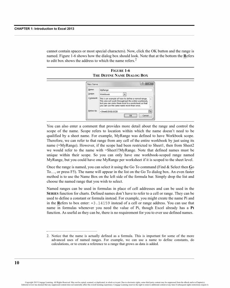
10
cannot contain spaces or most special characters). Now, click the OK button and the range isnamed. Figure 1-6 shows how the dialog box should look. Note that at the bottom the Refersto edit box shows the address to which the name refers.2
FIGURE 1-6THE DEFINE NAME DIALOG BOX
You can also enter a comment that provides more detail about the range and control thescope of the name. Scope refers to location within which the name doesn’t need to bequalified by a sheet name. For example, MyRange was defined to have Workbook scope.Therefore, we can refer to that range from any cell of the entire workbook by just using itsname (=MyRange). However, if the scope had been restricted to Sheet1, then from Sheet2we would refer to the name with =Sheet1!MyRange. Note that defined names must beunique within their scope. So you can only have one workbook-scoped range namedMyRange, but you could have one MyRange per worksheet if it is scoped to the sheet level.
Once the range is named, you can select it using the Go To command (Find & Select then GoTo…, or press F5). The name will appear in the list on the Go To dialog box. An even fastermethod is to use the Name Box on the left side of the formula bar. Simply drop the list andchoose the named range that you wish to select.
Named ranges can be used in formulas in place of cell addresses and can be used in theSERIES function for charts. Defined names don’t have to refer to a cell or range. They can beused to define a constant or formula instead. For example, you might create the name Pi andin the Refers to box enter: =3.14159 instead of a cell or range address. You can use thatname in formulas whenever you need the value of Pi, though Excel already has a PIfunction. As useful as they can be, there is no requirement for you to ever use defined names.
2. Notice that the name is actually defined as a formula. This is important for some of the moreadvanced uses of named ranges. For example, we can use a name to define constants, docalculations, or to create a reference to a range that grows as data is added.
Copyright 2015 Cengage Learning. All Rights Reserved. May not be copied, scanned, or duplicated, in whole or in part. Due to electronic rights, some third party content may be suppressed from the eBook and/or eChapter(s).Editorial review has deemed that any suppressed content does not materially affect the overall learning experience. Cengage Learning reserves the right to remove additional content at any time if subsequent rights restrictions require it.

11
Navigating the Worksheet
Entering Text and NumbersEach cell in an Excel worksheet can be thought of as a miniature word processor. Text can beentered directly into the cell and then formatted in a variety of ways. To enter a text string,first select the cell where you want the text to appear and then begin typing. It is that simple.
Excel is smart enough to know the difference between numbers and text, so there are noextra steps for entering numbers. Let’s try the following example of entering numbers andtext into the worksheet.
Select cell A1 and type: Microsoft Corporation Sales. In cell A2 enter:(Millions of Dollars). Select A3 and type: 2008 to 2013. Note that the entry incell A3 will be treated as text by Excel because of the spaces and letters included. In cells A4to F4 we now want to enter the years. In A4 type: 2013, in B4 type: 2012, select A4:B4,and move the mouse pointer over the lower right corner of the selection. The mouse pointerwill now change to a skinny cross indicating that you can use the AutoFill feature.3 Clickand drag the mouse to the right to fill in the remaining years. Notice that the most recent datais typically entered at the left and the most distant data at the right. This convention allowsus to easily recognize and concentrate on what is usually the most important data.
We have set up the headings for our first worksheet. Now let’s add Microsoft’s sales (inmillions of dollars) for the years 2008 to 2013 into cells A5 to F5 as shown in Exhibit 1-1.
EXHIBIT 1-1THE FIRST WORKSHEET
Formatting and Alignment OptionsThe worksheet in Exhibit 1-1 isn’t very attractive. Notice that the text is displayed at the leftside of the cells, while the numbers are at the right. By default, this is the way that Excelaligns text and numbers. However, we can easily change the way that these entries aredisplayed through the use of the formatting and alignment options.
3. The AutoFill feature can be used to fill in any series that Excel can recognize. For example, typeJanuary in a cell and drag the AutoFill handle to automatically fill in a series of month names.You can also define your own series by clicking the Edit Custom Lists button under General in theAdvanced category of Excel Options.
Source: Microsoft Corporation, Microsoft® Investor Relations, http://www.microsoft.com Retrieved: Nov 2013.
Copyright 2015 Cengage Learning. All Rights Reserved. May not be copied, scanned, or duplicated, in whole or in part. Due to electronic rights, some third party content may be suppressed from the eBook and/or eChapter(s).Editorial review has deemed that any suppressed content does not materially affect the overall learning experience. Cengage Learning reserves the right to remove additional content at any time if subsequent rights restrictions require it.

CHAPTER 1: Introduction to Excel 2013
12
Before continuing, we should define a few typographical terms. A “typeface” is a particularstyle of drawing letters and numbers. For example, the main text of this book is set in theTimes New Roman typeface. However, the text that you are expected to enter into aworksheet is displayed in the Courier New typeface. Typeface also refers to whether thetext is drawn in bold, italics, or perhaps bold italics.
The term “type size” refers to the size of the typeface. We normally refer to the type size in“points.” Each point represents an increment of 1/72nd of an inch, so there are 72 pointsto the inch. A typeface printed at a 12-point size is larger than the same typeface printed at asize of 10 points.
Informally, we refer to the typeface and type size combination as a font. So when we say“change the font to 12-point bold Times New Roman,” it is understood that we are referringto a particular typeface (Times New Roman, bolded) and type size (12 points).
For text entries, the term “format” refers to the typeface, size, text color, and cell alignmentused to display the text. Let’s change the font of the text that was entered to Times NewRoman, 12 points, bold. First, select the range A1:A3. Now, on the Home tab, click on the Fontlist so that the font choices are displayed and then select Times New Roman from the list.
Next, click the Bold button and then choose 12 from the font size list. Notice that as youscroll through the Font and Size lists, the selected text is displayed as will look on theworksheet. This is known as Live Preview, and it works for many, but not all, of theformatting features in Excel 2013. Because none of these changes actually take effect untilyou validate them by clicking, you can scroll through the choices until the text looks exactlyright. You can also make these changes by right-clicking the selected cells and choosingFormat Cells… from the menu. The choices that we made can be found on the Font tab.
We can just as easily change the font for numbers. Suppose that we want to change the years incells A4:F4 to 12-point italic Times New Roman. First select the range A4:F4. Select theproper attributes from the Home tab, or right-click and choose Format Cells. Note that thischange could also have been made at the same time as the text was changed, or you could nowpress Ctrl+Y to repeat the last action. You could also add the Repeat button to the QuickAccess toolbar. Just click arrow at the right of the Quick Access toolbar and choose MoreCommands…. Now select the Repeat button and then click the Add button in the dialog box.
Our worksheet is now beginning to take on a nicer look, but it still isn’t quite right. We areused to seeing the titles of tables nicely centered over the table, but our title is way over atthe left. We can remedy this by using Excel’s alignment options. Excel provides for sevendifferent horizontal alignments within a cell. We can have the text (or numbers) aligned withthe left or right sides of the cell or centered within the cell boundaries. Excel also allowscentering text across a range of cells.
Let’s change the alignment of our year numbers first. Highlight cells A4:F4 and then clickthe Center button in the Alignment section of the Home tab. Notice that the numbers are allcentered within their respective cells.
Copyright 2015 Cengage Learning. All Rights Reserved. May not be copied, scanned, or duplicated, in whole or in part. Due to electronic rights, some third party content may be suppressed from the eBook and/or eChapter(s).Editorial review has deemed that any suppressed content does not materially affect the overall learning experience. Cengage Learning reserves the right to remove additional content at any time if subsequent rights restrictions require it.

13
Navigating the Worksheet
Next, we will center our table title across the whole range of numbers that we have entered.To do this, select the entire range across which we want to center our titles. Highlight cellsA1:F3 and select Format Cells from the right-click menu. Click on the Alignment tab andthen select “Center across selection” from the Horizontal alignment list. Click on the OKbutton and notice that the titles are indeed centered across columns A to F.
Be aware that there is also a button on the Home tab that will “Merge and Center” theselected cells. This button will have the appearance of doing the same thing as “Centeracross selection,” but it doesn’t. In addition to centering the text, it also merges all of theselected cells into one big cell that spans multiple columns and/or rows. Using this buttonmay create alignment and many other problems if you later decide to insert additionalcolumns into the worksheet. At some point, you will probably find that you need to unmergethe cells in order to, say, sort a range. Generally speaking, it is better not to use the Mergeand Center button. If necessary, there is an Unmerge Cells command in the same button.
Formatting NumbersAside from changing the typeface and type size, when dealing with numbers we can alsochange their appearance by adding commas and dollar signs and by altering the number ofdecimal places displayed. Furthermore, we can make the numbers appear differentlydepending on whether they are positive or negative. For example, we might want negativenumbers to be red in color and displayed in parentheses rather than using the negative sign.You can also experiment with designing custom number formats, but for now we will stickto the more common predefined formats.
Microsoft is a large company, and its sales have ranged from $60 billion to over $77 billionduring 2008 to 2013. Numbers this large, even when expressed in millions of dollars,become difficult to read unless they are written with commas separating every third digit.Let’s format our sales numbers so that they are easier to read.
Select the range of sales numbers (A5:F5) and choose Format Cells from the right-clickmenu and then click on the Number tab. You are presented with the Number Format dialogbox which contains a list of formatting categories. For now, select Number from theCategory list. This will give you the option to choose the number of decimal placesdisplayed, choose whether or not to use a 1000 separator, and select the format of negativenumbers. We want to display the sales numbers with commas separating every third digitand two decimal places, so change the decimal places to 2 and check the box to add a 1000separator.4 Click on the OK button and notice that the numbers are now displayed in a morereadable format. You could accomplish almost exactly the same format by clicking the
4. Note that in the United States we use a comma as the 1000 separator. In many other countries adecimal point is used instead. Excel determines which to use based on the settings in the WindowsControl Panel’s Region and Language settings utility.
Copyright 2015 Cengage Learning. All Rights Reserved. May not be copied, scanned, or duplicated, in whole or in part. Due to electronic rights, some third party content may be suppressed from the eBook and/or eChapter(s).Editorial review has deemed that any suppressed content does not materially affect the overall learning experience. Cengage Learning reserves the right to remove additional content at any time if subsequent rights restrictions require it.

CHAPTER 1: Introduction to Excel 2013
14
Comma Style button on the Ribbon (there is a slight alignment difference between the twomethods—you cannot center numbers formatted with the comma style).
At this point, we have made several formatting changes to the Microsoft Sales worksheet.Your worksheet should look like the one in Exhibit 1-2. All of this formatting may seemtedious at the moment, but it will quickly become easy as you become more familiar with thechoices. Furthermore, the payoff in readability will be worth far more than the few secondsspent formatting the worksheet.
EXHIBIT 1-2ORIGINAL WORKSHEET REFORMATTED
Adding Borders and ShadingText formatting is not the only design element available in Excel. We can also liven upworksheets by placing borders around cells and shading them. In your worksheet, select A4:F4(the years). Right-click the selection and choose Format Cells and then select the Border tabfrom the dialog box. There are 13 different line styles that can be applied, and you can changethe color of the lines. Click on the thick solid line (fifth down on the right side) and then clickon both of the top and bottom lines in the sample view. Click the OK button to see the change.
Next, with A4:F4 still selected, we will add shading. As before, choose Format Cells fromthe menu but this time select the Fill tab. This tab allows you to set the background color andpattern of the cells. Click on a light gray color and then press the OK button. Now, to makethe numbers more readable make them bold. Your worksheet should now look like the onein Exhibit 1-3.
EXHIBIT 1-3THE WORKSHEET WITH BORDERS AND SHADING
Source: Microsoft Corporation, Microsoft® Investor Relations, http://www.microsoft.com Retrieved: Nov 2013.
Source: Microsoft Corporation, Microsoft® Investor Relations, http://www.microsoft.com Retrieved: Nov 2013.
Copyright 2015 Cengage Learning. All Rights Reserved. May not be copied, scanned, or duplicated, in whole or in part. Due to electronic rights, some third party content may be suppressed from the eBook and/or eChapter(s).Editorial review has deemed that any suppressed content does not materially affect the overall learning experience. Cengage Learning reserves the right to remove additional content at any time if subsequent rights restrictions require it.
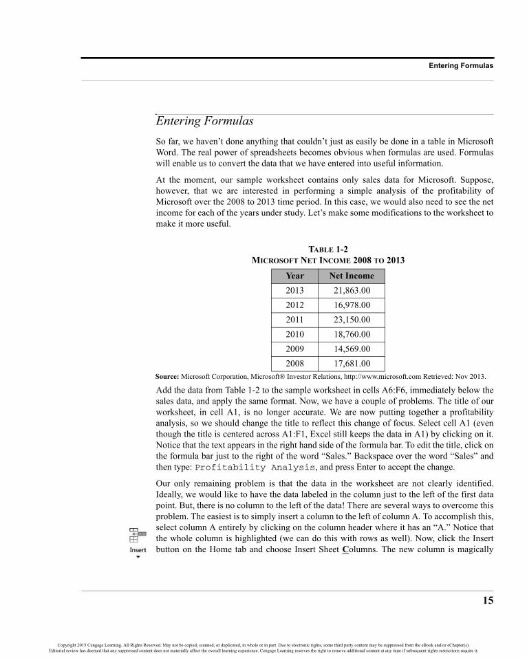
15
Entering Formulas
Entering FormulasSo far, we haven’t done anything that couldn’t just as easily be done in a table in MicrosoftWord. The real power of spreadsheets becomes obvious when formulas are used. Formulaswill enable us to convert the data that we have entered into useful information.
At the moment, our sample worksheet contains only sales data for Microsoft. Suppose,however, that we are interested in performing a simple analysis of the profitability ofMicrosoft over the 2008 to 2013 time period. In this case, we would also need to see the netincome for each of the years under study. Let’s make some modifications to the worksheet tomake it more useful.
Add the data from Table 1-2 to the sample worksheet in cells A6:F6, immediately below thesales data, and apply the same format. Now, we have a couple of problems. The title of ourworksheet, in cell A1, is no longer accurate. We are now putting together a profitabilityanalysis, so we should change the title to reflect this change of focus. Select cell A1 (eventhough the title is centered across A1:F1, Excel still keeps the data in A1) by clicking on it.Notice that the text appears in the right hand side of the formula bar. To edit the title, click onthe formula bar just to the right of the word “Sales.” Backspace over the word “Sales” andthen type: Profitability Analysis, and press Enter to accept the change.
Our only remaining problem is that the data in the worksheet are not clearly identified.Ideally, we would like to have the data labeled in the column just to the left of the first datapoint. But, there is no column to the left of the data! There are several ways to overcome thisproblem. The easiest is to simply insert a column to the left of column A. To accomplish this,select column A entirely by clicking on the column header where it has an “A.” Notice thatthe whole column is highlighted (we can do this with rows as well). Now, click the Insertbutton on the Home tab and choose Insert Sheet Columns. The new column is magically
TABLE 1-2MICROSOFT NET INCOME 2008 TO 2013
Year Net Income2013 21,863.002012 16,978.002011 23,150.002010 18,760.002009 14,569.002008 17,681.00
Source: Microsoft Corporation, Microsoft® Investor Relations, http://www.microsoft.com Retrieved: Nov 2013.
Copyright 2015 Cengage Learning. All Rights Reserved. May not be copied, scanned, or duplicated, in whole or in part. Due to electronic rights, some third party content may be suppressed from the eBook and/or eChapter(s).Editorial review has deemed that any suppressed content does not materially affect the overall learning experience. Cengage Learning reserves the right to remove additional content at any time if subsequent rights restrictions require it.

CHAPTER 1: Introduction to Excel 2013
16
inserted, and all of our data have been moved one column to the right. In cell A5 type:Sales and in A6 type: Net Income.
If you are following the examples exactly, the words Net Income probably do not fit exactlyinto A6. Instead, part of the text is cut off so as not to overflow onto the data in B6. We caneasily remedy this by changing the width of column A. Click the Format button on the Hometab and choose Column Width. In the edit box type: 20 and press the Enter key. Column Ashould now be wide enough to hold the text that we have added and will add later.
We can now proceed with our profitability analysis. Because of the dramatic growth in salesover the years, it isn’t immediately clear from the data whether Microsoft’s profitability hasimproved or not, even though net income has increased over this time. In this type ofsituation, it is generally preferable to look at net income as a percentage of sales (the netprofit margin) instead of dollar net income. Thankfully, we don’t have to type in more datato do this. Instead, we can let Excel calculate these percentages for us. All we need to do is toenter the formulas.
Formulas in Excel are based upon cell addresses. To add two cells together, we simply tellExcel to take the contents of the first cell and add it to the contents of the second. The resultof the formula will be placed in the cell in which the formula is entered. In our problem, weneed to find net income as a percentage of sales. We will do this first for 2013.
Before entering our first formula, we should insert a label identifying the data. In cell A7type: Net Profit Margin. Change the active cell to B7 where we want to place the resultof the calculation. The problem that we want to solve is to take the number in cell B6 (netincome) and divide it by the number in B5 (sales). In Excel, division is represented by theforward slash (/), so in B7 type: =B6/B5. The equals sign must precede all formulas inExcel, otherwise it will treat the formula as text and will not calculate the result. Press theEnter key to calculate the result of the formula. You should get 0.2808 as the result.
In this example, we typed the formula directly into the cell because the small size of ourworksheet made it easy to know what cells we wanted to use in the formula. In manyinstances, this is not the case. In more complicated worksheets, it is usually easier to usepointer mode to enter formulas. In pointer mode, we use the mouse to point to the cells thatwe want to be included, and Excel inserts them into the formula. Move to C7 and we willenter the formula using pointer mode. First, type = to place Excel in edit mode. Now, insteadof typing C6, click on C6 with the mouse. Notice that C6 appears in the formula bar to theright of the equals sign. Press the forward slash key to indicate division and then click on C5.In the formula bar you should see the formula “=C6/C5.” Press the Enter key to calculate theresult of the formula. The result should be 0.2303.
Let’s change the format of these cells so that they are easier to read. In this case, it would benice to see them in percentage format with two decimal places. First, highlight cells B7:C7.Right-click and choose Format Cells, and click on the Number tab. From the Category list,
Copyright 2015 Cengage Learning. All Rights Reserved. May not be copied, scanned, or duplicated, in whole or in part. Due to electronic rights, some third party content may be suppressed from the eBook and/or eChapter(s).Editorial review has deemed that any suppressed content does not materially affect the overall learning experience. Cengage Learning reserves the right to remove additional content at any time if subsequent rights restrictions require it.

17
Entering Formulas
click on Percentage and then set the Decimal places to 2. Press the Enter key or click the OKbutton. You could also apply this format by using the Percent Style button on the Ribbon. Toget two decimal places, you would then need to click the Increase Decimal button in thesame group. Figure 1-7 shows these and other formatting icons.
FIGURE 1-7NUMBER FORMATTING ICONS
Copying and Moving FormulasWe have now calculated the net profit margin for 2013 and 2012, but that still leaves fouryears for which we need to enter formulas. Repeatedly typing essentially the same formulacan get tedious. Fortunately, we can simply copy the formula, and Excel will update the celladdresses to maintain the same relative relationships. For example, we know that for 2011the formula should read “=D6/D5.” If we copy the formula from C7 to D7, Excel willchange the formula from “=C6/C5” to “=D6/D5” automatically.
This works because Excel treats all cell references as relative. When you typed the formulain cell B7 (=B6/B5) Excel read that as “take the contents of the cell that is one row above thecurrent cell and divide that by the contents of the cell that is two rows above the currentcell.” When copying formulas, Excel maintains the same relative cell relationships so thatthe formulas are updated. When we copy to the left or right, Excel updates the columns inthe formulas. When we copy up or down, Excel changes the rows.
To change this behavior, we could use absolute references instead. An absolute referencealways refers to the same cell, no matter where you copy it. To create an absolute reference,type dollar signs before the column letter and row number. For example, $B$6 will alwaysrefer to cell B6. The “$” tells Excel to not change the reference. We can also create mixedreferences. In a mixed reference only the column or row remains constant, not both. Forexample, $B6 is a mixed reference (column absolute, row relative). If the formula is copieddown, it will change to $B7, but if it is copied across it will still be $B6. On the other hand,B$6 (column relative, row absolute) will still be B$6 if copied down, but will change to C$6if copied across. We will make heavy use of absolute and mixed references in later chapters.Note that you can use the F4 key to cycle through every possible reference type. Simplyenter a cell address and repeatedly press F4 until you get the type of reference you need (e.g.,$B$6, B$6, $B6, B6).
Copyright 2015 Cengage Learning. All Rights Reserved. May not be copied, scanned, or duplicated, in whole or in part. Due to electronic rights, some third party content may be suppressed from the eBook and/or eChapter(s).Editorial review has deemed that any suppressed content does not materially affect the overall learning experience. Cengage Learning reserves the right to remove additional content at any time if subsequent rights restrictions require it.

CHAPTER 1: Introduction to Excel 2013
18
EXHIBIT 1-4A PROFITABILITY ANALYSIS FOR MICROSOFT
Rather than retyping the formula for our other cells, let’s simply copy from C7. First, selectC7 and then click the Copy button on the Ribbon. Now highlight cells D7:G7 and click thePaste button. At this point, your worksheet should closely resemble the one in Exhibit 1-4.
We can see from Exhibit 1-4 that Microsoft’s net profit margin has varied somewhat overthis period, but despite the ups and downs, the margins are quite high compared to those ofmost other companies.
In addition to copying formulas (which maintains the relative cell references), they can alsobe moved. Moving a formula to a different cell has no effect on the cell references. Forexample, we could move the formula in B7 (=B6/B5) to B8. To do this, select B7 and thenclick the Cut button (scissors icon). Next, select B8 and then click Paste. Notice that theresult in B8 is exactly the same as B7 because the formula is unchanged. Now click theUndo button on the Quick Access toolbar to return the formula to B7.
Formulas (or anything else) may also be moved with the mouse. Simply select the cellscontaining the data that you want to move, position the mouse pointer at the edge of the cellso that it changes to an arrow, and then click the left mouse button and drag the cell to itsnew location. Now move the formula back to B7. The worksheet should again resemble theone pictured in Exhibit 1-4.
Mathematical OperatorsAside from division, which we have already seen, there are four additional primarymathematical operations: addition, subtraction, multiplication, and exponentiation. Table 1-3summarizes the five basic operations and the result that you should get from entering theexample formula into cell B8.
Source: Microsoft Corporation, Microsoft® Investor Relations, http://www.microsoft.com Retrieved: Nov 2013.
Copyright 2015 Cengage Learning. All Rights Reserved. May not be copied, scanned, or duplicated, in whole or in part. Due to electronic rights, some third party content may be suppressed from the eBook and/or eChapter(s).Editorial review has deemed that any suppressed content does not materially affect the overall learning experience. Cengage Learning reserves the right to remove additional content at any time if subsequent rights restrictions require it.

19
Entering Formulas
Parentheses and the Order of OperationsUsing the mathematical operators provided by Excel is straightforward in most instances.However, there are times when it gets a bit complicated. For example, let’s calculate the rates ofgrowth of Microsoft’s sales and net income. To calculate the growth rates we usually want thecompound annual growth rate (CAGR, which is the geometric mean growth rate) rather than thearithmetic average growth rate. The general equation for the geometric mean growth rate is:
(1-1)
where is the geometric mean, N is the count of the numbers in the series, X0 is the firstnumber in the series (2008 sales in our example), and XN is the last number in the series(2013 sales).
Translating this equation into Excel is not as simple as it may at first appear. Doing thiscorrectly requires knowledge of operator precedence. In other words, Excel doesn’tnecessarily evaluate formulas from left to right. Instead, some operations are performedbefore others. Exponentiation is usually performed first. Multiplication and division areusually performed next, but they are considered equal in precedence so any multiplicationand division are evaluated from left to right. Finally, addition and subtraction are evaluatedand they are also considered equal in precedence to each other.
We can modify the order of operations by using parentheses. Operations enclosed inparentheses are always evaluated first. As a simple example, how would you evaluate thefollowing expression?
TABLE 1-3MATHEMATICAL OPERATIONS
Operation Key Formula Result in B8Addition + =B5+B6 99,712Subtraction – =B5–B6 55,986Multiplication * =B5*B7 21,863Division / =B6/B7 77,849Exponentiation ^ =15^2 225
GXN
X0------N 1–( ) 1–
XN
X0------⎝ ⎠⎛ ⎞
1N 1–( )
-----------------
1–= =
G
X 2 4 3⁄+=
Copyright 2015 Cengage Learning. All Rights Reserved. May not be copied, scanned, or duplicated, in whole or in part. Due to electronic rights, some third party content may be suppressed from the eBook and/or eChapter(s).Editorial review has deemed that any suppressed content does not materially affect the overall learning experience. Cengage Learning reserves the right to remove additional content at any time if subsequent rights restrictions require it.

CHAPTER 1: Introduction to Excel 2013
20
Is X equal to 2 or 3.33? Algebraically, X is equal to 3.33 because the division should beperformed before the addition as Excel would do. If the answer we were seeking was 2, wecould rewrite the expression using parentheses to clarify:
The parentheses clearly indicate that the addition should be performed first, so the answer is2. When in doubt, always use parentheses because using them unnecessarily will not causeany problems.
To calculate the compound annual growth rate of sales, move to cell A8 and type: SalesGrowth. Now, enter the following into B8 using equation (1-1): =(B5/G5)^(1/5)-1.Pressing the Enter key will reveal that the growth rate of sales for the five-year period was5.20% per year (you may have to reformat the cell to display as a percentage with two decimalplaces). To determine the average growth rate of net income, type: Net Income Growth intoA9 and then copy the formula from B8 to B9. You should find that the compound annual rate ofgrowth of net income has been 4.34% per year and that the formula in B9 is: =(B6/G6)^(1/5)-1. Notice how the row references were updated when you copied the formula down.
Using Excel’s Built-In FunctionsWe could build some pretty impressive worksheets with the techniques that we haveexamined so far. But why should we have to build all of our formulas from scratch,especially when some of them can be quite complex and therefore error-prone? Excel comeswith hundreds of built-in functions, and more than 50 of them are financial functions. Thesefunctions are ready to go; all they need is for you to supply cell references as inputs. We willbe demonstrating the use of many of these functions throughout the book, but for now let’sredo our growth rate calculations using the built-in functions.
Because we want to know the compound annual rate of growth, we can use Excel’s built-inGEOMEAN function.5 To use this function the syntax is:
=GEOMEAN(NUMBER1, NUMBER2, …)
The GEOMEAN function takes up to 255 cell addresses (or ranges) separated by commas. Asis usual in Excel, we can also supply a range of cells rather than specifying the cellsindividually. Remember, we want to find the geometric mean rate of growth of sales, not the
5. We could calculate the arithmetic mean using the AVERAGE function, but this would ignore thecompounding and overstate the true average growth rate. This function is defined as=AVERAGE(NUMBER1, NUMBER2, . . .).
X 2 4+( ) 3⁄=
Copyright 2015 Cengage Learning. All Rights Reserved. May not be copied, scanned, or duplicated, in whole or in part. Due to electronic rights, some third party content may be suppressed from the eBook and/or eChapter(s).Editorial review has deemed that any suppressed content does not materially affect the overall learning experience. Cengage Learning reserves the right to remove additional content at any time if subsequent rights restrictions require it.

21
Using Excel’s Built-In Functions
geometric mean of the dollar amount of sales. Because the GEOMEAN function simplycalculates the N th root of the product of the inputs, we need to redefine our inputs (we usedthe dollar amount of sales in our custom-built formula). Let’s add a row of percentagechanges in sales to our worksheet.
Move to A10 and enter the label: % Change in Sales, then select B10 and enter theformula: =B5/C5-1. The result in B10 should be 0.0560, indicating that sales grew by5.60% from 2012 to 2013. Now copy the formula from B10 to each cell in the C10:F10range. Note that we don’t copy the formula into G10 because that would cause an error sinceH10 doesn’t contain any data (try it, and you will see #DIV/0! in G10, meaning that yourformula tried to divide by zero).
Now, to calculate the compound average annual rate of sales growth we need to enter theGEOMEAN function into B11: =GEOMEAN(B10:F10). Because our data points are in onecontiguous range, we chose to specify the range rather than each individual cell. Let’s alsosupply a label so that when we come back later we can recall what this cell represents. Moveto A11 and enter: Sales Growth.
Have you noticed any problems with the result of the GEOMEAN function? The resultwas a #NUM! error, rather than the 5.20% that we got when using our custom formula.Either our custom formula is incorrect or we have misused the GEOMEAN function.Actually, this type of error is common and easily overlooked. What has happened is thatwhen using the GEOMEAN function, we didn’t fully understand what goes on behind thescenes. Remember that GEOMEAN simply takes the N th root of the product of thenumbers. When multiplying numbers that are less than 1, the result is even smaller, notlarger as is the case with numbers greater than 1. What we should have done iscalculated the geometric mean of the price relative changes (i.e., one plus the percentagechange).
To correct the error, replace the formula in B10 with: =B5/C5 and copy it to the other cells.Now replace the formula in B11 with: =GEOMEAN(B10:F10)-1. The result is 5.20%,exactly the same as our previous result. To avoid errors like this one, you must absolutelyunderstand what the built-in formula is doing. Never blindly accept results just becauseExcel has calculated them for you. There is an old saying in computer science: “garbage in,garbage out.”
At this point, your worksheet should closely resemble the one pictured in Exhibit 1-5.
Copyright 2015 Cengage Learning. All Rights Reserved. May not be copied, scanned, or duplicated, in whole or in part. Due to electronic rights, some third party content may be suppressed from the eBook and/or eChapter(s).Editorial review has deemed that any suppressed content does not materially affect the overall learning experience. Cengage Learning reserves the right to remove additional content at any time if subsequent rights restrictions require it.
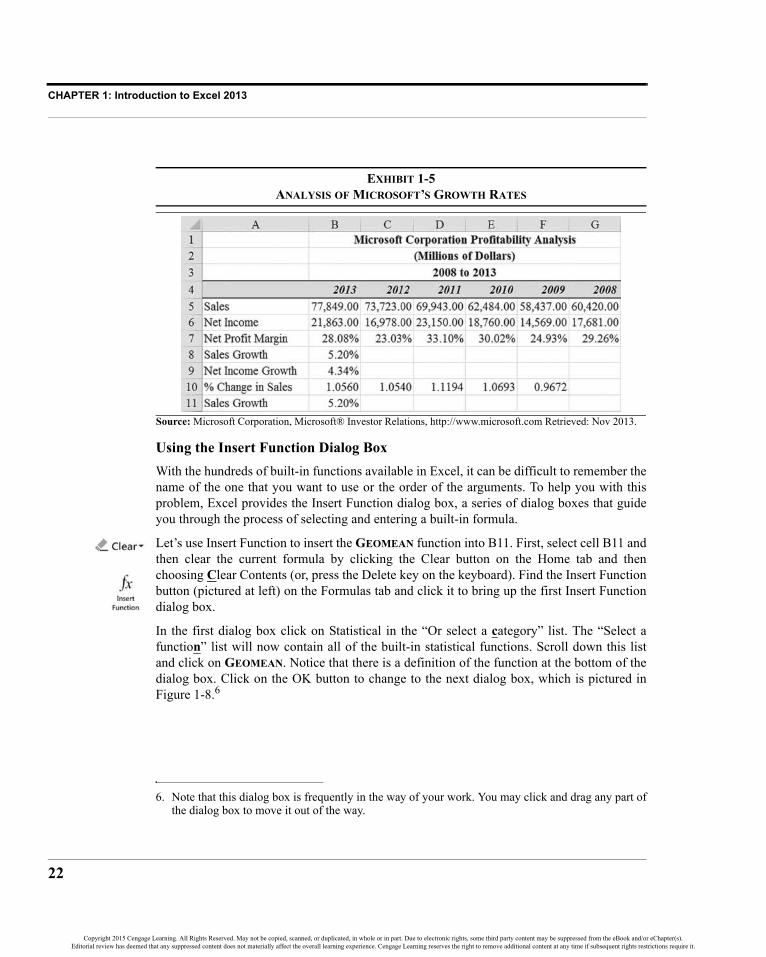
CHAPTER 1: Introduction to Excel 2013
22
EXHIBIT 1-5ANALYSIS OF MICROSOFT’S GROWTH RATES
Using the Insert Function Dialog BoxWith the hundreds of built-in functions available in Excel, it can be difficult to remember thename of the one that you want to use or the order of the arguments. To help you with thisproblem, Excel provides the Insert Function dialog box, a series of dialog boxes that guideyou through the process of selecting and entering a built-in formula.
Let’s use Insert Function to insert the GEOMEAN function into B11. First, select cell B11 andthen clear the current formula by clicking the Clear button on the Home tab and thenchoosing Clear Contents (or, press the Delete key on the keyboard). Find the Insert Functionbutton (pictured at left) on the Formulas tab and click it to bring up the first Insert Functiondialog box.
In the first dialog box click on Statistical in the “Or select a category” list. The “Select afunction” list will now contain all of the built-in statistical functions. Scroll down this listand click on GEOMEAN. Notice that there is a definition of the function at the bottom of thedialog box. Click on the OK button to change to the next dialog box, which is pictured inFigure 1-8.6
6. Note that this dialog box is frequently in the way of your work. You may click and drag any part ofthe dialog box to move it out of the way.
Source: Microsoft Corporation, Microsoft® Investor Relations, http://www.microsoft.com Retrieved: Nov 2013.
Copyright 2015 Cengage Learning. All Rights Reserved. May not be copied, scanned, or duplicated, in whole or in part. Due to electronic rights, some third party content may be suppressed from the eBook and/or eChapter(s).Editorial review has deemed that any suppressed content does not materially affect the overall learning experience. Cengage Learning reserves the right to remove additional content at any time if subsequent rights restrictions require it.

23
Using Excel’s Built-In Functions
FIGURE 1-8THE EXCEL 2013 FUNCTION ARGUMENTS DIALOG BOX
In the Function Arguments dialog box, you will see prompts and definitions for each of theinputs to the selected function. In this case, we want to click and drag the mouse over theB10:F10 range. This range will appear in the “Number 1” edit box. Click on the OK buttonto have the function entered. Notice that the result is 105.20%, not the 5.20% that weexpected. We need to subtract 1 from the result of the function, so click in the Formula barand type -1 after the GEOMEAN function and then press Enter. The formula in B11 shouldbe: =GEOMEAN(B10:F10)-1. Note that the 1 that we are subtracting represents 100% ofthe starting value.
Insert Function is an easy way to discover new functions and to use familiar ones. You canalso find functions by using the function category buttons on the Formulas tab. Choosing afunction from one of those lists will lead to the same Function Arguments dialog box.However you get there, using it will make Excel much easier for you to learn and use.
If you already know the name of the function that you need, you can skip the Insert Functiondialog box. Just type = and then start typing the function name. Excel will automaticallycreate a Formula AutoComplete menu listing functions that match what you have typed.When you see the function name, you can use the arrow keys to select it and then press theTab key to begin entering the arguments. As you enter the function arguments, you will see aToolTip that reminds you of their order.
FIGURE 1-9FORMULA AUTOCOMPLETE
Copyright 2015 Cengage Learning. All Rights Reserved. May not be copied, scanned, or duplicated, in whole or in part. Due to electronic rights, some third party content may be suppressed from the eBook and/or eChapter(s).Editorial review has deemed that any suppressed content does not materially affect the overall learning experience. Cengage Learning reserves the right to remove additional content at any time if subsequent rights restrictions require it.

CHAPTER 1: Introduction to Excel 2013
24
“Dot Functions” in Excel 2013
In Excel 2010, Microsoft introduced a new naming convention for some functions. The newfunctions contain a “dot” in their names. For example, the STDEV.S function calculates asample standard deviation and is identical to the STDEV function that has been in all earlierversions of Excel. In this case, the new naming convention is meant to more clearly conveythe purpose of the function. In other cases, a dot function uses a new algorithm to calculatemore precise results.
In all cases, the older versions of the functions are available for compatibility with olderversions of Excel. If a file is created using the dot functions in Excel 2013 and then openedin Excel 2007 or earlier, the result will be a #NAME! error. That happens because olderversions aren’t aware of the existence of new functions. In this book, we will use thecompatibility functions unless otherwise noted.
If a worksheet that you create may be used on older versions of Excel, you should run theCompatibility Checker before saving the file. This will warn of compatibility problems,including the use of the new dot functions. To use the Compatibility Checker, click the Filetab and then Info. Click the Check for Issues button and then choose Check Compatibility.This will launch a dialog box like that shown in Figure 1-10, which is showing that there is apotential problem in Sheet1 of the workbook due to the use of functions that areincompatible with versions from Excel 97 to Excel 2007. Note that the dialog box shows thenumber of occurrences of each problem and the sheet on which they are located. If there isonly one problem then clicking the Find link will take you to that cell. If there is more thanone problem, then the easiest way to find them is by clicking the Copy to New Sheet button.This will create a new worksheet with a report that identifies each cell with a problem,including a hyperlink that will take you straight to that cell.
FIGURE 1-10THE COMPATIBILITY CHECKER
Copyright 2015 Cengage Learning. All Rights Reserved. May not be copied, scanned, or duplicated, in whole or in part. Due to electronic rights, some third party content may be suppressed from the eBook and/or eChapter(s).Editorial review has deemed that any suppressed content does not materially affect the overall learning experience. Cengage Learning reserves the right to remove additional content at any time if subsequent rights restrictions require it.

25
Using Excel’s Built-In Functions
Using User-Defined FunctionsThere are times when you need to calculate a complex formula and Excel doesn’t have abuilt-in function that will do the job. In this case, you can either type the formula into a cell(which can be very tedious) or use a user-defined function. A user-defined function is similarto a built-in function, except that it was created by somebody other than the Exceldevelopment team at Microsoft. User-defined functions can be purchased, downloaded fromthe Internet, or you can create your own. Writing them in Excel’s macro language (VisualBasic for Applications, see Chapter 14) is beyond the scope of this chapter, but I haveincluded several functions in the Famefncs.xlam file, which can be found on the official Website for this book.7 Download the file and save it to your hard drive in an easy-to-rememberlocation. These functions will be used occasionally throughout the book, especially in laterchapters.
Before using a function you must open Famefncs.xlam. This file is a special type of Excelfile known as an add-in. An add-in can be opened just like any other Excel file, or it can beset to open automatically every time you start Excel. To make the functions in this fileavailable at all times, click the File tab and then Options. Click Add-Ins and then chooseExcel Add-ins from the Manage list and click the Go button. This will open the Add-Insdialog box as pictured in Figure 1-11.
FIGURE 1-11THE ADD-INS DIALOG BOX
7. In Excel 2007 and later, file names with extensions that are .xlsm or .xlam contain macros. Thesefiles may require special security settings before Excel will allow the macros to run. Go to the Filetab, then Options, and set up your Trusted Locations in the Trust Center. You may still receivewarnings for some files, but if you are sure that they are safe then allow the macros to run.
Copyright 2015 Cengage Learning. All Rights Reserved. May not be copied, scanned, or duplicated, in whole or in part. Due to electronic rights, some third party content may be suppressed from the eBook and/or eChapter(s).Editorial review has deemed that any suppressed content does not materially affect the overall learning experience. Cengage Learning reserves the right to remove additional content at any time if subsequent rights restrictions require it.

CHAPTER 1: Introduction to Excel 2013
26
Click the Browse button, navigate to the directory where you saved the file, and chooseFamefncs.xlam. It will be added to the Add-Ins dialog box as shown above, and thefunctions in the file will now be available to use in all of your workbooks. If you can’t accessthe functions, make sure that you save the file in one of your trusted locations as mentionedin footnote 7.
Using a user-defined function is almost exactly the same as using a built-in function. Theonly difference is that the file containing the functions must be opened in order for thefunctions to be known to Excel. You can even use the Insert Function dialog box (select theUser Defined function category, which is only available when user-defined functions areinstalled).
As an example of the use of user-defined functions, I have created one to calculate thegeometric mean rate of growth of sales from the dollar amounts instead of the price relativesthat we used earlier. The function is defined as8:
FAME_GEOMEAN(SALES)
FAME_GEOMEAN is the name of the function, and SALES is the required range of cells thatcontain the sales figures. The function automatically calculates the formula given inequation (1-1) on page 19.
Now, in your original worksheet, select cell B12 and then bring up the Insert Function dialogbox. Choose the User Defined category to display the list of functions that were suppliedwith this book. In the “Select a function” list, select the macro named FAME_GEOMEANand then click the OK button. In the edit box for Dollar Values enter B5:G5, which isthe range that contains Microsoft’s sales. Click on the OK button and see that the answeris exactly the same as before. The function in B12 is: =FAME_GEOMEAN(B5:G5).
We will use more of the user-defined functions from this add-in in later chapters.
Creating GraphicsIn our simple profitability analysis, it is obvious that Microsoft’s profit margins have beensomewhat volatile over the last six years. Many times, you will build much morecomplicated worksheets where the key trends are not so easy to spot, especially by otherswho didn’t build the worksheet. You may also find that you need to give a presentation,perhaps to a group of investors to convince them to invest in your firm. In cases such as
8. This function was written specifically to calculate a compound average growth rate from dollarvalues. It does not duplicate Excel’s GEOMEAN function, so do not use it as a substitute for thatfunction.
Copyright 2015 Cengage Learning. All Rights Reserved. May not be copied, scanned, or duplicated, in whole or in part. Due to electronic rights, some third party content may be suppressed from the eBook and/or eChapter(s).Editorial review has deemed that any suppressed content does not materially affect the overall learning experience. Cengage Learning reserves the right to remove additional content at any time if subsequent rights restrictions require it.

27
Creating Graphics
these, tables full of numbers may actually obscure your point. People (and students too!)tend to get a glazed look in their eyes when examining tables of numbers. The solution tothis problem is to present a chart of the numbers to illustrate your point. Fortunately, high-quality graphics are a snap with Excel.
There are three ways that charts can be created in Excel: in separate chart sheets, embeddedin the worksheet, or as in-cell charts known as Sparklines. We will cover each of thesemethods in turn.
Creating Charts in a Chart SheetWhen you want to focus only on a chart, then it is best to create it in its own chart sheet. Wecan create a chart separate from the worksheet by selecting the data and inserting a new chartsheet. Let’s try creating a graph of Sales versus Net Income for Microsoft.
First select the data in the A4:G6 range and then right-click the tab for the current worksheet(which is probably labeled “Sheet 1”). From the menu that appears, choose Insert. You willnow be presented with a list of different file types from which to select. Because we want tocreate a chart, select Chart from the list and press Enter or click OK.
A chart sheet will open with your data displayed automatically in a Column chart. It won’thave a chart title or axis titles and will require a few other enhancements. Note that you nowhave two additional tabs in the Ribbon (Design and Format) that are specific to working withcharts. These are known as contextual tabs because they only appear in the context of editinga chart. If you want another type of chart, you can click the Change Chart Type button on theDesign tab.
Let’s begin to fix our chart by adding a title. Select the chart and then click the ChartElements button that appears in the upper-right corner. Click the Chart Title item and choosethe Centered Overlay option. In the text box that appears, type: Microsoft Sales vs.Net Income and then click outside the box to lock in the title.
You will follow a similar procedure for the axis titles. Click the Axis Titles item in the ChartElements button and then choose Primary Horizontal Axis Title to insert both the x and yaxis titles. For the x-axis double click the “Axis Text” label and then type: Years, and forthe y-axis type: Millions of Dollars for the title.
Your chart should now resemble the one in Exhibit 1-6. We will see how to fix the reversedx-axis after the next section.
Copyright 2015 Cengage Learning. All Rights Reserved. May not be copied, scanned, or duplicated, in whole or in part. Due to electronic rights, some third party content may be suppressed from the eBook and/or eChapter(s).Editorial review has deemed that any suppressed content does not materially affect the overall learning experience. Cengage Learning reserves the right to remove additional content at any time if subsequent rights restrictions require it.

CHAPTER 1: Introduction to Excel 2013
28
EXHIBIT 1-6A STAND-ALONE CHART
Creating Embedded ChartsYou may want to create a chart that will be saved and displayed within the worksheet itself.Such a chart is referred to as an “embedded chart” because it appears within the worksheet.Unlike a separate chart sheet, embedded charts can be displayed and printed on the same page asthe worksheet data. If necessary, embedded charts can be printed separately from the worksheet.
To create an embedded chart, first switch to your worksheet. Now select A4:G6 as beforeand then click the Insert tab. Click the Column button in the Charts group and then choosethe first type listed under 2-D Column. The chart will appear in the middle of yourworksheet. To resize the chart, click and drag any of the selection boxes on its perimeter. Tomove the chart, click on a blank area inside the chart and drag it to wherever you want it tobe. Your worksheet should now resemble the one in Exhibit 1-7, except for some minorformatting changes. You can enter the chart and axis titles exactly as before.
Note that you can move your embedded chart into a separate chart sheet and vice versa. Justright-click in the chart and choose Move Chart from the shortcut menu. There is also a MoveChart button on the Design tab. You can even move your chart to a different worksheet inthis way.
Source: Microsoft Corporation, Microsoft® Investor Relations, http://www.microsoft.com Retrieved: Nov 2013.
Copyright 2015 Cengage Learning. All Rights Reserved. May not be copied, scanned, or duplicated, in whole or in part. Due to electronic rights, some third party content may be suppressed from the eBook and/or eChapter(s).Editorial review has deemed that any suppressed content does not materially affect the overall learning experience. Cengage Learning reserves the right to remove additional content at any time if subsequent rights restrictions require it.

29
Creating Graphics
EXHIBIT 1-7A WORKSHEET WITH AN EMBEDDED CHART
Formatting ChartsWe have now created a basic chart of Sales versus Net Income, but it probably isn’t quitewhat you expected. First of all, we normally expect that the most recent data in a chart is onthe right side and the oldest on the left. Because we have created our worksheet data in theopposite direction (a common convention), our chart is backward and a quick glance mightsuggest that sales and profits have been declining.
In Excel, every element of a chart is treated as a separate “object.” This means that eachelement can be selected and edited separately from the other elements. In addition, thesechart objects are somewhat intelligent. They “know” what actions can be performed on themand will present a menu of these actions if you right-click on them. The major objects in anychart include each data series, the plot area, the gridlines, the axes, the axis titles, the charttitle, and any text boxes entered into the chart. To select an object, all that you need to do isto click on it. Once the object is selected, it will have small squares (selection handles)surrounding it. In some cases this will result in the selection of multiple items (e.g., the
Source: Microsoft Corporation, Microsoft® Investor Relations, http://www.microsoft.com Retrieved: Nov 2013.
Copyright 2015 Cengage Learning. All Rights Reserved. May not be copied, scanned, or duplicated, in whole or in part. Due to electronic rights, some third party content may be suppressed from the eBook and/or eChapter(s).Editorial review has deemed that any suppressed content does not materially affect the overall learning experience. Cengage Learning reserves the right to remove additional content at any time if subsequent rights restrictions require it.

CHAPTER 1: Introduction to Excel 2013
30
entire data series, or the entire legend), but you can often narrow the selection with a secondclick (not a double-click). With this knowledge, let’s edit our chart.
First, we want to turn the x-axis around so that the data are presented in the order that wenormally expect. Right-click on the x-axis (or the axis labels) to show the shortcut menu.Once the menu appears, choose Format Axis. This will launch the Format Axis panel on theright side of the window. Under Axis Options, choose the Date Axis type so that Excelunderstands that our year numbers are dates. It will flip the axis so that it reads left to right aswe would expect. If we had entered full dates in the heading (e.g., 6/30/2014), then Excelwould have recognized the dates and created a date axis that we wouldn’t need to flip.
We could also flip the axis by selecting “Categories in reverse order” from the same panel.This will reverse the x-axis, but also move the y-axis to the right side of the chart. If that isn’twhat you want, click on “At maximum category” in the same dialog box to move the y-axisback to the left side. This method is best used when your x-axis labels are text. If they aredates, then the previous method is better.
Now suppose that we wanted to change the chart title so that it shows the years that arecovered by the data. Simply click on the chart title to select it, then click at the end of thetitle. You could begin typing immediately, but we want to put the new text on a second line.Press Enter to begin a new line and then type: 2008 to 2013 and press the Esc key orclick anywhere else on the chart. You may need to resize the font to make the title fit.
Next, let’s move the legend to the bottom of the chart to see if it looks better there. Right-click on the legend and choose Format Legend from the shortcut menu. Select Bottom fromthe choices presented. Click the X in the upper-right of the Format Legend panel to close itand return to the chart. Now the plot area of the chart looks squashed. To fix this, click in theplot area to select it and drag the selection handles until the plot area is the proper size. Yourworksheet should now resemble the one in Exhibit 1-8.
Changing the Chart TypeExcel offers many different types of charts: everything from the column chart that we havecreated to 3-D bar charts and radar plots. Some of these chart types are very sophisticated,even allowing you to rotate them to see a different view of the data. Despite these potentialcomplexities, changing the chart type is very straightforward.
Let’s assume that we would prefer to see the data in our chart presented as two lines, ratherthan as columns. To make this change, right-click anywhere inside the chart and chooseChange Chart Type from the menu (or the button on the Design tab). Select a type of Linechart and click OK. The chart is now displayed as a line chart. You can even change the typeof an individual data series. For example, you might want to see Sales as a Column chart and
Copyright 2015 Cengage Learning. All Rights Reserved. May not be copied, scanned, or duplicated, in whole or in part. Due to electronic rights, some third party content may be suppressed from the eBook and/or eChapter(s).Editorial review has deemed that any suppressed content does not materially affect the overall learning experience. Cengage Learning reserves the right to remove additional content at any time if subsequent rights restrictions require it.
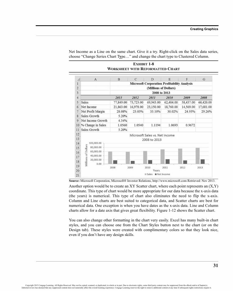
31
Creating Graphics
Net Income as a Line on the same chart. Give it a try. Right-click on the Sales data series,choose “Change Series Chart Type…” and change the chart type to Clustered Column.
EXHIBIT 1-8WORKSHEET WITH REFORMATTED CHART
Another option would be to create an XY Scatter chart, where each point represents an (X,Y)coordinate. This type of chart would be more appropriate for our data because the x-axis data(the years) is numerical. This type of chart also eliminates the need to flip the x-axis.Column and Line charts are best suited to categorical data, and Scatter charts are best fornumerical data. One exception is when you have dates as the x-axis data. Line and Columncharts allow for a date axis that gives great flexibility. Figure 1-12 shows the Scatter chart.
You can also change other formatting in the chart very easily. Excel has many built-in chartstyles, and you can choose one from the Chart Styles button next to the chart (or on theDesign tab). These styles were created with complimentary colors so that they look nice,even if you don’t have any design skills.
Source: Microsoft Corporation, Microsoft® Investor Relations, http://www.microsoft.com Retrieved: Nov 2013.
Copyright 2015 Cengage Learning. All Rights Reserved. May not be copied, scanned, or duplicated, in whole or in part. Due to electronic rights, some third party content may be suppressed from the eBook and/or eChapter(s).Editorial review has deemed that any suppressed content does not materially affect the overall learning experience. Cengage Learning reserves the right to remove additional content at any time if subsequent rights restrictions require it.

CHAPTER 1: Introduction to Excel 2013
32
FIGURE 1-12SALES VS. NET INCOME AS A SCATTER CHART
If you want to change just the color of the columns (or line) for Sales, simply right-click onone of the data points and choose Format Data Series. Select Fill and then Solid Fill. Youcan now choose the exact color that you want to apply to the data series. You can also changethe border around the bars and add a shadow for a three-dimensional effect.
Be careful about applying too much “eye candy.” Excel 2013’s charting ability makes it easyto fill the chart with effects that add nothing to the viewer’s understanding of the data.Typically, excessive formatting distracts from the message of the chart (e.g., see just aboutany so-called info-graphic on the Internet). Excel charting and data visualization experts9
generally recommend that you use the correct type of chart and keep the formatting assimple as possible. After all, the purpose of a chart is to make data easier to understand; itisn’t supposed to be a work of art.
Creating Sparkline Charts
Sparklines are a type of “word” chart created by Edward Tufte, a statistician and datavisualization expert. They are tiny charts that are intended to be presented as a “word” in aline of text or next to data in a table. Their chief purpose is to display trends and variabilityin a very compact space.
Let’s add a few sparklines to our worksheet to show the trend in sales, net income, and netprofit margin over time. Select cell C5 and then click the Insert tab and choose the Linebutton in the Sparklines group. In the dialog box choose B5:G5 as the Data Range and thenclick OK.
9. For example, see Jon Peltier, an Excel charting expert who maintains the PTS blog at http://peltiertech.com/WordPress. Stephen Few is a data visualization expert and author who maintainsthe Visual Business Intelligence blog at http://www.perceptualedge.com/blog/.
Source: Microsoft Corporation, Microsoft® Investor Relations, http://www.microsoft.com Retrieved: Nov 2013.
Copyright 2015 Cengage Learning. All Rights Reserved. May not be copied, scanned, or duplicated, in whole or in part. Due to electronic rights, some third party content may be suppressed from the eBook and/or eChapter(s).Editorial review has deemed that any suppressed content does not materially affect the overall learning experience. Cengage Learning reserves the right to remove additional content at any time if subsequent rights restrictions require it.

33
Printing
You will now have the sparkline chart in H5, but notice that it seems to indicate that saleshave been declining. As before, this is because our data is listed from newest to oldest so weneed to flip the x-axis. On the Design tab for the sparkline, click the Axis button and choosePlot Data Right-to-left. Now we can easily see, in a very compact space, that sales have beentrending upward for the last six years.
You can follow the same steps to create sparklines for net income and the net profit margin,or you can simply use the AutoFill handle to copy the sparkline from H5. We can now applyadditional formatting, such as adding markers to each data point by making use of theoptions available on the Design tab.
EXHIBIT 1-9PROFITABILITY ANALYSIS WITH SPARKLINES
If you want to change the type of Sparkline chart, simply select the Sparklines and then clickthe type of chart that you want in the Design tab. Note that you cannot delete Sparklines bypressing the Delete key. Instead, click the Clear button in the Design tab, or right-click themand delete them using the shortcut menu.
PrintingThere are many times when a worksheet displayed on screen accomplishes all that you need.Other times there is no escaping the need for a hard copy. Excel makes printing a worksheetboth easy and flexible. For small worksheets all that needs to be done is to click the File tab,and then on the Print tab click the Print button. This will print the worksheet immediately,using the default printer and settings. Note that the preview of the printout is shown in thistab instead of a separate window as in older versions of Excel.
Source: Microsoft Corporation, Microsoft® Investor Relations, http://www.microsoft.com Retrieved: Nov 2013.
Copyright 2015 Cengage Learning. All Rights Reserved. May not be copied, scanned, or duplicated, in whole or in part. Due to electronic rights, some third party content may be suppressed from the eBook and/or eChapter(s).Editorial review has deemed that any suppressed content does not materially affect the overall learning experience. Cengage Learning reserves the right to remove additional content at any time if subsequent rights restrictions require it.

CHAPTER 1: Introduction to Excel 2013
34
Larger printing tasks are only slightly more complex. Suppose that our profitability analysisof Microsoft needs to be printed so that it can be distributed at a meeting. As a first step, weneed to decide if we want to print the entire worksheet or only a portion of it. In this case,let’s assume that we wish to print the whole worksheet, except that we want to print thegraph on a separate page so that it can more easily be converted to an overhead transparency.
Because we wish to print the numbers and chart separately, we need to tell Excel the range ofcells that we want printed. Select the range A1:G11, choose Print Area on the Page Layouttab, and then Set Print Area. Notice that a light gray line now surrounds the range that wehave selected for printing. Before actually printing a worksheet, it is good practice topreview the output to make sure that it looks exactly as we want. This will save both timeand paper. From the File tab choose the Print tab. Excel will now display a likeness of theactual printed page. If it doesn’t look exactly the way that you want, you can change someoptions. For example, if the gridlines appear on the print preview, you can turn them off onthe Page Layout tab by unchecking the Print option under Gridlines.
If you have followed the examples to this point, you might, depending on the type of printeryou are using and the font size, notice that our worksheet is too wide to fit on one page.Because we would ideally like to fit the whole worksheet on one page, we have someadjustments to make. Essentially we have two options: either change the page orientation toprint sideways (i.e., landscape mode) or have Excel reduce the printout to fit on one page.Each of these methods is equally viable, but let’s go for the reduction to one page.
From the Print tab, we can click the button that shows the current scaling choice (probablyNo Scaling) and choose an option from the list. You can also set custom scaling options byclicking the Page Setup link, which will launch the Page Setup dialog box. In the Fit to:pages wide by tall and enter a 1 in both boxes. We also don’t want the gridlines to print.Click on the Sheet tab and make sure that the Gridlines option is deselected (no check markin the box). Click OK to return to Print Preview.
At this point, everything should be ready for printing, so click on the Print button. Excel nowreturns to the normal view and presents you with the print dialog box. Because we want toprint the whole range that we have selected, make sure your printer is ready (turned on, haspaper, etc.) and click OK. Your page should look nearly identical to the on-screen version.
To print the chart on a separate page, we first need to click on it so that it is selected. Now, toprint the chart simply select Print from the File tab. Presto! The chart prints out on its ownpage. Of course, you will still see the Print Preview and be able to use the page setup optionsfor charts just as we did for the worksheet.
What if you wanted to print the chart on the same page as the worksheet? Simple, just selectthe entire range that you want to print, including the chart. Now repeat the steps from above(resetting the print area), and the worksheet and chart will print on the same page. An easier
Copyright 2015 Cengage Learning. All Rights Reserved. May not be copied, scanned, or duplicated, in whole or in part. Due to electronic rights, some third party content may be suppressed from the eBook and/or eChapter(s).Editorial review has deemed that any suppressed content does not materially affect the overall learning experience. Cengage Learning reserves the right to remove additional content at any time if subsequent rights restrictions require it.

35
Using Excel with Other Applications
alternative is to select the range to print, choose Print from the File tab, and make sure thatPrint Selection is selected in the Settings section.
Using Excel with Other ApplicationsSuppose that you are writing a report on the profitability of Microsoft for the past six years.Chances are good that you are writing the report in one of the major word processingprograms. Your word processor probably allows for the creation of tables that can display allof the information that you have created in Excel, but it lacks the computationalsophistication and graphics power of Excel. Similarly, Excel lacks the text processing powerthat you need to write the report. Fortunately, it is very easy to harness the strengths of bothprograms and combine the results.
While some word processors will read Excel files directly from your disk, this is not usuallythe easiest way to incorporate spreadsheets into your word processing files. Instead, it isusually easiest to use some variant of copy and paste, just like we’ve used within Excelitself. Every time you copy data from Excel, it goes to the clipboard. The contents of theclipboard are available to any other application that cares to access them. All you need to dois copy the data from within Excel, switch to the other application, and then paste from itsmenus.
Simply pasting the Excel data into a word processor usually results in the word processorreading the data and creating a table. While this may be all that you need, many times itwould be more convenient if you could still edit the data in its native environment. In otherwords, it would be nice if you could still take advantage of Excel’s built-in functions andrecalculation ability. You can. Instead of using the paste command, use Paste Special.
The Paste Special command allows much more freedom in how the data is stored inside theword processor. For example, if you choose to paste the data as a “Microsoft ExcelWorksheet Object” you will be able to edit the data from within the word processor bysimply double-clicking on it. If you are using Microsoft Word 2013, the Ribbon will changeto that of Excel, and you can edit the data exactly as if you were in Excel.
Alternatively, you can link the data to your worksheet so that when you make changes inExcel, they are automatically reflected in your word processor. Finally, you can paste anoneditable picture of your data into your document. Either of these last two methods willconsume less memory than embedding the worksheet.
Copyright 2015 Cengage Learning. All Rights Reserved. May not be copied, scanned, or duplicated, in whole or in part. Due to electronic rights, some third party content may be suppressed from the eBook and/or eChapter(s).Editorial review has deemed that any suppressed content does not materially affect the overall learning experience. Cengage Learning reserves the right to remove additional content at any time if subsequent rights restrictions require it.

CHAPTER 1: Introduction to Excel 2013
36
Quitting ExcelIn previous versions, you could exit from Excel by selecting Exit from the File tab.However, due to user confusion between closing files and exiting, this option was eliminatedin Excel 2013. Now to close the workbook and exit you must repeatedly click the Exit buttonin the upper right corner of the Excel window to close each open workbook and eventuallythe program itself. Note that if you attempt to close a file without saving your work, Excelwill warn you and ask if you would like to save the file.
Best Practices for Spreadsheet ModelsA spreadsheet model (specifically a financial model in this book) is simply a spreadsheetdesigned to solve a particular problem. A properly designed model requires a good deal ofthought before the first formula is written. It should be functional, flexible, well-organized,easy to use, and nice looking. While we cannot tell you what font you should use, we canprovide several rules that are common to good spreadsheet design.
1. Create an area specifically for the variables (inputs) in the model. Theinput area should be separate from the calculation area whenever possible.If there are a lot of variables, then the input area should be on a separateworksheet (usually the first worksheet in the workbook). This will make iteasy to change the assumptions behind the model. Further, cells containingformulas that should not be modified by end users should be protected(Review tab, Protect Sheet).
2. Do not enter a number directly into a formula, unless it will never change.Numbers that may be changed should be entered into the input area, orcalculated if possible. This will help to minimize errors in the model andgreatly simplify the changing of assumptions. It is much better to change anumber in one cell than to have to remember to change it in five formulas.
3. Your model should be well-organized and nicely formatted. This will notonly help you to minimize errors, but will also make it easier for others tounderstand. A haphazardly created model may return the correct answers,but it will be difficult to understand. Even if nobody else will ever see yourspreadsheet, you will probably have to look it over in the future. The effortthat you expend in designing the model will be paid back many times overin future time savings.
4. If your formulas are long or use complex logic, make sure to documentthem. A simple explanatory cell comment (choose New Comment fromthe Review tab) or a textbox describing the logic of the model can save
Copyright 2015 Cengage Learning. All Rights Reserved. May not be copied, scanned, or duplicated, in whole or in part. Due to electronic rights, some third party content may be suppressed from the eBook and/or eChapter(s).Editorial review has deemed that any suppressed content does not materially affect the overall learning experience. Cengage Learning reserves the right to remove additional content at any time if subsequent rights restrictions require it.

37
Summary
enormous effort when debugging formulas. Writing your own user-defined functions in Visual Basic for Applications (VBA, see Chapter 14)can help to simplify your model, particularly if the formula is needed inseveral places.
5. Always test your model thoroughly before declaring it finished. Whileyour model may produce correct answers for your expected input values,it may not work properly in every conceivable case. It is important tochange your inputs several times, and verify the output. Make sure to usesome numbers that don’t seem realistic to see what happens. This willoften uncover errors in formula logic. Your formulas should be written sothat they can handle anything that you may throw at them. IF statements,Data Validation, and Conditional Formatting are quite useful in thisregard.
Keep these five rules in mind when building your models, and you will be much moreproductive and less likely to create flawed models.10
SummaryIn this chapter, we have discussed the basics of Microsoft Excel 2013. You should havegained a basic understanding of such topics as entering text and numbers, entering formulas,formatting, graphics, and printing. We have also discussed some important considerationsfor designing spreadsheet models.
In the chapters ahead, we will cover many of these topics in more depth. We will, at the sametime, introduce you to financial analysis and describe how Excel can make this analysiseasier and more productive. Along the way, we hope to help you develop the reasoning,critical thinking, and quantitative skills that are so necessary in the field of finance today.
10.The IT Faculty of The Institute of Chartered Accountants in England and Wales (ICAEW) haspublished “Twenty Principles for Good Spreadsheet Practice” that is worth reading. It is availableat: http://www.ion.icaew.com/itcounts/post/twenty-principles-for-good-spreadsheet-practice.
Copyright 2015 Cengage Learning. All Rights Reserved. May not be copied, scanned, or duplicated, in whole or in part. Due to electronic rights, some third party content may be suppressed from the eBook and/or eChapter(s).Editorial review has deemed that any suppressed content does not materially affect the overall learning experience. Cengage Learning reserves the right to remove additional content at any time if subsequent rights restrictions require it.

CHAPTER 1: Introduction to Excel 2013
38
Problems
1. Suppose that at the end of December 2008 you purchased shares in Apple,Inc. (Nasdaq: AAPL). It is now five years later and you decide to evaluateyour holdings to see if you have done well with this investment. The tablebelow shows the end-of-year market prices of AAPL.
a. Enter the data, as shown, into a worksheet and format the table asshown.
b. Create a formula to calculate your rate of return for each year. Formatthe results as percentages with two decimal places.
c. Calculate the total return for the entire five-year holding period. Whatis the compound average annual rate of return?
TABLE 1-4FUNCTIONS INTRODUCED IN THIS CHAPTER
Purpose Function PageCalculate the geometric mean GEOMEAN(NUMBER1, NUMBER2,…) 20Calculate the arithmetic mean AVERAGE(NUMBER1, NUMBER2,…) 20An alternate way to calculate the geometric mean using dollar values
FAME_GEOMEAN(SALES) 26
AAPL Stock PricesDate Price2008 82.532009 203.762010 311.892011 391.602012 519.132013 561.02
Copyright 2015 Cengage Learning. All Rights Reserved. May not be copied, scanned, or duplicated, in whole or in part. Due to electronic rights, some third party content may be suppressed from the eBook and/or eChapter(s).Editorial review has deemed that any suppressed content does not materially affect the overall learning experience. Cengage Learning reserves the right to remove additional content at any time if subsequent rights restrictions require it.

39
Problems
d. Create a Line chart showing the stock price from December 2008 toDecember 2013. Make sure to title the chart and label the axes. Now,create an XY Scatter chart of the same data. What are the differencesbetween these types of charts? Which type of chart is moreappropriate for this data?
e. Experiment with the formatting possibilities of the chart. Forexample, you might try changing it to a 3-D Line chart and fill theplot area with a marble background. Is there any reason to use thistype of chart to display this data? Do the “enhancements” help you tounderstand the data?
2. In your position as research assistant to a portfolio manager, you need toanalyze the profitability of the companies in the portfolio. Using the datafor 3M Co. below:
a. Calculate the net profit margin for each year.
b. Calculate the average annual growth rates for revenue and net incomeusing the GEOMEAN function. Is net income growing more slowly orfaster than total revenue? Is this a positive for your investment in thecompany?
c. Calculate the average annual growth rate of total revenue using theAVERAGE function. Is this result more or less accurate than yourresult in the previous question? Why?
d. Create a Column chart of total revenue and net income. Be sure tochange the chart so that the x-axis labels contain the year numbers,and format the axis so that 2013 is on the far right side of the axis.
Fiscal Year 2013 2012 2011 2010 2009Total Revenue 30,871 29,904 29,611 26,662 23,123Net Income 4,659 4,444 4,283 4,085 3,193
Copyright 2015 Cengage Learning. All Rights Reserved. May not be copied, scanned, or duplicated, in whole or in part. Due to electronic rights, some third party content may be suppressed from the eBook and/or eChapter(s).Editorial review has deemed that any suppressed content does not materially affect the overall learning experience. Cengage Learning reserves the right to remove additional content at any time if subsequent rights restrictions require it.

CHAPTER 1: Introduction to Excel 2013
40
3. Repeat Problem 2 using the data below for Yahoo! Inc. However, this timeyou should create a copy of your worksheet to use as a template. Replacethe data for 3M with that of Yahoo.
a. Do you notice anything unusual about Yahoo’s growth rates? Do thegrowth rates that you calculated seem reasonable going forward?
b. Which company was more profitable in 2013? Which was moreprofitable if you take a longer view? Would this affect your desire toinvest in one company over the other?
4. Using the data for Adobe Systems Inc. (Nasdaq: ADBE), presented below:
a. Calculate the ratio of each years’ data to the previous year for each ofthe above items for Adobe. For example, for the year 2013, the ratiofor sales is $4,055/$4,404 = 0.92075.
Fiscal Year 2013 2012 2011 2010 2009Total Revenue 4,680 4,987 4,984 6,325 6,460Net Income 1,366 3,945 1,049 1,232 598
Fiscal Year 2013 2012 2011 2010 2009Sales $4,055 $4,404 $4,216 $3,800 $2,946EBIT 423 1,180 1,099 993 691Interest Expense 68 67 67 57 3Total Net Income 290 833 833 775 387Basic EPS from Total Operations 0.58 1.68 1.67 1.49 0.74
Total Assets 10,380 9,975 8,991 8,141 7,282Accounts Payable 62 50 87 52 59Total Liabilities 3,656 3,309 3,208 2,949 2,392Retained Earnings 6,929 7,003 6,529 5,981 5,300Net Cash from Operating Activities 1,152 1,500 1,543 1,113 1,118
Free Cash Flow 963 1,229 1,333 943 998
Copyright 2015 Cengage Learning. All Rights Reserved. May not be copied, scanned, or duplicated, in whole or in part. Due to electronic rights, some third party content may be suppressed from the eBook and/or eChapter(s).Editorial review has deemed that any suppressed content does not materially affect the overall learning experience. Cengage Learning reserves the right to remove additional content at any time if subsequent rights restrictions require it.

41
Internet Exercise
b. From your calculations in part a, calculate each year’s rate of growth.Using the example in part a, the ratio is 0.92075, so the percentagegrowth in sales for 2013 is 0.92075 – 1 or –7.925%.
c. Calculate the average growth rate (using the AVERAGE function) ofeach of the above items using the results you calculated in part b.These averages are arithmetic averages.
d. Use the GEOMEAN function to estimate the compound annual averagegrowth rate (CAGR) for each of the above items using the results thatyou calculated in part a. Be sure to subtract 1 from the result to arriveat a percent change. These are geometric averages.
e. Compare the results from part c to those for part d for each item. Is ittrue that the arithmetic average growth rate is always greater than orequal to the geometric average (CAGR)?
f. Contrast the results for the geometric averages to those for thearithmetic average for the variables listed below. What do youobserve about the differences in the two growth estimates for InterestExpense and Net Income? What do you observe about the differencesin the two estimates for Total Liabilities and Retained Earnings? Hint:Look at the results from part b (the individual yearly growth rates) foreach variable to draw some conclusions about the variation betweenthe arithmetic and geometric averages.1. Sales2. EBIT3. Total Assets4. Accounts Payable5. Retained Earnings
Internet Exercise
1. Choose your own company and repeat the analysis from Problem 3. Youcan get the data from MSN Money at http://money.msn.com/investing. Toretrieve the data for your company, enter the ticker symbol. Now chooseFinancials and then Income Statement from the menu. Display the annualincome statement and copy the sales and net income data. Now enter thedata into your template.
Copyright 2015 Cengage Learning. All Rights Reserved. May not be copied, scanned, or duplicated, in whole or in part. Due to electronic rights, some third party content may be suppressed from the eBook and/or eChapter(s).Editorial review has deemed that any suppressed content does not materially affect the overall learning experience. Cengage Learning reserves the right to remove additional content at any time if subsequent rights restrictions require it.

Copyright 2015 Cengage Learning. All Rights Reserved. May not be copied, scanned, or duplicated, in whole or in part. Due to electronic rights, some third party content may be suppressed from the eBook and/or eChapter(s).Editorial review has deemed that any suppressed content does not materially affect the overall learning experience. Cengage Learning reserves the right to remove additional content at any time if subsequent rights restrictions require it.

43
CHAPTER 2 The Basic Financial Statements
Much of financial analysis takes as its starting point the basic financial statements of thefirm. It is therefore crucial that the analyst have a strong fundamental understanding of thesestatements. There are three basic financial statements:
1. The income statement summarizes the results of the firm’s operations overa period of time. The income statement tells us the total revenues andexpenses for the time period and also contains several different measuresof the accounting profits earned by the firm. Typically, income statementsare prepared for different time periods, usually monthly, quarterly, andannually.
After studying this chapter, you should be able to:1. Explain the purpose and format of the firm’s three basic financial statements: the
income statement, the balance sheet, and the statement of cash flows.2. Build these statements in Excel with data for any company, and create
common-size versions of them.3. Link worksheets together so that formulas in one worksheet can reference data
in another and update automatically when changes are made.4. Use Excel’s Outline tool to selectively display or hide parts of a financial statement. 5. Use Data Validation to prevent data entry errors.
Copyright 2015 Cengage Learning. All Rights Reserved. May not be copied, scanned, or duplicated, in whole or in part. Due to electronic rights, some third party content may be suppressed from the eBook and/or eChapter(s).Editorial review has deemed that any suppressed content does not materially affect the overall learning experience. Cengage Learning reserves the right to remove additional content at any time if subsequent rights restrictions require it.

CHAPTER 2: The Basic Financial Statements
44
2. The balance sheet describes the assets, liabilities, and equity of the firm ata specific point in time. Assets are the (tangible or intangible) things that afirm owns. Liabilities are the firm’s debts. Equity is the differencebetween what the firm owns and what it owes to others. Because thebalance sheet is specific to a point in time, it is much like a photograph.What it shows was true when the snapshot was taken, but is notnecessarily true when it is viewed.
3. The statement of cash flows outlines the sources of the firm’s cash inflowsand shows where the cash outflows went. Activities that bring cash intothe firm are referred to as sources of cash, while those that take cash out ofthe firm are referred to as uses of cash.
In this chapter, we will build each of these three statements for Elvis Products International,a small producer of Elvis memorabilia. Each financial statement will be created in its ownworksheet in the workbook, and we will create links between the sheets as necessary. Beforebeginning, open a new workbook.
The Income StatementThe income statement is a fairly simple document that begins by listing a firm’s revenues(perhaps by sources or in total) followed by all of the firm’s expenses. The result of theincome statement is the net income for the period. Net income represents the accountingprofit left over after all expenses and taxes have been paid from the revenue for the period.
Building an Income Statement in ExcelExhibit 2-1 presents the income statement for Elvis Products International (EPI) for the yearending December 31, 2014. We will build this income statement first and then use it as abase for creating the 2013 income statement.
While we are building the income statement, we want to keep a couple of general principlesin mind. Principle 1 says that we want to make Excel do as much of the work as possible.Any time a value can be calculated, we should use Excel to do so. The reasoning behind thisprinciple is that we want to avoid mistakes and increase productivity. A little thought beforebeginning the design of a worksheet can help minimize data entry errors and increaseproductivity by reducing the amount of data that needs to be entered.
Principle 2 says that we should format the worksheet in such a way as to make it easy tocomprehend. There are many times that you will create a worksheet for others to use or foryour own use at a later date.
Principle 1: Make Excel do as much of the work as possible. Whenever possible, a formula should be used rather than entering numbers. In the long run this will minimize errors.
Principle 2:Format the worksheet so that it is easy to understand. Borders, shading, and font choices are more than just decorations. Properly chosen, they can make important numbers stand out and get the attention they deserve.
Copyright 2015 Cengage Learning. All Rights Reserved. May not be copied, scanned, or duplicated, in whole or in part. Due to electronic rights, some third party content may be suppressed from the eBook and/or eChapter(s).Editorial review has deemed that any suppressed content does not materially affect the overall learning experience. Cengage Learning reserves the right to remove additional content at any time if subsequent rights restrictions require it.

45
The Income Statement
EXHIBIT 2-1EPI’S INCOME STATEMENT FOR 2014 AND 2013
Properly organizing the data and the judicious use of color and fonts can make the worksheeteasier to use and modify.1 Worksheets that are disorganized and sloppily formatted waste thetime of the audience and do not engender faith in their results.
It is usually helpful when working with multiple worksheets in a workbook for each sheet tobe given a name other than the default. Worksheets can be renamed using the Format buttonon the Home tab or by right-clicking the sheet tab. Right-click “Sheet1,” choose Rename,and then type Income Statement over the existing name. This step is important becausewhen we later begin referencing data on this sheet, the references will require the name ofthe sheet in addition to the cell reference. Note, however, that you can always rename thesheet later and any formulas referencing it will automatically be updated.2
1. We would like to emphasize the word “judicious.” Some people overuse fonts and end upproducing documents with a definite ransom note appearance. Do yourself, and others, a favor bylimiting your use of fonts to one or two per document.
2. This is always true for references within the same workbook. However, suppose that we have twoworkbooks called X and Y. If X contains a reference to a cell in Y, it will be updated automaticallyas long as both workbooks are open. If X is closed when the sheet name is changed in Y, then youwill see a #REF! error the next time you open X and will have to manually change the reference.
Copyright 2015 Cengage Learning. All Rights Reserved. May not be copied, scanned, or duplicated, in whole or in part. Due to electronic rights, some third party content may be suppressed from the eBook and/or eChapter(s).Editorial review has deemed that any suppressed content does not materially affect the overall learning experience. Cengage Learning reserves the right to remove additional content at any time if subsequent rights restrictions require it.

CHAPTER 2: The Basic Financial Statements
46
We will begin building the income statement with the titles in A1:A3. Remember, if the needarises, we can always insert new rows or columns into the worksheet at a later time. In A1type: Elvis Products International; in A2: Income Statement; in A3: Forthe Year Ended Dec. 31, 2014. The first line of the title identifies the company, thesecond identifies the type of statement, and the third identifies the time period that thestatement covers. Now center the titles by selecting A1:C3. Choose Format Cells, select theAlignment tab, and then select “Center Across Selection” under Horizontal. Note that Excelprovides an icon in the Alignment group of the Home tab that is titled “Merge and Center” andaccomplishes a similar alignment. However, in addition to centering the titles over the selectedcolumns it also merges the cells into one. This can create problems if we later decide to insert anew column or change formatting. In general, you should never use the Merge and Center icon.
How to proceed from this point is largely a matter of preference. We could move line by linethrough the income statement, entering a label followed by the value. An alternative is toenter all of the labels and then all of the numbers. The second method seems preferable atthis point so that we may concentrate on the numbers. The labels are going to be in column Aand the numbers in column B. It is good practice to enter a label indicating the end of theperiod above the data, so move to B4 and type: 2014.
Beginning in A5, enter the labels exactly as they appear in Exhibit 2-1. It is likely that youwill find that some of these labels are too long to fit in only one cell. To fix this problem, weneed to change the width of column A. There are several ways to accomplish this in Excel.The slowest method is to select a cell in column A and then click the Format button on theHome tab. Next, choose Column Width and enter: 30 in the edit box. If you are using somefont other than 12-point Times New Roman, you will have to experiment with differentnumbers to find the appropriate width for the column. Alternatively, we could let Exceldetermine the appropriate width. Select column A, and click the Format button. Now chooseAutofit Column Width and Excel will automatically make the column wide enough toaccommodate the longest text in the column.
As usual, there is a shortcut available. Move the mouse pointer over the column headers,and you will notice that the pointer changes its shape (to that pictured at left) as it passesover the boundary between columns. Click while the pointer is over this boundary and draguntil the column is wide enough to accommodate the text. You can also double-click on thecolumn boundary, and Excel will set the column width to the best fit for the data. Each ofthese techniques can also be used to change the height of a row.
When entering large numbers, it is often preferable to display them in thousands or millionsof dollars, instead of the full amount. For EPI, we will enter the numbers in full precisionand later apply a custom number format. Move to B5 and enter: 3,850,000.3
3. There is no need for you to type the commas. However, Excel will accept numbers with commas ifyou type them in. If you don’t type them, you will need to apply a format that includes commas.
Copyright 2015 Cengage Learning. All Rights Reserved. May not be copied, scanned, or duplicated, in whole or in part. Due to electronic rights, some third party content may be suppressed from the eBook and/or eChapter(s).Editorial review has deemed that any suppressed content does not materially affect the overall learning experience. Cengage Learning reserves the right to remove additional content at any time if subsequent rights restrictions require it.

47
The Income Statement
Keeping principle 2 in mind, we would like the numbers to display with commas and nodecimal places. Because each cell can maintain a number format, regardless of whether itcontains any numbers, we will pre-format the cells that we are going to use. Select cellsB5:C15 and click the Comma Style button in Home tab. Now click the Decrease Decimalbutton twice so that no decimal places are displayed. When we enter numbers into thesecells, they will automatically take on the format that we want.
Move to B6 and type: 3,250,000 for cost of goods sold. This is the total cost of theproducts sold to customers, including inventory shrinkage and write-downs for damaged oroutdated products. Notice that, as promised, the number in B6 appears with commas.
Gross profit is the amount left over after paying for the goods that were sold. To calculategross profit, we subtract cost of goods sold from sales. Again, we want Excel to make all ofthe calculations, so in B7 type: =B5-B6. Selling, general and administrative (SG&A)expense is an input, so enter: 330,300 in B8. Fixed expenses (rent, salaries, etc.) for theperiod are an input, so enter: 100,000 in B9. Depreciation is also an input in this case, soin B10 enter: 20,000.
Earnings before interest and taxes (EBIT) is gross profit less all remaining expenses otherthan interest and taxes. Any of several formulas could be used for this calculation, forexample, the obvious formula for EBIT in B11 is: =B7-B8-B9-B10. However, obviousformulas aren’t always the best. We could simplify this equation somewhat by making use ofthe SUM function. The new formula would be: =B7-SUM(B8:B10). SUM is a built-inExcel function that returns the summation of the arguments. SUM is defined as:
SUM(NUMBER1, NUMBER2, …)
where NUMBER1 is the first number (or cell address), NUMBER2 is the second, and so on. Excelwill also accept ranges in place of any individual cell reference. There are two advantages ofusing the SUM function in this case: (1) It is faster and more compact and (2) the range willautomatically expand if we insert a new row. The second advantage is the most important. Ifwe add another category of expense by adding another row above row 9, for example, ourformula would automatically incorporate the new row by changing to: B7 – Sum (B8:B11). Ifwe used the original formula, we would have to remember to change it after adding the newrow.
SUM is one of the more commonly used built-in functions, so common that Microsoft hasincluded the AutoSum button (pictured at left) in the Editing group on the Home tab toautomate the summation of rows or columns of numbers. To use the AutoSum button,simply select the cell where you want the formula to be placed and then click the button. Or,you can use the Alt+= keyboard shortcut. Excel will make an intelligent guess about whichcells you want included, and it is usually correct. If it guesses wrongly, simply select the
Copyright 2015 Cengage Learning. All Rights Reserved. May not be copied, scanned, or duplicated, in whole or in part. Due to electronic rights, some third party content may be suppressed from the eBook and/or eChapter(s).Editorial review has deemed that any suppressed content does not materially affect the overall learning experience. Cengage Learning reserves the right to remove additional content at any time if subsequent rights restrictions require it.

CHAPTER 2: The Basic Financial Statements
48
range that you wish to include and Excel will make the change. Note that the AutoSumbutton doesn’t work when you are editing a formula in the formula bar.
The AutoSum button has proved so popular that its functionality has been improved. If youclick the little arrow to the right of the AutoSum button, it will drop down a list of alternativefunctions. Now you can more quickly use the AVERAGE, COUNT, MAX, or MIN functionsjust by choosing a function from the menu.
In B12 enter 76,000 for the interest expense. Next, we will calculate earnings before taxeswith the formula: =B11-B12 in cell B13. EPI pays taxes at the rate of 40% on taxableincome, so in B18 type 40%. We will calculate the dollar amount of taxes in B14 with:=B13*$B18. Note that this lets us easily change the tax rate without having to editformulas. Finally, net income is the profit earned by the firm after all revenues and expenseshave been taken into account. To calculate net income, enter =B13-B14 in cell B15.
As you can see, EPI’s net income for the fiscal year 2014 was $44,220. However, foranalysis purposes, we normally are not overly concerned with net income. Net income doesnot accurately represent the funds that a firm has available to spend. In the calculation of netincome, we include depreciation expense (and/or other noncash expenses such as depletionor amortization), which ostensibly accounts for the decline in the value of the long-termassets of the firm. Because nobody actually wrote a check for the depreciation expense, itshould be added back to the net income number to give a better, though not complete, pictureof the cash flow for the period. Cash flow is the number one concern for financial analysts.
Creating EPI’s income statement for 2013 doesn’t take nearly as much work. First, selectB4:B15 and copy the cells using the Copy button on the Home tab. Select C4 and click thePaste button. Don’t forget to change C4 to: 2013. Now you have an exact copy of the 2014income statement. Enter the numbers from Table 2-1 into the appropriate cells.
Notice that you only had to enter the new numbers. The formulas are updated andrecalculated automatically. So instead of entering 11 cells of formulas or numbers, you only
TABLE 2-1EPI’S 2013 INCOME AND EXPENSES
Category ValueSales 3,432,000Cost of Goods Sold 2,864,000SG&A Expenses 240,000Depreciation Expense 18,900Interest Expense 62,500
Copyright 2015 Cengage Learning. All Rights Reserved. May not be copied, scanned, or duplicated, in whole or in part. Due to electronic rights, some third party content may be suppressed from the eBook and/or eChapter(s).Editorial review has deemed that any suppressed content does not materially affect the overall learning experience. Cengage Learning reserves the right to remove additional content at any time if subsequent rights restrictions require it.

49
The Balance Sheet
had to enter six numbers and no formulas at all. Your worksheet should now resemble theone in Exhibit 2-1, page 45.
The layout of the income statement that we have seen is the one normally used by analystsoutside the firm. Those inside the firm will have more information and may find that Excel’sOutline display will make the worksheet easier to understand and maintain. To learn aboutoutlining, see page 62.
The Balance SheetThe balance sheet is usually depicted in two sections: the assets section at the top or left side,and the liabilities and owner’s equity section at the bottom or right side. It is important torealize that the balance sheet must balance (thus the name). That is, total assets must equalthe sum of total liabilities and total owner’s equity. Each of these sections is usually furtherdivided into subsections.
On the asset side, there are two subsections. The current assets section describes the value ofthe firm’s short-term assets. Short-term, in this case, is defined as one year or the time ittakes for the asset to go through one operating cycle (i.e., from purchase of raw materials tosale to collection of cash). Typical current assets are cash, accounts receivable, andinventories. Fixed assets are those assets with lives longer than one year. Examples of fixedassets include vehicles, property, and buildings.
Like assets, liabilities can be subdivided into two sections. Current liabilities are thoseliabilities that are expected to be retired within one year. Examples are items such asaccounts payable and wages payable. Long-term liabilities are those that will not be paid offwithin the current year. Generally, long-term liabilities are made up of various types ofbonds, bank loans, and so on.
Owner’s equity represents the difference between the value of the total assets and liabilitiesof the firm. This part of the balance sheet is subdivided into contributed capital and retainedearnings. Contributed capital is the investment made by the common and preferredstockholders of the firm. Retained earnings is the accumulation of the undistributed profitsof the firm.
Building a Balance Sheet in ExcelThe process of building a balance sheet in Excel is very similar to building the incomestatement. EPI’s 2014 and 2013 balance sheets, as shown in Exhibit 2-2, will serve as anexample.
Copyright 2015 Cengage Learning. All Rights Reserved. May not be copied, scanned, or duplicated, in whole or in part. Due to electronic rights, some third party content may be suppressed from the eBook and/or eChapter(s).Editorial review has deemed that any suppressed content does not materially affect the overall learning experience. Cengage Learning reserves the right to remove additional content at any time if subsequent rights restrictions require it.

CHAPTER 2: The Basic Financial Statements
50
EXHIBIT 2-2EPI’S BALANCE SHEET
We will keep EPI’s balance sheets in the same workbook, but on a different worksheet, asthe income statement. Keeping related data in the same workbook allows for easyreferencing. Using separate worksheets allows us to keep the worksheets uncluttered andmakes it easier to design the worksheets. Right-click on the Sheet2 tab and selectRename from the menu. Type Balance Sheet as the new name for this worksheet.
Enter the labels from Exhibit 2-2 into the blank worksheet. Notice that many of the labels inthe balance sheet are indented. There are two ways to accomplish this effect. The methodthat we usually use, and are using here, is to first type the text into the cell and then click the“Increase Indent” button (pictured at left) in the Alignment group of the Home tab.
An alternative method would be to insert the indented labels into column B instead ofcolumn A. This way, by controlling the width of column A, we could control the depth of theindentation. The labels in column A will simply overlap into column B as long as there is notext in the cell to the right. However, this method can cause problems if a new column isinserted between A and B, so the increase indent button method is a better choice.
Copyright 2015 Cengage Learning. All Rights Reserved. May not be copied, scanned, or duplicated, in whole or in part. Due to electronic rights, some third party content may be suppressed from the eBook and/or eChapter(s).Editorial review has deemed that any suppressed content does not materially affect the overall learning experience. Cengage Learning reserves the right to remove additional content at any time if subsequent rights restrictions require it.

51
Improving Readability: Custom Number Formats
In EPI’s balance sheet, nearly everything is a direct input so we won’t discuss every cell. Theitalicized entries are formulas that we will discuss for 2014. The formulas for the 2013balance sheet can be copied from the 2014 balance sheet. As with the income statement, youshould enter the numbers as shown and apply the same number format.
In the asset section, the first formula is for total current assets in B8. This is simply the sumof all of the current asset accounts, so the formula is: =SUM(B5:B7). Next, we calculateEPI’s net fixed assets. This is equal to plant and equipment less accumulated depreciation, soin B11 enter: =B9-B10. Finally, calculate total assets by adding the current assets and netfixed assets with the formula: =B8+B11.
The liabilities and owner’s equity section is similar. We will calculate several subtotals andthen a grand total in B23. Total current liabilities in B17 is calculated with:=SUM(B14:B16). Total liabilities is calculated with the formula: =B17+B18 in B19.Total shareholder’s equity is calculated in B22 with: =B20+B21. And, finally, we calculatethe total liabilities and owner’s equity in B23 with: =B19+B22. Copy these formulas intothe appropriate cells in column C and enter the numbers from Exhibit 2-2 to create the 2013balance sheet.
To achieve the underlining and shading effects pictured in the exhibits, select the cells andthen choose Format Cells from the shortcut menu and click on the Border tab. To set the typeof border, first click on the line style on the left side of the dialog, and then click on thelocation of the line in the Border area of the dialog. If you want to shade the selection, clickon the Fill tab and then select the color and pattern for the shading. It is usually best to makethe text in a shaded cell bold so that it can be clearly seen. Before continuing, make sure thatyour worksheet looks like the one in Exhibit 2-2.
Improving Readability: Custom Number FormatsWhen the dollar amounts on a financial statement are very large they can be a littleconfusing and hard to read. To make the numbers easier to read, we can display them inthousands (or millions) of dollars using a custom number format. For example, EPI’s salesfor 2014 were 3,850,000. We can apply a custom number format that will display thisamount as 3,850.00. This is commonly done in annual reports or any other report that listslarge dollar amounts.
Return to the Income Statement worksheet and select B5:C15. To create the custom numberformat, choose Format Cells from the shortcut menu. On the Number tab choose theCustom category, which is where we will define our own number format. We can begin bychoosing a predefined number format. Here we will choose the “#,##0.00” format from thelist. If we add a comma after the format then Excel will display the numbers as if they have
Copyright 2015 Cengage Learning. All Rights Reserved. May not be copied, scanned, or duplicated, in whole or in part. Due to electronic rights, some third party content may be suppressed from the eBook and/or eChapter(s).Editorial review has deemed that any suppressed content does not materially affect the overall learning experience. Cengage Learning reserves the right to remove additional content at any time if subsequent rights restrictions require it.

CHAPTER 2: The Basic Financial Statements
52
EXHIBIT 2-3THE INCOME STATEMENT WITH A CUSTOM NUMBER FORMAT
been divided by 1,000. Two commas would display the numbers as if they had been dividedby 1,000,000 and so on. In the Type edit box add a single comma after the chosen format sothat it looks like “#,##0.00,”. You will see an example of what your formatted numbers willlook like in the Sample area of the dialog box. The numbers that you have entered willappear to have been divided by 1,000, but this affects only the appearance of the numbers.You should always enter the full number and then format it to look the way that you wish.The manner in which Excel displays numbers will not affect any calculations. Regardless ofthe format, numbers are always saved with full precision. The format only changes what wesee on the screen, not what is kept in memory. To see the full number, select the cell and lookin the formula bar.
Before continuing, edit cell A3 so that it says: For the Year Ended Dec. 31, 2014 ($in 000's). This will allow anyone looking at your worksheet to instantly understand thatthe numbers are displayed in thousands of dollars. Your income statement should now looklike the one above in Exhibit 2-3.
Because the income statement has been reformatted, it makes sense to use the same numberformat on the balance sheet for consistency. Switch to the Balance Sheet worksheet andselect cells B5:C23 (see Exhibit 2-2, page 50). Now, choose Format Cells and go to theCustom category. Select the format that you just created from the list (it should be at thebottom of the list). Finally, change the title in A3 so that it indicates that the dollar amountsare shown in thousands. Your balance sheet should now look like the one in Exhibit 2-4.
Copyright 2015 Cengage Learning. All Rights Reserved. May not be copied, scanned, or duplicated, in whole or in part. Due to electronic rights, some third party content may be suppressed from the eBook and/or eChapter(s).Editorial review has deemed that any suppressed content does not materially affect the overall learning experience. Cengage Learning reserves the right to remove additional content at any time if subsequent rights restrictions require it.

53
Improving Readability: Custom Number Formats
EXHIBIT 2-4THE BALANCE SHEET WITH A CUSTOM NUMBER FORMAT
Creating your own number formats in Excel is easy, if you understand a few key points. Thenumber format code is a series of wildcard characters. Both the # sign and 0 work as a stand-in for any digit. The difference between them is how leading and trailing zeros around thedecimal point are handled. The # sign will not display leading or trailing zeros, while 0 will.Generally, use # signs to the left of the decimal point and 0 to the right. For example, todisplay 1542.2 with a thousand separator and two decimal places, we might use a formatcode of “#,###.00” and see 1,542.20. If we left off the last 0 in the code, the result would be1,542.2 (notice that the trailing zero is missing). If some of your numbers will be less thanone, then using “#,##0.00” would be better because that will preserve the zero to the left ofthe decimal point.
Custom formats can do many other tricks. You can add color that varies based on the sign ofthe number, have different formats for positive and negative numbers, add text, and makenumbers align on the decimal point. Note that custom formats are saved with the workbook,so you will have to recreate them in any future workbooks. To learn more about creatingcustom formats search for “create or delete a custom number format” in the online help.
Copyright 2015 Cengage Learning. All Rights Reserved. May not be copied, scanned, or duplicated, in whole or in part. Due to electronic rights, some third party content may be suppressed from the eBook and/or eChapter(s).Editorial review has deemed that any suppressed content does not materially affect the overall learning experience. Cengage Learning reserves the right to remove additional content at any time if subsequent rights restrictions require it.

CHAPTER 2: The Basic Financial Statements
54
Common-Size Financial StatementsA technique widely used by financial analysts is to examine common-size financialstatements, which display the data not as dollar amounts, but as percentages. Thesestatements provide the analyst with two key benefits:
1. They allow for easy comparisons between firms of different sizes.2. They can aid in spotting important trends, which otherwise might not be
obvious when looking at dollar amounts.
As we’ll see, common-size financial statements are easy to create and make it simple toglean important insights that are not immediately obvious when looking at dollar amounts.
Creating Common-Size Income StatementsA common-size income statement is one that shows all of the data as a percentage of thefirm’s total revenues. Before beginning, remember that we want to make full use of Excel’scapabilities to be as productive as possible. Instead of creating a new, blank worksheet andre-typing all of the labels, we will make a copy of the Income Statement worksheet. Right-click on the sheet tab and choose Move or Copy… from the shortcut menu. To create a copy,be sure to click on “Create a copy” at the bottom of the dialog box. Note that the copy can beplaced anywhere in the current workbook, in a new workbook, or any other open workbook.Place it before the Balance Sheet workbook. Right-click on the sheet tab and rename theworksheet to Common-Size Income Statement.
We now have a perfect copy of the income statement that we can convert into a common-size income statement. The formulas that we use will reference data from the IncomeStatement worksheet; so it is helpful to understand how these references are created. In orderfor Excel to know where to get the data it has to be told the location and name of the file, thename of the worksheet, and the cell address. For example, a reference to a cell in anotherworkbook would look something like the following:
=C:\'[File Name.xlsx]Sheet1'!A1
Notice that the path to the file is listed first, then the name of the file is in brackets. Thisallows Excel to find the file on your computer. The file name is followed by the name of theworksheet, then an exclamation point, and then the cell address. If the path, file name, orworksheet name contains spaces, then everything after the equals sign and before theexclamation point will be enclosed in single quotes. Fortunately, you won’t have to type allof this. Instead, just type an equals sign and then switch to the appropriate worksheet andclick on the cell you want to reference. Excel will fill in all of the details. If the data in theoriginal worksheet changes, then the data will be updated automatically in the worksheetwith the reference.
Copyright 2015 Cengage Learning. All Rights Reserved. May not be copied, scanned, or duplicated, in whole or in part. Due to electronic rights, some third party content may be suppressed from the eBook and/or eChapter(s).Editorial review has deemed that any suppressed content does not materially affect the overall learning experience. Cengage Learning reserves the right to remove additional content at any time if subsequent rights restrictions require it.

55
Common-Size Financial Statements
We can now create the common-size income statement with only two simple changes. First,in B5 type = and then switch to the Income Statement worksheet. Now click on B5 and type/ and then click on B5 again. Finally, press the Enter key and your formula will be:='Income Statement'!B5/'Income Statement'!B5. Now, change the numberformat to a Percentage format with 2 decimal places. You should now see that the result is100.00%.
We are going to copy that formula to every cell in the income statement, so we need to use amixed reference (see page 17) in the denominator so that it will update appropriately.Therefore, you will need to edit the reference in the denominator so that it will alwaysreference row 5. Change the formula by adding a $ before the 5, so that it becomes:='Income Statement'!B5/'Income Statement'!B$5.
At this point, we want to copy this formula to every other cell in the worksheet. However, ifwe do a normal copy and paste, our underline formatting will be destroyed. To get aroundthis problem, copy the cell and then select all of the other cells (B6:C15 and C5). Now,instead of pasting, choose Paste Special from bottom of the Paste menu on the Home tab. Asshown in Figure 2-1, this allows us to choose exactly what and how to paste the data. In thelist of options, choose Formulas and number formats.
FIGURE 2-1THE PASTE SPECIAL DIALOG BOX
You have now created a common-size income statement with a minimum number of steps. Itshould resemble the one shown in Exhibit 2-5. You can easily see why this is a useful toolfor analysts. At a glance, you can see that Cost of Goods Sold has risen by about 1% and thatSG&A expense has risen by about 1.5% in 2014 relative to sales. Also, looking at row 15instantly shows that the firm’s net profit margin (see page 121) has decreased by more thanhalf.
We can see how the changes in each of the items contributed to the decline in net income bydoing a contribution analysis. Simply calculate the change in each item and sum them to get
Copyright 2015 Cengage Learning. All Rights Reserved. May not be copied, scanned, or duplicated, in whole or in part. Due to electronic rights, some third party content may be suppressed from the eBook and/or eChapter(s).Editorial review has deemed that any suppressed content does not materially affect the overall learning experience. Cengage Learning reserves the right to remove additional content at any time if subsequent rights restrictions require it.

CHAPTER 2: The Basic Financial Statements
56
the change in net income. In E4 type: Contribution and then select C4 and click theFormat Painter on the Home tab to copy the format. Now click E4 to paste that format. In E6enter the formula: =C6-B6 and then copy it to the other cells shown in Exhibit 2-5. Fromthis we can easily see that the change in Cost of Goods and SG&A were the largestcontributor to the decline in net income.
EXHIBIT 2-5EPI’S COMMON-SIZE INCOME STATEMENTS
Creating a Common-Size Balance SheetThe common-size balance sheet can be created just as we did for the income statement. Theonly difference is that the balance sheet entries are displayed as a percentage of the firm’stotal assets instead of total revenues.
To make the common-size balance sheets for EPI, proceed in the same manner as for thecommon-size income statements. Create a copy of the existing Balance Sheet worksheet andrename the sheet to Common-Size Balance Sheet. In cell B5 enter: ='BalanceSheet'!B5/'Balance Sheet'!B$12. That formula will calculate the cash balance as apercentage of total assets. We want to do the same for every item, so copy the formula and thenselect all of the cells on the balance sheet. Use Paste Special to paste only the Formulas andnumber formats. Your common-size balance sheet should look like the one in Exhibit 2-6.
Copyright 2015 Cengage Learning. All Rights Reserved. May not be copied, scanned, or duplicated, in whole or in part. Due to electronic rights, some third party content may be suppressed from the eBook and/or eChapter(s).Editorial review has deemed that any suppressed content does not materially affect the overall learning experience. Cengage Learning reserves the right to remove additional content at any time if subsequent rights restrictions require it.

57
Building a Statement of Cash Flows
EXHIBIT 2-6EPI’S COMMON-SIZE BALANCE SHEET
Building a Statement of Cash Flows4
Boiled down to its essence, a firm participates in two kinds of financial transactions: thosethat increase the cash balance (cash inflows, or sources of funds) and those that decrease thecash balance (cash outflows, or uses of funds).
One way that a financial analyst can determine how well a firm’s management is performingis to examine how they are managing the shareholder’s money. The accounting professionhas developed the Statement of Cash Flows, which is useful for this type of analysis. Thestatement of cash flows summarizes the causes of changes in the firm’s cash balance.Essentially, it converts the accrual-based net income into cash flow.
4. We present the indirect method of constructing the statement of cash flows because this method isused by most companies. The alternative is known as the direct method, but it is rarely used.
Copyright 2015 Cengage Learning. All Rights Reserved. May not be copied, scanned, or duplicated, in whole or in part. Due to electronic rights, some third party content may be suppressed from the eBook and/or eChapter(s).Editorial review has deemed that any suppressed content does not materially affect the overall learning experience. Cengage Learning reserves the right to remove additional content at any time if subsequent rights restrictions require it.

CHAPTER 2: The Basic Financial Statements
58
Changes in the cash balance can be determined as shown in Table 2-2:
The statement of cash flows is organized into three sections according to how the cash flowswere generated:
1. Cash Flows from Operations – cash flows that are generated by the firm inthe ordinary course of conducting its business.
2. Cash Flows from Investing – cash flows that result from buying and/orselling long-term assets such as land, buildings, machinery, and long-termsecurities.
3. Cash Flows from Financing – cash flows resulting from obtaining orrepaying long-term capital. This includes changes in long-term debt,common equity (but not retained earnings), and the payment of dividends.
The most obvious source of operating cash flow is sales and other revenues. Similarly, themost obvious uses of cash are the firm’s expenses. However, we already have thisinformation on the income statement and don’t need to repeat it in the statement of cashflows. Therefore, instead of putting nearly the entire income statement into the Cash Flowsfrom Operations section, we will only enter net income, which is a summary of the entireincome statement. In addition, we will add back the depreciation expense (and other noncashcharges) because, in reality, there was no cash outflow associated with depreciation. The restof the entries on the statement of cash flows will be changes in balance sheet items, though afew will be left out for reasons that we will discuss later.
Unlike the income statement and balance sheet, which are mostly exercises in data entry, thestatement of cash flows is primarily made up of formulas. Because these formulas referencemany different cells in the workbook it is generally easiest to use Excel’s pointer mode whenentering them. To begin, insert a new worksheet and rename it to Statement of CashFlows. Enter the labels as shown in Exhibit 2-7 and then apply our custom number formatto the cells in B5:C21.
TABLE 2-2DETERMINING THE CHANGE IN THE CASH BALANCE
Beginning Cash Balance+ Cash inflows (sources)– Cash outflows (uses)= Ending Cash Balance
Copyright 2015 Cengage Learning. All Rights Reserved. May not be copied, scanned, or duplicated, in whole or in part. Due to electronic rights, some third party content may be suppressed from the eBook and/or eChapter(s).Editorial review has deemed that any suppressed content does not materially affect the overall learning experience. Cengage Learning reserves the right to remove additional content at any time if subsequent rights restrictions require it.

59
Building a Statement of Cash Flows
EXHIBIT 2-7STATEMENT OF CASH FLOWS FOR EPI
The first two items under Cash Flows from Operations are Net Income and DepreciationExpense. As previously mentioned, these are unique items because they are the only ones onthe statement of cash flows that come from the income statement and are also the only itemsthat are not represented as changes from a previous period.5 Also realize that Net Incomesummarizes every other item on the income statement. Therefore, if we were to includeSales, for example, we would be double counting. To enter the net income first type an = inB5 and then (before pressing the Enter key) click on the sheet tab for the Income Statement.Excel will change to the worksheet containing the income statement. Now click on B15 andpress Enter. At this point, Excel will switch back to the Statement of Cash Flows worksheetand your formula in B5 should read: ='Income Statement'!B15. This formula directsExcel to pull the value from cell B15 on the Income Statement worksheet into B5. If wechange some values in the income statement, any change in net income will automatically bereflected in the statement of cash flows.
We can make referencing other sheets slightly easier if we display two or more sheets on thescreen at once. We will use this technique to complete the statement of cash flows.
5. Actually, we could calculate depreciation expense as the change in accumulated depreciation.
Copyright 2015 Cengage Learning. All Rights Reserved. May not be copied, scanned, or duplicated, in whole or in part. Due to electronic rights, some third party content may be suppressed from the eBook and/or eChapter(s).Editorial review has deemed that any suppressed content does not materially affect the overall learning experience. Cengage Learning reserves the right to remove additional content at any time if subsequent rights restrictions require it.

CHAPTER 2: The Basic Financial Statements
60
First, switch to the Income Statement sheet and then click the New Window button on the Viewtab. This will open a second copy of the workbook. Click the Arrange All button and then chooseVertical from the dialog box. You should now see two identical copies of the workbook. In one ofthe copies, click on the sheet tab for the Statement of Cash Flows. In B6, type = and then clickanywhere on the income statement. Now scroll down so that cell B10 is visible and click on it andpress the Enter key. The formula in B6 of the Statement of Cash Flows should read: ='IncomeStatement'!B10, and the value should be 20,000. If you didn’t already apply the customnumber format that we used on the income statement, then you will need to apply it now. SelectB5:C21 and then select Format Cells from the right-click menu and apply the same custom format.Alternatively, you can click on any cell in the Income Statement worksheet and then click theFormat Painter icon on the Home tab to copy the format. Now, select B5:C21 on the Statement ofCash Flows worksheet to paste the format. Regardless of the method you use, the value in B6 willbe displayed as 20.00, although the actual value in the cell is 20,000.
The rest of the statement of cash flows can be completed in a similar manner, except that wewill be calculating changes in balance sheet items. Because we are done with the incomestatement, we now want to display the balance sheet in that copy of the workbook. Click onthe sheet tab labeled Balance Sheet. You should now have both the Statement of Cash Flowssheet and the Balance Sheet displayed.
At this point, we must be careful with respect to the signs of the numbers entered into thestatement of cash flows. In general, when an asset increases that represents a cash outflow(i.e., a use of funds). An asset that decreases represents a cash inflow (i.e., a source offunds). Liability and equity items are exactly the opposite. We represent uses of funds asnegative numbers and sources of funds as positive numbers on the statement of cash flows.
Table 2-3 shows how to always get the sign correct. As an example, EPI’s accountsreceivable balance increased from $351,200 in 2013 to $402,000 in 2014. Because the firminvested in accounts receivable by making more loans to customers, it represents a use offunds and should be indicated with a negative sign on the statement of cash flows. On theother hand, the accounts payable balance increased and, because it is a liability, represents asource of funds. It will have a positive sign on the statement of cash flows.
TABLE 2-3SIGNS OF CASH FLOWS FOR THE STATEMENT OF CASH FLOWS
Direction of Change Order of SubtractionType of Item Increase Decrease
Asset – + Older – NewerLiability or Equity + – Newer – Older
Copyright 2015 Cengage Learning. All Rights Reserved. May not be copied, scanned, or duplicated, in whole or in part. Due to electronic rights, some third party content may be suppressed from the eBook and/or eChapter(s).Editorial review has deemed that any suppressed content does not materially affect the overall learning experience. Cengage Learning reserves the right to remove additional content at any time if subsequent rights restrictions require it.

61
Building a Statement of Cash Flows
The formula for the change in accounts receivable in B7 should be: ='BalanceSheet'!C6-'Balance Sheet'!B6. Because it is an asset, we are subtracting thenewer value from the older value as shown in Table 2-3. The change in inventories can befound by simply copying this formula down to B8. For liability and equity items thedirection of the subtraction will be reversed. This will ensure that the sign is always correctno matter how the numbers change.
The formula to calculate the change in accounts payable in B9 is: ='BalanceSheet'!B14-'Balance Sheet'!C14. In B10, to get the change in other currentliabilities, we use the formula: ='Balance Sheet'!B16-'Balance Sheet'!C16.Now we calculate the total cash flows from operations in C11 with: =SUM(B5:B10). Notethat we have skipped over the short-term notes payable. That is because notes payable is notan operating current liability. Generally, any interest-bearing liability is included in the CashFlows from Financing section.
If you are paying close attention, then you probably noticed that we haven’t included thechange in the cash balance in this section. The reason is that the change in the cash balance isthe final result of the statement of cash flows. We will calculate that by summing thesubtotals from each of the three sections (see C21 in Exhibit 2-7). Remember, the purpose ofthe statement of cash flows is to explain the actions that resulted in the new cash balance, soincluding the change in cash would be double counting.
Cash flows from investing are those cash flows generated from investments (or dis-investments) in long-term assets. In the case of EPI, that means plant and equipment.6 Thischange can be calculated in B13 by the formula: ='Balance Sheet'!C9-'BalanceSheet'!B9. Even though we only have one number in this section, for consistency we willcalculate the total cash flows from investing in C14 with: =B13.
For the final section, our first item is the change in notes payable. This item increased from$200,000 in 2013 to $225,000 in 2014, representing a cash inflow of $25,000. In B16 enterthe formula: ='Balance Sheet'!B15-'Balance Sheet'!C15. Next, we cancalculate the change in long-term debt with the formula: ='Balance Sheet'!B18-'Balance Sheet'!C18. Even though common stock didn’t change during the year, itshould still be included. In B18, enter: ='Balance Sheet'!B20-'BalanceSheet'!C20.
Cash dividends paid to shareholders in 2014 were $22,000. This is calculated with theformula:
6. We do not use Net Fixed Assets, as that would result in double-counting depreciation expense.
Dividends Paid Net Income Change in Retained Earnings–=
Copyright 2015 Cengage Learning. All Rights Reserved. May not be copied, scanned, or duplicated, in whole or in part. Due to electronic rights, some third party content may be suppressed from the eBook and/or eChapter(s).Editorial review has deemed that any suppressed content does not materially affect the overall learning experience. Cengage Learning reserves the right to remove additional content at any time if subsequent rights restrictions require it.

CHAPTER 2: The Basic Financial Statements
62
Dividends paid are always a use of funds, so in B19 enter the formula: =-('IncomeStatement'!B15-('Balance Sheet'!B21-'Balance Sheet'!C21)). Notethat the parentheses are important in this case and that the result should be –22,000. Again,we can total the cash flows from financing in C20 with: =SUM(B16:B19).
Finally, in C21 we calculate the net change in the cash balance by adding up the subtotals, sothe formula is: =SUM(C11:C20). Note that this should exactly equal the actual change in thecash balance from 2013 to 2014, otherwise you have made an error. The most common errorsare likely to be either a wrong sign or an omitted item.
Because you no longer need the second copy of the worksheet, you may close either copy byclicking the Close button in the upper right corner of the window. Note that if you save theworkbook with more than one view, it will retain that setting and both views will be visiblewhen you reopen the workbook.
Before continuing, make sure that your worksheet resembles that pictured in Exhibit 2-7 onpage 59.
Using Excel’s OutlinerMost people were first introduced to outlining as a tool to help organize a paper byconsidering the major ideas first and progressively moving to the details. Excel’s outlinerworks similarly, except that it is not really a tool for organizing ideas, but a tool to show orhide whatever level of detail is appropriate in a spreadsheet. It is reminiscent of the“directory tree” that is used in Windows Explorer for browsing through directories.
Excel can automatically build an outline based on the formulas that you have entered. Itlooks for cells that summarize information in other cells and considers those to be top level.For example, consider the statement of cash flows that we created in Exhibit 2-7. Once anoutline is applied to this sheet, we can collapse it so that it appears like the screen fragmentin Exhibit 2-8.
Excel is sometimes smart enough to apply an outline automatically, but we will do itmanually to get exactly the result that we want. Select A4:C10 on the Statement of CashFlows worksheet and then press Shift+Alt+Right arrow (or click the top half of the Groupbutton on the Data tab). In this case we want to group by rows, so just press Enter when thedialog box appears. You will see an outline symbol appear at the left of the selected cells. Ifyou click on the symbol, the outline will collapse so that it shows only the summary cell.Clicking the outline symbol again will restore the display. To create the other parts of theoutline, select A12:C13 and A15:C19 and repeat the above steps for each range.
Copyright 2015 Cengage Learning. All Rights Reserved. May not be copied, scanned, or duplicated, in whole or in part. Due to electronic rights, some third party content may be suppressed from the eBook and/or eChapter(s).Editorial review has deemed that any suppressed content does not materially affect the overall learning experience. Cengage Learning reserves the right to remove additional content at any time if subsequent rights restrictions require it.

63
Building a Statement of Cash Flows
EXHIBIT 2-8STATEMENT OF CASH FLOWS WITH ONLY LEVEL 1 DISPLAYED
If you make a mistake or decide that you don’t like the outline feature, you can clear theoutline by clicking the lower half of the Ungroup button and choosing Clear Outline fromthe menu.
Outlining is especially useful for presentations to people who don’t need to see all of thedetails. It frees you from creating a separate summary worksheet. For example, we couldcreate an outline of an income statement. Suppose that the income statement worksheet thatwe use inside the firm contains a breakdown of sales by product, several categories of cost ofgoods sold, and so on. When we need to provide the income statement to those outside thefirm we may not wish to provide all of that detail. Instead, simply print a copy from theoutline with the appropriate level of detail. Note that if you print an outlined worksheet, onlythe levels displayed on-screen will print. However, if you copy an outlined worksheet, all ofthe details will be copied and will be visible to anybody who has the copy.
Distributing workbooks with “hidden” data has been the source of many embarrassing, andpotentially costly, stories. For example, a lawyer working for Barclays Capital on itsagreement to purchase some of the assets of Lehman Brothers reformatted a worksheet andaccidentally exposed 179 hidden rows before creating a PDF file for submission to thebankruptcy court. Those previously hidden rows contained information regarding contractsthat Barclays did not want to purchase but that were inadvertently included in the offer.7
Excel 2013 has a feature designed to avoid this and similar errors. Before distributing aworkbook use the Inspect Document feature to search for and remove, if necessary, hiddendata. This feature can be found in the Info tab under the File tab. Click the Check for Issuesbutton and choose Inspect Document.
7. See http://abovethelaw.com/2008/10/the-case-for-sleep-what-happens-in-excel-after-dark/.
Copyright 2015 Cengage Learning. All Rights Reserved. May not be copied, scanned, or duplicated, in whole or in part. Due to electronic rights, some third party content may be suppressed from the eBook and/or eChapter(s).Editorial review has deemed that any suppressed content does not materially affect the overall learning experience. Cengage Learning reserves the right to remove additional content at any time if subsequent rights restrictions require it.

CHAPTER 2: The Basic Financial Statements
64
Common-Size Statement of Cash FlowsEarlier we saw that the common-size income statement and balance sheet were usefulanalysis tools. We can also create a common-size statement of cash flows though they areless commonly used.
Unlike the income statement and balance sheet, there are at least two different numbers thatare used as denominators: sales or the beginning cash balance. We will start by using sales inthe denominator and then see how we can create a worksheet that can be toggled betweenthe two different versions.
As before, create an exact copy of your statement of cash flows worksheet. In B4 enter: % ofSales so that it is clear that we are using sales in the denominator. Now for each item,except the subtotals, divide the original formula by the 2014 sales from the incomestatement. For example, in B5 our original formula was ='Income Statement'!B15. We wantto change this to be a percentage of sales, so edit the formula to: ='IncomeStatement'!B15/'Income Statement'!$B$5. When you have changed eachformula in this way, your worksheet should look like the one in Exhibit 2-9.
EXHIBIT 2-9COMMON-SIZE STATEMENT OF CASH FLOWS USING SALES
Copyright 2015 Cengage Learning. All Rights Reserved. May not be copied, scanned, or duplicated, in whole or in part. Due to electronic rights, some third party content may be suppressed from the eBook and/or eChapter(s).Editorial review has deemed that any suppressed content does not materially affect the overall learning experience. Cengage Learning reserves the right to remove additional content at any time if subsequent rights restrictions require it.

65
Building a Statement of Cash Flows
It can also be useful for the beginning cash balance to be the denominator. We can createanother copy of the statement of cash flows and proceed as before, or we can change this oneso that it can toggle between the two versions. This is what we will do.
We need to be able to switch the denominator in our formulas, depending on which versionthe user wants to view. The CHOOSE function picks a value based on an index number, andis defined as:
CHOOSE(INDEX, VALUE1, VALUE2,…)
where INDEX is a number between 1 and 254, and the VALUE arguments are the items fromwhich to choose. The VALUE arguments can be numbers, text, cell references, definednames, and so on. We will use CHOOSE to select the cell to use in the denominator based onan index number entered by the user in cell F1. Enter: Denominator as a label into E1,and 2 into cell F1 before proceeding.
Change the denominator in cell B5 so that the formula is: ='Income Statement'!B15/CHOOSE($F$1,'Income Statement'!$B$5,'Balance Sheet'!$C$5). Now, copy theCHOOSE function from the denominator and then paste it into the denominator of each of theother items. Your worksheet should now resemble Exhibit 2-10.
EXHIBIT 2-10COMMON-SIZE STATEMENT OF CASH FLOWS USING BEGINNING CASH
Copyright 2015 Cengage Learning. All Rights Reserved. May not be copied, scanned, or duplicated, in whole or in part. Due to electronic rights, some third party content may be suppressed from the eBook and/or eChapter(s).Editorial review has deemed that any suppressed content does not materially affect the overall learning experience. Cengage Learning reserves the right to remove additional content at any time if subsequent rights restrictions require it.

CHAPTER 2: The Basic Financial Statements
66
Finally, we need to change the label in B4 so that it shows the correct denominator. We canuse the same idea, so in B4 enter: ="% of "&CHOOSE($F$1,"Sales","BeginningCash"). Note that we are using a text formula here to build a text string. This concept isfully explained in “Calculating Text Strings” on page 74.
One other number could be used as the basis of the common-size statement of cash flows:the net change in the cash balance (cell C21). We leave this as an exercise for the reader.
Using Data Validation to Prevent Input ErrorsA user of your common-size statement of cash flows could enter anything into cell F1, butwe would like to restrict them to entering only a 1 or 2 (or 3, if you completed the exerciseabove). This can be done by applying a Data Validation rule to the cell.
Excel allows for seven different types of validation rules, or you can write a formula to testfor valid entries. Select cell F1 and then go to the Data tab and click the Data Validationbutton. This will launch a dialog box where you can set the rule for the cell (Figure 2-2).
FIGURE 2-2THE DATA VALIDATION DIALOG BOX
We want to restrict the user’s choices to a list of numbers, so from the Allow dropdownchoose List, and enter 1, 2 in Source. This will create a dropdown list when the cell isselected so that the user can make a valid choice. Because the user can still type in the cell,we will also show a prompt and, if necessary, an error message.
Set a prompt for the user by going to the Input Message tab and typing Enter 1 for aSales-based statement, or 2 for a beginning cash balance-basedstatement in the Input message box. This message will appear whenever cell F1 isselected. Finally, go to the Error Alert tab and type Only 1 or 2 are allowed in theError message box. If the user enters anything else in the cell then a message box will appearalerting them to the error.
Copyright 2015 Cengage Learning. All Rights Reserved. May not be copied, scanned, or duplicated, in whole or in part. Due to electronic rights, some third party content may be suppressed from the eBook and/or eChapter(s).Editorial review has deemed that any suppressed content does not materially affect the overall learning experience. Cengage Learning reserves the right to remove additional content at any time if subsequent rights restrictions require it.

67
Summary
SummaryIn this chapter, we have discussed the three primary financial statements: the incomestatement, the balance sheet, the statement of cash flows, and common-size versions of each.You should have a basic understanding of the purpose of each of these statements and knowhow to build them in Excel.
We have demonstrated how worksheets can be linked so that formulas in one worksheet canreference data on another sheet. Custom number formatting was introduced, and we sawhow outliner can be a useful tool for selectively displaying or hiding data. Finally, we haveshowed how Data Validation can be used to prevent users from making data entry errors.
Make sure that you have saved a copy of the EPI workbook because we will be making useof this data in future chapters.
TABLE 2-4FUNCTIONS INTRODUCED IN THIS CHAPTER
Purpose Function PageTotal numbers or a range of cells
SUM(NUMBER1,NUMBER2, …) 47
Average numbers or a range of cells
AVERAGE(NUMBER1,NUMBER2,…) 48
Count the numbers in a range
COUNT(VALUE1, VALUE2, …) 48
Find the maximum of numbers in a range
MAX(NUMBER1,NUMBER2, …) 48
Find the minimum of numbers in a range
MIN(NUMBER1,NUMBER2, …) 48
Select a value based on an index number
CHOOSE(INDEX, VALUE1, VALUE2,…) 65
Copyright 2015 Cengage Learning. All Rights Reserved. May not be copied, scanned, or duplicated, in whole or in part. Due to electronic rights, some third party content may be suppressed from the eBook and/or eChapter(s).Editorial review has deemed that any suppressed content does not materially affect the overall learning experience. Cengage Learning reserves the right to remove additional content at any time if subsequent rights restrictions require it.

Problems1. Using the data presented below:
Copyright 2015 Cengage Learning. All Rights Reserved. May not be copied, scanned, or duplicated, in whole or in part. Due to electronic rights, some third party content may be suppressed from the eBook and/or eChapter(s).Editorial review has deemed that any suppressed content does not materially affect the overall learning experience. Cengage Learning reserves the right to remove additional content at any time if subsequent rights restrictions require it.

69
Problems
a. Recreate the income statement and balance sheet using formulaswherever possible. Each statement should be on a separate worksheet.Try to duplicate the formatting exactly.
b. On another worksheet, create a statement of cash flows for 2014. Donot enter any numbers directly on this worksheet. All formulas shouldbe linked directly to the source on previous worksheets.
c. Using Excel’s outlining feature, create an outline on the statement ofcash flows that, when collapsed, shows only the subtotals for eachsection.
d. Suppose that sales were $2,850,000 in 2014 rather than $2,625,000.What is the 2014 net income and retained earnings?
e. Undo the changes from part d, and change the tax rate to 40%. Whatis the 2014 net income and retained earnings?
2. Using the data from the previous problem:
a. Create a common-size income statement for 2013 and 2014. Thisstatement should be created on a separate worksheet with all formulaslinked directly to the income statement.
b. Create a common-size balance sheet for 2013 and 2014. Thisstatement should be created on a separate worksheet with all formulaslinked directly to the balance sheet.
c. Create a common-size statement of cash flows for 2014 that can beswitched between using sales and the 2013 cash balance in thedenominator.
3. Download the file named “Chapter 2 Problem 3.xlsx” from the textsupport Web site. (www.cengage.com/finance/mayes)
a. Fill in the blanks on the financial statements for Winter Park WebDesign with formulas. Some of the formulas will require links to datagiven in other worksheets in the workbook.
b. Create a common-size income statement and balance sheet using youranswers from above. Using the techniques you have learned in thischapter, you should be able to do these statements in less than oneminute with formatting that is identical to the original worksheets.
Copyright 2015 Cengage Learning. All Rights Reserved. May not be copied, scanned, or duplicated, in whole or in part. Due to electronic rights, some third party content may be suppressed from the eBook and/or eChapter(s).Editorial review has deemed that any suppressed content does not materially affect the overall learning experience. Cengage Learning reserves the right to remove additional content at any time if subsequent rights restrictions require it.

CHAPTER 2: The Basic Financial Statements
70
Internet Exercise
1. Choose your own company and repeat the analysis from Problems 1 and 2.You can get the data from MSN Money at http://money.msn.com/investing.To retrieve the data for your company, go to the Stocks area and enter theticker symbol. Then, under Financials in the menu on the left side, choose thestatement type.
a. On the page that appears, click on the link for the Income Statementand copy the data to a new worksheet. Reformat the data so that it ismore readable, and insert formulas in place of the numbers wherepossible.
b. Repeat part a for the Balance Sheet.
c. Create a common-size income statement and balance sheet based onthe data from parts a and b.
Copyright 2015 Cengage Learning. All Rights Reserved. May not be copied, scanned, or duplicated, in whole or in part. Due to electronic rights, some third party content may be suppressed from the eBook and/or eChapter(s).Editorial review has deemed that any suppressed content does not materially affect the overall learning experience. Cengage Learning reserves the right to remove additional content at any time if subsequent rights restrictions require it.

71
CHAPTER 3 The Cash Budget
Of all the topics covered in this book, perhaps no other task benefits so much from the use ofspreadsheets as the cash budget. As we’ll see, the cash budget can be a complex documentwith many interrelated entries. Manually updating a cash budget, especially for a large firm,is not a chore for which one volunteers. However, once the initial cash budget is set up in aspreadsheet, updating and playing “what if” becomes very easy.
A cash budget is simply a listing of the firm’s anticipated cash inflows and outflows over aspecified period. Unlike a pro forma income statement (discussed in Chapter 5), the cashbudget includes only actual cash flows. For example, depreciation expense (a noncashexpense) does not appear on the cash budget, but principal payments on debt obligations
After studying this chapter, you should be able to:1. Explain the purpose of the cash budget and how it differs from an income statement.2. Calculate a firm’s expected total cash collections and disbursements for a
particular month.3. Calculate a firm’s expected ending cash balance and short-term borrowing needs.4. Demonstrate how Excel can be used to determine the optimal timing of major
cash expenditures.5. Use the Scenario Manager to evaluate different assumptions in a model.6. Use the debugging tools that Excel provides to find and fix errors in formulas.
Copyright 2015 Cengage Learning. All Rights Reserved. May not be copied, scanned, or duplicated, in whole or in part. Due to electronic rights, some third party content may be suppressed from the eBook and/or eChapter(s).Editorial review has deemed that any suppressed content does not materially affect the overall learning experience. Cengage Learning reserves the right to remove additional content at any time if subsequent rights restrictions require it.

CHAPTER 3: The Cash Budget
72
(which are not on the income statement) do. Because of its emphasis on cash income andexpenditures, the cash budget is particularly useful for planning short-term borrowing andthe timing of expenditures. As with all budgets, another important benefit of the cash budgetcomes from reconciling actual after-the-fact cash flows with those from the forecast.
We’ll see that a cash budget is composed of three parts:1. The worksheet area, where we will do some preliminary calculations;2. A listing of each of the cash inflows (collections) and outflows
(disbursements); and3. Calculation of the ending cash balance and short-term borrowing needs.
We are simplifying things somewhat. In reality, many of the given variables in this chapterwould come from other budgets. For example, a firm would usually have at least a salesbudget from which the sales forecasts are taken, a salary budget, a capital expenditurebudget, and so on. All of these different budgets would be created before the final cashbudget and require a great deal of thought and research. The cash budget worksheet wouldthen pull values from those other budgeting worksheets.
Throughout the chapter, we will create a complete cash budget for June to September 2015for Bithlo Barbecues, a small manufacturer of barbecue grills. The financial staff of the firmhas compiled the following set of assumptions and forecasts to be used in the cash budgetingprocess:
1. Actual and expected sales through October are as given in Table 3-1 onpage 75.
2. 40% of sales are for cash. Of the remaining 60% of sales, 75% is collectedin the following month and 25% is collected two months after the sale.
3. Raw materials inventory purchases are equal to 50% of the followingmonth’s sales (e.g., June purchases are 50% of expected July sales). 60%of purchases are paid for in the month following the purchase, and theremainder are paid in the following month.
4. Wages are forecasted to be equal to 20% of expected sales.5. Payments on leases for equipment are $10,000 per month.6. Interest payments of $30,000 on long-term debt are due in June and
September.7. A $50,000 dividend will be paid to shareholders in June.8. Tax prepayments of $25,000 will be paid in June and September.9. $200,000 is scheduled to be paid in July for a capital investment, but
management is flexible on the scheduling of this outlay.10. Bithlo Barbecues must keep a minimum cash balance of $15,000 by
agreement with its bank. Its cash balance at the end of May was $20,000.
Copyright 2015 Cengage Learning. All Rights Reserved. May not be copied, scanned, or duplicated, in whole or in part. Due to electronic rights, some third party content may be suppressed from the eBook and/or eChapter(s).Editorial review has deemed that any suppressed content does not materially affect the overall learning experience. Cengage Learning reserves the right to remove additional content at any time if subsequent rights restrictions require it.

73
The Worksheet Area
The Worksheet AreaThe worksheet area is not necessarily a part of the cash budget. However, it is useful becauseit summarizes some of the most important calculations in the budget. This section includes abreakdown of expected sales, collections on accounts receivable, and payments for materials(inventory) purchases. This section could, perhaps should, be included on a separateworksheet along with all of the assumptions. Alternatively, the values could be drawn fromseparate budget worksheets (e.g., the expected sales figure could be linked to the salesbudget worksheet, which would include a sales forecast for each product line). It might alsoinclude some other preliminary calculations. Because our model is small, we will keep all ofthe assumptions and preliminary calculations on one worksheet.
Open a new workbook and rename Sheet1 to Cash Budget. Like any other financialstatement, we begin the cash budget with the titles. In A1 enter: Bithlo Barbecues; inA2 type: Cash Budget; and in A3 enter: For the Period June to September2015. Center these titles across columns A to I. Next, enter the names of the months fromExhibit 3-1 in C4:I4 using the AutoFill feature (see page 11).
EXHIBIT 3-1CASH BUDGET HEADINGS
Using Date FunctionsAs we will see, a cash budget spreadsheet is ideally suited for reuse in future budget cycles.After all, why should you recreate the entire worksheet just because the dates and numberswill be different in the future? With a little bit of planning, we can set up the worksheet tomake it easy to use for future budgets.
Let’s start by considering how we enter the dates into row 4. Instead of typing the names ofthe months, we can automate them with formulas. In particular, we would like to be able tochange the date in C4 and have the other dates automatically update. To do so, we will needto use the DATE function in combination with the YEAR, MONTH, and DAY functions.
Recall that Excel treats dates as the number of days that have elapsed since January 1, 1900.The DATE function calculates the serial number for any date and is defined as:
Copyright 2015 Cengage Learning. All Rights Reserved. May not be copied, scanned, or duplicated, in whole or in part. Due to electronic rights, some third party content may be suppressed from the eBook and/or eChapter(s).Editorial review has deemed that any suppressed content does not materially affect the overall learning experience. Cengage Learning reserves the right to remove additional content at any time if subsequent rights restrictions require it.

CHAPTER 3: The Cash Budget
74
DATE(YEAR, MONTH, DAY)
For example, enter the formula =Date(2015,2,4) into a blank cell (say, K4). This willreturn 42,039, which is the serial number for February 4, 2015. This number can beformatted using any built-in or custom date format to be displayed as a date instead of aninteger. In fact, Excel will automatically apply the Short Date format to the result.
We can also reference a cell that contains a date and extract the year, month, or day using theappropriately named functions:
YEAR(SERIAL_NUMBER)
MONTH(SERIAL_NUMBER)
DAY(SERIAL_NUMBER)
In each case, SERIAL_NUMBER represents a date serial number. For example, type=Year(K4) into K5 and the result will be 2015. Similarly, =Month(K4) would return 2,and =Day(K4) would return 4.
With that as background, enter 4/1/2015 into C4. This is the date that will control theothers. In D4 enter the formula: =DATE(YEAR(C4),MONTH(C4)+1,DAY(C4)). Thatformula looks at the date in the cell C4 and returns a date that is exactly one month later.Now copy the formula from D4 to E4:I4.
If you now change the date in C4, the others will update automatically. Note also that,because we are using dates instead of text, we can use these cells as the basis forcalculations. For example, an entry in the budget might vary depending on the month of theyear. We can now calculate that automatically so that it is always correct, no matter how thedates change. Now apply the custom number format “mmmm” to the values in C4:I4 so thatonly the month names are displayed.
Calculating Text StringsIt is often useful to calculate text results, just as we calculate numeric results. For example, itwould be helpful if the heading in A3, which shows the relevant period for the cash budget,was updated when the date in C4 is changed. We can accomplish this by using stringconcatenation and the TEXT function.
Concatenation is the process of joining two or more text strings into one. Excel has a built-infunction to perform this task:
CONCATENATE(TEXT1, TEXT2, …)
but it is rarely used. Instead, the & operator is used because it performs the same task and ismuch more economical to type. For example, type Hello into K8 and World into K9. In
Copyright 2015 Cengage Learning. All Rights Reserved. May not be copied, scanned, or duplicated, in whole or in part. Due to electronic rights, some third party content may be suppressed from the eBook and/or eChapter(s).Editorial review has deemed that any suppressed content does not materially affect the overall learning experience. Cengage Learning reserves the right to remove additional content at any time if subsequent rights restrictions require it.

75
The Worksheet Area
K10 enter the formula: =K8&" "&K9 and the result will be the string Hello World. Notethat to produce a space between the words, we had to include an empty string.
The TEXT function takes a number (or the result of a formula) as an argument and converts itto text with a particular number format. It is defined as:
TEXT(VALUE, FORMAT_TEXT)
where VALUE is the number and FORMAT_TEXT is a custom number format mask (seepage 51).
Finally, enter the formula: ="For the Period "&TEXT(E4,"mmmm")&" to"&TEXT(H4,"mmmm yyyy") into A3. Now change the date in C4 a few times tounderstand how it works.
Sales and CollectionsThe starting point for a cash budget is the sales forecast. Many of the other forecasts in thecash budget are driven (at least indirectly) by this forecast. The sales forecast has beenprovided for us by Bithlo’s marketing department in Table 3-1. In A5 enter the label Sales,and then copy the expected sales from the table into C5:I5 in your worksheet.
Note that sales have a strong seasonal component. In this case, barbecuing is mostly asummer phenomenon, and we expect that sales will peak in June before falling dramaticallyin the fall and winter months. Such seasonality is important in many types of business: forexample, sales in the fourth quarter (October to December) may be 30% or more of annual
TABLE 3-1BITHLO BARBECUES ACTUAL AND EXPECTED SALES FOR 2015*
* April and May sales are actual.
Month SalesApril 291,000May 365,000June 387,000July 329,000August 238,000September 145,000October 92,000
Copyright 2015 Cengage Learning. All Rights Reserved. May not be copied, scanned, or duplicated, in whole or in part. Due to electronic rights, some third party content may be suppressed from the eBook and/or eChapter(s).Editorial review has deemed that any suppressed content does not materially affect the overall learning experience. Cengage Learning reserves the right to remove additional content at any time if subsequent rights restrictions require it.

CHAPTER 3: The Cash Budget
76
sales for many retailers.1 Seasonal patterns must be included in your sales forecast if yourcash budget is to be accurate.
At most firms, a portion of sales are made on credit. It is therefore important to know howquickly the sales can be collected. For Bithlo Barbecues, experience has shown that about40% of its sales are cash and 60% are on credit. Of the 60% of sales made on credit, about75% will be collected during the month following the sale and the remaining 25% will becollected two months after the sale. Therefore, 45% (= 0.60 × 0.75) of total sales will becollected in the following month, and 15% (= 0.60 × 0.25) will be collected in two months.2
Our goal is to determine the total collections in each month. In A6 type: Collections:,and then in A7 enter the label: Cash. This will indicate the cash sales for the month. In A8enter: First Month to indicate collections from the sales made in the previous month. InA9 enter: Second Month to indicate collections on sales made two months earlier.Because our estimates of the collection percentages may change, it is important that they notbe entered directly into formulas. Instead, enter these percentages in B7:B9.
Because the budget is for June to September, we will begin our estimates of collections inE7. (April and May sales are included here only because we need to reference sales from thetwo previous months to determine the collections from credit sales.) To calculate the cashcollections for June, we multiply the expected June sales by the percentage of cash sales, soenter: =E5*$B7 into E7. To calculate collections from cash sales for the other months,simply copy this formula to F7:H7.
Collections on credit sales can be calculated similarly. In E8, we will calculate Junecollections from May sales with the formula: =D5*$B8. Copy this formula to F8:H8.Finally, collections from sales two months ago, in E9, can be calculated with the formula:=C5*$B9. After copying this formula to F9:H9, calculate the total collections in row 10 foreach month by using the SUM function. Check your numbers against those in Exhibit 3-2 andformat your worksheet to match. This is a good time to save your workbook.
Purchases and PaymentsIn this section of the worksheet area, we calculate the payments made for inventorypurchases. Bithlo Barbecues purchases inventory (equal to 50% of sales) the month beforethe sale is made. For example, June inventory purchases will be 50% of expected July sales.However, it does not pay for the inventory immediately. Instead, 60% of the purchase priceis paid in the following month, and the other 40% is paid two months after the purchase.
1. As an example, at Target Corp. fourth-quarter revenues averaged 31.10% of full year sales in theyears 2004 to 2013. The comparable first-quarter average was only 22.71%.
2. For simplicity, we assume that 100% of sales will be collected. Most firms would include anallowance for “bad debts” or returns based on historical patterns.
Copyright 2015 Cengage Learning. All Rights Reserved. May not be copied, scanned, or duplicated, in whole or in part. Due to electronic rights, some third party content may be suppressed from the eBook and/or eChapter(s).Editorial review has deemed that any suppressed content does not materially affect the overall learning experience. Cengage Learning reserves the right to remove additional content at any time if subsequent rights restrictions require it.

77
The Worksheet Area
EXHIBIT 3-2CALCULATING COLLECTIONS AND PAYMENTS IN THE WORKSHEET AREA
We first need to calculate the amount of inventory purchased in each month. As noted, this is50% of the following month’s sales. So in A11 type: Purchases and in B11 enter: 50%.We will calculate April purchases in C11 with the formula: =$B11*D5. Copying thisformula to D11:H11 completes the calculation of purchases.
Credit purchases are not cash outflows, so we need to calculate the actual cash payments forinventory in each month. This is very similar to the way we calculated total cash collections.First, enter labels. In A12 type: Payments:. In A13 and A14 enter: First Month andSecond Month, respectively, and enter: Total Payments in A15. Now enter 60% inB13 and 40% in B14. In June, Bithlo Barbecues will pay for 60% of purchases made in May,so the formula in E13 is: =$B13*D11. Copy this to F13:H13 to complete the first month’spayments. To calculate the June payment for April purchases in E14, use the formula:=$B14*C11. Copy this to F14:H14 and then calculate the total payments for each month inrow 15.
At this point, your worksheet should look like the one in Exhibit 3-2. Check your numberscarefully to make sure that they agree with those in the exhibit. To clarify the logic of theseformulas, examine Exhibit 3-3, which is the same as Exhibit 3-2, except it has arrows drawnin to show the references for June.
Because this portion of the cash budget contains only preliminary calculations, it isn’tnecessary that it be visible at all times. Therefore, we can hide it using Excel’s group andoutline feature as discussed on page 62. Select rows 5:16 and then go to the Data tab. In the
Copyright 2015 Cengage Learning. All Rights Reserved. May not be copied, scanned, or duplicated, in whole or in part. Due to electronic rights, some third party content may be suppressed from the eBook and/or eChapter(s).Editorial review has deemed that any suppressed content does not materially affect the overall learning experience. Cengage Learning reserves the right to remove additional content at any time if subsequent rights restrictions require it.

CHAPTER 3: The Cash Budget
78
EXHIBIT 3-3THE WORKSHEET AREA OF A CASH BUDGET
Outline group, click the upper portion of the Group button and then collapse the outline.When it is necessary to view this area we can simply expand the outline.
Collections and DisbursementsThis section of the cash budget is the easiest to set up in a spreadsheet because there are nocomplex relationships between the cells as there are in the worksheet area. The collectionsand disbursements area is very much like a cash-based income statement. However, note thatthere are no noncash expenses listed, and certain items (e.g., principal payments) that are noton the income statement will be on the cash budget. We need to list all of the actual cashflows that are expected for each month, whether they are on the income statement or not.
We will begin by summarizing the cash collections for each month. Enter the label:Collections in A17. In E17:H17, the formulas simply reference the total collections thatwere calculated in E10:H10. So, for example, the formula in E17 is: =E10. Copy thisformula to F17:H17. Had there been other cash inflows expected, for example proceeds froma loan, then they would also be listed in this section.
In A18, enter the label: Less Disbursements:. The first cash outflow that we will enteris the inventory payment, which was calculated in the worksheet area. Enter InventoryPayments as the label in A19 and the formula in E19 is: =E15. Wages are assumed to beequal to 20% of sales. In A20 add the label: Wages and in B20 type: 20%, which will be
Copyright 2015 Cengage Learning. All Rights Reserved. May not be copied, scanned, or duplicated, in whole or in part. Due to electronic rights, some third party content may be suppressed from the eBook and/or eChapter(s).Editorial review has deemed that any suppressed content does not materially affect the overall learning experience. Cengage Learning reserves the right to remove additional content at any time if subsequent rights restrictions require it.

79
Collections and Disbursements
EXHIBIT 3-4COLLECTIONS AND DISBURSEMENTS
used to calculate the expected monthly wage expense. The formula to calculate wages inE20 is: =$B20*E5. Now copy these formulas to F20:H20. By now, you should be able tofinish this section by entering the remaining labels and numbers as pictured in Exhibit 3-4.
There are a couple of points to note about this portion of the cash budget. First, we haveassumed that the only cash inflows are from selling the firm’s products. In other cases,however, it is possible that the firm might plan to sell some assets or bonds or stock. Any ofthese actions would bring cash into the firm and should be included under collections.
Second, we have included dividend payments, which do not appear on the income statement,on row 23. The reason that they are on the cash budget is that dividends represent a very realcash expenditure for the firm. They don’t appear on the income statement because dividendsare paid from after-tax dollars. In other problems, there may be other similar outlays, such asa principal payment to be made on a loan. Remember, the cash budget is not an incomestatement. For the cash budget, we do not use accrual accounting; we include all cashinflows and outflows when they are expected to occur, whether they will be on the incomestatement or not.
Finally, Bithlo Barbecues has scheduled capital outlays of $200,000 in July. Even thoughthey are paying the full cost in July, it is unlikely that they would be allowed to expense thisentire amount during 2015. Instead, the income statement would reflect the depreciation ofthese assets over a longer period of time. Regardless of tax laws or accounting conventions,it is important to include all expected cash inflows and outflows on the cash budget whenthey are scheduled to occur.
Copyright 2015 Cengage Learning. All Rights Reserved. May not be copied, scanned, or duplicated, in whole or in part. Due to electronic rights, some third party content may be suppressed from the eBook and/or eChapter(s).Editorial review has deemed that any suppressed content does not materially affect the overall learning experience. Cengage Learning reserves the right to remove additional content at any time if subsequent rights restrictions require it.

CHAPTER 3: The Cash Budget
80
Calculating the Ending Cash BalanceThis last section of the cash budget calculates the expected ending cash balance at the end ofeach month. This is an important part of the cash budget because it helps the managerunderstand how the firm’s cash balance will fluctuate and thus its short-term borrowingneeds. Knowing the borrowing requirements in advance allows managers to arrange forfinancing before they need it and provides the time necessary to evaluate possiblealternatives. Managers can also use this information to determine the best timing for majorexpenditures.
Table 3-2 shows the series of calculations necessary to determine the firm’s ending cashbalance. Essentially, this is the same procedure we saw in Table 2-2 on page 58 with theaddition of short-term borrowing. In the next section we will add a few steps to thiscalculation, but the basic procedure is always as outlined in Table 3-2.
We have already made most of the calculations necessary to complete the cash budget.Before we finish this last section, however, we need to add another detail. The managementof Bithlo Barbecues has decided that they would like to keep a minimum cash balance of$15,000 to meet any unexpected expenses. If the projected cash balance falls below thisamount, they will need to borrow to bring the balance back to this minimum. In A32 enterthe label: Notes:. We will use cells below A32 to list important assumptions about ourcash budget. The first of these is the minimum cash balance requirement. In A33 enter thelabel: Minimum Acceptable Cash and in B33 enter: 15,000.
In cells A27:A31 enter the labels as shown in Exhibit 3-5. (Notice that this is exactly thesame as was outlined in Table 3-2.) We start with the ending cash balance in May. Enter:20,000 into D31. The ending cash balance for the month is simply the unadjusted cashbalance plus current borrowing, so the formula in E31 is: =SUM(E29:E30). This formulawill be the same for each month, so copy it across to F31:H31.
TABLE 3-2CALCULATING THE ENDING CASH BALANCE
Beginning Cash Balance+ Total Collections– Total Disbursements= Unadjusted Cash Balance+ Current Borrowing= Ending Cash Balance
Copyright 2015 Cengage Learning. All Rights Reserved. May not be copied, scanned, or duplicated, in whole or in part. Due to electronic rights, some third party content may be suppressed from the eBook and/or eChapter(s).Editorial review has deemed that any suppressed content does not materially affect the overall learning experience. Cengage Learning reserves the right to remove additional content at any time if subsequent rights restrictions require it.

81
Calculating the Ending Cash Balance
EXHIBIT 3-5ENDING CASH BALANCE CALCULATION
The beginning cash balance for any month is the same as the ending cash balance from theprevious month. Therefore, we can simply reference the previous month’s ending cashbalance calculation. In E27 enter the formula: =D31 and copy this across to F27:H27. Atthis point, your beginning cash balance for each month, except for June, will be 0 becausewe have not yet entered any formulas in E28:H30.
Because we have already calculated the total collections and total disbursements, there is noneed to have separate rows for those calculations in this section. Instead, we will calculatethe net collections for June in E28 with the formula: =E17-E26. Copy this formula toF28:H28. For June, the result is –$18,800, which indicates that the firm expects to spendmore than it will collect. In other words, the cash balance is expected to decline by $18,800in June. This decline will be reflected in the unadjusted cash balance.
The unadjusted cash balance is what the cash balance would be if the firm did not have anyshort-term borrowing during the month. We add the beginning cash balance and the netcollections for the month. The formula in E29 is: =SUM(E27:E28). The result is $1,200,which is less than the firm’s minimum acceptable cash balance of $15,000. Therefore, BithloBarbecues will need to borrow $13,800 to bring the balance up to this minimum.
How did we determine that the firm needs to borrow $13,800? It is probably obvious to you,even without giving it much thought. However, you need to think it through carefully tocreate a formula that will work under all circumstances. We could use the followingequation:
Current Borrowing = Minimum Cash – Unadjusted Cash (3-1)
In this case we find that Bithlo Barbecues needs to borrow:
Copyright 2015 Cengage Learning. All Rights Reserved. May not be copied, scanned, or duplicated, in whole or in part. Due to electronic rights, some third party content may be suppressed from the eBook and/or eChapter(s).Editorial review has deemed that any suppressed content does not materially affect the overall learning experience. Cengage Learning reserves the right to remove additional content at any time if subsequent rights restrictions require it.

CHAPTER 3: The Cash Budget
82
$13,800 = $15,000 – $1,200
Equation (3-1) works in this case, but it is not appropriate in all circumstances. Suppose, forexample, that the unadjusted cash balance had been $20,000. This would suggest that thefirm needs to borrow –$5,000, which is absurd.3 In a case such as this, we would like to seecurrent borrowing at 0.
The calculation that we need can be stated as follows: “If the unadjusted cash balance is lessthan the minimum, then we borrow an amount equal to minimum cash – unadjusted cash.Otherwise, current borrowing is zero.” With the formulas that we have used so far, this typeof calculation is impossible. However, Excel has a built-in function that can handlesituations where the result depends on some condition—the IF statement.
The IF statement returns one of two values, depending on whether a statement is true orfalse:
IF (LOGICAL_TEST, VALUE_IF_TRUE, VALUE_IF_FALSE)
LOGICAL_TEST is any statement that can be evaluated as being either true or false (i.e.,boolean), and VALUE_IF_TRUE and VALUE_IF_FALSE are the return values that depend onwhether LOGICAL_TEST was true or false. If you are familiar with computer programming,you will recognize this as the equivalent of the If–Then–Else construct that is supported bymost programming languages.
The formula to calculate the firm’s borrowing needs for June, in E30, is: =IF(E29<=$B33,$B33-E29,0). Because the unadjusted cash balance is only $1,200, the resultshould indicate the need to borrow $13,800 as we found earlier. Copy this formula toF30:H30 to complete the calculation of current borrowing. Notice that, because of largepositive net collections, the firm does not need to borrow funds in August or September.
We have already entered formulas for the ending cash balance in each month. You shouldnow check your numbers and formatting against those in Exhibit 3-5.
Repaying Short-Term BorrowingIn the previous section, we calculated the amount that the firm needs to borrow each month,but it wasn’t repaid when excess cash was available. For example, in August the firm isexpecting to have a large unadjusted cash balance that could be used to reduce the loanbalance. It should be obvious that keeping the outstanding short-term loan balance as smallas possible is a good idea.
3. Unless, of course, you assume that negative borrowing is the same as investing. But we willconsider investing excess funds in the next section.
Copyright 2015 Cengage Learning. All Rights Reserved. May not be copied, scanned, or duplicated, in whole or in part. Due to electronic rights, some third party content may be suppressed from the eBook and/or eChapter(s).Editorial review has deemed that any suppressed content does not materially affect the overall learning experience. Cengage Learning reserves the right to remove additional content at any time if subsequent rights restrictions require it.

83
Calculating the Ending Cash Balance
Before altering our formulas to account for loan repayment, we need to know the cumulativeoutstanding loan balance at the end of each month. Select row 32 and insert a row. In A32enter the label: Cumulative Borrowing. In D32 enter the formula: =C32+D30, whichdetermines the cumulative loan balance by adding the previous balance to any newborrowing during the month. Copy this formula across E32:H32.
We can now change the formula in E30 so that it incorporates repayment. Note that theVALUE_IF_FALSE part of the formula was set to 0 if the firm doesn’t need to borrow. This iswhere we will calculate the amount to repay whenever there is excess cash.
Look at the unadjusted cash balance for August in Exhibit 3-5. This is the first month inwhich the firm has a short-term loan balance and also excess cash. How much can theyafford to pay back without going below the minimum cash balance? Obviously, they canrepay the entire $105,200. However, we can’t just assume that repaying the entire loan willalways be the correct decision as that will sometimes leave the firm with a cash balancebelow the minimum, or negative. Instead, we need to figure out which is smaller: the loanbalance or the amount of excess cash. In order to do this we will use the MIN function,which returns the smallest of the arguments and is defined as:
MIN(NUMBER1, NUMBER2, …)
In E30 our new formula is: =IF(E29<=$B34,$B34-E29,-MIN(D32,E29-$B$34)). Note that the second part of the IF statement will be triggered only if there isexcess cash available, and that it will never overpay the loan. That is, Current Borrowingwill be 0 whenever there is excess cash without a loan balance.
At this point, the managers of Bithlo Barbecues know that they will need to arrange toborrow $13,800 before June and $91,400 before July. It is also obvious that they will haveenough cash to pay off these borrowings in August. Your worksheet should look like the onein Exhibit 3-6.
Using the Cash Budget for What-If AnalysisBesides being useful for planning the firm’s short-term borrowing needs, the cash budgetcan be useful in timing collections and expenditures. For example, suppose that the firm isconcerned about the amount of borrowing that will be necessary in June and July. What wemay want to do is to see what happens if we make certain changes in our assumptions.
Copyright 2015 Cengage Learning. All Rights Reserved. May not be copied, scanned, or duplicated, in whole or in part. Due to electronic rights, some third party content may be suppressed from the eBook and/or eChapter(s).Editorial review has deemed that any suppressed content does not materially affect the overall learning experience. Cengage Learning reserves the right to remove additional content at any time if subsequent rights restrictions require it.
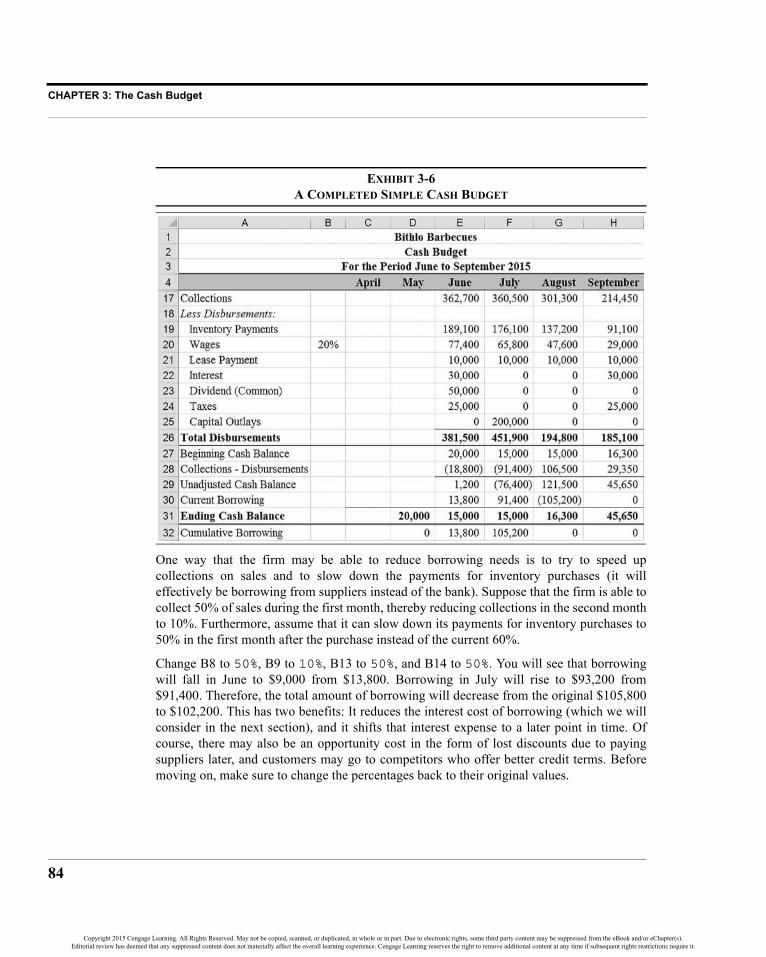
CHAPTER 3: The Cash Budget
84
EXHIBIT 3-6A COMPLETED SIMPLE CASH BUDGET
One way that the firm may be able to reduce borrowing needs is to try to speed upcollections on sales and to slow down the payments for inventory purchases (it willeffectively be borrowing from suppliers instead of the bank). Suppose that the firm is able tocollect 50% of sales during the first month, thereby reducing collections in the second monthto 10%. Furthermore, assume that it can slow down its payments for inventory purchases to50% in the first month after the purchase instead of the current 60%.
Change B8 to 50%, B9 to 10%, B13 to 50%, and B14 to 50%. You will see that borrowingwill fall in June to $9,000 from $13,800. Borrowing in July will rise to $93,200 from$91,400. Therefore, the total amount of borrowing will decrease from the original $105,800to $102,200. This has two benefits: It reduces the interest cost of borrowing (which we willconsider in the next section), and it shifts that interest expense to a later point in time. Ofcourse, there may also be an opportunity cost in the form of lost discounts due to payingsuppliers later, and customers may go to competitors who offer better credit terms. Beforemoving on, make sure to change the percentages back to their original values.
Copyright 2015 Cengage Learning. All Rights Reserved. May not be copied, scanned, or duplicated, in whole or in part. Due to electronic rights, some third party content may be suppressed from the eBook and/or eChapter(s).Editorial review has deemed that any suppressed content does not materially affect the overall learning experience. Cengage Learning reserves the right to remove additional content at any time if subsequent rights restrictions require it.

85
Calculating the Ending Cash Balance
As another example, consider Bithlo Barbecues’ $200,000 capital expenditure currentlyplanned for July 2015. This expenditure is the primary cause of the borrowing needed inJuly. Indeed, without this $200,000 outlay, the firm wouldn’t need to borrow in July.
Assuming that there is some flexibility in scheduling this outlay, in which month should theexpenditure be made? The answer, of course, depends on a number of factors, but we mightdecide to make the decision based on minimizing borrowing needs. That is, schedule theproject such that the firm’s short-term borrowing needs are minimized. This might beespecially important if the firm expected borrowing needs in excess of its line of credit in agiven month.
You can experiment a bit by changing the month in which the capital expenditure is made.First, however, it would be helpful to know the maximum expected borrowing for the four-month period. To do this we can make use of the MAX function, which is similar to MINexcept that it returns the largest of the arguments:
MAX(NUMBER1, NUMBER2, …)
In J32, enter the formula: =MAX(D32:H32) to calculate maximum borrowing. Now, bymoving the capital expenditure to different months, you should be able to verify the numbersin Table 3-3..
Obviously, by this criteria, the best time to schedule the outlay would be in either August orSeptember. Before continuing, be sure to move the $200,000 outlay back to July.
The Scenario ManagerIn the previous section, we performed what has come to be called a “What if?” analysis.That is, we changed the timing of the large capital expenditure to see what would happen tothe total amount of borrowing for the period. The problem with doing it “by hand” as we did
TABLE 3-3OPTIMAL SCHEDULING FOR A CAPITAL EXPENDITURE
Month of Outlay
Total Four-Month Borrowing
June $213,800July 105,200August 13,800September 13,800
Copyright 2015 Cengage Learning. All Rights Reserved. May not be copied, scanned, or duplicated, in whole or in part. Due to electronic rights, some third party content may be suppressed from the eBook and/or eChapter(s).Editorial review has deemed that any suppressed content does not materially affect the overall learning experience. Cengage Learning reserves the right to remove additional content at any time if subsequent rights restrictions require it.

CHAPTER 3: The Cash Budget
86
is that you lose the original results of your analysis after it is done. Also, every person wholooks at your spreadsheet will need to perform that same analysis. Excel provides a betterway—the Scenario Manager.
This tool allows us to store several scenarios (alternative input variables) in the spreadsheetand to display them at will. Once the scenario inputs are defined, we simply select a scenariofrom the list and Excel will enter the appropriate numbers into the spreadsheet andrecalculate. Figure 3-1 shows the Scenario Manager dialog box before any scenarios havebeen created.
FIGURE 3-1SCENARIO MANAGER DIALOG BOX WITH NO SCENARIOS DEFINED
To launch this tool, go to the Data tab. In the Data Tools group, click the What-If Analysisbutton and then choose Scenario Manager. When the dialog box is displayed, we can createour four scenarios. To begin, click the Add button. In the next dialog box enter:Expenditure in June for the Scenario name. The Changing cells are those cells thatwill contain different numbers under each scenario. In this case, they will be the capitaloutlay for each month, so enter: E25:H25 and click the OK button.
You will now be prompted to enter values for each of the changing cells for this scenario.Because our first scenario calls for the expenditure to be made in June, enter 200000 in thefirst box and 0 in each of the others. The Scenario Values dialog box should look like that inFigure 3-2.
Copyright 2015 Cengage Learning. All Rights Reserved. May not be copied, scanned, or duplicated, in whole or in part. Due to electronic rights, some third party content may be suppressed from the eBook and/or eChapter(s).Editorial review has deemed that any suppressed content does not materially affect the overall learning experience. Cengage Learning reserves the right to remove additional content at any time if subsequent rights restrictions require it.

87
Calculating the Ending Cash Balance
FIGURE 3-2SCENARIO VALUES DIALOG BOX FOR JUNE EXPENDITURE
Click the Add button to create the next scenario. Repeat these steps until you have fourscenarios with the expenditure occurring in different months.
Note that the Scenario Values dialog box prompts you for values by using the celladdresses as labels. That can be confusing, especially if the cells are not visible on thescreen. One way to make this situation better is to use defined names for the cells, as wasdiscussed in Chapter 1 (page 9). Close the Scenario Manager and then select E25. On theFormulas tab, click the Define Name button. Now, type June in the Name edit box. Selectthe worksheet name from the Scope drop-down list to limit this name to this worksheet andthen click the OK button. Name the other cells similarly. Launch the Scenario Managerand select the “Expenditure in June” scenario. Click the Edit button, then the OK button onthe Edit Scenario dialog, and your Scenario Values dialog box should look like the one inFigure 3-3.
FIGURE 3-3SCENARIO VALUES DIALOG BOX WITH DEFINED NAMES
Many of the other tools supplied with Excel work with range names in a similar way. This isa useful trick to remember as it can simplify entering data. As we will see shortly, usingrange names will also improve the Scenario Summary sheets. After creating your scenarios,the Scenario Manager dialog box will look like the one in Figure 3-4.
Copyright 2015 Cengage Learning. All Rights Reserved. May not be copied, scanned, or duplicated, in whole or in part. Due to electronic rights, some third party content may be suppressed from the eBook and/or eChapter(s).Editorial review has deemed that any suppressed content does not materially affect the overall learning experience. Cengage Learning reserves the right to remove additional content at any time if subsequent rights restrictions require it.

CHAPTER 3: The Cash Budget
88
FIGURE 3-4SCENARIO MANAGER DIALOG BOX WITH FOUR SCENARIOS
To display a particular scenario, simply select it from the list and click the Show button.Excel will alter the contents of your changing cells to reflect the values that you entered. Ofcourse, the entire worksheet will be recalculated and you can see the results of the selectedscenario. Note that to be able to scroll around and see the entire worksheet you must clickthe Close button on the Scenario Manager dialog box. Take a look at the results of eachscenario, but remember to reset the scenario to “Expenditure in July” (our default case)before continuing. If you forget to reset to the default scenario, Excel will always display thelast chosen scenario. This can cause confusion when you later open your workbook.
Being able to quickly change between scenarios is quite helpful, but the real advantage ofthe Scenario Manager is its ability to summarize the results of all of your scenarios. In thiscase, we would like to compare the total borrowing that results under each scenario todetermine the best time for the expenditure. Recall that we added a formula in J32 tocalculate the maximum borrowing for the period. Before continuing, define a name for thiscell such as “Max_Borrowing.” (Remember that we use the underscore in place of a spacebecause spaces are not allowed in range names.)
Return to the Scenario Manager and click on the Summary button. You will be asked to enterResult cells. A result cell is a cell (or several cells) that shows the end result of eachscenario. In this case, we are interested in maximum borrowing, so enter: J32 as the Resultcell and click the OK button. Excel will now create a new worksheet that summarizes yourscenario results. For our scenarios, the results are in Exhibit 3-7. Note that these results areexactly the same as those in Table 3-3.
Copyright 2015 Cengage Learning. All Rights Reserved. May not be copied, scanned, or duplicated, in whole or in part. Due to electronic rights, some third party content may be suppressed from the eBook and/or eChapter(s).Editorial review has deemed that any suppressed content does not materially affect the overall learning experience. Cengage Learning reserves the right to remove additional content at any time if subsequent rights restrictions require it.

89
Adding Interest and Investment of Excess Cash
EXHIBIT 3-7SCENARIO SUMMARY
Column D contains the values that were active when the scenario summary was created. Inmost cases that will just be a repeat of one of the existing scenarios. It is a good practice tomake sure that one of your scenarios reflects the default assumptions so that you can returnto the defaults easily. In this example, the numbers in columns D and F are identical, socolumn D can be safely deleted.
Adding Interest and Investment of Excess CashIn the previous section you created a basic cash budget for Bithlo Barbecues. In this sectionwe will refine the calculation of the ending cash balance by considering two additionalfactors. First, we will add interest payments on borrowed funds and then we will considerthe investment of excess cash.
Before beginning, let’s create a copy of the previous cash budget in the same workbook.Right-click the sheet tab labeled “Cash Budget” and select Move or Copy… from the menu.In the dialog box make sure to check the box labeled Create a copy and select “(move toend)” from the list. The copied sheet will now be named Cash Budget (2). Right-click thesheet tab and rename the new sheet to Complex Cash Budget.
Next, we will need to make a few additions to the notes at the bottom of the worksheet. Wewill now assume that Bithlo Barbecues will invest any cash in excess of $40,000. In A35 addthe label: Maximum Acceptable Cash and in B35 enter: 40,000. Furthermore, thefirm will have to pay interest on its short-term borrowings and will earn interest on invested
Copyright 2015 Cengage Learning. All Rights Reserved. May not be copied, scanned, or duplicated, in whole or in part. Due to electronic rights, some third party content may be suppressed from the eBook and/or eChapter(s).Editorial review has deemed that any suppressed content does not materially affect the overall learning experience. Cengage Learning reserves the right to remove additional content at any time if subsequent rights restrictions require it.

CHAPTER 3: The Cash Budget
90
funds. In A36 type: Borrowing Rate (Annual) and in B36 enter: 8%. In A37 add thelabel: Lending Rate (Annual) and enter: 6% in B37.
Because we are working with monthly time periods, we need to convert these annual ratesinto monthly rates of interest. So, in C36 and C37 enter the label: Monthly. We willconvert the annual rate to a monthly rate by dividing by 12. In D36 enter the formula:=B36/12, and copy this to D37.4 You should see that the monthly borrowing rate is 0.67%,and the monthly lending rate is 0.50%.
We are now ready to expand the cash budget to include investing and the interest expenseand income. Before entering any new formulas we need to insert a few new rows. Select row23 (the dividend), and then click the upper half of the Insert button on the Home tab. Thiswill insert a row above the selection. In A23 enter the label: Short-Term InterestExpense (Inc.). Next, select row 32 (the ending cash balance), insert a row, and enter:Current Investing into A32. Finally, select row 35 and insert a row. In A34 change thelabel to: Cumulative Borrowing (Investing) and in A35 type: CumulativeInterest Expense (Inc.). We need to keep track of the cumulative amount that isborrowed/invested so that we can calculate the monthly short-term interest expense/income.
We will enter the formula to calculate the cumulative amount of borrowing (investing) inD34. Positive amounts will represent borrowing, while negative numbers will representinvesting. To calculate the cumulative amount, add the previous period’s cumulative amountto current borrowing and subtract current investing. For May, in D34, the formula is:=C34+D31-D32, and the result should be 0. Copy this formula to E34:H34. Note that atthis point the result for each month should be equal to the cumulative current borrowing.
Short-term interest expense (income) can now be calculated by multiplying the cumulativeamount of borrowing (investing) from the previous month by the appropriate interest rate.So, in E23 we will use an IF statement to determine which rate to use. If the cumulativeamount of borrowing (investing) is positive, we will multiply it by the borrowing rate.Otherwise, use the lending rate. The formula for June, E23, is: =IF(D34>0,D34*$D$39,D34*$D$40). For June, because the firm has not had previous borrowing orlending, the result should be 0. Copy this across to F23:H23.
We can now calculate the cumulative interest expense (income) in E35. To do this, wesimply add the previous month’s interest expense (income) to the current month’s interestexpense (income). For June, the formula is: =D35+E23. This formula should be copiedacross to F35:H35. The only purpose of this row is to help evaluate the results of a scenariothat we will examine later. At this point, your worksheet should resemble the one inExhibit 3-8.
4. Entering the 12 into the denominator might seem to violate our prohibition on entering numbersinto formulas. However, there will always be 12 months in a year, so this number will never change.
Copyright 2015 Cengage Learning. All Rights Reserved. May not be copied, scanned, or duplicated, in whole or in part. Due to electronic rights, some third party content may be suppressed from the eBook and/or eChapter(s).Editorial review has deemed that any suppressed content does not materially affect the overall learning experience. Cengage Learning reserves the right to remove additional content at any time if subsequent rights restrictions require it.
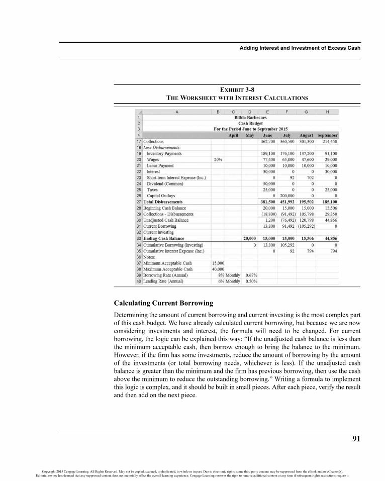
91
Adding Interest and Investment of Excess Cash
EXHIBIT 3-8THE WORKSHEET WITH INTEREST CALCULATIONS
Calculating Current BorrowingDetermining the amount of current borrowing and current investing is the most complex partof this cash budget. We have already calculated current borrowing, but because we are nowconsidering investments and interest, the formula will need to be changed. For currentborrowing, the logic can be explained this way: “If the unadjusted cash balance is less thanthe minimum acceptable cash, then borrow enough to bring the balance to the minimum.However, if the firm has some investments, reduce the amount of borrowing by the amountof the investments (or total borrowing needs, whichever is less). If the unadjusted cashbalance is greater than the minimum and the firm has previous borrowing, then use the cashabove the minimum to reduce the outstanding borrowing.” Writing a formula to implementthis logic is complex, and it should be built in small pieces. After each piece, verify the resultand then add on the next piece.
Copyright 2015 Cengage Learning. All Rights Reserved. May not be copied, scanned, or duplicated, in whole or in part. Due to electronic rights, some third party content may be suppressed from the eBook and/or eChapter(s).Editorial review has deemed that any suppressed content does not materially affect the overall learning experience. Cengage Learning reserves the right to remove additional content at any time if subsequent rights restrictions require it.

CHAPTER 3: The Cash Budget
92
Writing this formula requires the use of nested IF statements. That is, we embed additionalIF statements within the first. In pseudocode this is:
If Unadjusted Cash < Minimum Cash then {Firm needs to raise funds}If Cumulative Borrowing (Investing) < 0 then {Firm has investments it can sell}
Current Borrowing = Max(Minimum Cash + Cumulative Borrowing (Investing) – Unadjusted Cash, 0)Else Current Borrowing = Minimum Cash – Unadjusted Cash {Must Borrow it all}
Else {Firm doesn’t need to raise funds}If Cumulative Borrowing (Investing) > 0 then {Use excess funds to reduce previous borrowings}
Current Borrowing = –Min(Cumulative Borrowing (Investing), Unadjusted Cash – Minimum Cash)Else Current Borrowing = 0
End If
The formula to calculate current borrowing in June, E31, is: =IF(E30<$B$37,IF(D34<0,MAX($B$37+D34-E30,0),$B$37-E30),IF(D34>0,-MIN(D34,E30-$B$37),0)). Type this formula carefully, and then copyit to F31:H31. Note that we have also used the built-in MAX and MIN functions as discussedearlier in the chapter. In this formula, the MAX function is required to be sure that we don’tend up with negative borrowing if the investments are more than sufficient to cover cashneeds (i.e., we don’t want to sell all of the investments if we don’t need to). The MINfunction is used when the firm has excess cash and has some outstanding loans to pay off. Itfinds the minimum of either (1) the cumulative amount of borrowing outstanding or (2) thedifference between the unadjusted cash balance and the minimum acceptable cash balance.Note that we had to negate the result of the MIN function in order to get the correct result.
Using the Formula Auditing Tools to Avoid ErrorsSometimes the logic you need to solve a problem can get a bit complicated, as above. It isimportant to carefully think it through and build your formulas one small piece at a time. Inthis way we can slowly build up to a large, complex formula that always works. That’sexactly how the above formula was created. However, no matter how careful you are inbuilding a complex formula there is always the possibility of errors creeping in. Fortunately,there are several ways to identify these errors before they become serious problems (i.e., costyou or your company real money).
One of the best ways to avoid errors is to thoroughly test your formulas. The easiest way todo this is to change some numbers that the formula depends on and make sure that you arestill getting correct answers. For example, we might temporarily change our ending cashbalance in May. Then, carefully work through the ending cash balance calculations to makesure that they are working correctly.
Finding errors in the first version of a complex formula is very common. Fortunately, Excelprovides several tools to help find and correct the cause. In the following subsections, wewill take a short detour from our example to discuss these tools.
Copyright 2015 Cengage Learning. All Rights Reserved. May not be copied, scanned, or duplicated, in whole or in part. Due to electronic rights, some third party content may be suppressed from the eBook and/or eChapter(s).Editorial review has deemed that any suppressed content does not materially affect the overall learning experience. Cengage Learning reserves the right to remove additional content at any time if subsequent rights restrictions require it.

93
Adding Interest and Investment of Excess Cash
Using the F9 Function KeyOne of Excel’s first, most useful, and probably least known debugging tools is the F9function key. Normally, pressing F9 causes a worksheet to recalculate, but when you use itin the formula bar it shows the contents of a cell address or the result of a calculation. Forexample, select E31 and highlight the first condition in the IF statement as shown inFigure 3-5.
FIGURE 3-5USING THE F9 KEY IN THE FORMULA BAR
When you press F9, Excel evaluates the expression “E30<$B$37” and then reports that theresult is true (E30 is, in fact, less than B37). Note that we also could have highlighted just the“E30” part of this expression and, after pressing F9, Excel would show that the value in E30is equal to 1,200. Now, applying the same technique to the other part of the expressionwould show that B37 is equal to 15,000. At this point, the first part of the formula wouldshow as “1200<15000” which is obviously true. This technique is very useful for checkingparts of a formula to make sure they are accurate.
One important caveat is that if you now press Enter to return to the worksheet, your formulawill be changed to include the results instead of reverting to the cell addresses. It is crucial topress the Esc key rather than Enter in order to avoid locking in the changes you’ve made.
Color-Coded Cell AddressesAnother member of the error-checking toolkit is the use of color coding in formulas. Whenyou create or edit a formula, Excel colors the cell addresses and highlights each of thosecells in that same color. This makes it easy to see which cells are being used. If you noticethat you’ve used an incorrect cell or range, you can grab the colored outline and expand,contract, or move it to another location. This will change the appropriate cell or range ofcells in your formula.
Formula Auditing ToolsThe tools in the Formula Auditing group help you to trace errors, step through a calculationsequence, and watch the result in one cell as you edit another. To access these tools, click theFormulas tab of the Ribbon and look for the group shown in Figure 3-6.
Copyright 2015 Cengage Learning. All Rights Reserved. May not be copied, scanned, or duplicated, in whole or in part. Due to electronic rights, some third party content may be suppressed from the eBook and/or eChapter(s).Editorial review has deemed that any suppressed content does not materially affect the overall learning experience. Cengage Learning reserves the right to remove additional content at any time if subsequent rights restrictions require it.

CHAPTER 3: The Cash Budget
94
FIGURE 3-6THE FORMULA AUDITING TOOLBAR
Tracing Precedent and Dependent CellsThe three buttons on the left side of the Formula Auditing group are for tracing precedent ordependent cells. A precedent cell is one upon which a formula depends, while a dependentcell is one that depends on the result of the formula in the active cell. If the active cellcontains a formula, clicking Trace Precedents will display arrows from the precedent cells.The arrows in Exhibit 3-3 (page 78) were created in this way. The Trace Dependents iconworks in the same way, except that the arrows point to dependent cells.
To remove all of the arrows click the Remove Arrows button, or save the file. Note that thisbutton is also a drop-down list that allows you to remove only the precedent or dependentarrows.
Background Error CheckingUnless this option is disabled, Excel will examine the worksheet for common types of errorsas you work. If background error checking is on, a green triangle will appear in the upper leftcorner of the cell along with a Smart Tag that explains the error and offers a solution. Errorsin logic cannot, of course, be detected, but it can identify many other types of errors.
Be aware that in some cases Excel will think that you’ve made an error when you have not.Don’t automatically accept the proposed fix. If this happens repeatedly, you can tell Excel tostop checking for that type of error, or turn off background error checking completely. Tochange the error checking rules, go to the Formulas area in Options from the File tab.
The Watch WindowWhen working on a large worksheet, it is common to find yourself changing a value in onelocation and then scrolling to another to check the result. The Watch Window is a powerfultool that helps speed up formula debugging by letting you watch a distant cell withouthaving to scroll to it. It even works with cells in other worksheets, but only in the sameworkbook. To activate this tool, click on the Watch Window button in the Formula Auditinggroup.
Copyright 2015 Cengage Learning. All Rights Reserved. May not be copied, scanned, or duplicated, in whole or in part. Due to electronic rights, some third party content may be suppressed from the eBook and/or eChapter(s).Editorial review has deemed that any suppressed content does not materially affect the overall learning experience. Cengage Learning reserves the right to remove additional content at any time if subsequent rights restrictions require it.

95
Adding Interest and Investment of Excess Cash
FIGURE 3-7THE WATCH WINDOW
Once the Watch Window is displayed, you can choose one or more cells to watch by clickingthe Add Watch button and choosing the cell. In Figure 3-7, we have selected E31. With thiswindow displayed you can scroll to any part of the worksheet, change a cell value, and seewhat happens to E31. Note that if you close the Watch Window (or even save and close theworkbook), the watch cells are not cleared. That allows you to open it again to continuewatching the cell.
The Evaluate Formula ToolFinally, perhaps the best feature for formula debugging is the Evaluate Formula tool. Thistool lets you step through a formula piece by piece as Excel evaluates it. It works much likethe F9 function key, except that it will step through the entire formula one step at a time. Toactivate this tool, click the Evaluate Formula button shown in Figure 3-6.
Figure 3-8 shows the Evaluate Formula dialog box with the formula in E31 ready to beevaluated. Note that E30 is underlined, indicating that it will be evaluated first. Simply clickthe Evaluate button and “E30” will be replaced with “1200.” Now, $B$37 will be underlinedand ready to be evaluated. You can continue to click the Evaluate button to work through theentire formula.
FIGURE 3-8THE EVALUATE FORMULA TOOL
An additional feature is the Step In function. For those expressions that themselves are theresult of a formula, you can “step in” to the previous formula and evaluate it. For example,D34 is actually the result of the formula =C34+D31–D32. When D34 is underlined, clicking
Copyright 2015 Cengage Learning. All Rights Reserved. May not be copied, scanned, or duplicated, in whole or in part. Due to electronic rights, some third party content may be suppressed from the eBook and/or eChapter(s).Editorial review has deemed that any suppressed content does not materially affect the overall learning experience. Cengage Learning reserves the right to remove additional content at any time if subsequent rights restrictions require it.
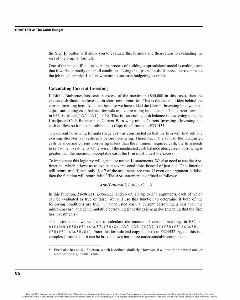
CHAPTER 3: The Cash Budget
96
the Step In button will allow you to evaluate this formula and then return to evaluating therest of the original formula.
One of the most difficult tasks in the process of building a spreadsheet model is making surethat it works correctly under all conditions. Using the tips and tools discussed here can makethe job much simpler. Let’s now return to our cash budgeting example.
Calculating Current InvestingIf Bithlo Barbecues has cash in excess of the maximum ($40,000 in this case), then theexcess cash should be invested in short-term securities. This is the essential idea behind thecurrent investing item. Note that because we have added the Current Investing line, we mustadjust our ending cash balance formula to take investing into account. The correct formula,in E33, is: =SUM(E30:E31)-E32. That is, our ending cash balance is now going to be theUnadjusted Cash Balance plus Current Borrowing minus Current Investing. (Investing is acash outflow so it must be subtracted.) Copy this formula to F33:H33.
The current borrowing formula (page 92) was constructed so that the firm will first sell anyexisting short-term investments before borrowing. Therefore, if the sum of the unadjustedcash balance and current borrowing is less than the minimum required cash, the firm needsto sell some investments. Otherwise, if the unadjusted cash balance plus current borrowing isgreater than the maximum acceptable cash, the firm must invest the excess.
To implement this logic we will again use nested IF statements. We also need to use the ANDfunction, which allows us to evaluate several conditions instead of just one. This functionwill return true if, and only if, all of the arguments are true. If even one argument is false,then the function will return false.5 The AND statement is defined as follows:
AND(LOGICAL1, LOGICAL2, …)
In this function, LOGICAL1, LOGICAL2, and so on, are up to 255 arguments, each of whichcan be evaluated as true or false. We will use this function to determine if both of thefollowing conditions are true: (1) unadjusted cash + current borrowing is less than theminimum cash, and (2) cumulative borrowing (investing) is negative (meaning that the firmhas investments).
The formula that we will use to calculate the amount of current investing, in E32, is:=IF(AND(E30+E31<$B$37,D34<0),E30+E31-$B$37,IF(E30+E31>$B$38,E30+E31-$B$38,0)). Enter this formula and copy it across to F32:H32. Again, this is acomplex formula, but it can be broken down into more understandable components:
5. Excel also has an OR function, which is defined similarly. However, it will return true when one, ormore, of the arguments is true.
Copyright 2015 Cengage Learning. All Rights Reserved. May not be copied, scanned, or duplicated, in whole or in part. Due to electronic rights, some third party content may be suppressed from the eBook and/or eChapter(s).Editorial review has deemed that any suppressed content does not materially affect the overall learning experience. Cengage Learning reserves the right to remove additional content at any time if subsequent rights restrictions require it.

97
Adding Interest and Investment of Excess Cash
If Unadjusted Cash + Borrowing < Minimum Cash AND Cumulative Borrowing (Investing) < 0 thenCurrent Investing = Unadjusted Cash + Borrowing – Minimum Cash
ElseIf Unadjusted Cash + Borrowing > Maximum Cash then
Current Investing = Unadjusted Cash + Borrowing – Maximum CashElse
Current Investing = 0End.
Your cash budget should now resemble that in Exhibit 3-9.
EXHIBIT 3-9CALCULATING THE CASH BALANCE WITH BORROWING AND INVESTING
Working Through the ExampleIn order to understand the complex cash budget, you must work through it line by line. Inthis section, we will do just that. Follow along in Exhibit 3-9.
June (column E): The unadjusted cash balance in June is projected to be only $1,200. Because this is less than the $15,000 minimum, the firm needs to raise funds. In this case it has no investments to sell, so it must borrow $13,800 to bring the ending cash balance to $15,000.July (column F): The firm is projecting that it will be overdrawn by $76,492. Again, it has no investments to sell and must borrow an additional $91,492. Note that the cumula-tive borrowing is now $105,292.August (column G): The firm is projecting an unadjusted cash balance of $120,798, well in excess of the maximum allowable cash. Before investing the excess, however, it needs to pay off the $105,292 of existing short-term debt. In this case, the firm can pay
Copyright 2015 Cengage Learning. All Rights Reserved. May not be copied, scanned, or duplicated, in whole or in part. Due to electronic rights, some third party content may be suppressed from the eBook and/or eChapter(s).Editorial review has deemed that any suppressed content does not materially affect the overall learning experience. Cengage Learning reserves the right to remove additional content at any time if subsequent rights restrictions require it.

CHAPTER 3: The Cash Budget
98
off the entire balance and still remain above the minimum cash requirement. However, after paying down the loans, its cash balance is not high enough to cause investment of excess funds.September (column H): The firm is projecting that the unadjusted cash balance will be $44,856. In this case, there is no borrowing balance, so the $4,856 in excess of the max-imum allowable cash can be invested and the ending cash balance will be $40,000. Note that the Cumulative Borrowing (Investing) in H34 is negative, indicating that the funds represent investments.
In any complex worksheet, such as this one, it is important that you work through thecalculations by hand to check the results. Never accept the output until you are sure that it isabsolutely correct. With this in mind, let’s make two changes: First, set the maximumacceptable cash in B38 to $15,000. Now, set the unadjusted cash balance for May to$20,000 and copy E31:E33 to D31:D33. Make sure that this portion of your worksheet isthe same as that in Exhibit 3-10, and then carefully go over the worksheet.
EXHIBIT 3-10CASH BALANCE AFTER CHANGING MAXIMUM CASH TO $15,000
May (column D): The unadjusted cash balance is greater than the minimum cash, so it does not need to borrow. In fact, it has $5,000 more than the maximum allowable cash that can be invested. The ending cash balance is $15,000.June (column E): The firm is projecting the unadjusted cash balance to be –$3,775, but it does not borrow $18,775 because it has $5,000 in investments from May that reduce the borrowing need to only $13,775. Current Investing, therefore, is –$5,000.July (column F): The unadjusted cash balance is projected to be –$76,492 and there are no investments that can be sold. Therefore, the firm must borrow $91,492. The cumula-tive borrowing is now $105,267.
Copyright 2015 Cengage Learning. All Rights Reserved. May not be copied, scanned, or duplicated, in whole or in part. Due to electronic rights, some third party content may be suppressed from the eBook and/or eChapter(s).Editorial review has deemed that any suppressed content does not materially affect the overall learning experience. Cengage Learning reserves the right to remove additional content at any time if subsequent rights restrictions require it.

99
Summary
August (column G): The firm is expected to have a large surplus of funds, which can be used to pay off the entire loan balance. Furthermore, it will have $531 in excess of the maximum allowable cash that is available to invest.September (column H): The unadjusted cash balance is expected to be $44,353, which is $29,353 in excess of the maximum. This amount can be invested.
You are encouraged to experiment by changing values throughout the cash budget to seewhat happens. In particular, changing the projected sales and/or the payment schedule can bevery enlightening. For example, suppose that Bithlo Barbecues’ management decides toslow down payments for inventory purchases. Specifically, assume that it decides to payonly 40% in the month after the purchase and 60% two months after the purchase. Youshould find that this is not as good an idea as it sounds. Table 3-4 shows CumulativeBorrowing (Investing) before and after the change, assuming that the maximum cash is still$15,000. Note that the firm would end up borrowing a little more under this scenario, and thetotal interest paid would be higher.
SummaryIn this chapter, we have seen that the cash budget is simply a listing of the firm’s expectedcash inflows and outflows over a period of time. Cash budgets are useful in determining thefirm’s short-term borrowing and investing needs as well as scheduling transactions.Furthermore, it can be used when forecasting the financial statements. The cash budget iscomposed of three sections: (1) the worksheet area; (2) a listing of collections and
TABLE 3-4CUMULATIVE BORROWING (INVESTING)
Month Before AfterMay (5,000) (5,000)June 13,775 11,575July 105,267 108,852August (531) 12,178September (29,984) (7,791)Cumulative Interest Expense Through September 766 859
Copyright 2015 Cengage Learning. All Rights Reserved. May not be copied, scanned, or duplicated, in whole or in part. Due to electronic rights, some third party content may be suppressed from the eBook and/or eChapter(s).Editorial review has deemed that any suppressed content does not materially affect the overall learning experience. Cengage Learning reserves the right to remove additional content at any time if subsequent rights restrictions require it.
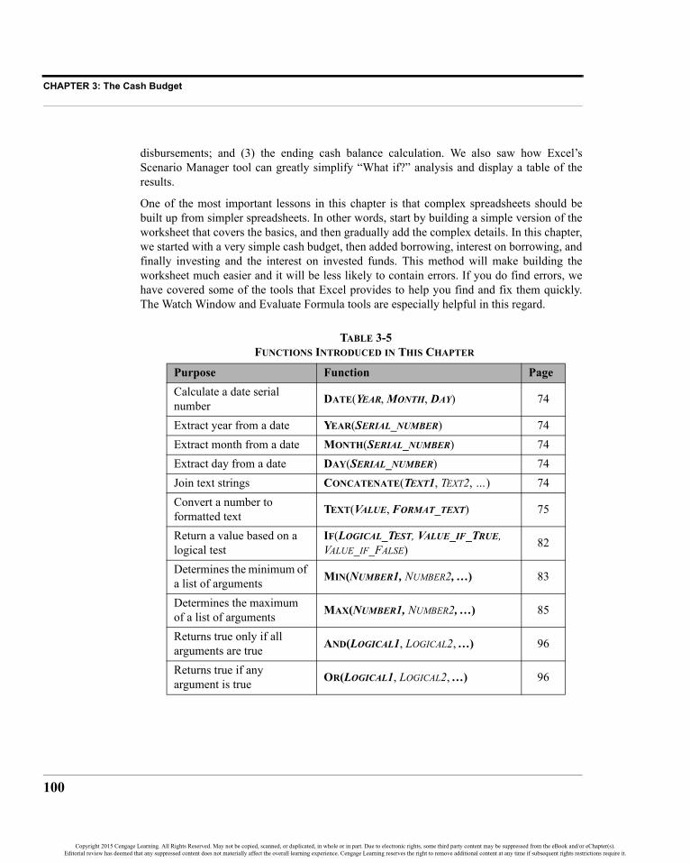
CHAPTER 3: The Cash Budget
100
disbursements; and (3) the ending cash balance calculation. We also saw how Excel’sScenario Manager tool can greatly simplify “What if?” analysis and display a table of theresults.
One of the most important lessons in this chapter is that complex spreadsheets should bebuilt up from simpler spreadsheets. In other words, start by building a simple version of theworksheet that covers the basics, and then gradually add the complex details. In this chapter,we started with a very simple cash budget, then added borrowing, interest on borrowing, andfinally investing and the interest on invested funds. This method will make building theworksheet much easier and it will be less likely to contain errors. If you do find errors, wehave covered some of the tools that Excel provides to help you find and fix them quickly.The Watch Window and Evaluate Formula tools are especially helpful in this regard.
TABLE 3-5FUNCTIONS INTRODUCED IN THIS CHAPTER
Purpose Function PageCalculate a date serial number DATE(YEAR, MONTH, DAY) 74
Extract year from a date YEAR(SERIAL_NUMBER) 74Extract month from a date MONTH(SERIAL_NUMBER) 74Extract day from a date DAY(SERIAL_NUMBER) 74Join text strings CONCATENATE(TEXT1, TEXT2, …) 74Convert a number to formatted text TEXT(VALUE, FORMAT_TEXT) 75
Return a value based on a logical test
IF(LOGICAL_TEST, VALUE_IF_TRUE, VALUE_IF_FALSE) 82
Determines the minimum of a list of arguments MIN(NUMBER1, NUMBER2, …) 83
Determines the maximum of a list of arguments MAX(NUMBER1, NUMBER2, …) 85
Returns true only if all arguments are true AND(LOGICAL1, LOGICAL2, …) 96
Returns true if any argument is true OR(LOGICAL1, LOGICAL2, …) 96
Copyright 2015 Cengage Learning. All Rights Reserved. May not be copied, scanned, or duplicated, in whole or in part. Due to electronic rights, some third party content may be suppressed from the eBook and/or eChapter(s).Editorial review has deemed that any suppressed content does not materially affect the overall learning experience. Cengage Learning reserves the right to remove additional content at any time if subsequent rights restrictions require it.

101
Problems
Problems
1. Lakewood Laser SkinCare’s ending cash balance as of January 31, 2015(the end of its fiscal year 2014) was $15,000. Its expected cash collectionsand payments for the next six months are given in the following table.
a. Calculate the firm’s expected ending cash balance for each month.
b. Assuming that the firm must maintain an ending cash balance of atleast $12,000, how much must they borrow during each month?
c. If the firm must pay 5% annual interest on its short-term borrowing,what are your ending cash balances for each month?
d. What are the ending cash balances if the firm uses any cash in excessof the minimum to pay off its short-term borrowing in each month?
2. Loblaw Manufacturing has asked you to create a cash budget in order todetermine its borrowing needs for the June to October period. You havegathered the following information.
Month Collections PaymentsFebruary $24,750 $29,100March 27,450 31,200April 34,050 32,400May 43,650 36,450June 48,750 40,050July 54,000 40,800
Month Sales Other PaymentsJune 2015 $223,600 $104,000July 184,600 97,500August 157,300 91,000September 120,900 65,000October 98,800 58,500November 105,300
Copyright 2015 Cengage Learning. All Rights Reserved. May not be copied, scanned, or duplicated, in whole or in part. Due to electronic rights, some third party content may be suppressed from the eBook and/or eChapter(s).Editorial review has deemed that any suppressed content does not materially affect the overall learning experience. Cengage Learning reserves the right to remove additional content at any time if subsequent rights restrictions require it.

CHAPTER 3: The Cash Budget
102
April and May sales were $149,500 and $175,500, respectively. The firmcollects 25% of its sales during the month, 60% the following month, and15% two months after the sale. Each month it purchases inventory equal to60% of the next month’s expected sales. The company pays for 40% of itsinventory purchases in the same month and 60% in the following month.However, the firm’s suppliers give it a 2% discount if it pays during thesame month as the purchase. A minimum cash balance of $25,000 must bemaintained each month, and the firm pays 4% annually for short-termborrowing from its bank.
a. Create a cash budget for June to October 2015. The cash budgetshould account for short-term borrowing and payback of outstandingloans as well as the interest expense. The firm ended May with a$30,000 unadjusted cash balance.
b. Bob Loblaw, the president, is considering stretching out its inventorypayments. He believes that it may be less expensive to borrow fromsuppliers than from the bank. He has asked you to use the ScenarioManager to see what the total interest cost for this time period wouldbe if the company paid for 0%, 10%, 30%, or 40% of its inventorypurchases in the same month. The remainder would be paid in thefollowing month. Create a scenario summary, and describe whetherthe results support Bob’s beliefs.
3. Camp and Fevurly Financial Planners have forecasted revenues for thefirst six months of 2015, as shown in the following table.
The firm collects 60% of its sales immediately, 39% one month after thesale, and 1% are written off as bad debts two months after the sale. Thefirm assumes that wages and benefits paid to clerical personnel will be$7,000 per month while commissions to sales associates average 25% ofcollectable sales. Each of the two partners is paid $5,000 per month or20% of net sales, whichever is greater. Commissions and partner salariesare paid one month after the revenue is earned. Rent expense for theiroffice space is $3,500 per month, and lease expense for office equipment
Month Revenue Month RevenueNovember 2014 $38,400 March 24,000December 36,000 April 30,400January 2015 20,000 May 32,000February 21,600 June 36,000
Copyright 2015 Cengage Learning. All Rights Reserved. May not be copied, scanned, or duplicated, in whole or in part. Due to electronic rights, some third party content may be suppressed from the eBook and/or eChapter(s).Editorial review has deemed that any suppressed content does not materially affect the overall learning experience. Cengage Learning reserves the right to remove additional content at any time if subsequent rights restrictions require it.

103
Problems
is $800. Utilities average $250 per month, except in May and June whenthey average only $150. The ending cash balance in December 2014 was$12,000.
a. Create a cash budget for January to June 2015, and determine thefirm’s ending cash balance in each month assuming that the partnerswish to maintain a minimum cash balance of $10,000.
b. Camp and Fevurly are thinking of obtaining a line of credit from theirbank. Based on their expectations for the first six months of the year,what is the minimum amount that would be necessary? Round youranswer to the next highest $1,000 and ignore interest charges onshort-term debt. (Hint: Look up the ROUNDUP function in the onlinehelp.)
c. Create three scenarios (best case, base case, and worst case) assumingthat revenues are 10% better than expected, exactly as expected, or10% worse than expected. What is the maximum that the firm wouldneed to borrow to maintain its minimum cash balance in all threecases? Use the Scenario Manager, and create a summary of yourresults. Would this change your answer in part b?
4. You were recently hired to improve the financial condition of IdahoSprings Hardware, a small chain of three hardware stores in Colorado. Onyour first day the owner, Chuck Vitaska, told you that the biggest problemfacing the firm has been periodic unexpected cash shortages that havemade it necessary for him to delay wage payments to his employees.Having recently received a degree in finance, you immediately realize thatyour first priority is to develop a cash budget and to arrange for a short-term borrowing agreement with the firm’s bank. After looking at thefirm’s past financial records, you developed a sales forecast for theremainder of the year, as is presented in the following table.
In addition to the seasonality of sales, you have observed several otherpatterns. Individuals account for 40% of the firm’s sales, and they pay incash. The other 60% of sales are to contractors with credit accounts, and
Month Sales Month SalesJune 2015 $68,200 October 64,900July 80,300 November 51,700August 83,600 December 45,100September 77,000
Copyright 2015 Cengage Learning. All Rights Reserved. May not be copied, scanned, or duplicated, in whole or in part. Due to electronic rights, some third party content may be suppressed from the eBook and/or eChapter(s).Editorial review has deemed that any suppressed content does not materially affect the overall learning experience. Cengage Learning reserves the right to remove additional content at any time if subsequent rights restrictions require it.

CHAPTER 3: The Cash Budget
104
they have up to 60 days to pay. As a result, about 20% of sales tocontractors are paid one month after the sale, and the other 80% is paidtwo months after the sale. Each month the firm purchases inventory equalto about 45% of the following month’s sales. About 30% of this inventoryis paid for in the month of delivery, while the remaining 70% is paid onemonth later.
Each month the company pays its hourly employees a total of $10,000,including benefits. Its salaried employees are paid $14,000, also includingbenefits. In the past, the company had to borrow to build its stores and forthe initial inventories. This debt has resulted in monthly interest paymentsof $4,000 and monthly principal payments of $221. On average,maintenance at the stores is expected to cost about $800 per month, exceptOctober to December when snow removal costs will add about $200 permonth. Sales taxes are 7% of quarterly sales and must be paid in June,September, and December. Other taxes are also paid during those monthsand are expected to be about 4% of quarterly sales in each of thosemonths. The owner wishes to maintain a cash balance of at least $12,000to limit the risk of cash shortages. The cash balance at the end of May isexpected to be $15,000 (before any borrowing or investing).
a. Create a simple cash budget for Idaho Springs Hardware for June toDecember. Note that your records indicate that sales in April and Maywere $56,100 and $62,700, respectively. January 2016 sales areexpected to be $39,600. What would be the ending cash balances ifthe firm does not borrow to maintain its $12,000 minimum?
b. Now assume that the firm can borrow from the bank at a rate of 6%per annum to maintain its liquidity and meet its required minimumcash balance. In addition, if the firm has funds in excess of theminimum, it will use the excess to pay off any previous balance.
c. While negotiating a line of credit, the firm’s bank offered to sweepany cash in excess of the minimum into a money market fund that willreturn an average of 4% per year after expenses. If you accept thisoffer, how will it affect the firm’s ending cash balances and need toborrow in each month? Note that the firm must have paid off all short-term loans before any excess cash can be invested, and invested fundswill be used instead of borrowing when needed.
d. After completing the cash budget, you begin to think of ways tofurther reduce the firm’s borrowing needs. One idea that comes tomind is changing the firm’s credit policy with contractors because
Copyright 2015 Cengage Learning. All Rights Reserved. May not be copied, scanned, or duplicated, in whole or in part. Due to electronic rights, some third party content may be suppressed from the eBook and/or eChapter(s).Editorial review has deemed that any suppressed content does not materially affect the overall learning experience. Cengage Learning reserves the right to remove additional content at any time if subsequent rights restrictions require it.

105
Problems
they seem to always pay at the last minute. Three scenarios come tomind: (1) In the best case, contractors are required to pay for 100% oftheir purchases during the month after the sale. You believe that thiswould cause a 5% decline in sales. (2) In the base case, everythingremains as already outlined. (3) In the worst case, contractors wouldbe required to pay for 100% of their purchases during the month afterthe sale, and you believe that this would cause a 20% drop in sales.You decide to use the Scenario Manager to evaluate these scenarios.To summarize the impact of the change, you will examine the impacton the firm’s maximum borrowing needs and cumulative net interestcost (after accounting for investment earnings). In your opinion,should the firm change its credit policy?
Copyright 2015 Cengage Learning. All Rights Reserved. May not be copied, scanned, or duplicated, in whole or in part. Due to electronic rights, some third party content may be suppressed from the eBook and/or eChapter(s).Editorial review has deemed that any suppressed content does not materially affect the overall learning experience. Cengage Learning reserves the right to remove additional content at any time if subsequent rights restrictions require it.

Copyright 2015 Cengage Learning. All Rights Reserved. May not be copied, scanned, or duplicated, in whole or in part. Due to electronic rights, some third party content may be suppressed from the eBook and/or eChapter(s).Editorial review has deemed that any suppressed content does not materially affect the overall learning experience. Cengage Learning reserves the right to remove additional content at any time if subsequent rights restrictions require it.

107
CHAPTER 4 Financial Statement Analysis Tools
In previous chapters, we have seen how the firm’s basic financial statements are constructed.In this chapter, we will see how financial analysts can use the information contained in theincome statement and balance sheet for various purposes.
Many tools are available for use when evaluating a company, but some of the most valuableare financial ratios. Ratios are an analyst’s microscope; they allow us to get a better view ofthe firm’s financial health than just looking at the raw financial statements. A ratio is simply acomparison of two numbers by division. We could also compare numbers by subtraction, buta ratio is superior in most cases because it is a measure of relative size. Relative measures
After studying this chapter, you should be able to:1. Describe the purpose of financial ratios and who uses them.2. Define the five major categories of ratios (liquidity, efficiency, leverage,
coverage, and profitability).3. Calculate the common ratios for any firm by using income statement and
balance sheet data.4. Use financial ratios to assess a firm’s past performance, identify its current
problems, and suggest strategies for dealing with these problems.5. Calculate the economic profit earned by a firm.
Copyright 2015 Cengage Learning. All Rights Reserved. May not be copied, scanned, or duplicated, in whole or in part. Due to electronic rights, some third party content may be suppressed from the eBook and/or eChapter(s).Editorial review has deemed that any suppressed content does not materially affect the overall learning experience. Cengage Learning reserves the right to remove additional content at any time if subsequent rights restrictions require it.
CHAPTER 4: Financial Statement Analysis Tools
108
are more easily compared to previous time periods or to other firms than changes in dollaramounts.
Ratios are useful to both internal and external analysts of the firm. For internal purposes,ratios can be useful in planning for the future, setting goals, and evaluating the performanceof managers. External analysts use ratios to decide whether or not to grant credit, to monitorfinancial performance, to forecast financial performance, and to decide whether to invest inthe company.
We will look at many different ratios, but you should be aware that these are, of necessity,only a sampling of the ratios that might be useful. Furthermore, different analysts maycalculate ratios slightly differently, so you will need to know exactly how the ratios arecalculated in a given situation. The keys to understanding ratio analysis are experience andan analytical mind.
We will divide our discussion of the ratios into five categories based on the informationprovided:
1. Liquidity ratios describe the ability of a firm to meets its short-termobligations. They compare current assets to current liabilities.
2. Efficiency ratios describe how well the firm is using its investment invarious types of assets to produce sales. They may also be called assetmanagement ratios.
3. Leverage ratios reveal the degree to which debt has been used to financethe firm’s asset purchases. These ratios are also known as debtmanagement ratios.
4. Coverage ratios are similar to liquidity ratios in that they describe theability of a firm to pay certain expenses.
5. Profitability ratios provide indications of how profitable a firm has beenover a period of time.
One additional category, relative value ratios, will be discussed in Chapter 8 on page 254.Before we begin the discussion of individual financial ratios, open your Elvis ProductsInternational workbook from Chapter 2, and add a new worksheet named “Ratios.”
Liquidity RatiosThe term “liquidity” refers to the speed with which an asset can be converted into cashwithout large discounts to its value. Some assets, such as accounts receivable, can easily beconverted into cash with only small discounts. Other assets, such as buildings, can beconverted into cash very quickly only if large price concessions are given. We therefore saythat accounts receivable are more liquid than buildings.
Copyright 2015 Cengage Learning. All Rights Reserved. May not be copied, scanned, or duplicated, in whole or in part. Due to electronic rights, some third party content may be suppressed from the eBook and/or eChapter(s).Editorial review has deemed that any suppressed content does not materially affect the overall learning experience. Cengage Learning reserves the right to remove additional content at any time if subsequent rights restrictions require it.

109
Liquidity Ratios
All other things being equal, a firm with more liquid assets will be more able to meet itsmaturing obligations (e.g., its accounts payable and other short-term debts) than a firm withfewer liquid assets. As you might imagine, creditors are particularly concerned with a firm’sability to pay its bills. To assess this ability, it is common to use the current ratio and/or thequick ratio.
The Current RatioGenerally, a firm’s current assets are converted to cash (e.g., collecting on accountsreceivable or selling its inventories) and this cash is used to retire its current liabilities.Therefore, it is logical to assess a firm’s ability to pay its bills by comparing the size of itscurrent assets to the size of its current liabilities. The current ratio does exactly this. It isdefined as:
(4-1)
Obviously, the higher the current ratio, the higher the likelihood that a firm will be able topay its bills. So, from the creditor’s point of view, higher is better. However, from ashareholder’s point of view this is not always the case. Current assets usually have a lowerexpected return than do fixed assets, so the shareholders would like to see that only theminimum amount of the company’s capital is invested in current assets. Of course, too littleinvestment in current assets could be disastrous for both creditors and owners of the firm.
We can calculate the current ratio for 2014 for EPI by looking at the balance sheet (Exhibit2-2, page 50). In this case, we have:
meaning that EPI has 2.39 times as many current assets as current liabilities. We willdetermine later whether this is sufficient or not.
Exhibit 4-1 shows the beginnings of our “Ratios” worksheet. Enter the labels as shown. Wecan calculate the current ratio for 2014 in B5 with the formula: ='Balance Sheet'!B8/'Balance Sheet'!B17. After formatting to show two decimal places, you will see thatthe current ratio is 2.39. Copy the formula to C5.
Current Ratio Current AssetsCurrent Liabilities--------------------------------------------=
Current Ratio 1,290.00540.20
--------------------- 2.39 times= =
Copyright 2015 Cengage Learning. All Rights Reserved. May not be copied, scanned, or duplicated, in whole or in part. Due to electronic rights, some third party content may be suppressed from the eBook and/or eChapter(s).Editorial review has deemed that any suppressed content does not materially affect the overall learning experience. Cengage Learning reserves the right to remove additional content at any time if subsequent rights restrictions require it.

CHAPTER 4: Financial Statement Analysis Tools
110
EXHIBIT 4-1RATIO WORKSHEET FOR EPI
Notice that we have applied a custom number format (see page 51 to refresh your memory)to the result in B5. In this case, the custom format is 0.00”x”. Any text that you include inquotes will be shown along with the number. However, the presence of the text in the displaydoes not affect the fact that it is still a number and may be used for calculations. As anexperiment, in B6 enter the formula: =B5*2. The result will be 4.78 just as if we had notapplied the custom format. Now, in B7 type: 2.39x and then copy the formula from B6 toB8. You will get a #VALUE! error because the value in B7 is a text string, not a number.This is one of the great advantages to custom number formatting: We can have both text andnumbers in a cell and still use the number for calculations. Delete B6:B8 so that we can usethe cells in the next section.
The Quick RatioInventories are often the least liquid of the firm’s current assets.1 For this reason, manybelieve that a better measure of liquidity can be obtained by excluding inventories. Theresult is known as the quick ratio (sometimes called the acid-test ratio) and is calculated as:
(4-2)
For EPI in 2014 the quick ratio is:
Notice that the quick ratio will always be less than the current ratio, unless the firm has noinventory. This is by design. However, a quick ratio that is too low relative to the currentratio may indicate that inventories are higher than they should be. As we will see later, this
1. That is why you so often see 50% off sales when firms are going out of business.
Quick Ratio Current Assets Inventories–Current Liabilities
--------------------------------------------------------------------=
Quick Ratio 1,290.00 836.00–540.20
------------------------------------------- 0.84 times= =
Copyright 2015 Cengage Learning. All Rights Reserved. May not be copied, scanned, or duplicated, in whole or in part. Due to electronic rights, some third party content may be suppressed from the eBook and/or eChapter(s).Editorial review has deemed that any suppressed content does not materially affect the overall learning experience. Cengage Learning reserves the right to remove additional content at any time if subsequent rights restrictions require it.
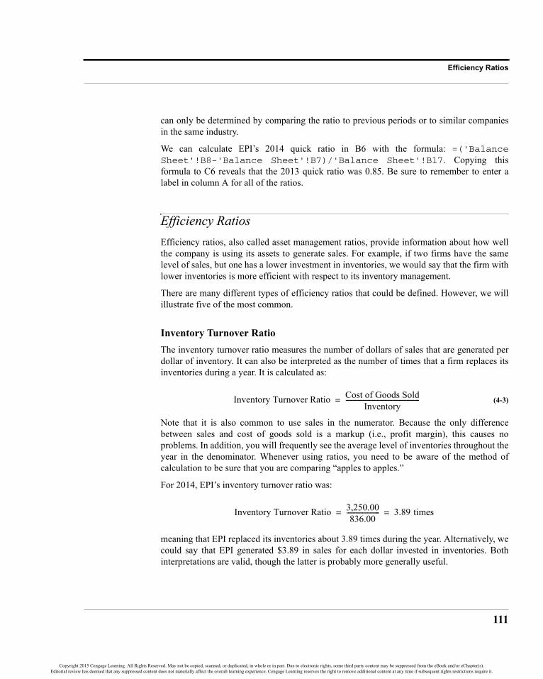
111
Efficiency Ratios
can only be determined by comparing the ratio to previous periods or to similar companiesin the same industry.
We can calculate EPI’s 2014 quick ratio in B6 with the formula: =('BalanceSheet'!B8-'Balance Sheet'!B7)/'Balance Sheet'!B17. Copying thisformula to C6 reveals that the 2013 quick ratio was 0.85. Be sure to remember to enter alabel in column A for all of the ratios.
Efficiency RatiosEfficiency ratios, also called asset management ratios, provide information about how wellthe company is using its assets to generate sales. For example, if two firms have the samelevel of sales, but one has a lower investment in inventories, we would say that the firm withlower inventories is more efficient with respect to its inventory management.
There are many different types of efficiency ratios that could be defined. However, we willillustrate five of the most common.
Inventory Turnover RatioThe inventory turnover ratio measures the number of dollars of sales that are generated perdollar of inventory. It can also be interpreted as the number of times that a firm replaces itsinventories during a year. It is calculated as:
(4-3)
Note that it is also common to use sales in the numerator. Because the only differencebetween sales and cost of goods sold is a markup (i.e., profit margin), this causes noproblems. In addition, you will frequently see the average level of inventories throughout theyear in the denominator. Whenever using ratios, you need to be aware of the method ofcalculation to be sure that you are comparing “apples to apples.”
For 2014, EPI’s inventory turnover ratio was:
meaning that EPI replaced its inventories about 3.89 times during the year. Alternatively, wecould say that EPI generated $3.89 in sales for each dollar invested in inventories. Bothinterpretations are valid, though the latter is probably more generally useful.
Inventory Turnover Ratio Cost of Goods SoldInventory
-----------------------------------------------=
Inventory Turnover Ratio 3,250.00836.00
--------------------- 3.89 times= =
Copyright 2015 Cengage Learning. All Rights Reserved. May not be copied, scanned, or duplicated, in whole or in part. Due to electronic rights, some third party content may be suppressed from the eBook and/or eChapter(s).Editorial review has deemed that any suppressed content does not materially affect the overall learning experience. Cengage Learning reserves the right to remove additional content at any time if subsequent rights restrictions require it.

CHAPTER 4: Financial Statement Analysis Tools
112
To calculate the inventory turnover ratio for EPI, enter the formula: ='IncomeStatement'!B6/'Balance Sheet'!B7 into B8 and copy this formula to C8. Noticethat this ratio has deteriorated somewhat from 4 times in 2013 to 3.89 times in 2014.Generally, high inventory turnover is considered to be good because it means that theopportunity costs of holding inventory are low, but if it is too high the firm may be riskinginventory outages and the loss of customers.
Accounts Receivable Turnover RatioBusinesses grant credit to customers for one main reason: to increase sales. It is important,therefore, to know how well the firm is managing its accounts receivable. The accountsreceivable turnover ratio (and the average collection period) provides us with this information.It is calculated by:
(4-4)
For EPI, the 2014 accounts receivable turnover ratio is (assuming that all sales are creditsales):
So each dollar invested in accounts receivable generated $9.58 in sales. In cell B9 of yourworksheet, enter: ='Income Statement'!B5/'Balance Sheet'!B6. The result is9.58, which is the same as we found above. Copy this formula to C9 to get the 2013 accountsreceivable turnover ratio.
Whether or not 9.58 is a good accounts receivable turnover ratio is difficult to know at thispoint. We can say that higher is generally better, but too high might indicate that the firm isdenying credit to creditworthy customers (thereby losing sales). If the ratio is too low, itwould suggest that the firm might be having difficulty collecting on its sales. We would haveto see if the growth rate in accounts receivable exceeds the growth rate in sales to determinewhether the firm is having difficulty in this area. We can see that is the case by looking at thecommon-size balance sheet in Exhibit 2-6 on page 57. Accounts receivable has grown from23.91% of sales to 24.35%; a slight increase, but an increase nonetheless.
Average Collection PeriodThe average collection period (also known as days sales outstanding, or DSO) tells us howmany days, on average, it takes to collect on a credit sale. It is calculated as follows:
Accounts Receivable Turnover Ratio Credit SalesAccounts Receivable--------------------------------------------------=
Accounts Receivable Turnover Ratio 3,850.00402.00
--------------------- 9.58 times= =
Copyright 2015 Cengage Learning. All Rights Reserved. May not be copied, scanned, or duplicated, in whole or in part. Due to electronic rights, some third party content may be suppressed from the eBook and/or eChapter(s).Editorial review has deemed that any suppressed content does not materially affect the overall learning experience. Cengage Learning reserves the right to remove additional content at any time if subsequent rights restrictions require it.

113
Efficiency Ratios
(4-5)
Note that the denominator is simply credit sales per day.2 In 2014, it took EPI an average of37.59 days to collect on their credit sales:
We can calculate the 2014 average collection period in B10 with the formula: ='BalanceSheet'!B6/('Income Statement'!B5/360). Copy this to C10 to find that in 2013the average collection period was 36.84 days, which was slightly better than in 2014.
Note that this ratio actually provides us with the same information as the accounts receivableturnover ratio. In fact, it can easily be demonstrated by simple algebraic manipulation:
Or alternatively:
Because the average collection period is (in a sense) the inverse of the accounts receivableturnover ratio, it should be apparent that the inverse criteria apply to judging this ratio. Inother words, lower is usually better, but too low may indicate lost sales.
Many firms offer a discount for fast payment in order to get customers to pay more quickly.For example, the credit terms on an invoice might specify 2/10n30, which means that thereis a 2% discount for paying within 10 days otherwise the entire balance is due in 30 days.Such a discount is very attractive for customers, but whether it makes sense for a particularfirm is for them to decide. Remember that accounts receivable represents short-term loansmade to customers, and those funds have an opportunity cost. Regardless, offering adiscount will almost certainly reduce the average collection period and increase the accountsreceivable turnover. You should always compare the average collection period to the creditterms that the company offers its customers.
2. The use of a 360-day year dates back to the days before computers. It was derived by assuming thatthere are 12 months, each with 30 days (known as a “Banker’s Year”). You may also use 365 days;the difference is irrelevant as long as you are consistent.
Average Collection Period Accounts ReceivableCredit Sales 360⁄
--------------------------------------------------=
Average Collection Period 402.003,850.00 360⁄---------------------------------- 37.59 days= =
Accounts Receivable Turnover Ratio 360Average Collection Period----------------------------------------------------------------=
Average Collection Period 360Accounts Receivable Turnover Ratio-----------------------------------------------------------------------------------------=
Copyright 2015 Cengage Learning. All Rights Reserved. May not be copied, scanned, or duplicated, in whole or in part. Due to electronic rights, some third party content may be suppressed from the eBook and/or eChapter(s).Editorial review has deemed that any suppressed content does not materially affect the overall learning experience. Cengage Learning reserves the right to remove additional content at any time if subsequent rights restrictions require it.

CHAPTER 4: Financial Statement Analysis Tools
114
Fixed Asset Turnover RatioThe fixed asset turnover ratio describes the dollar amount of sales that are generated by eachdollar invested in fixed assets. It is given by:
(4-6)
For EPI, the 2014 fixed asset turnover is:
So, EPI generated $10.67 in revenue for each dollar invested in fixed assets. In your“Ratios” worksheet, entering: ='Income Statement'!B5/'Balance Sheet'!B11into B11 will confirm that the fixed asset turnover was 10.67 times in 2014. Again, copy thisformula to C11 to get the 2013 ratio.
Note that because we use net fixed assets in the denominator, a firm can improve its fixedasset turnover ratio by simply delaying the replacement of its long-term assets. Asaccumulated depreciation increases net fixed assets will decrease, all other things being thesame. However, this is a short-term gimmick since those assets will eventually wear out.
Total Asset Turnover RatioLike the other ratios discussed in this section, the total asset turnover ratio describes howefficiently the firm is using all of its assets to generate sales. In this case, we look at thefirm’s total asset investment:
(4-7)
In 2014, EPI generated $2.33 in sales for each dollar invested in total assets:
This ratio can be calculated in B12 on your worksheet with: ='Income Statement'!B5/'Balance Sheet'!B12. After copying this formula to C12, you should see thatthe 2013 value was 2.34, essentially the same as 2014.
We can interpret the asset turnover ratios as follows: Higher turnover ratios indicate moreefficient usage of the assets and are therefore preferred to lower ratios. However, you shouldbe aware that some industries will naturally have lower turnover ratios than others. For
Fixed Asset Turnover SalesNet Fixed Assets-----------------------------------------=
Fixed Asset Turnover 3,850.00360.80
--------------------- 10.67 times= =
Total Asset Turnover SalesTotal Assets-----------------------------=
Total Asset Turnover 3,850.001,650.80--------------------- 2.33 times= =
Copyright 2015 Cengage Learning. All Rights Reserved. May not be copied, scanned, or duplicated, in whole or in part. Due to electronic rights, some third party content may be suppressed from the eBook and/or eChapter(s).Editorial review has deemed that any suppressed content does not materially affect the overall learning experience. Cengage Learning reserves the right to remove additional content at any time if subsequent rights restrictions require it.
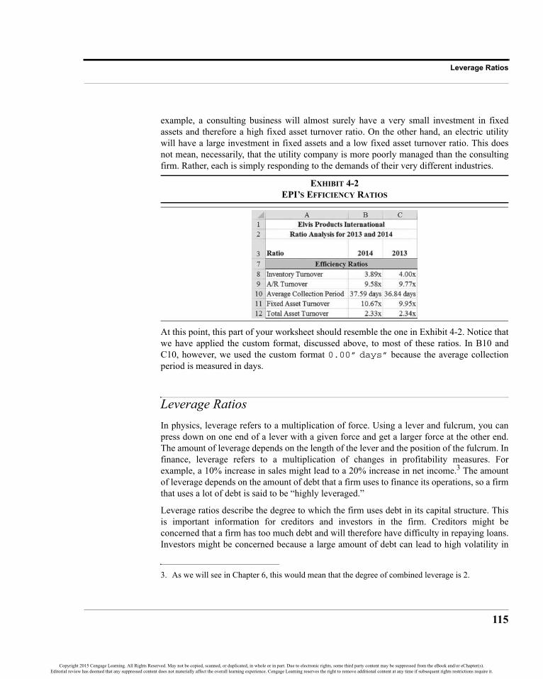
115
Leverage Ratios
example, a consulting business will almost surely have a very small investment in fixedassets and therefore a high fixed asset turnover ratio. On the other hand, an electric utilitywill have a large investment in fixed assets and a low fixed asset turnover ratio. This doesnot mean, necessarily, that the utility company is more poorly managed than the consultingfirm. Rather, each is simply responding to the demands of their very different industries.
EXHIBIT 4-2EPI’S EFFICIENCY RATIOS
At this point, this part of your worksheet should resemble the one in Exhibit 4-2. Notice thatwe have applied the custom format, discussed above, to most of these ratios. In B10 andC10, however, we used the custom format 0.00” days” because the average collectionperiod is measured in days.
Leverage RatiosIn physics, leverage refers to a multiplication of force. Using a lever and fulcrum, you canpress down on one end of a lever with a given force and get a larger force at the other end.The amount of leverage depends on the length of the lever and the position of the fulcrum. Infinance, leverage refers to a multiplication of changes in profitability measures. Forexample, a 10% increase in sales might lead to a 20% increase in net income.3 The amountof leverage depends on the amount of debt that a firm uses to finance its operations, so a firmthat uses a lot of debt is said to be “highly leveraged.”
Leverage ratios describe the degree to which the firm uses debt in its capital structure. Thisis important information for creditors and investors in the firm. Creditors might beconcerned that a firm has too much debt and will therefore have difficulty in repaying loans.Investors might be concerned because a large amount of debt can lead to high volatility in
3. As we will see in Chapter 6, this would mean that the degree of combined leverage is 2.
Copyright 2015 Cengage Learning. All Rights Reserved. May not be copied, scanned, or duplicated, in whole or in part. Due to electronic rights, some third party content may be suppressed from the eBook and/or eChapter(s).Editorial review has deemed that any suppressed content does not materially affect the overall learning experience. Cengage Learning reserves the right to remove additional content at any time if subsequent rights restrictions require it.

CHAPTER 4: Financial Statement Analysis Tools
116
the firm’s earnings. However, most firms use some debt. This is because the tax deductibilityof interest can increase the wealth of the firm’s shareholders. We will examine several ratiosthat help to determine the amount of debt that a firm is using. How much is too muchdepends on the nature of the business.
The Total Debt RatioThe total debt ratio measures the total amount of debt (long-term and short-term) that thefirm uses to finance its assets:
(4-8)
Calculating the total debt ratio for EPI, we find that debt financing makes up about 58.45%of the firm’s capital structure:
The formula to calculate the total debt ratio in B14 is: ='Balance Sheet'!B19/'Balance Sheet'!B12. The result for 2014 is 58.45%, which is higher than the 54.81%in 2013.
The Long-Term Debt RatioMany analysts believe that it is more useful to focus on just the long-term debt (LTD) insteadof total debt. The long-term debt ratio is the same as the total debt ratio, except that thenumerator includes only long-term debt:
(4-9)
EPI’s long-term debt ratio is:
In B15, the formula to calculate the long-term debt ratio for 2014 is: ='BalanceSheet'!B18/'Balance Sheet'!B12. Copying this formula to C15 reveals that in2013 the ratio was only 22.02%. Obviously, EPI has increased its long-term debt at a fasterrate than it has added assets.
Total Debt Ratio Total LiabilitiesTotal Assets
-------------------------------------- Total Assets Total Equity–Total Assets
------------------------------------------------------------------= =
Total Debt Ratio 964.811,650.80--------------------- 58.45%= =
Long-Term Debt Ratio Long-Term DebtTotal Assets
----------------------------------------=
Long-Term Debt Ratio 424.611,650.80--------------------- 25.72%= =
Copyright 2015 Cengage Learning. All Rights Reserved. May not be copied, scanned, or duplicated, in whole or in part. Due to electronic rights, some third party content may be suppressed from the eBook and/or eChapter(s).Editorial review has deemed that any suppressed content does not materially affect the overall learning experience. Cengage Learning reserves the right to remove additional content at any time if subsequent rights restrictions require it.

117
Leverage Ratios
The Long-Term Debt to Total Capitalization RatioSimilar to the previous two ratios, the long-term debt to total capitalization ratio tells us thepercentage of long-term sources of capital4 that is provided by long-term debt (LTD). It iscalculated by:
(4-10)
For EPI, we have:
Because EPI has no preferred equity, its total capitalization consists of long-term debt andcommon equity. Note that common equity is the total of common stock and retainedearnings. We can calculate this ratio in B16 of the worksheet with: ='BalanceSheet'!B18/('Balance Sheet'!B18+'Balance Sheet'!B22). In 2013 thisratio was only 32.76%.
The Debt to Equity RatioThe debt to equity ratio provides exactly the same information as the total debt ratio, but in aslightly different form that some analysts prefer:
(4-11)
For EPI, the debt to equity ratio is:
In B17, this is calculated as: ='Balance Sheet'!B19/'Balance Sheet'!B22.Copy this to C17 to find that the debt to equity ratio in 2013 was 1.21 times.
To see that the total debt ratio and the debt to equity ratio provide the same information,realize that:
(4-12)
4. Some analysts will include notes payable and the LTD due in one year in total capitalization.
LTD to Total Capitalization LTDLTD Preferred Equity Common Equity+ +--------------------------------------------------------------------------------------------------------=
LTD to Total Capitalization 424.61424.61 685.99+--------------------------------------- 38.23%= =
Debt to Equity Total DebtTotal Equity------------------------------=
Debt to Equity 964.81685.99---------------- 1.41 times= =
Total DebtTotal Equity------------------------------ Total Debt
Total Assets----------------------------- Total Assets
Total Equity------------------------------×=
Copyright 2015 Cengage Learning. All Rights Reserved. May not be copied, scanned, or duplicated, in whole or in part. Due to electronic rights, some third party content may be suppressed from the eBook and/or eChapter(s).Editorial review has deemed that any suppressed content does not materially affect the overall learning experience. Cengage Learning reserves the right to remove additional content at any time if subsequent rights restrictions require it.

CHAPTER 4: Financial Statement Analysis Tools
118
but from rearranging equation (4-8) we know that:
(4-13)
so, by substitution we have:
(4-14)
We can convert the total debt ratio into the debt to equity ratio without any additionalinformation (the result is not exact due to rounding):
The Long-Term Debt to Equity RatioOnce again, many analysts prefer to focus on the amount of long-term debt that a firmcarries. For this reason, many analysts like to use the long-term debt to total equity ratio:
(4-15)
EPI’s long-term debt to equity ratio is:
The formula to calculate EPI’s 2014 long-term debt to equity ratio in B18 is: ='BalanceSheet'!B18/'Balance Sheet'!B22. After copying this formula to C18, note thatthe ratio was only 48.73% in 2013.
This portion of your worksheet should now look like the one in Exhibit 4-3.
Coverage RatiosThe coverage ratios are similar to liquidity ratios in that they describe the quantity of fundsavailable to “cover” certain expenses. We will examine two very similar ratios that describethe firm’s ability to meet its interest payment obligations. In both cases, higher ratios aredesirable to a degree. However, if they are too high, it may indicate that the firm is under-utilizing its debt capacity and therefore not maximizing shareholder wealth.
Total AssetsTotal Equity------------------------------ 1
1 Total Debt Ratio–-------------------------------------------------=
Total DebtTotal Equity------------------------------ Total Debt
Total Assets----------------------------- 1
1 Total DebtTotal Assets-----------------------------–
---------------------------------------×=
Total DebtTotal Equity------------------------------ 0.5845 1
1 0.5845–-------------------------× 1.41= =
Long-Term Debt to Equity LTDPreferred Equity Common Equity+--------------------------------------------------------------------------------------=
Long-Term Debt to Equity 424.61685.99---------------- 61.90%= =
Copyright 2015 Cengage Learning. All Rights Reserved. May not be copied, scanned, or duplicated, in whole or in part. Due to electronic rights, some third party content may be suppressed from the eBook and/or eChapter(s).Editorial review has deemed that any suppressed content does not materially affect the overall learning experience. Cengage Learning reserves the right to remove additional content at any time if subsequent rights restrictions require it.
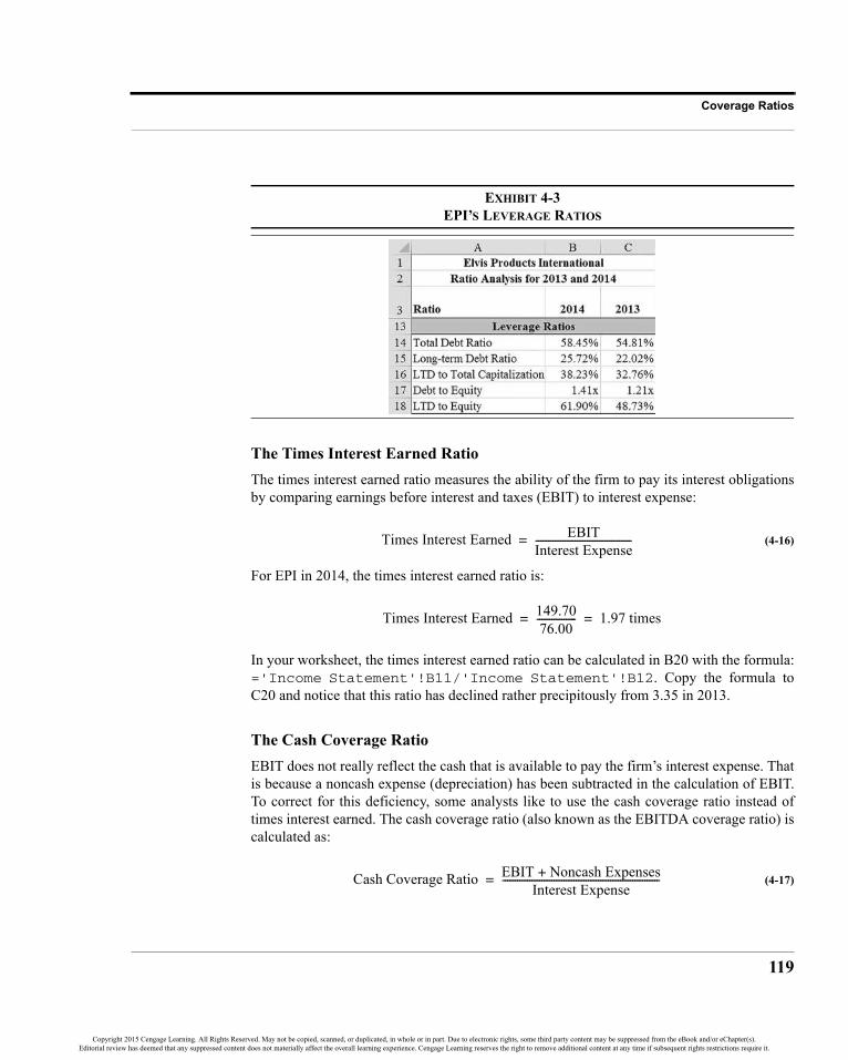
119
Coverage Ratios
EXHIBIT 4-3EPI’S LEVERAGE RATIOS
The Times Interest Earned RatioThe times interest earned ratio measures the ability of the firm to pay its interest obligationsby comparing earnings before interest and taxes (EBIT) to interest expense:
(4-16)
For EPI in 2014, the times interest earned ratio is:
In your worksheet, the times interest earned ratio can be calculated in B20 with the formula:='Income Statement'!B11/'Income Statement'!B12. Copy the formula toC20 and notice that this ratio has declined rather precipitously from 3.35 in 2013.
The Cash Coverage RatioEBIT does not really reflect the cash that is available to pay the firm’s interest expense. Thatis because a noncash expense (depreciation) has been subtracted in the calculation of EBIT.To correct for this deficiency, some analysts like to use the cash coverage ratio instead oftimes interest earned. The cash coverage ratio (also known as the EBITDA coverage ratio) iscalculated as:
(4-17)
Times Interest Earned EBITInterest Expense---------------------------------------=
Times Interest Earned 149.7076.00---------------- 1.97 times= =
Cash Coverage Ratio EBIT Noncash Expenses+Interest Expense
----------------------------------------------------------------=
Copyright 2015 Cengage Learning. All Rights Reserved. May not be copied, scanned, or duplicated, in whole or in part. Due to electronic rights, some third party content may be suppressed from the eBook and/or eChapter(s).Editorial review has deemed that any suppressed content does not materially affect the overall learning experience. Cengage Learning reserves the right to remove additional content at any time if subsequent rights restrictions require it.

CHAPTER 4: Financial Statement Analysis Tools
120
The calculation for EPI in 2014 is:
Note that the cash coverage ratio will always be higher than the times interest earned ratio.The difference depends on the amount of depreciation expense and therefore the amount andage of fixed assets.
The cash coverage ratio can be calculated in cell B21 of your “Ratios” worksheetwith: =('Income Statement'!B11+'Income Statement'!B10)/'IncomeStatement'!B12. In 2013, the ratio was 3.65.
EXHIBIT 4-4EPI’S COVERAGE RATIOS
Profitability RatiosInvestors, and therefore managers, are particularly interested in the profitability of the firmsthat they own. As we’ll see, there are many ways to measure profits. Profitability ratiosprovide an easy way to compare profits to earlier periods or to other firms. Furthermore, bysimultaneously examining the first three profitability ratios, an analyst can discovercategories of expenses that may be out of line.
Profitability ratios are the easiest of all the ratios to analyze. Without exception, high ratiosare preferred. However, the definition of high depends on the industry in which the firmoperates. Generally, firms in mature industries with lots of competition will have lowerprofitability measures than firms in faster growing industries with less competition. Forexample, grocery stores will have lower profit margins than computer software companies.In the grocery business, a net profit margin of 3% would be considered quite good. Thatsame margin would be abysmal in the software business, where 15% or higher is common.
Cash Coverage Ratio 149.70 20.00+76.00
------------------------------------ 2.23 times= =
Copyright 2015 Cengage Learning. All Rights Reserved. May not be copied, scanned, or duplicated, in whole or in part. Due to electronic rights, some third party content may be suppressed from the eBook and/or eChapter(s).Editorial review has deemed that any suppressed content does not materially affect the overall learning experience. Cengage Learning reserves the right to remove additional content at any time if subsequent rights restrictions require it.

121
Profitability Ratios
The Gross Profit MarginThe gross profit margin measures the gross profit relative to sales. It indicates the amount offunds available to pay the firm’s expenses other than its cost of sales. The gross profitmargin is calculated by:
(4-18)
In 2014, EPI’s gross profit margin was:
which means that cost of goods sold consumed about 84.42% ( ) of salesrevenue. We can calculate this ratio in B23 with: ='Income Statement'!B7/'Income Statement'!B5. After copying this formula to C23, you will see that thegross profit margin has declined from 16.55% in 2013.
The Operating Profit MarginMoving down the income statement, we can calculate the profits that remain after the firmhas paid all of its operating (nonfinancial) expenses.
The operating profit margin is calculated as:
(4-19)
For EPI in 2014:
The operating profit margin can be calculated in B24 with the formula: ='IncomeStatement'!B11/'Income Statement'!B5. Note that this is significantly lowerthan the 6.09% from 2013, indicating that EPI seems to be having problems controlling itsoperating costs.
The Net Profit MarginThe net profit margin relates net income to sales. Because net income is profit after allexpenses, the net profit margin tells us the percentage of sales that remains for theshareholders of the firm (either dividends or retained earnings):
Gross Profit Margin Gross ProfitSales
-----------------------------=
Gross Profit Margin 600.003,850.00--------------------- 15.58%= =
1 0.1558–=
Operating Profit Margin Net Operating IncomeSales
-----------------------------------------------------=
Operating Profit Margin 149.703,850.00--------------------- 3.89%= =
Copyright 2015 Cengage Learning. All Rights Reserved. May not be copied, scanned, or duplicated, in whole or in part. Due to electronic rights, some third party content may be suppressed from the eBook and/or eChapter(s).Editorial review has deemed that any suppressed content does not materially affect the overall learning experience. Cengage Learning reserves the right to remove additional content at any time if subsequent rights restrictions require it.
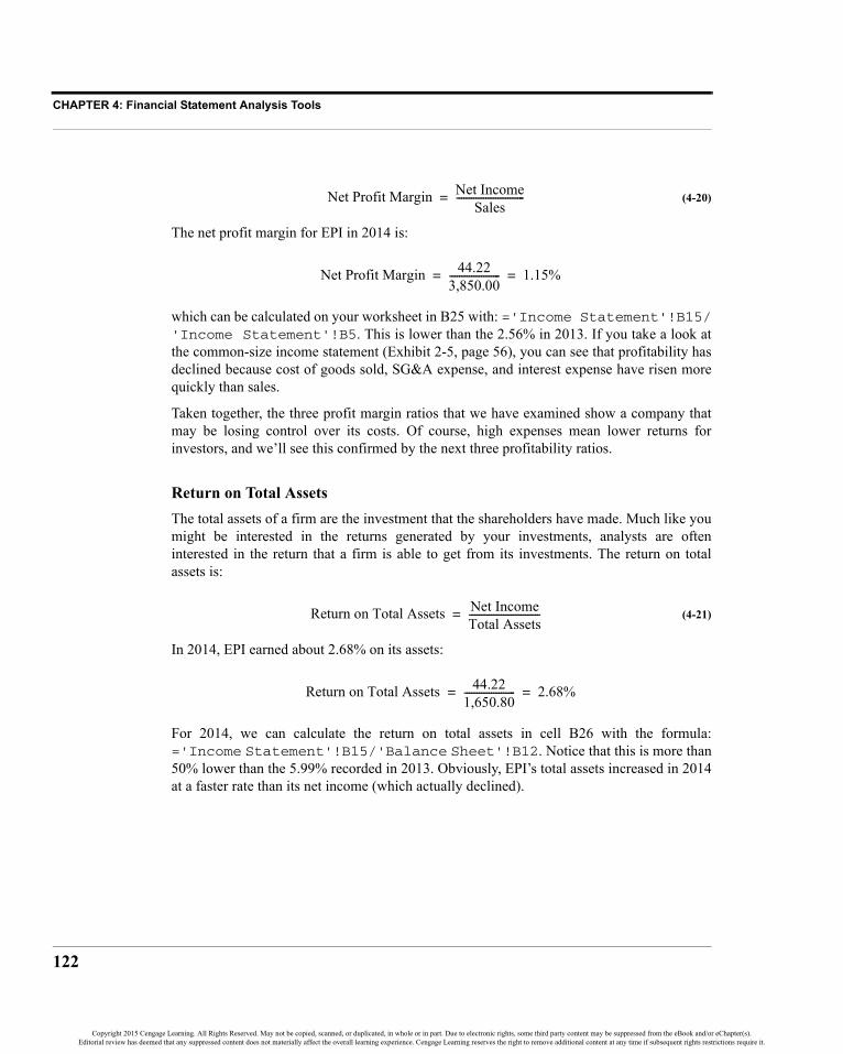
CHAPTER 4: Financial Statement Analysis Tools
122
(4-20)
The net profit margin for EPI in 2014 is:
which can be calculated on your worksheet in B25 with: ='Income Statement'!B15/'Income Statement'!B5. This is lower than the 2.56% in 2013. If you take a look atthe common-size income statement (Exhibit 2-5, page 56), you can see that profitability hasdeclined because cost of goods sold, SG&A expense, and interest expense have risen morequickly than sales.
Taken together, the three profit margin ratios that we have examined show a company thatmay be losing control over its costs. Of course, high expenses mean lower returns forinvestors, and we’ll see this confirmed by the next three profitability ratios.
Return on Total AssetsThe total assets of a firm are the investment that the shareholders have made. Much like youmight be interested in the returns generated by your investments, analysts are ofteninterested in the return that a firm is able to get from its investments. The return on totalassets is:
(4-21)
In 2014, EPI earned about 2.68% on its assets:
For 2014, we can calculate the return on total assets in cell B26 with the formula:='Income Statement'!B15/'Balance Sheet'!B12. Notice that this is more than50% lower than the 5.99% recorded in 2013. Obviously, EPI’s total assets increased in 2014at a faster rate than its net income (which actually declined).
Net Profit Margin Net IncomeSales
----------------------------=
Net Profit Margin 44.223,850.00--------------------- 1.15%= =
Return on Total Assets Net IncomeTotal Assets-----------------------------=
Return on Total Assets 44.221,650.80--------------------- 2.68%= =
Copyright 2015 Cengage Learning. All Rights Reserved. May not be copied, scanned, or duplicated, in whole or in part. Due to electronic rights, some third party content may be suppressed from the eBook and/or eChapter(s).Editorial review has deemed that any suppressed content does not materially affect the overall learning experience. Cengage Learning reserves the right to remove additional content at any time if subsequent rights restrictions require it.

123
Profitability Ratios
Return on EquityWhile total assets represent the total investment in the firm, the owners’ investment(common stock and retained earnings) usually represent only a portion of this amount (someis debt). For this reason, it is useful to calculate the rate of return on the shareholder’sinvested funds. We can calculate the return on (total) equity as:
(4-22)
Note that if a firm uses no debt, then its return on equity will be the same as its return onassets. The more debt a firm uses, the higher its return on equity will be relative to its returnon assets (see DuPont Analysis on page 124).
In 2014, EPI’s return on equity was:
which can be calculated in B27 with: ='Income Statement'!B15/'BalanceSheet'!B22. Again, copying this formula to C27 reveals that this ratio has declined from13.25% in 2013.
Return on Common EquityFor firms that have issued preferred stock in addition to common stock, it is often helpful todetermine the rate of return on just the common stockholders’ investment:
(4-23)
Net income available to common is net income less preferred dividends. In the case of EPI,this ratio is the same as the return on equity because it has no preferred shareholders:
For EPI, the worksheet formula for the return on common equity is exactly the same as forthe return on equity.
Return on Equity Net IncomeTotal Equity------------------------------=
Return on Equity 44.22685.99---------------- 6.45%= =
Return on Common Equity Net Income Available to CommonCommon Equity
-----------------------------------------------------------------------------------=
Return on Common Equity 44.22 0–685.99
---------------------- 6.45%= =
Copyright 2015 Cengage Learning. All Rights Reserved. May not be copied, scanned, or duplicated, in whole or in part. Due to electronic rights, some third party content may be suppressed from the eBook and/or eChapter(s).Editorial review has deemed that any suppressed content does not materially affect the overall learning experience. Cengage Learning reserves the right to remove additional content at any time if subsequent rights restrictions require it.

CHAPTER 4: Financial Statement Analysis Tools
124
DuPont AnalysisThe return on equity (ROE) is important to both managers and investors. The effectivenessof managers is often measured by changes in ROE over time, and their compensation may betied to ROE-based goals. Therefore, it is important that they understand what they can do toimprove the firm’s ROE and that requires knowledge of what causes changes in ROE overtime. For example, we can see that EPI’s return on equity dropped precipitously from 2013to 2014. As you might imagine, both investors and managers are probably trying to figureout why this happened. The DuPont system is one way to look at this problem.
The DuPont system is a way to break down the ROE into its components so thatmanagement can understand how to improve the firm’s ROE. Let’s first take another look atthe return on assets (ROA):
(4-24)
So, the ROA shows the combined effects of profitability (as measured by the net profitmargin) and the efficiency of asset usage (the total asset turnover). Therefore, ROA could beimproved by increasing profitability or by using assets more efficiently.
As mentioned earlier, the amount of leverage that a firm uses is the link between ROA andROE. Specifically:
(4-25)
Note that the second term in (4-25) is sometimes called the “equity multiplier” and from (4-13) we know it is equal to:
(4-26)
Substituting (4-26) into (4-25) and rearranging, we have:
(4-27)
We can now see that the ROE is a function of the firm’s ROA and the total debt ratio. If twofirms have the same ROA, the one using more debt will have a higher ROE.
We can make one more substitution to completely break down the ROE into its components.Because the first term in (4-27) is the ROA, we can replace it with (4-24):
ROA Net IncomeTotal Assets----------------------------- Net Income
Sales---------------------------- Sales
Total Assets-----------------------------×= =
ROE Net IncomeEquity
---------------------------- Net IncomeTotal Assets----------------------------- Total Assets
Equity-----------------------------×= =
Total AssetsTotal Equity------------------------------ 1
1 Total Debt Ratio–------------------------------------------------- 1
1 Total DebtTotal Assets-----------------------------–
---------------------------------------= =
ROE Net IncomeTotal Assets----------------------------- 1 Total Debt
Total Assets -------------------------------–⎝ ⎠
⎛ ⎞÷=
Copyright 2015 Cengage Learning. All Rights Reserved. May not be copied, scanned, or duplicated, in whole or in part. Due to electronic rights, some third party content may be suppressed from the eBook and/or eChapter(s).Editorial review has deemed that any suppressed content does not materially affect the overall learning experience. Cengage Learning reserves the right to remove additional content at any time if subsequent rights restrictions require it.

125
Profitability Ratios
(4-28)
Or, to simplify it somewhat:
(4-29)
To prove this to yourself, in A30 enter the label: DuPont ROE. Now, in B30 enter theformula: =(B25*B12)/(1-B14). The result will be 6.45% as we found earlier. Note thatif a firm uses no debt then the denominator of equation (4-29) will be 1, and the ROE will bethe same as the ROA.
Extended DuPont AnalysisWe can take the decomposition of ROE one step further by breaking the net profit margininto three components:
1. The operating profit margin, which measures the basic profitability fromthe firm’s day-to-day operations;
2. The interest burden, which measures the impact of interest expense onpre-tax earnings; and
3. The tax burden, which shows the impact of taxes on overall earnings.
We have already discussed the operating profit margin in equation (4-19) on page 121. Theinterest burden is calculated as:
(4-30)
and the tax burden is calculated as:
(4-31)
Multiplying these three ratios together gives us the net profit margin:
(4-32)
Finally, if we substitute equation (4-32) into the numerator of (4-28), we have:
ROE
Net IncomeSales
---------------------------- SalesTotal Assets-----------------------------×
1 Total DebtTotal Assets-----------------------------–
----------------------------------------------------------------=
ROE Net Profit Margin Total Asset Turnover×1 Total Debt Ratio–
----------------------------------------------------------------------------------------------------=
Interest Burden Earnings Before TaxesEarnings Before Interest and Taxes------------------------------------------------------------------------------------ EBT
EBIT-------------= =
Tax Burden Net IncomeEarnings Before Taxes------------------------------------------------------- NI
EBT-----------= =
Net Profit Margin Net IncomeSales
---------------------------- EBITSales------------- EBT
EBIT-------------× NI
EBT-----------×= =
Copyright 2015 Cengage Learning. All Rights Reserved. May not be copied, scanned, or duplicated, in whole or in part. Due to electronic rights, some third party content may be suppressed from the eBook and/or eChapter(s).Editorial review has deemed that any suppressed content does not materially affect the overall learning experience. Cengage Learning reserves the right to remove additional content at any time if subsequent rights restrictions require it.

CHAPTER 4: Financial Statement Analysis Tools
126
(4-33)
The extended DuPont system for calculating the ROE, equation (4-33), tells us that thereturn on equity is a function of operating profitability, the interest rate, the tax rate, theefficiency with which the firm uses its assets, and the amount of debt that it uses. At thispoint, this part of your worksheet should resemble Exhibit 4-5.
EXHIBIT 4-5EPI’S PROFITABILITY RATIO AND DUPONT ROE
Analysis of EPI’s Profitability RatiosObviously, EPI’s profitability has slipped rather dramatically in the past year. The sources ofthese declines can be seen most clearly if we look at all of EPI’s ratios.
The gross profit margin in 2014 is lower than in 2013, but not significantly (at leastcompared to the declines in the other ratios). The operating profit margin, however, issignificantly lower in 2014 than in 2013. This indicates potential problems in controlling thefirm’s operating expenses, particularly SG&A expenses. The other profitability ratios arelower than in 2013 partly because of the “trickle down” effect of the increase in operatingexpenses. However, they are also lower because EPI has taken on a lot of extra debt in 2014,resulting in interest expense increasing faster than sales. This can be confirmed byexamining EPI’s common-size income statement (Exhibit 2-5, page 56).
Extended DuPont ROE
EBITSales------------- EBT
EBIT-------------× NI
EBT-----------× Sales
Total Assets-----------------------------×
1 Total DebtTotal Assets-----------------------------–
---------------------------------------------------------------------------------------=
Copyright 2015 Cengage Learning. All Rights Reserved. May not be copied, scanned, or duplicated, in whole or in part. Due to electronic rights, some third party content may be suppressed from the eBook and/or eChapter(s).Editorial review has deemed that any suppressed content does not materially affect the overall learning experience. Cengage Learning reserves the right to remove additional content at any time if subsequent rights restrictions require it.
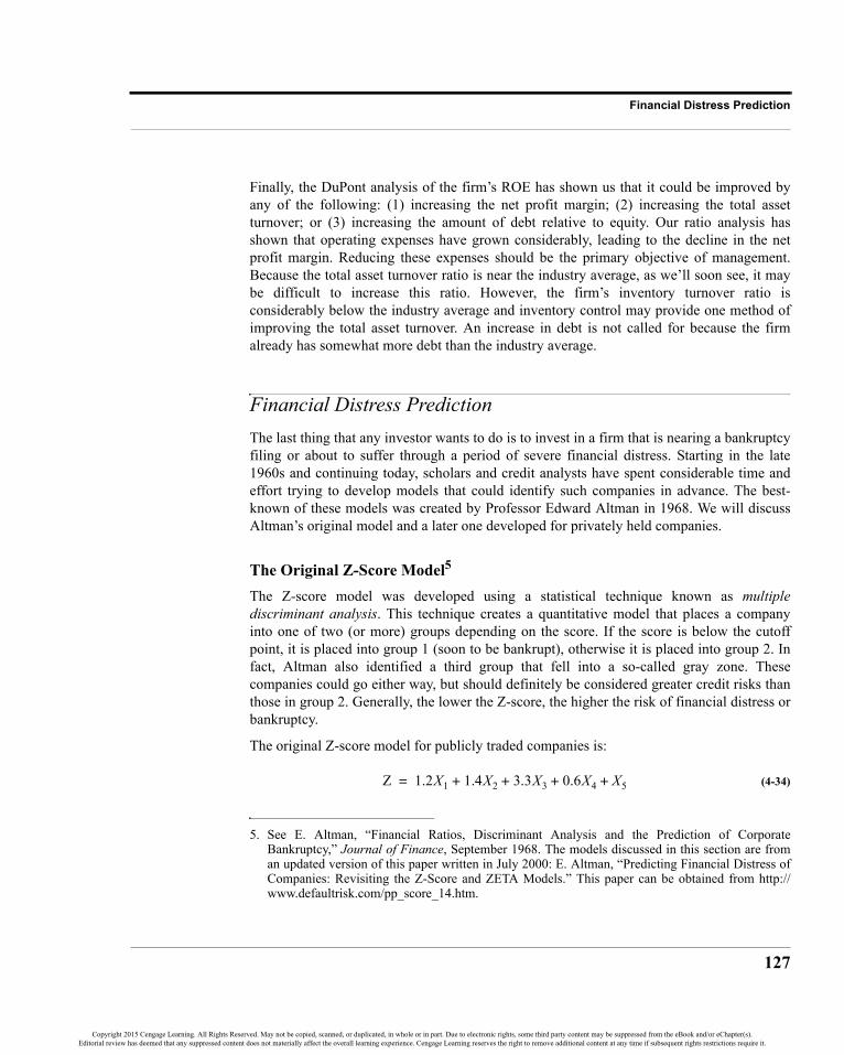
127
Financial Distress Prediction
Finally, the DuPont analysis of the firm’s ROE has shown us that it could be improved byany of the following: (1) increasing the net profit margin; (2) increasing the total assetturnover; or (3) increasing the amount of debt relative to equity. Our ratio analysis hasshown that operating expenses have grown considerably, leading to the decline in the netprofit margin. Reducing these expenses should be the primary objective of management.Because the total asset turnover ratio is near the industry average, as we’ll soon see, it maybe difficult to increase this ratio. However, the firm’s inventory turnover ratio isconsiderably below the industry average and inventory control may provide one method ofimproving the total asset turnover. An increase in debt is not called for because the firmalready has somewhat more debt than the industry average.
Financial Distress PredictionThe last thing that any investor wants to do is to invest in a firm that is nearing a bankruptcyfiling or about to suffer through a period of severe financial distress. Starting in the late1960s and continuing today, scholars and credit analysts have spent considerable time andeffort trying to develop models that could identify such companies in advance. The best-known of these models was created by Professor Edward Altman in 1968. We will discussAltman’s original model and a later one developed for privately held companies.
The Original Z-Score Model5
The Z-score model was developed using a statistical technique known as multiplediscriminant analysis. This technique creates a quantitative model that places a companyinto one of two (or more) groups depending on the score. If the score is below the cutoffpoint, it is placed into group 1 (soon to be bankrupt), otherwise it is placed into group 2. Infact, Altman also identified a third group that fell into a so-called gray zone. Thesecompanies could go either way, but should definitely be considered greater credit risks thanthose in group 2. Generally, the lower the Z-score, the higher the risk of financial distress orbankruptcy.
The original Z-score model for publicly traded companies is:
(4-34)
5. See E. Altman, “Financial Ratios, Discriminant Analysis and the Prediction of CorporateBankruptcy,” Journal of Finance, September 1968. The models discussed in this section are froman updated version of this paper written in July 2000: E. Altman, “Predicting Financial Distress ofCompanies: Revisiting the Z-Score and ZETA Models.” This paper can be obtained from http://www.defaultrisk.com/pp_score_14.htm.
Z 1.2X1 1.4X2 3.3X3 0.6X4 X5+ + + +=
Copyright 2015 Cengage Learning. All Rights Reserved. May not be copied, scanned, or duplicated, in whole or in part. Due to electronic rights, some third party content may be suppressed from the eBook and/or eChapter(s).Editorial review has deemed that any suppressed content does not materially affect the overall learning experience. Cengage Learning reserves the right to remove additional content at any time if subsequent rights restrictions require it.

CHAPTER 4: Financial Statement Analysis Tools
128
where the variables are the following financial ratios:
Altman reports that this model is 80–90% accurate if we use a cutoff point of 2.675. That is,a firm with a Z-score below 2.675 can reasonably be expected to experience severe financialdistress, and possibly bankruptcy, within the next year. The predictive ability of the model iseven better if we use a cutoff point of 1.81. There are, therefore, three ranges of Z-scores:
We can easily apply this model to EPI in the Ratios worksheet. However, first note that we haven’tsupplied information regarding the market value of EPI’s common stock. In A31, enter the label:Market Value of Equity and in B31 enter 884,400. The market value of the equity isfound by multiplying the share price by the number of shares outstanding. Next, enter: Z-Scoreinto A32, and in B32 enter the formula: =1.2*('Balance Sheet'!B8-'Balance Sheet'!B17)/'Balance Sheet'!B12+1.4*('Balance Sheet'!B21/'Balance Sheet'!B12)+3.3*('IncomeStatement'!B11/'Balance Sheet'!B12)+0.6*(B31/'Balance Sheet'!B19)+('Income Statement'!B5/'Balance Sheet'!B12).
If you’ve entered the equation correctly, you will find that EPI’s Z-score in 2014 is 3.92,which is safely above 2.675, so bankruptcy isn’t predicted.
The Z-Score Model for Private FirmsBecause variable X4 in equation (4-34) requires knowledge of the firm’s marketcapitalization (including both common and preferred equity), we cannot easily use the modelfor privately held firms. Estimates of the market value of these firms can be made, but theresult is necessarily very uncertain. Alternatively, we could substitute the book value ofequity for its market value, but that wouldn’t be correct. Most publicly traded firms trade forseveral times their book value, so such a substitution would seem to call for a newcoefficient for X4. In fact, all of the coefficients in the model changed when Altmanreestimated it for privately held firms.
X1 = net working capital/total assetsX2 = retained earnings/total assetsX3 = EBIT/total assetsX4 = market value of all equity/book value of total liabilitiesX5 = sales/total assets
Z < 1.81 Bankruptcy predicted within one year1.81 < Z < 2.675 Financial distress, possible bankruptcyZ > 2.675 No financial distress predicted
Copyright 2015 Cengage Learning. All Rights Reserved. May not be copied, scanned, or duplicated, in whole or in part. Due to electronic rights, some third party content may be suppressed from the eBook and/or eChapter(s).Editorial review has deemed that any suppressed content does not materially affect the overall learning experience. Cengage Learning reserves the right to remove additional content at any time if subsequent rights restrictions require it.

129
Using Financial Ratios
The new model for privately held firms is:
(4-35)
where all of the variables are defined as before, except that X4 uses the book value of equityinstead of market value. Altman reports that this model is only slightly less accurate than theone for publicly traded firms when we use the new cutoff points shown below.
If we treat EPI as a privately held firm, its Z-score for 2014 is 3.35 and for 2013 is 3.55.These scores show that EPI is not likely to file for bankruptcy anytime soon.
Using Financial RatiosCalculating financial ratios is a pointless exercise unless you understand how to use them.One overriding rule of ratio analysis is this: A single ratio provides very little informationand may be misleading. You should never draw conclusions from a single ratio. Instead,several ratios and other information should support any conclusions that you make.
With that precaution in mind, there are several ways that ratios can be used to drawimportant conclusions.
Trend AnalysisTrend analysis involves the examination of ratios over time. Trends, or the lack of trends,can help managers gauge their progress toward a goal. Furthermore, trends can highlightareas in need of attention. While we don’t really have enough information on Elvis ProductsInternational to perform a trend analysis, it is obvious that many of its ratios are moving inthe wrong direction.
For example, all of EPI’s profitability ratios have declined in 2014 relative to 2013, somerather dramatically. Management should immediately try to isolate the problem areas. Forexample, the gross profit margin has declined only slightly, indicating that increasingmaterials costs are not a major problem, though a price increase may be called for. Theoperating profit margin has fallen by about 36%, and since we can’t blame increasing costsof goods sold, we must conclude that operating costs have increased at a more rapid rate thanrevenues. The common-size income statement (Exhibit 2-5, page 56) shows that the culprit
Bankruptcy predicted within one yearFinancial distress, possible bankruptcyNo financial distress predicted
Z′ 0.717X1 0.847X2 3.107X3 0.420X4 0.998X5+ + + +=
Z′ 1.21<1.23 Z′ 2.90< <Z′ 2.90>
Copyright 2015 Cengage Learning. All Rights Reserved. May not be copied, scanned, or duplicated, in whole or in part. Due to electronic rights, some third party content may be suppressed from the eBook and/or eChapter(s).Editorial review has deemed that any suppressed content does not materially affect the overall learning experience. Cengage Learning reserves the right to remove additional content at any time if subsequent rights restrictions require it.

CHAPTER 4: Financial Statement Analysis Tools
130
is SG&A expense. This increase in operating costs has led, to a large degree, to the declinein the other profitability ratios.
One potential problem area for trend analysis is seasonality. We must be careful to comparesimilar time periods. For example, many firms generate most of their sales during theholidays in the fourth quarter of the year. For this reason they may begin building inventoriesin the third quarter when sales are low. In this situation, comparing the third-quarterinventory turnover ratio to the fourth-quarter inventory turnover would be misleading.
Comparing to Industry AveragesAside from trend analysis, one of the most beneficial uses of financial ratios is to comparesimilar firms within a single industry. This can be done by comparing to industry averageratios, which are published by organizations such as the Risk Management Association(RMA) and Standard & Poor’s. Industry averages provide a standard of comparison so thatwe can determine how well a firm is performing relative to its peers.
Consider Exhibit 4-6, which shows EPI’s ratios and the industry averages for 2014. You canenter the industry averages into your worksheet starting in D3 with the label: Industry2014. Now select D5:D28, type 2.70 into D5, and then press the Enter key. Notice that theactive cell will change to D6 when the Enter key is pressed. This is an efficient method ofentering a lot of numbers because your fingers never have to leave the number keypad. It isespecially helpful when entering numbers into multiple columns and discontiguous cells.
It should be obvious that EPI is not being managed as well as the average firm in theindustry. From the liquidity ratios, we can see that EPI is less able to meet its short-termobligations than the average firm, though they are probably not in imminent danger ofmissing payments. The efficiency ratios show us that EPI is not managing its assets as wellas would be expected, especially inventories. It is also obvious that EPI is using substantiallymore debt than its peers. The coverage ratios indicate that EPI has less cash to pay its interestexpense than the industry average. This is due to carrying more than average debt. Finally,all of these problems have led to subpar profitability measures, which seem to be gettingworse, rather than better.
It is important to note that industry averages may not be appropriate in all cases. In manycases, it is probably more accurate to define the “industry” as the target company’s mostclosely related competitors. This group is probably far smaller (maybe only three to fivecompanies) than the entire industry as defined by the 4-digit SIC code. The newer 6-digitNAICS code6 improves, but doesn’t eliminate, this situation.
6. North American Industry Classification System. This system was created by the U.S. CensusBureau and its Canadian and Mexican counterparts in 1997 and is replacing the SIC codes. Seehttp://www.census.gov/eos/www/naics/ for more information.
Copyright 2015 Cengage Learning. All Rights Reserved. May not be copied, scanned, or duplicated, in whole or in part. Due to electronic rights, some third party content may be suppressed from the eBook and/or eChapter(s).Editorial review has deemed that any suppressed content does not materially affect the overall learning experience. Cengage Learning reserves the right to remove additional content at any time if subsequent rights restrictions require it.

131
Using Financial Ratios
EXHIBIT 4-6EPI’S RATIOS VS. INDUSTRY AVERAGES
Company Goals and Debt CovenantsFinancial ratios are often the basis of company goal setting. For example, a CEO mightdecide that one goal of the firm should be to earn at least 15% on equity (ROE = 15%).Obviously, whether or not this goal is achieved can be determined by calculating the returnon equity. Further, by using trend analysis, managers can gauge progress toward meetinggoals, and they can determine whether the goals are realistic or not.
Another use of financial ratios can be found in covenants to loan contracts. When companiesborrow money, the lenders (bondholders, banks, or other lenders) place restrictions on thecompany, very often tied to the values of certain ratios. For example, the lender may require
Copyright 2015 Cengage Learning. All Rights Reserved. May not be copied, scanned, or duplicated, in whole or in part. Due to electronic rights, some third party content may be suppressed from the eBook and/or eChapter(s).Editorial review has deemed that any suppressed content does not materially affect the overall learning experience. Cengage Learning reserves the right to remove additional content at any time if subsequent rights restrictions require it.
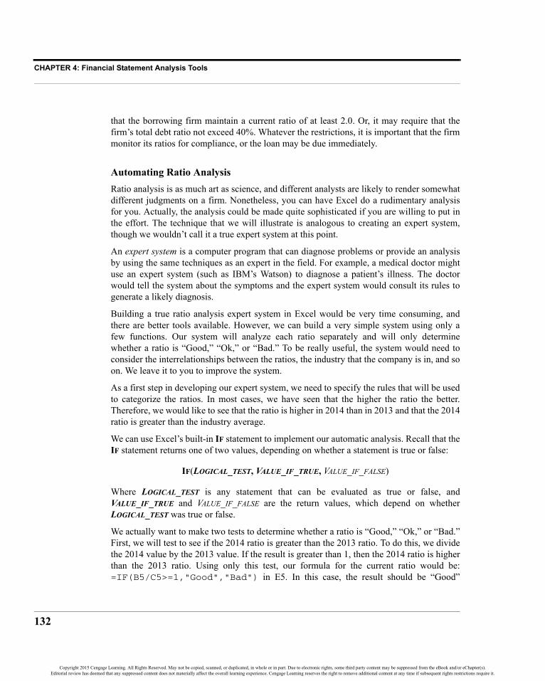
CHAPTER 4: Financial Statement Analysis Tools
132
that the borrowing firm maintain a current ratio of at least 2.0. Or, it may require that thefirm’s total debt ratio not exceed 40%. Whatever the restrictions, it is important that the firmmonitor its ratios for compliance, or the loan may be due immediately.
Automating Ratio AnalysisRatio analysis is as much art as science, and different analysts are likely to render somewhatdifferent judgments on a firm. Nonetheless, you can have Excel do a rudimentary analysisfor you. Actually, the analysis could be made quite sophisticated if you are willing to put inthe effort. The technique that we will illustrate is analogous to creating an expert system,though we wouldn’t call it a true expert system at this point.
An expert system is a computer program that can diagnose problems or provide an analysisby using the same techniques as an expert in the field. For example, a medical doctor mightuse an expert system (such as IBM’s Watson) to diagnose a patient’s illness. The doctorwould tell the system about the symptoms and the expert system would consult its rules togenerate a likely diagnosis.
Building a true ratio analysis expert system in Excel would be very time consuming, andthere are better tools available. However, we can build a very simple system using only afew functions. Our system will analyze each ratio separately and will only determinewhether a ratio is “Good,” “Ok,” or “Bad.” To be really useful, the system would need toconsider the interrelationships between the ratios, the industry that the company is in, and soon. We leave it to you to improve the system.
As a first step in developing our expert system, we need to specify the rules that will be usedto categorize the ratios. In most cases, we have seen that the higher the ratio the better.Therefore, we would like to see that the ratio is higher in 2014 than in 2013 and that the 2014ratio is greater than the industry average.
We can use Excel’s built-in IF statement to implement our automatic analysis. Recall that theIF statement returns one of two values, depending on whether a statement is true or false:
IF(LOGICAL_TEST, VALUE_IF_TRUE, VALUE_IF_FALSE)
Where LOGICAL_TEST is any statement that can be evaluated as true or false, andVALUE_IF_TRUE and VALUE_IF_FALSE are the return values, which depend on whetherLOGICAL_TEST was true or false.
We actually want to make two tests to determine whether a ratio is “Good,” “Ok,” or “Bad.”First, we will test to see if the 2014 ratio is greater than the 2013 ratio. To do this, we dividethe 2014 value by the 2013 value. If the result is greater than 1, then the 2014 ratio is higherthan the 2013 ratio. Using only this test, our formula for the current ratio would be:=IF(B5/C5>=1,"Good","Bad") in E5. In this case, the result should be “Good”
Copyright 2015 Cengage Learning. All Rights Reserved. May not be copied, scanned, or duplicated, in whole or in part. Due to electronic rights, some third party content may be suppressed from the eBook and/or eChapter(s).Editorial review has deemed that any suppressed content does not materially affect the overall learning experience. Cengage Learning reserves the right to remove additional content at any time if subsequent rights restrictions require it.

133
Using Financial Ratios
because the 2014 value is greater than the 2013 value. If you copy this formula to E6, theresult will be “Bad” because the 2014 quick ratio is lower than the 2013 quick ratio.
We can modify this formula to also take account of the industry average. If the 2014 ratio isgreater than the 2013 ratio and the 2014 ratio is greater than the industry average, then theratio is “Good.” To accomplish this we need to use the AND function. This function willreturn true only if all arguments are true:
AND(LOGICAL1, LOGICAL2, . . .)
In this function, LOGICAL1 and LOGICAL2 are the arguments to be evaluated as either true orfalse. You can have up to 255 arguments, but only one is required. The modified function inE5 is now: =IF(And(B5/C5>=1,B5/D5>=1),"Good","Bad"). Now, the ratio willonly be judged as “Good” if both conditions are true. Note that they are not for the currentratio, so the result is “Bad.”
One final improvement can be made by adding “Ok” to the possible outcomes. We will saythat the ratio is “Ok” if the 2014 value is greater than the 2013 value, or the 2014 value isgreater than the industry average. We can accomplish this by nesting a second IF statementinside the first in place of “Bad.” For the second IF statement, we need to use Excel’s ORfunction:
OR(LOGICAL1, LOGICAL2, . . .)
This function is identical to the AND function, except that it returns true if any of itsarguments are true. The final form of our equation is: =IF(AND(B5/C5>=1,B5/D5>=1),"Good",IF(OR(B5/D5>=1,B5/C5>=1),"Ok","Bad")). For the currentratio, this will evaluate to “Ok.” You can now evaluate all of EPI’s ratios by copying thisformula to E6:E28.
One more change is necessary. Recall that for leverage ratios, lower is generally better.Therefore, change all of the “>=” to “<=” in E14:E18. You also need to make the samechange in E10 for the average collection period. Your worksheet should now resemble thatshown in Exhibit 4-7.
Copyright 2015 Cengage Learning. All Rights Reserved. May not be copied, scanned, or duplicated, in whole or in part. Due to electronic rights, some third party content may be suppressed from the eBook and/or eChapter(s).Editorial review has deemed that any suppressed content does not materially affect the overall learning experience. Cengage Learning reserves the right to remove additional content at any time if subsequent rights restrictions require it.

CHAPTER 4: Financial Statement Analysis Tools
134
EXHIBIT 4-7EPI’S RATIOS WITH AUTOMATIC ANALYSIS
You should see that nearly all of EPI’s ratios are judged to be “Bad.” This is exactly what ourprevious analysis has determined, except that Excel has done it automatically. There aremany changes that could be made to improve on this simple ratio analyzer, but we will leavethat job as an exercise for you.
Economic Profit Measures of PerformanceEconomic profit is the profit earned in excess of the firm’s costs, including its implicitopportunity costs (primarily its cost of capital). Accounting profit (net income), however,measures profit as revenues minus all of the firm’s explicit costs. It takes into account a
Copyright 2015 Cengage Learning. All Rights Reserved. May not be copied, scanned, or duplicated, in whole or in part. Due to electronic rights, some third party content may be suppressed from the eBook and/or eChapter(s).Editorial review has deemed that any suppressed content does not materially affect the overall learning experience. Cengage Learning reserves the right to remove additional content at any time if subsequent rights restrictions require it.

135
Economic Profit Measures of Performance
firm’s cost of debt capital (interest expense), but it ignores the implicit cost of the firm’sequity capital. The concept of economic profit is an old one, but it has been revived byconsulting firms promising to improve the financial performance and executivecompensation practices of their clients.7 Some large firms have switched to variousmeasures of economic profit—some with good results and some not. In any case, the methodhas generated a lot of interest, and we will include a short discussion of measuring economicprofit in this section.
The basic idea behind economic profit measures is that the firm cannot increase shareholderwealth unless it makes a profit in excess of its cost of capital.8 Because we will be takingaccount of the cost of capital explicitly, we cannot use the normal accounting measures ofprofit directly. The adjustments to the financial statements vary depending on the firm andwho is doing the calculations. At the moment, there is no completely accepted standard.With this in mind, we will present a simplified economic profit calculation.
Mathematically, economic profit is:
(4-36)
where NOPAT is net operating profit after taxes. The after-tax cost of operating capital is thedollar cost of all interest-bearing debt instruments (i.e., bonds and notes payable) plus thedollar cost of preferred and common equity. Generally, the firm’s after-tax cost of capital (apercentage amount) is calculated and then multiplied by the amount of operating capital toobtain the dollar cost.
To calculate the economic profit, we must first calculate NOPAT, total operating capital, andthe firm’s cost of capital. For our purposes in this chapter, the cost of capital will be given(see Chapter 10 for the calculations). NOPAT is the after-tax operating profit of the firm:
(4-37)
Note that the NOPAT calculation does not include interest expense because it will beexplicitly accounted for when we subtract the cost of all capital.
Total operating capital is the sum of non-interest-bearing current assets and net fixed assets,less non-interest-bearing current liabilities. We ignore interest-bearing current assets because
7. The leader in this effort is the consulting firm Stern Stewart and Company who refer to economicprofit by the copyrighted name Economic Value Added (EVA).
8. Economic profit is also measured by net present value (NPV), which is introduced in Chapter 11.The primary difference is that in this chapter we are trying to calculate the actual economic profitthat was earned over some previous time period (usually the previous year). NPV measures theexpected economic profit of a future investment.
Economic Profit NOPAT After-tax cost of operating capital–=
NOPAT Total Net Operating Capital WACC×( )–=
NOPAT EBIT 1 tax rate–( )=
Copyright 2015 Cengage Learning. All Rights Reserved. May not be copied, scanned, or duplicated, in whole or in part. Due to electronic rights, some third party content may be suppressed from the eBook and/or eChapter(s).Editorial review has deemed that any suppressed content does not materially affect the overall learning experience. Cengage Learning reserves the right to remove additional content at any time if subsequent rights restrictions require it.

CHAPTER 4: Financial Statement Analysis Tools
136
they are not operating assets, and we ignore interest-bearing current liabilities (e.g., notespayable) because the cost of these liabilities is included in the cost of capital.
We will demonstrate the calculation of economic profit using the Elvis ProductsInternational data for 2013 and 2014. Make sure that the workbook containing EPI’sfinancial statements is open, and insert a new worksheet for our economic profitcalculations. Set up your new worksheet as shown in Exhibit 4-8, and rename the sheet“Economic Profit.”
EXHIBIT 4-8ECONOMIC PROFIT CALCULATION FOR EPI
Note that we are assuming that the firm’s cost of capital is 13%, and the tax rate should bepulled from the income statement with the formula: ='Income Statement'!$B18. Allof the other numbers must be calculated as discussed above.
Recall that NOPAT is simply EBIT times 1 - the tax rate, so in B5 enter the formula:='Income Statement'!B11*(1-B4). You should see that EPI has generated an after-tax operating profit of $89,820 in 2014. Copy this formula to C5 to get the NOPAT for 2013.
The next step is to calculate the amount of operating capital. Because EPI has no short-terminvestments, we merely add current assets to net fixed assets and then subtract currentliabilities less notes payable. In B6 enter the formula: ='BalanceSheet'!B8+'Balance Sheet'!B11-('Balance Sheet'!B17-'BalanceSheet'!B15). Your result should show that the total operating capital for 2014 was$1,335,600. Copy the formula to C6.
To calculate the dollar cost of capital in B8, enter the formula: =B7*B6; copy this to C8.Recall that economic profit is simply NOPAT minus the dollar cost of capital, so we cancalculate the economic profit in B9 with the formula: =B5-B8. You should find that EPIearned an economic profit of –$83,808 in 2014. Copy this formula to C9, and you will seethat EPI’s economic profit in 2013 was –$28,876.
Copyright 2015 Cengage Learning. All Rights Reserved. May not be copied, scanned, or duplicated, in whole or in part. Due to electronic rights, some third party content may be suppressed from the eBook and/or eChapter(s).Editorial review has deemed that any suppressed content does not materially affect the overall learning experience. Cengage Learning reserves the right to remove additional content at any time if subsequent rights restrictions require it.

137
Summary
This example shows how misleading accounting measures of profit (particularly net income)can be. In this case, EPI reported profits in both 2013 and 2014, but it was actually reducingshareholder wealth over the past two years. This mirrors the results from our ratio analysis.EPI’s management has not been doing a good job, at least over this period. Your economicprofit worksheet should now look like the one shown in Exhibit 4-9.
EXHIBIT 4-9EPI’S COMPLETED ECONOMIC PROFIT WORKSHEET
SummaryIn this chapter, we have seen how various financial ratios can be used to evaluate thefinancial health of a company and therefore the performance of the managers of the firm.You have also seen how Excel can make the calculation of ratios quicker and easier thandoing it manually. We looked at five categories of ratios: Liquidity ratios measure the abilityof a firm to pay its bills; efficiency ratios measure how well the firm is making use of itsassets to generate sales; leverage ratios describe how much debt the firm is using to financeits assets; coverage ratios tell how much cash the firm has available to pay specificexpenses; and profitability ratios measure how profitable the firm has been over a period oftime.
We have also seen how Excel can be programmed to do a rudimentary ratio analysisautomatically, using only a few of the built-in logical functions. Table 4-1 provides asummary of the ratio formulas presented in this chapter. Finally, we looked at the concept ofeconomic profit and how it can give a much clearer picture of a firm’s financial health thantraditional accounting profit measures.
Copyright 2015 Cengage Learning. All Rights Reserved. May not be copied, scanned, or duplicated, in whole or in part. Due to electronic rights, some third party content may be suppressed from the eBook and/or eChapter(s).Editorial review has deemed that any suppressed content does not materially affect the overall learning experience. Cengage Learning reserves the right to remove additional content at any time if subsequent rights restrictions require it.

CHAPTER 4: Financial Statement Analysis Tools
138
TABLE 4-1SUMMARY OF FINANCIAL RATIOS
Name of Ratio Formula PageLiquidity Ratios
Current Ratio 109
Quick Ratio 110
Efficiency Ratios
Inventory Turnover 111
Accounts Receivable Turnover 112
Average Collection Period 113
Fixed Asset Turnover 114
Total Asset Turnover 114
Leverage Ratios
Total Debt Ratio 116
Long-Term Debt Ratio 116
LTD to Total Capitalization 117
Debt to Equity 117
LTD to Equity 118
Current AssetsCurrent Liabilities--------------------------------------------
Current Assets Inventories–Current Liabilities
--------------------------------------------------------------------
Cost of Goods SoldInventory
-----------------------------------------------
Credit SalesAccounts Receivable--------------------------------------------------
Accounts ReceivableAnnual Credit Sales 360⁄-------------------------------------------------------------
SalesNet Fixed Assets-----------------------------------------
SalesTotal Assets-----------------------------
Total DebtTotal Assets-----------------------------
Long-Term DebtTotal Assets
----------------------------------------
LTDLTD Preferred Equity Common Equity+ +--------------------------------------------------------------------------------------------------------
Total DebtTotal Equity------------------------------
LTDPreferred Equity Common Equity+--------------------------------------------------------------------------------------
Copyright 2015 Cengage Learning. All Rights Reserved. May not be copied, scanned, or duplicated, in whole or in part. Due to electronic rights, some third party content may be suppressed from the eBook and/or eChapter(s).Editorial review has deemed that any suppressed content does not materially affect the overall learning experience. Cengage Learning reserves the right to remove additional content at any time if subsequent rights restrictions require it.

139
Summary
Coverage Ratios
Times Interest Earned 119
Cash Coverage Ratio 119
Profitability Ratios
Gross Profit Margin 121
Operating Profit Margin 121
Net Profit Margin 122
Return on Total Assets 122
Return on Equity 123
Return on Common Equity 123
DuPont Analysis of ROE 125
TABLE 4-2FUNCTIONS INTRODUCED IN THIS CHAPTER
Purpose Function Page
Return a value dependent on test IF(LOGICAL_TEST, VALUE_IF_TRUE, VALUE_IF_FALSE) 132
Returns true if all arguments true AND(LOGICAL1, LOGICAL2, …) 133Returns true if one argument is true OR(LOGICAL1, LOGICAL2,…) 133
TABLE 4-1 (CONTINUED)SUMMARY OF FINANCIAL RATIOS
Name of Ratio Formula Page
EBITInterest Expense---------------------------------------
EBIT Noncash Expenses+Interest Expense
----------------------------------------------------------------
Gross ProfitSales
-----------------------------
Net Operating IncomeSales
-----------------------------------------------------
Net IncomeSales
----------------------------
Net IncomeTotal Assets-----------------------------
Net IncomeTotal Equity------------------------------
Net Income Available to CommonCommon Equity
-----------------------------------------------------------------------------------
Net Profit Margin Total Asset Turnover×1 Total Debt Ratio–
----------------------------------------------------------------------------------------------------
Copyright 2015 Cengage Learning. All Rights Reserved. May not be copied, scanned, or duplicated, in whole or in part. Due to electronic rights, some third party content may be suppressed from the eBook and/or eChapter(s).Editorial review has deemed that any suppressed content does not materially affect the overall learning experience. Cengage Learning reserves the right to remove additional content at any time if subsequent rights restrictions require it.

CHAPTER 4: Financial Statement Analysis Tools
140
Problems
1. Copy the Mike Owjai Manufacturing financial statements from Problem 1in Chapter 2 into a new workbook.
a. Set up a ratio worksheet similar to the one in Exhibit 4-6, page 131,and calculate all of the ratios for Mike Owjai Manufacturing.
b. Identify at least two areas of potential concern using the ratios.Identify at least two areas that have shown improvement.
c. In 2014 Mike Owjai Manufacturing’s ROE increased. Explain, inwords, why this increase occurred using the DuPont method fromequation (4-29). Now use the extended DuPont method from (4-33).
d. Mike Owjai Manufacturing has shown an accounting profit in each ofthe past two years. Calculate the economic profit for these years andcompare it to net income. The WACC is 11%.
e. Using Altman’s model for privately held firms, calculate the Z-scorefor Mike Owjai Manufacturing. Does it appear that the firm is inimminent danger of bankruptcy?
2. A computer problem at Southglenn Photography Studios has resulted inincomplete financial statements. Management of the company has askedyou to see if you can fill in the missing data.
Copyright 2015 Cengage Learning. All Rights Reserved. May not be copied, scanned, or duplicated, in whole or in part. Due to electronic rights, some third party content may be suppressed from the eBook and/or eChapter(s).Editorial review has deemed that any suppressed content does not materially affect the overall learning experience. Cengage Learning reserves the right to remove additional content at any time if subsequent rights restrictions require it.
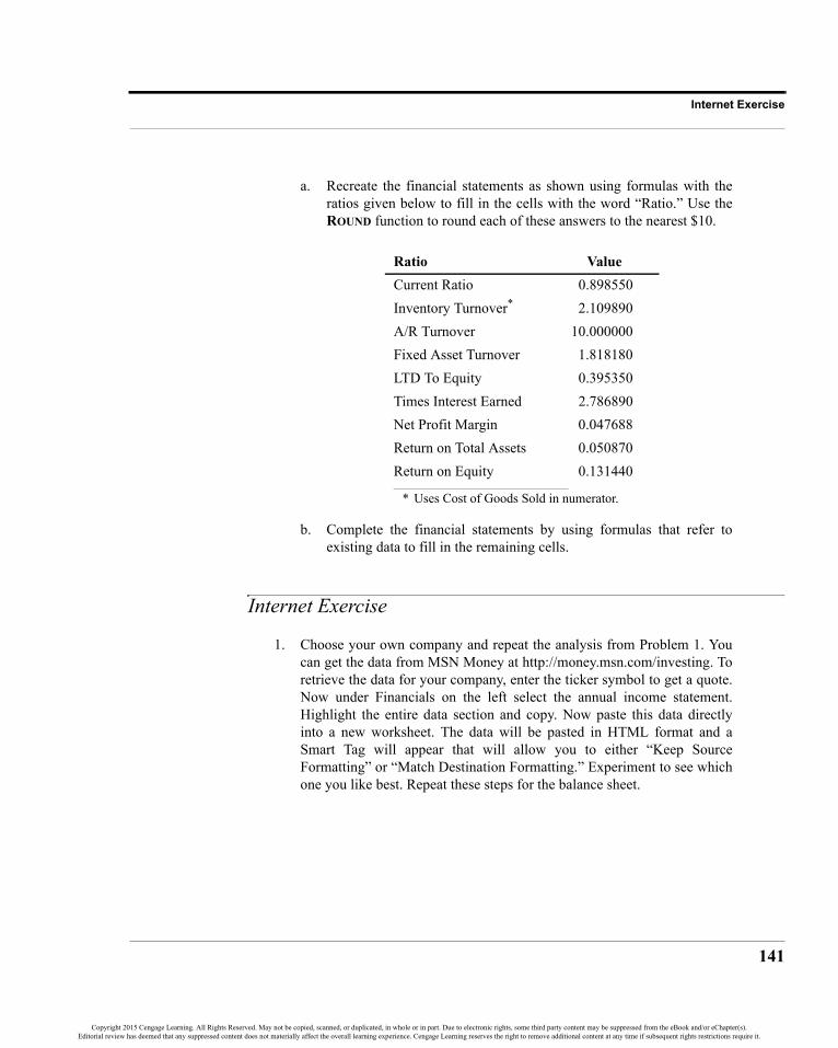
141
Internet Exercise
a. Recreate the financial statements as shown using formulas with theratios given below to fill in the cells with the word “Ratio.” Use theROUND function to round each of these answers to the nearest $10.
b. Complete the financial statements by using formulas that refer toexisting data to fill in the remaining cells.
Internet Exercise
1. Choose your own company and repeat the analysis from Problem 1. Youcan get the data from MSN Money at http://money.msn.com/investing. Toretrieve the data for your company, enter the ticker symbol to get a quote.Now under Financials on the left select the annual income statement.Highlight the entire data section and copy. Now paste this data directlyinto a new worksheet. The data will be pasted in HTML format and aSmart Tag will appear that will allow you to either “Keep SourceFormatting” or “Match Destination Formatting.” Experiment to see whichone you like best. Repeat these steps for the balance sheet.
Ratio ValueCurrent Ratio 0.898550Inventory Turnover*
* Uses Cost of Goods Sold in numerator.
2.109890A/R Turnover 10.000000Fixed Asset Turnover 1.818180LTD To Equity 0.395350Times Interest Earned 2.786890Net Profit Margin 0.047688Return on Total Assets 0.050870Return on Equity 0.131440
Copyright 2015 Cengage Learning. All Rights Reserved. May not be copied, scanned, or duplicated, in whole or in part. Due to electronic rights, some third party content may be suppressed from the eBook and/or eChapter(s).Editorial review has deemed that any suppressed content does not materially affect the overall learning experience. Cengage Learning reserves the right to remove additional content at any time if subsequent rights restrictions require it.

Copyright 2015 Cengage Learning. All Rights Reserved. May not be copied, scanned, or duplicated, in whole or in part. Due to electronic rights, some third party content may be suppressed from the eBook and/or eChapter(s).Editorial review has deemed that any suppressed content does not materially affect the overall learning experience. Cengage Learning reserves the right to remove additional content at any time if subsequent rights restrictions require it.

143
CHAPTER 5 Financial Forecasting
Forecasting is an important activity for a wide variety of business people. Nearly all of thedecisions made by financial managers are made on the basis of forecasts of one kind oranother. For example, in Chapter 3 we’ve seen how the cash budget can be used to forecastshort-term borrowing and investing needs. Every item in the cash budget is itself a forecast.Further, the ratios that we saw in Chapter 4 can be combined with forecasts to help achievecompany goals. In this chapter, we will examine several methods of forecasting. The first,the percent of sales method, is the simplest. We will also look at more advanced techniques,such as regression analysis.
After studying this chapter, you should be able to:1. Explain how the “percent of sales” method is used to develop pro forma financial
statements and how to construct such statements in Excel.2. Use circular references to perform iterative calculations.3. Use the TREND function for forecasting sales or any other trending variables.4. Perform a regression analysis with Excel’s built-in regression tools.5. Determine if a variable is statistically significant in a regression analysis.
Copyright 2015 Cengage Learning. All Rights Reserved. May not be copied, scanned, or duplicated, in whole or in part. Due to electronic rights, some third party content may be suppressed from the eBook and/or eChapter(s).Editorial review has deemed that any suppressed content does not materially affect the overall learning experience. Cengage Learning reserves the right to remove additional content at any time if subsequent rights restrictions require it.
CHAPTER 5: Financial Forecasting
144
The Percent of Sales MethodForecasting financial statements is important for a number of reasons. Among these areplanning for the future and providing information to the company’s investors. The simplestmethod of forecasting income statements and balance sheets is the percent of sales method.This method has the added advantage of requiring relatively little data to make a forecast.
The fundamental premise of the percent of sales method is that some, but not all, incomestatement and balance sheet items maintain a constant relationship with the level of sales.For example, if the cost of goods sold has averaged 65% of sales over the last several years,we would assume that this relationship would hold for the next year. If sales are expectedto be $10 million next year, our cost of goods forecast would be $6.5 million
.
Of course, this method assumes that the forecasted level of sales is already known. There aretwo primary methods of forecasting sales. The top-down method relies on forecasts ofmacroeconomic variables (e.g., GDP, inflation rates) and of the condition of the industry as awhole. These expectations are then converted into a sales forecast for the entire firm, andsales targets for each division or product. The bottom-up method involves discussions withcustomers to determine the expected demand for each product and expectations regardingprices, which are then summed to calculate a firm-wide sales forecast. Of course, firms canuse a combination of the two methods. We will take the sales forecast as a given.
Forecasting the Income StatementAs an example of income statement forecasting, consider the Elvis Products International(EPI) statements that you created in Chapter 2. The income statement is recreated here inExhibit 5-1. Recall that we have used a custom number format to display this data inthousands of dollars, but that the full-precision numbers are there. Open the workbook thatyou created for Chapter 2, and make a copy of the Income Statement worksheet. Rename thenew worksheet to PF Income Statement, where PF stands for pro forma.1
The level of detail that you have in an income statement will affect the number of itemsthat will fluctuate directly with sales. In general, we will proceed through the incomestatement line by line asking the question, “Is it likely that this item will changeproportionally with sales?” If the answer is yes, then we calculate the percentage of salesand multiply the result by the sales forecast for the next period. Otherwise, we will takeone of two actions: Leave the item unchanged, or use other information to change
1. Pro forma is a Latin word that, for our purposes, can be interpreted to mean “as if.” That is, theseforecasted financial statements are presented as if the forecast time period has already happened.
(10 million 0.65× 6.5 million)=
Copyright 2015 Cengage Learning. All Rights Reserved. May not be copied, scanned, or duplicated, in whole or in part. Due to electronic rights, some third party content may be suppressed from the eBook and/or eChapter(s).Editorial review has deemed that any suppressed content does not materially affect the overall learning experience. Cengage Learning reserves the right to remove additional content at any time if subsequent rights restrictions require it.

145
The Percent of Sales Method
the item.2 If you don’t know the answer, then you can create a chart that compares the itemto sales over the last several quarters or years. It should be obvious if there is arelationship, though you may need to use some of the statistical tools, discussed onpage 156, to determine the form of the relationship.
EXHIBIT 5-1EPI’S INCOME STATEMENTS FOR 2013 AND 2014
For EPI, only one income statement item will clearly change with sales: the cost of goodssold. Another item, SG&A (selling, general, and administrative) expense, is an aggregationof many things, some of which will probably change with sales and some that won’t. For ourpurposes we choose to believe that, on balance, SG&A will change along with sales (that is,we assume that SG&A is mostly variable costs).
Changes in the other items are not directly related to a change in sales in the short term.Depreciation expense, for example, depends on the amount and age of the firm’s fixedassets. Interest expense is a function of the amount and maturity structure of debt in thefirm’s capital structure. These items may, and probably will, change but we will needadditional information to forecast them. Taxes depend directly on the firm’s taxable income,though this indirectly depends on the level of sales. All of the other items on the incomestatement are calculated directly.
2. For example, if you know that the lease for the company’s headquarters building has a scheduledincrease, then you should be sure to include this information in your forecast for fixed costs.
Copyright 2015 Cengage Learning. All Rights Reserved. May not be copied, scanned, or duplicated, in whole or in part. Due to electronic rights, some third party content may be suppressed from the eBook and/or eChapter(s).Editorial review has deemed that any suppressed content does not materially affect the overall learning experience. Cengage Learning reserves the right to remove additional content at any time if subsequent rights restrictions require it.

CHAPTER 5: Financial Forecasting
146
Before getting started with the forecast, insert a column to the left of column B. Select a cellin column B and click the Insert button on the Home tab and then choose Insert SheetColumns. Note that a Smart Tag will appear that will give you three choices: (1) FormatSame As Left; (2) Format Same As Right; or (3) Clear Formatting. Choose the secondoption so that the custom number formats and column width will automatically be applied.So that we can experiment later if we choose, enter 40% for the tax rate in B18 and C18.
To generate our income statement forecast, we first determine the percentage of sales foreach of the prior years for each item that changes. In this case, for 2014 we have:
The 2013 percentages (83.45% and 6.99%, respectively) can be found in exactly the samemanner. We now calculate the average of these percentages over the past few years, and usethis average as our estimate of the 2015 percentage of sales. The forecast is then found bymultiplying these percentages by next year’s sales forecast. Assuming that sales areforecasted to be $4,300,000 in 2015 we have:
To calculate the arithmetic average in Excel use the AVERAGE function, which is defined as:
Average(NUMBER1, NUMBER2, …)
where NUMBER1 is required, and you may have as many as 255 numbers or ranges.
Exhibit 5-2 shows a forecast of the complete 2015 income statement. To create this forecastin your worksheet, in B4 enter: 2015.3 Because the 2015 income statement will becalculated in exactly the same way as 2014, the easiest way to proceed is to copy C5:C15into B5:B15. This will save you from entering formulas to calculate subtotals (e.g., EBIT)and will apply the cell borders. Insert a row above row 17, and in A16 type: *Forecast.
Cost of Goods Sold 2014 Percentage of Sales
SG&A Expense 2014 Percentage of Sales
Cost of Goods Sold 2015 ForecastSG&A Expense 2015 Forecast
3. We have chosen to apply a custom format so that the number has an asterisk to indicate a footnotethat informs the reader that these are forecasts. The custom format is #”*”.
$3,250,0003,850,000
--------------------------- 0.8442 84.42%= =
$330,3003,850,000------------------------ 0.0858 8.58%= =
$4,300,000 0.8393× 3,609,108=
$4,300,000 0.0779× 334,803=
Copyright 2015 Cengage Learning. All Rights Reserved. May not be copied, scanned, or duplicated, in whole or in part. Due to electronic rights, some third party content may be suppressed from the eBook and/or eChapter(s).Editorial review has deemed that any suppressed content does not materially affect the overall learning experience. Cengage Learning reserves the right to remove additional content at any time if subsequent rights restrictions require it.

147
The Percent of Sales Method
EXHIBIT 5-2PERCENT OF SALES FORECAST FOR 2015
First, in B5 enter the sales forecast: 4,300,000. Now, we can calculate the 2015 cost ofgoods forecast in B6 with the formula: =AVERAGE(C6/C$5,D6/D$5)*B$5. Thisformula calculates the average of the cost of goods as a percentage of sales for the last twoyears and then multiplies it by the sales forecast. The result should be as shown above. Nowcopy this formula and paste it into B8 (using Paste Special Formulas to avoid pasting theunderline) to get the forecast for SG&A expense.
Instead of performing the entire calculation in cells B6 and B8, we could have used a helpercolumn. A helper column is used to do intermediate calculations and is sometimes useful. Inthis case, we could have calculated the average percentage of sales for each item in, say,column K. We would then use these values to perform the final calculation in column B. Forexample, K6 might contain the formula: =AVERAGE(C6/C$5,D6/D$5). Then theformula in B6 would be: =K6*B$5. This technique would allow you to easily see theaverage percentages (as in a common-size income statement) that are being used to generatethe forecast. Although this might be useful, it can be an inefficient use of the spreadsheetunless it is necessary and may be confusing to others who view your work.
Copyright 2015 Cengage Learning. All Rights Reserved. May not be copied, scanned, or duplicated, in whole or in part. Due to electronic rights, some third party content may be suppressed from the eBook and/or eChapter(s).Editorial review has deemed that any suppressed content does not materially affect the overall learning experience. Cengage Learning reserves the right to remove additional content at any time if subsequent rights restrictions require it.

CHAPTER 5: Financial Forecasting
148
Assume that we do not have any information regarding changes in fixed expenses, so copythe value from C9. However, we have been informed that the firm intends to invest $50,000in fixed assets in 2015. This will cause depreciation expense to rise by $5,000. We need todocument this assumption, so in A20 type: Additional Depreciation, and in B20enter: 5,000. We will come back to add a formula in B20 in the next section. Don’t forgetto apply the same custom number format to this cell that we used in the others.
The formula to calculate depreciation expense in B10 is: =C10+B20. Because we don’t yetknow how the firm will finance these investments, leave the interest expense at the samelevel as 2014. To calculate the taxes, in B14, use the formula: =B19*B13. Your worksheetshould now look like the one in Exhibit 5-2, page 147.
Forecasting Assets on the Balance SheetWe can forecast the balance sheet in exactly the same way as the income statement, withsome major exceptions. For those items that can be expected to vary directly with sales, ourformulas will be similar to those we have already seen. We will explain how to handle theother items below. Make a copy of the Balance Sheet and rename it PF Balance Sheet.
Create the percent of sales balance sheet for 2015 by selecting column B and inserting a newcolumn. Change the heading to say Pro Forma Balance Sheet so that it is clear that weare working with a forecast. In B4 type the label: 2015. As before, apply a custom numberformat to display an asterisk after the number. Like we did with the income statement, wewill move, line by line, through the balance sheet to determine which items will vary withsales.
The firm’s cash balance is the first, and perhaps the most difficult, item with which we needto work. Does the cash balance vary, in constant proportion, with sales? Your first responsemight be, “Of course it does. As the firm sells more goods, it accumulates cash.” This line ofreasoning neglects two important facts. The firm has other things to do with its cash besidesaccumulating it, and because cash is a low-return asset, firms should seek to minimize theamount of their cash balance.4 For these reasons, even though the cash balance will probablychange, it probably will not change by the same percentage as sales and cash levels tend tobe volatile. Therefore, we will simply use the cash balance from 2014 as our forecast, soenter: =C5 into cell B5.
The next two items, accounts receivable and inventory, are much easier. Both of these arelikely to fluctuate roughly in proportion to sales. Using the same methodology that we usedfor the pro forma income statement, we will find the average percentage of sales for the past
4. Within reason, of course. Firms need some amount of cash to operate, but the amount needed doesnot necessarily vary directly with the level of sales.
Copyright 2015 Cengage Learning. All Rights Reserved. May not be copied, scanned, or duplicated, in whole or in part. Due to electronic rights, some third party content may be suppressed from the eBook and/or eChapter(s).Editorial review has deemed that any suppressed content does not materially affect the overall learning experience. Cengage Learning reserves the right to remove additional content at any time if subsequent rights restrictions require it.

149
The Percent of Sales Method
two years and multiply that amount by our sales forecast for 2015. For accounts receivable,the formula in B6 is: =AVERAGE(C6/'PF Income Statement'!C$5,D6/'PFIncome Statement'!D$5)*'PF Income Statement'!$B$5. Instead of typingthe references to the pro forma income statement, it is easier to insert them by displayingboth the income statement and the balance sheet and selecting the appropriate cells with themouse. Click the View tab and select New Window. This will create an additional view ofthe workbook. Next, click on the Arrange All button and choose how you would like theworksheets arranged. In the second view, change to the PF Income Statement worksheet.Now that both worksheets are visible, it is easier to select cells. Because we will use thesame formula for inventory, we can simply copy this formula down to B7. Total currentassets in B8 is a calculated value, so we can copy the formula directly from cell C8.
In B9, we have the 2015 gross plant and equipment. This is the historical purchase price ofthe buildings and equipment that the firm owns. As noted earlier, the firm plans to make netnew investments of $50,000 in 2015. We will document this assumption by entering NetAddition to Plant and Equipment in A28 and 50,000 in B28. The formula in B9is: =C9+B28. Note that this increase is not necessarily due to the expected increase in sales.Although gross fixed assets may rise or fall in any given year, most companies alwaysoperate with spare capacity so the changes are not, in the short run, directly related to sales.
We now need to calculate the additional depreciation. We will assume that the expected lifeof the new equipment is 10 years and that it will be depreciated using the straight-linemethod to a salvage value of zero. In A29 enter the label: Life of New Equipment inYears, and in B29 enter 10. In A30 enter: New Depreciation (Straight-line).In B30 we will calculate the depreciation using the SLN function, which is defined as:
SLN(COST, SALVAGE, LIFE)
where the arguments are defined as you would expect. In B30 enter: =SLN(B28,0,B29).The additional depreciation expense will be $5,000. Now, return to the pro forma incomestatement where we will enter a formula in B20: ='PF Balance Sheet'!B30. This laststep allows us to change the amount of the new investment and have the additionaldepreciation expense reflected on the pro forma income statement.
Now, return to the pro forma balance sheet. Accumulated depreciation will definitelyincrease in 2015 but not because of the forecasted change in sales. Instead, accumulateddepreciation will increase by the amount of the depreciation expense for 2015. To determinethe accumulated depreciation for 2015, we will add 2015’s depreciation expense to 2014’saccumulated depreciation. The formula is: =C10+'PF Income Statement'!B10.
To complete the asset side of the balance sheet, we note that both net fixed assets and totalassets are calculated values. We can simply copy the formulas from C11:C12 and paste theminto B11:B12.
Copyright 2015 Cengage Learning. All Rights Reserved. May not be copied, scanned, or duplicated, in whole or in part. Due to electronic rights, some third party content may be suppressed from the eBook and/or eChapter(s).Editorial review has deemed that any suppressed content does not materially affect the overall learning experience. Cengage Learning reserves the right to remove additional content at any time if subsequent rights restrictions require it.

CHAPTER 5: Financial Forecasting
150
Forecasting Liabilities on the Balance SheetOnce the assets are completed, the rest of the balance sheet is comparatively simple becausewe can mostly copy formulas already entered. Before continuing, however, we need todistinguish among the types of financing sources. We have already seen that the types offinancing that a firm uses can be divided into three categories:
• Current liabilities• Long-term liabilities• Owner’s equity
These categories are not sufficiently distinguished for our purposes here. Instead, we willdivide the liabilities and equity of a firm into two categories:
• Spontaneous sources of financing—These are the sources of financing thatarise during the ordinary course of doing business. One example isaccounts payable. After a credit account is established with a supplier, noadditional work is required to obtain credit; it just happens spontaneouslywhen the firm makes a purchase. Note that not all current liabilities arespontaneous sources of financing (e.g., short-term notes payable, long-term debt due in one year).
• Discretionary sources of financing—These are the financing sources thatrequire a large effort on the part of the firm to obtain. In other words, thefirm must make a conscious decision to obtain these funds. Furthermore,the firm’s upper-level management will use its discretion to determine theappropriate type of financing to use. Examples of this type of financinginclude any type of bank loan, bonds, preferred stock, and common stock(but not retained earnings).
Generally speaking, spontaneous sources of financing can be expected to vary directly withsales. Changes in discretionary sources, on the other hand, will not have a direct relationshipwith changes in sales. We always leave discretionary sources of financing unchanged forreasons that will soon become clear.
Returning now to our forecasting problem, the first item to consider is accounts payable. Asnoted above, accounts payable is a spontaneous source of financing and will, therefore,change directly with sales. To enter the formula, all that is necessary is to copy the formulafrom one of the other items that we have already completed. Copy the contents of B6 (or B7,it doesn’t matter which) and paste it into B14. The result should indicate a forecastedaccounts payable of $189.05.
The next item to consider is the short-term notes payable. Because this is a discretionarysource of financing, we will leave it unchanged from 2014. In reality, we might handle thisitem differently if we had more information. For example, if we knew that the notes would
Copyright 2015 Cengage Learning. All Rights Reserved. May not be copied, scanned, or duplicated, in whole or in part. Due to electronic rights, some third party content may be suppressed from the eBook and/or eChapter(s).Editorial review has deemed that any suppressed content does not materially affect the overall learning experience. Cengage Learning reserves the right to remove additional content at any time if subsequent rights restrictions require it.

151
The Percent of Sales Method
be retired before the end of 2015, we would change our forecast to zero. Alternatively, if thepayments on the notes include both principal and interest, our forecast would be the 2014amount less principal payments that we expect to make in 2015. Because we are leaving itunchanged, the formula in B15 is: =C15.
If we assume that the “other current liabilities” item represents primarily accrued expenses,then it is a spontaneous source of financing. We can, therefore, simply copy the formulafrom B14 and paste it into B16. The forecasted amount is $163.38.
Long-term debt, in B18, and common stock, in B20, are both discretionary sources offinancing. We will leave these balances unchanged from 2014. In B18 the formula is: =C18and in B20 the formula is: =C20.
The final item that we must consider is retained earnings. Recall that retained earningsaccumulates over time. That is, the balance in any year is the accumulated amount that hasbeen added in previous years plus any new additions. The amount that will be added toretained earnings is given by:
Change in Retained Earnings = Net Income – Dividends
where the dividends are those paid to both the common and preferred stockholders. Theformula for retained earnings will require that we reference forecasted 2015 net income fromthe income statement and the dividends from the statement of cash flows (see Exhibit 2-7, page59). Note that we are assuming that 2015 dividends will be the same as the 2014 dividends.We can reference these cells in exactly the same way as before, so the formula is:=C21+'PF Income Statement'!B15+'Statement of Cash Flows'!B19. Theresults should show that we are forecasting retained earnings to be $297.04 in 2015.
At this point, you should go back and calculate the subtotals in B17, B19, and B22. Finally,we calculate the total liabilities and owner’s equity in B23 with =B19+B22.
Discretionary Financing NeededSharp-eyed readers will notice that our pro forma balance sheet does not balance. Althoughthis appears to be a serious problem, it actually represents one of the purposes of the proforma balance sheet. The difference between total assets and total liabilities and owner’sequity is referred to as discretionary financing needed (DFN, also called additional fundsneeded or required new funds). In other words, this is the amount of discretionary financingthat the firm thinks it will need to raise in the next year. Because of the amount of time andeffort required to raise these funds, it is important that the firm be aware of its needs well inadvance. The pro forma balance sheet fills this need. Frequently, the firm will find that it isforecasting a higher level of assets than liabilities and equity. In this case, the managerswould need to arrange for more liabilities and/or equity to finance the level of assets needed
Copyright 2015 Cengage Learning. All Rights Reserved. May not be copied, scanned, or duplicated, in whole or in part. Due to electronic rights, some third party content may be suppressed from the eBook and/or eChapter(s).Editorial review has deemed that any suppressed content does not materially affect the overall learning experience. Cengage Learning reserves the right to remove additional content at any time if subsequent rights restrictions require it.

CHAPTER 5: Financial Forecasting
152
to support the volume of sales expected. This is referred to as a deficit of discretionary funds.If the forecast shows that there will be a higher level of liabilities and equity than assets, thefirm is said to have a surplus of discretionary funds. Remember that, in the end, the balancesheet must balance. The “plug figure” necessary to make this happen is the DFN.
We should add an extra line at the bottom of the pro forma balance sheet to calculate theDFN. Type Discretionary Financing Needed in A25, and in B25 add theformula =B12-B23. This calculation tells us that EPI expects to need $38,119.50(displayed as 38.12 with the custom number format) more in discretionary funds tosupport its forecasted level of assets. In this case, EPI is forecasting a deficit ofdiscretionary funds. Apply the custom number format to this number and to the rest of thebalance sheet.
EXHIBIT 5-3EPI’S PRO FORMA BALANCE SHEET FOR 2015
Copyright 2015 Cengage Learning. All Rights Reserved. May not be copied, scanned, or duplicated, in whole or in part. Due to electronic rights, some third party content may be suppressed from the eBook and/or eChapter(s).Editorial review has deemed that any suppressed content does not materially affect the overall learning experience. Cengage Learning reserves the right to remove additional content at any time if subsequent rights restrictions require it.

153
Using Iteration to Eliminate DFN
To make clear that this amount is a deficit (note that the sign is the opposite of what mightbe expected when using that word), we can have Excel inform us whether we will havea surplus or deficit of discretionary funds. Use an IF statement and realize that if the DFNis a positive number, then we have a deficit; otherwise we have a surplus or DFN iszero. So the formula in C25 is: =IF(B25>0,"Deficit", IF(B25<0,"Surplus","Balanced")).5 Your balance sheet should now resemble that in Exhibit 5-3.
Using Iteration to Eliminate DFNCircular errors result when a formula refers back to itself, either directly or indirectlythrough another formula. A simple example would be if the formula in B18 was =B18. Excelcannot calculate this because the result depends on itself (it is self-referential). In most cases,this is undesirable even if the formula eventually converges to a solution. However, there arecircumstances that are necessarily self-referential and cannot be solved in any other way.
For example, if we wish to eliminate the DFN deficit, then the firm must raise that amount ofmoney. Suppose that any discretionary funds will be raised with long-term debt. Simplyadding $38.12 to the long-term debt in B18 will not quite solve the problem because that willlead to other changes. Specifically, additional long-term debt will increase interest expenseresulting in lower net income. In turn, this will reduce retained earnings and still leave uswith a (smaller) deficit of funding. This new DFN can then be added to long-term debtagain, setting off the same chain of calculations. We repeat this cycle as many times asnecessary until DFN is equal to zero (or within some allowable tolerance).
By default, Excel will not allow such calculations because the result may not converge. Thiswould lead to an infinite loop of calculations that would tie up your computer in an endlessseries of calculations. However, if we know that the result will converge (as it will in thiscase) we can enable these kinds of self-referential, or iterative, calculations. To do so, clickOptions in the File tab and then go to Formulas. Check the Enable iterative calculationoption. Note that we can set the maximum number of iterations as well as the convergencecriteria. The default settings will cause the calculation to stop after 100 iterations or if thechange in the result is 0.001 or less. Because we should need only a few iterations, leavethese at their default settings.
Before we can eliminate the DFN, we need to make a few changes to the pro forma incomestatement and balance sheet. On the pro forma income statement, we need to add an interestrate. In A21 add the label: Interest Rate and then type 11.70% into B21. This will
5. You could also design a custom number format. One possible format is: #,###.00,"Deficit";#,###.00, "Surplus". The benefits of this approach are that you don’t needto use a separate cell and you don’t need to enter a formula.
Copyright 2015 Cengage Learning. All Rights Reserved. May not be copied, scanned, or duplicated, in whole or in part. Due to electronic rights, some third party content may be suppressed from the eBook and/or eChapter(s).Editorial review has deemed that any suppressed content does not materially affect the overall learning experience. Cengage Learning reserves the right to remove additional content at any time if subsequent rights restrictions require it.
CHAPTER 5: Financial Forecasting
154
allow us to calculate the total interest expense as the amount of debt changes. In B12 we willcalculate the interest expense for 2015 with the formula: =B21*('PF BalanceSheet'!B15+'PF Balance Sheet'!B18). Note that the interest expense is 11.70%of the sum of short-term notes payable and long-term debt. At this point, the value in B12should be the same as before (76.00).
On the pro forma balance sheet, we need to add our self-referential formula. Our goal is tohave the long-term debt (in B18) increase by the amount of the DFN (in B25). However, wecan’t just set the formula in B18 to =B25. If we did, then the long-term debt would be 38.12,which would lead to a bigger DFN. This would then cause the debt to grow and the DFN toshrink, which would then cause the debt to shrink and the DFN to grow. It will neverconverge and will bounce back and forth until it hits the limit on the number of iterations.
To solve this problem by hand, we would start with the current amount of long-term debt(424.61) and then add the DFN to that. This will increase long-term debt, increase interestexpense, lower net income, and reduce retained earnings leading to a lower DFN. We nowstart over again by adding the new DFN amount to long-term debt and the cycle will repeat.If we do this three or four times, DFN will get very close to zero. It may take 20 or 30 cyclesfor DFN to converge to exactly zero.6
Fortunately, we don’t have to do this by hand. With the right formula for long-term debt, wecan make the amount accumulate over many cycles. In B18 enter the formula: =B18+B25.This formula will take the current amount of long-term debt and add the DFN. This will leadto a chain of calculations that will lead to lower DFN. This amount will then be added to thelong-term debt, and so on. Eventually, it will converge so that DFN equals zero and long-term debt is 465.61. Note also that interest expense is 80.80, net income is 90.17, andretained earnings is 294.16. The pro forma balance sheet should now look similar to the onein Exhibit 5-4 on page 155, except that we have a couple of important modifications tomake.
This whole process will occur very rapidly, and you may not even see the changes takingplace. It will be instructive to step through the process one iteration at a time. To do this, goto the Formulas tab in Options and set the Maximum Iterations to 1 (the default is 100).Now, reenter the formula in B18 (you must do this to reset the calculation). You should seethat long-term debt is now 0.00, and DFN is 465.61. To step through the calculation, simplypress the F9 key. This will cause the workbook to recalculate one cycle of the iterativeformula. Long-term debt will now be 465.61 and DFN will be −32.69. Press F9 again torepeat the calculation and you will see how the numbers change. Keep pressing F9 until
6. You are strongly urged to try doing this by hand. This exercise will greatly improve yourunderstanding of the process.
Copyright 2015 Cengage Learning. All Rights Reserved. May not be copied, scanned, or duplicated, in whole or in part. Due to electronic rights, some third party content may be suppressed from the eBook and/or eChapter(s).Editorial review has deemed that any suppressed content does not materially affect the overall learning experience. Cengage Learning reserves the right to remove additional content at any time if subsequent rights restrictions require it.

155
Using Iteration to Eliminate DFN
DFN goes to zero for several keystrokes. Make sure to go back and reset the maximumnumber of iterations to 100 or more before continuing.
Let’s now improve our iterative calculations a bit. It is very helpful to have the capability toenable or disable the iterative calculations. This can be done as discussed above, but that istedious. Instead, we can use a cell value (0 or 1) combined with IF statements to do the job.In A31, enter: Iteration and in B31 enter: 0. This will disable iteration, while a 1 willenable iteration. Now, in B18 change the formula for long-term debt so that it is:=IF(B31=1,B18+B25,C18). If iteration is turned on (B31 = 1) then the formula will bethe same as before. If iteration is off then long-term debt will be the same as it was in 2014.It can also be helpful to have a note appear when iteration is on. So, in C31 enter theformula: =IF(B31=1,"Iteration is ON","").
EXHIBIT 5-4THE PRO FORMA BALANCE SHEET AFTER ITERATION
Copyright 2015 Cengage Learning. All Rights Reserved. May not be copied, scanned, or duplicated, in whole or in part. Due to electronic rights, some third party content may be suppressed from the eBook and/or eChapter(s).Editorial review has deemed that any suppressed content does not materially affect the overall learning experience. Cengage Learning reserves the right to remove additional content at any time if subsequent rights restrictions require it.

CHAPTER 5: Financial Forecasting
156
One final change is necessary. We would like to know exactly how much new financing isrequired. It should be clear that the original $38.12 is not the correct answer because eachtime that we iterate we add more long-term debt. So, we need a cell to calculate theaccumulated DFN. Select row 26 and insert a new row. Now, in A26 enter the label: TotalAccumulated DFN, and in B26 enter the formula: =IF(B32=1,B26+B25,B25). Ifiteration is on, this formula will keep track of the additions to DFN. Otherwise, it will beequal to the DFN without iteration. Experiment by changing B32 to 0 and back to 1 to seethe effect of these changes.
This worksheet could be further refined in several ways. As one example, instead of raisingall of the DFN using long-term debt, we could allocate some of it to new equity. In this case,we might use the long-term debt ratio to determine how much should be long-term debt. Thebalance would be allocated to equity. Note that additional equity would result in moredividends, which would complicate the situation a bit.
Using circular references should be the last resort. They should be used only whenabsolutely necessary, as in this case. If your calculation does not converge to a single value,then Excel will eventually stop trying to calculate it and you will have wrong answers.Furthermore, this technique is quite calculation intensive and will cause recalculation of alarge spreadsheet to slow to a crawl. If at all possible, you should try to find another methodof solving the problem that doesn’t involve circular references.7
Other Forecasting MethodsThe primary advantage of the percent of sales forecasting method is its simplicity. There aremany other more sophisticated forecasting techniques that can be implemented in aspreadsheet program. In the rest of this chapter, we will look at techniques based on linearregression analysis.
Linear Trend ExtrapolationSuppose that you were asked to perform the percent of sales forecast for EPI. The first stepin that analysis requires a sales forecast. Because EPI is a small company, nobody regularlymakes such forecasts and you will have to generate your own. Where do you start?
Your first idea might be to see if there has been a clear trend in sales over the past severalyears and to extrapolate that trend, if it exists, to 2015. To see if there has been a trend, you
7. For an alternative to iterative calculations, see T. Arnold and P.C. Eismann, “Debt Financing DoesNOT Create Circularity Within Pro Forma Analysis,” Advances in Financial Education, Vol 6,Summer 2008, pp. 96–102.
Copyright 2015 Cengage Learning. All Rights Reserved. May not be copied, scanned, or duplicated, in whole or in part. Due to electronic rights, some third party content may be suppressed from the eBook and/or eChapter(s).Editorial review has deemed that any suppressed content does not materially affect the overall learning experience. Cengage Learning reserves the right to remove additional content at any time if subsequent rights restrictions require it.

157
Other Forecasting Methods
first gather data on sales for EPI for the past five years. Table 5-1 presents the data that youhave gathered. Add a new worksheet to your EPI workbook and rename it “Trend Forecast”so that it can be easily identified. Enter the data from Table 5-1 into your worksheetbeginning in A1.
The easiest way to see if there has been a trend in sales is to create a chart that plots the salesdata versus the years. Select A1:B6, and then insert a scatter chart8 by clicking the Insert tab,then Insert Scatter (X,Y) or Bubble Chart, and choosing “Scatter with Straight Lines andMarkers” as the type. Once the chart is created, click the Chart Elements button and insertthe title: EPI Sales for 2010 to 2014. Your worksheet should resemble Exhibit 5-5.
EXHIBIT 5-5EPI TREND FORECAST WORKSHEET
Examining the chart leads to the conclusion that sales have definitely been increasing overthe past five years, but not at a constant rate. There are several ways to generate a forecastfrom this data, even though the sales are not increasing at a constant rate.
TABLE 5-1EPI SALES FOR 2010 TO 2014
Year Sales2010 1,890,5322011 2,098,4902012 2,350,3082013 3,432,0002014 3,850,000
8. A line chart would also work. However, because our x-axis labels (years) are numeric, a scatterchart is the better choice.
Copyright 2015 Cengage Learning. All Rights Reserved. May not be copied, scanned, or duplicated, in whole or in part. Due to electronic rights, some third party content may be suppressed from the eBook and/or eChapter(s).Editorial review has deemed that any suppressed content does not materially affect the overall learning experience. Cengage Learning reserves the right to remove additional content at any time if subsequent rights restrictions require it.

CHAPTER 5: Financial Forecasting
158
One method is to let Excel draw a linear trend line. That is, let Excel fit a straight line to thedata and extrapolate that line to 2015 (or beyond). The line generated is in the form of:
which you should recognize as the same equation used in algebra courses to describe astraight line. In this equation, m is the slope and b is the intercept.
To determine the parameters for this line (m and b) Excel uses regression analysis, which wewill examine later. To generate a forecast based on the trend, we need to use the TRENDfunction which is defined as:
TREND(KNOWN_Y’S, KNOWN_X’S, NEW_X’S, CONST)
In the TREND function definition, KNOWN_Y’S is the range of the data that we wish toforecast (the dependent variable) and KNOWN_X’S is the optional range of data (theindependent variables) that we want to use to determine the trend in the dependent variable.9Because the TREND function is generally used to forecast a time-based trend, KNOWN_X’Swill usually be a range of years, though it can be any set of consecutive numbers (e.g., 1, 2,3,…). NEW_X’S is a continuation of the KNOWN_X’S for which we don’t yet know the value ofthe dependent variable. CONST is a boolean (True/False) variable that tells Excel whether or notto include an intercept in its calculations (generally this should be set to true or omitted).
To generate a forecast for 2015, first enter 2015 into A7. This will provide us with theNEW_X’S value that we will use to forecast 2015 sales. Next, enter the TREND function as:=TREND(B$2:B$6,A$2:A$6,A7,TRUE) into B7. The result is a sales forecast of$4,300,000, which is the same sales forecast that we used in the percent of sales forecastingmethod for the financial statements.
We can extend our forecast to 2016 and 2017 quite easily. To do this, first enter 2016 intoA8 and 2017 into A9. Now copy the formula from B7 to B8:B9. You should see that theforecasted sales for 2016 and 2017 are $4,825,244 and $5,350,489, respectively.
Adding Trend Lines to ChartsAn interesting feature of charts in Excel is that we can tell Excel to add a trend line to thechart. Adding this line requires no more work than making a menu choice; we do not have tocalculate the data ourselves. To add a trend line to our chart, right-click the data series in the
9. While KNOWN_X’S and NEW_X’S are technically optional arguments, they should not be omitted inmost cases. If both are omitted, then TREND returns an array of values on the trend line instead ofthe next forecasted value. In this case, if you neglect to array enter (Ctrl+Shift+Enter) and selectmultiple cells then the result will be the first value that is on the trend line.
Y mX b+=
Copyright 2015 Cengage Learning. All Rights Reserved. May not be copied, scanned, or duplicated, in whole or in part. Due to electronic rights, some third party content may be suppressed from the eBook and/or eChapter(s).Editorial review has deemed that any suppressed content does not materially affect the overall learning experience. Cengage Learning reserves the right to remove additional content at any time if subsequent rights restrictions require it.

159
Other Forecasting Methods
chart and then choose Add Trendline from the shortcut menu to see the default linear trendline. In the Format Trendline panel, you can set the formatting options for the line. You canalso show trend lines that aren’t linear. For example, if sales had been increasing at anincreasing rate, you might want to fit an exponential trend instead of a linear one. Excel alsooffers five other trend lines that it can calculate, including a moving average of user-determined length.
Excel can even do a forecast automatically in the chart, though you will not get the actualnumerical forecast using this method. First, right-click the data series and choose FormatTrendline. Before closing the Format Trendline panel, look at the Forecast section and setForward to 1 unit. After clicking on the Close button, you will see a trend line that extends to2015. We could also extend the forecast to 2016 or 2017 by setting Forward to 2 or 3.
If you decide that you no longer want to see the trend line, simply right-click on it andchoose Delete from the shortcut menu.
Recall that we said that Excel generates the equation for the trend line and uses this equationto make the forecast. We can have Excel show this equation on the chart by selecting theappropriate options. Right-click on the trend line and choose Format Trendline from theshortcut menu. Near the bottom of the panel click on Display Equation on Chart. Click onthe Close button and you should see the equation appear on the chart.
The equation that Excel displays, using scientific notation, is:
which is Excel’s way of saying:
However, you should be suspicious of rounding problems any time you see scientificnotation. In some cases the rounding isn’t important, but in this case it is. We can fix theproblem by right-clicking on the equation and choosing Format Trendline Label from theshortcut menu. Apply another format in the Label Options section and you should now seethat the equation is:
We can see that this equation does indeed generate the forecast for 2015 by substituting 2015for x in the equation. At this point, your worksheet should look like the one in Exhibit 5-6.
y 525245x 1E+09–=
y 525,245x 1,000,000,000–=
y 525,244.60x 1,054,067,869.20–=
Copyright 2015 Cengage Learning. All Rights Reserved. May not be copied, scanned, or duplicated, in whole or in part. Due to electronic rights, some third party content may be suppressed from the eBook and/or eChapter(s).Editorial review has deemed that any suppressed content does not materially affect the overall learning experience. Cengage Learning reserves the right to remove additional content at any time if subsequent rights restrictions require it.
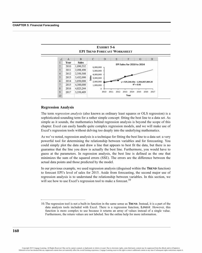
CHAPTER 5: Financial Forecasting
160
EXHIBIT 5-6EPI TREND FORECAST WORKSHEET
Regression AnalysisThe term regression analysis (also known as ordinary least squares or OLS regression) is asophisticated-sounding term for a rather simple concept: fitting the best line to a data set. Assimple as it sounds, the mathematics behind regression analysis is beyond the scope of thischapter. Excel can easily handle quite complex regression models, and we will make use ofExcel’s regression tools without delving too deeply into the underlying mathematics.
As we’ve noted, regression analysis is a technique for fitting the best line to a data set: a verypowerful tool for determining the relationship between variables and for forecasting. Youcould simply plot the data and draw a line that appears to best fit the data, but there is noguarantee that the line you draw is actually the best line. Furthermore, you would have toguess at the parameters. In regression analysis, the best line is defined as the one thatminimizes the sum of the squared errors (SSE). The errors are the difference between theactual data points and those predicted by the model.
In our previous example, we used regression analysis (disguised within the TREND function)to forecast EPI’s level of sales for 2015. Aside from forecasting, the second major use ofregression analysis is to understand the relationship between variables. In this section, wewill see how to use Excel’s regression tool to make a forecast.10
10.The regression tool is not a built-in function in the same sense as TREND. Instead, it is a part of thedata analysis tools included with Excel. There is a regression function, LINEST. However, thisfunction is more complex to use because it returns an array of values instead of a single value.Furthermore, the return values are not labeled. See the online help for more information.
Copyright 2015 Cengage Learning. All Rights Reserved. May not be copied, scanned, or duplicated, in whole or in part. Due to electronic rights, some third party content may be suppressed from the eBook and/or eChapter(s).Editorial review has deemed that any suppressed content does not materially affect the overall learning experience. Cengage Learning reserves the right to remove additional content at any time if subsequent rights restrictions require it.

161
Other Forecasting Methods
Consider the following example in which we will make use of regression analysis to try toget an alternative forecast of next year’s cost of goods sold for EPI. Table 5-2 provides thehistorical data for sales and cost of goods sold.
Note that the data for the variables must be in columns when using the regression tool. Excelwill misinterpret the data if it is in rows.
Recall that we previously calculated the average percentage of sales for 2013 and 2014 andused that average to generate our forecast for 2015. Suppose, however, that you areconcerned that there may possibly be a more systematic relationship between sales and costof goods sold. For example, it is entirely possible that as sales rise, cost of goods sold willrise at a slower rate. This may be due to efficiencies in the production process, quantitydiscounts on materials, and so on. Alternatively, there may be another relationship, or noneat all. Regression analysis can help us to gain a better understanding of the historicalrelationship and, hopefully, generate better forecasts of the future cost of goods sold.
Before running the regression, let’s create a chart of the data to help get a visual picture ofthe historical relationship. Enter the data from Table 5-2 into a new worksheet beginning incell A1. Now select B1:C6 and create a scatter chart of the data.
To facilitate our visualization, change the scale on each axis as follows: Right-click the y-axis and choose Format Axis. On the Axis Options tab, under Bounds, change the Minimumto 1,000,000, the Maximum to 4,000,000, and the Major unit to 1,000,000. Repeatthose settings for the x-axis. This will ensure that the scale of each axis is the same, whichmakes it much easier to see the relationship between our two variables. Note that you willprobably need to change the width of the chart so that the distance between tick marks is thesame on the x-axis as on the y-axis. This can be done in the Size group on the Chart ToolsFormat tab of the Ribbon.
TABLE 5-2EPI’S HISTORICAL SALES AND COST OF GOODS
Year Sales Cost of Goods2010 $ 1,890,532 $ 1,570,2002011 2,098,490 1,695,6942012 2,350,308 1,992,4002013 3,432,000 2,864,0002014 3,850,000 3,250,000
Copyright 2015 Cengage Learning. All Rights Reserved. May not be copied, scanned, or duplicated, in whole or in part. Due to electronic rights, some third party content may be suppressed from the eBook and/or eChapter(s).Editorial review has deemed that any suppressed content does not materially affect the overall learning experience. Cengage Learning reserves the right to remove additional content at any time if subsequent rights restrictions require it.

CHAPTER 5: Financial Forecasting
162
FIGURE 5-1CHART OF COST OF GOODS SOLD VS. SALES
The chart in Figure 5-1 shows what appears to be a fairly consistent relationship.Furthermore, the slope of the line is something less than 45 degrees so we know that achange in sales of $1 will lead to a change of less than $1 in cost of goods sold (as we wouldexpect). We can’t know the exact relationship just by reading the chart, but we can run aregression analysis on the data to find the exact slope and intercept of the best-fitting line forthis data.
Excel provides several functions to calculate the parameters of a regression equation. Forexample, the INTERCEPT, SLOPE, and LINEST functions all return the parameters of aregression line, while the TREND and FORECAST functions use linear regression to generateforecasts. There are also functions for nonlinear regression (e.g., GROWTH and LOGEST).
However, Excel also includes another method that we will cover here: the regression tool inthe Analysis ToolPak add-in. This tool works very much like any statistical program that youmay have used. It will ask for the data and then output a table of the regression results,including diagnostic data that is used to determine whether the relationship between thevariables is statistically significant.
Make sure that the Analysis ToolPak add-in is installed and enabled on your PC. Click theFile tab and go to Options, and then click Add-Ins. Look for Analysis ToolPak under “ActiveApplication Add-ins.” If it is listed, then the add-in is ready to use. If it isn’t, then check tosee if it is listed under “Inactive Application Add-ins.” If so, then you will need to enable theadd-in by clicking the Go button and then placing a check mark next to the add-in name. Ifyou don’t see the add-in listed in either location, then you will need to do a custom installfrom the Office 2013 installation media.
Copyright 2015 Cengage Learning. All Rights Reserved. May not be copied, scanned, or duplicated, in whole or in part. Due to electronic rights, some third party content may be suppressed from the eBook and/or eChapter(s).Editorial review has deemed that any suppressed content does not materially affect the overall learning experience. Cengage Learning reserves the right to remove additional content at any time if subsequent rights restrictions require it.

163
Other Forecasting Methods
To run the regression tool, click the Data Analysis button on the Data tab. Next, selectRegression from the list of analysis tools that are available. Figure 5-2 shows the dialog boxwith the data ranges and other options already entered.
Before running the analysis, we need to determine the theoretical relationship between thevariables of interest. In this case, we are hypothesizing that the level of sales can be used topredict the cost of goods sold. Therefore, we say that the cost of goods sold is dependent onsales. So the cost of goods sold is referred to as the dependent (Y ) variable, and sales is theindependent (X ) variable.11 Our mathematical model is:
(5-1)
where is the intercept, is the slope, and is the random error term in period t.
FIGURE 5-2THE REGRESSION TOOL FROM THE ANALYSIS TOOLPAK
There are many options on this dialog box, but for our simple problem we are onlyconcerned with four of them. First, we need to tell Excel where the dependent (Y ) variabledata are located. In the “Input Y Range” edit box enter $C$1:$C$6. In the “Input XRange” edit box enter $B$1:$B$6. Because we have included the labels in our inputranges, we must make sure to check the Labels box.12 Finally, we want to tell Excel to create
11.Many regression models have more than one X variable. These models are known as multipleregressions and Excel can handle them just as easily as our example. The only restriction is thatyour X variables must be in a single contiguous range.
12.Be careful with the Labels checkbox. If you check it when you have not selected any labels, thenExcel will assume that the first data points are labels and they will be excluded from the regression.
Cost of Goods Soldt α β Salest( ) et++=
α β et
Copyright 2015 Cengage Learning. All Rights Reserved. May not be copied, scanned, or duplicated, in whole or in part. Due to electronic rights, some third party content may be suppressed from the eBook and/or eChapter(s).Editorial review has deemed that any suppressed content does not materially affect the overall learning experience. Cengage Learning reserves the right to remove additional content at any time if subsequent rights restrictions require it.

CHAPTER 5: Financial Forecasting
164
a new worksheet within the current workbook for the output. Click the radio button to theleft of “New Worksheet Ply:” in the Output options section, and type RegressionResults in the edit box to name the new worksheet.
After clicking the OK button, Excel will calculate the regression statistics and create a newworksheet named “Regression Results.” We could also have Excel enter the output in thesame worksheet by specifying the desired Output Range. (Beware that Excel has a minorbug. When you click on the radio button for any of the output options, the cursor will returnto the edit box for the Y range. Before selecting your output range, you must click in theproper edit box, otherwise you will overwrite your Y range.)
EXHIBIT 5-7REGRESSION RESULTS
Exhibit 5-7 shows the output of the regression tool (it has been reformatted to make it a biteasier to read). The output may appear to be complex if you are not familiar with regressionanalysis. However, we are primarily concerned with the part of the output that gives theparameters of the regression line.13 In cells B17:B18 are the parameters of the regressionequation. If we substitute these numbers into equation (5-1) we find:
13. We are not trying to minimize the importance of this other output. On the contrary, it would befoolish to attempt to use regression methods for any important purpose without understanding themodel completely. We are merely trying to illustrate how Excel can be used for this type ofanalysis as simply as possible.
Cost of Goods Soldt 63,680.8247– 0.8583 Salest( ) et+ +=
Copyright 2015 Cengage Learning. All Rights Reserved. May not be copied, scanned, or duplicated, in whole or in part. Due to electronic rights, some third party content may be suppressed from the eBook and/or eChapter(s).Editorial review has deemed that any suppressed content does not materially affect the overall learning experience. Cengage Learning reserves the right to remove additional content at any time if subsequent rights restrictions require it.

165
Other Forecasting Methods
The equation tells us that, all other things being equal, each $1 increase in sales will onaverage lead to an $0.8583 increase in cost of goods sold.
Statistical Significance
Before we use this equation to make our forecast, we should make sure that there is astatistically significant relationship between the variables. If the relationship is notsignificant, then any forecast would be of dubious quality. Furthermore, in a multipleregression it is possible that some X variables are significant while others are not.
We will begin by looking at the R Square (R2) in cell B5. The R2 is the coefficient ofdetermination and tells us the proportion of the total variation in the dependent variable thatis explained by the independent variable(s). In this case, changes in sales are able to explainnearly 100% of the variability in the cost of goods sold. That is a stronger relationship thanyou will normally find, but it indicates that this equation is likely to work very well, as longas we have a good forecast of next years’ sales.
It is important to understand that R2 does not indicate statistical significance. Indeed, it canbe increased by simply adding an additional independent variable; even a random variable.This problem can be avoided by using the adjusted R2, which modifies the original R2 toaccount for the number of independent variables. The adjusted R2 will only increase if theadditional variables actually improve the predictive abilities of the model.
To judge the statistical significance of the individual X variables, we look at the t-statistics for ourregression coefficients (D18; normally we aren’t too concerned with the significance of theintercept). Usually we want to know whether a coefficient is statistically distinguishable fromzero (i.e., “statistically significant”). Note that the magnitude of the coefficient is not the issue. Ifthe coefficient for sales is significantly different from zero, then we know that sales is useful inpredicting cost of goods sold. The t-statistic tells us how many standard errors the coefficient isaway from zero. The higher this number, the more confidence we have that the coefficient isdifferent from zero. In this case, the t-statistic is 41.81. A general rule of thumb is that, for largesamples, a t-statistic greater than about 2.00 is significant at the 95% confidence level ormore. Even though we don’t have a large sample, we can be quite sure that the coefficientfor sales is significant. Note that we can also use the p-value (E18) to determine the exactconfidence level. Simply subtract the p-value from 1 to find the confidence level. Here, thep-value is 0.00003, so we are essentially 100% (actually, 99.997%) confident that ourcoefficient is significant.
In a multiple regression analysis we can judge the significance of the entire model, asopposed to individual variables, by looking at the F statistic. A high F statistic indicates thatthe model is significant. To judge the F statistic without consulting statistical tables, Excelprovides the Significance F in F12. As with the p-value, discussed above, the closer thisvalue is to 0 the better the model. Generally, we look for Significance F to be less than 0.05.
Copyright 2015 Cengage Learning. All Rights Reserved. May not be copied, scanned, or duplicated, in whole or in part. Due to electronic rights, some third party content may be suppressed from the eBook and/or eChapter(s).Editorial review has deemed that any suppressed content does not materially affect the overall learning experience. Cengage Learning reserves the right to remove additional content at any time if subsequent rights restrictions require it.

CHAPTER 5: Financial Forecasting
166
In the case of a single X variable, the F statistic provides the same information as the t-statistic. Like the adjusted R2, the F statistic will only increase if additional variables addvalue to the model.
We are very confident that the coefficient for sales is not zero, but we don’t know for sure ifthe correct value is 0.8583. That number is simply the best point estimate given our set ofsample data. Note that in F18:G18 we have numbers labeled “Lower 95%” and “Upper95%.” This gives us a range of values between which we can be 95% sure that the true valueof this coefficient lies. In other words, we can be 95% confident that the true change in costof goods sold per dollar change in sales is between $0.7929 and $0.9236. Of course, there isa small chance (5%) that the true value lies outside of this range.14
As an aside, note that the 95% confidence range for the intercept contains 0. This indicatesthat we cannot statistically distinguish the intercept coefficient from zero. This is alsoconfirmed by the rather high p-value, and low t-statistic, for the intercept. However, becausewe are merely using this model for forecasting, the significance of the intercept is notimportant.
We are now quite confident that our model is useful for forecasting cost of goods sold. Tomake a forecast for the 2015 cost of goods sold, we simply plug the 2015 sales forecast intothe equation:
Recall that using the percent of sales method our forecast for 2015 cost of goods sold was$3,609,107.56. Our regression result agrees fairly closely with this number, so either numberis probably usable for a forecast. However, note that both of these methods depend criticallyon our sales forecast. Without a good forecast of sales, all of our other forecasts arequestionable.
To generate this forecast yourself, return to your worksheet with the data from Table 5-2. In A7enter: 2015 for the year and in B7 enter the sales forecast of 4,300,000. Now, calculatethe forecast by using the regression output. The equation in C7 is: ='RegressionResults'!B17+'Regression Results'!B18*B7.
As we did with the TREND function, we can replicate this regression directly in the chart thatwas completed earlier. Right-click on data series and choose Add Trendline. Now, place theequation on the chart. Your worksheet should now look like the one in Exhibit 5-8.
14. Again, we are using quite a small sample with only five observations. This reduces our confidencesomewhat and widens the 95% confidence interval. It would be preferable to use higher frequencydata such as quarterly sales and cost of goods sold.
Cost of Goods Sold2015 63,680.82– 0.8583 4,300,000( )+ 3,626,854.68= =
Copyright 2015 Cengage Learning. All Rights Reserved. May not be copied, scanned, or duplicated, in whole or in part. Due to electronic rights, some third party content may be suppressed from the eBook and/or eChapter(s).Editorial review has deemed that any suppressed content does not materially affect the overall learning experience. Cengage Learning reserves the right to remove additional content at any time if subsequent rights restrictions require it.

167
Other Forecasting Methods
EXHIBIT 5-8COMPLETED REGRESSION WORKSHEET WITH FORECAST
Using Built-in Functions for Regression ParametersAs noted earlier, Excel has several functions that can perform regression analysis directly inthe worksheet without needing to use the Analysis ToolPak add-in. These functions areconvenient, though they do not provide the statistics that we need to evaluate the statisticalsignificance of the coefficients.
The chart in Exhibit 5-8 shows a more or less linear relationship, so we can use theINTERCEPT and SLOPE functions to find the parameters of the regression equation. Thesefunctions do exactly what their names imply, and are defined as:
INTERCEPT(KNOWN_Y’S, KNOWN_X’S)
SLOPE(KNOWN_Y’S, KNOWN_X’S)
On the same worksheet that you used for Exhibit 5-8 enter the labels Intercept andSlope into cells E2:E3. In F2, enter the formula: =INTERCEPT(C2:C6,B2:B6) and inF3 enter: =SLOPE(C2:C6,B2:B6). You will find that you get the same results as above.To use these results to forecast cost of goods sold in C7, enter: =F2+F3*B7. Check to besure that your answer matches that in Exhibit 5-8.
Copyright 2015 Cengage Learning. All Rights Reserved. May not be copied, scanned, or duplicated, in whole or in part. Due to electronic rights, some third party content may be suppressed from the eBook and/or eChapter(s).Editorial review has deemed that any suppressed content does not materially affect the overall learning experience. Cengage Learning reserves the right to remove additional content at any time if subsequent rights restrictions require it.

CHAPTER 5: Financial Forecasting
168
SummaryIn this chapter, we have examined three methods of forecasting financial statements andvariables. We used the percent of sales technique to forecast the firm’s income statement andbalance sheet based upon an estimated level of sales. We used a time-trend technique toforecast sales as an input to the percent of sales method. Finally, we looked at regressionanalysis to help generate a better forecast of the cost of goods sold by using the relationshipbetween that and sales over the past five years.
We have barely scratched the surface of forecasting methodologies. However, we hope thatthis chapter has stimulated an interest in this important subject. If so, be assured that Excel,either alone or through an add-in program, can be made to handle nearly all of yourforecasting problems. Please remember that any forecast is almost assuredly wrong. We canonly hope to get reasonably close to the actual future outcome. How close you get dependsupon the quality of your model and the inputs to that model.
TABLE 5-3FUNCTIONS INTRODUCED IN THIS CHAPTER
Purpose Function PageCalculate an arithmetic average Average(NUMBER1, NUMBER2, …) 146
Calculate straight-line depreciation SLN(COST, SALVAGE, LIFE) 149
Forecast future outcomes based on a time trend
TREND(KNOWN_Y’S, KNOWN_X’S, NEW_X’S, CONST) 158
Find the intercept of a regression equation INTERCEPT(KNOWN_Y’S, KNOWN_X’S) 167
Find the slope of a regression equation SLOPE(KNOWN_Y’S, KNOWN_X’S) 167
Copyright 2015 Cengage Learning. All Rights Reserved. May not be copied, scanned, or duplicated, in whole or in part. Due to electronic rights, some third party content may be suppressed from the eBook and/or eChapter(s).Editorial review has deemed that any suppressed content does not materially affect the overall learning experience. Cengage Learning reserves the right to remove additional content at any time if subsequent rights restrictions require it.

169
Problems
Problems
1. Using the data in the student spreadsheet file P&G.xlsx (to find the studentspreadsheets for Financial Analysis with Microsoft Excel, seventh edition,go to www.cengagebrain.com) forecast the June 30, 2014, incomestatement and balance sheet for Procter & Gamble. Use the percent ofsales method and the following assumptions: (1) Sales in FY 2014 will be$85,000; (2) The tax rate will be 25.24%; (3) Each item that changes withsales will be the five-year average percentage of sales; (4) No preferreddividends will be paid; and (5) The common dividend payout ratio will be50% of income available to common stockholders. Use your judgment onall other items.
a. What is the discretionary financing needed in 2014? Is this a surplusor deficit?
b. Assume that the DFN will be absorbed by long-term debt and that the totalinterest rate is 4.38% of LTD. Set up an iterative worksheet to eliminate it.
c. Create a chart of cash vs. sales and add a linear trend line. Is the cashbalance a consistent percentage of sales? Does the relationship fityour expectations?
d. Use the regression tool to verify your results from part c. Is the trendstatistically significant? Use at least three methods to show why orwhy not.
e. Turn off iteration, and use the Scenario Manager to set up threescenarios: 1) Best Case — Sales are 5% higher than expected.2) Base Case — Sales are exactly as expected.3) Worst Case — Sales are 5% less than expected.What is the DFN under each scenario?
2. Use the same data as in Problem 1.
a. Recalculate the percentage of sales income statement, but this timeuse the TREND function to forecast other income and interest expense.
b. Recalculate the percentage of sales balance sheet, but this time use theTREND function to forecast cash, gross property plant and equipment,goodwill, intangible assets, and other long-term assets.
Copyright 2015 Cengage Learning. All Rights Reserved. May not be copied, scanned, or duplicated, in whole or in part. Due to electronic rights, some third party content may be suppressed from the eBook and/or eChapter(s).Editorial review has deemed that any suppressed content does not materially affect the overall learning experience. Cengage Learning reserves the right to remove additional content at any time if subsequent rights restrictions require it.
CHAPTER 5: Financial Forecasting
170
c. Do these new values appear to be more realistic than the originalvalues? Does this technique make sense for each of these items?Might other income statement or balance sheet items be forecasted inthis way?
3. The spreadsheet file “Chapter 5 Problem 3.xlsx” (to find the studentspreadsheets for Financial Analysis with Microsoft Excel, seventh edition,go to www.cengagebrain.com) contains monthly total returns for the S&P500 index (using SPY as a proxy), Cypress Semiconductor (CY), andFidelity Contrafund (FCNTX) from February 2009 to February 2014.
a. Create a scatter plot to show the relationship between the returns onCY and the S&P 500. Describe, in words, the relationship betweenthe returns of CY and the S&P 500. Estimate the slope of a regressionequation of this data. Repeat for FCNTX.
b. Add a linear trend line to the chart, and place the equation and R2 onthe chart. Does this equation confirm your guess from part a? Howmuch of the variability in CY returns can be explained by variabilityin the broad market? Repeat for FCNTX.
c. Using the Analysis ToolPak add-in, run a regression analysis on thisdata. Your dependent variable is the CY returns, and the independentvariable is the S&P 500 returns. Does this confirm the earlier results?The slope coefficient is CY’s beta. Is the beta of this stock statisticallysignificant? Explain.
d. Repeat part c using the returns on FCNTX and the S&P 500. Comparethe R2 from both regressions. What conclusions can you draw fromthe difference?
Internet Exercises
1. Because you are reading this after the end of Procter & Gamble’s fiscalyear 2014, how do your forecasts from the previous problems compare tothe actual FY 2014 results? Does it appear that more information wouldhave helped to generate better forecasts? Insert Procter & Gamble’s actualsales for 2014 into your forecast. Does this improve your forecast ofearnings?
Copyright 2015 Cengage Learning. All Rights Reserved. May not be copied, scanned, or duplicated, in whole or in part. Due to electronic rights, some third party content may be suppressed from the eBook and/or eChapter(s).Editorial review has deemed that any suppressed content does not materially affect the overall learning experience. Cengage Learning reserves the right to remove additional content at any time if subsequent rights restrictions require it.
171
Internet Exercises
2. Choose your own company and repeat Problem 3. The data can be easilyobtained from Yahoo! Finance (http://finance.yahoo.com). Enter a tickersymbol and get a stock price quote. On the left side of the page clickthe link for “Historical Prices.” Set the dates for a five-year period and thefrequency to monthly. Click the link at the bottom of the page to load thedata into Excel. Now, repeat the steps using the ticker symbol SPY (anexchange traded fund that mimics the S&P 500). Now, combine themonthly closing prices onto one worksheet and calculate the monthlypercentage changes. You should now have the data necessary to answerthe questions from Problem 3. Note that to improve your results, you canalso get the dividends and calculate the monthly total returns.
Copyright 2015 Cengage Learning. All Rights Reserved. May not be copied, scanned, or duplicated, in whole or in part. Due to electronic rights, some third party content may be suppressed from the eBook and/or eChapter(s).Editorial review has deemed that any suppressed content does not materially affect the overall learning experience. Cengage Learning reserves the right to remove additional content at any time if subsequent rights restrictions require it.

Copyright 2015 Cengage Learning. All Rights Reserved. May not be copied, scanned, or duplicated, in whole or in part. Due to electronic rights, some third party content may be suppressed from the eBook and/or eChapter(s).Editorial review has deemed that any suppressed content does not materially affect the overall learning experience. Cengage Learning reserves the right to remove additional content at any time if subsequent rights restrictions require it.

173
CHAPTER 6 Break-Even and Leverage Analysis
In this chapter, we will consider the decisions that managers make regarding the coststructure of the firm. These decisions will, in turn, impact the decisions they make regardingmethods of financing the firm’s assets (i.e., its capital structure) and pricing the firm’sproducts.
In general, we will assume that the firm faces two kinds of costs:1. Variable costs are those costs that are expected to change at the same rate
as the firm’s sales. Variable costs are constant per unit, so as more units aresold, the total variable costs rise. Examples of variable costs include salescommissions, costs of raw materials, hourly wages, and so on.
After studying this chapter, you should be able to:1. Differentiate between fixed and variable costs.2. Calculate operating, cash, and total break-even points, and find the number of
units that need to be sold to reach a target level of EBIT.3. Define the terms “business risk” and “financial risk,” and describe the origins
of each of these risks.4. Use Excel to calculate the DOL, DFL, and DCL, and explain the significance
of each of these risk measures.5. Explain how the DOL, DFL, and DCL are related to the break-even points.
Copyright 2015 Cengage Learning. All Rights Reserved. May not be copied, scanned, or duplicated, in whole or in part. Due to electronic rights, some third party content may be suppressed from the eBook and/or eChapter(s).Editorial review has deemed that any suppressed content does not materially affect the overall learning experience. Cengage Learning reserves the right to remove additional content at any time if subsequent rights restrictions require it.
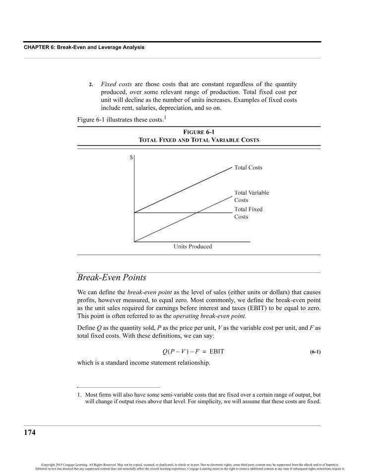
CHAPTER 6: Break-Even and Leverage Analysis
174
2. Fixed costs are those costs that are constant regardless of the quantityproduced, over some relevant range of production. Total fixed cost perunit will decline as the number of units increases. Examples of fixed costsinclude rent, salaries, depreciation, and so on.
Figure 6-1 illustrates these costs.1
FIGURE 6-1TOTAL FIXED AND TOTAL VARIABLE COSTS
Break-Even PointsWe can define the break-even point as the level of sales (either units or dollars) that causesprofits, however measured, to equal zero. Most commonly, we define the break-even pointas the unit sales required for earnings before interest and taxes (EBIT) to be equal to zero.This point is often referred to as the operating break-even point.
Define Q as the quantity sold, P as the price per unit, V as the variable cost per unit, and F astotal fixed costs. With these definitions, we can say:
(6-1)
which is a standard income statement relationship.
1. Most firms will also have some semi-variable costs that are fixed over a certain range of output, butwill change if output rises above that level. For simplicity, we will assume that these costs are fixed.
Q P V–( ) F– EBIT=
Copyright 2015 Cengage Learning. All Rights Reserved. May not be copied, scanned, or duplicated, in whole or in part. Due to electronic rights, some third party content may be suppressed from the eBook and/or eChapter(s).Editorial review has deemed that any suppressed content does not materially affect the overall learning experience. Cengage Learning reserves the right to remove additional content at any time if subsequent rights restrictions require it.

175
Break-Even Points
If we set EBIT in equation (6-1) to zero, we can solve for the break-even quantity (Q*):
(6-2)
Assume, for example, that a firm is selling widgets for $30 per unit while variable costs are$20 per unit and fixed costs total $100,000. In this situation, the firm must sell 10,000 unitsto break even:
The quantity P – V is often referred to as the contribution margin per unit, because this is theamount that each unit sold contributes to covering the firm’s fixed costs. Using equation (6-1), you can verify that the firm will break even if it sells 10,000 widgets:
We can now calculate the firm’s break-even point in dollars by simply multiplying Q* by theprice per unit:
(6-3)
In this example, the result shows that the firm must sell $300,000 worth of widgets to breakeven.
Note that we can substitute equation (6-2) into (6-3):
(6-4)
So, if we know the contribution margin as a percentage of the selling price (CM%), we caneasily calculate the break-even point in dollars. In the previous example, CM% is 33.33%,so the break-even point in dollars must be:
which confirms our earlier result.
Q* FP V–-------------=
Q* 100,00030 20–------------------- 10,000 units= =
10,000 30 20–( ) 100,000– 0=
$BE P Q*×=
$BE P FP V–( )
------------------× FP V–( ) P⁄
------------------------- FCM%---------------= = =
$BE 100,0000.3333
------------------- $300,000= =
Copyright 2015 Cengage Learning. All Rights Reserved. May not be copied, scanned, or duplicated, in whole or in part. Due to electronic rights, some third party content may be suppressed from the eBook and/or eChapter(s).Editorial review has deemed that any suppressed content does not materially affect the overall learning experience. Cengage Learning reserves the right to remove additional content at any time if subsequent rights restrictions require it.

CHAPTER 6: Break-Even and Leverage Analysis
176
Calculating Break-Even Points in ExcelWe can, of course, calculate break-even points in Excel. Consider the income statement forSpuds and Suds, a very popular sports bar that serves only one product: A plate of gourmetfrench fries and a pitcher of imported beer for $16 per serving. The income statement ispresented in Exhibit 6-1.
EXHIBIT 6-1INCOME STATEMENT FOR SPUDS AND SUDS
Before calculating the break-even point, enter the labels into a new worksheet as shown inExhibit 6-1. Because we will be expanding this example, it is important that you enterformulas where they are appropriate. Before doing any calculations, enter the numbers inB20:B23.
We will first calculate the dollar amount of sales (in B5) by multiplying the per unit price bythe number of units sold: =B20*B21. Variable costs are always 60% of sales (as shown inB22), so the formula in B6 is: =B22*B5. Both fixed costs (in B7) and interest expense (inB9) are constants, so they are simply entered directly. The simple subtraction andmultiplication required to complete the income statement through B12 should be obvious.
In B14:B17, we have added information that is not immediately useful, but the figures willbecome central when we discuss operating and financial leverage. In cell B14, we have
Copyright 2015 Cengage Learning. All Rights Reserved. May not be copied, scanned, or duplicated, in whole or in part. Due to electronic rights, some third party content may be suppressed from the eBook and/or eChapter(s).Editorial review has deemed that any suppressed content does not materially affect the overall learning experience. Cengage Learning reserves the right to remove additional content at any time if subsequent rights restrictions require it.

177
Break-Even Points
added preferred dividends, which will be subtracted from net income. The result (in B15) isnet income available to the common shareholders. Preferred dividends are simply input intoB14, and the formula in B15 is: =B12-B14. In B16, enter the number of common sharesoutstanding: 1,000,000. Earnings per share is then calculated as: =B15/B16 in cell B17.
Now we can calculate the break-even points. In cell A25 enter the label: OperatingBreak-even Point (Units). Next, copy this label to A26, and change the word“Units” to Dollars. In B25, we can calculate the break-even point in units using equation(6-2). The formula is: =B7/(B20-B6/B21). Notice that we have to calculate the variablecost per unit by dividing total variable costs (B6) by the number of units sold (B21). You cansee that Spuds and Suds must sell 62,500 units in order to break even and that they are wellabove this level. We can calculate the break-even point in dollars simply by multiplying theunit break-even point by the price per unit. In B26, enter the formula: =B25*B20. You willsee that the result is $1,000,000.
Other Break-Even PointsRecall that we found the break-even point by setting EBIT, in equation (6-1), equal to zero.However, there is no reason that we can’t set EBIT equal to any amount that we mightdesire. For example, if we define EBITTarget as the target level of EBIT, we find that the firmcan earn the target EBIT amount by selling:
(6-5)
Consider that Spuds and Suds might want to know the number of units that they need to sell inorder to have EBIT equal $800,000. Mathematically, we can see that:
need to be sold to reach this target. You can verify that this number is correct by typing 187,500into B21 and checking the value in B8. To return the worksheet to its original values, press Ctrl+Zor reenter 156,250 into B21.
We can do the same thing, with more flexibility, by modifying our worksheet. Select row 22and insert a new row. In A22 enter the label: Target EBIT and in B22 enter: 800,000. InA29 type: Units to Meet EBIT Target and then in B29 enter the formula:=(B7+B22)/(B20-B6/B21). The result will be 187,500 units as before. However, wecan now easily change the target EBIT and see the unit sales required to reach the goal. Yourworksheet should now look like the one in Exhibit 6-2.
Q*Target
F EBITTarget+
P V–----------------------------------=
Q*800,000
400,000 800,000+16 9.60–
--------------------------------------------- 187,500 units= =
Copyright 2015 Cengage Learning. All Rights Reserved. May not be copied, scanned, or duplicated, in whole or in part. Due to electronic rights, some third party content may be suppressed from the eBook and/or eChapter(s).Editorial review has deemed that any suppressed content does not materially affect the overall learning experience. Cengage Learning reserves the right to remove additional content at any time if subsequent rights restrictions require it.

CHAPTER 6: Break-Even and Leverage Analysis
178
EXHIBIT 6-2BREAK-EVEN POINTS
Recall from page 48 that we defined cash flow as net income plus noncash expenses. We dothis because the presence of noncash expenses (principally depreciation) in the accountingnumbers distort the actual cash flows. We can make a similar adjustment to our break-evencalculations by setting EBITTarget equal to the negative of the depreciation expense. Thisresults in a type of break even that we refer to as the cash break-even point:
(6-6)
Note that the cash break-even point will always be lower than the operating break-even pointbecause we don’t have to cover the depreciation expense.
Q*Cash
F Depreciation–P V–
----------------------------------------=
Copyright 2015 Cengage Learning. All Rights Reserved. May not be copied, scanned, or duplicated, in whole or in part. Due to electronic rights, some third party content may be suppressed from the eBook and/or eChapter(s).Editorial review has deemed that any suppressed content does not materially affect the overall learning experience. Cengage Learning reserves the right to remove additional content at any time if subsequent rights restrictions require it.

179
Using Goal Seek to Calculate Break-Even Points
Similarly, we can calculate the break-even point in terms of earnings per share (i.e., whereEPS = 0):
(6-7)
Note that we are adding both interest expense and preferred dividends back to fixed costs toget the total fixed costs (operating and financial). Preferred dividends are not tax deductible,so we adjust them to determine the number of pre-tax dollars that are needed to pay thepreferred dividends after taxes.
In A29 enter: Total Break-even Point (Units), and in B29 enter the formula:=(B7+B9+B14/(1-B25))/(B20-B6/B21). You should see that sales of 104,166.67units will lead to EPS being equal to zero.
Using Goal Seek to Calculate Break-Even PointsAs we’ve shown, the break-even point can be defined in numerous ways, and we don’t evenneed to define it in terms of EBIT. For example, in equation (6-7) we showed a formula tocalculate how many units need to be sold to break even in terms of earnings per share.However, we don’t really need an equation and you may someday want to define break-evenin terms for which we haven’t derived an equation.
Excel has a tool, called Goal Seek, to help with problems like this.2 To use Goal Seek, youmust have a target cell with a formula and another cell on which it depends. For example,earnings per share in B17 depends indirectly on the unit sales in B21. So, changing B21changes B17. When we use Goal Seek, we’ll simply tell it to keep changing B21 until B17equals zero.
Launch the Goal Seek tool by choosing What-If Analysis on the Data tab. In the dialog box,the Set Cell is the cell that you want to take on a particular value, To value is the target value,and the By changing cell is the cell that can be changed until the target cell takes on thedesired value. Essentially, Goal Seek mimicks what you might do if you were using trial anderror to find the number of units to make EPS equal to zero.
Fill in the dialog box as shown in Figure 6-2 and click the OK button. You should find that,as we calculated above, unit sales of 104,166.67 will cause EPS to be equal to zero. You canexperiment with this tool to find the other break-even points. Set B21 back to 156,250.
2. For more complicated problems, use the Solver add-in.
QTotal*
F Interest Exp. PD1 t–( )
---------------+ +
P V–--------------------------------------------------------------=
Copyright 2015 Cengage Learning. All Rights Reserved. May not be copied, scanned, or duplicated, in whole or in part. Due to electronic rights, some third party content may be suppressed from the eBook and/or eChapter(s).Editorial review has deemed that any suppressed content does not materially affect the overall learning experience. Cengage Learning reserves the right to remove additional content at any time if subsequent rights restrictions require it.

CHAPTER 6: Break-Even and Leverage Analysis
180
FIGURE 6-2THE GOAL SEEK TOOL
Leverage AnalysisIn Chapter 4 (page 115), we defined leverage as a multiplication of changes in sales intoeven larger changes in profitability measures. Firms that use large amounts of operatingleverage will find that their EBIT will be more variable than firms that do not. We would saythat such a firm has high business risk. Business risk is one of the major risks faced by a firmand can be defined as the variability of EBIT.3 The more variable a firm’s revenues, relativeto its costs, the more variable its EBIT will be. Also, the likelihood that the firm won’t beable to pay its expenses will be higher. As an example, consider a software company and agrocery chain. It should be apparent that the future revenues of the software company aremuch more uncertain than those of the grocery chain. This uncertainty in revenues causesthe software company to have a much greater amount of business risk than the grocerychain. The software company’s management can do little about this business risk; it issimply a function of the industry in which they operate. Software is not a necessity of life.People do, however, need to eat. For this reason, the grocery business has much lowerbusiness risk.
Business risk results from the environment in which the firm operates. Such factors as thecompetitive position of the firm in its industry, the state of its labor relations, and thevariability of demand for its products all affect the amount of business risk a firm faces. Inaddition, as we will see, the degree to which the firm’s costs are fixed (as opposed tovariable) will affect the amount of business risk. Many of the components of business riskare beyond the control of the firm’s managers. However, managers do have some control.For example, when making investment decisions managers may be able to choose between
3. The use of EBIT for this analysis assumes that the firm has no extraordinary income or expenses.Extraordinary items are one-time events that are not a part of the firm’s ordinary businessoperations. If the firm does have these items, use its net operating income (NOI) instead of EBIT.
Copyright 2015 Cengage Learning. All Rights Reserved. May not be copied, scanned, or duplicated, in whole or in part. Due to electronic rights, some third party content may be suppressed from the eBook and/or eChapter(s).Editorial review has deemed that any suppressed content does not materially affect the overall learning experience. Cengage Learning reserves the right to remove additional content at any time if subsequent rights restrictions require it.

181
Leverage Analysis
labor-intensive and capital-intensive production methods, or they may choose betweenmethods that have differing levels of fixed costs.
In contrast, the amount of financial risk is determined directly by management. Financialrisk refers to the probability that the firm will be unable to meet its fixed financingobligations (which includes both interest and preferred dividends). Obviously, all otherthings being equal, the more debt a firm uses to finance its assets, the higher its interest costwill be. Higher interest costs lead directly to a higher probability that the firm won’t be ableto pay. Furthermore, the use of debt financing concentrates the firm’s business risk ontofewer shareholders, making the stock riskier. Because the amount of debt is determined bymanagerial choice, the financial risk that a firm faces is also determined by management.
Managers need to be aware that they face both business risk and financial risk, and that bothaffect the stock’s beta. Therefore, these risks also affect the value of the stock and the firm’scost of capital. If they are in an industry with high business risk, they should control theoverall amount of risk by limiting the amount of financial risk that they face. Alternatively,firms that face low levels of business risk can better afford more financial risk.
We examine these concepts in more detail by continuing with our Spuds and Suds example.
The Degree of Operating LeverageEarlier we mentioned that a firm’s business risk can be measured by the variability of itsearnings before interest and taxes. If a firm’s operating costs are all variable, then anyvariation in sales will be reflected by exactly the same variation in EBIT. However, if a firmhas some fixed operating expenses then EBIT will be more variable than sales. We refer tothis concept as operating leverage.
We can measure operating leverage by comparing the percentage change in EBIT to a givenpercentage change in sales. This measure is called the degree of operating leverage (DOL):
(6-8)
So, if a 10% change in sales results in a 20% change in EBIT, we would say that the DOL is2. As we will see, this is a symmetrical concept. As long as sales are increasing, a high DOLis desirable. However, if sales begin to decline, a high DOL will result in EBIT declining atan even faster pace than sales.
To make this concept more concrete, let’s extend the Spuds and Suds example. Assume thatmanagement believes that unit sales will increase by 10% in 2015. Furthermore, they expectthat variable costs will remain at 60% of sales and fixed costs will stay at $400,000. CopyB4:B27 to C4:C27. Now, insert a row above the tax rate in row 24. Enter the label:Projected Sales Growth, and in C24 enter: 10%. We need to have the 2015 unit sales
DOL %Δ in EBIT%Δ in Sales------------------------------=
Copyright 2015 Cengage Learning. All Rights Reserved. May not be copied, scanned, or duplicated, in whole or in part. Due to electronic rights, some third party content may be suppressed from the eBook and/or eChapter(s).Editorial review has deemed that any suppressed content does not materially affect the overall learning experience. Cengage Learning reserves the right to remove additional content at any time if subsequent rights restrictions require it.
CHAPTER 6: Break-Even and Leverage Analysis
182
in C21, so enter: =B21*(1+C24) into C21. (Note that you have just created a percent ofsales income statement forecast for 2015, just as we did in Chapter 5.) Change the label inC4 to 2015 and you have completed the changes.
Before continuing, notice that the operating break-even points (C27:C28) have not changed.This will always be the case if fixed costs are constant and variable costs are a constantpercentage of sales. The break-even point is always driven by the level of fixed costs.
Because we wish to calculate the DOL for 2014, we first need to calculate the percentagechanges in EBIT and sales. In A32 enter the label: % Change in Sales from PriorYear, and in A33 enter: % Change in EBIT from Prior Year. To calculate thepercentage changes, enter: =C5/B5-1 in cell C32 and then: =C8/B8-1 in C33. Youshould see that sales increased by 10%, while EBIT increased by 16.67%. According toequation (6-8), the DOL for Spuds and Suds in 2014 is:
So, any change in sales will be magnified by 1.667 times in EBIT. To see this, recall that theformula in C21 increased the 2014 unit sales by 10%. Temporarily, change the value in C24to 20%. You should see that if sales increase by 20%, EBIT will increase by 33.33%.Recalculating the DOL, we see that it is unchanged:
Furthermore, if we change the value in C24 to -10%, so that sales decline by 10%, we findthat EBIT declines by 16.67%. In this case the DOL is:
So leverage is indeed a double-edged sword. You can see that a high DOL would bedesirable as long as sales are increasing, but very undesirable when sales are decreasing.Unfortunately, most businesses don’t have the luxury of altering their DOL immediatelybefore a change in sales.
Calculating the DOL with equation (6-8) is actually more cumbersome than is required.With that equation we needed to use two income statements. However, a more direct methodof calculating the DOL is to use the following equation:
(6-9)
DOL 16.67%10.00%------------------ 1.667= =
DOL 33.33%20.00%------------------ 1.667= =
DOL 16.67%–10.00%–
--------------------- 1.667= =
DOL Q P V–( )Q P V–( ) F–-------------------------------- Sales Variable Costs–
EBIT------------------------------------------------------= =
Copyright 2015 Cengage Learning. All Rights Reserved. May not be copied, scanned, or duplicated, in whole or in part. Due to electronic rights, some third party content may be suppressed from the eBook and/or eChapter(s).Editorial review has deemed that any suppressed content does not materially affect the overall learning experience. Cengage Learning reserves the right to remove additional content at any time if subsequent rights restrictions require it.

183
Leverage Analysis
For Spuds and Suds in 2014, we can calculate the DOL using equation (6-9):
which is exactly as we found with equation (6-8).
Continuing with our example, enter the label: Degree of Operating Leverage inA36. In B36, we will calculate the DOL for 2014 with the formula: =(B5-B6)/B8. Youshould get the same result as before. If you copy the formula from B36 to C36, you will findthat in 2015 the DOL will decline to 1.57. We will examine this decline in the DOL later.
Before continuing, it is worth discussing a refinement of the formula in B36. The formulathat we entered could potentially cause a division by zero (#DIV/0!) error if EBIT is zero(that is, if the firm is operating exactly at its break-even point). We could use an IF statementto avoid this error. If EBIT = 0, then the function will return #N/A (Not Available) as theresult. This is better than having a #DIV/0! error or simply returning zero or a blank as theresult. Returning a zero can throw off the results of other formulas. For example, the COUNTfunction would count a zero, but not an #N/A. To return #N/A as a result in the case of anerror, we can use the NA function. This function takes no arguments, but you must put aclosed pair of parentheses after it:
NA( )
Instead of using an IF statement and calculating the formula twice, we can modify theformula in B36 as follows: =IFERROR((B5-B6)/B8,NA()). Note that we have usedthe IFERROR function to check if the result will be an error. This function will return the firstargument if it doesn’t result in an error, or the second if it does. It is defined as:
IFERROR(VALUE, VALUE_IF_ERROR)
where VALUE is any statement or formula that can be evaluated by Excel. This technique isuseful anytime a formula could result in an error that might render any dependent formulasincorrect. It is better to see a result of #N/A than to see an incorrect result.
Your worksheet should now appear similar to the one in Exhibit 6-3.
DOL 2,500,000 1,500,000–600,000
------------------------------------------------------ 1.667= =
Copyright 2015 Cengage Learning. All Rights Reserved. May not be copied, scanned, or duplicated, in whole or in part. Due to electronic rights, some third party content may be suppressed from the eBook and/or eChapter(s).Editorial review has deemed that any suppressed content does not materially affect the overall learning experience. Cengage Learning reserves the right to remove additional content at any time if subsequent rights restrictions require it.

CHAPTER 6: Break-Even and Leverage Analysis
184
EXHIBIT 6-3SPUDS AND SUDS BREAK-EVEN AND LEVERAGE WORKSHEET
The Degree of Financial LeverageFinancial leverage is similar to operating leverage, but the fixed costs that we areinterested in are the fixed financing costs. These are the interest expense and preferreddividends.4
4. Preferred stock, as we’ll see in Chapter 8, is a hybrid security, similar to both debt and equitysecurities. How it is treated is determined by one’s goals. When discussing financial leverage, wetreat preferred stock as if it were a debt security.
Copyright 2015 Cengage Learning. All Rights Reserved. May not be copied, scanned, or duplicated, in whole or in part. Due to electronic rights, some third party content may be suppressed from the eBook and/or eChapter(s).Editorial review has deemed that any suppressed content does not materially affect the overall learning experience. Cengage Learning reserves the right to remove additional content at any time if subsequent rights restrictions require it.

185
Leverage Analysis
We can measure financial leverage by relating percentage changes in EPS to percentagechanges in EBIT. This measure is referred to as the degree of financial leverage (DFL):
(6-10)
For Spuds and Suds, we have already calculated the percentage change in EBIT, so all thatremains is to calculate the percentage change in EPS. In A34 add the label: % Change inEPS from Prior Year, and in C34 add the formula: =C17/B17-1. Note that EPS isexpected to increase by 30% in 2015 compared to only 16.67% for EBIT. Using equation (6-10) we find that the degree of financial leverage employed by Spuds and Suds in 2014 is:
Therefore, any change in EBIT will be multiplied by 1.80 times in earnings per share. Likeoperating leverage, financial leverage works both ways. When EBIT is increasing, EPS willincrease even more. And when EBIT decreases, EPS will decline by a larger percentage.
As with the DOL, there is a more direct method of calculating the DFL:
(6-11)
In equation (6-11), PD is the amount of preferred dividends paid by the firm, and t is the taxrate. The second term in the denominator, , requires some explanation. Becausepreferred dividends are paid out of after-tax dollars, we must determine how many pre-taxdollars are required to meet this expense. In this case, Spuds and Suds pays taxes at a rate of40%, so they require $166,666.67 in pre-tax dollars in order to pay $100,000 in preferreddividends:
We can use equation (6-11) in the worksheet to calculate the DFL for Spuds and Suds. In cellA37, enter the label: Degree of Financial Leverage. In B37, enter:=IFERROR(B8/(B10-B14/(1-B25)),NA()). You should find that the DFL is 1.80,which is the same as we found by using equation (6-10). Copying this formula to C37reveals that in 2015 we expect the DFL to decline to 1.62.
DFL %Δ in EPS%Δ in EBIT------------------------------=
DFL 30.00%16.67%------------------ 1.80= =
DFL Q P V–( ) F–
Q P V–( ) F Interest Exp. PD1 t–( )
---------------+ +⎝ ⎠⎛ ⎞–
------------------------------------------------------------------------------------------------- EBIT
EBT PD1 t–( )
---------------–---------------------------------= =
PD 1 t–( )⁄
100,0001 0.40–( )
------------------------ 166,666.67=
Copyright 2015 Cengage Learning. All Rights Reserved. May not be copied, scanned, or duplicated, in whole or in part. Due to electronic rights, some third party content may be suppressed from the eBook and/or eChapter(s).Editorial review has deemed that any suppressed content does not materially affect the overall learning experience. Cengage Learning reserves the right to remove additional content at any time if subsequent rights restrictions require it.

CHAPTER 6: Break-Even and Leverage Analysis
186
The Degree of Combined LeverageMost firms make use of both operating and financial leverage. Because they are using twotypes of leverage, it is useful to understand the combined effect. We can measure the totalleverage employed by the firm by comparing the percentage change in sales to thepercentage change in earnings per share. This measure is called the degree of combinedleverage (DCL):
(6-12)
Because we have already calculated the relevant percentage changes, it is a simple matter todetermine that the DCL for Spuds and Suds in 2014 was:
Therefore, any change in sales will be multiplied threefold in EPS. Recall that we earliersaid that the DCL was a combination of operating and financial leverage. You can see this ifwe rewrite equation (6-12) as follows:
Therefore, the combined effect of using both operating and financial leverage ismultiplicative rather than simply additive. Managers should take note of this and use cautionin increasing one type of leverage while ignoring the other. They may end up with more totalleverage than anticipated. As we have just seen, the DCL is the product of DOL and DFL, sowe can rewrite equation (6-12) as:
(6-13)
To calculate the DCL for Spuds and Suds in your worksheet, first enter the label: Degreeof Combined Leverage into A38. In B38, enter the formula: =B36*B37, and copy thisto C38 to find the expected DCL for 2015. At this point, the lower part of your worksheetshould look like Exhibit 6-4.
DCL %Δ in EPS%Δ in Sales-----------------------------=
DCL 30.00%10.00%------------------ 3.00= =
DCL %Δ in EPS%Δ in Sales----------------------------- %Δ in EBIT
%Δ in Sales------------------------------ %Δ in EPS
%Δ in EBIT------------------------------×= =
DCL DOL DFL×=
Copyright 2015 Cengage Learning. All Rights Reserved. May not be copied, scanned, or duplicated, in whole or in part. Due to electronic rights, some third party content may be suppressed from the eBook and/or eChapter(s).Editorial review has deemed that any suppressed content does not materially affect the overall learning experience. Cengage Learning reserves the right to remove additional content at any time if subsequent rights restrictions require it.

187
Leverage Analysis
EXHIBIT 6-4SPUDS AND SUDS WORKSHEET WITH THREE MEASURES OF LEVERAGE
Extending the ExampleComparing the three leverage measures for 2014 and 2015 shows that in all cases the firmwill be using less leverage in 2015. Recall that the only change in 2015 was that sales wereincreased by 10% over their 2014 level. The reason for the decline in leverage is that fixedcosts (both operating and financial) have become a smaller portion of the total costs of thefirm. This will always be the case: As sales increase above the break-even point, leveragewill decline regardless of the measure that is used.
We can see this by extending our Spuds and Suds example. Suppose that management isforecasting that sales will increase by 10% each year for the foreseeable future. Furthermore,because of contractual agreements, the firm’s fixed costs will remain constant through atleast 2018. In order to see the changes in the leverage measures under these conditions, copyC4:C38 and paste into D4:F38. This will create pro forma income statements for threeadditional years. Change the labels in D4:F4 to 2016, 2017, and 2018.
You should see that the DOL, DFL, and DCL are all decreasing as sales increase. This iseasier to see if we create a chart. Select A36:F38 and then create a Line chart of the data. Besure to set B4:F4 as the x-axis labels by right-clicking the chart and choosing Select Data.Under Horizontal (Category) Axis Labels click the Edit button and select the range. Youshould end up with a chart that resembles the one in Figure 6-3.
Copyright 2015 Cengage Learning. All Rights Reserved. May not be copied, scanned, or duplicated, in whole or in part. Due to electronic rights, some third party content may be suppressed from the eBook and/or eChapter(s).Editorial review has deemed that any suppressed content does not materially affect the overall learning experience. Cengage Learning reserves the right to remove additional content at any time if subsequent rights restrictions require it.

CHAPTER 6: Break-Even and Leverage Analysis
188
FIGURE 6-3CHART OF VARIOUS LEVERAGE MEASURES AS SALES INCREASE
Obviously, as we stated earlier, the amount of leverage declines as the sales level increases.One caveat to this is that in the real world, fixed costs are not necessarily the same year afteryear. Furthermore, variable costs do not always maintain an exact percentage of sales. Forthese reasons, leverage may not decline as smoothly as depicted in our example. However,the general principle is sound and should be understood by all managers.
Linking Break-Even Points and Leverage MeasuresWhile it may not be obvious, there is a connection between the break-even points and thevarious measures of leverage that we have defined. In this section we will reveal the links.5
Recall our definition of the operating break-even point in equation (6-2), page 175. Usingthat definition, we can solve for fixed costs (F):
(6-14)
Substituting the definition of F from (6-14) into our definition of the DOL in (6-9) frompage 182 results in:
(6-15)
5. See Zivney, T. & Goebel. J. (2013), The Relationship Between the Breakeven Point and Degrees ofLeverage, Advances in Financial Education, 11, pp. 122–126. I expand on that to include preferreddividends when calculating the DFL.
F QOperating* P V–( )×=
DOL Q P V–( )Q P V–( ) QOperating
* P V–( )–----------------------------------------------------------------------- Q
Q QOperating*–
----------------------------------= =
Copyright 2015 Cengage Learning. All Rights Reserved. May not be copied, scanned, or duplicated, in whole or in part. Due to electronic rights, some third party content may be suppressed from the eBook and/or eChapter(s).Editorial review has deemed that any suppressed content does not materially affect the overall learning experience. Cengage Learning reserves the right to remove additional content at any time if subsequent rights restrictions require it.

189
Summary
So, we can clearly see (as was shown in Figure 6-3) that as sales rise above the operatingbreak-even point, the DOL will decline.
In a similar fashion, we can derive the DFL in terms of the total break-even point as definedin equation (6-7), page 179. First, solve for the total fixed operating and financial costs:
(6-16)
Now, substitute into equation (6-11) on page 185:
(6-17)
Finally, recall from equation (6-13) on page 186 that the DCL is the product of the DOL andDFL. Therefore, using the results from (6-15) and (6-17):
(6-18)
So, the degree of combined leverage will decline as the unit sales rises above the total break-even point.
To verify that these results are correct, return to your worksheet and copy the labels fromA36:A38 and paste them into A41:A43. In B41 enter the formula: =B21/(B21-B27) tocalculate the DOL. In B42 enter: =(B21-B27)/(B21-B29) for the DFL. Finally, in B43enter: =B21/(B21-B29) for the DCL. You should find that all of your answers matchthose that were previously calculated.
SummaryWe started this chapter by discussing the firm’s operating break-even point. The break-evenpoint is determined by a product’s price and the amount of fixed and variable costs. Theamount of fixed costs also played an important role in the determination of the amount ofleverage a firm employs. We studied three measures of leverage:
1. The degree of operating leverage (DOL) measures the degree to which thepresence of fixed costs multiplies changes in sales into even largerchanges in EBIT.
F Interest Exp. PD1 t–( )
---------------+ + QTotal* P V–( )×=
DFLQ P V–( ) QOperating
* P V–( )–
Q P V–( ) QTotal* P V–( )–
-----------------------------------------------------------------------Q QOperating
*–
Q QTotal*–
----------------------------------= =
DCL QQ QOperating
*–----------------------------------
Q QOperating*–
Q QTotal*–
----------------------------------× QQ QTotal
*–-------------------------= =
Copyright 2015 Cengage Learning. All Rights Reserved. May not be copied, scanned, or duplicated, in whole or in part. Due to electronic rights, some third party content may be suppressed from the eBook and/or eChapter(s).Editorial review has deemed that any suppressed content does not materially affect the overall learning experience. Cengage Learning reserves the right to remove additional content at any time if subsequent rights restrictions require it.
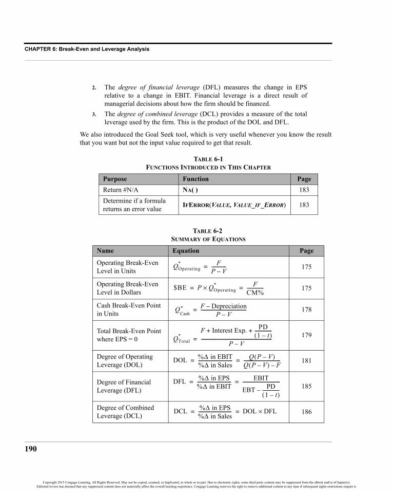
CHAPTER 6: Break-Even and Leverage Analysis
190
2. The degree of financial leverage (DFL) measures the change in EPSrelative to a change in EBIT. Financial leverage is a direct result ofmanagerial decisions about how the firm should be financed.
3. The degree of combined leverage (DCL) provides a measure of the totalleverage used by the firm. This is the product of the DOL and DFL.
We also introduced the Goal Seek tool, which is very useful whenever you know the resultthat you want but not the input value required to get that result.
TABLE 6-1FUNCTIONS INTRODUCED IN THIS CHAPTER
Purpose Function PageReturn #N/A NA( ) 183Determine if a formula returns an error value IFERROR(VALUE, VALUE_IF_ERROR) 183
TABLE 6-2SUMMARY OF EQUATIONS
Name Equation Page
Operating Break-Even Level in Units 175
Operating Break-Even Level in Dollars 175
Cash Break-Even Point in Units 178
Total Break-Even Point where EPS = 0 179
Degree of Operating Leverage (DOL) 181
Degree of Financial Leverage (DFL) 185
Degree of Combined Leverage (DCL) 186
QOperating* F
P V–-------------=
$BE P QOperating*× F
CM%---------------= =
Q*Cash
F Depreciation–P V–
----------------------------------------=
QTotal*
F Interest Exp. PD1 t–( )
---------------+ +
P V–--------------------------------------------------------------=
DOL %Δ in EBIT%Δ in Sales------------------------------ Q P V–( )
Q P V–( ) F–--------------------------------= =
DFL %Δ in EPS%Δ in EBIT------------------------------ EBIT
EBT PD1 t–( )
---------------–---------------------------------= =
DCL %Δ in EPS%Δ in Sales----------------------------- DOL DFL×= =
Copyright 2015 Cengage Learning. All Rights Reserved. May not be copied, scanned, or duplicated, in whole or in part. Due to electronic rights, some third party content may be suppressed from the eBook and/or eChapter(s).Editorial review has deemed that any suppressed content does not materially affect the overall learning experience. Cengage Learning reserves the right to remove additional content at any time if subsequent rights restrictions require it.

191
Problems
Problems
1. Meyerson’s Bakery is considering the addition of a new line of pies to itsproduct offerings. It is expected that each pie will sell for $15 and thevariable costs per pie will be $9. Total fixed operating costs are expectedto be $20,000. Meyerson’s faces a marginal tax rate of 35%, will haveinterest expense associated with this line of $3,000, and expects to sellabout 4,000 pies in the first year.
a. Create an income statement for the pie line’s first year. Is the lineexpected to be profitable?
b. Calculate the operating break-even point in both units and dollars.
c. How many pies would Meyerson’s need to sell in order to achieveEBIT of $15,000?
d. Use the Goal Seek tool to determine the selling price per pie thatwould allow Meyerson’s to break even in terms of its net income.
e. Calculate the DOL, DFL, and DCL for the new pie line.
2. Income Statements for Xcel Energy from 2011 to 2013 appear below.
a. Enter the data into your worksheet. Assume that Cost of Revenue andOperation and Maintenance costs are variable. Depreciation andOther operating expenses are fixed costs. Ignore Other income whencalculating EBT for the questions below.
Copyright 2015 Cengage Learning. All Rights Reserved. May not be copied, scanned, or duplicated, in whole or in part. Due to electronic rights, some third party content may be suppressed from the eBook and/or eChapter(s).Editorial review has deemed that any suppressed content does not materially affect the overall learning experience. Cengage Learning reserves the right to remove additional content at any time if subsequent rights restrictions require it.

CHAPTER 6: Break-Even and Leverage Analysis
192
b. Given that Xcel Energy is a power company, would you expect that itwould have more operating leverage or financial leverage?
c. Calculate the degree of operating leverage for each year using theassumptions from part a.
d. Calculate the degree of financial leverage for each year.
e. Calculate the degree of combined leverage for each of the three years.Does it appear that Xcel’s leverage measures have been increasing ordecreasing over this period?
f. Create a line chart that shows how the various leverage measures havechanged over this three-year period.
3. The following is information for three local auto dealers:
a. Using the information given in the above table, construct incomestatements for each company and the industry average. Assume thateach company faces a tax rate of 35%.
b. Calculate the break-even points and the degrees of operating,financial, and combined leverage for each company and the industryaverage.
c. Compare the companies to each other and the industry average. Whatconclusions can you draw about each operation?
Bell’s Domestics
Junior’s Used
Europe’s Best
Industry Average
Average Selling Price $34,650 $26,730 $51,480 $29,700
Unit Sales 1,350 1,665 765 1,125
Interest Expense 742,500 990,000 2,970,000 1,485,000
Variable Costs (% of Sales) 60% 45% 40% 48%
Fixed Costs 9,000,000 6,300,000 18,000,000 9,900,000
Preferred Dividends 900,000 0 540,000 270,000
Common Shares 4,500,000 7,200,000 2,700,000 6,300,000
Copyright 2015 Cengage Learning. All Rights Reserved. May not be copied, scanned, or duplicated, in whole or in part. Due to electronic rights, some third party content may be suppressed from the eBook and/or eChapter(s).Editorial review has deemed that any suppressed content does not materially affect the overall learning experience. Cengage Learning reserves the right to remove additional content at any time if subsequent rights restrictions require it.

193
Internet Exercise
Internet Exercise
1. Following the instructions from Internet Exercise 2 in Chapter 5, get theincome statements for the company of your choice for the past three yearsfrom MSN Money. Now repeat the analysis from Problem 2. Whatdifferences do you note between the leverage measures for your companyand Xcel Energy?
Copyright 2015 Cengage Learning. All Rights Reserved. May not be copied, scanned, or duplicated, in whole or in part. Due to electronic rights, some third party content may be suppressed from the eBook and/or eChapter(s).Editorial review has deemed that any suppressed content does not materially affect the overall learning experience. Cengage Learning reserves the right to remove additional content at any time if subsequent rights restrictions require it.

Copyright 2015 Cengage Learning. All Rights Reserved. May not be copied, scanned, or duplicated, in whole or in part. Due to electronic rights, some third party content may be suppressed from the eBook and/or eChapter(s).Editorial review has deemed that any suppressed content does not materially affect the overall learning experience. Cengage Learning reserves the right to remove additional content at any time if subsequent rights restrictions require it.

195
CHAPTER 7 The Time Value of Money
“A bird in the hand is worth more than two in the bush.” That old aphorism, when translatedinto the language of finance, becomes “A dollar today is worth more than a dollartomorrow.” Intuitively, it probably makes sense, but why? Stated very simply, you can takethat dollar today and invest it with the expectation of having more than a dollar tomorrow.
Because money can be invested to grow to a larger amount in the future, we say that moneyhas a “time value.” This concept of a time value of money underlies much of the theory offinancial decision making, and you will be required to understand this material in order tocomplete the remaining chapters.
After studying this chapter, you should be able to:1. Explain the concept of the time value of money.2. Calculate the present value and future value of a stream of cash flows using
Excel.3. Explain the types of cash flows encountered in financial analysis and how to
adjust for each type in making time value calculations in Excel.4. Differentiate between the alternative compounding periods, and use Excel to
compare present and future values under different compounding schemes.
Copyright 2015 Cengage Learning. All Rights Reserved. May not be copied, scanned, or duplicated, in whole or in part. Due to electronic rights, some third party content may be suppressed from the eBook and/or eChapter(s).Editorial review has deemed that any suppressed content does not materially affect the overall learning experience. Cengage Learning reserves the right to remove additional content at any time if subsequent rights restrictions require it.

CHAPTER 7: The Time Value of Money
196
Future ValueImagine that you have $1,000 available to invest. If you earn interest at the rate of 10% peryear, then you will have $1,100 at the end of one year. The mathematics behind this exampleis quite simple:
In other words, after one year you will have your original $1,000 (the principal amount) plusthe 10% interest earned on the principal. Because you won’t have the $1,100 until one yearin the future, we refer to this amount as the future value. The amount that you have today,$1,000, is referred to as the present value. If, at the end of the year, you choose to make thesame investment again, then at the end of the second year you will have:
The $1,210 at the end of the second year can be broken down into its components: theoriginal principal, the first year’s interest, the interest earned in the second year on the firstyear’s interest, and the second year’s interest on the original principal. Note that we couldrestate the second year calculation to be:
Or, by factoring out the 1,100 we get:
Notice that in the second year the interest is earned on both the original principal and theinterest earned during the first year. The idea of earning interest on previously earnedinterest is known as compounding. This is why the total interest earned in the second year is$110 versus only $100 the first year.
Returning to our original one-year example, we can generalize the formula for any one-yearinvestment as follows:
where FV1 is the future value at the end of year 1, PV is the present value, and i is the one-year interest rate (compounding rate). The above equation is not in its simplest form. We canfactor PV from both terms on the right-hand side, simplifying the future value equation to:
(7-1)
1,000 1,000 0.10( )+ 1,100=
1,000 1,000 0.10( ) 100 0.10( ) 1,000 0.10( )+ ++ 1,210=
1,100 1,100 0.10( )+ 1,210=
1,100 1 0.10+( ) 1,210=
FV1 PV PV i( )+=
FV1 PV 1 i+( )=
Copyright 2015 Cengage Learning. All Rights Reserved. May not be copied, scanned, or duplicated, in whole or in part. Due to electronic rights, some third party content may be suppressed from the eBook and/or eChapter(s).Editorial review has deemed that any suppressed content does not materially affect the overall learning experience. Cengage Learning reserves the right to remove additional content at any time if subsequent rights restrictions require it.

197
Future Value
Recall that in our two-year example, we earned interest on both the principal and interestfrom the first year. In other words, the first year FV became the second year PV.Symbolically, the second year FV is:
Substituting PV(1 + i) for FV1 and simplifying, we have:
We can actually further generalize our future value equation. Realize that the exponent (on theright-hand side) is the same as the subscript (on the left-hand side) in the future value equation.When we were solving for the future value at the end of the first year, the exponent was 1. Whenwe were solving for the future value at the end of the second year, the exponent was 2. In general,the exponent will be equal to the number of the period for which we wish to find the future value.
(7-2)
Equation (7-2) is the basis for all of the time value equations that we will look at in thesections ahead. Using this version of the equation, you can see that investing $1,000 for twoyears at 10% per year will leave you with $1,210 at the end of two years. In other words:
Using Excel to Find Future ValuesIt is easy enough to calculate future values with a hand calculator, especially a financialcalculator. But, as we will see in the sections and chapters ahead, it is often necessary to usefuture values in worksheets. Excel makes these calculations easy with its FV function:
FV(RATE, NPER, PMT, PV, TYPE)
There are five arguments to the Fv function. RATE is the interest rate per period (year,month, day, etc.), NPER is the total number of periods, and PV is the present value. PMT andTYPE are included to handle annuities (a series of equal payments, equally spaced over time),which we will deal with later. For the problem types we are currently solving, we will setboth PMT and TYPE to 0.1
1. The TYPE argument tells Excel whether the cash flows occur at the end (0) or beginning (1) of theperiod.
FV2 FV1 1 i+( )=
FV2 PV 1 i+( ) 1 i+( ) PV 1 i+( )2= =
FVN PV 1 i+( )N=
FV2 1,000 1.10( )2 1,210= =
Copyright 2015 Cengage Learning. All Rights Reserved. May not be copied, scanned, or duplicated, in whole or in part. Due to electronic rights, some third party content may be suppressed from the eBook and/or eChapter(s).Editorial review has deemed that any suppressed content does not materially affect the overall learning experience. Cengage Learning reserves the right to remove additional content at any time if subsequent rights restrictions require it.

CHAPTER 7: The Time Value of Money
198
EXHIBIT 7-1FUTURE VALUE OF A SINGLE CASH FLOW
Let’s set up a simple worksheet to calculate the future value of a single sum. Starting with ablank worksheet, enter the labels and numbers as shown in Exhibit 7-1.
We want to use the FV function to calculate the future value of $1,000 for one year at 10%per year. In B5 enter the formula: =FV(B4,B3,0,-B2,0). The result, $1,100, is exactlythe same as we found earlier. Note that we have entered –B2 for the PV argument. Thereason for the negative sign is because Excel realizes that either the PV or the FV must be acash outflow. If we had not used the negative sign, the result (FV) would have been negative.Users of financial calculators will recognize this as the cash flow sign convention.
You can now experiment with different values for the arguments. Try replacing the 1 in B3with a 2. Excel immediately updates the result in B5 with $1,210, just as we found in thesecond part of our example. To see just how powerful compounding can be, insert 30 intoB3. The result, $17,449.40, indicates that each $1,000 invested at 10% per year will grow to$17,449.40 after just 30 years. If we double the investment in B2 to $2,000, then weshould double the future value. Try it; you should get a result of $34,898.80, exactly twicewhat we got with a $1,000 investment. In general, any money invested for 30 years at 10%per year will grow to 17.449 times its initial value. To see even more powerful examples ofcompounding, try increasing the interest rate.
Present ValueOur future value equation can be solved for any of its variables. We may wish to turn ourexample problem around to solve for the present value. Suppose that the problem is restatedas, “What initial investment is required so that you will accumulate $1,210 after two years ifyou expect to earn an interest rate of 10% per year?” In this case, we want to solve for thepresent value—we already know the future value.
Mathematically, all that we need to do is to solve the future value equation (7-2) for thepresent value:
Copyright 2015 Cengage Learning. All Rights Reserved. May not be copied, scanned, or duplicated, in whole or in part. Due to electronic rights, some third party content may be suppressed from the eBook and/or eChapter(s).Editorial review has deemed that any suppressed content does not materially affect the overall learning experience. Cengage Learning reserves the right to remove additional content at any time if subsequent rights restrictions require it.

199
Present Value
(7-3)
Of course, we already know that the answer must be $1,000:
In Excel, we can solve problems of this type by using the built-in PV function:
PV(RATE, NPER, PMT, FV, TYPE)
The arguments to the PV function are exactly the same as those for the FV function, exceptthat PV is replaced by FV. For this example, modify your worksheet by entering data intocells D1:E5 as shown in Exhibit 7-2.
EXHIBIT 7-2PRESENT VALUE OF A SINGLE CASH FLOW
In cell E5 place the formula: =PV(E4,E3,0,-E2,0). Again, we enter the future valuereference as negative so that the present value result will be positive. The result will be$1,000, exactly as expected.
We have purposely constructed our future value and present value examples side by side inthe worksheet to demonstrate that present value and future value are inverse functions. Let’schange our worksheet to make this concept clear. We want to link the references in thepresent value function to the cells used in the future value function. This will allow changesin the future value arguments to change the present value arguments. First, select E2 andenter: =B5, in E3 type: =B3, and in E4 enter: =B4. Now, regardless of the changes made tothe future value side of the worksheet, the present value should be equal to the value in B2.Try making some changes to the inputs in B2, B3, and B4. No matter what changes youmake, the calculated present value (in E5) is always the same as the present value input inB2. This is because the present value and future value are inverse functions of each other.
PVFVN
1 i+( )N-------------------=
PV 1,2101.10( )2
----------------- 1,000= =
Copyright 2015 Cengage Learning. All Rights Reserved. May not be copied, scanned, or duplicated, in whole or in part. Due to electronic rights, some third party content may be suppressed from the eBook and/or eChapter(s).Editorial review has deemed that any suppressed content does not materially affect the overall learning experience. Cengage Learning reserves the right to remove additional content at any time if subsequent rights restrictions require it.

CHAPTER 7: The Time Value of Money
200
AnnuitiesThus far, we have examined the present and future values of single cash flows (also referredto as lump sums). These are powerful concepts that will allow us to deal with more complexcash flows. Annuities are a series of nominally equal cash flows, equally spaced in time.Examples of annuities abound. Your car payment is an annuity, so is your mortgage (or rent)payment. If you don’t already, you may someday own annuities as part of a retirementprogram. The cash flow pictured in Figure 7-1 is another example.
FIGURE 7-1A TIMELINE FOR AN ANNUITY CASH FLOW
How do we find the value of a stream of cash flows such as that pictured in Figure 7-1? Theanswer involves the principle of value additivity. This principle says that “the value of astream of cash flows is equal to the sum of the values of the components.” As long as thecash flows occur at the same time, they can be added together. Therefore, if we can moveeach of the cash flows to the same time period (any time period), we can add them to find thevalue as of that time period. Cash flows can be moved around in time by compounding ordiscounting.
Present Value of an AnnuityOne way to find the present value of an annuity is to find the present value of each of thecash flows separately and then add them together. Equation (7-4) summarizes this method:
(7-4)
where PVA is the present value of the annuity, t is the time period, N is the total number ofpayments, Pmtt is the payment in period t, and i is the discount rate.
Of course, this equation works fine for any annuity (or any stream of cash flows), but it canbe very tedious for annuities with more than just a few payments. Imagine finding thecurrent balance (i.e., present value) of a mortgage with more than 300 payments to go beforeit is paid off! We can find a closed-form solution (the above equation is an “open-form”solution because the number of additions is indefinite) by taking the summation:
PVAPmtt
1 i+( )t-----------------
t 1=
N
∑=
Copyright 2015 Cengage Learning. All Rights Reserved. May not be copied, scanned, or duplicated, in whole or in part. Due to electronic rights, some third party content may be suppressed from the eBook and/or eChapter(s).Editorial review has deemed that any suppressed content does not materially affect the overall learning experience. Cengage Learning reserves the right to remove additional content at any time if subsequent rights restrictions require it.

201
Annuities
(7-5)
where all terms are as previously defined. Notice that we have dropped the subscript tbecause this solution does not depend on our taking the present values separately. Instead,because each payment is the same, we can value the entire stream of cash flows in one step.
Let’s find the present value of the cash flow pictured in Figure 7-1. Assuming that thediscount rate for this cash flow is 8%, the equation is:
This means that if you were to deposit $399.27 into an account today that pays 8% interestper year, you could withdraw $100 at the end of each year and be left with a balance of $0.00at the end of the five years.
Recall from our earlier discussion of single cash flows that we can use Excel’s built-in PVfunction to find present values. To recap, the PV function is defined as:
PV(RATE, NPER, PMT, FV, TYPE)
When dealing with single cash flows we set PMT and TYPE to 0. Those arguments are usedonly in the case of annuities. PMT will be set to the dollar amount of the periodic payment.TYPE is an optional binary (0 or 1) variable that controls whether Excel assumes the paymentoccurs at the end (0) or the beginning (1) of the period. For the time being, we will assumethat all payments occur at the end of the period (i.e., they are regular annuities).
EXHIBIT 7-3PRESENT VALUE OF AN ANNUITY
PVA Pmt1 1
1 i+( )N-------------------–
i----------------------------=
PVA 1001 1
1.08( )5-----------------–
0.08--------------------------- 399.27= =
Copyright 2015 Cengage Learning. All Rights Reserved. May not be copied, scanned, or duplicated, in whole or in part. Due to electronic rights, some third party content may be suppressed from the eBook and/or eChapter(s).Editorial review has deemed that any suppressed content does not materially affect the overall learning experience. Cengage Learning reserves the right to remove additional content at any time if subsequent rights restrictions require it.

CHAPTER 7: The Time Value of Money
202
Set up a worksheet with the data pictured in Exhibit 7-3 in cells A1:B5. In B5 we wish tofind the present value of the annuity presented in Figure 7-1, so enter:=PV(B3,B4,B2,0,0). Note that we have entered the payment as a positive number andthe result is –$399.27. The interpretation is that if you were to make a deposit (a cashoutflow) of $399.27 today, you could make a withdrawal of (a cash inflow) $100 each yearfor the next five years. Had we made the payment (B2) negative instead, the present valuewould have been a positive $399.27. The answer is the same, except for the sign, but theinterpretation is different. In this case, the interpretation is that if you were to take out a loanof $399.27 (a cash inflow) today, you would need to repay $100 (a cash outflow) per year foreach of the next five years to retire the loan.
We can, of course, experiment with various arguments. For example, suppose that instead offive withdrawals of $100 each you wanted to make ten withdrawals of $50 each. How muchwould you need to deposit into this account in order to deplete the account after 10withdrawals? Change the number of payments in B4 to: 10 and the payment in B2 to: 50.After these changes, you will see that an initial deposit of only $335.50 will allow you toachieve your goal.
Returning now to our original example, reset the payment amount to: 100 and the numberof payments to: 5. How much would you have to deposit if you want to make your firstwithdrawal today, rather than one year from today? (An annuity that begins payingimmediately is known as annuity due.) To answer this question, realize that the only thingwe have changed is the timing of the first withdrawal. We will still make a total of fivewithdrawals of $100 each, but they occur at the beginning of each period. In B5, change theTYPE argument to 1, from 0 originally, so that the formula is now: =PV(B3,B4,B2,0,1).The result is –$431.21, indicating that, because the first withdrawal occurs immediately, youwill have to make a larger initial deposit. Note that the amount of the deposit must be largerbecause you will not earn the first year’s interest before making the first withdrawal.
Another way to look at this is that we are effectively depositing $331.21 (= $431.21 deposit–$100 withdrawal) in order to be able to make four future withdrawals of $100 each. To seethat this is the case, change the PV formula back to its original form (set TYPE = 0) andchange the number of payments to 4. The present value is then shown to be $331.21, exactlyas claimed.
Future Value of an AnnuityImagine that you have recently begun planning for retirement. One of the attractive optionsavailable is to set up a traditional Individual Retirement Account (IRA). What makes theIRA so attractive is that you can deposit up to $5,500 per year, and the investment gains willaccrue tax free until you begin to make withdrawals after age 59½. Furthermore, dependingon your situation, the IRA deposits may reduce your taxable income.
Copyright 2015 Cengage Learning. All Rights Reserved. May not be copied, scanned, or duplicated, in whole or in part. Due to electronic rights, some third party content may be suppressed from the eBook and/or eChapter(s).Editorial review has deemed that any suppressed content does not materially affect the overall learning experience. Cengage Learning reserves the right to remove additional content at any time if subsequent rights restrictions require it.

203
Annuities
To determine the amount that you will have accumulated in your IRA at retirement, youneed to understand the future value of an annuity. Recalling the principle of value additivity,we could simply find the future value of each year’s investment and add them together atretirement. Mathematically this is:
(7-6)
Alternatively, we could use the closed-form solution of equation (7-6):
(7-7)
Assume that you are planning on retirement in 30 years. If you deposit $5,500 each year intoan IRA account that will earn an average of 7.5% per year, how much will you have after 30years? Because of the large number of deposits, equation (7-7) will be easier to use thanequation (7-6), though we could use either one. The solution is:
As usual, Excel provides a built-in function to handle problems such as this one. The FVfunction, which we used to find the future value of a single sum earlier, will also find thefuture value of an annuity. Its use is nearly identical to the PV function; the only difference isthe substitution of PV for FV. Set up a new worksheet like the one in Exhibit 7-4.
EXHIBIT 7-4FUTURE VALUE OF AN ANNUITY
In B5 place the formula: =FV(B3,B4,-B2,0,0). The result of $568,696.71 agreesexactly with the result from the formula. What if that amount is less than what you hadhoped for? One solution is to start making the investments this year, rather than next (i.e., thebeginning of this period rather than the end of this period). To see the effect of this changeall that needs to be done is to change the TYPE argument to 1 so that the formula is now:
FVA Pmtt 1 i+( )N t–
t 1=
N
∑=
FVA Pmt 1 i+( )N 1–i
----------------------------=
FVA 5,500 1.075( )30 1–0.075
------------------------------- 568,696.71= =
Copyright 2015 Cengage Learning. All Rights Reserved. May not be copied, scanned, or duplicated, in whole or in part. Due to electronic rights, some third party content may be suppressed from the eBook and/or eChapter(s).Editorial review has deemed that any suppressed content does not materially affect the overall learning experience. Cengage Learning reserves the right to remove additional content at any time if subsequent rights restrictions require it.

CHAPTER 7: The Time Value of Money
204
=FV(B3,B4,-B2,0,1). That minor change in your investment strategy will net youabout $42,652 extra at retirement. Perhaps a better alternative is to accept a little extra risk(we assume that you are young enough that this makes sense) by investing in stock mutualfunds that will return an average of about 10% per year over the 30-year horizon. In thiscase, still assuming that you start investing right now, you will have $995,188.84 atretirement. Significantly better! The extra 2.5% return each year added more than $400,000to your retirement fund. This is the magic of compounding.
Solving for the Annuity PaymentSuppose that you want to know the amount that must be deposited in order to accumulate agiven sum after a number of years. For example, assume that you are planning to purchase ahouse five years from now. Because you are currently a student, you will begin saving forthe $10,000 down payment one year from today. How much will you need to save each year,if your savings will earn interest at a rate of 4% per year? Figure 7-2 diagrams the problem.
FIGURE 7-2A TIMELINE FOR ANNUAL SAVINGS TO OBTAIN $10,000 IN FIVE YEARS
In this case, we wish to solve for the payment that you would have to make each year. Thefuture value of the annuity is already known, so the FV function would be inappropriate.What we need is Excel’s PMT function:
PMT(RATE, NPER, PV, FV, TYPE)
The arguments for the PMT function are similar to those for the PV and FV functions, exceptthat it has PV and FV arguments in place of the PMT argument.
Enter the information from Exhibit 7-5 into cells A1:B6 of a new worksheet. In cell B6 enterthe PMT function: =PMT(B5,B4,-B2,B3,0). The result indicates that you will have tosave $1,846.27 per year (a cash outflow) in order to accumulate $10,000 for the downpayment in five years.
Copyright 2015 Cengage Learning. All Rights Reserved. May not be copied, scanned, or duplicated, in whole or in part. Due to electronic rights, some third party content may be suppressed from the eBook and/or eChapter(s).Editorial review has deemed that any suppressed content does not materially affect the overall learning experience. Cengage Learning reserves the right to remove additional content at any time if subsequent rights restrictions require it.

205
Annuities
EXHIBIT 7-5ANNUITY PAYMENT WHEN PV OR FV IS KNOWN
The PMT function allows both PV and FV to be inputs. In the previous example, it wasassumed that PV was 0. However, let’s suppose that you have recently inherited $3,000 fromyour uncle and that you want to use this money to begin saving now for that down payment.Because the $3,000 will grow to only $3,649.96 after five years at 4% per year (this can beverified by using the worksheet created for Exhibit 7-1), you will still need to save someamount every year. How much will you need to save each year? To find out, simply set thepresent value, in B2, to 3,000 leaving the other values unchanged. Because the initialinvestment reduces the total amount that you need to save to $6,350.04 (why?), your annualsaving requirement is reduced to $1,172.39.
Solving for the Number of Periods in an AnnuitySolving for the present value, future value, and payment for annuities are fairly simpleproblems. That is, the formulas are straightforward and easy to apply. Solving for thenumber of periods, N, is not as obvious mathematically. To do so requires knowledge oflogarithms. If you know the present value of the annuity, then solving equation (7-5) for Nwe get:
(7-8)
where ln(·) is the natural logarithm operator. If you know the future value, then solvingequation (7-7) for N results in:
(7-9)
N1
iPVA
Pmt------------–⎝ ⎠
⎛ ⎞ln
1 i+( )ln–--------------------------------=
N1
iFVA
Pmt------------+⎝ ⎠
⎛ ⎞ln
1 i+( )ln---------------------------------=
Copyright 2015 Cengage Learning. All Rights Reserved. May not be copied, scanned, or duplicated, in whole or in part. Due to electronic rights, some third party content may be suppressed from the eBook and/or eChapter(s).Editorial review has deemed that any suppressed content does not materially affect the overall learning experience. Cengage Learning reserves the right to remove additional content at any time if subsequent rights restrictions require it.

CHAPTER 7: The Time Value of Money
206
Return now to our original example of saving for the down payment for a house. Recall thatit was determined that by saving $1,846.27 per year you could afford the down paymentafter five years, assuming no initial investment. Set up the worksheet in Exhibit 7-6.
EXHIBIT 7-6NUMBER OF ANNUITY PAYMENTS WHEN PV OR FV IS KNOWN
We can solve this problem using equation (7-9) and the built-in LN function:2
LN(NUMBER)
In B6 enter the formula: =LN(B5*B3/B4+1)/LN(1+B5). The result is five years as wewould expect.
Excel also offers the built-in NPER function, which also works with lump sums, to solveproblems of this type directly. This function is defined as:
NPER(RATE, PMT, PV, FV, TYPE)
where all of the arguments are as previously defined. To use this function, you must knowthe payment, per period interest rate, and either the present value or future value or both.
Because we want to solve for the number of periods, insert the NPER function into B6:=NPER(B5,-B4,-B2,B3,0). Notice that both the PV and PMT arguments are madenegative in this function. Again, this is because of the cash flow sign convention. In thiscase, we wish to be able to withdraw the future value (a cash inflow and, therefore, positive)and deposit the PV and PMTs (cash outflows, therefore negative). The result is five years,exactly as we would expect. If you enter the $3,000 inheritance into B2, then you will havethe down payment in only 3.39 years.
2. Logarithms are often useful tools, and Excel offers functions to handle them. In addition to LN, theother logarithm functions are LOG10 and LOG. The former calculates the base 10 logarithm, andthe latter can calculate a logarithm with any base.
Copyright 2015 Cengage Learning. All Rights Reserved. May not be copied, scanned, or duplicated, in whole or in part. Due to electronic rights, some third party content may be suppressed from the eBook and/or eChapter(s).Editorial review has deemed that any suppressed content does not materially affect the overall learning experience. Cengage Learning reserves the right to remove additional content at any time if subsequent rights restrictions require it.

207
Annuities
Solving for the Interest Rate in an AnnuityUnlike the present value, future value, payment, and number of periods, there is no closed-form solution for the rate of interest of an annuity. The only way to solve this problem is touse a trial-and-error approach, perhaps an intelligent one such as the Newton–Raphsontechnique or the bisection method.3
Excel, however, offers the RATE function that will solve for the interest rate. It is defined as:
RATE(NPER, PMT, PV, FV, TYPE, GUESS)
where the arguments are as defined earlier, and GUESS is your optional first guess at thecorrect answer. Ordinarily, the GUESS can be safely omitted.
Suppose that you are approached with an offer to purchase an investmentthat will provide cash flows of $1,500 per year for 10 years. The cost ofpurchasing this investment is $10,500. If you have an alternativeinvestment opportunity, of equal risk, that will yield 8% per year, whichone should you accept?
There are actually several ways that a problem such as this could be solved. One method isto realize that 8% is your opportunity cost of funds and should therefore be used as yourdiscount rate. Using the worksheet created in Exhibit 7-3 we find that the present value (i.e.,current worth to you) of the investment is only $10,065.12. Because the price ($10,500) isgreater than the value, you should reject the investment and accept your alternative.4
Another method of solving this dilemma is to compare the yields (i.e., compound annualreturn) offered by the investments. All other things being equal, the investment with thehighest yield should be accepted. We already know that your alternative investment offers an8% yield, but what is the yield of your new opportunity?
Create a new worksheet and enter the data as shown in Exhibit 7-7. Note that we are enteringthe PV, in B2, as a negative number in order to allow the function to work regardless of thedirection of the cash flows. This is to maintain flexibility so that you can change the numbersin the worksheet without editing the function. Just remember to use the correct signs.
3. These are powerful techniques for solving this type of problem. The bisection method, briefly,involves choosing two initial guesses at the answer that are sure to bracket the true answer. Eachsuccessive guess is halfway between the two previous guesses that bracket the solution. TheNewton–Raphson technique requires calculus and is beyond the scope of this book. For moreinformation, consult any numerical methods textbook.
4. Note that we are simply comparing the cost of the investment to its perceived benefit (presentvalue). If the cost is greater than the benefit, the investment should be rejected. We will expand onthis method in future chapters.
Copyright 2015 Cengage Learning. All Rights Reserved. May not be copied, scanned, or duplicated, in whole or in part. Due to electronic rights, some third party content may be suppressed from the eBook and/or eChapter(s).Editorial review has deemed that any suppressed content does not materially affect the overall learning experience. Cengage Learning reserves the right to remove additional content at any time if subsequent rights restrictions require it.

CHAPTER 7: The Time Value of Money
208
EXHIBIT 7-7YIELD ON AN ANNUITY
In B6 place the function: =RATE(B5,B4,B2,B3,0,0.1). The result is 7.07% per year,so you should reject the new investment in favor of the alternative that offers 8% per year.This is the same result we obtained with the present value methodology, as expected. Later,we will see that this will always be the case when comparing mutually exclusive investmentopportunities.5
Deferred AnnuitiesNot all annuities begin their payments during the year following the analysis period. Forexample, if you are planning for your retirement, you will probably start by determining theamount of income that you will need each year during retirement. However, if you are astudent, you will probably not retire for many years. Your retirement income, then, is anannuity that won’t begin until you retire. In other words, it is a deferred annuity. How do wedetermine the value of a deferred annuity?
Assume that you own a time machine (made of a super-strong futuristic metal that canwithstand the gravitational forces of a black hole in space). This machine can transport youto any time period that you choose. If we use this time machine to transport you to the yearjust prior to retirement, then valuing the stream of retirement income becomes a simplematter. Just use Excel’s PV function as we did earlier. The year before the first withdrawal isnow considered to be year 0, the first year of retirement is year 1, and so on. Figure 7-3demonstrates this time-shifting technique.
5. Mutually exclusive investment opportunities are those in which you may choose one investment orthe other, but not both. That is, the choice of one precludes you also choosing the other.
Copyright 2015 Cengage Learning. All Rights Reserved. May not be copied, scanned, or duplicated, in whole or in part. Due to electronic rights, some third party content may be suppressed from the eBook and/or eChapter(s).Editorial review has deemed that any suppressed content does not materially affect the overall learning experience. Cengage Learning reserves the right to remove additional content at any time if subsequent rights restrictions require it.

209
Annuities
FIGURE 7-3TIME-SHIFTING AS A FIRST STEP IN SOLVING DEFERRED ANNUITY PROBLEMS
In constructing Figure 7-3, we have assumed that you will retire 30 years from now, and willrequire an income of $125,000 per year during retirement. If we further assume that you willneed your retirement income for 35 years and expect to earn 6% per year, then you will needto have accumulated $1,812,280.80 by year 30 to provide this income. In other words,$1,812,280.80 is the present value, at year 30, of $125,000 per year for 35 years at 6%. Youcan use the worksheet created for Exhibit 7-3 to verify these numbers.6
The problem in Figure 7-3 is that knowing the amount that we will need 30 years from nowdoesn’t directly tell us how much we need to save today. The present value function inExcel, or the PVA equation (7-5), must be thought of as a transformation function. That is, ittransforms a series of payments into a lump sum. That lump sum ($1,812,280.80 in ourexample) is then placed one period before the first payment occurs. In our earlier examples,the annuities began payment at the end of period 1, so the present value was at time period 0(one period earlier than period 1). In the current example, the present value is at time period30, also one period before the first payment.
In order to determine the amount that we need to invest today, we must treat the requiredsavings at retirement as a future value. This sum must then be discounted back to period 0.For example, if we assume that you can earn 8% per year before retirement, then you wouldneed to invest $180,099.63 today in order to meet your retirement goals.
Exhibit 7-8 presents a simple worksheet to determine the investment required today in orderto provide a particular income during retirement. Open a new worksheet and enter the dataand labels from Exhibit 7-8.
6. Although $125,000 per year may seem like a lot of money, we arrived at this figure by assumingthat you would need $50,000 per year in today’s dollars. We then adjusted that amount for anaverage inflation rate of 3% per year for 31 years to arrive at $125,000. In fact, that won’t beenough because inflation will continue during retirement. So, your retirement income will need torise each year to keep pace with inflation. We will deal with this in the next section.
Copyright 2015 Cengage Learning. All Rights Reserved. May not be copied, scanned, or duplicated, in whole or in part. Due to electronic rights, some third party content may be suppressed from the eBook and/or eChapter(s).Editorial review has deemed that any suppressed content does not materially affect the overall learning experience. Cengage Learning reserves the right to remove additional content at any time if subsequent rights restrictions require it.

CHAPTER 7: The Time Value of Money
210
EXHIBIT 7-8PLANNING FOR RETIREMENT
To complete our retirement worksheet, we need to enter functions into cells B7:B9. Recallthat the first step in our retirement income problem was to determine the present value ofyour retirement income at period 30. To do this in our worksheet, enter the PV function intoB7: =PV(B6,B4,-B2,0,0). The result, $1,812,280.80, tells us that you will need to havesaved this amount in order to provide the income indicated in B2 for the number of yearsindicated in B4. To determine the amount that you would need to invest today (a lump sum),you need to determine the present value, at time period 0, of the amount in B7. To do this, inB8 enter the formula: =PV(B5,B3,0,-B7,0). As before, the amount required today is$180,099.63.
Another feature of the retirement planning worksheet is that it will calculate the annualsavings required to reach your goal. To make Excel do this calculation, we need to use thePMT function. In B9 enter: =PMT(B5,B3,0,-B7,0). The result is $15,997.79, whichmeans that if you can save this amount each year for the next 30 years, and earn an averageof 8% interest each year, you will reach your goal. As difficult as that may be, it is mucheasier than investing the lump sum today.
We have ignored the effects of inflation and taxes on your retirement planning for thisworksheet. But if we assume that you save the amount in B9 in a tax-deferred account, theresults are a bit more realistic. Experiment with this worksheet. You may be surprised at thedifficulty of saving for a comfortable retirement.
Graduated AnnuitiesPreviously, we defined an annuity as a series of nominally equal cash flows, equally spacedin time. However, not everything that is called an annuity has equal cash flows each period.
Copyright 2015 Cengage Learning. All Rights Reserved. May not be copied, scanned, or duplicated, in whole or in part. Due to electronic rights, some third party content may be suppressed from the eBook and/or eChapter(s).Editorial review has deemed that any suppressed content does not materially affect the overall learning experience. Cengage Learning reserves the right to remove additional content at any time if subsequent rights restrictions require it.

211
Graduated Annuities
For example, it is common today for people to invest a lump sum today in exchange for aseries of payments that will escalate over time to maintain constant purchasing power. Aninsurance company may offer such an investment opportunity to retirees who are concernedabout inflation in the future, and some lotteries offer an “annuitized” payout that increaseseach year.
Return to our example in the previous section. Your stated goal was to receive $125,000each year for the 35 years that you expect to spend in retirement. However, if your incomedoesn’t rise each year then your purchasing power will decline dramatically by the end of the35 years. In fact, if inflation averages 3% per year, your income in the last year will have thesame purchasing power as only about $44,423 (about one-third as much as needed) wouldhave had at the beginning of your retirement. Clearly, then, it would be beneficial if yourretirement income would grow to keep up with the rate of inflation.
Present Value of a Graduated AnnuitySuppose that you expect inflation to be 3% per year during retirement, so you have revisedyour retirement income needs so that your income grows by 3% each year. Figure 7-4 showsthe revised timeline.
FIGURE 7-4RETIREMENT INCOME GROWING AT 3% PER YEAR
How do we find the present value of such a cash flow stream? It would appear that wecannot use the PV function because it assumes that all of the cash flows are the same in eachperiod. That leaves us with the fallback position of using the principle of value additivity. Inother words, calculate the present value of each cash flow separately, and then add themtogether to get the total present value. This method requires a table that lists all of the cashflows and the use of equation (7-4) on page 200.
Fortunately, if we can assume that the growth rate of the cash flows will be constant, as it isin this case, then there is a closed-form solution for the present value of a graduated annuitywhen the first payment occurs one period from now:
(7-10)PVGAPmt1
i g–------------ 1 1 g+
1 i+------------⎝ ⎠⎛ ⎞
N–=
Copyright 2015 Cengage Learning. All Rights Reserved. May not be copied, scanned, or duplicated, in whole or in part. Due to electronic rights, some third party content may be suppressed from the eBook and/or eChapter(s).Editorial review has deemed that any suppressed content does not materially affect the overall learning experience. Cengage Learning reserves the right to remove additional content at any time if subsequent rights restrictions require it.

CHAPTER 7: The Time Value of Money
212
where Pmt1 is the first cash flow, i is the interest rate, g is the growth rate, and N is thenumber of cash flows.
As before, if we assume that you will earn 6% per year during retirement and yourwithdrawals grow 3% per year to keep up with inflation, then you will need to accumulate$2,641,257.55 in order to meet your income goals.
We can use the PV function to calculate the same result, but only after modifying the interestrate. In the case of a graduated annuity we have two rates: a discount rate and a growth rate.These rates work against each other, so you might expect that we could use a “net” interestrate. In this case that would be 6% – 3% = 3%, but that won’t work properly because interestrates compound. In other words, they are multiplicative instead of additive. Therefore, weneed a slightly more complicated formula:
(7-11)
Instead of subtracting, we need to divide. In this case, the net interest rate is:
One final adjustment is necessary; we must also divide the result of the PV function by(1 + g). This adjustment effectively changes the payment at period 1 into its inflation-adjusted value at period 0.
We can now easily modify the retirement worksheet presented in Exhibit 7-8 to handle ournew assumption regarding inflation. Make a copy of that worksheet, and then select row 5and insert a new row. In A5 enter the label: Expected Inflation Rate, and in B5enter: 3%. Now, we need to change the formula in B8 to: =-PV((1+B7)/(1+B5)-1,B4,B2)/(1+B5). You will see that the result is $2,641,257.55, exactly the same asbefore. Furthermore, the results in B9:B10 have automatically updated to include our newassumption. As you can see, you will now need to save $23,315.53 per year beforeretirement. That is about $7,318 more per year than the original projection, but this willallow you to maintain constant purchasing power during retirement. Exhibit 7-9 shows thenew retirement planning worksheet.
PVGA125,000
0.06 0.03–--------------------------- 1 1.03
1.06----------⎝ ⎠⎛ ⎞
35– 2,641,257.55= =
Net Rate 1 i+( )1 g+( )
----------------- 1–=
Net Rate 1.061.03---------- 1– 0.02913≅=
Copyright 2015 Cengage Learning. All Rights Reserved. May not be copied, scanned, or duplicated, in whole or in part. Due to electronic rights, some third party content may be suppressed from the eBook and/or eChapter(s).Editorial review has deemed that any suppressed content does not materially affect the overall learning experience. Cengage Learning reserves the right to remove additional content at any time if subsequent rights restrictions require it.
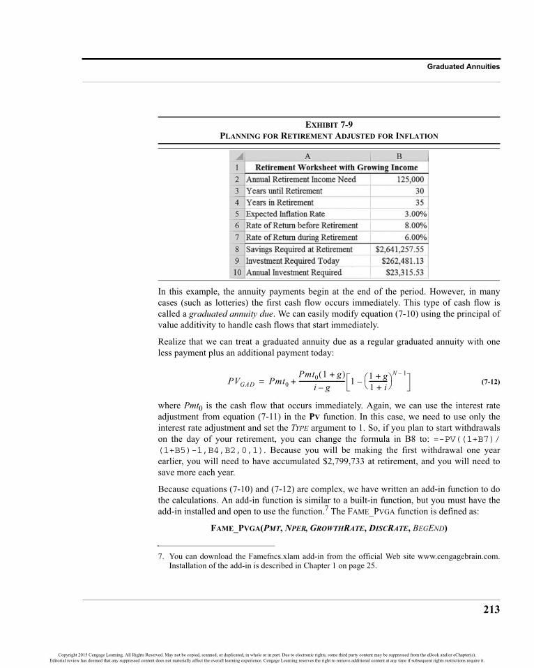
213
Graduated Annuities
EXHIBIT 7-9PLANNING FOR RETIREMENT ADJUSTED FOR INFLATION
In this example, the annuity payments begin at the end of the period. However, in manycases (such as lotteries) the first cash flow occurs immediately. This type of cash flow iscalled a graduated annuity due. We can easily modify equation (7-10) using the principal ofvalue additivity to handle cash flows that start immediately.
Realize that we can treat a graduated annuity due as a regular graduated annuity with oneless payment plus an additional payment today:
(7-12)
where Pmt0 is the cash flow that occurs immediately. Again, we can use the interest rateadjustment from equation (7-11) in the PV function. In this case, we need to use only theinterest rate adjustment and set the TYPE argument to 1. So, if you plan to start withdrawalson the day of your retirement, you can change the formula in B8 to: =-PV((1+B7)/(1+B5)-1,B4,B2,0,1). Because you will be making the first withdrawal one yearearlier, you will need to have accumulated $2,799,733 at retirement, and you will need tosave more each year.
Because equations (7-10) and (7-12) are complex, we have written an add-in function to dothe calculations. An add-in function is similar to a built-in function, but you must have theadd-in installed and open to use the function.7 The FAME_PVGA function is defined as:
FAME_PVGA(PMT, NPER, GROWTHRATE, DISCRATE, BEGEND)
7. You can download the Famefncs.xlam add-in from the official Web site www.cengagebrain.com.Installation of the add-in is described in Chapter 1 on page 25.
PVGAD Pmt0Pmt0 1 g+( )
i g–------------------------------ 1 1 g+
1 i+------------⎝ ⎠⎛ ⎞
N 1––+=
Copyright 2015 Cengage Learning. All Rights Reserved. May not be copied, scanned, or duplicated, in whole or in part. Due to electronic rights, some third party content may be suppressed from the eBook and/or eChapter(s).Editorial review has deemed that any suppressed content does not materially affect the overall learning experience. Cengage Learning reserves the right to remove additional content at any time if subsequent rights restrictions require it.
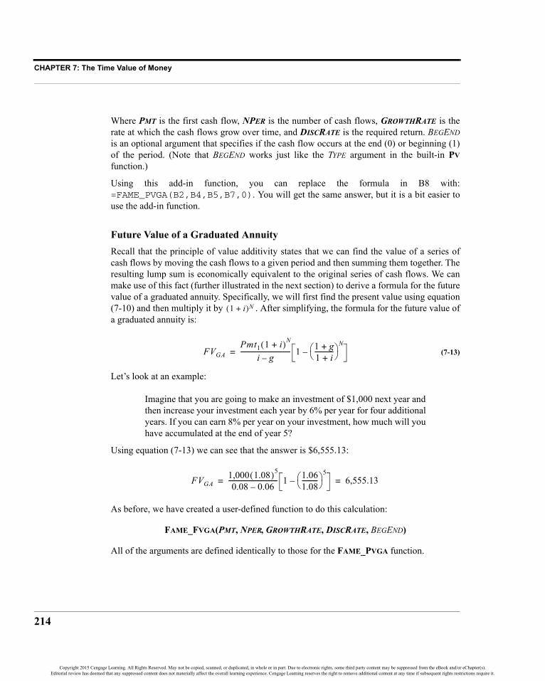
CHAPTER 7: The Time Value of Money
214
Where PMT is the first cash flow, NPER is the number of cash flows, GROWTHRATE is therate at which the cash flows grow over time, and DISCRATE is the required return. BEGENDis an optional argument that specifies if the cash flow occurs at the end (0) or beginning (1)of the period. (Note that BEGEND works just like the TYPE argument in the built-in PVfunction.)
Using this add-in function, you can replace the formula in B8 with:=FAME_PVGA(B2,B4,B5,B7,0). You will get the same answer, but it is a bit easier touse the add-in function.
Future Value of a Graduated AnnuityRecall that the principle of value additivity states that we can find the value of a series ofcash flows by moving the cash flows to a given period and then summing them together. Theresulting lump sum is economically equivalent to the original series of cash flows. We canmake use of this fact (further illustrated in the next section) to derive a formula for the futurevalue of a graduated annuity. Specifically, we will first find the present value using equation(7-10) and then multiply it by . After simplifying, the formula for the future value ofa graduated annuity is:
(7-13)
Let’s look at an example:
Imagine that you are going to make an investment of $1,000 next year andthen increase your investment each year by 6% per year for four additionalyears. If you can earn 8% per year on your investment, how much will youhave accumulated at the end of year 5?
Using equation (7-13) we can see that the answer is $6,555.13:
As before, we have created a user-defined function to do this calculation:
FAME_FVGA(PMT, NPER, GROWTHRATE, DISCRATE, BEGEND)
All of the arguments are defined identically to those for the FAME_PVGA function.
1 i+( )N
FVGAPmt1 1 i+( )N
i g–-------------------------------- 1 1 g+
1 i+------------⎝ ⎠⎛ ⎞
N–=
FVGA1,000 1.08( )5
0.08 0.06–------------------------------- 1 1.06
1.08----------⎝ ⎠⎛ ⎞
5– 6,555.13= =
Copyright 2015 Cengage Learning. All Rights Reserved. May not be copied, scanned, or duplicated, in whole or in part. Due to electronic rights, some third party content may be suppressed from the eBook and/or eChapter(s).Editorial review has deemed that any suppressed content does not materially affect the overall learning experience. Cengage Learning reserves the right to remove additional content at any time if subsequent rights restrictions require it.

215
Uneven Cash Flow Streams
Uneven Cash Flow StreamsAnnuities are very neat from a cash flow point of view, but most investments don’t havecash flows that are the same in each period. When the cash flows are different in each period,we refer to them as uneven cash flow streams. Investments of this type are not as easy to dealwith, though conceptually they are the same.
Recall our discussion of the principle of value additivity. This principle says that as long ascash flows occur in the same period, we can add them together to determine their combinedvalue. The principle applies to any time period, not just to time period 0. So, to determinethe present value of an uneven stream of cash flows, one option is to determine the presentvalue of each cash flow separately, and then add them together. The same technique appliesto the future value of an uneven stream. Simply find the future value of each cash flowseparately, and then add them together.
Excel’s PV and FV functions cannot be directly used for uneven cash flow streams becausethey assume equal (annuity) payments or a lump sum (though they can be used as arrayfunctions). Set up the worksheet in Exhibit 7-10 and we’ll see what needs to be done.
EXHIBIT 7-10PV AND FV FOR UNEVEN CASH FLOWS
First, we want to solve for the present value of the cash flows in B3:B7. To do this, we willuse the net present value (NPV) function. This function will be especially valuable forcapital budgeting in Chapter 11. The NPV function is defined as:
NPV(RATE, VALUE1, VALUE2, …)
where RATE is the per period rate of return (i.e., the discount rate), VALUE1 is the first cashflow (or range of cash flows), VALUE2 is the second cash flow, and so on. Excel will accept
Copyright 2015 Cengage Learning. All Rights Reserved. May not be copied, scanned, or duplicated, in whole or in part. Due to electronic rights, some third party content may be suppressed from the eBook and/or eChapter(s).Editorial review has deemed that any suppressed content does not materially affect the overall learning experience. Cengage Learning reserves the right to remove additional content at any time if subsequent rights restrictions require it.

CHAPTER 7: The Time Value of Money
216
up to 255 cash flows in the list. To find the present value of the cash flows, enter:=NPV(B8,B3:B7) into B9.8 Note that we have entered the cash flows as a range, ratherthan as individual values. Excel will accept the arguments either way, though a range isgenerally easier to enter. The result is $10,319.90. To verify this result, you can find thepresent value of each cash flow at 11% per year and then add them together.
Finding the future value of an uneven stream is a bit more difficult because Excel has nobuilt-in function to perform this calculation. Recall, however, the principle of valueadditivity. If we can get all of the cash flows into the same period, we can add them togetherand then move the result to the desired period. Figure 7-5 shows this solution.
FIGURE 7-5FINDING THE FUTURE VALUE OF AN UNEVEN CASH FLOW STREAM
First, we find the present value of the uneven stream of cash flows, perhaps using the NPVfunction, and then we find the future value of the present value of the cash flows. The easiestway to implement this method in Excel is to use the NPV function nested within the FVfunction. A nested function is one that is used as an input to another function. In B10 enter:=FV(B8,A7,0,-NPV(B8,B3:B7),0). The future value is found to be $17,389.63.Notice that we have used the NPV function inside the FV function. As an alternative, wecould have entered –B9 for the present value argument because we have already calculatedit, but the result would be the same. Using nested functions can often simplify a worksheetby making use of fewer cells, though the formulas tend to be more complex.
Solving for the Yield in an Uneven Cash Flow StreamOften in financial analysis, it is necessary to determine the yield of an investment given itsprice and cash flows. For example, we have seen that one way to choose between alternativeinvestments is to compare their yields, and we will see more examples in Chapter 11. This
8. If you are familiar with the definition of Net Present Value (NPV), you should know that Excel’sNPV function does not calculate the NPV as it is normally defined. Instead, it merely calculates thepresent value of uneven cash flows. This is covered in more depth in Chapter 11.
Copyright 2015 Cengage Learning. All Rights Reserved. May not be copied, scanned, or duplicated, in whole or in part. Due to electronic rights, some third party content may be suppressed from the eBook and/or eChapter(s).Editorial review has deemed that any suppressed content does not materially affect the overall learning experience. Cengage Learning reserves the right to remove additional content at any time if subsequent rights restrictions require it.

217
Uneven Cash Flow Streams
was easy when dealing with annuities and lump-sum investments, where we could use theRATE function. But, what about the case of uneven cash flow investments? We will use theworksheet in Exhibit 7-11 to find out.
EXHIBIT 7-11YIELD ON AN UNEVEN CASH FLOW STREAM
To solve for the yield in problems such as this, we need to make use of the IRR (internal rateof return) function. The IRR is defined as the rate of return that equates the present value offuture cash flows with the cost of the investment ($10,319.90 in this problem). In Excel, theIRR function is defined as:
IRR(VALUES, GUESS)
where VALUES is a range of cash flows (including the cost), and GUESS is the optional firstguess at the correct interest rate. We will study this function in depth in Chapter 11, but fornow we will just make use of it.
Before we find the solution, notice a couple of things about the worksheet. The cash flowsare listed separately, so we cannot use the IRR function like we used the FV, PV, and PMTfunctions. Also, we must include the cost of the investment as one of the cash flows. To findthe yield on this investment, insert into B9: =IRR(B3:B8,0.10). The result is 11%,which means that if you purchase this investment you will earn a compound annual rate of11%.
We have used one form of the IRR function in B9. Another option is to omit the GUESS (0.10in our example). In this case, either form will work. Sometimes, however, Excel will not beable to converge on a solution without a GUESS being specified. Remember that this isessentially a trial-and-error process, and sometimes Excel needs a little help to go in the rightdirection.
Copyright 2015 Cengage Learning. All Rights Reserved. May not be copied, scanned, or duplicated, in whole or in part. Due to electronic rights, some third party content may be suppressed from the eBook and/or eChapter(s).Editorial review has deemed that any suppressed content does not materially affect the overall learning experience. Cengage Learning reserves the right to remove additional content at any time if subsequent rights restrictions require it.

CHAPTER 7: The Time Value of Money
218
A few situations may cause an error when using the IRR function. One that we’ve alreadydiscussed is that Excel may not converge to a solution. In this case, you can usually find theanswer by supplying Excel with a different GUESS. Another occurs if you have no negativecash flows. As an example, change the purchase price to a positive 10,319.90. Excel willreturn the #NUM! error message indicating that there is a problem. In this case the problemis that your return is infinite (why?). A third problem can result from more than one negativecash flow in the stream. In general, there will be one solution to the problem for each signchange in the cash flow stream. In our original example, there is only one sign change (fromnegative to positive after the initial purchase.)
Nonannual Compounding PeriodsThere is no reason why we should restrict our analyses to investments that pay cash flowsannually. Many investments make payments (e.g., interest) semiannually, monthly, daily, oreven more frequently. Everything that we have learned to this point still applies, with only aminor change.
Recall our basic time value of money formula (7-2):
Originally, we defined i as the annual rate of interest and N as the number of years. Actually,i is the periodic rate of interest and N is the total number of periods. As an example, i mightbe the weekly interest rate and N the total number of weeks for which we will hold theinvestment. Because rates are usually quoted in terms of simple (i.e., not compounded)annual rates, we can restate our basic formula as:
(7-14)
where i is the annual rate, N is the number of years, and m is the number of periods per year.Because there are 52 weeks in a year (m = 52), we would calculate the weekly rate as theannual rate divided by 52. Similarly, the number of weeks would be calculated bymultiplying the number of years (perhaps a fractional number of years) by 52.
Excel can handle nonannual compounding just as easily as annual compounding. Just enterthe rate and number of periods adjusted for the length of the compounding period. Let’slook at an example.
FVN PV 1 i+( )N=
FVN PV 1 im----+⎝ ⎠
⎛ ⎞Nm
=
Copyright 2015 Cengage Learning. All Rights Reserved. May not be copied, scanned, or duplicated, in whole or in part. Due to electronic rights, some third party content may be suppressed from the eBook and/or eChapter(s).Editorial review has deemed that any suppressed content does not materially affect the overall learning experience. Cengage Learning reserves the right to remove additional content at any time if subsequent rights restrictions require it.
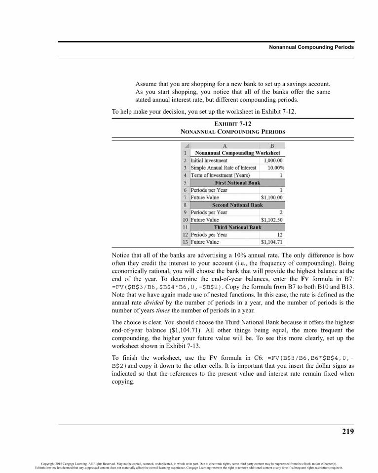
219
Nonannual Compounding Periods
Assume that you are shopping for a new bank to set up a savings account.As you start shopping, you notice that all of the banks offer the samestated annual interest rate, but different compounding periods.
To help make your decision, you set up the worksheet in Exhibit 7-12.
EXHIBIT 7-12NONANNUAL COMPOUNDING PERIODS
Notice that all of the banks are advertising a 10% annual rate. The only difference is howoften they credit the interest to your account (i.e., the frequency of compounding). Beingeconomically rational, you will choose the bank that will provide the highest balance at theend of the year. To determine the end-of-year balances, enter the FV formula in B7:=FV($B$3/B6,$B$4*B6,0,-$B$2). Copy the formula from B7 to both B10 and B13.Note that we have again made use of nested functions. In this case, the rate is defined as theannual rate divided by the number of periods in a year, and the number of periods is thenumber of years times the number of periods in a year.
The choice is clear. You should choose the Third National Bank because it offers the highestend-of-year balance ($1,104.71). All other things being equal, the more frequent thecompounding, the higher your future value will be. To see this more clearly, set up theworksheet shown in Exhibit 7-13.
To finish the worksheet, use the FV formula in C6: =FV(B$3/B6,B6*$B$4,0,-B$2)and copy it down to the other cells. It is important that you insert the dollar signs asindicated so that the references to the present value and interest rate remain fixed whencopying.
Copyright 2015 Cengage Learning. All Rights Reserved. May not be copied, scanned, or duplicated, in whole or in part. Due to electronic rights, some third party content may be suppressed from the eBook and/or eChapter(s).Editorial review has deemed that any suppressed content does not materially affect the overall learning experience. Cengage Learning reserves the right to remove additional content at any time if subsequent rights restrictions require it.

CHAPTER 7: The Time Value of Money
220
EXHIBIT 7-13COMPARING VARIOUS NONANNUAL COMPOUNDING PERIODS
As before, more frequent compounding leads to higher future values. Furthermore, thefuture value increases at a decreasing rate as the number of compounding periods increases.This can be seen more easily if we create a chart of the future values. Select the labels inA5:A14 and the numbers in C5:C14 (remember, you can select discontiguous ranges byholding down the Ctrl key while dragging the mouse). Note that you are selecting one extrarow because we will use this worksheet again later to add one more data point. Now, clickthe Insert tab and create a Column chart formatted as shown in Exhibit 7-14.
EXHIBIT 7-14NONANNUAL COMPOUNDING RESULTS
Copyright 2015 Cengage Learning. All Rights Reserved. May not be copied, scanned, or duplicated, in whole or in part. Due to electronic rights, some third party content may be suppressed from the eBook and/or eChapter(s).Editorial review has deemed that any suppressed content does not materially affect the overall learning experience. Cengage Learning reserves the right to remove additional content at any time if subsequent rights restrictions require it.

221
Nonannual Compounding Periods
Effective Annual Interest RatesAnother way that we can look at the results of changing the compounding frequency is bycalculating the effective annual interest rate (EAR). The EAR is the rate that is actuallyearned when compounding is more frequent than annual. It is calculated as:
(7-15)
where i is the simple (or stated) annual rate and m is the number of compounding periods peryear.
Return to our example of the three banks, in Exhibit 7-12, all of which were promising a10% interest rate. The Second National Bank was compounding interest semiannually, so itwas offering an effective annual rate of 10.25%:
Excel offers the EFFECT function to calculate the effective annual interest rate:
EFFECT(NOMINAL_RATE, NPERY)
where NOMINAL_RATE is the stated annual interest rate and NPERY is the number ofcompounding periods per year. To calculate the EAR being offered by the Second NationalBank, return to that worksheet and enter the formula: =EFFECT($B$3,B9). You shouldget a result of 10.25% as above. Doing the same for the Third National Bank will return anEAR of 10.47% per year.
Less commonly, you will know the EAR and need to determine the simple (or nominal)annual rate. In these cases you can use the NOMINAL function:
NOMINAL(EFFECT_RATE, NPERY)
where EFFECT_RATE is the EAR. Applying this function to the EARs that were justcalculated will return 10% for all three banks.
Continuous CompoundingWe have seen that more frequent compounding leads to higher future values. However, ourexamples extended this idea only as far as daily compounding. There is no reason that wecan’t also compound every half-day, every hour, or even every minute. In fact, this conceptcan be extended to the smallest imaginable time period: the instant. This type ofcompounding is referred to as continuous compounding.
EAR 1 im----+⎝ ⎠
⎛ ⎞m1–=
EAR 1 0.102
----------+⎝ ⎠⎛ ⎞ 2
1– 0.1025= =
Copyright 2015 Cengage Learning. All Rights Reserved. May not be copied, scanned, or duplicated, in whole or in part. Due to electronic rights, some third party content may be suppressed from the eBook and/or eChapter(s).Editorial review has deemed that any suppressed content does not materially affect the overall learning experience. Cengage Learning reserves the right to remove additional content at any time if subsequent rights restrictions require it.

CHAPTER 7: The Time Value of Money
222
Continuous compounding is an extension of what we have seen already. To recap, recall thatwe changed the basic future value function:
The more frequently we compound, the larger m is going to be. For example, withsemiannual compounding m = 2, but with daily compounding m = 365. What if we set mequal to infinity? We can’t do that because i/∞ is effectively equal to zero. Instead we cantake the limit as m approaches infinity. When we do this, we get:
(7-16)
where e is the base of the natural logarithm and is approximately equal to 2.718.
Excel does not offer functions to solve for the present or future value when compounding iscontinuous. However, we can easily create the formulas using the EXP function, which raisese to a specified power.9 This function is defined as:
EXP(NUMBER)
Using the worksheet in Exhibit 7-14, we can add in cell C14: =B2*exp(B3*B4). Becausewe assumed a one-year period, the power to which e is raised is simply the interest rate. Addthe label: Continuous in A14 and the worksheet is complete. Continuous compoundingdoesn’t offer much of an increase over daily compounding. The advantage gets larger as theamount invested grows, but it would take huge sums to make a significant difference. Notethat we can get a good approximation of continuous compounding by using the EFFECTfunction with a large number for NPERY. To see this, change the formula in C14 to:=B2*(1+EFFECT(B3,100000)) and notice that the answer is essentially the same.
We can also calculate the present value of a continuously compounded sum. All that needs tobe done is to solve equation (7-16) for PV:10
(7-17)
9. e is the base of the natural logarithm, so exp(·) is the inverse of ln(·). In other words, exp(ln(x)) = x.10. Many students find that the continuous compounding equations are easier to recall if we change
the notation slightly. Specifically, let P be the present value, F be the future value, r is the annualrate of interest, and T is the number of years (which can be fractional). With this notation, equation
(7-16) becomes: , and equation (7-17) becomes: . This is easier becausethe formulas can be pronounced. For example, equation (7-16) is pronounced “Pert.”
FVN PV 1 im----+⎝ ⎠
⎛ ⎞Nm
=
FVNm ∞→lim PVeiN=
F PerT= P Fe rT–=
PVm ∞→lim FVNe i– N=
Copyright 2015 Cengage Learning. All Rights Reserved. May not be copied, scanned, or duplicated, in whole or in part. Due to electronic rights, some third party content may be suppressed from the eBook and/or eChapter(s).Editorial review has deemed that any suppressed content does not materially affect the overall learning experience. Cengage Learning reserves the right to remove additional content at any time if subsequent rights restrictions require it.

223
Summary
SummaryIn this chapter, we have discussed the concept of the time value of money. Present valuerepresents the amount of money that needs to be invested today in order to purchase a futurecash flow or stream of cash flows. Future value represents the amount of money that will beaccumulated if we invest known cash flows at known interest rates. Further, we havediscussed various types of cash flows. Annuities are equal cash flows, equally spacedthrough time. Graduated annuities are similar to normal annuities, but the cash flows growby a certain amount each period. Uneven cash flows are those in which the periodic cashflows are not equal.
Before continuing with future chapters, you should be comfortable with these concepts.Practice by changing the worksheets presented in this chapter until you develop a sense forthe type of results that you will obtain.
TABLE 7-1FINANCIAL FUNCTIONS USED IN THIS CHAPTER
Purpose Function PageFind the future value FV(RATE, NPER, PMT, PV, TYPE) 197Find the present value PV(RATE, NPER, PMT, FV, TYPE) 199Payment of an annuity PMT(RATE, NPER, PV, FV, TYPE) 204Number of periods NPER(RATE, PMT, PV, FV, TYPE) 206Natural logarithm LN(NUMBER) 206Yield of an annuity RATE(NPER, PMT, PV, FV, TYPE, GUESS) 207Present value of a graduated annuity
FAME_PVGA(PMT, NPER, GROWTHRATE, DISCRATE, BEGEND) 213
Future value of a graduated annuity
FAME_FVGA(PMT, NPER, GROWTHRATE, DISCRATE, BEGEND) 214
Present value of unequal cash flows NPV(RATE,VALUE1, VALUE2,…) 215
Yield of uneven cash flows IRR(VALUES, GUESS) 211Effective Annual Rate EFFECT(NOMINAL_RATE, NPERY) 221Nominal Annual Rate NOMINAL(EFFECT_RATE, NPERY) 221Raise e to a power EXP(NUMBER) 222
Copyright 2015 Cengage Learning. All Rights Reserved. May not be copied, scanned, or duplicated, in whole or in part. Due to electronic rights, some third party content may be suppressed from the eBook and/or eChapter(s).Editorial review has deemed that any suppressed content does not materially affect the overall learning experience. Cengage Learning reserves the right to remove additional content at any time if subsequent rights restrictions require it.
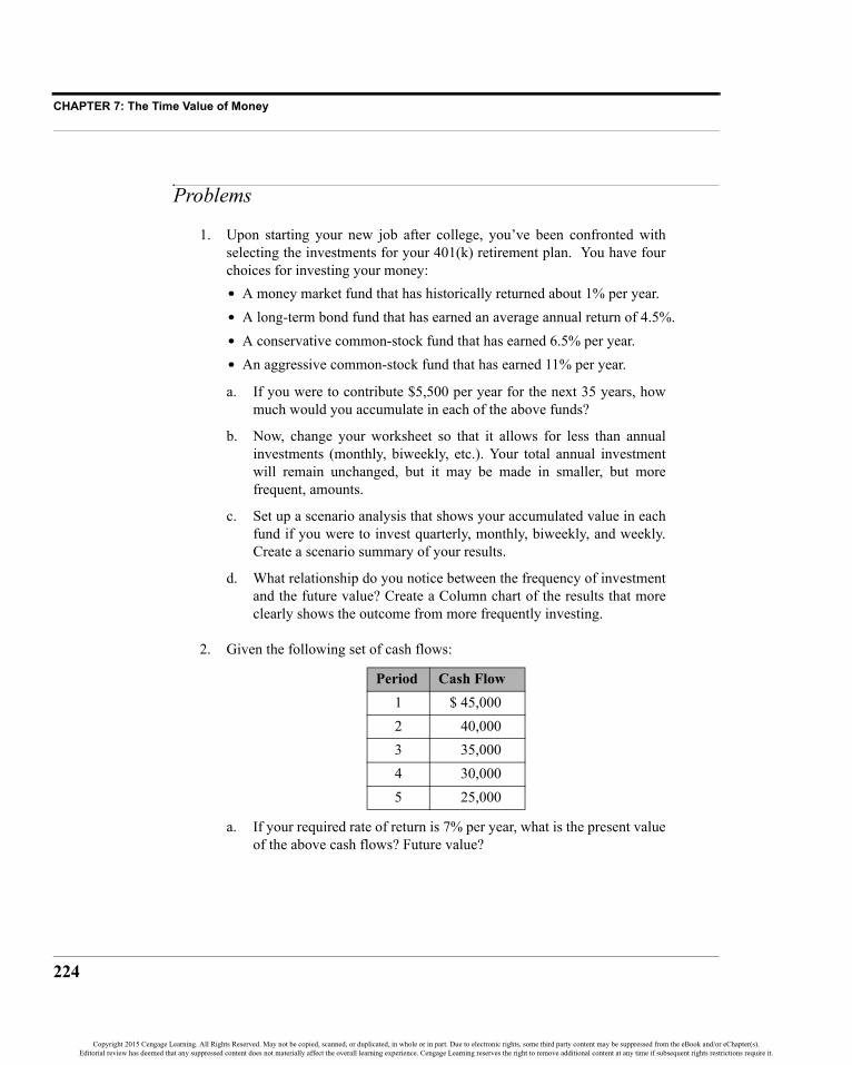
CHAPTER 7: The Time Value of Money
224
Problems
1. Upon starting your new job after college, you’ve been confronted withselecting the investments for your 401(k) retirement plan. You have fourchoices for investing your money:• A money market fund that has historically returned about 1% per year.• A long-term bond fund that has earned an average annual return of 4.5%.• A conservative common-stock fund that has earned 6.5% per year.• An aggressive common-stock fund that has earned 11% per year.
a. If you were to contribute $5,500 per year for the next 35 years, howmuch would you accumulate in each of the above funds?
b. Now, change your worksheet so that it allows for less than annualinvestments (monthly, biweekly, etc.). Your total annual investmentwill remain unchanged, but it may be made in smaller, but morefrequent, amounts.
c. Set up a scenario analysis that shows your accumulated value in eachfund if you were to invest quarterly, monthly, biweekly, and weekly.Create a scenario summary of your results.
d. What relationship do you notice between the frequency of investmentand the future value? Create a Column chart of the results that moreclearly shows the outcome from more frequently investing.
2. Given the following set of cash flows:
a. If your required rate of return is 7% per year, what is the present valueof the above cash flows? Future value?
Period Cash Flow1 $ 45,0002 40,0003 35,0004 30,0005 25,000
Copyright 2015 Cengage Learning. All Rights Reserved. May not be copied, scanned, or duplicated, in whole or in part. Due to electronic rights, some third party content may be suppressed from the eBook and/or eChapter(s).Editorial review has deemed that any suppressed content does not materially affect the overall learning experience. Cengage Learning reserves the right to remove additional content at any time if subsequent rights restrictions require it.

225
Problems
b. Now, suppose that you are offered another investment that isidentical, except that the cash flows are reversed (i.e., cash flow 1 is25,000, cash flow 2 is 30,000, etc.). Is this worth more, or less, thanthe original investment? Why?
c. If you paid $130,000 for the original investment, what average annualrate of return would you earn? What return would you earn on thereversed cash flows?
d. Still assuming that your required return is 7%, would you be willingto purchase either of these investments? Explain why, or why not.
3. Your five-year-old daughter has just announced that she would like toattend college. The College Board has reported that the average cost oftuition, room, board, and other expenses at public four-year colleges is$18,391 in the 2013–2014 academic year.11 The cost has risen 3.2% overthe last year. You believe that you can earn a rate of 8% on investments tomeet this goal.
a. If costs continue to rise at 3.2% per year, how much will it cost for thefirst year of tuition in 13 years?
b. Assuming that you plan to have enough money saved in 13 years tocover all four years of college costs, how much will you need to haveaccumulated by that time? Note that the tuition, room, and board is agraduated annuity growing 3.2% per year, and assume that you willpay all costs at the beginning of each year.
c. If you were to invest a lump sum today in hopes of covering yourdaughter’s college costs, how much would you have to invest?
d. If you decided to invest annually instead, how much would you haveto invest each year? What if you make investments monthly?
e. You just learned of a $10,000 inheritance and plan to invest it in yourdaughter’s college fund. Given this new source of funds, how muchwill you now have to invest each year?
11.See http://trends.collegeboard.org/college_pricing/ for the full results.
Copyright 2015 Cengage Learning. All Rights Reserved. May not be copied, scanned, or duplicated, in whole or in part. Due to electronic rights, some third party content may be suppressed from the eBook and/or eChapter(s).Editorial review has deemed that any suppressed content does not materially affect the overall learning experience. Cengage Learning reserves the right to remove additional content at any time if subsequent rights restrictions require it.

CHAPTER 7: The Time Value of Money
226
4. You have decided to invest in a small commercial office building that hasone tenant. The tenant has a lease that calls for annual rent payments of$20,000 per year for the next three years. However, after that lease expiresyou expect to be able to increase the rent by 5% per year for the next sevenyears. You plan to sell the building for $300,000 ten years from now.
a. Create a table showing the projected cash flows for this investmentassuming that the next lease payment will be made in one year.
b. Assuming that you need to earn 11% per year on this investment,what is the maximum price that you would be willing to pay for thebuilding today? Use the NPV function.
c. Notice that the cash flow stream starts out as a three-year regularannuity, but it then changes into a seven-year graduated annuity plus alump sum in year 10. Use the principal of value additivity to calculatethe present value of the cash flows.
d. Suppose that the current owner of the building is asking $200,000 forthe building. If you paid this price, what annual rate of return wouldyou earn? Should you buy the building at this price?
5. Congratulations! You have just won the State Lottery. The lottery prizewas advertised as an annuitized $105 million paid out in 30 equal annualpayments beginning immediately. The annual payment is determined bydividing the advertised prize by the number of payments. You now haveup to 60 days to determine whether to take the cash prize or the annuity.
a. If you were to choose the annuitized prize, how much would youreceive each year?
b. The cash prize is the present value of the annuity payments. If interestrates are 4.5%, how much will you receive if you choose the cashoption?
c. Now suppose that, as many lotteries do, the annuitized cash flows willgrow by 3% per year to keep up with inflation, but they still add up to$105 million. In this case, the first payment will be $2,207,022.23today. If you took the cash prize instead, how much would youreceive (before taxes)?
Copyright 2015 Cengage Learning. All Rights Reserved. May not be copied, scanned, or duplicated, in whole or in part. Due to electronic rights, some third party content may be suppressed from the eBook and/or eChapter(s).Editorial review has deemed that any suppressed content does not materially affect the overall learning experience. Cengage Learning reserves the right to remove additional content at any time if subsequent rights restrictions require it.

227
CHAPTER 8 Common Stock Valuation
Determining the value of financial assets is important to both investors and corporatefinancial managers. The obvious reason is that nobody wants to pay more than an asset isworth, because such behavior would lead to lower returns. Less obvious, but equallyimportant, is that we can draw some valuable conclusions from the observed prices of assets.We will examine one of these conclusions in detail in Chapter 10 when we use the marketvalue of corporate securities to determine the required rate of return on investments.
In this chapter we will look at several models that can be used to determine the value of ashare of common or preferred stock.
After studying this chapter, you should be able to:1. Differentiate among the definitions of “value,” and explain the importance of
intrinsic value in making financial decisions.2. Explain how intrinsic value is calculated by considering the size, timing, and
perceived riskiness of the cash flows.3. Explain the concept of “required rate of return,” and calculate this rate using
the Capital Asset Pricing Model (CAPM).4. Use several discounted cash flow (DCF) models to value a common stock.5. Use relative valuation models, especially for stocks that do not meet the
assumptions of DCF models.
Copyright 2015 Cengage Learning. All Rights Reserved. May not be copied, scanned, or duplicated, in whole or in part. Due to electronic rights, some third party content may be suppressed from the eBook and/or eChapter(s).Editorial review has deemed that any suppressed content does not materially affect the overall learning experience. Cengage Learning reserves the right to remove additional content at any time if subsequent rights restrictions require it.
CHAPTER 8: Common Stock Valuation
228
What Is Value?The term “value” has many different meanings depending on the context in which it is used.For our purposes, there are four important types of value.
Most generally, value can be defined as the amount that a willing and able buyer agrees topay for an asset to a willing and able seller. In order to establish the value of an asset, it isimportant that both the buyer and seller be willing and able. Otherwise, no legitimatetransaction can take place, and value cannot be determined without a voluntary exchange.Notice that we did not say that the value of an asset is always the same as its price. Price andvalue are distinct, though related, concepts. The price of an asset can be greater than its value(in which case we say that the asset is overvalued), less than its value (undervalued), orequal to its value (fairly valued).
Book value is the price of an asset less its accumulated depreciation. Depreciation is asystematic method of accounting for the reduction in the value of an asset over its useful life.Because of the systematic nature of depreciation (i.e., it is determined in advance accordingto some well-defined formula), book value does not necessarily fairly represent the actualmarket value of the asset. Because of this and other distortions of value, so-called valueinvestors exist. These investors seek out the stocks of companies that they believe to beundervalued, in hopes that the market will eventually recognize the true value of thecompany.
Intrinsic value is the value of an asset to a particular investor. Intrinsic value can bedetermined by calculating the present value of the expected future cash flows at thatinvestor’s required rate of return. Because we use the investor’s required rate of return in thecalculation, and because each investor has different preferences and perceptions, intrinsicvalue is unique to each individual. Without these differences in intrinsic values, marketswould not function smoothly.
Market value is the price of an asset as determined in a competitive marketplace. The marketprice is the price that the marginal investor is willing to pay and will fluctuate (sometimeswildly) throughout the trading day. Investors will purchase assets with market values belowtheir intrinsic values (undervalued assets) and sell assets with market values above theirintrinsic values (overvalued assets). It is easy to determine the market value of securitiestraded in the public markets, but not so easy for many other types of assets. Houses, forexample, are traded only rarely, so it is difficult to determine their true market value. In thesecases, we must rely on estimates of market value made by experts (e.g., appraisers).
Unless otherwise modified, or obvious from the context, all references to the term “value”from this point forward will refer to the individual’s intrinsic value.
Copyright 2015 Cengage Learning. All Rights Reserved. May not be copied, scanned, or duplicated, in whole or in part. Due to electronic rights, some third party content may be suppressed from the eBook and/or eChapter(s).Editorial review has deemed that any suppressed content does not materially affect the overall learning experience. Cengage Learning reserves the right to remove additional content at any time if subsequent rights restrictions require it.

229
Fundamentals of Valuation
Fundamentals of ValuationAs noted earlier, the intrinsic value of an asset is the present value of the expected futurecash flows provided by the asset. Mathematically, intrinsic value is given by:
(8-1)
where Cft is the expected cash flow in period t and i is the required rate of return for theinvestor performing the calculation.1 If N is finite, then the last cash flow will include theexpected selling price of the asset.
The most important components of value are likely to be the size and timing of the expectedcash flows. The larger the expected cash flows and the more quickly they are to be received,the higher the value will be. In other words, there is a positive relationship between the sizeof the cash flows and value and a negative relationship between the time until the cash flowsare received and value.
The other component of value is the investor’s required rate of return. The required return isaffected by the rates of return offered by competing investment vehicles and the riskiness ofthe investment. For example, if bonds are offering higher returns than stocks, we wouldexpect that the prices of stocks would drop (and the prices of bonds would rise) as investorsmoved their money out of stocks and into bonds. This would occur because investors wouldrecognize that bonds are less risky than stocks, and they would raise their required returnsfor stocks. Because an increase in the required return will decrease value, investors wouldsell stocks, thereby driving down the prices. This process would continue until the prices ofstocks had fallen enough and bond prices risen enough, so that the expected returns revertedto the equilibrium relationship.
To determine the value of a security, then, we must first determine three things:
1. What are the expected future cash flows?2. When will the cash flows occur?3. What is the required rate of return for this particular stream of cash flows?
As we discuss the methods of valuing securities, keep these ideas in mind as they are thefundamentals of all security valuation.
1. At this point, we will assume that all future cash flows are known with certainty. In Chapter 12, wewill examine what happens when future cash flows are uncertain.
VCft
1 i+( )t-----------------
t 1=
N
∑=
Copyright 2015 Cengage Learning. All Rights Reserved. May not be copied, scanned, or duplicated, in whole or in part. Due to electronic rights, some third party content may be suppressed from the eBook and/or eChapter(s).Editorial review has deemed that any suppressed content does not materially affect the overall learning experience. Cengage Learning reserves the right to remove additional content at any time if subsequent rights restrictions require it.

CHAPTER 8: Common Stock Valuation
230
Determining the Required Rate of ReturnAs mentioned earlier, one of the determinants of the required return for any stream of cashflows is the perceived riskiness of those cash flows. We will leave an in-depth discussion ofrisk for Chapter 12, but for now we will assume that the risk of a security is known.
In general, each investor can be classified by risk preference into one of three basiccategories:
1. Risk Averse—The risk-averse investor prefers less risk for a given rate ofreturn. The risk averter can be encouraged to accept nearly any level ofrisk, but only if the rate of return is expected to compensate him fairly. Inother words, he must be paid in order to accept risk.
2. Risk Neutral—The risk-neutral investor is indifferent to the level of risk.His required rate of return will not change, regardless of the risk involved.
3. Risk Lover—The risk-loving investor will actually lower his requiredrate of return as the risk increases. In other words, he is willing to pay totake on extra risk.
Under ordinary circumstances, we assume that all investors are risk averse and must receivea higher rate of return in order to accept a higher risk. Realize, however, that even investorsin the same category can have different risk preferences, so two risk-averse investors willlikely have different required returns for the same asset.
FIGURE 8-1THEORETICAL RISK-RETURN TRADE-OFF FOR TWO RISK-AVERSE INVESTORS
Figure 8-1 illustrates the ex-ante (expected) risk-return trade-off for two risk-averseinvestors. We know they are risk averse because the lines have a positive slope. In this case,security B is riskier than A and therefore has the higher expected return for both investors.Investor I1 can be seen to be more risk averse than I2 because the slope of the risk-return lineis steeper. In other words, the risk premium grows at a faster rate for I1 than it does for I2.
Copyright 2015 Cengage Learning. All Rights Reserved. May not be copied, scanned, or duplicated, in whole or in part. Due to electronic rights, some third party content may be suppressed from the eBook and/or eChapter(s).Editorial review has deemed that any suppressed content does not materially affect the overall learning experience. Cengage Learning reserves the right to remove additional content at any time if subsequent rights restrictions require it.

231
Determining the Required Rate of Return
A Simple Risk Premium ModelAn easy method of determining the required rate of return for a security can be derived byassuming that the relationship pictured in Figure 8-1 is constant. If this is the case, then wecan define the expected rate of return for an asset as a base rate (y-axis intercept) plus apremium that is based on the riskiness of the security. In equation form:
E(Ri) = Base Rate + Risk Premium
where E(Ri) is the expected rate of return for security i, the base rate is the rate of return onsome benchmark security, and the risk premium is subjectively determined (though it mustbe greater than zero).
The problem with this model is that it is entirely subjective. Both the security chosen to providethe base rate and the risk premium are defined by the individual using the model. For example,one individual might choose the rate of return on bonds issued by his company as the base rate,while another might choose the average rate paid on AAA-rated corporate bonds. Furthermore,because of individual differences in risk preferences, each individual is likely to assign a differentvalue to the risk premium. Obviously, what is needed is a more objective approach that applies tothe entire market instead of just to individual investors if we are to develop an explanation ofsecurity values.
CAPM: A More Scientific ModelThe Capital Asset Pricing Model (CAPM) provides us with a more objective version of thesimple risk premium model for determining expected returns. For our purposes, we canconsider the CAPM to be a version of the simple risk premium model, with its inputs morerigorously defined. The CAPM is given by (we will see how to derive this equation inChapter 13):
(8-2)
where Rf is the risk-free rate of interest, βi is a measure of the riskiness of security i relativeto the riskiness of the market portfolio, and E(Rm) is the expected rate of return on themarket portfolio.
In the CAPM, Rf serves as the base rate of interest. It is defined as the rate of return on asecurity with zero risk. Sometimes Rf is referred to as the “pure time value of money,” or,in other words, the rate of return earned for delaying consumption but not accepting anyrisk. Because it is risk-free, we know Rf with certainty in advance. Ordinarily, Rf is assumedto be the rate of return on a U.S. Treasury security with time to maturity equal to theexpected holding period of the security in question. Treasury securities are chosen as aproxy for the theoretical risk-free rate because they are free of default risk and are thereforethe closest of all securities to being truly risk-free.
E Ri( ) Rf βi E Rm( ) Rf–[ ]+=
Copyright 2015 Cengage Learning. All Rights Reserved. May not be copied, scanned, or duplicated, in whole or in part. Due to electronic rights, some third party content may be suppressed from the eBook and/or eChapter(s).Editorial review has deemed that any suppressed content does not materially affect the overall learning experience. Cengage Learning reserves the right to remove additional content at any time if subsequent rights restrictions require it.
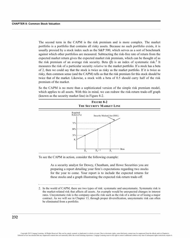
CHAPTER 8: Common Stock Valuation
232
The second term in the CAPM is the risk premium and is more complex. The marketportfolio is a portfolio that contains all risky assets. Because no such portfolio exists, it isusually proxied by a stock index such as the S&P 500, which serves as a sort of benchmarkagainst which other portfolios are measured. Subtracting the risk-free rate of return from theexpected market return gives the expected market risk premium, which can be thought of asthe risk premium of an average risk security. Beta (β) is an index of systematic risk.2 Itmeasures the risk of a particular security relative to the market portfolio. If a stock has a betaof 2, then we could say that the stock is twice as risky as the market portfolio. If it is twice asrisky, then common sense (and the CAPM) tells us that the risk premium for this stock should betwice that of the market. Likewise, a stock with a beta of 0.5 should carry half of the riskpremium of the market.
So the CAPM is no more than a sophisticated version of the simple risk premium model,which applies to all assets. With this in mind, we can redraw the risk-return trade-off graph(known as the security market line) in Figure 8-2.
FIGURE 8-2THE SECURITY MARKET LINE
To see the CAPM in action, consider the following example:
As a security analyst for Dewey, Cheatham, and Howe Securities you arepreparing a report detailing your firm’s expectations regarding two stocksfor the year to come. Your report is to include the expected returns forthese stocks and a graph illustrating the expected risk-return trade-off.
2. In the world of CAPM, there are two types of risk: systematic and unsystematic. Systematic risk isthe market-related risk that affects all assets. An example would be unexpected changes in interestrates. Unsystematic risk is the company-specific risk such as the risk of a strike or of losing a majorcontract. As we will see in Chapter 13, through proper diversification, unsystematic risk can oftenbe eliminated from a portfolio.
Copyright 2015 Cengage Learning. All Rights Reserved. May not be copied, scanned, or duplicated, in whole or in part. Due to electronic rights, some third party content may be suppressed from the eBook and/or eChapter(s).Editorial review has deemed that any suppressed content does not materially affect the overall learning experience. Cengage Learning reserves the right to remove additional content at any time if subsequent rights restrictions require it.

233
Determining the Required Rate of Return
Other analysts at DCH have informed you that the firm expects the S&P500 to earn a return of 11% in the year ahead, and that the risk-free rate is5%. According to Morningstar, the betas for stocks X and Y are 0.5 and1.5, respectively. What are the expected returns for X and Y?
To work this example, open a new workbook and enter the data so that it resembles theworksheet in Exhibit 8-1.
EXHIBIT 8-1CALCULATING EXPECTED RETURNS WITH THE CAPM
Before continuing, it is important to understand some of these inputs. The example problemdid not mention the betas of the risk-free asset or of the market portfolio. How did we knowthat the beta of the risk-free asset is 0? Recall that beta measures the riskiness of the assetrelative to the market. Because the risk-free asset has no risk, by definition, any measure ofrisk must be equal to zero. By definition, the market has a beta of 1.00 because the risk ismeasured relative to the market itself.
To complete this example, we need to enter the formula for the CAPM, equation (8-2), intoC4 and E4. In C4 enter: =$B$4+C3*($D$4-$B$4) and then copy this cell to E4. Youshould see that security X has an expected return of 8% and Y has an expected return of14%. Notice that the expected return of X is not one-half that of the market, nor is theexpected return of Y 50% greater than that of the market. Instead, it is the risk premium ofthese securities that is one-half (for X) or one and one-half (for Y) the risk premium of themarket. The portion of the expected return that comes from delaying consumption (the risk-free rate) is the same for both securities.
Finally, we can create a graph of the security market line (SML) with these data points.Select B3:E4 and then click the Insert Scatter (X,Y) button on the Insert tab. Choose ascatter chart with straight lines and markers. The betas in the first row will be placed on thex-axis automatically.
You can experiment with the SML by changing the expected return for the market or therisk-free rate. You will notice that the slope of the SML changes as you change the marketrisk premium. In other words, the slope changes as market participants become more, orless, risk averse. At this point, your worksheet should match the one in Exhibit 8-2.
Copyright 2015 Cengage Learning. All Rights Reserved. May not be copied, scanned, or duplicated, in whole or in part. Due to electronic rights, some third party content may be suppressed from the eBook and/or eChapter(s).Editorial review has deemed that any suppressed content does not materially affect the overall learning experience. Cengage Learning reserves the right to remove additional content at any time if subsequent rights restrictions require it.

CHAPTER 8: Common Stock Valuation
234
EXHIBIT 8-2EXPECTED RETURNS AND THE SECURITY MARKET LINE
Valuing Common StocksThe first question to ask when attempting to value any security is, “What are the expectedcash flows?” In the case of common stocks, there are two types of cash flows: dividends andthe price received at the time of the sale. Consider the following problem:
Suppose that you are interested in purchasing shares of the common stockof the XYZ Corporation. XYZ recently paid a dividend of $2.40, and youexpect that this dividend will continue to be paid into the foreseeablefuture. Furthermore, you believe (for reasons that will become clear) thatyou will be able to sell this stock in three years for $20 per share. If yourrequired return is 12% per year, what is the maximum amount that youshould be willing to pay for a share of XYZ common stock?
To clarify the problem, it helps to examine it in terms of a timeline as in Figure 8-3.
FIGURE 8-3TIMELINE FOR XYZ COMMON STOCK
Copyright 2015 Cengage Learning. All Rights Reserved. May not be copied, scanned, or duplicated, in whole or in part. Due to electronic rights, some third party content may be suppressed from the eBook and/or eChapter(s).Editorial review has deemed that any suppressed content does not materially affect the overall learning experience. Cengage Learning reserves the right to remove additional content at any time if subsequent rights restrictions require it.

235
Valuing Common Stocks
Calculating the value of this stock is a simple matter of calculating the present value of itscash flows (equation (8-1)). Given that your required return is 12%, the intrinsic value mustbe:
If the stock is currently selling for $24 (the market value), would you purchase any shares?Obviously not, because the market value exceeds your intrinsic value by $4. If you didpurchase the shares, and your cash flow expectations were realized, your average annual rateof return would be less than your required return.
Of course, the XYZ example problem is somewhat contrived because there is no way toknow, for sure, what the dividends and selling price are going to be in the future. Withdividends this is not so much of a problem, because firms tend to have a somewhat stabledividend policy and are reluctant to cut dividends. The advanced knowledge of the sellingprice is a different matter. It is impossible to know exactly what the market price will betomorrow and even more difficult to know the price three years hence.
The Constant-Growth Dividend Discount ModelTo eliminate these problems, we can make a couple of assumptions. The first assumption isthat dividends will grow at a constant rate.3 With this assumption, knowing the most recentdividend (D0) is equivalent to knowing all future dividends. Also assume that we have aninfinite holding period. In other words, we will never sell the stock, so we don’t have toworry about forecasting the selling price. While this second assumption may soundludicrous, we will see that it is little more than a mathematical trick that allows us to developa model.
These assumptions lead to a model for the valuation of common stock that is known as theconstant-growth dividend discount model (DDM) or the Gordon Growth Model. Recall thatwe have defined the value of a common stock as the present value of future dividends plusthe present value of the selling price. Because the stock will never be sold, due to the infiniteholding period, the model becomes:
3. Note that this is not an assumption that the dividend stream will always get larger. The growth ratecould be negative, in which case the dividends would be shrinking over time. Furthermore, thegrowth rate could be zero, which means that the dividends are constant.
V 2.401.12---------- 2.40
1.12( )2----------------- 2.40 20+
1.12( )3----------------------+ + 20= =
VCSD1
1 kCS+( )----------------------
D2
1 kCS+( )2------------------------
D3
1 kCS+( )3------------------------ . . . D∞
1 kCS+( )∞-------------------------+ + + +=
Copyright 2015 Cengage Learning. All Rights Reserved. May not be copied, scanned, or duplicated, in whole or in part. Due to electronic rights, some third party content may be suppressed from the eBook and/or eChapter(s).Editorial review has deemed that any suppressed content does not materially affect the overall learning experience. Cengage Learning reserves the right to remove additional content at any time if subsequent rights restrictions require it.

CHAPTER 8: Common Stock Valuation
236
where VCS is the value of the common stock, the D’s are the dividends in each period, andkCS is the required return.4 Because the dividends are growing at a constant rate, they can beexpressed as a function of the most recently paid dividend (D0):
This equation can be restated in closed form as:
(8-3)
Returning to the example, realize that XYZ’s dividend growth rate is 0% (i.e., the dividendstream is not growing). Therefore, the value of a share is:
which is exactly the same value as was found when assuming that you knew the value of thestock three years hence.
To see how you knew that the value of the stock would be $20 in three years, we can againuse the time-shifting technique from Figure 7-3 (page 209). Let’s look at another example.
Suppose you are interested in purchasing a share of the common stock ofthe ABC Corporation. ABC has not recently paid any dividends, nor is itexpected to for the next three years. However, ABC is expected to beginpaying a dividend of $1.50 per share four years from now. In the future,that dividend is expected to grow at a rate of 7% per year. If your requiredreturn is 15% per year, what is the maximum amount that you should bewilling to pay for a share of ABC common stock?
In order to determine the value of ABC common stock as of today (period 0), we must firstfind the value as of some future time period. The constant-growth DDM can be used at anytime period and will always provide the value of the stock at the time period that is oneperiod before the dividend which is used in the numerator:
(8-4)
4. kCS is the same as i, but is the more common notation for this model. This notation also helps todistinguish between the investor’s required return for the different securities issued by the firm.
VCSD0 1 g+( )
1 kCS+( )------------------------
D0 1 g+( )2
1 kCS+( )2--------------------------
D0 1 g+( )3
1 kCS+( )3-------------------------- . . . D0 1 g+( )∞
1 kCS+( )∞---------------------------+ + + +=
VCSD0 1 g+( )
kCS g–------------------------
D1
kCS g–-----------------= =
VCS2.40 1 0+( )
0.12 0–---------------------------- 20= =
VNDN 1+
kCS g–( )---------------------=
Copyright 2015 Cengage Learning. All Rights Reserved. May not be copied, scanned, or duplicated, in whole or in part. Due to electronic rights, some third party content may be suppressed from the eBook and/or eChapter(s).Editorial review has deemed that any suppressed content does not materially affect the overall learning experience. Cengage Learning reserves the right to remove additional content at any time if subsequent rights restrictions require it.

237
Valuing Common Stocks
FIGURE 8-4VALUING ABC COMMON STOCK WITH TIME-SHIFTING
For this particular problem, the future time period we choose is somewhat arbitrary as longas it is period 3 or later (but period 3 is the easiest). In this case, let’s find the value as ofperiod 3 (using the period 4 dividend):
So we know that the stock will be worth $18.75 per share three years from today.Remembering that the value of a stock is the present value of its cash flows and that the onlyrelevant cash flow in this case is the value at year 3 (which encapsulates the value of allfuture dividends), the value as of today must be:
We could also begin the valuation process at period 5 (or any other period). In this case, thevalue at period 5 (using the period 6 dividend) is:
Next, find the present value of all future cash flows (in this case: D4, D5, and V5):
The $0.02 difference in values is due to rounding. Incidentally, note that had we onlydiscounted back to period 3, the value at that time would have been $18.75.
Earlier we said that the assumption of an infinite holding period was not as ludicrous as itsounds. Let’s examine this assumption in more detail. Open a new worksheet and enter thelabels as shown so that it matches the fragment of a worksheet in Exhibit 8-3.
V3D4
kCS g–----------------- 1.50
0.15 0.07–--------------------------- 18.75= = =
V018.751.153------------- 12.33= =
V51.72
0.15 0.07–--------------------------- 21.50= =
V01.501.154------------ 1.61 21.50+
1.155------------------------------+ 12.35= =
Copyright 2015 Cengage Learning. All Rights Reserved. May not be copied, scanned, or duplicated, in whole or in part. Due to electronic rights, some third party content may be suppressed from the eBook and/or eChapter(s).Editorial review has deemed that any suppressed content does not materially affect the overall learning experience. Cengage Learning reserves the right to remove additional content at any time if subsequent rights restrictions require it.

CHAPTER 8: Common Stock Valuation
238
EXHIBIT 8-3WORKSHEET TO TEST THE INFINITE HOLDING PERIOD ASSUMPTION
Note that the series of numbers representing the periods extends from 1 to 120 in cellsA3:A122. To easily input these numbers, enter a 1 in A3 and then click the Fill button in theEditing group on the Home tab, and choose Series from the drop-down menu. In the Seriesdialog box, set the Step value to 1 and the Stop value to 120. Also be sure to set the seriesType to Linear and Series in to Columns. The dialog box should look like Figure 8-5.
FIGURE 8-5THE SERIES DIALOG BOX
In this worksheet, we want to calculate the value of the stock with various numbers ofdividends included. From the example problem, we know that ABC will first pay a dividendof $1.50 in period 4 and that the dividend will grow at a 7% (cell E2) rate each year. Beforecontinuing, enter the dividends into the worksheet as follows: First, enter a 0 for each of thefirst three dividends. For period 4, enter: 1.50 in B6. In B7, we want to calculate the period5 dividend, so enter: =B6*(1+E$2). Now copy this formula to each cell in the range
Copyright 2015 Cengage Learning. All Rights Reserved. May not be copied, scanned, or duplicated, in whole or in part. Due to electronic rights, some third party content may be suppressed from the eBook and/or eChapter(s).Editorial review has deemed that any suppressed content does not materially affect the overall learning experience. Cengage Learning reserves the right to remove additional content at any time if subsequent rights restrictions require it.

239
Valuing Common Stocks
B8:B122. To make sure that the copy was successful, note that the value in B122 should be3,842.46 (the power of compounding!).
Now, in C3:C122, we want to find the cumulative present values of the dividends as we addmore and more of them. We will use the NPV function to calculate the present values of thedividends. In C3 enter: =NPV(E$3,B$3:B3). The dollar sign will effectively freeze thefirst cell reference, so if we copy this formula down the range will expand. Copy the formulaover the range C4:C122. Column C gives the value of the stock if we include only thedividends through the selected period. For example, the value in C20 ($8.15) is the value ofthe stock if we consider only the first 18 dividends. Similarly, the value in C50 ($11.85) isthe value of the stock if we consider only the first 48 dividends.
Notice how the present value of the dividends converges to the value of the stock ($12.33) aswe include more and more dividends in the calculation. It is not necessary to include morethan about 120 dividends because the present value of all dividends beyond that point iseffectively zero. This is easier to see if we create a graph of the values versus the number ofdividends. Highlight the ranges A3:A122 and C3:C122. Now click the Insert tab and choosea scatter chart with straight lines and no markers.
EXHIBIT 8-4THE INFINITE HOLDING PERIOD IS JUST FOR SIMPLICITY
Your worksheet should now resemble the one in Exhibit 8-4, except that we have added adotted line to represent the known value of the stock ($12.33). If you wish to add the samedotted straight line, remember that it only takes two points to define a line. So, choose anempty area of the worksheet, say D6:E7. In D6 enter 0, and in D7 enter 120. These cellsrepresent the two x values for the line. In E6 calculate the value of the stock with theformula: =B6/(E3-E2)/(1+E3)^3. In E7 enter: =E6 because the y values for the line
Copyright 2015 Cengage Learning. All Rights Reserved. May not be copied, scanned, or duplicated, in whole or in part. Due to electronic rights, some third party content may be suppressed from the eBook and/or eChapter(s).Editorial review has deemed that any suppressed content does not materially affect the overall learning experience. Cengage Learning reserves the right to remove additional content at any time if subsequent rights restrictions require it.

CHAPTER 8: Common Stock Valuation
240
are the same (that’s what makes it horizontal). Finally, right-click in the chart and chooseSelect Data. Click the Add button, and select D6:D7 for the x values and E6:E7 for the yvalues. Note that in Exhibit 8-4 we have moved the chart so that it hides the data for this linebecause it doesn’t need to be visible.
The Two-Stage Growth ModelAssuming that the dividends will grow at a constant rate forever is convenient from amathematical perspective, but it isn’t very realistic. Other dividend-based valuation modelshave been developed, which are more true to life. For example, there is a two-stage growthmodel that allows for a period of supra-normal growth followed by constant growth forever.5In addition, there are several three-stage models which modify the two-stage model to allowfor some pattern of decline into the constant-growth stage. All of these models are morecomplex than the constant-growth model, but keep in mind that they are still present valuecalculations. The only thing that has changed is the pattern of the future cash flows.
The two-stage valuation model allows for the dividend to grow at one rate for severalperiods and then to grow at a (usually, but not necessarily) slower rate from that pointonward. This is a much more realistic model because a firm’s dividends may be growing at afast rate now, but that rate of growth is unlikely to be continued forever. All companies willeventually mature and find that their earnings growth slows so their dividend growth ratemust slow as well. The two-stage model assumes that the change in the dividend growth ratewill happen instantaneously at some point.
Let g1 represent the dividend growth rate from period 1 to n, and g2 be the dividend growthrate for the remainder of time. Assuming that D0 ≠ 0, g1 ≠ kCS, and g2 < kCS, the model is:
(8-5)
Note that the first term in equation (8-5) is simply the present value of the first n dividendsgrowing at a rate of g1 (a graduated annuity, see equation (7-10) on page 211). The secondterm is the present value of all the remaining dividends growing at a constant rate of g2. Thisis exactly the same procedure we used earlier to value ABC’s common stock, except thatABC not only had two growth rates (0% and 7%), but also was not originally paying adividend.6 Note that if g1 = g2 then equation (8-5) simplifies to equation (8-3).
5. Actually, the growth rate in the first phase can be less than the long-run constant rate.6. Note that we cannot use equation (8-5) in that case because D0 was equal to $0.00. Plugging in
$0.00 for D0 would give a value of $0.00 for the stock.
VCSD0 1 g1+( )
kCS g1–-------------------------- 1
1 g1+
1 kCS+-----------------⎝ ⎠⎛ ⎞
n–
D0 1 g1+( )n 1 g2+( )kCS g2–
------------------------------------------------
1 kCS+( )n-------------------------------------------------+=
Copyright 2015 Cengage Learning. All Rights Reserved. May not be copied, scanned, or duplicated, in whole or in part. Due to electronic rights, some third party content may be suppressed from the eBook and/or eChapter(s).Editorial review has deemed that any suppressed content does not materially affect the overall learning experience. Cengage Learning reserves the right to remove additional content at any time if subsequent rights restrictions require it.
241
Valuing Common Stocks
To demonstrate the use of this model, let’s use an example.
Oviedo Paper, Inc. is a major producer of paper products. Due to itsimmensely popular new stationery product, analysts expect that the firm’searnings and dividends will grow at a rate of 15% per year for the next fiveyears. After that, analysts expect that the firm’s growth rate will decline toits historical value of 8% per year as competitors launch similar products.If Oviedo Paper recently paid a dividend (D0) of $0.35 and your requiredreturn is 12%, what is the value of the stock today?
To find the value, use equation (8-5):
While quite long, we can use the formula: =B2*(1+B3)/(B6-B3)*(1-((1+B3)/(1+B6))^B5)+((B2*(1+B3)^B5*(1+B4))/(B6-B4))/(1+B6)^B5 to verifythat the value is $12.68 per share. We could also use the PV function to value the dividendsin the first growth phase (see page 211 for the technique), though it doesn’t really simplifythings in this case since we still have to value the constant-growth phase with a formula.
Because this equation is quite tedious, and Excel has no built-in function for this model, wehave written a user-defined function to do the calculations. Make sure that you have theFameFncs.xlam add-in installed so that you have access to the function. Now, return to youroriginal workbook and open a new worksheet. The user-defined function we will use iscalled FAME_TWOSTAGEVALUE and is defined as:
FAME_TwoStageValue(DIV1, REQRATE, GROWTHRATE1, GROWTHRATE2, G1PERIODS)
where DIV1 is the dividend to be paid at the end of period 1, REQRATE is the required return,GROWTHRATE1 and GROWTHRATE2 are the two growth rates, and G1PERIODS is the lengthof the first growth period.
Set up your new worksheet to look like the one in Exhibit 8-5. To get the value in B8, use theInsert Function dialog box. Choose the User Defined category, and then selectFAME_TWOSTAGEVALUE from the list. After entering the appropriate addresses, theformula in B8 should be: =FAME_TwoStageValue(B2*(1+B3),B6,B3,B4,B5).Note that to get the dividend at period 1 (DIV1), we need to multiply the period 0 dividendby 1 + B3, which is the first growth rate. Your answer in B8 should confirm the calculationswe made using equation (8-5).
VCS0.35 1.15( )0.12 0.15–--------------------------- 1 1.15
1.12----------⎝ ⎠⎛ ⎞
5–
0.35 1.15( )5 1.08( )0.12 0.08–
--------------------------------------------
1.12( )5--------------------------------------------+ 12.68= =
Copyright 2015 Cengage Learning. All Rights Reserved. May not be copied, scanned, or duplicated, in whole or in part. Due to electronic rights, some third party content may be suppressed from the eBook and/or eChapter(s).Editorial review has deemed that any suppressed content does not materially affect the overall learning experience. Cengage Learning reserves the right to remove additional content at any time if subsequent rights restrictions require it.

CHAPTER 8: Common Stock Valuation
242
As noted earlier, if both growth rates are the same (i.e., we have a single, constant-growthrate), then this model will give the same value as equation (8-3). Let’s assume that the long-run growth rate is 8%. Change the value in B3 to 8%, and you will see that the constant-growth value of the stock is $9.45. Obviously, then, the higher initial growth rate in the earlyyears adds a bit over $3 per share in value to the stock.
EXHIBIT 8-5THE TWO-STAGE GROWTH MODEL
Three-Stage Growth ModelsThere are any number of growth phases that could be assumed for a firm’s dividends, butthree is the typical limit used in practice. In this section, we will see three different three-stage models, each of which makes slightly different assumptions about how the growth ratechanges. The three-stage growth models are very similar in concept to the two-stage model.The difference is that the two-stage model assumes that the change in the growth rate occursinstantaneously, whereas the three-stage models assume a more gradual decline in thegrowth rate over some period. This is a more realistic assumption. Figure 8-6 shows acomparison of the growth rate assumptions compared to the two-stage model.
FIGURE 8-6MULTI-STAGE GROWTH MODELS
Copyright 2015 Cengage Learning. All Rights Reserved. May not be copied, scanned, or duplicated, in whole or in part. Due to electronic rights, some third party content may be suppressed from the eBook and/or eChapter(s).Editorial review has deemed that any suppressed content does not materially affect the overall learning experience. Cengage Learning reserves the right to remove additional content at any time if subsequent rights restrictions require it.

243
Valuing Common Stocks
The Three-Step ModelThe three-step model is very similar to the two-stage model, except that it has a transitionphase with constant growth (generally between g1 and g2, but it could be any rate).Therefore, we have three steps: two graduated annuities followed by a constant-growthperpetuity, which is how we will value the stock. Assuming that D0 ≠ 0, g1 ≠ kCS, gT ≠ kCS,and g2 < kCS, the three-step model is given by:
(8-6)
where gt is the growth rate during the transition step, T is the length of the transition step,and all other variables are as previously defined. While equation (8-6) looks intimidating, itis just the present value of this particular pattern of cash flows.
Again, because of the length of equation (8-6), we have written a user-defined function toperform the calculations:
FAME_THREESTEPVALUE(DIV1, REQRATE, GROWTHRATE1, TRANSGROWTHRATE, GROWTHRATE2, G1PERIODS, TRANSPERIODS)
where the arguments are the same as for FAME_TWOSTAGEVALUE, except for the inclusionof another growth rate (TRANSGROWTHRATE is the growth rate during the transition phase).
Let’s change our worksheet to assume that there will now be a three-year transition periodwith a growth rate of 10% per year. Modify your worksheet by inserting a row above row 4,and entering Transition Growth Rate in A4, and 10% in B4. Insert another row aboverow 7 and enter Transition Period Length in A7, and 3 in B7. In A11, enter thelabel: Three-Step Value of Stock.
In B11 enter: =FAME_ThreeStepValue(B2*(1+B3),B8,B3,B4,B5,B6,B7). Youshould find that the value of the stock using this model is $13.27 per share, which is about$0.59 higher than the two-stage model due to the higher average growth rate.
The Three-Stage ModelThe three-stage model differs from the three-step model because it assumes that the growthrate declines linearly in each year of the transition period. So, instead of one rate in thetransition phase, the growth rate is different in each year as can be seen in Figure 8-6.
VCSD0 1 g1+( )
kCS g1–-------------------------- 1
1 g1+
1 kCS+-----------------⎝ ⎠⎛ ⎞
n–
D0 1 g1+( )n 1 gt+( ) 11 gt+
1 kCS+-----------------⎝ ⎠⎛ ⎞
T–
kCS gt–( ) 1 kCS+( )n----------------------------------------------------------------------------------------
D0 1 g1+( )n 1 gt+( )T 1 g2+( )
kCS g2–( ) 1 kCS+( )n T+----------------------------------------------------------------------
+
+
=
Copyright 2015 Cengage Learning. All Rights Reserved. May not be copied, scanned, or duplicated, in whole or in part. Due to electronic rights, some third party content may be suppressed from the eBook and/or eChapter(s).Editorial review has deemed that any suppressed content does not materially affect the overall learning experience. Cengage Learning reserves the right to remove additional content at any time if subsequent rights restrictions require it.

CHAPTER 8: Common Stock Valuation
244
The declining growth rate complicates the model because we have to calculate each dividendduring the transition phase. The formula is:
(8-7)
where all variables are as previously defined, and the transition phase goes from period n+1to n+T. Note that T is the length of the transition phase. The growth rates in the transition aregiven by:
Because of the changing growth rates during the transition, this model is very difficult to usein a spreadsheet without a user-defined function. Therefore, we have included one:
FAME_THREESTAGEVALUE(DIV1, REQRATE, GROWTHRATE1, GROWTHRATE2, G1PERIODS, TRANSPERIODS)
where all arguments are the same as in the FAME_TWOSTAGEVALUE function, except forTRANSPERIODS, which is the length of the transition phase.
Our spreadsheet already has all of the needed information, so we only need to add a labeland the calculation. In A12 enter the label: Three-Stage Value of Stock, and in B12enter: =FAME_ThreeStageValue(B2*(1+B3),B8,B3,B5,B6,B7). You shouldfind that the value using this model is $13.38, slightly higher than the result of the three-stepmodel.
The H-ModelBecause of the complexity of the three-stage model (as well as the three-step model), Fullerand Hsia developed the H-Model as an approximation.7 This model assumes that the growthrate declines linearly from the first period to the beginning of the constant-growth phase.The “H” in the name refers to the “halfway” point between now and the constant-growthphase. Mathematically, the H-Model is given by:
(8-8)
where H is often substituted for the term.
7. Russel J. Fuller and Chi-Cheng Hsia, “A Simplified Common Stock Valuation Model,” FinancialAnalysts Journal, September–October 1984.
VCSD0 1 g1+( )
kCS g1–-------------------------- 1
1 g1+
1 kCS+-----------------⎝ ⎠⎛ ⎞
n–
Dt 1– 1 gt+( )
1 kCS+( )t-------------------------------
t n 1+=
n T+
∑Dn T+ 1 g2+( )
kCS g2–( ) 1 kCS+( )n T+--------------------------------------------------------+ +=
gt g1 g1 g2–( ) t n–( )T
---------------–=
VCSD0
kCS g2–------------------- 1 g2+( ) n T 2⁄+( ) g1 g2–( )+[ ]=
n T 2⁄+( )
Copyright 2015 Cengage Learning. All Rights Reserved. May not be copied, scanned, or duplicated, in whole or in part. Due to electronic rights, some third party content may be suppressed from the eBook and/or eChapter(s).Editorial review has deemed that any suppressed content does not materially affect the overall learning experience. Cengage Learning reserves the right to remove additional content at any time if subsequent rights restrictions require it.

245
Valuing Common Stocks
Note that equation (8-8) looks quite similar to the constant-growth equation (8-3). Thedifference is that rather than using a single growth rate, the term in brackets in the H Modelrepresents a factor by which the constant-growth model must be multiplied to account forthe higher initial growth rates.
It should be obvious that the average growth rate in the H-Model will be higher than theaverage growth rate in the two-stage model. For this reason, the H-Model will always give asomewhat higher valuation than the two-stage model. How much higher depends on thelength of the transition period. It will tend to be near the values given by the three-step andthree-stage models (sometimes higher, sometimes lower).
Let’s return to our example using Oviedo Paper, Inc. Recall that the growth rate willtransition from 15% to 8% over a three-year period. That makes the time in the first stagefive years (n), and the transition phase (T) equals three. Using equation (8-8), we find thatthe value of the stock is:
As with the other models, we have written a user-defined function to do the calculations forthe H-Model. This function is defined as:
FAME_HModelValue(DIV1, REQRATE, GROWTHRATE1, GROWTHRATE2,G1PERIODS,TRANSPERIODS)
All of the function’s arguments are the same as before. Note that even though equation (8-8)uses D0, we have set up the function to ask for D1 for consistency with the other user-definedfunctions.
In A13 enter: H-Model Value of Stock. In B13, use the Insert Function dialog box toenter the function (note that you will have to scroll down in the dialog box to enter the lastargument). It is: =FAME_HModelValue(B2*(1+B3),B9,B3,B5,B6,B8). As youcan see in Exhibit 8-6, the three-year transition period adds $0.75 to the value of the stock ascompared to the two-stage model.
Ultimately, it’s important to remember that all of these common stock valuation models are nothingmore than present value functions. Each uses a different assumption about the growth pattern ofthe dividends, but they are still present value calculations. When faced with a problem thatdoesn’t fit the assumptions of any of these models, simply forecast the dividends in the futureusing whatever growth assumptions are appropriate. Then, calculate the present value of thefuture dividends using the NPV function. This is the method that was used to find the value ofABC common stock in the example problem on page 236.
VCS0.35
0.12 0.08–--------------------------- 1.08 5 3 2⁄+( ) 0.15 0.08–( )+[ ] 13.43= =
Copyright 2015 Cengage Learning. All Rights Reserved. May not be copied, scanned, or duplicated, in whole or in part. Due to electronic rights, some third party content may be suppressed from the eBook and/or eChapter(s).Editorial review has deemed that any suppressed content does not materially affect the overall learning experience. Cengage Learning reserves the right to remove additional content at any time if subsequent rights restrictions require it.

CHAPTER 8: Common Stock Valuation
246
EXHIBIT 8-6MULTI-STAGE DIVIDEND GROWTH MODEL RESULTS
Alternative Discounted Cash Flow ModelsAs noted previously, the value of a stock is given by the present value of its expected futurecash flows—that is, the dividends that it will pay. However, we can restructure these modelsin a way that provides some additional insight into the valuation process. The two modelspresented in this section do just that.
The Earnings ModelImagine a company that pays out 100% of its earnings as dividends. In this case, thedividend is equal to earnings per share (EPS), and the growth rate must be 0% because it isinvesting only enough (through the depreciation charge) to maintain the assets it currentlyowns. Using the constant-growth dividend discount model with g = 0%, equation (8-3), thevalue of the common stock would be:
This is the value of the stock if the firm doesn’t reinvest and therefore doesn’t grow. Mostfirms do reinvest at least some of their earnings, so the value of the stock must be equal tothe value if it doesn’t grow plus the present value of its future growth opportunities (PVGO):
(8-9)
VCSEPS1
k-------------=
VCSEPS1
k------------- PVGO+=
Copyright 2015 Cengage Learning. All Rights Reserved. May not be copied, scanned, or duplicated, in whole or in part. Due to electronic rights, some third party content may be suppressed from the eBook and/or eChapter(s).Editorial review has deemed that any suppressed content does not materially affect the overall learning experience. Cengage Learning reserves the right to remove additional content at any time if subsequent rights restrictions require it.

247
Alternative Discounted Cash Flow Models
The future earnings growth rate will be driven by the rate of return that is generated by thereinvested earnings (the ROE). If we let b = the retention ratio and r = the return on equity,then the growth rate (g) will be:8
(8-10)
Incidentally, recall the extended DuPont method of calculating the ROE from Chapter 4 onpage 125. From this, we know that the growth rate depends on the operating profit margin,the interest rate on debt, the tax rate, the efficiency with which the firm uses its assets, andthe amount of debt that it has in addition to its dividend payout ratio. Thus, the value of thestock always depends on how well-run the firm is.
The value of the stock will increase only if the firm’s ROE (r) is greater than its requiredreturn (k). In other words, if the firm generates a positive net present value (NPV).9 PVGO isequal to the present value of the future NPVs generated by the reinvested earnings (RE). Ifwe assume that the NPV is a perpetuity and that it will grow at a constant rate of g, then:
(8-11)
The NPV in any given year is the present value of the earnings generated by the investmentless the cost of the investment. Mathematically, the NPV is given by:
By substituting this result into equation (8-11), it can be rewritten as:
(8-12)
Now substitute equation (8-12) into equation (8-9) and we have the earnings model:
(8-13)
This model is important because it directly links the company’s ROE to the value of thestock. Specifically, note that the stock price can only rise if r > k. In fact, if r < k (the
8. Note that if b = 0% (100% payout ratio), then g must also be 0%.9. Net present value is discussed in detail in Chapter 11 beginning on page 345.
g br=
PVGONPVt
1 k+( )t------------------
t 1=
∞
∑NPV1
k g–--------------= =
NPV1RE1 r×
k------------------ RE1–=
PVGO
RE1 r×k
------------------ RE1–
k g–----------------------------------
RE1rk-- 1–⎝ ⎠⎛ ⎞
k g–---------------------------= =
VCSEPS1
k-------------
RE1rk-- 1–⎝ ⎠⎛ ⎞
k g–---------------------------+=
Copyright 2015 Cengage Learning. All Rights Reserved. May not be copied, scanned, or duplicated, in whole or in part. Due to electronic rights, some third party content may be suppressed from the eBook and/or eChapter(s).Editorial review has deemed that any suppressed content does not materially affect the overall learning experience. Cengage Learning reserves the right to remove additional content at any time if subsequent rights restrictions require it.

CHAPTER 8: Common Stock Valuation
248
company earns less than its required return), then the value of the stock will fall. Let’s lookat an example:
Analysts expect that Aurora Foods will earn $1.40 per share in the comingyear and pay a dividend of $0.49 per share. Historically, the firm’s ROEhas been 15%, and its required return on investments is 12%. What is thevalue of the stock?
Note that RE1 will be equal to EPS1 – D1, or $0.91 per share, and that the retention ratio is65%. The growth rate is . So, using equation (8-13), we see that thevalue of the stock is:
We can create a worksheet that will make it easy to change the assumptions in the problem.Exhibit 8-7 shows the worksheet.
EXHIBIT 8-7THE EARNINGS MODEL
The values given in the example are in B2:B5. In B7:B9 are the intermediate calculationsthat need to be done before using the model. Retained earnings is calculated in B7 with theformula: =B2-B3. The retention ratio, in B8, is found with: =1-B3/B2, and the growthrate is: =B4*B8.
We have chosen to separate the components of the value into cells B11:B12 to highlightthem separately. In B11 add the formula: =B2/B5. The value of the growth opportunities is
0.65 0.15× 0.0975=
VCS1.400.12----------
0.91 0.150.12---------- 1–⎝ ⎠⎛ ⎞
0.12 0.0975–------------------------------------+ 11.67 10.11+ 21.78= = =
Copyright 2015 Cengage Learning. All Rights Reserved. May not be copied, scanned, or duplicated, in whole or in part. Due to electronic rights, some third party content may be suppressed from the eBook and/or eChapter(s).Editorial review has deemed that any suppressed content does not materially affect the overall learning experience. Cengage Learning reserves the right to remove additional content at any time if subsequent rights restrictions require it.

249
Alternative Discounted Cash Flow Models
given in B12 by the formula: =B7*(B4/B5-1)/(B5-B9). The total value of the stock isthe sum of B11:B12. You should find that it is $21.78, exactly as we found earlier.
Using this worksheet, you can experiment with some of the assumptions. In particular,notice that if you change the ROE so that it is less than the required return then the value ofthe growth opportunities will be negative. For example, if you change the ROE to 10%, thenthe value of the growth opportunities is –$2.76 and reduces the total value of the stock to$8.91. This demonstrates that growth just for the sake of growth doesn’t make economicsense; only profitable growth opportunities are worth pursuing.
Using Data TablesInstead of randomly plugging numbers into the spreadsheet to understand how this modelworks, we can use an Excel feature known as a data table. Essentially, a data table tellsExcel to plug various numbers into the model and recalculate the result. To see how thisworks, set up a data table to calculate the growth rate and stock value as the ROE changes.
In D2 enter the label: ROE, and then in D3:D8 enter a series of numbers from 10% to 20% in2% increments. In E2:F2 we need formulas that Excel will use to calculate the results ofchanging the ROE. Because we already have our model set up, we can simply reference thegrowth rate and stock value. In E2 enter: =B9 and in F2 enter: =B13. Apply a customnumber format of just the name. Excel will plug the new ROEs into B4, and then record thevalues from B9 and B13 in the data table. This will not affect your original model at all.
To create the data table, select D2:F8 (the data table range) and then choose Data Table fromthe What-If Analysis button on the Data tab. Since our ROEs are in a column, we will enterB4 as the Column input cell. After clicking the OK button, you should see the data tablepopulated with the results. Exhibit 8-8 shows the data table that was created.
EXHIBIT 8-8A DATA TABLE SHOWING GROWTH RATE AND VALUE AS ROE CHANGES
Note that the stock value rises as ROE increases, until the growth rate exceeds the requiredreturn. At that point, the model fails and says that the value is negative.
Copyright 2015 Cengage Learning. All Rights Reserved. May not be copied, scanned, or duplicated, in whole or in part. Due to electronic rights, some third party content may be suppressed from the eBook and/or eChapter(s).Editorial review has deemed that any suppressed content does not materially affect the overall learning experience. Cengage Learning reserves the right to remove additional content at any time if subsequent rights restrictions require it.
CHAPTER 8: Common Stock Valuation
250
Before leaving the earnings model, note that it is mathematically equivalent to the constant-growth dividend discount model. In this case, the company will pay a dividend of $0.49 nextyear, and its growth rate is 9.75%. Therefore, the value of the stock must be $21.78:
The Free Cash Flow ModelFree cash flow is defined as total operating cash flow after taxes less the reinvestment inoperating assets that is required to maintain the firm’s growth rate.10 Recall from ourdiscussion of economic profit in Chapter 4 (see page 134) that we defined net operatingprofit after tax (NOPAT) as:
We can now define after-tax operating cash flow as:
Where “noncash expenses” are depreciation, amortization, and sometimes other noncashcharges. Operating cash flow (after tax) is the cash flow available for the firm to reinvest inassets and/or pay out to investors (interest, principal, dividends, share repurchases).Therefore, operating cash flow belongs to both the creditors and the shareholders of the firm.
As was noted earlier, all firms must reinvest in the business to maintain a positive growthrate. To calculate the required investment in operating assets, we first forecast the level ofoperating assets for the next period (see Chapter 5) and then calculate the current level ofthose assets. The difference is the required investment:
where NOWC is net operating working capital (operating current assets less operatingcurrent liabilities). Note that we are referring to operating assets as defined on page 135.Therefore, we need to exclude any nonoperating assets and current liabilities (e.g.,marketable securities and notes payable) from our calculations. We will account for thesenonoperating items later.
10. Free cash flow is a non-GAAP financial metric, so definitions can vary. Some are very complexand some are quite simple. For example, Morningstar defines it as Cash Flows from Operationsless in Capital Expenditures. Both numbers are available on the statement of cash flows.
VCS0.49
0.12 0.0975–( )------------------------------------- 21.78= =
NOPAT EBIT 1 tax rate–( )=
After-Tax Operating Cash Flow NOPAT Noncash Expenses+=
Δ Operating Assets Δ NOWC Δ Operating Fixed Assets+=
Copyright 2015 Cengage Learning. All Rights Reserved. May not be copied, scanned, or duplicated, in whole or in part. Due to electronic rights, some third party content may be suppressed from the eBook and/or eChapter(s).Editorial review has deemed that any suppressed content does not materially affect the overall learning experience. Cengage Learning reserves the right to remove additional content at any time if subsequent rights restrictions require it.

251
Alternative Discounted Cash Flow Models
If we subtract the required reinvestment in operating assets from the operating cash flow,then we have free cash flow (FCF):
(8-14)
This free cash flow belongs to all of the firm’s capital providers. Therefore, the value of thefirm’s operating assets is the present value of the future free cash flows, discounted at thefirm’s WACC. However, we have omitted any nonoperating assets from our calculations,and these assets have value too. For this reason, we must add the value of these nonoperatingassets to the present value of the FCF in order to arrive at the value of the entire firm:11
(8-15)
where WACC is the firm’s weighted average cost of capital. Now, if we assume (as we didfor dividends in earlier models) that the FCF will grow at a constant rate (g) forever, then thevalue of the entire firm (VF) is:
(8-16)
Note that we can make other assumptions about the growth pattern of FCF. For example, wemight forecast FCF for each year over the next five years and assume constant growththereafter. In that case, we would use the general non-constant-growth model developedearlier. Or, we could assume that it will grow in two or three stages. In those cases, we coulduse the two-stage or one of the three-stage models to find the present value, instead of thesingle-stage constant-growth model, for the first term in equation (8-16).
Ultimately, we are trying to get to the per share value of the common stock. The value of theentire firm is also given by:
(8-17)
where VD is the market value of the debt, VP is the value of the preferred equity, and VC isthe value of the common equity. Note that equation (8-17) is nothing more than arestatement of the familiar balance sheet equation:
except that equation (8-17) is stated in terms of current market values instead of book values.
11. Note that value of the nonoperating assets is the PV of their future cash flows. However, especiallyfor short-term investments, the values on the balance sheet are very close to their market value.
Free Cash Flow Operating Cash Flow Δ Operating Assets–=
VFFCFt
1 WACC+( )t---------------------------------
t 1=
∞
∑ Nonoperating Assets+=
VFFCF1
WACC g–( )------------------------------- Nonoperating Assets+=
VF VD VP VC+ +=
Total Assets Total Liabilities Total Equity+=
Copyright 2015 Cengage Learning. All Rights Reserved. May not be copied, scanned, or duplicated, in whole or in part. Due to electronic rights, some third party content may be suppressed from the eBook and/or eChapter(s).Editorial review has deemed that any suppressed content does not materially affect the overall learning experience. Cengage Learning reserves the right to remove additional content at any time if subsequent rights restrictions require it.
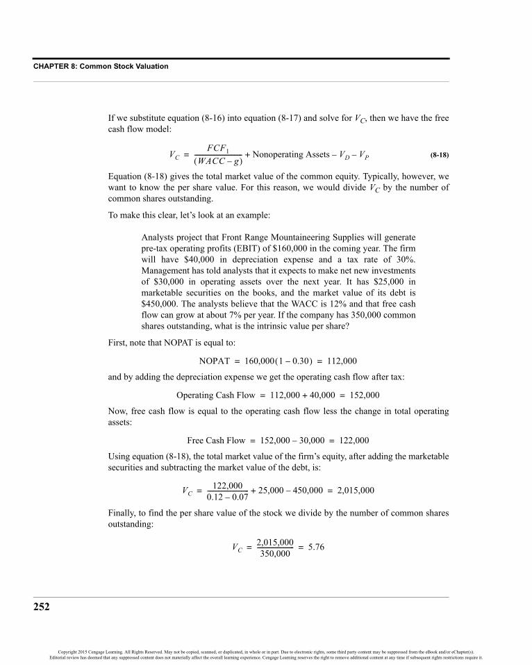
CHAPTER 8: Common Stock Valuation
252
If we substitute equation (8-16) into equation (8-17) and solve for VC, then we have the freecash flow model:
(8-18)
Equation (8-18) gives the total market value of the common equity. Typically, however, wewant to know the per share value. For this reason, we would divide VC by the number ofcommon shares outstanding.
To make this clear, let’s look at an example:
Analysts project that Front Range Mountaineering Supplies will generatepre-tax operating profits (EBIT) of $160,000 in the coming year. The firmwill have $40,000 in depreciation expense and a tax rate of 30%.Management has told analysts that it expects to make net new investmentsof $30,000 in operating assets over the next year. It has $25,000 inmarketable securities on the books, and the market value of its debt is$450,000. The analysts believe that the WACC is 12% and that free cashflow can grow at about 7% per year. If the company has 350,000 commonshares outstanding, what is the intrinsic value per share?
First, note that NOPAT is equal to:
and by adding the depreciation expense we get the operating cash flow after tax:
Now, free cash flow is equal to the operating cash flow less the change in total operatingassets:
Using equation (8-18), the total market value of the firm’s equity, after adding the marketablesecurities and subtracting the market value of the debt, is:
Finally, to find the per share value of the stock we divide by the number of common sharesoutstanding:
VCFCF1
WACC g–( )------------------------------- Nonoperating Assets VD VP––+=
NOPAT 160,000 1 0.30–( ) 112,000= =
Operating Cash Flow 112,000 40,000+ 152,000= =
Free Cash Flow 152,000 30,000– 122,000= =
VC122,000
0.12 0.07–--------------------------- 25,000 450,000–+ 2,015,000= =
VC2,015,000350,000
------------------------ 5.76= =
Copyright 2015 Cengage Learning. All Rights Reserved. May not be copied, scanned, or duplicated, in whole or in part. Due to electronic rights, some third party content may be suppressed from the eBook and/or eChapter(s).Editorial review has deemed that any suppressed content does not materially affect the overall learning experience. Cengage Learning reserves the right to remove additional content at any time if subsequent rights restrictions require it.

253
Alternative Discounted Cash Flow Models
Exhibit 8-9 shows a worksheet for performing the valuation. The data in A3:B11 are takendirectly from the example problem. Once the data and labels are entered, the formulas arequite simple. As we did earlier, the first step is to calculate NOPAT in B13 with the formula:=B3*(1-B5). Operating cash flow, in B14, is: =B13+B4 and free cash flow is: =B14-B6.
Again, the value of the entire firm, including debt, is the present value of the free cash flowplus the value of the nonoperating assets. We assume that free cash flow is growing at aconstant rate forever, so the formula in B17 is: =B15/(B9-B10)+B7. To calculate thevalue of the firm’s equity in B18, we subtract debt: =B17-B8. Finally, the per share value ofthe stock is determined by dividing the market value of the equity by the number of sharesoutstanding: =B18/B11. The result is $5.76 per share, exactly as we got from the formulas.
EXHIBIT 8-9FREE CASH FLOW VALUATION MODEL
We have assumed that the company is in a constant-growth phase, but this may not becorrect for less mature companies. In that case, an analyst will typically create a model of thecompany over the next five years or so and then assume constant growth after that. In thiscase, the non-constant-growth model should be used. The procedure is similar to that shownin Figure 8-4, except that we substitute free cash flow estimates for the dividends and get thevalue of the entire firm instead of the value of the stock. At that point, proceed as we didearlier by adding the current value of nonoperating assets and subtracting the current valueof the debt to get the market value of the equity.
Copyright 2015 Cengage Learning. All Rights Reserved. May not be copied, scanned, or duplicated, in whole or in part. Due to electronic rights, some third party content may be suppressed from the eBook and/or eChapter(s).Editorial review has deemed that any suppressed content does not materially affect the overall learning experience. Cengage Learning reserves the right to remove additional content at any time if subsequent rights restrictions require it.

CHAPTER 8: Common Stock Valuation
254
Relative Value ModelsThe models presented earlier are generally known as DCF (discounted cash flow) models.Although these models are commonly used by analysts, they rely on forecasts of future cashflows that are often very uncertain. We can mitigate that problem somewhat by usingscenario analysis, with several alternative growth rates giving a range of values. However,we can also use a different kind of model altogether: relative value models.
Relative value models provide a way to value a stock relative to other similar stocks usingvaluation ratios such as the Price to Earnings (P/E) ratio. These models have two majoradvantages: They are easy to use, and they can be used to value stocks for which the DCFmodels fail. For example, it is difficult to use the dividend discount models for stocks thatdon’t currently pay a dividend and may not for the foreseeable future. However, as long asthe company has positive earnings, you can use the P/E model. If the company is losingmoney, then you can (with great care) use the Price to Sales (P/S) or Price to Book Value (P/B) models instead.
The P/E ratio is defined as the current stock price divided by the expected earnings per shareover the next year:
(8-19)
The essential idea is that the P/E ratio tells us how much investors are willing to pay for eachdollar of expected earnings. Therefore, all we need is an estimate of earnings and a“justified” P/E ratio. For two identical companies, the P/E ratio should be the same. No twocompanies are ever identical, but if they are similar (in the same industry and share othercharacteristics), then their P/E ratios should be in the same general area. The justified P/Eratio is often calculated by averaging the P/E ratios of comparable firms. To value a stockusing this model, we merely multiply the expected earnings by the justified P/E ratio:
(8-20)
Any differences in P/E ratios should be explained by differences in perceived risk or growthrates. If we substitute equation (8-3) into the numerator of equation (8-19), then we can seehow the growth rate and required return (which is influenced by risk from a number ofsources) affect the P/E ratio:
(8-21)
Note that a higher required return, as would be used for a riskier firm, will lead to a lowerP/E ratio. Also, a company with a higher growth rate should have a higher P/E ratio. Nowwe can determine if a stock is undervalued or overvalued by comparing its P/E ratio to the
Price to Earnings Price per ShareEarnings per Share---------------------------------------------=
V EPS1 PE×=
P/ED1 kCS g–( )⁄
EPS1--------------------------------=
Copyright 2015 Cengage Learning. All Rights Reserved. May not be copied, scanned, or duplicated, in whole or in part. Due to electronic rights, some third party content may be suppressed from the eBook and/or eChapter(s).Editorial review has deemed that any suppressed content does not materially affect the overall learning experience. Cengage Learning reserves the right to remove additional content at any time if subsequent rights restrictions require it.
255
Preferred Stock Valuation
average of its peers. If it has a higher than average P/E that doesn’t seem to be justified bylower risk or higher growth, then the stock is overvalued relative to its peers. We can alsocompare the current P/E to the historical average for the firm to determine if it undervaluedor overvalued compared to the past.
Now suppose that the company doesn’t have any earnings. A negative P/E ratio ismeaningless, so we can’t use that model. However, we can use the P/S ratio or the P/B ratiosinstead. In addition to the above ratios, several others can be used. For example, theEnterprise Value to EBIT (or EBITDA) ratio is commonly used by analysts, particularly tocompute the takeover value of a company. Enterprise value is defined as the market value ofthe firm’s equity (stock price times shares outstanding) plus the market value of debt less theamount of cash and equivalents on the balance sheet.
The relative value models are very commonly used by analysts these days, but they are notwithout their drawbacks. One of the problems is that there is no way to know what absolutevalue of a P/E ratio is appropriate. Instead, the models are relative. Therefore, if you arecomparing one company to several other overvalued stocks, you will come up with a valuethat is too high. Another problem is that no two companies are the same, and it can bedifficult to figure out whether valuation differences are due to expectations about risk,growth rates, or both. Finally, the relationship that should exist between earnings growth,risk, and P/E ratio is not clear and may change over time. Still, used with caution, relativevalue models can be used to validate the results of a DCF analysis.
Preferred Stock ValuationPreferred stock is a kind of hybrid security. It represents an ownership claim on the assets ofthe firm, like common stock, but holders of preferred stock do not benefit from increases inthe firm’s earnings and they generally cannot vote in corporate elections, like bonds. Further,like a bond, preferred stock generally pays a fixed dividend payment each period. Also, likea common stock, there is no predefined maturity date, so the life of a share of preferred stockis effectively infinite.
With the complex nature of preferred stock, it is natural to assume that it must be difficult tovalue. As we will see, preferred stock valuation is actually quite easy. To see how we canderive the valuation formula for preferred stock, consider the following example:
The XYZ Corporation has issued preferred stock that pays a 10% annualdividend on its $50 par value. If your required return for investments ofthis type is 12%, what is the maximum amount that you should be willingto pay for a share of XYZ preferred?
Copyright 2015 Cengage Learning. All Rights Reserved. May not be copied, scanned, or duplicated, in whole or in part. Due to electronic rights, some third party content may be suppressed from the eBook and/or eChapter(s).Editorial review has deemed that any suppressed content does not materially affect the overall learning experience. Cengage Learning reserves the right to remove additional content at any time if subsequent rights restrictions require it.
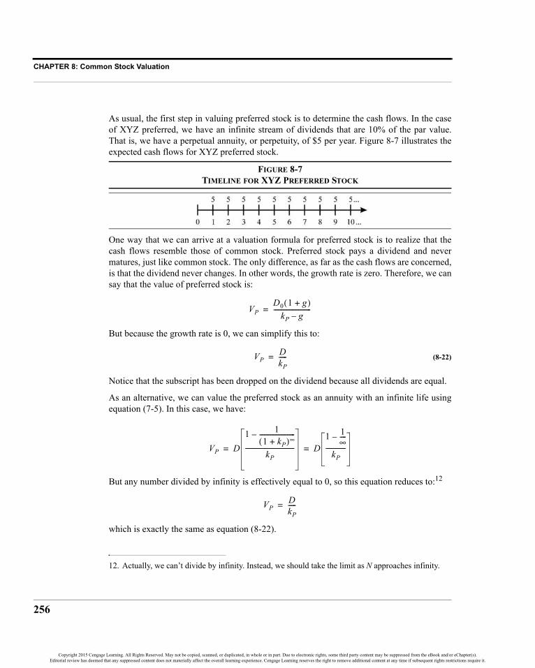
CHAPTER 8: Common Stock Valuation
256
As usual, the first step in valuing preferred stock is to determine the cash flows. In the caseof XYZ preferred, we have an infinite stream of dividends that are 10% of the par value.That is, we have a perpetual annuity, or perpetuity, of $5 per year. Figure 8-7 illustrates theexpected cash flows for XYZ preferred stock.
FIGURE 8-7TIMELINE FOR XYZ PREFERRED STOCK
One way that we can arrive at a valuation formula for preferred stock is to realize that thecash flows resemble those of common stock. Preferred stock pays a dividend and nevermatures, just like common stock. The only difference, as far as the cash flows are concerned,is that the dividend never changes. In other words, the growth rate is zero. Therefore, we cansay that the value of preferred stock is:
But because the growth rate is 0, we can simplify this to:
(8-22)
Notice that the subscript has been dropped on the dividend because all dividends are equal.
As an alternative, we can value the preferred stock as an annuity with an infinite life usingequation (7-5). In this case, we have:
But any number divided by infinity is effectively equal to 0, so this equation reduces to:12
which is exactly the same as equation (8-22).
12. Actually, we can’t divide by infinity. Instead, we should take the limit as N approaches infinity.
VPD0 1 g+( )
kP g–------------------------=
VPDkP-----=
VP D1 1
1 kP+( )∞-----------------------–
kP-------------------------------- D
1 1∞----–
kP-------------= =
VPDkP-----=
Copyright 2015 Cengage Learning. All Rights Reserved. May not be copied, scanned, or duplicated, in whole or in part. Due to electronic rights, some third party content may be suppressed from the eBook and/or eChapter(s).Editorial review has deemed that any suppressed content does not materially affect the overall learning experience. Cengage Learning reserves the right to remove additional content at any time if subsequent rights restrictions require it.

257
Summary
So, for valuation purposes, regardless of whether we treat preferred stock like common stockor perpetuity, we arrive at exactly the same valuation formula. To find the value of a share ofpreferred stock, we simply need to divide its dividend payment by our required rate ofreturn. Therefore, the value of XYZ’s preferred stock must be:
You can prove this by recreating Exhibit 8-4 (page 239), with all of the dividends set to 5.
SummaryThe valuation process is important to both financial managers and investors. As we will seein future chapters, understanding the valuation process is crucial to making sound financialdecisions.
In this chapter, we found that the value of a security depends on several factors:• The size of the expected future cash flows• The timing of the expected cash flows• The perceived riskiness of the expected cash flows
Once the cash flows and required rate of return have been determined, we can value thesecurity by finding the present value of its future cash flows. The dividend discount modelsdiffer only in the expected pattern of dividend growth. They all reduce to the present valueof future cash flows to the stockholders.
We also derived the earnings model, which is important because it shows that the firm mustmake productive investments (ROE > k) in order to increase the stock price. The free cashflow model shows that the value of the entire firm is the present value of the expected futureoperating cash flows less expected investments.
Finally, we examined relative value models. These models do not rely (at least directly) onthe present value of future cash flows. Instead, they attempt to value a stock much likehouses are valued: by looking at “comparables” and then assuming that the valuation shouldbe similar, though some adjustments can be made.
VP5
0.12---------- 41.66= =
Copyright 2015 Cengage Learning. All Rights Reserved. May not be copied, scanned, or duplicated, in whole or in part. Due to electronic rights, some third party content may be suppressed from the eBook and/or eChapter(s).Editorial review has deemed that any suppressed content does not materially affect the overall learning experience. Cengage Learning reserves the right to remove additional content at any time if subsequent rights restrictions require it.

CHAPTER 8: Common Stock Valuation
258
TABLE 8-1SELECTED FORMULAS USED IN THIS CHAPTER
Valuation Formula Page
Constant-growth common stock 236
Two-stage growth common stock
240
H-Model common stock 244
Earnings Model 247
Free Cash Flow Model 252
Preferred stock 256
TABLE 8-2FUNCTIONS INTRODUCED IN THIS CHAPTER
Purpose Function PageTwo-stage model FAME_TwoStageValue(DIV1, REQRATE,GROWTHRATE1,
GROWTHRATE2,G1PERIODS) 241
Three-step modelFAME_THREESTEPVALUE(DIV1, REQRATE, GROWTHRATE1, TRANSGROWTHRATE, GROWTHRATE2, G1PERIODS, TRANSPERIODS)
243
Three-stage model FAME_ThreeStageValue(DIV1, REQRATE,GROWTHRATE1,GROWTHRATE2,G1PERIODS,TRANSPERIODS) 245
H-Model FAME_HModelValue(DIV1, REQRATE, GROWTHRATE1, GROWTHRATE2,G1PERIODS,TRANSPERIODS) 245
VCSD0 1 g+( )
kCS g–------------------------
D1
kCS g–-----------------= =
VCSD0 1 g1+( )
kCS g1–-------------------------- 1
1 g1+
1 kCS+-----------------⎝ ⎠⎛ ⎞
n–
D0 1 g1+( )n 1 g2+( )kCS g2–
------------------------------------------------
1 kCS+( )n-------------------------------------------------+=
VCSD0
kCS g2–------------------- 1 g2+( ) n T 2⁄+( ) g1 g2–( )+[ ]=
VEPS1
k-------------
RE1rk-- 1–⎝ ⎠⎛ ⎞
k g–---------------------------+=
VCFCF1
WACC g–( )------------------------------- Nonoperating Assets VD VP––+=
VPDkP-----=
Copyright 2015 Cengage Learning. All Rights Reserved. May not be copied, scanned, or duplicated, in whole or in part. Due to electronic rights, some third party content may be suppressed from the eBook and/or eChapter(s).Editorial review has deemed that any suppressed content does not materially affect the overall learning experience. Cengage Learning reserves the right to remove additional content at any time if subsequent rights restrictions require it.

259
Problems
Problems
1. Bob’s Rawhide Company has a dividend payout ratio of 30%. Next year itwill earn $2.50 per share and have a return on equity of 15%. Theshareholders’ required return is 12%.
a. Calculate the company’s growth rate of EPS.
b. Using the earnings model, what is the value of the stock?
c. Construct a data table that shows how the growth rate and value of thestock will change if the ROE ranges between 10% and 20%, in 1%increments. Now, using that data, create a scatter chart to show therelationship between the value of the stock and the ROE. Is therelationship linear? At what point does the model break down?
d. Using the constant-growth dividend discount model, what is the valueof the stock?
2. As an analyst at Churnem & Burnem Securities, you are responsible formaking recommendations to your firm’s clients regarding common stocks.After gathering data on Denver Semiconductors, you have found that itsdividend has been growing at a rate of 5% per year to the current (D0)$0.60 per share. The stock is now selling for $20 per share, and youbelieve that an appropriate rate of return for this stock is 9% per year.
a. If you expect that the dividend will grow at a 5% rate into theforeseeable future, what is the highest price at which you wouldrecommend purchasing this stock to your clients?
b. Suppose now that you believe that the company’s new product linewill cause much higher growth in the near future. Your new estimateis for a three-year period of 15% annual growth to be followed by areturn to the historical 5% growth rate. Under these new assumptions,what is the value using the two-stage dividend growth model?
c. You now realize that it is likely that the growth will transition from15% down to 5% gradually, rather than instantaneously. If you believethat the transition will take five years, what is the value of the stock?Use the three-stage and H-Model valuation methods.
d. For each of the answers from above, create an IF statement that showswhether the stock is undervalued, overvalued, or fairly valued.
Copyright 2015 Cengage Learning. All Rights Reserved. May not be copied, scanned, or duplicated, in whole or in part. Due to electronic rights, some third party content may be suppressed from the eBook and/or eChapter(s).Editorial review has deemed that any suppressed content does not materially affect the overall learning experience. Cengage Learning reserves the right to remove additional content at any time if subsequent rights restrictions require it.

CHAPTER 8: Common Stock Valuation
260
e. Create a data table showing the stock value using the two-stage, three-stage, and H-Model for long-run growth rates between 0% and 10%in 1% increments. Use an XY Scatter chart to visualize the results.
3. The Miracle Clean Company has some new products that it expects to leadto high growth in the near future. It has given analysts the followingforecasts for the next three years:
The firm’s debt has a current market value of $600,000 and it has $50,000in marketable securities. There are 100,000 common shares outstanding.The expected tax rate is 35%, and the WACC is estimated to be 12%.
a. Calculate the free cash flow for each of the next three years.
b. After 2017 free cash flow growth is expected to slow to 8% per yearpermanently. What is the value of the stock today?
c. Without the new products, free cash flow in 2015 would be $63,000and it would grow at 8% per year forever. What is the value of thestock if the new products aren’t introduced?
2015 2016 2017Depreciation 20,250 28,350 36,450EBIT 168,750 195,750 222,750Investment in Operating Assets 47,000 34,000 15,000
Copyright 2015 Cengage Learning. All Rights Reserved. May not be copied, scanned, or duplicated, in whole or in part. Due to electronic rights, some third party content may be suppressed from the eBook and/or eChapter(s).Editorial review has deemed that any suppressed content does not materially affect the overall learning experience. Cengage Learning reserves the right to remove additional content at any time if subsequent rights restrictions require it.

261
Internet Exercise
Internet Exercise
1. Using the Yahoo! Finance Web site (http://finance.yahoo.com) get thecurrent price and five-year dividend history for Intel. To gather this data,enter the ticker symbol (INTC) in the search box at the top of the page,and select Intel Corporation from the list. Record the current price fromthis page. Now, at the left side of the quote page, click on the HistoricalPrices link. To get a table of previous dividends, select Dividends Only atthe top of the table, set the Start Date to five years before today’s date, andclick the Get Prices button. Click the Download to Spreadsheet link at thebottom of the table to download a file with this data. You may have thechoice of either saving the file or opening it directly in Excel. It is easier tolet it open in Excel. Otherwise, save the .csv (comma separated variables)file, and then open it with Excel. It shouldn’t need any further processingother than some formatting. You now have the dividends in a worksheet.
a. Because INTC pays dividends quarterly, for each quarter calculate thepercentage change in the dividends. Now, calculate the compoundquarterly growth rate of the dividends using the GEOMEAN function.
b. Now, annualize the quarterly dividend growth rate.
c. Calculate the intrinsic value of the stock using a 14% required rate ofreturn and the calculated annual growth rate. Use the sum of the mostrecent four dividends as D0.
d. Now assume that INTC’s dividend growth rate will remain the samefor the next five years, and then fall to 75% of its current rate. What isthe value of the stock using the two-stage dividend discount model?
e. If the dividend growth rate begins declining immediately from thecurrent level to its long-term rate over 20 years (15-year transitionplus the initial 5 years), what is the value of the stock according to theH-Model? What is the value using the three-stage model? Use thesame assumptions as in part d.
f. How does the calculated intrinsic value compare to the actual marketprice of the stock for each of the models used? Use an IF statement todisplay whether the stock is undervalued, overvalued, or fairlyvalued. Would you buy the stock at its current price?
Copyright 2015 Cengage Learning. All Rights Reserved. May not be copied, scanned, or duplicated, in whole or in part. Due to electronic rights, some third party content may be suppressed from the eBook and/or eChapter(s).Editorial review has deemed that any suppressed content does not materially affect the overall learning experience. Cengage Learning reserves the right to remove additional content at any time if subsequent rights restrictions require it.

Copyright 2015 Cengage Learning. All Rights Reserved. May not be copied, scanned, or duplicated, in whole or in part. Due to electronic rights, some third party content may be suppressed from the eBook and/or eChapter(s).Editorial review has deemed that any suppressed content does not materially affect the overall learning experience. Cengage Learning reserves the right to remove additional content at any time if subsequent rights restrictions require it.

263
CHAPTER 9 Bond Valuation
Fixed-income securities have long been an important source of capital for governments andcorporations, and a relatively secure investment for both individual and institutionalinvestors (pension funds, mutual funds, and insurance companies, to name a few). Bonds aresecure for investors because they are contractual obligations of the issuer. In the case ofcorporate bonds, they are much safer than common stock of the same firm because in theevent of liquidation the bondholders will be paid before the shareholders.
Bonds are the focus of this chapter, but you should understand that much of the material inthis chapter applies to any kind of cash flow. For example, we can calculate the duration of amortgage, common stock, and so on.
After studying this chapter, you should be able to:1. Calculate the value of a bond using formulas and built-in functions.2. Describe the factors that determine the price of a bond.3. Calculate the various bond return measures in Excel.4. Create a U.S. Treasury yield curve using live data from the Internet.5. Understand and demonstrate Malkiel’s five bond pricing theorems.6. Calculate duration and convexity, and use them to make investment decisions.
Copyright 2015 Cengage Learning. All Rights Reserved. May not be copied, scanned, or duplicated, in whole or in part. Due to electronic rights, some third party content may be suppressed from the eBook and/or eChapter(s).Editorial review has deemed that any suppressed content does not materially affect the overall learning experience. Cengage Learning reserves the right to remove additional content at any time if subsequent rights restrictions require it.

CHAPTER 9: Bond Valuation
264
Bond ValuationA bond is an interest-bearing security that obligates the issuer to pay the bondholder periodicinterest payments and to repay the principal at maturity. Discounted securities are typicallyshort-term debt obligations that do not pay interest.1 Instead, they are sold for less than facevalue and redeemed for the full face value at maturity. Bonds and discounted securities arevalued in the same manner as most other securities. That is, the value of a bond is the presentvalue of its future cash flows.
For a bond the cash flows consist of periodic (usually semiannual) interest payments and thereturn of the principal at maturity. The cash flow at maturity will therefore consist of boththe last interest payment and the principal repayment. Often, but not always, the principal(usually called the face value) of the bond is $1,000. For a four-year semiannual paymentbond the timeline is shown in Figure 9-1.
FIGURE 9-1TIMELINE FOR A FOUR-YEAR BOND WITH SEMIANNUAL INTEREST PAYMENTS
As Figure 9-1 makes clear, a bond consists of two types of cash flows: an annuity (theinterest payments) and a lump sum (the principal). Recalling the principle of value additivityfrom Chapter 7, we know that this stream of cash flows can be valued by adding the presentvalues of its components. For a bond, the value (VB) is given by:
(9-1)
where Pmt is the periodic interest payment, kB is the periodic required rate of return for thebond, N is the number of periods, and FV is the face value. The first term in equation (9-1) isthe present value of the stream of interest payments, and the second is the present value ofthe principal. A word of warning is in order: This formula is valid only on an interestpayment date. We will soon discuss the adjustments necessary to fix this problem.
1. There are many types of discounted securities such as Treasury bills, commercial paper, certificatesof deposit, and banker’s acceptances. The term to maturity is typically less than one year.
VB Pmt1 1
1 kB+( )N----------------------–
kB-------------------------------- FV
1 kB+( )N----------------------+=
Copyright 2015 Cengage Learning. All Rights Reserved. May not be copied, scanned, or duplicated, in whole or in part. Due to electronic rights, some third party content may be suppressed from the eBook and/or eChapter(s).Editorial review has deemed that any suppressed content does not materially affect the overall learning experience. Cengage Learning reserves the right to remove additional content at any time if subsequent rights restrictions require it.

265
Bond Valuation
Consider an example problem:
Nanoterials, Inc. has issued bonds with 20 years to maturity, an 8%coupon rate, and $1,000 face value. If your required rate of return is 9%and the bonds pay interest semiannually, what is the value of these bonds?
Before solving this problem, some definitions are required. Historically, bonds were printedon ornately decorated paper with small detachable coupons around the edges. These couponswere to be presented to the issuer in order to collect the periodic interest payments. Becauseof this practice, the interest payment has come to be known as the coupon payment, and therate of interest that the issuer has promised to pay is referred to as the coupon rate. Theannual interest payment is determined by multiplying the face value (principal) by thecoupon rate. For bonds that pay interest more frequently than annually, the annual interestpayment is divided by the number of payments per year. Most often, interest is paid twiceper year, so the annual interest payment must be divided by two.
For the Nanoterials bonds, the annual interest payment is $80 ( ), but thesemiannual payment is $40 ( ). Furthermore, because the interest is paid twice peryear, we must also adjust the required return and number of periods to a semiannual basis.The required return is 9% per year, which is 4.5% ( ) per six-month period.Because there are 20 years to maturity, there are 40 ( ) six-month periods tomaturity. Therefore, the value of the bonds is:
As you have probably guessed, we can use Excel’s PV function to find the value of thisbond. Recall that this function allows for both annuity payments and a future value. Now, setup the worksheet shown in Exhibit 9-1.
EXHIBIT 9-1BOND VALUATION USING THE PV FUNCTION
Notice that we have added the payment frequency in row 5. This will allow us to change thebond to annual, quarterly, or monthly payments, if necessary. To complete the worksheet,
0.08 1,000×=80 2÷=
0.09 2÷=20 2×=
VB 401 1
1.04540------------------–
0.045--------------------------- 1,000
1.04540------------------+ 907.99= =
Copyright 2015 Cengage Learning. All Rights Reserved. May not be copied, scanned, or duplicated, in whole or in part. Due to electronic rights, some third party content may be suppressed from the eBook and/or eChapter(s).Editorial review has deemed that any suppressed content does not materially affect the overall learning experience. Cengage Learning reserves the right to remove additional content at any time if subsequent rights restrictions require it.

CHAPTER 9: Bond Valuation
266
enter Value into A8, and then in B8 add the formula: =PV(B4/B5,B2*B5,-B3*B6/B5,-B6). Take note of the fact that we have made adjustments for the semiannual nature ofthe payments. Specifically, the required return and payment amount have been divided bythe frequency, and the time to maturity was multiplied by the frequency. Also, the paymentamount and the face value were made negative so that the resulting bond value will be apositive number. As expected, the result is a value of $907.99.
Valuing Bonds Between Coupon DatesAs noted earlier, equation (9-1) works only on coupon payment dates (it is correct twice ayear!). The cause of the problem is accrued interest. Specifically, interest does notcompound between coupon dates. Instead, interest accrues equally on each day. Forexample, three months into a coupon period, the Nanoterials bond will have accrued (i.e.,earned but not yet paid) interest equal to one-half of the full-period interest, or $20.
Before continuing, let’s calculate the value of the bond at the end of period 1. Realize thatafter one period has elapsed, the bond will now have 39 periods remaining to maturity. Thebond will be worth:
The price has increased by $0.86 (about 0.095%), but your required return is 4.5% perperiod. Where is the rest of your return? You have also earned $40 in interest, so your totalincome is $40.86, or 4.5% ( ). Equation (9-1) assumes that the bond is beingvalued instantaneously after the interest payment is made. So, the total value of yourinvestment, including interest earned, at the end of period 1 is $948.85. Note that we canalso arrive at this price by using the future value formula:
This provides the necessary clue to valuing bonds between coupon dates: If we value thebond as of the previous coupon date and then move it forward by the amount of timeelapsed, we will find the total value of the bond. This is known as the invoice price (or dirtyprice) of the bond. It is the amount that you would actually pay, including the accruedinterest, to the previous owner of the bond. However, bond dealers quote prices without theaccrued interest (the clean, or quoted, price). If we subtract the accrued interest from theinvoice price ($948.85), we get the quoted price ($908.85) at the end of period 1.
So, what is the value of the Nanoterials bond if two months (1/3 of a period) have elapsedsince the last coupon was paid? The invoice price (VB,Invoice) would be:
VB 401 1
1.04539------------------–
0.045--------------------------- 1,000
1.04539------------------+ 908.85= =
40 .869 07.99⁄=
907.99 1.045( )1 948.85=
Copyright 2015 Cengage Learning. All Rights Reserved. May not be copied, scanned, or duplicated, in whole or in part. Due to electronic rights, some third party content may be suppressed from the eBook and/or eChapter(s).Editorial review has deemed that any suppressed content does not materially affect the overall learning experience. Cengage Learning reserves the right to remove additional content at any time if subsequent rights restrictions require it.

267
Bond Valuation
and, to get the quoted price (VB,Quoted), we subtract the accrued interest:
Note that if you change your worksheet to reflect the fact that there are 39 2/3 periods(19.83333 years) remaining, you will get the wrong answer ($908.27, off by about $0.19).We can fix this by modifying our worksheet. Make a copy of your bond valuation worksheetand change the label in A2 to Time to Maturity (Periods). In B2, enter 39 2/3(Excel will interpret this as 39.666…). Switching to periods, rather than years, will makethings a bit easier.
Before entering the formulas, we need to discuss the ROUNDUP function. This functionrounds a number upward and is defined as:
ROUNDUP(NUMBER, NUM_DIGITS)
where NUMBER is the number to be rounded and NUM_DIGITS is the number of digits toround to. If NUM_DIGITS is negative, the NUMBER will be rounded to that power of 10. Forexample, 100 = 1, so if NUM_DIGITS is 0 the number will be rounded to the next highestinteger. If NUM_DIGITS is –1, the number will be rounded to the next highest 10, and so on.You are encouraged to experiment with this function until you understand how it works.
Now, change the label in A8 to Invoice Price. The formula, in B8, will be: =PV(B4/B5,ROUNDUP(B2,0),-B3*B6/B5,-B6)*(1+B4/B5)^(ROUNDUP(B2,0)-B2).This looks complicated, but the ROUNDUP function is being used to adjust the number ofperiods so that it is equal to the remaining number of periods as of the last coupon date. Inthis case, 39 2/3 gets rounded up to 40. The resulting invoice price is $921.41.
In A9 enter the label Accrued Interest, and then in B9 enter the formula:=(ROUNDUP(B2,0)-B2)*B3*B6/B5. Here, the first part of the formula calculates thefractional portion of the period that has elapsed and then multiplies that by the periodiccoupon payment. Finally, to get the quoted price in B10, enter the formula: =B8-B9. Thefinal answer is $908.08, exactly as we found earlier. Your new worksheet should look likethe one in Exhibit 9-2.
VB Invoice, 401 1
1.04540------------------–
0.045--------------------------- 1,000
1.04540------------------+
⎝ ⎠⎜ ⎟⎜ ⎟⎛ ⎞
1.045( )1 3⁄ 921.41= =
VB Quoted, 921.41 13--- 40( )– 908.08= =
Copyright 2015 Cengage Learning. All Rights Reserved. May not be copied, scanned, or duplicated, in whole or in part. Due to electronic rights, some third party content may be suppressed from the eBook and/or eChapter(s).Editorial review has deemed that any suppressed content does not materially affect the overall learning experience. Cengage Learning reserves the right to remove additional content at any time if subsequent rights restrictions require it.
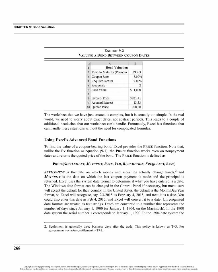
CHAPTER 9: Bond Valuation
268
EXHIBIT 9-2VALUING A BOND BETWEEN COUPON DATES
The worksheet that we have just created is complex, but it is actually too simple. In the realworld, we need to worry about exact dates, not abstract periods. This leads to a couple ofadditional headaches that our worksheet can’t handle. Fortunately, Excel has functions thatcan handle these situations without the need for complicated formulas.
Using Excel’s Advanced Bond FunctionsTo find the value of a coupon-bearing bond, Excel provides the PRICE function. Note that,unlike the PV function or equation (9-1), the PRICE function works even on nonpaymentdates and returns the quoted price of the bond. The PRICE function is defined as:
PRICE(SETTLEMENT, MATURITY, RATE, YLD, REDEMPTION, FREQUENCY, BASIS)
SETTLEMENT is the date on which money and securities actually change hands,2 andMATURITY is the date on which the last coupon payment is made and the principal isreturned. Excel uses the system date format to determine if what you have entered is a date.The Windows date format can be changed in the Control Panel if necessary, but most userswill accept the default for their country. In the United States, the default is the Month/Day/Yearformat, so Excel will recognize, say, 2/4/2015 as February 4, 2015, and treat it as a date. Youcould also enter this date as Feb 4, 2015, and Excel will convert it to a date. Unrecognizeddate formats are treated as text strings. Dates are converted to a number that represents thenumber of days since January 1, 1900 (or January 1, 1904, on the Macintosh). In the 1900date system the serial number 1 corresponds to January 1, 1900. In the 1904 date system the
2. Settlement is generally three business days after the trade. This policy is known as T+3. Forgovernment securities, settlement is T+1.
Copyright 2015 Cengage Learning. All Rights Reserved. May not be copied, scanned, or duplicated, in whole or in part. Due to electronic rights, some third party content may be suppressed from the eBook and/or eChapter(s).Editorial review has deemed that any suppressed content does not materially affect the overall learning experience. Cengage Learning reserves the right to remove additional content at any time if subsequent rights restrictions require it.
269
Bond Valuation
serial number 1 corresponds to January 2, 1904 (January 1, 1904, is 0). To see the actualserial number, you can use the General number format. The difference in date systems isimportant to those transferring files from PCs to Macs. Using serial numbers makes datemath quite simple. For example, you can determine the number of days between two dateswith simple subtraction.3 Also, note that the date serial number is independent of the dateformat applied.
RATE is the annual coupon rate and YLD is the annual required rate of return. In Excelfunctions, rates are always entered in decimal form, which is different from the conventionfor financial calculators. If the coupon rate is 10%, you must enter it as 0.10, although Excelwill convert a number followed by a percent sign (%) to this format. The effect of thepercent sign is to cause Excel to divide the preceding number by 100.
REDEMPTION is the amount to be received per $100 of face value when the bond isredeemed. It is important to realize that the redemption price can be different than the facevalue of the bond. This would be the case, for example, if the bond was called by the issuer.Calling a bond issue is very similar to refinancing a mortgage, in that the issuer usuallywishes to reissue debt at a lower interest rate. There is often a premium paid to bondholderswhen bonds are called, and this premium plus the face value is the redemption price. If abond issue has a 4% call premium, then REDEMPTION would be set to 104. For noncallablebonds, this will be set to 100.
FREQUENCY is the number of coupons paid in a year. Most often this will be 2, thoughother values are possible. Excel will return the #NUM! error if FREQUENCY is any valueother than 1, 2, or 4 (annual, semiannual, or quarterly). Note that bonds that pay intereston a monthly basis, while rare, do exist.4 This function does not work with such bonds.
BASIS describes the assumption regarding the number of days in a month and year.Historically, different financial markets have made different assumptions regarding thenumber of days in a month and a year. Corporate, agency, and municipal bonds are pricedassuming that there are 30 days in a month and 360 days in a year (a “bankers year”).Treasury bonds are priced assuming a 365-day year (366 days in a leap year) and the actual
3. As an interesting demonstration of the power of serial date numbers and custom formatting,consider the following: To determine exactly how old you are, enter your birth date in a blank cellof a worksheet, say A1. In A2 enter the formula: =TODAY()-A1. The TODAY() function returnsthe serial number of the current date. Now, choose the Custom category in the Number Formatdialog box and type the following format in the Type box: y" years,"m" months, and "d"days" and click on OK.
4. For example, GE Capital has a 3.6% bond that matures on 8/15/2031 and pays monthly coupons.The CUSIP number is 36966TGG1. Monthly payment bonds are most often issued by firms in thefinancial services industry.
Copyright 2015 Cengage Learning. All Rights Reserved. May not be copied, scanned, or duplicated, in whole or in part. Due to electronic rights, some third party content may be suppressed from the eBook and/or eChapter(s).Editorial review has deemed that any suppressed content does not materially affect the overall learning experience. Cengage Learning reserves the right to remove additional content at any time if subsequent rights restrictions require it.

CHAPTER 9: Bond Valuation
270
number of days in a month.5 Excel allows for five possibilities [days per month/days peryear (code)]:
• 30/360 (0, or omitted) • actual/actual (1)• actual/360 (2)• actual/365 (3)• European 30/360 (4)
Any number greater than 4 will result in an error. For corporate and municipal bonds in theUnited States, use a basis of 0, and for U.S. Treasury bonds use a basis of 1.
It is easy to determine the number of days between two dates using both the actual/actualand 30/360 day count techniques. Recall that Excel stores dates as a serial number thatrepresents the number of days since January 1, 1900. Therefore, we can calculate the actualnumber of days between any two dates using simple subtraction, even in a leap year. For the30/360 day count basis, Excel provides the DAYS360 function:
DAYS360(START_DATE, END_DATE, METHOD)
where the first two arguments are obvious, and METHOD is an optional argument specifyingwhether to use the U.S. (0, or omitted) or European (1) standard. You can see the differencebetween actual/actual and 30/360 by entering two dates, at least a few months apart. For ourpurposes, the basis is unlikely to make a difference in the calculated price. However, if youare trading in large numbers of bonds, the basis can make a significant difference.
To see how the PRICE function works, open a new worksheet and enter the data displayed inExhibit 9-3, which is taken from the example. The settlement date should be entered bysimply typing the date as it appears. As noted earlier, Excel will automatically recognize it asa date. Recall that the Nanoterials bonds mature in 20 years. We have assumed that thesettlement date is 2/15/2015 and that the maturity date is 2/15/2035. In actual practice, thematurity date of the bond could be found in the indenture, by asking a broker, or by viewingthe appropriate Form 424B2 in the SEC’s Edgar database.6
The current value of the bond can now be found by entering the function:=PRICE(B2,B3,B4,B5,B6/B6*100,B7,B8)/100*B6 in B10. Because the PRICEfunction returns the price as a percentage of the face value (90.799), we must divide by 100
5. For more information on day count conventions, see Standard Securities Calculation Methods, byJohn J. Lynch, Jr., and Jan H. Mayle, Securities Industry Association, 1986.
6. This site may be accessed at http://www.sec.gov/edgar/searchedgar/companysearch.html. Select thecompany of interest, and then enter 424B2 into the Filing Type box in the search area. Note thatolder bonds may not be in the system.
Copyright 2015 Cengage Learning. All Rights Reserved. May not be copied, scanned, or duplicated, in whole or in part. Due to electronic rights, some third party content may be suppressed from the eBook and/or eChapter(s).Editorial review has deemed that any suppressed content does not materially affect the overall learning experience. Cengage Learning reserves the right to remove additional content at any time if subsequent rights restrictions require it.

271
Bond Return Measures
EXHIBIT 9-3BOND VALUATION WORKSHEET USING THE PRICE FUNCTION
and multiply by the face value in order to convert it to a dollar amount. The result is $907.99,exactly as we found manually. Notice that we have not made any adjustment for the fact thatthe bond pays interest semiannually. Excel automatically makes this adjustment for youbased on the function’s FREQUENCY argument.
What is the value of the bond two months after the settlement date? Earlier, we found thatthe quoted price was $908.08, but that required a complicated formula using both the PV andROUNDUP functions. The PRICE function will automatically calculate the quoted pricebetween coupon dates, so all we need to do is set the settlement date to 4/15/2015 in B2. Theanswer is $908.08, as we found earlier.
Bond Return MeasuresMost often, investors don’t decide to buy a bond just because the price is below somecalculated intrinsic value. Instead, they will examine available alternative investments andcompare bonds on the basis of the returns that they offer. There are several ways to calculatethe returns offered by bonds. In this section, we will cover three return measures for bondsand two additional measures for discounted debt securities.
Before starting, modify your worksheet by entering Return Measures in A11. This willserve to separate these results from the previous calculations.
Current YieldThe current yield is defined as the annual coupon payment divided by the current price of thebond:
Copyright 2015 Cengage Learning. All Rights Reserved. May not be copied, scanned, or duplicated, in whole or in part. Due to electronic rights, some third party content may be suppressed from the eBook and/or eChapter(s).Editorial review has deemed that any suppressed content does not materially affect the overall learning experience. Cengage Learning reserves the right to remove additional content at any time if subsequent rights restrictions require it.
CHAPTER 9: Bond Valuation
272
(9-2)
The current yield is a rough measure of the return earned over the next year. We say that it isrough because it ignores compounding and the change in price which may occur over the lifeof the bond. The current yield measures the income yield only; like a stock’s dividend yield,it ignores capital gains.
Excel has no built-in function to calculate the current yield, but it is a simple matter to write theformula yourself. On your worksheet, move to A12 and type: Current Yield. Now, in B12enter: =(B4*B6)/B10. In our example the current yield is 8.81%, which is, in fact, the returnthat you would earn over the next year if you received $80 in interest on an investment of$907.99. However, if interest rates remain unchanged over the year, the value of the bond willincrease to $909.75. The capital gain of $1.76 is ignored in the current yield calculation. Note thatwhen a bond is selling at a discount to its face value, the current yield will understate the totalreturn. If the bond is selling at a premium, then the current yield will overstate the total return.
Yield to MaturityThe yield to maturity is the compound annual rate of return that can be expected if the bondis held to maturity. The yield to maturity is not without its problems as a return measure, butit is superior to the current yield because it accounts for both interest payments and capitalgains. It is also more complex to calculate.
Essentially, the yield to maturity is found by taking the bond price as given and solving thevaluation equation for the required return (kB).7 No method exists, however, to solve directlyfor the yield to maturity. The yield can be found by using a trial-and-error approach, but it isa bit tedious. Excel makes the yield calculation simple with its built-in YIELD function,which is defined as:
YIELD(SETTLEMENT, MATURITY, RATE, PR, REDEMPTION, FREQUENCY, BASIS)
All of the variables are the same as previously defined with the exception of PR, which is theprice of the bond as a percentage of the face value.
7. It should be noted that for most purposes, the terms “required return” and “yield to maturity” can beused interchangeably and often are. However, there is a slight, but important, difference betweenthe terms. Specifically, the required return is specified by the investor and can be different for otherinvestors. The yield to maturity is not under the control of the investor; instead it is merely afunction of the current bond price and cash flows promised from the bond. As such, the yield tomaturity will be the same regardless of who calculates it.
CY Annual PmtVB
----------------------------=
Copyright 2015 Cengage Learning. All Rights Reserved. May not be copied, scanned, or duplicated, in whole or in part. Due to electronic rights, some third party content may be suppressed from the eBook and/or eChapter(s).Editorial review has deemed that any suppressed content does not materially affect the overall learning experience. Cengage Learning reserves the right to remove additional content at any time if subsequent rights restrictions require it.

273
Bond Return Measures
To make the calculation, first place the label: Yield to Maturity in A13 and then enter:=YIELD(B2,B3,B4,B10/B6*100,B6/B6*100,B7,B8) in B13. Note that the onlydifference from the PRICE function is that we replaced YLD with the current price of thebond as a percentage of par. In this case, we had to convert the bond price (in B10) back to apercentage of par by dividing it by the face value and multiplying by 100. The result, asshould be expected, is 9%.
We could also use the RATE function (see page 207) to find the yield to maturity if weassume that the settlement date is also an interest payment date for the bond. This techniqueis especially useful if you don’t know the exact settlement and maturity dates for the bond,and if you are calculating the yield on a payment date. Rather than replace our YIELDfunction, we’ll simply insert the RATE function in B14 so that we can compare the results. InA14 type the label Yield Using Rate Function. In B14 enter the function:=RATE(YEARFRAC(B2,B3,B8)*B7,B4*B6/B7,-B10,B6)*B7.
In order to use this function, we’ve had to embed several calculations. For the number ofperiods, we are using the YEARFRAC function, which calculates the fraction of a yearbetween any two dates using an appropriate day count basis. This function is defined as:
YEARFRAC(START_DATE, END_DATE, METHOD)
YEARFRAC returns the number of years between the settlement and maturity dates, and wethen multiply by the payment frequency to get the number of periods. The payment amountis simply the coupon rate times the face (redemption) value divided by two. You’ll note thatafter annualizing the result by doubling (because it pays semiannually), the answer is thesame 9% as before. Again, it is important to remember that the RATE function will providethe correct answer only on a payment date. If the bond is between payment dates, then usethe YIELD function.
As mentioned earlier, there are a few potential problems with the yield to maturity. Implicitin the calculation are some key assumptions: (1) that you hold the bond to maturity; and(2) that you reinvest the cash flows for the rest of the life of the bond at a rate equal to theyield to maturity. Note that if market returns change, and you have to sell the bond before itmatures, you will receive a price that is different than you expected. This is known as pricerisk. Furthermore, if market rates change, you will be reinvesting the cash flows at adifferent rate than expected. This is known as reinvestment risk. Either or both of thesefactors can cause your actual return to be different from the yield to maturity that wascalculated when you purchased the bond. Thus, the combination of price and reinvestmentrisk is known as interest rate risk (see page 289 for more information).
Copyright 2015 Cengage Learning. All Rights Reserved. May not be copied, scanned, or duplicated, in whole or in part. Due to electronic rights, some third party content may be suppressed from the eBook and/or eChapter(s).Editorial review has deemed that any suppressed content does not materially affect the overall learning experience. Cengage Learning reserves the right to remove additional content at any time if subsequent rights restrictions require it.

CHAPTER 9: Bond Valuation
274
EXHIBIT 9-4CURRENT YIELD AND YIELD TO MATURITY
Yield to CallOne other common measure of return is the yield to call. As noted earlier, many issuersreserve the right to buy back the bonds that they sell if it serves their interests. In most cases,bonds will be called if interest rates drop substantially so that the firm will save money byrefinancing at a lower rate. If we calculate the yield to maturity assuming that the bond willbe called at the first opportunity, we will have calculated the yield to call. Because it iscommon to have a contractual obligation to pay a premium over par value if the bonds arecalled, this must be taken into account in our calculation. Note that the call schedulespecifies the exact call dates (typically, once per year on an anniversary date) and thepremiums on those dates. The premiums typically fall over time to zero.
In order to make this calculation, we must add a couple of lines to our worksheet. First,insert a row above row 4. To do this, highlight row 4 and click the top of the Insert button onthe Home tab. Now, in A4 type: First Call Date to indicate that this is the first date atwhich the firm has the option of calling the bonds. In B4 enter: 2/15/2020. This datereflects the fact that the first call date is often a few years after the issue date (which we areassuming is the same as the settlement date in this case). Next, insert a row above row 8 andlabel it in A8: Call Price. Cell B8 will be the price at which the bonds can be called, inthis case 5% over par value, so enter: 1050. In A17, enter the label: Yield to Call.
Finally, we will calculate the yield to call in B17 with the formula: =YIELD(B2,B4,B5,B12/B7*100,B8/B7*100,B9,B10). This is exactly the same formula as the yield tomaturity, except that we have changed the maturity date to the call date and the redemption
Copyright 2015 Cengage Learning. All Rights Reserved. May not be copied, scanned, or duplicated, in whole or in part. Due to electronic rights, some third party content may be suppressed from the eBook and/or eChapter(s).Editorial review has deemed that any suppressed content does not materially affect the overall learning experience. Cengage Learning reserves the right to remove additional content at any time if subsequent rights restrictions require it.

275
Bond Return Measures
EXHIBIT 9-5BOND VALUATION WORKSHEET WITH YIELD TO CALL ADDED
value to the call price. Note that the call premium plus the earlier receipt of the face valuehas caused the yield to call to be 11.23%. Of course, the issuer would never call the bondunder these circumstances because interest rates have risen since the bond was originallyissued. Your worksheet should now resemble the one in Exhibit 9-5.
Make-Whole Call Provisions
The type of call provision that we have demonstrated is known as a regular call feature, andwas typical until about 15 years ago. Recently, though, most callable corporate bonds havebeen issued with a make-whole call feature.8 In a regular call the bond is typically called at aprice below market value because interest rates have declined (i.e., the price is above theface value plus the call premium). Thus, investors are worse off than if the bond hadn’t beencalled. In a make-whole call, however, the call provision specifies that investors will be paidthe present value of all remaining cash flows, or the par value, whichever is greater. Thediscount rate used in the calculation is the current Treasury rate with a maturity equal to theremaining life of the bond plus a spread—typically 15 to 50 basis points, depending oncredit rating. The spread is specified in the bond’s indenture and is set at issuance.
8. For more in-depth discussion, see Mann, S. V., & Powers, E. A. (2003). “Indexing a Bond’s CallPrice: An Analysis of Make-Whole Call Provisions,” Journal of Corporate Finance, 9, 535–554.
Copyright 2015 Cengage Learning. All Rights Reserved. May not be copied, scanned, or duplicated, in whole or in part. Due to electronic rights, some third party content may be suppressed from the eBook and/or eChapter(s).Editorial review has deemed that any suppressed content does not materially affect the overall learning experience. Cengage Learning reserves the right to remove additional content at any time if subsequent rights restrictions require it.
CHAPTER 9: Bond Valuation
276
Using this method, investors are no worse off than if the bond hadn’t been called. Becausethe make-whole call feature makes calling a bond more expensive for the issuer, it is onlyrarely invoked. However, the bonds are continuously callable, on short notice, as opposed toonly once a year. When calculating the yield to call with a make-whole call feature, theREDEMPTION argument of the YIELD function would be calculated using the PRICEfunction, with its YLD argument being equal to the Treasury rate plus the spread.
Returns on Discounted Debt SecuritiesNot all debt instruments are bonds of the type that we have discussed earlier. Money marketsecurities are short-term, high-quality, debt instruments sold on a discounted basis. That is,they do not pay interest; instead, they are sold for less than their face value. Because the fullface value is returned to the investor at maturity, the interest is the difference between theface value and the purchase price. Examples of this type of security would include U.S.Treasury Bills, commercial paper, banker’s acceptances, and short-term municipals.
Returns on discounted securities are usually quoted on a bank discount basis. The bankdiscount rate (BDR) is calculated as follows:
(9-3)
where FV is the face value of the security, P0 is the purchase price, and M is the number ofdays until maturity. For example, if you purchase a 26-week (181-day) T-Bill for $985, thebank discount rate is:
We can calculate the bank discount rate in Excel using the DISC function:
DISC(SETTLEMENT, MATURITY, PR, REDEMPTION, BASIS)
All of the variables are as previously defined. To see how this function works, insert a newworksheet into your workbook and enter the data in Exhibit 9-6.
Notice that both the redemption value and purchase price are entered as a percentage of par,though we could enter the actual values. In B8 enter the DISC function as:=DISC(B2,B3,B5,B4,2). Note that we have set the BASIS to 2 because equation (9-3)uses the actual/360 day count convention. The answer is 2.983%, exactly as we calculatedusing the equation.
BDRFV P0–
FV------------------- 360
M---------×=
BDR 1,000 985–1,000
---------------------------- 360181---------× 0.02983 2.983%= = =
Copyright 2015 Cengage Learning. All Rights Reserved. May not be copied, scanned, or duplicated, in whole or in part. Due to electronic rights, some third party content may be suppressed from the eBook and/or eChapter(s).Editorial review has deemed that any suppressed content does not materially affect the overall learning experience. Cengage Learning reserves the right to remove additional content at any time if subsequent rights restrictions require it.

277
Bond Return Measures
EXHIBIT 9-6CALCULATING THE BANK DISCOUNT RATE
The bank discount rate is the method used to quote discount securities in the market.However, it does have a couple of problems: (1) It uses the face value as the basis forcalculating the return, but you have only paid the purchase price, not the face value. (2) Itassumes that there are only 360 days in a year, instead of 365 (366 in a leap year). We cansolve these problems by calculating the bond equivalent yield:
(9-4)
The bond equivalent yield is simply a “fixed” version of the bank discount rate: We are usingthe purchase price as the basis for calculating the return and changing the day countconvention to actual/actual. This allows us to compare the yield to yields on coupon-bearingbonds. In this example the bond equivalent yield is:
As you might expect, Excel has a built-in function to calculate the bond equivalent yield:
YIELDDISC(SETTLEMENT, MATURITY, PR, REDEMPTION, BASIS)
In A9 of your worksheet enter the label: Bond Equivalent Yield, and in B9 enter theformula: =YIELDDISC(B2,B3,B5,B4,1). Note that the BASIS is set to 1 (actual/actual)in this case. The answer is 3.071% as we found using the equation.
BEY BDR FVP0------- 365
360---------××
FV P0–
P0------------------- 365
M---------×= =
BEY 0.02983 1,000985
------------- 365360---------×× 1,000 985–
985---------------------------- 365
181---------× 0.03071 3.071%= = = =
Copyright 2015 Cengage Learning. All Rights Reserved. May not be copied, scanned, or duplicated, in whole or in part. Due to electronic rights, some third party content may be suppressed from the eBook and/or eChapter(s).Editorial review has deemed that any suppressed content does not materially affect the overall learning experience. Cengage Learning reserves the right to remove additional content at any time if subsequent rights restrictions require it.
CHAPTER 9: Bond Valuation
278
The U.S. Treasury Yield CurveA yield curve is a chart that shows yields across the maturity spectrum and is useful forgiving investors an idea of the yields that are currently available in the market. Professionalsuse the U.S. Treasury yield curve,9 along with information about yield spreads for varioustypes of bonds, to determine the required yield on the bonds that they are trying to value.
We can create yield curves for different types of securities (e.g., Treasuries, corporates,municipals). One should be careful that the securities used to construct the yield curve differas little as possible, except for term to maturity. U.S. Treasury securities are almost ideal forthis purpose because they are all free of default risk. In this section, we will show how toconstruct a U.S. Treasury yield curve using data that is freely available on the Internet.
Excel provides tools that can be used to obtain data directly from databases, text files, orWeb sites. For our purposes, we wish to use the Web Query tool to gather data from a tableon a Web site. Specifically, we will use a Web Query to get data on Treasury yields from theU.S. Department of the Treasury. This query can be refreshed (automatically or manually) tograb the most recent data from the site.
Open a new workbook, select the Data tab, and then click the From Web button in the GetExternal Data group. This will launch the New Web Query dialog box, which includes abrowser that we can use to navigate to a Web page. In the address bar of the browser, enterthe URL: http://www.treasury.gov/resource-center/data-chart-center/interest-rates/Pages/TextView.aspx?data=yield and you should see the pageload. Scroll down until you see the table containing the yield curve data for the last five daysas shown in Figure 9-2.
To import one or more tables from the page, you will simply click the arrows at the left ofthe table. Select the table by clicking the yellow arrow and then click the Import button topull the data into cell A2 of your worksheet. You have now created a link to this table, and itcan be refreshed at any time by clicking the Refresh All button in the Connections group onthe Data tab. By default, every time you open this workbook the query will pull the new datafrom the Web site. You can change the settings for the Web Query by right-clicking the dataand choosing Data Range Properties.
9. Technically, we should use a curve constructed from the yields available on U.S. Treasury couponSTRIPS. This data is available from the Wall Street Journal at http://online.wsj.com/mdc/public/page/2_3020-tstrips.html. Unfortunately, it cannot be accessed directly from Excel in the mannerdemonstrated here. Instead, it must be copied and pasted.
Copyright 2015 Cengage Learning. All Rights Reserved. May not be copied, scanned, or duplicated, in whole or in part. Due to electronic rights, some third party content may be suppressed from the eBook and/or eChapter(s).Editorial review has deemed that any suppressed content does not materially affect the overall learning experience. Cengage Learning reserves the right to remove additional content at any time if subsequent rights restrictions require it.

279
The U.S. Treasury Yield Curve
FIGURE 9-2THE WEB QUERY DIALOG BOX
We can now format the table and create the yield curve chart. In order to have the data pointsproperly spaced on the chart, we need to convert the maturities from text (e.g., 1 Month) tonumbers. We cannot place formulas inside the query results (A1:L7), so we will create thedata for our chart to the right of the query results. You could also place these calculations onanother worksheet. In O3:P13 enter the number of years. For example, in O3 enter 0.0833because three months is equal to 0.0833 years. Do the same for the other maturities (e.g., 0.5 for 6months). In P3:P13 we will calculate today’s yields. So, in P3 enter: =B7/100 and format theresult as a percentage. Repeat this for each of the other maturities.
If you are going to apply formatting to the query, as shown earlier, be aware that refreshingthe query can remove the formatting. To avoid this, right-click within the data range andchoose Data Range Properties. Make sure that the Preserve cell formatting option ischecked.
Finally, select O3:P13 and insert a scatter chart with straight lines and markers. For the charttitle, use a text formula in P1: ="U.S. Treasury Yield Curve "&CHAR(10)&TEXT(A7,"m/dd/yyyy"). (The Char(10) inserts a new line character.) Insert a charttitle, select it, and then click on cell P1. The result should look like Exhibit 9-7.
Copyright 2015 Cengage Learning. All Rights Reserved. May not be copied, scanned, or duplicated, in whole or in part. Due to electronic rights, some third party content may be suppressed from the eBook and/or eChapter(s).Editorial review has deemed that any suppressed content does not materially affect the overall learning experience. Cengage Learning reserves the right to remove additional content at any time if subsequent rights restrictions require it.

CHAPTER 9: Bond Valuation
280
EXHIBIT 9-7THE U.S. TREASURY YIELD CURVE USING A WEB QUERY
Bond Price SensitivitiesAs should be clear, bond values are a function of several variables: coupon rate, face value,term to maturity, and the required return. It is useful to understand how changes in thesevariables lead to changes in bond prices because these relationships help identify investmentstrategies and guide the choices that corporations make when making capital structuredecisions.
Burton Malkiel set forth, and rigorously proved, five bond pricing theorems that will help usunderstand how bond prices react to changing circumstances:10
1. Bond prices move inversely with interest rates.2. For a given change in yield, long-term bond prices will change more than
short-term bond prices.
10. B. G. Malkiel, “Expectations, Bond Prices, and the Term Structure of Interest Rates,” QuarterlyJournal of Economics, May 1962, pp. 197–218.
Copyright 2015 Cengage Learning. All Rights Reserved. May not be copied, scanned, or duplicated, in whole or in part. Due to electronic rights, some third party content may be suppressed from the eBook and/or eChapter(s).Editorial review has deemed that any suppressed content does not materially affect the overall learning experience. Cengage Learning reserves the right to remove additional content at any time if subsequent rights restrictions require it.

281
Bond Price Sensitivities
3. The sensitivity of bond prices to yield changes increases at a decreasingrate as term to maturity increases.
4. For a given change in yields, bond prices will respond asymmetrically.That is, bond prices will rise more when rates fall than they will fall whenrates rise.
5. High-coupon bonds are less sensitive to changes in yields than are low-coupon bonds.
In this section, we will examine these theorems in detail.
Changes in the Required ReturnBecause the value of a bond is the present value of its future cash flows, you probably expectthat the value will increase as the interest rate declines, and vice versa. And you would becorrect. Let’s examine this idea to fix it in your mind and to point out a factor which you maynot have considered.
Return to the bond valuation worksheet (Exhibit 9-5). We want to create a new section onthis worksheet that will show the value of the bond at various interest rates. Move to A20and enter: YTM, and in B20 enter: Bond Value. Starting in A21, we want a column ofinterest rates ranging from 1% to 15% in steps of 1% (i.e., 0.01). Create this data series usingthe Fill Series command on the Home tab. In B21 we need the value of the bond, using 1%as the required return. Using the PRICE function, this can be done with the formula:=PRICE(B$2,B$3,B$5,A21,B$7/B$7*100,B$9,B$10)/100*B$7. This is thesame formula as we used previously in B12, except that we have replaced the rate with thevalue in A21. Further, we have added dollar signs to fix most of the cell references so thatthey do not change as we copy this formula down. The interest rate is not fixed because wewant it to change in each row. Copy the formula over the range B22:B35.
If you now create a scatter chart with the yield on the x-axis and the bond value on the y-axis, your worksheet should look similar to the one in Exhibit 9-8. We have embellished ourgraph to show the current price and the required rate of return. If you wish to add the samedotted straight lines, remember that it takes only two points to define a line. We need twolines, one horizontal and one vertical. Choose an empty area of the worksheet, say E20:F24.In E20 enter 0, and in E21 enter: =B6. These cells represent the two x values for thehorizontal line. In F20:F21 enter: =B12 (the current price) for the y coordinates. Create thepoints for the vertical line in a similar fashion using cells E23:F24. Finally, right-click in thechart and choose Select Data. Click the Add button, and add a new data series using thenewly entered data. You can also copy and Paste Special in the chart.
If you wish to replicate the data labels on the chart in Exhibit 9-8, simply click once on thenew data series, and then click a second time on one of the end points. This will select only
Copyright 2015 Cengage Learning. All Rights Reserved. May not be copied, scanned, or duplicated, in whole or in part. Due to electronic rights, some third party content may be suppressed from the eBook and/or eChapter(s).Editorial review has deemed that any suppressed content does not materially affect the overall learning experience. Cengage Learning reserves the right to remove additional content at any time if subsequent rights restrictions require it.

CHAPTER 9: Bond Valuation
282
EXHIBIT 9-8BOND VALUE FOR VARIOUS REQUIRED RETURNS
one point on the line. Right-click the point and choose Add Data Label (there is no need tochoose it a second time from the flyout menu). Next, right-click the data label and chooseFormat Data Labels. In the Format Data Label panel under Label Options, you can choosethe options that you wish to display. Note that “Leader Lines” are the lines that connect thedata point to the label.
Confirming Malkiel’s first theorem, we can see that the price is inversely related to therequired return. Furthermore, the relationship is not linear; instead it is convex to the origin.As we will see, this nonlinear relationship (known as convexity) also demonstrates the fourththeorem.
Move the chart to the right so that column C is exposed. In C20 enter the label: Change. InC21:C35 we want to enter the change in the bond price from the current price. In otherwords, the numbers in this range will be the gain or loss that would be experienced if youpurchased the bond and then interest rates changed from the original 9% to the value incolumn A. In C21 enter the formula: =B21-$B$29 (which will fix the subtracted price atB29). Now copy the formula down the entire range.
Figure 9-3 shows how the bond price will change. Examine cells C21:C35 in yourworksheet carefully. In particular, notice that the price changes are not symmetric. Forexample, if the yield falls by 4% (to 5%), the price rises by $468.55. However, if the raterises by 4% (to 13%), the price falls by only $261.63. In other words, as yields drop theprice rises by more than it falls if yields rise a similar amount. This confirms Malkiel’sfourth theorem.
Copyright 2015 Cengage Learning. All Rights Reserved. May not be copied, scanned, or duplicated, in whole or in part. Due to electronic rights, some third party content may be suppressed from the eBook and/or eChapter(s).Editorial review has deemed that any suppressed content does not materially affect the overall learning experience. Cengage Learning reserves the right to remove additional content at any time if subsequent rights restrictions require it.
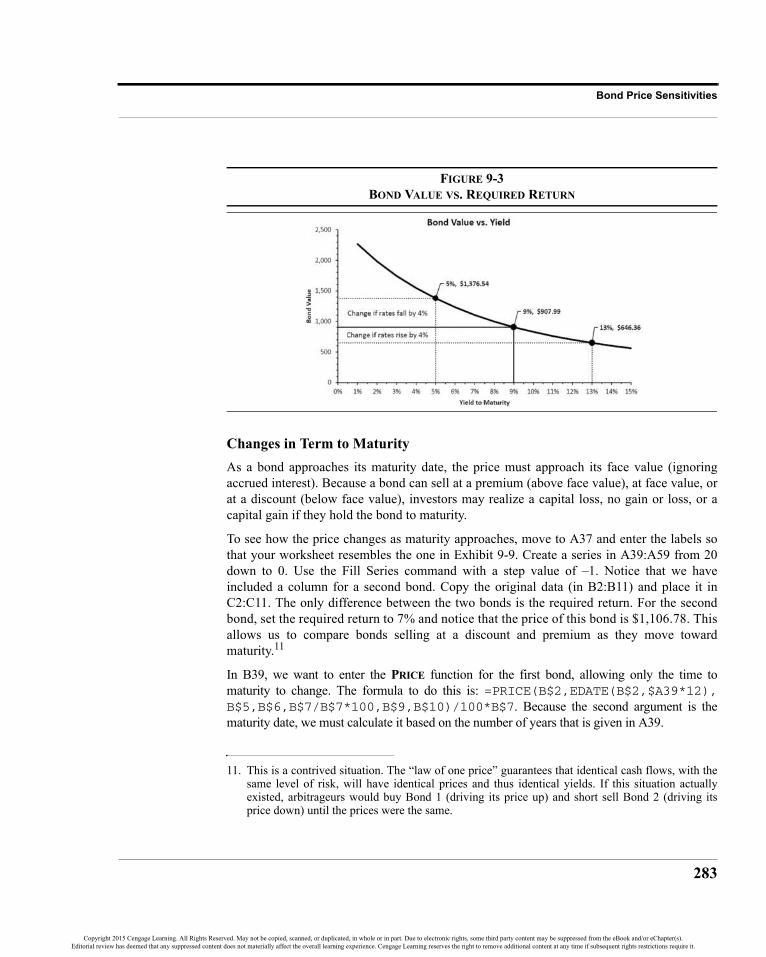
283
Bond Price Sensitivities
FIGURE 9-3BOND VALUE VS. REQUIRED RETURN
Changes in Term to MaturityAs a bond approaches its maturity date, the price must approach its face value (ignoringaccrued interest). Because a bond can sell at a premium (above face value), at face value, orat a discount (below face value), investors may realize a capital loss, no gain or loss, or acapital gain if they hold the bond to maturity.
To see how the price changes as maturity approaches, move to A37 and enter the labels sothat your worksheet resembles the one in Exhibit 9-9. Create a series in A39:A59 from 20down to 0. Use the Fill Series command with a step value of –1. Notice that we haveincluded a column for a second bond. Copy the original data (in B2:B11) and place it inC2:C11. The only difference between the two bonds is the required return. For the secondbond, set the required return to 7% and notice that the price of this bond is $1,106.78. Thisallows us to compare bonds selling at a discount and premium as they move towardmaturity.11
In B39, we want to enter the PRICE function for the first bond, allowing only the time tomaturity to change. The formula to do this is: =PRICE(B$2,EDATE(B$2,$A39*12),B$5,B$6,B$7/B$7*100,B$9,B$10)/100*B$7. Because the second argument is thematurity date, we must calculate it based on the number of years that is given in A39.
11. This is a contrived situation. The “law of one price” guarantees that identical cash flows, with thesame level of risk, will have identical prices and thus identical yields. If this situation actuallyexisted, arbitrageurs would buy Bond 1 (driving its price up) and short sell Bond 2 (driving itsprice down) until the prices were the same.
Copyright 2015 Cengage Learning. All Rights Reserved. May not be copied, scanned, or duplicated, in whole or in part. Due to electronic rights, some third party content may be suppressed from the eBook and/or eChapter(s).Editorial review has deemed that any suppressed content does not materially affect the overall learning experience. Cengage Learning reserves the right to remove additional content at any time if subsequent rights restrictions require it.

CHAPTER 9: Bond Valuation
284
EXHIBIT 9-9BOND PRICES VS. TIME TO MATURITY
To do this we used the EDATE function, which returns a date that is a number of months after theSTART_DATE:
EDATE(START_DATE, MONTHS)
In this case, we are using the settlement date for the START_DATE, and the number of monthsis the number of remaining years to maturity multiplied by 12 to convert it to months. Copythis formula to C39 to find the price of the second bond and then copy both of these downthe entire range. Note that the PRICE function will return a #NUM! error when the term tomaturity is 0. Therefore, in B59 and C59 enter the formula: =B$7 to get the face value. Thenumbers in your worksheet should be the same as those in Exhibit 9-9.
Notice that the first bond slowly increases in price as the time to maturity declines. Thesecond bond’s price, however, slowly decreases as time to maturity declines. Thisdemonstration assumes that yields remain constant for the next 20 years. In actuality,required yields change on a daily basis, so the change in price will not be as smooth as theworksheet shows.
To see this more clearly, create a scatter chart of this data by selecting A38:C59. Once thechart is created, you may want to adjust the scale of the y-axis. Right-click the y-axis and
Copyright 2015 Cengage Learning. All Rights Reserved. May not be copied, scanned, or duplicated, in whole or in part. Due to electronic rights, some third party content may be suppressed from the eBook and/or eChapter(s).Editorial review has deemed that any suppressed content does not materially affect the overall learning experience. Cengage Learning reserves the right to remove additional content at any time if subsequent rights restrictions require it.

285
Bond Price Sensitivities
choose Format Axis. Now set the Minimum edit box to 850. This will change the scale sothat the origin of the y-axis is at 850, effectively magnifying the area of the chart that we areinterested in. Note that we have also added a line to indicate the par value of the bond. In cellD39 enter 1000 and copy it down to the rest of the range. Now, right-click the chart andchoose Select Data. Click the Add button and add a series with A39:A59 as the x values, andD39:D59 as the y values. After adding labels to the chart, this part of your worksheet shouldlook like Figure 9-4.
FIGURE 9-4BOND PRICE VS. TIME TO MATURITY
Comparing Two Bonds with Different MaturitiesWhen investors decide to purchase bonds, they have myriad choices, including manycombinations of term to maturity and coupon rates. Malkiel’s second theorem says that long-term bond prices will change more than short-term bond prices when yields change. To seethis, make a copy of A1:C12 from your worksheet and paste it into a new worksheet.
Our first goal is to set up the worksheet so that both bonds are identical, and then we willchange the maturity date of the second bond. Previously, the only difference between thebonds was the required return. So, change that to 9% for the second bond (cell C6). Now, setthe maturity date for the second bond, in C3, to 2/15/2025. It is now a 10-year bond,while the first is a 20-year bond. Set up the rest of the worksheet as shown in Exhibit 9-10.
In B15:C16 we will calculate the prices of the two bonds at the yields given in A15:A16.This will allow us to see how the prices change at different yields. In B15, enter the formula:=PRICE(B$2,B$3,B$5,$A15,B$7/B$7*100,B$9,B$10)/100*B$7, and thencopy it to the other cells. In B17:C17 we want to calculate the price changes, so the formula
Copyright 2015 Cengage Learning. All Rights Reserved. May not be copied, scanned, or duplicated, in whole or in part. Due to electronic rights, some third party content may be suppressed from the eBook and/or eChapter(s).Editorial review has deemed that any suppressed content does not materially affect the overall learning experience. Cengage Learning reserves the right to remove additional content at any time if subsequent rights restrictions require it.

CHAPTER 9: Bond Valuation
286
EXHIBIT 9-10PRICE CHANGES WITH DIFFERENT MATURITIES
in B17 is: =B16-B15. Copy that to C17. Finally, calculate the percentage change in B18with: =B16/B15-1 and copy that formula to C18.
Notice that our starting yield is 9%, as before. If you purchased either bond and thenrates instantaneously rose to 12% the prices would fall by $208.92 (–23.01%) and $164.36(–17.58%), respectively. Recall that the bonds are identical, except for their terms tomaturity. The price of Bond 1 fell by more because it is a longer term bond. Now, change theyield in A16 to 6%, so that the prices will now rise. Note that the price of Bond 1 rises bymore than the price of Bond 2, as expected.
Now, change the maturity date on Bond 2 to 2/15/2020, so that it has only five years tomaturity. Note how the price of Bond 2 now changes by even less than it did as a 10-yearbond. This is just as Malkiel’s second theorem claims: Long-term bond prices will change bymore (in percentage terms) than short-term bonds when yields change.
Malkiel’s third theorem says that the sensitivity to yield changes increases at a decreasingrate as maturity lengthens. This means that, for example, when compared to a 20-year bond,a 30-year bond isn’t that much more sensitive to yield changes. However, a 10-year bondwill be considerably less sensitive to yield changes than the 20-year bond.
Copyright 2015 Cengage Learning. All Rights Reserved. May not be copied, scanned, or duplicated, in whole or in part. Due to electronic rights, some third party content may be suppressed from the eBook and/or eChapter(s).Editorial review has deemed that any suppressed content does not materially affect the overall learning experience. Cengage Learning reserves the right to remove additional content at any time if subsequent rights restrictions require it.

287
Bond Price Sensitivities
We can see this in our worksheet very easily. Bond 1 will serve as our point of comparison.First, change the maturity of Bond 2 to 2/15/2025, and note that its price will rise by22.87% when yields fall from 9% to 6%. This compares to a 35.59% for Bond 1, which has10 additional years to maturity. That is a difference of about 12.72%.
Now, change the maturity date of Bond 2 (in C3) to 2/15/2045. Note that the price changeis 42.37%. That is a difference of only 6.78% compared to Bond 1. Finally, change thematurity date to 2/15/2055. Table 9-1 shows the results.
This confirms Malkiel’s third theorem. While longer term bonds change more when yieldschange, the sensitivity decreases as the term increases. So, the difference in interest ratesensitivity between a 30-year and a 40-year bond is much less than the difference between a10-year and a 20-year bond.
Comparing Two Bonds with Different Coupon RatesThe fifth theorem says that high-coupon bonds are less sensitive to yield changes than low-coupon bonds. We can use a slightly modified version of our worksheet to demonstrate thistheorem. Make a copy of the previous worksheet, and reset the maturity date of Bond 2 to2/15/2035. Change the coupon rate of Bond 2 to 4%, so that the bonds are identical,except that Bond 2 has a lower coupon rate.
Again, we will modify the yield in A16 to see how the changing yields affect the prices ofbonds with different coupon rates. Enter 12% in A16, and notice that Bond 2 (with a lowercoupon rate) has a larger percentage loss than Bond 1 (with a higher coupon rate). Now,change A15 to 6% and see that Bond 2 shows a greater percentage gain than Bond 1. Exhibit9-11 shows this result.
In both cases, Bond 1 actually had a larger change in dollar terms. However, that ismisleading because the price of Bond 2 starts out at a much lower price (only $539.96)because of its lower coupon rate. It is the percentage change that matters most, so thisconfirms theorem five.
TABLE 9-1CHANGES IN PRICE WHEN YIELDS DROP FROM 9% TO 6%
Maturity Date(Term) Change in Price
Difference from20-Year Bond
2/15/2025 (10) 22.87% 12.72%2/15/2035 (20) 35.59% 0.00%2/15/2045 (30) 42.37% 6.78%2/15/2055 (40) 45.94% 10.35%
Copyright 2015 Cengage Learning. All Rights Reserved. May not be copied, scanned, or duplicated, in whole or in part. Due to electronic rights, some third party content may be suppressed from the eBook and/or eChapter(s).Editorial review has deemed that any suppressed content does not materially affect the overall learning experience. Cengage Learning reserves the right to remove additional content at any time if subsequent rights restrictions require it.

CHAPTER 9: Bond Valuation
288
EXHIBIT 9-11PRICE CHANGES WITH DIFFERENT COUPON RATES
Duration and ConvexityWe have just demonstrated that long-term bonds and those with low coupon rates are muchmore sensitive to changes in yields than are short-term bonds and those with high couponrates. This suggests a trading strategy for bond investors: If you believe that interest rateswill rise, you should move into short-term bonds with high coupon rates. On the other hand,if you think that rates will fall, you should move into long-term bonds with low coupon rates.
Investors frequently make such directional trades based on interest rate forecasts. However,there are many combinations of coupon rates and maturities. Suppose that you have tochoose between two bonds: a long-term bond with a high coupon rate or a short-term bondwith a low coupon rate. Which bond will lose less if interest rates rise? Which one will gainmore if rates fall? In other words, which bond has the most interest rate risk?
Copyright 2015 Cengage Learning. All Rights Reserved. May not be copied, scanned, or duplicated, in whole or in part. Due to electronic rights, some third party content may be suppressed from the eBook and/or eChapter(s).Editorial review has deemed that any suppressed content does not materially affect the overall learning experience. Cengage Learning reserves the right to remove additional content at any time if subsequent rights restrictions require it.

289
Duration and Convexity
DurationIt is difficult to answer those questions without doing the actual calculations. However, in1938 Frederick Macaulay developed a measure of interest rate risk that can answer thisquestion.12 Duration is a weighted average of the time to receive the cash flows of the bondin present value terms.
Duration combines the effects of maturity, coupon rate, and yield into a single number thatwe can use to measure the interest rate sensitivity of a bond. The longer the duration, thegreater the interest rate risk of the bond. As you might imagine, this allows investors toimmediately determine which bond will better suit their portfolio, given their expectationsabout future interest rate movements.
Mathematically, Macaulay’s duration is calculated as:
(9-5)
where Pmtt is the cash flow in period t, YTM is the per period (usually semiannual) yield tomaturity, and VB is the current price. The fractional part of the numerator is the present valueof each cash flow as a percentage of the bond’s price, which serves as the weighting in theaverage, and t is the number of periods until each cash flow is received. As with equation (9-1), this formula is only accurate on a payment date.
Let’s calculate the Macaulay duration (DMac) of Bond 1 from our previous example:
Note that the semiannual payment is $40, the semiannual yield is 4.5% (= 9%/2), and thecurrent bond price is $907.99. This results in a duration of 19.67 semiannual periods.Duration is actually expressed in years, so we need to divide the result by the paymentfrequency. Therefore, the Macaulay duration of Bond 1 is 9.83 years.
Excel has a built-in function called, naturally, DURATION:
DURATION(SETTLEMENT, MATURITY, COUPON, YLD, FREQUENCY, BASIS)
12. F. R. Macaulay, Some Theoretical Problems Suggested by the Movements of Interest Rates, BondYields and Stock Prices in the United States Since 1856. New York: National Bureau of EconomicResearch, 1938.
DMac
Pmtt
1 YTM+( )t---------------------------- t( )
t 1=
N
∑VB
--------------------------------------------=
DMac
401.0451--------------- 1( ) 40
1.0452--------------- 2( ) 40
1.0453--------------- 3( ) … 1040
1.04540----------------- 40( )+ + + +
907.99------------------------------------------------------------------------------------------------------------------------------------- 19.67 periods= =
Copyright 2015 Cengage Learning. All Rights Reserved. May not be copied, scanned, or duplicated, in whole or in part. Due to electronic rights, some third party content may be suppressed from the eBook and/or eChapter(s).Editorial review has deemed that any suppressed content does not materially affect the overall learning experience. Cengage Learning reserves the right to remove additional content at any time if subsequent rights restrictions require it.

CHAPTER 9: Bond Valuation
290
Using the worksheet from Exhibit 9-11, let’s calculate the duration of both bonds. In A20type the label: Macaulay Duration, and in B20 enter the formula: =DURATION(B2,B3,B5,B6,B9,B10). Now copy the formula to C20 to find the duration of Bond 2.
Duration is accurate only for very small changes in the yield, so change the yield in A16 to10%, so that the change in yield is 1%. The duration of Bond 1 is 9.83 years, and for Bond 2it is 11.45 years. Note that as we left things, the only difference between the two bonds is thecoupon rate. In this case, Bond 2 has a longer duration so it should be more sensitive tointerest rate changes than Bond 1. If you look at the percentage changes in row 18, you willsee that Bond 2 does change more than Bond 1.
EXHIBIT 9-12CALCULATING THE MACAULAY DURATION
If you make changes to the coupon rates and maturity dates, you will see how the durationchanges. Pay particular attention to the fact that the bond with the longer duration always hasthe bigger percentage price change. So, you can see that duration can be a useful tool forinvestors trying to gauge interest rate risk.
Copyright 2015 Cengage Learning. All Rights Reserved. May not be copied, scanned, or duplicated, in whole or in part. Due to electronic rights, some third party content may be suppressed from the eBook and/or eChapter(s).Editorial review has deemed that any suppressed content does not materially affect the overall learning experience. Cengage Learning reserves the right to remove additional content at any time if subsequent rights restrictions require it.

291
Duration and Convexity
Modified DurationIf you paid careful attention to the previous exercise, you may have noticed that theMacaulay duration is close to the percentage change in the bond’s price. In our originalexample, changing the yield in A16 to 10% from the original 9% caused a –8.76% change inthe price of Bond 1. That isn’t too different from the duration of 9.83 years. So, the durationcan be used to estimate the percentage change in the value if interest rates change by 1%.
We can get a closer approximation to the percentage change in the bond price by using themodified duration (DMod):
(9-6)
where m is the payment frequency. In this case, the modified duration of Bond 1 is:
Excel has the MDURATION function to calculate modified duration. It is defined as:
MDURATION(SETTLEMENT, MATURITY, COUPON, YLD, FREQUENCY, BASIS)
All of the arguments are identical to those in the DURATION function. Let’s add this functionto our worksheet. In A21 the label is: Modified Duration, and in B21 the formula is:=MDURATION(B2,B3,B5,B6,B9,B10). This gives the same result that we got fromthe equation above. Now copy this formula to C21.
This is closer to the percentage change in the bond’s price, but it still isn’t very accurate for a1% change in the yield. The reason is that the approximation holds only for very smallchanges in yields (it is a linear approximation to a nonlinear function). For small yieldchanges, we can get a very good approximation by using the following formula:
(9-7)
If we change the yield by 0.10% (say, from 9% to 9.1%), then the price of Bond 1 willchange by:
DModDMac
1 YTMm
------------+⎝ ⎠⎛ ⎞---------------------------=
DMod9.83
1 0.092
----------+⎝ ⎠⎛ ⎞------------------------- 9.41= =
% Change in Price DMod– ΔYTM×≈
% Change in Price 9.41– 0.001×≈ 0.0094– 0.94%–= =
Copyright 2015 Cengage Learning. All Rights Reserved. May not be copied, scanned, or duplicated, in whole or in part. Due to electronic rights, some third party content may be suppressed from the eBook and/or eChapter(s).Editorial review has deemed that any suppressed content does not materially affect the overall learning experience. Cengage Learning reserves the right to remove additional content at any time if subsequent rights restrictions require it.

CHAPTER 9: Bond Valuation
292
This is very close to the actual price change of –0.934%. We can easily see this in ourworksheet. First, change the yield in A16 to 9.10%. Now, in A22 add the label:Predicted % Change, and in B22 the formula is: =-B21*($A16-$A15). Copy thatformula to C22, and then notice how similar the values in B22:C22 are to the exactcalculations in B18:C18.
EXHIBIT 9-13CALCULATING THE PERCENTAGE PRICE CHANGE USING MODIFIED DURATION
Visualizing the Predicted Price ChangeThe modified duration is the slope of the price/yield function (at the current price and yield)divided by the price of the bond. In calculus, we would write the formula as:
(9-8)
That is, modified duration is equal to the partial derivative of the price function with respectto the yield, divided by the price. The slope of the price/yield curve, at any particular point,is given by the numerator of equation (9-8). We can calculate the slope by multiplying themodified duration by the price of the bond:
DMod∂P ∂Y⁄
P-----------------=
Copyright 2015 Cengage Learning. All Rights Reserved. May not be copied, scanned, or duplicated, in whole or in part. Due to electronic rights, some third party content may be suppressed from the eBook and/or eChapter(s).Editorial review has deemed that any suppressed content does not materially affect the overall learning experience. Cengage Learning reserves the right to remove additional content at any time if subsequent rights restrictions require it.

293
Duration and Convexity
(9-9)
Recalling from your math classes that the slope of a line is defined as “rise over run,” youwill see that equation (9-9) gives a hint as to how we can visualize the modified duration in achart. We will simply create a chart of the price/yield relationship and then add a chart of aline with the same slope that is tangent to the curve at a point representing the current priceand yield. The slope of the tangent line is given by equation (9-9), so we simply construct aline with the same slope that also passes through the point that represents the current priceand yield. This line will show the predicted price for any yield that you choose.
We have already created a chart of the price/yield function in Exhibit 9-8 (page 282). Returnto that worksheet and make a copy of it so that we can add a line to the chart. We need onlytwo points to draw the line, but it is helpful to have a third point in this case. The middlepoint will be the current price and yield. The two end points will be offsets from this point.Starting in H1, enter the text shown in Exhibit 9-14.
EXHIBIT 9-14DATA FOR TANGENT LINE
In I2, we calculate the slope of our line as described in equation (9-9): =MDURATION(B2,B3,B5,B6,B9,B10)*B12. The x values, which are simply three yields, are in column I.The “High Point” in I3 is the bond yield less 6%: =B6-0.06. The 6% offset is an arbitraryamount to extend the line leftward. Similarly, in I5 enter: =B6+0.06. This will extend theline rightward. In I4 enter: =B6 for the mid point. In column J we have the y values for theline. In J3 enter the formula: =($I$4-I3)*$I$2+$B$12 and copy it down. This gives usthe prices on the line with the slope that was calculated in I2.
To add this line to the chart, right-click the chart and choose Select Data. Add a newseries with the x values in I3:I5 and the y values in J3:J5. The result should look likeFigure 9-5.
We can now change the yield and see how it affects the slope of the line. For example,decreasing the yield (in B6) will result in the line having a greater slope. So, when yieldsdecrease, modified duration (and Macaulay duration) will increase. Conversely, increasingthe yield will result in a flatter line, implying a lower modified duration.
Slope DMod P× RiseRun----------= =
Copyright 2015 Cengage Learning. All Rights Reserved. May not be copied, scanned, or duplicated, in whole or in part. Due to electronic rights, some third party content may be suppressed from the eBook and/or eChapter(s).Editorial review has deemed that any suppressed content does not materially affect the overall learning experience. Cengage Learning reserves the right to remove additional content at any time if subsequent rights restrictions require it.

CHAPTER 9: Bond Valuation
294
FIGURE 9-5PRICE PREDICTED BY CHANGE IN YIELD
ConvexityAs noted earlier, equation (9-7) works well only for small changes in the yield. The reason isthat it is a linear approximation to a nonlinear function. Take another look at Figure 9-5, andrecall that the price/yield function is curved. More specifically, it is convex to the origin.Notice how our straight line approximation departs from the price/yield function for largechanges in the yield. A measure of this curvature is called convexity, and it can be used toimprove our approximation of the change in price. Convexity (C) can be calculated with:
(9-10)
Again, as usual, YTM is the per period yield to maturity, and equation (9-10) works only on apayment date. We can calculate the convexity of Bond 1 as follows:
As with the duration, we need to convert the convexity to an annual number. To do this, wedivide by the payment frequency squared. So, the annual convexity is:
C
11 YTM+( )2
----------------------------Pmtt
1 YTM+( )t---------------------------- t2 t+( )
t 1=
N
∑VB
-----------------------------------------------------------------------------------------=
C
11.0452--------------- 40
1.0451--------------- 12 1+( ) 40
1.0452--------------- 22 2+( ) … 1 040,
1.04540----------------- 402 40+( )+ + +
907.99------------------------------------------------------------------------------------------------------------------------------------------------------------------- 545.92= =
C 545.9222
---------------- 136.48= =
Copyright 2015 Cengage Learning. All Rights Reserved. May not be copied, scanned, or duplicated, in whole or in part. Due to electronic rights, some third party content may be suppressed from the eBook and/or eChapter(s).Editorial review has deemed that any suppressed content does not materially affect the overall learning experience. Cengage Learning reserves the right to remove additional content at any time if subsequent rights restrictions require it.

295
Duration and Convexity
What does this number mean? Technically, convexity is the second derivative of the pricefunction with respect to the yield, divided by the price of the bond. Therefore, it can bethought of as the rate of change of the bond’s duration. In practice, it is just a measure of thedegree of curvature in the price/yield function. The higher the convexity, the more curvedthe function.
Unfortunately, Excel does not have a built-in function to calculate convexity. However, wehave included the FAME_CONVEXITY function in the Famefncs.xlam add-in. It willcalculate convexity on a payment date and is defined as:
FAME_CONVEXITY(SETTLEMENT, MATURITY, FV, COUPON, YLD, FREQUENCY)
where all of the arguments are as before, except that FV is the face value of the bond.
Return to the worksheet created for Exhibit 9-13 (page 292). Select row 22 in yourworksheet and insert a new row. In A22 enter: Convexity. Now, enter the formula:=FAME_Convexity(B2,B3,B7,B5,B6,B9) in B22. Copy this formula to C22. Theconvexity of Bond 1 is 136.48, and for Bond 2 it is 174.52.
We can use the convexity to improve our approximation of the percentage change in pricebecause it accounts for the curvature of the price/yield function. To do this, we will modifyequation (9-7) as follows:
(9-11)
In your worksheet, change the formula in B22 to: =-B21*($A16-$A15)+0.5*B22*($A16-$A15)^2, and copy this formula to C22. Note that our approximation is nowcorrect to two decimal places. For bigger changes in the yield, the approximation improvesdramatically over using only modified duration. For example, change the yield in A16 to10%, and notice how close the approximation is to the exact result. Exhibit 9-15 shows thefinal worksheet.
Convexity is not only useful for improving the estimate of the percentage change in bondprices. Frankly, with computers we can easily calculate the exact change. Instead, convexityis very useful when comparing bonds that have the same, or similar, durations. The moreconvex bond will gain more, or lose less, if yields change. Therefore, more convexity ispreferred to less.
% Change in Price DMod– ΔYTM 12---C ΔYTM2×+×≈
Copyright 2015 Cengage Learning. All Rights Reserved. May not be copied, scanned, or duplicated, in whole or in part. Due to electronic rights, some third party content may be suppressed from the eBook and/or eChapter(s).Editorial review has deemed that any suppressed content does not materially affect the overall learning experience. Cengage Learning reserves the right to remove additional content at any time if subsequent rights restrictions require it.

CHAPTER 9: Bond Valuation
296
EXHIBIT 9-15USING CONVEXITY TO IMPROVE THE ESTIMATED PRICE CHANGE
SummaryWe have seen that the value of a bond is a function of its term to maturity, coupon rate,required return, and face value. More specifically, as with other securities, the value of abond is the present value of its future cash flows. The required return (yield) relative to thecoupon rate determines whether the bond sells at par value or at a discount or premium topar. We have seen how to determine the value of a bond either on or between payment datesusing the PV and PRICE functions.
The rate of return that is expected for a bond may be computed in several ways. The currentyield measures only the income portion of the return, while the yield to maturity takes bothincome and capital gains (or losses) into account. Therefore, the yield to maturity is superiorto the current yield for most purposes. When a bond is callable by the issuer, the yield to callinforms us about the return that would be earned if the bond is called at the next call date.
Copyright 2015 Cengage Learning. All Rights Reserved. May not be copied, scanned, or duplicated, in whole or in part. Due to electronic rights, some third party content may be suppressed from the eBook and/or eChapter(s).Editorial review has deemed that any suppressed content does not materially affect the overall learning experience. Cengage Learning reserves the right to remove additional content at any time if subsequent rights restrictions require it.

297
Summary
Interest rate risk comprises both price risk and reinvestment rate risk. If yields rise, thenprices will fall. However, rising yields also mean that interest payments can be reinvested athigher returns. Duration can be used as a measure of the sensitivity of a bond’s value tochanges in interest rates. The longer the duration, the more the bond price will fluctuate inresponse to changing rates. Duration takes account of the term to maturity, the coupon rate,and the yield to determine interest rate sensitivity.
Convexity measures the curvature of the price/yield relationship. When comparing bondswith identical durations, more convexity equates to less risk. We can also use convexity toimprove estimates of the change in a bond’s price when yields change.
TABLE 9-2FORMULAS USED IN THIS CHAPTER
Purpose Formula Page
Value of a bond on a coupon date
264
Current Yield 272
Bank Discount Rate
276
Bond Equivalent Yield
277
Macaulay Duration 289
Modified Duration 291
VB Pmt1 1
1 kB+( )N----------------------–
kB-------------------------------- FV
1 kB+( )N----------------------+=
CY Annual PmtVB
----------------------------=
BDRFV P0–
FV------------------- 360
M---------×=
BEY BDY FVP0------- 365
360---------××
FV P0–
P0------------------- 365
M---------×= =
DMac
Pmtt
1 YTM+( )t---------------------------- t( )
t 1=
N
∑VB
--------------------------------------------=
DModDMac
1 YTMm
------------+⎝ ⎠⎛ ⎞---------------------------=
Copyright 2015 Cengage Learning. All Rights Reserved. May not be copied, scanned, or duplicated, in whole or in part. Due to electronic rights, some third party content may be suppressed from the eBook and/or eChapter(s).Editorial review has deemed that any suppressed content does not materially affect the overall learning experience. Cengage Learning reserves the right to remove additional content at any time if subsequent rights restrictions require it.
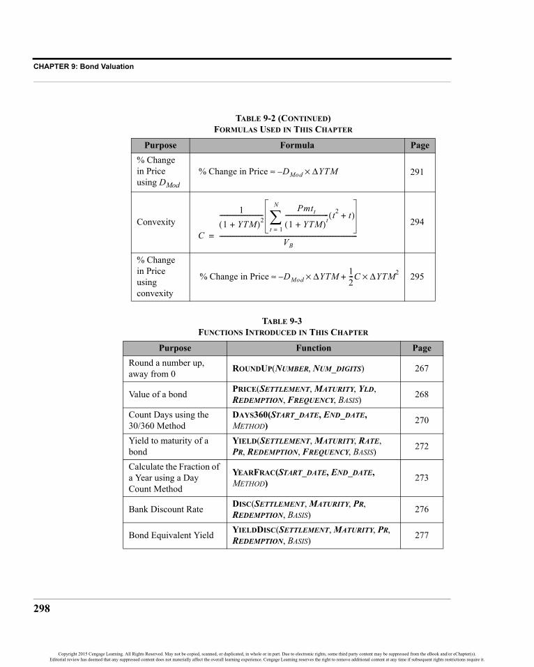
CHAPTER 9: Bond Valuation
298
% Change in Price using DMod
291
Convexity 294
% Change in Price using convexity
295
TABLE 9-3FUNCTIONS INTRODUCED IN THIS CHAPTER
Purpose Function PageRound a number up, away from 0 ROUNDUP(NUMBER, NUM_DIGITS) 267
Value of a bond PRICE(SETTLEMENT, MATURITY, YLD,REDEMPTION, FREQUENCY, BASIS) 268
Count Days using the 30/360 Method
DAYS360(START_DATE, END_DATE, METHOD) 270
Yield to maturity of a bond
YIELD(SETTLEMENT, MATURITY, RATE, PR, REDEMPTION, FREQUENCY, BASIS) 272
Calculate the Fraction of a Year using a Day Count Method
YEARFRAC(START_DATE, END_DATE, METHOD) 273
Bank Discount Rate DISC(SETTLEMENT, MATURITY, PR, REDEMPTION, BASIS) 276
Bond Equivalent Yield YIELDDISC(SETTLEMENT, MATURITY, PR, REDEMPTION, BASIS) 277
TABLE 9-2 (CONTINUED)FORMULAS USED IN THIS CHAPTER
Purpose Formula Page
% Change in Price DMod– ΔYTM×≈
C
11 YTM+( )2
----------------------------Pmtt
1 YTM+( )t---------------------------- t2 t+( )
t 1=
N
∑VB
-----------------------------------------------------------------------------------------=
% Change in Price DMod– ΔYTM 12---C ΔYTM2×+×≈
Copyright 2015 Cengage Learning. All Rights Reserved. May not be copied, scanned, or duplicated, in whole or in part. Due to electronic rights, some third party content may be suppressed from the eBook and/or eChapter(s).Editorial review has deemed that any suppressed content does not materially affect the overall learning experience. Cengage Learning reserves the right to remove additional content at any time if subsequent rights restrictions require it.

299
Problems
Problems
1. As an investor, you are considering an investment in the bonds of theFront Range Electric Company. The bonds pay interest quarterly, willmature in 12 years, and have a coupon rate of 3.25% on a face value of$1,000. Currently, the bonds are selling for $800.
a. If your required return is 5.40% for bonds in this risk class, what isthe highest price you would be willing to pay? (Use the PV function.)
b. What is the current yield of these bonds?
c. What is the yield to maturity on these bonds if you purchase them atthe current price? (Use the RATE function.)
d. If you hold the bonds for one year, and interest rates do not change,what total rate of return will you earn, assuming that you pay themarket price? Why is this different from the current yield and YTM?
e. If the bonds can be called in three years with a call premium of 4% ofthe face value, what is the yield to call on these bonds? (Use the RATEfunction.)
f. Now assume that the settlement date for your purchase is 7/30/2015,the maturity date is 7/30/2027, and the first call date is 7/30/2018.Using the PRICE and YIELD functions recalculate your answers toparts a, c, and d.
Find a date months after a specified date EDATE(START_DATE, MONTHS) 284
Macaulay Duration DURATION(SETTLEMENT, MATURITY, COUPON, YLD, FREQUENCY, BASIS) 289
Modified Duration MDURATION(SETTLEMENT, MATURITY, COUPON, YLD, FREQUENCY, BASIS) 291
Convexity on a payment date
FAME_CONVEXITY(SETTLEMENT, MATURITY, FV, COUPON, YLD, FREQUENCY)
295
TABLE 9-3 (CONTINUED)FUNCTIONS INTRODUCED IN THIS CHAPTER
Purpose Function Page
Copyright 2015 Cengage Learning. All Rights Reserved. May not be copied, scanned, or duplicated, in whole or in part. Due to electronic rights, some third party content may be suppressed from the eBook and/or eChapter(s).Editorial review has deemed that any suppressed content does not materially affect the overall learning experience. Cengage Learning reserves the right to remove additional content at any time if subsequent rights restrictions require it.

CHAPTER 9: Bond Valuation
300
g. If market interest rates remain unchanged, do you think it is likely thatthe bond will be called in three years? Why or why not?
h. Create a chart that shows the relationship of the bond’s price to yourrequired return. Use a range of 0% to 15% in calculating the prices.
2. After recently receiving a bonus, you have decided to add some bonds toyour investment portfolio. You have narrowed your choice down to thefollowing bonds (assume semiannual payments):
a. Using the PRICE function, calculate the intrinsic value of each bond.Are any of the bonds currently undervalued? How much accruedinterest would you have to pay for each bond?
b. Calculate the current yield of each bond. Is this the total return thatyou would earn each year? If you were on a fixed income, would youcare about this number?
c. Using the YIELD function, calculate the yield to maturity of eachbond using the current market prices. How do the YTMs compare tothe current yields of the bonds?
d. Calculate the duration and modified duration of each bond. Create achart that shows both measures versus term to maturity. Does durationincrease linearly with term? If not, what relationship do you see?
e. Which bond would you rather own if you expect market rates to fallby 2% for all bonds? What if rates will rise by 2%? Why?
Bond A Bond B Bond CSettlement Date 2/15/2015 2/15/2015 2/15/2015Maturity Date 8/15/2025 5/15/2035 6/15/2045Coupon Rate 5.00% 7.50% 8.00%Market Price $987 $1,040 $1,098Face Value $1,000 $1,000 $1,000Required Return 5.25% 7.00% 7.25%
Copyright 2015 Cengage Learning. All Rights Reserved. May not be copied, scanned, or duplicated, in whole or in part. Due to electronic rights, some third party content may be suppressed from the eBook and/or eChapter(s).Editorial review has deemed that any suppressed content does not materially affect the overall learning experience. Cengage Learning reserves the right to remove additional content at any time if subsequent rights restrictions require it.
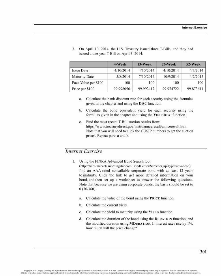
301
Internet Exercise
3. On April 10, 2014, the U.S. Treasury issued three T-Bills, and they hadissued a one-year T-Bill on April 3, 2014:
a. Calculate the bank discount rate for each security using the formulasgiven in the chapter and using the DISC function.
b. Calculate the bond equivalent yield for each security using theformulas given in the chapter and using the YIELDDISC function.
c. Find the most recent T-Bill auction results from: https://www.treasurydirect.gov/instit/annceresult/annceresult.htm.Note that you will need to click the CUSIP numbers to get the auctionprices. Repeat parts a and b.
Internet Exercise
1. Using the FINRA Advanced Bond Search tool (http://finra-markets.morningstar.com/BondCenter/Screener.jsp?type=advanced),find an AAA-rated noncallable corporate bond with at least 12 yearsto maturity. Click the link to get more detailed information on yourbond, and then set up a worksheet to answer the following questions.Note that because we are using corporate bonds, the basis should be set to0 (30/360).
a. Calculate the value of the bond using the PRICE function.
b. Calculate the current yield.
c. Calculate the yield to maturity using the YIELD function.
d. Calculate the duration of the bond using the DURATION function, andthe modified duration using MDURATION. If interest rates rise by 1%,how much will the price change?
4-Week 13-Week 26-Week 52-WeekIssue Date 4/10/2014 4/10/2014 4/10/2014 4/3/2014Maturity Date 5/8/2014 7/10/2014 10/9/2014 4/2/2015Face Value per $100 100 100 100 100Price per $100 99.998056 99.992417 99.974722 99.873611
Copyright 2015 Cengage Learning. All Rights Reserved. May not be copied, scanned, or duplicated, in whole or in part. Due to electronic rights, some third party content may be suppressed from the eBook and/or eChapter(s).Editorial review has deemed that any suppressed content does not materially affect the overall learning experience. Cengage Learning reserves the right to remove additional content at any time if subsequent rights restrictions require it.

Copyright 2015 Cengage Learning. All Rights Reserved. May not be copied, scanned, or duplicated, in whole or in part. Due to electronic rights, some third party content may be suppressed from the eBook and/or eChapter(s).Editorial review has deemed that any suppressed content does not materially affect the overall learning experience. Cengage Learning reserves the right to remove additional content at any time if subsequent rights restrictions require it.

303
CHAPTER 10 The Cost of Capital
Suppose that you are offered an investment opportunity that you believe will earn a return of8%. If your required rate of return is 10%, would you make this investment? Clearly not.Even though you might earn a profit, in the accounting sense of the word, you wouldn’t bemaking as much as required to make the investment attractive. Presumably, you have otherinvestment alternatives, with similar risk, that will earn your required return. So, 10% is theopportunity cost of your funds, and you will reject investments that earn less than this rate.This rate is also known as your cost of capital, and corporations use the concept every day tomake investment decisions.
After studying this chapter, you should be able to:1. Define “hurdle rate” and show how it relates to the firm’s weighted average
cost of capital (WACC).2. Calculate the WACC using both book- and market-value weights.3. Calculate component costs of capital with flotation costs and taxes.4. Explain how and why a firm’s WACC changes as total capital requirements
change.5. Use Excel to calculate the “break-points” in a firm’s marginal WACC curve,
and graph this curve in Excel.
Copyright 2015 Cengage Learning. All Rights Reserved. May not be copied, scanned, or duplicated, in whole or in part. Due to electronic rights, some third party content may be suppressed from the eBook and/or eChapter(s).Editorial review has deemed that any suppressed content does not materially affect the overall learning experience. Cengage Learning reserves the right to remove additional content at any time if subsequent rights restrictions require it.

CHAPTER 10: The Cost of Capital
304
Knowledge of a firm’s cost of capital is vital if managers are to make appropriate decisionsregarding the use of the firm’s funds. Without this knowledge, poor investments may bemade that actually reduce shareholder wealth. In this chapter, you will learn what the cost ofcapital is and how to calculate it.
The Appropriate “Hurdle” RateA firm’s required rate of return on investments is often referred to as the hurdle rate becauseall projects must earn a rate of return high enough to clear this rate. Otherwise, while theproject may earn an accounting profit (covering its operating and interest costs), it may notearn enough to cover its cost of equity. It will, therefore, earn a negative economic profit andreduce shareholder wealth. But what is the appropriate rate to use when evaluatinginvestment opportunities? Let’s look at an example:
The managers of Rocky Mountain Motors (RMM) are considering the purchase of anew tract of land that will be held for one year. The purchase price of the land is$10,000. RMM’s capital structure is currently made up of 40% debt, 10% preferredstock, and 50% common equity. Because this capital structure is considered to be optimal,any new financing will be raised in the same proportions. RMM must raise the newfunds as indicated in Table 10-1.
Before making the decision, RMM’s managers must determine what required rate of return will simultaneously satisfy all of their capital providers. What is the minimum rate of return that will accomplish this goal?
Looking at the third column of Table 10-1, it is clear that the total financing cost is $980. So,the project must generate at least $980 in excess of its cost in order to cover the financingcosts. This represents a minimum required return of 9.8% on the investment of $10,000.Table 10-2 shows what would happen under three alternative rate of return scenarios.
TABLE 10-1FUNDING FOR RMM’S LAND PURCHASE
Source of Funds Amount Dollar CostAfter-Tax
CostDebt $ 4,000 $ 280 7%Preferred Stock 1,000 100 10%Common Stock 5,000 600 12%Total 10,000 980 9.8%
Copyright 2015 Cengage Learning. All Rights Reserved. May not be copied, scanned, or duplicated, in whole or in part. Due to electronic rights, some third party content may be suppressed from the eBook and/or eChapter(s).Editorial review has deemed that any suppressed content does not materially affect the overall learning experience. Cengage Learning reserves the right to remove additional content at any time if subsequent rights restrictions require it.

305
The Appropriate “Hurdle” Rate
Recall that the common shareholders’ required rate of return is 12% on the $5,000 that theyprovided. This means that the shareholders expect to get back at least $5,600. If RMM earnsonly 8%, the common shareholders will receive only $5,420, $180 less than required. Weassume that the common shareholders have alternative investment opportunities (with equalrisk) that would return 12%. Therefore, if the project can return only 8%, the best decisionfor managers to make would be to allow the common shareholders to hold on to their money.In other words, the project should be rejected.
On the other hand, if the project is expected to return 9.8%, the common shareholders willreceive exactly the amount that they require. If the project returns 11%, they will be morethan satisfied. Under these latter two scenarios the project should be accepted becauseshareholder wealth will be either increased by the amount required ($600) or increased bymore than required ($720).1
The Weighted Average Cost of CapitalIt still remains to determine, in a general way, what required rate of return willsimultaneously satisfy all of the firm’s stakeholders. Recall that 40% of RMM’s funds wereprovided by the debt holders. Therefore, 40% of this minimum required rate of return mustgo to satisfy the debt holders. For the same reason, 10% of this minimum required rate ofreturn must go to satisfy the preferred stockholders, and 50% will be required for thecommon stockholders.
In general, the minimum required rate of return must be a weighted average of the individualrequired rates of return on each form of capital provided. Therefore, we refer to thisminimum required rate of return as the weighted average cost of capital (WACC). TheWACC can be found as follows:
TABLE 10-2ALTERNATIVE SCENARIOS FOR RMM
Rate of Return 8% 9.8% 11%Total Funds Available $ 10,800 $ 10,980 $ 11,100Less: Debt Costs 4,280 4,280 4,280Less: Preferred Costs 1,100 1,100 1,100Available to Common Shareholders 5,420 5,600 5,720
1. The difference between the amount that is available to the common shareholders and the amountrequired is known as the net present value (NPV). This concept will be explored in Chapter 11.
Copyright 2015 Cengage Learning. All Rights Reserved. May not be copied, scanned, or duplicated, in whole or in part. Due to electronic rights, some third party content may be suppressed from the eBook and/or eChapter(s).Editorial review has deemed that any suppressed content does not materially affect the overall learning experience. Cengage Learning reserves the right to remove additional content at any time if subsequent rights restrictions require it.

CHAPTER 10: The Cost of Capital
306
(10-1)
where the w’s are the weights of each source of capital and the k’s are the costs (requiredreturns) for each source of capital. In the case of RMM, the WACC is:
which is exactly the required return that we found earlier.
Determining the WeightsThe weights that one uses in the calculation of the WACC will obviously affect the result.Therefore, an important question is, “Where do the weights come from?” Actually, there arethree possible answers to this question. Perhaps the most obvious answer is to find theweights on the balance sheet.
The balance sheet weights (usually referred to as the book-value weights) can be obtained bythe following procedure: Find the total long-term debt, total preferred equity, and the totalcommon equity. Add together each of these to arrive at the grand total of the long-termsources of capital. Finally, divide each component by the grand total to discover thepercentage that each source is of total capital. Table 10-3 shows these calculations for RMM.
The problem with book-value weights is that they represent the weights as they were whenthe securities were originally sold. That is, the book-value weights represent historicalweights. The calculated WACC would better represent current reality if we used the presentweights. Because the market constantly revalues the firm’s securities, and we assume thatthe capital markets are efficient, we can find the weights by using the current market valuesof the securities.
The procedure for determining the market-value weights is similar to that used to find thebook-value weights. First, determine the total market value of each type of security. Total the
TABLE 10-3CALCULATION OF BOOK-VALUE WEIGHTS FOR RMM
Source of Capital Total Book Value Percentage of TotalLong-Term Debt $ 400,000 40%Preferred Equity 100,000 10%Common Stock 500,000 50%Grand Total 1,000,000 100%
WACC wdkd wPkP wcskcs+ +=
WACC 0.40 0.07( ) 0.10 0.10( ) 0.50 0.12( )+ + 0.098 9.80%= = =
Copyright 2015 Cengage Learning. All Rights Reserved. May not be copied, scanned, or duplicated, in whole or in part. Due to electronic rights, some third party content may be suppressed from the eBook and/or eChapter(s).Editorial review has deemed that any suppressed content does not materially affect the overall learning experience. Cengage Learning reserves the right to remove additional content at any time if subsequent rights restrictions require it.

307
WACC Calculations in Excel
results and then divide the market value of each source of capital by the total to determinethe weights.
Table 10-4 shows RMM’s current capital structure in market-value terms. Note that, inmarket-value terms, the percentage of common equity has risen considerably, while thepercentages of debt and preferred equity have fallen. Using these weights we can see thattheir WACC is:
The third type of weights that may be used are the target capital structure weights. Ifmanagement believes that the current capital structure is less than optimal, then they mayhave an optimal capital structure in mind. Presumably, over time, the firm will raise capitalin a manner that ultimately results in the firm achieving its target capital structure. Thesetarget weights are ideal for calculating the WACC because we care most about the cost ofcapital over the life of a project.
In this example, the book-value WACC and the market-value WACC are quite closetogether. This is not always the case. Whenever possible, use the target weights or themarket-value weights to determine the WACC.
WACC Calculations in ExcelWe can easily set up a worksheet to do the calculations for the WACC as in Table 10-4. Todo this, first copy the data from Table 10-4 into a new worksheet, starting with the headingsin A1.
In column D we want to calculate the total market value of the securities, which is the pricetimes the number of units outstanding. So, in D2 enter: =B2*C2 and copy the formula downto D3 and D4. Cell D5 should have the total market value of the securities, so enter:=Sum(D2:D4). In column E we need the percentage that each security represents of the total
TABLE 10-4CALCULATION OF MARKET-VALUE WEIGHTS FOR RMM
SourcePrice
per Unit UnitsTotal
Market ValuePercentage
of TotalDebt $ 904.53 400 $ 361,812 31.14%Preferred 100.00 1,000 100,000 8.61%Common 70.00 10,000 700,000 60.25%Totals 1,161,812 100.00%
WACC 0.3114 0.07( ) 0.0861 0.10( ) 0.6025 0.12( )+ + 0.1027 10.27%= = =
Copyright 2015 Cengage Learning. All Rights Reserved. May not be copied, scanned, or duplicated, in whole or in part. Due to electronic rights, some third party content may be suppressed from the eBook and/or eChapter(s).Editorial review has deemed that any suppressed content does not materially affect the overall learning experience. Cengage Learning reserves the right to remove additional content at any time if subsequent rights restrictions require it.

CHAPTER 10: The Cost of Capital
308
market value. These are the weights that we will use to calculate the WACC. In E2 enter:=D2/D$5 and copy down to E3 and E4. As a check, calculate the total in E5.
Next, we want a column for the after-tax costs of each source of capital and the WACC. InF1 enter the label: After-Tax Cost. Now, in F2:F4 enter the after-tax cost of eachcomponent from Table 10-1. We could calculate the WACC in F5 with the formula:=E2*F2+E3*F3+E4*F4. Even easier would be to use the SUMPRODUCT function, whichis defined as:
SUMPRODUCT(ARRAY1, ARRAY2, …)
where ARRAY1, ARRAY2, and so on, are up to 255 ranges. This function multiplies thecorresponding values in each array and then adds together the results. It is perfect forcalculating weighted averages. we can calculate the WACC in cell F5 with the formula:=SUMPRODUCT(E2:E4,F2:F4).2
The completed worksheet appears in Exhibit 10-1. Note that the WACC is exactly as wecalculated earlier. You are encouraged to experiment by changing the market prices of thesecurities to see how the weights and the WACC change.
EXHIBIT 10-1WORKSHEET TO CALCULATE RMM’S WACC
Calculating the Component CostsUp to this point, we have taken the component costs of capital as a given. In reality, thesecosts are anything but given, and, in fact, change continuously. How we calculate thesecosts is the subject of this section.
To begin, note that the obvious way of determining the required rates of return is to simplyask capital providers what their required rate of return is for the particular security that they
2. We could also use an array formula: =SUM(E2:E4*F2:F4); just remember to pressCtrl+Shift+Enter when entering this formula.
Copyright 2015 Cengage Learning. All Rights Reserved. May not be copied, scanned, or duplicated, in whole or in part. Due to electronic rights, some third party content may be suppressed from the eBook and/or eChapter(s).Editorial review has deemed that any suppressed content does not materially affect the overall learning experience. Cengage Learning reserves the right to remove additional content at any time if subsequent rights restrictions require it.

309
Calculating the Component Costs
own. For all but the most closely held of firms, this would be exceedingly impractical andyou would likely get some outlandish responses. However, there is a way by which we canaccomplish the same end result.
Recall from Chapter 8 that the market value of a security is equal to its intrinsic value to themarginal investor. Further, if investors are rational, they will buy (sell) securities as theexpected return rises above (falls below) their required return. Therefore, we can say that theinvestors in the firm “vote with their dollars” on the issue of the firm’s cost of capital. Thisforce operates in all markets.3 So at any given moment, the price of a security will reflect theoverall required rate of return for that security. All we need, then, is a method of convertingthe observed market prices of securities into required rates of return.
Because we have already discussed the valuation of securities (common stock, preferredstock, and bonds), you should recall that a major input was the investor’s required rate ofreturn. As we will see, we can simply take the market price as a given and then solve thevaluation equations for the required rate of return.
The Cost of Common EquityBecause of complexities in the real world, finding a company’s cost of common equity is notalways straightforward. In this section, we will look at two approaches to this problem, bothof which we have seen previously in other guises.
Using the Dividend Discount ModelRecall that a share of common stock is a perpetual security, which we assume willperiodically pay a cash flow that grows over time. We have previously demonstrated that thepresent value of such a stream of cash flows is given by equation (8-3):
assuming an infinite holding period and a constant rate of growth for the cash flows.
If we know the current market price of the stock, we can use this knowledge to solve for thecommon shareholder’s required rate of return. Simple algebraic manipulation will revealthat this rate of return is given by:
(10-2)
3. Anybody who isn’t convinced should check the history of stock prices for companies such asLehman Brothers and VeraSun Energy. They were falling long before the firms filed for bankruptcy.
VCSD0 1 g+( )
kCS g–------------------------
D1
kCS g–-----------------= =
kCSD0 1 g+( )
VCS------------------------ g+
D1
VCS--------- g+= =
Copyright 2015 Cengage Learning. All Rights Reserved. May not be copied, scanned, or duplicated, in whole or in part. Due to electronic rights, some third party content may be suppressed from the eBook and/or eChapter(s).Editorial review has deemed that any suppressed content does not materially affect the overall learning experience. Cengage Learning reserves the right to remove additional content at any time if subsequent rights restrictions require it.

CHAPTER 10: The Cost of Capital
310
Note that this equation says that the required rate of return on common equity is equal to thesum of the expected dividend yield and the growth rate of the dividend stream. We couldalso use any of the other common stock valuation models (see Chapter 8), though solving forthe required return is slightly more complicated.
Using the CAPMNot all common stocks will meet the assumptions of the dividend discount models. Inparticular, many companies do not pay dividends. An alternative approach to determiningthe cost of equity is to use the Capital Asset Pricing Model (CAPM).
The CAPM gives the expected rate of return for a security if we know the risk-free rate ofinterest, the market risk premium, and the riskiness of the security relative to the marketportfolio (i.e., the security’s beta). The CAPM, you will recall, is the equation for thesecurity market line:
Assuming that the stockholders are all price-takers, their expected return is the same as thefirm’s required rate of return.4 Therefore, we can use the CAPM to determine the requiredrate of return on equity.
The Cost of Preferred EquityPreferred stock, for valuation purposes, can be viewed as a special case of the commonstock, with the growth rate of dividends equal to zero. We can carry this idea to the processof solving for the preferred stockholders’ required rate of return. First, recall that the valueof a share of preferred stock was given by equation (8-22):
As with common stock, we can algebraically manipulate this equation to solve for therequired return if the market price is known:
(10-3)
4. A price-taker cannot materially affect the price of an asset through individual buying or selling.This situation generally exists in the stock market because most investors are small when comparedto the market value of the firm’s common stock.
E Ri( ) Rf βi E Rm( ) Rf–( )+=
VPDkP-----=
kPDVP------=
Copyright 2015 Cengage Learning. All Rights Reserved. May not be copied, scanned, or duplicated, in whole or in part. Due to electronic rights, some third party content may be suppressed from the eBook and/or eChapter(s).Editorial review has deemed that any suppressed content does not materially affect the overall learning experience. Cengage Learning reserves the right to remove additional content at any time if subsequent rights restrictions require it.

311
Calculating the Component Costs
The Cost of DebtFinding the cost of debt is more difficult than finding the cost of either preferred or commonequity because there is no formula (except for trivial cases). Instead, we must use analgorithm. The process is similar: Get the market price of the security, and then find thediscount rate that makes the present value of the expected future cash flows equal to thecurrent price. This rate is the same as the yield to maturity (see page 272). However, wecannot directly solve for this discount rate. Instead, we must use an iterative trial-and-errorprocess.
Recall that the value of a bond is given by equation (9-1):
The problem is to find kd such that the equality holds between the left and right sides of theequation. Suppose that, as in Exhibit 10-1, the current price of RMM’s bonds is $904.53, thecoupon rate is 10%, the face value of the bonds is $1,000, and the bonds will mature in 10years. If the bonds pay interest annually, our equation looks as follows:
We must make an initial, but intelligent, guess as to the value of kd. Because the bond isselling at a discount to its face value, we know that the yield to maturity (kd) must be greaterthan the coupon rate. Therefore, our first guess should be something greater than 10%. If wechoose 12% we will find that the price would be $886.99, which is lower than the actualprice. Our first guess was incorrect, but we now know that the answer must lie between 10%and 12%. The next logical guess is 11%, which is the halfway point. Inserting this for kd weget a price of $941.11, which is too high, but not by much. Further, we have narrowed therange of possible answers to those between 11% and 12%. Again, we choose the halfwaypoint, 11.5%, as our next guess. This results in an answer of $913.48. Continuing thisprocess we will eventually find the correct answer to be 11.67%.5
5. The method presented here is known as the bisection method. Briefly, the idea is to quickly bracketthe solution and to then choose as the next approximation the answer that is exactly halfwaybetween the previous possibilities. This method can lead to very rapid convergence to the solution ifa good beginning guess is used.
VB Pmt1 1
1 kd+( )N----------------------–
kd------------------------------- FV
1 kd+( )N----------------------+=
904.53 1001 1
1 kd+( )10-----------------------–
kd-------------------------------- 1,000
1 kd+( )10-----------------------+=
Copyright 2015 Cengage Learning. All Rights Reserved. May not be copied, scanned, or duplicated, in whole or in part. Due to electronic rights, some third party content may be suppressed from the eBook and/or eChapter(s).Editorial review has deemed that any suppressed content does not materially affect the overall learning experience. Cengage Learning reserves the right to remove additional content at any time if subsequent rights restrictions require it.

CHAPTER 10: The Cost of Capital
312
Of course, as we will soon see, we can use Excel’s RATE or YIELD function instead ofmanually solving for the before-tax cost of debt.
Making an Adjustment for TaxesNotice that the answer that we found for the cost of debt, 11.67%, is not the same as thatlisted in Exhibit 10-1. Because interest is a tax-deductible expense, interest paymentsactually cost the firm less than the full amount of the payment. In this case, if RMM were tomake an interest payment of $116.70, and the marginal tax rate is 40%, it would cost themonly $70.02 ( ). Observe that , or 7%, which isthe after-tax cost of debt listed in Exhibit 10-1.
In general, we need to adjust the cost of debt to account for the deductibility of the interestexpense by multiplying the before-tax cost of debt (i.e., the yield to maturity) by 1 – t, wheret is the marginal tax rate.6 Note that we do not make the same adjustment for the cost ofcommon or preferred equity because dividends are not tax deductible.
Using Excel to Calculate the Component CostsA general principle that we have relied on in constructing our worksheets is that we shouldmake Excel do the calculations whenever possible. We will now make changes to ourworksheet in Exhibit 10-1 to allow Excel to calculate the component costs of capital.
The After-Tax Cost of Debt
We cannot calculate any of the component costs on our worksheet without adding someadditional information. We will first add information which will be used to calculate theafter-tax cost of debt. Beginning in A7 with the label: Additional Bond Data, add theinformation from Table 10-5 into your worksheet. For simplicity, we assume that the bondspay interest annually.
6. This is just a close approximation, but close enough for most purposes because the cost of capital isan estimate anyway. It would be more accurate to use the after-tax cash flows in the equation. Thiswill result in the after-tax cost of debt with no adjustment required and will differ slightly from thatgiven earlier. Due to uncertainty regarding future tax rates, this is unlikely to be more “exact.”
116.70 1 0.40–( )×= 70.02 1,000⁄ 0.07≈
Copyright 2015 Cengage Learning. All Rights Reserved. May not be copied, scanned, or duplicated, in whole or in part. Due to electronic rights, some third party content may be suppressed from the eBook and/or eChapter(s).Editorial review has deemed that any suppressed content does not materially affect the overall learning experience. Cengage Learning reserves the right to remove additional content at any time if subsequent rights restrictions require it.
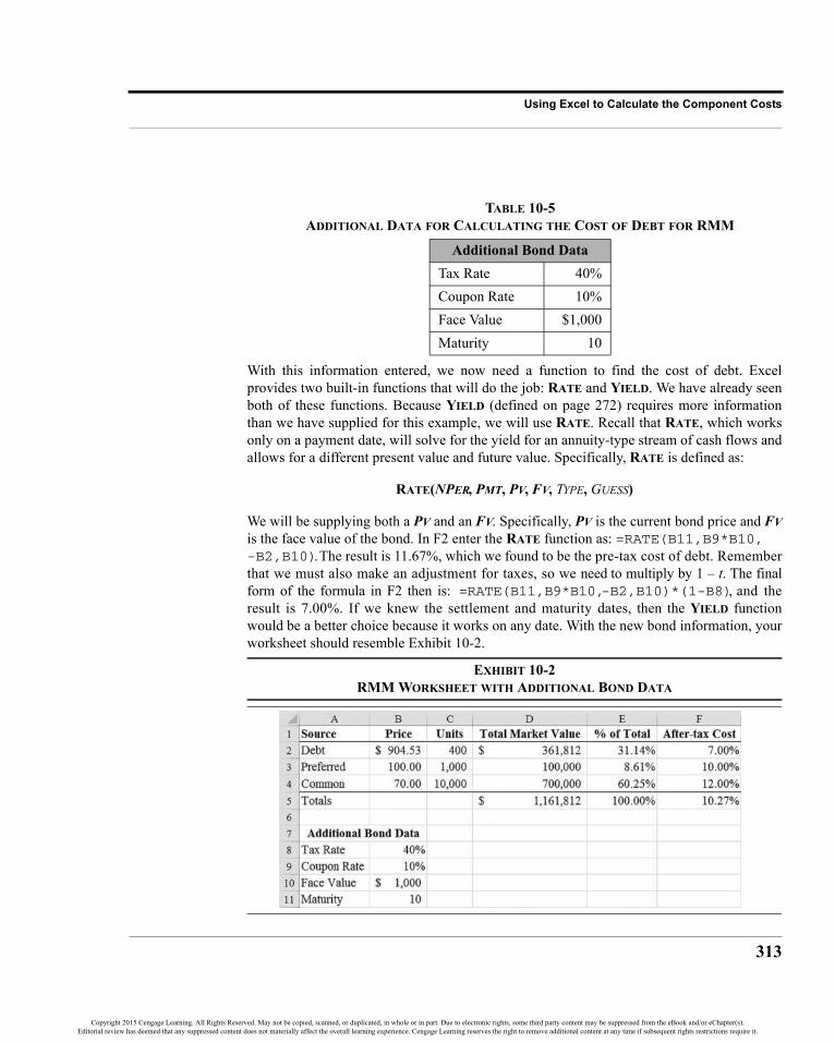
313
Using Excel to Calculate the Component Costs
With this information entered, we now need a function to find the cost of debt. Excelprovides two built-in functions that will do the job: RATE and YIELD. We have already seenboth of these functions. Because YIELD (defined on page 272) requires more informationthan we have supplied for this example, we will use RATE. Recall that RATE, which worksonly on a payment date, will solve for the yield for an annuity-type stream of cash flows andallows for a different present value and future value. Specifically, RATE is defined as:
RATE(NPER, PMT, PV, FV, TYPE, GUESS)
We will be supplying both a PV and an FV. Specifically, PV is the current bond price and FVis the face value of the bond. In F2 enter the RATE function as: =RATE(B11,B9*B10,-B2,B10). The result is 11.67%, which we found to be the pre-tax cost of debt. Rememberthat we must also make an adjustment for taxes, so we need to multiply by 1 – t. The finalform of the formula in F2 then is: =RATE(B11,B9*B10,-B2,B10)*(1-B8), and theresult is 7.00%. If we knew the settlement and maturity dates, then the YIELD functionwould be a better choice because it works on any date. With the new bond information, yourworksheet should resemble Exhibit 10-2.
EXHIBIT 10-2RMM WORKSHEET WITH ADDITIONAL BOND DATA
TABLE 10-5ADDITIONAL DATA FOR CALCULATING THE COST OF DEBT FOR RMM
Additional Bond DataTax Rate 40%Coupon Rate 10%Face Value $1,000Maturity 10
Copyright 2015 Cengage Learning. All Rights Reserved. May not be copied, scanned, or duplicated, in whole or in part. Due to electronic rights, some third party content may be suppressed from the eBook and/or eChapter(s).Editorial review has deemed that any suppressed content does not materially affect the overall learning experience. Cengage Learning reserves the right to remove additional content at any time if subsequent rights restrictions require it.

CHAPTER 10: The Cost of Capital
314
The Cost of Preferred StockCompared to calculating the after-tax cost of debt, finding the cost of preferred stock is easy.We need to add only one piece of information: the preferred dividend. In C7 type:Additional Preferred Data. In C8 type: Dividend and in D8 enter: 10.
We know from equation (10-3) that we need to divide the preferred dividend by the currentprice of the stock. Therefore, the equation in F3 is: =D8/B3.
The Cost of Common StockTo calculate the cost of common stock, we need to know the most recent dividend and thedividend growth rate in addition to the current market price of the stock. In E7 type:Additional Common Data. In E8 type: Dividend 0 and in F8 enter: 3.96. In E9enter the label: Growth Rate and in F9 enter: 6%.
Finally, we will use equation (10-2) to calculate the cost of common stock in F4. Because weknow the most recent dividend (D0) we need to multiply that by 1 + g. The formula in F4 is:=(F8*(1+F9))/B4+F9, and the result is 12% as we found earlier.
As you will see, we have not yet completed the calculation of the component costs forRMM. We have left out one crucial piece which we will discuss in the next section. At thispoint, your worksheet should resemble that in Exhibit 10-3.
EXHIBIT 10-3RMM COST OF CAPITAL WORKSHEET
Copyright 2015 Cengage Learning. All Rights Reserved. May not be copied, scanned, or duplicated, in whole or in part. Due to electronic rights, some third party content may be suppressed from the eBook and/or eChapter(s).Editorial review has deemed that any suppressed content does not materially affect the overall learning experience. Cengage Learning reserves the right to remove additional content at any time if subsequent rights restrictions require it.

315
The Role of Flotation Costs
The Role of Flotation CostsAny action that a corporation takes has costs associated with it. Up to this point, we haveimplicitly assumed that securities can be issued without cost, but this is not the case. Sellingsecurities directly to the public is a complicated procedure, generally requiring a lot ofmanagement time as well as the services of an investment bank. An investment bank is afirm that serves as an intermediary between the issuing firm and the public, which usuallybuys the securities from the firm at a discount (the underwriting spread). In addition toforming the underwriting syndicate to sell the securities, the investment banker alsofunctions as a consultant to the firm. As a consultant, the investment banker usually advisesthe firm on the pricing of the issue and is responsible for preparing the registration statementfor the Securities and Exchange Commission (SEC).
The cost of the investment banker’s services and other costs of issuance are referred to asflotation costs. (The term derives from the fact that the process of selling a new issue isgenerally referred to as floating a new issue.) Flotation costs add to the total cost of the newsecurities to the firm, so we must increase the component cost of capital to account for them.
There are two methods of accounting for flotation costs. The most popular method is the costof capital adjustment. Under this method, the market price of new securities is decreased bythe per unit flotation costs. This results in the net amount that the company receives from thesale of the securities. The component costs are then calculated in the usual way except thatthe net amount received, not the market price, is used in the equation.
The second, less common, method is the investment cost adjustment. Under thismethodology, we increase the initial outlay for the project under consideration to account forthe total flotation costs. Component costs are then calculated as we did earlier. The primarydisadvantage of this technique is that, because it assigns all flotation costs to one project, itimplicitly assumes that the securities used to finance a project will be retired when theproject is completed.7
Because it is more common, and its assumptions are more realistic, we will use the cost ofcapital adjustment technique. When flotation costs are included in the analysis, the equationsfor the component costs are given in Table 10-6.
7. For more information on both methods, see E. F. Brigham and L. C. Gapenski, “Flotation CostAdjustments,” Financial Practice and Education, Vol. 1, No. 2, Fall/Winter 1991, pp. 29–34.
Copyright 2015 Cengage Learning. All Rights Reserved. May not be copied, scanned, or duplicated, in whole or in part. Due to electronic rights, some third party content may be suppressed from the eBook and/or eChapter(s).Editorial review has deemed that any suppressed content does not materially affect the overall learning experience. Cengage Learning reserves the right to remove additional content at any time if subsequent rights restrictions require it.

CHAPTER 10: The Cost of Capital
316
* In these equations, the flotation costs (f) are a dollar amount per unit. It is also common for flotation costs to be stated as a percentage of the unit price.
Adding Flotation Costs to Our WorksheetWe can easily incorporate the adjustment for flotation costs into our worksheet. All that weneed to do is change the references to the current price in each of our formulas to the currentprice minus the per unit flotation costs. These costs are given in Table 10-7.
Enter the information from Table 10-7 into your worksheet. For each security, we haveadded the information at the end of the “Additional information” section. For example, inA12 enter: Flotation Cost and then in B12 enter: 1%, which is the flotation cost forbonds. Add similar entries for preferred and common stock.
TABLE 10-6COST OF CAPITAL EQUATIONS WITH FLOTATION COST ADJUSTMENT
Component Equation*
Cost of new common equity
Cost of preferred equity
Pre-tax cost of debt (solve for kd)
TABLE 10-7FLOTATION COSTS AS A PERCENTAGE OF SELLING PRICE FOR RMM
Security Flotation CostBonds 1%Preferred Stock 2%Common Stock 5%
kCSD0 1 g+( )
VCS f–------------------------ g+
D1
VCS f–---------------- g+= =
kPD
VP f–--------------=
VB f– Pmt1 1
1 kd+( )N----------------------–
kd------------------------------- FV
1 kd+( )N----------------------+=
Copyright 2015 Cengage Learning. All Rights Reserved. May not be copied, scanned, or duplicated, in whole or in part. Due to electronic rights, some third party content may be suppressed from the eBook and/or eChapter(s).Editorial review has deemed that any suppressed content does not materially affect the overall learning experience. Cengage Learning reserves the right to remove additional content at any time if subsequent rights restrictions require it.

317
The Role of Flotation Costs
To account for flotation costs, change your formulas to the following:
Once these changes have been made, you will notice that the cost of each component hasrisen. The overall WACC has increased from 10.27% to 10.51% as a result of the flotationcosts. Your worksheet should now resemble the one shown in Exhibit 10-4.
EXHIBIT 10-4COST OF CAPITAL WORKSHEET WITH FLOTATION COSTS
The Cost of Retained EarningsWe have shown how to calculate the required returns for purchasers of new common equity,preferred stock, and bonds, but firms also have another source of long-term capital: retainedearnings. Is there a cost to such internally generated funding, or is it free? Consider thatmanagers generally have two options as to what they do with the firm’s internally generatedfunds. They can either reinvest them in profitable projects or return them to the shareholdersin the form of dividends or a share repurchase. Because these funds belong to the commonshareholders alone, the definition of a “profitable project” is one that earns at least thecommon shareholder’s required rate of return. If these funds will not be invested to earn atleast this return, they should be returned to the common shareholders. So there is a cost (anopportunity cost) to internally generated funds: the cost of common equity.
Note that the only difference between retained earnings (internally generated commonequity) and new common equity is that the firm must pay flotation costs on the sale of new
F2 =RATE(B11,B9*B10,-B2*(1-B12),B10)*(1-B8)
F3 =D8/(B3*(1-D9))
F4 =(F8*(1+F9))/(B4*(1-F10))+F9
Copyright 2015 Cengage Learning. All Rights Reserved. May not be copied, scanned, or duplicated, in whole or in part. Due to electronic rights, some third party content may be suppressed from the eBook and/or eChapter(s).Editorial review has deemed that any suppressed content does not materially affect the overall learning experience. Cengage Learning reserves the right to remove additional content at any time if subsequent rights restrictions require it.

CHAPTER 10: The Cost of Capital
318
common equity. Because no flotation costs are paid for retained earnings, we can find thecost of retained earnings in the same way we did before learning about flotation costs. Inother words,
(10-4)
This notion of an opportunity cost for retained earnings is important for a couple of reasons.Most importantly, managers should be disabused of the notion that the funds on hand are“free.” As you now know, there is a cost to these funds, and it should be accounted for whenmaking decisions. In addition, there may be times when a project that otherwise appears tobe profitable is really unprofitable when the cost of retained earnings is correctly accountedfor. Accepting such a project is contrary to the principle of shareholder wealth maximizationand will result in the firm’s stock price falling.
The Marginal WACC CurveA firm’s WACC is not constant. Changes can occur in the WACC for a number of reasons.As a firm raises more and more new capital, its WACC will likely increase due to an increasein supply relative to demand for the firm’s securities. Furthermore, total flotation costs mayincrease as more capital is raised. Additionally, no firm has an unlimited supply of projectsthat will return more than the cost of capital, so the risk that new funds will be investedunprofitably increases.
We will see in Chapter 11 that these increases in the WACC play an important role indetermining the firm’s optimal capital budget. For the remainder of this chapter, we willconcentrate on determining the WACC at varying levels of total capital.
Finding the Break-PointsWe can model a firm’s marginal WACC curve with a step function. This type of functionresembles a staircase when plotted. They are commonly used as a linear (thoughdiscontinuous) approximation to nonlinear functions. The accuracy of the approximationimproves as the number of steps increases.
Estimating the marginal WACC (MCC) curve is a two-step process:1. Determine the levels of total capital at which the marginal WACC is
expected to increase. These points are referred to as break-points.2. Determine the marginal WACC at each break-point.
kRED0 1 g+( )
VCS------------------------ g+
D1
VCS--------- g+= =
Copyright 2015 Cengage Learning. All Rights Reserved. May not be copied, scanned, or duplicated, in whole or in part. Due to electronic rights, some third party content may be suppressed from the eBook and/or eChapter(s).Editorial review has deemed that any suppressed content does not materially affect the overall learning experience. Cengage Learning reserves the right to remove additional content at any time if subsequent rights restrictions require it.

319
The Marginal WACC Curve
Figure 10-1 illustrates what a marginal WACC curve might look like for RMM. Notice thatthe break-points are measured in terms of dollars of total capital. In this section, we willestimate where these break-points are likely to occur and the WACC at the break-points.
FIGURE 10-1THE MARGINAL WACC (MCC) CURVE AS A STEP FUNCTION
After consulting with their investment bankers, the managers of RMM have determined thatthey can raise new money at the costs indicated in Table 10-8. Open a new worksheet andenter the data from Table 10-8 beginning in cell A1. The percentages in the “% of Total”column should be referenced from the worksheet that was created for Exhibit 10-4.
Note that you should enter just the numbers from the “Amounts That Can Be Sold” column.You can define custom formats, so the numbers are displayed with the text. This allows us tohave the text and still use the numbers for the calculations that follow. For example, you can
TABLE 10-8ROCKY MOUNTAIN MOTORS INFORMATION
Source % of TotalAmounts That Can
Be SoldMarginal
After-Tax CostCommon 60.25% Up to 100,000 12.31%
100,001 to 500,000 15.00%More than 500,000 17.00%
Preferred 8.61% Up to 50,000 10.20%More than 50,000 13.00%
Debt 31.14% Up to 250,000 7.10%More than 250,000 8.00%
Copyright 2015 Cengage Learning. All Rights Reserved. May not be copied, scanned, or duplicated, in whole or in part. Due to electronic rights, some third party content may be suppressed from the eBook and/or eChapter(s).Editorial review has deemed that any suppressed content does not materially affect the overall learning experience. Cengage Learning reserves the right to remove additional content at any time if subsequent rights restrictions require it.

CHAPTER 10: The Cost of Capital
320
format the first cell as “Up to “#,##0 (which will cause the number to be displayed asshown in the table). The second number (500,000) can be formatted with “100,001 to“#,##0 so that it will display as shown.
RMM feels that its current capital structure is optimal, so any new money will be raised inthe same proportions. For example, if the firm decides to raise $200,000 in total capital, then$120,500 (60.25% of $200,000) will come from common equity, $62,280 (31.14%) will bedebt, and $17,220 (8.61%) will be preferred equity.
Using the information in Table 10-8, we can determine the location of the break-points inRMM’s marginal WACC curve. To do this, first realize that a break will occur whenever thecost of an individual source of capital changes because that will cause the WACC to rise.There will be a break-point associated with the issuance of $100,000 in common stock, forexample. But recall that break-points are measured in dollars of total capital. So the questionis, “How do we convert this $100,000 in common stock into the amount of total capital?”
Because the capital will be raised in constant proportions, we can use the followingequation:
(10-5)
In this case, we can see that if RMM raised $100,000 in new common stock, then it musthave raised $165,973 in total capital. Using equation (10-5):
We can use this information to see that if RMM issued $100,000 in new common stock, thenit must also have raised $51,684 ( ) in new debt, and $14,290( ) in new preferred stock.
To locate all of the break-points, all we need to do is find the points at which the cost of eachsource of capital changes, and then convert those into dollars of total capital using the sameidea as expressed in equation (10-5).
Table 10-9, using the information from Table 10-8, shows how to find these break-points.
$ Total Capital $ Common Stock% Common Stock--------------------------------------------=
$165,973 $100,0000.6025
----------------------≈
$165,973 0.3114×=
$165,973 0.0861×=
Copyright 2015 Cengage Learning. All Rights Reserved. May not be copied, scanned, or duplicated, in whole or in part. Due to electronic rights, some third party content may be suppressed from the eBook and/or eChapter(s).Editorial review has deemed that any suppressed content does not materially affect the overall learning experience. Cengage Learning reserves the right to remove additional content at any time if subsequent rights restrictions require it.

321
The Marginal WACC Curve
In your worksheet enter Break-Points in cell E1. The first break-point is associated withthe $100,000 level of new common stock. In E2, enter the formula =C2/B$2. The result is$165,973, exactly as we found in Table 10-9. Copy this formula to E3. In E5 the formula is:=C5/B$5. In E7 your formula will be: =C7/$B$7. Note that the denominator changes asthe source of the break-point changes.
The next step is to determine the WACC at each of the break-points. To find the WACC wemust convert each break-point into its components and then determine the cost of eachcomponent. There are a number of ways we might approach this problem in the worksheet.Because we would ultimately like to generate a chart of the marginal WACC, we will set upa table that shows the amount of total capital, the cost of each component, and the WACC atthat level of total capital.
Begin by entering the labels in A10:E10. In A10 enter: Total Capital. In B10: Cost ofEquity. In C10: Cost of Preferred. In D10: Cost of Debt. In E10: WACC. Now, inA11, enter 0 for the starting total capital. In A12, we want to enter the first break-point. Wecould just reference E2, which has the smallest break-point, but that may not be the smallestof the break-points if the weights or other data change. To ensure that A12 always has thesmallest break-point, we should use the SMALL function:
SMALL(ARRAY, K)
where ARRAY is a range of numbers and K is the position that you want to return. In A12,enter: =SMALL(E2:E7,1) to get the smallest of the break-points. In A13, enter=SMALL(E2:E7,2) to get the second smallest break-point, and so on. To finish this serieswith a round number, in A16 enter: =ROUNDUP(MAX(E2:E7),-5). This will round thelargest break-point up to the next $100,000.
Next, we will determine the cost of each source for each level of total capital. In B11, weneed to find the cost of equity at $0 of total capital. To facilitate later copying, we will set up
TABLE 10-9FINDING THE BREAK-POINTS IN RMM’S MARGINAL WACC CURVE
Source Calculation* Break-PointCommon Stock $ 165,973Common Stock 829,866Preferred Stock 580,906Debt 802,773* The weights are rounded to four decimal places. The actual calculation uses the weights as calculated in Exhibit 10-4.
100,000 0.6025⁄500,000 0.6025⁄
50,000 0.0861⁄250,000 0.3114⁄
Copyright 2015 Cengage Learning. All Rights Reserved. May not be copied, scanned, or duplicated, in whole or in part. Due to electronic rights, some third party content may be suppressed from the eBook and/or eChapter(s).Editorial review has deemed that any suppressed content does not materially affect the overall learning experience. Cengage Learning reserves the right to remove additional content at any time if subsequent rights restrictions require it.

CHAPTER 10: The Cost of Capital
322
a nested IF statement. In this case, the formula is: =IF(A11*$B$2<=$C$2,$D$2,IF(A11*$B$2<=$C$3,$D$3,$D$4)). In words, this formula says, “If the amount oftotal capital (in A11) times the percentage of common stock (B2) is less than or equal to$100,000 (C2) then the cost is 12.31% (D2). Otherwise, if the amount is less than or equal to$500,000 then the cost is 15% (D3). Otherwise, the cost is 17% (D4).”
We use similar, but less complicated, formulas to determine the cost of preferred stock anddebt at each level of total capital. For preferred stock, enter the formula: =IF(A11*$B$5<=$C$5,$D$5,$D$6) into C11. In D11 enter the formula: =IF(A11*$B$7<=$C$7,$D$7,$D$8) to determine the appropriate cost of debt. At this point, the cost of eachsource of funds should be at its lowest level.
Finally, we can calculate the marginal WACC (in E11), with the formula: =$B$2*B11+$B$5*C11+$B$7*D11. This formula calculates a weighted average of the costs calculatedin B11:D11. Make sure that you have entered the formulas exactly as given, and then copythem down through B12:E16. Your worksheet should now match the one in Exhibit 10-5.
EXHIBIT 10-5THE WACC AT EACH BREAK-POINT
Copyright 2015 Cengage Learning. All Rights Reserved. May not be copied, scanned, or duplicated, in whole or in part. Due to electronic rights, some third party content may be suppressed from the eBook and/or eChapter(s).Editorial review has deemed that any suppressed content does not materially affect the overall learning experience. Cengage Learning reserves the right to remove additional content at any time if subsequent rights restrictions require it.

323
The Marginal WACC Curve
Creating the Marginal WACC ChartRecall that we want to create a chart of the marginal cost of capital, approximated by a stepfunction. To create this chart, we need the WACCs and the break-points created earlier.Select A10:A16 and then hold down the Ctrl key while selecting E10:E16. Insert a scatterchart with straight lines.8 We don’t need, or want, markers for this chart.
FIGURE 10-2THE MARGINAL WACC CURVE FOR RMM
The chart in Figure 10-2 obviously does not depict a perfect step function, as shown inFigure 10-1. With a little trick, we can easily change this chart into a perfect step function.
First, realize that we want the line to be perfectly vertical at each break-point. In order to dothat, we must have two y values (WACC) corresponding to each particular x value (amountof total capital). However, if we use the exact break-point twice, then our calculated WACCwill be the same. To get the WACC to increase, we need to increase the break-point by a verytiny amount. To see this, select row 13 and insert a new row. Now, in A13 enter the formula:=A12+0.01. Then copy the other formulas in row 12 down to row 13. The WACC in E13is now higher than that in E12. Take a look at your chart and notice that you now have a nicestep for the first break-point. If you zoomed far enough into the chart, you would see that thestep is slightly sloped, but at normal size the slope isn’t visible.
Repeat these steps with the other three break-points, and then your chart should look like theone in Exhibit 10-6.
8. The most common error in making this type of chart correctly is choosing the wrong type of scatterchart. If you choose a scatter chart with smoothed lines, the result will be a little too smooth. Try it.Also note that you will not get a good step function using a line chart.
Copyright 2015 Cengage Learning. All Rights Reserved. May not be copied, scanned, or duplicated, in whole or in part. Due to electronic rights, some third party content may be suppressed from the eBook and/or eChapter(s).Editorial review has deemed that any suppressed content does not materially affect the overall learning experience. Cengage Learning reserves the right to remove additional content at any time if subsequent rights restrictions require it.

CHAPTER 10: The Cost of Capital
324
EXHIBIT 10-6RMM’S MARGINAL WACC CURVE AS A STEP FUNCTION
SummaryWe began this chapter with a discussion of the appropriate required rate of return to use inthe evaluation of a company’s scarce capital resources. We demonstrated that a weightedaverage of the cost of each source of capital would be sufficient to simultaneously satisfy allof the providers of capital. In addition, we showed that the costs of the sources of capital canbe found by simply inverting the valuation equations from Chapters 8 and 9 and includingflotation costs (except for retained earnings). Finally, we saw that the firm’s marginal WACCchanges as the amount of total capital changes. We showed how to determine the location ofthe break-points and how to plot the marginal WACC curve as a step function.
Copyright 2015 Cengage Learning. All Rights Reserved. May not be copied, scanned, or duplicated, in whole or in part. Due to electronic rights, some third party content may be suppressed from the eBook and/or eChapter(s).Editorial review has deemed that any suppressed content does not materially affect the overall learning experience. Cengage Learning reserves the right to remove additional content at any time if subsequent rights restrictions require it.

325
Problems
Problems
1. The Dempere Imports Company’s EPS in 2014 was $1.85, and in 2009 itwas $1.12. The company’s payout ratio is 40%, and the stock is currentlyvalued at $62.35. Flotation costs for new equity will be 12%. Net incomein 2015 is expected to be $15 million.
The company’s investment banker estimates that it could sell 10-yearsemiannual bonds with a coupon rate of 7%. The face value would be$1,000 and the flotation costs for a bond issue would be 3%. The market-value weights of the firm’s debt and equity are 30% and 70%, respectively.The firm faces a 35% tax rate.
a. Based on the five-year track record, what is Dempere’s EPS growthrate? What will the dividend be in 2015?
b. Calculate the firm’s cost of retained earnings and the cost of newcommon equity.
c. Calculate the break-point associated with retained earnings.
d. What is the firm’s after-tax cost of new debt?
e. If Dempere’s after-tax cost of debt is 6%, what is the WACC withretained earnings? With new common equity?
f. Create a scatter chart that shows the firm’s marginal WACC as a stepfunction. The x-axis should go to at least $20 million. Be sure to fullylabel the chart, including a data label with leader lines that shows thevalue of the break-point.
TABLE 10-10FUNCTIONS INTRODUCED IN THIS CHAPTER
Purpose Function PageCalculate the sum of the product of corresponding cells SUMPRODUCT(ARRAY1, ARRAY2, …) 308
Return the Kth smallest number in a range SMALL(ARRAY, K) 321
Copyright 2015 Cengage Learning. All Rights Reserved. May not be copied, scanned, or duplicated, in whole or in part. Due to electronic rights, some third party content may be suppressed from the eBook and/or eChapter(s).Editorial review has deemed that any suppressed content does not materially affect the overall learning experience. Cengage Learning reserves the right to remove additional content at any time if subsequent rights restrictions require it.

CHAPTER 10: The Cost of Capital
326
2. TRM Consulting Services currently has the following capital structure:
New debt would mature on June 30, 2040, have a coupon rate of 8%, andwould be sold for their par value of $1,000. The bonds pay interestsemiannually, and flotation costs would be 2% of the selling price. Thebonds would be issued on June 30, 2015.
The preferred stock pays a $7 dividend annually and is currently valued at$67.50 per share. Flotation costs on new preferred equity would be 4% ofthe price.
The common stock, which can be bought for $28.00, has experienced a6% annual growth rate in dividends and is expected to pay a $1.60dividend next year. Flotation costs on new common equity would be 8%.The stock has a beta of 1.25, the risk-free rate is 3%, and the expectedmarket risk premium is 7%.
In addition, the firm expects to generate $150,000 of retained earnings.Assume that TRM’s marginal tax rate is 35%.
a. Set up a worksheet with all of the data from the problem in a well-organized input area.
b. Calculate the book-value weights for each source of capital.
c. Calculate the market-value weights for each source of capital.
d. Calculate the component costs of capital (i.e., debt, preferred equity,retained earnings, and new common equity). Use the YIELD function(see page 277) when finding the after-tax cost of debt. Use the CAPMto find the cost of retained earnings, and the constant growth modelfor new common equity.
e. Calculate the weighted average costs of capital using both the market-value and book-value weights with retained earnings and also newcommon equity.
Source Book Value QuantityCommon Stock $ 25,000,000 1,250,000Preferred Stock 5,000,000 100,000Debt 8,600,000 8,600
Copyright 2015 Cengage Learning. All Rights Reserved. May not be copied, scanned, or duplicated, in whole or in part. Due to electronic rights, some third party content may be suppressed from the eBook and/or eChapter(s).Editorial review has deemed that any suppressed content does not materially affect the overall learning experience. Cengage Learning reserves the right to remove additional content at any time if subsequent rights restrictions require it.

327
Internet Exercise
3. Suppose that TRM Consulting Services has discussed its need for capitalwith its investment bankers. The bankers have estimated that TRM canraise new funds in the capital markets under the following conditions:
a. Using the information from the previous problem, calculate each ofthe break-points, including the break-point due to retained earnings.
b. Create a chart of TRM’s marginal WACC curve using the market-value weights. Make sure that it is a perfect step function.
Internet Exercise
1. Using the Yahoo! Finance Web site (http://finance.yahoo.com) get thecurrent price and five-year dividend history for PPG Industries, Inc.(NYSE: PPG). Use the same procedure as in the Internet Exercise ofChapter 8 to gather this data. In addition, get the beta for PPG from itsprofile page on Yahoo! Finance, and the five-year U.S. Treasury yield(ticker: ^FVX). Note that you will need to divide the index value by 100 toget the yield.
a. Calculate the annualized dividend growth rate from the five-yeardividend history using the same procedure as in Chapter 8.
b. Using the stock’s current price, dividend, and growth rate, calculatethe cost of retained earnings for PPG.
Source RangeAfter-Tax
Cost
Retained Earnings Up to 150,000 11.75%Common Equity Up to 1,000,000 12.21%
1,000,001 to 3,000,000 12.80%More than 3,000,000 13.20%
Preferred Equity Up to 200,000 10.80%More than 200,000 11.05%
Debt Up to 1,000,000 5.32%1,000,001 to 2,000,000 6.00%More than 2,000,000 6.50%
Copyright 2015 Cengage Learning. All Rights Reserved. May not be copied, scanned, or duplicated, in whole or in part. Due to electronic rights, some third party content may be suppressed from the eBook and/or eChapter(s).Editorial review has deemed that any suppressed content does not materially affect the overall learning experience. Cengage Learning reserves the right to remove additional content at any time if subsequent rights restrictions require it.

CHAPTER 10: The Cost of Capital
328
c. Assuming that the average market return over the next five years willbe 8%, calculate the cost of retained earnings using the CAPM. Usethe actual beta and five-year Treasury yield (risk-free rate) in themodel.
d. To get your final estimate of the cost of retained earnings, simplyaverage the results from parts b and c.
Copyright 2015 Cengage Learning. All Rights Reserved. May not be copied, scanned, or duplicated, in whole or in part. Due to electronic rights, some third party content may be suppressed from the eBook and/or eChapter(s).Editorial review has deemed that any suppressed content does not materially affect the overall learning experience. Cengage Learning reserves the right to remove additional content at any time if subsequent rights restrictions require it.

329
CHAPTER 11 Capital Budgeting
Capital budgeting is the term used to describe the process of determining how a firm shouldallocate scarce capital resources to available long-term investment opportunities. Some ofthese opportunities are expected to be profitable, while others are not. Because the goal ofthe firm is to maximize shareholder’s wealth, the financial manager is responsible forselecting only those investments that are expected to increase shareholder wealth. As we willsee, capital budgeting is simply a comparison of costs versus benefits; and only projectswhere the benefit equals or exceeds the cost should be accepted.
The techniques that you will learn in this chapter have wide applicability beyond corporateasset management. Lease analysis, bond refunding decisions, mergers and acquisition
After studying this chapter, you should be able to:1. Identify the relevant cash flows in capital budgeting.2. Demonstrate the use of Excel in calculating the after-tax cash flows used as
inputs to the various decision-making techniques.3. Calculate depreciation expense using the straight-line method and MACRS.4. Compare and contrast the six major capital budgeting decision techniques
(payback period, discounted payback, NPV, PI, IRR, and MIRR).5. Explain scenario analysis, and show how it can be done in Excel.6. Use Solver to find the firm’s optimal capital budget under capital rationing.
Copyright 2015 Cengage Learning. All Rights Reserved. May not be copied, scanned, or duplicated, in whole or in part. Due to electronic rights, some third party content may be suppressed from the eBook and/or eChapter(s).Editorial review has deemed that any suppressed content does not materially affect the overall learning experience. Cengage Learning reserves the right to remove additional content at any time if subsequent rights restrictions require it.

CHAPTER 11: Capital Budgeting
330
analysis, corporate restructuring, and new product decisions are all examples of where thesetechniques are used. On a more personal level, decisions regarding mortgage refinancing,renting versus buying, and choosing a credit card are but a few examples of where thesetechniques are useful.
On the surface, capital budgeting decisions are simple. If the benefits exceed the costs, thenthe project should be accepted, otherwise it should be rejected. Unfortunately, quantifyingcosts and benefits is not always straightforward. We will examine this process in this chapterand then extend it to decision making under conditions of uncertainty in Chapter 12.
Estimating the Cash FlowsBefore we can determine whether an investment will increase shareholder wealth or not, weneed to estimate the cash flows that it will generate. Although this is usually easier said thandone, there are some general guidelines to keep in mind. There are two important conditionsthat a cash flow must meet in order to be included in our analysis.
The cash flows must be:
1. Incremental—The cash flows must be in addition to those that the firmalready has. For example, a firm may be considering an addition to anexisting product line. But the new product may cause some currentcustomers to switch from another of the firm’s products. In this case, wemust consider both the cash flow increase from the new product and thecash flow decrease from the existing product. In other words, only the netnew cash flows are considered.
2. After-tax—The cash flows must be considered on an after-tax basis. Theshareholders are not concerned with before-tax cash flows because theycan’t be reinvested or paid out as dividends until the taxes have been paid.Remember that the relevant tax rate is the marginal tax rate because we areevaluating additional cash flows.
But we should disregard cash flows that are:
1. Sunk costs—These are cash flows that have occurred in the past andcannot be recovered, regardless of the investment decision. Because valueis defined as the present value of the expected future cash flows, we areonly concerned with the future cash flows. Therefore, sunk costs areirrelevant for capital budgeting purposes.
2. Financing costs—The cost of financing is obviously important in theanalysis, but it will be implicitly included in the discount rate used toevaluate the profitability of the project. Explicitly including the dollar
Copyright 2015 Cengage Learning. All Rights Reserved. May not be copied, scanned, or duplicated, in whole or in part. Due to electronic rights, some third party content may be suppressed from the eBook and/or eChapter(s).Editorial review has deemed that any suppressed content does not materially affect the overall learning experience. Cengage Learning reserves the right to remove additional content at any time if subsequent rights restrictions require it.

331
Estimating the Cash Flows
amount of financing costs (e.g., extra interest expense) would amount todouble-counting. For example, suppose that you discovered an investmentthat promised a sure 15% return. If you could borrow money at 10% tofinance the purchase of this investment, it obviously makes sense becauseyou will earn 5% over your cost. Notice that the dollar interest cost isimplicitly included because you must earn at least 10% to cover yourfinancing costs.
With these points in mind, we can move on to discuss the estimation of the relevantcash flows. We will classify all cash flows as a part of one of the three groups illustrated inFigure 11-1.
FIGURE 11-1TIMELINE ILLUSTRATING PROJECT CASH FLOWS
The Initial OutlayThe initial outlay (abbreviated IO in Figure 11-1) represents the net up-front cost of theproject. Though we will presume that the initial outlay occurs at time period 0 (today), there aremany cases, perhaps most, in which the cost of a project is spread out over several periods.For example, the contractor in large construction projects is usually paid some percentagewhen construction begins, with additional monies being paid as the project reaches variousstages of completion. Furthermore, there is usually some delay between the analysis phase ofa project and its implementation. So to be technically correct, the initial outlay actuallyoccurs over some near-term future time period.
The initial outlay comprises several cash flows. It is impossible to enumerate all of thecomponents for all possible projects, but we will provide some basic principles. The mostobvious is the cash outlay required to purchase the project. The prices of a piece ofmachinery or of a building are clear examples. There are other components however. Anyshipping expenses, labor costs to install machinery, or initial employee training costs shouldbe included. Together, the costs to get a project up and running are referred to as thedepreciable base for the project because this is the amount that we will depreciate over thelife of the project.
There may also be cash flows that serve to reduce the initial outlay. For example, in areplacement decision (e.g., replacing an existing machine with a newer model) there is oftensome salvage value for the old machine. This amount will be deducted from the initial
Copyright 2015 Cengage Learning. All Rights Reserved. May not be copied, scanned, or duplicated, in whole or in part. Due to electronic rights, some third party content may be suppressed from the eBook and/or eChapter(s).Editorial review has deemed that any suppressed content does not materially affect the overall learning experience. Cengage Learning reserves the right to remove additional content at any time if subsequent rights restrictions require it.

CHAPTER 11: Capital Budgeting
332
outlay. However, there may be taxes associated with the sale of the old equipment.Whenever an asset is sold for an amount that differs from its book value, there are taxconsequences. If an asset is sold for more than its book value, tax is owed on the difference.If it is sold for less than book value, the difference is used to offset the firm’s taxable income,thus resulting in a tax savings. These extra taxes (tax savings) will increase (decrease) theinitial outlay.
Finally, there may be costs that are not at all obvious. For example, suppose that a companyis considering an investment in a new machine that is substantially faster than the oldermodel currently being used. Because of the extra speed, the company may find that it needsto increase its investment in raw materials. The portion of the cost of these extra rawmaterials that is financed by long-term sources of funds should be included as an increase inthe initial outlay because they would not be purchased unless the project is undertaken. Thiscost is referred to as the change in net operating working capital (NOWC).
The calculation of the initial outlay can be summarized by the following equation:
IO = Price of Project + Shipping + Installation + Training – (Salvage Value – Taxes onSalvage) + ΔNOWC
Again, every project is different. The formula given is merely a summary of the possiblecomponents of the initial outlay. The key is to focus on any nonoperating cash flows thatoccur at the beginning of the project’s life.
The Annual After-Tax Operating Cash FlowsCalculating the initial outlay, as complicated as it may appear, is relatively easy comparedwith accurately calculating the annual after-tax operating cash flows (ATCF). The reason isthat we really can’t be sure of the cash flows in the future. For the time being, we willassume that we do know exactly what the future cash flows will be, and in Chapter 12 wewill consider the complications of uncertainty.
Generally, the annual after-tax cash flows are made up of five components, but notnecessarily all five:
1. Additional revenue—New or improved products can lead to net newrevenue. Remember that we must consider only the incremental revenues.
2. Cost savings—There may be some savings that will accompany theacceptance of a project. For example, the firm may decide to replace amanually operated machine with a fully automated version. Part of thesavings would be the salary and benefits of the operators of the oldmachine. Other savings might come from lower maintenance costs, lowerpower consumption, or fewer defects.
Copyright 2015 Cengage Learning. All Rights Reserved. May not be copied, scanned, or duplicated, in whole or in part. Due to electronic rights, some third party content may be suppressed from the eBook and/or eChapter(s).Editorial review has deemed that any suppressed content does not materially affect the overall learning experience. Cengage Learning reserves the right to remove additional content at any time if subsequent rights restrictions require it.

333
Estimating the Cash Flows
3. Additional expenses—Instead of purchasing a fully automated machine,the firm might opt for a process that is more labor intensive. This wouldallow the company more flexibility to adjust to changes in the market, butthe extra labor costs must be considered when determining the cash flows.
4. Investments in net operating working capital—If sales are expected toincrease each year, then it is likely that net operating working capital willalso increase each year. These investments represent negative cash flowsand must be included.
5. Additional depreciation benefits—Whenever the asset mix of the firmchanges, there is likely to be a change in the amount of depreciationexpense. Because depreciation expense is a noncash expense that serves toreduce taxes, we need to consider the tax savings, or extra taxes, duechanges in depreciation expense.
We must be careful to remember that the only relevant cash flows are those that are after-taxand incremental. Keeping this in mind, we can summarize the calculation of the after-taxcash flows as follows:
ATCF = (ΔRevenues + Savings – Expenses) × (1 – tax rate) + (ΔDepreciation × tax rate) –ΔNOWC
Or, equivalently, we could write that equation as follows:
ATCF = (ΔRevenues – ΔNet Expenses – ΔDepreciation) × (1 – tax rate) + ΔDepreciation –ΔNOWC
The difference is whether we treat the depreciation tax benefit explicitly, or implicitly. Thesecond version looks rather like the income statement, except that it only has incrementaloperating cash flows. For this reason, we refer to it as an operating cash flow statement. Wewill demonstrate this method in Chapter 12.
The Terminal Cash FlowThe terminal cash flow consists of those nonoperating cash flows that occur only in the finaltime period of the project. Normally, there will also be operating cash flows that occurduring this period, but we have categorized those as the final period after-tax cash flows. Theterminal cash flow will consist of things such as the expected salvage value of the newmachine, any tax effects associated with the sale of the machine, recovery of anyinvestments in net working capital, and perhaps some shut-down costs.
TCF = Recovery of ΔNOWC – (Shut-down Expenses × (1 – tax rate)) + Salvage Value – Taxes on Salvage of New Machine
Copyright 2015 Cengage Learning. All Rights Reserved. May not be copied, scanned, or duplicated, in whole or in part. Due to electronic rights, some third party content may be suppressed from the eBook and/or eChapter(s).Editorial review has deemed that any suppressed content does not materially affect the overall learning experience. Cengage Learning reserves the right to remove additional content at any time if subsequent rights restrictions require it.

CHAPTER 11: Capital Budgeting
334
Estimating the Cash Flows: An ExampleThroughout this chapter, we will demonstrate the concepts with the following example.
The Supreme Shoe Company is considering the purchase of a new, fullyautomated machine to replace a manually operated one. The machinebeing replaced, now five years old, originally had an expected life of 10years, is being depreciated using the straight-line method from $40,000down to $0 and can now be sold for $22,000. It takes one person tooperate the machine and he earns $29,000 per year in salary and benefits.The annual costs of maintenance and defects on the old machine are$6,000 and $4,000, respectively. The replacement machine beingconsidered has a purchase price of $75,000 and an expected salvage valueof $15,000 at the end of its five-year life. There will also be shipping andinstallation expenses of $6,000. Because the new machine would workfaster, investment in net working capital would increase by a total of$3,000. The company expects that annual maintenance costs on the newmachine will be $5,000 while defects will cost $2,000.
Before considering this project, the company undertook an engineeringanalysis of current facilities to determine if other changes would benecessitated by the purchase of this machine. The study cost the company$5,000 and determined that existing facilities could support this newmachine with no other changes. In order to purchase the new machine, thecompany would have to take on new debt of $30,000 at 10% interest,resulting in increased interest expense of $3,000 per year. The requiredrate of return for this project is 15% and the company’s marginal tax rate is34%. Furthermore, management has determined that the maximumallowable time to recover its investment is three years. Is this projectacceptable?
For this type of problem, it is generally easiest to separate the important data from the text.This is true regardless of whether you are doing problems by hand or with a spreadsheetprogram. Of course, a spreadsheet offers many advantages that we will examine later. Fornow, open a new worksheet and enter the data displayed in Exhibit 11-1.
Notice that in creating Exhibit 11-1 we have simply listed all of the relevant data from theSupreme Shoe problem. There are also some minor calculations entered. Remember, it isimportant that you set up your worksheets so that Excel does all of the possible calculationsfor you. This will allow us to more easily experiment with different values (i.e., perform a“what-if” analysis) or change assumptions later.
We have left the cost of the engineering study out of our model. Because the $5,000 wasspent before our analysis, it is considered to be a sunk cost. That is, there is no way to
Copyright 2015 Cengage Learning. All Rights Reserved. May not be copied, scanned, or duplicated, in whole or in part. Due to electronic rights, some third party content may be suppressed from the eBook and/or eChapter(s).Editorial review has deemed that any suppressed content does not materially affect the overall learning experience. Cengage Learning reserves the right to remove additional content at any time if subsequent rights restrictions require it.

335
Estimating the Cash Flows
recover that money, so it is irrelevant to any future decisions. Adding this to the cost of theproject would unnecessarily penalize the project. Furthermore, we haven’t considered the$3,000 in extra interest expense that will be incurred each year. The money spent to financea project must be ignored because we will account for it in the required return. In addition,Supreme Shoe has decided to take on the debt for 10 years, which is longer than the expectedlife of the new machine. Therefore, it wouldn’t be correct to apply all of the interest expenseto this one project.
EXHIBIT 11-1RELEVANT CASH FLOWS FOR SUPREME SHOE
We calculate the book value of the current machine in B10 because the book value and thesalvage value together will determine the tax liability from the sale of this machine. Bookvalue is calculated as the difference between the depreciable base and the accumulateddepreciation. In this instance, the depreciable base is found by adding B4 and B5. Theaccumulated depreciation is the annual depreciation expense times the number of years ofthe original life that have passed. In our worksheet this is B12*(B6–B7). So the formula inB10 is: =B4+B5-B12*(B6-B7). For informational purposes, copy the formula to C10.
The difference column presents the savings that the new machine will provide. The formulasare simply the difference between the expenses of the current machine and those of theproposed machine. In D12 place the formula: =B12-C12 and then copy it to cells D13:D15.To avoid confusion, we only calculate differences for the relevant cells. Your worksheetshould now resemble Exhibit 11-1.
Copyright 2015 Cengage Learning. All Rights Reserved. May not be copied, scanned, or duplicated, in whole or in part. Due to electronic rights, some third party content may be suppressed from the eBook and/or eChapter(s).Editorial review has deemed that any suppressed content does not materially affect the overall learning experience. Cengage Learning reserves the right to remove additional content at any time if subsequent rights restrictions require it.

CHAPTER 11: Capital Budgeting
336
Calculating Straight-Line Depreciation Expense
Supreme Shoe uses the straight-line method for analysis purposes. Straight-line depreciationapplies depreciation equally throughout the expected useful life of the project and iscalculated as follows:
Excel has built-in functions for calculating depreciation in five different ways: straight-line(SLN), double-declining balance (DDB), fixed-declining balance (DB), sum of the years’ digits(SYD), and variable-declining balance (VDB). We will use the VDB function to calculate MACRSdepreciation in the next section. Because Supreme Shoe uses the straight-line method, we willuse the SLN function that is defined as:
SLN(COST, SALVAGE, LIFE)
where COST is the depreciable base of the asset, SALVAGE is the estimated salvage value, andLIFE is the number of years over which the asset is to be depreciated.
Recall that the depreciable base includes the price of the asset plus the shipping andinstallation costs. For the old machine, then, in cell B12 enter: =SLN(B4+B5,B8,B6).Because the annual depreciation will be calculated the same way for the new machine,simply copy the formula in B12 to C12.
Calculating Depreciation Expense Using MACRSAn alternative to using straight-line depreciation is MACRS (Modified Accelerated CostRecovery System). As the name suggests, MACRS accelerates the depreciation allowancecompared to straight-line. This allows companies to receive the tax savings fromdepreciation more quickly, which improves the profitability of a project.
Unlike straight-line depreciation, MACRS doesn’t directly use the economic life of an assetto determine the recovery period. Instead, the IRS provides guidance on the types of assetsthat fall into the allowable recovery periods.1 Also, all assets are depreciated to a terminalvalue of zero, so an estimated salvage value is unnecessary for MACRS purposes.
For recovery periods that are 10 years or less, MACRS starts by depreciating at twice thestraight-line rate. For the 15- and 20-year classes, the rate is 150% of straight-line. MACRSswitches to the straight-line rates when that becomes advantageous. One complication is the
1. Most assets will fall into the 3-, 5-, 7-, 10-, 15-, or 20-year classes. Some assets may be depreciatedover longer periods. See IRS Publication 946 at http://www.irs.gov/publications/p946/ch04.html.
Depreciable Base Salvage Value–Useful Life
-----------------------------------------------------------------------------------
Copyright 2015 Cengage Learning. All Rights Reserved. May not be copied, scanned, or duplicated, in whole or in part. Due to electronic rights, some third party content may be suppressed from the eBook and/or eChapter(s).Editorial review has deemed that any suppressed content does not materially affect the overall learning experience. Cengage Learning reserves the right to remove additional content at any time if subsequent rights restrictions require it.

337
Estimating the Cash Flows
half-year convention, which assumes that the asset was acquired exactly half way throughthe year, regardless of the actual date. This means that the first year’s depreciation is onlyhalf of what it would otherwise be and that there is an extra half-year of depreciation at theend of the class life. That is, an asset is actually depreciated over a period that is one yearlonger than the class life.
The IRS provides tables of percentages for each year’s depreciation, as shown in Table 11-1.We could use the VLOOKUP function to find the correct percentage and calculate a givenyear’s depreciation. This function performs a vertical lookup in the first column of a tableand then returns the result from that row in the specified column. VLOOKUP is defined as:
VLOOKUP(LOOKUP_VALUE, TABLE_ARRAY, COL_INDEX_NUM, RANGE_LOOKUP)
where LOOKUP_VALUE is the value to look for in the first column, TABLE_ARRAY is theaddress of the table data, COL_INDEX_NUM is the column from which the result should bereturned, and RANGE_LOOKUP is an optional argument that tells the function to return anexact or approximate match. As an example, assume that a copy of Table 11-1 is located inA2:E12, and we wish to find the percentage for the third year of a project in the 7-year class.We could use this function: =VLOOKUP(3,A2:E12,4). This would find 3 in the first columnand then return 17.49% from the fourth column. That percentage would then be multipliedby the depreciable base to determine the depreciation amount.
We can calculate the depreciation more easily (no table required) and accurately usingExcel’s VDB function. VDB stands for “variable-declining balance,” and this function allowsus to specify the rate at which the depreciable base is written off. It also allows us to switch
TABLE 11-1MACRS PERCENTAGES BY CLASS LIFE
Year 3-Year 5-Year 7-Year 10-Year1 33.33% 20.00% 14.29% 10.00%2 44.45% 32.00% 24.49% 18.00%3 14.81% 19.20% 17.49% 14.40%4 7.41% 11.52% 12.49% 11.52%5 11.52% 8.93% 9.22%6 5.76% 8.92% 7.37%7 8.93% 6.55%8 4.46% 6.55%9 6.56%
10 6.55%11 3.28%
Copyright 2015 Cengage Learning. All Rights Reserved. May not be copied, scanned, or duplicated, in whole or in part. Due to electronic rights, some third party content may be suppressed from the eBook and/or eChapter(s).Editorial review has deemed that any suppressed content does not materially affect the overall learning experience. Cengage Learning reserves the right to remove additional content at any time if subsequent rights restrictions require it.

CHAPTER 11: Capital Budgeting
338
to straight-line depreciation in the period where that would be advantageous. The VDBfunction is defined as:
VDB(COST, SALVAGE, LIFE, START_PERIOD, END_PERIOD, FACTOR, NO_SWITCH)
The COST, SALVAGE, and LIFE arguments are the same as in the SLN function. TheSTART_PERIOD and END_PERIOD arguments must be specified because this function can beused to calculate the accumulated depreciation between two periods. FACTOR specifies therate of decline (1 for straight-line, 2 for double-declining balance, etc.), and NO_SWITCH is anoptional argument that specifies whether to switch over to straight-line or not.
For MACRS, SALVAGE is always 0, LIFE is equal to the class life, FACTOR will be 2 (or 1.5for 15- or 20-year classes), and we can omit NO_SWITCH. Because of the half-yearconvention, specifying the starting and ending periods is a bit complicated. For the first year,the start period must be 0, and end period must be 0.50. For the last year, the start period isthe year minus 1.50, and the end period is the class life. For the periods in between, thestarting period is the year minus 1.5, and the ending period is the year minus 0.5. So, forexample, in the second year START_PERIOD would be 0.5 and END_PERIOD would be 1.5.
For the moment, assume that the example project was being depreciated using the MACRS3-year class. Enter the data shown in Exhibit 11-2.
EXHIBIT 11-2MACRS CALCULATIONS
To calculate the MACRS depreciation for year 1, enter this formula in I12: VDB($I$10,0,$I$9,MAX(0,I11-1.5),MIN($I$9,I11-0.5),2). Notice that we can calculatethe starting period using the MAX function. It will return 0 in year 1, 0.5 in year 2, and so on.We calculate the ending period using the MIN function. It will return either the class life orthe year minus 0.5, whichever is less. This way, we can just copy the formula across and getthe correct depreciation for each year.
If you copy the formula to M12, which is beyond the class life, then you will get a #NUM!error message. The VDB function will return an error if you try to calculate depreciation afterthe asset is fully depreciated. We can get around this problem by wrapping the function inthe IFERROR function. This function will test a calculation for an error. If no error is found,
Copyright 2015 Cengage Learning. All Rights Reserved. May not be copied, scanned, or duplicated, in whole or in part. Due to electronic rights, some third party content may be suppressed from the eBook and/or eChapter(s).Editorial review has deemed that any suppressed content does not materially affect the overall learning experience. Cengage Learning reserves the right to remove additional content at any time if subsequent rights restrictions require it.

339
Calculating the Relevant Cash Flows
it will return the result of the calculation. Otherwise, it will return an alternate value that youspecify. This function is defined as:
IFERROR(VALUE, VALUE_IF_ERROR)
In this case, we wish to return a zero if the asset has been fully depreciated. So, in I12 enter:=IFERROR(VDB($I$10,0,$I$9,MAX(0,I11-1.5),MIN($I$9,I11-0.5),2),0). Now copy that across J12:M12, and your results should match those shown in Exhibit11-2. Try extending the formula to more cells and changing the MACRS class in I9.
Because the above formula is hard to remember, we have provided a user-defined functionnamed FAME_MACRS in the Famefncs.xlam add-in. It will calculate MACRS depreciationfor class lives from 3 to 20 years and is defined as:
FAME_MACRS(COST, MACRSCLASS, YEAR, TABLE)
where TABLE is an optional argument that tells the function whether to use the exactcalculation or the table percentages. This function, like VDB, will return an error for periodsbeyond the class life. If you have the add-in installed, you can replace the formula in I12with: =IFERROR(FAME_MACRS($I$10,$I$9,I11,0),0).
Because the Supreme Shoe Company uses straight-line depreciation for project evaluation,we will return to that method for the remainder of this chapter.
Calculating the Relevant Cash FlowsReturn now to the example problem with the data as presented in Exhibit 11-1 (page 335).We will use that data to calculate the cash flows that we will need to use when evaluatingthis potential investment.
The initial outlay consists of the price of the new machine, the shipping and installationcosts, and the salvage value of the old machine and any taxes that might be due from thatsale. We will calculate the initial outlay in B19 as: =-(C4+C5-B9+(B9-B10)*B16+C11).The formula is less complex than it looks. The first three terms simply represent the totalcost of the new machine less the salvage value of the old machine. The next part of theformula calculates the tax due on the sale of the old machine. Notice that if the book valuewere less than the salvage value, this formula will add a negative value thus reducing theinitial outlay. Finally, we add the increase in net working capital because this investmentwould not be necessary unless the new machine was purchased.
Next, we need to calculate the annual after-tax cash flows for this project. We will separatethe calculation of the depreciation tax benefit from the other cash flows because it is
Copyright 2015 Cengage Learning. All Rights Reserved. May not be copied, scanned, or duplicated, in whole or in part. Due to electronic rights, some third party content may be suppressed from the eBook and/or eChapter(s).Editorial review has deemed that any suppressed content does not materially affect the overall learning experience. Cengage Learning reserves the right to remove additional content at any time if subsequent rights restrictions require it.

CHAPTER 11: Capital Budgeting
340
informative to see the savings generated by the increased depreciation (also because, as wewill see in Chapter 12, the depreciation tax benefit is a less risky cash flow than the others).In B20 we calculate the annual after-tax savings as: =SUM(D13:D15)*(1-B16). Wehave used the SUM function because it is more compact than simply adding the three celladdresses individually. Also, if we later discover any other savings (or extra costs), we caninsert them into the range and the formula will automatically reflect the change. Note thatthis project will not have any impact on overall revenues.
The depreciation tax benefit represents the savings in taxes that we will have because of theextra depreciation expense. Remember that depreciation is a noncash expense so that theonly result of increasing depreciation is to reduce taxes and thereby increase cash flow. Tocalculate the depreciation tax benefit in cell B21, enter the formula: =-D12*B16. We makethe depreciation amount negative because the change in depreciation in D12 is negative(indicating extra expense). In B22 we total the annual after-tax savings and the depreciationtax benefit with the formula: =SUM(B20:B21).
Finally, the terminal cash flow consists of any nonoperating cash flows that occur only in thefinal period. For the Supreme Shoe project, the additional cash flows are the after-taxsalvage value and the recovery of the investment in raw materials. In this case, there is notax consequence of salvaging the machine for $15,000 because that is the same as the bookvalue, but we will calculate the taxes regardless because we may later wish to make changes.The formula in B23 is: =C8-(C8-(SUM(C4:C5)-C12*C6))*B16+C11.
Don’t forget that the terminal cash flow is only the nonoperating part of the total cash flow inyear 5. We will have to add on the annual after-tax cash flow (operating cash flows) in year 5before analyzing the profitability of the project. At this point, your worksheet shouldresemble the one shown in Exhibit 11-3.
EXHIBIT 11-3CASH FLOWS FOR SUPREME SHOE
Copyright 2015 Cengage Learning. All Rights Reserved. May not be copied, scanned, or duplicated, in whole or in part. Due to electronic rights, some third party content may be suppressed from the eBook and/or eChapter(s).Editorial review has deemed that any suppressed content does not materially affect the overall learning experience. Cengage Learning reserves the right to remove additional content at any time if subsequent rights restrictions require it.

341
Making the Decision
Making the DecisionWe are now ready to make a decision as to the profitability of this project. Financialmanagers have a number of tools at their disposal to evaluate profitability. We will examinesix of these. Before beginning the analysis, examine the timeline presented in Figure 11-2,which summarizes the cash flows for the Supreme Shoe replacement decision.
FIGURE 11-2TIMELINE FOR THE SUPREME SHOE REPLACEMENT DECISION
The Payback MethodThe payback method answers the question, “How long will it take to recoup the initialinvestment?” If the answer is less than or equal to the maximum allowable period, theproject is considered to be acceptable. If the payback period is longer than is acceptable,then the project is rejected. Note that the payback period serves as a kind of break-evenperiod, and thus provides some information regarding the liquidity of the project underanalysis.
There are two ways to calculate the payback period. The easiest method, which we can usefor the Supreme Shoe problem, is used when the cash flows are an annuity. To calculate thepayback for these types of cash flows, simply divide the initial outlay by the annuitypayment:
For Supreme Shoe, the cash flows are not strictly an annuity, except for the first four years.If the payback period is less than four years, then we can use this method. For this project,the payback period is calculated as:
Because Supreme Shoe requires that projects have a maximum payback period of threeyears, the replacement machine is acceptable by this criteria. In A25, enter the label:
Payback Period Initial OutlayAnnuity Payment------------------------------------------=
Payback Period 62,68024,248---------------- 2.58 years= =
Copyright 2015 Cengage Learning. All Rights Reserved. May not be copied, scanned, or duplicated, in whole or in part. Due to electronic rights, some third party content may be suppressed from the eBook and/or eChapter(s).Editorial review has deemed that any suppressed content does not materially affect the overall learning experience. Cengage Learning reserves the right to remove additional content at any time if subsequent rights restrictions require it.

CHAPTER 11: Capital Budgeting
342
Payback Period and in B25 enter the formula: =-B19/B22. Your result should be2.58 years.
An alternative way to calculate the payback period, which must be used if the cash flows arenot an annuity, subtracts the cash flows from the initial outlay until the outlay is recovered.This method is much easier to demonstrate than to describe. So let’s look at the SupremeShoe problem using this method. Table 11-2 illustrates this procedure.
At this point, we know that the payback period must be between two and three years and thatthe remainder will be recovered during the third year. Assuming that the cash flow in year 3is earned evenly through the year, we can simply divide the amount yet to be recovered bythe cash flow in year 3 to arrive at the fraction of the year required to recover this amount. Inthis case, it will take 0.58 years ( ). Add this to the two years that we havealready counted, and we arrive at 2.58 years, exactly as before.
Although the payback period makes a great deal of sense intuitively, it is not without itsproblems. Specifically, the principal problem is that the payback method ignores the timevalue of money. You know, from the discussion of time value in Chapter 7, that we cannotsimply add cash flows that occur in different time periods. Furthermore, it should be obviousthat most investments become increasingly attractive as the firm’s required return (WACC)falls and less attractive when the required return rises. However, the payback period doesn’tchange when the WACC changes. We will address this problem shortly.
A second difficulty with the payback period is that it does not take all of the cash flows intoaccount. Because it ignores all cash flows beyond the payback period, it can lead to less thanoptimal decisions. Suppose, for example, that the year 5 cash flow for the Supreme Shoeproject was –$100,000 instead of $42,248. The payback period is still 2.58 years, whichsuggests that it should be accepted, but anybody taking even a cursory look at the cash flowswould reject the project immediately. This second problem will be remedied when we lookat the NPV, PI, IRR, and MIRR techniques.
TABLE 11-2CALCULATING THE PAYBACK PERIOD
Calculation Comments Cumulative Payback62,680 Initial outlay
– 24,248 minus first cash flow 1 year= 38,432 left to be recovered– 24,248 minus second cash flow 2 years= 14,184 left to be recovered 2 years < payback < 3 years
14,184 24,248÷=
Copyright 2015 Cengage Learning. All Rights Reserved. May not be copied, scanned, or duplicated, in whole or in part. Due to electronic rights, some third party content may be suppressed from the eBook and/or eChapter(s).Editorial review has deemed that any suppressed content does not materially affect the overall learning experience. Cengage Learning reserves the right to remove additional content at any time if subsequent rights restrictions require it.

343
Making the Decision
The Discounted Payback PeriodWe can fix the time value of money problem by using the discounted payback period. Thismethod is identical to the payback period, except that we use the present value of the cashflows instead of the nominal values. Because present values are always less than nominalvalues, the discounted payback period will always be longer than the regular payback period.
For Supreme Shoe, the discounted payback period is 3.53 years. Calculating this number isslightly more difficult than calculating the regular payback period because the present valuesof the cash flows are different in each period. For this reason, we must use the method shownin Table 11-2 to calculate the discounted payback period.2
Because Excel does not have a payback function, we have included one in theFamefncs.xlam add-in.3 It contains a function called FAME_PAYBACK that can be usedexactly like a built-in function, as long as the add-in is active. The function is defined as:
FAME_PAYBACK(CASHFLOWS, RATE)
where CASHFLOWS is a contiguous range of cash flows, and RATE is the optional discountrate to be used to calculate the present values of the cash flows. If RATE is left out the defaultdiscount rate is 0%, so this function will calculate the regular payback period. Be aware thatthe initial outlay (i.e., the first cash flow in the list) must be negative, or else you will getunpredictable results. All other cash flows may be either positive or negative.
Before using the FAME_PAYBACK macro, and the other functions that we will be using later,we need to set up a table of cash flows. In cells C18:D24 set up the following table:
EXHIBIT 11-4CASH FLOWS FOR CALCULATING THE DISCOUNTED PAYBACK PERIOD
2. In the case where all of the nominal cash flows are equal (an annuity), we could use the NPERfunction. This function calculates the number of periods that an annuity must pay to have thepresent value of the cash flows equal to the price. We can also use this function to calculate theregular payback period for an annuity if we set the discount rate to zero.
3. Please see “Using User-Defined Functions” on page 25 to learn more about the add-in.
Copyright 2015 Cengage Learning. All Rights Reserved. May not be copied, scanned, or duplicated, in whole or in part. Due to electronic rights, some third party content may be suppressed from the eBook and/or eChapter(s).Editorial review has deemed that any suppressed content does not materially affect the overall learning experience. Cengage Learning reserves the right to remove additional content at any time if subsequent rights restrictions require it.
CHAPTER 11: Capital Budgeting
344
In order to set up the table in Exhibit 11-4, very little data input is required because most ofthe data already exists or can be calculated. Start by typing the column labels in cells C18and D18. To enter the period numbers, in cell C19 type a zero and then select the rangeC19:C24. Click the Fill button on the Home tab and then choose Series. Click on OK whenthe dialog box appears (the default options should work fine). This command will enter aseries of numbers starting with the first number in the selected range. It can be very helpfulin situations where you need a list of consecutive numbers or dates.
The cash flows are most easily entered by using references to the cells where the originalcalculations exist. Entering the numbers in this way, rather than retyping them, will laterallow us to experiment with various scenarios. In cell D19 enter: =B19 to capture the initialoutlay. In cell D20 we need the first cash flow, so enter: =B$22. Note that the dollar signwill freeze the cell reference so that it will remain at row 22 when we copy it. Copy theformula from D20 to the range D21:D23, and note that the value is the same in each cell as itwas in D20. Finally, to get the total cash flow for year 5 (in D24) enter: =B22+B23.Remember that the cash flow in the final year of the life of a project is the sum of its annualafter-tax cash flow and the terminal cash flow. In the timeline pictured in Figure 11-2, weshowed these cash flows separately, but we must add them together in Exhibit 11-4 for thefollowing analysis.
Calculating the discounted payback period is a simple matter. In cell B26 enter the formula:=FAME_Payback(D19:D24,B17). The discounted payback period is 3.53 years, whichis longer than the maximum acceptable payback. You should verify this result by hand.
Using the three-year benchmark in this case would be incorrect because it was presumablydetermined under the assumptions of the regular payback period. Some allowance must bemade for the fact that the discounted payback period will always be greater than the regularpayback period. Suppose then that management decides that the discounted payback must be3.75 years or less to be acceptable. With the new criteria, the project is acceptable under bothpayback methods.
However, the benefit of the discounted payback period technique is that the acceptability ofa project will change as required returns change. If the required return should rise to 18%,the discounted payback period will rise to 3.80 years and the project would be rejected.Because the regular payback period ignores the time value of money it would still suggestthat the project is acceptable, regardless of the required return. Try changing the requiredreturn in B17 to verify this for yourself.
Note that the discounted payback period still ignores cash flows beyond the period wherepayback is achieved. All of the remaining techniques that we will introduce are consideredto be superior because they recognize the time value of money and all of the cash flows areconsidered in the analysis.
Copyright 2015 Cengage Learning. All Rights Reserved. May not be copied, scanned, or duplicated, in whole or in part. Due to electronic rights, some third party content may be suppressed from the eBook and/or eChapter(s).Editorial review has deemed that any suppressed content does not materially affect the overall learning experience. Cengage Learning reserves the right to remove additional content at any time if subsequent rights restrictions require it.

345
Making the Decision
Net Present ValueNeither the regular payback period nor the discounted payback period is an economicallycorrect decision criterion. Even with the discounted payback method we are ignoring cashflows beyond the payback period. How then can the financial analyst make the correctdecision? In this section, we will cover the net present value decision criteria, which is themost theoretically correct method.
Most people would agree that purchasing an asset for less than its value is a good deal.Further, purchasing an asset for exactly its value isn’t bad. What most people try to avoid ispurchasing an asset for more than its value.4 If we define value as the present value of futurecash flows (see Chapter 8), then the net present value (NPV) represents the excess value(i.e., economic profit) captured by purchasing an asset. More specifically:
NPV = PVCF – IO = Value – Cost
Or more mathematically:
(11-1)
There are a couple of important things to note about the NPV. Most importantly, becausevalue can be greater than, equal to, or less than cost, the NPV can be greater than, equal to,or less than zero. If the value is less than the cost, the NPV will be negative, and the projectwill be rejected. Otherwise, the project will be accepted because the value is greater than (orequal to) the cost. In the latter case, the wealth of the shareholders will be increased (or atleast unchanged) by the acceptance of the project. So NPV really represents the change inshareholder wealth that accompanies the acceptance of an investment. Because the goal ofmanagement is to maximize shareholder wealth, they must accept all projects where theNPV is greater than or equal to zero.
Why does NPV represent a change in shareholder wealth? To see this important point,remember that any cash flows in excess of expenses accrue to the common stockholders ofthe firm. Therefore, any project that generates cash flows sufficient to cover its costs willresult in an increase in shareholder wealth. Consider the following example:
Huey and Louie are considering the purchase of a lemonade stand thatwill operate during the summer months. It will cost them $100 to build
4. Theoretically, nobody would ever purchase an asset for more than it is worth to them at the time thedecision is made. Purchasing an asset proves, ipso facto, that the cost is, at most, equal to the valueto that individual at that moment (assuming a voluntary exchange).
NPVCFt
1 i+( )t----------------- IO–
1 t=
N
∑=
Copyright 2015 Cengage Learning. All Rights Reserved. May not be copied, scanned, or duplicated, in whole or in part. Due to electronic rights, some third party content may be suppressed from the eBook and/or eChapter(s).Editorial review has deemed that any suppressed content does not materially affect the overall learning experience. Cengage Learning reserves the right to remove additional content at any time if subsequent rights restrictions require it.

CHAPTER 11: Capital Budgeting
346
and operate the stand. Because they have only $50 of their own(common equity) they will need to raise the additional capital elsewhere.Huey’s father agrees to loan the pair $30 (debt) with the understandingthat they will repay him a total of $33 at the end of the summer. Theother $20 can be raised in a preferred stock offering to several ofthe other kids in the neighborhood. The preferred stock is sold with thepromise to pay a $3 dividend at the end of the summer. Huey and Louiewould have to earn at least $10 in order to compensate them for theirtime, effort, and money invested. Assuming that the stand will bedemolished, and all capital returned, at the end of the summer, shouldthey undertake this project?
The answer to this question depends on the cash flows that Huey and Louie expect thelemonade stand to generate. Note that the weighted average cost of capital is 16%:
The three scenarios in Table 11-3 will demonstrate the possibilities.
Notice that the required returns of each of the stakeholders is unchanged in each scenario.The only variable is the cash inflow after operating expenses and taxes (NOPAT). In the firstscenario, all of the capital providers are exactly satisfied, even Huey and Louie get the $10return that they have demanded. Therefore, the project is acceptable, and it has a net presentvalue of zero (as indicated by the remainder). Under the second scenario, everybody issatisfied and there is an extra $4 that goes directly to Huey and Louie (the shareholders).This is an example of a positive NPV.
TABLE 11-3POSSIBLE SCENARIOS FOR THE LEMONADE STAND
Scenario 116% Return
Scenario 220% Return
Scenario 38% Return
Total cash inflow after operating expenses and taxes $116 $120 $108
Less cost of debt (33) (33) (33)Less cost of preferred stock (23) (23) (23)Less cost of common equity (60) (60) (60)Remainder to common stockholders (NPV) 0 4 –8
WACC 0.30 330------⎝ ⎠⎛ ⎞ 0.20 3
20------⎝ ⎠⎛ ⎞ 0.50 10
50------⎝ ⎠⎛ ⎞++ 0.16= =
Copyright 2015 Cengage Learning. All Rights Reserved. May not be copied, scanned, or duplicated, in whole or in part. Due to electronic rights, some third party content may be suppressed from the eBook and/or eChapter(s).Editorial review has deemed that any suppressed content does not materially affect the overall learning experience. Cengage Learning reserves the right to remove additional content at any time if subsequent rights restrictions require it.
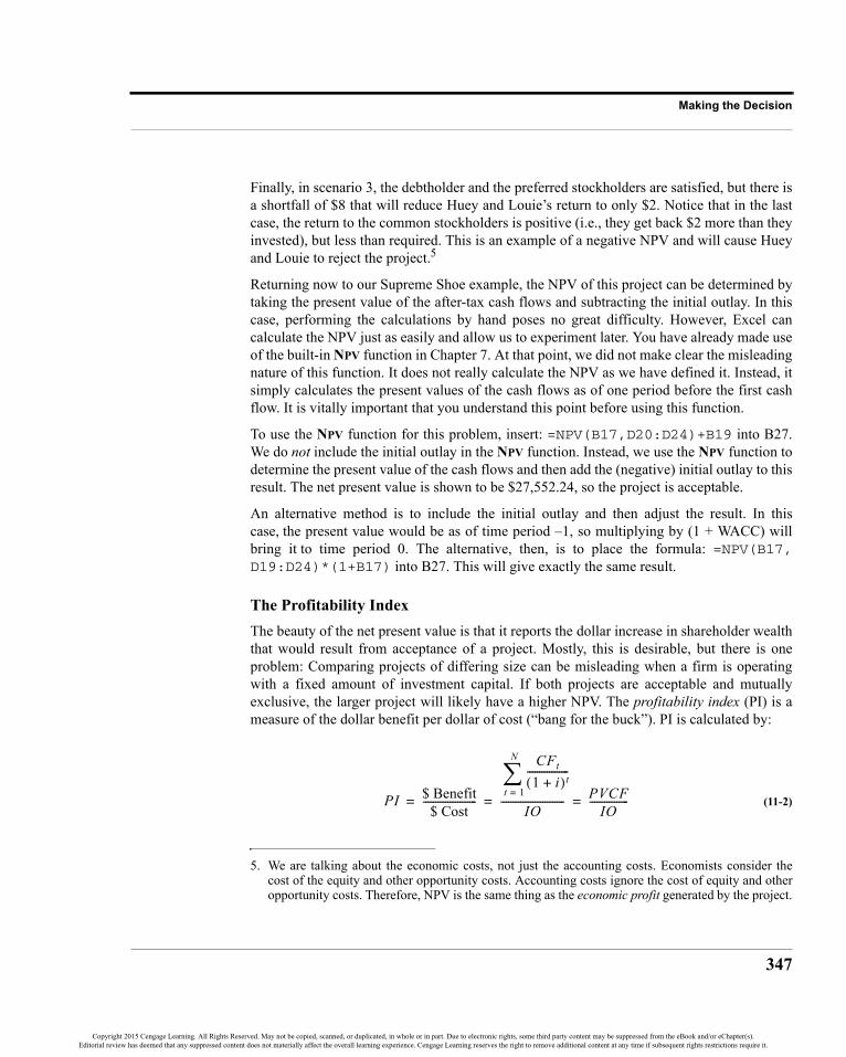
347
Making the Decision
Finally, in scenario 3, the debtholder and the preferred stockholders are satisfied, but there isa shortfall of $8 that will reduce Huey and Louie’s return to only $2. Notice that in the lastcase, the return to the common stockholders is positive (i.e., they get back $2 more than theyinvested), but less than required. This is an example of a negative NPV and will cause Hueyand Louie to reject the project.5
Returning now to our Supreme Shoe example, the NPV of this project can be determined bytaking the present value of the after-tax cash flows and subtracting the initial outlay. In thiscase, performing the calculations by hand poses no great difficulty. However, Excel cancalculate the NPV just as easily and allow us to experiment later. You have already made useof the built-in NPV function in Chapter 7. At that point, we did not make clear the misleadingnature of this function. It does not really calculate the NPV as we have defined it. Instead, itsimply calculates the present values of the cash flows as of one period before the first cashflow. It is vitally important that you understand this point before using this function.
To use the NPV function for this problem, insert: =NPV(B17,D20:D24)+B19 into B27.We do not include the initial outlay in the NPV function. Instead, we use the NPV function todetermine the present value of the cash flows and then add the (negative) initial outlay to thisresult. The net present value is shown to be $27,552.24, so the project is acceptable.
An alternative method is to include the initial outlay and then adjust the result. In thiscase, the present value would be as of time period –1, so multiplying by (1 + WACC) willbring it to time period 0. The alternative, then, is to place the formula: =NPV(B17,D19:D24)*(1+B17) into B27. This will give exactly the same result.
The Profitability IndexThe beauty of the net present value is that it reports the dollar increase in shareholder wealththat would result from acceptance of a project. Mostly, this is desirable, but there is oneproblem: Comparing projects of differing size can be misleading when a firm is operatingwith a fixed amount of investment capital. If both projects are acceptable and mutuallyexclusive, the larger project will likely have a higher NPV. The profitability index (PI) is ameasure of the dollar benefit per dollar of cost (“bang for the buck”). PI is calculated by:
(11-2)
5. We are talking about the economic costs, not just the accounting costs. Economists consider thecost of the equity and other opportunity costs. Accounting costs ignore the cost of equity and otheropportunity costs. Therefore, NPV is the same thing as the economic profit generated by the project.
PI $ Benefit$ Cost
----------------------
CFt
1 i+( )t-----------------
t 1=
N
∑IO
-------------------------- PVCFIO
----------------= = =
Copyright 2015 Cengage Learning. All Rights Reserved. May not be copied, scanned, or duplicated, in whole or in part. Due to electronic rights, some third party content may be suppressed from the eBook and/or eChapter(s).Editorial review has deemed that any suppressed content does not materially affect the overall learning experience. Cengage Learning reserves the right to remove additional content at any time if subsequent rights restrictions require it.

CHAPTER 11: Capital Budgeting
348
As indicated in the equation, the benefit is calculated as the present value of the after-tax cash flows and the cost is the initial outlay. Obviously, if the PI is greater than orequal to 1, the project is acceptable because the benefits exceed, or at least equal, thecosts. Otherwise, the benefits are less than the costs and the project would be rejected.The profitability index will always result in the same accept/reject answer as NPV.
There are two ways that we can calculate the PI in Excel. The most apparent is to use theNPV function and to divide that result by the initial outlay. In other words, in B28 type:=NPV(B17,D20:D24)/-B19. This will give 1.4396 as the result, indicating that theproject is acceptable. The alternative is to make use of the following relationship:
NPV = PVCF – IO
Or by rearranging we get:
PVCF = NPV + IO
Therefore, because we have already calculated the NPV in B27, we can calculate the PIwith: =(B27-B19)/-B19. This method will be slightly faster because Excel doesn’t haveto recalculate the present values. In all but the largest problems, the increase in speedprobably won’t be noticeable on a PC, but the technique is especially helpful when doingproblems by hand.
The Internal Rate of ReturnThe internal rate of return (IRR) provides a measure of the compound average annual rate ofreturn that a project will provide. If the IRR equals, or exceeds, the required return for aproject, the project will be accepted. Because it is a measure of the percentage return, manyanalysts prefer it to the other methods that we have discussed, but there are problems withthe IRR.
The IRR is the discount rate that makes the net present value equal to zero. An alternative,but equivalent, definition is that the IRR is the discount rate that equates the present value ofthe cash flows to the initial outlay. In other words, the IRR is the discount rate that makes thefollowing equality hold:
(11-3)
Unfortunately, in most cases there is no closed-form method for solving for the IRR. Theprimary method of solving this equation is an iterative trial-and-error approach. Althoughthis may sound tedious, generally a solution can be found within three or four iterations if
IOCFt
1 IRR+( )t-------------------------
t 1=
N
∑=
Copyright 2015 Cengage Learning. All Rights Reserved. May not be copied, scanned, or duplicated, in whole or in part. Due to electronic rights, some third party content may be suppressed from the eBook and/or eChapter(s).Editorial review has deemed that any suppressed content does not materially affect the overall learning experience. Cengage Learning reserves the right to remove additional content at any time if subsequent rights restrictions require it.
349
Making the Decision
some intelligence is used. However, there is little need for this procedure because Excel hasa built-in function that performs this operation.
The built-in RATE function in Excel will find the IRR for an annuity type of cash flowstream, but it cannot accept a series of uneven cash flows. To deal with uneven cash flows,Excel provides the IRR function that is defined as:
IRR(VALUES, GUESS)
where VALUES is the contiguous range of cash flows and GUESS is the optional initialguess at the true IRR. The cash flow stream must include at least one negative cash flow,or else the IRR would be infinite (why?). Because solving for the IRR is an iterativeprocess, it is possible that Excel will not converge to a solution. Excel will indicate thissituation by displaying #NUM! in the cell rather than an answer. If this error occurs, onepossible solution is to change your GUESS until Excel can converge to a solution.
To calculate the IRR for the Supreme Shoe example, enter: =IRR(D19:D24) into B29.The result is 30.95%, which is greater than the WACC of 15%. So the project is acceptable.
At this point, let’s try an experiment to prove our definition of the IRR. Recall that the IRRwas defined as the discount rate that makes the NPV equal zero. To prove this, temporarilychange the value in B17 to: =B29. Notice that the net present value in B27 changes to $0.00,which proves the point. Note also that the profitability index changes to 1.00. Beforecontinuing, change the required return back to its original value of 15%.
Problems with the IRRThe internal rate of return is a popular profitability measure because, as a percentage, it iseasy to understand and easy to compare to the required return. However, the IRR suffersfrom several problems that could potentially lead to less-than-optimal decisions. In thissection, we will discuss these difficulties and solutions where they exist.
Earlier, we mentioned that the NPV will almost always lead you to the economically correctdecision. Unfortunately, the IRR and NPV will not always lead to the same decision whenprojects are mutually exclusive. Mutually exclusive projects are those where the selection ofone project precludes the acceptance of another. When projects being compared are mutuallyexclusive, a ranking conflict may arise between the NPV and IRR.6 In other words, the NPVmethod may suggest that Project A be accepted, while the IRR may suggest Project B. If youcan’t select both, which profitability measure do you believe?
6. This is not a problem with independent projects because all independent projects with a positiveNPV (IRR > WACC) will be accepted, so ranking is not required.
Copyright 2015 Cengage Learning. All Rights Reserved. May not be copied, scanned, or duplicated, in whole or in part. Due to electronic rights, some third party content may be suppressed from the eBook and/or eChapter(s).Editorial review has deemed that any suppressed content does not materially affect the overall learning experience. Cengage Learning reserves the right to remove additional content at any time if subsequent rights restrictions require it.

CHAPTER 11: Capital Budgeting
350
There are two causes of this type of problem: (1) The projects are of greatly different sizes;or (2) the timing of the cash flows is different. To see the size problem more clearly, considerthe following question: “Would you rather earn a 100% return on a $10 investment (Project A),or a 10% return on a $1,000 investment (Project B)?” Obviously, most of us would bemore concerned with the dollar amounts and would choose the 10% return because thatwould provide $100 versus only $10 in the other case. The solution to this problem isactually quite simple. If you can raise $1,000 for Project B, then the correct comparison isnot between A and B, but between B and A plus whatever you could do with the other $990(call it Project C) that is available if you choose Project A. If Project C would return 10%,then you could earn $109 by investing in both A and C, which is preferable to investing in B.
The timing problem is more difficult to deal with. Suppose you are given the task ofevaluating the two mutually exclusive projects in Table 11-4, with a 10% required return.
Which would you choose? Obviously there is a conflict because Project A would be selectedunder the NPV criteria, but Project B would be selected by the IRR criteria. We can use logicsimilar to that used for the size problem to see that NPV is the correct criteria. If Project B isaccepted, we must reject Project A and the differential cash flows (Project C). If thedifferential cash flows provide a positive NPV, then they should not be rejected. In effect,what we are arguing is that Project A is equivalent to Project B plus the differential cashflows. So choosing between these projects is effectively deciding whether the differentialcash flows are profitable or not. Conveniently, all that we really need to do is accept theproject with the highest NPV. Note that Project A would be preferred as long as the discountrate is less than 12.48%. At higher discount rates, Project B would be preferred. A usefultool for these kinds of problems is the NPV profile chart, which is introduced on page 354.
TABLE 11-4CASH FLOW TIMING CAN CAUSE A RANKING CONFLICT
Period Project A Project BProject C(= A – B)
0 (1,000) (1,000) 01 0 400 (400)2 200 400 (200)3 300 300 04 500 300 2005 900 200 700
NPV $291.02 $248.70 $42.32IRR 17.32% 20.49% 12.48%
Copyright 2015 Cengage Learning. All Rights Reserved. May not be copied, scanned, or duplicated, in whole or in part. Due to electronic rights, some third party content may be suppressed from the eBook and/or eChapter(s).Editorial review has deemed that any suppressed content does not materially affect the overall learning experience. Cengage Learning reserves the right to remove additional content at any time if subsequent rights restrictions require it.

351
Making the Decision
Yet another problem with the IRR is that there may be more than one IRR. Specifically,because the general equation for the IRR is an Nth degree polynomial, it will potentiallyhave as many as N solutions. In the usual case, where there is one cash outflow followed byseveral inflows, there will be only one solution. However, when there are net cash outflowsin the outlying periods (nonnormal cash flows), we may be able to find more than onesolution. In particular, there can be, at most, one real solution per sign change in the cashflow stream.7
FIGURE 11-3NONNORMAL CASH FLOWS MAY HAVE MULTIPLE IRRS
Consider, as an example, the cash flows depicted in Figure 11-3. Solving for the IRR in thisexample will lead to three solutions: 207.82%, –31.54%, and –76.27%. The answer that youget from Excel will depend on the initial GUESS that you supply. If you don’t provide Excelwith a GUESS, it will give –31.54% as the answer. Any GUESS of 11.8% or greater will get ananswer of 207.82%, and a guess of –68.35% will get an answer of –76.27%. It is impossibleto say which of these answers is correct because all will result in an NPV of zero if used asthe discount rate (try it!). So, even though these IRRs are mathematically correct, they haveno economic meaning. The IRR should be ignored whenever there are multiple results.
The Modified Internal Rate of ReturnAn easy solution to the problems of the IRR is to simply use the NPV instead. This is notlikely to please everyone, however. Despite its problems, executives continue to prefer theIRR to the NPV because, as a percentage, it is easy to compare to the firm’s cost of capital.To understand how we can use an IRR-type calculation and still arrive at correct answersrequires that you understand the root cause of the problems with the IRR.
Implicit in the calculation of the IRR is the assumption that the cash flows are reinvested atthe IRR. In other words, the IRR method assumes that as each cash flow is received, it isreinvested for the remaining life of the project at a rate that is the same as the IRR.8 Forprojects with a very high or very low IRR, this assumption is likely to be violated. If the cashflows are reinvested at some other rate, the actual average annual rate of return will bedifferent than the IRR. To see this assumption at work, consider again our Supreme Shoe
7. The interested reader is advised to study Descartes’ Rule of Signs.8. This also explains why we cannot solve directly for the IRR: We must know the IRR to know the
reinvestment rate, and without knowing the reinvestment rate we can’t solve for the IRR.
Copyright 2015 Cengage Learning. All Rights Reserved. May not be copied, scanned, or duplicated, in whole or in part. Due to electronic rights, some third party content may be suppressed from the eBook and/or eChapter(s).Editorial review has deemed that any suppressed content does not materially affect the overall learning experience. Cengage Learning reserves the right to remove additional content at any time if subsequent rights restrictions require it.

CHAPTER 11: Capital Budgeting
352
project. The timeline is pictured in Figure 11-4 with the explicit reinvestment of the cashflows at the IRR of 30.945%.
FIGURE 11-4SUPREME SHOE CASH FLOWS WITH EXPLICIT REINVESTMENT AT THE IRR
Assuming that the cash flows are reinvested at 30.945% per year, at the end of year 5Supreme Shoe will have accumulated $241,310 from its original investment of $62,680. Thecompound average annual return, then, must be:
which is exactly the same as the IRR. Note that we have used the geometric mean, equation(1-1) from Chapter 1, though you could use the RATE function.
It seems unlikely that Supreme Shoe can earn a rate this high over a five-year period. If wechange the reinvestment rate to a more reasonable 15% (the WACC), then we have thetimeline in Figure 11-5.
FIGURE 11-5SUPREME SHOE CASH FLOWS WITH EXPLICIT REINVESTMENT AT 15%
In this case, Supreme Shoe will have accumulated only $181,489 by the end of the fifth year.Its average annual rate of return with a 15% reinvestment rate will be:
241,31062,680
-------------------5 1 30.945%≈–
181,48962,680
-------------------5 1 23.69%≈–
Copyright 2015 Cengage Learning. All Rights Reserved. May not be copied, scanned, or duplicated, in whole or in part. Due to electronic rights, some third party content may be suppressed from the eBook and/or eChapter(s).Editorial review has deemed that any suppressed content does not materially affect the overall learning experience. Cengage Learning reserves the right to remove additional content at any time if subsequent rights restrictions require it.

353
Making the Decision
which is substantially lower than the 30.95% IRR. When we calculate the average annualreturn with a reinvestment rate that is different than the IRR, we refer to it as the modifiedinternal rate of return, or MIRR. For Supreme Shoe, the MIRR is 23.69%, which is greaterthan the required return of 15%, so the project should be accepted.
Excel has a built-in function to calculate the MIRR. The function is defined as:
MIRR(VALUES, FINANCE_RATE, REINVEST_RATE)
where VALUES is the range of cash flows, FINANCE_RATE is the required rate of return, andREINVEST_RATE is the rate at which the cash flows are to be reinvested. To calculate theMIRR in your Supreme Shoe worksheet, enter: =MIRR(D19:D24,B17,B17) into B30.Exactly as we calculated earlier, the answer is 23.69%. In this example, we have used thesame rate for the required return and the reinvestment rate. This is normally the appropriateassumption to make (it is the same assumption that is implicit within the NPV calculation).But if you have other information that suggests a different reinvestment rate, then thatdifferent rate should be used.
An alternative calculation method shows the relationship between the profitability index(and therefore the NPV) and the MIRR:9
(11-4)
So, for this example we have:
This method will not give the same answer as Excel’s MIRR function if you have nonnormalcash flows, given the way that we have defined PI [see equation (11-2) on page 347]. That isbecause there is more than one methodology for calculating MIRR and PI when you havecash outflows after the initial outlay. Excel calculates the MIRR by finding the discount ratethat equates the present value of the outflows to the future value of the cash inflows.
The methodology used in equation (11-4) is different from the one used by Excel. It finds thediscount rate that equates the initial outlay to the future value of all other cash flows,regardless of the sign. This methodology, while different, is just as valid and is preferred bysome (your author included). Both methodologies will give the same accept/reject decision(though different numbers for nonnormal cash flows), and this useful equation will alwaysgive the same answer as Excel’s MIRR function when you have normal cash flows.
9. See T. Arnold and T. Nixon, “An Easy Method to Introduce MIRR into Introductory Finance,”Advances in Financial Education, Vol 11 (2013), pp. 70–74.
MIRR PIN 1 WACC+( ) 1–× NPVIO
------------ 1+⎝ ⎠⎛ ⎞
N 1 WACC+( ) 1–×= =
MIRR 1.43965 1.15 1–× 0.2369= =
Copyright 2015 Cengage Learning. All Rights Reserved. May not be copied, scanned, or duplicated, in whole or in part. Due to electronic rights, some third party content may be suppressed from the eBook and/or eChapter(s).Editorial review has deemed that any suppressed content does not materially affect the overall learning experience. Cengage Learning reserves the right to remove additional content at any time if subsequent rights restrictions require it.

CHAPTER 11: Capital Budgeting
354
Sensitivity and Scenario AnalysisProbably the most important benefit of using a spreadsheet program is that it allows us toplay “what-if” games with the data. That is, we can experiment with different values todetermine how our results would change if there are changes in the assumptions.
NPV Profile Charts
One useful technique that we can use is referred to as the NPV profile. This is simply a chartof the NPV at various discount rates. The analyst can determine, at a glance, how sensitivethe NPV is to the assumed discount rate. To create an NPV profile chart, we merely set up arange of discount rates and NPV calculations and then create a chart.
To create an NPV profile chart for Supreme Shoe, let’s create a range of discount rates from0% to 35% in 5% increments. Move to cell A36 and enter: 0. To create the range of discountrates, select A36:A43 and then click Fill on the Home tab and then choose Series. In thedialog box, change the Step Value to: 0.05 (you could type 5% instead) and then click theOK button. You should now have a range of discount rates from 0% to 35%. We will usethese rates in our NPV calculations.
To calculate the NPV at each discount rate, enter: =NPV(A36,D$20:D$24)+D$19 inB36. This is exactly the same formula as in B27, except that we have added a few dollarsigns to freeze the references and we changed the discount rate to reference A36. Copyingthis formula to B37:B43 will calculate the NPV at each discount rate. Note that the NPVbecomes negative at a discount rate somewhere between 30% and 35%. Of course, we knewthis already because the IRR is 30.95%. Finally, to create the chart select the A36:B43 andinsert a scatter chart with straight lines. Your worksheet should now resemble Exhibit 11-5.
EXHIBIT 11-5NPV PROFILE FOR SUPREME SHOE
Copyright 2015 Cengage Learning. All Rights Reserved. May not be copied, scanned, or duplicated, in whole or in part. Due to electronic rights, some third party content may be suppressed from the eBook and/or eChapter(s).Editorial review has deemed that any suppressed content does not materially affect the overall learning experience. Cengage Learning reserves the right to remove additional content at any time if subsequent rights restrictions require it.

355
Sensitivity and Scenario Analysis
Observe that the chart clearly shows the IRR is just over 30%. This is the point where theNPV line crosses the x-axis of the NPV profile chart. Furthermore, it is obvious that for anydiscount rate below 30% the project has a positive NPV; thus it is acceptable. In fact, it isobviously acceptable at any reasonable discount rate.
Typically, an NPV profile chart is used to compare two mutually exclusive projects.Whenever there is a ranking conflict, the NPV profiles will cross at a rate at which the firmwould be indifferent between the two projects. You can try this by entering the data forprojects A and B from Table 11-4 and then creating an NPV profile chart for the projects.
FIGURE 11-6NPV PROFILE CHART FOR TWO PROJECTS
This “crossover rate,” where the NPVs are the same, can be found by calculating the IRR ofthe difference between the cash flows of the two projects. If you placed the cash flows forthe projects into B2:C7, then this formula will calculate the crossover rate: =IRR(B2:B7–C2:C7). Note that this is the rate found in the lower right corner of Table 11-4 on page 350.
Scenario AnalysisExcel contains a very powerful tool called the Scenario Manager that helps in analyzing theeffects of different assumptions. Scenario Manager can be used to toggle your worksheetbetween various alternative scenarios, or it can create a summary of the effects of changingthe assumptions. We will create three scenarios in which the estimates of maintenance anddefect costs are different than expected. The three scenarios are listed in Table 11-5.
TABLE 11-5THREE POSSIBLE SCENARIOS FOR SUPREME SHOE
Best Case Expected Case Worst CaseMaintenance $ 2,000 $ 5,000 $ 8,000Defects 1,000 2,000 5,000
Copyright 2015 Cengage Learning. All Rights Reserved. May not be copied, scanned, or duplicated, in whole or in part. Due to electronic rights, some third party content may be suppressed from the eBook and/or eChapter(s).Editorial review has deemed that any suppressed content does not materially affect the overall learning experience. Cengage Learning reserves the right to remove additional content at any time if subsequent rights restrictions require it.

CHAPTER 11: Capital Budgeting
356
In the Best Case scenario, both maintenance and defects are lower than those in the ExpectedCase (which represents the original estimates). In the Worst Case, both are higher thanexpected. Because we are going to be changing our assumed values for maintenance anddefects, it will be helpful to first define range names for these cells. Select C14 and thenclick the Formulas tab and choose Define Name. Assign the name Maintenance to thiscell, give a worksheet-level scope, and enter a comment about its purpose. Now define thename Defects for cell C15 (see page 9 for a discussion of named ranges).
The Scenario Manager can be found by clicking the What-If Analysis button on the Data tab.Because no scenarios are defined at this point, the first dialog box will ask you to click theAdd button to define your scenarios. In this case, we want the maintenance and defectestimates to change, so click the Add button and then enter: Best Case for the scenarioname. Click in the Changing cells edit box, highlight cells C14:C15, and then click the OKbutton.
The next dialog box will ask you to supply the new values for the changing cells like inFigure 11-7. In the edit box labeled “Maintenance:” enter: 2000 and in the edit box labeled“Defects:” type: 1000. Note that this dialog box prompts you for the values using the namesthat we earlier defined for these cells. If you didn’t define the names, then you will beprompted with the cell addresses instead of names.
FIGURE 11-7THE SCENARIO VALUES DIALOG BOX
Click the Add button to enter the next scenario. Now, repeat these steps for the other twocases using the names “Expected Case” and “Worst Case” and the appropriate values fromTable 11-5.
Figure 11-8 shows how the dialog box will look when you have entered all three scenarios.
At this point, you can change the worksheet to display the scenario of your choice byhighlighting the name of the case and clicking the Show button. For example, if youhighlight “Worst Case” and click the Show button, the maintenance and defect cells willchange and the worksheet will update. You can now see the effects of these changes on thecash flows and profitability measures (e.g., the NPV is $14,277.70 under the Worst Casescenario).
Copyright 2015 Cengage Learning. All Rights Reserved. May not be copied, scanned, or duplicated, in whole or in part. Due to electronic rights, some third party content may be suppressed from the eBook and/or eChapter(s).Editorial review has deemed that any suppressed content does not materially affect the overall learning experience. Cengage Learning reserves the right to remove additional content at any time if subsequent rights restrictions require it.

357
Sensitivity and Scenario Analysis
FIGURE 11-8THE SCENARIO MANAGER
Return to the original data by choosing “Expected Case” from the list and pressing the Showbutton. This type of flexibility is one of the promised results of proper worksheet design.Scenario analysis will not work properly unless you are diligent about using formulas, ratherthan retyping values, whenever possible.
It would be nice to see a summary of the different scenarios, and we can do just that. Butfirst, exit from the Scenario Manager and define a name for each cell in B25:B30 so that theoutput will be easier to understand. Now, bring back the Scenario Manager and click theSummary button. When the Scenario Summary dialog box appears, select cells B25:B30 forthe Result cells and click OK. Excel will then automatically create a new worksheet thatdisplays the changed values and the resulting profitability measures. Exhibit 11-6 shows thesummary worksheet.
We have defined three simple scenarios, but other problems may require more scenarios ormore changing variables. You can define as many scenarios as your PC’s memory will hold,but only the first 251 will be displayed on the scenario summary worksheet. There is also alimit of 32 changing cells per scenario. Note that you can safely delete the “Current Values”column since it shows the same data as our “Expected Case.” It is a good idea to alwaysdefine a scenario that uses the default values so that you can easily return the spreadsheet tothe original values.
Copyright 2015 Cengage Learning. All Rights Reserved. May not be copied, scanned, or duplicated, in whole or in part. Due to electronic rights, some third party content may be suppressed from the eBook and/or eChapter(s).Editorial review has deemed that any suppressed content does not materially affect the overall learning experience. Cengage Learning reserves the right to remove additional content at any time if subsequent rights restrictions require it.

CHAPTER 11: Capital Budgeting
358
EXHIBIT 11-6SCENARIO SUMMARY REPORT FOR SUPREME SHOE
The Optimal Capital BudgetHow large a firm’s capital budget should be is a serious problem that confronts financialmanagers. One solution that is often chosen is capital rationing. Capital rationing is thearbitrary limiting of the amount of capital available for investment purposes. This solutionis, in theory, contrary to the goal of the firm. In order to maximize shareholder wealth, thefirm must accept all positive NPV projects. Remember that a positive NPV project is onethat will cover the cost of financing (i.e., the weighted average cost of capital). In effect, apositive NPV project is self-liquidating, so there should be no problem raising the requiredfunds to make the investment. No matter how much must be raised, as long as positive NPVprojects exist, a firm should continue to invest until the cost of investing exceeds the benefitsto be gained.10
Optimal Capital Budget Without Capital RationingWe have seen in the previous chapter that a firm’s weighted average cost of capital willincrease as the amount of capital to be raised increases. We can make use of this fact todetermine exactly what a firm’s optimal capital budget should be in the absence of capitalrationing. Briefly, we rank all projects by their IRR and compare this ranking to the marginalWACC schedule.
10. From your economics classes, recall that to maximize profits a firm should continue to produceuntil the marginal cost equals the marginal revenue. This is the same idea, but in a differentcontext. Furthermore, we are evaluating costs and benefits in present value terms and, as we willsee in Chapter 12, we are taking risk into account.
Copyright 2015 Cengage Learning. All Rights Reserved. May not be copied, scanned, or duplicated, in whole or in part. Due to electronic rights, some third party content may be suppressed from the eBook and/or eChapter(s).Editorial review has deemed that any suppressed content does not materially affect the overall learning experience. Cengage Learning reserves the right to remove additional content at any time if subsequent rights restrictions require it.

359
The Optimal Capital Budget
Recall the Rocky Mountain Motors (RMM) example from Chapter 10, and create a copy ofthe worksheet used for Exhibit 10-6 (page 324). Assume that RMM has found ten potentialnew projects, each of which would be profitable at their current WACC of 10.51% (i.e., allhave IRRs > 10.51%). The projects are listed in Table 11-6.
Enter the data from Table 11-6 into your RMM worksheet beginning with the labels inA22:C22. The cumulative cost can be calculated by entering: =SUM(A$23:A23) into B23and then copying the formula to the other cells. The first step in determining the optimalcapital budget is to sort all of the projects by their IRR. Select A22:C32 and click the Sort &Filter button on the Home tab. Because we want to sort based on the third column (instead ofthe first column, which is the default), we need to choose Custom Sort from the menu.Choose IRR from the “Sort by” list and Largest to Smallest in the Order list. This sorted listof IRRs is known as the Investment Opportunity Schedule (IOS).
Next, we want to add the project IRRs to the marginal WACC chart created earlier (seeExhibit 10-6 on page 324). To add the new data, right-click in the chart area and chooseSelect Data from the shortcut menu. In the dialog box, click on the Add button to create anew data series. For the Series name type: IOS, and then enter B23:B32 for the X Valuesand C23:C32 for the Y Values. Finally, notice that the MCC schedule goes out only to$900,000, but the IOS extends out to over $2,700,000. To fix this, change the value in A20to: 3,000,000. Your worksheet should look like the one in Exhibit 11-7.
TABLE 11-6ROCKY MOUNTAIN MOTORS PROJECTS
Cost Cumulative Cost IRR$445,529 $445,529 15.02%
439,207 884,736 15.87%407,769 1,292,505 16.51%396,209 1,688,714 16.16%271,477 1,960,191 15.38%201,843 2,162,034 11.69%189,921 2,351,955 13.82%146,661 2,498,616 12.19%138,298 2,636,914 11.48%
74,950 2,711,864 13.00%
Copyright 2015 Cengage Learning. All Rights Reserved. May not be copied, scanned, or duplicated, in whole or in part. Due to electronic rights, some third party content may be suppressed from the eBook and/or eChapter(s).Editorial review has deemed that any suppressed content does not materially affect the overall learning experience. Cengage Learning reserves the right to remove additional content at any time if subsequent rights restrictions require it.

CHAPTER 11: Capital Budgeting
360
EXHIBIT 11-7MARGINAL WACC AND THE IOS FOR RMM
As was shown on page 323, we can make the IOS line into a step function. The process isexactly the same as before: We must add additional data points for the cumulative cost andIRR, so that we have two points at each change in the IRR. Once that is finished we cansimply edit the data series by right-clicking the IOS and choosing Select Data from themenu. Now, edit the X and Y data ranges to the new ones. Once complete, your chart shouldlook like the one in Exhibit 11-8.
The optimal capital budget without capital rationing is the level of total capital at which themarginal WACC schedule and the IOS cross. In this case, that would be $1,960,191. In otherwords, the five projects with the highest IRRs should be selected.
EXHIBIT 11-8COMPLETED MCC AND IOS CHART
Copyright 2015 Cengage Learning. All Rights Reserved. May not be copied, scanned, or duplicated, in whole or in part. Due to electronic rights, some third party content may be suppressed from the eBook and/or eChapter(s).Editorial review has deemed that any suppressed content does not materially affect the overall learning experience. Cengage Learning reserves the right to remove additional content at any time if subsequent rights restrictions require it.

361
The Optimal Capital Budget
Optimal Capital Budget Under Capital RationingThough technically irrational, capital rationing is common. How then can we determine theoptimal capital budget in the presence of restricted capital? In this situation, we need to findthe combination of projects that maximizes the total net present value subject to the capitalspending constraint.
This can be a tedious exercise when there are a large number of positive NPV projects fromwhich to choose. For example, assume that we have four positive NPV projects available. Ata minimum we must select one project, but we can select up to four. If we look at everypossible combination of these four projects, then we will examine 16 possible combinations.As the number of projects grows, the number of combinations grows even faster. In general,there are 2N possible combinations, where N is the number of positive NPV projects. Notethat negative NPV projects are excluded from this calculation and further considerationbecause we cannot increase the total NPV by adding a negative NPV project.11
Excel provides a tool called the Solver that can be used in any type of constrainedmaximization or minimization problem. The Solver provides a dialog box in which youspecify a cell to be optimized, the cells that may be changed, and the constraints under whichthe Solver must operate. It then finds the optimal solution. Let’s look at an example.
Because of declining demand for high-pressure frammis valves, theFrammis Valve Corporation of America (FVCA) is considering expandinginto a number of other businesses. The managers of FVCA havedetermined that it has 13 potential new investments (see Exhibit 11-9).The total cost of these investments would be $7,611,990, but they arelimited to a maximum total investment of only $3,000,000. Your job is todetermine the combination of the projects the company should choose.
Because there are 13 acceptable projects, you will have to examine each of the 8,192 (= 213)possible combinations and determine which provides the highest total NPV, while keepingthe total cost less than $3,000,000. This problem is obviously going to be time consuming ifyou have to do it by hand. Enter the data from Exhibit 11-9 into a new worksheet beginningin cell A4.
To solve this problem, we need a way to determine the sum of the costs and NPVs for onlythose projects that are selected. Because each project will either be selected or not, this is aperfect use for a binary variable. A binary variable can take on one of two values, mostcommonly 0 or 1. We will set up a column with 0s and 1s, where 1 indicates that a project isselected, and 0 indicates rejection. Your worksheet should resemble that in Exhibit 11-9.
11. Strictly speaking, this is not always true. Under a multi-period capital budgeting scenario withmulti-period cash flow constraints, it is possible that adding negative NPV projects could increasethe total NPV if they provide needed cash flows at the right time.
Copyright 2015 Cengage Learning. All Rights Reserved. May not be copied, scanned, or duplicated, in whole or in part. Due to electronic rights, some third party content may be suppressed from the eBook and/or eChapter(s).Editorial review has deemed that any suppressed content does not materially affect the overall learning experience. Cengage Learning reserves the right to remove additional content at any time if subsequent rights restrictions require it.

CHAPTER 11: Capital Budgeting
362
EXHIBIT 11-9FVCA’S CAPITAL BUDGETING PROBLEM
Note that we have initially set each cell in D4:D16 to 1. Due to the nature of the problem, wecannot use an ordinary SUM function to total columns B and C. Recall that we want only thesum of the costs and NPVs of the projects that are to be selected. There are several ways todo this, but we will use array formula.12
An array formula is one that operates on each element in a range, but without specifyingeach element separately. Array formulas are therefore easier to write and save space. Tocalculate the total cost of the accepted projects in B17, we want to write a formula thatmultiplies the costs in column B by the corresponding 0 or 1 in column D and keeps arunning total of the results. One way to do this is to write a formula such as: =B4*D4 +B5*D5 + B6*D6… However, this would be a long formula to enter. The equivalent arrayformula would be: =Sum(B4:B16*$D4:$D16). This is much shorter and easier tounderstand.
Excel will not understand this formula unless you enter it in a specific way. You must enterarray formulas with the Shift+Ctrl+Enter key combination. After correctly entering an arrayformula, it will appear in the formula bar surrounded by a pair of curly braces ({}). The
12. We could also use the SUMIF or SUMPRODUCT functions.
Copyright 2015 Cengage Learning. All Rights Reserved. May not be copied, scanned, or duplicated, in whole or in part. Due to electronic rights, some third party content may be suppressed from the eBook and/or eChapter(s).Editorial review has deemed that any suppressed content does not materially affect the overall learning experience. Cengage Learning reserves the right to remove additional content at any time if subsequent rights restrictions require it.

363
The Optimal Capital Budget
formula in B17 will be displayed as: {=SUM(B4:B16*$D4:$D16)}. Note that you do nottype the braces. They are only displayed as an indicator that the formula is an array formula.If you see a #VALUE! error in B17, then you probably did not hold down Shift+Ctrl whenpressing the Enter key. Copy the formula from B17 to C17, and your totals should be thesame as those in Exhibit 11-9.
To restate the problem, we want to maximize the total NPV in C17 by changing the cells inD4:D16 subject to two constraints. The first constraint is that the total cost, in B17, must beless than or equal to 3,000,000. Next we must constrain the values in D4:D16 to be either 0or 1, but they cannot take on any noninteger values (i.e., they must be binary values).
Launch the Solver from the Analysis group on the Data tab.13 In the Set Target Cell edit boxenter: C17 and then click on the Max radio button. This tells the Solver that we want tomaximize the function in C17. Note that, under different circumstances, we could alsominimize this formula or force it to a specific value. Next we need to tell Solver which cellsit may change to find a solution. In the By Changing Cells edit box enter: D4:D16.
The hardest part of solving many optimization problems is setting up the appropriateconstraints. In this problem we have two constraints, and it will take only two statements tofully specify them. In other cases, it may take more than one statement to fully specify asingle constraint. To add a constraint, click on the Add button. This will bring up a seconddialog box in which we can enter a cell reference (or range) and the constraint. Note that thedialog box contains a drop-down list in the center that describes the possible relationships.These are <=, =, >=, int, bin, and dif. The last three are all integer constraints. “int” tells theSolver that the values in the cells must be an integer, and “bin” that they must be either 0 or1. “dif” is a type of integer constraint that allows you to specify that all cells in the rangemust be different.
Add the first constraint by entering B17 in the Cell Reference edit box, select <=, and enterB18 in the constraint exit box. This will make sure that the total cost is less than the$3,000,000 constraint. For the second constraint, we must constrain the cells in D4:D16 tobe binary (0 or 1). Add this constraint and the problem is almost ready to solve.
Because of the large number of possible solutions, the default configuration of the Solvermay not find the solution, or it may find a less than optimal solution. In the main Solverdialog box choose the Simplex LP method because this is a linear programming problem.Now, click on the Options button. This will bring up another dialog box containing theoptions that you can set. Most of these are beyond the scope of this text. Set the Max Time toat least 500 seconds (higher if you have a very slow PC) and Iterations to at least 500. Thesetwo options control how long the Solver will try to solve the problem (they are maximums,
13. If you don’t see the Solver button, then you need to activate the Solver add-in. Click the File taband then click Options. You can activate Solver from the Add-Ins section.
Copyright 2015 Cengage Learning. All Rights Reserved. May not be copied, scanned, or duplicated, in whole or in part. Due to electronic rights, some third party content may be suppressed from the eBook and/or eChapter(s).Editorial review has deemed that any suppressed content does not materially affect the overall learning experience. Cengage Learning reserves the right to remove additional content at any time if subsequent rights restrictions require it.

CHAPTER 11: Capital Budgeting
364
and Solver will stop as soon as it finds the solution). Because our binary constraint is reallyan integer constraint, make sure that Ignore Integer Constraints is not checked and thatInteger Optimality (%) is set to 0. The latter is a convergence tolerance requirement and thedefault of 5% is too loose to find the optimal solution in the problem.
FIGURE 11-9THE SOLVER DIALOG BOX
Finally, to start the Solver working on the problem click the Solve button. When Solver findsthe solution, it will present you with a dialog box that asks if you would like to save thesolution or return to the original values. If you choose to save the optimal solution, yourworksheet will resemble the one in Exhibit 11-10. Note that projects A, C, D, F, H, and L areselected; we know this because they have a 1 in the Include column.
One final point about the Solver: You can easily change the constraint of $3,000,000 to anyother value and then run the Solver again. Because the Solver settings are saved, you do notneed to reenter the data every time.
Copyright 2015 Cengage Learning. All Rights Reserved. May not be copied, scanned, or duplicated, in whole or in part. Due to electronic rights, some third party content may be suppressed from the eBook and/or eChapter(s).Editorial review has deemed that any suppressed content does not materially affect the overall learning experience. Cengage Learning reserves the right to remove additional content at any time if subsequent rights restrictions require it.

365
The Optimal Capital Budget
EXHIBIT 11-10THE OPTIMAL SOLUTION FOR THE FVCA CAPITAL BUDGET
Once the optimal solution is found you can save it as a named scenario and then use theScenario Analysis tool to view all of the different scenarios. For example, we could createscenarios with total investment constraints of $3 million, $5 million, and $7 million. Onceyou’ve run the Solver with each of those constraints, choose What-If Analysis from the Datatab and view the scenarios. You can also create a scenario summary as shown in Exhibit 11-11. In this case, we have edited the worksheet a bit to label the result cells (B17:D17) andhidden the changing cells to improve readability.
EXHIBIT 11-11SCENARIO SUMMARY FOR OPTIMAL CAPITAL BUDGETING PROBLEM
Copyright 2015 Cengage Learning. All Rights Reserved. May not be copied, scanned, or duplicated, in whole or in part. Due to electronic rights, some third party content may be suppressed from the eBook and/or eChapter(s).Editorial review has deemed that any suppressed content does not materially affect the overall learning experience. Cengage Learning reserves the right to remove additional content at any time if subsequent rights restrictions require it.

CHAPTER 11: Capital Budgeting
366
Other TechniquesFor those who don’t have a computer or the skills required to maximize the total NPV, othertechniques can be used to approximate the optimal capital budget. The first is to select theprojects with the highest profitability indices. You may have to discard some high PIprojects, and you will likely not achieve the maximum NPV, but the solution can often befound with less work than maximizing NPV. As an alternative, we could choose the projectswith the highest IRRs. However, this could be misleading if the projects are of greatlydifferent sizes (as in the RMM example).
SummaryCapital budgeting is one of the most important functions of the corporate financial manager.In this chapter, we have seen how to calculate the relevant cash flows and how to evaluatethose cash flows to determine the profitability of accepting the project. We havedemonstrated six profitability measures that are summarized in Table 11-7.
In addition, we introduced the Scenario Analysis and Solver tools provided by Excel. TheScenario Analysis tool allows us to easily compare the outcomes based on various inputs.The Solver allows us to find optimal values for a cell in a model.
TABLE 11-7SUMMARY OF PROFITABILITY MEASURES
Profitability Measure Acceptance CriteriaPayback Period <= Maximum allowable periodDiscounted Payback <= Maximum allowable periodNet Present Value >= 0Profitability Index >= 1Internal Rate of Return >= WACCModified IRR >= WACC
Copyright 2015 Cengage Learning. All Rights Reserved. May not be copied, scanned, or duplicated, in whole or in part. Due to electronic rights, some third party content may be suppressed from the eBook and/or eChapter(s).Editorial review has deemed that any suppressed content does not materially affect the overall learning experience. Cengage Learning reserves the right to remove additional content at any time if subsequent rights restrictions require it.
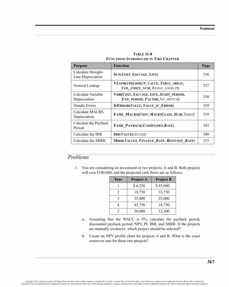
367
Problems
Problems
1. You are considering an investment in two projects, A and B. Both projectswill cost $100,000, and the projected cash flows are as follows:
a. Assuming that the WACC is 8%, calculate the payback period,discounted payback period, NPV, PI, IRR, and MIRR. If the projectsare mutually exclusive, which project should be selected?
b. Create an NPV profile chart for projects A and B. What is the exactcrossover rate for these two projects?
TABLE 11-8FUNCTIONS INTRODUCED IN THIS CHAPTER
Purpose Function PageCalculate Straight-Line Depreciation SLN(COST, SALVAGE, LIFE) 336
Vertical Lookup VLOOKUP(LOOKUP_VALUE, TABLE_ARRAY, COL_INDEX_NUM, RANGE_LOOKUP) 337
Calculate Variable Depreciation
VDB(COST, SALVAGE, LIFE, START_PERIOD, END_PERIOD, FACTOR, NO_SWITCH) 338
Handle Errors IFERROR(VALUE, VALUE_IF_ERROR) 339Calculate MACRS Depreciation FAME_MACRS(COST, MACRSCLASS, YEAR, TABLE) 339
Calculate the Payback Period FAME_PAYBACK(CASHFLOWS,RATE) 343
Calculate the IRR IRR(VALUES,GUESS) 349Calculate the MIRR MIRR(VALUES, FINANCE_RATE, REINVEST_RATE) 353
Year Project A Project B1 $ 6,250 $ 45,0002 18,750 33,7503 35,000 25,0004 43,750 18,7505 50,000 12,500
Copyright 2015 Cengage Learning. All Rights Reserved. May not be copied, scanned, or duplicated, in whole or in part. Due to electronic rights, some third party content may be suppressed from the eBook and/or eChapter(s).Editorial review has deemed that any suppressed content does not materially affect the overall learning experience. Cengage Learning reserves the right to remove additional content at any time if subsequent rights restrictions require it.

CHAPTER 11: Capital Budgeting
368
2. The Ocean City water park is considering the purchase of a new log flumeride. The cost to purchase the equipment is $3,500,000, and it will cost anadditional $250,000 to have it installed. The equipment has an expectedlife of 6 years, and it will be depreciated using a MACRS 7-year class life.Management expects to run about 150 rides per day, with each rideaveraging 25 riders. The season will last for 120 days per year. In the firstyear, the ticket price per rider is expected to be $4.00, and it will beincreased by 4% per year. The variable cost per rider will be $1.40, andtotal fixed costs will be $320,000 per year. After six years, the ride will bedismantled at a cost of $115,000 and the parts will be sold for $450,000.The cost of capital is 12%, and its marginal tax rate is 35%.
a. Calculate the initial outlay, annual after-tax cash flow for each year,and the terminal cash flow.
b. Calculate the NPV, IRR, and MIRR of the new equipment. Is theproject acceptable?
c. Create a Data Table that shows the NPV, IRR, and MIRR for MACRSclasses of 3, 5, 7, 10, 15, and 20 years. What do you conclude aboutthe speed of depreciation and the profitability of an investment?
d. Using the Goal Seek tool, calculate the minimum ticket price thatmust be charged in the first year in order to make the projectacceptable.
3. Arroy Snackfoods is considering replacing a five-year-old machine thatoriginally cost $50,000. It was being depreciated using straight-line to anexpected salvage value of zero over its original 10-year life, and couldnow be sold for $40,000. The replacement machine would cost $190,000and have a five-year expected life. It would be depreciated using theMACRS 5-year class life. The actual expected salvage value of thismachine after 5 years is $20,000. The new machine is expected to operatemuch more efficiently, saving $10,000 per year in energy costs. Inaddition, it will eliminate one salaried position saving another $45,000annually. The firm’s marginal tax rate is 35% and the WACC is 9%.
a. Set up an operating cash flow statement, and calculate the payback,discounted payback, NPV, IRR, and MIRR of the replacementproject. Should the project be accepted?
b. At what discount rate would you be indifferent between keeping theexisting equipment and purchasing the new equipment?
Copyright 2015 Cengage Learning. All Rights Reserved. May not be copied, scanned, or duplicated, in whole or in part. Due to electronic rights, some third party content may be suppressed from the eBook and/or eChapter(s).Editorial review has deemed that any suppressed content does not materially affect the overall learning experience. Cengage Learning reserves the right to remove additional content at any time if subsequent rights restrictions require it.

369
Problems
4. Chicago Turkey is considering a new turkey farm to service its westernregion stores. The stores currently require 650,000 turkeys per year, andthey are purchased from various local turkey farms for an average price of$8 per bird. The managers believe that their new farm would lower thecost per bird to $7, while maintaining the average selling price of $10 perbird. However, due to the centralized structure of this operation, shippingexpenses will increase to $1.25 per bird from the current $1.00. The firmwill need to increase its inventory of live turkeys by $45,000. It will cost$150,000 to purchase the land and $300,000 to construct the buildings andpurchase equipment. In addition, labor expense will rise by $250,000 peryear. The buildings and equipment will be depreciated using the straight-line method over five years to a salvage value of $100,000. After fiveyears, the company will sell the farm for $300,000 ($100,000 for thebuildings and equipment, $200,000 for the land). The firm’s marginal taxrate is 35%, and note that land is not depreciable.
a. Calculate the initial outlay, after-tax cash flows, and terminal cashflow for this project.
b. If the WACC is 11%, calculate the payback period, discountedpayback period, NPV, PI, IRR, and MIRR.
c. Management is uncertain about several of the variables in youranalysis and have asked you to provide three different scenarios.
Create a scenario analysis showing the profitability measures for thisinvestment using the information in the table above. (Note: The salvagevalue of the buildings is the actual forecasted salvage value, not that usedfor depreciation.)
ScenarioLabor
ExpenseSalvage Value of Buildings
Salvage Value of Land
Best Case $200,000 $150,000 $300,000Expected Case 250,000 100,000 200,000Worst Case 350,000 20,000 40,000
Copyright 2015 Cengage Learning. All Rights Reserved. May not be copied, scanned, or duplicated, in whole or in part. Due to electronic rights, some third party content may be suppressed from the eBook and/or eChapter(s).Editorial review has deemed that any suppressed content does not materially affect the overall learning experience. Cengage Learning reserves the right to remove additional content at any time if subsequent rights restrictions require it.
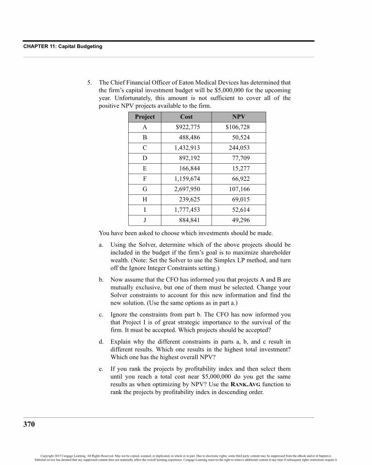
CHAPTER 11: Capital Budgeting
370
5. The Chief Financial Officer of Eaton Medical Devices has determined thatthe firm’s capital investment budget will be $5,000,000 for the upcomingyear. Unfortunately, this amount is not sufficient to cover all of thepositive NPV projects available to the firm.
You have been asked to choose which investments should be made.
a. Using the Solver, determine which of the above projects should beincluded in the budget if the firm’s goal is to maximize shareholderwealth. (Note: Set the Solver to use the Simplex LP method, and turnoff the Ignore Integer Constraints setting.)
b. Now assume that the CFO has informed you that projects A and B aremutually exclusive, but one of them must be selected. Change yourSolver constraints to account for this new information and find thenew solution. (Use the same options as in part a.)
c. Ignore the constraints from part b. The CFO has now informed youthat Project I is of great strategic importance to the survival of thefirm. It must be accepted. Which projects should be accepted?
d. Explain why the different constraints in parts a, b, and c result indifferent results. Which one results in the highest total investment?Which one has the highest overall NPV?
e. If you rank the projects by profitability index and then select themuntil you reach a total cost near $5,000,000 do you get the sameresults as when optimizing by NPV? Use the RANK.AVG function torank the projects by profitability index in descending order.
Project Cost NPVA $922,775 $106,728B 488,486 50,524C 1,432,913 244,053D 892,192 77,709E 166,844 15,277F 1,159,674 66,922G 2,697,950 107,166H 239,625 69,015I 1,777,453 52,614J 884,841 49,296
Copyright 2015 Cengage Learning. All Rights Reserved. May not be copied, scanned, or duplicated, in whole or in part. Due to electronic rights, some third party content may be suppressed from the eBook and/or eChapter(s).Editorial review has deemed that any suppressed content does not materially affect the overall learning experience. Cengage Learning reserves the right to remove additional content at any time if subsequent rights restrictions require it.

371
CHAPTER 12 Risk and Capital Budgeting
Risk is a difficult concept to define, but most people recognize such obvious risks asswimming in shark-infested waters. If you consider risky situations for a moment, you willrealize that the thing that they all have in common is uncertainty about the outcome and thepossibility of a loss. Many times, we face the loss of life or money. In this chapter, we areconcerned with the possibility of a financial loss. Specifically, we will say that the larger thepossibility of loss, the larger the risk.
We will begin by attempting to measure the riskiness of an investment, and then we willconsider how we can adjust our decision-making process to account for the risk that we havemeasured. In Chapter 13, we will see how we can reduce risk through diversification.
After studying this chapter, you should be able to:1. Define the five major statistical measures used in finance, and calculate them
manually and in Excel.2. Explain five techniques for incorporating risk into the capital budgeting
decision process.3. Perform sensitivity and scenario analysis with data tables and Scenario
Manager.4. Perform a Monte Carlo simulation to determine the expected NPV of an
investment.
Copyright 2015 Cengage Learning. All Rights Reserved. May not be copied, scanned, or duplicated, in whole or in part. Due to electronic rights, some third party content may be suppressed from the eBook and/or eChapter(s).Editorial review has deemed that any suppressed content does not materially affect the overall learning experience. Cengage Learning reserves the right to remove additional content at any time if subsequent rights restrictions require it.

CHAPTER 12: Risk and Capital Budgeting
372
Review of Some Useful Statistical ConceptsAny situation that has an uncertain outcome can be said to have a probability distribution,which is simply a listing of the potential outcomes and their associated probabilities.A probability distribution is said to be discrete if there are a limited number of potentialoutcomes and continuous if an infinite number of possible outcomes can occur. Figure 12-1illustrates both continuous and discrete probability distributions. Continuous probabilitydistributions can be approximated by discrete distributions if we have enough possibleoutcomes. To keep things simple, in this chapter we will use only discrete distributions inour examples.
FIGURE 12-1CONTINUOUS VS. DISCRETE PROBABILITY DISTRIBUTIONS
One type of probability distribution has numerous properties that make it especiallyattractive for our use: the normal distribution. In particular, the normal distribution can becompletely described by its mean and variance, which will prove useful in our efforts tounderstand risk.
The Expected ValueThe expected value of a distribution is a weighted average of all possible outcomes wherethe weights are the probabilities of occurrence. The expected value can be thought of as themost likely outcome or the average outcome if we could run an experiment thousands oftimes. For any discrete probability distribution, the expected value is given by:
where E(X) is the expected or most likely X, Xt is the tth possible outcome, and ρt is theprobability that Xt will occur. For the normal distribution, the expected value is the same asthe more familiar arithmetic mean.
(12-1)E X( ) ρt Xt
t 1=
N
=
Copyright 2015 Cengage Learning. All Rights Reserved. May not be copied, scanned, or duplicated, in whole or in part. Due to electronic rights, some third party content may be suppressed from the eBook and/or eChapter(s).Editorial review has deemed that any suppressed content does not materially affect the overall learning experience. Cengage Learning reserves the right to remove additional content at any time if subsequent rights restrictions require it.

373
Review of Some Useful Statistical Concepts
To illustrate the calculation of the expected value, suppose that you have been offered anopportunity to participate in a game of chance. The rules of this particular game are such thatyou must pay $200 to play, and Table 12-1 describes the possible payoffs.
To determine whether you should play this game, we must compare the expected payoff tothe cost of playing. If the expected cash flow exceeds your cost, then it makes sense to play.The expected cash flow, E(Cf ), of this game is:
so that you expect to break even after paying to play (this is known as a fair bet and wouldbe rejected by a risk averse investor). Note that in actuality, if the game is played only onceyou could lose as much as $100 or win as much as $100 net of your cost of entry. However,the most likely outcome is a net gain of $0.00. The arithmetic mean of cash flows (Cf) is:
and subtracting your cost, you can see that they are the same. Again, in this case, theexpected value and the arithmetic mean are the same because the outcomes of this game aresymmetrically distributed.
It is important to understand that many times the assumption of a symmetrical distribution isnot accurate, and in this case the arithmetic mean and the expected value will not be thesame. This is particularly true in many financial situations where your maximum loss islimited to 100% of the investment, but your potential gain is unlimited. This results in adistribution that is skewed to the right. In this type of situation it is often helpful to transformthe data. For example, with financial assets we often calculate log-price relatives instead ofthe usual percentage changes:
(12-2)
where Ln is the natural logarithm operator, P1 is the ending price, and P0 is the beginningprice. This transformation converts a skewed variable into a normally distributed variable, atleast approximately, and allows us to use statistics that assume normality.
TABLE 12-1PROBABILITY DISTRIBUTION FOR A GAME OF CHANCE
Probability Cash Flow0.25 $ 1000.50 2000.25 300
E Cf( ) 0.25 100( ) 0.50 200( ) 0.25 300( )+ + 200= =
Cf 100 200 300+ +3
--------------------------------------- 200= =
Log-Price Relative LnP1
P0-----⎝ ⎠
⎛ ⎞=
Copyright 2015 Cengage Learning. All Rights Reserved. May not be copied, scanned, or duplicated, in whole or in part. Due to electronic rights, some third party content may be suppressed from the eBook and/or eChapter(s).Editorial review has deemed that any suppressed content does not materially affect the overall learning experience. Cengage Learning reserves the right to remove additional content at any time if subsequent rights restrictions require it.

CHAPTER 12: Risk and Capital Budgeting
374
Measures of DispersionWhenever we use an expected value, it is useful to know how much, on average, the actualoutcome might deviate from the expected outcome. The larger these potential deviations, theless confidence we have that the expected outcome, or something near it, will actually occur.Another way of saying this is that the larger the potential deviations from the expected value,the higher the probability of an outcome far away from the expected outcome.
Recall that we earlier said that high probabilities of loss indicate a high-risk situation.Therefore, when comparing distributions we can say that the distribution with the largerpotential deviations has a higher probability of greater loss and so it is more risky.
The Variance and Standard DeviationTo measure risk, we need a way to measure the size of the potential deviations from themean. One measure that we could use is the average deviation from the mean:
But the average deviation is, by definition, always zero. So we need another measure ofdispersion that doesn’t suffer from this flaw. We could calculate the average of theabsolute values of the deviations, but historically we have used the variance and standarddeviation. The variance is the average of the squared deviations from the mean and iscalculated as:1
Because we are squaring the deviations from the mean, and the result of squaring a numberis always positive, the variance must be positive.2 The larger the variance, the less likely it isthat the actual outcome will be near the expected outcome and the riskier it is considered tobe. Figure 12-2 illustrates this by comparing two normal distributions.
1. Note that in your beginning statistics class, you probably defined the population variance as:
Our definition is equivalent if we assume that all outcomes are equally likely.
2. It is possible that the variance could be zero, but only if just one possible outcome exists.
(12-3)D ρt Xt E X( )–( )t 1=
N
=
(12-4)σX2 ρt Xt E X( )–( )2
t 1=
N
=
σX2 1
N---- Xt X–( )2
t 1=
N
=
Copyright 2015 Cengage Learning. All Rights Reserved. May not be copied, scanned, or duplicated, in whole or in part. Due to electronic rights, some third party content may be suppressed from the eBook and/or eChapter(s).Editorial review has deemed that any suppressed content does not materially affect the overall learning experience. Cengage Learning reserves the right to remove additional content at any time if subsequent rights restrictions require it.

375
Review of Some Useful Statistical Concepts
FIGURE 12-2COMPARISON OF THE RISKINESS OF TWO DISTRIBUTIONS
Returning to the example in Table 12-1, we can calculate the variance of possible outcomesas follows:
So the variance of possible outcomes is 5,000. But 5,000 in what units? In this case the unitsare squared dollars, an unusual unit of measurement to be sure. In order to make thismeasurement more understandable we take the square root of the variance, which gives usthe standard deviation in the original units:
The standard deviation of potential outcomes in our game example is:
which means that about 68% of all outcomes will be within one standard deviation of themean (200 ± 70.71), and about 95.5% will be within two standard deviations (200 ± 141.42).Furthermore, it is exceedingly unlikely (<0.30%), but not impossible, that the actualoutcome will fall beyond three standard deviations from the mean.3
3. This is known as the empirical rule. For nonnormal distributions, Chebyshev’s Theorem givessimilar (though not as precise) results.
σ2 0.25 100 200–( )2 0.50 200 200–( )2 0.25 300 200–( )2+ + 5,000= =
σ 5,000 70.71= =
(12-5)σX σX2 ρt Xt E X( )–( )2
t 1=
N
= =
Copyright 2015 Cengage Learning. All Rights Reserved. May not be copied, scanned, or duplicated, in whole or in part. Due to electronic rights, some third party content may be suppressed from the eBook and/or eChapter(s).Editorial review has deemed that any suppressed content does not materially affect the overall learning experience. Cengage Learning reserves the right to remove additional content at any time if subsequent rights restrictions require it.

CHAPTER 12: Risk and Capital Budgeting
376
The Coefficient of VariationSuppose that after playing the original game, you are offered a chance to play the gameagain. This time, though, the game is 10 times larger and so is your cost to play. The possibleoutcomes are presented in Table 12-2.
Is this game riskier than the old game? Let’s look at the standard deviation to see:
Because the standard deviation is 10 times larger, it appears that the new game is muchriskier. Recall, however, that we said that high risk was associated with a high probability ofloss. In the new game, your probability of loss is unchanged (25%). Since the probability ofloss is unchanged, the risk should be the same.
Apparently the standard deviation has a scale problem. That is, larger numbers cause largerstandard deviations, even if the relative dispersion is unchanged. The coefficient of variationhandles the scale problem by dividing the standard deviation by the mean, so it is a measureof risk per unit of return:
(12-6)
If the new game is truly riskier than the old game, it will have a higher coefficient ofvariation. Let’s compare the coefficients of variation for both games:
Because , both games must be equally risky. The coefficient of variation is usefulany time the expected values of two distributions are significantly different. The standarddeviation has no meaning without reference to the expected value. Because it provides ameasure of risk relative to return, the coefficient of variation can always be used to compareinvestments without regard to the size of the investment.
TABLE 12-2SAME GAME, BUT 10 TIMES LARGER
Probability Cash Flow0.25 $ 1,0000.50 2,0000.25 3,000
σ 0.25 1,000 2,000–( )2 0.50 2,000 2,000–( )2 0.25 3,000 2,000–( )2+ +σ 707.106
==
γXσX
E X( )------------=
γ170.7106
200------------------- 0.3535
γ2707.106
2,000------------------- 0.3535
= =
= =
γ1 γ2=
Copyright 2015 Cengage Learning. All Rights Reserved. May not be copied, scanned, or duplicated, in whole or in part. Due to electronic rights, some third party content may be suppressed from the eBook and/or eChapter(s).Editorial review has deemed that any suppressed content does not materially affect the overall learning experience. Cengage Learning reserves the right to remove additional content at any time if subsequent rights restrictions require it.

377
Using Excel to Measure Risk
Using Excel to Measure RiskNow that we understand how risk can be evaluated, let’s look at how Excel might be used tosimplify the calculations. In this section, we will introduce several of Excel’s built-infunctions and user-defined functions that are contained in the file Famefncs.xlam. Beforecontinuing, make sure that the add-in is enabled and open a new workbook, into which wewill enter data from an example of a capital budgeting project.
The Freshly Frozen Fish Company Example
The Freshly Frozen Fish Company currently markets frozen fish filletsand other related products. While seeking expansion ideas, managementof the company decided to look into the possibility of a line of frozencatfish fillets. Entry into this business would require the purchase of anexisting 80-acre catfish farm in western Alabama at a cost of $250,000 forthe land and $400,000 for the buildings and equipment. The buildings andequipment will be depreciated using MACRS with a class life of 20 years.At the end of the five years, management anticipates that the farm will besold for $550,000 ($350,000 for the land and $200,000 for the buildingsand equipment).
The marketing department estimates that the firm will be able to sell200,000 pounds of fillets at an average wholesale price of $2.50 per poundduring the first year. Unit demand is expected to grow at a rate of 8%annually thereafter. Variable operating expenses are expected to average60% of gross sales, and fixed costs (not including depreciation) will be$80,000 per year. The company’s marginal tax rate is 35% and its WACCis 10%.
Before we can determine the riskiness of this project, we must determine its cost and annualcash flows. Let’s begin by entering all the data from the problem into the worksheet startingin cell A1. The easiest way to extract data from a problem such as this is to take it as it comesand enter it into the worksheet in that order, being careful to label every row. This way, youare less likely to overlook an important piece of data. That is exactly what we’ve done inExhibit 12-1. If necessary, we can rearrange this table later.
Recall from Chapter 11 (page 331) that our first task is to determine the initial outlay. Theexample problem in that chapter was a little different than this one because it was areplacement problem. However, exactly the same techniques can be used to determine thecash flows. Just realize that in the case of this entirely new project we aren’t replacinganything, so any cash flows associated with old equipment are set to zero. Otherwise, themethodology is exactly the same.
Copyright 2015 Cengage Learning. All Rights Reserved. May not be copied, scanned, or duplicated, in whole or in part. Due to electronic rights, some third party content may be suppressed from the eBook and/or eChapter(s).Editorial review has deemed that any suppressed content does not materially affect the overall learning experience. Cengage Learning reserves the right to remove additional content at any time if subsequent rights restrictions require it.

CHAPTER 12: Risk and Capital Budgeting
378
EXHIBIT 12-1FRESHLY FROZEN FISH COMPANY INPUTS
Before continuing, let’s take a little time to set up our calculation area on the worksheet.Realize that the annual after-tax cash flows are going to be different in each of the five years.To keep things as simple as possible, we will set up the calculations in an operating cashflow format, which is similar to an income statement but includes only operating cash flows.In A16 enter: Annual Cash Flows for Frozen Catfish Fillet Project, andcenter this title over A16:G16. Next, in B17 enter: 0 and use AutoFill to extend that to 5 inG17. Now apply a custom number format of: “Year “0 to the range.
We have purposely simplified this example, so we have no shipping, installation, training, orconstruction costs. The initial outlay is simply the cost of the land and buildings. In A18enter: Initial Outlay, and in B18 enter: =-(B2+B3). This will give us the initialoutlay as a negative number. The result is –$650,000.
Our next step is to calculate the annual after-tax cash flows for each year. As noted earlier,the cash flows will be different each year because sales and variable operating expenses areexpected to increase every year by 8%. Additionally, the depreciation expense will differeach year because we are using MACRS instead of straight-line depreciation. We willcalculate the ATCF for each year as:
where SN is the total revenue in year N, VN is the total variable costs, FN is the fixed costs,DN is the annual depreciation expense, and t is the marginal tax rate. This is exactly the same
ATCFN SN VN– FN– DN–( ) 1 t–( ) DN+=
Copyright 2015 Cengage Learning. All Rights Reserved. May not be copied, scanned, or duplicated, in whole or in part. Due to electronic rights, some third party content may be suppressed from the eBook and/or eChapter(s).Editorial review has deemed that any suppressed content does not materially affect the overall learning experience. Cengage Learning reserves the right to remove additional content at any time if subsequent rights restrictions require it.

379
Using Excel to Measure Risk
equation as shown on page 333, except that it has been modified slightly to suit this problem.The operating cash flow statement uses this equation, but in a vertical format.
In A19 enter: Sales as the label. We will calculate the first year sales in C19 bymultiplying unit sales (200,000 pounds) by the selling price ($2.50), so the equation is:=B8*B9. This gives us $500,000 in sales revenue for the first year. Each additional year’ssales will be 8% greater than previous sales, so in D19 enter: =C19*(1+$B$10). Nowcopy this formula over the range E19:G19. As a check, note that under these assumptionssales will grow to $680,244.48 by year 5.
Next, to calculate the annual variable costs enter: =C19*$B$11 into C20, and copy itacross D20:G20. In A20 enter: Variable Costs as the label for the row. In A21enter: Fixed Costs for the label, and then in C21 enter: =$B$12. Copy this overD21:G21.
We will calculate the depreciation expense in row 22, so enter: DepreciationExpense in A22. Because we are using MACRS depreciation (see page 336), we will usethe FAME_MACRS function included in the Famefncs.xlam add-in. Recall that this functionis defined as:
FAME_MACRS(COST, MACRSCLASS, YEAR, TABLE)
where TABLE is an optional argument that tells the function whether to use the exactcalculation or the table percentages. In this case, we will use the exact calculation, so in C22enter: =IFERROR(FAME_MACRS($B$3,$B$4,C17,FALSE),0). Remember that wecannot depreciate land, only the buildings and equipment. Note that we are referencing theyear number in row 17, which explains why we used a custom number format in that row.Copy the formula from C22 to D22:G22. The depreciation expense will be $15,000 in year 1and $22,853 in year 5.
We can now calculate the taxable cash flows in row 23. In A23 add the label: TaxableCash Flows. Subtract the total costs from sales in C23 with the formula: =C19-SUM(C20:C22) and copy this across the other columns. In A24 enter the label: Taxes,and in C24 enter: =C23*$B$13 and copy it to D24:G24.
At this point, to get the ATCF we need to add back the depreciation expense that waspreviously subtracted. In A25 enter: Add: Depreciation as the label and then in C25:=C22. Copy this to the remaining cells, and then in A26 enter: Annual After-Tax CashFlows. Finally, in C26 we can enter: =C23-C24+C25. Copy this to the other cells inD26:G26. The ATCF for year 1 should be $83,250.
The last cash flow that we must calculate is the terminal cash flow, so in A27 enter the label:Terminal Cash Flow. Recall that this is the sum of the nonoperating cash flows thatoccur at the end of the life of the project. In this problem, those would be the sale of the landand buildings as well as any taxes required on the gains. The land is not depreciable, so any
Copyright 2015 Cengage Learning. All Rights Reserved. May not be copied, scanned, or duplicated, in whole or in part. Due to electronic rights, some third party content may be suppressed from the eBook and/or eChapter(s).Editorial review has deemed that any suppressed content does not materially affect the overall learning experience. Cengage Learning reserves the right to remove additional content at any time if subsequent rights restrictions require it.

CHAPTER 12: Risk and Capital Budgeting
380
gain on the sale of land is taxable. We will start building this formula in G27 by calculatingthe after-tax proceeds from selling the land with the formula: =B6-(B6-B2)*B13.
To calculate the tax on the buildings and equipment, we must first determine the book valuein year 5 so that we can compare that to the salvage value. The book value is the original costless the accumulated depreciation. If this is different from the salvage value, the difference istaxable. Therefore, the cash inflow from selling the buildings and equipment can becalculated with the formula: =B7-(B7-(B3-SUM(C22:G22)))*B13.
The terminal cash flow will be the sum of the after-tax cash flows received from selling theland and from selling the buildings. So, in G27 your formula is: =B6-(B6-B2)*B13+B7-(B7-(B3-SUM(C22:G22)))*B13.
In order to summarize our calculations, we will add one more row. In A28 enter: TotalAnnual Cash Flows. In B28 enter: =B18. In C28 enter: =C26+C27 and copy it across.Check your worksheet against that shown in Exhibit 12-2 to be sure that your calculationsare correct.
EXHIBIT 12-2CALCULATION OF THE ANNUAL AFTER-TAX CASH FLOWS
At this point, we are ready to calculate the net present value to give a preliminary assessmentof the merits of this project. In A30 enter: Net Present Value, and in B30 enter:=NPV(B14,C28:G28)+B28. The NPV is $91,272.55, which would seem to indicate thatthe project is acceptable. If you calculate the other profitability measures, you will find thatthe IRR is 13.77%, the MIRR is 12.93%, the profitability index is 1.14, the payback periodis 4.35 years, and the discounted payback is 4.78 years.
Copyright 2015 Cengage Learning. All Rights Reserved. May not be copied, scanned, or duplicated, in whole or in part. Due to electronic rights, some third party content may be suppressed from the eBook and/or eChapter(s).Editorial review has deemed that any suppressed content does not materially affect the overall learning experience. Cengage Learning reserves the right to remove additional content at any time if subsequent rights restrictions require it.

381
Introducing Uncertainty
Introducing UncertaintyIf we lived in a world of perfect certainty, the catfish fillet project would be accepted withoutquestion. After all, it appears that it will increase shareholder wealth by $91,272.55.Unfortunately, the world is not certain. Even in this simplified example, it should be clearthat many sources of uncertainty may arise. For example, the marketing department doesn’treally know that the firm will sell 200,000 pounds of catfish fillets in the first year. Likewise,it doesn’t know that it will be able to get the assumed $2.50 per pound or that demand willgrow at an annual rate of 8% per year. Consumer demand may be far less than expected.This could lead to a double whammy: Not only would unit demand be less than expected,but the wholesale price would likely be less than $2.50 per pound. Poor first year acceptancecould also mean lower subsequent growth rates. These and many other uncertaintiesnaturally result in uncertainty surrounding our expected annual cash flows that, in turn,results in uncertainty surrounding the estimated NPV.
In such an uncertain world, it is helpful to develop models that allow us to determine howmuch uncertainty surrounds our estimate of the NPV. For example, we might like to make aneducated guess as to the probability that the NPV will actually turn out to be less than zero.The following sections will lead us to an answer to this question.
Sensitivity AnalysisAs noted earlier, many uncertain variables exist in our catfish fillet example. In fact, wecould say that virtually all of the variables are uncertain, as are many others that we have notexplicitly considered. However, some of these variables have more of an impact on the NPVthan others. Because it would take a lot of time and effort to generate precise forecasts ofevery variable, it is helpful to concentrate on only the most important variables. Sensitivityanalysis is the tool that helps us to identify the variables that deserve the most attention.
The idea is to make small changes in variables, one at a time, and observe the effect on theNPV (or any other decision criteria). For example, we might change the selling price from$2.50 per pound to $2.25 (a change of –10%) and then calculate that the NPV would declineto $34,291.68. Record this fact and reset the selling price to its original value. Now, reducethe terminal value of the land to $315,000 (a change of –10%) and note that the NPVdeclines to $77,146.59. Reducing the selling price by 10% leads to a much bigger decline inthe NPV than does a similar reduction in the terminal value of the land. Therefore, weshould devote more resources to accurately determining the selling price, and not spendmuch time estimating the value of the land.
There are two problems with the procedure outlined earlier. First, by making only a singlesmall change to each variable, we may miss nonlinear relationships. Second, carrying outthis procedure for each uncertain variable would be cumbersome. We would have to change
Copyright 2015 Cengage Learning. All Rights Reserved. May not be copied, scanned, or duplicated, in whole or in part. Due to electronic rights, some third party content may be suppressed from the eBook and/or eChapter(s).Editorial review has deemed that any suppressed content does not materially affect the overall learning experience. Cengage Learning reserves the right to remove additional content at any time if subsequent rights restrictions require it.
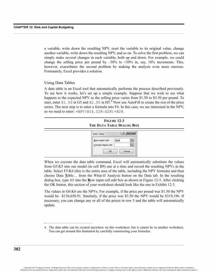
CHAPTER 12: Risk and Capital Budgeting
382
a variable, write down the resulting NPV, reset the variable to its original value, changeanother variable, write down the resulting NPV, and so on. To solve the first problem, we cansimply make several changes in each variable, both up and down. For example, we couldchange the selling price per pound by –30% to +30% in, say, 10% increments. This,however, exacerbates the second problem by making the analysis even more onerous.Fortunately, Excel provides a solution.
Using Data TablesA data table is an Excel tool that automatically performs the process described previously.To see how it works, let’s set up a simple example. Suppose that we wish to see whathappens to the expected NPV as the selling price varies from $1.50 to $3.50 per pound. Tostart, enter $1.50 in G5 and $2.00 in H5.4 Now use AutoFill to create the rest of the priceseries. The next step is to enter a formula into F6. In this case, we are interested in the NPV,so we need to enter: =NPV(B14,C28:G28)+B28.
FIGURE 12-3THE DATA TABLE DIALOG BOX
When we execute the data table command, Excel will automatically substitute the valuesfrom G5:K5 into our model (in cell B9) one at a time and record the resulting NPVs in thetable. Select F5:K6 (this is the entire area of the table, including the NPV formula) and thenchoose Data Table… from the What-If Analysis button on the Data tab. In the resultingdialog box, type B9 into the Row input cell edit box as shown in Figure 12-3. After clickingthe OK button, this section of your worksheet should look like the one in Exhibit 12-3.
The values in G6:K6 are the NPVs. For example, if the price per pound was $1.50 the NPVwould be –$136,650.91. Similarly, if the price was $3.50 the NPV would be $319,196. Ifnecessary, you can change any or all of the prices in row 5 and the table will automaticallyupdate.
4. The data table can be created anywhere on this worksheet, but it cannot be in another worksheet.You can get around this limitation by carefully constructing your formulas.
Copyright 2015 Cengage Learning. All Rights Reserved. May not be copied, scanned, or duplicated, in whole or in part. Due to electronic rights, some third party content may be suppressed from the eBook and/or eChapter(s).Editorial review has deemed that any suppressed content does not materially affect the overall learning experience. Cengage Learning reserves the right to remove additional content at any time if subsequent rights restrictions require it.

383
Introducing Uncertainty
EXHIBIT 12-3THE DATA TABLE FOR DIFFERENT PRICES
The original NPV formula in F6 is not a part of the table per se, and it might confuse somepeople. It is only there so that Excel knows what formula to use when calculating the table.We can easily hide this value by simply selecting F6 and changing the font color to white, orusing a custom number format with just a semicolon. This will make the table easier to read.
Excel allows for other types of data tables than we have demonstrated here. The data table inExhibit 12-3 is called a row-oriented one-variable table because our prices are in a row. Ifthe prices were in a column instead, we could create a column-oriented one-variable table.To create a column-oriented table, the only difference is that you would enter the changingcell (B9) into the Column input cell edit box (see Figure 12-3). The result would be exactlythe same, except for the orientation table. We can also create two-variable data tables thatallow for two changing variables. The procedure is similar, but you should check the onlinehelp for the details.
Because we have more than one uncertain variable in our catfish fillet problem, we will needseveral data tables. It will also be helpful, for comparison purposes, to deviate a bit from themethodology described earlier. Specifically, we can set up several data tables based onpercentage changes in our uncertain variables. This will make it easier to compare the resultfrom a change in unit sales to the result from a change in the growth rate.
Let’s start by changing the input area of the worksheet so that it can accommodate this typeof sensitivity analysis more easily. In D5 enter: Sensitivity %, and then in D6:D11enter: 0% in each cell. Change B6 so that it has a formula rather than a number:=350000*(1+D6). Now if we put 10% into D6, for example, the terminal value of theland will change from $350,000 to $385,000. Make similar changes in cells B7:B11 so thatthose values change as we change the corresponding percentages. Your input area shouldnow look like the one in Exhibit 12-4. Note that we will be doing the sensitivity analysis ononly six of the variables.
At this point, we can proceed in a similar manner as we did earlier. Let’s first create apercentage-based data table for the terminal value of the land. Go to A38 and enter:Terminal Value of Land. In B38:H38 enter a series of numbers from –30% to +30% in10% increments (–30%, –20%, –10%, etc.). In A39, enter the NPV function:=NPV(B14,C28:G28)+B28.
Copyright 2015 Cengage Learning. All Rights Reserved. May not be copied, scanned, or duplicated, in whole or in part. Due to electronic rights, some third party content may be suppressed from the eBook and/or eChapter(s).Editorial review has deemed that any suppressed content does not materially affect the overall learning experience. Cengage Learning reserves the right to remove additional content at any time if subsequent rights restrictions require it.

CHAPTER 12: Risk and Capital Budgeting
384
EXHIBIT 12-4THE INPUT AREA SET UP FOR SENSITIVITY ANALYSIS
We have now set up the table and all that remains is to select it and execute the Data Table…command. In this case the row input cell is D6, which is the percentage that corresponds tothe terminal value of the land. The data table will plug –30% into D6, which will change theterminal land value in B6 resulting in a different NPV. Next, it will plug in –20%, and so on.
Using the same procedure, create data tables for each of the uncertain variables, each timechanging the row input cell (D7, D8, etc.). You should end up with six data tables as shownin Exhibit 12-5. Note that, as mentioned earlier, we have hidden the original NPV formula sothat the table is easier to read.
Sensitivity DiagramsSome people can look at the data tables and see at a glance that the most important variablesare the unit sales, price per pound, and the variable cost as a percentage of sales. Others,however, find it helpful to create charts of the data. We can either create a separate chart foreach variable or put all of the variables in one chart.
To create one chart that shows all of the variables, select B38:H39 and then Ctrl+click eachof the NPV other series. Create a scatter chart and place it somewhere convenient in theworksheet. For this example problem, it turns out that some of the lines overlap, so it isimpossible to tell them apart on the chart. This is not always the case. However, even whenwe don’t have this problem, it can be much easier to see which variables are most importantif they are all in separate charts. This is particularly true when we have a lot of variables.
Copyright 2015 Cengage Learning. All Rights Reserved. May not be copied, scanned, or duplicated, in whole or in part. Due to electronic rights, some third party content may be suppressed from the eBook and/or eChapter(s).Editorial review has deemed that any suppressed content does not materially affect the overall learning experience. Cengage Learning reserves the right to remove additional content at any time if subsequent rights restrictions require it.

385
Introducing Uncertainty
EXHIBIT 12-5DATA TABLES FOR THE UNCERTAIN VARIABLES
Creating a separate chart for each variable is more time consuming, and you need to makesure that the scaling of the axes is the same in each chart so that you can compare the slopes.The advantage to this approach is that it is much easier to identify the individual data series.As can be seen in Figure 12-4, the lines with the steepest slopes are the same as thosepreviously identified as the most important variables.
In order to make this comparison, it is vital that the axis scaling is identical in each chart. Tomake creating all of these charts easier, you can copy and paste the first one and then simplychange the data ranges. To change the data series in a chart, right-click in the chart andchoose Select Data… In the dialog box, select the series and then click the Edit button tochange the data ranges.
An alternative to the visual approach is to use the SLOPE function to determine the slope ofeach line. This function calculates a regression equation and returns the slope. It is defined as:
SLOPE(KNOWN_Y’S, KNOWN_X’S)where KNOWN_Y’S and KNOWN_X’S are the Y and X data ranges, respectively. For ourpurpose, the Y variables are the NPVs and the X variables are the percentage changes. Forexample, we can use =SLOPE(B39:H39,B38:H38) to find that the slope of the line forthe terminal land value is 141,259.60. This can then be numerically compared to the slopesof the other lines. The larger the slope, the more important the variable. Note that if any ofthe slopes might be negative, then it is helpful to use the ABS function to return the absolute
Copyright 2015 Cengage Learning. All Rights Reserved. May not be copied, scanned, or duplicated, in whole or in part. Due to electronic rights, some third party content may be suppressed from the eBook and/or eChapter(s).Editorial review has deemed that any suppressed content does not materially affect the overall learning experience. Cengage Learning reserves the right to remove additional content at any time if subsequent rights restrictions require it.

CHAPTER 12: Risk and Capital Budgeting
386
FIGURE 12-4SENSITIVITY DIAGRAMS FOR EACH VARIABLE
value of the slope. Adding this function to the formula will change it to:=ABS(SLOPE(B39:H39,B38:H38)). This allows us to compare magnitudes withoutregard to signs.
Clearly, the most important variables are the unit sales, price per pound, and the variable costas a percentage of sales. These are the variables that we will use in our scenario analysis inthe next section.
Scenario AnalysisThe sensitivity analysis has identified the three most important variables, but we’ve onlyseen their impact on the NPV in isolation. A scenario analysis will allow us to see thecombined effects of changing all of these variables simultaneously. Suppose that after seeingthe sensitivity analysis report, a meeting was held to determine three possible scenarios. Thebest and worst cases are shown in Table 12-3 along with the base case, which represents theoriginal expectations. It also shows the probability that each scenario will actually occur.
The worst-case scenario is one in which all of the variables are at their worst possible values.Similarly, the best case assumes that all of the variables take on their best possible valuessimultaneously. Although such outcomes are unlikely, they are useful for determining theextreme boundaries around the expected NPV. It is common to add a few additional, andmore realistic, scenarios to these.
Copyright 2015 Cengage Learning. All Rights Reserved. May not be copied, scanned, or duplicated, in whole or in part. Due to electronic rights, some third party content may be suppressed from the eBook and/or eChapter(s).Editorial review has deemed that any suppressed content does not materially affect the overall learning experience. Cengage Learning reserves the right to remove additional content at any time if subsequent rights restrictions require it.

387
Introducing Uncertainty
Excel provides the Scenario Manager to help us analyze such scenarios. In Chapter 3(page 85), we used the Scenario Manager to perform a sensitivity analysis to see the effect ofthe timing of a large capital expenditure on total borrowing. In Chapter 11 (page 355), weperformed a scenario analysis to determine the combined effect of changing maintenanceand defect costs on the profitability measures of a replacement project.5
In this section, we will again use the Scenario Manager, but our goal is to get a betterunderstanding of the riskiness of the frozen catfish product. Specifically, we want to get anidea of the probability distribution around the expected NPV, especially the range of possibleoutcomes. Before using the Scenario Manager, it is helpful to define names for the changingcells. Set up the scenarios given in Table 12-3, and create a scenario summary report with theNPV as the result cell.
EXHIBIT 12-6SCENARIO SUMMARY REPORT
TABLE 12-3THREE SCENARIOS
VariableWorst Case
20%Base Case
60%Best Case
20%Unit Sales 125,000 200,000 275,000Price per Pound $2.25 $2.50 $2.65Variable Cost % 65% 60% 55%
5. We could have used the Scenario Manager to do the sensitivity analysis, but that would haverequired 42 different scenarios. It is much easier to use data tables for sensitivity analysis, but theyare not adequate for scenario analysis because data tables allow only (at most) two variables tochange at the same time.
Copyright 2015 Cengage Learning. All Rights Reserved. May not be copied, scanned, or duplicated, in whole or in part. Due to electronic rights, some third party content may be suppressed from the eBook and/or eChapter(s).Editorial review has deemed that any suppressed content does not materially affect the overall learning experience. Cengage Learning reserves the right to remove additional content at any time if subsequent rights restrictions require it.

CHAPTER 12: Risk and Capital Budgeting
388
Exhibit 12-6 shows the scenario summary report, with the “Current Values” column deleted.Note that in the worst case, where the price and unit sales are low and variable costs arehigh, the NPV is significantly negative. On the other hand, the NPV is very high in the bestcase. So far, the scenario analysis has shown a risk of a negative NPV. However, we haven’tyet quantified that risk.
Assume that the experts who defined the three scenarios were also asked to assign theprobabilities of occurrence to each scenario. Feeling that the extreme scenarios are relativelyunlikely, they assigned a probability of 20% to the best and worst cases. This leaves 60% forthe base case. On your Scenario Summary worksheet, enter: Probabilities in C12,20% in D12, 60% in E12, and 20% in F12. Figure 12-5 shows a histogram of the probabilitydistribution.
FIGURE 12-5PROBABILITY DISTRIBUTION OF NPV
Calculating the Expected NPV from the ScenariosWith this information, we can now calculate the expected NPV for the project. Your firstthought might be to try using the AVERAGE function. Recall from Chapter 1 that theAVERAGE function calculates the arithmetic (equally weighted) average of the observations.However, a glance at Figure 12-5 shows that the distribution is somewhat skewed to theright, and the possible outcomes are not all equally likely, so the average will overstate theexpected value (as was discussed on page 373).
It would be more appropriate to calculate the expected value (see page 372). Recall that theexpected value is found by multiplying each possible outcome by its associated probabilityand summing the results. In C13 of the Scenario Summary worksheet enter: ExpectedNPV. We can make this calculation in any of several different ways. For example, in D13 wecould enter: =D10*D12+E10*E12+F10*F12, but that’s not the best way. A better way
Copyright 2015 Cengage Learning. All Rights Reserved. May not be copied, scanned, or duplicated, in whole or in part. Due to electronic rights, some third party content may be suppressed from the eBook and/or eChapter(s).Editorial review has deemed that any suppressed content does not materially affect the overall learning experience. Cengage Learning reserves the right to remove additional content at any time if subsequent rights restrictions require it.
389
Introducing Uncertainty
would be to use an array formula: =SUM(D10:F10*D12:F12), just remember to holddown the Shift+Ctrl keys when pressing the Enter key. Finally, we have supplied a user-defined function called FAME_EXPVALUE that will calculate the expected value of aprobability distribution. It is defined as:
FAME_EXPVALUE(VALUES, PROBABILITIES)
where VALUES is the range of possible outcomes and PROBABILITIES is the range ofprobabilities. To use this function, make sure that the Famefncs.xlam add-in is installed andenabled, and then enter: =Fame_ExpValue(D10:F10,D12:F12) into D13. As analternative, you can use the Insert Function dialog box that will list this function in the “UserDefined” category.
Whichever way you choose to calculate it, the expected NPV for this project is $106,301.25.This means that, if our assumptions are correct, it is likely that this project is a goodinvestment. If we could repeat this investment thousands of times under the same conditions,the average NPV would be $106,301.25. Unfortunately, we get only one chance, so it wouldbe nice to know a little more about the dispersion of the possible outcomes around theexpected value.
Calculating the Variance and Standard DeviationThe scenario summary report makes it obvious that a negative NPV is possible. The questionto ask is, “How risky is this project, and what is the likelihood that the NPV will benegative?” The first step toward answering this question is to calculate one or more of themeasures of dispersion (variance, standard deviation, or coefficient of variation) mentionedearlier in this chapter.
Excel provides two functions for calculating the variance of a range of numbers: VAR.S (orVAR if you are using the older functions) calculates a sample variance, while VAR.P (orVARP) calculates a population variance.6 These functions are defined as:
VAR.S(NUMBER1, NUMBER2, …)
and
VAR.P(NUMBER1, NUMBER2, …)
6. The difference between a sample statistic and a population parameter is that the sample statisticincludes an adjustment to account for the bias introduced because we aren’t dealing with the fullpopulation. In this case, the adjustment is to divide by N–1 instead of N.
Copyright 2015 Cengage Learning. All Rights Reserved. May not be copied, scanned, or duplicated, in whole or in part. Due to electronic rights, some third party content may be suppressed from the eBook and/or eChapter(s).Editorial review has deemed that any suppressed content does not materially affect the overall learning experience. Cengage Learning reserves the right to remove additional content at any time if subsequent rights restrictions require it.

CHAPTER 12: Risk and Capital Budgeting
390
Again, we can substitute a range of numbers for the individual numbers in the definition. Forour purposes, we should use VAR.P because we know the entire set of possible outcomes. InC14 enter: Variance, and in D14 enter: =VAR.P(D10:F10). The result is71,568,179,048.23, which is a huge number!
One problem with this is that it ignores the probabilities that we assigned to the scenarios,and ignoring valuable information is never a good idea. To calculate the variance correctly,using all of the available information, we can use equation (12-4). Again, we have somechoices about how to implement the equation. One way is to use an array formula:=SUM(D12:F12*(D10:F10-D13)^2). If you can remember the formula for thevariance, this will give the correct answer of 43,091,482,025.75.
We can make this calculation much easier by using a user-defined function fromFamefncs.xlam called FAME_VAR. This function, which will make use of the probabilities,is defined as:
FAME_VAR(VALUES, PROBABILITIES)
and the inputs are the same as with the FAME_EXPVALUE function. To use this functionenter: =FAME_Var(D10:F10,D12:F12) into D14. Whether you use the array formulaor the macro, you will get the correct answer of 43,091,482,025.75.
Of course, the problem with the variance is that it is difficult to interpret because the basicunits (dollars) are squared. The standard deviation will correct this problem. As with thevariance, Excel provides two functions: STDEV.P (or STDEVP) and STDEV.S (or STDEV).These functions are defined as:
STDEV.P(NUMBER1, NUMBER2, …)
and
STDEV.S(NUMBER1, NUMBER2, …)
However, these functions do not take into account the probabilities that have been provided.7Because we have already calculated the variance in D14, the easiest way to calculate thestandard deviation is to enter: =SQRT(D14) into D15. Alternatively, we could use an arrayfunction or FAME_STDDEV:
FAME_STDDEV(VALUES, PROBABILITIES)
7. That’s not to say that VAR.S, VAR.P, STDEV.S, and STDEV.P are useless functions. Anytime youdon’t have information regarding probabilities (say, historical data), or anytime you can safelyassume that your data are normally distributed, they are very useful.
Copyright 2015 Cengage Learning. All Rights Reserved. May not be copied, scanned, or duplicated, in whole or in part. Due to electronic rights, some third party content may be suppressed from the eBook and/or eChapter(s).Editorial review has deemed that any suppressed content does not materially affect the overall learning experience. Cengage Learning reserves the right to remove additional content at any time if subsequent rights restrictions require it.

391
Introducing Uncertainty
where the arguments are the same as with FAME_VAR. To use this function, enter:=Fame_StdDev(D10:F10,D12:F12) in D15. The result is 207,584.88.
Now we know quite a bit more about the distribution around the expected NPV. Forexample, we know that the 95.5% confidence interval for the NPV is from –$308,861 to$521,471 (plus or minus two standard deviations). Implied by that wide confidence interval isthe fact that the probability of a negative NPV is quite high.
Calculating the Probability of a Negative NPVGiven the expected NPV and its standard deviation, we can calculate the probability of anegative NPV using a test statistic. Specifically, we would like to know the probability of theNPV being less than zero, so the test statistic is:
(12-7)
Equation (12-7) tells us how many standard deviations 0 is away from the mean. Using theexpected NPV and the standard deviation from the scenario analysis, we find:
This means that zero is 0.5121 standard deviations below the expected value. We can lookup this value in a statistical table showing the area under a standard normal curve todetermine the probability that the NPV is less than or equal to zero. Go ahead, pull out yourdusty old statistics textbook, and you’ll see that the probability is about 30.43% (–0.5121isn’t in the table, so look up –0.51 as an approximation).
Of course, we can automate this calculation. Excel provides the NORM.S.DIST (orNORMSDIST) function that calculates the area under a standard normal curve. This functionis defined as:
NORM.S.DIST(Z, CUMULATIVE)
where Z is calculated as done earlier and measures the number of standard deviations aboveor below the expected value. CUMULATIVE tells the function whether to use the cumulativedistribution function (true) or the probability mass function (false). In C16 enter:Prob(NPV <= 0) as the label, and in D16 enter: =NORM.S.DIST((0-D13)/D15,TRUE). The result is that we have a 30.43% chance of the NPV being less than zero.
Obviously, we have learned a lot more about the nature of this project than we knew before.But, what are we to make of this 30% chance of a negative NPV? Should we accept theproject because it has a positive expected NPV or reject it because there is a relatively highprobability of a negative NPV? There is no easy answer. The individual decision maker must
z 0 E NPV( )–σNPV
-----------------------------=
z 0 106,301.25–207,584.88
------------------------------------ –0.5121= =
Copyright 2015 Cengage Learning. All Rights Reserved. May not be copied, scanned, or duplicated, in whole or in part. Due to electronic rights, some third party content may be suppressed from the eBook and/or eChapter(s).Editorial review has deemed that any suppressed content does not materially affect the overall learning experience. Cengage Learning reserves the right to remove additional content at any time if subsequent rights restrictions require it.

CHAPTER 12: Risk and Capital Budgeting
392
EXHIBIT 12-7COMPLETED SCENARIO SUMMARY WORKSHEET
decide. However, this result certainly suggests that it would be prudent to go back andexpend more effort to firm up the estimates of the uncertain variables, which would reducethe uncertainty surrounding the estimated NPV.
Monte Carlo SimulationStill another method for dealing with risk is Monte Carlo simulation. A simulation is similarto a scenario analysis, but a computer generates thousands of scenarios automatically. Eachof the uncertain variables in the model is assumed to be a random variable with a knownprobability distribution. So, we can create a scenario by randomly drawing a value for eachof the uncertain variables from their probability distributions and plugging those numbersinto the model. The model is then recalculated and the model outputs (e.g., NPV) arecollected and stored. This process is then repeated thousands of times, resulting in thousandsof potential NPVs.
From this long list of potential NPVs, we can get a much better understanding of theexpected NPV of the project and the amount of uncertainty surrounding it. As we saw in thescenario analysis, we can learn about the range of potential NPVs, the standard deviation ofthe NPVs, and the probability that the NPV will actually turn out to be negative (or positive,depending on how you choose to look at it). Furthermore, instead of seeing just unlikelybest- and worst-case scenarios, we can see many of the potential in-between scenarios. Theresult is that we better understand the risks of the project. An additional benefit of simulationover scenario analysis is that it should result in less uncertainty (standard deviation aroundthe expected NPV) because we have many more, and more realistic, possible outcomes.
Copyright 2015 Cengage Learning. All Rights Reserved. May not be copied, scanned, or duplicated, in whole or in part. Due to electronic rights, some third party content may be suppressed from the eBook and/or eChapter(s).Editorial review has deemed that any suppressed content does not materially affect the overall learning experience. Cengage Learning reserves the right to remove additional content at any time if subsequent rights restrictions require it.

393
Introducing Uncertainty
The key to getting good results from a simulation is to choose the correct probabilitydistributions and correlation structure for the variables. This can be difficult and may requirea good deal of judgment on the part of the analyst, especially when historical data is notavailable. On occasion, the analyst can use general principles or theoretical knowledge todetermine the correct distribution of a variable. For example, any variable that is the productof two normally distributed variables will be lognormally distributed. Suppose that we needto make a guess at the distribution of total revenue. Because total revenue is the product ofunit sales and the price per unit, and because it could be very large but never fall below zero,a lognormal distribution would seem to be appropriate.
Excel does not have any built-in simulation tools, though it does have a random numbergenerator, and Data Tables can be made to do simple simulations. However, we haveincluded an add-in to do simulations on the book’s Web site. Download the add-in and saveit on your PC. Install it through Excel Options in the same way that you have installedFamefncs.xlam. We will use this add-in to perform a Monte Carlo simulation on the catfishfillet problem. Make sure that your workbook is on the catfish fillet worksheet that you usedto do the scenario analysis and then open the ExcelSim.xlam file.8 When the add-in is active,a new “ExcelSim 2015” button will appear on the Data tab.
Before beginning the simulation, let’s define the problem. We have identified threeimportant uncertain variables in the model: Unit sales in the first year, price per unit, and thevariable costs as a percentage of sales. Further, let’s assume that management has specifiedthe probability distributions for each of these variables as shown in Table 12-4.
8. Please see the “ExcelSim 2015 Documentation” file on the Web site for more information oninstalling and using this add-in. Especially, note that the add-in is intended for educational purposesonly. It is missing several features, such as the ability to specify correlations between variables, thatmake it inappropriate for real-world usage.
TABLE 12-4PROBABILITY DISTRIBUTIONS FOR SIMULATION
Variable Probability Distribution
Unit sales in pounds Normal with mean 200,000 and standard deviation of 25,000.
Price per pound Triangular with minimum of 2.25, most likely of 2.50, and maximum of 2.65.
Variable cost as % of sales Uniform with minimum of 55% and maximum of 65%.
Copyright 2015 Cengage Learning. All Rights Reserved. May not be copied, scanned, or duplicated, in whole or in part. Due to electronic rights, some third party content may be suppressed from the eBook and/or eChapter(s).Editorial review has deemed that any suppressed content does not materially affect the overall learning experience. Cengage Learning reserves the right to remove additional content at any time if subsequent rights restrictions require it.

CHAPTER 12: Risk and Capital Budgeting
394
These distributions were chosen primarily to demonstrate three of the most commonly useddistributions, but also with some logic. We assume that unit sales will tend to cluster around200,000 pounds in the first year. Even though the distribution of unit sales will be skewed tothe right (it can be very high, but not below 0), it was felt that the skewness will be so minoras to be safely ignored. Therefore, a normal distribution seems appropriate. A triangulardistribution was chosen for the unit price because management feels confident that it canidentify the minimum, maximum, and most likely prices but is not confident in choosing anyparticular distribution. Finally, a uniform distribution was chosen for variable costs becausemanagement feels that it could be anywhere between 55% and 65%, but isn’t comfortable insaying that any one value is more likely than another. Figure 12-6 shows the distributionsgraphically.
FIGURE 12-6GRAPHS OF PROBABILITY DISTRIBUTIONS
Again, make sure that your catfish fillet worksheet is open and then click the ExcelSimbutton on the Data tab. The main ExcelSim dialog box will appear. The first edit box is forthe “Changing Cells.” These are the cells that contain the uncertain variables (unit sales,etc.). Type B8,B9,B11 into this edit box, or you may select the cells with the mouse (holddown the Ctrl key as you click on each cell). Next we need to select the “Watch Cells,”which are the cells that will be stored after each trial. In this case, we would like to keeptrack of the NPV for each trial, so enter B30 into the edit box. The “Watch Names” edit boxis optional. You can use it to specify a cell that contains a descriptive label for each of thewatch cells. Type A30 into this edit box.
At this point, all that remains is to tell ExcelSim how many trials to run and what to name theworksheet that will be created for the output (this is optional). Keep in mind that the moretrials you run, the more accurate the simulation will be. The maximum number of iterationsis 30,000 but we will run only 500 to keep the output more manageable. Type 500 into the“Iterations” edit box. Finally, enter Frozen Catfish Simulation into the “SheetName” edit box. If you choose not to enter a sheet name for the output, it will be named“Simulation Report” by default. Figure 12-7 shows the main dialog box with the dataentered.
Copyright 2015 Cengage Learning. All Rights Reserved. May not be copied, scanned, or duplicated, in whole or in part. Due to electronic rights, some third party content may be suppressed from the eBook and/or eChapter(s).Editorial review has deemed that any suppressed content does not materially affect the overall learning experience. Cengage Learning reserves the right to remove additional content at any time if subsequent rights restrictions require it.

395
Introducing Uncertainty
FIGURE 12-7EXCELSIM MAIN DIALOG BOX
After clicking the OK button, you will be presented with the first of the distribution dialogboxes. These dialog boxes are where you will describe the probability distribution for theuncertain variables. There will be one for each changing cell. Note that if you have useddefined names for the changing cells (as we have already done before running the scenarioanalysis), the names will be shown in the title bar. The first variable is the unit sales. Table12-4 tells us that the distribution is normal with a mean of 200,000 and standard deviation of25,000. So, select “Normal” from the distribution list. At this point, the dialog box willchange to prompt you for a mean and standard deviation for the distribution. Enter200,000 for the mean, and 25,000 for the standard deviation. Figure 12-8 shows thecompleted dialog box.
FIGURE 12-8DISTRIBUTION DIALOG BOX FOR UNIT SALES
Copyright 2015 Cengage Learning. All Rights Reserved. May not be copied, scanned, or duplicated, in whole or in part. Due to electronic rights, some third party content may be suppressed from the eBook and/or eChapter(s).Editorial review has deemed that any suppressed content does not materially affect the overall learning experience. Cengage Learning reserves the right to remove additional content at any time if subsequent rights restrictions require it.

CHAPTER 12: Risk and Capital Budgeting
396
Click the OK button, and we will repeat this process for the other two changing cells. Thenext dialog box is for the unit price. Note that the dialog box is, at first, showing the exactsettings as were previously entered. This is helpful if the distribution is the same, but weneed to choose a different distribution. Choose a triangular distribution from the drop-downlist. You will now be prompted for the left side, mode (or most likely), and right side of thisdistribution. Enter 2.25 for the left side, 2.50 for the mode, and 2.65 for the right side, asshown in Figure 12-9, and then click the OK button.
FIGURE 12-9DISTRIBUTION DIALOG BOX FOR PRICE PER POUND
Finally, choose a uniform distribution for the variable costs. In this case, you will be asked tosupply the lower and upper limits of the distribution. Because variable costs are expected tobe somewhere between 55% and 65% of sales, enter 0.55 for the lower limit and 0.65 forthe upper limit (Figure 12-10).
FIGURE 12-10DISTRIBUTION DIALOG BOX FOR VARIABLE COSTS
Copyright 2015 Cengage Learning. All Rights Reserved. May not be copied, scanned, or duplicated, in whole or in part. Due to electronic rights, some third party content may be suppressed from the eBook and/or eChapter(s).Editorial review has deemed that any suppressed content does not materially affect the overall learning experience. Cengage Learning reserves the right to remove additional content at any time if subsequent rights restrictions require it.

397
Introducing Uncertainty
When you click the OK button, the simulation will begin to run. You can follow the progressby watching the status bar at the lower left corner of the Excel window. (If you re-run thesimulation, uncheck the Screen Updating Off box and you can watch the spreadsheetchange.) After a few seconds, a new worksheet containing the output will be displayed.
EXHIBIT 12-8THE SIMULATION OUTPUT
The output consists of the 500 NPVs generated during the simulation and some descriptivestatistics at the bottom. Exhibit 12-8 shows the results of the first three and last three trials(the rest are hidden to save space), as well as the summary statistics. Because these resultsare based on random draws from the probability distributions, your results will be somewhatdifferent. However, the mean and standard deviation of the NPVs should be similar.
Just as we did with the output from the scenario analysis, we can draw some importantconclusions from this data. It will also be useful to compare the results of the simulation tothe scenario analysis. First, note that the mean NPV was $87,408, while the minimum andmaximum NPVs were –$112,714 and $383,078, respectively. Second, the minimum andmaximum NPVs are not as extreme as the worst-case and best-case NPVs from the scenarioanalysis. This suggests that the extra information provided by the simulation has reduced theuncertainty.
The standard deviation of the NPVs is $80,766, which is considerably less than the standarddeviation from the scenario analysis. The reason for the reduction in uncertainty is that we
Copyright 2015 Cengage Learning. All Rights Reserved. May not be copied, scanned, or duplicated, in whole or in part. Due to electronic rights, some third party content may be suppressed from the eBook and/or eChapter(s).Editorial review has deemed that any suppressed content does not materially affect the overall learning experience. Cengage Learning reserves the right to remove additional content at any time if subsequent rights restrictions require it.

CHAPTER 12: Risk and Capital Budgeting
398
have run many more scenarios, and most of them are not nearly as extreme as the best- andworst-case scenarios. The reduction in uncertainty is also reflected in the probability that theNPV is less than or equal to zero. Recall that we can use the NORM.S.DIST function tocalculate this probability as we did for the scenario analysis. In D506 enter the labelProb(NPV <= 0), and in E506 enter the formula =NORM.S.DIST((0-B506)/B510,TRUE). The result shows a 13.96% chance of a negative NPV (again, your resultswill vary depending on the mean and standard deviation from your simulation). We can alsoverify this by doing an actual count of the NPVs that are less than 0. Copy the label fromD506 and paste it into D507. Excel has a useful function called COUNTIF that is defined as:
COUNTIF(RANGE, CRITERIA)
where RANGE is the range of numbers and CRITERIA is the particular counting rule that youwish to apply. In this case, we wish to count the number of NPVs that are less than or equalto 0, so in E507 enter the formula: =COUNTIF(B4:B503,"<=0")/500. From oursimulation of 500 trials, there were 68 negative NPVs, or 13.60%, which conforms closelyto the previous result.9 So, the project appears to be far less risky than was suggested by thescenario analysis.
Finally, we can use Excel’s built-in Histogram tool to get a visual look at the probabilitydistribution. Click the Data Analysis button on the Data tab and choose the Histogram toolfrom the list. This will display the dialog box shown in Figure 12-11.
FIGURE 12-11THE HISTOGRAM DIALOG BOX
9. The array formula =SUM((B4:B503<=0)*1)/500 will give the same result.
Copyright 2015 Cengage Learning. All Rights Reserved. May not be copied, scanned, or duplicated, in whole or in part. Due to electronic rights, some third party content may be suppressed from the eBook and/or eChapter(s).Editorial review has deemed that any suppressed content does not materially affect the overall learning experience. Cengage Learning reserves the right to remove additional content at any time if subsequent rights restrictions require it.

399
Introducing Uncertainty
All you need to do is specify the Input Range (B3:B503), check the Labels box, specify theOutput Range (D509), and select Chart Output. Excel will decide how to group the data andwill create the histogram as shown in Figure 12-12.
FIGURE 12-12HISTOGRAM OF NPVS FROM THE SIMULATION
The Risk-Adjusted Discount Rate MethodYet another method of incorporating risk into our capital budgeting decision process is to usea risk-adjusted discount rate (RADR). When we discussed how to determine the requiredrate of return in Chapter 8, we mentioned a model referred to as a “simple risk premiummodel.” The RADR is an example of this model. Recall that the simple risk premium modelwas defined as:
Required Return = Base Rate + Risk Premiumand that the base rate and risk premium are subjectively determined. The idea behind thismodel is that the investor (or firm) has some minimum required return for tying up her fundsto which a premium is added in order to compensate for risk. Projects with greater riskrequire larger risk premiums. In using the RADR technique, we will modify this model sothat it becomes:
RADR = WACC + Risk PremiumNote that the risk premium is still subjectively determined, but the base rate is the firm’sWACC. The correct discount rate for average risk projects is the WACC, but for riskier-than-average projects, a positive risk premium is added. This higher discount rate is meant topenalize the riskier project and will result in a lower, and possibly negative, NPV. If theproject still has a positive NPV, then the project is expected to more than compensate theshareholders for the extra risk, and it should be accepted. For projects with less risk thanaverage, the risk premium would be negative.
Copyright 2015 Cengage Learning. All Rights Reserved. May not be copied, scanned, or duplicated, in whole or in part. Due to electronic rights, some third party content may be suppressed from the eBook and/or eChapter(s).Editorial review has deemed that any suppressed content does not materially affect the overall learning experience. Cengage Learning reserves the right to remove additional content at any time if subsequent rights restrictions require it.

CHAPTER 12: Risk and Capital Budgeting
400
Normally, the risk premium will be determined according to a schedule that has beenapproved by the firm’s upper management. This schedule will typically assign riskpremiums according to the type of project. For example, if the firm is analyzing thepossibility of replacing an existing machine, it would probably be considered a very low-riskproject and the risk premium might be –2%. On the other hand, a new product line, such asthe one we are examining in this chapter, would be considered quite risky and might requirea 3% risk premium. Expansion of an existing and successful project would probably beconsidered an average risk and the WACC with no risk premium would be used as thediscount rate. Ultimately, the risk premium will be determined by managerial judgment. Thisjudgment may be based on experience, some statistical measure of risk, or the outcome of ascenario analysis or a Monte Carlo simulation.
In our Freshly Frozen Fish problem, suppose that management has determined that a 3% riskpremium is required. Because the WACC for the firm is 10%, the required return for thisproject would be 13%. Plugging this rate into your frozen catfish fillet worksheet revealsthat the risk-adjusted NPV is $17,379.29. The fact that the NPV is still positive suggests thatthis is a good investment. It will likely more than compensate shareholders for the extra risk.
We can also look at the IRR of the project and turn the question around. Instead of askingwhat risk premium is required, we can ask if the expected risk premium is sufficient. Underthe original assumptions, the IRR was calculated to be 13.77%. Recall that the IRR is thediscount rate that would result in the NPV being equal to zero. Because the IRR is 3.77%greater than the WACC, this is the expected risk premium. The project will obviously have apositive NPV for any risk premium up to 3.77%. Therefore, the question is, “Is an extra3.77% per year enough of a risk premium to compensate for the extra risk of this project?” Ifthe answer is “yes,” then the project should be accepted.
The Certainty-Equivalent ApproachThe problem with the RADR approach to adjusting for risk is that it combines twoadjustments: one for risk and another for time. This approach implicitly assumes that risk isan increasing function of time. In many cases this may be true. Cash flow forecasts for aperiod of five years from now are generally less certain than are forecasts for next year.However, such is not necessarily the case. For example, suppose that a firm has amaintenance contract that calls for a major overhaul of a machine in three years. If the costof this overhaul is specified in the contract, this is a very low-risk cost, even though it occursin three years.
The certainty-equivalent (CE) approach separates the adjustments for time and risk. Wherethe RADR technique increases the discount rate to adjust for risk, the CE approach decreasesthe cash flow. To adjust for risk with the CE approach, we multiply the cash flow by thecertainty-equivalent coefficient. The net result is the same: The cash flow is penalized for
Copyright 2015 Cengage Learning. All Rights Reserved. May not be copied, scanned, or duplicated, in whole or in part. Due to electronic rights, some third party content may be suppressed from the eBook and/or eChapter(s).Editorial review has deemed that any suppressed content does not materially affect the overall learning experience. Cengage Learning reserves the right to remove additional content at any time if subsequent rights restrictions require it.

401
Introducing Uncertainty
risk. To adjust for time, we discount the cash flows at the risk-free rate of interest. This is thebasis for the theoretical superiority of the CE approach: It makes separate adjustments forrisk and time, rather than the intermingled adjustments of the RADR.
Certainty-equivalent coefficients are determined as follows: Decision makers are asked whatcertain cash flow they would be willing to accept in exchange for the risky cash flow atsome point in the future. The ratio of these cash flows determines the CE coefficient (α).
(12-8)
As an example, assume that you are willing to accept $95 dollars for sure in place of a risky$100 one year from now. Your CE coefficient for this cash flow would be:
Riskier cash flows will be deflated with lower CE coefficients. In effect, this is the amount that you would be willing to pay for an
insurance policy to guarantee that you receive the risky cash flow (we are ignoring the timevalue of money for the moment). The CE coefficient will always be between 0 and 1, andwill usually decrease with time because of increased risk. To use the CE approach, each cashflow is multiplied by the appropriate coefficient, αn, and then the net present value is foundusing the risk-free rate of interest as the discount rate. The risk-free rate is used to discountthe cash flows because all of the risk has been removed by the CE adjustment. Effectively,the CE technique converts a risky stream of cash flows into a risk-free stream of cash flows.
Let’s remake our Freshly Frozen Fish worksheet to see how the CE approach works. First,make a copy of your worksheet. Now, in the new worksheet, change A14 to: Risk-FreeRate, and B14 to: 4%. Assume that management has given you the CE coefficients shownin Table 12-5:
TABLE 12-5FRESHLY FROZEN FISH CE COEFFICIENTS
Year CE Coefficient (α)0 1.001 0.952 0.903 0.854 0.805 0.75
α Riskless cash flowRisky cash flow
--------------------------------------------=
α 95100--------- 0.95= =
risky cash flow times 1 α–( )
Copyright 2015 Cengage Learning. All Rights Reserved. May not be copied, scanned, or duplicated, in whole or in part. Due to electronic rights, some third party content may be suppressed from the eBook and/or eChapter(s).Editorial review has deemed that any suppressed content does not materially affect the overall learning experience. Cengage Learning reserves the right to remove additional content at any time if subsequent rights restrictions require it.

CHAPTER 12: Risk and Capital Budgeting
402
Select rows 29 and 30 and then insert two new rows just below the annual cash flows. InA29 enter Certainty Equivalent Coefficients and then enter the CE coefficientsfrom the table into B28:G28. In A30 enter Risk-Adjusted Cash Flows. In B30 enterthe formula =B28*B29 and copy it across. To calculate the risk-adjusted NPV, in B32 enterthe formula: =NPV(B14,C30:G30)+B30. Note that the risk-adjusted NPV is $89,737.37,which is very close to our previous result. We don’t need to calculate the risk-adjusted cashflows in separate cells (B30:G30). Instead, we could calculate the NPV with the arrayformula: =NPV(B14,C28:G28*C29:G29)+B28. Just remember to enter that formulausing Shift+Ctrl+Enter.
We can also calculate the IRR and MIRR of the risk-adjusted cash flows. The formula forthe IRR in B33 is: =IRR(B30:G30). Similarly, the formula for the MIRR is:=MIRR(B30:G30,B14,B14). Remember that these measures must now be compared tothe risk-free rate of interest, not to the firm’s WACC. Because both are greater than the 4%risk-free rate, the project is acceptable. Exhibit 12-9 shows the completed worksheet.
EXHIBIT 12-9THE CATFISH FILLET WORKSHEET USING THE CE METHOD
If the certainty equivalents and the RADR are correctly determined, the decision that resultsfrom both methods will usually be the same. However, the CE technique suffers from theneed to understand the utility function of the decision maker and thus is very difficult tocorrectly implement in practice. At best, the CE coefficients could be found by interviewing
Copyright 2015 Cengage Learning. All Rights Reserved. May not be copied, scanned, or duplicated, in whole or in part. Due to electronic rights, some third party content may be suppressed from the eBook and/or eChapter(s).Editorial review has deemed that any suppressed content does not materially affect the overall learning experience. Cengage Learning reserves the right to remove additional content at any time if subsequent rights restrictions require it.

403
Summary
the relevant decision maker as described earlier. Unfortunately, most modern corporationsare owned by many shareholders and it is their risk preferences that we need to be concernedabout, not those of some individual corporate officer. For this reason, the CE method is notgenerally used in practice.
SummaryWe began this chapter with a discussion of risk and determined that it is roughly equivalentto the probability of a loss. The higher the probability of a loss, the higher the risk. We alsofound that we could measure risk in any of several ways, but that the standard deviation orcoefficient of variation are the generally preferred methods.
Risk can be incorporated into the analysis of capital investments in many ways. We’vedemonstrated that sensitivity analysis is an important first step in order to identify thevariables that most impact the NPV. Once identified, we can focus our efforts on gettinggood estimates of these variables. Next, we can perform a scenario analysis or a MonteCarlo simulation to better understand the uncertainty surrounding the expected NPV.
Although Monte Carlo simulation is beginning to be more widely used, the primary methodof incorporating risk into capital budgeting is the risk-adjusted discount rate technique. Thistechnique involves the addition of a premium to the WACC in order to account for theriskiness of the investment. We also discussed the certainty-equivalent method whereby therisky cash flows are deflated according to a decision maker’s utility function. This method issuperior to the RADR in theory, but is difficult to use in practice.
TABLE 12-6FUNCTIONS INTRODUCED IN THIS CHAPTER*
Purpose Function PageCalculate MACRS depreciation expense
FAME_MACRS(COST, MACRSCLASS, YEAR, TABLE) 379
Calculate the slope of a regression line SLOPE(KNOWN_Y’S, KNOWN_X’S) 385
Calculate the expected value FAME_EXPVALUE(VALUES, PROBABILITIES) 389Calculate a population variance VAR.P(NUMBER1, NUMBER2, …) 389
Calculate a sample variance VAR.S(NUMBER1, NUMBER2, …) 389
Copyright 2015 Cengage Learning. All Rights Reserved. May not be copied, scanned, or duplicated, in whole or in part. Due to electronic rights, some third party content may be suppressed from the eBook and/or eChapter(s).Editorial review has deemed that any suppressed content does not materially affect the overall learning experience. Cengage Learning reserves the right to remove additional content at any time if subsequent rights restrictions require it.

CHAPTER 12: Risk and Capital Budgeting
404
* All functions with names beginning in FAME_ are macros supplied on the Famefncs.xlam add-in, which is available from the official Web site.
Calculate variance when the probability distribution is known
FAME_VAR(VALUES, PROBABILITIES) 390
Calculate a population standard deviation STDEV.P(NUMBER1, NUMBER2, …) 390
Calculate a sample standard deviation STDEV.S(NUMBER1, NUMBER2, …) 390
Calculate standard deviation when the probabilities are known
FAME_STDDEV(VALUES, PROBABILITIES) 390
Calculate coefficient of variation when the probabilities are known
FAME_CV(VALUES, PROBABILITIES) N/A
Calculate the area under a standard normal curve NORM.S.DIST(Z, CUMULATIVE) 391
Count the numbers in a range that meet a specified criteria
COUNTIF(RANGE,CRITERIA) 398
TABLE 12-6 (Continued)FUNCTIONS INTRODUCED IN THIS CHAPTER*
Purpose Function Page
Copyright 2015 Cengage Learning. All Rights Reserved. May not be copied, scanned, or duplicated, in whole or in part. Due to electronic rights, some third party content may be suppressed from the eBook and/or eChapter(s).Editorial review has deemed that any suppressed content does not materially affect the overall learning experience. Cengage Learning reserves the right to remove additional content at any time if subsequent rights restrictions require it.

405
Problems
Problems
1. Telluride Tours is currently evaluating two mutually exclusiveinvestments. After doing a scenario analysis and applying probabilities toeach scenario, it has determined that the investments have the followingdistributions around the expected NPVs.
Several members of the management team have suggested that Project Ashould be selected because it has a higher potential NPV. Other membershave suggested that Project B appears to be more conservative and shouldbe selected. They have asked you to resolve this question.
a. Calculate the expected NPV for both projects. Can the question beresolved with this information alone?
b. Calculate the variance and standard deviation of the NPVs for bothprojects. Which project appears to be riskier?
c. Calculate the coefficient of variation for both projects. Does thischange your opinion from part b?
d. Calculate the probability of a negative NPV for both projects.
e. Which project should be accepted? Why?
2. The Salida Salt Company is considering making a bid to supply thehighway department with rock salt to drop on roads in the countyduringthe winter. The contract will guarantee a minimum of 25,000 tons ineach year, but the actual quantity may be above that amount if conditionswarrant. Management believes that the actual quantity will average40,000 tons per year. The firm will need an initial $2,300,000 investmentin processing equipment to get the project started. The contract will last forfive years and is not expected to be renewed. The accounting departmenthas estimated that annual fixed costs will be $500,000 and that variablecosts should be about $94 per ton of the final product. The new equipment
Probability NPVA NPVB
10% –$30,600 –$11,47520% –7,650 1,91340% 15,300 15,30020% 38,250 28,68810% 61,200 42,075
Copyright 2015 Cengage Learning. All Rights Reserved. May not be copied, scanned, or duplicated, in whole or in part. Due to electronic rights, some third party content may be suppressed from the eBook and/or eChapter(s).Editorial review has deemed that any suppressed content does not materially affect the overall learning experience. Cengage Learning reserves the right to remove additional content at any time if subsequent rights restrictions require it.

CHAPTER 12: Risk and Capital Budgeting
406
will be depreciated using MACRS with a class life of five years. At theend of the project, it is estimated that the equipment could be sold for$150,000. The marketing department estimates that the state will grant thecontract at a selling price of $125 per ton, though it may get some lowerbids if the contract is opened for competitive bidding. The engineeringdepartment estimates that the project will need an initial net workingcapital investment of $115,000. The firm’s WACC is 12%, and themarginal tax rate is 35%.
a. Set up a worksheet containing all of the relevant information in thisproblem, and operating cash flow statement that shows the totalannual cash flows for each year, including the initial outlay.
b. Calculate the payback period, discounted payback period, NPV, IRR,and MIRR of this project. Is the project acceptable?
c. If the state decides to open the project for competitive bidding, whatis the lowest bid price that you can enter without reducing shareholderwealth? Explain why your answer is correct.
d. Perform a Monte Carlo simulation with 1,000 trials to determine theexpected NPV and the standard deviation of the expected NPV. Theuncertain variables and their probability distributions are given below.The quantity of rock salt sold should be simulated for each yearindependently of the others (i.e., it is five separate variables).
e. Create a histogram showing the probability distribution of NPV.
f. Using the output of the simulation, what is the probability that theNPV will be less than or equal to zero? Would you suggest that theproject be accepted?
Variable Distribution
Tons of rock salt in each year
Triangular with a minimum of 25,000, most likely of 40,000, and maximum of 50,000.
Variable cost per ton Normal with a mean of $95 and a standard deviation of $5.
Salvage value of equipment
Uniform with a minimum of $70,000 and a maximum of $200,000.
Copyright 2015 Cengage Learning. All Rights Reserved. May not be copied, scanned, or duplicated, in whole or in part. Due to electronic rights, some third party content may be suppressed from the eBook and/or eChapter(s).Editorial review has deemed that any suppressed content does not materially affect the overall learning experience. Cengage Learning reserves the right to remove additional content at any time if subsequent rights restrictions require it.

407
Problems
3. Montrose Manufacturing is considering two potential investments. Eachproject will cost $115,000 and have an expected life of five years. The CFOhas estimated the probability distributions for each project’s cash flows asshown in the following table:
The company believes that the probability distributions apply to each yearof the five years of the projects’ lives. Montrose Manufacturing uses therisk-adjusted discount rate technique to evaluate potential investments.
As a guide for assigning the risk premiums, the CFO has put together thefollowing table based on the coefficient of variation.
a. Calculate the expected cash flows, standard deviation, and coefficientof variation for each project.
b. If the firm’s WACC for average risk projects is 10%, what is theappropriate risk-adjusted discount rate for each project? Use theVLOOKUP function to calculate the project WACC.
c. Using the appropriate discount rates, calculate the payback period,discounted payback period, NPV, PI, IRR, and MIRR for eachproject.
d. If the projects are mutually exclusive, which should be accepted?What if they are independent?
Potential Cash FlowsProbability Project 1 Project 2
30% $18,000 $15,00040% 40,500 45,00030% 54,000 69,000
Coefficient of Variation Risk Premium0.00 –1.50%0.20 0.00%0.30 1.00%0.40 1.50%0.50 2.50%
Copyright 2015 Cengage Learning. All Rights Reserved. May not be copied, scanned, or duplicated, in whole or in part. Due to electronic rights, some third party content may be suppressed from the eBook and/or eChapter(s).Editorial review has deemed that any suppressed content does not materially affect the overall learning experience. Cengage Learning reserves the right to remove additional content at any time if subsequent rights restrictions require it.

Copyright 2015 Cengage Learning. All Rights Reserved. May not be copied, scanned, or duplicated, in whole or in part. Due to electronic rights, some third party content may be suppressed from the eBook and/or eChapter(s).Editorial review has deemed that any suppressed content does not materially affect the overall learning experience. Cengage Learning reserves the right to remove additional content at any time if subsequent rights restrictions require it.

409
CHAPTER 13 Portfolio Statistics and Diversification
In the previous chapter, we examined investment risk in isolation. However, investments arerarely held in isolation. Instead, investors (whether individuals, money managers, orcorporations) typically own many investments simultaneously. In a world withoutuncertainty, an investor would choose to own the investment that will provide the highestreturn over their holding period. In the real world, fraught with uncertainty, investors cannotpossibly know which investment will provide the highest return, or even if an investmentwill earn a profit. Therefore, it makes sense to spread one’s funds across several investmentsin the hope that some will be profitable enough to more than offset the losses of others. Thisis known as diversification, and it is the subject of the current chapter.
After studying this chapter, you should be able to:1. Define the concept of diversification and explain why it reduces risk.2. Calculate the expected return and standard deviation of a portfolio with any
number of securities.3. Create a variance/covariance matrix using two different methods.4. Explain the concept of the efficient frontier, and locate portfolios that are on
the frontier so that they can be charted.5. Explain why adding a risk-free asset into the universe of securities used to
create the efficient frontier results in the CML and CAPM.6. Use a utility function to identify the optimal portfolio for an investor.
Copyright 2015 Cengage Learning. All Rights Reserved. May not be copied, scanned, or duplicated, in whole or in part. Due to electronic rights, some third party content may be suppressed from the eBook and/or eChapter(s).Editorial review has deemed that any suppressed content does not materially affect the overall learning experience. Cengage Learning reserves the right to remove additional content at any time if subsequent rights restrictions require it.

CHAPTER 13: Portfolio Statistics and Diversification
410
Portfolio Diversification EffectsA portfolio is a collection of assets. An individual’s portfolio consists of all of the assets thatthe individual owns. For the manager of a mutual fund, the portfolio comprises all assetsunder management, whether they are stocks, bonds, real estate, another asset class, or acombination of asset classes. From the stockholder’s point of view, a corporation is similarto a mutual fund. That is, a corporation is simply a portfolio of investments (projects)managed by a professional management team.
Why do investors, whether individuals or corporations, typically own portfolios that consistof more than one asset? Because a portfolio of multiple investments typically offers lowerrisk than owning a single asset. Often, a portfolio will have less risk than any of theindividual investments that it contains. There may be a cost, in the form of a somewhatlower expected return when compared to the highest return alternative, but the overall risk/return trade-off is improved. This reduction in risk is known as the diversification effect.
It will be helpful to examine the effect that the addition of risky assets has on the overall riskof the portfolio. Let’s look at an example using stock selection (though the same conceptapplies to capital investment projects).
Suppose that you have $10,000 available for investment purposes. Yourstockbroker has suggested that you invest in either stock A or stock B, butyou are concerned about the riskiness of these stocks. During yourinvestigation you gathered the historical returns for these stocks presentedin Table 13-1.
To quantify your concerns about the riskiness of these stocks, you open a new worksheet andenter the data from Table 13-1.
Because both firms have had their ups and downs, you want to calculate the average annualreturn for the last five years. Further, to get a feeling for their riskiness, you want to calculatethe standard deviation of these returns. Assuming that you have entered the data from Table
TABLE 13-1HISTORICAL ANNUAL RETURNS FOR A AND B
YearStock A Returns
Stock B Returns
2010 10.30% 10.71%2011 –0.10% 25.00%2012 23.30% 0.38%2013 2.20% 26.20%2014 14.00% 11.52%
Copyright 2015 Cengage Learning. All Rights Reserved. May not be copied, scanned, or duplicated, in whole or in part. Due to electronic rights, some third party content may be suppressed from the eBook and/or eChapter(s).Editorial review has deemed that any suppressed content does not materially affect the overall learning experience. Cengage Learning reserves the right to remove additional content at any time if subsequent rights restrictions require it.

411
Portfolio Diversification Effects
13-1 starting with the labels in row 1, you can calculate the average return for stock A in B7with: =AVERAGE(B2:B6). Copying this to C7 will calculate the average return for stock B.Exhibit 13-1 shows that stock A has earned an average of 9.94% per year over the last fiveyears, while stock B has earned 14.76% per year.1 Note that because we are using historicalreturns we assume that all returns are equally likely, so we can use the built-in AVERAGEfunction instead of calculating a probability-weighted average.
Obviously, if the average historical return reflects the expected future average return, stock B isto be preferred. Recall, however, that higher returns are generally accompanied by higherrisk. We can measure the riskiness of these returns with the standard deviation. To calculatethe sample standard deviation of stock A’s returns enter: =STDEV.S(B2:B6)in B8 andcopy it to C8. We can use Excel’s built-in formula in this case because we do not haveinformation regarding the probability distribution of returns, so we assume that each one isequally likely. The results show that the standard deviation of returns is 9.43% for stock Aand 10.83% for stock B.
EXHIBIT 13-1RISK AND RETURN FOR STOCKS A AND B
Now you have a problem. Stock B provides a higher return, but stock A is less risky. Whichshould you choose? The answer depends on your risk/return preferences. Investors who arevery risk averse would likely prefer stock A, while others who are more risk willing wouldprefer stock B. Fortunately, you have another alternative.
Suppose that you decide to purchase both stocks instead of just one of them. You will put50% of your funds in stock A and 50% in stock B. We can determine the returns that thisportfolio would have earned in each year by calculating a weighted average of each stock’sreturn. In D1, enter: Portfolio, and in D2, enter the formula: =0.5*B2+0.5*C2. This
1. We are calculating the arithmetic mean because it gives us the “typical” annual return. In this case,we have no interest in the geometric mean.
Copyright 2015 Cengage Learning. All Rights Reserved. May not be copied, scanned, or duplicated, in whole or in part. Due to electronic rights, some third party content may be suppressed from the eBook and/or eChapter(s).Editorial review has deemed that any suppressed content does not materially affect the overall learning experience. Cengage Learning reserves the right to remove additional content at any time if subsequent rights restrictions require it.

CHAPTER 13: Portfolio Statistics and Diversification
412
shows that our portfolio would have earned 10.51% in the year 2010. Copy this formula toeach cell in the range D3:D6, and then copy the expected return formula from C7 to D7.
Notice that the expected portfolio return is 12.35%, exactly halfway between the returns onthe individual stocks (remember that you put 50% into each stock). Now, let’s see whathappens to the standard deviation. Copy the formula from C8 to D8. Notice that the standarddeviation of the portfolio is only 1.35%—significantly less than the standard deviation ofeither stock alone! This is a demonstration of the benefits of diversification. Exhibit 13-2shows these results.
EXHIBIT 13-2PORTFOLIO OF STOCKS A AND B
Because the portfolio provides a higher return and less risk than stock A, you wouldcertainly prefer the portfolio over stock A alone. We cannot, however, definitively say thatyou would prefer the portfolio to stock B. To determine which you would pick, we wouldneed information regarding your risk/return preferences as indicated by your utility function(see page 436). In this case, most people would probably prefer the portfolio because thedifference in returns is slight, but the difference in risk is relatively large.
Determining Portfolio Risk and ReturnAs you have seen in the previous example, combining assets into a portfolio (whether thatportfolio consists of stocks or equipment or product lines) may result in the reduction of riskbelow that of any individual asset. You have also seen that the expected return for a portfoliowill be between the lowest return asset and the highest return asset. In general, we can saythat the expected return of a portfolio is a weighted average of the expected returns of theindividual assets. The weights are given by the proportion of total portfolio value that eachasset represents. In mathematical terms:
Copyright 2015 Cengage Learning. All Rights Reserved. May not be copied, scanned, or duplicated, in whole or in part. Due to electronic rights, some third party content may be suppressed from the eBook and/or eChapter(s).Editorial review has deemed that any suppressed content does not materially affect the overall learning experience. Cengage Learning reserves the right to remove additional content at any time if subsequent rights restrictions require it.

413
Determining Portfolio Risk and Return
(13-1)
where wt is the weight and E(Rt) is the expected return of the tth asset. Equation (13-1) isapplicable regardless of the number of assets in the portfolio. From the previous example,the expected return for the portfolio is:
which is exactly the result we got when we calculated it in D7 using a differentmethodology. The difference with equation (13-1) is that we can use it without needing toknow each year’s returns. All that we need are the expected returns for each asset.
Portfolio Standard DeviationWhile the expected return of the portfolio is a weighted average of the expected returns ofthe assets, the portfolio standard deviation is not so simple. If we calculated a weightedaverage of the standard deviations of stocks A and B, we would get:
But we know that the portfolio standard deviation is 1.35% from our previous calculations.Obviously, there is something else going on here.
What is going on is that we have ignored the correlation between these two stocks. Becausethe returns don’t always move in exactly the same direction, some of the volatility in onestock tends to cancel out volatility in the other. Correlation describes how strongly thereturns of two assets tend to move together through time. We can measure this with thecorrelation coefficient (r):
(13-2)
The correlation coefficient can range from –1 to +1. With perfect negative correlation, thereturns always move in exactly the opposite direction. When returns always move in exactlythe same direction, they are said to be perfectly positively correlated. Figure 13-1 illustratesthe extremes that the correlation coefficient can have.
E RP( ) 0.5 0.0994( ) 0.5 0.1476( )+ 0.1235 12.35%= = =
Weighted average σ 0.5 0.0943( ) 0.5 0.1083( )+ 0.1013 10.13%= = =
E RP( ) wt E Rt( )t 1=
N
=
rX Y,
ρt Xt X–( ) Yt Y–( )t 1=
N
σXσY
----------------------------------------------------=
Copyright 2015 Cengage Learning. All Rights Reserved. May not be copied, scanned, or duplicated, in whole or in part. Due to electronic rights, some third party content may be suppressed from the eBook and/or eChapter(s).Editorial review has deemed that any suppressed content does not materially affect the overall learning experience. Cengage Learning reserves the right to remove additional content at any time if subsequent rights restrictions require it.

CHAPTER 13: Portfolio Statistics and Diversification
414
FIGURE 13-1PERFECT POSITIVE AND PERFECT NEGATIVE CORRELATION
The extremes shown in Figure 13-1 are rarely seen in practice. Instead, the correlation forany two investments will be somewhere in between.2 In fact, most investments tend to bepositively correlated, but to varying degrees. This positive correlation is due to the fact thatmost investments tend to move in the same direction as the overall economy. However,industry and company-specific factors tend to lower the correlations. For example, imagine afurniture manufacturer is considering the purchase of another company. If that othercompany is also in the furniture business, then the correlation with the existing assets islikely to be quite high (close to 1). However, if the other company is in a completelyunrelated industry, then the correlation is likely to be lower (though probably still positive).
A closely related way to measure the co-movement of returns is the covariance. Thecovariance is similar to the variance, except that we have two return series rather than one.The covariance is calculated as:
The correlation coefficient measures the same thing as the covariance, but it has beentransformed so that it will always be between –1 and +1, which makes it much easier to
2. At the time of this writing, the average correlation between companies in the S&P 500 index was31.83% based on the last three years of monthly returns.
(13-3)
Note that equation (13-3) is the numerator of equation (13-2). The covariance is a veryuseful statistic, but it is difficult to interpret because it is not scaled. The correlationcoefficient is related to the covariance as follows:
(13-4)
σX Y, ρt Xt X–( ) Yt Y–( )t 1=
N
=
rX Y,σX Y,
σXσY
------------=
Copyright 2015 Cengage Learning. All Rights Reserved. May not be copied, scanned, or duplicated, in whole or in part. Due to electronic rights, some third party content may be suppressed from the eBook and/or eChapter(s).Editorial review has deemed that any suppressed content does not materially affect the overall learning experience. Cengage Learning reserves the right to remove additional content at any time if subsequent rights restrictions require it.

415
Determining Portfolio Risk and Return
interpret. However, the covariance has its advantages, especially when computing portfoliostatistics because it reduces the number of calculations that must be done.
Assume that you wish to form a portfolio consisting of 50% in stock 1 and 50% in stock 2(from Figure 13-1). Because these stocks are perfectly positively correlated, a plot of theportfolio returns would be exactly halfway between the plots of the returns for stocks 1 and2. Your portfolio returns would be just as volatile as if you owned either stock alone. Thereis no diversification of risk when the correlation is perfectly positive.
On the other hand, a similar portfolio of stocks 3 and 4 would result in a substantialreduction in volatility. Notice that the volatility of the returns of stock 3 is canceled out bythe volatility of the returns of stock 4. This is an extreme example, but the lesson is thatwhenever the correlation is less than +1, there will be some risk reduction.
The correlation is obviously important in the calculation of the portfolio risk. For a portfolioof two securities, the variance is given by:
Holding all other variables constant, it is clear that the lower the correlation (r1,2) betweenthe securities, the lower the risk of the portfolio will be. In other words, the lower thecorrelation, the greater the benefits of diversification.
Returning to our example with stocks A and B, we can calculate the correlation coefficientwith Excel’s built-in function CORREL. This function is defined as:
CORREL(ARRAY1, ARRAY2)
where ARRAY1 and ARRAY2 are the two ranges containing the stocks’ returns. Before usingthe CORREL function, create a chart of the returns to see if you can guess the correlationcoefficient. Select A1:C6 and then create a scatter chart of the returns.
Examining the chart, it is clear that when stock A’s returns are high, stock B’s returns arelow, and vice versa. The correlation coefficient is obviously negative and probably near –1. We can confirm this by using the CORREL function. In B9, enter the formula:=CORREL(B2:B6,C2:C6). Note that the answer is –0.9741, so our suspicions areconfirmed. This low correlation is the reason that the standard deviation of the portfolio isso low.
(13-5)
where the w’s are the weights of each security, and r1,2 is the correlation coefficient for thetwo securities. The standard deviation of a two-security portfolio is the square root of itsvariance:
(13-6)
σP2 w1
2σ12 w2
2σ22 2w1w2r1 2, σ1σ2+ +=
σP w12σ1
2 w22σ2
2 2w1w2r1 2, σ1σ2+ + σP2= =
Copyright 2015 Cengage Learning. All Rights Reserved. May not be copied, scanned, or duplicated, in whole or in part. Due to electronic rights, some third party content may be suppressed from the eBook and/or eChapter(s).Editorial review has deemed that any suppressed content does not materially affect the overall learning experience. Cengage Learning reserves the right to remove additional content at any time if subsequent rights restrictions require it.

CHAPTER 13: Portfolio Statistics and Diversification
416
EXHIBIT 13-3WORKSHEET DEMONSTRATING LOW CORRELATION BETWEEN STOCKS A AND B
Now copy D1:D6, select the chart, and then use Paste Special… to add the portfolio returnsas a new data series. Your worksheet should now resemble that in Exhibit 13-3.
We can also calculate the portfolio standard deviation using the covariance instead of thecorrelation:
Equation (13-7) is mathematically equivalent to equation (13-6), but is slightly easier tocalculate. Referring back to equation (13-4), you can see that in order to calculate thecorrelation coefficient you must first calculate the covariance. That means that it is morecomputationally efficient to use the covariance.
Just as with the correlation, Excel has a built-in function to calculate the sample covariance:
COVARIANCE.S(ARRAY1, ARRAY2)
We can calculate the covariance between the returns on stocks A and B in B10 with theformula: =COVARIANCE.S(B2:B6,C2:C6). The result is –0.00995. Using equation(13-7), the portfolio standard deviation is:
Changing the Weights
In the example above, we set the weights such that half of your money was invested in stockA and the other half was invested in stock B. We can examine how the portfolio standard
(13-7)σP w12σ1
2 w22σ2
2 2w1w2σ1 2,+ +=
σP 0.52 0.09432× 0.52 0.10832× 2 0.5( ) 0.5( ) 0.00995–( )+ + 0.0135 1.35%= = =
Copyright 2015 Cengage Learning. All Rights Reserved. May not be copied, scanned, or duplicated, in whole or in part. Due to electronic rights, some third party content may be suppressed from the eBook and/or eChapter(s).Editorial review has deemed that any suppressed content does not materially affect the overall learning experience. Cengage Learning reserves the right to remove additional content at any time if subsequent rights restrictions require it.

417
Determining Portfolio Risk and Return
deviation changes as we change the weights of A and B. Place the following labels in yourworksheet. In A13: Stock A, in B13: Stock B, and in C13: Port Std Dev. Enter a seriesin A14:A24 ranging from 100% down to 0% in increments of 10%. These will represent theweights allocated to stock A.
EXHIBIT 13-4PORTFOLIO STANDARD DEVIATION AS WEIGHTS CHANGE
Because the weights must sum to 100%, we can calculate the weight of stock B in B14 with:=1-A14. The portfolio standard deviation, in cell C14, can be found using equation (13-7):=SQRT(A14^2*B$8^2+B14^2*C$8^2+2*A14*B14*$B$10). Now simply copy theformulas in B14:C14 down to the rest of the range. If you create a scatter chart of the data(use the ranges: A13:A24, C13:C24), your worksheet should resemble that in Exhibit 13-4.
It is instructive to examine the extremes in the chart in Exhibit 13-4. First, note that when100% of your funds are allocated to stock A, the portfolio standard deviation is equal to thatof stock A. Similarly, if 100% is allocated to stock B, the portfolio standard deviation isequal to that of stock B. Also, notice that the minimum standard deviation is achieved withabout one-half of your funds allocated to each stock.3
The benefits of diversification in an individual’s investment portfolio should be clear. Byselecting securities that are less than perfectly positively correlated (in different industries,different countries, etc.) you can reduce risk significantly while reducing return slightly.Diversification works exactly the same way within corporations. A firm that invests inprojects that are not perfectly correlated will reduce the volatility of its earnings. However,although diversification is undoubtedly a good idea for individuals, many believe that
3. The actual weights are 53.50% in stock A and 46.50% in stock B. We leave it as an exercise for youto find these weights using the Solver.
Copyright 2015 Cengage Learning. All Rights Reserved. May not be copied, scanned, or duplicated, in whole or in part. Due to electronic rights, some third party content may be suppressed from the eBook and/or eChapter(s).Editorial review has deemed that any suppressed content does not materially affect the overall learning experience. Cengage Learning reserves the right to remove additional content at any time if subsequent rights restrictions require it.

CHAPTER 13: Portfolio Statistics and Diversification
418
corporations should not seek to diversify. The reason is that the shareholders are perfectlycapable of diversifying away company-specific risks on their own, and they can do it in away that suits their unique purposes. On the other hand, a firm’s managers, employees, andother stakeholders will benefit if the company diversifies because of a lower possibility offinancial distress. Whether or not a firm should diversify is, however, an open question.
Portfolios with More than Two SecuritiesObviously, we can create portfolios of more than two securities. Most individuals who ownstocks own more than two. Corporations have many ongoing projects and multiple brands,and many mutual funds own hundreds of stocks and/or other securities.
Regardless of the number of securities in a portfolio, the expected return is always aweighted average of the individual expected returns. The standard deviation is, however,more complicated. Recall that when we were evaluating the standard deviation of the two-stock portfolio, we had to account for the covariance between the two stocks. Similarly,when we have a three-stock portfolio, we must account for the covariance between each pairof stocks. The standard deviation of a three-stock portfolio is thus given by (using thecovariance form):
(13-8)
Obviously, the expression for the portfolio standard deviation gets to be cumbersome formore than two securities. To add a fourth security to equation (13-8) would require fouradditional terms. Therefore, when more than two securities are included, the expression isusually written as:
(13-9)
or, in the equivalent covariance form:
(13-10)
σP w12σ1
2w2
2σ22
w32σ3
22w1w2σ1 2, 2w1w3σ1 3, 2w2w3σ2 3,+ + + + +=
σP wiwjri j, σiσj
j 1=
N
i 1=
N
=
σP wiwjσi j,
j 1=
N
i 1=
N
=
Copyright 2015 Cengage Learning. All Rights Reserved. May not be copied, scanned, or duplicated, in whole or in part. Due to electronic rights, some third party content may be suppressed from the eBook and/or eChapter(s).Editorial review has deemed that any suppressed content does not materially affect the overall learning experience. Cengage Learning reserves the right to remove additional content at any time if subsequent rights restrictions require it.
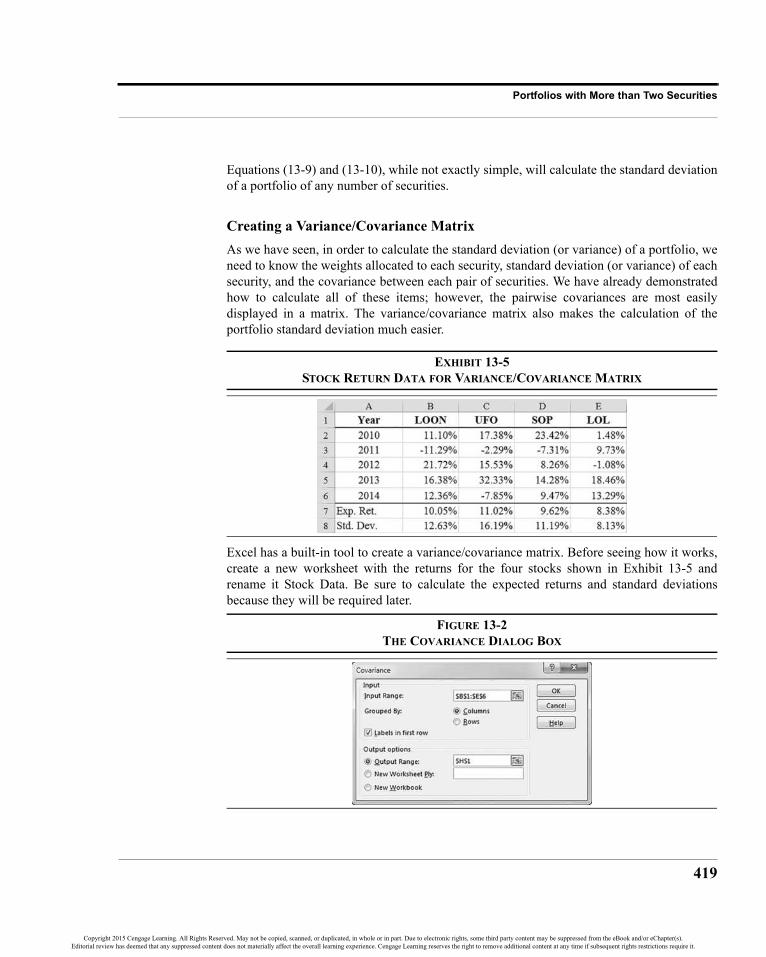
419
Portfolios with More than Two Securities
Equations (13-9) and (13-10), while not exactly simple, will calculate the standard deviationof a portfolio of any number of securities.
Creating a Variance/Covariance MatrixAs we have seen, in order to calculate the standard deviation (or variance) of a portfolio, weneed to know the weights allocated to each security, standard deviation (or variance) of eachsecurity, and the covariance between each pair of securities. We have already demonstratedhow to calculate all of these items; however, the pairwise covariances are most easilydisplayed in a matrix. The variance/covariance matrix also makes the calculation of theportfolio standard deviation much easier.
EXHIBIT 13-5STOCK RETURN DATA FOR VARIANCE/COVARIANCE MATRIX
Excel has a built-in tool to create a variance/covariance matrix. Before seeing how it works,create a new worksheet with the returns for the four stocks shown in Exhibit 13-5 andrename it Stock Data. Be sure to calculate the expected returns and standard deviationsbecause they will be required later.
FIGURE 13-2THE COVARIANCE DIALOG BOX
Copyright 2015 Cengage Learning. All Rights Reserved. May not be copied, scanned, or duplicated, in whole or in part. Due to electronic rights, some third party content may be suppressed from the eBook and/or eChapter(s).Editorial review has deemed that any suppressed content does not materially affect the overall learning experience. Cengage Learning reserves the right to remove additional content at any time if subsequent rights restrictions require it.
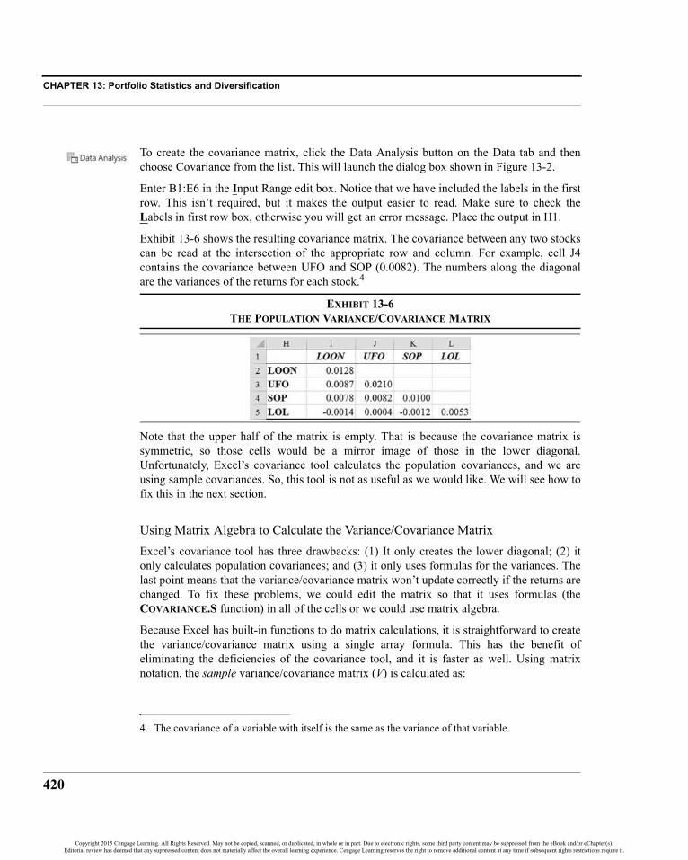
CHAPTER 13: Portfolio Statistics and Diversification
420
To create the covariance matrix, click the Data Analysis button on the Data tab and thenchoose Covariance from the list. This will launch the dialog box shown in Figure 13-2.
Enter B1:E6 in the Input Range edit box. Notice that we have included the labels in the firstrow. This isn’t required, but it makes the output easier to read. Make sure to check theLabels in first row box, otherwise you will get an error message. Place the output in H1.
Exhibit 13-6 shows the resulting covariance matrix. The covariance between any two stockscan be read at the intersection of the appropriate row and column. For example, cell J4contains the covariance between UFO and SOP (0.0082). The numbers along the diagonalare the variances of the returns for each stock.4
EXHIBIT 13-6THE POPULATION VARIANCE/COVARIANCE MATRIX
Note that the upper half of the matrix is empty. That is because the covariance matrix issymmetric, so those cells would be a mirror image of those in the lower diagonal.Unfortunately, Excel’s covariance tool calculates the population covariances, and we areusing sample covariances. So, this tool is not as useful as we would like. We will see how tofix this in the next section.
Using Matrix Algebra to Calculate the Variance/Covariance MatrixExcel’s covariance tool has three drawbacks: (1) It only creates the lower diagonal; (2) itonly calculates population covariances; and (3) it only uses formulas for the variances. Thelast point means that the variance/covariance matrix won’t update correctly if the returns arechanged. To fix these problems, we could edit the matrix so that it uses formulas (theCOVARIANCE.S function) in all of the cells or we could use matrix algebra.
Because Excel has built-in functions to do matrix calculations, it is straightforward to createthe variance/covariance matrix using a single array formula. This has the benefit ofeliminating the deficiencies of the covariance tool, and it is faster as well. Using matrixnotation, the sample variance/covariance matrix (V) is calculated as:
4. The covariance of a variable with itself is the same as the variance of that variable.
Copyright 2015 Cengage Learning. All Rights Reserved. May not be copied, scanned, or duplicated, in whole or in part. Due to electronic rights, some third party content may be suppressed from the eBook and/or eChapter(s).Editorial review has deemed that any suppressed content does not materially affect the overall learning experience. Cengage Learning reserves the right to remove additional content at any time if subsequent rights restrictions require it.

421
Portfolios with More than Two Securities
where D is the difference matrix, D' is the transpose of D, and n is the number of returns foreach security. The difference matrix is a matrix of the returns less the expected return.Matrix multiplication can be done using the MMULT function:
MMULT(ARRAY1, ARRAY2)
where both arguments are ranges on the worksheet or in memory. Following the rules ofmatrix algebra, the number of columns in ARRAY1 must be equal to the number of rows inARRAY2. We also need to calculate the transpose of the difference matrix, so we can use theTRANSPOSE function:
TRANSPOSE(ARRAY)
where ARRAY is a range on the worksheet or in memory. Because MMULT and TRANSPOSEinherently return multiple values, they are array functions. Therefore, you must select arange that will hold all of the output (instead of a single cell) and press Shift+Ctrl+Enterwhen entering them from the formula bar. This also means that you only need to enter theformula once to get all of the results.
Because we are using an array formula, we can calculate the difference array in memory,rather than creating it on the worksheet. To create the covariance matrix, select I2:L5 andthen enter: =MMULT(TRANSPOSE(B2:E6-B7:E7),(B2:E6-B7:E7))/4. This willcreate the output shown in Exhibit 13-7. If you get a #VALUE! error instead, then you needto remember to enter the formula using Shift+Ctrl+Enter.5
EXHIBIT 13-7THE SAMPLE VARIANCE/COVARIANCE MATRIX
5. On the official Web site http://www.cengagebrain.com/, you can download the cov-matrix.xlamadd-in that creates a variance/covariance matrix with some additional capabilities and options.Once installed, it will appear on the Data tab.
(13-11)V D′Dn 1–------------=
,
Copyright 2015 Cengage Learning. All Rights Reserved. May not be copied, scanned, or duplicated, in whole or in part. Due to electronic rights, some third party content may be suppressed from the eBook and/or eChapter(s).Editorial review has deemed that any suppressed content does not materially affect the overall learning experience. Cengage Learning reserves the right to remove additional content at any time if subsequent rights restrictions require it.

CHAPTER 13: Portfolio Statistics and Diversification
422
This is similar to the output of the covariance tool, except that it is the full sample variance/covariance matrix and will update automatically if any of the returns are changed. It will alsofacilitate the calculation of the portfolio standard deviation in the next section.
In this example, because we are using historical data, we are assuming that all possibleoutcomes are equally likely. However, we often have probability distributions with unequalprobabilities. In that case, assuming that the probabilities are in A2:A6, we would change theabove formula to: =MMULT(TRANSPOSE(A2:A6*(B2:E6-B7:E7)),(B2:E6-B7:E7)). Try itby replacing each of the years in A2:A6 with 0.20 (20% probability). This will give the samepopulation covariance matrix as Exhibit 13-6, but with the flexibility of changing theprobabilities. Remember to reset the formula to match Exhibit 13-7 before continuing.
Calculating the Portfolio Standard DeviationWe have seen earlier that we can use equation (13-10) to calculate the portfolio standarddeviation. However, the number of terms in that equation grows very quickly as the numberof securities increases. It simply isn’t practical to type in that equation if there are more thantwo or three securities. The total number of covariances (including variances) required in theformula is given by:
(13-12)
Therefore, it is impractical to try to create a worksheet formula to calculate the portfoliostandard deviation of a portfolio with more than a few securities. Not only would theformula be very long, but the chance of making an error is high. Therefore, we should eitheruse matrix algebra or a user-defined function to do the calculation. We will demonstrate bothtechniques in this section.
We have all the data required to calculate the portfolio standard deviation, except for theweights. Let’s begin by assuming that our portfolio will hold all four stocks in equalproportions (i.e., 25% in each). Starting in A10, set up the data as shown in Exhibit 13-8.
In any portfolio, the weights of the individual securities must sum to 100%. So, as a check,in B15 enter the formula: =SUM(B11:B14). To calculate the expected return of theportfolio in B16 enter: =SUM(TRANSPOSE(B11:B14)*$B$7:$E$7) as an arrayformula. Note that we need to transpose one of the ranges because their orientation differs.The expected return of the equally weighted portfolio is 9.77%.
Number of Covariances N N 1+( )2
----------------------=
Equation (13-12) counts only the lower half of the covariance matrix as shown in Exhibit13-6 (there are covariances). The full covariance matrix in Exhibit 13-7requires N2 covariances to fill the entire matrix.
4 4 1+( ) 2⁄ = 10
Copyright 2015 Cengage Learning. All Rights Reserved. May not be copied, scanned, or duplicated, in whole or in part. Due to electronic rights, some third party content may be suppressed from the eBook and/or eChapter(s).Editorial review has deemed that any suppressed content does not materially affect the overall learning experience. Cengage Learning reserves the right to remove additional content at any time if subsequent rights restrictions require it.

423
Portfolios with More than Two Securities
EXHIBIT 13-8CALCULATING THE PORTFOLIO STANDARD DEVIATION
We can restate equation (13-10) to calculate the portfolio standard deviation in matrixnotation:
where W is the column vector (range) of weights, V is the variance/covariance matrix, andW' is the transpose of the weight vector. In B17 enter the formula: =SQRT(MMULT(MMULT(TRANSPOSE(B11:B14),$I$2:$L$5),B11:B14)). Remember to enter theformula using Shift+Ctrl+Enter because it is an array formula. You should find that theportfolio standard deviation is 8.56%.
Instead of using the matrix functions, we can use the FAME_PORTVAR1 user-definedfunction from the Famefncs.xlam add-in. This function calculates the portfolio variancegiven the variance/covariance matrix and the weights. It is defined as:
FAME_PORTVAR1(VARCOVMAT,WEIGHTS)
where VARCOVMAT is the variance/covariance matrix, and WEIGHTS is the range of weightsfor each security. To calculate the portfolio standard deviation in B17, replace the formulawith: =SQRT(FAME_PortVar1($I$2:$L$5,B11:B14)). Your answer should be thesame.
You can experiment by changing the weights to see how the expected return and standarddeviation changes. There are an infinite number of portfolios that can be created from thesestocks by varying the weights.
(13-13)σP W′VW=
Copyright 2015 Cengage Learning. All Rights Reserved. May not be copied, scanned, or duplicated, in whole or in part. Due to electronic rights, some third party content may be suppressed from the eBook and/or eChapter(s).Editorial review has deemed that any suppressed content does not materially affect the overall learning experience. Cengage Learning reserves the right to remove additional content at any time if subsequent rights restrictions require it.

CHAPTER 13: Portfolio Statistics and Diversification
424
The Efficient FrontierAs noted above, an infinite number of portfolios can be constructed from any universe ofsecurities. Some will be better than others. If we were to create a graph showing the risk andreturn combination for every possible portfolio, it would be known as the feasible set.
FIGURE 13-3THE FEASIBLE SET AND EFFICIENT FRONTIER
Figure 13-3 shows the feasible set and some additional information. Notice that portfolios A,B, and C are within the feasible set, so they could be created. However, portfolio B is on theedge of the feasible set and has the same expected return as A, but with less risk. Therefore,given a choice, any investor would prefer B over A. Similarly, portfolio C has the same amountof risk as A, but it has a much higher return. So, any investor would prefer C over A.
Portfolios B and C are both on the upper edge of the feasible set, which is known as theefficient frontier. Portfolios that are located on the efficient frontier will always be preferredover portfolios that are inside the feasible set because they offer either: (1) a higher returnwith the same risk; or (2) the same return with less risk. For this reason, investors willalways choose from among the portfolios that lie on the efficient frontier.
Unless we know an investor’s utility function, however, we cannot determine whichportfolio on the efficient frontier would be chosen by that investor. For example, we cannotsay whether you would prefer B or C (or some other portfolio on the efficient frontier)without knowing your utility function. We will examine the process of choosing the optimalportfolio with a utility function in a later section.
Finally, note the portfolio labeled “Minimum Variance Portfolio.” This is the least riskyportfolio that is located on the efficient frontier.
Copyright 2015 Cengage Learning. All Rights Reserved. May not be copied, scanned, or duplicated, in whole or in part. Due to electronic rights, some third party content may be suppressed from the eBook and/or eChapter(s).Editorial review has deemed that any suppressed content does not materially affect the overall learning experience. Cengage Learning reserves the right to remove additional content at any time if subsequent rights restrictions require it.

425
The Efficient Frontier
Locating Portfolios on the Efficient Frontier in ExcelFinding the portfolios that lie on the efficient frontier is a quadratic (nonlinear) optimizationproblem. Specifically, we want to find the set of portfolios that minimize the risk for eachfeasible expected return subject to two (sometimes three or more) constraints: (1) The sumof the weights must equal 1; (2) the calculated return must equal the specified target return;and, sometimes, (3) each of the weights must be between 0 and 1. The third constraintspecifies that short sales are not allowed, which is a common constraint for individual andinstitutional investors. Also note that corporations cannot short sell their projects, so thatconstraint would often be appropriate. For our theoretical purposes, we will allow short salesand, therefore, disregard constraint 3. We will also assume that the proceeds from theshorted securities can be used to purchase more of the long positions.
In Chapter 11 (pages 361 to 365), we used the Solver to find the solution to an optimal capitalbudgeting problem. We can use the Solver for any type of optimization, so we will use it tolocate a couple of the portfolios on the efficient frontier. Because the efficient frontier beginsat the minimum variance portfolio, we will first solve for the set of weights for our four stocksthat result in the smallest possible portfolio standard deviation, without regard to the return.This is the minimum variance portfolio that was pictured in Figure 13-3.
Click the Solver button on the Data tab to get the Solver dialog box as shown in Figure 13-4.
FIGURE 13-4USING THE SOLVER TO GET THE MINIMUM VARIANCE PORTFOLIO
Copyright 2015 Cengage Learning. All Rights Reserved. May not be copied, scanned, or duplicated, in whole or in part. Due to electronic rights, some third party content may be suppressed from the eBook and/or eChapter(s).Editorial review has deemed that any suppressed content does not materially affect the overall learning experience. Cengage Learning reserves the right to remove additional content at any time if subsequent rights restrictions require it.

CHAPTER 13: Portfolio Statistics and Diversification
426
For the minimum variance portfolio, we are seeking to minimize the portfolio standarddeviation in B17, so that is the Target Cell. Select the Min radio button so that the Solverwill minimize the function. The By Changing Variable Cells should be the weights inB11:B14. Now, click the Add button so that we can add the constraint: B15=1. This assuresthat the weights will add up to 1 (i.e., 100% of your money will be invested).
Because we are solving a nonlinear optimization problem, we cannot use the Simplex LPsolver as we did in Chapter 11. Instead, be sure to set the solving method to use the GRGNonlinear solver. The default options should work fine, so we don’t need to change them, butbe sure that Make Unconstrained Variables Non-Negative is not checked.
Make sure that your dialog box looks like the one in Figure 13-4 and then click the Solvebutton. After a few seconds, you should be notified that Solver has found a solution. Chooseto keep that solution, and you will see that the expected return of the minimum varianceportfolio is 8.84% and the standard deviation is 5.87%.6
We will follow an almost identical process to find one more portfolio on the efficientfrontier. We only need one more because every portfolio on the frontier can be calculateddirectly from any two frontier portfolios.
We need to specify the target return for this other portfolio and add another constraint. First,copy B10:B17 across to column C. This will set up the formulas for the other portfolio. InC10 change the name of the portfolio to: Max Return.
Now that we have the cells set up, relaunch the Solver. Change the Target Cell to C17, theChanging Cells to C11:C14, and then change the existing constraint to: C15 = 1. We alsoneed to add a new constraint so that: C16 = C7. This ensures that the calculated return (C16)is equal to our target return (C7) for this portfolio. The target return will be the same as thatof the stock with the highest return (UFO in this example).7 The main Solver dialog boxshould now look like the one in Figure 13-5.
6. When allowing short sales, as we are here, we can analytically solve for the weights of theminimum variance portfolio directly using:
where V--1 is the inverse of the variance/covariance matrix and e is a column vector of ones. See Grinold, R.C. & Kahn, R.N. (1995), Active Portfolio Management. Chicago: Irwin ProfessionalPublishing.
7. This is just a convenience, and we could set it to any other value. In fact, because we are allowingshort sales, just about any return is achievable in theory. If we did not allow short sales, then thehighest achievable return would be equal to that of the highest returning stock.
Min Var Weights V 1– ee′V 1– e------------------=
Copyright 2015 Cengage Learning. All Rights Reserved. May not be copied, scanned, or duplicated, in whole or in part. Due to electronic rights, some third party content may be suppressed from the eBook and/or eChapter(s).Editorial review has deemed that any suppressed content does not materially affect the overall learning experience. Cengage Learning reserves the right to remove additional content at any time if subsequent rights restrictions require it.
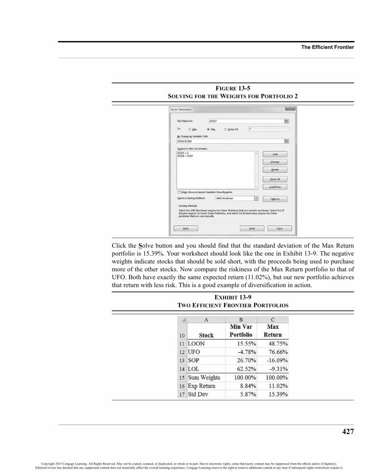
427
The Efficient Frontier
FIGURE 13-5SOLVING FOR THE WEIGHTS FOR PORTFOLIO 2
Click the Solve button and you should find that the standard deviation of the Max Returnportfolio is 15.39%. Your worksheet should look like the one in Exhibit 13-9. The negativeweights indicate stocks that should be sold short, with the proceeds being used to purchasemore of the other stocks. Now compare the riskiness of the Max Return portfolio to that ofUFO. Both have exactly the same expected return (11.02%), but our new portfolio achievesthat return with less risk. This is a good example of diversification in action.
EXHIBIT 13-9TWO EFFICIENT FRONTIER PORTFOLIOS
Copyright 2015 Cengage Learning. All Rights Reserved. May not be copied, scanned, or duplicated, in whole or in part. Due to electronic rights, some third party content may be suppressed from the eBook and/or eChapter(s).Editorial review has deemed that any suppressed content does not materially affect the overall learning experience. Cengage Learning reserves the right to remove additional content at any time if subsequent rights restrictions require it.

CHAPTER 13: Portfolio Statistics and Diversification
428
Charting the Efficient FrontierWe have located two portfolios that are on the efficient frontier, and we could create a chartnow. However, having only two portfolios will produce a line, not a smooth curve, so wewill create several more before charting the frontier. Before beginning, select C10:C17 andmove it to L10:L17 by dragging. This will give us some space to create the other portfolios.
We will now make use of a special property of portfolios on the efficient frontier: Everyportfolio on the frontier is a combination of two other portfolios that are on the frontier, sothe weights are a weighted average of the weights in the other two portfolios:
(13-14)
We have the weights for two portfolios already, so we’ll start by creating a portfolio that isexactly 90% invested in the Minimum Variance portfolio, and 10% invested in the MaxReturn portfolio (though we could use any two portfolios for which we know the weights).This will be located toward the left part of the efficient frontier.
In C9 enter the weight: 90%. Enter a formula to calculate the weight of LOON in C11:=C$9*$B11+(1-C$9)*$L11. You should see that LOON will have a weight of 18.87%in this new frontier portfolio. Copy this formula down through C14 to get the weights of theother stocks. The weight in row 9 is the proportion that is invested in the minimum varianceportfolio, and the remainder of your funds will be invested in the maximum return portfolio.
To get the weights, returns, and standard deviations for the remaining portfolios, simplycopy C11:C17 across to D11:K17. Your worksheet should match Exhibit 13-10.
EXHIBIT 13-10WEIGHTS FOR PORTFOLIOS ON THE EFFICIENT FRONTIER
Once the portfolios are located, then creating a chart of the efficient frontier is as easy ascreating a scatter chart. If you refer back to Figure 13-3, you will see that we want theexpected returns on the y-axis and the standard deviations on the x-axis. Select A16:L17 andinsert a scatter chart with straight lines and markers. At first, your chart will have thevariables on the wrong axes, so we need to edit the chart to fix this problem.
WP xWMin Var 1 x–( )WMax Return+=
Copyright 2015 Cengage Learning. All Rights Reserved. May not be copied, scanned, or duplicated, in whole or in part. Due to electronic rights, some third party content may be suppressed from the eBook and/or eChapter(s).Editorial review has deemed that any suppressed content does not materially affect the overall learning experience. Cengage Learning reserves the right to remove additional content at any time if subsequent rights restrictions require it.

429
The Capital Market Line
FIGURE 13-6A CHART OF THE EFFICIENT FRONTIER
Right-click in the chart and choose Select Data… from the shortcut menu. In the Select DataSource dialog box, click the Edit button. Now change the Series X values so that it points toB17:L17. Change the Series Y values to B16:L16. This will “flip” the chart so that thevalues are on the correct axes. After adding the appropriate chart title and axis titles, yourchart should look like the one in Figure 13-6.
The efficient frontier in the chart isn’t quite a smooth curve. This is because we have onlyplotted 11 portfolios. If we had found, say, 20 portfolios with more of them near the apex ofthe curve, then it would be much smoother. Another way is to change the chart type toscatter with smooth lines. This is generally not recommended because it applies artificialsmoothing to the data so that the chart is not necessarily a good representation of the data.
The Capital Market LineSo far, we have included only risky assets in the portfolios. Now imagine that a completelyrisk-free asset is also available. This is an asset that has a standard deviation of returns ofzero, and its expected return is equal to the risk-free rate. Of course, this asset exists only intheory. In the real world, U.S. Treasury bills come closest to being risk-free assets becausethey are free of default risk. We will use a theoretical risk-free asset with an expected returnof 7%. We are interested in seeing how the efficient frontier changes when a risk-free asset isadded to the universe of securities.
To begin, create a copy of the worksheet that you used to create Exhibit 13-9. We will makea few modifications to include this additional asset. In F1 enter Risk-Free for the name ofthe asset and then enter 7% as the return for each year. Now copy E7:E8 to F7:F8 to calculatethe expected return and standard deviation of the risk-free asset. This section of yourworksheet should now look like the one in Exhibit 13-11.
Copyright 2015 Cengage Learning. All Rights Reserved. May not be copied, scanned, or duplicated, in whole or in part. Due to electronic rights, some third party content may be suppressed from the eBook and/or eChapter(s).Editorial review has deemed that any suppressed content does not materially affect the overall learning experience. Cengage Learning reserves the right to remove additional content at any time if subsequent rights restrictions require it.

CHAPTER 13: Portfolio Statistics and Diversification
430
EXHIBIT 13-11DATA INCLUDING THE RISK-FREE ASSET
We also need to add the risk-free asset to the variance/covariance matrix. In M1 and H6enter the label: Risk-Free. Now select I2:M6 and enter the formula: =MMULT(TRANSPOSE(B2:F6-B7:F7),(B2:F6-B7:F7))/4. This is the same formula that weused previously, except that the ranges have been expanded to include the risk-free asset.The variance/covariance matrix is shown in Exhibit 13-12.
Note that the covariance (and correlation) of the risk-free asset with any other asset is 0.Because the returns on the risk-free asset don’t vary, they certainly can’t vary with thereturns on any other asset. It is this fact that makes the risk-free asset so good fordiversification purposes, as we will see shortly.
EXHIBIT 13-12THE VARIANCE/COVARIANCE MATRIX WITH THE RISK-FREE ASSET
Finally, we need to add the risk-free asset into the portfolio section of the worksheet. Selectrow 15 and insert a new row. Type Risk-Free into A15, and then edit the formulas inB16, B17, and B18 so that they include the new data. The new formulas are:
B16: =SUM(B11:B15)
B17: =SUM(TRANSPOSE(B11:B15)*$B$7:$F$7)
B18: =SQRT(MMULT(MMULT(TRANSPOSE(B11:B15),$I$2:$M$6),B11:B15))
Copyright 2015 Cengage Learning. All Rights Reserved. May not be copied, scanned, or duplicated, in whole or in part. Due to electronic rights, some third party content may be suppressed from the eBook and/or eChapter(s).Editorial review has deemed that any suppressed content does not materially affect the overall learning experience. Cengage Learning reserves the right to remove additional content at any time if subsequent rights restrictions require it.

431
The Capital Market Line
Remember that the formulas in B17 and B18 are array formulas, so they must be enteredusing Shift+Ctrl+Enter.
Now, we will run the Solver exactly as before. Remember that we are allowing unlimitedshort sales because that is one of the assumptions made in the derivation of the capitalmarket line (CML). Furthermore, we assume that any proceeds from short sales can be usedto purchase additional long positions in other assets.
The minimum variance portfolio will be 100% invested in the risk-free asset because theportfolio standard deviation can never be below 0. Therefore, set the weights in B11:B14 to0% and B15 to 100%. You should see that the expected return on this portfolio is 7% and thestandard deviation is 0%. We don’t need to use the Solver for this portfolio.
As before, we will minimize the standard deviation of the Max Return portfolio, so the TargetCell is L18. The Changing Cells are the weights in L11:L15. Because we are allowing shortsales, we only need to set two constraints. The first is that the sum of the weights must equal 1,so click the Add button and enter the constraint: L16 = 1. The second is that the calculatedportfolio return must equal the target return (11.02%), so enter the constraint: L17 = C7.
FIGURE 13-7SOLVER SETTINGS FOR THE MAX RETURN PORTFOLIO
Make sure that your Solver dialog box matches the one shown in Figure 13-7, and then clickthe Solve button. You should find that the expected return for the Max Return portfolio is11.02% and the standard deviation is 11.51%. The other portfolios should have updatedautomatically. Your worksheet should look like the one pictured in Exhibit 13-13.
Copyright 2015 Cengage Learning. All Rights Reserved. May not be copied, scanned, or duplicated, in whole or in part. Due to electronic rights, some third party content may be suppressed from the eBook and/or eChapter(s).Editorial review has deemed that any suppressed content does not materially affect the overall learning experience. Cengage Learning reserves the right to remove additional content at any time if subsequent rights restrictions require it.

CHAPTER 13: Portfolio Statistics and Diversification
432
EXHIBIT 13-13PORTFOLIOS ON THE CML
Charting the Capital Market LineWe are now ready to create a chart of the CML. First, return to your efficient frontierworksheet and copy the chart of the efficient frontier (Figure 13-6). Now paste the chart intothe CML worksheet. This will maintain the links to the original data, so the chart shouldlook the same.
We want to add the CML to this chart so that we can compare the efficient frontier with theCML. Right-click in the chart and choose Select Data. Next, click the Add button so that wecan add the new series. In the Series name edit box, type: =”CML” to name the series. Forthe Series X values select B18:F18, and for the Series Y values select B17:F17. Your chartshould now look like the one in Figure 13-8.
FIGURE 13-8CHART OF THE CML AND THE EFFICIENT FRONTIER
Copyright 2015 Cengage Learning. All Rights Reserved. May not be copied, scanned, or duplicated, in whole or in part. Due to electronic rights, some third party content may be suppressed from the eBook and/or eChapter(s).Editorial review has deemed that any suppressed content does not materially affect the overall learning experience. Cengage Learning reserves the right to remove additional content at any time if subsequent rights restrictions require it.

433
The Capital Market Line
There are several important points to note about this chart. First, notice that the CML is astraight line. That is, adding a risk-free asset to our universe of securities creates a linearrisk/return trade-off.
Second, notice that the CML provides a better risk/return trade-off than the efficient frontier.For any portfolio that lies on the efficient frontier, there is a superior portfolio on the CML.This is important because it means that if a risk-free asset (such as Treasury bills) isavailable, then investors will no longer choose portfolios from among those on the efficientfrontier. Rather, they will choose a portfolio that lies on the CML.
Finally, notice that there is one point of commonality between the CML and the efficientfrontier. The CML is tangent to the efficient frontier at the location of a very specialportfolio known as the market portfolio. The market portfolio contains all risky assets (allfour stocks in our example) in proportion to their market values. In other words, it is acapitalization-weighted portfolio.
The market portfolio does not hold the risk-free asset. Every other portfolio on the CML ismade up of some portion of the risk-free asset and the market portfolio. Therefore, allinvestors will invest in a portfolio that holds the market portfolio and the risk-free asset (i.e.,somewhere on the CML).
This means that the investment decision is the same for all investors—they all invest in themarket portfolio. The only choice that they have to make is how much of the risk-free assetto own. This choice is known as the financing decision. A long position is equivalent tomaking a loan at the risk-free rate, while a short position in the risk-free asset is equivalent toborrowing at the risk-free rate and using the proceeds to purchase more of the marketportfolio.
By introducing a risk-free asset, we have separated the investing and financing decisions.This is known as the Tobin’s separation theorem and is illustrated in Figure 13-9.
FIGURE 13-9THE CML AND THE SEPARATION THEOREM
Copyright 2015 Cengage Learning. All Rights Reserved. May not be copied, scanned, or duplicated, in whole or in part. Due to electronic rights, some third party content may be suppressed from the eBook and/or eChapter(s).Editorial review has deemed that any suppressed content does not materially affect the overall learning experience. Cengage Learning reserves the right to remove additional content at any time if subsequent rights restrictions require it.

CHAPTER 13: Portfolio Statistics and Diversification
434
Identifying the Market Portfolio
The market portfolio plays a central role in modern portfolio theory. It would be helpful ifwe could identify its exact location on the efficient frontier. By looking at Figure 13-9, youshould be able to see that the equation (in slope-intercept form) of the CML is:
(13-15)
The slope of the CML is known as the market price of risk and is given by:
(13-16)
The market price of risk is a measure of the excess return per unit of risk that is available inthe market. Because the CML is a straight line, it has the same slope at every point.Therefore, we can generalize that to any portfolio by substituting for RM and σM. This givesus the Sharpe ratio, which is a well-known portfolio performance metric. The equation forthe Sharpe ratio is:
(13-17)
In Figure 13-8, it appears that the market portfolio is very close to portfolio 3 on the efficientfrontier, but we don’t know for sure what the weights are. We can find its exact position onthe efficient frontier by using the Solver to find the weights for the portfolio that maximizesthe Sharpe ratio.
The risk-free asset could be combined with any portfolio on the efficient frontier, with theresulting line known as a capital allocation line. Investors will prefer portfolios on thesteepest capital allocation line, which is the one with the highest Sharpe ratio (i.e., the CML).
We will use M10:M19 to solve for the market portfolio. So, select L10:L19 and copy therange to M10:M19. Change the label in M10 to: Market Portfolio, and in A19 enter:Sharpe Ratio. In B19 enter the formula: =IFERROR((B17-$B$17)/B18,0) andthen copy it across C19:M19. We are using the IFERROR function to avoid a #DIV/0! errorfor the minimum variance portfolio.
Our goal is to use the Solver to maximize the Sharpe ratio in M19 by changing the weightsin M11:M15, subject to the constraints that M16 = 1, and M15 = 0 (the market portfolio doesnot hold the risk-free asset). Launch the Solver and set up the dialog box so that it matchesFigure 13-10.
E RP( ) RFRM RF–( )
σM------------------------σP+=
Slope of CMLRM RF–( )
σM------------------------=
Sharpe RatioRP RF–( )
σP-----------------------=
Copyright 2015 Cengage Learning. All Rights Reserved. May not be copied, scanned, or duplicated, in whole or in part. Due to electronic rights, some third party content may be suppressed from the eBook and/or eChapter(s).Editorial review has deemed that any suppressed content does not materially affect the overall learning experience. Cengage Learning reserves the right to remove additional content at any time if subsequent rights restrictions require it.

435
The Capital Market Line
FIGURE 13-10SOLVER DIALOG BOX TO FIND THE MARKET PORTFOLIO
After running the Solver, you will find that the market portfolio has a Sharpe ratio of 0.3494,which is also the slope of the CML. Your output should match Exhibit 13-14 (some columnsare hidden).
EXHIBIT 13-14THE MARKET PORTFOLIO AND OTHERS ON THE EFFICIENT FRONTIER
The market portfolio is located at the point of tangency between the CML and the efficientfrontier because that is the point at which their slopes are equal. We have now exactlyidentified the market portfolio. We know how much of each stock it holds, and we know itsreturn and standard deviation.
Copyright 2015 Cengage Learning. All Rights Reserved. May not be copied, scanned, or duplicated, in whole or in part. Due to electronic rights, some third party content may be suppressed from the eBook and/or eChapter(s).Editorial review has deemed that any suppressed content does not materially affect the overall learning experience. Cengage Learning reserves the right to remove additional content at any time if subsequent rights restrictions require it.

CHAPTER 13: Portfolio Statistics and Diversification
436
As noted earlier, the market portfolio is located very close to portfolio 3 on the efficientfrontier. You can add it to the chart of the efficient frontier and CML (Figure 13-8). Right-click the chart and choose Select Data. Click the Add button and set the Series name toMarket Portfolio, the X value to the market portfolio’s standard deviation, and the Yvalue to its expected return. Figure 13-11 shows the result.
FIGURE 13-11THE MARKET PORTFOLIO WITH THE CML AND EFFICIENT FRONTIER
Utility Functions and the Optimal PortfolioEach investor will prefer a different portfolio; which one depends upon their preferencesregarding risk and return. As noted in Chapter 8, some investors are more tolerant of riskthan others, and we would expect these investors to choose a riskier portfolio with a higherexpected return. In order to identify the optimal portfolio we need to know the investor’sutility function and degree of risk aversion. For our purposes, we will use the followingutility function (which is just one of many possible utility functions):
Charting Indifference CurvesAn indifference curve shows all possible combinations of risk and return that would providethe same amount of utility for a given investor. We can rearrange equation (13-18) asfollows:
(13-18)
where E(R) is the expected return of the portfolio, σ2 is the variance, and A is the coefficientof relative risk aversion (-∞ ≤ A ≤ ∞). When A > 0 the investor is risk averse, and highervalues of A indicate greater risk aversion (i.e., less risk tolerance). When A = 0, the investoris risk neutral. Equation (13-18) will allow us to calculate the utility of a portfolio on theefficient frontier, and to find the portfolio that maximizes the utility for any given investor.
E U( ) E R( ) 12---Aσ2
–=
Copyright 2015 Cengage Learning. All Rights Reserved. May not be copied, scanned, or duplicated, in whole or in part. Due to electronic rights, some third party content may be suppressed from the eBook and/or eChapter(s).Editorial review has deemed that any suppressed content does not materially affect the overall learning experience. Cengage Learning reserves the right to remove additional content at any time if subsequent rights restrictions require it.

437
Utility Functions and the Optimal Portfolio
which will allow us to specify levels of utility, risk aversion, and risk and then solve for thereturn. We can then plot the combinations that result in the specified level of utility. Whenwe plot multiple indifference curves, we call it an indifference map.
Create a new worksheet and name it Indifference Curves. In A1 enter: Risk Aversion,and in B1 enter: 2.5. In A2 enter: Utility, and in B2:D2 enter 7%, 8%, and 9%. InA4:A19 enter a series going from 0 to 15% in 1% increments. In B4 enter the formula tocalculate the return: =B$2+0.5*$B$1*$A4^2, and copy it over the range. Now copy thechart that you created for Figure 13-6 into this worksheet, and add each of the indifferencecurves. Your worksheet should look like the one in Exhibit 13-15.
We could add many more indifference curves, as there are an infinite number of them.However, we are seeking the portfolio on the efficient frontier that maximizes the expectedutility for the investor. This portfolio will be located at the point where an indifference curveis tangent to the efficient frontier. Indifference curve 3 is close to the frontier, but outside ofthe feasible set. So, the investor cannot quite achieve that level of utility.
EXHIBIT 13-15THE EFFICIENT FRONTIER AND THREE INDIFFERENCE CURVES
To find the optimal portfolio, return to the worksheet that you used to create the CML. CopyM10:M19 over to column N. In A20 enter the label: Utility, and then in B20 enter theformula: =B17-0.5*'Indifference Curves'!$B$1*B18^2. Copy this acrossC20:N20 to calculate the utility for each portfolio.
(13-19)E R( ) E U( ) 12---Aσ2
+=
Copyright 2015 Cengage Learning. All Rights Reserved. May not be copied, scanned, or duplicated, in whole or in part. Due to electronic rights, some third party content may be suppressed from the eBook and/or eChapter(s).Editorial review has deemed that any suppressed content does not materially affect the overall learning experience. Cengage Learning reserves the right to remove additional content at any time if subsequent rights restrictions require it.

CHAPTER 13: Portfolio Statistics and Diversification
438
Finally, launch the Solver and set it to maximize cell N20 by changing N11:N15 with aconstraint of N16 = 1. You should find that the portfolio with the highest utility has anexpected return of 11.88% and a standard deviation of 13.98%. This is the optimal portfoliofor the investor with a risk aversion coefficient of 2.5. You can easily change the riskaversion coefficient and then find the optimal portfolio for a different investor.
Exhibit 13-16 shows the CML and the efficient frontier along with the indifference curve forthe highest achievable level of utility (0.0944) for this investor. It was created in the sameway as Exhibit 13-15, except that only the tangency indifference curve was calculated.
Notice that the optimal portfolio is well above the efficient frontier. This portfolio is onlyavailable because we added the risk-free asset. Without the risk-free asset, the optimalportfolio would have an expected return of 9.78% and utility of 0.0888. We leave it as anexercise for you to find this portfolio using the Solver.
EXHIBIT 13-16OPTIMAL PORTFOLIO FOR THE INVESTOR
The Capital Asset Pricing ModelOne of the best known models in finance is the capital asset pricing model (CAPM). In thissection, we will see how to derive this model and its famous risk measure, beta (β). Recallthat the market portfolio sits at the tangency point of the CML and the efficient frontier. So,at that point, the slopes are equal. The slope of the efficient frontier at point M is given by:
Copyright 2015 Cengage Learning. All Rights Reserved. May not be copied, scanned, or duplicated, in whole or in part. Due to electronic rights, some third party content may be suppressed from the eBook and/or eChapter(s).Editorial review has deemed that any suppressed content does not materially affect the overall learning experience. Cengage Learning reserves the right to remove additional content at any time if subsequent rights restrictions require it.

439
The Capital Asset Pricing Model
According to modern portfolio theory, there are two types of risk: (1) market (or systematic)risk; and (2) company-specific (or unsystematic) risk. Market risk is the risk associated withmarket-wide factors, such as unexpected changes in GDP or inflation rates. Market riskaffects all investments to some degree. Company-specific risk factors (such as increasedcompetition or employees going on strike) affect only individual investments. When wecreate a diversified portfolio, the risk that we are eliminating is the company-specific, ordiversifiable, risk. Market risk cannot be diversified away.
The CAPM says that the portfolio return is equal to the risk-free rate plus a risk premium. Therisk premium is determined by the product of the market risk premium and the portfolio beta.Beta is an index of market risk, so it tells us how sensitive the portfolio is to market risk factors.Note that the CAPM does not contain a risk premium associated with company-specific risk.Because company-specific risks can be diversified away, investors will not receive anyadditional return for holding a less than perfectly diversified portfolio.
(13-20)
where RP is the expected return on a portfolio, and σP,M is the covariance between thatportfolio and the market portfolio. If we now set equation (13-20) equal to equation (13-16),then we get:
Now, cross multiply and simplify to solve for RP and the solution is:
(13-21)
Note that beta is defined as:
(13-22)
Finally, substitute (13-22) into (13-21) to get the familiar form of the CAPM with beta as itsmeasure of risk:
(13-23)
Slope of frontier at MRP RM–( )σM
σP M, σM2–( )
--------------------------------=
RP RM–( )σM
σP M, σM2–( )
--------------------------------RM RF–( )
σM
------------------------=
RP RF
σP M,
σM2
------------ RM RF–( )+=
βPσP M,
σM2
------------=
RP RF βP RM RF–( )+=
Copyright 2015 Cengage Learning. All Rights Reserved. May not be copied, scanned, or duplicated, in whole or in part. Due to electronic rights, some third party content may be suppressed from the eBook and/or eChapter(s).Editorial review has deemed that any suppressed content does not materially affect the overall learning experience. Cengage Learning reserves the right to remove additional content at any time if subsequent rights restrictions require it.

CHAPTER 13: Portfolio Statistics and Diversification
440
The Security Market LineWhen we create a chart of the CAPM equation, it is referred to as the security market line(SML). In this section, we will calculate the betas of our four stocks and create a chart of theSML. To begin, return to the worksheet that you used to create Exhibit 13-14.
We have already determined the weights of each of the stocks in the market portfolio and theexpected return and standard deviation of that portfolio. We will now work backward tocalculate the market portfolio’s return in each year. In F1 enter the label: Market.Remember that the return on a portfolio is a weighted average of the returns of the individualsecurities. So, we can calculate the rate of return on the market portfolio in 2010 by entering:=MMULT(B2:E2,$M$11:$M$14) into F2. Copy that formula to F3:F6 to complete thecalculation. Now we can copy E7:E8 to F7:F8 to get the expected return and standarddeviation of the market portfolio. You should get the same values as we previouslycalculated in M16:M17.
We can calculate the betas for each of the stocks using equation (13-22). In A9 enter: Beta,and calculate the beta for LOON in B9 with the formula: =COVARIANCE.S(B2:B6,$F$2:$F$6)/$F$8^2. You should find that LOON’s beta is 1.339. Now copy thatformula across C9:F9 to calculate the other betas. Your worksheet should match the one inExhibit 13-17.
EXHIBIT 13-17BETAS FOR THE STOCKS AND THE MARKET PORTFOLIO
To chart the SML, we will need to add the data for the risk-free asset. In A21 type: Betaand in A22 type: Exp. Return. In B20 enter: Risk-Free, in B21 enter: 0.000, and inB22 enter: 7.00%. Now copy the labels from B1:F1 and paste them into C20:G20. In C21enter the formula: =B9, and in C22 enter: =B7. Copy the formulas from C21:C22 acrossD21:G22.
To create the chart, select A21:G22 and insert a scatter chart. Your chart should now looklike the one in Figure 13-12.
Copyright 2015 Cengage Learning. All Rights Reserved. May not be copied, scanned, or duplicated, in whole or in part. Due to electronic rights, some third party content may be suppressed from the eBook and/or eChapter(s).Editorial review has deemed that any suppressed content does not materially affect the overall learning experience. Cengage Learning reserves the right to remove additional content at any time if subsequent rights restrictions require it.
Tim
Sticky Note
Accepted set by Tim

441
Summary
FIGURE 13-12THE SECURITY MARKET LINE
SummaryDiversification is the process of allocating capital across multiple investments in order toreduce the riskiness of the portfolio. Diversification reduces risk because assets are notperfectly positively correlated, so volatility in one asset tends to cancel out volatility inanother. Therefore, it is important to choose assets that are not highly correlated.
We demonstrated that the expected return of a portfolio is a weighted average of theexpected returns of the individual assets, but that the standard deviation is more complicated.When calculating the portfolio standard deviation, we have to include each of the pairwisecovariances. We showed how to calculate the variance/covariance matrix and then how touse it to calculate the portfolio standard deviation.
We then discussed the efficient frontier and why investors will choose only from among theportfolios that are located on it. We used the Solver to find a sample of the portfolios on theefficient frontier and then created a chart of it.
Next, we added a risk-free asset to our universe of securities and showed how the efficientfrontier changes into the CML. Portfolios on the CML provide a better risk/return trade-offthan those on the efficient frontier. When a risk-free asset is available, investors will chooseto hold it in some combination with the market portfolio. The exact portfolio chosen willdepend upon the investor’s utility function.
Finally, we derived the CAPM by equating the slopes of the CML and the efficient frontier.This provided us with an important way to view the risk/return trade-off and a measureof risk known as beta. Beta is an index of systematic risk and shows how sensitive an assetis to market risk factors. We also saw that if the CAPM is correct investors are only
Copyright 2015 Cengage Learning. All Rights Reserved. May not be copied, scanned, or duplicated, in whole or in part. Due to electronic rights, some third party content may be suppressed from the eBook and/or eChapter(s).Editorial review has deemed that any suppressed content does not materially affect the overall learning experience. Cengage Learning reserves the right to remove additional content at any time if subsequent rights restrictions require it.

CHAPTER 13: Portfolio Statistics and Diversification
442
rewarded for taking on market risk. There is no reward for holding a less than perfectlydiversified portfolio.
Problems
1. You are considering an investment in the stock market and have identifiedtwo potential stocks (XYZ and ABC) to purchase. The historical returns forthe past five years are shown in the table below.
TABLE 13-2FUNCTIONS INTRODUCED IN THIS CHAPTER*
* All functions with names beginning in FAME_ are macros supplied in the Famefncs.xlam add-in, which is available from the official Web site.
Purpose Function PageCalculate the correlation coefficient CORREL(ARRAY1, ARRAY2) 415
Calculate the covariance COVARIANCE.S(ARRAY1, ARRAY2) 416Matrix multiplication MMULT(ARRAY1, ARRAY2) 421Matrix transpose TRANSPOSE(ARRAY) 421Calculate the portfolio variance FAME_PORTVAR1(VARCOVMAT,WEIGHTS) 423
Calculate the portfolio variance FAME_PORTVAR2(CORRMAT,WEIGHTS) N/A
Calculate covariance using probabilities
FAME_COVAR(VALUES1, VALUES2, PROBABILITIES) N/A
Calculate correlation using probabilities
FAME_CORR(VALUES1, VALUES2, PROBABILITIES) N/A
Year XYZ Returns ABC Returns2010 12.35% 22.28%2008 17.01% 8.75%2009 13.18% 17.78%2010 8.51% 19.66%2014 16.85% 4.03%
Copyright 2015 Cengage Learning. All Rights Reserved. May not be copied, scanned, or duplicated, in whole or in part. Due to electronic rights, some third party content may be suppressed from the eBook and/or eChapter(s).Editorial review has deemed that any suppressed content does not materially affect the overall learning experience. Cengage Learning reserves the right to remove additional content at any time if subsequent rights restrictions require it.

443
Problems
a. Calculate the average return and standard deviation of returns for eachstock over the past five years. Which stock would you prefer to own?Would everyone make the same choice?
b. Calculate the correlation coefficient between the two stocks. Does itappear that a portfolio consisting of XYZ and ABC would providegood diversification?
c. Calculate the annual returns that would have been achieved had youowned a portfolio consisting of 50% in XYZ and 50% in ABC overthe past five years.
d. Calculate the average return and standard deviation of returns for theportfolio. How does the portfolio compare with the individual stocks?Would you prefer the portfolio to owning either of the stocks alone?
e. Create a chart that shows how the standard deviation of the portfolio’sreturns changes as the weight of XYZ changes.
f. Using the Solver, what is the minimum standard deviation that couldbe achieved by combining these stocks into a portfolio? What are theexact weights of the stocks that result in this minimum standarddeviation?
2. You have decided to investigate a number of exchange-traded funds(ETFs) in an attempt to build a diversified portfolio. You believe that thetransportation, consumer goods, energy, financials, and health care sectorsare the best in which to invest. To begin, you have gathered the monthlytotal returns for the last five years from some ETFs (IYT, IYK, IYE, IYF,IYH) in each of these sectors.
a. Download the Five ETFs Monthly Returns.xlsx file from the officialWeb site http://www.cengagebrain.com/. This contains the data forthis, and the next two problems.
b. What are the average monthly returns and standard deviations foreach of the ETFs?
c. Which performed best on a risk/return basis during this period?Which was the worst? Use the Sharpe ratio and assume that the risk-free rate averaged 0.165% per month during this period.
d. Create an equally weighted portfolio of all the ETFs. Calculate theexpected return and standard deviation of this portfolio.
Copyright 2015 Cengage Learning. All Rights Reserved. May not be copied, scanned, or duplicated, in whole or in part. Due to electronic rights, some third party content may be suppressed from the eBook and/or eChapter(s).Editorial review has deemed that any suppressed content does not materially affect the overall learning experience. Cengage Learning reserves the right to remove additional content at any time if subsequent rights restrictions require it.

CHAPTER 13: Portfolio Statistics and Diversification
444
3. Using the ETF data from the previous problem:
a. Create a sample variance/covariance matrix using the ETF returns.Use the matrix algebra functions or the COVARIANCE.S function.(Hint: The matrix function will be less work.)
b. Using the Solver, find the weights for the minimum varianceportfolio.
c. Using the Solver, find the optimal weights for a portfolio with a returnequal to that of the ETF with the highest return. Now, create 9additional portfolios with returns between that of the minimumvariance and maximum return portfolios.
d. Create a chart of the efficient frontier. Now add a new series thatshows the returns and standard deviations of the individual ETFs.How does the efficient frontier compare to the ETFs?
e. Find the weights for the market portfolio. What is its return andstandard deviation?
f. Add the capital market line (CML) to your chart.
4. Do problem 3 again, but this time do not allow short sales (i.e., nonegative weights).
a. Create a new chart that shows the efficient frontiers from this problemand problem 3.
b. From which frontier would you prefer to choose your investments?
5. You are considering investing in the following securities and havedeveloped the probability distributions for their returns over the next year.
a. Calculate the expected return and standard deviation of each security.
Economic Outlook Probability
Expected ReturnsOMG BRB NOOB T-bills
Recession 0.10 –29% –9% 16% 3%Slow growth 0.20 –14% 3% 11% 3%Average 0.40 14% 7% 4% 3%Fast growth 0.20 23% 11% –7% 3%Boom 0.10 34% 14% –14% 3%
Copyright 2015 Cengage Learning. All Rights Reserved. May not be copied, scanned, or duplicated, in whole or in part. Due to electronic rights, some third party content may be suppressed from the eBook and/or eChapter(s).Editorial review has deemed that any suppressed content does not materially affect the overall learning experience. Cengage Learning reserves the right to remove additional content at any time if subsequent rights restrictions require it.

445
Internet Exercise
b. Create a variance/covariance matrix for the four securities. Seepage 422 for an example of how to create a formula that usesprobabilities instead of historical (equally weighted) data.
c. Using the Solver, create a set of 11 portfolios that make up the capitalmarket line. Create a chart of the CML from your results, and add aplot of the original securities.
d. Find the weights of each security in the market portfolio bymaximizing the Sharpe ratio.
e. How does the risk/return trade-off of the original securities compareto that available on the CML?
Internet Exercise
1. Choose two stocks from different industries that you think would have alow correlation. Get the closing prices for each month over the past fiveyears for both stocks. To get the prices from Yahoo! Finance (http://finance.yahoo.com) follow the same procedure as was used in the Chapter8 Internet Exercise to get the dividends, but this time select “Monthly”rather than “Dividends.” Download the data into Excel.
a. Calculate the returns for both stocks in each month during thefive-year period using log-price relatives (see equation (12-2) onpage 373).
b. Calculate the average monthly return and standard deviation ofmonthly returns for each stock. Using only this information, which ofthe two stocks would you have preferred to own over this period?
c. Calculate the correlation coefficient for the two sets of returns usingthe CORREL function. Is it as low as you expected?
d. If the historical returns, standard deviations, and correlation fairlyrepresent the future, calculate the expected return and standarddeviation of a portfolio consisting of 50% invested in each stock.How does the portfolio compare with the individual stocks?
e. Using the Solver, find the weights for each stock that would result inthe minimum portfolio standard deviation.
Copyright 2015 Cengage Learning. All Rights Reserved. May not be copied, scanned, or duplicated, in whole or in part. Due to electronic rights, some third party content may be suppressed from the eBook and/or eChapter(s).Editorial review has deemed that any suppressed content does not materially affect the overall learning experience. Cengage Learning reserves the right to remove additional content at any time if subsequent rights restrictions require it.

Copyright 2015 Cengage Learning. All Rights Reserved. May not be copied, scanned, or duplicated, in whole or in part. Due to electronic rights, some third party content may be suppressed from the eBook and/or eChapter(s).Editorial review has deemed that any suppressed content does not materially affect the overall learning experience. Cengage Learning reserves the right to remove additional content at any time if subsequent rights restrictions require it.

447
CHAPTER 14 Writing User-Defined Functions with VBA
Despite its hundreds of built-in functions, Excel doesn’t always have the one you need.Fortunately, it does provide a method by which you can add your own functions to theprogram and use them in your worksheets.
In previous chapters, we have used several custom functions that extend Excel in ways thatare useful. Those custom functions, known as user-defined functions (UDFs), are written inthe Visual Basic for Applications (VBA) programming language. VBA is available in all ofthe Microsoft Office applications and in some third-party applications.
After studying this chapter, you should be able to:1. Describe the two types of “macros” and explain the difference between them.2. Identify and explain the parts of the VB editor.3. Write your own VBA user-defined function for any given formula.4. Write a user-defined function that allows for optional arguments.5. Use the debugging tools that are available in the VB editor.6. Create an Excel add-in program.
Copyright 2015 Cengage Learning. All Rights Reserved. May not be copied, scanned, or duplicated, in whole or in part. Due to electronic rights, some third party content may be suppressed from the eBook and/or eChapter(s).Editorial review has deemed that any suppressed content does not materially affect the overall learning experience. Cengage Learning reserves the right to remove additional content at any time if subsequent rights restrictions require it.

CHAPTER 14: Writing User-Defined Functions with VBA
448
In this chapter, we will provide a brief demonstration of how to use VBA to create functionsthat meet your needs. If you have ever done any computer programming, you will find iteasy to learn. If not, don’t worry. If you can understand a mathematical formula, it is likelythat you will be able to convert it into a user-defined function without much trouble afterreading this chapter.
VBA is quite powerful and can be used for everything from something as simple aschanging the formatting of a cell in a worksheet to writing complete applications that don’tappear to be Excel worksheets, and everything in between.
Before continuing, be sure to enable the Developer tab in the Ribbon. Click the File tab andthen go to Options. In the Customize Ribbon category, choose Main Tabs in the Customizethe Ribbon drop-down on the right side of the dialog box and place a checkmark next toDeveloper in the right-side pane.
FIGURE 14-1THE DEVELOPER TAB
What Is a Macro?In computer science, a macro is a word or keystroke that serves as a substitute for a longseries of commands. Excel has many built-in macros of this type. For example, you canpress Ctrl+B to make the font in a cell, or range, bold. This is a shortcut for the series ofsteps that would otherwise be required. When you press Ctrl+B, Excel will automaticallyperform all of those steps behind the scenes. This type of macro is known as a keystrokemacro.
Although we can create VBA programs that replicate the functionality of keystroke macros,VBA is not, strictly speaking, a macro language. Instead, it is a fully functional object-oriented programming language. Still, in common usage, VBA programs are often calledmacros.
Two Types of MacrosIn Excel, there are two types of macros. Closest to the traditional definition of keystrokemacros are procedure macros (also known as subroutines). Procedure macros can do thingssuch as activating another worksheet, opening a file, formatting a range of cells, and so on.
Copyright 2015 Cengage Learning. All Rights Reserved. May not be copied, scanned, or duplicated, in whole or in part. Due to electronic rights, some third party content may be suppressed from the eBook and/or eChapter(s).Editorial review has deemed that any suppressed content does not materially affect the overall learning experience. Cengage Learning reserves the right to remove additional content at any time if subsequent rights restrictions require it.

449
What Is a Macro?
As an example, I have written a procedure macro called “ConvertIS” that I use to reformatincome statements that are imported from a particular database. It does several things, veryquickly and consistently, that would be time consuming to do manually:
1. Deletes several blank rows.2. Sets the font size, borders, and background colors for each of the cells.3. Changes some text to my preference.
Because the income statements from this database are all similar, this macro can be used onevery income statement that I import.
Macros such as this one are more easily recorded than written from scratch. Excel has amacro recorder that will record everything that you do while recording and convert it intothe VBA language. The recorded macro will be saved into a code module within the VBEditor. Once it is recorded, you can easily assign a key combination to run the macro, andyou can edit it to make it better suit your purposes. Editing recorded macros is an excellentway to learn the VBA language. You can launch the macro recorder by clicking the RecordMacro button on the Developer tab or by clicking the button in the status bar (below thesheet tabs).
Procedure macros can be incredibly useful, but they are not the focus of this chapter. Instead,we are more concerned with writing functions. Function macros (more correctly called user-defined functions) cannot modify Excel worksheets like procedure macros. Instead, all thatthey can do is to take some inputs (arguments), process them through an algorithm, and thenreturn a result to the spreadsheet. User-defined functions (UDFs) are identical to the built-infunctions like SUM, PV, GEOMEAN, and so on. The difference is that you can create yourown UDFs that calculate results for which there are no built-in functions.
UDFs are useful for frequently used formulas that would require an excessive amount oftime to type into a cell. A good example of this would be the FAME_TWOSTAGEVALUEfunction that is included in the Famefncs.xlam add-in. If you look back to equation (8-5) onpage 240, you will see that this equation would be time consuming to accurately type into acell. The UDF saves time and effort and assures accuracy.
In other cases, UDFs can calculate results that would be difficult, or impossible, to performin a single cell formula. For example, try to write a worksheet formula to calculate thepayback period for any set of cash flows. Although it is easy to write such a formula for aparticular set of cash flows, making it generic enough to work for any stream of cash flows ismuch more difficult. In this case, it is far easier to write a UDF to do the job. That is exactlywhat the FAME_PAYBACK function does.
In the next section, we will introduce you to the VB editor that is used to create both types ofmacros. Later, we will focus on how to write your own UDFs.
Copyright 2015 Cengage Learning. All Rights Reserved. May not be copied, scanned, or duplicated, in whole or in part. Due to electronic rights, some third party content may be suppressed from the eBook and/or eChapter(s).Editorial review has deemed that any suppressed content does not materially affect the overall learning experience. Cengage Learning reserves the right to remove additional content at any time if subsequent rights restrictions require it.

CHAPTER 14: Writing User-Defined Functions with VBA
450
The Visual Basic EditorVisual Basic macros are not written in worksheets. Instead, they are created in the VisualBasic editor, which provides many useful tools for writing code, keeping track of it, anddebugging it. The editor can be thought of as a word processor that was specifically designedfor writing macros. You can open the editor by clicking the Visual Basic button on theDeveloper tab or by using Alt+F11. The Alt+F11 keystroke will allow you to easily moveback and forth between Excel and the VB editor.
FIGURE 14-2THE VISUAL BASIC EDITOR
Figure 14-2 shows the VB editor with several useful windows open. Most of your work willbe done in the Code Window, as that is where the macros are written. The Project Explorerallows you to choose the project and particular code module to work on. The PropertiesWindow allows you to set properties (names, visibility, behavior) of code modules andworksheets. The Watch Window allows you to monitor the values of variables as you aredebugging your code, much like the Watch Window in a spreadsheet as shown in Figure 3-7(page 95). Finally, the Immediate Window is used like a scratchpad to test or evaluate linesof code that are typed into it. If these windows are not visible on the screen, you can enablethem by selecting them in the View menu of the VB editor.
Copyright 2015 Cengage Learning. All Rights Reserved. May not be copied, scanned, or duplicated, in whole or in part. Due to electronic rights, some third party content may be suppressed from the eBook and/or eChapter(s).Editorial review has deemed that any suppressed content does not materially affect the overall learning experience. Cengage Learning reserves the right to remove additional content at any time if subsequent rights restrictions require it.

451
The Visual Basic Editor
The Project ExplorerThe Project Explorer shows a list of all the open VBA projects. A VBA project is part of anordinary Excel workbook, but it may also have VBA code modules attached. Note that anyVBA code that you write for a project is saved with the workbook, not in a separate file.However, you can easily export the code to a text file for backup purposes or so that you canimport it into another workbook.
FIGURE 14-3THE VBA PROJECT EXPLORER
In Figure 14-3, you can see that there are seven open projects. Each one has a name and acollapsible outline to show or hide its components. Note that every open workbook will havean associated project, and every worksheet will have a code module. For example, you willsee that Book1 is an open workbook with three worksheets.
The first project shown in Figure 14-3 is FameFncs.xlam, which contains one worksheet, theThisWorkbook code module, and another code module named “FAME_Functions.” All ofthis is hidden from the casual user. Because FameFncs.xlam is an add-in, even its worksheetis invisible outside of the VB editor, though it is available for macros to use for variouspurposes (it is storing the MACRS table for the FAME_MACRS function). ThisWorkbook isa special code module used for procedure macros that respond to workbook-level events,such as when there is a right-click, when the workbook is deactivated, or when theworkbook is about to be closed.
The real work in FameFncs.xlam is done in the FAME_Functions code module. This iswhere the user-defined functions reside. To see what the functions look like, make sure thatthe Famefncs.xlam add-in is enabled. Now, open the VB editor and double-click on theFameFncs project. To see the code for all of the user-defined functions, simply double-clickthe FAME_Functions code module. The code will appear in the code window.
Copyright 2015 Cengage Learning. All Rights Reserved. May not be copied, scanned, or duplicated, in whole or in part. Due to electronic rights, some third party content may be suppressed from the eBook and/or eChapter(s).Editorial review has deemed that any suppressed content does not materially affect the overall learning experience. Cengage Learning reserves the right to remove additional content at any time if subsequent rights restrictions require it.

CHAPTER 14: Writing User-Defined Functions with VBA
452
The Code WindowAs mentioned above, the code window is a sort of specialized word processor. It has manyfeatures that are specially designed to make writing macros easier. For example, some of thetext will be color-coded to make it easier to understand: Reserved keywords are shown inblue and comments are shown in green. Of course, this can be customized to yourpreferences.
FIGURE 14-4THE CODE WINDOW
Figure 14-4 shows the code window with three user-defined functions visible. These arethree of the least complex UDFs in the add-in, but they contain all of the required elementsto calculate and return a result to your worksheet. Even without any programmingexperience, you can probably understand what each function does because they are likeExcel’s built-in functions in that they take arguments, do calculations, and return a result.
Take note of the procedure drop-down list in the upper right corner of the editor. This listcontains the names of all the procedures and functions in the current code module. Byselecting a particular function from the list, you can immediately jump to the code for thatfunction. This is especially useful if you prefer to use the code window in its ProcedureView, which shows only one function at a time in the editor. Figure 14-4 shows the editor inits Full Module View, which shows the entire contents of the module. In this view, you caneither jump directly to a function, or scroll through the code module until you find the onethat you want to work on. The icons in the lower left corner are used to switch between thedifferent views.
Copyright 2015 Cengage Learning. All Rights Reserved. May not be copied, scanned, or duplicated, in whole or in part. Due to electronic rights, some third party content may be suppressed from the eBook and/or eChapter(s).Editorial review has deemed that any suppressed content does not materially affect the overall learning experience. Cengage Learning reserves the right to remove additional content at any time if subsequent rights restrictions require it.

453
The Parts of a Function
The Parts of a FunctionEvery user-defined function must have at least five elements in order to work:
1. The keyword “Function” at the beginning of the first line. This tells VBAthat you are beginning a new function, as opposed to a procedure thatbegins with the keyword “Sub.”
2. The name of the function. You can choose nearly any name for yourfunctions, except that they must be unique within a code module. Also, thename cannot contain spaces and must not be a reserved keyword. Thename will be used when calling the function from your worksheets, somake it meaningful.
3. A list of the function arguments, surrounded by parentheses. Thesearguments are the variables that must be passed to the function from yourworksheet. Even if your function doesn’t require any arguments, it stillneeds to have a set of closed parentheses after the function name.
4. An assignment of the result of the calculations to the name of the function.This tells VBA the value to return to the cell on your worksheet fromwhich the function was called.
5. The last part is the “End Function” statement. This informs VBA that ithas reached the end of the function.
This is nearly everything that you need to know in order to write simple functions. However,just as we suggested in Chapter 1 (page 36) that you should document the complex formulasin your spreadsheets, you should do the same with your user-defined functions. In VBA, youcan use comments to provide explanations of how your functions work. Comments beginwith an apostrophe and can contain any text that you require. Comments are ignored byVBA, but they are invaluable to the humans who may read your code. You cannot use toomany comments, so make liberal use of them. This simple step will avoid many difficultieswhen you revisit your code in the future.
Writing Your First User-Defined FunctionLet’s begin by writing a very simple function to calculate a firm’s net profit margin, whichwas the first worksheet formula discussed in Chapter 1. There is really no need for a functionlike this because it is so easy to create a worksheet formula to do the job, but it will serve asan easy starting point.
Start by opening a new workbook, and then open the VB editor. In the Project Explorerwindow, you should see a list of open VBA projects, including one named “VBAProject
Copyright 2015 Cengage Learning. All Rights Reserved. May not be copied, scanned, or duplicated, in whole or in part. Due to electronic rights, some third party content may be suppressed from the eBook and/or eChapter(s).Editorial review has deemed that any suppressed content does not materially affect the overall learning experience. Cengage Learning reserves the right to remove additional content at any time if subsequent rights restrictions require it.

CHAPTER 14: Writing User-Defined Functions with VBA
454
(Book1),” or something similar. The part of the name in parentheses will match the name ofthe workbook, so it may be Book2 or Book3 depending on how many other workbooks youhave opened previously in this session. Now, right-click on the project name and selectInsert Module from the shortcut menu. This will insert a new code module named Module1into your project. The code window will now be available to enter new code into thismodule, and the VB editor should look very much like Figure 14-2. Note that you can easilytell which code module you are working on by checking the text in the title bar of the editor.
Recall that the net profit margin is calculated by dividing sales by net income. We will callour user-defined function “NetProfitMargin,” and it will require two arguments: net incomeand sales. The easiest way to begin a new function is to let the VB editor insert a functiontemplate for you, though you are free to do the typing for yourself. Choose Insert Procedurefrom the menu. This will launch the Add Procedure dialog box where you can specify somebasic information about the function as shown in Figure 14-5.
FIGURE 14-5THE ADD PROCEDURE DIALOG BOX
Make sure that you type the name and specify that the type of procedure is “Function.”When you click the OK button, the following text will appear in the code window:1
Public Function NetProfitMargin()
End Function
All that remains is to type in the arguments after the function name and add the code tocalculate the result. In this case, we need two arguments (inputs): net income and sales. Wecan name these arguments nearly anything, but it is best to use descriptive names. So, inside
1. The keyword “Public” indicates that the function may be called from outside the current module.Functions are public by default, so this is not required. You may also use the keyword “Private.”
Copyright 2015 Cengage Learning. All Rights Reserved. May not be copied, scanned, or duplicated, in whole or in part. Due to electronic rights, some third party content may be suppressed from the eBook and/or eChapter(s).Editorial review has deemed that any suppressed content does not materially affect the overall learning experience. Cengage Learning reserves the right to remove additional content at any time if subsequent rights restrictions require it.

455
Writing Your First User-Defined Function
the parentheses type: NetIncome, Sales. Just like function names, the names of thearguments cannot contain spaces, though you could use an underscore character if you feelthat it would improve readability (e.g., Net_Income). At this point, your function looks likethis:
Public Function NetProfitMargin(NetIncome, Sales)
End Function
So far, the function doesn’t actually do anything, but we can now call it from a worksheet.Set up the worksheet pictured in Exhibit 14-1 (this is the same as Exhibit 1-4, on page 18)and save it as “Chapter 14 Worksheets.xlsm.”
EXHIBIT 14-1MICROSOFT PROFITABILITY ANALYSIS WORKSHEET
Now select B7 and bring up the Insert Function dialog box. Choose the User Definedcategory, and scroll down the list to NetProfitMargin and select it. This will launch theFunction Arguments dialog box just as it would for any built-in Excel function. Notice howyou are prompted for the arguments with the names that you supplied in the functiondefinition. This is why it is important to give meaningful names to the arguments.
FIGURE 14-6THE FUNCTION ARGUMENTS DIALOG BOX FOR NETPROFITMARGIN
Source: Microsoft Corporation, Microsoft® Investor Relations, http://www.microsoft.com Retrieved: Nov 2013.
Copyright 2015 Cengage Learning. All Rights Reserved. May not be copied, scanned, or duplicated, in whole or in part. Due to electronic rights, some third party content may be suppressed from the eBook and/or eChapter(s).Editorial review has deemed that any suppressed content does not materially affect the overall learning experience. Cengage Learning reserves the right to remove additional content at any time if subsequent rights restrictions require it.

CHAPTER 14: Writing User-Defined Functions with VBA
456
Enter B6 for NetIncome and B5 for Sales. When you press the OK button, the function willbe inserted into cell B7 as =NetProfitMargin(B6,B5). However, the answer will be 0.00because the function doesn’t yet do any calculations.
Recall that every function must assign a value to the function name in order to return a valueto the worksheet. Let’s now add the calculation to our function:
Public Function NetProfitMargin(NetIncome, Sales)NetProfitMargin = NetIncome / Sales
End Function
In VBA, the “=” is the assignment operator.2 That is, it assigns the value of the right-handside to the variable on the left-hand side. In this case, we are assigning the result of dividingnet income by sales to the name of the function. This is how we pass the result back to theworksheet.
Finally, let’s add a comment that describes the purpose of the function so that anybody whoreads the code can easily figure out what it does. Remember that comments are denoted byan apostrophe at the beginning of the comment:
Public Function NetProfitMargin(NetIncome, Sales)'Calculates Net Profit Margin given Net Income and Sales
NetProfitMargin = NetIncome / SalesEnd Function
Return to your worksheet, and notice that the result is still 0.00. Whenever you change afunction, you must force the worksheet to recalculate in order to see the new result. To dothis, simply select B7, then click in the formula bar at the end of the formula, and then pressthe Enter key. You should now see that the result is 28.08%, exactly as we had originallycalculated using a worksheet formula. You can now copy the formula to C7:G7.
The NetProfitMargin function is available for use in any workbook, as long as the workbookthat contains the code is open. As an example, create a copy of this worksheet in a newworkbook. Right-click on the sheet tab and choose Move or Copy from the shortcut menu.In the “To Book:” drop-down list, choose (new book), and make sure to check the “Create acopy” box.
The first thing you should notice in the new workbook is that the NetProfitMargin functionreturns the #NAME! error. This is because Excel doesn’t recognize the name of the functionbecause it isn’t contained in this workbook. We need to change the reference to the functionname so that it contains the name of the file that contains the function. We can do this eitherby re-entering the function using the Insert Function dialog box or by typing the full pathand file name. It is easiest to reenter the function through the Insert Function dialog box.
2. It can also be used as a comparison operator to compare the values of two variables. For example,we can use a statement such as: If X = Y Then Z = 2*Y Else Z = 2*X
Copyright 2015 Cengage Learning. All Rights Reserved. May not be copied, scanned, or duplicated, in whole or in part. Due to electronic rights, some third party content may be suppressed from the eBook and/or eChapter(s).Editorial review has deemed that any suppressed content does not materially affect the overall learning experience. Cengage Learning reserves the right to remove additional content at any time if subsequent rights restrictions require it.

457
Writing Your First User-Defined Function
After you have done that, you should see that the formula now contains the file name as wellas the name of the function: ='Chapter 14 Worksheets.xlsm'!NetProfitMargin(B6,B5).
Whenever you link to an external worksheet, or a function in an external worksheet, Excelneeds to know the name and location of the file to which you are linking. This is so that itcan find the function or data. If it cannot find the file, it will give the #NAME! error in everycell that contains a broken link and others that are dependent on those cells.
Typically, this problem arises because the source file has been moved or deleted. Save thisnew workbook, and then close both workbooks. Now, move “Chapter 14 Worksheets.xlsm”into a different directory. When you reopen the workbooks, you should see the #NAME!error in the new workbook. If you look at the formula, you will see a reference to “Chapter14 Worksheets.xlsm,” but the path to the file will be incorrect.
FIGURE 14-7THE EDIT LINKS DIALOG BOX
To fix this problem, choose Edit Links from the Data tab and tell Excel where to find“Chapter 14 Worksheets.xlsm.” Figure 14-7 shows the Edit Links dialog box. Click on theChange Source button and then navigate to the file location. Be aware that the file thatcontains the function must also be opened in order for the function to recalculate.
As we will see later, one easy way around this problem is to create an Excel add-in from theworkbook that contains your functions. As you know, add-ins can be “installed” through theAdd-Ins dialog box so that they are always opened automatically when you start Excel. Thatway the functions contained within the add-in are also always available.
Copyright 2015 Cengage Learning. All Rights Reserved. May not be copied, scanned, or duplicated, in whole or in part. Due to electronic rights, some third party content may be suppressed from the eBook and/or eChapter(s).Editorial review has deemed that any suppressed content does not materially affect the overall learning experience. Cengage Learning reserves the right to remove additional content at any time if subsequent rights restrictions require it.

CHAPTER 14: Writing User-Defined Functions with VBA
458
Writing More Complicated FunctionsNormally, you won’t write user-defined functions to do calculations that are easily done bywriting worksheet formulas. Instead, you will probably write UDFs for longer formulas thatyou need to use repeatedly, perhaps in several different workbooks. In this section, wediscuss several additional features of VBA that make more complex functions easy to write.
Variables and Data TypesA variable is temporary storage location that can be used to hold values until you need themagain in your function. Variables can hold many different types of data and can be declaredso as to hold only a specific data type (say, an integer value or a text string) or any of the datatypes supported by VBA (variant).
Because you will most likely be writing functions to do mathematical calculations, wehave summarized the numerical data types in Table 14-1. VBA also supports many othertypes that may be useful. For example, variables that are declared to be the Boolean datatype can be either true or false. We can manipulate dates with variables that are declared tobe the Date data type. Finally, we can declare variables to be a String if they will hold textvalues.
TABLE 14-1SOME OF VBA’S NUMERIC DATA TYPES1
1 There are additional numeric data types, and some in the 64-bit version of Excel 2013 can handle larger numbers. For the full list, see http://msdn.microsoft.com/EN-US/library/office/gg251528.aspx.
Type Name Numeric RangeByte 0 to 255Integer –32,768 to 32,767Long Integer –2,147,483,648 to 2,147,483,647Currency –922,337,203,685,477.5808 to 922,337,203,685,477.5807Single –3.40 × 1038 to –1.40 × 10–45 for negative values;
1.40 × 10–45 to 3.40 × 1038 for positive valuesDouble –1.79 × 10308 to –4.94 × 10–324 for negative values;
4.94 × 10–324 to 1.79 × 10308 for positive valuesVariant Variants can hold any data type, including numbers up to
the range of a double. This is the most flexible data type and is the default type if a variable is not declared.
Copyright 2015 Cengage Learning. All Rights Reserved. May not be copied, scanned, or duplicated, in whole or in part. Due to electronic rights, some third party content may be suppressed from the eBook and/or eChapter(s).Editorial review has deemed that any suppressed content does not materially affect the overall learning experience. Cengage Learning reserves the right to remove additional content at any time if subsequent rights restrictions require it.

459
Writing More Complicated Functions
It is good programming practice to announce the names and data types of variables beforeyou use them so that memory can be set aside to hold them. This is known as declaring yourvariables and is done with the Dim statement. Consider the following examples:
Dim SmallNumber As ByteDim X As Integer, Y As Integer, Z As IntegerDim BigNumber As DoubleDim UnknownType As Variant
There are several things to note about the declarations above. First, note that the Byte andInteger data types can only hold whole numbers. That is, we can assign them a value such as1 or 19, but we cannot assign a value of 1.618 (a real number). We can assign either whole orreal numbers to variables that are declared to be Single, Double, or Variant. If you don’tknow whether a variable will hold whole numbers or real numbers, it is generally best todeclare them as Single. Secondly, notice that we can declare multiple variables with a singleDim statement. This saves space in your code and makes it easier to read. Finally, you don’thave to declare variables before using them. If you use an undeclared variable, VBA willimplicitly declare it to be a Variant so that it can hold any type of data that you may want tostore. However, this is discouraged as it can lead to errors if your code implicitly expects aparticular data type.
Declaring your variables has a couple of advantages: It makes your code less susceptible toerrors, and it makes your functions run faster. Because of these advantages, it is a good ideato make VBA force you to declare all of your variables before using them with the OptionExplicit statement at the beginning of the file. If you look back at Figure 14-4, you will seethat I have used this statement at the beginning of the FameFncs.xlam code.3
It is important to understand the lifetime and scope of a variable. The lifetime of a variabledefines whether or not the variable retains its value after the function exits. Most of the time,variables have a lifetime limited to the running time of the function in which they are used.Unless you use the keyword Static when declaring the variable, it will lose its value whenthe function completes its work. The scope of a variable determines whether its value can beread outside of a function or not. Variables that are declared within a function can only beread within the function itself: they are local. You can also use global variables outside offunctions that will be visible to, and can be modified by, all functions within a module. It isusually best to use variables that have a local scope rather than global, but sometimes youwill need a global variable that can be referenced by several functions.
3. The VBA editor can be made to automatically insert Option Explicit in every new module. To setthis up, go to Tools and then Options. On the Editor tab, select Require Variable Declaration.
Copyright 2015 Cengage Learning. All Rights Reserved. May not be copied, scanned, or duplicated, in whole or in part. Due to electronic rights, some third party content may be suppressed from the eBook and/or eChapter(s).Editorial review has deemed that any suppressed content does not materially affect the overall learning experience. Cengage Learning reserves the right to remove additional content at any time if subsequent rights restrictions require it.

CHAPTER 14: Writing User-Defined Functions with VBA
460
The If-Then-Else StatementIn Chapter 3 (page 82), we introduced Excel’s IF statement, which returns one value oranother depending on the result of a logical test. VBA has a similar, though more powerful,construct. As with the worksheet function, this is useful when a function needs to returndifferent results depending on whether a particular condition is true or false. The If-Then-Else statement has two possible forms: the single-line form and the block form. A single-linestatement looks like this:
If condition is true Then do this Else do this instead
For simple tests, the single-line format works well. The drawback is that you can only takeone action if the condition is true, or one action if it is false. In other words, it works exactlylike a single IF statement in a worksheet. The block form can take multiple actions andserially evaluate multiple conditions. The block form looks like this:
If condition is true Thendo this firstdo this second
Elsedo this instead
End If
Notice that the block form must be terminated with the End If statement so that VBA knowsthat you are done with the If-Then-Else statement.
Let’s create a function that calculates the present value of a lump sum (it will not handleannuities). Recall that the formula to calculate the present value of a lump sum is:
where FV is the future value, i is the per period interest rate, and N is the number of periods.Let’s call our function MyPV and it will require three arguments to represent the variables inthe formula.
Return to the “Chapter 14 Worksheets.xlsm” file that we created earlier for theNetProfitMargin function. Open the VB editor and go to Module1. Now, click in the codewindow below the NetProfitMargin function, and type the following:
Public Function MyPV(FV, Rate, NPer)'Calculates the present value of a lump sum
MyPV = FV / (1 + Rate) ^ NPerEnd Function
Can you think of any potential problems with this function? One very important thing toalways keep in mind is that users are unpredictable. Therefore, it is helpful to try to
PV FV1 i+( )N
------------------=
Copyright 2015 Cengage Learning. All Rights Reserved. May not be copied, scanned, or duplicated, in whole or in part. Due to electronic rights, some third party content may be suppressed from the eBook and/or eChapter(s).Editorial review has deemed that any suppressed content does not materially affect the overall learning experience. Cengage Learning reserves the right to remove additional content at any time if subsequent rights restrictions require it.

461
Writing More Complicated Functions
anticipate everything and anything that they might do wrong. Switch back to your Excelworkbook and create the worksheet pictured in Exhibit 14-2.
EXHIBIT 14-2PRESENT VALUE WORKSHEET
Select B6 and enter the formula: =MyPV(B2,B3,B4). You should find that the presentvalue of $1,000 to be received five years from now at 10% is $620.92. You can easily verifythat this is correct by using Excel’s PV function or your financial calculator.
So, what is wrong with the MyPV function? Notice that we entered the interest rate (in B3)in decimal form. That is, 10% is entered as 0.10. We have built our function on the implicitassumption that users will understand that they must enter percentages in this way. Suppose,however, that some hapless user doesn’t understand this and enters 10 into B3 instead of0.10. They probably don’t realize it, but they are telling the function that the interest rate is1,000% per period! Try it yourself and you will see that the answer is $0.0062. Not quitewhat the user expected.
We can anticipate this kind of error and handle it automatically with the function by usingthe If-Then-Else statement. Edit your function so that it looks like the one below:
Public Function MyPV(FV, Rate, NPer)'Calculates the present value of a lump sum'If Rate is greater than or equal to 1, it will be divided by 100
If Rate >= 1 Then Rate = Rate / 100MyPV = FV / (1 + Rate) ^ NPer
End Function
Now, if the user puts any number greater than or equal to 1 into B3, the function willautomatically assume that they meant it to be a percentage and automatically adjust. Returnto your worksheet and force the function to recalculate. You will now get $620.92, exactly asyou expected.
Note that we have done something that may be unexpected in the Then clause. We haveassigned a different value to the Rate argument by modifying the Rate argument itself. Thisis a common programming technique to avoid declaring a variable that isn’t really needed.
Copyright 2015 Cengage Learning. All Rights Reserved. May not be copied, scanned, or duplicated, in whole or in part. Due to electronic rights, some third party content may be suppressed from the eBook and/or eChapter(s).Editorial review has deemed that any suppressed content does not materially affect the overall learning experience. Cengage Learning reserves the right to remove additional content at any time if subsequent rights restrictions require it.

CHAPTER 14: Writing User-Defined Functions with VBA
462
Instead, we could have declared a new variable to stand in for the rate. In this case, ourfunction might look like this:
Public Function MyPV(FV, Rate, NPer)'Calculates the present value of a lump sum'If Rate is greater than or equal to 1, it will be divided by 100Dim IntRate as Single
If Rate >= 1 Then IntRate = Rate / 100 Else IntRate = RateMyPV = FV / (1 + IntRate) ^ NPer
End Function
Note that we declared the variable IntRate to be the Single data type because it is a realnumber. There is no need to declare it as a Double because we would never need an interestrate as large as that data type can handle. Using the Single data type saves a small amount ofmemory. It is good practice to always use the smallest data type that will get the job done.Don’t forget to replace Rate with IntRate in the last line of the function. If you do, you willget the wrong answer if a user types in 10 instead of 0.10. This is exactly the type of bug thatcan be difficult to spot in your code.
To make the function less subject to errors, we should take the further step of declaring thedata types of our function arguments. This will make sure that the user doesn’t call thefunction with, say, a text string instead of a number for the FV argument. It will also makesure that the user can only supply single cells as arguments, rather than ranges of cells.Change the function declaration to:
Public Function MyPV(FV As Single, Rate As Single, NPer As Single)
Now, return to your worksheet and force a recalculation of the function. It should stillproduce the correct answer. However, if you now change B4 to Five (a String value), youwill get a #VALUE! error. In fact, you would get that error whether the arguments weredeclared or not. Still, with the arguments’ data types specified, if the user passes the wrongdata type the function will immediately return an error value. The function will not beexecuted at all, which may avoid other types of errors.
Looping StatementsSome kinds of formulas can be calculated only by cycling through the same calculationmultiple times. An example would be any formula that has a summation sign, such as theexpected value formula. The formula for calculating the expected value of a set of possibleoutcomes is:
E X( ) ρt Xt
t 1=
N
=
Copyright 2015 Cengage Learning. All Rights Reserved. May not be copied, scanned, or duplicated, in whole or in part. Due to electronic rights, some third party content may be suppressed from the eBook and/or eChapter(s).Editorial review has deemed that any suppressed content does not materially affect the overall learning experience. Cengage Learning reserves the right to remove additional content at any time if subsequent rights restrictions require it.
463
Writing More Complicated Functions
where E(X) is the expected or most likely X, Xt is the tth possible outcome, and ρt is theprobability that Xt will occur. You will no doubt recognize this as equation (12-1) frompage 356. In order to do this calculation, we must cycle through each possible outcome andmultiply it by its probability. We also need to keep a running total as we work through thecalculation.
VBA has several statements that can loop through calculations such as this one. We will usethe For…Next loop.4 This looping statement requires a variable to serve as a counter so thatit can keep track of how many times it goes through the loop. After each pass through theloop, the counter variable is incremented and then it returns to the beginning of the loop. Ifthe counter still hasn’t reached its ending value, then the calculation continues. As anexample, consider the following code snippet:
X = 0For t = 1 to 10
X = X + tNext t
In this case, the variable X is first assigned a value of 0 (this is known as initializing thevariable), then it is increased with each of the 10 passes through the loop by the value of t.On the first pass, X will be set equal to 1. After the next pass (with t = 2), X will be equal to3. This process will continue until t gets incremented to 11, at which point the loop will endand X will equal 55. Clearly, this kind of calculation is difficult to do with a normalworksheet formula, though we can sometimes achieve the result with an array formula or theSUMPRODUCT worksheet function.
VBA also has two kinds of Do…Loop. Do…Loops are similar to For…Next loops in thatthey will repeatedly run code, but their stopping condition is indeterminate. Do…Whileloops will continually run as long as the condition is true, whereas Do…Until loops will runas long as the condition is false (i.e., until it becomes true). With Do…Loops, it is possiblethat they will never run at all. The following code shows an example of a Do…While loop:
X = 0Do While X < 10
X = X + 1Loop
This code simply increments the variable X by 1 each time through the loop as long as X isless than 10. If you change the first line so that X = 15, then the loop will never run at all.Similarly, if you replace the “While” with “Until” in the original code (with X = 0) then theloop won’t be executed because the condition is true immediately. Note that it is possible forDo…Loops to run forever (an infinite loop), so you must be careful with them. To avoid
4. Open the VBA help and do a search for “looping through code” to see some examples of otherlooping constructs.
Copyright 2015 Cengage Learning. All Rights Reserved. May not be copied, scanned, or duplicated, in whole or in part. Due to electronic rights, some third party content may be suppressed from the eBook and/or eChapter(s).Editorial review has deemed that any suppressed content does not materially affect the overall learning experience. Cengage Learning reserves the right to remove additional content at any time if subsequent rights restrictions require it.

CHAPTER 14: Writing User-Defined Functions with VBA
464
infinite loops, you can use the Exit Do statement within the loop. If you find your code stuckin an infinite loop, you can press the ESC key to get out of it.
Let’s create a function to calculate the expected value of a variable using a For…Next loop,but first create the worksheet shown in Exhibit 14-3.
EXHIBIT 14-3A WORKSHEET FOR THE EXPECTED VALUE FUNCTION
Return to Module1 in the VB editor and type in the following function:Public Function ExpValue(Values As Range, Weights As Range)'Calculates the expected value of a probability distributionDim t as Integer, VarCount As IntegerDim EV As Single
VarCount = Values.Count ‘Number of values in the rangeEV = 0 'Initialize variableFor t = 1 To VarCount
EV = EV + Values(t) * Weights(t)Next tExpValue = EV
End Function
Aside from the For…Next loop, there are a couple of new things in this function. First,notice that we have declared our arguments to be of the Range data type. The Range datatype represents a collection of worksheet cells, not a specific numeric type. It is a type ofarray and may contain one or more worksheet cells. Even though we expect that each of thevalues and weights will be of the Single data type, we cannot declare the arguments to beSingle. Doing so would limit the function only one value and one weight. Secondly, noticethat we have added comments at the end of some of the lines of code. This can be useful tosave space and improve the readability of the code.
Now, take another look at the following line of code:VarCount = Values.Count
Recall that we said that VBA is an object-oriented programming language. An object is acombination of VBA code and data that can be operated on as a single unit. In VBA an Excelworkbook is an object (as are worksheets, ranges, cells, charts, and many other things), and
Copyright 2015 Cengage Learning. All Rights Reserved. May not be copied, scanned, or duplicated, in whole or in part. Due to electronic rights, some third party content may be suppressed from the eBook and/or eChapter(s).Editorial review has deemed that any suppressed content does not materially affect the overall learning experience. Cengage Learning reserves the right to remove additional content at any time if subsequent rights restrictions require it.

465
Writing More Complicated Functions
it has certain properties that we can access (read or write to) programmatically. We can readthe name of the workbook object as follows:
WbName = MyWorkbook.Name
Assuming that WbName is a String variable and MyWorkbook refers to a specific workbookobject, this line of code will assign the name of the workbook to the string variable. Weaccess object properties by using “dot notation.” The .Name that appears after MyWorkbooktells VBA that we want to know the Name property of the workbook object. Most objectshave at least several properties that we can access in this way.
In our ExpValue function, we have defined both of our arguments to be of the Range datatype. Ranges are objects in VBA, so we can learn about their properties by using the dotnotation. In this case, Values.Count tells VBA to look at the Values range that was passed asan argument and tell us how many cells are contained in the range.
We can also find out about the properties of the individual cells in a Range object. Each cellis also an object, so we can use dot notation to find the value that a cell holds. If we want toknow the value of the second cell in the Values range, we could use the following code:
X = Values(2).Value
Assuming that the variable X is of the correct data type, this will assign the value of thesecond cell in the range to X. Note that the Value property is the default property of a cellobject, so we could accomplish the same thing with this code:
X = Values(2)
In other words, to read the default property we don’t need to use the .Value syntax. Now takeanother look at the line of code in our For…Next loop:
EV = EV + Values(t) * Weights(t)
Notice that we are referencing Values(t) and Weights(t). Depending on the value of t (ourcounter variable) this will read the values of the cells that are in the Values and Weightsranges. In our example problem, Values(2) is equal to 150 and Weights(2) is equal to 0.50.As the code cycles through the loop, the appropriate values and weights are read, multipliedtogether, and then added to EV so as to create a running sum of the results. The last line ofcode assigns EV to the function name to return the value to the worksheet cell.
Using Worksheet Functions in VBAExcel has hundreds of built-in functions, and there is no need to recreate them for use in yourVBA functions. Instead, we can use the WorksheetFunction object to call the built-infunctions. For example, we could rewrite our MyPV function using this object instead ofdoing the PV calculation in the code. Copy the code that you entered earlier, and rename thefunction to MyPV2:
Copyright 2015 Cengage Learning. All Rights Reserved. May not be copied, scanned, or duplicated, in whole or in part. Due to electronic rights, some third party content may be suppressed from the eBook and/or eChapter(s).Editorial review has deemed that any suppressed content does not materially affect the overall learning experience. Cengage Learning reserves the right to remove additional content at any time if subsequent rights restrictions require it.

CHAPTER 14: Writing User-Defined Functions with VBA
466
Public Function MyPV2(FV, Rate, NPer)'Calculates the present value of a lump sum'If Rate is greater than or equal to 1, it will be divided by 100
If Rate >= 1 Then Rate = Rate / 100MyPV2 = –Application.WorksheetFunction.PV(Rate, NPer, 0, FV)
End Function
Note that the WorksheetFunction object is a child of the Application object, so we access itusing dot notation as discussed above. This isn’t strictly required, but it is good practice andcan prevent some obscure errors. All, or nearly all, of Excel’s built-in functions can be usedin this manner. Using built-in functions in this way can make your functions easier to codeand less likely to contain errors.
Using Optional ArgumentsMany of Excel’s built-in functions have optional arguments; that is, arguments that you donot need to supply for the function to work properly. For example, the PV function requiresthat you supply the RATE, NPER, and PMT arguments, but the FV and TYPE arguments areoptional. These optional arguments have default values that are used if they are not suppliedwhen the function is called (both are set to 0).
VBA also allows functions to have optional arguments by using the Optional keyword priorto the argument name. Note that optional arguments must come at the end of the argumentlist. That is, once an argument is declared to be optional, then all following arguments mustbe optional as well. As we will see optional arguments can be given a default value, thoughthey are not required.
Let’s create a function to calculate net present value that properly handles the initial outlay(unlike the built-in NPV function as pointed out on page 347). Enter the following code inthe same module as the other functions for this chapter:
Public Function NetPresentValue(Rate As Single, IO As Double, CF1 As Double, Optional CF2 As Double = 0, Optional CF3 As Double = 0)'Calculates the true net present value, unlike the built-in NPV function
If IO > 0 Then IO = -IONetPresentValue = CF1 / (1 + Rate) + CF2 / (1 + Rate) ^ 2 + CF3 / (1 + Rate) ^ 3 + IO
End Function
This function has some limitations. For example, it will only handle up to three cash flows.However, it demonstrates the use of optional arguments. Notice that both CF2 and CF3 areoptional, and that they are assigned a value of 0 if they are not supplied. To see the functionin action, create a new worksheet with the data shown in Exhibit 14-4.
Copyright 2015 Cengage Learning. All Rights Reserved. May not be copied, scanned, or duplicated, in whole or in part. Due to electronic rights, some third party content may be suppressed from the eBook and/or eChapter(s).Editorial review has deemed that any suppressed content does not materially affect the overall learning experience. Cengage Learning reserves the right to remove additional content at any time if subsequent rights restrictions require it.

467
Writing More Complicated Functions
EXHIBIT 14-4USING THE NETPRESENTVALUE FUNCTION
To use the UDF in cell B7, enter: =NetPresentValue(B1,B4,B5,B6). Notice thatwe have supplied all of the arguments except for CF3, which was automatically given avalue of 0. You can verify that this answer is correct by using the built-in NPV function.
Using ParamArray for Unlimited ArgumentsIn the previous section, our NetPresentValue function was limited to only three cash flows.We can get around that limitation by using ParamArray for the last argument. Consider thecode for NetPresentValue2:
Public Function NetPresentValue2(Rate As Single, IO As Double, ParamArray CashFlows() As Variant)'Calculates the true net present value, unlike the built-in NPV function'This version allows an unlimited number of cash flowsDim NumCashFlows As IntegerDim i As IntegerDim PresentValue As Double
If IO > 0 Then IO = -IONumCashFlows = UBound(CashFlows) - LBound(CashFlows) + 1 'Count cash flowsPresentValue = 0For i = 0 To (NumCashFlows - 1)
PresentValue = PresentValue + CashFlows(i) / (1 + Rate) ^ (i + 1)Next iNetPresentValue2 = PresentValue + IO 'Return the NPV
End Function
There are many changes in the function, but for our discussion here the most is in thefunction declaration. Notice that the last argument is: ParamArray CashFlows() As Variant.This says that we expect an array of arguments. An array is essentially a list of zero or morevalues that can be referenced by their index number (starting at 0 for the first item). In thiscase, the array will hold the cash flows that the user enters.
Copyright 2015 Cengage Learning. All Rights Reserved. May not be copied, scanned, or duplicated, in whole or in part. Due to electronic rights, some third party content may be suppressed from the eBook and/or eChapter(s).Editorial review has deemed that any suppressed content does not materially affect the overall learning experience. Cengage Learning reserves the right to remove additional content at any time if subsequent rights restrictions require it.
CHAPTER 14: Writing User-Defined Functions with VBA
468
The function begins by declaring three variables, and then making sure that the initial outlay(IO) is a negative number. It then determines how many cash flows are in the CashFlowsarray by using the UBound and LBound functions. UBound gives the upper-bound of thearray (i.e., the position of the last item in the array), while LBound gives the lower-bound(usually 0, but it can be 1). The rest of the function consists of a For…Loop that calculatesthe present value of the cash flows and then returns the NPV.
Using the worksheet created in Exhibit 14-4, you would call the function with:=NetPresentValue2(B1,B4,B5,B6). You should get the same answer as before. Ifthere were more than two cash flows, you would simply add them to the list of arguments.Note that this function cannot handle ranges from the spreadsheet as doing so would make itmore complicated.
One important caution is that we have omitted any error checking on the cash flows. It ispossible that the user could pass invalid values to the function. For example, if you called thefunction with: =NetPresentValue2(B1,B4,B5,B6,“string”), then the function would return a#VALUE! error. It would be better to catch this error within the function, but error handlingis beyond the scope of this chapter.
Debugging VBA CodeIt would be nice if we could write functions that always work perfectly under all conditions.Unfortunately, nobody is perfect and errors (bugs) in software are a regular occurrence.Therefore, it is important that you have some idea of the tools that are available to help youfind the errors in your code.
The VB editor provides many tools for debugging code: breakpoints, the Watch Window, theImmediate Window, and several others. We will cover these tools in this section.
Breakpoints and Code SteppingTypically, when a user-defined function is called from a worksheet, the code runs frombeginning to end without interruption. However, if the function is returning incorrectanswers, it would be helpful to be able to interrupt the code execution so that you canexamine its current state. This is exactly what breakpoints allow us to do. Before a functionruns, we can enter the VB editor and set a breakpoint on a particular line of code using theF9 function key or the Debug Toggle Breakpoint menu choice. When the code is executedand reaches the line where the breakpoint is set, the code will stop running and the VB editorwill appear. Figure 14-8 shows the code window with the code stopped at a breakpoint.
Copyright 2015 Cengage Learning. All Rights Reserved. May not be copied, scanned, or duplicated, in whole or in part. Due to electronic rights, some third party content may be suppressed from the eBook and/or eChapter(s).Editorial review has deemed that any suppressed content does not materially affect the overall learning experience. Cengage Learning reserves the right to remove additional content at any time if subsequent rights restrictions require it.
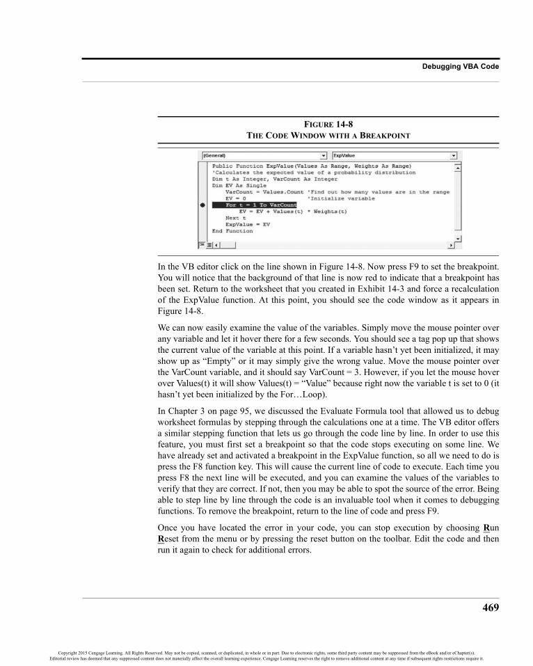
469
Debugging VBA Code
FIGURE 14-8THE CODE WINDOW WITH A BREAKPOINT
In the VB editor click on the line shown in Figure 14-8. Now press F9 to set the breakpoint.You will notice that the background of that line is now red to indicate that a breakpoint hasbeen set. Return to the worksheet that you created in Exhibit 14-3 and force a recalculationof the ExpValue function. At this point, you should see the code window as it appears inFigure 14-8.
We can now easily examine the value of the variables. Simply move the mouse pointer overany variable and let it hover there for a few seconds. You should see a tag pop up that showsthe current value of the variable at this point. If a variable hasn’t yet been initialized, it mayshow up as “Empty” or it may simply give the wrong value. Move the mouse pointer overthe VarCount variable, and it should say VarCount = 3. However, if you let the mouse hoverover Values(t) it will show Values(t) = “Value” because right now the variable t is set to 0 (ithasn’t yet been initialized by the For…Loop).
In Chapter 3 on page 95, we discussed the Evaluate Formula tool that allowed us to debugworksheet formulas by stepping through the calculations one at a time. The VB editor offersa similar stepping function that lets us go through the code line by line. In order to use thisfeature, you must first set a breakpoint so that the code stops executing on some line. Wehave already set and activated a breakpoint in the ExpValue function, so all we need to do ispress the F8 function key. This will cause the current line of code to execute. Each time youpress F8 the next line will be executed, and you can examine the values of the variables toverify that they are correct. If not, then you may be able to spot the source of the error. Beingable to step line by line through the code is an invaluable tool when it comes to debuggingfunctions. To remove the breakpoint, return to the line of code and press F9.
Once you have located the error in your code, you can stop execution by choosing RunReset from the menu or by pressing the reset button on the toolbar. Edit the code and thenrun it again to check for additional errors.
Copyright 2015 Cengage Learning. All Rights Reserved. May not be copied, scanned, or duplicated, in whole or in part. Due to electronic rights, some third party content may be suppressed from the eBook and/or eChapter(s).Editorial review has deemed that any suppressed content does not materially affect the overall learning experience. Cengage Learning reserves the right to remove additional content at any time if subsequent rights restrictions require it.

CHAPTER 14: Writing User-Defined Functions with VBA
470
The Watch WindowThe Watch Window, pictured at the bottom of Figure 14-2, allows us to more easily keeptrack of the values of variables and expressions as we step through the code. To add avariable or expression to the Watch Window, right-click on it to bring up the Add Watchdialog box. Right-click on VarCount and choose Add Watch.
FIGURE 14-9THE ADD WATCH DIALOG BOX
Figure 14-9 shows the Add Watch dialog box. Note that we can actually set three differenttypes of watches. Typically, you will select Watch Expression, which will add the variable tothe Watch Window where its value will be updated as you step through the code. The othertwo types set an automatic breakpoint either when the value is true or when it changes. Clickthe OK button to add VarCount to the Watch Window. Now, add a couple of other watchesand step through the code.
FIGURE 14-10THE WATCH WINDOW
Figure 14-10 shows the Watch Window with the values of five variables immediately beforethe function exits. That is, the function has finished running, except that it hasn’t yetreturned the value to the worksheet. EV has a value of 155, which we know is the correctvalue to return. Notice that Values(t) and Weights(t) are ranges, so you can expand them inthe Watch Window to look at their properties in detail by clicking the plus sign.
Copyright 2015 Cengage Learning. All Rights Reserved. May not be copied, scanned, or duplicated, in whole or in part. Due to electronic rights, some third party content may be suppressed from the eBook and/or eChapter(s).Editorial review has deemed that any suppressed content does not materially affect the overall learning experience. Cengage Learning reserves the right to remove additional content at any time if subsequent rights restrictions require it.

471
Debugging VBA Code
The Immediate WindowThe Immediate Window allows us to query for the current value of a variable, reset avariable to a different value, or execute VBA commands. If the Immediate Window is notvisible, select View Immediate Window from the menu or press Ctrl+G on your keyboard.
The Immediate Window is mainly useful if we have triggered a breakpoint and codeexecution has been paused. Return to your worksheet and force a recalculation of theExpValue function. Step through the For…Next loop exactly one time. In the ImmediateWindow type ?EV and then press the Enter key. This will generate a query for the value ofthe EV variable at this point in the code. You should see that it is equal to 25. This samevalue is displayed in the Watch Window because we previously set a watch for this variable.
Figure 14-11 shows the Immediate Window with two queries. The second one asks for thecurrent value of Values(t). Note that we can put Values(t) into the Watch Window as well,but it won’t display the current value because Values is a range variable.5 The ImmediateWindow doesn’t have this problem.
FIGURE 14-11THE IMMEDIATE WINDOW
As mentioned above, we can also execute VBA commands. For example, we could changethe value of EV by typing EV = 200 into the Immediate Window. Notice that we don’t usethe leading question mark if we want to execute a statement. Depending on where the code iswhen you execute this command, you will end up with a different result from the function. Ifyou enter that command when t = 2, the function will ultimately return 255 as the result.
The Immediate Window can also be used when we aren’t debugging code. It can beespecially useful for testing snippets of code. For example, type ?Application.Nameand then press enter. You should see that you are using an application called MicrosoftExcel.
There are more debugging tools, but these should be enough to get you started. You mayconsult the online help to learn more about debugging your VBA code.
5. Actually, we can force the Watch Window to display the value by entering Values(t).Value, or bydrilling down into the outline.
Copyright 2015 Cengage Learning. All Rights Reserved. May not be copied, scanned, or duplicated, in whole or in part. Due to electronic rights, some third party content may be suppressed from the eBook and/or eChapter(s).Editorial review has deemed that any suppressed content does not materially affect the overall learning experience. Cengage Learning reserves the right to remove additional content at any time if subsequent rights restrictions require it.

CHAPTER 14: Writing User-Defined Functions with VBA
472
Creating Excel Add-InsOftentimes, you will create user-defined functions (or procedures) that are primarily of usein a single workbook. If you aren’t likely to use a function outside of that workbook, then itmakes sense to write it in a code module attached to the workbook. This is what we havedone above. However, if you want to use your functions in multiple workbooks, or makethem available for others to use, then it is best to create an Excel add-in. This is exactly whatI have done with the FameFncs.xlam add-in that is distributed with this book. Add-ins canbe distinguished from regular Excel workbooks by the .xlam file extension, as opposed to.xlsm used for workbooks containing macros.
Add-ins are created from normal Excel workbooks, but they have several advantages:1. If you distribute your functions in an add-in, users can install the add-in
once through Excel Options and then never have to worry about openingthe file again. As long as there is a checkmark next to the add-in’s name inthe Add-Ins dialog box, it will automatically be opened every time Excelis started. This means that your functions are always available to be used.
2. Referencing functions is less complicated if they are contained in an add-in. To access one of the above functions from another workbook, we mustspecify the name and full path to the workbook. For example, to call theMyPV function, we would have to use this formula:='Chapter 14 Worksheets.xlsm'!MyPV(A1,A2,A3). However, if thefunction was in an active add-in, we could call the same function from anyworkbook with: =MyPV(A1,A2,A3).
3. The worksheets in an add-in are hidden from the user. This means lessconfusion on their part because they won’t feel like they have to use yourworksheets to use the functions.
4. It is easier to protect your code from prying eyes and restrict access to it.Because the workbook is hidden from the user, and you can protect thecode with a password, users can’t view or modify the code without yourpermission.
Fortunately, creating an add-in is very easy. First, you will open a new workbook and writeyour code, just as we have done above. Then, choose Save As from the File tab, and then inthe Save as type drop-down list, select the “Excel Add-In (*.xlam)” type. Make sure that yousave the add-in in a location that you can remember.
You have now created an add-in. To use it, close your “Chapter 14 Worksheets.xlam” file,and then go to Options and then Add-Ins. Click the Go button, then the Browse button in theAdd-Ins dialog box, and then navigate to the directory where you saved the add-in. Finally,
Copyright 2015 Cengage Learning. All Rights Reserved. May not be copied, scanned, or duplicated, in whole or in part. Due to electronic rights, some third party content may be suppressed from the eBook and/or eChapter(s).Editorial review has deemed that any suppressed content does not materially affect the overall learning experience. Cengage Learning reserves the right to remove additional content at any time if subsequent rights restrictions require it.

473
Best Practices for VBA
select the add-in file, click the OK button, and then make sure there is a checkmark next tothe name. You can now use your functions in any workbooks that you create.
One last thing to note is that you can covert the add-in back into a normal workbook if youever need to do so. Simply go into the VB Editor and select the ThisWorkbook module foryour add-in. In the Properties Window set the “IsAddin” property to False and then save theworkbook using the .xlsm format.
Best Practices for VBAAs with creating spreadsheets, there are some best practices that are good to follow whenwriting VBA code. In this section we will list some of them.
1. Remember that user-defined functions should not attempt to modify theformating or contents of any cell other than the one from which is wascalled. Doing so will create a #VALUE! error.
2. User-defined functions should accept as arguments all of the values thatthey need to do the calculation. Reading required values from theworksheet will create problems with recalculation because Excel won’tknow to recalculate the function when the referenced cell changes.
3. Declare all variables using the Dim statement at the beginning of eachfunction. To be sure that none slip by, use Option Explicit at the top ofeach module. While you can declare variables anywhere within yourfunction, it is best to do so at the top so that you always know where tocheck the types.
4. When declaring variables, be sure to give them an explicit type (e.g., DimX as Integer). If you don’t assign a type VBA will make it a variant, whichgives you some flexibility, but at the cost of speed and memory efficiency.
5. Give all variables a descriptive name. This will help immensely whendebugging your code. Many programmers go a step further and use anaming convention that also indicates the type of the variable. There aremany such conventions; probably the most famous is Hungarian notation,which uses one or more letters at the beginning of the variable name. Forexample, iCounter (integer) or strName (string). Whatever convention youuse, be consistent with it.
6. Indent your code for easier reading. If all lines of code start at thebeginning of a line it can be difficult to follow the flow of the logic.Indenting also makes it much easier to identify different blocks of code.
Copyright 2015 Cengage Learning. All Rights Reserved. May not be copied, scanned, or duplicated, in whole or in part. Due to electronic rights, some third party content may be suppressed from the eBook and/or eChapter(s).Editorial review has deemed that any suppressed content does not materially affect the overall learning experience. Cengage Learning reserves the right to remove additional content at any time if subsequent rights restrictions require it.

CHAPTER 14: Writing User-Defined Functions with VBA
474
7. Use comments liberally throughout your code. Ideally, you will have acomment at the top of each function that describes its purpose and defineseach of the arguments. Many programmers also list their name and thatdate that the code was written. Furthermore, you should have a commentfor each line of code where its purpose or method isn’t clear at a glance.
8. Create a “library” of your commonly used functions. This will make iteasier for you to find them when you want to reuse them for futureprojects. Your library can be a simple as a single text file that holds all ofyour useful functions, or it can be a more complex system.
9. Try not to create monolithic functions that do everything. Using single-purpose functions makes it easier to understand the code, locate errors,and reuse the functions elsewhere.
10. If your function will be writing large amounts of data to a worksheet, thendisable screen updating with Application.ScreenUpdating = False. Thiswill dramatically speed up the execution of the code. Reenable this settingprior to exiting the function with Application.ScreenUpdating = True.
11. Don’t reinvent the wheel. Search your own code library and the Internetfor code that does what you need. Not only is this faster, but the code thatyou find will most likely have been optimized.
12. Much like you should be doing with your spreadsheets, test your VBAcode extensively before putting it to use.
SummaryIn this chapter, we have provided a few short lessons in how to use the VB editor to writeand debug user-defined formulas. We have discussed the components of the VB editor, thefive requirements for a user-defined function that returns a value to the worksheet, severalprogramming concepts, and the tools that are available for debugging your code. We coveredthe steps that are necessary to convert your code into an Excel add-in so that your functionscan be used in any workbook, or even distributed to others who may find the functionsuseful. Finally, we discussed 12 “best practices” to use when writing VBA code.
Clearly, one short chapter in a textbook is not enough instruction for you to be completelycomfortable working in VBA. Also, due to space constraints we didn’t have time to discussprocedure macros or more advanced concepts. Hopefully, though, this chapter has taughtyou something useful and you will try your hand at writing some user-defined functions. Ifyou want to learn more about VBA programming, I can recommend several very usefulresources:
Copyright 2015 Cengage Learning. All Rights Reserved. May not be copied, scanned, or duplicated, in whole or in part. Due to electronic rights, some third party content may be suppressed from the eBook and/or eChapter(s).Editorial review has deemed that any suppressed content does not materially affect the overall learning experience. Cengage Learning reserves the right to remove additional content at any time if subsequent rights restrictions require it.

475
Problems
1. I am a big fan of John Walkenbach and can highly recommend any of hisbooks. In particular, Excel 2013 Power Programming with VBA (Wiley,2013) is excellent. I refer to it often when attempting something that Ihaven’t done before, or don’t do often.
2. Chip Pearson, of Pearson Software Consulting, LLC, has an excellent Website devoted to Excel and VBA programming located at: http://www.cpearson.com/excel.htm.
3. Microsoft hosts user-to-user forums where you can search for answers orask questions. Go to http://social.msdn.microsoft.com/Forums/en-US/home?forum=isvvba.
If those sources fail to answer your questions, there is always the World Wide Web. Do asearch and you are almost guaranteed to find your answer or something else interesting.
Problems
1. Write a user-defined function to calculate a firm’s return on equity usingthe DuPont method as defined by (4-29) on page 125. You will need thefunction to accept three arguments: the net profit margin, total assetturnover ratio, and the debt ratio. Now, write another function to calculatethe extended DuPont ROE as defined in equation (4-33) on page 126. Thissecond function will require five arguments: the operating profit margin,interest burden, tax burden, total asset turnover, and the debt ratio.
2. Create a user-defined function to calculate the value of a common stockusing the earnings model that was introduced in Chapter 8 on page 246.
a. What arguments will you need to accept in order to implementequation (8-13) exactly as it is displayed?
b. Now change your function so that it requires the retention ratio,instead of the expected retained earnings.
c. Use your function to solve parts a and b of problem 1 on page 259.
Copyright 2015 Cengage Learning. All Rights Reserved. May not be copied, scanned, or duplicated, in whole or in part. Due to electronic rights, some third party content may be suppressed from the eBook and/or eChapter(s).Editorial review has deemed that any suppressed content does not materially affect the overall learning experience. Cengage Learning reserves the right to remove additional content at any time if subsequent rights restrictions require it.

CHAPTER 14: Writing User-Defined Functions with VBA
476
3. A stock’s beta coefficient can be calculated using the following equation:
a. Write a user-defined function that can calculate the beta coefficient.The arguments to the function should be the covariance between thestock and market returns, and the variance of the market’s returns. Forexample, BETA(COVAR AS SINGLE, MARKETVAR AS SINGLE).
b. Rewrite your function so that it accepts ranges of returns and thencalculates the beta directly from the returns. It should be defined as:BETA(STOCKRETURNS AS RANGE, MARKETRETURNS AS RANGE).Your function should make use of Application.WorksheetFunction tocalculate the covariance and variance (use Excel’s COVAR.S andVAR.S functions). In the code, be sure to check to see if the number ofstock returns is equal to the number of market returns. The functionshould return an error if the count of returns is not equal.
4. Write a user-defined function that calculates the average collection periodwith two arguments: accounts receivable, and annual credit sales, andassumes that there are 360 days per year.
Now, write another version of the function that accepts an optional thirdargument that indicates whether to use 360 or 365 days in a year. Thisthird argument should default to using a 360-day year. The secondfunction should return an error value (look up CVErr in the help) if theuser specifies any number other than 360 or 365 days per year.
βiσi m,
σm2
----------=
Copyright 2015 Cengage Learning. All Rights Reserved. May not be copied, scanned, or duplicated, in whole or in part. Due to electronic rights, some third party content may be suppressed from the eBook and/or eChapter(s).Editorial review has deemed that any suppressed content does not materially affect the overall learning experience. Cengage Learning reserves the right to remove additional content at any time if subsequent rights restrictions require it.

477
CHAPTER 15 Analyzing Datasets with Tables and Pivot Tables
Businesses generate large amounts of data of all kinds, and somebody has to process it into aformat that is usable for analysis and reporting. For example, a sales manager may have aspreadsheet (or database) that contains the details of every sale. These data might include thedate, the name of the customer, the product, the price, and so on. Or, a financial planner mayhave a dataset that contains information on every mutual fund that she might recommend toa client. These data may include the name of the fund, its ticker symbol, several measures ofperformance and risk, and other useful information.
Whatever the dataset contains, the analyst needs to be able to quickly categorize it intouseful groups, summarize it in various ways, and make calculations from the data.
After studying this chapter, you should be able to:1. Use a sorted and filtered Excel table present only the information of interest.2. Build a pivot table and use it to present data in specific ways.3. Add, remove, and rearrange data fields in a pivot table.4. Create calculated columns in tables and calculated fields in pivot tables.5. Use pivot charts to illustrate trends in data from a pivot table.
Copyright 2015 Cengage Learning. All Rights Reserved. May not be copied, scanned, or duplicated, in whole or in part. Due to electronic rights, some third party content may be suppressed from the eBook and/or eChapter(s).Editorial review has deemed that any suppressed content does not materially affect the overall learning experience. Cengage Learning reserves the right to remove additional content at any time if subsequent rights restrictions require it.

CHAPTER 15: Analyzing Datasets with Tables and Pivot Tables
478
Ultimately, the results will need to be presented in a report. Excel has a number of tools thatcan help, but our focus in this chapter will be on Excel tables and pivot tables.
Although you may think of the worksheet itself as a table, the term has a more specificmeaning in Excel. A table is a data structure that contains related data and allows the user tomore easily manage and update the dataset as new information arrives. For example, you canfilter the dataset to show only those items that meet certain criteria, or sort the dataset by anyfield. Tables automatically grow as new data is added, and shrink if data is deleted.Furthermore, formulas and formatting in the table are automatically extended to new recordsthat are added.
A pivot table is an even more flexible data structure that allows the analyst to quickly sliceand dice a dataset into a useful report. For example, the financial planner from above mightwant to group all of the mutual funds by investment type (stocks, bonds, etc.), show the year-to-date return for each fund, and then calculate the average return by investment type. Apivot table makes this task fast and easy, even though the original dataset isn’t sorted in thatmanner. Furthermore, it is easy to rearrange the pivot table to organize and present the samedata differently; perhaps by fund family instead of by investment type.
Learning to use tables and pivot tables will dramatically increase your productivity andyour understanding of the data. Because the datasets used in this chapter arelarge, workbooks containing the raw data are available on the official Web site for this book,http://www.cengagebrain.com/.
Creating and Using an Excel TableImagine that you are an investment advisor who invests in exchange-traded funds andexchange-traded notes (ETFs and ETNs, respectively) on behalf of your clients. You askyour assistant to gather data for all of the 763 funds on your approved list. The data willconsist of the fund name, ticker symbol, legal structure, brand, advisor, category, star rating,average premium to NAV, size, returns for the last three years, expense ratio, correlationwith benchmark, average daily volume, and some performance measures (alpha, beta, etc.).Your goal is to be able to comb through this data to find the funds that meet various criteria.
Exhibit 15-1 shows a small portion of the data in the ETF Data.xlsx workbook, which isavailable on the official Web site. Note how the data are organized. Data fields (name, tickersymbol, etc.) are in columns, and records (each individual fund) are in rows. The full datasethas 22 fields and 772 records, though some of them are duplicates. As useful as the datasetmight be, it is simply too large to easily find data points or analyze the funds. Imaginescrolling through the data to find all of the bond funds or the funds provided by the VanguardGroup.
Copyright 2015 Cengage Learning. All Rights Reserved. May not be copied, scanned, or duplicated, in whole or in part. Due to electronic rights, some third party content may be suppressed from the eBook and/or eChapter(s).Editorial review has deemed that any suppressed content does not materially affect the overall learning experience. Cengage Learning reserves the right to remove additional content at any time if subsequent rights restrictions require it.

479
Creating and Using an Excel Table
EXHIBIT 15-1PARTIAL ETF DATASET
As mentioned above, converting this data into an Excel table will allow you to easilymanage the dataset. To create the table, simply select any cell within the data area (say, D9)and then choose Table from the Insert tab. Excel will make a guess as to the range that youwant to use, and whether there are headings. It typically guesses correctly, but if it doesn’tthen you can easily select the correct range. Figure 15-1 shows the Create Table dialog boxas it appears for this dataset.
FIGURE 15-1THE CREATE TABLE DIALOG BOX
After clicking the OK button, you will see that Excel has applied some formatting and thatthere is a drop-down arrow button next to each field name. There is also a new contextual tabin the Ribbon that is labeled Design. On the Design tab, which is only visible when theactive cell is in a table, you can choose a different style for the table if you don’t like thedefault choice. Simply move the mouse pointer over the styles available in the Table Stylesgroup until you find one that you like.
There are a few things on the Design tab that are not related to the look of the table. Forexample, you can rename the table, convert it back to an ordinary range of cells, create apivot table, or add a slicer. We will look at pivot tables later in this chapter (see page 485).
Source: Based on data from Morningstar Direct
Copyright 2015 Cengage Learning. All Rights Reserved. May not be copied, scanned, or duplicated, in whole or in part. Due to electronic rights, some third party content may be suppressed from the eBook and/or eChapter(s).Editorial review has deemed that any suppressed content does not materially affect the overall learning experience. Cengage Learning reserves the right to remove additional content at any time if subsequent rights restrictions require it.

CHAPTER 15: Analyzing Datasets with Tables and Pivot Tables
480
EXHIBIT 15-2PART OF THE ETF TABLE
Another nice feature of tables is that the column headings will now replace the usual A, B, Cheadings as you scroll down the worksheet. As shown in Exhibit 15-2, this makes it easy tokeep track of your fields in a large table.
Removing Duplicate Records from the TableIt isn’t obvious at a glance, but our dataset contains nine duplicate records. This is quite acommon occurrence, so the Design tab has a tool for removing such records. If you scrolldown to row 148, you will see two ETFs from ALPS. Looking more closely, you will seethat it is actually one fund listed twice. There are other duplicates as well, and they could beanywhere in the table so it would be difficult to remove them manually.
To permanently delete all of the duplicate records in the table, click the Remove Duplicatesbutton on the Data tab (it is also on the Design tab). Because we only want to delete recordsthat are exact matches in each field, make sure that all columns are selected in the dialog boxand then click OK. You should see a message box saying that 9 duplicate records have beenremoved and that 763 remain.
If you had wanted to keep the duplicate records, but not see them, then you could haveapplied an Advanced Filter from the Data tab. Just be sure to check Unique records only atthe bottom of the dialog box. Note that for the purposes of this chapter we have chosen topermanently remove the duplicates.
Filtering the TableWhen you created the table, Excel automatically added an AutoFilter drop-down to eachcolumn header. By clicking the arrow for any column, you can perform operations to sort orfilter the table in various ways. Figure 15-2 shows the drop-down for the Fund Name field.
Source: Based on data from Morningstar Direct
Copyright 2015 Cengage Learning. All Rights Reserved. May not be copied, scanned, or duplicated, in whole or in part. Due to electronic rights, some third party content may be suppressed from the eBook and/or eChapter(s).Editorial review has deemed that any suppressed content does not materially affect the overall learning experience. Cengage Learning reserves the right to remove additional content at any time if subsequent rights restrictions require it.

481
Creating and Using an Excel Table
FIGURE 15-2THE AUTOFILTER FOR THE FUND NAME FIELD
If you choose a Sort option, the entire table will automatically be sorted according to the datain the column to which the sort is applied. Note also that you can select or deselect any of thefunds in the Search area. For example, to hide certain funds simply uncheck the boxes nextto their names. They will remain in the table, but the rows will be hidden. To restore them,click Clear Filter From “Fund Name.”
We can apply more advanced filtering techniques by applying a Text Filter. For example,suppose that you want to only see the funds that contain the word “Bond” in their name.Select Text Filters and choose the “Contains…” filter and then enter Bond into the dialogbox. You should see that there are only 39 funds that meet this criteria.
We can easily add a second criteria to this filter by choosing Text Filters again and enteringthe text into the second box. For example, we could add a filter for fund names that containboth the word “Bond” and the word “Long.” If you do this, you will find that there are onlyfour that meet the criteria. Be sure to clear this filter before continuing.
It is important to note that the fund name isn’t always indicative of its investment style. So, ifyou want to filter for all of the long-term bond funds, it would be better to filter on theMorningstar Category field. Click the drop-down arrow next to Morningstar Category,remove the checkmark from the (Select All) item, and then scroll down the list and select theLong-Term Bond and Long Government categories, as shown in Figure 15-3.
Copyright 2015 Cengage Learning. All Rights Reserved. May not be copied, scanned, or duplicated, in whole or in part. Due to electronic rights, some third party content may be suppressed from the eBook and/or eChapter(s).Editorial review has deemed that any suppressed content does not materially affect the overall learning experience. Cengage Learning reserves the right to remove additional content at any time if subsequent rights restrictions require it.

CHAPTER 15: Analyzing Datasets with Tables and Pivot Tables
482
FIGURE 15-3FILTERING FOR LONG-TERM BOND FUNDS
The result of this filter is that there are 12 long-term bond funds in the table. There may besome long-term bond funds that were missed because they didn’t meet the criteria that werespecified. For example, there are categories named “Muni California Long,” “Muni NationalLong,” and “Muni New York Long” that we could have selected. If you go back and selectthe latter two categories (you aren’t interested in California bonds), you will find that thereare five additional long-term bond funds. There may still be other funds that do not includethe word “Long” in their category, in which case you would need to search further.
Sorting and Filtering Numeric FieldsThe drop-downs for numeric fields are similar to those for text fields, except that they have adifferent set of numeric filters. We can extend our previous filter operation by choosing toSort Largest to Smallest based on the Return 2013 field. You can see that 2013 was a badyear for these long-term bond funds.
In addition to the sort, we can also add a filter to the Return 2013 field. After sorting by totalreturn, you will notice that some of the funds have dramatically outperformed others. Youmight wish to see only those funds that lost less than 10% in 2013. Click the Greater Thanoption after selecting Number Filters and enter -0.10 into the dialog box. You will see that12 bonds meet these criteria.
Copyright 2015 Cengage Learning. All Rights Reserved. May not be copied, scanned, or duplicated, in whole or in part. Due to electronic rights, some third party content may be suppressed from the eBook and/or eChapter(s).Editorial review has deemed that any suppressed content does not materially affect the overall learning experience. Cengage Learning reserves the right to remove additional content at any time if subsequent rights restrictions require it.

483
Creating and Using an Excel Table
EXHIBIT 15-3LONG-TERM BOND ETFS SORTED AND FILTERED BY RETURN1
Note that this filter seems as though it only applies to the already filtered data, but it isactually filtering the entire table. The filters on the Morningstar Category field still ensurethat we only see long-term bond funds. Exhibit 15-3 shows the result of our filters. Clear thefilters before continuing.You may have noticed that the drop-down buttons change to indicate when a filter or sort hasbeen applied to the field. Figure 15-4 shows the different buttons and the conditions that theyrepresent.
FIGURE 15-4POSSIBLE COLUMN HEADER BUTTONS
There are many other filters available, but be aware that if you filter on more than one fieldthen the results may not be what you expect. For example, you might want to see the top-performing ETFs based on 2013 returns sorted from largest to smallest. Further, you want torestrict the list to the ProShares Advisors funds.
First, sort the table from largest to smallest by Return 2013. Now, filter the Branding Namefield by selecting only ProShares from the list of brands. Next, click the arrow button for theReturn 2013 field and choose the Top 10 filter from Number Filters.
1. Several columns have been hidden for purposes of the illustration. Because of the size of thedataset, we will continue to hide columns and rows in other exhibits when necessary.
Source: Based on data from Morningstar Direct
Copyright 2015 Cengage Learning. All Rights Reserved. May not be copied, scanned, or duplicated, in whole or in part. Due to electronic rights, some third party content may be suppressed from the eBook and/or eChapter(s).Editorial review has deemed that any suppressed content does not materially affect the overall learning experience. Cengage Learning reserves the right to remove additional content at any time if subsequent rights restrictions require it.

CHAPTER 15: Analyzing Datasets with Tables and Pivot Tables
484
EXHIBIT 15-4PROSHARES ADVISORS ETFS IN TOP 10 PERFORMERS FOR 2013
(You can choose a different number in the dialog box, but 10 is the default.) This operationresults in only four funds being displayed, as seen in Exhibit 15-4. The reason that you don’tsee the top 10 ProShares funds is because multiple filters do not build upon each other. Aswe will soon see, pivot tables can do this and much more.
Using Formulas in TablesUnlike in an ordinary range, when you add a formula to a cell in a table it is automaticallyextended to all other cells in the column. This is a great time saver, and it helps to ensureconsistency and avoid errors. If necessary you can override this default behavior, but most ofthe time this is what you want.
Table formulas use a different style of cell referencing than the usual A1 style. Tablestypically use a structured reference, though you can still force the A1 style by typing celladdresses directly. The advantage of structured referencing is primarily that it allows you toeasily refer to entire columns of data, to special items such as column headers, or to thetotals row. These formulas are also easier to understand as they use column header names ina way that is similar to defined names (see page 9).
Creating a structured reference can be complex, but Excel helps by automatically creatingthe references when you click on cells in the table while entering the formula. For example,we might want to calculate the average of the expense ratios for all of the funds. Select ablank cell outside of the table and enter: =AVERAGE(Table1[Expense Ratio %]).Note that we use the AVERAGE function as usual, but the range is specified using astructured reference. The first part of the reference, Table1, specifies the name of the tablefrom which the data is to be obtained.2 The second part, [Expense Ratio %], specifies thecolumn to use. By using structured references, the formula is easy to understand, and thereference will automatically include new data as it gets added to the bottom of the table.
Let’s now create a calculated column in our table. A calculated column is a data field thatwasn’t included in the original data, but is calculated using data in the table (or elsewhere).
2. Tables are automatically named Table1, Table2, and so on. You can rename the table on the Designtab.
Source: Based on data from Morningstar Direct
Copyright 2015 Cengage Learning. All Rights Reserved. May not be copied, scanned, or duplicated, in whole or in part. Due to electronic rights, some third party content may be suppressed from the eBook and/or eChapter(s).Editorial review has deemed that any suppressed content does not materially affect the overall learning experience. Cengage Learning reserves the right to remove additional content at any time if subsequent rights restrictions require it.

485
Using Pivot Tables
Our formula will calculate the average return in 2013 for all funds in the same category asthe one in the current row. To do this, we need a function that will average only those itemsthat meet certain criteria. The AVERAGEIF function does exactly this, and is defined as:
AVERAGEIF(RANGE, CRITERIA, AVERAGE_RANGE)
where RANGE is the range of cells to check against the CRITERIA, and AVERAGE_RANGE isthe range of cells to use in the calculation. If Average_Range is omitted then the cells inRange will be averaged. So, Range will refer to the entire column of fund categories, Criteriawill be the category of the fund in the current row, and Average_Range will be theReturn 2013 values. Using the traditional A1 referencing, the formula would be:=AVERAGEIF($G$2:$G$764,G2,$M$2:$M$764). Since it uses absolute references,this formula will only work until we add new data at the bottom of the table. However, if weuse structured referencing the ranges will automatically expand if we add new data.
To create the formula using structured references, first insert a new column to the left ofcolumn N. In N1 overwrite the default column header with Cat 2013 Return. In N2 type:=AVERAGEIF([Morningstar Category],[@[Morningstar Category]],[Return
2013]). Again, you don’t need to actually type the parts in square brackets, you can selectthe ranges or click the cells and Excel will automatically enter the column names.
In this formula [Morningstar Category] tells Excel to use the entire range of categories(column G), while [@[Morningstar Category]] tells it to use just the single value in thecurrent row. The @ sign is interpreted to mean “this row.” Similarly, [Return 2013] refers tothe entire column because it lacks the @ sign. Note also that you don’t need to use the tablename in the reference because it is implicitly assumed to be in the same table as the formula.If you were referencing data from a different table, then you would have to explicitlyreference the table name as we did in our first formula.
Structured referencing is a powerful tool, and we have just scratched the surface. You canalso use structured references to refer to special items such as the column headers, grandtotals, and more. Check Excel’s help for more information.
Using Pivot TablesIn the previous section, we have seen how tables can make it easy to manage, sort, and filtera dataset. As useful as that is, it doesn’t do much to help us to gain valuable insight into thedata. A pivot table is another type of table that allows us to easily summarize, filter, andrearrange a dataset in useful ways that increase our understanding. For example, we might beinterested in knowing the average expense ratio by fund family. Or, we might want to knowthe average return of the funds by category, as we just did with a calculated column in thetable. It is much easier, though, with a pivot table.
Copyright 2015 Cengage Learning. All Rights Reserved. May not be copied, scanned, or duplicated, in whole or in part. Due to electronic rights, some third party content may be suppressed from the eBook and/or eChapter(s).Editorial review has deemed that any suppressed content does not materially affect the overall learning experience. Cengage Learning reserves the right to remove additional content at any time if subsequent rights restrictions require it.

CHAPTER 15: Analyzing Datasets with Tables and Pivot Tables
486
The data for a pivot table can come from a table or range in a worksheet, from an externalsource such as a table or query from a database file, or even from a text file. It is important tonote that the pivot table stores a snapshot of the data in the pivot table cache. Once created,the cache is separate from the original data. Therefore, if the underlying data changes youmust refresh the pivot table. Otherwise it will be using outdated data.
Creating a Pivot TableBefore creating the first pivot table, we should make sure that an option is turned off to avoidpotential problems. Go to the File tab and choose Options. Select the Advanced tab on theleft side and scroll down to the Data section. Be sure that the check box for Prefer the ExcelData Model when creating Pivot Tables, Query Tables and Data Connections is turned off.
For this example we will be using the ETF/ETN data from the ETF Data worksheet as thesource for our pivot table. Make sure that the active cell is within the table and then go to theInsert tab and click the PivotTable button. You will see the dialog box shown in Figure 15-5.Here, as is typical, we will click OK to accept the defaults.
FIGURE 15-5THE CREATE PIVOTTABLE DIALOG BOX
This will create a new worksheet as shown in Exhibit 15-5. If you have never created a pivottable before, it will look quite confusing. On the right-hand side you will see a list of thefields that were in the table. Below that are four “drop zones” where you can drag fields toadd them to the pivot table. It may take having a few pivot tables under your belt for the dropzones to make sense, but here is a quick description of each of them:• Filters – Any field in this area will appear above the pivot table and will be used to filter
the report. For example, if you want to filter by fund family then you could drag the Branding Name field into this area.
Copyright 2015 Cengage Learning. All Rights Reserved. May not be copied, scanned, or duplicated, in whole or in part. Due to electronic rights, some third party content may be suppressed from the eBook and/or eChapter(s).Editorial review has deemed that any suppressed content does not materially affect the overall learning experience. Cengage Learning reserves the right to remove additional content at any time if subsequent rights restrictions require it.

487
Using Pivot Tables
EXHIBIT 15-5A BLANK PIVOT TABLE
• Columns – Drag a field to this area to create a column in the pivot table for each value of the field. For example, dragging the Structure field to this area will create three columns: ETF, ETN, and UIT. Often, you will leave this area empty.
• Rows – This area is where the fields that you want to use as labels will go. For example, we might want to use the ticker symbol as the label for each row. You can have more than one row label by dragging more fields to this area. You can change their order by simply rearranging them within the area.
• Values – This area holds the fields that you want to summarize. Fields can be summarized by a number of functions, including Sum, Count, Average, and several others. By default, numeric fields will be summed, and text fields will be counted.
You can drag as many fields as necessary into any of the areas. In fact, you can drag a fieldinto more than one of the areas, or even into the same area, so that it appears twice or more.To remove a field from the pivot table, just drag it back to the Pivot Table Field area. Theability to move fields in this way and instantly get an updated report is referred to as“pivoting” and is what gives pivot tables their name.
Recall that for Exhibit 15-4 we tried to show the top 10 ProShares funds by year-to-datereturns. However, because the table filters don’t build upon each other, we wereunsuccessful and ended up with only four funds displayed. We can easily organize our pivottable to show this data.
Copyright 2015 Cengage Learning. All Rights Reserved. May not be copied, scanned, or duplicated, in whole or in part. Due to electronic rights, some third party content may be suppressed from the eBook and/or eChapter(s).Editorial review has deemed that any suppressed content does not materially affect the overall learning experience. Cengage Learning reserves the right to remove additional content at any time if subsequent rights restrictions require it.

CHAPTER 15: Analyzing Datasets with Tables and Pivot Tables
488
EXHIBIT 15-6UNFORMATTED PIVOT TABLE SHOWING 2013 RETURNS FOR EACH ETF
To begin, drag the Branding Name field into the Filters area. This will allow us to displayone fund family at a time in the pivot table. Next, drag both the Fund Name and Ticker fieldsinto the Rows area. Finally, drag the Return 2013 field into the Values area. Your pivot tableshould now look like the one in Exhibit 15-6.
Formatting the Pivot TableWe now have the basic structure of the pivot table, but it needs to be cleaned up a bit in orderto be useful. First notice that the ticker symbol for each fund appears on the row below itsname. This layout, known as the Compact Form, would be useful if we had multiple tickersymbols for each name, but that isn’t the case. We can make the ticker symbol appear next tothe name by changing to Tabular Form. On the Design tab click the Report Layout buttonand choose Show in Tabular Form.
Notice that the return for each fund is now shown twice. The first is the return for theSymbol, and the second is a subtotal of the Fund Name field. Again, since there is only onefund per name, this makes no sense and is confusing. To remove the subtotals click theSubtotals button on the Design tab and choose Do Not Show Subtotals.
The next step in formatting the pivot table is to display the 2013 returns as percentages.Right-click on any row in the Sum of Return 2013 field and choose Number Format. Selecta number format from the Percentage category with two decimal places.
Source: Based on data from Morningstar Direct
Copyright 2015 Cengage Learning. All Rights Reserved. May not be copied, scanned, or duplicated, in whole or in part. Due to electronic rights, some third party content may be suppressed from the eBook and/or eChapter(s).Editorial review has deemed that any suppressed content does not materially affect the overall learning experience. Cengage Learning reserves the right to remove additional content at any time if subsequent rights restrictions require it.

489
Using Pivot Tables
We will now change the way that the Return 2013 field is summarized. As mentioned above,the default is to sum numeric fields. Because there is only one year-to-date return for eachfund, it doesn’t much matter which function we choose. However, the summary functionwill affect any subtotals and grand totals. Summing returns from different funds doesn’tmake much sense, so we will change the summary function to the average instead. Right-click any cell in the field, select Summarize Values By and then choose Average. Scroll allthe way to the bottom of the pivot table and notice that the average 2013 return for all 763funds is 16.29%.
Now, let’s change the text at the top of the column by typing 2013 Return into C3. Youcan change the label to any text as long as it doesn’t replicate an existing field name. Byreplacing the text, we can remove the summary method from the name. You can also applyany other formatting to the column header, so center the text and set the column width to anappropriate value.
We now have a pivot table report that shows all of our funds (sorted by name), their tickersymbols, and their 2013 returns. However, recall that we want to see only the top performingProShares funds. From the Report Filter choose ProShares to limit the report to these funds.
To show only the top 10 ProShares funds, we need to apply a filter to the 2013 Return field.Click the drop-down for Fund Name and choose Value Filters. Select the Top 10 filter, makesure that it is selecting items by 2013 Return, and click OK. Lastly, we want to sort the listfrom the highest return to the lowest. Click the drop-down for the Fund Name again andchoose More Sort Options. In the dialog box select Descending and 2013 Return for thefield. The pivot table should now look like the one in Exhibit 15-7.
You can see that these ETFs did very well in 2013, with an average return of 91.76%.However, go back to the Top 10 value filter for the Fund Name. This time change it from aTop 10 to a Bottom 10 filter. You will see that the 10 worst ProShares ETFs had an averagereturn in 2013 of –53.12%. The reason for the dramatic results is that these are leveragedfunds.
Now that the pivot table report has been created, it can be copied into a new worksheet or aword processing document for presentation to a client. Note that if you copy only a portionof the pivot table, say A3:C14, and then paste into another worksheet you will end up with anormal range of data. However, if you were to select the entire pivot table (A1:C14) thenyou would create a new pivot table that uses the same pivot cache. Having two or more pivottables based on the same data can be useful at times. On the other hand, if all that you wantis a copy of the report, then copy the pivot table and use Paste Special Values.
Copyright 2015 Cengage Learning. All Rights Reserved. May not be copied, scanned, or duplicated, in whole or in part. Due to electronic rights, some third party content may be suppressed from the eBook and/or eChapter(s).Editorial review has deemed that any suppressed content does not materially affect the overall learning experience. Cengage Learning reserves the right to remove additional content at any time if subsequent rights restrictions require it.

CHAPTER 15: Analyzing Datasets with Tables and Pivot Tables
490
EXHIBIT 15-7TOP 10 PROSHARES ETFS BY 2013 RETURN
Rearranging the Pivot Table and Adding FieldsImagine that you now wish to look at average 2013 returns by brand name. Because we nowonly care about the brand, and not the individual funds, drag the Fund Name and Tickerfields back to the Pivot Table Field List to remove them from the pivot table. Next drag theBranding Name field from the Report Filter area into the Row Labels area. Finally, click thedrop-down next to Branding Name, choose More Sort Options, and sort in descending orderbased on the 2013 Return field.
Fidelity has the best performance of all of the providers. However, this may be misleadingdue to the number of funds offered and the diversity of categories. So, to begin investigating,you want to know how many ETFs each provider offers. Drag the Ticker field into theValues area to get this count. Because this is a text item, the only summary method that willprovide useful data is count, which is the default. You can now see that Fidelity only has oneETF in our list, and it performed well, which explains why it has the highest average return.
To investigate further, drag the Ticker field from the Values area into the Rows area. Thiswill allow us to see the return of each fund in each family as shown in Exhibit 15-8. Notethat the new Ticker column (B) will not show any symbols if the Branding Name field iscollapsed. To view the funds for a single brand expand the list by clicking the outline buttonto the left of the provider name. To view all of the funds, right-click any cell in the BrandingName column, select Expand/Collapse, and then choose Expand Entire Field. Finally, clickthe Subtotals button on the Design tab to add subtotals at the bottom of each group.
Source: Based on data from Morningstar Direct
Copyright 2015 Cengage Learning. All Rights Reserved. May not be copied, scanned, or duplicated, in whole or in part. Due to electronic rights, some third party content may be suppressed from the eBook and/or eChapter(s).Editorial review has deemed that any suppressed content does not materially affect the overall learning experience. Cengage Learning reserves the right to remove additional content at any time if subsequent rights restrictions require it.

491
Using Pivot Tables
EXHIBIT 15-82013 RETURNS BY FUND WITH SUBTOTALS BY BRANDING NAME
We can now see that average returns by provider can be misleading because some firms offermore ETFs than others. To mitigate the problem somewhat, you might decide that you onlywant to see those brands that offer at least 30 funds. To filter the pivot table for this criteria,we need to know how many funds are offered by each provider. Drag another copy of theTicker field into the Values area. Note that this field is now shown in two different areas ofthe pivot table. Since Ticker is a text field, it will be summarized by count. Now click thedrop-down next to Branding Name and choose Value Filters. Select the Greater Than OrEqual To filter and choose Count of Ticker as the field and 30 for the value. Finally, collapsethe pivot table to the Branding Name level and the result is shown in Exhibit 15-9.
Transforming the Data Field PresentationSuppose that we aren’t interested in the number of funds per family, and instead we wouldlike to know the percentage of funds in our list that are offered by each provider. First, clearthe filter that we applied in the previous section so that all providers are shown. Now right-click on any of the values in column D and select Show Values As. This allows us totransform the data in the column in a number of useful ways.
For example, to see the percentage of the total number of funds by provider, simply choose% of Grand Total. By looking at the percentages, you can easily see that Fidelity has thesmallest number of funds in our list, and iShares has the largest number.
Source: Based on data from Morningstar Direct
Copyright 2015 Cengage Learning. All Rights Reserved. May not be copied, scanned, or duplicated, in whole or in part. Due to electronic rights, some third party content may be suppressed from the eBook and/or eChapter(s).Editorial review has deemed that any suppressed content does not materially affect the overall learning experience. Cengage Learning reserves the right to remove additional content at any time if subsequent rights restrictions require it.

CHAPTER 15: Analyzing Datasets with Tables and Pivot Tables
492
EXHIBIT 15-9AVERAGE 2013 RETURNS FOR BRANDING NAMES WITH 30 OR MORE FUNDS
Another way to accomplish a similar result is to rank the providers by the number of funds.Again, right-click in column D and choose Show Values As. Now select Rank Largest toSmallest. You can see that iShares is ranked number 1, and Fidelity and JP Morgan areranked 19. Note that ties are given the same rank.
If you now perform the same ranking based on the 2013 Return field, you can see thatFidelity is the best performing provider, as we saw earlier. To change the ranking so that it isdone at the fund level go back to Rank Largest to Smallest, but choose Ticker as the BaseField. Now, right-click any Branding Name and choose Expand/Collapse and then ExpandEntire Field.
Before continuing, reset the 2013 Return field to No Calculation, and drag the Ticker fieldfrom the Values area back to the PivotTable field list.
Calculations in Pivot TablesWe can create completely new fields that are calculated from existing fields. This type offield is known as a calculated field, and it is analogous to the calculated column that wecreated in our original table.
Recall that on page 485 we added a calculated column, Cat 2013 Return, to our originaltable. That field is available in the pivot table, so we will use it as a part of our calculatedfield. Specifically, we will create a field that calculates the difference between each fund’s
Source: Based on data from Morningstar Direct
Copyright 2015 Cengage Learning. All Rights Reserved. May not be copied, scanned, or duplicated, in whole or in part. Due to electronic rights, some third party content may be suppressed from the eBook and/or eChapter(s).Editorial review has deemed that any suppressed content does not materially affect the overall learning experience. Cengage Learning reserves the right to remove additional content at any time if subsequent rights restrictions require it.

493
Using Pivot Tables
2013 return and the same for the category. The result will allow us to easily see which fundsare outperforming (or underperforming) their peers.
To create a calculated field, start by clicking the Fields, Items, & Sets button on the Analyzetab and choose Calculated Field. This will launch the dialog box shown in Figure 15-6. Givethe field a name by typing Relative to Cat into the Name box. To define the formulaselect the Return 2013 field from the Fields list and then click the Insert Field button. Nowtype a minus sign and then select and insert the Cat YTD Return field. Click the OK buttonto add the calculated field to the bottom of the PivotTable Field List. You can now use thecalculated field just like any other field.
FIGURE 15-6THE INSERT CALCULATED FIELD DIALOG BOX
Drag the Cat 2013 Return and Relative to Cat fields into the Values area, summarize both bythe Average, and format them as a percentages with two decimal places. Next, replace theBranding Name field in the Row Labels area with the Fund Name field. You should now seeeach fund name, ticker, 2013 return, category 2013 return, and the return relative to thecategory.
Remember that we want to see only those funds that have outperformed their peers. Youmight think that you could filter the pivot table with a Greater Than filter that specifies thatthe 2013 Return field is greater than the Cat YTD Return. However, that filter only allowsyou to specify a number, not another field. That is why we need the calculated field. So,click the drop-down next to Fund Name and select the Greater Than filter. Choose theAverage of Relative to Cat field in the list, and enter 0 into the appropriate edit box. Yourpivot table should now look like the one in Exhibit 15-10.
Another useful way to look at this same data is by category. Drag the Fund Name field backto the Pivot Table Field List, and replace it with the Broad Category field. This will make iteasy to see which funds in each category are outperforming. You can also rank funds withinthe categories by right-clicking the Relative to Cat field and selecting Show Values As.Choose to Rank Largest to Smallest with Ticker as the Base Field.
Copyright 2015 Cengage Learning. All Rights Reserved. May not be copied, scanned, or duplicated, in whole or in part. Due to electronic rights, some third party content may be suppressed from the eBook and/or eChapter(s).Editorial review has deemed that any suppressed content does not materially affect the overall learning experience. Cengage Learning reserves the right to remove additional content at any time if subsequent rights restrictions require it.

CHAPTER 15: Analyzing Datasets with Tables and Pivot Tables
494
EXHIBIT 15-10FUNDS THAT ARE OUTPERFORMING THEIR PEERS
Pivot Tables for Financial StatementsWe can also use pivot tables to analyze a company’s financial statements over time. For thissection we will be using the GOOG Financials.xlsx workbook, which is available on theofficial Web site of this book. This workbook contains quarterly financial statements forGoogle from March 2009 to December 2013 (five years). We will only use the incomestatements in this chapter, but the end-of-chapter problems will also make use of the balancesheets.
As we’ve seen in previous chapters, financial statements are typically organized with timeperiods in the first row and items in the first column. However, since the items are the datafields we will need to transpose the financial statements for use in a pivot table. Exhibit 15-11 shows the result that we want to achieve. To do so, select A5:U21 on the GOOGQuarterly IS worksheet and copy it. Next right-click A24, choose Paste Special, and thenselect the checkbox next to Transpose.
Once the data is transformed, type Date into A24. This will provide a field name for thedates. To create the pivot table, click anywhere within the transformed data area and clickthe PivotTable button on the Insert tab. Rename the pivot table worksheet to IS PivotTable.
Source: Based on data from Morningstar Direct
Copyright 2015 Cengage Learning. All Rights Reserved. May not be copied, scanned, or duplicated, in whole or in part. Due to electronic rights, some third party content may be suppressed from the eBook and/or eChapter(s).Editorial review has deemed that any suppressed content does not materially affect the overall learning experience. Cengage Learning reserves the right to remove additional content at any time if subsequent rights restrictions require it.

495
Pivot Tables for Financial Statements
EXHIBIT 15-11TRANSPOSING THE INCOME STATEMENT
Grouping Data by DatePivot tables allow you to group records together by selecting some values (they don’t need tobe in a contiguous range) in the Row Labels area and clicking the Group Selection button onthe Analyze tab. This is useful because it allows you to calculate subtotals by any groups thatyou choose to define.
When the data in the pivot table are date related, as in a financial statement, you can easilycreate groups by date. You can choose to group by time (hours, minutes, seconds) and bydate (days, months, quarters, years). In order to use this functionality, Excel must be able torecognize the dates and this is not always the case. Often when you retrieve financialstatements from Web sites or databases the dates will be in an unusual format that Excel willsee as text or a number, instead of a date. For example, if you download a balance sheet fromthe SEC’s Edgar Web site, a date may appear as “March 31, 2015” and Excel will see it astext. You must either retype the date in a format that Excel will recognize (e.g., 3/31/2015)or use the various text functions (e.g., LEFT, RIGHT, and MID) to process the text into adate. This has already been done in the GOOG Financials.xlsx workbook.
Because our income statement data are provided quarterly, we will choose to group this datainto months, quarters, and years. Drag the Date field into the Row Labels area and Revenueinto the Values area. Now right-click in A4 and select Group. The dialog box shown inFigure 15-7 will appear, and you should select Months, Quarters, and Years as shown.Format the Revenue field as a number with no decimal places.
Source: Based on data from Morningstar Direct
Copyright 2015 Cengage Learning. All Rights Reserved. May not be copied, scanned, or duplicated, in whole or in part. Due to electronic rights, some third party content may be suppressed from the eBook and/or eChapter(s).Editorial review has deemed that any suppressed content does not materially affect the overall learning experience. Cengage Learning reserves the right to remove additional content at any time if subsequent rights restrictions require it.

CHAPTER 15: Analyzing Datasets with Tables and Pivot Tables
496
FIGURE 15-7THE GROUPING DIALOG BOX FOR DATES
Two additional fields have been added to the pivot table: Quarters and Years. These fieldscan be used in any of the pivot table areas, though they are most useful as either report filtersor row labels. Change the Report Layout to Show in Tabular Form. This allows us to seequarterly Revenue (or any other field) by Year. Turn on subtotals by clicking the SubTotalsbutton and selecting Show all Subtotals at Bottom of Group. By adding subtotals, we canalso see full-year sales for each year, as shown in Exhibit 15-12.
EXHIBIT 15-12QUARTERLY REVENUE BY YEAR FOR GOOGLE
Source: Based on data from Morningstar Direct
Copyright 2015 Cengage Learning. All Rights Reserved. May not be copied, scanned, or duplicated, in whole or in part. Due to electronic rights, some third party content may be suppressed from the eBook and/or eChapter(s).Editorial review has deemed that any suppressed content does not materially affect the overall learning experience. Cengage Learning reserves the right to remove additional content at any time if subsequent rights restrictions require it.

497
Pivot Tables for Financial Statements
Typically, analysts are more interested in growth rates than in actual revenue. So, we mightwant to look at year-over-year growth in quarterly revenue. To change our pivot table so thatit displays these growth rates, right-click in C4 and select Show Values As and then% Difference From. In the dialog box choose Years as the base field and (Previous) as thebase item. Your pivot table should now look like the one in Exhibit 15-13.
EXHIBIT 15-13YEAR-OVER-YEAR QUARTERLY REVENUE GROWTH FOR GOOGLE
You can now see, for example, that Qtr1 Revenue in 2010 was 22.98% higher than in theQtr1 of 2009. Note that the subtotal for each year shows the full year percentage change inrevenue. So, 2010 sales were 23.98% higher than in 2009. There are no growth rates for2009 because we don’t have data from 2008.
Using Pivot Charts to Show Trends Over TimeIn the previous section, we created a pivot table that shows sales growth over time. You mayhave noticed that while Google’s sales have been growing rapidly, the rate of growth may beslowing a bit. We can show this trend in a pivot chart, which is simply a chart createddirectly from pivot table data.
A pivot chart will include each of the fields that is in the Values area, so they are best usedwhen you have only a few fields. Otherwise, the chart can quickly become crowded anddifficult to understand. To create the pivot chart, click the PivotChart button on the Analyzetab, and it will automatically appear. Figure 15-8 shows the pivot chart after a small amountof formatting. You can see that sales growth has been quite volatile, and may be slowing.
Source: Based on data from Morningstar Direct
Copyright 2015 Cengage Learning. All Rights Reserved. May not be copied, scanned, or duplicated, in whole or in part. Due to electronic rights, some third party content may be suppressed from the eBook and/or eChapter(s).Editorial review has deemed that any suppressed content does not materially affect the overall learning experience. Cengage Learning reserves the right to remove additional content at any time if subsequent rights restrictions require it.

CHAPTER 15: Analyzing Datasets with Tables and Pivot Tables
498
FIGURE 15-8A PIVOT CHART SHOWING REVENUE GROWTH RATES YEAR-OVER-YEAR
Take note of the field buttons in the pivot chart. These can be used to filter or sort the data,and you can rearrange the chart. For example, right-click on the Quarters button and chooseMove Up. This will display four charts that show growth rates by quarter for each year. Inthis case, you can easily see that over this period, first quarter revenue growth has trendedup, second and third quarter revenue growth has been very volatile, and fourth quartergrowth has been relatively flat.
Changes made to the pivot chart are also made to the pivot table, and vice versa. The fieldbuttons can be turned on or off with the Field Buttons button on the Analyze tab.
Displaying Multiple SubtotalsThe pivot tables that we have created so far either don’t show subtotals, or show only one.For example, the pivot table in Exhibit 15-13 shows the total sales for each year. Supposethat you are also interested in seeing the average level of quarterly sales for each year.
First, right-click in the Revenue field, select Show Values As, and choose No Calculation. This willreturn the Revenue field to the actual dollar amount of sales for each quarter. Now right-click in anyof the subtotals in column A (say, A8) and then select Field Settings from the menu. Click theCustom radio button and then choose both the Sum and Average functions as shown in Figure 15-9.
You will now see, for example, that total revenue in 2009 was $23.65 million, while averagequarterly sales were $5.91 million. You can use this same technique to change the subtotalcalculation. For example, the values in the Revenue field are summed and the defaultsubtotal is also the sum. You could change that to the average by following the steps above.Before continuing, drag the Revenue field out of the pivot table. Leave the Years andQuarters fields in the Row area as we will be using them in the next section.
Source: Based on data from Morningstar Direct
Copyright 2015 Cengage Learning. All Rights Reserved. May not be copied, scanned, or duplicated, in whole or in part. Due to electronic rights, some third party content may be suppressed from the eBook and/or eChapter(s).Editorial review has deemed that any suppressed content does not materially affect the overall learning experience. Cengage Learning reserves the right to remove additional content at any time if subsequent rights restrictions require it.

499
Pivot Tables for Financial Statements
FIGURE 15-9THE FIELD SETTINGS DIALOG BOX FOR SUBTOTALS
Using Calculated Fields for Financial RatiosIn Chapter 4 we saw how financial ratios can provide valuable analytical information. Nowthat we have the income statement in a pivot table we might want to closely examine someof the ratios over time. We can use calculated fields (see page 492) to add ratios to the pivottable. If we need to have all of the ratios in the pivot table, it would be easier to usecalculated columns in the original table. In this case we will use a calculated field becausewe only need to examine one ratio.
Suppose that we are interested in seeing if there is any significant seasonality in Google’s netoperating profit margin. We know that some companies earn most of their profits in certainquarters of the year, but we don’t know if Google follows a similar pattern. Becauserevenues have been growing, it would be difficult to see the seasonality, if it exists, in eithersales or net operating profits.
To eliminate the problems inherent in using dollar values, we will create a calculated fieldfor the operating profit margin. On the Analyze tab click the Fields, Items, & Sets button andchoose to create a calculated field. Give the field a name of NOPM, and set the formula to:='Operating income'/Revenue. This will immediately add the NOPM field into theValues area of the pivot table (if not, then drag it there).
Format the numbers to a percentage format with two decimal places, and drag the Quartersfield above the Years field in the Rows area. If there are no subtotals displayed, click theSubtotals button and select Show all Subtotals at Bottom of Group.
Copyright 2015 Cengage Learning. All Rights Reserved. May not be copied, scanned, or duplicated, in whole or in part. Due to electronic rights, some third party content may be suppressed from the eBook and/or eChapter(s).Editorial review has deemed that any suppressed content does not materially affect the overall learning experience. Cengage Learning reserves the right to remove additional content at any time if subsequent rights restrictions require it.

CHAPTER 15: Analyzing Datasets with Tables and Pivot Tables
500
EXHIBIT 15-14QUARTERLY OPERATING PROFIT MARGINS
Exhibit 15-14 shows the resulting pivot table along with a pivot chart of the data. Note thatwhile there is some year-to-year variability, there doesn’t seem to be any obvious seasonalityin Google’s net operating profit margin. We can see, however, that year-over-year operatingprofitability appears to be declining over time. This may be more obvious if you change thechart type to a Line chart.
It is important to understand how the subtotals are calculated. In C9 the Qtr1 Total is30.86%, but that is not the sum of the first quarter operating profit margins, nor is it theaverage of them. Instead, Excel calculates these totals using the sum of all first quarteroperating profits divided by the sum of all first quarter sales. In effect, this creates aweighted average of NOPM. You can confirm this by dragging the Revenues and OperatingIncome fields into the Values area and doing the calculation by hand.
To get a clearer view of the data we will pivot the table. Drag the Years field from the RowLabels area to the Column Labels area. Next, enable grand totals by clicking the GrandTotals button on the Design tab and choosing On for Rows and Columns. By comparing thevalues in column G (the row grand totals), you can see that the operating profit margin isquite similar regardless of the quarter of the year. Exhibit 15-15 shows the result.
Source: Based on data from Morningstar Direct
Copyright 2015 Cengage Learning. All Rights Reserved. May not be copied, scanned, or duplicated, in whole or in part. Due to electronic rights, some third party content may be suppressed from the eBook and/or eChapter(s).Editorial review has deemed that any suppressed content does not materially affect the overall learning experience. Cengage Learning reserves the right to remove additional content at any time if subsequent rights restrictions require it.

501
Pivot Tables for Financial Statements
EXHIBIT 15-15QUARTERLY OPERATING PROFIT MARGIN BY YEAR
Filtering Data with Slicers and TimelinesIn our original ETF pivot table (see Exhibit 15-7 on page 490), we saw that you can filter thedata in a pivot table by dragging a field to the Filters area. Although that works well in mostcases, there are some drawbacks. First, when multiple items are selected, the report filterdrop-down displays “(Multiple Items).” That doesn’t make it easy to see which items arebeing used in the filter. Second, the filter only works with one pivot table at a time.
In Excel 2010 slicers were introduced as a way to mitigate these problems and to makefiltering less cumbersome. A slicer is a visual control that allows you to more easily filterone or more pivot tables. Furthermore, a slicer can be on a different worksheet than the pivottable, making interactive dashboards much easier to create.
To add a slicer, simply click the Insert Slicer button on the Analyze tab, and select one ormore fields. A separate slicer will be created for each field selected, and they willautomatically be connected to the active pivot table. In this case, select only the Quartersfield. The new slicer is shown in Figure 15-10.
Source: Based on data from Morningstar Direct
Copyright 2015 Cengage Learning. All Rights Reserved. May not be copied, scanned, or duplicated, in whole or in part. Due to electronic rights, some third party content may be suppressed from the eBook and/or eChapter(s).Editorial review has deemed that any suppressed content does not materially affect the overall learning experience. Cengage Learning reserves the right to remove additional content at any time if subsequent rights restrictions require it.
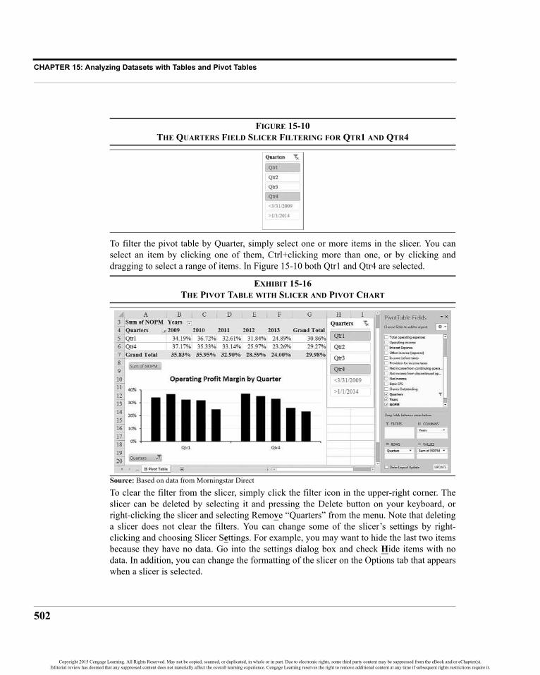
CHAPTER 15: Analyzing Datasets with Tables and Pivot Tables
502
FIGURE 15-10THE QUARTERS FIELD SLICER FILTERING FOR QTR1 AND QTR4
To filter the pivot table by Quarter, simply select one or more items in the slicer. You canselect an item by clicking one of them, Ctrl+clicking more than one, or by clicking anddragging to select a range of items. In Figure 15-10 both Qtr1 and Qtr4 are selected.
EXHIBIT 15-16THE PIVOT TABLE WITH SLICER AND PIVOT CHART
To clear the filter from the slicer, simply click the filter icon in the upper-right corner. Theslicer can be deleted by selecting it and pressing the Delete button on your keyboard, orright-clicking the slicer and selecting Remove “Quarters” from the menu. Note that deletinga slicer does not clear the filters. You can change some of the slicer’s settings by right-clicking and choosing Slicer Settings. For example, you may want to hide the last two itemsbecause they have no data. Go into the settings dialog box and check Hide items with nodata. In addition, you can change the formatting of the slicer on the Options tab that appearswhen a slicer is selected.
Source: Based on data from Morningstar Direct
Copyright 2015 Cengage Learning. All Rights Reserved. May not be copied, scanned, or duplicated, in whole or in part. Due to electronic rights, some third party content may be suppressed from the eBook and/or eChapter(s).Editorial review has deemed that any suppressed content does not materially affect the overall learning experience. Cengage Learning reserves the right to remove additional content at any time if subsequent rights restrictions require it.

503
Extracting Data from a Pivot Table
Another filtering tool, the timeline, was made available in Excel 2013. A timeline allows youto filter based on dates, and is very useful for dashboard creation. To insert a timeline, clickthe Insert Timeline button. The result will look similar to that in Figure 15-11.
FIGURE 15-11A TIMELINE FILTERING FOR 2012 AND 2013 DATA
To use the timeline, simply click on the line and drag to select the time periods of interest.You can change the time level of detail by clicking the drop-down list (it says quarters inFigure 15-11) and selecting Years, Quarters, Months, or Days. You can also do some simpleformatting in the Options tab that appears when a timeline is selected. To delete a timeline,right-click it and select Remove Timeline from the menu.
Extracting Data from a Pivot TableIt is common to use a pivot table as a source of data for formulas outside of the pivot table.That is, a formula that you create will refer to data in the pivot table. One way to do this is tosimply type a cell reference as usual. For example, using the same pivot table as in Exhibit15-15 select I5 and type: =F5. The result should be the operating profit margin for 2013(24.89%). Now, rearrange the pivot table by dragging the Years field to the Rows area.Notice that the formula in I5 now returns 0% because cell F5 is no longer in the pivot tableand is blank. Drag Years back to the Column Labels area and the value will return.
Directly referencing cells in a pivot table works fine as long as you know that the pivot tablewill never be changed. But that is an unrealistic expectation in many cases. Therefore, weneed a way to consistently refer to data in the pivot table even if it is changed. Excelprovides the GETPIVOTDATA function for exactly this purpose. It is defined as:
GETPIVOTDATA(DATA_FIELD, PIVOT_TABLE, FIELD1, ITEM1, …)
where DATA_FIELD is the name of the field (must be in quotes), PIVOT_TABLE is a celladdress anywhere in the pivot table, FIELD1 and ITEM1 are a field/item pair. You can specifyup to 126 field/item pairs. This function can be used on any worksheet, not just the one thatcontains the pivot table.
Copyright 2015 Cengage Learning. All Rights Reserved. May not be copied, scanned, or duplicated, in whole or in part. Due to electronic rights, some third party content may be suppressed from the eBook and/or eChapter(s).Editorial review has deemed that any suppressed content does not materially affect the overall learning experience. Cengage Learning reserves the right to remove additional content at any time if subsequent rights restrictions require it.

CHAPTER 15: Analyzing Datasets with Tables and Pivot Tables
504
The GETPIVOTDATA function has some flaws, for example it will return a #REF! error ifthe field is removed from the pivot table. Still, it is better than directly referencing data bycell address. The function is also complicated to type, but Excel can helpfully generate it foryou. To tell Excel to generate the function, click in the pivot table and go to the Analyze tab.At the far left drop the Options menu and make sure that Generate GetPivotData is checked.
As an example of using this function, delete the formula in I5 and then type = and click oncell F5. Excel should generate the formula: =GETPIVOTDATA("NOPM",$A$3,"Quarters",1,"Years",2013). Now try rearranging the pivot table by dragging the Years fieldto the Rows area and notice that the value in I5 doesn’t change. That is because theGetPivotData function isn’t referencing a particular cell. Instead, it is referencing aparticular value. In this case the NOPM for the first quarter of the year 2013.
Another way to get data from a pivot table is to simply copy and paste. If you do this, Excelwill only paste the data from the visible cells. The result will not be in a pivot table, unlessyou copy and paste the entire pivot table.
SummaryIn this chapter we have demonstrated how to use Excel tables and pivot tables to sort, filter,and analyze large datasets. Tables allow us to easily manage a dataset by adding and deletingdata, sorting it, or filtering it to show only those data that meet certain criteria. Pivot tablesare much more powerful, allowing us to summarize and rearrange the data in useful ways.Furthermore, pivot tables enable us to create custom fields that don’t exist in the originaldataset, create pivot charts that show the data graphically, and display data fields differently(e.g., as a percentage of the grand total, or as a rank).
TABLE 15-1FUNCTIONS INTRODUCED IN THIS CHAPTER
Purpose Function PageCalculate an average of the data that meet the criteria
AVERAGEIF(RANGE, CRITERIA, AVERAGE_RANGE)
485
Return values from a pivot table
GETPIVOTDATA(DATA_FIELD, PIVOT_TABLE, FIELD1, ITEM1, …)
503
Copyright 2015 Cengage Learning. All Rights Reserved. May not be copied, scanned, or duplicated, in whole or in part. Due to electronic rights, some third party content may be suppressed from the eBook and/or eChapter(s).Editorial review has deemed that any suppressed content does not materially affect the overall learning experience. Cengage Learning reserves the right to remove additional content at any time if subsequent rights restrictions require it.

505
Problems
Problems
1. Using the data in the GOOG Financials.xlsx workbook that was used inthe chapter:
a. Convert the balance sheet into a format that is suitable for a pivottable by transposing the data. Don’t forget to enter the word “Date”above the dates.
b. Build a pivot table from the data and group the dates by months,quarters, and years.
c. Create a calculated field that shows the current ratio in the pivot table,and format the numbers with two decimal places.
d. Create a pivot chart that shows the current ratio over time. HasGoogle’s short-term liquidity position deteriorated or improved overthis five-year period?
e. Now, use a Timeline to filter the pivot table so that it only shows 2009to 2010. Now show only 2012 to 2013. Is there a difference in thetrend of the current ratio in the two time periods?
2. Using the same workbook, copy both datasets into one worksheet so thatthey can be used together in a pivot table.
a. Create a pivot table that shows the quarter over quarter change in bothRevenue and Total Assets.
b. Create a pivot line chart that shows the data from part a. Does thereappear to be a strong correlation between the two data series? Nowput Revenue on a secondary y-axis so that the scales are comparable.Does that change your original answer?
c. Create a calculated field that shows Google’s return on equity for eachquarter.
d. Create a pivot line chart that shows the ROE over time. Does it appearthat there is any trend in the ROE? If so, is it up or down?
e. Add a linear trend line to the pivot chart from part d, and show theequation on the chart. Does this change or confirm your previousanswer?
Copyright 2015 Cengage Learning. All Rights Reserved. May not be copied, scanned, or duplicated, in whole or in part. Due to electronic rights, some third party content may be suppressed from the eBook and/or eChapter(s).Editorial review has deemed that any suppressed content does not materially affect the overall learning experience. Cengage Learning reserves the right to remove additional content at any time if subsequent rights restrictions require it.

CHAPTER 15: Analyzing Datasets with Tables and Pivot Tables
506
3. Using the ETF Data.xlsx workbook from the chapter:
a. Create a calculated column in the original data that calculates thethree-year total return for each ETF and for each MorningstarCategory. Be sure to properly account for compounding of returns.
b. Create a pivot table to show the average three-year total return foreach category, and sort the pivot table from the highest returncategory to the lowest. Which category did the best? The worst?
c. Create a pivot bar chart that shows the returns of the top 10 bestperforming fund categories over the last three years.
d. Create another pivot table from this dataset, and then a calculatedfield that shows each ETF’s three-year return less the category three-year return. Which fund did best compared to its category over thethree-year period? Which did the worst?
4. Financial researchers have found various violations of market efficiencythat are referred to as “calendar effects.” Using the S&P 500 1950 to 2013Daily.xlsx file from the official website:
a. Create a pivot table and pivot chart that shows the average percentagechange by day of the week for the entire period. Are the averagereturns different for each day? If so, which are the best and worst daysof the week?
b. Now add the Decade field to the Row area of your pivot table. Arethere any decades in which Mondays had a positive average return?
c. Change your pivot table to show the average daily return by monthfor the entire period. What is the best month on average? Which is theworst? Does this vary by decade?
d. What was the best decade in which to invest based on average dailyreturn? What was the sum of the daily returns in each decade (ignorecompounding of returns)?
5. Using the S&P 500 Company Data.xlsx workbook from the officialwebsite:
a. Create a calculated column that calculates the total return for the lastthree years. Name it “Total Return 3 Yr.” Make a pivot table thatshows the average three-year total return by S&P Sector.
Copyright 2015 Cengage Learning. All Rights Reserved. May not be copied, scanned, or duplicated, in whole or in part. Due to electronic rights, some third party content may be suppressed from the eBook and/or eChapter(s).Editorial review has deemed that any suppressed content does not materially affect the overall learning experience. Cengage Learning reserves the right to remove additional content at any time if subsequent rights restrictions require it.

507
Problems
b. Now add the S&P Industry field to the pivot table. Which industrywas the best performer in the worst sector over the past three years?Sort the fields in your pivot table so that this sector and industry is atthe very top of the table.
c. Create a new pivot table from the data that shows the top 20 S&PSub-Industries by market capitalization. Also include a count of thenumber of companies in each sub-industry.
d. Use the GetPivotData function to calculate the average marketcapitalization of each Sub-Industry in a column that is outside of thepivot table created for part c.
e. Create a new pivot table that shows the average net profit margin byS&P Industry. Which is the most profitable industry? Which is theleast profitable industry?
f. Create a pivot table that shows beta and the Total Return 3 Yr for eachcompany. Now, copy and paste the data to another location in theworksheet. Create a regular XY Scatter chart of the data. Whatrelationship do you see between beta and historical three-yearreturns?
6. In footnote 1. on page 76 some claims were made about the average levelof fourth quarter sales for Target Corp. Using the Target QuarterlySales.xlsx workbook from the official website verify those claims.
a. Create a line chart of Target’s quarterly revenue and net income, withnet income on a secondary y-axis. Does there appear to be anyseasonality in its revenue? Net income?
b. Create a pivot table that has Fiscal Year and Fiscal Quarter in theRows field, and Revenue in the Values field. Be sure to showsubtotals for each year at the bottom of each group.
c. Add Revenue to the Values field a second time. Use Show Values As% of Parent Total to show quarterly sales as a percentage of full yearsales. What is the average for the fourth quarter? First quarter?
d. Add Revenue to the Values field a third time. Use Show Values As %Difference From to show the year-over-year percentage change inquarterly sales.
Copyright 2015 Cengage Learning. All Rights Reserved. May not be copied, scanned, or duplicated, in whole or in part. Due to electronic rights, some third party content may be suppressed from the eBook and/or eChapter(s).Editorial review has deemed that any suppressed content does not materially affect the overall learning experience. Cengage Learning reserves the right to remove additional content at any time if subsequent rights restrictions require it.
CHAPTER 15: Analyzing Datasets with Tables and Pivot Tables
508
Internet Exercise
1. Go to http://www.microsoft.com/Investor/EarningsAndFinancials/TrendedHistory/AnnualStatements.aspx and download Microsoft’s annualincome statements from 1994 to the most recent year available. There is adirect link to the Excel file on that page.
a. Reformat the worksheet so that it is suitable for a pivot table. Thiswill require changing the year headings to actual dates, deleting anyblank rows or columns, and then transposing the data.
b. Create a pivot table that shows the net profit margin for each year andformat it appropriately. This will require you to create a calculatedfield.
c. Add a pivot chart that displays the results from part b over time.
d. Filter the dates so that only the last five years are displayed in thepivot table and pivot chart. This will require a custom date filter usingthe “is after or equal to” option.
e. How does Microsoft’s net profit margin compare to the average of thecompany’s in the S&P 500 index? (Hint: Use the data file fromproblem 5 to calculate this answer.)
Copyright 2015 Cengage Learning. All Rights Reserved. May not be copied, scanned, or duplicated, in whole or in part. Due to electronic rights, some third party content may be suppressed from the eBook and/or eChapter(s).Editorial review has deemed that any suppressed content does not materially affect the overall learning experience. Cengage Learning reserves the right to remove additional content at any time if subsequent rights restrictions require it.
509
APPENDIX Directory of User-Defined Functions in Famefncs.xlam
Famefncs.xlam is an Excel 2007 to 2013 add-in that contains user-defined functions that areuseful but not available in Excel. The add-in may be obtained as a download from theofficial Web site for this book (http://www.cengagebrain.com/). Once installed and activatedon your computer, Excel will automatically open the add-in every time you start Excel andthe functions will be available via the User Defined category in the Insert Function dialogbox.
Once downloaded, the add-in is easy to install. Click the File tab and then choose Options.Choose the Add-Ins category and then click the Go button. Use the Add-Ins dialog box tobrowse to the directory where you saved the add-in file. Click on the file name and thenpress the OK button. You should now see “Functions for Financial Analysis” appear in thelist of add-ins. It is now installed, activated, and ready to use. If you ever wish to disable theadd-in, simply remove the check mark in the Add-Ins dialog box.
The following functions are included in the add-in:
FAME_CAPM(RISKFREERATE, MARKETRETURN, BETA)Calculates the expected return of a security or portfolio using the CAPM (CapitalAsset Pricing Model).
FAME_CONVEXITY(SETTLEMENT, MATURITY, FACEVALUE, COUPON, YLD, FREQUENCY)Calculates the convexity of a bond on a coupon date. It is important to note that thisonly works on a coupon date, not between coupon dates. This function was createdbecause, although Excel has functions for duration and modified duration, it does nothave one for convexity.
Copyright 2015 Cengage Learning. All Rights Reserved. May not be copied, scanned, or duplicated, in whole or in part. Due to electronic rights, some third party content may be suppressed from the eBook and/or eChapter(s).Editorial review has deemed that any suppressed content does not materially affect the overall learning experience. Cengage Learning reserves the right to remove additional content at any time if subsequent rights restrictions require it.

APPENDIX: Directory of User-Defined Functions in Famefncs.xlam
510
FAME_CORR(VALUES1, VALUES2, PROBABILITIES)Calculates the correlation coefficient between two variables using the probabilities ofoccurrence for each value. Excel’s CORREL function does not handle the probabilitiesof occurrence.
FAME_COVAR(VALUES1, VALUES2, PROBABILITIES)Calculates the covariance between two variables using the probabilities of occurrencefor each value. Excel’s COVAR function does not handle the probabilities ofoccurrence.
FAME_CV(VALUES, PROBABILITIES)Calculates the coefficient of variation using the probabilities of occurrence. Exceldoes not have a similar function. This is a measure of risk per unit of return and iscalculated by dividing the standard deviation by the expected value.
FAME_EAR(PERIODIC_RATE, NPERYEAR)Calculates the effective annual rate of a periodic rate. For example, if you know that aquarterly rate is 2%, this function will tell you that it is 8.24% annualized. This doesthe same thing as Excel’s EFFECT function.
FAME_EXPVALUE(VALUES, PROBABILITIES)Calculates the expected value of a random variable using the probabilities ofoccurrence for each potential value.
FAME_GEOMEAN(DOLLARVALUES)Calculates the geometric mean rate of growth from a range of dollar values. Note thatExcel’s GEOMEAN function does not (necessarily) calculate the geometric mean rateof growth (unless you feed in a range of growth rates). Instead it will calculate thegeometric mean in the same units as the original data. This function should only beused for the data in Chapter 1.
FAME_GGMCOSTEQUITY(DIV1, VALUE, GROWTHRATE)Calculates the cost of equity, or required return, of a stock using the constant-growthdividend discount model (also known as the Gordon Growth Model).
FAME_GGMVALUE(DIV1, REQRET, GROWTHRATE)Calculates the intrinsic value of a stock using the constant-growth dividend discountmodel (also known as the Gordon Growth Model).
FAME_HMODELVALUE(DIV1, REQRATE, GROWTHRATE1, GROWTHRATE2, G1PERIODS, TRANSPERIODS)
Calculates the intrinsic value of a stock using the H-model. Note that G1PERIODS isthe length of the first period of growth, and TRANSPERIODS is the length of thetransition period between fast growth and constant-growth.
Copyright 2015 Cengage Learning. All Rights Reserved. May not be copied, scanned, or duplicated, in whole or in part. Due to electronic rights, some third party content may be suppressed from the eBook and/or eChapter(s).Editorial review has deemed that any suppressed content does not materially affect the overall learning experience. Cengage Learning reserves the right to remove additional content at any time if subsequent rights restrictions require it.

511
APPENDIX: Directory of User-Defined Functions in Famefncs.xlam
FAME_MACRS(COST, MACRSCLASS, YEAR, TABLE)Calculates the MACRS depreciation for an asset with a MACRS class of 3, 5, 7, 10,15, or 20 years. This function returns the depreciation expense for a selected YEAR.TABLE is an optional argument (True or False) that specifies whether the function usesa table lookup or an exact calculation. It will return a #VALUE! error if eitherMACRSCLASS or YEAR are incorrect.
FAME_MIRR(CASHFLOWS, REINVESTRATE)Calculates the Modified Internal Rate of Return for a series of cash flows. This isdifferent than Excel’s built-in function in the way it handles negative cash flows afterperiod 0. This function calculates the total future value of all cash flows after period 0(using the specified reinvestment rate). Excel’s MIRR function first calculates thepresent value of all negative cash flows and then calculates the future value of allpositive cash flows. Normally, both functions will return the same answer. However,when there are negative cash flows after period 0, there will be a difference(sometimes significant).
FAME_PAYBACK(CASHFLOWS, RATE)Calculates the Payback Period of a series of cash flows, assuming that the first cashflow (period 0) is negative. RATE is an optional argument. If you include a discountrate, the function will calculate the discounted payback period. For the regularPayback Period, either don’t supply a rate or make it equal to 0%.
FAME_PORTRET(VALUES, WEIGHTS)Calculates the expected return for a portfolio of securities given the expected returnsof each security and their weight in the portfolio.
FAME_PORTVAR1(VARCOVMAT, WEIGHTS)Calculates the variance of a portfolio of securities given a variance/covariance matrixand the weights of the individual securities. Note that you must supply a completevariance/covariance matrix, not just the upper or lower diagonal.
FAME_PORTVAR2(CORRMAT, STDDEVS, WEIGHTS)Calculates the variance of a portfolio of securities given a correlation matrix, thestandard deviations, and weights of the individual securities. Note that you mustsupply a complete variance/covariance matrix, not just the upper or lower diagonal.
FAME_PVGA(PMT, NPER, GROWTHRATE, DISCRATE, BEGEND)Calculates the present value of a graduated (growing) annuity. Note that BegEnd is anoptional argument that tells the function whether the first cash flow is at the end of theperiod (0) or the beginning (1) of the period. End of period (0) is the default if noBegEnd argument is supplied.
Copyright 2015 Cengage Learning. All Rights Reserved. May not be copied, scanned, or duplicated, in whole or in part. Due to electronic rights, some third party content may be suppressed from the eBook and/or eChapter(s).Editorial review has deemed that any suppressed content does not materially affect the overall learning experience. Cengage Learning reserves the right to remove additional content at any time if subsequent rights restrictions require it.

APPENDIX: Directory of User-Defined Functions in Famefncs.xlam
512
FAME_STDDEV(VALUES, PROBABILITIES)Calculates the standard deviation of a random variable given the probabilities of eachpotential outcome (it is a population standard deviation). Note that this function isdifferent from Excel’s built-in STDEV.P function in that it allows the probabilities todiffer. Excel’s function assumes that all probabilities are equal.
FAME_THREESTAGEVALUE(DIV1, REQRATE, GROWTHRATE1, GROWTHRATE2, G1PERIODS, TRANSPERIODS)
Calculates the intrinsic value of a stock using the three-stage dividend discountmodel. Note that G1PERIODS is the length of the first period of growth, andTRANSPERIODS is the length of the transition period between fast growth andconstant-growth.
FAME_THREESTEPVALUE(DIV1, REQRATE, GROWTHRATE1, GROWTHRATE2, GROWTHRATE3, G1PERIODS, TRANSPERIODS)
Calculates the intrinsic value of a stock using the three-step dividend discount model(three constant-growth periods). Note that G1PERIODS is the length of the first periodof growth, and TRANSPERIODS is the length of the transition period between fastgrowth and constant-growth.
FAME_TWOSTAGEVALUE(DIV1, REQRATE, GROWTHRATE1, GROWTHRATE2, G1PERIODS)
Calculates the intrinsic value of a stock using the two-stage dividend discount model.Note that G1PERIODS is the length of the first period of growth.
FAME_VAR(VALUES, PROBABILITIES)Calculates the variance of a random variable given the probabilities of each potentialoutcome. Note that this function is different from Excel’s built-in VAR and VARPfunctions in that it allows the probabilities to differ. Excel’s functions assume that allprobabilities are equal.
Copyright 2015 Cengage Learning. All Rights Reserved. May not be copied, scanned, or duplicated, in whole or in part. Due to electronic rights, some third party content may be suppressed from the eBook and/or eChapter(s).Editorial review has deemed that any suppressed content does not materially affect the overall learning experience. Cengage Learning reserves the right to remove additional content at any time if subsequent rights restrictions require it.

513
AAbsolute reference, 17Accounting profit, 134, 137Accounts payable, in liabilities forecasting, 150Accounts receivable
sales change and, 148sales growth vs., 112turnover ratio, 112, 113
Acid-test ratio, 110Add button, 426, 431Add-In files, 25
creating, 472–473installing, 457
Add-in, functions using, 25–26Add Watch button, 95After-tax cash flow (ATCF), 332–333
calculating, 339–340, 380components of, 332–333equation for, 332in risk measurement, 379
Altman, Edward, 127Analysis ToolPak, 162–163AND function/statement, 96, 100, 133Annuities, 200–201
deferred, 208–210FV function for, 203–204graduated, 210–214PV of, 203–204RATE function and, 207solving for interest rate, 207–208solving for payments, 204–205
solving for periods in, 205–206yield on, 208
ARRAY, 421Array formulas, 362ATCF. See After-tax cash flowAutoFill feature, 11Automatic ratio analysis, 132–134AutoSum button, 47Average collection period, 112–113AVERAGE function, 38, 39, 41, 146, 411
AutoSum button and, 48for growth rate analysis, 39, 41
AVERAGEIF function, 485Axis labels, 30
BBackstage view, 3Balance sheets
assets forecasting, 148–149assets/liabilities in, 49–51common-size, 56–57custom numbering in, 51–53liabilities forecasting, 150–151percent of sales forecast, 144–153
Bank discount rate, 276–277Banker’s Year, 113n2Bankruptcy, predicting, 127–128BASIS, in PRICE function, 272Beta, 441Binary variable, 361Bisection method, 207
Bond(s)calculating price change in, 292–294comparing, with different coupon rates,
287–288comparing, with different maturities,
285–287coupon payment, 265coupon rate, 265interest payment calculation, 265invoice price of, 266–267long-term vs. short term, 286, 288prices vs. coupon rates chart, 288prices vs. time to maturity, 284–285rate of return, calculating, 295
Bond equivalent yield, 277Bond price sensitivities, 280–288
changes in required return, 281–283changes in term to maturity, 283–285forecasting, 288–296
Bond return measures, 271–277current yield, 272yield to call, 274–276yield to maturity, 272–274
Bond valuation, 263–301between coupon dates, 266–268, 271formulas, 264, 266, 297–298interest vs. value in, 293PRICE function in, 268, 296PV function in, 265yield in, 281–282
Book value, 228
Index
Copyright 2015 Cengage Learning. All Rights Reserved. May not be copied, scanned, or duplicated, in whole or in part. Due to electronic rights, some third party content may be suppressed from the eBook and/or eChapter(s).Editorial review has deemed that any suppressed content does not materially affect the overall learning experience. Cengage Learning reserves the right to remove additional content at any time if subsequent rights restrictions require it.

Index
514
Book-value weights, 306Borders/shading, 14, 44Borrowing requirements
calculating, 81–82, 90reducing, 84timing, 83
Break-even points, 174–179calculating, 176–177EBIT in, 173–174, 175, 177equations for, 175, 177, 190Goal Seek for, 179and leverage measures, 187, 188–189
Break-points, 318–322debugging with, 468–469in Visual Basic editor, 468–469WACC, 323–324
Built-in functions, 20–26Business risk, 180–181
CCAGR. See Compound annual growth rateCalculated field, 493Call provision, 275–276Capital allocation line, 434Capital asset pricing model (CAPM), 231, 310,
438–441calculating expected returns in, 233derivation of, 438–441interest in, 231–232risk premium in, 232risk types in, 232n2security market line, 440–441
Capital budgeting, 329–370ATCF, 332–333decision techniques, 341–343definition of, 329depreciation in, 336–337estimating cash flows, 334–339initial outlay, 339, 341optimal, 358–366sensitivity analysis, 354–358TCF, 333
Capital, cost of. See Cost of capitalCapital Market Line (CML), 429–436
charting, 432–433market portfolio identification, 434–436slope of (See Market price of risk)
Capital rationingoptimal capital budget under, 361–365optimal capital budget without, 358–360
CAPM. See Capital asset pricing modelCash
sources of, 44uses of, 44
Cash balancebeginning, 58, 81
calculating, 80calculating change in, 62calculating with borrowing/investing, 96–99ending, 58, 80–89unadjusted, 81
Cash break-even point, 178Cash budget, 71–105
collections/disbursements in, 78–79collections in, 75–76definition of, 71–72income statements vs., 78, 79inflows/outflows, 57–58, 71, 79interest/investment of excess cash in, 89–99parts of, 72sales forecast in, 72for timing collections/expenditures, 83
Cash coverage ratio, 119–120Cash flow. See also After-tax cash flow
common-size statement of, 64–66from financing, 58income vs., 48incremental, 330from investing, 58from operations, 58sign convention, 198statements, 44, 57–66sunk costs in, 330uneven, 215–216
CE. See Certainty-equivalent approachCells
formatting, 12range selection, 9
Certainty-equivalent approach (CE), 400–403coefficients, 401–402vs. RADR, 403
Chart(s)changing types of, 30–32creating charts, 27embedded/stand alone, 28–29formatting, 29–30sparkline charts, 32–33titling, 30
Chebyshev’s theorem, 375n3CHOOSE function, 65Circular references
avoiding, 156using, 156
Clean price, 266Coefficient of variation, 376Collections, 78–79
calculating, 78–79, 81in cash budget, 75–76
Color coding, in error detection, 93Column Labels, 487Columns
inserting, 15width change, 16
Common equity, cost of, 309–310, 317–318Common-size balance sheets, 56–57Common-size income statements, 54–57Common-size statement of cash flows, 64–66Common stock valuation, 227–261. See also
Dividendsalternative models, 246–253cash flow in, 234, 256dividend discount models, 235–240free cash flow model, 250–253relative value models, 254–255required rate of return in, 241
Company-specific risk, 439Compound annual growth rate (CAGR), 41Compounding, 196
continuous, 221–222non-annual, 218–222
CONCATENATE function, 74Concatenation, 74Constant-growth dividend discount model
(DDM), 235–240two/three-stage models vs., 240
Contextual tabs, 27Convexity, 282
and duration, 288–295in price change projection, 294–296
Correlation, between stocks, 414–416Correlation coefficient, 415–416. See also
CovarianceCORREL function, 415Cost of capital, 303–328
adjustment technique, 315–316component costs in, 308–312cost of debt in, 311–312cost of equity in, 309–310in economic profit, 134, 135, 136equations, 315flotation costs, 315–318in investment decisions, 303
Cost of capital componentsadjusting for taxes, 312common equity, 309–310common stock, 314debt, 311–313preferred stock, 314
Cost of debt, 311–312COUNT function, 48COUNTIF function, 398, 404Coupon payment, 265Coupon rate, 265Covariance, 414–416
matrix, 419–422COVARIANCE.S function, 416, 420, 444Coverage ratios, 118
cash coverage ratio, 119times interest earned, 119–120
Copyright 2015 Cengage Learning. All Rights Reserved. May not be copied, scanned, or duplicated, in whole or in part. Due to electronic rights, some third party content may be suppressed from the eBook and/or eChapter(s).Editorial review has deemed that any suppressed content does not materially affect the overall learning experience. Cengage Learning reserves the right to remove additional content at any time if subsequent rights restrictions require it.

515
Index
Current ratiocalculating, 109quick ratio vs., 109
Current yield, 272Customize quick access toolbar, 4Custom number formats, 46, 51–53, 110
DData Analysis ToolPak, 163Data tables, 249–250, 382–384Data validation, 66DATE function, 73–74DAY function, 74DAYS360 function, 270DB function, 336DCF. See Discounted cash flowDCL. See Degree of combined leverageDDB function, 336DDM. See Constant-growth dividend discountDebt
after-tax cost of, 312–313cost of, 311–312
Debugging formulaswith breakpoints, 468–469color coding for, 93with Evaluate Formula tool, 95–96, 469F9 key for, 93formula auditing and, 94–95with Immediate Window, 468, 471VBA, 468–471Watch Window for, 95, 468, 470
Deferred annuities, 208–210Define name dialog box, 10Degree of combined leverage (DCL), 186–187,
190Degree of financial leverage (DFL), 184–185,
190Degree of operating leverage (DOL), 181–184,
189Depreciation
calculating, 336–339in capital budgeting, 336–339formula for, 148functions for, 336in Statement of Cash Flows, 57–62
DFL. See Degree of financial leverageDFN. See Discretionary financing neededDirect method, statement of cash flows, 57n4Dirty prices of bonds, 266 DISC function, 276Discounted cash flow (DCF), 227, 254Discounted debt securities, returns on, 276–277Discounted payback period, 343–344Discretionary financing needed (DFN), 151–156Discretionary sources of financing, 150
Diversification, 410–412benefits of, 417defined, 409, 441
Dividend discount model, 309–310Dividends
earnings model for, 246–250growth rate of, 236in stock valuation, 234–244, 255–257three-stage growth model, 242–245two-stage growth model, 240–242
DOL. See Degree of operating leverageDot functions, 24Dot notation, in VBA, 465DuPont analysis, 124–126DuPont ROE, 126Duration, for bond forecasts, 289–293, 295DURATION function, 291
EEarnings before interest and taxes (EBIT)
business risk and, 180EPS and, 182in income statements, 47NOPAT and, 135
Earnings model, 246–250Earnings per share (EPS), 246
EBIT and, 182in financial leverage, 185
EBIT. See Earnings before interest and taxesEconomic profit, 134–136
accounting profit vs., 134, 137EDATE function, 283, 284Edit button, 429EFFECT function, 221Effective annual interest rate (EAR), 221Efficiency ratios
accounts receivable turnover, 112average collection period, 112–113fixed asset turnover, 114inventory turnover, 111–112total asset turnover, 114–115
Efficient Frontier, 424–429charting, 428–429locating in Excel, 425–427slope of, 435
Enterprise value, 255EPS. See Earnings per shareEquals sign (=)
in formulas, 16in VBA, 456
Equitycost of common, 309–310cost of preferred, 310multiplier, 124return on, 123
Errorscircular, 153detecting, 92–94EXP function, 222F9 key for, 93in IRR function, 217–218regression analysis, 160
Evaluate Formula tool, 95–96Excel tables, 478–480
duplicate records, removing, 480filtering, 480–482formulas in, 484–485sorting and filtering numeric fields,
482–484Exit button, 36Expected portfolio return, 412–418Expected value, 372–373
calculating, 388–389formula, 462–463in VBA calculations, 464
EXP function, 222Extended DuPont analysis, 125–126
FFace value, 264, 265FAME_CONVEXITY function, 295FAME_CV function, 404FAME_EXPVALUE function, 389–390, 403FAME_FVGA function, 214FAME_GEOMEAN function, 26, 38FAME_HModelValue, 245FAME_MACRS function, 339, 379FAME_PAYBACK macro, 343–344FAME_PORTVAR1 function, 423, 442FAME_PORTVAR2 function, 442FAME_PORTVAR1 user-defined function, 423FAME_PVGA function, 213, 214FAME_STDDEV function, 390, 404FAME_ThreeStageValue macro, 244, 258FAME_THREESTEPVALUE, 243FAME_TwoStageValue macro, 241–242, 449FAME_VAR macro, 390–391, 404FCF. See Free cash flowFeasible set, 424File tab, 3–4Financial distress prediction, 127–129
original Z-score model, 127–128Z-score model for private firms, 128–129
Financial forecasting, 143–171assets, 148–149liabilities, 150–151linear trend extrapolation, 156–158percent of sales method, 144–153regression analysis, 160–165statistical significance, 165–167
Copyright 2015 Cengage Learning. All Rights Reserved. May not be copied, scanned, or duplicated, in whole or in part. Due to electronic rights, some third party content may be suppressed from the eBook and/or eChapter(s).Editorial review has deemed that any suppressed content does not materially affect the overall learning experience. Cengage Learning reserves the right to remove additional content at any time if subsequent rights restrictions require it.

Index
516
TREND function in, 143uses of, 149
Financial ratioscategories of, 108coverage, 108, 118–120, 137current, 109–110efficiency, 108, 111–115, 137leverage, 108, 115–118, 137liquidity, 108, 137profitability, 108, 120–127, 137summary of, 137–138uses of, 107–108, 129–134
Financial risk, business risk vs., 181Financial statements. See Income statementsFinancing costs, 330–331Financing decision, 433Financing sources, 150Fixed asset turnover ratio, 114Fixed costs, 174Flotation costs, 315–318FORECAST function, in regression analysis,
162Forecasting. See Financial forecastingFormat Cells command, 46, 51–52, 60Formatting, 11–14
and alignment options, 11, 13borders/shading, 14, 44cells, 12custom numbers in, 51–53
importance of, 46Formula(s). See also Debugging formulas
copying/moving, 17–18entering, 15–17pointer mode for, 16
Formula Auditing toolbar, 94Formula auditing tools, 93–94Formula bar, 6Formula debugging
Evaluate Formula tool for, 95–96Watch Window, 95, 468
Free cash flow (FCF), 250–253Free cash flow valuation model, 250–253FREQUENCY
in PRICE function, 271in YIELD function, 272
FunctionAVERAGEIF, 485GETPIVOTDATA, 504
Function argument dialog box, 23Functions. See also Macro functions;
User-defined functionAND, 133add-in, 213AVERAGE, 38, 39, 41, 48, 146CHOOSE, 65CONCATENATE, 74
CORREL, 415COUNT, 48COUNTIF, 398, 404COVARIANCE.S, 416, 420, 444DATE, 73–74DAY, 74DAYS360, 270DB, 336DDB, 336DISC, 276DURATION, 291EDATE, 284EFFECT, 221EXP, 222ExpValue, 469, 471FAME_CONVEXITY, 295FAME_CV, 404FAME_EXPVALUE, 389, 390, 403FAME_FVGA, 214FAME_GEOMEAN, 26, 38FAME_HModelValue, 245FAME_MACRS, 339, 379FAME_PORTVAR1, 442FAME_PORTVAR2, 442FAME_PVGA, 213–214FAME_STDDEV, 390, 404FAME_ThreeStageValue macro, 244, 258FAME_THREESTEPVALUE, 243FAME_TWOSTAGEVALUE, 449FAME_TwoStageValue macro, 241–242FAME_VAR macro, 390–391, 404FORECAST, 162FV, 196–199, 201, 203–207, 215–217, 219,
221GEOMEAN, 20–23, 26, 38, 39, 41, 449GROWTH, 162IF, 132IFERROR, 183, 338, 339INTERCEPT, 167IRR, 217–218, 349LINEST, 160n10, 162LN, 206LOGEST, 162MAX/MIN, 48, 85, 92, 100MDURATION, 291MIRR, 353MMULT, 421MONTH, 74NA, 183NOMINAL, 221NORMSDIST, 391, 398, 404NPER, 206, 343n2NPV, 215–216, 347, 383OR, 96n5, 133PMT, 197, 199, 201, 204, 205, 206, 210,
214, 217
PRICE, 268, 270–271, 273, 276, 296PV, 198–199, 201, 203, 265, 268, 299, 461RATE, 207, 313, 349ROUNDUP, 103, 267, 271SLN, 149, 336SLOPE, 167, 385SMALL, 321, 325STDEV, 390, 404STDEVP, 390, 404step, 318–319, 323–324SUM, 47, 76SUMPRODUCT, 308, 463SYD, 336TEXT, 74, 75TRANSPOSE, 421TREND, 143, 156–159, 166, 168User-defined, 447–476VAR, 389, 403VARP, 389, 390, 403VAR.S, 389VDB, 336–337VLOOKUP, 337YEAR, 74YEARFRAC, 273YIELD, 272, 313YIELDDISC, 277
Future value (FV), 196–199. See also FV function
of annuities, 202–204equations for, 196–198of uneven cash stream, 215–216
FV function, 197–198
GGEOMEAN function, 20–23, 26, 38, 39, 41, 449GETPIVOTDATA function, 504Goal Seek, 180, 190Gordon model. See Constant-growth dividendGo To command, 9–10Graduated annuities, 210–214Graphics, 26–27Gross profit, 47Gross profit margin, 121GROWTH function, 162
HHelper columns, 147Histograms, 398–399H-model, 244–246Home Tab, 4–5“Hurdle” rate, 304–307
Copyright 2015 Cengage Learning. All Rights Reserved. May not be copied, scanned, or duplicated, in whole or in part. Due to electronic rights, some third party content may be suppressed from the eBook and/or eChapter(s).Editorial review has deemed that any suppressed content does not materially affect the overall learning experience. Cengage Learning reserves the right to remove additional content at any time if subsequent rights restrictions require it.

517
Index
IIFERROR function, 183, 338, 339IF function/statement, 132IF statements, 82If-Then-Else statement, in VBA, 460–462Immediate Window, 468, 471Income statements, 43, 44–49
common-size, 54–57custom numbering in, 51–53, 62forecasting, 144–148level of detail in, 144
Indifference curves, 436charting, 436–438
Indifference map, 437Indirect method, statement of cash flows, 57n4Initial outlay, 331–332
calculating, 332equation for, 332
Insert function dialog box, 22–23Inserting columns, 15INTERCEPT functions, 167Interest burden, 125Interest rates, 288–289
annuity, 207–208bond strategy and, 288
Internal rate of return (IRR), 217, 348–349, 351–353, 359
Intrinsic value, 228, 309Investment opportunity schedule (IOS), 359Investments, comparing. See Capital budgetingIOS. See Investment opportunity scheduleIRR function, 217. See also Internal rate of
returnmarginal WACC and, 358modified, 351–353multiple, 351NPV vs., 351–353problems with, 349–351RATE function for, 349
Iteration, to eliminate DFN, 153–156
LLeverage analysis, 180–188Leverage measures, 188–189Leverage ratios, 115–118
debt to equity, 117–118LTD, 116–117LTD debt to equity, 118LTD to total capitalization, 117total debt, 117
Liabilitiesforecasting, 150–151spontaneous/discretionary financing and,
150
LINEST function, 160n10in regression analysis, 160
Liquidity ratios, 108current ratio, 109–110quick ratio, 110–111
LN function, 206LOGEST function, 162Long-term debt to total capitalization ratio, 117Lump sum/single cash flow, 200–201, 460
MMacaulay duration, calculating, 289–291Macaulay, Frederick, 289Macro functions. See also Visual Basic for
Applicationsvs. built-in functions, 25–26definition of, 448keystroke, 39procedure, 448–449types of, 448–449using, 25–26
Macro recorder, 449MACRS. See Modified accelerated cost recovery
systemMalkiel, Burton, 280Malkiel's bond pricing theorems, 280–288Marginal WACC curve
breakpoints in, 318–322chart for, 323–324finding breakpoints in, 318–322IOS and, 359–360in optimal capital budget, 361–365step function, 318–319, 323–324
Market portfolio, 433Market price of risk, 434Market risk, 439Market value, 228Market-value weights, 306–307Mathematical operators, 18–19MATURITY, in PRICE function, 268MAX/MIN functions, 85, 92, 101MCC curve. See Marginal WACC curveMDURATION function, 291Min radio button, 426Min. variance portfolio, 425–426MIRR function, 353Mixed references, creating, 17MMULT function, 421
in calculating portfolio standard, 423deviation, 422in variance/covariance matrix, 421
Modified accelerated cost recovery system (MACRS), 336–337
Modified internal rate of return (MIRR), 351–353
Money market securities, 276
Monte Carlo simulations, 392–399, 403MONTH function, 74Multiple discriminant analysis, 127Mutually exclusive investment opportunities,
208
NNA function, 183Named ranges, 9–10, 10n2Name edit box, 432Net income
in income statements, 48in Statement of Cash Flows, 59
Net operating profit after taxes (NOPAT), 135defined, 250EBIT and, 135–136in free cash flow model, 250, 252in stock valuation, 250
Net operating working capital (NOWC), 250, 332
in operating assets forecast, 250Net present value (NPV), 134n8, 305n1
capital rationing vs., 358in Excel, 216n8for investment decisions, 345–347IRR vs., 349–350PI vs., 347positive/negative, 347probability of negative, 391–392profile charts, 354–355sensitivity analysis for, 381stock valuation, 247
Net profit margin, 121–122, 125NOMINAL function, 221Nonannual compounding periods, 218–220
continuous compounding, 221–222effective annual interest rate (EAR), 221
NOPAT. See Net operating profit after taxesNORMSDIST function, 391, 398, 404NPER function, 197, 206, 343n2NPV. See Net present valueNPV function
definition of, 209misleading, 347in PI calculation, 347for uneven cash flows, 215–216
Numbersaligning, 13custom format, 46, 51–53entering, 11, 13formatting, 13–14separator, 13n4signs of, 60
Copyright 2015 Cengage Learning. All Rights Reserved. May not be copied, scanned, or duplicated, in whole or in part. Due to electronic rights, some third party content may be suppressed from the eBook and/or eChapter(s).Editorial review has deemed that any suppressed content does not materially affect the overall learning experience. Cengage Learning reserves the right to remove additional content at any time if subsequent rights restrictions require it.

Index
518
OOperating break-even point, 174Operating capital, 135Operating leverage, 181–183Operating profit margin, 121, 125Opportunity cost, 134, 207, 303Optimal capital budget, 358–366
under capital rationing, 361–365without capital rationing, 358–360
Optimal portfolio, 436–438Ordinary least squares (OLS) regression. See
Regression analysisOR function, 96n5, 133Outline tool, 62–63
PParentheses and order of operations, 19–20Paste special command, 35Paste special dialog box, 55Payback period, 341–344P/E. See Price to earnings ratioPercent of sales method, 144–153
balance sheet, 148–149income statement, 144–148inventory in, 148other methods vs., 156–167premise of, 144
PI. See Profitability indexPivot tables, 485
calculations, 492–494creating, 486–488displaying multiple subtotals, 498–499extracting data, 503–504filtering data with slicers, 501–503financial ratios, 499–501for financial statements, 494–495formatting, 488–489grouping data by date, 495–497rearranging, 490–491to show trends over time, 497–498transforming data field presentation,
491–492PMT function, 197, 201
in annuity payment calculation, 204–205in retirement planning, 210
Pointer mode, 16Portfolio(s)
defined, 410, 441diversification effects, 410–412expected return of, 412–413with more than two securities, 415, 418–423
standard deviation, 422–423variance/covariance matrix creation,
419–422optimal portfolio, 436–438
risk and return, 412–418standard deviation, 413–416
Portfolio diversification effects, 410–412Portfolio risk and return, 412–418
for multiple securities, 418standard deviation in, 413–416
Preferred equity, cost of, 310Preferred stock valuation, 255–257
cost of capital, 314formula for, 255–257
Present value (PV), 196, 198–199. See also PV function
of annuities, 200–201of continuously compounded sum, 222intrinsic value and, 228solving for, 198–199stock valuing, 237of uneven cash stream, 215
Present value of future growth opportunities (PVGO), 246
PRICE functionBASIS in, 269for bond valuation, 268, 281, 283FREQUENCY in, 271MATURITY in, 268REDEMPTION in, 268, 272SETTLEMENT in, 268
Price to earnings (P/E) ratio, 254–255Price/yield function, 294Principle of value additivity, 200, 203, 211,
214–216Printing, 33–35PROBABILITIES, in FAME_VAR macro, 389Probability distribution, 372–373
continuous, 372discrete, 372expected value of, 372–373normal, 372risk in, 374in simulation, 392, 393
Profitability index (PI)calculating, 347equation for, 348
Profitability measures, 366discounted payback period, 343–344IRR, 349–350modified IRR, 351–353net present value, 345–347payback period, 341–344profitability index, 347–348
Profitability ratiosgross profit margin, 121model analysis of, 126–127net profit margin, 121–122operating profit margin, 121return on equity, 123
return on total assets, 122Pro forma balance sheet, 149, 151, 154, 155Pro forma income statement, 153PV. See Present valuePV function
in bond valuation, 265definition of, 201FV vs., 198–199VBA and, 460
QQuick access toolbar (QAT), 3–4Quick ratio, 110–111
RRANGE, 485Range names, 87–88. See also Named rangesRATE
in FV function, 197in PRICE function, 268
RATE functionfor annuity interest, 207in cost of capital, 313for IRR, 349
Readability. See Custom number formatsREDEMPTION, in PRICE function, 269References, absolute/mixed, 17Regression analysis
FORECAST function in, 162LINEST function in, 162multiple, 163n11non-linear, 162parameters, 167trend analysis and, 156TREND function in, 162
Regression results, 164Regression tools, 160–165Reinvestment
IRR and, 352rate, 250, 352timeline for, 352
Relative value models, 254–255Repayment, 82–83Replacement decision, 331, 341Report Filter, 487Required rate of return
bonds vs. stocks, 229changes in, 264–265converting market price to, 309determining, 230–234, 304“hurdle” rate in, 304–307in price of securities, 309in stock valuation, 237WACC and, 305–306
Copyright 2015 Cengage Learning. All Rights Reserved. May not be copied, scanned, or duplicated, in whole or in part. Due to electronic rights, some third party content may be suppressed from the eBook and/or eChapter(s).Editorial review has deemed that any suppressed content does not materially affect the overall learning experience. Cengage Learning reserves the right to remove additional content at any time if subsequent rights restrictions require it.

519
Index
Retained earningscost of, 317–318in percent of sales method, 151
Retirement planning, 202–204, 208–210PMT function in, 210rate of inflation in, 210–211
Return on assets (ROA), 123–124in Du Pont analysis, 124–126
Return on common equity, 123Return on equity (ROE), 123–124
in Du Pont analysis, 124–126ROA and, 124in stock valuation, 247
Return on total assets, 122Ribbon, 4, 5Risk
investors and, 230premium, 231–233, 399–400probability distribution in, 372, 373, 374,
376rate of return modeling and, 230–234types of, 232n2
Risk-adjusted discount rate method (RADR), 399–400, 403
Risk measurement, 377–380calculating standard deviation, 389–391certainty-equivalent approach, 400–403historical annual returns in, 410–411NPV in, 381portfolio diversification effects in, 410–412scenario manager in, 387sensitivity analysis in, 381–386
Risk-return trade-off, 230ROE. See Return on equityRounding problems, scientific notation and, 159ROUNDUP function, 103, 267, 271Row Labels, 487
SSales forecast, 103
in cash budget, 75and collection, 75–76regression analysis, 166
SALVAGE, in SLN function, 336Salvage value, 331–336, 339–340Saving worksheets, 35Scenario analysis, 354–358
simulation vs., 392, 397uncertainty variables, 386–388
Scenario Manager, 85–89, 102, 355–358Security market line (SML), 440–441Select Data, 429Selling, general, and administrative expense, 47,
145Sensitivity analysis, 354–358
data tables in, 382–384input area set up for, 384for NPV, 381–382in risk measurement, 381–386scenario manager for, 387uncertainty variables, 381–386
Sensitivity diagrams, 385–386Series dialog box, 238SERIES function, 10SETTLEMENT, in PRICE function, 268SG&A. See Selling, general, and administrative
expenseSharpe ratio, 434Sheet tabs, 7Shift+Ctrl+Enter, 421, 423, 431Short-term borrowing, repayment, 82–83Simulation
NORMSDIST function in, 398scenario analysis vs., 392, 397
Single cash flows, PV/FV of, 198–199SLN function, 149, 336SLOPE function, 385SLOPE functions, 167SMALL function, 321, 325Smart Tags, 141SML. See Security market lineSolve button, 426, 427, 431Solver tool, 363–366, 425–426Spark lines, 27
charts, 32–33Spontaneous sources of financing, 150Spreadsheets, 1
applications for, 2rules for design of, 36–37uses of, 2
Standard deviationcalculating, 389–391for multiple securities, 418portfolio, 413–416, 422–423in risk calculation, 375
Statement of cash flows, 57–62. See also Cash flow
Statement of Changes in Financial Position, 57n4Statistical concepts
coefficient of variation, 376expected value, 374, 376measures of dispersion, 374–376variance/standard deviation, 374–375
Status bar, 7–8STDEV function, 390, 403STDEVP function, 390, 404Step function, 318Stock. See Common stock valuation; Preferred
stock valuationSUM function, 47Summary button, 88
Sum of squared errors (SSE), 160SUMPRODUCT function, 308, 463Sunk costs, 330SYD function, 336Systematic risk, 232n2
TTabs
file, 3–4sheet, 7
Tax burden, 125TCF. See Terminal cash flowTerminal cash flow (TCF), 333, 340Text
aligning, 13changing font, 12entering, 11, 13format, 12
TEXT function, 74, 75Three-stage growth model, 242–245
H-model, 244–246three-stage model, 243–244three-step model, 243
Time-shifting, 208, 236–237Times interest earned ratio, 119–120Time value of money, 195–226Tobin's separation theorem, 433ToolTip, 4Total asset turnover ratio, 114–115Total debt ratio, 116TRANSPOSE function, 421–423
in calculating portfolio standard deviation, 423
in variance/covariance matrix, 421Trend analysis, 129–130, 131, 156–158TREND function, 156–160, 160n10, 169Trend line
adding, 158–160displaying equation for, 159
Two-stage growth model, 240–242
UUncertainty, 381Uncertainty variables
data tables for, 384scenario analysis, 386–388sensitivity analysis, 381–386sensitivity diagrams for, 385–386in simulation, 392
Uneven cash flows, 215–218NPV function for, 215–216PV and FV for, 215solving for yield in, 216–218
Ungroup sheets, 7Unsystematic risk, 232n2
Copyright 2015 Cengage Learning. All Rights Reserved. May not be copied, scanned, or duplicated, in whole or in part. Due to electronic rights, some third party content may be suppressed from the eBook and/or eChapter(s).Editorial review has deemed that any suppressed content does not materially affect the overall learning experience. Cengage Learning reserves the right to remove additional content at any time if subsequent rights restrictions require it.

Index
520
User-defined functions (UDF), 25–26, 447–476. See also Visual Basic editor; Visual Basic for applications
parts of, 453sharing, 469starting to write, 453–457uses of, 449
U.S. treasury yield curve, 278–280Utility functions, 436–438
VValuation, fundamentals of, 229Value, 487
cash flow size/timing in, 229types of, 228
VAR function, 389, 403Variable costs, 173Variance, 374–375
calculating, 389–391functions for, 389interpreting, 390
Variance/covariance matrix, 419–422Variance/covariance matrix (VARCOVMAT),
portfolio, 423calculation of, using matrix algebra,
420–422VARP function, 389VAR.S function, 389VBA. See Visual Basic for ApplicationsVDB function, 336Visual Basic editor, 450–452
breakpoints, 468–469, 471Code Window, 452comments in, 453equals sign (=) in, 456Full Module view, 452
opening, 450Procedure View, 452Project Explorer, 451
Visual Basic for Applications (VBA), 37, 447–448
debugging, 468–471Dim statement, 459dot notation in, 465errors in, 468–471help/resources, 472, 474–475If-Then-Else statement, 460–462looping statements, 462–465macro recorder for, 449numeric data types, 458, 464objects, 465optional arguments, 466–467ParamArray, 467–468Ranges, 464variables, 458–459
VLOOKUP function, 337
WWACC. See Weighted average cost of capitalWatch Window, 95, 470
debugging with, 470formula debugging with, 95, 470
Weighted average cost of capital (WACC). See also Marginal WACC curve
calculating, 308in FCF, 251IRR and, 358marginal curve for, 318–324payback period and, 342in RADR, 399in required rate of return, 305–306step function for, 318–319
Weights, in cost of capital calculations, 306–307What-if analysis, 83–85Word documents, pasting Excel files into, 35Workbooks, 7
keeping related data in, 50naming sheets within, 45
Worksheet area, 6
XX-axis, reversing, 30
YYEARFRAC function, 273YEAR function, 74Yield. See also Required rate of return
on annuities, 208bond equivalent, 268, 288, 290bond value vs., 283to call, 274–276coupon rate vs., 289current, 272in duration calculations, 289–290to maturity, 272–274to maturity vs. current, 296–297price change vs., 287sensitivity to, 287in uneven cash flow stream, 216–218
YIELDDISC function, 277YIELD function, 272, 313YLD, in PRICE function, 268
ZZ-score model
original, 127–128for private firms, 128–129
Copyright 2015 Cengage Learning. All Rights Reserved. May not be copied, scanned, or duplicated, in whole or in part. Due to electronic rights, some third party content may be suppressed from the eBook and/or eChapter(s).Editorial review has deemed that any suppressed content does not materially affect the overall learning experience. Cengage Learning reserves the right to remove additional content at any time if subsequent rights restrictions require it.