Microsoft Excel Pivot Table Data Crunching (Office 2021 and ...
79
-
Upload
khangminh22 -
Category
Documents
-
view
3 -
download
0
Transcript of Microsoft Excel Pivot Table Data Crunching (Office 2021 and ...


Microsoft Excel Pivot Table Data Crunching (Office 2021 and Microsoft 365)
Bill Jelen
A01_Jelen_FM_pi-pxxxii_new.indd 1 29/10/21 10:59 PM

Microsoft Excel Pivot Table Data Crunching (Office 2021 And Microsoft 365)Published with the authorization of Microsoft Corporation by: Pearson Education, Inc.Copyright © 2022 by Pearson Education, Inc.
All rights reserved. This publication is protected by copyright, and permission must be obtained from the publisher prior to any prohibited reproduction, storage in a retrieval system, or transmission in any form or by any means, electronic, mechanical, photo-copying, recording, or likewise. For information regarding permissions, request forms, and the appropriate contacts within the Pearson Education Global Rights & Permissions Department, please visit www.pearson.com/permissions.
No patent liability is assumed with respect to the use of the information contained herein. Although every precaution has been taken in the preparation of this book, the publisher and author assume no responsibility for errors or omissions. Nor is any liabil-ity assumed for damages resulting from the use of the information contained herein.
ISBN-13: 978-0-13-752183-8 ISBN-10: 0-13-752183-9
Library of Congress Control Number: 2021948294
ScoutAutomatedPrintCode
Trademarks
Microsoft and the trademarks listed at http://www.microsoft.com on the “Trademarks” webpage are trademarks of the Microsoft group of companies. All other marks are property of their respective owners.
Warning and Disclaimer
Every effort has been made to make this book as complete and as accurate as possible, but no warranty or fitness is implied. The information provided is on an “as is” basis. The author, the publisher, and Microsoft Corporation shall have neither liability nor respon-sibility to any person or entity with respect to any loss or damages arising from the information contained in this book or from the use of the programs accompanying it.
Special Sales
For information about buying this title in bulk quantities, or for special sales opportunities (which may include electronic versions; custom cover designs; and content particular to your business, training goals, marketing focus, or branding interests), please contact our corporate sales department at [email protected] or (800) 382-3419.
For government sales inquiries, please contact [email protected].
For questions about sales outside the U.S., please contact [email protected].
EDITOR-IN-CHIEF
Brett Bartow
EXECUTIVE EDITOR
Loretta Yates
SPONSORING EDITOR
Charvi Arora
DEVELOPMENT EDITOR
Rick Kughen
MANAGING EDITOR
Sandra Schroeder
TECHNICAL EDITOR
Bob Umlas
SENIOR PROJECT EDITOR
Tracey Croom
COPY EDITOR
Rick Kughen
INDEXER
Timothy Wright
PROOFREADER
Donna Mulder
EDITORIAL ASSISTANT
Cindy Teeters
COVER DESIGNER
Twist Creative, Seattle
COMPOSITOR
codeMantra
A01_Jelen_FM_pi-pxxxii_new2.indd 2 03/11/21 5:50 PM

Pearson’s Commitment to Diversity, Equity, and Inclusion
Pearson is dedicated to creating bias-free content that reflects the diversity of all learners. We embrace the many dimensions of diversity, including but not limited to race, ethnic-ity, gender, socioeconomic status, ability, age, sexual orientation, and religious or political beliefs.
Education is a powerful force for equity and change in our world. It has the potential to deliver opportunities that improve lives and enable economic mobility. As we work with authors to create content for every product and service, we acknowledge our responsibility to demonstrate inclusivity and incorporate diverse scholarship so that everyone can achieve their potential through learning. As the world’s leading learning company, we have a duty to help drive change and live up to our purpose to help more people create a better life for themselves and to create a better world.
Our ambition is to purposefully contribute to a world where:
■ Everyone has an equitable and lifelong opportunity to succeed through learning.
■ Our educational products and services are inclusive and represent the rich diversity of learners.
■ Our educational content accurately reflects the histories and experiences of the learners we serve.
■ Our educational content prompts deeper discussions with learners and motivates them to expand their own learning (and worldview).
While we work hard to present unbiased content, we want to hear from you about any concerns or needs with this Pearson product so that we can investigate and address them.
■ Please contact us with concerns about any potential bias at https://www.pearson.com/report-bias.html.
iii
A01_Jelen_FM_pi-pxxxii_new.indd 3 29/10/21 10:59 PM

This page intentionally left blank

v
Dedication
To Howie Dickerman at Microsoft. Have a great retirement!
—Bill Jelen
A01_Jelen_FM_pi-pxxxii_new.indd 5 29/10/21 10:59 PM

vi
Contents at a Glance
Acknowledgments xxi
About the Author xxiii
Introduction xxv
CHAPTER 1 Pivot table fundamentals 1
CHAPTER 2 Creating a basic pivot table 11
CHAPTER 3 Customizing a pivot table 43
CHAPTER 4 Grouping, sorting, and filtering pivot data 77
CHAPTER 5 Performing calculations in pivot tables 121
CHAPTER 6 Using pivot charts and other visualizations 149
CHAPTER 7 Analyzing disparate data sources with pivot tables 175
CHAPTER 8 Sharing dashboards with Power BI 207
CHAPTER 9 Using cube formulas with the Data Model or OLAP data 225
CHAPTER 10 Unlocking features with the Data Model and Power Pivot 257
CHAPTER 11 Analyzing geographic data with 3D Map 285
CHAPTER 12 Enhancing pivot table reports with macros 301
CHAPTER 13 Using VBA or TypeScript to create pivot tables 321
CHAPTER 14 Advanced pivot table tips and techniques 389
CHAPTER 15 Dr. Jekyll and Mr. GetPivotData 435
CHAPTER 16 Creating pivot tables in Excel Online 453
CHAPTER 17 Pivoting without a pivot table using dynamic arrays or Power Query 465
CHAPTER 18 Unpivoting in Power Query 479
Afterword 495
Index 497
A01_Jelen_FM_pi-pxxxii_new.indd 6 29/10/21 10:59 PM

vii
Contents
Acknowledgments . . . . . . . . . . . . . . . . . . . . . . . . . . . . . . . . . . . . . . . . . . . . . . . . . . . xxi
About the Author . . . . . . . . . . . . . . . . . . . . . . . . . . . . . . . . . . . . . . . . . . . . . . . . . . . xxiii
Introduction . . . . . . . . . . . . . . . . . . . . . . . . . . . . . . . . . . . . . . . . . . . . . . . . . . . . . . . . xxv
Chapter 1 Pivot table fundamentals 1Why you should use a pivot table . . . . . . . . . . . . . . . . . . . . . . . . . . . . . . . . . . . . . 2
When to use a pivot table . . . . . . . . . . . . . . . . . . . . . . . . . . . . . . . . . . . . . . . . . . . . 3
Anatomy of a pivot table . . . . . . . . . . . . . . . . . . . . . . . . . . . . . . . . . . . . . . . . . . . . . 4Values area . . . . . . . . . . . . . . . . . . . . . . . . . . . . . . . . . . . . . . . . . . . . . . . . . . . . 4Rows area . . . . . . . . . . . . . . . . . . . . . . . . . . . . . . . . . . . . . . . . . . . . . . . . . . . . . 5Columns area . . . . . . . . . . . . . . . . . . . . . . . . . . . . . . . . . . . . . . . . . . . . . . . . . . 6Filters area . . . . . . . . . . . . . . . . . . . . . . . . . . . . . . . . . . . . . . . . . . . . . . . . . . . . . 6
Pivot tables behind the scenes . . . . . . . . . . . . . . . . . . . . . . . . . . . . . . . . . . . . . . . . 7
Pivot table backward compatibility . . . . . . . . . . . . . . . . . . . . . . . . . . . . . . . . . . . . 7A word about compatibility . . . . . . . . . . . . . . . . . . . . . . . . . . . . . . . . . . . . . 8
Next steps . . . . . . . . . . . . . . . . . . . . . . . . . . . . . . . . . . . . . . . . . . . . . . . . . . . . . . . . . . . 9
Chapter 2 Creating a basic pivot table 11Ensuring that data is in a Tabular layout . . . . . . . . . . . . . . . . . . . . . . . . 12Avoiding storing data in section headings . . . . . . . . . . . . . . . . . . . . . . 12Avoiding repeating groups as columns . . . . . . . . . . . . . . . . . . . . . . . . . . 13Eliminating gaps and blank cells in the data source . . . . . . . . . . . . . . 14Applying appropriate type formatting to fields . . . . . . . . . . . . . . . . . 14Summary of good data source design . . . . . . . . . . . . . . . . . . . . . . . . . . 14
How to create a basic pivot table . . . . . . . . . . . . . . . . . . . . . . . . . . . . . . . . . . . . . 19Adding fields to a report . . . . . . . . . . . . . . . . . . . . . . . . . . . . . . . . . . . . . . 22Fundamentals of laying out a pivot table report . . . . . . . . . . . . . . . . 23Adding layers to a pivot table . . . . . . . . . . . . . . . . . . . . . . . . . . . . . . . . . . 25Rearranging a pivot table . . . . . . . . . . . . . . . . . . . . . . . . . . . . . . . . . . . . . . 25Creating a report filter . . . . . . . . . . . . . . . . . . . . . . . . . . . . . . . . . . . . . . . . . 28
A01_Jelen_FM_pi-pxxxii_new.indd 7 29/10/21 10:59 PM

viii Contents
Understanding the Recommended PivotTable and the Analyze Data features . . . . . . . . . . . . . . . . . . . . . . . . . . . . . . . . . . . . . . . . . . . . 28
Using slicers to filter your report . . . . . . . . . . . . . . . . . . . . . . . . . . . . . . . . . . . . . . 31Creating a standard slicer . . . . . . . . . . . . . . . . . . . . . . . . . . . . . . . . . . . . . . 31Creating a Timeline slicer. . . . . . . . . . . . . . . . . . . . . . . . . . . . . . . . . . . . . . . 34
Keeping up with changes in the data source . . . . . . . . . . . . . . . . . . . . . . . . . . 37Dealing with changes made to the existing data source . . . . . . . . . 37Dealing with an expanded data source range due
to the addition of rows or columns . . . . . . . . . . . . . . . . . . . . . . . . . . . 37
Sharing the pivot cache or creating a new cache . . . . . . . . . . . . . . . . . . . . . . 38
Side effects of sharing a pivot cache . . . . . . . . . . . . . . . . . . . . . . . . . . . . . . . . . 39
Saving time with PivotTable tools . . . . . . . . . . . . . . . . . . . . . . . . . . . . . . . . . . . . 40Deferring layout updates . . . . . . . . . . . . . . . . . . . . . . . . . . . . . . . . . . . . . . 40Starting over with one click . . . . . . . . . . . . . . . . . . . . . . . . . . . . . . . . . . . . 41Relocating a pivot table . . . . . . . . . . . . . . . . . . . . . . . . . . . . . . . . . . . . . . . 41
Next steps . . . . . . . . . . . . . . . . . . . . . . . . . . . . . . . . . . . . . . . . . . . . . . . . . . . . . . . . . . 42
Chapter 3 Customizing a pivot table 43Making common cosmetic changes . . . . . . . . . . . . . . . . . . . . . . . . . . . . . . . . . . 44
Applying a table style to restore gridlines . . . . . . . . . . . . . . . . . . . . . . 45Changing the number format to add thousands separators . . . . . . 46Replacing blanks with zeros . . . . . . . . . . . . . . . . . . . . . . . . . . . . . . . . . . . 47Changing a field name . . . . . . . . . . . . . . . . . . . . . . . . . . . . . . . . . . . . . . . . 49
Making report layout changes . . . . . . . . . . . . . . . . . . . . . . . . . . . . . . . . . . . . . . . 50Using the Compact layout . . . . . . . . . . . . . . . . . . . . . . . . . . . . . . . . . . . . . . 51Using the Outline layout . . . . . . . . . . . . . . . . . . . . . . . . . . . . . . . . . . . . . . . 52Using the traditional Tabular layout . . . . . . . . . . . . . . . . . . . . . . . . . . . . 54Controlling blank lines, grand totals, and other settings . . . . . . . . . 56
Customizing a pivot table’s appearance with styles and themes . . . . . . . . 59Customizing a style . . . . . . . . . . . . . . . . . . . . . . . . . . . . . . . . . . . . . . . . . . . 60Modifying styles with document themes . . . . . . . . . . . . . . . . . . . . . . . . 61
Changing summary calculations . . . . . . . . . . . . . . . . . . . . . . . . . . . . . . . . . . . . . 64The Excel team fixed the Count Of Revenue bug . . . . . . . . . . . . . . . . 64
Changing the calculation in a value field . . . . . . . . . . . . . . . . . . . . . . . . . . . . . . 64
A01_Jelen_FM_pi-pxxxii_new.indd 8 29/10/21 10:59 PM

Contents ix
Showing percentage of total . . . . . . . . . . . . . . . . . . . . . . . . . . . . . . . . . . . 68Using % Of to compare one line to another line . . . . . . . . . . . . . . . . . 68Showing rank . . . . . . . . . . . . . . . . . . . . . . . . . . . . . . . . . . . . . . . . . . . . . . . . . 69Tracking running total and percentage of running total . . . . . . . . . 69Displaying a change from a previous field . . . . . . . . . . . . . . . . . . . . . . 70Tracking the percentage of a parent item . . . . . . . . . . . . . . . . . . . . . . . 71Tracking relative importance with the Index option . . . . . . . . . . . . . 71
Adding and removing subtotals . . . . . . . . . . . . . . . . . . . . . . . . . . . . . . . . . . . . . 72Suppressing subtotals with many row fields . . . . . . . . . . . . . . . . . . . . . 72Adding multiple subtotals for one field . . . . . . . . . . . . . . . . . . . . . . . . . 73
Formatting one cell is new in Microsoft 365 . . . . . . . . . . . . . . . . . . . . . . . . . . 74
Next steps . . . . . . . . . . . . . . . . . . . . . . . . . . . . . . . . . . . . . . . . . . . . . . . . . . . . . . . . . . 76
Chapter 4 Grouping, sorting, and filtering pivot data 77Using the PivotTable Fields list . . . . . . . . . . . . . . . . . . . . . . . . . . . . . . . . . . . . . . . 77
Docking and undocking the PivotTable Fields list . . . . . . . . . . . . . . . 79Minimizing PivotTable Fields pane . . . . . . . . . . . . . . . . . . . . . . . . . . . . . 80Rearranging the PivotTable Fields list . . . . . . . . . . . . . . . . . . . . . . . . . . . 80Using the Areas section drop-downs . . . . . . . . . . . . . . . . . . . . . . . . . . . 81
Sorting in a pivot table . . . . . . . . . . . . . . . . . . . . . . . . . . . . . . . . . . . . . . . . . . . . . . 82Sorting customers into high-to-low sequence based
on revenue . . . . . . . . . . . . . . . . . . . . . . . . . . . . . . . . . . . . . . . . . . . . . . . . . 82Using a manual sort sequence . . . . . . . . . . . . . . . . . . . . . . . . . . . . . . . . . 85Using a custom list for sorting . . . . . . . . . . . . . . . . . . . . . . . . . . . . . . . . . 87
Filtering a pivot table: an overview . . . . . . . . . . . . . . . . . . . . . . . . . . . . . . . . . . . 89
Using filters for row and column fields . . . . . . . . . . . . . . . . . . . . . . . . . . . . . . . 90Filtering using the check boxes . . . . . . . . . . . . . . . . . . . . . . . . . . . . . . . . 90Filtering using the search box . . . . . . . . . . . . . . . . . . . . . . . . . . . . . . . . . . 92Filtering using the Label Filters option . . . . . . . . . . . . . . . . . . . . . . . . . . 93Filtering a Label column using information in a Values column . . . 94Creating a top-five report using the Top 10 filter . . . . . . . . . . . . . . . . . 95Filtering using the Date filters in the Label drop-down menu . . . . 97
Filtering using the Filters area . . . . . . . . . . . . . . . . . . . . . . . . . . . . . . . . . . . . . . . . 99
A01_Jelen_FM_pi-pxxxii_new.indd 9 29/10/21 10:59 PM

x Contents
Adding fields to the Filters area . . . . . . . . . . . . . . . . . . . . . . . . . . . . . . . . 99Choosing one item from a filter . . . . . . . . . . . . . . . . . . . . . . . . . . . . . . . . 99Choosing multiple items from a filter . . . . . . . . . . . . . . . . . . . . . . . . . . . 99Replicating a pivot table report for each item in a filter . . . . . . . . . 100Filtering using slicers and timelines . . . . . . . . . . . . . . . . . . . . . . . . . . . . 102Using timelines to filter by date . . . . . . . . . . . . . . . . . . . . . . . . . . . . . . . 104Driving multiple pivot tables from one set of slicers . . . . . . . . . . . . 105
Grouping and creating hierarchies in a pivot table . . . . . . . . . . . . . . . . . . . 107Grouping numeric fields . . . . . . . . . . . . . . . . . . . . . . . . . . . . . . . . . . . . . . 107Grouping date fields manually . . . . . . . . . . . . . . . . . . . . . . . . . . . . . . . . . 111Including years when grouping by months . . . . . . . . . . . . . . . . . . . . . 113Grouping date fields by week . . . . . . . . . . . . . . . . . . . . . . . . . . . . . . . . . . 113Creating an easy year-over-year report . . . . . . . . . . . . . . . . . . . . . . . . . 114
Creating hierarchies . . . . . . . . . . . . . . . . . . . . . . . . . . . . . . . . . . . . . . . . . . . . . . . . . 117
Next steps . . . . . . . . . . . . . . . . . . . . . . . . . . . . . . . . . . . . . . . . . . . . . . . . . . . . . . . . . 120
Chapter 5 Performing calculations in pivot tables 121Introducing calculated fields and calculated items . . . . . . . . . . . . . . . . . . . . 121
Method 1: Manually add a calculated field to the data source . . . 122Method 2: Use a formula outside a pivot table to
create a calculated field . . . . . . . . . . . . . . . . . . . . . . . . . . . . . . . . . . . . 123Method 3: Insert a calculated field directly into a pivot table . . . . 124
Creating a calculated field . . . . . . . . . . . . . . . . . . . . . . . . . . . . . . . . . . . . . . . . . . 125
Creating a calculated item . . . . . . . . . . . . . . . . . . . . . . . . . . . . . . . . . . . . . . . . . . 134
Understanding the rules and shortcomings of pivot table calculations . . . . . . . . . . . . . . . . . . . . . . . . . . . . . . . . . . . . . . . . . . . . . . . . . . . . . 137
Remembering the order of operator precedence . . . . . . . . . . . . . . 138Using cell references and named ranges . . . . . . . . . . . . . . . . . . . . . . . 139Using worksheet functions . . . . . . . . . . . . . . . . . . . . . . . . . . . . . . . . . . . 139Using constants . . . . . . . . . . . . . . . . . . . . . . . . . . . . . . . . . . . . . . . . . . . . . . 139Referencing totals . . . . . . . . . . . . . . . . . . . . . . . . . . . . . . . . . . . . . . . . . . . . 139Rules specific to calculated fields . . . . . . . . . . . . . . . . . . . . . . . . . . . . . . 139Rules specific to calculated items . . . . . . . . . . . . . . . . . . . . . . . . . . . . . . 145
Managing and maintaining pivot table calculations . . . . . . . . . . . . . . . . . . 146
A01_Jelen_FM_pi-pxxxii_new.indd 10 29/10/21 10:59 PM

Contents xi
Editing and deleting pivot table calculations . . . . . . . . . . . . . . . . . . . 146Changing the solve order of calculated items . . . . . . . . . . . . . . . . . . 147Documenting formulas . . . . . . . . . . . . . . . . . . . . . . . . . . . . . . . . . . . . . . . 148
Next steps . . . . . . . . . . . . . . . . . . . . . . . . . . . . . . . . . . . . . . . . . . . . . . . . . . . . . . . . . 148
Chapter 6 Using pivot charts and other visualizations 149What is a pivot chart…really? . . . . . . . . . . . . . . . . . . . . . . . . . . . . . . . . . . . . . . . . 149
Creating a pivot chart . . . . . . . . . . . . . . . . . . . . . . . . . . . . . . . . . . . . . . . . . . . . . . . 150Understanding pivot field buttons . . . . . . . . . . . . . . . . . . . . . . . . . . . . 152Creating a Pivot Chart from scratch . . . . . . . . . . . . . . . . . . . . . . . . . . . 153
Keeping pivot chart rules in mind . . . . . . . . . . . . . . . . . . . . . . . . . . . . . . . . . . . 154Changes in the underlying pivot table affect a pivot chart . . . . . . 154Placement of data fields in a pivot table might not
be best suited for a pivot chart . . . . . . . . . . . . . . . . . . . . . . . . . . . . . . 154A few formatting limitations still exist in Excel . . . . . . . . . . . . . . . . . . 156
Examining alternatives to using pivot charts . . . . . . . . . . . . . . . . . . . . . . . . . 160Method 1: Turn the pivot table into hard values . . . . . . . . . . . . . . . . . 161Method 2: Delete the underlying pivot table . . . . . . . . . . . . . . . . . . . 162Method 3: Distribute a picture of the pivot chart . . . . . . . . . . . . . . . 162Method 4: Use cells linked back to the pivot table as the
source data for the chart . . . . . . . . . . . . . . . . . . . . . . . . . . . . . . . . . . . 163
Using conditional formatting with pivot tables . . . . . . . . . . . . . . . . . . . . . . 165An example of using conditional formatting . . . . . . . . . . . . . . . . . . . 165Preprogrammed scenarios for condition levels . . . . . . . . . . . . . . . . . 167
Creating custom conditional formatting rules . . . . . . . . . . . . . . . . . . . . . . . 168
Next steps . . . . . . . . . . . . . . . . . . . . . . . . . . . . . . . . . . . . . . . . . . . . . . . . . . . . . . . . . 173
Chapter 7 Analyzing disparate data sources with pivot tables 175Using the Data Model . . . . . . . . . . . . . . . . . . . . . . . . . . . . . . . . . . . . . . . . . . . . . . 176
Building out your first Data Model . . . . . . . . . . . . . . . . . . . . . . . . . . . . 176Managing relationships in the Data Model . . . . . . . . . . . . . . . . . . . . 179Adding a new table to the Data Model . . . . . . . . . . . . . . . . . . . . . . . . 180Limitations of the Data Model . . . . . . . . . . . . . . . . . . . . . . . . . . . . . . . . 180
A01_Jelen_FM_pi-pxxxii_new1.indd 11 02/11/21 3:14 PM

xii Contents
Building a pivot table using external data sources . . . . . . . . . . . . . . . . . . . . 180Building a pivot table with Microsoft Access data . . . . . . . . . . . . . . . 181Building a pivot table with SQL Server data . . . . . . . . . . . . . . . . . . . . 184
Leveraging Power Query to extract and transform data . . . . . . . . . . . . . . 187Power Query basics . . . . . . . . . . . . . . . . . . . . . . . . . . . . . . . . . . . . . . . . . . 188Understanding applied steps . . . . . . . . . . . . . . . . . . . . . . . . . . . . . . . . . 193Refreshing Power Query data . . . . . . . . . . . . . . . . . . . . . . . . . . . . . . . . . 196Managing existing queries . . . . . . . . . . . . . . . . . . . . . . . . . . . . . . . . . . . . 196Understanding column-level actions . . . . . . . . . . . . . . . . . . . . . . . . . . 198Understanding table actions . . . . . . . . . . . . . . . . . . . . . . . . . . . . . . . . . . 200Power Query connection types . . . . . . . . . . . . . . . . . . . . . . . . . . . . . . . 202One more Power Query example . . . . . . . . . . . . . . . . . . . . . . . . . . . . . 204
Next steps . . . . . . . . . . . . . . . . . . . . . . . . . . . . . . . . . . . . . . . . . . . . . . . . . . . . . . . . . 206
Chapter 8 Sharing dashboards with Power BI 207Getting started with Power BI Desktop . . . . . . . . . . . . . . . . . . . . . . . . . . . . . . 207
Preparing data in Excel . . . . . . . . . . . . . . . . . . . . . . . . . . . . . . . . . . . . . . . 208Importing data to Power BI . . . . . . . . . . . . . . . . . . . . . . . . . . . . . . . . . . . 208Getting oriented to Power BI . . . . . . . . . . . . . . . . . . . . . . . . . . . . . . . . . 209Preparing data in Power BI . . . . . . . . . . . . . . . . . . . . . . . . . . . . . . . . . . . . . 211Defining synonyms in Power BI Desktop . . . . . . . . . . . . . . . . . . . . . . . 213
Building an interactive report with Power BI Desktop . . . . . . . . . . . . . . . . 213Building your first visualization . . . . . . . . . . . . . . . . . . . . . . . . . . . . . . . 213Building your second visualization . . . . . . . . . . . . . . . . . . . . . . . . . . . . 217Cross-filtering charts . . . . . . . . . . . . . . . . . . . . . . . . . . . . . . . . . . . . . . . . . 218Creating a drill-down hierarchy . . . . . . . . . . . . . . . . . . . . . . . . . . . . . . . 219Importing a custom visualization . . . . . . . . . . . . . . . . . . . . . . . . . . . . . 221
Publishing to Power BI . . . . . . . . . . . . . . . . . . . . . . . . . . . . . . . . . . . . . . . . . . . . . 222Designing for the mobile phone . . . . . . . . . . . . . . . . . . . . . . . . . . . . . . 222Publishing to a workspace . . . . . . . . . . . . . . . . . . . . . . . . . . . . . . . . . . . . 223
Next steps . . . . . . . . . . . . . . . . . . . . . . . . . . . . . . . . . . . . . . . . . . . . . . . . . . . . . . . . . 224
A01_Jelen_FM_pi-pxxxii_new.indd 12 29/10/21 10:59 PM

Contents xiii
Chapter 9 Using cube formulas with the Data Model or OLAP data 225
Converting your pivot table to cube formulas . . . . . . . . . . . . . . . . . . . . . . . . 226
Introduction to OLAP . . . . . . . . . . . . . . . . . . . . . . . . . . . . . . . . . . . . . . . . . . . . . . 234
Connecting to an OLAP cube . . . . . . . . . . . . . . . . . . . . . . . . . . . . . . . . . . . . . . . 235
Understanding the structure of an OLAP cube . . . . . . . . . . . . . . . . . . . . . . . 238
Understanding the limitations of OLAP pivot tables . . . . . . . . . . . . . . . . . . 240
Creating an offline cube . . . . . . . . . . . . . . . . . . . . . . . . . . . . . . . . . . . . . . . . . . . . 240
Breaking out of the pivot table mold with cube functions . . . . . . . . . . . . 243Exploring cube functions . . . . . . . . . . . . . . . . . . . . . . . . . . . . . . . . . . . . . 243
Adding calculations to OLAP pivot tables . . . . . . . . . . . . . . . . . . . . . . . . . . . . 245Creating calculated measures . . . . . . . . . . . . . . . . . . . . . . . . . . . . . . . . . 246Creating calculated members . . . . . . . . . . . . . . . . . . . . . . . . . . . . . . . . . 249Managing OLAP calculations . . . . . . . . . . . . . . . . . . . . . . . . . . . . . . . . . 252Performing what-if analysis with OLAP data . . . . . . . . . . . . . . . . . . . 253
Next steps . . . . . . . . . . . . . . . . . . . . . . . . . . . . . . . . . . . . . . . . . . . . . . . . . . . . . . . . . 255
Chapter 10 Unlocking features with the Data Model and Power Pivot 257
Replacing VLOOKUP with the Data Model . . . . . . . . . . . . . . . . . . . . . . . . . . . 257
Unlocking hidden features with the Data Model . . . . . . . . . . . . . . . . . . . . . 261Counting Distinct in a pivot table . . . . . . . . . . . . . . . . . . . . . . . . . . . . . 262Including filtered items in totals . . . . . . . . . . . . . . . . . . . . . . . . . . . . . . . 264Creating median in a pivot table using DAX measures . . . . . . . . . . 266Reporting text in the Values area . . . . . . . . . . . . . . . . . . . . . . . . . . . . . . 268
Processing big data with Power Query . . . . . . . . . . . . . . . . . . . . . . . . . . . . . . 269Adding a new column using Power Query . . . . . . . . . . . . . . . . . . . . . 271Power Query is like the Macro Recorder but better . . . . . . . . . . . . . 273Avoiding the Excel grid by loading to the Data Model . . . . . . . . . . 273Adding a linked table . . . . . . . . . . . . . . . . . . . . . . . . . . . . . . . . . . . . . . . . . 275Defining a relationship between two tables using
Diagram View . . . . . . . . . . . . . . . . . . . . . . . . . . . . . . . . . . . . . . . . . . . . . . 276Adding calculated columns in the Power Pivot grid . . . . . . . . . . . . 276
A01_Jelen_FM_pi-pxxxii_new.indd 13 29/10/21 10:59 PM

xiv Contents
Sorting one column by another column . . . . . . . . . . . . . . . . . . . . . . . 277Creating a pivot table from the Data Model . . . . . . . . . . . . . . . . . . . 278
Using advanced Power Pivot techniques . . . . . . . . . . . . . . . . . . . . . . . . . . . . 279Handling complicated relationships . . . . . . . . . . . . . . . . . . . . . . . . . . . 279Using time intelligence . . . . . . . . . . . . . . . . . . . . . . . . . . . . . . . . . . . . . . . 280
Overcoming limitations of the Data Model . . . . . . . . . . . . . . . . . . . . . . . . . . 281Enjoying other benefits of Power Pivot . . . . . . . . . . . . . . . . . . . . . . . . 282Create all future pivot tables using the Data Model . . . . . . . . . . . . 282Learning more . . . . . . . . . . . . . . . . . . . . . . . . . . . . . . . . . . . . . . . . . . . . . . . 283
Next steps . . . . . . . . . . . . . . . . . . . . . . . . . . . . . . . . . . . . . . . . . . . . . . . . . . . . . . . . . 283
Chapter 11 Analyzing geographic data with 3D Map 285Analyzing geographic data with 3D Map . . . . . . . . . . . . . . . . . . . . . . . . . . . . 285
Preparing data for 3D Map . . . . . . . . . . . . . . . . . . . . . . . . . . . . . . . . . . . . 285Geocoding data . . . . . . . . . . . . . . . . . . . . . . . . . . . . . . . . . . . . . . . . . . . . . . 286Building a column chart in 3D Map . . . . . . . . . . . . . . . . . . . . . . . . . . . . 288Navigating through the map . . . . . . . . . . . . . . . . . . . . . . . . . . . . . . . . . . 289Labeling individual points . . . . . . . . . . . . . . . . . . . . . . . . . . . . . . . . . . . . . 290Building pie or bubble charts on a map . . . . . . . . . . . . . . . . . . . . . . . . 290Using heat maps and region maps . . . . . . . . . . . . . . . . . . . . . . . . . . . . . 291Exploring 3D Map settings . . . . . . . . . . . . . . . . . . . . . . . . . . . . . . . . . . . . 292Fine-tuning 3D Map . . . . . . . . . . . . . . . . . . . . . . . . . . . . . . . . . . . . . . . . . . 293Combining two data sets . . . . . . . . . . . . . . . . . . . . . . . . . . . . . . . . . . . . . . 293Animating data over time . . . . . . . . . . . . . . . . . . . . . . . . . . . . . . . . . . . . . 294Building a tour . . . . . . . . . . . . . . . . . . . . . . . . . . . . . . . . . . . . . . . . . . . . . . . 294Creating a video from 3D Map . . . . . . . . . . . . . . . . . . . . . . . . . . . . . . . . 295
Next steps . . . . . . . . . . . . . . . . . . . . . . . . . . . . . . . . . . . . . . . . . . . . . . . . . . . . . . . . . 299
Chapter 12 Enhancing pivot table reports with macros 301Using macros with pivot table reports . . . . . . . . . . . . . . . . . . . . . . . . . . . . . . . 301
Recording a macro . . . . . . . . . . . . . . . . . . . . . . . . . . . . . . . . . . . . . . . . . . . . . . . . . 302
Creating a user interface with form controls . . . . . . . . . . . . . . . . . . . . . . . . . . 304
A01_Jelen_FM_pi-pxxxii_new.indd 14 29/10/21 10:59 PM

Contents xv
Altering a recorded macro to add functionality . . . . . . . . . . . . . . . . . . . . . . 306Inserting a scrollbar form control . . . . . . . . . . . . . . . . . . . . . . . . . . . . . 307
Creating a macro using Power Query . . . . . . . . . . . . . . . . . . . . . . . . . . . . . . . . 310
Next steps . . . . . . . . . . . . . . . . . . . . . . . . . . . . . . . . . . . . . . . . . . . . . . . . . . . . . . . . . 320
Chapter 13 Using VBA or TypeScript to create pivot tables 321Enabling VBA in your copy of Excel . . . . . . . . . . . . . . . . . . . . . . . . . . . . . . . . . . 322
Using a file format that enables macros . . . . . . . . . . . . . . . . . . . . . . . . . . . . . 323
Visual Basic Editor . . . . . . . . . . . . . . . . . . . . . . . . . . . . . . . . . . . . . . . . . . . . . . . . . . 323
Visual Basic tools . . . . . . . . . . . . . . . . . . . . . . . . . . . . . . . . . . . . . . . . . . . . . . . . . . . 324
The macro recorder . . . . . . . . . . . . . . . . . . . . . . . . . . . . . . . . . . . . . . . . . . . . . . . . 324
Understanding object-oriented code . . . . . . . . . . . . . . . . . . . . . . . . . . . . . . . . 325
Learning tricks of the trade . . . . . . . . . . . . . . . . . . . . . . . . . . . . . . . . . . . . . . . . . 325Writing code to handle a data range of any size . . . . . . . . . . . . . . . . 325Using super-variables: Object variables . . . . . . . . . . . . . . . . . . . . . . . . 327Using With and End With to shorten code . . . . . . . . . . . . . . . . . . . . . 328
Understanding versions . . . . . . . . . . . . . . . . . . . . . . . . . . . . . . . . . . . . . . . . . . . . 328
Building a pivot table in Excel VBA . . . . . . . . . . . . . . . . . . . . . . . . . . . . . . . . . . 329Adding fields to the data area . . . . . . . . . . . . . . . . . . . . . . . . . . . . . . . . . 331Formatting the pivot table . . . . . . . . . . . . . . . . . . . . . . . . . . . . . . . . . . . . 332
Dealing with limitations of pivot tables . . . . . . . . . . . . . . . . . . . . . . . . . . . . . . 334Filling blank cells in the data area . . . . . . . . . . . . . . . . . . . . . . . . . . . . . 334Filling blank cells in the row area . . . . . . . . . . . . . . . . . . . . . . . . . . . . . . 335Preventing errors from inserting or deleting cells . . . . . . . . . . . . . . 335Controlling totals . . . . . . . . . . . . . . . . . . . . . . . . . . . . . . . . . . . . . . . . . . . . 336Converting a pivot table to values . . . . . . . . . . . . . . . . . . . . . . . . . . . . . 337
Pivot table 201: Creating a report showing revenue by category . . . . . . . 340Ensuring that Tabular layout is utilized . . . . . . . . . . . . . . . . . . . . . . . . 342Rolling daily dates up to years . . . . . . . . . . . . . . . . . . . . . . . . . . . . . . . . 342Eliminating blank cells . . . . . . . . . . . . . . . . . . . . . . . . . . . . . . . . . . . . . . . . 344Controlling the sort order with AutoSort . . . . . . . . . . . . . . . . . . . . . . 345Changing the default number format . . . . . . . . . . . . . . . . . . . . . . . . . 345
A01_Jelen_FM_pi-pxxxii_new.indd 15 29/10/21 10:59 PM

xvi Contents
Suppressing subtotals for multiple row fields . . . . . . . . . . . . . . . . . . 346Copying a finished pivot table as values to a new workbook . . . . 347Handling final formatting . . . . . . . . . . . . . . . . . . . . . . . . . . . . . . . . . . . . . 348Adding subtotals to get page breaks . . . . . . . . . . . . . . . . . . . . . . . . . . 348Putting it all together . . . . . . . . . . . . . . . . . . . . . . . . . . . . . . . . . . . . . . . . 349
Calculating with a pivot table . . . . . . . . . . . . . . . . . . . . . . . . . . . . . . . . . . . . . . . 352Addressing issues with two or more data fields . . . . . . . . . . . . . . . . 352Using calculations other than Sum . . . . . . . . . . . . . . . . . . . . . . . . . . . . 354Using calculated data fields . . . . . . . . . . . . . . . . . . . . . . . . . . . . . . . . . . . 356Using calculated items . . . . . . . . . . . . . . . . . . . . . . . . . . . . . . . . . . . . . . . .357Calculating groups . . . . . . . . . . . . . . . . . . . . . . . . . . . . . . . . . . . . . . . . . . . 359Using Show Values As to perform other calculations . . . . . . . . . . . 360
Using advanced pivot table techniques . . . . . . . . . . . . . . . . . . . . . . . . . . . . . . 363Using AutoShow to produce executive overviews . . . . . . . . . . . . . . 363Using ShowDetail to filter a Recordset . . . . . . . . . . . . . . . . . . . . . . . . . 365Creating reports for each region or model . . . . . . . . . . . . . . . . . . . . . 367Manually filtering two or more items in a pivot field . . . . . . . . . . . . 371Using the conceptual filters . . . . . . . . . . . . . . . . . . . . . . . . . . . . . . . . . . . 372Using the search filter . . . . . . . . . . . . . . . . . . . . . . . . . . . . . . . . . . . . . . . . 375Setting up slicers to filter a pivot table . . . . . . . . . . . . . . . . . . . . . . . . . 376
Using the Data Model in Excel . . . . . . . . . . . . . . . . . . . . . . . . . . . . . . . . . . . . . . 379Adding both tables to the Data Model . . . . . . . . . . . . . . . . . . . . . . . . 379Creating a relationship between the two tables . . . . . . . . . . . . . . . . 380Defining the pivot cache and building the pivot table . . . . . . . . . . 381Adding model fields to the pivot table . . . . . . . . . . . . . . . . . . . . . . . . 381Adding numeric fields to the Values area . . . . . . . . . . . . . . . . . . . . . . 381Putting it all together . . . . . . . . . . . . . . . . . . . . . . . . . . . . . . . . . . . . . . . . 382
Using TypeScript in Excel Online to create pivot tables . . . . . . . . . . . . . . . 384
Next steps . . . . . . . . . . . . . . . . . . . . . . . . . . . . . . . . . . . . . . . . . . . . . . . . . . . . . . . . . 387
Chapter 14 Advanced pivot table tips and techniques 389Tip 1: Force pivot tables to refresh automatically . . . . . . . . . . . . . . . . . . . . . 390
Tip 2: Refresh all pivot tables in a workbook at the same time . . . . . . . . . 390
A01_Jelen_FM_pi-pxxxii_new.indd 16 29/10/21 10:59 PM
Contents xvii
Tip 3: Sort data items in a unique order, not ascending or descending . . . . . . . . . . . . . . . . . . . . . . . . . . . . . . . . . . . . . . . . . . . . . . . . . . . . . 391
Tip 4: Using (or prevent using) a custom list for sorting your pivot table . . . . . . . . . . . . . . . . . . . . . . . . . . . . . . . . . . . . . . . . . . . . . . . . . 392
Tip 5: Use pivot table defaults to change the behavior of all future pivot tables . . . . . . . . . . . . . . . . . . . . . . . . . . . . . . . . . . . . . . . . . . . . 394
Tip 6: Turn pivot tables into hard data . . . . . . . . . . . . . . . . . . . . . . . . . . . . . . . 395
Tip 7: Fill the empty cells left by row fields . . . . . . . . . . . . . . . . . . . . . . . . . . . 396Option 1: Implement the Repeat All Item Labels feature . . . . . . . . 397Option 2: Use Excel’s Go To Special functionality . . . . . . . . . . . . . . . 398
Tip 8: Add a rank number field to a pivot table . . . . . . . . . . . . . . . . . . . . . . . 399
Tip 9: Reduce the size of pivot table reports . . . . . . . . . . . . . . . . . . . . . . . . . 401Delete the source data worksheet . . . . . . . . . . . . . . . . . . . . . . . . . . . . . 401
Tip 10: Create an automatically expanding data range . . . . . . . . . . . . . . . . 401
Tip 11: Compare tables using a pivot table . . . . . . . . . . . . . . . . . . . . . . . . . . . 402
Tip 12: AutoFilter a pivot table . . . . . . . . . . . . . . . . . . . . . . . . . . . . . . . . . . . . . . 404
Tip 13: Force two number formats in a pivot table . . . . . . . . . . . . . . . . . . . . 407
Tip 14: Format individual values in a pivot table . . . . . . . . . . . . . . . . . . . . . . 408
Tip 15: Format sections of a pivot table . . . . . . . . . . . . . . . . . . . . . . . . . . . . . . 410
Tip 16: Create a frequency distribution with a pivot table . . . . . . . . . . . . . 412
Tip 17: Use a pivot table to explode a data set to different tabs . . . . . . . . 414
Tip 18: Apply restrictions on pivot tables and pivot fields . . . . . . . . . . . . . 415Pivot table restrictions . . . . . . . . . . . . . . . . . . . . . . . . . . . . . . . . . . . . . . . . 415Pivot field restrictions . . . . . . . . . . . . . . . . . . . . . . . . . . . . . . . . . . . . . . . . 417
Tip 19: Use a pivot table to explode a data set to different workbooks . . . . . . . . . . . . . . . . . . . . . . . . . . . . . . . . . . . . . . . . . . . . . . . . . . . . . . 418
Tip 20: Use percentage change from previous for year-over-year . . . . . 420
Tip 21: Do a two-way VLOOKUP with Power Query . . . . . . . . . . . . . . . . . . . 423
Tip 22: Slicer to control data from two different data sets . . . . . . . . . . . . . 428
Tip 23: Format your slicers . . . . . . . . . . . . . . . . . . . . . . . . . . . . . . . . . . . . . . . . . . 432
Next steps . . . . . . . . . . . . . . . . . . . . . . . . . . . . . . . . . . . . . . . . . . . . . . . . . . . . . . . . . 434
A01_Jelen_FM_pi-pxxxii_new.indd 17 29/10/21 10:59 PM

xviii Contents
Chapter 15 Dr. Jekyll and Mr. GetPivotData 435Avoiding the evil GetPivotData problem . . . . . . . . . . . . . . . . . . . . . . . . . . . . 436
Preventing GetPivotData by typing the formula . . . . . . . . . . . . . . . 439Simply turning off GetPivotData . . . . . . . . . . . . . . . . . . . . . . . . . . . . . . 439Speculating on why Microsoft forced GetPivotData on us . . . . . . 440
Using GetPivotData to solve pivot table annoyances . . . . . . . . . . . . . . . . . .441Building an ugly pivot table . . . . . . . . . . . . . . . . . . . . . . . . . . . . . . . . . . . 443Building the shell report . . . . . . . . . . . . . . . . . . . . . . . . . . . . . . . . . . . . . . 446Using GetPivotData to populate the shell report . . . . . . . . . . . . . . . 448Updating the report in future months . . . . . . . . . . . . . . . . . . . . . . . . . 451
Next steps . . . . . . . . . . . . . . . . . . . . . . . . . . . . . . . . . . . . . . . . . . . . . . . . . . . . . . . . . 452
Chapter 16 Creating pivot tables in Excel Online 453How to sign in to Excel Online . . . . . . . . . . . . . . . . . . . . . . . . . . . . . . . . . . . . . . 454
Creating a pivot table in Excel Online . . . . . . . . . . . . . . . . . . . . . . . . . . . . . . . . 455
Changing pivot table options in Excel Online . . . . . . . . . . . . . . . . . . . . . . . . . 458
Where are the rest of the features? . . . . . . . . . . . . . . . . . . . . . . . . . . . . . . . . . . 462
Next steps . . . . . . . . . . . . . . . . . . . . . . . . . . . . . . . . . . . . . . . . . . . . . . . . . . . . . . . . . 463
Chapter 17 Pivoting without a pivot table using dynamic arrays or Power Query 465
Creating cross-tabs using an Advanced Filter and a Data Table . . . . . . . 465Getting a unique list of values with Advanced Filter . . . . . . . . . . . . 466Aggregating revenue with DSUMS . . . . . . . . . . . . . . . . . . . . . . . . . . . . 468Replicating DSUM for each combination of sector
and region . . . . . . . . . . . . . . . . . . . . . . . . . . . . . . . . . . . . . . . . . . . . . . . . . 468What are the pros and cons of this method? . . . . . . . . . . . . . . . . . . . 470
Creating a cross-tab report using three dynamic array formulas . . . . . . 471Getting a unique list of values using dynamic arrays . . . . . . . . . . . . 471Filling in the revenue amounts using SUMIFS . . . . . . . . . . . . . . . . . . 472What are the pros and cons of this method? . . . . . . . . . . . . . . . . . . . 472
Creating a cross-tab using Power Query . . . . . . . . . . . . . . . . . . . . . . . . . . . . . 473Getting your data into Power Query . . . . . . . . . . . . . . . . . . . . . . . . . . . 473Summarizing revenue by sector and region in power query . . . . 474
A01_Jelen_FM_pi-pxxxii_new1.indd 18 02/11/21 3:14 PM

Contents xix
Sorting and pivoting in Power Query . . . . . . . . . . . . . . . . . . . . . . . . . . 475Cleaning final steps . . . . . . . . . . . . . . . . . . . . . . . . . . . . . . . . . . . . . . . . . . 476What are the pros and cons of Power Query? . . . . . . . . . . . . . . . . . . 477
Next steps . . . . . . . . . . . . . . . . . . . . . . . . . . . . . . . . . . . . . . . . . . . . . . . . . . . . . . . . . 478
Chapter 18 Unpivoting in Power Query 479Data in headings creates bad pivot tables . . . . . . . . . . . . . . . . . . . . . . . . . . . 479
Using Unpivot in Power Query to transform the data . . . . . . . . . . . . . . . . . 481
Unpivoting from two rows of headings . . . . . . . . . . . . . . . . . . . . . . . . . . . . . . 484
Unpivoting from a delimited cell to new rows . . . . . . . . . . . . . . . . . . . . . . . . 492
Conclusion . . . . . . . . . . . . . . . . . . . . . . . . . . . . . . . . . . . . . . . . . . . . . . . . . . . . . . . . 494
Afterword 495
Index 497
A01_Jelen_FM_pi-pxxxii_new1.indd 19 02/11/21 3:14 PM

This page intentionally left blank

xxi
Acknowledgments
At Microsoft, thanks to the Excel team for always being willing to answer questions about various features. At MrExcel.com, thanks to an entire community of people
who are passionate about Excel. Thanks to Bob Umlas for his tech editing of this book and to the Kughens for their project management. Finally, thanks to my wife, Mary Ellen, for her support during the writing process.
—Bill Jelen
A01_Jelen_FM_pi-pxxxii_new.indd 21 29/10/21 10:59 PM

This page intentionally left blank

xxiii
About the Author
Bill Jelen, Excel MVP and the host of MrExcel.com, has been using spreadsheets since 1985, and he launched the MrExcel.com website in 1998. Bill was a regular guest on Call for Help with Leo Laporte and has produced more than 2,400 episodes of his daily video podcast, Learn Excel from MrExcel. He is the author of 64 books about Micro-soft Excel and writes the monthly Excel column for
Strategic Finance magazine. Before founding MrExcel.com, Bill spent 12 years in the trenches, working as a fi nancial analyst for the fi nance, marketing, accounting, and operations departments of a $500 million public company. He lives in Merritt Island, Florida, with his wife, Mary Ellen.
A01_Jelen_FM_pi-pxxxii_new.indd 23 29/10/21 10:59 PM

This page intentionally left blank

xxv
Introduction
The pivot table is the single most powerful tool in all of Excel. Pivot tables came along during the 1990s, when Microsoft and Lotus were locked in a bitter battle for domi-
nance of the spreadsheet market. The race to continually add enhanced features to their respective products during the mid-1990s led to many incredible features, but none as powerful as the pivot table.
With a pivot table, you can transform one million rows of transactional data into a summary report in seconds. If you can drag a mouse, you can create a pivot table. In addition to quickly summarizing and calculating data, pivot tables enable you to change your analysis on the fly by simply moving fields from one area of a report to another.
No other tool in Excel gives you the flexibility and analytical power of a pivot table. The Power Query tools that debuted between Excel 2013 and Excel 2016 come close to the power of a pivot table. You will see some Power Query examples in Chapter 17, “Pivoting without a pivot table using dynamic arrays or Power Query,” and Chapter 18, “Unpivoting in Power Query.”
What you will learn from this book
It is widely agreed that close to 60 percent of Excel customers leave 80 percent of Excel untouched—that is, most people do not tap into the full potential of Excel’s built-in utili-ties. Of these utilities, the most prolific by far is the pivot table. Despite the fact that pivot tables have been a cornerstone of Excel for almost 30 years, they remain one of the most underutilized tools in the entire Microsoft Office suite.
Having picked up this book, you are savvy enough to have heard of pivot tables—and you have perhaps even used them on occasion. You have a sense that pivot tables pro-vide a power that you are not using, and you want to learn how to leverage that power to increase your productivity quickly.
Within the first two chapters, you will be able to create basic pivot tables, increase your productivity, and produce reports in minutes instead of hours. Within the first seven chapters, you will be able to output complex pivot reports with drill-down capabilities and accompanying charts. By the end of the book, you will be able to build a dynamic pivot table reporting system.
A01_Jelen_FM_pi-pxxxii_new.indd 25 29/10/21 10:59 PM

xxvi Introduction
What is new in Microsoft 365 Excel’s pivot tables
You can now create a pivot table while using Excel Online. It does not offer all the features of Excel for Windows, but being able to create a pivot table in Excel Online is a giant leap for the online version of Excel. It was just three years ago that I wrote in the previous edition of this book that Excel Online would never allow you to create pivot tables, and three years later, they do it. You can’t tweak them like you can in Windows, but you can create pivot tables.
Office 365 offers a new Analyze Data feature that is powered by Artificial Intelligence. Select a data set with up to 250,000 cells and ask Excel to analyze the data. Excel will sug-gest about 30 interesting analyses, including several pivot tables.
The Analyze Data feature allows you to ask a question about your data. There is a fairly high chance that the answer will be provided as a pivot table or a pivot chart. So, Analyze Data and Ask a Question become new entry points for creating pivot tables.
If you missed the 2019 edition of this book, these features were new since Excel 2016:
■ You can specify default settings for all future pivot tables.
■ The automatic date grouping introduced in Excel 2016 pivot tables can now be turned off. A mix of empty cells and numeric cells will be treated like a numeric column and will default to Sum instead of Count.
■ Power Pivot is now included in all Windows versions of Excel 2019 and Office 365.
Case Study: Life Without Pivot TablesSay that your manager asks you to create a one-page summary of a sales database. He would like to see total revenue by region and product. Suppose you do not know how to use pivot tables. You will have to use dozens of keystrokes or mouse clicks to complete this task.
This sample data set (included with the download files for the book—see page xxxii) has headings in row 1 and data in rows 2 through 564 and columns in column A through column I.
First, you have to get a sorted, unique list of products down the left side of the summary report and a sorted unique list of products across the top. In the past, this might involve an Advanced Filter or the Remove Duplicates command. But today, it is easiest with a formula.
1. Enter =SORT(UNIQUE(B2:B564)) in cell K2. You will have a list of the unique region names spilling to K2:K5.
2. To get a list of unique products across the top of the report, enter =TRANSPOSE(SORT(UNIQUE(C2:C564))) in cell L1.
A01_Jelen_FM_pi-pxxxii_new.indd 26 29/10/21 10:59 PM

Introduction xxvii
At this point, with 57 keystrokes, you’ve built the shell of the final report, but there are no numbers inside yet (see Figure I-1).
FIGURE I-1 It took 57 keystrokes to get to this point.
Next, you need to build a SUMIFS function to total the revenue for each Region and Product. As shown in Figure I-2, the formula =SUMIFS(G2:G564,B2:B564,K2#,C2:C564,L1#) does the trick. It takes 40 characters plus the Enter key to finish the formula
FIGURE I-2 If Before Dynamic Arrays were introduced, the formula in L2 would have needed dollar signs and then been copied to all sixteen cells showing numbers.
Enter the heading Total for the total row and for the total column. You can do this in nine keystrokes if you type the first heading, press Ctrl+Enter to stay in the same cell, and then use Copy, select the cell for the second heading, and use Paste.
If you select K1:P6 and press Alt+= (that is, Alt and the equal sign key), you can add the total formula in three keystrokes.
With this method, which takes 110 clicks or keystrokes, you end up with a nice sum-mary report, as shown in Figure I-3. If you could pull this off in 5 or 10 minutes, you would probably be fairly proud of your Excel prowess; there are some good tricks among those 110 operations.
FIGURE I-3 A mere 110 operations later, you have a summary report.
A01_Jelen_FM_pi-pxxxii_new.indd 27 29/10/21 10:59 PM

xxviii Introduction
You hand the report to your manager. Within a few minutes, he comes back with one of the following requests, which will certainly cause a lot of rework:
■ Could you put products down the side and regions across the top?
■ Could you show me the same report for only the manufacturing customers?
■ Could you show profit instead of revenue?
■ Could you copy this report for each of the customers?
Invention of the pivot table
When the actual pivot table was invented is in dispute. The Excel team coined the term pivot table, which appeared in Excel in 1993. However, the concept was not new. Pito Salas and his team at Lotus were working on the pivot table concept in 1986 and released Lotus Improv in 1991. Before then, Javelin offered functionality similar to that of pivot tables.
The core concept behind a pivot table is that the data, formulas, and data views are stored separately. Each column has a name, and you can group and rearrange the data by dragging field names to various positions on the report.
Case Study: Life After Pivot TablesSay that you’re tired of working so hard to remake reports every time your manager wants a change. You’re in luck: You can produce the same report as in the last case study but use a pivot table instead. Excel offers you 10 thumbnails of recommended pivot tables to get you close to the goal. Follow these steps:
1. Click the Insert tab of the ribbon.
2. Click Recommended PivotTables. The first recommended item is Revenue By Region (see Figure I-4).
3. Click OK to accept the first pivot table.
4. Drag the Product field from the PivotTable Fields list to the Columns area (see Figure I-5).
A01_Jelen_FM_pi-pxxxii_new.indd 28 29/10/21 10:59 PM

Introduction xxix
FIGURE I-4 The first recommended pivot table is as close as you will get to the required report.
FIGURE I-5 To finish the report, drag the Product heading to the Columns area.
With just four clicks of the mouse, you have the report shown in Figure I-6.
A01_Jelen_FM_pi-pxxxii_new.indd 29 29/10/21 10:59 PM

xxx Introduction
FIGURE I-6 It took five clicks to create this report.
In addition, when your manager comes back with a request like the ones near the end of the prior case study, you can easily use the pivot table to make the changes. Here’s a quick overview of the changes you’ll learn to make in the chapters that follow:
■ Could you put products down the side and regions across the top? (This change will take you 10 seconds: Drag Product to Rows and Region to Columns.)
■ Could you show me the same report for only the manufacturing customers? (15 seconds: Select Insert Slicer, Sector; click OK; click Manufacturing.)
■ Could you show profit instead of revenue? (10 seconds: Clear the check box for Revenue, select the check box for Profit.)
■ Could you copy this report for each of the customers? (30 seconds: Move Customer to Report Filter, open the tiny drop-down menu next to the Options button, choose Show Report Filter Pages, click OK.)
Creating a Pivot Table Using Artificial Intelligence
The new Analyze Data tool uses artificial intelligence to analyze a data set. You can type a question in natural language and Excel will create a pivot table.
With one cell in your data set selected, choose the Analyze Data command on the right side of the Home tab. The Analyze Data pane appears with several suggested analyses. In the Ask a Question box at the top, type Revenue by Product and Region as Table and press Enter.
Excel will draw a thumbnail of your report. Click +Insert PivotTable at the bottom of the thumbnail.
A01_Jelen_FM_pi-pxxxii_new.indd 30 29/10/21 10:59 PM

Introduction xxxi
FIGURE I-7 Slightly more typing, but certainly easier to create
Who this book is for
This book is a comprehensive-enough reference for hard-core analysts yet relevant to casual users of Excel.
We assume that you are comfortable navigating in Excel and that you have some large data sets that you need to summarize.
How this book is organized
The bulk of the book covers how to use pivot tables in the Excel user interface. Chapter 10, “Unlocking features with the Data Model and Power Pivot,” delves into the Power Pivot window. Chapter 13, “Using VBA or TypeScript to create pivot tables,” describes how to create pivot tables in Excel’s powerful VBA macro language. Anyone who has a firm grasp of basics such as preparing data, copying, pasting, and entering simple formulas should not have a problem understanding the concepts in this book.
A01_Jelen_FM_pi-pxxxii_new.indd 31 29/10/21 10:59 PM
xxxii Introduction
About the companion content
The download files for this book include all of the data sets used to produce the book, so you can practice the concepts in the book. You can download this book’s companion content from the following page:
MicrosoftPressStore.com/Excel365pivotdata/downloads
System requirements
You need the following software and hardware to build and run the code samples for this book:
Microsoft Excel running on a Windows computer. (Yes, Excel runs on an iPad, on an Android tablet but none of those are going to support creation of pivot tables anytime soon.) For people using Excel on a Mac, some of the basic pivot table concepts will apply. Power Query and Power Pivot will not run on a Mac. For people using Excel Online, you can make many of the pivot tables in this book, but you won’t be able to do as much formatting.
Errata, updates, and book support
We’ve made every effort to ensure the accuracy of this book and its companion content. You can access updates to this book—in the form of a list of submitted errata and their related corrections—at the following page:
MicrosoftPressStore.com/Excel365pivotdata/errata
If you discover an error that is not already listed, please submit it to us at the same page.
For additional book support and information, please visit:
MicrosoftPressStore.com/Support
Please note that product support for Microsoft software and hardware is not offered through the previous addresses. For help with Microsoft software or hardware, go to http://support.microsoft.com.
Stay in touch
Let’s keep the conversation going! We’re on Twitter:
http://twitter.com/MicrosoftPress
http://twitter.com/MrExcel
A01_Jelen_FM_pi-pxxxii_new2.indd 32 03/11/21 5:50 PM

43
C H A P T E R 3
Customizing a pivot table
In this chapter, you will:
■ Make common cosmetic changes
■ Make report layout changes
■ Customize a pivot table’s appearance with styles and themes
■ Change summary calculations
■ Change the calculation in a value field
■ Add and remove subtotals
Although pivot tables provide an extremely fast way to summarize data, sometimes the pivot table defaults are not exactly what you need. In such cases, you can use many powerful settings to tweak pivot tables. These tweaks range from making cosmetic changes to changing the underlying calcula-tion used in the pivot table.
Many of the changes in this chapter can be customized for all future pivot tables using the new pivot table default settings. If you find yourself always making the same changes to a pivot table, consider making that change in the pivot table defaults.
In Excel, you find controls to customize a pivot table in myriad places: the PivotTable Analyze tab, Design tab, Field Settings dialog box, Data Field Settings dialog box, PivotTable Options dialog box, and context menus.
Rather than cover each set of controls sequentially, this chapter covers the following functional areas in making pivot table customizations:
■ Minor cosmetic changes—Change blanks to zeros, adjust the number format, and rename a field. If you find yourself making the same changes to each pivot table, see Tip 5: Use Pivot Table Defaults To Change Behavior Of All Future Pivot Tables in Chapter 14.
■ Layout changes—Compare three possible layouts, show/hide subtotals and totals, and repeat row labels.
■ Major cosmetic changes—Use pivot table styles to format a pivot table quickly.
■ Summary calculations—Change from Sum to Count, Min, Max, and more.
9780137521838_print.indb 43 29/10/21 8:43 PM

44 CHAPTER 3 Customizing a pivot table
■ Advanced calculations—Use settings to show data as a running total, percent of total, rank, percent of parent item, and more.
■ Other options—Review some of the obscure options found throughout the Excel interface.
Making common cosmetic changes
You need to make a few changes to almost every pivot table to make it easier to understand and interpret. Figure 3-1 shows a typical pivot table. To create this pivot table, open the Chapter 3 data file. Select Insert, Pivot Table, OK. Select the Sector, Customer, and Revenue fields check boxes, and drag the Region field to the Columns area.
FIGURE 3-1 A typical pivot table before customization.
This default pivot table contains several annoying items that you might want to change quickly:
■ The default table style uses no gridlines, which makes it difficult to follow the rows and columns across and down.
■ Numbers in the Values area are in a general number format. There are no commas, currency symbols, and so on.
9780137521838_print.indb 44 29/10/21 8:44 PM

CHAPTER 3 Customizing a pivot table 45
■ For sparse data sets, many blanks appear in the Values area. The blank cell in E5 indicates that there were no Associations sales in the Midwest. Most people prefer to see zeros instead of blanks.
■ Excel renames fields in the Values area with the unimaginative name Sum Of Revenue. You can change this name.
You can correct each of these annoyances with just a few mouse clicks. The following sections address each issue.
Tip Excel MVP Debra Dalgleish sells a Pivot Power Premium add-in that fixes most of the issues listed here. Debra’s add-in offers a few more features than the new PivotTable Defaults. This add-in is great if you will be creating pivot tables frequently. For more infor-mation, visit http://mrx.cl/pivpow16.
Applying a table style to restore gridlinesThe default pivot table layout contains no gridlines and is rather plain. Fortunately, you can apply a table style. Any table style that you choose is better than the default.
Follow these steps to apply a table style:
1. Make sure that the active cell is in the pivot table.
2. From the ribbon, select the Design tab. Three arrows appear at the right side of the PivotTable Style gallery.
3. Click the bottom arrow to open the complete gallery, which is shown in Figure 3-2.
FIGURE 3-2 The gallery contains 85 styles to choose from.
4. Choose any style other than the first style from the drop-down menu. Styles toward the bottom of the gallery tend to have more formatting.
5. Select the check box for Banded Rows to the left of the PivotTable Styles gallery. This draws gridlines in light styles and adds row stripes in dark styles.
9780137521838_print.indb 45 29/10/21 8:44 PM

46 CHAPTER 3 Customizing a pivot table
It does not matter which style you choose from the gallery; any of the 84 other styles are better than the default style.
Note For more details about customizing styles, see “Customizing a pivot table’s appear-ance with styles and themes,” later in this chapter.
Changing the number format to add thousands separatorsIf you have gone to the trouble of formatting your underlying data, you might expect that the pivot table will capture some of this formatting. Unfortunately, it does not. Even if your underlying data fields were formatted with a certain numeric format, the default pivot table presents values formatted with a general format. As a sign of some progress, when you create pivot tables from Power Pivot, you can specify the number format for a field before creating the pivot table. This functionality has not come to regular pivot tables yet.
Note For more about Power Pivot, read Chapter 10, “Unlocking features with the Data Model and Power Pivot.”
For example, in the figures in this chapter, the numbers are in the thousands or tens of thousands. At this level of sales, you would normally have a thousands separator and probably no decimal places. Although the original data had a numeric format applied, the pivot table routinely formats your num-bers in an ugly general style.
What is the fastest way to change the number format? It depends if you have a single value field or multiple value fields.
In Figure 3-3, the pivot table Values area contains Revenue. There are many columns in the pivot table because Product is in the Columns area. In this case, right-click any number and choose Number Format.
FIGURE 3-3 For a single value field, right-click any number and choose Number Format.
9780137521838_print.indb 46 29/10/21 8:44 PM

CHAPTER 3 Customizing a pivot table 47
In contrast to Figure 3-3, the pivot table in Figure 3-4 contains three fields in the Values area: Rev-enue, Cost, and Profit. Rather than applying the Number Format to each individual column, you can format the entire pivot table by following these steps:
1. Select from the first numeric cell to the last numeric cell, including the Grand Total row or column if it is present.
2. Press Ctrl+1 to display the Format Cells dialog box.
3. Choose the Number tab across the top of the dialog box.
4. Select a number format.
5. Click OK.
Until a coding change in Excel 2010, the preceding steps would not change the number format in cases where the pivot table became taller. However, provided you include the Grand Total in your selection, these steps will change the number format for all the fields in the Values area.
FIGURE 3-4 With multiple fields in the Values area, select all number cells as shown here and change the format using the Format Cells dialog box.
Replacing blanks with zerosOne of the elements of good spreadsheet design is that you should never leave blank cells in a numeric section of a worksheet.
A blank tells you that there were no sales for a particular combination of labels. In the default view, an actual zero is used to indicate that there was activity, but the total sales were zero. This value might mean that a customer bought something and then returned it, resulting in net sales of zero. Although
9780137521838_print.indb 47 29/10/21 8:44 PM

48 CHAPTER 3 Customizing a pivot table
there are limited applications in which you need to differentiate between having no sales and having net zero sales, this seems rare. In 99% of the cases, you should fill in the blank cells with zeros.
Follow these steps to change this setting for the current pivot table:
1. Right-click any cell in the pivot table and choose PivotTable Options.
2. On the Layout & Format tab in the Format section, type 0 next to the field labeled For Empty Cells Show (see Figure 3-5). Alternatively, you can unselect the For Empty Cells Show option. Or, you can type anything here, such as a dash or even the words zip, nada, nothing.
Enter a zero here
FIGURE 3-5 Enter a zero in the For Empty Cells Show box to replace the blank cells with zero.
3. Click OK to accept the change.
The result is that the pivot table is filled with zeros instead of blanks, as shown in Figure 3-6.
FIGURE 3-6 Your report is now a solid contiguous block of non-blank cells.
9780137521838_print.indb 48 29/10/21 8:44 PM
CHAPTER 3 Customizing a pivot table 49
Changing a field nameEvery field in a final pivot table has a name. Fields in the row, column, and filter areas inherit their names from the heading in the source data. Fields in the values section are given names such as Sum Of Revenue. In some instances, you might prefer to print a different name in the pivot table. You might prefer Total Revenue instead of the default name. In these situations, the capability to change your field names comes in quite handy.
Tip Although many of the names are inherited from headings in the original data set, when your data is from an external data source, you might not have control over field names. In these cases, you might want to change the names of the fields as well.
To change a field name in the Values area, follow these steps:
1. Select a cell in the pivot table that contains the appropriate type of value. You might have a pivot table with both Sum Of Quantity and Sum Of Revenue in the Values area. Choose a cell that contains a Sum Of Revenue value.
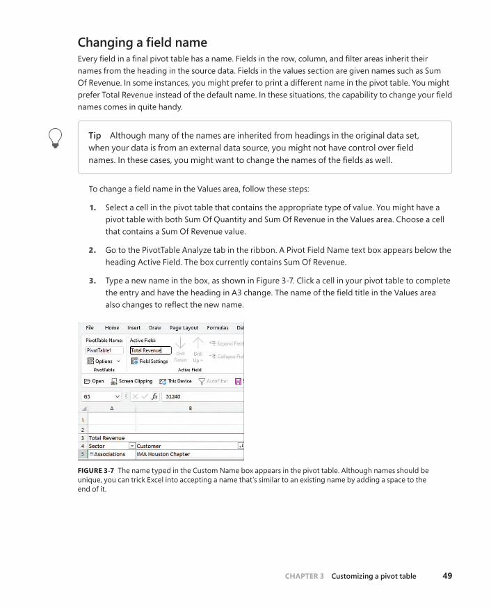
2. Go to the PivotTable Analyze tab in the ribbon. A Pivot Field Name text box appears below the heading Active Field. The box currently contains Sum Of Revenue.
3. Type a new name in the box, as shown in Figure 3-7. Click a cell in your pivot table to complete the entry and have the heading in A3 change. The name of the field title in the Values area also changes to reflect the new name.
FIGURE 3-7 The name typed in the Custom Name box appears in the pivot table. Although names should be unique, you can trick Excel into accepting a name that’s similar to an existing name by adding a space to the end of it.
9780137521838_print.indb 49 29/10/21 8:44 PM

50 CHAPTER 3 Customizing a pivot table
Tip When you can see the value field name such as “Sum of Revenue” in the Excel work-sheet, you can directly type a new value to rename the field. For example, in Figure 3-7, you could type Sales in cell A3 to rename the field.
Note One common frustration occurs when you would like to rename Sum Of Revenue to Revenue. The problem is that this name is not allowed because it is not unique; you already have a Revenue field in the source data. To work around this limitation, you can name the field and add a space to the end of the name. Excel considers “Revenue ” (with a space) to be different from “Revenue” (with no space). Because this change is only cosmetic, the readers of your spreadsheet do not notice the space after the name.
Making report layout changes
Excel offers three report layout styles. The Excel team continues to offer the Compact layout as the default report layout. If you prefer a different layout, change it using the default settings for pivot tables.
If you consider three report layouts, and the ability to show subtotals at the top or bottom, plus choices for blank rows and Repeat All Item Labels, you have 16 different layout possibilities available.
Layout changes are controlled in the Layout group of the Design tab, as shown in Figure 3-8. This group offers four icons:
■ Subtotals—Moves subtotals to the top or bottom of each group or turns them off.
■ Grand Totals—Turns the grand totals on or off for rows and columns.
■ Report Layout—Uses the Compact, Outline, or Tabular forms. Offers an option to repeat item labels.
■ Blank Rows—Inserts or removes blank lines after each group.
Note You mathematicians in the audience might think that 3 layouts × 2 repeat options × 2 subtotal location options × 2 blank row options would be 24 layouts. However, choos-ing Repeat All Item Labels does not work with the Compact layout, thus eliminating 4 of the combinations. In addition, Subtotals At The Top Of Each Group does not work with the Tabular layout, eliminating another 4 combinations.
9780137521838_print.indb 50 29/10/21 8:44 PM

CHAPTER 3 Customizing a pivot table 51
FIGURE 3-8 The Layout group on the Design tab offers different layouts and options for totals.
Using the Compact layoutBy default, all new pivot tables use the Compact layout that you saw in Figure 3-6. In this layout, mul-tiple fields in the row area are stacked in column A. Note in the figure that the Consultants sector and the Andrew Spain Consulting customer are both in column A.
The Compact form is suited for using the Expand and Collapse icons. If you select one of the Sector value cells such as Associations in A5 and then click the Collapse Field icon on the Analyze tab, Excel hides all the customer details and shows only the sectors, as shown in Figure 3-9.
FIGURE 3-9 Click the Collapse Field icon to hide levels of detail.
After a field is collapsed, you can show detail for individual items by using the plus icons in column A, or you can click Expand Field on the PivotTable Analyze tab to see the detail again.
9780137521838_print.indb 51 29/10/21 8:44 PM

52 CHAPTER 3 Customizing a pivot table
Tip If you select a cell in the innermost row field and click Expand Field on the Options tab, Excel displays the Show Detail dialog box, as shown in Figure 3-10, to enable you to add a new innermost row field.
FIGURE 3-10 When you attempt to expand the innermost field, Excel offers to add a new innermost field.
Using the Outline layoutWhen you select Design, Layout, Report Layout, Show In Outline Form, Excel puts each row field in a separate column. The pivot table shown in Figure 3-11 is one column wider, with revenue values starting in C instead of B. This is a small price to pay for allowing each field to occupy its own column. Soon, you will find out how to convert a pivot table to values so you can further sort or filter. When you do this, you will want each field in its own column.
The Excel team added the Repeat All Item Labels option to the Report Layout tab starting in Excel 2010. This alleviated a lot of busy work because it takes just two clicks to fill in all the blank cells along the outer row fields. Choosing to repeat the item labels causes values to appear in cells A6:A7, A9:A14, as shown in Figure 3-11.
Figure 3-11 shows the same pivot table from before, now in Outline form and with labels repeated.
Caution This layout is suitable if you plan to copy the values from the pivot table to a new location for further analysis. Although the Compact layout offers a clever approach by squeezing multiple fields into one column, it is not ideal for reusing the data later.
9780137521838_print.indb 52 29/10/21 8:44 PM

CHAPTER 3 Customizing a pivot table 53
FIGURE 3-11 The Outline layout puts each row field in a separate column.
By default, both the Compact and Outline layouts put the subtotals at the top of each group. You can use the Subtotals drop-down menu on the Design tab to move the totals to the bottom of each group, as shown in Figure 3-12. In Outline view, this causes a not-really-useful heading row to appear at the top of each group. Cell A5 contains “Associations” without any additional data in the columns to the right. Consequently, the pivot table occupies 44 rows instead of 37 rows because each of the 7 sector categories has an extra header.
FIGURE 3-12 With subtotals at the bottom of each group, the pivot table occupies several more rows.
9780137521838_print.indb 53 29/10/21 8:44 PM

54 CHAPTER 3 Customizing a pivot table
Using the traditional Tabular layoutFigure 3-13 shows the Tabular layout. This layout is similar to the one that has been used in pivot tables since their invention through Excel 2003. In this layout, the subtotals can never appear at the top of the group. The Repeat All Item Labels works with this layout, as shown in Figure 3-13.
FIGURE 3-13 The Tabular layout is similar to pivot tables in legacy versions of Excel.
The Tabular layout is the best layout if you expect to use the resulting summary data in a subsequent analysis. If you wanted to reuse the table in Figure 3-13, you would do additional “flattening” of the pivot table by choosing Subtotals, Do Not Show Subtotals and Grand Totals, Off For Rows And Columns.
Case study: Converting a pivot table to values
Say that you want to convert the pivot table shown in Figure 3-13 to be a regular data set that you can sort, filter, chart, or export to another system. You don’t need the Sectors totals in rows 7, 14, 18, and so on. You don’t need the Grand Total at the bottom. And, depending on your future needs, you might want to move the Region field from the Columns area to the Rows area. This would allow you to add Cost and Profit as new columns in the final report.Finally, you want to convert from a live pivot table to static values. To make these changes, follow these steps:
1. Select any cell in the pivot table.
2. From the Design tab, select Grand Totals, Off For Rows And Columns.
3. Select Design, Subtotals, Do Not Show Subtotals.
4. Drag the Region tile from the Columns area in the PivotTable Fields list. Drop this field between Sector and Customer in the Rows area.
9780137521838_print.indb 54 29/10/21 8:44 PM

CHAPTER 3 Customizing a pivot table 55
5. Check Profit and Cost in the top of the PivotTable Fields list. Because both fields are numeric, they move to the Values area and appear in the pivot table as new columns. Rename both fields using the Current Field box on the PivotTable Analyze tab. The report is now a contigu-ous solid block of data, as shown in Figure 3-14.
FIGURE 3-14 The pivot table now contains a solid block of data.
6. Select one cell in the pivot table. Press Ctrl+* to select all the data in the pivot table.
7. Press Ctrl+C to copy the data from the pivot table.
8. Select a blank section of a worksheet.
9. Right-click. To the right of the words “Paste Special” is a greater-than sign that leads to a flyout with 14 ways to Paste Special Choose Paste Values And Number Formatting, as shown in Figure 3-15. Excel pastes a static copy of the report to the worksheet.
Paste Values andNumber Formatting
FIGURE 3-15 Use Paste Values And Number Formatting to create a static version of the data.
10. If you no longer need the original pivot table, select the entire pivot table and press the Delete key to clear the cells from the pivot table and free up the area of memory that was holding the pivot table cache. One way to select the entire pivot table is to use the Select drop-down menu on the PivotTable Analyze tab and choose Entire PivotTable.
9780137521838_print.indb 55 29/10/21 8:44 PM

56 CHAPTER 3 Customizing a pivot table
The result is a solid block of summary data. These 27 rows are a summary of the 500+ rows in the original data set, but they also are suitable for exporting to other systems.
Controlling blank lines, grand totals, and other settingsAdditional settings on the Design tab enable you to toggle various elements.
The Blank Rows drop-down menu offers the choice Insert Blank Line After Each Item. This setting applies only to pivot tables with two or more row fields. Blank rows are not added after each item in the inner row field. You see a blank row after each group of items in the outer row fields. As shown in Figure 3-16, the blank row after each sector makes the report easier to read. However, if you remove Sector from the report, you have only Customer in the row fields, and no blank rows appear (see Figure 3-17).
FIGURE 3-16 The Blank Rows setting makes the report easier to read.
FIGURE 3-17 Blank rows will not appear when there is only one item in the row field.
9780137521838_print.indb 56 29/10/21 8:44 PM

CHAPTER 3 Customizing a pivot table 57
Grand totals can appear at the bottom of each column and/or at the end of each row, or they can be turned off altogether. Settings for grand totals appear in the Grand Totals drop-down menu of the Layout group on the Design tab. The wording in this drop-down menu is a bit confusing, so Figure 3-18 shows what each option provides. The default is to show grand totals for rows and columns.
FIGURE 3-18 The wording is confusing, but you can toggle off the grand total column, row, or both.
If you want a grand total column but no grand total at the bottom, choose On For Rows Only, as shown at the top of Figure 3-18. To me, this seems backward. To keep the grand total column, you have to choose to turn on grand totals for rows only. I guess the rationale is that each cell in F5:F8 is a grand total of the row to the left of the cell. Hence, you are showing the grand totals for all the rows but not for the columns. Perhaps someday Microsoft will ship a version of Excel in English-Midwest where this setting would be called “Keep the Grand Total Column.” But for now, it remains confusing.
In a similar fashion, to show a grand total row but no grand total column, you open the Grand Totals menu and choose On For Columns Only. Again, in some twisted version of the English language, cell B18 is totaling the cells in the column above it.
The final choice, Off For Rows And Columns, is simple enough. Excel shows neither a grand total column nor a grand total row.
9780137521838_print.indb 57 29/10/21 8:44 PM

58 CHAPTER 3 Customizing a pivot table
Tip You can abandon these confusing menu choices by using the right-click menu. If you right-click on any cell that has the words “Grand Total,” you can choose Remove Grand Total.
Back in Excel 2003, pivot tables were shown in Tabular layout and logical headings such as Region and Product would appear in the pivot table, as shown in the top pivot table in Figure 3-19. When the Excel team switched to Compact form, they replaced those headings with Row Labels and Column Labels. These add nothing to the report. To toggle off those headings, look on the far-right side of the PivotTable Analyze tab for an icon called Field Headers and click it to remove Row Labels and Column Labels from your pivot tables in Compact form.
Region and Product headings
Row Labels and Column Labels
Field Headers off
FIGURE 3-19 The Compact form replaces useful headings with Row Labels. You can turn these off.
Caution When you arrange several pivot tables vertically, as in Figure 3-19, you’ll notice that changes in one pivot table change the column widths for the entire column, often caus-ing #### to appear in the other pivot tables. By default, Excel changes the column width to AutoFit the pivot table but ignores anything else in the column. To turn off this default behavior, right-click each pivot table and choose PivotTable Options. In the first tab of the Options dialog box, the second-to-last check box is AutoFit Column Widths On Update. Clear this check box. This is another setting that you might want to adjust in Pivot Table Defaults. See Tip 5 in Chapter 14.
9780137521838_print.indb 58 29/10/21 8:44 PM

CHAPTER 3 Customizing a pivot table 59
Customizing a pivot table’s appearance with styles and themes
You can quickly apply color and formatting to a pivot table report by using the 85 built-in styles in the PivotTable Styles gallery on the Design tab. These 85 styles are further modified by the four check boxes to the left of the gallery. Throw in the 48 themes on the Page Layout tab, and you have 65,280 easy ways to format a pivot table. If none of those provide what you need, you can define a new style.
Start with the four check boxes in the PivotTable Style Options group of the Design tab of the rib-bon. You can choose to apply special formatting to the row headers, column headers, banded rows, or banded columns. My favorite choice here is banded rows because it makes it easier for the reader’s eye to follow a row across a wide report. You should choose from these settings first because the choices here will modify the thumbnails shown in the Styles gallery.
As mentioned earlier, the PivotTable Styles gallery on the Design tab offers 85 built-in styles. Grouped into 28 styles each of Light, Medium, and Dark, the gallery offers variations on the accent colors used in the current theme. In Figure 3-20, you can see which styles in the gallery truly support banded rows and which just offer a bottom border between rows.
True banded rows
Borders between items
FIGURE 3-20 The styles are shown here with accents for row headers, column headers, and alternating colors in the columns.
Tip Note that you can modify the thumbnails for the 85 styles shown in the gallery by using the four check boxes in the PivotTable Style Options group.
The Live Preview feature in Excel works in the Styles gallery. As you hover your mouse cursor over style thumbnails, the worksheet shows a preview of the style.
9780137521838_print.indb 59 29/10/21 8:44 PM

60 CHAPTER 3 Customizing a pivot table
Customizing a styleYou can create your own pivot table styles, and the new styles are added to the gallery for the current workbook only. To use the custom style in another workbook, copy and temporarily paste the format-ted pivot table to the other workbook. After the pivot table has been pasted, apply the custom style to an existing pivot table in your workbook and then delete the temporary pivot table.
Say that you want to create a pivot table style in which the banded colors are three rows high. Fol-low these steps to create the new style:
1. Find an existing style in the PivotTable Styles gallery that supports banded rows. Right-click the style in the gallery and select Duplicate. Excel displays the Modify PivotTable Quick Style dialog box.
2. Choose a new name for the style. Excel initially appends a 2 to the existing style name, which means you have a name such as PivotStyleDark3 2. Type a better name, such as Greenbar.
3. In the Table Element list, click First Row Stripe. A new section called Stripe Size appears in the dialog box.
4. Select 3 from the Stripe Size drop-down, as shown in Figure 3-21.
5. To change the stripe color, click the Format button. The Format Cells dialog box appears. Click the Fill tab and then choose a fill color. If you want to be truly authentic, choose More Colors, Custom and use Red=200, Green=225, and Blue=204 to simulate 1980s-era greenbar paper. Click OK to accept the color and return to the Modify PivotTable Quick Style dialog box.
6. In the Table Element List, click Second Row Stripe. Select 3 from the Stripe Size drop-down. Modify the format to use a lighter color, such as white.
7. If you plan on creating more pivot tables in this workbook, choose the Set As Default Pivot-Table Style For This Document check box in the lower left.
8. Optionally, edit the colors for Header Row and Grand Total Row.
9. Click OK to finish building the style. Strangely, Excel doesn’t automatically apply this new style to the pivot table. After you put in a few minutes of work to tweak the style, the pivot table does not change.
10. Your new style should be the first thumbnail visible in the Styles gallery. Click that style to apply it to the pivot table.
Tip If you have not added more than seven custom styles, the thumbnail should be visible in the closed gallery, so you can choose it without reopening the gallery.
9780137521838_print.indb 60 29/10/21 8:44 PM
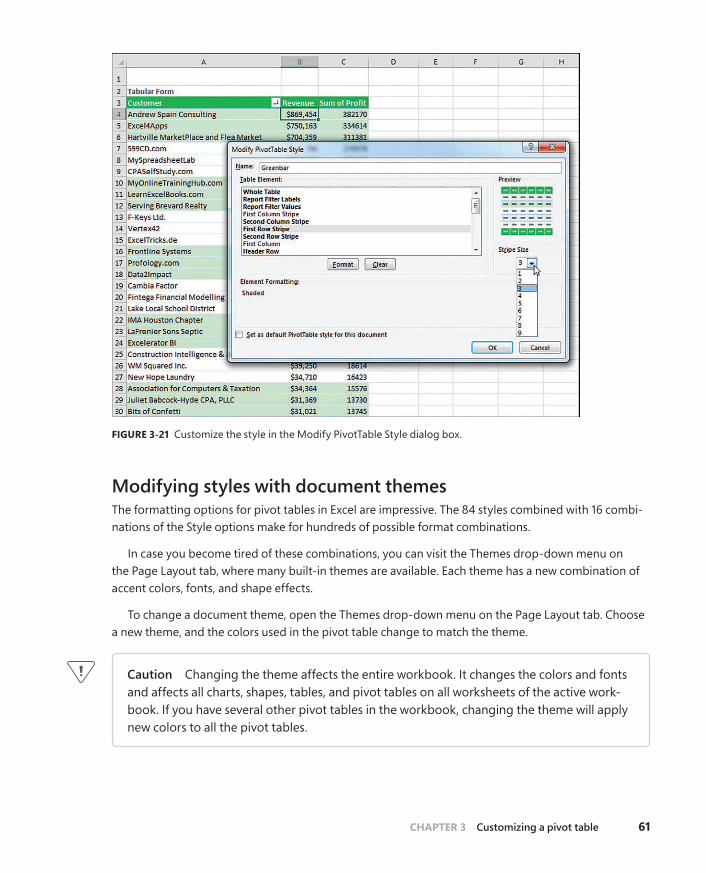
CHAPTER 3 Customizing a pivot table 61
FIGURE 3-21 Customize the style in the Modify PivotTable Style dialog box.
Modifying styles with document themesThe formatting options for pivot tables in Excel are impressive. The 84 styles combined with 16 combi-nations of the Style options make for hundreds of possible format combinations.
In case you become tired of these combinations, you can visit the Themes drop-down menu on the Page Layout tab, where many built-in themes are available. Each theme has a new combination of accent colors, fonts, and shape effects.
To change a document theme, open the Themes drop-down menu on the Page Layout tab. Choose a new theme, and the colors used in the pivot table change to match the theme.
Caution Changing the theme affects the entire workbook. It changes the colors and fonts and affects all charts, shapes, tables, and pivot tables on all worksheets of the active work-book. If you have several other pivot tables in the workbook, changing the theme will apply new colors to all the pivot tables.
9780137521838_print.indb 61 29/10/21 8:44 PM

62 CHAPTER 3 Customizing a pivot table
Tip Some of the themes use unusual fonts. You can apply the colors from a theme with-out changing the fonts in your document by using the Colors drop-down menu next to the Themes menu, as shown in Figure 3-22.
FIGURE 3-22 Choose new colors from the Colors menu.
Case Study: Excel Pivot Table Archaeology
At Microsoft, a great person named Howie Dickerman has been in charge of pivot tables for the last few years. Howie was an architect of Power Pivot and was always happy to engage the MVPs when we had some crazy pivot table idea. Occasionally, we would find a pivot table oddity and Howie would dig in to the code to try to figure out why. He called this Excel Archaeology. Howie retired in 2021 and his willingness to go deep into the Excel code base on archaeological expeditions will be missed.
This oddity would have been right up his alley. Excel MVP Wyn Hopkins from Access Ana-lytic recently uncovered a feature in pivot tables that allows you to quickly apply a border to several sections inside the pivot table.
Say that you have a pivot table such as the one in Figure 3-23. Leave a blank row and column on each side of the pivot table, but then completely surround the pivot table with a border. The border shown in Figure 3-23 has a different style on each side to illustrate how each side of the border will be translated to the pivot table.
To transfer the outer border to the pivot table, right-click any cell in the pivot table and choose Refresh. The borders from outside the pivot table are applied to various sections inside the pivot table.
9780137521838_print.indb 62 29/10/21 8:44 PM

CHAPTER 3 Customizing a pivot table 63
FIGURE 3-23 A relatively plain pivot table, with a border just outside the pivot table.
To transfer the outer border to the pivot table, right-click any cell in the pivot table and choose Refresh. The borders from outside the pivot table are applied to various sections inside the pivot table.
FIGURE 3-24 The border styles from the outer border are applied to the pivot table.
In a very specific pattern, the border styles used in the outer border are applied throughout the pivot table. The dashed border used above row 2 is applied above rows 3, 4 and above cell C11. The dotted border used below row 12 is applied in the pivot table below row 11. A similar pattern happens with the left border being applied to most vertical lines in the pivot table. The right border is applied to the right edge of the pivot table.
Why is this feature in Excel? It had to pre-date the Formatting Gallery. It must have been a way to build your own Pivot Table Styles before there were styles.
9780137521838_print.indb 63 29/10/21 8:44 PM

64 CHAPTER 3 Customizing a pivot table
Changing summary calculations
When you create a pivot table report, by default Excel summarizes the data by either counting or summing the items. Instead of Sum or Count, you might want to choose functions such as Min, Max, and Count Numeric. In all, 11 options are available.
The Excel team fixed the Count Of Revenue bugIn early 2018, Microsoft fixed a bug that caused many pivot tables to provide a count of revenue instead of a sum. If a data column contains all numbers, Excel will default to Sum as the calculation. If a column contains text, the pivot table will default to Count. But up until 2018, a bug appeared if you had a mix of numbers and empty cells. An empty cell would cause your pivot table to Count instead of Sum.
One Excel customer wrote a letter to the Excel team describing this bug: “Why are you treating empty cells as text? Treat them like any other formula would treat them and consider them to be zero. A mix of numbers and zeroes should not cause a Count of that field.”
Without a single vote on Excel.UserVoice.com, someone on the Excel team patched the bug. If you have a mix of numbers and blank cells, you will no longer get a Count Of Revenue. This is a nice improvement.
Changing the calculation in a value field
The Value Field Settings dialog box offers 11 options on the Summarize Values As tab and 15 main options on the Show Values As tab. The options on the first tab are the basic Sum, Average, Count, Max, and Min options that are ubiquitous throughout Excel; the 15 options under Show Values As are inter-esting ones such as % of Total, Running Total, and Ranks.
There are several ways to open the Value Field Settings dialog box:
■ If you have multiple fields in the Values area, double-click the heading for any value field.
■ Choose any number in the Values area and click the Field Settings button in the PivotTable Analyze tab of the ribbon.
■ In the PivotTable Fields list, open the drop-down menu for any item in the Values area. The last item will be Value Field Settings.
■ If you right-click any number in the Values area, you have a choice for Value Field Settings, plus two additional flyout menus offering six of the eleven choices for Summarize Values By and most of the choices for Show Values As (see Figure 3-25).
9780137521838_print.indb 64 29/10/21 8:44 PM

CHAPTER 3 Customizing a pivot table 65
The following examples show how to use the various calculation options. To contrast the settings, you can build a pivot table where you drag the Revenue field to the Values area nine separate times. Each one shows up as a new column in the pivot table. Over the next several examples, you will see the settings required for the calculations in each column.
To change the calculation for a field, select one Value cell for the field and click the Field Settings button on the PivotTable Analyze tab of the ribbon. The Value Field Settings dialog box is similar to the Field Settings dialog box, but it has two tabs. The first tab, Summarize Values By, contains Sum, Count, Average, Max, Min, Product, Count Numbers, StdDev, StdDevP, Var, and VarP. You can choose 1 of these 11 calculation options to change the data in the column. In Figure 3-26, columns B through D show vari-ous settings from the Summarize Values By tab.
FIGURE 3-25 The right-click menu for any number in the Values area offers a flyout menu with the popular calculation options.
The following examples show how to use the various calculation options. To contrast the settings, you can build a pivot table where you drag the Revenue field to the Values area nine separate times. Each one shows up as a new column in the pivot table. Over the next several examples, you will see the settings required for the calculations in each column.
To change the calculation for a field, select one Value cell for the field and click the Field Settings button on the PivotTable Analyze tab of the ribbon. The Value Field Settings dialog box is similar to the Field Settings dialog box, but it has two tabs. The first tab, Summarize Values By, contains Sum, Count, Average, Max, Min, Product, Count Numbers, StdDev, StdDevP, Var, and VarP. You can choose 1 of these 11 calculation options to change the data in the column. In Figure 3-26, columns B through D show various settings from the Summarize Values By tab.
9780137521838_print.indb 65 29/10/21 8:44 PM

66 CHAPTER 3 Customizing a pivot table
FIGURE 3-26 Choose from the 11 summary calculations on this tab.
Column B is the default Sum calculation. It shows the total of all records for a given market. Column C shows the average order for each item by market. Column D shows a count of the records. You can change the heading to say # Of Orders or # Of Records or whatever is appropriate. Note that the count is the actual count of records, not the count of distinct items.
Note Counting distinct items has been difficult in pivot tables but is now easier using PowerPivot. See “Unlocking hidden features with the data model” in Chapter 10 for more details.
Far more interesting options appear on the Show Values As tab of the Value Field Settings dialog box, as shown in Figure 3-27. Fifteen options appear in the drop-down. Depending on the option you choose, you might need to specify either a base field or a base field and a base item. Columns E through J in Figures 3-26 and 3-27 show some of the calculations possible using Show Values As.
9780137521838_print.indb 66 29/10/21 8:44 PM

CHAPTER 3 Customizing a pivot table 67
Rename field as appropriate
Base Field and Base Item are selectively enabled
FIGURE 3-27 Fifteen different ways to show that data is available on this tab.
Table 3-1 summarizes the Show Values As options.
TABLE 3-1 Calculations in Show Values As
Show Values As Additional Required Information
Description
No Calculation None
% of Grand Total None Shows percentages so all the detail cells in the pivot table total 100%.
% of Column Total None Shows percentages that total up and down the pivot table to 100%.
% of Row Total None Shows percentages that total across the pivot table to 100%.
% of Parent Row Total None With multiple row fields, shows a percentage of the par-ent item’s total row.
% of Parent Column Total None With multiple column fields, shows a percentage of the parent column’s total.
Index None Calculates the relative importance of items. For an example, see Figure 3-31.
% of Parent Total Base Field only With multiple row and/or column fields, calculates a cell’s percentage of the parent item’s total.
Running Total In Base Field only Calculates a running total.
% Running Total In Base Field only Calculates a running total as a percentage of the total.
Rank Smallest to Largest Base Field only Provides a numeric rank, with 1 as the smallest item.
Rank Largest to Smallest Base Field only Provides a numeric rank, with 1 as the largest item.
9780137521838_print.indb 67 29/10/21 8:44 PM

68 CHAPTER 3 Customizing a pivot table
Show Values As Additional Required Information
Description
% of Base Field and Base Item Expresses the values for one item as a percentage of another item.
Difference From Base Field and Base Item Shows the difference of one item compared to another item or to the previous item.
% Difference From Base Field and Base Item Shows the percentage difference of one item compared to another item or to the previous item.
The capability to create custom calculations is another example of the unique flexibility of pivot table reports. With the Show Values As setting, you can change the calculation for a particular data field to be based on other cells in the Values area.
The following sections illustrate a number of Show Values As options.
Showing percentage of totalIn Figure 3-26, column E shows % Of Total. Jade Miller, with $2.1 million in revenue, represents 31.67% of the $6.7 million total revenue. Column E uses % Of Column Total on the Show Values As tab. Two other similar options are % Of Row Total and % Of Grand Total. Choose one of these based on whether your text fields are going down the report, across the report, or both down and across.
Using % Of to compare one line to another lineThe % Of option enables you to compare one item to another item. For example, in the current data set, Anne was the top sales rep in the previous year. Column F shows everyone’s sales as a percentage of Anne’s. Cell F7 in Figure 3-28 shows that Jeff’s sales were almost 58% of Anne’s sales.
FIGURE 3-28 This report is created using the % Of option with Anne Troy as the Base Item.
To set up this calculation, choose Show Values As, % Of. For Base Field, choose Rep because this is the only field in the Rows area. For Base Item, choose Anne Troy. The result is shown in Figure 3-26.
9780137521838_print.indb 68 29/10/21 8:44 PM

CHAPTER 3 Customizing a pivot table 69
Showing rankTwo ranking options are available. Column G in Figure 3-29 shows Rank Largest To Smallest. Jade Miller is ranked #1, and Sabine Hanschitz is #12. A similar option is Rank Smallest To Largest, which would be good for the pro golf tour.
FIGURE 3-29 The Rank options will rank ascending or descending.
To set up a rank, choose Value Field Settings, Show Values As, Rank Largest To Smallest. You are required to choose Base Field. In this example, because Rep is the only row field, it is the selection under Base Field.
These rank options show that pivot tables have a strange way of dealing with ties. I say strange because they do not match any of the methods already established by the Excel functions =RANK(), =RANK.AVG(), and =RANK.EQ(). For example, if the top two markets have a tie, they are both assigned a rank of 1, and the third market is assigned a rank of 2.
Tracking running total and percentage of running totalRunning total calculations are common in reports where you have months running down the column or when you want to show that the top N customers make up N% of the revenue.
In Figure 3-30, cell I8 shows that the top four sales reps account for 76.97% of the total sales.
Note To produce this figure, you have to use the Sort feature, which is discussed in depth in Chapter 4, “Grouping, sorting, and filtering pivot data.” To create a similar analysis with the sample file, go to the drop-down menu in A4 and choose More Sort Options, Descend-ing, By Total. Also note that the % Change From calculation shown in the next example is not compatible with sorting.
9780137521838_print.indb 69 29/10/21 8:44 PM

70 CHAPTER 3 Customizing a pivot table
FIGURE 3-30 Show running totals or a running percentage of total.
To specify Running Total In (as shown in Column H) or % Running Total In (Column I), select Field Settings, Show Values As, Running Total In. You have to specify a Base Field, which in this case is the Row Field: Rep.
Displaying a change from a previous fieldFigure 3-31 shows the % Difference From setting. This calculation requires a Base Field and Base Item. You could show how each market compares to Anne Troy by specifying Anne Troy as the Base Item. This would be similar to Figure 3-26, except each market would be shown as a percentage of Anne Troy.
FIGURE 3-31 The % Difference From options enable you to compare each row to the previous or next row.
9780137521838_print.indb 70 29/10/21 8:44 PM

CHAPTER 3 Customizing a pivot table 71
With date fields, it would make sense to use % Difference From and choose (previous) as the base item. Note that the first cell will not have a calculation because there is no previous date in the pivot table.
Tracking the percentage of a parent itemThe legacy % Of Total settings always divides the current item by the grand total. In Figure 3-32, cell E4 says that Chicago is 2.75% of the total data set. A common question at the MrExcel.com message board is how to calculate Chicago’s revenue as a percentage of the Midwest region total. This was possible but difficult in older versions of Excel. Starting in Excel 2010, though, Excel added the % Of Parent Row, % Of Parent Column, and % Of Parent Total options.
FIGURE 3-32 An option in Excel enables you to calculate a percentage of the parent row.
To set up this calculation in Excel, use Field Settings, Show Values As, % Of Parent Row Total. Cell D4 in Figure 3-32 shows that Chicago’s $184,425 is 10.59% of the Midwest total of $1,741,424.
Although it makes sense, the calculation on the subtotal rows might seem confusing. D4:D8 shows the percentage of each market as compared to the Midwest total. The values in D9, D11, D16, and D19 compare the region total to the grand total. For example, the 31.67% in D11 says that the Northeast region’s $2.1 million is a little less than a third of the $6.7 million grand total.
Tracking relative importance with the Index optionThe final option of the 11 calculations is Index. It creates a somewhat obscure calculation. Microsoft claims that this calculation describes the relative importance of a cell within a column. In Figure 3-33, Georgia peaches have an index of 2.55, and California peaches have an index of 0.50. This shows that if the peach crop is wiped out next year, it will be more devastating to Georgia fruit production than to California fruit production.
9780137521838_print.indb 71 29/10/21 8:44 PM

72 CHAPTER 3 Customizing a pivot table
FIGURE 3-33 Using the Index function, Excel shows that peach sales are more important in Georgia than in California.
Here is the exact calculation:
1. First, divide Georgia peaches by the Georgia total. This is 180/210, or 0.857.
2. Next, divide total peach production (285) by total fruit production (847). This shows that peaches have an importance ratio of 0.336.
3. Now, divide the first ratio by the second ratio: 0.857/0.336.
In Ohio, apples have an index of 4.91, so an apple blight would be bad for the Ohio fruit industry.
I have to admit that, even after writing about this calculation for 10 years, there are parts that I don’t quite comprehend. What if a state like Hawaii relied on productions of lychees, but lychees were nearly immaterial to U.S. fruit production? If lychees were half of Hawaii’s fruit production but 0.001 of U.S. fruit production, the Index calculation would skyrocket to 500.
Adding and removing subtotals
Subtotals are an essential feature of pivot table reporting. Sometimes you might want to suppress the display of subtotals, and other times you might want to show more than one subtotal per field.
Suppressing subtotals with many row fieldsWhen you have many row fields in a report, subtotals can obscure your view. For example, in Figure 3-34, there is no need to show subtotals for each market because there is only one sales rep for each market.
9780137521838_print.indb 72 29/10/21 8:44 PM

CHAPTER 3 Customizing a pivot table 73
FIGURE 3-34 Sometimes you do not need subtotals at every level.
If you used the Subtotals drop-down menu on the Design tab, you would turn off all subtotals, including the Region subtotals and the Market subtotals. The Region subtotals are still providing good information, so you want to use the Subtotals setting in the Field Settings dialog box. Choose one cell in the Market column. On the PivotTable Analyze tab, choose Field Settings. Change the Subtotals setting from Automatic to None (see Figure 3-35).
FIGURE 3-35 Use the Subtotals setting in the Field list to turn off subtotals for one field.
To remove subtotals for the Market field, click the Market field in the bottom section of the PivotTable Fields list. Select Field Settings. In the Field Settings dialog box, select None under Subtotals, as shown in Figure 3-33. Alternatively, right-click a cell that contains a Market and remove the check mark from Subtotal Market.
Adding multiple subtotals for one fieldYou can add customized subtotals to a row or column label field. Select the Region field in the bottom of the PivotTable Fields list, and select Field Settings.
9780137521838_print.indb 73 29/10/21 8:44 PM

74 CHAPTER 3 Customizing a pivot table
In the Field Settings dialog box for the Region field, select Custom and then select the types of subtotals you would like to see. The dialog box in Figure 3-36 shows five custom subtotals selected for the Region field. It is rare to see pivot tables use this setting. It is not perfect. Note that the count of 211 records in cell D25 automatically gets a currency format like the rest of the column, even though this is not a dollar figure. Also, the average of $12,333 for South is an average of the detail records, not an average of the individual market totals.
FIGURE 3-36 By selecting the Custom option in the Subtotals section, you can specify multiple subtotals for one field.
Tip If you need to calculate the average of the four regions, you can do it with the DAX formula language and Power Pivot. See Chapter 10.
Formatting one cell is new in Microsoft 365
In the summer of 2018, a new trick appeared for Microsoft 365 customers. You can format a cell in a pivot table, and the formatting will follow that position.
For example, in Figure 3-37, a white font on dark fill has been applied to Revenue for Doodads sales to the Software sector.
9780137521838_print.indb 74 29/10/21 8:44 PM

CHAPTER 3 Customizing a pivot table 75
FIGURE 3-37 A new Format Cells option appears in the right-click context menu.
If you rearrange the pivot table, the dark formatting will follow the cell in the pivot table. While cell B9 was formatted in Figure 3-37, the formatting has moved to D5 in Figure 3-38.
Note that the formatting will persist if you remove the cell due to a filter. If you unselect Software from the Slicer and then reselect Software, the formatting will return.
However, if you remove Sector, Product, or Revenue from the pivot table, the individual cell format-ting will be lost.
FIGURE 3-38 Rearrange the pivot table and the formatting moves so that revenue for Doodads sales to the Software sector stays formatted.
In Figure 3-39, a Customer field has been added as the inner-row field. The dark formatting applied to Doodads sales of Software is now expanded to C5:C8 to encompass all four customers in this group. Note that in cell C9, the subtotal for Doodads sold to the Software sector is not formatted.
9780137521838_print.indb 75 29/10/21 8:44 PM

76 CHAPTER 3 Customizing a pivot table
FIGURE 3-39 If you add an inner-row field, the formatting will expand to encompass all customers for Doodads in the Software sector.
Next steps
Note that the following pivot table customizations are covered in subsequent chapters:
■ Sorting a pivot table is covered in Chapter 4, “Grouping, sorting, and filtering pivot data.”
■ Filtering records in a pivot table is covered in Chapter 4.
■ Grouping daily dates up to months or years is covered in Chapter 4.
■ Adding new calculated fields is covered in Chapter 5, “Performing calculations in pivot tables.”
■ Using data visualizations and conditional formatting in a pivot table is covered in Chapter 4.
9780137521838_print.indb 76 29/10/21 8:44 PM

497
Index
Numerics3D Map, 285
animating data over time, 294bubble charts, 290–291column charts
building, 288labeling individual points, 290navigating, 289–290zooming in and out, 289
combining two data sets, 293–294data cards, 293fine-tuning, 293geocoding, 286–287geographic data, 286heat maps, 291–292layers, 288preparing data for, 285–286region maps, 291–292rendering a video, 295–296settings, 292store maps, 296–299tours, 294–295
10-BigData.txt, 269, 273–275
AActiveX controls, 305Add function, 356Add This Data To The Data Model checkbox, 257, 261, 262,
294hidden features of
Distinct Count, 262–264including filtered items in totals, 264–265median calculation, 266–268reporting text in the values area, 268–269
AddFields method, 330–331add-ins, 45Advanced Filter, cross-tabular reports and, 465–467advanced tips, 389–390
add a rank number field to a pivot table, 399–400AutoFilter a pivot table, 404–406
compare tables using a pivot table, 402–404create a frequency distribution, 412–413create an automatically expanding data range, 401–402delete the source data worksheet, 401explode a data set to different tabs, 414–415explode a data set to different workbooks, 418–420fill empty cells left by row fields, 396
implement the Repeat All Item Labels feature, 397using Go To Special functionality, 398
force pivot tables to refresh automatically, 390force two number formats in a pivot table, 407–408format individual values in a pivot table, 408–410format sections of a pivot table, 410–412format your slicers, 432–434pivot field restrictions, 417–418pivot table restrictions, 415–417reducing the size of pivot table reports, 401refresh all pivot tables in a workbook at the same time,
390–391slicer to control data from two different data sets,
428–431sort data items in a unique order, 391–392sort using custom lists, 392–394turn pivot tables into hard data, 395–396use defaults to change behavior of all future pivot
tables, 394–395use percentage change from previous for year-over-
year reports, 420–423Alexander, Mike, 432, 495Analyze Data feature, 29–30animating data over time, 294–295AutoShow method, 363–365AutoSort method, 345
Bbackward compatibility
pivot table and, 7Timeline slicers and, 36
big dataData Model and, 273–275Power Query and, 269–270
Z01_Jelen_Index_p497-p512_new.indd 497 02/11/21 3:11 PM

blank cells
498
blank cells, 25cleaning up, 15–19eliminating, 344–345filling, 334, 335
implement the Repeat All Item Labels feature, 397using Go To Special functionality, 398
replacing with zeros, 47–48borders, 63–64bubble charts, 290–291bugs, 97
alphabetic sequence for months, 277Count of Revenue, 64
buttonspivot field, 152–153removing, 163
CCALCULATE function, 280calculated fields, 121, 122
adding to the data source, 122–123creating, 123–124, 125–133data, 357inserting in a pivot table, 124–125measures, 121rules, 139–145
calculated groups, VBA and, 359–360calculated items, 121–122
changing the solve order of, 147creating, 134–137GetPivotData function and, 436–439rules, 145–146VBA and, 357–359
calculated measures, 246–249calculated members, creating, 249–252calculations, 146, 354–356. See also formulas
adding to OLAP pivot tables, 245–246cell ranges and, 139constants and, 139COUNT function and, 355–356editing and deleting, 146–147functions and, 139median, 266–268named ranges and, 139OLAP, 252–253referencing totals, 139Value Field Settings dialog box and, 360–362
case sensitivity, functions and, 271
cellsblank, 14, 15–16, 25
eliminating, 344–345filling, 397–398replacing with zeros, 47–48
cleaning up, 15–19formatting, 74–76
charts, 149. See also pivot chartsbubble, 290–291column
building in 3D Map, 288labeling individual points, 290navigating, 289–290zooming in and out, 289
cross-filtering, 218–219pie, 290–291XY scatter, 165
check box filter, 90–91cleaning up data, 15–19Collie, Rob, 143, 229, 435column charts
building, 288labeling individual points, 290navigating, 289–290
Column From Examples, 271–272columns. See also cells; rows
adding in the Power Pivot grid, 276–277adding with Power Query, 271–273changing width of, 58cleaning up, 15–19empty, 14sorting by another column, 277–278
Columns area, 6combining, datasets in 3D Map, 293–294Compact layout, 51–52, 58, 332
Fields list and, 77–79comparing tables using a pivot table, 402–404compatibility, 8–9. See also backward compatibilitycomplex relationships, 279–280CONCATENATEX function, 268–269conceptual filters, 372–375conditional formatting, 165–167
custom rules, 168–173preprogrammed scenarios for condition levels,
167–168removing, 168
connections, Power Query, 202
Z01_Jelen_Index_p497-p512_new.indd 498 02/11/21 3:11 PM

dashboards
499
constants, 131–132, 139controls
ActiveX, 305form, creating a user interface, 304–306
copying, pivot table values to a new workbook, 347–348cosmetic changes, 44–45
applying a table style to restore gridlines, 45–46blank lines and, 56changing the number format to add thousands sepa-
rators, 46–47grand totals and, 57–58layout, 50
Compact, 51–52, 58Outline, 52–53Tabular, 54–56
renaming fields, 49–50replacing blanks with zeros, 47–48styles, 59, 60
document themes and, 61–64Value Field Settings dialog box and, 64–68
COUNT function, 355–356Count of Revenue bug, 64Create PivotTable dialog box, 20–21CreatePivotTable method, 330creating
calculated fields, 123–124, 125–133calculated items, 134–137calculated members, 249–252cross-tabular reports
using Advanced Filter and a data table, 465–470using Power Query, 473–478using three dynamic array formulas, 471–473
custom conditions, 168–173drill-down hierarchy, 219–220frequency distributions, 412–413hierarchies, 117–120macros, with Power Query, 310–320. See also macros;
VBA (Visual Basic for Applications)new pivot cache, 38–39offline cube, 240–243pivot charts, 150–152, 153–154pivot tables, 19–22
from the Data Model, 278, 282–283using Excel Online, 455–458
relationships, 259–260, 276, 380–381slicers, 31–34Timeline slicer, 34–36visualizations, 213–218
cross-filtering charts, 218–219cross-tabular reports, creating, 465
using Advanced Filter and a data table, 465–466aggregating revenue with DSUM, 468getting a unique list of values, 466–467pros and cons of this method, 470replicating DSUM for each combination of sector
and region, 468–470using Power Query, 473
cleaning final steps, 476–477getting your data into Power Query, 473pros and cons of this method, 477–478sorting and pivoting, 475–476summarizing revenue by sector and region, 474
using three dynamic array formulas, 471filling in the revenue amounts using SUMIF, 472getting a unique list of values, 471pros and cons of this method, 472–473
CUBEMEMBER function, 228CUBERANKEDMEMBER function, 229–231cube(s). See also OLAP (Online Analytical Processing)
formulas, 225converting pivot tables to, 226–233
functions, 243–245offline, creating, 240–243
CUBESET function, 229CUBEVALUE formula, 227–228custom lists, 87–89, 392–394Custom Lists dialog box, 87–89customization
cosmetic changesapplying a table style to restore gridlines, 45–46blank lines, 56changing the layout, 50, 51–53, 54–56, 58changing the number format to add thousands
separators, 46–47document themes, 61–64grand totals and, 57–58renaming fields, 49–50replacing blanks with zeros, 47–48styles, 59, 60
summary calculations, 64Value Field Settings dialog box and, 64–68
DDalgleish, Debra, 45dashboards, 207
Z01_Jelen_Index_p497-p512_new.indd 499 02/11/21 3:11 PM

Data Model
500
Data Model, 176, 225, 226, 257, 379. See also Add This DataTo The Data Model checkboxadding tables to, 379–380
linked tables, 275–276new tables, 180
big data and, 273–275building out your first, 176–179creating a pivot table from, 278, 282–283defining the pivot cache, 381Distinct Count, 262–264Excel Online and, 462limitations of, 180model fields, adding to the pivot table, 381numeric fields, adding to the Values area, 381–382overcoming limitations of, 281–282Power Pivot and, 257primary key, 177–178relationships
creating, 259–260, 380–381managing, 179–180
replacing VLOOKUP with, 257–261unlocking hidden features with, 261–262VBA and, 382–384
data ranges, automatically expanding, 401–402data source(s), 11, 479–481. See also external data sources
adding calculated fields to, 122–123cleaning up, 15–19deleting, 401external, building a pivot table using, 180–181Microsoft Access, building a pivot table using, 181–184Power Query and, 202preparing
applying formatting to fields, 14avoid repeating groups as columns, 13–14eliminating gaps and blank cells, 14ensuring the data is in Tabular layout, 12, 14–15section headings, 12–13
preparing for 3D Map, 285–286transposing, 202–204updating, 37
database centric layout, 12Date filters, 97–98. See also timelinesdates, summarizing, 342–344DAX (Data Analysis Expressions), 121, 144, 145
CALCULATE function, 280median calculation, 266–268
deferring updates, 40–41
deletingcalculations, 146–147data from pivot tables, 335pivot table(s), 162
dialog boxesCreate PivotTable, 20–21Custom Lists, 87–89Grouping, 107–111Insert Slicers, 31Macro, 309Manage Relationships, 179–180Measure, 266–267Modify Slicer, 433Move PivotTable, 41Record Macro, 302Report Connections, 33Select Table, 183Sort, 84–85. See also sortingValue Field Settings, 64–68
adding and removing subtotals, 72–74displaying a change from a previous field, 70–71Index option, 71–72running total calculations, 69–70Show Values As tab, 360–362showing percentage of total, 68showing rank, 69tracking the percentage of a parent item, 71using % Of to compare one line to another line, 68
Dickerman, Howie, 456dimensions, 2266disparate data sources, 175. See also Data Model; data
source(s)docking the Fields list, 79document themes, 61–64dragging and dropping, 26–27drill-down hierarchy, creating, 219–220DSUM function, 468–470Dynamic Arrays, 495dynamic reports, creating with GetPivotData
build the shell report, 446–447create a pivot table, 443–446populate the shell report, 448–451updating the report in future months, 451–452
Eediting, calculations, 146–147Excel, versions, 328–329
Z01_Jelen_Index_p497-p512_new.indd 500 02/11/21 3:11 PM

formatting
501
Excel Online, 384, 453, 462Data Model and, 462Google Sheets and, 453Home screen, 454–455icons, 458–459pivot tables
creating, 455–458layouts, 459–461
PivotTable Settings task pane, 459Alt Text, 461–462options, 461
signing in, 454–455executive overviews, creating in VBA, 363–365exploding a data set
to different tabs, 414–415to different workbooks, 418–420
external data sourcesbuilding a pivot table using, 180–181Microsoft Access, building a pivot table using, 181–184Power Query and, 187–188SQL, building a pivot table using, 184–187
Ffields. See also cells
adding to a pivot table report, 22adding to Filters area, 99calculated. See calculated fieldsdate, grouping, 111–112dragging and dropping, 26–27filter, 367formatting, 14geographic, 287grouping, 107–111pivot chart, 154–156rank number, adding to a pivot table, 399–400renaming, 49–50
Fields list, 77–79, 132–133Areas section, 81–82docking and undocking, 79minimizing, 80OLAP pivot tables, 238, 239rearranging, 80–81sorting
high-to-low, 82–85manual, 85–87
FILTER function, 233
filter(s), 89–90. See also slicersAdvanced, 465–467check box, 90–91conceptual, 372–375Data, 404–406Date, 97–98fields, 367including filtered items in totals, 264–265label, 93–94pivot table report, 28report, 100–102for row and column fields, 90search, 375–376search box, 92setting up in VBA, 367slicers, 102–104
controlling data from two different data sets, 428–431
driving multiple pivot tables from, 105–107formatting, 432–434Timeline, 104–105, 159–160VBA and, 376–379
timelines, 104–105value, 94–95
Top 10, 95–97, 264VBA and, 371–372
Filters area, 6–7, 99adding fields to, 99choosing items from, 99–100
fine-tuning, 3D Map, 293form controls
creating a user interface, 304–306scrollbar, 307–310
formattingcells, 74–76conditional, 165–167
custom rules, 168–173preprogrammed scenarios for condition levels,
167–168numbers
adding thousands separator, 46–47default, changing, 345–346
pivot charts, 156pivot tables, 332–334sections of a pivot table, 410–412slicers, 432–434values, 408–410VBA and, 348
Z01_Jelen_Index_p497-p512_new.indd 501 02/11/21 3:11 PM

formulas
502
formulas, 129calculated items, 135–137creating a calculated field, 123–124cube, 225
converting pivot tables to, 226–233CUBEVALUE, 227–228documenting, 148referencing totals, 139
frequency distribution, creating with a pivot table, 412–413
functions, 139Add, 356CALCULATE, 280case sensitivity, 271CONCATENATEX, 268–269COUNT, 355–356cube, 243–245CUBEMEMBER, 228CUBERANKEDMEMBER, 229–231CUBESET, 229DSUM, 468–470FILTER, 233GetPivotData, 164, 226, 435–436, 441–442.
See also GetPivotDataavoiding, 439calculated items and, 436–439speculation on, 440–441turning off, 439–440
MAKEARRAY, 231–233Sum, 336, 354SUMIFS, 472time intelligence, 280–281VLOOKUP, 206, 423–428
replacing with the Data Model, 257–261
Ggeocoding, 286–287geographic data, 286GetPivotData function, 164, 226, 435–436, 441–442
avoiding, 439building dynamic reports
build the shell report, 446–447creating a pivot table, 443–446populate the shell report, 448–451updating the report in future months, 451–452
calculated items and, 436–439speculation on, 440–441
turning off, 439–440Google Sheets, Excel Online and, 453grand totals. See totals, 57–58gridlines, adding to pivot tables, 45–46Group method, 343–344grouping
date fields, 111–112by months, 113by week, 113–114
numeric fields, 107–111
Hhard data, turning pivot tables into, 395–396headings, source data and, 479–481heat maps, 291–292hierarchies, 234, 238
creating, 117–120drill-down, 219–220
high-to-low sorting, 82–85Hopkins, Wyn, 453
Iicon(s)
Column From Examples, 271–272Excel Online, 458–459slicer, 104
importingdata into Power BI, 208–209visualizations, 221–222
Index function, 71–72Insert Slicers dialog box, 31inserting, scrollbar form control, 307–310
J-K-Ljoining two data sets, 425–428label filters, 93–94laying out a pivot table report, 23–25layout
Compact, 51–52, 58, 77–79, 332customizing, 50for Excel Online, 459–461Outline, 52–53Tabular, 54–56, 332, 342
levels, 238lookup tables, 258–260
Z01_Jelen_Index_p497-p512_new.indd 502 02/11/21 3:11 PM

Outline layout
503
MM programming language
code, viewing, 195–196Power Query ribbon and, 483
Macro dialog box, 309macros, 301–302, 324–325. See also VBA (Visual Basic for
Applications)adding functionality, 306–307creating a user interface, 304–306creating with Power Query, 310–320Power Query and, 273recording, 302–303RefreshData, 303security and, 303TopNthCusts, 306, 308–309TypeScript, 385–387VBA code, 309–310workbooks and, 323
MAKEARRAY function, 231–233Manage Relationships dialog box, 179–180manual sorting, 85–87mapping tools. See 3D MapMarket slicer, 105MDX (multidimensional expressions), 245–246Measure dialog box, 266–267measures, 121, 145, 239, 266–268, 381
calculated, 246–249median calculation, 266–268members, 238, 249–252memory
Excel performance and, 282pivot cache, 7
sharing, 38–39starting from scratch and, 41
roll-ups, 107Merge Columns command, 486–488Merge queries, 425–428methods, 325
AddFields, 330–331AutoShow, 363–365AutoSort, 345CreatePivotTable, 330Group, 343–344PivotFilters.Add, 372–373ShowPages, 368SlicerCache, 377
Microsoft Access data, building a pivot table using, 181–184
minimizing, Fields list, 80mobile phones, designing reports for, 222–223Modify Slicer dialog box, 433Move PivotTable dialog box, 41
NNadella, Satya, 453named ranges, 139naming, pivot tables, 34numbers. See also values
adding thousands separator, 46–47changing the default format, 345–346Count of Revenue bug, 64forcing two format types in a pivot table, 407–408grand totals, 57–58grouping, 107–111replacing blanks with zeros, 47–48running total calculations, 69–70subtotals, 72–74summary calculations, 64
Oobject variables, 327object-oriented code, 325offline cube, creating, 240–243OLAP (Online Analytical Processing), 234
calculated measures, 246–249calculated members, creating, 249–252calculations, managing, 252–253cube(s)
connecting to, 235–237functions, 243–245offline, creating, 240–243structure of, 238–239
MDX and, 245–246pivot tables
adding calculations to, 245–246limitations of, 240performing what-if analysis, 253–254
transactional databases and, 234operators, order of precedence, 138order of operator precedence, 138Outline layout, 52–53
Z01_Jelen_Index_p497-p512_new.indd 503 02/11/21 3:11 PM

Photoshop
504
PPhotoshop, 296–299pie charts, 290–291pivot cache, 7, 8
formatting, 156refreshing, 7sharing, 38–39starting from scratch and, 41VBA and, 381
pivot charts, 149–150alternatives to using, 160–161
delete the underlying pivot table, 162distribute a picture of the pivot chart, 162–163turn the pivot table into hard values, 161–162use cells linked back to the pivot table as the data
source, 163–165creating, 150–152, 153–154fields, placement, 154–156pivot field buttons, 152–153pivot tables and, 154reports and, 157–159
pivot field buttons, 152–153pivot table reports, 1. See also reports
creating a filter, 28fields, adding, 22laying out, 23–25macros, 301–302. See also macros
adding functionality, 306–307recording, 302–303
pivot table(s). See also advanced tips; data source(s); VBA (Visual Basic for Applications)adding layers to, 25backward compatibility, 7borders, 63–64building from external data sources, 180–181building with VBA, 329–331
adding fields to the data area, 331–332calculated fields
creating, 125–133inserting, 124–125rules, 139–145
calculated itemscreating, 134–137rules, 145–146
calculations, 146cell ranges and, 139editing and deleting, 146–147named ranges and, 139order of operations, 138
Columns area, 6conditional formatting, 165–167converting to cube formulas, 226–233converting to values, 337–340creating, 19–22
from the Data Model, 278, 282–283using Excel Online, 455–458using TypeScript, 384–387
data source(s), updating, 37–38default settings, 43, 394–395deleting, 162deleting data from, 335Distinct Count, 262–264filling blank cells
in the data area, 334in the row area, 335
filter fields, 367Filters area, 6–7, 99
adding fields to, 99choosing items from, 99–100
formattingselecting different areas, 410–412with VBA, 332–334
formulas, 129calculated items, 135–137creating a calculated field, 123–124documenting, 148
gridlines, adding, 45–46including filtered items in totals, 264–265layout
Compact, 51–52, 58Outline, 52–53Tabular, 54–56
limitations, 8naming, 34OLAP
adding calculations to, 245–246limitations of, 240performing what-if analysis, 253–254
pivot charts and, 154preparing the data
applying formatting to fields, 14avoid repeating groups as columns, 13–14eliminating gaps and blank cells, 14ensuring the data is in Tabular layout, 12, 14–15section headings, 12–13
producing a static summary from, 338–340rearranging, 25–27reasons for using, 2–3
Z01_Jelen_Index_p497-p512_new.indd 504 02/11/21 3:11 PM

Report Connections dialog box
505
relocating, 41restrictions, 417–418Rows area, 5turning into hard data, 395–396Values area, 4–5
adding numeric fields, 381–382allowing multiple fields in, 352–354reporting hidden text in, 268–269
when to use, 3–4PivotFilters.Add method, 372–373PivotLayout object, 150Power BI
cross-filtering charts, 218–219defining synonyms in, 213designing for the mobile phone, 222–223drill-down hierarchy, creating, 219–220Fields panel, 209importing data to, 208–209preparing data in, 211–212preparing data in Excel, 208publishing to, 222, 223–224views, 210visualizations
building, 213–218importing, 221–222
Visualizations panel, 209Power BI Desktop, 207–208Power Pivot, 257, 282. See also Data Model
adding calculated columns in the grid, 276–277Data Model and, 257Diagram View, 276time intelligence functions, 280–281
Power Query, 187–188, 204–206, 495adding a new column, 271–273applied steps, 193–196cleaning up data, 15–19Column From Examples, 314–315column-level actions, 198–200connection types, 202creating a macro, 310–320cross-tabular reports, creating, 473–478macros and, 273Merge Columns command, 486–488processing big data, 269–270queries
managing, 196–198web, 188–193
Query Editor window, 190refreshing data, 196
table-level actions, 200–201transposing a data set, 202–204two-way VLOOKUPs, 423–428Unpivot command, 481–484
unpivoting from a delimited cell to new rows, 492–494
unpivoting from two rows of headings, 484–491viewing M code, 195–196
preparing data sourcesapplying formatting to fields, 14avoid repeating groups as columns, 13–14eliminating gaps and blank cells, 14ensuring the data is in Tabular layout, 12, 14–15section headings and, 12–13
primary key, 177–178. See also Data Modelproduct line manager reports, 349–352publishing, to Power BI, 222, 223–224
Q-Rqueries
Merge, 425–428natural language, 213
rank number field, adding to a pivot table, 399–400rearranging
Fields list, 80–81pivot tables, 25–27
Recommended PivotTable feature, 28–30Record Macro dialog box, 302recording macros, 302–303, 324–325, 385–387RefreshData macro, 303refreshing
all pivot tables in a workbook, 390–391automatically, 390data sources, 37–38pivot cache, 7Power Query data, 196
region maps, 291–292relationships, 211–212, 234. See also Data Model
complex, 279–280creating, 259–260, 276, 380–381
relocating, pivot tables, 41removing
blank cells, 344–345conditional formatting, 168data sources, 401subtotals, 396
renaming, fields, 49–50Report Connections dialog box, 33
Z01_Jelen_Index_p497-p512_new.indd 505 02/11/21 3:11 PM

report filter
506
report filter, 100–102reports
cross-tabular, creating, 465using Advanced Filter and a data table, 465–470using Power Query, 473–478using three dynamic array formulas, 471–473
designing for the mobile phone, 222–223dynamic, creating with GetPivotData
build the shell report, 446–447create a pivot table, 443–446populate the shell report, 448–451updating the report in future months, 451–452
pivot charts and, 157–159product line manager, 349–352reducing the size of, 401retrieving top three customer details, 366–367showing revenue by category, 340–342top 5 customers by region, 369–371Top 5 Markets, 363–365year-over-year, 114–116, 420–423
revenue, showing by category, 340–342roll-ups, 107rows. See also cells
cleaning up, 15–19empty, 14, 15–16
Rows area, 5rules
for calculated field, 139–145for calculated items, 145–146for conditional formatting, 168–173
Sscrollbar form control, inserting, 307–310search box, filtering and, 92search filter, 375–376section headings, 12–13security, macros and, 303Select Table dialog box, 183settings, 3D Map, 292sharing, pivot cache, 38–39Show Report Filter Pages feature, 414–415ShowDetail property, filtering recordsets with, 365–367ShowPages method, 368signing in to Excel Online, 454–455SlicerCache method, 377slicers, 7, 31, 102–104
controlling data from two different data sets, 428–431
creating, 31–34driving multiple pivot tables from, 105–107formatting, 432–434icon, 104Market, 105Timeline, 34–36, 104–105, 159–160VBA and, 376–379
smartphones, designing reports for, 222–223solve order of calculated items, 147Sort dialog box, 84–85. See also sortingsorting
columns, 277–278high-to-low, 82–85manual, 85–87in a unique order, 391–392using a custom list, 87–89, 392–394
source data. See also data source(s)headings and, 479–481
spreadsheets, 11SQL Server data, building a pivot table using, 184–187styles, 59
applying, 45–46customizing, 60
subtotals, 72–74, 348–349formatting, 348removing, 396suppressing for multiple row fields, 346
Sum function, 336, 354SUMIFS function, 472summary calculations, 64synonyms, defining in Power BI, 213
Ttables. See also relationships
adding to the Data Model, 180, 275–276comparing using a pivot table, 402–404relationships, creating, 259–260
Tabular layout, 12, 14–15, 54–56, 332Excel Online and, 459–461totals and, 332VBA and, 342
themes, 61–64time intelligence, 280–281Timeline slicer, 159–160
backward compatibility and, 36creating, 34–36
timelines, 104–105tools, Visual Basic, 324
Z01_Jelen_Index_p497-p512_new.indd 506 02/11/21 3:11 PM

VBA (Visual Basic for Applications)
507
top 5 customers by region report, 369–371Top 5 Markets report, 363–365Top 10 filter, 95–97TopNthCusts macro, 306, 308–309totals. See also subtotals
controlling, 336–337including filtered items in, 264–265referencing, 139rolling daily dates up to years, 342–344showing revenue by category, 340–342Tabular layout and, 332
tours, 294–295. See also 3D Maptransactional databases, OLAP and, 234transposing a data set, 202–204trusted locations, 303turning off GetPivotData, 439–440two-way VLOOKUPs, 423–428TypeScript, creating pivot tables with, 384–387. See also
VBA (Visual Basic for Applications)
Uundocking the Fields list, 79Unpivot command, 481–484
unpivoting from a delimited cell to new rows, 492–494
unpivoting from two rows of headings, 484–491updating
data ranges, 401–402data sources, 37–38deferring, 40–41reports, 451–452
user interface, creating for macros, 304–306
VValue Field Settings dialog box, 64–68. See also
calculationsadding and removing subtotals, 72–74displaying a change from a previous field, 70–71Index option, 71–72running total calculations, 69–70Show Values As tab, 360–362showing percentage of total, 68showing rank, 69tracking the percentage of a parent item, 71using % Of to compare one line to another line, 68
valuesconstants, 131–132, 139converting a pivot table to, 337–340filter, 94–95, 264formatting, 408–410
Values area, 4–5adding numeric fields, 381–382allowing multiple fields in, 352–354format individual values in, 408–410reporting hidden text in, 268–269
VBA (Visual Basic for Applications), 321. See also advanced tipsAdd function, 356adding subtotals to get page breaks, 348–349AutoShow method, 363–365calculated data fields, 357calculated groups, 359–360calculated items, 357–359calculation options, 360–362changing the default number format, 345–346conceptual filters, 372–375creating worksheets for each region or model, 367–371Data Model, 379, 382–384
adding model fields to the pivot table, 381adding numeric fields to the Values area, 381–382adding tables to, 379–380creating a relationship between two tables,
380–381defining the pivot cache, 381
enabling, 322End With statement, 328exploding a data set to different workbooks, 418–420filtering a recordset with ShowDetail property,
365–367handling final formatting, 348macro recorder, 324–325manually filtering two or more items in a pivot field,
371–372measures, 381methods
AddFields, 330–331AutoSort, 345CreatePivotTable, 330Group, 343–344PivotFilters.Add, 372–373ShowPages, 368SlicerCache, 377
Z01_Jelen_Index_p497-p512_new.indd 507 02/11/21 3:11 PM

508
VBA (Visual Basic for Applications)
object variables, 327object-oriented code, 325pivot field restrictions, 417–418pivot tables
adding fields to the data area, 331–332building, 329–331converting to values, 337–340copying as values to a new workbook, 347–348eliminating blank cells, 344–345filling blank cells in the data area, 334filling blank cells in the row area, 335formatting, 332–334limitations of, 334multiple value fields, 352–354preventing errors from inserting or deleting cells,
335restrictions, 415–417
product line manager reports, 349–352properties, 325rolling daily dates up to years, 342–344search filter and, 375–376Set keyword, 327slicers and, 376–379With statement, 328suppressing subtotals for multiple row fields, 346Tabular layout and, 342
tools, 324totals, controlling, 336–337writing code to handle any data range, 325–327
versions, 328–329videos, rendering in 3D Map, 295–296Visual Basic Editor, 309–310, 323–324visualizations, 209–210
creating, 213–218importing into Power BI, 221–222
VLOOKUP function, 206, 423–428replacing with the Data Model, 257–261
Wweb queries, 188–193what-if analysis, 253–254workbooks, 326
enabling macros, 323exploding a datasets to different, 418–420pasting pivot table values in, 347–348
X-Y-ZXY scatter charts, 165year-over-year reports, 420–423
creating, 114–116zooming in and out, 3D Map, 289
Z01_Jelen_Index_p497-p512_new.indd 508 02/11/21 3:11 PM