States of Nature

Solutions to Practice Problems forDecision Analysis

1. Luther Tai is thinking of buying a bankrupt private airport for $5 million. Assuming he borrows the money, he expects to incur an annual cost of $500,000 to service his debt, plus an additional cost of $200,000 per year to run the new venture. At acontemplated landing fee of $100, the probabilities are 0.10, 0.50, and 0.40, respectively, that 6,000 planes, 7,000 planes, or8,000 planes will land per year. Use a decision tree to determineLuther’s optimal action, given his desire to maximize expected monetary value and given the option not to make the investment atall.First, we need a payoff table.Basic Revenue Data:

States ofNature

Probability Planes Revenue

s1 0.1 6000 $600,000s2 0.5 7000 $700,000s3 0.4 8000 $800,000

Basic Expense Data:Debt Other Total

$500,000 $200,000 $700,000Payoff Table:

States ofNature Revenue

Expenses

NetIncome

s1 $600,000

$700,000 -$100,000

s2 $700,000

$700,000 $0

s3 $800,000

$700,000 +$100,000

Now, we construct the decision tree:10.0%

-$100,000TRUE Expected Value

0 $30,00050.0%

$040.0%

$100,000Expected Value

3000010.0%

$0FALSE Expected Value

0 050.0%

$040.0%

$0

Luther Tai

Buy Airport

Don't Buy Airport

6000 Planes

7000 Planes

8000 Planes

6000 Planes

7000 Planes

8000 Planes

On the basis of expected value, it looks like a good idea to buy the airport. This is, of course, a simplistic model, in which we ignore the possibility that Luther will have even better investments to consider. (This one has an expected annual return of $30,000 / $700,000 = 4.3%.)

Managerial Statistics 804 Prof. Juran

2. Consider the following profit payoff table.States of Nature

s1 s2 s3 s4

DecisionAlternativ

es

d1 14 9 10 5d2 11 10 8 7d3 9 10 10 11d4 8 10 11 13

Suppose the decision maker obtains information that leads to fourprobability estimates: P(s1) = 0.5, P(s2) = 0.2, P(s3) = 0.20, and P(s4) = 0.10.(a) Use the expected value approach to determine the optimal

decision.The optimal decision alternative is d1, with an expected value of11.3:

50.0%14

20.0%9

TRUE Expected Value0 11.3

20.0%10

10.0%5

50.0%11

20.0%10

FALSE Expected Value0 9.8

20.0%8

10.0%7

Expected Value11.3

50.0%9

20.0%10


20.0%10

10.0%11

50.0%8

20.0%10


20.0%11

10.0%13

Problem 2

d1

d2

d3

d4

s1

s2

s3

s4

s1

s2

s3

s4

s1

s2

s3

s4

s1

s2

s3

s4


(b) Now assume that the entries in the payoff table are costs; use the expected value approach to determine the optimal decision.

The optimal decision alternative is d4, with an expected value of9.5:

50.0%14

20.0%9


20.0%10

10.0%5

50.0%11

20.0%10


20.0%8

10.0%7

Expected Value9.5

50.0%9

20.0%10


20.0%10

10.0%11

50.0%8

20.0%10


20.0%11

10.0%13

Problem 2

d1

d2

d3

d4

s1

s2

s3

s4

s1

s2

s3

s4

s1

s2

s3

s4

s1

s2

s3

s4


3. The Bizri Manufacturing Company must decide whether it should purchase a component from a supplier or manufacture the componentat its Tuckahoe, New York, plant. If demand is high, it would be to Bizri’s advantage to manufacture the component. However, if demand is low, Bizri’s unit manufacturing cost will be high due to underutilization of equipment. The projected profit figures inthousands of dollars for Bizri’s make-or-buy decision follow.

DemandHigh Medium Low

DecisionAlternatives

Manufacture Component 100 40 -20Purchase Component 70 45 10

The states of nature have the following probabilities: P(high demand) = 0.30, P(medium demand) = 0.35, and P(low demand) = 0.35.

(a) Use a decision tree to recommend a decision.In this tree, we can see that the “purchase option has a higher expected profit ($40,250 as opposed to $37,000).

30.0%100

FALSE M anufacture0 37.00

35.0%40

35.0%-20

M ake or Buy40.25

30.0%70

TRUE Purchase0 40.25

35.0%45

35.0%10

Bizri

M anufacture

Purchase

High

M edium

Low

High

M edium

Low


The expected value calculations are as follows:For manufacturing,

For purchasing,

(b) Use EVPI to determine whether Bizri should attempt to obtain a better estimate of demand.

DemandProbabilit

iesNet ProfitManufacture Net Profit Purchase

OptimalDecision

High 0.30 $100,000 $70,000 ManufactureMedium 0.35 $40,000 $45,000 PurchaseLow 0.35 $(20,000) $10,000 Purchase

We calculate the expected value with perfect information by summing up the probability-weighted best payoffs for each state of nature.

The expected value of perfect information is $49,250 - $40,250 = $9,000.


A test market study of the potential demand for the product is expected to indicate either a favorable (I1) or unfavorable (I2) condition. The relevant conditional probabilities follow.

=0.60

=0.40

=0.40

=0.60

=0.10

=0.90

(c) What is the probability that the market research reportwill be favorable?

Probabilities

States Prior Conditional Joint Posterior

High 0.30 0.60 0.180 0.507

Medium 0.35 0.40 0.140 0.394Low 0.35 0.10 0.035 0.099

Total

The total probability of a favorable report is 35.5%.Similarly, for the unfavorable report:

Probabilities


High 0.30 0.40 0.120 0.186

Medium 0.35 0.60 0.210 0.326Low 0.35 0.90 0.315 0.488

Total

The total probability of an unfavorable report is 64.5%.


(d) What is Bizri’s optimal decision strategy?In this tree diagram, we see that the best course of action is tomanufacture if the report is favorable, but to purchase if the report is unfavorable.

50.7%100

TRUE M anufacture0 64.51

39.4%40

9.9%-20

35.5% Expected Value0 64.51

50.7%70

FALSE Purchase0 54.23

39.4%45

9.9%10

Expected Value43.9

18.6%100

FALSE M anufacture0 21.86

32.6%40

48.8%-20

64.5% Expected Value32.56

18.6%70

TRUE Purchase0 32.56

32.6%45

48.8%10

Bizri

Favorable Report

Unfavorable Report

M anufacture

Purchase

High

M edium

Low

High

M edium

Low

M anufacture

Purchase

High

M edium

Low

High

M edium

Low

(e) What is the expected value of the market research information?

The expected value of the system with the report is $43,900. Without the report the expected value was only $40,250, so the extra information is worth $3,650.

(f) What is the efficiency of the information?


$3,650/$9,000 = 0.4056, or about 41%.


4. Witkowski TV Productions is considering a pilot for a comedy series for a major television network. The network may reject thepilot and the series, or it may purchase the program for one or two years. Witkowski may decide to produce the pilot or transfer the rights for the series to a competitor for $100,000. Witkowski’s profits are summarized in the following profit ($1000s) payoff table:

States of Natures1 =

Rejects2 = 1Year

s3 = 2Years

Produce Pilotd1 -100 50 150

Sell to Competitor

d2 100 100 100

(a) If the probability estimates for the states of nature are P(Reject) = 0.20, P(1 Year) = 0.30, and P(2 Years) = 0.50, what should Witkowski do?

On the basis of expected value, the best thing to do is to sell to the competitor:

20.0%-100

FALSE Expected Value0 70

30.0%50

50.0%150

Expected Value100

20.0%100

TRUE Expected Value0 100

30.0%100

50.0%100

W itkowski

Produce Pilot

Sell to Com petitor

Reject

1 Year

2 Years

Reject

1 Year

2 Years


For a consulting fee of $2,500, the O’Donnell agency will review the plans for the comedy series and indicate the overall chance of a favorable network reaction.

(b) Show a decision tree to represent the revised problem.A revised payoff table:

States of Natures1 =

Rejects2 = 1Year

s3 = 2Years

NoReport

d1 = Produce Pilot

-100 50 150

d2 = Sell to Competitor 100 100 100

GetReport

I1 = Favorable Report

d1 = Produce Pilot

-102.5 47.5 147.5

d2 = Sell to Competitor 97.5 97.5 97.5

I2 = Unfavorable Report

d1 = Produce Pilot

-102.5 47.5 147.5

d2 = Sell to Competitor 97.5 97.5 97.5

Probability calculations:Probabilities


Reject 0.20 0.30 0.06 0.087

1 Year 0.30 0.60 0.18 0.2612-Year 0.50 0.90 0.45 0.652

Total

The total probability of a favorable O’Donnell report is 69%.Probabilities



Reject 0.20 0.70 0.14 0.452

1 Year 0.30 0.40 0.12 0.3872-Year 0.50 0.10 0.05 0.161

Total

The total probability of an unfavorable O’Donnell report is 31%.


8.7%-102.5

TRUE Expected Value0.0 99.7

26.1%47.5

65.2%147.5

0.7 Expected Value0.0 99.7

8.7%97.5

FALSE Expected Value0.0 97.5

26.1%97.5

65.2%97.5


45.2%-102.5

FALSE Expected Value0.0 -4.1

38.7%47.5

16.1%147.5


45.2%97.5


38.7%97.5

16.1%97.5

Expected Value100.0TRUE Expected Value

0.0 100.020.0%-100.0


30.0%50.0

50.0%150.0


20.0%100.0


30.0%100.050.0%100.0

W itkowski

G et O 'Donnell Report

Do Not Get O'Donnell Report

Favorable

Unfavorable

Produce Pilot

Sell to Com petitor

Reject

1 Year

2 Years

Reject

1 Year

2 Years

Produce Pilot

Sell to Com petitor

Reject

1 Year

2 Years

Reject

1 Year

2 Years

Produce Pilot

Sell to Com petitor

Reject

1 Year

2 Years

Reject

1 Year

2 Years

(c) What should Witkowski’s strategy be? What is the expected value of this strategy?

The best thing to do is to forget about O’Donnell and sell the rights for $100,000.

(d) What is the expected value of the O’Donnell agency’s sample information? Is the information worth the $2,500 fee?

The information has no value; no matter what O’Donnell’s report says, it won’t affect Witkowski’s decision or improve the expected value of the situation.


(e) What is the efficiency of the O’Donnell’s sample information?

Zero.


5. Decelles Oil Company can drill for oil on a given site now (with equal probability of s1 = finding oil or s2 = not finding oil) or sell its rights to the site for $10 million. If Decelles drills and finds oil, a net payoff of $100 million is expected; if no oil is found, that payoff equals –$15 million. Alternatively, Decelles can instead contract for a $10 million seismic test, performed by the geologic firm of Dempsey & McKenna. If the test predicts oil, the company can drill (and geta net payoff of $90 million if oil is in fact found and of -$25 million if none is found) or sell the rights for $20 million. If the Dempsey & McKenna test predicts no oil, Decelles can drill (and get a net payoff of $90 million if oil is in fact found and of -$25 million if none is found) or sell the rights for $1 million.Dempsey & McKenna’s track record is given below:

Subsequent EventsD&M ReportIssued

s1 = Oil isFound

s2 = Oil is NotFound

I1 = Oil Expected

I2 = Oil Not Expected

(a) Use a decision tree to formulate the problem. What should Decelles do?

First, some preliminary analysis. Here is a payoff table:States of Nature

DecisionAlternatives I

SampleInformation

DecisionAlternatives II

FindOil

Find NoOil

No Report (None)Drill 100 -15Sell 10 10

Get Report

Report PredictsOil

Drill 90 -25Sell 20 20

Report PredictsNo Oil

Drill 90 -25Sell 1 1

Here are the calculations for the various probabilities of finding oil:Probabilities



Oil 0.50 0.60 0.30 0.75

No Oil 0.50 0.20 0.10 0.25Total

The total probability of a favorable report is 40%.


Similarly, for the unfavorable report:Probabilities


Oil 0.50 0.40 0.20 0.333

No Oil 0.50 0.80 0.40 0.667Total

The total probability of an unfavorable report is 60%.Here is the decision tree, which suggests that the best course ofaction is to forget about the report and just go ahead and drill.


75.0%$90,000,000

TRUE Expected Value90 $61,250,090

25.0%-$25,000,000

40.0% Expected Value0 $61,250,090

75.0%$20,000,000

FALSE Expected Value$20,000,000 $20,000,000

25.0%$20,000,000

FALSE Expected Value0 $32,500,090

33.3%$90,000,000


66.7%-$25,000,000

60.0% Expected Value0 $13,333,423

33.3%$1,000,000


66.7%$1,000,000

Expected Value$42,500,090

50.0%$100,000,000


50.0%-$15,000,000


50.0%$10,000,000


50.0%$10,000,000

Decelles

Get Report

No Report

Report Predicts Oil

Report Predicts No Oil

Drill

Sell

Oil

No Oil

Drill

Sell

Oil

No Oil

Drill

Sell

Oil

No Oil

Oil

No Oil

Oil

No Oil

Oil

No Oil


(b) If Decelles decides not to hire Dempsey & McKenna, what is the expected value of perfect information?


The expected value of perfect information is $55,000,000 - $42,500,000 = $12,500,000.

(c) What is the expected value of the sample information from Dempsey & McKenna?

The expected value of the system with the report is $32,500,000. Without the report the expected value is $42,500,000, so the extra information is actually worth negative $10,000. Dempsey & McKenna would have to cut the price of their seismic test by morethan $10,000 for it to be worth buying. It is conventional in these types of problems to assume that the decision maker is rational, and will always decide to go with thedecision alternative with the highest expected value (in this case, not to get the sample information). It is also conventionalto round any information with a negative expected value up to zero. So we would say that the test has no value, as opposed to saying that it has a negative expected value.Another way to see the worthlessness of the test is to observe that the information from the test doesn’t change our decision, no matter what the information turns out to be. In the tree, we see that we would drill whether or not the report predicts oil.

(d) What is the efficiency of the sample information from Dempsey & McKenna?

The efficiency of this information is zero.


6. Use the payoff table below for this question. Assume that P(s1) = 0.80 and P(s2) = 0.20.

s1 s2d1 15 10d2 10 12d3 8 20

(a) Find the optimal decision using a decision tree.80.0%

15TRUE Expected Value

0 1420.0%

10Expected Value

1480.0%

10FALSE Expected Value

0 10.420.0%

1280.0%

8FALSE Expected Value

0 10.420.0%

20

d1

d2

d3

s1

s2

s1

s2

s1

s2

As you can see, the optimal decision is d1, assuming we want to maximize the value.

(b) Find the expected value of perfect information.

State ofNature

OptimalDecision

Value

s1 d1 15s2 d3 20


The expected value of perfect information (the difference in expected value between perfect information and no information) is2.


(c) Suppose some indicator information I is obtained with P(I|s1)= 0.20 and P(I|s2) = 0.75.

(i) Find the posterior probabilities P(s1|I) and P(s2|I).

Probabilities


s1 0.80 0.20 0.16 0.516

s2 0.20 0.75 0.15 0.484Total

The total probability of I is 31%.The answer to the question is P(s1|I) = 0.516 and P(s2|I) = 0.484.Similarly for :

Probabilities


s1 0.80 0.80 0.64 0.928

s2 0.20 0.25 0.05 0.072Total

The total probability of is 69%.


(ii) Recommend a decision alternative based on these probabilities.

51.6%15


48.4%10


51.6%10


48.4%12

51.6%8


48.4%20

Expected Value14.4

92.8%15


7.2%10


92.8%10


7.2%12

92.8%8


7.2%20

I

Not I

d1

d2

d3

s1

s2

s1

s2

s1

s2

d1

d2

d3

s1

s2

s1

s2

s1

s2

The best course of action seems to be to get the sample information. Then, if I is true, go with d3. If I is not true, then go with d1.


7. Paulson Foods, Inc., produces Mystery Meat (a perishable food product) at a cost of $10 per case. Mystery Meat sells for $15 per case. For planning purposes, the company is considering possible demand of 100, 200, or 300 cases. If demand is less than production, the excess production is lost.If demand is more than production, the firm, in an attempt to maintain a good service image, will satisfy excess demand with a special production run at a cost of $18 per case. Mystery Meat always sells at $15 per case.(a) Set up the payoff table for the Paulson Foods problem.

States of Natures1 s2 s3

100 cases 200 cases 300 casesd1 = 100

(100*15) – [(100*10)] = $500

(200*15) – [(100*10) + (100*18)] = $200

(300*15) – [(100*10) + (200*18)] = -$100

d2 = 150

(100*15) – [(150*10)] = $0

(200*15) – [(150*10) + (50*18)] = $600

(300*15) – [(150*10) + (150*18)] = $300

d3 = 200

(100*15) – [(200*10)] = -$500

(200*15) – [(200*10)] = $1,000

(300*15) – [(200*10) + (100*18)] = $700

d4 = 250

(100*15) – [(250*10)] = -$1,000

(200*15) – [(250*10)] = $500 (300*15) – [(250*10) + (50*18)] = $1,100

d5 = 300

(100*15) – [(300*10)] = -$1,500

(200*15) – [(300*10)] = $0 (300*15) – [(300*10)] = $1,500


(b) If P(100) = 0.20, P(200) = 0.20, and P(300) = 0.60, should the company produce 100, 200, or 300 cases?

The best decision, in terms of expected value, is to produce 300 cases of Mystery Meat. The expected value of this decision is $600.

20.0%500


20.0%200

60.0%-100

20.0%0


20.0%600

60.0%300

Expected Value600

20.0%-500


20.0%1000

60.0%700

20.0%-1000


20.0%500

60.0%1100

20.0%-1500

TRUE Expected Value0 600

20.0%0

60.0%1500

Paulson

d1

d2

d3

d4

d5

Dem and = 100

Dem and = 200

Dem and = 300

Dem and = 100

Dem and = 200

Dem and = 300

Dem and = 100

Dem and = 200

Dem and = 300

Dem and = 100

Dem and = 200

Dem and = 300

Dem and = 100

Dem and = 200

Dem and = 300


(c) What is the expected value of perfect information?Here is a simplified version of the payoff table, with the optimal decision alternative indicated for each state of nature:

s1 s2 s3100 200 300

d1 = 100 500 200 -100d2 = 150 0 600 300d3 = 200 -500 1000 700d4 = 250 -1000 500 1100d5 = 300 -1500 0 1500OptimalDecision d1 d3 d5

The expected value of perfect information (the difference in expected value between perfect information and no information) is$1,200 - $600 = $600.

(d) Say something intelligent about the riskiness of the variousdecision alternatives.

Even though d5 is the best choice for expected value, it is also the riskiest alternative, as measured by standard deviation (see scatter plot below).Each of the alternatives except for d1 is reasonable, depending on the decision maker’s risk tolerance. For example d4 has a lower expected profit than d5, but is also significantly less risky. For some people, that might be a more desirable choice. The only unreasonable alternative is d1, because it is both riskier and less profitable than d2. Note that d2 is the only alternative guaranteed not to ever lose money.


Risk vs. Return - Paulson Foods

$-

$100

$200

$300

$400

$500

$600

$700

$- $200 $400 $600 $800 $1,000 $1,200 $1,400

Standard Deviation ($)

Expe

cted

Ret

urn

($)

M ake 100 cases

M ake 300 casesM ake 250 cases

M ake 200 cases

M ake 150 cases


8. Nomura Inc. has a contract with one of its customers, Mackenzie Tar & Grease to supply a unique liquid chemical productthat is used by Mackenzie in the manufacture of a lubricant for aircraft engines. Because of the chemical process used by Nomura,batch size for the liquid chemical product must be 1000 pounds. Mackenzie has agreed to adjust manufacturing to the full batch quantities, and will order either one, two, or three batches every three months. Since an aging process of one month is necessary for the product, Nomura will have to make its production (how much to make) decision before Mackenzie places anorder. Thus, Nomura can list the product demand alternatives of 1000, 2000, or 3000 pounds, but the exact demand is unknown. Unfortunately, Nomura’s product cannot be stored more than two months without degenerating into a viscous and highly corrosive toxic compound, linked in laboratory tests to the Ebola virus.Nomura’s manufacturing costs are $150 per pound, and the product sells at the fixed contract price of $200 per pound. If Mackenzieorders more than Nomura has produced, Nomura has agreed to absorbthe added cost of filling the order by purchasing a higher quality substitute product from Miyamoto, another chemical firm. The substitute Miyamoto product, including transportation expenses, will cost Nomura $240 per pound. Since the product cannot be stored more than two months, Nomura cannot inventory excess production until Mackenzie’s next three-month order. Therefore, if Mackenzie’s current order is less than Nomura has produced, the excess production will be reprocessed and valued at$50 per pound.The inventory decision in this problem is how much Nomura should produce given the costs and the possible demands of 1000, 2000, and 3000 pounds. From historical data and an analysis of Mackenzie’s future demands, Nomura has assessed the probability distribution for demand shown in the table below.

Demand Probability

1000 0.302000 0.503000 0.20


(a) Develop a payoff table for the Nomura problem.States of Nature

s1 s2 s31000 pounds 2000 pounds 3000 pounds

d1 = 1000

[(1000*200)] – [(1000*150)]= $50,000

[(2000*200)] – [(1000*150)+(1000*240)] = $10,000

[(3000*200)] – [(1000*150)+(2000*240)] = -$30,000

d2 = 2000

[(1000*200)+(1000*50)]– [(2000*150)] = -$50,000

[(2000*200)] – [(2000*150)]= $100,000

[(3000*200)] – [(2000*150)+(1000*240)] = $60,000

d3 = 3000

[(1000*200)+(2000*50)]– [(3000*150)] = -$150,000

[(2000*200)+(1000*50)] – [(3000*150)] = $0

[(3000*200)] – [(3000*150)]= $150,000

(b) How many batches should Nomura produce every three months?The best course of action is to produce 2,000 pounds, with an expected value of $47,000.

30.0%$50,000

FALSE Expected Value0 $14,000

50.0%$10,00020.0%

-$30,000Expected Value

$47,00030.0%

-$50,000TRUE Expected Value

0 $47,00050.0%

$100,00020.0%

$60,00030.0%

-$150,000FALSE Expected Value

0 -$15,00050.0%

$020.0%

$150,000

Nom ura

d1 = M ake 1000

d2 = M ake 2000

d3 = M ake 3000

s1 = Sell 1000

s2 = Sell 2000

s3 = Sell 3000

s1 = Sell 1000

s2 = Sell 2000

s3 = Sell 3000

s1 = Sell 1000

s2 = Sell 2000

s3 = Sell 3000


(c) How much of a discount should Nomura be willing to allow Mackenzie for specifying in advance exactly how many batches will be purchased?

This question is the same as asking for the expected value of perfect information.

Demand Probabilities

Profitd1

Profitd2

Profitd3

OptimalDecision

1000 0.30 $50,000 -$50,000

-$150,00

0d1

2000 0.50 $10,000 $100,000 $0 d2

3000 0.20 -$30,000 $60,000

$150,000 d3


The expected value of perfect information is $95,000 - $47,000 = $48,000.

Nomura has detected a pattern in the demand for the product basedon Mackenzie’s previous order quantity. Let

I1= Mackenzie’s last order was 1000 pounds



The conditional probabilities are as follows:

(d) Develop an optimal decision strategy for Nomura.If Mackenzie’s last order was for 1000 pounds:

ProbabilitiesStates Prior Conditiona Joint Posterior


l

s1 0.30 0.10 0.030 0.100s2 0.50 0.22 0.110 0.367s3 0.20 0.80 0.160 0.533

Total

The total probability that Mackenzie’s last order was for 1000 pounds is 30%, which is consistent with what we already know and reassures us that we have calculated the joint probabilities correctly.


Similarly, for I2 (that Mackenzie’s last order was for 2000 pounds):

Probabilities


s1 0.30 0.40 0.120 0.24s2 0.50 0.68 0.340 0.68s3 0.20 0.20 0.040 0.08

Total

Finally, for I3 (that Mackenzie’s last order was for 3000 pounds):

Probabilities


s1 0.30 0.50 0.15 0.75s2 0.50 0.10 0.05 0.25s3 0.20 0.00 0.00 0

Total

Using these probabilities, we can revise our decision tree (see next page).The optimal strategy is to look at the most recent order, and then proceed as follows:

Mackenzie’s Last Order Next Production Run Expected Value1000 3000 $65,0002000 2000 $60,8003000 1000 $40,000

(e) What is the expected value of sample information?The expected value of this strategy is:


There fore, the expected value of the sample information is $57,900 – $47,000 = $10,900.

(f) What is the efficiency of the information for the most recent order?

$10,900 / $48,000 = 0.227, or 22.7%.


Decision tree for Nomura:


9. A quality-control procedure involves 100% inspection of parts received from a supplier. Historical records indicate that the defect rates shown in the table below have been observed.

PercentDefective

Probability

0 0.151 0.252 0.403 0.20

The cost to inspect 100% of the parts received is $250 for each shipment of 500 parts. If the shipment is not 100% inspected, defective parts will cause rework problems later in the production process. The rework cost is $25 for each defective part.(a) Complete the following payoff table, where the entries

represent the total cost of inspection and rework.Note that the total rework costs without inspection are $25 timesthe number of defective parts (out of 500):

DefectRate

Number of DefectiveParts

ReworkCost

0% 0 $01% 5 $1252% 10 $2503% 15 $375

Percent Defective0 1 2 3

Inspection

100%Inspection $250 $250 $250 $250

No Inspection $0 $125 $250 $375

(b) Karim Nazer, the plant manager, is considering eliminating the inspection process to save the $250 inspection cost per shipment. Do you support this action? Why or why not?

On the basis of expected value, Nazer is correct; the inspection is not cost-effective.


(c) Show a decision tree representing this problem.15.0%$250

25.0%$250

FALSE Expected Value0 $250

40.0%$250

20.0%$250

Expected Value$206

15.0%$0

25.0%$125

TRUE Expected Value0 $206

40.0%$250

20.0%$375

Nazer

100% Inspection

No Inspection

0% Defects

1% Defects

2% Defects

3% Defects

0% Defects

1% Defects

2% Defects

3% Defects

(d) Suppose a sample of five parts is selected from the shipmentand one defect is found. Let I = 1 defect in a sample of five.Use the binomial probability distribution to compute ,

, , and , where the state of nature identifies the value for p in the binomial distribution. (For example, if the state of nature is s1, then the p in the binomial is 0.00, etc.)

%defective Probability of 1 Defective out of 5

s1 0.00 = 0.0000

s2 0.01 = 0.0480

s3 0.02 = 0.0922

s4 0.03 = 0.1328


(e) If I occurs, what are the revised probabilities for the states of nature?

Probabilities


s0 0.15 0.0000 0.0000 0.0000s1 0.25 0.0480 0.0120 0.1591s2 0.40 0.0922 0.0369 0.4889s3 0.20 0.1328 0.0266 0.3520

Total

(f) Should the entire shipment be 100% inspected whenever one defect is found in a sample of size five?

If this happens, then it is cost-effective to perform 100% inspection. Here is a decision tree, conditional upon having found one defect in the test sample of five parts:

0.0%$250

15.9%$250

TRUE Expected Value0 $250

48.9%$250

35.2%$250

Expected Value$250

0.0%$0

15.9%$125

FALSE Expected Value0 $274

48.9%$250

35.2%$375

Nazer

100% Inspection

No Inspection

0% Defects

1% Defects

2% Defects

3% Defects

0% Defects

1% Defects

2% Defects

3% Defects


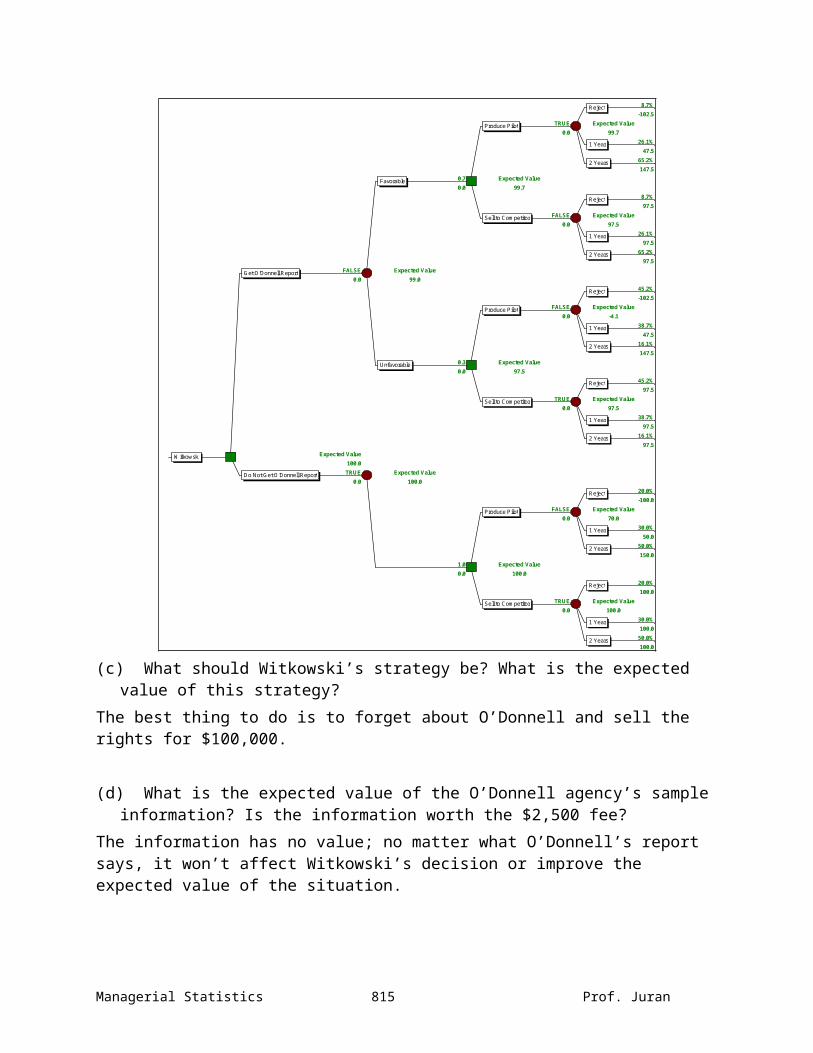
Of course, this ignores the other possibility, that we will find zero defects out of the five parts.1

Let’s analyze the probabilities associated with I2, the event that zero defects are found:

%defective Probability of 0 Defective out of 5

s1 0.00 =1.0000

s2 0.01 =0.9510

s3 0.02 =0.9039

s4 0.03 =0.8587

Probabilities


s0 0.15 1.0000 0.1500 0.1629s1 0.25 0.9510 0.2377 0.2581s2 0.40 0.9039 0.3616 0.3926s3 0.20 0.8587 0.1717 0.1865

Total

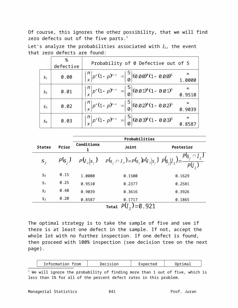
The optimal strategy is to take the sample of five and see if there is at least one defect in the sample. If not, accept the whole lot with no further inspection. If one defect is found, then proceed with 100% inspection (see decision tree on the next page).

Information from Decision Expected Optimal1 We will ignore the probability of finding more than 1 out of five, which is less than 1% for all of the percent defect rates in this problem.


Sample Alternatives Value Decision

I1 = 1 defect found

d1 = 100% inspection $250.00

d1d2 = no inspection $274.10

I1 = 0 defects found

d1 = 100% inspection $250.00

d2d2 = no inspection $200.33


Decision tree for Karim Nazer problem:0.0%$250

15.9%$250

TRUE Expected Value0 $250.00

48.9%$250

35.2%$250

7.5% Expected Value0 $250.00

0.0%$0

15.9%$125

FALSE Expected Value0 $274.10

48.9%$250

35.2%$375

Expected Value$204.09

16.3%$250

25.8%$250

FALSE Expected Value0 $250.00

39.3%$250

18.6%$250

92.1% Expected Value0 $200.33

16.3%$0

25.8%$125

TRUE Expected Value0 $200.33

39.3%$250

18.6%$375

Nazer

1 Defect Found

0 Defects Found

100% Inspection

No Inspection

0% Defects

1% Defects

2% Defects

3% Defects

0% Defects

1% Defects

2% Defects

3% Defects

100% Inspection

No Inspection

0% Defects

1% Defects

2% Defects

3% Defects

0% Defects

1% Defects

2% Defects

3% Defects

(g) What is the cost savings associated with having the sample information? In other words, what is it worth to have the sample of five taken as opposed to having no inspection or having 100% inspection?


As shown in the decision tree, there is a $250.00 - $204.09 = $45.91 expected cost reduction when the sample of five is inspected.


States of Nature

Documents

Transcript of States of Nature