The (non{)Gibbsian nature of states invariant understochastic transformationsChristian Maes� and Koen Vande VeldeyInstituut voor Theoretische FysicaK.U. LeuvenCelestijnenlaan 200DB-3001 Leuven (Belgium)e{mail: Christian=Maes%TF%FYS@cc3.kuleuven.ac.bee{mail: Koen=Van=de=Velde%TF%FYS@cc3.kuleuven.ac.beAbstractWe investigate the Gibbsian nature of systems that are invariant under somestochastic transformation. A prime example concerns stationary measures for inter-acting particle systems. We bring together various types of results concerning thisquestion using entropy techniques and large deviation estimates.Keywords: entropy inequalities, non{Gibbsianess, large deviations, stationary states,stochastic transformations, Toom model, restrictions of equilibrium measures.

�Aangesteld Navorser N.F.W.O. Belgium.yAspirant N.F.W.O. Belgium. 1

1 Introduction.Equilibrium statistical mechanics has to do with the study of Gibbs states. They de-scribe large systems in equilibrium for some given microscopic interaction potential. Alot is known about them, in particular for lattice spin systems, due to the rather ex-plicit construction of the state. In this paper we ask for the Gibbsian nature of stateson lattice spin con�gurations that are invariant under certain stochastic transformations.Understandably, invariance is a rather implicit way of de�ning the physical state andyet, this happens quite often to be the only information we have about it. Considerfor example the problem of determining the character of the steady state in models ofnon{equilibrium statistical mechanics. We have in mind here the study of the stationarystates of certain stochastic dynamics, such as interacting particle systems or probabilisticcellular automata. Given are the updating rules that de�ne the continuous time or dis-crete time stochastic evolution and the question is whether a state that after updating istransformed back into itself, is a Gibbs state for some (and what) interaction. It shouldbe clear in that respect that there is more to the question of \Gibbsianess" than beingable to take the logarithm of the probabilities. One wants to see if in some bulk limit, thesystem can be consistently described in terms of a relative energy function. This couldfor example be related to the type of large deviations one sees. A detailed account of therelevance and the consequences of these type of considerations can be found in [1].This paper grew out of the question how to unify various results in the literatureconcerning the nature of states that are not de�ned in terms of some explicit interactionpotential. Crucial in these questions is the in uence of applying stochastic transformationson the relative entropy density of two probability measures, de�ned on spin systems on alattice. We deduce that for the type of transformations that we consider, the translationinvariant stationary measures either are all Gibbsian with respect to the same interactionor either are non{Gibbsian. In the context of Markov spin ip processes on a lattice, asimilar statement has been proven by Holley [2] and K�unsch [3].This result is important not only to get a characterization of so called interacting particlesystems, but also, to learn more about the restrictions to a lower dimensional sublatticeof certain Gibbs measures. Indeed, some equilibrium systems can be seen as Markov ex-tensions of stationary measures for some transition operator (or, having a global Markovproperty) [4]. In fact, stationary measures of discrete time Markov processes can alsobe obtained from a projection of corresponding equilibrium systems on the space-timelattice [5]. A relevant question is, whether the above stationary measures and restrictionsof Gibbs measures are again Gibbsian.In the high{noise, high{temperature regime respectively, this is indeed the case. Therewe do not have long range order and the weak correlations make the probability of acon�guration in a �nite box to depend continuously on the con�guration far away. Forprobabilistic cellular automata (PCA), discrete time Markov processes on a lattice withlocal and parallel updating, it was proven in [6] that for high enough noise, the unique2

stationary measure is Gibbsian. A similar statement for continuous time spin ip processeswas proven in [7]. The situation is also quite clear in the case when the detailed balancecondition is satis�ed ; see [8] for a discussion of the stochastic or kinetic Ising model.Very little is however known about the stationary measures of dynamics that are not re-versible. A typical example is the Toom model [9], [6], on which we will come back later.As for the projections of Gibbs measures, it is also straightforward to check that theserestrictions are Gibbsian at high temperature (see e.g. [10]). However, for the case of thetwo-dimensional ferromagnetic Ising model below the critical temperature, Schonmann[11] has proven that the restrictions of the + and � phase to a one-dimensional layer areboth non{Gibbsian.It would also be interesting to study �xed point measures of real space renormalizationgroup transformations [1], but our methods are not adapted to treat these kind of trans-formations, because the rescaling of the lattice induces a rescaling in the entropy densityas well, making the entropy density inequalities of Section 2 useless. We will come backto this at the end of the paper.The paper is organized as follows:In section 2 some de�nitions and notation is given. Thereafter the main result is pre-sented. In Section 3 we discuss the situation for stochastic spin ip dynamics. Section 4is devoted to a discussion of related problems.2 Invariance for stochastic transformations.2.1 De�nitions and notation.We will consider spin systems on the regular lattice d and on �nite sublattices. For anysubset � � d the con�guration space is � = f�1;+1g� and we write � d . Thespace � is equipped with the usual product topology and Borel �-�eld F�. The set ofprobability measures on (�;F�) is denoted by P� and we let P � Pd denote the setof probability measures on the full lattice. For �; � in , we say that � = � on � i��(x) = �(x) for all x in �. Further we denote �(�) � Qx2� �(x). For x 2 d we de�nethe translation �x : ! : � 7! �x�, where �x�(y) = �(y + x). �x acts on a probabilitymeasure � 2 P as �x�(f) = �(f ���x), for all measurable functions f on . We call � 2 Ptranslation invariant if �x� = �, for all x 2 d. We denote the set of translation invariantmeasures in P by Ptr.De�nition 1 For a �nite set � and �; � 2 P� the relative entropy of � w.r.t. � isI(�; �) = X�2� �(�) log �(�)�(�) (2.1)(with 0log0=0). It is not hard to verify that I(�; �) � 0 and I(�; �) = 0 i� � = �. For anin�nite volume the relative entropy is almost always in�nite, but for translation invariant3

measures we can work with the concept of relative entropy density. For � 2 P and � � d,let �� denote the restriction of � on (�;F�). Further denote I�(�; �) = I(��; ��). Wemake the followingDe�nition 2 Let �; � 2 Ptr. Consider the sequence of boxes � = [�L; L]d. The relativeentropy density of � w.r.t. � is de�ned asi(�; �) = limL"1 1Ld I�(�; �); (2.2)provided this limit exists.The existence of the limit (2:2) is a non{trivial problem. This limit is known to existin case � is a Gibbs measure for a translation invariant interaction [12]. We recall thede�nition of Gibbs measure for a translation invariant interaction.De�nition 3 We call � 2 Ptr a Gibbs measure w.r.t. the translation invariant interactionfJV gV�d, if there exists a version of the local conditional probabilities of the form�[� = � on �j� = ! on �c] = Z�1� (!) exp[ XV \�6=; JV �(�)!(V n�)] (2.3)and PV 3o jJV j <1.With this de�nition, these conditional probabilities are continuous functions of ! 2 .Of course, there exist also other (non{continuous) versions, because these conditionalprobabilities are only de�ned �-a.s.. We denote by G(J) the set of all translation invariantGibbs measures with respect to fJV gV�d. We will use the following results:Lemma 1 [12] Suppose � is Gibbs for a translation invariant interaction, then � is Gibbsfor the same interaction i� i(�; �) = 0.Lemma 2 [13] � 2 Ptr is Gibbs for some translation invariant interaction i� the onepoint conditional probability �[�(o) = �(o)j� = ! on fogc] is positive and has a versioncontinuous in ! 2 .Often it is more convenient to work with relative energies instead of conditional proba-bilities.De�nition 4 Let � 2 G(J). The relative energy h� of � for a spin ip in the origin isthe continuous function de�ned byh�(�) =XV JV �o(V )�XV JV �(V ) = �2XV 3oJV �(V ); (2.4)where �o is the con�guration � ipped in the origin, so �o(x) = �(x) if x 6= o and �o(o) =��(o). 4

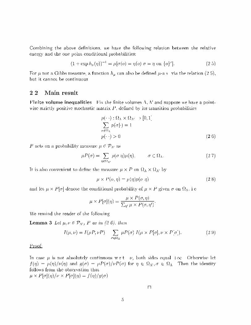
Combining the above de�nitions, we have the following relation between the relativeenergy and the one point conditional probabilities:(1 + exp h�(�))�1 = �[�(o) = �(o)j� = � on fogc]: (2.5)For � not a Gibbs measure, a function h� can also be de�ned �-a.s. via the relation (2.5),but it cannot be continuous.2.2 Main result.Finite volume inequalities Fix the �nite volumes �;�0 and suppose we have a point-wise strictly positive stochastic matrix P , de�ned by its transition probabilitiesp(�j�) : � � �0 ! [0; 1]X�2� p(�j�) = 1p(�j�) > 0 (2.6)P acts on a probability measure � 2 P�0 as�P (�) = X�2�0 p(�j�)�(�); � 2 �: (2.7)It is also convenient to de�ne the measure �� P on � � �0 by�� P (�; �) = �(�)p(�j�) (2.8)and let �� P [�] denote the conditional probability of �� P given � on �, i.e.�� P [�](�) = �� P (�; �)P�0 �� P (�; �0) :We remind the reader of the followingLemma 3 Let �; � 2 P�0, P as in (2.6), thenI(�; �) = I(�P; �P ) + X�2� �P (�) I(�� P [�]; � � P [�]): (2.9)Proof:In case � is not absolutely continuous w.r.t. �, both sides equal +1. Otherwise letf(�) = �(�)=�(�) and g(�) = �P (�)=�P (�) for � 2 �0 ; � 2 �. Then the identityfollows from the observation that�� P [�](�)=� � P [�](�) = f(�)=g(�). 25

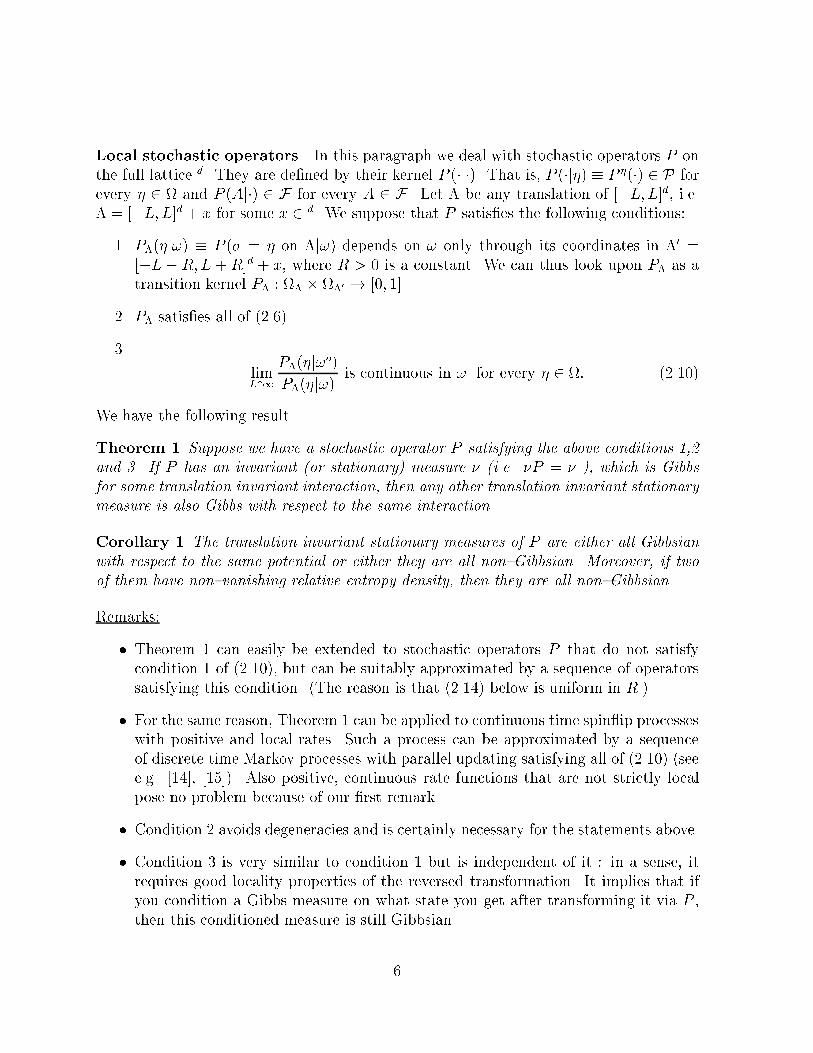
Local stochastic operators In this paragraph we deal with stochastic operators P onthe full lattice d. They are de�ned by their kernel P (�j�). That is, P (�j�) � P �(�) 2 P forevery � 2 and P (Aj�) 2 F for every A 2 F . Let � be any translation of [�L; L]d, i.e.� = [�L; L]d + x for some x 2 d. We suppose that P satis�es the following conditions:1. P�(�j!) � P (� = � on �j!) depends on ! only through its coordinates in �0 =[�L � R;L + R]d + x, where R > 0 is a constant. We can thus look upon P� as atransition kernel P� : � � �0 ! [0; 1].2. P� satis�es all of (2.6).3. limL"1 P�(�j!o)P�(�j!) is continuous in ! for every � 2 : (2.10)We have the following result.Theorem 1 Suppose we have a stochastic operator P satisfying the above conditions 1,2and 3. If P has an invariant (or stationary) measure � (i.e. �P = � ), which is Gibbsfor some translation invariant interaction, then any other translation invariant stationarymeasure is also Gibbs with respect to the same interaction.Corollary 1 The translation invariant stationary measures of P are either all Gibbsianwith respect to the same potential or either they are all non{Gibbsian. Moreover, if twoof them have non{vanishing relative entropy density, then they are all non{Gibbsian.Remarks:� Theorem 1 can easily be extended to stochastic operators P that do not satisfycondition 1 of (2.10), but can be suitably approximated by a sequence of operatorssatisfying this condition. (The reason is that (2.14) below is uniform in R.)� For the same reason, Theorem 1 can be applied to continuous time spin ip processeswith positive and local rates. Such a process can be approximated by a sequenceof discrete time Markov processes with parallel updating satisfying all of (2.10) (seee.g. [14], [15]). Also positive, continuous rate functions that are not strictly localpose no problem because of our �rst remark.� Condition 2 avoids degeneracies and is certainly necessary for the statements above.� Condition 3 is very similar to condition 1 but is independent of it : in a sense, itrequires good locality properties of the reversed transformation. It implies that ifyou condition a Gibbs measure on what state you get after transforming it via P ,then this conditioned measure is still Gibbsian.6

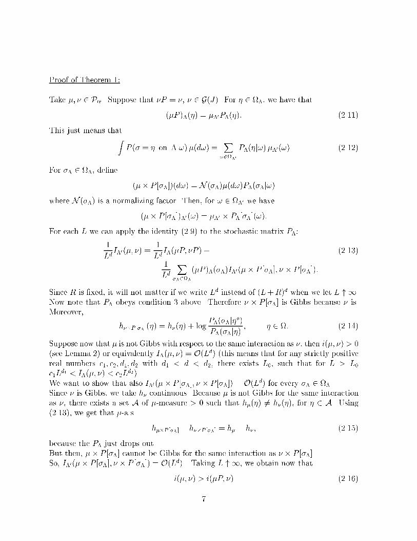
Proof of Theorem 1:Take �; � 2 Ptr. Suppose that �P = �, � 2 G(J). For � 2 �, we have that(�P )�(�) = ��0P�(�): (2.11)This just means thatZ P (� = � on �j!)�(d!) = X!2�0 P�(�j!)��0(!) (2.12)For �� 2 �, de�ne (�� P [��])(d!) = N (��)�(d!)P�(��j!)where N (��) is a normalizing factor. Then, for ! 2 �0 we have(�� P [��])�0(!) = ��0 � P�[��](!):For each L we can apply the identity (2.9) to the stochastic matrix P�:1Ld I�0(�; �) = 1Ld I�(�P; �P ) + (2.13)1Ld X��2�(�P )�(��)I�0(�� P [��]; � � P [��]):Since R is �xed, it will not matter if we write Ld instead of (L+R)d when we let L " 1.Now note that P� obeys condition 3 above. Therefore � � P [��] is Gibbs because � is.Moreover, h��P [��](�) = h�(�) + log P�(��j�o)P�(��j�) ; � 2 : (2.14)Suppose now that � is not Gibbs with respect to the same interaction as �, then i(�; �) > 0(see Lemma 2) or equivalently I�(�; �) = O(Ld) (this means that for any strictly positivereal numbers c1; c2; d1; d2 with d1 < d < d2, there exists L0, such that for L > L0c1Ld1 < I�(�; �) < c2Ld2).We want to show that also I�0(�� P [��]; � � P [��]) = O(Ld) for every �� 2 �.Since � is Gibbs, we take h� continuous. Because � is not Gibbs for the same interactionas �, there exists a set A of �-measure > 0 such that h�(�) 6= h�(�), for � 2 A. Using(2.13), we get that �-a.s. h��P [��] � h��P [��] = h� � h�; (2.15)because the P� just drops out.But then, �� P [��] cannot be Gibbs for the same interaction as � � P [��].So, I�0(�� P [��]; � � P [��]) = O(Ld) . Taking L " 1, we obtain now thati(�; �) > i(�P; �) (2.16)7

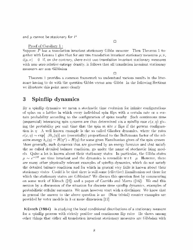
and � cannot be stationary for P . 2Proof of Corollary 1 :Suppose P has a translation invariant stationary Gibbs measure. Then Theorem 1 to-gether with Lemma 1 give that for any two translation invariant stationary measures �; �,i(�; �) = 0. If, on the contrary, there exist two translation invariant stationary measureswith non{zero relative entropy density, it follows that all translation invariant stationarymeasures are non{Gibbsian. 2Theorem 1 provides a common framework to understand various results in the liter-ature having to do with the question Gibbs versus non{Gibbs. In the following Sectionswe illustrate this point more clearly.3 Spin ip dynamics.By a spin ip dynamics we mean a stochastic time evolution for in�nite con�gurationsof spins on a lattice in which every individual spin ips with a certain rate or a cer-tain probability according to the con�guration of spins nearby. Such continuous time(sequential) interacting spin systems are thus determined via a spin ip rate c(x; �) giv-ing the probability per unit time that the spin at site x ips if the present con�gura-tion is �. A well known example is the so called Glauber dynamics, where the ratesc(x; �) � exp[��hx(�)] are (essentially) proportional to the Boltzmann factor of the rel-ative energy hx(�) = H(�x)�H(�) for some given Hamiltonian given of the spin system.More generally, such dynamics that are governed by an energy function and that satisfythe so called detailed balance condition, go under the name of stochastic Ising mod-els. Quite a lot is known about their stationary states. In particular, the Gibbs states� � e��H are time invariant and the dynamics is reversible w.r.t. �. However, thereare many other physically relevant examples of spin ip dynamics, which do not satisfythe detailed balance condition and for which in general very litlle is known about theirstationary states. Could it be that there is still some (e�ective) Hamiltonian out there forwhich the stationary states are Gibbsian? We discuss this question �rst by commentingon some work of K�unsch ([3]) and a paper of Garrido and Marro ([16]). We end thissection by a discussion of the situation for discrete time spin ip dynamics, examples ofprobabilistic cellular automata. We must however start with a disclaimer. We know thatin general the answer to the above question is no. (Non{trivial) counter examples areprovided by voter models in 3 or more dimension [17].K�unsch (1984) is studying the local conditional distributions of a stationary measurefor a spin ip process with strictly positive and continuous ip rates. He shows amongother things that either all translation invariant stationary measures are Gibbsian with8

the same potential or no translation invariant stationary Gibbs measure exists. This hasto be compared with our Theorem 1 (Remarks). Moreover, he constructs an examplewith in�nitely many stationary measures (all of which are Gibbsian), but no reversiblemeasures. In fact, the general tone of the paper is that, again for strictly positive and con-tinuous rates, reversible or not, all stationary measures should be Gibbsian. In particular,this would mean that the local conditional distributions of a single spin given all otherspins are the same for all stationary measures. Although this last statement is formulatedas a conjecture in the paper, we wish to point out here that local conditional distributionsas such, carry very little information unless assumed to have continuous versions. Moreprecisely, if � and � are both stationary measures, we can always �nd a function h on for which �[�(o) = �(o)j�(x) = �(x); x 6= o] = h(�) �� a.s.�[�(o) = �(o)j�(x) = �(x); x 6= o] = h(�) � � a.s.and � and � need not be Gibbsian.E�ective Hamiltonian description? It has been suggested in Garrido and Marro(1989) that strictly positive and local ip rates for the dynamics always give rise to Gibbsstates as stationary states. In fact they give an explicit form of the interaction potential(they call it the e�ective Hamiltonian). It basically amounts to writing down the equation(c(x; �) can be for example a sum of Glauber rates with di�erent temperatures)exp[�2�XA3xJA�(A)] = c(x; �)c(x; �x) (3.1)for the coupling constants fJAg which would appear in the (e�ective) Hamiltonian\H(�) = �XA JA�(A)". (3.2)Then, the Gibbs measures with respect to this Hamiltonian are of course invariant underthe dynamics. There is however only a consistent solution to (3.1) if the rates satisfy thecondition X� �(A) log c(x; �)c(x; �x) c(y; �)c(y; �y) = 0 (3.3)for every �nite set A and all x; y 2 A. It is easy to see that this condition implies in factthat we are really dealing with a stochastic Ising model and (3.3) can never be satis�edby a dynamics which is not reversible.Discrete time In this paragraph, we deal with probabilistic cellular automata (PCA).They can be viewed as discrete time versions of spin ip dynamics. PCA are discrete time9

Markov processes on d, with local and parallel updating of Ising type spins. The �nitevolume transition probabilities can be written asP�(�j�) = Yx2�Pfxg(�(x)j�) (3.4)and we take the Pfxg(�(x)j�) positive and local in � (cf. conditions 1 and 2). It is easyto check that also our condition 3 is veri�ed. Theorem 1 can thus be applied to them. Inthe reversible case, where the PCA satis�es the detailed balance condition (see [6]) withrespect to some Gibbs measure for some translation invariant interaction fJ(V )gV�d , itis a consequence of Theorem 1 that the translation invariant stationary measures are pre-cisely all Gibbs measures for fJ(V )gV�d.At high noise (i.e. when the dependence for a spin on the value of its neighboring spinon the previous timestep is small) it is known that there is a unique stationary Gibbsmeasure [6].In the non{reversible case, practically nothing is known about the nature of the station-ary measures in the regime where there is more than one stationary measure. Perhapsit is possible that these stationary measures are non{Gibbsian. To prove such a state-ment, it would be su�cient (because of Theorem 1) to prove that the relative entropydensity between two di�erent stationary measures is nonzero. A typical example of anon{reversible PCA (for which it is conjectured that the stationary measures at low noiseare non{Gibbsian [1]) is the Toom model. The simplest version of the Toom model isa PCA which can be seen as a North{East{Center majority vote model on the squarelattice. That is, in (3.19) one takesPfxg(�(x)j�) = 1=2(1� (1� 2�)�(x)sgn[�(x) + �(x0) + �(x00)]) (3.5)with x0 = x+ (1; 0) and x00 = x+ (0; 1) the \eastern" and \northern" nearest neighbor ofx on 2. Equivalently, we can de�ne the Toom model on the triangular lattice, but arrangeit so that, for the space-time lattice, each site is the center of a triangle on the previouslayer. More precisely, if we denote by Ln the layer at time t = �n, then under projectionperpendicular to the lattice plane, the sites of Ln�1 coincide with the centers of alternatetriangles in Ln, i.e. those with some �xed orientation. The sites of Ln�2 coincide withthe centers of the similarly oriented triangles in Ln�1 and �nally Ln�3 coincides with Ln.The deterministic Toom rule (� = 0) assigns to the spin at site x the majority of the spinsat the corners of the triangle directly above. The evolution in the stochastic Toom modelfollows the deterministic rule with probability (at least) 1 � � and does something elsewith probability (at most) �.The deterministic dynamics has �(x) � +1 and �(x) � �1 as stationary states. More-over, these states are stable against �nite excitations of the opposte sign. In fact, suchexcitations shrink at a constant rate and hence disappear in a �nite time. This is the socalled eroder property. For � small but di�erent from zero, there are still (at least) twostationary measures, in one of which most spins are +1, in the other of which most are10

�1, obtained from + and � begin conditions respectively (they will be called �+ and ��in the following). For more information, see [6]. We take as basis vectors to generate ourthree dimensional space-time lattice, the vectors e1; e2; e3 connecting the origin o with thecorners of the triangle directly above o. The time coordinate t(x) of a space{time pointx is given by t(x) = x:(e1 + e2 + e3).As mentioned before, to prove that �+; �� are non{Gibbsian, one should show thati(�+; ��) > 0. It is equivalent to show the probability for �+ of having a large clus-ter of minusses is (at least) exponentially small in the volume of the cluster. (see forexample [1]). This would be true if the probability to �nd �x � �1 in the triangle� � fxjt(x) = �K; x:e1; x:e2; x:e3 � Kg, starting from the all + con�guration at timet = �N , is smaller than cte �j�j, for all K > 0 and for all N > K; (j�j is the cardinalityof the set �).In [9], it is shown that Prob[�(o) = �1] � 2� (3.6)by making an expansion in graphs for this probability. However, this expansion cannot beused to prove our statement. In fact, there is a model of Domany (see [6]) for which Toom'sexpansion can be used to prove non{ergodicity, but for which the stationary measures areGibbsian. The transition function for this model isPfxg(�(x)j�) = 1=2[1 + �(x) tanh�(�(x) + �(x0) + �(x00)]: (3.7)It is not hard to see that, if one sets 1�2� = 1=2(tanh 3�+tanh �), this transition functionappoaches that of the Toom model (3.5) if � " 1; � # 0. So, it is not clear that one shouldexpect the stationary measures of the Toom model at low noise to be non{Gibbsian.For this reason we are trying to extract the necessary information from simulations onthe Toom model. However, so far this has not given conclusive evidence. Althoughwe are inclined to interpret the simulation data as showing Gibbsian behavior for thestationary states, a further and more systematic search needs to be done before drawingany conclusions.One can also see from here that the question of Gibbsianess is more than an academicquestion. Of course it is an important characterization of the stationary states but morethan that, here we see that the question is equivalent to an estimate of the e�ciency of therepeated transformation in removing mistakes : saying that the relative entropy densityof the two stationary states is non{zero means that you need to create a volume fractionof \mistakes" to see in one stationary state, an island of the opposite stationary state |for equilibrium dynamics relaxing towards one of the extremal stationary Gibbs states,it su�ces to essentially introduce a boundary of the \wrong" phase for the dynamics toautomatically �ll up the enclosed volume with this (for example, opposite) phase. It mayalso happen that you need less than a boundary (such as in the voter model, see [17])and then the stationary states may again be non{Gibbsian even though their relativeentropy densites are zero. The picture that emerges is therefore that the stationary states11

are Gibbsian whenever, when the dynamics is started from a particular stationary state,by introducing on the boundary of a volume a con�guration that is \typical" of anotherstationary state, after a time of the order of the diameter of that volume, one sees this\wrong" state in the interior of the volume.4 Relation with other problems.4.1 Restriction of + and � phases of the Ising model.Consider the standard ferromagnetic Ising model in d dimensions. In �nite boxes � =[�L; L]d we consider + and � boundary conditions : the corresponding Gibbs measures��� � exp(��H�� ) converge as L " 1 to Gibbs measures ��. At low temperatures (� " 1)�+ 6= �� are two extremal, translation invariant Gibbs measures. Both are satisfying theglobal Markov property [4]. For both measures, we can consider the restrictions �� to a(d�1)-dimensional hypersurface (�= d�1). Schonmann [11] proved that in d = 2 dimensionsand below the critical temperature, both these measures �� are non{Gibbsian (i.e. (2.3)is never satis�ed). We wish to add here two remarks:1. The higher dimensional situation (d > 2) (open question 6 in [1]): Schonmann'sanalysis consists of two main steps: a large deviation estimate and the study of awetting problem. The large deviation estimate boils down to the statement thatthe relative entropy density of the projected phases is non{zero: i(�+; ��) > 0. Ifwe allow to look at very small temperatures, this result is valid in any dimensiond � 2, from standard arguments [18]. As for the wetting problem, one has to provethat for each n, there exists an N(n) such that�+[�j~� = �1 on An;N ]! �� as N " 1;where ~� is a con�guration on the (d� 1)-dimensional annulusAn;N = fx = (i; 0); i 2 d�1 : n � jikj � N; k = 1; : : : ; d� 1g:The proof of this statement is a consequence of the recent work of Holick�y andZahradn��k [19] on the problem of entropic repulsion in low temperature Ising mod-els. Therefore, for any dimension (d � 2) the projection of the Ising phases on ahypersurface is non{Gibbsian at low temperatures.2. The transfer matrixA well known tool in the analysis of the Ising model is the machinery of the transfermatrix formalism. In some sense one could say that the projections on hypersurfacesare invariant measures for this transfer matrix. Therefore, Corrolary 1 (with P=transfer matrix) very much resembles the statement of Proposition 2 in [11] that if12

�+ is Gibbsian, then �� is Gibbsian for the same potential. We show however thatthere exists no stochastic operator P , satisfying the conditions of (2.10), for whichboth �+ and �� are invariant.Consider a box B = [�K;K]�VL;VL = [�L; L]d�1. Let the (�nite volume) transfermatrix aL be de�ned by its matrix elements aL(�; � 0); �; � 0 2 VL :aL(�; � 0) = exp[�=2( X<xy>�VL(�(x)�(y) + � 0(x)� 0(y)) + � Xx2VL �(x)� 0(x)]: (4.1)(here we sum over nearest neighbor pairs)>From the Perron{Frobenius theorem, we have that the largest eigenvalue �L of aLis non{degenerate. Let us call the corresponding normalized eigenvector L andits components L(�); � 2 VL . The matrix aL can be normalized to become astochastic matrix �L:�L(�j�) = aL(�; �) L(�)�L L(�) �; � 2 VL : (4.2)Note that the combination �L(�j�) 2L(�)is symmetric in (�; �) which is the analogue of the detailed balance condition forPCA.Consider now �K;L, the Gibbs state on the �nite box B, corresponding to the Hamil-tonian HB with free boundary conditions:HB(�) = � X<xy>�B �(x)�(y): (4.3)We have that�K;L[� on f0g � VLj� on f�1g � VL] = aL(�; �) P� aKL (�; �)P� aK+1L (�; �) (4.4)and thus limK"1�K;L[� on f0g � VLj� on f�1g � VL] = �L(�j�): (4.5)Hence, �[� on f0g � d�1j� on f�1g � d�1] = limL"1 �L(�j�) for �-a.e. �: (4.6)The left hand side is the probability on the zero'th layer (the hypersurface passingthrough the origin) in the measure � = 1=2(�++��) conditioned on the \previous"layer. Any P that leaves �+ and �� invariant also leaves � = 1=2(�++��) invariant.Therefore its kernel should satisfyP [�j�] = �[� on f0g � d�1j� on f�1g � d�1] (4.7)13

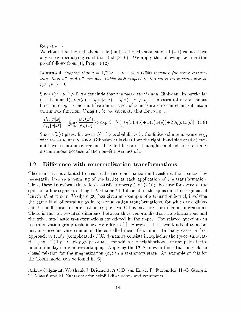
for �-a.e. �.We claim that the right-hand side (and so the left-hand side) of (4.7) cannot haveany version satisfying condition 3 of (2.10). We apply the following Lemma (theproof follows from [1], Prop. 4.12)Lemma 4 Suppose that � = 1=2(�+ + ��) is a Gibbs measure for some interac-tion, then �+ and �� are also Gibbs with respect to the same interaction and soi(�+; ��) = 0.Since i(�+; ��) > 0, we conclude that the measure � is non{Gibbsian. In particular(see Lemma 1), �[�(o) = �(o)j�(x) = �(x); x 6= o] is an essential discontinuousfunction of �, i.e. no modi�cation on a set of �-measure zero can change it into acontinuous function. Using (4.3), we calculate that for �-a.e. !PVL[�j!]PVL[�j!o] = limN"1f N (!o) N (!) g�exp[� Xx:<ox>(�(x)�(o)+!(x)!(o))+2��(o)!(o)]: (4.8)Since 2N(�) gives, for every N , the probabilities in the �nite volume measure �VN ,with �N ! �, and � is not{Gibbsian, it is clear that the right{hand side of (4.8) can-not have a continuous version. The �rst factor of that right-hand side is essentiallydiscontinuous because of the non{Gibbsianess of �.4.2 Di�erence with renormalization transformations.Theorem 1 is not adapted to treat real space renormalization transformations, since theynecessarily involve a rescaling of the lattice at each application of the transformation.Thus, these transformations don't satisfy property 1 of (2.10), because for every t, thespins on a line segment of length L at time t+1 depend on the spins on a line segment oflength 3L at time t. Vasilyev [20] has given an example of a transition kernel, involvingthe same kind of rescaling as in renormalization transformations, for which two di�er-ent Bernoulli measures are stationary (i.e. two Gibbs measures for di�erent interaction).There is thus an essential di�erence between these renormalization transformations andthe other stochastic transformations considered in the paper. For related questions inrenormalization group techniques, we refer to [1]. However, these two kinds of transfor-mations become very similar in the so called mean �eld limit. In many cases, a �rstapproach to study (complicated) PCA dynamics consists in replacing the space{time lat-tice (say, d+1) by a Cayley graph or tree, for which the neighborhoods of any pair of sitesin one time layer are non{overlapping. Applying the PCA rules in this situation yields aclosed relation for the magnetization h�xi in a stationary state. An example of this forthe Toom model can be found in [6].Acknowledgment: We thank J. Bricmont, A.C.D. van Enter, R. Fern�andez, H.-O. Georgii,T. Matsui and M. Zahradn��k for helpful discussions and comments.14

References[1] A.C.D. van Enter, R. Fern�andez, A.D. Sokal: Regularity properties and pathologiesof position-space renormalization transformations, to appear in J. Stat. Phys..[2] R. Holley: Free energy in a Markovian model of a lattice spin system, Commun.Math. Phys. 23, 87-99 (1971).[3] H. K�unsch: Non reversible stationary measures for in�nite interacting particle sys-tems, Z. Wahrsch. Verw. Gebiete 66, 407-424 (1984).[4] S. Goldstein, R Kuik and A.G. Schlijper: Entropy and Global Markov properties,Commun. Math. Phys. 126, 496{482 (1990).[5] S. Goldstein, R. Kuik, J.L. Lebowitz and C.Maes: From PCA to equilibrium systemsand back, Commun. Math. Phys. 125, 71-79 (1989).[6] J.L. Lebowitz, C. Maes and E.R. Speer: Statistical mechanics of probabilistic cellularautomata, J. Stat. Phys. 59, 117-170 (1990).[7] C. Maes and K. Vande Velde: The interaction potential of the stationary measure ofa high-noise spin ip process, to appear in J. Math. Phys..[8] T.M. Liggett: Interacting paricle systems, Springer, Berlin (1985).[9] A. Toom: Nonergodic multidimensional systems of automata, Prob. Inform. Transm.10, 239-246 (1974).[10] C. Maes and K. Vande Velde: De�ning relative energies for the projected Ising mea-sure, Helv. Phys. Acta 65, 1055-1068 (1992).[11] R.H. Schonmann: Projections of Gibbs measures may be non{Gibbsian, Commun.Math. Phys. 124, 1-7 (1989).[12] H.-O. Georgii: Gibbs measures and phase transitions, de Gruyter, Berlin (1988).[13] W.G. Sullivan: Potentials for almost Markovian random �elds, Commun. Math.Phys. 33, 61-74 (1973).[14] J.E. Steif: The ergodic structure of interacting partical systems, Stanford Mathemat-ics department Ph.D. thesis (1988).[15] C. Maes and S.B. Shlosman: When is an interacting paricle system ergodic?, Com-mun. Math. Phys. 151, 447-466 (1993).[16] P.L. Garrido and J. Marro: E�ective Hamiltonian description of non{equilibriumspin systems, Phys. Rev. Letters 62, 1929-1932 (1989).15

[17] J.L. Lebowitz and R. Schonmann: pseudo{free energies and large deviations for non{Gibbsian FKG measures, Probab. Th. Rel. Fields 77, 49-64 (1988).[18] J. Bricmont: private communication.[19] P. Holick�y and M. Zahradn��k: On entropic repulsion in low temperature Ising models,Preprint.[20] N. Vasilyev: Bernoulli and Markov stationary measures in discrete local interactionsin Locally interacting systems and their applications in biology, Lecture notes in math.653, Springer, Berlin (1978).

16