Stateful Detection in High Throughput Distributed Systems

Gunjan Khanna, Ignacio Laguna, Fahad A. Arshad, Saurabh Bagchi Dependable Computing Systems Lab (DCSL)

School of Electrical and Computer Engineering, Purdue University Email: {gkhanna, ilaguna, faarshad, sbagchi}@purdue.edu

Abstract

With the increasing speed of computers and the complexity of applications, many of today’s distributed systems exchange data at a high rate. Significant work has been done in error detection achieved through external fault tolerance systems. However, the high data rate coupled with complex detection can cause the capacity of the fault tolerance system to be exhausted resulting in low detection accuracy. We present a new stateful detection mechanism which observes the exchanged application messages, deduces the application state, and matches against anomaly-based rules. We extend our previous framework (the Monitor) to incorporate a sampling approach which adjusts the rate of verified messages. The sampling approach avoids the previously reported breakdown in the Monitor capacity at high application message rates, reduces the overall detection cost and allows the Monitor to provide accurate detection. We apply the approach to a reliable multicast protocol (TRAM) and demonstrate its performance by comparing it with our previous framework.

1. Introduction The proliferation of high bandwidth applications

and the increase in the number of consumers of distributed applications have caused them to operate at increasingly high data rates. Many of these distributed systems form parts of critical infrastructures, with real-time requirements. Hence it is imperative to provide error detection functionality to the applications. Error detection can broadly be classified as stateless detection and stateful detection. In the former, detection is done on individual messages by matching certain characteristics of the message, such as the length of the payload of the message. A more powerful approach for error detection is the stateful approach, in which the error detection system builds up state related to the application by aggregating multiple messages.

The rules are then based on the state, thus on aggregated information rather than on instantaneous information. Stateful detection is looked upon as a powerful mechanism for building dependable distributed systems [19][20]. The stateful detection models can be specified using various formalisms, such as, State Transition Diagrams, PetriNets or UML. Though the merits of stateful detection seem to be well accepted, scaling a stateful detection system with increasing application entities or data rate is a challenge. This is due to the increased processing load of tracking application state and rule matching based on the state. This problem has been documented for stateful firewalls that are matching rules on state spread across multiple, possibly distant, messages [19]. The stateful error detection system has to be designed without increasing the footprint of the system. Thus throwing hardware or memory at the problem is not enough because the application system also scales up and demands more from the detection system.

In our earlier work on developing an error detection system, we developed the Monitor([1], [7]) which provides detection by only observing the messages exchanged between the protocol entities (PEs). The Monitor is said to verify a set of PEs when it is monitoring them. The Monitor is provided a representation of the protocol behavior (using a state transition diagram i.e., STD) of the PEs being verified along with a set of stateful anomaly based rules. The Monitor uses an observer model whereby it does not have any information about the internal state of the PEs. The Monitor performs two primary tasks on observing a message. First, it performs the state transition corresponding to the PE based on the observed message. Note that the state of the PE estimated by the Monitor may differ from the real state of the entity since not all messages related to state changes are necessarily observable at the Monitor. Second, it performs rule matching for the rules associated with the particular state and message combination. We observe that the Monitor has a

breaking point in terms of (1) the incoming message rate or (2) the number of entities that it can verify, beyond which the accuracy and latency of its detection suffer [7]. The drop in accuracy or rise in latency is very sharp beyond the breaking point. We observe through a test-bed experiment that as the incoming packet rate into a single Monitor is increased beyond 100 pkt/s, the Monitor system breaks down on a standard Linux box. In other words, its latency becomes exceedingly high and accuracy of detection tends to zero. This effect is shown in Figure 1. This breakdown is caused by the processing capacity at the Monitor being exhausted. Hence, messages see long waiting times and, on the buffer becoming full, the messages also get dropped. Thus, for reasonable operation, the Monitor can only support data rates below the breaking point.

0

200

400

600

800

1000

1200

0 100 200 300 400 500

Late

ncy

(ms)

Rate of Packets (Pkt/s)

Monitor (baseline)

Figure 1: Latency variation with increasing packet rate. The graph depicts the breaking of the Monitor

system at an incoming rate of 100 pkts/s

In the current work, we devise a stateful detection approach which scales with the increasing data rate of applications, or equivalently, the number of PEs being verified. We observe that in order to make stateful detection feasible; firstly the processing of each message must be made extremely efficient and secondly the system must reduce the total processing workload (e.g., by selectively dropping incoming messages). The amount of work at the Monitor per unit time can be conceived as the rate of messages being processed for detection × the amount of work performed for each message. Our approach optimizes both these terms. The goal is to provide an error detection system for high throughput distributed streams and correspondingly push the knee to the right (Figure 1). Existing detection systems like [15][16] which aim at handling high data rate provide detection of changes in high rate streams using mean and higher order moments. This approach cannot capture the

richness in the error detection rules that is needed for specifying verifiable behavior.

As a first aspect, we minimize the processing cost of an individual incoming message into the Monitor. We do this by using multistage hash tables for look ups when a state transition needs to be performed at the Monitor. We observe that for realistic systems, multiple rules will be active concurrently. The rules take the form of verifying values of some state variables or counts of messages (events) lying within a range. There exists significant overlap in the state variables or counts being referred to in the rules. Since processing for an incoming message most often involves updating these counts, we optimize this operation by compact representation of the state variables.

In the second aspect, we minimize the number of messages that the Monitor has to process by sampling. We set a threshold for the incoming rate guided by the breaking point of the Monitor. Sampling the incoming stream to reduce the rate of messages is a logical start. However, since the Monitor provides stateful detection, dropping messages can cause the Monitor to lose track of the PE’s current state with resultant decrease in accuracy of rule matching. This phenomenon is called state non-determinism, whereby to the Monitor it is non-deterministic which state the PE is in. In our approach the Monitor tracks the set of possible states the application could have reached given that a sequence of messages is dropped. The Monitor aggressively pre-computes information about the states for possible sequences of messages to reduce the cost of computing the non-deterministic state set. While the cost of processing each (sampled) message now increases over the baseline case, through careful design, the Monitor’s total amount of work is reduced by reducing the rate of messages that it needs to process. The sampling is adaptive to tolerate fluctuations in the message rate generated by the PEs. Also, the sampling scheme necessitates changes in the rules to prevent false detections due to the sampling.

We implement the two aspects of efficient stateful detection in the Monitor and use it to detect errors in a reliable multicast protocol called TRAM[4]. TRAM provides a motivating application since it is at the core of many e-learning applications which feed high bandwidth streams to a large set of receivers. We inject errors into the TRAM PEs and compare the accuracy and latency to the baseline system. The sharp decrease in performance beyond the breaking point is no longer observed; in fact, a sharp breaking point is completely eliminated and a gradual decrease in performance with increasing message rates is observed instead.

Dat

aA

ck

Dat

a

NA

ck

Hea

d B

ind

Figure 2: An example State Transition Diagram

for a TRAM receiver Section 2 provides a background on the existing

Monitor approach and identifies changes for an approach which can work in high data rate applications. In section 3 we present the new stateful approach, and in section 4 and 5 we describe it. Section 0 and 0 provide details on the application and experimental results respectively. Related research is discussed in section 8 followed by conclusions in section 9.

2. Background

2.1 Black-box detection through the Monitor Previously we developed a detection framework in

terms of hierarchical Monitor(s) based on black-box semantics [1][7]. The Monitor obtains the protocol messages either through modification to the communication middleware layer to forward the messages or by a passive snooping mechanism. In either scenario the components of the application are treated as black-box for the detection process. There are advantages to this treatment—the application does not have to be modified, the solution is generalizable across multiple applications, and the set of errors to be detected can be extended in a modular manner without changes to either the application or the Monitor algorithms. The Monitor consists of a hierarchy of Local, Intermediate and Global monitors. The Local Monitor, abbreviated later as the Monitor, is in charge of verifying the behavior of a set of PEs and it is given as input the reduced STDs of these PEs. The STD is reduced because internal transitions are not visible to the Monitor and hence not included. At runtime, it observes the external message interactions between the PEs that it is verifying and it deduces the current state of the PE from it. The Local Monitor also matches the PE’s behavior against a set of rules. The combination of current state and incoming event determines the set of rules to be matched. The Intermediate Monitor gathers information from several local Monitors, each verifying a set of PEs. The Global Monitor verifies some global properties of the protocol. Message capturing by the Monitor can be through passive monitoring of traffic or using active forwarding

support from the PEs. We will refer to this initial version of the Monitor described in [1][7] as Monitor-Baseline.

2.2 Creation of rules The rules used by the Monitor are anomaly based

rules since the potential universe of PE misbehavior is too large to be enumerated. The rule base provided by the system administrator comes from two sources: formal protocol specifications and QoS specifications. The first class of rules is derived from a complete STD specification of the protocol while the second class is specified by the system administrator based on the application requirements—performance requirements (such as, data rate of 20 kbps must be sustained) or security requirements (such as, no more than 3 unsuccessful login attempts will be allowed). Any deviation from the rules can be detected by the Monitor. Thus, the universe of detectable errors includes implementation bugs, configuration errors, security exploits or performance problems.

The running protocol that we use as example is the TRAM [4] protocol for reliable multicast of data from a single sender to multiple receivers through intermediate routing nodes called the repair head (RH). In TRAM, the receiver Acks correct data packets and sends Nacks for missing data packets to the RH above. The receiver maintains a counter for the number of Nacks sent, and if it crosses a threshold, receiver begins to rejoin a different RH assuming the old RH has failed.

The STD in Figure 2 shows an example STD for a receiver receiving data from the sender or the RH. An explanation of the different types of messages in TRAM is provided in the Appendix. Under correct operation, the receiver will oscillate between states S0 and S4, getting data and sending Acks. Rules can be derived from the STD using the states, events, state variables and time of transitions. Each state has a set of state variables. Events may cause transitions between states. In our context, events are messages sent and received. In Figure 2, the receiver moves from state S4 to state S5 if it sends a Nack because no data packet is received. Hence a rule can be derived if for all t ∈ (ti, ti+a), S4 ∧ ¬D ⇒ ¬S4.; where ti is time when S4 becomes the present state and a is a constant. Here predicate D implies data packet received. Subsequent Nacks will cause the state to remain at S5 but a local state counter will be incremented. Eventually if the number of Nacks is greater than Nmax, then the Monitor should see a Head Bind message indicating a change of affiliation to a different RH. Thus the rule becomes |Nacks| ≥ Nmax ⇒ Head Bind. Hence rules can be derived from the STD specifications. The

system administrator may add rules specifying QoS conditions that the application should meet, e.g., a minimum data rate that must be met at each receiver. In addition, the system administrator may augment the rule base with rules to catch manifestations of any protocol vulnerability. Creation of the STDs to be verified may be a manual process. Alternately several applications are formally specified as state charts, communicating finite state machines, using UML diagrams, etc. and automated tools can be built to convert other formal representations to STDs.

We have a formally defined syntax for rules in the system. The syntax represents a balance between expressiveness of the rules and efficient matching of the rules at runtime. Rules are of two kinds – combinatorial and temporal. Combinatorial rules are expected to be valid for the entire period of execution of the system, except for transient periods of protocol instability.

2.3 Temporal rules The rule base for the Monitor-Baseline is specified

using a broad class of rules which captures a majority of protocol behavior (see [1][7]). The syntax of the rules is presented in Appendix B and is identical to that presented in [1][7]. The Monitor-Baseline has five broad categories of temporal rules (R1-R5) with each one designed to provide verification of state changes, verify event counts in specific states, causal dependence, and combination of these conditions for PEs. Examples of rules based on Figure 2 are:

R4 S4 E11 30 500 5000 S4 E2 1 8 4000 7000: (Rule of type 4) If a receiver gets 1 to 30 Data messages in 4000 ms then it should send at least 1 Ack response within the next 3000ms. R3 S5 E15 0 10 5000: (Rule of type 3) Restrict

the number of Acks to 10 within 5000ms. The complete set of rules used in our experiments

is presented in Appendix A. In the Monitor-Baseline, every time a new rule is

instantiated, local variables are created for that rule. As messages are received the local variables for all the active rules are updated. For example, if two rules of type III are active which are verifying the same state variable Vi then each rule will be holding a local copy of Vi. Every receipt of a message corresponding to the

state variable Vi would cause two local variables to be updated.

3. Scalable stateful detection In developing a suitable approach for stateful

detection we carefully study the tasks performed by the Monitor-Baseline for error detection. Thus, the main steps on the receipt of a message are: (1) perform the state transition; (2) instantiate any rule corresponding to the state and event combination. Upon expiry of the time specified in a rule, the Monitor checks the value of the variable(s) mentioned in the rule to verify that they lie in the permissible range. It is observed for the Monitor-Baseline that as the number of incoming messages increases, the latency of detection breaks down beyond a threshold. We attribute this problem quite intuitively to two root causes: (1) High cost of processing per message, and (2) High rate of incoming messages. We target both these causes and solutions to them are described respectively in Sections 4 and 5.

4. Making rule matching efficient In the modified approach, henceforth called the

Monitor-HT (for Hash Table, due to its widespread use in the redesign), we perform several modifications to the Monitor-Baseline data structure to achieve efficient per message processing. Figure 3(b) depicts the logical organization of multi-level hashtables used in the Monitor-HT. These hashtables are organized by carefully observing the processing path that a message takes after being received by the Monitor-Baseline. We designed the data structure consisting of multi-level hashtables to provide constant order look-up. The STDs of the PEs are organized as multi-level hashtables to provide constant order lookup. PE address is used in PESTD table to obtain the STD for that PE. The STD table is indexed using a state Si which provides a list of events possible in that state (again organized as a hashtable). In the Event table each event ID maps to an event object, which contains information like event ID, event Name and rules pertinent to that event. The entire redesign using multiple hash tables makes the processing of an incoming message efficient at the expense of higher memory overhead.

Event HTPE addr Event HTPE addr

key Object

Event CountEvent ID Event CountEvent ID

PEEvent Table EventCount Table (a)

STDPE addr STDPE addr

key Object

EventsState EventsState

PESTD Table STD Table

Event Objects

Event ID Event Objects

Event ID

Event Table (b)

Figure 3: Data Structure used in the Monitor-HT for (a) Storing Incoming Event Counts; (b) Storing the STDs. The first column represents the key of the hash table

Next, in the Monitor-Baseline, for every rule instantiation, its own copy of state variables is created. When a message arrives, active rules that depend on the message (through a state variable) are searched and every rule’s local copy of the state variable is updated. This process is expensive because for every message, a long list is traversed. We observe that there exists significant sharing of state variables between the different rules and this makes the design of separate copy for each active rule inefficient. As an example, consider that multiple rules are tracking the data rate around different events, say within 5 seconds of a Nack being sent. All the rules would be counting the number of data messages (the state variable) received over different time intervals.

The Monitor-HT removes the above-mentioned source of inefficiency by having a central store of the state variables. The Monitor-HT keeps a hashtable to store the updates for a given message (see EventCount table in Figure 3(a)). We use a multi-level hashtable where PEEvent indexes all the PEs in the system and the EventCount table contains all the events corresponding to the given PE. The incoming messages can be thought of as a tuple as (ai, ei), where ai is the PE address (IP address or some logical address) and ei is the event ID.

The value ai is used to look up PEEvent table for the events. The ei is used to index in EventCount table and increment the event count for ei (currently all increments are by a value of 1). Because of this organization every unique PE × Event ID symbol is only incremented once.

Regarding the rule matching procedure, instead of having every active rule use local variables, every rule instance reads the value of the associated state variable from the hashtable. When a new rule is created it reads the value of the current event count from the EventCount table to see the current value of the state variable referenced in the rule, call it vinit. Later, at the

time of rule matching, the Monitor-HT again reads the value of the state variable, call it vfinal. Thus, the EventCount table is read from the rule instances only twice, and written by a separate thread which handles the incoming messages from the PEs. The advantage of the Monitor-HT over the Monitor-Baseline, quantified in the experiments, is dominated by the effect of this design choice.

5. Handling high rate streams: Sampling Even with the modifications made in the Monitor-

HT, a constant amount of work is performed for every incoming message. In the next optimization, not all messages are processed; instead messages are sampled and only the sample set is processed. This version is called the Monitor-Sampling, or the Monitor-S. Sampling raises a few obvious questions: 1. How and what sampling approach should be taken? 2. How are the rules modified due to sampling? 3. How does the Monitor-S track the PE’s STD in the

presence of sampling? The first two questions are answered in Section 5.1

and the third one in Section 5.2.

5.1 Design of sampling We propose uniform sampling approach which is

agnostic to the kind of messages coming in. This prevents the Monitor-S from having to deduce the type of the incoming message before deciding to drop it or keep it. This would have imposed per message processing overhead on the Monitor-S and defeated the purpose of our design. With sampling, the corresponding parameters in the detection rules have to be re-adjusted for matching. Assume that the Monitor gives a desired latency and accuracy of matching for an incoming rate of up to Rth (threshold) . Any rate R > Rth the Monitor chooses to drop the messages uniformly with a rate of 1 in every R /(R - Rth)

S1

S4S3S2

S1 S2 S3 Sj

f = depth / sampling rate

Example State Vectors at a depth

S1

S4S3S2

S1 S2 S3 Sj

f = depth / sampling rate

Example State Vectors at a depth

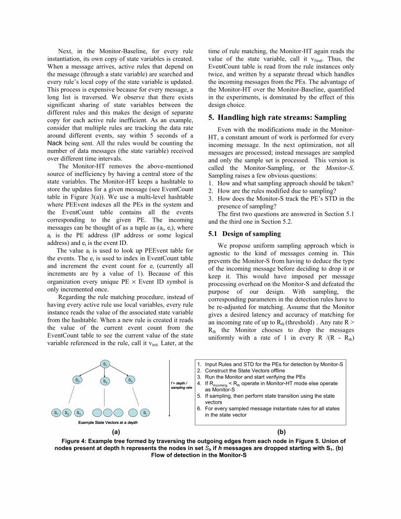
1. Input Rules and STD for the PEs for detection by Monitor-S 2. Construct the State Vectors offline 3. Run the Monitor and start verifying the PEs4. If Rincoming < Rth operate in Monitor-HT mode else operate

as Monitor-S5. If sampling, then perform state transition using the state

vectors 6. For every sampled message instantiate rules for all states

in the state vector

(a) (b)

Figure 4: Example tree formed by traversing the outgoing edges from each node in Figure 5. Union of nodes present at depth h represents the nodes in set Sh if h messages are dropped starting with S1. (b)

Flow of detection in the Monitor-S

messages. The behavior of the Monitor switches from the Monitor-HT to the Monitor-S because sampling kicks in after Rth. Since the messages being processed by the Monitor-S are a sample of the entire set of messages, the rules originally specified by the system administrator are not valid on the sampled stream.

Once a new sampling rate is chosen based on the incoming traffic rate, the rules are also modified. We keep the rule type the same but the constants get scaled according to the sampling rate. This is necessary because rules are defined according the normal operation of the PEs but, because of sampling, the Monitor-S is viewing an alternate sampled view of the operation of PEs. If the incoming rate is R and the threshold rate is Rth then the constants in the rules must be scaled by a factor of Rth/R. For example: if a rule states “receive 10 Acks in 100 sec” then because of sampling the rule is modified to “receive 10.(Rth / R) Acks in 100 sec”. This rate will be changed as and when the incoming rate is changed. We measure the incoming rate over non-overlapping time windows of length ∆ by counting the number of incoming messages in the window. At each rate computation, the new rate is compared with Rth and if it exceeds Rth then a new sampling rate is determined based on this new incoming message rate. To reduce the overhead of rate computation, ∆ is kept higher than the time period over which a rule is matched.

S1

S3

S4S2

e1e2

e3

e4e1

e1 e2e5

e5

e1

State Transition Diagram (STD)

S1

S3

S4S2

(a)Directed Graph

(b)

S1

S3

S4S2

e1e2

e3

e4e1

e1 e2e5

e5

e1

S1

S3

S4S2

e1e2

e3

e4e1

e1 e2e5

e5

e1

State Transition Diagram (STD)

S1

S3

S4S2

(a)Directed Graph

(b) Figure 5: A sample STD which is converted to a

directed graph by removing the event labels

5.2 STD transition with sampling If all incoming messages are not processed, this

will cause the Monitor-S to lose track of the current state of the PE. We modify the approach of STD transitioning at the Monitor-S such that instead of tracking the current state, the Monitor-S keeps a state vector S which contains all the possible states the given PE can be in S = {S1, S2….SK}. The reason for having multiple possible states is that the Monitor-S does not know which of several possible paths the PE has taken given a start state Sstart.

As a result of sampling, instead of knowing exactly which state the PE is in, the Monitor-S will know a possible set of states the PE is in (based on the

transition edges outgoing from the current state). For example: In Figure 5(a) if the current state is S1 and a packet is dropped then the next possible state is one of {S2, S3, S4}. To determine this set, the Monitor-S pre-computes the possible states which can be reached in steps of size 1, 2, 3 and so on. Each set of these states form the state vector S if 1, 2, 3 and so on messages are dropped. In other words if a single message is dropped starting from the start state Sstart, then S1 will consist of all the states Si such that Si has an incoming edge from Sstart in the graph. Si vector starting from state Sstart gives the state vector if i packets are dropped. Now given the rate of sampling one can transform one state vector S1 to another state vector S2. Let us say S0 = {Si | i ∈ (1, g); g is the number of nodes in the initial state vector} be the initial state vector. If the Monitor-S dropped one message then the new state vector S1 = {Sj | Si Sj is reachable using a single edge AND Si ∈ S0}. Similarly if 2 messages are dropped then S2 = {Sm | Sj Sm is reachable using a single edge AND Sj ∈ S1}.

The state vectors (S1 and S2) are created offline because the STD is already known to the Monitor-S. Figure 4(a) illustrates for the STD in Figure 5, a tree structure for maintaining the state vectors after different numbers of messages are dropped. Nodes at the depth h form the state vector Sh and represents the states after h messages are dropped starting from S1. At runtime, the Monitor-S tracks how many messages are dropped and looks up the appropriate state vector.

5.3 Error detection with sampling Figure 4(b) represents the flow of detection in the

Monitor-S when sampling is taking place. If the incoming rate is below Rth then no sampling occurs and the Monitor-S simply runs as the Monitor-HT. During sampling, the state transition is performed between various state vectors S which have been computed offline. When a message is sampled, all detection rules corresponding to that event ID and states in the current S are instantiated for matching. When messages are being dropped, the size of the state vector |S| increases. Once a message is sampled, the state vector is pruned since the message may not be valid for all the states in the state vector. Consider that the state vector is Sa- just before sampling and Sa+ just after sampling message M. Then Sa+ = {Si | Si ∈ Sa- and M is a valid message in state Si according to the PE’s STD}. Qualitatively, the sampling scheme will be beneficial only if the pruning in the size of the state vector is significant compared to the growth due to message drops. For example: let S initially consists of {S1, S2, S3} and the sampled message be e2. Then from Figure 5 we can see that only S2 and S3 can have

a valid event e2 and therefore the state vector becomes {S2, S3}.

This ambiguity about which state the PE is in and the design of using the entire state vector may give rise to false alarms since the Monitor-S may match some rules that are not applicable to the actual state the PE is in.

Computing the state vectors offline imposes a memory requirement on the system. If we assume that at most τ messages will be dropped by the Monitor-S then the offline computation should have state vectors up to Sτ. The total number of states in this state vector tree is given by k(kτ-1)/(k-1) assuming a k-regular structure of connectivity between the states. Thus the space required to store these state vectors is proportional to k(kτ-1)/(k-1). However the total number of states in the STD also imposes a cap on the size of the state vectors and prevents further increase in |S|. If there exists a ω s. t. kω> N (total states in STD), then the space required to store the state vectors is proportional to k(kω-1-1)/(k-1)+(τ-ω+1)N. The exact memory required is dependent on the data structure used to store these state vectors. Bit vector representation for storing them is an efficient option to reduce the overall memory used.

s*0

s8

Hello

s9

TimeOut

HelloReply

Resend Hello

Drop the PE

s*0

s1

Head Adv

s2

TimeOut

Resends Head Advs3

Head Bind

Accept/Reject

TimeOut

(a) (b)

s*0

s8

Hello

s9

TimeOut

HelloReply

Resend Hello

Drop the PE

s*0

s8

Hello

s9

TimeOut

HelloReply

Resend Hello

Drop the PE

s*0

s1

Head Adv

s2

TimeOut

Resends Head Advs3

Head Bind

Accept/Reject

TimeOut

(a) (b) Figure 6: Example State Transition Diagrams

(STDs); (a) TRAM sender adding new receivers in TRAM; (b) TRAM entities (sender, receiver, RH)

sending liveness messages (Hello)

6. Experimental setup

6.1 Application: TRAM We demonstrate the use of the Monitor on the

running example protocol ― a reliable multicast protocol called TRAM [6]. TRAM is a tree-based reliable multicast protocol consisting of a single sender, multiple repair heads (RH), and receivers. Data is multicasted by the sender to the receivers with an RH being responsible for local repairs of lost messages. The reliability guarantee implies that a continuous media stream is to be received by each receiver in spite of failures of some intermediate nodes and links. An Ack message is sent by a receiver after

every Ack window worth of messages has been received, or an Ack interval timer goes off. The RHs aggregate Acks from all its members and send an aggregate Ack up to the higher level to avoid the problem of Ack implosion (see Figure 2).

The multicast tree is formed via sender sending Head Advertisement messages and new nodes joining using the Head Bind message (see Figure 6(a)). Nodes ensure liveness of other neighbor nodes by periodically sending Hello messages as depicted in the STD shown in Figure 6(b).

The detection approach is provided with a rule base for detection which is derived from the STDs (shown in Figure 6). Some example of rules are as follows: R4 S4 E11 30 500 5000 S4 E2 1 8 4000 7000 If a Data message is seen then the Monitor must see an Ack message following it; T R4 S1 E9 1 2 1000 S1 E8 1 2 2000 3000: If the entity is in state S1 then the Monitor should observe one or more Head Bind messages followed by Accept message; T R3 S0 E14 10 30 5000: The number of Hello message within a time window should be bounded to prevent Hello flooding. A complete list of rules used in our experiments is provided in the Appendix A. It is evident from the set of rules that several of them verify the message count for the same message type (such as, Data, Hello, Ack). Therefore the redesign of the Monitor-HT of keeping only a shared writable copy of the state variables is likely to be beneficial.

6.2 Emulator In order to be able to study the performance of the

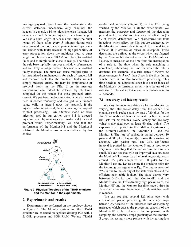
Monitor under high data rate conditions, we emulate the TRAM protocol [4][6]. This is necessary because operating multicast protocol across Purdue’s shared wide area network at a high data rate causes multiple switches to crash. The extra beacon messages sent out for advertising the multicast channel causes an overload of the LAN switches leading them to crash. In order to avoid this problem and to have the ability to perform experiments in a controlled environment, we emulate the topology of TRAM depicted in Figure 7. The emulated messages following the STDs in Figure 6 are forwarded to the Monitor.

6.3 Fault injection We perform random fault injection in the header of

the emulated TRAM messages to induce failures. In random injection we randomly choose a header field and change it to a randomly selected value. The randomly selected value may or may not be a valid field of the TRAM protocol. These errors model protocol errors which cannot be detected by simple measures like cyclic redundancy check (CRC) on the

message payload. We choose the header since the current detection mechanism only examines the header. In general, a PE to inject is chosen (sender, RH or receiver) and faults are injected for a burst length. We use a burst length of 500 ms and inject the burst length of faults after every 5 minutes during each experimental run. For these experiments we inject only the sender with faults because of high probability of error propagation down the multicast tree. A burst length is chosen since TRAM is robust to isolated faults and to mimic faults close to reality. The rules in the rule base typically run over a window of messages and are likely to not get violated because of an isolated faulty message. The burst can cause multiple rules to be instantiated simultaneously for each of sender, RH and receiver. Note that the emulated faults are not simply message errors, but may be symptomatic of protocol faults in the PEs. Errors in message transmission can indeed be detected by checksum computed on the header but these protocol errors cannot. We perform random injection where a header field is chosen randomly and changed to a random value, valid or invalid w.r.t. the protocol. If the injected value is not valid, then the message is dropped without processing. An alternate mode of error injection used in our earlier work [1] is directed injection whereby messages are transformed to a valid protocol value. Experimentally, we find that the performance of the Monitor-HT and the Monitor-S relative to the Monitor-Baseline is not affected by this choice.

r2

r3

RH

r1

RH

………

LM

GMmin.ecn.purdue.edu

dcsl-lab

Packet Forwarding

S

S: Sender (TRAM)RH: Repair Head (TRAM)

GM: Global MonitorLM: Local Monitor

r2

r3

RH

r1

RH

………

LM

GMmin.ecn.purdue.edu

dcsl-lab

Packet Forwarding

S

S: Sender (TRAM)RH: Repair Head (TRAM)

GM: Global MonitorLM: Local Monitor

Figure 7: Physical Topology of the TRAM emulator and the Monitor in the experiments

7. Experiments and results Experiments are performed on the topology shown

in Figure 7. The Monitor system and the TRAM emulator are executed on separate desktop PCs with a 2.4GHz processor and 1GB RAM. We use TRAM

sender and receiver (Figure 7) as the PEs being verified by the Monitor in all the experiments. We measure the accuracy and latency of the detection procedure for the Monitor. Accuracy is defined as (1- % of missed detections). We characterize the fault injections which affect the PEs but are undetected by the Monitor as missed detections. A PE is said to be affected if it crashes or raises an exception. False detections are defined as the errors which are flagged by the Monitor but do not affect the TRAM entities. Latency is measured as the time from the instantiation of a rule to the time when the rule matching is completed, subtracting the time for which the rule is dormant. For example, if a rule states “Observe 32 data messages in 5 sec” then 5 sec is the time during which there is no Monitor-related processing. This time needs to be subtracted since it is not an index of the Monitor’s performance; rather it is a feature of the rule itself. The value of ∆ in our experiments is set to 30 seconds.

7.1 Accuracy and latency results We vary the incoming data rate for the Monitor by

varying the inter-packet delay from the sender. The emulator sends packets at a low rate of 20 pkt/s for the first 30 seconds and then increases it. Each experiment run lasts for 20 minutes. Every latency and accuracy value is averaged over at least 60 data points. The experiment is repeated for three different systems i.e., the Monitor-Baseline, the Monitor-HT, and the Monitor-S. The rate of packets is varied between 10 pkt/s and 500 pkt/s. Figure 8(a) shows the variation of accuracy with packet rate. The 95% confidence interval is plotted for the Monitor-S and is seen to be very small indicating that the variance in the results is small. We can see that with an improved data structure the Monitor-HT’s knee, i.e., the breaking point, occurs around 125 pkt/s compared to 100 pkt/s for the Monitor-Baseline. Let us denote the breaking point for the incoming message rate as Rbp. The improvement of 25% is due to the sharing of the state variables and the efficient hash table lookup. The false alarms vary between 0-6% for both the Monitor-HT and the Monitor-Baseline. For extremely high packet rates, the Monitor-HT and the Monitor-Baseline have a drop in false alarms because the number of rule matches itself is reduced.

We can see that beyond 125 pkt/s even with efficient per packet processing, the accuracy drops below 40% because of the increased rate of incoming messages which causes the processing capacity of the Monitor-HT to be exhausted. In comparison, with sampling, the accuracy drops gradually as the Monitor-S drops increasingly more packets with increasing data

rate to maintain the rate below Rbp. We can observe from Figure 8(a) that with increasing packet rate the Monitor-S has a small decrease in accuracy but it still maintains accuracy at approximately 70% compared to the Monitor-HT’s 16% accuracy. The Monitor-S has a marginal increase in the rate of false alarms due to the knowing of the state vector rather than the precise state. The false alarms vary between 0-9%. At high data rates we observe lower false alarm rates for the Monitor-S compared to low data rates.

An example of a rule which does not get violated due to sampling resulting in loss of accuracy is R1 S0 E1 1000 S8 1500 2500. This rule verifies that for a TRAM PE (sender, receiver) the state has successfully changed to S8 from S1 after receiving E1 (Hello message). At high data rates if a large number of packets is getting dropped, it happens that S still contains state S8 causing this rule not be violated and hence decreasing the accuracy.

0

20

40

60

80

100

0 100 200 300 400 500

Acc

urac

y (%

)

Rate of Packets (Pkt/s)

Monitor (baseline)Monitor-HT

Monitor-S

(a)

0

200

400

600

800

1000

1200

0 100 200 300 400 500

Late

ncy

(ms)

Rate of Packets (Pkt/s)

Monitor (baseline)Monitor-HT

Monitor-S

(b)

Figure 8: Variation of (a) Accuracy and (b) Latency with increasing rate of packets

The latency plot in Figure 8(b) provides a similar

picture. The breaking points for the Monitor-Baseline and the Monitor-HT are the same as in the accuracy

plot – 100 pkt/s and 125 pkt/s respectively. For the Monitor-S, we can see a small jump in latency around 65 pkt/s (Rth in this experiment) because the algorithm switches to sampling and the probability of dropping a packet increases (being zero previously). This results in a higher overhead for processing each packet and the attendant marginal increase in latency. The processing done by the Monitor-S is proportional to |S| times the number of detection invocations. Increasing data rate causes higher |S| leading to higher latency of rule matching. However, the growth of |S| slows down with increasing packet rate causing the latency to saturate. We observe that even at high packet rates the Monitor-S maintains a low latency of rule matching (~200ms) because of effective adjustment to the sampling rate reducing the rate of packets that are processed. This provides an 83.3% decrease in latency compared to the latency of 1200ms for the Monitor-Baseline.

For a fixed Rth, as the data rate is increased, the size of the state vector |S| increases but it saturates at higher packet rates. The processing for the rule matching is directly proportional to |S|. Also, as the data rate is increased beyond Rth, the number of rule invocations of the Monitor-S stays constant. The latency is proportional to the total work done by the Monitor-S, which is given by: processing for the rule matching × number of rule invocations of the Monitor-S. Therefore, initially when the data rate is increased beyond Rth, the latency increases, but beyond a point, it saturates.

7.2 Effects of varying Rth Figure 9(a) depicts the behavior of accuracy and

latency for different values of Rth in the Monitor-S. Recollect that when the incoming message rate goes above Rth, the Monitor switches to the sampling mode. For all cases the accuracy is almost the same at high data rates and low data rates. Let us consider a single curve (say Rth = 50 pkt/s). For data rates below 50 pkt/s there is no sampling and since this threshold is much below the breaking point (125 pkt/s from Figure 1) the latency remains quite low (~65ms). As the data rate increases beyond 50 pkt/s, sampling starts and with increasing data rate an increasing number of packets is dropped. Difference in characteristics of the curve around Rth provides the system administrator a useful tuning parameter to choose a suitable latency value for the requirements of the distributed application. Clearly picking Rth > Rbp is unsuitable due to the spike in latency (see the 140 pkt/s curve). It is tempting to choose Rth as close to Rbp as possible (notice the delayed increase in latency for Rth = 100 pkt/s compared to Rth = 50 pkt/s). However, in practice

the breaking point cannot be exactly determined since it depends on the kinds of messages (and hence, the kinds of rules) that are coming into the Monitor. Thus the system administrator has to choose a Rth suitably below Rbp. For our experimental setup, if a latency of less than 100 ms is desired for data rates up to 100 pkt/s, then Rth of 100 pkt/s is an appropriate choice.

When Rth is 140 pkt/s, i.e., greater than the breaking point (125 pkt/s), it causes a heavy load and higher latency of matching for the region (125 pkt/s, 140 pkt/s). But as the run of experiment continues, sampling starts and this brings down the average latency to just over 300ms. The jump in the latency is because the incoming rate is close to the Rth because of which the Monitor switches between sampling and non-sampling modes. However in the non-sampling mode, since incoming rate is greater than Rbp, the Monitor-S incurs a high latency. This oscillation between the modes happens when the rate is close to Rth which explains the high latency (275-330 ms) around the incoming message rate of Rth.

0

20

40

60

80

100

0 100 200 300 400 500

Acc

urac

y (%

)

Rate of Packets (Pkt/s)

50 Pkt/s65 Pkt/s

100 Pkt/s

(a)

0

50

100

150

200

250

300

350

0 100 200 300 400 500

Late

ncy

(ms)

Rate of Packets (Pkt/s)

50 Pkt/s65 Pkt/s

100 Pkt/s140 Pkt/s

(b)

Figure 9: Effect of Rth on the (a) Accuracy and (b) Latency

7.3 Variation of state vector size (|S|) As described before, the amount of processing

done by the Monitor-S is dependent on size of state vector i.e., |S|. We investigate the variation of |S| with time in an experimental run. In this experiment we keep the Rth fixed at 65 pkt/s and run the emulator to provide an incoming rate of 250 pkt/s. This experiment is targeted at bringing out the dynamics of the Monitor-S when the incoming message rate is higher than the breaking point, forcing sampling to kick in. For this configuration, approximately one in four packets is sampled. Figure 10 shows the variation of |S| with time. We measure the size of state vector once every 2 packets. Instead of displaying the entire run of 20 minutes, we pick a representative 100 contiguous samples of |S|. We can see the large fluctuations of |S| due to the sampling. We can see that |S| grows to as large as 10, multiple times during the experimental run. The number of rules which get instantiated for each packet is proportional to |S|. However the rules get instantiated after a message is sampled. When a message is sampled, it will likely cause |S| to decrease because all the states in S do not have the message as a valid message in that state. Thus the rule instantiations take place at the troughs and not at the peaks of the plot in Figure 10. We can see that in Region 1, |S| drops in steps from 9 to 6 and finally to 1. The drop in |S| is because of the unique possibility of the sampled event in only some of the states.

Region 1

Region 2 0

2

4

6

8

10

0 20 40 60 80 100

Sta

te v

ecto

r siz

e

Time (seconds)

Rate=250 Pkt/s, Rth = 65 Pkt/s

Figure 10: Variation of State size S in a sample run

|S| can also remain the same if the dropped event

corresponds to some self-loops. This explains the small plateaus in Region 2. In Region 2, |S| increases from 1 to 3 because of a message drop. It stays at 3 even with further message drops and then reduces to 1 with a newly sampled message.

8. Related research Change Detection in Networking: Recently there is an increased effort in finding changes in high throughput network streams. Scalability is an important challenge in such environments. Authors in [16] propose a sketch based approach. Sketch is a set of hash tables which provides probabilistic guarantees compared to a single hashtable which provides 100% accuracy (assuming no collisions)[18] . The authors build a forecast model for the streams based on the observed data in the Sketch. Differences in the forecasted values and actual stream values are flagged as errors and reported. In [14][15] authors extend the sketch based approach of [16] providing reversibility to identify the streams which have changed. Authors in [15] provide an efficient reversible-hashing scheme to quickly identify the streams which have significantly changed. The paper also generalizes the approach provided in [14]. In all of the above approaches the central idea is to obtain a statistical model of the stream. The new incoming values of the stream is matched against this statistical model to find errors. In comparison, the sampling approach presented in this paper aims to maintain a closer application state. Detection provided by the Monitor is at a much different granularity as compared to approaches in [14][15]. The Monitor provides a much finer detection granularity. Statistical properties like mean and variance used in [14] do not account for spikes which the Monitor-S handles effectively. Authors in [17] provide an efficient way of performing sampling to obtain φ-quantile approximation of the incoming stream but the paper does not address fault detection. Stateful Detection: The issue of stateful detection has received attention from the security community due to the prevalence of attacks that are spread over multiple packets necessitating intrusion detection systems (IDS) to build state over multiple packets. The popular IDS Snort has an IP fragmentation-reassembly module which assembles fragmented IP packets. Also, for TCP packets, it has a stream4 reassembly module that can aggregate TCP packets within the same TCP session (like a FTP session) into a conglomerate pseudo packet. After this, the same pattern-matching algorithm is employed on the pseudo packet. The WebSTAT system [20], which builds on STAT, provides stateful intrusion detection for web servers. WebSTAT operates on multiple event streams, and is able to correlate both network-level and operating system-level events with entries contained in server logs. Our previous work on VoIP IDS, called SciDive [19], built a stateful detection engine for VoIP with state being spread across multiple signaling packets (SIP packets)

or data packets (RTP packets) or across the two protocols. All this work is targeted at specific protocols and its state aggregation and matching are therefore restricted to the domain. The Monitor sampling approach would not be suitable for intrusion detection in scenarios where a single packet can contain the event of interest. In such a scenario, the Monitor has to operate in the non-sampling mode. However, when the intrusion depends on behavior in aggregate (such as, flooding based denial of service), then the sampling approach is suitable. The attempts to make stateful intrusion detection scalable have concentrated on making per packet processing efficient, possibly with the addition of hardware nodes and reducing coordination traffic. [21][22] present a scalable stateful IDS which shares the load of processing messages through multiple hosts using commodity hardware. This approach requires the presence of more detection systems (called sensors) in comparison with ours, where one local Monitor handles detection in multiple entities in the network. Detection in Distributed Systems: Previous approaches of detection in distributed systems have varied from heartbeats, watchdog etc [8]-[10]. There is previous work [11][12] that has approached the problem of detection and diagnosis in distributed applications modeled as communicating finite state machines. The designs have looked at a restricted set of errors (such as, livelocks) or depended on alerts from the PEs themselves. A detection approach using event graphs is proposed in [13], where the only property being verified is whether the number of usages of a resource, executions of a critical section, or some other event globally lies within an acceptable range. Similar observer-observed framework is also presented in [3]. These approaches have focused on accuracy of fault detection and not scalability. Some approaches have focused on scalability but assume simpler failure semantics such as crash failures [23]. Although it is shown that this approach can scale well in large applications by a hierarchical algorithms [24], it can only detect a restricted set of application failures compared to the Monitor’s sampling approach. Other approaches have focused on detection in a distributed manner where failure detectors are embedded in the application component on each node [25].

9. Conclusion In this paper we presented a novel approach of

performing stateful detection in high data rate scenarios. We extend an existing detection approach (the Monitor) by identifying inefficiencies in the rule matching process and proposing a sampling approach to reduce the rate of incoming packets to be examined

for rule violations. We modify the data structure to produce the Monitor-HT (HT for hashtable) which leverages the commonality of messages in rules being matched for detection. The Monitor-S (S for sampling) uses a novel approach to incorporate sampling of the incoming stream while performing suitable modifications to the detection rules. We measure the performance of the Monitor-S and the Monitor-HT against the Monitor-Baseline on a multicast protocol TRAM. The efficiency of the new data structure causes the Monitor-HT to break at 125 pkt/s as compared to 100 pkt/s in the Monitor-Baseline. The Monitor-S outperforms the Monitor-Baseline via achieving a much higher accuracy with lower latency of rule matching at high packet rates (up to 500 pkt/s).

We are currently working on providing theoretical guarantees on the new sampling approach. We are also designing algorithms that will let the Monitor detect when it has lost track of the application state due to the sampling and is consequently suffering from high false and missed alarms. In such a case, several successive messages will be sampled to come back in sync with the application.

10. References [1] G. Khanna, P. Varadharajan, and S. Bagchi, “Self

Checking Network Protocols: A Monitor Based Approach,” In Proceedings of the 23rd IEEE Symposium on Reliable Distributed Systems (SRDS ’04), pp. 18-30, October 2004.

[2] M. Diaz, G. Juanole, and J.-P. Courtiat, “Observer-A Concept for Formal On-Line Validation of Distributed Systems,” IEEE Trans. on Software Engineering, vol. 20, no. 12, pp. 900-913, Dec 1994.

[3] M. Zulkernine and R. E. Seviora, “A Compositional Approach to Monitoring Distributed Systems,” IEEE International Conference on Dependable Systems and Networks (DSN'02), pp. 763-772, Jun 2002.

[4] D. M. Chiu, M. Kadansky, J. Provino, J. Wesley, H. Bischof, and H. Zhu, “A Congestion Control Algorithm for Tree-based Reliable Multicast Protocols,” In Proceedings of INFOCOM ’02, pp.1209-1217, 2002.

[5] S. Kliger, S. Yemini, Y. Yemini, D. Ohsie, and S. Stolfo, “A coding approach to event correlation,” Intelligent Network Management, pp. 266-277, 1997.

[6] http://www.experimentalstuff.com/Technologies/JRMS/ [7] G. Khanna, P. Varadharajan, and S. Bagchi,

“Automated Online Monitoring of Distributed Applications through External Monitors,” In the IEEE Transactions on Dependable and Secure Computing (TDSC), vol. 3, no. 2, pp. 115-129, Apr-Jun, 2006.

[8] W. Chen, S. Toueg, and M. K. Aguilera, “On the Quality of Service of Failure Detectors,” In IEEE International Conference on Dependable Systems and Networks (DSN'00), pp. 191-201, Jun 2000.

[9] R. Baldoni, J.-M. Helary, and M. Raynal, “From Crash Fault-Tolerance to Arbitrary-Fault Tolerance: Towards a Modular Approach,” In IEEE International Conference on Dependable Systems and Networks (DSN'00), pp. 273-282, Jun 2000.

[10] S. Krishna, T. Diamond, and V. S. S. Nair, “Hierarchical Object Oriented Approach to Fault Tolerance in Distributed Systems,” In Proceedings of IEEE International Symposium on Software Reliability Engineering (ISSRE ’93), pp. 168-177, Nov 1993.

[11] B. Berthomieu and M. Diaz, “Modeling and Verification of Time Dependent Systems using Time Petri Nets,” IEEE Trans. on Software Engineering, vol. 17 , no. 3 , pp. 259-273, Mar 1991.

[12] W. Peng, “Deadlock Detection in Communicating Finite State Machines by Even Reachability Analysis,” IEEE Conference on Computer Communications and Networks (ICCCN), pp. 656-662, Sep 1995.

[13] L. B. Chen and I-C. Wu, “Detection of Summative Global Predicates,” IEEE Conference on Parallel and Distributed Systems (ICPADS '97), pp. 466-473, Dec 1997.

[14] G. Cormode and S. Muthukrishnan, “What's new: finding significant differences in network data streams,” In INFOCOM 2004, Vol. 3, pp 1534- 1545, 2004.

[15] R. Schweller, Y. Chen, E. Parsons, A. Gupta, G. Memik, and Y. Zhang, “Reverse Hashing for Sketch-based Change Detection on High-speed Networks,” In INFOCOM 2006, pp1-12, April 2006.

[16] B. Krishnamurthy, S. Sen, Y. Zhang, and Y. Chen, “Sketch-based Change Detection,” In ACM Internet Measurement Conference, IMC, 2003.

[17] G. Singh Manku and R. Motwani. "Approximate Frequency Counts over Data Streams". VLDB, 2002.

[18] N. Alon, Y. Matias, and M. Szegedy, “The space complexity of approximating the frequency moments,” In Proceedings of the twenty-eighth annual ACM symposium on Theory of computing, p.20-29, May 22-24, 1996.

[19] S. Bagchi, Y. Wu, Sachin Garg, N. Singh, and T. Tsai, “SCIDIVE: A Stateful and Cross Protocol Intrusion Detection Architecture for Voice-over-IP Environments,” At IEEE Dependable Systems and Networks (DSN 2004), June 28-July 1, 2004, Florence, Italy.

[20] G. Vigna, W. Robertson, V. Kher, and R.A. Kemmerer, “A Stateful Intrusion Detection System for World-Wide Web Servers,” In Proc. of the Annual Computer Security Applications Conference (ACSAC), 2003.

[21] M. Vallentin, R. Sommer, J. Lee, C. Leres, V. Paxson, B. Tierney, “The NIDS Cluster: Scalable, Stateful Network Intrusion Detection on Commodity Hardware,” Proc. of the Symp. on Recent Advances in Intrusion Detection (RAID), Queensland, Australia, September 2007.

[22] V. Paxson, “Bro: A System for Detecting Network Intruders in Real-Time,” Computer Networks 31(23–24) (1999) 2435–2463.

[23] M. Bertier, O. Marin, P. Sens, “Performance analysis of a hierarchical failure detector,” Proc. of the Int. Conf. on Dependable Systems and Networks (DSN), 2003.

[24] Gupta, R van Renesse, KP Birman, “Scalable fault-tolerant aggregation in large process groups,” In Proc. Conf. on Dependable Systems and Networks (DSN), 2001.

[25] R van Renesse, Y Minsky, M Hayden, “A gossip-style failure detection service,” Middleware, 1998.

Appendix A. Rule base T R4 S4 E11 30 500 5000 S4 E2 1 8 4000 7000: The rule has a precondition to check data packets (E11) arrival within 5000msec. This causes the post condition that at least one ack(E2) (between 1 and 8) must be sent. T R3 S5 E13 0 2 5000: This rule ensures that the number of re-affiliation packets (E13) is no more than 2 within 5000ms in state S7. T R3 S5 E15 0 10 5000: Restrict the Nacks (E15). T R4 S0 E11 2 50 500 S4 E2 1 2 5000 7000: T R4 S5 E13 2 500 5000 S6 E9 1 4 4000 9000 T R3 S0 E1 10 30 5000: This rule of type 3 checks for the hello packet(E1) rate. The E1 message count should be between 10 and 30 for the next 5000 msec. T R4 S0 E1 1 2 1000 S8 E14 1 2 2000 3000: Hello messages should be followed with Hello replies T R3 S0 E14 10 30 5000: T R1 S0 E1 1000 S8 1500 2500: T R1 S0 E10 1000 S8 1000 3500: T R2 S0 E10 50: This rule verifies that state of the receiver changes from S0 once Head Adv is received T R4 S0 E10 1 4 1000 S1 E9 1 2 2000 3000: Head Adv. messages should be followed by Head Bind T R4 S0 E10 1 4 1000 S3 E8 1 2 3000 4000: Head Adv. messages should be eventually followed by Accept message T R4 S1 E9 1 2 1000 S1 E8 1 2 2000 3000: T R3 S1 E9 1 10 5000: T R3 S2 E8 1 2 10000:

B. Rule types in the Monitor and TRAM

messages 1. Type I: (ST=Sp) = true for T∈(tN, tN+k) ⇒ (ST=Sq) = true for T∈(ti, ti+b), where T represents the global time at the Monitor, ti > tN, and k, b≥ 0. The above rule represents the fact that if for some time interval k starting at tN, a node is in state Sp i.e., the state predicate ST=Sp is true, then it will cause the system to be in another state Sq for some time b

starting from time ti. The time tN is when state changes to Sp, irrespective of which event causes the transition. This rule is defined completely in terms of states of the entity and no events or state variable. 2. Type II: St is the state predicate of an object at global time T : St ≠ St+∆, if event Ei takes place at t, the state St will not remain constant for ∆ time units from t. 3. Type III: L ≤ |Vt| ≤ U ; t∈( ti,ti +k); The state variable Vt in a particular state Si will have its count bounded by L and U over a time window of k starting at time ti when the defined event corresponding to the rule first occurs. 4. Type IV: ∀t∈(ti,ti +k), L ≤ |Vt| ≤ U ⇒ L’ ≤ |Bq| ≤ U’ , ∀q∈(tn, tn+b); tN > ti ; If a state variable Vt has a bounded count from above and below over a time window k, it will cause another state variable Bq to be bounded for a time window b starting from tn. This rule is in fact the master rule and the three previous rule types are special cases of it. But we still need the first three rule types because matching this class of rule entails matching more variables, which increases the latency of detection. 5. Type V: If s = Si ∀t∈(ti,ti +k) ⇒ s≠ Si ∀t∈(tN, tN+a) ; tN > ti. This rule prevents a state transition back in state Si within some time of first arriving at Si.

E13Join a new Repair Head; sent by the receiver

Sender(RH), Receivers(RH)

Re-affiliation

E1, E14Indication of Liveliness of the members.

RH(Receiver), Receiver(RH)

Hello Messages (Reply)

E4Message sent by a receiver seeking to join a group when group formation is started by receiver.

Receiver, RH(Sender)

Member Solicitation

E2 (E15)Aggregate Acknowledgement sent by the receiver to the repair head.

Receiver, Repair Head(Sender)

Ack Packet (NackPacket)

E7, E8Acceptance or Rejection message sent by the repair head to the seeking receiver.

Repair Head(Sender), Receiver(RH)

Accept/Reject

E9Receiver sends a request to join group in the form of Head Bind

Receiver, Repair Head(Sender)

Head Bind

E11Multicast Data sent from head to group members

Sender(RH), Receivers(RH)

Data

E10Repair Heads send advertisement of the channel

Sender(RH), Receivers

Head Adv.

Event ID

Interpretation(Source, Destination)

Message Name

E13Join a new Repair Head; sent by the receiver

Sender(RH), Receivers(RH)

Re-affiliation

E1, E14Indication of Liveliness of the members.

RH(Receiver), Receiver(RH)

Hello Messages (Reply)

E4Message sent by a receiver seeking to join a group when group formation is started by receiver.

Receiver, RH(Sender)

Member Solicitation

E2 (E15)Aggregate Acknowledgement sent by the receiver to the repair head.

Receiver, Repair Head(Sender)

Ack Packet (NackPacket)

E7, E8Acceptance or Rejection message sent by the repair head to the seeking receiver.

Repair Head(Sender), Receiver(RH)

Accept/Reject

E9Receiver sends a request to join group in the form of Head Bind

Receiver, Repair Head(Sender)

Head Bind

E11Multicast Data sent from head to group members

Sender(RH), Receivers(RH)

Data

E10Repair Heads send advertisement of the channel

Sender(RH), Receivers

Head Adv.

Event ID

Interpretation(Source, Destination)

Message Name