State Regulations, Job Search and Wage Bargaining: A Study in the Economics of the Informal Sector

THE WILLIAM DAVIDSON INSTITUTE AT THE UNIVERSITY OF MICHIGAN BUSINESS SCHOOL

State Regulations, Job Search and Wage Bargaining: A Study in the Economics of the Informal Sector

By: Maxim Bouev

William Davidson Institute Working Paper Number 764 April 2005

State Regulations, Job Search and Wage Bargaining:

A Study in the Economics of the Informal Sector

Maxim BouevSt.Antony’s CollegeOxford OX2 6JF

[email protected]

April 3, 2005

Abstract

This paper analyses the emergence of the informal economy in the environment characterisedby non-competitive labour markets with wage bargaining. We develop a simple extension of thestandard search model à la Pissarides (2000) with formal and informal sectors to show howa government’s auditing of informal firms and barriers to firms’ entry erected in the formalsector by corrupt bureaucracy can make for stable coexistence of formal and informal jobs inthe long term. In equilibrium, wage differentials for homogeneous and risk-neutral workersemerge because different types of jobs have different lifetimes and/or have different creationcosts. The former are explained by the auditing activities of the government that in the simpleset-up destroy informal matches, while keeping formal jobs intact; the latter are due to varyingcapital costs, or costs associated with red tape and bureaucratic extortion (bribing). Searchfrictions introduce rent sharing between firms and workers in both formal and informal sectors.This has an important implication for policy making. In particular, we show that if ceterisparibus a firms’ bargaining position vis-à-vis workers is stronger in the formal rather than inthe informal sector, governments can afford to appropriate a larger part of a productive matchsurplus (e.g. by levying higher taxes), without endangering the qualitative outcome in the longrun. Rent sharing also implies that both formal and informal sector employees may receivewages above marginal product. We investigate efficiency properties of an equilibrium withformal and informal jobs and discuss the role of the government in creating and eliminatingsuch inefficiencies partially arising from a version of the hold-up problem (Grout, 1984). Somelessons are drawn for normative analyses of policies aimed at reduction of informality in set-upswith non-competitive labour markets. In particular, the conditions are given under which areduction in size of the informal sector is likely to be detrimental for economic welfare.

JEL classification: E24, E26, H26, J31, J41, J42, J64, O17Keywords: informal economy, regulations, wage bargaining, labour markets, search models0 I am grateful to Margaret Stevens for numerous fruitful discussions of various versions of this paper. Comments

by participants of the Gorman Workshop in Oxford, May 2002, and the Unofficial Economies in Transition Conferencein Zagreb, October 2002, were often very helpful. The work has undoubtedly benefited from remarks by PhurichaiRungcharoenkitkul, Edgar Feige, Klarita Gërxhani. Irina Denisova has provided very helpful insights into the Russian

1

1 Introduction

An increase in the size of informal sectors all over the world has recently been the focus of a debate

in many studies. The situation in OECD countries since 1960 has been analysed by Schneider (2000,

2001) and Schneider and Enste (2000) who point to the fact that for all countries investigated the

informal economy has reached a remarkably large size. Other authors note that in most transitional

countries of Eastern Europe (CEE) and the former Soviet Union (FSU) the irregular sectors have

been growing over the last 15 years too (see, e.g., Johnson et al., 1997; Lackó, 2000; Feige and

Urban, 2003). In such countries as Georgia, Russia, and Ukraine an increase in the share of the

informal sector has been especially notable and its persistent character is clearly observed. As

regards CEE and FSU countries, the primary motivation for this essay, it has been argued that the

increase may well be a transitional feature en route to the market economy, prompted by an increase

in unemployment at the start of economic reforms in the region (Bouev, 2004). At the same time,

long-run strengthening of informality should not be excluded. In the main the literature on the

informal sector is yet to do much work in dotting the i’s and crossing the t’s as regards preconditions

and mechanisms leading to stable coexistence of formal and informal sectors in the longer term.

Generally, it is held that it is the burden of governmental regulations of various nature that

forces firms and entrepreneurs to move underground. The ratio of reported to unreported activities

depends largely on costs and benefits of operating in each economy (Kaufmann, 1997), which often

are derivatives of governmental actions as can be seen from the discussion in, for example, de Soto

(1989) and Loayza (1996). Schneider and Enste (2000) and Boeri and Garibaldi (2001) point, in

particular, to the constraints on formal firms in labour markets - the fact that leads to an increase

in size of the underground labour force (see Schneider, 2000, 2001).

According to Castells and Portes (1989), considerations of labour costs are among the most

important factors forcing entrepreneurs to "go shadow" across the globe. Significant wage differ-

entials between formal and informal sectors are a notable stylised fact (see Mønsted, 2000, and

Gindling and Terrell, 2004 for evidence from some developing countries, while Kolev, 1998, and

Roshchin and Razumova, 2002, report on the situation in Russia). Part of these differences is

explained by minimum wage laws and productivity differentials.1 However, in many FSU countries

minimum wages are not binding, while both formal and informal jobs can often coexist in the

same enterprises, and workers can receive part of their salary in black cash - "under the table", so

that the "productivity gap" explanation is not applicable. Such facts suggest that the interaction

of firms and employees in the labour market is especially worthy of attention in addressing the

questions of emergence and development of the irregular sector. Nonetheless, as noted in Kolm and

Larsen (2004), the previous theoretical research on informal economies has been mainly conducted

labour market. Finally, I am indebted to N M Rothschild & Sons Ltd., London, for their financial support. Otherusual caveats apply.

1Productivity differentials are traditionally used in modelling of the formal-informal segmentation - for examplessee Agénor and Aizenman (1999), Friedman et al. (2000), or Boeri and Garibaldi (2001).

2

within the public finance tradition. In that literature labour markets are competitive, while wages

are either assumed fixed or determined by market clearing. In such a framework the burden of

regulations cannot cause formal-informal segmentation unless specific assumptions are made about

preferences or risk attitudes of workers, heterogeneity of the labour force, built-in technological

externalities, etc. Modelling of those aspects has received all the attention of researchers, while

the issue of wage formation is effectively left out. As discussed later on in this work, such ad

hoc assumptions are not always justified by evidence. However, dropping them would imply that

economic agents just choose the sector where the effect of regulations is least onerous. Thus, in

that literature a non-corner equilibrium with both sectors is effectively presupposed, while the role

of labour costs in the formal-informal split is neglected.

Recently it has become popular to invoke the theory of search in the labour market to model

the formal-informal duality (Kolm and Larsen, 2001, 2004; Boeri and Garibaldi, 2001; Bouev,

2002; Fugazza and Jacques, 2004). The focus of those studies has been mainly the effect of various

governmental policies on the size of the informal sector and the level of involuntary unemployment.

The models suffer from a great number of parameters, and are often built around the same specific

assumptions as are made in earlier studies, which sometimes adds a lot to complication of the work.

At the same time, in our opinion, they camouflage a rather simple mechanism that can make for

the emergence of the long-term formal-informal split of the labour market, even when workers are

assumed to be homogeneous, risk-neutral, and there are no presupposed technological externalities.

In this work we look into the interaction of firms and workers in the non-Walrasian labour

market to see a) if wage bargaining and search can be conducive to the emergence of informal

labour markets in the long term, and b) where the government regulations blamed for being a

main cause of informality fit in with this framework. In such labour markets productive matches of

firms and workers are costly, they take time to accomplish, while wages are determined in bilateral

negotiations. Following Loayza (1996) we distinguish two types of government regulations that

affect the result of the bargaining and, hence, the equilibria in our model. First, it is the measures

that impact on the costs of functioning in a particular sector. Such policies, as for example,

taxes or social security contributions in the formal economy, and penalties for running business

underground in the informal sector, determine the size of the surplus generated by a productive

match and subject to sharing during wage bargains. In addition, auditing of informal firms by

the government generates asymmetries in match duration across sectors, which affects the values

of expected or averaged surpluses. Second, it is the activities of the low tier of the government,

such as bureaucracy that, if corrupt, can through red tape, license fees, extortion of bribes, and so

forth, erect artificial barriers to entry into the formal sector, and thus raise relative costs of access

to legality (see, also, de Soto, 1989; Djankov et al., 2002). In the presence of search frictions these

increase opportunity costs of vacancy posting for firms looking for workers in the labour market

and weaken firms’ outside option in wage negotiations. We show that as a consequence, when

3

entry costs differ and/or match lifetimes are not the same in the two sectors, wage differentials

can ensue in long-run equilibrium, thus leading to labour market segmentation. Search and rent

sharing are very important for this result, because without them the system would produce only

corner solutions. However, these features are inherent in labour markets of many countries and have

been confirmed for Eastern Europe, in particular (see Smirnova, 2003, and Roshchin and Markova,

2004, for evidence on time-consuming job search, and Grosfeld and Nivet, 1999, and Shakhnovich

and Yudashkina, 2001, on rent sharing). Thus, it can be concluded that wage bargaining in the

presence of costs of entry can be one of the main channels through which informality is brought

about. Having said that we compare our result with the previous studies of the informal economies,

stressing its independence of preferences of workers, and other assumptions mentioned above. This

work can certainly be extended to incorporate a great deal of those additional features, which would

not, however, diminish the role performed jointly by government regulations and wage bargaining

in the presence of costly search in splitting the labour market.

Having described the workings of and equilibria in our model, we turn to consideration of its

implications for policy making and welfare. The aforementioned studies of informality featuring

the non-competitive labour market with job search and costly matching often attempt a normative

analysis of policies aimed at reduction in the size of the shadow economy (see, e.g., Kolm and

Larsen, 2001; Bouev, 2002; Fugazza and Jacques, 2004). However, they do not take into account

a number of inefficiencies arising in the labour market that may well affect the conclusions of such

exercises as regards welfare improving measures. We show that labour market externalities arising

in such environments should not be expected to be internalised. In general, no equilibrium is

efficient in our model. One of the sources of welfare losses in this work is a version of Grout’s

(1984) hold-up problem, whereby workers appropriate part of return on firms’ start-up investment.

It is shown that while the first-best solutions are not likely, a benevolent government can achieve

sub-optimal allocations of resources. However, the upshot of standard policies, such as variation

in the tax rate, efficiency of monitoring of the informal firms, and the penalty rate, depends upon

the state of the labour market. In particular, the relation between the bargaining power of workers

and the elasticity of the matching function prominently figured in the Hosios efficiency condition

(Hosios, 1990) affects the ultimate effect on economic welfare. This point has been completely

overlooked in the previous research.

The essay is organised as follows. The next section provides a quick overview of the previous

theoretical literature on the informal sector, highlighting a few important soft spots, the main

of which is the absence of a proper account of the labour market, especially wage determination

process. Then Section 3 introduces a two-sector search model à la Pissarides (2000), solves it by

deriving steady state equilibria and discusses how state regulations lead to formal-informal wage

differentials and, hence, labour market segmentation. Implications for policies and their welfare

impact are discussed in Section 4. Section 5 concludes.

4

2 The Informal Sector: A Glimpse of the Literature

There exists an extensive literature concentrating on various aspects of informality. For the most

recent review the reader is referred to Gërxhani (2004), while the effects of regulations on the

emergence and development of the informal sector both from theoretical and empirical perspectives

are discussed in inter alia Kaufmann and Kaliberda (1996), Loayza (1996), Fortin et al. (1997),

Johnson et al. (1997), Friedman et al. (2000), etc. The large body of previous theoretical research,

however, has suffered from a few significant deficiencies, in our opinion. First, it does not make

clear whether the informal sector can exist in the long run, i.e. whether or not it is just a short-run

product of adjustment in the economy, after some sort of a shock has pulled it out of an equilibrium

state. Second, in many both static and dynamic models an interior equilibrium with both formal

and informal economies is often possible only due to a number of restrictive assumptions about the

utility function of workers, penalties for concealing income, etc. Finally, as regards mechanisms

whereby governmental regulations affect the segmentation of the economy, the literature has mainly

ignored the fact that the decision to ”go underground” is essentially a result of both employers and

employees interacting in the labour market. We briefly discuss these points below.

2.1 Long-run Informality

Empirically the existence of the informal sector provokes no doubt, whereas theoretical substan-

tiation of its existence, especially in the long run, has been not satisfactory. When modelling

informality researchers often restrict their attention to those ad hoc combinations of parameters

alone that generate interior equilibria with an informal sector in their models (see, e.g., Kolm and

Larsen, 2001). Their inattention to corner equilibria (which often are the most probable result),

i.e. equilibria with formal or informal sectors alone, is understandable: on the one hand, an equi-

librium with the formal sector alone does not allow analysis of informality, and, on the other hand,

an equilibrium with the informal sector alone is not conceivable as a realistic long-run outcome.2

At the same time, the reasons for or possibilities of emergence of interior equilibria (let alone their

stability) with both formal and informal sectors are not explained nor explored. However, the

existence of the informal sector can be a transitional phenomenon of adjustment in the economy as

shown, for example, by Bouev (2004) in a theoretical model for countries of Eastern Europe. The

2 In general, it is possible to think of a number of reasons why governments may be interested in increasing thenumber of official firms. Shleifer and Vishny (1998), for example, suggest that such reasons may emanate fromproperly organised fiscal systems, politicians’ desire to win greater support for elections, or direct financial interestsof politicians (shareholding). On the other hand, while the state itself can have stakes in enterprises, the firms canrepeatedly interact with public officials in their own turn. Such interaction may result from historical ability of somefirms to influence the government so that they enjoy considerable private gains. Other, de novo firms can engage inattempts to capture the state, i.e. make private payments to state officials to affect the rules of the game, as a strategyto compete with influential incumbents. In other words, powerful firms can collude with state authorities to extractrents through manipulation of state power (Hellman et al., 2000). Thus, all this suggests that in general conditionsleading to the emergence of corner equilibria with the informal sector alone should be considered as implausible.

5

underground sector can be around for some time, even when an economy converges to a long-run

steady state, where informality is not present eventually. Still, it begs the question of whether and

when the informal sector can stably coexist with the formal one in the long term. The conditions

for such coexistence, if any, are of great interest, in our opinion. A recent strand of endogenous

growth literature allowing for the informal sector (e.g., Loayza, 1996; Sarte, 2000) has partially

succeeded in showing that long-run mixed equilibria are indeed possible. Nevertheless, it either

imposes ad hoc restrictions leading to the existence of such outcomes (Loayza, 1996, models the

effective penalty rate for producing informally as an endogenous function of the relative size of the

informal sector), or is still lacking in a proper account of the labour market (Sarte, 2000).

2.2 Restrictive Assumptions

Dependence of the interior equilibrium on specific assumptions has also characterised other, less

recent, branches of the theoretical literature concerned with informality. For instance, in tax evasion

studies (for recent reviews see, e.g., Andreoni et al., 1998; or Slemrod and Yitzhaki, 2002), evasion

(and hence, the existence of underground activities) arises in a gamble where a risk-averse tax-

payer trades off the utility from tax savings and disutility of extra risk taken on of having her

income understatement detected by the authorities and penalised. The seminal Allingham and

Sandmo (1972) tax evasion model, for example, predicts that in a situation where individuals are

risk-neutral only corner solutions are possible - an individual would either do no evasion or remit

no tax at all. In the work on unrecorded activity emanating from Allingham and Sandmo (1972)

the equilibrium with coexisting recorded and unrecorded activities is possible only under certain

assumptions about the utility function, i.e., in particular, risk aversion of an individual.

In a similar vein, static models of labour supply to the formal sector and underground economy

are often based on restrictive assumptions about the utility function. This may include imperfect

substitutability of output from the compliant and evading sectors, heterogeneity of workers in

evasion costs (Kesselman, 1989) or skill levels (Sandmo, 1981). Interior equilibria in models with

home production or moonlighting (see, e.g., Becker, 1965; Gronau, 1977) are also a product of

the choice of a specific utility function, namely preferences over consumption, work in a particular

sector and leisure.

A specific choice of other functions, such as, for example, a probability of detection, that can

be made an endogenous function of the amount of unrecorded activities (Slemrod and Yitzhaki,

2002), have both characterised interior equilibria in the tax evasion literature mentioned above,

and featured in more recent work on underground economies (see, again, Loayza, 1996). The

main problem with this approach, however, as well as with the one where an interior equilibrium

hinges upon specific non-economic costs of evasion - moral considerations (Kolm and Larsen, 2001)

or psychic costs (Fugazza and Jacques, 2004), - is that viability and implications of such analyses

depend on the precise way the concepts are formalised (Andreoni et al., 1998; Slemrod and Yitzhaki,

6

2002).

All in all, although the contribution of the literature briefly considered here is undisputable,

especially in that it provides a useful framework for an investigation into the effect of various

governmental policies on the relative size and growth of the informal sector, the assumptions made

there do not always stand up to the evidence. For example, as regards different preferences over

formal and informal output it can be noted that some goods are produced in both the formal

and informal sectors, or/and individuals may have no clear idea if the supplier is operating in the

formal or the irregular sector (see, e.g., Thomas, 1992, Ch.8). Even when it is claimed that in

countries of, for example, Western Europe the informal sector is concentrated within particular

industries, such as services or construction, so that, on a large scale, different goods are produced

in the formal and informal sectors (Kolm and Larsen, 2004), in countries of Eastern Europe, and,

particularly Russia, this assumption may not be correct as the practice of informal contracts is often

widespread (Ingster, 2003). In relation to the dependence of an interior equilibrium with formal and

underground activities on the existence of moral or social considerations it should be stressed that,

although there is little dispute that those factors are important in individual compliance decisions,

but little is agreed upon on how best to incorporate these effects in a theoretical analysis (Andreoni

et al., 1998).

2.3 A Need for Labour Markets

Having said that, another substantial weakness in theory of the informal sector is still its lack of

proper attention to labour markets. Empirical facts such as a drop in participation rates (for a

discussion of situation in Eastern Europe see Boeri, 2000), widespread informal (not registered)

contracts (e.g., Haltiwanger and Vodopivec, 2002, and Ingster, 2003, mention such practices in

Estonia and Russia, respectively), significant formal-informal wage differentials (for Russian ex-

perience see Kolev, 1998; Roshchin and Razumova, 2002), beg for more research to be done in

the area. Mention by Castells and Portes (1989) of labour costs as one of the key factors causing

informality points to a special interest that should be attracted to revealing the role played by

wages in propagating the effects of governmental regulations and their impact on formal-informal

segmentation. However, as has been noted in the introduction, in the large body of the previous

work on informality wages are either treated as exogenous or assumed to be determined through

market clearing, i.e. no proper theoretical foundation has as yet been established in regard to that

role.

A few recent studies (Boeri and Garibaldi, 2001; Kolm and Larsen, 2001, 2004; Bouev, 2002;

Fugazza and Jacques, 2004) have made an attempt to incorporate the theory of search and matching

functions into the models with the informal sector. The focus of that literature is implications for

policies aimed at the reduction in informality and involuntary unemployment. At the same time,

they provide a hint that wage bargaining in the presence of costly search in the labour market may

7

serve as an important channel through which preconditions for formal-informal duality emerge.

In the next section we present a model of the informal sector, which serves to illustrate three

important moments, either not clearly stated or absent completely in the previous studies of the

informal sector. First, it shows that under a broad set of conditions the long-run equilibrium with

both formal and informal sectors is possible. Second, it highlights the role of the wage determination

process in shaping the equilibrium outcome. Finally, all the results are obtained in the absence of

many restrictive assumptions characterising much preceding work.

3 A Model of Informal Employment

The model developed in this section captures the impact of governmental regulations and labour

market institutions, such as wage bargaining, on sectoral reallocation of jobs and workers as well as

wage rates in an economy with formal and informal sectors. It is assumed that the labour market

in such an economy is characterised by risk-neutral firms and workers searching for each other to

form a match to start production. Search and rent sharing in the process of wage bargains are

crucial to the results we obtain. The approach is similar to that used by Acemoglu (2001) who

studied reallocation of labour across jobs with different capital costs. In this work we abstract from

goods and capital markets (both of which are assumed to clear) in order to highlight the joint effect

of state regulations, search frictions, and rent sharing on job composition, rather than on prices of

both capital input and final output.3

3.1 The Main Idea

The informal sector is seen as representing productive (not rent-seeking4) activities that are not

associated with crime or household production.5,6 Thus, we take the approach that views informal

employment as resulting from efforts of entrepreneurs to trade off costs and benefits of functioning

in compliance with formal regulations.

It is assumed that goods produced both in formal and informal sectors are perfect substitutes,

3See Kolm and Larsen (2004) for a general equilibrium model with wage bargaining and costly search where pricesabsorb part of the effect of governmental policies.

4Acemoglu (1995) and Acemoglu and Verdier (1998) study the allocation of talent between productive and rent-seeking activities. Vostroknutova (2003) extends their models to include an underground sector.

5 In the literature on informal activities it is normal to distinguish between household activities, informal sector,irregular sector and criminal sector (see, for example, Thomas, 1992). While the idea behind home production andcriminal activities should be obvious, one might become confused over the difference between informal and irregularsectors. Usually it is small workshops and self-employment which are regarded as the informal sector. It can alsocomprise home production that is traded in the market. All these activities are not illegal. The sector that weconsider in this model is indeed irregular, which comprises production of legal output, but involves tax evasion andavoidance of formal regulations. However, we will use both terms ”irregular” and ”informal” interchangeably. Othersynonyms used are the "shadow" or "underground" economy.

6On models of crime see inter alia Becker (1968), and Fiorentini and Peltzman, eds. (1995); on householdproduction see Becker (1965), and Gronau (1977).

8

while marginal productivity of formal and informal matches is the same. We do not go along the

lines of the prevalent view of the informal economy (see, for example, Agénor and Aizenman, 1999;

Boeri and Garibaldi, 2001) that assumes underground jobs to be less productive and, hence, paying

lower wages. We shall see that what is important for the conclusions we draw is not the differentials

in productivity but the differences in surpluses that formal and informal matches generate.

Both formal and informal firms have to sink some costs before opening a vacancy, meeting

a worker and starting production. Those can be capital costs, vacancy advertisement costs, or

bribes and other extortionary payments that firms have to bear before starting their businesses.

We assume that these costs are greater in the formal sector than in the informal one, which can

be explained by higher entrance barriers into the formal sector or access costs to legality (Loayza,

1996) associated with bribery, license fees and registration requirements (de Soto, 1989; Djankov

et al., 2002). In the appendix we muse on departures from this set-up. Another main conceptual

difference between the two sectors is in the relation to official regulations and costs associated with

them. To firms producing formally, and hence, abiding by the rules and regulations imposed by

the state, they imply additional costs of production such as, for example, taxes, social security

contributions, etc. (in what follows we refer to all such costs as "taxes" to keep things simple). On

the other hand, functioning informally does not involve those expenses. Jobs can be undeclared in

order to avoid costs of functioning openly. Although such concealment of production is possible it

is prosecuted by officials. Thus, each hiding firm faces some positive probability of being caught,

fined, and closed as a result of government monitoring or audit. This, in turn, implies that informal

matches on average last for a shorter time.

Workers in the model can either work formally or informally or be unemployed. We neglect

possibilities of moonlighting, so workers can perform only one activity at a time. Aggregate labour

supply is inelastic.

Once having met, workers and firms bargain over wages and, as a result, employees can ap-

propriate some rents. Given different entrance and production costs and varying average match

duration across sectors, rent sharing leads to equilibrium wage differentials. In turn, different labour

costs and different production surpluses in the two sectors provide an opportunity for the formal

and informal sectors to coexist in the long run. The equilibrium allocation of jobs and workers

in steady state is eventually determined by zero profit conditions as free entry in each sector is

assumed.

3.2 Matching Technology

In the absence of on-the-job search it is only the unemployed workers who look for jobs. We assume

that search is random or undirected, i.e. workers search for any employment and accept the first

job that offers them prospects at least as good as their currently expected life-time income. In

the presence of undirected search both formal and informal vacancies have the same probability of

9

meeting workers. Then it is the total number of vacancies that enters the matching function.

The number of job matches is given by M(n, v), where n is the number of workers seeking jobs

(i.e. the number of the unemployed) and v is the number of vacancies created in the economy.

With constant returns to matching, the instantaneous probability that a vacant job meets a

job-seeker is given by

M (n, v)

v=M

³nv, 1´= q (θ) ,

where θ ≡ vn .

The first derivative of the flow rate of matching for a vacancy, q0 (θ), is negative, becausethe greater is the value of θ the more difficult for firms it becomes to fill the job. In the matching

literature θ is referred to as market tightness from the firms’ standpoint (see, for example, Pissarides,

2000).

Similarly, the flow rate of matching for an unemployed worker is given by

M (n, v)

n=M

³1,

v

n

´= α (θ) = θq (θ) ,

where α0 (θ) > 0.When q (θ) <∞ and α (θ) <∞ then matching is not instantaneous and takes some time.

We will also make the additional Inada-type assumptions that limθ→∞

q (θ) = 0, limθ→0

q (θ) = ∞,limθ→∞

α (θ) =∞, and limθ→0

α (θ) = 0.

3.3 Formal and Informal Jobs

Jobs are created in either the formal or the informal sector. We do not necessarily define one job

as one firm by assuming constant returns in production. Before opening a vacancy a risk-neutral

firm has to decide in which sector the potential match will produce and, at this point, will have

to bear some costs. These costs are either kf or ki, if the firm is to open a vacancy in the formal

economy or underground, respectively. These start-up costs are incurred before the firm meets

its employees and can be thought of as capital expenditure, job advertisement costs as well as a

registration fee or bribes to be paid, for example, to prevent a delay in registration in the formal

sector or to guarantee security of the job in the informal sector.7 The important assumption we

make is that access to legality is more costly than access to informal production, i.e. kf > ki. In

other words, we postulate that the presence of extortion costs at the moment of entry in the formal

sector implies higher instant start-up costs to entrepreneurs (see de Soto, 1989, and Loayza, 1996,

for justification of this assumption). The latter are generally thought of as being wealthy enough

to meet the start-up costs without resorting to external credit.

7Gërxhani (2004) points out that, although the ease of entry is used by various researchers as one of the criterionfor defining the informal sector, entry costs into informality do exist.

10

All matches in the economy, either formal or informal, die at rate δ, in which case the job is

destroyed while the worker becomes unemployed.8

Both formal and informal jobs are equally productive. Wages are paid out of the match product,

y. In addition to wages, formal jobs have to pay a lump sum tax, τ , whereas informal jobs enjoy

tax evasion.

In the model it is implicitly assumed that there are some taxation authorities, e.g. the tax

police, whose aim is to collect taxes and reveal cases of tax evasion. So, there is an exogenous flow

probability m that an employer gets caught in engaging in underground business and fined by the

amount F . When m strikes the informal match is liquidated and the burden of the fine is borne

by the employer, not the employee. An alternative to match liquidation may be its continuation or

transformation into a formal match. However, if detected parties fear that continuing the match

either formally or informally would result in more frequent visits by the tax police, our assumption

of match destruction is reasonable9,10 (see, e.g., Kolm and Larsen, 2004).

The Bellman equation11 for a formal job is

rJf = y − wf − τ + δ (0− Jf ) , (1)

where r is the flow rate of return on having the job filled (the interest or discount rate), Jf is the

value of the filled formal job to the employer, and wf is the formal wage. The equation reads that

the return to the firm on a filled job in the formal sector is equal to the difference between worker’s

productivity and costs, plus a potential change in value in the case of the match break-up. At this

stage we shall assume very generally that the productivity of a match, y, is high enough to cover

wages and taxes, while more exact restrictions on parameters of the model are given in Section

3.6.2.

By analogy, for an informal job we have

8Alternatively, one can consider a situation when δ (or m - see below) strikes, the match is destoyed but the jobis not. That is, the job turns into a vacancy, rather than is liquidated. However, such alteration does not change thequalitative results of the analysis.

9Here we also exclude the possibility that firms can avoid penalties and liquidation by paying a bribe to the taxinspector. However, in reality the agents directly carrying out monitoring may often side-contract with firms, thusallowing the latter to evade payment of fines (see, e.g., Chander and Wilde, 1992, and Wane, 2000, for models ofcollusion between tax inspectors and tax evaders).10Safavian et al. (2001) note that visits of firms by the tax police are closely linked to corruption - regulatory

inspections are positively correlated with amount of bribes paid. Interestingly, tax authorities can often changeregulation without notifying entrepreneurs and then pay them a visit to obtain a fine or extorting a bribe foravoidance of restrictions implied by the regulation. Evidence suggests, however, that, e.g. in Russia, firms withhigher reservation profits (i.e., revenues allowing them to function just without making losses) are less likely to becharged excessive bribe payments and, hence, less likely to be checked by monitoring bodies. Above we have assumedthat kf is higher than ki, which in turn implies higher reservation revenues in the formal sector. Thus, in our modelthe absence of monitoring and fines in the formal sector can be justified not only by the nature of official functioning:it can also be interpreted in the light of the results obtained by Safavian et al.11Hereafter we consider only steady state values of the Bellman equations since the focus of the paper is the

irregular sector in the long run. Out of steady states each Bellman equation should be augmented to include a firsttime derivative of an appropriate value function.

11

rJi = y − wi −mF + (δ +m) (0− Ji) , (2)

where Ji is the value of the filled informal job and wi is the informal wage. The equation implies

that the return on a filled job in the informal sector is equal to the difference between the product

of the match and the worker’s wage, less an expected fine in the case of being caught by tax

authorities, plus a change in value due to the match cessation.

It is assumed that vacancy maintenance in either formal or irregular sector involves no flow

costs.12 Then the Bellman equations for vacancies in formal and informal sectors are:

rVf = q(θ)(Jf − Vf ), (3)

rVi = q(θ)(Ji − Vi), (4)

where q(θ) is the flow rate of filling a vacancy as defined above.

3.4 Workers

There is a fixed (normalised to 1, for convenience) mass of identical workers in the economy. They

are risk-neutral, have the same discount rate r as firms, and derive utility solely from the wage.

Workers can be either employed in one of the sectors or unemployed.

Formal employment provides workers with wage wf , so that the value of working formally

satisfies the Bellman equation

rEf = wf + δ(Eu −Ef ).13 (5)

It reads that the return on formal employment is equal to the wage income plus a change in

unemployment in case of the match break-up.

As informal employment brings in wage wi, by analogy we have

rEi = wi + (δ +m)(Eu −Ei). (6)

That is, the return on informal employment is equal to the wage income plus a potential change into

unemployment as a result of either the match cessation or job closure due to tax evasion detected

by the authorities.

Finally, the Bellman equation for the unemployed is

12 It can readily be shown that the presence of maintenance costs does not change the model qualitatively.13 In order to keep things simple, we neglect the impact of income taxes on the value of being employed in the

formal sector. At the same time there is evidence (e.g., Lemieux et al., 1994) on unimportance of taxes for sectorchoice.

12

rEu = bu + α(θ)(φ(Ef −Eu) + (1− φ) (Ei −Eu)), (7)

where bu is the unemployment benefit, φ is the probability of meeting a formal vacancy, 0 < φ < 1,

and α(θ) is the flow rate of finding a job in either sector. The equation says that the return on

being unemployed equals unemployment compensation plus a potential change into employment in

one of the sectors.

3.5 Wage Determination

Wages in the model are determined through a wage bargaining process with the bargaining power

of workers, β, given exogenously and such that 0 < β < 1. Then the Nash (1950) bargaining

solution implies:

(1− β) (Ef −Eu) = β (Jf − Vf ) , (8)

(1− β) (Ei −Eu) = β (Ji − Vi) . (9)

The Nash solution in this case assumes that the threat (reservation) points of employers and

employees are represented by the value of unfilled vacancy in an appropriate sector and the value

of unemployment, respectively. This implies that bargaining is actually ex post, i.e. it takes place

before the consummation of a match, but after a producer has opened a vacancy. Thus, firms

are assumed to commit to wages over which the consensus was reached: they cannot change the

contract once a worker gets employed.

3.6 Steady State Equilibria

It is assumed that entry in our economy is free, so that firms’ profits have to equal zero in equi-

librium. This implies that it should not be possible for an additional vacancy in both formal and

informal sectors to open and make expected net profits. Hence,

Vf = kf , (10)

Vi = ki. (11)

That is, the condition of zero profits implies that start-up costs equal to kf and ki in formal and

informal sectors, respectively, must be just recouped in equilibrium.

A steady state equilibrium in the model is characterised by the labour market tightness, θ, a

proportion of formal vacancies, φ, and by value functions Jf , Ji, Vf , Vi, Ef , Ei, and Eu, such

13

that equations (1)-(11) are all simultaneously satisfied. As we have assumed undirected search, in

steady state both formal and informal vacancies meet workers at the same rate and both types of

job are accepted if they offer a reward at least as large as a worker’s outside option.

In order to see what equilibrium allocations of jobs and workers are possible in our economy we

shall proceed through the analysis by re-expressing equations (10) and (11) as functions of θ and

φ, and then studying their behaviour in the (θ, φ)-plane.

3.6.1 Zero profit conditions

Solving (1) and (2) for Jf and Ji we arrive at

Jf =y − wf − τ

π, (12)

Ji =y − wi −mF

ρ, (13)

where π = r + δ and ρ = r + δ +m are the effective discount rates in formal and informal sectors,

respectively. These account both for the interest rate r (equal to the workers’ and firms’ rate of

time preference under risk neutrality) and "depreciation", δ or δ +m, which differs across the two

sectors.

Substituting these solutions together with conditions (10) and (11) for (8) and (9), and com-

bining the results with equations (5) and (6), simple algebra gives

wf = β (Sf + bu) + (1− β)rEu, (14)

wi = β (Si + bu) + (1− β)rEu. (15)

For readability of formulae in (14) and (15), and in the rest of the paper by Sf = y− τ − πkf − bu

and Si = y −mF − ρki − bu we denote the total flow surpluses of a match net of unemployment

benefits in the formal and informal economies, respectively. These equations imply that the worker

gets share β of the surplus of a match plus (1− β) times her outside option.

Having obtained the expressions for wf and wi, by using equations (12) and (13) together with

(3) and (4), we can define two functions Πf (θ, φ) and Πi (θ, φ) that represent profits made in the

formal and the informal sectors, respectively:

Πf (θ, φ) = Vf − kf =(1− β) q(θ)

(r + q(θ))π

µy − τ − πkf − rπkf

q (θ)− βrπkf(1− β) q (θ)

− rEu

¶, (16)

14

Πi (θ, φ) = Vi − ki =(1− β) q (θ)

(r + q (θ)) ρ

µy −mF − ρki − rρki

q (θ)− βrρki(1− β) q (θ)

− rEu

¶. (17)

From (7) it also follows that Eu = Eu (θ, φ) , i.e. the value of being unemployed is also a function

of the market tightness, θ, and the proportion of formal vacancies, φ.

Complicated as they are at first sight, the expressions (16) and (17) above allow, in fact, an

easy interpretation. The terms in brackets times either (1−β)q(θ)(r+q(θ))π orq(θ)

(r+q(θ))ρ give the expected rents

that formal and informal matches will generate when a firm and a worker meet. These rents are

shared between the two parties in a bilateral monopoly bargaining game (see, e.g., Shaked and

Sutton, 1984), so that in the end the firm gets share (1− β) of the rent according to its bargaining

power. Consider for example formal profit (16). After consummation the match generates product

y. Out of this product the firm has to: a) pay off taxes, τ ; b) cover start-up costs (taking account of

"depreciation"), πkf ; c) cover opportunity costs of having kf units of resources invested in creation

of this particular vacancy, rπkfq(θ) (i.e. the vacancy that on average costs πkf , will be idle until it meets

a worker after an average time of search, 1q(θ) , elapses - all this can be invested elsewhere at rate

r); d) pay a premium to a hired worker for saving of opportunity costs that the representative firm

enjoys when a job is formed, βrπkf(1−β)q(θ) (for a similar intuition see, e.g., Pissarides, 2000, p.17); and,

finally, e) the firm has to compensate the worker for her outside option rEu. The remaining surplus

is split between the firm and the worker according to their bargaining powers given by (1− β) and

β, respectively. In particular, in the case of θ → 0, i.e. q(θ) → ∞ (so that firms have no problem

finding a match, which is effectively aWalrasian labour market from the firms’ standpoint) and when

firms expect to make positive profits the expression above is reduced to (1− β)(y−τ−πkf−rEu(0,φ))

π .

That is, firm’s (averaged) profits are given by share (1− β) of the expected surplus, while workers

capture share β of the expected surplus in addition to being paid their outside option rEu (0, φ) . In

contrast to the case when θ > 0, now workers are not compensated for saving of opportunity costs

as matching is instant for firms. If however, θ → ∞, i.e. q(θ) → 0 (so that workers find a match

instantly, while firms on average wait infinitely long), by using the properties of function Eu (θ, φ)

that are studied below, it is possible to show that formal profits are reduced to −kf . In this case allthe match rents are appropriated by workers in the process of bargaining, while firms gain nothing

and should not expect to recover even their start-up costs kf . The expression for informal profit

(17) can be analysed by analogy.

From (16) and (17) the zero profit conditions (10) and (11) can be re-expressed as Πf (θ, φ) = 0

and Πi (θ, φ) = 0, or, as in general(1−β)q(θ)(r+q(θ))π > 0 and (1−β)q(θ)

(r+q(θ))ρ > 0,

y − τ − πkf − rπkfq (θ)

− βrπkf(1− β) q (θ)

− rEu (θ, φ) = 0, (18)

y −mF − ρki − rρkiq (θ)

− βrρki(1− β) q (θ)

− rEu (θ, φ) = 0. (19)

15

Each of the equations (18) and (19) defines θ as a function of φ and parameters of the model

kf , ki, β, r, δ, bu, τ , m, and F.

To close the circle we now need to analyse properties of Eu (θ, φ) .

3.6.2 The value of being unemployed

The value of being unemployed follows from (7) and equals

Eu(θ, φ) =buπρ+ α (θ)β (φρ (Sf + bu) + (1− φ)π (Si + bu))

r (α (θ)β ((1− φ)π + φρ) + πρ). (20)

For the function Eu(θ, φ) it can easily be verified that it is continuous and bounded by bur from

below and by 1r (max (Sf , Si) + bu) from above. Also, it is strictly increasing in θ provided that y

is big enough.14 The intuition behind this result is straightforward: the value of being unemployed

is increasing in market tightness, as it becomes easier to find a job. In contrast, without additional

assumptions about the parameters of the model Eu(θ, φ) cannot be shown to be increasing or

decreasing in φ everywhere. The sign of the derivative ∂Eu(θ,φ)∂φ hinges upon the relative value of

employment in formal and informal sectors, Ef and Ei, respectively. In particular, whenever Ef is

greater than Ei,∂Eu(θ,φ)

∂φ is positive, and negative otherwise. This result implies that the value of

being unemployed rises whenever does the proportion of vacancies posted in the sector where the

value of employment is higher.

The relative value of Ef and Ei depends on various combinations of the model’s parameters and

may also depend on the level of market tightness. A formal analysis in Appendix A shows that the

variety of parameter combinations is effectively reduced to, on the one hand, the relation between

the values of sector flow surpluses,15 Sf and Si, and, on the other hand, the relation between

their discounted or expected values, Sfπ and Si

ρ . Thus, all possible situations can be graphically

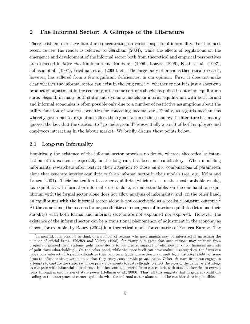
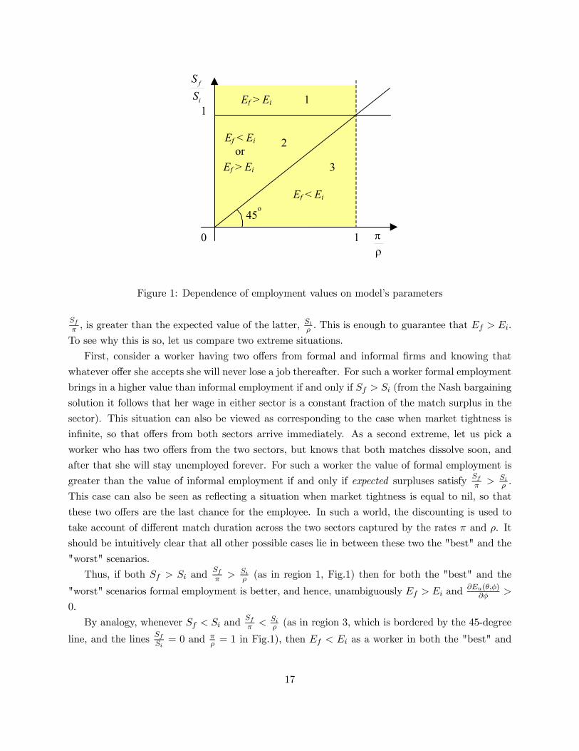
represented in the³SfSi, πρ

´-plane. Fig.1 illustrates the cases,16 while here we provide their intuitive

explanation.

Region 1 is restricted by the horizontal line SfSi= 1 from below and vertical lines π

ρ = 0 andπρ = 1 from the left and the right sides, respectively. In this region the total surplus of a formal

match, Sf , is greater than the total informal surplus, Si, while the expected value of the former,

14 In particular, to guarantee ∂Eu(θ,φ)∂θ

> 0 we must reasonably claim that at least y > τ + kπ+ bu, or, equivalently,Sf > 0, i.e. the product of a match, y, is at least as large as to pay all the flow costs of functioning in the formalsector and the wage equal to the reservation value, bu. This condition implies also that Ef > Eu holds. Analogously,to insure Ei > Eu, we must guarantee y > mF + kρ+ bu or Si > 0. Otherwise, whenever any of these conditions isnot met, an appropriate sector simply does not exist.15Although for convenience we refer to Sf and Si as surpluses, in fact they are the sector surpluses net of unem-

ployment benefits as has been mentioned when the notation was introduced. It is these values on top of bu that firmsand workers worry about when compare attractiveness of either sector. This is explained by that fact that a match ineither sector has to pay workers at least unemployment compensation so that they do not prefer to stay unemployed.16Note that by assumption ρ > π, so all possible cases are situated to the left of the vertical line π

ρ= 1 in Fig.1

(shaded areas).

16

0

1i

f

SS

ρπ

Ef > Ei

Ef < Eior

2

1

3

Ef < Ei

Ef > Ei

45o

1

Figure 1: Dependence of employment values on model’s parameters

Sfπ , is greater than the expected value of the latter, Siρ . This is enough to guarantee that Ef > Ei.

To see why this is so, let us compare two extreme situations.

First, consider a worker having two offers from formal and informal firms and knowing that

whatever offer she accepts she will never lose a job thereafter. For such a worker formal employment

brings in a higher value than informal employment if and only if Sf > Si (from the Nash bargaining

solution it follows that her wage in either sector is a constant fraction of the match surplus in the

sector). This situation can also be viewed as corresponding to the case when market tightness is

infinite, so that offers from both sectors arrive immediately. As a second extreme, let us pick a

worker who has two offers from the two sectors, but knows that both matches dissolve soon, and

after that she will stay unemployed forever. For such a worker the value of formal employment is

greater than the value of informal employment if and only if expected surpluses satisfy Sfπ > Si

ρ .

This case can also be seen as reflecting a situation when market tightness is equal to nil, so that

these two offers are the last chance for the employee. In such a world, the discounting is used to

take account of different match duration across the two sectors captured by the rates π and ρ. It

should be intuitively clear that all other possible cases lie in between these two the "best" and the

"worst" scenarios.

Thus, if both Sf > Si andSfπ > Si

ρ (as in region 1, Fig.1) then for both the "best" and the

"worst" scenarios formal employment is better, and hence, unambiguously Ef > Ei and∂Eu(θ,φ)

∂φ >

0.

By analogy, whenever Sf < Si andSfπ < Si

ρ (as in region 3, which is bordered by the 45-degree

line, and the lines SfSi= 0 and π

ρ = 1 in Fig.1), then Ef < Ei as a worker in both the "best" and

17

the "worst" situation prefers informal employment. Hence, ∂Eu(θ,φ)∂φ < 0 in this case.

Finally, when Sf < Si butSfπ > Si

ρ (region 2, which lies in between regions 1 and 3 in Fig.1)

the worker has different preferences depending on circumstances. In particular, there must exist a

threshold level of the market tightness that separates the effects of the two scenarios on the total

value of formal and informal employment. Specifically, it can be shown that as θ → 0 (no offers

are available, infinite duration of search) Ef > Ei as the effect of the "worst" scenarioSfπ > Si

ρ

dominates. However, as θ → ∞ (instant re-employment) Ef < Ei as the effect of the "best"

scenario Sf < Si dominates the other one. The proposition below extends the result on the sign of

the derivative ∂Eu(θ,φ)∂φ (its proof is relegated to the appendix).

Proposition 1 There exists some threshold value of the market tightness θ, defined by parameterskf , ki, β, r, δ, bu, τ , m, F, and parameters of the matching function, such that for parameter values

satisfying conditions in region 2, Fig.1, and for any θ > θ the derivative ∂Eu(θ,φ)∂φ is negative, and

for any θ < θ it is positive.17

Having established the properties of function Eu(θ, φ) we command all the knowledge necessary

to derive and study equilibria in our model.

3.6.3 Finding equilibria

If there exists an equilibrium with both formal and informal jobs then both formal and informal

profits must be equal to zero at the equilibrium point. That is, the equations (18) and (19) are

simultaneously satisfied. Alternatively, there can exist equilibria with only one type of job. In that

case, profits in one of the sectors would be negative and only one of the equations (18) and (19)

would hold.

Two loci The two zero profit conditions (18) and (19) define two loci of formal and informal jobs

in the (θ, φ)-plane. Both must be evaluated with the expression for Eu(θ, φ) (20) substituted in.

By using simple algebra and invoking the implicit function theorem it can easily be verified that

the locus of formal jobs (18) has a slope

∂θ

∂φ|f =

∂Eu(θ,φ)∂φ

∂q(θ)∂θ

πkf(1−β)q2(θ) − ∂Eu(θ,φ)

∂θ

. (21)

Since ∂Eu(θ,φ)∂θ is always positive, whereas ∂q(θ)

∂θ < 0, it is obvious that the denominator is negative.

Then the slope of the locus of formal jobs has a sign opposite to the sign of ∂Eu(θ,φ)∂φ .

Analogously, the slope of the locus of informal jobs (19) in the (θ, φ)-plane is

17 In fact this value of the market tightness, θ, is a bifurcation point that separates two regions with differentdynamics of our economy. We reflect on this issue at more length in the appendix.

18

∂θ

∂φ|i =

∂Eu(θ,φ)∂φ

∂q(θ)∂θ

ρki(1−β)q2(θ) − ∂Eu(θ,φ)

∂θ

, (22)

which, again, by the same token, has a sign opposite to the sign of ∂Eu(θ,φ)∂φ .

Remark 1 Both the locus of formal jobs (18) and the locus of informal jobs (19) have slopes ofthe same sign.

For different combinations of parameters represented by regions 1-3 in Fig.1, the two loci will be

either positively or negatively sloped. However, the fact that they always have slopes of the same

sign implies that only four qualitatively different situations are possible. They are represented in

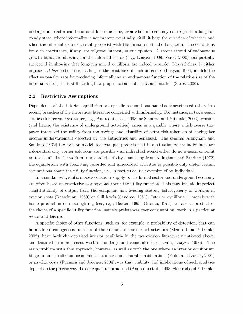
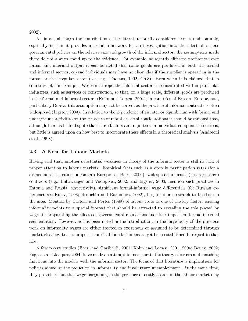
Fig.2-5, assuming that both loci have negative slopes.

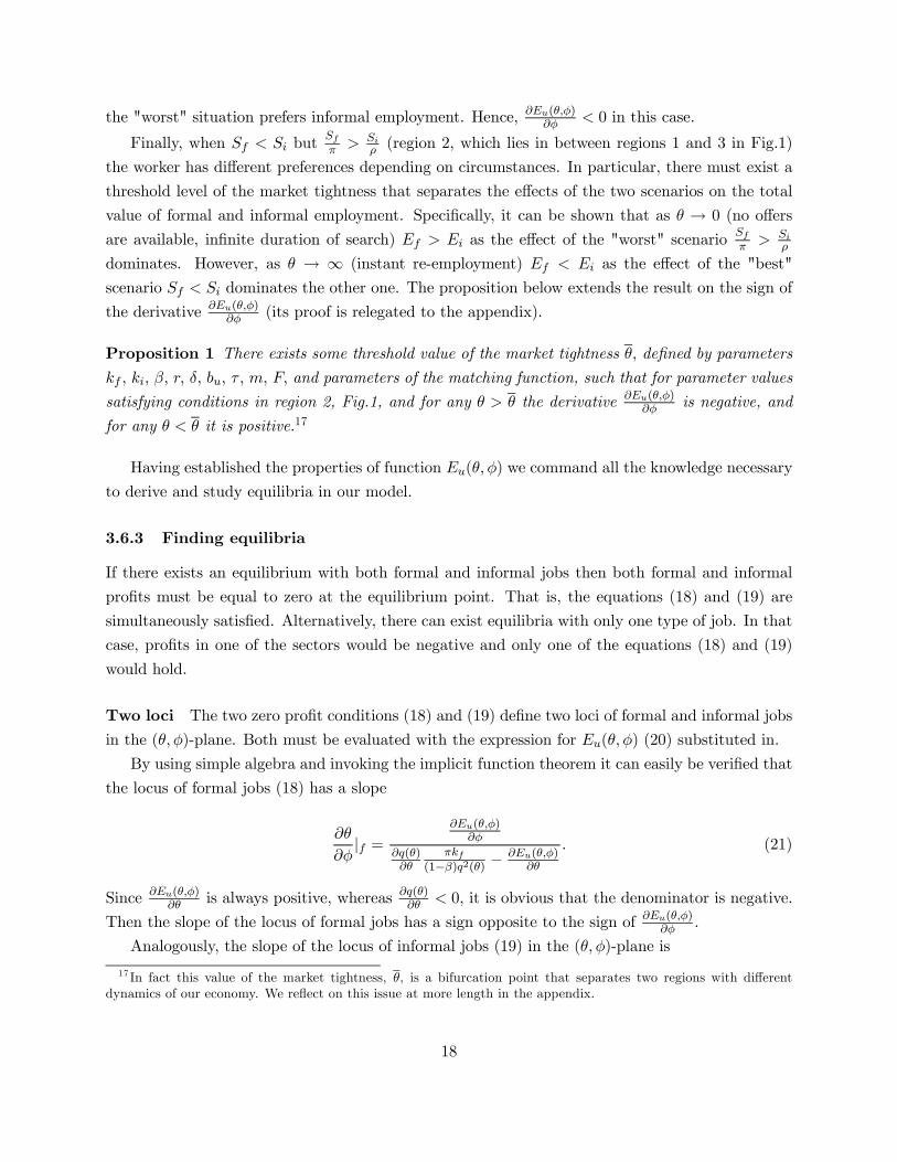
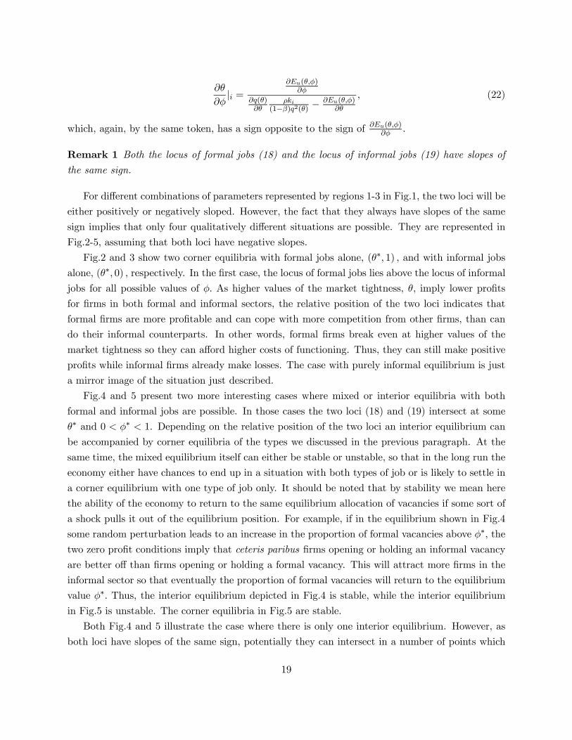
Fig.2 and 3 show two corner equilibria with formal jobs alone, (θ∗, 1) , and with informal jobsalone, (θ∗, 0) , respectively. In the first case, the locus of formal jobs lies above the locus of informaljobs for all possible values of φ. As higher values of the market tightness, θ, imply lower profits

for firms in both formal and informal sectors, the relative position of the two loci indicates that

formal firms are more profitable and can cope with more competition from other firms, than can

do their informal counterparts. In other words, formal firms break even at higher values of the

market tightness so they can afford higher costs of functioning. Thus, they can still make positive

profits while informal firms already make losses. The case with purely informal equilibrium is just

a mirror image of the situation just described.

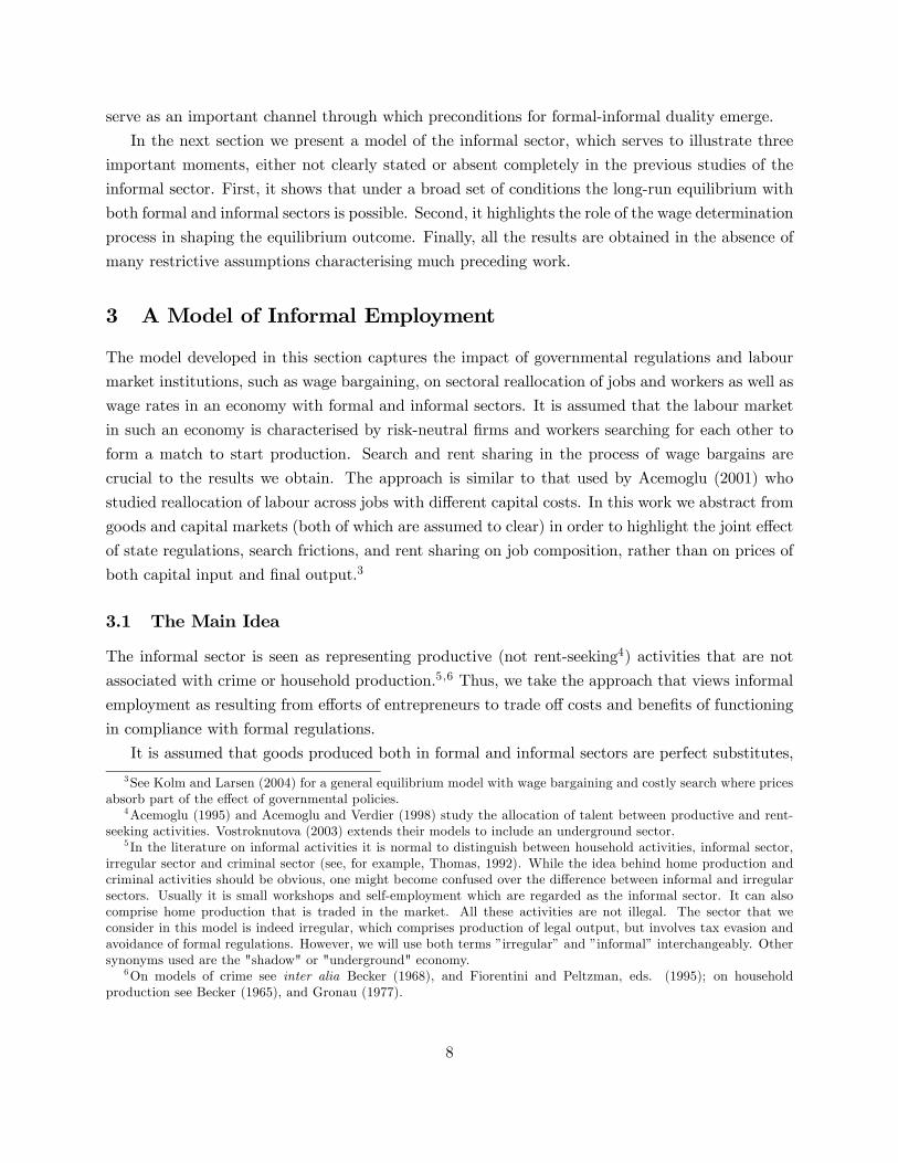
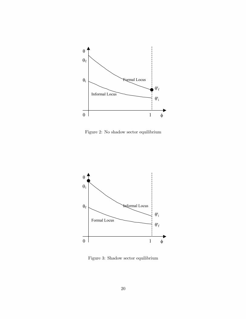
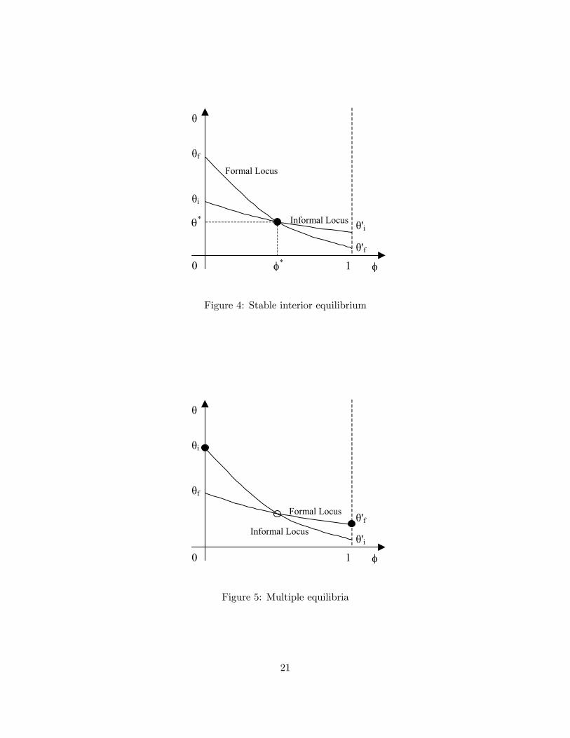
Fig.4 and 5 present two more interesting cases where mixed or interior equilibria with both

formal and informal jobs are possible. In those cases the two loci (18) and (19) intersect at some

θ∗ and 0 < φ∗ < 1. Depending on the relative position of the two loci an interior equilibrium can

be accompanied by corner equilibria of the types we discussed in the previous paragraph. At the

same time, the mixed equilibrium itself can either be stable or unstable, so that in the long run the

economy either have chances to end up in a situation with both types of job or is likely to settle in

a corner equilibrium with one type of job only. It should be noted that by stability we mean here

the ability of the economy to return to the same equilibrium allocation of vacancies if some sort of

a shock pulls it out of the equilibrium position. For example, if in the equilibrium shown in Fig.4

some random perturbation leads to an increase in the proportion of formal vacancies above φ∗, thetwo zero profit conditions imply that ceteris paribus firms opening or holding an informal vacancy

are better off than firms opening or holding a formal vacancy. This will attract more firms in the

informal sector so that eventually the proportion of formal vacancies will return to the equilibrium

value φ∗. Thus, the interior equilibrium depicted in Fig.4 is stable, while the interior equilibrium

in Fig.5 is unstable. The corner equilibria in Fig.5 are stable.

Both Fig.4 and 5 illustrate the case where there is only one interior equilibrium. However, as

both loci have slopes of the same sign, potentially they can intersect in a number of points which

19

θ

φ0 1

Formal Locus

Informal Locus

θi

θ'f

θ'i

θf

Figure 2: No shadow sector equilibrium

θ

φ0 1

Informal Locus

Formal Locus

θf

θ'i

θ'f

θi

Figure 3: Shadow sector equilibrium

20

θ

φ0 1

Informal Locus

Formal Locus

θi

θ'i

θ'f

θf

θ*

φ*

Figure 4: Stable interior equilibrium

θ

φ0 1

Formal Locus

Informal Locus

θf

θ'f

θ'i

θi

Figure 5: Multiple equilibria

21

would correspond to different interior equilibria. Nevertheless, in the case of our model it can readily

be verified that the interior equilibrium is always unique, whenever it exists. The conditions for

existence of equilibria of different types shown in Fig.2-5 are given in the next subsection. It also

provides an intuition underlying our results.

Conditions for existence and stability of equilibria Any equilibrium in our model results

from interaction of unemployed workers and firms in the labour market when they bargain over the

rents to be generated by the match.

When one of the sides completely dominates the market its preferences unambiguously de-

fine which sector of employment exists in equilibrium. For example, when the market tightness

is zero, a firm has no problem finding a match and enters the sector that provides the highest

averaged return on start-up expenditures. Recalling the discussion of profit functions in Section

3.6.1, in such a situation the firm should expect to receive a share (1− β)Sfπ of rents in the formal

sector or a share (1− β) Siρ of informal rents. Thus the returns on start-up costs kf and ki are

given by (1− β)Sfπkf

and (1− β) Siρki

in formal and informal sectors, respectively. If, for instance,

(1− β)Sfπkf

> (1− β) Siρki

, or alternatively, SfSi

>πkfρki

, the firm prefers the formal sector.

To the contrary, in a situation when the market tightness is infinite, it is the workers who

instantly receive offers from both formal and informal firms. From expressions (14) and (15) and

the properties of function Eu (θ, φ) it follows that workers receive wages wf = Sf and wi = Si in

formal and informal sectors, respectively. Thus in competing for workers firms cannot do any better

than offer the whole surpluses of the match in any sector. Obviously, in such a situation workers

will turn down offers of a lower wage, i.e. if, for example, Sf > Si, workers will never accept offers

from the informal sector.18

In the process of bargaining the balance of power shifts either to one or the other side depending

on the level of market tightness. Thus, it should be intuitively clear that if in the two extreme cases

just considered both firms and workers prefer the same sector, then in equilibrium with matching

frictions on both sides only jobs in that sector are created. Then the equilibrium market tightness

is stabilised at such a level that profits of firms are equal to zero. If, however, given full control

of the market, preferences of firms and workers do not coincide, an equilibrium with both types of

job can result.

As preferences of both firms and workers over the sector choice when they do not face matching

problems are determined by the relative values of sector surpluses Sf and Si, and respective returnsSfπkf

and Siρki

, all possible situations can again be graphically represented in the³SfSi, πρ

´-plane. The

possible cases are illustrated in Fig.6 that shows four non-overlapping regions 1-4, each of which

corresponds to various combinations of parameters and represents a particular equilibrium type.

To bear a resemblance to Fig.1 we measure the ratio of formal and informal surpluses, SfSi, on the

18Also, condition Sf > Si implies that the value of formal employment is greater than the value of informalemployment, Ef > Ei, as has been explained in section 3.6.2.

22

��

0

1

i

f

SS

ρπ

f

i

kk

2

4

3

1

45o

1

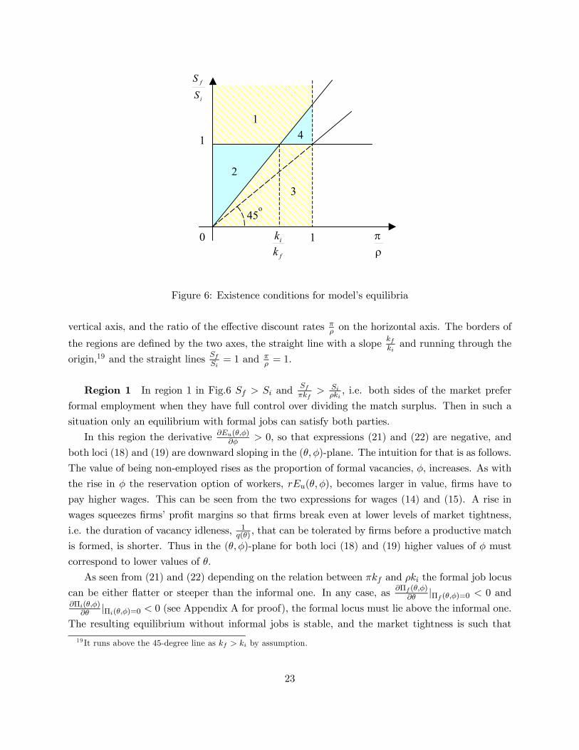
Figure 6: Existence conditions for model’s equilibria

vertical axis, and the ratio of the effective discount rates πρ on the horizontal axis. The borders of

the regions are defined by the two axes, the straight line with a slope kfkiand running through the

origin,19 and the straight lines SfSi= 1 and π

ρ = 1.

Region 1 In region 1 in Fig.6 Sf > Si andSfπkf

> Siρki

, i.e. both sides of the market prefer

formal employment when they have full control over dividing the match surplus. Then in such a

situation only an equilibrium with formal jobs can satisfy both parties.

In this region the derivative ∂Eu(θ,φ)∂φ > 0, so that expressions (21) and (22) are negative, and

both loci (18) and (19) are downward sloping in the (θ, φ)-plane. The intuition for that is as follows.

The value of being non-employed rises as the proportion of formal vacancies, φ, increases. As with

the rise in φ the reservation option of workers, rEu(θ, φ), becomes larger in value, firms have to

pay higher wages. This can be seen from the two expressions for wages (14) and (15). A rise in

wages squeezes firms’ profit margins so that firms break even at lower levels of market tightness,

i.e. the duration of vacancy idleness, 1q(θ) , that can be tolerated by firms before a productive match

is formed, is shorter. Thus in the (θ, φ)-plane for both loci (18) and (19) higher values of φ must

correspond to lower values of θ.

As seen from (21) and (22) depending on the relation between πkf and ρki the formal job locus

can be either flatter or steeper than the informal one. In any case, as ∂Πf (θ,φ)∂θ |Πf (θ,φ)=0 < 0 and

∂Πi(θ,φ)∂θ |Πi(θ,φ)=0 < 0 (see Appendix A for proof), the formal locus must lie above the informal one.

The resulting equilibrium without informal jobs is stable, and the market tightness is such that

19 It runs above the 45-degree line as kf > ki by assumption.

23

profits in the formal sector are nil, while profits in the informal sector are negative (Fig.2).

Region 2 In region 2 in Fig.6 restrictions on parameters suggest that the formal surplus

is smaller than the informal surplus, Sf < Si, while the ratio of returns on entry costs impliesSfπkf

> Siρki

. This means that, on the one hand, the formal sector is more appealing to employers

when they dominate the market, but, on the other hand, workers would prefer being employed

informally if they had no problem landing a job. Thus, there must exist a value of the market

tightness, θ∗, and the proportion of formal vacancies, φ∗ ∈ (0, 1) , such that firms are indifferent asto the sector where to place a vacancy. It is easy to verify, that indeed in this case the locus of

formal jobs (18) and the locus of informal jobs (19) have an intersection point for some 0 < φ∗ < 1,i.e. an interior equilibrium with both types of job exists. From Sf < Si and

Sfπkf

> Siρki

it follows

that the flow value of formal start-up costs, πkf , must be smaller then the flow value of informal

start-up costs, ρki, in this region, i.e. the formal jobs locus is steeper than its informal counterpart

in some neighbourhood of an interior equilibrium (θ∗, φ∗) . As regards the sign of the slopes ofthe two loci, by comparing Fig.1 and Fig.6 it can be seen that in region 2 the partial derivative∂Eu(θ,φ)

∂φ can be either negative or positive, so from (21) and (22) the loci can be either positively

or negatively sloped. From Proposition 1 we know that the sign of the derivative is negative for

any θ > θ, and positive for any θ < θ, where θ is some threshold value of the market tightness.

Then for θ > θ the two loci will both be positively sloped, whereas for θ < θ they will be downward

sloping. The outcome bears on the stability of the interior equilibrium.

Proposition 2 Let θ be a threshold value of market tightness such that ∂Eu(θ,φ)∂φ = 0, and let (θ∗, φ∗)be a point of an interior equilibrium in region 2, Fig.6. Then given kf > ki and ρ > π, θ∗ is alwaysless than θ.

Proof: see Appendix A.

Proposition 2 implies that if the two loci of formal and informal jobs intersect and an interior

equilibrium results we can confine ourselves to the situation with a less tight labour market, i.e.

θ < θ. Then ∂Eu(θ,φ)∂φ > 0, the two loci have negative slopes and the formal jobs locus crosses the

informal jobs locus from above: the resulting equilibrium is unique and stable (Fig.4).

Region 3 The situation in this region mirrors the one in region 1: both the formal surplus

is less than the informal surplus, Sf < Si, and the return on start-up costs in the formal sector is

less than the return on entry into the informal sector, Sfπkf

< Siρki

. Thus, both sides of the labour

market favour the informal sector, so that the equilibrium with informal jobs only results. In this

region ∂Eu(θ,φ)∂φ can potentially be either negative or positive, while πkf can be either greater or

less than ρki, so that the relative steepness of the loci and the sign of their slopes are ambiguous

in general. However, whatever case comes about the informal locus lies above the formal one, and

24

the outcome is stable to changes in parameters (Fig.3). The equilibrium market tightness drives

informal profits to zero, while formal profits are negative.

Region 4 Finally, in region 4, Sfπkf

< Siρki

, while Sf > Si. So, the employers prefer the informal

sector when face no problem meeting workers, while the workers are unambiguously after formal

jobs when market tightness is infinite. By analogy with the case of region 2, the locus of formal jobs

(18) and the locus of informal jobs (19) intersect at some φ∗ ∈ (0, 1) , i.e. there exists an interiorequilibrium. The restrictions on parameters in region 4 can hold only if πkf > ρki, i.e. the formal

locus is flatter than the informal locus in the vicinity of (θ∗, φ∗) . As ∂Eu(θ,φ)∂φ > 0, the two loci

are negatively sloped, and hence, the formal locus crosses the informal one from below at (θ∗, φ∗) .This situation is shown in Fig.5, where it can be seen that the interior equilibrium is unique but

not stable in this case, while there exist two stable corner equilibria with informal and formal jobs

alone.

3.7 Discussion

Above we have found general conditions for existence of equilibria of different types. It has been

shown that whenever both sides of the labour market - firms and workers - prefer formal (informal)

employment in the situation when they do not face matching problems, the resulting equilibrium

will comprise only formal (informal) jobs. However, if given full control of the labour market the

demand and supply sides differ in their preferences over the sectors, frictions in matching can ensure

that there exists an interior equilibrium with both types of job so that firms become indifferent as

to which sector to enter. This last result is especially important for two major reasons.

First, it shows the importance of labour market institutions, such as wage bargaining, for the

emergence of equilibria where two sectors coexist in the long run. Wages act as a channel through

which asymmetry in governmental regulations in relation to formal and informal firms leads to

market duality. Governmental regulations affect the size of match surpluses in the two sectors, as

well as the outside options of both firms and workers in the wage bargaining process.

Second, such an interior equilibrium is obtained in the absence of specific ad hoc assumptions

about ex ante characteristics of workers, their preferences, or various externalities simply built in

models’ technologies to provide for formal-informal segmentation of the economy. All externalities

present in our model are derived from market interactions. This is in contrast with the previous

theoretical literature which overview was given in Section 2.

In the rest of this section we examine implications of the above analysis of the model and

emphasise the role of various assumptions for the outcomes we obtain. In particular, we expound on

the mechanism whereby government regulations, wage bargains and imperfect labour markets make

for the emergence of the informal sector in the long run. The section is concluded by touching upon

the issue of stability of the long-run equilibrium with formal and informal jobs before summarising

25

the main points.

3.7.1 Important assumptions

An important meaning of the above analysis is that in a standard model of the labour market

it indeed reveals possibilities for stable coexistence of formal and informal sectors in the long

term. In the model, this result depends almost exclusively on the parameters reflecting the degree

of regulations of the economy (i.e. taxes, fines for running business informally, the degree of

monitoring), and costs to access a particular sector, kf and ki. It is likely that many (or even all) of

those parameters are effective or potential policy tools in reality. At the same time, the outcome is

independent of, for example, preferences of workers over formal and informal goods, heterogeneity

of workers, production technology parameters, a form of a monitoring function or the penalty rate.

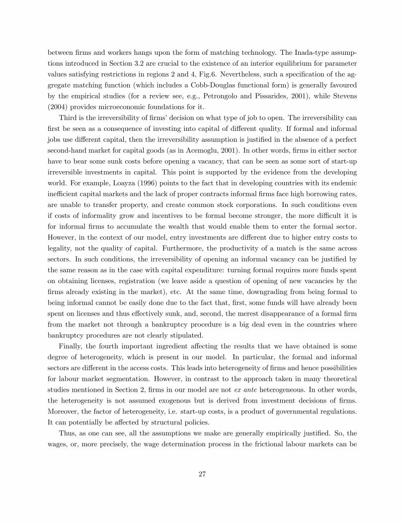
The result, however, hinges upon four important assumptions.

First, let us take the assumption of wage bargaining. It can be shown that dropping this

assumption and, for example, assuming ceteris paribus wage posting, leads to corner solutions.

Indeed, consider equilibrium wages in our model. The two zero profit conditions (18) and (19)

combined with (14) and (15), can be solved for equilibrium values of wf and wi, which are

wf =βrπkf

(1− β) q (θ)+ rEu (θ, φ) , (23)

wi =βrρki

(1− β) q (θ)+ rEu (θ, φ) . (24)

That is, the equilibrium wage differential is

wf − wi =β

(1− β)

r (πkf − ρki)

q (θ). (25)

Wage posting can be seen as a situation, in which all the bargaining power is vested with firms, or,

in other words, β = 0. From (23) and (24) above it is clear that putting β equal to 0 eliminates the

equilibrium wage differential (25) and, thus, preconditions for labour market segmentation.

In constructing our model we keep in mind not advanced but transitional economies, so the

question arises of whether the assumption of wage bargaining is reasonable in the context of the

countries of Eastern Europe. The empirical studies by Grosfeld and Nivet (1999), Luke and Schaffer

(1999), Shakhnovich and Yudashkina (2001) provide evidence in full support of the presumption.

In the most recent work Basu et al. (2004) indicate that if at the end of the communist period

evidence of worker sharing in their enterprise rents and losses was a feature only in some transitional

economies, within a year after the start of transition rent sharing has become prevalent in all the

economies they study (which are the Czech Republic, Slovakia, Poland and Hungary).

The second important assumption is the presence of search frictions. The modelling of matching

26

between firms and workers hangs upon the form of matching technology. The Inada-type assump-

tions introduced in Section 3.2 are crucial to the existence of an interior equilibrium for parameter

values satisfying restrictions in regions 2 and 4, Fig.6. Nevertheless, such a specification of the ag-

gregate matching function (which includes a Cobb-Douglas functional form) is generally favoured

by the empirical studies (for a review see, e.g., Petrongolo and Pissarides, 2001), while Stevens

(2004) provides microeconomic foundations for it.

Third is the irreversibility of firms’ decision on what type of job to open. The irreversibility can

first be seen as a consequence of investing into capital of different quality. If formal and informal

jobs use different capital, then the irreversibility assumption is justified in the absence of a perfect

second-hand market for capital goods (as in Acemoglu, 2001). In other words, firms in either sector

have to bear some sunk costs before opening a vacancy, that can be seen as some sort of start-up

irreversible investments in capital. This point is supported by the evidence from the developing

world. For example, Loayza (1996) points to the fact that in developing countries with its endemic

inefficient capital markets and the lack of proper contracts informal firms face high borrowing rates,

are unable to transfer property, and create common stock corporations. In such conditions even

if costs of informality grow and incentives to be formal become stronger, the more difficult it is

for informal firms to accumulate the wealth that would enable them to enter the formal sector.

However, in the context of our model, entry investments are different due to higher entry costs to

legality, not the quality of capital. Furthermore, the productivity of a match is the same across

sectors. In such conditions, the irreversibility of opening an informal vacancy can be justified by

the same reason as in the case with capital expenditure: turning formal requires more funds spent

on obtaining licenses, registration (we leave aside a question of opening of new vacancies by the

firms already existing in the market), etc. At the same time, downgrading from being formal to

being informal cannot be easily done due to the fact that, first, some funds will have already been

spent on licenses and thus effectively sunk, and, second, the merest disappearance of a formal firm

from the market not through a bankruptcy procedure is a big deal even in the countries where

bankruptcy procedures are not clearly stipulated.

Finally, the fourth important ingredient affecting the results that we have obtained is some

degree of heterogeneity, which is present in our model. In particular, the formal and informal

sectors are different in the access costs. This leads into heterogeneity of firms and hence possibilities

for labour market segmentation. However, in contrast to the approach taken in many theoretical

studies mentioned in Section 2, firms in our model are not ex ante heterogeneous. In other words,

the heterogeneity is not assumed exogenous but is derived from investment decisions of firms.

Moreover, the factor of heterogeneity, i.e. start-up costs, is a product of governmental regulations.

It can potentially be affected by structural policies.

Thus, as one can see, all the assumptions we make are generally empirically justified. So, the

wages, or, more precisely, the wage determination process in the frictional labour markets can be

27

critical in transmitting the effect of governmental actions on the formal-informal divide. That said,

the model can be extended to include preferences of workers, sector good specificity (as was done,

e.g., in a similar study by Kolm and Larsen, 2004), moral costs (Kolm and Larsen, 2001; Fugazza

and Jacques, 2004), and so forth, which will not change the qualitative result, but will just distract

attention from main mechanisms in action. Formal regulations have a strong direct bearing on

long-term emergence of segmented labour markets when the economy is characterised by search

and rent sharing. We take this point further in the next subsection.

3.7.2 Regulations and non-competitive labour markets

From the most general perspective the various government regulations aimed at both formal and

informal sectors determine the size of a surplus that a potential match generates. These rents are

to be divided between the two parties forming a match - the firm and the worker. If we assume

a perfectly competitive benchmark, where matching between firms and workers is instantaneous,

firms hire workers at the same wage equal to their marginal product, and receive the rest of the

surplus. Clearly, there will be no equilibrium wage differences, while firms will prefer the sector

with a higher surplus, so that a corner equilibrium will result. As soon as we enter the world of

search, however, the fact that matching for both firms and workers takes time implies that there

will be some rent sharing in a bilateral monopoly game (as in, e.g., Shaked and Sutton, 1984). In

such conditions a worker appropriates part of the match surplus, as a firm now has to compensate

the job-seeker for the time it would spend searching for a replacement if the worker quits the

negotiations to take her outside option. As our model suggests, depending on the parameters, such

as taxes, fines, and so forth, the match surpluses in the formal and informal sectors are not equal in

general, hence nor should potentially be the equilibrium wages. There is a scope for labour market

segmentation.

A higher surplus implies a higher wage in equilibrium, as can be seen, for example, from (14) and

(15). At the same time it implies higher proceeds to firms as well. Thus the sector which is more

attractive for its high surplus, is, at the same time, less attractive for its high labour costs. How does

this bear on the resulting equilibrium? The outcome depends on outside options or/and status-quo

positions of firms and workers in wage negotiations.20 If firms have the same threat points when

bargaining over wages in formal and informal sectors the Nash bargaining solution implies that

firms will choose a sector with a higher surplus. The same applies to workers. Then preferences

of firms and workers over the sector of employment, when they face no matching problem, are

driven by the sector surplus size and always coincide, i.e. only corner equilibria will be possible.

If, however, either party in the bargaining process has different, i.e. sector specific outside options,

then in general it is not necessarily the case that the sector with the highest surplus is preferred

20The reader can be referred to Sutton (1986) for initial insights into the effect of outside options in non-cooperativebargaining theory.

28

by both parties. For the party with sector specific status-quo positions the result depends on the

relative value of outside options and the relative value of sector surpluses. In such a situation the

preferences over the sector of production given the full bargaining power can potentially be different

for firms and workers, depending on the extent of asymmetries. Suppose that the asymmetries are

on the side of the party that actually makes the decision as to which sector to enter (in the case

of our model it is the firms, whereas workers search randomly without choosing a particular sector

in advance). Then if in equilibrium these asymmetries in the outside options are levelled off by

wage differentials - an interior equilibrium arises where the entering party is just indifferent as

to which sector is better. If, however, the potential wage differentials cannot compensate for the

asymmetries in the outside options the entering party will always prefer a particular sector, so that

a corner equilibrium results.

In our model the firms do have different outside options depending on the sector when they

bargain over wages with workers. In particular, their options are defined by the value of sunk start-

up costs, kf and ki, and effective discount rates, π and ρ. The upfront expenditure kf and ki must

be borne before the firm meets a job-seeker, so that when it happens and wage bargaining starts the

expected flow values of firm’s outside option are −πkf and −ρki in the formal and informal sectors,respectively. Thus, what they care about when deciding on which sector to enter is not the size of

the sector surplus, i.e. not the payoff, but the return on the start-up investments, Sfπkf

and Siρki

. At

the same time what matters for workers is the size of surpluses, Sf and Si. In particular, as seen

from (23) and (24), wages in formal and informal sectors depend positively on πkf and ρki, while

the difference between the two defines the equilibrium wage differential - see (25). In an interior

equilibrium as in Fig.4 or 5 the wage differences precisely compensate firms for the differences in

the returns Sfπkf

and Siρki

, so firms can make zero profits in both sectors.

Thus, asymmetries in flow values of start-up costs are crucial for an interior equilibrium to

ensue. These asymmetries in our model are due to factors directly affected by the state of the

government and its regulations. In particular, a value of kf higher than a value of ki is explained

by bureaucratic extortion, i.e. by corruption at the lower tier of government officials. A differential

between the effective discount rates, π and ρ, is due to government monitoring activities that crack

down on the informal sector. From (23) and (24) it is easy to see that if, for some reason, πkf = ρki,

wage differences disappear in long-run equilibrium, so that the relative value of returns Sfπkf

and Siρki

is determined by the relative value of surpluses, Sf and Si. Similarly, if, for instance, kf = ki = 0

the wages in both sectors are equal to workers’ outside option rEu. In all such cases firms’ and

workers’ preferences over the sector of production are the same and only corner equilibria can result.

To sum up, search and rent sharing in the presence of asymmetries in start-up costs caused by

activities of various levels of the government, can bring about a long-term interior equilibrium with

formal and informal jobs. From Fig.4 and 5 we can see that such an equilibrium, when it exists, can

be either stable or unstable. The same asymmetries discussed here play a leading role in stability

29

of equilibrium too, which is a focus of the following section.

3.7.3 Notes on stability of an interior equilibrium

The analysis of Fig.4 and 5 in Section 3.6.3 shows that the stability of an interior equilibrium

depends on the sign and relative value of slopes of the two loci (21) and (22). Those in turn depend

on the sign of ∂Eu(θ,φ)∂φ and the relative value of πkf and ρki. Here, we provide insights into the

stability issue from the perspective of the effect of the value of being unemployed, Eu(θ, φ), and

flow values of start-up costs on wages, and hence, profits in the formal and informal sector.

As we have seen in (23) and (24) the equilibrium wages paid by firms in the formal and infor-

mal sectors can be represented as a sum of two terms - the basis equivalent to worker’s outside

option, rEu, and the "top-up" term paid to a hired worker for saving of opportunity costs that a

representative firm enjoys when a job is formed.21

Proposition 1 and Appendix A ascertain that for kf > ki and π < ρ the value of being unem-

ployed is increasing in the proportion of formal vacancies, φ, in regions 2 and 4, Fig.6, around the

points of interior equilibria. Thus a second term in (23) and (24) is increasing in φ and θ. Either

a rise in φ or θ (or in both) improves prospects of the unemployed. Such a change affects both

the formal and informal wage in the same manner, but the cost of it is always higher to firms in

a sector with smaller surplus: the same absolute increase in φ or θ eats away a larger percentage

share of profits in that sector.

At the same time, the top-up term is independent of φ and varies only with the market tightness,

θ. Both the absolute effect of a change in θ and the effect of such a change relative to the size of

sector surplus are always larger in the sector with a higher flow value of start-up costs, i.e. with a

lower outside option to firms once entry costs have been sunk.

As firms enter the economy, market tightness θ rises, so that workers bid wages higher and

higher. It can be verified that in such a situation for low values of φ profit margins of firms in the

sector with smaller surplus are reduced more slowly. This happens because the relative effect on

such firms of a wage rise due to changes in the worker’s outside option, rEu, is dominated by the

relative top-up effect in wage changes on profits in the sector where outside options of firms are

lower.22 Eventually, as the firms in the latter sector break even, the firms in the other sector still

make positive profits, even though in absolute value their surplus is lower. Thus, the proportion of

21The value of the first term in the expressions for equilibrium wages (23) and (24) depends on the average durationof a vacancy. This represents the worker’s compensation for saving firms the opportunity costs. Indeed, from thediscussion in Section 3.6.1 it follows that when θ → 0 and q(θ)→∞, the equilibrium converges to the Walrasian limitpoint, and both wages wf and wi converge to the value of being unemployed, rEu. In this case resources investedbefore entrance never remain idle and workers are not compensated for saving of opportunity costs. If, however,θ > 0 workers have to be compensated as the opportunity costs of idleness are significant. In the other extreme case,i.e. when θ →∞ and q(θ)→ 0, the opportunity costs of idleness become very high, wages grow large, until workersappropriate all the sector surpluses.22Conditions for the existence of an interior equilibrium imply that a sector with a lower surplus and a sector with

a lower firms’ outside option are necessarily different.

30

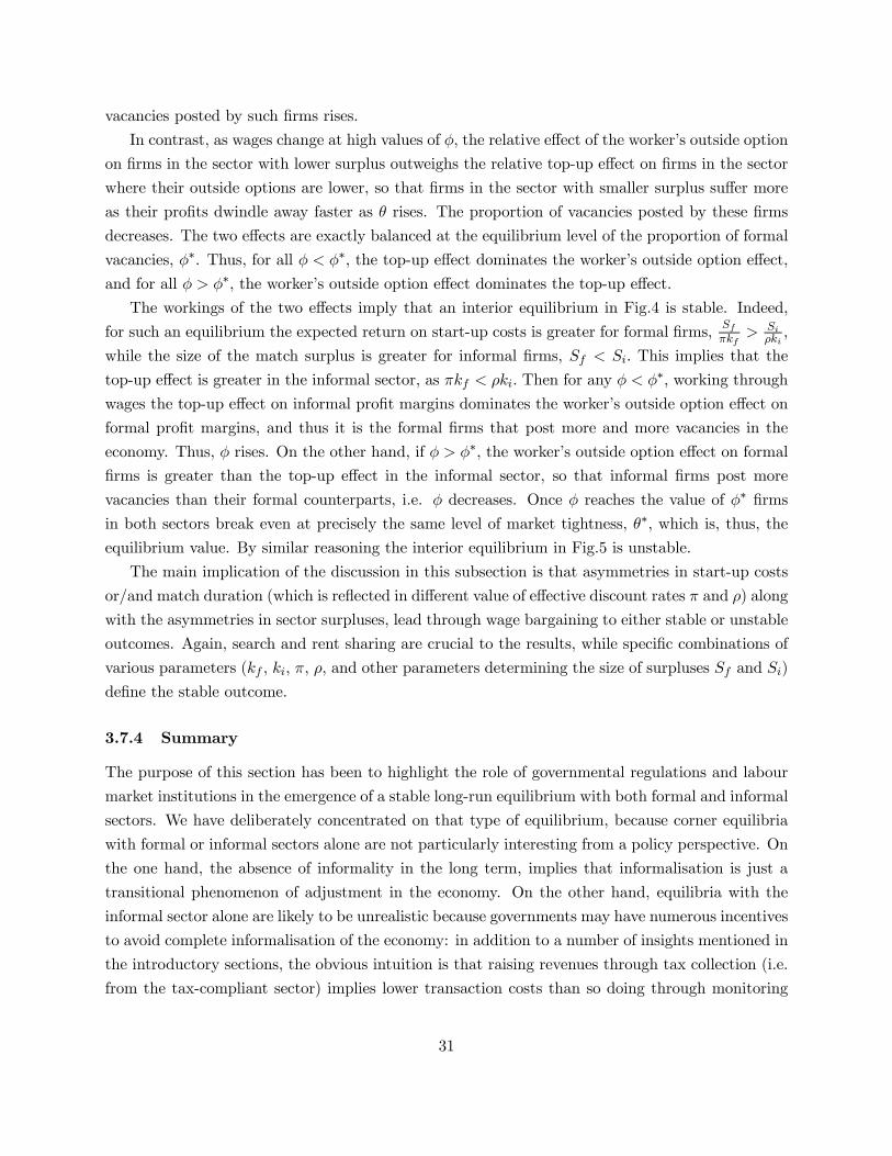
vacancies posted by such firms rises.

In contrast, as wages change at high values of φ, the relative effect of the worker’s outside option

on firms in the sector with lower surplus outweighs the relative top-up effect on firms in the sector

where their outside options are lower, so that firms in the sector with smaller surplus suffer more

as their profits dwindle away faster as θ rises. The proportion of vacancies posted by these firms

decreases. The two effects are exactly balanced at the equilibrium level of the proportion of formal

vacancies, φ∗. Thus, for all φ < φ∗, the top-up effect dominates the worker’s outside option effect,and for all φ > φ∗, the worker’s outside option effect dominates the top-up effect.

The workings of the two effects imply that an interior equilibrium in Fig.4 is stable. Indeed,

for such an equilibrium the expected return on start-up costs is greater for formal firms, Sfπkf

> Siρki

,

while the size of the match surplus is greater for informal firms, Sf < Si. This implies that the

top-up effect is greater in the informal sector, as πkf < ρki. Then for any φ < φ∗, working throughwages the top-up effect on informal profit margins dominates the worker’s outside option effect on

formal profit margins, and thus it is the formal firms that post more and more vacancies in the

economy. Thus, φ rises. On the other hand, if φ > φ∗, the worker’s outside option effect on formalfirms is greater than the top-up effect in the informal sector, so that informal firms post more

vacancies than their formal counterparts, i.e. φ decreases. Once φ reaches the value of φ∗ firmsin both sectors break even at precisely the same level of market tightness, θ∗, which is, thus, theequilibrium value. By similar reasoning the interior equilibrium in Fig.5 is unstable.

The main implication of the discussion in this subsection is that asymmetries in start-up costs

or/and match duration (which is reflected in different value of effective discount rates π and ρ) along

with the asymmetries in sector surpluses, lead through wage bargaining to either stable or unstable

outcomes. Again, search and rent sharing are crucial to the results, while specific combinations of

various parameters (kf , ki, π, ρ, and other parameters determining the size of surpluses Sf and Si)

define the stable outcome.

3.7.4 Summary

The purpose of this section has been to highlight the role of governmental regulations and labour

market institutions in the emergence of a stable long-run equilibrium with both formal and informal

sectors. We have deliberately concentrated on that type of equilibrium, because corner equilibria

with formal or informal sectors alone are not particularly interesting from a policy perspective. On

the one hand, the absence of informality in the long term, implies that informalisation is just a

transitional phenomenon of adjustment in the economy. On the other hand, equilibria with the

informal sector alone are likely to be unrealistic because governments may have numerous incentives

to avoid complete informalisation of the economy: in addition to a number of insights mentioned in

the introductory sections, the obvious intuition is that raising revenues through tax collection (i.e.

from the tax-compliant sector) implies lower transaction costs than so doing through monitoring

31

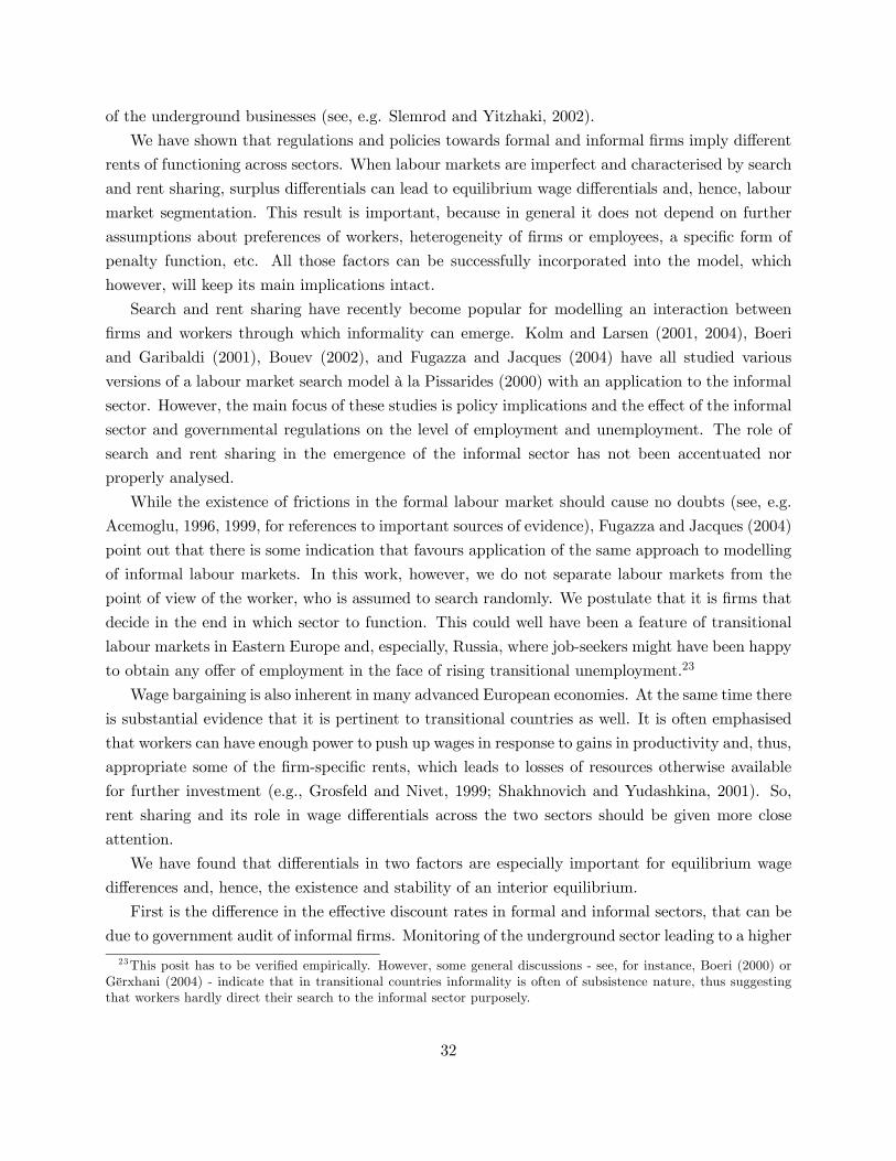
of the underground businesses (see, e.g. Slemrod and Yitzhaki, 2002).

We have shown that regulations and policies towards formal and informal firms imply different

rents of functioning across sectors. When labour markets are imperfect and characterised by search

and rent sharing, surplus differentials can lead to equilibrium wage differentials and, hence, labour

market segmentation. This result is important, because in general it does not depend on further

assumptions about preferences of workers, heterogeneity of firms or employees, a specific form of

penalty function, etc. All those factors can be successfully incorporated into the model, which

however, will keep its main implications intact.

Search and rent sharing have recently become popular for modelling an interaction between

firms and workers through which informality can emerge. Kolm and Larsen (2001, 2004), Boeri

and Garibaldi (2001), Bouev (2002), and Fugazza and Jacques (2004) have all studied various

versions of a labour market search model à la Pissarides (2000) with an application to the informal

sector. However, the main focus of these studies is policy implications and the effect of the informal

sector and governmental regulations on the level of employment and unemployment. The role of

search and rent sharing in the emergence of the informal sector has not been accentuated nor

properly analysed.

While the existence of frictions in the formal labour market should cause no doubts (see, e.g.

Acemoglu, 1996, 1999, for references to important sources of evidence), Fugazza and Jacques (2004)

point out that there is some indication that favours application of the same approach to modelling

of informal labour markets. In this work, however, we do not separate labour markets from the

point of view of the worker, who is assumed to search randomly. We postulate that it is firms that

decide in the end in which sector to function. This could well have been a feature of transitional

labour markets in Eastern Europe and, especially, Russia, where job-seekers might have been happy

to obtain any offer of employment in the face of rising transitional unemployment.23

Wage bargaining is also inherent in many advanced European economies. At the same time there

is substantial evidence that it is pertinent to transitional countries as well. It is often emphasised

that workers can have enough power to push up wages in response to gains in productivity and, thus,

appropriate some of the firm-specific rents, which leads to losses of resources otherwise available

for further investment (e.g., Grosfeld and Nivet, 1999; Shakhnovich and Yudashkina, 2001). So,

rent sharing and its role in wage differentials across the two sectors should be given more close

attention.

We have found that differentials in two factors are especially important for equilibrium wage

differences and, hence, the existence and stability of an interior equilibrium.

First is the difference in the effective discount rates in formal and informal sectors, that can be

due to government audit of informal firms. Monitoring of the underground sector leading to a higher

23This posit has to be verified empirically. However, some general discussions - see, for instance, Boeri (2000) orGërxhani (2004) - indicate that in transitional countries informality is often of subsistence nature, thus suggestingthat workers hardly direct their search to the informal sector purposely.

32

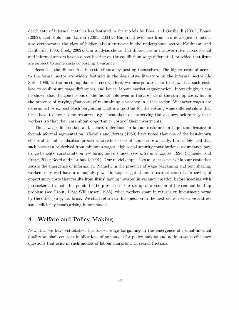
death rate of informal matches has featured in the models by Boeri and Garibaldi (2001), Bouev

(2002), and Kolm and Larsen (2001, 2004). Empirical evidence from less developed countries

also corroborates the view of higher labour turnover in the underground sector (Kaufmann and

Kaliberda, 1996; Hoek, 2002). Our analysis shows that differences in turnover rates across formal

and informal sectors have a direct bearing on the equilibrium wage differential, provided that firms

are subject to some costs of posting a vacancy.

Second is the differentials in costs of vacancy posting themselves. The higher costs of access

to the formal sector are widely featured in the descriptive literature on the informal sector (de

Soto, 1989, is the most popular reference). Here, we incorporate them to show that such costs

lead to equilibrium wage differences, and hence, labour market segmentation. Interestingly, it can

be shown that the conclusions of the model hold even in the absence of the start-up costs, but in

the presence of varying flow costs of maintaining a vacancy in either sector. Whenever wages are

determined by ex post Nash bargaining what is important for the ensuing wage differentials is that

firms have to invest some resources, e.g. spent them on preserving the vacancy, before they meet

workers, so that they care about opportunity costs of their investments.

Thus, wage differentials and, hence, differences in labour costs are an important feature of

formal-informal segmentation. Castells and Portes (1989) have noted that one of the best-known

effects of the informalisation process is to reduce costs of labour substantially. It is widely held that

such costs can be derived from minimum wages, high social security contributions, redundancy pay,

fringe benefits, constraints on free hiring and dismissal (see inter alia Loayza, 1996; Schneider and

Enste, 2000; Boeri and Garibaldi, 2001). Our model emphasises another aspect of labour costs that

assists the emergence of informality. Namely, in the presence of wage bargaining and rent sharing,

workers may well have a monopoly power in wage negotiations to extract rewards for saving of

opportunity costs that results from firms’ having invested in vacancy creation before meeting with

job-seekers. In fact, this points to the presence in our set-up of a version of the seminal hold-up

problem (see Grout, 1984; Williamson, 1985), when workers share in returns on investment borne

by the other party, i.e. firms. We shall return to this question in the next section when we address

some efficiency issues arising in our model.

4 Welfare and Policy Making

Now that we have established the role of wage bargaining in the emergence of formal-informal

duality we shall consider implications of our model for policy making and address some efficiency

questions that arise in such models of labour markets with search frictions.

33

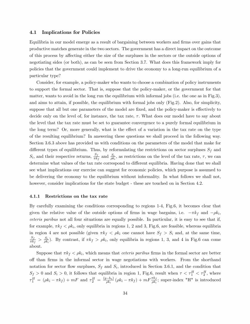
4.1 Implications for Policies

Equilibria in our model emerge as a result of bargaining between workers and firms over gains that

productive matches generate in the two sectors. The government has a direct impact on the outcome

of this process by affecting either the size of the surpluses in the sectors or the outside options of

negotiating sides (or both), as can be seen from Section 3.7. What does this framework imply for

policies that the government could implement to drive the economy to a long-run equilibrium of a

particular type?

Consider, for example, a policy-maker who wants to choose a combination of policy instruments

to support the formal sector. That is, suppose that the policy-maker, or the government for that

matter, wants to avoid in the long run the equilibrium with informal jobs (i.e. the one as in Fig.3),

and aims to attain, if possible, the equilibrium with formal jobs only (Fig.2). Also, for simplicity,

suppose that all but one parameters of the model are fixed, and the policy-maker is effectively to

decide only on the level of, for instance, the tax rate, τ . What does our model have to say about

the level that the tax rate must be set to guarantee convergence to a purely formal equilibrium in

the long term? Or, more generally, what is the effect of a variation in the tax rate on the type

of the resulting equilibrium? In answering these questions we shall proceed in the following way.

Section 3.6.3 above has provided us with conditions on the parameters of the model that make for

different types of equilibrium. Thus, by reformulating the restrictions on sector surpluses Sf and

Si, and their respective returns,Sfπkf

and Siρki

, as restrictions on the level of the tax rate, τ , we can

determine what values of the tax rate correspond to different equilibria. Having done that we shall

see what implications our exercise can suggest for economic policies, which purpose is assumed to

be delivering the economy to the equilibrium without informality. In what follows we shall not,

however, consider implications for the state budget - these are touched on in Section 4.2.

4.1.1 Restrictions on the tax rate

By carefully examining the conditions corresponding to regions 1-4, Fig.6, it becomes clear that

given the relative value of the outside options of firms in wage bargains, i.e. −πkf and −ρki,ceteris paribus not all four situations are equally possible. In particular, it is easy to see that if,

for example, πkf < ρki, only equilibria in regions 1, 2 and 3, Fig.6, are feasible, whereas equilibria

in region 4 are not possible (given πkf < ρki one cannot have Sf > Si and, at the same time,Sfπkf

> Siρki). By contrast, if πkf > ρki, only equilibria in regions 1, 3, and 4 in Fig.6 can come

about.

Suppose that πkf < ρki, which means that ceteris paribus firms in the formal sector are better

off than firms in the informal sector in wage negotiations with workers. From the shorthand

notation for sector flow surpluses, Sf and Si, introduced in Section 3.6.1, and the condition that

Sf > 0 and Si > 0, it follows that equilibria in region 1, Fig.6, result when τ < τH1 < τH2 , where

τH1 = (ρki − πkf ) + mF and τH2 = (y−bu)ρki

(ρki − πkf ) + mFπkfρki; super-index "H" is introduced

34

to indicate that we are dealing with the case when formal firms enjoy a higher reservation option

than their informal counterparts. By the same token, equilibria in region 2 come about when

τH1 < τ < τH2 . Finally, equilibria in region 3 occur when τH1 < τH2 < τ.

So, the three types of equilibrium result when the tax rate falls in one of the three non-

overlapping regions, which borders are defined by τH1 and τH2 . As we know, equilibria in region

1 have only formal firms present in the market, equilibria in region 2 are mixed, while equilibria

in region 3 are purely informal. Thus, the restrictions on the tax rate indicate that while having

other parameters fixed, a tax rate above τH2 leads to an equilibrium comprising only informal jobs,

a rate below τH1 makes for an equilibrium with formal jobs alone, while the values of τ in between

τH1 and τH2 generate interior equilibria with both formal and informal firms present.

Consider now a situation when πkf > ρki, i.e. formal firms are now worse off in wage ne-

gotiations than the informal ones, all other things being equal. In this case, only equilibria in

regions 1, 3, and 4 in Fig.6 can come about. Again, from the definition of Sf and Si and the

condition of their positivity it follows that equilibria in region 1 result whenever τ < τL1 < τL2 ,

where τL1 =(y−bu)ρki

(ρki − πkf ) +mFπkfρki

, τL2 = mF + (ρki − πkf ) , and super-index "L" indicates

the case when the outside option of formal firms is lower than that of the informal firms. Similarly,

equilibria in region 3 are possible under condition τL1 < τL2 < τ, while equilibria in region 4 happen

whenever τL1 < τ < τL2 .

Similarly to the case with πkf < ρki, a tax rate above the upper bound τL2 implies getting into

the region 3, i.e. where only long-run equilibria with the informal sector alone are possible, while

a rate below the lower bound, τL1 , brings the economy into region 1, where the informal sector is

eliminated in equilibrium. The values of the tax rate in between τL1 and τL2 make for equilibria in

region 4. In this latter case, since the interior equilibrium is not stable, a likely long-run outcome

is either a purely formal or a purely informal equilibrium: much depends on the initial proportion

of formal vacancies in the economy when it starts converging to the long-run destination. A higher

initial proportion of formal vacancies increases chances of getting into an equilibrium with formal

jobs alone (Fig.5).

4.1.2 Implications

The two cases just considered provide several implications for economic policy. We discuss them

in turn below. The first one relates, in particular, to the effect of the level of the tax rate on the

probability of ending up in the equilibrium with formal jobs alone. Other implications are of a

more general interest and highlight specificity of policy making in the two-sector economy where

wages are determined by bargaining.

The first finding that can readily be discovered from analysing the restrictions on the tax

rate above indicate that lower tax rates raise the odds of ending up in an equilibrium without the

informal sector. This echoes a standard conclusion often made in the literature related to our topic.

35

In particular, it is widely held that higher taxes always increase an incentive for informalisation

(see, for instance, Johnson et al., 1997; Friedman et al., 2000). Thus, in general governments that

aim to weed out informality in the longer term should avoid excessively high tax rates. As seen

from the above, however, the margins that allow one to call a tax rate "excessively high", depend on

the relation between outside options of firms bargaining over wages in formal and informal sectors.

Obviously, in general, τL2 and τH2 are not equal to each other, hence the same tax rate may well be

excessively high under one condition (say πkf > ρki) but not so under the other (πkf < ρki). This

is a matter of the second implication.

The cases πkf > ρki and πkf < ρki are mutually exclusive. Still, however, from the analysis of

the border values τL1 , τL2 , τ

H1 , and τH2 one can easily ascertain that they always satisfy the relation

τL1 < τL2 < τH1 < τH2 . This implies that there can exist some tax rate τ∗ such that τL2 < τ∗ < τH1 ,

and that leads the economy to an equilibrium with informal jobs alone when πkf > ρki, but to

an equilibrium without the underground sector when πkf < ρki. Moreover, if the economy starts

at some τ∗ < τL1 , and the government wants to achieve a long-run equilibrium without informal

jobs, but needs for some purpose to increase taxes, it should be more cautious about raising the

level of τ∗ too much when πkf > ρki holds, rather than when πkf < ρki maintains. In other

words, a "safety margin" for the tax increase is broader in the latter situation. Thus, in general

governments can afford to levy higher tax rates on formal firms when πkf < ρki, and still drive

the economy to an equilibrium without informal jobs. To put it differently, when the bargaining

position of formal firms vis-à-vis workers in wage negotiations is stronger in the formal sector,

governments can appropriate a larger part of the match surplus by levying higher taxes, and still

eradicate informality eventually. Thus, in this case, other things being equal, firms appropriate

more rents while haggling with workers over wages, while the government takes these gains away

through taxation.

The third implication is derived from factors affecting the border values τL1 , τL2 , τ

H1 , and τH2 .

They all inter alia depend on the size of the expected fine for running business informally, mF,

and costs of bribing in the formal sector, kf . Thus, the tax rate cannot be "excessively high" per

se, but rather in relation to the potential fine levied on informal firms or/and an additional burden

of bureaucratic extortion in the formal sector. This is well in line with some empirical findings

indicating that higher taxes do not necessarily correspond to a higher share of the informal sector

(see e.g. Friedman et al., 2000). Contribution of other factors to an increase (or a decrease for that

matter) in the size of shadow economy can prevail over the effect of taxes. For instance, Friedman

et al. (2000) point out that entrepreneurs go underground not to avoid official taxes but to reduce

the burden of bureaucracy and corruption. In our model, application of their logic would imply that

the higher such costs are, the higher is kf , and the more likely it is that πkf > ρki. Hence, higher

taxes in such a situation are perceived by formal firms as more onerous which makes their move

underground more likely. As regards the relative effect of taxes in the formal sector and expected

36

fines in the informal economy, Bouev (2004) in a dynamic model of transition from plan to market

in the presence of the informal sector illustrates that it is not higher taxes per se that lead the

economy to an equilibrium with informal firms, but rather the burden they create on formal firms

in comparison with factors affecting productivity growth in the shadow economy.

Finally, the last but not the least implication of our model is that the government itself can

affect the regime or situation in which it occurs. In other words, governments do possess ways and

means of setting relative values of πkf and ρki. Indeed, this can be done, for example, through

some structural or administrative reform that would reduce the scope for corruption in the economy,

and thus decrease the value of kf , and, hence, increase the outside option of formal firms in wage

bargains with workers. However, a more straightforward and, possibly, less costly method is to affect

the effectiveness of the informal sector monitoring, m, which can be accomplished, for example,

through financing of the tax police or other similar authorities. Recall that ρ = π+m as introduced

in Section 3.6.1. Thus, by varying the value of m the government in fact affects the size of the

outside option of firms bargaining with workers over wages in the informal sector. It is easy to

verify that for all mL such that mL < m∗, the case πkf > ρki will result, while for all mH

such that m∗ < mH , the case πkf < ρki will take place, where m∗ is such that πkf = ρki, i.e.

m∗ = π(kf−ki)ki

. In this simple model, after choosing a level of monitoring the government can then

easily determine the border values of τ and choose a level of taxation, and, thus, foreordain a desired

type of equilibrium in the long run. In particular, for any mL and mH such that mL < m∗ < mH

the restriction τL1¡mL¢< τL2

¡mL¢< τH1

¡mH

¢< τH2

¡mH

¢will still maintain. A consequence

of these relationships and the previous implications, other things being equal, can be that in the

economies with a high level of bureaucratic extortion, or/and where higher taxes are favoured by

the public office, governments may well need to spend more on the monitoring of the informal

sector or/and levy higher fines for running informal businesses. This would make convergence to

equilibria without the informal sector more likely. At the same time, in the economies with a priori

highly effective audit of the informal sector (high m) governments are likely to be more flexible in

setting tax rates, as a wider "safety margin" would allow them to achieve formal equilibria with

greater probability. It should be noted, however, that in a more realistic modelling the efficiency of

audit or monitoring, m, is itself likely to be a function of collected taxes, because it can be seen as

representing a public good provided by the state. Then the determination of the border values of

τ will be much more complicated and will depend on the form of the function m (τ) . Implications

for government behaviour will also be more complex.

4.1.3 Summary

Let us now summarise the above discussion. Our model indicates that, while keeping other param-

eters fixed, each type of long-run equilibrium is univocally related to a range of tax rates, which

does not overlap with similar ranges for other types of equilibria under this fixed set of param-

37

eters. In general, higher tax rates raise the probability that an equilibrium with informal jobs

alone will occur. However, the precise effect (the type of equilibrium) of choosing a particular tax

rate depends on relative values of reservation options of formal and informal firms in their wage

bargaining with workers. So, whenever formal firms enjoy a stronger position in wage bargaining

with job-seekers than their informal counterparts do, governments can, in principle, afford to set

higher tax rates while achieving the same type of equilibrium, other things being equal. As the

reservation option of firms in the formal sector depends on the costs of bribing, it implies that in

more corrupt economies firms are less determine to cope with high taxes and more likely to go

underground - in other words, higher taxes are more likely to lead to long-run equilibria with the

informal sector if the level of bribing is high. Meanwhile, the reservation option of firms in the

informal sector depends on the probability of being caught by monitoring authorities, such as the

tax police. So, if the level of monitoring of the underground sector is high, higher taxes are less

likely to lead to long-run equilibria with the informal sector, i.e. in general governments should be

less restricted as to the choice of tax rates in such economies. Thus, an important implication is

that the government can itself affect the likely effect of changing the tax rate by influencing the

outside options of firms - it can either be done by pursuing reforms aimed at a reduction in severity

of corruption in the economy or, which may be easier to accomplish, by choosing some level of

monitoring of the informal sector. Finally, while we have discussed the influence of government on

reservation options of firms, we have not said anything about its impact on reservation options of

workers. Obviously, our arguments as regards the tax rate can easily be appropriately reformulated

for any of the parameters captured by shorthand notation Sf and Si, including the unemployment

benefits, bu, - the instrument which affects the value of worker’s outside option. However, it should

be noted, that as workers search randomly in our set-up, i.e. they do not differentiate between

vacancies coming from the formal and informal sectors, a change in bu affects wage negotiations in

both sectors in the same manner. So, focusing on the ability to influence firms’ reservation values

is far more important.

In this section we have assumed that elimination of the informal sector is what governments

want to achieve in the long run. However, this is not necessarily the objective governments do or

should pursue in reality. We leave the question of what governments actually do want to achieve

beyond the scope of this essay - the reader can be referred to Buchanan (1975) and Shleifer and

Vishny (1998) for some discussions of possible motivation that governments could have. In what

follows, we rather attempt to provide some insights into whether the elimination of the informal

sector can be justified on the efficiency grounds. In particular, for convenience we mainly focus on

an interior equilibrium with both formal and informal jobs (such as the one that results in region

2, Fig.6, and is shown in Fig.4) - a most complicated stable steady state that can occur in our

model in the long run. This steady state is also an interim case between two degenerate equilibria

with formal and informal jobs alone. We shall assess its efficiency properties and look into what

38

benevolent governments should do to achieve efficient or sub-efficient outcomes if they start out in

such an equilibrium.

4.2 Implications for Welfare

The welfare analysis below is structured in the following way. We begin it by investigating the

general conditions under which equilibria in our economy are efficient, i.e. represent first-best

optima in terms of maximisation of a welfare function reflecting gains of private agents, i.e. firms

and workers. This provides us with understanding of the underlying causes of potential inefficiency.

Then we look into the possibility of achieving first-best solutions or, at least, making them more

probable. We are interested in what the benevolent government24 can do for correcting the causes

of inefficiency. At the same time, we learn the implications of those measures for the presence

or the size of the informal sector in steady state. If, however, attainment of first-best allocations

is not realistic, it makes sense to analyse what the government can do to lead the economy to a

sub-optimal outcome as opposed to a first-best one. In particular, it is interesting whether or not

a reduction in size of informality can improve on welfare if the economy starts out in the interior

equilibrium.

Before embarking on a substantive part of the efficiency analysis, however, we need to introduce

some measure of economic welfare.

4.2.1 Steady state surplus

Consider a private surplus, as customary in search-in-the-labour-market models (see, e.g., Hosios,

1990; Acemoglu and Shimer, 1999; Pissarides, 2000; Acemoglu, 2001):

Ξ (θ, φ) = N (y − τ − πkf ) + I (y −mF − ρki)− θU (φrkf + (1− φ) rki) + Ubu. (26)

This measure is what firms and workers care about before entering the economy. The surplus is equal

to flows of net output generated in formal and informal sectors plus the income of the unemployed.

In particular, it consists of the number of workers in formal jobs, N = (1− U)φ δ+mδ+φm , times the

formal sector output net of taxes and flow costs of creating a vacancy, y−τ−πkf , plus the number ofworkers in informal jobs, I = (1− U) (1− φ) δ

δ+φm , times the informal sector output less expected

fines and flow vacancy costs, y − mF − ρki, minus the flow costs of job creation to formal and

informal vacancies (respectively, θUφrkf and θU(1−φ)rki), plus total flow benefits received by theunemployed, Ubu. Notice that the proportion of formal vacancies among all vacancies, φ, and the

proportion of filled formal jobs among all filled jobs, φ δ+mδ+φm , do not coincide due to different job

duration rates in different sectors. Also, it can be shown that U = δ(δ+m)(δ(δ+m)+α(θ)(δ+φm)) , the stock

24Throughout this section we assume that the government is benevolent in the sense that its aim is to maximisesocial welfare represented by gains of firms and workers, rather than to pursue other objectives, such as, for example,maximisation of the budget revenue.

39

of unemployed workers in steady state, is in fact a function of θ and φ. The derivation of all these

results is relegated to Appendix A. Here we shall just note that the private surplus is a measure of

what the social planner should be concerned about in steady state, disregarding a specific way that

wages are determined in equilibrium. Indeed as Pissarides (2000, p.184) notes: "the social planner

is not interested in wages, since wages determine only the distribution of output and distributional

consideration are excluded from the social welfare function."

4.2.2 Inefficiency of corner equilibria: a standard result

In order to provide the reader with a useful background to our main results for the economy with

two sectors let us start the analysis of efficiency with examination of a corner equilibrium. In such

a somewhat degenerate case, whether it is an equilibrium with formal jobs only (Fig.2) or the one

with informal jobs only (Fig.3), it is effectively a one sector environment. So, not surprisingly, the

implications for efficiency of corner equilibria in our model are standard to the literature on search

in the labour market (Pissarides, 2000), that for the most part concentrates on an economy with

one type of employment.

In a search economy with one sector the efficiency of an equilibrium would imply that the

relative amount of search, represented by the ratio of the number of vacancies to the number of

job-seekers, is optimal. As we focus here on the decision of firms to enter the economy, the efficiency

of equilibrium can be said to imply that the economy creates the right number of jobs. The standard

result in the search-in-the-labour-market literature is that the socially optimal amount of search

or job creation, for that matter, is achieved if the so-called Hosios (1990) efficiency condition is

maintained. In particular, it is known that in search equilibrium in a one sector economy there will

be too little job creation if the bargaining power of workers, β, is greater than the elasticity of the

matching function, η (θ) = −q0 (θ) θq(θ) , and there will be too much job creation if β is less than the

elasticity of the matching function, η (θ). In order the allocation of jobs and workers to be efficient

in models of search, first, matching must exhibit constant returns, and, second, the elasticity of the

matching function with respect to unemployment must be equal to the bargaining power of workers

(Hosios, 1990; Pissarides, 2000). To see that this applies as well to the case of a corner equilibrium

with formal jobs in our model (a case with informal jobs is easy to analyse by analogy), consider a

problem of maximisation of the private surplus25 (26). For the infinitely lived economy it consists

in maximising

∞Z0

Ξ (θ, φ) =

∞Z0

e−rt (N (y − τ − πkf )− θUrkf + Ubu) dt (27)

25Following Pissarides (2000) the approach that we take in the comparison of the social and private outcomes is toderive the social outcome by ignoring wage bargaining equations (8) and (9), and then investigate whether there arewage rates determined according to (8) and (9) that make the social and private conditions for job creation identical.

40

subject to restrictions

·N = α(θ)φU − δN,·U = δN − α(θ)U,

1 = N + U. (28)

Equation (27) is the private surplus (26) discounted back to the initial time and when I = 0.

Restrictions (28) are standard equations describing the evolution of unemployment and formal

sector employment: an increase in a number of workers in a particular labour market state is

equal to the flow into that state minus the outflow. The solution of the programme is relegated to

the appendix, while here we just give the condition that the socially efficient level of the market

tightness must satisfy:

Sf = rkf

µπ + α (θ)− θα0 (θ)

α0 (θ)

¶. (29)

At the same time, from the zero profit condition (18) and (20) it follows that the level of the market

tightness in the wage bargaining equilibrium satisfies:

Sf = rkf(π + α (θ)β)

(1− β) q (θ). (30)

The two expressions (29) and (30) are identical if and only if α0 (θ) = (1− β) q (θ) or, recalling

properties of α (θ) and q (θ) , β = q(θ)−α0(θ)q(θ) = −q0 (θ) θ

q(θ) = η (θ) . In other words, the corner

equilibrium in our model is efficient if and only if the Hosios efficiency condition is satisfied.

An intuition underlying this result is as follows. The elasticity of the matching function η (θ)

can be seen as a measure of relative effectiveness of the unemployed in making contacts, while

1−η (θ) is a measure of relative effectiveness of firms in making contacts. From Shaked and Sutton(1984) we know that in search economies with wage bargaining the relative bargaining position of

firms vis-à-vis workers depends on the time it takes a firm to switch, if necessary, from the worker

it currently bargains with to a substitute workforce. In models with matching functions this time

is a function of q (θ) . The lower is q (θ) the longer is the time that firms have to wait for a worker,

and the weaker is the bargaining position of firms in bargaining with workers they have already

met. In other words, in labour markets characterised by search workers have more monopoly power

over extracting the match surplus the longer firms have to wait to fill the vacancy, i.e. the lower

is q (θ) , or the greater is θ, for that matter. Thus, as η (θ) reflects the relative effectiveness of the

unemployed vis-à-vis firms in searching for a match, it can also be seen as a measure of worker’s

monopoly power, implied by the labour market conditions, over the surplus of the match to be

41

shared in wage bargains. Hence, if, for instance, η (θ) is higher than β in equilibrium, then firms

in practice receive a greater share of the surplus in bargaining than they should have done if the

split were arranged by the social planner. The asymmetry between the monopoly power in wage

bargains commensurate with labour market conditions, η (θ), and the going bargaining power of

workers, β, causes firms to open more vacancies in the equilibrium than it is socially optimal.

That is firms are taking advantage of this asymmetry by overinvesting in job creation. This, of

course, would imply that at the margin firms are causing more congestion to each other than the

congestion that the unemployed are causing to other unemployed workers. In contrast, if β > η (θ) ,

firms will underinvest in job creation as the going bargaining power of workers, β, will be greater

than the one that would be justified by labour market frictions. Only in the case when β = η (θ)

the equilibrium is socially optimal, so the Hosios efficiency condition balances out the going and

true bargaining positions of workers in wage negotiations. From a slightly different point of view it

also internalises all congestion externalities that firms and workers create to each other in labour

markets characterised by time-consuming search.

The moral of this exposition is that in general even the simplest outcome in our model, i.e. the

corner equilibrium, should not be expected to be efficient. Efficiency hinges upon the particular

choice of the bargaining power of workers. Although it is a standard result, from a perspective of

the discussion of the welfare impact of policies reducing the size of informality it is important that

inefficiency is not caused by a particular combination of policy parameters set by the government,

it is essentially of labour market origins.

Now let us investigate the interior equilibrium and see what lessons for efficiency of the steady

state outcome we can derive from there.

4.2.3 Inefficiency of the interior equilibrium

Our economy has two sectors so that if a non-degenerate outcome occurs with both formal and

informal jobs present in equilibrium the concept of efficiency becomes a little more advanced. With

two sectors the efficiency of equilibrium implies not only that the right number of jobs is created, but

also that jobs are allocated optimally across the sectors. However, our main result below indicates

that in contrast to the corner equilibrium case, in the interior equilibrium the allocation of jobs is

generally not optimal even when matching exhibits constant returns (as we have assumed) and the

Hosios condition holds. Indeed, it turns out that in the interior equilibrium with both formal and

informal jobs such as in Fig.4 or 5, the restriction on the bargaining power is no longer enough to

guarantee efficiency. There exist other factors responsible for creating another type of inefficiency,

and which bring about a non-optimal allocation of jobs and workers across the two sectors. With

this type of allocative inefficiency firms underinvest in job creation in a particular sector. As a

consequence, the amount of job creation in the economy as a whole is not optimal either.

Consider a stable long-run outcome in Fig.4, and continue along the lines of the analysis of the

42

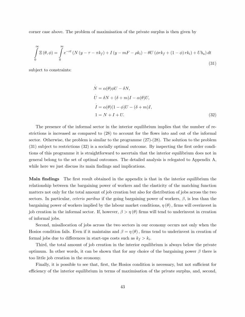
corner case above. The problem of maximisation of the private surplus is then given by

∞Z0

Ξ (θ, φ) =

∞Z0

e−rt (N (y − τ − πkf ) + I (y −mF − ρki)− θU (φrkf + (1− φ) rki) + Ubu) dt

(31)

subject to constraints:

·N = α(θ)φU − δN,·U = δN + (δ +m)I − α(θ)U,·I = α(θ)(1− φ)U − (δ +m)I,

1 = N + I + U. (32)

The presence of the informal sector in the interior equilibrium implies that the number of re-

strictions is increased as compared to (28) to account for the flows into and out of the informal

sector. Otherwise, the problem is similar to the programme (27)-(28). The solution to the problem

(31) subject to restrictions (32) is a socially optimal outcome. By inspecting the first order condi-

tions of this programme it is straightforward to ascertain that the interior equilibrium does not in

general belong to the set of optimal outcomes. The detailed analysis is relegated to Appendix A,

while here we just discuss its main findings and implications.

Main findings The first result obtained in the appendix is that in the interior equilibrium the

relationship between the bargaining power of workers and the elasticity of the matching function

matters not only for the total amount of job creation but also for distribution of jobs across the two

sectors. In particular, ceteris paribus if the going bargaining power of workers, β, is less than the

bargaining power of workers implied by the labour market conditions, η (θ) , firms will overinvest in

job creation in the informal sector. If, however, β > η (θ) firms will tend to underinvest in creation

of informal jobs.

Second, misallocation of jobs across the two sectors in our economy occurs not only when the

Hosios condition fails. Even if it maintains and β = η (θ) , firms tend to underinvest in creation of

formal jobs due to differences in start-ups costs such as kf > ki.

Third, the total amount of job creation in the interior equilibrium is always below the private

optimum. In other words, it can be shown that for any choice of the bargaining power β there is

too little job creation in the economy.

Finally, it is possible to see that, first, the Hosios condition is necessary, but not sufficient for

efficiency of the interior equilibrium in terms of maximisation of the private surplus, and, second,

43

that the sufficient condition for efficiency is that both the Hosios condition is met and kf = ki.26

An implication of these results is that in the two sector environment in general two factors affect

both the total amount of job creation in the economy and the allocation of jobs across formal and

informal sectors. First is the standard relation between the bargaining power of workers and the

elasticity of the matching function. The second factor is the relation between the start-up costs

that firms bear before entering the economy. Let us consider them in turn.

The effect of the relation between β and η (θ) on the total amount of job creation is standard

and similar to the case of a one sector environment discussed above. More interesting is its role in

creating allocative inefficiencies across the sectors. Our results suggest, intuitively, that firms tend

to take advantage of their bargaining position vis-à-vis workers in the sector where surplus of a

match is greater. Indeed, recall that in the stable interior equilibrium, as in Fig.4, Si > Sf . At the

same time, if β < η (θ) firms gain additional rents because of the discrepancy between the going

bargaining power of workers and the one implied by the labour market conditions. Those rents

are larger in the informal sector, so firms create too many informal jobs. By contrast, if β > η (θ)

firms miss out on potential rents because of the too high a going bargaining power of workers, β.

Those foregone rents are, again, greater in the informal sector, thus, there is underinvestment into

the informal sector job creation.

However, even if the Hosios condition holds, i.e. β = η (θ) , the equilibrium in our economy does

not represent a socially optimal allocation of jobs because of the difference in values of kf and ki. In

general, the presence of start-up costs that firms have to bear unilaterally before entering one sector

or another in fact implies that workers gain additional advantage in wage negotiations. Indeed,

while firms start wage bargains with some costs already borne, workers enter into negotiations

without incurring any costs previously. So, while firms, in the first place, are concerned with

recouping the costs, workers are just interested in receiving as high a wage as possible. In such a

situation workers are able to capture excessive rents in the process of wage negotiations, so that

firms may underinvest in creation of jobs in the economy in general, and in one of the sectors in

particular. Obviously, it may well lead to inefficiency of the equilibrium. This result is closely

linked with the presence in our framework of a version of the so-called hold-up problem, already

mentioned above briefly.

The hold-up problem: a source of inefficiency In relation to investments the hold-up prob-

lem arises when one party pays the cost while others share in the payoff. The problem has attracted

attention in numerous studies, beginning from the earliest discussions (Williamson, 1975), first for-

malisation (Grout, 1984), and coinage of the term (Williamson, 1985), to more recent investigation

into the causes and possible remedies (e.g. MacLeod and Malcomson, 1993; Malcomson, 1997). The

26Note, however, the proof of Proposition 1, Appendix A, shows that when kf = ki the stability properties of theinterior equilibrium may change - in fact it then coincides with the bifurcation point separating two regions withdifferent phase dynamics of θ and φ.

44

search-in-the-labour-market literature has addressed the problem both as regards firms (Acemoglu

and Shimer, 1999; Acemoglu, 2001) and workers (Acemoglu, 1996), who unilaterally invest into

either physical or human capital, respectively.

Grout (1984) has shown that the hold-up problem leads to inefficiency of investment arising

in the absence of binding contracts, when workers can negotiate wages and employment once the

firm has committed itself to a specific investment.27 Furthermore, as pointed out by Malcomson

(1997), in the presence of labour turnover costs there can be hold-up of general, as well as specific

investments. The underlying cause of hold-ups is incompleteness of contracts. If contracts were to

be complete all the parties who benefit from an investment could be made to pay their share of the

cost. Acemoglu and Shimer (1999) note that even when contracts are incomplete an appropriate

arrangement of relationship between agents can prevent the problem. However, in a situation when

investment must be sunk before agents meet contracts and related arrangements are impossible

because at the time they invest agents do not know who their trade partner is going to be (Acemoglu,

1996).

If investments made by firms are exogenous to the economy considered, the hold-up problem

does not necessarily lead to inefficiency under an appropriate choice of bargaining power of workers.

Acemoglu and Shimer (1999) has shown that in, for example, a one sector search environment the

standard Hosios condition guarantees a socially optimal outcome. In that case workers still share

in returns, but their ability to appropriate rents does not have a negative externality effect on the

decision of firms to invest. The only externality that must be internalised in such an economy

is the one of the number of vacancies on worker’s outside option in the bargaining process. In

other words, it is the externality of congestion that firms and workers cause to its peers. As we

have mentioned in Section 4.2.2, the Hosios condition achieves precisely that - it eliminates the

congestion externality. However, once the investments are made endogenous the Hosios condition

is no longer sufficient: even if it is possible to make the level of wages to be equal to the social

shadow value of labour, it is impossible to guarantee that both the level and the slope of the wage

function are equal to appropriate social values (Acemoglu and Shimer, 1999). With endogenous

investment there is a negative externality of worker’s bargaining power on firms’ investment, which

is not internalised even when the Hosios condition is met.

The hold-up problem in our model In our model firms sink non-specific investments, which

are treated as exogenous parameters. These costs, kf and ki, are incurred before meeting potential

employees. Given a non-competitive labour market and wage bargaining, the presence of search

frictions and, hence, switching costs (i.e. costs of finding a new trade partner) implies that workers

exert monopoly power in sharing the surplus of a match. During wage negotiations workers capture

part of the return on kf and ki as indicated by the equilibrium wage equations (23) and (24). Thus,

27MacLeod and Malcomson (1993, p.813) state that "in contrast to general investments, specific investments arevaluable for trade only with the chosen partner, not for trade with third parties".

45

we are clearly dealing with the hold-up problem.

As investments kf and ki are non-specific and, importantly, exogenous, following Acemoglu

and Shimer (1999) we should not expect hold-ups to cause a problem for efficiency of equilibrium.

Indeed in the corner solution case in Section 4.2.2 the presence of start-up investments unilaterally

borne by firms does not affect optimality of the outcome. There is no externality of the worker’s

bargaining power on firms’ investment. At the same time, there is a standard congestion externality

which is internalised when the Hosios condition is met.

However, in the interior equilibrium the presence of the start-up costs will in general cause an

efficiency problem. To see that consider the expressions (23) and (24) re-written as

(wf − rEu (θ, φ))

π=

βrkf(1− β) q (θ)

(33)

and

(wi − rEu (θ, φ))

ρ=

βrki(1− β) q (θ)

. (34)

The terms on the left hand side represent average or expected wage mark-ups that workers are

paid on top of their outside option. It can be seen that as kf > ki the formal wage mark-up is

larger than its informal counterpart. Thus, intuitively, in equilibrium ceteris paribus firms will

underinvest into formal job creation (and, hence, in the economy as a whole) as in the formal

sector they on average forego more rents to workers than in the informal sector. Obviously, such a

situation implies that the interior equilibrium is not efficient. Indeed, it can be verified that with

kf > ki in the interior equilibrium the value of being formally employed, Ef , is always higher than

the value of being informally employed, Ei, regardless of the value of β. Thus, firms do not take

into account that creating a formal rather than informal vacancy has a positive externality effect

on workers. The Hosios condition cannot internalise this externality which works not through the

market tightness, θ, but through the proportion of formal vacancies, φ.28 Thus, with kf 6= ki the

Hosios condition is necessary but not sufficient for efficiency of the equilibrium with two sectors

even when the investments are exogenous.

If, however, kf = ki in equilibrium the expected wage mark-ups will be equal across the two

sectors, the value of formal employment for workers will be equal to the value of being informally

employed, Ef = Ei, and the creation of a formal rather than an informal vacancy will not have

any effect on worker’s welfare. In fact workers will be indifferent as to what proportion of formal

vacancies φ is achieved in equilibrium. Thus, the allocative externality will disappear and the

Hosios condition will again be sufficient to guarantee the efficiency of the interior equilibrium in

terms of maximisation of the private surplus (26).

28The reader can be referred to Acemoglu (2001) for a study of a similar uninternalised allocative externality in amodel of labour market segmentation.

46

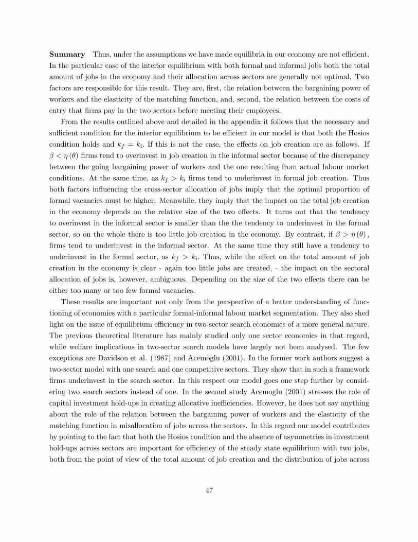
Summary Thus, under the assumptions we have made equilibria in our economy are not efficient.

In the particular case of the interior equilibrium with both formal and informal jobs both the total

amount of jobs in the economy and their allocation across sectors are generally not optimal. Two

factors are responsible for this result. They are, first, the relation between the bargaining power of

workers and the elasticity of the matching function, and, second, the relation between the costs of

entry that firms pay in the two sectors before meeting their employees.

From the results outlined above and detailed in the appendix it follows that the necessary and

sufficient condition for the interior equilibrium to be efficient in our model is that both the Hosios

condition holds and kf = ki. If this is not the case, the effects on job creation are as follows. If

β < η (θ) firms tend to overinvest in job creation in the informal sector because of the discrepancy

between the going bargaining power of workers and the one resulting from actual labour market

conditions. At the same time, as kf > ki firms tend to underinvest in formal job creation. Thus

both factors influencing the cross-sector allocation of jobs imply that the optimal proportion of

formal vacancies must be higher. Meanwhile, they imply that the impact on the total job creation

in the economy depends on the relative size of the two effects. It turns out that the tendency

to overinvest in the informal sector is smaller than the the tendency to underinvest in the formal

sector, so on the whole there is too little job creation in the economy. By contrast, if β > η (θ) ,

firms tend to underinvest in the informal sector. At the same time they still have a tendency to

underinvest in the formal sector, as kf > ki. Thus, while the effect on the total amount of job

creation in the economy is clear - again too little jobs are created, - the impact on the sectoral

allocation of jobs is, however, ambiguous. Depending on the size of the two effects there can be

either too many or too few formal vacancies.

These results are important not only from the perspective of a better understanding of func-

tioning of economies with a particular formal-informal labour market segmentation. They also shed

light on the issue of equilibrium efficiency in two-sector search economies of a more general nature.

The previous theoretical literature has mainly studied only one sector economies in that regard,

while welfare implications in two-sector search models have largely not been analysed. The few

exceptions are Davidson et al. (1987) and Acemoglu (2001). In the former work authors suggest a

two-sector model with one search and one competitive sectors. They show that in such a framework

firms underinvest in the search sector. In this respect our model goes one step further by consid-

ering two search sectors instead of one. In the second study Acemoglu (2001) stresses the role of

capital investment hold-ups in creating allocative inefficiencies. However, he does not say anything

about the role of the relation between the bargaining power of workers and the elasticity of the

matching function in misallocation of jobs across the sectors. In this regard our model contributes

by pointing to the fact that both the Hosios condition and the absence of asymmetries in investment

hold-ups across sectors are important for efficiency of the steady state equilibrium with two jobs,

both from the point of view of the total amount of job creation and the distribution of jobs across

47

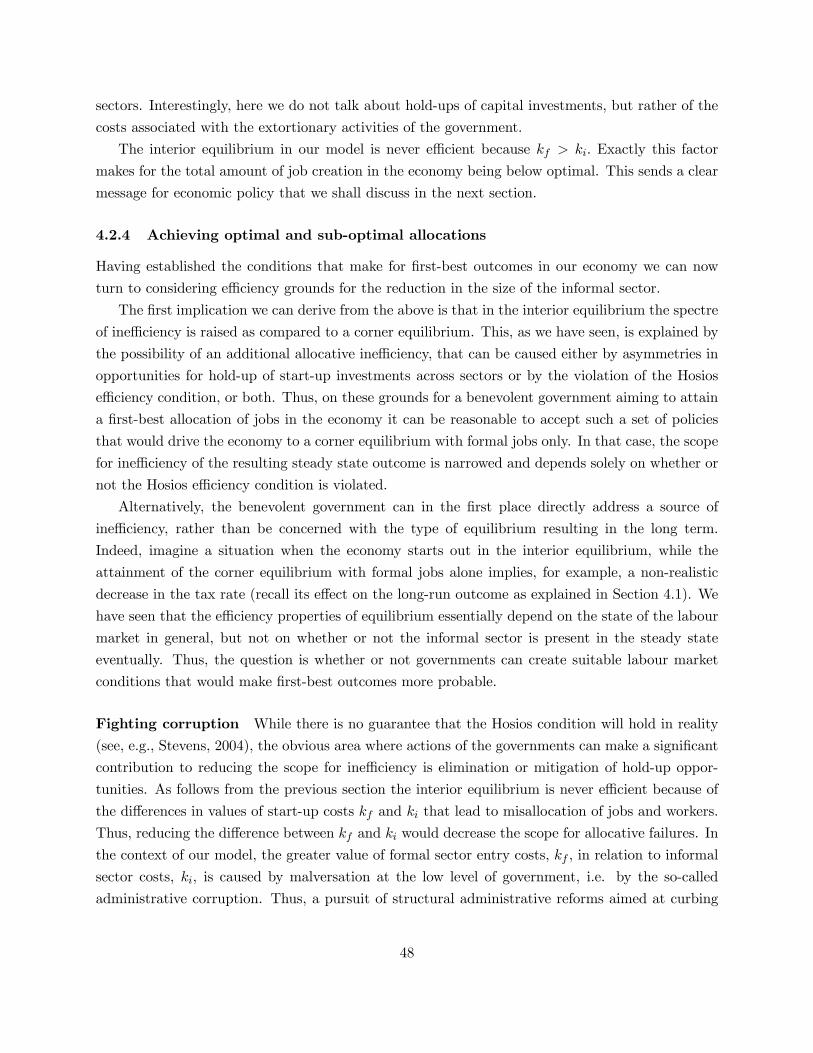
sectors. Interestingly, here we do not talk about hold-ups of capital investments, but rather of the

costs associated with the extortionary activities of the government.

The interior equilibrium in our model is never efficient because kf > ki. Exactly this factor

makes for the total amount of job creation in the economy being below optimal. This sends a clear

message for economic policy that we shall discuss in the next section.

4.2.4 Achieving optimal and sub-optimal allocations

Having established the conditions that make for first-best outcomes in our economy we can now

turn to considering efficiency grounds for the reduction in the size of the informal sector.

The first implication we can derive from the above is that in the interior equilibrium the spectre

of inefficiency is raised as compared to a corner equilibrium. This, as we have seen, is explained by

the possibility of an additional allocative inefficiency, that can be caused either by asymmetries in

opportunities for hold-up of start-up investments across sectors or by the violation of the Hosios

efficiency condition, or both. Thus, on these grounds for a benevolent government aiming to attain

a first-best allocation of jobs in the economy it can be reasonable to accept such a set of policies

that would drive the economy to a corner equilibrium with formal jobs only. In that case, the scope

for inefficiency of the resulting steady state outcome is narrowed and depends solely on whether or

not the Hosios efficiency condition is violated.

Alternatively, the benevolent government can in the first place directly address a source of

inefficiency, rather than be concerned with the type of equilibrium resulting in the long term.

Indeed, imagine a situation when the economy starts out in the interior equilibrium, while the

attainment of the corner equilibrium with formal jobs alone implies, for example, a non-realistic

decrease in the tax rate (recall its effect on the long-run outcome as explained in Section 4.1). We

have seen that the efficiency properties of equilibrium essentially depend on the state of the labour

market in general, but not on whether or not the informal sector is present in the steady state

eventually. Thus, the question is whether or not governments can create suitable labour market

conditions that would make first-best outcomes more probable.

Fighting corruption While there is no guarantee that the Hosios condition will hold in reality

(see, e.g., Stevens, 2004), the obvious area where actions of the governments can make a significant

contribution to reducing the scope for inefficiency is elimination or mitigation of hold-up oppor-

tunities. As follows from the previous section the interior equilibrium is never efficient because of

the differences in values of start-up costs kf and ki that lead to misallocation of jobs and workers.

Thus, reducing the difference between kf and ki would decrease the scope for allocative failures. In

the context of our model, the greater value of formal sector entry costs, kf , in relation to informal

sector costs, ki, is caused by malversation at the low level of government, i.e. by the so-called

administrative corruption. Thus, a pursuit of structural administrative reforms aimed at curbing

48

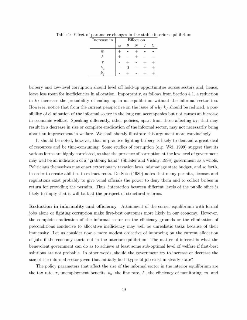
Table 1: Effect of parameter changes in the stable interior equilibriumIncrease in Effect on

φ θ N I U

m + - + - -F + - + - -τ - + - + +bu - 0 - + +kf - + - + +

bribery and low-level corruption should level off hold-up opportunities across sectors and, hence,

leave less room for inefficiencies in allocation. Importantly, as follows from Section 4.1, a reduction

in kf increases the probability of ending up in an equilibrium without the informal sector too.

However, notice that from the current perspective on the issue of why kf should be reduced, a pos-

sibility of elimination of the informal sector in the long run accompanies but not causes an increase

in economic welfare. Speaking differently, other policies, apart from those affecting kf , that may

result in a decrease in size or complete eradication of the informal sector, may not necessarily bring

about an improvement in welfare. We shall shortly illustrate this argument more convincingly.

It should be noted, however, that in practice fighting bribery is likely to demand a great deal

of resources and be time-consuming. Some studies of corruption (e.g. Wei, 1999) suggest that its

various forms are highly correlated, so that the presence of corruption at the low level of government

may well be an indication of a "grabbing hand" (Shleifer and Vishny, 1998) government as a whole.

Politicians themselves may enact extortionary taxation laws, mismanage state budget, and so forth,

in order to create abilities to extract rents. De Soto (1989) notes that many permits, licenses and

regulations exist probably to give venal officials the power to deny them and to collect bribes in

return for providing the permits. Thus, interaction between different levels of the public office is

likely to imply that it will balk at the prospect of structural reforms.

Reduction in informality and efficiency Attainment of the corner equilibrium with formal

jobs alone or fighting corruption make first-best outcomes more likely in our economy. However,

the complete eradication of the informal sector on the efficiency grounds or the elimination of

preconditions conducive to allocative inefficiency may well be unrealistic tasks because of their

immensity. Let us consider now a more modest objective of improving on the current allocation

of jobs if the economy starts out in the interior equilibrium. The matter of interest is what the

benevolent government can do as to achieve at least some sub-optimal level of welfare if first-best

solutions are not probable. In other words, should the government try to increase or decrease the

size of the informal sector given that initially both types of job exist in steady state?

The policy parameters that affect the size of the informal sector in the interior equilibrium are

the tax rate, τ , unemployment benefits, bu, the fine rate, F , the efficiency of monitoring, m, and

49

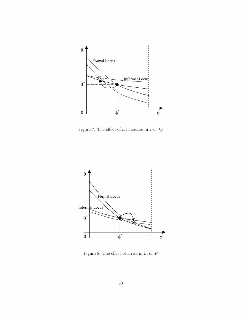
θ

φ0 1

Informal Locus

Formal Locus

θ*

φ*

Figure 7: The effect of an increase in τ or kf

θ

φ0 1

Informal Locus

Formal Locus

θ*

φ*

Figure 8: The effect of a rise in m or F

50

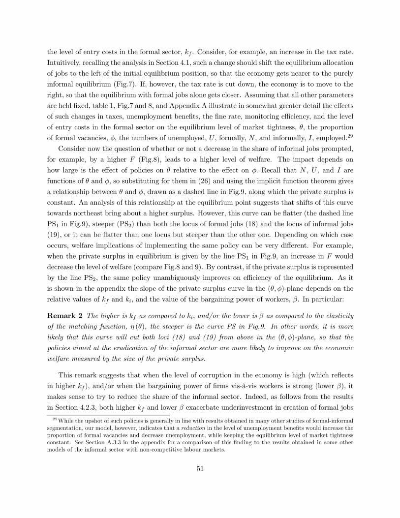
the level of entry costs in the formal sector, kf . Consider, for example, an increase in the tax rate.

Intuitively, recalling the analysis in Section 4.1, such a change should shift the equilibrium allocation

of jobs to the left of the initial equilibrium position, so that the economy gets nearer to the purely

informal equilibrium (Fig.7). If, however, the tax rate is cut down, the economy is to move to the

right, so that the equilibrium with formal jobs alone gets closer. Assuming that all other parameters

are held fixed, table 1, Fig.7 and 8, and Appendix A illustrate in somewhat greater detail the effects

of such changes in taxes, unemployment benefits, the fine rate, monitoring efficiency, and the level

of entry costs in the formal sector on the equilibrium level of market tightness, θ, the proportion

of formal vacancies, φ, the numbers of unemployed, U , formally, N , and informally, I, employed.29

Consider now the question of whether or not a decrease in the share of informal jobs prompted,

for example, by a higher F (Fig.8), leads to a higher level of welfare. The impact depends on

how large is the effect of policies on θ relative to the effect on φ. Recall that N , U , and I are

functions of θ and φ, so substituting for them in (26) and using the implicit function theorem gives

a relationship between θ and φ, drawn as a dashed line in Fig.9, along which the private surplus is

constant. An analysis of this relationship at the equilibrium point suggests that shifts of this curve

towards northeast bring about a higher surplus. However, this curve can be flatter (the dashed line

PS1 in Fig.9), steeper (PS2) than both the locus of formal jobs (18) and the locus of informal jobs

(19), or it can be flatter than one locus but steeper than the other one. Depending on which case

occurs, welfare implications of implementing the same policy can be very different. For example,

when the private surplus in equilibrium is given by the line PS1 in Fig.9, an increase in F would

decrease the level of welfare (compare Fig.8 and 9). By contrast, if the private surplus is represented

by the line PS2, the same policy unambiguously improves on efficiency of the equilibrium. As it

is shown in the appendix the slope of the private surplus curve in the (θ, φ)-plane depends on the

relative values of kf and ki, and the value of the bargaining power of workers, β. In particular:

Remark 2 The higher is kf as compared to ki, and/or the lower is β as compared to the elasticityof the matching function, η (θ), the steeper is the curve PS in Fig.9. In other words, it is more

likely that this curve will cut both loci (18) and (19) from above in the (θ, φ)-plane, so that the

policies aimed at the eradication of the informal sector are more likely to improve on the economic

welfare measured by the size of the private surplus.

This remark suggests that when the level of corruption in the economy is high (which reflects

in higher kf ), and/or when the bargaining power of firms vis-à-vis workers is strong (lower β), it

makes sense to try to reduce the share of the informal sector. Indeed, as follows from the results

in Section 4.2.3, both higher kf and lower β exacerbate underinvestment in creation of formal jobs

29While the upshot of such policies is generally in line with results obtained in many other studies of formal-informalsegmentation, our model, however, indicates that a reduction in the level of unemployment benefits would increase theproportion of formal vacancies and decrease unemployment, while keeping the equilibrium level of market tightnessconstant. See Section A.3.3 in the appendix for a comparison of this finding to the results obtained in some othermodels of the informal sector with non-competitive labour markets.

51

θ

φ0 1

Informal Locus

Formal Locus

PS1

PS2

PS2

PS1

θ*

φ*

++

+

+-

-

-

-

Figure 9: Private surplus and interior equilibrium

and overinvestment in creation of informal jobs, respectively. On the one hand, firms avoid the

formal sector where they have to give up more rents to the workers during wage bargains; on the

other hand, they aim to make the most of their stronger bargaining position in the informal sector,

other things being equal. Thus, under these conditions the allocative failure to distribute jobs

properly towards the formal sector is more acute, so that policies, making investments in creation

of informal workplaces less attractive, would be more likely to increase the level of economic welfare.

By contrast, if the difference between kf and ki is negligible, whereas β is significantly greater than

η (θ) a reduction in size of informality prompted by a change in τ , F, etc., is more likely to be

detrimental for economic welfare.

Obviously, a precise set of policies pursued by the government will depend on the fiscal stance

and other restrictions.30 By applying the same approach as we did above to the private surplus, it

is possible to show that the budget revenue

R (θ, φ) = Nτ + ImF − Ubu (35)

can also be represented as a negatively-sloped line in the (θ, φ)-plane. Its slope will be the larger

in absolute value the larger is the tax rate τ in comparison with the expected value of the fine in

the underground sector, mF. Thus,

Remark 3 The higher is τ as compared to mF the more likely policies reducing the proportion of

30So, for example, a type of the government obviously affects policies it opts for. A "benevolent dictator" (asdiscussed in Buchanan, 1975) is likely to act differently from a "grabbing hand" government (as in Shleifer andVishny, 1998). Also, political objectives may and often do differ depending on the part of the Laffer curve that theeconomy currently sits on (if, for instance, revenue maximisation is assumed). Buchanan and Lee (1982) illustratethis by drawing destinctions between short run and long run Laffer curves.

52

informal vacancies are to result in the higher budget revenue.

It should be clear that such policies can lead to an increase in both the budget revenue (35)

and the private surplus (26), so that the total gain of both the private agents and the government

rises. The result will depend on the relative slopes of the budget revenue level curve and the PS

curve in the (θ, φ)-plane.

4.2.5 Summary

In this section we have generally addressed the issue of what governments should do to improve on

the efficiency of equilibrium allocation of jobs and workers across the formal and informal sectors.

We have split the analysis in two steps.

Firstly, we have shown that inefficiency of equilibria is inherent in our model. Any steady

state is not optimal due to congestion externalities of a standard type. In order to internalise such

externalities, the so-called Hosios efficiency condition (Hosios, 1990), equating the bargaining power

of workers and the elasticity of the matching function, must hold. However, if the economy ends up

in a steady state with both formal and informal sectors, such a long-run equilibrium suffers from an

additional market failure caused by the so-called hold-up problem (Grout, 1984; Williamson, 1985).

The preconditions for hold-ups in our model are exacerbated by the lower tier of the government -

corrupt bureaucracy - that extorts rents from firms entering the formal market. In this situation

the Hosios condition is no longer enough to guarantee the attainment of first-best optimum, as

it can never internalise the allocative inefficiency. In turn, because of that firms underinvest in

creation of formal vacancies, while workers gain higher rents in the formal economy during wage

bargaining. Importantly, the inefficiency of equilibria that we have considered here is not provoked

by a particular size of the informal economy, but rather by particular conditions in the labour

market. Thus, in order to make first-best outcomes more probable the government has to address

causes of inefficiencies but not try to scale down the informal sector in the first place. Still, reduction

in the size of the latter can come about as a by-product of particular efficiency-improving policies.

As a second exercise we have looked into the ability of the government to attain sub-optimal

levels of welfare if the economy starts out in the interior equilibrium. We have especially been

interested whether a reduction in informality in such a situation can be efficiency improving. It

turned out that welfare effect of such policies as changes in the tax rate, fines for running businesses

informally, unemployment benefits, or monitoring efficiency, depends on the same factors which lead

to inefficiency of the equilibrium. In particular, the stronger is the position of firms vis-à-vis workers

in wage bargains, and/or the better are the opportunities for hold-up in the formal sector, the more

acute is underinvestment in formal job creation. So, the more likely is the reduction in the share of

informal vacancies to bring about an improvement in economic welfare. Thus, the main conclusion

that can be drawn from this discussion is that conditions in the labour market do affect welfare

implications of policies. An important result is that the relation between the bargaining power of

53

workers and the elasticity of the matching function must be taken into account before deciding on

reducing the scope of informality. However, the previous literature (Kolm and Larsen, 2001; Bouev,

2002; and Fugazza and Jacques, 2004), that incorporates the search-in-the-labour-market approach

to the modelling of the formal-informal segmentation and that assesses welfare implications of

various policies, has completely overlooked the considerations outlined here.

5 Concluding Remarks

In this work we have broadly pursued two main objectives.

First, it has been shown that labour market institutions, such as wage bargaining may be a

very important channel through which state regulations lead to stable emergence of informality in

the long run. Labour costs are widely held to be one of the main culprits of causing a firms’ drive

of moving businesses underground, however, the issue of wage negotiations have not as yet been

addressed in this respect.

The model presented in this essay suggests that general conditions for the emergence of long-

term mixed equilibria with formal and informal sectors imply that the two negotiating sides, i.e.

firms and workers, have to prefer different sectors if given full power to appropriate the whole surplus

of a productive match. Such a difference in preferences may be possible due to differences in both

sector surpluses and the outside options of firms and workers. The former are caused by standard

government regulations, such as taxation, penalties for involvement into irregular activities, etc.

The latter are linked with both the impact of the government’s auditing activities whereby they

destroy informal matches and cause asymmetries in match lifetimes across the two sectors, and the

venal practices of the state bureaucracy extorting bribes and erecting artificial barriers to entry.

Costly time-consuming search for trade partners acts as a catalyst of the effects of government

audit and bureaucratic extortion, as it rases opportunity costs of idleness of sunk investments and

leads to rent sharing.

The role of wage bargaining and rent sharing in the emergence of equilibria with the informal

sector has important implications for policy-makers - a second major issue analysed in this essay.

We have illustrated many implications by considering such a standard policy tool as the tax rate. It

has been found that, in general, higher tax rates raise the probability of an equilibrium with informal

jobs alone. However, the precise effect (i.e. the type of equilibrium that the economy eventually

attains) of choosing a particular tax rate depends on relative values of reservation options of formal

and informal firms in their wage bargaining with workers. More specifically, other things being equal

governments can afford setting higher tax rates and still achieve a long-run equilibrium without

informality whenever formal firms enjoy a stronger position in wage bargains with job-seekers than

their informal counterparts do. This significance of firms’ reservation options in bargaining for the

effect of policies is an important implication for policy making that has hardly been given any

attention in the previous literature on the topic. As we have seen, governments can affect these

54

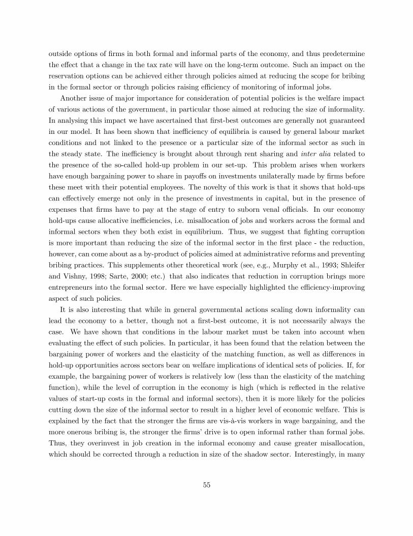
outside options of firms in both formal and informal parts of the economy, and thus predetermine

the effect that a change in the tax rate will have on the long-term outcome. Such an impact on the

reservation options can be achieved either through policies aimed at reducing the scope for bribing

in the formal sector or through policies raising efficiency of monitoring of informal jobs.

Another issue of major importance for consideration of potential policies is the welfare impact

of various actions of the government, in particular those aimed at reducing the size of informality.

In analysing this impact we have ascertained that first-best outcomes are generally not guaranteed

in our model. It has been shown that inefficiency of equilibria is caused by general labour market

conditions and not linked to the presence or a particular size of the informal sector as such in

the steady state. The inefficiency is brought about through rent sharing and inter alia related to

the presence of the so-called hold-up problem in our set-up. This problem arises when workers

have enough bargaining power to share in payoffs on investments unilaterally made by firms before

these meet with their potential employees. The novelty of this work is that it shows that hold-ups

can effectively emerge not only in the presence of investments in capital, but in the presence of

expenses that firms have to pay at the stage of entry to suborn venal officials. In our economy

hold-ups cause allocative inefficiencies, i.e. misallocation of jobs and workers across the formal and

informal sectors when they both exist in equilibrium. Thus, we suggest that fighting corruption

is more important than reducing the size of the informal sector in the first place - the reduction,

however, can come about as a by-product of policies aimed at administrative reforms and preventing

bribing practices. This supplements other theoretical work (see, e.g., Murphy et al., 1993; Shleifer

and Vishny, 1998; Sarte, 2000; etc.) that also indicates that reduction in corruption brings more

entrepreneurs into the formal sector. Here we have especially highlighted the efficiency-improving

aspect of such policies.

It is also interesting that while in general governmental actions scaling down informality can

lead the economy to a better, though not a first-best outcome, it is not necessarily always the

case. We have shown that conditions in the labour market must be taken into account when

evaluating the effect of such policies. In particular, it has been found that the relation between the

bargaining power of workers and the elasticity of the matching function, as well as differences in

hold-up opportunities across sectors bear on welfare implications of identical sets of policies. If, for

example, the bargaining power of workers is relatively low (less than the elasticity of the matching

function), while the level of corruption in the economy is high (which is reflected in the relative

values of start-up costs in the formal and informal sectors), then it is more likely for the policies

cutting down the size of the informal sector to result in a higher level of economic welfare. This is

explained by the fact that the stronger the firms are vis-à-vis workers in wage bargaining, and the

more onerous bribing is, the stronger the firms’ drive is to open informal rather than formal jobs.

Thus, they overinvest in job creation in the informal economy and cause greater misallocation,

which should be corrected through a reduction in size of the shadow sector. Interestingly, in many

55

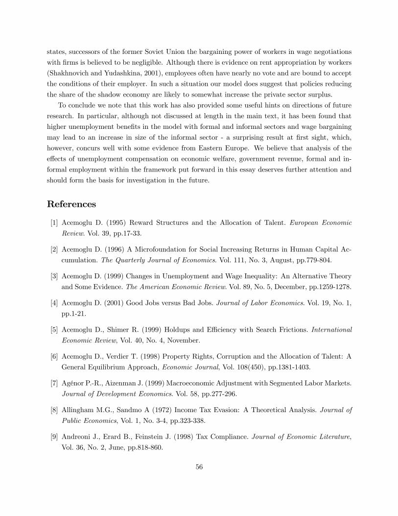
states, successors of the former Soviet Union the bargaining power of workers in wage negotiations

with firms is believed to be negligible. Although there is evidence on rent appropriation by workers

(Shakhnovich and Yudashkina, 2001), employees often have nearly no vote and are bound to accept

the conditions of their employer. In such a situation our model does suggest that policies reducing

the share of the shadow economy are likely to somewhat increase the private sector surplus.

To conclude we note that this work has also provided some useful hints on directions of future

research. In particular, although not discussed at length in the main text, it has been found that

higher unemployment benefits in the model with formal and informal sectors and wage bargaining

may lead to an increase in size of the informal sector - a surprising result at first sight, which,

however, concurs well with some evidence from Eastern Europe. We believe that analysis of the

effects of unemployment compensation on economic welfare, government revenue, formal and in-

formal employment within the framework put forward in this essay deserves further attention and

should form the basis for investigation in the future.

References

[1] Acemoglu D. (1995) Reward Structures and the Allocation of Talent. European Economic

Review. Vol. 39, pp.17-33.

[2] Acemoglu D. (1996) A Microfoundation for Social Increasing Returns in Human Capital Ac-

cumulation. The Quarterly Journal of Economics. Vol. 111, No. 3, August, pp.779-804.

[3] Acemoglu D. (1999) Changes in Unemployment and Wage Inequality: An Alternative Theory

and Some Evidence. The American Economic Review. Vol. 89, No. 5, December, pp.1259-1278.

[4] Acemoglu D. (2001) Good Jobs versus Bad Jobs. Journal of Labor Economics. Vol. 19, No. 1,

pp.1-21.

[5] Acemoglu D., Shimer R. (1999) Holdups and Efficiency with Search Frictions. International

Economic Review, Vol. 40, No. 4, November.

[6] Acemoglu D., Verdier T. (1998) Property Rights, Corruption and the Allocation of Talent: A

General Equilibrium Approach, Economic Journal, Vol. 108(450), pp.1381-1403.

[7] Agénor P.-R., Aizenman J. (1999) Macroeconomic Adjustment with Segmented Labor Markets.

Journal of Development Economics. Vol. 58, pp.277-296.

[8] Allingham M.G., Sandmo A (1972) Income Tax Evasion: A Theoretical Analysis. Journal of

Public Economics, Vol. 1, No. 3-4, pp.323-338.

[9] Andreoni J., Erard B., Feinstein J. (1998) Tax Compliance. Journal of Economic Literature,

Vol. 36, No. 2, June, pp.818-860.

56

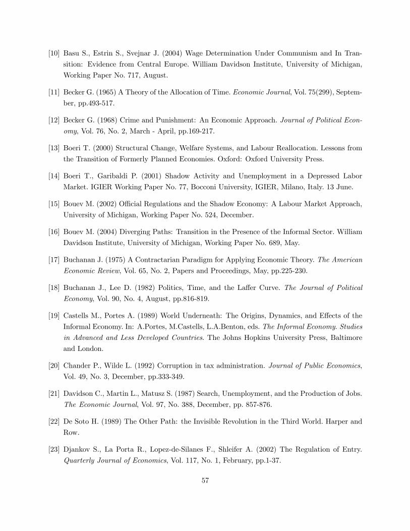
[10] Basu S., Estrin S., Svejnar J. (2004) Wage Determination Under Communism and In Tran-

sition: Evidence from Central Europe. William Davidson Institute, University of Michigan,

Working Paper No. 717, August.

[11] Becker G. (1965) A Theory of the Allocation of Time. Economic Journal, Vol. 75(299), Septem-

ber, pp.493-517.

[12] Becker G. (1968) Crime and Punishment: An Economic Approach. Journal of Political Econ-

omy, Vol. 76, No. 2, March - April, pp.169-217.

[13] Boeri T. (2000) Structural Change, Welfare Systems, and Labour Reallocation. Lessons from

the Transition of Formerly Planned Economies. Oxford: Oxford University Press.

[14] Boeri T., Garibaldi P. (2001) Shadow Activity and Unemployment in a Depressed Labor

Market. IGIER Working Paper No. 77, Bocconi University, IGIER, Milano, Italy. 13 June.

[15] Bouev M. (2002) Official Regulations and the Shadow Economy: A Labour Market Approach,

University of Michigan, Working Paper No. 524, December.

[16] Bouev M. (2004) Diverging Paths: Transition in the Presence of the Informal Sector. William

Davidson Institute, University of Michigan, Working Paper No. 689, May.

[17] Buchanan J. (1975) A Contractarian Paradigm for Applying Economic Theory. The American

Economic Review, Vol. 65, No. 2, Papers and Proceedings, May, pp.225-230.

[18] Buchanan J., Lee D. (1982) Politics, Time, and the Laffer Curve. The Journal of Political

Economy, Vol. 90, No. 4, August, pp.816-819.

[19] Castells M., Portes A. (1989) World Underneath: The Origins, Dynamics, and Effects of the

Informal Economy. In: A.Portes, M.Castells, L.A.Benton, eds. The Informal Economy. Studies

in Advanced and Less Developed Countries. The Johns Hopkins University Press, Baltimore

and London.

[20] Chander P., Wilde L. (1992) Corruption in tax administration. Journal of Public Economics,

Vol. 49, No. 3, December, pp.333-349.

[21] Davidson C., Martin L., Matusz S. (1987) Search, Unemployment, and the Production of Jobs.

The Economic Journal, Vol. 97, No. 388, December, pp. 857-876.

[22] De Soto H. (1989) The Other Path: the Invisible Revolution in the Third World. Harper and

Row.

[23] Djankov S., La Porta R., Lopez-de-Silanes F., Shleifer A. (2002) The Regulation of Entry.

Quarterly Journal of Economics, Vol. 117, No. 1, February, pp.1-37.

57

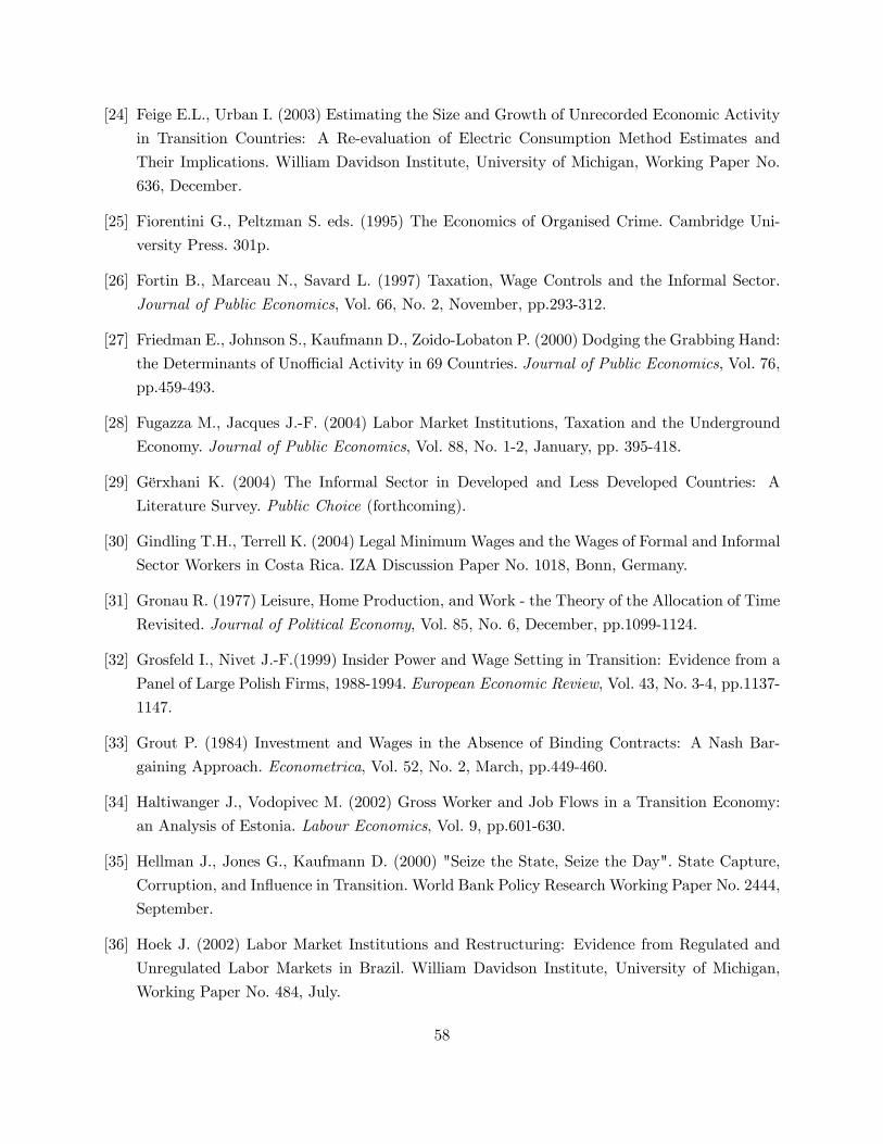
[24] Feige E.L., Urban I. (2003) Estimating the Size and Growth of Unrecorded Economic Activity

in Transition Countries: A Re-evaluation of Electric Consumption Method Estimates and

Their Implications. William Davidson Institute, University of Michigan, Working Paper No.

636, December.

[25] Fiorentini G., Peltzman S. eds. (1995) The Economics of Organised Crime. Cambridge Uni-

versity Press. 301p.

[26] Fortin B., Marceau N., Savard L. (1997) Taxation, Wage Controls and the Informal Sector.

Journal of Public Economics, Vol. 66, No. 2, November, pp.293-312.

[27] Friedman E., Johnson S., Kaufmann D., Zoido-Lobaton P. (2000) Dodging the Grabbing Hand:

the Determinants of Unofficial Activity in 69 Countries. Journal of Public Economics, Vol. 76,

pp.459-493.

[28] Fugazza M., Jacques J.-F. (2004) Labor Market Institutions, Taxation and the Underground

Economy. Journal of Public Economics, Vol. 88, No. 1-2, January, pp. 395-418.

[29] Gërxhani K. (2004) The Informal Sector in Developed and Less Developed Countries: A

Literature Survey. Public Choice (forthcoming).

[30] Gindling T.H., Terrell K. (2004) Legal MinimumWages and the Wages of Formal and Informal

Sector Workers in Costa Rica. IZA Discussion Paper No. 1018, Bonn, Germany.

[31] Gronau R. (1977) Leisure, Home Production, and Work - the Theory of the Allocation of Time

Revisited. Journal of Political Economy, Vol. 85, No. 6, December, pp.1099-1124.

[32] Grosfeld I., Nivet J.-F.(1999) Insider Power and Wage Setting in Transition: Evidence from a

Panel of Large Polish Firms, 1988-1994. European Economic Review, Vol. 43, No. 3-4, pp.1137-

1147.

[33] Grout P. (1984) Investment and Wages in the Absence of Binding Contracts: A Nash Bar-

gaining Approach. Econometrica, Vol. 52, No. 2, March, pp.449-460.

[34] Haltiwanger J., Vodopivec M. (2002) Gross Worker and Job Flows in a Transition Economy:

an Analysis of Estonia. Labour Economics, Vol. 9, pp.601-630.

[35] Hellman J., Jones G., Kaufmann D. (2000) "Seize the State, Seize the Day". State Capture,

Corruption, and Influence in Transition. World Bank Policy Research Working Paper No. 2444,

September.

[36] Hoek J. (2002) Labor Market Institutions and Restructuring: Evidence from Regulated and

Unregulated Labor Markets in Brazil. William Davidson Institute, University of Michigan,

Working Paper No. 484, July.

58

[37] Hosios A. (1990) On the Efficiency of Matching and Related Models of Search and Unemploy-

ment. Review of Economic Studies, Vol. 57, No. 2, April, pp.279-298.

[38] Ingster A.Yu. (2003) Informal Contracts in Transition Economies. A Dynamic Approach. Eco-

nomics Education and Research Consortium Working Paper Series, WP No. 03/05, Moscow,

Russia.

[39] Johnson S., Kaufmann D., McMillan J., Woodruff C. (2000) Why do Firms Hide? Bribes

and Unofficial Activity after Communism. Journal of Public Economics, Vol. 76, No. 3, June,

pp.495-520.

[40] Johnson S., Kaufmann D., Shleifer A. (1997) The Unofficial Economy in Transition. Brookings

Papers on Economic Activity, No. 2, 159-239.

[41] Kamien M., Schwartz N. (2001) Dynamic Optimization. The Calculus of Variations and Op-

timal Control in Economics and Management. Second Edition. North-Holland.

[42] Kaufmann D. (1997) Why is Ukraine’s Economy - and Russia’s - not Growing? Transition.

The World Bank. April.

[43] Kaufmann D., Kaliberda A. (1996) Integrating the Unofficial Economy into the Dynamics of

Post-Socialist Economies: A Framework of Analysis and Evidence. The World Bank Policy

Research Working Paper No. 1691, August.

[44] Kesselman J.R. (1989) Income Tax Evasion: An Intersectoral Analysis. Journal of Public

Economics, Vol. 38, No. 2, pp.137-148.

[45] Kolev A. (1998) Labour Supply in the Informal Economy in Russia during Transition. CEPR

Discussion Paper No. 2024, CEPR, London.

[46] Kolm A-S., Larsen B. (2001) Moral Costs, the Informal Sector and Unemployment. Working

paper 1-2001, Institut for Nationaløkonomi, Handelshøjskolen i København, Department of

Economics, Copenhagen Business School.

[47] Kolm A-S., Larsen B. (2004) Wages, Unemployment, and the Underground Economy. Forth-

coming in MIT press.

[48] Lackó M. (2000) Hidden Economy - an Unknown Quantity? Comparative Analysis of Hidden

Economies in Transition Countries, 1989-1995. Economics of Transition, Vol. 8, No. 1, pp.117-

149.

[49] Lemieux T., Fortin B., Frechette P. (1994) The Effects of Taxes on Labour Supply in the

Underground Economy. American Economic Review, Vol. 84, No. 1, March, pp.231-254.

59

[50] Loayza N. (1996) The Economics of the Informal Sector: A Simple Model and Some Empirical

Evidence from Latin America. Carnegie-Rochester Conference Series on Public Policy, Vol.

45, pp.129-162.

[51] Luke P.J., Schaffer M.E. (1999) Wage Determination in Russia: An Econometric Investigation.

Centre for Economic Reform and Transformation Discussion Paper No. 99/08, Heriot-Watt

University, Edinburgh.

[52] MacLeod W.B., Malcomson J.M. (1993) Investments, Holdup, and the Form of Market Con-

tracts. The American Economic Review, Vol. 83, No. 4, September, pp.811-837.

[53] Malcomson J. M. (1997) Contracts, Hold-up, and Labor Markets. Journal of Economic Liter-

ature, Vol. 35, No. 4, December, pp.1916-1957.

[54] Mønsted T. (2000) Wage Differentials Between the Formal and the Informal Sector in Urban

Bolivia. Instituto de Investigaciones Socio-Económicas, Universidad Católica Boliviana, La

Paz, Bolivía. February.

[55] Murphy K.M., Shleifer A., Vishny R.W. (1993) Why is Rent-Seeking So Costly to Growth?

American Economic Review Papers and Proceedings, Vol. 83, No. 2, May, pp.409-414.

[56] Nash J. (1950) The Bargaining Problem. Econometrica, Vol. 18, No. 2, April, pp.155-162.

[57] Petrongolo B., Pissarides C.A. (2001) Looking into the Black Box: A Survey of the Matching

Function. Journal of Economic Literature, Vol. 39, No. 2, June, pp.390-431.

[58] Pissarides C.A. (2000) Equilibrium Unemployment Theory. 2nd edition, Cambridge, MA, Lon-

don, UK, MIT press.

[59] Roshchin S., Markova K. (2004) Choice among Different Job Search Channels: the Evidence

from Russian Labor Market. Economics Education and Research Consortium Working Paper

Series, WP No. 04/05, Moscow.

[60] Roshchin S., Razumova T. (2002) Secondary Employment in Russia: Labour Supply Model-

ing. Economics Education and Research Consortium Working Paper Series, WP No. 02/07E,

Moscow.

[61] Safavian M, Graham D., Gonzalez-Vega C. (2001) Corruption and Microenterprises in Russia.

World Development Vol. 29, No. 7, pp.1215-1224.

[62] Sandmo A. (1981) Income Tax Evasion, Labour Supply, and the Equity-Efficiency Tradeoff.

Journal of Public Economics, Vol. 16, No. 3, December, pp.265-288.

60

[63] Sarte P-D.G. (2000) Informality and Rent-seeking Bureaucracies in a Model of Long-run

Growth. Journal of Monetary Economics, Vol. 46, pp.173-197.

[64] Schneider F. (2000) The Value Added of Underground Activities: Size and Measurement of the

Shadow Economies and Shadow Economy Labor Force All Over the World. Johannes Kepler

University of Linz, Austria. July.

[65] Schneider F. (2001) The Size and Development of the Shadow Economies and Shadow Economy

Labor Force of 18 Asian and 21 OECD Countries: First Results for the 90s. Invited paper

prepared for the Asia Pacific Finance Association (APFA) Conference 2001 ”Rebuilding Our

Financial Architecture” held in Bangkok, Thailand, July 22-25, 2001.

[66] Schneider F., Enste D.H. (2000) Shadow Economies: Size, Causes, and Consequences. Journal

of Economic Literature, Vol. 38, No. 1, pp.77-114

[67] Shaked A., Sutton J. (1984) Involuntary Unemployment as a Perfect Equilibrium in a Bar-

gaining Model. Econometrica, Vol. 52, No. 6, November, pp.1351-1364.

[68] Shakhnovich R., Yudashkina G. (2001) Wage-Setting and Employment Behavior of Enterprises

during the Period of Economic Transition. Economics Education and Research Consortium

Working Paper Series, WP No. 01/04, Moscow.

[69] Shleifer A., Vishny R.W. (1998) The Grabbing Hand. Government Pathologies and Their

Cures. Harvard University Press, Cambridge, MA, London, England. 278p.

[70] Slemrod J., Yitzhaki S. (2002) Tax Avoidance, Evasion, and Administration. In: A.J.Auerbach

and M.Feldstein, eds. Handbook of Public Economics, Vol. 3, pp. 1423-1470, Elsevier Science

B.V.

[71] Smirnova N. (2003) Job Search Behavior of Unemployed in Russia. William Davidson Working

Paper No. 629, November. William Davidson Institute, University of Michigan Business School,

Ann-Arbor, USA.

[72] Stevens M. (2004) New Microfoundations for the Aggregate Matching Function. University of

Oxford, Department of Economics Series.

[73] Sutton J. (1986) Non-Cooperative Bargaining Theory: An Introduction. The Review of Eco-

nomic Studies, Vol. 53, No. 5, October, pp.709-724.

[74] Thomas J.J. (1992) Informal Economic Activity. LSE Handbooks in Economics. London.

[75] Vostroknutova E. (2003) Shadow Economy, Rent-Seeking Activities and the Perils of Rein-

forcement of the Rule of Law. William Davidson Institute, University of Michigan, Working

Paper No. 578, March.

61

[76] Wane W. (2000) Tax Evasion, Corruption, and the Remuneration of Heterogeneous Inspectors.

World Bank Policy Research Working Paper No. 2394, July.

[77] Wei S.-J. (1999) Corruption in Economic Development: Beneficial Grease, Minor Annoyance,

or Major Obstacle? World Bank Policy Research Working Paper No. 2048, February.

[78] Williamson O.E. (1975) Markets and Hierarchies: Analysis and Antitrust Implications. New

York: the Free Press, London: Collier Macmillan Publishers, 286p.

[79] Williamson O.E. (1985) The Economic Institutions of Capitalism. New York: the Free Press,

450p.

62

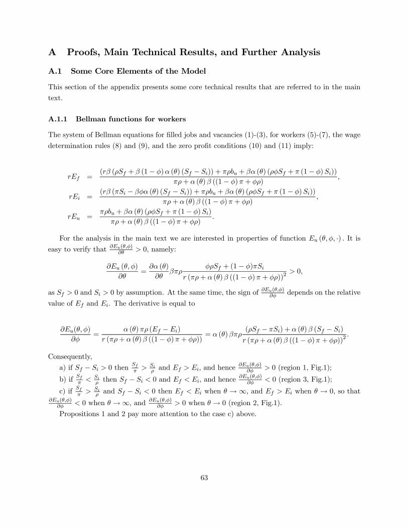
A Proofs, Main Technical Results, and Further Analysis

A.1 Some Core Elements of the Model

This section of the appendix presents some core technical results that are referred to in the main

text.

A.1.1 Bellman functions for workers

The system of Bellman equations for filled jobs and vacancies (1)-(3), for workers (5)-(7), the wage

determination rules (8) and (9), and the zero profit conditions (10) and (11) imply:

rEf =(rβ (ρSf + β (1− φ)α (θ) (Sf − Si)) + πρbu + βα (θ) (ρφSf + π (1− φ)Si))

πρ+ α (θ)β ((1− φ)π + φρ),

rEi =(rβ (πSi − βφα (θ) (Sf − Si)) + πρbu + βα (θ) (ρφSf + π (1− φ)Si))

πρ+ α (θ)β ((1− φ)π + φρ),

rEu =πρbu + βα (θ) (ρφSf + π (1− φ)Si)

πρ+ α (θ)β ((1− φ)π + φρ).

For the analysis in the main text we are interested in properties of function Eu (θ, φ, ·) . It iseasy to verify that ∂Eu(θ,φ)

∂θ > 0, namely:

∂Eu (θ, φ)

∂θ=

∂α (θ)

∂θβπρ

φρSf + (1− φ)πSi

r (πρ+ α (θ)β ((1− φ)π + φρ))2> 0,

as Sf > 0 and Si > 0 by assumption. At the same time, the sign of∂Eu(θ,φ)

∂φ depends on the relative

value of Ef and Ei. The derivative is equal to

∂Eu(θ, φ)

∂φ=

α (θ)πρ (Ef −Ei)

r (πρ+ α (θ)β ((1− φ)π + φρ))= α (θ)βπρ

(ρSf − πSi) + α (θ)β (Sf − Si)

r (πρ+ α (θ)β ((1− φ)π + φρ))2.

Consequently,

a) if Sf − Si > 0 thenSfπ > Si

ρ and Ef > Ei, and hence∂Eu(θ,φ)

∂φ > 0 (region 1, Fig.1);

b) if Sfπ < Si

ρ then Sf − Si < 0 and Ef < Ei, and hence∂Eu(θ,φ)

∂φ < 0 (region 3, Fig.1);

c) if Sfπ > Si

ρ and Sf − Si < 0 then Ef < Ei when θ → ∞, and Ef > Ei when θ → 0, so that∂Eu(θ,φ)

∂φ < 0 when θ →∞, and ∂Eu(θ,φ)∂φ > 0 when θ → 0 (region 2, Fig.1).

Propositions 1 and 2 pay more attention to the case c) above.

63

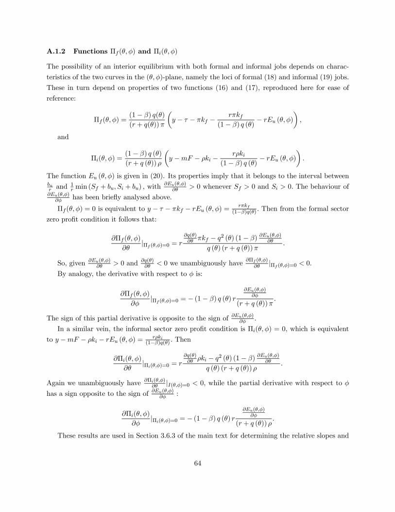
A.1.2 Functions Πf (θ, φ) and Πi(θ, φ)

The possibility of an interior equilibrium with both formal and informal jobs depends on charac-

teristics of the two curves in the (θ, φ)-plane, namely the loci of formal (18) and informal (19) jobs.

These in turn depend on properties of two functions (16) and (17), reproduced here for ease of

reference:

Πf (θ, φ) =(1− β) q(θ)

(r + q(θ))π

µy − τ − πkf − rπkf

(1− β) q (θ)− rEu (θ, φ)

¶,

and

Πi(θ, φ) =(1− β) q (θ)

(r + q (θ)) ρ

µy −mF − ρki − rρki

(1− β) q (θ)− rEu (θ, φ)

¶.

The function Eu (θ, φ) is given in (20). Its properties imply that it belongs to the interval betweenbur and

1r min (Sf + bu, Si + bu) , with

∂Eu(θ,φ)∂θ > 0 whenever Sf > 0 and Si > 0. The behaviour of

∂Eu(θ,φ)∂φ has been briefly analysed above.

Πf (θ, φ) = 0 is equivalent to y − τ − πkf − rEu (θ, φ) =rπkf

(1−β)q(θ) . Then from the formal sector

zero profit condition it follows that:

∂Πf (θ, φ)

∂θ|Πf (θ,φ)=0 = r

∂q(θ)∂θ πkf − q2 (θ) (1− β) ∂Eu(θ,φ)∂θ

q (θ) (r + q (θ))π.

So, given ∂Eu(θ,φ)∂θ > 0 and ∂q(θ)

∂θ < 0 we unambiguously have ∂Πf (θ,φ)∂θ |Πf (θ,φ)=0 < 0.

By analogy, the derivative with respect to φ is:

∂Πf (θ, φ)

∂φ|Πf (θ,φ)=0 = − (1− β) q (θ) r

∂Eu(θ,φ)∂φ

(r + q (θ))π.

The sign of this partial derivative is opposite to the sign of ∂Eu(θ,φ)∂φ .

In a similar vein, the informal sector zero profit condition is Πi(θ, φ) = 0, which is equivalent

to y −mF − ρki − rEu (θ, φ) =rρki

(1−β)q(θ) . Then

∂Πi(θ, φ)

∂θ|Πi(θ,φ)=0 = r

∂q(θ)∂θ ρki − q2 (θ) (1− β) ∂Eu(θ,φ)∂θ

q (θ) (r + q (θ)) ρ.

Again we unambiguously have ∂Πi(θ,φ)∂θ |I(θ,φ)=0 < 0, while the partial derivative with respect to φ

has a sign opposite to the sign of ∂Eu(θ,φ)∂φ :

∂Πi(θ, φ)

∂φ|Πi(θ,φ)=0 = − (1− β) q (θ) r

∂Eu(θ,φ)∂φ

(r + q (θ)) ρ.

These results are used in Section 3.6.3 of the main text for determining the relative slopes and

64

positions of the two loci (18) and (19) in the (θ, φ)-plane (see Fig.2-5).

A.1.3 Stocks and proportions

In Section 4 of the main text in the formula for the private surplus (26) we use expressions for

the stocks of workers in steady state. From Bellman equations (5)-(7), stocks at steady state must

satisfy:

δN = α(θ)φU,

(δ +m)I = α(θ)(1− φ)U,

α(θ)U = δN + (δ +m)I,

1 = I +N + U.

The solution to this system is

U =δ (δ +m)

δ(δ +m) + α (θ) (δ + φm),

I =δα (θ) (1− φ)

δ(δ +m) + α (θ) (δ + φm),

N =α (θ)φ (δ +m)

δ(δ +m) + α (θ) (δ + φm).

Thus, it is straightforward to see that the proportion of filled formal jobs in the total number

of filled jobs is not equal to φ, but given by

N

N + I=

α(θ)φUδ

α(θ)φUδ + α(θ)(1−φ)U

(δ+m)

= φδ +m

δ + φm.

Analogously, the proportion of informal jobs in the total number of jobs is

I

N + I=

α(θ)(1−φ)U(δ+m)

α(θ)φUδ + α(θ)(1−φ)U

(δ+m)

= (1− φ)δ

δ + φm.

All these results are useful for the analysis of dynamic maximisation problems (see below).

A.2 Proof of Propositions and Analysis of the Bifurcation Point

The variant of the model considered in the main text assumes that kf > ki. This assumption bears

on the conditions, under which an interior equilibrium with formal and informal jobs exists and is

stable. Here we provide proofs of the two propositions from the main text that help explain the

65

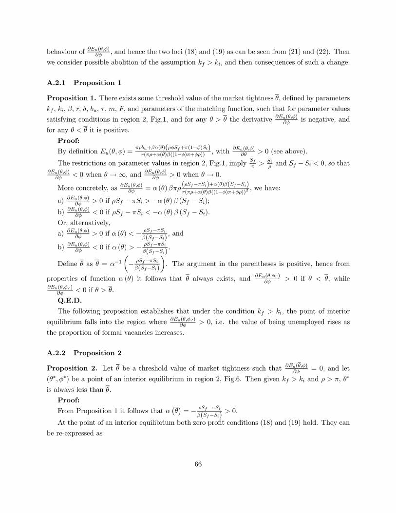
behaviour of ∂Eu(θ,φ)∂φ , and hence the two loci (18) and (19) as can be seen from (21) and (22). Then

we consider possible abolition of the assumption kf > ki, and then consequences of such a change.

A.2.1 Proposition 1

Proposition 1. There exists some threshold value of the market tightness θ, defined by parameterskf , ki, β, r, δ, bu, τ , m, F, and parameters of the matching function, such that for parameter values

satisfying conditions in region 2, Fig.1, and for any θ > θ the derivative ∂Eu(θ,φ)∂φ is negative, and

for any θ < θ it is positive.

Proof:By definition Eu(θ, φ) =

πρbu+βα(θ)(ρφSf+π(1−φ)Si)r(πρ+α(θ)β((1−φ)π+φρ)) , with ∂Eu(θ,φ)

∂θ > 0 (see above).

The restrictions on parameter values in region 2, Fig.1, imply Sfπ > Si

ρ and Sf −Si < 0, so that∂Eu(θ,φ)

∂φ < 0 when θ →∞, and ∂Eu(θ,φ)∂φ > 0 when θ → 0.

More concretely, as ∂Eu(θ,φ)∂φ = α (θ)βπρ

(ρSf−πSi)+α(θ)β(Sf−Si)r(πρ+α(θ)β((1−φ)π+φρ))2 , we have:

a) ∂Eu(θ,φ)∂φ > 0 if ρSf − πSi > −α (θ)β (Sf − Si);

b) ∂Eu(θ,φ)∂φ < 0 if ρSf − πSi < −α (θ)β (Sf − Si).

Or, alternatively,

a) ∂Eu(θ,φ)∂φ > 0 if α (θ) < − ρSf−πSi

β(Sf−Si) , and

b) ∂Eu(θ,φ)∂φ < 0 if α (θ) > − ρSf−πSi

β(Sf−Si) .

Define θ as θ = α−1µ− ρSf−πSi

β(Sf−Si)

¶. The argument in the parentheses is positive, hence from

properties of function α (θ) it follows that θ always exists, and ∂Eu(θ,φ,·)∂φ > 0 if θ < θ, while

∂Eu(θ,φ,·)∂φ < 0 if θ > θ.

Q.E.D.The following proposition establishes that under the condition kf > ki, the point of interior

equilibrium falls into the region where ∂Eu(θ,φ,·)∂φ > 0, i.e. the value of being unemployed rises as

the proportion of formal vacancies increases.

A.2.2 Proposition 2

Proposition 2. Let θ be a threshold value of market tightness such that ∂Eu(θ,φ)∂φ = 0, and let

(θ∗, φ∗) be a point of an interior equilibrium in region 2, Fig.6. Then given kf > ki and ρ > π, θ∗

is always less than θ.

Proof:From Proposition 1 it follows that α

¡θ¢= − ρSf−πSi

β(Sf−Si) > 0.

At the point of an interior equilibrium both zero profit conditions (18) and (19) hold. They can

be re-expressed as

66

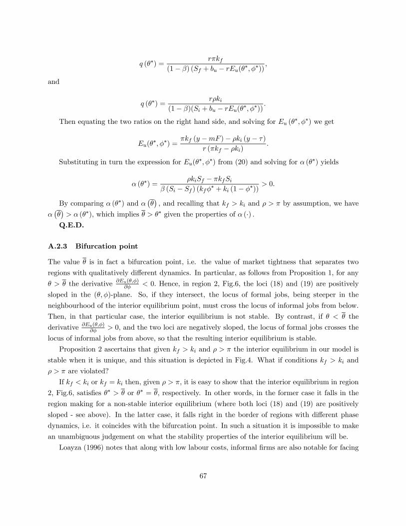
q (θ∗) =rπkf

(1− β) (Sf + bu − rEu(θ∗, φ∗))

,

and

q (θ∗) =rρki

(1− β)(Si + bu − rEu(θ∗, φ∗))

.

Then equating the two ratios on the right hand side, and solving for Eu (θ∗, φ∗) we get

Eu(θ∗, φ∗) =

πkf (y −mF )− ρki (y − τ)

r (πkf − ρki).

Substituting in turn the expression for Eu(θ∗, φ∗) from (20) and solving for α (θ∗) yields

α (θ∗) =ρkiSf − πkfSi

β (Si − Sf ) (kfφ∗ + ki (1− φ∗))

> 0.

By comparing α (θ∗) and α¡θ¢, and recalling that kf > ki and ρ > π by assumption, we have

α¡θ¢> α (θ∗), which implies θ > θ∗ given the properties of α (·) .

Q.E.D.

A.2.3 Bifurcation point

The value θ is in fact a bifurcation point, i.e. the value of market tightness that separates two

regions with qualitatively different dynamics. In particular, as follows from Proposition 1, for any

θ > θ the derivative ∂Eu(θ,φ)∂φ < 0. Hence, in region 2, Fig.6, the loci (18) and (19) are positively

sloped in the (θ, φ)-plane. So, if they intersect, the locus of formal jobs, being steeper in the

neighbourhood of the interior equilibrium point, must cross the locus of informal jobs from below.

Then, in that particular case, the interior equilibrium is not stable. By contrast, if θ < θ the

derivative ∂Eu(θ,φ)∂φ > 0, and the two loci are negatively sloped, the locus of formal jobs crosses the

locus of informal jobs from above, so that the resulting interior equilibrium is stable.

Proposition 2 ascertains that given kf > ki and ρ > π the interior equilibrium in our model is

stable when it is unique, and this situation is depicted in Fig.4. What if conditions kf > ki and

ρ > π are violated?

If kf < ki or kf = ki then, given ρ > π, it is easy to show that the interior equilibrium in region

2, Fig.6, satisfies θ∗ > θ or θ∗ = θ, respectively. In other words, in the former case it falls in the

region making for a non-stable interior equilibrium (where both loci (18) and (19) are positively

sloped - see above). In the latter case, it falls right in the border of regions with different phase

dynamics, i.e. it coincides with the bifurcation point. In such a situation it is impossible to make

an unambiguous judgement on what the stability properties of the interior equilibrium will be.

Loayza (1996) notes that along with low labour costs, informal firms are also notable for facing

67

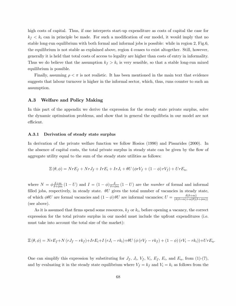
high costs of capital. Thus, if one interprets start-up expenditure as costs of capital the case for

kf < ki can in principle be made. For such a modification of our model, it would imply that no

stable long-run equilibrium with both formal and informal jobs is possible: while in region 2, Fig.6,

the equilibrium is not stable as explained above, region 4 ceases to exist altogether. Still, however,

generally it is held that total costs of access to legality are higher than costs of entry in informality.

Thus we do believe that the assumption kf > ki is very sensible, so that a stable long-run mixed

equilibrium is possible.

Finally, assuming ρ < π is not realistic. It has been mentioned in the main text that evidence

suggests that labour turnover is higher in the informal sector, which, thus, runs counter to such an

assumption.

A.3 Welfare and Policy Making

In this part of the appendix we derive the expression for the steady state private surplus, solve

the dynamic optimisation problems, and show that in general the equilibria in our model are not

efficient.

A.3.1 Derivation of steady state surplus

In derivation of the private welfare function we follow Hosios (1990) and Pissarides (2000). In

the absence of capital costs, the total private surplus in steady state can be given by the flow of

aggregate utility equal to the sum of the steady state utilities as follows:

Ξ (θ, φ) = NrEf +NrJf + IrEi + IrJi + θU (φrVf + (1− φ) rVf ) + UrEu,

where N = φ δ+mδ+φm (1− U) and I = (1 − φ) δ

δ+φm (1− U) are the number of formal and informal

filled jobs, respectively, in steady state. θU gives the total number of vacancies in steady state,

of which φθU are formal vacancies and (1− φ) θU are informal vacancies; U = δ(δ+m)(δ(δ+m)+α(θ)(δ+φm))

(see above).

As it is assumed that firms spend some resources, kf or ki, before opening a vacancy, the correct

expression for the total private surplus in our model must include the upfront expenditures (i.e.

must take into account the total size of the market):

Ξ (θ, φ) = NrEf+N (rJf − rkf )+IrEi+I (rJi − rki)+θU (φ (rVf − rkf ) + (1− φ) (rVi − rki))+UrEu.

One can simplify this expression by substituting for Jf , Ji, Vf , Vi, Ef , Ei, and Eu, from (1)-(7),

and by evaluating it in the steady state equilibrium where Vf = kf and Vi = ki as follows from the

68

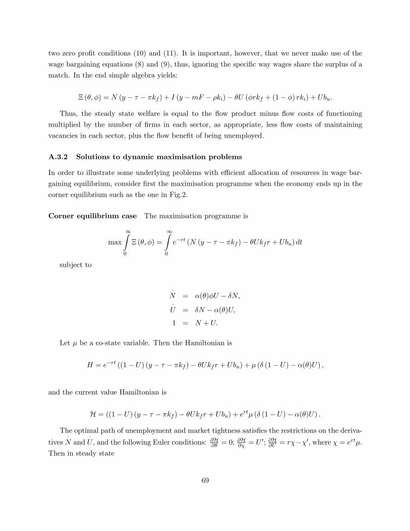
two zero profit conditions (10) and (11). It is important, however, that we never make use of the

wage bargaining equations (8) and (9), thus, ignoring the specific way wages share the surplus of a

match. In the end simple algebra yields:

Ξ (θ, φ) = N (y − τ − πkf ) + I (y −mF − ρki)− θU (φrkf + (1− φ) rki) + Ubu.

Thus, the steady state welfare is equal to the flow product minus flow costs of functioning

multiplied by the number of firms in each sector, as appropriate, less flow costs of maintaining

vacancies in each sector, plus the flow benefit of being unemployed.

A.3.2 Solutions to dynamic maximisation problems

In order to illustrate some underlying problems with efficient allocation of resources in wage bar-

gaining equilibrium, consider first the maximisation programme when the economy ends up in the

corner equilibrium such as the one in Fig.2.

Corner equilibrium case The maximisation programme is

max

∞Z0

Ξ (θ, φ) =

∞Z0

e−rt (N (y − τ − πkf )− θUkfr + Ubu) dt

subject to

·N = α(θ)φU − δN,·U = δN − α(θ)U,

1 = N + U.

Let µ be a co-state variable. Then the Hamiltonian is

H = e−rt ((1− U) (y − τ − πkf )− θUkfr + Ubu) + µ (δ (1− U)− α(θ)U) ,

and the current value Hamiltonian is

H = ((1− U) (y − τ − πkf )− θUkfr + Ubu) + ertµ (δ (1− U)− α(θ)U) .

The optimal path of unemployment and market tightness satisfies the restrictions on the deriva-

tives·N and

·U, and the following Euler conditions: ∂H

∂θ = 0;∂H∂χ = U 0; ∂H∂U = rχ−χ0, where χ = ertµ.

Then in steady state

69

∂H∂θ

= −Ukfr − α0(θ)χU = 0,

∂H∂χ

= δ (1− U)− α(θ)U = 0,

∂H∂U

= − (y − τ − πkf )− θkfr + bu − χ (δ + α(θ)) = rχ− χ0.

By solving this we get χ = −kfrα0(θ) , so that χ

0 = 0 and

Sf = rkf

µπ + α(θ)− θα0(θ)

α0 (θ)

¶.

The last expression is formula (29) given in the main text, which the efficient allocation must

satisfy. In turn, it is easy to check that the zero profit condition (18) implies

Sf = rkf(π + α (θ)β)

(1− β) q (θ).

In other words, the wage bargaining equilibrium satisfying the expression above, also given by (30)

in the main text, coincides with the efficient allocation (29) only if α0 (θ) = (1− β) q (θ) , which is

the standard result in the matching function literature (see Hosios, 1990). If this efficiency condition

does not hold, the wage bargaining equilibrium is not efficient.

Interior equilibrium case In the case of the interior equilibrium there is even more scope for

potential inefficiencies. Consider the maximisation programme

max

∞Z0

Ξ (θ, φ) =

∞Z0

e−rt (N (y − τ − πkf ) + I (y −mF − ρki)− θU (φkfr + (1− φ) kir) + Ubu) dt

subject to

·N = α (θ)φU − δN,·I = α (θ) (1− φ)U − (δ +m) I,·U = δN + (δ +m) I − α (θ)U,

1 = N + I + U.

Let µ and γ be co-state variables, so that the Hamiltonian is

70

H = e−rt (N (y − τ − πkf ) + (1−N − U) (y −mF − ρki)− θU (φkfr + (1− φ) kir) + Ubu)

+µ (δN + (δ +m) (1− U −N)− α (θ)U) + γ (α (θ)φU − δN) ,

Then the current value Hamiltonian is

H = (N (y − τ − πkf ) + (1−N − U) (y −mF − ρki)− θU (φkfr + (1− φ) kir) + Ubu)

+ertµ (δN + (δ +m) (1− U −N)− α (θ)U) + ertγ (α (θ)φU − δN) .

The optimal path of formal employment, unemployment and market tightness satisfies the

restrictions on·N,

·U, and

·I, and the following Euler conditions (see Kamien and Schwartz, 2001,

p.144): ∂H∂θ = 0, ∂H

∂φ = 0, ∂H∂µ = U 0, ∂H

∂γ = N 0, ∂H∂U = −µ0, ∂H

∂N = −γ0. Or, alternatively, for thecurrent value Hamiltonian we must have: ∂H

∂θ = 0, ∂H∂φ = 0, ∂H

∂χ = U 0, ∂H∂ψ = N 0, ∂H

∂U = rχ − χ0,∂H∂N = rψ − ψ0, where χ = ertµ and ψ = ertγ.

Thus

∂H∂θ

= −U (φkfr + (1− φ) kir)− α0 (θ)χU + α0 (θ)ψφU = 0,

∂H∂φ

= −θU (kfr − kir) + ψα (θ)U = 0,

∂H∂χ

= U 0 = δN + (δ +m) (1− U −N)− α (θ)U = 0,

∂H∂ψ

= N 0 = α (θ)φU − δN = 0,

∂H∂U

= − (y −mF − ρki − bu)− θ (φkfr + (1− φ) kir)− (δ +m+ α (θ))χ+ ψα (θ)φ = rχ− χ0,

∂H∂N

= (y − τ − πkf )− (y −mF − ρki)−mχ− δψ = rψ − ψ0.

By solving the first two equations we get

ψ = rθ (kf − ki)

α (θ)= r

(kf − ki)

q (θ),

χ =

µφr

θ (kf − ki)

α (θ)− r

(φkf + (1− φ) ki)

α0 (θ)

¶, (36)

so that ψ0 = 0 and χ0 = 0.Thus, at the point of optimum we must have

71

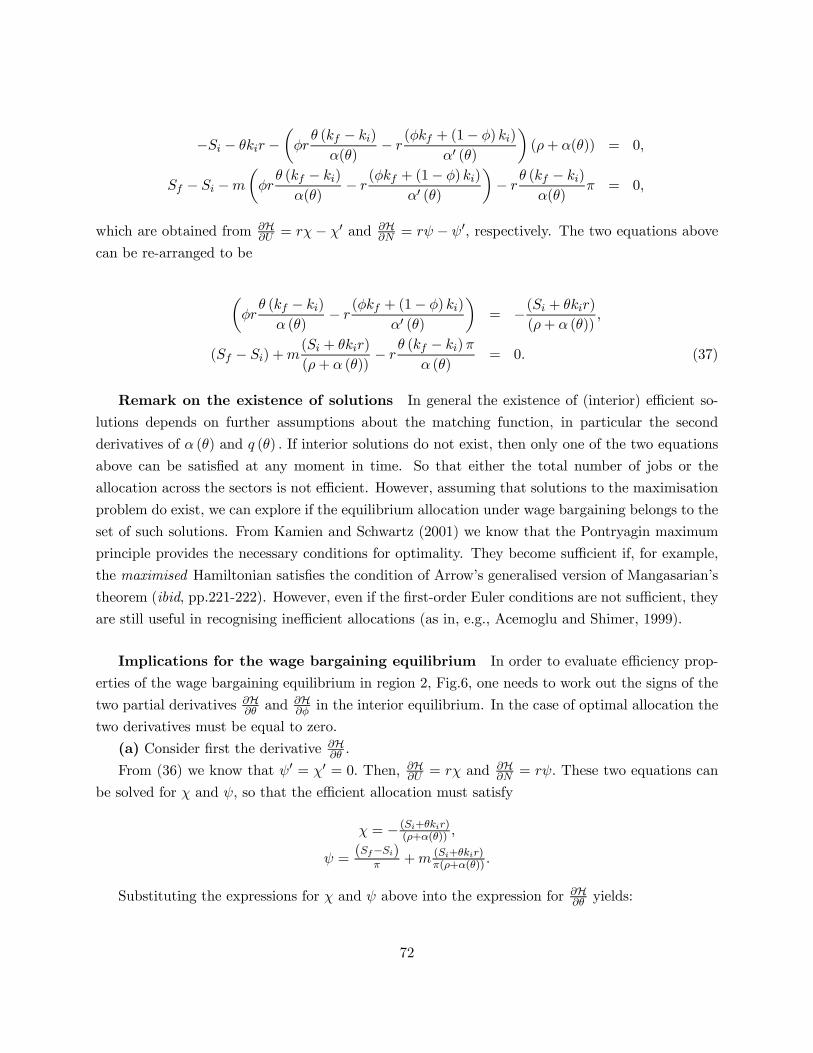
−Si − θkir −µφr

θ (kf − ki)

α(θ)− r

(φkf + (1− φ) ki)

α0 (θ)

¶(ρ+ α(θ)) = 0,

Sf − Si −m

µφr

θ (kf − ki)

α(θ)− r

(φkf + (1− φ) ki)

α0 (θ)

¶− r

θ (kf − ki)

α(θ)π = 0,

which are obtained from ∂H∂U = rχ− χ0 and ∂H

∂N = rψ − ψ0, respectively. The two equations abovecan be re-arranged to be

µφr

θ (kf − ki)

α (θ)− r

(φkf + (1− φ) ki)

α0 (θ)

¶= −(Si + θkir)

(ρ+ α (θ)),

(Sf − Si) +m(Si + θkir)

(ρ+ α (θ))− r

θ (kf − ki)π

α (θ)= 0. (37)

Remark on the existence of solutions In general the existence of (interior) efficient so-

lutions depends on further assumptions about the matching function, in particular the second

derivatives of α (θ) and q (θ) . If interior solutions do not exist, then only one of the two equations

above can be satisfied at any moment in time. So that either the total number of jobs or the

allocation across the sectors is not efficient. However, assuming that solutions to the maximisation

problem do exist, we can explore if the equilibrium allocation under wage bargaining belongs to the

set of such solutions. From Kamien and Schwartz (2001) we know that the Pontryagin maximum

principle provides the necessary conditions for optimality. They become sufficient if, for example,

the maximised Hamiltonian satisfies the condition of Arrow’s generalised version of Mangasarian’s

theorem (ibid, pp.221-222). However, even if the first-order Euler conditions are not sufficient, they

are still useful in recognising inefficient allocations (as in, e.g., Acemoglu and Shimer, 1999).

Implications for the wage bargaining equilibrium In order to evaluate efficiency prop-

erties of the wage bargaining equilibrium in region 2, Fig.6, one needs to work out the signs of the

two partial derivatives ∂H∂θ and

∂H∂φ in the interior equilibrium. In the case of optimal allocation the

two derivatives must be equal to zero.

(a) Consider first the derivative ∂H∂θ .

From (36) we know that ψ0 = χ0 = 0. Then, ∂H∂U = rχ and ∂H

∂N = rψ. These two equations can

be solved for χ and ψ, so that the efficient allocation must satisfy

χ = − (Si+θkir)(ρ+α(θ)) ,

ψ =(Sf−Si)

π +m (Si+θkir)π(ρ+α(θ)) .

Substituting the expressions for χ and ψ above into the expression for ∂H∂θ yields:

72

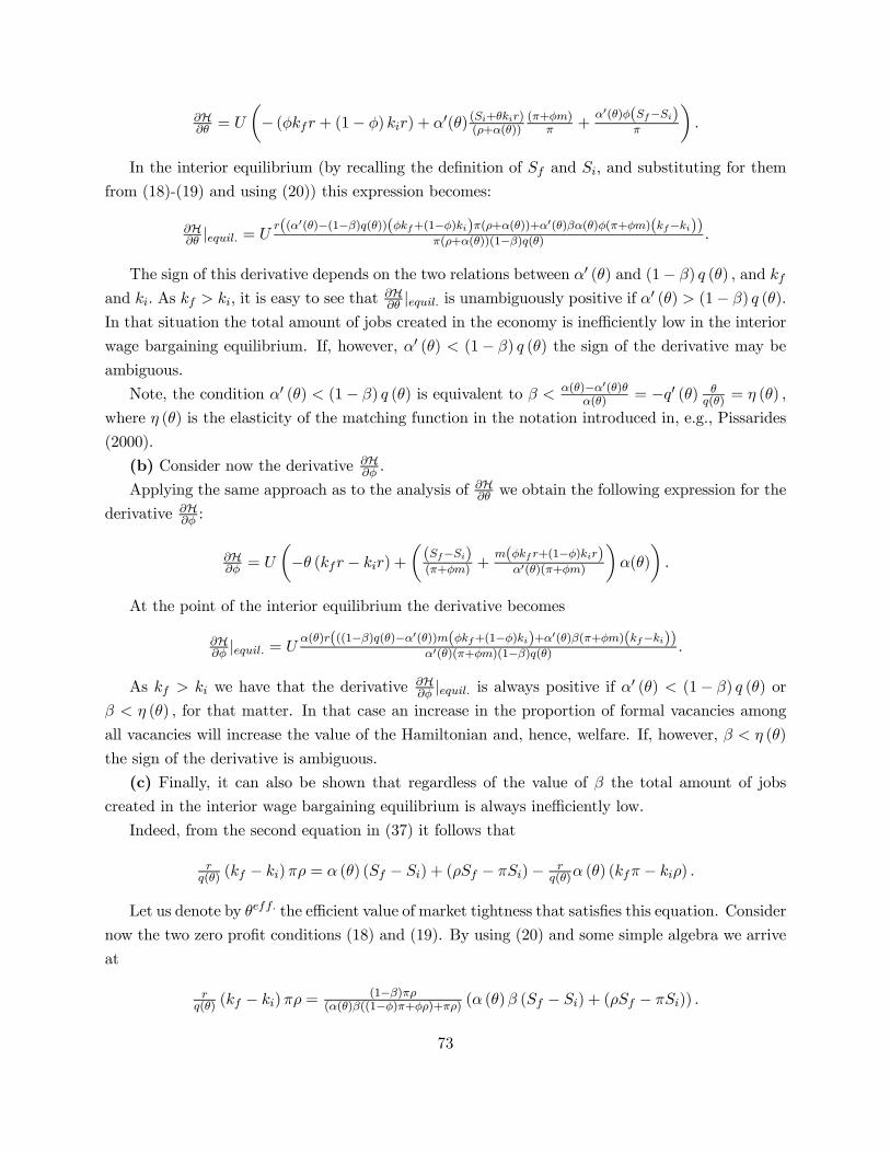
∂H∂θ = U

µ− (φkfr + (1− φ) kir) + α0(θ) (Si+θkir)(ρ+α(θ))

(π+φm)π +

α0(θ)φ(Sf−Si)π

¶.

In the interior equilibrium (by recalling the definition of Sf and Si, and substituting for them

from (18)-(19) and using (20)) this expression becomes:

∂H∂θ |equil. = U

r((α0(θ)−(1−β)q(θ))(φkf+(1−φ)ki)π(ρ+α(θ))+α0(θ)βα(θ)φ(π+φm)(kf−ki))π(ρ+α(θ))(1−β)q(θ) .

The sign of this derivative depends on the two relations between α0 (θ) and (1− β) q (θ) , and kfand ki. As kf > ki, it is easy to see that ∂H

∂θ |equil. is unambiguously positive if α0 (θ) > (1− β) q (θ).

In that situation the total amount of jobs created in the economy is inefficiently low in the interior

wage bargaining equilibrium. If, however, α0 (θ) < (1− β) q (θ) the sign of the derivative may be

ambiguous.

Note, the condition α0 (θ) < (1− β) q (θ) is equivalent to β < α(θ)−α0(θ)θα(θ) = −q0 (θ) θ

q(θ) = η (θ) ,

where η (θ) is the elasticity of the matching function in the notation introduced in, e.g., Pissarides

(2000).

(b) Consider now the derivative ∂H∂φ .

Applying the same approach as to the analysis of ∂H∂θ we obtain the following expression for thederivative ∂H

∂φ :

∂H∂φ = U

µ−θ (kfr − kir) +

µ(Sf−Si)(π+φm) +

m(φkf r+(1−φ)kir)α0(θ)(π+φm)

¶α(θ)

¶.

At the point of the interior equilibrium the derivative becomes

∂H∂φ |equil. = U

α(θ)r(((1−β)q(θ)−α0(θ))m(φkf+(1−φ)ki)+α0(θ)β(π+φm)(kf−ki))α0(θ)(π+φm)(1−β)q(θ) .

As kf > ki we have that the derivative ∂H∂φ |equil. is always positive if α0 (θ) < (1− β) q (θ) or

β < η (θ) , for that matter. In that case an increase in the proportion of formal vacancies among

all vacancies will increase the value of the Hamiltonian and, hence, welfare. If, however, β < η (θ)

the sign of the derivative is ambiguous.

(c) Finally, it can also be shown that regardless of the value of β the total amount of jobscreated in the interior wage bargaining equilibrium is always inefficiently low.

Indeed, from the second equation in (37) it follows that

rq(θ) (kf − ki)πρ = α (θ) (Sf − Si) + (ρSf − πSi)− r

q(θ)α (θ) (kfπ − kiρ) .

Let us denote by θeff. the efficient value of market tightness that satisfies this equation. Consider

now the two zero profit conditions (18) and (19). By using (20) and some simple algebra we arrive

at

rq(θ) (kf − ki)πρ =

(1−β)πρ(α(θ)β((1−φ)π+φρ)+πρ) (α (θ)β (Sf − Si) + (ρSf − πSi)) .

73

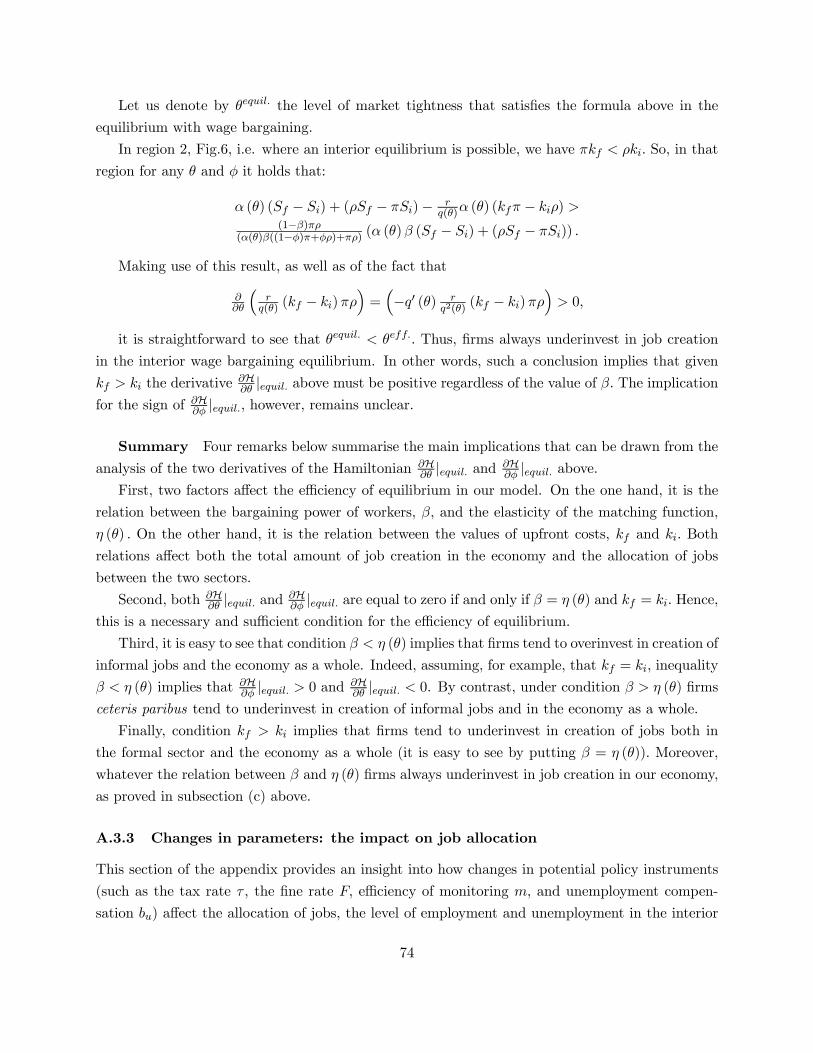
Let us denote by θequil. the level of market tightness that satisfies the formula above in the

equilibrium with wage bargaining.

In region 2, Fig.6, i.e. where an interior equilibrium is possible, we have πkf < ρki. So, in that

region for any θ and φ it holds that:

α (θ) (Sf − Si) + (ρSf − πSi)− rq(θ)α (θ) (kfπ − kiρ) >

(1−β)πρ(α(θ)β((1−φ)π+φρ)+πρ) (α (θ)β (Sf − Si) + (ρSf − πSi)) .

Making use of this result, as well as of the fact that

∂∂θ

³r

q(θ) (kf − ki)πρ´=³−q0 (θ) r

q2(θ)(kf − ki)πρ

´> 0,

it is straightforward to see that θequil. < θeff.. Thus, firms always underinvest in job creation

in the interior wage bargaining equilibrium. In other words, such a conclusion implies that given

kf > ki the derivative ∂H∂θ |equil. above must be positive regardless of the value of β. The implication

for the sign of ∂H∂φ |equil., however, remains unclear.

Summary Four remarks below summarise the main implications that can be drawn from the

analysis of the two derivatives of the Hamiltonian ∂H∂θ |equil. and ∂H

∂φ |equil. above.First, two factors affect the efficiency of equilibrium in our model. On the one hand, it is the

relation between the bargaining power of workers, β, and the elasticity of the matching function,

η (θ) . On the other hand, it is the relation between the values of upfront costs, kf and ki. Both

relations affect both the total amount of job creation in the economy and the allocation of jobs

between the two sectors.

Second, both ∂H∂θ |equil. and ∂H

∂φ |equil. are equal to zero if and only if β = η (θ) and kf = ki. Hence,

this is a necessary and sufficient condition for the efficiency of equilibrium.

Third, it is easy to see that condition β < η (θ) implies that firms tend to overinvest in creation of

informal jobs and the economy as a whole. Indeed, assuming, for example, that kf = ki, inequality

β < η (θ) implies that ∂H∂φ |equil. > 0 and ∂H

∂θ |equil. < 0. By contrast, under condition β > η (θ) firms

ceteris paribus tend to underinvest in creation of informal jobs and in the economy as a whole.

Finally, condition kf > ki implies that firms tend to underinvest in creation of jobs both in

the formal sector and the economy as a whole (it is easy to see by putting β = η (θ)). Moreover,

whatever the relation between β and η (θ) firms always underinvest in job creation in our economy,

as proved in subsection (c) above.

A.3.3 Changes in parameters: the impact on job allocation

This section of the appendix provides an insight into how changes in potential policy instruments

(such as the tax rate τ , the fine rate F, efficiency of monitoring m, and unemployment compen-

sation bu) affect the allocation of jobs, the level of employment and unemployment in the interior

74

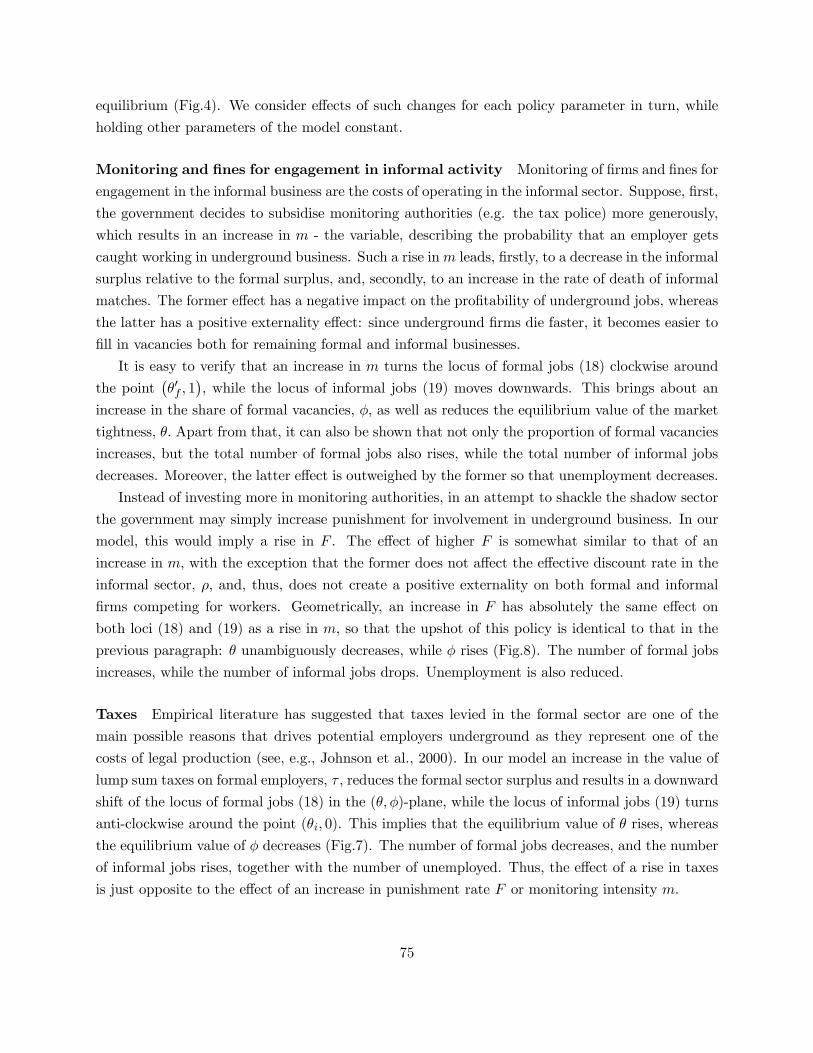
equilibrium (Fig.4). We consider effects of such changes for each policy parameter in turn, while

holding other parameters of the model constant.

Monitoring and fines for engagement in informal activity Monitoring of firms and fines for

engagement in the informal business are the costs of operating in the informal sector. Suppose, first,

the government decides to subsidise monitoring authorities (e.g. the tax police) more generously,

which results in an increase in m - the variable, describing the probability that an employer gets

caught working in underground business. Such a rise inm leads, firstly, to a decrease in the informal

surplus relative to the formal surplus, and, secondly, to an increase in the rate of death of informal

matches. The former effect has a negative impact on the profitability of underground jobs, whereas

the latter has a positive externality effect: since underground firms die faster, it becomes easier to

fill in vacancies both for remaining formal and informal businesses.

It is easy to verify that an increase in m turns the locus of formal jobs (18) clockwise around

the point¡θ0f , 1

¢, while the locus of informal jobs (19) moves downwards. This brings about an

increase in the share of formal vacancies, φ, as well as reduces the equilibrium value of the market

tightness, θ. Apart from that, it can also be shown that not only the proportion of formal vacancies

increases, but the total number of formal jobs also rises, while the total number of informal jobs

decreases. Moreover, the latter effect is outweighed by the former so that unemployment decreases.

Instead of investing more in monitoring authorities, in an attempt to shackle the shadow sector

the government may simply increase punishment for involvement in underground business. In our

model, this would imply a rise in F . The effect of higher F is somewhat similar to that of an

increase in m, with the exception that the former does not affect the effective discount rate in the

informal sector, ρ, and, thus, does not create a positive externality on both formal and informal

firms competing for workers. Geometrically, an increase in F has absolutely the same effect on

both loci (18) and (19) as a rise in m, so that the upshot of this policy is identical to that in the

previous paragraph: θ unambiguously decreases, while φ rises (Fig.8). The number of formal jobs

increases, while the number of informal jobs drops. Unemployment is also reduced.

Taxes Empirical literature has suggested that taxes levied in the formal sector are one of the

main possible reasons that drives potential employers underground as they represent one of the

costs of legal production (see, e.g., Johnson et al., 2000). In our model an increase in the value of

lump sum taxes on formal employers, τ , reduces the formal sector surplus and results in a downward

shift of the locus of formal jobs (18) in the (θ, φ)-plane, while the locus of informal jobs (19) turns

anti-clockwise around the point (θi, 0). This implies that the equilibrium value of θ rises, whereas

the equilibrium value of φ decreases (Fig.7). The number of formal jobs decreases, and the number

of informal jobs rises, together with the number of unemployed. Thus, the effect of a rise in taxes

is just opposite to the effect of an increase in punishment rate F or monitoring intensity m.

75

Unemployment benefits Contrary to taxes, fines and monitoring, the effect of unemployment

benefits on both formal surplus Sf and informal surplus Si is symmetric: both are reduced to the

same degree if unemployment compensation is made more generous. An increase in bu makes both

loci (18) and (19) shift down. In the case of an interior equilibrium it is straightforward to verify

that dφdbu

< 0, while dθdbu

= 0 by totally differentiating (18) and (19) with respect to θ, φ and bu,

and then solving the system of resulting equations in a stable equilibrium for dφdbu

and dθdbu

. This

result implies that in effect for a given θ both loci shift by the same distance, i.e. the equilibrium

proportion of formal jobs, φ, decreases, whereas the equilibrium value of market tightness, θ, does

not change. Thus, in the mixed case the introduction of more generous unemployment benefits

leads to crowding out of formal vacancies by informal ones. It will also decrease the number of

formal jobs, whereas both the number of informal jobs and unemployment will rise.

Other institutional changes Apart from parameters representing primary policy instruments,

the allocation of jobs across the sectors in the model depends on the value of entry costs, kf and

ki. These parameters reflect an institutional climate or environment in the economy: spreading

corruption and bribery, for instance, increases kf in relation to ki.

Consider, for example, a decrease in kf , which corresponds to less bribing and extortion in

the formal sector. This can possibly be achieved by restructuring bureaucracy and by better

enforcement of laws cracking down on corruption. With such a decrease in kf the locus of formal

jobs moves up, while the locus of informal jobs turns clockwise around the point (θi, 0). The

outcome is a drop in the equilibrium value of θ, and an increase in the equilibrium value of φ. The

number of formal jobs also rises, whereas the number of informal jobs decreases along with the level

of unemployment. By contrast, an upsurge in corruption and rent-seeking in the economy would

result in an increase in kf , scare firms away from the formal sector, and increase unemployment.

This would also support informal production and shift the allocation of vacancies and jobs towards

informality (Fig.7).

Table 1 in the main text summarises the effects of all changes considered here.

Some further notes on policies In order not to move the focus of discussion away from the

welfare effect of various policies, summarised in table 1 in the main text, we use this section of the

appendix to look more closely at two particular implications that could be drawn from analysing

the table. The first is concerned with the effect of various policies on the size of the informal sector.

The second is related to the impact on unemployment. Let us consider them in turn.

The table suggests that a decrease in m, F , and/or a increase in τ , kf , and bu raise the share

of the informal sector in the economy measured both by the proportion of informal vacancies in

the total number of vacancies, (1− φ) , and by the ratio of filled informal jobs to filled formal jobs,

i.e. I/N . The effects of a change in the intensity of monitoring, the severity of punishment for

concealing business underground, as well as the effect of higher taxes and impact of corruption

76

in general concur well with results obtained in many other empirical and theoretical studies of

informal economies, which, however, often lacked a proper account of the labour market (for just a

few examples the reader can be referred to the studies by Murphy et al., 1993; Shleifer and Vishny,

1998; Friedman et al., 2000; Johnson et al., 2000; Sarte, 2000). It is interesting, however, that our

model suggests that an increase in the size of the informal sector may be a result of policies aimed

at making unemployment compensation more generous. Such an outcome can be contrasted to two

recent theoretical results by Boeri (2000) and Fugazza and Jacques (2004) as regards the effect of

unemployment benefits on the size of the informal economy.

Boeri (2000) has observed that overly generous non-employment benefits at the outset of tran-

sition from planned to market economy in some countries of Eastern Europe favoured a labour

drive to non-employment, which in his model effectively implies employment in the informal sector.

He explained that by the effect that open-ended unemployment benefits have on the decision of

the non-employed to actively search for jobs in the formal part of the economy. Higher benefits

imply that more non-employed workers would prefer to receive the compensation and on top of

that enjoy readily available work in the subsistence sector. In other words, higher benefits weaken

worker incentives to search for jobs in the formal sector.

A qualitatively different result has been obtained by Fugazza and Jacques (2004) in the dual

labour market model where workers have to direct their search towards formal or informal vacancies.

In their work higher unemployment benefits raise the worker’s value of being attached to the regular

sector, so that more individuals are likely to search for a job in the formal economy. The contrast

with the Boeri’s conclusion arises because of the assumption that unemployed workers searching

for jobs in the irregular sector do not receive unemployment compensation.

The crucial difference between our work and the two studies just mentioned is that there a

change in the value of benefits does not affect the decision of employers to take off in the informal

economy. In our model an increase in that value affects the relative size of surpluses in each sector

and strengthens the bargaining position of job-seekers vis-à-vis employers. In the stable interior

equilibrium the surplus of a match is smaller in the formal sector, so the relative losses that firms

have to bear during wage bargains in the wake of the increase are higher in the formal part of the

economy. Hence, this urges more firms into the shadow sector.

The second point that can be seen from table 1 is that policies leading to an increase in informal

employment also cause an increase in unemployment. The existence of links between unemploy-

ment and underground employment is well-known. In many developing and transitional countries

informal activities have been argued to be of a subsistence nature (Gërxhani, 2004). They often

involve the individuals who are affected most severely by changes in the economy and who cannot

find a decent option in the formal sector. Not surprisingly, the unemployed, as a most vulnerable

cohort in the labour market, are, thus, the primary candidates for supplying labour in the infor-

mal sector. Theoretically it has already been suggested (Boeri and Garibaldi, 2001) that policies

77

aimed at reducing unemployment pay off by scaling down the shadow sector. At the same time, a

conclusion has been made (ibid) that attempts to reduce, in the first place, shadow employment

will result in higher open unemployment. Our model highlights that it is not always necessarily

true. Indeed, if one takes into account that labour turnover is higher in the shadow sector (as in

this essay is reflected in a shorter duration of an informal match), then crowding out of formal

vacancies by informal ones inevitably leads to a higher steady state unemployment. If, however,

the share of formal jobs in the economy increases, their on average longer duration makes for a

decrease in open unemployment. This is a general intuition for the results presented in table 1. By

contrast Boeri’s and Garibaldi’s (2001) argument is related to a specific view of the informal sector.

In particular, in their economy all jobs are necessarily formal when they are created. Informal

jobs are seen as a means not to sack a worker when some shock hits a formal production unit:

under certain conditions firms may find it profitable to convert formal, highly productive jobs into

informal, low-productive ones, and maintain them thereafter instead of closing down their business

completely. Meanwhile, workers employed in informal jobs have to look for better paid formal jobs

and compete in their search with the unemployed. In that case cracking down on the shadow sector

leads to an increase in open unemployment. At the same time, policies reducing unemployment

imply that it becomes easier for informally employed workers to find a formal job, as competition

from the unemployed, also looking for formal jobs, subsides. As a result, the duration of shadow

jobs drops and the size of the shadow sector is reduced.

In the absence of on-the-job search in our framework we draw attention specifically to the

moment of entry into the economy, and suggest that it is important to create conditions attracting

more firms into the formal sector, which will pay off by decreasing steady state unemployment.

A.3.4 Level curves for surpluses and state revenue

In the main text we consider the level curves of private surplus (26) and government revenue (35)

in the (θ, φ)-plane. Here we highlight the factors that their slopes depend upon.

Private surplus The private surplus is given by (26). Its partial derivative with respect to θ is

given by

∂Ξ(θ,φ)∂θ = α0(θ)δ(δ+m)

(δ(δ+m)+α(θ)(δ+φm))2(φ (δ +m)Sf + (1− φ) δSi)−

δ(δ+m)(φkf r+(1−φ)kir)δ(δ+m)+α(θ)(δ+φm)

³δ(δ+m)+(δ+φm)(α(θ)−θα0(θ))

(δ(δ+m)+α(θ)(δ+φm))

´.

In the interior equilibrium it is equal to

∂Ξ(θ,φ)∂θ |equil. =

rδ(δ+m)(α0(θ)r((δ+m)φkf+δ(1−φ)ki)+(φkf+(1−φ)ki)(α0(θ)(δ(δ+m)+(δ+φm)α(θ)β)−(1−β)q(θ)(δ(δ+m)+(δ+φm)(α(θ)−θα0(θ)))))(δ(δ+m)+α(θ)(δ+φm))2(1−β)q(θ) .

78

This derivative is unambiguously positive if α0 (θ) ≥ (1− β) q (θ) or, for that matter, β ≥ η (θ) .

The derivative of the private surplus with respect to φ is given by

∂Ξ(θ,φ)∂φ =

α(θ)(δ+m)δ((δ+m+α(θ))Sf−(δ+α(θ))Si)(δ(δ+m)+α(θ)(δ+φm))2

+ θα(θ)mδ(δ+m)(φkf r+(1−φ)kir)

(δ(δ+m)+α(θ)(δ+φm))2− θ

δ(δ+m)r(kf−ki)δ(δ+m)+α(θ)(δ+φm) .

In the interior equilibrium it is always positive and equal to

∂Ξ(θ,φ)∂φ |equil. = θ

r(δ+m)δ(mrki+(kf−ki)(α(θ)βφm+(δ+m+α(θ))(r+βδ)))(δ(δ+m)+α(θ)(δ+φm))2(1−β) > 0.

Thus, by using the implicit function theorem, the slope of the level curve of the private surplus

in the (θ, φ)-plane is

∂θ∂φ |PS; equil. =

− α(θ)(mrki+(kf−ki)(α(θ)βφm+(δ+m+α(θ))(r+βδ)))(α0(θ)r((m+δ)φkf+δ(1−φ)ki)+(φkf+(1−φ)ki)(α0(θ)(δ(δ+m)+(δ+φm)α(θ)β)−(1−β)q(θ)(δ(δ+m)+(δ+φm)(α(θ)−θα0(θ))))) .

From the expression above it can be seen that the higher is kf as compared to ki, and the lower

is β as compared to the elasticity of the matching function, η (θ), the steeper is the level curve in

the (θ, φ)-plane at the point of the interior equilibrium (see Fig.9).

State revenue The government revenue is given in (35). Its partial derivative with respect to θ

is always positive and equal to

∂R(θ,φ)∂θ = α0(θ)δ(δ+m)

(δ(δ+m)+α(θ)(δ+φm))2(φ (δ +m) τ + (1− φ) δmF + (δ + φm) bu) > 0.

The partial derivative with respect to φ is

∂R(θ,φ)∂φ = α(θ)(δ+m)δ

(δ(δ+m)+α(θ)(δ+φm))2((δ +m+ α (θ)) τ − (δ + α (θ))mF +mbu) > 0.

It is unambiguously positive in the interior equilibrium as τ > mF.

Then the slope of the government revenue level curve in the (θ, φ)-plane is

∂θ∂φ |R; equil. = −α(θ)((δ+m+α(θ))τ−(δ+α(θ))mF+mbu)

α0(θ)(φ(δ+m)τ+(1−φ)δmF+(δ+φm)bu)< 0.

Thus, the bigger is τ as compared to mF the steeper is the level curve.

79

DAVIDSON INSTITUTE WORKING PAPER SERIES - Most Recent Papers The entire Working Paper Series may be downloaded free of charge at: www.wdi.bus.umich.edu

CURRENT AS OF 4/05/05 Publication Authors Date No. 764: State Regulations, Job Search and Wage Bargaining: A Study in the Economics of the Informal Sector

Maxim Bouev Apr. 2005

No. 763: The Feldstein-Horioka Puzzle Revisited: An “European-Regional” Perspective

Jérôme Hericourt and Mathilde Maurel

Apr. 2005

No. 762: Transatlantic Differences in Labour Markets Changes in Wage and Non-Employment Structures in the 1980s and the 1990s

Patrick A. Puhani Mar. 2005

No. 761: Resolution, Recovery and Survival: The Evolution of Payment Disputes in Post-Socialist Europe

William Pyle Mar. 2005

No. 760: Official Foreign Exchange Interventions in the Czech Republic: Did They Matter?

Balázs Égert and Luboš Komárek Mar. 2005

No. 759: Assessing Market Expectations on Exchange Rates and Inflation: A Pilot Forecasting System for Bulgaria

Michael Berlemann, Kalina Dimitrova, & Nikolay Nenovsky

Mar. 2005

No. 758: Attitudes and Performance: An Analysis of Russian Workers Susan J. Linz and Anastasia Semykina

Mar. 2005

No. 757: Barter, Credit, and Welfare: A theoretical inquiry into the barter phenomenon in Russia

José Noguera and Susan J. Linz

Mar. 2005

No. 756: Sorting, Selection, and Transformation of the Return to College Education In China

Belton M. Fleisher, Haizheng Li, Shi Li, and Xiaojun Wang

Mar. 2005

No. 755: Foreign Exchange Interventions in Emerging Europe: Should We Give a Damn? The Case of Croatia and Turkey

Balázs Égert Mar. 2005

No. 754: Targeting Relative Inflation Forecast as Monetary Policy Framework for Adopting Euro

Lucjan T. Orlowski Feb. 2005

No. 753: Internet Entrepreneurship: Networks and Performance of Internet Ventures In China

Bat Batjargal Feb. 2005

No. 752: Network Triads: Transitivity, Referral and Venture Capital Decisions in China and Russia


No. 751: Software Entrepreneurship: Knowledge Networks and Performance Of Software Ventures In China and Russia


No. 750: Retained State Shareholding in Chinese PLCs: Does Government Ownership Reduce Corporate Value?

Lihui Tian and Saul Estrin Feb. 2005

No. 749: Financial Development and Technology Solomon Tadesse Feb. 2005 No. 748: Banking Fragility and Disclosure: International Evidence Solomon Tadesse Feb. 2005 No. 747: Consolidation, Scale Economies and Technological Change in Japanese Banking

Solomon Tadesse Feb. 2005

No. 746: Trade Creation and Diversion Effects of Europe’s Regional Liberalization Agreements

Yener Kandogan Feb. 2005

No. 745: Quality of Institutions, Credit Markets and Bankruptcy Christa Hainz Feb. 2005 No. 744: How Transition Paths Differ: Enterprise Performance in Russia and China

Sumon Bhaumik and Saul Estrin Jan. 2005

No. 743: Inflation Targeting, Between Rhetoric and Reality. The Case of Transition Economies

Daniel Daianu and Laurian Lungu Jan. 2005

No. 742: How Does Law Affect Finance? An Empirical Examination of Tunneling in an Emerging Market

Vladimir Atanasov, Conrad S. Ciccotello, & Stanley B. Gyoshev

Jan. 2005

No. 741: Do Insider Trading Laws Matter? Some Preliminary Comparative Evidence

Laura Nyantung Beny Jan. 2005

No. 740: Autopsy on an Empire: Understanding Mortality in Russia and the Former Soviet Union

Elizabeth Brainerd and David M. Cutler

Jan. 2005

No. 739: Not Separate, Not Equal: Poverty and Inequality in Post-Apartheid South Africa

Johannes G. Hoogeveen and Berk Özler

Jan. 2005

No. 738: The Marketing Structure in Agribusiness during the Transition in Bulgaria

Steve Murray, Yordan Staykov, and Valentin Katzerov

Jan. 2005

No. 737: Passive Creditors Koen Schoors and Konstantin Sonin

Jan. 2005

State Regulations, Job Search and Wage Bargaining: A Study in the Economics of the Informal Sector

Documents

Transcript of State Regulations, Job Search and Wage Bargaining: A Study in the Economics of the Informal Sector