arX

iv:0

803.

3850

v2 [

cs.IT

] 11

Jun

200

9

State Estimation Over Wireless Channels UsingMultiple Sensors: Asymptotic Behaviour and

Optimal Power AllocationAlex S. Leong, Subhrakanti Dey, and Jamie S. Evans

Abstract

This paper considers state estimation of linear systems using analog amplify and forwarding with multiplesensors, for both multiple access and orthogonal access schemes. Optimal state estimation can be achieved at thefusion center using a time varying Kalman filter. We show thatin many situations, the estimation error covariancedecays at a rate of1/M when the number of sensorsM is large. We consider optimal allocation of transmissionpowers that 1) minimizes the sum power usage subject to an error covariance constraint and 2) minimizes theerror covariance subject to a sum power constraint. In the case of fading channels with channel state informationthe optimization problems are solved using a greedy approach, while for fading channels without channel stateinformation but with channel statistics available a sub-optimal linear estimator is derived.

Index Terms

Distributed estimation, Kalman filtering, power allocation, scaling laws, sensor networks

I. INTRODUCTION

Wireless sensor networks are collections of sensors which can communicate with each other or to a central nodeor base station through wireless links. Potential uses include environment and infrastructure monitoring, healthcareand military applications, to name a few. Often these sensors will have limited energy and computational abilitywhich imposes severe constraints on system design, and signal processing algorithms which can efficiently utilisethese resources have attracted great interest.

In recent years there has been a considerable literature on estimation and detection schemes designed specificallyfor use in wireless sensor networks. Work on detection in wireless sensor networks include [1] which studies theasymptotic optimality of using identical sensors in the presence of energy constraints, and [2]–[4] which derivesfusion rules for distributed detection in the presence of fading. Parameter estimation or estimation of constantsignals is studied in e.g. [5]–[8] where issues of quantization and optimization of power usage are addressed. Typebased methods for detection and estimation of discrete sources are proposed and analyzed in [9]–[11]. Estimationof fields is considered has been considered in e.g. [12]–[14].

A promising scheme for distributed estimation in sensor networks is analog amplify and forward [15] (indistributed detection analog forwarding has also been considered in e.g. [16], [17]), where measurements fromthe sensors are transmitted directly (possibly scaled) to the fusion center without any coding, which is motivated byoptimality results on uncoded transmissions in point-to-point links [18], [19]. (Other related information theoreticresults include [20], [21].) Analog forwarding schemes areattractive due to their simplicity as well as the possibilityof real-time processing since there is no coding delay. In [15] the asymptotic (large number of sensors) optimalityof analog forwarding for estimating an i.i.d. scalar Gaussian process was shown, and exact optimality was laterproved for a “symmetric” sensor network [22]. Analog forwarding with optimal power allocation is studied in [23]and [24] for multi-access and orthogonal schemes respectively. Lower bounds and asymptotic optimality results forestimating independent vector processes, is addressed in [25]. Estimation with correlated data between sensors isstudied in [26], [27]. Other aspects of the analog forwadingtechnique that have been studied include the use of

The authors are with the ARC Special Research Center for Ultra-Broadband Information Networks (CUBIN, an affiliated program ofNational ICT Australia), Department of Electrical and Electronic Engineering, University of Melbourne, Parkville, Vic. 3010, Australia.

Tel: 613-8344-3819. Fax: 613-8344-6678. E-mail{asleong, sdey, jse}@unimelb.edu.auThis work was supported by the Australian Research Council

2

different network topologies [28], other multiple access schemes such as slotted ALOHA [29], and considerationof the impact of channel estimation errors [30] on estimation performance.

Most of the previous work on analog forwarding have dealt with estimation of processes which are either constantor i.i.d over time. In this paper we will address the estimation of dynamical systems using analog forwarding ofmeasurements. In particular, we will consider the problem of state estimation of discrete-time linear systems usingmultiple sensors. As is well known, optimal state estimation of a linear system can be achieved using a Kalmanfilter. Other work on Kalman filtering in sensor networks include studies of optimal sensor data quantization [31],Kalman filtering using one bit quantized observations [32] where performance is shown to lie within a constantfactor of the standard Kalman filter, and estimation of random fields with reduced order Kalman filters [14]. Anotherrelated area with a rich history is that of distributed Kalman filtering, where the main objectives include doinglocal processing at the individual sensor level to reduce the computations required at the fusion center [33], [34],or to form estimates at each of the individual sensors in a completely decentralized fashion without any fusioncenter [35]. However in our work we assume that computational resources available at the sensors are limited sothat they will only take measurements and then transmit themto the fusion center for further processing, usinguncoded analog forwarding.

Summary of Contributions:In this paper we will mainly focus on estimation of scalar1 linear dynamical systems using multiple sensors, as thevector case introduces additional difficulties such that only partial results can be obtained. We will be interested inderiving the asymptotic behaviour of the error covariance with respect to the number of sensors for these schemes,as well as optimal transmission power allocation to the sensors under a constraint on the error covariance at thefusion center, or a sum power constraint at the sensor transmitters. We consider both static and fading channels,and in the context of fading channels, we consider various levels of availability of channel state information (CSI)at the transmitters and the fusion center. More specifically, we make the following key contributions:

• We show that (for static channels with full CSI) for the multi-access scheme, the asymptotic estimation errorcovariance can be driven to the process noise covariance (which is the minimum attainable error) as the numberof sensorsM goes to infinity, even when the transmitted signals from eachsensor is scaled by1√

M(which

implies that total transmission power across all sensors remains bounded while each sensor’s transmissionpower goes to zero). This is a particularly attractive result since sensor networks operate in a energy limitedenvironment. For the orthogonal access scheme, this resultholds when the transmitted signals are unscaled,but does not hold when the transmitted signals are scaled by1√

M.

• The convergence rate of these asymptotic results (when theyhold) is shown to be1M , although it is seen via

simulation results that the asymptotic approximations arequite accurate even forM = 20 to 30 sensors.• In the case of a small to moderate number of sensors, we derivea comprehensive set of optimal sensor

transmit power allocation schemes for multi-access and orthogonal medium access schemes over both staticand fading channels. For static channels, we minimize totaltransmission power at the sensors subject to aconstraint on the steady state Kalman estimation error covariance, and also solve a corresponding converseproblem: minimizing steady state error covariance subjectto a sum power constraint at the sensor transmitters.For fading channels (with full CSI), we solve similar optimization problems, except that the error covariance(either in the objective function or the constraint) is considered at a per time instant basis, since there is no welldefined steady state error covariance in this case. For the fading channel case with no CSI (either amplitude orphase), the results are derived for the best linear estimator which relies on channel statistics information andcan be applied to non-zero mean fading channels. It is shown that these optimization problems can be posedas convex optimization problems. Moreover, the optimization problems will turn out to be very similar toproblems previously studied in the literature (albeit in the context of distributed estimation of a static randomsource), namely [23], [24], and can actually be solved in closed form.

• Numerical results demonstrate that for static channels, optimal power allocation results in more benefit for theorthogonal medium access scheme compared to the multi-access scheme, whereas for fading channels, it isseen that having full CSI is clearly beneficial for both schemes, although the performance improvement via theoptimal power allocation scheme is more substantial for theorthogonal scheme than the multi-access scheme.

The rest of the paper is organized as follows. Section II specifies our scalar models and preliminaries, and

1By scalar linear system we mean that both the states and individual sensor measurements are scalar.

3

gives a number of examples between multi-access and orthogonal access schemes, which show that in generalone scheme does not always perform better than the other. We investigate the asymptotic behaviour for a largenumber of sensorsM in Section III. Power allocation is considered in Section IV, where we formulate and solveoptimization problems for 1) an error covariance constraint and 2) a sum power constraint. We first do this forstatic channels, before focusing on fading channels. In thecase where we have channel state information (CSI) weuse a greedy approach by performing the optimization at eachtime step. When we don’t have CSI, we will derivea sub-optimal linear estimator similar to [36]–[38], whichcan be used for non-zero mean fading. Numerical studiesare presented in Section V. Extensions of our model to vectorand MIMO systems is considered in Section VI,where we formulate the models and optimization problems, and outline some of the difficulties involved.

II. M ODELS AND PRELIMINARIES

Throughout this paper,i represents the sensor index andk represents the time index. Let the scalar linear systembe

xk+1 = axk + wk

with the M sensors each observingyi,k = cixk + vi,k, i = 1, . . . ,M

with wk and vi,k being zero-mean Gaussians having variancesσ2w and σ2

i respectively, with thevi,k’s beingindependent between sensors. Note that the sensors can havedifferent observation matricesci and measurementnoise variancesσ2

i , and we allowa and ci to take on both positive and negative values. It is assumed that theparametersa, ci, σ

2w andσ2

i are known.2 Furthermore, we assume that the system is stable, i.e.|a| < 1.

A. Multi-access scheme

In the (non-orthogonal) multi-access scheme the fusion center receives the sum

zk =

M∑

i=1

αi,khi,kyi,k + nk (1)

wherenk is zero-mean complex Gaussian with variance2σ2n, hi,k are the complex-valued channel gains, andαi,k

are the complex-valued multiplicative amplification factors in an amplify and forward scheme. We assume that alltransmitters have access to their complex channel state information (CSI),3 and the amplification factors have theform

αi,k = αi,k

h∗i,k

|hi,k|whereαi,k is real-valued, i.e. we assume distributed transmitter beamforming. Defininghi,k ≡ |hi,k|, zk ≡ ℜ[zk],nk ≡ ℜ[nk], we then have

zk =

M∑

i=1

αi,khi,kyi,k + nk (2)

Note that the assumption of CSI at the transmitters is important in order for the signals to add up coherently in (2).In principle, it can be achieved by the distributed synchronization schemes described in e.g. [39], [40], but may notbe feasible for large sensor networks. However, in studies such as [16], [39] it has been shown in slightly differentcontexts that for moderate amounts of phase error much of thepotential performance gains can still be achieved.

Continuing further, we may write

zk =

M∑

i=1

αi,khi,kcixk +

M∑

i=1

αi,khi,kvi,k + nk = ckxk + vk

2We assume that these parameters are static or very slowly time-varying, and hence can be accurately determined beforehand usingappropriate parameter estimation/system identification algorithms.

3The case where the channel gains are unknown but channel statistics are available is addressed in Section IV-E. This can also be usedto model the situation where perfect phase synchronizationcannot be achieved [25].

4

whereck ≡∑Mi=1 αi,khi,kci and vk ≡∑M

i=1 αi,khi,kvi,k + nk. Hence, we have the following linear system

xk+1 = axk + wk, zk = ckxk + vk (3)

with vk having variancerk ≡∑Mi=1 α2

i,kh2i,kσ

2i + σ2

n. Define the state estimate and error covariance as

xk+1|k = E [xk+1|{z0, . . . , zk}]Pk+1|k = E

[

(xk+1 − xk+1|k)2|{z0, . . . , zk}

]

where againPk+1|k is scalar. Then it is well known that optimal estimation of the statexk in the minimum meansquared error (MMSE) sense can be achieved using a (in general time-varying) Kalman filter [41]. Using theshorthand notationPk+1 = Pk+1|k, the error covariance satisfies the recursion:

Pk+1 = a2Pk − a2P 2k c2

k

c2kPk + rk

+ σ2w =

a2Pk rk

c2kPk + rk

+ σ2w (4)

We also remark that even if the noises are non-Gaussian, the Kalman filter is still the bestlinear estimator.

B. Orthogonal access scheme

In the orthogonal access scheme each sensor transmits its measurement to the fusion center via orthogonalchannels (e.g. using FDMA or CDMA), so that the fusion centerreceives

zi,k = αi,khi,kyi,k + ni,k, i = 1, . . . ,M

with the ni,k’s being independent, zero mean complex Gaussian with variance2σ2n,∀i. We will again assume CSI

at the transmitters and useαi,k = αi,kh∗

i,k

|hi,k|, with αi,k ∈ R. Let hi,k ≡ |hi,k|, zi,k ≡ ℜ[zi,k], ni,k ≡ ℜ[ni,k]. The

situation is then equivalent to the linear system (using thesuperscript “o” to distinguish some quantities in theorthogonal scheme from the multi-access scheme):

xk+1 = axk + wk, zok = Co

kxk + vok

where

zok ≡

z1,k...

zM,k

, Co

k ≡

α1,kh1,kc1...

αM,khM,kcM

, vo

k ≡

α1,kh1,kv1,k + n1,k...

αM,khM,kvM,k + nM,k

with the covariance ofvok being

Rok ≡

α21,kh

21,kσ

21 + σ2

n 0 . . . 0

0 α22,kh

22,kσ

22 + σ2

n . . . 0...

.... . .

...0 0 . . . α2

M,kh2M,kσ

2M + σ2

n

The state estimate and error covariance are now defined as

xok+1|k = E [xk+1|{zo

0, . . . , zok}]

P ok+1|k = E

[

(xk+1 − xok+1|k)

2|{zo0, . . . , zo

k}]

Optimal estimation ofxk in the orthogonal access scheme can also be achieved using a Kalman filter, with theerror covariance now satisfying the recursion:

P ok+1 = a2P o

k − a2(P ok )2CoT

k (CokP

ok CoT

k + Rok)

−1Cok + σ2

w

whereCok andRo

k as defined above are respectively a vector and a matrix. To simplify the expressions, note that

CoT

k (CokP

ok CoT

k + Rok)

−1Cok =

CoT

k Ro−1

k Cok

1 + P ok CoT

k Ro−1

k Cok

,

5

which can be shown using the matrix inversion lemma. Hence

P ok+1 =

a2P ok

1 + P ok CoT

k Ro−1

k Cok

+ σ2w (5)

where one can also easily computeCoT

k Ro−1

k Cok =

∑Mi=1 α2

i,kh2i,kc

2i /(α

2i,kh2

i,kσ2i + σ2

n). The advantage of theorthogonal scheme is that we do not need carrier-level synchronization among all sensors, but only requiresynchronization between each individual sensor and the fusion center [24].

C. Transmit powers

The powerγi,k used at timek by theith sensor in transmitting its measurement to the fusion center is defined asγi,k = α2

i,kE[y2i,k]. For stable scalar systems, it is well known that if{xk} is stationary we haveE[x2

k] = σ2

w

1−a2 ,∀k.In both the multi-access and orthogonal schemes, the transmit powers are then:

γi,k = α2i,k

(

c2i

σ2w

1 − a2+ σ2

i

)

D. Steady state error covariance

In this and the next few sections we will lethi,k = hi (and hencehi,k = hi) ,∀k be time-invariant, deferring thediscussion of time-varying channels until Section IV-D. Wewill also assume in this case thatαi,k = αi,∀k, i.e.the amplification factors don’t vary with time, and we will drop the subscriptk from quantities such asck and rk.

From Kalman filtering theory, we know that the steady state (as k → ∞) error covarianceP∞ (provided it exists)in the multi-access scheme satisfies (c.f.(4))

P∞ =a2P∞r

c2P∞ + r+ σ2

w (6)

where r and c are the time-invariant versions ofrk and ck.4 For stable systems, it is known that the steady stateerror covariance always exists [41, p.77]. Forc 6= 0, the solution to this can be easily shown to be

P∞ =(a2 − 1)r + c2σ2

w +√

((a2 − 1)r + c2σ2w)2 + 4c2σ2

wr

2c2(7)

In the “degenerate” case wherec = 0, we haveP∞ = σ2w/(1 − a2). It will also be usful to write (7) as

P∞ =a2 − 1 + σ2

wS +√

(a2 − 1 + σ2wS)2 + 4σ2

wS

2S(8)

with S ≡ c2/r regarded as a signal-to-noise ratio (SNR). We have the following property.Lemma 1: P∞ as defined by (8) is a decreasing function ofS.

Proof: See the Appendix.Similarly, in the orthogonal access scheme, the steady state error covarianceP o

∞ satisfies (c.f.(5))

P o∞ =

a2P o∞

1 + P o∞CoT

Ro−1

Co+ σ2

w (9)

whereRo andCo are the time-invariant versions ofRok andCo

k. We can easily computeCoT

Ro−1

Co=∑M

i=1 α2i h

2i c

2i /(α

2i h

2i σ

2i +

σ2n) with So ≡ CoT

Ro−1

Co regarded as a signal-to-noise ratio. The solution to (9) canthen be found as

P o∞ =

a2 − 1 + σ2wSo +

√

(a2 − 1 + σ2wSo)2 + 4σ2

wSo

2So(10)

Lemma 2: P o∞ as defined by (10) is a decreasing function ofSo

The proof is the same as that of Lemma 1 in the Appendix.

4The assumption of time-invariance is important. For time-varying rk and ck, the error covariance usually will not converge to a steadystate value.

6

Comparing (8) and (10) we see that the functions forP∞ and P o∞ are of the same form, except that in the

multi-access scheme we have

S ≡ c2

r=

(

∑Mi=1 αihici

)2

∑Mi=1 α2

i h2i σ

2i + σ2

n

and in the orthogonal scheme we have

So ≡ CoT

Ro−1

Co=

M∑

i=1

α2i h

2i c

2i

α2i h

2i σ

2i + σ2

n

E. Some examples of multi-access vs orthogonal access

A natural question to ask is whether one scheme always performs better than the other, e.g. whetherS ≥ So

given the same values forαi, hi, ci, σ2i , σ

2n are used in both expressions. We present below a number of examples

to illustrate that in general this is not true. Assume for simplicity that theαi’s are chosen suchαici are positivefor all i = 1, . . . ,M .

1) Consider first the case whenσ2n = 0. Then we have the inequality

M∑

i=1

α2i h

2i c

2i

α2i h

2i σ

2i

≥

(

∑Mi=1 αihici

)2

∑Mi=1 α2

i h2i σ

2i

which can be shown by applying Theorem 65 of [42]. So whenσ2n = 0, So ≥ S and consequentlyP o

∞ will besmaller thanP∞. The intuitive explanation for this is that if there is no noise introduced at the fusion center,then receiving the individual measurements from the sensors is better than receiving a linear combination of themeasurements, see also [43].

2) Next we consider the case when the noise varianceσ2n is large. We can expressS − So as

1

(∑M

i=1 α2i h

2i σ

2i + σ2

n)∏M

i=1(α2i h

2i σ

2i + σ2

n)

(

(

M∑

i=1

αihici)2

M∏

i=1

(α2i h

2i σ

2i + σ2

n)

− α21h

21c

21(

M∑

i=1

α2i h

2i σ

2i + σ2

n)∏

i:i6=1

(α2i h

2i σ

2i + σ2

n) − · · · − α2Mh2

Mc2M (

M∑

i=1

α2i h

2i σ

2i + σ2

n)∏

i:i6=M

(α2i h

2i σ

2i + σ2

n))

The coefficient of the(σ2n)M term in the numerator is

(

∑Mi=1 αihici

)2− α2

1h21c

21 − · · · − α2

Mh2M c2

M > 0. For σ2n

sufficiently large, this term will dominate, henceS > So and the multi-access scheme will now have smaller errorcovariance than the orthogonal scheme.

3) Now we consider the “symmetric” situation whereαi = α, ci = c, σ2i = σ2

v , hi = h,∀i. Then we have

S =M2α2h2c2

Mα2h2σ2v + σ2

n

=Mα2h2c2

α2h2σ2v + σ2

n/MandSo =

Mα2h2c2

α2h2σ2v + σ2

n

HenceS ≥ So, with equality only whenσ2n = 0 (or M = 1). Thus, in the symmetric case, the multi-access scheme

outperforms the orthogonal access scheme.4) Supposeσ2

n 6= 0. We wish to know whether it is always the case thatS > So for M sufficiently large. Thefollowing counterexample shows that in general this assertion is false. Letαi = 1, hi = 1, σ2

i = 1,∀i. Let M/2 ofthe sensors haveci = 1, and the otherM/2 sensors haveci = 2. We find that

S =(M/2 + M)2

M + σ2n

=9

4

M

1 + σ2n/M

andSo =M

2

1 + 4

1 + σ2n

=5

2

M

1 + σ2n

If e.g. σ2n = 1/8, then it may be verified thatSo > S for M < 10, So = S for M = 10, andS > So for M > 10,

so eventually the multi-access scheme outperforms the orthogonal scheme. On the other hand, if 52(1+σ2

n) > 94 or

σ2n < 1/9, we will haveSo > S no matter how largeM is.

7

III. A SYMPTOTIC BEHAVIOUR

SinceP∞ is a decreasing function ofS (similar comments apply for the orthogonal scheme), increasing S willprovide an improvement in performance. AsS → ∞, we can see from (8) thatP∞ → σ2

w, the process noisevariance. Note that unlike e.g. [15], [24] where the mean squared error (MSE) can be driven to zero in situationssuch as when there is a large number of sensors, here the lowerboundσ2

w on performance is always strictly greaterthan zero. When the number of sensors is fixed, then it is not too difficult to show thatS will be bounded no matterhow large (or small) one makes theαi’s, so getting arbitrarily close toσ2

w is not possible. On the other hand, ifinstead the number of sensorsM is allowed to increase, thenP∞ → σ2

w as M → ∞ can be achieved in manysituations, as will be shown in the following. Moreover we will be interested in the rate at which this convergenceoccurs.

In this section we will first investigate two simple strategies, 1)αi = 1,∀i, and 2)αi = 1/√

M,∀i.5 For the“symmetric” case (i.e. the parameters are the same for each sensor) we will obtain explicit asymptotic expressions.We then use these results to bound the performance in the general asymmetric case in Section III-C. Finally, wewill also investigate the asymptotic performance of a simple equal power allocation scheme in Section III-D. Wenote that the results in this section assume that largeM is possible, e.g. ability to synchronize a large number ofsensors in the multi-access scheme, or the availability of alarge number of orthogonal channels in the orthogonalscheme, which may not always be the case in practice. On the other hand, in numerical investigations we havefound that the results derived in this section are quite accurate even for20−30 sensors, see Figs. 1 and 2 in SectionV.

A. No scaling: αi = 1,∀i

Let αi = 1,∀i, so measurements are forwarded to the fusion center withoutany scaling. Assume for simplicitythe symmetric case, whereci = c, σ2

i = σ2v , hi = h,∀i.

In the multi-access scheme,c = Mhc, and vk has variancer = Mh2σ2v + σ2

n, so thatS = M2h2c2

Mh2σ2v+σ2

n

. SinceS → ∞ asM → ∞, we have by the previous discussion thatP∞ → σ2

w. The rate of convergence is given by thefollowing:

Lemma 3: In the symmetric multi-access scheme withαi = 1,∀i,

P∞ = σ2w +

a2σ2v

c2

1

M+ O

(

1

M2

)

(11)

asM → ∞.Proof: See the Appendix.

Thus the steady state error covariance for the multi-accessscheme converges to the process noise varianceσ2w,

at a rate of1/M . This result matches the rate of1/M achieved for estimation of i.i.d. processes using multi-accessschemes, e.g. [15], [44].

In the orthogonal scheme we haveSo = Mh2c2

h2σ2v+σ2

n

, so So → ∞ asM → ∞ also. By similar calculations to theproof of Lemma 3 we find that asM → ∞

P o∞ = σ2

w +a2(h2σ2

v + σ2n)

h2c2

1

M+ O

(

1

M2

)

= σ2w +

a2(σ2v + σ2

n/h2)

c2

1

M+ O

(

1

M2

)

. (12)

Therefore, the steady state error covariance again converges toσ2w at a rate of1/M , but the constanta

2(σ2

v+σ2

n/h2)c2

in front is larger. This agrees with example 3) of Section II-E that in the symmetric situation the multi-accessscheme will perform better than the orthogonal scheme.

B. Scaling αi = 1/√

M,∀i

In the previous case withαi = 1,∀i, the power received at the fusion center will grow unboundedasM → ∞.Suppose instead we letαi = 1/

√M,∀i, which will keep the power received at the fusion center bounded (and

5These strategies are similar to the case of “equal power constraint” and “total power constraint” in [44] (also [16]), and various versionshave also been considered in the work of [15], [23]–[25], in the context of estimation of i.i.d. processes.

8

is constant in the symmetric case), while the transmit powerused by each sensor will tend to zero asM → ∞.Again assume for simplicity thatci = c, σ2

i = σ2v , hi = h,∀i.

In the multi-access scheme we now haveS = Mh2c2

h2σ2v+σ2

n

, so that asM → ∞,

P∞ = σ2w +

a2(σ2v + σ2

n/h2)

c2

1

M+ O

(

1

M2

)

. (13)

Thus we again have the steady state error covariance converging to the process noise varianceσ2w at a rate of

1/M . In fact, we see that this is the same expression as (12) in theorthogonal scheme, but where we were usingαi = 1,∀i. The difference here is that this performance can be achieved even when the transmit power used byeach individual sensor willdecrease to zero as the number of sensors increases, which could be quite desirable inpower constrained environments such as wireless sensor networks. For i.i.d. processes, this somewhat surprisingbehaviour when the total received power is bounded has also been observed [25], [44].

In the orthogonal scheme we haveSo = h2c2

h2σ2v/M+σ2

n

, and we note that nowSo is bounded even asM → ∞, soP o∞ cannot converge toσ2

w asM → ∞. For a more precise expression, we can show by similar computations tothe proof of Lemma 3 that for largeM ,

P o∞ =

(a2 − 1)σ2n + h2c2σ2

w +√

(a2 − 1)2σ4n + 2(a2 + 1)σ2

nh2c2σ2w + h4c4σ4

w

2h2c2

+

[

(a2 − 1)σ2v

2c2+

(a2 + 1)h4σ2vc

2σ2w + (a2 − 1)2σ2

nh2σ2v

2h2c2√

(a2 − 1)2σ4n + 2(a2 + 1)σ2

nh2c2σ2w + h4c4σ4

w

]

1

M+ O

(

1

M2

) (14)

Noting that(a2−1)σ2

n+h2c2σ2

w+√

(a2−1)2σ4n+2(a2+1)σ2

nh2c2σ2w+h4c4σ4

w

2h2c2 > σ2w, the steady state error covariance will con-

verge asM → ∞ to a value strictly greater thanσ2w, though the convergence is still at a rate1/M . Analogously,

for i.i.d. processes it has been shown that in the orthogonalscheme the MSE does not go to zero asM → ∞ whenthe total power used is bounded [24].

C. General parameters

The behaviour shown in the two previous cases can still hold under more general conditions onci, σ2i andhi.

Suppose for instance that they can be bounded from both aboveand below, i.e.0 < cmin ≤ |ci| ≤ cmax < ∞,0 < σ2

min ≤ σ2i ≤ σ2

max < ∞, 0 < hmin ≤ hi ≤ hmax < ∞,∀i. We have the following:Lemma 4: In the general multi-access scheme, asM → ∞, using either no scaling of measurements, or scaling

of measurements by1/√

M , results in

P∞ = σ2w + O

(

1

M

)

In the general orthogonal scheme, using no scaling of measurements results in

P o∞ = σ2

w + O

(

1

M

)

as M → ∞, but P o∞ does not converge to a limit (in general) asM → ∞ when measurements are scaled by

1/√

M .Proof: See the Appendix.

D. Asymptotic behaviour under equal power allocation

When the parameters are asymmetric, the above rules will in general allocate different powers to the individualsensors. Another simple alternative is to use equal power allocation. Recall that the transmit power used by eachsensor isγi = α2

i

(

c2i

σ2

w

1−a2 + σ2i

)

. If we allocate powerγ to each sensor, i.e.γi = γ,∀i, then

αi =

√

γ(1 − a2)

c2i σ

2w + σ2

i (1 − a2)(15)

9

If instead the total powerγtotal is to be shared equally amongst sensors, thenγi = γtotal/M,∀i, and

αi =

√

γtotal(1 − a2)

M(

c2i σ

2w + σ2

i (1 − a2)) (16)

Asymptotic results under equal power allocation are quite similar to Section III-C, namely:Lemma 5: In the general multi-access scheme, asM → ∞, using the equal power allocation (15) or (16) results

in

P∞ = σ2w + O

(

1

M

)

In the general orthogonal scheme, using the equal power allocation (15) results in

P o∞ = σ2

w + O

(

1

M

)

asM → ∞, but P o∞ does not converge to a limit asM → ∞ when using the power allocation (16).

Proof: See the Appendix

E. Remarks

1) Most of the previous policies in this section give a convergence rate of1/M . We might wonder whether onecan achieve an even better rate (e.g.1/M2) using other choices forαi, though the answer turns out to be no. Tosee this, following [15], consider the “ideal” case where sensor measurements are received perfectly at the fusioncenter, and which mathematically corresponds to the orthogonal scheme withσ2

n = 0, αi = 1, hi = 1,∀i. Thisidealized situation provides a lower bound on the achievable error covariance. We will haveSo =

∑Mi=1 c2

i /σ2i ,

which can then be used to show thatP o∞ converges toσ2

w at the rate1/M . Hence1/M is the best rate that can beachieved with any coded/uncoded scheme.

2) In the previous derivations we have not actually used the assumption that|a| < 1, so the results in SectionsIII-A - III-C will hold even when the system is unstable (assuming C 6= 0). However for unstable systems,E[x2

k]becomes unbounded ask → ∞, so if theαi,k ’s are time invariant, then more and more power is used by the sensorsas time passes. If the application is a wireless sensor network where power is limited, then the question is whetherone can choose theseαi,k’s such thatboth the power used by the sensors and the error covariances will be boundedfor all times. Now if there is no noise at the fusion center, i.e. nk = 0, then a simple scaling of the measurements atthe individual sensors will work. But whennk 6= 0, as will usually be the case in analog forwarding, we have notbeen able to find a scheme which can achieve this. Note howeverthat for unstable systems, asymptotic results areof mathematical interest only. In practice, in most cases, we will be interested in finite horizon results for unstablesystems where the system states and measurements can take onlarge values but are still bounded. In such finitehorizon situations, one can perform optimum power allocation at each time step similar to Section IV-D but fora finite number of time steps, or use a finite horizon dynamic programming approach similar to Section IV-D.4.However these problems will not be addressed in the current paper.

IV. OPTIMAL POWER ALLOCATION

When there are a large number of sensors, one can use simple strategies such asαi = 1/√

M,∀i, or the equalpower allocation (16), which will both give a convergence ofthe steady state error covariance toσ2

w at a rate of1/M in the multi-access scheme, while bounding the total power used by all the sensors. However when the numberof sensors is small, one may perhaps do better with differentchoices of theαi’s. In this section we will study somerelevant power allocation problems. These are considered first for static channels in the multi-access and orthogonalschemes, in Sections IV-A and IV-B respectively. Some features of the solutions to these optimization problemsare discussed in Section IV-C. These results are then extended to fading channels with channel state information(CSI) and fading channels without CSI in Sections IV-D and IV-E respectively.

10

A. Optimization problems for multi-access scheme

1) Minimizing sum power: One possible formulation is to minimize the sum of transmit powers used by thesensors subject to a boundD on the steady state error covariance. More formally, the problem is

min

M∑

i=1

γi =

M∑

i=1

α2i

(

c2i σ

2w

1 − a2+ σ2

i

)

subject toP∞ ≤ D

with P∞ given by (7). Some straightforward manipulations show thatthe constraint can be simplified to

r(

a2D + σ2w − D

)

+ c2D(σ2w − D) ≤ 0 (17)

i.e.(

M∑

i=1

α2i h

2i σ

2i + σ2

n

)

(

a2D + σ2w − D

)

+

(

M∑

i=1

αihici

)2

D(σ2w − D) ≤ 0

Now defines = h1c1α1 + · · · + hMcMαM . Then the optimization problem becomes

minα1,...,αM ,s

M∑

i=1

α2i

(

c2i σ

2w

1 − a2+ σ2

i

)

subject to

(

M∑

i=1

α2i h

2i σ

2i + σ2

n

)

(

a2D + σ2w − D

)

≤ s2D(D − σ2w) ands =

M∑

i=1

hiciαi

(18)

Before continuing further, let us first determine some upperand lower bounds onD. From Section III, a lowerbound isD ≥ σ2

w, the process noise variance. For an upper bound, supposec = 0 so we don’t have any informationaboutxk. Since we are assuming the system is stable, one can still achieve an error covariance ofσ

2

w

1−a2 (just let

xk = 0,∀k), soD ≤ σ2

w

1−a2 . Hence in problem (18) bothD − σ2w anda2D + σ2

w − D are positive quantities.To reduce the amount of repetition in later sections, consider the slightly more general problem

minα1,...,αM ,s

M∑

i=1

α2i κi

subject to

(

M∑

i=1

α2i τi + σ2

n

)

x ≤ s2y ands =

M∑

i=1

αiρi

(19)

wherex > 0, y > 0, κi > 0, ρi ∈ R, τi > 0, i = 1, . . . ,M are constants. In the context of (18),x = a2D + σ2w −D,

y = D(D − σ2w), ρi = hici, τi = h2

i σ2i andκi =

(

c2

i σ2

w

1−a2 + σ2i

)

for i = 1, . . . ,M .

The objective function of problem (19) is clearly convex. Noting that τi, σ2n, x andy are all positive, the set of

points satisfying(

∑Mi=1 τiα

2i + σ2

n

)

x = ys2 is then a quadric surface that consists of two pieces, corresponding

to s > 0 ands < 0.6 Furthermore, the set of points satisfying(

∑Mi=1 τiα

2i + σ2

n

)

x ≤ ys2 ands > 0, and the set

of points satisfying(

∑Mi=1 τiα

2i + σ2

n

)

x ≤ ys2 ands < 0, are both known to be convex sets, see e.g. Prop. 15.4.7of [45]. Hence the parts of the feasible region corresponding to s > 0 ands < 0 are both convex, and the globalsolution can be efficiently obtained numerically. Furthermore, following similar steps to [23], a solution in (mostly)closed form can actually be obtained. We omit the derivations but shall summarise what is required.

One first solves numerically forλ the equation

M∑

i=1

λρ2i

κi + λτix=

1

y

6In three dimensions this surface corresponds to a “hyperboloid of two sheets”.

11

Since the left hand side is increasing withλ solutions to this equation will be unique provided it exists. Takinglimits asλ → ∞, we see that a solution exists if and only if

M∑

i=1

ρ2i

τi>

x

y(20)

Equation (20) thus provides a feasibility check for the optimization problem (19). In the context of (18), one caneasily derive that (20) implies

∑Mi=1

c2

i

σ2

i

> a2D+σ2

w−DD(D−σ2

w) , which indicates that the sum of the sensor signal to noiseratios must be greater than a threshold (dependent on the error covariance thresholdD) for the optimization problem(18) to be feasible.

Next, we computeµ from

µ2 = σ2nx

(

M∑

i=1

ρ2i κi

4λ(κi + λτix)2

)−1

Finally we obtain the optimalαi’s (denoted byα∗i )

α∗i =

µρi

2(κi + λτix), i = 1, . . . ,M. (21)

with the resulting powers

γi = α∗2i κi = α∗2

i

(

c2i

σ2w

1 − a2+ σ2

i

)

, i = 1, . . . ,M

Note that depending on whether we chooseµ to be positive or negative, two different sets ofα∗i ’s will be obtained,

one of which is the negative of the other, though theγi’s and hence the optimal value of the objective functionremains the same.

Another interesting relation that can be shown (see [23]) isthat the optimal sum power satisfies

γ∗total =

M∑

i=1

α∗2i κi = λσ2

nx (22)

This relation will be useful in obtaining an analytic solution to problem (23) next.2) Minimizing error covariance: A related problem is to minimize the steady state error covariance subject to

a sum power constraintγtotal. Formally, this is

minP∞

subject toM∑

i=1

α2i

(

c2i σ

2w

1 − a2+ σ2

i

)

≤ γtotal

with P∞ again given by (7). For this problem, the feasible region is clearly convex, but the objective functionis complicated. To simplify the objective, recall from Lemma 1 thatP∞ is a decreasing function ofS = c2/r.Thus maximizingc2/r (or minimizing r/c2) is equivalent to minimizingP∞, which has the interpretation thatmaximizing the SNR minimizesP∞. Hence the problem is equivalent to

minα1,...,αM ,s

∑Mi=1 α2

i h2i σ

2i + σ2

n

s2

subject toM∑

i=1

α2i

(

c2i σ

2w

1 − a2+ σ2

i

)

≤ γtotal ands =M∑

i=1

hiciαi

We again introduce a more general problem

minα1,...,αM ,s

∑Mi=1 α2

i τi + σ2n

s2

subject toM∑

i=1

α2i κi ≤ γtotal ands =

M∑

i=1

αiρi

(23)

12

with x > 0, y > 0, κi > 0, ρi ∈ R, τi > 0, i = 1, . . . ,M being constants. The objective function is still non-convex,however by making use of the properties of the analytical solution to problem (19), such as the relation (22), ananalytical solution to problem (23) can also be obtained. The optimalαi’s can be shown to satisfy:

α∗2i = γtotal

M∑

j=1

ρ2j

(κj + γtotalτj

σ2n

)2κj

−1

ρ2i

(κi + γtotalτi

σ2n

)2κi (24)

The details on obtaining this solution are similar to [23] and omitted.

B. Optimization problems for orthogonal access scheme

1) Minimizing sum power: The corresponding problem of minimizing the sum power in theorthogonal schemeis

min

M∑

i=1

γi =

M∑

i=1

α2i

(

c2i σ

2w

1 − a2+ σ2

i

)

subject toP o∞ ≤ D

with P o∞ now given by (10). By a rearrangement of the constraint, thiscan be shown to be equivalent to

minα2

1,...,α2

M

M∑

i=1

α2i

(

c2i σ

2w

1 − a2+ σ2

i

)

subject toM∑

i=1

α2i h

2i c

2i

α2i h

2i σ

2i + σ2

n

≥ a2D + σ2w − D

D(D − σ2w)

(25)

Note that in contrast to the multi-access scheme, we now write the minimization overα2i rather thanαi. Since each

of the functions−α2

i h2i c

2i

α2i h

2i σ

2i + σ2

n

=−c2

i

σ2i

+σ2

nc2i /σ

2i

α2i h

2i σ

2i + σ2

n

is convex inα2i , the problem will be a convex optimization problem in(α2

1, . . . , α2M ). Note that without further

restrictions onαi we will get 2M solutions with the same values of the objective function, corresponding to thedifferent choices of positive and negative signs on theαi’s. This is in contrast to the multi-access scheme wherethere were two sets of solutions. For simplicity we can take the solution corresponding to allαi ≥ 0.7

An analytical solution can also be obtained. To reduce repetition in later sections, consider the more generalproblem

minα2

1,...,α2

M

M∑

i=1

α2i κi

subject toM∑

i=1

α2i ρ

2i

α2i τi + σ2

n

≥ x

y

(26)

wherex > 0, y > 0, κi > 0, ρi ∈ R, τi > 0, i = 1, . . . ,M are constants and have similar interpretations as inSection IV-A.1. Since the derivation of the analytical solution is similar to that found in [24] (though what theyregard asαk is α2

i here), it will be omitted and we will only present the solution.Firstly, the problem will be feasible if and only if

M∑

i=1

ρ2i

τi>

x

y

7In general this is not possible in the multi-access scheme. For instance, if we have two sensors withc1 being positive andc2 negative,the optimal solution will involveα1 being positive andα2 negative, or vice versa. Restricting bothαi’s to be positive in the multi-accessscheme will result in a sub-optimal solution.

13

Interestingly, this is the same as the feasibility condition (20) for problem (19) in the multi-access scheme, indicatingthat the total SNR for the sensor measurements must be greater than a certain threshold (dependent onD). Theoptimal αi’s satisfy

α∗2i =

1

τi

√

λρ2i σ

2n

κi− σ2

n

+

(27)

where(x)+ is the function that is equal tox whenx is positive, and zero otherwise. To determineλ, now assumethat the sensors are ordered such that

ρ21

κ1≥ · · · ≥ ρ2

M

κM.

Note that in the context of problem (25),ρ2

i

κi= h2

i

σ2w/(1−a2)+σ2

i /c2

i

. Clearly, this ordering favours the sensors with betterchannels and higher measurement quality. Then the optimal values ofα2

i (and henceα∗i ) can also be expressed as

α∗2i =

{

1τi

(√

λρ2

i σ2n

κi− σ2

n) , i ≤ M1

0 , otherwise

where√

λ =

∑M1

i=1|ρi|τi

√

κiσ2n

∑M1

i=1ρ2

i

τi− x

y

and the number of sensors which are active,M1 (which can be shown to be unique [6]), satisfies

M1∑

i=1

ρ2i

τi− x

y≥ 0,

∑M1

i=1|ρi|τi

√

κiσ2n

∑M1

i=1ρ2

i

τi− x

y

√

ρ2M1

σ2n

κM1

− σ2n > 0 and

∑M1+1i=1

|ρi|τi

√

κiσ2n

∑M1+1i=1

ρ2

i

τi− x

y

√

ρ2M1+1σ

2n

κM1+1− σ2

n ≤ 0

2) Minimizing error covariance: The corresponding problem of minimizing the error covariance in the orthogonalscheme is equivalent to

minα2

1,...,α2

M

−M∑

i=1

α2i h

2i c

2i

α2i h

2i σ

2i + σ2

n

subject toM∑

i=1

α2i

(

c2i σ

2w

1 − a2+ σ2

i

)

≤ γtotal

which is again a convex problem in(α21, . . . , α

2M ). For an analytical solution [24], consider a more general problem

minα2

1,...,α2

M

−M∑

i=1

α2i ρ

2i

α2i τi + σ2

n

subject toM∑

i=1

α2i κi ≤ γtotal

(28)

wherex > 0, y > 0, κi > 0, ρi ∈ R, τi > 0, i = 1, . . . ,M are constants. Then the optimalαi’s satisfy

α∗2i =

1

τi

√

ρ2i σ

2n

λκi− σ2

n

+

. (29)

Assuming that the sensors are ordered so that

ρ21

κ1≥ · · · ≥ ρ2

M

κM

the optimal values ofα2i to problem (28) can also be expressed as

α∗2i =

{

1τi

(√

ρ2

i σ2n

λκi− σ2

n) , i ≤ M1

0 , otherwise

14

where1√λ

=γtotal +

∑M1

i=1κi

τiσ2

n∑M1

i=1|ρi|τi

√

κiσ2n

and the number of sensors which are active,M1 (which is again unique), satisfies

γtotal +∑M1

i=1κi

τiσ2

n∑M1

i=1|ρi|τi

√

κiσ2n

√

ρ2M1

σ2n

κM1

− σ2n > 0 and

γtotal +∑M1+1

i=1κi

τiσ2

n∑M1+1

i=1|ρi|τi

√

κiσ2n

√

ρ2M1+1σ

2n

κM1+1− σ2

n ≤ 0

C. Remarks

1) In the orthogonal scheme, the solutions of the optimization problems (26) and (28) take the form (27) and(29) respectively. These expressions are reminiscent of the “water-filling” solutions in wireless communications,where only sensors of sufficiently high quality measurements will be allocated power, while sensors with lowerquality measurements are turned off. On the other hand, the solutions for problems (19) and (23) have the form (21)and (24) respectively, which indicates that all sensors will get allocated some non-zero power when we performthe optimization. The intuition behind this is that in the multi-access scheme some “averaging” can be done whenmeasurements are added together, which can reduce the effects of noise and improve performance, while this can’tbe done in the orthogonal scheme so that turning off low quality sensors will save power.

2) The four optimization problems we consider (problems (19), (23), (26) and (28)) have analytical solutions,and can admit distributed implementations, which may be important in large sensor networks. For problem (19) thefusion center can calculate the valuesλ andµ and broadcast them to all sensors, and for problem (23) the fusion

center can calculate and broadcast the quantity(

∑Mj=1

ρ2

j

(κj+γtotalτj/σ2n)2 κj

)−1to all sensors. The sensors can then

use these quantities and their local information to computethe optimalαi’s, see [23]. For problems (26) and (28),the fusion center can compute and broadcast the quantityλ to all sensors, which can then determine their optimalαi’s usingλ and their local information, see [24].

D. Fading channels with CSI

We will now consider channel gains that are randomly time-varying. In this section we let both the sensors andfusion center have channel state information (CSI), so thatthe hi,k ’s are known, while Section IV-E considersfading channels without CSI. We now also allow the amplification factorsαi,k to be time-varying.

1) Multi-access: Recall from (4) that the Kalman filter recursion for the errorcovariances is

Pk+1 =a2Pk rk

c2kPk + rk

+ σ2w

whereck ≡∑M

i=1 αi,khi,kci and rk ≡∑M

i=1 α2i,kh

2i,kσ

2i + σ2

n.One way in which we can formulate an optimization problem is to minimize the sum of powers used at each

time instant, subject toPk+1|k ≤ D at all time instancesk. That is, for allk, we want to solve

min

M∑

i=1

γi,k =

M∑

i=1

α2i,k

(

c2i σ

2w

1 − a2+ σ2

i

)

subject toPk+1 =a2Pk rk

c2kPk + rk

+ σ2w ≤ D

(30)

The constraint can be rearranged to be equivalent to

rk

(

a2Pk + σ2w − D

)

+ c2kPk(σ

2w − D) ≤ 0

which looks rather similar to (17). In fact, once we’ve solved the problem (30) at an initial time instance, e.g.k = 1, then P2 = D is satisfied, so that further problems become essentially identical to what was solved inSection IV-A.1. Therefore, the only slight difference is inthe initial optimization problem, though this is alsocovered by the general problem (19).

15

Another possible optimization problem is to minimizePk+1|k at each time instant subject to a sum powerconstraintγtotal at each timek, i.e.

min Pk+1 =a2Pk rk

c2kPk + rk

+ σ2w

subject toM∑

i=1

α2i,k

(

c2i σ

2w

1 − a2+ σ2

i

)

≤ γtotal

(31)

As we can rewrite the objective asa2Pk rk/c

2k

Pk + rk/c2k

+ σ2w

it is clear that minimizing the objective function is equivalent to minimizing rk/c2k. So at each time step we

essentially solve the same problem (23) considered in Section IV-A.2, while updating the value ofPk+1 every time.2) Orthogonal access: Recall from (5) that in the orthogonal scheme, the Kalman filter recursion for the error

covariance is:

P ok+1 =

a2P ok

1 + P ok CoT

k Ro−1

k Cok

+ σ2w

If we wish to minimize the sum power while keepingP ok+1 ≤ D at all time instances, the constraint becomes

CoT

k Ro−1

k Cok =

M∑

i=1

α2i,kh

2i,kc

2i

α2i,kh

2i,kσ

2i + σ2

n

≥ a2P ok + σ2

w − D

P ok (D − σ2

w)

If we wish to minimizeP ok+1 at each time instance subject to a sum power constraint at alltimesk, then this is

the same as maximizing

CoT

k Ro−1

k Cok =

M∑

i=1

α2i,kh

2i,kc

2i

α2i,kh

2i,kσ

2i + σ2

n

In both cases, the resulting optimization problems which are to be solved at each time instant are variants ofproblems (26) and (28), and can be handled using the same techniques.

3) Remarks: As discussed in Section IV-C, these problems can be solved ina distributed manner, with the fusioncenter broadcasting some global constants that can then be used by the individual sensors to computer their optimalpower allocation. The main issue with running these optimizations at every time step is the cost of obtaining channelstate information. If the channels don’t vary too quickly one might be able to use the same values for the channelgains over a number of different time steps. However if the channels vary quickly then estimating the channels ateach time step may not be feasible or practical. In this case we propose one possible alternative, which is the useof a linear estimator that depends only on the channel statistics, and which will be derived in Section IV-E.

4) A dynamic programming formulation: The optimization problems we have formulated in this section followa “greedy” approach where we have constraints that must be satisfied at each time step, which allows us to use thesame techniques as in Sections IV-A and IV-B. The motivationbehind this follows from the monotonic propertiesof the solution to the Riccati equations (4) or (5). An alternative formulation is to consider constraints on the longterm averages of the estimation error and transmission powers. For instance, instead of problem (31), one mightconsider instead the infinite horizon problem:

min limT→∞

1

T

T∑

k=1

E [Pk+1]

subject to limT→∞

1

T

T∑

k=1

E[

M∑

i=1

γi,k] ≤ γtotal

where we wish to determine policies that will minimize the expected error covariance subject to the average sumpower being less than a thresholdγtotal. Solving such problems will require dynamic programming techniques, andwould involve discretization of the optimization variables similar to [46], where optimal quantizers were designedfor HMM state estimation over bandwidth contrained channels using a stochastic control approach. This approach

16

is however highly computationally demanding. A thorough study of these problems is beyond the scope of thispaper and is currently under investigation.

E. Fading channels without CSI

Suppose now that CSI is not available at either the sensors orfusion center, though channel statistics are available.8

The optimal filters in this case will be nonlinear and highly complex, see e.g. [47]. An alternative is to considerthe bestlinear estimator in the minimum mean squared error (MMSE) sense, based on [37]. In our notation, thesituation considered in [37] would be applicable to the model xk+1 = axk + wk, zk = αkhkcxk + vk. While this isnot quite the same as the situations that we are considering in this paper, their techniques can be suitably extended.

1) Multi-access scheme: Since we do not have CSI we cannot do transmitter beamformingand must return tothe full complex model (1). We will also restrictαi,k = αi,∀k to be time invariant. The main difference from [37]is that the innovations is now defined as

[

ℜ[zk]ℑ[zk]

]

−[ ∑M

i=1 E[ℜ[αihi]]ci∑M

i=1 E[ℑ[αihi]]ci

]

xk|k−1

Assuming that the processes{hi,k}, i = 1, . . . ,M are i.i.d. over time, with real and imaginary componentsindependent of each other, and{hi,k} independent of{wk} and{vi,k}, i = 1, . . . ,M , the linear MMSE estimatorfor scalar systems can then be derived following the methodsof [37] (also see [48]) as follows:

xk+1|k = axk|kPk+1|k = a2Pk|k

xk+1|k+1 = xk+1|k + Pk+1|k¯CT(

¯CPk+1|k¯CT + ¯R

)−1 (

(ℜ[zk+1],ℑ[zk+1])T − ¯Cxk+1|k

)

Pk+1|k+1 = Pk+1|k − P 2k+1|k

¯CT(

¯CPk+1|k¯CT + ¯R

)−1

(32)

where ¯C ≡[∑M

i=1 E[ℜ[αihi]]ci∑M

i=1 E[ℑ[αihi]]ci

]Tand

¯R ≡

∑Mi=1

(

Var[ℜ[αihi]]c2

i σ2

w

1−a2 + E[ℜ2[αihi]]σ2i

)

+ σ2n]

∑Mi=1 E[ℜ[αihi]]E[ℑ[αihi]]σ

2i

∑Mi=1 E[ℜ[αihi]]E[ℑ[αihi]]σ

2i

∑Mi=1

(

Var[ℑ[αihi]]c2

i σ2

w

1−a2 + E[ℑ2[αihi]]σ2i

)

+ σ2n

using the shorthandℜ2[X] = (ℜ[X])2 andℑ2[X] = (ℑ[X])2.These equations look like the Kalman filter equations but with different C and R matrices, so much of our

previous analysis will apply.9 For instance, since the estimator is not using the instantaneous time-varying channelgains but only the channel statistics (which are assumed to be constant), therewill be a steady state error covariancegiven by

P∞ =(a2 − 1) + σ2

wS +√

(a2 − 1 + σ2wS)2 + 4σ2

wS

2S

with S ≡ ¯CT ¯R−1 ¯C. Note that for circularly symmetric fading channels e.g. Rayleigh, we have¯C = [ 0 0 ], andestimates obtained using this estimator will not be useful.10 Thus we will now restrict ourselves to non-zero meanfading processes. Motivated by transmitter beamforming inthe case with CSI, let us use amplification factors ofthe form

αi = αi(E[hi])

∗

|E[hi]|with αi ∈ R. ThenS simplifies to

S =

(

∑Mi=1 E[ℜ[αihi]]ci

)2

∑Mi=1

(

Var[ℜ[αihi]]c2i

σ2w

1−a2 + E[ℜ2[αihi]]σ2i

)

+ σ2n

8We note that this can also be used to model the situation wherethe sensors are not perfectly synchronized [25].9In fact one can regard it as an “equivalent” linear system (with a stable dynamics and stationary noise processes) along the lines of [48].10Other work where there are difficulties with circularly symmetric fading include [9], [25], [44]. A possible scheme for estimation of

i.i.d. processes and zero-mean channels which can achieve a1/ log M scaling has been proposed in [44].

17

where we can find

E[ℜ[αihi]] = αi|E[hi]|

Var[ℜ[αihi]] =α2

i

|E[hi]|2(

E2[ℜhi]Var[ℜhi] + E

2[ℑhi]Var[ℑhi])

E[ℜ2[αihi]] =α2

i

|E[hi]|2(

E2[ℜhi]E[ℜ2hi] + 2E

2[ℜhi]E2[ℑhi] + E

2[ℑhi]E[ℑ2hi])

(33)

using the shorthandE2[X] = (E[X])2,ℜ2[X] = (ℜ[X])2 and ℑ2[X] = (ℑ[X])2. If the real and imaginaryparts are identically distributed, we have the further simplifications Var[ℜ[αihi]] = α2

i Var[ℜhi] andE[ℜ2[αihi]] =

α2i

(

E[ℜ2hi] + E2[ℜhi]

)

.Power allocation using this sub-optimal estimator can thenbe developed, and the resulting optimization problems

(which are omitted for brevity) will be variants of problems(19) and (23). We note however that the optimizationproblems will only need to be runonce since ¯C and ¯R are time-invariant quantities, rather than at each time instanceas in the case with CSI.

Since we have a steady state error covariance using this estimator, asymptotic behaviour can also be analyzedby using the techniques in Sections III. The details are omitted for brevity.

2) Orthogonal access scheme: For orthogonal access and no CSI, the equations for the linear MMSE can alsobe similarly derived and will be of the form (32), substituting ¯Co in place of ¯C, ¯Ro in place of ¯R, etc. We have¯Co ≡

[

E[ℜ[α1h1]]c1 E[ℑ[α1h1]]c1 . . . E[ℜ[αM hM ]]cM E[ℑ[αM hM ]]cM

]Tand

¯Ro ≡

¯Ro11 . . . 0...

. . ....

0 . . . ¯RoMM

with each ¯Roii being a block matrix

¯Roii ≡

[

Var[ℜ[αihi]]c2i

σ2

w

1−a2 + E[ℜ2[αihi]]σ2i + σ2

n E[ℜ[αihi]]E[ℑ[αihi]]σ2i

E[ℜ[αihi]]E[ℑ[αihi]]σ2i Var[ℑ[αihi]]c

2i

σ2

w

1−a2 + E[ℑ2[αihi]]σ2i + σ2

n

]

There will be a steady state error covariance given by

P o∞ =

(a2 − 1) + σ2wSo +

√

(a2 − 1 + σ2wSo)2 + 4σ2

wSo

2So

with So = ¯CoT ¯Ro−1 ¯Co. If we chooseαi = αi(E[hi])∗

|E[hi]|thenSo can be shown to be

So =

M∑

i=1

(

E[ℜ[αihi]]ci

)2

(

Var[ℜ[αihi]]c2i

σ2w

1−a2 + E[ℜ2[αihi]]σ2i

)

+ σ2n

where we also refer to (33) for further simplifications of these quantities.Asymptotic behaviour and optimal power allocation can alsobe analyzed using the techniques in Sections III

and IV-B respectively, and the details are omitted for brevity.

V. NUMERICAL STUDIES

A. Static channels

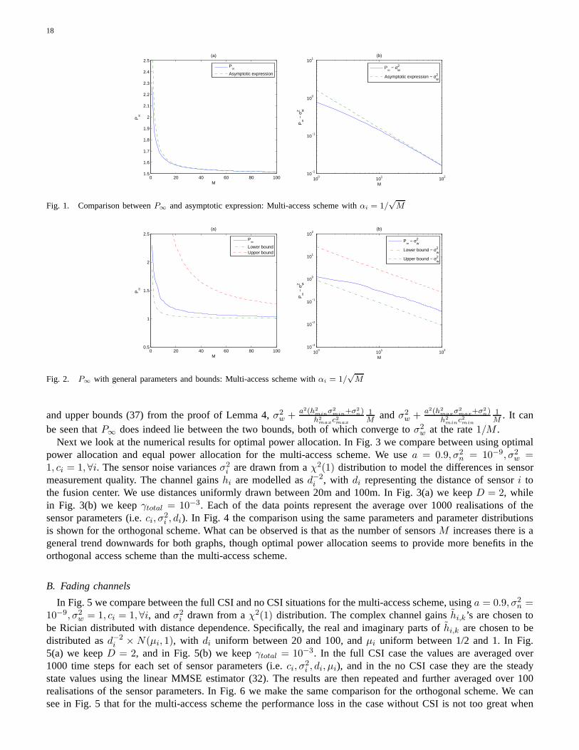
First we show some plots for the asymptotic results of Section III. In Fig. 1 (a) we plotP∞ vs M in the multi-access scheme for the symmetric situation withαi = 1/

√M , anda = 0.8, σ2

w = 1.5, σ2n = 1, c = 1, σ2

v = 1, h = 0.8.We compare this with the asymptotic expressionσ2

w + a2(σ2

v+σ2

n/h2)c2

1M from (13). Fig. 1 (b) plots the difference

betweenP∞ − σ2w, and compares this with the terma

2(σ2

v+σ2

n/h2)c2

1M . We can see thatP∞ is well approximated by

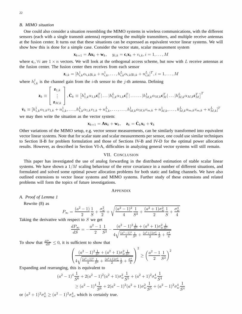
the asymptotic expression even for 20-30 sensors.In Fig. 2 we plotP∞ vs M in the multi-access scheme withαi = 1/

√M,a = 0.9, σ2

w = 1, σ2n = 1 and values

for ci, σ2i , hi chosen from the range0.5 ≤ Ci ≤ 1, 0.5 ≤ Ri ≤ 1, 0.5 ≤ hi ≤ 1. We also plot the (asymptotic) lower

18

0 20 40 60 80 1001.5

1.6

1.7

1.8

1.9

2

2.1

2.2

2.3

2.4

2.5

M

P∞

(a)

100

101

102

10−2

10−1

100

101

M

P∞

− σ

w2

(b)

P∞Asymptotic expression

P∞ − σw2

Asymptotic expression − σw2

Fig. 1. Comparison betweenP∞ and asymptotic expression: Multi-access scheme withαi = 1/√

M

0 20 40 60 80 1000.5

1

1.5

2

2.5

M

P∞

(a)

100

101

102

10−3

10−2

10−1

100

101

102

M

P∞

− σ

w2

(b)

P∞Lower boundUpper bound

P∞ − σw2

Lower bound − σw2

Upper bound − σw2

Fig. 2. P∞ with general parameters and bounds: Multi-access scheme with αi = 1/√

M

and upper bounds (37) from the proof of Lemma 4,σ2w + a2(h2

minσ2

min+σ2

n)h2

maxc2max

1M andσ2

w + a2(h2

maxσ2

max+σ2

n)h2

minc2

min

1M . It can

be seen thatP∞ does indeed lie between the two bounds, both of which converge to σ2w at the rate1/M .

Next we look at the numerical results for optimal power allocation. In Fig. 3 we compare between using optimalpower allocation and equal power allocation for the multi-access scheme. We usea = 0.9, σ2

n = 10−9, σ2w =

1, ci = 1,∀i. The sensor noise variancesσ2i are drawn from aχ2(1) distribution to model the differences in sensor

measurement quality. The channel gainshi are modelled asd−2i , with di representing the distance of sensori to

the fusion center. We use distances uniformly drawn between20m and 100m. In Fig. 3(a) we keepD = 2, whilein Fig. 3(b) we keepγtotal = 10−3. Each of the data points represent the average over 1000 realisations of thesensor parameters (i.e.ci, σ

2i , di). In Fig. 4 the comparison using the same parameters and parameter distributions

is shown for the orthogonal scheme. What can be observed is that as the number of sensorsM increases there is ageneral trend downwards for both graphs, though optimal power allocation seems to provide more benefits in theorthogonal access scheme than the multi-access scheme.

B. Fading channels

In Fig. 5 we compare between the full CSI and no CSI situationsfor the multi-access scheme, usinga = 0.9, σ2n =

10−9, σ2w = 1, ci = 1,∀i, andσ2

i drawn from aχ2(1) distribution. The complex channel gainshi,k ’s are chosen tobe Rician distributed with distance dependence. Specifically, the real and imaginary parts ofhi,k are chosen to bedistributed asd−2

i × N(µi, 1), with di uniform between 20 and 100, andµi uniform between 1/2 and 1. In Fig.5(a) we keepD = 2, and in Fig. 5(b) we keepγtotal = 10−3. In the full CSI case the values are averaged over1000 time steps for each set of sensor parameters (i.e.ci, σ

2i , di, µi), and in the no CSI case they are the steady

state values using the linear MMSE estimator (32). The results are then repeated and further averaged over 100realisations of the sensor parameters. In Fig. 6 we make the same comparison for the orthogonal scheme. We cansee in Fig. 5 that for the multi-access scheme the performance loss in the case without CSI is not too great when

19

0 5 10 15 200

0.5

1

1.5

2

2.5

3

3.5

4

4.5

5x 10

−3

M

Sum

Pow

er

(a)

0 5 10 15 201

1.2

1.4

1.6

1.8

2

2.2

2.4

2.6

2.8

3

M

Err

or C

ovar

ianc

e

(b)

equal power allocationoptimal power allocation

equal power allocationoptimal power allocation

Fig. 3. Multi-access. Comparison between optimal and equalpower allocation schemes, with (a) an error covariance constraint and (b) asum power constraint

0 5 10 15 200

1

2

3

4

5

6

7

8

x 10−3

M

Sum

Pow

er

(a)

0 5 10 15 201

1.5

2

2.5

3

3.5

4

M

Err

or C

ovar

ianc

e

(b)

equal power allocationoptimal power allocation

equal power allocationoptimal power allocation

Fig. 4. Orthogonal access. Comparison between optimal and equal power allocation schemes, with (a) an error covarianceconstraint and(b) a sum power constraint

compared to the case with full CSI. Thus even if one has full CSI, but doesn’t want to perform power allocationat every time step, using the linear MMSE estimator (32) instead could be an attractive alternative. On the otherhand, for the orthogonal scheme in Fig. 6 there is a more significant performance loss in the situation with no CSI.

VI. EXTENSION TO VECTOR STATES ANDMIMO

In Section VI-A we formulate a possible extension of our workto vector state linear systems. We outline someof the differences and difficulties that will be encounteredwhen compared with the scalar case. In Section VI-B weconsider a situation similar to a MIMO system, where the fusion center has multiple receive antennas (and eachsensor operating with a single transmit antenna), and we show how they can be written as an equivalent vectorlinear system.

A. Vector states

We consider a general vector modelxk+1 = Axk + wk

with x ∈ Rn, A ∈ R

n×n, and wk ∈ Rn being Gaussian with zero-mean and covariance matrixQ. For a stable

system all the eigenvalues of the matrixA will have magnitude less than 1. TheM sensors each observe

yi,k = Cixk + vi,k, i = 1, . . . ,M

with yi,k ∈ Rm, Ci ∈ R

m×n, andvi,k ∈ Rm being Gaussian with zero-mean and covariance matrixRi. We assume

that each of the individual components of the measurement vectors yi,k are amplified and forwarded to a fusioncenter via separate orthogonal channels.11 We will consider real channel gains for simplicity.

11Another possibility is to apply compression on the measuredsignal [7], [23], so that the dimensionality of the signal that the sensortransmits is smaller than the dimension of the measurement vector, but for simplicity we will not consider this here.

20

0 5 10 15 200

0.5

1

1.5

2

2.5

3

3.5

4

4.5

5x 10

−3

M

Sum

Pow

er

(a)

0 5 10 15 201

1.2

1.4

1.6

1.8

2

2.2

2.4

2.6

2.8

3

M

Err

or C

ovar

ianc

e

(b)

No CSIWith CSI

No CSIWith CSI

Fig. 5. Multi-access. Comparison between the full CSI and noCSI situations, with (a) an error covariance constraint and(b) a sum powerconstraint

0 5 10 15 200

1

2

3

4

5

6

7

8

x 10−3

M

Sum

Pow

er

(a)

0 5 10 15 201

1.2

1.4

1.6

1.8

2

2.2

2.4

2.6

2.8

3

M

Err

or C

ovar

ianc

e

(b)

No CSIWith CSI

No CSIWith CSI

Fig. 6. Orthogonal access. Comparison between the full CSI and no CSI situations, with (a) an error covariance constraint and (b) a sumpower constraint

In the multi-access scheme the fusion center then receives

zk =

M∑

i=1

Hi,kαi,kyi,k + nk

whereαi,k ∈ Rm×m is a matrix of amplification factors,Hi,k ∈ R

m×m a matrix of channel gains, andnk ∈ Rm

is Gaussian with zero-mean and covariance matrixN. We can express the situation as

xk+1 = Axk + wk, zk = Ckxk + vk

whereCk ≡∑Mi=1 Hi,kαi,kCi, vk ≡∑M

i=1 Hi,kαi,kvi,k+nk, with vk having covariance matrixRk ≡∑Mi=1 Hi,kαi,kRiα

Ti,kHT

i,k+N. The error covariance updates as follows:

Pk+1 = APkAT − APkCTk (CkPkCT

k + Rk)−1CkPkAT + Q

The transmit power of sensori at timek is

γi,k = Tr(αi,kE[ykyTk ]αT

i,k)

= Tr(αi,k(CiE[xkxTk ]CT

i + Ri)αTi,k)

where Tr(•) denotes the trace, andE[xkxTk ] satisfies (see [41, p.71])

E[xkxTk ] − AE[xkxT

k ]AT = Q

In the static channel case, the steady state error covariance P∞ satisfies

P∞ = AP∞AT − AP∞CT(CP∞CT

+ R)−1CP∞AT + Q

21

However, unlike the scalar case where the closed form expression (7) exists, in the vector case no such formula forP∞ is available, and thus asymptotic analysis is difficult to develop. For time-varying channels, we can pose similaroptimization problems as considered in Section IV. For instance, minimization of the error covariance subject to asum power constraint can be written as:

minα1,k,...,αM,k

Tr(Pk+1)

subject toM∑

i=1

(αi,k(CiE[xkxTk ]CT

i + Ri)αTi,k) ≤ γtotal

(34)

This problem is non-convex, and unlike the scalar case does not appear to be able to be reformulated into aconvex problem. Similar problems have been considered previously in the context of parameter estimation, andsub-optimal solutions were presented using techniques such as deriving bounds on the error covariance [27], andconvex relaxation techniques [23].

In the orthogonal access scheme the fusion center receives

zi,k = Hi,kαi,kyi,k + ni,k, i = 1, . . . ,M

We can express the situation asxk+1 = Axk + wk, zo

k = Cokxk + vo

k

by defining

zok ≡

z1,k...

zM,k

, Co

k ≡

H1,kα1,kC1...

HM,kαM,kCM

, vo

k ≡

H1,kα1,kv1,k + n1,k...

HM,kαM,kvM,k + nM,k

with the covariance ofvok being

Rok ≡

H1,kα1,kR1αT1,kHT

1,k + N 0 . . . 0

0 H2,kα2,kR2αT2,kHT

2,k + N . . . 0...

.... . .

...0 0 . . . HM,kαM,kRMα

TM,kHT

M,k + N

The error covariance updates as follows:

Pok+1 = APo

kAT − APokCoT

k (CokPo

kCoT

k + Rok)

−1CokPo

kAT + Q

The termCoT

k (CokPo

kCoT

k + Rok)

−1Cok can be rewritten using the matrix inversion lemma as

CoT

k (CokPo

kCoT

k + Rok)

−1Cok = CoT

k Ro−1

k CoT

k − CoT

k Ro−1

k CoT

k (Po−1

k + CoT

k Ro−1

k CoT

k )−1CoT

k Ro−1

k CoT

k

where we have the simplification

CoT

k Ro−1

k CoT

k =

M∑

i=1

(Hi,kαi,kCi)T (Hi,kαi,kRiα

Ti,kHT

i,k + N)−1(Hi,kαi,kCi)

Minimization of the error covariance subject to a sum power constraint can be written as:

minα1,k,...,αM,k

Tr(Pok+1)

subject toM∑

i=1

(αi,k(CiE[xkxTk ]CT

i + Ri)αTi,k) ≤ γtotal

(35)

This problem is non-convex and also does not appear to be ableto be reformulated into a convex problem. In thecontext of parameter estimation with sensors communicating to a fusion center via orthogonal channels, a similarproblem was considered in [49], and was in fact shown to be NP-hard, although sub-optimal methods for solvingthat problem were later studied in [7].

As the techniques involved are quite different from what hascurrently been presented, a comprehensive studyof optimization problems such as (34) and (35) is beyond the scope of this paper and will be studied elsewhere.

22

B. MIMO situation

One could also consider a situation resembling the MIMO systems in wireless communications, with the differentsensors (each with a single transmit antenna) representingthe multiple transmitters, and multiple receive antennasat the fusion center. It turns out that these situations can be expressed as equivalent vector linear systems. We willshow how this is done for a simple case. Consider the vector state, scalar measurement system

xk+1 = Axk + wk, yi,k = cixk + vi,k, i = 1, . . . ,M

whereci,∀i are1 × n vectors. We will look at the orthogonal access scheme, but now with L receive antennas atthe fusion center. The fusion center then receives from eachsensor

zi,k = [h1i,kαi,kyi,k + n1

i,k, . . . , hLi,kαi,kyi,k + nL

i,k]T , i = 1, . . . ,M

wherehji,k is the channel gain from thei-th sensor to thej-th antenna. Defining

zk ≡

z1,k...

zM,k

, Ck ≡

[

h11,kα1,kcT

1 | . . . |hL1,kα1,kcT

1 | . . . . . . |h1M,kαM,kcT

M | . . . |hLM,kαM,kcT

M

]T

vk ≡ [h11,kα1,kv1,k + n1

1,k, . . . , hL1,kα1,kv1,k + nL

1,k, . . . , . . . , h1M,kαM,kvm,k + n1

M,k, . . . , hLM,kαm,kvm,k + nL

M,k]T

we may then write the situation as the vector system:

xk+1 = Axk + wk, zk = Ckxk + vk

Other variations of the MIMO setup, e.g. vector sensor measurements, can be similarly transformed into equivalentvector linear systems. Note that for scalar state and scalarmeasurements per sensor, one could use similar techniquesto Section II-B for problem formulation and those of Sections IV-B and IV-D for the optimal power allocationresults. However, as described in Section VI-A, difficulties in analyzing general vector systems will still remain.

VII. C ONCLUSION

This paper has investigated the use of analog forwarding in the distributed estimation of stable scalar linearsystems. We have shown a1/M scaling behaviour of the error covariance in a number of different situations, andformulated and solved some optimal power allocation problems for both static and fading channels. We have alsooutlined extensions to vector linear systems and MIMO systems. Further study of these extensions and relatedproblems will form the topics of future investigations.

APPENDIX

A. Proof of Lemma 1

Rewrite (8) as

P∞ =(a2 − 1)

2

1

S+

σ2w

2+

√

(a2 − 1)2

4

1

S2+

(a2 + 1)σ2w

2

1

S+

σ4w

4Taking the derivative with respect toS we get

dP∞dS

= −a2 − 1

2

1

S2− (a2 − 1)2 1

S3 + (a2 + 1)σ2w

1S2

4

√

(a2−1)2

41S2 + (a2+1)σ2

w

21S + σ4

w

4

To show thatdP∞

dS ≤ 0, it is sufficient to show that

(a2 − 1)2 1S3 + (a2 + 1)σ2

w1S2

4

√

(a2−1)2

41S2 + (a2+1)σ2

w

21S + σ4

w

4

2

≥(

a2 − 1

2

1

S2

)2

Expanding and rearranging, this is equivalent to

(a2 − 1)41

S6+ 2(a2 − 1)2(a2 + 1)σ2

w

1

S5+ (a2 + 1)2σ4

w

1

S4

≥ (a2 − 1)41

S6+ 2(a2 − 1)2(a2 + 1)σ2

w

1

S5+ (a2 − 1)2σ4

w

1

S4

or (a2 + 1)2σ4w ≥ (a2 − 1)2σ4

w, which is certainly true.

23

B. Proof of Lemma 3

We first substitute the simplified expressions forc and r into (7):

P∞ =

(a2 − 1)(Mh2σ2v + σ2

n) + M2h2c2σ2w +

√

((a2 − 1)(Mh2σ2v + σ2

n) + M2h2c2σ2w)2 + 4M2h2c2σ2

w(Mh2σ2v + σ2

n)

2M2h2c2

Regarded as a function ofM , we are interested in the behaviour ofP∞ asM → ∞. Now√

((a2 − 1)(Mh2σ2v + σ2

n) + M2h2c2σ2w)2 + 4M2h2c2σ2

w(Mh2σ2v + σ2

n)

=(

h4c4σ4wM4 + 2(a2 − 1)σ2

vh4c2σ2

wM3 + 4h4c2σ2wσ2

vM3 + O(M2)

)1/2

= h2c2σ2wM2

(

1 +2(a2 + 1)σ2

v

c2σ2wM

+ O

(

1

M2

))1/2

= h2c2σ2wM2

(

1 +1

2

2(a2 + 1)σ2v

c2σ2wM

+ O

(

1

M2

))

= h2c2σ2wM2 + (a2 + 1)h2σ2

vM + O(1)

(36)

where we have used the expansion(1 + x)1/2 = 1 + x/2 + O(x2) for |x| < 1 [50, p.15], which is valid whenMis sufficiently large. Hence

P∞ = σ2w +

a2σ2v

c2

1

M+ O

(

1

M2

)

C. Proof of Lemma 4

We first prove the statements for the multi-access scheme. WehaveMhmincmin ≤∑Mi=1 hici ≤ Mhmaxcmax and

Mh2minσ2

min ≤∑Mi=1 h2

i σ2i ≤ Mh2

maxσ2max. Recall from Lemma 1 thatP∞ is a decreasing function ofS = c2/r.

If we chooseαi ∈ {+1,−1} such thatαici is positive for alli, we have

Mh2minσ2

min + σ2n

M2h2maxc2

max

≤ r

c2≤ Mh2

maxσ2max + σ2

n

M2h2minc2

min

and by a similar calculation to (36) we can show that asM → ∞

σ2w +

a2h2minσ2

min

h2maxc2

max

1

M+ O

(

1

M2

)

≤ P∞ ≤ σ2w +

a2h2maxσ2

max

h2minc2

min

1

M+ O

(

1

M2

)

If instead we chooseαi ∈ {1/√

M,−1/√

M} such thatαici is positive for all i, we can similarly show that asM → ∞

σ2w +

a2(h2minσ2

min + σ2n)

h2maxc2

max

1

M+ O

(

1

M2

)

≤ P∞ ≤ σ2w +

a2(h2maxσ2

max + σ2n)

h2minc2

min

1

M+ O

(

1

M2

)

(37)

In either case, as the upper and lower bounds both converge toσ2w at a rate of1/M , P∞ itself will also do so.

For the orthogonal scheme, a similar argument to the above shows that choosingαi ∈ {+1,−1} gives convergenceof P o

∞ to σ2w at the rate1/M for general parameters.

To show thatP o∞ in general does not converge to a limit asM → ∞, when using the scaling1/

√M in the

orthogonal scheme, consider the following example. Suppose there are two distinct sets of “symmetric” parameterswith behaviour as in (14), such that if all the sensors had thefirst set of parameters the error covariance wouldconverge toP o

∞,1, and if all the sensors had the second set of parameters the error covariance would convergeto P o

∞,2, with P o∞,2 6= P o

∞,1. Then let the firstM1 sensors have the first set of parameters, the nextM2 (withM2 >> M1) sensors the second set, the nextM3 (with M3 >> M2) sensors the first set, the nextM4 (withM4 >> M3) sensors the second set, etc... ThenP o

∞ would alternate between approachingP o∞,1 andP o

∞,2, and willnot converge to a limit asM → ∞.

24

D. Proof of Lemma 5

With the multi-access scheme and the allocation (15), by defining

α2max =

γ(1 − a2)

c2minσ2

w + σ2min(1 − a2)

, α2min =

γ(1 − a2)

c2maxσ2

w + σ2max(1 − a2)

we can show similar to the proof of Lemma 4 that

Mα2minh2

minσ2min + σ2

n

M2α2maxh2

maxc2max

≤ r

c2≤ Mα2

maxh2maxσ2

max + σ2n

M2α2minh2

minc2min

.

Hence asM → ∞ we have

σ2w +

a2α2minh2

minσ2min

α2maxh2

maxc2max

1

M+ O

(

1

M2

)

≤ P∞ ≤ σ2w +

a2α2maxh2

maxσ2max

α2minh2

minc2min

1

M+ O

(

1

M2

)

.

The other cases can be treated similarly as in the proof of Lemma 4.

REFERENCES

[1] J.-F. Chamberland and V. V. Veeravalli, “Decentralizeddetection in sensor networks,”IEEE Trans. Signal Processing, vol. 51, no. 2,pp. 407–416, Feb. 2003.

[2] C. Rago, P. Willett, and Y. Bar-Shalom, “Censoring sensors: A low-communication-rate scheme for distributed detection,” IEEE Trans.Aerosp. Electron. Syst., vol. 32, no. 2, pp. 554–568, Apr. 1996.

[3] B. Chen, R. Jiang, T. Kasetkasem, and P. K. Varshney, “Channel aware decision fusion in wireless sensor networks,”IEEE Trans.Signal Processing, vol. 52, no. 12, pp. 3454–3458, Dec. 2004.

[4] R. Jiang and B. Chen, “Fusion of censored decisions in wireless sensor networks,”IEEE Trans. Wireless Commun., vol. 4, no. 6, pp.2668–2673, Nov. 2005.

[5] A. Ribeiro and G. B. Giannakis, “Bandwidth-constraineddistributed estimation for wireless sensor networks, PartI: Gaussian case,”IEEE Trans. Signal Processing, vol. 54, no. 3, pp. 1131–1143, Mar. 2006.

[6] J.-J. Xiao, S. Cui, Z.-Q. Luo, and A. J. Goldsmith, “Powerscheduling of universal decentralized estimation in sensor networks,”IEEETrans. Signal Processing, vol. 54, no. 2, pp. 413–422, Feb. 2006.

[7] I. D. Schizas, G. B. Giannakis, and Z.-Q. Luo, “Distributed estimation using reduced-dimensionality sensor observations,” IEEE Trans.Signal Processing, vol. 55, no. 8, pp. 4284–4299, Aug. 2007.

[8] J.-Y. Wu, Q.-Z. Huang, and T.-S. Lee, “Minimal energy decentralized estimation via exploiting the statistical knowledge of sensor noisevariance,”IEEE Trans. Signal Processing, vol. 56, no. 5, pp. 2171–2176, May 2008.

[9] G. Mergen and L. Tong, “Type based estimation over multiaccess channels,”IEEE Trans. Signal Processing, vol. 54, no. 2, pp. 613–626,Feb. 2006.

[10] G. Mergen, V. Naware, and L. Tong, “Asymptotic detection performance of type-based multiple access over multiaccess fading channels,”IEEE Trans. Signal Processing, vol. 55, no. 3, pp. 1081–1092, Mar. 2007.

[11] K. Liu and A. M. Sayeed, “Type-based decentralized detection in wireless sensor networks,”IEEE Trans. Signal Processing, vol. 55,no. 5, pp. 1899–1910, May 2007.

[12] R. Nowak, U. Mitra, and R. Willett, “Estimating inhomogenous fields using wireless sensor networks,”IEEE J. Select. Areas Commun.,vol. 22, no. 6, pp. 999–1006, Aug. 2004.

[13] Y. Wang, P. Ishwar, and V. Saligrama, “One-bit distributed sensing and coding for field estimation in sensor networks,” IEEE Trans.Signal Processing, vol. 56, no. 9, pp. 4433–4445, Sept. 2008.

[14] H. Zhang, J. M. F. Moura, and B. Krogh, “Dynamic field estimation using wireless sensor networks: Tradeoffs between estimationerror and communication cost,”IEEE Trans. Signal Processing, vol. 57, no. 6, pp. 2383–2395, June 2009.

[15] M. Gastpar and M. Vetterli, “Source-channel communication in sensor networks,”Springer Lecture Notes in Computer Science, vol.2634, pp. 162–177, Apr. 2003.

[16] W. Li and H. Dai, “Distributed detection in wireless sensor networks using a multiple access channel,”IEEE Trans. Signal Processing,vol. 55, no. 3, pp. 822–833, Mar. 2007.

[17] X. Zhang, H. V. Poor, and M. Chiang, “Optimal power allocation for distributed detection over MIMO channels in wireless sensornetworks,” IEEE Trans. Signal Processing, vol. 56, no. 9, pp. 4124–4140, Sept. 2008.

[18] T. J. Goblick, “Theoretical limitations on the transmission of data from analog sources,”IEEE Trans. Inform. Theory, vol. 11, no. 4,pp. 558–567, Oct. 1965.

[19] M. Gastpar, B. Rimoldi, and M. Vetterli, “To code, or notto code: Lossy source-channel communication revisited,”IEEE Trans. Inform.Theory, vol. 49, no. 5, pp. 1147–1158, May 2003.

[20] H. Viswanathan and T. Berger, “The quadratic Gaussian CEO problem,”IEEE Trans. Inform. Theory, vol. 43, no. 5, pp. 1549–1559,Sept. 1997.

[21] P. Ishwar, R. Puri, K. Ramchandran, and S. S. Pradhan, “On rate-constrained distributed estimation in unreliable sensor networks,”IEEE J. Select. Areas Commun., vol. 23, no. 4, pp. 765–775, Apr. 2005.

[22] M. Gastpar, “Uncoded transmission is exactly optimal for a simple Gaussian sensor network,”IEEE Trans. Inform. Theory, vol. 54,no. 11, pp. 5247–5251, Nov. 2008.

[23] J.-J. Xiao, S. Cui, Z.-Q. Luo, and A. J. Goldsmith, “Linear coherent decentralized estimation,”IEEE Trans. Signal Processing, vol. 56,no. 2, pp. 757–770, Feb. 2008.

25

[24] S. Cui, J.-J. Xiao, A. Goldsmith, Z.-Q. Luo, and H. V. Poor, “Estimation diversity and energy efficiency in distributed sensing,”IEEETrans. Signal Processing, vol. 55, no. 9, pp. 4683–4695, Sept. 2007.

[25] M. Gastpar and M. Vetterli, “Power, spatio-temporal bandwidth, and distortion in large sensor networks,”IEEE J. Select. Areas Commun.,vol. 23, no. 4, pp. 745–754, Apr. 2005.

[26] I. Bahceci and A. K. Khandani, “Linear estimation of correlated data in wireless sensor networks with optimum powerallocation andanalog modulation,”IEEE Trans. Commun., vol. 56, no. 7, pp. 1146–1156, July 2008.

[27] J. Fang and H. Li, “Power constrained distributed estimation with correlated sensor data,”IEEE Trans. Signal Processing, to bepublished.

[28] G. Thatte and U. Mitra, “Sensor selection and power allocation for distributed estimation in sensor networks: Beyond the star topology,”IEEE Trans. Signal Processing, vol. 56, no. 7, pp. 2649–2661, July 2008.

[29] Y.-W. P. Hong, K.-U. Lei, and C.-Y. Chi, “Channel-awarerandom access control for distributed estimation in sensornetworks,” IEEETrans. Signal Processing, vol. 56, no. 7, pp. 2967–2980, July 2008.

[30] H. Senol and C. Tepedelenlioglu, “Performance of distributed estimation over unknown parallel fading channels,” IEEE Trans. SignalProcessing, vol. 56, no. 12, pp. 6057–6068, Dec. 2008.

[31] K. Zhang and X. R. Li, “Optimal sensor data quantizationfor best linear unbiased estimation fusion,” inProc. IEEE Conf. Decisionand Control, Atlantis, Bahamas, Dec. 2004, pp. 2656–2661.

[32] A. Ribeiro, G. B. Giannakis, and S. I. Roumeliotis, “SOI-KF: Distributed Kalman filtering with low-cost communications using thesign of innovations,”IEEE Trans. Signal Processing, vol. 54, no. 12, pp. 4782–4795, Dec. 2006.

[33] D. Willner, C. B. Chang, and K. P. Dunn, “Kalman filter algorithms for a multi-sensor system,” inProc. IEEE Conf. Decision andControl, Clearwater, FL, Dec. 1976, pp. 570–574.

[34] H. R. Hashemipour, S. Roy, and A. J. Laub, “Decentralized structures for parallel Kalman filtering,”IEEE Trans. Automat. Contr.,vol. 33, no. 1, pp. 88–94, Jan. 1988.

[35] B. S. Rao and H. F. Durrant-Whyte, “Fully decentralisedalgorithm for multisensor Kalman filtering,”IEE Proceedings-D, vol. 138,no. 5, pp. 413–420, Sept. 1991.

[36] N. E. Nahi, “Optimal recursive estimation with uncertain observation,”IEEE Trans. Inform. Theory, vol. 15, no. 4, pp. 457–462, July1969.

[37] P. K. Rajasekaran, N. Satyanarayana, and M. D. Srinath,“Optimum linear estimation of stochastic signals in the presence of multiplicativenoise,” IEEE Trans. Aerosp. Electron. Syst., vol. 7, no. 3, pp. 462–468, May 1971.

[38] M. T. Hadidi and S. C. Schwartz, “Linear recursive stateestimators under uncertain observations,”IEEE Trans. Automat. Contr., vol. 24,no. 6, pp. 944–948, Dec. 1979.

[39] R. Mudumbai, G. Barriac, and U. Madhow, “On the feasibility of distributed beamforming in wireless networks,”IEEE Trans. WirelessCommun., vol. 6, no. 5, pp. 1754–1763, May 2007.

[40] J. A. Bucklew and W. A. Sethares, “Convergence of a classof decentralized beamforming algorithms,”IEEE Trans. Signal Processing,vol. 56, no. 6, pp. 2280–2288, June 2008.

[41] B. D. O. Anderson and J. B. Moore,Optimal Filtering. New Jersey: Prentice Hall, 1979.[42] G. H. Hardy, J. E. Littlewood, and G. Polya,Inequalities, 2nd ed. Cambridge, Great Britain: Cambridge University Press, 1952.[43] Q. Gan and C. J. Harris, “Comparison of two measurement fusion methods for Kalman-filter-based multisensor data fusion,” IEEE

Trans. Aerosp. Electron. Syst., vol. 37, no. 1, pp. 273–280, Jan. 2001.[44] K. Liu, H. El Gamal, and A. M. Sayeed, “Decentralized inference over multiple-access channels,”IEEE Trans. Signal Processing,

vol. 5, no. 7, pp. 3445–3455, July 2007.[45] M. Berger,Geometry II. Berlin: Springer-Verlag, 1987.[46] N. Ghasemi and S. Dey, “Power-efficient dynamic quantization for multisensor HMM state estimation over fading channels,” in Proc.

ISCCSP, Malta, Mar. 2008, pp. 1553–1558.[47] A. G. Jaffer and S. C. Gupta, “Recursive Bayesian estimation with uncertain observations,”IEEE Trans. Inform. Theory, vol. 17, no. 5,

pp. 614–616, Sept. 1971.[48] J. K. Tugnait, “Stability of optimum linear estimatorsof stochastic signals in white multiplicative noise,”IEEE Trans. Automat. Contr.,

vol. 26, no. 3, pp. 757–761, June 1981.[49] Z.-Q. Luo, G. B. Giannakis, and S. Zhang, “Optimal linear decentralized estimation in a bandwidth constrained sensor network,” in

Proc. IEEE Int. Symp. Inf. Theory, Adelaide, Australia, Sept. 2005, pp. 1441–1445.[50] M. Abramowitz and I. A. Stegun,Handbook of Mathematical Functions. New York: Dover Publications, 1965.