STATE AND OUTPUT FEEDBACK CONTROL IN MODEL-BASED NETWORKED

CONTROL SYSTEMS

Luis A. Montestruque, Panos J. Antsaklis

University of Notre Dame, Notre Dame, IN 46556, U.S.A.

Department of Electrical Engineering fax: (574) 631-4393

e-mail: {lmontest, pantsakl}@nd.edu

Abstract

In this paper the control of a continuous linear plant where the sensor is connected to a linear controller/actuator via a network is addressed. Both state and output feedback are considered. The work focuses on reducing the network usage using knowledge of the plant dynamics. Necessary and sufficient conditions for stability are derived in terms of the update time h, the network delay, and the parameters of the plant and of its model. The deterioration of behavior when either h, the delay τ, or the modeling error increase is explicitly shown and examples are used to illustrate the results.

1 Introduction

The use of networks as a media to interconnect the different components in an industrial control system is rapidly increasing. A network introduces bandwidth restrictions. To overcome these bandwidth constraints several approaches have been proposed. In [1] Brockett introduces the notion of minimum attention control that attempts to reduce the time and state feedback dependence of the control law. This can be viewed as a tradeoff between open loop and closed loop control.

In [8, 7], Walsh et al introduce the notion of maximal allowable transfer interval, MATI, to place an upper bound on the time between transfers of information from the sensor to the controller. In this case the controller is designed without taking the network into account, a desirable feature. However, serious behavior degradation can result if the MATI is too large and the network is slow.

Other approaches include the study of quantization effects and algorithms over networked control systems [2, 3], and scheduling algorithms [4].

It is clear that the reduction of bandwidth necessitated by the communication network in a networked control system is a major concern. This can perhaps be addressed by two methods: the first is to reduce the number of data packet exchanges between the sensor and the controller/actuator.

The second method is to compress or reduce the size of the data transferred at each transaction.

Actually deployed and popular networks in the industry include CAN bus, PROFIBUS, DeviceNet, ControlNet, Fieldbus Foundation, and Ethernet among others. Among the shared characteristics are the small transport time and big overhead (network control information included in the packet). For example, an Ethernet frame with 1 byte of data will have the same length as one with 46 bytes of data. This means that data compression by reducing the size of the data transmitted has negligible effects over the overall system performance. So reducing the number of packets transmitted brings better benefits than data compression. This brings us again to the idea of reducing the data transfer rate as much as possible. In this manner more bandwidth will be available to allocate more resources without sacrificing stability and ultimately performance of the overall system.

We will consider the case where the controller and the actuator are combined together into a single node. That is, the network is between the sensor and the controller/actuator nodes. Assuming that the controller and the actuator physically coexist is reasonable since embedded microprocessors are usually incorporated into the actuator to process the data received by the network and execute the commands received.

Figure 1: Proposed configuration of a state feedback

networked control system.

In this paper we will concentrate on characterizing the time between information exchanges from the sensor to the controller/actuator. In order to increase the transfer time we will use the knowledge we have of the plant dynamics. The plant model is used at the controller/actuator side to recreate the plant behavior so that the sensor can delay sending data since the model can provide an approximation of the plant dynamics. The main idea is to perform the feedback by updating the model’s state using the actual state of the plant that is provided by the sensor. The rest of the time the control action is based on a plant model that is incorporated in the controller/actuator and is running open loop for a period of h seconds. The setup is shown in Figure1. Output feedback is used in Figure 2, and state feedback with network delays is used in Figure 3.

When all the states are available, the sensors can send this information through the network to update the model’s vector state. For our analysis we will assume that the compensated model is stable and that the transportation delay is negligible. We will assume that the frequency at which the network updates the state in the controller is constant.

This paper is organized as follows: in Section 2 necessary and sufficient conditions are developed for the setup shown in Figure 1. This is the case where the state vector is directly measurable and sent through the network to the controller/actuator. It is shown that the networked control system depicted in Figure 1 is globally exponentially stable if and only if the eigenvalues of a test matrix M are inside the unit circle. This matrix M depends on the plant dynamics, the model uncertainties and the model update time. The case of output feedback control is analyzed in Section 3. An extension of the state feedback system in the presence on network delays is presented in Section 4. A numeric example is given in Section 5. Conclusions are presented in Section 6. Note that the state feedback case has been studied in [6].

2 A State Feedback Networked Control System

Consider the control system of Figure 1 where plant is given by BuAxx += , the plant model by uBxAx ˆˆˆˆ += , and the controller by xKu ˆ= .

The sensor has the full state vector available and its function will be to send the state information through the network at times kt . The state error is defined as

)(ˆ)()( txtxte −= , and represents the difference between the plant state and the model state. The modeling error matrices ˆA A A= − and ˆB B B= − represent the difference between the plant and the model. Finally, the update times are kt , where htt kk =− −1 for all k. Since the model state is updated at times kt , 0)( =kte for

...,2,1,0=k . The resetting of the state error every update time is a key element of our control system.

Now for 1[ , )k kt t t +∈ , we have that xKu ˆ= so

+

=

xx

KBABKA

xx

ˆˆˆ0ˆ with initial conditions

)()(ˆ kk txtx = . It is easy to see that the dynamics of the overall system for 1[ , )k kt t t +∈ can be described by

1 1

( ) ( ),ˆ( ) ( )

( ) ( ),

( ) 0[ , ),

k k

k

k k k k

A BK BKx t x te t e tA BK A BK

x t x te t

t t t with t t h

−

+ +

+ − = + −

=

∀ ∈ − =

(1)

Define

=

)()(

)(tetx

tz , and

−+

−+=Λ

KBAKBA

BKBKA~ˆ~~ so that

Equation (1) can be rewritten as zz Λ= for ),[ 1+∈ kk ttt . We will now express z(t) in terms of the initial condition x(t0). Then we will show under what conditions the system will be stable.

Proposition #1

The system described by Equation (1) with initial conditions [ ]0 0 0( ) ( ) 0 Tz t x t z= = , has the following response:

httwithttt

zI

eI

etz

kkkk

khtt k

=−∈

=

++

Λ−Λ

11

0)(

),,[

000

000

)(

The system response can be obtained by noting that on the interval ),[ 1+∈ kk ttt , the system response is

)(0

)()()(

)( )()(k

ttktt tzetx

etetx

tz kk −Λ−Λ =

=

= (2)

and that at times kt , [ ]( ) ( ) 0 Tk kz t x t= , that is, the error

e(t) is reset to zero. So this can be represented by

)(000

)( −

= kk tz

Itz . A complete proof can be found in

[5,6]♦

A necessary and sufficient condition for stability of the networked system will now be presented.

Theorem #1

The system described by Equation (1) is globally exponentially stable around the solution

[ ] [ ]0 0T Tz x e= = if and only if the eigenvalues of

= Λ

000

000 I

eI

M h are strictly inside the unit circle.

Sufficiency can be shown by bounding the expression in Proposition 1 by any consistent norm and noting that

1)())((

22

)( ...)(!2

)()()(1

Kee

tttte

htt

kk

tt

k

k

=≤=

Λ−

+Λ−+≤

Λ−Λ

−Λ

σσ

σσ

Necessity is shown by sampling the response in Proposition 1 and obtaining a discrete representation of the sampled response. A complete proof can be found in [5].

It can be shown (as in [5]) that the eigenvalues of

= Λ

000

000 I

eI

M h are inside the unit circle if and only if

the eigenvalues of ˆ ˆ( )A BK hN e += + ∆ , with

τττ deKBAee KBAh AAh )ˆˆ(

0)~~( +− +=∆ ∫ , are inside the unit

circle. One can gain a better insight to the system by observing the structure of N. To start with, we observe that the eigenvalues of the compensated model appear in the first term of N. In that sense we can see the term ∆ as a perturbation over the desired eigenvalues. Even if the eigenvalues of the original plant were unstable the perturbation ∆ can be made small enough by having h and

KBA ~~ + small and thus minimizing their impact over the stable eigenvalues of the compensated plant.

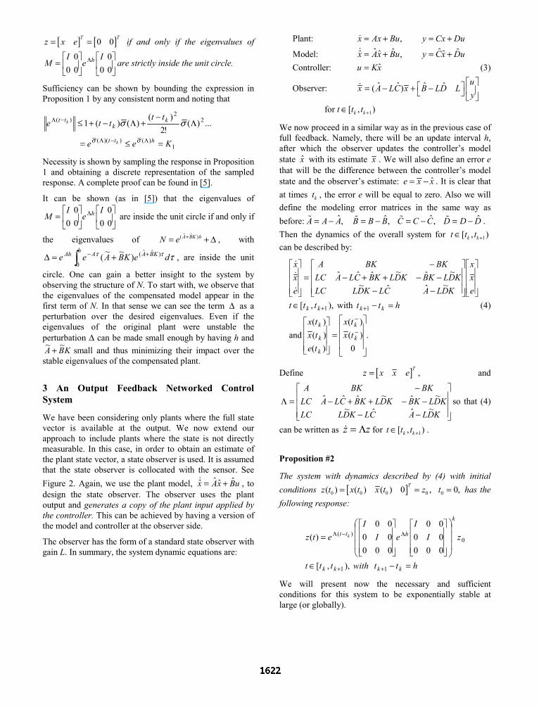
3 An Output Feedback Networked Control System

We have been considering only plants where the full state vector is available at the output. We now extend our approach to include plants where the state is not directly measurable. In this case, in order to obtain an estimate of the plant state vector, a state observer is used. It is assumed that the state observer is collocated with the sensor. See Figure 2. Again, we use the plant model, uBxAx ˆˆˆˆ += , to design the state observer. The observer uses the plant output and generates a copy of the plant input applied by the controller. This can be achieved by having a version of the model and controller at the observer side.

The observer has the form of a standard state observer with gain L. In summary, the system dynamic equations are:

1

Plant: ,ˆ ˆˆ ˆˆ ˆ ˆModel: ,

ˆController:

ˆ ˆ ˆ ˆObserver: ( )

for [ , )k k

x Ax Bu y Cx Du

x Ax Bu y Cx Duu Kx

ux A LC x B LD L

yt t t +

= + = +

= + = +=

= − + − ∈

(3)

We now proceed in a similar way as in the previous case of full feedback. Namely, there will be an update interval h, after which the observer updates the controller’s model state x with its estimate x . We will also define an error e that will be the difference between the controller’s model state and the observer’s estimate: ˆe x x= − . It is clear that at times kt , the error e will be equal to zero. Also we will define the modeling error matrices in the same way as before: ˆ ˆˆ ˆ, , ,A A A B B B C C C D D D= − = − = − = − . Then the dynamics of the overall system for 1[ , )k kt t t +∈ can be described by:

.0

)()(

)()()(

and

with),,[

~ˆˆ~~ˆ~ˆˆˆ

11

=

=−∈

−−−−++−

−=

−

−++

k

k

k

k

k

kkkk

txtx

tetxtx

htttttexx

KDLACLKDLLCKDLKBKDLKBCLALC

BKBKA

exx

(4)

Define [ ]Tz x x e= , and

−−−−++−

−=Λ

KDLACLKDLLCKDLKBKDLKBCLALC

BKBKA

~ˆˆ~~ˆ~ˆˆˆ so that (4)

can be written as zz Λ= for 1[ , )k kt t t +∈ .

Proposition #2

The system with dynamics described by (4) with initial conditions [ ]0 0 0 0 0( ) ( ) ( ) 0 , 0,Tz t x t x t z t= = = has the following response:

httwithttt

zII

eII

etz

kkkk

k

htt k

=−∈

=

++

Λ−Λ

11

0)(

),,[

0000000

0000000

)(

We will present now the necessary and sufficient conditions for this system to be exponentially stable at large (or globally).

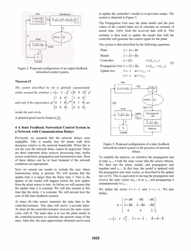
Figure 2: Proposed configuration of an output feedback

networked control system.

Theorem #2

The system described by (4) is globally exponentially stable around the solution [ ] [ ]0 0 0T Tz x x e= = if

and only if the eigenvalues of

Λ

0000000

0000000

II

eII

h are

inside the unit circle.

A detailed proof can be found in [5].

4 A State Feedback Networked Control System in a Network with Communication Delays

Previously we assumed that the network delays were negligible. This is usually true for plants with slow dynamics relative to the network bandwidth. When this is not the case the network delay cannot be neglected. There are three important delay sources: processing time, media access contention, propagation and transmission time. Most of these delays can be at least bounded if the network conditions are appropriate.

Next we extend our results to include the case where transmission delay is present. We will assume that the update time h is larger than the delay time τ. That is, the update of the model will happen before the next update from the plant sensor is sent. As before we will assume that the update time h is constant. We will also assume at this time that the delay τ is constant. We will present here the case of full state feedback systems.

At times kh-τ the sensor transmits the state data to the controller/actuator. This data will arrive τ seconds latter. At times kh the controller/actuator receives the state vector value x(kh-τ). The main idea is to use the plant model in the controller/actuator to calculate the present value of the state. After this, the state approximate obtained can be used

to update the controller’s model as in previous setups. The system is depicted in Figure 3.

The Propagation Unit uses the plant model and the past values of the control input u(t) to calculate an estimate of actual state )(khx from the received data x(kh-τ). This estimate is then used to update the model that with the controller will generate the control signal for the plant.

The system is then described by the following equations:

1

1 1

1

1

Plant:ˆ ˆˆ ˆModel:

ˆController: , [ , )ˆ ˆPropagation Unit: , [ , ]

Update law: at ˆ at

k k

k k

k

k

x Ax Bu

x Ax Buu Kx t t t

x Ax Bu t t tx x t tx x t t

ττ

+

+ +

+

+

= +

= += ∈

= + ∈ −← = −← =

(5)

Figure 3: Proposed configuration of a state feedback networked control system in the presence of network

delays.

To simplify the analysis, we initialize the propagation unit at time tk+1-τ with the state vector that the sensor obtains. We then run the plant, model, and propagation unit together until tk+1. At this time, the model is updated with the propagation unit state vector, as described in the update law of (5). This is equivalent to having the propagation unit receive the state vector x(tk+1-τ) at tk+1 and propagating it instantaneously to tk+1.

We define the errors xxe ˆˆ −= and xxe −= . We also define:

ˆ

ˆ0 0

A BK BK BK

A BK A BK BK

A

+ − −

Λ = + − −

ˆ ˆˆ , , .Tz x e e A A A B B B= = − = −

1 2

0 0 0 00 0 , 0 0 00 0 0 0

I II I I

I I

= =

With these definitions we proceed to present the system described by (5) in a compact form. The dynamics of the overall system for ),[ 1+∈ kk ttt can be described by

( ) ( ),z t z t= Λ with state reset equations:

1

1

1 1

1

( )( ) ( )

0

(( ) )( ) 0

ˆ(( ) ) (( ) )

, 0 .

k

k k

k

k

k k

k k

x tz t e t

x tz t

e t e t

t t h h

ττ

τ τ

τ

−

−

−+

+− −

+ +

+

= − − = − + −

− = < <

(6)

Proposition #3

The system with dynamics described by (6) with initial conditions 0 0 0 0 0 0ˆ( ) , 0,Tz t x e e z t= = = has the following response:

( )

( )1

( ) ( )1 2 0

1

( ) ( ) ( )2 1 2 0

1 1

( )

for [ , )

( )

for [ , ).

k

k

kt t h

k kkt t h h

k k

z t e I e I e z

t t t

z t e I e I e I e z

t t t

τ τ

τ τ τ τ

τ

τ

+

Λ − Λ Λ −

+

Λ − + Λ − Λ Λ −

+ +

=

∈ −

=

∈ −

with 1 ,k kt t h hτ+ − = < .

We will present now the necessary and sufficient conditions for this system to be exponentially stable at large (or globally).

Theorem #3

The system described by (6) is globally exponentially stable around the solution [ ]ˆ 0 0 0T Tz x e e= = if

and only if the eigenvalues of ( )1 2

hM I e I eτ τΛ Λ −= are inside the unit circle.

It is interesting to note that the results on Theorem #3 can be seen as a generalization of Theorem #1. This can be shown by driving τ to zero. The details for the proof of Proposition #3 and Theorem #3 can be found in [5].

5 Networked Control System Example

Consider the following unstable plant (double integrator):

[ ] 0;01;10

;0010

==

=

= DCBA

We will use the state feedback controller given by u=Kx with [ ]21 −−=K . Usually it is assumed that the actuator/controller will hold the last value received from the sensor until the next time the sensor transmits and a packet is received. We will analyze this situation. To do so, we will transform the plant model so that it holds the last state update presented to it by the network. The model designed to behave as a zero order hold when updated is

given by:0 0 0ˆ ˆ, .0 0 0

A B

= =

From a plot of the

maximum eigenvalue magnitude of 0 0

0 0 0 0hI I

M eΛ =

versus the update time, we see that

the condition for stability is to have h < 1 second. If we use the results by [8] we would have obtained that, in order to stabilize the system, we would need to have h<2.1304E-4, which is very conservative. Simulations of the system with update times of 2.1304E-4, 0.5, and 1 seconds are in Figure 4. Note that the plant was initialized with an initial condition of [1 1]T.

Figure 4: System response with h=2.1304E-4, 0.5, and 1s.

It can be seen that for h=1 second the system is marginally stable. It is also clear that the performance obtained with h=0.5 seconds is not too different to the one obtained with h=2.1304E-4 seconds, but the difference in the amount of bandwidth used is large. If we were to use Ethernet (72byte frames) the data rate would be 2.7Mbits/sec for the case of h=2.1304E-4 seconds, and only 1.2Kbits/sec for the case of h=0.5 seconds.

We will now present an example for the output feedback case. We will use the same state gain [ ]21 −−=K , and

state estimator with gain [ ]20 100 TL = ( eigenvalues at –10). The model used is a perturbed version of the original plant:

[ ]

0.0958 1.0604 0.0518ˆ ˆ; ;0.0066 0.0134 1.0269

ˆ ˆ0.9734 0.0137 ; 0.0396

A B

C D

− = = − −

= − = −

On a plot of the magnitude of the largest eigenvalue for the test matrix versus the update time, not shown here stability is observed for h<12 seconds.

Figure 5: System response with h=1 sec.

Figure 6: System response for h=0.5 and τ = 0.25 sec.

A simulation of the system with an update time of 1 second, an initial state of the plant at [1 1]T, and zero initial conditions for the estimator and controller’s state is shown in Figure 5.

Finally an example of a networked control system with network delays is presented. We will use the same plant and controller we have been using before with randomly

generated plant model

−−

=3560.03089.09225.03444.0

A ,

−=

3159.10098.0

B . The maximum value h can have to

preserve stability is reduced when τ is increased: 1.5s for

τ =0.00s, 1.35s for τ =0.25s, and 1.05s for τ =0.50s. Figure 6 shows the response of the system for h=0.5s and τ =0.25s, a stable configuration.

6 Conclusions

The presented control architecture represents a natural way of placing critical information about the plant on the network so as to reduce the data traffic load. By making the sensor and actuator more “intelligent” the networked control system is able to predict the future behavior of the plant, and send the precise information at critical times so to ensure the plant stability. The presence of computational load at any end of the feedback path is not considered a limitation of the applicability of the presented setups given the advances in microcomputing.

Acknowledgements

The partial support of the DARPA/ITO-NEST Program (AF-F30602-01-2-0526) is gratefully acknowledged.

References

[1] R. Brockett, “Minimum Attention Control,” Proceedings of the 36th Conference on Decision and Control, 1997, pp. 262e-2632.

[2] N. Elia and S. Mitter., “Stabilization of Linear Systems With Limited Information,” IEEE Transactions on Automatic Control, 2001, pp. 1384-1400.

[3] H. Ishii and B. Francis, “Stabilization With Control Networks,” Control 2000, Cambridge UK, Sept 4-7, 2000

[4] A.S. Matveev, A.V. Savkin, “Optimal State Estimation in Networked Systems with Asynchronous Communication Channels and Switched Sensors,” Proceedings of the 40th IEEE Conference on Decision and Control, December 2001, pp. 825-830.

[5] L.A. Montestruque, P.J. Antsaklis, “Model-Based Networked Control Systems: Stability,” ISIS Technical Report ISIS-2002-001, University of Notre Dame, www.nd.edu/~isis/, January 2002.

[6] L.A. Montestruque, P.J. Antsaklis, “Model-Based Networked Control Systems: Necessary and Sufficient Conditions for Stability,” 10th Mediterranean Conference On Control And Automation, July 2002.

[7] G. Walsh, O. Beldiman, and L. Bushnell, “Asymptotic Behavior of Networked Control Systems,” Proceedings of the International Conference on Control Applications, August 1999.

[8] G. Walsh, H. Ye, and L. Bushnell, “Stability Analysis of Networked Control Systems,” Proceedings of American Control Conference, June 1999.