Standard Oriented Environmental Policy: Cost-Effectiveness and Incentives for âGreen Technologyâ

Standard OrientedEnvironmental Policy:Cost-Effectiveness and Incentivesfor ‘Green Technology’

Alfred EndresUniversity of Hagen andUniversity of Witten/Herdecke

Bianca RundshagenUniversity of Hagen

Abstract. In their seminal 1971 paper, W. J. Baumol and W. E. Oates analyzedeffluent charges and ‘command and control’ regarding their ability to attain a givenstandard of environmental quality at minimum cost. In the subsequent literature,transferable discharge permits (TDPs) have been added to the portfolio of standardoriented environmental policy instruments. We place these instruments in a dynamiccontext. Here, cost minimization is defined in an intertemporal setting allowing forinduced technical change. It turns out that the relative performance of alternative policyinstruments regarding their ‘dynamic cost-effectiveness’ crucially depends on theinformation available to the involved agents. Under adverse informational conditions,only a TDP system with future markets is dynamically cost-effective.

JEL classification: Q58, Q55.

Keywords: ‘Pricing and standards’ approach; environmental policy; inducedtechnical change; asymmetric information.

1. INTRODUCTION

Traditionally, the economic theory of environmental policy has followed theLeitbild of internalizing externalities: external effects destroy the socialoptimality property of a competitive market system. Applying strategies ofinternalization (e.g. Pigouvian taxes), the policy-maker may restore the socialoptimality of private equilibria.

In their seminal 1971 contribution, W. J. Baumol and W. E. Oates propose asomewhat more modest approach: due to the obvious difficulties in assessing

r 2009 The AuthorsJournal Compilation r Verein fur Socialpolitik and Blackwell Publishing Ltd. 2009, 9600 Garsington Road,Oxford OX4 2DQ, UK and 350 Main Street, Malden, MA 02148, USA.

German Economic Review 11(1): 86–107

marginal damage, full internalization may be impossible. Instead of aiming toachieve the socially optimal allocation, the policy-maker may have to becontent to achieve ‘somewhat arbitrary standards for an acceptable environ-ment’ (Baumol and Oates, 1971, p. 44), which are not Pareto-optimal, ingeneral. It is crucial to note that going from internalization to standardorientation is not the end of the economic approach to environmental issues.The economic impetus is just narrowed down from optimality to cost-effectiveness: environmental law has to be designed in a manner where thepredetermined environmental standard is met at minimum abatement cost.

Environmental policy instruments that are used within this framework arecalled ‘standard oriented environmental policy instruments’ (as opposed tointernalization strategies) in this paper. Obvious candidates are effluentcharges, transferable discharge permits (TDPs) and individual emissionstandards (‘command and control’).1

Consider the literature in the two strands of environmental economics: theinternalization approach and the standard oriented approach (e.g. Endres,2007; Faure and Skogh, 2003). Both original approaches are static and so isthe majority of the subsequent discussion. However, over the past decade, theincentives of environmental policy instruments to introduce progress inabatement technology have grown to become a major topic in environmentaleconomics.

A review of these dynamic approaches allowing for induced technicalchange shows that most contributions follow the internalization approach.2

In this context, the ‘right’ technology is defined by the socially optimalallocation. Only a minority of contributions analyzes induced technicalprogress in a standard oriented framework, defining ‘the right’ technology bythe cost-effective allocation.3

There is a fundamental divergence between the dynamic internalizationapproaches and the dynamic standard oriented approaches in the literature.

1. There is a possible source of confusion in how the term ‘standard’ has been used in theliterature. On the one hand, ‘standard’ is meant to be an aggregate level of emissions. Thegoal of environmental policy is to make sure that equilibrium aggregate emissions do notexceed this ceiling. It is in this sense of the term that we use the expression ‘standardoriented environmental policy’ in this paper. (This is also the sense in which the term is usedin the quotation from Baumol and Oates, 1971, above.) On the other hand, the term‘standard’ has been used in the literature to denote an instrument of environmental policy.Here, the standard is an upper emission limit addressed to the individual polluter. Thestandard in this sense is one of many instruments with which the standard in the formersense (the policy goal) may be achieved. To avoid confusion we use the terms ‘command andcontrol’ or ‘quota’ when referring to the individual emission standard in the instrumentalsense.

2. Surveys can be found in, for example, Jaffe et al. (2002) and Requate (2005a).3. Requate (2005a, Tables 1 and 2) compares 28 papers on induced environmental technical

progress according to a variety of criteria. Twenty-three of those use a damage function,which is a prerequisite for internalization. Only five do without, as is warranted within thestandard oriented approach.

Standard Oriented Environmental Policy

r 2009 The AuthorsJournal Compilation r Verein fur Socialpolitik and Blackwell Publishing Ltd. 2009 87

https://www.researchgate.net/publication/5146530_Environmental_Policy_and_Technological_Change?el=1_x_8&enrichId=rgreq-823859a5-3c36-4256-a90a-f2fa53c1858c&enrichSource=Y292ZXJQYWdlOzQ2NTM5MzIwO0FTOjIxNzY5NzEwMDAxMzU2OEAxNDI4OTE0NDQxMzI5

With the exception of some older papers, in the internalization literature aclear-cut intertemporal norm of social optimality is defined against which theintertemporal equilibria of alternative internalization strategies are measured.Socially optimal activity levels are compared with instrument-specificequilibrium activity levels, regarding emission abatement quantities indifferent periods and regarding investments into technical progress.4

Surprisingly, a convincing analogous measuring rod serving to evaluatealternative policy instruments within the standard oriented framework hasnot yet been presented in the literature. A concept of achieving predeter-mined environmental standards that are defined over time at minimum costto society still needs to be developed in a setting allowing for inducedtechnical progress. What kind of cost? In the static model, the relevantconcept of cost is the pollution abatement cost. In the dynamic model, thisunderstanding of ‘cost’ has to be adjusted in two respects: first, the pollutionabatement cost has to be observed in different periods of time; second, thecost of investing in better future abatement technology has to be acknowl-edged as an element of the cost to society.

Instead of creating this kind of a normative concept, most of the literatureon standard oriented environmental policy and induced technical changehas ranked the alternative instruments according to how strong an incentivethey provide to polluters to invest in better abatement technology.5 However,this criterion is not necessarily in accordance with the requirements ofstandard oriented environmental policy striving to achieve a predeterminedenvironmental goal at minimum cost.

Another criterion used in the literature on the dynamics of standardoriented environmental policy is that the regulator’s aim is ‘simply toimplement a target, E, irrespective of damage or abatement cost’ (Requate andUnold, 2001, p. 543). Obviously, this is also at odds with the idea of cost-effectiveness.

The first motivation of the paper at hand is to develop the missingmeasuring rod for the evaluation of standard oriented environmental policyinstruments in a dynamic framework allowing for induced technical change.Then, we analyze under which conditions effluent charges, TDPs andcommand and control meet this norm. It turns out that the results cruciallydepend on the quality of information the economic agents (the regulator and

4. See, for example, Endres and Bertram (2006), Endres and Rundshagen (2008), Endres et al.(2007), Fischer et al. (2003), Hoel and Karp (2002), Parry (1998), as well as Requate and Unold(2001; 2003).

5. See the seminal paper by Milliman and Prince (1989), as well as, for example, Jung et al.(1996) and Montero (2002). This criterion is also part of the folklore in environmentaleconomics textbooks; see, for example, Hanley et al. (2001, p. 258), Perman et al. (2003, Table7.1, p. 203 and pp. 236–237) and Russell (2001, pp. 202–203). The latter author observes‘that the relevant published research avoids the efficiency question and explores instead thesimpler question of which instrument provides the largest incentive for seeking and adoptingtechnical change . . .’ (p. 202).

A. Endres and B. Rundshagen

r 2009 The Authors88 Journal Compilation r Verein fur Socialpolitik and Blackwell Publishing Ltd. 2009

the polluters) have. The second motivation of this paper is to design alternativeinformation scenarios and to show how the relative performances of thealternative standard oriented policy instruments change with changinginformation scenarios.

The paper is organized as follows. In Section 2 we very briefly review thetraditional static model of standard oriented environmental policy. In Section3, we introduce our intertemporal model allowing for technical change andderive the conditions for cost-effective levels of abatement and investmentinto technical progress. In Section 4, we examine alternative types ofstandard oriented environmental policy instruments, i.e. command andcontrol, effluent charges, as well as tradable permit regimes under differentinformation scenarios. In Section 5, we conclude and point to questionsfor future research. In the Appendix we consider an extension of ourfundamental two-period model and discuss learning by ‘trial and error’.

2. THE TRADITIONAL ECONOMIC MODEL OF STANDARDORIENTED ENVIRONMENTAL POLICY

Consider pollution generated by n emitters. The goal of environmental policyis to reduce the aggregate amount of emissions of these polluters by �X units.Economics comes into this picture by the requirement that the aggregateemission load is supposed to be allocated among the n polluters in a mannerminimizing the aggregate abatement cost. Thus, policy-makers strive torealize their ecological goal cost-effectively. Formally, the solution to theproblem of designing a cost-effective environmental policy is to find theindividual emission reduction quantities X**

1 ; . . . ;X**n , minimizing the total

abatement cost function TC ¼Pn

i¼1 CiðXiÞ under the constraint ofPni¼1 Xi ¼ �X, where Ci is the abatement cost function of polluter i.The solution to this problem of constrained cost minimization is well

known from environmental economics textbooks: emission reduction loads(adding up to the aggregate emission reduction goal of �X ) have to beallocated among the individual polluters such that the marginal abatementcosts of any two polluters (say, i and j) are equal to each other. More formally,the necessary condition for the constrained cost minimum is C0i ¼ C0j.

3. NORMATIVE ANALYSIS: COST-EFFECTIVENESS INABATEMENT AND INNOVATION

Having defined cost-effectiveness in the traditional static model above, wecan now extend this idea to a model allowing for progress in abatementtechnology. We do this in a most simple way.

The static model of the last section is extended to a model with twoconsecutive periods, 0 and 1, with period-specific individual and aggregate



abatement cost functions. The ‘trick’ of the exposition is the link between thetwo periods: it is assumed that the firms make investments into environmen-tally friendly (‘green’) technical progress in period 0. The effect of thisinvestment is that the abatement cost in the next period (1) is reduced.6 Tokeep matters as simple as possible, the relationship between the amountinvested into technical change and the extent of technical change gained bythis investment is assumed to be deterministic. A ‘technology productionfunction’ is assumed to exist and to be known by the decision-maker. Ofcourse, investment into technical change is costly.

In this extended setting, the constrained cost-minimization problem issomewhat more complicated than in the static case. Now, a two-periodaggregate cost function is to be minimized and consists of the abatement costin both periods and the investment in period 0. A constraint indicating theecological goal of environmental policy is to be observed in each of the twoperiods. Moreover, the technology constraints embedded in the productionfunction for technical progress have to be observed. Let us make the pointmore formally as follows.

We consider an industry with n firms, i[N ¼ f1; . . . ; ng, which emit a globalpollutant, E, in a two-period setting. Without regulation, the equilibriumemission level of each firm is assumed to be Emax=n in each period.

Aggregate emissions of period t, tA{0, 1}, shall be reduced to theexogenously given policy target level (‘emission ceiling’) �Et with�E1r�E0 < Emax. Thus, the corresponding emission abatement targets are �Xt ¼Emax � �Et with �X1Z

�X0 > 0.Emission abatement causes firm-specific costs:7

CðiÞ0 ðX

ðiÞ0 Þ þ I

ðiÞ0 þ C

ðiÞ1 ðX

ðiÞ1 ; I

ðiÞ0 Þ ð1Þ

where CðiÞ0 and C

ðiÞ1 are twice continuously differentiable with @C

ðiÞt =@X

ðiÞt > 0,

@2CðiÞt =@ðX

ðiÞt Þ

2 > 0;CðiÞ1 ðX

ðiÞ1 ;0Þ ¼ C

ðiÞ0 ðX

ðiÞ1 Þ, @C

ðiÞ1 =@I

ðiÞ0 < 0, @2C

ðiÞ1 =@ðI

ðiÞ0 Þ

2 > 0 and

@2CðiÞ1 =@X

ðiÞ1 @I

ðiÞ0 < 0.

Abatement costs of period 1 may be reduced by investments intoimprovements of abatement technology, I0, in period 0. Note thatabatement cost functions may (and in general do) differ between the firms.In particular, for period 1, this may be due to unequal productivity ofinvestments.

The aggregated abatement levels are given by Xt ¼P

i

XðiÞt with

tA{0, 1}.

6. This is one of the two most popular ways to model the ‘greening of technology’ in theenvironmental economics literature. The other one is learning by doing. See Endres et al.(2008) as an example where both of these approaches are used. (This paper does not dealwith standard oriented environmental policy.)

7. In contrast to this, the analysis of standard oriented environmental policy in Montero (2002)is limited to the case of symmetric firms.



https://www.researchgate.net/publication/222581093_Permits_Standards_and_Technology_Innovation?el=1_x_8&enrichId=rgreq-823859a5-3c36-4256-a90a-f2fa53c1858c&enrichSource=Y292ZXJQYWdlOzQ2NTM5MzIwO0FTOjIxNzY5NzEwMDAxMzU2OEAxNDI4OTE0NDQxMzI5

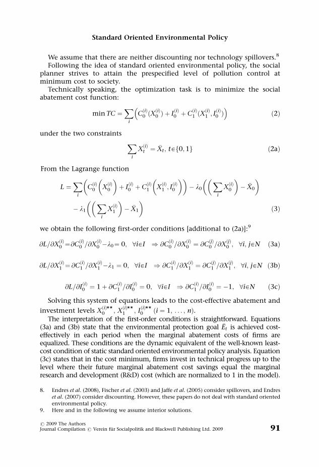
We assume that there are neither discounting nor technology spillovers.8

Following the idea of standard oriented environmental policy, the socialplanner strives to attain the prespecified level of pollution control atminimum cost to society.

Technically speaking, the optimization task is to minimize the socialabatement cost function:

min TC ¼X

i

CðiÞ0 ðX

ðiÞ0 Þ þ I

ðiÞ0 þ C

ðiÞ1 ðX

ðiÞ1 ; I

ðiÞ0 Þ

� �ð2Þ

under the two constraints

Xi

XðiÞt ¼ �Xt ; t [f0;1g ð2aÞ

From the Lagrange function

L ¼X

i

CðiÞ0

�XðiÞ0

�þ IðiÞ0 þ C

ðiÞ1

�XðiÞ1 ; I

ðiÞ0

�� l0

��Xi

XðiÞ0

�� X0

�

� l1

��Xi

XðiÞ1

�� X1

�ð3Þ

we obtain the following first-order conditions [additional to (2a)]:9

@L=@XðiÞ0 ¼@C

ðiÞ0 =@X

ðiÞ0 �l0¼ 0; 8i[I ) @C

ðiÞ0 =@X

ðiÞ0 ¼ @C

ðjÞ0 =@X

ðjÞ0 ; 8i; j[N ð3aÞ

@L=@XðiÞ1 ¼ @C

ðiÞ1 =@X

ðiÞ1 �l1 ¼ 0; 8i[I ) @C

ðiÞ1 =@X

ðiÞ1 ¼ @C

ðjÞ1 =@X

ðjÞ1 ; 8i; j[N ð3bÞ

@L=@IðiÞ0 ¼ 1þ @C

ðiÞ1 =@I

ðiÞ0 ¼ 0; 8i[I ) @C

ðiÞ1 =@I

ðiÞ0 ¼ �1; 8i[N ð3cÞ

Solving this system of equations leads to the cost-effective abatement and

investment levels XðiÞ**0 ; X

ðiÞ**1 ; I

ðiÞ**0 ði ¼ 1; . . . ; nÞ.

The interpretation of the first-order conditions is straightforward. Equations(3a) and (3b) state that the environmental protection goal �Et is achieved cost-effectively in each period when the marginal abatement costs of firms areequalized. These conditions are the dynamic equivalent of the well-known least-cost condition of static standard oriented environmental policy analysis. Equation(3c) states that in the cost minimum, firms invest in technical progress up to thelevel where their future marginal abatement cost savings equal the marginalresearch and development (R&D) cost (which are normalized to 1 in the model).

8. Endres et al. (2008), Fischer et al. (2003) and Jaffe et al. (2005) consider spillovers, and Endreset al. (2007) consider discounting. However, these papers do not deal with standard orientedenvironmental policy.

9. Here and in the following we assume interior solutions.



4. POSITIVE ANALYSIS: ABATEMENT AND INNOVATIONEQUILIBRIA UNDER ALTERNATIVE ENVIRONMENTALREGIMES

4.1. Introduction

Below, the performance of three alternative environmental policies, com-mand and control, TDPs and effluent charges are assessed. The cost-effectiveallocation described above is used as the measuring rod. The question iswhether the equilibrium abatement and investment levels, holding underalternative environmental laws, X

ðiÞ*0 ; X

ðiÞ*1 ; I

ðiÞ*0 are equal to the cost-effective

values XðiÞ**0 ; X

ðiÞ**1 ; I

ðiÞ**0 :

It will be shown below that the quality and the distribution of informa-tion are a key issue in the comparative dynamic analysis of different standardoriented environmental policy instruments. The question of ‘who needs toknow what in order to make the instrument work’ has to be answeredcompletely differently for alternative instruments. The economic agentsconsidered here (‘who’) are the individual polluters deciding on abatementand investment into technical change, on the one hand, and the environ-mental policy-maker, on the other. The relevant information (‘what’) is theaggregate marginal abatement costs [equations (4) and (5)] and the individualmarginal abatement costs [equations (6) and (7)] for each period, respectively.

These marginal abatement cost functions are given by

MCS0 ðX0Þ ¼

dCS0

dX0ð4Þ

with

CS0 ðX0Þ ¼min

XðiÞ0

Xi

CðiÞ0 ðX

ðiÞ0 Þ; s:t:

Xi[ I

XðiÞ0 ¼ X0 ð4aÞ

MCS1 ðX1Þ ¼

dCS1

dX1ð5Þ

with10,11

10. Note that (5a) could also be written as CS1 ðX1Þ ¼min

XðiÞ1

Pi ð ~C

ðiÞ1 ðX

ðiÞ1 ÞÞ s.t.

Pi[ I

XðiÞ1 ¼ X1 and with

IðiÞ0 ðX

ðiÞ1 Þ ¼ arg min ðIðiÞ0 þ C

ðiÞ1 ðX

ðiÞ1 ; I

ðiÞ0 ÞÞ, ~C

ðiÞ1 ðX

ðiÞ1 Þ ¼ I

ðiÞ0 ðX

ðiÞ1 Þ þ C

ðiÞ1 ðX

ðiÞ1 ; I

ðiÞ0 ðX

ðiÞ1 ÞÞ. That is, each

XðiÞ1 corresponds to a cost-effective investment level I

ðiÞ0 ðX

ðiÞ1 Þ. Equation (5) implies that this

investment level [which is determined by (3c)] is chosen. This corresponds to theequilibrium behavior of the firms that know their individual marginal abatement costs ineach information scenario.

11. Note that from (4a) and (5a) again we obtain the first-order conditions (3a)–(3c).



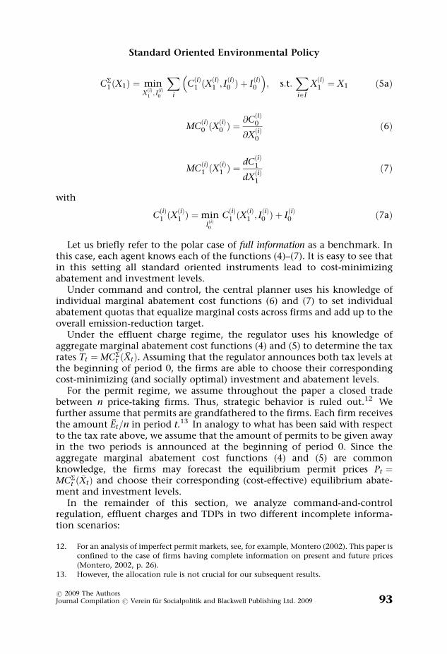
CS1 ðX1Þ ¼ min

XðiÞ1; IðiÞ0

Xi

CðiÞ1 ðX

ðiÞ1 ; I

ðiÞ0 Þ þ I

ðiÞ0

� �; s:t:

Xi[ I

XðiÞ1 ¼ X1 ð5aÞ

MCðiÞ0 ðX

ðiÞ0 Þ ¼

@CðiÞ0

@XðiÞ0

ð6Þ

MCðiÞ1 ðX

ðiÞ1 Þ ¼

dCðiÞ1

dXðiÞ1

ð7Þ

with

CðiÞ1 ðX

ðiÞ1 Þ ¼min

IðiÞ0

CðiÞ1 ðX

ðiÞ1 ; I

ðiÞ0 Þ þ I

ðiÞ0 ð7aÞ

Let us briefly refer to the polar case of full information as a benchmark. Inthis case, each agent knows each of the functions (4)–(7). It is easy to see thatin this setting all standard oriented instruments lead to cost-minimizingabatement and investment levels.

Under command and control, the central planner uses his knowledge ofindividual marginal abatement cost functions (6) and (7) to set individualabatement quotas that equalize marginal costs across firms and add up to theoverall emission-reduction target.

Under the effluent charge regime, the regulator uses his knowledge ofaggregate marginal abatement cost functions (4) and (5) to determine the taxrates Tt ¼ MCS

t ð �XtÞ. Assuming that the regulator announces both tax levels atthe beginning of period 0, the firms are able to choose their correspondingcost-minimizing (and socially optimal) investment and abatement levels.

For the permit regime, we assume throughout the paper a closed tradebetween n price-taking firms. Thus, strategic behavior is ruled out.12 Wefurther assume that permits are grandfathered to the firms. Each firm receivesthe amount �Et=n in period t.13 In analogy to what has been said with respectto the tax rate above, we assume that the amount of permits to be given awayin the two periods is announced at the beginning of period 0. Since theaggregate marginal abatement cost functions (4) and (5) are commonknowledge, the firms may forecast the equilibrium permit prices Pt ¼MCS

t ð �XtÞ and choose their corresponding (cost-effective) equilibrium abate-ment and investment levels.

In the remainder of this section, we analyze command-and-controlregulation, effluent charges and TDPs in two different incomplete informa-tion scenarios:

12. For an analysis of imperfect permit markets, see, for example, Montero (2002). This paper isconfined to the case of firms having complete information on present and future prices(Montero, 2002, p. 26).

13. However, the allocation rule is not crucial for our subsequent results.



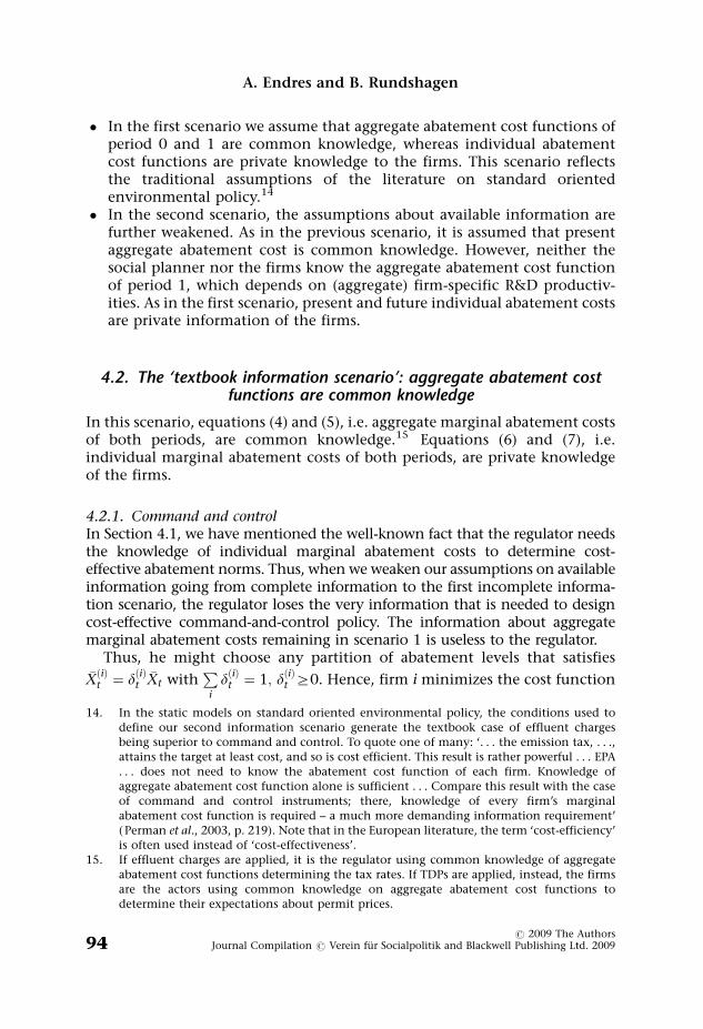
� In the first scenario we assume that aggregate abatement cost functions ofperiod 0 and 1 are common knowledge, whereas individual abatementcost functions are private knowledge to the firms. This scenario reflectsthe traditional assumptions of the literature on standard orientedenvironmental policy.14

� In the second scenario, the assumptions about available information arefurther weakened. As in the previous scenario, it is assumed that presentaggregate abatement cost is common knowledge. However, neither thesocial planner nor the firms know the aggregate abatement cost functionof period 1, which depends on (aggregate) firm-specific R&D productiv-ities. As in the first scenario, present and future individual abatement costsare private information of the firms.

4.2. The ‘textbook information scenario’: aggregate abatement costfunctions are common knowledge

In this scenario, equations (4) and (5), i.e. aggregate marginal abatement costsof both periods, are common knowledge.15 Equations (6) and (7), i.e.individual marginal abatement costs of both periods, are private knowledgeof the firms.

4.2.1. Command and controlIn Section 4.1, we have mentioned the well-known fact that the regulator needsthe knowledge of individual marginal abatement costs to determine cost-effective abatement norms. Thus, when we weaken our assumptions on availableinformation going from complete information to the first incomplete informa-tion scenario, the regulator loses the very information that is needed to designcost-effective command-and-control policy. The information about aggregatemarginal abatement costs remaining in scenario 1 is useless to the regulator.

Thus, he might choose any partition of abatement levels that satisfies�XðiÞt ¼ dðiÞt

�Xt withP

i

dðiÞt ¼ 1; dðiÞt Z0. Hence, firm i minimizes the cost function

14. In the static models on standard oriented environmental policy, the conditions used todefine our second information scenario generate the textbook case of effluent chargesbeing superior to command and control. To quote one of many: ‘. . . the emission tax, . . .,attains the target at least cost, and so is cost efficient. This result is rather powerful . . . EPA. . . does not need to know the abatement cost function of each firm. Knowledge ofaggregate abatement cost function alone is sufficient . . . Compare this result with the caseof command and control instruments; there, knowledge of every firm’s marginalabatement cost function is required – a much more demanding information requirement’(Perman et al., 2003, p. 219). Note that in the European literature, the term ‘cost-efficiency’is often used instead of ‘cost-effectiveness’.

15. If effluent charges are applied, it is the regulator using common knowledge of aggregateabatement cost functions determining the tax rates. If TDPs are applied, instead, the firmsare the actors using common knowledge on aggregate abatement cost functions todetermine their expectations about permit prices.



CðiÞQ ðI

ðiÞ0 Þ ¼ C

ðiÞ0 ðd

ðiÞ0

�X0Þ þ IðiÞ0 þ C

ðiÞ1 ðd

ðiÞ1

�X1; IðiÞ0 Þ ð8Þ

Of course, the chosen partition of the regulator will deviate from the cost-effective solution in general. Since without regulation the equilibriumemission level of each firm equals Emax=n, it is plausible to assume that theregulator chooses the uniform abatement quota �X

ðiÞt ¼ �Xt=n, which leads to

the cost-effective solution in the polar case of symmetric firms. The cost-effective solution may also result if firms are heterogeneous. However,this occurs only in the special case of MC

ðiÞt ð �Xt=nÞ ¼ MC

ðjÞt ð �Xt=nÞ

¼ MCSt ð �XtÞ

� �; 8i 6¼ j.

If firms are asymmetric with respect to their marginal abatement cost,except for the special case described above, a uniform abatement quotaimplies that firms with marginal abatement costs below (above) MCS

t ð �XtÞabate too little (too much) compared with the cost-effective solution. SincedIðiÞ0 =dX

ðiÞ1 > 0, the same holds for the individual investment levels.16

It is important to note that the corresponding aggregate investment levelsmay exceed or fall below the cost-effective aggregate investment level ifabatement norms are set on non-cost-minimizing levels. In general, theaggregate investment level exceeds the cost-effective aggregate investment levelif there exists a firm i with a very strict abatement target, i.e. �X

ðiÞ1 � X

ðiÞ**1 or

dðiÞ1 ! 1, respectively. Because of @2CðiÞ1 =@ðX

ðiÞ1 Þ

2 > 0, in this case, firm i suffersfrom high marginal abatement costs in period 1 and reacts by choosing anexcessive investment level (compared with the socially optimal one). Because of@2C

ðiÞ1 =@X

ðiÞ1 @I

ðiÞ0 < 0, the over-investment of firm i generally outweighs the

under-investment of the firm(s) with low abatement target(s).

4.2.2. Effluent chargesSince the regulator only needs equations (4) and (5) to set the cost-effectivetax rate (see Section 4.1), the weakening of information assumptions from thebenchmark setting of complete information to scenario 1 does not influenceequilibrium and abatement levels in the effluent charge regime.

Thus, the fundamental result of the cost-effectiveness of the standards andcharges approach carries over from the traditional static model to thedynamic case of information scenario 1.

16. Total differentiation of (3c) [which implicitly defines the best reply function IðiÞ0 ðX

ðiÞ1 Þ] gives

@2CðiÞ1

@ðIðiÞ0 Þ2

dIðiÞ0 þ

@2CðiÞ1

@XðiÞ1 @I

ðiÞ0

dXðiÞ1 ¼ 0, dI

ðiÞ0 =dX

ðiÞ1 ¼ �

@2CðiÞ1 =@X

ðiÞ1 @I

ðiÞ0

@2CðiÞ1 =@I

ðiÞ20

> 0

From (3c) follows@CðiÞ1

@IðiÞ0

ðXðiÞ1 ; IðiÞ0 ðX

ðiÞ1 ÞÞ ¼ �1. Note that this does not imply that

@CðiÞ1

@IðiÞ0

ðXðiÞ1 ; IðiÞ0 Þ

is constant in IðiÞ0 .



4.2.3. PermitsAs in the effluent charge regime, equilibrium abatement levels are the same asin the full information scenario. The reason is that the firms only needinformation about aggregate marginal abatement costs to be able to calculatethe future permit price and thus to make the individual cost-minimizinginvestment decisions in period 0.

Thus, permits are dynamically equivalent to effluent charges as well assuperior to command and control within the framework of informationscenario 1, just as they are in the static models traditionally analyzed in theliterature.

4.2.4. ComparisonThe worsening of information conditions from complete information toscenario 1 turned out to be fatal in the case of command-and-controlregulation. In contrast to this, it has no consequences for effluent charges orTDPs. Using these kinds of policies, no common knowledge of individual costfunctions is necessary to generate cost-effective equilibria. In fact, for each ofthese policies, information requirements for the cost-effective solution areeven lower than their ‘common knowledge’ specification in scenario 1. Underthe effluent charge regime, only the regulator, but not the firms, needsinformation about aggregate marginal abatement costs. Under the permitregime it is just the other way around.17

4.3. The weak information scenario: the present aggregate abatementcost function is common knowledge

In this scenario, equation (4), i.e. the current aggregate marginal abatementcost function, is common knowledge. Equations (6) and (7), the individualmarginal abatement cost functions, are private knowledge to the firms. Theseassumptions are the same as in the previous scenario. The difference betweenthe first and the second scenario relates to the information available aboutthe future aggregate marginal abatement cost. To calculate these, the partiesinvolved must be informed about each firm’s individual R&D productivity. Inthe weak information scenario, we assume that none of the involved agentshas this information. Therefore, the future aggregate marginal abatementcost function (5) is unknown. (However, each firm is still assumed to know itsown R&D productivity.)

17. In a permit regime without future market, the firms’ information about aggregate marginalabatement costs is necessary to forecast the equilibrium permit price of period 1 and thus tochoose the optimal investment level in period 0. However, if there is a future market thefirms need not even know the aggregate abatement cost. They learn about the permit pricein the future market and adjust accordingly in terms of abatement and investment. In thesubsequent section (Section 4.3), we elaborate on permits without future markets (Section4.3.3) as opposed to permits with future markets (Section 4.3.4).



4.3.1. Command and controlAs explained above, the regulator applying command and control loses all theinformation needed to design this kind of a policy cost-effectively, wheninformation conditions deteriorate going from complete information toscenario 1. Thus, the further withdrawal of information from the first to thesecond scenario is of no concern to the regulator assigning individualreduction quotas within the command-and-control approach.

4.3.2. Effluent chargesIf the regulator has no information about the productivity of innovation(and thereby no information on the future aggregate marginal abatementcost) the question arises of how the tax rate in the future period isto be calculated. An obvious possibility is that the rate is based on the

aggregate marginal abatement cost of period 0, i.e. T01 ¼ MCS

0 ð �X1Þ.18 Hence,

from MCS1 ð �X1Þ<MCS

0 ð �X1Þ ¼ T01 ¼ MCS

1 ðP

i XðiÞ1 ðT0

1 ÞÞ, it follows that aggregate(and individual) abatement in period 1 exceeds the abatement target (as is

well known to the literature). Additionally, from dIðiÞ0 =dX

ðiÞ1 > 0 (see Section

4.2.1), it follows that the individual and aggregate innovation levels exceedthe cost-minimizing ones, irrespective of the degree of heterogeneity betweenfirms.

4.3.3. PermitsIf firms have no information about the future aggregate marginal abatementcost, the permit market equilibrium in period 1 depends on firms’expectations about the future permit price. In the following, we considertwo kinds of price expectations.

In a first case we assume that firms form their expectations concerning thepermit price in period 1 based on the aggregate marginal abatement costfunction of period 0, i.e.19

P01 ¼ MCS

0 ðEmax � �E1Þ ¼ MCS0ð �X1Þ ð9Þ

We analyze this case because it provides a frame under which theconditions of the TDP system are most similar (and thereby most comparable)to the situation under the effluent charge policy as described above. In thetransferable permit case, the firms’ expectations that aggregate marginalabatement cost (and thereby the permit price in case of �X1 ¼ �X0Þ will not

18. This is an assumption widely used in the literature. (See the seminal paper by Milliman andPrince (1989) as well as, e.g., Fischer et al. (2003); Jung et al. (1996); Montero (2002). Thepaper by Fischer et al. (2003) assumes that policies remain fixed at their pre-innovationlevels for the most part of their analysis; p. 525.)

19. It should be noted that this assumption is consistent with the assumption that firms areprice takers in the permit market (implying that a single firm cannot affect the aggregatemarginal abatement cost function of period 1 by investment in R&D).



change from period 0 to period 1 are analogous to the assumption used abovefor the effluent charge policy: the regulator assumes that the aggregatemarginal abatement cost does not change over time and fixes the tax ratesaccordingly. Therefore, the expected permit price P0

1 in this price-expectationcase is identical to the tax rate T0

1 explained above.Thus, investment levels in period 0 are the same as under the effluent

charge regime. However, abatement levels in period 1 are lower than underthe effluent charge regime, since, under the effluent charge regime, abate-ment exceeds the target �X1, which is not possible under the permit regime, bydefinition.

Thus, irrespective of the degree of heterogeneity between firms, under thepermit regime, the overestimation of the future permit price leads to veryhigh investment levels in period 0, given the exogenous aggregate abatementtarget of period 1.

In the case briefly examined above, each firm decides to invest (and therebychanges its individual marginal abatement cost function) but expects theaggregate marginal abatement cost to be unchanged over time. However, thissetting is not very plausible. It requires the firms to be ‘presumptuous’ in thateach firm believes it is the only one to understand the dynamic incentives ofthe TDP policy and thereby being the only one deciding to invest.

For higher plausibility, we investigate a second case regarding priceexpectations. Here, we assume that firms anticipate that aggregate invest-ment in R&D decreases the abatement cost in period 1 and hence lowers thefuture permit price.

More specifically, we assume that firm i forms its price expectationsaccording to the following mechanism:

� First, we consider the optimal abatement level of firm i in period 1. Sincefirm i does not know the future aggregate marginal abatement cost, it isnot possible to determine the optimal abatement level from

MCðiÞ1 ð �X

ðiÞ1 Þ ¼ MCS

1 ð �X1Þ ð10Þ

Thus, firm i must form an expectation concerning its optimal abatementlevel in period 1. It assumes that firms are symmetric in R&D productivityin so far as the cost-effective division of a given abatement level, and inparticular of the abatement level �X1, remains unchanged from period 0 toperiod 1. That is, firm i assumes that the solution �X

ðiÞ1 from (10) equals the

solution �XðiÞ;01 from (11):

MCðiÞ0 ð �X

ðiÞ;01 Þ ¼ MCS

0 ð �X1Þ ð11Þ

Thus, firm i plans to abate �XðiÞ;01 in period 1.

� Second, the firms act on the assumption that the relation of theirindividual marginal abatement cost (with/without optimal investmentsin technical progress) equals the relation of aggregate marginal



abatement cost. Thus, expected aggregate marginal abatement costsare determined by

EðiÞ MCS1 ð �X1Þ

� MCS

0 ð �X1Þ¼ MC

ðiÞ1 ð �X

ðiÞ;01 Þ

MCðiÞ0 ð �X

ðiÞ;01 Þ

ð12Þ

and the expected price is given by20

EðiÞ P½ � ¼ EðiÞ MCS1 ð �X1Þ

� ¼ MCS

0 ð �X1ÞMC

ðiÞ0 ð �X

ðiÞ;01 Þ

MCðiÞ1 ð �X

ðiÞ;01 Þ ¼ MC

ðiÞ1 ð �X

ðiÞ;01 Þ ð13Þ

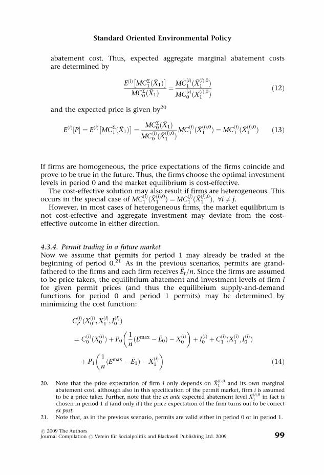
If firms are homogeneous, the price expectations of the firms coincide andprove to be true in the future. Thus, the firms choose the optimal investmentlevels in period 0 and the market equilibrium is cost-effective.

The cost-effective solution may also result if firms are heterogeneous. Thisoccurs in the special case of MC

ðiÞ1 ð �X

ðiÞ;01 Þ ¼ MC

ðjÞ1 ð �X

ðjÞ;01 Þ; 8i 6¼ j.

However, in most cases of heterogeneous firms, the market equilibrium isnot cost-effective and aggregate investment may deviate from the cost-effective outcome in either direction.

4.3.4. Permit trading in a future marketNow we assume that permits for period 1 may already be traded at thebeginning of period 0.21 As in the previous scenarios, permits are grand-fathered to the firms and each firm receives �Et=n. Since the firms are assumedto be price takers, the equilibrium abatement and investment levels of firm ifor given permit prices (and thus the equilibrium supply-and-demandfunctions for period 0 and period 1 permits) may be determined byminimizing the cost function:

CðiÞP ðX

ðiÞ0 ;X

ðiÞ1 ; I

ðiÞ0 Þ

¼ CðiÞ0 ðX

ðiÞ0 Þ þ P0

�1

nðEmax � �E0Þ � X

ðiÞ0

�þ IðiÞ0 þ C

ðiÞ1 ðX

ðiÞ1 ; I

ðiÞ0 Þ

þ P1

�1

nðEmax � �E1Þ � X

ðiÞ1

�ð14Þ

20. Note that the price expectation of firm i only depends on �XðiÞ;01 and its own marginal

abatement cost, although also in this specification of the permit market, firm i is assumedto be a price taker. Further, note that the ex ante expected abatement level �X

ðiÞ;01 in fact is

chosen in period 1 if (and only if ) the price expectation of the firm turns out to be correctex post.

21. Note that, as in the previous scenario, permits are valid either in period 0 or in period 1.



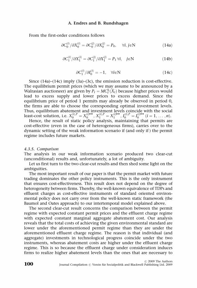
From the first-order conditions follows

@CðiÞ0 =@X

ðiÞ0 ¼ @C

ðjÞ0 =@X

ðjÞ0 ¼ P0; 8i; j[N ð14aÞ

@CðiÞ1 =@X

ðiÞ1 ¼ @C

ðjÞ1 =@X

ðjÞ1 ¼ P1 8i; j[N ð14bÞ

@CðiÞ1 =@I

ðiÞ0 ¼ �1; 8i[N ð14cÞ

Since (14a)–(14c) imply (3a)–(3c), the emission reduction is cost-effective.The equilibrium permit prices (which we may assume to be announced by aWalrasian auctioneer) are given by Pt ¼ MCS

t ð �XtÞ because higher prices wouldlead to excess supply and lower prices to excess demand. Since theequilibrium price of period 1 permits may already be observed in period 0,the firms are able to choose the corresponding optimal investment levels.Thus, equilibrium abatement and investment levels coincide with the socialleast-cost solution, i.e. X

ðiÞ;P0 ¼ X

ðiÞ**0 ; X

ðiÞ;P1 ¼ X

ðiÞ**1 ; I

ðiÞ;P0 ¼ I

ðiÞ**0 ði ¼ 1; . . . ;nÞ.

Hence, the result of static policy analysis, maintaining that permits arecost-effective (even in the case of heterogeneous firms), carries over to thedynamic setting of the weak information scenario if (and only if ) the permitregime includes future markets.

4.3.5. ComparisonThe analysis in our weak information scenario produced two clear-cut(unconditional) results and, unfortunately, a lot of ambiguity.

Let us first turn to the two clear-cut results and then shed some light on theambiguities.

The most important result of our paper is that the permit market with futuretrading dominates the other policy instruments. This is the only instrumentthat ensures cost-effectiveness. This result does not depend on the degree ofheterogeneity between firms. Thereby, the well-known equivalence of TDPs andeffluent charges as cost-effective instruments of standard oriented environ-mental policy does not carry over from the well-known static framework (theBaumol and Oates approach) to our intertemporal model explained above.

The second clear-cut result concerns the comparison between the permitregime with expected constant permit prices and the effluent charge regimewith expected constant marginal aggregate abatement cost. Our analysisreveals that the total costs of achieving the given environmental standard arelower under the aforementioned permit regime than they are under theaforementioned effluent charge regime. The reason is that individual (andaggregate) investments in technological progress coincide under the twoinstruments, whereas abatement costs are higher under the effluent chargeregime. This is so because the effluent charge under consideration inducesfirms to realize higher abatement levels than the ones that are necessary to



make sure that the emission ceiling is respected.22 It should be noted thatthis result is independent of the degree of heterogeneity between firms.

Beyond these two clear-cut results, there is no unconditional rank orderingof policy instruments. Fortunately, however, it can be said what the relativecost-(in)effectiveness of the instruments depends on. The most importantparameter is the heterogeneity of the individual marginal abatement costfunctions across firms.

Let us illustrate this point by comparing command and control, effluentcharges and permits with constant price expectations. Somewhat surprisingly,command and control may turn out to be more cost-effective than the variantsof effluent charges and TDPs under consideration here. This is so in the casewhere the degree of asymmetry in the individual marginal abatement cost issufficiently low to make the failure of command and control to equalize themarginal abatement cost across firms less severe than the cost-ineffectivenessgenerated by each of the other two instruments. Only if the differences inmarginal abatement costs are large enough does the cost-ineffectiveness ofuniform abatement quotas under command-and-control regulation over-compensate the problem of over-abatement and over-investment under theeffluent charges and the permit regime, respectively. We emphasize that thisresult is in contrast to the static model where command and control can neverfare better in terms of cost-effectiveness than charges and transferable permits do.

An analogous conclusion holds true if we compare the weak informationscenario with the textbook information scenario (instead of the static model):in the weak information scenario, the command-and-control regime gainssome ground over the other instruments, compared with the standardinformation scenario, where the command-and-control regime was generallyinferior to these instruments.23

5. SUMMARY, CONCLUSIONS AND QUESTIONS FOR FUTURERESEARCH

In this paper, we evaluated the standard oriented environmental policyinstruments, command and control (i.e. non-transferable quotas), effluent

22. An over-achievement of the abatement target might be desirable from the social point ofview if the abatement target is set too low according to a welfare function that comprisesenvironmental damages as well as abatement and investment cost. However, the positiveeffect on environmental damages is not appreciated within the limits of the standardoriented approach by definition.

23. In the text, above, we did not refer to the permit regime with price decline anticipation.However, it should be briefly noted that a general proof of the superiority of the permitregime with price decline anticipation over the permit market with expected constantpermit prices is not possible. The reason is that, in the case of asymmetric firms, some ofthem may over-estimate the price decline and thus make too low investments in R&D. Itcannot be ruled out that this negative over-estimation effect may be stronger than thepositive price decline anticipation effect.



charges and TDPs in a dynamic framework allowing for induced technicalchange in abatement technology. It turned out that only under theassumption of full information with respect to firm-specific marginalabatement cost, do all policy instruments achieve the cost-effective abate-ment and the corresponding investment target. In case of incompleteinformation, the relative performance of the different instruments dependson the quality of information and the degree of heterogeneity between firms.

In the textbook information scenario, where the involved parties know onlythe aggregate marginal abatement cost, the environmental goal is alwaysachieved cost-effectively under effluent charges and permits. In contrastto this, a uniform abatement quota leads to cost-ineffectiveness in caseof asymmetric firms. This result is the intertemporal analog to classical(static) analysis of standard oriented environmental policy originating withthe seminal 1971 article by Baumol and Oates.

Things change in the weak information scenario, where the involved partieshave no information about R&D productivity and, hence, the futureabatement cost of the industry. In this case, only a permit regime with afuture market ensures cost-effectiveness when firms are heterogeneous.

Obviously, the pessimistic assumptions about the availability of informa-tion on future abatement technology applied in this scenario are suggestivefor many real-world applications. Therefore, even within the limits of thehighly stylized model presented above, the findings under the weakinformation scenario have some policy implications. These relate to thechoice of environmental policy instruments in general, and to the design ofTDP systems in particular. For example, consider the carbon emission tradingsystem, as has recently been introduced by the European Union. The purposeof this policy has been to enable the member states to carry the emissionreduction loads they accepted within the EU burden-sharing agreementunder the Kyoto Protocol ‘in a cost-effective and economically efficientmanner’.24 The system is doomed to miss this goal since there is no provisionfor trading in future markets. To the contrary, it is not even clear how manypermits will be allocated in future periods. Moreover, firms must makeinvestment decisions with long time horizons (particularly in the energysector) in a situation where it is unclear whether the system will be extendedbeyond the year 2012, and, if so, what the future design of the system will be.Under these circumstances, there is no reason to assume that firms will beable to anticipate future permit prices and thereby make intertemporally cost-effective decisions on abatement and investment.25 The results presentedabove produce prima facie evidence that the cost-effectiveness of the system

24. EU Directive 2003/87/EC, Article 1.25. There are some (rather restrictively designed) possibilities for banking and borrowing of

permits. However, these provisions are not allocatively equivalent to future markets forpermits. An economic assessment of EU emissions trading is given in Ellerman and Buchner(2007), Endres and Ohl (2005) and Kruger et al. (2007).



can be improved by establishing markets in which permits for future periodsmay be traded.

It is an obvious task for future research to investigate whether the resultspresented in this paper carry over to a framework that is more general thanthe one used above. For example, the analysis might be extended allowing fornon-competitive firms, imperfect research and/or permit markets, uncer-tainty with respect to the success of research and knowledge spilloversbetween firms. In addition, technical progress might be modelled as a processof learning by doing, which could affect the results of our comparativeanalysis of environmental policy instruments. Finally, a longer time horizonshould be modelled, since not only cost-effective and equilibrium levels ofinvestment are important issues but also cost-effective and equilibrium timingof investment.26 For this question, the analysis must be extended beyond thesimple two-period world to which this paper has been confined up to thispoint. In the Appendix, we take a first step in this direction. We non-formallydiscuss whether the effluent charge regime performs better in a multiperiodmodel due to learning effects.

APPENDIX: EXTENSION: ACQUISITION OF INFORMATIONBY ‘TRIAL AND ERROR’ IN A MULTIPERIOD MODEL

We now discuss how learning by ‘trial and error’ affects the performance ofthe effluent charge regime in the weak information scenario if the number ofperiods in our dynamic model with technological innovations is increased toT42.27

Consider a starting point model with extended periodicity that ischaracterized by the following three assumptions:

(A) The pollutant is a flow pollutant (as hitherto). Correspondingly, there isan abatement target for each period.

(B) Investments in technical progress are only possible once, namely inperiod 0.

(C) As in Section 4.3, the tax rate chosen in period 1 is based on the aggregatemarginal abatement cost of period 0, which is anticipated by the firms.

Afterwards we discuss how changes in each of these assumptions affect ourresults.

26. See, for example, Requate (2005b).27. We restrict our attention to effluent charges since under command and control there are no

learning effects through trial and error. Under a permit regime without a future market,there may be learning effects for the firms with respect to future permit prices (see Section4.3.3). However, a permit regime with a future permit market already reaches theenvironmental goal cost-effectively, beginning from the first period. Thus, it would not beinteresting to dwell upon inferior variants of the TDP system.



In the two-period model considered in the main parts of this paper, the taxchosen in period 1 is cost-ineffective for two reasons. First, the environmentaltarget is overfulfilled because of MCS

1 ð �X1Þ<MCS0 ð �X1Þ ¼ T0

1 (see Section 4.3.2).Second, the investment level chosen in period 0 is too high. If the number ofperiods is increased, learning by ‘trial and error’ diminishes the firstdeficiency in later periods. However, the second deficiency persists due tothe irreversibility of the investment decision.

Now consider three modifications of the starting point model. In each ofthese modifications, one (and only one) of the three assumptions presentedabove is changed:

� If we deviate from assumption (C) and assume instead that the regulatorrecognizes that investments in technical progress may reduce futureabatement costs and this, in turn, is anticipated by the firms, the regulatorwill choose a tax rate that is smaller than MCS

0 ð �X1Þ. Correspondingly, theover-investment in technical progress of the firms is decreased comparedwith the model using assumption (C). However, neither does the regulatorknow how far the tax rate for period 1 has to be reduced compared withMCS

0 ð �X1Þ, nor do the firms know which level the regulator will chooseexactly in period 1 and in the later periods. Thus, even though a deviationfrom assumption (C) works in favor of the performance of the effluentcharge regime, cost-effectiveness may only be reached by coincidence.

� Now we go back to the starting point model regarding assumption (C) andmodify assumption (B) instead. Assume that in contrast to assumption (B),investments in technical progress are possible in each period. Then, thefirm-specific marginal abatement cost in period t depends on theabatement level Xt and the previous investments in technical progressI0; . . . ; It�1. Thus, the firm-specific marginal abatement cost functionsmay be interpreted as a composition of the marginal abatement costfunction for a given technology level and the production function oftechnological innovation. This complexity reduces the ability of theregulator to learn through ‘trial and error’ even if the regulator is able toobserve the firm-specific abatement levels for a chosen tax rate. The factthat a firm responds to the chosen tax rate with a certain abatement levelmay be explained by an infinite number of combinations of the two typesof functions. Thus, the (more realistic) possibility of multiple investmentsworks against the cost-effectiveness of the effluent charge regime.

� As a last modification of our starting point model, we deviate fromassumption (A) and go back to the starting point model regarding (B).Instead of assumption (A), we take the pollutant under consideration to bea stock pollutant. The consequence is that the ceiling on emissionsdetermining the constraints in our cost-minimization problem does notrelate to pollution in each period but to cumulative pollution. In thissetting, the optimization task is even more ambitious, since the regulatornot only has to estimate which tax rate corresponds to the period-specific



abatement levels of the starting point model. Additionally, he has toestimate the cost-effective division of the cumulative abatement target onthe single periods. Since the regulator does not have the relevantinformation for the determination of the optimal period-specific targets,this additional challenge weakens the cost-effectiveness of effluentcharges.28,29 On the other hand, in case of a stock pollutant, inefficienciesthat are caused by the over-achievement of period-specific abatementtargets may be attenuated by lowering the abatement targets for laterperiods. This effect works in favor of the efficiency of effluent charges(compared with the command-and-control regime). However, an inter-periodical balance of marginal abatement cost (and thus cost-effective-ness) is left to pure regulatory luck.

Still, the effects described above suggest a relative improvement of theperformance of the effluent charge regime compared with the command-and-control regime. This is so since command and control cannot benefit fromlearning effects if the time horizon is extended.

ACKNOWLEDGEMENTS

An earlier version of this paper has been presented at the Annual Conference ofthe German Economic Association (Verein f ur Socialpolitik) held in Munich, 8–12October 2007. The authors are indebted to the session participants and toRegina Bertram, University of Hagen, for their helpful comments. Hereafter, theauthors considerably benefited from the illuminating discussions given byMichael Finus, University of Stirling, Rudiger Pethig, University of Siegen, andby two anonymous referees. The usual disclaimer applies.

Address for correspondence: Alfred Endres, Department of Economics,University of Hagen, Profilstr. 8, 58084 Hagen, Germany. Tel.: þ 49 2331 987301; fax: þ 49 2331 987 302; e-mail: [email protected]

REFERENCES

Baumol, W. J. and W. E. Oates (1971), ‘The Use of Standards and Prices for Protectionof the Environment’, Swedish Journal of Economics 73, 42–54.

Ellerman, A. D. and B. K. Buchner (2007), ‘The European Union Emissions TradingScheme: Origins, Allocations and Early Results’, Review of Environmental Economicsand Policy 1, 66–87.

Endres, A. (2007), Umweltokonomie, Kohlhanner, Stuttgart.

28. Note that the same informational problem arises under the command-and-control regime.In general, the command-and-control regime is not cost-effective in the regulation of stockpollutants, even in the case of symmetric firms. This is in striking contrast to the flowpollutant case analyzed in Section 4.3.1.

29. In the case of the permit regime, inefficiencies may be avoided by a permit system withfuture markets, which additionally allows banking and borrowing of permits across periods.



mailto:[email protected]

Endres, A. and R. Bertram (2006), ‘The Development of Care Technology under

Liability Law’, International Review of Law and Economics 26, 503–518.Endres, A. and C. Ohl (2005), ‘Kyoto Europe? – An Economic Evaluation of the

European Emission Trading Directive’, European Journal of Law and Economics 19,

17–39.Endres, A. and B. Rundshagen (2008), ‘A Note on Coasean Dynamics’, Environmental

Economics and Policy Studies 9, 57–66.Endres, A., R. Bertram and B. Rundshagen (2007), ‘Environmental Liability Law and

Induced Technical Change – The Role of Discounting’, Environmental and Resource

Economics 36, 341–366.Endres, A., B. Rundshagen and R. Bertram (2008), ‘Environmental Liability Law and

Induced Technical Change – The Role of Spillovers’, Journal of Institutional and

Theoretical Economics 164, 254–279.Faure, M. and G. Skogh (2003), The Economic Analysis of Environmental Law and Policy,

Edward Elgar, Cheltenham.Fischer, C., I. W. H. Parry and W. A. Pizer (2003), ‘Instrument Choice for

Environmental Protection When Technological Innovation is Endogenous’, Journal

of Environmental Economics and Management 45, 523–545.Hanley, N., J. F. Shogren and B. White (2001), Introduction to Environmental Economics,

Oxford University Press, Oxford.Hoel, M. and L. Karp (2002), ‘Taxes versus Quotas for a Stock Pollutant’, Resource and

Energy Economics 24, 367–384.Jaffe, A. B., R. G. Newell and R. N. Stavins (2002), ‘Environmental Policy and

Technological Change’, Environmental and Resource Economics 22, 41–69.Jaffe, A. B., R. G. Newell and R. N. Stavins (2005), ‘A Tale of Two Market

Failures: Technology and Environmental Policy’, Ecological Economics 54,

164–174.Jung, C., K. Krutilla and R. Boyd (1996), ‘Incentives for Advanced Pollution Abatement

Technology at the Industry Level: An Evaluation of Policy Alternatives’, Journal of

Environmental Economics and Management 30, 143–150.Kruger, J., W. E. Oates and W. A. Pizer (2007), ‘Decentralization in the EU Emissions

Trading Scheme and Lessons for Global Policy’, Review of Environmental Economics

and Policy 1, 112–133.Milliman, S. R. and R. Prince (1989), ‘Firm Incentives to Promote Technological

Change in Pollution Control’, Journal of Environmental Economics and Management

17, 247–265.Montero, J.-P. (2002), ‘Permits, Standards, and Technology Innovation’, Journal of

Environmental Economics and Management 44, 23–44.Parry, I. W. H. (1998), ‘Pollution Regulation and the Efficiency Gains from

Technological Innovation’, Journal of Regulatory Economics 14, 229–254.Perman, R., Y. Ma, J. McGilvray and M. Common (2003), Natural Resource and

Environmental Economics, 3rd ed., Prentice Hall, Harlow.Requate, T. (2005a), ‘Dynamic Incentives by Environmental Policy Instruments – A

Survey’, Ecological Economics 54, 175–195.Requate, T. (2005b), ‘Commitment and Timing of Environmental Policy, Adoption of

New Technology, and Repercussions on R&D’, Environmental and Resource Economics

31, 175–199.



Requate, T. and W. Unold (2001), ‘On the Incentives of Environmental PolicyInstruments to Adopt Advanced Abatement Technology if Firms are Asymmetric’,Journal of Institutional and Theoretical Economics 157, 536–554.

Requate, T. and W. Unold (2003), ‘Environmental Policy Incentives to AdoptAdvanced Abatement Technology: Will the True Ranking Please Stand Up?’,European Economic Review 47, 125–146.

Russell, C. S. (2001), Applying Economics to the Environment, Oxford University Press,New York.



Standard Oriented Environmental Policy: Cost-Effectiveness and Incentives for âGreen Technologyâ

Documents

Transcript of Standard Oriented Environmental Policy: Cost-Effectiveness and Incentives for âGreen Technologyâ