Stand-level yield model for Scots pine (Pinus sylvestris L.)in north-east Spain

M. Palahí1,2*, J. Miina3, M. Tomé4, G. Montero5

1 European Forest Institute, Torikatu 34, FIN-80100 Joensuu, Finland.2 Centre Tecnológic Forestal de Catalunya. Pujada del seminari s/n, 25280, Solsona, Spain.

3 The Finnish Forest Research Institute, Joensuu Research Centre, P.O.Box 68,80101, Joensuu, Finland.

4 Departamento de Engenharia Florestal, Instituto Superior de Agronomia,Tapada de Ajuda, 1349-017 Lisboa, Portugal.

5 Departamento de Selvicultura. CIFOR-INIA. Carretera de La Coruña, Km 7. 28080 Madrid, Spain.

marc.palahi@efi.fi.

SUMMARY

Simultaneous stand-level growth and yield models for Pinus sylvestris in north-east Spain were developedbased on 21 permanent sample plots established in 1964 by the Instituto Nacional de Investigaciones Agrarias(INIA). The plots ranged in site index from 13 to 26 m (dominant height at 100 years), and were measured anaverage of 5 times. The estimation data consisted of 79 growth periods of stands ranging in age from 36 to 132years. Non-linear three-stage least squares method was used to simultaneously fit prediction and projectionequations for stand basal area, volume and stand density. An existing model for dominant height growth fittedwith the same estimation data was used to project dominant height. The models were evaluated both quantita-tively and qualitatively. Correlation among error components of the prediction equations for basal area and vol-ume as well as the projection equations for number of trees per hectare and volume were strong and significant.The mean biases for basal area, volume and number of trees per hectare predictions were positive. The presentedsystem of models can serve for forest-level management planning as a simple yield prediction system that re-quires only stand level input data.

Key words: non-linear multistage regression, simulation, simultaneous equations

Invest. Agr.: Sist. Recur. For. Vol. 11 (2), 2002

* Autor para correspondencia:Recibido: 28-1-02Aceptado para su publicación: 27-6-02

INTRODUCTION

Pinus sylvestris L. plays an important role in Spanish forestry because of its econo-mic, ecological and social relevance. P. sylvestris forms large forests in most of themountainous areas of Spain, occupying an area of 1,280,000 ha (Montero et al., 2001).Efficient forest management planning of Scots pine in Spain needs reliable informationon forest stand development under different treatment alternatives for evaluating the nu-merous forest management alternatives. Yield prediction models can be categorised bythe complexity of the mathematical approach involved. Clutter et al. (1983) divided yieldprediction models into: (a) models in tabular form; and (b) equations and systems ofequations. In Spain, yield predictions have been traditionally taken from yield tables-tabu-lar records showing the expected volume of wood per hectare by combinations of measu-rable characteristics of the forest stand (age, site quality, stand density). Yield tables arestatic models that usually apply to fully stocked or normal stands. Examples of yield ta-bles for Scots pine in Spain are in García Abejón (1981), García Abejón and Gómez Lo-ranca (1984), Garcia Abejón and Tella Ferreiro (1986) and Rojo and Montero (1996). Ho-wever, during the last decade several forest growth modelling studies expressing standgrowth and yield as systems of interrelating equations that can predict future stand deve-lopment with any desired combination of inputs have been undertaken in Spain [e.g., byEspinel et al. (1997) for Pinus radiata in País Vasco, by Río (1998) for Pinus sylvestris L.in Sistema Central and Ibérico, by Álvarez González et al. (1999) for Pinus pinaster Ait.and by Palahí et al. (2002b) for Pinus sylvetris in north-east Spain].

Forest stand modelling approaches may be thought to lie on a continuum with respectto structural complexity and output detail (Daniels and Burkhart, 1988). This continuummay be broken into three broad categories: (1) whole-stand models (2) size-class distribu-tion models, and (3) individual-tree models.

A number of researchers have used multiple regression to construct aggregate standgrowth and yield expression (e.g., Bennet et al., 1959; Schumacher and Coile, 1960; Clut-ter, 1963; Burkhart et al., 1972; Sullivan and Clutter, 1972; Murphy, 1983; Burkhart andSprinz, 1984; Borders and Bailey, 1986; Pienaar and Harrison, 1989; Amaro et al., 1997;Río, 1998). These models provide growth and yield estimates for the whole stand as afunction of stand level attributes such as age, density and site index, as well as interac-tions among these variables. Stand density, in turn, might be taken to be a function of aninitial measure of stand density, age and site quality. Site quality, expressed by site index,depends on the development of dominant height in relation to age (Clutter et al., 1983). Itis apparent that forest growth and yield models are an interdependent system of underly-ing growth processes. In such a system each equation describes a different relationshipamong a set of variables in the system, but all relationships are assumed to hold simulta-neously (Borders and Bailey, 1986). Clutter (1963) introduced the notion of compatibilityin growth and yield equations by recognising that the algebraic form of the yield modelcan be derived by mathematical integration of the growth model. Sullivan and Clutter(1972) extended Clutter’s models by simultaneously estimating yield and cumulativegrowth as a function of initial stand age, initial basal area, site index, and future age.Burkhart and Sprinz (1984) presented a method for simultaneously estimating the param-eters in the Sullivan-Clutter equation system. Furnival and Wilson (1971) suggested thattechniques commonly used to fit interdependent multiequation models in econometricsmight be applicable for growth and yield modelling situations. Murphy and Sternitzke

410 M. PALAHÍ et al.

(1979) and Murphy and Beltz (1981) applied a technique known as restricted three-stageleast squares to fit simultaneous growth and yield models. The successful application ofthese techniques (e.g., by Borders and Bailey, 1986; Pienaar and Harrison, 1989; Río,1998; Mabvurira and Miina, 2001), provided foresters with simulation tools developedusing theoretically sound statistical procedures. In Spain, Río (1998) applied the abovementioned techniques to fit simultaneous growth and yield models for Scots pine inSistema Central and Sistema Ibérico.

The objective of this study was to develop a system of interdependent and compatibleequations to predict stand growth and yield of Scots pine stands in north-east Spain usingthree-stage least squares techniques as the estimation procedure.

MATERIAL AND METHODS

Data

The data were measured in 21 permanent sample plots (Table 1) established in 1964by the Instituto Nacional de Investigaciones Agrarias (INIA) to represent most Scots pinesites in north-east Spain. The plots were located in the 3 provinces of Huesca, Lérida andTarragona. The plots were naturally regenerated and thinned between the first and secondmeasurement. The sites ranged in site index (at an index age of 100 years) from 13 to 26m according to the site index model developed by Palahí et al. (2002a). The mean plotarea was 0.1 ha. The plots were measured at 5-year intervals, except for the last measure-ment where the interval varied from 10 to 16 years. The last measurement was conducted

Invest. Agr.: Sist. Recur. For. Vol. 11 (2), 2002

A YIELD MODEL FOR SCOTS PINE IN NE SPAIN 411

Table 1

Summary of the characteristics of the 21 permanent plots as computed from the79 observations used in the study. The stand characteristics are given for the

beginning of the growth period

Variable Average (min, max) Standard deviation

Stand age (yr) 67.4(36, 132)

23.2

Site index (m) 19.9(13.7, 25.8)

3.30

Basal area (m2 ha–1) 41.7(22.6, 60.9)

8.7

Number of trees ha–1 1,199.7(424, 2896)

684.0

Dominant height (m) 15.6(8.7, 23.3)

3.3

Volume (m3 ha–1) 312.2(97.3, 602.6)

109.0

Number of measurements per plot 4.7(2, 6)

1.0

during the year 2000 and there was an average of 5 measurements per plot. At each mea-surement, tree diameter at 1.3 meters height (dbh) from all trees thicker than 5 cm, andtree heights of a sample of at least 20 trees per plot from different diameter classes wererecorded. A height-diameter regression equation for each plot at a time was fitted usingthe sample tree data. The regression equation was then used to estimate the height of treesother than sample trees. The total tree volumes were computed using the formula devel-oped by Pita Carpenter (1967):

v = –28.34 + 2.16 " h + 16.59 " d2 + 2.794 " d2 " h [1]

where v is tree volume in dm3, h is tree height in m and d is dbh in dm.Stand aggregates (dominant height, basal area, number of trees and volume per hect-

are) were computed for each plot and measurement. Site index was determined from thedominant height and age of each plot, using the site index model developed by Palahí etal. (2002a).

Most plots were thinned after the first measurement. Many of the removed trees weredying or already dead when the thinning was carried out. Because it was not knownwhether a removed tree was living or dead the first measurement interval was not used inthe estimation process.

System of equations

Several basal area and volume prediction and projection models (Amaro et al., 1997,Mabvurira and Miina, 2001) as well as survival functions (Pienaar and Shiver, 1986) werefitted to the data using ordinary least squares. The best models as determined by percentof variation explained, residual analysis and biological realism were selected. The use ofsequential measurements with the objective of predicting over discrete time intervals iscommonly done by using difference forms of the integral functions (e.g., Tomé, 1988;Borders, 1989; Huang 1994; Amaro et al., 1997; Mabvurira and Miina, 2001). These arederived from the integral form using the functional equivalence at two different times.This algebra frees one of the function parameters in that its value becomes independent ofthe ratio of the function´s value at the two times (Amaro et al., 1997). Compatible basalarea and volume projection equations using the methodology described above were de-rived from the selected prediction equations [3] and [5]. The simultaneous system of com-patible prediction and projection equations consisted of stand basal area and volume pre-diction models and a model for number of trees per hectare (henceforth referred to as sur-vival function) (Equations 2-6):

N = N e +2 1[ (T -T )]

10 2 1" " $ [2]

G = e H N +1 0T

1 1 2

1

1 2 3� $�

� �" " " [3]

G = G eH

H

N2 1

a1

T-

1

T 2

1

12 2

2

" "

���

�

��� "

"

���

�

���

���

�

���

� 2

1 3N

+3

���

�

���

�

$ [4]

V = G H N +1 0 1 1 1 41 2 3% $% % %" " " [5]

412 M. PALAHÍ et al.

V = VG

G

H

H

N

N2 1

2

1

2

1

2

1

1 2 3

"

���

�

��� "

���

�

��� "

���

�

���

% % %

+ 5$ [6]

where N1, N2 and V1, V2 and G1, G2 and H1, H2 are, number of trees per hectare, volume(m3/ha), basal area (m2/ha) and dominant height (m) at stand ages (years) T1 and T2 re-spectively, and i, �i, %i, are unknown parameters to be estimated from the data and ei areunknown stochastic error terms.

Since the use of the system of the equations requires the estimation of the future dom-inant height (H2) with a dominant height growth model, estimated H2 was used instead ofmeasured H2 when the system was fitted. The dominant height growth model (Equation 7)developed by Palahí et al. (2002a), using the same permanent sample plots data as in thisstudy, was used for this purpose:

H =T

18.6269 + TT

H- 0.03119 T -

18.6269

T+ 0.03119

222

21

1

1

1

" " "�

��

�

��T2

[7]

Equations 2-6 form a recursive system of equations exhibiting sequential relation-ships. Variables on the left-hand side are endogenous (N2, G1, G2, V1, V2) and all othervariables are exogenous (N1, H1, H2, T1, T2). Endogenous variables can occur on both theleft-hand side (LHS) and right-hand side (RHS) of an equation. For this type of equationsystem, ordinary least squares (OLS) can be used to obtain parameter estimates if there isno cross-equation correlation between error components of the various equations in thesystem, but the resultant prediction and projection models would not be compatible.When cross-equation correlation between error components exist, the RHS endogenousvariables might be correlated with error components of LHS endogenous variables (Bor-ders, 1989). In OLS, variables on the RHS are assumed to be uncorrelated with the errorterms, and are usually assumed to be non random. Because of this, parameter estimates byOLS can be shown to be biased and inconsistent, commonly called least squares bias. Dueto the limitations of OLS for fitting interdependent systems of equations, for fitting thesystem of equations [2] to [6] the non-linear 3-stage least square method (N3SLS) wasused. In the first step, ordinary least squares are used to estimate the parameters of each ofthe equations which do not have any dependent variables on the right hand side of theequation. The predicted values are then used in equations where they appear on theright-hand side in order to estimate parameters in these equations by ordinary leastsquares. Residuals from the fitted equations are used to estimate the contemporaneouscovariance matrix between equations in the second step. This covariance matrix is usedin a generalised least squares estimation procedure in the third step in which parameterconstraints across equations are also imposed. The MODEL procedure in SAS software(SAS, 1999) was used to implement this fitting technique. This method (N3SLS) main-tains compatibility between all prediction and projection equations and account for all in-terdependencies in the system of equations. Details of multistage regression theory arefound in works by Dutta (1975), Judge et al. (1980), Pindyck and Rubinfeld (1981) andFomby et al. (1984).

Invest. Agr.: Sist. Recur. For. Vol. 11 (2), 2002

A YIELD MODEL FOR SCOTS PINE IN NE SPAIN 413

Models evaluation

The models were evaluated both qualitatively and quantitatively according to themethods recommended by Soares et al. (1995), von Gadow and Hui (1998) and appliedby Amaro et al. (1997), Tomé and Soares (1999) and Mabvurira and Miina (2001). As aconsequence of the small size of the available data set, it was decided to use all data forfitting the model, therefore it was not possible to evaluate the prediction ability of themodels on the basis of prediction residuals. Quantitative evaluation was then based on or-dinary residuals. Comparison of observed and simulated growth series for the availableplots was also performed.

Qualitative evaluation involved the examination of model predictions to ensure theirconsistency and adherence to current biological theories on forest growth.

Fitting statistics

Quantitative evaluation involved the characterisation of model error (bias and preci-sion) and the computation of the model efficiency (R2). In addition, residuals were exa-mined to detect any obvious patterns and systematic discrepancies. Model bias and preci-sion were evaluated by computing the mean residuals (MRES), the absolute mean resi-duals (AMRES), and the root mean square error (RMSE) (Equations 8, 10 and 12). Thesewere also expressed in relative terms as percentages of predicted mean values (Equations9, 11 and 13). The bias and precision of the projection models of the system were also ex-amined using different projection intervals.

MRES =(y - y )

ni i� � [8]

MRES% =100(y - y ) / n

y / ni i

i

" ��

�

�

[9]

RMSE =(y - y )

n -1

i i2� � [10]

RMSE% =100(y - y ) / (n -1)

y / n

i i2

i

"�

��

�

[11]

AMRES =|y - y |

ni i� � [12]

AMRES% =100|y - y |/n

y / ni i

i

" ��

�

�

[13]

where n is the number of observations, and yi and �yi are observed and predicted values,respectively.

414 M. PALAHÍ et al.

In addition, the error component in the projection equations G2 and V2 was dividedinto the prediction error component and the projection error component. The projectionerror component was calculated using the actual values of G1, and V1 as predictors so thatonly the projection equations of the system are used. The prediction error component wascalculated as the difference between the total error component, calculated using the pre-dicted G1, and V1 in the projection equations G2 and V2, and the projection error compo-nent.

Simulations

In addition, the models were further evaluated by graphical comparisons betweenmeasured and simulated stand development. The simulations were based on the set ofmodels developed in this study and on the dominant height model developed by Palahí etal. (2002a). The simulation of one time step consisted of the following steps:

1. For each plot, compute the initial basal area (Eq. 3) based on the initial numberof trees per hectare, dominant height and current age.

2. Calculate initial stand volume from Eq. 5.3. For each plot, increment stand age by the time step and project the number of

trees per hectare at the projection age by using Eq. 2.4. Project dominant height at the projection age by using Eq. 7.5. Project basal area and stand volume at the projection age by using Eqs. 4 and 6.

The stand volume development of four plots representing different site indices andstand densities at different stand ages was simulated over the whole life period of the plot.In addition all growth intervals of all plots were simulated and the simulated 5-yearchange in stand characteristics was compared to the measured change. The change of thelast period, which was longer than 5 years, was converted into 5-year change by multi-plying by 5/interval (interval is the time period between the last two measurements inyears).

RESULTS

Table 2 shows the parameter estimates of the system of Equations 2-6, as well as theirassociated standard errors. All parameter estimates were logical and significant at 0.01level. Because of the simultaneous estimation of parameters, prediction and projectionmodels for both volume and basal area are compatible.

Correlation among some error components for basal area and volume as well as fornumber of trees per hectare and volume were significant (Table 3). A negativecross-equation correlation between the residuals for the basal area and volume at the sameage means that if the basal area (Eq. 3) is over predicted, it is likely that stand volume isunder predicted (Eq. 5). On the other hand, the cross equation correlation between the re-siduals of the stand volume prediction equation (Eq. 5) and the stand volume projectionequation (Eq. 6) is positive which means that if the stand volume is over predicted in thebeginning of the growth period, then it is likely to be over predicted also in the end of thefive-year growth period.

Invest. Agr.: Sist. Recur. For. Vol. 11 (2), 2002

A YIELD MODEL FOR SCOTS PINE IN NE SPAIN 415

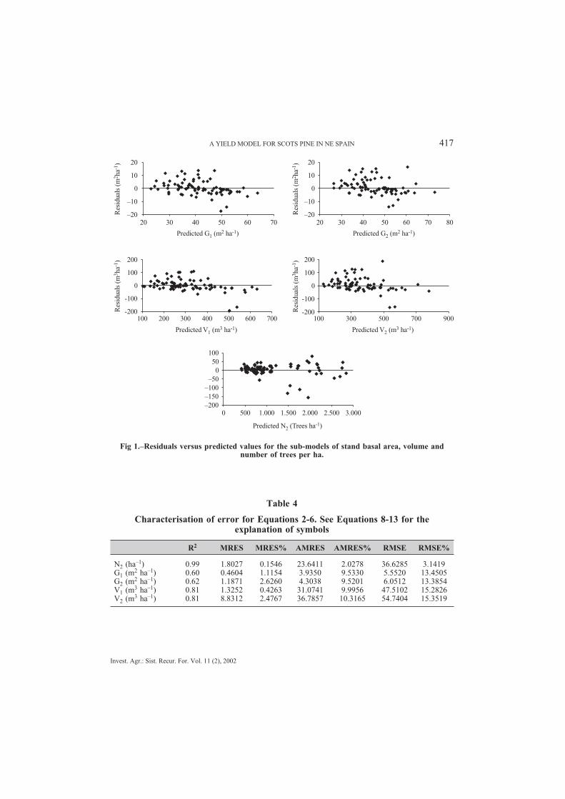
There were no serious patterns on the distribution of residuals in the volume, basalarea, and stand density models (Fig. 1). Mean residuals were positive for all equations ofbasal area, volume and number of stems per ha (Table 4), showing that some positive biasexists in the set of models. Relative and absolute mean residuals, which are measures ofprecision, were largest for stand volume equations (V1 and V2) at around 10 %. Themodel efficiency (R2) was rather low for the basal area equations (G1 and G2). Further-more, the error component of the projection sub-models for basal area and volume wasanalysed by dividing it into prediction error component and the projection error compo-nent. Since the predicted variables of the prediction sub-models (Equations 3 and 5) areused as predictors in the projection sub-models (Equations 4 and 6), the error componentof the projection sub-models includes the error induced by the prediction sub-models. Inthe projection equations for basal area and volume (Eqs. 4 and 6) around 74 % and 70 %of the total residual mean square error and mean absolute error, respectively, was due tothe use of the prediction sub-models.

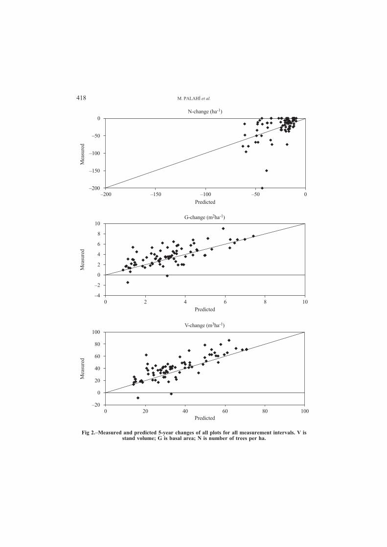
Figure 2 shows the measured and predicted changes of different stand variables forall plots in all the measurements. There is some bias in the model predictions as it was al-ready mentioned above, but no special trend can be appreciated between the predicted andthe measured change in the stand variables analysed.

416 M. PALAHÍ et al.

Table 2

Parameter estimates and their standard errors for Equations 2-6

Parameter Estimate Standard error

0 –0.0043 0.0004�0 0.0876 0.0412�1 –16.8549 2.6139�2 1.3635 0.0851�3 0.3865 0.0374!0 1.8882 0.2163!1 1.1788 0.0320!2 0.5423 0.0430!3 –0.1160 0.0133

Table 3

Cross-equation correlation matrix of residuals of the simultaneous equationsystem (Equations 2-6)

N2 G1 V1 G2 V2

N2 1.0000 0.0023 –0.1504 –0.0079 –0.3862 **G1 1.0000 –0.5598 ** –0.2131 ** 0.2415 **V1 1.0000 0.1244 0.0052G2 1.0000 –0.1290V2 1.0000

** Significant (� = 0.005).

Invest. Agr.: Sist. Recur. For. Vol. 11 (2), 2002

A YIELD MODEL FOR SCOTS PINE IN NE SPAIN 417

Fig 1.–Residuals versus predicted values for the sub-models of stand basal area, volume andnumber of trees per ha.

Table 4

Characterisation of error for Equations 2-6. See Equations 8-13 for theexplanation of symbols

R2 MRES MRES% AMRES AMRES% RMSE RMSE%

N2 (ha–1) 0.99 1.8027 0.1546 23.6411 2.0278 36.6285 3.1419G1 (m2 ha–1) 0.60 0.4604 1.1154 3.9350 9.5330 5.5520 13.4505G2 (m2 ha–1) 0.62 1.1871 2.6260 4.3038 9.5201 6.0512 13.3854V1 (m3 ha–1) 0.81 1.3252 0.4263 31.0741 9.9956 47.5102 15.2826V2 (m3 ha–1) 0.81 8.8312 2.4767 36.7857 10.3165 54.7404 15.3519

–20 –20

–10 –10

0 0

10 10

20 20

20 30 40 50 60 70

Predicted G (m ha )12 -1

Predicted V (m ha )13 -1

Predicted N (Trees ha )2-1

Predicted V (m ha )23 -1

Predicted G (m ha )22 -1

20 30 40 50 60 70 80

-200 -200

-100 -100

0 0

100 100

200 200

100 200 300 400 500 600 700 300100 500 700 900

–200–150–100

–500

50100

0 500 1.000 1.500 2.000 2.500 3.000

Res

idua

ls(m

ha)

3-1

Res

idua

ls(m

ha)

3-1

Res

idua

ls(m

ha)

2-1

Res

idua

ls(m

ha)

2-1

418 M. PALAHÍ et al.

Fig 2.–Measured and predicted 5-year changes of all plots for all measurement intervals. V isstand volume; G is basal area; N is number of trees per ha.

N-change (ha )-1

G-change (m ha )2 -1

V-change (m ha )3 -1

–200

–150

–100

–50

0

–200 –150 –100 –50 0

Predicted

–4

–2

0

2

4

6

8

10

0 2 4 6 8 10Predicted

–20

0

20

40

60

80

100

0 20 40 60 80 100Predicted

Mea

sure

dM

easu

red

Mea

sure

d

Figure 3 shows the bias (mean residual) and precision (mean absolute residual) byeach of the projection models of the system using different projections intervals. On onehand, the predictive ability of all projection sub-models decreases as the projection lengthincreases. On the other hand, the projection sub-models for basal area and volume under-estimate G2 and V2, respectively, for a projection length less than or equal to 15 years,while they give overestimates for projection lengths longer than 15 years. The N2

sub-model gives overestimates for a projection length longer than 5 years.

To demonstrate the practical application of the system of equations, simulations ofstand volume and basal area were produced and compared with real stand developmentfor three different site indices (Fig. 4). The projections of stand development are inva-riant, regardless of the number of intermediate projection intervals used. The starting pointsfor the past and projected stand volume and basal area simulations are the initial numberof trees per hectare and dominant heights at the stand age of the first plot measurement.

Invest. Agr.: Sist. Recur. For. Vol. 11 (2), 2002

A YIELD MODEL FOR SCOTS PINE IN NE SPAIN 419

Fig 3.–Dependence of model bias (Mean residual) and precision (Mean absolute residual) on theprojection length for the projection sub-models of number of trees per hectare (N2), basal area

(G2) and volume (V2).

N2

G2

V2

N2

G2

V2

–25–20–15–10

–505

5 10 15 20 25 30

Projection interval (years)

0

20

40

60

80

5 10 15 20 25 30

Projection interval (years)

–2–1.5

–1–0.5

00.5

1

5 10 15 20 25 30

Projection interval (years)

0123456

5 10 15 20 25 30

Projection interval (years)

–15

–10

–5

0

5

10

5 10 15 20 25 30

Projection interval (years)

0

10

20

30

40

50

5 10 15 20 25 30

Projection interval (years)

Mea

nre

sidu

al(t

rees

ha)

-1M

ean

resi

dual

(tre

esha

)-1

Mea

nre

sidu

al(t

rees

ha)

-1

Mea

nab

solu

tere

sidu

al(t

rees

ha)

-1M

ean

abso

lute

resi

dual

(tre

esha

)-1

Mea

nab

solu

tere

sidu

al(t

rees

ha)

-1

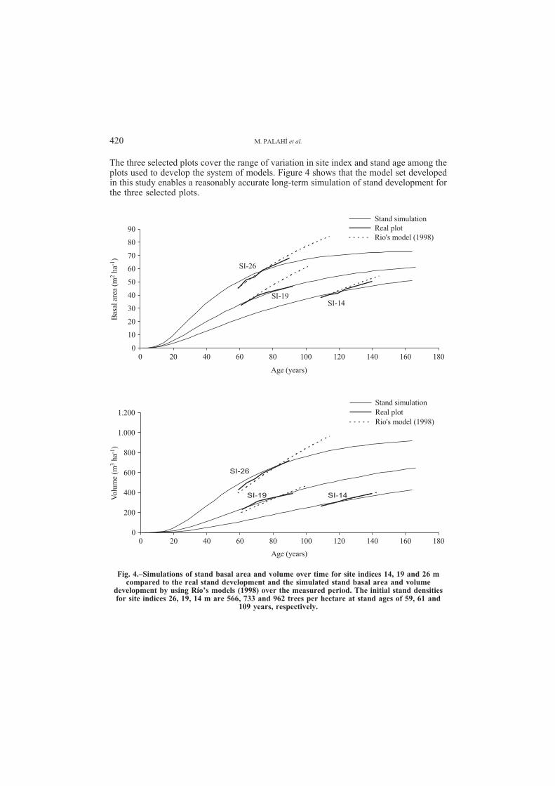
The three selected plots cover the range of variation in site index and stand age among theplots used to develop the system of models. Figure 4 shows that the model set developedin this study enables a reasonably accurate long-term simulation of stand development forthe three selected plots.

420 M. PALAHÍ et al.

Fig. 4.–Simulations of stand basal area and volume over time for site indices 14, 19 and 26 mcompared to the real stand development and the simulated stand basal area and volume

development by using Río’s models (1998) over the measured period. The initial stand densitiesfor site indices 26, 19, 14 m are 566, 733 and 962 trees per hectare at stand ages of 59, 61 and

109 years, respectively.

Bas

alar

ea(m

ha)

2-1

Vol

ume

(mha

)3

-1

0

10

20

30

40

50

60

70

80

90

0 20 40 60 80 100 120 140 160 180

Age (years)

Stand simulationReal plotRio's model (1998)

SI-26

SI-19SI-14

0

200

400

600

800

1.000

1.200

0 20 40 60 80 100 120 140 160 180

Age (years)

Stand simulationReal plotRio's model (1998)

DISCUSSION

We were aware of the restrictions of our data, with a small number of permanentplots and having only three plots with measurements over the age of one hundred years.The lack of permanent sample plots measured at young ages was also an importantrestriction. The initial assumptions concerning the model error term, namely non-indepen-dence of explanatory variables and the possibility of serial correlation, are violated tosome degree due to the structure of the data; all permanent sample plots were measuredseveral times. But, for instance, Río et al. (2001) did not detect any serial autocorrelationin a similar data set for Scots pine in Spain, in which several diameter-density relation-ships were modelled.

This study presents stand-level growth and yield models for Scots pine in north-eastSpain. The models for stand density, stand basal area and volume were fitted simulta-neously using non-linear three-stage least square method (N3SLS), while the dominantheight model developed by Palahí et al. (2002a) was used independently to predict domi-nant height development. It would have been possible to include a dominant height pro-jection model into the simultaneous system of equations, i.e. estimating it simultaneouslywith the other equations as applied by Borders and Bailey (1986) and Pienaar and Harri-son (1989). However, because dominant height drives the system of the growth and yieldmodels and it is also used to estimate the site index of a given stand as well as in othergrowth models for the species [for instance, an available individual tree model developedby Palahí et al. (2002b)], it had to be assured that a robust and reliable projection modelfor dominant height, not connected to a particular growth model, is available.

The functional form of the basal area equation appeared to be the most difficult to es-timate. One explanation for the poor coefficient of determination of the selected basalarea prediction model might be found in the data structure used for fitting the models. Thestand characteristics were very variable among plots, not being possible to see any rela-tionship between basal area and age and basal area and number of trees per hectare. A so-lution would have been to exclude the basal area prediction equation from the simulta-neous system of equations and use only the projection for basal area since basal area isusually measured in forestry practice. The problem with this option would have been theimpossibility to predict basal area after thinnings in a compatible way, by knowing onlythe remaining number of trees per hectare in the stand. However, although growth simula-tions for thinned stands are possible using the system of models presented in this study,they might not be as reliable as for unthinned stands due to the lack of data from thinnedstands. As suggested by Piennar and Harrison (1989), an additional predictor variable thataccounts for thinning effects would need to be introduced in the current system of equa-tions to obtain more accurate growth simulations for thinned stands.

The performance of Río’s models (1998) for Scots pine in Sistema Central andIbérico was compared to the models presented in this study (Fig. 4). The recursive systemof equations developed by Río (1998) to model stand growth and yield did not include abasal area prediction equation, but only a projection equation. Therefore, observed basalarea of the first plot measurement was needed to initialise the simulation of stand basalarea and volume development with Río’s model, while predicted basal using Equation 3was used to initialise the simulated stand development with the models presented in thisstudy. Figure 4 shows that Río’s basal area model clearly overpredicts basal area for theplot with site index 19 m, and does not logically describe, specially for the best sites, the

Invest. Agr.: Sist. Recur. For. Vol. 11 (2), 2002

A YIELD MODEL FOR SCOTS PINE IN NE SPAIN 421

asymptotic trend that characterises stand basal area growth. The stand volume develop-ment predicted by Río’s model is quite accurate for the plot measurement period. How-ever, for the best site Río’s model (1998) shows a non-asymptotic trend of stand volumedevelopment that might not be realistic. One explanation for the non-asymptotic trend instand basal area and volume development using Río’s model might be due to the charac-teristics of the modelling data set for fitting the models, which included permanent sam-ple plots ranging in stand age from 20 to 75 years. The overprediction of basal areagrowth for the plot with site index 19 m, is not reflected in an overprediction of standvolume development as it would be expected. The reason could be that Río (1998) usedthe dominant height growth model developed by Rojo and Montero (1996) for estimatingthe site index, which is later used as a predictor in the stand volume model. Palahí et al.(2002a) showed how the dominant height model of Rojo and Montero (1996)underpredicts dominant height growth development in the modelling data of this study,which concerns north-east Spain, for the best sites and at young to medium ages.

Parameter estimates of the system of equations are consistent with current knowledgeof forest growth relationships and ensure compatibility between prediction and projectionfunctions for both volume and basal area (Table 2). Furthermore, the strong cross-equa-tion correlation among some error components in the system of equations (Table 3) pro-vides further justification for the use of N3SLS method in fitting simultaneous systems ofequations.

Simulations of volume and basal area growth for different stand densities and site in-dices as presented in Figure 4 follow accurately the actual growth pattern of real plots andseem to behave logically out of the range of ages of the estimation data. The system ofmodels presented in this study can serve as a simple-to-use yield prediction system forforest-level management planning since the system requires only stand level inventory in-put, namely, stand age, number of trees per hectare and dominant height or site index.

ACKNOWLEDGMENTS

We thank Prof. Timo Pukkala (Finland) for his valuable suggestions. Financial support for this project wasgiven by the Forest Technology Centre of Catalonia (Solsona, Spain). We gratefully acknowledge the data pro-vided by the Instituto Nacional de Investigaciones Agrarias (Spain).

RESUMEN

Elaboración de un modelo de crecimiento y producción para rodales de masasregulares de Pinus sylvestris L. en el noreste pensinsular

Se presenta un sistema interdependiente y compatible de modelos de crecimiento y mortalidad obtenidomediante el método de estimación no lineal de mínimos cuadrados en tres-etapas, obtenido a partir de 21 parce-las permanentes de Pinus sylvestris establecidas en 1964 por el Instituto Nacional de Investigaciones Agrariasen el noreste peninsular. Las parcelas permanentes con una calidad de sitio, definida como la altura dominante alos 100 años de edad, de entre 13 a 26 m fueron inventariadas una media de 5 veces. El método no lineal de mí-nimos cuadrados en tres etapas fue utilizado para fijar simultáneamente ecuaciones de predicción y proyeccióndel área basal, volumen del rodal y número de pies por hectárea. Un modelo de crecimiento dinámico para la al-tura dominante, ya existente y fijado con los mismos datos que los del presente estudio, fue utilizado para pro-yectar la altura dominante. Los modelos fueron evaluados cuantitativa y cualitativamente. La correlación entre

422 M. PALAHÍ et al.

los componentes del error de las ecuaciones de predición del área basal y volumen del rodal, así como entre lasecuaciones de proyección del número de pies por hectárea y volumen del rodal fueron significativas. La mediadel sesgo para todos los modelos fue positiva. El estudio describe las ventajas de este tipo de sistemas de mode-los compatibles e interdependientes. Se discute su posible uso práctico en la planificación y gestión forestal delpino silvestre dada su simplicidad y a que el tipo de datos de entrada para realizar simulaciones es sólo informa-ción a nivel de rodal (número de pies por hectárea y altura dominante o índice de sitio a una edad determinada).

Palabras clave: Modelos de producción y crecimiento, regresión no lineal en múltiples etapas, simulación.

REFERENCES

ÁLVAREZ GONZÁLEZ J.G., RODRÍGUEZ SOALLEIRO R., VEGA ALONSO G., 1999. Elaboración de unmodelo de crecimiento dinámico para rodales regulares de Pinus pinaster Ait en Galicia. Invest. Agr.: Re-cur. For. Vol. 8 (2): 319-334.

AMARO A., REED D., THEMIDO I., TOMÉ M., 1997. Stand growth modelling for first rotation Eucalyptusglobus Labill in Portugal. In: Amaro A., and Tomé T. (Eds.), Empirical and process based models for fo-rest tree and stand growth simulation. Edições Salamandra. pp. 99-110.

BENNETT F.A., McGEE C.E., CLUTTER J.L., 1959. Yield of old-field slash pine plantations. USDA For.Serv. Stn. Pap. 107, 19 pp.

BORDERS B.E., 1989. Systems of equations in forest stand modelling. For. Sci. 35: 548-556.BORDERS B.E., BAILEY R.L., 1986. A compatible system of growth and yield equations for slash pine fitted

with restricted three-stage least squares. For. Sci. 32: 185-201.BURKHART H.E., SPRINZ P.T., 1984. Compatible cubic volume and basal area projections for thinned

old-field Loblolly pine plantations. For. Sci. 30: 86-93.BURKHART H.E., PARKER R.C., ODERWALD R.G., 1972. Yields for natural stands of Loblolly pine. Div.

For. Wildl. Resour. Va. Polytech. Inst. State Univ. Publ. FWS-2-72, 63 pp.CLUTTER J.L., 1963. Compatible growth and yield models for Loblolly pine. For. Sci. 9: 354-371.CLUTTER J.L., FORSTON J.C., PIENAAR L.V., BRISTER G.H., BAILEY R.L., 1983. Timber management -

a quantitative approach. Wiley, New York.DANIELS R.F., BURKHART H., 1988. An Integrated System of Forest Stand Models. For. Ecol. Manage. 23:

159-177.DUTTA M., 1975. Econometric methods South-Western Publ Co, Cincinnati, Ohio. 382 p.ESPINEL S., CANTERO A., SÁENZ D., 1997. Un modelo de simulación para rodales de Pinus radiata D. Don

en el País Vasco. IRATI 97. I Congreso Forestal Hispano Luso. Mesa 3, 201-206.FOMBY T.B., HILL R.C., JOHNSON S.R., 1984. Advance econometric methods. Springer-Verlag, New York.

624 p.FURNIVAL G.M., WILSON R.W., 1971. Systems of equations for predicting forest growth and yield. Statist.

Ecol. 3: 43-55.GARCÍA ABEJÓN J.L., 1981. Tablas de producción de densidad variable para Pinus sylvestris en el Sistema

Ibérico. Comunicaciones I.N.I.A Serie: Recursos Naturales. N.º 10, 47 p.GARCÍA ABEJÓN J.L., GÓMEZ LORANCA J.A., 1984. Tablas de producción de densidad variable para Pi-

nus sylvestris en el sistema Central. Comunicaciones I.N.I.A Serie: Recursos Naturales. N.º 29, 36 p.GARCÍA ABEJÓN J.L., TELLA FERREIRO G., 1986. Tablas de producción de densidad variable para Pinus

sylvestris L. en el Sistema Pirenaico. Comunicaciones I.N.I.A. serie: Recursos Naturales, N-43, 28 p.HUANG S., 1994. Ecologically based reference-age invariant polymorphic height growth and site index curves

for White spruce in Alberta. Tech. Paper. Alberta Env. Prot. Land & Forest Serv. For. Manag. Div.JUDGE G., GRIFFITHS W.E., HILL R. C., LEE T., 1980. The theory and practice of econometrics. John Wiley

and sons, New York. 793 p.MABVURIRA D., MIINA J., 2001. Simultaneous growth and yield models for Eucalyptus grandis (Hill) Mai-

den plantations in Zimbabwe. S. Afr. For. J. 191: 1-8.MONTERO G., CAÑELLAS I., ORTEGA C., DEL RÍO M., 2001. Results from a thinning experiment in a

Scots pine (Pinus sylvestris L.) natural regeneration stand in the Sistema Ibérico Mountain Range (Spain).For. Ecol. Manage. 145: 151-161.

MURPHY P.A., 1983. A nonlinear timber yield equation system for Loblolly pine. For. Sci. 29: 582-591.MURPHY P.A., BELTZ R.C., 1981. Growth and yield of Shortleaf pine in the west Gulf region. USDA Forest

Serv. Res. Pap. SO-169, 15 p. South Forest Exp. Stn, New Orleans, LA.

Invest. Agr.: Sist. Recur. For. Vol. 11 (2), 2002

A YIELD MODEL FOR SCOTS PINE IN NE SPAIN 423

MURPHY P.A., STERNITZKE S., 1979. Growth and yield estimation for Lobolly pine in the West Gulf.USDA Forest Serv. Res. Pap. SO-154, 8 p. South Forest Exp. Stn, New Orleans, LA.

PALAHÍ M., TOMÉ M., PUKKALA T., TRASOBARES A., MONTERO, G., 2002a. Site index model forScots pine (Pinus sylvestris L.) in north-east Spain. Submitted to Forest Ecology and Management.

PALAHÍ M., PUKKALA T., MIINA J., MONTERO G., 2002b. Individual-tree growth and mortality modelsfor Scots pine (Pinus sylvestris L.) in north-east Spain, Submitted to Ann. Sci. For.

PIENAAR L.V., HARRISON W.M., 1989. Simultaneous growth and yield prediction equations for Pinus elliot-tii plantations in Zululand. S. Afr. For. J. 149: 48-53.

PIENAAR L.V., SHIVER B.D., 1986. Basal area prediction and projection equations for pine plantations. For.Sci. 32: 626-633.

PINDYCK R.S., RUBINFELD D.L., 1981. Econometric models and economic forecast. McGraw-Hill, NewYork. 630 p.

PITA CARPENTER A., 1967. Tablas de cubicación por diámetros normales y alturas totales, Instituto Forestalde Investigaciones y Experiencias, Ministerio de Agricultura, Marid.

RÍO M. del., 1998. Régimen de claras y modelo de producción para Pinus sylvestris L. en los sitemas Central eIbérico. Tesis Doctoral, ETSIM-UPM, 219 pp, unpublished.

RÍO M. del., MONTERO G., BRAVO F., 2001. Analysis of diameter-density relationships and self-thinning innon-thinned even-aged Scots pine stands, For. Ecol. Manage. 142: 79-87.

ROJO A., MONTERO G., 1996. El pino silvestre en la Sierra de Guadarrama. Centro de publicaciones del Mi-nisterio de Agricultura, Pesca y Alimentación, 293 p.

SAS Institute Inc., 1999. SAS/ETS User’s guide, version 8, Cary, NC: SAS Institute Inc., 1596 pp.SOÁRES P., TOMÉ M., SKOVSGAARD J.P., VANCLAY J.K., 1995. Evaluating a growth model for forest

management using continuous forest inventory data. For. Ecol. Manage. 71: 251-265.SCHUMACHER F.X., COILE T.S., 1960. Growth and Yield of Natural Stands of the Southern Pines. T.S. Coi-

le, Inc., Durham, NC, 115 pp.SULLIVAN A.D., CLUTTER J.L., 1972. A simultaneous growth and yield model for Loblolly pine. For. Sci.

18: 76-86.TOMÉ M., 1988. Modelação do crecimento da Árvore Individual em povoamentos de Eucalyptus globulus La-

bill. (1.ª rotação). Região Centro de Portugal. Tese Dout. Eng. Silv. UTL. ISA.TOMÉ M., SOÁRES P., 1999. A comparative evaluation of three growth models for eucalypt plantation man-

agement in coastal Portugal. In: Amaro, A., and Tomé, T. (Eds.), Empirical and process based models forforest tree and stand growth simulation.. Edições Salamandra, pp. 517-533.

VON GADOW K., HUI G., 1998. Modelling forest development. Faculty of Forest and Woodland Ecology,University of Gottingen, 213 pp.

424 M. PALAHÍ et al.