C CO CO C CO COD

C CO C CO CO CO C CO COD

C CO C CO CO CO C CO COD

C CO C CO CO CO C CO COD

C CO C CO CO CO C CO COD

C CO C CO CO CO C CO COD

C CO C CO CO CO C CO COD

C CO C CO CO CO C CO COD

C CO C CO CO CO C CO COD

C CO C CO CO CO C CO COD

C CO C CO CO CO C CO COD

C CO C CO CO CO C CO COD

C CO C CO CO CO C CO COD

C CO C CO CO CO C CO COD

C CO C CO CO CO C CO COD

C CO C CO CO CO C CO COD

C CO C CO CO CO C CO COD

C CO C CO CO CO C CO COD

C CO C CO CO CO C CO COD

C CO C CO CO CO C CO COD

C CO C CO CO CO C CO COD

C CO C CO CO CO C CO COD

C CO C CO CO CO C CO COD

C CO C CO CO CO C CO COD

C CO C CO CO CO C CO COD

C CO C CO CO CO C CO COD

C CO C CO CO CO C CO COD

C CO C CO CO CO C CO COD

C CO C CO CO CO C CO COD

C CO C CO CO CO C CO COD

Staff Working Paper No. 580Centralized trading, transparency andinterest rate swap market liquidity:evidence from the implementation of the Dodd-Frank ActEvangelos Benos, Richard Payne and Michalis Vasios

May 2018This is an updated version of the Staff Working Paper originally published on 15 January 2016

Staff Working Papers describe research in progress by the author(s) and are published to elicit comments and to further debate. Any views expressed are solely those of the author(s) and so cannot be taken to represent those of the Bank of England or to stateBank of England policy. This paper should therefore not be reported as representing the views of the Bank of England or members ofthe Monetary Policy Committee, Financial Policy Committee or Prudential Regulation Committee.

Staff Working Paper No. 580Centralized trading, transparency and interest rate swap market liquidity: evidence from theimplementation of the Dodd-Frank ActEvangelos Benos,(1) Richard Payne(2) and Michalis Vasios(3)

Abstract

We use proprietary transaction data on interest rate swaps to assess the effects of centralized trading, asmandated by Dodd-Frank, on market quality. Contracts with the most extensive centralized trading seeliquidity metrics improve by between 12% and 19% relative to those of a control group. This is drivenby a clear increase in competition between dealers, particularly in US markets. Finally, centralizedtrading has caused inter-dealer trading in EUR swap markets to migrate from the US to Europe. Thisevidence is consistent with swap dealers attempting to avoid being captured by the trade mandate inorder to maintain market power.

Key words: Interest rate swaps, pre-trade transparency, market power, liquidity, swap executionfacilities.

JEL classification: G10, G12, G14.

(1) Bank of England. Email: evangelos.benos@bankofengland.co.uk(2) Cass Business School. Email: richard.payne@city.ac.uk (3) Bank of England. Email: michalis.vasios@bankofengland.co.uk

We are grateful to Darrell Due, Chester Spatt, Angelo Ranaldo, David Bailey, Paul Bedford, Jean-Edouard Colliard, Pedro Gurrola-Perez, Wenqian Huang, Rhiannon Sowerbutts, Esen Onur, Peter Van Tassel, and seminar participants at the Bank of England, the Bank of Greece, the Bank of Lithuania, the US Commodity Futures Trading Commission (CFTC), the US Securities and Exchange Commission (SEC), the European Securities and Markets Authority (ESMA), the EuropeanSystemic Risk Board (ESRB), the Federal Reserve Board, the UK Financial Conduct Authority (FCA), the 12th Annual Central Bank conference on the Microstructure of Financial Markets, the 2016 European Finance Association meeting, the2017 American Finance Association meeting, the 2017 conference on OTC derivatives at the New York Fed, the 2017 Mid-West Finance Association meetings, the Brunel University, the University of Belfast, the University of St. Gallen and theUniversity of Southampton for helpful comments and suggestions. The views expressed in this paper are those of the authorsand not necessarily those of the Bank of England.

Information on the Bank’s working paper series can be found atwww.bankofengland.co.uk/research/Pages/workingpapers/default.aspx

Publications Team, Bank of England, Threadneedle Street, London, EC2R 8AH Telephone +44 (0)20 7601 4030 Fax +44 (0)20 7601 3298 email publications@bankofengland.co.uk

© Bank of England 2018ISSN 1749-9135 (on-line)

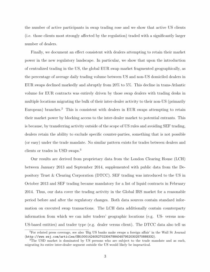
1 Introduction

A key regulatory response to the 2008 Global Financial Crisis has been to improve the

resilience and transparency of Over The Counter (OTC) markets for derivative securities.

To this end, over the last decade these markets have seen the introduction of clearing and

margining and also increases in pre- and post-trade transparency, via centralized trading

requirements and the creation of repositories containing information on completed trades.

This study focusses on a particular aspect of this regulatory change, an increase in pre-

trade transparency in OTC markets, and we investigate how this has affected the competitive

structure and liquidity of interest rate swap (IRS) markets. The global swap market is by far

the largest OTC derivatives market1, and this is the first study of the impact of post-crisis

regulation on that market. Historically, global swap trading was decentralized and relatively

opaque. However, a centralized trading requirement was introduced in the US in 2014 via

the “Dodd-Frank Act”, which required that any trade in a sufficiently liquid IRS contract

involving a US counter-party must take place on a Swap Execution Facility (SEF). SEFs are

multi-lateral trading venues, featuring open limit order book (LOB) and request for quote

(RFQ) functionalities, allowing customers to solicit quotes from multiple dealers and/or an

order book simultaneously. Thus SEFs introduced pre-trade transparency to a previously

dark market and reduced customers’ costs of searching for liquidity.

We show that the introduction of SEF trading had several important effects on IRS

markets. First, swaps that were subject to the SEF-trading mandate saw significant im-

provements in liquidity. For example, relative to EUR mandated swaps (where SEF trading

is much less prevalent), measures of liquidity for USD mandated swaps improve by between

12% and 19%. This translates to daily execution costs for end-investors in USD mandated

swaps falling by about $3 - $6 million relative to EUR mandated swaps.

Second, we provide evidence that links this improvement in liquidity to more intense

competition between swap dealers. Following the introduction of the SEF trading mandate,

1BIS, November 2016: http://www.bis.org/publ/otc_hy1611.pdf

2

the number of active participants in swap trading rose and we show that active US clients

(i.e. those clients most strongly affected by the regulation) traded with a significantly larger

number of dealers.

Finally, we document an effect consistent with dealers attempting to retain their market

power in the new regulatory landscape. In particular, we show that upon the introduction

of centralized trading in the US, the global EUR swap market fragmented geographically, as

the percentage of average daily trading volume between US and non-US domiciled dealers in

EUR swaps declined markedly and abruptly from 20% to 5%. This decline in trans-Atlantic

volume for EUR contracts was entirely driven by those swap dealers with trading desks in

multiple locations migrating the bulk of their inter-dealer activity to their non-US (primarily

European) branches.2 This is consistent with dealers in EUR swaps attempting to retain

their market power by blocking access to the inter-dealer market to potential entrants. This

is because, by transferring activity outside of the scope of US rules and avoiding SEF trading,

dealers retain the ability to exclude specific counter-parties, something that is not possible

(or easy) under the trade mandate. No similar pattern exists for trades between dealers and

clients or trades in USD swaps.3

Our results are derived from proprietary data from the London Clearing House (LCH)

between January 2013 and September 2014, supplemented with public data from the De-

pository Trust & Clearing Corporation (DTCC). SEF trading was introduced to the US in

October 2013 and SEF trading became mandatory for a list of liquid contracts in February

2014. Thus, our data cover the trading activity in the Global IRS market for a reasonable

period before and after the regulatory changes. Both data sources contain standard infor-

mation on executed swap transactions. The LCH data additionally contain counterparty

information from which we can infer traders’ geographic locations (e.g. US- versus non-

US-based entities) and trader type (e.g. dealer versus client). The DTCC data also tell us

2For related press coverage, see also ‘Big US banks make swaps a foreign affair’ in the Wall St Journal(http://www.wsj.com/articles/SB10001424052702304788404579520302570888332).

3The USD market is dominated by US persons who are subject to the trade mandate and as such,migrating its entire inter-dealer segment outside the US would likely be impractical.

3

whether a trade was executed on a SEF.

We employ a difference-in-differences technique to isolate the effects of the introduction of

SEF trading on liquidity and competition. The treatment group of assets in our difference-

in-differences tests is the set of USD swaps that were required to trade on a SEF after

February 2014. Our control group is either the USD swaps that were not captured by the

SEF trading mandate or the EUR swaps that were mandated, but which are mostly traded

by non-US persons who, in turn, are not captured by the SEF trading requirement. We

measure liquidity using various price dispersion measures based on the metric proposed by

Jankowitsch et al. (2011), complemented with Amihud’s price impact measure (Amihud

(2002)), plus a bid-ask spread derived from swap quote data.

To place our analysis within the context of recent theory work on transparency, our

result that centralized trading has improved liquidity and increased dealer competition for

mandated swaps lends support to the research of Duffie et al. (2005) and Yin (2005). They

argue that pre-trade quote transparency is a necessary condition for competitive liquidity

provision and lowers transaction costs for customers, as it reduces search frictions. Along

similar lines, Foucault et al. (2013) argue that in the presence of positive search costs, a

unique Nash equilibrium exists where dealers quote monopolist prices i.e. prices that equal

end-users’ reservation values. Thus, reducing search costs allows customers to access keener

pricing.4 Hendershott and Madhavan (2015) examine the efficacy of electronic venues at

facilitating trading in OTC markets. They show that periodic one-sided electronic auction

mechanisms, similar to the RFQ mechanism we see on SEFs, encourage dealer competition

and result in better prices while limiting information leakage. Our results run counter to the

intuition in de Frutos and Manzano (2002) and Foucault et al. (2007). The former argue

that risk-averse dealers price less keenly in transparent markets, since, to induce trades that

correct an inventory imbalance, they only need to marginally improve the quote on the

4Vayanos and Wang (2012) survey the literature and explain how illiquidity is related to various marketimperfections. They show that participation costs, imperfect competition and search frictions all have adetrimental effect on liquidity.

4

relevant side of the market relative to their competitors. Foucault et al. (2007) show that

when informed trading intensities are low, lower transparency (in the form of hiding trader

identity information) can lead to higher liquidity.

The empirical work on the link between transparency and liquidity contains some mixed

results. Boehmer et al. (2005) show that NYSE stocks experienced a significant increase in

liquidity when the exchange began to publish the limit order book to traders not located

on the exchange floor. Green et al. (2007) study municipal bond dealers. They argue

that opacity in this market increases dealer market power and they then show how dealer

market power increases execution costs. Goldstein et al. (2007), Edwards et al. (2007) and

Bessembinder et al. (2006) show that introducing post-trade transparency to US corporate

bond markets had, on balance, a positive effect on liquidity (exceptions were found for very

thinly-traded bonds and for the largest trades).5. In contrast, Foucault et al. (2007) show

that imposing anonymity on trading activity, i.e. reducing transparency, increased liquidity

in Euronext stock trading. Friederich and Payne (2014) find the same result in data from

the London Stock Exchange, attributing the finding to the possibility of predatory trading

under transparency (i.e. when identities are revealed). Our results chime with those above

that suggest a positive link between transparency and liquidity.6

Our work is also related to other recent studies focusing on regulatory developments in

OTC derivative markets markets (see Spatt (2017) and Acharya et al. (2009) for an overview

of the post-crisis derivatives reform agenda). Loon and Zhong (2014) and Loon and Zhong

(2015) study the effects of centralized clearing and post-trade reporting on CDS markets.

Both of these reforms, mandated by Dodd-Frank, are shown to improve liquidity, while

the former also reduces credit risk. Our focus is different, in that we study the impact of

pre-trade transparency as related to the third pillar of the Dodd-Frank OTC derivatives

regulation (i.e. the mandate for centralized trading) and we also examine the IRS market,

5Other evidence that links transparency with liquidity can also found in Harris and Piwowar (2006), Naiket al. (1999) and Boehmer et al. (2005).

6Our results are also in line with the experimental evidence in Flood et al. (1999).

5

which is much larger than the CDS market. It is worth noting that Loon and Zhong (2015)

include a SEF dummy variable in their panel regressions but as their sample period ends

before the introduction of the CFTC trading mandate in February 2014 they cannot say

anything about the impact of the centralized trading requirement on liquidity.

Our result that EUR swap markets have fragmented as a result of the US SEF trading

mandate ties into a recent regulatory literature on the efficacy of the reform and its impact

on markets (see Giancarlo (2015), Massad (2016), Powell (2016)). The result suggests that

there are costs, pecuniary or otherwise, to trading on SEFs that dealers wish to avoid.

As mentioned earlier, one possibility is that dealers move activity from their US desks to

their European desks in order to retain control over who they deal with. This could allow

them to exclude new entrants from the inter-dealer EUR swap market which, in turn, would

preclude those new entrants from trading effectively in the client market.7 Thus, the observed

geographic fragmentation is consistent with dealers attempting to maintain entry barriers to

(EUR) swap trading.

Overall, our analysis highlights the importance of dealer market power in understanding

how financial markets react to changes in their transparency regimes. This remains an area

of policy interest. As of January 2018 Europe has adopted new centralized trading rules for

swaps as part of the Markets in Financial Instruments Regulation (MiFIR). This has the

potential to improve conditions for customers and also to remove the imbalance in regulation

that has led to the geographical fracture in swaps markets. At the same time, in the US,

there is uncertainty as to whether all parts of the Dodd-Frank Act will be retained as law

with the new CFTC trading rules being at the heart of this discussion among policy makers

and practitioners.8

The rest of the paper is organized as follows. Section 2 sets out the regulatory changes

that affected swap markets as a result of Dodd-Frank and gives a detailed description of SEFs.

7This would not be feasible for USD swaps as the inter-dealer market is well established, geographically,in the US, while the bulk of EUR swap trading already happens in Europe.

8See, for example, related reporting by Bloomberg: https://www.bloomberg.com/gadfly/articles/

2017-02-23/wall-street-girds-for-regulatory-battles-loud-and-quiet

6

Section 3 describes our data sources and presents summary statistics. Section 4 presents the

difference-in-differences tests of the impact of the SEF trading mandate on market activity

and liquidity. Section 5.1 shows how the mandate has changed the relationships between

dealers and customers. Section 5.2 describes the changes in the geography of swap trading

and how those changes may be linked to market power. Section 6 concludes.

2 Policy Context and Institutional Details

2.1 OTC derivatives and the Dodd-Frank Act

A major pillar of the US Wall Street Reform and Consumer Protection Act (the “Dodd-Frank

Act”) concerns OTC derivatives markets. In particular, owing to concerns that insufficient

collateralization and opacity in these markets contributed to systemic risk during the crisis,

Title VII of the Act implemented a series of reforms aimed at mitigating counterparty risk

and improving pre- and post-trade transparency in swaps markets. It mandates central-

ized clearing for eligible contracts, requires real-time reporting and public dissemination of

transactions and also requires that eligible contracts should be traded on a SEF, a form of

multilateral electronic trading venue. SEF trading brings about a marked increase in the

level of pre-trade transparency for the affected swap contracts.

The Dodd-Frank trading mandate was implemented by the CFTC in two phases. First,

on October 2, 2013, SEF trading became available for OTC derivatives on a voluntary

basis. As of that date, newly authorized trading venues had to comply with a number of

principles and requirements. A principal one of these requirements was the obligation to

operate a limit order book (LOB).9 In the second phase, specific contracts were explicitly

9This does not mean that there were no electronic venues in operation or that no swaps were being tradedon limit order books or other multilateral trading platforms before October 2, 2013. It only means that afterthis date, any venue that was officially recognized as a SEF had to comply with the specific CFTC minimumrequirements mentioned above. Unfortunately, we have no data on the methods of execution prior to October2, 2103. Nevertheless, if swaps were already being traded on pre-trade transparent electronic platforms beforethis date, this should bias us against finding any differences in market conditions when making a “beforeversus after” comparison. Our analysis shows that the differences were actually substantial.

7

required to be executed on SEFs. The mandate captured a wide range of interest rate swap

(IRS) contracts of various currencies and maturities as well as several credit default swap

(CDS) indices. The determination of the mandated contracts was (and still is) primarily

SEF-driven, through the Made Available to Trade (MAT) procedure. A SEF can submit

a determination that a swap is available for trade to the CFTC, which then reviews the

submission. Once a swap is certified as available to trade, all other SEFs that offer this

swap for trading must do so in accordance with the requirements of the trade mandate. The

criteria for MAT determination include the trading volume of the swap and the frequency of

transactions. Table 1 shows the mandated maturities along with the mandate date for the

plain vanilla USD- and EUR-denominated IRS contracts which we use in our analysis. Most

maturities were mandated on February 15 2014 with a couple more maturities following suit

a few days later on the 26th.

The SEF trading mandate only captures “US persons”, with that definition being rela-

tively broad.10 Importantly, the mandate affects the trades of US persons regardless of who

their counterparty is. In other words, if a US person is to trade a mandated contract with

a non-US person, the trade has to be executed on a SEF.

2.2 Swap Execution Facility (SEF) Characteristics

SEFs are electronic trading platforms where, according to the CFTC, “multiple participants

have the ability to execute swaps by accepting bids and offers made by multiple participants

in the platform”. In practice, SEFs have two different functionalities to facilitate this.

The first is a fully fledged central limit order book which allows any market participant

10Apart from US-registered swap dealers and major participants, the definition of a US person alsoincludes foreign entities that carry guarantees from a US person (e.g. the foreign branch of a USdealer) and also any entities with personnel on US soil which is substantially involved in arranging,negotiating or executing a transaction. According to market reports this created initially some uncer-tainty as to who is captured. See for example: http://www.risk.net/risk-magazine/news/2256600/

broader-us-person-definition-could-cause-clearing-avalanche-participants-warn

8

to supply liquidity by posting bids and offers.11 All SEFs must offer an order book and,

theoretically, this functionality allows end-users to bypass dealers altogether in concluding a

trade, assuming of course that the order book has sufficient liquidity.

The second functionality is a modification of the existing request-for-quote (RFQ) dealer-

centric model. The innovation, relative to pre-existing single-dealer platforms, is that a

client’s request for a quote is disseminated simultaneously and instantly to multiple dealers

instead of just one. Thus clients can easily compare prices across dealers and this promotes

competition for client order flow between dealers. Up until October 2014, the law required

that a RFQ be communicated to no less than two market participants and, after that date,

to no less than three. Having received a RFQ, dealers respond by posting their quotes to the

client.12 Importantly, dealers cannot see each others’ quotes nor do they know which other

dealers have received the request. In addition, the market participants responding to the

RFQ cannot be affiliated with the RFQ requester and may not be affiliated with each other.

This arrangement makes it hard for dealers to collude and effectively renders the bidding

process a first-price, sealed bid auction.

The two trading functionalities are designed to operate in conjunction for swaps that

are subject to the trade execution mandate.13 This means that a SEF must provide a RFQ

requester with any resting bid or offer on the SEF’s order book alongside any quotes received

by the dealers from whom quotes have been requested. The requester retains the discretion to

execute either against the resting quotes on the LOB or against the RFQ responses.14 After

11For swaps that are subject to the trade mandate, SEF regulation also requires that broker-dealers, whohave the ability to execute against a customer’s order or execute two customers against each other, besubject to a 15-second timing delay between the entry of the two orders on the LOB. This is intended tolimit broker-dealer internalization of trades and to incentivize competition between market participants.

12It is worth noting that CFTC did not impose any requirement that the identity of the RFQ requester bedisclosed. This was due to concerns expressed by market participants that the disclosure of the RFQ requesteridentity would cause information leakages about future trading intentions. See Foucault et al. (2007) andNolte et al. (2015) for a discussion on the implications of the disclosure of counterparty identities.

13Any trades of swap contracts that are not subject to the mandate can still be executed on a SEF andthe SEF must offer an order book. However, the SEF is also free to offer any other method of execution(including bilateral trading and voice-based systems) for these trades.

14In their analysis of SEF trading of Index CDS, Collin-Dufresne et al. (2016) demonstrate that themajority of dealer to customer trades use the RFQ mechanism, while inter-dealer trades use several differentexecution mechanisms, with work-ups and mid-market matches being important.

9

a LOB or RFQ trade, the SEF can establish a short work-up session open to all market

participants. During the work-up, market participants can trade an additional quantity of

the same swap at the same price as the initial trade, with first priority in execution given

to counterparties who initiated the first trade. Duffie and Zhu (2015) show that work-up

protocols can enhance price discovery and liquidity.

Many SEFs are available for trade in the interest-rate swaps that we study. Data from

the London Clearing House for April to September 2014 identifies the venues on which trades

occurred and they show that, for USD swaps, the most active SEFs were Tradeweb (with

a market share of 20.6%), ICAP (19.8%), Tullet Prebon (17.2%) and Bloomberg (15%).

Total USD trading activity for this period was at $4,770bn. For trading in EUR swaps,

ICAP had the largest market share (at 34.8%), followed by BGC Partners (25.0%), Tullet

Prebon (15.0%) and Tradeweb (10.6%). Total trading volume in the EUR contracts was

e4,444bn. In both cases, no other SEF has a market share above 10%. Thus, some of

the most active SEFs are operated by brokers while others are run by firms specializing in

operating electronic markets and information systems. We have little data on how much of

the SEF trading in interest rate swaps occurs on limit order books and how much occurs via

RFQ. However, Riggs et al. (2018) look at detailed data on SEF trading of index CDS and

indicate that limit order book usage is very limited.

Overall, SEFs change the microstructure of the market in two important ways. First, they

increase pre-trade transparency by allowing market participants to observe prices quoted

by dealers much more easily. Second, SEFs increase competition between swap liquidity

suppliers. SEFs make comparison of dealer quotes much more straightforward, they allow

new entrants to the swap dealing business to start supplying liquidity on LOBs and they

allow end-users to trade directly with each other and to bypass dealers completely. While,

in practice, most of the liquidity provision is still being done by traditional dealers, we will

see that SEFs have eroded their market power and increased competitive pressures.

10

3 Data and Summary Statistics

3.1 Swap Transaction Data

In our analysis we use transaction data for USD and EUR denominated vanilla spot interest

rate swaps, which we obtain from the LCH and the DTCC.

LCH clears approximately 50% of the global interest rate swap market and more than

90% of overall cleared interest rate swaps through its SwapClear platform. Its services are

used by almost 100 financial institutions from over 30 countries, including all major dealers.

We obtain reports of all new trades that were cleared by LCH between January 1, 2013 and

September 15, 2014.

Each LCH report contains information on the trade date, effective date, maturity date,

notional, swap rate, and other contract characteristics. In addition, a report includes the

identities of the counterparties, which allows us to categorize trades by type of counterparty

(dealer vs. non-dealer) and location (US, EU etc).15 As is standard in this market, we

classify the top 16 banks by volume in our sample as dealers, while any other counterparty

is classified as a client.16 Since April 2014 LCH reports also contain information on whether

a transaction is executed on a trading venue, the name of the venue, as well as whether the

venue is authorized as a SEF.

We apply a number of filters to clean the data. First, we keep only spot starting swaps,

by removing any reports whose effective date is more than 2 business days from the trade

date. Next, we remove duplicate reports, which arise because one report is generated for

each side of a cleared trade. We also remove any portfolio or compression trades as they are

15Identities are reported in Business Identifier Codes (BIC). BIC is a unique identification designation forfinancial institutions approved by the International Organization for Standardization (ISO). It has typically8 characters made up of (i) 4 letters that identify the bank, (ii) 2 letters that identify the country, and (iii)2 letters or digits that identify the city.

16This choice is not arbitrary as these 16 banks are classified as “Participating Dealers” in the OTCDerivatives Supervisors Group, chaired by the New York Fed: https://www.newyorkfed.org/markets/

otc_derivatives_supervisors_group.html

11

not price-forming.17 Finally, to remove any inaccurate or false reports we keep only trades

where the percentage difference between the reported swap rate and Bloomberg’s end-of-day

rate for the same currency and maturity is less than 5% in absolute value.

Although LCH is the global leader in clearing interest rate swaps, there are other clearing

houses that offer competing services, e.g. the Chicago Mercantile Exchange (CME). To

ensure that our results are representative of the whole market, we complement the LCH

data with data from the DTCC, a trade repository (TR) operator. The DTTC was the

first to begin operating a TR on December 31, 2012. We extract all transactions that were

reported to them between January 1, 2013 and September 15, 2014. DTCC reports contain

information on many contract characteristics, including whether a trade is centrally cleared

or executed on a SEF. We filter the DTCC data in a similar way to the LCH data. Finally,

we remove of any trades that were reported to both LCH and DTCC, via an algorithm that

matches LCH and DTCC reports based on contract characteristics that are common to both

data sets.

After filtering the data, we are left with a sample of 628,896 trade reports which account

for a total $58.17 trillion in notional. In Figure 1 we show the time series of trading volume

by currency. This figure illustrates the sheer size of the swap market with volumes hovering

around $70-80 billion for each currency on a daily basis. We can also see that total volume

is roughly equally split between USD and EUR denominated swaps.

In Figure 2 we present the shares of volume by type of counterparty. The majority

of trades are inter-dealer, consistent with the commonly held view that a small number of

dealers dominates the OTC swap market. Dealer-to-client trades account for about one-third

of the market in both currencies. One difference between the two currencies is that the share

of client-to-client trading activity for USD-denominated swaps is twice as large as that in

EUR-denominated swaps.

17Compression trades are used in order to reduce the total notional amounts outstanding of participatinginstitutions, while leaving their net notional amounts unchanged. The purpose of this is to reduce the amountof counterparty risk (which is a function of gross notional) while maintaining the same level of exposure tomarket risk.

12

With regard to location, we split trading activity into (i) trades between US financial

institutions, (ii) trades between US and non-US financial institutions, and (iii) trades between

non-US financial institutions. Figure 3 presents these data. About 50% of trading in USD-

denominated swaps involves a US and a non-US counterparty, 30% two US counterparties,

and 20% two non-US counterparties. For EUR-denominated swaps, US to non-US trading

activity is only 14% of the sample, with the vast majority of trades, about 80%, between non-

US counterparties. This means that the CFTC does not have the power to enforce the SEF

trading mandate in EUR swap markets, as they are dominated by non-US counterparties.

This observation motivates part of the empirical strategy employed later in the paper.

4 SEF Trading and Market Quality

4.1 Liquidity Variables

We measure liquidity using 5 metrics that are drawn from either transactional data or intra-

day bid-ask quotes provided by Thomson Reuters. One limitation of the trade reports is

that they are not time-stamped. As a result we cannot construct liquidity metrics that rely

on transaction sequencing. Instead, we mainly use metrics that only require executed trades

and bid-ask quotes.

We first use three price dispersion measures to proxy for execution costs. The first is

that proposed by Jankowitsch et al. (2011):

DispJNSi,t =

√√√√Ni,t∑k=1

V lmk,i,t

V lmi,t

(Pk,i,t −mi,t

mi,t

)2

(1)

where Ni,t is the total number of trades executed for contract i on day t, mi,t is the end-

of-day t mid-quote for contract i, as reported by Bloomberg, Pk,i,t is the execution price

of transaction k, V lmk,i,t is the volume of transaction k and V lmi,t =∑

k V lmk,i,t is the

total volume for contract i on day t. Jankowitsch et al. (2011) derive this measure from a

13

market microstructure model where it is shown to capture inventory and search costs. Low

dispersion of prices around the benchmark indicates low trading costs and high liquidity,

and vice versa.

The use of end-of-day midquotes as a benchmark for a contract’s fair value might be

problematic in days of high intra-day volatility. For example, the value of a contract might

be very different before and after a macroeconomic announcement. For this reason, we also

employ a variation of the Jankowitsch et al. (2011) measure that uses the average execution

price on a day as the price benchmark and is less susceptible to intraday volatility bias:

DispVWi,t =

√√√√Ni,t∑k=1

V lmk,i,t

V lmi,t

(Pk,i,t − Pi,t

Pi,t

)2

(2)

where notation is as above and Pi,t is the average execution price on contract i and day t.

We require at least four intraday observations to determine the average execution price.

While the second dispersion metric reduces the intra-day volatility bias, it does not

eliminate it. The same average execution price can be obtained from both extremely volatile

and relatively stable intra-day paths for the mid-quote. Thus, we also employ the spread

estimator proposed in Benos and Zikes (2018) which, subject to weak assumptions about

prices, is bias-free.18 The estimator is a function of equally weighted versions of the two

dispersion metrics above and equals:

DispBZi,t =√

max{2(3DispEW 2i,t −DispJNS EW 2

i,t), 0} (3)

where DispEW and DispJNS EW are given by the formulas for the previous dispersion

metrics but whereV lmk,i,t

V lmi,tis replaced by 1

Ni,t.

To further account for any mechanical effect of intra-day volatility on liquidity, contract-

specific daily realized variance is included as an explanatory variable in all empirical specifi-

cations. Note that all dispersion metrics are comparable across contracts with different base

18Zikes (2017) explores the asymptotic properties of this estimator.

14

currencies and maturities as they are percentage deviations from a price benchmark.

We also use the Amihud (2002) price impact measure, defined as:

Amihudi,t =|Ri,t|V lmi,t

(4)

where Ri,t is the price change for contract i on day t and V lmi,t is the total volume expressed

in $ trillions. All of these liquidity measures have been used before in the context of OTC

derivatives markets and are shown to strongly relate to other conventional liquidity proxies,

see for example the evidence in Goyenko et al. (2009), Friewald et al. (2012), Friewald et al.

(2014), Loon and Zhong (2014), Loon and Zhong (2015) and Benos and Zikes (2018) among

others.

Finally, we also measure liquidity with the relative quoted spread based on intra-day data

obtained from Thomson Reuters. Bid and ask quotes for each contract are sampled every

10 minutes across the trading day and, assuming N intervals in a day, we calculate the daily

average quoted spread for contract i on day t as:

QSpreadi,t =1

N

N∑k=1

2(Askk,i,t −Bidk,i,t)Askk,i,t +Bidk,i,t

(5)

This liquidity measure is included to ensure robustness since it is not dependent on execution

prices, which are used for all other liquidity metrics.

4.2 Panel diff-in-diff specifications

To assess the impact of SEF trading on market liquidity and activity, we estimate two panel

difference-in-differences models. We wish to see if the introduction of SEF trading for a

treatment group of IRS contracts causes their liquidity to diverge from that of a control

group after our event dates. These dates are the 2nd of October 2013 when SEFs were

officially authorized by the CFTC (and trades could be executed on them on a voluntary

basis) and the CFTC mandate effective dates shown in Table 1. On these dates (which

15

vary across contract maturities) it became mandatory for US persons to trade the specific

maturities on SEFs.19 Table 2 summarizes the main variables used in the models that follow.

Before presenting the results of our estimations, it is worth noting that a problem with

our simple diff-in-diff approach is that the set of contracts mandated for SEF trading is

not necessarily exogenous. In fact, as detailed in Section 2.1, SEFs themselves determine

which contracts they trade through the MAT procedure. Then, if the set of contracts made

available to trade are precisely those that are most likely to benefit (in liquidity terms) from

SEF trading, any evidence of liquidity improvement that we obtain will be a biased estimate

of the true liquidity benefit associated with SEF trading. However, while it is clear that

SEFs made available for trade contracts that were already the most liquid, this is not the

same as saying that they chose contracts that were most likely to benefit in liquidity terms

from SEF trading. Thus, while it worth acknowledging there has been selection on average

liquidity in this setting, we suspect that any bias might not be too severe.

Another possible issue with our diff-in-diff estimation technique is that, if SEF trading

causes liquidity to improve for mandated swaps, this liquidity improvement might spill over

to non-mandated swaps. For example, if dealers quote tighter spreads for the mandated 10

year USD swap, this may lead to tighter spreads in the (non-mandated) 9 year USD swap

that is only a short distance away on the curve. If anything, though, this should create a

bias towards us finding no significant effects and, in addition, it is a problem that should not

contaminate the comparison of USD and EUR swaps.

Test 1: USD vs. EUR mandated contracts

For our first diff-in-diff test we use the mandated USD-denominated contracts as a treatment

group and the mandated EUR-denominated contracts as a control group. The USD segment

of the IRS market has a substantially higher proportion of U.S. participants who are captured

19These event dates are well after the implementation of the trade reporting mandate on December 31,2012 and the clearing mandate on March 11, 2013. The clearing mandate implementation date occursduring our pre-event sample period, but excluding data prior to this date does not change our results in anyimportant way.

16

by the CFTC mandate. The EUR contracts, however, may be mandated but they are mainly

traded by non-US persons who are not required to trade on a SEF (e.g. Figure 3 tells us

that over 80% of trading in the EUR contracts does not involve a US person and thus, for

these trades, the SEF trading mandate can be ignored). Thus, if transparency improves

liquidity, we would expect the liquidity of USD contracts to improve relative to that of

EUR contracts.20 An advantage of using the mandated EUR contracts as a control group is

that the treatment and control groups have similar liquidity profiles, which implies that our

results are not subject to the selection bias mentioned above. On the other hand, liquidity

and activity in the EUR segment of the market might be driven by different fundamentals.

We control for this by including a number of contract and currency specific control variables

in our specifications.

We implement this test by estimating the following panel specification:

Lit = αi + β1Date(1)t + β2CurriDate

(1)t + β3Date

(2)t + β4CurriDate

(2)t (6)

+ γSwap RVit + δ′Xt + εit

where i indexes the set of swap contracts (defined by maturity and currency) such that the

αi are contract-specific fixed effects and t denotes days. Lit is a liquidity or market activity

variable. The liquidity variables are defined in equations (1) to (5) whereas our activity

variables include daily volume traded, the daily number of trades executed and the number

of unique market participants active on a given day. Date(j)t , j = 1, 2 are dummies for the two

event dates equalling one after the respective events and zero otherwise, Curri is a currency

dummy that is equal to one for USD contracts and zero for EUR contracts. Swap RV is

the contract-specific realized variance, which is calculated using Thomson Reuters’ intra-

day quote data. Specifically, we compute 10-minutely squared mid-quote returns, sum them

across a day to give a daily realized variance and then compute a 30-day rolling average of the

20Of course, to the extent that SEFs are also used by those trading in EUR mandated contacts, albeit toa lower degree, we might expect (small) improvements in their liquidity too.

17

daily variances. It is included so as to ensure that our results are not driven by any differences

in the volatility of the EUR- and USD-denominated contracts. Xt is a vector of aggregate

currency-specific control variables which includes stock market returns, stock index implied

volatilities as proxies for overall market uncertainty, overnight unsecured borrowing rate

spreads for both markets as proxies for dealer funding costs and yield curve slopes intended

to capture differences in fundamentals between the USD and EUR market segments. Our

specification explicitly disentangles liquidity/activity in the two currency groups as well as

any changes in liquidity after the two events. The coefficients β1 and β3 capture any effects

that are common to both market segments and coefficients β2 and β4 capture incremental

effects that are particular to the USD segment. We cluster the standard errors by both

maturity and currency.

The left-column of plots in Figure 4 displays time-series of cross-swap mean values of

our key dependent variables, separately for the EUR MAT and USD MAT samples, in the

window prior to the SEF mandate date. These are displayed to shed light on the ‘parallel

trends’ assumption that underlies our difference-in-differences analysis. The assumption

appears to be a reasonable one for these data as the liquidity variables all evolve in rather

similar fashion in the period of time before the SEF trading mandate came into force.

Tables 3 and 4 show the results of these estimations for the liquidity and activity variables

respectively. The models are estimated with and without the control variables. A first result

to note is that after SEF trading became available on 2 October 2013 (Date(1) dummy)

there is an improvement in liquidity for both market segments as the significantly negative

coefficients on Date(1) and the insignificant interaction terms indicate. The only exception

to this is for the quoted spreads, where a small but significant reduction in liquidity for USD

contracts can be seen. Following the enforcement of the SEF trading mandate there is a

clear differential effect between the USD and EUR segments of the market with the USD

contracts showing a significant further liquidity improvement relative to the EUR contracts.

This improvement is visible across all liquidity measures, with 11 of the 12 interaction terms

18

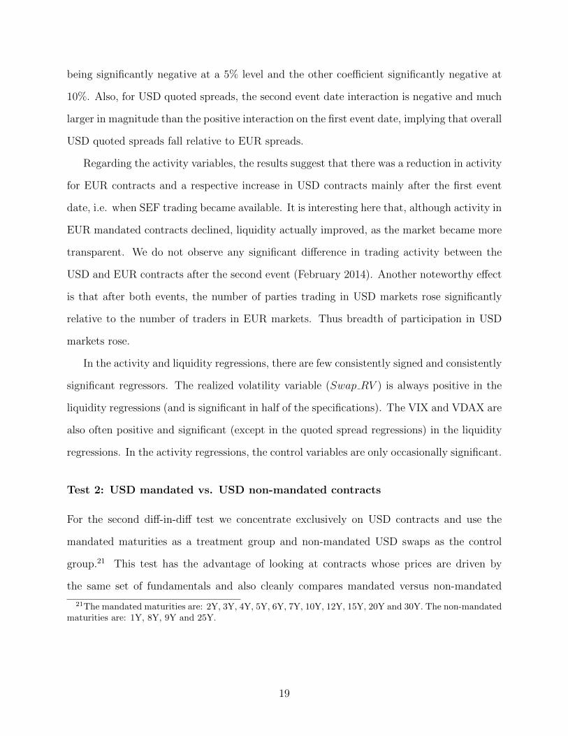
being significantly negative at a 5% level and the other coefficient significantly negative at

10%. Also, for USD quoted spreads, the second event date interaction is negative and much

larger in magnitude than the positive interaction on the first event date, implying that overall

USD quoted spreads fall relative to EUR spreads.

Regarding the activity variables, the results suggest that there was a reduction in activity

for EUR contracts and a respective increase in USD contracts mainly after the first event

date, i.e. when SEF trading became available. It is interesting here that, although activity in

EUR mandated contracts declined, liquidity actually improved, as the market became more

transparent. We do not observe any significant difference in trading activity between the

USD and EUR contracts after the second event (February 2014). Another noteworthy effect

is that after both events, the number of parties trading in USD markets rose significantly

relative to the number of traders in EUR markets. Thus breadth of participation in USD

markets rose.

In the activity and liquidity regressions, there are few consistently signed and consistently

significant regressors. The realized volatility variable (Swap RV ) is always positive in the

liquidity regressions (and is significant in half of the specifications). The VIX and VDAX are

also often positive and significant (except in the quoted spread regressions) in the liquidity

regressions. In the activity regressions, the control variables are only occasionally significant.

Test 2: USD mandated vs. USD non-mandated contracts

For the second diff-in-diff test we concentrate exclusively on USD contracts and use the

mandated maturities as a treatment group and non-mandated USD swaps as the control

group.21 This test has the advantage of looking at contracts whose prices are driven by

the same set of fundamentals and also cleanly compares mandated versus non-mandated

21The mandated maturities are: 2Y, 3Y, 4Y, 5Y, 6Y, 7Y, 10Y, 12Y, 15Y, 20Y and 30Y. The non-mandatedmaturities are: 1Y, 8Y, 9Y and 25Y.

19

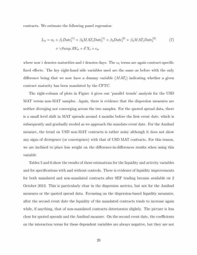
contracts. We estimate the following panel regression:

Lit = αi + β1Date(1)t + β2MATiDate

(1)t + β3Date

(2)t + β4MATiDate

(2)t (7)

+ γSwap RVit + δ′Xt + εit

where now i denotes maturities and t denotes days. The αi terms are again contract-specific

fixed effects. The key right-hand side variables used are the same as before with the only

difference being that we now have a dummy variable (MATi) indicating whether a given

contract maturity has been mandated by the CFTC.

The right-column of plots in Figure 4 gives our ‘parallel trends’ analysis for the USD

MAT versus non-MAT samples. Again, there is evidence that the dispersion measures are

neither diverging nor converging across the two samples. For the quoted spread data, there

is a small level shift in MAT spreads around 4 months before the first event date, which is

subsequently and gradually eroded as we approach the mandate event date. For the Amihud

measure, the trend on USD non-MAT contracts is rather noisy although it does not show

any signs of divergence (or convergence) with that of USD MAT contracts. For this reason,

we are inclined to place less weight on the difference-in-differences results when using this

variable.

Tables 5 and 6 show the results of these estimations for the liquidity and activity variables

and for specifications with and without controls. There is evidence of liquidity improvements

for both mandated and non-mandated contracts after SEF trading became available on 2

October 2013. This is particularly clear in the dispersion metrics, but not for the Amihud

measures or the quoted spread data. Focussing on the dispersion-based liquidity measures,

after the second event date the liquidity of the mandated contracts tends to increase again

while, if anything, that of non-mandated contracts deteriorates slightly. The picture is less

clear for quoted spreads and the Amihud measure. On the second event date, the coefficients

on the interaction terms for these dependent variables are always negative, but they are not

20

quite significant at conventional levels (with t-statistics between -1.30 and -1.50).

Overall, though, the broad picture here is one of increased liquidity for both mandated

and non-mandated USD contracts with the increase being significantly greater for the former.

It is fair to say, however, that the evidence of a liquidity improvement for mandated contracts

from these estimations is less strong than the evidence obtained from the comparison of USD

and EUR mandated contracts (especially for quoted spreads).

One interpretation of this finding is that the liquidity improvements in the mandated

contracts spilled over - to some extent - to non-mandated contracts. This is possible because

market participants might also have chosen to trade non-mandated contracts on SEFs as soon

as the functionality became available, and presumably also because, as discussed above, more

transparency for some quoted prices on the USD maturity curve gives market participants

a better idea of what a fair quote is for other USD maturities.

As far as activity and participation are concerned, 6 shows that, as for the estimations

using the EUR control sample, there are positive effects only for the mandated contracts

occurring in the period after 2 October 2013.

Economic Significance of Liquidity Improvement

We next assess the economic significance of the observed improvements in liquidity. For this,

we calculate the dollar reduction in execution costs for market end-users. The market value

of an IRS is set to zero at initiation by selecting the fixed rate such that the present values

of the fixed and floating legs are the same. However, a bid-ask spread charged by a dealer

on top of the fixed rate, would affect the value of the swap and thus introduce an additional

cost incurred by the end-user. The total dollar value of this cost can be approximated by:

Cost($) ≈ ESpread Adj × P ×m× Trade Size

where ESpread Adj is the effective spread of a transaction in an IRS contract with a

maturity of m years, P is the prevailing swap rate and Trade Size is the amount of notional

21

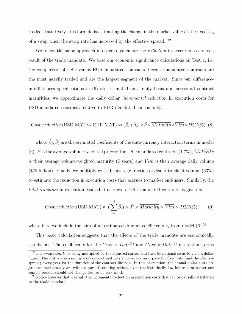
traded. Intuitively, this formula is estimating the change in the market value of the fixed leg

of a swap when the swap rate has increased by the effective spread. 22

We follow the same approach in order to calculate the reduction in execution costs as a

result of the trade mandate. We base our economic significance calculations on Test 1, i.e.

the comparison of USD versus EUR mandated contracts, because mandated contracts are

the most heavily traded and are the largest segment of the market. Since our difference-

in-differences specifications in (6) are estimated on a daily basis and across all contract

maturities, we approximate the daily dollar incremental reduction in execution costs for

USD mandated contracts relative to EUR mandated contracts by:

Cost reduction(USD MAT vs EUR MAT) ≈ (β2+β4)×P×Maturity×V lm×D2C(%) (8)

where β2, β4 are the estimated coefficients of the date-currency interaction terms in model

(6), P is the average volume-weighted price of the USD mandated contracts (1.7%), Maturity

is their average volume-weighted maturity (7 years) and V lm is their average daily volume

($75 billion). Finally, we multiply with the average fraction of dealer-to-client volume (33%)

to estimate the reduction in execution costs that accrues to market end-users. Similarly, the

total reduction in execution costs that accrues to USD mandated contracts is given by:

Cost reduction(USD MAT) ≈( 4∑

i=1

βi)× P ×Maturity × V lm×D2C(%) (9)

where here we include the sum of all estimated dummy coefficients βi from model (6).23

This basic calculation suggests that the effects of the trade mandate are economically

significant. The coefficients for the Curr × Date(1) and Curr × Date(2) interaction terms

22The swap rate, P , is being multiplied by the adjusted spread and then by notional so as to yield a dollarfigure. The cost is also a multiple of contract maturity since an end-user pays the fixed rate (and the effectivespread) every year for the duration of the contract lifespan. In this calculation, the annual dollar costs arejust summed aross years without any discounting which, given the historically low interest rates over oursample period, should not change the result very much.

23Notice however that it is only the incremental reduction in execution costs that can be causally attributedto the trade mandate.

22

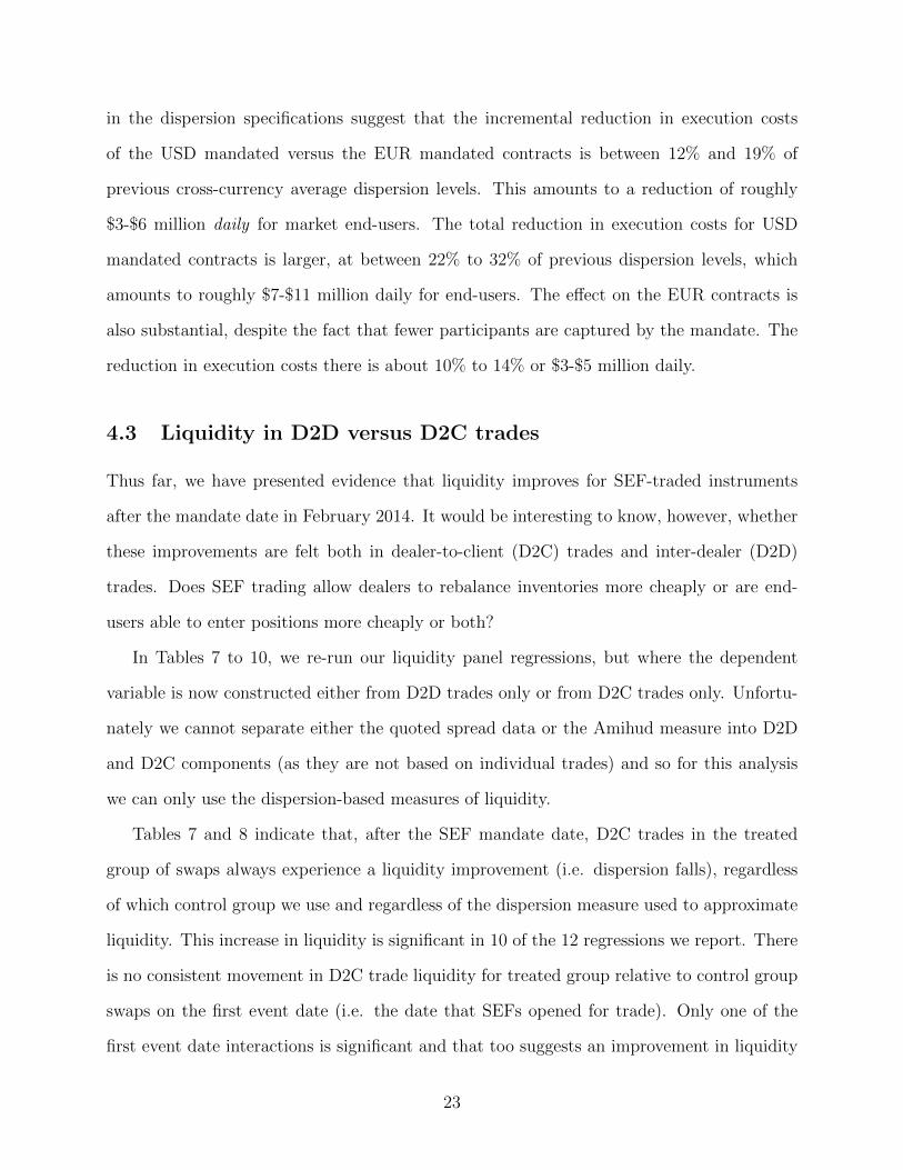
in the dispersion specifications suggest that the incremental reduction in execution costs

of the USD mandated versus the EUR mandated contracts is between 12% and 19% of

previous cross-currency average dispersion levels. This amounts to a reduction of roughly

$3-$6 million daily for market end-users. The total reduction in execution costs for USD

mandated contracts is larger, at between 22% to 32% of previous dispersion levels, which

amounts to roughly $7-$11 million daily for end-users. The effect on the EUR contracts is

also substantial, despite the fact that fewer participants are captured by the mandate. The

reduction in execution costs there is about 10% to 14% or $3-$5 million daily.

4.3 Liquidity in D2D versus D2C trades

Thus far, we have presented evidence that liquidity improves for SEF-traded instruments

after the mandate date in February 2014. It would be interesting to know, however, whether

these improvements are felt both in dealer-to-client (D2C) trades and inter-dealer (D2D)

trades. Does SEF trading allow dealers to rebalance inventories more cheaply or are end-

users able to enter positions more cheaply or both?

In Tables 7 to 10, we re-run our liquidity panel regressions, but where the dependent

variable is now constructed either from D2D trades only or from D2C trades only. Unfortu-

nately we cannot separate either the quoted spread data or the Amihud measure into D2D

and D2C components (as they are not based on individual trades) and so for this analysis

we can only use the dispersion-based measures of liquidity.

Tables 7 and 8 indicate that, after the SEF mandate date, D2C trades in the treated

group of swaps always experience a liquidity improvement (i.e. dispersion falls), regardless

of which control group we use and regardless of the dispersion measure used to approximate

liquidity. This increase in liquidity is significant in 10 of the 12 regressions we report. There

is no consistent movement in D2C trade liquidity for treated group relative to control group

swaps on the first event date (i.e. the date that SEFs opened for trade). Only one of the

first event date interactions is significant and that too suggests an improvement in liquidity

23

when SEF trading is available.

For D2D trading, the picture is much less clear. Comparing D2D trades in mandated

USD contracts versus those in mandated EUR swaps, Table 9 shows that there is a liquidity

improvement for the former relative to the latter after the SEF mandate date for all of

the dispersion measures. However, Table 10 shows that there is no improvement in D2D

liquidity for mandated USD contracts relative to non-mandated USD contracts. The results

suggest that D2D liquidity improves for both mandated and non-mandated USD contracts,

in particular on the first event date (with results for one of our liquidity proxies showing

that the liquidity improves more for non-mandated contracts than for mandated contracts

on the first event date).

Thus, overall, our regressions show that end-users of swaps have experienced consistent

liquidity benefits from mandated SEF trading. The picture for inter-dealer trades is less

clear, in that we do not see uniform evidence that their trading has become less expensive.

4.4 SEF flag panel specifications

We next test how the fraction of SEF trading affects liquidity and market activity. For this,

we utilize the DTCC segment of our data which contains a flag indicating whether a given

trade was executed on a SEF. We estimate the following panel specification for mandated

USD and EUR-denominated contracts only, on a daily frequency:

Lit = αi + β1SEFit + β2Date(1)t + γSwap RVit + δ′Xt + εit (10)

where Lit is one of the previously defined liquidity or market activity variables for contract

i on day t, SEFit is the percentage of SEF trading, Date(1)t is a date dummy taking the

value of 1 after the authorization of SEFs on 2 October 2013 and Xt is the usual vector

of controls. We include the date dummy in the specification so as to see if the time and

cross-sectional variation in SEF trading, conditional on SEF trading being available, has

24

incremental explanatory power.24 Because it is possible that SEF trading is itself caused by

market liquidity, we also estimate this model by IV, instrumenting SEFit with its own lags.

Tables 11 and 12 show the results of these estimations. The coefficients on the percentage

of SEF trading are significant in 14 of the 16 regressions and consistent with the previous

findings. A higher fraction of SEF trading is associated with increased levels of liquidity

as captured by reduced values for both the dispersion metrics as well as the Amihud and

quoted spread variables. Similarly, SEF trading is positive and statistically significant in the

regressions for activity variables: a higher fraction of SEF trading is associated with higher

volumes, more trades and a larger number of market participants. Overall, these results

suggest that SEF trading is associated with robust and measurable improvements in market

quality.

5 SEFs and Dealer Market Power

5.1 Relationships between Dealers and Clients

Duffie et al. (2005) and Yin (2005) argue that the beneficial effects of pre-trade transparency

on liquidity come via the effect of transparency on dealer competition. More intense dealer

competition leads to better prices for customers. We have already seen, in Tables 4 and

6, that the introduction of SEF trading increased the number of parties trading swaps,

potentially making these markets more competitive. In this section we explore whether the

trading relationships between individual customers and dealers have changed as a result of

the CFTC trade mandate. If SEF trading has led to more intense competition between

dealers, we would expect the number of dealers that the average customer trades with to

have risen for securities subject to the SEF trading mandate.

Thus we create a variable that we call Ndealersit. This variable is a count of the number

24We also estimate model (10) only using data after the introduction of SEF trading. The results for theliquidity variables are similar to those reported below and for this reason they are omitted.

25

of unique dealers with whom customer i trades in month t. It is based on completed trades

across all EUR and USD mandated swaps.25 As a first pass, we aggregate Ndealersit across

months and end-users for the period before mandatory SEF trading and then do the same

for the period after the mandate came into force and in Figure 5 display the frequency

distributions of those two samples. It is clear that SEF trading is associated with a dramatic

rightwards shift in the distribution, with the fraction of clients trading with only a few

dealers being substantially reduced and the fraction of clients trading with more dealers

rising correspondingly. For example, prior to the cutoff date, around 28% of customers dealt

only with a single dealer. With the introduction of the SEF trading mandate, this number

dropped to 8%. Similarly, prior to February 2014, over 50% of customers dealt with 3 or

fewer dealers, while after this date the corresponding number was around 20%.

These numbers immediately suggest that there have been profound changes in the nature

of the interactions between swap dealers and customers. Prior to the trading mandate strong

ties existed between individual customers and particular dealers. With the improvements

in pre-trade transparency, customer search costs have fallen and it has become easier for

customers to trade with the dealer showing the best price. Thus, effective competition

between dealers has risen and, as we have shown above, this has led to lower execution costs.

Given that the CFTC trade mandate only captures US persons (i.e. US legal entities),

one would further expect that any changes in the dealer-client relationships should be more

pronounced for US persons. To test this, we estimate a difference-in-differences specification

using the cross-section of all clients in our sample. In particular, we build our Ndealersit

variable for every customer and every month and estimate the following model:

25Another interesting measure would be the number of unique dealers that a particular customer contractedthrough requests for quotes in a particular period, but unfortunately we do not observe the RFQ processand thus cannot build such a variable.

26

Ndealersit = ai + bUSi + c1Date(1)t + c2 (Date

(1)t × USi) + c3 (Date

(1)t × ACTIV Ei)

+d1Date(2)t + d2 (Date

(2)t × USi) + d3 (Date

(2)t × ACTIV Ei)

+f1ACTIV Ei + f2 (USi × ACTIV Ei) + f3 (Date(1)t × USi × ACTIV Ei)

+f4 (Date(2)t × USi × ACTIV Ei) + γ′Xit + uit (11)

where t denotes months, i indexes end-users and ai is a fixed effect for end-user i. Date(1)

is the October 2013 SEF introduction dummy, Date(2) is the February 2014 SEF mandate

dummy and the Xi,t vector contains a set of end-user specific trading activity variables

(including number of trades and total volume executed). US is a dummy for any client that

is a US-person, while ACTIV Eit is a dummy that identifies a client who trades at least 20

times per month on average (i.e. roughly once a day or more). In our data, there are a large

number of end-users who trade very infrequently (e.g. once a week or less) and, thus, for

whom our dependent variable is always likely to be low regardless of the trading environment.

Thus, in order to avoid focussing on those clients and to shift attention towards clients for

whom increased dealer competition and greater liquidity is going to be most valuable, we

separate the active from the less active clients in the dummy specification in the regression

Table 13 shows the results of this estimation. The implementation of the SEF trading

mandate leads to the active set of US clients executing against a significantly larger number

of dealers. Prior to the mandate date, and focussing on the results without control variables

for clarity of interpretation, the significant coefficients indicate that those active US clients

dealt with around 9 dealers per month on average and afterwards this increases by around

17%, or 1.6 dealers, on average. This change is statistically significant, while there are no

significant shifts for non-US or inactive clients. The specification with control variables yields

qualitatively similar findings, although in that case the less active US clients see a small,

marginally significant drop in the number of dealers they trade with after the mandate date.

27

Thus, our graphical and econometric evidence is consistent. After the introduction of

mandatory SEF trading competition between dealers intensified, particularly for the set of

active US clients, and this likely contributes to the fall we observe in clients’ trading costs.

5.2 The Geography of Trading and Dealer Market Power

Shortly after the SEF trading mandate took effect, one concern among market participants

and regulators was that it might lead the global swaps market to fragment along geographical

lines (ISDA (2014)). Since the mandate only applied to US persons it was conceivable that,

for example, European counterparties who wished to avoid trading on a SEF might do so by

trading exclusively with other European counterparties. Indeed, some reports released after

the implementation of the mandate suggested that the market was becoming fragmented

and that this was causing market quality to deteriorate (e.g. Giancarlo (2015)).

In this section, we exploit our knowledge of counterparty identities in the LCH data and

investigate this issue in detail. First, we classify all market participants in the LCH data as

US or non-US-based and calculate the percentage of trading volume executed between US

and non-US counterparties (US-to-non-US).

Figure 6 plots this percentage for USD and EUR-denominated contracts. It is evident

that whereas no substantial effect takes place in USD-denominated contracts, after the in-

troduction of SEF trading there is a clear reduction in the fraction of US-to-non-US volume

in EUR-denominated swaps, from around 20% to 5%. More formally, the first two columns

of Table 14 show the results of time-series regressions of the fractions of US-to-non-US vol-

umes in USD and EUR contracts on the SEF introduction event dummy and a number of

controls. The dummy coefficient is highly significant and negative for the EUR contracts

and insignificant for USD contracts. Thus the EUR segment of the swap market did become

significantly more geographically fragmented following the introduction of SEF trading.

It is likely that the observed difference between the two market segments is because of

the much smaller proportion of US market participants in the EUR-denominated segment

28

of the market: if a non-US counterparty wants to trade with another non-US counterparty

and avoid executing on a SEF, this is much simpler for a EUR-denominated contract than

for a USD-denominated one. Given the preponderance of US persons trading USD swaps, it

is hard to avoid trading with a US person and thus on a SEF.

However, given the beneficial effects of SEF trading, the obvious question is why any (and

which) counterparties might want to avoid trading on SEFs. Figure 7 shows a breakdown

of the fraction of US-to-non-US volume in the EUR-denominated contracts according to

the type of counterparties. It is clear that the observed fragmentation is entirely driven by

inter-dealer trading and the last two columns of Table 14 confirm this. Thus, it appears that

it is swap dealers who are trying to avoid using SEFs where possible. There is no observable

fragmentation for EUR trades that involve at least one non-dealer. This might have been

expected, as there is no incentive for customers to avoid trading on SEFs given the liquidity

improvements they offer.

The question that remains is why cross-border activity by EUR swap dealers dropped

so clearly when the SEF trading mandate was introduced in the US. One possibility is

that inter-dealer trading between US-based and non-US-based dealers could genuinely have

exogenously declined and could have been replaced by local (intra-US and intra-European)

trading. Alternatively, inter-dealer trades between US and non-US firms could have been

executed by the non-US branches of swap dealers who happen to have trading desks in

multiple jurisdictions. For example, a trade in EUR between a US and a European dealer

that was being executed by the US desk of the former, could now be executed by the European

desk of the same dealer. In this case, it would be registered as an intra-European trade and

would not be subject to the SEF trade mandate.

To see if this is the case, we plot in Figure 8 the fraction of inter-dealer trading in EUR

contracts done by the US and non-US trading desks of only those swap dealers who have

desks in multiple jurisdictions and who execute more than 10% of their swap volumes from

a desk located in the United States. The figure shows that there is a sharp shift in inter-

29

dealer activity from the US desks to the non-US ones. The fraction of non-US desk trading

increases from a daily average of 75% prior to the introduction of SEFs, to an average of

95% after (with the corresponding fraction of US desk trading dropping from 25% to 5%).

Additionally, Figure 9 shows that there is virtually no change in the amount of inter-dealer

trading done exclusively by dealers who regularly trade the bulk (i.e. more than 90%) of

their derivatives from their European desks. We interpret this as implying that the observed

geographical fragmentation is artificial in the sense that it is entirely driven by EUR swap

dealers in large institutions using their non-US desks to do business that would previously

have passed through their US desk.

These results are consistent with (although not direct proof of) swap dealers strategically

choosing the location of the desk executing a particular trade in order to avoid trading in a

more transparent and competitive setting. A potential explanation for this lies in attempts

to maintain market power. By shifting the location of the inter-dealer market in EUR

swaps to Europe and using European entities to execute, the SEF trading mandate and the

associated CFTC impartial access requirements are avoided.26 This allows dealers to retain

power, in that they retain control over who they trade with and how, which in turn would

allow them to exclude any potential new competitors from inter-dealer trading. If a potential

competitor cannot access inter-dealer markets to manage inventory, their quotes are likely

to be less tight and thus they are less likely to attract business in the customer market.

6 Summary and Conclusion

One of the pillars of the G20 reform agenda for OTC derivatives markets is the requirement

to migrate trading activity to more centralized, more transparent venues. In response, as

part of Dodd-Frank, US regulators have mandated that US persons should trade certain

interest rate swap contracts on swap execution facilities (SEFs). These venues improve

26The CFTC guidance is available at:www.cftc.gov/idc/groups/public/@newsroom/documents/file/dmostaffguidance111413.pdf

30

transparency by automatically disseminating requests for quotes to multiple dealers and by

featuring an electronic order book which allows any market participant to compete with

dealers for liquidity provision by posting quotes. Thus, SEFs induce competition between

existing dealers and also lower the barriers to potential entrants to the dealing community.

Using transaction data from the IRS market we assess the impact of SEF introduction

on swap market activity and liquidity. We find that the move from an OTC to a more

centralized, competitive market structure leads to a substantial reduction in execution costs.

This is clearest for the mandated USD contracts, which are the most directly affected as

they are primarily traded by US persons who are captured by the trade mandate, and is also

most prominent for trades between dealers and clients. For these contracts, dispersion-based

liquidity measures for mandated USD swaps show that liquidity improves by between 12%

and 19% relative to that of EUR mandated contracts. This amounts to daily savings in

execution costs of as much as $3 - $6 million for end-users of USD swaps.

We then demonstrate that the introduction of centralized trading resulted in a sharp

increase in competition between swap dealers. The average active US client in this market

trades with a significantly greater number of dealers after the centralized trading mandate.

Thus, dealer competition rises and liquidity improves, as one would expect.

Additionally, we find that, for the EUR-denominated swap market, the bulk of inter-

dealer trading previously executed between US and non-US trading desks is now largely

executed by the non-US (mostly European) trading desks of the same institutions (i.e. banks

have shifted inter-dealer trading of their EUR swap positions from their US desks to their

European desks). We interpret this as an indication that swap dealers wish to avoid being

captured by the SEF trading mandate and the associated impartial access requirements.

Migrating the EUR inter-dealer volume off-SEFs enables dealers to choose who to trade

with and (more importantly) who not to trade with. This might allow them to erect barriers

to potential entrants to the dealing community. Thus this fragmentation of the global market

may be interpreted as dealers trying to retain market power, where possible. Importantly,

31

we find no evidence that customers in EUR swap markets try to avoid SEF trading and the

improved liquidity it delivers.

While our analysis suggests that so far there has been no incremental negative impact

on EUR contract liquidity as a result of this market fragmentation, it may have negated the

liquidity gains experienced in the USD segment of the market. Therefore, given the global

nature of OTC derivatives markets, our findings suggest that extending the scope of the

trading mandate to cover other sufficiently liquid swap markets would be desirable. Such

regulation has been implemented at the start of 2018 in the EU as part of MiFIR.

32

References

Acharya, V., Engle, R., Figlewski, S., Lynch, A., Subrahmanyam, M., 2009. CentralizedClearing for Credit Derivatives. In: Acharya, V., Richardson, M. (Eds.), Restoring Fi-nancial Stability: How to Repair a Failed System. John Wiley & Sons Inc, Hoboken,NJ.

Amihud, Y., 2002. Illiquidity and stock returns: Cross-section and time-series effects. Journalof Financial Markets 5 (1), 31–56.

Benos, E., Zikes, F., 2018. Funding constraints and liquidity in two-tiered OTC markets.forthcoming, Journal of Financial Markets.

Bessembinder, H., Maxwell, W., Venkataraman, K., 2006. Market transparency, liquidityexternalities, and institutional trading costs in corporate bonds. Journal of Financial Eco-nomics 82 (2), 251 – 288.

Boehmer, E., Saar, G., Yu, L., 2005. Lifting the veil: An analysis of pre-trade transparencyat the NYSE. The Journal of Finance 60 (2), 783–815.

Collin-Dufresne, P., Junge, B., Trolle, A., 2016. Market structure and transaction costs ofindex CDSs. Working Paper.

de Frutos, A., Manzano, C., 2002. Risk aversion, transparency, and market performance.Journal of Finance, 959–984.

Duffie, D., Garleanu, N., Pedersen, L. H., 2005. Over-the-counter markets. Econometrica73 (6), 1815–1847.

Duffie, D., Zhu, H., 2015. Size discovery. National Bureau of Economic Research WorkingPaper No. 21696.

Edwards, A. K., Harris, L. E., Piwowar, M. S., 2007. Corporate bond market transactioncosts and transparency. The Journal of Finance 62 (3), 1421–1451.

Flood, M. D., Huisman, R., Koedijk, K. G., Mahieu, R. J., 1999. Quote disclosure and pricediscovery in multiple-dealer financial markets. Review of Financial Studies 12 (1), 37–59.

Foucault, T., Moinas, S., Theissen, E., 2007. Does anonymity matter in electronic limit ordermarkets? Review of Financial Studies 20 (5), 1707.

Foucault, T., Pagano, M., Roell, A., 2013. Market Liquidity: Theory, Evidence and Policy.Oxford University Press.

Friederich, S., Payne, R., 2014. Trading anonymity and order anticipation. Journal of Finan-cial Markets 21, 1 – 24.

Friewald, N., Jankowitsch, R., Subrahmanyam, M. G., 2012. Illiquidity or credit deteriora-tion: A study of liquidity in the US corporate bond market during financial crises. Journalof Financial Economics 105 (1), 18 – 36.

33

Friewald, N., Jankowitsch, R., Subrahmanyam, M. G., 2014. Transparency and liquidity inthe structured product market. Unpublished working paper.

Giancarlo, C., 2015. Pro-reform reconsideration of the CFTC swaps trading rules: Returnto Dodd-Frank. White Paper.

Goldstein, M. A., Hotchkiss, E. S., Sirri, E. R., 2007. Transparency and liquidity: A con-trolled experiment on corporate bonds. Review of Financial Studies 20 (2), 235–273.

Goyenko, R. Y., Holden, C. W., Trzcinka, C. A., 2009. Do liquidity measures measureliquidity? Journal of Financial Economics 92 (2), 153–181.

Green, R. C., Hollifield, B., Schrhoff, N., 2007. Financial intermediation and the costs oftrading in an opaque market. Review of Financial Studies 20 (2), 275–314.

Harris, L. E., Piwowar, M. S., 2006. Secondary trading costs in the municipal bond market.The Journal of Finance 61 (3), 1361–1397.

Hendershott, T., Madhavan, A., 2015. Click or call? Auction versus search in the over-the-counter market. The Journal of Finance 70 (1), 419–447.

ISDA, 2014. Cross-border Fragmentation of Global OTC Derivatives: An Empirical Analysis.Research Note.

Jankowitsch, R., Nashikkar, A., Subrahmanyam, M. G., 2011. Price dispersion in OTCmarkets: A new measure of liquidity. Journal of Banking & Finance 35 (2), 343–357.

Loon, Y. C., Zhong, Z. K., 2014. The impact of central clearing on counterparty risk, liq-uidity, and trading: Evidence from the credit default swap market. Journal of FinancialEconomics 112 (1), 91 – 115.

Loon, Y. C., Zhong, Z. K., 2015. Does Dodd-Frank affect OTC transaction costs and liq-uidity? Evidence from real-time CDS trade reports. forthcoming, Journal of FinancialEconomics.

Massad, T., 2016. Testimony of Chairman Timothy G. Mas-sad Before the U.S. House Committee on Agriculture. , URLhttp://www.cftc.gov/PressRoom/SpeechesTestimony/opamassad-41.

Naik, N. Y., Neuberger, A., Viswanathan, S., 1999. Trade disclosure regulation in marketswith negotiated trades. Review of Financial Studies 12 (4), 873–900.

Nolte, I., Payne, R., Vasios, M., 2015. Profiting from mimicking strategies in non-anonymousmarkets. Working Paper.

Powell, J., 2016. Trends in Fixed Income Markets: Testimony of Governor Jerome H. Pow-ell Before the Subcommittee on Securities, Insurance, and Investment, and Subcommit-tee on Economic Policy, Committee on Banking, Housing, and Urban Affairs. , URLhttp://www.federalreserve.gov/newsevents/testimony/powell20160414.htm.

34

Riggs, L., Onur, E., Reiffen, D., Zhu, H., 2018. Swap trading after dodd-frank: Evidencefrom index CDS. Working Paper.

Spatt, C., 2017. Designing reliable clearing and settlement systems for enhancing the trans-parency and stability of derivatives markets. Working Paper.

Vayanos, D., Wang, J., 2012. Market liquidity–theory and empirical evidence. National Bu-reau of Economic Research Working Paper No. 18251.

Zikes, F., 2017. Measuring transaction costs in the absence of timestamps. Finance andEconomics Discussion Series, 045, Board of Governors of the Federal Reserve System.

Yin, X., 2005. A comparison of centralized and fragmented markets with costly search. TheJournal of Finance 60 (3), 1567–1590.

35

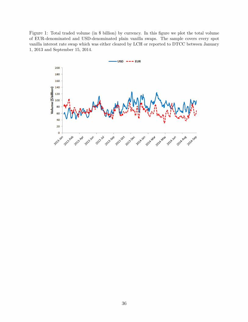
Figure 1: Total traded volume (in $ billion) by currency. In this figure we plot the total volumeof EUR-denominated and USD-denominated plain vanilla swaps. The sample covers every spotvanilla interest rate swap which was either cleared by LCH or reported to DTCC between January1, 2013 and September 15, 2014.

36

Figure 2: Volume shares by type of counterparty: In this figure we decompose the total volumeinto dealer-to-dealer (d2d), dealer-to-client (d2c), and client-to-client (c2c) trading. The innercircle presents the volumes of USD-denominated swaps, while the outer circle presents the volumesof EUR-denominated swaps. The sample covers every spot vanilla interest rate swap which wascleared by LCH between January 1, 2013 and September 15, 2014.

37

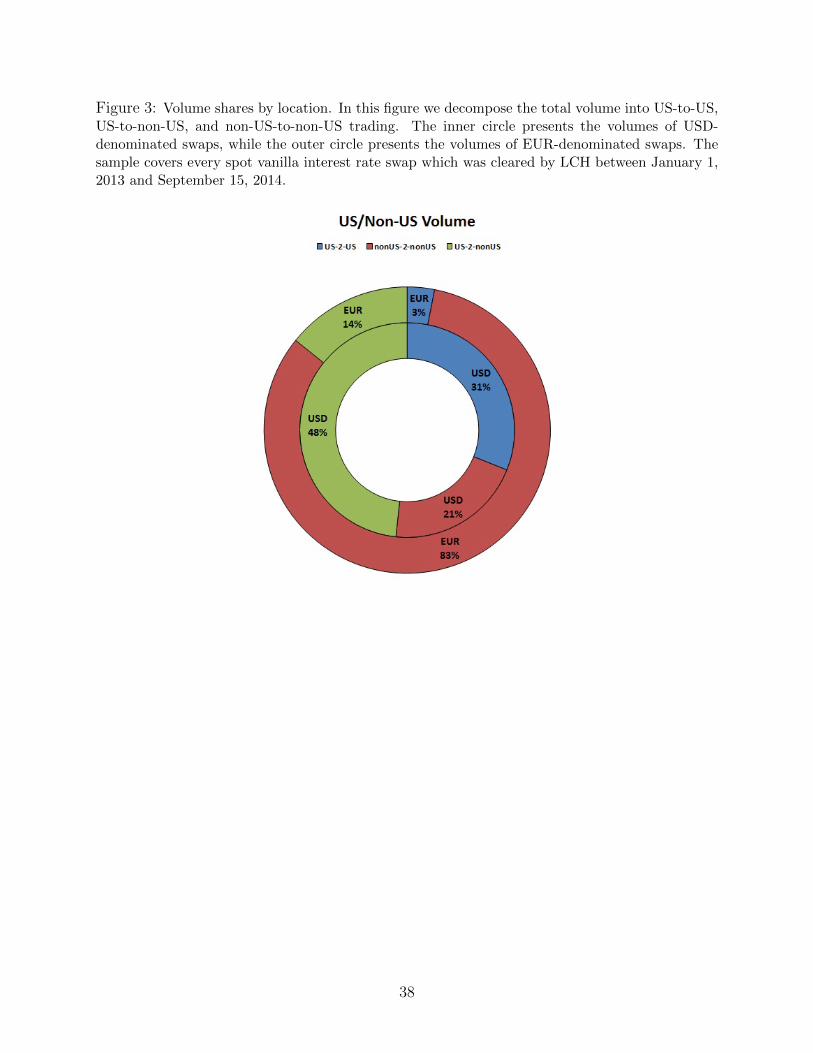
Figure 3: Volume shares by location. In this figure we decompose the total volume into US-to-US,US-to-non-US, and non-US-to-non-US trading. The inner circle presents the volumes of USD-denominated swaps, while the outer circle presents the volumes of EUR-denominated swaps. Thesample covers every spot vanilla interest rate swap which was cleared by LCH between January 1,2013 and September 15, 2014.

38

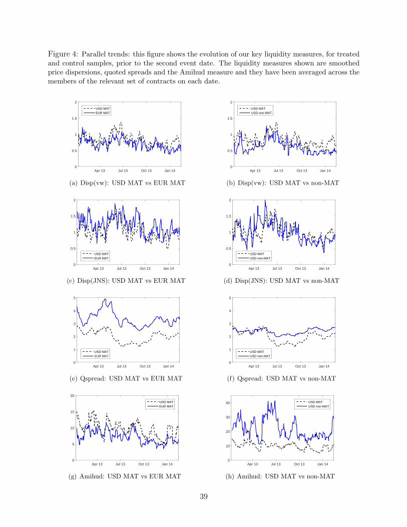
Figure 4: Parallel trends: this figure shows the evolution of our key liquidity measures, for treatedand control samples, prior to the second event date. The liquidity measures shown are smoothedprice dispersions, quoted spreads and the Amihud measure and they have been averaged across themembers of the relevant set of contracts on each date.

Apr 13 Jul 13 Oct 13 Jan 140

0.5

1

1.5

2

USD MATEUR MAT

(a) Disp(vw): USD MAT vs EUR MAT

Apr 13 Jul 13 Oct 13 Jan 140

0.5

1

1.5

2

USD MATUSD non-MAT

(b) Disp(vw): USD MAT vs non-MAT

Apr 13 Jul 13 Oct 13 Jan 140

0.5

1

1.5

2

USD MATEUR MAT

(c) Disp(JNS): USD MAT vs EUR MAT

Apr 13 Jul 13 Oct 13 Jan 140

0.5

1

1.5

2

USD MATUSD non-MAT

(d) Disp(JNS): USD MAT vs non-MAT

Apr 13 Jul 13 Oct 13 Jan 140

1

2

3

4

5

USD MATEUR MAT

(e) Qspread: USD MAT vs EUR MAT

Apr 13 Jul 13 Oct 13 Jan 140

1

2

3

4

5

USD MATUSD non-MAT

(f) Qspread: USD MAT vs non-MAT

Apr 13 Jul 13 Oct 13 Jan 140

5

10

15

20

USD MATEUR MAT

(g) Amihud: USD MAT vs EUR MAT

Apr 13 Jul 13 Oct 13 Jan 140

10

20

30

40 USD MATUSD non-MAT

(h) Amihud: USD MAT vs non-MAT

39

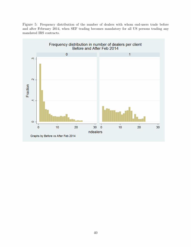
Figure 5: Frequency distribution of the number of dealers with whom end-users trade beforeand after February 2014, when SEF trading becomes mandatory for all US persons trading anymandated IRS contracts.

40

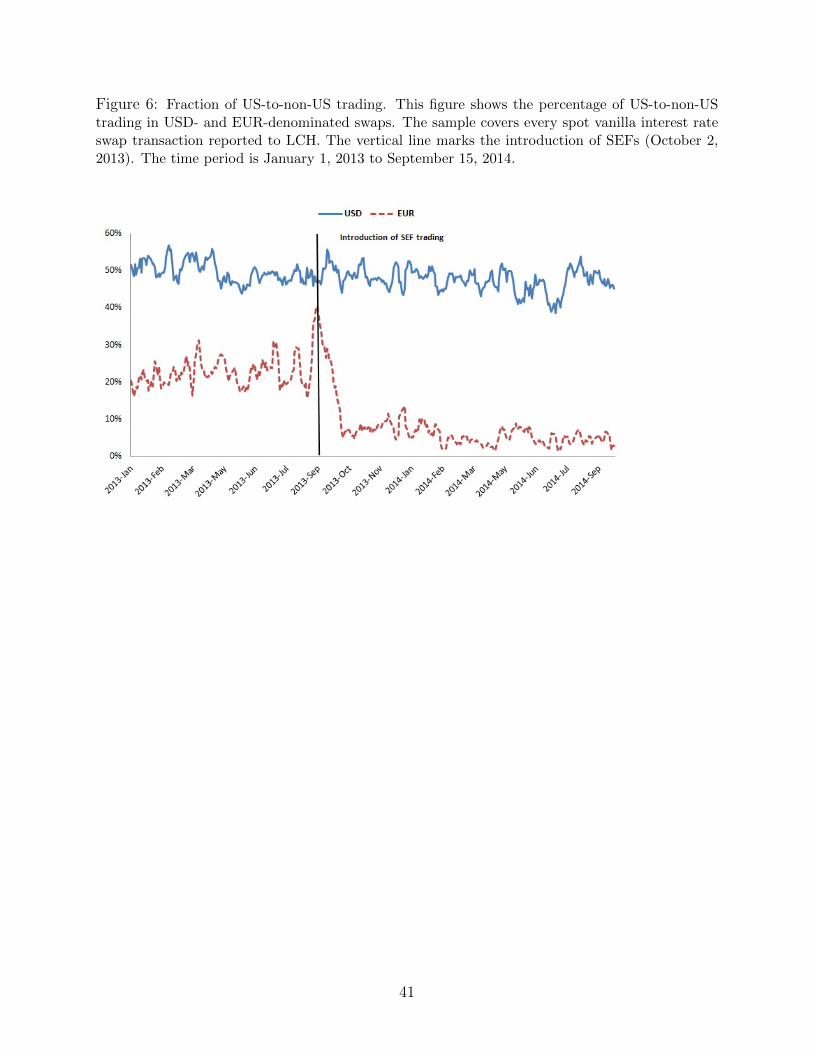
Figure 6: Fraction of US-to-non-US trading. This figure shows the percentage of US-to-non-UStrading in USD- and EUR-denominated swaps. The sample covers every spot vanilla interest rateswap transaction reported to LCH. The vertical line marks the introduction of SEFs (October 2,2013). The time period is January 1, 2013 to September 15, 2014.

41

Figure 7: Breakdown of US-to-non-US trading. This figure shows the breakdown of US-to-non-UStrading volume in EUR-denominated swaps into inter-dealer volume and all other trading volume.The sample covers every spot vanilla interest rate swap transaction reported to LCH. The verticalline marks the introduction of SEFs (October 2, 2013). The time period is January 1, 2013 toSeptember 15, 2014.

42

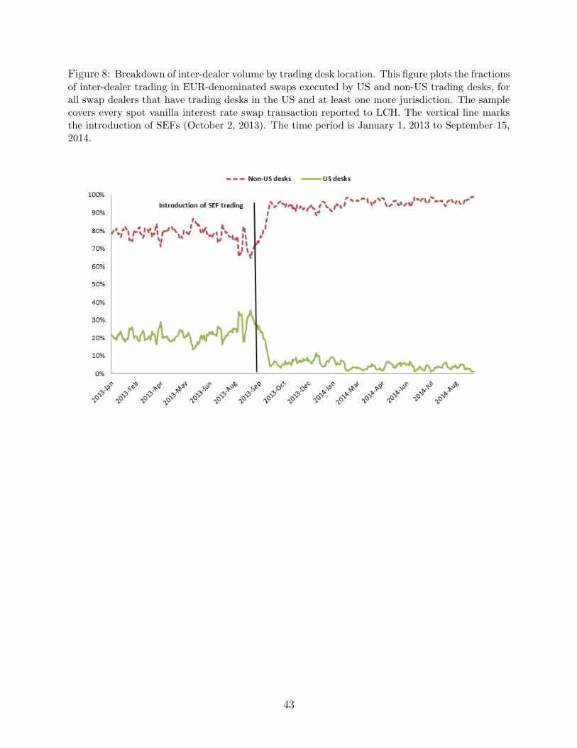
Figure 8: Breakdown of inter-dealer volume by trading desk location. This figure plots the fractionsof inter-dealer trading in EUR-denominated swaps executed by US and non-US trading desks, forall swap dealers that have trading desks in the US and at least one more jurisdiction. The samplecovers every spot vanilla interest rate swap transaction reported to LCH. The vertical line marksthe introduction of SEFs (October 2, 2013). The time period is January 1, 2013 to September 15,2014.

43

Figure 9: This figure plots the amount of inter-dealer trading in EUR-denominated swaps executedexclusively by swap dealers that have no trading desks in the US. The sample covers every spotvanilla interest rate swap transaction reported to LCH. The vertical line marks the introduction ofSEFs (October 2, 2013). The time period is January 1, 2013 to September 15, 2014.

44

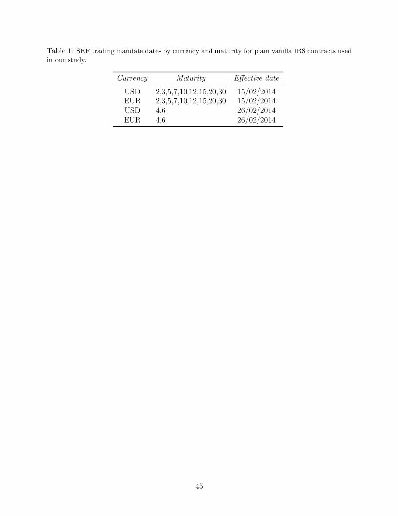
Table 1: SEF trading mandate dates by currency and maturity for plain vanilla IRS contracts usedin our study.

Currency Maturity Effective date

USD 2,3,5,7,10,12,15,20,30 15/02/2014EUR 2,3,5,7,10,12,15,20,30 15/02/2014USD 4,6 26/02/2014EUR 4,6 26/02/2014

45

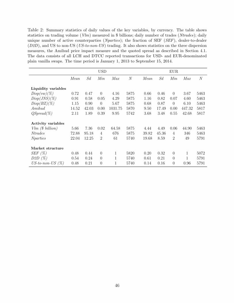
Table 2: Summary statistics of daily values of the key variables, by currency. The table showsstatistics on trading volume (Vlm) measured in $ billions; daily number of trades (Ntrades); dailyunique number of active counterparties (Nparties); the fraction of SEF (SEF ), dealer-to-dealer(D2D), and US to non-US (US-to-non-US ) trading. It also shows statistics on the three dispersionmeasures, the Amihud price impact measure and the quoted spread as described in Section 4.1.The data consists of all LCH and DTCC reported transactions for USD- and EUR-denominatedplain vanilla swaps. The time period is January 1, 2013 to September 15, 2014.

USD EUR

Mean Sd Min Max N Mean Sd Min Max N

Liquidity variables

Disp(vw)(%) 0.72 0.47 0 4.16 5875 0.66 0.46 0 3.67 5463Disp(JNS)(%) 0.91 0.58 0.05 4.29 5875 1.16 0.82 0.07 4.60 5463Disp(BZ)(%) 1.15 0.90 0 5.67 5875 0.68 0.87 0 6.10 5463Amihud 14.52 42.03 0.00 1031.75 5870 9.50 17.49 0.00 447.32 5817QSpread(%) 2.11 1.89 0.39 9.95 5742 3.68 3.48 0.55 42.68 5817

Activity variables

Vlm ($ billion) 5.66 7.36 0.02 64.58 5875 4.44 4.49 0.06 44.90 5463Ntrades 72.88 95.18 4 676 5875 39.82 45.36 4 346 5463Nparties 22.04 12.25 2 61 5740 19.68 8.59 2 49 5791

Market structure

SEF (%) 0.48 0.44 0 1 5820 0.20 0.32 0 1 5072D2D (%) 0.54 0.24 0 1 5740 0.61 0.21 0 1 5791US-to-non-US (%) 0.48 0.21 0 1 5740 0.14 0.16 0 0.96 5791

46

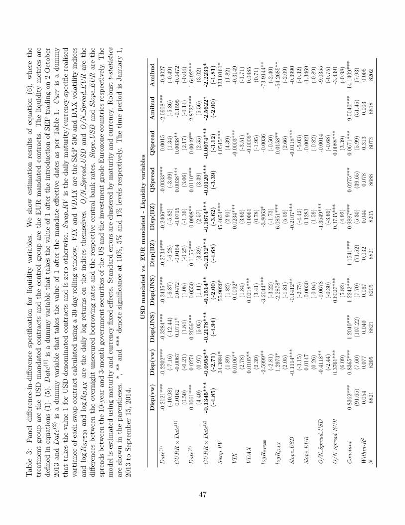
Tab

le3:

Pan

eld

iffer

ence

-in

-diff

eren

cesp

ecifi

cati

onfo

rli

qu

idit

yva

riab

les.

We

show

esti

mat

ion

resu

lts

ofeq

uat

ion

(6),

wh

ere

the

trea

tmen

tgro

up

are

the

US

Dm

an

date

dco

ntr

acts

and

the

contr

olgr

oup

are

the

EU

Rm

and

ated

contr

acts

.T

he

liqu

idit

ym

etri

csar

ed

efin

edin

equ

atio

ns

(1)-

(5).

Date

(1)

isa

du

mm

yva

riab

leth

atta

kes

the

valu

eof

1af

ter

the

intr

od

uct

ion

ofSE

Ftr

adin

gon

2O

ctob

er201

3an

dDate

(2)

isa

du

mm

yva

riab

leth

atta

kes

the

valu

eof

1af

ter

the

man

dat

eeff

ecti

ved

ates

asp

erT

able

1.C

urr

isa

du

mm

yth

at

take

sth

eva

lue

1fo

rU

SD

-den

omin

ate

dco

ntr

acts

and

isze

root

her

wis

e.S

wap

RV

isth

ed

aily

mat

uri

ty/c

urr

ency

-sp

ecifi

cre

alis

edva

rtia

nce

ofea

chsw

apco

ntr

act

calc

ula

ted

usi

ng

a30

-day

rollin

gw

indow

.V

IXan

dV

DA

Xar

eth

eS

&P

500

and

DA

Xvo

lati

lity

ind

ices

an

dlo

gR

SP500

an

dlo

gR

DAX

are

the

dai

lylo

gre

turn

son

the

ind

ices

them

selv

es.

O/N

Spre

ad

US

Dan

dO

/N

Spre

ad

EU

Rar

eth

ed

iffer

ence

sb

etw

een

the

over

nig

ht

un

secu

red

bor

row

ing

rate

san

dth

ere

spec

tive

centr

alb

ank

rate

s.S

lope

US

Dan

dS

lope

EU

Rar

eth

esp

read

sb

etw

een

the

10-

year

an

d3-m

onth

gove

rnm

ent

secu

riti

esof

the

US

and

the

inves

tmen

tgr

ade

Eu

rozo

ne

cou

ntr

ies

resp

ecti

vel

y.T

he

mod

elis

esti

mate

du

sin

gm

atu

rity

and

curr

ency

fixed

effec

ts.

Sta

nd

ard

erro

rsar

ecl

ust

ered

by

mat

uri

tyan

dcu

rren

cy.

Rob

ust

t-st

ati

stic

sar

esh

own

inth

ep

aren

thes

es.

*,**

and

***

den

ote

sign

ifica

nce

at10

%,

5%an

d1%

leve

lsre

spec

tive

ly.

Th

eti

me

per

iod

isJan

uar

y1,

2013

toS

epte

mb

er15,

2014

.

US

Dm

an

date

dvs.

EU

Rm

an

date

d-

Liq

uid

ity

vari

ab

les

Dis

p(v

w)

Dis

p(v

w)

Dis

p(J

NS)

Dis

p(J

NS

)D

isp

(BZ

)D

isp

(BZ

)Q

Sp

read

QS

pre

ad

Am

ihu

dA

mih

ud

Date

(1)

-0.2

121*

**-0

.220

2***

-0.3

284*

**-0

.343

5***

-0.2

734*

**-0

.240

6***

-0.0

033*

**0.

0015

-2.0

908*

**-0

.402

7(-

10.9

8)(-

7.16

)(-

12.4

4)(-

6.87

)(-

6.28

)(-

5.82

)(-

3.09

)(1

.34)

(-5.

86)

(-0.

49)

CURR×Date

(1)

0.01

62-0

.006

70.

0711

*0.

0472

-0.0

154

-0.0

715

0.00

38**

*0.

0038

**-0

.159

5-0

.047

2(0

.50)

(-0.

21)

(1.8

4)(1

.08)

(-0.

25)

(-1.

36)

(3.0

6)(2

.17)

(-0.

14)

(-0.

04)

Date

(2)

0.10

61**

*0.

0274

0.20

56**

*0.

0550

0.11

55**

*0.

0908

**0.

0110

***

0.00

49**

2.87

27**

*1.

6492

***

(4.4

0)(0

.97)

(5.0

5)(1

.11)

(3.3

9)(2

.57)

(3.3

9)(2

.55)

(5.5

6)(3

.02)

CURR×Date

(2)

-0.1

345***

-0.0

958**

-0.2

178***

-0.1

514**

-0.2

152***

-0.1

674***

-0.0

120***

-0.0

074***

-2.5

622*

-2.2

233*

(-4.8

5)

(-2.7

1)

(-4.9

4)

(-2.0

0)

(-4.6

8)

(-3.6

2)

(-3.3

9)

(-3.1

2)

(-2.0

0)

(-1.8

1)

Sw

apR

V34

.388

4*55

.902

0*45

.465

4***

4.05

45**

*32

3.01

61*

(1.8

9)(1

.82)

(2.9

1)(4

.39)

(1.8

2)V

IX0.

0106

**0.

0092

*0.

0234

***

-0.0

003*

**-0

.314

9(2

.78)

(1.8

4)(3

.69)

(-3.

51)

(-1.

71)

VD

AX

0.01

05**

0.02

18**

*0.

0061

-0.0

006*

0.04

85(2

.39)

(3.4

1)(0

.78)

(-1.

95)

(0.7

1)logR

SP500

-2.5

999*

*-3

.204

4***

-3.8

063*

-0.0

036

-73.

9144

**(-

2.81

)(-

3.22

)(-

1.73

)(-

0.50

)(-

2.40

)logR

DAX

1.29

73*

-2.2

878*

6.08

51**

*0.

0158

**-5

4.26

85**

(2.0

5)(-

1.81

)(5

.59)

(2.6

6)(-

2.09

)S

lope

US

D-0

.111

4***

-0.1

412*

*-0

.210

7***

-0.0

118*

**-0

.399

0(-

3.15

)(-

2.75

)(-

4.42

)(-

5.03

)(-

0.32

)S

lope

EU

R0.

0147

-0.0

030

0.12

83-0

.002

1-1

.346

9(0

.26)

(-0.

04)

(1.5

9)(-

0.82

)(-

0.89

)O

/NS

prea

dU

SD

-0.4

118*

*-0

.067

8-1

.354

9***

-0.0

014

-9.0

355

(-2.

44)

(-0.

30)

(-3.

69)

(-0.

68)

(-0.

75)

O/N

Spr

ead

EU

R0.

3761

***

0.60

27**

*0.

3735

***

0.00

88**

*-3

.439

1(6

.09)

(5.8

2)(4

.92)

(3.3

9)(-

0.98

)C

onst

ant

0.83

62**

*0.

8365

***

1.20

40**

*1.

2242

***

1.15

41**

*0.

9887

***

0.02

75**

*0.

0671

***

9.50

40**

*14

.140

9***

(91.

65)

(7.6

0)(1

07.2

2)(7

.70)

(71.

52)

(5.3

0)(3

9.65

)(5

.99)

(51.

45)

(7.9

3)W

ithi

n-R

20.

054

0.07

70.

040

0.06

70.

032

0.04

40.

078

0.31

30.

003

0.00

5N

8821

8205

8821

8205

8821

8205

8688

8073

8818

8202

47

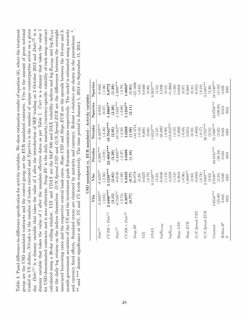
Tab

le4:

Pan

eld

iffer

ence

-in

-diff

eren

cesp

ecifi

cati

onfo

rac

tivit

yva

riab

les.

We

show

esti

mat

ion

resu

lts

ofeq

uat

ion

(6),

wh

ere

the

trea

tmen

tgro

up

are

the

US

Dm

an

date

dco

ntr

acts

an

dth

eco

ntr

olgr

oup

are

the

EU

Rm

and

ated

contr

acts

.Vlm

isth

eam

ount

ofgr

oss

not

ion

altr

ad

edin

US

dol

lars

,Ntrades

isth

enu

mb

erof

trad

esex

ecu

ted

andNparties

isth

enu

mb

erof

un

iqu

eco

unte

rpar

ties

acti

veon

agi

ven

day

.Date

(1)

isa

du

mm

yva

riab

leth

at

take

sth

eva

lue

of1

afte

rth

ein

trod

uct

ion

ofS

EF

trad

ing

on2

Oct

ober

2013

andDate

(2)

isa

du

mm

yva

riab

leth

at

take

sth

eva

lue

of

1af

ter

the

man

dat

eeff

ecti

ved

ates

asp

erT

able

1.C

urr

isa

du

mm

yth

atta

kes

the

valu

e1

for

US

D-d

enom

inate

dco

ntr

act

sand

isze

root

her

wis

e.S

wap

RV

isth

ed

aily

mat

uri

ty/c

urr

ency

-sp

ecifi

cvo

lati

lity

ofea

chsw

apco

ntr

act

calc

ula

ted

usi

ng

a30

-day

roll

ing

win

dow

.V

IXan

dV

DA

Xar

eth

eS

&P

500

and

DA

Xvo

lati

lity

ind

ices

and

logR

SP500

and

logR

DAX

are

the

dai

lylo

gre

turn

son

the

ind

ices

them

selv

es.

O/N

Spre

ad

US

Dan

dO

/N

Spre

ad

EU

Rar

eth

ed

iffer

ence

sb

etw

een

the

over

nig

ht

un

secu

red

borr

owin

gra

tes

an

dth

ere

spec

tive

centr

alb

ank

rate

s.S

lope

US

Dan

dS

lope

EU

Rar

eth

esp

read

sb

etw

een

the

10-y

ear

and

3-m

onth

gov

ern

men

tse

curi

ties

ofth

eU

San

dth

ein

vest

men

tgr

ade

Eu

rozo

ne

cou

ntr

ies

resp

ecti

vely

.T

he

mod

elis

esti

mat

edu

sin

gm

atu

rity

an

dcu

rren

cyfi

xed

effec

ts.

Sta

nd

ard

erro

rsar

ecl

ust

ered

by

mat

uri

tyan

dcu

rren

cy.

Rob

ust

t-st

ati

stic

sar

esh

own

inth

ep

aren

thes

es.

*,**

an

d**

*d

enote

sign

ifica

nce

at10

%,

5%an

d1%

leve

lsre

spec

tive

ly.

Th

eti

me

per

iod

isJan

uar

y1,

2013

toS

epte

mb

er15

,20

14.

US

Dm

an

date

dvs.

EU

Rm

an

date

d-

Act

ivit

yvari

ab

les

Vlm

Vlm

Ntr

ad

es

Ntr

ades

Np

art

ies

Np

art

ies

Date

(1)

-0.3

433*

*-0

.427

0**

-4.2

991*

**-6

.327

9***

0.05

83-0

.448

2(-

2.61

)(-

2.56

)(-

2.91

)(-

3.46

)(0

.27)

(-1.

06)

CURR×Date

(1)

2.4

496***

2.1

238***

22.4

662***

18.7

042***

1.4

968**

0.8

772

(3.1

5)

(2.8

5)

(3.2

9)

(2.9

5)

(2.2

6)

(1.3

9)

Date

(2)

-0.7

535*

*-0

.674

0-6

.493

5**

-10.

7412

**-1

.124

3***

-1.4

809*

**(-

2.74

)(-

1.69

)(-

2.37

)(-

2.32

)(-

3.06

)(-

3.70

)CURR×Date

(2)

0.3

077

0.3

333

4.0

289

4.0

268

1.1

234**

1.0

083*

(0.7

7)

(0.7

7)

(1.1

6)

(1.0

8)

(2.1

1)

(1.9

1)

Sw

apR

V20

.877

8-1

41.3

714

-121

.389

6(0

.20)

(-0.

16)

(-0.

63)

VIX

-0.0

227

0.20

910.

0460

(-0.

79)

(0.6

8)(0

.90)

VD

AX

0.15

49**

*1.

6553

***

0.26

51**

*(3

.23)

(3.1

2)(4

.54)

logR

SP500

-6.0

106

-48.

2967

4.53

98(-

1.13

)(-

0.90

)(0

.54)

logR

DAX

-4.2

459

-119

.452

7**

-11.

2663

(-1.

12)

(-2.

10)

(-1.

66)

Slo

peU

SD

-0.3

819

-3.2

920

0.63

34(-

0.96

)(-

0.89

)(0

.97)

Slo

peE

UR

1.28

89**

3.05

520.

2681

(2.8

3)(0

.59)

(0.3

1)O

/NS

prea

dU

SD

-0.8

503

-1.8

934

-0.5

551

(-0.

78)

(-0.

17)

(-0.

19)

O/N

Spr

ead

EU

R2.

1692

***

28.1

735*

**3.

1105

***

(3.8

3)(3

.54)

(3.3

6)C

onst

ant

5.65

16**

*2.

9138

**64

.854

1***

51.1

500*

**23

.079

3***

18.1

139*

**(2

5.80

)(2

.24)

(30.

44)

(3.9

2)(1

00.9

5)(1

1.02

)W

ithi

n-R

20.

042

0.04

90.

033

0.04

30.

013

0.02

8N

8821

8205

8821

8205

8821

8205

48

Tab

le5:

Pan

eld

iffer

ence

-in

-diff

eren

cesp

ecifi

cati

onfo

rli

qu

idit

yva

riab

les.

We

show

esti

mat

ion

resu

lts

ofsp

ecifi

cati

on(7

),w

her

eth

etr

eatm

ent

gro

up

con

sist

sof

the

US

Dm

and

ated

contr

acts

and

the

contr

olgr

oup

ofth

eU

SD

non

-man

dat

edco

ntr

acts

.T

he

liqu

idit

ym

etri

csare

defi

ned

ineq

uati

on

s(1

)-(5

).Date

(1)

isa

du

mm

yva

riab

leth

atta

kes

the

valu

eof

1af

ter

the

intr

od

uct

ion

ofS

EF

trad

ing

on

2O

ctob

er20

13

andDate

(2)

isa

du

mm

yva

riab

leth

atta

kes

the

valu

eof

1af

ter

the

man

dat

eeff

ecti

ved

ates

asp

erT

able

1.M

AT

isa

du

mm

yth

at

take

sth

eva

lue

1fo

rm

and

ated

contr

acts

and

isze

root

her

wis

e.S

wap

RV

isth

ed

aily

mat

uri

ty/c

urr

ency

-sp

ecifi

cre

alis

edva

rian

ceof

each

swap

contr

act

calc

ula

ted

usi

ng

a30

-day

roll

ing

win

dow

.V

IXis

the

S&

P50

0vo

lati

lity

ind

exan

dlo

gR

SP500

isth

elo

gd

ail

yre

turn

on

the

ind

exit

self

.O

/N

Spre

ad

US

Dis

the

diff

eren

ceb

etw

een

the

over

nig

ht

un

secu

red

bor

row

ing

rate

and

the

resp

ecti

vece

ntr

alb

an

kra

te.

Slo

peU

SD

isth

esp

read

sb

etw

een

the

10-y

ear

and

3-m

onth

Tre

asu

ryse

curi

ties

.T

he

mod

elis

esti

mat

edu

sin

gm

atu

rity

fixed

effec

ts.

Sta

nd

ard

erro

rsar

ecl

ust

ered

by

mat

uri

ty.

Rob

ust

t-st

ati

stic

sar

esh

own

inth

ep

aren

thes

es.

*,**

and

***

den

ote

sign

ifica

nce

at10

%,

5%

and

1%le

vel

sre

spec

tive

ly.

Th

eti

me

per

iod

isJan

uar

y1,

2013

toS

epte

mb

er15

,20

14.

US

Dm

an

date

dvs.

USD

non-m

an

date

d-

Liq

uid

ity

vari

ab

les

Dis

p(v

w)

Dis

p(v

w)

Dis

p(J

NS

)D

isp

(JN

S)

Dis

p(B

Z)

Dis

p(B

Z)

QS

pre

ad

QS

pre

ad

Am

ihu

dA

mih

ud

Date

(1)

-0.2

220*

**-0

.236

2***

-0.3

372*

**-0

.326

9***

-0.2

520*

**-0

.309

7***

0.00

170.

0052

***

-12.

6410

*-9

.554

7(-

3.87

)(-

4.72

)(-

6.37

)(-

6.91

)(-

3.60

)(-

5.21

)(0

.94)

(3.0

9)(-

1.89

)(-

1.75

)MAT×Date

(1)

0.02

610.

0273

0.07

990.

0694

-0.0

367

-0.0

091

-0.0

012

0.00

0210

.385

912

.105

5(0

.41)

(0.4

7)(1

.33)

(1.2

5)(-

0.44

)(-

0.12

)(-

0.64

)(0

.10)

(1.5

3)(1

.55)

Date

(2)

0.03

040.

0140

0.05

82**

0.00

23-0

.017

10.

0137

0.00

12**

*0.

0019

***

8.71

945.

2508

(1.7

3)(0

.64)

(2.1

8)(0

.06)

(-0.

74)

(0.4

0)(4

.52)

(3.1

9)(1

.37)

(1.0

9)MAT×Date

(2)

-0.0

589**

-0.0

611**

-0.0

704**

-0.0

742**

-0.0

827*

-0.0

764*

-0.0

022

-0.0

010

-8.4

310

-8.6

509

(-2.6

3)

(-2.6

5)

(-2.2

3)

(-2.2

6)

(-2.1

2)

(-2.0

8)

(-1.5

0)

(-1.3

0)

(-1.3

0)

(-1.3

5)

Sw

apR

V4.

0546

3.46

2029

.265

0*2.

6261

***

172.

3148

(0.4

4)(0

.28)

(1.8

3)(1

1.41

)(0

.88)

VIX

0.00

91*

0.00

670.

0209

**-0

.000

2**

-0.8

607

(2.0

1)(1

.30)

(2.5

4)(-

2.52

)(-

1.33

)V

DA

X0.

0212

***

0.03

07**

*0.

0294

**-0

.000

3***

0.70

18(4

.31)

(4.1

1)(2

.78)

(-3.

70)

(1.1

0)logR

SP500

-5.9

413*

**-5

.526

0***

-10.

8943

***

0.00

01-3

6.45

89(-

7.76

)(-

4.34

)(-

4.42

)(0

.02)

(-0.

41)

logR

DAX

1.82

09**

*0.

5032

5.28

05**

*0.

0014

-203

.776

5*(3

.04)

(0.6

2)(3

.62)

(0.4

8)(-

1.92

)S

lope

US

D-0

.366

4-0

.672

0***

-0.6

065

0.00

17-1

9.83

18(-

1.74

)(-

3.12

)(-

1.54

)(0

.93)

(-0.

98)

Slo

peE

UR

0.35

98**

*0.

4618

***

0.49

00**

*0.

0065

***

-4.9

971

(5.4

8)(6

.12)

(5.2

8)(5

.14)

(-0.

81)

O/N

Spr

ead

US

D-0

.140

4***

-0.2

023*

**-0

.163

7**

-0.0

122*

**-2

.503

4(-

4.83

)(-

5.38

)(-

2.75

)(-

4.03

)(-

0.95

)O

/NS

prea

dE

UR

0.11

76**

0.10

800.

2354

**0.

0064

**-3

.618

9(2

.78)

(1.6

4)(2

.88)

(2.3

3)(-

1.32

)C

onst

ant

0.84

41**

*0.

6170

***

1.09

16**

*0.

9398

***

1.34

02**

*0.

6650

**0.

0208

***

0.04

03**

*16

.469

2***

26.7

056*

**(6

5.67

)(5

.07)

(69.

89)

(5.7

3)(7

1.15

)(2

.50)

(51.

41)

(8.3

7)(3

4.91

)(3

.80)

Wit

hin

-R2

0.06

50.

098

0.06

50.

092

0.04

40.

072

0.01

40.

397

0.00

40.

009

N58

7554

5358

7554

5358

7554

5357

4253

2150

9050

41

49

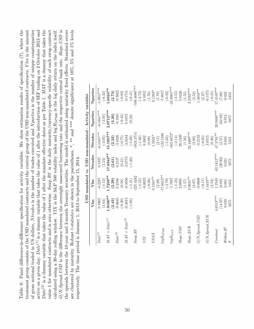
Tab

le6:

Pan

eld

iffer

ence

-in

-diff

eren

cesp

ecifi

cati

onfo

rac

tivit

yva

riab

les.

We

show

esti

mat

ion

resu

lts

ofsp

ecifi

cati

on(7

),w

her

eth

etr

eatm

ent

grou

pco

nsi

sts

of

the

US

Dm

an

dat

edco

ntr

acts

and

the

contr

olgr

oup

ofth

eU

SD

non

-man

dat

edco

ntr

acts

.Vlm

isth

eam

ount

of

gro

ssn

otio

nal

trad

edin

US

doll

ars,

Ntrades

isth

enu

mb

erof

trad

esex

ecu

ted

andNparties

isth

enu

mb

erof

un

iqu

eco

unte

rpar

ties

act

ive

ona

giv

end

ay.Date

(1)

isa

du

mm

yva

riab

leth

atta

kes

the

valu

eof

1af

ter

the

intr

od

uct

ion

ofS

EF

trad

ing

on2

Oct

ober

2013

and

Date

(2)

isa

du

mm

yva

riable

that

take

sth

eva

lue

of1

afte

rth

em

and

ate

effec

tive

dat

esas

per

Tab

le1.

MA

Tis

ad

um

my

that

takes

the

valu

e1

for

man

date

dco

ntr

act

san

dis

zero

oth

erw

ise.

Sw

ap

RV

isth

ed

aily

mat

uri

ty/c

urr

ency

-sp

ecifi

cvo

lati

lity

ofea

chsw

apco

ntr

act

calc

ula

ted

usi

ng

a30

-day

roll

ing

win

dow

.V

IXis

the

S&

P50

0vo

lati

lity

ind

exan

dlo

gR

SP500

isth

elo

gd

aily

retu

rnon

the

ind

exit

self

.O

/N

Spre

ad

US

Dis

the

diff

eren

ceb

etw

een

the

over

nig

ht

un

secu

red

bor

row

ing

rate

and

the

resp

ecti

vece

ntr

alb

ank

rate

.S

lope

US

Dis

the

spre

ads

bet

wee

nth

e10-y

ear

an

d3-m

onth

Tre

asu

ryse

curi

ties

.T

he

mod

elis

esti

mat

edu

sin

gm

atu

rity

fixed

effec

ts.

Sta

nd

ard

erro

rsare

clu

ster

edby

mat

uri

ty.

Rob

ust

t-st

ati

stic

sar

esh

own

inth

ep

aren

thes

es.

*,**

and

***

den

ote

sign

ifica

nce

at10

%,

5%an

d1%

level

sre

spec

tive

ly.

Th

eti

me

per

iod

isJanu

ary

1,20

13to

Sep

tem

ber

15,

2014

.

US

Dm

and

ate

dvs.

US

Dn

on

-man

date

d-

Act

ivit

yvari

ab

les

Vlm

Vlm

Ntr

ad

es

Ntr

ad

es

Np

art

ies

Np

art

ies

Date

(1)

0.19

63-0

.228

70.

5327

-6.1

345*

**-0

.516

1***

-1.9

857*

**(1

.64)

(-1.

12)

(1.2

4)(-

3.05

)(-

3.91

)(-

6.32

)MAT×Date

(1)

1.9

100**

1.7

259**

17.6

343**

15.1

957**

2.0

712***

1.6

324**

(2.4

3)

(2.2

9)

(2.6

1)

(2.3

3)

(3.2

0)

(2.7

3)

Date

(2)

-0.0

645

0.21

860.

2127

-3.4

326

-0.1

081

-0.3

922

(-0.

30)

(0.5

6)(0

.41)

(-0.

75)

(-0.

45)

(-0.

83)

MAT×Date

(2)

-0.3

813

-0.5

056

-2.6

773

-3.8

244

0.10

72-0

.175

1(-

1.05

)(-

1.41

)(-

1.20

)(-

1.69

)(0

.23)

(-0.

41)

Sw

apR

V-2

25.4

282

-182

4.37

14-5

48.4

686*

**(-

1.55

)(-

1.46

)(-

3.73

)V

IX-0

.002

30.

3802

0.10

52(-

0.06

)(0

.88)

(1.7

6)V

DA

X0.

1501

**1.

5821

*0.

1283

*(2

.29)

(2.1

1)(1

.79)

logR

SP500

-17.

6012

**-1

23.1

580

-7.8

017

(-2.

79)

(-1.

65)

(-0.

92)

logR

DAX

-5.7

087

-165

.887

2*-2

4.89

85**

*(-

1.23

)(-

2.14

)(-

3.55

)S

lope

US

D2.

0095

20.1

599

5.04

26(1

.57)

(1.5

6)(1

.55)

Slo

peE

UR

2.06

31**

32.4

400*

**3.

2482

***

(2.9

7)(2

.99)

(3.5

2)O

/NS

prea

dU

SD

-0.0

608

-0.2

133

1.46

58**

(-0.

17)

(-0.

05)

(2.3

7)O

/NS

prea

dE

UR

1.44

10**

3.05

73-0

.147

5(2

.54)

(0.4

6)(-

0.21

)C

onst

ant

4.65

13**

*1.

2543

62.1

412*

**47

.178

1**

20.9

446*

**17

.454

9***

(14.

97)

(0.6

9)(2

0.93

)(2

.57)

(62.

82)

(7.6

6)W

ithi

n-R

20.

049

0.06

10.

031

0.04

50.

013

0.03

3N

5875

5453

5875

5453

5875

5453

50

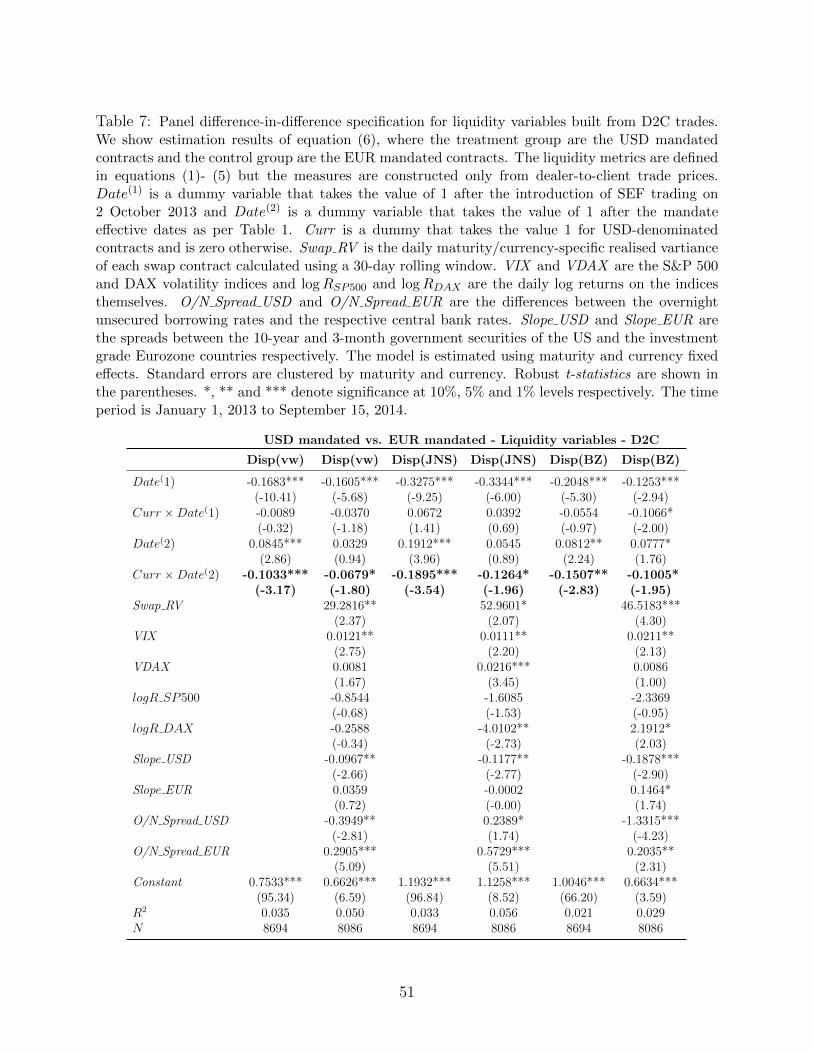
Table 7: Panel difference-in-difference specification for liquidity variables built from D2C trades.We show estimation results of equation (6), where the treatment group are the USD mandatedcontracts and the control group are the EUR mandated contracts. The liquidity metrics are definedin equations (1)- (5) but the measures are constructed only from dealer-to-client trade prices.Date(1) is a dummy variable that takes the value of 1 after the introduction of SEF trading on2 October 2013 and Date(2) is a dummy variable that takes the value of 1 after the mandateeffective dates as per Table 1. Curr is a dummy that takes the value 1 for USD-denominatedcontracts and is zero otherwise. Swap RV is the daily maturity/currency-specific realised vartianceof each swap contract calculated using a 30-day rolling window. VIX and VDAX are the S&P 500and DAX volatility indices and logRSP500 and logRDAX are the daily log returns on the indicesthemselves. O/N Spread USD and O/N Spread EUR are the differences between the overnightunsecured borrowing rates and the respective central bank rates. Slope USD and Slope EUR arethe spreads between the 10-year and 3-month government securities of the US and the investmentgrade Eurozone countries respectively. The model is estimated using maturity and currency fixedeffects. Standard errors are clustered by maturity and currency. Robust t-statistics are shown inthe parentheses. *, ** and *** denote significance at 10%, 5% and 1% levels respectively. The timeperiod is January 1, 2013 to September 15, 2014.

USD mandated vs. EUR mandated - Liquidity variables - D2C

Disp(vw) Disp(vw) Disp(JNS) Disp(JNS) Disp(BZ) Disp(BZ)

Date(1) -0.1683*** -0.1605*** -0.3275*** -0.3344*** -0.2048*** -0.1253***(-10.41) (-5.68) (-9.25) (-6.00) (-5.30) (-2.94)

Curr ×Date(1) -0.0089 -0.0370 0.0672 0.0392 -0.0554 -0.1066*(-0.32) (-1.18) (1.41) (0.69) (-0.97) (-2.00)

Date(2) 0.0845*** 0.0329 0.1912*** 0.0545 0.0812** 0.0777*(2.86) (0.94) (3.96) (0.89) (2.24) (1.76)

Curr ×Date(2) -0.1033*** -0.0679* -0.1895*** -0.1264* -0.1507** -0.1005*(-3.17) (-1.80) (-3.54) (-1.96) (-2.83) (-1.95)

Swap RV 29.2816** 52.9601* 46.5183***(2.37) (2.07) (4.30)

VIX 0.0121** 0.0111** 0.0211**(2.75) (2.20) (2.13)

VDAX 0.0081 0.0216*** 0.0086(1.67) (3.45) (1.00)

logR SP500 -0.8544 -1.6085 -2.3369(-0.68) (-1.53) (-0.95)

logR DAX -0.2588 -4.0102** 2.1912*(-0.34) (-2.73) (2.03)

Slope USD -0.0967** -0.1177** -0.1878***(-2.66) (-2.77) (-2.90)

Slope EUR 0.0359 -0.0002 0.1464*(0.72) (-0.00) (1.74)

O/N Spread USD -0.3949** 0.2389* -1.3315***(-2.81) (1.74) (-4.23)

O/N Spread EUR 0.2905*** 0.5729*** 0.2035**(5.09) (5.51) (2.31)

Constant 0.7533*** 0.6626*** 1.1932*** 1.1258*** 1.0046*** 0.6634***(95.34) (6.59) (96.84) (8.52) (66.20) (3.59)

R2 0.035 0.050 0.033 0.056 0.021 0.029N 8694 8086 8694 8086 8694 8086

51

Table 8: Panel difference-in-difference specification for liquidity variables for D2C trades. We showestimation results of specification (7), where the treatment group consists of the USD mandatedcontracts and the control group of the USD non-mandated contracts. The liquidity metrics aredefined in equations (1)- (5) but are constructed from dealer-to-client trade prices only. Date(1)

is a dummy variable that takes the value of 1 after the introduction of SEF trading on 2 October2013 and Date(2) is a dummy variable that takes the value of 1 after the mandate effective dates asper Table 1. MAT is a dummy that takes the value 1 for mandated contracts and is zero otherwise.Swap RV is the daily maturity/currency-specific realised variance of each swap contract calculatedusing a 30-day rolling window. VIX is the S&P 500 volatility index and logRSP500 is the log dailyreturn on the index itself. O/N Spread USD is the difference between the overnight unsecuredborrowing rate and the respective central bank rate. Slope USD is the spreads between the 10-yearand 3-month Treasury securities. The model is estimated using maturity fixed effects. Standarderrors are clustered by maturity. Robust t-statistics are shown in the parentheses. *, ** and ***denote significance at 10%, 5% and 1% levels respectively. The time period is January 1, 2013 toSeptember 15, 2014.

USD mandated vs. USD non-mandated - Liquidity variables - D2C

Disp(vw) Disp(vw) Disp(JNS) Disp(JNS) Disp(BZ) Disp(BZ)

Date(1) -0.1979*** -0.1757*** -0.2903*** -0.2757*** -0.2326*** -0.1961**(-5.93) (-5.63) (-4.52) (-4.40) (-3.79) (-2.70)

MAT ×Date(1) 0.0207 0.0134 0.0300 0.0264 -0.0276 -0.0198(0.51) (0.37) (0.42) (0.37) (-0.37) (-0.30)

Date(2) 0.0518*** 0.0447 0.0359*** -0.0233 0.0515 0.0983*(6.68) (1.63) (3.17) (-0.67) (1.29) (1.81)

MAT ×Date(2) -0.0706*** -0.0713*** -0.0342 -0.0393 -0.1210** -0.1108*(-4.44) (-4.50) (-1.32) (-1.59) (-2.16) (-2.10)

Swap RV 7.7447 6.1456 38.8071***(1.22) (0.68) (3.32)

VIX 0.0104 0.0090 0.0209(1.67) (1.65) (1.49)

VDAX 0.0176** 0.0267*** 0.0254*(2.69) (4.29) (2.13)

logR SP500 -3.7757** -3.8327* -7.4619**(-2.73) (-2.14) (-2.24)

logR DAX 0.4674 -0.1334 1.2727(0.50) (-0.12) (0.79)

Slope USD -0.2546 -0.2468 -0.7301*(-1.59) (-1.51) (-1.98)

Slope EUR 0.2419*** 0.4442*** 0.2265*(3.60) (4.67) (1.77)

O/N Spread USD -0.1193*** -0.1956*** -0.1436*(-4.15) (-5.36) (-1.86)

O/N Spread EUR 0.0913 0.0726 0.1983*(1.69) (1.04) (2.03)

Constant 0.7463*** 0.4960*** 1.0699*** 0.9949*** 1.1369*** 0.3963(70.02) (3.67) (68.05) (4.82) (60.88) (1.60)

R2 0.044 0.063 0.047 0.064 0.029 0.047N 5740 5329 5740 5329 5740 5329

52

Table 9: Panel difference-in-difference specification for liquidity variables built from D2D trades.We show estimation results of equation (6), where the treatment group are the USD mandatedcontracts and the control group are the EUR mandated contracts. The liquidity metrics are de-fined in equations (1)- (5) but the measures are constructed only from inter-dealer trade prices.Date(1) is a dummy variable that takes the value of 1 after the introduction of SEF trading on2 October 2013 and Date(2) is a dummy variable that takes the value of 1 after the mandateeffective dates as per Table 1. Curr is a dummy that takes the value 1 for USD-denominatedcontracts and is zero otherwise. Swap RV is the daily maturity/currency-specific realised vartianceof each swap contract calculated using a 30-day rolling window. VIX and VDAX are the S&P 500and DAX volatility indices and logRSP500 and logRDAX are the daily log returns on the indicesthemselves. O/N Spread USD and O/N Spread EUR are the differences between the overnightunsecured borrowing rates and the respective central bank rates. Slope USD and Slope EUR arethe spreads between the 10-year and 3-month government securities of the US and the investmentgrade Eurozone countries respectively. The model is estimated using maturity and currency fixedeffects. Standard errors are clustered by maturity and currency. Robust t-statistics are shown inthe parentheses. *, ** and *** denote significance at 10%, 5% and 1% levels respectively. The timeperiod is January 1, 2013 to September 15, 2014.

USD mandated vs. EUR mandated - Liquidity variables - D2D

Disp(vw) Disp(vw) Disp(JNS) Disp(JNS) Disp(BZ) Disp(BZ)

Date(1) -0.2073*** -0.2077*** -0.3200*** -0.3253*** -0.2745*** -0.2277***(-10.57) (-6.46) (-12.72) (-6.52) (-6.78) (-4.75)

Curr ×Date(1) 0.0194 0.0002 0.0509 0.0240 0.0336 -0.0148(0.61) (0.01) (1.30) (0.59) (0.54) (-0.27)

Date(2) 0.0815*** 0.0021 0.1895*** 0.0263 0.1039*** 0.0521(3.43) (0.08) (4.56) (0.50) (3.95) (1.29)

Curr ×Date(2) -0.1326*** -0.0923** -0.2232*** -0.1441** -0.2137*** -0.1707***(-4.40) (-2.47) (-4.75) (-2.29) (-5.58) (-3.80)

Swap RV 34.0819* 64.3465* 36.6113(1.75) (1.89) (1.67)

VIX 0.0083* 0.0043 0.0180*(1.81) (0.91) (2.07)

VDAX 0.0124** 0.0260*** 0.0113(2.57) (4.04) (1.28)

logRSP500 -2.9483*** -4.1101*** -4.0304*(-2.93) (-3.96) (-1.81)

logRDAX 1.4921** -1.5449 6.3466***(2.18) (-1.33) (5.34)

Slope USD -0.1337*** -0.1579** -0.2190***(-3.09) (-2.41) (-3.80)

Slope EUR 0.0353 0.0196 0.0962(0.52) (0.21) (0.93)

O/N Spread USD -0.3408 -0.0427 -1.0397***(-1.70) (-0.18) (-2.83)

O/N Spread EUR 0.4028*** 0.6490*** 0.4054***(5.89) (6.16) (3.90)

Constant 0.7820*** 0.8072*** 1.1886*** 1.2133*** 1.0276*** 0.9657***(81.73) (5.73) (97.67) (6.78) (64.51) (4.41)

R2 0.050 0.068 0.039 0.064 0.026 0.034N 8694 8086 8694 8086 8694 8086

53

Table 10: Panel difference-in-difference specification for liquidity variables for D2D trades. Weshow estimation results of specification (7), where the treatment group consists of the USD man-dated contracts and the control group of the USD non-mandated contracts. The liquidity metricsare defined in equations (1)- (5) but are constructed from inter-dealer trade prices only. Date(1)

is a dummy variable that takes the value of 1 after the introduction of SEF trading on 2 October2013 and Date(2) is a dummy variable that takes the value of 1 after the mandate effective dates asper Table 1. MAT is a dummy that takes the value 1 for mandated contracts and is zero otherwise.Swap RV is the daily maturity/currency-specific realised variance of each swap contract calculatedusing a 30-day rolling window. VIX is the S&P 500 volatility index and logRSP500 is the log dailyreturn on the index itself. O/N Spread USD is the difference between the overnight unsecuredborrowing rate and the respective central bank rate. Slope USD is the spreads between the 10-yearand 3-month Treasury securities. The model is estimated using maturity fixed effects. Standarderrors are clustered by maturity. Robust t-statistics are shown in the parentheses. *, ** and ***denote significance at 10%, 5% and 1% levels respectively. The time period is January 1, 2013 toSeptember 15, 2014.

USD mandated vs. USD non-mandated - Liquidity variables - D2D

Disp(vw) Disp(vw) Disp(JNS) Disp(JNS) Disp(BZ) Disp(BZ)

Date(1) -0.2206*** -0.2378*** -0.3670*** -0.3557*** -0.2648*** -0.3111***(-5.22) (-4.58) (-10.79) (-10.16) (-4.75) (-3.75)

MAT ×Date(1) 0.0327 0.0342 0.0979** 0.0843* 0.0239 0.0338(0.66) (0.61) (2.15) (2.14) (0.33) (0.40)

Date(2) -0.0475* -0.0618* 0.0050 -0.0448 -0.0388 -0.0239(-1.98) (-2.07) (0.12) (-1.03) (-0.87) (-0.40)

MAT ×Date(2) -0.0036 -0.0064 -0.0386 -0.0402 -0.0709 -0.0739(-0.12) (-0.21) (-0.84) (-0.82) (-1.34) (-1.35)

Swap RV -0.9503 5.4553 3.1516(-0.11) (0.35) (0.20)

VIX 0.0086* 0.0045 0.0200*(1.80) (0.99) (1.88)

VDAX 0.0205*** 0.0351*** 0.0252**(3.73) (4.12) (2.24)

logR SP500 -5.4071*** -4.0018** -10.6833***(-4.94) (-2.20) (-4.62)

logR DAX 1.4733** -0.3310 4.8861***(2.73) (-0.29) (3.95)

Slope USD -0.0251 -0.4298 -0.3192(-0.13) (-1.55) (-0.85)

Slope EUR 0.4794*** 0.5890*** 0.6621***(6.05) (7.06) (5.10)

O/N Spread USD -0.2032*** -0.2575*** -0.2880***(-5.38) (-4.70) (-4.11)

O/N Spread EUR 0.1680*** 0.1799** 0.2756**(3.19) (2.87) (2.57)

Constant 0.7450*** 0.6464*** 1.0580*** 0.9113*** 1.0981*** 0.8199**(66.76) (3.84) (63.32) (4.01) (64.10) (2.89)

R2 0.065 0.090 0.062 0.084 0.036 0.057N 5740 5329 5740 5329 5740 5329

54

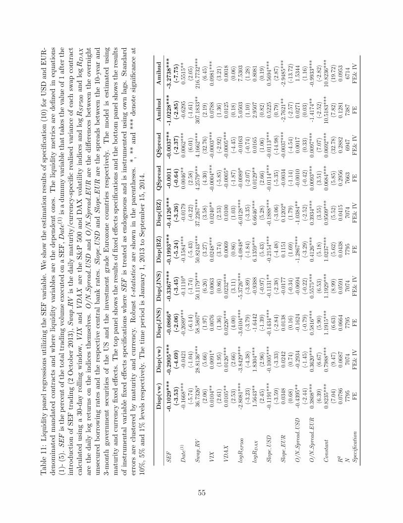
Tab

le11

:L

iqu

idit

yp

anel

regr

essi

ons

uti

lizi

ng

the

SE

Fva

riab

le.

We

show

the

esti

mat

ion

resu

lts

ofsp

ecifi

cati

on(1

0)fo

rU

SD

and

EU

R-

den

omin

ate

dm

an

dat

edco

ntr

act

san

dw

her

eli

qu

idit

yva

riab

les

are

the

dep

end

ent

ones

.T

he

liqu

idit

ym

etri

csar

ed

efin

edin

equ

atio

ns

(1)-

(5).

SE

Fis

the

per

cent

ofth

eto

taltr

adin

gvo

lum

eex

ecu

ted

ona

SE

F,Date

(1)

isa

du

mm

yva

riab

leth

atta

kes

the

valu

eof

1af

ter

the

intr

od

uct

ion

of

SE

Ftr

adin

g(2

Oct

ob

er20

13),

Sw

ap

RV

isth

ed

aily

mat

uri

ty/c

urr

ency

-sp

ecifi

cre

alis

edva

rian

ceof

each

swap

contr

act

calc

ula

ted

usi

ng

a30

-day

roll

ing

win

dow

,V

IXan

dV

DA

Xar

eth

eS

&P

500

and

DA

Xvol

atil

ity

ind

ices

and

logR

SP500

and

logR

DAX

are

the

dai

lylo

gre

turn

son

the

ind

ices

them

selv

es.

O/N

Spre

ad

US

Dan

dO

/N

Spre

ad

EU

Rar

eth

ed

iffer

ence

sb

etw

een

the

over

nig

ht

un

secu

red

borr

owin

gra

tes

and

the

resp

ecti

ve

centr

alb

ank

rate

s.S

lope

US

Dan

dS

lope

EU

Rar

eth

esp

read

sb

etw

een

the

10-y

ear

and

3-m

onth

gove

rnm

ent

secu

riti

esof

the

US

and

the

inve

stm

ent

grad

eE

uro

zon

eco

untr

ies

resp

ecti

vely

.T

he

mod

elis

esti

mat

edu

sin

gm

atu

rity

an

dcu

rren

cyfi

xed

effec

ts.

The

top

pan

elsh

ows

the

resu

lts

offi

xed

effec

tssp

ecifi

cati

ons

and

the

bot

tom

pan

elsh

ows

the

resu

lts

ofin

stru

men

tal

vari

able

fixed

effec

tssp

ecifi

cati

ons

wh

ere

SE

Fis

trea

ted

asen

dog

enou

san

dis

inst

rum

ente

du

sin

gow

nla

gs.

Sta

nd

ard

erro

rsare

clu

ster

edby

mat

uri

tyan

dcu

rren

cy.

Rob

ust

t-st

ati

stic

sar

esh

own

inth

ep

aren

thes

es.

*,**

and

***

den

ote

sign

ifica

nce

at10

%,

5%

and

1%le

vel

sre

spec

tive

ly.

Th

eti

me

per

iod

isJan

uar

y1,

2013

toS

epte

mb

er15

,20

14.

Dis

p(v

w)

Dis

p(v

w)

Dis

p(J

NS

)D

isp

(JN

S)

Dis

p(B

Z)

Dis

p(B

Z)

QS

pre

ad

QS

pre

ad

Am

ihu

dA

mih

ud

SE

F-0

.1029***

-0.2

905***

-0.0

866*

-0.3

367***

-0.1

993***

-0.4

126***

-0.0

011

-0.0

037**

-1.0

228***

-3.2

738***

(-3.5

3)

(-4.6

9)

(-2.0

6)

(-3.4

5)

(-5.2

4)

(-3.2

6)

(-0.6

4)

(-2.3

7)

(-2.8

5)

(-7.7

5)

Date

(1)

-0.1

668*

**-0

.042

1-0

.268

9***

-0.1

110*

-0.1

584*

**-0

.017

90.

0046

**0.

0062

***

-0.6

295

0.55

15**

(-5.

74)

(-1.

04)

(-6.

14)

(-1.

74)

(-5.

43)

(-0.

22)

(2.5

8)(6

.01)

(-1.

61)

(2.0

5)S

wap

RV

36.7

326*

28.8

136*

**58

.580

7*50

.117

9***

50.8

243*

**37

.226

7***

4.25

79**

*4.

1662

***

307.

1833

**21

6.77

32**

*(2

.06)

(5.6

6)(1

.97)

(6.2

6)(3

.27)

(3.5

8)(4

.30)

(32.

76)

(2.1

9)(6

.45)

VIX

0.01

04**

0.00

91*

0.00

760.

0063

0.02

48**

*0.

0240

**-0

.000

4***

-0.0

003*

**0.

0788

0.09

81**

*(2

.61)

(1.9

5)(1

.36)

(0.8

6)(3

.74)

(2.5

3)(-

5.85

)(-

2.92

)(1

.36)

(3.2

1)V

DA

X0.

0105

**0.

0126

***

0.02

26**

*0.

0232

***

0.00

690.

0100

-0.0

005*

-0.0

005*

**0.

0125

0.00

18(2

.53)

(2.6

6)(4

.00)

(3.1

1)(0

.86)

(1.0

3)(-

1.87

)(-

4.45

)(0

.18)

(0.0

6)logR

SP500

-2.8

081*

**-3

.842

9***

-3.6

104*

**-5

.372

6***

-4.0

848*

-6.0

128*

**-0

.008

9*-0

.016

35.

0503

7.53

03(-

3.23

)(-

4.38

)(-

3.79

)(-

3.89

)(-

1.84

)(-

3.35

)(-

2.07

)(-

0.74

)(1

.10)

(1.2

8)logR

DAX

1.56

43**

1.83

04**

*-1

.644

2-0

.938

86.

1359

***

6.66

46**

*0.

0129

**0.

0165

2.95

070.

8081

(2.4

5)(2

.96)

(-1.

39)

(-0.

97)

(5.4

3)(5

.28)

(2.6

6)(1

.06)

(0.8

2)(0

.19)

Slo

peU

SD

-0.1

191*

**-0

.100

5***

-0.1

434*

**-0

.113

1**

-0.2

154*

**-0

.188

8***

-0.0

114*

**-0

.011

3***

0.52

250.

5694

***

(-3.

59)

(-3.

33)

(-2.

84)

(-2.

38)

(-4.

48)

(-3.

06)

(-5.

35)

(-14

.98)

(0.7

9)(2

.87)

Slo

peE

UR

0.03

480.

0242

0.01

38-0

.017

70.

1151

0.12

02*

-0.0

034

-0.0

037*

**-2

.762

1**

-2.9

485*

**(0

.68)

(0.7

4)(0

.16)

(-0.

34)

(1.6

9)(1

.79)

(-1.

14)

(-4.

54)

(-2.

57)

(-13

.72)

O/N

Spr

ead

US

D-0

.439

5**

-0.2

934

-0.1

624

-0.0

694

-1.2

867*

**-1

.038

4**

-0.0

010

0.00

170.

0271

1.53

44(-

2.44

)(-

1.45

)(-

0.79

)(-

0.22

)(-

3.29

)(-

2.52

)(-

0.42

)(0

.33)

(0.0

3)(1

.16)

O/N

Spr

ead

EU

R0.

3808

***

0.36

20**

*0.

5816

***

0.55

75**

*0.

4126

***

0.39

34**

*0.

0093

***

0.00

97**

*-1

.417

4**

-0.9

933*

**(6

.39)

(6.6

7)(5

.90)

(6.5

3)(5

.18)

(3.5

5)(3

.51)

(7.0

7)(-

2.52

)(-

2.82

)C

onst

ant

0.82

35**

*0.

7988

***

1.19

15**

*1.

1929

***

1.02

37**

*0.

9509

***

0.06

84**

*0.

0692

***

10.5

183*

**10

.823

6***

(7.0

4)(9

.47)

(6.6

3)(8

.99)

(5.6

2)(5

.52)

(5.8

5)(3

2.78

)(7

.82)

(19.

72)

R2

0.07

860.

0687

0.06

640.

0591

0.04

380.

0415

0.29

560.

2882

0.12

810.

0953

N77

9570

7477

9570

7477

9570

7476

6369

4773

8767

14S

peci

fica

tion

FE

FE

&IV

FE

FE

&IV

FE

FE

&IV

FE

FE

&IV

FE

FE

&IV

55

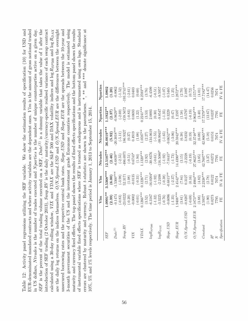
Tab

le12

:A

ctiv

ity

pan

elre

gre

ssio

ns

uti

lizi

ng

the

SE

Fva

riab

le.

We

show

the

esti

mat

ion

resu

lts

ofsp

ecifi

cati

on(1

0)fo

rU

SD

and

EU

R-d

enom

inat

edm

and

ate

dco

ntr

acts

an

dw

her

eac

tivit

yva

riab

les

are

the

dep

end

ent

ones

.Vlm

isth

eam

ount

ofgr

oss

not

ion

altr

aded

inU

Sd

olla

rs,Ntrades

isth

enu

mb

erof

trad

esex

ecu

ted

andNparties

isth

enu

mb

erof

un

iqu

eco

unte

rpar

ties

acti

veon

agi

ven

day

.S

EF

isth

ep

erce

nt

ofth

eto

tal

trad

ing

volu

me

exec

ute

don

aS

EF

,Date

(1)

isa

du

mm

yva

riab

leth

atta

kes

the

valu

eof

1af

ter

the

intr

od

uct

ion

ofS

EF

tradin

g(2

Oct

ober

201

3),

Sw

ap

RV

isth

ed

aily

mat

uri

ty/c

urr

ency

-sp

ecifi

cre

alis

edva

rian

ceof

each

swap

contr

act

calc

ula

ted

usi

ng

a30

-day

roll

ing

win

dow

,V

IXan

dV

DA

Xar

eth

eS

&P

500

and

DA

Xvol

atil

ity

ind

ices

and

logR

SP500

and

logR

DAX

are

the

dai

lylo

gre

turn

son

the

ind

ices

them

selv

es.

O/N

Spre

ad

US

Dan

dO

/N

Spre

ad

EU

Rar

eth

ed

iffer

ence

sb

etw

een

the

over

nig

ht

un

secu

red

borr

owin

gra

tes

and

the

resp

ecti

ve

centr

alb

ank

rate

s.S

lope

US

Dan

dS

lope

EU

Rar

eth

esp

read

sb

etw

een

the

10-y

ear

and

3-m

onth

gove

rnm

ent

secu

riti

esof

the

US

and

the

inve

stm

ent

grad

eE

uro

zon

eco

untr

ies

resp

ecti

vely

.T

he

mod

elis

esti

mat

edu

sin

gm

atu

rity

an

dcu

rren

cyfi

xed

effec

ts.

The

top

pan

elsh

ows

the

resu

lts

offi

xed

effec

tssp

ecifi

cati

ons

and

the

bot

tom

pan

elsh

ows

the

resu

lts

ofin

stru

men

tal

vari

able

fixed

effec

tssp

ecifi

cati

ons

wh

ere

SE

Fis

trea

ted

asen

dog

enou

san

dis

inst

rum

ente

du

sin

gow

nla

gs.

Sta

nd

ard

erro

rsare

clu

ster

edby

mat

uri

tyan

dcu

rren

cy.

Rob

ust

t-st

ati

stic

sar

esh

own

inth

ep

aren

thes

es.

*,**

and

***

den

ote

sign

ifica

nce

at10

%,

5%

and

1%le

vel

sre

spec

tive

ly.

Th

eti

me

per

iod

isJan

uar

y1,

2013

toS

epte

mb

er15

,20

14.

Vlm

Vlm

Ntr

ad

es

Ntr

ades

Np

art

ies

Np

art

ies

SE

F1.0

991**

3.5

368***

12.5

107**

36.0

019***

1.1

922**

1.0

802

(2.3

9)

(6.0

0)

(2.4

6)

(5.9

2)

(2.3

7)

(1.2

0)

Date

(1)

-0.1

474

-1.5

360*

**-6

.683

9**

-20.

3018

***

-0.9

629*

*-0

.896

2(-

0.83

)(-

3.98

)(-

2.55

)(-

5.11

)(-

2.69

)(-

1.52

)S

wap

RV

-23.

0222

52.3

171

-486

.697

118

6.93

27-1

59.5

672

-193

.274

5***

(-0.

20)

(1.0

8)(-

0.51

)(0

.37)

(-0.

83)

(-2.

61)

VIX

-0.0

002

-0.0

135

0.67

43*

0.49

190.

0693

0.04

03(-

0.01

)(-

0.31

)(1

.94)

(1.0

8)(1

.22)

(0.6

0)V

DA

X0.

1266

***

0.12

26**

*1.

1320

***

1.05

97**

0.22

41**

*0.

2593

***

(3.5

2)(2

.71)

(2.9

2)(2

.27)

(3.5

3)(3

.76)

logR

SP500

-6.3

167

-16.

0204

*-3

0.83

76-1

34.0

619

2.00

93-6

.459

9(-

1.32

)(-

1.92

)(-

0.61

)(-

1.55

)(0

.30)

(-0.

51)

logR

DAX

-3.3

225

-2.2

498

-116

.508

0*-9

9.99

45*

-9.8

547

-9.5

957

(-0.

76)

(-0.

38)

(-1.

92)

(-1.

65)

(-1.

35)

(-1.

07)

Slo

peU

SD

-0.6

096

-0.6

815*

*-7

.044

5*-9

.065

2***

0.32

290.

5465

(-1.

35)

(-2.

37)

(-1.

73)

(-3.

06)

(0.4

7)(1

.25)

Slo

peE

UR

1.94

08**

*2.

4542

***

14.4

390*

**20

.594

2***

1.25

971.

2872

***

(3.8

1)(7

.84)

(3.1

5)(6

.38)

(1.5

8)(2

.70)

O/N

Spr

ead

US

D-0

.820

70.

3127

-2.2

228

3.82

32-0

.579

72.

1097

(-0.

69)

(0.1

6)(-

0.19

)(0

.19)

(-0.

19)

(0.7

2)O

/NS

prea

dE

UR

2.18

73**

*2.

4904

***

27.8

625*

**32

.374

8***

2.96

34**

*3.

1571

***

(3.8

8)(4

.82)

(3.8

5)(6

.08)

(3.4

0)(4

.01)

Con

stan

t2.

5937

*2.

2338

***

42.7

607*

**42

.866

5***

17.7

379*

**17

.718

2***

(1.9

0)(2

.78)

(3.3

7)(5

.18)

(12.

67)

(14.

47)

R2

0.02

730.

0122

0.02

720.

0151

0.02

370.

0256

N77

9570

7477

9570

7477

9570

74S

peci

fica

tion

FE

IV&

FE

FE

IV&

FE

FE

IV&

FE

56

Table 13: Difference-in-differences regression of the number of unique dealers per client. We showthe estimation results of model (11). Ndealersit is the number of unique dealers with whom client

i trades in month t. Date(1)t is a dummy variable that takes the value of 1 after the introduction

of SEF trading (2 October 2013) and Date(2)t is the February 2014 mandated trading dummy. USi

is a dummy for clients that are US legal entities and USACTIV Ei is a dummy for US clients whotrade more than 20 times a month (on average). V lmit, Ntradesit and Ncontractsit are the volumetraded (in £billions), the number of trades executed and the number of different contracts tradedrespectively by client i in month t. Robust t-statistics are shown in the parentheses. *, ** and ***denote significance at 10%, 5% and 1% levels respectively. The time period is January 1, 2013 toSeptember 15, 2014.

Ndealers Ndealers

Date(1) 0.3557* 0.1572(1.94) (1.04)

Date(2) -0.0161 0.0965(-0.06) (0.46)

US ×Date(1) 0.1904 0.1875(0.59) (0.68)

US ×Date(2) -0.6695 -0.7345*(-1.44) (-1.92)

ACTIV E 3.6733*** 1.9699***(8.28) (5.85)

Date(1) × ACTIV E -0.0479 0.3396(-0.18) (1.58)

Date(2) × ACTIV E 0.0066 -0.2495(0.02) (-0.74)

US × ACTIV E 0.6325 0.6239(0.95) (1.17)

US ×Date(1) × ACTIV E -0.3178 -0.2169(-0.59) (-0.49)

US ×Date(2) × ACTIV E 1.5754*** 1.8168***(2.62) (3.29)

Ntrades 0.0064***(5.83)

Trade size 0.2022(0.25)

Ncontracts 0.4966***(14.94)

Constant 5.3342*** 2.7448***(37.99) (13.32)

Fixed Effects Yes Yes

R2 0.620 0.841N 2633 2633

57

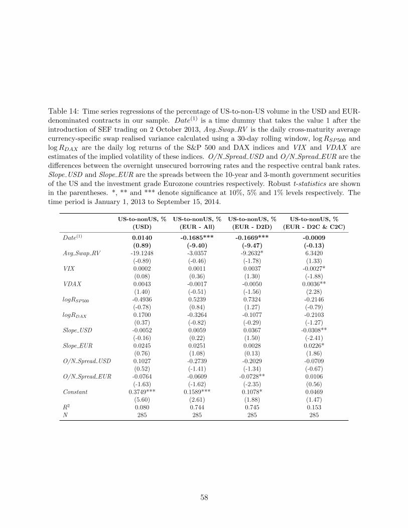
Table 14: Time series regressions of the percentage of US-to-non-US volume in the USD and EUR-denominated contracts in our sample. Date(1) is a time dummy that takes the value 1 after theintroduction of SEF trading on 2 October 2013, Avg Swap RV is the daily cross-maturity averagecurrency-specific swap realised variance calculated using a 30-day rolling window, logRSP500 andlogRDAX are the daily log returns of the S&P 500 and DAX indices and VIX and VDAX areestimates of the implied volatility of these indices. O/N Spread USD and O/N Spread EUR are thedifferences between the overnight unsecured borrowing rates and the respective central bank rates.Slope USD and Slope EUR are the spreads between the 10-year and 3-month government securitiesof the US and the investment grade Eurozone countries respectively. Robust t-statistics are shownin the parentheses. *, ** and *** denote significance at 10%, 5% and 1% levels respectively. Thetime period is January 1, 2013 to September 15, 2014.

US-to-nonUS, % US-to-nonUS, % US-to-nonUS, % US-to-nonUS, %

(USD) (EUR - All) (EUR - D2D) (EUR - D2C & C2C)

Date(1) 0.0140 -0.1685*** -0.1669*** -0.0009(0.89) (-9.40) (-9.47) (-0.13)

Avg Swap RV -19.1248 -3.0357 -9.2632* 6.3420(-0.89) (-0.46) (-1.78) (1.33)

VIX 0.0002 0.0011 0.0037 -0.0027*(0.08) (0.36) (1.30) (-1.88)

VDAX 0.0043 -0.0017 -0.0050 0.0036**(1.40) (-0.51) (-1.56) (2.28)

logRSP500 -0.4936 0.5239 0.7324 -0.2146(-0.78) (0.84) (1.27) (-0.79)

logRDAX 0.1700 -0.3264 -0.1077 -0.2103(0.37) (-0.82) (-0.29) (-1.27)

Slope USD -0.0052 0.0059 0.0367 -0.0308**(-0.16) (0.22) (1.50) (-2.41)

Slope EUR 0.0245 0.0251 0.0028 0.0226*(0.76) (1.08) (0.13) (1.86)

O/N Spread USD 0.1027 -0.2739 -0.2029 -0.0709(0.52) (-1.41) (-1.34) (-0.67)

O/N Spread EUR -0.0764 -0.0609 -0.0728** 0.0106(-1.63) (-1.62) (-2.35) (0.56)

Constant 0.3749*** 0.1589*** 0.1078* 0.0469(5.60) (2.61) (1.88) (1.47)

R2 0.080 0.744 0.745 0.153N 285 285 285 285

58