staff papers - IMF eLibrary - International Monetary Fund
209
-
Upload
khangminh22 -
Category
Documents
-
view
1 -
download
0
Transcript of staff papers - IMF eLibrary - International Monetary Fund


STAFF PAPERS
CHARLES S. GARDNER, Acting Editor
JENNIE LEE CARTER and JAMES MCEUEN
Assistant Editors
Editorial Committee
Charles S. Gardner, Acting Chairman
Bijan B. Aghevli Peter S. Heller
Gerard Belanger Anthony Lanyi
Morris Goldstein M. Ranji P. Salgado
Ernesto Hernandez-Cata V. Sundararajan
From the Foreword to the first issue:
Among the responsibilities of the International Monetary Fund, as setforth in the Articles of Agreement, is the obligation to "act as a center for thecollection and exchange of information on monetary and financial prob-lems," and thereby to facilitate "the preparation of studies designed to assistmembers in developing policies which further the purposes of the Fund."The publications of the Fund are one way in which this responsibility isdischarged.
Through the publication of Staff Papers, the Fund is making availablesome of the work of members of its staff. The Fund believes that thesepapers will be found helpful by government officials, by professionaleconomists, and by others concerned with monetary and financial problems.Much of what is now presented is quite provisional. On some internationalmonetary problems, final and definitive views are scarcely to be expected inthe near future, and several alternative, or even conflicting, approachesmay profitably be explored. The views presented in these papers are not,therefore, to be interpreted as necessarily indicating the position of theExecutive Board or of the officials of the Fund.
The authors of the papers in this issue have received considerable assistancefrom their colleagues on the staff of the Fund. This general statement ofindebtedness may be accepted in place of a detailed list of acknowledgments.
Subscription: US$15.00 a volume or the approximate equivalent in thecurrencies of most countries. Four numbers constitute a volume. Single copiesmay be purchased at $4.00. Special rates to university libraries, faculty members,and students: $7.50 a volume; $4.00 a single copy. Subscriptions and ordersshould be sent to:
Publications UnitInternational Monetary FundWashington, D.C. 20431, U.S.A.
Telephone number: (202) 623-7430Cable address: Interfund
©International Monetary Fund. Not for Redistribution

©International Monetary Fund. Not for Redistribution
INTERNATIONAL MONETARY FUND
STAFF
PAPERS
VOLUME 33, 1986
WASHINGTON, D.C.

©International Monetary Fund. Not for Redistribution
EDITOR'S NOTE
The Editor invites from contributors outside the Fund brief comments (not more than 1 ,000 words) on published articles in Staff Papers. These comments should be addressed to the Editor, who will forward them to the author of the original article for reply. Both the comments and the reply will be published in the same issue of Staff Papers.
The Ediror regrets that, owing to production difficulties. publication of this
issue of Staff Papers has been delayed.
The term "country," as used in this publication, may not refer to a territorial entity that is a state as understood by international law and practice; the term may also cover sorne territorial entities that are not states but for which statistical data are maintained and provided intemationally on a separate and independent basis.
4:> 1986 by the International Monetary Fund International Standard Seriai Number: ISSN 0020-8027
The U.S. Library of Congress has cataloged this seria/ publication as follows:
International Monetary Fund Staff papers - International Monetary Fund. v. 1- Feb. 1950-
(Washington] International Monetary Fund.
HG3810.15
v. tables. diagrs. 23 cm.
Three no. a year. 1950-1977; four no. a year. 1978-Text in English with summaries in English. French. and Spanish. Indexes:
Vols. 1-27. 1950-80. 1 v.
ISSN 0020-8027 = Staff papers - International Munetary Fund.
1. Foreign exchange-Periodicals. 2. Commerce-Periodicals. 3. Cu.rren· cy question--Periodicals.
332.082 53-35483

©International Monetary Fund. Not for Redistribution
Contents of Volume 33
Volume 33 (1986) consists of four issues, as follows: March, pages 1-198 June, pages 199-386 September, pages 387-632
December, pages 633-821. English, French, and Spanish summaries appear at the end of each issue (March, pages 185-98; June, pages 373-86; September, pages 616-32; December, pages 812-21. The French and Spanish summaries are listed below by title, beginning on pages vi and vii, respectively.
Au thors
Adams, Charles, and Daniel Gros. The Consequences of Real Exchange Rate Rules for Inflation: Sorne lllustrative Examples............. 439
Argy, Victor, J.J. Polak, Gottfried Haberler, Richard S. Thorn, and H. Robert Helier. William H. White (1922-83): An Appreciation 199
Buiter, Willem H. Macroeconomie Policy Design in an Interdependent World Economy: An Analysis of Three Contingencies............ 541
Chopra, Ajai, and Peter Montiel. Output and Unanticipated Money with lmported lntermediate Goods and Foreign Exchange Rationing . . . 697
Chu, Ke-young, and Thomas K. Morrison. World Non-Oïl Primary Commodity Markets: A Medium-Term Framework of Analysis ........ 139
Dewald, William G. Government Deficits in a Generalized Fisherian Credit Market: Theory with an Application to Indexing Interest Taxation . . . . . . . . . . . . . . . . . . . . . . . . . . . . . . . . . . . . . . . . . . . . . . . . . . . . 243
De Wulf, Luc, and David Goldsbrough. The Evolving Role of Monetary Policy in China . . . . . . . . . . . . . . . . . . . . . . . . . . . . . . . . . . . . . . . . . . . . . . 209
Feige, Edgar L. A Re-Examination of the "Underground Economy" in the United States: A Comment on Tanzi . . . . . . . . . . . . . . . . . . . . . . . 768
Feltenstein, Andrew. Financial Crowding Out: Theory with an Applica-tion to Australia . . . . . . . . . . . . . . . . . . . . . . . . . . . . . . . . . . . . . . . . . . . . . 60
Frenkel, Jacob A., and Morris Goldstein. A Guide to Target Zones . . . 633 Goldsbrough, David, and Luc De Wulf. The Evolving Role of Monetary
Policy in China . . . . . . . . . . . . . . . . . . . . . . . . . . . . . . . . . . . . . . . . . . . . . . 209
lll

©International Monetary Fund. Not for Redistribution
iv CONTENTS OF VOLUME 33
Goldstein, Morris, and Jacob A. Frenkel. A Guide to Target Zones . . . 633 Goldstein, Morris, and Peter Montiel. Evaluating Fund Stabilization Pro
grams with Multicountry Data: Sorne Methodological Pitfalls. . . . . . 304 Gros, Daniel. Wage Indexation and the Real Exchange Rate in Small
Open Economies: A Study of the Effects of Fluctuations in Export Earnings . . . . . . . . . . . . . . . . . . . . . . . . . . . . . . . . . . . . . . . . . . . . . . . . . . . . 117
Gros, Daniel, and Charles Adams. The Consequences of Real Exchange Rate Rules for Inflation: Sorne Illustrative Examples............. 439
Haas, Richard D., and Paul R. Masson. MINIMOD: Specification and Sim-ulation Results . . . . . . . . . . . . . . . . . . . . . . . . . . . . . . . . . . . . . . . . . . . . . . 722
Haberler, Gottfried, J.J. Polak, Richard S. Thorn, Victor Argy, and H. Robert Helier. William H. White (1922-83): An Appreciation 199
Helier, H. Robert, J.J. Polak, Gottfried Haberler, Richard S. Thorn, and Victor Argy. William H. White (1922-83): An Appreciation...... 199
Khan, Mohsin S. Islamic lnterest-Free Banking . . . . . . . . . . . . . . . . . . . . . 1 Knight, Malcolm, and Paul R. Masson. International Transmission of
Fiscal Policies in Major Industrial Countries . . . . . . . . . . . . . . . . . . . . 387 Masson, Paul R., and Malcolm Knight. International Transmission of
Fiscal Policies in Major lndustrial Countries . . . . . . . . . . . . . . . . . . . . 387 Masson, Paul R., and Richard D. Haas. MJNIMOO: Specification and Sim-
ulation Results . . . . . . . . . . . . . . . . . . . . . . . . . . . . . . . . . . . . . . . . . . . . . . 722 Molho, Lazaros E. Interest Rates, Saving, and Investment in Developing
Countries: A Re-examination of the McKinnon-Shaw Hypotheses 90 Molho, Lazaros E. Selective Credit Controls in Greece: A Test of Their
Effectiveness .... ............................................ 477 Montiel, Peter. Long-Run Equilibrium in a Keynesian Mode! of a Small
Open Economy. . . . . . . . . . . . . . . . . . . . . . . . . . . . . . . . . . . . . . . . . . . . . . 28 Montiel, Peter. An Optimizing Mode! of Household Behavior Under
Credit Rationing............................................. 583 Montiel, Peter, and Ajai Chopra. Output and Unanticipated Money with
Imported Intermediate Goods and Foreign Exchange Rationing . . . 697 Montiel, Peter, and Morris Goldstein. Evaluating Fund Stabilization Pro
grams with Multicountry Data: Sorne Methodological Pitfalls. . . . . . 304 Morrison, Thomas K., and Ke-young Chu. World Non-Oïl Primary Com
modity Markets: A Medium-Term Framework of Analysis........ 139 Phelps, Edmund S. Profits Theory and Profits Taxation . . . . . . . . . . . . . . 674 Polak, J.J., Gottfried Haberler, Richard S. Thorn, Victor Argy, and
H. Robert Heller. William H. White (1922-83): An Appreciation 199 Riechel, Klaus-Walter. Labor Market Disequilibrium and the Scope for
Work-Sharing: A Case Study of the Netherlands. . . . . . . . . . . . . . . . . 509 Schadler, Susan M. Effect of a Slowdown in Industrial Economies on
Selected Asian Countries . . . . . . . . . . . . . . . . . . . . . . . . . . . . . . . . . . . . . 345 Tanzi, Vito. The Underground Economy in the United States: Reply to
Comments by Feige, Thomas, and Zilberfarb . . . . . . . . . . . . . . . . . . . 799 Thomas, J.J. The Underground Economy in the United States: A Com-
ment on Tanzi. . . . . . . . . . . . . . . . . . . . . . . . . . . . . . . . . . . . . . . . . . . . . . . 782

©International Monetary Fund. Not for Redistribution
CONTENTS OF VOLUME 33 V
Thorn, Richard S., J.J. Polak, Gottfried Haberler, Victor Argy, and H. Robert Helier. William H. White (1922-83): An Appreciation 199
Zaidi, Iqbal M. Currency Depreciation and Nonclearing Markets in Developing Economies. . . . . . . . . . . . . . . . . . . . . . . . . . . . . . . . . . . . . . . . . . 276
Zilberfarb, Ben-Zion. Estimates of the Underground Economy in the United States, 1930-80: A Comment on Tanzi . . . . . . . . . . . . . . . . . . 790
Titi es
The Consequences of Real Exchange Rate Rules for Inflation: Sorne Illustrative Examples. By Charles Adams and Daniel Gros . . . . . . . 439
Currency Depreciation and Nonclearing Markets in Developing Econo-mies. By Iqbal M. Zaidi . . . . . . . . . . . . . . . . . . . . . . . . . . . . . . . . . . . . . . 276
Effect of a Slowdown in Industrial Economies on Selected Asian Coun-tries. By Susan M. Schadler. . . . . . . . . . . . . . . . . . . . . . . . . . . . . . . . . . . 345
Estima tes of the Underground Eco nom y in the United States, 1930-80: A Comment on Tanzi. By Ben-Zion Zilberfarb . . . . . . . . . . . . . . . . . . . . 790
Evaluating Fund Stabilization Programs witb Multicountry Data: Sorne Methodological Pitfalls. By Morris Goldstein and Peter Montiel . . . 304
The Evolving Role of Monetary Policy in China. By Luc De Wulf and David Goldsbrough . . . . . . . . . . . . . . . . . . . . . . . . . . . . . . . . . . . . . . . . . . 209
Financial Crowding Out: Theory with an Application to Australia. By Andrew Feltenstein . . . . . . . . . . . . . . . . . . . . . . . . . . . . . . . . . . . . . . . . . . 60
Government Deficits in a Generalized Fisherian Credit Market: Theory with an Application to Indexing Interest Taxation. By William G. Dewald ..................................................... 243
A Guide to Target Zones. By Jacob A. Frenkel and Morris Goldstein 633 Interest Rates, Saving, and lnvestment in Developing Countries: A Re
examination of the McKinnon-Shaw Hypotheses. By Lazaros E. Molho...................................................... 90
International Transmission of Fiscal Policies in Major lndustrial Coun-tries. By Paul R. Masson and Malcolm Knight . . . . . . . . . . . . . . . . . . 387
Islamic Interest-Free Banking. By Mohsin S. Khan . . . . . . . . . . . . . . . . . . 1 Labor Market Disequilibrium and the Scope for Work-Sharing: A Case
Study of the Netherlands. By Klaus-Walter Riechel .............. 509 Long-Run Equilibrium in a Keynesian Model of a Small Open Economy.
By Peter Montiel . . . . . . . . . . . . . . . . . . . . . . . . . . . . . . . . . . . . . . . . . . . . 28 Macroeconomie Policy Design in an Interdependent World Economy: An
Analysis of Three Contingencies. By Willem H. Buiter........... 541 MINIMOD: Specification and Simulation Results. By Richard D. Haas and
Paul R. Masson . . . . . . . . . . . . . . . . . . . . . . . . . . . . . . . . . . . . . . . . . . . . . 722 An Optirnizing Model of Household Behavior Under Credit Rationing.
By Peter Montiel . . . . . . . . . . . . . . . . . . . . . . . . . . . . . . . . . . . . . . . . . . . . 583

©International Monetary Fund. Not for Redistribution
vi CONTENTS OF VOLUME 33
Output and Unanticipated Money with Imported lntermediate Goods and Foreign Exchange Rationing. By Ajai Chopra and Peter Montiel . . 697
Profits Theory and Profits Taxation. By Edmund S. Phelps . . . . . . . . . . . 674 A Re-Examination of the "Underground Economy" in the United States:
A Comment on Tanzi. By Edgar L. Feige . . . . . . . . . . . . . . . . . . . . . . 768
Selective Credit Controls in Greece: A Test of Their Effe.ctiveness. By Lazaros E. Molho . . . . . . . . . . . . . . . . . . . . . . . . . . . . . . . . . . . . . . . . . . . 477
The Underground Economy in the United States: A Comment on Tanzi. By J .J. Thomas ............................... ,. . . . . . . . . . . . . . . 782
The Underground Economy in the United States: Reply to Comments by Feige, Thomas, and Zilberfarb. By Vito Tanzi................... 799
Wage Indexation and the Real Exchange Rate in Small Open Economies: A Study of the Effects of Fluctuations in Export Earnings. By Daniel Gros ....................................................... 117
William H. White (1922-83): An Appreciation. By J.J. Polak, Gottfried Haberler, Richard S. Thorn, Victor Argy, and H. Robert. Helier . . 199
World Non-Oil Primary Commodity Markets: A Medium-Term Frame-work of Analysis. By Ke-young Chu and Thomas K. Morrison . . . . 139
Résumés
Conception de la politique macroéconomique dans une économie mondiale interdépendante: analyse de trois éventualités. Par Willem H. Buiter . . . . . . . . . . . . . . . . . . . . . . . . . . . . . . . . . . . . . . . . . . . . . . . . . . . . . . 624
Déficits publics dans le contexte d'un marché du crédit décrit par un modèle général de type Fisher: théorie et application à l'indexation des impôts frappant les intérêts. Par William G. Dewald. . . . . . . . . . 378
Dépréciation de la monnaie et marchés qui ne s'équilibrent pas dans les pays en développement. Par Iqbal M. Zaidi...................... 378
Déséquilibre du marché du travail et effets du partage du travail : étude du cas des Pays-Bas. Par Klaus-Walter Riechel............ .. . . . . . . . . 623
Effets du ralentissement de la croissance économique dans les pays industrialisés sur certains pays asiatiques. Par Susan M. Schadler . . . . . . . 380
Encadrement sélectif du crédit en Grèce : test de son efficacité. Par Lazaros E. Molho . . . . . . . . . . . . . . . . . . . . . . . . . . . . . . . . . . . . . . . . . . . 622
Equilibre à long terme dans un modèle keynésien décrivant une petite économie ouverte. Par Peter Montiel. . . . . . . . . . . . . . . . . . . . . . . . . . . 190
Evaluation des programmes de stabilisation du Fonds à partir de données sur divers pays : quelques écueils méthodologiques. Par Morris Goldstein et Peter Montiel . . . . . . . . . . . . . . . . . . . . . . . . . . . . . . . . . . . . 379
Éviction en matière de financement : théorie et application au cas de l'Australie. Par Andrew Feltenstein ............................ 190
Evolution du rôle de la politique monétaire en Chine. Par Luc De Wulf et David Goldsbrough . . . . . . . . . . . . . . . . . . . . . . . . . . . . . . . . . . . . . . . . . . 377

©International Monetary Fund. Not for Redistribution
CONTENTS OF VOLUME 33 vii
Incidence sur l'inflation des règles régissant le taux de change réel: quelques exemples. Par Charles Adams et Daniel Gros. . . . . . . . . . . 622
Indexation des salaires et taux de change réel dans de petits pays à économie ouverte : étude des effets des fluctuations des recettes d'exportation. Par Daniel Gros ................................ 192
Marchés internationaux de produits primaires non pétroliers : cadre d'analyse à moyen terme. Par Ke-young Chu et Thomas K. Morrison 193
MINlMOD : spécification et résultats des simulations. Par Richard D. Haas et Paul R. Masson . . . . . . . . . . . . . . . . . . . . . . . . . . . . . . . . . . . . . . . . . . . 817
Un modèle d'optimisation du comportement des ménages dans une situation de rationnement du crédit. Par Peter Montiel . . . . . . . . . . . . . 625
Le point sur les zones-objectifs. Par Jacob A. Frenkel et Morris Goldstein . . . . . . . . . . . . . . . . . . . . . . . . . . . . . . . . . . . . . . . . . . . . . . . . . . . 815
Production et variations imprévues de la masse monétaire dans le contexte de produits intermédiaires importés et d'un rationnement des devises. Par Ajai Chopra et Peter Montiel.............................. 816
Le système bancaire islamique : analyse théorique d'un système qui ne fait pas appel à l'intérêt. Par Mohsin S. Khan....................... 189
Taux d'intérêt, épargne et investissement dans les pays en développement : réexamen des hypothèses de McKinnon et de Shaw. Par Lazaros E. Molho . . . . . . . . . . . . . . . . . . . . . . . . . . . . . . . . . . . . . . . . . . . 191
Témoignage de gratitude à M. William H. White (1922-83). Par J.J. Polak, Gottfried Haberler, Richard S. Thorn, Victor Argy et H. Robert Helier . . . . . . . . . . . . . . . . . . . . . . . . . . . . . . . . . . . . . . . . . . . . 377
Théorie des bénéfices et imposition des bénéfices. Par Edmund S. Phelps 815 Transmission sur le plan international des effets des politiques budgétaires
des grands pays industrialisés. Par Paul R. Masson et Malcolm Knight 621
Resumenes
Controles selectivos al crédita en Grecia: Comprobaci6n de su eficacia. Por Lazaros E. Molho. . . . . . . . . . . . . . . . . . . . . . . . . . . . . . . . . . . . . . . . 628
Los déficit estatales en un mercado de crédita generalizado de "Fisher": Teorfa y aplicaci6n a la indizaci6n de los impuestos sobre los inte-reses. Por William G. Dewald . . . . . . . . . . . . . . . . . . . . . . . . . . . . . . . . . 383
La depreciaci6n cambiaria y los mercados desequilibrados en las economfas en desarrollo. Por Iqbal M. Zaidi .................... 383
El desequilibrio del mercado de trabajo y posibilidades de coparticipaci6n en los puestos de trabajo: Estudio del caso de los Pafses Bajos. Por Klaus-Walter Riechel. . . . . . . . . . . . . . . . . . . . . . . . . . . . . . . . . . . . . . . . . 629
El desplazamiento financiero: Exposici6n te6rica y aplicaci6n al caso de Australia. Por Andrew Feltenstein . . . . . . . . . . . . . . . . . . . . . . . . . . . . . 195
Efecto de una desaceleraci6n de las economfas industriales en determinados pafses asiaticos. Por Susan M. Schadler. . . . . . . . . . . . . . . . . 385
©International Monetary Fund. Not for Redistribution
viii CONTENTS OF VOLUME 33
En reconocimiento de William H. White (1922-83). Por J. J. Polak, Gottfried Haberler, Richard S. Thorn, Victor Argy y H. Robert Helier...................................................... 382
Equilibrio a largo plazo en un modelo keynesiano de una economfa abierta pequena. Por Peter Montiel . . . . . . . . . . . . . . . . . . . . . . . . . . . . . . . . . . . 195
La evaluaci6n de los programas de estabilizaci6n del Fondo con los datos de diversos pafses: algunas dificultades metodol6gicas. Por Morris Goldstein y Peter Montiel . . . . . . . . . . . . . . . . . . . . . . . . . . . . . . . . . . . . 384
Evoluci6n de la funci6n desempeiiada por la polftica monetaria en China. Por Luc De Wulf y David Goldsbrough . . . . . . . . . . . . . . . . . . . . . . . . 382
Formulaci6n de la polftica macroecon6mica en una economfa mundial interdependiente: Analisis de tres casos. Por Willem H. Buiter. . . . 630
Una gufa para las zonas de referencia. Por Jacob A. Frenkel y Morris Goldstein . . . . . . . . . . . . . . . . . . . . . . . . . . . . . . . . . . . . . . . . . . . . . . . . . . . 819
La indizaci6n de sueldos y salarios y el tipo real de cambio en economfas abiertas pequeiias: Estudio de los efectos de Jas fluctuaciones de los ingresos de exportaci6n. Por Daniel Gros....................... 197
Mercados mundiales de productos basicos, excluido el petr61eo: Marco analftico a plazo mediano. Por Ke-young Chu y Thomas K. Morrison 197
MINIMOD: Especificaci6n y resultados de simulaci6n. Por Richard D. Haas y Paul R. Masson . . . . . . . . . . . . . . . . . . . . . . . . . . . . . . . . . . . . . . . . . . . . 821
Modelo de optimizaci6n del comportamiento de las unidades familiares con racionamiento del crédito. Por Peter Montiel . . . . . . . . . . . . . . . . 631
Producci6n y dinero no anticipado con bienes intermedios importados y racionamiento de las divisas. Por Ajai Chopra y Peter Montiel . . . . 820
La prohibici6n islamica de los intereses bancarios: Analisis te6rico. Por Mohsin S. Khan . . . . . . . . . . . . . . . . . . . . . . . . . . . . . . . . . . . . . . . . . . . . . 194
Repercusi6n en la inflaci6n de las reglas de tipo de cambio real: Algunos ejemplos. Por Charles Adams y Daniel Gros. . . . . . . . . . . . . . . . . . . . 628
Teoria y tributaci6n de las utilidades. Por Edmund S. Phelps.......... 819
Tipos de interés, ahorro e inversi6n en los pafses en desarrollo: Reconsideraci6n de la tesis de McKinnon-Shaw. Por Lazaros E. Molho.. 196
Transmisi6n internacional de la polftica fiscal de los grandes pafses industriales. Por Paul R. Masson v Malcolm Knil!ht . . . . . . . . . . . . . . . . . . 627

©International Monetary Fund. Not for Redistribution
CONTENTS OF VOLUME 33
Subject Index
For the scheme of classification, see "Index, Volumes 1-27 (1950-80)," Staff Papers (November 1981), pages 75-76.
A. International Monetary Fund
1. ROLE AND POLICIES
Evaluating Fund Stabilization Programs with Multicountry Data: Sorne Methodological Pitfalls. By Morris Goldstein and Peter
ix
Montiel. . . . . . . . . . . . . . . . . . . . . . . . . . . . . . . . . . . . . . . . . . . . . . . 304
4. BrBLIOGRAPHY
William H. White (1922-83): An Appreciation. By J.J. Polak, Gottfried Haberler, Richard S. Thorn, Victor Argy, and H. Robert Helier ...................................... 199
B. Balance of Payments
1. GENERAL ANALYSIS
Long-Run Equilibrium in a Keynesian Mode! of a Small Open Economy. By Peter Montiel. . . . . . . . . . . . . . . . . . . . . . . . . . . . . 28
C. International Trade
2. PRIMARY COMMODITY STUDIES
World Non-Oil Primary Commodity Markets: A Medium-Term Framework of Analysis. By Ke-young Chu and Thomas K. Morrison . . . . . . . . . . . . . . . . . . . . . . . . . . . . . . . . . . . . . . . . . . . . . 139
E. Excbange Rates
1. DEVALUATION AND REVALUATION
Currency Depreciation and Nonclearing Markets in Developing Economies. By lqbal M. Zaidi . . . . . . . . . . . . . . . . . . . . . . . . . . 276
The Consequences of Real Excbange Rate Rules for Inflation: Sorne lllustrative Examples. By Charles Adams and Daniel Gros ................................................. 439

©International Monetary Fund. Not for Redistribution
x CONTENTS OF VOLUME 33
2. FLEXIBLE RATES
Wage Indexation and the Real Exchange Rate in Small Open Economies: A Study of the Effects of Fluctuations in Export Eam-ings. By Daniel Gros ................................... 117
International Transmission of Fiscal Policies in Major lndustrial Countries. By Paul R. Masson and Malcolm Knight. . . . . . . . 387
A Guide to Target Zones. By Jacob A. Frenkel and Morris Goldstein . . . . . . . . . . . . . . . . . . . . . . . . . . . . . . . . . . . . . . . . . . . . . 633
MINIMOD: Specification and Simulation Results. By Richard D. Haas and Paul R. Masson . . . . . . . . . . . . . . . . . . . . . . . . . . . . . . 722
F. Monetary Systems
1. GENERAL ANALYSIS
An Optimizing Mode! of Household Bebavior Under Credit Rationing. By Peter Montiel . . . . . . . . . . . . . . . . . . . . . . . . . . . . 583
G. Monetary AnaJysis
1. GENERAL ANALYSIS
Islamic Interest-Free Banking. By Mohsin S. Khan . . . . . . . . . . . . 1 Interest Rates, Saving, and Investment in Developing Countries:
A Re-examination of the McKinnon-Shaw Hypotheses. By Lazaros E. Molho . . . . . . . . . . . . . . . . . . . . . . . . . . . . . . . . . . . . . 90
William H. White (1922-83): An Appreciation. By J.J. Polak, Gottfried Haberler, Richard S. Thorn, Victor Argy, and H. Robert Helier...................................... 199
Macroeconomie Policy Design in an Interdependent World Econ-omy: An Analysis of Three Contingencies. By Willem H. Buiter................................................ 541
MINIMOD: Specification and Simulation Results. By Richard D. Haas and Paul R. Masson . . . . . . . . . . . . . . . . . . . . . . . . . . . . . . 722
2. EMPIRICAL STUDIES
lslamic Interest-Free Banking. By Mohsin S. Khan . . . . . . . . . . . . 1
Selective Credit Con trois in Greece: A Test of Their Effectiveness. By Lazaros E. Molho . . . . . . . . . . . . . . . . . . . . . . . . . . . . . . . . . . 477
3. BANKING AND ÛTHER FINANCIAL INSTITUTIONS
b. Country Studies
The Evolving Rote of Monetary Policy in China. By Luc De Wulf and David Goldsbrough . . . . . . . . . . . . . . . . . . . . . . . . 209

©International Monetary Fund. Not for Redistribution
CONTENTS OF VOLUME 33 Xi
Selective Credit Controls in Greece: A Test of Their Effective-ness. By Lazaros E. Molho . . . . . . . . . . . . . . . . . . . . . . . . . . 477
H. Economie Growth, Inflation, and Business Fluctuations
1. GENERAL ANALYSIS
Effect of a Slowdown in Industrial Economies on Selec:ted Asian Countries. By Susan M. Schadler ............... _ . . . . . . . . 345
An Optimizing Mode! of Household Behavior Under Credit Rationing. By Peter Montiel . ...... ............ _ . . . . . . . . 583
Output and Unanticipated Money with Imported Intermediate Goods and Foreign Exchange Rationing. By Ajai Chopra and Peter Montiel . . . . . . . . . . . . . . . . . . . . . . . . . . . . . . . . . . . . . . . . . 697
4. EMPLOYMENT AND W AGES
b. Country Studies
Labor Market Disequilibrium and the Scope for Work-Sharing: A Case Study of the Netherlands. By Klaus-Walter Riechel 509
1. Fiscal Analysis and Policy, and Public Finance
1. FISCAL ANAL Y SIS
a. General Analysis
Financial Crowding Out: Theory with an Application to Austra-lia. By Andrew Feltenstein. . . . . . . . . . . . . . . . . . . . . . . . . . . 60
Government Deficits in a Generalized Fisherian Credit Market: Theory with an Application to Indexing Interest Taxation. By William G. Dewald .............................. 243
International Transmission of Fiscal Policies in Major Indus trial Countries. By Paul R. Masson and Malcolm Knight..... 387
Profits Theory and Profits Taxation. By Edmund S. Phelps . . 674
b. Country Studies
A Re-Examination of the "Underground Economy" in the United States: A Comment on Tanzi. By Edgar L. Feige 768
The Underground Economy in the United States: A Comment on Tanzi. By J.J. Thomas............................ 782
Estimates of the Underground Economy in the United States, 1930-80: A Comment on Tanzi. By Ben-Zion Zilberfarb 790
The Underground Economy in the United States: Reply to Comments by Feige, Thomas, and Zilberfarb. By Vito Tanzi.............................................. 799

©International Monetary Fund. Not for Redistribution
CONTENTS OF VOLUME 33
4. TAX MEASURES
a. General Analysis
Government Deficits in a Generalized Fisherian Credit Market:
Theory with an Application to lndexing lnterest Taxation. By William G. Dewald .............................. 243
J. Economie Systems
1. REGIONAL STUDIES
lslamic Interest-Free Banking. By Mohsin S. Khan . . . . . . . . . . . . 1
Effect of a Slowdown in lndustrial Economies on Selected Asian Countries. By Susan M. Schadler . . . . . . . . . . . . . . . . . . . . . . . . 345
2. COUNTRY STUDIES
The Evolving Role of Monetary Policy in China. By Luc De Wulf
and David Goldsbrough . . . . . . . . . . . . . . . . . . . . . . . . . . . . . . . . 209

©International Monetary Fund. Not for Redistribution
Vol. 33 No. 4
INTERNATIONAL MONETARY FUND
STAFF
PAPERS
DECEMBER 1986

©International Monetary Fund. Not for Redistribution
This page intentionally left blank

©International Monetary Fund. Not for Redistribution
CONTENTS
Vol. 33 No. 4 DECEMBER 1986
A Guide to Target Zones
JACOB A. FRENIŒL and MORRIS GOLDSTEIN • 633
Profits Theory and Profits Taxation
EDMUND S. PHELPS • 674
Output and Unanticipated Money with lmported Intermediate Goods and Foreign Exchange Rationing
AJA! CHOPRA and PETER MONTIEL • 697
MINIMOD: Specification and Simulation Results
RICHARD D. HAAS and PAUL R. MASSON • 722
Summaries • 812
Comment
EDGAR L. FEIGE • 768
J.J. THOMAS • 782
BEN-ZION ZILBERFARB • 790
Reply
VITO T ANZI • 799
Contents of Volume 33 • iii
Résumés • 815 Resumenes • 819
©International Monetary Fund. Not for Redistribution
This page intentionally left blank

©International Monetary Fund. Not for Redistribution
A Guide to Target Zones
JACOB A. FRENKEL and MORRIS GOLDSTEIN*
Introduction
THIS PAPER IDENTIFIES key issues surrounding the advisabiliity and practicality of adopting "target zones" for the exchange
rates of major currencies. 1 At present there are wide differences of view on the subject of
target zones. This reflects at least three factors: first, different assessments of the performance of the existing exchange rate system of managed floating; second, different evaluations of whether a system of target zones could remedy the perceived weaknesses of the existing system; and third, different conceptions of the preferred form of target zones.
The purpose of this paper is not to make the case either for or against the adoption of target zones. Indeed, we have tried to avoid expressing our own view on this central issue. Rather, the intention is to raise and discuss factors that should be considered in any serious examination of the topic. As such, the paper not only outlines potential strengths and weaknesses of various versions of the target zone approach but also confronts operational
• Mr. Frenkel, Economie Counsellor and Director of the Research Department from January 1987, is a gradua te of Hebrew University and the University of Chicago. When this paper was written, he was consultant to the Research Department and the David Rockefeller Professor of International Economies at the University of Chicago.
Mr. Goldstein, Deputy Director of the Research Department from January 1987, is a graduate of Rutgers University and New York University. When this paper was written, he was an Advisor in the Research Department
'At its meeting in Seoul, Korea on October 6-7, 1985, the Interim Committee of the Board of Governors of the International Monetary Fund requested the Executive Board of the Fu nd " . . . to study the issues raised in these rel?orts [the reports on the international monetary system presented by the Deput1es of the Group of Ten and the Deputies of the Group of Twenty-Four] with a view to facilitating a substantial consideration by the Comrnittee at its next meeting." This paper is one of the series of papers prepared in late 1985 in response to t!hat request.
633

©International Monetary Fund. Not for Redistribution
634 JACOB A. FRENIŒL and MORRIS GOLDSTEIN
questions that would have to b e faced if the target zone approach to exchange rate management were adopted.
The paper is organized as follows. Section I addresses four fundamental questions concerning the definition of and the rationale for target zones: first, what is generally meant by a target zone approach to exchange rate management and how can "hard" and "soft" versions of this approach be defined; second, what are the perceived deficiencies in the existing exchange rate system which motivate the cali for the adoption of target zones; third, how might target zones remedy these deficiencies; and fourth, what factors are behind much of the skepticism over and opposition to target zones?
Section II deals with a series of operational questions and issues of a more technical and specifie nature that weigh heavily on the practicality of implementing a target zone approach. The issues discussed are the following: how would the target zones be calculated; what currencies would be included in the system of target zones; how wide should the target zones be and how frequently should they be revised; and what policy instruments would be employed to keep actual exchange rates within the target zones, and with what consequences for other policy objectives? A brief postscript appears as Section II of the paper.
Finally, three caveats relevant to the nature and scope of this study should be mentioned. First, there should be no presumption that advocates of target zones see this as the only proposai for improving ex change rate stability. Indeed, most advocates of target zones would also rely on stronger surveillance of a broader nature to help reach that objective. Second, since the paper does not attempt to compare the target zone proposai to other proposais for improving exchange rate stability, the re should likewise be no presumption that the strengths and weaknesses outlined here are more or less significant than those associated with other proposals.2 Third, since many of the precise operational features of a system of target zones re main largely conjectural ( e.g., which currencies would be included, how target zones would be calculated, etc.), the views expressed on these operational features should be seen more as aids to discussion and debate than as definite conclusions.
2 Sorne other proposais for improving exchange rate stability are analyzed in Crockett and Goldstein (1987).

©International Monetary Fund. Not for Redistribution
GUIDE TO TARGET ZONES
1. The Meaning and Rationale for Target Zones
What Are Target Zones?
635
Target zones mean different things to different people. Perhaps the easiest way to think of them is as a hybrid exchange rate system that combines sorne of the attributes and characteristics of both pegged and flexible exchange rate systems.3
How Does a System of Target Zones Differ from Other Ex change Regimes?
Target zones differ from a pure system of clean floating in that the authorities are permitted (and indeed are likely) to intervene in the exchange market, and, more generally, are encouraged "to take a view" on the desirable level of the exchange rate. Target zones differ from the present system of managed floating in at least two principal respects:4 (i) the authorities establish a target zone for the exchange rate for sorne future period; and (ii) the authorities are expected to keep more of an "eye" on the exchange rate in the conduct of monetary policy so as to keep the actual ex change rate within the target zone. 5 Compared to the adjustable peg system, target zones need not entai! a formai commitment to intervene in ali circumstances in the exchange market to keep actual rates within the zone. Indeed, the only concrete intervention guideline that is typically mentioned is that the au-
3 Ln the Group of Ten report, target zones are described as follows: " . . . the authorities concerned would define wide margins around an adjustable set of exchange rates devised to be consistent with a sustainable pattern of balances of payments" (para. 31). (See Lnternational Monetary Fu nd, 1974b through 198Sa.)
4 A noth er way of summarizing the difference between a system of target zones and the present system of managed floating would be as follows. Under target zones, authorities must come to a mutually agreed view on the appropria te zones for major currency exchange rates. In contras!, under the present system, authorities have not generally expressed their own view on appropriate zones for exchange rates, let alone come to a common view with other authorities.
5Target zones are intended to reflect estimates of real equilibrium exchange rates because it is the real exchange rate that is most relevant for resource allocation decisions and for balance of payments adjustment; however, it is usually assumed that for operational purposes these real rate calcula lions would be translated into nominal exchange rate zones. The assumption is that the authorities cao alter real rates by operating on nominal rates. Also, whereas a breach of the target zone is expected to initiate a review of the whole range of a country's macroeconomie and structural policies, most target zone proposais assume that monetary policy will carry the primary responsibility for managing the exchange rate.

©International Monetary Fund. Not for Redistribution
636 JACOB A. FRENKEL and MORRIS GOLDSTEIN
thorities refrain from "destabilizing intervention," that is, buying their own currency when it is above the top of the zone and selling it below the bottom of the zone. This specifie guideline was also included in the Fund's 1974 "Guidelines for the Management of Floating Exchange Rates. "6 Finally, target zones differ from a pure system of rigidly fixed exchange rates in that, in addition to the lack of a formai intervention obligation, the zones themselves are to be occasionally reviewed and changed if deemed necessary.
How Can "Hard" and "Soft" Versions of Target Zones Be Defined?
In general, ·various versions of target zones can be distinguished by reference to the following four characteristics:
(i) width of the target zone ( outside of which the exchange rate is viewed as "out of line"),
(ii) the frequency of changes in the target zones, (iii) the degree of publicity given to the zones; in this context,
one may distinguish between public announcement of the target zones and confidential disclosure in official circles (for purposes of exchange rate surveillance, intervention, multilateral policy coordination, and consultation), that is, "loud zones" versus "quiet zones," and
(iv) the degree of commitment to keeping exchange rates within the zone.
Obviously, these characteristics define a spectrum of possible approaches to target zones. At one end, a "hard" version of target zones might entai) a monetary policy that is heavily geared to maintaining the ex change rate within the narrow, infrequently revised, and publicly announced zone. At the other end of the spectrum lies a "soft" version of target zones that might be characterized by a monetary policy paying only limited attention to the level of the exchange rate, and by zones tbat are wide, frequent! y revised, and kept confidential. The hard and soft po�es, in turn, may serve as useful benchmarks for the analysis and evaluation of intermediate versions of target zones.
The hard version of target zones shares sorne of the attributes of the existing European Monetary System (EMS). In particular, hard target zones can be considered a close relative of the EMS's fixed.but adjustable rates with narrow margins and a "divergence
6 International Monetary Fund (1974b).

©International Monetary Fund. Not for Redistribution
GUIDE TO TARGET ZONES 637
indicator." However, unlike the EMS, hard target zones do not entail a formai commitment for exch.ange rate intervention; nor need there be an analogue to the credit facilities of the EMS. The soft version of target zones differs from existing Fund surveillance procedures ( e.g., the requirement for reporting real exchange rate changes in excess of 10 percent to the Executive Board) in that the former introduces a more explicit and formai framework for defining the appropriate pattern of exchange rates and for establishing the links between exch.ange rates and macroeconomie policies.7
What Considerations Underlie the Cali for Adoption of Target Zones?
Proponents of target zones proceed from two basic perceptions: first, that the present system of managed floating has exhibited serious deficiencies; and second, that the adoption of a system of target zones could remedy at least sorne of these deficiencies. Among the alleged deficiencies, the most attention has been paid to the following considerations.
Exchange Rates Have Been Highly Volatile and Unpredictable
Wh.ether measured in real or nominal terms, bilateral or effective terms, the short-run variability of exchange rates over the period of managed floating has been high-indeed, significantly h.igher than during the previous Bretton Woods system. In addition, most exchange rate changes have been unpredictable (as suggested by market indicators like forward exchange rates). While high short-term volatility and unpredictability of exchange rates is usually deemed to be less serious than longer-term "misalignments," this volatility is still regarded as costly because it generates uncertainty, and hence leads to lower levels of investment and trade. Further, developing countries are alleged to be especially hurt by this volatility because they do not have welldeveloped financial markets (particularly forward cover arrangements).
7 Existing procedures do not rely on the assessment of appropriate zones but rather use as a starting point the last occasion on which exchange rate developments were brought to the attention of the Executive Board.

©International Monetary Fund. Not for Redistribution
638 JACOB A. FRENKEL and MORRIS GOLDSTEIN
Exchange Rates of Major Currencies Have Been Subject to Large and Persistent Misalignments
A second complaint against the present system is that exchange rates of major currencies have been subject to large and persistent "misalignments" over the past dozen years. Such misalignments are commonly measured by cumulative departures from purchasing power parity, or by the sheer magnitude of changes in real exchange rates themselves, or by departures from more comprehensive concepts of the "equilibrium" real exchange rate (e.g., the exchange rate that yields a cyclically adjusted current account balance equal to normal net private capital flows). Not surprisingly, charges of misalignment were particularly pronounced over the period 1981-85. A representative estimate of misalignment is provided by Williamson (1985). He estimated that by the end of 1984 the extent of misalignment in the real effective exchange rate was 39 percent (overvaluation) for the U.S. dollar and 19 percent (undervaluation) for the Japanese yen. Such misalignments are, in turn, deemed costly because they have an adverse impact on resource allocation, induce adjustment costs (including unemployment), distort optimal levels of capital formation, and encourage protectionism.
Under the Existing Exchange Rate System) Macroeconomie Policies in Major Industrial Countries Have Been Undisciplined and Uncoordinated
Perhaps the chief criticism by the proponents of target zones is that the existing system of floating exchange rates lacks an effective mechanism for ensuring policy discipline and coordination.8 As supporting evidence, the critics cite, inter alia, the doubling of industrial-country average inflation rates as between 1963-72 and 1973-85, and the tripling of the ratio of industrial countries' govemment fiscal deficits to GNP over the same period. On lack of coordination, they point to the frequent conflicts among the major industrial countries on both the stance and mix of macroeconomie policies, as weil as on the need for structural reform. Also, despite the efforts made at coordination, critics emphasize
8ln what follows, coordination may be thought of as encompassing ali international influences on domestic policymaking; see Polak (1981).
lt might be regarded as the chief criticism because short-term volatility and longer-term misalignment of exchange rates are generally regarded as manifestations of the Jack of discipline and coordination.

©International Monetary Fund. Not for Redistribution
GUIDE TO TARGET ZONES 639
the absence of binding agreements during the floating-rate period on either rates of monetary expansion or exchange rate norms. Undisciplined and uncoordinated policies, in turn, are said to be costly because such behavior is incompatible with financial stability and sustainable growth, and also because such policies are the main driving force behind both short-term volatility and longer-term misalignment of exchange rates.
lM F Surveillance Under the Existing Ex change Rate System Has Been Large/y Ineffective in Respect of Major lndustrial Countries, Resulting in Asymmetry in the International Adjustment Mechanism
Y et a fourth alleged weakness of the existing system is that Fu nd surveillance bas not been sufficiently effective in respect of the very industrial countries whose policies have the most significant "spillover effects" on the world economy, thereby producing, among other things, an asymmetric distribution in the burden of adjustment. As evidence for this position, the critics cite the magnitude and persistence of current account imbalances in the United States and Japan, especially over the past three years. The seeming inability of surveillance to bring about a correction of the structural U.S. budget deficit is regarded as another striking example of this Jack of symmetry. Further, it is argued that an inappropriate mix of macroeconomie policies in the major industrial countries during the early 1980s resulted in high real interest rates and in sluggish economie activity. A consequence of this was that developing countries faced ( during 1981-83) a sharp increase in debt service requirements, a significant decline in export earnings, a compression of their imports, and unusually slow growth. Thus, so it is argued, adverse spillover effects from poor policies in industrial countries were substantial, and the burden of adjustment fell disproportionately on the developing countries.
How Would the Introduction of Target Zones for the Major Currencies Remedy These Four Perceived Deficiencies of the Existing Ex change Rate System?
A central argument advanced by proponents of target zones (see, for example, Roosa (1984)) is that their introduction would restore sorne of the useful characteristics of the Bretton Woods

©International Monetary Fund. Not for Redistribution
640 JACOB A. FRENIŒL and MORRIS GOLDSTETN
system without being subject to the flaws that led to the collapse of that system.
Restoring an Anchor for Medium-Term Exchange Rate Expectations
It is often argued that one reason why exchange rate·s have been so volatile under the present exchange rate system is that market participants lack an "anchor" for medium-term expectations about exchange rates. In such an environment, new information, rumors, or announcements can lead to large revisions of expectations about the future which in turn induce "large" changes in current exchange rates. Furthermore, under sorne circumstances, such events may set the stage for the emergence of "bandwagon" effects and speculative "bubbles" that can dominate the evolution of the exchange rate and divorce it increasingly from "fundamentals ."
It is claimed that target zones will reduce exchange rate volatility and misalignment on two counts. First, the obligation (albeit an informai one) or the intention to keep the ex change rate within the zone provides market participants with useful information about the likely conduct of future macroeconomie policies, especially monetary po licy. The easier it is to make an informed judgment about the future course of policies, the less one can expect the erroneous extrapolation of short-term events and the more forgiving will be the market of short-term deviations of policy. Second, the publication of target zones provides market participants with information on the authorities' collective estimate of future equilibrium exchange rates. Therefore, it is said to reduce the risk that market participants use the "wrong mode!'' in translating (even perfectly foreseen) future policy changes into forecasts of future exchange rates.
Restoring Discipline and Coordination to the Conduct of Macroeconomie Policies
Target zones are said to restore discipline to macroeconomie policymaking for two reasons. First, if exchange rates are maintained within the target zones, then macroeconomie policies, again particularly monetary po licy, are disciplined by the exchange rate constraint. Second, even if the authorities opt to alter the target zone rather than their policies, they would still be obliged both to negotiate a new zone and to explain why a new

©International Monetary Fund. Not for Redistribution
GUIDE TO TARGET ZONES 641
zone is appropriate. These obligations themselves are said to introduce stronger peer pressure into policy formation.
Turning to the coordination of policies, the following points are noteworthy. The very fact that a system of target zones has to be negotiated and must display mu tuai consistency of cross exchange rates is said to enhance the degree of international policy coordination. Under a system of target zones, so it is argued, the exchange rate implications of alternative stances and mixes of policies would be directly confronted, thereby ending the undesirable current practice whereby exchange rates emerge as a "residual" of other policy actions of individual cou·ntries. Also, the requirement that target zones be negotiated and mutually agreed is said to reduce the risk of competitive devaluations.
And to the extent that target zones do restore discipline and coordination to the conduct of macroeconomie po licy, they will reduce misalignment and volatility of exchange rates.
Increasing the Effectiveness of /MF Surveillance and Reducing the Asymmetry in the Adjustment Process
Proponents of target zones argue that the need to negotiate, to ensure consistency, and to revise the zones could provide a natural focal point for multilateral Fund surveillance. Just as important, such surveillance procedures when applied to target zones will be aimed at the policies of the major industrial countries, that, in turn, are likely to constitute the membership of the target zone system. It is alleged therefore that target zones will remove the Achilles heel of the present surveillance procedures, nam ely, the inability to effect a meaningful change in policies of large industrial countries. Since the asymmetry of adjustment is said to depend critically on policy behavior in industrial countries, more effective surveillance of them would also produce more symmetrica/ adjustment.
The remediai properties of a target zone approach would obviously depend on the particular version adopted. The "harder" versions, by virtue of being doser images of the Bretton Woods regime, clearly offer a stronger dose of external pressure on domestic policy. But, as is discussed in subsequent sections, the alleged benefits associated with the harder versions may also entai! higher costs.
Proponents of the "softer" versions of the target zone approach argue that their adoption would enhance the surveillance process for at !east three reasons. First, even if the zones were wide and

©International Monetary Fund. Not for Redistribution
642 JACOB A. FRENKEL and MORRIS GOLDSTEIN
were frequently revised, they would exert sorne disciplinary force on the most flagrant and persistent cases of inappropriate policies. Thus, while soft target zones may not do much to catch misalignments on the order of 10 percent or less, they will, so their supporters argue, catch the 20-40 percent real exchange rate misalignments that do most damage to the system. Second, even if the zones were not announced to the public, they still are likely to provoke helpful discussion and analysis of policy interdependence among officiais of participating members. Also, such "quiet" zones provide another channel for peer pressure against inappropriate policies. Third, since the Fund's current practices in any case involve evaluating the appropriateness of members' exchange rates, supporters argue that even unpublished zones may prove useful in generating a more concrete framework for evaluating exchange rate implications of alternative macroeconomie policies.
Escaping the Same Fate as the Bretton Woods System
Supporters of target zones acknowledge tlhat many of the factors associated with the collapse of Bretton Woods have not gone away (e.g., high international mobility of capital, larger financial resources for private speculators than for central banks, existence of large and suddenly changing interest rate differentiais across countries, etc.). Nevertheless, they con tend th at a system of target zones can survive pressure from "hot money" flows. They argue that so long as policy adjustments are made when necessary orso long as the target zones are revised frequently to reflect inflation differentiais and needs for real exchange rate adjustment, expectations of large and discontinuous exchange rate adjustments that provide the motive for speculative attacks will seldom arise. In their view, the viability of the EMS provides testimony that it is possible to operate an adjustable peg system in the 1980s provided that there is sufficient political commitment, active exchange market intervention policies, and a presumptive indicator for adjustment. Since a target zone system shares many of these characteristics, it too is viable.9
9 See Ungerer, Evans, and Nyberg (1983) for a review of the EMS experience during the 1979-82 period.

©International Monetary Fund. Not for Redistribution
GUIDE TO TARGET ZONES 643
What Factors are Behind Much of the Skepticism About and Opposition to Target Zones?
Opposition to the adoption of target zones stems from a more sanguine appraisal of the performance of the existing system; doubts about the capacity of target zones to remedy alleged deficiencies; and concerns that target zones would introduce new problems. Each of these elements is discussed in turn.
Has the Existing System Failed?
Exchange rate volatility. While the short-run volatility of both nominal and real exchange rates has indeed been high during the period of managed floating, this begs the question of whether that volatility was "excessive." In this connection, opponents of target zones raise two points.
First , the period since 1973 bas witnessed great turbulence in the world economy and great uncertainty about the future course of economie and political events. In this environment, al/ asset priees, not only exchange rates, have shown high volatility. In fact, exchange rate changes have been smaller than changes in priees of ether assets ( e.g., national stock market priees, changes in short-term interest rates, changes in commodity priees). As such, conclusions about the excessive nature of exchange rate fluctuations depend upon the specifie yardstick selected.
Second, they note that there is an intrinsic difference between asset priees on the one band and wages and goods priees on the ether band. The former are auction priees that depend heavily on expectations about the future whereas the latter are more sticky in the short run, reflecting in large part contractual arrangements made in the past. Thus, wages and priees of national output may not serve as a proper yardstick for assessing exchange rate volatility. Indeed, sorne wou id say th at it is precisely because wages and priees are so slow to ad just to current and expected economie conditions that it is desirable to allow for "excessive" adjustment in exchange rates.
As regards the unpredictable nature of exchange rate changes under the present system, opponents of target zones note that the foreign exchange market is one in which risk can be covered relatively easily (via access to forward markets, options markets,

©International Monetary Fund. Not for Redistribution
644 JACOB A. FRENKEL and MORRIS GOLDSTEIN
etc.). For this reason, it is argued that it may be preferable to concentrate the disturbances in this market rather than transfer them to other markets, such as labor markets, where dealing with them would be more difficult.
Turning to the cast of short-mn volatility of exchange rates, opponents point to the sporadic nature of the evidence linking exchange rate volatility to the volume of international trade and investment. 10 They also argue that it is doubtful th at the system of pegged rates could have survived in the turbulent environment of the past 15 years without severe limits on trade and capital movements being imposed by many countries. 11 Such restrictions on trade and capital flows, in turn, could well have been more costly for the world economy than the short-mn volatility of exchange rates experienced under the present system.
Exchange rate misalignment. Almost all observers, even many staunch opponents of target zones, agree that there have been serious misalignments of major currency exchange rates during the past few years, particularly as regards the sharp real appreciation of the U .S. dollar. Opponents of target zones suggest however that in evaluating both the extent and the cost of such rnisalignments several factors ought to be recognized.
• Changes in real economie conditions requiring adjustments in the relative priees of different national outputs occur aU the time ( continuing intercountry differences in growth of la bor productivity, permanent changes in the terms of trade, intercountry shifts in both the marginal productivity of capital and the propensity to save, etc.). Under a system of pegged rates, relative priee adjustments are achieved through the slow changes of national priee levels and through occasional changes of parity. Under floating rates, adjustments in the relative priee of different national outputs occur rapidly and in anticipation of changes in economie conditions rather than after the need for adjustment bas become apparent. In the absence of an explicit specification of relative costs, there is no general presumption that slow adjustment of relative priees is preferable to rapid adjustment, or that priee adjustments should not occur in anticipation of events requiring such adjustments. Hence, what may seem to be rnisalignments may in part represent equilibrating changes.
• Cri tics of target zones argue that one should not overlook the 10 International Monetary Fu nd (1984a). 11 See, for example, Bryant (1983) and Obstfeld (1985).

©International Monetary Fund. Not for Redistribution
GUIDE TO TARGET ZONES 645
fact that significant misalignment of major currency exchange rates also occurred during the Bretton Woods period, especially in its later years. ln this connection, they caution that misalignment of real exchange rates cao derive from too little nominal exchange rate flexibility as weil as from too much. The frequency of misaligned real exchange rates in countries with "pegged" exchange arrangements, where there is often a reluctance to alter nominal rates in the face of large inflation differentiais, should stand as a warning to the dangers involved.
• The size of estimated misalignments in major currency exchange rates is, according to defenders of the present system, highly uncertain. To take but one example, calculations of misalignment done by Williamson (1985) and others are strongly affected by the assumption that "normal" net capital flows are zero for the United States. This assumption is important because the equilibrium exchange rate is defined in su ch calcula ti ons as the exchange rate th at would produce a current account balance equal to the assumed normal net priva te ca pi tai flow. But a country th at is a "normal" net capital exporter under one set of macroeconomie policies, tax considerations, and political events abroad may become a natural importer under others. In this connection, a judgment that normal net private capital flows for the United. States were, say, a $30 billion annual inflow (to reflect high expected profitability , relatively low domestic savings, and safe-haven considerations) rather than zero would reduce the estimated misalignment considerably; 12 yet the theoretical reasons for preferring the latter estimate to the former are, so the critics argue, debatable at best.
• Defenders of the present system argue that explanations that attribute long-term misalignment to a speculative bubble are highly questionable. They point out that the (narrow) theoretical models that are frequently used to generate a speculative bubble in the exchange rate (i.e., a fully expected continuous priee change not justified by fundamentals) also imply that such a bubble could prevail for only a short period of time-certainly not for five years or so.
Discipline and coordination. Defenders of the current exchange rate system question the allegation that it exerts less disci-
12 This assumes that such an order of magnitude is compatible over the long run with a reasonable buildup of debt and with an acceptable maturity profile.

©International Monetary Fund. Not for Redistribution
646 JACOB A. FRENKEL and MORRIS GOLDSTEIN
pline than regimes with greater fixity of exchange rates. As a theoretical matter, it is pointed out that changes in exchange rates are highly visible and are transmitted promptly into domestic priees. As a result, the consequences of undisciplined macroeconomie policies are readily apparent. In contrast, undisciplined policies under fixed exchange rates show up only in reserve changes, and then usually become public only after a significant delay. Therefore, it is argued, the supposed su peri or disciplining force of a fixed rate regime is not obvious. Furthermore, as an empirical matter, the 1979-86 policy experience in industrial countries can be viewed as evidence that anti-inflationary discipline can be restored without fixed exchange rates. Indeed, the deceleration in growth rates of narrow and broad money that took place in the face of high unemployment in most of the major industrial countries in 1979-82 coincided with relatively high variability of both nominal and real exchange rates.
As for coordination, defenders of the present system note th at there have been sorne successful coordination efforts during the past decade. In this context, they mention the U .S. dollar support package of November 1, 1978, agreements on short-term exchange rate management policies ( e.g., intermittent joint countering of disorderly market conditions), the agreements of the Bonn economie summit of 1978, and the Group of Five agreement (of September 22, 1985) in New York on foreign exchange intervention and other policies. 13
In addition, it can be argued that the optimal degree of coordination is less than complete. For example, the perception of independent monetary policy may be necessary in sorne countries for sustaining confidence th at monetary po licy will not be inflationary in the long run (particularly if not ali potential partners in a target zone system have a track record of consistently sound monetary policy). 14
In sum, the very point of departure for the proponents of target zones, namely, the overall appraisal th at the existing system has failed, is itself not universally accepted. Opponents of target zones acknowledge that the present system has weaknesses but do not see these weaknesses as more serious than those demonstrated by earlier systems. In addition, opponents emphasize that
13 Cri tics of the present system might reply that the Group of Five a�reement was a reaction to the absence of coordmation and the large misaltgnments fostered by the present system. 14 See Solomon (1982) on this point.

©International Monetary Fund. Not for Redistribution
GUIDE TO TARGET ZONES 647
the present system has demonstrated sorne "valuable strengths." Specifically, exchange rate changes are viewed as having made a positive contribution to securing effective external payments adjustment over the medium to long run. The present system is also credited with having maintained a mechanism of conflict resolution (namely, the foreign exchange market) that has not involved either suspension of currency convertibility or large-scale restrictions on trade and capital flows; indeed, supporters of the present system daim that floating rates allowed the removal of certain restrictions. Furthermore, it is argued that independent monetary po licy, facilitated by the existing exchange rate system, permitted the application of successful disinflationary policies. Fin ally, it is argued that no exchange rate regime would have emerged unscathed from the combination of shocks, portfolio shifts, and structural and institutional changes that occurred during the years of managed floating.
Would the Introduction of Target Zones lmprove Matters?
Would target zones provide an anchor? As noted earlier, one of the central arguments for the introduction of target zones is that such zones would provide an anchor for medium-term exchange rate expectations. But would it, and at what costs? Skeptics make the following points.
• If the absence of an anchor stems from lack of information about future government policies, then it is not clear that publication of target zones, rather than announcement of the future course of policies themselves, is the preferred way to provide that information. Obviously, if the zones are not published (i.e., quiet zones), th en their adoption will not alleviate the policy uncertainty problem at ali. 15
• If the source of uncertainty is that market participants do not possess information on the model linking government policies with the consequent levels of exchange rates, then target zones (loud zones) do indeed provide the missing information. This presupposes, however, either that the government has superior information about the "true mode!'' or that the government carries enough credibility to convince market participants that it will adjust its policies to consistently maintain exchange rates within the announced zone (i.e., it will
15 Sorne observers also doubt wh ether in practice quiet zones cou Id be quiet for long. They argue th.at it is not possible for the Fund and national authorities to know what target zones are without this information leaking out.

©International Monetary Fund. Not for Redistribution
648 JACOB A. FRENKEL and MORRIS GOLDSTEIN
adjust its policies to make the exchange rate forecast come true). Opponents of target zones see no evidence that governments have such superior information or knowledge about such a model. Further, they point out that experience with preannounced exchange rate targets in Latin America suggests that countries would probably find it difficult to adhere to such targets. 16
• Even if the target zones were credible for sorne period of time, cri tics argue that the occasional need for revision of the target zones will invite the same type of one-way bet for speculators that ultimately felled the Bretton Woods system. Of course, since governments are not formally committed to defend the target zones, they may choose to allow exchange rates to depart from the zone (white subsequently announcing a revised zone). But in that case, the zones themselves would soon lose their credibility.
• Even if the zones are announced, critics contend that "soft" versions of target zones characterized by wide and frequently revised zones are not likely to provide a strong and reliable anchor because they will not sufficiently narrow expectations about the future rate. Yet such wide and frequently revised zones are said to be necessary (by critics) to account for our measure of ignorance about the equilibrium exchange rate and for changing real conditions.
• Even if the anchor is credible and durable, its introduction may be cos tl y. The argument he re is th at the volatility or misalignment of exchange rates is not the likely source of difficulties but rather a manifestation of the prevailing package of macroeconomie policies. Without introducing a significant change into the conduct of policies, a manipulation of exchange rates to satisfy the zones may not improve matters at ali. In fact, the absence of the exchange rate as a market gauge for assessing policies will then only confuse matters and reduce the information essential for policymaking.
Would target zones provide discipline? It is widely agreed that misalignment of real exchange rates arises to a large extent from undisciplined and uncoordinated macroeconomie policies. Hence, the ability of target zones to reduce misalignment rests in good measure on their ability to enhance discipline. Skeptics put forward the following points.
16See Calvo {1983).

©International Monetary Fund. Not for Redistribution
GUIDE TO TARGET ZONES 649
• Experience suggests to them that national governments are unlikely to ad just appreciably the conduct of domestic policies so as to satisfy the constraints imposed by the exchange rate regime. Rather, it is argued, it is more likely that the exchange rate regime adjusts to whatever discipline national governments choose to bave. As an illustration, it is pointed out that other external pressures aimed at restoring discipline to policy in major industrial countries (e.g., individual Article IV consultations, Fund Executive Board discussions of the world economie outlook, Group of Five surveillance meetings, OECD country reports) have met with only limited success. Why then should target zones succeed where other similar measures have produced such limited results?
• Evidence from earlier periods during which exchange rates were more rigid does not suggest that greater fixity of exchange rates induced either lower average extemal imbalances, or more rapid adjustment of such imbalances, or grea ter symmetry of adjustment as between either surplus and deficit countries, or between reserve and nonreserve currency countries. 17 Why then should target zones provide the impetus to discipline when exchange regimes with greater formai commitment have not consistently done so?
• In a related vein, it is argued that by focusing attention on exchange rates rather than on the root cause of misalignment, namely, the stance and mix of macroeconomie policies, one may lessen the pressures for corrective action on the ultimate sources of the problem.
• Critics argue that if the nominal target zones reflect rigid targets for real exchange rates, they can destabilize the priee level.18 Take, for example, the case of a country that experiences an unexpected wage push that raises its priee level relative to that abroad. Its real exchange rate will then have appreciated relative to its initial level. If the authorities attempt to restore the original real exchange rate by announcing a more depreciated nominal target zone, then the implied expansion in monetary policy (needed to keep the actual exchange rate within the new target zone) will increase the priee level. In short, critics warn that while a rigid real excbange rate may be helpful for preventing trade balance deteriorations due to eroding competitiveness, it can also present
17 See International Monetary Fund (1984c), Tables 2 and 3. 18 See Adams and Gros (1986) for an analysis of the dangers for inflation of
real exchange rate targets.

©International Monetary Fund. Not for Redistribution
650 JACOB A. FRENKEL and MORRIS GOLDSTEIN
new dangers for controlling inflation. More broadly, monetary policy is not the appropriate policy response to ali types of disturbances.
• Critics also point out that while target zones cao supply information on intercountry divergences in po licy, they don't provide guidance on the right stance of po licy within a country. For example, if two countries each have inflation rates of 10 percent, the exchange rate may be stable but few would argue that monetary policy in either country was appropriate. Again, so the critics argue, target zones do not ensure discipline.
Would target zones enhance coordination and strengthen surveillance? In appraising the effects of the adoption of target zones on policy coordination and on Fund surveillance, skeptics make the following observations.
• Whatever the exchange rate regime, there are strong barriers to coordination for at least two reasons: (i) exchange rates are by their very nature "competitive" in the sense that one country's gain is frequently another country's loss; (ii) various compromises on growth, inflation, and income distribution at the national level often leave little room for further compromise on policies at the international levet. 19 Target zones, so say their critics, cannot overcome these barriers.
• The process of negotiating target zones could produce dangerous frictions among the negotiating parties and could lead ultimately to a reduced level of coordination in this and other are as.
• One cannot rule out the possibility that the cumbersome negotiation of target zones would land the system back in the management delays of the latter days of the Bretton Woods system, with adverse effects on the desired flexibility of real exchange rates. With target zones, one loses the "safety valve" provided by the marketplace for foreign exchange as a mode of conflict resolution.
• To the extent that the adoption of target zones results in a significant loss in independence in the conduct of domestic monetary po licy, the authorities may be tempted to adopt discriminatory trade practices and other measures of protection in order to compensate for the loss of a powerful policy instrument.
19 See Polak (1981).

©International Monetary Fund. Not for Redistribution
GUIDE TO TARGET ZONES 651
• Fin ally, the use of target zones as a possible focal point for Fund surveillance raises three related potential problems. First, the use of the exchange rate as a primary indicator of disequilibria in macroeconomie policies could send misleading signais. Critics note that the more general Fund practice as applied to adjustment programs and financial programming is to employ a who le set of macroeconomie indicators for diagnostic purposes. Would exchange rate movements vis-àvis the target zone constitute a "sufficient statistic" for monitoring macroeconomie policies? If one believes that the answer to that question is negative, then orienting Fund surveillance around th at single indicator, in addition to possibly diverting attention from the root causes of disequilibria, may jeopardize the quality of surveillance.
The second problem raised by skeptics is that the target zone approach is agnostic about which policy instruments should be used to respond to departures of exchange rates from the zone. The usual presumption is that it will be monetary po licy. 20 However, if the root cause of the disequilibrium is an inappropriate monetary-fiscal policy m ix, theo an excessive emphasis on monetary policy could produce compliance with the target zones and yet leave the fundamental problem unsolved. In short, critics argue that the calculation of the target zones would have to be based on an appropriate and broad set of indicators to avoid sending false signais about both the need for adjustment and the appropriate corrective measures.
Third, critics contend that target zones do not resolve the problem of how to allocate and enforce the burden of adjustment among member countries. When more th an one member's ( effective) exchange rate leaves the zone, it will be necessary to specify who does what if an effective and coordinated policy response is to take place. But target zones, so the critics argue, offer no solution to this "N-1 problem."
Could target zones escape the fate of the Bretton Woods system? Opponents of the target zone approach to exchange rate management remain unconvinced that target zones could escape the fate of Bretton Woods. They make essentially three arguments. First,
20Most proposais for target zones (e.g., Williamson (1985)) assume that fiscal policy is not well suited to be an instrument of exchange rate po licy because it IS too inflexible and because its (alleged) comparative advantage (vis-à-vis monetary policy) is in influencing domest1c demand rather than the balance of payments.

©International Monetary Fund. Not for Redistribution
652 JACOB A. FRENKEL and MORRIS GOLDSTEIN
technological advances in transferring funds across national boundaries, in combination with absence of parallel growth in official reserves, means that the capital mobility problem (hot money flows) is now even more formidable than in the early 1970s. Second, difficulties associated with negotiating mutually consistent target zones would, as before, produce large discontinuous changes in exchange rates, thus motivating strong speculation. In addition, if the timing of exchange rate changes were done unpredictably to prevent such speculation, this would destroy the raison d'être of the target zone scheme itself. Third, the viability of the EMS owes much to the unusual political commitment behind it, to capital controls imposed by sorne members, and to the structural characteristics of its members. 21 None of these factors would, according to the critics, necessarily transfer to an exchange rate arrangement among a larger and more heterogeneous group of countries. As such, to them, the viability of the EMS does not imply much about the viability or desirability of a target zone system.
ll. Operational Questions Associated with the Possible Implementation of Target Zones
How Would the Target Zones Be Calculated?
An important implicit assumption in the target zone approach to exchange rate management is that the authorities can approximate the equilibrium (real) exchange rate to a useful degree. But by what methods or techniques? Three methods deserve explicit consideration.
The first is the purchasing-power-parity (PPP) approach. If the authorities can identify a base period when the country was in externat balance, then the equilibrium value for the nominal exchange rate in the current period is the value of the exchange rate in the base period adjusted for the intercountry difference in inflation rates between the current and base periods. This is equivalent to restoring the value of the real exchange rate in the base period. Since the real exchange rate, in turn, is often viewed as a measure of the country's competitive position, the PPP approach can be regarded as an analysis of cornpetitiveness as well.
21 See Ungerer (1984) for a discussion of the implications of the EMS for the likely success of a retum to a system of fixed but adjustable exchange rates.

©International Monetary Fund. Not for Redistribution
GUIDE TO TARGET ZONES 653
The exchange rate used for such calculations would typically be an index of effective exchange rates using bilateral trade weights or more sophisticated combinations of trade weights and trade priee elasticities ( e.g., MERM weights). Inflation differentiais could be measured by consumer priee indices, or more likely, by indices of either unit labor costs or priees in manufacturing.
The PPP approach carries the advantage of simplicity and ease of computation. Arrayed against this, however, are several rather serious disadvantages for use in a target zone context.
First, PPP will be a suitable indicator of the equilibrium exchange rate when all disturbances between the base and curtent periods are monetary in origin. In this case, general priee levels will be altered but relative priees (of imports and exports, or of tradables and nontradables, or of individu al tradables like food or fuel) will not. In contrast, when disturbances are real and do alter relative priees, then it will be desirable to have a departure from PPP (i.e., a change in the real exchange rate). This point is relevant because there have been numerous real disturbances over the past 13 years of managed floating (e.g., large changes in oil priees, changes in savings and investment propensities), and there is little reason to believe that such real disturbances will not occur in the future. This means that if a PPP formula were used to compute the equilibrium rate in a target zone, there would probably have to be a manual "override opt!Ïon" to permit departures from PPP whenever there were real disturbances to the system. But this override option robs PPP of its simplicity and computational facility.
Another disadvantage of the PPP approach is that actual exchange rates of major currencies during the 1970s and earl y 1980s have not followed the paths implied by PPP-and for both the short and long run. 22 To most observers, the empirical failure of PPP in the short run is attributable to an intrinsic difference between exchange rates and priees of national outputs. The former are jumpy, forward-Jooking, auction priees that move in anticipation of future events, whereas the latter are sticky, backward-looking, administered priees that may largely reflect previous events. In the long run, structural changes and permanent supply shocks may cause PPP to miss the mark. In any
22 See Frenkel (1981a). Qf .course, to the extent that actual exchange rates have been subject to misalignrnents, one would not want the actual rates to closely follow a PPP path. However, divergencies from PPP have been so rnarked and so persistent as to raise doubts about the credibility of exchange rate forecasts based on PPP.

©International Monetary Fund. Not for Redistribution
654 JACOB A. FRENKEL and MORR1S GOLDSTEIN
case, the poor empirical track record of PPP suggests that exchange rate forecasts based on PPP might not be credible to market participants.
A third difficulty with PPP is that the results themselves appear to be quite sensitive to the choice among alternative priee indices and base periods to the income levels and income growth rates of the countries involved in the comparison (i.e., the so-called productivity-bias in PPP)23 and to the level of aggregation in the data (manufacturing versus the entire economy).24 Such sensitivity, in turn, makes it difficult to speak with confidence about ali but very large misalignments.
A second method of calculating equilibrium exchange rates for target zones is to employ an estimated structural model of exchange rate determination that relates the (nominal) exchange rate to "fundament�ls." Two popular such models are the monetary model and the portfolio balance model. In the monetary model, the change in the exchange rate is usually explained by changes in the ratio of home to foreign money supplies and by changes in the ratio of the demand for money at home to that abroad (where the demand for money is a function of, inter alia, real income, nominal interest rates). The portfolio balance model relates the (nominal) exchange rate to the stocks of assets denominated in the home and foreign currencies (where these asset stocks include money supplies as well as interest-bearing securities). Since the stocks of financiâl assets can be related to cumulative budget deficits, cumulative current account imbalances, open market operations, and exchange market intervention, the portfolio balance model provides a direct role for such policies in influencing exchange rates. In the monetary model, such policies affect exchange rates only to the extent that they affect the supply or demand for mo ney.
Given estimates for such a structural model of exchange rates, the equilibrium exchange rate could be defined as the rate corresponding to the desired path of the explanatory fundamentals in the equation (i.e., money supplies, real income, interest rates, budget positions). This estimate of the equilibrium nominal exchange rate, combined with sorne assumed consistent path for priees at home and abroad, could then be translated into an estimate of the equilibrium real exchange rate.
This structural approach has three advantages: (i) it is forward-
23 See Balassa (1964). 24See International Monetary Fund (1984b).

©International Monetary Fund. Not for Redistribution
GUIDE TO TARGET ZONES 655
looking and thus compatible with the intrinsic nature of the priee behavior of such assets as securities denominated in different currencies; (ii) it provides a direct link between macroeconomie policy variables and exchange rates; and (iii) it recognizes that in today's world of high international mobility of capital, the proximate determinants of exchange rates, at least in the short run, probably lie in asset markets rather than goods markets. At the same time, the structural exchange rate equation approach is subject to at least two serious deficiencies.
The most serious shortcoming is that ali known structural models of exchange rate determination have been shown to have very limited forecasting ability. In fact, extensive empirical testing over the past few years has demonstrated that the out-of-sample performance of structural exchange rate models is frequently no better than that yielded by "naive" models (e.g., a random-walk model).25 With the benefit of hindsight, it seems that an important reason for the poor performance of the various models is the nature of exchange rates as asset priees. As indicated above, exchange rates are very sensitive to expectations concerning future events and policies. Periods that are dominated by rumors, announcements, and "news" which alter expectations are likely to indu ce a relatively large degree of ex change rate volatility. Sin ce by definition "news" cannat be predicted on the basis of past information, it follows that by and large the resulting fluctuations of exchange rates are unpredictable. In a way, this asset market perspective suggests that one should not expect to be 'able to forecast accurately exchange rate changes with the aid of simple structural models. The role of the simple structural models is to account for the systematic component of the evolution of ex change rates. In cases where the systematic, predictable component is relatively small, one may expect to account for only a small fraction of the variability of exchange rates. The main message of ali this is that target zones based on exchange rate forecasts from such models might not carry sufficient credibility to act as an anchor.
Another problem with the structural exchange rate models is that the explanatory variables can be difficult to measure and interpret on a timely basis. For example, the portfolio balance mode! requires measurement of asset stocks by currency, by country of issuance, and by residence of the bolder. But such data only become available much after the fact and estimates based on
25 Meese and Rogoff (1983) and Isard (1986).

©International Monetary Fund. Not for Redistribution
656 JACOB A. FRENKEL and MORRIS GOLDSTEIN
extrapolation of benchmark figures may introduce substantial error into the calculations. Similarly, in the monetary model one faces the problems of which monetary aggregate to use (in view of fin an cial market innovations), how to forecast that aggregate over the relevant time horizon, and how to distinguish short-term movements in velocity from trends. For these reasons, the prospects of obtaining timely forecasts (target zones) from these models are not encouraging.
The third method for calculating equilibrium exchange rates is the underlying balance approach. In this approach, the (real) equilibrium exchange rate is defined as the rate that would make the "underlying" current account (i.e., the actual current account adjusted for temporary factors) equal to "normal" net capital flows during the next two or three years, given (i) anticipated macroeconomie policies in the subject countries, (ii) the delayed effects of past exchange rate changes, and (iii) a number of other expected developments. Furthermore, the equality between underlying current accounts and normal capital flows must not be achieved either by wholesale unemployment, or by artificial incentives to incoming or outgoing capital, or by undue restrictions on tracte. 26 If after accounting for these factors, "underlying" current accounts are calculated to be quite different from "normal" capital flows, the implication is tbat either planned macroeconomie policies or present exchange rates need to change to prevent such undesirable balance of payments scenarios from taking place.
This underlying balance approach to exchange rate assessment was developed by the Fund staff in the early 1970s (see International Monetary Fund (1984b)); it similarly serves as the framework for calculation of "misalignments" in Williamson (1985). The inputs for the calculations come from various sources. Estimates of "anticipated macroeconomie policies," and their associated real growth and inflation paths, can be obtained from national projections or from the Fund's world economie outlook projections. Estimates of "normal" net capital flows typically come from an analysis of past trends adjusted for expected future structural developments (e.g., capital liberalization measures). Finally, estima tes of the effect of exchange rate changes on current accounts can be derived, for example, from either of
26This description of the real equilibrium exchange rate is a close relative of those outlined m Nurkse (1945) and International Monetary Fund (1970) and (1985b), par. 69.

©International Monetary Fund. Not for Redistribution
GUIDE TO TARGET ZONES 657
the Fund's two operating trade models, namely the multilateral exchange rate model or the world trade model.27
For application in a system of target zones, the underlying balance approach carries three advantages. First, it recognizes that judgments about the appropriateness of current exchange rates cannot be divorced from either future anticipated macroeconomie policies, or from delayed effects of past exchange rates that are not yet visible but are likely to emerge in the future, or from particular factors ( e.g., dock strikes) that are temporary in nature. In this sense, it not only focuses attention on the root cause of misalignment (i.e., inappropriate policies) but also addresses the "time dimension" in the misalignment problem.
Second, the underlying balance approach appreciates that a desirable or sustainable payments position need not imply a zero current account balance. SpecificaUy, it recognizes that a country with a relatively low domestic savings rate but with relatively attractive domestic investment opportunities can run a persistent current account deficit by drawing on foreign savings if (i) it invests those foreign savings wisely; and (ii) the return on dornestic investments is not artificially high (because of special incentives for or restrictions on international capital flows, or because of unsustainably high government borrowing).
A third advantage of the underlying balance approach is that, at least in principle, it ensures that the co�uted equilibrium exchange rates are consistent across countries. This is so because the trade models that underlie such exchange rate calculations are specifically designed to be used in a multilateral setting. Since target zones must be mutually consistent, this is not a trivial consideration.
Moving to the negative side of the ledger, the underlying balance approach is subject to ,a number of problems.
First and foremost, the concept of "normal" net private capital flows is a particularly ambiguous one; yet estimates of these capital flows play a key role in the estimate of the equilibrium real exchange rate. The reasons why the concept is so slippery include the following: (i) While private saving rates are reasonably stable over time and across countries, the geographie loci of perceived investment opportunities are not; the latter depend on a wide set
27 See Artus and McGuirk (1981) and Deppler and Ripley (1978). 28 This advantage must be qualified in view of the large global discrepancy in
current accouot positions. Tb1s discrepancy makes it harder to reach agreement on what constitutes an equilibrium pattern of current account positions.

©International Monetary Fund. Not for Redistribution
658 JACOB A. FRENKEL and MORRIS GOLDSTEIN
of expected policies in both the origin and host countries-many of which can change precipitately. (ii) Various con trois on capital flows make it difficult to determine what is "normal," especially when these controls change over time. (iü) Acquisition of foreign assets subjects the bolder to risks (e.g., expropriation risk) that are fundamentally different from those associated with domestic assets, and therefore consideration of such risks may limit exposure even wh en average real rates of return on foreign assets are high. (iv) Large changes in government fiscal positions, and drastic shifts in private portfolio composition, can lead to large swings in observed capital flows, the duration of which is highly uncertain. The end result of all this is that estimates of "normal" net capital flows for the likely participants in a target zone system are subject to a considerable margin of error.
A second problem with the underlying balance approach is that it is not weil suited to the analysis and diagnosis of the mix of macroeconomie policies. In general, macroeconomie policies influence the equilibrium exchange rate in this approach via their effect on anticipated real output and inflation paths over the next two to three years. Thus, the mode! will produce different estimates of the equilibrium exchange rate for different real output and inflation paths. But it cannot distinguish among policy mixes that yield the same output and inflation paths. This must be regarded as a shortcoming since the cause of misalignment may lie more with an inappropriate mix of policies (e.g., overly loose fiscal policy cum overly tight monetary policy) than with an inappropriate stance of policies (e.g., excessively expansionary monetary and fiscal po licy).
The third difficulty with the underlying balance approach is that it is operationally complex. Data requirements are substantial, computations depend on large-scale trade models, the rationale behind sorne of the calculations is not transparent, and estimates of sorne key parameters (e.g., short-run and long-run trade elasticities) are uncertain. 29 All of this, in turn, might be burdensome for agreement on, and continuous revision of, target zones.
Fourth, the large-scale trade models that are likely to be used in this approach do not pay sufficient attention to either financial variables or to the important distinction between expected and unexpected values of key economie variables. These omissions render this approach somewhat remote from the mechanisms
29See, for example, Goldstein and Khan (1985).

©International Monetary Fund. Not for Redistribution
GUIDE TO TARGET ZONES 659
usually associated with the determination of market exchange rates. Therefore, target zones based on forecasts from the underlying balance approach may again be questioned by market participants.
To summarize, each of the three methods of calculating equilibrium exchange rates has strengths and weaknesses. It might, however, not be necessary to follow just one method. Instead, one could construct a "consensus" forecast on the basis of estimates from severa! methods. Such an exercise would also provide information on the comparative performance of each method which, in turn, could aid in the ultimate selection of the proper calculation method. Finally, in appraising the methods of calcula ting equilibrium exchange rates, it is important to recognize that such methods are already being applied to sorne degree whenever the Fund "takes a view" on the appropriateness of major currency exchange rates. In this sense, the problems raised are not new on es. The differences are th at in a system of target zones (especially the "harder" versions) the method of calculating equilibrium exchange rates would be more explicit and subject to great er scrutin y, and th at the results of su ch calculations would be shared with the market.
What Currencies Should Be Included in the System of Target Zones?
Another central issue for a system of target zones is the number and choice of currencies to be included. Severa! considerations seem paramount.
• For administrative efficiency, it is desirable that membership should be kept fairly small. This is because the complexity of negotiations, and the danger of conflicts that might bring about a collapse of the system, can be said to increase rapidly as the number of partners rises. This position is consistent with the view that centralized management of exchange rates is feasible only when the number of decisions to be made is reasonable small.30 In this connection, it is useful to recall that although a large number of currencies were managed under the Bretton Woods system, countries took the initiative for par value changes, the Fund could only concur with or object
30 Of course, exchange rates established in a target zone would have clear implications for nonparticipants to which they would have to ad just and/or react.

©International Monetary Fund. Not for Redistribution
660 JACOB A. FRENKEL and MORRIS GOLDSTEIN
to par value changes proposed by a member, and par values were changed rather infrequently. 31 Similarly, the present system of managed floating is a decentralized system that permits "market-based" decisions to act as a safety valve when more centralized decisions about adjustment responsibilities and exchange rate alignments do not prove possible. In short, since international decision-making on exchange rates is likely to be difficult, one should not unduly burden the system with too many players.
• For a target zone system to have an appreciable impact on conditions in foreign exchange markets, it is desirable that the membership include major currency countries. Although the vast majority of countries currently maintain sorne form of "pegged" exchange arrangements, the largest trading countries main tain either "limited flexibility" ( e.g., the EMS) or "more flexible" exchange arrangements, including "independent floating" by four of the largest industrial countries (Canada, Japan, the United Kingdom, and the United States). 32 Reflecting this, it has been estimated th at about two thirds to four fifths of world tracte is conducted at floating rates. 33 The key to progressing toward more fixity in exchange rates therefore lies not in inducing many countries to adopt constraints on exchange rate flexibility-this is already a fact of life-but rather in inducing the largest trading countries to accept such constraints. This consideration has no doubt influenced the leading proposais (e.g., Roosa (1984)) that the key members of a target zone be either the three largest industrial countries or the Group of Five (or perhaps Group of Seven) countries.
• A further consideration is the characteristics of the potential member countries. These characteristics, emphasized in the literature on so-called optimal currency areas, are relevant not for choosing the right number of countries for a target zone but rather for assessing the likely membership.
31 The Bretton Woods system also had the U .S. dollar as the numeraire. With the dollar as anchor, exchange rate decisions could take place one-at-a-time. When this was no longer the case (e.g., August-December 1971), negotiations over exchange rates were much more difficult. It is not clear what currency or currency basket would serve as numeraire in a target zone.
32It is worth recalling that the currencies of EMS members float against currencies of many nonmembers.
33See International Monetary Fund (1984c) and (198Sa), par. 9.

©International Monetary Fund. Not for Redistribution
GUIDE TO TARGET ZONES 661
The more important country characteristics are the following: (i) The openness of the economy. This criterion suggests
that relatively open economies should prefer greater fixity of exchange rates because exchange rate fluctuations induce larger domestic priee changes in more open economies, thereby complicating the task of domestic stabilization policies.
(ii) The size of the economy. Small economies are said to be more inclined to join currency unions because, in the absence of such monetary integration, their effective economie size would be suboptimal. This of course begs the question of which currency to peg to.
(iii) The degree of commodity diversification. Highly diversified economies are deemed more likely candidates for greater fixity of exchange rates because their diversification provides sorne natural insulation against a variety of shocks; hence, there is less need for the insulation properties of a flexible exchange rate.
(iv) The degree of factor mobility. Countries between which there is a high degree of factor mobility are viewed as better candidates for currency unions because factor mobility provides a substitute for exchange rate flexibility in promoting extemal adjustment. Since factor mobility is in tum likely to diminish with geographie distance, this criterion is often used to justify currency unions between small neighboring states.
(v) Similarity of inflation rates. The argument here is that countries with similar tastes for inflation-and more important, similar histories of inflation-will tend to prefer grea ter fixity of exchange rates. There is, however, a chicken-and-egg problem: do member countries of a currency union have similar inflation rates because they be long to the union, or have they joined the union because of their similar capacities to combat inflation?
Obviously, these country characteristics do not aU point in the same direction. For example, the criteria of openness, size, and factor mobility suggest that the United States, the Federal Republic of Germany, and Japan would have relatively weak incentives to join a target zone, relative say, to the smaller European countries that are members of the EMS. On the other hand, the criteria of commodity diversification and similarity of inflation rates lean the other way.
A final consideration is the relationship to existing currency blocs. In thinking about the potential membership of a target zone system, it is important to recognize that most countries are al-

©International Monetary Fund. Not for Redistribution
662 JACOB A. FRENKEL and MORRIS GOLDSTEIN
ready part of a currency bloc, be it via pegging to a single currency or currency basket, or via participation in an arrangement with limited exchange rate flexibility ( e.g., the EMS). This raises three points: (i) where members of the target zone system are also members of other (regional) currency blocs, provision would have to be made for ensuring consistency of cross exchange rates and for coordinating intervention practices between the "core" target zone and "satellite" currency blocs; (ii) countries that already have non-exchange-rate lin king arrangements ( e.g., a customs union) may be reluctant to undertake additional linkages (i.e., target zones) for fear of restricting too tightly their room for independent action; and (iii) if the most natural and profitable opportunities for currency union are exploited first, then it is likely that a target zone system among major currency countries may have to opera te with more flexibility ( e.g., wider margins and more frequent revision of central rates) than satellite currency blocs.
How Wide Should the Target Zones Be and How Frequently Should They Be Revised?
The equilibrium exchange rate-also sometimes referred to as the central rate-represents only one of severa! parameters that characterize target zones. Two others are the width of the zones surrounding the central rates. and the frequency by which the zones are revised. What considerations bear on the determination of these latter two parameters?
Concerning the width of the zones, four factors are relevant. First, the zones must be wide enough to accommodate transitory disturbances that do not alter long-run equilibrium real exchange rates. In this sense, the zone may be viewed as providing a buffer. The buffer not only guards against costly shifts in resources due to excessively frequent changes in central rates but also provides the authorities with breathing space to sort out permanent from transitory shocks. Second, the zone should be wide enough to reflect uncertainties about the equilibrium central rate itself. As noted earlier, the re are various approaches to calcula ting the real equilibrium exchange rate and there are uncertainties about the parameter values in each model. To many observers, little is gained by acting as if equilibrium exchange rates could be assessed with great precision. Recognizing this, sorne proposais for target zones recommend initial zones on the order of 10 percentage points on

©International Monetary Fund. Not for Redistribution
GUIDE TO TARGET ZONES 663
each side of the central rate (see, for example, Williamson (1985)). The third factor to be considered is speculation. A wellknown weakness of fixed exchange rates is that frequently they offer speculators "one-way bets" about the direction of changes in parities. Target zones must therefore be sufficiently wide to allow for occasional changes in central rates within the zone without provoking one-way speculation. Fourth, if central rates were specified in terms of a numeraire currency, then the width of the target zone linking nonnumeraire currencies will in general be different to that between each currency and the numeraire.
Also, there is no reason why the width of the zones should be constant over time. For example, if uncertainty about the equilibrium real exchange rate and about the nature of disturbances diminished with experience, then narrower zones could be adopted. On the other band, if turbulence increased over time, wider zones could be adopted. Finally, as a corollary of the above arguments, there is no logical presumption that the width of the zone should be the same for ali members. In this connection, it is relevant to note the experience of the EMS in which the currency of Ital y, a country th at bas bad relative) y high inflation in the past, is subject to wider margins than other currencies. Similarly, it bas been suggested that if the United Kingdom were to join the EMS, special provision should be made in the form of wider margins for the pound sterling to reflect the influence of oil priee developments on the exchange rate.
Turning to the frequency of adjustment, a number of points need to be considered. To begin with, the frequency with which the central rates (and zones around them) are adjusted should reflect the frequency of changes in real economie conditions, as well as, of course, the size of inflation differentiais across member countries. Examples of changes in real economie conditions would include permanent changes in the terms of tracte, continuing intercountry differences in Jabor productivity, and intercountry shifts in saving and investment propensities. Because such changes in real economie conditions generally do not occur at close intervals, they are unlikely to induce frequent changes in the target zones. The size of inflation differentiais depends primarily on how successful target zones are in inducing harmonization of members' macroeconomie and structural policies, particularly monetary policy. The second factor governing the desired frequency of adjustment is the flexibility of macroeconomie policy instruments. Specifically, sin ce a change in real economie conditions can be

©International Monetary Fund. Not for Redistribution
664 JACOB A. FRENKEL and MORRIS GOLDSTEIN
reconciled either by a change in macroeconomie policies with an unchanged zone or by a change in the zone with unchanged polides, it follows that inflexible policies cali for higher frequency of zone adjustment, and vice versa. Third, there is the credibility issue. Frequent revisions in the zones reduce credibility of the zones and thereby reduce their value as an anchor for expectations. On the other band, frequent changes in macroeconomie policies designed to sustain the zones may also reduce credibility-but this time of the policies. 34 Therefore, the optimal frequency of adjustment from a credibility viewpoint involves balancing between these two considerations. Fourth, sorne have argued that if target zones are adjusted frequently for inflation differentiais and the need for balance of payments adjustment, speculative attacks will be discouraged, since they are motivated by large discrete changes in exchange rates. Fifth, the frequency of adjustment must obviously be constrained by the availability of the data necessary for computations.
How Would Exchange Rates Be Kept Within the Zones and With What Consequences for Other Policy Objectives?
For a system of target zones to opera te successfully, it is necessary that exchange rates be kept within the agreed zones, at least most of the time. But how would participating countries assure this result? Three policy instruments should be considered.
• The most obvious instrument is domestic monetary policy. Indeed, as indicated in Section 1, a differentiating characteristic of target zones is that the authorities pay more attention to the exchange rate in the conduct of domestic monetary policy than they do under the present system of managed floating. Wbat this means is that participating members will have to seek greater coordination of monetary policies, with a consequent reduction in the ability to independently control the mo ney supply. For example, a member of the system that sees its nominal exchange rate fall to the bottom of the zone would be expected to slow its money growth rate and to increase its domestic interest rate vis-à-vis those of other
34 A counterargument is that changes in macroeconomie policies in response to real chaQges in the economy could act at times to enhance the credibility of policy if they were perceived as responsive to these changes.

©International Monetary Fund. Not for Redistribution
GUIDE TO TARGET ZONES 665
members;35 in this way, it would induce an appreciation in its nominal exchange rate, thereby keeping its exchange rate within the target zone. Assuming that the pass-through of nominal exchange rate changes into domestic priees is less than complete, the same monetary policy action would allow the member to satisfy its target for the real exchange rate as well.36
There is little doubt about the ability of major industrial countries to influence nominal and real exchange rates in the medium term using domestic monetary po licy. 37 The key question concerns the willingness to do so given the implied reduction in their ability to then use domestic monetary policy for internai objectives. To many observers, it is simply naive to believe that the United States, Japan, and the Federal Republic of Germany would be willing to override internai objectives for exchange rate targets in the formulation of domestic monetary po licy. Under this view, "soft" target zones are the strongest commitment one can reasonably envisage for the three largest potential members. Others argue, however, that the independence of monetary po licy is far from complete under the present system, even for those countries classified by the Fund as "independently floating." To take but one recent example, the U.K. authorities reacted to the large decline in the dollar/pound rate in early 1985 by encouraging large increases in domestic interest rates-and this even though there was strong domestic pressure for lower interest rates to help reduce unemployment. For this reason, supporters of target zones argue that ail countries already have implicit target zones beyond which they are willing to sacrifice internai objectives for the exchange rate. It is argued therefore that the loss of monetary independence at the margin wouid be minimal.
35 It is not clear what form monetary intervention would take. Members cou Id intervene in domestic financial markets (exchanging money for debt of the same currency of denomination) or in international financial markets (exchanging moneys of different currency denomination). If the latter were envisaged, questions could arise about the adequacy of intervention assets and about sterilization operations.
36 Obstfeld (1985) reports th at month-month correlations between nominal and real exchange rates for the 1976-85 period were above 0.95 for the U.S. dollar, the J apanese yen, and the deutsche mark.
37In the long run (say, three to five years), the ability to use monetary policy to affect the real exchange rate will be more modest. Also, even in the medium term, this ability will be lower for the smaller, more open, more highly indexed industrial countries than for the larger, less open, less indexed ones. See Goldstein and Khan (1985) for a survey of estimates of these "pass-through" effects.

©International Monetary Fund. Not for Redistribution
666 JACOB A. FRENKEL and MORRIS GOLDSTEIN
• A second possible policy instrument for keeping exchange rates within target zones is sterilized exchange market intervention (i.e., exchange market intervention that leaves the monetary base unchanged). Its main attraction is that, if effective, it would permit the authorities to influence exchange rates while simultaneously maintaining control of the dornestic money supply.
Unfortunately, the prognosis for using sterilized exchange market intervention as the primary instrument for controlling exchange rates is not favorable. The Jurgensen Report (1983), for example, supports the view that sterilized intervention by itself is unlikely to be an effective tool for influencinr the level of the ex change rate over the medium or long term. 3 Similarly, recent empirical work on exchange rate determination indicates that while domestic and foreign currency assets may weil be imperfect substitutes-a necessary condition for sterilized exchange market intervention to be effective-risk premiums in exchange markets are not weil explained by relative asset supplies (the very variables affected by excbange market intervention).39 In short, the effects of sterilized intervention on market exchange rates are likely to be small and uncertain in size. Nevertheless, sterilized intervention may have a useful role to play in dampening shortterm volatility of exchange rates, in countering disorderly market conditions, in complementing and supporting other policies, and in expressing an attitude toward excbange markets.
• Capital. controls represent a third instrument for keeping exchange rates within target zones. This is, however, generaily not regarded as an attractive option for two reasons. First, even aggressive capital control programs, such as those of the early 1970s, were not able to stem private capital flows, and the subsequent development of offshore banking markets suggests even lower effectiveness today. Second, capital control programs are most effective in altering exchange rates when they cover aU types of capital transactions. But in that case, there is no presumption that the resource allocation costs of impeding the international flow of capital would be less serious than departures of exchange rates from the zones themselves.
38 "Intervention will normally be useful only when complementing and supporting other policies." Jurgensen Report (1983).
39See, for example, Dooley and Isard (1983).

©International Monetary Fund. Not for Redistribution
GUIDE TO TARGET ZONES 667
The preceding discussion suggests that the primary instrument for keeping exchange rates within target zones is likely to be monetary policy. If this is so, then a second relevant question emerges: with monetary policy geared more to externat objectives, what policy instruments will be assigned to internai balance (i.e., priee stability and high employment)?
One logical answer is fiscal policy.40 Here, the key question is not so much whether fiscal policy can affect aggregate demand in major industrial countries. Experience suggests that it can. Rather, the issue is whether fiscal po licy is a sufficiently flexible policy instrument to be used for stabilization policy in a world in which sorne countries have medium-term targets for reducing the share of government expenditure in overaU economie activity, sorne are contemplating large structural changes in their tax system, sorne are committed to given levels of social programs and defense spending, sorne are wedded to preannounced public sector borrowing requirements, and sorne are facing legislatures that can take years (not months) to enact significant cuts in budget deficits.
A second policy option (favored for example by Meade (1984)) is to use labor market polie y for internai balance. In brief, the ide a is to lower the money wage rate in any sector which has excess supply of tabor and to raise it where there is excess demand. The problem, recognized by supporters, is that the implementation of such a policy would involve the substantial reform of la bor market institutions. In short, although sound in its internai logic, it begs the central question of how to bring ·such a tabor market po licy into being in advanced industrial economies. The slow progress in reducing structural rigidities in European tabor markets bears testimony to the difficulties involved.
In sum, because of the limitations of other policy instruments, monetary policy is often called on to serve both externat and internai objectives. If a move to target zones were made, it would require shifting more of the emphasis toward externat objectives. This might not create a major problem if ali members of the target zone geared monetary policy toward priee stability; or if coordinated, sterilized exchange market intervention could ease the externat obligations of monetary policy; or if fiscal policy could be made flexible enough to deal effectively with internai balance. However, sin ce none of these three outcomes is likely to be full y
40 Fiscal policy also has a rote to play in achieving a given real exchange rate on a sustainable basis.

©International Monetary Fund. Not for Redistribution
668 JACOB A. FRENKEL and MORRIS GOLDSTEIN
realized, members of a target zone system would probably still be faced with serious conflicts between external and internai balance. At the same time, the constraints on macroeconomie policies induced by a target zone system might make a contribution to the realization of these three outcomes.
III. Postscript
This paper, along with others th at examined issues raised in the reports on the international monetary system presented by the Deputies of the Group of Ten and Group of Twenty-Four, was discussed by the Fund's Executive Board in early 1986. Since then, efforts to improve the functioning of the exchange rate system have centered on enhancing economie policy coordination among the largest economies and on strengthening the multilateral setting for Fund surveillance, including the formulation of a set of "objective indicators."
At its meeting on April 9-10, 1986, the Interim Committee agreed that "if better exchange rate performance were to be achieved on a durable basis, it would be of the essence that economie policies be conducted in a sound and mutually consistent way and that exchange rate considerations should play their part in those policies" (International Monetary Fund (1986), p. 115). The Committee also reconfirtned the key role that Fund surveillance needs to play in the functioning of the international monetary system. "To improve the multilateral setting for surveillance, the Committee asked the Executive Board to consider ways in which its regular reviews of the world economie situation could be further adopted to improve the scope for discussing external imbalances, exchange rate developments, and policy interactions among members. An approach worth exploring further was the formulation of a set of objective indicators related to policy actions and economie performance, having regard to a mediumterm framework. Such indicators might help to identify a need for discussion of economie policies" (ibid., p. 115).
The leaders of the seven major industrial countries, meeting on May 4-6, 1986 in Tokyo at the twelfth annual economie summit, reinforced this commitment to doser coordination of economie policies. They asked that their finance ministers meet at least once a year" to review their individual economie objectives and forecasts collective! y, and th at they use a set of quantitative indicators of economie policies and performance with a particular view to

©International Monetary Fund. Not for Redistribution
GUIDE TO TARGET ZONES 669
examining their mutual compatibility" (International Monetary Fund (1986), p. 145). They welcomed the recent examples of improved coordination among the Group of Five countriesincluding the Plaza Agreement of September 22, 1985-but felt that additional measures were needed "to ensure that procedures for effective coordination of international economie policy are strengthened further " (ibid. , p. 157). Toward this goal, the leaders, together with the representatives of the European Community participating in the meeting, reaffirmed their intention "to cooperate with the IMF in strengthening multilateral surveillance, particularly among the countries (the Group of 5) whose currencies constitute the SDR" (ibid. , p. 157). Further, in conducting such surveillance and in conjunction with the Managing Director of the IMF, they asked that account be taken of "such indicators as growth rates of gross national product (GNP), interest rates, inflation rates, unemployment rates, ratios of fiscal deficits to GNP, current account and trade balances, money growth rates, international reserve holdings, and exchange rates" (ibid., p. 157).
In July 1986, the Fund's Executive Board discussed a staff paper on "Surveillance-Indieators Relating to Policy Actions and Economie Performance. "41 This was followed in September 1986 by the Executive Board's discussion of the staffs world economie outlook exercise, the published version of which appeared in October. In the context of analyzing the medium-term prospects of industrial countries, that exercise contains a section which reviews certain potential sources of tension in the interaction of economie developments and considers their implications for the stance of policies.
Wht:n Lhe Interim Cummittee next met un September 28, 1986 in Washington, it once again focused, inter alia, on the use of indicators in surveillance. The Committee agreed that "a key focus of indicators should be on points of interaction among national economies, in particular developments affecting the sustainability of balance of payments positions, and on the policies underlying them" (International Monetary Fund (1986), p. 309). The Committee also asked the Fund's Executive Board "to develop further the application of indicators in the context both of the period consultations with individual member countries and of the world economie outlook so as to facilitate the multilateral appraisal and coordination of economie policies" (ibid.).
41 See Crockett and Goldstein (1987) for a published version of that paper.
©International Monetary Fund. Not for Redistribution
670 JACOB A. FRENKEL and MORRIS GOLDSTEIN
BIBLIOGRAPHY
Adams, Charles, and Daniel Gros, "The Consequences of Real Exchange Rate Rules for Inflation: Sorne Illustrative Examples," Staff Papers, International Monetary Fund (Washington), Vol. 33 (September 1986), pp. 439-76.
Artus, Jacques R., and Andrew D. Crockett. Floating Exchange Rates and the Needfor Surveillance, Essays in International Finance, No. 127 (Princeton, New Jersey: Princeton University, 1978).
Artus, Jacques R., and Anne Kenney McGuirk, "A Revised Version of the Multilateral Exchange Rate Model," Staff Papers, International Monetary Fund (Washington), Vol. 28 (June 1981), pp. 275-309.
Artus, Jacques R., and John H. Young, "Fixe<! and Flexible Exchange Rates: A Renewal of the Debate," Staff Papers, International Monetary Fu nd (Washington), Vol. 26 (December 1979), pp. 654-98.
Bergsten, C. Fred, and John Williamson, "Exchange Rates and Trade Policy," in Trade Policy in the 1980s, ed. by William R. Cline (Washington: Institute for International Economies, 1983).
Bergstrand, Jeffrey H., "Is Exchange Rate Volatility 'Excessive'?" Federal Reserve Bank of Boston, New England Economie Review (Boston, September/ October 1983), pp. 5-14.
Bryant, Ralph C., "Comments and Discussion" on "Fioating Exchange Rates After Ten Years," Brookings Papers on Economie Activity: 1 (1983), The Brookings Institution (Washington), pp. 71-79.
Calvo, Guillermo, "Trying to Stabilize: Sorne Theoretical Reflections Based on the Case of Argentina," in Financial Policies and the World Capital Market: The Problem of Latin American Countries, ed. by P. Aspe, R. Dornbusch, and M. Obstfeld (Chicago: University of Chicago Press, 1983), pp. 199-216.
Cline, William R., International Monetary Reform and the Developing Countries (Washington: The Brookings Institution. 1976).
Crockett, Andrew D., and Morris Goldstein, Strengthening the International Monetary System: Exchange Rates, Surveillence, and Objective Indicators, Occasional Paper No. 50 (Washington: International Monetary Fund, forthcorning, 1987).
Deppler, Michael C., and Duncan M. Ripley, "The World Tracte Mode!: Merchandise Trade," Staff Papers, International Monetary Fund (Washington), Vol. 25 (March 1978), pp. 147-206.
Dooley, Michael P., and Peter Isard, "The Portfolio-Balance Mode! of Exchange Rates and Sorne Structural Estimates of the Risk Prernium," Staff Papers, International Monetary Fund (Washington), Vol. 30 (December 1983), pp. 683-702.
Dornbusch, Rudiger, "Exchange Rate Economies: Where Do We Stand?" Brookings Papers on Economie Activity: I (1980), The Brookings Institution (Washington), pp. 143-85.
Dunn, Robert M., Exchange Rate Rigidity, Investment Distortions, and the Faiture of Bretton Woods, Essays in International Finance, No. 97 (Princeton, New Jersey: Princeton University, 1973) ..

©International Monetary Fund. Not for Redistribution
GUIDE TO TARGET ZONES 671
Emminger, Otmar, Exchange Rate Policy Reconsidered, Occasional Paper No. 10 (New York: Group of Thirty, 1982).
--, The Do/lar's Borrowed Strength, Occasional Paper No. 19 (New York: Group of Thirty, 1985).
Ethier, Wilfred, and Arthur 1. Bloomfield, Managing the Managed Float, Essays in International Finance, No. 112 (Princeton, New Jersey: Princeton University, 1975).
Frenkel, Jacob A. "Reflections on European Monetary Integration," Weltwirtschaftliches Archiv (Kiel), Vol. 111 (No. 2, 1975), pp. 214-21.
-- (1981a), "The Collapse of Purchasing Power Parities During the 1970s," European Economie Review (Amsterdam), Vol. 16 (May 1981), pp. 145-65.
-- (1981b), "Flexible Exchange Rates, Priees, and the Rote of 'News': Lessons from the 1970s," Journal of Politica/ Economy (Chicago), Vol. 89 (August 1981), pp. 665-705.
--, "International Liquidity and Monetary Control," in International Money and Credit: The Policy Roles, ed. by George M. von Furstenberg (Washington: International Monetary Fund, 1983), pp. 65-109.
--, "Comments on Exchange Rate Arrangements in the Eigbties," in The International Monetary System, Federal Reserve Bank of Boston (Boston, May 1984), pp. 119-25.
--, "Seeking a Solution through Policy Coordination," in Exchange Rate Targets: Desirable or Disastrous, ed. by John H. Makin (Washington: American Enterprise Institute, 1986), pp. 10-22.
--, and Joshua Aizenman, "Aspects of the Optimal Management of Exchange Rates," Journal of International Economies (Amsterdam), Vol. 13 (November 1982), pp. 231-56.
Frenkel, Jacob A., and Michael L. Mussa, "The Efficiency of Foreign Exchange Markets and Measures of Turbulence," American Economie Review (Nashville, Tennessee), Vol. 60 (May 1970), pp. 374-81.
Genberg, Hans, "On Choosing the Right Rules for Exchange-Rate Management," World Economy (London), Vol. 7 (December 1984), pp. 391-406.
Goldstein, Morris, Have Flexible Exchange Rates Handicapped Macroeconomie Policy? Special Papers in International Economies, No. 14 (Princeton, New Jersey: Princeton University, 1980).
--, and Mohsin S. Khan, "Incarne and Priee Effe.cts in Foreign Trade," Cha.p. 20 in Handbook of International Economies, ed. by Ronald W. Jones and Peter B. Kenen (Amsterdam: North-Holland, 1985), pp. 1041-1105.
Group of Thirty, The Foreign Ex change Markets Under Floating Rates, A Study in International Finance, by the Exchange Markets Participants' Study Group (New York: Group of Thirty, 1980).
--, The Problem of Exchange Rates: A Policy Statement (New York: Group of Thirty, 1982).
Helleiner, Gerald K., Towards a New Bretton Woods: Challenges for the World Financial and Trading System: Report by a Commonwealth Study Group (London: Commonwealth Secretariat, 1983).

©International Monetary Fund. Not for Redistribution
672 JACOB A. FRENKEL and MORRIS GOLDSTEIN
International Monetary Fund (1970), The Role of Exchange Rates in the Adjustment of International Payments: A Report by the Executive Directors (Washington: International Monetary Fund, 1970).
-- (1974a), International Monetary Reform: Documents of the Committee of Twenty (Washington: International Monetary Fund, 1974).
-- (1974b), "Guidelines for the Management of Floating Rates," in Annual Report of the Executive Direc10rs for the Fiscal Year Ended April 30, 1974 (Washington: International Monetary Fund, 1974), pp. 112-16.
-- (1984a), Exchange Rate Volatility and World Trade, Occasional Paper No. 28 (Washington: International Monetary Fund, July 1984).
-- (1984b), Issues in the Assessment of the Exchange Rates of Industrial Countries, Occasional Paper No. 29 (Washington: International Monetary Fund, July 1984).
-- (1984c), The Exchange Rate System: Lessons of the Past and Options for the Future, Occasional Paper No. 30 (Washington: International Monetary Fund, July 1984).
-- (1985a), "Report of the Deputies: The Functioning of the International Monetary System," /MF Survey (Washington), Supplement, Vol. 14 (July 1985), pp. 2-14.
-- (1985b), "Deputies of lntergovernmental Group of 24 Cali for Major Changes in Monetary System," !MF Survey (Washington), Supplement on Group of 24, Vol. 14 (September 1985), pp. 2-16.
-- (1986), /MF Survey (Washington), Vol. 15.
Isard, Peter, "The Empirical Modeling of Exchange Rates: An Assessment of Alternative Approaches" (unpublished, International Monetary Fund, June 6, 1986).
Jurgensen Report, Report of the Working Group on Exchange Market intervention (Washington: U.S. Treasury, March 1983).
Kenen, Peter, "Reforming the International Monetary System" (unpublished, New York Academy of Sciences, September 1985).
McGuirk, Anne Kenney, "Oil Priee Changes and Real Exchange Rate Movements Among lndustrial Co un tries," Staff Papers, International Monetary Fund (Washington), Vol. 30 (December 1983), pp. 843-84.
McKinnon, Ronald 1., An international Standard for Monetary Stabilization, Policy Analyses in International Economies: 7 (Washington: Institute for International Economies, 1984).
Meade, James, "New Keynesian Bretton Woods," Three Banks Review (Edinburgh), Vol. 142 (June 1984), pp. 8--25.
Meese, Richard A, and Kenneth Rogoff, "Empirical Exchange Rate Models of the Seventies: Do They Fit Out of Sample?" Journal of International Economies (Amsterdam), Vol. 14 (February 1983), pp. 3-24.
Mikesell, Raymond F., and Henry N. Goldstein, Ru/es for a Floating-Rate Regime, Essays in International Finance, No. 109 (Princeton, New Jersey: Princeton University Press, 1975).
Mussa, Michael, The Rote of Official Intervention, Group of Thirty Occasional Paper, No. 6 (New York: Group of Thirty, 1981).

©International Monetary Fund. Not for Redistribution
GUIDE TO TARGET ZONES 673
---"Empirical Regularities in the Behavior of Exchange Rates and Theories of the Foreign Exchange Market," in Theory, Policy, Institutions: Papers from the Carnegie-Rochester Conferences on Public Policy, ed. by Karl Brunner and Allan H. Meltzer (Amsterdam; New York: North-Holland, 1983), pp. 165-213.
Nurkse, Ragnar, Conditions of International Monetary Equilibrium, Essays in International Finance, No. 4 (Princeton, New Jersey: Princeton University Press, 1945).
Obstfeld, Maurice, "Floating Exchange Rates: Performance and Prospects," Brookings Papers on Economie Activity: 2 (1985), The Brookings Institution (Washington), pp. 369-464.
Polak, Jacques J., Coordination of National Economie Policies, Group of Thirty Occasional Paper, No. 7 (New York: Group of Thirty, 1981).
Roosa, Robert V., "How to Create Exchange Rate Target Zones," Journal of Commerce (New York), June 3, 1983, p. 3.
---, "Exchange Rate Arrangements in the Eighties," in Federal Reserve Bank of Boston, The International Monetary System: Forty Years After Bretton Woods (Boston, May 1984), pp. 104-18.
Shafer, Jeffrey R., and Bonnie E. Loopesko, "Fioating Exchange Rates After Ten Years," Brookings Papers on Economie Activity: 1 (1983), The Brookings Institution (Washington), pp. 1-70.
Solomon, Anthony M., "International Coordination of Economie Policies: I. The Role of Economie Summitry; II. Coordinating Monetary Policy?" The David Horowitz Lectures at Tel A vi v University, Tel A vi v, and Hebrew University, Jerusalem, March 4 and 5, 1982 (unpublished).
Solomon, Robert, Reforming the Exchange-Rate Regime, International Economie Letter, RS Associates, loc. (Washington), Vol. 3, No. 7 (July 18, 1983).
Tobin, James, A Proposa/for International Monetary Reform, Cowles Foundation Discussion Paper No. 506, Cowles Foundation for Research in Economies (New Haven, Connecticut: Yale University Press, 1980).
Ungerer, Horst, Owen Evans, and Peter Nyberg, The European Monetary System: The Experience, I979-82, Occasional Paper No. 19 (Washington: International Monetary Fund, May 1983).
---, "The European Monetary System and the International Exchange Rate System" (unpublished, International Monetary Fund, January 19, 1984).
Willett, Thomas D., Floating .Exchange Rates and International Monetary Reform, American Enterprise Institute Studies in Economie Policy (Washington: American Enterprise lnstitute for Public Policy Research, 1977).
Williamson, John, The Exchange Rate System, Policy Analyses in International Economies: 5 (Washington: Institute for International Economies, 2nd ed., 1985).

©International Monetary Fund. Not for Redistribution
Profits Theory and Profits Taxation
EDMUND S. PHELPS*
THE 1970s SAW the rise of a field of fiscal economies called optimum income taxation. Its subject is the properties of
income tax structures, or tax tables, that are efficient, hence leaving no possibility for a general reduction of tax rates, except at a sacrifice of tax revenue, and no possibility for a reduction of the burden of taxation borne by one group, except at a cost to another. Thus far, research in this field has been confined to the taxation of persona} income: wages, interest, and rent; the economies of business, or company, income taxation has been left untouched. In the now standard models of optimum income taxation there are no company profits and indeed no companies at all, incorporated or unincorporated; these models are extensions of the competitive general equilibrium model of neoclassical theory.
lt is generally agreed that profits are common in most market economies, and there is a widespread (though far from unanimous) sense that they are a quantitatively important component in national income. Y et insofar as basic classical theory makes any room for profits, it sees each instance of profit as an exceptional and usually localized phenomenon of natural or unnatural monopoly power. Hence, it is generally conceded that an adequate theory of profits must rest on sorne different, nonclassical theory. Since there is not so far a modern theory of profits that approximates the clarity and precision of neoclassical theory, the recent discussions of profits taxation have not converged upon a unified
• The au thor is McVickar Professor of Political Economy at Columbia University. He wrote this paper while a Visiting Scholar in the Fiscal Affairs Department of the Fund. His collected papers were pub li shed in two volumes under the title Studies in Macroeconomie Theory (Academie Press) in 1979 and 1980. His most recent book is Political Economy: An Introductory Text (Norton, 1985). This year he was on sabbatical in Haly at the Banca d'Italia and the European University Institute.
674

©International Monetary Fund. Not for Redistribution
PROFITS THEORY AND PROFITS TAXATION 675
and fully articulated mode! of optimum profits taxation. Nevertheless, much progress toward that goal cao now be discerned.
This paper offers a review and integration of the two streams of thought on the efficiency effects-the so-called excess burdens and benefits--of a corporate income tax. One purpose of this analysis is to cast the discussion into the same theoretical terms employed elsewhere in the optimum taxation literature, where the lifetime prospects of a participant in the economy are seen as depending upon wealth (including human capital) and after-tax real priees (including after-tax wage rates and financial rates). The analysis further aims to cast the arguments for and against a positive tax on profits into a common general equilibrium model so that, at least in principle, the various welfare effects cao be compared and assessed .. To that end, the individual national economy will be modeled as an open economy operating in a world of perfect capital mobility (but not, in general, with perfect product and credit markets). Thus, foreign ownership of equity shares and terms of trade effects generally enter into the analysis. The last section of the paper sketches a microeconomie model of profits as a vanishing return to innovation with which to examine the costliness of taxing entrepreneurship, and there is a brief examination of cross-national evidence on the relationship between the rate of profits tax and economie efficiency.
1. Early Formulations of Two Opposing Doctrines
The indictment of the corporate profits tax by Harberger (1962, 1966) seems to mark the start of a long trial for profits taxation. Referring evidently to a closed economy, the indictment contains two counts. First, a profits tax reduces the real rate of interestthat is, the rate before persona! income tax-and thereby may reduce saving and, in turn, investment. Second, such a tax distorts the allocation of any given investment total between the corporate and noncorporate sectors. 1
Subsequent! y, with the increased openness of most countries' capital markets and the heightened mobility of capital (that is, the
1 Presumably the reason why, in countries having profits taxation, such a tax is not applied to unincorporated proprietorships is that it would be cumbersome and hazardous to try to decide how much of a proprietor's income represented profit and how much wages.

©International Monetary Fund. Not for Redistribution
676 EDMUND S. PHELPS
speed with which capital movements tend to erase interest disparities), Harberger (1983) revised the argument: unless the tax is large and imposed by a very large country, there will be only a negligible faU in the country's real rate of interest, which equals the world real interest rate. A contraction, however, of the nation's corporate capital stock will occur to the point where its rate of return net of the profits tax again equals the world real interest rate-the rate that cosmopolitan investors can earn by investing in capital abroad through foreign corporations.2 (Th us, capital moves from the home country's corporate sector to the rest of the world, not to the country's noncorporate sector as in the closed-economy argument.) To be precise, the reviseçl hypothesis states that if the before-tax rate of return is a decreasing function, J.l., of the dornestic capital stock, K, given the la bor supply, L, and if T is the profits tax rate, then
(1 - T)f.l.(K; L) = r* = const., d f.l.ldK < 0, L = const., (1)
where r* is the world real interest rate;3 hence K is decreasing in the "cost of capital," r* (1 - T)-\ and thus decreasing in T.
For simplicity we shaH suppose (with Harberger) that the capital stock adjusts quickly-in a figurative jump-in response to any shock to the cost of capital. Our focus, then, is on the Marshallian long run. A mode) made dynamic by the presence of rising ad justment costs to investment, in the manner of Hayashi (1982), implies that an increase in the profits tax rate causes investment to drop (via Tobin's q) and to recover only asymptotica11y as the capital stock approaches its new stationary level; a decrease in the tax rate has the opposite effect. But, it seems likely that most of
2 lt is implicit in the argument th at foreign corporations producing within the national border are impelled or required to set up subsidiaries under national laws of incorporation and so become equally liable to the national profits tax.
3Both 1.1. and r• are naturally defined, as the real wage is usually conceived, in terms of sorne consumer good, say, or mix of su ch goods consumed by the home country. If the home country produces a different mix, the product wage and product interest rate may differ from the real wage and real interest rate. The product interest rate will exceed the real rate if loans in terms of the domestic product bave to compensate for its falling real priee. But to the extent that the focus bere is kept on stationary states, no such disparity of rates can occur. Regarding J.l., it should be noted that a real appreciation of the currency, by increasing the real value of the marginal domestic product of physical capital, will increase the marginal productivity of capital insofar as sorne domestic investment takes the form of imported cap1tal goods wbose real priee is unaffected. lt will be assumed in the present paper that this effect is negligible or that there are no imported capital goods.

©International Monetary Fund. Not for Redistribution
PROFITS THEORY AND PROFITS TAXATION 677
this adjustment occurs within a few years, especially in an open economy, so we shall abstract from this refinement here.
Capital goods are not sacred objects so there is no ipso facto loss of welfare from the efflux of capital. To be complete, the argument against the profits tax needs to show a resulting welfare loss, or at least the conditions under which it will result. Consider therefore that a person's welfare, or set of opportunities, depends positively on the after-tax wage rate obtainable for his work and the after-tax real rate of interest available on his saving for bequests or retirement. This is the basic notion behind the "indirect utility function" of optimum tax theory, and it is presumably in these terms that any argument against profits taxation ought to be cast. 4 Consequent! y, proponents of the case against the profits tax are obliged to show that the revenue collected by a profits tax cannot provide sufficient wage income tax relief to ra ise the aftertax wage rate despite the contractionary effect on the nation's capital stock and th us on labor's productivity. It has to be shown that the revenue collected by a profits tax is necessarily insufficient, other things being equal, to prevent a resulting fall of aftertax wage rates.
Ascertaining this effect requires completion of the model with respect to the before-tax wage and rate of return. In what appears to be the usual interpretation of Harberger's position, the rate of return and the wage rate (both before tax) are taken to be determined competitively through the workings of a perfect labor market and perfect product markets. The rate of return is therefore equal to the marginal productivity of capital and the wage to the marginal productivity of labor. It is left unexplained why in such a case sorne or ali capital investment is equity financed, which leaves corporations with taxable corporate income despite the absence of "economie profit"-frequently called "pure profit"; however, this is a matter we will return to. In this "competitive" case, then, we have, omitting inessentials,
41t is also true that, if he is a shareowner in domestic corporations, a person's welfare will depend on his dividends from the corporate profits being taxed plus similar overseas income. Clearly, an increase in the corporate tax does temporarily reduce this income until the reallocation of depreciation allowances from replacing domestic capital to overseas investment has proceeded long enough to ratse 1.1. up to the new levet of the cost of capitaL Somewhat similarly, a decrease in the tax rate may cause a temporary rise of after-tax dividend income un til new capital bas rushed in to drive 1.1. down. It could be argued that the effect is of negligible significance for social welfare. In any case it will not be convenient in the present paper to attend to this transient effect.

©International Monetary Fund. Not for Redistribution
678 EDMUND S . PHELPS
� = <h(K, L 0)
} w = <h(K, L ) (2)
dcf>L . L + dcf>K . K = 0
w = (1 - t)w
l r* = (1 - T)� (3)
T�K + twL 0 = T = const.
Here w is the market wage �before persona! tax) and w the aftertax wage of households. L denotes the amount of labor that would be supplied if T, the profit tax rate, and therefore �. were left at their original, reference-level values. Of course, cf>K( · ) and cf>L( · ) denote the marginal products of capital and labor; by Samuelson's factor-priee relation, the increase, dcf>K, of the former when "weighted" by K gives the decrease, -dcf>L , of the latter if weighted by L. The tax rate on wage income is t and total tax revenue is constrained to equal T.
Profits tax revenue according to equation (1) is T�K, hence (� - r* )K, and therefore, by equation (2),
T�K = (cf>K - r* )K. (4)
Writing total tax revenue as (w - w)L 0 + (�- r* )K, by equation (3), we obtain at once the solution for w,
wL0 = wL0 + (cf>K - r* )K - T. (5)
To see how an increase of T, which increases cf>K provided r* > 0, affects w we may differentiate equation (5) with respect to cf>K , holding L 0 constant, thus obtaining
dw!dcf>K = dw/dcf>K + KIL 0 + (cf>K - r* )dK/dcf>K(1/L 0). (Sa)
Using equation (2), and noting that dw/dcf>K = dcf>ddcf>x , we ob tain
dw/dcf>K = -KIL0+ K/L0 + (cf>K - r*)[cf>KK(K, L 0)r1(11L 0)
= (T�)[cf>KK(K, L 0)r1(11L 0) < 0 if T > O. (6) This result says th at the after-tax wage rates facing households are reduced by the increased tax rate in proportion to the size of the wedge that was already created between � and r*. Note that an increased subsidy to corporate profits, dT< 0, when there is already a subsidy, th us T < 0, similarly diminishes the after-tax wage rate. Apparently, the optimum T is zero in the above mode!.
We have arrived at the root of the matter. Under the Harberger assumptions, the introduction or increase of the profits tax reduces wages beyond the power of the profits tax revenue thereby

©International Monetary Fund. Not for Redistribution
PROFITS THEORY AND PROFITS TAXATION 679
raised to compensate; and a decrease of the tax (when positive) raises wages by more than enough for "workers" (i.e., those supplying labor) to be able to compensate the treasury and still gain through a net rise of the after-tax wage rate. (Whether the latter rise induces a rise or a fall in the amount of labor supplied only affects the size, not the algebraic sign, of the welfare effect.5)
One can add a tax rate, ts , on persona! income from (past) savings, r* S0, so that the after-tax interest rate, p, becomes (1 - t5 )r*, and tax revenue becomes
( w - w )L 0 + (r* - p )S0 + (f..l - r* )K.
With the power to tax wages and interest differently-at rates t and ts-the governrnent could support w in the face of a fall of w owing to an increase of,. by reducing p; at least this route is open if saving is not taxed beyond its revenue producing capacity to begin with. But then the government is simply "taking out" the ineluctable welfare loss in the form of reduced p rather than reduced w. Either way the individual's opportunity to earn income by work and saving is worsened. There is contracted choice.
How does the introduction of sorne degree of monopoly power among sorne or ali of the corporations affect the above results? Sorne of these corporations' profits then represent an economie profit, or pure profit, rather than a competitive return to capital not offset by interest deductions. To keep the notation simple, imagine that the degree of monopoly ·power is uniform across all industries producing domestically made consumer goods. Letting 'Tl denote the so-called measure of monopoly power-that is, the proportionate shortfall of marginal cost from priee, and bence of the product wage from labor's marginal product-we have
w = (l - TJ)<h(K, L 0), tJ. = <f>K + TJ · <f>LL/K. (2a)
But we still have <!>K(K, L) = r* /(1 - T) , provided that the monopolistic firms can obtain their capital goods without a monopolistic markup; then, given L, capital is not contracted by the introduction of 'Tl· The reason is that capital goods priees, in terms of the monopolized product priee, drop in equal proportion with the marginal revenue product of physical capital at the point when the monopoly power is perceived and exploited; the marginal rate of
5 A proof of this proposition was shown to me by Arij L. Bovenberg, a colleague when 1 was at the Fund.

©International Monetary Fund. Not for Redistribution
EDMUND S. PHELPS
retum is th us left unchanged at a given level of labor input. 6 Hence, using equation (2a),
(1 - T)J.I. = r* + (1 - T)YJ!f>L L/K.
The revenue from the profits tax is now higher:
TJJ.K = ( !f>K - r* )K + TYJ!f>L L. ( 4a)
The after-tax wage bill is lower:
wL 0 = (1 - YJ) !f>LL 0 + (!f>K - r* + TYJ!f>LL 0/K)K - T . (Sb)
Now an increase of !f>K associated with a rise of T gives
dw/d!f>K = {1 - (1 - T)YJ}(d!f>Jd!f>K) + (K/L 0) + (dTfd!f>K)TJ!f>L
+ (!f>K - r* )(dK/d!f>K )(1/L 0)
= (1 - T)TJKfL 0 + (dT/d!f>K )TJ!f>L
+ (!f>K - r* )[!f>KK(K, L 0)r1(11L 0), (6a)
where (d,./d!f>K) = (1 - 7)/<h. A comparison of equations (6a) and (6) shows that 'rJ introduces two new terms, both positive, in the total effect of T upon w. The first measures the degree to which w falls by less (in absolute terms) than !f>L falls, when K contracts, since TJ reduces w to (1 - YJ)!f>L . The second is the enhanced extra tax revenue from the ,. increase that results from the fact that 'rJ makes the profits larger. Hence, in the presence of monopoly power, it is no longer theoretically certain that increased profits taxation will lower after-tax wages; up to a point, after-tax wages may benefit from profits taxation. A fuller and more general analysis of this issue is the subject of Section II of this paper.
What was the antecedent wisdom on profits taxation prior to the criticisms of such a tax made by Harberger? A number of countries have chosen the system of corporate taxation introduced by the United States in 1909.7 In broad outline, the corporation pays a flat tax rate on ali taxable profits without any tax credit going to the shareowner for his share of the profits tax paid. The shareowners are liable for the persona} income tax, if any, on their
6This is not the only case worth considering. Section II of this paper gives partial attention to the other case in wbicb capital goods priees are inflated in e�al proportion.
A recent history is given in King (1977). Australia, Denmark, the Netherlands, Luxembourg, Spain, and Switzerland are identified as using this tax system. "lt was employed in the U.K. in the period 1965-73, and also tried and subsequently abandoned in both France and West Germany" (King, p. 50).

©International Monetary Fund. Not for Redistribution
PROFITS THEORY AND PROFITS TAXATION 681
dividends and capital gains. Finally, on the principle that only income, not gross receipts, should be taxable, the corporations (and th us, indirectly, their owners) are permitted to deduct interest expense in the calculation of taxable profit income. The economie historian is left to infer the intended "economies" of this legislation. There was no formai defense of it using recognizable economie theory.
The term "classical system," which bas come increasingly to designate a tax structure of this type, suggests the rationale that is now imputed to it. 8 In classical theory, any profit produced by an enterprise, excluding here ali one-time capital gains, is seen as an economie profit, or surplus, and is attributable to monopoly power, which may be ascribed in tu rn to a monopolistic hold over sorne natural resource or to decreasing costs, which create obstacles to entry and competition. (Of course, such monopoly power is not a sufficient condition for the generation of a pure profit, only a necessary condition at one level of classical analysis.) In an economy displaying the competitive equilibrium of classical theory-from Ricardo and Mill to Samuelson, Arrow, and Debreu-no economie profit is generated; enterprises will avoid showing even an apparent profit if they merely finance all their capital expenditures by borrowing in the (perfect) credit market, which in classical theory is feasible and costless to do. Viewed through the lens of classical theory, then, taxable corperate profits are telltale evidence of corporate income beyond the retum needed by the enterprises to obtain their capital from sa vers. In theory, this surplus or, more accurately, an arbitrarily large fraction of it, can be taxed away without causing a decline in the rate of interest that enterprises can afford-and be willing to bid-for investible savings and thus without a diminution of investment and saving.
lt was from this classical perspective that Stiglitz (1973) registered the now well-known objection to Harberger's model. If firms finance their capital expenditures through borrowing, the profits tax (whether or not there are positive profits) will not raise the cost of capital and bence will not have the Harberger effects on the capital stock and wages. This objection might seem to be a mere debating point, and a highly academie one, as Harberger could reply that in fact firms do equity-finance a significant por-
8The earliest use of the term the au thor has found is in van den Tempe! (1970), wllich is summarized by him in an appendix to Chown (1971).

©International Monetary Fund. Not for Redistribution
682 EDMUND S. PHELPS
tion of their capital stock, including their marginal investment, and this is so because informational imperfections in the credit market frighten tenders from debt-financing the whole of a firm's capital outlays. But it is right to object: the Harberger argument asks to have its cake and eat it too; that is, to suppose that credit markets are seriously imperfect, so the classical option of financing purely (or even predominantly) with debt is closed, while the product and tabor markets reliably ensure that capital and tabor (before tax) receive their marginal products. One could add the observation that the proportion of the capital stock that is financed through equity bas been declining in recent years, partly as a result of powerful corporate takeovers that may have had just that objective.
A theoretical demonstration of the "classical" rationale for corporate profits taxation is given in the recent paper by Calvo and Phelps (1983). That exercise, although perhaps not the only formai analysis of the benefit from taxing economie profit, may be the first full general equilibrium treatment. The paper paints a starkly simple closed economy without possibilities for capital, and a homogeneous population of dynastie families of the Ricardo-Ramsey-Barro type. The novelty of the otherwise familiar setting is its non-Walrasian view of the product market. lt is a "customer market" subject to frictions in the transmission of priee information, as in the partial equilibrium model of non-Walrasian competition set out by Phelps and Winter (1970). Owing to this market imperfection, the competition of firms for market share will fail to wipe out ali pure profit, and so leave priee banging above average and marginal cost, provided that the real interest rate, which firms must pay (or charge themselves) when "investing" in a larger market share, is positive. The pure profit per unit of output will be greater the higher is the real interest rate. With this model Calvo and Phelps show that a flat rate of tax on profits, the proceeds of which are used to finance an employment subsidy or a eut in wage income taxes, will induce an increase in the amount of tabor supplied, through the incentive effects of the higher wage and lower dividend income, and thereby an increase of output that is worth more (in labor units) to households than it costs (since priee exceeds marginal cost, so labor's marginal product exceeds the wage). The re is expanded choice from the increased profits taxation.
The next section extends the model of profits as surplus to an economy that is open and uses capital. lt will be shown that the

©International Monetary Fund. Not for Redistribution
PROFITS THEORY AND PROFITS TAXATION 683
openness of the economy causes profits taxation to have sorne complicating side effects on national welfare that modifywhether bolstering or weakening-the case for a positive profits tax. That accomplished, it will then be possible to introduce the harmful Harberger effects, which arise insofar as there has to be sorne equity-financing of firms' capital stock, and to weigh these effects with the therapeutic Calvo-Phelps effects of the same tax (together with the ether side effects that arise in the analysis).
II. The Modifled Case for Profits Taxation in an Open Economy
The mode! here describes a homogeneous and stationary open economy-"our" economy-that produces a single consumer good, sorne (or all) of which is consumed at home, that amount being denoted C1 • Government purchase of the national output, excluding any outlay for employment subsidies, is a constant, G0• Export demand, X, is an increasing function, ve\ where v and -y are positive constants, of the real exchange rate, e ; the latter is the foreign priee leve! (P*) after conversion by the exchange rate to our currency units, EP*, as a ratio to our priee leve! (which is the GDP deflator). In stationary states these three demands add up to net domestic product,9 which we take to be a constant-returns-toscale function, <j>, of capital, K, and labor, L,
<!>(KIL, l)L = C1 + Go + ve"'�. (7) This is a balance relation stating that net investment equals zero.
The other macrobalance relation states that the balance on current account equals zero, bence that net national expenditure is equal to net national product. The latter will exceed, for example, the net domestic product by the amount of the excess of interest and dividend income from our past foreign investments, r*eF, over the opposite income that foreigners earn on their holdings of our firms' debt and equity; for simplicity it will be supposed that our nationals' relative share of our firms' equity at the moment of a hypothetical shift of the profits tax rate parameter happens to equal our nationals' relative share of our firms' debt, the common share being denoted h, where 0 5 h 5 1 . Our coun-
9 If we think of firms as having to import their replacement needs, sorne reinterpretation and a few amendments of the mode! are required.

©International Monetary Fund. Not for Redistribution
684 EDMUND S. PHELPS
try also spends foreign exchange on importing a quantity C2 of foreign-made consumer goods at a cost eC2 in terms of the home good.
<I>(K, L) + r*eF - (1 - h)[<I>(K, L ) - (w'L + T, )] = Go+ C1 + eC2 . (8)
Here w1L denotes the net wage bill of the firms, in terms of product, after subtracting any employment subsidies, cr, from the product wage, w, times labor input, L. That is, letting Tw denote wage in come taxes (positive or negative),
w1L = wL + Tw - cr ( = wL - cr).
Profits taxes, T"' , must match the sum of government expenditure and the subsidy (if any) not covered by wage taxes:
T"' = Go + CJ - Tw ( = Go + wL + Tw - w1L - Tw).
Adding these latter two equations gives
w1L + T, = wL + Go .
Renee equation (8) can be written as
r*eF + wL + Go + h[<I>(KIL, 1)L - (wL + Go)]
= Go + C1 + eC2 . (8a)
The strategy of the following analysis is to examine the welfare effects of a small increase of,. that succeeds in raising government revenue, calculated at the initial level of L, with which to finance wage-tax relief or employment subsidies in order to raise the after-tax wage rate. A useful relationship here is the following:
wL = wL - Tw
= w1L + CJ - (CJ + Go - T"')
= (1 - TÜ<I>L L + T[<I>L L - (1 - TÜ<!>L L] - Go
= [1 - (1 - T)'Tl]<I>L L - Go .
In this linkage we are free to regard w as the shift parameter and ,. as the variable. Thus, equations (7) and (8a) are viewed as containing a policy parameter, w, and five dependent variables, C1 , C2 , L, e, and K, given r* and bence the corresponding <I>K , <I>L , and <!>.
An expedient class of demand functions for present purposes are those of the form

©International Monetary Fund. Not for Redistribution
PROFITS THEORY AND PROFITS TAXATION 685
O < o: < 1, (9)
so that domestic consumption is a constant share of total consumption expenditure. Naturally, this feature of the model is best conceived as an approximation where nothing crucial hinges on it.
The problem of the behavior of the la bor supply, or demand for leisure, does not have so attractive a solution. When w is increased, do households increase or decrease their effort? There may be a positive net income effect here, for although there is a permanent loss of after-tax dividends resulting from a permanent decline in the firms' pure after-tax profits, the nationals' share of this offset, h, may be less than one; so this loss may not wash out the gain of income from the higher w. Rational choice theory says only that if consumer goods are not inferior a household's effort will not decrease (if at all) by so much as to prevent an increase of (after-tax) wage income when the (after-tax) wage rate rises. In the inadmissible borderline case, the effort change, dL, is given by -wdL = (1 - h)Ldw. For all admissible cases, therefore, we have
dL = (1 - h)[-L + �]dwlw, � > 0. (10)
An interesting case is � = L, so that L is perfectly inelastic; but, since the income effect is possibly weak (because our nationals may have owned a large fraction h of the profits taxed away), the case � > L would be a reasonable guess.
To determine (KIL) in equations (7) and (8a), we refer again to the cost of capital and the marginal rate of return. Let us fust take the pure case in which ali capital investment is costlessly bond financed; equity owners therefore receive only the economie profit. So the cost of capital is r*, independent of the profits tax rate, T. As noted earlier (p. 679), the marginal rate of return to investment-that is, the increase of a firm's revenue from investing an extra consumer-good unit's worth of physical capital in the production of that consumer good--decreases with the introduction of monopoly power, given the relative priee (PxiP) of the capital good, by the factor 11; but the relative priee of the capital good is also decreased by the same factor, so that the marginal rate of return remains equal to the familiar "marginal product of capital," <!>x :
(11)
Thus KIL is a constant, say k, determined by r*. The system (7), (8a), (9), (10), and (11) provides five equations
with which to solve for the five variables (C1 , C2 , L, K, and e).

©International Monetary Fund. Not for Redistribution
686 EDMUND S. PHELPS
Our interest in this system is its implications for the effect of higher w-achieved through higher T-upon household welfare. It is desired to calculate the change of welfare, d V, resulting from a small increase, dw, of the after-tax wage.
The first differentiai of the utility function, U(C1 , C2 , L ) , gives
dU = VI dCI + U2 dC2 + U3dL. (12)
From utility theory U2 = eU1 and U3 = wU1 , where U1 > O. Hence,
dU = U1(dC1 + edC2 - wdL ) . (13)
But the first differentiai of equation (Sa) is10
(1 - h)Ldw + [w + h(<h - w)]dL - (C2 - r* F)de
= dCt + edC2 ,
and bence
dC1 + edC2 - wdL
= (1 - h)Ldw + h (<h - w)dL - (C2 - r* F)de.
Therefore,
dU = Ut[h(<h - w)dL + (1 - h)Ldw - (C2 - r*F)de]. (14)
The above result shows that three separate welfare effects occur. The first of these terms in equation (14) is the work incentive effect on which the Calvo-Phelps model rests. Provided dL > 0 there is a utility gain in proportion to the gap between <f>L and w. (With tw > 0, T cannot be large enough to close the gap.) The new features here are that potentially dL < 0 and, second, as implied by the coefficient h, the force of the effect of dL is attenuated by the fact th at not ali of the increase (or decrease) of output will accrue to nationals since they are only part owners of the firms' equity.
The second term measures the gain from a higher profits tax that arises to the extent that the national firms being taxed are owned by foreigners rather than nationals. In Harberger's analysis, taxation of the foreigners' profits constitutes an increase in the cost of capital, but not here; the profits are a surplus that is a "sitting duck" for the national treasury.
10The change of the capital stock, dK, which equals kdL, drops out here since, at the margin, more K does not add to national income (after netting out foreigners' share of interest plus profits and adding nationals' overseas counterpart). If h is constant, for example, edF = -hdK costs r*hdK of national income while the benefit is only h<t>K
dK; since <h = r* there is no gain.

©International Monetary Fund. Not for Redistribution
PROFITS THEORY AND PROFITS TAXATION 687
The sum of these first two effects, in view of equation (10), is
U1(1 - h)Ldw(l - h (<!>L - w)/w + h(<!>L - w)!l/L ] , which can fail to be positive only if tl is very small, so that dL is negative and absolutely large, and w is very small in relation to <f>L .
· The last term captures the indirect welfare effect through the real exchange rate of the two direct effects of increased w just discussed. To determine the real exchange rate in the present stationary setting, we may view it as equilibrating the supply of the domestic consumer good,
Ct = <f>(k, l)L - G0- ve\
which is obtained from equation (7), and the demand for the domestic consumer good,
c: = a-1{er*F + wL + h [<f>(k, 1)L - (wL + G0)]},
which is derived from equations (8a) and (9). Consider now the ( C1 , 1/e) plane. The supply curve is rising with refe.rence to lie because a real appreciation causes foreigners to relinquish more of the domestic output for domestic consumption. The demand curve is falling because the appreciation reduces the purchasing power of nationals' overseas income, thus reducing consumption of the domestic consumer good.
In this supply-demand system, a rise of w. buoys domestic demand, provided h < 1 , as it transfers income from foreign owners to nationals, which, according to the model, bas no offsetting effect on supply; so the effect is to appreciate the currency (i.e., to raise 1/e). This produces a welfare gain or loss according to whether C2 exceeds or falls short of r* F, as the third term in equation (14) shows. But if and only if dL/dw > 0 there is an opposing effect. The induced increase of labor supplied and output produced increases the supply, Ct , by the amount <f>(k, 1) per unit of increased L, while it increases the demand, c: , by a-1[(1 - h)w + h<f>(k, 1)], which, if a is near enough to 1 , must be a smaller increase; so the effect here, at least for large a, is to depreciate the currency and to produce the opposite effect on welfare.
One could imagine, at least when only nationals own the firms, so that there is no possibility of aL :s 0, that if aU the domestic output were produced by a single monopolist he would aim to raise his priee enough from the standpoint of his shareownerswith account taken of his effect on the real exchange rate and his

©International Monetary Fund. Not for Redistribution
688 EDMUND S. PHELPS
shareowners' foreign holding.s and imported consumption-to maximize their utility while neglecting his disincentive effect on the amount of effort supplied. The increased w would then produce an unambiguous welfare gain: the labor incentive effect would outweigh the depreciation of the currency, at least un til w grew larger. If this is true, it can be seen that if the domestic output is produced instead by many firms, each with monopolistic power, the re will be no tendency for the firms to take account of their collective effect on the exchange rate, so that there may be too little real appreciation from the national standpoint. The monopolists, acting alone, do not replicate the optimum national tariff. Hence, increased w would not unambiguously produce a weifare gain: the benefit of increased labor might be outweighed by the loss, if C2 > r* F, from depreciation, but this is perhaps a remo te possibility. A welfare gain from sorne increase of w is more likely.
It remains to show the effect in the present model of supposing that firms cannat or will not finance ali their capital investments by borrowing. If b is the proportion that can be financed by debt, the cost of capital is calculable from the condition of zero profit on the marginal investment,
(1 - T)<h(K, L ) = b(1 - -r)r* + (1 - b)r*. (lla)
The implication is
<h(K, L) = r*( 1 - bT)/(1 - T). (llb)
lt follows th at for the term b < 1 , an increase of 'T bas the effect on <f>x emphasized by Harberger. The consequences for welfare of an increase of the profits tax rate must now be recalculated to include this effect.
In the foregoing analysis we relied upon constancy of <f>K to argue that increased 'T would boost w through the relation
wL = (1 - 'Jl)<f>L + 'T'Jl<f>L L - Go .
Now, with b < 1 , there are quasi-rents not offset by interest expense which add a taxable "profit" on top of the pure profit:
JJ-K = <f>K K - br* K + 'Tl<f>L L ( = II). (15)
Multiplying by 'T and using equation (l lb) yields
TJJ-K = ( <h - r* )K + 'T'Jl<f>L L ( = Y,). (16) Hence,
wL = (1 - 'Tl)<f>LL + <T - (a + Go - T.,)

©International Monetary Fund. Not for Redistribution
PROFITS THEORY AND PROFITS TAXATION 689
= (1 - 1l)<h L + ( <!>K - r* + 7114>L LI K)K - Go (17)
= 4>(K, L ) - r* K - (1 - 7)114>L L - G0 , (17a)
which is equivalent to equation (6a) after the introduction of any employment subsidies, cr. But in the present model, the wedge between 4>K and r* appearing in (17) is narrowed by the factor 1 - b, becoming 7(1 - b)r* /(1 - 7), according to equation (11). Hence,
wL = (1 - 11)4>L L
+ 7[(1 - b)r*K/(1 - 7) + 114>L L) - G0 . (17b)
For increased profits taxation to produce increased welfare it is not essential that the after-tax wage should increase as a result, but without it there would be little chance of a welfare gain. To determine whether increased 7 will increase w in the present case it is equivalent to determine, as in Section 1, whether increased 4>K will have that effect, since 4>K must increase with 7, as shown by
d4>K/d7 = (4>K - br* )/(1 - 7). ( llc)
This effect on w, at the initial labor level L 0, can be calculated from equations (17) or (17a) to be
dw/d4>K = -(1 - 7)1l(d4>dd4>K) + (d7/dtf>K )114>L
+(4>K - r* )[4>KK(K, L 0)](1/L 0), (18)
which is identical in form to equation (6a). But, with b > 0 rather than b = 0 as in equation (6a), a larger increase of 7 is needed to produce a given damage to 4>K , so that a given damage (a given increase of 4>K) buys a larger increase of 7 and thus a larger gain through the taxation of economie profit; the second term is larger since d7ld4>K is increased by the increased b. Equivalently,
dw/d7 = -(1 - 7)11(d4>dd4>K )(d4>K/d7) + 11<PL
+ ( 4>K - r* )[ 4>KK(K, L 0)](1/L 0)(d4>Kid7) (18a)
now shows diminished weight to the first and third terms, the sum of which could be negative, so the entire right-hand side is now more likely to be positive. As b approaches one-an extreme case-increased 7 must result in higher w, provided 11 > 0, and in any case not a lower w.
The findings contained in equation (18) make clear what is the direction of the effect on the after-tax wage of increasing the profits tax rate at least up to a point. Evidently, the effect is

©International Monetary Fund. Not for Redistribution
690 EDMUND S. PHELPS
positive at least when T is small. Theo the wedge, <!>K - r*, is likewise small so that increasing T has no first-order cost via <J>.KK while it does have first-order benefits through the two channels that depend on 1)-the first two terms in equation (18a). From the viewpoint of maximizing w, theo, the optimum T is necessarily positive. This maximum occurs when <!>K is such as to make the right-hand side of equation (18) equal to zero, in which casen
0 = -[(1 - b)r*I(<!>K - br*)]Tt(-KIL0)
+ Tt<l>d(1 - b )r* /( <!>K - br* )]/( <!>K - br* )
+ ( <!>K - r* )[ <!>KK(K, L 0) ](1/ L 0)
= Tt[(1 - b)r* /( <!>K - br* )][K( <!>K - br*) + <!>L L 0]
+ (<!>K - br* )(<!>K - r*)[<!>KK(K, L 0)] . (19)
An implication is that the maximizing T is less than one-<lespite the omission of special additions to the model applying at T = 1 that would protect the model against the imagined possibility that no interior optimum, at sorne T less than one, would occur.
lt remains true that an increase of after-tax wages is not suffident for an increase of welfare. The analysis of equation (14) showed that increased w may decrease welfare if there is a decrease of labor owing to income effects or the increase of labor produces an excessive real depreciation of the currency. The reanalysis of this matter, now with the more general provision that b < 1, does not fundamentally differ. But the net income effect of the profit tax is larger now. If, for example, nationals own aU of the national equity shares, in which case there was no income effect before, sorne of the decline of after-tax domestic profits is finally replaced by overseas dividend income or interest as more of national wealth is transformed into capital abroad. So a decrease of la bor is made less unlikely, assuming leisure to be a normal good. But, by the same token, a real appreciation of the currency is also less unlikely. The main point to bear in mind, however, is that the net increase of households' income, as dividends ultimately fall by less than the (hypothetical) rise of aftertax wages, is itself a source of a welfare gain-and this positive element in the total welfare effect is also larger now. That is wh y when b = 0 the rise or faU of the after-tax wage rate is decisive. lt is a reasonable assumption that the net force of these income-
11 The result bere uses equation (lla) to find that 1 - ,. = (1 - b)r* l(<l>x - br* ).

©International Monetary Fund. Not for Redistribution
PROFITS THEORY AND PROFITS TAXATION 691
effect complications will not be so strong as to outweigh the weifare gain from improved after-tax wages.
III. Concluding Observations
The main objective of this paper has been reached: to embed the profits-as-surplus notion into an open-economy mode! with capital goods and to integrate into the analysis of that mode! the assumption, implicitly introduced by Harberger, that firms are compelled to equity-finance sorne (or all) of their marginal investment, either through retained earnings or new share issues, possibly because of credit-rationing phenomena arising in (necessarily imperfect) credit markets.
The conclusion to which this analysis points, considered in isolation from other factors, is that up to a point the imposition of a tax rate on corporate profits is welfare-increasing. The principal benefit is that the siphoning off of sorne of the firms' pure profit, originating from the information frictions prevailing in product markets or more classical sources, makes possible a net addition to total tax revenue out of which there can be a lightening of the marginal tax rates on work, a consequent narrowing of the wedge between the after-tax real wage and the marginal productivity of la bor, and a resulting increase in the amount of work do ne and output produced. The principal cost is that the consequent efflux of capital reduces the before-tax wage, which finally limits the optimum size of the profits tax rate to something less than 100 percent. There are side benefits if there is a real appreciation of the currency or if foreign shareowners bear sorne of the redistributive burden of the profits tax-and a side cost if instead there is a real exchange rate depreciation. With the introduction of partial equity-financing it is still possible, though less likely, that an increase of after-tax wages will result. It was noted that any improvement of the after-tax wage will be less than offset by the fall of dividends-some capital will move abroad to restore sorne of the dividends; consequently there is a greater possibility of a net income effect strong enough to induce a cutback in the amount of labor supplied; but the resulting damage cannot erase the extra net income created (when after-tax wages rise by more than households' dividends finally fall), since it is only because their after-tax income has increased that households would work less.
lt is reasonable to conclude that the profits-as-surplus view of the benefit from a profits tax rate (up to a point) survives in an

©International Monetary Fund. Not for Redistribution
692 EDMUND S . PHELPS
open-economy model and may weil survive even though a sizable portion of capital investment (including investment at the margin) bas to be equity-financed. lt is perhaps true that the element of surplus, or pure profit, in taxable corporate profits is not typically large as a proportion of the capital stock; but it should be noted that the effect of profits taxation on the cost of capital is proportional to the real rate of interest, which is also not typically largenear zero in the decade before the enactment in 1981 of fiscal incentives to invest in the United States.
It is less clear, at this stage, that the profits-as-surplus view would survive certain extensions of the model. One of the needed extensions is to recognize that sorne or ali young workers might not share in the loss (or gain) of dividends from a profits tax (or tax eut) through their parents' bequests or inter vivos gifts. Then the increase of after-tax wage rates permitted by an increased profits tax cannot be counted on to induce an increase in the amount of work supplied. (There is an income effect pulling against the substitution effect.) One simply bas to hope that, as an empirical matter, such an outcome will occur. In fact, direct econometrie studies do indicate sorne positive wage elasticity in the supply of la bor. But if in fact the young decrease their effort as the result of their higher wages after tax, they cannot sufferthey will be found working less hard only if they are better off! At worst the re is a one-time further loss of in come to the shareowners as a result of the reduced amount of la bor, as long as capital is stuck in the short run.
A more radical extension of the model would recognize that the profits-as-surplus view does not serve as a complete theory of profits. In what bas come to be known as the Schumpeterian view, innovators--called entrepreneurs-need finance to develop and try out their new ideas. The unsuccessful venture fails to recoup the investment-type outlay, recording a loss. The successful innovation earns a profit until-next period, as it were-imitators wipe out the profit by driving down the market priee. In this view, a tax on profits is a fiscal penalty on innovation, or entrepreneurship. Since everyone likes progress, this fact is reason enough, in the minds of sorne commentators, to oppose the taxation of profits.
lt might seem at first blush that there is nothing fundamentally different in this view of profits from the profits-as-surplus view. If innovators are able wholly to debt-finance their development costs, then there can be no harm from a profits tax, as Stiglitz argued; and if there is sorne pure profit arising from the fact that

©International Monetary Fund. Not for Redistribution
PROFITS THEORY AND PROFITS TAXATION 693
there are informational frictions in product markets (so innovators' early retums cannot be abruptly competed away by imitators owing to frictions in the flow of information to customers and to would-be imita tors) one can expect a welfare gain to result from the introduction of a profits tax rate (at least up to sorne point); if innovators must always equity-finance a portion of these development costs, then there is sorne cost from a profits tax to be weighed against the expectable benefit. It would seem, then, that the analysis of this different view of profit would simply repeat the arguments that we have already beard (and integrated in the present paper). However, there are sorne significant differences between the political economy of innovation and the political economy of capital investment.
A familiar tenet of the now standard economies of innovation is that investments in ideas generate an externat economy. The innovator is able at best to collect the increment in the national product accruing from his investment only in. the first period, un til imitators have had a chance to rush in. In subsequent periods the innovator is unable to appropriate the social return of his investment. Hence, it is argued, there is an underproduction of new ideas. An extremely de ar analysis of this view, with careful regard for certain qualifications, is contained in a paper by Arrow (1962). If this is so, the introduction of a profits tax rate generates a first-order cost-curtailing investment in ideas when there is already a gap between marginal social product and the private cost of capital-that might overwhelrn the first-order benefit that can be expected from the redistribution of some of the economie profit originating in product market imperfections.
But perhaps it can sometimes be shown that room should be made in our theory of innovation and profit for another image of the process. It would seem possible to argue that ideas are like an extractable (whether or not exhaustible) natural resource, such as fish or natural gas. Then it seems likely that just as there can be overfishing there can also be overspending in the competition to develop a new idea. There is a largely duplicative and bence somewhat wasteful competition to be first with the development of what is essentially the same idea that numerous other innovators would have brought out only a little la ter. On this revised view, then, it is no longer clear that there is underinvestment in ideas even before profits taxation is introduced; on balance there may be overinvestment in the development of new products and techniques. In that case there is a new first-order benefit to be

©International Monetary Fund. Not for Redistribution
694 EDMUND S. PHELPS
obtained from introducing a profits tax rate (at least up to a point).
In view of the uncertainty over the consequences for profits tax incidence raised by these needed extensions of our analytical model, one is compelled to admit that economie theorizing does not provide a strong a priori basis for a high corporate profits tax nor for a zero profits tax rate. It is of more than usual interest therefore to see the evidence on the association of profits taxation and economie efficiency. One is not in a position to argue th at a statistical association is presumably spurious, since one is not sure what direction of association to expect, nor is one prepared to argue that a Jack of association in either direction is merely the result of a failure to control properly for other variables, since one is not sure there is a true relationship.
An informai examination of the cross-national evidence on the relation between profits taxation and efficiency does not disclose a reliable relationship. The accompanying figure relates 1970 output per worker in seven countries, nations not radically dissimilar in cultural dimensions, to the leve! of profits tax revenue as a ratio to the gross domestic product over the preceding five years. There is sorne positive association here, although the steepness of the relationship cannot be taken seriously. One can imagine such a positive association as having arisen because reduced wage taxation, made possible by higher profits tax revenue, encourages a longer or more intensive workweek or because the extra tax revenue was used to finance socially productive government investments. However, this positive relationship is not preserved in 1980. The most plausible inference appears to be that there is not a simple relationship between profits taxation and output per worker and that any partial relationship will be uncovered only by controlling for the other influential factors. A rather similar study of a much larger set of countries has recently been conducted by Vito Tanzi (1985). That study likewise disclosed no relationship between the two variables that could not be explained as a spurious association (one involving mineral endowments). But these findings, limited though they are, are not altogether without significance. They tend sorne empirical evidence on top of the theoretical analyses discussed here in favor of the Scotch verdict, not proved. Neither evidence nor theory so far provides clear support for the position that profits taxation ought to be reduced.

©International Monetary Fund. Not for Redistribution
PROFITS THEORY AND PROFITS TAXATION
Output per worker/GOP, 1970
16
1 5 r-
14 r-
13 -
12 -
I l -
lO r-
9 r-
Netherlands //
. / Belgium /
/ . /
France / . /
/ /
/
/
/ /
/ /
/ /
/ /
/.,Federal Republic of German y
/ /
/
/ /
/
/ /
/ /
Ital y •
/
• United Kingdom
/ /
/ /
/
United States//
. / /
/ /
/ /
/ /
/
695
8�--�·�--�·----�·----�·----�·-----�·----�·--� 1.0 1.5 2.0 2.5 3.0 3.5 4.0 4.5 5.0
Corporate income tax revenue/GOP, 1965-69
REFERENCES
Arrow, Kenneth J., "Economie Welfare and the Allocation of Resources for Invention," in The Rate and Direction of Inventive Activity: Economie and Social Factors, A Report of the National Bureau of Economie Research, New York (Princeton: Princeton University Press, 1962), pp. 609-25.

©International Monetary Fund. Not for Redistribution
696 EDMUND S. PHELPS
Calvo, Guillermo A., and Edmund S. Phelps, "A Mode! of Non-Walrasian General Equilibrium," in Priees, Quantities, and Macroeconomies, ed. by James Tobin (Washington: The Brookings Institution, 1983).
Chown, John F., The Reform of Corporation Tax, Institute for Fiscal Studies, Publication No. 2 (London, March 1971).
Giovannini, Alberto, "Exchange Rate, the Capital Stock, and Fiscal Policy," First Boston Working Paper Series, No. FB-84-13: 1-24 (New York: Columbia University Graduate School of Business, April 1985).
Harberger, Arnold C., "The Incidence of the Corporate Income Tax," Journal of Political Economy (Chicago), Vol. 70 (June 1962), pp. 215-40.
--, "Efficiency Effects of Taxes on Income from Capital," in Effects of Corporation lncome Tax, Papers presented at the Symposium on Business Taxation, ed. by Marian Kreyzaniak (Detroit: Wayne State University Press, 1966).
--, "The State of the Corporate Income Tax: Who Pays It? Should It be Repealed?" in New Directions in Federal Tax Policy for the /980s, American Council for Capital Formation: Center for Policy Research, Papers prepared for a Conference sponsored by the Center, Washington, 1983, ed. by Charls E. Walker and Mark A. Bloomfield (Cambridge, Massachusetts: Ballinger, 1983).
Hayashi, Fumio, "Tobin's Marginal q and Average q: A Neoclassical Interpretation," Econometrica (Evanston, Illinois), Vol. 50 (January 1982), pp. 213-24.
King, Mervyn A., Public Policy and the Corporation (London: Chapman and Hall; New York: Wiley, 1977).
Phelps, Edmund S., and Sidney G. Winter, Jr., "Optimal Priee Policy under Atomistic Competition," in Edmund S. Phelps and others, Microeconomie Foundations of Employment and Inflation Theory (New York: Norton, 1970).
Roy, A.D., "Labour Productivity in 1980: An International Comparison," National lnstitute Economie Review (London, August 1982).
Stiglitz, Joseph E., "Taxation, Corporate Financial Policy, and the Cost of Capital," Journal of Public Economies (Amsterdam), Vol. 2 (February 1973), pp. 1-34.
Tanzi, Vito, "Quantitative Characteristics of the Tax Systems of Developing Countries," in Modern Tax Theory for Developing Countries, ed. by David Newbury and Nicholas Stern (Washington: The World Bank, forthcoming).
van den Tempe!, A.J., "Corporation Tax and lndividual Incarne Tax in the European Communities," Commission of the European Communities, Studies Collection, No. 15 (Brussels: European Communities, 1970).

©International Monetary Fund. Not for Redistribution
Output and Unanticipated Money with
Imported Intermediate Goods and
Foreign Exchange Rationing
AJAI CHOPRA AND PETER MONTIEL *
THE ADVENT OF "NEW CLASSICAL" MACROECONOMICS bas shaken the macroeconomie consensus about the causes of
short-run fluctuations in real economie activity in industrial countries. The "policy ineffectiveness" proposition associated with Lucas (1973) and Sargent and Wallace (1975), which daims that only unanticipated changes in aggregate demand can cause output to deviate from its "natural" leve!, bas been hotly contested on both theoretical and empirical grounds in an extensive literature. An important contribution to this debate was the development by Barro (1977) of a methodology for implementing empirical tests of Lucas-Sargent-Wallace equilibrium business cycle models. Undoubtedly the ability of Barro's reduced-form equations to track aggregate U .S. time series data and the favorable results of various tests of new classical propositions within his framework contributed to the wide acceptance that new classical macroeconomies received.
Although most applications of Barro's methodology have focused on the United States, severa! studies have extended the approach to other industrial countries. Evidence consistent with new classical propositions has been presented by Wogin (1980) for
• Mr. Chopra, an economist in the Exchange and Trade Relations Department, holds degrees from the University of Bombay and the University of Virginia. This paper was prepared while he was with the Developing Country Studies Division of the Research Department.
Mr. Montiel, an economist in the Developing Country Studies Division of the Research Department when this paper was written, is now in the Macroeconomies Division of the Development Research Department, The World Bank. He is a graduate of Yale University and the Massachusetts Institute of Technology.
697

©International Monetary Fund. Not for Redistribution
698 AJAI CHOPRA and PETER MONTIEL
Canada and by Attfield, Demery, and Duck (1981a, 1981b) for the United Kingdom. Results for developing countries have been mixed. Barro (1979) applied his methodology to Mexico, Colombia, and Brazil and achieved satisfactory results only in the case of Mexico. While Hanson (1980) found significant coefficients on unanticipated money in reduced-form output equations for five Latin American countries, these results were disputed by Edwards (1983a, 1983b). Adverse results were also reported by Sheehey (1984) for the majority of cases in his 15-country sample of Latin American countries. On the other hand, the results of Blejer and Fernandez (1980), Alogoskoufis (1982), Attfield and Duck (1983), and Kormendi and Meguire (1984) generally support the new classical view of short-run output determination in various developing countries.
The new classical models developed by Lucas and by Sargent and Wallace were intended to analyze the causes of real output fluctuations in a closed industrial economy. An important flaw in the literature testing Barro's reduced-form equations in developing countries is that, in almost ali, the authors have failed to reformulate the underlying structural model to take into account the special characteristics of small, open developing economies.1 ln some-Hanson (1980), Attfield and Duck (1983), and Kormendi and Meguire (1984)-reduced-form regressions similar to Barro's have been estimated directly with only minor modifications. More commonly, variables thought to be relevant to open economies or to developing countries have been added to the reduced-form output regression in ad hoc fashion. Barro (1979), for example, adds deviations from purchasing power parity, the terms of trade, and deviations of real experts from trend in various combinations to his output equations for Mexico, Colombia, and Brazil . Edwards (1983a, 1983b) uses domestic credit rather than money as his monetary policy variable. In addition, his output equations also include the terms of trade and unanticipated growth in world money (proxied by unanticipated U.S. monetary growth). In addition to the terms of trade, Sheehey (1984) introduces the real exchange rate and the relative priee of agricultural goods. Finally, Alogoskoufis (1982) uses both actual and unanticipated levels of world trade.
1 Blejer and Fernandez (1980) are an exception. However, their mode! is somewhat unortbodox. For a furtber discussion, see Montiel (1987).

©International Monetary Fund. Not for Redistribution
OUTPUT AND UNANTICIPATED MONEY 699
Neither approach to the estimation of new classical reduced forms in developing countries seems satisfactory. The exclusion of relevant open-economy variables from the regressions is likely to result in familiar omitted-variable problems in the context of developing countries. Nevertheless, this problem cannot be resolved by the arbitrary addition of "reasonable" open-economy variables at the reduced-form stage for at least two reasons. First, if the "reasonable" variables added to the output equation are in fact endogenous, then that equation is no longer a proper reduced form, and parameter estimates are subject to simultaneity bias. This is likely to be true, for example, in the case of the real exchange rate or the level of real exports. Second, unless the reduced-form output equation is derived from the underlying structural model, it is difficult to ascertain the form in which the open-economy variables should appear. The distinction between anticipated and unanticipated values of exogenous variables is critical in new classical models. Is it the actual or only the unanticipated component of externat demand, for example, that affects domestic output in a small open economy? Unless the appropriate form of such open-economy variables is chosen, their inclusion in the reduced-form equation for domestic output will not correct its misspecification.
This paper derives and estimates a Barro-type reduced-form equation for domestic real output from a simple structural mode! of an open developing economy in which markets clear continuously and expectations are rational. Unlike in the original Barro formulation, open-economy variables appear as important explanatory variables. Unlike the existing literature, the form in which these variables appear is explicitly derived from an underlying structural model. The mode! is adapted to a developing country setting by according an important role to imported intermediate goods and by allowing for the presence of foreign exchange rationing. The resulting equation is estimated for the Philippines over the period 1959-84, and appears to fit the data quite weil.
The remainder of the paper is in three sections. The first section describes a small, new classical structural model for an open economy that imports intermediate goods and rations foreign exchange. The reduced-form equation for output is derived and its properties are discussed. This equation is estimated for the Philippines in Section II. The final section consists of a brief summary and sorne conclusions.

©International Monetary Fund. Not for Redistribution
700 AJA! CHOPRA and PETER MONTIEL
1. An Open-Economy Model with lmported Intermediate Goods and Foreign Exchange Rationing
This section specifies a simple structural model of a small open economy under fixed exchange rates. The madel is characterized by continuous market clearing and rational expectations. Production is assumed to require the importation of intermediate goods. However, the presence of an effective system of foreign ex change rationing ensures that the quantity of such goods imported each period is policy determined. A reduced-form expression for domestic real output is derived, and properties of the madel are discussed.
We adopt the familiar Mundell-Fleming structure of production (see Mundell (1960) and Fleming (1962)).2 That is, the domestic economy is completely specialized in the production of a ( composite) exportable commodity which is an imperfect substitute for the output of the rest of the world. The home country possesses sorne market power over the priee of this commodity. To simplify matters, we assume that the imported commodity is used only as an intermediate good. The home country is small in the market for this commodity, so its priee is taken as exogenously determined.
The short-run production function for domestic output is given by
(1)
where y is the log of domestic real output, n is the log of employment, z is the log of the real quantity of the intermediate good used in production, and t is a time trend which captures the effects of technological progress and capital accumulation. 3 The parameters a1 and a2 are each positive and less th an unity, a1 + az < 1, and a3 � O. Et is a random shock which is serially uncorrelated with zero mean and finite variance.
In the course of administering the exchange control regime, the authorities set an upper bound .ï on the quantity of intermediate goods th at will be allowed to enter the country. Th us z must satisfy
Z :5 .Ï . This constraint is assumed to be binding. Domestic firms there-
2 A Swan-Salter "dependent economy" version of this model is analyzed in Montiel (1987).
3 The results of this section would be unaffected by the explicit inclusion of the capital stock in equation (1). The assumption that the capital stock grows at a constant rate is needed only for the empirical implementation of the model, in the absence of capital stock series for most countries of interest.

©International Monetary Fund. Not for Redistribution
OUTPUT AND UNANTICIPATED MONEY 701
fore maximize profits by choosing the optimum level of employment subject to the constraint z = .ï . This yields the familiar first-order condition that the real wage be equal to the (constrained) marginal product of labor:
w - p = K0 - (1 - a, )n + a2 .ï + a3 t + E, , where K0 = a0 + log a1 and w and p are the logs of the nominal wage and of the domestic priee leve!, respectively. This equation can be solved for the labor demand function:
nD = K1 - -1- ( w - p) + � .ï + � t + -1-E1 . (2) 1 - a1 1 - a1 1 - a1 1 - a1 K1 = (a0 + 1oga1 )/(1 - a1 ) is a positive constant. Equation (2) is an effective labor demand function in the Clower (1973) sense, since it is condition al on the rationed quantity of the intermediate good.4
The aggregate supply of labor embodies the Friedman-Phelps natural rate hypothesis-that is, the supply of labor depends on the expected real wage. 5 Th us it can be written as
ns = bo + b1(w -pe) + E2 , (3) where p e is the log of the priee leve} expected to prevail in the current period, based on information available last period, that is, pe = E(p I!L1 ) , where n_, is the information set available one period earlier. 6
Labor market equilibrium holds continuously in this mode!. Setting ns = n D and solving for the market-clearing real wage after substituting from equations (2) and (3) yields
- bt(1 - ai ) e a2 -w -P - K2 - 1 + b1(1 - a1 {P -p ) + 1 + bt(1 - a1 ) z
a3 Et - (1 - a1 )E2 + 1 + b1(1 - a i ) t + 1 + b1(1 - ai ) ' (4)
4 It can readily be shown that the effective demand for la bor given by equation (2) falls short of notional labor demand-that is, the amount of la bor that would be employed in the absence of controls-when the foreign exchange constraint is binding.
5 See Friedman (1968) and Phelps (1967). 6ln the Friedman-Phelps formulation, workers essentially negotiate a labor
supply schedule one period ahead based on the priee leve! they expect to prevail dunng that period on the basis of current information. In contrast to the Lucas (1973) supply function, changes in current priees have real effects to the extent that they were unanticipated last period, not to the extent that they are unperceived this period.

©International Monetary Fund. Not for Redistribution
702 AJAI CHOPRA and PETER MONTIEL
with K2 = (a0 + loga1 - bo(1 - a. ))/(1 + b.(1 - a.)). Note that a domestic priee level "surprise" lowers the equilibrium real wage. Substituting equation ( 4) in equation (2) produces the equilibrium level of employment:
K bt ( •) a2 b1 _ n = 3 + 1 + b1(1 - a. ) p -p + 1 + b,(1 - a, ) z
+ a3bt t + btEt + E2 (5) 1 + b1(1 - a. ) 1 + b1(1 - at )
with K3 = (b0 + b1(a0 + loga1 ))/(1 + b1(1 - a1 )) . Finally, to derive the aggregate supply curve for domestic output, substitute equation (5) into the production function (1). The result is
ys = f3o + f3t(P - p•) + f32z + f33 t + E3. (6)
The parameters are given by
Il _ a0(1 + b. ) + a1(bo + b, Ioga1) 0 �o - > 1 + b1(1 - a1 )
at b1 f3t = 1 + bt(1 - a1 ) >
0
Il _ a2(1 + b. ) 0 �2 - >
1 + b1(1 - a. )
f3 _ a3(1 + b1 ) >-0 3 - 1 + b1(1 - a1 ) :c:::
_ (1 + bt )e, + a1e2 €3 - 1 + b1(1 - a.) This aggregate supply relationship is quite similar to those that appear in closed-economy equilibrium business cycle models. Notice that open-economy considerations enter only through the presence of imported intermediate goods. If such goods are not present-that is, if a2 = 0 in equation (1)-then f32 = 0, and equation (6) takes the familiar form
y• = f3o + f3,(p - p") + f33 t + E3 . With imported intermediate goods and in the presence of foreign exchange rationing, the "normal" leve! of output, denoted yn (the leve! of output produced in the absence of unanticipated shocks), is a function of the availability of intermediate goods:

©International Monetary Fund. Not for Redistribution
OUTPUT AND UNANTICIPATED MONEY 703
Y n = 13o + 132 .Ï + 133 t. Thus, administration of the exchange control regime provides policymakers with direct leverage over the supply side of the economy. Aggregate demand policies, on the other band, can affect the domestic level of output only to the extent that they produce priee level surprises.
Additional open-economy considerations are introduced on the demand side of the economy. Since the home country's exportable and importable commodities are imperfect substitutes, the rest of the world's demand for domestic output depends, in Mundell-Fleming fashion, on relative priees (p F -p) and on foreign real incarne, denoted (in log form) YF. As is conventional in equilibrium business cycle models, real domestic demand is taken to be a function of the real domestic money supply. These considerations suggest the aggregate demand relationship:
y0 = <Xo + <Xt(m - p) + n2(PF - p) + <XJYF + E4 , (7)
where m is the log of the domestic mo ney supply, and ali parameters are positive.
The retention of the money supply as a determinant of aggregate demand in the present setting requires sorne comment. In a small economy with fixed exchange rates, if domestic and foreign interest-bearing assets are perfect substitutes and capital is perfectly mobile internationally, the monetary authorities cannat control the domestic mo ney supply. As long as the authorities are committed to defending an exchange parity, the supply of money will be determined by the demand for money and will therefore be an endogenous variable even in the short run. In such a setting, the monetary authorities can only control the stock of domestic credit. This was an important insight of the monetary approach to the balance of payments (see Frenkel and Johnson (1976)). Such considerations led Blejer and Fernandez (1980) and Edwards (1983a, 1983b) to replace money with dornes tic credit in their reduc.ed-form output equations. However, under such circumstances, it is not clear that the monetary authorities can have any influence over domestic demand at all.7 An expansion of domestic credit, for example, would simply give rise to a capital outflow as domestic residents ad just their portfolios to maintain their desired stock of money. Although the central bank's stock of foreign
7 See Montiel (1986).

©International Monetary Fund. Not for Redistribution
704 AJAI CHOPRA and PETER MONTIEL
exchange reserves would decrease, aggregate demand would remain unaffected. The inclusion of m in equation (7) reflects the alternative assumption that capital is imperfectly mobile. In many countries, this is. due in part to the existence of controls on capital movements. In the presence of controls, domestic residents are prevented from achieving their desired portfolio allocations and the authorities thereby retain control over the domestic money supply: this is likely to be the empirically relevant case in many developing countries.8
To derive the reduced-form expression for domestic output, set y
s= y0 to impose equilibrium in the commodity market. From
equations (6) and (7) this yields the equilibrium value of the domestic priee level as a function of the expected priee level:
P = (131 + a1 + a2)-1[(ao - 13o) + a1 m + 13lpe + a2PF
(8)
Taking expectations conditional on information available the previous period and solving for p e
pe = (a1 + a2 )-1[(ao - 13o) + a1 m e + a2p; + a3y;
-132 .ze - 133 t]. (9)
Using equation (9) to eliminate pe from equation (8):
p = (13t + at + a2)-1[(ao - f3o)(1 + 13t(at + a2))
+ at m + a2pF+ a3yF- l32.ï + 133(1 + f3t/(a + a2))t
+ 13t(al + a2)-1(al m e + a2p; + a3y; - f32.ïe)
+ (e4 - E3)]. (10)
The unanticipat·ed portion of the domestic priee level can be derived by subtracting equation (9) from equation (10). The result is
p -pe = (131 + a1 + a2 )-1[at(m - me) + a2(pF- p; )
+ a3(yF - y; ) - 132(.ï - .ze) - (e4 - e3 )]. (11)
Thus priee level "surprises" result from innovations in monetary po licy, from unforeseen externat priee and output shocks, and from other unforeseen disturbanees to aggregate demand and
8ln this connection, it is noteworthy that Edwards (1983b) had more success with the use of money than with domestic credit in his output equations for several Latin American countries.

©International Monetary Fund. Not for Redistribution
OUTPUT AND UNANTICIPATED MONEY 705
supply. Finally, the reduced-form expression for domestic output can be derived by substituting equation (11) in the aggregate supply equation (6):
Y = 1To + 1T1(m - me) + 1T2(pF- p� ) + 1rJ{yF- Y�)
where
1To = 13o
1T1 = ct1 131 /(l31 + ct1 + ct2) > 0
1T2 = ct2 l31 /(13t + ct1 + ct2) > 0
1T3 = ct3l31 /(13t + ct1 + ct2) > 0
1T4 = 132 131 /(13t + ctt + ct2) < 0
1Ts = 132 > 0
1T6 = 133 � 0
_ 131 E4 + (ct 1 + ct2 )E3 Es - .
131 + ct1 + ct2
This analysis gives rise to the following observations:
(12)
1. The reduced-form expression for domestic output in this model is a straightforward generalization of its closed-economy analogue.
To close this economy, remove the influence of foreign demand by setting a2 = a3 = 0 , and eliminate imports cf intermediate goods by setting a2 = O. The result is 1T2 = 1T3 = 1T4 = 1Ts = 0, so that equation (12) becomes
y = 1To + 1Tt(m - me) + 1T6t + Es ,
which is the equation estimated by Barro and others under closedeconomy assumptions.
2. As is true in a closed economy, systematic domestic monetary policy has no effect on domestic output, since such policies would be foreseen by the public and would be incorporated into the public's expectations for the mo ney supply.
Only the unanticipated portion of m appears in equation (12). On the other hand, as indicated earlier, systematic changes in the allocation of foreign exchange for the acquisition of imported intermediate goods do affect output, even though such changes are foreseen by the public. The reasons for this effect are 'explored below.

©International Monetary Fund. Not for Redistribution
706 AJAI CHOPRA and PETER MONTIEL
3. Only the unanticipated portion of external shocks affect domestic output.
Anticipated changes in aggregate demand, whether originating at home or abroad, cannot affect domestic output, essentially because they cannot give rise to unforeseen priee changes and, according to equation ( 6), the re is no other channel through which changes in aggregate demand can affect output. Thus, to the extent that variables such as world output and world tracte are meant to capture the effects of changes in external demand, it is incorrect to include (like Barro (1979) and Alogoskoufis (1982)) actual values of these variables in equations such as (12). Notice also that in the context of the present model, the inclusion of an unanticipated world money term as in Edwards (1983b) is only partially correct. Such a variable is an imperfect proxy for unanticipated foreign output. The domestic effects of unanticipated foreign "real" shocks would be ignored under this procedure.
4. Although anticipated monetary policy bas no effect on real output, it nonetheless does have other real effects. Specifically, an anticipated increase in the domestic money supply increases domestic absorption and thus causes a deterioration in the tracte balance.
To see this, note from equation (10) that an anticipated increase in the domestic money supply (so that d(m - me) = 0) causes the domestic priee level to rise by
dp = a 1 + J31 a1 dm J31 + a 1 + az (a 1 + a2 )(J3 1 + a 1 + a2 )
< dm.
Thus the real supply of money increases and domestic absorption rises. Since output is unchanged, however, this implies a deterioration in the tracte balance. Such a deterioration is brought about as foreigners are induced to shift demand away from domestic goods owing to the increase in their relative priee. It can be shown, using equation (11), that this effect of anticipated monetary policy changes is absent if such changes are accompanied by proportional exchange rate devaluations, so that dm = dme = dpF = dp;.
5. As a corollary to the third observation above, an unanticipated devaluation (d(p -p;) > 0) stimulates domestic output.

©International Monetary Fund. Not for Redistribution
OUTPUT AND UNANTICIPATED MONEY 707
The channel through which this effect operates is by giving rise to an unanticipated increase in external demand as the relative priee of domestic output falls. Through reasoning similar to the analysis of an anticipated increase in the money supply, it can be seen that an anticipated devaluation will have no output effects, but will diminish domestic absorption and improve the trade balance.
6. A change in the availability of foreign exchange for the importation of intermediate goods affects real output, even if such increases are perfectly anticipated.
This is demonstrated by setting i = i• in equation (12). Then dy/die = 'TT's > O. The intuitive reason for this result is that workers and firms will not find it mutually advantageous to offset the real effects of anticipated changes in i . Consider, for example, the case of an anticipated reduction in i . From equation (11), sin ce the change in i is anticipated, we have d(p - p•) = 0-that is, its priee effects are anticipated. From the production fonction (1), a reduction in i would require an increase in n to maintain y unchanged (dn/dz IY = -a2/a1 < 0). However, workers and firms cannot mutually agree to this increase in employment, since according to equation (2), an increase in n° requires a reduction in the actual real wage, whereas by equation (3) an increase in ns requires an increase in the anticipated real wage. Since an announced reduction in z cannot drive a wedge between actual and anticipated real wages, workers cannot be "tricked" into supplying additional labor at a lower real wage.
7. The stimulative effects on output of an anticipated increase in the availability of intermediate imports are larger than those of an unanticipated increase in such imports.
To derive the effect of an anticipated increase in i , set i = i• in equation (12) and differentiate. The result is dyldz• = 'TT's . The effect of an unanticipated increase in i is dy/di (i.e., i• is held constant), which, from equation (12), is 'TT's + 1T'4• Since 1T'4 is negative and smaller in absolute value than 'TT's , the result follows. Intuitive! y, the reason for this is that an increase in i represents a positive "supply shock." From equation (10) workers will th us expect a lower priee level, and from equation (3) will moderate their nominal wage demands (by dw = -(j32/(cx1 + a2 ))di•). This shift is absent when the increase in .ï is unanticipated, and the higher real wage and lower employment level as a result imply lower real output in this case.
8. An anticipated loosening of restrictions on the importation

©International Monetary Fund. Not for Redistribution
708 AJAl CHOPRA and PETER MONTIEL
of intermediate goods increases output, even if such anticipations are not subsequently validated.
The case in which such expectations are validated ex post falls under point number six above. The effect of an increase in z• with unchanged ï is given by dy /dz• = -1T4 > O. Thus 1T4 is properly interpreted as the effect of an anticipated tightening of exchange .restrictions (decrease in ï") that is not subsequently borne out by experience (so ï is unaffected). Intuitively, an increase in ï" lowers the expected priee level (see equation (10)), which causes a rightward shift in the labor supply curve (equation (3)), thus imparting a positive supply shock to the economy, which results in increased y.
One additional step is necessary before moving to an empirical application of the model analyzed above. According to equation (12), deviations of real output from its "normal" level are serially uncorrelated. However, measures of cyclical economie activity in industrial countries are weil known to exhibit substantial persistence over time, so empirical applications of the closed-economy version of equation (12) typically include distributed lags of the independent variables or at least one lag of the dependent variable. One way to motivate the inclusion of a lagged dependent variable in the model of this section is to interpret the aggregate supply equation (6) as a long-run relationship to which graduai adjustment is optimal owing to the presence of increasing costs associated with changes in production levels. However, the resulting supply equation would no longer be consistent with profitmaximizing behavior on the part of firms, sin ce the la bor demand function (2) would be unchanged.
To remedy this problem, we instead move back one step and assume that convex adjustment costs are specifically associated with variations in the level of employment. Th us, n ° is the longrun desired level of employment, and the short-run demand for labor adjusts gradually to this level according to:
n - n-t = À(n° - n-t) ; Ü < À < l. (13)
The short-run demand for labor therefore becomes:
o· À ( ) Àa2 _ Àa3 n = ÀK1 - -- w - p + -- z + --t 1 - a1 1 - a1 1 - a1
À + (1 - À)n-1 + 1 _ a1 Et .

©International Monetary Fund. Not for Redistribution
OUTPUT AND UNANTICIPATED MONEY 709
Using equation (2a) instead of equation (2), the model can then be solved as before. The aggregate supply equation becomes
with
ys = �o + ��(p -pe) + �2.Ï + �3t + �4n-l + É3 , (6a)
�0 = [ao(Àal b1 + <f>1) + a1 À(bo + b1 loga1 )]/<f>1 . �1 = Àa1 b1 /<f>1 > 0 �z = a1(Àa1 b1 /<f>1 )/<f>t > 0 �3 = a3(Àa1 bt /<f>1 )/<f>t � 0 �4 = a1 b1(l - À)(1 - a1 )/<f>1 > 0 É4 = [(ÀaJ b1 + <f>1 )e1 + Àa1 Ez]/<f>J <f>1 = À + bt(1 - a 1 ) > O.
Equation (6a) is a generalization of equation (6), and reduces to çquation (6) when À = 1. The coefficient on lagged employment, �4 , becomes zero in this case. Otherwise, it is bounded between zero and one. Using equation (6a) together with the aggregate demand equation (7) produces a new reduced-form expression for real output which is similar to equation (12) except for the addition of a term in lagged employment. This term can be eliminated by lagging the production function one period, solving it for n_1 , and substituting. This yields the final reduced-form expression:
Y = fro + fr1(m - me) + frz(pF- p;) + fr3(yF- y; ) + ir4(.i - .ie) + irs.Ï + ir6t + ir1Y-1 + irs.Ï-1 + És ,
where
- _ ii + (a3 - ao )(1 - À)b1(1 - at ) 'TTo - 1-'0 À + b1(1 - a 1 ) _ Àa1b1 'Tf1 = a1 Àa1 bt + <f>t <f>2 > 0
_ Àa1b1 'TT2 = az Àa1 bt + <f>t <f>2 > 0
_ Àat bt 'TT3 = a3 Àat bt + <f>t <f>2 > 0
(12a)

©International Monetary Fund. Not for Redistribution
710 AJAI CHOPRA and PETER MONTIEL
_ (Àa1 b1 + <1>1 )Àa1 b1 0 11'4 = - az < <1>1 (Àa1 bt + 4>t 4>z )
_ _ (Àat b 1 + 4>t ) > 0 'TTs - az 4>1 _ Àat bt >- 0 1T6 = a3�:c:::
fr7 = (1 - À)bt(1� al ) > 0
_ (1 " )b1(1 - al ) 0 'TTs = - az -
n. 4>1 <
_ Àat b1 E4 + (Àat bt + 4>t )4>z Et + Àat 4>z Ez Es - Àat b1 + 4>t 4>z
(1 - À)bt(1 - a1 ) -4>t Et_1
<1>2 = at + az > O. ln contrast to equation (12), equation (12a) contains additional lagged terms in both output and imports (with the latter bearing a negative coefficient) and serially correlated residuals.
In addition to the signs of the coefficients, the model also predicts that their magnitudes will obey certain restrictions:
O < fr7 < 1 0 < -frs/fr7 = az < 1 Àatbt + 4>t = fr:_fr7 > 1
4>t 'TTs
1 _ 1 _ -Àatbl 0
-<
11'4 'TTs = Àa1 b1 + <1>1 4>z
< ·
II. Empirical Application of the Model to the Philippine Economy
The model developed in the previous sections is now applied to the Philippine economy over the 1959-84 period. The Philippines was considered to be particularly suitable for illustrating the model since it is an open economy that possesses several of the characteristics that were stressed in the theoretical model, at least

©International Monetary Fund. Not for Redistribution
OUTPUT AND UNANTICIPATED MONEY 711
to a first approximation. First, foreign exchange and import rationing have been prevalent in the Philippines since the early 1950s. These exchange and trade restrictions have been alternatively strengthened and relaxed over the years, but they have been in place in one form or another over most of the period. A detailed description of the evolution of the exchange and trade system in the Philippines is contained in Zaidi (1984). 9
Second, the structure of Philippine merchandise imports indicates that the bulk of imports consists of intermediate goods rather than final goods. In 1981, 58 percent of Philippine imports consisted of machinery, transport equipment, and other manufactured goods, and 30 percent of imports came under the category of fuels. Third, the Philippines bas begun to rely increasingly on exports of manufactured goods to enhance its growth prospects. In 1981 , 45 percent of Philippine merchandise exports consisted of manufactured goods. Such goods are more Iikely to be imperfect substitutes for the output of the rest of the world than would be true for primary commodities. 10
The first characteristic of the Philippine economy, rationing of foreign exchange and bence imports, is consistent with the specification of aggregate supply in the theoretical model. The third characteristic, exports of mainly manufactured goods, is consistent with the aggregate demand side of the model. The second characteristic, imports of mainly intermediate goods, plays a role in the specification of both aggregate supply and aggregate demanéi-. The closed-economy version of the model, which does not take these special characteristics into account, bas been estimated for the Philippines by other researchers. For example, Attfield and Duck (1983) and Kormendi and Meguire (1984) examine the influence of unanticipated money growth on real output in the Philippines, among other countries. Their results indicate that unanticipated money growth has only limited success in explaining real output in the Philippines. It would therefore be useful and interesting to evalua te the empirical success of the open-economy version of the model, allowing for the special characteristics of economies such as the Philippines.
9See also Baldwin (1975), and the various issues of the Annual Report on Exchange Arrangements and Exchange Restrictions published by the International Monetary Fund.
10lnternational Bank for Reconstruction and Development, World Development Report (Washington, 1984), Tables 10-11, pp. 236-38.

©International Monetary Fund. Not for Redistribution
712 AJA! CHOPRA and PETER MONTIEL
The empirical application of the reduced-form output equation derived in the previous section necessitates the choice of the data counterparts for variables such as y F , p F , m, and z. While the time series used are described in greater detail in an appendix, the following observations may be helpful at this stage. The foreign real income variable used for YF is industrial country real GDP. The foreign priee variable p F needs to be expressed in domestic currency units, and therefore its choice is limited by the exchange rate series that are available for the Philippines. Since an exchange rate for the Philippine peso against the aggregate of industrial countries or the world is not available, the U .S. wholesale priee index and the peso!U.S. dollar exchange rate are used to construct the series for p F . The wholesale priee index is chosen over the other indices since it contains the highest proportion of traded goods.
The choice for the monetary variable m is more complex. As is weil known, there is seant theoretical guidance for the selection of a monetary variable between narrow mo ney (Ml) and broad money (M2). Therefore, as Laidler (1977, p. 103) observes, "the correct definition of mo ney becomes an empirical matter." The reduced form output equation was bence estimated separately using Ml, M2, and DC. Broad money was eventually chosen as the monetary aggregate since it yielded the "best" results in terms of the significance and signs of the estimated reduced-form coefficients.
For the import variable z, clearly it would be ideal to use only imports of intermediate goods rather than total imports. However, a time series of imports of intermediate goods in the Philippines is not readily available, and bence a series for total import volume is used.
The main practical estimation problem in the model outlined above is the estimation of anticipated and unanticipated components of y F , p F , m, and z . Tests of the model hinge on forming accurate proxies for y;, p;, m�, and z�. Clearly, misspecification is always a danger in this line of research. If the proxies for y;, p;, m�, and z" include a measurement error, such misspecification will lead to an errors-in-variables bias in the coefficients of the reduced-form output equation.
It is assumed th at aU expectations are formed rationally. That is, expectations are assumed to be equivalent to optimal, oneperiod-ahead forecasts, conditional on available information. Strictly speaking, of course, the use of rational expectations re-

©International Monetary Fund. Not for Redistribution
OUTPUT AND UNANTICIPATED MONEY 713
quires that expectations be related to the underlying macroeconomie structure. Since this is empirically quite intractable, in this paper we follow most researchers in this area, and attempt to satisfy the key property of rationality: orthogonality of expectational errors to the variables in the information set (see Sargent (1973)).
The assumption of rational expectations implies the condition
X," = E(X, I!Ll ) = X, - 8, (14)
where E (X, I0-1 ) denotes the expectation of X, conditional on the past values of a set of variables included in the information set n, and 8 is a random term orthogonal to 0_1 , E(8I0-1 ) = 0.1 1 Under the assumption that the conditional expectation in equation (14) is linear, it follows that
E(X, I0- 1 ) = an_) and bence
x, = an_l + 8,
(15)
(16)
where a is a vector of regression coefficients conformable to O. Thus, X," is in effect formed as the prediction from a linear regression of X, on n_l .
The prediction equations and the output equation may be estimated separately in a two-step procedure using ordinary least squares. In the first step, the prediction equations for YF, pF, m, and z are estimated. The fitted values from these equations are used as proxies for y;, p;, m", and z" in the second-stage equation explaining real output. Assuming serially independent errors and no omitted variables in the four prediction equations, this twostep procedure yields consistent, but inefficient, estimates of the parameters in the model. The parameter estimates are inefficient, since the two-step procedure does not take into account the crossequation restrictions between the prediction equations and the output equation. By estimating the prediction equations and the mode! for output at the same time, using a procedure such as full information maximum likelihood (FIML), more efficient parameter estimates could be generated, and also the validity of the cross-equation restrictions could be tested. With only 26 data points, however, jointly estimating a five-equation system with a
11 The varial:!_le X' in equation (14) may be taken to represent alternatively y� or pf.or m'or z". The specifie composition of the information sets for these four variables is discussed below.

©International Monetary Fund. Not for Redistribution
714 AJAJ CHOPRA and PETER MONTIEL
host of cross-equation restrictions using FIML is hardly justified. Hence, the two-step estimation procedure is used in this paper.
We now turn to the selection of variables that should enter the information set in the prediction equations. For all four variables (YF ,pF, m, and z), the information set includes at least two lagged values of the variable itself. The additional variables th at enter the information set were selected on the basis of considerable experimentation with bivariate autoregressions involving numerous potential explanatory variables. For the M2 prediction equation, two lagged values of world M2 (WM2) are also included in the information set. The information set for the import prediction equation includes two lagged values of international reserves and two lagged values of real GDP. The inclusion of international reserves (R) in this prediction equation is consistent with the foreign exchange rationing element of the model, since allocations of foreign exchange by the authorities are likely to depend on reserve adequacy and on recent levels of economie activity. For the prediction of industrial country real GD P, y F , the information set consists of four lagged values of industrial country M2 (ICM2), besides the two lagged values of YF. Finally, for the U .S. wholesale priee index, p F , the information set consists only of four lagged values of p F •
In short, the prediction equation for M2 is a bivariate autoregression with world M2. The prediction equation for import volume is a trivariate autoregression with international reserves and real incarne. The prediction equation for YF is a bivariate autoregression with industrial country M2. And, the prediction equation for PF is a fourth-order autoregression. The prediction equations were aU estimated in growth rate form to ensure stationarity. The estimation results are presented in Table- 1. The fitted values from the prediction equations were used to calculate the levels of y;, p;, me, and .ze.
The test for white noise residuals from the prediction equations involved an examination of the residual's autocorrelation function. The pertinent F-statistics for testing the hypothesis of white noise residuals, using third-order autoregressions of the residuals themselves, are also reported in Table 1 . These F -statistics are below their critical values, indicating that the residuals from all four prediction equations are white noise.
Having obtained the pro xi es for y;, p;, me, and .ï e from the prediction equations, we can proceed to the second step of the estimation process where these proxies are used in the reduced

©International Monetary Fund. Not for Redistribution
OUTPUT AND UNANTICIPATED MONEY
Table 1 . The Prediction Equations, 1959-84•
A. Money prediction m, = 0.093 + [0.335 + 0.048 L]m,_, + [0.00055 + 0.00069 L] WM2,_,
(0.033) (0.194) (0.188) (0.00036) (0.00037) R2 = 0.385, SEE = 0.053, F (3, 19) = 0.277b
B. I,mport prediction • z, = -0.165 - [0.116 + 0.369L] z,_, + [3.232 + 0.632L]y,_,
(0.084) (0.236) (0.195) (1. 106) (1.319) + [0.024 + 0.034L] f?.._,
(0.038) (0.039) R2 = 0.516, SEE = 0.088,
C. Foreign income prediction YF.t = 0.048 + [0.236 + 0.126L]9F.t-l
(0.027) (0.0228) (0.0232)
F (3, 19) = 0.157b
+ [0.376 - 0.472L - 0.248L 2+ 0.112U] /CM2,_, (0.205) (0.233) (0.241) (0.213)
R2 = 0.451, SEE = 0.016, F(3, 19) = 0.067b D. Foreign priee prediction
PF.t = 0.011 + [1.232 - 0.866L + 0.396L 2 + 0.007 L 3]h.t-t (0.009) (0.221) (0.341) (0.354) (0.234)
R2 = 0.693, SEE = 0.031, F(3, 19) = 0.334b
715
• L is the lag opera tor defined by the operation L 1X = X -• · The bats denote growth rates. The variables m , z, y , yF, and PF are defined in the text. The remaining variables are WM2 = world broad money, R =international reserves, and ICM2 = industrial country broad money. The figures in parentheses are standard errors of the coefficients.
bThe F-statistics are for testing the hypothesis of white noise residuals using third-order residuals' autoregressions, and not for testing the sign.ificance of the regression.
form output equation derived in Section 1. Three versions of the output equation are estimated. The first version is the closedeconomy version with only unanticipated money. The second version is an open-economy version that includes unanticipated foreign income and unanticipated foreign priees. Finally, the third and most complete version includes the import variables besides the other closed- and open-economy variables. The estimation results are presented in Table 2. For ali versions a Cochrane-Orcutt estimation procedure was used.
The estimation results show that the closed-economy version of the model, regression (i), performs fairly well. The coefficient on unanticipated money growth is significant at the 10 percent levet. In regression (ii), the estimated coefficient on unanticipated for-

©In
tern
atio
nal M
onet
ary
Fund
. Not
for R
edis
tribu
tion
Tab
le 2
. T
he R
educ
ed F
onn O
utput
Eq
uations
, 1
959
-84
•
Regr
essio
n
Nu
mbe
r Co
nsta
nt
(yF
-y;
) (p
F-y;
) ( m
-m
' ) (i
-i)
i
Lt
Y-
1 T
une
R2
SE
E
Du
rbin
H
(i)
0.0
13
0.1
50
* 1.
014
•••
-0
.002
0.9
50 0
.009 i
maginary
(0
.54
1 )
(0.0
79
) (0
. 288 )
(0.007
)
(ii)
-0
.14
7
0.1
63
0.2
43
0.1
79*
1.09
5**
* -
0.00
3
0.9
85 0
.009 i
magi
na
ry
(0.5
27
) (0
.338
) (0
.167
) (0
.088)
(0.28
1)
(0.007
)
(iü)
-0
.047
0
.438
0
.17
5
0.3
13**
-
0.2
63
*"*
0.282
* ..
-
0.1
6()·• .
. 0
.93
5* .
. -
0.00
1 0
.999 0
.008 0
.925
(0.2
39
) (0
.340
} (0
.165
) (0
.111
) (0
.08
2)
(0.0
59
) (0
.051
) (0
.13
2)
(0.00
3)
• T
he
figu
res in
pa
ren
thes
es a
re s
tan
dar
d e
rro
rs o
f th
e coe
ffici
ents
. A s
ing
le a
ster
isk
den
ote
s si
gnifi
can
ce a
t th
e 10
perce
nt
lev
el,
a d
ou
bl.e
ast
eris
k d
enot
es s
ignifica
nce
at
the
5 pe
rcen
t l.e
vel,
an
d a
tri
ple
ast
eris
k d
eno
tes
sign
ifica
nce
at
the
1 pe
rcen
t le
vel
.

©International Monetary Fund. Not for Redistribution
OUTPUT AND UNANTICIPATED MONEY 717
eign income bas the correct sign, and while the coefficient on unanticipated foreign priees bas the correct sign, it is not significant. The complete model, regression (iii), performs exceptionally weiL Ali the coefficients have the signs predicted by theory. In particular, the coefficients on unanticipated imports and lagged imports have the expected negative sign, while the coefficient on current imports is positive. Furthermore, the three coefficients on the import variables are significant at the 1 percent level.
On the basis of the three regressions, two tests of exclusion restrictions were performed. First, we tested for the exclusion of the three import variables (i - .ze), i, and z_1 , and obtained the following test statistic: F(3, 16) = 4.39 (5 percent critical value = 3.24). We can thus reject the null hypothesis that these three variables should be excluded from the regression. Second, we tested for the exclusion of all the open-economy variables in the model [(i - .ze), z , Z-t , (yF- y;), and (p1 - p;)], and obtained the following test statistic: F(5, 16) = 3.24 (5 percent critical value = 2.85). Hence, the null hypothesis that ali the openeconomy variables should be excluded from the regression can also be rejected.
Finally, the restrictions on the magnitudes of the coefficients are ali satisfied. fr7 , the coefficient on lagged output, is positive and less than unity. The estimate of a2 (derived from -fr8/fr7) is 0.171, which also falls between the bounds of zero and one. The quantity -7r5 7r7 /7r8 = 1.648 is grea ter than unity, as expected, and fr4/7r5 = -0.933 is negative and greater than minus one. In sum, the regression results using data from the Philippines provides strong support for the open-economy model of short-run output determination developed in this paper. 12
Ill. Summary and Conclusions
This paper bas reformulated a simple "new classical" structural model to take account of features that are likely to be important in small, open developing economies. Previous attempts to esti-
121t is interesting to note (see Table 2) that the coefficient of unanticipated money increases as addition al open-economy variables are included. The closedeconomy version is reasonably close to Hanson's 10 percent rule for Latin American countries, but the final version is more than twice this large. Thus the weak output effects of monetary policy in developing countries uncovered in Khan and Knight's (1985) survey may be related to misspecification of reduced-form output regressions in small, open economies.

©International Monetary Fund. Not for Redistribution
718 AJA! CHOPRA and PETER MONTIEL
mate Barro-type reduced-form equations for output for developing countries have either estimated regressions appropriate to closed-economy models or added open-economy variables in an arbitrary fashion. There are many ways to "open up" closedeconomy new classical models, and ours is a simple example consisting of an adaptation of the Mundell-Fleming framework with imported intermediate goods, limited capital mobility, and foreign exchange rationing. The resulting mode) bas sorne familiar properties, such as the irrelevance of anticipated monetary policy for short-run deviations of domestic output from its "normal" level. Consistent with this, only the unanticipated components of extemal priee changes and of changes in the level of external economie activity cause domestic output to deviate from normal. In contrast, both anticipated and unanticipated changes in the availability of imported intermediate goods affect real output, since these variables operate through the supply side of the economy. Though the mode) is rather specialized and therefore unlikely to be applicable to a majority of developing countries, it produced good empirical results for the Philippines, a case for which the importance of foreign exchange rationing during our sample period bas been weil documented by Zaidi (1984).
The policy implications of the model may be illustrated by the following example. Consider the effects of a stabilization program adopted to take effect during period t and consisting of an announced tightening of monetary policy during period t, a devaluation that takes effect at the beginning of period t, and a Joan to the authorities during this period that is expressly intended to loosen foreign exchange restrictions and make available an increased supply of imported intermediate goods. According to the analysis of Section 1 the monetary tightening, since it is anticipated, would have no effect on real domestic output in the short run. The reduction in the money supply would result in a Jess than proportionate reduction in the priee level, so the real money supply would decrease, domestic absorption would fall, and owing to the improvement in competitiveness, externat demand for domestic output would rise. The devaluation implies a lower foreign currency priee of domestic output and thus a further increase in external demand. Since this effect is anticipated at the beginning of period t, it would not affect real output, but would increase the domestic priee leve) less than in proportion to the devaluation, reinforcing the negative effect of the monetary contraction on the real supply of money and thus on domestic absorption. Whether

©International Monetary Fund. Not for Redistribution
OUTPUT AND UNANTICIPATED MONEY 719
the domestic priee leve! would rise or fall as a result of these measures depends on the magnitudes of the devaluation and of the monetary contraction and on the parameters of the model. In any case, domestic output would be unaffected, real absorption would fall, and the economy's external competitiveness would improve.
To these effects must be added the impact of an actual and anticipated increase in the availability of intermediate goods imports, which, as shown in Section 1, is an increase in output. Since such an increase in intermediate imports represents a positive "supply shock," the domestic priee leve! will fall. The result is to further improve domestic competitiveness and to increase the real mo ney supply.
The unambiguous effects of the package are therefore an increase in domestic output and an improvement in the economy's competitiveness. Whether the domestic priee leve!, the real money supply, and real domestic absorption will increase or decrease depends on the magnitudes of the various measures adopted and the parameters that characterize a specifie economy. lt is certain! y possible that these measures could simultaneously increase domestic output, reduce the rate of inflation, and improve the balance of trade. The empirical relevance of a mode! with such properties would seem to merit further investigation.
APPENDIX
Data Description
Ali time series were obtained from International Financial Statistics (IFS). The individual time series used are described below. Lower case letters denote natural logarithms.
1. Real output (y): y = real GDP (IFS line 99b.p). 2. Money (m): m = money plus quasi-money (IFS !ines 34 + 35). Quarterly
end-of-period data were used to obtain annual averages. 3. Imports (z): z = import volume (IFS !ine 73). 4. Foreign priees (pF): pF= U.S. wholesale priee index (IFS line 63), con
verted to peso terms using the peso/U.S. doUar exchange rate (IFS line rf). 5. Foreign real income (yF ): yF= industrial country real income (IFS line
110.99bpx). 6. World money (WM2): WM2 = world money plus quasi-money (IFS line
001.351x). 7. International reserves (R): R = total reserves minus gold (IFS line l l.d). 8. lndustrial country money (/CM2): ICM2 = industrial country money plus
quasi-money (IFS line 110.351x).

©International Monetary Fund. Not for Redistribution
720 AJAI CHOPRA and PETER MONTIEL
REFERENCES
Alogoskoufis, G.S., "Unanticipated Money, Output and Priees in Greece," European Economie Review (Amsterdam), Vol. 19 (October 1982), pp. 289-303.
Attfield, C.L.F., P. Demery, and N.W. Duck (1981a), "Unanticipated Monetary Growth, Output and the Priee Leve!: U.K. 1946-77," European Economie Review (Amsterdam), Vol. 16 (June/July 1981), pp. 367-85.
-- (1981b), "A Quarterly Mode! of Unanticipated Monetary Growth, Output and the Priee Leve! in the U.K., 1963-1978," Journal of Monetary Economies (Amsterdam), Vol. 8 (November 1981), pp. 331-50.
Attfield, Clifford L.F., and Nisel W. Duck, "Influence of Unanticipated Money Growth on Real Output: Sorne Cross-Country Estimates," Journal of Money, Credit, and Banking (Columbus, Ohio), Vol. 15 (November 1983), pp. 442-54.
Baldwin, Robert E., Foreign Trade Regimes and Economie Development: The Philippines, National Bureau of Economie Research (New York: Columbia University Press, 1975).
Barro, Robert J., "Unanticipated Money Growth and Unemployment in the United States," American Economie Review (Nashville, Tennessee), Vol. 67 (March 1977), pp. 101-15.
--, "Unanticipated Money, Output, and the Priee Leve! in the United States," Journal of Political Economy (Chicago), Vol. 86 (August 1978), pp. 549-80.
--, "Money and Output in Mexico, Colombia, and Brazil," in Short-Term Macro-Economie Policy in Latin America, ed. by Jere Behrman and James A. Hanson, National Bureau of Economie Research (Cambridge, Massachusetts: Ballinger, 1979).
Blejer, Mario 1., and Roque B. Fernandez, "The Effects of Unanticipated Money Growth on Priees and on Output and lts Composition in a FixedExchange-Rate Open Economy," Canadian Journal of Economies (Toronto), Vol. 13 (February 1980), pp. 82-95.
Clower, Robert W., "The Keynesian Counter-Revolution: A Theoretical Appraisal," in Monetary Theory (Baltimore: Penguin Books, 1973), pp. 270-97.
Edwards, Sebastian (1983a), "The Short-Run Relation Between Growth and Inflation in Latin America: Comment," American Economie Review (Nashville, Tennessee), Vol. 73 (June 1983), pp. 477-82.
--(1983b), "The Relation Between Money and Growth Under Alternative Exchange Arrangements: Sorne Evidence from Latin American Countries" (unpublished; University of California at Los Angeles, 1983).
Fleming, J. Marcus, "Domestic Financial Policies Under Fixed and Under Floating Exchange Rates," Staff Papers, International Monetary Fund (Washington), Vol. 9 (November 1962), pp. 369-80.
Frenkel, Jacob A., and Harry G. Johnson (eds.), The Monetary Approach to the Balance of Payments (London: Allen & Unwin, 1976; Toronto: University of Toronto Press, 1976).

©International Monetary Fund. Not for Redistribution
OUTPUT AND UNANTICIPATED MONEY 721
Friedman, Milton, "The Role of Monetary Po licy," American Economie Review (Nashville, Tennessee), Vol. 58 (March 1968), pp. 1-17.
Hanson, James A., "The Short-Run Relation Between Growth and Inflation in Latin America: A Quasi-Rational or Consistent Expectations Approach," American Economie Review (Nashville, Tennessee), Vol. 70 (December 1980), pp. 972-89.
International Bank for Reconstruction and Development, World Development Report (Washington, 1984).
Khan, Mobsin S., and Malcolm D. Knight, Fund-Supported Adjustment Programs and Economie Growth, Occasional Paper No. 41 (Washington: International Monetary Fund, 1985).
Kormendi, Roser C., and Philip G. Meguire, "Cross-Regime Evidence of Macroeconomie Raticinality," Journal of Political Economy (Chicago), Vol. 92 (October 1984), pp. 875-908.
Laidler, David E.W., The Demand for Money: Theories and Evidence (New York: Dun-Donnelley, 2nd ed., 1977).
Lucas, Robert E., Jr., "Sorne International Evidence on Output-Inflation Tradeoffs," American Economie Review (Nashville, Tennessee), Vol. 63 (June 1973), pp. 326-34.
Montiel, Peter J., "Domestic Credit and Output Determination in a 'New Classical' Mode! of a Small, Open Economy with Perfect Capital Mobility," DRD Discussion Paper No. 181 (International Bank for Reconstruction and Development, 1986).
, "Output and Unanticipated Money in the 'Dependent Economy' Mode!,'' Staff Papers, International Monetary Fund (forthcoming 1987).
Mundell, Robert A., "The Monetary Dynamics of International Adjustment Under Fixed and Aexible Exchange Rates," Quarter/y Journal of Economies (Cambridge, Massachusetts), Vol. 24 (May 1960), pp. 227-57.
Phelps, Edmund S., "Phillips Curves, Expectations of Inflation, and Optimal Unemployment Over Time," Economica (London), Vol. 34 (August 1967), pp. 254-81.
Sargent, Tihomas J., "Rational Expectations, the Real Rate of lnterest, and the Natural Rate of Unemployment," Brookings Papers on Economie Activity: 2 (Washington: The Brookings Institution, 1973), pp. 429-72.
---, and Neil Wallace, " 'Rational' Expectations, the Optimal Monetary Instrument, and the Optimal Money Supply Rule," Journal of Political Economy (Chicago), Vol. 83 (April 1975), pp. 241-54.
Sheehey, Edmund J., "Money and Output in Latin America: Sorne Tests of a Rational Expectations Approach," Journal of Development Economies (Amsterdam), Vol. 14 (January/February 1984), pp. 203-18.
Wogin, Gillian, "Unemployment and Monetary Policy Under Rational Expectations: Sorne Canadian Evidence," Journal of Monetary Economies (Amsterdam), Vol. 6 (January 1980), pp. 59-68.
Zaidi, Iqbal Mehdi, "A Rationing Mode! of lmports and the Balance of Payments in Developing Countries: Theoretical Framework and an Application to the Philippine Economy" (unpublished, International Monetary Fund, October 12, 1984).

©International Monetary Fund. Not for Redistribution
MINIMOD : Specification and Simulation
Results
RICHARD D. HAAS AND PAUL R. MASSON*
THIS PAPER DESCRIBES MINIMOD, a small international macroeconomie model. The construction of MINIMOD was under
taken for two reasons. The first was the desire to have a readily understandable and transparent model of manageable size suitable primarily for policy analysis rather than forecasting. Transparency of results is especially important because it is clear that models are only a rough, and often flawed, representation of reality; it is therefore important to be able to explain why simulation results are what they are, and to ensure that they are related to important economie linkages and not to errors of specification. This is much easier to do for a small model than for a large one. In the context of a multicountry model it is also an advantage to have small, identically specified models for all countries because they permit comparison of certain key parameters and identification of relationships that may explain differences of behavior between economies-for example, the degree of wage indexation or the interest elasticity of money demand.
The second reason was a need for a macroeconomie model small enough to allow what are often called "rational expecta-
• The au thors are, respective! y, Assistant Chief and Senior Economist in the Extemal Adjustment Division of the Research Department. Mr. Haas holds a Ph.D. from Duke University. Mr. Masson obtained his doctorate from the London School of Economies.
Simulation results similar to those reported here were presented to a conference at the Brookings Institution, "Empirical Macroeconomies for Interdependent Economies: Where Do We Stand ? " March 10-11, 1986. The authors are grateful to the,Division of International Finance of the Board of Govemors of the Federal Reserve System for providing a recent version of its multicountry mode!, and to colleagues at the Fund for helpful comments. The authors are also indebted to William de Vijlder for his able research assistance, to Flint Bryton, Dick Porter, and Ralph Tryon for advice, and to the members of the Brookings macroeconomie modeling workshop for stimulation and encouragement.
722

©International Monetary Fund. Not for Redistribution
MINIMOD: SPECIFICATION AND SIMULATION RESULTS 723
tions" simulations-that is, simulations where expectations are made consistent with the model's predictions-tc be performed inexpensively. Such simulations are perhaps better termed "consistent expectations" simulations, and this latter terminology is used in what follows. 1 Although advances in computer tecbnology have meant that the cost of simulations is not usually a factor for a model without forward-looking endogenous variables, the calculation of consistent expectations solutions can be prohibitively expensive for large nonlinear models. If a model is small, these costs are reduced considerably.
MINIMOD is a small, two-country model in which the equations for the United States and an aggregate rest of the industrial world region are based on the same theoretical framework. The model's size is the minimum needed to capture the major macroeconomie relationships. The parameters of the model were obtained not by direct estimation but rather by simulation of a larger model. Endogenous variables in the larger model were aggregated and exogenous variables that are not relevant for policy simulations were dropped, yielding a much more compact version of the model while retaining its essential properties.
Section I describes the theoretical structure of MINIMOD. Section II explains how its parameters were extracted from the larger model using simulation techniques. Section III describes the results of several policy-simulation experiments using both consistent expectations and adaptive expectations, in which expectations are formed on the basis of past values of the variable. The final section contains our concluding observations and suggestions for further work. Appendix I presents the simulation model.
1. The Theoretical Model
MINIMOD is a model of two economies with the same structure (see accompanying table). The models are driven by conventional aggregate demand functions and are linked by goods and financial markets. Expectations of the future levels of inflation and of long-term bond rates in the two economies, as well as exchange rate expectations, are made explicit in the model. In the simulations discussed below, the mode! is simulated with both adaptive expectations and consistent expectations of these variables.
1 The term "consistent expectations" was proposed by Walters (1971), but it bas not been widely used by economists.

©International Monetary Fund. Not for Redistribution
724 RICHARD O. HAAS and PAUL R. MASSON
MINIMOD
Theoretical Model
1. Real domestic absorption
a = c + k + 8 · k + g
2. Real domestic GDP
y = a + x - i 3. Real consumption
Home Country
c = -a · g + c(w,yd, rl - 'ii') where
and
yd = y · pqlp - 8 · k - t/p + (r - 'TT)(b + f)/p - (1 - Àb )b/p
4. Net investment
le = TJ · (� ·y/cc - k) + n · k
where
cc = (ri - 'ii' + 8)/(1 - �) 5. Government budget constraint
b + m =p ·g - t + r · b
6. Nominal tax receipts
t = t[pq · y - 8 · p · k + (r - 'A,· 'TT)(b + f))
7. Capacity output
y< = A · e<•-ll>n• . kil
8. GNP
q = y + r ·flpq
9. Domestic absorption deflator
p = [pq ·(y -x) + e · p; · i )la 10. Inflation rate

©International Monetary Fund. Not for Redistribution
MINIMOD: SPECIFICATION AND SIMULATION RESULTS 725
11. Demand for m1 m1/p = m(q, r) where
m1 = f.l.· m 12. Long-term interest rate
r = rl - rl'lrl
13. Exports of goods and nonfactor services
x =x(e ·p; lpq ,a*)
14. Imports of goods and nonfactor services
i = i(e ·p; lpq ,a)
15. Open parity condition
r = r* + ë'/e
16. Accumulation of net daims on foreigners
f = r · f + pq · x - p; · e · i
Foreign Country
17. Real domestic absorption
a* ;;;;;; c* + ic. + s• . k* + g*
18. Real domestic GDP
y* = a* + i - x
19. Real consumption
c* = -a• · g• + c(w*, yd*, rl* -ïf*)
where
and
w* =À! · m*lp* + À� · b*lp* -f!(p* · e) + k*
yd* ""' y* . p; tp* - s• . k* - t*Jp*
+ (r* - 1r*) · b* lp* - (r - ë/e - 1r*) -fl(p*·e)
- (1 - À6 ) · b*lp*
20. Net investment
ic• = 11* • (13* ·y* !cc* - k*) + n• · k*
where
cc* = (rt• -ïf* + S*)/(1 - Ç*)

©International Monetary Fund. Not for Redistribution
726 RICHARD O. HAAS and PAUL R. MASSON
21. Government budget constraint
b . + m * = p* . g* - t* + r* . b*
22. Nominal tax receipts
t* = t(p; ·y* - S* · p* · k* + (r* -'Ai · Tr*) · b*
- (r - èle - 'A,* • Tr)fle)
23. Capacity output
y<• = A* ·e <•-p•)n·· ·k*11•
24. GNP
q* = y* - r -fl(e · p; )
25. Domestic absorption deflator
p* = (p; · (y* - i ) +pq·xle]la*
26. Inflation rate
p; lp; = Tr*' + <t>*(y* !y"")
27. Demand for m1
mi lp* = m(q*, r*)
where
mi = f.L* · m*
28. Long-term interest rate
r* = ri* - ri* '/ri*
Variables
* lndicates foreign variables Indicates a time derivative
EXOGENOUS
g = real government expenditure m = nominal base money f.L = money multiplier � = marginal tax rate T = time ïT = long-run expected inflation
ENDOGENOUS
Real Variables
a = absorption c = private consumption

©International Monetary Fund. Not for Redistribution
MINIMOD: SPECIFICATION AND SIMULATION RESULTS 727
i = imports of goods and nonfactor services k = capital stock q = gross national product w = wealth x = exports of goods and nonfactor services y = gross domestic product yc = potential gross domestic product yd = disposable income
Priees
p = absorption deflator pq = gross national product deflator Tl' = inflation rate (rate of change of p) Tr' = short-run expected inflation rate
Financial Variables
b = nominal stock of government bonds m1 = nominal money supply (Ml) f = nominal stock of net daims on foreigners ( denominated in home
currency) t = government tax receipts, net of transfers
Interest Rates and Exchange Rates
cc = user cost of capital e = exchange rate (the unit priee of foreign currency in terms of home
currency) e• = expected exchange rate r = short-term interest rate rl = Iong-term interest rate rl' = expected Iong-term interest rate
PARAMETERS
a = proportion of a change in government expenditure that is directly offset by a change in private consumption
� = the relative share of capital in output 8 = the depreciation rate Àm = the proportion of base money that is included in wealth Àb = the proportion of government bonds that is included in wealth À, = the degree to which the tax system is neutra) with respect to the
inflation premium in interest receipts 'Tl = the speed of adjustment of the capital stock to its desired level n = the sum of rates of growth of the la bor force and of tabor productivity,
that is, the economy's steady state real growth rate

©International Monetary Fund. Not for Redistribution
728 RICHARD D. HAAS and PAUL R. MASSON
A number of characteristics of the mode! are worth mentioning at the outset. Outside assets, in the form of government bonds, net daims on foreigners, and the physical capital stock, are endogenous to the model; budget constraints link these asset stocks to the appropria te flow variables. 2 The investment function is specified as a lagged adjustment process of the actual capital stock to its desired long-run levet, which is derived from a CobbDouglas production function. In the long run, the marginal product of capital is equal to the user cost of capital, which depends on the long-term real rate of interest and on tax rates.
There are two composite final goods in the model, with each economy specialized in the production of one of the goods. However, consumption and investment in each country in eludes both goods, and the deflators for consumption, investment, and government spending are assumed to be the same. Correspondingly, there are four priees in the model: an output price-that is, the GNP deflator-and an absorption defia tor, for each of the two countries. The absorption deflator is a weighted sum of home output priees and of import priees, the latter being simply the trading partner's output priee expressed in the home currency.
The labor market is implicit in the model; both wages and employment have been solved out. MINIMOD contains an equation for the rate of change of the GNP defia tor, which depends positively on the rate of capacity utilization and on the expected rate of change of the absorption deflator (with a unit coefficient). Such an equation can be derived from an expectations-augmented Phillips curve which determines contract wages; a priee equation with a constant markup over actual wages calculated as an exponentially declining weighted average of contract wages; and an Okun's Law relationship between unemployment and output.3 The absorption deflator enters the equation for the GNP deflator because it affects the real consumption wage relevant to workers. The rate of capacity utilization, calculated as the ratio of actual output to capacity output obtained from the production function, captures demand pressures on both priees and wages. The mode! implies that there is a normal rate of capacity utilization, which
2 Base money is also included in the mode!, but it is exogenous. 3 Such a mode! is a restricted version of the mode! described in Taylor (1979),
where expected unemployment (or output) during the duration of a contract is also important.

©International Monetary Fund. Not for Redistribution
MlNIMOD: SPECIFICATION AND SIMULATION RESULTS 729
corresponds to a "natural rate" of unemployment, at which changes in output priees will equal the expected rate of change of absorption priees. Therefore, at this rate of capacity utilization, if import priees grow at a fully anticipated, constant rate, output priees will also grow at that rate.
Consumption depends on real wealth, real disposable income and real long-term interest rates. Real disposable income is defined to include only the real portion of interest payments and thus differs from the conventional national accounts definition. Taxes are a function of national income and the private sector's interest earnings. There is a parameter, À1, that measures the neutrality of the tax system with respect to the inflation cornpanent in interest rates; if it is unity, then taxes are levied only on real interest receipts. Real wealth is defined as the sum of outside money, government bonds, and net daims on foreigners, each divided by the absorption deflator, and the real capital stock. Government bonds are assumed to pay the short-term interest rate, and to be fixed in priee; net daims on foreigners are assumed to be denominated in U.S. dollars, and their foreign-currency value thus varies with the exchange rate, e. No attempt is made to explain the market valuation of the physical capital stock, as opposed to its replacement cost.
A parameter, 'Ab , specifies the degree to which government bonds are net wealth: if it is zero, then Ricardian equivalence holds, and the choice between financing government expenditure through bond issues or lump-sum taxes has no real effect; if it is unity, the priva te sector do es not offset anticipated future taxes needed to service the debt against any part of its current holdings of bonds. Correspondingly, one minus 'Ab , multiplied by the change in government bonds outstanding, is subtracted from disposable income (see Hodrick (1980)). There is also a parameter, a , that measures the extent to which government consumption is a direct substitute for private consumption. Government expenditure is assumed to faU on home and foreign goods in the same proportions as private spending; thus import and export volumes can be expressed as functions of relative priees and total domestic absorption.
Perfect substitutability is assumed between home and foreign short-term bonds and between short-term and long-term bonds in each economy. The first assumption--open parity-means th at the short-term home and foreign interest rates differ only by the

©International Monetary Fund. Not for Redistribution
730 RICHARD D. HAAS and PAUL R. MASSON
expected exchange rate change. 4 The second assumption implies that holding-period yields on short-term and long-term bonds, allowing for expected capital gains on the latter, are equalized.
II. The Empirical Model
The parameters appearing in behavioral equations of the theoretical model described above were for the most part obtained by simulating the Federal Reserve Board's Multicountry Mode! (MCM). Our decision not to try to estimate the parameters directly reflected a concern that estimation of an aggregated mode! may give unsatisfactory results. Given the small samples that are available, data on macroeconomie variables are often dominated by special events and by institutional changes that heavily influence the historical data but may not be relevant to future periods over which the rnodel will be simulated. Mode! builders often have to include dummy variables or make ad hoc adjustments for these past events; not to do so would distort the coefficients on the variables of interest. Such events may be considered random from a longer-term perspective , and bence in principle they should not bias the structural coefficients. However, in practice it is not possible in small samples to relegate these events to the error terms of structural equations; the change in parameter estimates owing to the addition of a few observations could be unacceptably large. 5 A large part of the time spent in estima ting a model consists of identifying and adjusting for these special factors; it is more straightforward to do so when a mode! is disaggregated and contains institutional detail. A small version of the resulting model can retain the interesting interactions, while discarding the extra exogenous variables that are needed to track the historical data but that are not relevant for simulations of future policy changes relative to a baseline path.
We therefore chose to profit from the work of ether modellers and used the MCM because it is a well-documented model of five industrial countries with a large data base. The structure of the
4This equation in the model, however, bas a residual that can be interpreted as an exogenous risk premium. In the simulations plotted in Chart 5 below, this residual is changed in order to gauge the effect of a portfolio shift away from U.S. dollar assets.
5 Sims (1980) bas argued for treating regime changes as random errors. However, the resulting estima tes of model parameters would be so unstable as to remove any confidence in simulation results.

©International Monetary Fund. Not for Redistribution
MINIMOO: SPECIFICATION AND SIMULATION RESULTS 731
MCM is roughly consistent with the theoretical model described above; where there were conflicts, we imposed our theoretical structure and functional forms. For instance, we identified lagged priee variables in the MCM's wage equation as resulting from expectational lags, to be consistent with equations (10) and (26) in the table, and we scaled real interest rates in the consumption equation by GNP in order to allow consumption to grow with output in steady state. We have based the "home economy" of the MINIMOD on the MCM's U.S. model and the "foreign economy" of the MINIMOD on an aggregation of the MCM models of Canada, the Federal Republic of Germany, Japan, and the United Kingdom. The model is, in principle, a closed model, as we scale up the foreign economy's exports and imports to make them consistent with U.S. imports and exports, respectively. Implicitly, then, variables for countries not included in the MCM are assumed to move proportionally with those of the countries that are included.
The idea of creating smaller models from larger models is not new; in the mid-1970s a small structural6 model of the Federal Reserve Board's MPS model was constructed in order to perform optimal control experiments. 7 More recently, Malgrange and others have studied the properties of larger models by constructing "maquettes" of those models that capture the essential dynamic features but ignore "second order" linkages.11 Masson and others have applied these procedures to the Organization for Economie Cooperation and Development's (OECD) INTERLINK model to obtain a small structural model that is in many ways a precursor to MINIMOD.9
An alternative to crea ting a small structural version of the larger model would be generating its reduced form, aggregated appropriately, and doing simulation experiments with that. 10 This has two disadvantages for our purposes. First, it does not allow us easily to modify the model by replacing sorne of the structural equations or by changing sorne of the structural parameters. This may be desirable either because of perceived inadequacies of the large model or because of a desire to gauge the sensitivity of simulation results to certain key parameters. Second, the reduced-
6The word "structural" is used here in opposition to "reduced-form." The models are not structural in the sense of identifying utility function parameters.
7 See Battenberg, Enzler, and Havenner (1975) . 8Deleau, Malgrange, and Muet (1984). 9Masson and Richardson (1986) and Masson and Blundell-Wignall (1986). 10Such a methodology is used by Maciejowski and Vines (1984).

©International Monetary Fund. Not for Redistribution
732 RICHARD O. HAAS and PAUL R. MASSON
form approach means working with a linear model, which may not give satisfactory long-term properties. Though it is usually possible to linearize most of the mode! in the logarithms of appropriately defined variables, there are essential nonlinearities, for instance those resulting from budget or balance sheet constraints, that one may want to retain. The use of partial simulations in order to generate a small structural model allows one to do this.
The methodology used in the construction of MINIMOD is described in detail in Masson (1986b); however, it can be summarized as follows. First, sections of the large mode! that correspond to single equations in the small model are isolated. Right-hand-side (RHS) variables of the small-model equations are exogenous to the isolated block of the large mode! ( though not necessarily exogenous to the model itself). Each of these variables is, in turn, given a shock, and the mode! is simulated for a sufficient number of periods so that the endogenous variable settles down to its long-run value. The "shock-minus-control" results of the left-hand-side (LHS) variable are then regressed on the "shock-minus-control" values of the RHS variables in order to generate coefficient estimates.
Following Jorgenson (1966), we have used ratios of polynomials in the lag operator to capture the dynamic responses of the model. By regression of the dependent variable on lagged values of itself, as well as on contemporaneous and lagged values of the independent variable, we were able adequately to model the dynamic patterns of the large model in a parsimonious way. In practice, lags of more than two periods on either dependent or independent variables were seldom required. We were able to capture the lag distributions to a high degree of precision using rational lags of this form.11
The MCM, as published in 1983, was used to generate the simulation results, with the following four exceptions. First, the link between capacity utilization and wage inflation in the United States incorporates more recent information. Second, the demand for Ml in the United States is based on work done by Brayton, Farr, and Porter (1983), also at the Federal Reserve Board. Third, the Ml demand function in other industrial countries is based on work done at the OECD and published in Atkinson and ethers (1984). Finally, we imposed a Cobb-Douglas production function with parameters that reflect the relative shares of labor and capital.
11 Measures of goodness-of-fit are available from the authors.

©International Monetary Fund. Not for Redistribution
MINIMOD: SPECIFICATION AND SIMULATION RESULTS 733
In each case the equations were estimated without a constant term; this ensures that when the RHS variables are at their steadystate values, so are the LHS variables. Two typesofconstraints were imposed in estimation: the effect of inflationary expectations on actual inflation is constrained to have a unit coefficient in the long run and, in the net investment equations, the coefficients on the desired and actual capital stocks are constrained such that the actual capital stock is equal to the desired capital stock in the long run.
III. Simulation Results
This section presents the results of severa! simulation experiments using MINIMOD. The simulations were performed with both an adaptive expectations version of the model and a consistent expectations version. In the adaptive expectations version, expectations of next period;s inflation rates and long-term bond rates in each of the two economies, as weil as of the exchange rate, are formed on the basis of current and past movements of the respective variables (as generated by the model), with adaptation parameters, which, though chosen arbitrarily, roughly replicate the simulation properties of the MCM (see the Appendix for a list of the parameters used). In the consistent expectations version of the model, this period's expectations of these variables are made to equal the model's solution values for next period.
The consistent expectations solution-a more common, but somewhat misleading, term is rational expectations solution-was calculated using a version of the algorithm described by Fair and Taylor (1983). This algorithm is iterative, and, starting from initial guesses, it revises expectations of a variable on the basis of what the model calculates for that variable in a later period. Furthermore, it successively extends the horizon for the formation of expectations until variables differ between iterations by less than sorne predetermined tolerance. After experimentation, we discovered that the solution path could be quite sensitive both to the tolerance and to the values provided as initial guesses each time the horizon was extended. Consequent! y, we created a steadystate version of the model, calculated the long-run effects of the policy changes, and used these values each time the horizon was extended. For the steady-state solution to exist, we bad to impose sorne further assomptions: from 1991 on, taxes are assumed to ad just so that eventually a given value for the stock of government bonds as a ratio to GNP is obtained; the two economies are

©International Monetary Fund. Not for Redistribution
734 RICHARD D. HAAS and PAUL R. MASSON
assumed to settle down eventually to the same real growth rate; and the wealth elasticity of consumption spending in the United States is set equal to its long-run value in the ROW (.0438), rather than its estimated value ( .0049). 12
We begin by analyzing the results of fiscal shocks applied to each economy under the two alternative expectational assumptions. We then examine monetary and exchange rate shocks in a similar fashion. The policy simulations are done with ali other policies fixed; thus the fiscal shocks assume ali monetary aggregates are unchanged while the monetary shocks treat real government expenditure as unchanged. The results of ali of the simulations are discussed relative to a common baseline for 1985-90 that reflects instructions of the organizers of a conference at the Brookings Institution. 13
Fiscal Shocks
Chart 1 shows the response of the major macroeconomie variables to a previously unexpected, sustained U.S. fiscal contraction that is implemented when it is announced. Specifically, U .S. real government expenditure was permanently decreased by an amount equal to 1 percent of U .S. GNP in the first quarter of 1985. Narrowly defined money in both economies was fixed while in te rest rates were allowed to vary.
The differences in the two versions of the madel are perhaps most apparent in the behavior of the exchange rate. In the consistent expectations (CE) version, the exchange rate jumps a good deal-the dollar depreciates by about 4 percent on impact-and then apprecia tes gradually. In the adaptive expectations (AE) version, the exchange rate deprecia tes very little initially, but continues to depreciate throughout the simulation. The long-run effects are, however, identical for both versions of the madel, and a nondynamic version of the model was used to calculate them; they involve an appreciation, not a depreciation, of the dollar, by about 2 percent. The dollar appreciates in the long run because
12The importance of tax rules and wealth effects in consumption for the stability of the madel is discussed in Masson (1986a).
13 "Empirical Macroeconomies for Interdependent Economies," March 10-11, 1986. The simulation results differ from th ose presented at that conference, because here they have been redone with a tighter convergence criterion. For most shocks, differences are minor.

©International Monetary Fund. Not for Redistribution
MINIMOD: SPECIFICATION AND SIMULATION RESULTS 735
the fiscal contraction brings about an increase in net daims on foreigners, and hence an improvement of the balance on investment income: this is consistent with a lower trade balance and, ultimately, an appreciation of the dollar's real exchange rate. As can be seen from Chart 1, even after six years of simulation the exchange rate is far from its long-run level. The CE simulations in fact solve the model sorne ten years beyond that point, using as terminal values for the expectations variables their calculated steady-state values.
The difference in dynamic paths for the exchange rate has a simple intuitive explanation. The interest parity condition implies that the expected rate of change of the exchange rate must equal the interest differentiai, or roughly (ee - e)/e = r - r*, where ee is the exchange rate expected for next period. The fiscal contraction in the United States, by lowering r more than r*, implies that ee - e must be negative-that is, the U.S. dollar is expected to appreciate in effective terms between this period and next. Under consistent expectations, actual exchange rate changes must therefore also be negative, after an initial jump when the previously unanticipated policy change occurs. Since in the long run the exchange rate appreciates, in principle the initial jump could be positive or negative, as long as it did not exceed the long-run appreciation. Given the size of the cumulative interest differentiai, however, an initial depreciation is required in our model. Under adaptive expectations, exchange rate expectations are given by
ee - ee ( - 1) = 'll( e - ee ( -1)).
For ee - e to be negative, e must continually be greater than the value that was expected last period to prevail this period, since
ee - e = ( 'll - 1) ( e - ee (-1))
and 'll < 1. At the beginning of the simulation, e = ee; since subsequent changes in ee are a fraction, between zero and one, of movements in e, it must therefore be the case that e continually increases under adaptive expectations, even though it is expected to decrease. 14
14 Of course, since in the long run e is Jower than in the baseline solution, at sorne point there must be a reversai, and this occurs when the interest differentiai moves in favor of the United States.

©International Monetary Fund. Not for Redistribution
736 RICHARD D. HAAS and PAUL R. MASSON
Chart 1 . Reduction in U.S. Governmenc Purchases
{ 't��J.\1,\/('U/ c• �J'I'l'IUIUIII\ ==-==-= Adopflt'.t' c'\/II'C'ItliiWI\ ==-=-::-:
EFFECTS ON THE EXCHANGE RATE3 Pcrccntagc deviation Crom ba�linc 5.0
3.0
J . O
EFf'ECTS O N U.S INTEREST RATES Dcvlatl(lO from ba!'ldinc in pen:cntagc puims
EFFCCTS ON ROW INTEREST RATES Deviation from ba!'léline in percentagc p<)Înt�
0.5 0.25
0 0
-0.5
Slml't·U'J'm
-1.0 -0.50
l 'IX5 l 'IX(> I 'IX7 1 \IXX 1 \IK<I l'J'JO
" lncrease indicates U.S. dollar depreciation.

©International Monetary Fund. Not for Redistribution
MINIMOD: SPECIFICATION AND SIMULATION RESULTS 737
Chart 1 (concluded). Reduction in U.S. Government Purchases
Con.(;,,·tt·lll t',tf'<'<'taiÎmt.\ --
AdCifllit't' t'XJ'<'t'ltllhm.\ ---
EFFECTS ON U.S. REAL GNP Pcn:cntagc deviation from baseline
EFFE<.TS ON ROW REAL GNP Pcn..-cntagc tlrvi:.uinn lmm Oa�lin�
1.0
0
-1.0
EFFECTS ON U.S.
ABSORPTION DEFLATOR Perccntagc Ucviation from basclinc
1.0
-1.0
0.25
-0.25
L..L.l--l...L..L...J.....JL..L.J...J.....L..LJ...J..J....LL...U....J--L.l...J...J -0. 50 IYX� l'IX� l'!X7 l'lXX I'IXY l'l'Xl
EFrECTS ON ROW ABSORPTION DErLATOR
f)� n. :l" IHaè! l" ,.,11,:- , t <t llon lrt l l11 ha ,•.:ln h .'
0
-0.25
-0.50

©International Monetary Fund. Not for Redistribution
738 RICHARD D. HAAS and PAUL R. MASSON
Long-term interest rates in both economies also exhibit different dynamic patterns under consistent and adaptive expectations. In the CE version long-term interest rates fall more on impact and continue with a flatter trajectory than in the AE version. Steadystate effects on both long-term and short-term interest rates, in both countries, imply a fall of 16 basis points in response to the eut in U.S. fiscal expenditure, whether expectations are formed rationally or adaptively. The larger initial dollar depreciation and forward-looking inflationary expectations in the CE version of the model cause priees to move more quickly than in the AE version, but inflation rates in the long run are unaffected since money growth has been held fixed.
The relatively larger dollar depreciation and larger declines in the long-term U .S. interest rate earl y in the simulations cause the decrease in U.S. GNP in the CE version to be smaller initially and to reverse itself sooner than in the AE version. In the long run, output will be higher in both the United States and the rest of the world as lower interest rates lead to capital accumulation by their private sectors. In the meantiime, however, the U.S. fiscal contraction has a different effect on the rest of the world depending on the expectations formation assumption: under consistent expectations, long-term bond rates faU enough in the ROW that output actually rises in the short run.
Chart 2 shows the results of a fiscal shock in ROW. This shock is an unanticipated, sustained increase in real ROW government expenditure that is the mirror image of the U.S. spending decrease discussed above-the expenditure change is equal to 1 percent of ROW real GNP. The charts show that the resulting macroeconomie effects differ somewhat quantitatively-for example, the dollar depreciation is Jess than in Chart 1-but the qualitative results are similar. The dollar deprecia tes more on impact-but by Jess at the end of the simulation-in the CE version of the mode! than in the AE version; the initial increase in long-term interest rates is larger under CE, in both the United States and the ROW. These effects serve to moderate the changes in both ROW and U.S. output in the CE version of the mode! relative to the AE version. In the new steady state, the dollar appreciates by 2.5 percent, and interest rates decline by roughly 50 basis points.

©International Monetary Fund. Not for Redistribution
MINIMOD: SPECIFICATION AND SIMULATION RESULTS 739
Chart 2. Increase in Non-U.S. Government Purchases
Consistent expectations :-===-= Adaptivt' expectmions ===-=-=:
EFFECTS ON THE EXCHANGE RATE3 Percentage deviation from baseline 1 .5
EFFECTS ON U.S . INTEREST RATES Deviation from baseline in percentage points
EFFECTS ON ROW INTEREST RATES Deviation from baseline in percentage points
1.0 1.5
0.5 1.0 ShorJ.term
Lcng·term
0
1\ ..r..:-_: --- - - - -+_.J. ___ __ --- 0.5
---------
• Increase indicates U .S. dollar depreciation.

©International Monetary Fund. Not for Redistribution
740 RICHARD D. HAAS and PAUL R. MASSON
Chart 2 (concluded). Increase in Non-U.S. Government Purchases
('omiMt'tll ('.'Jic•ctutitm,\ --
AtlufUÎI't' c•xpc•c·tutùm.\ ---EFFECTS ON ROW REAL GNP EFFECTS ON U.S. REAL GNP
Percenrage dcviaaion from baseline Percenaage deviaaion from b=line
0.2
0.1
0
I 'IX5 I 'IXC. I'IX7 I YXK IIJX9 l'l'JO
EFFECTS ON U.S.
ABSORPTION DEFLATOR Percentagc deviation from basclinc 1.0
2.0
1.0
0
L.J...Jw....L..t....L..L.I...L...L-L.L..I-.l....L..L..I.-LJ....I....L.J....I...J - 1 .0 IIJX5 11Jl(6 l'IX? I<JKX l'lXI} 19'10
EFFECTS ON ROW
ABSORPTION DEFLATOR
Perccntage deviation from baseline
l 'lXX 1\IX'I 1'1\10
2.0
1.0
0

©International Monetary Fund. Not for Redistribution
MINIMOD: SPECIFICATION AND SIMULATION RESULTS 741
Monetary Shocks
Monetary expansions were simulated in each economy; in both economies the shock was a permanent increase in the money supply of 4 percent distributed evenly over the first four quarters of the simulation. The increase in the money supply was assumed to be unexpected prior to the initial period of simulation, but, under consistent expectations, agents are assumed thereafter correctly to anticipate the subsequent path of the money supply as weil as of the other macroeconomie variables. Real government expenditure in both economies, as weil as Ml in the economy not receiving the shock, was unchanged during the simulation.
Chart 3 presents the simulation results for the U.S. monetary shock. In the AE version the exchange rate begins to depreciate monotonically to its new long-run leve!, which is a 4 percent dollar depreciation. The same shock applied to the CE version of the mode! displays the well-known property of exchange rate overshooting. Sticky priees, combined with perfect asset substitutability, lead to an impact depreciation in ex cess of the amount required in the long run, as an interest differentiai opens up in favor of the ROW currency that must be compensated by an expected dollar appreciation. Long-term interest rates fall more on impact in the CE version than in the AE version, but, by the end of the simulation, their decrease relative to baseline is less than in the adaptive version. These interest and exchange rate effects are reflected in the behavior of U .S. output; the relative! y large-but temporary-real exchange rate effects in the CE version of the mode!, combined with the initial sharp fall in long-term interest rates, lead to a more pronounced increase in output, but it is reversed more quickly. Output in ROW increases in the short run in response to a rise in U.S. activity; soon, however, in both versions of the model, output falls-more in the CE version where the exchange rate effects are larger. In other words, MINIMOD
shows a negative transmission of U .S. monetary shocks abrmid, as does a simple version of the Mundell-Fleming model. In the long run, money is neutra! in the model, so priees in the United States go up by 4 percent and outputs in both countries return to their baseline levels. By 1990, in the CE simulation, U.S. absorption priees have increased by about three fourths of their ultimate change.

©International Monetary Fund. Not for Redistribution
742 RICHARD D. HAAS and PAUL R. MASSON
Chart 3. U.S. Monetary Expansion
(',11.\1.\lt•llf npc'( tullmr,\ ==-===: Atlaf)lln' c'.\flt'c'lat;um =-=-==:
EFI'ECTS 0 THE EXCHANGt:: RATE3
Pcrccntagc dcvi:.ttion l'rom ba.-.clinc 10.0
7.5
5.0
EFFECTS ON U.S. INTEREST RATES Deviation (rom basclinc in pcrccntagc poims
EFFECTS ON ROW INTERt::ST RATES Deviation from hasclinc tn J')Ctçcntagc pt:nnt!\
2.5 0.25
-2.5
-0.50
a lncrease indicates u .s. dollar depreciation.

©International Monetary Fund. Not for Redistribution
MINIMOD: SPECIFICATION AND SIMULATION RESULTS 743
Chart 3 (concluded). U.S. Monetary Expansion
Crmxut!'lll e.,p�·c·1munu --Adaprin· ('Xpt'c·taflow ---
EFFECTS ON U.S. REAL GNP Pcrccntagc deviation from basclinc
EFFECTS ON ROW REAL GNP Pcrœntag..: UcvHttinn from ha�din..::
2.0
19K5 1 9Xô 1 9X7 I <JXX 19X9 19<)()
EFFECTS ON U.S.
ABSORPTION DEFLA TOR Perccmagc deviation from hascline
3.0
2.0
1.0
0.5
0
-0.5
L.L.l...L.L.J.....L.JL.Ll...I....LL.LJ....L..J...L.J..J...L.J...u...J -1.0 l<JX5 19Mb 19X7 I<JXX I'IX<J l'l'Xl
EFFECTS ON ROW
ABSORPTION DEFLATOR
Pcrccnlagc c.Jcviation from ba.\Ciinc
1.0
0.5

©International Monetary Fund. Not for Redistribution
744 RICHARD D. HAAS and PAUL R. MASSON
Chart 4 shows the results of the same monetary experiment in ROW. Qualitatively the results are nearly the same as those discussed above for a U.S. monetary expansion. The exchange rate overshoots in the CE version of the model, although by less than with the U.S. monetary expansioll!; long-term interest rates drop more in ROW on impact-but less at the end of the simulation peri od-in the CE version th an in the AE version. Consequently, output in ROW increases more initially, but less by the end of the simulation, in the CE version of the model. One difference worth noting is the behavior of U.S. GNP. In the AE version of the model alone, the eventual decrease in the U.S. long-term interest rate is enough to cause U.S. output after four years to be higher in response to a ROW monetary expansion than in the baseline.
Exchange Rate Shock
In MINIMOD the exchange rate is an endogenous variable, and assets denominated in the two cm-rencies are perfect substitutes for one another. These two facts make it impossible to view an exchange rate shock to the model in the same way as the two policy shocks discussed above or in the same way that an interest rate shock resulting from open market operations might be assessed. To examine the behavior of the model in response to an imposed exchange rate change, however, a residual was introduced into the open parity relaHonship that equates expected retums on dollar and nondollar assets. The simulation can be interpreted as an increase in the perceived risk of holding dollardenominated assets that induces investors to demand an annual retum on dollar assets that is higher by 1 percentage point.
Chart 5 shows the result of imposing this constant risk premium of 1 percentage point starting in 1985. In the long· run, the risk premium will require U.S. real interest rates-short term and long term-to rise relative to ROW interest rates by 1 percentage point, as there will be no ongoing nominal or real exchange rate changes relative to baseline once the new steady state is reached. In equilibrium, this will result from an 80 basis-point rise in U.S. rates, and a 20 basis-point decline in ROW rates. · In the meantime, however, U.S. rates do not rise by the full amount relative to foreign rates, and the increased expected retum on dollar assets is obtained through expected dollar appreciation. In the CE version, this requires an initial large depreciation-a 6.5 percent

©International Monetary Fund. Not for Redistribution
MINIMOO: SPECIFICATION AND SIMULATION RESULTS 745
Chart 4. Non-U.S. Monetary Expansion
('onH\f«'Jtl t'\fti'CitUIIJII\ ====-= Adapln ,. '''P''' IOittllh -=-==-=--=
EI'I'ECTS ON THI: EXt l iANGI: RATI: a Pcrccnra!!.: tkvwtiun fmm h�a"-'lilh.' 0
-2.5
-5.0
-7.5
EI'I'ECTS ON U.S. INTERI::ST RATES
Deviation from ba�elînc in pcn:cnli.tt!C puinh
EFFI:CTS ON RO\\. I;>."TI:RI:ST R:\TI:S
O � vhuion fmm h!J �Itlll' m pl'rt.'t.' nt:.a !!�: p u i n h 0.5 1.0
0
-0.5
-1.0
" lncrease indicates U .S. dollar depreciation.

©International Monetary Fund. Not for Redistribution
746 RICHARD O. HAAS and PAUL R. MASSON
Chart 4 (concluded). Non-U.S. Monetary Expansion
Consistent expt(tations --Adoptive txpecrarions ---
EFFECfS ON U.S. REAL GNP Percentagc deviation from baseline
EFFECfS ON ROW REAL GNP Percentage deviation from baseline
0.50
0.25
0
1985 1986 1987 19gg 1989 1 990
EFFECfS ON U.S.
ABSORPTION DEFLATOR Percentage deviation from baseline
0
-0.25
-0.50
1985 19K6 1987 1 988 1 989 1990
EFFECfS ON ROW ABSORPTION DEFLA TOR
3.0
Percentage deviation from baseline
2.0

©International Monetary Fund. Not for Redistribution
MINIMOD: SPECIFICATION AND SIMULATION RESULTS 747
Chart 5. Increase in Risk Premium on V. S. Dollar Assets
Cumt.\1('111 ('.\fU'c'tallwJ,\ ==-==-:: AJapti�·r <',(J'c'ctatimt,· =-===-=:
EFFECTS ON THE EXCHANGE RATE3
Percemage devia1ion from ba,;clinc
7.5
5.0
2.5
I' I�X l 'I X'! 1'1' 10
EFFECTS ON U.S. INTEREST RATES
Devia! ion from bascline in percen1age poim,
F.FFECTS ON ROW INTEREST RATES
Deviation from baselin� in pcrccnlagc pllinb
1.0 0.1
====-��-�����- 0 -0. 1
Slttlfl·tenu -0.2
-0.3
-0.4
19K5 19K6 19K7 I IJXR I 'JX'J 1 '.190

©International Monetary Fund. Not for Redistribution
748 RJCHARD O. HAAS and PAUL R. MASSON
Chart 5 ( concluded). lncrease in Risk Premium on U. S. Dollar Assets
Co,si.,·trnt expl'<'tulimu --Atlaptil'f t•.:q>f<'l<ltiuns ---
EFFECfS ON U.S. REAL GNP Pcrccntage deviation from bascline
0.25
1985 1986 1987 1 988 1989 1990
EFFECfS ON U.S.
ABSORPTION DEFLATOR Percemage dcvialion from baseline
0.5
0.4
0.2
0.1
1990
EFFECrS ON ROW REAL GNP Pcrccn�age dcvia1ion from ba�linc
1985 1986 1987 1988 1989 1990
EFFECTS ON ROW
ABSORPTION DEFLATOR
0.25
0
Pcrccntage tkvialion from baseline
0.25

©International Monetary Fund. Not for Redistribution
MINIMOD: SPECIFICATION AND SIMULATION RESULTS 749
decline in the value of the dollar-followed by a graduai appreciation. ln the AE version, for the reasons discussed above, the exchange rate exhibits a continuai depreciation during the simulation period.
Long-term interest rates rise substantially under CE from the start of the simUJlation, and this more than offsets the stimulative effect on U.S. output of a fall in the real value of the dollar. Under AE, in contrast, output declines by a negligible amount in the first two quarters, and then remains slightly above its baseline value. ROW output is lower under botb CE and AE after the first few periods, as the decline in interest rates does not offset the negative effects of ROW appreciation.
Announcement Effect Simulations
Additional experiments were undertaken with the consistent expectations version of MINIMOD to gauge the announcement effects15 of credible policy. Specifically, the same U.S. fiscal and monetary policies described above were applied to the model three years after the simulations began; this has the effect of providing agents with full knowledge of the policies, and their consequences, three full years before the policies take effect. Thus these agents can alter the ir behavior, and thereby affect macroeconomie variables, before the actual implementation of the policy changes.
Chart 6 reproduces the U.S. fiscal shock already discussed and shows, in addition, the results of the same shock announced at the beginning of the simulation period (first quarter 1985) but taking effect in 1988. Fiscal contraction causes the dollar to depreciate and long-term U .S. interest rates to fall. The announcement of a future fiscal contraction, combined with the assumption of consistent expectations, brings sorne of the future effects forward to the present; thus the expansionary effects of the exchange rate depreciation and the interest rate decline come into play before the contractionary effect of the actual decrease in government expenditure. Consequent! y, U .S. GNP rises for twelve quarters and by the fourth quarter of 1987 is about lh of 1 percent above its baseline value. In the next period of the simulation, output declines in response to the government spending eut, but by a smaller amount than if the announcement and implementation
15 These simulations were performed in response to a request from John Taylor.

©International Monetary Fund. Not for Redistribution
750 RICHARD D. HAAS and PAUL R. MASSON
Chart 6. Reduction in U.S. Government Purchases, Under Consistent Expectations
WWumt ùnt'lc•mt•lllatiml tox _'"'="""'= With implc•nwmmim1 Ja�
EFFECTS ON THE EXCHANGE RATEa
Pcrcenta e deviation from baseline 5.0
4.0
3.0
2.0
1.0
I YK5 1 '1�6 I'IX7
EFFCCTS ON U.S. JNTEREST RATES Deviation from baseline in percentage points
EFFECTS ON ROW JNTEREST RATES Deviation from baseline in percentage points
1.0 0.25
0.5
0
0
-- --=---=--=--v--:..-: . .-:.:-::.:
-0.5
..... _ v--- s-------- ----- <:; -0.25
LonR·ttrm
• Increase indicates U .S. dollar depreciation.

©International Monetary Fund. Not for Redistribution
MINIMOD: SPECIFICATION AND SIMULATION RESULTS 751
Chart 6 (concluded). Reduction in U.S. Government Purchases, Under Consistent Expectations
Witlrmo imph·mcmwion log --With imph·mt'lutuimt 111,1: --
EFFECTS ON U.S. REAL GNP Percentage deviation from baseline
EFI'ECTS ON ROW REAL GNP Pcrc..'I.!OI:.Igt: t.lc\•iation rrum h��clinc
0.5
-0.5
-1.0 L.i..i....L...L.1-1....1...L.J.J...i_L.J.....L....I....L.L.L.Jl...LL-'....J....J 19�5 19S6 19S7 19�� 19S9 1990
EFFECTS ON U.S. ABSORPTION OEFLA TOR
Percentage deviation from baseline
1.0
0.5
0.50
0.25
0
L..L..JL.i...L.L..LL.W.-L..J...L.J.....L...J.....I..J.....LJ-L..L...L.J..J -0.2 5
EH'ECTS ON ROW ABSORPTION DEFLATOR
Pcrccnt:.�gc dc"îauon lmm h:.t�luw 0
-0.05
-----0.10
-0.15

©International Monetary Fund. Not for Redistribution
752 RJCHARD D. HAAS and PAUL R. MASSON
were contemporaneous. The long-run effects of the two shocks are the same, however, and they were discussed above in the context of Chart 1 . As for ROW output, it is higher throughout both simulations, aside from a few quarters near the end, but when there is an implementation lag, the stimulative effects are larger.
Chart 7 presents the results of a similar monetary experiment; the U .S. monetary expansion described above is a pp lied to the CE version of the model both with and without a tbree-year lag between the announcement and the implementation of the po licy. The announcement of the policy is enough to cause the exchange rate to depreciate immediately even though monetary expansion occurs later-indeed the exchange rate overshoots its long-run value before the money supply is actually increased, at which point it depreciates further for two periods, then appreciates to its long-run level. As a result, the expansionary effect on U.S. output begins before the policy is implemented. The peak output effect in the United States is lower when the policy is announced beforehand, however.16
IV. Conclusions
In the construction of MINIMOD, we have deliberately sacrificed sorne detail from the Federal Reserve's multicountry model, but have endeavored to capture the essential features of the larger model, including the nonexpectational dynamics and the key stock-flow relationships. We have not presented a direct comparison of full model simulations of MINIMOD and MCM because our purpose was not to create a replica of the MCM. For example, we have added sorne structure to the non-U.S. mode! to make it symmetric with the U.S. model, updated the wage/price block, and used demand-for-money functions as weil as production func-
16The fact that U .S. output actually falls slightly in the first quarter of simulation in the delayed policy scenario, but not in the contemporaneous policy scenario, can be traced to the behavior of priees. In both simulations real disposable income falls because output is valued at output priees but deflated at absorption priees and because absorption priees are more sensitive to exchange rate changes. The fall in real disposable income causes consumption and thus GNP to fall. This effect is transitory, and in the contemporaneous shock, it is more than offset by the effect of lower long-term interest rates on investment. In the delayed policy shock, higher priees cause ali U.S. interest rates to rise, not fall. Short-term rates faU in the United States only when the money supply is actually increased.

©International Monetary Fund. Not for Redistribution
MINIMOD: SPECIFICATION AND SIMULATION RESULTS 753
Cbart 7. U.S. Monetary Expansion, Under Consistent Expectations
Wit/umt impf,·Hwllfatwn Ja.r.:. _--=-Wrth tmplr•mrltltlfÎun ltiJ.: _----
EFFECTS ON THE EXCHANGE RATE3
Percent3J!C deviation from baselinc
10.0
7.5
5.0
EFFECTS ON U.S. INTEREST RATES Deviation from basclinc in perccnragc point�
EFFECTS ON ROW INTEREST RATES
Deviation from baseline in percentage points
2.0 0.5
1.0 Lmv.:·ttrm
0
-0.5
-2.0 l..J.....t....J...L. ......... .1....L.o....J...I.... ......... ..J...J...I....I..l.� 1 'JM5 19�6 19M7 19XM 1 'IX<) 1 'J'JO
" Increase indicates U.S. dollar depreciation.

©International Monetary Fund. Not for Redistribution
754 RICHARD D. HAAS and PAUL R. MASSON
Chart 7 ( concluded). U. S. Monetary Expansion, Un der Consistent Expectations
Withour implemenUllion faR -With impltmtmurhJn lug EFFECTS ON U.S. REAL GNP
Pen:entage deviation from baseline
2.0
1 .0
0
1985 1986 1987 1988 1989 1990
EFFECTS ON U.S. ABSORPTION DEFLA TOR
Percentage deviation from baseline
3.0
2.0
1 .0
1985 1986 1987 1 988 1989 1990
EFFECTS ON ROW REAL GNP Pcn:entage deviation from baseline
0.5
0
-0.5
LJ....I...J.....L..L.J....J....I...J....L..L.l.�L....L..J...J....L..I ......... J-.J -1.0 1985 1986 1987 1988 1989 1990
EFFECTS ON U.S.
ABSORPTION DEFLATOR Percentage deviation from baseline
1.0
0.5
0
L..............o....L. ............ ....L.<..........I .......... .o..J....o. .......... L..............,J -0.5 1985 1986 1987 1988 1989 1990

©International Monetary Fund. Not for Redistribution
MINIMOD: SPECIFICATION AND SIMULATION RESULTS 755
tions from other sources. Nevertheless, the adaptive expectations version of MINIMOD seems to behave similarly to the MCM.
In contrast, the consistent expectations version of MINIMOD, in which expectations of the exchange rate and of U.S. and ROW long-term bond rates and inflation rates are made equal to their realized values next period, behaves qui te differently. In general, this version exhibits greater flexibility of financial priees and, to a lesser extent, of goods priees, and the initial output effects of monetary shocks are smaller than for the adaptive version. In addition, the dynamics are quite different in the two versions.
The consistent expectations version of the model, because of its forward-looking expectations, allows experiments in which announcement of a policy change th at is to be implemented la ter can have effects now (provided the announcement is believed). In these simulations, future contractionary fiscal policy can have an expansionary effect now because the exchange rate depreciates and long-term interest rates decline immediately. In contrast, future deflationary monetary policy bas contractionary effects now, because in te rest rates rise and the ex change rate appreciates from the outset. However, in both cases, these real effects depend on expectations of future demand not having an offsetting effect on current demand. An obvious extension is to allow sorne middle ground between lack of forward-looking expectations (as in the adaptive version) and complete credibility of future policy (which we now impose in the consistent version). An example would be where announced fiscal policy was unsustainable because it involved a continuai increase in the ratio of government debt to income. In these circumstances expectations would likely reflect the probability of an eventual change in po licy, and a judgment as to what form the change might take.
Future work with MINIMOD centers on two areas: simulation work with the existing version of the model and further developmental work. There are a number of questions that can be addressed with the current version of MINIMOD. Among those is one that was just mentioned, the sustainability of fiscal deficits. The fact that financial wealth, the capital stock, and foreign indebtedness are ali endogenous variables in the model suggests that it is weil suited to address policy questions of this sort. Further development of the model will likely focus on disaggregating the ROW sector to make macroeconomie models of the Federal Republic of Germany and Japan explicit and the inclusion of an abbreviated developing countries model.

©International Monetary Fund. Not for Redistribution
756 RICHARD D. HAAS and PAUL R. MASSON
APPENDIX
MINIMOD: Equations and Coefficients
ADAPTIVE EXPECTATIONS VERSION OF MINIMOD. CONSISTENT EXPECTATIONS VERSION OMITS EQS 68-72 AND FORCES EE = E( + 1), ETC.
SYMBOL DECLARATIONS
ENDOGENOUS: DELRP _pi -PARTIAL EFFECT OF INFLATION EXPECTATIONS
ON ROW INFLATION DELUP-PI -PARTIAL EFFECT OF INFLATION EXPECTATIONS
E EE EPSILONE
F
RA RB RC RC..W
RC_Y
RCU RGDP RGNP RK RMONE RP RPGNP RPIE
RRL RRLE
RRS RTAX RTl RW RYCAP RYD UA UB uc
ON U.S. INFLATION -EXCHANGE RATE ($ PER FOREIGN CURRENCY) -EXPECTED VALUE OF E NEXT PERIOD -EXPECTED RATE OF CHANGE OF E AT ANNUAL
RATES -NET CLAIMS OF U.S. ON ROW (ASSUMED
DENOMINATED IN U.S. $) -ROW REAL ABSORPTION -ROW NOMINAL STOCK OF GOVT. DEBT -ROW REAL CONSOMPTION EXPENDITURE -PARTIAL EFFECT OF ROW WEALTH ON
CONSUMPTION -PARTIAL EFFECT OF DISPOSABLE INCOME ON
ROW CONSUMPTION -RATE OF CAPACITY UTILIZATION IN ROW -ROW REAL GROSS DOMESTIC PRODUCT -ROW REAL GROSS NATIONAL PRODUCT -ROW REAL PHYSICAL CAPITAL STOCK -ROW MONEY SUPPLY (Ml) -ROW ABSORPTION DEFLATOR -ROW GNP DEFLATOR -EXPECTED RATE OF CHANGE OF ABSORPTION
PRICE IN ROW NEXT PERIOD -ROW LONG-TERM BOND RATE -EXPECTED ROW LONG-TERM BOND RATE NEXT
PERIOD -ROW SHORT-TERM BOND RATE -NOMINAL ROW TAX RECEIPTS -ROW TAX PARAMETER -ROW REAL PRIVATE SECTOR NET WEALTH -ROW CAPACITY OUTPUT -ROW REAL DISPOSABLE INCOME -U .S. REAL ABSORPTION -U.S. NOMINAL STOCK OF GOVERNMENT DEBT -U .S. REAL CONSUMPTION EXPENDITURE

©International Monetary Fund. Not for Redistribution
uc_R
uc_y
ucu UGDP UGNP UI
ULACf
ULE
UK UMONE UP UPGNP UPIE
URL URLE
URS UTAX UTl UT2 uw ux
UXACf
U:x.E
UYCAP UYD
MINIMOD: SPE·CIFICATION AND SIMULATION RESULTS 757
-PARTIAL EFFECf OF REAL INTEREST RATE ON U.S. CONSOMPTION
-PARTIAL EFFECf OF DISPOSABLE INCOME ON U.S. CONSOMPTION
-RATE OF U.S. CAPACITY UTILIZATION -U.S. REAL GROSS DOMESTIC PRODUCf -U.S. REAL GROSS NATIONAL PRODUCf -VOLUME OF U.S. IMPORTS OF GOODS AND
NON-FACfOR SERVICES -PARTIAL EFFECf OF U.S. ABSORPTION ON U.S.
IMPORTS -PARTIAL EFFECf OF REAL EXCHANGE RATE
ON U.S. IMPORTS -STOCK OF U.S. REAL PHYSICAL CAPITAL -U.S. MONEY SUPPLY (Ml) -U.S. ABSORPTION DEFLATOR -U.S. GNP DEFLATOR -EXPECTED RATE OF CHANGE OF THE U.S.
ABSORPTION DEFLATOR NEXT PERIOD -U.S. LONG-TERM BOND RATE -EXPECTED U.S. LONG-TERM BOND RATE NEXT
PERIOD -U.S. SHORT-TERM BOND RATE -U.S. NOMINAL TAX RECEIPTS -A U.S. TAX PARAMETER -A U.S. TAX PARAMETER -U.S. REAL PRIVATE SECfOR NET WEALTH -VOLUME OF U.S. EXPORTS OF GOODS AND
NON-FACfOR SERVICES -PARTIAL EFFECf OF ROW ABSORPTION ON U.S.
EXPORTS -PARTIAL EFFECf OF REAL EXCHANGE RATE
ON U.S. EXPORTS -U.S. CAPACITY OUTPUT -U.S. REAL DISPOSABLE INCOME
DEFINITIONS: EPSILON
RCURBAL RGDEF RGE
RPI
RRLR
RRSQ
-RATE OF CHANGE OF THE EXCHANGE RATE, AT ANNUAL RATES
-ROW CURRENT ACCOUNT BALANCE -ROW GENERAL GOVERNMENT DEFICIT -TOTAL ROW GENERAL GOVERNMENT
EXPENDITURES -RATE OF CHANGE IN ROW ABSORPTION
DEFLATOR, AT ANNUAL RATES (DECIMAL FRACTION)
-ROW REAL EX POST LONG-TERM INTEREST RATE
-ROW QUARTERLY SHORT-TERM INTEREST RATE

©International Monetary Fund. Not for Redistribution
758
RRSR
RUCSTCAP UCURBAL UGDEF UGE
UPI
URLR
URSQ URSR
UUCSTCAP
EXOGENOUS: DUM
RB RATIO
RDELTA
RG
RM RMRT
RMULT RPIBAR RSCALE
RTl BAR RT2 T TRADSCAL
UBRATIO
UDELTA
UG
UGEXOG
UM UMRT
RICHARD D. HAAS and PAUL R. MASSON
-ROW REAL EX POST SHORT-TERM INTEREST RATE
-ROW USER COST OF CAPITAL -U.S. CURRENT ACCOUNT BALANCE -U.S. GENERAL GOVERNMENT DEFICIT -TOTAL U.S. GENERAL GOVERNMENT
EXPENDITURES -RATE OF CHANGE OF U.S. ABSORPTION
DEFLATOR, AT ANNUAL RATES (DECIMAL FRACTION)
-U.S. REAL EX POST LONG-TERM INTEREST RATE
-U.S. QUARTERLY SHORT-TERM INTEREST RATE -U.S. REAL EX POST SHORT-TERM INTEREST
RATE -U.S. USER COST OF CAPITAL
-DUMMY VARIABLE EQUALS 1 FROM 1991 Ql ONWARDS
-EQUILIBRIUM RATIO OF ROW BOND STOCK TO GNP
-DEPRECIATION RATE FOR ROW PHYSICAL CAPITAL
-ROW GOVERNMENT EXPENDITURE ON GOODS AND SERVICES
-ROW MONETARY BASE -ROW MARGINAL TAX RATE (NET OF
TRANSFERS, CORPORATE AND PERSONAL) -ROW MONEY MULTIPLIER -ROW LONG-RUN INFLATION EXPECTATIONS -$CALE FACTOR IN ROW PRODUCTION
FUNCTION -'NORMAL' VALUE OF RTl -A ROW TAX PARAMETER -TIME TREND -MULTIPLIER THAT REFLECTS RATIO OF TOTAL
U.S. TRADE TO THAT WITH MCM COUNTRIES (JAP, GER, UK, CAN)
-EQUILIBRIUM RATIO OF U.S. BOND STOCK TO GNP
-DEPRECIATION RATE FOR U.S. PHYSICAL CAPITAL
-U.S. REAL GOVERNMENT EXPENDITURE ON GOODS AND SERVICES
-U.S. GOVT. TRANSFERS TO FOREIGNERS AND NET SUBSIDIES TO GOVT. ENTERPRISES
-U.S. MONETARY BASE -U.S. MARGINAL TAX RATE (NET OF
TRANSFERS, CORPORATE AND PERSONAL)

©International Monetary Fund. Not for Redistribution
MINIMOD: SPECIFICATION AND SIMULATION RESULTS 759
UMULT UPIBAR US CALE UTlBAR UT2BAR
-U.S. MONEY MULTIPLIER -U.S. LONG-RUN INFLATION EXPECfATIONS -SCALE FACTOR IN U.S. PRODUCTION FUNCTION -'NORMAL' VALUE OF UTl -'NORMAL' VALUE OF UT2
RESIDUALS: RESl RESlO RESll RES12 RES18 RES19 RES2 RES20 RES26 RES27 RES28 RES29 RES33 RES34 RES35 RES36 RES43 RES44 RES45 RES46 RES51 RES52 RES53 RES54 RES59 RES6 RES60 RES61
COEFFICIENTS:
RES14 RES15 RES16 RES21 RES22 RES23 RES24 RES3 RES30 RES31 RES32 RES38 RES39 RES4 RES40
RES47 RES49 RES5 RES50 RES55 RES57 RES58
RES7 RES9
ETA ETARPI ETARRL ETAUPI ETAURL MUGNP RALPHA RBETA RCl RC2 RC3 RC4 RC5 RC6 RINl RIN2 RIN3 RIN4 RIN5 RIN6 RMl RM2 RM3 RN RPl RP2 RP3 RTAU UALPHA UBETA UCl UC2 UC3 UC4 UC5 UC6 UC7 UINl UIN2 Ull Ul2 UI3 UI4 UI5 UI6 UI7 UI8 UMl UM2 UM3 UM4 UM5 UN UPl UP2 UP3 UP4 UP5 UP6 UP7 UTAU UXl UX2 UX3 UX4 UX5
PARAMETERS: RLAMBDAB -PROPORTION OF ROW GOVERNMENT DEBT
INCLUDED IN ROW PRIVA TE NET WEALTH
RLAMBDAM-PROPORTION OF ROW MONETARY BASE INCLUDED IN ROW PRIVATE NET WEALTH
RLAMBDAT -DEGREE OF ROW TAX INDEXATION OF INFLATION PREMIUM IN INTEREST INCOME
ULAMBDAB-PROPORTION OF U.S. GOVERNMENT DEBT INCLUDED IN U.S. PRIVATE NET WEALTH
ULAMBDAM-PROPORTION OF U.S. MONETARY BASE INCLUDED IN U.S. PRIVATE NET WEALTH
ULAMBDAT -DEGREE OF U.S. TAX INDEXATION OF INFLATION PREMIUM IN INTEREST JNCOME
EQUATIONS: RATE OF CHANGE OF U.S. ABSORPTION DEFLATOR:
1: UPI = = (UP/UP( -1))**4- 1
RATE OF CHANGE OF ROW ABSORPTION DEFLATOR: 2: RPI = = (RP/RP( -l))u4- 1

©International Monetary Fund. Not for Redistribution
760 RICHARD D. HAAS and PAUL R. MASSON
QUARTERLY U.S. SHORT-TERM INTEREST RATE: 3: URSQ = = (1 + URS( -1)/100)**0.25 - 1
QUARTERLY ROW SHORT-TERM INTEREST RATE: 4: RRSQ = = (1 + RRS( -1)/100)u0.25 - 1
SHORT-TERM U.S. REAL INTEREST RATE: 5: URSR = = (1 + URS( -1)/100)/(1 + UPI) - 1
SHORT-TERM ROW REAL INTEREST RATE: 6: RRSR = = (1 + RRS( -1)/100)/(1 + RPI) - 1
LONG-TERM U.S. REAL INTEREST RATE: 7: URLR = = (1 + URL( -1)/100)/(1 + UPI) - 1
LONG-TERM ROW REAL INTEREST RATE: 8: RRLR = = (1 + RRL( -1)/100)/(1 + RPI) - 1
RATE OF CHANGE OF EXCHANGE RATE: 9: EPSILON = = (EIE( -1))•�4 - 1
U.S. USER COST OF CAPITAL: 10: UUCSTCAP = = ((1 + URL/100)/(1 + UPIBAR) - 1 + UDELTA)/
(1 - UMRT)
ROW USER COST OF CAPITAL: 11: RUCSTCAP = = ((1 + RRU100)/(1 + RPIBAR) - 1 + RDELTA)/
(1 - RMRT)
U.S. GENERAL GOVERNMENT DEFICIT: 12: UGDEF = = 4•DEL(1 : UB + UM)
ROW GENERAL GOVERNMENT DEFICIT: 13: RGDEF = = 4•DEL ( 1 : RB + RM)
U.S. CURRENT ACCOUNT BALANCE: 14: UCURBAL = = 4•DEL(1 : F)
ROW CURRENT ACCOUNT BALANCE: 15: RCURBAL = = ( -4)•DEL(1 : F)/E
NOMINAL U .S. GENERAL GOVERNMENT EXPENDITURES: 16: UGE = = UP•UG + URSQ•UB( -1) + UGEXOG
NOMINAL ROW GENERAL GOVERNMENT EXPENDITURES: 17: RGE = = RP•RG + RRSQ•RB( -1)
U.S. REAL ABSORPTION: 18: UA= UC + 4•DEL(1 : UK) + UDELTA•UK( -1)
+ UG + RESt

©International Monetary Fund. Not for Redistribution
MINIMOD: SPECIFICATION AND SIMULATION RESULTS 761
U.S. REAL GROSS DOMESTIC PRODUCf: 19: UGDP = UA + UX - UI + RES2
PARTIAL EFFECf OF DISPOSABLE INCOME ON U.S. CONSOMPTION:
20: UC_ Y = (1 - UC3)/(UC1 + UC2)*(UC1•UYD + UC2•UYD(-1)) + UC3•UC_Y(- l) + RES3
PARTIAL EFFECf OF REAL INTEREST RATE ON U.S. CONSOMPTION:
21: uc_R = UC4•(1 - UC6)/(UC4 + UC5)•100 •((1 + URL( -2)/100)/(1 + UPIBAR( -2)) - 1) + UC5•(1 - UC6)/ (UC4 + UC5)•100•((1 + URL( -3)/100)/(1 + UPIBAR( -3))- 1) + UC6•Uc_R(-1) + RES4
U.S. REAL CONSOMPTION EXPENDITURE: 22: UC = (-UALPHA)• UG + (UCl + UC2)/(1 - UC3)• UC_ Y
+ (UC4 + UCS)/(1 - UC6)•UC-R•UGNP/MUGNP + UC7•UW( -1) + RES5
U.S. REAL NET PRIYATE SECTOR WEALTH: 23: UW = ULAMBDAM•(UMIUP) + ULAMBDAB•(UB/UP) + F/UP
+ UK + RES6
U.S. REAL DISPOSABLE INCOME: 24: UYD = UGDP•UPGNP/UP - UDELTA•UK( -1) - UTAXIUP
+ URSR•(UB( -1) + F( - 1))/UP- (1 - ULAMBDAB)•DEL(1 : UB)/ UP + RES7
U.S. REAL NET CAPITAL FORMATION: 25: DEL(l : UK) = UINl•DEL(l : UK( - 1)) + UIN2•(UBETAI
UUCSTCAP•UGDP - UK( -1)) + UN•UK( -1) + RES9
U.S. GENERAL GOVERNMENT BUDGET CONSTRAINT: 26: DEL(l : UB) + DEL(l : UM) = URSQ•UB( -1) + (UP•UG - UTAX
+ UGEXOG)/4 + RESIO
U.S. GENERAL GOVERNMENT TAX RECEIPTS NET OF TRANSFERS:
27: UTAX = UTh(UPGNP•UGDP - UDELTA•UK(-1)•UP + URS(-1)/100•(UB(-1) + F(-1)) - ULAMBDAT•UPI •(1 + URSR)*(UB( -1) + F( -1))) + UT2•(UPGNP( -1)•UGDP( -1) - UDELTA•UK( -2)•UP( - 1) + URS( -2)/lOO•(UB( -2) + F( -2)) - ULAMBDAT•UPI( -1)*(1 + URSR( -1))*(UB( -2) + F( -2))) + RESll
NATIONAL ACCOUNTS IDENTITY IN NOMINAL TERMS: 28: UPGNP•(UGNP - UX) = UP•UA - UhE•RPGNP
+ URS(-1)/100•F(-1) + RES12

©International Monetary Fund. Not for Redistribution
762 RICHARD D. HAAS and PAUL R. MASSON
PARTIAL EFFECT OF INFLATION EXPECTATIONS ON U.S. GNP DEFLATOR:
29: DELUP _p1 = UP4•((1 + UPIE)u0.25- 1) + UP5 •((1 + UPIE( -1))u0.25 - 1) + UP6 •DELUP _pJ( -1) + UP7•DELUP _pi( -2) + RES14
RATE OF CHANGE OF U.S. GNP DEFLATOR: 30: DEL(1 : UPGNP)/UPGNP( -1) = UP1•LOG(UCU)
+ UP2•LOG(UCU(-1)) + UP3•LOG(UCU(-2)) + DELUP_PI + RES16
MULTIPLIER RELATIONSHIP BETWEEN THE BASE AND U.S. Ml MONEY SUPPLY:
31: UMONE = UMULT•UM + RES15
PRODUCTION FUNCTION FOR U.S. CAPACITY OUTPUT: 32: LOG(UYCAP) = USCALE + LOG(1 + UN)•T•(l - UBETA)
+ LOG(UK( -1))•UBETA
RATE OF U.S. CAPACITY UTILIZATION: 33: UCU = lOO•UGDP/UYCAP + RES18
PARTIAL EFFECT OF FOREIGN ACTIVITY ON U.S. EXPORTS: 34: Ux...ACT = ( 1 - UX2)•LOG(RA) + UX2•Ux...ACT( -1) + RES19
PARTIAL EFFECT OF COMPETITIVENESS ON U.S. EXPORTS: 35: Ux...E = (1 - UX5)•UX3/(UX3 + UX4)•LOG(E•RPGNP/UPGNP)
+ UXS•U:x...E(-1) + (1 - UX5)•UX4/(UX3 + UX4) •LOG(E( - 1)•RPGNP( -1)/UPGNP( -1)) + RES20
VOLUME OF U.S. EXPORTS OF GOODS AND NON-FACTOR SERVICES:
36: LOG(UX) = UXl/(1 - UX2)•Ux...ACT + (UX3 + UX4)/ (1 - UX5)• Ux...E + RES21
PARTIAL EFFECT OF U.S. ACTIVITY ON U.S. IMPORTS: 37: ULACT = (1 - UI3)/(Uil + UI2)•(Uil•LOG(UA) + UI2
•LOG(UA( -1))) + UI3•ULACT( -1) + RES22
PARTIAL EFFECT OF COMPETITIVENESS ON U.S. IMPORTS: 38: U� = UI4/((UI4 + UIS + UI6)/(1 - UI7- UI8))
•LOG(E•RPGNP/UPGNP) + UI5/((UI4 + UIS + UI6)/ (1 - Ul7 - UI8))•LOG(E( -1)•RPGNP( -1)/UPGNP( -1)) + UI6/((UI4 + UIS + UI6)/(1 - UI7 - UI8))•LOG(E( -2) •RPGNP( -2)/UPGNP( -2)) + UI7•U�(-1) + UI8 • U�(-3) + RES23
VOLUME OF U.S. IMPORTS OF GOODS AND NON-FACTOR SERVICES:
39: LOG(UI) = (Uil + UI2)/(1 - UI3)•ULACT + (UI4 + UI5 + UI6)/(1 - UI7 - UI8)•U� + RES24

©International Monetary Fund. Not for Redistribution
MINIMOD: SPECIFICATION AND SIMULATION RESULTS 763
U.S. CURRENT ACCOUNT BALANCE (EQUAL TO THE CHANGE IN U.S. NET CLAIMS ON FOREIGNERS):
40: DEL(l : F) = URSQ•F( -1) + (UPGNP•UX -RPGNP •UhE)/4 + RES26
INTEREST PARITY CONDITION EQUATING EX ANTE RETURNS ON U.S. AND ROW SHORT-TERM BONDS:
41: 1 + URS/100 = (1 + RRS/100)*(1 + EPSILONE) + RES27
ARBITRAGE CONDITION EQUATING EX ANTE RETURNS ON U.S. SHORT-TERM AND LONG-TERM BONDS:
42: URS/100 = URL/100 - ((URLEIURL)**4 - 1) + RES28
DEMAND FUNCTION FOR U.S. Ml: 43: LOG(UMONE/UP) = UM1•LOG(UGNP) + UM2•LOG(UGNP( -1))
+ UM3•0.01•URS + UM4•0.0l•URS( -1) + UM5•LOG(UMONE(-l)!UP(-1)) + RES29
ROW REAL ABSORPTION: 44: RA = RC + 4•DEL(l : RK) + RDELTA•RK( -1) + RG + RES30
ROW REAL GDP (NET EXPORTS ARE SCALED DOWN BY THE SHARE OF MCM COUNTRIES IN U.S. TRADE):
45: RGDP = RA + (UI - UX)/TRADSCAL + RES31
PARTIAL EFFECT OF DISPOSABLE INCOME ON ROW CONSUMPTION:
46: RL Y = ( 1 - RC2)•RYD + RC2•RL Y( -1) + RES32
PARTIAL EFFECT OF WEALTH ON ROW CONSUMPTION: 47: RLW = RC3/((RC3 + RC4)/(1 - RC5 - RC6))•RW + RC4/
((RC3 + RC4)/(l - RC5 - RC6))•RW(-1) + RC5•RLW(-1) + RC6•RLW(-2) + RES33
ROW REAL CONSUMPTION EXPENDITURE: 48: RC = (-RALPHA)•RG + RCl/(1 - RC2)•RL Y + (RC3 + RC4)/
(1 - RC5 - RC6)•RLW + RES34
ROW REAL NET PRIVATE SECTOR WEALTH: 49: RW = RLAMBDAM•(RM/RP) + RLAMBDAB•(RB/RP)
- FIE/TRADSCAL!RP + RK + RES35
ROW REAL DISPOSABLE INCOME: 50: RYD = RGDP•RPGNP/RP - RDELTA•RK( -1) - RTAX/RP
+ RRSR•(RB( -1)/RP) - ((1 + URS( -1)/100)/(1 + EPSILON)/(1 + RPI) - l)•(F( -1)/E/TRADSCAL)/RP - (1 - RLAMBDAB) •DEL(l : RB)/RP + RES36
ROW REAL NET CAPITAL ACCUMULATION: 51: DEL(1 : RK) = RIN1•(RBETA•RGDP/RUCSTCAP)
+ RIN2•(RBETA•RGDP(-1)/RUCSTCAP( -1))

©International Monetary Fund. Not for Redistribution
764 RICHARD D. HAAS and PAUL R. MASSON
+ RIN3•(RBETA•RGDP( -4)/RUCSTCAP(-4)) + RIN4•RK(-1) + RIN5•RK( -2) + RIN6•RK( -5) +. RN•RK( -1) + RES38
ROW GENERAL GOVERNMENT BUDGET CONSTRAINT: 52: DEL(l : RB) + DEL(l : RM) = (RP•RG - RTAX)/
4 + RRSQ•RB(-1) + RES39
ROW NOMINAL GOVERNMENT TAX RECEIPTS NET OF TRANSFERS:
53: RTAX = RTl•(RPGNP•RGDP - RDELTA•RK( -l)•RP + RRS( - 1)/100•RB( -1) - ((1 + URS(-1)/100)/(1 + EPSILON) - 1) •(F( - 1)/E/TRADSCAL) - RLAMBDAT•RPI-((1 + RRSR) •RB(-1) - (1 + URS(-1)/100)/(1 + EPSILON)/(1 + RPI)•F(-1)/ TRADSCALIE)) + RT2•RTAX(-1) + RES40
PARTIAL EFFECT OF INFLATION EXPECTATIONS ON THE RATE OF CHANGE IN ROW GNP DEFLATOR:
54: DELRP _pJ = RP3•((1 + RPIE)u0.25 - 1) + (1 - RP3) •DELRP_pJ(-1) + RES43
RATE OF CHANGE OF ROW GNP DEFLATOR: 55: DEL(l : RPGNP)IRPGNP( -1) = RP1•LOG(RCU)
+ RP2•LOG(RCU(-1)) + DELRP_pi + RES44
NATIONAL ACCOUNTS IDENTITY IN NOMINAL TERMS FOR ROW:
56: RPGNP•(RGNP - UIITRADSCAL) = RP•RA- UX/ TRADSCAb UPGNP/E - URS( -1 )/lOO• F( - 1 )IE/TRADSCAL + RES45
ARBITRAGE CONDITION EQUATING EX ANTE RETURNS ON SHORT-TERM AND LONG-TERM BONDS IN ROW:
57: RRS/100 = RRUlOO- ((RRLE/RRL)u4 - 1) + RES46
DEMAND FUNCTION FOR ROW Ml:
58: LOG(RMONE/RP) = RMl•LOG(RGNP) + RM2•0.0l•RRS + RM3•LOG(RMONE(-1)/RP(-1)) + RES47
PRODUCTION FUNCTION EXPLAINING ROW CAPACITY OUTPUT:
59: LOG(RYCAP) = RSCALE + LOG(l + RN)•T•(1 - RBETA) + LOG(RK(-l))•RBETA
ROW RATE OF CAPACITY UTILIZATION: 60: RCU = lOO•RGDP/RYCAP + RES49
MULTIPLIER RELATIONSHIP BETWEEN ROW MONETARY BASE AND Ml:
61: RMONE = RMULT•RM + RES50

©International Monetary Fund. Not for Redistribution
M1NIMOD: SPECIFICATION AND SIMULATION RESULTS 765
U.S. REAL GROSS NATIONAL PRODUCf: 62: UGNP = UGDP + URS( - 1)/100•F( -1)/UPGNP + RES57
ROW REAL GROSS NATIONAL PRODUCf: 63: RGNP = RGDP - URS( - 1)/lOO•F( - 1)/EITRADSCALI
RPGNP + RES58
EXPECfED RATE OF CHANGE OF THE EXCHANGE RATE: 64: EPSILONE = (EE/E)n4 - 1 + RES59
TAX CHANGES TO STABILIZE U.S. GOVT. DEBT RATIO: 65: UTl = UTlBAR + UTAU•DUM•(UB( -1)/UPGNP( -1)/
UGNP(-1) - UBRATIO) + RES60
U.S. TAX PARAMETERS ASSUMED TO MOYE TOGETHER: 66: UT1/UT2 = UT1BAR/UT2BAR
TAX CHANGES TO STABILIZE ROW GOVT. DEBT RATIO: 67: RTl = RTl BAR+ RTAU•DUM•(RB( -1)/RPGNP( -1)/
RGNP( -1) - RBRATIO) + RES61
ADAPTIVE EXPECfATIONS OF THE RATE OF CHANGE OF U.S. ABSORPTION PRICE:
68: UPIE = ETAUPI-UPI + (1 - ETAUPI)•UPIE( -1) + RES51
ADAPTIVE EXPECfATIONS OF THE RATE OF CHANGE OF ROW ABSORPTION PRICE:
69: RPIE = ETARPI•RPI + ( 1 - ETARPI)•RPIE( -1) + RES52
ADAPTIVE EXPECfATIONS OF THE EXCHANGE RATE: 70: EE = ETA•E + (1 - ETA)•EE( -1) + RES53
ADAPTIVE EXPECfATIONS OF THE U.S. LONG-TERM BOND RATE:
71: URLE = ETAURL-URL + (1 - ETAURL)•URLE( -1) + RES54
ADAPTIVE EXPECfATIONS OF THE ROW LONG-TERM BOND RATE:
72: RRLE = ETARRL-RRL + (1 - ETARRL)•RRLE( -1) + RES55
ETA 0.3 ETARPI 0.3 ETARRL 0.3 ETAUPI 0.3 ET A URL 0.3 MUGNP 1361.01 RALPHA O. RB ETA 0.383 RC1 0.201055 RC2 0.56857 RC3 0.00634 RC4 0.022152 RC5 0.24771 RC6 0.101305 RGAMMA 0.908193 RIN1 0.0023 RIN2 0.00534 RIN3 0.00252 RIN4 0.6545 RIN5 -0.66217 RIN6 -0.00252 RMRT 0.39995 RMl 0.22 RM2 -0.518863 RM3 0.72497 RN 0.00579 RPl 0.052141

©International Monetary Fund. Not for Redistribution
766 RICHARD D. HAAS and PAUL R. MASSON
RP2 -0.03061 RP3 0.241165 RP4 -0.182324 RTAU 0.1 RTl 0.332668 RT2 0.168227 UALPHA o. UBETA 0.326 UCl 0.252096 UC2 0.021982 UC3 0.594668 UC4 -3.05811 ucs -0.456031 UC6 0.42672 UC7 0.043768 UGAMMA 0.934533 UINl 0.27905 UIN2 0.02937 un 1.37984 UI2 -0.722509 UI3 0.711355 UI4 -0.ü70178 UI5 -0.016281 UI6 -0.099974 Ul7 0.761522 UI8 -0.087122 UMRT 0.494668 UM1 0.259104 UM2 0.099481 UM3 -0.339518 UM4 -0.130362 UMS 0.616057 UN 0.00579 UP1 0.02248 UP2 0.048106 UP3 -0.032238 UP4 0.17689 UP5 -0.10243 UP6 1.4634 UP7 -0.53786 UTAU 0.1 UTRATIO 0.962673 UTl 0.242634 UT2 0.252042 UXl 0.78992 UX2 -0.03281 UX3 0.023369 UX4 0.106272 UX5 0.882563
REFERENCES
Atkinson, Paul, and others, "The Efficacy of Monetary Targeting: The Stability of Demand for Money in Major OECD Countries," OECD Economie Studies (Paris), No. 3 (Autumn 1984), pp. 145-76.
Battenberg, Douglas, Jared Enzler, and Arthur Havenner, "MINNIE: A Small Version of the MIT-PENN-SSRC Econometrie Mode!," Federal Reserve Bulletin (Washington), Vol. 61 (November 1975), pp. 721-27.
Brayton, Flint, Terry Farr, and Richard Porter, "Alternative Money Demand Specüications and Recent Growth in Ml," (mimeographed; Washington: Board of Governors of the Federal Reserve System, May 23, 1983).
Deleau, Michel, Pierre Malgrange, and Pierre-Alain Muet, "A Study of ShortRun and Long-Run Properties of Macroeconomie Dynamic Models by Means of an Aggregative Core Mode!," in Contemporary Macroeconomie Modelling, ed. by Pierre Malgrange and Pierre-Alain Muet (Oxford and New York: Blackwell, 1984).
Fair, Ray, and John Taylor, "Solution and Maximum Likelihood Estimation of Dynamic Nonlinear Rational Expectations Models," Econometrica (Evanston, Illinois), Vol. 51 (July 1983), pp. 1169-85.
Federal Reserve Board Multicountry Mode[ (mimeographed; Washington: Board of Governors of the Federal Reserve System, Division of Internai Finance, August 1983).
Hodrick, Robert J., "Dynamic Effects of Govemment Policies in an Open Economy," Journal of Monetary Economies (Amsterdam), Vol. 6 (April 1980), pp. 213-39.
Jorgenson, Dale W., "Rational Distributed Lag Functions," Econometrica (Evanston, Illinois), Vol. 34 (January 1966), pp. 135-49.

©International Monetary Fund. Not for Redistribution
MINIMOD: SPECIFICATION AND SIMULATION RESULTS 767
Maciejowski, J.M., and David Vines, "Decoupled Control of a Macroeconomie Model Using Frequency-Domain Methods," Journal of Economie Dynamics and Control (Amsterdam), Vol. 7 (February 1984), pp. 55-77.
Masson, Paul R. (1986a), "The Dynamics of a Two-Country Minimodel Under Rational Expectations." Scheduled to be published in Annales d'Economie et de Statistique (Paris).
-- (1986b), "The Methodology of Creating Minimodels from Large Structural Macroeconomie Models." Scheduled to be published in Empirical Macroeconomies for lnterdependent Economies, ed. by R. Bryant and others (Washington: The Brookings Institution).
--, and Adrian Blundell-Wignall, "Fiscal Policy and the Exchange Rate in the Big Seven: Transmission of U .S. Govemment Spending Shocks," European Economie Review (Amsterdam), Vol. 28 (June/July 1985), pp. 11-42.
Masson, Paul R., and Peter Richardson, "Exchange Rate Expectations and Current Balances in the OECD INTERLINK System," in International Macroeconomie Modeling for Policy Decisions, ed. by P. Artus and O. Guvenen (Dordrecht: Nijhoff, 1986).
Sims, Christopher A., "Macroeconomies and Reality," Econometrica (Evanston, Illinois), Vol. 48 (January 1980), pp. 1-48.
Stevens, Guy, and others, The U.S. Economy in an lnterdependent World: A Multicountry Mode! (Washington: Board of Governors of the Federal Reserve System, 1984).
Taylor, John B., "Estimation and Control of a Macroeconomie Model with Rational Expectations," Econometrica (Evanston, Tilinois), yoJ. 47 (September 1979), pp. 1267-86.
Walters, Alan A., "Consistent Expectations, Distributed Lags, and the Quantity Theory," Economie Journal (London), Vol. 81 (June 1971), pp. 273-81.

©International Monetary Fund. Not for Redistribution
A Re-Examination of the
"Underground Economy"
in the United States
A Comment on Tanzi
EDGAR L. FEIGE*
THE PROCEDURES EMPLOYED by Vito Tanzi in a series of pa pers (1982, 1983, 1984) purport to estimate the size and growth of
the "underground economy" in the United States. The motivation for this ·Critique is the concern that Tanzi's methodology for measuring the "underground economy" is seriously flawed both conceptually and empirically.
Since the popular term "underground economy" is difficult to define precisely, the term "unreported income" is used to refer to the difference between the amount of income that ought to be reported to the tax authority under full compliance with the tax code and the amount actually reported.1 Acharya (1984) has criticized Tanzi's failure to state clearly precisely what he sets out to measure, and finds fault with several of the assumptions that underlie his procedure. However, Acharya's critique neither ex-
* Professor of Economies, University of Wisconsin-Madison. Because of editorial space limitations, a complete technical appendix is available from the au thor upon request. The author gratefully acknowledges research support from the Alfred P. Sloan Foundation.
1 The concept of unreported incarne should not be confused with the concept of unrecorded income. Unrecorded incarne refers to the amount of incarne that is inadvertently omitted from national incarne and product account (NIPA) measures of aggregate economie activity. To the extent that NIPA measures depend on tax source data that are biased downward as a result of unreported incarne, an increase in the latter can also increase the former. The relationship between the two measures is, however highly complex, as is indicated by recent efforts on the part of the U.S. Department of Commerce, Bureau of Economie Analysis (1985) to revise NIPA statistics in order to take account of discovered misreporting in tax source information.
768

©International Monetary Fund. Not for Redistribution
RE-EXAMINATION OF THE UNDERGROUND ECONOMY: COMMENT 769
amines Tanzi's empirical results in detail nor presents an acceptable alternative procedure.
The present comment specifies a general currency ratio model (GCR) for estimating the size and growth of unreported income.2 The model helps to identify Tanzi's contribution to the literature and makes explicit the shortcornings of his particular approach. The GCR model is general enough to permit derivations of special cases that include earlier attempts to estima te unreported incarne. One of tihe special cases is a corrected version of the approach employed by Tanzi. Alternative estimates derived from special cases of the GCR model indicate that Tanzi's published empirical results grossly underestimate both the size and the growth path of unreported income.
The identification of the specifie errors in Tanzi's method, and the presentation of an alternative framework, will, it is hoped, encourage a re-examination of other studies based on his approach. Despite the inherent complexity of attempting to estimate a phenomenon whose raison d'être is to defy detection, the framework for analysis presented in this paper is intended to encourage further research on what is increasingly recognized as a significant area of investigation. Noncompliance with tax laws has important implications for macroeconomie analysis, fiscal policy, and the reliability of macroeconomie information systems.
A General Currency Ratio Model
Mode/ Specification
One method for obtaining estimates of unrecorded income relies on variations in the ratio of currency to demand deposits. The specifie assumptions required to implement the estimation of unrecorded income by means of a currency ratio metho� are clarified by reference to a particular model. The GCR model presented below is sufficiently general to encompass all previous currency ratio methods (including a correct variant of Tanzi's method) as special cases.
Let C = actual currency stock D = actual stock of checkable deposits
2This model was fust discussed in Feige (1980).

©International Monetary Fund. Not for Redistribution
770 EDGAR L. FEIGE
Y., = reported income3 u = subscript to denote the unreported sector o = subscript to denote the "official" or reported sector ko = the ratio of currency to checkable deposits in the reported
sector ku = the ratio of currency to checkable deposits in the un-
reported sector vu = unreported sector income velocity V0 = reported sector income velocity
The general currency ratio model contains the following specifications:
C = Cu + Co
D = Du + Do
k = Co o Do
k = Cu u Du
Y., Vo = Co + Do
Y.. Vu =
Cu + Du
f3 = Vo. Vu
(1)
(2)
(3)
(4)
(5)
(6)
(7)
Equations (1) and (2) decompose the actual stocks of currency and checkable deposits4 into their unreported and reported corn-
3 Since the object of the analysis is to estima te the amount of income that is not properly reported to the tax authority, reported income refers to the amou nt of income actually reported to the tax authority, namely, "adjusted gross income." Alternatively, when Y., is chosen to be a recorded NlP A income measure such as measured gross national product (GNP) (the variable employed by Tanzi), the GCR mode! must be adapted in order to produce an estimate of unrecorded income, namely the amount of income that ought to be recorded in NIPA income measures but is in fact excluded. The implementation of estimates of unrecorded income is empirically complex and is beyond the scope of the present paper. Acharya (1984) has criticized Tanzi's inappropriate use of measured GNP in his analysis. This same error is found in Gutmann (1977).
4The appropriate definition of the assets that constitute the money supply must be !united to those assets that function as a final medium of exchange. In practice, currency, demand deposits, and other checkable deposits comprise the final exchange media in the United States. Tanzi's estimation procedure incor-

©International Monetary Fund. Not for Redistribution
RE-EXAMINATION OF THE UNDERGROUND ECONOMY: COMMENT 771
ponents. Equations (3) and (4) are definitions of the terms ko and ku , which can be specified as constants or stable functions of other variables. Similarly, equations (5) and (6) define income velocity in the two sectors. To solve the model for Yu , equation (6) is evaluated in terms of the model's observable variables, namely C, D, and Y, . Repeated substitution and rearrangement of terms yields the general solution for Yu as
_ 1 (ku + 1) • (C - k0D) Y,. - j3 • Y, • (ko + 1) • (ku D - C) ' (8)
which expresses unreported income as a function of the observable variables Y, , C, and D and three parameters or functions, 13, ku' and ko .5
The simplest variants of the general CID method employ the following restrictive assumptions:6
(1) Currency is the exclusive medium of exchange for unreported transactions (Du ..--+0 ku ...-+oo). (2) The amount of unreported income produced by a dollar of currency transacted in the unreported sector is the same as the amount of reported income produced by a dollar of currency transacted in the reported sector (13 = 1).
(3) The ratio of currency to cbeckable deposits remains constant except for changes induced by the growth of unreported income (k01 = ko for all t). Imposing these restrictions on the GCR model yields a simpler form of equation (8), namely,
Y v {Co - koD } u = Lo . (ko + l)D . (Sa)
Assumptions (1) and (2) are implicit in Tanzi's approach and have been questioned by Feige (1980) and Acbarya (1984). Tanzi's
rectly employs the ratio of (C/M2). The M2 measure includes time deposits that do not funct10n as a final medium of exchange. Tanzi's procedure is intemally inconsistent: he estimates the demand for money in terms of the (CIM2) ratio, but later he applies the M l income velocity to determine "underground" income. Travelers checks and credit cards are sometimes considered to be media of exchange; however, since the purchase of travelers checks or the settlement of credit card accounts requires the use of currency or checkable deposits, the inclusion of these assets would amount to double counting.
5 Four of the five critiques mentioned in Acharya's (1984) comment on Tanzi's work refer to the appropriate specification of the parameters �. k. , and ko . Specifically, Acharya questions Tanzi's assumptions that (1) � is a constant and equal to unity; (2) ku-+oo; and (3) ko can be represented as a simple function of tax rates.
6These are the assumptions employed by Cagan (1958) and Gutmann (1977).

©International Monetary Fund. Not for Redistribution
772 EDGAR L. FEIGE
sole contribution to the literature is his effort to relax assumption (3), namely, to consider ko as a stable function rather than as a constant over time.
Econometrie Specifications of ko
The simplest versions of the GCR model assumed that the benchmark estimate of ko was a constant rather than a function of other economie variables. In the spirit of Cagan's (1958) original investigation of the currency ratio, ko is specified as a function to be estimated by econometrie means. The advantage of this approach is that it takes explicit account of those economie factors that are believed to have affected observed variations in the currency ratio over time. ko varies over time as a function of the behavioral determinants of the currency ratio in the reported sector of the economy. Since ko is itself unobserved, it is necessary to derive an expression for ko in terms of observed variables. Maintaining Tanzi's assumption that demand deposits are never used for the payment of unreported incomes (D,--?0), it follows that the observed CID ratio is defined as
(9)
Tanzi's papers suggest that the ratio ko can be approximated by a function such as
ko = ft(y, r, ws) (10)
and
(11)
where (y) is an appropriate measure of income, (r) is an interest rate, (ws) is the income share of wages and salaries, and ('r) is an appropriately defined tax rate that represents the incentives for tax evasion. Since the left-hand side ratios in equations (10) and (11) are unobservable, an estimate of ko must be obtained from a regression of the observed CID ratio as shown in equation (9). Th us,
c D =ft( Y, r, ws) + /2(-r). (12)
Equation (12) reveals that the observed currency ratio is the sum of two functions. Tanzi's choice of a multiplicative (log linear)
©International Monetary Fund. Not for Redistribution
RE-EXAMINATION OF THE UNDERGROUND ECONOMY: COMMENT 773
functional form to estimate the currency ratio therefore violates the additive specification implied by equation (12). 7
Tanzi's empirical implementation of the simple Cl D model is further flawed by his choice of variables and his method for estimating ko . Tanzi specifies the currency ratio as CIM2 rather than CID, but later he employs the income velocity of Ml to calculate Y;, . Tanzi does not explain this inconsistent treatment. Acharya (1984, p. 744) bas correctly objected to Tanzi's use of measured gross national product as a proxy for y, but acknowledges that the appropriate income variable "is not easy to construct-and it is not offered by Tanzi" (p. 744). The closest approximation to the desired income variable is the income series produced by the U.S. Department of Commerce, Bureau of Economie Analysis that estimates the amount of total adjusted gross income (AGI) implied by independent NIPA income measures. 8 This latter income estima te is employed in the results presented below.
The choice of an appropria te tax rate ( T) to re present incentives for misreporting income is also of importance. Tanzi's (1983) results are based on two inadequate tax rate proxies. The first is a "weighted average tax rate on interest income" which does not reflect tax incentives on other income sources, and the second is the "ratio of persona! income taxes to persona! income net of transfers" which reflects the ex post average tax rate rather than the average effective marginal tax rate. Barro and Sahasakul (1983) have constructed time series estimates of the "average effective marginal tax rate," and these are employed in the pres-ent paper. 9 .
To derive the predicted time path of ko , it is necessary to estimate equation (12) and then to obtain the dynamic forecast of ko by setting /2(T) = O. The estimating equation is assumed to be linear and the disturbance term is modeled as a first-order ARMA process. The reported results are derived by estimating equation (12) for the periods 1940-80 and 1947-80.
7This appears to be the point suggested by Acharya (1984, p. 744) who notes, "either the estimate of the underground economy is wholly additive . . . or . . . is lo�ically flawed."
The Bureau's estimate of total AGI (Park, 1981) is based on reported personal income (PI), which is adjusted by reconciliation items reflecting items of income included in PI but excluded from AGI and items of income included in AGI but excluded from Pl. -9Tiîe author's appen<lix (see n. l atiove) revea s t at tb1s tax rate is Sigru1icantly different in both level and temporal pattern than the tax rates employed by Tanzi. ·

©International Monetary Fund. Not for Redistribution
774 EDGAR L. FEIGE
Figure 1. Ratio of Unreported to Reported lncome: Altemate Specifications
Percent
35 30
,..... 1 • 1 25 i . 1 ..... • • 1 / ·.._ .!
1 .._ i . /- · DS40 20 j 1 \ • / '., . ..-· , ...... ".\.. r · - · .... . 1 Il . - /
I l li-/ \/ i 1 1 . 15 . 1 1 1 1 i 1 10 . 1 1 1 i 1 5 . l
1. -· ,·
..... /
-5L---�----�--�----�----�--�----�----�� 40 45 50 55 60 65 70 75 80
Both periods abstract from the effects of the Great Depression.10 The shorter estimation period also excludes the period of priee, wage, and interest controls that obtained during World War Il. The reported results for the period 1940-46 and for 1981-82 are derived from dynamic aftcasts and forecasts from the estimated equation.11 The forecast values of ko are then substituted into equation (8a) in order to obtain a conceptually consistent estimate of YJY, .
Figure 1 presents the estima tes of Y., IYo that result from a dynamic simulation (DS40, DS47) of the GCR model allowing for a variable ko . Tanzi's reported results (TR) and the results from the simple CID specification (CD76) are included for comparison.12 Figure 1 reveals that the variable ko specifications (DS40, DS47) yield higher estimates of the percentage of adjusted gross income
10Tanzi estimates the mode! over the period 1930-80. Exclusion of the depression years is justified on the grounds that the CID ratio was primarily affected by bank failures during this period.
11 The estimated equations are available in the author's appendix. 12The CD76 results represent the fixed ko assumption and are obtained from
equation (Sa) em�loying as a benchmark for ko the IRS estimate of unreported income for 1976 (IRS, 1983).

©International Monetary Fund. Not for Redistribution
RE-EXAMINATION OF THE UNDERGROUND ECONOMY: COMMENT 775
that is unreported than those from the fixed ko specification. This result is expected, since many economists bad predicted the emergence of a "cashless society" implying a declining temporal pattern for ko ratio rather than constancy of ko over time. Figure 1 reveals that Tanzi's reported results are well below those obtained by the alternative procedures and that they display a very different temporal growth path than those obtained from a corrected version of the variable ko specifications.
It is also possible to relax the two remaining restrictions (ku�oo; 13 = 1) imposed by Tanzi and the simple (CID) method, namely, that currency is the exclusive medium of ex change in the underground economy, and th at the income velocities of the recorded and unrecorded sectors are identical.
Despite Tanzi's assertion that "in the United States, where the Internai Revenue Service can at any time get a statement of all checks written and cashed by any individual, I have difficulty in believing that many of these transactions occur through the banking system," there is, in fact, considerable evidence to suggest that payments of unreported incomes are by no means confined to the use of currency. For example, a study by the U.S. Internai Revenue Service-IRS-(1979, p. 13) on unreported income found that "the unreported income problem extends beyond incomes paid in currency." The IRS suggests that between one fourth and one third of unreported income did not represent proceeds from currency transactions. A more recent survey (conducted by the University of Michigan's Institute for Social Research and comrnissioned by the IRS)13 of "informai" markets found that only 50 percent of informai purchases of home repairs and catering services were paid with cash, and that approximately 25-30 percent of purchases of other informai services were made by noncash payments. These findings suggest that perhaps 75 percent of ali unreported income payments are made with cash, thus ku = 3.
Alternative estima tes of Yu IYo can th en be obtained by employing the general solution of the OCR model presented in equation (8) with ku = 3.14 lt is also possible to examine the sensitivity of the final estimates to variations in the parameter 13 describing the ratio of income velocities in the two sectors. Tanzi assumes equality between the two velocities (13 = 1). To the extent that unreported in come is largely derived from the service sector, which involves
13 Smith (1982; 1985). 14 For simplicity of exposition, we re tain the assumption th at ko is a constant
determioed by the 1976 IRS benchmark estimate (IRS, 1983).

©International Monetary Fund. Not for Redistribution
776 EDGAR L. FEIGE
fewer intermediate transactions th an does the nonservice sector, 13 < 1 . On the other hand, a lower propensity to consume unreported income would imply that 13 > 1 . The former assumption produces higher estimates of unreported income, whereas the latter assumption reduces estimated unreported in�ome.
Figure 2 presents estimates of Y.,IY, given the general currency ratio mode) with the specifications
ku = 3 ko, = ko = k1976 13 = 1 ; 13 = 1 . 1 ; 13 = 0.9
Relaxation of the assumption that currency is the exclusive medium of exchange for transacting unreported income increases the estimates of unreported income to Jevels that approach the range estimated by the variable ko specifications. Departures from the 13 = 1 assumptions impart inverse proportional changes to the estimated amount of unreported income.
A Summary of the Sensitivity Analysis Findings
The foregoing sensitivity analysis of the consequences of relaxing the most restrictive forms of the GCR model reveals that
Figure 2. Ratio of Unreported to Reported lncome: K. = 3 (Aite.rnate �) Percent 28
ku= 3: Alterna te B
24
20
16
12
8
4
0
-4 40 45 50 55 65 75 80

©International Monetary Fund. Not for Redistribution
RE-EXAMINATION OF THE UNDERGROUND ECONOMY: COMMENT 777
Figure 3. Estimated Unreported lncome: Alternate Estimates
Billion U .S. dollar 700 600 500 400 300
200 100
! 1
/ /
/ Ku3 / ..... �··· 1 ... 1 / / 1
/ // DS40 / / \,/ , ... . / .· / ... _ .. / .·
DS47 .,-""· 1.··/ /.,... .,-·""" · ,.,--� .. ·· -·-·-· -· -...:=-:J._ _ _ _ ., 0 ����-g· ����--�-�-�--���==�����
-100�--�--�----�--�----�--�----L----L� 40 45 50 55 60 65 70 75 80
estimates of the size and growth of unreported income significantly increase when a functional specification of ko replaces the assumption of a constant ko and when checks are permitted to function as a means of payment for unreported income.
Figure 3 summarizes the alternate estimates of unreported income. The figure reveals that Tanzi's reported estimate (TR) falls well below those obtained by either the simple CID method (CD76) or by the version of the OCR model that permits checks to be used for unreported transactions [Ku 3 ] . 15 The versions of the OCR model that permit a variable ko specification (DS47 and DS40), and are therefore closest to the spirit ofTanzi's approach, produce the largest estimates of unreported income. The analysis therefore suggests that earlier estimates of the unduly restrictive special cases of the OCR model, like that of Outmann (1977), produced significant underestimates of unreported income. Moreover, Tanzi's (1982, 1983) published estimates of unrecorded income are several hundred billion dollars below those obtained from a corrected specification incorporating the spirit of his approach.
15 The figures reported for (Ku 3) are based on an assumed value of unity for 13.

©International Monetary Fund. Not for Redistribution
778 EDGAR L. FEIGE
The author's appendix presents efforts to replicate Tanzi's reported results and attempts to determine the key factors that lead Tanzi to such gross underestimates of unreported income. The replication effort reveals that the major sources of underestimation are Tanzi's inappropriate use of static rather than dynamic forecasts, and his incorrect specification of the currency ratio as being multiplicative rather than additive. 16
The replication efforts indicate that Tanzi's erroneous results are due to his inappropriate use of static forecasting methods, his misspecification of the appropria te definition and functional form for the currency ratio, his incorrect choice of income and tax rate variables, and the particular time period he chose for analysis.
Estimates of Revenue Losses Due to Noncompliance
In light of the current concern with the problem of growing deficits, it is instructive to examine the implications of the aforementioned estimates of unreported income for the loss of tax revenues that result from underreporting of income on tax retums. A rough estima te of the implied tax !osses are calculated by applying the recent Barro and Sahasakul (1983) estimates of the average marginal tax rate on federal income taxes to the estimated amounts of unreported in come derived from sever al of the special cases of the OCR model. 17
Figure 4 displays various estimates of amounts of federal income tax revenue !osses owing to unreported income. The figure displays Tanzi's (1983) published estimates (TR), the estimates produced by the IRS (1983), and the estimates derived from the variable ko specification of the OCR model (DS47 and DS40). Figure 4 includes as a reference point the actual budget deficit.
16The author's appendix also includes a formai proof to demonstrate that Tanzi's reliance on static forecasting procedures produces a systematic downward bias in his estimates of "underground" income. Dynamic forecasts are shown to yield unbiased es ti mates of the counterfactual case that Tanzi seeks to estimate. When his procedure is replicated using correct dynamic forecasting methods, with his original data and misspecified functional form, his original model is shown to produce estimates of the "underground" economy that by 1980 exceed his reported estimates by $288 billion.
17 The estimated tax losses would be considera bi y higher if account were taken of the loss of social security contributions that result from unreported income and the fact that unreported income would be subject to higher marginal tax rates as a result of the progressivity in the tax schedules.

©International Monetary Fund. Not for Redistribution
RE-EXAMINATION OF THE UNDERGROUND ECONOMY: COMMENT 779
Figure 4. Federal Income Revenue Loss and Deficit: Alternate Estimates Billion U .S. doUar 200
175
150
125
100
75
50
25
0
-25 40 45 50 55
(Aiternate estimates)
Deficit 65 75
1 / 1
1 1
80
1•
The actual budget bas been in deficit since 1970. Both the IRS estimates and the variable ko in the GCR model estimates suggest that full compliance with existing tax codes would have produced sizable budget surpluses for most of the decade. Once again, this finding contradicts the results published by Tanzi.
Summary and Conclusions
The foregoing analysis bas sought to demonstrate that Tanzi's procedure for estimating the "underground economy" is seriously flawed in both concept and execution. Moreover, his characterization of his own erroneous results are inconsistent with recent independent estimates of unrecorded income. Tanzi's contribution to the literature lies in his effort to relax a particularly restrictive assumption that bas been implicitly imposed in several earlier efforts to estimate the size of unreported income by employing a currency ratio methodology. When this insight is correctly incorporated in the currency ratio model, it produces estimates of unreported income and tax revenue losses that are several times larger than th ose reported by Tanzi.
©International Monetary Fund. Not for Redistribution
780 EDGAR L. FEIGE
REFERENCES
Acharya, Shankar, "The Underground Economy in the United States: Comment on Tanzi," Staff Papers, International Monetary Fund (Washington), Vol. 31 (December 1984), pp. 742-46.
Barro, Robert J., and Chaipat Sahasakul, "Measuring the Average Marginal Tax Rate from the Individual Income Tax," Journal of Business (Chicago), Vol. 56 (October 1983), pp. 419-52.
Cagan, Phillip, "The Demand for Currency Relative to the Total Money Supply," Journal of Political Economy (Chicago), Vol. 66 (August 1958), pp. 303-28.
Feige, Edgar L. (1979), "How Big is the Irregular Economy?" Challenge (White Plains, New York), Vol. 22 (November/December 1979), pp. 5-14.
-- (1980), "A New Perspective on Macroeconomie Phenomena-The Theory and Measurement of the Unobserved Sector of the United States: Causes, Consequences and Implications" (unpublished; American Economie Association, Meeting, Denver, 1980).
-- (1985), "The Meaning of the 'Underground Economy' and the Full Compliance Deficit" in The Economies of the Shadow Economy: Proceedings of the International Conference on the Economies of the Shadow Economy held at the University of Bielefeld, West German y, October 10-14, 1983, ed. by Wulf Gaertner and Alois Wenig (Berlin; New York: SpringerVerlag, 1985).
-- (1986), "The Ana tom y of the Underground Economy" in The Unofficial Economy: Consequences and Perspectives in Different Economie Systems, ed. by Sergio Alessandrini and Bruno Dallago (Aldershot, En gland; Brookfield, Vermont: Gower, 1986).
Gutmann, Peter, "The Subterranean Economy," Financial Analysts Journal (New York), Vol. 33 (November/December 1977), pp. 26-27.
Park, Thae S., ''Relationship Between Persona! Income and Adjusted Gross Income, 1947-78," Survey of Current Business (Washington), Vol. 61 (November 1981), pp. 24-28.
Smith, J., "Market Motives in the Informai Economy" in The Economies of the Shadow Economy: Proceedings.of the International Conference on the Economies of the Shadow Economy held at the University of Bielefeld, West Germany, October 10-14, 1983, ed. by Wulf Gaertner and Alois Wenig (Berlin; New York: Springer-Verlag, 1985).
Smith, James D., "The Measurement of Selected Income Flows in Informai Markets" (University of Michigan, Survey Research Center: Ann Arbor, 1982).
Tanzi, Vito (1982), "The Underground Economy in the United States: Estimates and Implications," in The Underground Economy in the United States and Abroad, ed. by Vito Tanzi (Lexington, Massachusetts: Lexington Books, 1982), pp. 69-92.
-- (1983), "The Underground Economy in the United States: Annual Estimates, 1930-80," Staff Papers, International Monetary Fund (Washington), Vol. 30 (June 1983), pp. 283-305.

©International Monetary Fund. Not for Redistribution
RE-EXAMINATION OF THE UNDERGROUND ECONOMY: COMMENT 781
-- (1984), "The Underground Economy in the United States: Reply to Acharya," Staff Papers, International Monetary Fund (Washington), Vol. 31 (December 1984), pp. 747-50.
United States, Department of Commerce, Bureau of Economie Analysis (1985), "Revised Estimates of the National Income and Product Accounts of the United States, 1929-85: An Introduction," Survey of Current Business (Washington), Vol. 65 (December 1985), pp. 1-19.
United States, Internai Revenue Service (1979), Estimates of lncome Unreported on lndividual lncome Tax Returns, Publication No. 1104 (9-79), Department of the Treasury (Government Prin ting Office: Washington, September 1979).
-- (1983), lncome Tax Compliance Research: Estimates for 1973-1981, Department of the Treasury (Washington, July 1983).

©International Monetary Fund. Not for Redistribution
The Underground Economy in
the United States
A Comment on Tanzi
J.J. THOMAS*
THE STUDY OF THE UNDERGROUND ECONOMY has been pioneered by Vito Tanzi, both through his editorial work (1982)
and his empirical studies (1980, 1983). He argues that transactions in the underground economy are carried out in cash and that, since the avoidance of tax is a prime motive for entering the underground economy, the ratio of cash to deposits will be affected by tax variables. His model is
ln C/M2 = a0 + a1 ln T + a2 ln (WSINI) + a3 ln R + a4 ln Y + e, (1)
where (C/M2) is the ratio of currency holdings to broad money (including time deposits), T is the tax variable, (WS!Nl) is the share of wages and salaries in national income, R is the rate of interest on ttime deposits, Y is real per capita gross national product (GNP) and e is an error term.
All macroeconomie approaches to the measurement of the size of the underground economy involve heroic assumptions, but since those of Tanzi have already been the subject of a comment in these Staff Papers (Acharya 1984, Tanzi 1984), the degree of heroism will not be discussed here. Rather, the object of this comment is to point out sorne major shortcomings in Tanzi's econometrie analysis. Most important, Tanzi did not test his fitted equations for structural stability, and thereby failed to discover evidence of a structural break in 1945. While equation (1) fits the data for 1930-45, the tax variable is not significant for the period 1946-80; for this latter period a dynamic specification is superior.
• Leeturer in Economies, The London Sehool of Economies.
782

©International Monetary Fund. Not for Redistribution
UNDERGROUND ECONOMY: COMMENT 783
Tanzi's Results
Tanzi reports the parameter estimates for two versions of equation (1), using alternative tax variables T (income tax after credit over adjusted gross income) and 1W (weighted average tax rate), his equations being corrected with a first-order Cochrane-Orcutt (CO) transformation for seriai correlation. Thus, with t-statistics in parentheses, he reports for 1930-80
lnC/M2 = -5.0260 + 0.2479 ln(l + 7W) + 1.7303 ln(WS/N/) (3.61) (5.81) (5.33)
-0.1554 lnR - 0.2026 ln Y (3.66) (1.90)
.R"2 = 0.950 D-W = 1.576 (la)
ln C/M2 = -4.2005 + 0.3096ln(l + T) + 1.57911n(WS/NI) (2.93) (5.26) (4.76)
-0.1603 ln R - 0.2804 ln Y (3.37) (2.22)
.R"2 = 0.947 D-W = 1.677 (lb)
One point to note is that the Durbin-Watson statistics, computed after the CO transformation bad been applied, are both in the 0.95 inconclusive range, which suggests that the transformation may not have removed the seriai correlation. Moreover, additional diagnostic analysis is needed to test the specification of the model being estimated. In particular, it is important to consider the stability of the mode! and to apply a common factor (COMFAC) test to see whether Tanzi's static model with seriai correlation is appropriate when tested against a more general dynamic specification of equation (1).1
Since Tanzi followed the admirable but regrettably rare practice of publishing his data, it bas been possible to run the regressions necessary for the additional tests, and the results are presented in Tables 1 and 2.2
1 For a discussion of these tests see Thomas (1983) or Harvey (198i). 2The regression analysis was carried out using TSP 4.0 on a VAX computer. While the estimates of the slope parameters in the regressions for 1930-80 were of the same order of magnitude as those reported by Tanzi, the constant terms differed considerably. The differences in the slope parameter estima tes are Jarger than might have been expected merely as a result of different software packages being applied to the same data set.

©International Monetary Fund. Not for Redistribution
784 J.J. THOMAS
Table 1 . Diagnostic Tests on Equation (1) for 1930-45
(A) Tax variable ln(1 + TW)
lA.l. OLS(Static) LCM2 = -13.194 + 0.313LTW + 2.582LWS - 0.263LR + 0.299LY,
(1.677) (0.064) (0.404) (0.084) (0.154)
RSS = 0.028602, R2 = 0.972, D-W = 1.521
1A.2. AR1
LCM2 = -13.187 + 0.273L1W + 2.604LWS - 0.313LR -0.277 LY, (1.788) (0.061) (0.421) (0.090) (0.173)
RSS = 0.026526, R2 = 0.983, D-W = 1.776
1A.3. OLS(Dyoamic) LCM2 = -14.949 + 0.292LTW + 2.851LWS - 0.503LR - 0.035LY
(7.748) (0.100) (0.800) (0.473) (0.687)
-0.028LCM2-• + 0.024LTW -• + 0.093LWS-• + 0.300LR-• (0.485) (0.168) (1.569) (0.467)
-0.203Ly_1 , RSS = 0.020375, R2 = 0.980, D-W = 1.607. (0.594)
LR test for CO restrictions, CHISQ(4) = 4.221. Test for extra lagged variables, F(5, 6) = 0.485
(B) Tax variable ln(1 + T)
lB.l. OLS(Static) LCM2 = -14.704 + 0.321LT + 2.964LWS - 0.373LR - 0.148LY,
(1.762) (0.080) (0.420) (0.082) (0.156)
RSS = 0.036876, R 2 =O. 964, D-W = 1.448
1B.2. ARI
LCM2 = -14.034 + 0.319LT + 2.815LWS - 0.384LR - 0.191LY, (1.936) (0.086) (0.454) (0.092) (0.184)
RSS = 0.033660, R2 = 0.978, D-W = 1.922
1B.3. OLS(Dynamic) LCM2 = -16.697 + 0.361LT - 1.990LWS - 0.257 LR - 0.008LY
(5.745) (0.112) (0.793) (0.358) (0.506)
+ 0.023LCM2-• - 0.183LL. + 1.414LWS-1 - O.Ol9LR-1 (0.366) (0.116) (0.425) (0.353)

©International Monetary Fund. Not for Redistribution
UNDERGROUND ECONOMY: COMMENT
Table 1 (concluded). Diagnostic Tests on Equation (1) for 1930-45
+ 0.325LY-1 , RSS = 0.015434, R2 = 0.985, D-W = 2.056. (0.428)
785
LR test for CO restrictions, CHISQ(4) = 12.48(*); test for extra lagged variables, F(5, 6) = 1.667
Note: For notational simplicity, the following abbreviations are used: LCM2 = ln C/M2 , LTW = ln(1 + TW), LT = ln(1 + T), LWS = ln(WS!NI), LR = ln R and LY = ln Y. The subscript -1 denotes variables lagged one period. Standard errors are given in parentheses and RSS = Residual Sum of Squares. For diagnostic tests, (*), (**), and (***) indicate significance at 0.95, 0.99, and 0.999 probability levels, respectively.
Table 2. Diagnostic Tests on Equation (J) for 1946-80
(A) Tax variable ln(1 + TW)
2A.l. OLS(Static)
LCM2 = -0.605 + 0.214LTW - 0.399LWS -0.130LR - 0.253LY,
2A.2. AR1
(1.273) (0.075) (0.293) (0.040) (0.107)
RSS = 0.032853, R2 = 0.969, D-W = 0.951(**) Stability, F(5, 41) = 16.89(***)
LCM2 = -3.657 + 0.076LTW + 0.438LWS -0.056LR -0.213LY, (1.578) (0.086) (0.354) (0.045) (0.157)
RSS = 0.019832, R2 = 0.790, D-W = 1.878 Stability, F(5, 41) = 7.411(***)
2A.3. OLS(Dynamic) LCM2 = 0.359 + 0.041LTW + 0.178LWS + O.OlOLR - 0.308LY
(0.170) (0.058) (0.257) (0.036) (0.152)
+ 0.582LCM2_, + 0.057LTW_, - 0.520LWS_, - 0.063LR-1 (0.710) (0.064) (0.225) (0.040)
+ 0.255LY_, , RSS = 0.006668, R2 = 0.994, D-W = 2.402. (0.125)
Stability, F(10, 31) = 19.32(***). LR test for CO restrictions, CHISQ(4) = 38.15(***). Test for extra lagged variables, F(5,25) = 19.63(***)
(B) Tax variable ln(l + T)
2B.l. OLS(Static) LCM2 = 0.582 + 0.236LT - 0.661LWS - 0.208LR - 0.166LY,
(1.306) (0.093) (0.316) (0.028) (0.096)

©International Monetary Fund. Not for Redistribution
786 J.J. THOMAS
Table 2 (concluded). Diagnostic Tests on Equation (1) for 1946-80
RSS = 0.034382, R2 = 0.968, D-W = 1.300; Stability, F(5,41) = 14.81(***)
2B.2. AR1
LCM2 = -3.349 + 0.035LT + 0.419LWS - 0.056LR - 0.242LY, (1 .644) (0.080) (0.378) (0.046) (0.172)
RSS = 0.020155, R2 = 0.775, D-W = 1.905. Stability, F(5, 41) = 8.118(***)
2B.3. OLS(Dynamic)
LCM2 = 0.865 - 0.043LT + 0.277LWS - 0.017LR - O.ll7LY (0.724) (0.059) (0.261) (0.037) (0.148)
+ 0.650LCM2-1 + 0.127LL1 - 0.698LWS-1 - 0.064LR-1 (0.165) (0.063) (0.227) (0.040)
+ 0.139LY-1 , RSS = 0.006728, R2 = 0.994, D-W = 2.115 (0.130)
h = -1.567; stability, F(10,31) = 18.06(***); LR test for CO restrictions, CHISQ(4) = 38.40(***); test for extra lagged variables, F(5.25) = 20.55(***)
Note: For notation see Note to Table 1. The stability tests were based on a comparison of the RSS obtained from fitting each equation separately to 1930-45 and 1946-80 with the RSS obtained from fitting an equation to the whole period 1930-80. Superscript i indicates D-W statistic is in inconclusive region at 0.95 probability leve!; h is Durbin's test for AR(1) seriai correlation in dynamic equations containing the Jagged dependent variable.
A visual inspection of ln C/M2 , ln(l + T) and ln(l + TW) in the chart below shows that, while the three variables appear to move in a similar fashion between 1930 and 1945, their paths diverged during the period 1946-80, with C/M2 falling gently throughout the period while both LT and LTW show more irregular fluctuations. For this reason, equations were fitted to 1930-45 and 1946-80 separately to test for a structural break in 1945-46.
Results of the Diagnostic Tests
The diagnostic statistics are presented in Tables 1 and 2, where the F -tests for stability are ali highly significant, showing that ali the regressions are unstable and exhibit evidence of a structural

©International Monetary Fund. Not for Redistribution
ln(I+T) ln(I+TW) 4.0
3.5
3.0
2.5
2.0
1.0
0.5
UNDERGROUND ECONOMY: COMMENT
Movements in ln C/M2, ln (1 + TW), ln(l + T), 1930-80
.. -.. �···· ·•··· •.• ln(/+ TW) (Left scale) ·........... .. ........... � ......... . .........................................
ln{/+ T) (Left scale)
787
-1.6
-1.8
Source: Data on C, M2, TW, and T may be found in Tanzi (1983, Table 1).
break in 1945, though the CO transformed (AR1) equations appear to be less unstable than the OLS regressions. 3
For the period 1930-45 the tax variables are statistically significant in all equations, with the estimated parameters being of the same order of magnitude as those presented by Tanzi for 1930-80. The results of the COMFAC tests are somewhat mixed, with the general dynamic model rejecting the restrictions implied by the CO transformation for LT but not for LTW. Since the F-tests for the contribution of the extra lagged variables in the dynamic equations are insignificant, one may conclude that on balance the data do not reject the CO transformed equations.
However, a very different picture emerges wh en the results for the period 1946-80 are considered. While the tax variables are
3This may well reflect the fact that F-tests are sensitive to the presence of serial correlation and tend to overestimate the effects of instability. See Corsi, Pollock, and Prakken (1982).

©International Monetary Fund. Not for Redistribution
788 J.J. THOMAS
statistically significant in the static OLS equations, these exhibit evidence of seriai correlation. When the CO transformation is applied to produce the AR1 regressions, the seriai correlation is removed, but the tax variables become statistically insignificant. Further, the CO MF AC test results are highly significant, and since the F-tests for the contribution of the extra lagged variables in the dynamic models are also highly significant, one is led to a rejection of the ARl regressions in favor of the dynamic models. Fin ally, the F -tests for the effects of dropping the tax variables from the dynamic equations are 2.578 for LTand 2.741 for LTW, which are not statistically significant. 4
Conclusions
The regressions reported here suggest that the apparently significant results presented by Tanzi for 1930-80 are a statistical artifact constructed from a significant static relationship for 1930-45 and nonsignificant static misspecification of a dynamic relationship for 1946-80. As a result, his estimation of the size of the underground economy for 1946-80, the period in which the tax variables do not seem to have affected ln CIM2 , must be extremely suspect.
REFERENCES
Acharya, Shankar, "The Underground Economy in the United States: Comment on Tanzi," Staff Papers, International Monetary Fund (Washington), Vol. 31 (December 1984), pp. 742-46.
Corsi, P., R.E. Pollock, and J.L. Prakken, "The Chow test in the presence of serially correlated errors," Chap. 10 in Evaluating the Reliability of Macro· economie Mode/s, ed. by Gregory C. Chow and Paolo Corsi (New York: John Wiley, 1982).
Harvey, Andrew C., The Econometrie Analysis of Time Series (Oxford: Philip Allan, 1981).
Tanzi, Vito, "The Underground Economy in the United States: Estimates and Implications," Banca Nazionale del Lavoro, Quarter/y Review, No. 135 (December 1980), pp. 427-53.
4 1 would not daim that the dynamic equations reported here are the best possible expia nations of ln Cl M2• lt is suffic1ent for the purpose of this comment to show that they reject the ARl specification used by Tanzi for his computations.

©International Monetary Fund. Not for Redistribution
UNDERGROUND ECONOMY: COMMENT 789
--, "The Underground Economy in the United States: Annual Estimates, 1930-80," Staff Papers, International Monetary Fund (Washington), Vol. 30 (June 1983), pp. 283-305.
--, "The Underground Economy in the United States: Reply to Acharya," Staff Papers, International Monetary Fund (Washington), Vol. 31 (December 1984), pp. 747-50.
-- (ed.), The Underground Economy in the United States and Abroad (Lexington, Massachusetts: Lexington Books, 1982).
Thomas, J .J., An Introduction to Statistical Analys is for Economists (London: Weidenfeld and Nicolson, 2nd ed., 1983).

©International Monetary Fund. Not for Redistribution
Estimates of the Underground
Economy in the United States,
1930-80 A Comment on Tanzi
BEN-ZION ZILBERFARB*
IN A CONTRIBUTION to this journal, Tanzi (1983) bas presented annual estimates for the underground economy in the United
States in the 1930-82 period. The purpose of this comment is twofold:
(a) To present a variant of Tanzi's method which provides an upper bound for the estimates of the underground economy. This variant is described in section one and the upper bound estimates are provided in Table 1 .
( b) Recently, estima tes of the average marginal tax rates for the U .S. economy have been constructed for the 1916-80 period. Theoretically, these are the relevant tax rates for Tanzi's equation (rather than the average tax rates used by him). Utilizing the newly available data, Tanzi's equations and the dimension of the underground economy are re-estimated (section three). The resuhs are provided in Tables 2 and 3.
Variations on Tanzi's Method
Tanzi's approach is a sophisticated variant of the monetary approach suggested by Gutmann (1977) and Feige (1979), and it is based on a modified version of Cagan (1958). Tanzi (1983) regressed the currency to total money ratio (for the 1930-80 period) against various explanatory variables and the average tax
• Department of Economies, Bar-Ban University, Ramat-Gan, Israel, and Department of Economies, Vanderbilt University, Nashville, Tennessee.
790

©International Monetary Fund. Not for Redistribution
ESTIMATES OF THE UNDERGROUND ECONOMY: COMMENT 791
rate (T). Positing (1) Z = ln(C/M), where C denotes currency and M is currency plus demand deposits (DD) plus time deposits (TD), Tanzi obtained estima tes for Z1 and Z2 • Z1 is the predicted value of Z obtained from the regression equation (where ali explanatory variables and T are at their historie levels). Z2 is the corresponding, where tax rates are zero (T = 0). With (2) Z1 = ln(C/M) and (3) Z2 = ln(CW/M) (where CW is the amount of currency used with T = 0), it follows that (4) C = Me21 and (5) CW = Me22• From (4) and (5) Tanzi obtains (6) CB = C - CW = M(e21 - e22). CB is a measure of currency holdings which are tax induced (presumably to evade taxes). Tanzi re fers to this amount of eurre ney as illegal money. He th en proceeds to calculate the income velocity of legal money (V) by dividing GNP by legal money: (7) V = GNPI(M - CB). Assuming that the velocity of illegal money is the same as that of legal money, an estimate of the underground economy (UE) is obtained by multiplying illegal money by the velocity of money: (8) UE = CB · V. This is the basis for Tanzi's results reported in his tables (pp. 298-301).
One may, however, give a different interpretation to Z2 • Sin ce Z2 corresponds to an economy with T = 0 and currency holdings of CW, it follows that total money holdings with T = 0 equal (9) CW + DD + TD = M - CB (which is legal money in Tanzi's terminology). Accordingly, the appropriate definition of Z2 is (10) Z2 = ln[CW/(M - CB)] · Combining (4) and (10) it follows that (11) CB = M (e21 - e 2)/(1 - ez2). The estimates for the underground economy using this method (upper bound method hereafter) are higher than those of Tanzi since (1 - ez2) < 1. The estima tes of method one are provided in Table 1, and compared with those ofTanzi. They are indeed about 10 percent higher than Tanzi's estimates (see Table 4).
One may argue that money supply itself is an exogenous variable and is thus given. In this case M does not change, even when T = 0 and equation (3) rather than equation (10) is relevant, as assumed by Tanzi. 1
Since there is no-a priori way to argue for either of these methods of calcula ting the underground economy, it seems that both
1 Tanzi assumes that with T = 0, C + DD will decline (see equation (7)). Since M is constant, it implies that the reduction in currency holdings is offset by an equal increase in TD. However, if one estimates the currency to total money ratio, with C + DD defined as money, only the upper-bound method is appropriate.

©International Monetary Fund. Not for Redistribution
792 BEN-ZION ZILBERFARB
Table 1. U.S. Underground Economy as Percentage of GNP
Using Weighted Average Tax Rates Using Average Tax Rates
Tanzi's Upper-Bound Tanzi's Upper-Bound Year Method Method Method Method
1930 0.6 0.7 -0.2 -0.3 1931 0.6 0.7 -0.2 -0.2 1932 3.9 4.4 2.9 3.3 1933 2.2 2.5 2.6 3.0 1934 4.3 4.9 2.6 3.0 1935 2.5 2.8 2.1 2:4 1936 3.0 3.3 3.5 4.0 1937 3.0 3.3 1 . 1 1.2 1938 1 .3 1.5 0.5 0.5 1939 2.8 3.1 1.4 1 .6 1940 2.4 2.6 1.5 1.6 1941 5.1 5.7 3.5 3.9 1942 4.8 5.4 4.7 5.3 1943 4.1 4.7 4.2 4.9 1944 8.0 9.3 2.9 3.5 1945 6.1 7.2 3.8 4.6 1946 4.5 5.3 2.2 2.7 1947 5.2 6.1 3.3 3.9 1948 5.3 6.2 1 .4 1 .6 1949 4.9 5.7 2.5 3.0 1950 5.1 5.8 3.3 3.9 1951 4.7 5.4 3.6 4.2 1952 5.2 6.0 3.3 3.9 1953 4.8 5.5 2.9 3.4 1954 4.6 5.3 2.3 2.7 1955 3.2 3.6 2.8 3.2 1956 4.3 4.9 2.9 3.3 1957 4.1 4.7 2.7 3.0 1958 4.4 5.0 2.8 3.2 1959 4.0 4.5 2.8 3.1 1960 4.1 4.6 2.6 3.0 1961 4.2 4.7 2.9 3.3 1962 3.9 4.4 2.6 3.0 1963 4.0 4.5 2.8 3.1 1964 3.8 4.2 2.2 2.4 1965 3.8 4.2 2.5 2.8 1966 4.1 4.5 2.9 3.3 1967 4.5 5.0 3.2 3.5 1968 4.3 4.8 3.6 4.0 1969 4.5 5.0 3.3 3.7 1970 4.6 5.1 2.6 2.9 1971 4.7 5.2 2.8 3.1 1972 4.7 5.2 2.9 3.3

©International Monetary Fund. Not for Redistribution
ESTIMATES OF THE UNDERGROUND ECONOMY: COMMENT 793
Table 1 (concluded). U.S. Underground Economy as Percentage of GNP
Using Weighted Average Tax Rates Using Average Tax Rates
Tanzi's Upper-Bound Tanzi's Upper-Bound Year Method Method Method Method
1973 4.4 4.8 3.1 3.4 1974 4.9 5.4 3.4 3.8 1975 5.0 5.5 3.0 3.4 1976 5.5 6.0 3.6 3.9 1977 5.2 5.7 3.7 4.1 1978 5.3 5.8 3.8 4.2 1979 5.4 5.9 3.7 4.1 1980 6.1 6.6 4.5 5.0
Note: This table corresponds to Tables 4 and 5 in Tanzi (1983, pp. 298-301).
methods should be used to give lower and upper bounds for the dimension of the underground economy, using Tanzi's approach. The estima tes given in this paper put the upper bound for the U .S. unrecorded economy in 1980 at 6.1 percent of GNP according to the equation, which uses weighted average tax rates, and at 5.0 percent of GNP when average tax rates are used.
Marginal Tax Rates
Tanzi's approach is based on the assumption that higher tax rates increase the incentive to evade taxes. Tanzi (1980, pp. 440-41) argues that "it is the marginal tax rate on a taxpayer's income-rather than the average rate-that is more likely to determine whether he evades the tax on the marginal dollar." However, in his estima tes he used two me as ures for the tax variable, which are based on average taxes. This was done because of a Jack of data regarding marginal tax rates. How much does this affect Tanzi's estimates?
Recently, Barro and Sahasakul (1983) and Seater (1985), have provided estimates for the average marginal tax rates in the United States for the 1916-80 period. Using these measures, Tanzi's equations were re-estimated. The regression results are provided in Table 2. The results based on Seater's tax measures (equations 2.3-2.6), are surprising. AU of these equations have an R2 that is lower than in Tanzi 's equations (2.1 and 2.2). Moreover, in two equations (2.3 and 2.6) the income variable is significant

©International Monetary Fund. Not for Redistribution
794 BEN-ZION ZILBERFARB
Table 2. Regression Results with Various Tax Measures
R2 Measure Equation Constant ln T ln WSINI ln R ln Y D-W of Tax
(2.1) -5.02 .248 1.73 -.155 -.203 .950 Tl 3.61 5.81 5.33 3.66 1.90* 1.58
(2.2) -4.20 .310 1.58 -.160 -.280 .947 T2 2.93 5.26 4.76 3.37 2.22* 1.68
(2.3) -9.73 .231 1.83 -.191 -.189 .940 Sl 6.03 4.43 4.87 3.98 1.48+ 1.52
(2.4) -9.78 .253 1.84 -.195 -.229 .942 S2 6.13 4.63 4.96 4.25 1.76* 1.51
(2.5) -9.90 .264 1.87 -.203 -.248 .943 S3 6.29 4.77 5.10 4.56 1.90* 1.48
(2.6) -9.58 .252 1.74 -.181 -.161 .943 S4 6.30 4.65 4.91 3.69 1.33+ 1.64
(2.7) -9.05 .284 1.64 -.165 -.338 .950 BS 6.22 5.59 4.83 3.50 2.65 1.56
Note: The equations have been corrected with a first-order Cochrane-Orcutt correction for seriai correlation.
Ali variables are significant at a = 1 percent, unless marked by * (a = 5 percent) or + (a= 10 percent).
The tax measures are Tl-Weighted average tax rate on interest income (Tanzi, 1983, Table 1 , pp. 291-92). TI-Ratio of total incorne tax payments after credit to adjusted gross in
come (Tanzi, 1983, Table 1). S1-s4 adjusted for the fraction of GNP subject to the persona! iocome tax
(Seater, 1985, Table 1). S2-0verall average marginal tax rate on household income (Seater, 1985). S3--0verall average marginal tax rate on Iabor's marginal product (Seater,
1985). S4-Average marginal federal persona! income tax rate on adjusted gross
income (Seater, 1985). B$-Average marginal federal income tax (Barro and Sahasakul, 1983,
Table 2). Definitions of other variables are provided in Tanzi (1983, p. 290).
only at the 10 percent level (vs. a 5 percent level in Tanzi's equations).
The equation that is based on Barro and Sahasakul's measure of the marginal tax rate (equation 2.7) gives an lF that is the same as Tanzi's highest IF (equation 2 .1) . One slight improvement in equation (2.7) is that ali variables in this equation (including income) are significant at the 1 percent level. Since equation (2.7) gives empirical results at least as good as Tanzi's equations, while

©International Monetary Fund. Not for Redistribution
ESTIMATES OF THE UNDERGROUND ECONOMY: COMMENT 795
Table 3. U.S. Underground Economy as Percentage of GNP, Using Average Marginal Tax Rates
Tanzi's Upper-Bound Year Method Method
1930 0.0 0.1 1931 0.3 0.3 1932 3.5 3.9 1933 2.1 2.4 1934 2.1 2.3 1935 2.0 2.2 1936 3.0 3.4 1937 1.4 1.6 1938 0.6 0.7 1939 1 .9 2.1 1940 3.0 3.4 1941 4.9 5.4 1942 5.4 6.1 1943 3.8 4.4 1944 5.1 5.9 1945 4.6 5.4 1946 3.4 4.0 1947 4.3 5.0 1948 2.6 3.0 1949 3.5 4.1 1950 4.1 4.7 1951 4.6 5.2 1952 4.6 5.3 1953 4.2 4.9 1954 3.6 4.2 1955 4.0 4.6 1956 4.1 4.7 1957 3.9 4.5 1958 4.0 4.6 1959 4.0 4.6 1960 3.9 4.4 1961 4.1 4.7 1962 4.0 4.6 1963 4.1 4.6 1964 3.4 3.8 1965 3.5 3.9 1966 3.8 4.2 1967 4.1 4.5 1968 4.9 5.4 1969 4.7 5.3 1970 4.1 4.6 1971 4.5 5.0 1972 4.7 5.2 1973 4.5 4.9 1974 4.7 5.2

©International Monetary Fund. Not for Redistribution
796 BEN-ZION ZILBERFARB
Table 3 (concluded). V. S. Underground Economy as Percentage of GNP, Using Average Marginal Tax Rates
Tanzi's Upper-Bound Year Method Method
1975 4.9 5.5 1976 5.3 5.8 1977 5.3 5.9 1978 5.8 6.3 1979 4.6 5.0 1980 5.4 6.0
Note: For average marginal tax rates, see Barro and Sahasakul (1983; equation (2. 7)).
using a theoretically superior tax variable, it is interesting to derive the estimates of the underground economy from this equation. These estimates are provided in Table 3. The diagram shows the size of the underground economy as a percentage of GDP using Tanzi's method and his tax variables and the Barro and Sahasakul's tax variable.
Comparing Tables 1 and 3 and looking at Diagram 1, one sees that the estima tes of the underground economy based on equation
The Underground Economy as a Percentage of GNP
-1�--�--�----�--�--�----�--J----L----�--� 30 35 40 45 50 55 60 65 70 75 80
Note: For Tl, T2, and BS tax variables, see the note to Table 2.

©International Monetary Fund. Not for Redistribution
ESTIMATES OF THE UNDERGROUND ECONOMY: COMMENT 797
(2.7) are much doser to Tanzi's estimates based on equation (2.1) than to estimates based on equation (2.2). The Barro and Sahasakul tax variable provides estimates of the underground economy that are, on average, 1 1 percent lower than Tanzi's (see Tables 1, 3, and 4). However, this difference is significant in the years 1944-55. If only the 1956-80 period is compared, the difference between these estimates is a mere 3 percent (see Table 4).
Conclusions
This note introduces a variant of Tanzi's method for estimating the underground economy. While retaining Tanzi's basic approach, this variant provides an upper bound for Tanzi's estimates, and therefore it is recommended that it be used along with Tanzi's method. The upper-bound estimates are, on average, 12.5 percent higher than Tanzi's.
The use of marginal tax rates is theoretically superior to the use of average tax rates. Using recent estimates for marginal tax rates it is shown that
(a) Alternative measures of the tax variable do not alter Tanzi's basic results: ali coefficients have the predicted signs and are (with the exclusion of y, in sorne cases) highly significant.
(b) Using a marginal tax rate, estimates of the underground economy exhibit patterns sirnilar to Tanzi's estimates based on weighted average tax rates. The difference between these estimates is 11 percent on average, but in the more recent period (1956-80) this difference is quite small (3 percent).
Table 4. Average Size of the Underground Economy
1930-80 1947-80 1956-80 1960-80 1970-80
Tanzi's method Tl 4.24 4.62 4.56 4.62 5.07 T2 2.77 3.00 3.07 3.13 3.37 BS 3.79 4.29 4.42 4.50 4.90
Upper-bound method Tl 4.77 5.17 5.05 5.10 5.56 T2 3.14 3.39 3.43 3.48 3.72 BS 4.27 4.83 4.92 4.99 5.40
Note: For Tl, T2, and BS tax variables see the note to Table 2.

©International Monetary Fund. Not for Redistribution
798 BEN-ZION ZILBERFARB
REFERENCES
Barro, Robert J., and Chai pat Sahasakul, "Measuring the Average Marginal Tax Rate from the lndividual Income Tax," Journal of Business (Chicago), Vol. 56 (October 1983), pp. 419-52.
Cagan, Phillip, "The Demand for Currency Relative to the Total Money Supply," Journal of Political Economy (Chicago), Vol. 66 (August 1958), pp. 303-28.
Feige, Edgar L., "How Big is the lrregular Economy?" Challenge (White Plains, New York), Vol. 22 (November/December 1979), pp. 5-14.
Gutmann, Peter, "Subterranean Economy," Financial Analysts Journal (New York), Vol. 33 (November/December 1977), pp. 26-27, 34.
Seater, J. J., "On the Construction of Marginal Federal Persona] and Social Security Tax Rates in the U.S.," Journal of Monetary Economies (Amsterdam), Vol. 15 (January 1985), pp. 121-35.
Tanzi, Vito, "The Underground Economy in the United States: Estimates and Implications," Quarter/y Review (Rome), Banca Nazionale del Lavoro, No. 135 (December 1980), pp. 427-53.
---, "The Underground Economy in the United States: Annual Estimates, 1930-80," Staff Papers, International Monetary Fund (Washington), Vol. 30 (June 1983), pp. 283-305.

©International Monetary Fund. Not for Redistribution
The Underground Economy
in the United States Reply to Comments by Feige, Thomas, and Zilberfarb
VITO TANZI*
THE FATE that an author should dread the most is to see his/ber writings ignored. While 1 have experienced this fate with sorne
of my writings, this is definitely not what bas happened to my articles on the underground economy in the United States. For these 1 have been "flattered" by more attention than 1 would perhaps have liked. The three comments and criticism� discussed here are quite different: they deal in part with the methodology of my work in this area and in part with the empirical results. There are severa! ways in which I could deal with them but perhaps the simplest is to take the au thors' comments alphabetically. 1 shall allocate far more space to Feige's "comment" than to the other two, largely because his is not just a comment on my paper but is also an attempt to "sell" his work to the readers of Staff Papers. Thus, 1 must inevitably discuss his method and results while attempting to answer his specifie criticism of my work.
Fei ge
Before going to the substance of Feige's comment 1 would like to react to its style. 1 feel that the message that he wants to convey to the readers would hav.e carried far more power of persuasion if it bad not been laced throughout with such expressions as "seriously flawed," "errors," "erroneous results," "inappropriate use of . . . , " "incorrect choice of . . . , " "misspecification of . . . , " "gross underestimates of . . . . " These strong judgments add nothing to his basic points and are likely to predispose sorne readers against them.
• Mr. Tanzi is Director of the Fiscal Affairs Department. He holds a Ph. O. from Harvard University. His writings have been in the areas of public finance, monetary economies, and macroeconomies.
799

©International Monetary Fund. Not for Redistribution
800 VITO TANZI
Feige's comment consists of three main elements: first, the specifie criticism of my method; second, a presentation of his own method; and third, an attempt to convince the reader that his results are the more believable. The first and second of these elements are somewhat intermingled. The criticism of my work is presented as an aside while he describes his own method. He identifies "the specifie errors in Tanzi's method" by presenting his alternative framework for estimating "unreported income." As 1 read his comment, my cardinal sins are reported to be the following:
(1) to assume "that currency is the exclusive medium of exchange" for unreported transactions (italics added);
(2) to assume "that the amou nt of unreported income produced by a dollar of currency transacted in the unreported sector is the same as the amount of reported income produced by a dollar of currency transacted in the reported sector" (italics added);
(3) "Tanzi's choice of a multiplicative . . . functional form to estimate the currency ratio therefore violates the additive specification implied by [Feige's) equation (12)";
( 4) "Tanzi 's . . . choice of variables and his method for estimating Ko . "
Let me take these criticisms in turn. Feige does not seem to realize that "Tanzi's method" never assumed that "currency is the exclusive medium of exchange for unreported transactions" (italics added) or that currency usage is closely related to unreported income as Feige defines the latter. 1 Feige's is a general definition of tax evasion, while my "estimates attempt to measure the incornes that were generated through the excessive use of currency and that presumably were not reported to the tax authorities" (Tanzi, 1983, p. 303).
Far from being the same, there is a wide difference between these two definitions. Feige's covers ali tax evasion; mine covers only those forms of tax evasion associated with the use of currency and thus more properly considered as part of the phenomenon popularly called the underground economy. Tax evasion bas been discussed by tax experts since taxes were instituted. The concept
1 He defines unreported income as "the difference between the a mount of income that ought to be reported to the tax authoritr under full compliance with the tax code and the amount actually reported" (p. 1). This is the same definition of unreported income used by the U.S. Internai Revenue Service. However, the IRS has often go ne to great length to ex plain th at unreported income and income earned in the underground economy are two very different things (see Cox, 1984).

©International Monetary Fund. Not for Redistribution
UNDERGROUND ECONOMY: REPLY 801
of the underground economy is only a few years old. Thus, there must be a difference between tax evasion and underground economy. A detailed discussion of these differences cao be found in Tanzi (1980, pp. 437-41). In that article (pp. 438-40) I explained clearly that there are many forms of tax evasion that "neither necessarily lead to greater currency use nor . . . bias the national accounts data."
Suppose, for example, that Mrs. Smith receives a check from her bank for interest earned on her savings deposit but fails to report that income to the tax authorities when she files her return.2 Suppose that Mr. Jones receives a check from his tenant for the rent on an apartment that he owns and also fails to declare it. Suppose that Mrs. Taylor daims a large deduction for cash contributions to a church when in fact she contributed only a small part of the amount claimed. What do these actions have in cornmon? First, they aU contribute to total tax evasion. Second, the nondeclaration of these incomes or the excessive deduction claimed have absolutely nothing to do with either currency use or with the use of checkable deposits. In other words, these forms of tax evasion cannot possibly be estimated by the use of monetary statistics; yet, they are part of Feige's "unreported income" that he daims to be measuring with his method. Thus, Feige cannot es.timate aU tax evasion in the United States by the use of monetary statistics. He should daim that his estimates, as extraordinary as. they are, are lower-bound estimates of tax evasion in the United States. He should, thus, redefine what he is measuring.
Feige seems to be bothered by two assumptions made in my work: (a) that the income velocity of money is the same in the underground economy as in the official economy; and (b) that the underground economy is fueled mainly by the use of currency rather than by checks. That is, using his symbols,
jj =v,
= l Yu Du�O; Ku�oo.
2ln recent years only a fraction of interest received has been reported to the tax authorities by those who receive these incomes.
3 As Dennis Cox of the Internai Revenue Service has written: "it is important to emphasize that the tax gap relates to a large variety of errors and misrepresentations, including overstatements of persona! and business deductions, persona! exemptions and statutory adjustments as weil as understatement of mcome" (see Cox, p. 283). For 1981, the IRS estimated this "tax gap" at $81.5 billion. This is the value used by Feige in Figure 4. But, as 1 shall explain later,

©International Monetary Fund. Not for Redistribution
802 VITO TANZI
In view of the importance that he attaches to these assumptions and of his critical attitude vis-à-vis them, let us examine them in his work. As 1 wrote in my 1980 article, my assumption about (a) was "the result of agnosticism. The author is unable to take a position between those who would argue that the velocity of money in the underg�ound economy must be lower than in the legal economy and th ose who would argue the contrary. The first alternative was backed by Nancy H . Teeters [th en Governor of the Federal Reserve Board) in a recent statement before a congressional committee. See Federal Reserve Bulletin (September 1979), pp. 742-43. The second alternative (i.e., � < 1) is backed by Professor Edgar Feige . . . " (Tanzi, 1980, p. 449). If Feige has any strong reason to make a different assumption, he should state it and declare what precise value of j3 he would use and why he chose that value. What bothers me is that while in his earlier works (Feige 1979 and 1980) he assumed, arbitrarily, that the underground income velocity was 10 percent higher than its official counterpart, that is, th at � = (1/1.1), he seems to be less confident now about that parameter. Thus, in his comment, he uses a sensitivity analysis in which he assumes figures for � going from 0.9 to 1 . 1 . This analysis is an interesting academie exercise, but it does not carry our knowledge of the underground economy much further.
Time also seems to have affected Feige's position as to whether and how much the underground economy uses checks compared with eurre ney. He re again the distinction between the underground economy and the economy connected with "unreported income" is important. As 1 have mentioned already, checks are, of course, used in the latter economy. In fact, in sorne forms of tax evasion (say, when taxpayers do not report to the tax authorities interest received from banks), only checks may be involved. But, in the underground economy, as it is usually understood, the use of checks is likely to be much more limited, although 1 agree with him that sorne use of checks is also made, so that my assumption that Du = 0 is likely to be too extreme. But how much use? Weil, in his 1980 article, he assumed, arbitrarily, that Ku = 2; that is, in the underground (unreported?) economy, there is a one-dollar use of checks for every two-dollar use of currency. In the present
the tax loss associated with unreported incomes is somewbat smaller than the t<?tal tax gap ($?2.2 billion versus $81.5 billion). Thus, Feige is inconsistent with h1s own defimt1on.

©International Monetary Fund. Not for Redistribution
UNDERGROUND ECONOMY: REPLY 803
article, he assumes that there is a one-dollar use of checks for every three-dollar use of currency; that is, Ku bas gone from 2 to 3. He justifies this change by ci ting a University of Michigan study of informai markets. However, using the results of the University of Michigan study as a basis for determining the value of K indicates that Feige bas missed completely the point of what the underground economy is. In fact, as I shaH show later, the size of the "underground economy" as defined by the University of Michigan's survey team is only a small fraction (less than 10 percent) of Feige's estimate. There is hardly any relation between the "informai markets" of the Michigan study and the unreported income of Feige. Therefore, the information reported by the former study is of no relevance for Feige's study.
As explained in Feige's note, his method for estimating the underground economy (unreported income?) requires the availability of estimates for three parameters �. Ku , and Ko . I have already discussed how he derives estimates for � and Ku . This leaves Ko , the ratio of official currency to official checkable deposits ( CJDo ). Feige writes that "Tanzi's sole contribution to the literature is his effort to relax [the] assumption . . . that the ratio of currency to checkable deposits remains constant except for changes induced by the growth of unreported income." Qui te apart from whether that is my "sole contribution" to the literature, the implication is that it is a minor issue. Just how important is the relaxation of this assumption? The best way to answer this question is by providing the results obtained in a study prepared by Richard Porter and Amanda Bayer (1984) of the U.S. Federal Reserve Board's Division of Research and Statistics using Feige's currency ratio model (described in Feige's present comment) and Feige's transactions-ratio method used by him in earlier work. In both of these, the "sole contribution" by Tanzi has not been incorporated. The results of these studies are reported in Table 1 . It should be kept in mind that the three columns are supposed to be measuring the same thing.
1 am very happy to see that Feige has abandoned the fixed-ratio approach and moved to an approach which makes Ko a function of various behavioral determinants. While I welcome him to the spirit of the Tanzi approach, I have sorne difficulty with his econometrie specification of Ko .
In the first place, Feige should not have included the interest rate among the determinants of Ko in his equation (10). The rate of interest should be a determinant when the dependent variable

©International Monetary Fund. Not for Redistribution
804
Year
1950 1955 1960 1965 1970 1975 1980 1981 1982
1959 1955 1960 1965 1970 1975 1980 1981 1982
VITO TANZI
Table 1. Feige's Estimates of the Underground Economy
Using the Modified Currency Ratio Model1
Using the Transactions Approach
1939 Base 1964 Base•
(ln billions of U.S. dollars) 21.5 27.6 15.6 1.7 17.1 -3.4 38.6 9.6 88.5 101.0
246.0 467.3 666.9 1,095.6 767.6 1,765.6 810.5
(ln percentage, as a ratio to recorded GNP) 7.5 9.6 3.9 0.4 3.4 -0.7 5.6 1.4 8.9 10.2
15.9 30.2 25.3 41.6 26.0 59.8 26.4
43.1 21.6 21.5 44.3
155.2 567.1
1,280.1 1,999.2
15.1 5.4 4.2 6.4
15.6 36.6 48.6 67.7
Source: Richard D . Porter and Amanda S. Bayer, "A Monetary Perspective on Underground Economie Activity in the United States," Federal Reserve Bulletin ( Washington), March 1984, p. 178.
"lt is assumed that underground GNP equals 5 percent of observed GNP in 1964.
is taken as CIM2, as it was in my 1980 paper, but it should not be a determinant when the dependent variable is CID, as it was in my 1979 paper. The reason is obvious; when the dependent variable is CID, neither the numerator, C, nor the denominator, D, receives interest payments, so that the CID ratio should be largely insensitive to the rate of interest. 4 Th us, there is no justification to have the interest rate among the independent variables.
1 also have sorne diffîculty with Feige's argument that the observed currency ratio is the sum of two functions, as he daims in equation (12). Assume that the economy is divided into two neatly separated parts: one the reported, or above ground, economy and
4 Of course, this is true for the historical period covered by Feige. In recent yea�s, owing to financial deregulation, sorne checkable deposits have been earnmg mterest.

©International Monetary Fund. Not for Redistribution
UNDERGROUND ECONOMY: REPLY 805
one the unreported, or underground, economy. Those in the reported economy earn their income only in that economy. Those in the underground economy earn their income only in that one. It is realistic to assume that both of these groups spend their income in both economies. Under these assumptions, I cannot understand why variables such as the appropriate measure of income (y), or the interest rate, or the share of wages and salaries should not affect the currency ratio in the underground economy. Wh y, for example, shouldn't those in the underground economy economize, in their capacity as spenders, on their use of currency when economie development reduces the use of currency for everyone? But perhaps 1 am missing Feige's point.
Feige also objects to my use of M2 as the denominator for the currency ratio and finds my procedure to use M 1 in come velocity to determine underground income "internally inconsistent." I find this criticism puzzling and somewhat frustrating. In my fust article on the underground economy (1979), 1 bad in fact used the CID ratio, as Feige does, rather than the CIM2 ratio. The frustrating thing is that severa! readers bad objected to that,5 pointing out tbat the CID ratio rnight rise not because the use of currency rises but because the use of checkable deposits, D, falls.6 This rnight happen, for example, if institutional changes make it easier for individuals to get money out of savings deposits when needed. In such cases individuals would increase their holdings in the banks in the form of savings deposits and decrease those in the forrn of checkable deposits. And, of course, this might also happen when, ceteris paribus, the rate of interest on savings deposits rises. However, transactions are still conducted either with currency or with checks. Therefore, 1 do not find anything inconsistent ("internally" or externally) in using Ml income velocity to determine the income behind a given "underground" use of currency. lt would have been wrong to use M2 income velocity and, as 1 have argued,7 it is preferable to use CIM2 as the dependent variable.
Finally, Feige objects to my use of variables. 1 agree with him that the series on average effective marginal tax rate prepared by Barro and Sahasakul is probably better than the three alternative series that I used in my articles. But (a) the Barro and Sahasakul series was not available when my article was written, and (b) as
5Tbe most convincing of these readers was the late William H. White. 6See on this Garcia and Pak (1979) and Garcia (1978). 7 See also Tanzi (1980, pp. 434-35).

©International Monetary Fund. Not for Redistribution
806 VITO TANZI
the comment by Zilberfarb shows "alternative measures of the tax variable do not alter Tanzi's basic results . . . " (p. 5).
Feige presents various estima tes of the unreported income "that are several times larger than those reported by Tanzi" (p. 12). In fact, if 1980 is taken as the reference point, a year for which my estimate of the underground economy was about $160 billion, his estima tes range from a minimum of $448 billion (or about 17 percent of GNP) to somewhere in the trillions (see Table 1). In 1980 there were 60.3 million families in the United States with a median income of $26,500. Even the lowest estimate of "unreported income" by Feige would imply that the average family was underreporting its income by about $7 ,400.ll And, of course, sorne of Feige's estimates are much higher than $448 billion. The reader should ask himself if he is really spending 28 percent of his income on the underground economy or if he is underreporting that much income. With figures as buge as that we should ali be immersed in the underground up to our necks.
How do Feige's and my estimates compare with those of other researchers? Let me start with a study cited by Feige in support of one of his points. This is the study by a team from the University of Michigan commissioned by the U.S. Internai Revenue Service to survey informai markets. Let me quote the conclusion:
This study estimated the amount of informai supplier receipts by measuring the value of household purchases from informai suppliers. Based on a national probability sample of approximately 2,100 households the upper limit of informai supplier receipts . . . is estimated to be about $42 billion in 1981. (See McCrohan and Smith, 1983, p. 31.)
ln view of this small estimate, the authors speculate that the perception that people have large amounts of income "on the side" may be due, in part, to the pervasiveness of the informai economy in small amounts throughout the economy.
A study by Frank de Leeuw, Chief Statistician of the U.S. Department of Commerce, using a new, indirect technique for measuring the underground economy, gives a lower-bound estimate for 1977 of $88 billion. For that year Tanzi's estimate was $99.6 billion while Feige's estimate was severa! hundred billion dollars. In de Leeuw's words: "Feige's estimate is four or five times as large. Tanzi's estimate, however, is about the same size" (p. 71).
8 Remember that the estima te of median income is made by the national accounts authorities and not by the Internai Revenue Service. Feige's "unreported income" is unreported to the tax authorities.

©International Monetary Fund. Not for Redistribution
UNDERGROUND ECONOMY: REPLY 807
A study prepared for the Joint Economie Committee of the U .S. Congress using data based direct! y on the current population survey estimated, for 1981, an underground economy of 7.5 percent of total output. Tanzi's estimate for 1980, the latest year for which it was calculated, is 6.1 percent of GNP (see O'Neill, 1983).
A study on the difference between the adjusted gross income as reported to the Internai Revenue Service and the adjusted gross income as derived by the Bureau of Economie Analysis of the U.S. Department of Commerce, a difference that should be closely related to Feige's unreported income, estimated this difference at 6.9 percent of the total in 1976 and 8.6 percent in 1980 (see Park, 1985).
Finally, since Feige has cited the IRS estima tes of the so-called tax gap, let me provide sorne figures prepared by that service. As Table 2 shows, the tax gap calculated on the basis of income unreported by filers was estimated by the IRS at about $52 billion in 1981.9 A look at this table will indicate that much of the gap has little to do with the underground economy or with the use of currency or checks in that economy. For example, part of it was associated with dividends, interest, and capital gains ($14.4 billion), and part of it was associated with unreported pensions and annuities, rents, royalties, state income tax refunds, alimony income, and so on. These data should not have been used, because this type of tax evasion cannot be detected by monetary statistics.
Interestingly enough, applying, as Feige does in his comment, the recent Barro and Sahasakul estima tes of the average marginal tax rate to the measure of the underground economy estimated by Tanzi gives a tax gap very close to the one reported by the Internai Revenue Service (see Table 2). In other words, taxing Tanzi's estima te of the underground economy of $160 · billion with an average marginal tax rate of about 31 percent (see Barro and Sahasakul, p. 435) would give a tax gap very close to that reported in Table 2. This is hardly surprising, as the total unreported income (for filers and nonfilers) estimated by the IRS for 1981 was
9This excludes, as it should, tax evasion associated with overstated deductions. As 1 have mentioned earlier, Feige reports the full tax gap in his Figure 4 while he should report only the federal mcome revenue loss due to unreported income. The IRS has estimated that the tax gap of $52.2 billion was associated with an unreported income of $133.8 billion. To this income unreported by filers, one must add another $29.8 billion unreported by nonfilers. The tax due on this latter income was estimated by the IRS to be only $4.7 billion, as these nonfilers were often individuals with low wages who bad already paid sorne taxes through withholding by their employers.
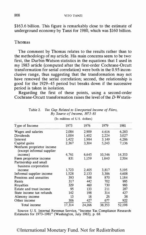
©International Monetary Fund. Not for Redistribution
808 VITO TANZI
$163.6 billion. This figure is remarkably close to the estimate of underground economy by Tanzi for 1980, which was $160 billion.
Thomas
The comment by Thomas relates to the results rather than to the methodology of my article. His main concerns seem to be two: first, the Durbin-Watson statistics in the equations th at I used in my 1983 article ( computed after the first-order Cochrane-Orcutt transformation for seriai correlation) were both in the 0.95 inconclusive range, thus suggesting that the transformation may not have removed the seriai correlation; second, the relationship is good for the 1929-45 period but breaks down if the successive period is taken in isolation.
Regarding the first of these points, using a second-order Cochrane-Orcutt transformation raises the leve) of the D-W statis-
Table 2. Tax Gap Related to Unreported lncome of Fifers, By Source of lncome, 1973-81
(In millions of U.S. dollars)
Type of Income 1973 1976 1979 1981
Wages and salaries 2,084 2,909 4,616 6,283 Dividends 1,004 1,402 2,224 3,027 Interest 1,422 1,984 3, 149 4,286 Capital gains 2,367 3,304 5,243 7,136 Nonfarm proprietor income
( except informai supplier income) 4,761 6,645 10,546 14,353
Farm proprietor income 831 1,159 1,840 2,504 Partnership and small
business corporation income 1,723 2,405 3,817 5,195
Informai supplier income 1,528 2,133 3,386 4,608 Pensions and annuities 393 548 870 1,184 Rents 317 442 702 995 Royalties 329 460 730 993 Estate and trust income 95 133 211 287 State income tax refunds 142 198 314 427 Alimony income 13 18 28 38 Other income 306 427 677 922
Total income 17,314 24,166 38,353 52,198
Source: U.S. Internai Revenue Service, "Income Tax Compliance Research: Estimates for 1973-1981" (Washington, July 1983), p. 68.

©International Monetary Fund. Not for Redistribution
UNDERGROUND ECONOMY: REPLY 809
tic to the tully acceptable level. This change provides estimations of the underground economy that are larger than those estimated earlier. The 1980 estimate, for example, is now about 8 percent of GNP rather than the previously estimated 6 percent. This, of course, raises my estimate for tax evasion to about $20 billion, from the previously estimated figure of $15 billion. Thus, although there are sorne changes in the parameters, the broad conclusions remain unaffected.
The second point raised by Thomas is certainly an important one, although not a new one. In fact, it bad been made by Porter and Bayer (1984). As they put it (p. 182): "The data reveal that the positive relationship between the ratio of currency to M2 and taxes is strong only for the period from 1930 to 1945" (italics in original). I must confess that I have sorne difficulty with this point. On purely economie grounds I do not see much justification for breaking the period. The fact is that the level of taxation rose enormously from 1929 to 1945 but then feil and did not change much after the 1945 period. It started rising again in the late 1960s. If a more recent period, say, one starting about 1970, is isolated, the tax variable becomes again highly significant.
Zilberfarb
I have no particular difficulty with the comment by Zilberfarb. His suggestion to estimate an upper-bound limit to my estimates seems valid and his re-estimation of my results, using the recently constructed average marginal tax rates by Barro and Sahasakul and the marginal federal personal and social security tax rates by Seater provides a test of whether my results were excessively influenced by the variable chosen for the tax rate. His conclusions in this context are reassuring. One small qualification to his comment is perhaps necessary. He mentions that both of the tax measures that I used are based on "average" taxes. While this is true for the variable T in my 1983 article, which represented the ratio of income tax after credit to adjusted gross income, it is not true for the variable TW, the weighted average tax rate. This is usually an average marginal tax rate just like that constructed by Barro and Sahasakul. The difference is that TW was constructed with reference only to interest incomes, while Barro and Sahasakul's was constructed with reference to total incarnes of individuals.

©International Monetary Fund. Not for Redistribution
810 VITO TANZI
REFERENCES
Barro, Robert J., and Chai pat Sahasakul, "Measuring the Average Marginal Tax Rate from the Individual Income Tax," Journal of Business (Chicago), Vol. 56 (October 1983), pp. 419-52.
Cox, Dennis, "Raising Revenue in the Underground Economy," National Tax Journal (Columbus, Ohio), Vol. 37 (September 1984), pp. 283-88.
de Leeuw, Frank, "An Indirect Technique for Measuring the Underground Econorny," Survey ofCurrent Business (Washington), Vol. 65 (April 1985), pp. 64-72.
Feige, Edgar L. (1979), "How Big is the Irregular Economy?" Challenge (White Plains, New York), Vol. 22 (November/December 1979), pp. 5-13.
-- (1980), "A New Perspective on Macroeconomie Phenomena-The Theory and Measurement of the Unobserved Sector of the United States: Causes, Consequences and Implications," American Economie Association Meeting, Denver, Colorado, 1980.
Garcia, Gillian, "The Currency Ratio and the Subterranean Economy," FinanciaJ Analysts Journal (New York), Vol. 32 (November/December 1978), pp. 1-5.
--, and Simon Pak, "The Ratio of Currency to Demand Deposits in the United States," Journal of Finance (New York), Vol. 34 (June 1979), pp. 703-15.
McCrohan, Kevin F., and James D. Smith, "Informai Suppliers in the Underground Economy" in SDI Bulletin of the Internai Revenue Service, Vol. 3, No. 1 (Summer 1983), pp. 27-33.
O'Neill, David M., "Growth of the Underground Economy, 1950-81: Sorne Evidence from the Current Population Survey," A Study Prepared for the Use of the Joint Economie Committee, Congress of the United States (Washington: Government Printing Office, December 9, 1983).
Park, Thae S., "Persona! Incarne and Adjusted Income, 1981-83," Survey of Current Business (Washington), Vol. 65 (April 1985), pp. 32-35.
Parker, Robert P. (1984), "lmproved Adjustments for Misreporting of Tax Return Information Used to Estimate the National Income and Product Accou·nts, 1977," Survey of Current Business (Washington), Vol. 64 (June 1984), pp. 17-25.
Porter, Richard D., and Amanda S. Bayer, "A Monetary Perspective on Underground Economie Activity in the United States," Federal Reserve Bulletin (Washington), Vol. 70 (March 1984), pp. 177-90.
--, "Evaluating Underground Economie Activity in the U.S. Using Monetary Statistics" (mimeographed; Federal Reserve Board, n.d.).
Tanzi, Vito (1979), "Underground &onomy, Incarne Tax Evasion, and the Demand for Currency in the United States, 1929-76" (unpublished; International Monetary Fund, November 5, 1979).
-- (1980), "The Underground Economy in the United States: Estimates and Implications," Banca Nazionale del Lavoro, Quarter/y Review, No. 135 (December 1980), pp. 427-53.
©International Monetary Fund. Not for Redistribution
UNDERGROUND ECONOMY: REPLY 811
-- (1982) (ed.), The Underground Economy in the United States and Abroad (Lexington, Massachusetts: Lexington Books, 1982).
-- (1983), "The Underground Economy in the United States: Annual Estimates, 1930-80," Staff Papers, International Monetary Fund (Washington), Vol. 30 (June 1983), pp. 283-305.
-- (1984), "The Underground Economy in the United States: Reply to Acharya," Staff Papers, International Monetary Fund (Washington), Vol. 31 (December 1984), pp. 747-50.
United States, Internai Revenue Service (1979), Estimates of Income Unreported on lndividuallncome Tax Returns, Publication No. 1104(9-79), Department of the Treasury (Washington: Government Printing Office, Department of the Treasury, September 1979).
-- (1983), Income Tax Compliance Research: Estimates for 1973-1981 (Washington, July 1983).

©International Monetary Fund. Not for Redistribution
SUMMARIES
A Guide to Target Zones-JACOB A. FRENKEL and MORRJS GOLDSTEIN (pages 633-73)
This paper identifies key issues surrounding the advisability and practicality of adopting "target zones" for the exchange rates of major currencies.
Four fundamental questions concerning the definition of and the rationale for target zones are adldressed: first, what is generally meant by a "target zone" approach to exchange rate management and how can "hard" and "soft" versions of this approach be defined; second, what are the perceived deficiencies in the existing exchange rate system of managed floating which motiva te the cali for the adoption of target zones; third, how might target zones remedy these deficiencies; and fourth, what factors are behind much of the skepticism over and opposition to target zones?
ln addition, the paper deals with a series of operational questions of a more technical nature that weigh heavily on the practicality of implementing a target zone approach. The issues discussed include the following: how would the target zones be calculated; what currencies would be included in the system of target zones; how wide should the target zones be and how frequently should they be revised; and what policy instruments would be employed to keep actua.l exchange rates within the target zones, and with what consequences for other policy objectives?
The purpose of the paper is not to make the case either for or against the adoption of target zones. Rather, the intention is to raise and discuss factors that should be considered in any serious discussion of the topic.
Profits Theory and Profits Taxation- EDMUND S. PHELPS (pages 674-96)
In what has been called the "classical" fiscal system, corporate profits are subject to heavy taxation on the ground that they can be siphoned off to the government without giving rise to costly disincentives. Corporations in turn . minimize their profits tax liability for the benefit of their shareowners by debt financing their entire investment. Hence the remaining profit, if any, equals the surplus of capital income over the interest cost caused by monopolistic elements. But with regard to open economies in which firms are forced to equity-finance, this view has been cballenged.
This paper considers the welfare effects of a tax on profits in a small open economy in which the firms operate in world "customer markets" so that their profits are not entirely competed away. The conclusion of the analysis is th at, up to a point, a tax on corporate profits increases welfare. The principal benefit is that siphoning off sorne of the firms' pure profit makes possible a net addition to total tax revenue out of which there can be a lightening of marginal tax rates
812

©International Monetary Fund. Not for Redistribution
SUMMARIES 813
on work, a consequent narrowing of the wedge between the after-tax real wage and the marginal productivity of la bor, and a resulting: increase in the amount of work done and output produced. The principal cost is that the consequent outflow of capital reduces the before-tax wage, which ultimately limits the optimum size of the profits tax rate to something less than 100 percent. Si de benefits occur if a real appreciation of the currency results or if foreign shareowners bear sorne of the redistributive burden of the profits tax, and a side cost if a real exchange rate depreciation occurs instead. With the introduction of partial equity financing it is still possible, though not certain, that an increase in aftertax wages will result.
Output and Unanticipated Money with lmported Intermediate Goods and Foreign Exchange Rationing-AJAI CHOPRA and PETER MONTIEL (pages 697-721)
Short-run fluctuations in the growth of real output are an important concern of policymakers in developing countries. And yet, in spite of the considerable amount of attention that this subject has received in the context of industrial countries during the past fifty years, surprisingly little analytical-much less empirical-work bas been done for developing countries.
For the industrial countries, the ad vent of "new classical" macroeconomies has shaken the consensus about the causes of short-run output fluctuations. Successful estimation of reduced-form output equations gen,erated by "new classical" models contributed to the acceptance of these models. 1t is natural, therefore, to extend this framework to the explanation of short-run output fluctuations in developing countries, and this has been done by severa! authors. However, structural features that are likely to be particularly important in the developing country context have typically been either ignored or introduced in an arbitrary fashion.
This paper develops a simple "new classical" structural mode! that includes severa! features likely to be of importance in developing countries. The economy is modeled as an open economy along Mundeli-Fleming !ines, imported intermediate goods are introduced, and foreign exchange is assumed to be rationed. A reduced-form output equation is derived from this mode!, which is a generalization of its closed economy analogue. After the properties of the mode! are analyzed, the reduced-form output equation is estimated for the Philippines. The empirical results conform quite closely to the predictions of the mode!.
MINIMOD: Specification and Simulation Results-RICHARD D. HAAS and PAUL R.
MASSON (pages 722-fJ7)
This paper describes the construction and use of a small macroeconomie mode!, MINIMOD, of the United States and its major industrial trading partners. The goal is to have a readily understandable and transparent mode! of manageable size that is sui table for po licy analysis. Consequently, an eclectic theoretical mode! has been specified for each of the two economies, with equations for aggregate demand and supply of goods and capital accumulation, and with consistent treatment of government and private sector flows of funds. The mode! was specified such that it has desirable long-run properties, including the neutrality of money and the property that govemment debt cannot grow

©International Monetary Fund. Not for Redistribution
814 INTERNATIONAL MONETARY FUND
without limit relative to output. Values for the parameters of the mode! were obtained, with a few exceptions, from the properties of a Iarger, multicountry mode!; the paper describes the methodology of reducing a larger mode! to its core interactions using partial simulation techniques.
The mode! is simulated to gauge the effects of changes in monetary and fiscal policies under two alternative assumptions concerning expectations of future rates of inflation, of long-term bond rates, and of the exchange rate: (i) expectations adapt to past movements in the variables, or (ii) expectations are consistent with the model's own predictions. The simulations imply that an increase in the money supply is likely to depreciate the exchange rate and to stimulate output in the home country, as priees are slow to adjust; in the long run, however, real magnitudes will be unaffected. Government spending increases also have a temporary stimulatory effect on output in the home country, but, for unchanged money supplies, tend to appreciate the exchange rate.
These conclusions are common to many macroeconomie rnodels. However, MINIMOD also makes it possible to see how sensitive the results are to assumptions concerning expectations. lt is shown that the paths of major macroeconomie variables may be quite different in the two cases mentioned above. In particular, in response to a money supply change, the exchange rate is likely to overshoot its equilibrium value under consistent expectations, though not under adaptive expectations, and output effects are likely to be smaller under consistent expectations. Government expenditure changes seem to have more similar effects in the model under the two expectations assumptions, though the changes induced in the exchange rate and in long-term bond rates are larger with modelconsistent expectations. It is also shown that in this case, credible, preannounced policy changes may have substantial effects before they are actually implemented: a future fiscal contraction may in fact have a stimulatory effect on output wh en it is announced, because of a decline in long-term interest rates and a depreciation of the currency.

©International Monetary Fund. Not for Redistribution
RESUMES
Le point sur les zones-objec tifs-JACOB A. FRENKEL et MORRIS GOLDSTEIN (pages 633-73)
Les auteurs de la présente étude identifient les problèmes clés liés à la mesure dans laquelle il convient d'adopter des zones-objectifs pour les taux de change des principales monnaies et à leur applicabilité.
Quatre questions fondamentales sont soulevées, qui se rapportent à la définition des zones-objectüs et à leur raison d'être : premièrement, qu'entend-on généralement par système de taux de change à "zones-objectifs", et comment définir les variantes "rigides" et "souples" de ce système? Deuxièmement, quels sont les défauts du système actuel de flottement dirigé des taux de change invoqués par les partisans des zones-objectifs? Troisièmement, comment ces zones-objectifs pourraient-elles éventuellement pallier les défauts du système actuel? Quatrièmement, quels sont les facteurs qui sous-tendent en grande partie le scepticisme et l'opposition auxquels se heurtent les zones-objectifs?
Sont également passés en revue une série de points pratiques et plus techniques qui conditionnent dans une large mesure J'applicabilité d'un système de zonesobjectifs. Les points traités sont les suivants: comment calculer les zones objectifs? Quelles monnaies conviendrait-il d'inclure dans le système de zonesobjectifs? Quelle devrait être aa largeur de ces zones et avec quelle fréquence devraient-elles être révisées? A quels instruments de la politique économique aurait-on recours pour maintenir les taux de change effectifs à l'intérieur des zones-objectifs, et quelles en seraient les conséquences probables pour les autres objectifs poursuivis?
En conclusion, cette étude n'a pas pour but de plaider en faveur de l'adoption ou du rejet des zones-objectifs, mais de faire apparaître et d'examiner les éléments à prendre en considération lors de toute discussion approfondie du sujet.
Théorie des bénéfices et imposition des bénéfices-EDMUND s. PHELPS (pages 674-96)
Dans Je système de finances publiques dit "classique", les bénéfices des sociétés sont assujettis à une Jourde imposition pour la raison qu'ils peuvent être transférés à l'Etat sans que ce transfert soit un anti-stimulant coûteux. Les sociétés, quant à elles, minimisent, au profit de leurs actionnaires, leur cotisation fiscale au titre de l'impôt sur les bénéfices en finançant par l'endettement la totalité de leurs investissements. Les bénéfices qui restent, Je cas échéant, correspondent donc à l'excédent du revenu des investissements par rapport au coût de l'intérêt inhérent à des éléments monopolistiques. Dans Je cas, toutefois, des économies ouvertes où les entreprises sont obligées de financer leurs investissements en faisant appel aux prises de participation au capital, la validité de cette théorie a été contestée.
815

©International Monetary Fund. Not for Redistribution
816 INTERNATIONAL MONETARY FUND
La présente étude est consacrée aux effets qu'un impôt sur les bénéfices peut avoir sur le bien-être dans une petite économie ouverte où les entreprises opèrent sur des marchés dominés par les acheteurs, certes, mais où la concurrence ne les empêche toutefois pas de réaliser certains bénéfices. L'analyse aboutit à la conclusion que, jusqu'à un certain point, un impôt sur les bénéfices des sociétés a pour effet d'accroître le bien-être. Le principal avantage est que le transfert à l'Etat d'une fraction des bénéfices purs des sociétés entraîne un accroissement net des recettes fiscales totales; cet accroissement des recettes permet d'alléger les taux d'imposition marginaux sur le travail, ce qui a pour effet de rétrécir l'écart entre les salaires réels après impôts et la productivité marginale de la main-d'oeuvre, et, par conséquent, d'augmenter le volume du travail et celui de la production. Le principal coût vient de ce que les sorties de capitaux qui s'ensuivent réduisent les salaires avant impôts, ce qui finit par ramener le taux optimum de l'impôt sur les bénéfices à un peu moins de lOO%. L'impôt sur les bénéfices présente certains avantages secondaires si la monnaie s'apprécie en termes réels ou si les actionnaires étrangers assument une partie de la charge qu'entraîne la redistribution de l'impôt sur les bénéfices; mais il présente, en revanche, certains coûts secondaires si, au lieu de s'apprécier, la monnaie se déprécie en termes réels. Même si une partie du financement prend la forme de participations au capital, il reste possible que les salaires après impôts augmentent, bien que cela ne soit pas certain.
Production et variations imprévues de la masse monétaire dans le contexte de produits intermédiaires importés et d'un rationnement des devises-AJA! CHOPRA et PETER MONTIEL (pages 697-721)
Les fluctuations à court terme de la croissance de la production réelle sont une préoccupation importante des dirigeants des pays en développement. Pourtant, malgré toute l'attention que cette question a reçue dans le contexte des pays industrialisés au cours des cinquante dernières années, les travaux analytiques, et plus encore les travaux empiriques, sur ce sujet, ont été étonnamment limités en ce qui concerne les pays en développement.
Dans les pays industrialisés, l'avènement de la nouvelle macroéconomie "classique" a ébranlé le consensus qui régnait quant aux causes des fluctuations à court terme de la production. L'exactitude des estimations d'équations de forme réduite de la production effectuées dans les modèles "classiques" a contribué à faire accepter ces derniers. Il est par conséquent naturel d'élargir le cadre de ces modèles à l'explication des fluctuations à court terme de la production dans les pays en développement, ce qui a été fait par plusieurs auteurs. Toutefois, des aspects structurels qui sont en principe particulièrement importants dans le contexte des pays en développement ont été généralement ignorés ou introduits de manière arbitraire.
La présente étude élabore un modèle structurel simple "classique" comprenant plusieurs aspects qui sont en principe importants dans les pays en développement. Le modèle est fondé sur une économie ouverte du type MundellFleming, dans laquelle des produits intermédiaires sont importés et où l'on suppose que les devises sont rationnées. Une équation de forme réduite de la production est tirée de ce modèle, qui est une généralisation de l'économie fermée qui est son analogue. Une fois les propriétés du modèle analysées,

©International Monetary Fund. Not for Redistribution
RESUMES 817
l'équation de forme réduite de la production est estimée pour les Philippines. Les résultats empiriques correspondent de très près aux prévisions du modèle.
MINIMOD : spécification et résultats des simulations- RICHARD o. HAAS et PAUL R. MASSON (pages 722-67) La présente étude décrit la construction et l'application d'un petit modèle
macroéconomique, MINIMOD, des Etats-Unis et du groupe des principaux partenaires commerciaux industriels. L'objectif est d'obtenir un modèle facilement compréhensible, transparent et de taille suffisamment réduite, qui se prête à l'analyse de la politique économique. Par conséquent, un modèle théorique éclectique a été spécifié pour chacune des deux économies, avec des équations de la demande et de J'offre globales de biens et de l'accumulation de capital, et un traitement cohérent des flux de capitaux publics et privés. Le modèle a été spécifié de manière à avoir des propriétés souhaitables à long terme, y compris la neutralité de la monnaie et la limitation de l'accroissement de la dette publique par rapport à la production. Les valeurs des paramètres du modèle ont été tirées, à quelques exceptions près, des propriétés d'un plus grand modèle pour plusieurs pays; l'étude décrit la méthode qui permet de réduire un grand modèle à ses interactions essentielles au moyen de techniques de simulation partielle.
Le modèle est simulé dans le but d'évaluer les effets de modifications de la politique monétaire et de la politique de finances publiques sur la base de deux hypothèses possibles en ce qui concerne les anticipations relatives aux taux d'inflation futurs, aux taux des obligations à long terme et aux taux de change : i) les anticipations s'adaptent aux fluctuations antérieures des variables, ou ii) les anticipations correspondent aux prévisions du modèle. Les simulations impliquent qu'une augmentation de la masse monétaire entraînera vraisemblablement une dépréciation du taux de change et stimulera la production intérieure, étant donné que les prix s'ajustent lentement; toutefois, à long terme, les grandeurs réelles ne changeront pas. Les augmentations des dépenses publiques ont aussi un effet stimulant temporaire sur la production dans le pays, mais, si les agrégats monétaires ne varient pas, elles auront tendance à entraîner une appréciation du taux de change.
Ces conclusions sont celles d'un grand nombre de modèles macroéconomiques. Toutefois, MJNIMOD permet aussi de voir dans quelle mesure les hypothèses relatives aux anticipations influent sur les résultats. Il est démontré que l'évolution de variables macroéconomiques importantes peut être très diffe'rente dans les deux cas susmentionnés. En particulier, il est probable qu'en réaction à une variation de la masse monétaire, il y aura surajustement du taux de change par rapport à sa valeur d'équilibre dans l'hypothèse d'anticipations conformes aux prévisions du modèle, mais non pas dans l'hypothèse d'anticipations adaptatives, et il est probable que les effets sur la production seront plus faibles dans l'hypothèse d'anticipations conformes aux prévisions. Les variations des dépenses publiques ont apparemment des effets plus semblables dans les deux hypothèses relatives aux anticipations, bien que les variations du taux de change et des taux des obligations à long terme qui en résultent soient plus fortes dans le cas des anticipations conformes aux prévisions du modèle. Il est aussi démontré que, dans ce cas, des changements de politique crédibles et annoncés à l'avance pourront avoir des effets considérables avant

©International Monetary Fund. Not for Redistribution
818 INTERNATIONAL MONETARY FUND
même que ces changements soient effectivement apportés : la perspective d'une compression des dépenses publiques peut, en fait, avoir un effet stimulant sur la production au moment où cette compression est annoncée, en raison d'une baisse des taux d'intérêt à long terme et d'une dépréciation de la monnaie.

©International Monetary Fund. Not for Redistribution
RESUMENES
Una gufa para las zonas meta-JACOB A. FRENKEL y MORRIS GOLDSTEIN (paginas 633-73)
En este trabajo se identifican cuestiones clave en torno a la conveniencia y posibilidades de poner en practica un régimen de "zonas meta" para los tipos de cambio de las principales monedas.
En relaci6n con la definici6n y fundamento 16gico de las zonas meta, se abordan cuatro cuestiones fundamentales: primera, qué significa generalmente adoptar para la gesti6n de los tipos de cambio un régimen de "zonas meta" y c6mo podrfan definirse sus versiones "estricta" y "flexible"; segunda, cuales son las deficiencias observadas en el actual sistema de flotaci6n dirigida de los tipos de cambio que hacen proponer la adopci6n de zonas meta; tercera, c6mo podrfan las zonas meta remediar dichas deficiencias, y, cuarta, qué factores se esconden tras gran parte del escepticismo y de la oposici6n que las zonas meta suscitan.
Ademas, el trabajo se ocupa de una serie de cuestiones operativas, de naturaleza mas técnica y sumamente importantes para determinar si seria practico implantar un enfoque seme jante. Entre otros aspectos tratados cabe mencionar los siguientes: c6mo se calcularîan las zonas meta; qué monedas deberîan incluirse en el sistema; cual deberîa ser la amplitud de las zonas y cada cuanto habrîa que revisarlas, y qué instrumentos de polftica econ6mica se utilizarfan para mantener los tipos de cambio observados dentro de los lîmites de las zonas y con qué consecuencias sobre los otros objetivos de la polftica econ6mica.
Con este trabajo no se pretende justificar ni la adopci6n ni el rechazo del sistema de las zonas meta, sino s6Io identificar y analizar los factores que han de tenerse en cuenta en cualquier discusi6n seria del tema que nos ocupa.
Teorfa y tributaci6n de las u tilidades-EDMUND s. PHELPS (paginas 674-96)
En el sistema fiscal "clasico", las utilidades de las empresas pagan impuestos elevados porque se cree que el trasvase de utilidades hacia el Fisco no causa un desincentivo costoso. Las empresas, a su vez, intentan minimizar la obligaci6n tributaria sobre sus utilidades en provecho de los accionistas, financiando la inversi6n mediante emisi6n de deuda. En consecuencia, las utilidades que resten, si acaso, equivalen al excedente de renta de capital frente al costo en intereses causados por elementos monopolisticos. Ahora bien, se han expresado opiniones contrarias cuando se trata de econornfas abiertas y empresas que se ven obligadas a financiar su inversi6n con cargo al capital propio.
En este trabajo se examinan los efectos de bienestar social del impuesto sobre las utilidades en una economfa abierta pequena en la que las empresas operan en "mercados de clientes" mundiales, de manera que las utilidades no de-
819

©International Monetary Fund. Not for Redistribution
820 INTERNATIONAL MONETARY FUND
saparecen totalmente por efecto de la competencia. La conclusi6n del analisis es que, hasta un determinado nive!, el impuesto a las utilidades de las empresas aumenta el bienestar social. La ventaja principal es que la recaudaci6n de una parte de las utilidades puras de algunas empresas permite un incremento neto de la recaudaci6n tributaria total, Jo que alivia las tasas tributarias marginales sobre el trabajo, reduce la cuna entre el salario real-una vez deducidos los impuestosy la productividad marginal del trabajo, Jo que trae como consecuencia un aumento del trabajo realizado y del producto. La principal desventaja es que la consiguiente salida de capital reduce el salario antes de deducir impuestos, Jo que eventualmente limita el tamaiio 6ptimo de la tasa tributaria sobre las utilidades a algo menos del lOO%. Se pueden anadir otras venta jas si se produce una apreciaci6n real de la moneda, o si existen accionistas en el ex teri or sobre los que recae parte de la carga redistributiva del impuesto a las utilidades y, por otro lado, entrana un costo si tiene lugar una depreciaci6n real del tipo de cambio. Con introducci6n de la financiaci6n parcial con capital propio es posible, aunque no seguro, que se produzca un aumento de los salarios después de deducir los impuestos.
Produccion y dinero no anticipado con bienes intermedios importados y racionamiento de las divisas-AJA! CHOPRA y PETER MONTIEL (paginas 697-721) Las fluctuaciones a corto plazo del crecimiento del producto real constituyen
una cuesti6n muy importante para los gobiemos de los pafses en desarrollo. Sin embargo, pese a la considerable atenci6n que se ha prestado a este asunto en el contexto de los paises industriales durante los iiltimos cincuenta anos, es sorprendente el poco trabajo anaütico-mucho menas empîrico--que se ha efectuado en relaci6n con los paises en desarrollo.
En el caso de los paises industriales, el surgimiento de la macroeconomfa "neoclasica" ha alterado el consenso sobre las causas de las fluctuaciones a corto plazo del producto. El éxito de la estimaci6n de las ecuaciones de forma reducida del producto generadas por los modelos "neoclasicos" ha contribuido a la aceptaci6n de los mismos. Por consiguiente, es natural que se aplique este marco a la explicaci6n de las fluctuaciones a corto plazo del producto en los paîses en desarrollo, y asi Jo han hecho varios autores. Sin embargo, norrnalmente se ha hecho caso omiso de los aspectos estructurales que probablemente jugaran un pape! importante en el contexto de los paîses en desarrollo o se les ha incorporado de manera arbitraria.
En el presente estudio se elabora un modelo estructural "neoclasico" sencillo que incluye diversas caracterîsticas que probablemente resultaran importantes en los paises en desarrollo. Se elabora un modelo de una economfa abierta, en el marco de la teorîa de Mundell-Flemming, se incluyen los bienes intermedios importados y se supooe que las divisas estân racionadas. A partir de este modelo se obtiene una ecuaci6n del producto de forma reducida que e� una generalizaci6n de la ecuaci6n correspondiente en una economfa cerrada. Tras analizar las propiedades del modelo, se estima la ecuaci6n de forma reducida del producto para el caso de Filipinas. Los resultados empiricos se ajustan en gran medida a las predicciones del modelo.

©International Monetary Fund. Not for Redistribution
RESUMENES 821
MINIMOD: Especificacion y resultados de simulacion-RICHARD D. HAAS y PAUL R. MASSON (paginas 722-Q7)
En este estudio se describe la elaboraci6n y la utilizaci6n de un modelo macroecon6mico pequeiio, MINIMOD, de Estados Unidos y de los pafses industriales con que éste mantiene intercambios comerciales de gran volumen. El objetivo es disponer de un modelo comprensible y transparente de dimensi6n manejable que se pueda utilizar con fines de analisis de polftica. Por consiguiente, se ha especificado un modelo téorico ecléctico para cada una de las dos economfas, que contiene ecuaciones de demanda y de oferta agregadas de productos y de acumulaci6n de capital. Se han tratado de manera coherente las corrientes de fondos del sector publico y del sector privado. El modelo presenta caracterîsticas adecuadas para el anâlisis a largo plazo, incluidas la neutralidad del dinero y la propiedad de que la deuda publica no puede aumentar sin limite en relaci6n con el producto. Los valores correspondientes a los parâmetros del modelo se obtuvieron, salvo en algunos casos, a partir de las propiedades de un modelo mas amplio de varios pafses; en el estudio se describe la metodologfa que consiste en reducir un modelo mas amplio a sus interacciones basicas empleando técnicas de simulaci6n parcial.
Se ha simulado este modelo con el fin de determinar los efectos de las variaciones de las polfticas monetaria y fiscal basandose en dos supuestos alternativos concernientes a las expectativas de la tasa de inflaci6n futura, de los tipos de interés de los bonos a largo plazo y del tipo de cambio: i) las expectativas se adaptan a las fluctuaciones anteriores de las variables o ii) las expectativas son compatibles con las predicciones del modelo. Las simulaciones implican que un aumento de la oferta monetaria probablemente provoca una depreciaci6n del tipo de cambio y estimulara la producci6n en el pais de referencia dado que los precios se ajustan con lentitud; sin embargo, a largo plazo no resultaran afectadas las magnitudes reales. Los aumentos del gasto publico también constituyen un estimulo temporal para la producci6n en el pais de referencia aunque, si no varia la oferta monetaria, tendera a apreciarse el tipo de cambio.
Estas conclusiones son comunes a muchos modelos macroecon6micos. NÇ> obstante, con el modelo MINIMOD también se puede medir la sensibilidad de los resultados ante los supuestos relativos a las expectativas. Se demuestra que la trayectoria de las principales variables macroecon6micas puede ser muy diferente en los dos casos antes mencionados. En especial, como consecuencia de una variaci6n de la oferta monetaria, lo mas probable es que el tipo de cambio supere su valor de equilibrio si las expectativas son coherentes; esto no sucede si las expectativas son adaptables; los efectos en la producci6n probablemente seran menores en el caso de las expectativas coherentes. Los efectos de la variaci6n del gasto publico en el modelo son mas parecidos en los dos supuestos de expectativas, aunque las variaciones inducidas en el tipo de cambio y en el tipo de interés de los bonos a largo plazo son mayores cuando las expectativas son coherentes. También se senala que, en este caso, las modificaciones de polftica dignas de crédito y anunciadas con anticipaci6n pueden tener efectos considerables antes de ser aplicadas; la perspectiva de una contracci6n fiscal puede, de hecho, tener un efecto estimulante al anunciarse, debido a que provoca un descenso del tipo de interés a largo plazo y una depreciaci6n de la moneda.

©International Monetary Fund. Not for Redistribution
This page intentionally left blank

©International Monetary Fund. Not for Redistribution
In statistical matter (except in the résumés and resumenes) throughout this issue,
Dots ( . . . ) indicate that data are not available;
A dash (-) indicates that the figure is zero or Jess than half the final digit shown, or that the item does not exist;
A single dot ( . ) indicates decimais;
A comma (,) separates thousands and millions;
"Billion" means a thousand million, and "trillion" means a thousand billion;
A short dash (-) is used between years or months (for example, 1981-83 or January-October) to indicate a total of the years or months inclusive of the beginning and ending years or months;
A stroke (/) is used between years (for example, 1981/82) to indicate a fiscal year or a crop year;
Components of tables may not add to totals shown because of rounding.