Stability of Icelandic type Berm Breakwaters - CiteSeerX
118
Faculty of Civil Engineering and Geosciences Department of Hydraulic Engineering Stability of Icelandic type Berm Breakwaters Pétur Ingi Sveinbjörnsson MSc Thesis May 2008
-
Upload
khangminh22 -
Category
Documents
-
view
3 -
download
0
Transcript of Stability of Icelandic type Berm Breakwaters - CiteSeerX

Faculty of Civil Engineering and Geosciences
Department of Hydraulic Engineering
Stability of Icelandic type Berm Breakwaters
Pétur Ingi Sveinbjörnsson
MSc Thesis
May 2008

ii

iii
Preface
This thesis project represents the final work of my M.Sc. study at Delft University of
Technology, the faculty of Civil Engineering. My studies were focused on Coastal
Engineering and the subject of this final project is “Stability of Icelandic type Berm
Breakwaters”. The project is carried out in cooperation with Witteveen+Bos Consulting
Engineers.
This project consists of model test experiments as well as general literature study. The scale
model experiments were carried out in the long wave flume of the Laboratory of Fluid
Mechanics at Delft University of Technology. I would like to thank the members of the
graduation committee as well as co-workers in the Laboratory for their assistant during this
project. I would also like to thank Mr. Arnar B. Sigurdsson for proofreading the document.
The work was supervised by a graduation committee with members from TU Delft,
Witteveen+Bos Consulting Engineers and the Icelandic Maritime Administration:
Prof. dr. ir. M.J.F. Stive Delft University of Technology
ir. H.J. Verhagen Delft University of Technology
dr. ir. W.S.J. Uijttewaal Delft University of Technology
ir. M. Caljouw Witteveen+Bos Consulting Engineers
S. Sigurdarson Icelandic Maritime Administration
Pétur Ingi Sveinbjörnsson
Delft, May 2008

iv
Summary
A major part of the breakwaters constructed in the world are the so-called conventional rouble
mound breakwaters, Figure 1a), that consist of a core, a filter layer and a heavy armour layer.
An alternative to the conventional rouble mound breakwater is a berm breakwater. Berm
breakwaters have mainly developed in two directions over the last couple of decades. On the
one hand a dynamically stable structure, where reshaping is allowed, Figure 1b). And on the
other hand a more stable multi layered structure often referred to as Icelandic type berm
breakwater, Figure 1c).
Figure 1. Example of different types of breakwaters, a) Conventional rubble mound breakwater, b)
dynamically stable berm breakwater and c) Icelandic type berm breakwater
When there is a quarry, relatively close to the construction site, which is dedicated to the
breakwater project, the Icelandic type has proven to be very attractive economically. The
basic reason for that is that unlike the other types the Icelandic type utilizes the quarry 100%.
This M.Sc. thesis focuses on the Icelandic type berm breakwater. Before an Icelandic type
berm breakwater is constructed the stones are divided into classes depending on their size.
The smaller armour stones are then placed rather deep where the influence of the wave attack
is less, while the largest stones are placed where the largest wave attack is expected.
Goals of this project:
• Design rules for the transaction of stone classes with depth have not yet evolved and
the main goal of this project was to develop a stability criterion for the stones in that
area. (Primary goal)
• Stones on berm. Since the total amount of the largest stones (Class I) is usually
limited, the combination of the amount of large stones on the berm and down the berm
is important. (Secondary goal)
• Recession. Recession will be measured in each test and thereby a large database on the
subject will be made available for further research on the subject. (Secondary goal)

v
• The location of the transition of the original and the reshaped profiles as the berm
height changes as well as for different stone setups. This is also closely related to the
primary goal of the project. (Secondary goal)
Figure 2. Different model setups used in the model tests
Numbers of model tests were performed in order to reach those goals or a total of 70 tests
with 6 different model setups (Figure 2). To follow the influence of different model setups
and different berm heights on the behaviour of the structure the following measures were
used:
• Visual observation with the help of a camera that was use to take photos regularly
during the tests (500, 1000, 2000 and 3000 waves) and a video camera.
• Recession measurements. After each test the recession at berm level was measured.
• General erosion measurements. After each test the cross section profile was measured
and from that the total erosion was evaluated.
• To follow the location of the transition of the original and the reshaped profiles after
each test, the cross section profile was used.
After analysing the test results the main conclusions were the following:
1. Class I stones on the berm are recommended to reach at least further into the berm
than the expected recession from a design storm.
2. Class I stones are recommended to reach as far down as:
hI-II ≥ 1.45·∆Dn50, Class I
or

vi
hI-II ≥ 1.85·∆Dn50, Class II
The one of the two that gives the larger hI-II in each case is the recommended choice.
3. If there is more of Class I stones available after meeting the recommendations above,
(1 and 2) they should be placed on the berm.
4. Class II stones should in any case reach at least down to the transition of the original
and the expected reshaped profile, hf.

vii
Table of Contents
1 Introduction..................................................................................................................................................... 1
1.1 General .................................................................................................................................................. 1
1.2 Historical review.................................................................................................................................... 2
1.3 Benefits of the Icelandic type berm breakwater .................................................................................... 3
1.4 Project definition ................................................................................................................................... 5
1.5 Outline ................................................................................................................................................... 6
2 Literature study of the theory.......................................................................................................................... 8
2.1 Waves .................................................................................................................................................... 8
2.1.1 Wave impact.................................................................................................................................... 8 2.1.2 Waves on slope ............................................................................................................................... 9
2.2 Reshaping measurements..................................................................................................................... 11
2.2.1 Recession....................................................................................................................................... 11 2.2.2 Damage definition, Sd ................................................................................................................... 12
2.3 Design methods for uniform slope....................................................................................................... 13
2.3.1 Hudson .......................................................................................................................................... 13 2.3.2 Van der Meer................................................................................................................................. 14
2.4 Design methods for Icelandic type berm breakwaters ......................................................................... 16
3 Experimental setup........................................................................................................................................ 18
3.1 The Wave Flume ................................................................................................................................. 18
3.2 Observation equipments ...................................................................................................................... 18
3.3 Model setup ......................................................................................................................................... 21
3.3.1 Wave conditions............................................................................................................................ 23 3.3.2 Wave spectra ................................................................................................................................. 24 3.3.3 Water depth ................................................................................................................................... 24
3.4 Material................................................................................................................................................ 25
3.4.1 Shape of stones.............................................................................................................................. 25 3.4.2 Characteristic of stones ................................................................................................................. 26 3.4.3 Law of scaling ............................................................................................................................... 27
4 Analysis......................................................................................................................................................... 30
4.1 Damage development .......................................................................................................................... 30
4.1.1 Setup 1........................................................................................................................................... 30 4.1.2 Setup 2........................................................................................................................................... 31 4.1.3 Setup 3........................................................................................................................................... 32 4.1.4 Setup 4........................................................................................................................................... 32 4.1.5 Setup 5........................................................................................................................................... 33 4.1.6 Setup 6........................................................................................................................................... 33 4.1.7 Compilation................................................................................................................................... 34
4.2 Recession............................................................................................................................................. 35
4.2.1 Comparison with recession formulas ............................................................................................ 35 4.2.2 Influence of berm height on recession........................................................................................... 37 4.2.3 Influence of stones on berm, on berm recession ........................................................................... 38 4.2.4 Influence of stones on the front slope, on berm recession............................................................. 38 4.2.5 Comparison of setups .................................................................................................................... 39
4.3 Damage number Sd .............................................................................................................................. 41
4.3.1 Influence of berm height on the damage number .......................................................................... 41 4.3.2 Comparison of setups .................................................................................................................... 42
4.4 Duration until failure/core erosion....................................................................................................... 44
4.5 Transition of original and reshaped profile, hf..................................................................................... 45

viii
4.5.1 Interpretation of test results ........................................................................................................... 46 4.6 Uncertainties........................................................................................................................................ 48
4.6.1 Uncertainties of tests ..................................................................................................................... 48 4.6.2 General uncertainties..................................................................................................................... 49
5 Discussion of model tests.............................................................................................................................. 50
5.1 Discussion of current design rules ....................................................................................................... 51
5.2 Discussion of test results ..................................................................................................................... 52
5.2.1 Stones on the berm ........................................................................................................................ 52 5.2.2 Berm level ..................................................................................................................................... 52 5.2.3 Transition of Class I and Class II stones ....................................................................................... 53 5.2.4 Transition of Class II and Class III stones..................................................................................... 54
6 Conclusions and suggestions for further work .............................................................................................. 56
6.1 Conclusions ......................................................................................................................................... 56
6.1.1 Suggested additions to current design rules .................................................................................. 56 6.2 Suggested further research................................................................................................................... 57
7 References..................................................................................................................................................... 59
A Appendices.................................................................................................................................................... 62
A.1 Model setup, key parameters expressed dimensionless ....................................................................... 62
A.1.1 Key parameters expressed as a function of wave height ............................................................... 62 A.1.2 Key parameters as a function of median nominal diameter, Dn50, of different stone classes ........ 63
A.2 Wave measurements ............................................................................................................................ 64
A.2.1 Setup 1........................................................................................................................................... 64 A.2.2 Setup 2........................................................................................................................................... 64 A.2.3 Setup 3........................................................................................................................................... 65 A.2.4 Setup 4........................................................................................................................................... 65 A.2.5 Setup 5........................................................................................................................................... 66 A.2.6 Setup 6........................................................................................................................................... 66
A.3 Stone measurements ............................................................................................................................ 67
A.3.1 Class I............................................................................................................................................ 67 A.3.2 Class II .......................................................................................................................................... 68 A.3.3 Class III ......................................................................................................................................... 69 A.3.4 Core............................................................................................................................................... 70 A.3.5 Mixture of all stones...................................................................................................................... 70
A.4 Cross sections and reshaping process .................................................................................................. 72
A.4.1 Setup 1........................................................................................................................................... 73 A.4.2 Setup 2........................................................................................................................................... 74 A.4.3 Setup 3........................................................................................................................................... 76 A.4.4 Setup 4........................................................................................................................................... 77 A.4.5 Setup 5........................................................................................................................................... 78 A.4.6 Setup 6........................................................................................................................................... 79
A.5 Recession graphs ................................................................................................................................. 81
A.5.1 Comparison with Tørum ............................................................................................................... 81 A.5.2 Influence of berm height on recession on the edge of berm.......................................................... 82 A.5.3 Comparison of different setups ..................................................................................................... 85 A.5.4 Uncertainties ................................................................................................................................. 86
A.6 Damage number – graphs .................................................................................................................... 88
A.6.1 Influence of berm height on damage development ....................................................................... 88 A.6.2 Comparison of different setups ..................................................................................................... 91 A.6.3 Uncertainties ................................................................................................................................. 92
A.7 Transition of original and reshaped profile, hf..................................................................................... 94
A.7.1 Influence of distance from berm level to water level, hB, on hf..................................................... 94 A.7.2 Comparison of different setups ..................................................................................................... 96

ix
A.8 Wave spectra ....................................................................................................................................... 97
A.9 Damage measurement photos .............................................................................................................. 99
A.10 Photos from laboratory ...................................................................................................................... 101

x
List of Figures
Figure 1.1 Example of different types of breakwaters, a) Conventional rubble mound breakwater, b) dynamically
stable berm breakwater and c) Icelandic type berm breakwater ............................................................................. 2
Figure 1.2 Sirevåg berm breakwater, stock pile of stone classes I and II. Sigurdarson et al 2001.......................... 2
Figure 1.3 Inspection of the front slope of the berm of the Sirevåg breakwater, a section with Class I stones.
Sigurdarson et al 2001............................................................................................................................................. 3
Figure 1.4 Area under consideration ....................................................................................................................... 5
Figure 2.1 Breaker types as a function of the surf similarity parameter................................................................ 10
Figure 2.2 Recession of berm breakwaters ........................................................................................................... 11
Figure 2.3 Explanation figure for the damage number Sd ..................................................................................... 13
Figure 2.4 Permeability coefficients, P, for various structures for the formula of Van der Meer (1988).............. 15
Figure 2.5 Key parameters in berm breakwater design......................................................................................... 16
Figure 3.1 Overview of the wave flume................................................................................................................ 18
Figure 3.2 Overview of the observation equipments in the wave flume ............................................................... 19
Figure 3.3 A view from the video camera, setup S03TM, Hs = 0.12m ................................................................. 20
Figure 3.4 Equipment used for profile measurements........................................................................................... 20
Figure 3.5 Explanation figure of the model setup ................................................................................................. 21
Figure 3.6 Overview of the different setups.......................................................................................................... 22
Figure 3.7 Illustration of the measurements of the LT ratio.................................................................................. 26
Figure 4.1 Overview of the different setups.......................................................................................................... 30
Figure 4.2 Recession, comparison of test results with recession formulas, setups 1-5, Class I stones used as
reference................................................................................................................................................................ 35
Figure 4.3 Recession, comparison of test results with recession formulas, setups 1-5, Class I stones used as
reference................................................................................................................................................................ 36
Figure 4.4 Recession, comparison of different water levels, setup 4 .................................................................... 37
Figure 4.5 Recession, comparison of different setups, water level 0.590m .......................................................... 39
Figure 4.6 Recession, comparison of different setups, water level 0.645m .......................................................... 40
Figure 4.7 Damage number, comparison of different water levels for setup 2 ..................................................... 41
Figure 4.8 Damage number, comparison of different setups with water level 0.590m......................................... 42
Figure 4.9 Damage number, comparison of different setups with water level 0.645m......................................... 43
Figure 4.10 Transition of original and reshaped profile, hf, water level 0.590m.................................................. 46
Figure 4.11 Damage number, comparison of original and repeated test of setup 4, with water level 0.590m...... 48
Figure A.1 Sieve curve for Class I stones ............................................................................................................. 67
Figure A.2 Sieve curve for Class II stones............................................................................................................ 68
Figure A.3 Sieve curve for Class III stones........................................................................................................... 69
Figure A.4 Sieve curve for the mixture of all stones............................................................................................. 70
Figure A.5 Explanation figure for the damage development. ............................................................................... 72
Figure A.6 Damage development of setup 1, water level 0.545m. ....................................................................... 73
Figure A.7 Damage development of setup 1, water level 0.590m. ....................................................................... 73
Figure A.8 Damage development of setup 1, water level 0.645m. ....................................................................... 74

xi
Figure A.9 Damage development of setup 2, water level 0.590m, first test.......................................................... 74
Figure A.10 Damage development of setup 2, water level 0.590m, repeated test. ............................................... 75
Figure A.11 Damage development of setup 2, water level 0.645m. ..................................................................... 75
Figure A.12 Damage development of setup 3, water level 0.590m. ..................................................................... 76
Figure A.13 Damage development of setup 3, water level 0.645m. ..................................................................... 76
Figure A.14 Damage development of setup 4, water level 0.590m, first test........................................................ 77
Figure A.15 Damage development of setup 4, water level 0.590m, repeated test. ............................................... 77
Figure A.16 Damage development of setup 4, water level 0.590m. ..................................................................... 78
Figure A.17 Damage development of setup 5, water level 0.590m. ..................................................................... 78
Figure A.18 Damage development of setup 5, water level 0.645m. ..................................................................... 79
Figure A.19 Damage development of setup 6, water level 0.590m. ..................................................................... 79
Figure A.20 Damage development of setup 6, water level 0.645m. ..................................................................... 80
Figure A.21 Recession, setup 6 compared to the modified formula of Tørum for mixed stones.......................... 81
Figure A.22 Recession, setup 4 compared to the modified formula of Tørum for Class I stones ......................... 82
Figure A.23 Recession, comparison of different water levels, setup 1 ................................................................. 82
Figure A.24 Recession, comparison of different water levels, setup 2 ................................................................. 83
Figure A.25 Recession, comparison of different water levels, setup 3 ................................................................. 83
Figure A.26 Recession, comparison of different water levels, setup 4 ................................................................. 84
Figure A.27 Recession, comparison of different water levels, setup 5 ................................................................. 84
Figure A.28 Recession, comparison of different setups, water level 0.590m ....................................................... 85
Figure A.29 Recession, comparison of different setups, water level 0.645m ....................................................... 85
Figure A.30 Recession, comparison of original and repeated test of setup 2, with water level 0.590m ............... 86
Figure A.31 Recession, comparison of the original and the repeated test of setup 2, with water level 0.590m. H0
used instead of H0T0.............................................................................................................................................. 87
Figure A.32 Recession, comparison of original and repeated test of setup 4, with water level 0.590m ............... 87
Figure A.33 Damage number, comparison of different water levels for setup 1 .................................................. 88
Figure A.34 Damage number, comparison of different water levels for setup 2 .................................................. 88
Figure A.35 Damage number, comparison of different water levels for setup 3 .................................................. 89
Figure A.36 Damage number, comparison of different water levels for setup 4 .................................................. 89
Figure A.37 Damage number, comparison of different water levels for setup 5 .................................................. 90
Figure A.38 Damage number, comparison of different water levels for setup 6 .................................................. 90
Figure A.39 Damage number, comparison of different setups with water level 0.590m...................................... 91
Figure A.40 Damage number, comparison of different setups with water level 0.645m...................................... 91
Figure A.41 Damage number, comparison of original and repeated test of setup 2, with water level 0.590m..... 92
Figure A.42 Damage number, comparison of the original and the repeated test of setup 2, with water level
0.590m. H0 used instead of H0T0........................................................................................................................... 92
Figure A.43 Damage number, comparison of original and repeated test of setup 4, with water level 0.590m..... 93
Figure A.44 Transition of original and reshaped profile, hf, setup 1..................................................................... 94
Figure A.45 Transition of original and reshaped profile, hf, setup 2..................................................................... 94
Figure A.46 Transition of original and reshaped profile, hf, setup 4..................................................................... 95

xii
Figure A.47 Transition of original and reshaped profile, hf, setup 6..................................................................... 95
Figure A.48 Transition of original and reshaped profile, hf, water level 0.590m ................................................. 96
Figure A.49 Transition of original and reshaped profile, hf, water level 0.645m.................................................. 96
Figure A.50 Pierson-Moskowitz and Jonswap spectrum ...................................................................................... 98
Figure A.51 Damage measurement photos, S02TM_rep, wave test #2, after a) 500 waves, b) 1000 waves, c)
2000 waves and d) 3000 waves............................................................................................................................. 99
Figure A.52 Damage measurement photos, S02TM_rep, a) wave test #2 after 3000 waves, b) wave test #3 after
3000 waves, c) wave test #4 after 3000 waves, d) wave test #5 after failure ...................................................... 100
Figure A.53 Photo from laboratory, the wave board........................................................................................... 101
Figure A.54 Photo from laboratory, the camera stand and the structure............................................................. 101
Figure A.55 Photo from laboratory, taken behind the structure.......................................................................... 102
Figure A.56 Photo from laboratory, measurement equipment ............................................................................ 102
Figure A.57 Photo from laboratory, overview, looking in the direction of the structure .................................... 103
Figure A.58 Photo from laboratory, overview, looking in the direction of the wave generator.......................... 103

xiii
List of tables
Table 2.1 Stability criterion for modest angle of wave attack β = ±20°.................................................................. 9
Table 3.1 Explanation table for test setups, parameters from Figure 3.4 .............................................................. 21
Table 3.2 Further explanation for test setups, parameters from Figure 3.5 and Figure 2.5................................... 22
Table 3.3 Wave series planned for the tests .......................................................................................................... 23
Table 3.4 h/L ratio for all water levels used in the experiments ........................................................................... 25
Table 4.1 Duration of tests, water level 0.545m ................................................................................................... 44
Table 4.2 Duration of tests, water level 0.590m ................................................................................................... 44
Table 4.3 Duration of tests, water level 0.645m ................................................................................................... 44
Table 4.4 Expected transition points of original and reshaped profiles, Class I.................................................... 45
Table 4.5 Expected transition points of original and reshaped profiles, mixed stone sample ............................... 45
Table A.1 Key parameters expressed as a function of wave height 0.085m ......................................................... 62
Table A.2 Key parameters expressed as a function of wave height 0.100m ......................................................... 62
Table A.3 Key parameters expressed as a function of wave height 0.120m ......................................................... 62
Table A.4 Key parameters expressed as a function of wave height 0.135m ......................................................... 62
Table A.5 Key parameters expressed as a function of wave height 0.155m ......................................................... 63
Table A.6 Key parameters expressed as a function of wave height 0.170m ......................................................... 63
Table A.7 Key parameters expressed as a function of Dn50=0.032m .................................................................... 63
Table A.8 Key parameters expressed as a function of Dn50=0.025m .................................................................... 63
Table A.9 Key parameters expressed as a function of Dn50=0.020m .................................................................... 63
Table A.10 Wave properties of setup 1, water level 0.545m ................................................................................ 64
Table A.11 Wave properties of setup 1, water level 0.590m ................................................................................ 64
Table A.12 Wave properties of setup 1, water level 0.645m ................................................................................ 64
Table A.13 Wave properties of setup 2, water level 0.590m, first test ................................................................. 64
Table A.14 Wave properties of setup 2, water level 0.590m, repeated test .......................................................... 64
Table A.15 Wave properties of setup 2, water level 0.645m ................................................................................ 65
Table A.16 Wave properties of setup 3, water level 0.590m ................................................................................ 65
Table A.17 Wave properties of setup 3, water level 0.645m ................................................................................ 65
Table A.18 Wave properties of setup 4, water level 0.590m, first test ................................................................. 65
Table A.19 Wave properties of setup 4, water level 0.590m, repeated test .......................................................... 65
Table A.20 Wave properties of setup 4, water level 0.645m ................................................................................ 65
Table A.21 Wave properties of setup 5, water level 0.590m ................................................................................ 66
Table A.22 Wave properties of setup 3, water level 0.645m ................................................................................ 66
Table A.23 Wave properties of setup 6, water level 0.590m ................................................................................ 66
Table A.24 Table A.16 Wave properties of setup 6, water level 0.645m ............................................................. 66
Table A.25 Class I stones, key nominal diameters................................................................................................ 67
Table A.26 Class II stones, key nominal diameters. ............................................................................................. 68
Table A.27 Class III stones, key nominal diameters. ............................................................................................ 69
Table A.28 Core material, key nominal diameters................................................................................................ 70
Table A.29 Mixture of all stones, key nominal diameters..................................................................................... 71

xiv
List of symbols
Ae Erosion area on rock profile (m2)
BB Berm width (m)
D Diameter of stone (m)
Dn Nominal block diameter, Dn = (M/ρs)1/3 (m)
Dn50 Median nominal diameter, Dn50 = (M50/ρs)1/3 (m)
Dn85 85% value of sieve curve (m)
Dn15 15% value of sieve curve (m)
fd Water depth factor, Tørum (-)
fg Gradation factor, Tørum (-)
g Gravitational acceleration (m/s2)
H Wave height, from trough to crest (m)
H0 Stability number, Ns = H0 = Hs/(∆Dn50) (-)
H0T0 Period stability number H0T0 = Hs/(∆Dn50)√(g/Dn50)·Tz (-)
H0T0p Period stability number with Tp (-)
H1/10 Average of 10% highest waves (m)
Hm0 Significant wave height calculated from the spectrum, Hm0 = 4√m0 (m)
Hs Significant wave height (m)
h Water depth; water depth at structure toe (m)
hf Distance from water level to profile transitions (m)
hB Distance from berm level to water level (m)
hI-II Distance from the water level to the transaction of Class I and
Class II stones (m)
hII-III Distance from the water level to the transaction of Class II and
Class III stones (m)
KD Stability coefficient, Hudson formula (-)
L Wavelength, in the direction of propagation (m)
Lo Deep-water wavelength, L0 = g/T2/2π (m)
Lom Deep-water wavelength of mean period, Tm (m)
Lop Deep-water wavelength of peak period, Tp (m)
Lm , Lp Wavelength at structure toe, based on Tm and Tp (m)
M Mass of an armour unit (kg)
M50 Mass of particle for which 50% of the granular material is lighter (kg)

xv
N Number of waves over the duration test (-)
P Permeability parameter (-)
Rec Recession (m)
Sd Non-dimensional damage, Sd = Ae/D2
n50 (-)
Sc Scatter in recession measurements (-)
s Wave steepness, s = H/L (-)
s0 Wave steepness, defined as Hs/L0 = 2πHs/(gT2m) (-)
som Wave steepness for mean period wave, som = 2πHs = (gT2m ) (-)
soz Wave steepness for zero up crossing period wave, som = 2πHs=(gT2z ) (-)
sop Wave steepness for peak period wave, sop = 2πHs = (gT2p ) (-)
sp Wave steepness at toe for peak period wave, sp = Hs/Lop (-)
T Wave period (s)
Tm Mean wave period (s)
Tz Zero up-crossing wave period (s)
Tp Spectral peak period, inverse of peak frequency (s)
α Structure slope angle (°)
∆ Relative buoyant density of material, ie for stones ∆ = (ρs - ρw)/ρw (-)
ξ Surf similarity parameter or Iribarren number, ξ = tanα/√so (-)
ξ transition Critical surf similarity parameter, Van der Meer formula (-)
ξ m Surf similarity parameter for mean wave period Tm (-)
ξ z Surf similarity parameter for mean wave period Tz (-)
ξ p Surf similarity parameter for mean wave period Tp (-)
ρ Mass density (kg/m3)
ρs Mass density of stones (kg/m3)
ρw Mass density of water (kg/m3)

1
1 Introduction
1.1 General
This document presents my M.Sc. thesis in Hydraulic Engineering at the faculty of Civil
Engineering of Delft University of Technology. This project is carried out in cooperation with
Witteveen+Bos Consulting Engineers.
Breakwaters are designed and constructed all over the world. The function of a breakwater is
to protect coastal areas from waves and currents. The most common use is to protect the
sailing path of vessels when approaching harbours. Furthermore, sometimes breakwaters
serve as protection against coastal erosion.
When it comes to designing a breakwater there are many types to choose from, constructed
with natural rock or concrete blocks or a combination of the two. In rocky areas rocks are
usually a relatively cheaper construction material than concrete blocks, thus the choice in
those areas is likely to be between different breakwaters constructed with of rocks or in some
cases a combination with concrete blocks might be interesting.
The most common type of breakwaters constructed from rocks is the so called conventional
rubble mound breakwater, Figure 1.1a), which is a stable structure consisting of a quarry run
core which is protected with one or more filter layers and larger and heavier armour layer.
This structure is usually designed as a stable structure and movement of rocks during extreme
storm events is limited.
An alternative solution is a so called berm breakwater. Berm breakwaters have basically
developed in two directions over the last couple of decades. On the one hand a dynamically
stable berm breakwaters, where reshaping is allowed, Figure 1.1b). And on the other hand a
more stable structure often referred to as the Icelandic type berm breakwater, Figure 1.1c).
The latter one is a multi layer berm breakwater where the stones are divided into classes
depending on their size and lined up in such a way that the largest stones are the once that are
under the greatest wave attack. This MSc thesis report focuses on the Icelandic type berm
breakwater.

2
Figure 1.1 Example of different types of breakwaters, a) Conventional rubble mound breakwater, b)
dynamically stable berm breakwater and c) Icelandic type berm breakwater
1.2 Historical review
In 1983 a design for a berm breakwater for a tank terminal was accepted in Helguvik, Iceland,
where at that time there was an American army base. This project turned out to be a critical
point in the design of berm breakwaters. From that moment many berm breakwaters have
been designed and constructed in Iceland. The concept of dynamic berm breakwaters did
however never establish itself there, where from the beginning the development was in the
direction of a more stable structure, later known as Icelandic type berm breakwaters. Whereas
elsewhere, where berm breakwaters were designed the dynamically stable form was usually
chosen.
In the early stages of the learning curve of the Icelandic type berm breakwaters, one
breakwater failed to fulfil its expectation when it experienced a storm resulting in wave
conditions close to the design wave height. This breakwater was constructed in Bakkafjordur,
a small fishing village in the North-East of Iceland, construction was completed in 1984. The
poor quality of rocks is considered the main reasons for the failure. [Sigurdarson et al (1998)]
Figure 1.2 Sirevåg berm breakwater, stock pile of stone classes I and II. Sigurdarson et al 2001

3
Since then many Icelandic type berm breakwaters have been constructed, mainly in Iceland
and Norway. Some of those breakwaters have experienced a storm in the order of magnitude
of the design storm without considerable damage. The best known example is the breakwater
in Sirevåg, on the west coast of Norway. Where construction was completed in 2001 and
during the first winter in use it experienced a storm reaching the design wave height. The
breakwater survived the storm without considerable damage, and no repair work was needed.
Although it is unusual that a structure experiences a design storm in the first year in service it
shows the quality of the design of the Icelandic type berm breakwaters.
Figure 1.3 Inspection of the front slope of the berm of the Sirevåg breakwater,
a section with Class I stones. Sigurdarson et al 2001
1.3 Benefits of the Icelandic type berm breakwater
One of the biggest advantages of the Icelandic type berm breakwater is the complete
utilization of the quarry. This makes the Icelandic breakwater economically attractive, when
there is a quarry dedicated to the project, relatively close to the construction side. The design
and construction method focuses on tailor-making the structure around the design wave
conditions, possible quarry yield, available construction equipment, transport routs and
required functions. The Icelandic method has developed in close cooperation with all parties
involved, designers, geologists, supervisors, contractors and local governments.
Another advantage over the dynamic berm breakwater is the placement of the biggest armour
stones, from the berm and down the slope. The rocks are carefully placed in such a way that
they give good interlocking between them and therefore strengthen the structure.

4
Compared to the dynamic berm breakwaters the total volume of armour rocks needed in the
Icelandic type is less but on the other hand larger rocks are needed. Unlike the dynamic berm
breakwaters the Icelandic type has a narrow stone gradation which results in higher
permeability, which increases the ability to absorb wave energy. There is also less movement
of stones than in the dynamic structure, abrasion and breaking of stones it thereby minimized.
This can have effects in the long run resulting in longer service life of the structure.
Compared with the conventional rubble mound breakwater on the other hand the Icelandic
type requires less volume of big stones. The reason is that the conventional breakwater is
required to be almost statically stable whereas little movement is allowed in the Icelandic type
berm breakwaters.
There is a basic difference between the Icelandic type and the other two. That is that more
time and therefore cost is spent on design and preparation, starting with the quarry yield
prediction. This has proven to be economically attractive since costs are saved in other parts
of each project as a result of good planning.
There are a few disadvantages as well compared to the other types mentioned. The Icelandic
type is slightly more complicated to construct than the dynamic berm breakwater since the
structure is not homogenous and due to the fact that part of the rocks are placed carefully but
not dumped randomly. Another disadvantage is that more time is needed for preparation
work. That includes more work for the contractors in sorting the stones, since the stones have
to be divided in about 5 different groups instead of 1-2 for “normal” projects. But as stated
before it has proven to be economical where there is a quarry relatively close to the
construction site that is dedicated to the project. If a quarry is dedicated to a project of a
dynamic berm breakwater or a conventional breakwater it can however possibly be
economically attractive, depending on the design wave height and if some other usage is
found for the part of stones that is not used in the breakwater project. That is however beyond
the scope of this M.Sc. thesis project.

5
1.4 Project definition
The subject of this research project concerns the stability of so called Icelandic type berm
breakwaters. An Icelandic type berm breakwater is a multilayer berm breakwater, where the
stones are divided into classes depending on their size. Researches until now on the Icelandic
type berm breakwater have been focused on various aspects on, or closely related to, the
subject.
• Recession (Tørum (1998) (2000), Sigurdarson et al (2003))
• Stone breaking strength (Tørum et al (2003))
• Ice ride-up on berm breakwaters. (Myhra (2005))
• Variety of articles on constructed breakwaters and researches as preparation in the
design process. Special attention has been on the breakwater constructed in Sirevåg,
Norway.
When it comes to design methods for Icelandic type berm breakwaters, a design criterion does
exist for determining the stone size needed for the part of the breakwater that is exposed to the
biggest wave forces. For this part, where the largest stones are used the stability parameter,
H0, is recommended to be close to 2. This stability parameter is explained in chapter 2.1.1, it
has no connection with deep water wave height and should not be confused with that
parameter. This part reaches from the berm and at least down to the design water level.
Figure 1.4 Area under consideration
In the view of the above the following research goals were developed for this M.Sc. thesis:
• When looking at the part of the breakwater that is under water the design rules have
not fully developed. It is valuable to have a criterion for conditions under water, to
develop a better understanding on the structure as a whole. The main goal of this
project is therefore to develop design criterion for the location of the transition of the
Area under
consideration

6
different stone classes in that area. Figure 1.4 explains the part of the breakwater under
consideration. (Primary goal)
• Stones on the berm. Since the total amount of the largest stones (Class I) is usually
limited, the combination of those large stones on the berm and down the front slope of
the berm is important. This secondary goal is thereby closely related to the primary
goal of this project. (Secondary goal)
• Recession. Recession is an important subject in berm breakwater design. This subject
has been researched already to some degree, but more on structures with a
homogenous berm. Further research focused on recession on Icelandic type berm
breakwaters is recommended. The data gathered from the number of model tests in
this research can be helpful for further study on this subject. (Secondary goal)
• The behaviour of the transition of the original and the reshaped profiles as the berm
height changes as well as for different stone setups. This is also closely related to the
primary goal of the project. (Secondary goal)
To reach those goals, scale model tests were carried out in a wave flume in the Fluid
Mechanics Laboratory of the Faculty of Civil Engineering at TU Delft. The model tests are
described in chapter 3.
1.5 Outline
This introduction chapter is followed with a chapter (chapter two) of literature study. Wherein
the most important parameter considered in berm breakwater design and supervision are
considered as well as the relative wave parameters. The damage/reshape measurements used
in this research are then explained while the chapter is finalized with the current design rules
of Icelandic type berm breakwaters.
In chapter three the experimental setup is explained throughout. That includes the model setup
in the flume and an explanation of the different setups that were tested in this experiment. The
material used is analysed, the observation methods are explained as well as the equipments
related to the experiment.

7
The analyses takes place in chapter four where the different measures introduced in chapter
two are used to analyse the test results. Those measures are mostly related to the goals of this
M.Sc. thesis project.
Chapter five includes general discussion of the model tests. The report is then finalized with
chapter six where the conclusions of this research project are introduced and
recommendations are made for further work on the subject and related subjects.

8
2 Literature study of the theory
2.1 Waves
2.1.1 Wave impact
The following parameters are commonly used when considering the stability of berm
breakwaters.
When an Icelandic type berm breakwater is designed the most commonly used parameter is
the stability parameter Ns or H0, in this report referred to as H0. This parameter is
dimensionless and gives a relation between the armour layer and the impact of the incoming
wave, equation 2.1
(2.1)
where Hs (m) is the significant wave height, ∆ (-) the relative buoyant density, and Dn50 (m) is
the median nominal diameter of the armour stones
(2.2)
where ρs (kg/m3) is the density of the stones and ρw (kg/m3) is the density of water, and
(2.3)
where M50 (kg) is the median stone mass, the mass of a theoretical block for which 50 % of
the mass of the sample is lighter.
The wave period stability number H0T0 is another parameter where the effect of wave period
is added to the stability number H0,
(2.4)
50
0
n
s
sD
HHN
∆==
z
nn
s TD
g
D
HTH
5050
00∆
=
w
ws
ρ
ρρ −=∆
31
5050
=
s
n
MD
ρ
9
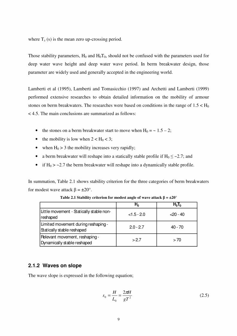
where Tz (s) is the mean zero up-crossing period.
Those stability parameters, H0 and H0T0, should not be confused with the parameters used for
deep water wave height and deep water wave period. In berm breakwater design, those
parameter are widely used and generally accepted in the engineering world.
Lamberti et al (1995), Lamberti and Tomasicchio (1997) and Archetti and Lamberti (1999)
performed extensive researches to obtain detailed information on the mobility of armour
stones on berm breakwaters. The researches were based on conditions in the range of 1.5 < H0
< 4.5. The main conclusions are summarized as follows:
• the stones on a berm breakwater start to move when H0 = ~ 1.5 – 2;
• the mobility is low when 2 < H0 < 3;
• when H0 > 3 the mobility increases very rapidly;
• a berm breakwater will reshape into a statically stable profile if H0 ≤ ~2.7; and
• if H0 > ~2.7 the berm breakwater will reshape into a dynamically stable profile.
In summation, Table 2.1 shows stability criterion for the three categories of berm breakwaters
for modest wave attack β = ±20°.
Table 2.1 Stability criterion for modest angle of wave attack β = ±20°
H0 H0T0
Little movement - Statically stable non-
reshaped<1.5 - 2.0 <20 - 40
Limited movement during reshaping -
Statically stable reshaped2.0 - 2.7 40 - 70
Relevant movement, reshaping -
Dynamically stable reshaped> 2.7 > 70
2.1.2 Waves on slope
The wave slope is expressed in the following equation;
20
0
2
gT
H
L
Hs
π== (2.5)

10
where, H [m] is the wave height, L0 [m] is the deep water wave length, T [s] is the wave
period and g [m/s2] the acceleration of gravity. This formula represents a state in deep water,
where H is the height of a single wave. To make this parameter useful for design purpose the
incident wave is usually given as significant wave height. This parameter can be given as a
time domain analysis H1/3 or as a spectral analysis Hm0, in this report it will from this point on
be referred to as Hs. For the wave period T, the zero up crossing period, Tz, and wave peak
period, Tp, are used and the slope is referred to as s0z and s0p, respectively.
To describe a wave action on a slope the dimensionless Iribarren number ξ (-), also known as
the surf similarity parameter, is important. The parameter is defined as:
0
tan
s
αξ = (2.6)
where α is the angle of the slope of the structure while s0 is a representative for the wave
slope. The formula used to calculate the wave length is valid for deep water conditions, L0,
the input in that formula in this case is however the local wave period, Tz or Tp. When s0z and
sop are used the surf similarity parameter becomes ξz and ξp respectively.
Battjes (1974) describes the different shapes of waves breaking, depending on the surf
similarity parameter. The transition between the breaker types is gradual and the values of the
transition between them are just an indication, Figure 2.1.
Figure 2.1 Breaker types as a function of the surf similarity parameter

11
2.2 Reshaping measurements
2.2.1 Recession
Recession is an important parameter when considering berm breakwaters, see Figure 2.2 for
explanation. Although the design of Icelandic type berm breakwaters does not really depend
on formulas for berm recession, it is an important tool in estimating the damage of the
structure.
Figure 2.2 Recession of berm breakwaters
Tørum (1998) presented a formula for recession, Rec (m), of the berm as a function of rock
diameter Rec/Dn50 (-) and hydraulic boundary conditions, H0T0 (-).
Rec/Dn50 = 0.0000027(H0T0)3 + 0.000009(H0T0)
2 + 0.11 H0T0 – 0.8 (2.7)
This formula has since been modified by Menze (2000), adding stone gradation and water
depth as factors in recession. The latter formula is to large extent based on test results from
multilayer berm breakwaters.
Rec/Dn50 = 0.0000027(H0T0)3 + 0.000009(H0T0)
2 + 0.11 H0T0 – (2.8)
(-9.9fg2+ 23.9fg– 10.5) - fd
with
fg = Dn85/Dn15 and
fd = -0.16 d/Dn50 + 4.0
where fg (-) represents a stone gradation factor, Dn85, Dn15 and Dn50 are the nominal diameters
for 85% , 15% and 50% respectively.
The gradation factor is the parameter that takes into account the narrow gradation of Icelandic
type berm breakwaters compared to a homogeneous one. It does not, however, include

12
parameters taking into account the effect of the smaller stones, if the Class I stones do not
reach far down the slope, and are not the cause of damage. That situation is, on the other
hand, quite complicated. Another parameter that is not included is the berm height, hB (see
Figure 2.5). Other parameters such as the shape of stones and different placement methods are
among the parameters that influence the large scatter in recession formulas.
Sigurdarson et al (2007) came up with a more simple formula wherein it is assumed that the
influence of stone grading and water depth on berm recession is rather small, especially given
the large overall scatter.
Rec/Dn50 = 0.037(H0T0 – Sc)1.34 (2.9)
with: Rec/Dn50 = 0 for H0T0 < Sc
with: µ(Sc) = 20 and σ(Sc) = 20,.
where, Sc, is the scatter in recession measurements.
2.2.2 Damage definition, Sd
The damage number Sd describes the damage using the area of erosion in the cross sections as
the basis. This damage number is a simple dimensionless parameter wherein only the eroded
area and the nominal diameter of the armour layer are included. Despite being simple it is a
very useful tool in damage estimation and, due to its simplicity, it can be applied to almost
any type of structure. Figure 2.3 further explains the formula for the stability number,
equation 2.10.
(2.10)
2
50n
e
d
D
AS =

13
Figure 2.3 Explanation figure for the damage number Sd
Although this damage number was designed for a uniform stable structure where very little
reshaping is accepted, it can also be used as a tool to compare the damage between individual
tests in this research.
2.3 Design methods for uniform slope
Many research projects have been completed on the subject of stability of stones on uniform
slope, starting with a research done by Iribarren in 1938. Hudson (1953 and 1959) did a great
deal of research on this subject, resulting in a formula that is still widely used today. Between
1965 and 1970 the first wave generators that could generate irregular waves according to a
predefined wave spectrum were introduced. After that, it became possible to replicate a real
sea state more accurately than before. Many researchers performed a number of experiments
in the following years without coming up with a formula that was accepted over the formula
of Hudson. In his PhD project at TU Delft in 1988, however, Van der Meer introduced a
formula that has been generally accepted in the engineering world. In the following sections,
the methods of Hudson and Van der Meer are briefly explained.
2.3.1 Hudson
Hudson (1953, 1959) introduced the following formula based on researches based on model
tests with regular waves on non-overtopped stone structure, with permeable core,

14
(2.11)
where KD is the stability coefficient and represents many different influences. Among those
influences is the shape of blocks, placement methods, type of wave attack, and wave period,
among others.
The original Hudson formula can be rewritten as a function of the stability number H0.
Originally the formula was used with H = Hs, but later was revised to use H = H1/10, since
H1/10 = 1.27Hs the formula written as a function of the stability parameter becomes
(2.12)
To include the damage level parameter, Sd, in equation 2.12, Van der Meer (1998) proposed
the use of equation 2.13 as the function of the stability number H0,
(2.13)
2.3.2 Van der Meer
Van der Meer conducted tests with relatively deep water at the toe of the structure. A large
amount of tests were performed with irregular waves on stone structures with uniform slope.
Different levels of permeability were used, resulting in the inclusion of permeability in the
formula. This research resulted in two formulas where one representing plunging breakers and
the other representing surging breakers. The transition between the two is also explained in a
formula.
For plunging breakers (ξm < ξtransition):
(2.14)
For surging breakers (ξm ≥ ξtransition):
α
ρ
cot3
3
50∆
=D
s
K
gHW
5.0
2.0
18.0
50
2.6 −
=
∆m
n
s
N
SP
D
Hξ
( )27.1
cot 31
50
αD
n
s K
D
H=
∆
( ) 15.031
50
cot7.0 dD
n
s SKD
Hα=
∆

15
(2.15)
Where ξtransition represents the transition between the two :
(2.16)
Where S (-) is the damage number, explained in chapter 2.2.2, P (-) is a permeability
parameter explained in Figure 2.4, while ξm is the surf similarity parameter explained in
section 2.1.2, where Tm is used.
Figure 2.4 Permeability coefficients, P, for various structures for the formula of Van der Meer (1988)
There are a few advantage of the Van der Meer formula over the formula represented by
Hudson. The research of Van der Meer was performed with irregular waves while the Hudson
formula is derived from regular waves. The Van der Meer formula does also includes the
duration of storm, the wave period, the permeability of structure, and has a clearly defined
damage level.
αξ cot0.1
2.0
13.0
50
P
m
n
s
N
SP
D
H
=
∆−
[ ]
+= 5.0
131.0 tan2.6 P
transition P αξ

16
2.4 Design methods for Icelandic type berm breakwaters
Strict rules for the main design parameters of Icelandic type berm breakwaters have not
evolved. There are, however, design guidelines that have been developed and are constantly
being reviewed. Those guidelines, as represented in Sigurdarson, et al (2007), are the
following.
Design rules:
• The upper layer of the berm consists of two layers of rock and extents on the down
slope at least to mean sea level;
• The rock size of this layer is determined by H0 = 2.0. Larger rock may be used too;
• Slopes below and above the berm are 1:1.5;
• The berm width is 2.5 - 3.0 HS;
• The berm level is 0.65 HS above design water level;
• The crest height is given by RC/HS*sop1/3 = 0.35;
According to the Rock Manual (2007), the Class I stones should preferably reach down to the
point where the reshaped profile crosses the original profile. Where the vertical distance from
the water level down to the transition of the two profiles is referred to as hf, see Figure 2.5.
This indicates that putting the transition between Class I and Class II stones higher would
decrease the stability of the structure.
Figure 2.5 Key parameters in berm breakwater design
17
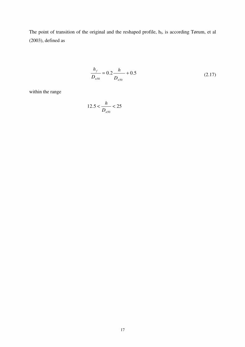
The point of transition of the original and the reshaped profile, hf, is according Tørum, et al
(2003), defined as
(2.17)
within the range
5.02.0
5050
+=
nn
f
D
h
D
h
255.1250
<<nD
h

18
3 Experimental setup
3.1 The Wave Flume
The scale model tests on the Icelandic type berm breakwaters were executed in a wave flume
in the Fluid Mechanics Laboratory of the Faculty of Civil Engineering at Delft University of
Technology. The flume was 42m long, 80cm wide and had a maximum height of 90cm, the
flume has a flat bottom profile. During the experiment the flume was divided into two parts,
the length of the part used in these model tests was 25m, see overview photo of the flume,
Figure 3.1.
Figure 3.1 Overview of the wave flume
On one end of the flume there was a wave generator which can generate regular or irregular
waves. The wave generator was equipped with an active reflection compensation system to
minimize wave reflection back from the wave board. The motion of the wave board
compensates with the reflected waves, preventing them from reflecting off the wave board
and back toward the model and thereby affecting the measurements.
3.2 Observation equipments
The observation equipments used in the experiments included, three wave gauges, a camera, a
video camera and profile measurement equipment. An overview of the setup of those
equipments is shown in Figure 3.2.
Computer
facilities
Wave
gauges
The structure
Wave
generator
Computer, related to wave generator

19
Figure 3.2 Overview of the observation equipments in the wave flume
The wave data was recorded with three wave gauges that were located in front of the
breakwater, 2m from the toe. The distance between the gauges was 40.6cm and 37.2cm.
These gauges gathered data from which the wave properties could be calculated from. The
measured waves represented the situation at the toe of the structure, excluding reflected
waves.
A camera was used to capture photos at different stages of the tests. Photos were taken after
500, 1000, 2000 and 3000 waves in each test in order to follow damage development. The
camera was located 140cm from the toe of the structure and 178cm above the bottom of the
flume. The camera was located on top of a movable plate but was however always located at
the same place when photos were taken.
A video camera was also used, to follow the motion of the stones during wave attack. The
video camera was not located at a fixed point but was generally placed in such a way that it
captured the profile of the structure. A few minutes of each test was recorded with the video
camera. A view of the capture from the video camera can be seen in Figure 3.3.

20
Figure 3.3 A view from the video camera, setup S03TM, Hs = 0.12m
To measure the profile, measurement equipment was used that consisted of a narrow stick
with a flexible plate at the end. The bottom area of the plate was approximately 2.5cm x
2.5cm. Figure 3.4 shows the equipment in use. The profiles were measured at the end of each
wave series, which was after 3000 waves.
Figure 3.4 Equipment used for profile measurements

21
3.3 Model setup
The first breakwater model setup tested was similar to the Sirevåg breakwater. The main
difference, however, was that the water depth in the model was relatively deeper. Then
depending on the damage development and failure of earlier tests, the setup of the structure
was changed and a total of six setups were tested. The first five setups are explained in Figure
3.5, Table 3.1, and Table 3.2. For setup number six which was the last one, all the stones were
mixed and, that setup is therefore not included in the explanation Figure/table. The cross
sections for each test can be viewed in Figure 3.6 and also along with the reshaping
development profiles in appendix A.4.
Figure 3.5 Explanation figure of the model setup
Table 3.1 Explanation table for test setups, parameters from Figure 3.4
In Table 3.2 the setups are further explained. In this table, hB is the vertical distance from the
berm level to the water level, Figure 2.5, while b-hB and c-hB represent the vertical distance
from the water level to the transitions between classes.

22
Table 3.2 Further explanation for test setups, parameters from Figure 3.5 and Figure 2.5
Setup hB [m] b-hB [m] c-hB [m] h [m] hB [m] b-hB [m] c-hB [m] h [m] hB [m] b-hB [m] c-hB [m] h [m]
1 0.015 0.078 0.194 0.645 0.07 0.023 0.139 0.590 0.115 0.022 - 0.094 0.545
2 0.015 0.136 0.194 0.645 0.07 0.081 0.139 0.590
3 0.015 0.078 0.113 0.645 0.07 0.023 0.058 0.590
4 0.015 - 0.194 0.645 0.07 - 0.139 0.590
5 0.015 0.078 0.164 0.645 0.07 0.023 0.109 0.590
Water level 0.645m Water level 0.590m Water level 0.545m
Figure 3.6 Overview of the different setups
For every setup, the geometry of the structure was the same. Specifically the berm width, BB
(m), the berm height, the crest height and the slopes α, were not changed between tests. The
parameters that changed between setups were the water level and the location of different
stone classes. For most setups, two water levels, 0.645m and 0.590m, were tested. A third
level, 0.545m, was tested for the first setup only. Other relevant parameters were:
BB = 0.30m (berm width)
α = 1:1.5 for all slopes
In appendix A.1 those dimensions are given as a function of the different wave heights, Hs, as
well as a function of the median nominal diameters, Dn50, of the different stone classes.
A total of thirteen setups were tested. For each setup the number of tests was based on the
moment of failure. This resulted in four to six tests for each setup or a total of 62 tests in the
wave flume. In addition to those tests, a total of eight tests for two setups were repeated.
Those tests were used to estimate the uncertainties of the tests and increased the total number
of tests to 70.

23
3.3.1 Wave conditions
For each setup, tests were carried out for up to six different wave conditions, see Table 3.3.
These tests started with the lowest waves (test 1) and then continued with higher waves until
there was a complete failure of the structure. A complete failure was defined as the start of
core erosion. The wave steps were based on the stone sizes as such that the stability number,
H0, was between 1.5 and 3.0 for Class I stones. The chosen wave conditions can be viewed in
Table 3.3.
Table 3.3 Wave series planned for the tests
Test # HHHHSSSS [m] [m] [m] [m] ssssopopopop Tp [s]Tp [s]Tp [s]Tp [s] W-SW-SW-SW-S DDDDn50n50n50n50 HHHH0000 HHHH0000TTTT0p0p0p0p
1 0.085 0.04 1.17 Jonswap
Class I 0.032 1.50 31
Class II 0.025 1.92 44
Class III 0.020 2.45 64
2 0.100 0.04 1.27 Jonswap
Class I 0.032 1.76 39
Class II 0.025 2.26 57
Class III 0.020 2.88 82
3 0.120 0.04 1.39 Jonswap
Class I 0.032 2.12 51
Class II 0.025 2.71 74
Class III 0.020 3.46 107
4 0.135 0.04 1.47 Jonswap
Class I 0.032 2.38 61
Class II 0.025 3.05 89
Class III 0.020 3.89 128
5 0.155 0.04 1.58 Jonswap
Class I 0.032 2.73 75
Class II 0.025 3.50 109
Class III 0.020 4.47 157
6 0.170 0.04 1.65 Jonswap
Class I 0.032 2.99 86
Class II 0.025 3.84 126
Class III 0.020 4.90 181
For all tests the target wave steepness was chosen to be fixed at s0p = 0.04.
Measured wave conditions during the model tests were not exactly the same as the target
values in Table 3.3 but were generally closed to those values. The measured values can be
viewed in Appendix A.2.

24
3.3.2 Wave spectra
In order to simulate the waves in front of the breakwater as realistically as possible, irregular
waves were used for the execution of all tests. When choosing wave spectra for irregular
waves the wave flume offers two possibilities apart from making new wave spectra. These
possibilities are the Pierson-Moskowitz spectrum (1964) and the Jonswap spectrum (1973).
The Pierson-Moskowitz spectrum represents a fully developed sea and was developed by
offshore industry. It assumes deep water conditions with unlimited fetch and was developed
using North-Atlantic data.
The Jonswap spectrum on the other hand represents a sea at young state and was also
developed by offshore industry. It represents conditions with limited fetch and was developed
using North Sea data. Since the wave spectrum is hardly ever fully developed in nature, the
Jonswap spectrum is often used. In this experiment the Jonswap spectrum was used with the
peak enhancement factor, γ = 3.3.
3.3.3 Water depth
Three water depths were used in the experiments, 0.645m and 0.590m. For one test, a water
depth of 0.545m was also tested. Waves can be classified as deep water waves, intermediate
water waves and shallow water waves according to the following definitions:
es water wavdeep2
1⇒>
L
h
es water wavteintermedia2
1
20
1⇒<<
L
h
es water wavshallow20
1⇒<
L
h

25
Table 3.4 h/L ratio for all water levels used in the experiments
Hs [m] Tp [s] h [m] L [m] h/ L [-] h [m] L [m] h/ L [-] h [m] L [m] h/ L [-]
0.085 1.17 0.645 2.05 0.31 0.590 2.03 0.29 0.545 2.00 0.27
0.100 1.27 0.645 2.36 0.27 0.590 2.32 0.25 0.545 2.28 0.24
0.120 1.39 0.645 2.73 0.24 0.590 2.67 0.22 0.545 2.62 0.21
0.135 1.47 0.645 2.98 0.22 0.590 2.91 0.20 0.545 2.85 0.19
0.155 1.58 0.645 3.30 0.20 0.590 3.21 0.18 0.545 3.13 0.17
0.170 1.65 0.645 3.52 0.18 0.590 3.42 0.17 0.545 3.33 0.16
For all the test series the combination of waves and water depth represents waves in
intermediate water depth.
3.4 Material
3.4.1 Shape of stones
Small stones, like the ones used for model tests, have a tendency to have a different shape
than the big rocks used for the armour layer of a breakwater. Therefore, the stones for the
model test have to be carefully chosen. Shape is particularly important for the Class I stones,
that are carefully placed, since it can significantly affect the armour layer stability. There are a
few useful measures concerning the shape of stones, including the length-to-thickness ratio
(LT), blockiness (BLc), roundness and angularity. In this study, the length-to thickness ratio
was measured and used as a criterion for armour stone selection of the model. The other
aspects were kept in mind when choosing the stones but not applied directly. This is
especially important when choosing the Class I stones since interlocking between them is an
important factor in the design of the breakwater and is very dependent on the shape of the
stones.
Length-to-thickness ratio (LT)
Length-to thickness ratio, LT (-), is defined as the maximum length, l (m), divided by the
minimum distance, d (m), between parallel lines through which the particle would just pass,
as is explained in Figure 3.7.

26
Figure 3.7 Illustration of the measurements of the LT ratio
For heavy armour stones in cover layers, the number of stones with LT ratio greater than 3:1
is recommended to be lower than 5%. While for light armour stones in cover layer, the same
ratio is recommended to be lower than 20%.
[CUR/CIRIA (2007)]
A sample of stones from each class was chosen randomly and the LT ratio measured, the
results are the following:
Class I stones with LT ratio > 2:1 = 30%
Class I stones with LT ratio > 3:1 = 0%
The average LT ratio of Class I stones is: 1:1.9
Class II stones with LT ratio > 2:1 = 60%
Class II stones with LT ratio > 3:1 = 3%
The average LT ratio of Class II stones is: 1:2.1
Class III stones with LT ratio > 2:1 = 50%
Class III stones with LT ratio > 3:1 = 0%
The average LT ratio of Class III stones is: 1:2.2
For all stone classes the samples meet the recommendations for heavy armour stones. The
stones are therefore considered a good representative for armour rocks in a real project.
3.4.2 Characteristic of stones
The density of the armour stones (Class I, Class II and Class III) is ρs = 2770 [kg/m3] while
the density of the core material is ρs = 2620 [kg/m3]. The nominal diameter, DnXX for different

27
percentages, XX, is widely used to estimate various aspects, including stability and filter
requirements. The XX is replaced by a percentage representing a diameter of a theoretical
block for which XX% of the mass of the sample is lighter.
One of the biggest different between an Icelandic type berm breakwater and a homogeneous
berm breakwater or a conventional breakwater, concerning stones is the gradation of the
stones. Since in the Icelandic type the gradation in each stone class is narrower due to the
sorting of stones by size into different classes. The gradation is grouped depending on the
Dn85/Dn15 ratio:
Narrow gradation if Dn85/Dn15 > 1.5
Wide gradation if 1.5 <Dn85/Dn15 <2.5
Very wide gradation or quarry run if Dn85/Dn15 > 2.5-5.0+
Measurements of the Dn85/Dn15 ratio for the three stone classes as well as for the core material
fell under the category of ‘Narrow gradation’. For comparison, toward the end of the
experiment all the stones were mixed together. That resulted in homogenous armour layer
with wide gradation. The sieve curve of this experiment becomes close to represent a sieve
curve of the situation before the stones are sorted. However, since all the cross sections did
not have exactly the same amount of stones from each class and the back side of the
breakwater was also not considered, this mixed sieve curve is more helpful as a comparison of
different setups and is only an approximation for a possible quarry result. Having one sample
with wide gradation eases comparison with earlier research, for example recession.
The sieve curves and additional basic information about the material can be found in appendix
A.3.
3.4.3 Law of scaling
Before a physical model test can be performed, the prototype must be scaled down to a size
which can be handled by the available test facility. Although the purpose of this research
project is not to look at a specific prototype, the breakwater in Sirevåg, Norway, was used as a
semi-prototype when deciding on stone diameter and other relevant parameters. One of the
problems with scaling is that certain parameters cannot be or are difficult to scale. Those
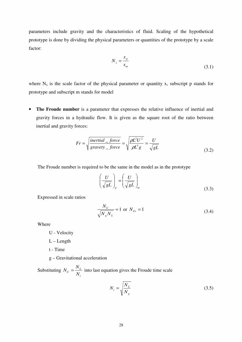
28
parameters include gravity and the characteristics of fluid. Scaling of the hypothetical
prototype is done by dividing the physical parameters or quantities of the prototype by a scale
factor:
m
p
xx
xN =
(3.1)
where Nx is the scale factor of the physical parameter or quantity x, subscript p stands for
prototype and subscript m stands for model
• The Froude number is a parameter that expresses the relative influence of inertial and
gravity forces in a hydraulic flow. It is given as the square root of the ratio between
inertial and gravity forces:
gL
U
gL
UL
forcegravety
forceinertialFr ===
3
22
_
_
ρ
ρ
(3.2)
The Froude number is required to be the same in the model as in the prototype
mpgL
U
gL
U
=
(3.3)
Expressed in scale ratios
1=Lg
U
NN
N or 1=FrN (3.4)
Where
U - Velocity
L – Length
t - Time
g – Gravitational acceleration
Substituting t
L
UN
NN = into last equation gives the Froude time scale
g
Lt
N
NN = (3.5)

29
For practical purpose gravity is not scaled, thus Ng = 1. The Froude time scale is thereby
simplified to
Lt NN = (3.6)
The majority of hydraulic models in coastal engineering are scaled according to the Froude
criterion. Consequently, this is usually the most important criterion to be studied when
designing a coastal scale model. Since in this experiment the most important parameter is the
wave attack, the Froude criterion will be used.
[Hughes, 1995]

30
4 Analysis
For analysis of this research, the profile measurements from the tests in the flume were used
along with photos and videos recorded during the tests. Visual observations during the tests
are also influential in the analysis. In appendix A.4, the profile developments of the tests can
be followed.
4.1 Damage development
Test results showed that the start of damage and the damage development changes for
different test setups. In this section the damage development and the failure mechanisms for
each test are briefly explained.
Figure 4.1 Overview of the different setups
4.1.1 Setup 1
Water level 0.545m
Setup 1 was the only setup where water level 0.545 was used. The water level was located
below the transition of Class I and Class II. The water level was also closer to the transition of
Class II and Class III than in the other setups, apart from setup 3.
Start of damage: The damage starts clearly in the part where the Class II stones are located,
where stones start moving with relatively small wave height. The reshaping that had already
taken place after the first wave set (Hs = 0.085m) is not acceptable for a stable structure.
Failure mechanism: The cause of the early failure of this setup is the low location of the
water level. The low location both minimized the effects of the berm in energy dissipation,
and caused the smaller stones to be located closer to the water level and therefore under
greater wave attack. Although the water level is lower than in the other tests, the Class III
stones were located deep enough not to be a part of the failure process.

31
Water level 0.590m
Start of damage: The structure is stable and without significant reshaping for the first two
wave sets. Lack of stability and sliding in Class II stones causes the start of severe movement
of Class I stones during the third wave set.
Failure mechanism: The relatively close position of Class II stones to the water level
influences the failure process from the third wave set, until there was a complete failure of the
structure.
Water level 0.645m
Class I and Class II stones started moving at similar time. The real reshaping started in Class
I, then the Class II stones started to give in as well and accelerate the damage process. The
lower parts were the Class II stones were located would therefore have been stronger if the
Class I stones had reached further down.
Start of damage: The Class I stones roll down due to the wave attack on the edge of the
berm. No influence on the Class II stones early on in the process. The behaviour is similar to
when the structure had a homogenous armour layer.
Failure mechanism: The Class II stones possibly play some part in the failure process at
latter stages.
4.1.2 Setup 2
Water level 0.590m
Start of damage: In Class I stones.
Failure mechanism: In this setup the failure mechanism is similar to if the structure had a
homogeneous armour layer. Specifically, all the real damage takes place in the Class I stones.
Water level 0.645m
When the recession reached the transition of Class I and Class II stones on the berm, it
increased. Apart from that it is similar to setup 1.
Start of damage: In Class I stones.
Failure mechanism: In this setup the failure mechanism is similar to if the structure had a
homogeneous armour layer. Specifically, all the real damage takes place in the Class I stones.
32
4.1.3 Setup 3
Water level 0.590m:
In this setup, the Class III stones are located closer to the water level than for the other setups.
The reason for this is to better understand the ideal location for the transition of Class II and
Class III stones.
Start of damage: The damage clearly starts in the location of the Class III stones, where
stones start moving with relatively small wave height. The reshaping that had already taken
place after the first wave set (Hs = 0.085m) is not acceptable for a stable structure.
Failure mechanism: The cause of the early failure of this setup is the low location of the
transition of Class II and Class III stones. The failure mechanism is the same as for setup 1
with water level 0.545m. The only difference in this case is that the Class III stones are the
main cause of this behaviour.
Water level 0.645m: The failure process is similar to the setup 1, which indicates that the
location of Class III stones is low enough not to affect the failure process.
Start of damage: In Class I stones.
Failure mechanism: It is possible that the Class II stones and even Class III stones play some
part in the failure process at latter stages.
4.1.4 Setup 4
Water level 0.590m
Setup 4 shows exactly the same damage development as setup 2 for this water level.
Start of damage: In Class I stones.
Failure mechanism: In this setup the failure mechanism is similar to if the structure had a
homogeneous armour layer. Specifically, all the real damage takes place in the Class I stones.
Water level 0.645m
When the recession reached the transition of Class I and Class II stones on the berm, it
increased. Apart from that, this setup behaves similar to setup 1. For this setup this influence
is clearer than for setup 2 with the same water level because the transition is closer to the edge
of the berm.
Start of damage: In Class I stones.

33
Failure mechanism: In this setup the failure mechanism is similar to the structure had a
homogeneous armour layer. Specifically, all the real damage takes place in the Class I stones.
4.1.5 Setup 5
Water level 0.590m
In this setup, the Class II stones are put as the top layer and the Class I stones below them.
This is the exact opposite of setup 1 when concerning those two classes.
Start of damage: In Class II stones that are located on the berm. The recession on the edge of
the berm early on in the process is more than in previous setups.
Failure mechanism: The failure process starts earlier then for setups 1, 2 and 4 but slows
down because of the location of Class I stones lower on the berm. In the end, the duration is
similar to those setups. The damage develops step by step throughout all the wave series.
Water level 0.645m
The recession of the berm starts earlier than in most of the other setups. However, the
existence of the thick layer of Class I stones below slows that process down. Towards the end
the recession is becomes less than for setup 2 and 4, but slightly more than in setup 1. This
shows that having the Class I stones in this position, influences the recession development in
a positive way, at the latter stages.
Start of damage: In Class II stones that are located on the berm. The recession on the edge of
the berm at the early stage of the process is more than before.
Failure mechanism: Damage starts from the edge of the berm as expected with the Class II
stones located there. The damage develops step by step throughout all the wave series.
4.1.6 Setup 6
The armour layer in setup 6 is homogeneous, where the failure mechanism is as expected for
such a structure. The reason for this setup is, however, to compare the damage level with the
other setups in order to assess the benefits of sorting stones into classes.

34
4.1.7 Compilation
Berm height
Comparing the water level 0.590m in setup 1 to the water level 0.645m in setup 2, where the
depth down to the transition of Class I and Class II is similar, it can be concluded that the
Class II stones are more affected when the water level is lower on the berm. This shows that,
for the different water levels 0.590m and 0.645m there is a basic difference. There is more
energy dissipated when the water level is closer to the berm. Therefore, the effects do not
reach as deep when the water level is close to the berm. This can be seen in the damage
figures where the transitions between Class I and Class II stones are at similar depth. While
on the other hand, when the water level is high, there is more movement of stones up the
berm.
On berm
From setups 1, 2 and 4, the effect of the transition
between Class I and Class II stones on the berm
can be seen. As soon as the recession reaches this
point of transition (in setup 2 and 4), the
recession increases quickly almost to the end of
the berm. While in setup 1, where there were Class I stones on the whole berm the
recession stabilized earlier. However, when Class I and Class II stones were switched in setup
5, it did not have the same effect. The conclusion of that is that by putting a thicker layer of
Class I stones lower on the berm, although the recession on the berm starts faster (due to the
Class II stones on the berm), it slows down the recession development at the later stages.
On slope
The point of transition between Class I and Class II
stones on the berm does not seem to affect what
happens on the slope of the berm. The location of the
transitions between classes on the slope is therefore
the only parameter that is looked at concerning this.
For each of those transitions there is an optimum
level, to locate this optimum level both for transition of Class I and Class II stones and the
transition of Class II and Class III is the primary goal of this research project.

35
4.2 Recession
Recession of the berm is an important part of the
damage process. In this chapter, the test results
will first be compared to existing recession
formulas. Then, the test results for different setups
will be analysed. In order to ease comparison of
different tests, the stone parameters from the
sample when the stones were mixed together was used. This provides a good ground for
comparison since the mixed sample represents the same material before being sorted into
classes. In appendix A.5, a variety of recession graphs are shown.
4.2.1 Comparison with recession formulas
In Figure 4.2 and Figure 4.3, the results of recession measurements are compared with two
formulas, the modified formula of Tørum (2.8) and formula 2.9. For the test results points in
the first graph (Figure 4.2), the stone parameters of the Class I stones are used when
comparing setups 1-5 with existing formulas. For the second graph (Figure 4.3) the stone
parameters of the mixed stone sample were used when comparing setup 6 to existing
formulas.
0
1
2
3
4
5
6
7
8
9
10
0 10 20 30 40 50 60 70 80 90 100
Rec/
Dn50
H0T0
Recession - data compared with other researches, setups 1-5, Class I
Formula(2.9)
-sigma
Formula(2.9)
+sigma
Formula
(2.9)
Formula of
Tørum (2.8) Class I
Figure 4.2 Recession, comparison of test results with recession formulas, setups 1-5, Class I stones used as
reference.

36
0
1
2
3
4
5
6
7
8
9
10
0 10 20 30 40 50 60 70 80 90 100
Rec/
Dn50
H0T0
Recession - data compared with other researches, setup 6, mixes stone sample
Formula(2.9)
-sigma
Formula(2.9)
+sigma
Formula
(2.9)
Formula of
Tørum (2.8) mixture
Figure 4.3 Recession, comparison of test results with recession formulas, setups 1-5, Class I stones used as
reference.
As can be seen from Figure 4.3, the results for the mixed stones fit reasonably well with the
formula of Tørum (2.8). However when looking at Figure 4.2, the comparison of setups 1-5
with the formula of Tørum, with stone parameters from Class I, the results do not fit well. The
test results give more recession than the formula predicts, some of the following factors might
be the cause of that.
• The narrow stone gradation; the recession might not be as sensitive to stone gradation
as formula 2.8 indicates.
• The placement method; what placement methods were used when the formulas were
derived, is unknown.
• The effect of the berm level; the berm level is not included in the formulas but has
effects on the recession.
• The influence of the different location of the transition of stone classes; for some of
the tests the Class I stones are not the only stones involved in the recession
development.
Formula 2.9 however is not sensitive to the gradation of stones as compared to the formula of
Tørum (2.8). For formula 2.9, the majority of the tests are within the limitation of one

37
standard deviation from the mean values. The general test results show that the average
recession from the tests is a little higher than the mean value. The reasons for this might be
the same as some of the ones mentioned above.
The results from this research indicate that the influence of stone gradation is overrated in
formula 2.8. The only setup that gave results that fit reasonably well to this formula was the
setup with a homogenous berm. This indicates that the formula is possibly not valid for the
narrow gradations used in other tests.
4.2.2 Influence of berm height on recession
For comparison figures of the recession with different berm height for each setup, appendix
A.5.2 can be viewed. Figure 4.4 shows, however, recession for setup 4 with different water
levels and thereby different berm heights. In the figure, S04TH stands for setup 4 with high
water level (0.645m), while the others are for the medium water level of the three that were
used in the research (0.590m).
0
2
4
6
8
10
12
0 10 20 30 40 50 60 70 80 90 100 110
Rec/
Dn50
H0T0
Recession - Setup 4, comparison of water levels
S04TH
S04TM
S04TM_rep
Formula of
Tørum (2.8) mixture
Figure 4.4 Recession, comparison of different water levels, setup 4
The general results show that the recession on the edge of the berm is usually more with a
higher water level. That is as expected, since wave attack is more intense on the berm when
the water level is closer to the berm. Setup 3 this turned out differently because the damage

38
process started early, since the water level was lower and thereby the distance down to the
Class III stones was shorter. Then, as mentioned before the failure mechanism is different and
the leading cause of recession is not the attack on the edge of the berm but the attack on the
smaller stones located further down the slope.
4.2.3 Influence of stones on berm, on berm recession
The effect of the stones that were placed on the
berm and the location of the transition of the
stone classes on the berm are briefly discussed
here.
Both for setup 2 and setup 4 for high water level
(0.645m) where the Class I stones do not reach all the way to the end of the berm, this
research shows that when the recession reaches the transition of Class I and Class II stones the
recession increases. This is especially notable for setup 4, where this transition is closer to the
berm than in setup 2, therein setup 4, the recession increases almost to the end of the berm
soon after it reaches this transition which is located 4Dn50 from the edge of the berm. For
setup 2, on the other hand, the recession does not reach this transition until the last wave
series, where the total damage of the structure is already close to failure. It can be concluded
that this transition should reach at least long enough into the berm, that the expected total
recession does wound not reach that point, because then the runs the risk of rapid increasing
of recession.
4.2.4 Influence of stones on the front slope, on berm recession
The stones on the berm are usually the ones that
cause the start of recession, although in some
cases it might be small. There are always a few
stones on the slope that role down early in the
process. In case of the weaker structures, that is
structures where the transition between Class I
and Class II stones is relatively close to the
water level, erosion in the part with Class II stones causes a large part of the stones above to
roll down. This causes a quick increase in the recession of the berm. This recession only
occurs when the larger stones do not reach far enough down the berm. This behaviour is not

39
attractive for such a structure because it causes too much damage relatively early on in the
process, when the structure should still be stable.
4.2.5 Comparison of setups
In Figure 4.5 and Figure 4.6, the different recession development for the different setups,
water levels 0.590 and 0.645 respectively, is compared. It should be noted that for the last
values of each setup, where the H0T0 value is the highest, the test series was not completed for
all the tests. The number of waves in the last measurements was therefore different for the last
point and was never 3000 waves like for the other points. In chapter 4.4 the duration until the
failure of each setup is explained.
0
2
4
6
8
10
12
0 10 20 30 40 50 60 70 80 90 100 110
Rec/
Dn50
H0T0
Recession - Water level 0.590, comparison of different setups
S01TM
S02TM_rep
S03TM
S04TM_rep
S05TM
S06TM
Figure 4.5 Recession, comparison of different setups, water level 0.590m

40
0
2
4
6
8
10
12
0 10 20 30 40 50 60 70 80 90 100 110
Rec/
Dn50
H0T0
Recession - Water level 0.645m, comparison of different setups
S01TH
S02TH
S03TH
S04TH
S05TH
S06TH
Figure 4.6 Recession, comparison of different setups, water level 0.645m

41
4.3 Damage number Sd
The damage number Sd is, as explained before (in chapter 2.2.2), a good tool to compare total
damage of different setups. This measure is, however, not as useful when comparing with
different structures such as conventional two layered breakwaters, where much less reshaping
is accepted and the Sd value therefore lower.
For comparison, the damage number is calculated by using the nominal diameter, Dn50, from
the sample of mixed stones. This is done for ease of comparison of different setups, while at
the same time create a dimensionless parameter to work with that represents the damage
development. In appendix A.6, a variety of damage development graphs are shown.
4.3.1 Influence of berm height on the damage number
In appendix A.6.1, the graphs from all setups, where the different effect of berm height on the
total damage/erosion is explained. From the results of setup 2, Figure 4.7, it can be seen that
the total amount of damage/erosion is more as the water level becomes lower. This turned out
to be the case for all setups, within the limitations of the three water levels tested.
0
10
20
30
40
50
0 10 20 30 40 50 60 70 80 90 100 110
S d
H0T0
Damage number - setup 2
S02TM
S02TM_rep
S02TH
Figure 4.7 Damage number, comparison of different water levels for setup 2
This difference is significant for all setups, there can be a few explanations for that.

42
• As the water level is changed, the distance from the water level down to the
transition of different stone classes changes as well. Therefore, for many of the
tests, this can explain more erosion as the distance down to the smaller stones is
less. This does, however, not explain why the same behaviour occurs with other
setups as well, both for setup 5 where Class I and Class II are switched and for the
mixed stones, setup 6.
• More energy dissipation due to the berm occurs when the water level is closer to
the berm level. There is more overtopping and attack on stones located further up
the berm. Individual stones are even, in some cases, moved far up the berm.
• With the water level closer to the berm the breakwater is closer to its natural
reshaped profile. Therefore less reshaping and, consequently, less erosion is
required to reach a stable reshaped profile.
4.3.2 Comparison of setups
In Figure 4.8 and Figure 4.9, the different erosion development for the different setups is
compared for the different water levels of 0.590m and 0.645m. It should be noted that for the
last values of each setup, where the H0T0 value is the highest, the test series was not
completed for all the tests. Consequently, the number of waves in the last measurements was
different between setups and never 3000 waves like for the other points. In chapter 4.4, the
duration until failure of each setup is explained.
0
10
20
30
40
50
0 10 20 30 40 50 60 70 80 90 100 110
S d
H0T0
Damage number - water level 0.590m
S01TM
S02TM_rep
S03TM
S04TM_rep
S05TM
S06TM
Figure 4.8 Damage number, comparison of different setups with water level 0.590m

43
0
10
20
30
40
50
0 10 20 30 40 50 60 70 80 90 100 110
S d
H0T0
Damage number - water level 0.645m
S01TH
S02TH
S03TH
S04TH
S05TH
S06TH
Figure 4.9 Damage number, comparison of different setups with water level 0.645m
For both water levels (0.590m and 0.645m), as expected, the most damage occurred for the
matching wave period stability number in setups 3 and 6. Setup 5 also had high level of
erosion when the water level was at 0.645m.
When looking into the situation where the water level is 0.590m, setups 1, 2 and 4 shows the
least damage for the matching wave period stability number. Setup 5 for this water level
caused more damage throughout the tests but the difference decreases with higher wave
stability number, H0T0.
Where the water level is at 0.645m, setups 2 and 4 show the best results. Setup 1 shows
similar total erosion development for the first four wave sets but then the damage increases in
the fifth wave set. The reason for this can possibly be traced to the fact that the distance down
to the transition of Class I and Class II stones is shorter for that setup than the other two and,
as a result, it starts to affect the damage development severely when the waves get higher.

44
4.4 Duration until failure/core erosion
The point of failure was defined as the point where core erosion started. For each test this
point of failure was noted. In most cases the test was also stopped around that moment but in
some cases later. The last points in the concerning recession and general erosion do therefore
not always represent the situation after 3000 waves. In the following tables, the duration until
core erosion for each test can be viewed. The planned wave properties for each wave series
can be viewed in Table 3.3, while the measured wave properties in each test can be viewed in
appendix A.2.
Table 4.1 Duration of tests, water level 0.545m
1 2 3 4 5 6
S01TL
Wave series #
Table 4.2 Duration of tests, water level 0.590m
1 2 3 4 5 6
S01TM
S02TM_rep
S03TM
S04TM_rep
S05TM
S06TM
Wave series #
Table 4.3 Duration of tests, water level 0.645m
1 2 3 4 5 6
S01TH
S02TH
S03TH
S04TH
S05TH
S06TH
Wave series #
Generally the duration of tests until failure, turned out to be longer with the water level close
to the berm than with lower water levels. For water level 0.590m, there is not much difference
in the duration between setups 1, 2, 4 and 5. While for the higher water level, 0.645m, setups
2 and 4 were the ones with the longest duration.

45
4.5 Transition of original and reshaped profile, hf
Expected values for the distance from the water level
down to the point of transition of the original and the
reshaped profile are expressed in Tables 4.4 and 4.5.
Where in Table 4.4 the Dn50 from Class I stones are
used while in Table 4.5 the Dn50 from the sample of
mixed stone is used.
Table 4.4 Expected transition points of original and reshaped profiles, Class I
L M H
h 0.545 0.59 0.645
Dn50 0.0320 0.0320 0.0320
h/Dn50 17.0 18.4 20.2
hf/Dn50 3.91 4.19 4.53
hf 0.125 0.134 0.145
hB 0.115 0.07 0.015
hB/Dn50 3.59 2.19 0.47
Table 4.5 Expected transition points of original and reshaped profiles, mixed stone sample
L M H
h 0.545 0.59 0.645
Dn50 0.0257 0.0257 0.0257
h/Dn50 21.2 23.0 25.1
hf/Dn50 4.74 5.09 5.52
hf 0.122 0.131 0.142
hB 0.115 0.07 0.015
hB/Dn50 4.47 2.72 0.58
As can be seen from the tables, the distance from the water level to the expected point of
transition of the profiles does not differ greatly whether Dn50 is used for Class I stones or for
stones of the mixed sample. The difference is well within the uncertainties of the tests,
because in relatively deep water, the influence of Dn50 is less and the difference of Dn50 of the
two samples is rather small. For setups 1-5, the Dn50 from Class I stones are used as a measure
of the relative parameters (hf/Dn50, hB/Dn50 and h/Dn50), while for setup 6 the Dn50 from the
sample of mixed stones was used. It should be noted that Tables 4.4 and 4.5 includes the
values for hB/Dn50 which is the distance from the berm down to water level as a function of
stone diameter. This parameter is the most likely one, apart from the once included in formula
2.17, to have influence on hf/Dn50.

46
4.5.1 Interpretation of test results
The results of the measurements are explained in graphs in appendix A.7. First, the graphs
compare different berm levels, hB/Dn50, in Figures A.44 – A.47, then compare the different
setups with the berm level fixed in Figures 4.10, A.48 and A.49.
0
1
2
3
4
5
6
7
8
9
0 10 20 30 40 50 60 70 80 90 100 110
hf/D
n50
H0T0
Intersection of original and reshaped profiles, water level 0.590m
S01TM
S02TM
S02TM_rep
S03TM
S04TM
S04TM_rep
S05TM
S06TM
Figure 4.10 Transition of original and reshaped profile, hf, water level 0.590m
The results of the measurements were derived from those graphs and are the following:
For Class I stones:
hB/Dn50 = 3.59 and h/Dn50 = 17.0 → hf/Dn50 = 6.0 (only one sample with water level, 0.545m)
hB/Dn50 = 2.19 and h/Dn50 = 18.4 → hf/Dn50 = 5.1 - 5.6 (water level 0.590m)
hB/Dn50 = 0.47 and h/Dn50 = 20.2 → hf/Dn50 = 4.0 - 4.5 (water level 0.645m)
For stones from mixed sample (only one measurement for each):
hB/Dn50 = 2.72 and h/Dn50 = 23.0 → hf/Dn50 = 7.3 (water level 0.590m)
hB/Dn50 = 0.58 and h/Dn50 = 25.1 → hf/Dn50 = 5.7 (water level 0.645m)
The results show that the value of hf/Dn50 gets larger as the berm height, hB/Dn50, gets larger.
That means that as the water level is lower on the berm, the point of transition gets not only
Expected values
Class I
Expected values
Mixed stones

47
lower compared to the berm but also compared to the water level. The influence of hB/Dn50 is
opposite to, and for these water depths, larger than the influence of water depth, h/Dn50. This
proved to be the case for every setup, which shows an influence of berm height, hB/Dn50, on
hf/Dn50. The influence can be explained by the fact that the lower the water level was
compared to the berm. This results in larger forces acting lower on the structure.
With the water level relatively close to the berm, hB/Dn50 relatively low, formula 2.17 gives
results close to the ones measured in the tests. However when that distance, hB/Dn50, increases
the test results give higher values compared to the formula. This suggests that to make the
formula valid for situations where the water level is lower on the berm, the inclusion of berm
height, hB/Dn50, would be needed.
An addition of 0.6hB/Dn50 to formula 2.17 gives a formula that better fits the results of the
experiment, both for the different berm heights. That is, with water level at 0.645m, 0.590m
and for the only test that was performed with the water level at 0.545m. It also fits reasonably
well for the different stone diameters, that is both where Class I was used and where the
mixed sample was used.
(4.1)
5.06.02.0505050
++=n
B
nn
f
D
h
D
h
D
h
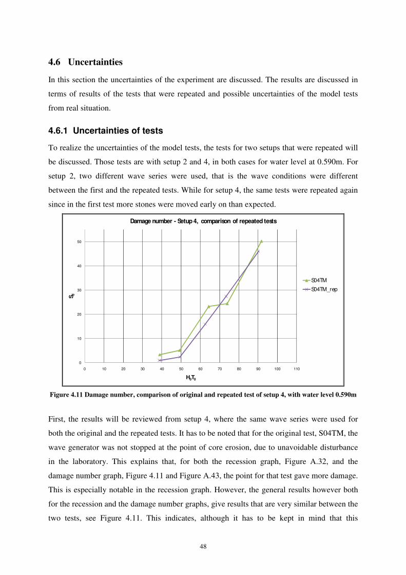
48
4.6 Uncertainties
In this section the uncertainties of the experiment are discussed. The results are discussed in
terms of results of the tests that were repeated and possible uncertainties of the model tests
from real situation.
4.6.1 Uncertainties of tests
To realize the uncertainties of the model tests, the tests for two setups that were repeated will
be discussed. Those tests are with setup 2 and 4, in both cases for water level at 0.590m. For
setup 2, two different wave series were used, that is the wave conditions were different
between the first and the repeated tests. While for setup 4, the same tests were repeated again
since in the first test more stones were moved early on than expected.
0
10
20
30
40
50
0 10 20 30 40 50 60 70 80 90 100 110
S d
H0T0
Damage number - Setup 4, comparison of repeated tests
S04TM
S04TM_rep
Figure 4.11 Damage number, comparison of original and repeated test of setup 4, with water level 0.590m
First, the results will be reviewed from setup 4, where the same wave series were used for
both the original and the repeated tests. It has to be noted that for the original test, S04TM, the
wave generator was not stopped at the point of core erosion, due to unavoidable disturbance
in the laboratory. This explains that, for both the recession graph, Figure A.32, and the
damage number graph, Figure 4.11 and Figure A.43, the point for that test gave more damage.
This is especially notable in the recession graph. However, the general results however both
for the recession and the damage number graphs, give results that are very similar between the
two tests, see Figure 4.11. This indicates, although it has to be kept in mind that this

49
assumption is only based on one repeated test, that the tests are reliable at least when
compared individually. Other general uncertainties are discussed in chapter 4.6.2.
For setup 2, the situation is different since in the original test, S02TM, the wave steepness was
different than for any other test. The comparison between the original and the repeated tests
for this setup did not give as convincing results as for setup 4. When the recession was looked
at as a function of H0T0, Figure A.30, as was done for every test, there was a large and
constant difference of more than 2Rec/Dn50 throughout the tests. This difference does,
however, decrease if the wave period part, T0, is neglected, Figure A.31, and the recession is
measured as a function of H0. For the total erosion of the structure that is measured with the
damage number, Sd, the difference is not as large. There is a notable difference in the original
graph, Figure A.41. However when looked at as a function of H0, Figure A.42, it fits well.
4.6.2 General uncertainties
One of the most important aspect when an Icelandic type berm breakwater is constructed is
the placement of the Class I stones on top of the berm and down to the water level. In reality
the stones are carefully placed one by one, in such a way that they give good interlocking
between them. This part is difficult to replicate in a model test. In this research the stones
were placed in a more stable way than just random dumping but most likely in a less stable
way than in a full size project.
The flume is rather narrow, 90cm (28Dn50 for Class I stones), and therefore it does not offer
the possibility of measuring many cross sections at different locations. There are also clear
effects from the sides of the flume that reach 10-15cm into the structure from each side. The
active width of the flume in this experiment was therefore 60-70cm. The profiles were
measured at the middle of the structure, with measurement equipment as is explained in
chapter 3.2 and with Figure 3.4. It would have been preferable to have some kind of scanning
equipment to measure the whole area and then afterwards the parts that are affected by the
sides of the flume and other abnormal behaviour could be excluded.

50
5 Discussion of model tests
In order to get the desired wave heights in the flume the water level was deeper than
originally planned. With the deep water condition, the biggest waves do not break like they
would in some cases due to the water depth in front of the structure. That means that almost
all the big waves hit the structure in the model, only the very biggest waves broke, but in most
cases where a breakwater is constructed the waves would break when they are relatively
smaller. The big waves are the ones that make the most damage and the top waves are not cut
off as in situations where they break due to water depth.
In the tests all waves were perpendicular to the structure, longshore transport is therefore not
taken into consideration in the research. When waves approach the structure at an angle the
stones do, however, not only move up and down in the same cross section but some stones are
also moved along the structure. This can affect the stability of the structure, but this is not
considered to be a problem for a rather stable structure such as the Icelandic type berm
breakwater, and will not be further discussed in this report.
Stone breaking strength is another factor that is not considered in this research. For the stable
Icelandic type berm breakwater there is generally not much movement of stones, except in the
largest storms. The stone breaking strength is therefore not as big an issue as when dynamic
berm breakwaters are considered. The quality of stones can however not be neglected, when
working with lower quality stones it is better to be more strict on the stability criteria.
Another idea would be to design some kind of a mix between the Icelandic type and the
dynamic type berm breakwaters. Where the structure would be allowed to reshape like a
dynamic berm breakwater but it would, however, be multi layered. I would reshape in such a
way that less amount of Class I stones would be lost in the process. For that kind of a
structure, which might be able to withstand bigger waves than the others, the stone breaking
strength would become more important.
When a breakwater is designed, it is usually at locations where tidal influences occur. The
magnitude of those tidal influences is, however, different for different locations. The fact that
the Icelandic type berm breakwater has smaller stones lower on the berm makes it a bit
sensitive when there is a large tidal difference. It is therefore important to look into both the

51
largest expected storms with a high water level and with a low water level. Although the
largest expected storms are likely to be smaller with a low water level, due to breakage of
wave as a result of water depth, it has to be kept in mind that with the water level lower on the
structure it takes smaller waves to cause damage.
When the water level was close to the berm there were some stones that moved up the berm.A
little movement up the berm is not a problem, if however there are stones that move over the
berm that might cause damage on vessels located on the other side of the structure. This
should not be a problem, but it needs to be considered.
5.1 Discussion of current design rules
The upper layer of the berm consists of two layers of rock and extents on the down slope
at least to mean sea level.
In this research the thickness of the layer on the berm consisted of two layers of Class I stones
or that thickness where other stone classes were used. Between setups the amount of Class I
stones on the berm was changed, in order to realize whether the Class I stones far up the berm
are important and to find an optimal usage of Class I stones.
The rock size of this layer is determined by H0 = 2.0. Larger rock may be used too.
Each setup was tested until failure, therefore different H0 are tested, from 1.5 to 3.0. It was not
one of this project’s goals to question this stability criterion.
Slopes below and above the berm are 1:1.5
The slope in this research was fixed at 1:1.5 and therefore this was not tested. It is known that
with a gentler slope the structure becomes stronger but on the other hand the total amount of
material increases, especially with relatively deep water.
The berm width is 2.5 - 3.0 HS
The berm width was constant throughout this research; this design rule is therefore outside the
scope of this research.
The berm level is 0.65 HS above design water level.
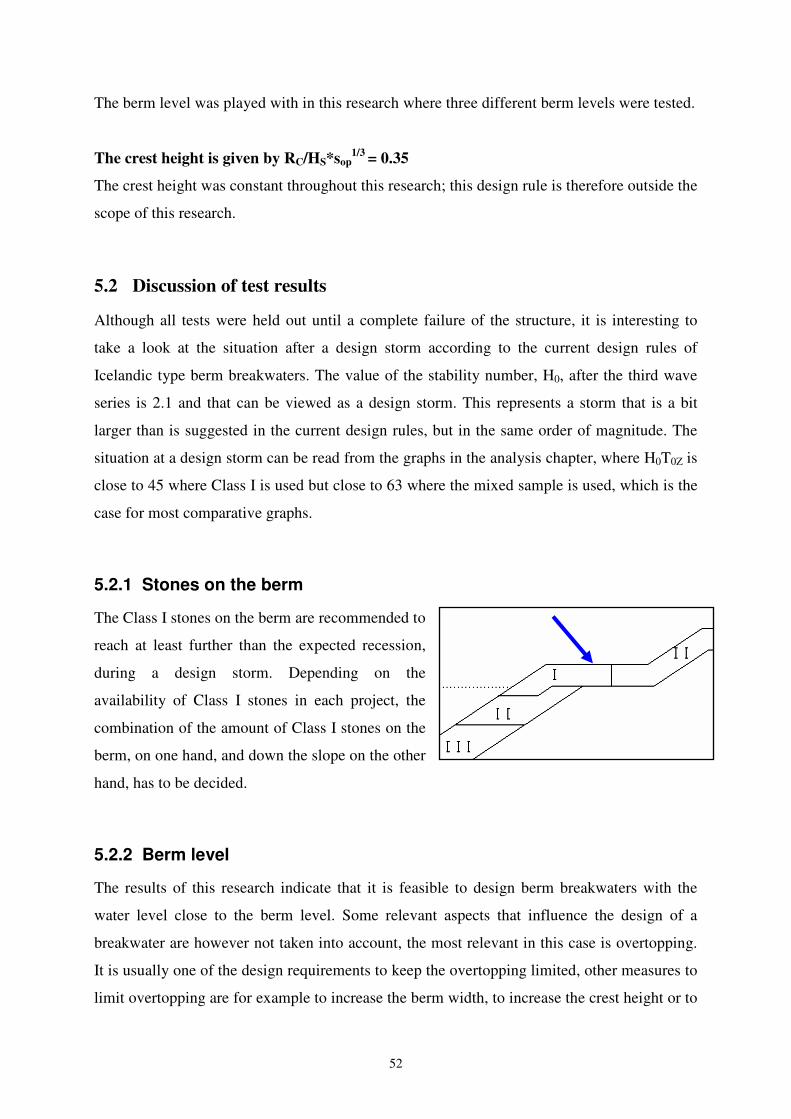
52
The berm level was played with in this research where three different berm levels were tested.
The crest height is given by RC/HS*sop1/3 = 0.35
The crest height was constant throughout this research; this design rule is therefore outside the
scope of this research.
5.2 Discussion of test results
Although all tests were held out until a complete failure of the structure, it is interesting to
take a look at the situation after a design storm according to the current design rules of
Icelandic type berm breakwaters. The value of the stability number, H0, after the third wave
series is 2.1 and that can be viewed as a design storm. This represents a storm that is a bit
larger than is suggested in the current design rules, but in the same order of magnitude. The
situation at a design storm can be read from the graphs in the analysis chapter, where H0T0Z is
close to 45 where Class I is used but close to 63 where the mixed sample is used, which is the
case for most comparative graphs.
5.2.1 Stones on the berm
The Class I stones on the berm are recommended to
reach at least further than the expected recession,
during a design storm. Depending on the
availability of Class I stones in each project, the
combination of the amount of Class I stones on the
berm, on one hand, and down the slope on the other
hand, has to be decided.
5.2.2 Berm level
The results of this research indicate that it is feasible to design berm breakwaters with the
water level close to the berm level. Some relevant aspects that influence the design of a
breakwater are however not taken into account, the most relevant in this case is overtopping.
It is usually one of the design requirements to keep the overtopping limited, other measures to
limit overtopping are for example to increase the berm width, to increase the crest height or to
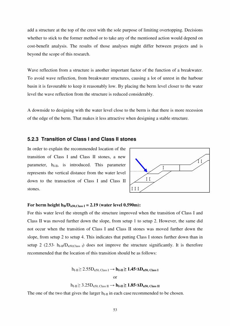
53
add a structure at the top of the crest with the sole purpose of limiting overtopping. Decisions
whether to stick to the former method or to take any of the mentioned action would depend on
cost-benefit analysis. The results of those analyses might differ between projects and is
beyond the scope of this research.
Wave reflection from a structure is another important factor of the function of a breakwater.
To avoid wave reflection, from breakwater structures, causing a lot of unrest in the harbour
basin it is favourable to keep it reasonably low. By placing the berm level closer to the water
level the wave reflection from the structure is reduced considerably.
A downside to designing with the water level close to the berm is that there is more recession
of the edge of the berm. That makes it less attractive when designing a stable structure.
5.2.3 Transition of Class I and Class II stones
In order to explain the recommended location of the
transition of Class I and Class II stones, a new
parameter, hI-II, is introduced. This parameter
represents the vertical distance from the water level
down to the transaction of Class I and Class II
stones.
For berm height hB/Dn50,Class I = 2.19 (water level 0.590m):
For this water level the strength of the structure improved when the transition of Class I and
Class II was moved further down the slope, from setup 1 to setup 2. However, the same did
not occur when the transition of Class I and Class II stones was moved further down the
slope, from setup 2 to setup 4. This indicates that putting Class I stones further down than in
setup 2 (2.53· hI-II/Dn50,Class I) does not improve the structure significantly. It is therefore
recommended that the location of this transition should be as follows:
hI-II ≥ 2.55Dn50, Class I → hI-II ≥ 1.45·∆Dn50, Class I
or
hI-II ≥ 3.25Dn50, Class II → hI-II ≥ 1.85·∆Dn50, Class II
The one of the two that gives the larger hI-II in each case recommended to be chosen.

54
For berm height hB/Dn50,Class I = 0.47 (water level 0.645m):
For this water level the strength of the structure did not improve significantly when the
transition of Class I and Class II stones was moved further down the slope, from setup 1 to
setup 2. This indicates that by locating Class I stones further down than in setup 1 (2.44· hI-
II/Dn50,Class I) does not improve the structure significantly. It is therefore recommended that the
location of this transition should be as follows:
hI-II ≥ 2.45Dn50, Class I → hI-II ≥ 1.40·∆Dn50, Class I
or
hI-II ≥ 3.15Dn50, Class II → hI-II ≥ 1.80·∆Dn50, Class II
The one of the two that gives the larger hI-II in each case is the recommended choice.
5.2.4 Transition of Class II and Class III stones
In order to explain the recommended location of
the transition of Class II and Class III stones, a
new parameter, hII-III, is introduced. This
parameter represents the distance from the water
level down to the transition of Class II and Class
III stones.
Class II stones should reach at least down to the expected transition of the original and the
reshaped profile, hf. For the transition of the Class II and Class III stones it turned out to
influence the damage progress severely the only time this transition was above this level
while it did not have an effect in the other tests. It is therefore recommended that:
hII-III > hf
The distance from the water level down to the transition of the original and the reshaped
profile, hf, in the model tests did not turn out to be the same as for formula 2.17 when the
water level was not close to the berm level. The formula is missing a parameter representing
the berm height, hB, which turned out to be very effective in this experiment.

55
For the situation where the water level is close to the berm level, hB/Dn50 ≈ 0.50, the results of
the experiment fit well with formula 2.17. However with the water level lower on the berm
this is not the case. An addition of 0.6hB/Dn50 to formula 2.17 gives a formula that better fits
the results of the experiment, both for the different berm heights, that is with water level at
0.645m, 0.590m and for the only test that was performed with the water level at 0.545m. It
also fits reasonably well for the different stone diameters that is both where Class I was used
and for the mixed sample as well.
(6.1)
It has to be kept in mind that the water level is relatively deep in this experiment. This
formula is not based on any tests in more shallow water where the influence of the water level
on hf/Dn50 is more. The formula is therefore not necessarily valid for that situation. It is,
however, clear that if different berm heights are to be considered, the inclusion of the berm
height parameter, hB/Dn50, is needed.
5.06.02.0505050
++=n
B
nn
f
D
h
D
h
D
h

56
6 Conclusions and suggestions for further work
6.1 Conclusions
The conclusions of this M.Sc. thesis project are derived from a limited number of model tests
of Icelandic type berm breakwaters. The results should therefore be approached with care and
further research is recommended on the subject.
The conclusions are based on the different aspects discussed in chapter four and chapter five.
That is recession and total erosion of different tests, as well as general interpretation of the
reshaping profiles and visual observations.
6.1.1 Suggested additions to current design rules
The following is suggested as an addition to the current design rules, based on some of the
current design rules being unchanged. Most importantly that the slope should be kept at 1:1.5
and the size of the largest stones should be determined by H0 = 2.0. These are four steps that
should give guidance of how to allocate the stones depending on the availability of different
stone classes in each case.
1. Class I stones on the berm are recommended to reach at least further into the berm
than the expected recession from a design storm.
2. Class I stones are recommended to reach as far down as:
hI-II ≥ 1.45·∆Dn50, Class I
or
hI-II ≥ 1.85·∆Dn50, Class II
The one of the two that gives the larger hI-II in each case are recommended to be
chosen. The strength of the structure did not seem to improve when the Class I stones
reached further down the berm.
3. If there is more of Class I stones available after meeting the recommendations above,
(1 and 2) they should be placed further into the berm.
4. Class II stones should in any case reach at least down to the transition of the original
and the expected reshaped profile, hf. In the only setup that it was not the case it
weakened the structure significantly while in the other setups it did not have any effect
on the damage development.

57
6.2 Suggested further research
There are still a few aspects of the Icelandic type berm breakwaters, like for most coastal
structures, that would gain from being further researched. During the work on this M.Sc.
thesis project some ideas for topics that would be interesting to further investigate, came to
light.
1. One of the important factors of the design of an Icelandic type berm breakwater is the
careful placement of the largest stones. This part turned out to be a bit difficult to
imitate since in reality the stones are carefully placed one by one. To have some kind
of a method to imitate the situation in a relatively easy way would be helpful. It should
be noted that this is a delicate subject and it is important also not to overdue the
interlocking between the stones.
2. Similar research as the one executed in this project. But use the results from the model
tests from this project to choose appropriate wave heights with the goal of approaching
more accurately the critical points in the failure process. Using more accurate cross
section measurements would also be helpful. To be able to measure the cross sections
at different location along the structure as well as measuring the cross sections more
often, for example for every 500 waves. That would also open the possibility of
investigating the influence of storm duration of the damage development as has proven
to be an important factor for conventional breakwaters, van der Meer (1988).
3. To combine the benefits of on one hand, the Icelandic type berm breakwater and on
the other hand, a dynamic berm breakwater would be an interesting subject. The idea
is that the structure would be like the Icelandic type, multi layered, but as for the
dynamic type it would be allowed to reshape. The setup should preferably be done in a
manner that makes the structure stronger after the main reshaping and where most of
the Class I stones will still be in the upper part. For the current setup of the Icelandic
type there are always some Class I stones that are lost (roll down the slope) early in
the process. Test setup number 5 in this research, where Class I and Class II stones
switched places, might be a possible starting point for such research.

58
4. To use the data gathered in this research to further develop the understanding of the
Icelandic type berm breakwater. That might be on the subject of recession where the
data gathered in this research might be compared with data from other research studies
on that subject, and possibly a new formula might be developed where the scatter
would be lower.
5. The influence of wave period or the wave steepness is another issue that was not
investigated in this research since the target wave steepness was the same throughout
the research. The results from the only test where accidentally different wave
steepness was used, indicates that it would be interesting to look further into that
subject. Research focusing on the wave steepness as well as the influence of storm
duration might be an interesting combination.
6. The influence of overtopping and different measures to decrease overtopping when the
water level is kept close to the berm level. It might also be interesting to measure the
difference in overtopping with different berm height while the crest height remains
constant. Such research might include playing with the berm width, the crest height or
by including of some structure with the purpose of decreasing overtopping.

59
7 References
Archetti, R. and Lamberti, A. (1999). “Stone movement and stresses during the reshaping of
berm breakwaters”. In: G.P. Mocke (ed), Proc 5th int conf coastal engg dev countries
(COPEDEC V), Cape Town, 19-23 Apr. Creda Communications, Cape Town, pp 1550-1561.
Bjørndal, S., Vold, S., Andersen, A. (2005). “Longshore transport on berm breakwaters due to
oblique and breaking waves”, International Coastal Symposium, Iceland.
CERC (1984). “Shore protection manual”. 4th edn. Coastal Engineering Research Center, US
Army Corps of Engineers, Vicksburg, MS.
CUR/CIRIA (2007). “The Rock Manual. The use of rock in hydraulic engineering” (2nd
edition). C683, CIRIA, London.
d’Angremond, K., van Roode, F.C. (2001). “Breakwaters and Closure Dams”, Delft
University Press, [Partially available online at http://www.vssd.nl/hlf/f011.htm]
Hughes, S.A. (1995). “Physical Modelling and Laboratory Techniques in Coastal
Engineering”, World Scientific Publishing Co. Pte. Ltd., Singapore.
J. A. Battjes (1974). “Computation of set-up, longshore currents, run-up and overtopping due
to wind generated waves”. Report 74-2, Comm on Hydraulics, Dept of Civil Eng, Univ of
Technology, Delft.
J. W. van der Meer (1988). “Rock slopes and gravel beaches under wave attack”. PhD thesis,
Delft University of Technology, Delft. Also WLjDelft Hydraulics publication no 396.
K. Hasselmann, T. P. Barnett, E. Bouws, H. Carlson, D. E. Cartwright, K. Enke, J. A. Ewing,
H. Gienapp, D. E. Hasselmann, P. Kruseman, A. Meerburg, P. Muller, D. J. Olbers, K.
Richter, W. Sell & H. Walden, 1973. “Measurements of wind-wave growth and swell decay
during the Joint North Sea Wave Project” (JONSWAP). Deutschen Hydrographischen
Zeitschrift, Reihe A , volume 8, no 12.

60
Lamberti, A. and Tomasicchio, G.R. (1997). “Stone mobility and longshore transport at
reshaping breakwaters”. Coastal Eng, vol 29, no 3, Jan, pp 263-289
Lamberti, A., Tomasicchio, G.R., and Guiducci, F. (1995). “Reshaping breakwaters in deep
and shallow water conditions”. In: B.L. Edge (ed), Proc 24th int conf coastal eng, Kobe, 23-28
Oct 1994. ASCE, New York, pp 1343-1358.
Menze, A (2000). “Stability of multilayer berm breakwaters”. Diploma thesis, University of
Braunschweig, Germany.
Myhra, H.A. (2005) “Berm breakwater: Influence of construction method and storm duration
on stability, Ice ride-up” M.Sc thesis, Norwegian University of Science and Technology
(NTNU), Norway.
PIANC WG12 (1991). “Analysis of rubble mound breakwaters”. PIANC.
PIANC WG40 (2003). “State-of-the-Art of Designing and Constructing Berm Breakwaters”.
PIANC.
R. Y. Hudson (1953). “Wave forces on breakwaters”. Trans Am Soc Civ Engrs, volume 118,
pp 653-674.
R. Y. Hudson (1959). “Laboratory investigations of rubble mound breakwaters”. J Waterways
Harbors Div & Am Soc Civ Engrs, volume 85, no WW3, Paper no 2171, pp 93-121.
Schiereck, G.J. (2001) “Introduction to Bed, Bank and Shore Protection”, Delft University
Press.
Sigurdarson, S., A. Jacobsen, O.B. Smarason, S. Bjørdal, G. Viggosson, C. Urrang, A. Tørum
(2003). “Sirevåg Berm Breakwater, design, construction and experience after design storm”.
Proc. Coastal Structures 2004, ASCE, 1212-1224.
Sigurdarson, S., Juhl, J., Sloth, P, Smarason, O.B. and Viggosson, G. (1998). “Advances in
Berm Breakwaters.” Coastlines, Structures and Breakwaters Conference, London.

61
Sigurdarson, S., Loftsson, A., Lothe A.E., Bjertness E., Smarason O.B., (2005). “Berm
Breakwater Protection for the Hammerfest LNG Plant in Norway - Design and Construction”.
Proc. Coastlines, Structures and Breakwaters 2005, ICE. 349-362.
Sigurdarson, S., Smarason, O.B., Viggosson, G. and Bjørdal, S., (2006). “Wave height limits
for the statically stable Icelandic-type Berm Breakwater”, Proc. ICCE 2006, ASCE, 5046-
5058.
Sigurdarson, S., Van der Meer, J.W., Burcharth, H.F., and Sørensen, J.D., (2007). “Optimum
safety levels and design rules for the Icelandic-type berm breakwater”. Coastal structures
conf. 2007, Venice.
Sigurdarson, S., Viggosson, G., Tørum, A. and Smarason, O.B., (2001). “Stable berm
breakwaters”, International Workshop on Advanced Design of Maritime Structures in the 21st
Century, Ed.: Y. Goda and S. Takahashi, PHRI, Japan, pp 152-159.
Sigurdarson, S., Viggosson, G., Tørum, A. and Smarason, O.B., (2005) “Recent Berm
Breakwater Projects”, International Coastal Symposium, Iceland.
Tørum, A., (1998). “On the stability of berm breakwaters in shallow and deep water”. Proc.
26th Int. Conf. Coastal Eng., ASCE, 1435–1448.
Tørum, A., Krogh S. R., Fjeld, S., (2002). “Berm Breakwaters: Stone Breaking Strength”.
Journal of Waterway, Port, Coastal and Ocean Engineering/ July/August 2002.
Tørum, A., Kuhnen F., Menze A., 2003. “On berm breakwaters. Stability, scour,
overtopping”. Coastal Eng. 49: 209-238.
Tørum, A., Løset, S., Myhra. H., (2005) “Sirevåg berm breakwater – comparison between
model and prototype reshaping”, International Coastal Symposium, Iceland.
W. J. Pierson & L. Moskowitz (1964). “A proposed spectral form for fully developed wind
seas based on the similarity law of S.A. Kitaigorodskii. J Geophys Res”, volume 69, no 24.

62
A Appendices
A.1 Model setup, key parameters expressed dimensionless
In this section the parameters expressed in chapter 3.3, as a function of first the different wave
heights used in the tests and then the different median nominal diameters, Dn50, of the three
different stone classes.
A.1.1 Key parameters expressed as a function of wave height
Table A.1 Key parameters expressed as a function of wave height 0.085m
HS [m]= 0.085
Setup hB/Hs (b-hB)/Hs (c-hB)/Hs h/Hs hB/Hs (b-hB)/Hs (c-hB)/Hs h/Hs hB/Hs (b-hB)/Hs (c-hB)/Hs h/Hs BB/Hs
1 0.18 0.92 2.28 7.59 0.82 0.27 1.64 6.94 1.35 -0.26 1.11 6.41 3.53
2 0.18 1.60 2.28 7.59 0.82 0.95 1.64 6.94
3 0.18 0.92 1.33 7.59 0.82 0.27 0.68 6.94
4 0.18 - 2.28 7.59 0.82 - 1.64 6.94
5 0.18 0.92 1.93 7.59 0.82 0.27 1.28 6.94
Water level 0.645m Water level 0.590m Water level 0.545m
Table A.2 Key parameters expressed as a function of wave height 0.100m
HS [m]= 0.100
Setup hB/Hs (b-hB)/Hs (c-hB)/Hs h/Hs hB/Hs (b-hB)/Hs (c-hB)/Hs h/Hs hB/Hs (b-hB)/Hs (c-hB)/Hs h/Hs BB/Hs
1 0.15 0.78 1.94 6.45 0.70 0.23 1.39 5.90 1.15 -0.22 0.94 5.45 3.00
2 0.15 1.36 1.94 6.45 0.70 0.81 1.39 5.90
3 0.15 0.78 1.13 6.45 0.70 0.23 0.58 5.90
4 0.15 - 1.94 6.45 0.70 - 1.39 5.90
5 0.15 0.78 1.64 6.45 0.70 0.23 1.09 5.90
Water level 0.645m Water level 0.590m Water level 0.545m
Table A.3 Key parameters expressed as a function of wave height 0.120m
HS [m]= 0.120
Setup hB/Hs (b-hB)/Hs (c-hB)/Hs h/Hs hB/Hs (b-hB)/Hs (c-hB)/Hs h/Hs hB/Hs (b-hB)/Hs (c-hB)/Hs h/Hs BB/Hs
1 0.13 0.65 1.62 5.38 0.58 0.19 1.16 4.92 0.96 -0.18 0.78 4.54 2.50
2 0.13 1.13 1.62 5.38 0.58 0.67 1.16 4.92
3 0.13 0.65 0.94 5.38 0.58 0.19 0.48 4.92
4 0.13 - 1.62 5.38 0.58 - 1.16 4.92
5 0.13 0.65 1.37 5.38 0.58 0.19 0.91 4.92
Water level 0.645m Water level 0.590m Water level 0.545m
Table A.4 Key parameters expressed as a function of wave height 0.135m
HS [m]= 0.135
Setup hB/Hs (b-hB)/Hs (c-hB)/Hs h/Hs hB/Hs (b-hB)/Hs (c-hB)/Hs h/Hs hB/Hs (b-hB)/Hs (c-hB)/Hs h/Hs BB/Hs
1 0.11 0.58 1.44 4.78 0.52 0.17 1.03 4.37 0.85 -0.16 0.70 4.04 2.22
2 0.11 1.01 1.44 4.78 0.52 0.60 1.03 4.37
3 0.11 0.58 0.84 4.78 0.52 0.17 0.43 4.37
4 0.11 - 1.44 4.78 0.52 - 1.03 4.37
5 0.11 0.58 1.21 4.78 0.52 0.17 0.81 4.37
Water level 0.645m Water level 0.590m Water level 0.545m

63
Table A.5 Key parameters expressed as a function of wave height 0.155m
HS [m]= 0.155
Setup hB/Hs (b-hB)/Hs (c-hB)/Hs h/Hs hB/Hs (b-hB)/Hs (c-hB)/Hs h/Hs hB/Hs (b-hB)/Hs (c-hB)/Hs h/Hs BB/Hs
1 0.10 0.50 1.25 4.16 0.45 0.15 0.90 3.81 0.74 -0.14 0.61 3.52 1.94
2 0.10 0.88 1.25 4.16 0.45 0.52 0.90 3.81
3 0.10 0.50 0.73 4.16 0.45 0.15 0.37 3.81
4 0.10 - 1.25 4.16 0.45 - 0.90 3.81
5 0.10 0.50 1.06 4.16 0.45 0.15 0.70 3.81
Water level 0.645m Water level 0.590m Water level 0.545m
Table A.6 Key parameters expressed as a function of wave height 0.170m
HS [m]= 0.170
Setup hB/Hs (b-hB)/Hs (c-hB)/Hs h/Hs hB/Hs (b-hB)/Hs (c-hB)/Hs h/Hs hB/Hs (b-hB)/Hs (c-hB)/Hs h/Hs BB/Hs
1 0.09 0.46 1.14 3.79 0.41 0.14 0.82 3.47 0.68 -0.13 0.55 3.21 1.76
2 0.09 0.80 1.14 3.79 0.41 0.48 0.82 3.47
3 0.09 0.46 0.66 3.79 0.41 0.14 0.34 3.47
4 0.09 - 1.14 3.79 0.41 - 0.82 3.47
5 0.09 0.46 0.96 3.79 0.41 0.14 0.64 3.47
Water level 0.645m Water level 0.590m Water level 0.545m
A.1.2 Key parameters as a function of median nominal diameter, Dn50, of
different stone classes
Table A.7 Key parameters expressed as a function of Dn50=0.032m
Dn50[m]= 0.032 Class I
Setup hB/Dn50 (b-hB)/Dn50 (c-hB)/Dn50 h/Dn50 hB/Dn50 (b-hB)/Dn50 (c-hB)/Dn50 h/Dn50 hB/Dn50 (b-hB)/Dn50 (c-hB)/Dn50 h/Dn50 BB/Dn50
1 0.47 2.44 6.06 20.16 2.19 0.72 4.34 18.44 3.59 -0.69 2.94 17.03 9.38
2 0.47 4.25 6.06 20.16 2.19 2.53 4.34 18.44
3 0.47 2.44 3.53 20.16 2.19 0.72 1.81 18.44
4 0.47 - 6.06 20.16 2.19 - 4.34 18.44
5 0.47 2.44 5.13 20.16 2.19 0.72 3.41 18.44
Water level 0.645m Water level 0.590m Water level 0.545m
Table A.8 Key parameters expressed as a function of Dn50=0.025m
Dn50[m]= 0.025 Class II
Setup hB/Dn50 (b-hB)/Dn50 (c-hB)/Dn50 h/Dn50 hB/Dn50 (b-hB)/Dn50 (c-hB)/Dn50 h/Dn50 hB/Dn50 (b-hB)/Dn50 (c-hB)/Dn50 h/Dn50 BB/Dn50
1 0.60 3.12 7.76 25.80 2.80 0.92 5.56 23.60 4.60 -0.88 3.76 21.80 12.00
2 0.60 5.44 7.76 25.80 2.80 3.24 5.56 23.60
3 0.60 3.12 4.52 25.80 2.80 0.92 2.32 23.60
4 0.60 - 7.76 25.80 2.80 - 5.56 23.60
5 0.60 3.12 6.56 25.80 2.80 0.92 4.36 23.60
Water level 0.645m Water level 0.590m Water level 0.545m
Table A.9 Key parameters expressed as a function of Dn50=0.020m
Dn50[m]= 0.020 Class III
Setup hB/Dn50 (b-hB)/Dn50 (c-hB)/Dn50 h/Dn50 hB/Dn50 (b-hB)/Dn50 (c-hB)/Dn50 h/Dn50 hB/Dn50 (b-hB)/Dn50 (c-hB)/Dn50 h/Dn50 BB/Dn50
1 0.76 3.94 9.80 32.58 3.54 1.16 7.02 29.80 5.81 -1.11 4.75 27.53 15.15
2 0.76 6.87 9.80 32.58 3.54 4.09 7.02 29.80
3 0.76 3.94 5.71 32.58 3.54 1.16 2.93 29.80
4 0.76 - 9.80 32.58 3.54 - 7.02 29.80
5 0.76 3.94 8.28 32.58 3.54 1.16 5.51 29.80
Water level 0.645m Water level 0.590m Water level 0.545m

64
A.2 Wave measurements
In this section there are tables that show the results of the wave measurements from the tests.
These are output numbers from each test along with some key numbers, among those numbers
are the stability number, H0 and the wave period stability number, H0T0, both for Dn50 from
Class I stones and from the mixture of the stones.
A.2.1 Setup 1 Table A.10 Wave properties of setup 1, water level 0.545m
S1TL
Test # HHHHSSSS [m] [m] [m] [m] ssss0p0p0p0p ssss0z0z0z0z TTTTpppp [s] [s] [s] [s] TTTTZZZZ [s] [s] [s] [s] ξp ξZ ReflReflReflRefl HHHH0000 HHHH0000TTTT0p0p0p0p HHHH0000TTTT0z0z0z0z HHHH0000 HHHH0000TTTT0p0p0p0p HHHH0000TTTT0z0z0z0z
1
2 0.102 0.051 0.057 1.13 1.07 2.9 2.8 0.27 1.80 36 34 2.25 50 47
3 0.122 0.042 0.053 1.36 1.21 3.2 2.9 0.31 2.16 51 46 2.69 72 64
4 0.138 0.044 0.056 1.42 1.26 3.2 2.8 0.32 2.43 60 53 3.03 84 75
5
6
Class I Mixed
Table A.11 Wave properties of setup 1, water level 0.590m S1TM
Test # HHHHSSSS [m] [m] [m] [m] ssss0p0p0p0p ssss0z0z0z0z TTTTpppp [s] [s] [s] [s] TTTTZZZZ [s] [s] [s] [s] ξp ξZ ReflReflReflRefl HHHH0000 HHHH0000TTTT0p0p0p0p HHHH0000TTTT0z0z0z0z HHHH0000 HHHH0000TTTT0p0p0p0p HHHH0000TTTT0z0z0z0z
1 0.088 0.045 0.052 1.12 1.04 3.2 2.9 0.28 1.54 30 28 1.93 42 39
2 0.103 0.040 0.053 1.29 1.12 3.4 2.9 0.29 1.81 41 35 2.26 57 49
3 0.122 0.042 0.053 1.37 1.21 3.3 2.9 0.31 2.15 52 46 2.69 72 64
4 0.137 0.044 0.055 1.41 1.27 3.2 2.9 0.29 2.41 59 53 3.01 83 74
5 0.158 0.045 0.055 1.50 1.36 3.1 2.8 0.29 2.78 73 66 3.47 102 92
6
Class I Mixed
Table A.12 Wave properties of setup 1, water level 0.645m S1TH
Test # HHHHSSSS [m] [m] [m] [m] ssss0p0p0p0p ssss0z0z0z0z TTTTpppp [s] [s] [s] [s] TTTTZZZZ [s] [s] [s] [s] ξp ξZ ReflReflReflRefl HHHH0000 HHHH0000TTTT0p0p0p0p HHHH0000TTTT0z0z0z0z HHHH0000 HHHH0000TTTT0p0p0p0p HHHH0000TTTT0z0z0z0z
1 0.084 0.041 0.049 1.15 1.05 3.3 3.0 0.20 1.48 30 27 1.85 42 38
2 0.101 0.039 0.052 1.29 1.12 3.4 2.9 0.22 1.78 40 35 2.23 56 49
3 0.121 0.041 0.053 1.37 1.21 3.3 2.9 0.26 2.13 51 45 2.66 71 63
4 0.136 0.043 0.055 1.42 1.26 3.2 2.8 0.26 2.40 60 53 3.00 83 74
5 0.155 0.042 0.054 1.54 1.35 3.3 2.9 0.25 2.72 73 64 3.40 102 90
Class I Mixed
A.2.2 Setup 2 Table A.13 Wave properties of setup 2, water level 0.590m, first test
S2TM
Test # HHHHSSSS [m] [m] [m] [m] ssss0p0p0p0p ssss0z0z0z0z TTTTpppp [s] [s] [s] [s] TTTTZZZZ [s] [s] [s] [s] ξp ξZ ReflReflReflRefl HHHH0000 HHHH0000TTTT0p0p0p0p HHHH0000TTTT0z0z0z0z HHHH0000 HHHH0000TTTT0p0p0p0p HHHH0000TTTT0z0z0z0z
1
2 0.109 0.051 0.055 1.17 1.12 3.0 2.8 0.26 1.91 39 37 2.39 55 52
3
4 0.130 0.047 0.060 1.33 1.18 3.1 2.7 0.29 2.29 53 47 2.86 74 66
5 0.156 0.051 0.062 1.40 1.27 3.0 2.7 0.33 2.75 67 61 3.43 94 85
6
Class I Mixed
Table A.14 Wave properties of setup 2, water level 0.590m, repeated test S2TM_rep
Test # HHHHSSSS [m] [m] [m] [m] ssss0p0p0p0p ssss0z0z0z0z TTTTpppp [s] [s] [s] [s] TTTTZZZZ [s] [s] [s] [s] ξp ξZ ReflReflReflRefl HHHH0000 HHHH0000TTTT0p0p0p0p HHHH0000TTTT0z0z0z0z HHHH0000 HHHH0000TTTT0p0p0p0p HHHH0000TTTT0z0z0z0z
1 0.085 0.036 0.048 1.23 1.07 3.5 3.0 0.26 1.50 32 28 1.88 45 39
2 0.103 0.039 0.052 1.29 1.12 3.4 2.9 0.27 1.80 41 35 2.25 57 49
3 0.122 0.042 0.053 1.37 1.21 3.3 2.9 0.31 2.14 51 45 2.68 72 63
4 0.137 0.044 0.055 1.41 1.27 3.2 2.9 0.30 2.40 59 53 3.00 83 74
5 0.155 0.042 0.054 1.54 1.36 3.3 2.9 0.28 2.73 74 65 3.41 103 91
6
Class I Mixed

65
Table A.15 Wave properties of setup 2, water level 0.645m S2TH
Test # HHHHSSSS [m] [m] [m] [m] ssss0p0p0p0p ssss0z0z0z0z TTTTpppp [s] [s] [s] [s] TTTTZZZZ [s] [s] [s] [s] ξp ξZ ReflReflReflRefl HHHH0000 HHHH0000TTTT0p0p0p0p HHHH0000TTTT0z0z0z0z HHHH0000 HHHH0000TTTT0p0p0p0p HHHH0000TTTT0z0z0z0z
1 0.084 0.039 0.049 1.18 1.05 3.4 3.0 0.17 1.48 30 27 1.84 42 38
2 0.102 0.039 0.052 1.29 1.12 3.4 2.9 0.19 1.79 40 35 2.23 56 49
3 0.120 0.041 0.053 1.37 1.21 3.3 2.9 0.24 2.12 51 45 2.64 71 63
4 0.136 0.043 0.055 1.42 1.26 3.2 2.8 0.25 2.40 60 53 2.99 83 74
5 0.158 0.043 0.056 1.53 1.35 3.2 2.8 0.24 2.78 74 66 3.47 104 92
6 0.170 0.041 0.053 1.62 1.43 3.3 2.9 0.23 2.98 85 75 3.73 118 104
Class I Mixed
A.2.3 Setup 3 Table A.16 Wave properties of setup 3, water level 0.590m
S3TM
Test # HHHHSSSS [m] [m] [m] [m] ssss0p0p0p0p ssss0z0z0z0z TTTTpppp [s] [s] [s] [s] TTTTZZZZ [s] [s] [s] [s] ξp ξZ ReflReflReflRefl HHHH0000 HHHH0000TTTT0p0p0p0p HHHH0000TTTT0z0z0z0z HHHH0000 HHHH0000TTTT0p0p0p0p HHHH0000TTTT0z0z0z0z
1 0.086 0.040 0.048 1.17 1.07 3.3 3.0 0.28 1.51 31 28 1.89 43 39
2 0.103 0.039 0.053 1.30 1.12 3.4 2.9 0.28 1.80 41 35 2.25 57 49
3 0.122 0.042 0.053 1.37 1.21 3.3 2.9 0.30 2.15 52 46 2.69 72 64
4 0.137 0.044 0.055 1.42 1.27 3.2 2.8 0.32 2.42 60 53 3.02 84 75
5
6
Class I Mixed
Table A.17 Wave properties of setup 3, water level 0.645m S3TH
Test # HHHHSSSS [m] [m] [m] [m] ssss0p0p0p0p ssss0z0z0z0z TTTTpppp [s] [s] [s] [s] TTTTZZZZ [s] [s] [s] [s] ξp ξZ ReflReflReflRefl HHHH0000 HHHH0000TTTT0p0p0p0p HHHH0000TTTT0z0z0z0z HHHH0000 HHHH0000TTTT0p0p0p0p HHHH0000TTTT0z0z0z0z
1 0.084 0.040 0.048 1.16 1.06 3.3 3.0 0.20 1.48 30 27 1.85 42 38
2 0.101 0.039 0.052 1.29 1.12 3.4 2.9 0.22 1.79 40 35 2.23 56 49
3 0.121 0.041 0.053 1.37 1.21 3.3 2.9 0.26 2.13 51 45 2.66 71 63
4 0.136 0.043 0.054 1.42 1.27 3.2 2.9 0.27 2.39 59 53 2.99 83 74
5 0.153 0.042 0.054 1.53 1.35 3.3 2.9 0.27 2.70 72 64 3.37 101 89
6
Class I Mixed
A.2.4 Setup 4 Table A.18 Wave properties of setup 4, water level 0.590m, first test
S4TM
Test # HHHHSSSS [m] [m] [m] [m] ssss0p0p0p0p ssss0z0z0z0z TTTTpppp [s] [s] [s] [s] TTTTZZZZ [s] [s] [s] [s] ξp ξZ ReflReflReflRefl HHHH0000 HHHH0000TTTT0p0p0p0p HHHH0000TTTT0z0z0z0z HHHH0000 HHHH0000TTTT0p0p0p0p HHHH0000TTTT0z0z0z0z
1 0.085 0.033 0.048 1.28 1.07 3.7 3.0 0.26 1.50 33 28 1.87 47 39
2 0.103 0.040 0.053 1.29 1.12 3.3 2.9 0.28 1.81 41 35 2.26 57 49
3 0.123 0.042 0.053 1.37 1.22 3.3 2.9 0.31 2.17 52 46 2.71 73 64
4 0.137 0.044 0.055 1.41 1.26 3.2 2.8 0.31 2.40 59 53 3.00 83 74
5 0.158 0.046 0.056 1.49 1.35 3.1 2.8 0.30 2.78 72 66 3.47 101 92
6
Class I Mixed
Table A.19 Wave properties of setup 4, water level 0.590m, repeated test S4TM_rep
Test # HHHHSSSS [m] [m] [m] [m] ssss0p0p0p0p ssss0z0z0z0z TTTTpppp [s] [s] [s] [s] TTTTZZZZ [s] [s] [s] [s] ξp ξZ ReflReflReflRefl HHHH0000 HHHH0000TTTT0p0p0p0p HHHH0000TTTT0z0z0z0z HHHH0000 HHHH0000TTTT0p0p0p0p HHHH0000TTTT0z0z0z0z
1 0.084 0.036 0.047 1.23 1.07 3.5 3.1 0.26 1.48 32 28 1.85 45 39
2 0.102 0.039 0.051 1.29 1.13 3.4 3.0 0.27 1.79 40 35 2.24 56 49
3 0.119 0.041 0.051 1.37 1.22 3.3 2.9 0.31 2.10 50 45 2.62 70 63
4 0.135 0.045 0.053 1.39 1.27 3.2 2.9 0.30 2.37 58 53 2.96 80 73
5 0.155 0.043 0.055 1.53 1.35 3.2 2.9 0.30 2.74 73 65 3.42 102 90
6
Class I Mixed
Table A.20 Wave properties of setup 4, water level 0.645m S4TH
Test # HHHHSSSS [m] [m] [m] [m] ssss0p0p0p0p ssss0z0z0z0z TTTTpppp [s] [s] [s] [s] TTTTZZZZ [s] [s] [s] [s] ξp ξZ ReflReflReflRefl HHHH0000 HHHH0000TTTT0p0p0p0p HHHH0000TTTT0z0z0z0z HHHH0000 HHHH0000TTTT0p0p0p0p HHHH0000TTTT0z0z0z0z
1 0.084 0.040 0.049 1.16 1.05 3.3 3.0 0.21 1.48 30 27 1.85 42 38
2 0.102 0.039 0.052 1.29 1.12 3.4 2.9 0.23 1.79 40 35 2.23 56 49
3 0.121 0.042 0.053 1.36 1.21 3.3 2.9 0.26 2.13 51 45 2.66 71 63
4 0.136 0.044 0.055 1.41 1.26 3.2 2.8 0.26 2.40 59 53 2.99 82 74
5 0.159 0.042 0.056 1.55 1.35 3.2 2.8 0.23 2.80 76 66 3.49 106 92
6 0.178 0.043 0.054 1.62 1.45 3.2 2.9 0.21 3.13 89 79 3.91 124 111
Class I Mixed

66
A.2.5 Setup 5 Table A.21 Wave properties of setup 5, water level 0.590m
S5TM
Test # HHHHSSSS [m] [m] [m] [m] ssss0p0p0p0p ssss0z0z0z0z TTTTpppp [s] [s] [s] [s] TTTTZZZZ [s] [s] [s] [s] ξp ξZ ReflReflReflRefl HHHH0000 HHHH0000TTTT0p0p0p0p HHHH0000TTTT0z0z0z0z HHHH0000 HHHH0000TTTT0p0p0p0p HHHH0000TTTT0z0z0z0z
1 0.086 0.035 0.048 1.26 1.07 3.6 3.0 0.27 1.51 33 28 1.88 46 39
2 0.100 0.037 0.051 1.31 1.12 3.5 3.0 0.20 1.75 40 34 2.19 56 48
3 0.122 0.042 0.053 1.37 1.22 3.3 2.9 0.30 2.15 52 46 2.69 72 64
4 0.137 0.044 0.055 1.41 1.27 3.2 2.9 0.30 2.40 59 53 3.00 83 74
5 0.155 0.044 0.055 1.50 1.34 3.2 2.8 0.29 2.73 72 64 3.41 100 89
6
Class I Mixed
Table A.22 Wave properties of setup 3, water level 0.645m S5TH
Test # HHHHSSSS [m] [m] [m] [m] ssss0p0p0p0p ssss0z0z0z0z TTTTpppp [s] [s] [s] [s] TTTTZZZZ [s] [s] [s] [s] ξp ξZ ReflReflReflRefl HHHH0000 HHHH0000TTTT0p0p0p0p HHHH0000TTTT0z0z0z0z HHHH0000 HHHH0000TTTT0p0p0p0p HHHH0000TTTT0z0z0z0z
1 0.083 0.042 0.048 1.13 1.05 3.3 3.0 0.20 1.47 29 27 1.83 40 38
2 0.100 0.038 0.050 1.29 1.13 3.4 3.0 0.20 1.75 40 35 2.19 55 48
3 0.119 0.041 0.052 1.37 1.21 3.3 2.9 0.24 2.09 50 44 2.62 70 62
4 0.134 0.043 0.054 1.42 1.26 3.2 2.9 0.24 2.36 59 52 2.95 82 73
5 0.156 0.041 0.054 1.56 1.36 3.3 2.9 0.24 2.75 75 65 3.43 105 91
6
Class I Mixed
A.2.6 Setup 6 Table A.23 Wave properties of setup 6, water level 0.590m
S6TM
Test # HHHHSSSS [m] [m] [m] [m] ssss0p0p0p0p ssss0z0z0z0z TTTTpppp [s] [s] [s] [s] TTTTZZZZ [s] [s] [s] [s] ξp ξZ ReflReflReflRefl HHHH0000 HHHH0000TTTT0p0p0p0p HHHH0000TTTT0z0z0z0z HHHH0000 HHHH0000TTTT0p0p0p0p HHHH0000TTTT0z0z0z0z
1 0.084 0.040 0.047 1.16 1.07 3.3 3.1 0.24 1.48 30 28 1.85 42 39
2 0.102 0.039 0.052 1.29 1.12 3.4 2.9 0.24 1.80 40 35 2.24 57 49
3 0.120 0.041 0.052 1.37 1.22 3.3 2.9 0.28 2.11 51 45 2.63 71 63
4 0.135 0.044 0.054 1.41 1.27 3.2 2.9 0.29 2.38 59 53 2.97 82 74
5
6
Class I Mixed
Table A.24 Table A.16 Wave properties of setup 6, water level 0.645m S6TH
Test # HHHHSSSS [m] [m] [m] [m] ssss0p0p0p0p ssss0z0z0z0z TTTTpppp [s] [s] [s] [s] TTTTZZZZ [s] [s] [s] [s] ξp ξZ ReflReflReflRefl HHHH0000 HHHH0000TTTT0p0p0p0p HHHH0000TTTT0z0z0z0z HHHH0000 HHHH0000TTTT0p0p0p0p HHHH0000TTTT0z0z0z0z
1 0.083 0.041 0.047 1.14 1.06 3.3 3.1 0.18 1.47 29 27 1.83 41 38
2 0.100 0.039 0.051 1.29 1.12 3.4 2.9 0.17 1.76 40 35 2.20 56 48
3 0.119 0.041 0.052 1.37 1.21 3.3 2.9 0.21 2.09 50 44 2.61 70 62
4 0.134 0.042 0.055 1.43 1.25 3.3 2.8 0.27 2.35 59 51 2.94 82 72
5 0.157 0.042 0.054 1.55 1.36 3.3 2.9 0.27 2.77 75 66 3.45 105 92
6
Class I Mixed

67
A.3 Stone measurements
A.3.1 Class I
0%
10%
20%
30%
40%
50%
60%
70%
80%
90%
100%
0,027 0,028 0,029 0,030 0,031 0,032 0,033 0,034
Perc
en
tag
e s
mall
er
Dn [m]
Sieve curve - Class I
Figure A.1 Sieve curve for Class I stones
Table A.25 Class I stones, key nominal diameters
gradingNarrowD
D
n
n _5,113,115
85 ⇒<=
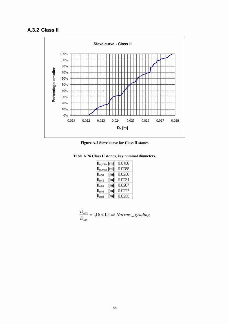
68
A.3.2 Class II
0%
10%
20%
30%
40%
50%
60%
70%
80%
90%
100%
0,021 0,022 0,023 0,024 0,025 0,026 0,027 0,028
Perc
en
tag
e s
mall
er
Dn [m]
Sieve curve - Class II
Figure A.2 Sieve curve for Class II stones
Table A.26 Class II stones, key nominal diameters.
gradingNarrowD
D
n
n _5,116,115
85 ⇒<=

69
A.3.3 Class III
0
0,1
0,2
0,3
0,4
0,5
0,6
0,7
0,8
0,9
1
0,016 0,017 0,018 0,019 0,020 0,021 0,022 0,023
Perc
en
tag
e s
mall
er
Dn [m]
Sieve curve - Class III
Figure A.3 Sieve curve for Class III stones
Table A.27 Class III stones, key nominal diameters.
gradingNarrowD
D
n
n _5,126,115
85 ⇒<=

70
A.3.4 Core
The stones used for the core are not the same kind of material as used for the armour layer.
Although that is the case when an Icelandic type berm breakwater is constructed, the core is
however not being considered in this project. This does not influence the behaviour of the
armour layer. The density of the core material is ρs = 2620 [kg/m3].
Table A.28 Core material, key nominal diameters.
gradingNarrowD
D
n
n _5,133,115
85 ⇒<=
A.3.5 Mixture of all stones
For comparison all the stones that were used in the experiment were mixed. The reason was to
make a homogenous berm breakwater, setup 6, with the same profile as in the other setups.
The reason for that setup was to be able to compare the results both with earlier researches,
for example recession, and also with the other setups.
0%
10%
20%
30%
40%
50%
60%
70%
80%
90%
100%
0,016 0,018 0,020 0,022 0,024 0,026 0,028 0,030 0,032 0,034
Perc
en
tag
e s
mall
er
Dn [m]
Sieve curve - mixed
Figure A.4 Sieve curve for the mixture of all stones

71
Table A.29 Mixture of all stones, key nominal diameters.
gradingWideD
D
n
n _5,263,15,163,115
85 ⇒><⇒=

72
A.4 Cross sections and reshaping process
Total of 70 tests were made, where 6 different cross sections or setups. Three different water
levels were tested where two of them were tested for every setup while the lowest water level
was only tested for setup 1. The key dimensions from every setup can be viewed in Figure 3.5
and are further explained in Table 3.1. As well as in appendix A.1 where it is explained as a
function of different the different wave heights used as well as the different median nominal
diameters, Dn50, of the different stone classes.
In Figure A.5 the colours used to explain the damage development are explained. The number
0 represents the original situation, before any wave action. While the numbers 1-6 each
represent a wave test as explained in Table 3.3, number 1 being the smallest waves while
number 6 are the largest.
Figure A.5 Explanation figure for the damage development.

73
A.4.1 Setup 1
Figure A.6 Damage development of setup 1, water level 0.545m.
Figure A.7 Damage development of setup 1, water level 0.590m.
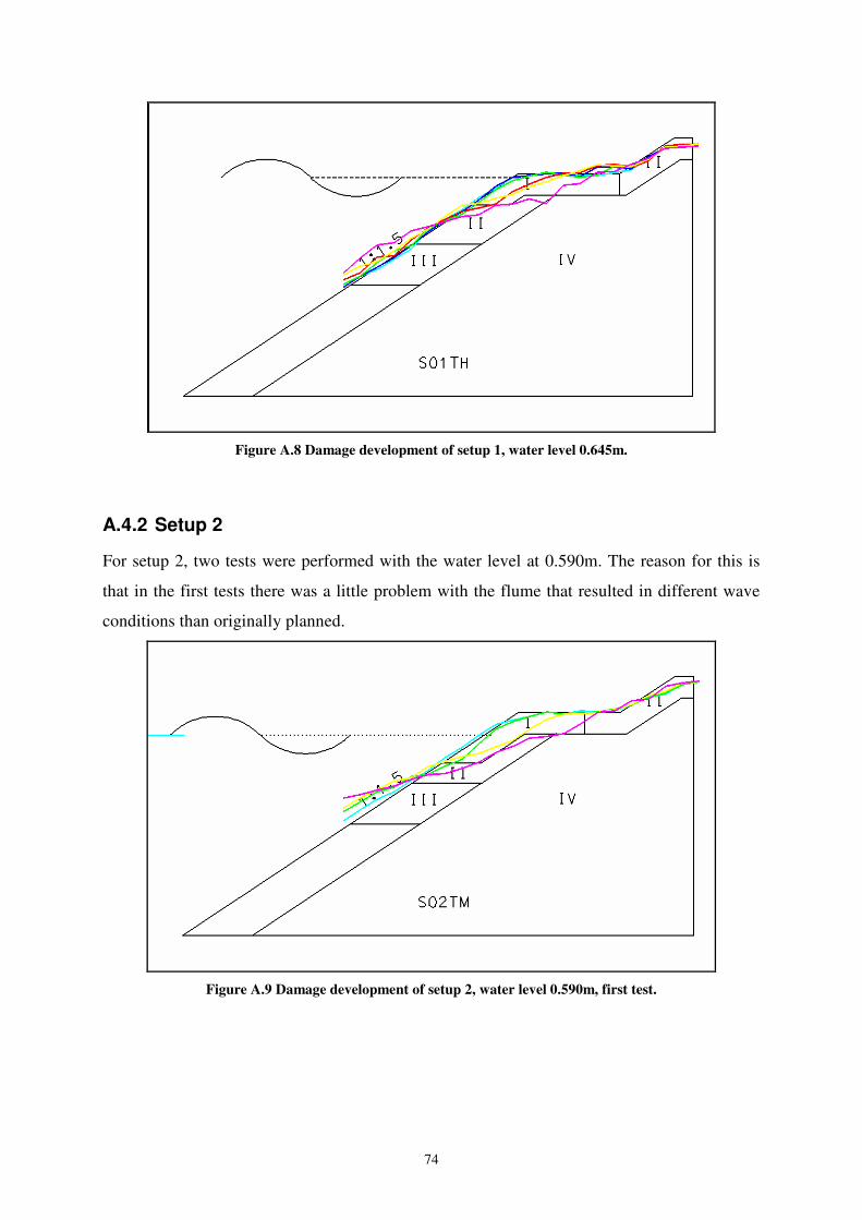
74
Figure A.8 Damage development of setup 1, water level 0.645m.
A.4.2 Setup 2
For setup 2, two tests were performed with the water level at 0.590m. The reason for this is
that in the first tests there was a little problem with the flume that resulted in different wave
conditions than originally planned.
Figure A.9 Damage development of setup 2, water level 0.590m, first test.

75
Figure A.10 Damage development of setup 2, water level 0.590m, repeated test.
Figure A.11 Damage development of setup 2, water level 0.645m.
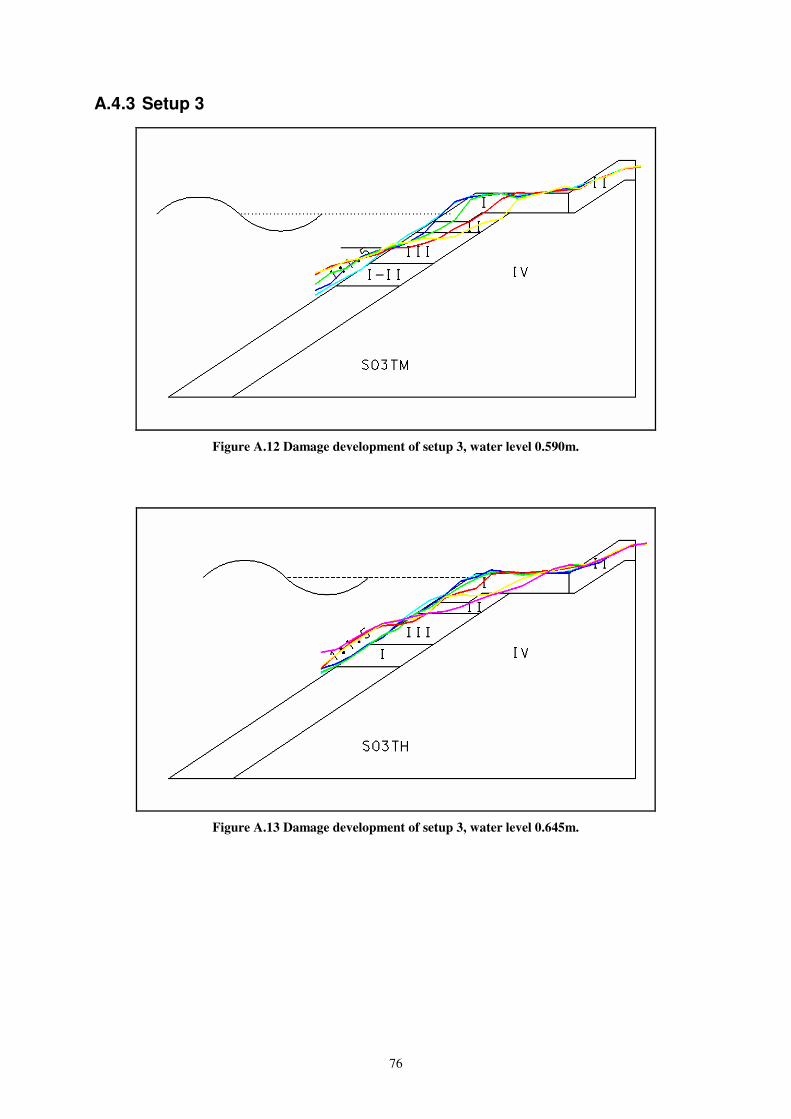
76
A.4.3 Setup 3
Figure A.12 Damage development of setup 3, water level 0.590m.
Figure A.13 Damage development of setup 3, water level 0.645m.

77
A.4.4 Setup 4
For setup 4 as for setup 2, two tests were performed with the water level at 0.590m. The
reason in this case was that many stones were moved in early in the test which was not in
context with other similar tests performed earlier.
Figure A.14 Damage development of setup 4, water level 0.590m, first test.
Figure A.15 Damage development of setup 4, water level 0.590m, repeated test.
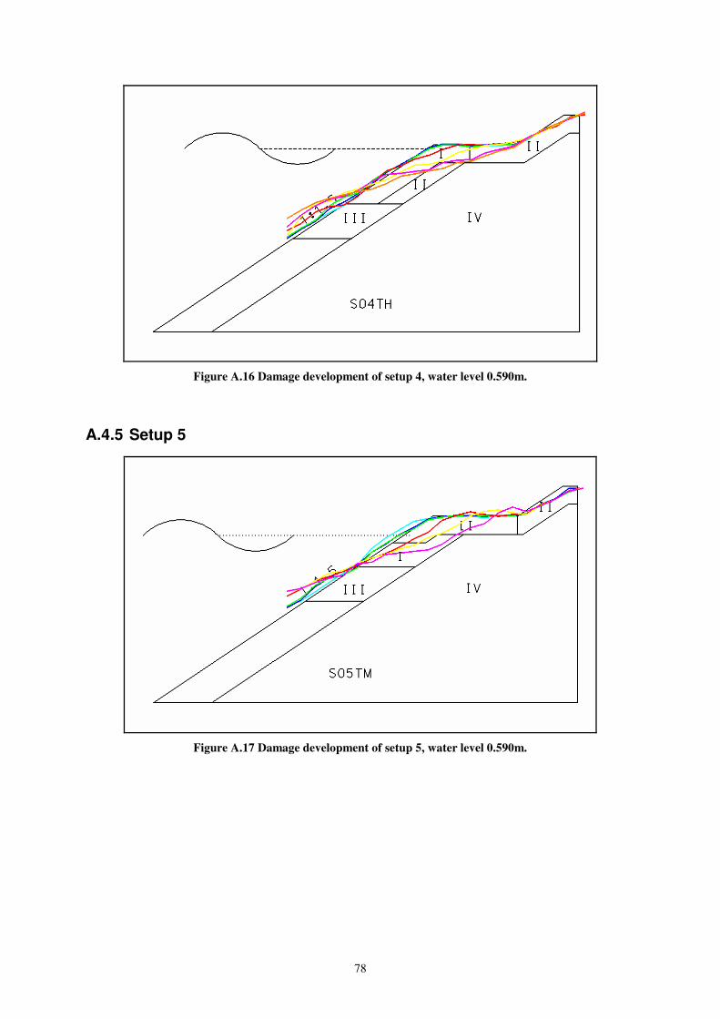
78
Figure A.16 Damage development of setup 4, water level 0.590m.
A.4.5 Setup 5
Figure A.17 Damage development of setup 5, water level 0.590m.

79
Figure A.18 Damage development of setup 5, water level 0.645m.
A.4.6 Setup 6
Figure A.19 Damage development of setup 6, water level 0.590m.

80
Figure A.20 Damage development of setup 6, water level 0.645m.

81
A.5 Recession graphs
For all recession graphs TH stands for the highest water level, 0.645m, TM stands for the
medium water level, 0.590m, while TL stands for the lowest water level tested, 0.545m, that
was only used for one test with setup 1.
A.5.1 Comparison with Tørum
In the following two figures, Figure A.21 and Figure A.22 the results from the recession
measurements of the tests are compared to the formula of Tørum. Figure A.21 compares the
results of setup 6, which is with the mixture of all stone classes and the formula of Tørum for
the same material, values of Dn50 both in Rec/Dn50 and H0T0 are from the mixture. Figure A.22
however compares the results of setup 4, which should be close to being a representative for
Class I, with the formula of Tørum for the same material, values Dn50 both in Rec/Dn50 and
H0T0 are from the Class I stones.
0
2
4
6
8
10
12
0 10 20 30 40 50 60 70 80 90 100 110
Rec/
Dn50
H0T0
Recession - Setup 6, comparison of water levels
S06TH
S06TM
Formula of
Tørum (2.8) mixture
Figure A.21 Recession, setup 6 compared to the modified formula of Tørum for mixed stones

82
0
2
4
6
8
10
12
0 10 20 30 40 50 60 70 80 90 100 110
Rec/
Dn50
H0T0
Recession - Setup 4 vs Tørum with Dn from Class I stones
S04TM
S04TM_rep
S04TH
Formula of
Tørum (2.7) Class I
Figure A.22 Recession, setup 4 compared to the modified formula of Tørum for Class I stones
A.5.2 Influence of berm height on recession on the edge of berm
The following graphs are recession measurements for different setups where the water levels
are compared. All stone parameters for all setups are taken from the mixed stone sample.
0,0
2,0
4,0
6,0
8,0
10,0
12,0
0,0 10,0 20,0 30,0 40,0 50,0 60,0 70,0 80,0 90,0 100,0 110,0
Rec/
Dn50
H0T0
Recession - Setup 1, comparison of water levels
S01TH
S01TM
S01TL
Formula of
Tørum (2.8) mixture
Figure A.23 Recession, comparison of different water levels, setup 1

83
0,0
2,0
4,0
6,0
8,0
10,0
12,0
0,0 10,0 20,0 30,0 40,0 50,0 60,0 70,0 80,0 90,0 100,0 110,0
Rec/
Dn50
H0T0
Recession - Setup 2, comparison of water levels
S02TH
S02TM
S02TM_rep
Formula of
Tørum (2.8) mixture
Figure A.24 Recession, comparison of different water levels, setup 2
0,0
2,0
4,0
6,0
8,0
10,0
12,0
0,0 10,0 20,0 30,0 40,0 50,0 60,0 70,0 80,0 90,0 100,0 110,0
Rec/
Dn50
H0T0
Recession - Setup 3, comparison of water levels
S03TH
S03TM
Formula of
Tørum (2.8) mixture
Figure A.25 Recession, comparison of different water levels, setup 3

84
0
2
4
6
8
10
12
0 10 20 30 40 50 60 70 80 90 100 110
Rec/
Dn50
H0T0
Recession - Setup 4, comparison of water levels
S04TH
S04TM
S04TM_rep
Formula of
Tørum (2.8) mixture
Figure A.26 Recession, comparison of different water levels, setup 4
0
2
4
6
8
10
12
0 10 20 30 40 50 60 70 80 90 100 110
Rec/
Dn50
H0T0
Recession - Setup 5, comparison of water levels
S05TH
S05TM
Formula of
Tørum (2.8) mixture
Figure A.27 Recession, comparison of different water levels, setup 5

85
A.5.3 Comparison of different setups
0
2
4
6
8
10
12
0 10 20 30 40 50 60 70 80 90 100 110
Rec/
Dn50
H0T0
Recession - Water level 0.590, comparison of different setups
S01TM
S02TM_rep
S03TM
S04TM_rep
S05TM
S06TM
Figure A.28 Recession, comparison of different setups, water level 0.590m
0
2
4
6
8
10
12
0 10 20 30 40 50 60 70 80 90 100 110
Rec/
Dn50
H0T0
Recession - Water level 0.645m, comparison of different setups
S01TH
S02TH
S03TH
S04TH
S05TH
S06TH
Figure A.29 Recession, comparison of different setups, water level 0.645m

86
A.5.4 Uncertainties
To estimate uncertainties of tests, the tests that were repeated are looked at.
0,0
2,0
4,0
6,0
8,0
10,0
12,0
0 10 20 30 40 50 60 70 80 90 100 110
Rec/
Dn50
H0T0
Recession - Setup 2, comparison of repeated tests
S02TM
S02TM_rep
Figure A.30 Recession, comparison of original and repeated test of setup 2, with water level 0.590m
In the following figure, Figure A.31, H0T0 is replaced by H0 as the value on the x-axis.

87
0,0
2,0
4,0
6,0
8,0
10,0
12,0
0,0 1,0 2,0 3,0 4,0
Rec/
Dn50
H0
Recession as a function of H0 - Setup 2, comparison of repeated tests
S02TM
S02TM_rep
Figure A.31 Recession, comparison of the original and the repeated test of setup 2, with water level
0.590m. H0 used instead of H0T0
0
2
4
6
8
10
12
0 10 20 30 40 50 60 70 80 90 100 110
Rec/
Dn50
H0T0
Recession - Setup 4, comparison of repeated tests
S04TM
S04TM_rep
Figure A.32 Recession, comparison of original and repeated test of setup 4, with water level 0.590m

88
A.6 Damage number – graphs
For all the damage development graphs, the stone diameters are taken from the sample of
mixed stones.
A.6.1 Influence of berm height on damage development
0
10
20
30
40
50
0 10 20 30 40 50 60 70 80 90 100 110
S d
H0T0
Damage number - setup 1
S01TM
S01TL
S01TH
Figure A.33 Damage number, comparison of different water levels for setup 1
0
10
20
30
40
50
0 10 20 30 40 50 60 70 80 90 100 110
S d
H0T0
Damage number - setup 2
S02TM
S02TM_rep
S02TH
Figure A.34 Damage number, comparison of different water levels for setup 2

89
0
10
20
30
40
50
0 10 20 30 40 50 60 70 80 90 100 110
S d
H0T0
Damage number - setup 3
S03TM
S03TH
Figure A.35 Damage number, comparison of different water levels for setup 3
0
10
20
30
40
50
0 10 20 30 40 50 60 70 80 90 100 110
S d
H0T0
Damage number - setup 4
S04TM
S04TM_rep
S04TH
Figure A.36 Damage number, comparison of different water levels for setup 4

90
0
10
20
30
40
50
0 10 20 30 40 50 60 70 80 90 100 110
S d
H0T0
Damage number - setup 5
S05TM
S05TH
Figure A.37 Damage number, comparison of different water levels for setup 5
0
10
20
30
40
50
0 10 20 30 40 50 60 70 80 90 100 110
S d
H0T0
Damage number - setup 6
S06TM
S06TH
Figure A.38 Damage number, comparison of different water levels for setup 6

91
A.6.2 Comparison of different setups
0
10
20
30
40
50
0 10 20 30 40 50 60 70 80 90 100 110
S d
H0T0
Damage number - water level 0.590m
S01TM
S02TM_rep
S03TM
S04TM_rep
S05TM
S06TM
Figure A.39 Damage number, comparison of different setups with water level 0.590m
0
10
20
30
40
50
0 10 20 30 40 50 60 70 80 90 100 110
S d
H0T0
Damage number - water level 0.645m
S01TH
S02TH
S03TH
S04TH
S05TH
S06TH
Figure A.40 Damage number, comparison of different setups with water level 0.645m

92
A.6.3 Uncertainties
To estimate uncertainties of tests, those tests that were repeated are looked at.
0
10
20
30
40
50
0 10 20 30 40 50 60 70 80 90 100 110
S d
H0T0
Damage number - Setup 2, comparison of repeated tests
S02TM
S02TM_rep
Figure A.41 Damage number, comparison of original and repeated test of setup 2, with water level 0.590m
In the following figure, Figure A.42, H0T0 is replaced by H0 as the value on the x-axis.
0
10
20
30
40
50
0 1 2 3 4
S d
H0
Damage number as a function of H0 - Setup 2, comparison of repeated tests
S02TM
S02TM_rep
Figure A.42 Damage number, comparison of the original and the repeated test of setup 2, with water level
0.590m. H0 used instead of H0T0

93
0
10
20
30
40
50
0 10 20 30 40 50 60 70 80 90 100 110
S d
H0T0
Damage number - Setup 4, comparison of repeated tests
S04TM
S04TM_rep
Figure A.43 Damage number, comparison of original and repeated test of setup 4, with water level 0.590m
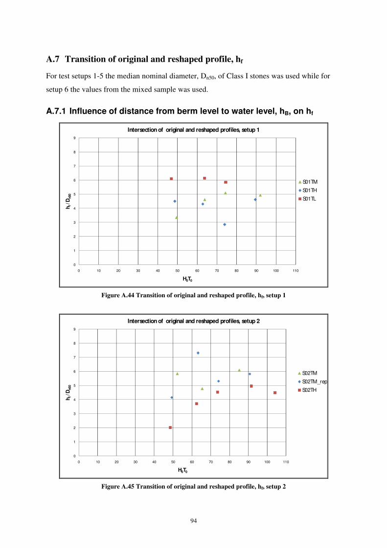
94
A.7 Transition of original and reshaped profile, hf
For test setups 1-5 the median nominal diameter, Dn50, of Class I stones was used while for
setup 6 the values from the mixed sample was used.
A.7.1 Influence of distance from berm level to water level, hB, on hf
0
1
2
3
4
5
6
7
8
9
0 10 20 30 40 50 60 70 80 90 100 110
hf/D
n50
H0T0
Intersection of original and reshaped profiles, setup 1
S01TM
S01TH
S01TL
Figure A.44 Transition of original and reshaped profile, hf, setup 1
0
1
2
3
4
5
6
7
8
9
0 10 20 30 40 50 60 70 80 90 100 110
hf/D
n50
H0T0
Intersection of original and reshaped profiles, setup 2
S02TM
S02TM_rep
S02TH
Figure A.45 Transition of original and reshaped profile, hf, setup 2

95
0
1
2
3
4
5
6
7
8
9
0 10 20 30 40 50 60 70 80 90 100 110
hf/D
n50
H0T0
Intersection of original and reshaped profiles, setup 4
S04TM
S04TM_rep
S04TH
Figure A.46 Transition of original and reshaped profile, hf, setup 4
0
1
2
3
4
5
6
7
8
9
0 10 20 30 40 50 60 70 80 90 100 110
hf/D
n50
H0T0
Intersection of original and reshaped profiles, setup 6
S06TM
S06TH
Figure A.47 Transition of original and reshaped profile, hf, setup 6

96
A.7.2 Comparison of different setups
0
1
2
3
4
5
6
7
8
9
0 10 20 30 40 50 60 70 80 90 100 110
hf/D
n50
H0T0
Intersection of original and reshaped profiles, water level 0.590m
S01TM
S02TM
S02TM_rep
S03TM
S04TM
S04TM_rep
S05TM
S06TM
Figure A.48 Transition of original and reshaped profile, hf, water level 0.590m
0
1
2
3
4
5
6
7
8
9
0 10 20 30 40 50 60 70 80 90 100 110
hf/D
n50
H0T0
Intersection of original and reshaped profiles, water level 0.645m
S01TH
S02TH
S03TH
S04TH
S05TH
S06TH
Figure A.49 Transition of original and reshaped profile, hf, water level 0.645m
Expected values
Class I
Expected values
Mixed stones
Expected values
Class I
Expected values
Mixed stones

97
A.8 Wave spectra
The type of waves used in the model test of this research are gravity waves propagating at the
surface of a water body which are locally generated by the action of the wind at the free
surface. This type of sea-state is called a wind-sea-state and is characterised by short wave
periods (2s to 10s typically) and provide an irregular aspect of the sea surface.
A sea-state can be described with a graph, table, or mathematical equation showing the
distribution of wave energy as a function of wave frequency, this is called a wave spectrum.
Two of the most widely used spectra are those described by Pierson & Moskowitz (1964) and
the JONSWAP spectrum, Hasselmann et al. (1973), shown in Figure A.50. These spectra are
formulated using a power function with respect to the frequency containing several scaling
parameters and constants.
The Pierson-Moskowitz spectrum represents a fully developed sea and was developed by
offshore industry. It assumes deep water conditions with unlimited fetch and was developed
using North-Atlantic data. The JOint North Sea WAve Project, that resulted in the JONSWAP
spectrum on the other hand represents a sea at young state and was also developed by offshore
industry. It represents conditions with limited fetch and was developed using North Sea data.
Since the wave spectrum is hardly ever fully developed in nature, the Jonswap spectrum is
often used. In this experiment the Jonswap spectrum was used with the peak enhancement
factor, γ = 3.3.
.
−
−−
−−
−=
2
2
2
1exp
4
542
4
5exp)2()(
σ
γπα
pff
pf
ffgfE
(8.1)
with:
E spectral energy density [m2/Hz]
α scaling parameter (Pierson-Moskowitz) [-]
f frequency [Hz]
fp peak frequency [Hz]
γ peak enhancement factor [-]
σ scaling parameter [-]
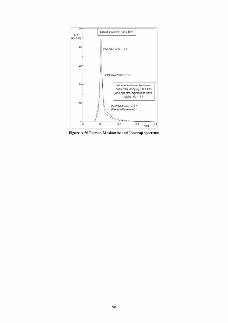
98
Figure A.50 Pierson-Moskowitz and Jonswap spectrum

99
A.9 Damage measurement photos
For explanation the damage development from one setup is shown here. The setup chosen is
setup 2 with water level 0.590m, since tests for that setup was repeated the repeated tests will
be shown here, S02TM_rep.
a) b)
c) d)
Figure A.51 Damage measurement photos, S02TM_rep, wave test #2, after a) 500 waves, b) 1000 waves, c)
2000 waves and d) 3000 waves

100
a) b)
c) d)
Figure A.52 Damage measurement photos, S02TM_rep, a) wave test #2 after 3000 waves, b) wave test #3
after 3000 waves, c) wave test #4 after 3000 waves, d) wave test #5 after failure

101
A.10 Photos from laboratory
Figure A.53 Photo from laboratory, the wave board
Figure A.54 Photo from laboratory, the camera stand and the structure

102
Figure A.55 Photo from laboratory, taken behind the structure
Figure A.56 Photo from laboratory, measurement equipment
Video camera

103
Figure A.57 Photo from laboratory, overview, looking in the direction of the structure
Figure A.58 Photo from laboratory, overview, looking in the direction of the wave generator
Computer
facilities
Wave
gauges
The structure
Wave
generator Computer, related to wave generator


![Íslenskur orðaforði íslenskra grunnskólanema sem eiga annað móðurmál en íslensku [Icelandic vocabulary among Icelandic second language learners]](https://static.fdokumen.com/doc/165x107/6344d24938eecfb33a064409/islenskur-ordafordi-islenskra-grunnskolanema-sem-eiga-annad-modurmal-en.jpg)