Stability, Erosion, and Morphology Considerations for ...

University of Tennessee, Knoxville University of Tennessee, Knoxville

TRACE: Tennessee Research and Creative TRACE: Tennessee Research and Creative

Exchange Exchange

Doctoral Dissertations Graduate School

5-2014

Stability, Erosion, and Morphology Considerations for Sustainable Stability, Erosion, and Morphology Considerations for Sustainable

Slope Design Slope Design

Isaac Andres Jeldes Halty University of Tennessee - Knoxville, [email protected]

Follow this and additional works at: https://trace.tennessee.edu/utk_graddiss

Part of the Civil Engineering Commons, Environmental Engineering Commons, Geomorphology

Commons, Geotechnical Engineering Commons, Hydrology Commons, Soil Science Commons, and the

Sustainability Commons

Recommended Citation Recommended Citation Jeldes Halty, Isaac Andres, "Stability, Erosion, and Morphology Considerations for Sustainable Slope Design. " PhD diss., University of Tennessee, 2014. https://trace.tennessee.edu/utk_graddiss/2702

This Dissertation is brought to you for free and open access by the Graduate School at TRACE: Tennessee Research and Creative Exchange. It has been accepted for inclusion in Doctoral Dissertations by an authorized administrator of TRACE: Tennessee Research and Creative Exchange. For more information, please contact [email protected].

https://trace.tennessee.edu/

https://trace.tennessee.edu/

https://trace.tennessee.edu/utk_graddiss

https://trace.tennessee.edu/utk-grad

https://trace.tennessee.edu/utk_graddiss?utm_source=trace.tennessee.edu%2Futk_graddiss%2F2702&utm_medium=PDF&utm_campaign=PDFCoverPages

http://network.bepress.com/hgg/discipline/252?utm_source=trace.tennessee.edu%2Futk_graddiss%2F2702&utm_medium=PDF&utm_campaign=PDFCoverPages








mailto:[email protected]

To the Graduate Council:

I am submitting herewith a dissertation written by Isaac Andres Jeldes Halty entitled "Stability,

Erosion, and Morphology Considerations for Sustainable Slope Design." I have examined the

final electronic copy of this dissertation for form and content and recommend that it be

accepted in partial fulfillment of the requirements for the degree of Doctor of Philosophy, with a

major in Civil Engineering.

Eric C. Drumm, Major Professor

We have read this dissertation and recommend its acceptance:

Daniel Yoder, Richard Bennett, John Schwartz, Dayakar Penumadu

Accepted for the Council:

Carolyn R. Hodges

Vice Provost and Dean of the Graduate School

(Original signatures are on file with official student records.)

Stability, Erosion, and Morphology Considerations for Sustainable Slope

Design

A Dissertation Presented for the

Doctor of Philosophy

Degree

The University of Tennessee, Knoxville

Isaac Andres Jeldes Halty

May 2014

ii

Copyright © 2014 by Isaac A. Jeldes Halty

All rights reserved.

iii

To my wife Daniela and my parents, whom I love more than anything.

iv

Acknowledgements

I would like to express my endless gratitude to my professor, Dr. Eric Drumm, for his enthusiastic

supervision, guidance, support, and infinite patience during this Ph.D. research. In him, I have not

only found a mentor, but also a good friend. I thank Dr. Daniel Yoder for his guidance and

insightful thoughts in topics related to concave slopes and erosion. I extend my sincere gratitude

to Dr. Richard Bennett for his valuable comments on the last chapter and for being an example of

life and professionalism. I thank Dr. John Schwartz for his support during the first years of my

Ph.D. journey and for his comments on the first two chapters of this manuscript. Finally, I would

like to express my gratitude to Dr. Dayakar Penumadu, whose early observations were very

beneficial for the overall scope of this work.

My gratitude to my parents Miguel and Lia, and my brothers Luis and Carlos for their continuous

encouragement through these years. Special thanks to Dan and Rosalie, for becoming part of our

family, and letting us be part of theirs. Thanks to my friends Hans, Rima, Miguel, Danielle, Justin,

Michaela, Fernando, and Emily for making this journey much more fun!

Finally, my deepest gratitude to my dear wife Daniela. Her love and support during these years

made this dreamed accomplishment a concrete reality.

v

Abstract

The construction of more natural and sustainable earth slopes requires the consideration of erosion

and runoff characteristics as an integral part of the design. These effects not only result in high

costs for removal of sediment, but also a profound damage to the ecosystem. In this dissertation,

innovative techniques are developed such that more natural appearing slopes can be designed to

minimize sediment delivery, while meeting mechanical equilibrium requirements. This was

accomplished by: a) examining the fundamental failure modes of slopes built with minimum

compaction (FRA) to enhance quick establishment of forest, b) investigating the geomechanical

and erosion stability of concave slopes, and c) developing design equations for a new type of

inclined-face retaining structure, the Piling Framed Retaining Wall (PFRW), which in the limit is

a confined slope. The analysis of several potential failures via Limit Equilibrium (LEM) and Finite

Element (FEM) suggested that the governing failure of FRA slopes is shallow and well represented

by infinite slope conditions, and laboratory and field data suggests that seasonal increase of

stability due to matric suction is possible, while instability may occur under local seismicity. The

investigation of the mechanical and erosion stability of concave slopes began with a mathematical

definition of critical concave slopes at limiting equilibrium. Based on this, a mechanism to design

concave slopes for a selected Factor of Safety (FS) was proposed. Results indicated that concave

slopes can yield 15-40% less sediment than planar slopes of equal FS, and the stability is not

compromised by errors in the construction. Concave slopes satisfying mechanical equilibrium are

not necessarily in erosion equilibrium as observed in many natural landscapes. It was shown that

when these two equilibrium conditions are met, the slopes become sustainable and a set of

equations describing sustainable concave slopes was proposed. Finally, rational design equations

vi

for the innovative PFRW were developed based on numerous FEM analyses for different soil and

geometry conditions. The equations provided a good prediction of the soil stresses measured on a

PFRW built in Knoxville, TN.

vii

Preface

This dissertation comprises the assembly of six manuscripts, which at the present time, are at

different stages of review and publication in various peer review journals. Each chapter

corresponds to a unique article, where methods, results, conclusions, references and in some cases

appendices are individually addressed. The first five chapters (articles) deal with geo-

environmental slope stability issues, where the main objective is to investigate, and finally provide,

mechanisms for more natural and sustainable design of earth slopes. This research was partially

funded by the Office of Surface Mining Reclamation and Enforcement, and was motivated from

the growing need for environmental-friendly techniques for landform construction and sustainable

land management. In these first five chapters efforts have been made to include surficial water

erosion as a key variable in the slope design, and attempts have been made to integrate water

erosion and slope stability, which are traditionally treated as separated sciences. Through these

chapters, the reader will find topics ranging from theoretical development of equations to

illustrative design examples, with the overall goal of providing practical tools that engineers can

use in design. The last article, on the other hand, addresses a different stability topic related to an

innovative retaining wall system comprising an inclined wall face, which in a practical sense can

be seen as a confined slope. This research was funded by the Tennessee Department of

Transportation, with the objective of creating a rational design methodology for this new type of

wall, eliminating the need to conduct extensive numerical analyses for each wall to be constructed.

viii

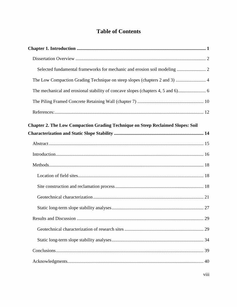
Table of Contents

Chapter 1. Introduction ............................................................................................................... 1

Dissertation Overview ................................................................................................................ 2

Selected fundamental frameworks for mechanic and erosion soil modeling ......................... 2

The Low Compaction Grading Technique on steep slopes (chapters 2 and 3) .......................... 4

The mechanical and erosional stability of concave slopes (chapters 4, 5 and 6) ........................ 6

The Piling Framed Concrete Retaining Wall (chapter 7) ......................................................... 10

References: ................................................................................................................................ 12

Chapter 2. The Low Compaction Grading Technique on Steep Reclaimed Slopes: Soil

Characterization and Static Slope Stability ............................................................................. 14

Abstract ..................................................................................................................................... 15

Introduction ............................................................................................................................... 16

Methods..................................................................................................................................... 18

Location of field sites............................................................................................................ 18

Site construction and reclamation process ............................................................................ 18

Geotechnical characterization ............................................................................................... 21

Static long-term slope stability analyses ............................................................................... 27

Results and Discussion ............................................................................................................. 29

Geotechnical characterization of research sites .................................................................... 29

Static long-term slope stability analyses ............................................................................... 34

Conclusions ............................................................................................................................... 39

Acknowledgments..................................................................................................................... 40

ix

References: ................................................................................................................................ 42

Chapter 3. Partial Saturation and Seismicity on Steep Reclaimed Slopes ............................ 47

Abstract ..................................................................................................................................... 48

Introduction ............................................................................................................................... 49

Background ............................................................................................................................... 50

Unsaturated soil shear strength ............................................................................................. 50

Shear strength and the pseudo-static forces for seismic analyses ......................................... 52

Field and experimental methods ............................................................................................... 55

Study sites: construction and site characterization ............................................................... 55

Soil water characteristic curves for unsaturated stability analyses ....................................... 59

Peak ground and spectral accelerations for seismic stability analyses ................................. 61

Analytical methods for stability analyses ................................................................................. 61

Infinite slope equation for unsaturated soil strength ............................................................. 61

Infinite Slope equation for horizontal and vertical pseudo-static forces .............................. 65

Summary of the methodology ................................................................................................... 67

Results and Discussion ............................................................................................................. 68

SWCCs and stability results for unsaturated FRA soils ....................................................... 68

Seismic stability analyses ..................................................................................................... 74

Conclusions ............................................................................................................................... 78

Acknowledgments..................................................................................................................... 79

References: ................................................................................................................................ 81

Chapter 4. An Approximate Solution to the Sokolovskiĭ Concave Slope at Limiting

Equilibrium ................................................................................................................................. 89

x

Abstract ..................................................................................................................................... 90

Introduction ............................................................................................................................... 90

Background: the slip line field theory and the characteristic equations ................................... 92

Elaboration of Sokolovskiĭ solution for the critical slope in a weightless medium.................. 96

Proposed solution for the critical slope in a medium with self-weight ..................................... 99

Validation of the WMA solution ............................................................................................ 104

Geometry of the concave slopes ......................................................................................... 104

Critical FS and observed failure mechanisms ..................................................................... 107

Effects of slope height on failure mechanisms and FS obtained from the proposed solution 110

Discussion and conclusions .................................................................................................... 113

References: .............................................................................................................................. 115

Appendix: The slip line field theory and the characteristic equations .................................... 118

Equations of internal equilibrium and principal stresses .................................................... 118

Formulation of the equations of the characteristics ............................................................ 119

Chapter 5. Design of Stable Concave Slopes for Reduced Sediment Delivery .................... 127

Abstract ................................................................................................................................... 128

Introduction ............................................................................................................................. 128

Background ............................................................................................................................. 130

Mechanical stability of concave profiles ............................................................................ 130

Concave slopes and soil erosion ......................................................................................... 131

Methods................................................................................................................................... 134

Mechanical stability ............................................................................................................ 134

Soil erosion and sediment yield .......................................................................................... 138

xi

Construction and sensitivity ................................................................................................ 140

Results and Discussion ........................................................................................................... 142

Concave slopes with pre-selected FS’s for long-term ( > 0) conditions ......................... 142

Stability check for short-term ( = 0) conditions .............................................................. 145

Soil loss from the mechanically stable concave slopes ...................................................... 145

Sensitivity to construction accuracy ................................................................................... 150

Illustrative Examples .............................................................................................................. 152

Finding the concave profile for long-term stability: ........................................................... 152

Checking the short-term stability of the concave slope: ..................................................... 154

Erosion analyses: ................................................................................................................ 156

Conclusions ............................................................................................................................. 156

References: .............................................................................................................................. 159

Chapter 6. Sustainable Concave Slopes .................................................................................. 164

Abstract ................................................................................................................................... 165

Introduction ............................................................................................................................. 166

Background ............................................................................................................................. 167

Concave profiles as erosion equilibrium shapes ................................................................. 167

Slope shape evolution and equilibrium profiles: A conceptual model ................................... 170

Methodology ........................................................................................................................... 173

Conceptual Development .................................................................................................... 173

RUSLE2 approximation to steady-state concave slopes .................................................... 178

Sustainable slopes: mechanical and erosion stability ......................................................... 182

xii


Concave slopes with constant rate of erosion ..................................................................... 185

Sustainable slopes ............................................................................................................... 187

Limitations of this work .......................................................................................................... 195

Conclusions ............................................................................................................................. 198

References: .............................................................................................................................. 199

Chapter 7. The Piling Framed Concrete Retaining Wall: Design Pressures and Stability

Evaluation .................................................................................................................................. 203

Abstract ................................................................................................................................... 204

Introduction ............................................................................................................................. 205

Background ............................................................................................................................. 206

The PFRW concept and the construction sequence ............................................................ 206

Theoretical expressions for active, passive, and at-rest earth pressure coefficients ........... 208

Methods................................................................................................................................... 212

Numerical Analyses ............................................................................................................ 212

Model stresses vs. field measured stresses: The SmartFix case ......................................... 220


Normal stresses on battered wall ........................................................................................ 222

Destabilizing moments for overturning stability ................................................................ 227

Design equations to predict earth pressures and destabilizing moments ............................ 229

The SmartFix case: predicted vs. measured stresses on the inclined wall .......................... 231

Conclusions ............................................................................................................................. 234

Acknowledgments................................................................................................................... 234

xiii

References: .............................................................................................................................. 236

Appendix ................................................................................................................................. 241

Active, passive, and at rest states of the soil mass .............................................................. 241

Active and passive lateral earth pressure coefficients: a literature review ......................... 242

At-rest lateral earth pressure coefficients: a literature review ............................................ 249

Definition of boundary condition and distance to boundaries ............................................ 251

Generalized FEM soil stresses in terms of the dimensionless quantities /Neq c and /H c

............................................................................................................................................. 254

Generalized FEM overturning moments in terms of the quantities /M c and /H c .... 256

Validation of simplified design equations .......................................................................... 258

Determination of soil strength parameters .......................................................................... 260

Chapter 8. Conclusions ............................................................................................................. 261

The Low Compaction Grading Technique on steep slopes (chapters 2 and 3) ...................... 262

The mechanical and erosional stability of concave slopes (chapters 4, 5 and 6) .................... 264

The Piling Framed Concrete Retaining Wall (chapter 7) ....................................................... 267

References: .............................................................................................................................. 270

Vita ............................................................................................................................................. 271

xiv

List of Tables

Table 2.1 Average slope length, width and inclination angle for the four plots at the Premium,

National and Mountainside sites ................................................................................................... 30

Table 2.2 Mean values of Liquid Limit, Plastic Index, soil texture and soil classification (USCS)

....................................................................................................................................................... 30

Table 2.3 Means, standard deviations, 95% confidence intervals (C.I.), and 90% tolerance

intervals (T.I) (80% coverage) for wet and dry unit weights for Premium, National and

Mountainside sites ........................................................................................................................ 32

Table 2.4 Summary of internal friction angle and cohesion for reclaimed mine materials ......... 35

Table 2.5 FS obtained for long-term static stability focused on the low strength surface layer .. 36

Table 3.1 Summary of recommended pseudo-static values and expressions available in the

literature (after Duncan and Wright, 2005)................................................................................... 54

Table 3.2 Average values of slope length, inclination angle, unit weights, water content, and

observed angles of repose for Premium, National and Mountainside sites. ................................. 60

Table 3.3 Soil texture (USDA) and unit weights for ROSETTA model...................................... 62

Table 3.4 Summary of hK , vK and obtained FS’s for a 2 and 10% P.E. in 50 yr. ..................... 75

Table 4.1 Maximum values of sH (m) reported by Sokolovskiĭ (1960) and used in stability

analyses (1960) solution from LEM ........................................................................................... 105

Table 4.2 Comparison of stability between proposed approximate solution and Sokolovskiĭ (1960)

solution from LEM ..................................................................................................................... 108

Table 5.1 Soil composition, classification, erodibility and assumed internal friction angle of

investigated soils ......................................................................................................................... 141

Table 5.2 Reduction in soil loss (1 /c pA A ) from concave contours reported in the literature 151

xv

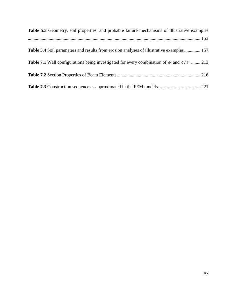
Table 5.3 Geometry, soil properties, and probable failure mechanisms of illustrative examples

..................................................................................................................................................... 153

Table 5.4 Soil parameters and results from erosion analyses of illustrative examples .............. 157

Table 7.1 Wall configurations being investigated for every combination of and /c ........ 213

Table 7.2 Section Properties of Beam Elements ........................................................................ 216

Table 7.3 Construction sequence as approximated in the FEM models .................................... 221

xvi

List of Figures

Fig. 1.1. Illustration of the superior mechanical and erosion resistances of concave slopes [adapted

from Schor and Gray (2007)]. ......................................................................................................... 7

Fig. 2.1. Location of field sites in northeastern Tennessee, referred to as Premium, National, and

Mountainside................................................................................................................................. 19

Fig. 2.2. National site after the FRA reclamation process and during the construction of the study

plots. .............................................................................................................................................. 19

Fig. 2.3. Depiction of the reclamation process according to FRA. .............................................. 20

Fig. 2.4. Randomized systematic sampling technique; a) area of interest subdivided into small sub-

areas (Sweigard et al. 2007c), where small circles represent the random measurement locations; b)

application of this technique for NDG measurements at the National site. .................................. 24

Fig. 2.5. Typical field determination of the angle of repose at National Site (White et al. 2009).

Camera placed on a level and photo taken of material in loose state. Note the large number of

oversize (> 0.3 m) particles in the reclaimed material. ................................................................. 26

Fig. 2.6. Shear strains and nodal displacements obtained from the FEM analysis assuming a very

strong core. Upper left corner illustrates the geometric dimensions employed for LEM and FEM

analyses. ........................................................................................................................................ 36

Fig. 2.7. Failure mechanisms and FS’s obtained from FEM stability analysis for tan / tancore loose

= 1.3. The FS = 1.94 shown for the deeper failure mechanism was obtained when the strength

reduction factor (SRF) search was restricted to be outside the zone where the shallow mechanism

occurred. Shear strains showed for SRF = 2.02 to emphasize failure mode. ............................... 38

Fig. 2.8. FEM analyses of the global stability for various values of tan / tancore loose and the

infinite slope equation ................................................................................................................... 38


Mountainside................................................................................................................................. 56

xvii

Fig. 3.2. Depiction of the reclamation process according to FRA (Jeldes et al. 2013). ............... 58

Fig. 3.3. Depiction of the 3 Spectral Accelerations for Premium, National and Mountainside

(USGS 2012). ................................................................................................................................ 62

Fig. 3.4. The Infinite Slope method. Figure modified from Salgado (2008). ............................... 64

Fig. 3.5. Infinite Slope method with horizontal and vertical pseudo-static forces. ...................... 66

Fig. 3.6. Soil water characteristic curves measured in laboratory experiments and the ROSETTA

model (Schaap et al. 2001), for the Premium site. ........................................................................ 69


model (Schaap et al. 2001), for the National site. ......................................................................... 69


model (Schaap et al. 2001), for the Mountainside site. ................................................................ 70

Fig. 3.9. Calculated monthly variations in stability (FS), volumetric water content and cumulative

monthly rainfall from July 2009 to August 2010 at the Premium site.......................................... 71


monthly rainfall from July 2009 to August 2010 at the National site. ......................................... 72


monthly rainfall from July 2009 to August 2010 at the Mountainside site. ................................. 73

Fig. 3.12. FS chart for Mountainside site as a function of spectral accelerations and initial

fundamental period. ...................................................................................................................... 77

Fig. 4.1. Orientation of slip lines in a soil mass at limiting equilibrium [adapted from Sokolovskiĭ

(1965)]........................................................................................................................................... 93

Fig. 4.2. Critical slope shape (planar) for a weightless medium. Inside zone AoC the principal

directions are aligned with the reference frame. On the slope surface, the principal directions are

aligned with the normal and tangential directions. ....................................................................... 97

xviii

Fig. 4.3. Slope surface in a medium possessing weight [after Sokolovskiĭ, (1965)].................. 100

Fig. 4.4. Weightless Medium Approximation: discretized weightless medium (e.g. rigid foam

beads) supporting thin, external loads (e.g. frictionless lead sheets) separated by a finite interval:

a) coarser discretization and b) finer discretization. ................................................................... 100

Fig. 4.5. Sokolovskiĭ’s critical slope vs the real (non-imaginary) component of the solution of Eq.

(4.21). .......................................................................................................................................... 102

Fig. 4.6. Comparison of Sokolovskiĭ (1960) numerical solution and the proposed analytical

solution for = 30˚ and /c = 2 m. .......................................................................................... 105


solution in dimensionless coordinates for = 20˚, 30˚, and 40˚. .............................................. 106

Fig. 4.8. FEM results in terms of shear strains for the Sokolovskiĭ (1960) critical concave slope.

..................................................................................................................................................... 108

Fig. 4.9. FEM results in terms of shear strains for the proposed critical concave slope. ........... 109

Fig. 4.10. Modes of failure depicted in the form of shear bands (maximum shear strains) as

observed in concave slopes (FEM). Figure illustrate case for = 20˚ and /c = 2 m, and two

values of sH . .............................................................................................................................. 111

Fig. 4.11. Computed FS (LEM) on concave slopes with different vertical heights sH and /c for

= 20˚. ...................................................................................................................................... 111

Fig. 4.12. Relationship between the limiting height Lh and /c . ............................................ 112

Fig. 4.13. Illustration of slip planes on Mohr-Coulomb diagram. .............................................. 120

Fig. 4.14. Orientation of slip lines (adapted from Sokolovskiĭ, 1965). ...................................... 123

xix

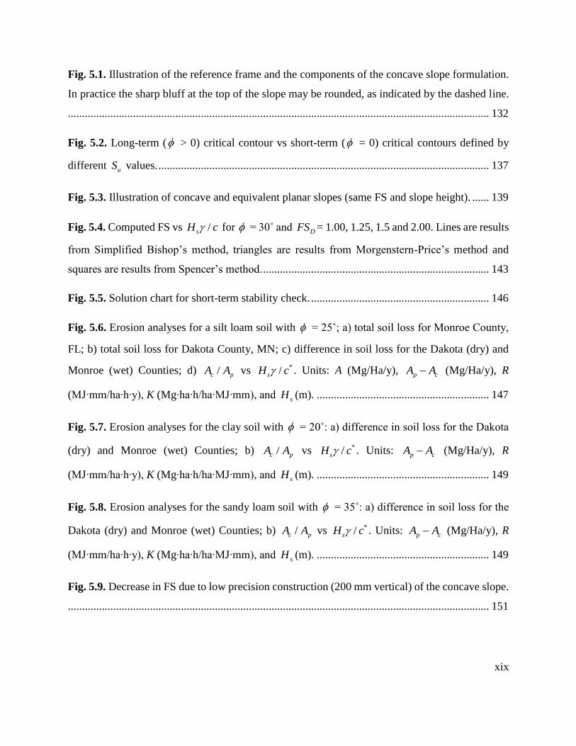
Fig. 5.1. Illustration of the reference frame and the components of the concave slope formulation.

In practice the sharp bluff at the top of the slope may be rounded, as indicated by the dashed line.

..................................................................................................................................................... 132

Fig. 5.2. Long-term ( > 0) critical contour vs short-term ( = 0) critical contours defined by

different uS values. ..................................................................................................................... 137

Fig. 5.3. Illustration of concave and equivalent planar slopes (same FS and slope height). ...... 139

Fig. 5.4. Computed FS vs /sH c for = 30˚ and DFS = 1.00, 1.25, 1.5 and 2.00. Lines are results

from Simplified Bishop’s method, triangles are results from Morgenstern-Price’s method and

squares are results from Spencer’s method. ................................................................................ 143

Fig. 5.5. Solution chart for short-term stability check. ............................................................... 146

Fig. 5.6. Erosion analyses for a silt loam soil with = 25˚; a) total soil loss for Monroe County,

FL; b) total soil loss for Dakota County, MN; c) difference in soil loss for the Dakota (dry) and

Monroe (wet) Counties; d) /c pA A vs */sH c . Units: A (Mg/Ha/y), p cA A (Mg/Ha/y), R

(MJ∙mm/ha∙h∙y), K (Mg∙ha∙h/ha∙MJ∙mm), and sH (m). ............................................................. 147

Fig. 5.7. Erosion analyses for the clay soil with = 20˚: a) difference in soil loss for the Dakota

(dry) and Monroe (wet) Counties; b) /c pA A vs */sH c . Units: p cA A (Mg/Ha/y), R


Fig. 5.8. Erosion analyses for the sandy loam soil with = 35˚: a) difference in soil loss for the

Dakota (dry) and Monroe (wet) Counties; b) /c pA A vs */sH c . Units: p cA A (Mg/Ha/y), R


Fig. 5.9. Decrease in FS due to low precision construction (200 mm vertical) of the concave slope.

..................................................................................................................................................... 151

xx

Fig. 5.10. Example case for sandy soil: = 35 ˚, c = 15 kN/m2, = 19 kN/m3 and sH = 15 m.

Required FS = 1.5. Shear strains showed for SRF = 1.52 to emphasize failure mode. .............. 155

Fig. 6.1. Conceptual model of slope morphology evolution by water erosion. .......................... 172

Fig. 6.2. Illustration of the parallel retreat concept. The sharp edge at the top of the slope may be

naturally eroded (becoming convex) if there is runoff coming over the top edge of the slope. This

effect is not included in the proposed model. ............................................................................. 172

Fig. 6.3. Erosion rates experienced by a planar profile as modeled by RUSLE2 perspective. .. 175

Fig. 6.4. Illustration of a potential family of concave slopes with constant rate of erosion: a) high

rate, b) intermediate rate, and c) low rate. .................................................................................. 177

Fig. 6.5. Discretization of the slope profile in small linear segments. ....................................... 180

Fig. 6.6. Illustration of steady-state or sustainable slope (profile 1) and a non-equilibrium slope

with cyclic morphology changes (profile 2). .............................................................................. 184

Fig. 6.7. Family of concave slopes with constant rate of erosion (equilibrium erosion profiles).

..................................................................................................................................................... 186

Fig. 6.8. The overall steepness (defined as the slope of the straight line that connects the top and

the bottom of the profile) increases at a much faster rate for 1

nA 1, as denoted by dashed line.

..................................................................................................................................................... 186

Fig. 6.9. Erosion equilibrium profiles and a critical concave contour for = 20˚ and /c = 1 m.

Concave slopes with 1

nA 1.05 are considered sustainable. ...................................................... 188

Fig. 6.10. Erosion equilibrium profiles and a critical concave contour for = 30˚ and /c = 0.5

m. Concave slopes with 1

nA 1.039 are considered sustainable. ............................................... 188

Fig. 6.11. Erosion equilibrium profiles and a critical concave contour for = 20˚, 25˚, 30˚, 35˚,

40˚ and /c = 0.5, 0.75, 1, 1.5, 2, 3 m. ..................................................................................... 190

xxi

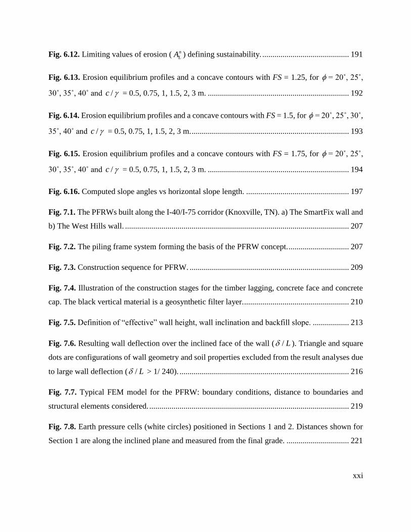
Fig. 6.12. Limiting values of erosion ( n

LA ) defining sustainability. ........................................... 191

Fig. 6.13. Erosion equilibrium profiles and a concave contours with FS = 1.25, for = 20˚, 25˚,

30˚, 35˚, 40˚ and /c = 0.5, 0.75, 1, 1.5, 2, 3 m. ...................................................................... 192

Fig. 6.14. Erosion equilibrium profiles and a concave contours with FS = 1.5, for = 20˚, 25˚, 30˚,

35˚, 40˚ and /c = 0.5, 0.75, 1, 1.5, 2, 3 m. .............................................................................. 193


30˚, 35˚, 40˚ and /c = 0.5, 0.75, 1, 1.5, 2, 3 m. ...................................................................... 194

Fig. 6.16. Computed slope angles vs horizontal slope length. ................................................... 197

Fig. 7.1. The PFRWs built along the I-40/I-75 corridor (Knoxville, TN). a) The SmartFix wall and

b) The West Hills wall. ............................................................................................................... 207

Fig. 7.2. The piling frame system forming the basis of the PFRW concept. .............................. 207

Fig. 7.3. Construction sequence for PFRW. ............................................................................... 209

Fig. 7.4. Illustration of the construction stages for the timber lagging, concrete face and concrete

cap. The black vertical material is a geosynthetic filter layer. .................................................... 210

Fig. 7.5. Definition of “effective” wall height, wall inclination and backfill slope. .................. 213

Fig. 7.6. Resulting wall deflection over the inclined face of the wall ( / L ). Triangle and square

dots are configurations of wall geometry and soil properties excluded from the result analyses due

to large wall deflection ( / L > 1/ 240). .................................................................................... 216

Fig. 7.7. Typical FEM model for the PFRW: boundary conditions, distance to boundaries and

structural elements considered. ................................................................................................... 219

Fig. 7.8. Earth pressure cells (white circles) positioned in Sections 1 and 2. Distances shown for

Section 1 are along the inclined plane and measured from the final grade. ............................... 221

xxii

Fig. 7.9. Typical FEM results for normal stresses on battered wall for H=7.62 m (SmartFix wall

height). Results shown for a sandy soil with = 30˚ and /c = 0.3 m. ................................... 223

Fig. 7.10. Definition of equivalent normal distributed pressures Neq : a) FEM and b) Coulomb and

Coulomb with tension correction. ............................................................................................... 225

Fig. 7.11. Equivalent normal uniform stress Neq vs. wall height H, for the = 30˚ and /c =

1 m soil case and the SmartFix wall inclination = 71.6˚. a) = 0˚ and b) = 20˚. .............. 225

Fig. 7.12. Illustration of a case when the theoretical Coulomb earth pressures are lower than FEM

predictions, and therefore unconservative ( = 30˚ and /c = 1 m, = 20˚, and = 50˚). .. 226

Fig. 7.13. Dimensionless equivalent normal earth pressures vs. stability number as predicted by

FEM for = 30˚. a) = 0˚ and b) = 20˚. .............................................................................. 226

Fig. 7.14. Forces and moment arms employed for overturning moments. a) Numerical FEM and

b) Theoretical Coulomb with tension correction on wall + at-rest condition on cap. ................ 228

Fig. 7.15. Destabilizing moment M vs. wall height H, for the = 30˚ and /c = 1 m soil case

and the SmartFix wall inclination = 71.6˚. ............................................................................. 228

Fig. 7.16. Normalized overturning moment vs. stability number as predicted by FEM for = 30˚.

..................................................................................................................................................... 230

Fig. 7.17. Validation of design equations: a) Neq (kPa) and b) M (kN-m/m). ........................ 230

Fig. 7.18. Field measured stresses over time vs. theoretical and numerical earth pressures. ..... 232

Fig. 7.19. Conceptual model of the different stress states on the retaining wall problem. ......... 243

Fig. 7.20. Two FEM models considered: a) the 0.5 m of the battered pile below the final grade is

truly pinned and b) the battered pile is truly pinned at the contact with the basal rock. ............ 252

xxiii

Fig. 7.21. Difference in resulting normal stresses from the two battered wall end conditions

investigated (SmartFix case). The model comprising a pinned condition at the 0.5 m below final

grade resulted in higher overall stresses. .................................................................................... 252

Fig. 7.22. Dimensionless equivalent normal earth pressures vs stability number as predicted by

FEM for = 20˚......................................................................................................................... 254


FEM for = 30˚......................................................................................................................... 254


FEM for = 40˚......................................................................................................................... 255

Fig. 7.25. Normalized overturning moment vs. stability number as predicted by FEM, = 20˚.

..................................................................................................................................................... 256


..................................................................................................................................................... 256

Fig. 7.27. Normalized overturning moment vs. stability number as predicted by FEM = 40˚.

..................................................................................................................................................... 257

Fig. 7.28. Validation of design equations: a) Neq and b) M for = 20˚. ............................... 258



Fig. 7.31. Selected M-C strength parameters based on triaxial p-q diagram at 14% strain level.

..................................................................................................................................................... 260

1

Chapter 1. Introduction

2

Dissertation Overview

The present dissertation is a collection of six manuscripts, each a single chapter, at different stages

of review and publication in various peer review journals. The original contributions of this work

are mostly centered on topics related to the broad area of slope stability, with efforts to integrate

the traditionally separate areas of mechanical slope stability and surficial rain-driven water erosion.

In this vein, chapters 2 and 3 addresses stability issues related to a new reclamation technique for

rapid reforestation and reduction of soil loss, while chapters 4, 5 and 6 focus on understanding the

role of the topography of concave contours--similar to those existing in nature--on the mechanical

and erosion stability of slopes. Through these first five chapters, topics ranging from theoretical

development of equations to illustrative design examples are offered with the overall goal of

providing mechanisms for the design of more natural and sustainable earth slopes. The last chapter

(chapter 7), on the other hand, addresses a different stability topic related to an innovative retaining

wall system comprising an inclined face, which in a practical sense can be seen as a confined slope.

In this section, equations to predict earth pressures and overturning moments are developed to

support the creation of a rational design methodology, eliminating the need to conduct extensive

numerical analyses for each wall to be constructed.

Selected fundamental frameworks for mechanic and erosion soil modeling

In soil mechanics, numerous constitutive laws defining failure have been proposed such that

strength and deformation characteristics of soils can be modeled for engineering purposes. For

frictional materials like soils, the Mohr-Coulomb (M-C) yield criterion arises as the “best known”

fundamental law (Smith and Griffiths 2004) and it has been the most widely used model for soil

shear strength prediction (Griffiths and Lane 1999, Salgado 2008). This constitutive model does

3

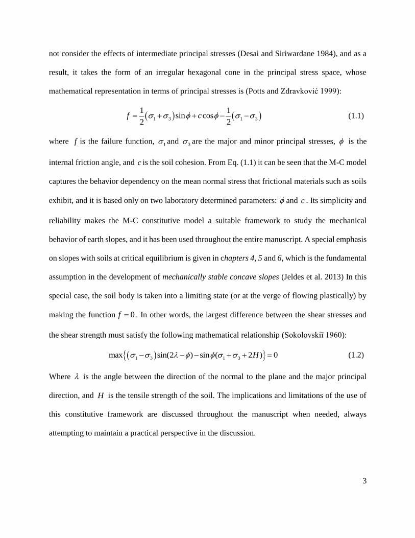
not consider the effects of intermediate principal stresses (Desai and Siriwardane 1984), and as a

result, it takes the form of an irregular hexagonal cone in the principal stress space, whose

mathematical representation in terms of principal stresses is (Potts and Zdravkovic 1999):

1 3 1 3

1 1sin cos

2 2f c (1.1)

where f is the failure function, 1 and 3 are the major and minor principal stresses, is the

internal friction angle, and c is the soil cohesion. From Eq. (1.1) it can be seen that the M-C model

captures the behavior dependency on the mean normal stress that frictional materials such as soils

exhibit, and it is based only on two laboratory determined parameters: and c . Its simplicity and

reliability makes the M-C constitutive model a suitable framework to study the mechanical

behavior of earth slopes, and it has been used throughout the entire manuscript. A special emphasis

on slopes with soils at critical equilibrium is given in chapters 4, 5 and 6, which is the fundamental

assumption in the development of mechanically stable concave slopes (Jeldes et al. 2013) In this

special case, the soil body is taken into a limiting state (or at the verge of flowing plastically) by

making the function 0f . In other words, the largest difference between the shear stresses and

the shear strength must satisfy the following mathematical relationship (Sokolovskiĭ 1960):

1 3 1 3max sin(2 ) sin ( 2 ) 0H (1.2)

Where is the angle between the direction of the normal to the plane and the major principal

direction, and H is the tensile strength of the soil. The implications and limitations of the use of

this constitutive framework are discussed throughout the manuscript when needed, always

attempting to maintain a practical perspective in the discussion.

4

The Revised Universal Soil Loss Equation RUSLE2 (USDA-ARS 2008) is one of the most widely

used erosion equations and is known for its effectiveness and simplicity in accounting for the

critical effects controlling erosion (Tiwari et al. 2000). RUSLE2 relies on concrete empirical soil

loss data to model the important processes involving soil erosion:

A R K LS C P (1.3)

where the predicted soil loss A is directly proportional to: the rainfall erosivity R quantifying the

rainfall’s erosive potential; the soil erodibility K defining the soil’s susceptibility to that erosivity;

the topographic factor LS representing slope length and steepness effects; the surface cover factor

C; and the conservation practices factor P. Its simplicity and accuracy in predicting erosion make

RUSLE2 an ideal and reliable framework for soil loss investigations involving more complex

(non-planar) slope topographies, and it was used here to investigate the effects of mechanically

stable concave profiles on soil loss (chapter 5) and also to investigate the morphology of slopes in

erosion equilibrium (chapter 6). The limitations of RUSLE2 in the context of this work were

identified and discussed, and the assumptions made to overcome these limitations were properly

justified throughout these two chapters.

The Low Compaction Grading Technique on steep slopes (chapters 2 and 3)

Mine reclamation activities have traditionally incorporated compaction procedures to augment the

strength of the reclaimed material and ensure stability of the restored slopes (Hoomehr et al. 2013,

Jeldes et al. 2013, Jeldes et al. 2010). However, while compaction is important for strength and

erosion resistance, it has negative impacts on tree survival and hampers reforestation efforts. The

quick establishment of forest and ground cover is an important consideration for long-term erosion

control, since vegetation absorbs raindrop impact, reduces flow energy by reducing runoff

5

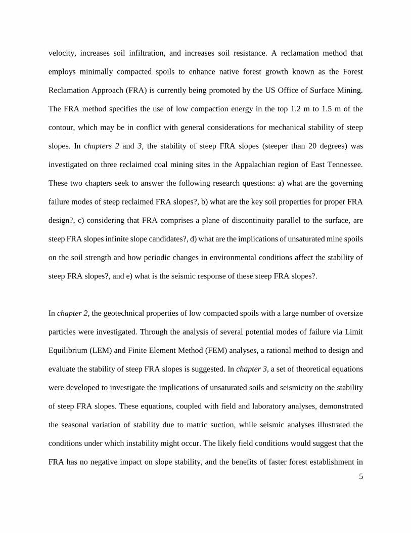
velocity, increases soil infiltration, and increases soil resistance. A reclamation method that

employs minimally compacted spoils to enhance native forest growth known as the Forest

Reclamation Approach (FRA) is currently being promoted by the US Office of Surface Mining.

The FRA method specifies the use of low compaction energy in the top 1.2 m to 1.5 m of the

contour, which may be in conflict with general considerations for mechanical stability of steep

slopes. In chapters 2 and 3, the stability of steep FRA slopes (steeper than 20 degrees) was

investigated on three reclaimed coal mining sites in the Appalachian region of East Tennessee.

These two chapters seek to answer the following research questions: a) what are the governing

failure modes of steep reclaimed FRA slopes?, b) what are the key soil properties for proper FRA

design?, c) considering that FRA comprises a plane of discontinuity parallel to the surface, are

steep FRA slopes infinite slope candidates?, d) what are the implications of unsaturated mine spoils

on the soil strength and how periodic changes in environmental conditions affect the stability of

steep FRA slopes?, and e) what is the seismic response of these steep FRA slopes?.

In chapter 2, the geotechnical properties of low compacted spoils with a large number of oversize

particles were investigated. Through the analysis of several potential modes of failure via Limit

Equilibrium (LEM) and Finite Element Method (FEM) analyses, a rational method to design and

evaluate the stability of steep FRA slopes is suggested. In chapter 3, a set of theoretical equations

were developed to investigate the implications of unsaturated soils and seismicity on the stability

of steep FRA slopes. These equations, coupled with field and laboratory analyses, demonstrated

the seasonal variation of stability due to matric suction, while seismic analyses illustrated the

conditions under which instability might occur. The likely field conditions would suggest that the

FRA has no negative impact on slope stability, and the benefits of faster forest establishment in

6

terms of reduced erosion and sediment delivery make the FRA very attractive for future

reclamation work.

The mechanical and erosional stability of concave slopes (chapters 4, 5 and 6)

Under the FRA concept, the quick establishment of ground cover and forest is important to reduce

the high initial erosion and sediment delivery on reclaimed and constructed slopes. The efforts in

chapters 4, 5 and 6 were then directed to understand the role of topography on erosion rates and

to investigate the role of non-planar contour shapes--similar to those existing in nature--on the

mechanical and erosion stability of slopes. While constructed slopes are traditionally designed to

be planar in cross section, in nature curvilinear slopes with concave shapes are naturally formed

as a result of evolutionary processes leading towards a state of erosion and sediment transport

equilibrium. The superiority of concave slopes in terms of mechanical stability and erosion

resistance can be explained by the conceptual model developed by Schor and Gray (2007).

Assuming that a planar slope of height H and angle can be discretized into a series of horizontal

layers with equal thickness (Fig. 1.1), where the strength properties (internal friction angle and

cohesion c ) and unit weight ( ) remain constant for the entire slope, the mechanical stability of

each layer will be dependent upon the particular stress-strength state and the angle on inclination

of each layer. With the acceleration of gravity acting vertically downwards, the vertical stresses at

each point within the soil mass increases proportional to the depth. To bring each layer into the

same degree of equilibrium or Factor of Safety (FS), the inclination of each layer must be adjusted;

steeper slopes will be allowed in the upper layers where less overburden mass exists, while gentler

slopes will be necessary in the lower layers. The result of this process is a concave profile, which

7

Fig. 1.1. Illustration of the superior mechanical and erosion resistances of concave slopes [adapted

from Schor and Gray (2007)].

8

provides a more uniform equilibrium state for the entire slope. On the other hand, surficial water

erosion increases with slope length and slope angle. In a planar slope, water tractive forces will

monotonically increase downslope, with higher energy in the lowest part of the contour. By

gradually decreasing the steepness of each layer in the direction of the water flow, the increased

erosion due to the increased slope length will be partially counteracted by the decreased erosion

due to decreasing slope steepness, ultimately resulting in a concave slope with a minimized

uniform erosion rate along the profile.

Realizing that not all concave shapes will be mechanically stable, it is desirable to have a

description of concave slopes that provide mechanical stability for given set of soil properties. In

these chapters answers for the following research questions are sought: a) what is the critical

concave profile for mechanical stability considerations as defined by the Mohr-Coulomb

constitutive model?, b) how can concave slopes be described such that they provide a desired

degree of stability (or FS) for given soil properties?, c) how effective are these mechanically

optimized concave slopes in reducing sediment delivery?, d) how does the accuracy of

construction affects the mechanical stability of concave slopes?, e) what is the equilibrium concave

profile for erosion considerations?, f) how do erosion equilibrium concave slopes compare with

critical concave slopes defined for mechanical stability?, and g) can slopes be constructed to

achieve both mechanical and erosional stability?

In chapter 4, an approximate analytical solution that defines the geometry of critical concave

slopes (FS ≈ 1) for frictional soils with self-weight ( > 0, c > 0, > 0) was developed, based

on the slip line field method of Sokolovskiĭ (1960). The fundamentals behind Sokolovskiĭ’s theory

9

were revisited, and the physical and mathematical derivations preceding the approximate solution

are presented in detail. The approximate solution was validated using LEM and FEM analyses.

Chapter 5 builds on the previous chapter to provide a practical design approach such that

geotechnical engineers will consider non-planar shapes, which provide a more natural appearance

in addition to offering improved erosion resistance. This was accomplished by creating a

mechanism to design slopes for a given FS, and suggesting a method for both long-term and short-

term stability investigations for concave slopes. The difference in soil loss (erosion) between

planar and concave slopes satisfying the same degree of mechanical stability was also investigated,

along with analyses to determine how sensitive concave slopes are to construction inaccuracies.

An illustrative example was provided to demonstrate the design process and the benefits of

meeting mass stability requirements while at the same time reducing surficial erosion and yielding

a more natural looking slope.

While mechanically stable, the proposed concave slopes in chapters 4 and 5 may not be in

equilibrium from a water erosion perspective. Evidence exists that natural fluvial systems, seeking

erosion and sediment transport equilibrium, may adjust the geometry in order to achieve a concave

steady-state form that will be somewhat unchanged over time. In chapter 6, the concept of steady-

state landforms was explored and a conceptual model of changes in slope morphology toward a

concave erosion equilibrium shape was described. Based on the assumptions inherent to the

RUSLE2 erosion model, concave profiles in water erosion equilibrium were identified and

described, and an approach was proposed to discern between long-term mechanically stable and

unstable erosion equilibrium shapes for any given combination of soil stresses and strength. A

definition of the approximate limiting erosion rate at which equilibrium erosion shapes become

10

mechanically stable and thus “sustainable” is explored, and a mathematical expression to obtain

this limiting erosion rate is offered as a function of the Mohr-Coulomb parameters.

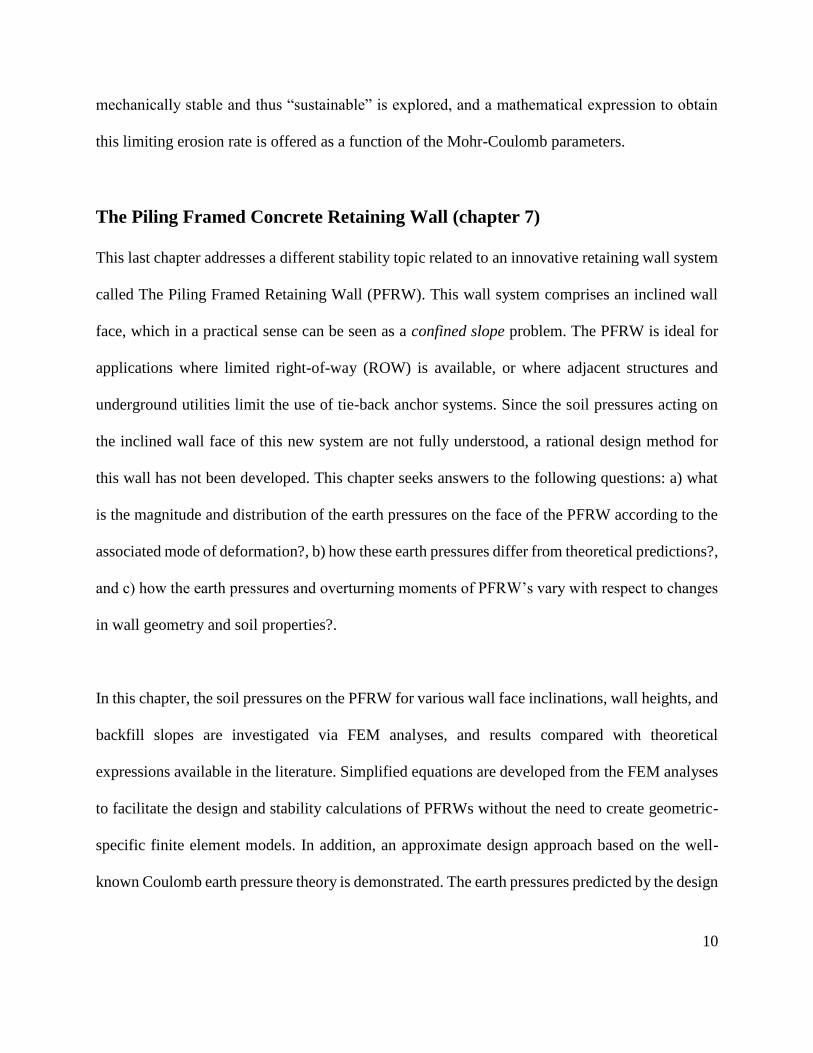
The Piling Framed Concrete Retaining Wall (chapter 7)

This last chapter addresses a different stability topic related to an innovative retaining wall system

called The Piling Framed Retaining Wall (PFRW). This wall system comprises an inclined wall

face, which in a practical sense can be seen as a confined slope problem. The PFRW is ideal for

applications where limited right-of-way (ROW) is available, or where adjacent structures and

underground utilities limit the use of tie-back anchor systems. Since the soil pressures acting on

the inclined wall face of this new system are not fully understood, a rational design method for

this wall has not been developed. This chapter seeks answers to the following questions: a) what

is the magnitude and distribution of the earth pressures on the face of the PFRW according to the

associated mode of deformation?, b) how these earth pressures differ from theoretical predictions?,

and c) how the earth pressures and overturning moments of PFRW’s vary with respect to changes

in wall geometry and soil properties?.

In this chapter, the soil pressures on the PFRW for various wall face inclinations, wall heights, and

backfill slopes are investigated via FEM analyses, and results compared with theoretical

expressions available in the literature. Simplified equations are developed from the FEM analyses

to facilitate the design and stability calculations of PFRWs without the need to create geometric-

specific finite element models. In addition, an approximate design approach based on the well-

known Coulomb earth pressure theory is demonstrated. The earth pressures predicted by the design

11

equations and the approximate design approach were compared with field measured soil stresses

on a PFRW built in Knoxville, TN.

12

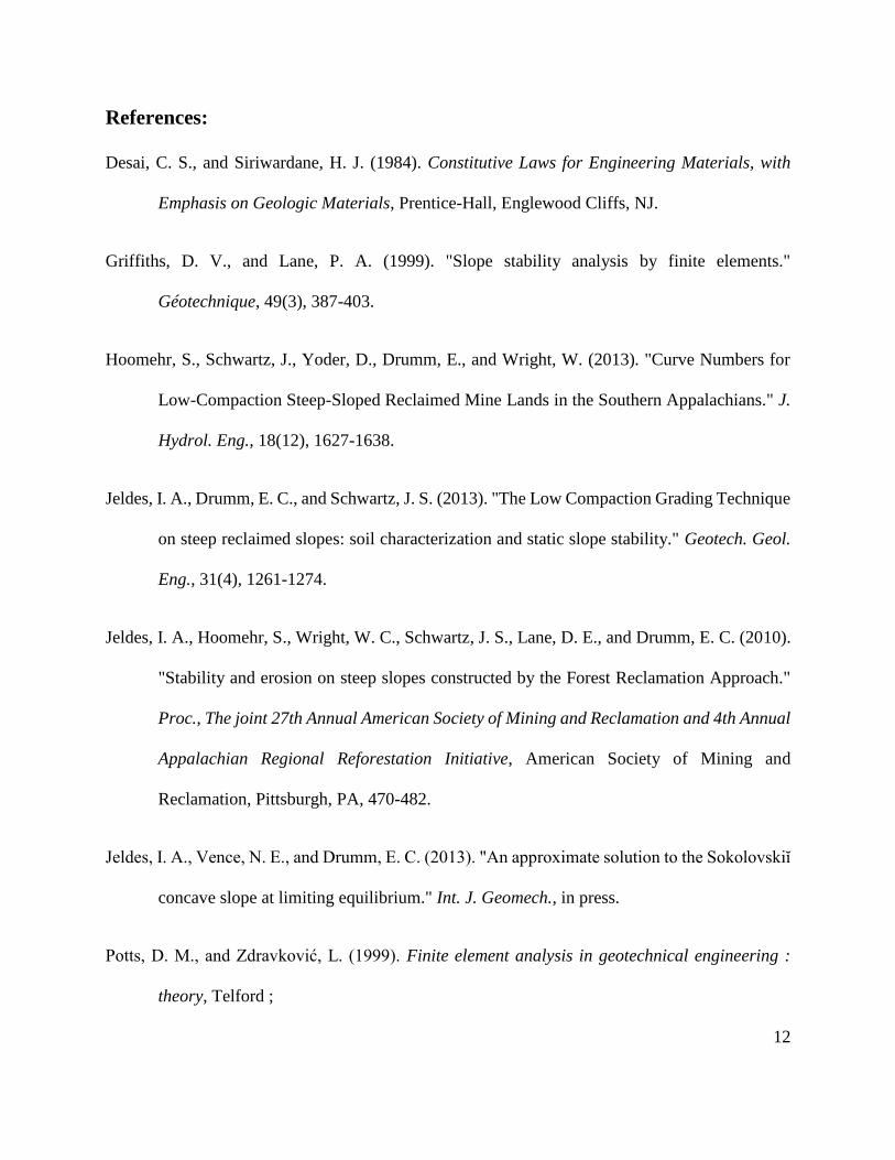
References:

Desai, C. S., and Siriwardane, H. J. (1984). Constitutive Laws for Engineering Materials, with

Emphasis on Geologic Materials, Prentice-Hall, Englewood Cliffs, NJ.

Griffiths, D. V., and Lane, P. A. (1999). "Slope stability analysis by finite elements."

Géotechnique, 49(3), 387-403.

Hoomehr, S., Schwartz, J., Yoder, D., Drumm, E., and Wright, W. (2013). "Curve Numbers for

Low-Compaction Steep-Sloped Reclaimed Mine Lands in the Southern Appalachians." J.

Hydrol. Eng., 18(12), 1627-1638.

Jeldes, I. A., Drumm, E. C., and Schwartz, J. S. (2013). "The Low Compaction Grading Technique

on steep reclaimed slopes: soil characterization and static slope stability." Geotech. Geol.

Eng., 31(4), 1261-1274.

Jeldes, I. A., Hoomehr, S., Wright, W. C., Schwartz, J. S., Lane, D. E., and Drumm, E. C. (2010).

"Stability and erosion on steep slopes constructed by the Forest Reclamation Approach."

Proc., The joint 27th Annual American Society of Mining and Reclamation and 4th Annual

Appalachian Regional Reforestation Initiative, American Society of Mining and

Reclamation, Pittsburgh, PA, 470-482.

Jeldes, I. A., Vence, N. E., and Drumm, E. C. (2013). "An approximate solution to the Sokolovskiĭ

concave slope at limiting equilibrium." Int. J. Geomech., in press.

Potts, D. M., and Zdravkovic, L. (1999). Finite element analysis in geotechnical engineering :

theory, Telford ;

13

Distributed by ASCE Press, London

Reston, VA.

Salgado, R. (2008). The engineering of foundations, McGraw Hill, Boston.

Schor, H. J., and Gray, D. H. (2007). Landforming : an environmental approach to hillside

development, mine reclamation and watershed restoration, John Wiley & Sons, Hoboken,

NJ.

Smith, I. M., and Griffiths, D. V. (2004). Programming the Finite Element Method, John Wiley &

Sons, Chichester, England.

Sokolovskiĭ, V. V. (1960). Statics of Soil Media, Butterworths Scientific Publications, London.

Tiwari, A. K., Risse, L. M., and Nearing, M. A. (2000). "Evaluation of WEPP and its comparison

with USLE and RUSLE." Transactions of the Asae, 43(5), 1129-1135.

USDA-ARS (2008). "RUSLE2 Science Documentation." U.S. Department of Agriculture -

Agricultural Research Service, Washington, DC.

14

Chapter 2. The Low Compaction Grading Technique on Steep

Reclaimed Slopes: Soil Characterization and Static Slope Stability

15

This chapter was published as an original paper in the Journal of Geotechnical and Geological

Engineering, Springer Publishing. The co-authors of this work are Dr. Eric Drumm and Dr. John

Schwartz. This article is cited as:


on steep reclaimed slopes: soil characterization and static slope stability." Geotech.

Geol. Eng., 31(4), 1261-1274. DOI: 10.1007/s10706-013-9648-0

Abstract

Since the Surface Mining and Control Reclamation Act of 1977, U.S. coal mining companies have

been required by law to restore the approximate ground contours that existed prior to mining. To

ensure mass stability and limit erosion, the reclaimed materials have traditionally been placed with

significant compaction energy. The Forest Reclamation Approach (FRA) is a relatively new

approach that has been successfully used to facilitate the fast establishment of native healthy

forests. The FRA method specifies the use of low compaction energy in the top 1.2 m to 1.5 m of

the contour, which may be in conflict with general considerations for mechanical slope stability.

Although successful for reforestation, the stability of FRA slopes has not been fully investigated

and a rational stability method has not been identified. Further, a mechanics-based analysis is

limited due to the significant amount of oversize particles which makes the sampling and

measurement of soil strength properties difficult. To investigate the stability of steep FRA slopes

(steeper than 20 degrees), three reclaimed coal mining sites in the Appalachian region of East

Tennessee were investigated. The stability was evaluated by several methods to identify the

predominant failure modes. The infinite slope method, coupled with the estimation of the shear

strength from field observations, was shown to provide a rational mean to evaluate the stability of

16

FRA slopes. The analysis results suggest that the low compaction of the surface materials may not

compromise the long-term stability for the sites and material properties investigated.

Introduction

A reclamation method that employs minimally compacted spoils to enhance native forest growth,

known as the Forest Reclamation Approach (FRA) is currently being promoted by the US Office

of Surface Mining (OSM) (Angel et al. 2007, Sweigard et al. 2007). Since the Surface Mining and

Control Reclamation Act of 1977 (SMCRA), coal companies in the U.S.A. have been required by

law to restore the land to its pre-mined contours (USDoI 1977). Reclamation activities have

traditionally incorporated compaction procedures to augment the strength of the reclaimed material

and ensure stability of the restored slopes. However, while compaction is important for strength

and erosion resistance, it diminishes soil porosity which restricts root penetration and reduces

water infiltration with negative impacts on tree survival and grass reestablishment (Angel et al.

2007, Sweigard et al. 2007). FRA employs a low compaction effort in the uppermost 1.2 m to 1.5

m. The low-compaction grading technique has proven to be successful in encouraging tree growth,

and demonstrates the potential for establishing healthy native forests on reclaimed mine lands

(Angel et al. 2007, Barton et al. 2007). However, with the exception of Torbert and Burger (1994),

most of these demonstrations were conducted on relatively flat lying terrain where stability issues

were negligible. The stability of steep FRA slopes, defined as steeper than 20 degrees by the

USDoI (2009), and the possible modes of failure have not been investigated and a rational stability

analysis method has not been suggested.

17

Slope stability analysis requires the knowledge of soil properties in terms of density and strength;

characteristics not easily determined for reclaimed mine spoil due to the significant amount of

oversize material (> 0.3 m). The in situ density of soils consisting of large rock particles can be

difficult to measure, which makes it difficult to quantify and awkward to provide proper

construction quality control. Sweigard et al. (2007) have suggested correlations between dry bulk

density and shovel penetration; though practical for reforestation efforts they are not appropriate

for the evaluation of slope stability. Furthermore, because of the difficulties associated with

sampling and testing due to the oversize particles, the shear strength properties are not typically

measured in laboratory or field tests. For mine reclamation projects, the design is typically

completed well in advance of mining activities and usually based on experience using assumed or

traditional regional soil properties (Bell et al. 1989). Naturally, there is uncertainty associated with

this practice, especially if low compaction is employed on steep reclaimed slopes. For example, in

Kentucky the majority of slope failures in abandoned mine lands have occurred via translational

and rotational failure mechanisms through the loose material placed prior to the SMCRA

(Iannacchione and Vallejo 1995). The lack of proper compaction is a known cause of failure in

constructed slopes, with the stability becoming worse under intense rainstorms (Chen et al. 2004).

The failure of Sau Mau Ping slopes in Hong Kong is one dramatic example of the danger associated

with poorly compacted slopes and lack of proper engineering design (Abramson 1996, Hong Kong

Geotechnical Engineering Office 2007).

The objectives of this paper are to 1) characterize the geotechnical properties of low compacted

spoils on steep slopes constructed according to the FRA, and 2) investigate the likely failure

mechanisms associated to steep slopes reclaimed using the FRA. This is accomplished using three

18

reclaimed field sites at which the material characteristics are evaluated, and the results will be used

to suggest a practical method to estimate the shear strength and evaluate the stability of slopes

constructed using the low compaction grading technique.

Methods

Location of field sites

To investigate the potential effects on stability resulting from the implementation of the low

compaction grading technique, three steep FRA slopes were studied. The three sites, referred to

here by the name of the initial coal operator (Premium, National and Mountainside), are located in

northeastern Tennessee, with Premium located in Anderson County, National in Campbell County

and Mountainside located in Claiborne County (Fig. 2.1). Each of the mine operators played an

instrumental role in the development of the study sites. Each site was divided into four different

plots which while not discussed here, were instrumented in order to concurrently investigate the

runoff hydrology and sediment yield on the FRA slopes (Hoomehr et al. 2013). Fig. 2.2 shows the

National site during construction of the study plots.

Site construction and reclamation process

At each of the three sites in this study, the construction procedure followed the contour haulback

method (Sweigard and Kumar 2010), where a ramp is constructed on the contour bench and spoil

is hauled up the ramp and dumped over the edge. The sequence of the construction process can be

divided into four major steps (Sweigard et al. 2007) depicted schematically in Fig. 2.3: a)

placement and compaction of the materials for the primary backfill core using traditional practices,

19


Mountainside.

Fig. 2.2. National site after the FRA reclamation process and during the construction of the study

plots.

20

Fig. 2.3. Depiction of the reclamation process according to FRA.

21

b) dumping of the soil that will constitute the loose surface layer (1.2 m-1.5 m thick), c) grading

of the loose soil layer with the lightest equipment available using the fewest passes possible, and

d) reforestation. The three research sites presented a very rough soil surface after the final grading,

which is consistent with the FRA recommendations for successful reforestation (Sweigard et al.

2007). However, because the final layer at all three sites often included boulder-sized material,

significant depressions and large rocks were left on the surface of the slope which is a deviation

of Sweigard’s recommendations for an ideal finished surface.

Geotechnical characterization

The investigation proceeded with the characterization of the research sites and the analysis of their

mechanical stability. The field characterization of the mine spoil included: a) determination of the

site geometry; b) particle size analysis, index tests, and classification of the materials; c)

determination of unit weight; and d) estimation of the Mohr-Coulomb (M-C) shear strength

parameters.

Geometry

The geometric characteristics of the research sites were determined via a series of TrimbleTM total

station topographical surveys. The purpose of these surveys was not only to obtain a more accurate

estimation of the slope angles, but also to gather data to geo-reference the instrumented sites

allowing an investigation of the spatial variation of material properties.

22

Particle size analyses, index tests, and classification of reclaimed materials

Four soil samples of 0.02 m3 each were randomly taken across the slope at each site for particle

size analyses, index tests and classification. All samples were collected from a depth of at least 30

cm below the slope surface to a) avoid samples with fewer fines due to erosion armoring and b)

avoid surficial soils affected by changes in fabric due to weathering. Particle size analysis (grain

size distribution and hydrometer) and Atterberg limits tests were conducted in general accordance

to ASTM D422-07 and ASTM D4318–10 respectively, and classification of the materials in

general accordance to the Unified Soil Classification System (USCS), ASTM D2487-10. Visual

inspection suggested that the materials may contain a large amount of agglomerated fines in the

form of large particles, and therefore, traditional dry particle size analysis would indicate a larger

amount of coarse material than really exists. This issue was investigated at all three sites by

allowing soil samples to soak in water for 14 days. Very few aggregated fines were found at the

Premium and National soils, but significant aggregated fines at Mountainside. For this reason, a

wet preparation of the Mountainside samples was conducted in general accordance to ASTM

D2217-04 before conducting the particle size analysis and index tests. The amount of oversize

material (> 0.3 m) was estimated on a surface basis. This was accomplished by dividing the plot

into multiple squares of 1 m side length; a photograph of each square was used to estimate the

percentage of oversize particles per surface area.

Unit weight

An extensive data collection of the unit weight of the loose surface layer at each of the three sites

was conducted using a Troxler 3411-B Nuclear Density Gage (NDG), in general accordance to the

ASTM D6938-10. The measurements were obtained shortly after each slope was constructed.

23

During the data collection, periodic calibration of the NDG device was conducted at the beginning

and middle of each work day, employing the calibration block provided by the manufacturer. A

randomized systematic sampling technique (Sweigard et al. 2007) was used at one plot per site to

reduce data tendency or bias in the measurements. The plot was divided into multiple squares of

3 m side length, where single measurements of bulk dry unit weight (d ), wet unit weight (

T )

and moisture content ( w ) were taken at random locations inside the squares (Fig. 2.4). The soil

surface was cautiously carved to obtain a planar surface before placing the nuclear gauge device,

avoiding air interchange between the gauge base and the soil surface. Then, a hole perpendicular

to the slope surface was driven inside each sub-area and the source rod inserted to obtain the

readings at 300 mm (which is the maximum length of the source rod of the Nuclear Density

Gauge). From previous observations of the materials it was concluded that the amount of

hydrocarbons present at each site was very small and unlikely to affect the NDG readings.

Shear strength parameters

Slope stability analysis for long-term conditions assumes that positive excess pore water pressure

dissipates during the construction or loading period, and thus, requires the estimation of the drained

or effective shear strength parameters. The shear strength of soil is typically described using the

Mohr-Coulomb (M-C) yield or failure criterion:

tann nc (2.1)

24

Fig. 2.4. Randomized systematic sampling technique; a) area of interest subdivided into small sub-

areas (Sweigard et al. 2007c), where small circles represent the random measurement locations; b)

application of this technique for NDG measurements at the National site.

25

where n and

n are the normal and shear stresses acting on the failure plane within the soil body,

and and c are the internal friction angle and cohesion. Outside of mine reclamation, the shear

strength material properties and c are often measured in laboratory or obtained through

correlations with in situ tests. However, due to the large particles present in mine spoils, traditional

tests are very difficult to conduct. The current practice in mine reclamation is usually based on

experience or assumed values of and c . As discussed earlier, the FRA technique consists on

having a 1.2 to 1.5 m of loose soil at the uppermost part of the contour, above a well compacted

and stable core. Thus, this low density/low strength zone should be evaluated for stability. Since

the angle of repose is the “steepest stable slope for loose packed granular material and represents

the angle of internal friction at its loosest state” (Holtz and Kovacs 1981), it is suggested as a good

representation of the internal friction angle of loose soil layer in a FRA slope. The use of observed

angles of repose offers the additional advantage that the overall strength of the mass, including the

contribution of the oversize particles, is captured. Angles of repose were obtained by observing

the placement of spoils piles, and measuring the angle at which they hold in place. Because these

tests were conducted during reclamation activities, the angle was measured via photographs of the

fresh piles using a hand held level, for safety reasons. The level helped to ensure that the picture

was taken parallel to the horizon. With a photo editing software the angles of the piles were

measured (Fig. 2.5). Regarding the strength properties of the stronger core material, stability

analysis will later show that the most critical condition for stability is insensitive to the selected

strength values of the core.

26

Fig. 2.5. Typical field determination of the angle of repose at National Site (White et al. 2009).

Camera placed on a level and photo taken of material in loose state. Note the large number of

oversize (> 0.3 m) particles in the reclaimed material.

27

On the other hand, short-term stability analyses (undrained soil conditions) are often conducted to

characterize the behavior of the soil during and immediately after construction, where the loading

occurs much faster than the rate of dissipation of positive excess pore water pressure. However, it

is assumed that the coarse mine spoil material will not develop significant excess positive pore

water pressure under typical loadings (Duncan and Wright 2005); thus, a drained response is

expected. This assumption is supported by the grain size distribution of the materials and relatively

high void ratios obtained for each site which are reported in the results section. Furthermore, short-

term stability is not considered to be important in the reclamation of mine slopes, since any short-

term failure would have minimum consequences and would be repaired during construction or

routine maintenance.

Static long-term slope stability analyses

The analyses of the mechanical stability focused on long-term analyses of the primary failure

modes that are likely to be experienced by FRA slopes: a) shallow or local failure modes within

the loose surface layer and b) global or deep rotational failure modes of the overall soil mass. Limit

Equilibrium Methods (LEM) and the Finite Element Method (FEM) were employed in the analyses

assuming 2-D plain strain conditions. LEM analyses were computed using Slide 6.0 (Rocscience

Inc. 2011) with 10,000 critical surfaces analyzed. The FEM analyses were computed using Phase2

(Rocscience Inc. 2011) employing an elastic perfectly plastic stress-strain behavior and the M-C

yield criterion with a non-associated flow rule (zero dilatancy angle) to avoid over-prediction of

dilation and failure load for purely frictional materials (Griffiths and Lane 1999). Since the

estimation of the factor of safety (FS) has been shown to be not significantly affected by the value

of the elastic constants E (Young’s modulus) and (Poisson’s ratio) used in the FEM solution

28

(Cheng et al. 2007, Griffiths and Lane 1999), nominal values of E = 105 kPa and = 0.3 were

assumed here for the surface and core materials. The model was created with 6-noded triangular

elements, with a maximum of 500 iterations solved by Gaussian elimination. Because the geometry

and material properties from all sites are reasonably similar, those from Mountainside ( = 28˚

from the horizontal and H = 21 m height) will be used here to explore the various failure modes.

These values are representative of all three sites and many steep slopes in the southern Appalachian

coal fields. The thickness of the low-strength layer ( z ) was assumed to be 1.5 m.

Shallow stability within the low strength surface layer

A shallow failure mode was investigated by assuming that the core was significantly stronger than

the surface layer. The methods used were: a) LEM restricting the analyses to the shallow surface

layer via the non-circular Janbu’s method and a search block feature, b) FEM and the shear strength

reduction method (Cheng et al. 2007, Griffiths and Lane 1999), and c) the infinite slope equation

for cohesionless soils without seepage ( FS tan / tan ) and seepage ( FS 0.5 tan / tan ). The

infinite slope equation idealizes the surface as an infinite plane with the failure mechanism running

parallel to the surface (Skempton and Delory 1957) and it is appropriate when the ratio of depth to

length of the sliding surface is small. The geometry of the reclaimed mine slopes constructed

according to the FRA is ideally suited for investigation by the infinite slope method.

Deep rotational stability of the overall soil mass

Because the strength of the compacted core was not known, the deep rotational failure mode was

investigated by performing a series of analyses where the strength of the loose surface material

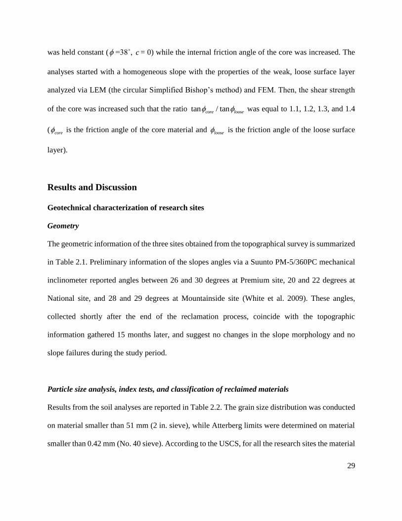
29

was held constant ( =38˚, c = 0) while the internal friction angle of the core was increased. The

analyses started with a homogeneous slope with the properties of the weak, loose surface layer

analyzed via LEM (the circular Simplified Bishop’s method) and FEM. Then, the shear strength

of the core was increased such that the ratio tan / tancore loose was equal to 1.1, 1.2, 1.3, and 1.4

( core is the friction angle of the core material and loose is the friction angle of the loose surface

layer).

Results and Discussion

Geotechnical characterization of research sites

Geometry

The geometric information of the three sites obtained from the topographical survey is summarized

in Table 2.1. Preliminary information of the slopes angles via a Suunto PM-5/360PC mechanical

inclinometer reported angles between 26 and 30 degrees at Premium site, 20 and 22 degrees at

National site, and 28 and 29 degrees at Mountainside site (White et al. 2009). These angles,

collected shortly after the end of the reclamation process, coincide with the topographic

information gathered 15 months later, and suggest no changes in the slope morphology and no

slope failures during the study period.

Particle size analysis, index tests, and classification of reclaimed materials

Results from the soil analyses are reported in Table 2.2. The grain size distribution was conducted

on material smaller than 51 mm (2 in. sieve), while Atterberg limits were determined on material

smaller than 0.42 mm (No. 40 sieve). According to the USCS, for all the research sites the material

30

Table 2.1 Average slope length, width and inclination angle for the four plots at the Premium,

National and Mountainside sites

Site

Average

slope

angle, β

(degrees)

Average

slope

length

(m)

Average slope

width

(m)

Top Bottom

Premium 28 32.2 28.1 25.0

National 20 48.4 22.4 25.4

Mountainside 28 45.4 23.6 23.1

Table 2.2 Mean values of Liquid Limit, Plastic Index, soil texture and soil classification (USCS)

Sites

Gravel

particles

51 mm –

4.75 mm

(%)

Sand

Particles

4.75 mm -

0.075 mm

(%)

Fines

< 0.075 mm

(%)

Clay

particles

< 2 μm

(%)

Liquid

Limit

(LL)

Plastic

Index

(PI)

Soil

classification

(USCS)

Premium 59 28 13 6 29 13 GC to GP-GC

National 52 28 20 10 27 14 GC

Mountainside 37 22 41 19 32 15 GC

31

classify as clayey gravel (GC) with the exception of one plot at the Premium site that classifies as

poorly graded clayey gravel (GP-GC) due to slightly less material finer than the number 200 sieve.

Regarding oversize particles, it was estimated that material larger than 300 mm occupies 0 to 25%

of 1 m2 at Premium site, 0 to 10% of 1 m2 at National site, and 5 to 40% of 1 m2 at Mountainside

site.

Unit weight

Results of the unit weight measurements were as follows: the maximum and minimum measured

d were 18.8 and 13.0 kN/m3 at Premium site, 21.4 and 14.6 kN/m3 at National site, and 22.8 and

14.9 kN/m3 at Mountainside site. Complementary results from statistical analyses are presented in

Table 2.3. Field measures of density at a similar mine site in Kentucky (Sweigard et al. 2011)

indicated similar variations as those found at Premium and National. The largest standard

deviations (S.D.) were observed at Mountainside, which is consistent with the largest range of unit

weights, and the largest amount of fines and observed number of oversize particles. At all sites,

the spatial variation of unit weight reflects the large range of particle sizes in these reclaimed

materials. A single unit weight measurement has a limited ability to represent the state of body

forces acting on the complete FRA slope, and thus, mean unit weights with the probable upper and

lower bounds (confidence and tolerance intervals) are desired for the mine material

characterization. While confidence intervals (C.I.) provide an upper and lower bound of the true

mean found at the constructed sites, tolerance intervals (T.I.) provide information of the probable

future range of unit weights that each site will have on average. In any case, as discussed later, the

determination of the unit weight for static long-term conditions may be of minor concern, but

necessary for static unsaturated and seismic stability analyses.

32

Table 2.3 Means, standard deviations, 95% confidence intervals (C.I.), and 90% tolerance

intervals (T.I) (80% coverage) for wet and dry unit weights for Premium, National and

Mountainside sites

95% C.I. for the Mean 90%/0.8 T.I. for the Mean

Sites Unit

Weight Mean kN/m3

S.D. kN/m3

Lower,

kN/m3 Upper,

kN/m3 Lower,

kN/m3 Upper,

kN/m3

Premium Dry 16.2 1.3 15.8 16.5 14.2 18.1

Wet 18.5 1.3 18.2 18.8 16.6 20.4

National Dry 18.5 1.0 18.3 18.7 17.2 19.9

Wet 20.3 1.0 20.1 20.5 18.9 21.7

Mountainside Dry 18.6 2.2 18.1 19.1 15.5 21.7

Wet 20.4 2.2 19.9 20.9 17.2 23.6

33

Water and sand cone replacement tests were previously conducted to determine bulk unit weights

at random locations on the four plots at each site (White et al. 2009). A comparison of the results

indicates that the NDG device gives on average about 25% higher average unit weights than

replacement methods at Premium site, 14% at National site and 21% at Mountainside. Since both

replacement methods involved the removal of small samples, they did not take into account the

effects of large rock fragments that are randomly embedded in the loose surface soil layer. On the

other hand, the NDG calculates unit weights based on the velocity travel of gamma rays between

the source and the detector, and any denser material that appears on the travel path will be counted

in the measurement. In this regard, the collection of a sufficient amount of NDG readings will

better represent the wide range of in-place density and provides a more representative average unit

weight for stress analyses. Replacement methods may be preferable for the calculation of void

ratio and soil porosity due to better representation of the soil matrix. The average void ratio of the

loose surface layer calculated via replacement methods was 1.0 at Premium, 0.6 at National and

0.7 at Mountainside. The largest void ratio was calculated for the soils found at Premium, which

is consistent with the lowest NDG unit weight measured. Overall, relatively large void ratios were

obtained for all three sites, which is consistent with the FRA requirements for healthy tree growth.

Shear strength parameters

The angle of repose of the looser soil layer was found to range between 37 and 39 degrees at

Premium and Mountainside, and between 36 and 38 degrees at National site. Zero cohesion is

usually employed for long-term analysis on coarse granular soils (Holtz and Kovacs 1981, Lambe

and Whitman 1969) and normally consolidated fine soils (Skempton 1964), and would be

appropriate for reclaimed materials receiving minimum compaction effort. While even a small

34

amount of compaction will increase the density and strength of the soil, the angle of repose is a

conservative estimate of the friction angle. Similar values of and c for loose spoils in the

Appalachian region were reported by Sweigard et al. (2011), while similar values for reclaimed

spoils outside the Appalachian were found in the literature (Gutierrez et al. 2008, Kasmer and

Ulusay 2006, Stormont and Farfan 2005, Sweigard et al. 2011, Ulusay et al. 1995) as summarized

in Table 2.4.

Static long-term slope stability analyses

Shallow stability within the low strength surface layer

Results from the limit equilibrium, finite element, and infinite slope analyses are summarized in

Table 2.5. From a practical perspective, all the analyses yielded very similar FS’s (approximately

1.47), implying that the shear strength along the most critical slip surface is about 47% greater

than that required to maintain equilibrium in the long-term. For all cases, the most critical failure

mechanism is shallow and is consistent with the assumed failure mechanism in the infinite slope

method. Fig. 2.6 shows the FEM model of the shallow failure mode with a section of the slope

enlarged (the 1.5 m thick surface layer is small with respect to the size of the model and may not

be clearly distinguished in the full model). It also shows nodal displacement vectors. Larger strains

are observed at the interface of the weak surface and core materials, with the displacement vectors

acting parallel to the surface suggesting a planar failure mechanism. The obtained long-term FS’s

are valid for drained conditions in the absence of seepage forces due to transient flow. However,

since the occurrence of downslope water flow through the complete thickness of the loose layer is

highly unlikely, this condition represents a lower bound or worst case value for the stability of

FRA, and would reduce the FS by a factor of 2.

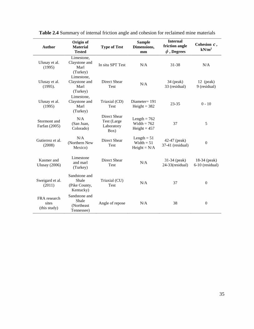
35

Table 2.4 Summary of internal friction angle and cohesion for reclaimed mine materials

Author

Origin of

Material

Tested

Type of Test

Sample

Dimensions,

mm

Internal

friction angle

, Degrees

Cohesion c ,

kN/m2

Ulusay et al.

(1995)

Limestone,

Claystone and

Marl

(Turkey)

In situ SPT Test N/A 31-38 N/A

Ulusay et al.

(1995).

Limestone,

Claystone and

Marl

(Turkey)

Direct Shear

Test N/A

34 (peak)

33 (residual)

12 (peak)

9 (residual)

Ulusay et al.

(1995)

Limestone,

Claystone and

Marl

(Turkey)

Triaxial (CD)

Test

Diameter= 191

Height = 382 23-35 0 - 10

Stormont and

Farfan (2005)

N/A

(San Juan,

Colorado)

Direct Shear

Test (Large

Laboratory

Box)

Length = 762

Width = 762

Height = 457

37 5

Gutierrez et al.

(2008)

N/A

(Northern New

Mexico)

Direct Shear

Test

Length = 51

Width = 51

Height = N/A

42-47 (peak)

37-41 (residual) 0

Kasmer and

Ulusay (2006)

Limestone

and marl

(Turkey)

Direct Shear

Test N/A

31-34 (peak)

24-33(residual)

18-34 (peak)

6-10 (residual)

Sweigard et al.

(2011)

Sandstone and

Shale

(Pike County,

Kentucky)

Triaxial (CU)

Test N/A 37 0

FRA research

sites

(this study)

Sandstone and

Shale

(Northeast

Tennessee)

Angle of repose N/A 38 0

36

Table 2.5 FS obtained for long-term static stability focused on the low strength surface layer

slope stability analysis results for generic slope ( = 28°, H = 21 m, = 38°, c = 0, T = 20.4 kN/m3)

Analysis Method Assumptions FS Critical failure mode

a) LEM Rigid core and Search Block - non-linear Janbu’s Method

with 10,000 critical surfaces analyzed 1.48

Shallow planar failure

surface

b) FEM

Core much stronger than loose surface layer, Shear

Strength Reduction Method to determine FS, with 500

iterations solved by Gaussian elimination

1.47 Shallow planar failure

surface

c) Analytical Infinite slope equation (no seepage) 1.47 Shallow planar failure

surface

Fig. 2.6. Shear strains and nodal displacements obtained from the FEM analysis assuming a very

strong core. Upper left corner illustrates the geometric dimensions employed for LEM and FEM

analyses.

37

Deep rotational stability of the overall soil mass

The results from LEM and FEM analyses of the deep failure mode of the homogeneous slope yield

a FS = 1.48, which is consistent with that obtained from the shallow stability analyses. Fig. 2.7

shows the results of a FEM analysis when the core strength was 30% stronger than the loose layer

(i.e. tan / tan 1.3core loose ). Here two possible failure mechanisms were observed in the form of

shear bands; a deeper mechanism through the core material with a FS = 1.94, and a shallow

mechanism with the lowest FS = 1.48 and highest shear strains at the interface of the materials.

The FS of the shallow mechanism is equal to those obtained from the shallow analyses above. A

similar trend is observed for cases when 1.1, 1.2, andtan / t 4an 1.core loose (Fig. 2.8). As the

strength of the core increases, the FS of the deeper mechanism increases; however, the lowest FS

is found to be constant with a consistent shallow failure mode and dependent only on the strength

level of the loose surface layer. Additional analyses at angles of inclination of 20 and 35 degrees

yielded similar results and confirm that the critical failure mode is a surface failure.

These results are consistent with the observation that the failure mechanisms through the loose

surface layer will govern and the determination of the strength parameters of the stronger dense

core are not important for FRA slope design. Furthermore, since the infinite slope method

adequately approximates the shallow failure mode, and accurately predicts the FS, it can be taken

as a simple and reliable method to evaluate the performance of FRA slopes and more sophisticated

computer analyses are not necessary for most applications. The use of the infinite slope method

also simplifies the field characterization of materials and disregards the unit weight determination,

because it only requires loose and for long-term conditions. The simplicity of the method is

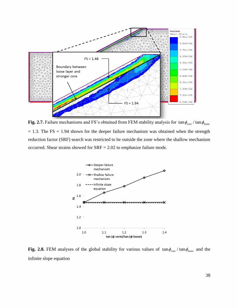
38

Fig. 2.7. Failure mechanisms and FS’s obtained from FEM stability analysis for tan / tancore loose

= 1.3. The FS = 1.94 shown for the deeper failure mechanism was obtained when the strength

reduction factor (SRF) search was restricted to be outside the zone where the shallow mechanism

occurred. Shear strains showed for SRF = 2.02 to emphasize failure mode.

Fig. 2.8. FEM analyses of the global stability for various values of tan / tancore loose and the

infinite slope equation

39

appropriate for design of reclaimed mine slopes which are typically designed in advance of mineral

extraction with assumed overburden properties. Accordingly, the lowest FS for drained or long-

term conditions at each instrumented site using the infinite slope equation is approximately 1.47

for Premium, 2.07 for National and 1.47 for Mountainside.

Conclusions

Characterization and stability evaluation of three FRA slopes in northeastern Tennessee

with inclinations as high as 28 degrees were conducted. A large number of oversize

particles were found in the reclaimed materials. In general, the material finer than 51 mm

classified as Clayey Gravels with the average Plasticity Index (PI) ranging from 13-15,

suggesting that the physical characteristic of the soils are similar across the three research

sites.

Unit weights determined using a Nuclear Density Gage were found to be higher than those

determined by replacement methods, yet vary significantly across the study plots. NDG

measures are preferred for stability analyses because they better capture the effect of

oversize particles on the in situ state of stresses of FRA slopes. It also allows more

measurements to characterize the wide range of in-place density. Tolerance intervals were

constructed to reflect the probable future range of unit weights that each site will have on

average.

The analysis of several potential modes of failure suggests that the governing failure mode

is shallow and contained within the weak, loose surface layer. The determination of the

strength parameters of the core is not important for FRA slope design.

40

Because the infinite slope method adequately approximates the shallow failure mode and

accurately predicts the FS, it may be an appropriate method to evaluate the performance of

FRA slopes and more sophisticated analyses are not necessary for most applications. Since

the unit weight of the material is not considered in the infinite slope expression, field

measurements of the highly variable unit weight are not required for long-term analyses.

The angle of repose was suggested to be a conservative estimate of the internal friction

angle and it is consistent with the loose nature of the FRA material. This provides a means

to quantify the friction angle of the mine spoil, which has been traditionally assumed based

on experience.

The shear strength along the most critical slip surface, for the typical FRA slope

investigated, is at least 47% greater than that required to maintain static equilibrium in the

long-term. In case that the entire loose surface zone becomes saturated with downslope

seepage and no infiltration into the core, the FS is reduced by a factor of 2, suggesting that

the slope would be unstable. However, these conditions are very unlikely and provide a

lower limit to the factor of safety

The likely conditions would suggest that the FRA has no negative impact on slope stability,

and the benefits of faster forest establishment in terms of reduced erosion and sediment

delivery make the FRA very attractive for future reclamation work.

Acknowledgments

This research was conducted as part of a project funded by the US Office of Surface Mines,

Applied Science Program Grant CA No. S08AP12822, 2008. The authors gratefully appreciate the

41

support and guidance provided by OSM staff David Lane, P.E., and Vic Davis, and the field

assistance provided by Patrick White, Wesley Wright, Esteban Zamudio, Mitch Groothuis and

Siavash Hoomehr.

42

References:

Abramson, L. W. (1996). Slope stability and stabilization methods, Wiley, New York.

Angel, P. C., Barton, C., Warner, R., Agouridis, C., Taylor, T., and Hall, S. (2007). "Hydrologic

characteristics, tree growth, and natural regeneration on three loose-graded surface mine

spoil types in Kentucky." Mid-Atlantic Stream Restoration Conference, Canaan Valley

Institute, Cumberland, MD.

Barton, C., Agouridis, C., Warner, R., Bidelspach, D., Angel, P., Jennings, G., Marchant, J., and

Osborne, R. (2007). "Recreating a Headwater Stream System on a Head-of-Hollow Fill."

Mid-Atlantic Stream Restoration Conference, Canaan Valley Institute, Cumberland, MD.

Bell, J. C., Daniels, W. L., and Zipper, C. E. (1989). "The practice of “approximate original

contour” in the central Appalachians. I. Slope stability and erosion potential." Landscape

and Urban Planning, 18(2), 127-138.

Chen, H., Lee, C. F., and Law, K. T. (2004). "Causative mechanisms of rainfall-induced fill slope

failures." J. Geotech. Geoenviron. Eng., 130(6), 593-602.

Cheng, Y. M., Lansivaara, T., and Wei, W. B. (2007). "Two-dimensional slope stability analysis

by limit equilibrium and strength reduction methods." Comput. Geotech., 34(3), 137-150.

Duncan, J. M., and Wright, S. G. (2005). Soil strength and slope stability, John Wiley & Sons,

Hoboken, N.J.



43

Gutierrez, L. A. F., Viterbo, V. C., McLemore, V. T., and Aimone-Martin, C. T. (2008).

"Geotechnical and geomechanical characterization of the Goathill North Rock Pile at the

Questa Molybdenum Mine, New Mexico, USA." Proc., First International Seminar on the

Management of Rock Dumps, Stockpiles and Heap Leach Pads, The Australian Centre for

Geomechanics, Perth, Australia, 19-32.

Holtz, R. D., and Kovacs, W. D. (1981). An introduction to geotechnical engineering, Prentice-

Hall, Englewood Cliffs, N.J.

Hong Kong Geotechnical Engineering Office (2007). "Engineering geological practice in Hong

Kong." Geo Publication No. 1/2007, The Government of the Hong Kong Special

Administration Region, Hong Kong, 129.



Hydrol. Eng., 18(12), 1627-1638.

Iannacchione, A. T., and Vallejo, L. E. (1995). "Factors affecting the slope stability of Kentucky

abandoned mine lands." Proc., Proceedings of the 35th U.S. Symposium on Rock

Mechanics, A. A. Balkema, Rotterdam, Netherlands, Reno, NV, 837-842.

Kasmer, O., and Ulusay, R. (2006). "Stability of spoil piles at two coal mines in Turkey:

Geotechnical characterization and design considerations." Environ. Eng. Geosci., 12(4),

337-352.

Lambe, T. W., and Whitman, R. V. (1969). Soil mechanics, Wiley, New York.

44

Rocscience Inc. (2011). "Phase2 7.0." Finite Element analysis for excavations and slopes,

Rocscience Inc., Toronto, Canada.

Rocscience Inc. (2011). "Slide 6.0." 2D Limit Equilibrium slope stability analysis, Rocscience

Inc., Toronto, Canada.

Skempton, A. W. (1964). "Long-term stability of clay slopes." Géotechnique, 14(2), 77-101.

Skempton, A. W., and Delory, F. A. "Stability of natural slopes in London clay." Proc., 4th

International Conference on Soil Mechanics & Foundation Engineering, London, 378-

381.

Stormont, J. C., and Farfan, E. (2005). "Stability evaluation of a mine waste pile." Environ. Eng.

Geosci., 11(1), 43-52.

Sweigard, R., Burger, J., Graves, D., Zipper, C., Barton, C., Skousen, J., and Angel, P. (2007).

"Loosening Compacted Soils on Mined Sites." Forest Reclamation Advisory No.4.U.S.

Office of Surface Mining.

Sweigard, R., Burger, J., Zipper, C., Skousen, J., Barton, C., and Angel, P. (2007). "Low

compaction grading to enhance reforestation success on coal surface mines." Forest

Reclamation Advisory No.3.

Sweigard, R., Hunt, K., and Kumar, D. (2011). "Field investigation of best practices for steep-

slope mine reclamation employing the Forestry Reclamation Approach, Final Report." US

Department of the Interior, Office of Surface Mining Reclamation and Enforcement,

Denver, CO.

45

Sweigard, R. J., Badaker, V., and Hunt, K. (2007). "Development of a field procedure to evaluate

the reforestation potential of reclaimed surface-mined land." Department of Mining

Engineering, University of Kentucky, Lexington, KY, 159.

Sweigard, R. J., and Kumar, D. (2010). "Filed investigation of best practices for steep slope mine

reclamation employing the forestry reclamation approach." Proc., Proceedings of the joint

27th Annual American Society of Mining and Reclamation and 4th Annual Appalachian

Regional Reforestation Initiative, American Society of Mining and Reclamation,

Pittsburgh, PA.

Torbert, J. L., and Burger, J. A. "Influence of grading intensity on ground cover establishment,

erosion, and tree establishment on steep slopes." Proc., International Land Reclamation

and Mine Drainage Conference and the Third International Conference on the Abatement

of Acidic Drainage, American Society of Mining and Reclamation, Pittsburgh, PA, 226-

231.

Ulusay, R., Arikan, F., Yoleri, M. F., and Caglan, D. (1995). "Engineering geological

characterization of coal mine waste material and an evaluation in the context of back-

analysis of spoil pile instabilities in a strip mine, SW Turkey." Eng. Geol., 40(1-2), 77-101.

USDoI (1977). "Surface mining reclamation and enforcement provisions." US Dept. of the

Interior, ed., Federal Register, Washington DC, 42, 62685-62688.

USDoI (2009). "30 CFR 701.5 - Permanent Regulatory Program." Fed. Regist., US Dept. of the

Interior, ed.Washington DC.

46

White, P. H., Drumm, E. C., Schwartz, J. S., and Johnson, A. M. (2009). "Geotechnical

Characterization of Steep Slopes on. Reclaimed Mine Lands in East Tennessee." 2009

ASABE Annual International Meeting, ASABE, ed., ASABE, Reno, NV.

47

Chapter 3. Partial Saturation and Seismicity on Steep Reclaimed Slopes

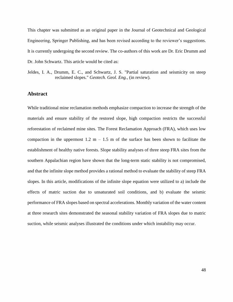
48

This chapter was submitted as an original paper in the Journal of Geotechnical and Geological

Engineering, Springer Publishing, and has been revised according to the reviewer’s suggestions.

It is currently undergoing the second review. The co-authors of this work are Dr. Eric Drumm and

Dr. John Schwartz. This article would be cited as:

Jeldes, I. A., Drumm, E. C., and Schwartz, J. S. "Partial saturation and seismicity on steep

reclaimed slopes." Geotech. Geol. Eng., (in review).

Abstract

While traditional mine reclamation methods emphasize compaction to increase the strength of the

materials and ensure stability of the restored slope, high compaction restricts the successful

reforestation of reclaimed mine sites. The Forest Reclamation Approach (FRA), which uses low

compaction in the uppermost 1.2 m – 1.5 m of the surface has been shown to facilitate the

establishment of healthy native forests. Slope stability analyses of three steep FRA sites from the

southern Appalachian region have shown that the long-term static stability is not compromised,

and that the infinite slope method provides a rational method to evaluate the stability of steep FRA

slopes. In this article, modifications of the infinite slope equation were utilized to a) include the

effects of matric suction due to unsaturated soil conditions, and b) evaluate the seismic

performance of FRA slopes based on spectral accelerations. Monthly variation of the water content

at three research sites demonstrated the seasonal stability variation of FRA slopes due to matric

suction, while seismic analyses illustrated the conditions under which instability may occur.

49

Introduction

The Forest Reclamation Approach (FRA) (Angel et al. 2007, Sweigard et al. 2007) is a method of

mine slope reclamation which maintains a loose surface layer (1.2 to 1.5 m thick) above a well

compacted core to facilitate tree growth. This method has been shown to be successful in

promoting healthy reforestation (Angel et al. 2007, Barton et al. 2007) and is currently being

promoted by the US Office of Surface Mining (OSM). However, there has been limited experience

with the FRA on steep slopes, which the OSM defines as those inclined at more than 20 degrees

(USDoI 2009). Jeldes et al. (2013) conducted a series of static slope stability analyses (including

effects of seepage water forces) via Finite Element Method (FEM) and Limit Equilibrium Methods

(LEM), and concluded that: 1) the static long-term stability of FRA slopes with inclinations as

much as 28 degrees is not compromised; 2) shallow failure modes inside the loose surface layer

are the dominant failure mechanism, regardless of the strength level of the core; and 3) the infinite

slope method using the angle of repose as a conservative estimate of the shear strength provides a

rational method to evaluate the stability of steep FRA slopes.

The theoretical idealizations for the static long-term stability overlook two field conditions that

affect the strength and the stress state of slopes: partial saturation of soils and seismicity.

Specifically, the long-term stability involves the analysis of saturated soils under drained loading,

which is not consistent with field conditions and the seasonal variations of soil water content. In

reality, the solid and liquid soil phases cohabit with air and, in most cases of geotechnical interest,

the water pore pressure can be negative with respect the air pore pressure, resulting in higher soil

strengths (Fredlund and Rahardjo 1993). On the other hand, static analyses do not include seismic-

induced forces that, if not accounted for, may trigger slope failures by increasing the shear stresses

50

and, sometimes, decreasing the strength (Abramson 1996). The Appalachian region is recognized

as one of the most seismically active areas in the eastern North America (Chapman et al. 1997),

with a concentration of events occurring in eastern Tennessee of magnitudes even larger than 4.5

(Bollinger et al. 1976, Chapman et al. 1997). Therefore, it becomes important to investigate the

seismic effects on steep FRA slopes.

The objectives of this paper are to 1) investigate the implications of unsaturated soils on steep FRA

slopes and 2) investigate the seismic response of steep FRA slopes. This is accomplished using

three reclaimed field sites at which the geometric and material characteristics were determined

(Jeldes et al. 2013). To evaluate the stability of unsaturated FRA slopes, an expansion of the

infinite slope equation to include the effects of matric suction is proposed here. Similarly, to

evaluate the seismic response of FRA slopes, an infinite slope equation which includes the spectral

response is developed with solutions presented in terms of charts for design applications.

Background

Unsaturated soil shear strength

The total shear strength of an unsaturated soil has been typically approached as an extension of

traditional saturated soil mechanics, where matric suction and net normal stress are considered to

be independent stress variables, and consequently the Mohr-Coulomb (M-C) failure criterion for

unsaturated soils can be extended as (Fredlund et al. 1978):

tan ( ) tan b

a a wc u u u (3.1)

51

where c and are the cohesion and the internal friction angle (effective strength parameters), au

is the pore air pressure, wu is the pore water pressure, ( )au is the net normal stress, ( )a wu u

the soil matric suction, and b is the rate of increase of shear strength due to matric suction.

Although this expression is widely used, it has been pointed out to be philosophically erroneous,

since the matric suction is not a stress variable and transfer functions are required to upscale the

negative pore pressure to a macroscopic level (Lu 2008). In this regard, an extension of the M-C

criteria based on the classical effective stress expression ' ( )a a wu u u (Bishop 1959)

may be more appropriate, since the effective stress parameter is indeed a transfer function:

( ) tana a wc u u u (3.2)

Naturally, is strongly related to the degree of saturation of the soil mass and it ranges from 0

(completely dry material) to 1 (complete saturation). Theoretical relationships to relate effective

stresses and the degree of saturation have been developed for ideal arrangements of spherical

particles (Cho and Santamarina 2001), which assume a matric suction only dependent on

capillarity and valid for cases with degree of saturation less than 25% (Lu and Griffiths 2004). For

higher degrees of saturation some empirical expressions have been proposed and reviewed

(Vanapalli and Fredlund 2000) with the one based on the Vanapalli et al. (1996) approach being

of particular interest since it allows the relationship between effective stresses and matric suction

via the Soil Water Characteristic Curve (SWCC) ,

r

s r

(3.3)

where is the volumetric water content (volume of water over total volume of soil) at some level

of matric suction, r is the residual volumetric water content, and s is the volumetric water

52

content at saturation. This expression [Eq. (3.3)] was shown to provide reasonable estimates of the

unsaturated shear strength for suctions in the range of 0 – 1500 kPa (Sheng et al. 2011, Vanapalli

and Fredlund 2000), but to be sensitive to small changes in residual water content (Sheng et al.

2011). On the other hand, the use of the SWCC to estimate the shear strength of unsaturated soils

has been suggested as an adequate framework for stability problems in soil mechanics (Lu and

Griffiths 2004) and also to overcome conceptual limitations regarding the stress suction (Lu 2008,

Lu 2010, Lu and Likos 2006). Accordingly, Eqs. (3.2) and (3.3) will be employed here to

investigate the stability of three steep FRA slopes under partially saturated conditions in the

Appalachian region.

Shear strength and the pseudo-static forces for seismic analyses

For seismic analyses, the saturated-undrained shear strength is typically used since seismic

excitation may be considered a short-term loading condition, and excess of positive pore water

pressure may develop. However, it is assumed that the coarse, low density material resulting from

the FRA compaction methods would drain appropriately, and the probability of significant

development of excess positive pore water pressure during an earthquake event is low (Duncan

and Wright 2005), especially during seasons of low water content where negative pore water

pressure arises. Consequently, drained strength parameters will be employed here for dynamic

slope stability analysis.

The pseudo-static approach remains as one of the most widely used methods for addressing seismic

hazards in civil engineering practice, due to its simplicity and practicality (Duncan and Wright

2005). This method is based on d’Alembert’s principle of mechanics, which assumes that

53

equilibrium may be achieved by adding a fictitious static inertial force equal to the maximum

acceleration of the body, with the inertial force expressed as a fraction of the acceleration of gravity

(g) (named pseudo-static coefficient K ) times the mass of the structure (Paz 1997). However, the

maximum horizontal acceleration experienced during an earthquake is usually not equivalent to

the horizontal pseudo-static coefficient hK (Towhata 2008), and therefore, many authors have

proposed either arbitrary values of maximum acceleration for design or reduction factors for the

maximum horizontal Peak Ground Acceleration hPGA (Table 3.1). Regarding the vertical

coefficient vK , it has been usual practice to either assume a fraction of hPGA or neglect its

contribution. Examples of recorded seismic activity (e.g. Towhata, 2008) show that the maximum

vertical acceleration can be assumed 0.5 hPGA with little error, while neglecting its effect may lead

to unstable slopes.

More recently, a procedure to calculate hK based on the 5% damped elastic spectral acceleration

at the degraded fundamental period aS , the maximum allowable displacement aD (in cm), the

initial fundamental period sT , the earthquake magnitude M , and a random normal distributed

variable was proposed (Bray and Travasarou 2009):

0.665

a b

hK e

(3.4)

2.83 0.566 ( )aa ln S (3.5)

2 2

2 2

1.33 ln 1.10 3.04ln 0.244 1.5 0.278 7 , 0.05

1.33 ln 0.22 3.04ln 0.244 1.5 0.278 7 , 0.05

a a a s s

a a a s s

a D S ln S T M Tb

a D S ln S T M T

(3.6)

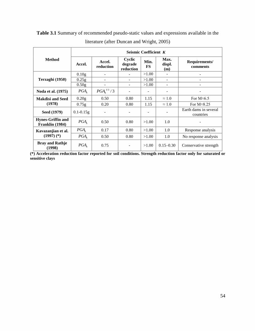
54

Table 3.1 Summary of recommended pseudo-static values and expressions available in the

literature (after Duncan and Wright, 2005)

Method

Seismic Coefficient K

Accel. Accel.

reduction

Cyclic

degrade

reduction

Min.

FS

Max.

displ.

(m)

Requirements/

comments

Terzaghi (1950)

0.10g - - >1.00 - -

0.25g - - >1.00 - -

0.50g - - >1.00 - -

Noda et al. (1975)

hPGA 1/3 / 3hPGA - - - -

Makdisi and Seed

(1978)

0.20g 0.50 0.80 1.15 ≈ 1.0 For M≈6.5

0.75g 0.20 0.80 1.15 ≈ 1.0 For M≈8.25

Seed (1979) 0.1-0.15g - - - - Earth dams in several

countries

Hynes-Griffin and

Franklin (1984)

hPGA 0.50 0.80 >1.00 1.0 -

Kavazanjian et al.

(1997) (*)

hPGA 0.17 0.80 >1.00 1.0 Response analysis

hPGA 0.50 0.80 >1.00 1.0 No response analysis

Bray and Rathje

(1998)

hPGA 0.75 - >1.00 0.15–0.30 Conservative strength

(*) Acceleration reduction factor reported for soil conditions. Strength reduction factor only for saturated or

sensitive clays

55

The form of hK in Eq. (3.4) was obtained from a semi-empirical probabilistic approach originally

developed to determine permanent displacements (Bray and Travasarou 2007). The relationship

between induced displacement and a single value of motion intensity was found to be optimally

satisfied not by PGA, but by the 5% damped elastic spectral acceleration at the degraded

fundamental period, aS . The degraded period was found to be well represented by 1.5

sT , due to

material non-linearity. Both, the traditional pseudo-static coefficients listed in Table 3.1 as well as

Eqs. (3.4) – (3.6) will be employed to investigate the seismic stability of three steep FRA slopes

constructed in the Appalachian region.

Field and experimental methods

Study sites: construction and site characterization

Location of field sites and construction process

To investigate the effects of the low-compaction grading technique on the mechanical stability of

steep slopes (> 20 degrees), three reclaimed mine sites in northeastern Tennessee were constructed

(Fig. 3.1), referred to here by the name of the initial coal operator (Premium, National and

Mountainside). Each site was instrumented with weather stations to concurrently investigate the

runoff hydrology and sediment erosion on the FRA slopes, as described elsewhere (Hoomehr et

al. 2013).

At each of the three sites in this study, the construction procedure followed the contour haulback

method (Sweigard and Kumar 2010), where a ramp is constructed on the contour bench and spoil

is hauled up the ramp and dumped over the edge. The sequence of the construction process can be

56


Mountainside.

57

divided into four major steps (Sweigard et al. 2007) depicted schematically in Fig. 3.2 (Jeldes et

al. 2013): a) placement and compaction of the materials for the primary backfill core using

traditional practices, b) dumping of the soil that will constitute the loose surface layer (1.2 -1.5 m

thick), c) grading of the loose soil layer with the lightest equipment available using the fewest

passes possible, and d) seeding of cover vegetation and reforestation.

Geometry, unit weight and saturated shear strength parameters

The slope lengths, widths, and angles of inclination of the research fields were determined using a

total station instrument, while unit weights and gravimetric water contents were measured in situ

through water and sand replacement methods and Nuclear Density Gauge (NDG) readings. A

randomized systematic sampling technique was employed for the data collection, as described by

Jeldes et al. (2013). Due to the extreme range of particles size (from clay particles to boulders),

the determination of the shear strength parameters is difficult to conduct in mine spoil. Since by

definition the angle of repose represents the friction angle at the soil’s loosest state (Holtz and

Kovacs 1981), it was chosen as a conservative estimate of the friction angle for the surface layer

which received minimum compaction effort. Because the design of these reclaimed slopes seldom

includes laboratory testing, it is suggested that the use of the angle of repose also captures the

overall strength of the mass, including the contribution of the oversize particles. A negligible value

of cohesion was assumed. Jeldes et al. (2013) provide a comparative summary of the employed

strength parameters and values reported in the literature. Similar values of and c for loose spoils

in the Appalachian region were reported by Sweigard et al. (2011), while similar values for

reclaimed spoils outside the Appalachian are reported in the literature (Gutierrez et al. 2008,

Kasmer and Ulusay 2006, Stormont and Farfan 2005, Sweigard et al. 2011, Ulusay et al. 1995).

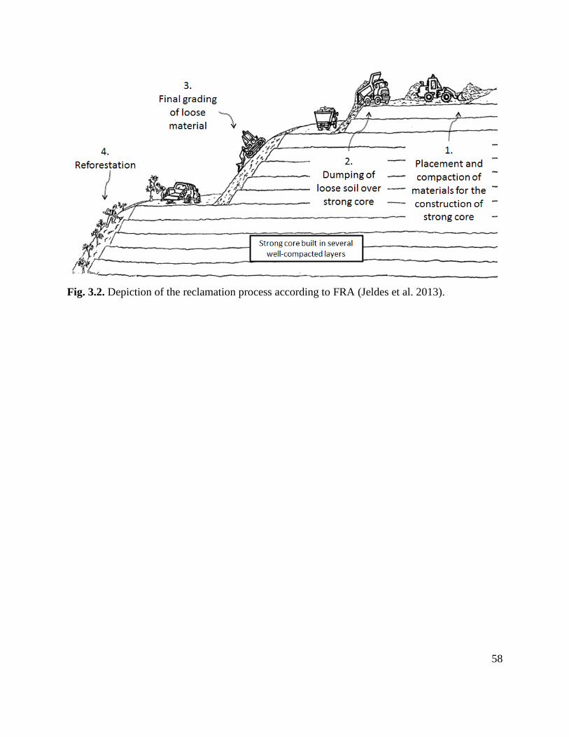
58

Fig. 3.2. Depiction of the reclamation process according to FRA (Jeldes et al. 2013).

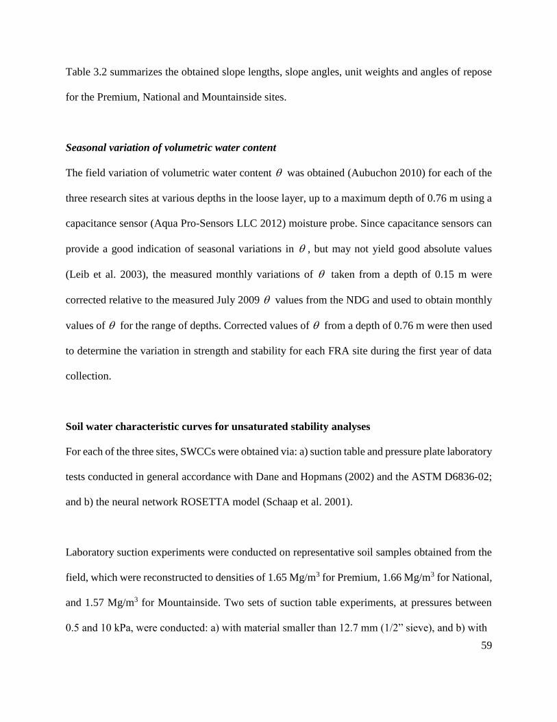
59

Table 3.2 summarizes the obtained slope lengths, slope angles, unit weights and angles of repose

for the Premium, National and Mountainside sites.

Seasonal variation of volumetric water content

The field variation of volumetric water content was obtained (Aubuchon 2010) for each of the

three research sites at various depths in the loose layer, up to a maximum depth of 0.76 m using a

capacitance sensor (Aqua Pro-Sensors LLC 2012) moisture probe. Since capacitance sensors can

provide a good indication of seasonal variations in , but may not yield good absolute values

(Leib et al. 2003), the measured monthly variations of taken from a depth of 0.15 m were

corrected relative to the measured July 2009 values from the NDG and used to obtain monthly

values of for the range of depths. Corrected values of from a depth of 0.76 m were then used

to determine the variation in strength and stability for each FRA site during the first year of data

collection.

Soil water characteristic curves for unsaturated stability analyses

For each of the three sites, SWCCs were obtained via: a) suction table and pressure plate laboratory

tests conducted in general accordance with Dane and Hopmans (2002) and the ASTM D6836-02;

and b) the neural network ROSETTA model (Schaap et al. 2001).

Laboratory suction experiments were conducted on representative soil samples obtained from the

field, which were reconstructed to densities of 1.65 Mg/m3 for Premium, 1.66 Mg/m3 for National,

and 1.57 Mg/m3 for Mountainside. Two sets of suction table experiments, at pressures between

0.5 and 10 kPa, were conducted: a) with material smaller than 12.7 mm (1/2” sieve), and b) with

60

Table 3.2 Average values of slope length, inclination angle, unit weights, water content, and

observed angles of repose for Premium, National and Mountainside sites.

Sites Slope

length

(m)

Slope angle

(Degrees)

Dry unit

weight,

dγ

(kN/m3)

Wet unit

weight,

Tγ

(kN/m3)

Gravimetric

water

content, w

(%)

Volumetric

water

content, θ

(%)

Angle of

repose,

(Degrees)

Premium 32 28 16.2 18.5 14.5 23.9 38

National 48 20 18.5 20.3 9.7 18.2 37

Mountainside 45 28 18.6 20.4 9.8 18.8 38

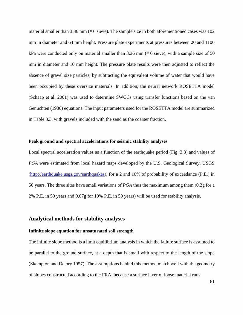
61

material smaller than 3.36 mm (# 6 sieve). The sample size in both aforementioned cases was 102

mm in diameter and 64 mm height. Pressure plate experiments at pressures between 20 and 1100

kPa were conducted only on material smaller than 3.36 mm (# 6 sieve), with a sample size of 50

mm in diameter and 10 mm height. The pressure plate results were then adjusted to reflect the

absence of gravel size particles, by subtracting the equivalent volume of water that would have

been occupied by these oversize materials. In addition, the neural network ROSETTA model

(Schaap et al. 2001) was used to determine SWCCs using transfer functions based on the van

Genuchten (1980) equations. The input parameters used for the ROSETTA model are summarized

in Table 3.3, with gravels included with the sand as the coarser fraction.

Peak ground and spectral accelerations for seismic stability analyses

Local spectral acceleration values as a function of the earthquake period (Fig. 3.3) and values of

PGA were estimated from local hazard maps developed by the U.S. Geological Survey, USGS

(http://earthquake.usgs.gov/earthquakes), for a 2 and 10% of probability of exceedance (P.E.) in

50 years. The three sites have small variations of PGA thus the maximum among them (0.2g for a

2% P.E. in 50 years and 0.07g for 10% P.E. in 50 years) will be used for stability analysis.

Analytical methods for stability analyses

Infinite slope equation for unsaturated soil strength

The infinite slope method is a limit equilibrium analysis in which the failure surface is assumed to

be parallel to the ground surface, at a depth that is small with respect to the length of the slope

(Skempton and Delory 1957). The assumptions behind this method match well with the geometry

of slopes constructed according to the FRA, because a surface layer of loose material runs

http://earthquake.usgs.gov/earthquakes

62

Table 3.3 Soil texture (USDA) and unit weights for ROSETTA model.

Soil Fraction (%)

Premium National Mountainside

Coarse (sand + gravel) 87.0 79.5 58.5

Silt 7.3 11.0 22.6

Clay 5.7 9.5 18.9

Dry unit weight (Mg/m3) 1.65 1.66 1.57

Fig. 3.3. Depiction of the 3 Spectral Accelerations for Premium, National and Mountainside

(USGS 2012).

63

approximately parallel to the contour of the strong, dense core (Fig. 3.4). Also, the ratio of

horizontal length to depth of the failure surface at each of the three research slopes is large enough

so that they can be considered infinite (Griffiths et al. 2011, Milledge et al. 2012). FEM and LEM

analyses conducted by Jeldes et al. (2013) demonstrated the appropriateness of the infinite slope

method for static long-term analysis of steep FRA slopes, and therefore, it is extended here to

include the effects of partially saturated soils. Fig. 3.4 shows a slip surface of thickness z below

the ground surface inclined at degrees from the horizontal. The weight of the slice is

/TW bz cos , where T is the total unit weight of the soil, b is the horizontal width of the

slice that can be expressed as b l cos , and l is the length of the corresponding slip segment. P

and T are the corresponding normal and shear resultant forces at the bottom of the slice.

Neglecting the effects of the side forces LQ and RQ and satisfying equilibrium of forces in a free

diagram space, the factor of safety (FS) defined here as the ratio of the magnitude of resisting

forces of the slide to the magnitude of the destabilizing forces becomes:

FS

( ) tan tan tan

T sin tan

ra w

s r

T

c u ucl P

z

(3.7)

where ´P is the force corresponding to the effective stress written in terms of Bishop’s

formulation. In the presence of pure coarse material, Eq. (3.7) is only valid for r , since below

this point capillarity decreases radically (Lu and Likos 2006). Similar expressions of the infinite

slope equation have been proposed by Uchaipichat (2012) and Lu and Godt (2008). While the

Uchaipichat (2012) equation incorporated the relationship between the effective stress parameter

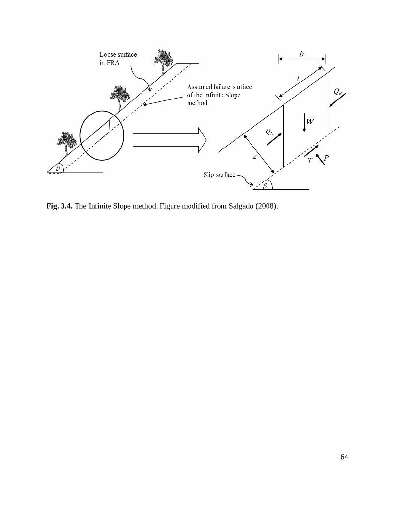
64

Fig. 3.4. The Infinite Slope method. Figure modified from Salgado (2008).

65

and the matric suction proposed by Uchaipichat and Man-Koksung (2011), Lu and Godt (2008)

assumed a form of stress suction that is a function of the infiltration rates, saturated hydraulic

conductivity and empirical fitting parameters obtained from van Genuchten (1980). Eq. (3.7)

provided here shares the same fundamental principles as the Lu and Godt (2008) approach, since

the empirical model proposed by van Genuchten (1980) is directly related to /r s r .

Infinite Slope equation for horizontal and vertical pseudo-static forces

Analogous to the formulation for the partially saturated soils, when horizontal and vertical pseudo-

static forces ( hK W and vK W ) are applied at the center of mass (Fig. 3.5), the following seismic

infinite slope equation is obtained:

FS

(1 )cos sin tan

(1 ) sin cos

T v h

T v h

c z K K

z K K

(3.8)

Note that when the effects of the vertical ground acceleration are neglected, Eq. (3.8) simplifies to

an equivalent form of the equation proposed by Duncan and Wright (2005). If hK in Eq. (3.8) is

forced to take the form defined by Eqs. (3.4) – (3.6), a single expression for the seismic infinite

FRA slope based on spectral accelerations is obtained here,

FS

1 0.5 exp( ) cos exp( ) sin tan0.665 0.665

1 0.5 exp( ) sin exp( ) cos0.665 0.665

T

T

a b a bc z

a b a bz

(3.9)

where a and b are defined by the Eqs. (3.5) and (3.6), and vK is assumed to be 0.5 hK .

66

Fig. 3.5. Infinite Slope method with horizontal and vertical pseudo-static forces.

67

Summary of the methodology

The stability of steep FRA slopes under partially saturated conditions will be accomplished by:

Obtaining experimental and model based SWCCs for each research site.

Using the measured field variations of .

Estimating the seasonal variations of FS via the proposed Eq. (3.7), for both sets of SWCCs

and the measured . The effective strength parameters, unit weights and geometry reported

in Table 3.2 will be used, with z = 1.5 m.

The seismic stability of steep FRA slopes will be investigated by:

Employing Eq. (3.8) and a variety of traditional pseudo-static coefficients (Table 3.1), for

the highest PGA among the three sites and the soil and geometrical characteristic of

Mountainside (Table 3.2) since they are the most critical among the 3 sites. Here, z = 1.5

m.

Comparing/validating results from Eq. (3.8) via the Simplified Bishop’s Method of slices

iterated with the software XSTABL (Interactive Software Designs INC 2008).

Calculating site specific FS’s based on the spectral accelerations of the field with the

proposed Eq. (3.9) and presenting the results in the form of solution charts for design

applications.

68


SWCCs and stability results for unsaturated FRA soils

The resulting SWCCs from the ROSETTA model and laboratory suction are compared in Figs.

3.6, 3.7 and 3.8, for Premium, National and Mountainside respectively. The corrected SWCCs

obtained from the pressure plate results on material < 3.36 mm, follow fairly well those obtained

from the suction table with material smaller than 12.7 mm (1/2” sieve), and provide a complete

SWCC for this case. Accordingly, SWCCs from the laboratory tests (material < 12.7 mm) and the

ROSETTA model are used in the stability calculations.

Resulting seasonal variations of the FS [Eq. (3.7)], along with the monthly cumulative

precipitation (obtained with the in situ weather stations) and measured water content are shown in

Figs. 3.9, 3.10 and 3.11 for each of the sites. The figures illustrate the increase in FS that

accompanies the dryer (higher suction) periods of the year, with the variation in FS depending

upon the method used to obtain the SWCC. Also, smaller levels of stress suction may be found

upon re-wetting of the loose surface layer (Likos and Lu 2004); however, these effects, related to

the hysteresis of SWCC, are neglected here. The laboratory measured SWCCs yield larger

variations in FS’s than the ROSETTA model for National and Mountainside, suggesting that

ROSETTA may yield more conservative estimates of suction for these soils. The maximum

seasonal increase in stability at Premium and National sites occurred in March 2010, while the

same occurred in June 2010 at Mountainside site. Saturation of the FRA material and a

corresponding minimum FS were observed at least once during the year at each research site.

69


model (Schaap et al. 2001), for the Premium site.


model (Schaap et al. 2001), for the National site.

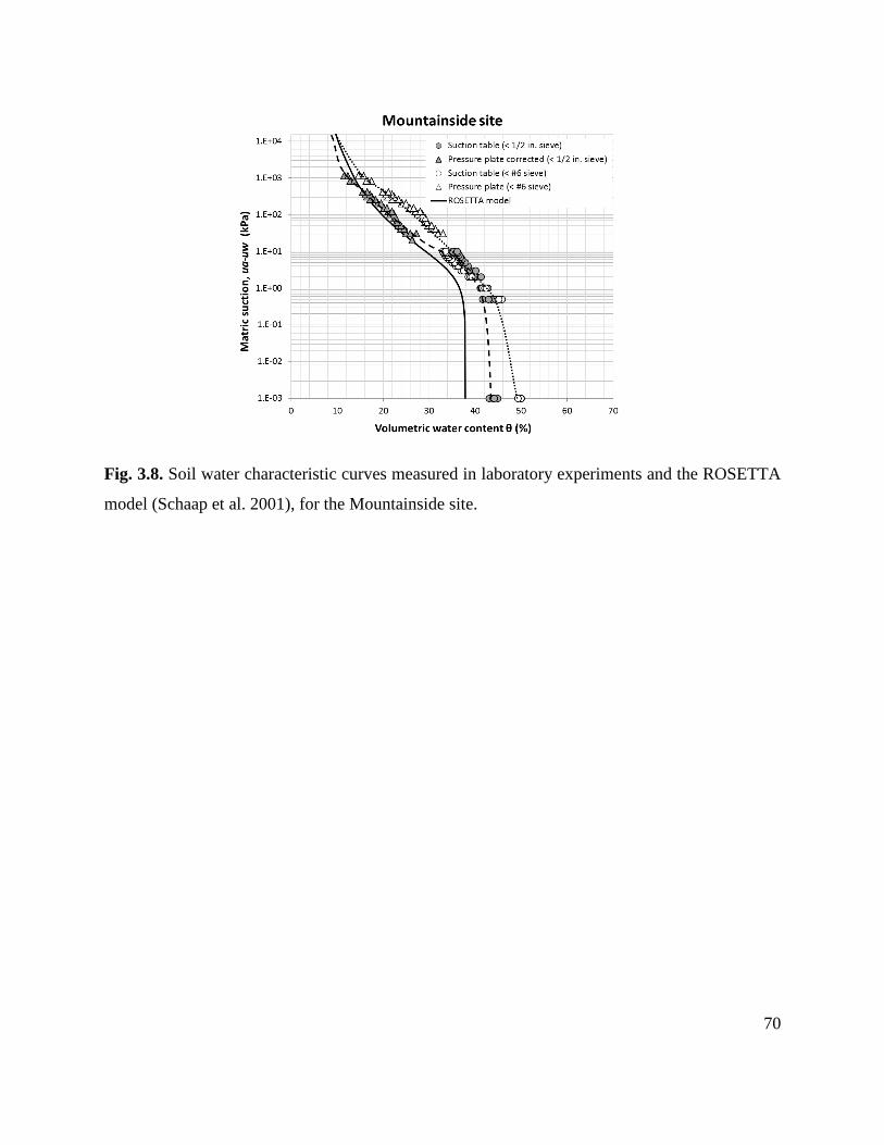
70


model (Schaap et al. 2001), for the Mountainside site.

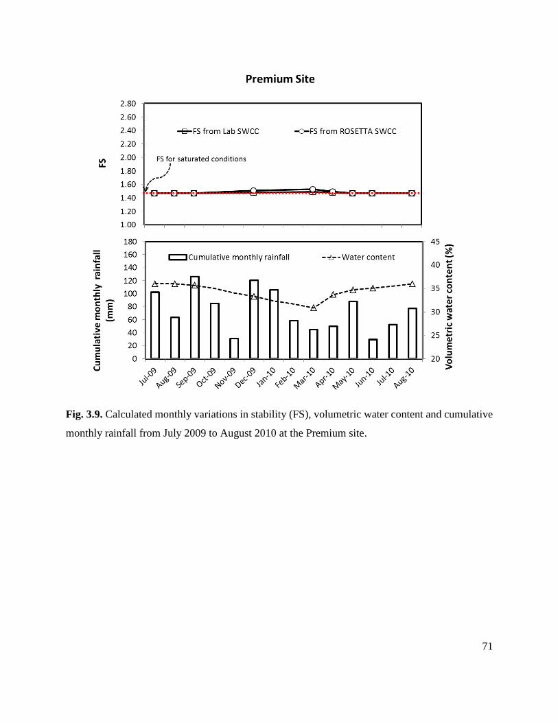
71


monthly rainfall from July 2009 to August 2010 at the Premium site.

72


monthly rainfall from July 2009 to August 2010 at the National site.

73


monthly rainfall from July 2009 to August 2010 at the Mountainside site.

74

Monthly cumulative rainfall data (Figs. 3.9, 3.10 and 3.11) shows that the sites were exposed to

relatively large amounts of rainfall during late spring, summer, and early winter. Precipitation

intensity was found to be significant during this period, with shorter and more intense rainfall

events at National and Mountainside and longer but less intense events at premium site (Hoomehr

et al. 2010). Rainfall events of this nature are capable of saturating the loose surface layer, and

therefore, stability analyses employing traditional saturated strength parameters should always

prevail in the design of FRA slopes.

Seismic stability analyses

Stability analysis with traditional pseudo-static coefficients

Results from the seismic stability analyses are shown in Table 3.4. All combinations of force

orientations were examined, with the most critical being when the vertical pseudo static force is

upward and the horizontal force is acting horizontally away from the slope.

Results show that the seismic infinite slope equation [Eq. (3.8)] is in good agreement with the

Simplified Bishop’s method, and it can be used with confidence. The Simplified Bishop’s method

with pseudo static forces predicts a shallow failure mechanism which is consistent with the

assumptions of the infinite slope method. For a 10% P.E. in 50 yr. it is expected that the shear

strength along the slip surface be 25-31% greater than the required to maintain equilibrium,

whereas for a 2% P.E. in 50 yr. the shear strength is only 2-15% greater and the slope may be at

the verge of failure. Since the static long-term FS was found to be 1.47 (Jeldes et al. 2013), the

stability of these slopes is reduced up to 30% when seismic forces are introduced. Notice that the

acceleration reduction proposed by Noda et al. (1975) for a 10% P.E. in 50 yr. yields a lower FS

75

Table 3.4 Summary of hK ,

vK and obtained FS’s for a 2 and 10% P.E. in 50 yr.

Method

Seismic Coefficient Computed Factor of Safety (FS)

K

2% P.E. in

50 yr. (PGA=0.2)

10% P.E.

in 50 yr.

(PGA=0.07)

Infinite

Slope

Equation

Simplified

Bishop’s

Method

Infinite

Slope

Equation

Simplified

Bishop’s

Method

2% P.E. in 50 yr. 10% P.E. in 50 yr.

Theoretical

d'Alembert’s Principle

(no reduction)

hK 0.20 0.07

0.91 0.92 1.24 1.25

vK 0.10 0.04

Makdisi and Seed

(1978) (M≈6.5)

hK 0.10 0.04

1.14 1.15 1.35 1.34

vK 0.10 0.04

Hynes-Griffin and

Franklin (1984)

hK 0.10 0.04

1.14 1.15 1.35 1.34

vK 0.10 0.04

Noda et al. (1975)

hK 0.19 0.14

0.92 0.94 1.07 1.07

vK 0.10 0.04

Bray and Rathje (1998)

hK 0.15 0.05

1.02 1.03 1.29 1.31

vK 0.10 0.04

Kavazanjian et al.

(1997) (without

response analysis)

hK 0.10 0.04

1.14 1.15 1.35 1.34

vK 0.10 0.04

76

than the case without reduction, which is an inconsistency. Noda et al. (1975) developed the

equation based on limit-equilibrium analysis of structures (quay walls) that were already damaged

by earthquakes, where the results and parameter selection probably have a high level of

subjectivism (Towhata 2008). Regarding the seismic coefficient to be used, Hynes-Griffin and

Franklin (1984), Bray and Rathje (1998) and Kavazanjian et al. (1997) are suggested here, because

they express the seismic coefficient in terms of hPGA rather than an arbitrary fraction of the

acceleration of gravity. Current hazard maps have broad coverage and easier access, and a more

site-based design is possible.

Slope stability charts based on spectral accelerations and an Illustrative example

Graphical chart solutions of Eq. (3.9) for different earthquake magnitudes, maximum allowable

displacements and soil properties were developed for each of the FRA reclaimed sites. Fig. 3.12

illustrates the solution chart for the conditions at Mountainside site when M = 5.0 (about the

highest earthquake magnitude recorded in the area) aD = 30 cm for a 2% P.E. in 50 years. The

random variable ε was selected to be 0.66 representing a 16% of allowable displacement

exceedance (Bray and Travasarou 2009). Similar solution charts for other values of M , aD and

probability of exceedance can be created. Fig. 3.12 suggest that failure may occur at Mountainside

when aS > 0.4g and sT > 1.5 s.

To illustrate the use of the solution charts, the Mountainside slope is used with M = 5.0 and aD =

30 cm. The initial fundamental period of the slope may be calculated using 4 /sT H Vs , where

H is the depth of the sliding plane and Vs average shear wave velocity. Since Vs has not been

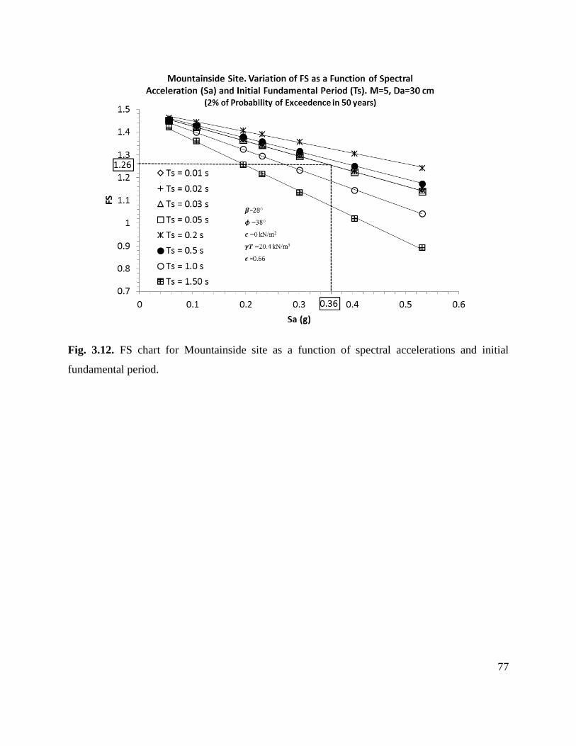
77

Fig. 3.12. FS chart for Mountainside site as a function of spectral accelerations and initial

fundamental period.

78

measured, an average Vs = 200 m/s is assumed. For a shallow failure mode in the upper 1.5 m, the

initial fundamental period becomes sT = 0.03 and the spectral acceleration at the degraded period

aS (T = 0.045) ≈ 0.36g (Fig. 3.3). Then, for sT = 0.03 s and aS = 0.36g the FS is found from Eq.

(3.9) or Fig. 3.12 to be approximately 1.26.

Conclusions

Static long-term stability analyses of the three constructed FRA slopes conducted by Jeldes et al.

(2013) showed that shear strength is at least 47% greater than that required to balance the

destabilizing forces, in the absence of downslope seepage. These results reflect the assumption of

total saturation of the soil at the slip surface, which is not always consistent with the in situ FRA

conditions, where the surface layer can be seen as an active unsaturated zone whose variations in

water content will be directly affected by periodic changes in environmental conditions. Slope

stability analyses for partially saturated mine soils showed that seasonal increments in the stability

of steep FRA slopes are possible, and the static long-term stability is a lower bound of the real

field performance. Naturally, the interpretation of results is restricted to the hydrological

conditions experienced during the time period at which the data was collected. This period was

characterized by relatively poor establishment of ground cover, and therefore, evaporation was

probably the main mechanism inducing matric suction and the relative increase in stability.

Different monthly stability patterns may be observed in the future depending on the amount of

vegetation, precipitation and variations in temperature affecting evapotranspiration rates. In any

case, temporal saturation of the loose surface layer is likely to occur and slope stability analysis

employing traditional saturated strength parameters should prevail in the design of FRA slopes.

79

Under seismic loading conditions, the proposed infinite slope equation showed good agreement

with the simplified Bishop’s method of the slices. The selection of the pseudo-static coefficient

requires an understanding of the assumptions behind the coefficient and practical knowledge of

the local seismicity. Site specific results were obtained when the horizontal seismic coefficient

proposed by Hynes-Griffin and Franklin (1984), Bray and Rathje (1998) and Kavazanjian et al.

(1997) were employed, and suggest that FS can be as low as 1.02. While these methods based on

a fraction of the probable PGA are most common, they do not consider the effects of frequency

and duration (Bray 2007). A method based on spectral response may provide a better tool for

evaluating slope stability, and a combination of Bray and Travasarou (2009) approach with the

proposed modification of the infinite slope equation was suggested. Charts were developed for this

method employing site-specific aS values and local soil properties and slope geometry. Here, the

FS is a function of parameters that have less selection subjectivity for the designer and are a

function of the importance of the project, available seismic data, and accuracy of the site

characterization. It is suggested that the use of spectral values for a 2% P.E. in 50 yr. or higher are

sufficient, except when the designer has reasons for using lower local values.

Acknowledgments

This research was conducted as part of a project funded by the US Office of Surface Mines,

Applied Science Program Grant CA No. S08AP12822, 2008. The authors gratefully appreciate the

support and guidance provided by OSM staff David Lane, P. E., and Vic Davis. The authors also

thank Dr. Jennifer Franklin for providing access to some of the volumetric water content data

80

employed in the stability analyses and Robert Raley for the technical support provided during the

suction table and pressure plate experiments.

81

References:

Abramson, L. W. (1996). Slope stability and stabilization methods, Wiley, New York.

Angel, P. C., Barton, C., Warner, R., Agouridis, C., Taylor, T., and Hall, S. (2007). "Hydrologic

characteristics, tree growth, and natural regeneration on three loose-graded surface mine

spoil types in Kentucky." Mid-Atlantic Stream Restoration Conference, Canaan Valley

Institute, Cumberland, MD.

Aqua Pro-Sensors LLC (2012). "AquaPro soil moisture sensors." <http://www.aquapro-

sensors.com/>. (27 April, 2012).

Aubuchon, E. A. (2010). "Soil moisture profiles and root growth of hardwood trees planted in

different groundcovers on the steep slopes of reclaimed mine sites." M.S. thesis, University

of Tennessee, Knoxville, TN.

Barton, C., Agouridis, C., Warner, R., Bidelspach, D., Angel, P., Jennings, G., Marchant, J., and

Osborne, R. (2007). "Recreating a Headwater Stream System on a Head-of-Hollow Fill."

Mid-Atlantic Stream Restoration Conference, Canaan Valley Institute, Cumberland, MD.

Bishop, A. W. (1959). "The principle of effective stress." Tecknish Ukebland, 106(39), 859-863.

Bollinger, G. A., Langer, C. J., and Harding, S. T. (1976). "The eastern Tennessee earthquake

sequence of October through December, 1973." Bull. Seismol. Soc. Am., 66(2), 525-547.

Bray, J. D. (2007). "Simplified seismic slope displacement procedures." Proc., 4th International

Conference on Earthquake Geotechnical Engineering-Invited Lectures, Springer

Netherlands.

http://www.aquapro-sensors.com/%3e

http://www.aquapro-sensors.com/%3e

82

Bray, J. D., and Rathje, E. M. (1998). "Earthquake-induced displacements of solid-waste landfills."

J. Geotech. Geoenviron. Eng., 124(3), 242-253.

Bray, J. D., and Travasarou, T. (2007). "Simplified procedure for estimating earthquake-induced

deviatoric slope displacements." J. Geotech. Geoenviron. Eng., 133(4), 381-392.

Bray, J. D., and Travasarou, T. (2009). "Pseudostatic coefficient for use in simplified seismic slope

stability evaluation." J. Geotech. Geoenviron. Eng., 135(9), 1336-1340.

Chapman, M. C., Powell, C. A., Vlahovic, G., and Sibol, M. S. (1997). "A statistical analysis of

earthquake focal mechanisms and epicenter locations in the eastern Tennessee seismic

zone." Bull. Seismol. Soc. Am., 87(6), 1522-1536.

Cho, G. C., and Santamarina, J. C. (2001). "Unsaturated particulate materials - particle-level

studies." J. Geotech. Geoenviron. Eng., 127(1), 84-96.

Dane, J. H., and Hopmans, J. W. (2002). "Water retention and storage." Methods of soil analysis.

Part 4, Physical methods, J. H. Dane, G. C. Topp, and G. S. Campbell, eds., Soil Science

Society of America, Madison, Wis., 671-796.

Duncan, J. M., and Wright, S. G. (2005). Soil strength and slope stability, John Wiley & Sons,

Hoboken, N.J.

Fredlund, D. G., Morgenstern, N. R., and Widger, R. A. (1978). "The shear strength of unsaturated

soils." Canadian Geotechnical Journal, 15(3), 313-321.

Fredlund, D. G., and Rahardjo, H. (1993). Soil mechanics for unsaturated soils, Wiley, New York.

83

Griffiths, D. V., Jinsong, H., and Giorgia, F. d. (2011). "Numerical and analytical observations on

long and infinite slopes." Int. J. Numer. Anal. Methods Geomech., 35, 569–585.

Gutierrez, L. A. F., Viterbo, V. C., McLemore, V. T., and Aimone-Martin, C. T. (2008).

"Geotechnical and geomechanical characterization of the Goathill North Rock Pile at the

Questa Molybdenum Mine, New Mexico, USA." Proc., First International Seminar on the

Management of Rock Dumps, Stockpiles and Heap Leach Pads, The Australian Centre for

Geomechanics, Perth, Australia, 19-32.





Hydrol. Eng., 18(12), 1627-1638.

Hoomehr, S., Schwartz, J. S., Wright, W. C., and Drumm, E. C. (2010). "Surface erosion and

sediment yields on steep-sloped coal mining reclamation sites in the Appalachian region."

World Water & Environmental Resources Congress, ASCE/EWRI, ed., ASCE,

Providence, RI.

Hynes-Griffin, M. E., and Franklin, A. G. (1984). "Rationalizing the seismic coefficient method."

Army Engineer Waterways Experiment Station Vicksburg Ms Geotechnical Lab

Vicksburg, MS.

84

Interactive Software Designs INC (2008). "XSTABL." 2D Limit Equilibrium Slope Stability

AnalysisMoscow, ID.


on steep reclaimed slopes: soil characterization and static slope stability." Geotech. Geol.

Eng., 31(4), 1261-1274.

Kasmer, O., and Ulusay, R. (2006). "Stability of spoil piles at two coal mines in Turkey:

Geotechnical characterization and design considerations." Environ. Eng. Geosci., 12(4),

337-352.

Kavazanjian, E., Matasovic, N., Hadj-Hamou, T., and Sabatini, P. J. (1997). "Design guidance:

geotechnical earthquake engineering for highways." Design principles, geotechnical

engineering circular 3, Federal Highways Administration, Washington, DC.

Leib, B. G., Jabro, J. D., and Matthews, G. R. (2003). "Field evaluation and performance

comparison of soil moisture sensors." Soil Science, 168(6), 396-408.

Likos, W. J., and Lu, N. (2004). "Hysteresis of capillary stress in unsaturated granular soil." J.

Eng. Mech., 130(6), 646-655.

Lu, N. (2008). "Is matric suction a stress variable?" J. Geotech. Geoenviron. Eng., 134(7), 899-

905.

Lu, N. (2010). "Discussion of "Is Matric Suction a Stress Variable?" by Ning Lu." J. Geotech.

Geoenviron. Eng., 136(2), 407-408.

85

Lu, N., and Godt, J. (2008). "Infinite slope stability under steady unsaturated seepage conditions."

Water Resour. Res., 44(11).

Lu, N., and Griffiths, D. V. (2004). "Profiles of steady-state suction stress in unsaturated soils." J.

Geotech. Geoenviron. Eng., 130(10), 1063-1076.

Lu, N., and Likos, W. J. (2006). "Suction stress characteristic curve for unsaturated soil." J.

Geotech. Geoenviron. Eng., 132(2), 131-142.

Makdisi, F. I., and Seed, H. B. (1978). "Simplified procedure for estimating dam and embankment

earthquake-induced deformations." Journal of the Geotechnical Engineering Division-

Asce, 104(7), 849-867.

Milledge, D. G., Griffiths, D. V., Lane, S. N., and Warburton, J. (2012). "Limits on the validity of

infinite length assumptions for modelling shallow landslides." Earth Surf. Processes

Landforms, 37, 1158-1166.

Noda, S., Uwabe, T., and Chiba, T. (1975). "Relation between seismic coefficient and ground

acceleration for gravity quay wall." Report of the Port and Harbour Research Institute, 67-

111.

Paz, M. (1997). Structural dynamics: theory and computation, Chapman & Hall, New York.


86

Schaap, M. G., Leij, F. J., and van Genuchten, M. T. (2001). "ROSETTA: a computer program for

estimating soil hydraulic parameters with hierarchical pedotransfer functions." J. Hydrol.,

251(3-4), 163-176.

Seed, H. B. (1979). "19th Rankine lecture - considerations in the earthquake resistant design of

earth and rockfill dams." Géotechnique, 29(3), 213-263.

Sheng, D., Zhou, A., and Fredlund, D. (2011). "Shear strength criteria for unsaturated soils."

Geotech. Geol. Eng., 29(2), 145-159.

Skempton, A. W., and Delory, F. A. (1957). "Stability of natural slopes in London clay." Proc.,

4th International Conference on Soil Mechanics & Foundation Engineering, London,

378-381.

Stormont, J. C., and Farfan, E. (2005). "Stability evaluation of a mine waste pile." Environ. Eng.

Geosci., 11(1), 43-52.

Sweigard, R., Burger, J., Zipper, C., Skousen, J., Barton, C., and Angel, P. (2007). "Low

compaction grading to enhance reforestation success on coal surface mines." Forest

Reclamation Advisory No.3.

Sweigard, R., Hunt, K., and Kumar, D. (2011). "Field investigation of best practices for steep-

slope mine reclamation employing the Forestry Reclamation Approach, Final Report." US

Department of the Interior, Office of Surface Mining Reclamation and Enforcement,

Denver, CO.

87

Sweigard, R. J., and Kumar, D. (2010). "Filed investigation of best practices for steep slope mine

reclamation employing the forestry reclamation approach." Proc., Proceedings of the joint

27th Annual American Society of Mining and Reclamation and 4th Annual Appalachian

Regional Reforestation Initiative, American Society of Mining and Reclamation,

Pittsburgh, PA.

Terzaghi, K. (1950). "Mechanisim of landslides." Eng. Geol., Berkey, 83-123.

Towhata, I. (2008). Geotechnical earthquake engineering, Springer, Berlin.

Uchaipichat, A. (2012). "Infinite Slope Stability Analysis forUnsaturated Granular Soils."

Electron. J. Geotech. Eng., 17, 361-368.

Uchaipichat, A., and Man-Koksung, E. (2011). "Bearing capacity characteristic of unsaturated

granular soils." Proc., 2011 International Conference on Civil Engineering and Building

Materials, CEBM 2011, July 29, 2011 - July 31, 2011, Trans Tech Publications, Kunming,

China, 989-993.

Ulusay, R., Arikan, F., Yoleri, M. F., and Caglan, D. (1995). "Engineering geological

characterization of coal mine waste material and an evaluation in the context of back-

analysis of spoil pile instabilities in a strip mine, SW Turkey." Eng. Geol., 40(1-2), 77-101.

USDoI (2009). "30 CFR 701.5 - Permanent Regulatory Program." Fed. Regist., US Dept. of the

Interior, ed.Washington DC.

van Genuchten, M. T. (1980). "A closed-form equation for predicting the hydraulic conductivity

of unsaturated soils." Soil Sci. Soc. Am. J., 44(5), 892-898.

88

Vanapalli, S. K., and Fredlund, D. G. (2000). "Comparison of different procedures to predict

unsaturated soil shear strength." Proc., Advances in unsaturated geotechnics, ASCE,

Denver, CO, 195-209.

Vanapalli, S. K., Fredlund, D. G., Pufahl, D. E., and Clifton, A. W. (1996). "Model for the

prediction of shear strength with respect to soil suction." Canadian Geotechnical Journal,

33(3), 379-392.

89

Chapter 4. An Approximate Solution to the Sokolovskiĭ Concave Slope

at Limiting Equilibrium

90

This chapter has been accepted for publication as an original paper in the ASCE International

Journal of Geomechanics. The co-authors of this work are Dr. Nicholas Vence and Dr. Eric

Drumm. This article is cited as:


concave slope at limiting equilibrium." Int. J. Geomech., in press. DOI:

10.1061/(ASCE)GM.1943-5622.0000330.

Abstract

The growth of precision auto-guidance systems on construction equipment suggests that non-

planar slopes and landforms can now be readily constructed. Slopes with concave cross sections

not only appear more like natural slopes, but can also have superior stability and erosion resistance.

Thus, it is desirable to have the description of concave slopes that provide mechanical stability for

given set of soil properties. In this article, an approximate solution that defines the geometry of

critical concave slopes (FS ≈ 1) in a frictional medium is developed, based on the slip line field

method of Sokolovskiĭ. The approximate solution is compared with the Sokolovskiĭ’s numerical

results and validated via Limit Equilibrium and Finite Element Method analyses. The proposed

solution is simple in form, and when implemented with precision construction equipment will

allow the construction of embankments and reclaimed mine lands which appear more like those in

nature, and yet are more erosion-resistant.

Introduction

The growth of precision of auto-guidance construction equipment and 3D mapping technology

allows more complex non-planar slopes and landforms to be readily constructed. This can lead to

engineered slopes of concave cross sections which appear more like natural slopes and have

91

superior stability and erosion resistance (Schor and Gray 2007). In fact, experimental and

numerical simulations have shown that concave slopes lead to less erosion than planar slopes

(Meyer and Kramer 1969, Rieke-Zapp and Nearing 2005). The general concept of “form follows

function” is observed in geomorphological evolutionary processes such us fluvial systems where

concave slopes are suggested as the most probable shape in landform evolution (Leopold and

Langbein 1962, Miyamoto et al. 2005). Furthermore, slopes subjected to physical weathering seem

to evolve into steady-state concave-like forms to achieve erosional equilibrium (Nash 1980,

Pelletier and Rasmussen 2009, Twidale 2007). The use of concave surfaces can become a powerful

ecological building technique to reduce sediment yield in constructed embankments, reclaimed

mine lands, and highway cut and fill sections, with shapes that appear more like those observed in

nature. Thus, it is important to investigate and define the optimum concave shape relative to

mechanical slope stability. While computational methods based on limit equilibrium and limit

analysis techniques (Ahmed et al. 2012, Liu and Zhao 2012, Michalowski 2010) prevail in slope

analyses and design, a rational mechanics approach based on the Sokolovskiĭ’s slip line field

theory was employed here to define concave slope shapes at critical equilibrium.

Sokolovskiĭ (1960, 1965) found that the slope surface at critical or limiting equilibrium has a

concave shape, mathematically described as a function of the Mohr-Coulomb (M-C) shear strength

parameters and the material unit weight. Since the solution for a non-frictional soil (i.e. undrained

loading conditions) is mathematically straightforward, this work focuses on the c - case ( is

the soil internal friction angle and c is the soil cohesion), which has no analytic solution. For a soil

with 0 , 0c , and unit weight 0 , Sokolovskiĭ (1960) implemented a numeric solution

92

reporting the slope surface as a function of the ratio /c . This solution, however, has some

practical design limitations. The Sokolovskiĭ geometric description of the contour is incomplete

which limits the application to distinct values of and slope heights /y c . In this article we: a)

revisit and fully describe Sokolovskiĭ’s formulation and solution based on slip line field theory for

a weightless slope ( 0 ), b) develop an approximate analytic solution which describes the

concave slope at critical equilibrium for a medium with self-weight ( 0 ), and c) validate the

solution via the Limit Equilibrium (LEM) the and Finite Element Method (FEM). While the main

objective of this piece of work is to provide a rational mathematic description of the critical

concave slope shape (FS = 1), the solution can be easily extended to FS’s > 1 as needed for design.

This issue, along with those related to transient underground water flow and constructability are

briefly addressed in the discussion.

Background: the slip line field theory and the characteristic equations

The slip line field theory in soil mechanics rests on the assumptions that the soil yield stress is

independent of the strain level and that the strain-stress behavior can be described by either elastic

perfectly plastic or rigid perfectly plastic idealizations. For frictional materials like soils, the Mohr-

Coulomb shear strength expression has been traditionally used as the constitutive law defining the

yield or maximum allowable stress. In this context, to bring the body into a limiting equilibrium

state or at the verge of flowing plastically, the largest difference between the shear stresses and the

shear strength must be zero (Sokolovskiĭ 1960). Expressed in terms of principal stresses:

1 3 1 3max sin(2 ) sin ( 2 ) 0H (4.1)

where 1 is the major principal stress, 3 is the minor principal stress (Fig. 4.1), cotH c is

93

Fig. 4.1. Orientation of slip lines in a soil mass at limiting equilibrium [adapted from Sokolovskiĭ

(1965)].

94

the tensile strength of the soil, and is the angle between the normal to the plane and the major

principal direction. Approaching [Eq. (4.1)] as a mathematical optimization problem, the limiting

condition is reached when

22

(4.2)

which implies that failure or slip line initiates at an angle (Fig. 4.1) inclined at 45 / 2 from

the direction of the major principal stress and 45 / 2 from the direction of the minor principal

stress. Note that the inclinations of the slip lines are independent of the strain level, which is not

always consistent with experimental observations. Roscoe (1970) concluded that a strain based

approach rather than a stress approach better predicts the inclination of the slip plane, and its

magnitude can be approximated by 45 / 2 (measured from the minor principal direction),

where is the dilatancy angle at failure. Later studies on shear band formation in plane strain

experiments confirmed Roscoe’s findings (Alshibli and Sture 2000). Nevertheless, this approach

is still valid in the context of associated plasticity ( ), which for relatively unconfined

problems such as slope stability, does not significantly influence the prediction of the Factor of

Safety (FS) (Griffiths and Lane 1999) nor the prediction of the critical slip or failure mechanism

(except for cases of very low friction angle and high cohesion) (Cheng et al. 2007). By combining

Eqs. (4.1) and (4.2), Sokolovskiĭ (1960) obtained the limiting equilibrium in terms of principal

stresses as:

1 3 1 3sin 2H (4.3)

If the Sokolovskiĭ (1965) x-y reference frame is adopted (see Fig. 4.1) where the normal of an

infinitesimal element located anywhere inside the soil mass is inclined at an angle from the x-

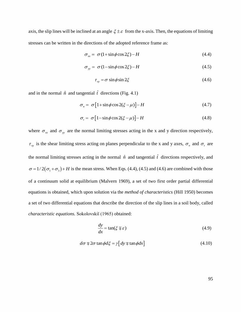
95

axis, the slip lines will be inclined at an angle from the x-axis. Then, the equations of limiting

stresses can be written in the directions of the adopted reference frame as:

(1 sin cos2 )xx H (4.4)

(1 sin cos2 )yy H (4.5)

sin sin 2xy (4.6)

and in the normal n and tangential t directions (Fig. 4.1)

1 sin cos2( )n H (4.7)

1 sin cos2( )t H (4.8)

where xx and yy are the normal limiting stresses acting in the x and y direction respectively,

xy is the shear limiting stress acting on planes perpendicular to the x and y axes, n and t are

the normal limiting stresses acting in the normal n and tangential t directions respectively, and

1 31/ 2 H is the mean stress. When Eqs. (4.4), (4.5) and (4.6) are combined with those

of a continuum solid at equilibrium (Malvern 1969), a set of two first order partial differential

equations is obtained, which upon solution via the method of characteristics (Hill 1950) becomes

a set of two differential equations that describe the direction of the slip lines in a soil body, called

characteristic equations. Sokolovskiĭ (1965) obtained:

tan( )dy

dx (4.9)

2 tan tand d dy dx (4.10)

96

Elaboration of Sokolovskiĭ solution for the critical slope in a weightless medium

By assuming a weightless medium ( 0 ), the first-order hyperbolic Eq. (4.10) yields an analytic

solution. Here, an alternative development of Sokolovskiĭ (1960) analytic solution of this problem

is offered, aiming to provide clarity to the mathematical formulation.

Consider the boundary conditions under an external stress q depicted in Fig. 4.2, where the origin

of the rectilinear system of coordinates is set at the intersection of the slope surface and the

horizontal ground surface. At the top of the slope (along the horizontal ground surface), the stresses

( 0xx , yy q , 0xy ) of the first boundary condition define the y-axis and the x-axis as the

major and minor principal directions. Here, / 2 and the mean normal stress surf from Eq.

(4.5) becomes:

1 sin

surf q H

,

2

(4.11)

Along the slope surface, the stresses redefine the major and minor principal directions as the

tangential t and normal n components respectively. Therefore, becomes the angle of the slope

measured from the x-axis. By defining the boundary normal stress 0 n and / 2 ,

Eq. (4.7) returns the magnitude of the mean normal stress along the slope surface cont :

1 sin

cont H

, (4.12)

Eqs. (4.11) and (4.12) establish the boundary conditions of the problem. For a weightless ( 0 )

medium, Eq. (4.10) becomes:

2 tan

dd

(4.13)

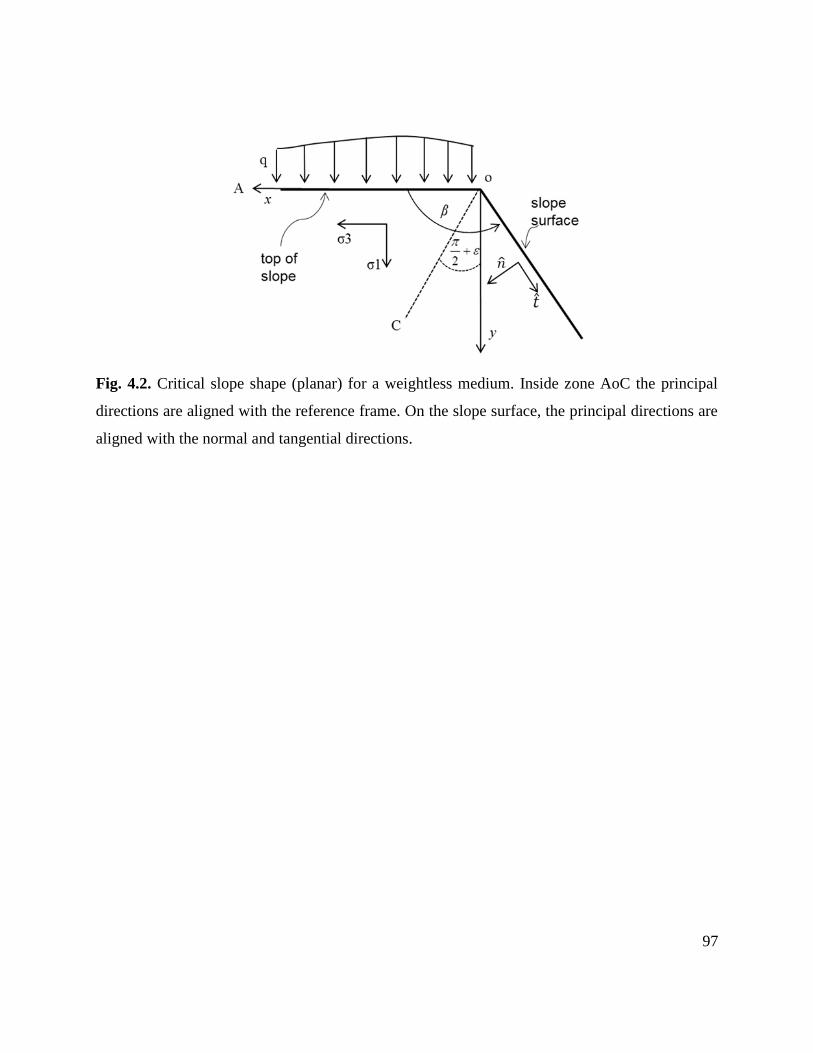
97

Fig. 4.2. Critical slope shape (planar) for a weightless medium. Inside zone AoC the principal

directions are aligned with the reference frame. On the slope surface, the principal directions are

aligned with the normal and tangential directions.

98

Integrating Eq. (4.13) and imposing the boundary condition along the slope surface from Eq. (4.12)

yields

cot

ln 1 2 1 sin

Hc

(4.14)

where 1c is the constant of integration. Eq. (4.14) reveals the existence of two planes satisfying

the stress condition; they have the same absolute inclination, but differ only in direction. Choosing

and imposing the surface boundary condition from Eq. (4.11):

cot

1 ln 2 1 sin 2

q Hc

(4.15)

Substituting Eq. (4.15) into Eq. (4.14) is found to be constant revealing a planar slope,

cot 1 sin

ln2 2 1 sin

q H

H

(4.16)

which is equivalent to the Sokolovskiĭ (1960) solution, with the discrepancy found only due to the

difference in the employed coordinate system. The x-y coordinates can be found by solving the

first equation of the characteristic system [Eq. (4.9)], with 0 and at the slope surface:

tandy

dx (4.17)

It is important to emphasize that for the case of a weightless medium, the slope is constant or

planar. However, a medium with self-weight induces changing stress conditions which influences

the principal directions, reducing the slope inclination downslope. Sokolovskiĭ’s general ( 0 )

solution of Eq. (4.10) is the result of a numeric boundary value problem, which has no analytical

counterpart. Unfortunately, Sokolovskiĭ’s solution is constrained geometrically (i.e. slope height),

limited by the ratio /c and restricted to specific values of . Furthermore, extending this

99

solution to other initial conditions requires the reconstruction of the sophisticated boundary value

problem making its implementation in practical slope design unlikely.

Proposed solution for the critical slope in a medium with self-weight

An analytical approximation for the slope shape of a medium with self-weight is proposed here,

based on a Weightless Medium Approximation (WMA). Our derivation begins with the initial

conditions of the uppermost layer supporting the maximum vertical height of a continuous

medium. This vertical height is limited by the height of the tension crack crh (Terzaghi 1943) and

defines the upper portion of the slope (Fig. 4.3) as a tension zone lying above the x-axis.

2 cos

1 sincr

ch

(4.18)

For the portion of the slope lying below the x-axis, the WMA assumes that the medium can be

discretized as a series of finite weightless intervals with constant surface inclination, each

supporting a line load representing the self-weight of the layer above. Fig. 4.4 depicts a model or

analog for a slope composed of multiple layers of weightless media (rigid foam beads), with layers

loaded by a line load (frictionless lead sheets). Each new layer adds a finite weight that changes

the slope by a finite amount. As the layer thickness 0y , the x-y concave slope emerges. The

weight of the material is therefore introduced as an external stress q including the weight of the

tension zone [ crh ] above the x-axis, and a linearly increasing component [ y ] starting from the

origin of the reference frame; thus:

( )crq y h y (4.19)

100

Fig. 4.3. Slope surface in a medium possessing weight [after Sokolovskiĭ, (1965)].

Fig. 4.4. Weightless Medium Approximation: discretized weightless medium (e.g. rigid foam

beads) supporting thin, external loads (e.g. frictionless lead sheets) separated by a finite interval:

a) coarser discretization and b) finer discretization.

101

The analytic solution from Eq. (4.16) can be modified by replacing the constant load q with Eq.

(4.19). Because q y is a function of the vertical direction, y is treated as the independent variable

and the angular coordinates are transformed to measure the angle from the y-axis. This change of

coordinates [ ' / 2 ] makes the slope of the first interval zero rather than infinite.

cot 1 sin

' ln 2 1 sin

q y Hy

H

(4.20)

Accordingly, the first equation of the characteristic [Eq. (4.9)] after transformation and integration

over the closed interval 0, y , becomes:

0

tan ' ' '

y

x y y dy (4.21)

The exact solution of Eq. (4.21) involves a Gauss hypergeometric function 2 1F with complex (real

and imaginary) arguments. If as a first approximation only the real component [ x y ] of Eq.

(4.21) is taken, it can be seen (Fig. 4.5) that a concave slope is depicted; however, this solution

does not satisfy the critical equilibrium requirement. The discrepancy between Sokolovskiĭ’s

critical slope and x y is illustrated in Fig. 4.5 (with x y plotted in the negative side of x-axis

to match Sokolovskiĭ). Notice that x y soon diverges into a horizontal asymptote corresponding

to an infinite slope ( /x y ). The resolution of this infinite-slope problem lies in a second

approximation.

While our first WMA is a physical discretization and modification of Eq. (4.10), our second

102

Fig. 4.5. Sokolovskiĭ’s critical slope vs the real (non-imaginary) component of the solution of Eq.

(4.21).

103

approximation is a mathematical modification of Eq. (4.21), via examination of the Taylor series

of the tangent of an angle

3 5

72tan Ο

3 15

(4.22)

with 7Ο representing truncation of the series from the 7th order. The higher order terms make

the Taylor expansion diverge sooner near / 2 . This effect is minimized by removing the

high-order terms, replacing tan . Applying the Taylor expansion without the high order

terms reduces Eq. (4.21) to:

0

' ' '

y

x y y dy (4.23)

which has the following analytical solution:

0 , 0

1 1 1 , 0

cr

y

h yx y

A B cosec H B cosec y

(4.24)

where:

cos

2 1 sinA

(4.25)

1 sin

1 1 1 sin

y y

aB ln ln KH H

(4.26)

y y (4.27)

cotH c (4.28)

Notice that the factor B is a function of the Rankine (1857) active coefficient of earth pressure

(1 sin ) / (1 sin )aK . The proposed solution describes a critical slope surface in the

104

quadrant where x-axis and y-axis are positive, with the tension zone crh above the x-axis from the

origin to the point of coordinates (0,- crh ).

Validation of the WMA solution

Comparisons between the concave slope surface from the proposed solution [Eq. (4.24)] and the

Sokolovskiĭ (1960) numerical approach were conducted in terms of geometry, critical FS, and

failure mechanism. For comparison, the results from Eq. (4.24) will be plotted in the negative side

of the x-axis to match Sokolovskiĭ’s results. Concave slopes for the range of and /c typically

observed in soils are employed here. For fine grained soils the range c = 5 – 40 kN/m2 covers the

majority of the cases reported by Mesri and Abdelghaffar (1993), while = 10 – 23 kN/m3 covers

most materials from clays to coarse granular soils (NAVFAC 1986). Thus, = 20˚, 30˚, and 40˚,

and /c = 0.2, 1, 2, 3, and 4 m are employed here to compare Sokolovskiĭ (1960) with the

proposed solution. The total vertical slope height ( sH ) employed was the maximum reported by

Sokolovskiĭ (1960) for the selected range of /c (Table 4.1). The influence of sH over the

computed FS and failure mechanisms is discussed later.

Geometry of the concave slopes

The slope surfaces for = 30˚ and for a /c = 2 m are compared in Fig. 4.6 for a maximum sH

= 47 m, while slopes for = 20˚, 30˚, and 40˚, are compared in terms of non-dimensional

coordinates ( /x c , /y c ) in Fig. 4.7. For all combinations of and /c , a very close

agreement at the upper portion of the slope is observed, while differences appear at the lower

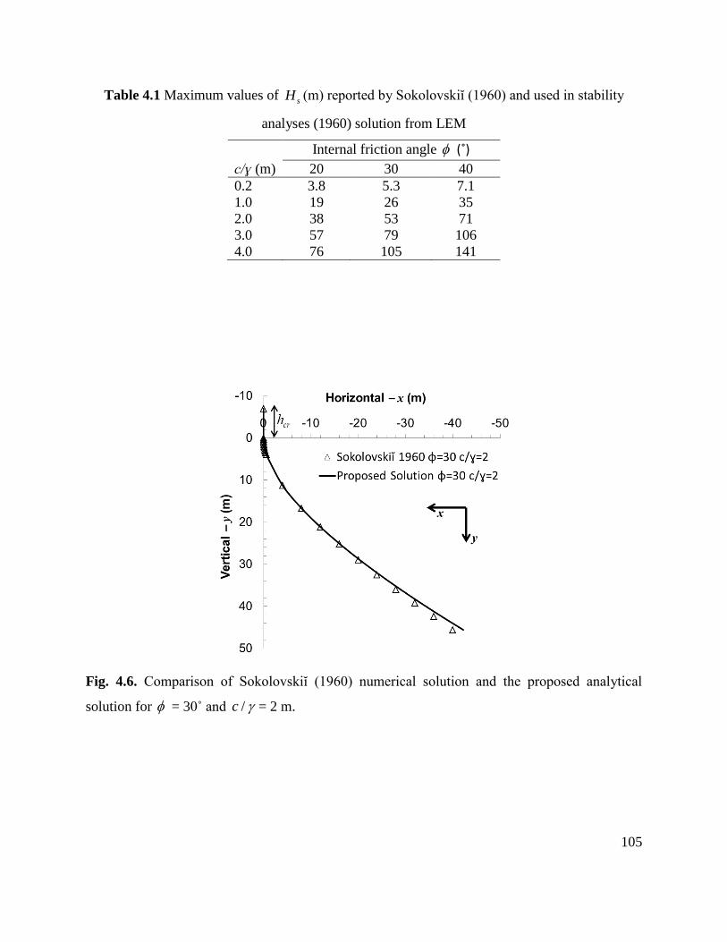
105

Table 4.1 Maximum values of sH (m) reported by Sokolovskiĭ (1960) and used in stability

analyses (1960) solution from LEM

Internal friction angle (˚)

c/ɣ (m) 20 30 40

0.2 3.8 5.3 7.1

1.0 19 26 35

2.0 38 53 71

3.0 57 79 106

4.0 76 105 141


solution for = 30˚ and /c = 2 m.

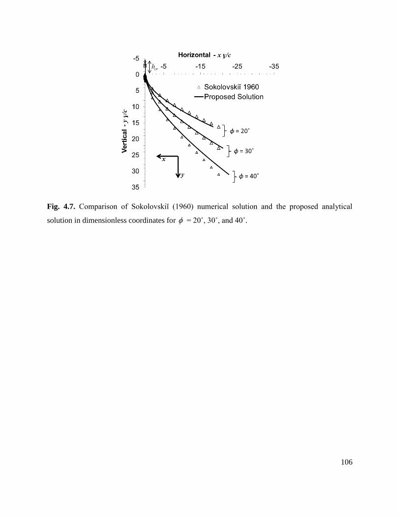
106


solution in dimensionless coordinates for = 20˚, 30˚, and 40˚.

107

portion of the slope. The amount of variation seems to depend only on the value of , with best

geometrical agreement found for 20˚ 30˚, which is the range found in many fine grained

soils. Nevertheless, as discussed in the subsequent section, these geometrical variances only induce

a minor difference in stability, because regardless of the value of the critical failure mechanism

develops in the upper zone of close agreement between the solutions.

Critical FS and observed failure mechanisms

Differences in stability between the two approaches were investigated via Finite Element Method

(FEM) and Limit Equilibrium Method (LEM). FEM analyses were computed using the software

Phase2 (Rocscience Inc. 2011), while LEM analyses using the Software Slide (Rocscience Inc.

2011). In the FEM model, a non-associated flow rule with 0 was employed to avoid effects

of computation domain size (Cheng et al. 2007) and to limit the over-prediction of dilation

(Griffiths and Lane 1999). Also, nominal values for Young’s modulus (E = 2x104 kPa) and

Poisson’s ratio (υ = 0.3) were used, since they play a minor role in the calculation of the FS (Cheng

et al. 2007, Griffiths and Lane 1999). In the LEM analyses, the Simplified Bishop’s Method was

used with 495,000 critical surfaces analyzed.

A comparison of the computed FS’s via LEM are reported in Table 4.2, while the FEM results for

Sokolovskiĭ’s and the proposed solutions when = 30˚ and /c = 2 m are shown in Figs. 4.8 and

4.9 respectively. Very similar results in terms of FS’s were obtained from FEM and LEM

approaches. For all combinations of and /c , the computed critical FS’s do not differ more

than 4% between the proposed and Sokolovskiĭ’s solutions. More importantly, all computed FS’s

108

Table 4.2 Comparison of stability between proposed approximate solution and Sokolovskiĭ

(1960) solution from LEM

Internal friction angle (˚)

20 30 40

c/ɣ (m) Proposed

approximate

Sokolovskiĭ

(1960)

Proposed

approximate

Sokolovskiĭ

(1960)

Proposed

approximate

Sokolovskiĭ

(1960)

0.2 1.00 1.04 1.04 1.03 1.06 1.03

1.0 1.00 1.04 1.04 1.03 1.06 1.03

2.0 1.00 1.04 1.04 1.03 1.06 1.03

3.0 1.00 1.04 1.04 1.03 1.06 1.03

4.0 1.00 1.04 1.04 1.03 1.06 1.03

Fig. 4.8. FEM results in terms of shear strains for the Sokolovskiĭ (1960) critical concave slope.

109

Fig. 4.9. FEM results in terms of shear strains for the proposed critical concave slope.

110

approximate 1, which is consistent with the limiting strength condition, and confirms the

appropriateness of Eq. (4.24). For the investigated range of , the proposed solution does not

deviate more than 6% from the theoretical FS = 1, which can be considered a minor difference in

terms of practical applications in geotechnical design.

Effects of slope height on failure mechanisms and FS obtained from the

proposed solution

To investigate the effects of the slope height sH on the stability of the proposed concave slopes,

LEM stability analyses were conducted for different values of , /c , and sH .

Analyses of the results indicate the existence of a limiting slope height ( Lh ) at which the failure

mechanism of the proposed concave slope changes. Concave slopes with heights sH < Lh develop

toe-failure mechanisms, whereas those with sH > Lh develop face-failure mechanisms (Fig. 4.10).

The change in failure mechanism naturally alters the computed FS, as illustrated in Fig. 4.11 for

the = 20˚ case. Concave slopes with sH < Lh tend to have slightly greater FS’s, which only in

few cases exceeded the theoretical FS = 1 by more than 10%. As sH approaches Lh , the FS

decreases until it reaches a steady value (FS ≈ 1) that remains constant for all sH > Lh . This steady

equilibrium condition coincides with a somewhat steady position of the critical failure surface, and

therefore, Lh defines the height of the failure slip for larger concave slopes. Similar analyses on

concave slopes with = 30˚, 38˚ and 45˚, not only yielded equivalent results, but also showed

that Lh can be approximated as a linear function of /c only (Fig. 4.12). Notice that over 99% of

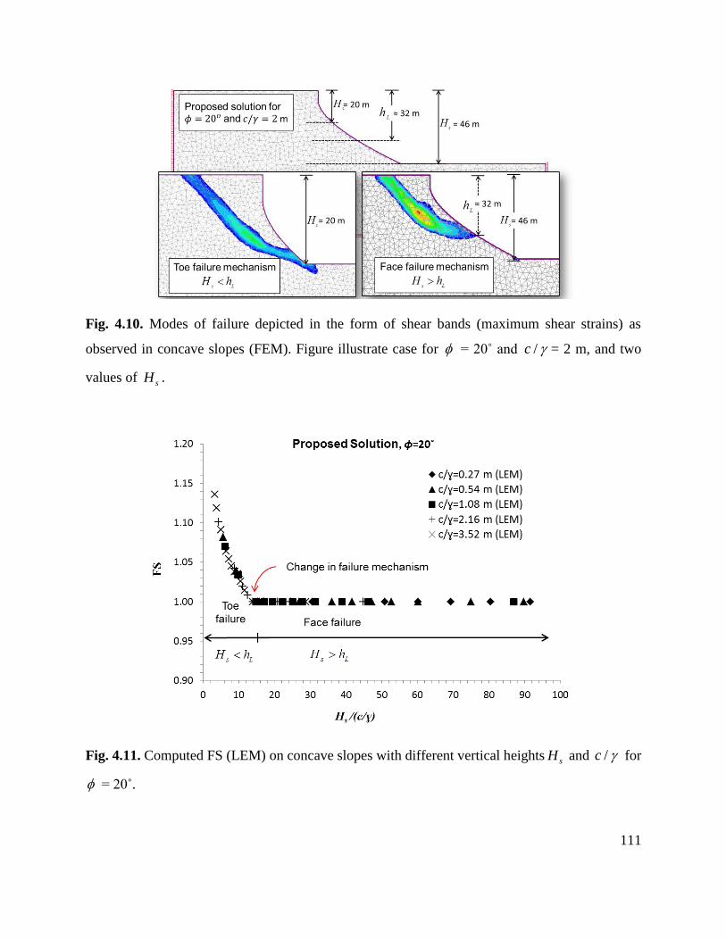
111

Fig. 4.10. Modes of failure depicted in the form of shear bands (maximum shear strains) as

observed in concave slopes (FEM). Figure illustrate case for = 20˚ and /c = 2 m, and two

values of sH .

Fig. 4.11. Computed FS (LEM) on concave slopes with different vertical heights sH and /c for

= 20˚.

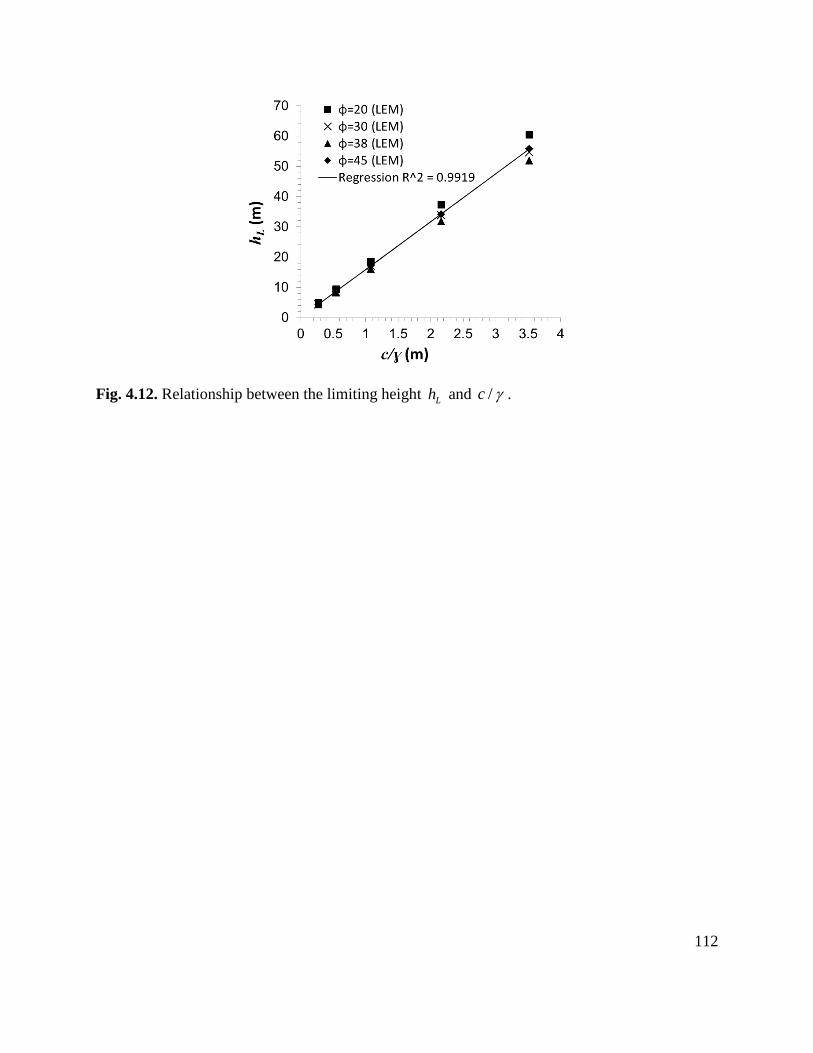
112

Fig. 4.12. Relationship between the limiting height Lh and /c .

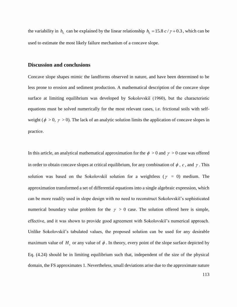
113

the variability in Lh can be explained by the linear relationship 15.8 0/ .3Lh c , which can be

used to estimate the most likely failure mechanism of a concave slope.

Discussion and conclusions

Concave slope shapes mimic the landforms observed in nature, and have been determined to be

less prone to erosion and sediment production. A mathematical description of the concave slope

surface at limiting equilibrium was developed by Sokolovskiĭ (1960), but the characteristic

equations must be solved numerically for the most relevant cases, i.e. frictional soils with self-

weight ( > 0, > 0). The lack of an analytic solution limits the application of concave slopes in

practice.

In this article, an analytical mathematical approximation for the > 0 and > 0 case was offered

in order to obtain concave slopes at critical equilibrium, for any combination of , c , and . This

solution was based on the Sokolovskiĭ solution for a weightless ( = 0) medium. The

approximation transformed a set of differential equations into a single algebraic expression, which

can be more readily used in slope design with no need to reconstruct Sokolovskiĭ’s sophisticated

numerical boundary value problem for the > 0 case. The solution offered here is simple,

effective, and it was shown to provide good agreement with Sokolovskiĭ’s numerical approach.

Unlike Sokolovskiĭ’s tabulated values, the proposed solution can be used for any desirable

maximum value of sH or any value of . In theory, every point of the slope surface depicted by

Eq. (4.24) should be in limiting equilibrium such that, independent of the size of the physical

domain, the FS approximates 1. Nevertheless, small deviations arise due to the approximate nature

114

of the solution. Though associated with the mode of failure, these deviations are small for

geotechnical applications and indicate that the stability of the proposed critical concave slopes will

range from FS = 1 - 1.1 for the majority of cases.

Although the solution for the concave slope was developed in terms of the critical slope shape (FS

= 1), the proposed solution can be used as a base line for practical applications. For design, a given

FS can be obtained if a strength reduction factor (Griffiths and Lane 1999, Spencer 1967) equal to

the desired FS is used with our proposed solution. The effects of an external semi-infinite surcharge

( eq ) acting on the ground surface can be included by adding eq to the right side of Eq. (4.19) and

modifying Eq. (4.18) as 2 cos / [ 1 sin ] /cr eh c q . Once the desired concave shape is

defined, the effects of transient ground water flow can be investigated using commercial slope

stability software. While the successful construction of concave slopes will depend on the

precision of the employed construction equipment, the increasing precision and availability of GPS

based auto-guidance equipment (Koehrsen et al. 2001) makes the construction of concave slopes

possible. Nevertheless, in actual slope construction the sharp bluff at the top (the tension crack

zone) is not likely to be constructed since it may erode over time; instead this would be rounded

for a more natural appearance, which would decrease the destabilizing forces and add conservatism

to concave slope performance.

115

References:

Ahmed, A., Ugai, K., and Yang, Q. (2012). "Assessment of 3D slope stability analysis methods

based on 3D Simplified Janbu and Hovland methods." Int. J. Geomech., 12(2), 81-89.

Alshibli, K. A., and Sture, S. (2000). "Shear band formation in plane strain experiments of sand."

J. Geotech. Geoenviron. Eng., 126(6), 495-503.





Hill, R. (1950). The mathematical theory of plasticity, Clarendon Press, Oxford.



Koehrsen, C., Sahm, W., and Keefer, C. "GPS —Based earthmoving for construction." Proc.,

Digital Earth Moving: First International Symposium, Springer Berlin / Heidelberg,

Manno, Switzerland, 4-17.

Leopold, L. B., and Langbein, W. B. (1962). The concept of entropy in landscape evolution, U.S.

Government Printing Office, Washington, DC.

Liu, F., and Zhao, J. (2012). "Limit Analysis of slope stability by rigid finite element method and

linear programming considering rotational failure." Int. J. Geomech., in press.

116

Malvern, L. E. (1969). Introduction to the mechanics of a continuous medium, Prentice-Hall,

Englewood Cliffs, N.J.

Mesri, G., and Abdelghaffar, M. E. M. (1993). "Cohesion intercept in effective stress-stability

analysis." Journal of Geotechnical Engineering, 119(8), 1229-1247.

Meyer, L. D., and Kramer, L. A. (1969). "Erosion equations predict land slope development."

Agric. Eng., 50(9), 522-523.

Michalowski, R. (2010). "Limit analysis and stability charts for 3D slope failures." J. Geotech.

Geoenviron. Eng., 136(4), 583-593.

Miyamoto, H., Baker, V., and Lorenz, R. (2005). "Entropy and the shaping of the landscape by

water " Non-equilibrium thermodynamics and the production of entropy: life, earth, and

beyond A. Kleidon, and R. Lorenz, eds., Springer Berlin / Heidelberg, 135-146.

Nash, D. (1980). "Forms of bluffs degraded for different lengths of time in Emmet county,

Michigan, USA." Earth Surf. Processes Landforms, 5(4), 331-345.

NAVFAC (1986). Design manual 7.01 - soil mechanics, U.S. Government Printing Office,

Washington, DC.

Pelletier, J. D., and Rasmussen, C. (2009). "Quantifying the climatic and tectonic controls on

hillslope steepness and erosion rate." Lithosphere, 1(2), 73-80.

Rankine, W. J. M. (1857). "On the stability of loose earth." Philosophical Transactions of the

Royal Society of London, 147, 9-27.

117

Rieke-Zapp, D. H., and Nearing, M. A. (2005). "Slope shape effects on erosion: A laboratory

study." Soil Sci. Soc. Am. J., 69(5), 1463-1471.





Roscoe, K. H. (1970). "The influence of strains in soil mechanics." Géotechnique, 20(2), 129-170.



NJ.

Scott, R. F. (1963). Principles of soil mechanics, Addison-Wesley Pub. Co., Reading, M.A.


Sokolovskiĭ, V. V. (1965). Statics of granular media, Pergamon Press, Oxford; New York.

Spencer, E. (1967). "A method of analysis of the stability of embankments assuming parallel inter-

slice forces." Géotechnique, 17(1), 11-26.

Terzaghi, K. (1943). Theoretical soil mechanics, J. Wiley and Sons, New York.

Twidale, C. R. (2007). "Backwearing of slopes - the development of an idea." Revista C&G, 21(1-

25), 135-146.

118

Appendix: The slip line field theory and the characteristic equations

Equations of internal equilibrium and principal stresses

From the assumption that soil medium can be treated as a continuum, the complete state of stresses

acting on any plane can be specified if the resultant stresses in the directions of the axes of the

reference frame are known (Malvern 1969). For the plane strain condition (e.g. the profile of a 2D

slope), strains and shear stresses in the z direction (perpendicular to the paper) vanish and

therefore, the equations of internal equilibrium in a xy space that not necessarily coincides with

the vertical and horizontal can be written as:

sinxyxx

x y

(4.29)

cosyx yy

x y

(4.30)

where xx and yy are the normal stresses acting in the x and y directions,

xy yx are the shear

stresses, is the unit weight of the material, and is the angle between an horizontal plane and

the x-axis. The complete state of stresses at a point, mathematically expressed as a second order

tensor, can be described by the principal stresses and directions, which are independent of the

selected reference frame. Any normal and tangential stress component on any plane can be

determined if the principal stresses are known (Holtz and Kovacs 1981):

1 3 1 3

1 1 cos 2

2 2n (4.31)

1 3

1 sin 2

2n (4.32)

119

where 1 is the major principal stress,

3 is the minor principal stress, and is the angle between

the direction of the normal to the plane and the major principal direction.

Formulation of the equations of the characteristics

The slip line field theory in soil mechanics rests on the assumptions that the soil yield stress is

independent on the strain level and that the strain-stress behavior can be described by either elastic

perfectly plastic or rigid perfectly plastic idealizations. In this way, the formulation of the problem

does not require stress and displacement boundary conditions, which combined impose a statically

indeterminate condition (Scott 1963). For frictional materials like soils, Mohr-Coulomb has been

traditionally used as the constitutive law defining the yield or maximum allowable stress. In this

context, to bring the body into a limiting equilibrium state or at the verge of flowing plastically,

the largest difference between the shear stresses and the shear strength must be zero (Sokolovskiĭ

1960):

max ( ) tan 0n n H (4.33)

where n and n are the normal and shear stresses acting on any plane within the soil body and

H is the tensile strength of the soil. If the stresses in the soil body exceed this liming state, plastic

deformation will occur. According to the slip line field theory, the plastic deformation will take

place by the relative movement of two planes on which the inclination of the stresses is maximum

(Scott 1963). These planes, called slip planes or shear bands, are oriented parallel to the straight

lines that connect the pole of the Mohr circle and its contact with the failure condition in a

stress space (Fig. 4.13). If n and n are written in terms of principal stresses [Eqs. (4.31) and

(4.32)], the limiting condition in Eq. (4.33) can be written as

120

Fig. 4.13. Illustration of slip planes on Mohr-Coulomb diagram.

121

1 3 1 3max sin(2 ) sin ( 2 ) 0H (4.34)

Approaching the condition of maximum difference as a mathematical optimization problem, it is

found that the maximum difference between shear stresses and strength is reached when:

22

(4.35)

According to Sokolovskiĭ (1960), at the limiting condition the absolute values of and (the

angle between the slip planes and the direction of the major principal stress) are complementary,

and therefore, the slip planes make an angle

(45 / 2) (4.36)

with the direction of the major principal stress and (45 / 2) with the direction of the minor

principal stress.

The solution in Eq. (4.36) is independent of the strain level, which is not always consistent with

experimental observations. Roscoe (1970) concluded that a strain based approach rather than a

stress approach better predicts the inclination of the slip plane, and its magnitude can be

approximated by 45 / 2 , where is the dilatancy angle at failure. Later studies on shear band

formation in plane strain experiments confirmed Roscoe’s findings (Alshibli and Sture 2000).

Nevertheless, Eq. (4.36) is still valid in the context of the associated plasticity ( ), which for

relatively unconfined problems such as slope stability, do not influence the prediction of the FS

(Griffiths and Lane 1999) neither the prediction of the critical slip or failure mechanism (except

for cases of very low friction angle and high cohesion) (Cheng et al. 2007). Accordingly, if Eqs.

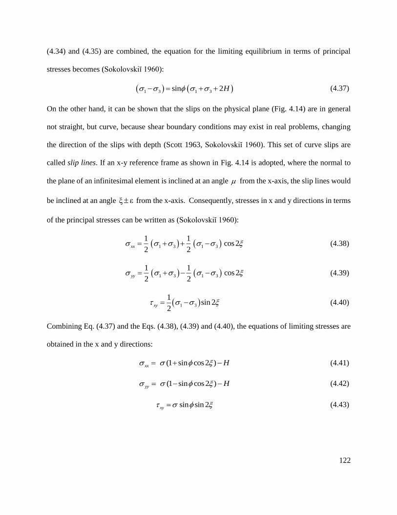
122

(4.34) and (4.35) are combined, the equation for the limiting equilibrium in terms of principal

stresses becomes (Sokolovskiĭ 1960):

1 3 1 3sin 2H (4.37)

On the other hand, it can be shown that the slips on the physical plane (Fig. 4.14) are in general

not straight, but curve, because shear boundary conditions may exist in real problems, changing

the direction of the slips with depth (Scott 1963, Sokolovskiĭ 1960). This set of curve slips are

called slip lines. If an x-y reference frame as shown in Fig. 4.14 is adopted, where the normal to

the plane of an infinitesimal element is inclined at an angle from the x-axis, the slip lines would

be inclined at an angle ξ ε from the x-axis. Consequently, stresses in x and y directions in terms

of the principal stresses can be written as (Sokolovskiĭ 1960):

1 3 1 3

1 1 cos 2

2 2xx (4.38)

1 3 1 3

1 1 cos 2

2 2yy (4.39)

1 3

1sin 2

2xy (4.40)

Combining Eq. (4.37) and the Eqs. (4.38), (4.39) and (4.40), the equations of limiting stresses are

obtained in the x and y directions:

(1 sin cos2 )xx H (4.41)

(1 sin cos2 )yy H (4.42)

sin sin 2xy (4.43)

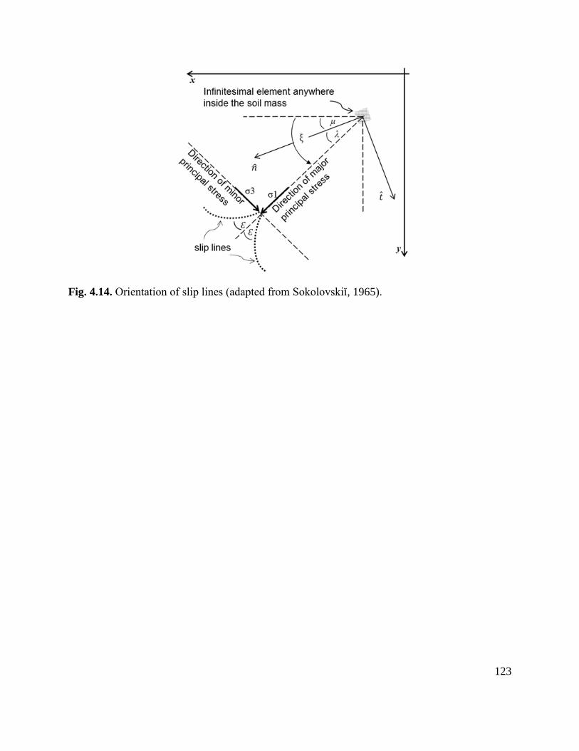
123

Fig. 4.14. Orientation of slip lines (adapted from Sokolovskiĭ, 1965).

124

Analogously, the equations of limiting stresses in the normal n and t directions can be obtained

(Sokolovskiĭ 1960):

1 sin cos2( )n H (4.44)

1 sin cos2( )t H (4.45)

sin sin 2( )nt (4.46)

where 1 31/ 2 H . When Eqs. (4.41), (4.42) and (4.43) are combined with the

equations of equilibrium [Eqs. (4.29) and (4.30)], a set of two first order partial differential

equations which govern the variation of the stresses in the x and y directions is obtained:

1 sin cos 2 sin sin 2 2 sin sin 2 cos 2 sinx y x y

(4.47)

sin sin 2 1 sin cos 2 2 sin cos 2 sin 2 cosx y x y

(4.48)

Applying the method of characteristics (Hill 1950), the system of Eqs. (4.47) and (4.48), can be

solved. Multiplying Eq. (4.47) by sin and Eq. (4.48) by cos and adding them, the

following expression is obtained:

sin cos

2 tan cos 2 tan sin 0cos cosx x y y

(4.49)

Using the auxiliary quantities M and N, as defined by:

sin

2 tan cos

Mx x

(4.50)

cos

2 tan cos

Ny y

(4.51)

Eq. (21) can be written as (Sokolovskiĭ 1960):

125

tan 0M N (4.52)

Obtaining the characteristic differential equations requires the expression of the auxiliary

quantities in ordinary derivative form:

d dx dyx y

(4.53)

d dx dyx y

(4.54)

Introducing a new a new auxiliary quantity P,

2 tan sin cos cos

d d dyP

dx dx dx

(4.55)

M and N, can be rewritten as:

sin

sin cos

PdxM

dx dy

(4.56)

cos

sin cos

PdxN

dx dy

(4.57)

Note that the characteristics will be found when the numerator and denominator of the Eqs. (4.56)

and (4.57) are simultaneously set to zero, and therefore the equations of characteristic are:

tan( )dy

dx (4.58)

2 tan sin cos cos

d d dx dy

(4.59)

Eq. (4.58) imposes the condition that the characteristics have to be inclined at o

from the x-

axis. Therefore, they are indeed slip lines in the x-y space (Sokolovskiĭ 1965). For cases when the

body forces are aligned in the direction of vertical y-axis, 0 and Eq. (4.59) simplifies to:

126

2 tan sin cos cos

d d dx dy

(4.60)

127

Chapter 5. Design of Stable Concave Slopes for Reduced Sediment

Delivery

128

This chapter was submitted as an original paper in the ASCE Journal of Geotechnical and

Geoenvironmental Engineering, and has been revised according to the reviewers’ suggestions. It

is currently undergoing the second review. The co-authors of this work are Dr. Eric Drumm and

Dr. Daniel Yoder. This article would be cited as:

Jeldes, I. A., Drumm, E. C., and Yoder, D. C. "Design of stable concave slopes for reduced

sediment delivery." J. Geotech. Geoenviron. Eng., (in review).

Abstract

Constructed slopes have traditionally taken a planar form. However, natural slopes are more likely

to be concave in cross section, and laboratory and computational studies have demonstrated that

concave slopes yield less sediment than planar slopes. With the current auto-guided construction

equipment, it is now possible to construct slopes with concave profiles and a more natural

appearance, yet a simple method to describe such concave slopes for a given level of mechanical

stability does not exist. This article begins with the examination of concave shapes satisfying a

desired degree of stability and compare results with those from Finite Element and Limit

Equilibrium methods. An erosion model is used to demonstrate that the concave slopes proposed

here can yield 15-40% less sediment than planar slopes with same Factor of Safety. Finally, a

sensitivity analysis suggests that reasonable construction deviations do not compromise the

stability of typical concave slopes.

Introduction

Constructed slopes designed with traditional planar cross sections are encountered in most land

development, including highway cut and fill sections, constructed embankments, and reclaimed

129

mines. Planar landscape profiles are seldom encountered in nature, however, where curvilinear

slopes with concave shapes usually arise as the result of evolutionary processes in fluvial systems

and hillslopes (Leopold and Langbein 1962, Miyamoto et al. 2005, Rodríguez-Iturbe et al. 1992,

Twidale 2007, Yang and Song 1979). Landforming approaches such as the Geomorphic

Reclamation of mine lands (Toy and Chuse 2005) include the construction of concave-like shapes

in both the transverse (cross-slope) and longitudinal (downslope) directions to create natural self-

sustainable ecosystems (Martín-Duque et al. 2010) with improved erosion resistance (Schor and

Gray 2007). Nevertheless, not all concave shapes are mechanically stable, requiring a rational

definition of those concave slopes that provide the desired degree of stability expressed in terms

of a desired Factor of Safety (FS). For example, Howard et al. (2011) point out the risk associated

with the growing practice of shaping slopes to reflect natural regional landforms without

appropriate stability and erosion analyses and without accounting for the limited precision of the

construction equipment employed to build concave profiles. Hence, the objectives of this work are

to 1) describe concave shapes that provide a desired degree of stability (or FS) for given soil

properties, 2) provide a quantitative measure of the difference in soil loss (erosion) between

concave and planar slopes that satisfy the same degree of mechanical stability, and 3) investigate

the precision to which concave forms can be constructed, and how this affects the desired slope

stability. To accomplish these objectives this work focuses on slopes with concavity in the

longitudinal direction, which have been shown to deliver less sediment than transversely-convex,

transversely-concave, longitudinally-convex and planar slopes (Rieke-Zapp and Nearing 2005).

130

Background

Mechanical stability of concave profiles

Although a number of studies have shown that concave slopes produce less sediment than planar

slopes, few studies have linked the benefits of concave slopes to mass stability. Utili and Nova

(2007) demonstrated by means of the upper bound method that concave log-spiral slopes result in

higher FS’s than planar slopes of same height and width and than planar slopes of same soil mass.

Based on the slip line field theory and the associated characteristic equations, Sokolovskiĭ (1960)

found a longitudinal concave critical slope contour (FS = 1) for plain strain conditions.

Sokolovskiĭ’s solution is the result of a numeric boundary value problem, which for a medium

with unit weight ( ) > 0 and friction angle ( ) > 0 has no analytical counterpart. Recently, Jeldes

et al. (2013) proposed an approximate analytical expression to obtain coordinates of the critical

contour for any desired combination of , c , and slope height ( sH ). This expression brings a

system of differential equations into a single algebraic expression, which highly simplifies the

manipulation and solution as:

0 , 0

1 1 1 , 0

cr

y

h yx


(5.1)

where:

cos

2 1 sinA

(5.2)

1 sin

1 1 1 sin

y y

aB ln ln KH H

(5.3)

y y (5.4)

131

cotH c (5.5)

2 cos

1 sincr

ch

(5.6)

Here, H is the tensile strength of the soil, 1 sin ) / (1 sin )(aK is the Rankine active

coefficient of earth pressure, y is the geo-static vertical stress, and crh is the height of the tension

zone. The equation describes a slope contour in the quadrant with x-axis positive to the right and

y-axis positive downward (Fig. 5.1), and with crh lying above the x-axis from the coordinates (0,0)

to (0,- crh ). A limiting slope height ( Lh ) was also found, defining where the failure mechanism

changes. Slopes of heights sH < Lh indicate a toe-failure mechanism with FS values slightly

greater than 1, while those with sH > Lh indicate a face-failure mechanism with a steady FS ≈ 1.

A linear correlation between Lh and /c was approximated by

15.8 0/ .3Lh c (5.7)

which can be used as a preliminary estimate of the most likely failure mechanism for a concave

slope (Jeldes et al. 2013). While in practice the sharp bluff at the top of the tension zone may be

removed or rounded (as indicated by the dashed line in Fig. 5.1) adding conservatism, the full

tension height was included in the development of the solution for mathematical completeness.

Concave slopes and soil erosion

Experimental and computational studies have shown that slopes with longitudinally-concave

shapes yield less sediment than slopes with planar or other curvilinear shapes. Thus, this work

focuses on the difference in soil loss between longitudinally concave (referred to henceforth as

concave) and planar slopes, which are the two shapes of interest in this study.

132

Fig. 5.1. Illustration of the reference frame and the components of the concave slope formulation.

In practice the sharp bluff at the top of the slope may be rounded, as indicated by the dashed line.

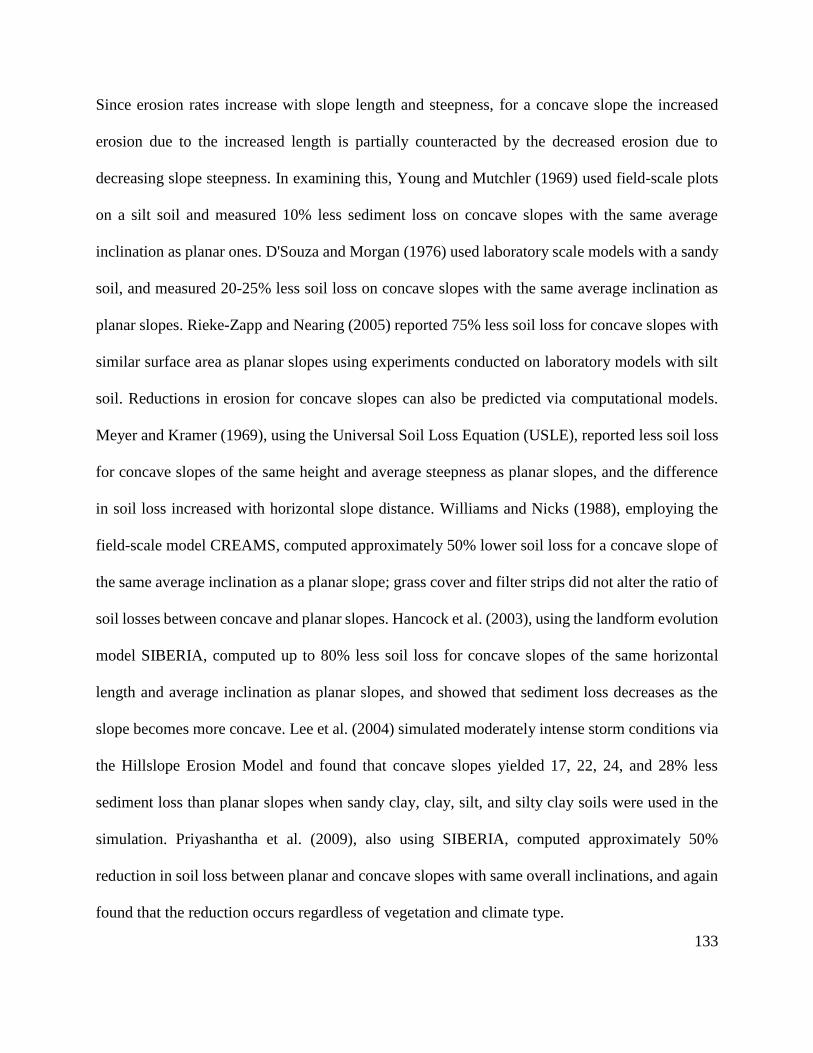
133

Since erosion rates increase with slope length and steepness, for a concave slope the increased

erosion due to the increased length is partially counteracted by the decreased erosion due to

decreasing slope steepness. In examining this, Young and Mutchler (1969) used field-scale plots

on a silt soil and measured 10% less sediment loss on concave slopes with the same average

inclination as planar ones. D'Souza and Morgan (1976) used laboratory scale models with a sandy

soil, and measured 20-25% less soil loss on concave slopes with the same average inclination as

planar slopes. Rieke-Zapp and Nearing (2005) reported 75% less soil loss for concave slopes with

similar surface area as planar slopes using experiments conducted on laboratory models with silt

soil. Reductions in erosion for concave slopes can also be predicted via computational models.

Meyer and Kramer (1969), using the Universal Soil Loss Equation (USLE), reported less soil loss

for concave slopes of the same height and average steepness as planar slopes, and the difference

in soil loss increased with horizontal slope distance. Williams and Nicks (1988), employing the

field-scale model CREAMS, computed approximately 50% lower soil loss for a concave slope of

the same average inclination as a planar slope; grass cover and filter strips did not alter the ratio of

soil losses between concave and planar slopes. Hancock et al. (2003), using the landform evolution

model SIBERIA, computed up to 80% less soil loss for concave slopes of the same horizontal

length and average inclination as planar slopes, and showed that sediment loss decreases as the

slope becomes more concave. Lee et al. (2004) simulated moderately intense storm conditions via

the Hillslope Erosion Model and found that concave slopes yielded 17, 22, 24, and 28% less

sediment loss than planar slopes when sandy clay, clay, silt, and silty clay soils were used in the

simulation. Priyashantha et al. (2009), also using SIBERIA, computed approximately 50%

reduction in soil loss between planar and concave slopes with same overall inclinations, and again

found that the reduction occurs regardless of vegetation and climate type.

134

While all the aforementioned erosional studies reported significantly less soil loss for concave

slopes, most compared the difference in soil loss between planar and concave slopes with similar

average steepness, and none of them linked the concave geometry to mechanical stability

considerations. Accordingly, the investigation begins with the examination of concave shapes

satisfying a desired degree of stability, and then proceeds by investigating their ability to reduce

sediment yield. This is accomplished by comparing the soil loss on concave and planar slopes with

the same FS. Finally, the impact of construction precision on the concave slope stability is

explored.

Methods

Mechanical stability

In this section concave slopes for a given design FS for long-term stability are defined and the

undrained shear strength required such that short-term stability is unlikely to govern is determined.

This approach is conservative in that it neglects any additional shear strength that may be present

due to partial saturation and resulting soil suction.

Stable concave slopes for > 0 (long-term stability) with pre-selected FS

While Eqs. (5.1) – (5.6) generate concave slopes at limiting equilibrium, a design factor of safety

( DFS ) > 1 is desired for design and construction. The expression for the concave slope can be

extended to any desired FS if a strength reduction factor (Griffiths and Lane 1999, Spencer 1967)

equal to DFS is used to reduce the strength parameters as follows:

135

* tan

arctan DFS

(5.8)

*

D

cc

FS (5.9)

where * and *c are reduced friction angle and cohesion employed in the design to achieve the

desired FS. To obtain a concave slope satisfying a pre-selected DFS , replace and c in Eqs. (5.1)

– (5.6) with * and *c and determine the x-y coordinates of the concave slope. The resulting

concave shape will satisfy a FS ≈ DFS under the original and c strength conditions.

The proposed methodology was compared with results obtained via Limit Equilibrium Method

(LEM) and Finite Element Method (FEM) analyses for soils with = 20˚, 30˚, and 40˚ and /c

ranging from 0.2 to 5 m, where the range c = 5 – 40 kN/m3 covers most of the cohesion values

reported by Mesri and Abdelghaffar (1993), and the range = 10 – 23 kN/m3 covers most

materials from clays to coarse granular soils (NAVFAC 1986). Each combination of and /c

describing a unique concave slope was analyzed for heights sH ranging from 2 to 100 m. The

FEM analyses were conducted using Phase2 (Rocscience Inc. 2011), and the LEM analyses using

Slide (Rocscience Inc. 2011). In the FEM analyses, an elastic perfectly plastic model with a Mohr-

Coulomb yield criterion and a non-associated flow rule (zero dilatancy angle) was employed since

it has been shown to provide reliable FS’s (Griffiths and Lane 1999). Also, nominal values for

Young’s modulus (E = 2x104 kPa) and Poisson’s ratio (υ = 0.3) were used, because they do not

influence the calculation of the FS (Cheng et al. 2007, Griffiths and Lane 1999). In the LEM

136

analyses, the Morgenstern-Price, the Spencer and the Simplified Bishop Methods were used with

over 30,000 critical surfaces analyzed for each set of variables.

Stability check for short- term ( = 0) loading conditions

Once the long-term ( > 0) stable concave shapes are defined, it is necessary to investigate under

what conditions short-term failure may occur, e.g., failure during the construction period where

the stability is controlled by the undrained shear strength (uS ), which is the soil shear strength for

= 0 conditions. The question then becomes: what would be the minimum value of undrained

shear strength ( min

uS ) such that the concave slope defined for long-term stability is also stable for

short-term conditions? This problem was approached by making use of the critical slope concept.

A critical contour implies that slopes less steep than this contour are safe, and steeper ones are

unsafe (under same soil properties and slope height). Thus, any critical contour defined for long-

term stability that is less or equally steep than a critical contour defined for short-term ( = 0) will

be stable in the short-term for a given height y. Although the long-term critical contour can be

obtained via Eqs. (5.1) – (5.6), the critical slope contour for the = 0 case can be obtained as a

closed form solution of the characteristic equations (Sokolovskiĭ 1965):

2

ln cos( ) , 02

uu

u

S yx y y

S

(5.10)

Here ux defines the horizontal projection of the slope contour. In the tension zone ( 0cruh y )

0ux , and 2 /cru uh S (Fig. 5.2). This concept is illustrated in Fig. 5.2, where the long-term

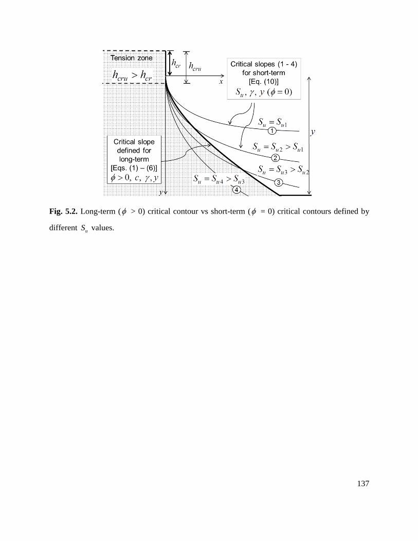
137

Fig. 5.2. Long-term ( > 0) critical contour vs short-term ( = 0) critical contours defined by

different uS values.

138

critical contour is steeper than the short-term critical contours 1, 2 and 3 that have undrained shear

strengths1uS , 2uS , and 3uS respectively, and therefore it is unsafe in the short-term. The opposite

yet desirable case is shown for contour 4, where 4uS is sufficiently large that the global stability

is governed by the long-term condition. The value of min

uS to satisfy this condition is found at the

intersection of the long and short-term contours. To find min

uS , we must a) enforce thatcru crh h ,

and b) numerically solve the transcendental equation u d crx y x y h , where

, 0cr cru cr crh h h h . It should be noted that min

uS is a conservative estimate of the necessary

undrained shear strength and can be taken as an upper limiting value of the exact solution.

Soil erosion and sediment yield

Soil loss for concave and planar slopes with same FS’s was investigated via the widely recognized

Revised Universal Soil Loss Equation RUSLE2 (USDA-ARS 2008):

A R K LS C P (5.11)

where the predicted soil loss A (units of / /Mg ha y ) is directly proportional to: the rainfall

erosivity R (units of /MJ mm ha h y ), quantifying the rainfall’s erosive potential; the soil

erodibility K (units of /Mg ha h ha MJ mm ) defining the soil’s susceptibility to that erosivity;

the topographic factor LS (dimensionless) representing slope length and steepness effects; the

surface cover factor C (dimensionless); and the conservation practices factor P (dimensionless).

Through RUSLE2 pairs of planar and concave slopes [Eqs. (5.1) – (5.6)] that had the same FS

under the same values of , c , and sH (Fig. 5.3) were investigated. For soil loss calculations,

139

Fig. 5.3. Illustration of concave and equivalent planar slopes (same FS and slope height).

140

the concave slopes were idealized using ten to twenty linear segments. Since RUSLE2 determines

soil loss over the horizontal projection of the slope, for slope segments steeper than 45˚ (which are

not defined in RUSLE2), the soil loss was calculated assuming a planar slope of 45˚ over the total

horizontal length occupied by the steeper part of the contour. Three different soil textures were

employed for the analyses: a silt loam (high erodibility), a clay (moderate erodibility), and a sandy

loam (moderately low erodibility). A range of possible K values for each soil texture (Haan et al.

1994, USDA-ARS 2008) was used (Table 5.1), which conservatively encompasses a large variety

of soils found in practice, even mine reclaimed soils (Hoomehr et al. 2014). All the simulations

were conducted for two locations with very different climates: Dakota County, Minnesota (R =

2,180 MJ∙mm/ha∙h∙y) representing dry weather conditions and Monroe County, Florida (R =

10,500 MJ∙mm/ha∙h∙y) representing high rainfall conditions. For simplicity, a bare surface (C = 1)

and no conservation practices (P = 1) were modeled. A representative value of friction angle was

assumed for each soil texture (Budhu 2011, Hough 1957). Values of /c ranging from 0.2 to 3

m were employed for the clay soils and from 0.2 to 2 m for the silt and sandy loam soils. Table 5.1

summarizes the erosion and mechanical properties of the investigated soils.

Construction and sensitivity

The widespread use of high accuracy auto guidance GPS-based construction equipment for

grading and earthwork operations suggests that the construction of more complex slope shapes can

become more commonplace. The effects of construction precision on the stability were

investigated by considering the worst case scenario: the vertical component of the contour is

constructed deeper than designed, resulting in a steeper slope. Although the vertical accuracy of

3D grade control systems is commonly within 30 mm (Trimble 2013), an accuracy T = 200 mm

141

Table 5.1 Soil composition, classification, erodibility and assumed internal friction angle of

investigated soils

RUSLE soil

texture

[USDA]

Composition [USDA], (%) Equivalent

USCS

classification

Range of

erodibility

(K)**

Assumed

(˚) Clay

<0.002 mm

Silt

<0.05-0.002 mm

Sand

<2-0.05 mm

Silt Loam 20 60 20 ML 0.037-0.057* 25

Clay 45 28 27 CL 0.032-0.042 20

Sandy Loam 10 25 65 SM 0.026-0.037* 35

* Upper bound reported for cases of low permeability and low organic matter content.

**All K values in SI units of /Mg ha h ha MJ mm .

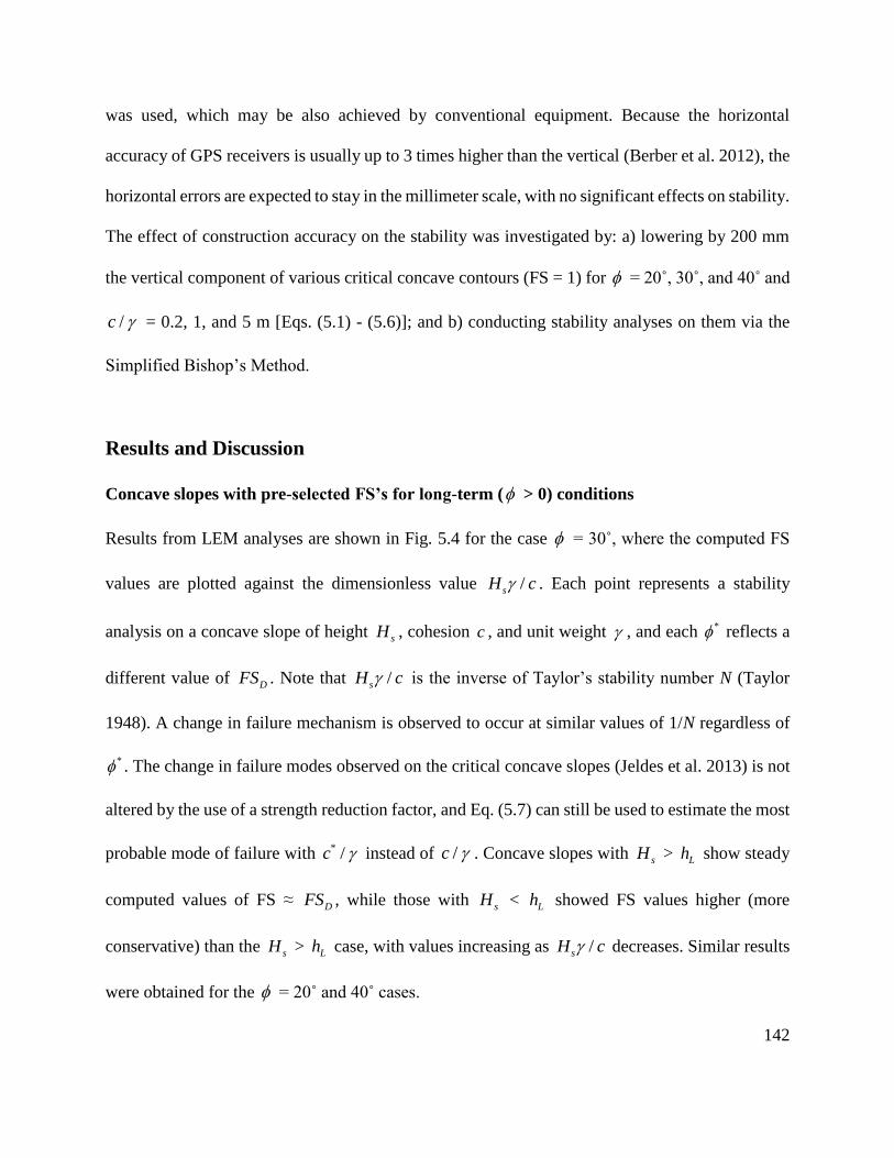
142

was used, which may be also achieved by conventional equipment. Because the horizontal

accuracy of GPS receivers is usually up to 3 times higher than the vertical (Berber et al. 2012), the

horizontal errors are expected to stay in the millimeter scale, with no significant effects on stability.

The effect of construction accuracy on the stability was investigated by: a) lowering by 200 mm

the vertical component of various critical concave contours (FS = 1) for = 20˚, 30˚, and 40˚ and

/c = 0.2, 1, and 5 m [Eqs. (5.1) - (5.6)]; and b) conducting stability analyses on them via the

Simplified Bishop’s Method.


Concave slopes with pre-selected FS’s for long-term ( > 0) conditions

Results from LEM analyses are shown in Fig. 5.4 for the case = 30˚, where the computed FS

values are plotted against the dimensionless value /sH c . Each point represents a stability

analysis on a concave slope of height sH , cohesion c , and unit weight , and each * reflects a

different value of DFS . Note that /sH c is the inverse of Taylor’s stability number N (Taylor

1948). A change in failure mechanism is observed to occur at similar values of 1/N regardless of

* . The change in failure modes observed on the critical concave slopes (Jeldes et al. 2013) is not

altered by the use of a strength reduction factor, and Eq. (5.7) can still be used to estimate the most

probable mode of failure with * /c instead of /c . Concave slopes with sH > Lh show steady

computed values of FS ≈ DFS , while those with sH < Lh showed FS values higher (more

conservative) than the sH > Lh case, with values increasing as /sH c decreases. Similar results

were obtained for the = 20˚ and 40˚ cases.

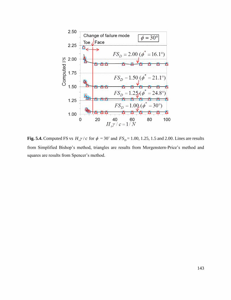
143

Fig. 5.4. Computed FS vs /sH c for = 30˚ and DFS = 1.00, 1.25, 1.5 and 2.00. Lines are results

from Simplified Bishop’s method, triangles are results from Morgenstern-Price’s method and

squares are results from Spencer’s method.

144

It is important to note that the methodology proposed here is based on the slip line field theory,

which requires a value of c ≠ 0 for a valid mathematical solution to exist. However, the method

can still be used to simulate long-term conditions using a very small value of cohesion, as it is

illustrated in the example problem. It must be also emphasized that Eqs. (5.1) – (5.6) constitute an

approximate solution in analytical form, so even when sH >

Lh there may not be a perfect match

between DFS and the actual FS. As seen in Fig. 5.4, the best match occurs when * ≈ 20˚. Concave

slopes with * > 20˚ yield FS values higher than the design DFS (4% higher when * = 30˚ and

6% higher when * = 40˚), which is conservative for design. On the other hand, slopes with * <

20˚ will have FS < DFS , which is not conservative. This is shown in Fig. 5.4 for the case * =

16.1˚, where the resulting FS = 1.92 is 4% less than the desired DFS = 2. Nevertheless, the

deviations from the target DFS obtained through the methodology do not compromise its

applicability for design, considering that neither the geometry nor the shear strength parameters

are usually determined within ±6% accuracy (Duncan 1996). Furthermore, since the FS values

calculated by limit equilibrium methods that satisfy all conditions of static equilibrium can vary

as much as 12% (Duncan 1996), an accuracy of ±6% is certainly acceptable. Once the desired

shape for the design FS has been obtained, verifications can be conducted employing commercial

slope stability software. In the same way, the effects of transient ground water flow and/or external

surcharges on the FS can be investigated, which extends the applications of this solution to other

field conditions.

145

Stability check for short-term ( = 0) conditions

The minimum undrained shear strength min

uS that the soil must possess for concave slopes to have

FS > DFS in the short term can be obtained from Fig. 5.5 as a function of the effective strength

parameters * and *c . Fig. 5.5 is a solution chart that assembles the numerical results from Eqs.

(5.1) and (5.10) and is presented in terms of the dimensionless parameters */y c and

min */ )( DuS c FS for a range of * . Here, y is the height of the slope below the tension zone

( , 0crsy hH y ). The inner chart in Fig. 5.5 provides higher resolution for low values of

*/y c . Note that Fig. 5.5 defines the conditions under which long-term stability will always

govern, so the solutions are conservative. Also, this chart is based on an assumed failure

mechanism, where the critical surface exists from or above the toe. Consequently, this solution

provides a first check for the short-term stability of concave slopes and does not replace the

necessity of conducting stability analyses once the undrained shear strength of the soil has been

determined.

Soil loss from the mechanically stable concave slopes

Soil loss results obtained from RUSLE2 for the silt loam are shown in Fig. 5.6. All the analyses

were conducted on concave and planar slopes with FS = DFS = 1 ( * and *c c ), since they

provide generic results that can be extended to any FS. Figs. 5.6a and 5.6b compare the predicted

total soil loss for concave and planar slopes of a silt loam with * /c = 1 under wet weather

conditions in Monroe County, FL, and dry conditions in Dakota County, MN. Planar slopes

146

Fig. 5.5. Solution chart for short-term stability check.

147

Fig. 5.6. Erosion analyses for a silt loam soil with = 25˚; a) total soil loss for Monroe County,

FL; b) total soil loss for Dakota County, MN; c) difference in soil loss for the Dakota (dry) and

Monroe (wet) Counties; d) /c pA A vs */sH c . Units: A (Mg/Ha/y), p cA A (Mg/Ha/y), R

(MJ∙mm/ha∙h∙y), K (Mg∙ha∙h/ha∙MJ∙mm), and sH (m).

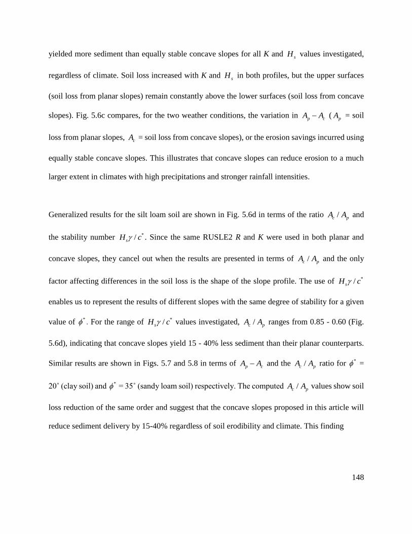
148

yielded more sediment than equally stable concave slopes for all K and sH values investigated,

regardless of climate. Soil loss increased with K and sH in both profiles, but the upper surfaces

(soil loss from planar slopes) remain constantly above the lower surfaces (soil loss from concave

slopes). Fig. 5.6c compares, for the two weather conditions, the variation in p cA A (

pA = soil

loss from planar slopes, cA = soil loss from concave slopes), or the erosion savings incurred using

equally stable concave slopes. This illustrates that concave slopes can reduce erosion to a much

larger extent in climates with high precipitations and stronger rainfall intensities.

Generalized results for the silt loam soil are shown in Fig. 5.6d in terms of the ratio /c pA A and

the stability number */sH c . Since the same RUSLE2 R and K were used in both planar and

concave slopes, they cancel out when the results are presented in terms of /c pA A and the only

factor affecting differences in the soil loss is the shape of the slope profile. The use of */sH c

enables us to represent the results of different slopes with the same degree of stability for a given

value of * . For the range of */sH c values investigated, /c pA A ranges from 0.85 - 0.60 (Fig.

5.6d), indicating that concave slopes yield 15 - 40% less sediment than their planar counterparts.

Similar results are shown in Figs. 5.7 and 5.8 in terms of p cA A and the /c pA A ratio for * =

20˚ (clay soil) and * = 35˚ (sandy loam soil) respectively. The computed /c pA A values show soil

loss reduction of the same order and suggest that the concave slopes proposed in this article will

reduce sediment delivery by 15-40% regardless of soil erodibility and climate. This finding

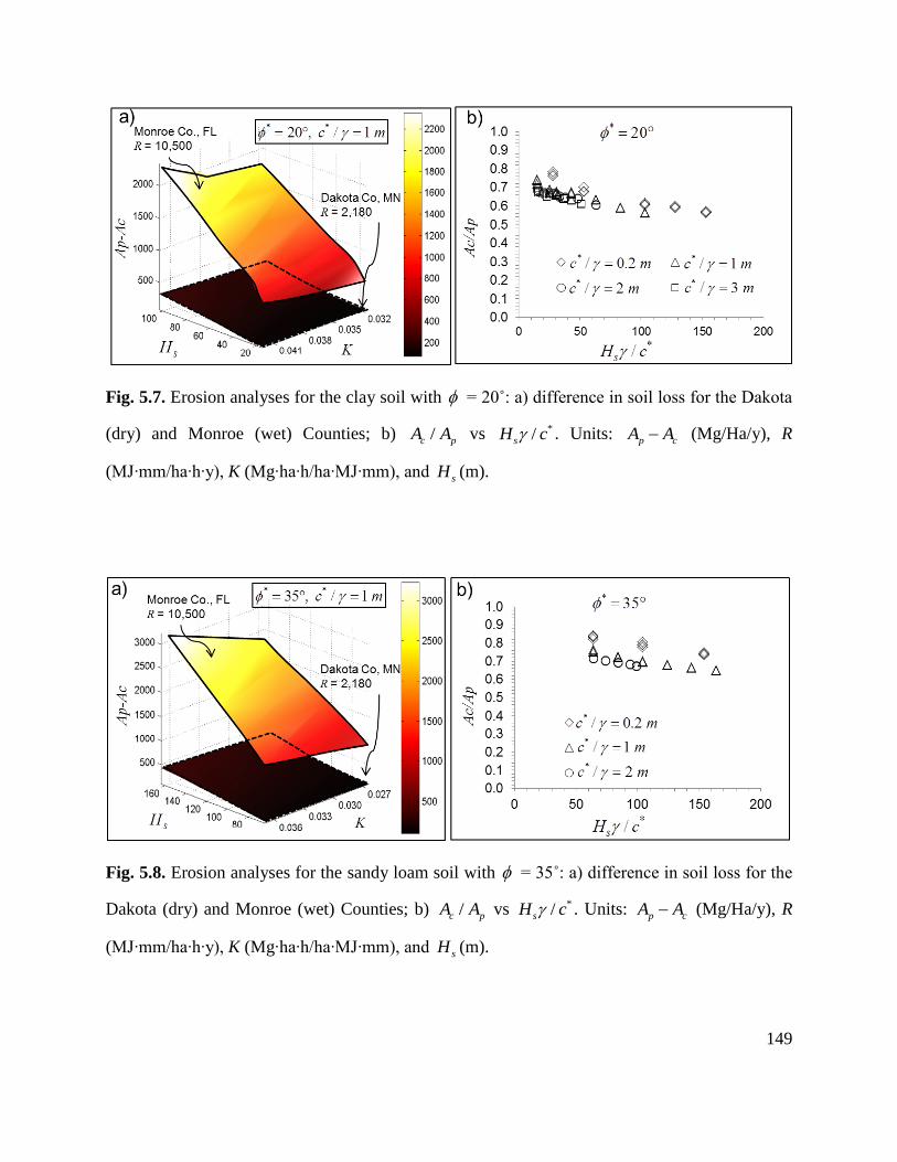
149

Fig. 5.7. Erosion analyses for the clay soil with = 20˚: a) difference in soil loss for the Dakota

(dry) and Monroe (wet) Counties; b) /c pA A vs */sH c . Units: p cA A (Mg/Ha/y), R


Fig. 5.8. Erosion analyses for the sandy loam soil with = 35˚: a) difference in soil loss for the

Dakota (dry) and Monroe (wet) Counties; b) /c pA A vs */sH c . Units: p cA A (Mg/Ha/y), R


150

is extendable to slopes having natural or artificial surface covers (C < 1) where the erosion is

proportionally reduced for both concave and planar slopes.

In Table 5.2 a comparison of the relative reduction in soil loss (1 /c pA A ) obtained here with

values reported in the literature is offered. Although a wide range of erosion reductions were found

there, it should be noted that the concave and planar slopes in those studies likely do not satisfy

the equal degree of mechanical stability (FS) purposely enforced here. Similar reductions were

obtained among the studies except for those reported by Meyer and Kramer (1969), Hancock et al.

(2003) and Rieke-Zapp and Nearing (2005), for which the reductions were significantly higher.

Meyer and Kramer (1969), and Rieke-Zapp and Nearing (2005) observed that an important amount

of sediment deposition occurred at the lowest part of the concave contours, which may explain the

higher overall reduction in sediment yield for those studies. In contrast, sediment deposition was

not indicated in the RUSLE2 prediction obtained here. Each segment of the concave slopes

proposed in this article is the steepest possible to satisfy mass equilibrium requirements, and

sedimentation on the profile will likely not occur, especially at large values of * .

Sensitivity to construction accuracy

Fig. 5.9 shows results obtained from the construction sensitivity analyses for concave slopes with

FS = DFS = 1 ( * and *c c ) for a range of * and */sH c values, with results expressed in

terms of the percent decrease in FS due to the construction error. Slopes with sH ≤ Lh were

excluded from the analyses, since it was previously shown that their performing FS’s are higher

than required (conservative), and they did not present stability variations below equilibrium.

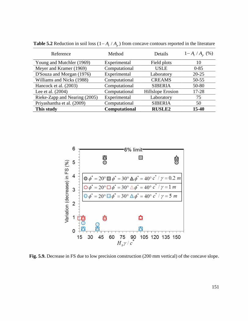
151

Table 5.2 Reduction in soil loss (1 /c pA A ) from concave contours reported in the literature

Reference Method Details 1 /c pA A (%)

Young and Mutchler (1969) Experimental Field plots 10

Meyer and Kramer (1969) Computational USLE 0-85

D'Souza and Morgan (1976) Experimental Laboratory 20-25

Williams and Nicks (1988) Computational CREAMS 50-55

Hancock et al. (2003) Computational SIBERIA 50-80

Lee et al. (2004) Computational Hillslope Erosion 17-28

Rieke-Zapp and Nearing (2005) Experimental Laboratory 75

Priyashantha et al. (2009) Computational SIBERIA 50

This study Computational RUSLE2 15-40

Fig. 5.9. Decrease in FS due to low precision construction (200 mm vertical) of the concave slope.

152

The results demonstrated that the FS’s are not significantly influenced by improper construction

within the 200 mm of vertical accuracy. The largest difference was found for slopes with * /c =

0.2 m, where 5 - 5.5% lower FS’s were obtained. Considering that the analyses were conducted

with a vertical accuracy only 1/6 that which can be achieved with typical auto-guidance equipment,

it is concluded that the stability of concave slopes is not significantly compromised by the precision

of GPS-guided equipment. In addition, practicality suggests that during construction, the top

vertical section will likely not be built, but will likely be rounded back to an average 2:1 (H:V) or

similar inclination. This in turn will increase the stability and add conservatism to the slope design.

Illustrative Examples

The design of concave slopes for long-term mechanical and erosion stability is illustrated for two

hypothetical soils in Monroe County, FL, indicating high-erosivity conditions. FEM analyses were

conducted to verify the mechanical stability for each case. The short-term stability was checked,

followed by erosion analyses for concave and planar slopes with equal FS. The two selected soils

were sand (SM or SC) and a fine grained soil (ML or CL), with the assumed mechanical properties

and design parameters for each case as shown in Table 5.3. A DFS = 1.5 was required for each

slope.

Finding the concave profile for long-term stability:

Table 5.3 summarizes the initial steps: i) obtain * and *c with Eqs. (5.8) and (5.9); and ii) estimate

the failure mechanism via Lh [Eq. (5.7)] with *c instead of c . The x-coordinates of the concave

profile were then obtained by introducing * and *c in Eqs. (5.1) – (5.6) for different values of y.

153

Table 5.3 Geometry, soil properties, and probable failure mechanisms of illustrative examples

Step i Step ii

Hypothetical

soil DFS

sH

m

(˚)

c

kPa

kN/m3

* (˚)

*c

kPa

* /c

m

Lh

m Condition

Predicted

failure

Sand

(e.g. SM or SC) 1.5 15

35 15 19 25.02 10.00 0.53 8.6 sLh H

Face failure

FS ≈ DFS

Fine grained

(e.g. CL or ML) 1.5 30 25 35 17 17.27 23.33 1.37 22 sLh H

Face failure

FS ≈ DFS

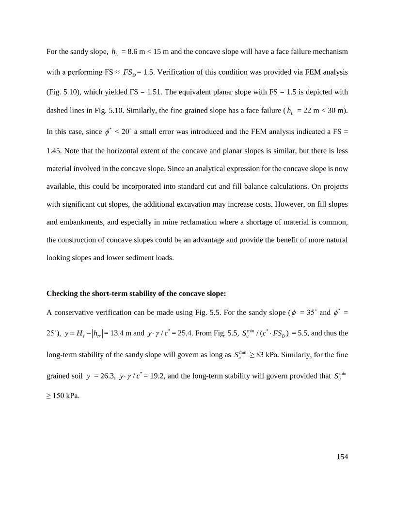
154

For the sandy slope, Lh = 8.6 m < 15 m and the concave slope will have a face failure mechanism

with a performing FS ≈ DFS = 1.5. Verification of this condition was provided via FEM analysis

(Fig. 5.10), which yielded FS = 1.51. The equivalent planar slope with FS = 1.5 is depicted with

dashed lines in Fig. 5.10. Similarly, the fine grained slope has a face failure (Lh = 22 m < 30 m).

In this case, since * < 20˚ a small error was introduced and the FEM analysis indicated a FS =

1.45. Note that the horizontal extent of the concave and planar slopes is similar, but there is less

material involved in the concave slope. Since an analytical expression for the concave slope is now

available, this could be incorporated into standard cut and fill balance calculations. On projects

with significant cut slopes, the additional excavation may increase costs. However, on fill slopes

and embankments, and especially in mine reclamation where a shortage of material is common,

the construction of concave slopes could be an advantage and provide the benefit of more natural

looking slopes and lower sediment loads.

Checking the short-term stability of the concave slope:

A conservative verification can be made using Fig. 5.5. For the sandy slope ( = 35˚ and * =

25˚), s cry H h = 13.4 m and */y c = 25.4. From Fig. 5.5, min */ )( DuS c FS = 5.5, and thus the

long-term stability of the sandy slope will govern as long as min

uS ≥ 83 kPa. Similarly, for the fine

grained soil y = 26.3, */y c = 19.2, and the long-term stability will govern provided that min

uS

≥ 150 kPa.

155

Fig. 5.10. Example case for sandy soil: = 35 ˚, c = 15 kN/m2, = 19 kN/m3 and sH = 15 m.

Required FS = 1.5. Shear strains showed for SRF = 1.52 to emphasize failure mode.

156

Erosion analyses:

Total soil loss was computed for low and high erodibility values for each soil texture (Table 5.4)

for the Monroe County, FL weather conditions. The results (Table 5.4) reveal that the sandy

concave slope yields on average 24% less sediment than its planar counterpart. Similarly, the fine

grained concave slope yields on average 35% less sediment than a planar slope with the same FS.

Conclusions

Concave slopes not only resemble natural contours, but also have superior erosion resistance. The

design of concave slopes requires: a) the definition of concave shapes that provide a desired FS,

b) a quantitative measure of the erosion/sediment delivery reduction, and c) determination of

possible loss of mechanical stability due to improper construction. In this article:

An approximate expression was described to provide the coordinates for concave slopes that

satisfy a desired FS (long-term conditions) for any combination of , c , and sH . The

methodology was shown to be conservative for * > 20˚, but provided slightly non-

conservative values of design FS for cases with * < 20˚. The errors introduced by the

methodology are less than ±6% for the majority of the cases, which is smaller than the accuracy

to which the strength parameters are typically determined.

A simplified graphical solution was developed to estimate the required undrained shear

strength min

uS such that the design long-term ( > 0) stability is assured. The value of min

uS for

concave slopes is obtained as a function of the effective strength parameters.

Results from RUSLE2 analyses indicate that the concave slopes proposed here yield 15-40%

less sediment than planar slopes of equal FS, regardless of soil erodibility and weather

157

Table 5.4 Soil parameters and results from erosion analyses of illustrative examples

Soil *

(˚) * *

1 sH

N c

R

(MJ∙mm/

ha∙h∙y)

K

(Mg∙ha∙h/

ha∙MJ∙mm)

cA

(Mg/Ha/y)

1 c

p

A

A

% avg

Sand 25.02 28.5 10,500 0.026 557 22

24 0.037 748 25

Fine

grained 17.27 21.8 10,500

0.037 1348 34 35

0.057 2347 37

158

conditions. Although the analyses were conducted on slopes with DFS = 1, the findings are

valid for slopes with other FS’s, as shown in the illustrative example.

Results from the sensitivity analyses reveal that the stability of concave slopes is not

significantly influenced by errors in the constructed profile of as great as 200 mm of vertical

deviation. Therefore, the stability is not compromised when typical high accuracy GPS

construction equipment is employed for concave slope construction.

The reduction of sediment delivery from constructed slopes is an important consideration in

limiting environmental impact during land reclamation and site development. The proposed

method suggests a rational design procedure which makes concave slopes an attractive eco-

technical alternative for more sustainable and natural appearing earthwork construction.

159

References:

Berber, M., Ustun, A., and Yetkin, M. (2012). "Comparison of accuracy of GPS techniques."

Measurement, 45(7), 1742-1746.

Budhu, M. (2011). Soil mechanics and foundations, Wiley, New York.



D'Souza, V. P. C., and Morgan, R. P. C. (1976). "A laboratory study of the effect of slope steepness

and curvature on soil erosion." J. Agric. Eng. Res., 21(1), 21-31.

Duncan, J. M. (1996). "State of the art: Limit equilibrium and finite-element analysis of slopes."

Journal of Geotechnical Engineering, 122(7), 577-596.



Haan, C. T., Barfield, B. J., and Hayes, J. C. (1994). Design hydrology and sedimentology for

small catchments, Academic Press, San Diego, CA.

Hancock, G. R., Loch, R. J., and Willgoose, G. R. (2003). "The design of post-mining landscapes

using geomorphic principles." Earth Surf. Processes Landforms, 28(10), 1097-1110.

Hoomehr, S., Schwartz, J. S., Yoder, D., Drumm, E. C., and Wright, W. (2014). "Erodibility of

low-compaction steep-sloped reclaimed surface mine lands in the southern Appalachian

region, USA." Hydrol. Processes, in press.

160

Hough, B. K. (1957). Basic soils engineering, Ronald Press Co., New York, NY.

Howard, E. J., Loch, R. J., and Vacher, C. A. (2011). "Evolution of landform design concepts."

Mining Technology: Transactions of the Institute of Mining & Metallurgy, Section A,

120(2), 112-117.



Lee, H., Koh, H., and Al'Rabia'Ah, H. A. "Predicting soil loss from logging in Malaysia." Proc.,

International Conference of GIS and Remote Sensing in Hydrology, Water Resources and

Environment (ICGRSHWE), IAHS Press, Three Gorges Dam, China, 308-315.



Martín-Duque, J. F., Sanz, M. A., Bodoque, J. M., Lucía, A., and Martín-Moreno, C. (2010).

"Restoring earth surface processes through landform design. A 13-year monitoring of a

geomorphic reclamation model for quarries on slopes." Earth Surf. Processes Landforms,

35(5), 531-548.



Meyer, L. D., and Kramer, L. A. (1969). "Erosion equations predict land slope development."

Agric. Eng., 50(9), 522-523.

161





Washington, DC.

Priyashantha, S., Ayres, B., O’Kane, M., and Fawcett, M. (2009). "Assessment of concave and

linear hillslopes for post-mining landscapes." Securing the Future and 8th ICARD,

Skellefteå, Sweden.

Rieke-Zapp, D. H., and Nearing, M. A. (2005). "Slope shape effects on erosion: A laboratory

study." Soil Sci. Soc. Am. J., 69(5), 1463-1471.





Rodríguez-Iturbe, I., Rinaldo, A., Rigon, R., Bras, R. L., Marani, A., and Ijjász-Vásquez, E. (1992).

"Energy dissipation, runoff production, and the three-dimensional structure of river

basins." Water Resour. Res., 28(4), 1095-1103.



NJ.

162


Sokolovskiĭ, V. V. (1965). Statics of granular media, Pergamon Press, Oxford; New York.

Spencer, E. (1967). "A method of analysis of the stability of embankments assuming parallel inter-

slice forces." Géotechnique, 17(1), 11-26.

Taylor, D. W. (1948). Fundamentals of soil mechanics, J. Wiley, New York, NY.

Toy, T. J., and Chuse, W. R. (2005). "Topographic reconstruction: a geomorphic approach." Ecol.

Eng., 24(1–2), 29-35.

Trimble (2013). <http://www.trimble.com/news/release.aspx?id=012203a>. (Feb. 11, 2013).


25), 135-146.



Utili, S., and Nova, R. (2007). "On the optimal profile of a slope." Soils and Foundations, 47(4),

717-729.

Williams, R. D., and Nicks, A. D. (1988). "Using CREAMS to simulate filter strip effectiveness

in erosion control." J. Soil Water Conserv., 43(1), 108-112.

Yang, C. T., and Song, C. C. (1979). "Theory of minimum rate of energy dissipation." Journal of

the Hydraulics Division, 105(7), 769-784.

http://www.trimble.com/news/release.aspx?id=012203a%3e

163

Young, R. A., and Mutchler, C. K. (1969). "Soil movement on irregular slopes." Water Resour.

Res., 5(5), 1084-1089.

164

Chapter 6. Sustainable Concave Slopes

165

This chapter is soon to be submitted to the Journal of Soil and Water Conservation or Journal of

Hydrological Processes. The co-authors of this work are Dr. Daniel Yoder and Dr. Eric Drumm.

Excerpts from this chapter will be presented at the 2014 ASABE International Meeting in

Montreal, QC, July 13-16, 2014

Abstract

While manmade slopes are traditionally constructed with planar cross sections, natural stable

slopes are usually curvilinear rather than planar. These curvilinear slope shapes with significant

concave portions are obtained as a result of evolutionary processes where entropy is maximized

through slope shape adjustments. Evidence suggests that this adjustment results in equilibrium

between rain-driven erosion and sediment transport, yielding stable concave slopes with relatively

constant shapes. This equilibrium shape is characterized by a parallel retreat with a uniform erosion

rate over time. Concave slopes are more likely to maintain stable profiles than are planar slopes,

where large amounts of soil are removed and delivered during the process of erosion equilibrium

adjustment. Since a truly stable slope must be stable in terms of both mechanical and erosion

processes, it becomes important to describe concave slopes in rainfall-erosion equilibrium and

evaluate their mechanical stability. In this article concave profiles in rainfall erosion equilibrium

are identified and described based on the well-known RUSLE2 model. Results indicate the

existence of a family of potential slope shapes satisfying the condition of uniform erosion rate

along the slope. Making use of the critical slope contour concept for a given mechanical soil

strength, those steady concave shapes that also satisfy long-term stability are investigated. A true

steady-state equilibrium slope is obtained when both erosion equilibrium and long-term

mechanical stability are achieved. This suggests that concave slopes can be constructed to achieve

166

both minimal steady-state erosion equilibrium as well as mechanical stability, leading also to more

“natural” landforms. Constructing slopes to reflect these stable shapes will provide more

aesthetically pleasing results and minimize sediment delivery during initial slope adjustment.

Introduction

Concave profiles have been presented as a way to optimize mechanical stability and water erosion

resistance of slopes (Jeldes et al. 2014, Jeldes et al. 2013). In that work, efforts were concentrated

on a) defining mechanically stable concave contours with a controlled degree of stability, and b)

quantifying their effectiveness in reducing erosion and sediment delivery while meeting mass

equilibrium requirements. This approach results in slopes that appear more natural, and constitutes

an eco-technical solution to the design of slopes as a function of geotechnical parameters familiar

to engineers. While effective in reducing erosion and providing mechanical stability, these concave

profiles may not be in equilibrium from an erosion perspective. Evidence exists that natural fluvial

systems seek erosion and sediment transport equilibrium, and in doing so may adjust their

geometry in order to achieve a steady-state form (Yang and Song 1979) that will be somewhat

unchangeable over time. This shape is usually referred as an equilibrium shape, with a concave-

like form characterized by a parallel retreat (Penck 1953, Schumm 1956, Twidale 2007). In other

words, man-made slopes (e.g., planar slopes) undergo continuous changes in slope morphology

triggered by water erosion forces in order to ultimately achieve this equilibrium condition. During

this process large amounts of soil are eroded.

Geomorphological evolution toward an erosion equilibrium state does not imply that the resulting

slopes are mechanically stable. A true equilibrium state will be achieved only when both erosion

167

equilibrium and long-term mechanical stability are satisfied. The unchangeable shape and the

minimization of sediment delivery to a relatively constant rate are attractive characteristics that

can positively impact the way slopes are constructed, and can promote a more natural and

“sustainable” design. The question becomes whether we can describe fully sustainable slopes,

where both erosion and mechanical equilibrium requirements are met.

In this article the concept of steady-state landforms is explored, and from a conceptual perspective,

the changes in slope morphology toward a concave erosion equilibrium shape are described. Based

on the fundamentals of the RUSLE2 erosion model, concave profiles in water erosion equilibrium

are identified and described, and a simple approach to discern between long-term mechanically

stable and unstable erosion equilibrium shapes is proposed for any given combination of soil

stresses and strength. A definition of the approximate limiting erosion rate at which equilibrium

erosion shapes become mechanically stable and thus sustainable is explored, and a mathematical

expression to obtain this limiting erosion rate is offered as a function of the Mohr-Coulomb

parameters.

Background

Concave profiles as erosion equilibrium shapes

In nature slope profiles are rarely uniform, but are usually curvilinear. This seems to be the result

of a natural geomorphological evolution process of streams and slopes, where an optimum

equilibrium profile is sought (Schor and Gray 2007). According to Leopold and Langbein (1962),

the distribution of the energy in a fluvial system tends toward a state of maximum entropy, which

is characterized by a uniform energy dissipation, where the same energy dissipation is experienced

168

at each point in the landscape (Miyamoto et al. 2005). Leopold and Langbein (1962) showed that

the most probable longitudinal profile in a fluvial system is concave. Later studies have validated

Leopold and Langbein’s ideas (Molnár and Ramírez 1998, Rodríguez-Iturbe et al. 1992, Yang and

Song 1979), but also have introduced new concepts such as minimum entropy production as a

characteristic of steady equilibrium of a geomorphic system (Miyamoto et al. 2005), and the

concept of minimum rate of energy dissipation experienced by equilibrium shapes (Yang and Song

1979). According to Yang and Song (1979), if fluvial systems deviate from an equilibrium state,

the properties of slope inclination, roughness, channel geometry, and flow velocity will experience

continuous adjustments in order to again achieve the steady equilibrium state. Other authors have

also proposed concave profiles as the equilibrium or steady shape in fluvial systems (Goldrick and

Bishop 2007, Larue 2008, Smith et al. 2000, Snyder et al. 2000).

Steady concave shapes have also been proposed as the result of hillslope evolution. According to

Pelletier and Rasmussen (2009), slopes in more humid areas tend to be more complex in cross

section (concave slope with convexity at the upper portion), while slopes in more arid regions tend

to have concave forms. According to Schumm (1956), complex slope shapes are formed mainly

by gravity driven forces, since in humid areas soils are usually covered by thick vegetation and the

role of water erosion is reduced. On the other hand, when the slope surface is affected by rainfall

driven erosion, the formation of concave equilibrium slopes is expected (Schumm 1956), and, at

the point of equilibrium, parallel or lateral slope retreat occurs where the equilibrium concave

shape is maintained over time (Nash 1980, Pelletier and Rasmussen 2009, Schumm 1956). The

equilibrium shape is characterized by a uniform rate of erosion everywhere on the slope profile

(Hack 1960, Montgomery 2001). Twidale and Milnes (1983) proposed that parallel retreat in

169

concave slopes occurs sequentially in a series of soil movement stages starting from the slope toe

and evolving upward until the same slope concavity shape is formed again.

This geomorphology concept of a steady-state condition is not exempt from criticisms. Bracken

and Wainwright (2008) reviewed several methods employed to measure geomorphological

equilibrium, and conclude that all are flawed. They also argued that the lack of a precise definition

of the spatial and temporal scales in geomorphology evolution makes many of the ideas related to

steady forms untestable. Phillips (2011) states that even though steady-state conditions are

sometime observed in nature, it is not a realistic representation of how geomorphologic evolution

works in general. He also suggests that the idea of concave profiles as the equilibrium shape in

fluvial systems is not well supported by empirical or theoretical evidence, casting doubt upon the

Yang and Song (1979) concept of continuous system adjustments to reach equilibrium.

Nevertheless, the fact that geomorphological studies cannot explain or include each and every

single variable involved in this very complex behavior does not imply that they explain nothing.

As Phillips (2011) recognized, steady-state assumptions have been useful in interpreting and

modeling the evolutionary behavior of earth systems. Furthermore, there is a universal tendency

for all natural processes--including geomorphological systems--to adjust and readjust themselves

to dynamic equilibrium, i.e., through continuous adjustments between processes like erosion and

soil resistance (Abrahams 1968, Ahnert 1994). Through these dynamic adjustments, steady-state

landform shapes may be obtained (Abrahams 1968, Thorn and Welford 1994). Steady-state forms

may indeed be dependent on the time scale and require unchanging boundary conditions (Thorn

and Welford 1994), but if any external agent disturbs this steady equilibrium condition dynamic

170

adjustments will exist, so that the system will be naturally reshaped to re-obtain the steady-state

form.

Slope shape evolution and equilibrium profiles: A conceptual model

Considering that slope water erosion is a process involving water flow and sediment transport, the

generalized principle of minimum rate of energy dissipation (Yang and Song 1979) may be used

to explain the concept of steady-state equilibrium shapes and parallel retreat observed in slope

evolution. Here, a simple conceptual model that attempts to explain the changes in morphology of

slopes actively eroded by water is offered. For a slope in an initial un-balanced state (e.g., a planar

slope), continuous changes in the slope geometry and water flow velocities are expected in order

for the system to adjust and reach equilibrium. In this process, the overall erosion rate would

gradually decrease until a constant rate of erosion along the profile is achieved. The evolution

toward a constant rate of erosion implies a reduction in the difference in energy entering and

leaving the system with respect to a previous point in time, eventually reaching a minimum.

According to Hack (1960), the steady-state equilibrium of the landscape requires the existence of

“opposing forces” counteracting and balancing each other, such that energy dissipation can exist.

As it is explained in the following paragraph, these “opposing forces” can conceptually be the

slope length and slope angle.

Erosion increases with slope length through the increase in cumulative runoff. The effectiveness

of that runoff in detaching sediment or in transporting eroded sediment depends, however, not only

on the amount of runoff, but also on its turbulent energy, which for a defined surface condition is

determined by the slope steepness. This means that on a planar slope the detachment and transport

171

rates will increase (Fig. 6.1), as the steepness is constant but the slope length is increasing (Young

and Mutchler 1969). In contrast, on a concave slope the steepness decreases with increased slope

length, so the increase in detachment and transport potential due to the increased slope length may

be counteracted by the reduction due to decreased steepness. This is consistent with Hack’s (1960)

idea of opposing effects balancing each other. This natural morphology evolution process toward

a concave slope requires a combination of soil detachment along the contour and soil deposition

at the slope base (Fig. 6.1) until an equilibrium state is reached, where the concave geometry will

experience a constant detachment and transport rate at every point along the slope. At this stage,

the slope profile will not suffer further adjustments and the slope will start eroding backwards in

a parallel retreat fashion as illustrated in Fig. 6.2. If the slope deviates from this equilibrium state,

the system will again experience continuous adjustments such that the steady equilibrium state is

reached again.

Notice that over time, the sharp edge at the top of the slope may be naturally shaped to a convex

form (Fig. 6.2), yielding a more complex slope contour as seen in many natural landscapes in more

humid areas. It is not clear if this convexity is formed due to high erodibility soil conditions

triggered by runoff coming over the top edge that would infiltrate and saturate the soil, or due to a

series of small mechanical failures given the steepness of the contour and the effects of transient

flow through the top edge. Since the mechanisms behind the formation of convexity at the upper

portion of the slope are not fully understood, this effect is not included in the development of the

model in the subsequent sections.

172

Fig. 6.1. Conceptual model of slope morphology evolution by water erosion.

Fig. 6.2. Illustration of the parallel retreat concept. The sharp edge at the top of the slope may be

naturally eroded (becoming convex) if there is runoff coming over the top edge of the slope. This

effect is not included in the proposed model.

173

Methodology

Conceptual Development

From the previous discussion it can be inferred that physical processes may shape slopes into

steady concave profiles, and it will be assumed that concave profiles represent a topographic

equilibrium condition that is more likely to remain steady over time than for planar profiles. Here,

our efforts are not concentrated on modeling the time-scale geomorphological evolution of slopes,

but rather on describing the equilibrium shape that will provide a parallel retreat. In this vein, once

the concave equilibrium shape has been developed the main mechanism inducing parallel retreat

is erosion, and therefore, soil deposition will not be included in this model.

As described above, the steady-state concave shape is characterized by a uniform water erosion

rate. However, there are many potential concave profiles that can satisfy this condition, and the

steady-state shape may not be unique. This may be explained using the widely recognized Revised

Universal Soil Loss Equation RUSLE2 (USDA-ARS 2008):

A R K LS C P (6.1)

where the predicted soil loss A (units of / /Mg ha y ) is directly proportional to: the rainfall

erosivity R (units of /MJ mm ha h y ) quantifying the rainfall’s erosive potential; the soil

erodibility K (units of /Mg ha h ha MJ mm ) defining the soil’s susceptibility to that erosivity;

the topographic factor LS (dimensionless) representing slope length and steepness effects; the

surface cover factor C (dimensionless); and the conservation practices factor P (dimensionless).

To observe solely the influence of the landscape topography or slope shape on the erosion rate, let

us assume that all the variables remain constant across the landscape except the topographic factor

174

LS, which corresponds to the combined action of the slope length factor L and the slope steepness

factor S. The length factor is not a function of the length along the profile, but of the slope

horizontal length . The steepness factor is a function of the angle of the slope with respect to the

horizontal, and it varies in form depending on the relative values of steepness and horizontal slope

length. The longer the horizontal slope length, the higher the observed erosion rate. Similarly, the

steeper the slope, the higher the erosion rate. Since in a planar slope the steepness is constant, the

erosion rate will uniformly increase downslope due to the increasing slope length. Fig. 6.3

illustrates the erosion rate experienced by four different points on a planar slope profile having

bare soil surface conditions, assuming that all other inputs are equal to one in order to display the

relative position differences. At the very top of the slope erosion is mainly controlled by raindrop

detachment (sheet erosion), and the erosion rate will be proportional to the slope angle. At this

point, little erosion is observed. As the runoff moves downslope it starts accumulating sufficient

energy to detach soil particles, with that energy directly proportional to the runoff length and the

slope angle. Thus, at point 1 on the profile, the experienced erosion rate 1pA will be equal to the

product of the length factor 1pL (function of the horizontal slope length 1p ) and the steepness

factor S (function of the slope angle ). Further down the slope runoff gains more energy due to

greater cumulative flow rate, and therefore the erosion rate at point 2 will be greater than at point

1 (2 1p pA A ). Analogously, the erosion rate at point 3 will be greater than at point 2, and the result

is an uninterrupted increasing erosion rate downslope (3 2 1 0p p p pA A A A ).

175

Fig. 6.3. Erosion rates experienced by a planar profile as modeled by RUSLE2 perspective.

176

On the other hand, what if any increment in slope length is compensated with a decrease in the

slope angle in such a way that the erosion remains equal along the profile? This would be the case

if the value of i iL S is constant for all segments. The resulting shape of this compensation process

would be concave with a constant rate of erosion along the profile. Notice that the whole erosion

phenomenon starts at the uppermost point of the slope, where only sheet erosion exists, and sheet

erosion is a function only of the slope angle. Different initial slope angles will yield different initial

rates of erosion, resulting in different subsequent downhill combinations of lengths and angles in

order to achieve the same rate of erosion everywhere. Thus, many concave shapes may satisfy the

condition of constant rate of erosion, each with a different level of constant erosion controlled by

the assumed angle of the top segment. Fig. 6.4a shows a profile with an initial angle 0h at the top

of the slope and an initial erosion rate 0 0( )h hA S . To maintain this erosion production constant

along the profile ( 0 1 2 3h h h hA A A A ), the angle of the slope i must continuously decrease.

Notice the erosion at i needs to be a function of iL and iS , which in turn are functions of i

and i respectively ( [ ( ) ( )]i i i if L S ). Fig. 6.4b shows a profile initially inclined at 0m at the

top. Since 0 0 m h the initial erosion rate for this case will be 0 0m hA A , and the adjustment

process to achieve a constant erosion rate will yield a profile somewhat less steep. Similarly, the

case illustrated in Fig. 6.4c corresponds to an even gentler concave profile, due to an even smaller

initial rate of erosion 0lA . Notice that for the same soil strength an increase of mechanical stability

from case a) to case c) is perceived due to the decrease in overall inclination.

177

Fig. 6.4. Illustration of a potential family of concave slopes with constant rate of erosion: a) high

rate, b) intermediate rate, and c) low rate.

178

RUSLE2 approximation to steady-state concave slopes

Normalized rate of erosion and equations for LS

Following this conceptual idea, different levels of constant erosion will determine the concavity

of the slope profile, starting from the initial angle at the top of the slope. To approach this problem,

let us first modify Eq. (6.1) and define a normalized erosion rate nA such that the amount of

erosion is identical to the topographic factor LS:

n

R

ALS

K PA

C

(6.2)

Notice that in reality R K C P is not truly constant over time. For example, the cover factor C

right after construction of a hillslope will be one (highly erodible and disturbed conditions), but as

the soil starts consolidating and vegetation starts growing on the slope surface, the factor C starts

decreasing. However, it is difficult to predict how C will change over time, and therefore, C is

assumed to be constant. Also, notice that nA is a dimensionless quantity of erosion and LS is a

function of slope length and slope angle [ ( , )LS ]. For horizontal slope lengths 0.92 m

(3 ft) LS is defined as (USDA-ARS 2008):

0.84.63 sin( ) 0.56

22.1

m

LS

(6.3)

where is the slope angle measured in degrees. The factor m in Eq. (6.3) is called the slope length

exponent, and can be calculated as follows (Foster et al. 1977):

1

m

(6.4)

where is the ratio of rill to inter-rill erosion defined as (McCool et al. 1989):

0.8

sin( ) / 0.0896

3 sin( ) 0.56

(6.5)

179

For 4.6 m (15 ft) LS is computed as:

10.8 sin( ) 0.3 , 5.122.1

, with in m (SI units)

16.8 sin( ) 0.5 , 5.122.1

m

mLS

(6.6a)

10.8 sin( ) 0.3 , 5.172.6

, with in ft (U.S. customary units)

16.8 sin( ) 0.5 , 5.172.6

m

mLS

(6.6b)

For slope lengths of 0.92- 4.6 m (3 - 15 ft), the algorithm employs a linear interpolation between

the natural logarithm of Eq. (6.3) and the natural logarithm of Eq. (6.6) with = 4.6 m (15 ft) to

calculate intermediate values of LS (USDA-ARS 2008). Notice that Eq. (6.3) is not a function of

the slope length , and the same erosion is computed at any point of the profile that is shorter than

0.92 m (3 ft). This is because only sheet erosion is observed for short flow lengths (Meyer and

Harmon 1989).

Discretization of the concave slope profile with linear segments of equal erosion rate

By assuming that a concave slope can be obtained from the assembly of a discrete number of small

linear segments (Fig. 6.5) where the same erosion rate holds on every segment of the entire length,

a selected initial erosion rate 1

nA can be employed to determine the angle of the first linear segment

1 at the top of the slope. From this point forward, each subsequent segment must produce on

average the same amount of erosion 1

nA on the segment’s length:

1

n nii

i

pA A

x (6.7)

180

Fig. 6.5. Discretization of the slope profile in small linear segments.

181

Here n

iA and ip are the erosion rate and the erosion production at the i-th segment respectively,

and ix is the horizontal length of the i-th segment. The erosion production is defined as the

product of the total erosion and the total horizontal distance at a particular point in the profile.

Therefore, ip becomes the subtraction of the erosion produced at the initial and final points of the

i-th segment (Fig. 6.5). Making use of Eq. (6.2), ip can be expressed as:

1 1 1( , ) ( , )i i i i i i ip LS LS (6.8)

Subsequently, the erosion rate at the i-th segment becomes:

1 1 11

( , ) ( , )n ni i i i ii

i

iLS

x

LSA A

(6.9)

Having a known initial erosion 1

nA and making the length of the first slope segment 1 1x = 0.92

m (since below this point erosion calculations are invariant), 1 can be determined, and with it the

coordinates of the end point of the first segment using simple trigonometry, with the initial point

as the origin of the coordinate system (Fig. 6.5). To obtain the coordinates of the second segment,

Eq. (6.9) can be employed. Here, 2 1 x ( x is the selected horizontal length of each

subsequent linear segment) and 2 1

n nA A , so 2 is the only remaining variable. Notice that 1i is

always known, and therefore i is the only variable to be determined. Repeating this process, the

angle of all the subsequent segments can be determined along with the associated (x, y) coordinates

of each point, with corresponding to the x coordinate. Notice that in the selected reference frame

the x-axis is positive to the right and y-axis is positive downward. Given the recursive nature of

the proposed methodology and the non-linearity of the RUSLE2 LS equations, a numerical solution

for i was created.

182

Since at the top of the slope ( 0.92 m) the erosion is dominated by raindrop detachment, the

prediction of the slope contour results on a linear segment. However, here the overland flow path

length is not important, and the linear shape of the first segment can be arbitrarily modified such

that it preserves the overall slope shape predicted for > 0.92 m (3 ft). A third-order polynomial

of the form

3 2( )V a b c d (6.10)

was chosen to construct a cubic spline for [0, 0.92 m]. The boundary conditions are:

( ) 0, at 0V (6.11)

1 1( ) 0.92 tan( ) at 0., 92 m (3 t) fV x (6.12)

2 1

( )tan( ) at 0.92 m (3 ft),

dVx

d

(6.13)

To satisfy a continuity condition,

2

12

( )0 at 0.92 m (3 ft),

d Vx

d

(6.14)

After imposing these boundary conditions on Eq. (6.10), the problem becomes a linear system of

equations that will provide the resulting values of a, b, c, and d, defining the polynomial function.

Different functions are obtained for different initial erosion rates 1

nA .

Sustainable slopes: mechanical and erosion stability

The approach described above produces a family of concave profiles that satisfy the water erosion

equilibrium condition. However, a truly stable slope must be stable in terms of both mechanical

and water erosion processes. Employing the critical slope contour approximation proposed by

Jeldes et al. (2013) those steady concave shapes that also have long-term stability for a given

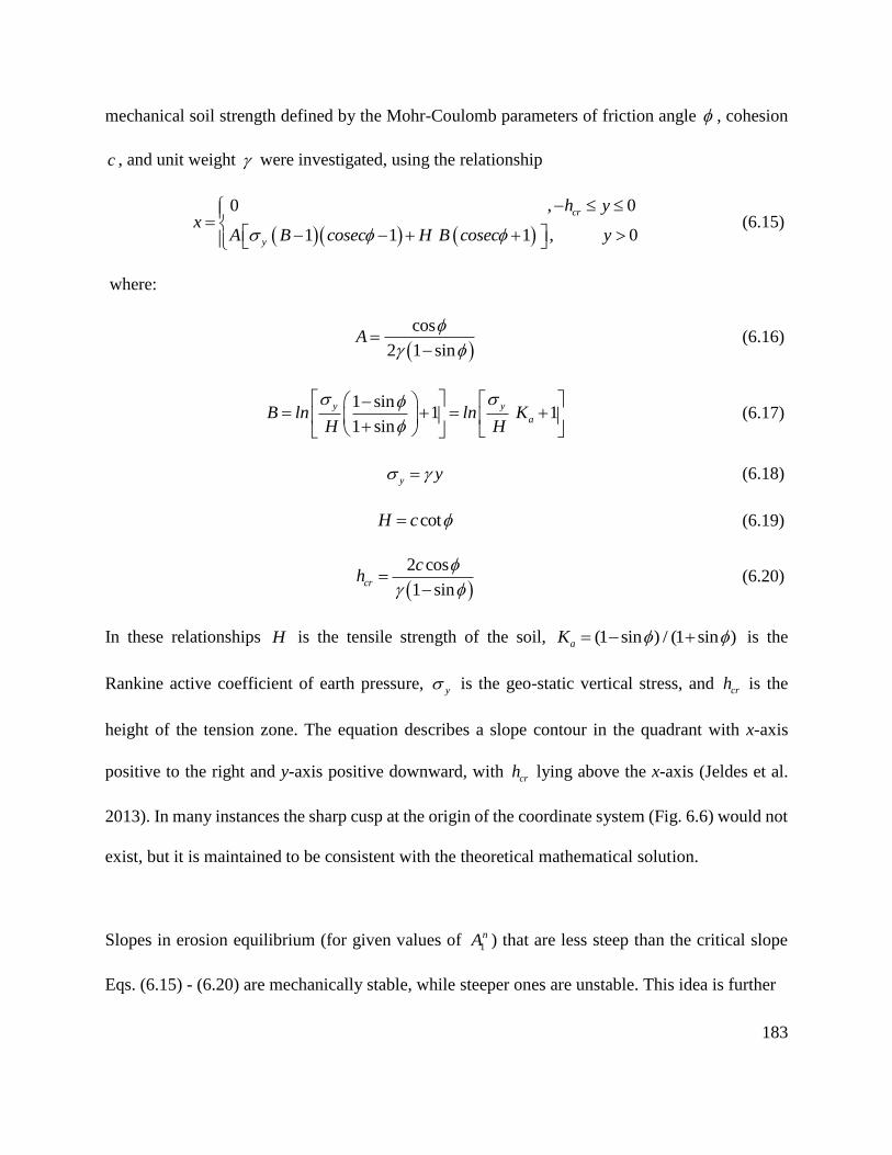
183

mechanical soil strength defined by the Mohr-Coulomb parameters of friction angle , cohesion

c , and unit weight were investigated, using the relationship

0 , 0

1 1 1 , 0

cr

y

h yx


(6.15)

where:

cos

2 1 sinA

(6.16)

1 sin

1 1 1 sin

y y

aB ln ln KH H

(6.17)

y y (6.18)

cotH c (6.19)

2 cos

1 sincr

ch

(6.20)

In these relationships H is the tensile strength of the soil, 1 sin ) / (1 sin )(aK is the

Rankine active coefficient of earth pressure, y is the geo-static vertical stress, and crh is the

height of the tension zone. The equation describes a slope contour in the quadrant with x-axis

positive to the right and y-axis positive downward, with crh lying above the x-axis (Jeldes et al.

2013). In many instances the sharp cusp at the origin of the coordinate system (Fig. 6.6) would not

exist, but it is maintained to be consistent with the theoretical mathematical solution.

Slopes in erosion equilibrium (for given values of 1

nA ) that are less steep than the critical slope

Eqs. (6.15) - (6.20) are mechanically stable, while steeper ones are unstable. This idea is further

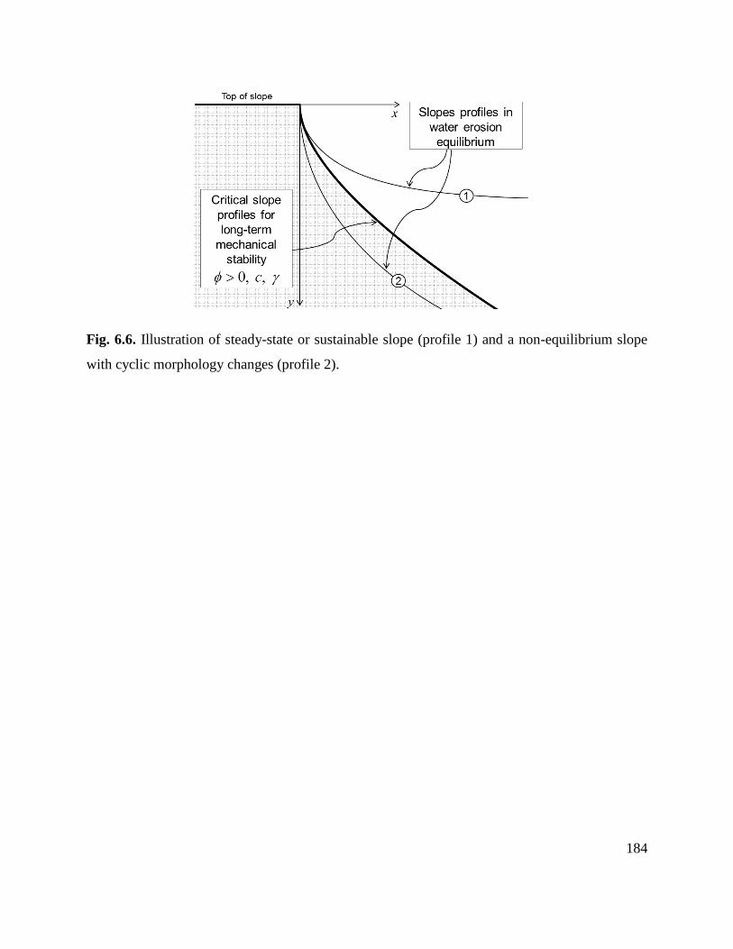
184

Fig. 6.6. Illustration of steady-state or sustainable slope (profile 1) and a non-equilibrium slope

with cyclic morphology changes (profile 2).

185

illustrated in Fig. 6.6, where two different slopes in erosion equilibrium are shown for a soil

defined by a unique combination of , , and c . Here, slope profile 1 satisfies both the erosion

and mechanical equilibrium requirements, and therefore becomes a sustainable slope with a

steady-state shape over time. Profile 2, on the other hand, only satisfies erosion equilibrium and

mechanical failures are expected, which would alter the erosion equilibrium shape. However,

natural adjustments may bring the slope to a new erosion equilibrium state, which if not

mechanically stable, will repeat the failure and natural re-shaping process, creating cyclic changes

in morphology over time.


Concave slopes with constant rate of erosion

A family of concave slopes with constant rates of erosion (1

nA = 0.506 to 1.068) along the profile

is shown in Fig. 6.7. These concave slopes are the result of a numerical solution of Eqs. (6.9) –

(6.14), with x = 0.03 m (0.1 ft). The chosen discretization length was selected to be small enough

such that the ratio 1/i i remained within the 0.9 – 0.99 range for the majority of slope length.

The computations stopped once i fell below 3°. In this family of profiles there is a clear increase

in the overall slope steepness as 1

nA increases. The overall steepness, defined as the slope of the

straight line that connects the top and the bottom of the slope, increases at a much faster rate for

1

nA 1 (Fig. 6.8). This means that the predicted equilibrium concave profiles are more sensitive

to values of 1LS . Although the entire family of profiles is in erosion equilibrium (equal erosion

rate along the profile), these concave slopes may or may not be mechanically stable, so their

stability must be analyzed based on the critical concave slope concept.

186

Fig. 6.7. Family of concave slopes with constant rate of erosion (equilibrium erosion profiles).

Fig. 6.8. The overall steepness (defined as the slope of the straight line that connects the top and

the bottom of the profile) increases at a much faster rate for 1

nA 1, as denoted by dashed line.

187

Notice that in the analyses the constant erosion is implied for the whole extent of the concave

slope. In reality, when the concave slope encounters a relatively horizontal surface (e.g., at the

bottom of the slope), part of the detached soil is deposited. For erosion to occur along a slope, the

transport capacity of the flow (cT ) must be greater than its sediment load ( q ). Transport capacity,

which is a measure of how much sediment the runoff can carry, is a function of the kinetic energy

of the flow, which decreases as the slope becomes less steep. When the flow reaches a relatively

flat area, cT becomes less than q , and the flow is not capable of detaching new soil nor transporting

the eroded soil, leading to deposition. Even though the employed equations do not capture this

effect, the eroding portion of the profile will not be affected by deposition at the bottom end of the

slope, so, the predicted profile with constant erosion rate would remain as predicted.

Sustainable slopes

Fig. 6.9 illustrates the sustainable slope concept for a medium soft clay soil with = 20˚ and /c

= 1 m. Using Eqs. (6.15) - (6.20), the critical concave slope (FS = 1) for this specific soil was

determined and plotted together with the erosion equilibrium shapes. For the purpose of this

comparison, the vertical tension zone of height crh is not displayed. The results suggest that, for

this specific soil erosion equilibrium slopes with 1

nA 1.05 would be mechanically stable, and

therefore would be sustainable with steady shapes over time. On the other hand, equilibrium

concave shapes with 1

nA > 1.05 (shown with dashed lines in Fig. 6.9) are likely to experience

mechanical failures, and changes in morphology may be observed. A second case is illustrated in

Fig. 6.10 for a sandy soil with = 30˚ and /c = 0.5 m. This time erosion equilibrium shapes

188

Fig. 6.9. Erosion equilibrium profiles and a critical concave contour for = 20˚ and /c = 1 m.

Concave slopes with 1

nA 1.05 are considered sustainable.

Fig. 6.10. Erosion equilibrium profiles and a critical concave contour for = 30˚ and /c = 0.5

m. Concave slopes with 1

nA 1.039 are considered sustainable.

189

with 1

nA 1.039 will be sustainable, while concave shapes with 1

nA > 1.039 will not. Note that

1

nA = 1.05 and 1.039 are approximated limiting values ( n

LA ) that separate sustainable and non-

sustainable concave slopes for the given soil mechanical properties. Similar chart results are shown

in Fig. 6.11 for a wide range of mechanical soil properties ( = 20˚, 25˚, 30˚, 35˚ and 40˚; /c =

0.5, 0.75, 1, 1.5, 2 and 3 m). Generalized values of n

LA are shown in Fig. 6.12 as a function and

/c . From this chart, the following approximation for n

LA is proposed: for the range of 1

nA , ,

and /c investigated here, concave erosion equilibrium slopes will be sustainable if:

1 0.02 ln[tan( )] 0.01 1.06nA

c

c

(6.21)

In practice, slopes are rarely designed for mechanical stability with FS = 1, and some additional

margin of safety is desired. Depending on the conditions and the impact of potential failure, slopes

are designed for a minimum FS always greater than 1. The concept of sustainable slopes is

extended in Figs. 6.13, 6.14, and 6.15 by introducing critical concave contours with FS > 1 (Jeldes

et al. 2014). Fig. 6.13 shows erosion equilibrium slopes and a concave contours satisfying FS

=1.25, for = 20˚, 25˚, 30˚, 35˚ and 40˚; and /c = 0.5, 0.75, 1, 1.5, 2, and 3 m. Erosion

equilibrium slopes less steep than the critical contour for a given set of and /c will not only

be sustainable, but also their shear strength along the most critical failure surface would be at least

25% greater than that required to maintain mechanical equilibrium in the long-term. Similar charts

for FS = 1.5 and 1.75 are shown in Figs. 6.14 and 6.15, respectively.

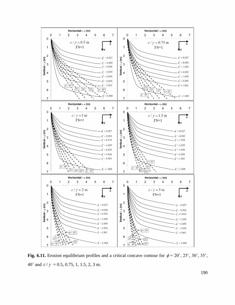
190

Fig. 6.11. Erosion equilibrium profiles and a critical concave contour for = 20˚, 25˚, 30˚, 35˚,

40˚ and /c = 0.5, 0.75, 1, 1.5, 2, 3 m.

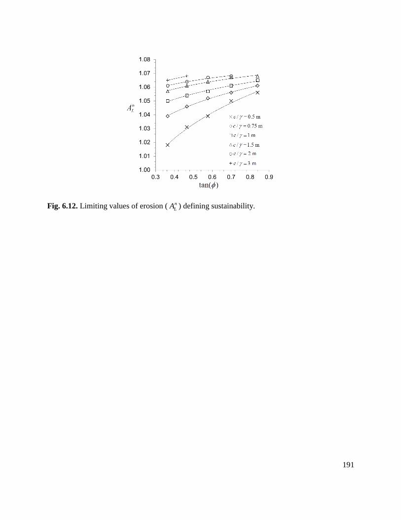
191

Fig. 6.12. Limiting values of erosion ( n

LA ) defining sustainability.

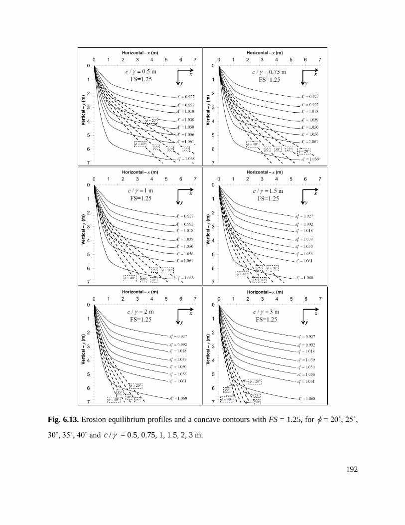
192


30˚, 35˚, 40˚ and /c = 0.5, 0.75, 1, 1.5, 2, 3 m.

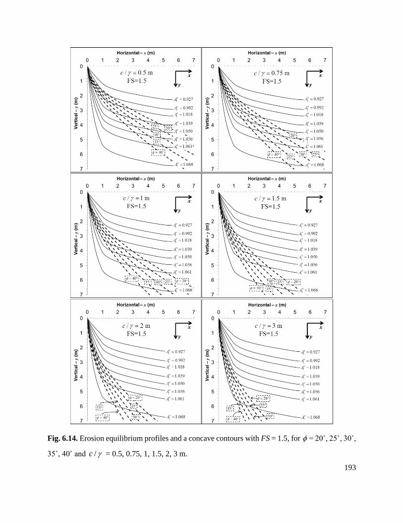
193

Fig. 6.14. Erosion equilibrium profiles and a concave contours with FS = 1.5, for = 20˚, 25˚, 30˚,

35˚, 40˚ and /c = 0.5, 0.75, 1, 1.5, 2, 3 m.

194


30˚, 35˚, 40˚ and /c = 0.5, 0.75, 1, 1.5, 2, 3 m.

195

In this article, the argument that slopes in nature are seldom planar, and concave contours are

naturally formed as a result of evolutionary processes that seek erosion equilibrium has been

presented. Therefore, why must constructed slopes be planar? The results presented here suggest

that concave slopes can be constructed to achieve both minimal steady-state erosion equilibrium

as well as mechanical stability. The desired slope profile could be selected by balancing erosion

rates and desired mechanical stability for specific site conditions and regulation requirements such

as discharge into sensitive waterbodies, highly erodible soils, and space limitations. Then, Figs.

6.13, 6.14, and 6.15 can be used as design tools for the construction of slopes reflecting more

natural landforms, while minimizing sediment delivery during initial slope shape adjustments. If

this is done, erosion and sediment control activities to handle the eroded sediment can be less

rigorous. The increasing precision of GPS-based construction equipment suggests that such

complex landforms can be now achieved with high accuracy, while deviations in the constructed

slope profile due to typical construction inaccuracies do not compromise the stability of concave

slopes (Jeldes et al. 2014). With the current construction technology, sustainable concave slopes

can become more than a theoretical exercise.

Limitations of this work

The methodology presented here has limitations that must be acknowledged. First, the topographic

equations of RUSLE2 provide the fundamental prediction of erosion equilibrium slopes. RUSLE2,

however, is defined for slope angles equal to or less than 45°, while in this analysis initial erosion

rates sometimes requiring an initial angle (angle of the first segment 1 1x = 0.92 m) exceeding

this definition were used. For example, the erosion equilibrium slope defined for 1

nA = 0.927

196

requires an initial angle of 50°, while the one defined for 1

nA = 1.068 requires an initial angle of

80°. In this sense, the limits of the empirical basis on which RUSLE2 was developed have been

stretched. However, as the flow path crosses the = 0.92 m limit, the angles rapidly decrease and

fall below the 45° definition (Fig. 6.16). Notice that the angles of the concave slope with the highest

erosion rate (1

nA = 1.068) reach 45° at x = 1.3 m, and therefore the assumption that RUSLE2 holds

for > 45° only affects a small portion of the slope. Future empirical work on slopes steeper than

45° with short flow paths is required to validate the solution for such steep initial segments.

In addition, natural slopes often include a convex portion at the top, which may be the result of

runoff coming over the top edge of the slope, increasing the soil detachment on a section that

otherwise is only affected by sheet erosion. This effect was not included in this model, and future

work is needed to understand and model this complex mechanism.

Finally, this approach does not consider the effects of transient subsurface flow, nor the short-term

stability of sustainable slopes. However, once the desired sustainable concave shape has been

selected, the effects of transient ground water flow can be investigated using commercial slope

stability software. Similarly, the short-term stability could be evaluated once the site specific

undrained shear strength has been determined. The use of sustainable concave slopes in practice

will not only provide more aesthetically pleasing results, but also contribute to the growing need

for environmental-friendly techniques for landform construction and sustainable land management

for agricultural development.

197

Fig. 6.16. Computed slope angles vs horizontal slope length.

198

Conclusions

Natural landforms adjust their shape over time in order to seek erosion and sediment transport

equilibrium. The resulting equilibrium shape is usually concave with a uniform erosion rate along

the profile. In theory, this equilibrium shape would not suffer further adjustments, so the total

erosion production is minimized. In this article, a conceptual model was offered attempting to

explain how concave equilibrium shapes slopes are formed in nature. Also from a conceptual

perspective, it was shown that the equilibrium shape may not be unique, and a family of potential

slope shapes can exist according to the level of constant erosion the slope experiences.

Using the fundamentals of the widely recognized RUSLE2 model, a set of equations to describe

concave slopes in erosion equilibrium at different levels of constant erosion was developed. The

resulting concave profiles were compared with critical concave slopes ( FS = 1) and concave slopes

having FS = 1.25, 1.5, and 1.75, identifying those shapes that satisfy both erosion equilibrium and

the desired degree of mechanical stability. A mathematical expression defining the limiting erosion

at which equilibrium erosion shapes become sustainable was provided as a function of the Mohr-

Coulomb parameters, and the limitations of this work were discussed. The obtained results suggest

that concave slopes can be constructed to achieve both minimal steady-state erosion equilibrium

as well as mechanical stability, and that the slope profile can be chosen such that erosion rates and

desired mechanical stability are balanced to satisfy site conditions and regulatory requirements.

Sustainable concave slopes not only offer superior erosion control, but also a more natural

appearing landform, being an attractive alternative to the traditional planar slopes that are typically

constructed today.

199

References:

Abrahams, A. D. (1968). "Distinguishing between the concepts of steady state and dynamic

equilibrium in geomorphology." Earth Science Journal, 2(2), 160-166.

Ahnert, F. (1994). "Equilibrium, scale and inheritance in geomorphology." Geomorphology, 11(2),

125-140.

Bracken, L. J., and Wainwright, J. (2008). "Equilibrium in the balance? Implications for landscape

evolution from dryland environments." Geological Society, London, Special Publications,

296(1), 29-46.

Foster, G., Meyer, L., and Onstad, C. (1977). "A runoff erosivity factor and variable slope length

exponents for soil loss estimates." Transactions of the ASAE [American Society of

Agricultural Engineers], 20, 683-687.

Goldrick, G., and Bishop, P. (2007). "Regional analysis of bedrock stream long profiles: evaluation

of Hack's SL form, and formulation and assessment of an alternative (the DS form)." Earth

Surf. Processes Landforms, 32(5), 649-671.

Hack, J. T. (1960). "Interpretation of Erosional Topography in Humid Temperate Regions." Am.

J. Sci., 258, 80-97.

Jeldes, I. A., Drumm, E. C., and Yoder, D. C. (2014). "Design of stable concave slopes for reduced

sediment delivery." J. Geotech. Geoenviron. Eng., (In review).



200

Larue, J.-P. (2008). "Effects of tectonics and lithology on long profiles of 16 rivers of the southern

Central Massif border between the Aude and the Orb (France)." Geomorphology, 93(3–4),

343-367.



McCool, D., Foster, G., Mutchler, C., and Meyer, L. (1989). "Revised slope length factor for the

Universal Soil Loss Equation." Transactions of the ASAE, 32, 1571-1576.

Meyer, L. D., and Harmon, W. C. (1989). "How row-sideslope length and steepness affect interrill

erosion." American Society of Agricultural Engineers, 32(2), 639-644.




Molnár, P., and Ramírez, J. A. (1998). "Energy dissipation theories and optimal channel

characteristics of river networks." Water Resour. Res., 34(7), 1809-1818.

Montgomery, D. R. (2001). "Slope distributions, threshold hillslopes, and steady-state

topography." Am. J. Sci., 301(4-5), 432-454.

Nash, D. (1980). "Forms of bluffs degraded for different lengths of time in Emmet county,

Michigan, USA." Earth Surf. Processes Landforms, 5(4), 331-345.

201

Pelletier, J. D., and Rasmussen, C. (2009). "Quantifying the climatic and tectonic controls on

hillslope steepness and erosion rate." Lithosphere, 1(2), 73-80.

Penck, W. (1953). Morphological analysis of land forms; a contribution to physical geology, St.

Martin's Press, New York,.

Phillips, J. D. (2011). "Emergence and pseudo-equilibrium in geomorphology." Geomorphology,

132(3-4), 319-326.

Rodríguez-Iturbe, I., Rinaldo, A., Rigon, R., Bras, R. L., Marani, A., and Ijjász-Vásquez, E. (1992).

"Energy dissipation, runoff production, and the three-dimensional structure of river

basins." Water Resour. Res., 28(4), 1095-1103.



NJ.

Schumm, S. A. (1956). "The Role of Creep and Rainwash on the Retreat of Badland Slopes." Am.

J. Sci., 254(11), 693-706.

Smith, T. R., Merchant, G. E., and Birnir, B. (2000). "Transient attractors: towards a theory of the

graded stream for alluvial and bedrock channels." Computers & Geosciences, 26(5),

541-580.

Snyder, N. P., Whipple, K. X., Tucker, G. E., and Merritts, D. J. (2000). "Landscape response to

tectonic forcing: Digital elevation model analysis of stream profiles in the Mendocino triple

202

junction region, Northern California." Bulletin of the Geological Society of America,

112(8), 1250-1263.

Thorn, C. E., and Welford, M. R. (1994). "The Equilibrium Concept in Geomorphology." Annals

of the Association of American Geographers, 84(4), 666-696.


25), 135-146.

Twidale, C. R., and Milnes, A. R. (1983). "Slope processes active late in arid scarp retreat." Z.

Geomorphol., 27, 343-361.



Yang, C. T., and Song, C. C. (1979). "Theory of minimum rate of energy dissipation." Journal of

the Hydraulics Division, 105(7), 769-784.

Young, R. A., and Mutchler, C. K. (1969). "Soil movement on irregular slopes." Water Resour.

Res., 5(5), 1084-1089.

203

Chapter 7. The Piling Framed Concrete Retaining Wall: Design

Pressures and Stability Evaluation

204

This chapter was submitted as an original paper to the ASCE Practice Periodical on Structural

Design and Construction, and it is currently undergoing the review process. The co-authors of this

work are Dr. Eric Drumm, Dr. Richard Bennett, and Nikola Zisi. This article would be cited as:

Jeldes, I. A., Drumm, E. C., Bennett, R. M., and Zisi, N. "The Piling Framed Concrete Retaining

Wall: design pressures and stability evaluation." Practice Periodical on Structural

Design and Construction, (In review).

Abstract

The Piling Framed Retaining Wall (PFRW) is an innovative earth retention system applicable for

soils underlain by rock, which is ideal for applications where only limited right-of-way is available

or adjacent structures limit the use of tie-back anchors. Two PFRW’s were successfully built along

the I-40/I-75 corridor in Knoxville, TN, with significant cost savings over traditional retaining wall

designs. Although the walls were designed using conventional earth pressure theories, the soil

pressures and forces acting on the wall face are not fully understood, and a rational design method

has not been fully developed. Traditional theories of lateral earth pressure assume rigid translations

or rotations as the fundamental deformation mode, when in reality more complex mechanisms of

deformation and earth pressure distributions may exist. A series of Finite Elements analyses were

used to evaluate the soils stresses on the face of the wall for various configurations of wall

geometry, backfill slopes and soil properties. From the results, simplified design equations were

developed to predict the earth pressures on the wall face and the overturning moments for stability

analyses. The proposed design equations were validated against traditional expressions, and

compared with earth pressures measured on the wall over a three year period. The measured

stresses and the numerical results suggest that the typical earth pressure distribution of the PFRW

is neither linear nor monotonically increasing, and the proposed design equations yield

205

conservative results for practical combinations of geometry and soil properties. The proposed

design methods offer a reliable way to predict wall pressures and overturning moments, and

eliminate the need to conduct extensive numerical analyses for each wall to be constructed.

Introduction

The Piling Framed Retaining Wall (PFRW) is an innovative earth retaining system, which is ideal

for applications where the overburden soil is underlain by competent rock and where only limited

right-of-way (ROW) is available or adjacent structures and underground utilities limit the use of

tie-back anchor systems. Traditional retaining structures, such as concrete cantilever walls, usually

require large excavations behind the wall, and thus may not be suitable when ROW is limited.

Similarly, the need for underground easements behind the wall to avoid buried utilities or adjacent

building foundations may constrain the use of tie-back walls. To overcome these limitations, the

Tennessee Department of Transportation (TDOT) developed this innovative PFRW concept (Pate

and Haddad 2007), and successfully implemented it in two walls along the I-40/I-75 corridor in

Knoxville, TN (Fig. 7.1). This wall concept was found to be more economical than traditional

retaining wall systems under the given geologic conditions. Despite its successful application, a

rational design method for this wall has not been fully developed, and the soil pressures and forces

acting on the structural elements are not fully understood. While traditional theories of lateral earth

pressure assume that the wall behaves like a rigid body undergoing translations and/or rotations,

in reality more complex mechanisms of deformation may exist, which in turn create earth pressure

distributions different than those predicted by classical theoretical expressions.

206

In this investigation, the Finite Element Method (FEM) was used to create numerical models to

investigate the soil pressures on the PFRW for various wall face inclinations, wall heights, and

backfill slopes. The results were compared with theoretical expressions available in the literature

for various configurations of wall geometry and soil properties. Simplified equations were

developed from the FEM analyses to facilitate the design and stability calculations of PFRWs

without the need to create geometric-specific finite element models. In addition, an approximate

design approach based on the well-known Coulomb earth pressure theory is demonstrated. Finally,

the earth pressures predicted by the design equations and the approximate design approach were

compared with soil stresses measured on one of the walls built in Knoxville, TN, referred to here

as the SmartFix wall (Fig. 7.1).

Background

The PFRW concept and the construction sequence

The PFRW configuration consists of vertical and battered driven H-piles supported on rock to

create the structural frame. The frames are spaced 3 m (10 ft) apart and are connected near the top

by a horizontal waler (Fig. 7.2). After the piles are driven, vertical tie-down anchors are installed

through the waler to provide stability against overturning (Fig. 7.2). The face of the wall is aligned

with the battered piles and consists of timber lagging that is placed sequentially from top to bottom

as the soil is being excavated. The face is finished with cast-in-place reinforced concrete placed

over the lagging and acting composite with the battered piles.

207

Fig. 7.1. The PFRWs built along the I-40/I-75 corridor (Knoxville, TN). a) The SmartFix wall and

b) The West Hills wall.

Fig. 7.2. The piling frame system forming the basis of the PFRW concept.

208

A large cast-in-place concrete cap or parapet provides mass for additional stability against

overturning. Pate and Haddad (2007) outline the details of construction of the first PFRW built in

Knoxville, Tennessee in 2005. The construction sequence can be summarized as follows: a) Initial

dry excavation and driving of battered piles (Fig. 7.3a), where the ground surface is excavated to

a depth slightly below the connection of the battered pile, the vertical pile and waler, and then the

battered piles are driven to refusal. b) Installation of walers and driving of vertical piles (Fig. 7.3b),

where the tops of the battered piles are coped to fit inside the waler which is installed with the

strong axis in the horizontal direction and welded to the top of the battered piles; the vertical piles

are driven to refusal using the waler as a template. c) Installation of tie-down anchors (Fig. 7.3c),

where holes are cut in the web of the waler, through which the tie-down anchors are drilled and

anchored to rock and a preload applied to resist overturning. d) Excavation of soil and installation

of timber lagging (Fig. 7.3d), where the soil in front of the wall is excavated and timber lagging

installed between the battered piles as the excavation progresses (Fig. 7.4). e) Construction of

structural concrete facing (Fig. 7.3e), where shear studs are installed on the top flange of the

battered pile, reinforcing steel placed, and the structural concrete facing poured; a decorative ashlar

stone finish can be obtained with a reusable form liner (Fig. 7.4). f) Pouring of concrete cap or

parapet wall (Fig. 7.3f) of 2.6 m x 0.9 m (8 ft x 3 ft) (Fig. 7.4), which provides a finished

appearance and is intended to introduce additional overturning resistance. The walls are then

backfilled and graded.

Theoretical expressions for active, passive, and at-rest earth pressure coefficients

Traditionally, lateral earth pressures for rigid walls have been estimated using simplifications or

assumptions based on elasticity and plasticity theory. The most rigorous expression for the at-rest

209

Fig. 7.3. Construction sequence for PFRW.

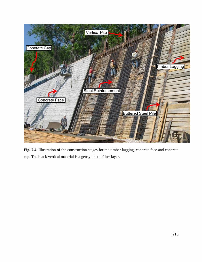
210

Fig. 7.4. Illustration of the construction stages for the timber lagging, concrete face and concrete

cap. The black vertical material is a geosynthetic filter layer.

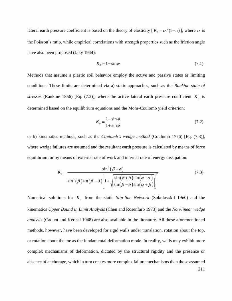
211

lateral earth pressure coefficient is based on the theory of elasticity [0 / (1 )K ], where is

the Poisson’s ratio, while empirical correlations with strength properties such as the friction angle

have also been proposed (Jaky 1944):

0 1 sinK (7.1)

Methods that assume a plastic soil behavior employ the active and passive states as limiting

conditions. These limits are determined via a) static approaches, such as the Rankine state of

stresses (Rankine 1856) [Eq. (7.2)], where the active lateral earth pressure coefficient aK is

determined based on the equilibrium equations and the Mohr-Coulomb yield criterion:

1 sin

1 sinaK

(7.2)

or b) kinematics methods, such as the Coulomb’s wedge method (Coulomb 1776) [Eq. (7.3)],

where wedge failures are assumed and the resultant earth pressure is calculated by means of force

equilibrium or by means of external rate of work and internal rate of energy dissipation:

2

2

2

sin

sin sinsin sin 1

sin sin

aK

(7.3)

Numerical solutions for aK from the static Slip-line Network (Sokolovskiĭ 1960) and the

kinematics Upper Bound in Limit Analysis (Chen and Rosenfarb 1973) and the Non-linear wedge

analysis (Caquot and Kérisel 1948) are also available in the literature. All these aforementioned

methods, however, have been developed for rigid walls under translation, rotation about the top,

or rotation about the toe as the fundamental deformation mode. In reality, walls may exhibit more

complex mechanisms of deformation, dictated by the structural rigidity and the presence or

absence of anchorage, which in turn creates more complex failure mechanisms than those assumed

212

by theoretical expressions. The distribution, magnitude and direction of the earth pressures acting

on the face of the PFRW remain unknown.

Methods

Numerical Analyses

When designing a PFRW the number of H pile sections available is relatively limited. For

modeling purposes sizes that were successfully used in the construction of the Tennessee walls

were employed. Then, the two important variables become a) the earth pressures on the wall face

that will dictate the bending stresses on the wall facing, which in turn will determine the thickness

and reinforcement of the concrete, and b) the overturning moments that will allow designers to

determine how much anchorage force is needed to provide overturning stability.

To understand how the magnitude and distribution of the earth pressures behave on the face of a

PFRW and to determine the magnitude of the overturning moments, a series of two-dimensional

plane strain models using the Finite Element Method (FEM) were created with the software

Phase2 (Rocscience Inc. 2011) for different backfill slopes ( ), wall face angles ( ), and

effective wall heights ( H ) (Fig. 7.5). Table 7.1 summarizes the wall configurations investigated;

note that =71.6˚ corresponds to a 1:3 (H:V) slope that was used on the Tennessee walls. This

inclination is commonly used in driven battered piles for bridge foundations and therefore easily

accommodated with typical pile driving equipment.

213

Fig. 7.5. Definition of “effective” wall height, wall inclination and backfill slope.

Table 7.1 Wall configurations being investigated for every combination of and /c

H = 5 m

(16 ft)

H = 7.62 m

(25 ft)

H = 10 m

(33 ft)

H = 15 m

(49 ft)

Wall Inclination

α = 0˚ α = 20˚ α = 0˚ α = 20˚ α = 0˚ α = 20˚ α = 0˚ α = 20˚

β = 50˚

β = 60˚

β = 71.6˚

β = 80˚

214

Soil properties for FEM modeling

To simulate the field conditions where the PFRW is appropriate, all the considered FEM models

consisted of soil overlaying a very strong and stiff rock. An elastic perfectly plastic stress-strain

behavior with a Mohr-Coulomb yield criterion was used to model the soil. For every combination

of wall geometry parameters , , and H (Table 7.1) values of friction angle = 20˚, 30˚, and

40˚ and cohesion over unit weight ( /c ) ranging from 0.3 to 3 m (1 to 10 ft), were considered,

where the range c = 5 - 40 kPa (104 – 835 psf) covers most of the cohesion values reported by

Mesri and Abdelghaffar (1993), and the range = 10 - 23 kN/m3 (64 – 146 pcf) would cover most

materials from clays to coarse granular soils (NAVFAC 1986). A total of 288 FEM models were

created. A different value of Young’s modulus ( E ) was input for each value of employed. An

E = 5x104 kPa (1,044 ksf) was used for soils with = 20˚ to represent a medium stiff clay, an

E = 1x105 kPa (2,089 ksf) was used for = 30˚ to represent a medium dense sand, and an E =

1.5x105 kPa (3,133 ksf) was used for = 40˚ to represent dense sand or medium dense gravel

(Bardet 1997). A single Poisson’s ratio = 0.3 was used for all the models, since it has a small

range of variation among soils (Bardet 1997). A non-associated flow rule (dilatancy angle = 0)

was implemented. The effects of using an associated flow rule ( ) in the model were also

investigated for the SmartFix case.

Structural and Geometric Properties for FEM modeling

Since there is only a limited number of H pile sections suitable for these conditions, the analysis

was limited to those employed in the construction of the Tennessee walls (e.g. the SmartFix wall)

for all the models. The battered pile was a HP 10x42 and the vertical pile was a HP 12x53. The

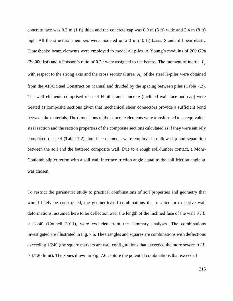
215

concrete face was 0.3 m (1 ft) thick and the concrete cap was 0.9 m (3 ft) wide and 2.4 m (8 ft)

high. All the structural members were modeled on a 3 m (10 ft) basis. Standard linear elastic

Timoshenko beam elements were employed to model all piles. A Young’s modulus of 200 GPa

(29,000 ksi) and a Poisson’s ratio of 0.29 were assigned to the beams. The moment of inertia gI

with respect to the strong axis and the cross sectional area gA of the steel H-piles were obtained

from the AISC Steel Construction Manual and divided by the spacing between piles (Table 7.2).

The wall elements comprised of steel H-piles and concrete (inclined wall face and cap) were

treated as composite sections given that mechanical shear connectors provide a sufficient bond

between the materials. The dimensions of the concrete elements were transformed to an equivalent

steel section and the section properties of the composite sections calculated as if they were entirely

comprised of steel (Table 7.2). Interface elements were employed to allow slip and separation

between the soil and the battered composite wall. Due to a rough soil-lumber contact, a Mohr-

Coulomb slip criterion with a soil-wall interface friction angle equal to the soil friction angle

was chosen.

To restrict the parametric study to practical combinations of soil properties and geometry that

would likely be constructed, the geometric/soil combinations that resulted in excessive wall

deformations, assumed here to be deflection over the length of the inclined face of the wall / L

> 1/240 (Council 2011), were excluded from the summary analyses. The combinations

investigated are illustrated in Fig. 7.6. The triangles and squares are combinations with deflections

exceeding 1/240 (the square markers are wall configurations that exceeded the more severe / L

> 1/120 limit). The zones drawn in Fig. 7.6 capture the potential combinations that exceeded

216

Table 7.2 Section Properties of Beam Elements

Cross Section Moment of Inertia, gI Area, gA

m4 in4 m4/m in4/ft m2 in2 m2/m in2/ft

Batter Pile

HP 10x42 8.75E-05 210 2.87E-05 21.0 7.98E-03 12.4 2.62E-03 1.24

Vertical Pile

HP 12x53 1.63E-04 393 5.37E-05 39.3 1.00E-02 15.5 3.28E-03 1.55

Batter Composite

(wall face) 1.43E-03 3436 4.70E-04 343.6 1.11E-01 172.1 3.65E-02 17.21

Vertical Pile

Top Encased 2.96E-03 7111 9.73E-04 711.1 1.54E-01 238.7 5.08E-02 23.87

Fig. 7.6. Resulting wall deflection over the inclined face of the wall ( / L ). Triangle and square

dots are configurations of wall geometry and soil properties excluded from the result analyses due

to large wall deflection ( / L > 1/ 240).

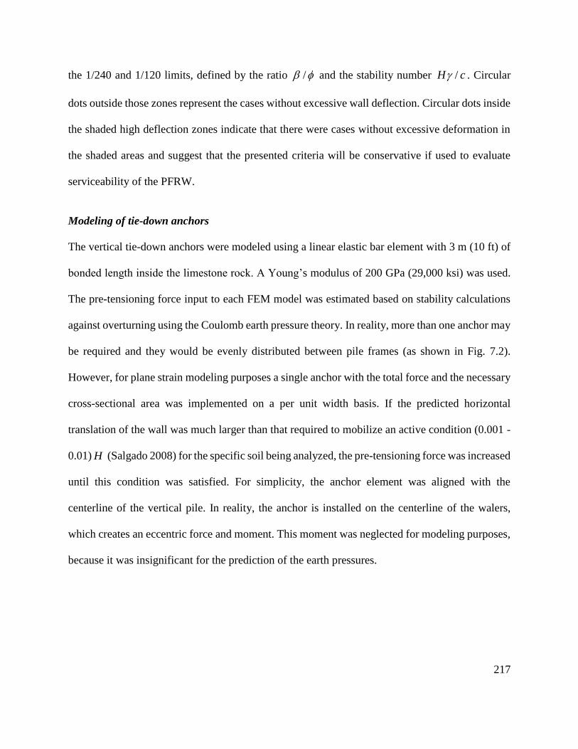
217

the 1/240 and 1/120 limits, defined by the ratio / and the stability number /H c . Circular

dots outside those zones represent the cases without excessive wall deflection. Circular dots inside

the shaded high deflection zones indicate that there were cases without excessive deformation in

the shaded areas and suggest that the presented criteria will be conservative if used to evaluate

serviceability of the PFRW.

Modeling of tie-down anchors

The vertical tie-down anchors were modeled using a linear elastic bar element with 3 m (10 ft) of

bonded length inside the limestone rock. A Young’s modulus of 200 GPa (29,000 ksi) was used.

The pre-tensioning force input to each FEM model was estimated based on stability calculations

against overturning using the Coulomb earth pressure theory. In reality, more than one anchor may

be required and they would be evenly distributed between pile frames (as shown in Fig. 7.2).

However, for plane strain modeling purposes a single anchor with the total force and the necessary

cross-sectional area was implemented on a per unit width basis. If the predicted horizontal

translation of the wall was much larger than that required to mobilize an active condition (0.001 -

0.01) H (Salgado 2008) for the specific soil being analyzed, the pre-tensioning force was increased

until this condition was satisfied. For simplicity, the anchor element was aligned with the

centerline of the vertical pile. In reality, the anchor is installed on the centerline of the walers,

which creates an eccentric force and moment. This moment was neglected for modeling purposes,

because it was insignificant for the prediction of the earth pressures.

218

Definition of boundary condition and distance to boundaries

The vertical boundaries of the soil mass were modeled such that only vertical translation and

rotation were allowed. In this way, the soil was free to experience settlement/heave at each

construction stage. The boundary conditions at the bottom of the soil mass were chosen to allow

rotation only. While the H-piles are deeply embedded into the soil which creates a soil-pile

connection somewhere between a fully fixed and truly pinned condition, they were modeled as

pinned at the contact with the rock. To reflect the additional horizontal restraint offered by the

pavement system, a second set of models were created where the battered concrete wall was pinned

at a depth of at least 0.5 m (1.6 ft) below final grade, which also corresponds to the depth of

embedment of the concrete wall face. Results indicated that this additional restraint resulted in

slightly higher normal stresses on the battered wall (Figs. 7.20 and 7.21 in Appendix), and thus it

was chosen for being more conservative.

The extent of the model boundaries was investigated via a series of FEM analyses. The analyses

indicated that boundary effects are negligible if the horizontal distance to the vertical boundaries

are not less than 6 H for the = 0˚ cases and no less than 12 H for the = 20˚ including 4 H of

sloped backfield as shown in Fig. 7.7. A soil depth below the excavation level equal to H was

implemented for each model. Even though this value is somewhat arbitrary, the pinned condition

of the wall at the final grade level helps to reduce the influence of the embedment depth of the

battered pile on the numerical computations, making the predicted stresses more insensitive to the

selected soil depth in the models.

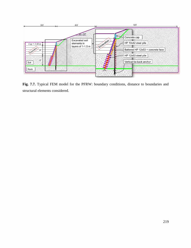
219

Fig. 7.7. Typical FEM model for the PFRW: boundary conditions, distance to boundaries and

structural elements considered.

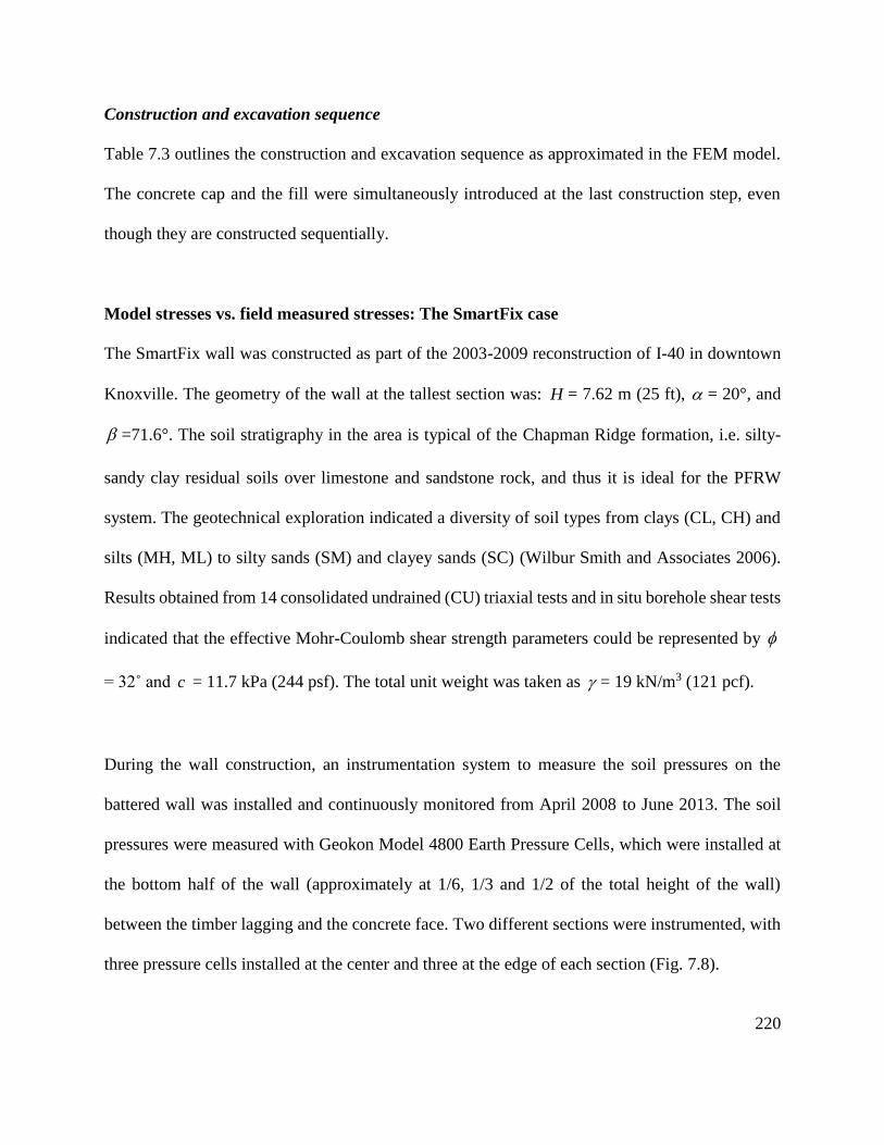
220

Construction and excavation sequence

Table 7.3 outlines the construction and excavation sequence as approximated in the FEM model.

The concrete cap and the fill were simultaneously introduced at the last construction step, even

though they are constructed sequentially.

Model stresses vs. field measured stresses: The SmartFix case

The SmartFix wall was constructed as part of the 2003-2009 reconstruction of I-40 in downtown

Knoxville. The geometry of the wall at the tallest section was: H = 7.62 m (25 ft), = 20°, and

=71.6°. The soil stratigraphy in the area is typical of the Chapman Ridge formation, i.e. silty-

sandy clay residual soils over limestone and sandstone rock, and thus it is ideal for the PFRW

system. The geotechnical exploration indicated a diversity of soil types from clays (CL, CH) and

silts (MH, ML) to silty sands (SM) and clayey sands (SC) (Wilbur Smith and Associates 2006).

Results obtained from 14 consolidated undrained (CU) triaxial tests and in situ borehole shear tests

indicated that the effective Mohr-Coulomb shear strength parameters could be represented by

= 32˚ and c = 11.7 kPa (244 psf). The total unit weight was taken as = 19 kN/m3 (121 pcf).

During the wall construction, an instrumentation system to measure the soil pressures on the

battered wall was installed and continuously monitored from April 2008 to June 2013. The soil

pressures were measured with Geokon Model 4800 Earth Pressure Cells, which were installed at

the bottom half of the wall (approximately at 1/6, 1/3 and 1/2 of the total height of the wall)

between the timber lagging and the concrete face. Two different sections were instrumented, with

three pressure cells installed at the center and three at the edge of each section (Fig. 7.8).

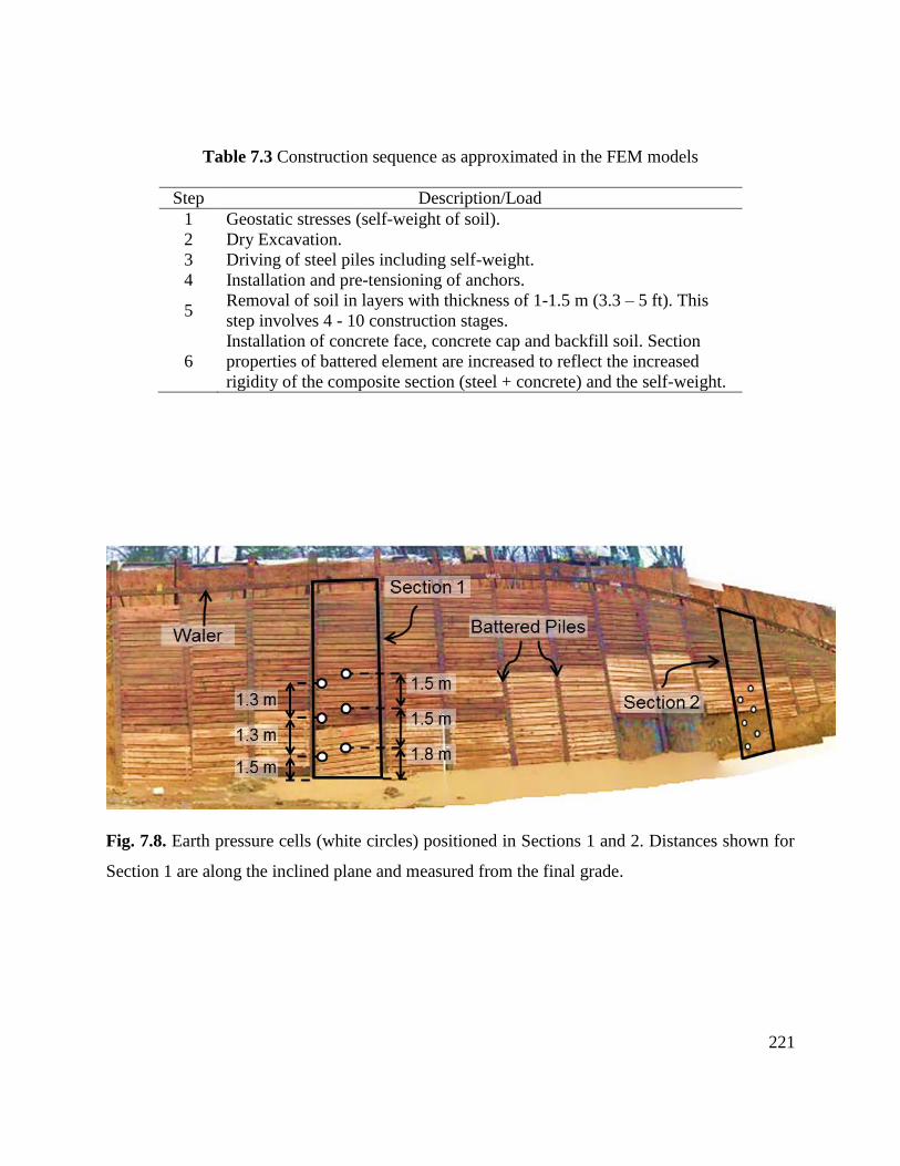
221

Table 7.3 Construction sequence as approximated in the FEM models

Step Description/Load

1 Geostatic stresses (self-weight of soil).

2 Dry Excavation.

3 Driving of steel piles including self-weight.

4 Installation and pre-tensioning of anchors.

5 Removal of soil in layers with thickness of 1-1.5 m (3.3 – 5 ft). This

step involves 4 - 10 construction stages.

6

Installation of concrete face, concrete cap and backfill soil. Section

properties of battered element are increased to reflect the increased

rigidity of the composite section (steel + concrete) and the self-weight.

Fig. 7.8. Earth pressure cells (white circles) positioned in Sections 1 and 2. Distances shown for

Section 1 are along the inclined plane and measured from the final grade.

222

The field measured earth pressures at different time points were compared with those predicted by

a FEM model with the geometry and material properties corresponding to the SmartFix wall. The

implemented elastic constants for the soil were E = 1x105 kPa (2,089 ksf) and = 0.3.


Normal stresses on battered wall

The typical distribution of the normal stresses on the battered wall obtained with FEM analyses

are shown in Fig. 7.9 for a wall of effective height H = 7.62 m (25 ft) (SmartFix height)

constructed in a sandy soil with = 30˚ and /c = 0.3 m (1 ft) [e.g. c = 5.7 kPa (119 psf) and

= 19 kN/m3 (121 pcf)]. The theoretical Rankine active stress on a vertical plane for this soil is

also plotted in dashed lines for comparison purposes. The FEM results are consistent with the

literature (Coulomb 1776, Sokolovskiĭ 1960) where for inclined walls the earth pressures decreases

as the wall face inclination approaches the friction angle . Higher earth pressures are obtained

when the backfill slope increases. The classical Rankine stresses are, in general, much higher

than those predicted by the FEM, and would produce over-conservative force resultants and

overturning moments for stability calculations. The FEM results for all the geometric combinations

show a sharp increase of stress as the depth approaches the final grade, which is a result of a higher

horizontal restraint at that point. This is particularly evident for the = 50˚ case where the large

inclination and pinned pile tip induce a more at-rest state of lateral soil pressure. Similar earth

pressure distributions were obtained for all the investigated cases.

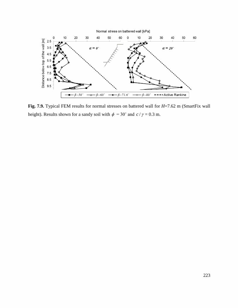
223

Fig. 7.9. Typical FEM results for normal stresses on battered wall for H=7.62 m (SmartFix wall

height). Results shown for a sandy soil with = 30˚ and /c = 0.3 m.

224

To provide a simplified means to design the structural members of the wall, equivalent uniform

pressures normal to the wall face (Neq ) were calculated for all the cases (Fig. 7.10a). The

equivalent uniform pressure is that pressure which will produce the same force resultant as the

original FEM pressure distribution, with no significant changes in the design moments and shear

forces. The resulting Neq vs. H are shown in Fig. 7.11 for the = 30˚ and /c = 1 m (3.3 ft)

soil case, for a wall with = 71.6˚ (SmartFix wall inclination) for = 0˚ and 20˚. Also shown in

Fig. 7.11 are the equivalent uniform pressures obtained via the theoretical Coulomb and the

Coulomb with tension correction methods (Bowles 1968) (Fig. 7.10b). The Coulomb theory

accounts for the effects of sloped backfills and inclined wall faces, and the tension correction

removes the small artificial tensile stress that is calculated due to the soil cohesion. The Coulomb

uniform pressures with tension correction resulted in a conservative prediction of the normal

stresses for the most detrimental conditions (high and steep walls with sloped backfills and soils

with low cohesion); however, the Coulomb predicted soil pressures become lower than the FEM

prediction (unconservative) as the soil cohesion increases and the wall inclination decreases as

illustrated in Fig. 7.12 for the = 50˚and = 20˚ case (same soil properties). The Coulomb

uniform pressure with tension correction may constitute a conservative simplified design approach

if the predicted stresses are higher than those predicted by the FEM. This matter is illustrated later

for the SmartFix field case study.

Generalized FEM results in terms of the dimensionless quantities /Neq c and /H c are shown

in Fig. 7.13 for the = 30° case. This figure shows the potential range of normal stresses over the

battered wall, represented here by the two bounds of wall inclinations investigated

225

Fig. 7.10. Definition of equivalent normal distributed pressures Neq : a) FEM and b) Coulomb and

Coulomb with tension correction.

Fig. 7.11. Equivalent normal uniform stress Neq vs. wall height H, for the = 30˚ and /c =

1 m soil case and the SmartFix wall inclination = 71.6˚. a) = 0˚ and b) = 20˚.

226

Fig. 7.12. Illustration of a case when the theoretical Coulomb earth pressures are lower than FEM

predictions, and therefore unconservative ( = 30˚ and /c = 1 m, = 20˚, and = 50˚).

Fig. 7.13. Dimensionless equivalent normal earth pressures vs. stability number as predicted by

FEM for = 30˚. a) = 0˚ and b) = 20˚.

227

( = 50˚ and 80˚), and can be used to obtain the expected equivalent uniform pressure given the

geometrical wall configuration ( , , and H ) and the Mohr-Coulomb soil properties ( and

/c ). Similar charts for the = 20° and 40° were created (Figs. 7.22, 7.23 and 7.24 in Appendix).

For each set of data, a linear regression was fit. Within each value of , the slope for = 50˚ is

somewhat similar for = 0˚ and 20˚, indicating that the stress /Neq c is not highly affected by

the backfill inclination at low values of . The role of the backfill, however, becomes significant

as the wall becomes steeper.

Destabilizing moments for overturning stability

The forces and moment arms used to calculate the wall overturning moments ( M ) are illustrated

in Fig. 7.14. FEM results are compared with theoretical values from Coulomb pressures acting on

the inclined wall and at-rest pressures acting on vertical cap. The FEM shear forces along the

vertical edge of the cap were neglected, since they create a moment that resists the overturning.

The FEM and Coulomb shear components on the battered wall act through the point of rotation

and do not play any role in the overturning moment. Fig. 7.15 shows results for the = 30˚ and

/c = 1 m (3.3 ft) soil case for walls with = 71.6˚ (SmartFix wall inclination) and = 0˚ and

20˚. Similarly to the normal stress cases, the moments calculated via Coulomb’s theory are a

conservative prediction for the most detrimental wall conditions, but it under predicts the moments

for the cases with low . Notice that FEM and Coulomb moments follow a similar trend as H

increases.

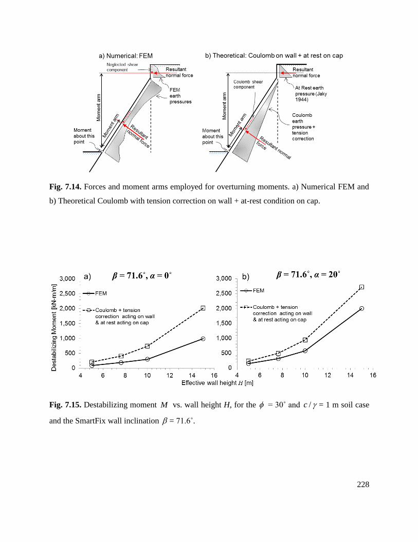
228

Fig. 7.14. Forces and moment arms employed for overturning moments. a) Numerical FEM and

b) Theoretical Coulomb with tension correction on wall + at-rest condition on cap.

Fig. 7.15. Destabilizing moment M vs. wall height H, for the = 30˚ and /c = 1 m soil case

and the SmartFix wall inclination = 71.6˚.

229

FEM results in terms of a normalized moment /eqM cM and the dimensionless number /H c

are shown in Fig. 7.16 for the = 30˚ case. The normalized moments follow a linear trend. Note

that the results in Fig. 7.16 include all the investigated values of , and therefore the regression

equation is independent of the wall inclination. For all the investigated cases R2 ≥0.85 and indicates

that a linear trend is appropriate. Similar resulting linear trends were also obtained for the = 20˚

and 40˚ cases (Figs. 7.25, 7.26 and 7.27 in Appendix).

Design equations to predict earth pressures and destabilizing moments

From the regression analyses based on the FEM results previously described, analytical

approximations were developed to predict the equivalent uniform pressures Neq and the

overturning moments M as a function of the wall geometry and the soil properties. By assuming

linear behavior of the quantities between = 0˚ and 20˚, and between = 20˚ and 30˚, and =

30˚ and 40˚, the following equations for Neq and M were obtained:

tan

0.018 (1 tan )tan

Neq H

(7.4)

45 (1 1.5 tan ), with in m (SI units)

3.1 (1 1.5 tan ), with in ft (U.S. customary units)

H H

H H

M

M

(7.5)

Note that M has SI units of kN-m/m, since the constant “45” has units of kN/m. Likewise, M

has U.S. customary units of kip-ft/ft. A validation of these simplified models is offered in Fig. 7.17

for all the cases comprising = 30˚. Here, Neq (Fig. 7.17a) and M (Fig. 7.17b) predicted by

Eqs. (7.4) and (7.5) respectively, are plotted against the FEM predictions. Notice that the

distribution of the points tends to follow the 1:1 (45˚) line, indicating correlation between the

230

Fig. 7.16. Normalized overturning moment vs. stability number as predicted by FEM for = 30˚.

Fig. 7.17. Validation of design equations: a) Neq (kPa) and b) M (kN-m/m).

231

simplified proposed equations and the FEM results. The ratio between the design equation and the

FEM prediction for Neq is 1.2 and for M is 1.5, suggesting that on average the design equations

predict 20% higher values of Neq and 50% higher values of M , making the design equations

more conservative than the FEM prediction. Similar ratios were obtained for the = 20˚ and 40˚

cases. The coefficients of variation of these ratios are less than or equal to 40% for all cases. It is

important to keep in mind that the range of applicability of the design equations is constrained to

values of = 0 - 20˚, = 50 - 80˚, H = 5 - 15 m (16 – 49 ft), = 20 - 40˚ and /c = 0.3 – 3 m

(1 – 10 ft), and values outside the range of applicability are not defined by the Eqs. (7.4) and (7.5).

The SmartFix case: predicted vs. measured stresses on the inclined wall

Measured earth pressures over a period of 3 years (2010 – 2013) are shown in Fig. 7.18, along

with the FEM predicted distribution of the earth pressures for the SmartFix model configuration

[ H = 7.62 m (25 ft), = 20°, = 71.6°, = 32˚, c = 11.7 kPa (244 psf), = 19 kN/m3 (121 pcf)]

using both, a non-associated ( = 0˚) and an associated ( ) flow rule, where is the dilation

angle. For comparison, two theoretical earth pressures that include the effects of , , and the

soil-wall interface friction angle are also shown: Wedge Equilibrium (Coulomb 1776) and Upper

Bound Limit Analyses (Chen and Rosenfarb 1973). The vertical line represents the corresponding

value of Neq obtained from the proposed design equation [Eq. (7.4)]. Also shown is the equivalent

uniform stress obtained from the simplified Coulomb design approach that includes tension

correction.

232

Fig. 7.18. Field measured stresses over time vs. theoretical and numerical earth pressures.

233

The results in Fig. 7.18 indicate that the pressures predicted by the numerical models are in

reasonable agreement with the field measurements, with the exception of the larger predicted

stresses near the bottom of the wall. The FEM predicted stresses comprising an associated soil

( ) are on average 11% higher than those obtained with the non-associated model; similar

behavior has been previously described in the literature (Benmeddour et al. 2012). While dilation

effects are observed in soils, they rarely follow an associated flow rule, and dilation angles are

usually smaller than . It has been also shown that associated models tend to over predict failure

loads in the context of “confined” problems. The PFRW can be considered as a partially confined

system, and thus the degree of “over-prediction” is moderated, which makes the model more

insensitive to the selected value of . The results in Fig. 7.18 suggest that the equivalent uniform

pressure Eq. (7.4) (developed from non-associated FEM results) predicts the measured earth

pressures with a moderate degree of conservatism, and it is a better representation than the

Coulomb and Chen approaches for this type of wall. The simplified desing approach based on

uniform Coulomb stresses with tension correction provides, for this particular wall configuration,

a prediction of stresses higher than those obtained from Eq. (7.4), and therefore can also be used

for design. It should be kept in mind that the classical solutions assume linearly increasing pressure

distributions, typical of walls with rigid translations as the deformation mode. It has been

demonstrated that the typical earth pressure distribution of the PFRW is neither linear nor

monotonicly increasing, and classical solution methods are not always conservative for this type

of wall. A PFRW specific method such as the design equations based on FEM analyses [Eqs. (7.4)

and (7.5)] and the uniform Coulomb stresses with tension correction (when predicted values are

higher than design equations), provides a more reasonable design prediction for the potential

geometrical configurations of PFRW systems covered here.

234

Conclusions

The Piling Framed Retaining Wall is a novel system which allows top-down construction and

requires minimal right of way. This wall concept was found to be significantly less expensive than

traditional retaining wall systems for two walls of this type successfully built along the I-40/I-75

corridor in Knoxville, TN. For their design, the magnitude and distribution of the earth pressures

and overturning moments were estimated based on traditional earth pressure theories. However, a

rational design procedure for this wall system has not been fully developed.

To develop a simple design approach, a series of FEM analyses were conducted to compute the

earth pressures on the wall face and the overall destabilizing moments for a range of wall

geometries and different soil properties. The numerical results were used to develop simplified

equations for design. It was found that the typical earth pressure distribution on the face of the

PFRW is neither linear nor monotonically increasing. The design equations yield conservative

results, relative to the FEM models, for most practical geometries and soil properties. Field

measured earth pressures on the SmartFix prototype were well predicted by both, the design

equations and the design method based on Coulomb stresses with tension correction. The proposed

methods can be used to design future configurations of PFRW systems with no need to create

advanced numerical models.

Acknowledgments

This research was conducted as part of a project funded by the Tennessee Department of

Transportation (TDOT) Contract No. RES 2011-16. The authors gratefully appreciate the support

235

and guidance provided by TDOT staff Saieb Haddad, Henry Pate and Len Oliver. The field

assistance provided by Katie Peay and the data acquisition expertise of Wesley Wright were

invaluable.

236

References:

Alpan, I. (1967). "The empirical evaluation of the coefficient Ko and Kor." Soil and foundation,

7(1), 31-40.

Antão, A. N., Santana, T. G., Vicente da Silva, M., and da Costa Guerra, N. M. (2011). "Passive

earth-pressure coefficients by upper-bound numerical limit analysis." Canadian

Geotechnical Journal, 48(5), 767-780.

Bardet, J.-P. (1997). Experimental soil mechanics, Prentice Hall, Upper Saddle River, N.J.

Benmeddour, D., Mellas, M., Frank, R., and Mabrouki, A. (2012). "Numerical study of passive

and active earth pressures of sands." Comput. Geotech., 40(0), 34-44.

Bowles, J. E. (1968). Foundation analysis and design, McGraw-Hill, New York,.

Brooker, E. W., and Ireland, H. O. (1965). "Earth pressures at rest related to stress history."

Canadian Geotechnical Journal, 2(1), 1-15.

Caquot, A. I., and Kérisel, J. L. (1948). Tables for the calculation of passive pressure, active

pressure and bearing capacity of foundations, Gautier-Villars, Paris.

Chen, W.-F. (2007). Limit analysis and soil plasticity, J. Ross Pub., Ft. Lauderdale, FL.

Chen, W. F., and Rosenfarb, J. L. (1973). "Limit analysis solutions of earth pressure problems."

Soils and Foundations, 13(4), 45-60.

Coulomb, C. A. (1776). Essai sur une application des règles de maximis & minimis à quelques

problèmes de statique, relatifs à l'architecture, De l'Imprimerie Royale, Paris.

237

Council, I. C. (2011). "Structural Provisions." International Building Code 2012, ICC (Distributed

by Cengage Learning).

Fioravante, V., Jamiolkowski, M., Lo Presti, D. C. F., Manfredini, G., and Pedroni, S. (1998).

"Assessment of the coefficient of the earth pressure at rest from shear wave velocity

measurements." Géotechnique, 48(5), 657-666.

Guojun, C., Songyu, L., Puppala, A. J., and Liyuan, T. (2011). "Assessment of the Coefficient of

Lateral Earth Pressure at Rest (Ko) from In Situ Seismic Tests." Geotech. Test. J., 34(4),

GTJ102520 (102511 pp.).

Hendron, A. J. (1963). "The behaviour of sand in one-dimensional compression." Ph.D. thesis,

University of Illinois, Urbana, IL.

Hendron, A. J., Fulton, R. E., Mohraz, B., Agency, U. S. D. A. S., and Center, U. S. A. F. S. W.

(1963). The energy absorption capacity of granular materials in one-dimensional

compression: final report, Research Directorate, Air Force Special Weapons Center, Air

Force Systems Command, Kirkland Air Force Base.

Jaky, J. (1944). "The coefficient of earth pressure at -rest." Journal for Society of Hungarian

Architects and Engineers, 355-358.

Kulhawy, F. H., Mayne, P. W., Institute, E. P. R., and Group, C. U. G. E. (1990). Manual on

estimating soil properties for foundation design, Prepared for Electric Power Research

Institute.

Lancellotta, R. (2002). "Analytical solution of passive earth pressure." Géotechnique

238

52(8), 617-619.

Loukidis, D., and Salgado, R. (2011). "Active pressure on gravity walls supporting purely

frictional soils." Canadian Geotechnical Journal, 49(1), 78-97.

Mayne, P. W., and Kulhawy, F. H. (1982). "Ko-OCR relationships in soil." Journal of the

Geotechnical Engineering Division, 108(GT6), 851-872.



Mesri, G., and Castro, A. (1987). "C alpha Cc concept and K0 during secondary compression."

Journal of Geotechnical Engineering, 113(3), 230-247.

Müller-Breslau, H. F. B. (1906). Erddruck auf stützmauern, [s.n.], Stuttgart.


Washington, DC.

Niedostatkiewicz, M., Lesniewska, D., and Tejchman, J. (2011). "Experimental analysis of shear

zone patterns in cohesionless for earth pressure problems using Particle Image

Velocimetry." Strain, 47, 218-231.

Pate, H., and Haddad, S. (2007). "Piling framed tie-down concrete retaining wall." The Magazine

of The Deep Foundations Institute, Spring 2007, 45-48.

Poncelet, and Woodbury, D. P. (1854). Sustaining walls; geometrical constructions to determine

their thickness under various circumstances, Taylor and Maury, Washington.

239

Rankine, W. J. M. (1856). "On the mathematical theory of the stability of earth-work and

masonry." Proceedings of the Royal Society of London, 8(ArticleType: research-article /

Full publication date: 1856 - 1857 /), 60-61.

Rebhann, G. (1871). Theorie des erddruckes und der futtermauern, C. Gerold's sohn, Wien.




Sherif, M. A., Fang, Y.-S., and Sherif, R. I. (1984). "Ka and K0 behind rotating and non-yielding

walls." Journal of Geotechnical Engineering, 110(1), 41-56.


Soubra, A. H., and Macuh, B. (2002). "Active and passive earth pressure coefficients by a

kinematical." Proceedings of the ICE - Geotechnical Engineering, 155, 119-131.

Sully, J. P., and Campanella, R. G. (1995). "Evaluation of in situ anisotropy from crosshole and

downhole shear wave velocity measurements." Géotechnique, 45(2), 267-282.

Tian, Q.-h., Xu, Z.-w., Zhou, G.-q., Zhao, X.-d., and Hu, K. (2009). "Coefficients of earth pressure

at rest in thick and deep soils." Mining Science and Technology (China), 19(2), 252-255.

Wilbur Smith and Associates (2006). "Report of Geotechnical Exploration Retaining No.

367102."Knoxville, Tennessee.

240

Zhao, X., Zhou, G., Tian, Q., and Kuang, L. (2010). "Coefficient of earth pressure at rest for

normal, consolidated soils." Mining Science and Technology (China), 20(3), 406-410.

Zhu, D. Y., and Qian, Q. H. (2000). "Determination of passive earth pressure coefficients by the

method of triangular slices." Canadian Geotechnical Journal, 37(2), 485-491.

241

Appendix

Active, passive, and at rest states of the soil mass

For a soil medium stressed only by its own weight, any point on a horizontal plane at depth z will

experience the same level vertical effective stress z ( is the unit weight of soil), with negligible

shear stresses. This vertical direction becomes therefore a principal stress direction 1 . From the

assumption that soil is an isotropic continuous medium, the other principal direction must be

orthogonal and act in the horizontal direction 3 . In reality, a third principal directions exist, but

for simplification of this model to 2-D, let us assume that plane strain conditions are valid and the

principal stress acting perpendicular to the paper remains intermediate between the two principal

directions described.

In geo-mechanics it is a usual practice to consider that the magnitude of the horizontal stress inside

the soil medium is proportional to the vertical stress by a constant K . In cases when the soil has

remained unaltered since formation, this constant is considered to be at-rest conditions and is

usually referred as 0K . In technical terms, 0K is the earth pressure coefficient when no lateral

deformation is allowed to occur and corresponds to the in situ state of most geo-materials. Thus,

when no external stresses act over the soil, the horizontal principal stress becomes 0K z . For most

normally consolidated soils 0 1K and the horizontal direction usually becomes the minor

principal direction. If, by some mechanism, the soil is permitted to yield laterally by gradually

decreasing the horizontal stress level and keeping the vertical stress constant, it will be observed a

progressive lateral expansion of the soil until a point when plastic deformation will start taking

place along slip lines, ideally, at constant stress values (for a perfectly plastic behavior). This point

242

corresponds to the active state in the soil medium. Since the vertical stress 1 z remained

constant, the horizontal stress has to be proportional to smaller value of K . This constant of

proportionality is called aK , the active earth pressure coefficient, and thus the lateral earth pressure

at an active state is 3a aK z , where

0aK K . On the other hand, if the soil is permitted to yield

by gradually increasing the level of lateral stress and keeping the vertical stress constant, it will be

observed a lateral compression until a point where the plastic deformation will start taking place.

At this point the soil has reached a passive condition and, analogously to the active case, the lateral

stress will be 3 p pK z , being

pK the passive earth pressure coefficient, where 0pK K . From

this discussion 3 3 3a p and therefore,

0a pK K K . Fig. 7.19 illustrates this concept

employing the Mohr-Coulomb yield criteria. These lateral extension and compression mechanisms

in the soil are observed in retaining wall problems. Wherever the structural rigidity of the system

is such as the wall will deform moving “away” from the soil a sufficient amount, an active

condition may be achieved. The opposite is true for the passive condition. The level of soil strain

required to achieve the active and passive condition is highly conditioned to the rigidity of the

structural system and its mode of deformation.

Active and passive lateral earth pressure coefficients: a literature review

Plasticity methods for the active and passive lateral earth pressure coefficient can be grouped in

two major categories: a) static based methods or b) kinematics based methods.

243

Fig. 7.19. Conceptual model of the different stress states on the retaining wall problem.

244

The static based approaches usually assume that portion of the material behind the wall is at the

verge of flowing plastically, and only the equilibrium equations and yield conditions are satisfied.

Some of the methods based on statics are listed below.

Slip-line network. This method attempts to determine the family of slip-line curves that will

develop inside the soil mass by combining the equations of equilibrium of a continuous medium

with the Mohr-Coulomb yield criterion. The results of the combination of these equations are the

differential equations of the characteristics that describe the planes where the plastic deformation

will take place. This formulation allows the implementation of more complex stress boundary

conditions; however, for materials possessing weight, the characteristic equations become

complex and exact mathematical solutions are available for a limited number of simple cases.

Sokolovskiĭ (1960), provided solutions for the lateral earth pressure problem by numerically

integrating the characteristic equations. Sokolovskiĭ reported values of active and passive lateral

and tangential earth pressures on a vertical wall considering: a) non-linearity of the slip-lines due

to soil-wall friction interaction, b) sloped backfields and c) surcharges. The shortcomings of the

slip-line method are in general related to the validity of the theoretical assumptions. Slip-line

methods only take into account stress boundary conditions, when in many practical problems

deformation conditions exist (Chen 2007); e.g. Sokolovskiĭ’s solution do not consider the amount

of deformation that must exist to bring the soil to a limiting condition. Also, in this technique, it is

assumed that only the zone inside the slip-network is in plastic equilibrium and outside this zone

the stress distribution is unknown (Chen 2007).

245

Rankine states of the soil mass. From the active and passive states of the soil defined by Rankine

(1856), expressions to calculate the active aK and passive pK earth pressure coefficients were

developed. If it is assumed that no friction exist in the soil-wall interface, any rigid rotation or

translation of the wall will develop a stress field composed of straight slip-lines that will intersect

the horizontal at 45 / 2 for the active condition and 45 / 2 for the passive case. For these

conditions the vertical and horizontal planes coincide with the principal planes and, therefore,

Rankine’s formulation [Eq. (7.6)] is an exact closed form solution of the slip-field problem.

1 1 sin

1 sina

p

KK

(7.6)

The more general expression includes the case of a vertical wall with a sloping backfield at .

degrees from the horizontal, as expressed in Eq. (7.7) (upper sign denotes the active condition and

lower sign the passive)

2 2

2 2

coscos

cos

a

p

K cos cos

K cos cos

(7.7)

The limitations of Rankine’s formulation are related to: a) the incapacity to include the soil-wall

friction interaction and b) the inability to obtain lateral earth pressures in planes other than vertical

ones.

Lower Bound in Limit Analysis. Limit analysis is a plasticity based theory that is rigorous within

the context of its assumptions. It defines two extremes, the lower and the upper bound, that

correspond to the lowest and highest collapse load that can be possibly found, whereas the true

collapse load is somewhere in between these two bounds. Similar to the slip-line method, the lower

bound theorem only requires the satisfaction of the equilibrium equations and yield conditions;

246

however, here a complete stress distribution satisfying equilibrium and yield condition everywhere

needs to be established. Lancellotta (2002), based on the lower bound theorem, developed an

analytical expression for the lateral active and passive earth pressures on vertical walls [Eqs. (7.8)

and (7.9)]. The solution includes the effects of the soil-wall friction ( ) and it simplifies to the

Rankine’s expression for frictionless soil-wall interfaces:

2 2coscos sin sin exp 2 tan

1 sin

a

p

K

K

(7.8)

1 sin

arcsin2 sin

(7.9)

Though rigorous, Lacellotta’s approach does not allow the evaluation of cases with a) sloped

backfield and b) non-vertical walls.

Kinematics based methods, on the other hand, usually involves a variety of assumed slip surfaces

that define different soil wedges. The resultant earth pressure is calculated by means of force

equilibrium or by means of external rate of work and internal rate of energy dissipation. Some of

the methods based on kinematics are listed below.

Coulomb’s wedge method. Based on the concept of limit equilibrium, Coulomb (1776) proposed

the existence of one critical slip plane where the failure of a soil mass will take place, and will

produce the maximum mobilized lateral stresses over the wall. In reality, many wedges of planar

failure surfaces can be constructed, and an optimization process to find most critical wedge is

necessary. Coulomb solved this problem in terms of force equilibrium, considering the soil weight

247

and soil-wall friction force, for a horizontal backfield. The maximum lateral force that resulted

from the equilibrium and optimization is:

21

2a aP K H (7.10)

2 1 sin

tan 452 1 sin

aK

(7.11)

where is the soil unit weight, H is the wall height. Note aK coincides with the coefficient of

earth pressure obtained from the Rankine’s stress analysis. Subsequent work conducted by

Poncelet and Woodbury (1854), Rebhann (1871) and Müller-Breslau (1906) extended Coulomb’s

wedge analysis to include the effects of a) soil-wall friction , b) sloped backfield at angle to

the horizontal and c) wall inclination at angle from to the vertical. The obtained active and

passive coefficients are (Salgado 2008):

2

2

2

sin

sin sinsin sin 1

sin sin

a

p

K

K

(7.12)

In Eq. (7.12) it is assumed that the slip failure is planar, when in reality the soil-friction along the

vertical boundary modifies the shape of the slip-lines to be curved. Also, this procedure does not

predict the distribution of the vertical and lateral stresses. Perhaps, those are the two major

shortcomings of the Coulomb’s formulation.

Non-linear wedge analysis. Recognizing the inconsistency of assuming a planar slip failure when

friction exists between soil and wall, Caquot and Kérisel (1948) provided an advanced

mathematical formulation for the earth pressure problem assuming a log-spiral failure mechanism.

248

Caquot and Kérisel reported tables of active and passive earth pressure coefficients as a function

of a) internal friction angle, b) soil-wall friction, c) angle of the sloped backfield and d) angle of

wall face inclination.

Upper Bound in Limit Analysis. This theorem states that an external load can only be resisted by

the soil mass if the external rate of work of an assumed deformation mode is less than the internal

rate of energy dissipation. If the velocity boundary conditions and the strain compatibility

equations are satisfied by any load resulting by equating the external and internal energy rates,

then the load is higher than the failure load. This theorem, assumes a perfectly plastic soil behavior

with an associated flow rule. Chen and Rosenfarb (1973) reported upper bound solutions for the

active and passive earth pressure coefficients from the optimization of a variety of assumed

failures. More recently, Soubra and Macuh (2002) proposed different active and passive earth

pressure coefficients for gravity loads, surcharge and soil cohesion, assuming a log-spiral failure

and the effects of soil-wall friction and sloped backfield. The combination of three coefficients

constitutes the lateral force acting on the wall.

Other kinematic based approaches for the passive earth pressure are a) the method of triangular

slices (Zhu and Qian 2000) and b) the upper-bond numerical analysis (Antão et al. 2011). In

general terms, all the methods previously described provide similar results; e.g. the lower and

upper bounds of the active earth pressure coefficients are close, and Sokolovskiĭ’s active

coefficients falls somewhere in between these two bounds (Loukidis and Salgado 2011). Also, in

one way or the other, all these methods assume a perfectly plastic soil behavior and they do not

account for progressive failure experienced in soils. In reality more than one active state can occur

249

after the peak or yielding has occurred (Loukidis and Salgado 2011). All methods, except those

based on Limit Analysis, do not include the effects of dilitancy and none of them include the effects

of volumetric strains in shear zones. Despite of the extensive research that has been conducted on

earth pressure coefficients, theoretical solutions still diverge from experimental results, perhaps

due to the complex soil deformational behavior (Niedostatkiewicz et al. 2011).

At-rest lateral earth pressure coefficients: a literature review

Among all the equations that have been proposed to calculate 0K , the expression based on the

Elasticity Theory seems to be the most theoretically rigorous. This expression is a function of the

Poisson’s ratio of the material:

01

K

(7.13)

For cohesionless normally consolidated materials, Jaky (1944) offered and empirical equation

based on the internal friction angle:

0 1 sinK (7.14)

Eq. (7.14) was validated for cases when the backfield is in a loose state and improved for dense

compacted backfield cases (Sherif et al. 1984). This expression [Eq. (7.15)] is a function of , the

in situ dry unit weight d and the dry unit weight of soil at the loosest state dmin

0 1 sin 1 5.5d

dmin

K

(7.15)

250

To consider the effects of the soil stress history, Jaky’s equation can be modified to include the

over consolidation ratio ' '/vp vOCR , where 'vp is the pre-consolidation effective pressure

and 'v is the effective vertical stress being experienced by the soil (Salgado 2008):

0(0 ) * 1 sinNCK K OCR OCR (7.16)

Mayne and Kulhawy (1982) also provided an empirical expression to account for the effects of

OCR on Jaky’s equation.

Hendron (1963) and Hendron et al. (1963) formulated a theoretical expression for 0K for a body

constituted of perfect uniform spheres as a function of and the friction coefficient f :

0

1 1

2 1

fK

f

(7.17)

3 6 / 8 sin 6 / 8f (7.18)

For normally consolidated cohesive soils, Brooker and Ireland (1965) suggested that Jaky’s

equation tends to over predict 0K values and proposed a new expression that better fit this

condition:

0 0.95 sinK (7.19)

Brooker and Ireland (1965) also studied the effect of OCR and plasticity index PI over oK , and

reported their findings in terms of a solution chart. For over consolidated clays, Fioravante et al.

(1998) suggested the following empirical expression based on in situ seismic shear waves

experiments:

5

0

0. 70.54*K OCR (7.20)

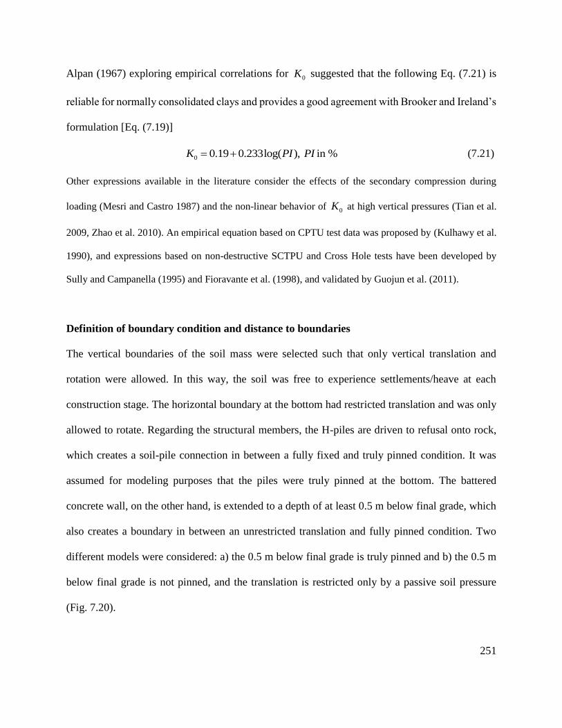
251

Alpan (1967) exploring empirical correlations for 0K suggested that the following Eq. (7.21) is

reliable for normally consolidated clays and provides a good agreement with Brooker and Ireland’s

formulation [Eq. (7.19)]

0 0.19 0.233log( ), in %K PI PI (7.21)

Other expressions available in the literature consider the effects of the secondary compression during

loading (Mesri and Castro 1987) and the non-linear behavior of 0K at high vertical pressures (Tian et al.

2009, Zhao et al. 2010). An empirical equation based on CPTU test data was proposed by (Kulhawy et al.

1990), and expressions based on non-destructive SCTPU and Cross Hole tests have been developed by

Sully and Campanella (1995) and Fioravante et al. (1998), and validated by Guojun et al. (2011).

Definition of boundary condition and distance to boundaries

The vertical boundaries of the soil mass were selected such that only vertical translation and

rotation were allowed. In this way, the soil was free to experience settlements/heave at each

construction stage. The horizontal boundary at the bottom had restricted translation and was only

allowed to rotate. Regarding the structural members, the H-piles are driven to refusal onto rock,

which creates a soil-pile connection in between a fully fixed and truly pinned condition. It was

assumed for modeling purposes that the piles were truly pinned at the bottom. The battered

concrete wall, on the other hand, is extended to a depth of at least 0.5 m below final grade, which

also creates a boundary in between an unrestricted translation and fully pinned condition. Two

different models were considered: a) the 0.5 m below final grade is truly pinned and b) the 0.5 m

below final grade is not pinned, and the translation is restricted only by a passive soil pressure

(Fig. 7.20).

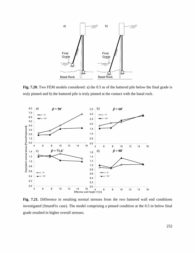
252

Fig. 7.20. Two FEM models considered: a) the 0.5 m of the battered pile below the final grade is

truly pinned and b) the battered pile is truly pinned at the contact with the basal rock.

Fig. 7.21. Difference in resulting normal stresses from the two battered wall end conditions

investigated (SmartFix case). The model comprising a pinned condition at the 0.5 m below final

grade resulted in higher overall stresses.

253

Preliminary FEM results indicated the first model (Fig. 7.20a) predicted in general higher normal

stresses on the battered wall (Fig. 7.21), and therefore, it was chosen for being more conservative.

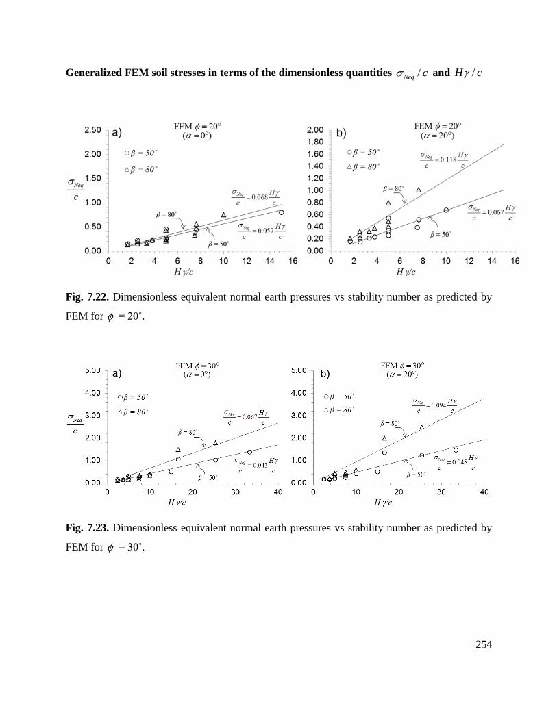
254

Generalized FEM soil stresses in terms of the dimensionless quantities /Neq c and /H c


FEM for = 20˚.


FEM for = 30˚.

255


FEM for = 40˚.

256

Generalized FEM overturning moments in terms of the quantities /M c and /H c



257

Fig. 7.27. Normalized overturning moment vs. stability number as predicted by FEM = 40˚.

258

Validation of simplified design equations

Fig. 7.28. Validation of design equations: a) Neq and b) M for = 20˚.


259


260

Determination of soil strength parameters

Fig. 7.31. Selected M-C strength parameters based on triaxial p-q diagram at 14% strain level.

261

Chapter 8. Conclusions

262

The Low Compaction Grading Technique on steep slopes (chapters 2 and 3)

The analysis of several potential modes of failures via LEM and FEM analyses suggest that for

FRA slopes the governing failure mode is shallow and contained within the weak loose surface

layer. The determination of the strength parameters of the core is not important for FRA slope

design. Because the infinite slope method adequately approximates the shallow failure mode and

accurately predicts the FS, it may be an appropriate method to evaluate the performance of FRA

slopes, so more sophisticated analyses are not necessary for most applications. Since the unit

weight of the material is not considered in the infinite slope expression, field measurements of the

highly variable unit weight are not required for long-term analyses, but necessary for partially

saturated conditions and seismic analyses. The angle of repose was suggested to be a conservative

estimate of the internal friction angle and it is consistent with the loose nature of the FRA material.

This provides a means to quantify the friction angle of mine spoil having large number of oversize

particles, which has been traditionally assumed based on experience.

Slope stability analyses for partially saturated mine soils showed that seasonal increments in the

stability of steep FRA slopes due to matric suction are possible, and the static long-term stability

is a lower bound of the real field performance. However, it was shown that temporal saturation of

the loose surface layer is likely to occur and slope stability analysis employing traditional saturated

strength parameters should prevail in the design of FRA slopes. The interpretation of results is

restricted to the hydrological conditions experienced during the time period at which the data was

collected. This period was characterized by relatively poor establishment of ground cover, and

therefore, evaporation was probably the main mechanism inducing matric suction and the relative

increase in stability. Under seismic loading conditions, the proposed infinite slope equation

263

showed good agreement with the simplified Bishop’s method of the slices. While the selection of

the pseudo-static coefficient based on a fraction of the probable PGA is common practice, the

effects of frequency and duration are not included. A method based on spectral response may

provide a better tool for evaluating slope stability, and a combination of the Bray and Travasarou

(2009) approach with the proposed modification of the infinite slope equation was suggested.

Charts were developed for this method employing site-specific aS values and local soil properties

and slope geometry. Here, the Factor of Safety (FS) is a function of parameters that have less

selection subjectivity for the designer and are a function of the importance of the project, available

seismic data, and accuracy of the site characterization.

The results presented in these two chapters suggest that the FRA has no negative impact on slope

stability. It is important to keep in mind that since the material receives minimum compaction

effort, as shearing takes place this material will initially densify, becoming stronger over time.

Also, further densification will occur through root reinforcement after reforestation, suggesting

that the most detrimental conditions for the stability of FRA slopes are those experienced during

the first years after construction. In this sense, the benefits of quick and proper establishment of

vegetation go beyond the reduction of soil loss by water erosion, influencing also the mechanical

stability of steep FRA slopes in the long-term. Future research work on steep FRA slopes could be

directed to understand the role of vegetation on the stability of this type of reclamation process.

Research questions to be addressed include the following: To what extent do plant roots positively

affect the soil strength and mechanical stability of steep FRA slopes over time? Is there any arching

soil effect that develops in the mine spoils due to this natural “anchor reinforcement” system? If

so, how would this arching effect be quantified in stability calculations for FRA slopes? Would

264

the fundamental failure mode of these slopes be changed? How will root transpiration rates affect

the unsaturated stability patterns observed on these sites? Would overloading and overturning of

woody vegetation during high velocity wind events counteract the positive effects of root

reinforcement on steep FRA slopes?

The answers to these research questions would help to understand the behavior of steep FRA slopes

once the vegetation has been successfully established, providing a broader picture of the field

performance in the very long-term.

The mechanical and erosional stability of concave slopes (chapters 4, 5 and 6)

Concave slopes not only resemble natural contours, but also have superior water erosion resistance.

The design of concave slopes requires: a) the definition of concave shapes that provide a desired

FS, b) a quantitative measure of the erosion/sediment delivery reduction, and c) determination of

possible loss of mechanical stability due to improper construction. A mathematical description of

the concave slope surface at limiting equilibrium (FS = 1) for the > 0 and > 0 case was

developed, based on the slip line field theory of Sokolovskiĭ (1960). The approximation

transformed a set of differential equations into a single algebraic expression, which was validated

using LEM and FEM analyses. Employing the developed equation, a mechanism to describe the

coordinates of concave slopes that satisfy a desired FS (long-term conditions) for any combination

of , c , and slope height was offered. A simplified graphical solution was developed to

estimate the required undrained shear strength such that the design long-term stability is assured.

Results from RUSLE2 analyses indicate that these concave slopes yield 15-40% less sediment than

265

planar slopes of equal FS, regardless of soil erodibility and weather conditions. Sensitivity analyses

reveal that the stability of concave slopes is not significantly influenced by errors in the constructed

profile of as great as 200 mm of vertical deviation. Therefore, the stability is not compromised

when typical high accuracy GPS construction equipment is employed for concave slope

construction.

Similarly, natural landforms seek to achieve erosion and sediment transport equilibrium, and in

doing so evolve into concave forms. In theory, this equilibrium shape would not suffer further

adjustments so the total erosion production is minimized. From a conceptual perspective, it was

shown that the equilibrium shape may not be unique, and a family of potential slope shapes exist

according to the level of constant erosion the slope experiences. From the fundamentals of the

widely recognized RUSLE2 model, a set of equations to describe concave slopes in erosion

equilibrium at different levels of constant erosion was developed. The resulting concave profiles

were compared with critical concave slopes ( FS = 1) and with concave slopes having FS = 1.25,

1.5, and 1.75, identifying those shapes that satisfy both erosion equilibrium and the desired degree

of mechanical stability. A mathematical expression defining the limiting erosion at which

equilibrium erosion shapes become sustainable was provided as a function of the Mohr-Coulomb

parameters.

The findings presented here suggest that concave slopes can be constructed to achieve both

minimal erosion as well as mechanical stability, and that the slope profile can be chosen such that

erosion rates and desired mechanical stability are balanced to satisfy site conditions and regulatory

requirements. Concave slopes not only offer superior erosion control, but also a more natural

266

appearing landform, being an attractive alternative to the traditional planar slopes that are typically

constructed today.

The results from the illustrative example in chapter 5 suggest that concave and planar slopes

having the same FS can potentially have a similar lateral extent, but that concave slopes comprise

significantly less amount of soil. Since an analytical expression for the concave slope is now

available, this could be incorporated into standard cut and fill balance calculations. On projects

with significant cut slopes, the additional excavation may be costly. However, on fill slopes and

embankments, and especially in mine reclamation where a shortage of material is common, the

construction of concave slopes could be an advantage. Notice that under the FRA reclamation idea,

as discussed in chapters 2 and 3, the quick establishment of vegetation is crucial for surficial water

erosion control. The results obtained in here indicate that erosion reduction could be significantly

enhanced if the FRA slopes are constructed with concave profiles. This requires, however, that not

only the loose surface, but also the strong core must be concave. Future research on mine

reclamation could be focused on understanding the erosion and mechanical slope stability

behaviors of concave FRA slopes. Full-scale concave FRA slopes could be constructed and

instrumented to investigate hydrology and sediment yield, and the results compared to those

reported by Hoomehr et al. (2012) and Hoomehr et al. (2013) on steep planar FRA slopes. The

quantitative benefit in terms of reduced soil loss when FRA slopes are built to be concave needs

to be determined. Since the plane of discontinuity is not planar anymore, it will be necessary to

investigate the fundamental failure modes of concave FRA slopes. Would the plane of

discontinuity be the governing failure condition instead of the toe and face failure mechanism

inherent of concave slopes? If yes, it will be necessary to investigate a new rational design

267

methodology for concave FRA slopes. On the other hand, what would be the implications of

concave FRA slopes on the construction methodology? Would the contour haulback method

typically used for FRA construction still be a valid construction methodology? The answer to these

research questions would guide the development of an improved FRA methodology (FRA 2.0)

that will be beneficial for erosion reduction not only post reforestation, but also during initial slope

adjustments before vegetation is well established.

The Piling Framed Concrete Retaining Wall (chapter 7)

The Piling Framed Retaining Wall or confined slope system is a novel concept allowing top-down

construction and requires minimal right of way. This wall concept was found to be significantly

less expensive than traditional retaining wall systems under these conditions. To develop a rational

design approach for this type of wall, a series of FEM analyses were conducted to compute the

earth pressures on the wall face and the overall destabilizing moments for a range of wall

geometries and different soil properties. The numerical results were used to develop simplified

equations for design. It was found that the typical earth pressure distribution on the face of the

PFRW is neither linear nor monotonically increasing. The design equations yield conservative

results--relative to the FEM models--for most practical geometries and soil properties. Field

measured earth pressures on the SmartFix prototype were well predicted by both the design

equations and a proposed design method based on Coulomb stresses with tension correction. The

proposed methods can be used to design future configurations of PFRW systems with no need to

create advanced numerical models.

268

The PFRW concept could be extended to applications beyond highway development. Smoother

integration of nature and structural reinforcing elements could be achieved thanks to the inclined

wall face. For example, in urban land development, there are cases where a combination of natural

slopes and retaining structures are required to avoid extensive cut or fill slopes and to preserve the

natural slope contour. In this sense, the PFRW can be an attractive alternative to the traditional

vertical or terrace walls, since the wall face inclination can be adjusted. Not only that, but the

decorative ashlar stone finish could be replaced with a combination of precast concrete blocks and

compacted soil installed in a staggered arrangement such that vegetation can grow over the wall.

This same idea would apply when concave slopes are used for more natural urban land

development, where additional reinforcement is needed at intermediate points on the landscape

(e.g., immediately below a roadway). In fact, the mode of deformation associated to PFRW

suggests that the reinforcement would not only benefit slopes below (or after) the wall, but also it

would prevent any potential development of progressive failure on excavated concave slopes

above (or before) wall construction.

In summary, this dissertation examined slopes and the many factors affecting them that are

typically overlooked during design and construction. It examined both compaction based slopes

like those constructed during mine reclamation, and excavated slopes like the confined slopes with

the piling framed retaining wall. The superior performance of concave slope contours in terms of

the mechanical and water erosion stability was demonstrated, as well as the interaction between

these two stability conditions. This dissertation examined novel ways of addressing some of the

many issues that govern the design and sustainability of slopes, and contributed to the continuing

269

development of our understanding of the behavior of soil slopes and to the growing need for

environmental friendly design and construction techniques.

270

References:

Bray, J. D., and Travasarou, T. (2009). "Pseudostatic coefficient for use in simplified seismic slope

stability evaluation." J. Geotech. Geoenviron. Eng., 135(9), 1336-1340.



Hydrol. Eng., 18(12), 1627-1638.

Hoomehr, S., Schwartz, J. S., Yoder, D. C., Wright, W. C., and Drumm, E. C. (2012). "Erodibility

of low-compaction steep-sloped reclaimed surface mine lands in southern Appalachian

region, USA." Journal of Hydrological Processes.


271

Vita

Isaac A. Jeldes Halty is a civil engineer whose passion is geotechnical engineering. He graduated

with a Bachelor of Science in Civil Engineering from the University of Santiago of Chile and

immediately after joined the R&V geotechnical consultants, where he conducted a variety of

geotechnical projects for two and half years. During this period of time he started to have

fundamental questions about some of the solutions that civil engineers employ in design, and felt

the necessity to increase his theoretical understanding. Since August 2008, Isaac has been working

in his doctoral degree under the guidance of Dr. Eric Drumm at the University of Tennessee. In

the course of his program he earned a Master’s Degree in Civil Engineering. Isaac’s research has

been primarily focused on: a) slope stability and restoration of mine reclaimed sites; b) the design

of eco-friendly slopes to reflect natural shapes with reduced erosion rates and optimum mechanical

stability; c) numerical modeling and stability analysis of a new type of retaining wall to support

the creation of a rational design methodology.

Stability, Erosion, and Morphology Considerations for ...

Documents

Transcript of Stability, Erosion, and Morphology Considerations for ...