
STA 6166, University of Florida, 2007
123
Ramin Shamshiri, UFID#: 9021-3353 Page 1 STA 6166, Section 8489, Fall 2007 Final Exam Part I Due 04 December 2007 RAMI SHAMSHIRI UFID#: 9021-3353
Transcript of STA 6166, University of Florida, 2007

Ramin Shamshiri, UFID#: 9021-3353 Page 1
STA 6166, Section 8489, Fall 2007
Final Exam
Part I Due 04 December 2007
RAMI" SHAMSHIRI UFID#: 9021-3353

Ramin Shamshiri, UFID#: 9021-3353 Page 2
A) Please read the attached paper by Bell et al. (2005, Science, 308, 1884 and
supplementary material; Attachments I and II) and answer the following questions:
a. State in words all sets of hypotheses that the authors are interested in testing (note that
the authors could be interested in more than one set of hypotheses!)
The main hypotheses that the scientists are claiming (HA) are the following
i. The slope of the taxa-area relationship for natural bacterial communities (which can be
considered Microbes) inhabiting small aquatic islands is comparable to the slope of the taxa-
area relationship for larger organisms. In the other words, the author claims that the mean of
diversity of natural bacterial communities inhabiting small aquatic islands is similar to that found
for larger organisms.
ii. The slope of species-area relationship for insular bacterial communities would be similar to that
found for communities of larger organism (on discrete islands).
The secondary hypotheses that the scientists are interested in are:
i. Analogous processes structure both microbial communities and communities of larger
organisms
ii. To check the possibility whether other mechanisms can underlie the difference between the
authors results and those of other microbial studies, for example, the Treehole habitat is more
heterogeneous, so diversity increases more rapidly with area size.
Expanding the answer:
First, based on recent studies, the slope of the relationship between Microbes and area differs from the
slope of the relationship between other species richness and area. Here, the authors claim to show that
the slope of the taxa-area relationship for natural bacterial communities (which can be considered
Microbes) inhabiting small aquatic islands is comparable to the slope of the taxa-area relationship for
larger organisms (which can represents other species richness).
Second; the previous studies indicate that the species-area relationship is expected to be steeper on
discrete islands, but the authors claim to predict that the slope of species-area relationship for insular
bacterial communities would be similar to that found for communities of larger organism (on discrete
islands).
As a result, the authors showed that bacterial genetic diversity in water-filled treeholes increases with
increasing island size (volume) which is similar with the linear relationship between island surface area
and bacterial genetic diversity. According to their equations,:
• Equation relating bacterial genetic diversity and island size (Volume): S=2.11V0.26
• Equation relating bacterial genetic diversity and island surface area (cm2): S=3.3A
0.28
They have also showed that treehole volume and surface area are correlated.
■

Ramin Shamshiri, UFID#: 9021-3353 Page 3
b. Is the research observational or experimental? This is an Observational study. Because the data are observed on a sample of population, and No
treatment is assigned to samples. Here the interest is describing population.
■
c. What factors or explanatory variables are they interested in studying for their effects on
the microbes? Based on the relationship between diversity and sampling area size (� = �. ��) which is stated in the
paper, we can write the equation as below: ln� = ln�. �� => ln� = ln� + �. ln� y = c + z. x Or y = β� + β�. x
x= (ln (A): size of area) is the explanatory variable and is measured as
• Island size (volume)
• Island surface area
Expanding answer:
The paper says that the number of Taxa can increase with the size of area. In addition, the number of
Taxa in a particular area results from the balance between the colonization of new taxa and the
extinction of the extant taxa.
The size of area also influences the rate of colonization and extinction which indirectly influences
biodiversity. The islands used in this research (area size) are water filled treeholes. The researcher
measured water volume (island size) which is the explanatory variable and the bacterial genetic diversity
(response variable) in 29 treehole islands.
■
d. What response variables are they measuring on the microbes? In the equation, y = c + z. x Or y = β� + β�. x
y= (ln(S): Number of Species) is the response variable which is bacterial Genetic Diversity (the number of
DGGE bands, S) in water-filled treeholes (shown to increases with increasing island size.)
Another variable that might be considered as a response variable since it’s behavior is studied in this
paper is the Slope z, (slope of the species-area relationship.)
β�= (ln(c): empirically derived taxon and location specific constant) is the intercept β�= slope of the line (slope of the relationship between Number of species and size of area)
■
e. Describe the population(s) of interest to the researchers (Hint: think in terms of the scope
of inference – what group(s) or set(s) do the scientists wish to make inferences about)?
The populations of interests are all the possible Microbial communities and all possible communities of
larger organism.
■

Ramin Shamshiri, UFID#: 9021-3353 Page 4
f. Describe the sample(s) that were collected, including the method used for selecting the
sample. The samples are water-filled holes of varying volume and surface area. The water volume (island size)
and the bacterial genetic diversity (taxon richness) are measured in 29 tree-hole islands by
homogenizing the water and sediment contained within the tree-holes and siphoning the liquid into
measuring cylinders. Surface area of the tree holes was determined from digital photographs using the
ImageJ 1.32 software package.
50ml of the mixed water and sediment from each tree-hole was then transferred into vials and kept
them at 4C before processing in the following day. (Tree-hole volume and surface area varied over two
orders of magnitude, so they were comparable to studies conducted on larger organisms.)
This method of sampling can be considered as two-stage sampling method.
The genotype diversity of each of the treehole bacterial communities are determined using denaturing
gradient gel electrophoresis which is a technique commonly used to compare bacterial communities
from environment samples.
More explanation:
The “islands” used by authors are water-filled tree-holes, a common feature of temperate and tropical
forest. Rainwater accumulates in barklined pans formed by the buttressing at the base of large
European beech trees to form small but often permanent bodies of water. Each of these islands houses
a micro ecosystem that derives its nutrients and energy from leaf litter.
■
g. Restate all sets of hypotheses in statistical terms, i.e. in terms of the population
parameters that are believed to be affected by the treatments.
1 − � H�: μ���� !�"#$.%.& = μ���� !�"#&.'.�H�: μ���� !�"#$.%.& ≠ μβ���� !�"#&.'.� ) or �H�: β $.%.& = β &.'.�
H�: β $.%.& ≠ β &.'.� )
��� !�"#$.%.& is the mean of diversity of Natural Bacterial communities which changes with area size and
*+,.-.. is the slope of relationship between species richness and area size for Natural Bacterial
communities inhabiting small aquatic islands. ��� !�"#$.%.& is the mean of diversity for communities of
larger organisms and *+../.0 is the slope relationship between species richness and area size for
communities of larger organisms.
2 − �2�: *+3.-.. > *+../.0 2�: *+3.-.. ≠ *+../.0 )
Where *+3.-.. is the slope of species-area relationship for insular bacterial communities and *+../.0 is the
slope of relationship found for communities of larger organism (on discrete islands).
■

Ramin Shamshiri, UFID#: 9021-3353 Page 5
h. Describe the statistical method used to test the hypotheses. Have all the assumptions of
the test been met? Explain.
The relationship between Bacterial genetic diversity and island size (Volume) has been first determined
with simple regression method. The result of this regression leads to the equation � = 2.115�.67. The
slope of this equation (z1=0.26) is compared with the slope (z2=0.28) of the linear relation between
island surface area (cm2) and bacterial genetic diversity, equation� = 3.30��.6:.
The statistical t-test or ANOVA can be used to test for any significant difference between the mean of
diversity for Natural bacterial communities and communities of larger organisms.
One of the assumptions of t-test is normality, and In fact, there is not enough evidence from the paper
that the data are not Normal. Perhaps the availability of linear relationship and the high value of R-
squared can be used to state that data are coming from a normal source.
The plot used to show the linear relationship between Island size and Bacterial diversity is in Logarithmic
scale. We already know that in the ANOVA, if σ is proportional to the Mean, use the Logarithm of the yij.
■

Ramin Shamshiri, UFID#: 9021-3353 Page 6
B) Suppose you are asked to design an observational study to answer the question: Are
undergraduate students on campus more likely to take classes during periods 1, 2, or 3 than
undergraduates students who commute to campus? You are to design a strategy for sampling 100
students from each population to test the hypothesis. So, please answer the following questions:
a. State the hypotheses to be tested in statistical terms.
Answer:
If we state our claim in the form of p1 > p2, then we would test the below hypotheses:
H0: p1≤ p2
H1: p1> p2
p1: Proportion of all of the undergraduate students on campus taking classes during periods 1,2 or 3.
p2: Proportion of all of the undergraduate students commuting to campus taking classes during periods 1,2 or 3
;�: Proportion of the sample of on campus undergraduate student taking classes in one of the periods 1 or 2 or 3. ;6: Proportion of the sample of on campus undergraduate student who has taken classes in one of the periods 1
or 2 or 3.
Note: The point estimators for p1 and p2 are ;� = =�/?� and ;6 = =6/?6. (Table 1)
■
b. What testing procedure will you use?
Answer:
Here we have two populations, one is all undergraduate students on campus and the other one all
undergraduate students commuting to campus. Now we want to compare proportions of students from
the first population who has registered in classes during periods 1, or 2 or 3 with the proportions of
students from the second population who has registered in classes during these periods.
If a student is observed to have registered in classes during periods 1 or 2 or 3, then the outcome is YES,
otherwise the outcome is NO. So, the testing procedure would be as follow:
Here we are comparing proportions using two independent samples. A hypothesis test involving a
population proportion can be considered as a binomial experiment when there are only two outcomes
and the probability of a success does not change from trial to trial.
The appropriate statistic for inferences on (p1-p2) is:
� = ;� − ;6 − ;� − ;6@;A1 − ;A 1?� + 1?6
BC = ,DEFDG,HEFH,DG,H Or BC = IDGIH
,DG,H

Ramin Shamshiri, UFID#: 9021-3353 Page 7
Explanations:
Because. Based on independent samples of size n1 and n2, we want to make inferences on the difference
between p1 and p2, that is p1-p2.
Assuming sufficiently large sample sizes, the difference ;� − ;6 is normally distributed with Mean= P1-P2
Variance= ED�JED
,D + EH�JEH,H and has the standard normal distribution: � = EFDJEFHJEDJEH
@KDDLKDMD GKHDLKH
MH. But the
problem is that the expression for the variance of the difference contains the unknown parameters p1
and p2. Thus we use an estimate of the common proportion BC for the variance formula.
P1: the probability of success in population 1 ;� = =�/?�: is the estimate of p1
P2: the probability of success in population 2 ;6 = =6/?6: is the estimate of p2
■
c. What are the assumptions of the test?
The assumptions must satisfy the binomial distribution. (Sampling should meet the conditions of a
Binomial Experiment). The sample sizes should be large enough that we can use the central limit
theorem and large enough so that we can use the Standard Normal rather than the T-distribution.
• Observations are independent of each other
• Each selection of an experimental unit (i.e. each trial) is a random selection from the population of
interest.
• The selections are taken with replacement or the total number of samples is less than 5% of the
population
• The probability of observing a success, π, in a single selection does NOT change between trials
• The probability of success is constant for all observations.
■
d. How will you design the sampling in order to ensure that the assumptions of the test are
met? Describe the sampling design you will use. If you are using any lists such as registrar
information please describe explicitly what information you are assuming is available for
you to use.
This is an observational study in which data are observed on a sample of the population. Sampling
strategy for observational studies must consider the followings:
• Good representation of the population
• No systematic bias
• Small sampling variability
• Cost constraints (time, money, feasibility)
• Precision of estimates
• Power of tests
For this problem, we can use Random Sampling in which every possible sample of n units is equally likely
to be observed. We can also use Stratified Sampling.

Ramin Shamshiri, UFID#: 9021-3353 Page 8
Random Sampling: The procedure for sampling students to make inference on the proportion of
undergraduate students who are living on campus or commuting to campus and take classes on the
periods 1 or 2 or 3 may be as follow:
First: Accessing to the registrar list of all undergraduate student which reveals below information:
Student living address, on campus or Off campus
Student class registration information
For example, there might be 3000 undergrad students in the list, of which 1300 are living on campus
(Group A) and 1700 are living off campus (Group B). We can then assign a ID numbers from n1_1 to
n1_1300 to students in group A and from n2_1 to n2_1700 to students in group B. Now we have unique
ID numbers for every element in the population. So we can use a random generator (table of random
digits, computer, calculator) to get a list of 100 randomly generated ID numbers from each population
(Group A and Group B).
As a result, we will have 100 randomly generated ID numbers (i.e. n1_150 , n1_27 ,.., n1_1011 , n2_1503 , n2_466 ,…,
n2_206 ) for each group and can make a table to check if a student has taken classed on periods 1, 2 or 3.
Based on the result of this table, we will find ;� = =�/100 and ;6 = =6/100
On Campus
Student ID
Group A
Has taken classes on periods
1 or 2 or 3
Off Campus
Student ID
Group B
Has taken classes on periods
1 or 2 or 3
Yes No Yes No
n1_150 n2_1
n1_27 n2_1
RANDOM
IDs
.
.
.
RANDOM
IDs
.
.
.
n1_1011 n2_100
Total n1=100 y2 Total n2=100 y2
■
e. How does your design ensure that the sample is representative of the population being
sampled (representative: sample estimates are unbiased for the population parameters
being estimated)?
We have supposed that we have two populations, each of them with a proportion (p) of Yes and we take
a binomial sample of size n=100 from each. As long as the sampling is done according to the
requirements for a Binomial random variable, the frequency distribution of the sample number of
successes has the characteristics that the shape of the distribution (which is exactly Binomial) can be
approximated as a bell-curve (Normal), if the sample size is relatively large and the population
proportion (p) is neither too small nor too large.
We can verify our assumptions with the general rule of thumb which says: the sample size should be
such that np>10 and n(1-p)≥10
■

RAMIN SHAMSHIRI, UFID#:9021-3353 Page 1
STA 6166, Section 8489, Fall 2007
Final Exam
Part II Due 13 December 2007
RAMI# SHAMSHIRI UFID#: 9021-3353
[email protected] Phone: 352-392-1864 ext:217

RAMIN SHAMSHIRI, UFID#:9021-3353 Page 2
A- During a study of the effect of an oil spill on the interstitial marine biota on sandy
beaches, a graduate student collected a total of 129 animals in a stretch of beach near
Catalina Island in California that had been “oiled”. For each animal measured, the
student recorded its species, length, weight, coordinates of the collection location (where
on the beach it was found), and the substrate on which it was found (sand, rock, wood,
pebbles, etc)
1- List the qualitative variables Answer:
The qualitative or categorical variables are:
• Animal’s ID, (either in the form of 1,..,129 or other ID formats assigned, i.e. name, random codes, etc)
• Animal Species
• The substrate
■
2- List the quantitative variables Answer:
• Animal’s Length
• Animal’s Weight
• Coordinates of the collection location if is in the form of (X, Y, Z). If the coordinate of the collection
location is in the form of North, South, Northwest, etc, it will be considered as a categorical variable.
■
3- The sample consists of the 129 oiled animals collected in a stretch of beach near Catalina Island.
■
4- Suppose the students plans to test whether the oil spill has decreased the average size
(weight and length) of individuals of the most abundant species.
a. Describe the population(s) appropriate for the inference from the test. Answer:
i. Population of Oiled and Not-Oiled animals(all species)
The first population contains all possible individuals of the most abundant species living under
similar circumstance near the Catalina Island but are Not- Oiled and the second population will
be all possible individuals of the most abundant species Oiled in the Catalina Island.
ii. Population of animals Species(individual species)
The 129 oiled animals are a collection of several species, i.e. fish, birds, etc. So, it is possible to
have inference on an oiled and Not-oiled particular species separately and independently from
another species of animals. In this case, we can consider species No.i as two populations, one is
the population of oiled, the other one population of not oiled.
(i=1 to all available species in the 129 observations)
■

RAMIN SHAMSHIRI, UFID#:9021-3353 Page 3
b. Describe the likely hypotheses to be tested. Answer:
Note: To answer this question, it is assumed that the 129 observed oiled-animals are different in species and may
contain fish, birds, etc. So, Species No.1 for example, refers to the fish group; Species No.2 refers to birds, etc.
i. Testing Mean Size(For Two population)
Testing if the Mean size (either Weight or Length) of a particular species of Oiled-animals is less than the
Mean size of that particular species of Not-oiled-animals, the hypotheses are:
H0: ���������� = ������� �����
H1: ���������� < ������� �����
H0: ������������ = ��������� �����
H1: ������������ < ��������� �����
H0: ������������ = ��������� �����
H1: ������������ < ��������� �����
ii. Testing relationship:
Testing whether there is a relationship between level of Oiled and the size of animals, (i.e, the more an
animal has been oiled, the smaller its size is). To test this, we need to construct a model as below to find
a relationship between x and y.
y=β0+β1x+Є
Then we can find ��� and ��� as below: ��� = �� − �����
��� = ∑�� − ����� − ���∑�� − ���� = !" !!
The hypotheses are then:
Is there a relationship between Oiled effect (Y) and animal Size (X)?
H0:β1=0
H1:β1≠0
Is the relationship positive?
H0:β1=0
H1:β1>0
Is the relationship negative?
H0:β1=0
H1:β1<0
iii. Testing Mean (Multiple and specific Comparison)
Testing if the Oil spill has had same effect on the size of different species animals, for example, if the 129
observed animals can be categorized into n species, the student can test if the means of changes in size
of different species are equal or not. In the other word, have all species received same size impact from
the oil spill? The hypotheses can be written as:
H0: �#�$���_��_����&'�(��� � = �#�$���_��_����&'�(��� � = ⋯ = �#�$���_��_����&'�(��� ���
H1: At least one of the Species has received a different (Higher or lower) size effect from oil spill.

RAMIN SHAMSHIRI, UFID#:9021-3353 Page 4
It is also possible to make this test more specific to understand which groups have received the highest
and lowest size impact from oil spill. An example hypothesis can be written as:
H0: �#�$���_��_����&'�(��� � ≤ �#�$���_��_����&'�(��� �
H1: �#�$���_��_����&'�(��� � > �#�$���_��_����&'�(��� �
■
c. Describe the testing procedure that should be used to test the hypotheses you gave.
What prior information, if any, is needed to perform this test?
Procedure 1: Testing Mean size for:
Here our two populations are: 1- Population of all the animals (regardless of species) oiled and 2- all the
animals in that area Not-oiled. Difference between the two means is defined by: δ= μ1- μ2
A sample size n1 = 129 is randomly selected from the first population and a sample of size n2 is
independently drawn from the second. The difference between the two sample means (��� − ���)
provides the unbiased point estimate of the difference (μ1- μ2). The sampling distribution of the
difference between these two means has a mean of μ1- μ2. It is important that the sample sizes are
sufficiently large, ���-./ ��� are normally distributed; so that we can apply the Central Limit Theorem
and ��� − ��� be also normally distributed.
Here our assumptions are that
• The two samples are independent
• The distributions of the two populations are normal or of such a size that the central limit theorem
is applicable.
• The variances of the two populations are equal or can be assumed equal.
Now we will have one of the following cases:
1- If our population variances are Known, then the variance of our (δ= μ1- μ2) distribution will be 0�� .�⁄ +0�� .�⁄ and we can use the statistic below which has the standard normal distribution to
test our hypotheses:
2 = ���� − ���� − ��� − ���3�0�� .�⁄ � + �0�� .�⁄ �
2- If our population variances are Unknown, and assumed equal, we will use the estimate of
variance and the pooled t-test which has the t distribution with .� + .� − 2 degrees of
freedom.
6'� = �.� − 1�6�� + �.� − 1�6���.� − 1� + �.� − 1�
8 = ���� − ���� − ��� − ���9:6'� .�⁄ ; + �6'� .�⁄ � = ���� − ���� − <�
96'��1 .�⁄ + 1/.��
3- If our population variances are Unknown and Not equal, we may first note that inference on
Means may not be very useful, however we can use the below statistic test if both n1 and n2 are
large (both over 30) considering the fact that if n1 and n2 are large, the central limit theorem will

RAMIN SHAMSHIRI, UFID#:9021-3353 Page 5
allow us to assume that the difference between the sample means will have approximately the
normal distribution. For the large sample case, we can replace σ1 and σ2 with s1 and s2 without
serious loss of accuracy. Therefore, the statistic 8 will have approximately the standard normal
distribution.
8 = ��� − ���3�6�� .�⁄ � + �6�� .�⁄ �
4- If either sample size was not large, we could compute the statistic 8 as in part 1. If the data come
from approximately normally distributed population, this statistic does have an approximate
student t distribution, but the degrees of freedom cannot be precisely determined. A reasonable
approximation is to use the degrees of freedom for the smaller sample; however, other
approximations may be used.
Procedure2: Testing relationship for:
We want to test whether there is a relationship between the effect of oil level on the size of the animal,
in the other word, if there is a relationship to show that the more an animal is oiled, the smaller its size
is. To test this, we need to use correlation test procedure as below:
ρ: The population correlation coefficient
r: Pearsons’s product moment correlation coefficient, (Sample correlation coefficient)
? = ∑�� − ����� − ���3∑�� − ���� ∑�� − ���� = !"
3 !! ""
?� = � !"�� !! "" = @A
r2: is known as coefficient of determination, is a measure of relative strength of the corresponding
regression. It is used to describe the effectiveness of linear regression model.
B = C @C D = �. − 2�?��1 − ?��
F: is the F statistic from the analysis of variance test for the hypothesis that β1=0
It is obvious that large values of r produce large values of F, both of which imply a strong linear
relationship. If the F-value from this test leads to a P-value smaller than our significant level, we will
reject the null hypothesis H0:β1=0 and conclude that there is enough evidence to show that a linear
relationship exists between oil level and animal size.

RAMIN SHAMSHIRI, UFID#:9021-3353 Page 6
Procedure 3: ANOVA for:
Multiple mean comparison with the hypothesis as below can be done with one-way ANOVA:
H0: �#�$���_��_����&'�(��� � = �#�$���_��_����&'�(��� � = ⋯ = �#�$���_��_����&'�(��� ���
H1: At least one of the Species has received a different (Higher or lower) size effect from oil spill.
Assumptions for the F test comparing three or more Means:
1- The population from which the samples were obtained must be normally or approximately normally
distributed.
2- The samples must be independent.
3- The variances of the populations must be equal.
Fining the F-test value for the Analysis of Variance:
Step 1- Finding the Mean and Variance of each sample
(E��, 6��),( E��, 6��),…( E�G, 6G�)
Step2- Finding the Grand Mean
E�HI = ∑ EJ
Step 3- Finding the between group variance, (variance of the Means)
6K� = ∑ .� �E�� − E�HI��L − 1 = MN OP QM-?R6 SR8TRR. U?OMV6 � K�/P� K�
Step 4- Find the within group variance; computing the variance using all the data and is not affected by
differences in the Means.
6�� = ∑�.� − 1�6��∑�.� − 1� = MN QM-?R6 PO? 8ℎR R??O6 � X�/P� X�
Step 5- Find the F-test Value.
B = 6K�6��
Degrees of freedom for Nominator: k-1 (Number of Groups -1)
Degrees of freedom for Denominator: N-k (Sum of the sample sizes of the groups – Number of Groups)
N=n1+n2+…+nk
For this test, we don’t need to have equal sample sizes. The F-test to comparing Means is always right-
tailed. If there is no difference in the Means, the between group variance estimate will be approximately
equal to the within group variance estimate and the F-test value will be approximately equal to 1 and
the null hypothesis will not be rejected. If the Means differs significantly, the between group variance
will be much larger than the within group variance, thus the F-test will be significantly greater than 1
and the null hypothesis will be rejected.

RAMIN SHAMSHIRI, UFID#:9021-3353 Page 7
For specific comparison, we can use The Scheffe test and the Tukey test. In order to conduct the Scheffe
test, one must compare the Means two at a time, using all possible combinations of Means.
E�� vs E�� E�� vs E�G E�� vs E�G …
Formula for the Scheffe test:
B� = �E�� − E�Y��6�� [[ 1.�\ + ] 1.Y^]
Where E�� and E�Y are the Means of the samples being compared, ni and nj are the respective sample
sizes, and 6�� is the within group variance.
To find the critical value for the Scheffe test, multiply the critical value for the F test by k-1. B= (K-1)(Critical Value)
There is a significant difference between the two means being compared when B� is greater than B.
The Tukey test can also be used after the analysis of variance has been completed to make pairwise
comparisons between the groups have the same sample size. The symbol for the test value in the Tukey
test is q
Q = E�� − E�Y36�� /.
Where E�� and E�Y are the Means of the samples being compared, n is the size of the samples and 6�� is
the within group variance.
When the absolute value of q is greater than the critical value for the Tukey test, there is a significant
difference between the two means being compared.
■

RAMIN SHAMSHIRI, UFID#:9021-3353 Page 8
B- Suppose a graduate student in your department shows you the following matrix of
Pearson correlation coefficients for four variables:
X1 X1 X1 X1 X2X2X2X2 X3X3X3X3 XXXX4444
X1X1X1X1 1.000 0.83343 -0.87627 0.09951
X2X2X2X2 1.0000 0.77677 0.47300
X3X3X3X3 1.0000 -0.17368
X4X4X4X4 1.00000
1. Which correlation coefficients in the matrix imply that the two variables are highly
correlated? Answer:
Based on the notes mentioned in a, b, c and d, my answer to this question is summarized in the table
below:
X1 X2 X3 X4
X1 Perfect (meaningless) Strong Positive Relation
(Highly correlated)
Strong Negative Relation
(Highly correlated)
Weak positive Relation
(Very low correlation)
X2 Perfect (meaningless) Strong Positive Relation
(Highly correlated)
Medium Positive Relation
(Medium correlated)
X3 Perfect (meaningless) Weak positive Relation
(low correlation)
X4 Perfect (meaningless)
Table 1
a) The Pearson’s Correlation Coefficient, r, is a quantitative assessment of the strength and direction of a linear
relationship between 2 variables and our assumption is that if a relationship exists, it is linear (Pearson’s r is
valid for linear relationships only). The stronger the relationship, the closer r is to ± 1 and the weaker the
relationship, the closer r is to 0. (If the relationship is perfect (every point falls exactly on a straight line), r = ± 1
depending on the sign of the slope.)In other words, if the variables are independent then the correlation is 0,
but the converse is not true because the correlation coefficient detects only linear dependencies between two
variables.
b) If the relationship is positive (slope>0), r > 0 and if the relationship is negative (slope<0), r < 0. If there is no
relationship at all, (slope = 0), r = 0, however the size of r does not depend on the size of the slope.
c) Interpretation of the size of a correlation
The interpretation of a correlation coefficient depends on the context and purposes. A correlation of 0.9 may be
very low if one is verifying a physical law using high-quality instruments, but may be regarded as very high in the
social sciences where there may be a greater contribution from complicating factors. Several authors have offered
guidelines for the interpretation of a correlation coefficient. Cohen (1988)[1]
, has suggested the following
interpretations for correlations in psychological research:
Correlation Negative Positive
Small −0.29 to −0.10 0.10 to 0.29
Medium −0.49 to −0.30 0.30 to 0.49
Large −1.00 to −0.50 0.50 to 1.00
Table 2
d) Any variable has a perfect relationship with itself, and it is meaningless since it is obvious. In the table, the
correlation value for X1 and X1 is 1.0, which can be inferred as a meaningless perfect relation.
■

RAMIN SHAMSHIRI, UFID#:9021-3353 Page 9
2. Suppose you are told that X2 is a purely categorical variable that was coded as 1,2,3,
or 4 (rather than names). Is the Pearson correlation coefficient appropriate to look
at the strength of the relationship between X2 and other variables? Explain. Answer:
No, if X2 is a categorical variable, the Pearson correlation coefficient is not appropriate to look at the
strength of the relationship between X2 and any of the other variables. In fact, Pearson’s r is only valid
for relationships between two quantitative variables and we should use other measures when one or
both variables are categorical. If we have used a computer program and did not mention that X2 is
categorical, then the value of X2 which are coded as 1,2,3 or 4 will be considered as a quantitative data
and can be misleading.
■

RAMIN SHAMSHIRI, UFID#:9021-3353 Page 10
C- The following experiment on reproductive fitness in ospreys was conducted back in
1970-1980. Review the description of the experiment and then answer the following
questions.
1. Suppose location was expected to have an effect on reproductive fitness but was not of
direct interest to the researcher. Should s/he simply ignore the location aspect in the
analysis and use CRD with Year as the factor of interest? Explain.
Answer:
Ignoring the location effect, the data will be ordered as below:
Year Mean SD Var
1970 3.53 4.27 3.82 3.28 5.12 2.85 2.6 2.42 2.76 2.18 3.283 0.918 0.843
1976 12.32 13.18 9.03 18.67 13.91 13.88 16.42 8.92 6.95 10.49 12.377 3.611 13.04
1982 36.49 29.06 19.12 30.39 23.98 21.69 31.15 28.01 16.5 19.72 25.611 6.389 40.82
With the following hypothesis:
H0: μ1970=μ1976=μ1982
H1: At least one of the above is not equal
α= any reasonable level (0.05 or 0.01)
Using one-way ANOVA for this hypothesis test, we need the assumptions below:
4- The population from which the samples were obtained must be normally or approximately normally
distributed.
5- The samples must be independent.
6- The variances of the populations must be equal.
Using the Levene test for homogeneity of variance, we get an F-value equal to 13.03 which leads to p-
value less than 0.0001, thus we conclude that the variances of the populations are not equal. The
variance column of the table above also confirms this result. Since at least one of the assumptions of
one-way ANOVA is not met here, we probably not able to receive a trusted result from this test.
A one-way ANOVA to test this hypothesis will result:
Test F-value = 69.13
Test P-value= <0.0001
Critical F-value= 3.53
This shows that our test F-value is larger than the critical F-value, (very small P-value, less than any
reasonable significant level α), thus we reject the null hypothesis and conclude that at least one of the
years is different in the mean value. This result is regardless of location effect.

RAMIN SHAMSHIRI, UFID#:9021-3353 Page 11
Considering location effect, we first need to know whether the location had any effect on the data
observed in a same year. The data and hypotheses can be written as below:
Location Mean Var F-value P-Value F-crit
GAR1970 2.85 2.6 2.42 2.76 2.18 2.562 0.0724 17.41 0.0031 5.3176
MAS1970 3.53 4.27 3.82 3.28 5.12 4.004 0.52473
Location Mean Var F-value P-Value F-crit
GAR1976 13.88 16.42 8.92 6.95 10.49 11.332 14.527 0.82 0.391 5.317
MAS1976 12.32 13.18 9.03 18.67 13.91 13.422 12.085
Location Mean Var F-value P-Value F-crit
GAR1982 21.69 31.15 28.01 16.5 19.72 23.414 36.3475 1.209 0.303 5.317
MAS1982 36.49 29.06 19.12 30.39 23.98 27.808 43.4365
H0: μMAS1970=μ GAR1970
H1: μMAS1970≠μ GAR1970
Result: P-value=0.0031 => reject H0
H0: μMAS1976=μ GAR1976
H1: μMAS1976≠μ GAR1976
Result: P-value=0.0031 => reject H0
H0: μMAS1982=μ GAR1982
H1: μMAS1982≠μ GAR1982
Result: P-value=0.0031 => reject H0
Based on the F-value and P-value results, we can see that the location has had effect only on the
first year data collection, (1970). For the other years, (1976 and 1982) the location did not have any
significant effect.
Since locations also have effect on the reproductive fitness, the researcher should not ignore the
location aspect in her analysis and use CRD which only uses year as factor of interest since it was
shown here that this method will not reveal the true effects of both Year and Location on the
reproductive fitness. The researcher shall consider RCBD and consider this problem as a block design
in which the blocks have more than t experimental units that are used in the experiment. This
method will provide a control on the effect of the two different locations.
■

RAMIN SHAMSHIRI, UFID#:9021-3353 Page 12
2. Review the attached output and choose the most appropriate analysis for this data.
(There are four different A#OVA in the output) Explain your choice including
specifically what aspects of the analyses led to your decision and why the other analyses
were inappropriate. At a minimum, you should discuss the intentions of the scientist
and assumptions of the alternative models.
Answer:
Reviewing the four different outputs, I would the fourth one because of the four below reasons:
1- One-Way Anova on index with year
The assumptions for this test is that error terms are independent, Normally distributed with constant
variance.
This One-Way ANOVA will test the below hypothesis:
H0: μ1970=μ1976=μ1982
H1: At least one of the above is not equal
The assumption of the homogeneity of variance is not met here according to the following output which
shows that the F-value from the Levene’s test is equal to 13.03 with degrees of freedom=2 leading to a
p-value smaller than any reasonable p-value, thus we reject the null hypothesis of equality of variances
(H0:σ�bc�� = σ�bcd� = σ�be�� )
Since the assumption of homogeneous variance is not met here, it is not appropriate to use One-Way
ANOVA. Moreover, as already mentioned earlier in the answer of previous question, this method does
not show the location effect. However, regardless of these facts, this test has lead to the following
results which rejects the Null hypothesis of equality of the means of productivity fitness through years.
(Reject H0: μ1970=μ1976=μ1982)
RAMIN SHAMSHIRI, UFID#:9021-3353 Page 13
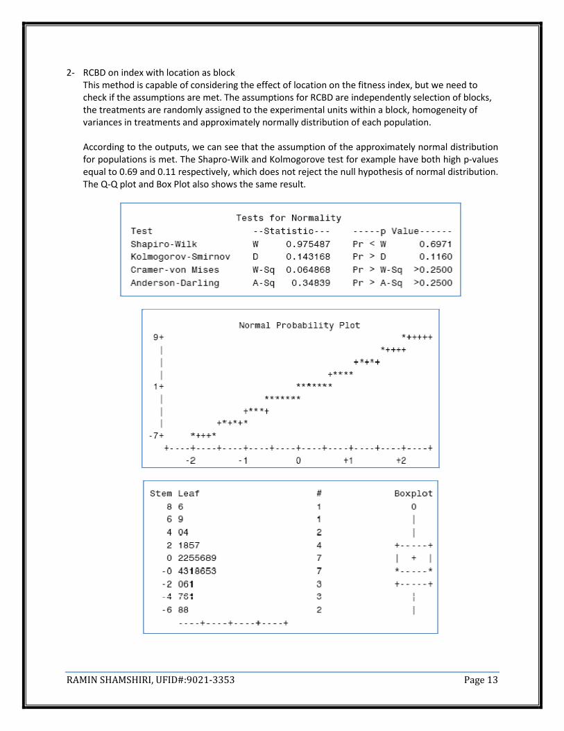
2- RCBD on index with location as block
This method is capable of considering the effect of location on the fitness index, but we need to
check if the assumptions are met. The assumptions for RCBD are independently selection of blocks,
the treatments are randomly assigned to the experimental units within a block, homogeneity of
variances in treatments and approximately normally distribution of each population.
According to the outputs, we can see that the assumption of the approximately normal distribution
for populations is met. The Shapro-Wilk and Kolmogorove test for example have both high p-values
equal to 0.69 and 0.11 respectively, which does not reject the null hypothesis of normal distribution.
The Q-Q plot and Box Plot also shows the same result.

RAMIN SHAMSHIRI, UFID#:9021-3353 Page 14
Checking the assumption of homogeneity of variance from the plots of residuals against
treatments, we can see that the distribution of the residuals of the model between years is not
homogeneous, indicating that the assumption of homogeneous variance between treatments is
not met.
The hypothesis of homogeneity of variance is also rejected with the Levene’s test, which has a
F-value of 2.70, leading to a P-value equal to 0.045<0.05.

RAMIN SHAMSHIRI, UFID#:9021-3353 Page 15
Since the assumptions of RCBD are not, it is not appropriate to use its results which are
mentioned as below:
3- RCBD on Log10(index)
Due to the problem of Unequal variance among factor levels, it may be useful to perform the analysis
using transformed values of the observations, which may satisfy the assumption of equal variances. If σ
is proportional to the Mean, we can use the Logarithm of the yij.
Checking the assumption of Normality, the Shapiro-Wilk and Kolmogorov test both have large P-values
which do not reject the null hypothesis of Normality distribution. The Q-Q plot and Box plot also confirm
this result graphically.
RAMIN SHAMSHIRI, UFID#:9021-3353 Page 16
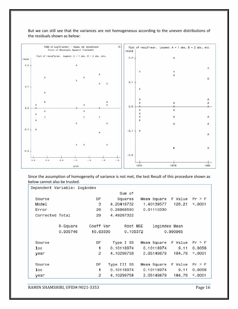
But we can still see that the variances are not homogeneous according to the uneven distributions of
the residuals shown as below:
Since the assumption of homogeneity of variance is not met, the test Result of this procedure shown as
below cannot also be trusted.

RAMIN SHAMSHIRI, UFID#:9021-3353 Page 17
4- RCBD on index - unequal variances for each year.
This method provides a more appropriate procedure for making inference on this problem. The
assumption of Normality is met by looking at Shapiro-Wilk and Kolmogorov P-values which are both
large enough in order to fail in rejecting the null hypothesis of normality. The relevant Q-Q plot and Box
plot also shows graphically that the populations are normally distributed. The plot of wtresid*Pred and
the plot of Plot of wtresid*year shows that we have met our assumption of homogeneity of variance.
Since all the assumptions of RCBD are met here, the results of this analysis can be trusted more than
other three analyses.
..
■
3. Based on your decision in (2), state the statistical model your chose. Be sure to identify
all terms in the model. Answer:
The model that I have selected is Randomize Complete Block Design (RCBD) which has the following
equation: Ygh = μ + αg + βh + εgh μ: is the Grand Mean of all the 30 fitness data observed in the two sites during the 3 experimental year
and is equal to:
αg: is the effect due to the ith
treatment. Here our treatments are the Years. We have three years, so we
have α� , α� and αG.
βh: is the effect due to the jth
block. In this model, our blocks are the two location, GAR and MAS, So we
have β� and β�.
εgh: is the error term. These error terms are independent observations from an approximately normally
distribution with Mean=0 and constant Variance = 0m�
■

RAMIN SHAMSHIRI, UFID#:9021-3353 Page 18
4. Given the model you chose, test the hypotheses of interest to the scientist. State the
hypotheses being tested. For each set of hypotheses (if there are more than one), give
the equation of the test statistic you are using and its distribution. From the output, give
the value of the test statistic, the associated degrees of freedom, the p-value for the test,
and your conclusion. State the conclusion in terms of the problem under study (“reject
the null hypothesis” is #OT sufficient here). If you have multiple hypotheses, also
discuss your choice of method for controlling the experiment-wise error rate.
Answer:
The main hypothesis that the scientist are testing is whether the ban of DDT led to a recovery by the
osprey in their fitness. This hypothesis can be written as:
no� = �p.����!rp��s K$� > �p.����!K�p�s� K$�o� = �p.����!rp��s K$� ≤ �p.����!K�p�s� K$� t
Other sets of hypotheses that the scientists are interested to test are:
H0: μ1970≥μ1976
H1: μ1970<μ1976 (Claim)
H0: μ1976≥μ1982
H1: μ1976<μ1982 (Claim)
H0: μ1970≥μ1982
H1: μ1970<μ1982 (Claim)
H0: μ1970=μ1976=μ1982
H1: At least one of the above is not equal
Using ANOVA test for RCBD, we will have a table of results as below:
The F-stat has F distribution with t-1 degrees of freedom for Numerator and (t – 1)(b – 1) degrees of
freedom for Denominator, where t is number of treatments and b is number of blocks. From the SAS
outputs, we have:
The F-value is equal to 92.57 leading to P-vale less than 0.0001, which rejects the null hypothesis of
equality of means between years. The degrees of freedom of Numerator is 2 and df of denominator is
11.7. Using Tukey test to find out where the difference falls, we have the following hypotheses.

RAMIN SHAMSHIRI, UFID#:9021-3353 Page 19
H0: μ1970=μ1976 H0: μ1976≥μ1982 H0: μ1970≥μ1982
H1: μ1970≠μ1976 (Claim) H1: μ1976≠μ1982 (Claim) H1: μ1970≠μ1982 (Claim)
Testing these hypothesis with Tukey, we have the following result from SAS:
The procedure for Tukey test is: 8 = u$!�"�v.� u���"�w.�9xyz{
Where n is the sample size for each treatment.
Conclusion:
Considering the p-values from the below SAS output table which is the results of our analyses, we
conclude that the ban of DDT has led to recovery of fitness since 1972. In the other words, we are
rejecting the null hypothesis of H0: μ1970=μ1976=μ1982 and conclude that there is not enough evidence to
show that the mean of the fitting index in the three years are equal.
■

RAMIN SHAMSHIRI, UFID#:9021-3353 Page 20
D- Do blood types of people tend to vary among states? Or
stated another way, is state and blood type
independent? The data for testing this hypothesis are
given below. There are four blood types and three
states; frequency is the number of observations in that
row’s combination of state and blood type. Perform the
analysis and state your conclusion. Give the equation of
the test statistic you are using and its distribution. Give
the value of the test statistic, the associated degrees of
freedom, the p-value for the test, and your conclusion.
State the conclusion in terms of the problem under
study, i.e. “reject the null hypothesis” is #OT sufficient
here. (#ote: if you decide to perform the test by hand,
please give the critical or cutoff value you are using to
determine whether to reject the null hypothesis).
Answer:
This problem can be solved with the procedure of testing independence of two categorical variables.
The two categorical variables here are 1- Blood Type and 2- State. The hypothesis then can be written in
the below form:
H0: The State and Blood type are independent
H1: H0 is not true
Our significant level, (type I error) α=0.01
The test used for this analysis is Chi-square with equation as below:
|� = } �~S6R?�R/ − D�VR�8R/��D�VR�8R/r�� #����
Expected Cell= D�Y = . [���������$�� \ [Y��������$�
� \
Degree of Freedom=df= (row-1)(Col-1)
The P-value will be the area to the right of the observed χ� in the chi-square distribution with the above
degree of freedom. Both of the assumptions are met.
1- The samples are random.
2- The sample sizes are sufficiently large so that the expected cell counts are all 5 or more.
In fact, we are using the idea that when two events, like E and F are independent, then
Pr (event E | event F occurred) =Pr (event E)
Pr (E and F) =Pr (E|F). Pr (F) =Pr (E).Pr (F)
Blood Type State Frequency
A FL 122
B FL 117
AB FL 19
O FL 244
A IA 1781
B IA 351
AB IA 289
O IA 3301
A MO 353
B MO 269
AB MO 60
O MO 713

RAMIN SHAMSHIRI, UFID#:9021-3353 Page 21
To perform the test manually, we re-arrange the data in the order of a table as below. Our grand sample
size here is equal to 7619 and our degrees of freedom equal to (4-1).(3-1)=6
Observed State
FL IA MO Total
Blood Type
A 122 1781 353 2256
B 117 351 269 737
AB 19 289 60 368
O 244 3301 713 4258
Total 502 5722 1395 7619 Table 3: Observed values
Expected Cell= D�Y = . [���������$�� \ [Y��������$�
� \
D�� = 7619 ]22567619^ ] 5027619^ = 148.64
.
.
D�G = 7619 ]42587619^ ]13957619^ = 779.6
Expected
State
FL IA MO Total
Blood Type
A 148.643129 1694.29479 413.062082 2256
B 48.559391 553.499672 134.940937 737
AB 24.2467515 276.374327 67.3789211 368
O 280.550728 3197.83121 779.61806 4258
Total 502 5722 1395 7619 Table 4: Expected Values
|� = } �~S6R?�R/ − D�VR�8R/��D�VR�8R/r�� #����
= �122 − 148.64��148.64 + ⋯ + �713 − 779.61��
779.61 = ���. ��
Degrees of freedom= (4-1).(3-1)=6
[(OBS-EXP)^2]/EXP
State
FL IA MO Total
Blood Type
A 4.77557442 4.43712251 8.7334418 17.9461387
B 96.4616084 74.0851697 133.182952 303.72973
AB 1.13534391 0.57678154 0.80809363 2.52021908
O 4.76190441 3.32844301 5.69248733 13.7828347
Total 107.134431 82.4275167 148.416975 337.978923 Table 5: (Observed Cell - Expected Cell)^2/expected Cell

RAMIN SHAMSHIRI, UFID#:9021-3353 Page 22
Performing the test in SAS also gives a similar Chi-square value.
Table 6: SAS outputs
P-value conclusion:
With degree of freedom=6, we search the chi-square table and see that the largest value in the table
associated with 6 degrees of freedom, is 18.548 with a right tail probability of 0.005. Since our chi-
square value is 337.97 which is much larger than 18.548, the p-value of our test is definitely less than
0.005. We can also see from SAS output that the p-value associated with our chi-square result is equals
to 0.0001.
Conclusion:
Under any reasonable choice of type I error (α), we reject the null hypotheses that the blood type and
state are independent. It means that there are not a same proportion of blood types in different states.
In the other words, blood type may have a kind of relationship with states.
■

RAMIN SHAMSHIRI, UFID#:9021-3353 Page 23
SAS Code for Part D:
data bloodtype;
input bloodtype$ state$ count@@;
datalines;
A FL 122 B FL 117
AB FL 19 O FL 244
A IA 1781 B IA 351
AB IA 289 O IA 3301
A MO 353 B MO 269
AB MO 60 O MO 713
;
proc freq data=bloodtype;
tables bloodtype*state
/ cellchi2 chisq expected norow nocol nopercent;
weight count;
quit;
References:
1- Cohen, J. (1988). Statistical power analysis for the behavioral sciences (2nd ed.) Hillsdale, NJ:
Lawrence Erlbaum Associates. ISBN 0-8058-0283-5.

STA 6166, Section 8489, Fall 2007
Final Exam
Part II Due 13 December 2007
RAMIN SHAMSHIRI UFID#: 9021-3353

C- The following experiment on reproductive fitness in ospreys was conducted back in
1970-1980. Review the description of the experiment and then answer the following
questions.
1. Suppose location was expected to have an effect on reproductive fitness but was not of
direct interest to the researcher. Should s/he simply ignore the location aspect in the
analysis and use CRD with Year as the factor of interest? Explain.
Answer: Ignoring the location effect, the data will be ordered as below:
Year Mean SD Var
1970 3.53 4.27 3.82 3.28 5.12 2.85 2.6 2.42 2.76 2.18 3.283 0.918 0.843
1976 12.32 13.18 9.03 18.67 13.91 13.88 16.42 8.92 6.95 10.49 12.377 3.611 13.04
1982 36.49 29.06 19.12 30.39 23.98 21.69 31.15 28.01 16.5 19.72 25.611 6.389 40.82
With the following hypothesis: H0: μ1970=μ1976=μ1982 H1: At least one of the above is not equal α= any reasonable level (0.05 or 0.01) Using one-way ANOVA for this hypothesis test, we need the assumptions below:
1- The population from which the samples were obtained must be normally or approximately normally distributed.
2- The samples must be independent. 3- The variances of the populations must be equal.
Using the Levene test for homogeneity of variance, we get an F-value equal to 13.03 which leads to p-value less than 0.0001, thus we conclude that the variances of the populations are not equal. The variance column of the table above also confirms this result. Since at least one of the assumptions of one-way ANOVA is not met here, we probably not able to receive a trusted result from this test. A one-way ANOVA to test this hypothesis will result: Test F-value = 69.13 Test P-value= <0.0001 Critical F-value= 3.53 This shows that our test F-value is larger than the critical F-value, (very small P-value, less than any reasonable significant level α), thus we reject the null hypothesis and conclude that at least one of the years is different in the mean value. This result is regardless of location effect.

Considering location effect, we first need to know whether the location had any effect on the data observed in a same year. The data and hypotheses can be written as below:
Location Mean Var F-value P-Value F-crit
GAR1970 2.85 2.6 2.42 2.76 2.18 2.562 0.0724 17.41 0.0031 5.3176
MAS1970 3.53 4.27 3.82 3.28 5.12 4.004 0.52473
Location Mean Var F-value P-Value F-crit
GAR1976 13.88 16.42 8.92 6.95 10.49 11.332 14.527 0.82 0.391 5.317
MAS1976 12.32 13.18 9.03 18.67 13.91 13.422 12.085
Location Mean Var F-value P-Value F-crit
GAR1982 21.69 31.15 28.01 16.5 19.72 23.414 36.3475 1.209 0.303 5.317
MAS1982 36.49 29.06 19.12 30.39 23.98 27.808 43.4365
H0: μMAS1970=μ GAR1970 H1: μMAS1970≠μ GAR1970 Result: P-value=0.0031 => reject H0 H0: μMAS1976=μ GAR1976 H1: μMAS1976≠μ GAR1976
Result: P-value=0.0031 => reject H0 H0: μMAS1982=μ GAR1982 H1: μMAS1982≠μ GAR1982 Result: P-value=0.0031 => reject H0 Based on the F-value and P-value results, we can see that the location has had effect only on the first year data collection, (1970). For the other years, (1976 and 1982) the location did not have any significant effect. Since locations also have effect on the reproductive fitness, the researcher should not ignore the location aspect in her analysis and use CRD which only uses year as factor of interest since it was shown here that this method will not reveal the true effects of both Year and Location on the reproductive fitness. The researcher shall consider RCBD and consider this problem as a block design in which the blocks have more than t experimental units that are used in the experiment. This method will provide a control on the effect of the two different locations.
■

2. Review the attached output and choose the most appropriate analysis for this data.
(There are four different ANOVA in the output) Explain your choice including
specifically what aspects of the analyses led to your decision and why the other analyses
were inappropriate. At a minimum, you should discuss the intentions of the scientist
and assumptions of the alternative models. Answer: Reviewing the four different outputs, I would the fourth one because of the four below reasons: 1- One-Way Anova on index with year The assumptions for this test is that error terms are independent, Normally distributed with constant variance. This One-Way ANOVA will test the below hypothesis: H0: μ1970=μ1976=μ1982 H1: At least one of the above is not equal The assumption of the homogeneity of variance is not met here according to the following output which shows that the F-value from the Levene’s test is equal to 13.03 with degrees of freedom=2 leading to a p-value smaller than any reasonable p-value, thus we reject the null hypothesis of equality of variances
(H0:σ19702 = σ1976
2 = σ19822 )
Since the assumption of homogeneous variance is not met here, it is not appropriate to use One-Way ANOVA. Moreover, as already mentioned earlier in the answer of previous question, this method does not show the location effect. However, regardless of these facts, this test has lead to the following results which rejects the Null hypothesis of equality of the means of productivity fitness through years. (Reject H0: μ1970=μ1976=μ1982)

2- RCBD on index with location as block This method is capable of considering the effect of location on the fitness index, but we need to check if the assumptions are met. The assumptions for RCBD are independently selection of blocks, the treatments are randomly assigned to the experimental units within a block, homogeneity of variances in treatments and approximately normally distribution of each population. According to the outputs, we can see that the assumption of the approximately normal distribution for populations is met. The Shapro-Wilk and Kolmogorove test for example have both high p-values equal to 0.69 and 0.11 respectively, which does not reject the null hypothesis of normal distribution. The Q-Q plot and Box Plot also shows the same result.

Checking the assumption of homogeneity of variance from the plots of residuals against treatments, we can see that the distribution of the residuals of the model between years is not homogeneous, indicating that the assumption of homogeneous variance between treatments is not met.
The hypothesis of homogeneity of variance is also rejected with the Levene’s test, which has a F-value of 2.70, leading to a P-value equal to 0.045<0.05.

Since the assumptions of RCBD are not, it is not appropriate to use its results which are mentioned as below:
3- RCBD on Log10(index)
Due to the problem of Unequal variance among factor levels, it may be useful to perform the analysis using transformed values of the observations, which may satisfy the assumption of equal variances. If σ is proportional to the Mean, we can use the Logarithm of the yij. Checking the assumption of Normality, the Shapiro-Wilk and Kolmogorov test both have large P-values which do not reject the null hypothesis of Normality distribution. The Q-Q plot and Box plot also confirm this result graphically.

But we can still see that the variances are not homogeneous according to the uneven distributions of the residuals shown as below:
Since the assumption of homogeneity of variance is not met, the test Result of this procedure shown as below cannot also be trusted.

4- RCBD on index - unequal variances for each year. This method provides a more appropriate procedure for making inference on this problem. The assumption of Normality is met by looking at Shapiro-Wilk and Kolmogorov P-values which are both large enough in order to fail in rejecting the null hypothesis of normality. The relevant Q-Q plot and Box plot also shows graphically that the populations are normally distributed. The plot of wtresid*Pred and the plot of Plot of wtresid*year shows that we have met our assumption of homogeneity of variance. Since all the assumptions of RCBD are met here, the results of this analysis can be trusted more than other three analyses.
..
■

3. Based on your decision in (2), state the statistical model your chose. Be sure to identify
all terms in the model.
Answer: The model that I have selected is Randomize Complete Block Design (RCBD) which has the following equation:
Yij = μ+ αi + βj + εij
Where: μ: is the Grand Mean of all the 30 fitness data observed in the two sites during the 3 experimental year and is equal to: αi : is the effect due to the ith treatment. Here our treatments are the Years. We have three years, so we have α1 , α2 and α3 . βj: is the effect due to the jth block. In this model, our blocks are the two location, GAR and MAS, So we
have β1 and β2. εij : is the error term. These error terms are independent observations from an approximately normally
distribution with Mean=0 and constant Variance = 𝜎𝜀2
■
4. Given the model you chose, test the hypotheses of interest to the scientist. State the
hypotheses being tested. For each set of hypotheses (if there are more than one), give
the equation of the test statistic you are using and its distribution. From the output, give
the value of the test statistic, the associated degrees of freedom, the p-value for the test,
and your conclusion. State the conclusion in terms of the problem under study (“reject
the null hypothesis” is NOT sufficient here). If you have multiple hypotheses, also
discuss your choice of method for controlling the experiment-wise error rate.
Answer: The main hypothesis that the scientist are testing is whether the ban of DDT led to a recovery by the osprey in their fitness. This hypothesis can be written as:
𝐻0 = 𝜇𝑓 .𝑖𝑛𝑑𝑒𝑥
𝐴𝑓𝑡𝑒𝑟 −𝐵𝑎𝑛 > 𝜇𝑓 .𝑖𝑛𝑑𝑒𝑥𝐵𝑒𝑓𝑜𝑟𝑒 −𝐵𝑎𝑛
𝐻1 = 𝜇𝑓 .𝑖𝑛𝑑𝑒𝑥𝐴𝑓𝑡𝑒𝑟 −𝐵𝑎𝑛 ≤ 𝜇𝑓 .𝑖𝑛𝑑𝑒𝑥
𝐵𝑒𝑓𝑜𝑟𝑒 −𝐵𝑎𝑛
Other sets of hypotheses that the scientists are interested to test are: H0: μ1970≥μ1976 H1: μ1970<μ1976 (Claim)
H0: μ1976≥μ1982 H1: μ1976<μ1982 (Claim)
H0: μ1970≥μ1982 H1: μ1970<μ1982 (Claim) H0: μ1970=μ1976=μ1982 H1: At least one of the above is not equal

Using ANOVA test for RCBD, we will have a table of results as below:
The F-stat has F distribution with t-1 degrees of freedom for Numerator and (t – 1)(b – 1) degrees of freedom for Denominator, where t is number of treatments and b is number of blocks. From the SAS outputs, we have:
The F-value is equal to 92.57 leading to P-vale less than 0.0001, which rejects the null hypothesis of equality of means between years. The degrees of freedom of Numerator is 2 and df of denominator is 11.7. Using Tukey test to find out where the difference falls, we have the following hypotheses. H0: μ1970=μ1976 H0: μ1976≥μ1982 H0: μ1970≥μ1982 H1: μ1970≠μ1976 (Claim) H1: μ1976≠μ1982 (Claim) H1: μ1970≠μ1982 (Claim) Testing these hypothesis with Tukey, we have the following result from SAS:
The procedure for Tukey test is: 𝑡 =𝑚𝑎𝑥 𝑦 𝑖. −𝑚𝑖𝑛 (𝑦 𝑗 .)
𝑀𝑆𝐸
𝑛
Where n is the sample size for each treatment.
Conclusion: Considering the p-values from the below SAS output table which is the results of our analyses, we conclude that the ban of DDT has led to recovery of fitness since 1972. In the other words, we are rejecting the null hypothesis of H0: μ1970=μ1976=μ1982 and conclude that there is not enough evidence to show that the mean of the fitting index in the three years are equal.
■

Ramin Shamshiri STA6166, HW#1, Sep.06.2007 Page 1
STA 6166, Section 8489, Fall 2007
Homework Assignment #1
Due Date: 6 September 2007
Please do the following Chapter Exercises in Freund and Wilson
Chapter 1
Concept Questions 6 to 15, inclusive (pg. 50-51)
Exercise 2 (pg. 53-54)
Data for Exercise 2 (the first 3 lines are SAS code for those of you familiar with SAS; if not, please
ignore):
Student Name: Ramin Shamshiri
UFL ID#: 9021-3353

Ramin Shamshiri STA6166, HW#1, Sep.06.2007 Page 2
1- What is the Median?
95-87-96-110-150-104-112-110
Solution:
Ordering the IQ-Scores from low to high, we will have the table below:
yi IQ-Score
1 87
2 95
3 96
4 104
5 110
6 110
7 112
8 150
The Median is the middle observation. The number of observations in this question is even, thus the Median is the average
of the 2 middle observation, which is (y4+y5)/2= (104+110)/2=107
2- The concentration of DDT in milligrams per liter is:
Answer:
A ratio Variable
3- If the interquartile range is zero, you can conclude that:
Answer:
At least 50% of the observations have the same value
4- The species of each insect found in a plot of cropland is
Answer:
Nominal Variable
5- The average type of grass used in Texas lawns is best described by:
Answer:
The Mean
6- A sample of 100 IQ scored produced the followings:
Mean= 95
Median= 100
Mode= 75
Lower Quartile= 70 (Q1)
Upper Quartile= 120 (Q3)
Standard Deviation= 30 (s)
Which statement(s) is/are correct?
Half of the scores are less than 95
Answer: Since the Median identify the middle of the observations when they are arranged in the order of low to high,
half of the scores are less than 100 Not 95. Thus the statement is NOT CORRECT
The middle 50% of scores are between 100 & 120

Ramin Shamshiri STA6166, HW#1, Sep.06.2007 Page 3
Answer: The middle half of the distribution is between the border of the interquartile which in this question is between
70 and 120. Thus the statement is NOT CORRECT.
Note: The middle point of the 50% of scores is defined as (Upper quartile + Lower Quartile) /2 = (120+70)/2=95. If the
Median (100) was in the center of the box, (equal to 95), then the middle portion of the distribution could be
symmetric
One-quarter of the scores are greater than 120.
Answer: Considering that 120 represents the 3rd quarter of the distribution, the next one quarter lies after than the 120
point, and thus are greater. So the statement is CORRECT.
The most common score is 95
Answer:Mode represents the most occurring observation. In this question, the most common score is 75, not 95, thus
the statement is NOT CORRECT.
7- A sample of 100 IQ scored produced the followings:
Mean= 100
Median= 95
Mode= 75
Lower Quartile= 70
Upper Quartile= 120
Standard Deviation= 30
Which statement(s) is/are correct?
Half of the scores are less than 100
Answer: Since the Median identify the middle of the observations when they are arranged in the order of low to high,
half of the scores are less than Median, which is 95 here and for sure they are also less than 100. Thus the statement is
CORRECT.
The middle 50% of the scores are between 70 and 120
Answer: The middle half of the distribution is between the border of the interquartile which in this question is between
70 and 120. Thus the statement is CORRECT.
One-quarter of the scores are greater than 100.
Answer: Based on the Box-plot, 25% of the observation is greater than Q3. The statement can be CORRECT if it says at
least one-quarter of the scores are greater than 100 and can be NOT CORRECT if it means that exactly one-quarter of
the scores are greater than 100.
The most common score is 95
Answer: Mode represents the most occurring observation. In this question, the most common score is 75, not 95, thus
the statement is NOT CORRECT.
Ramin Shamshiri STA6166, HW#1, Sep.06.2007 Page 4
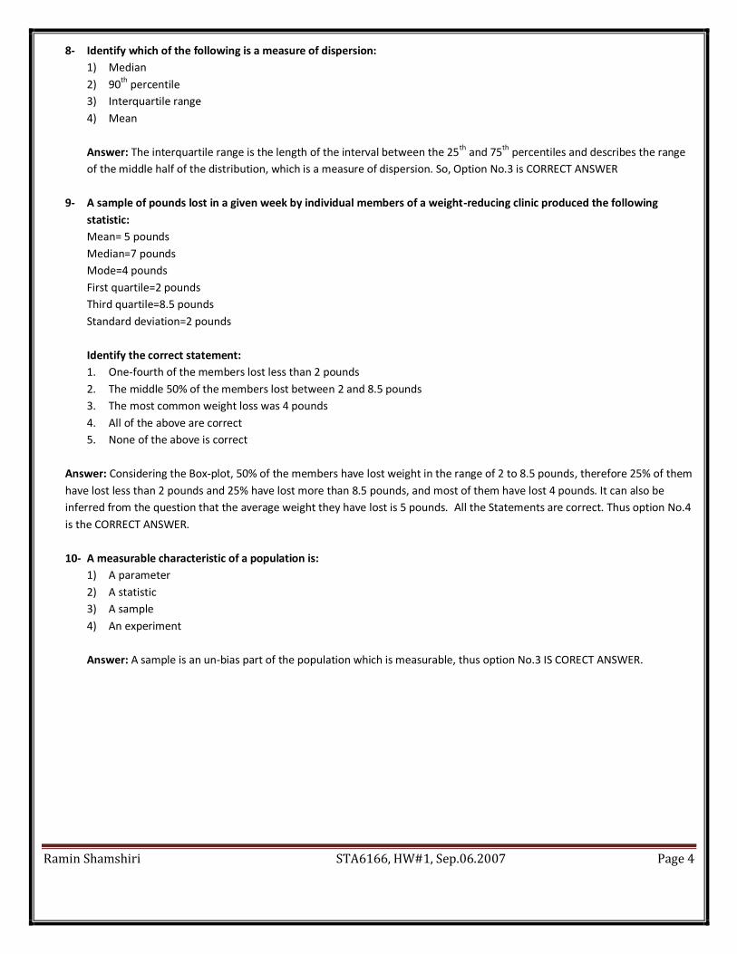
8- Identify which of the following is a measure of dispersion:
1) Median
2) 90th
percentile
3) Interquartile range
4) Mean
Answer: The interquartile range is the length of the interval between the 25th
and 75th
percentiles and describes the range
of the middle half of the distribution, which is a measure of dispersion. So, Option No.3 is CORRECT ANSWER
9- A sample of pounds lost in a given week by individual members of a weight-reducing clinic produced the following
statistic:
Mean= 5 pounds
Median=7 pounds
Mode=4 pounds
First quartile=2 pounds
Third quartile=8.5 pounds
Standard deviation=2 pounds
Identify the correct statement:
1. One-fourth of the members lost less than 2 pounds
2. The middle 50% of the members lost between 2 and 8.5 pounds
3. The most common weight loss was 4 pounds
4. All of the above are correct
5. None of the above is correct
Answer: Considering the Box-plot, 50% of the members have lost weight in the range of 2 to 8.5 pounds, therefore 25% of them
have lost less than 2 pounds and 25% have lost more than 8.5 pounds, and most of them have lost 4 pounds. It can also be
inferred from the question that the average weight they have lost is 5 pounds. All the Statements are correct. Thus option No.4
is the CORRECT ANSWER.
10- A measurable characteristic of a population is:
1) A parameter
2) A statistic
3) A sample
4) An experiment
Answer: A sample is an un-bias part of the population which is measurable, thus option No.3 IS CORECT ANSWER.

Ramin Shamshiri STA6166, HW#1, Sep.06.2007 Page 5
11- What is the primary characteristic of a set of data for which the standard deviation is zero?
1) All values of the variable appear with equal frequency
2) All values of the variable have the same value
3) The mean of the value is also zero
4) All of the above are correct
5) None of the above is correct
Answer: The standard deviation of a set of observed values is defined to be the positive root of the variance and the
variance of a set of n observed values is the sum of the squared deviations divided by (n-1). The difference (distance)
between the observed value (yi) and the mean is called the deviation of the yith
observation from the mean.
So if the Standard deviation is zero, it means that the yi-y is zero or yi=y which means that all of the values of the variable
have the same value. Thus option No.2 is the CORRECT ANSWER
12- Let X be the distance in miles from their present homes to residences when in high school of individuals at a class
reunion. The X is
1) A categorical (nominal) variable
2) A continuous variable
3) A discrete variable
4) A parameter
5) A Statistic
Answer: The distance is expressed in miles, and miles can be expressed as one mile, or two miles or any real and positive
digit. Distance is considered continues variable here and thus option No.2 IS CORRECT ANSWER.
13- A subset of a population is:
1- A parameter
2- A population
3- A statistic
4- A sample
5- None of the above
Answer: A subset of population is a Sample. Thus Option No.4 IS CORRECT ANSWER.
14- The median is a better measure of central tendency than the mean if:
1- The variable is discrete
2- The distribution is skewed
3- The variable is continues
4- The distribution is symmetric
5- None of the above is correct
Answer: Option No.2 is correct.
Ramin Shamshiri STA6166, HW#1, Sep.06.2007 Page 6
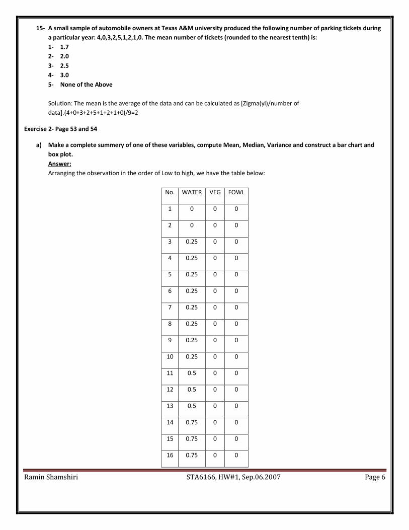
15- A small sample of automobile owners at Texas A&M university produced the following number of parking tickets during
a particular year: 4,0,3,2,5,1,2,1,0. The mean number of tickets (rounded to the nearest tenth) is:
1- 1.7
2- 2.0
3- 2.5
4- 3.0
5- None of the Above
Solution: The mean is the average of the data and can be calculated as [Zigma(yi)/number of
data].(4+0+3+2+5+1+2+1+0)/9=2
Exercise 2- Page 53 and 54
a) Make a complete summery of one of these variables, compute Mean, Median, Variance and construct a bar chart and
box plot.
Answer:
Arranging the observation in the order of Low to high, we have the table below:
No. WATER VEG FOWL
1 0 0 0
2 0 0 0
3 0.25 0 0
4 0.25 0 0
5 0.25 0 0
6 0.25 0 0
7 0.25 0 0
8 0.25 0 0
9 0.25 0 0
10 0.25 0 0
11 0.5 0 0
12 0.5 0 0
13 0.5 0 0
14 0.75 0 0
15 0.75 0 0
16 0.75 0 0

Ramin Shamshiri STA6166, HW#1, Sep.06.2007 Page 7
17 0.75 0 1
18 1 0 2
19 1 0 2
20 1 0 2
21 1 0 4
22 1 0 5
23 1 0 9
24 1.25 0 10
25 1.25 0 11
26 1.5 0 11
27 1.5 0 12
28 1.5 0 14
29 1.5 0 15
30 1.5 0 16
31 2 0 16
32 2 0.25 16
33 2 0.5 17
34 2 0.75 18
35 2 1 26
36 3 1 30
37 4 1 32
38 5 1.25 51
39 5 1.5 59
40 5 1.75 74
41 6 2 80
42 7 2 125
43 7 2 125

Ramin Shamshiri STA6166, HW#1, Sep.06.2007 Page 8
44 9 2 167
45 10 2.25 177
46 15 2.75 179
47 16 3 185
48 16 4 210
49 17 5.25 218
50 31 7 240
51 33 8 364
52 149 9 1410
WATER VEG FOWL
Mean 7.125 1.120192 75.63462
Median= 1.5 0 11.5
Variance= 452.864 4.327182 42197.33
Standard Deviation= 21.2806 2.080188 205.4199
Mode= 0.25 0 0
The Bar chart is plotted in MATLAB as shown below: (Data1=Water, Data 2= VEG, Data3=FOWL)

Ramin Shamshiri STA6166, HW#1, Sep.06.2007 Page 9
The process for constructing the Box-plot, is as follow:
Q1= 25% of the distribution= 0.25*52= 13 => y13th_Water= 0.5 y13th_VEG=0 y13th_FOWL=0
Q3=75% of the distribution= 0.75*52=39 => y39th_Water= 5 y39th_VEG=1.5 y39th_FOWL=59
It means that:
50% of the observed value of Water will lie between 0.5 and 5, 50% of the observed value of VEG will lie between 0 and 1.5,
50% of the observed value of FOWL will lie between 0 and 59
b) Constructing a frequency distribution for FOWL and using the frequency distribution to compute the mean and variance:
c) Make a scatter-plot relating WATER or VEG to FOWL
Answer: Relating Water to FOWL means that Water lies on vertical axes (y), and FOWL lies on the horizontal axes (x)

Ramin Shamshiri STA6166 Homework#2, Due. Sep.27.2007
STA 6166, Section 8489, Fall 2007,
Homework #2, Due September 27, 2007
Student Name: Ramin Shamshiri UFID#: 9021-3353

Ramin Shamshiri STA6166 Homework#2, Due. Sep.27.2007
B) Please read the two papers, Palleroni and Hauser (2003) and Arnold et al. (2002), that are
attached. For each paper answer the following questions:
Fluorescent Signaling in Parrots
a. Is the study observational or experimental?
Answer: Experiment
b. What factors or explanatory variables are they interested in studying for their affects on
the animals?
Answer: Fluorescent plumage, UV reflectance
c. What variables are they measuring on the animals?
Answer: Sexual and social choice
d. State in words all sets of hypotheses that the authors are interested in testing (note that the
authors could be interested in more than one set of hypotheses!)
Answer:
H0: there is no sexual preference for fluorescence between parrot sexes
HA: there is sexual preference for fluorescence between parrot sexes
H0: there is social preference for fluorescence between same sexes of parrots
HA: there is no social preference for fluorescence between same sexes of parrots
e. Restate all sets of hypotheses in statistical terms, i.e. in terms of the population
parameters that are believed to be affected by the treatments.
Answer:
H0: psexual preference ≥ 0.05
HA: psexual preference < 0.05
H0: psocial preference ≤ 0.5
HA: psocial preference > 0.5

Ramin Shamshiri STA6166 Homework#2, Due. Sep.27.2007
Experience-Dependent Plasticity for Auditory Processing in a Raptor
a. Is the study observational or experimental?
Answer: Observational
b. What factors or explanatory variables are they interested in studying for their affects on
the animals?
a. Answer: - Experienced subject and Naive subject
c. What variables are they measuring on the animals?
Answer: They measure Auditory processing
d. State in words all sets of hypotheses that the authors are interested in testing (note that the
authors could be interested in more than one set of hypotheses!)
Answer:
H0: Experience affects auditory processing in harpy eagles
HA: Experience has little effect on auditory processing in harpy eagles
e. Restate all sets of hypotheses in statistical terms, i.e. in terms of the population
parameters that are believed to be affected by the treatments.
Answer:
Ho: p < 0.001
HA: p ≥ 0.001

Ramin Shamshiri STA6166 Homework#2, Due. Sep.27.2007
C) Use the three approaches we learned in class (histograms, Q-Q plots, and hypothesis testing)
for determining if the sample data support the argument that the populations of FRACTION and
L_FRACTION are Normally Distributed.
Statistic FRACTION L_FRACTION
Mean 0.686 -0.37826
Variance 0.002592 0.005518
Standard Deviation 0.050911688 0.074284
95% Coefficient Interval 0.029812943 0.042114
Fraction Histogram L_Fraction Histogram

Ramin Shamshiri STA6166 Homework#2, Due. Sep.27.2007
Histogram:
0. 36 0. 48 0. 6 0. 72 0. 84 0. 96 1. 08
0
5
10
15
20
25
30
35
P
e
r
c
e
n
t
f r act i on
Fraction Histogram: Mostly Normal, with a little skewd to the left
- 0. 975 - 0. 825 - 0. 675 - 0. 525 - 0. 375 - 0. 225 - 0. 075 0. 075
0
5
10
15
20
25
30
35
P
e
r
c
e
n
t
l _f r act i on
L_Fraction Histogram: Not Normal, Skewed to the left

Ramin Shamshiri STA6166 Homework#2, Due. Sep.27.2007
Q-Q Plot:
Fraction
- 3 - 2 - 1 0 1 2 3
0. 2
0. 4
0. 6
0. 8
1. 0
1. 2
f
r
a
c
t
i
o
n
Nor mal Quant i l es
- 3 - 2 - 1 0 1 2 3
0. 2
0. 4
0. 6
0. 8
1. 0
1. 2
f
r
a
c
t
i
o
n
Nor mal Quant i l es
Fracton: Left end of the pattern is below the line and right end of pattern is also below the line, so we
have long tail on the left and short tail on the right, So it is not Normal

Ramin Shamshiri STA6166 Homework#2, Due. Sep.27.2007
L_Fraction
- 3 - 2 - 1 0 1 2 3
- 1. 25
- 1. 00
- 0. 75
- 0. 50
- 0. 25
0
0. 25
l
_
f
r
a
c
t
i
o
n
Nor mal Quant i l es
- 3 - 2 - 1 0 1 2 3
- 1. 25
- 1. 00
- 0. 75
- 0. 50
- 0. 25
0
0. 25
l
_
f
r
a
c
t
i
o
n
Nor mal Quant i l es
L_Fracton: Left end of the pattern is very below the line and right end of pattern is also below the line,
so we have a long tail on the left and a short tail on the right. (as observed in the Histogram), So it is not Normal

Ramin Shamshiri STA6166 Homework#2, Due. Sep.27.2007
Hypothesis testing:
H0: the population has a specified theoretical distribution (Is Normal) : P>0.05
HA: the distribution is Not the theoretical distribution (Is not Normal) : P<0.05
So, based on the test result, we decide whether to reject H0 or not.
The Kolmogorov-Smirnov test shows that Pr>0.15 which is larger than 0.05, so Null hypothesis
is not rejected for Fraction which means that the distribution is Normal.
For L-fraction, the Kolmogorov-Smirnov test shows that P>0.0137 which is smaller that 0.05,
thus the Null hypothesis is rejected and the distribution is not Normal.
Tests for Normality (Fraction) Test --Statistic--- -----p Value------ Shapiro-Wilk W 0.982163 Pr < W 0.2751 Kolmogorov-Smirnov D 0.066056 Pr > D >0.1500 Cramer-von Mises W-Sq 0.058087 Pr > W-Sq >0.2500 Anderson-Darling A-Sq 0.379258 Pr > A-Sq >0.2500
Tests for Normality (L_Fraction) Test --Statistic--- -----p Value------ Shapiro-Wilk W 0.921818 Pr < W <0.0001 Kolmogorov-Smirnov D 0.107913 Pr > D 0.0137 Cramer-von Mises W-Sq 0.218273 Pr > W-Sq <0.0050 Anderson-Darling A-Sq 1.366205 Pr > A-Sq <0.0050

Ramin Shamshiri STA6166 Homework#2, Due. Sep.27.2007
The UNIVARIATE Procedure Variable: l_fraction (l_fraction) Moments N 87 Sum Weights 87 Mean -0.2619755 Sum Observations -22.791868 Std Deviation 0.19759871 Variance 0.03904525 Skewness -1.2963243 Kurtosis 3.08046089 Uncorrected SS 9.32880233 Corrected SS 3.3578914 Coeff Variation -75.426408 Std Error Mean 0.02118481 Basic Statistical Measures Location Variability Mean -0.26198 Std Deviation 0.19760 Median -0.23067 Variance 0.03905 Mode -0.26919 Range 1.15493 Interquartile Range 0.24003
Basic Confidence Limits Assuming Normality Parameter Estimate 95% Confidence Limits Mean -0.26198 -0.30409 -0.21986 Std Deviation 0.19760 0.17197 0.23228 Variance 0.03905 0.02957 0.05395 Tests for Location: Mu0=0 Test -Statistic- -----p Value------ Student's t t -12.3662 Pr > |t| <.0001 Sign M -37.5 Pr >= |M| <.0001 Signed Rank S -1875 Pr >= |S| <.0001 Tests for Normality Test --Statistic--- -----p Value------ Shapiro-Wilk W 0.921818 Pr < W <0.0001 Kolmogorov-Smirnov D 0.107913 Pr > D 0.0137 Cramer-von Mises W-Sq 0.218273 Pr > W-Sq <0.0050 Anderson-Darling A-Sq 1.366205 Pr > A-Sq <0.0050

Ramin Shamshiri STA6166 Homework#2, Due. Sep.27.2007
The UNIVARIATE Procedure Variable: fraction (fraction) Moments N 87 Sum Weights 87 Mean 0.7833908 Sum Observations 68.155 Std Deviation 0.13988221 Variance 0.01956703 Skewness -0.4673428 Kurtosis 0.66359871 Uncorrected SS 55.074765 Corrected SS 1.68276471 Coeff Variation 17.8559928 Std Error Mean 0.01499695 Basic Statistical Measures Location Variability Mean 0.783391 Std Deviation 0.13988 Median 0.794000 Variance 0.01957 Mode 0.764000 Range 0.76300 Interquartile Range 0.18800 Basic Confidence Limits Assuming Normality Parameter Estimate 95% Confidence Limits Mean 0.78339 0.75358 0.81320 Std Deviation 0.13988 0.12174 0.16443 Variance 0.01957 0.01482 0.02704 Tests for Location: Mu0=0 Test -Statistic- -----p Value------ Student's t t 52.23669 Pr > |t| <.0001 Sign M 43.5 Pr >= |M| <.0001 Signed Rank S 1914 Pr >= |S| <.0001 Tests for Normality Test --Statistic--- -----p Value------ Shapiro-Wilk W 0.982163 Pr < W 0.2751 Kolmogorov-Smirnov D 0.066056 Pr > D >0.1500 Cramer-von Mises W-Sq 0.058087 Pr > W-Sq >0.2500 Anderson-Darling A-Sq 0.379258 Pr > A-Sq >0.2500

Ramin Shamshiri STA6166 Homework#2, Due. Sep.27.2007
Concept Questions
1. If two events are mutually exclusive then P(A or B)=P(A)+P(B)
Answer: True,
Mutually exclusive means that two events can not occur simultaneously, or can not happen together
which is equal to say P (A and B) = 0.
As a conclusion, we have the two following results;
if two events are independent, but NOT mutually exclusive, then P(A or B)=P(A)+P(B)-P(A and
B)
if two events are independent, and mutually exclusive, then P(A or B)=P(A)+P(B)
2. If A and B are two events, then P (A and B) =P (A).P (B), no matter what the relation between
A and B.
Answer= False,
P (A and B) =P (A).P (B) only if two events are independent. It should be noted that if two events are
NOT independent, more complex methods must be applied.
3. The probability distribution function of a discrete random variable can not have a value greater
than 1.
Answer: True
For P(y) to be considered as a discrete value of a variable Y, it should satisfy the following conditions;
0=<p(y) <=1
SUM [p(y)] =1
4. The probability distribution function of a continuous random variable can take on any value,
even negative ones.
Answer: False
The probability distribution function of a continuous random variable f(y) does not give the
probability that Y= y as did p(y) in the discrete case. This is because Y can take on an infinite number
of values in an interval, and therefore it is impossible to assign a probability value for each y. In fact
the value of f(y) is not a probability at all; hence f(y) can take any nonnegative value, including
values greater than 1.
5. The probability that a continuous random variable lies in the interval 4 to 7, inclusively, is the
sum of P(4)+P(5)+P(6)+P(7)
Answer: False
The probability the a continuous random variable lies in the interval 4 to 7 is equal to the area
between the curve and horizontal axes from the values 4 to the value 7.
6. The variance of the number of success in a binomial experiment of n trails is σ2=np(p-1)
Answer: True

Ramin Shamshiri STA6166 Homework#2, Due. Sep.27.2007
7. A normal distribution is characterized by its mean and its degree of freedom.
Answer: False
A normal distribution has only two parameters, μ and σ and knowing the values of these two
parameters completely determines the distribution.
8. The standard normal distribution has the mean zero and variance σ2
Answer: False
In the standard normal distribution, the Mean (μ) is zero and σ=1
Practice Exercises
1- The weather forecast says there is a 40% chance of rain today and 30% chance of rain
tomorrow.
a. What is the chance of the rain on both days?
Let Today: A Tomorrow: B
Answer: Since the two events are independent, P (A and B) =P (A).P (B)
So: The chance of the rain on both days= (0.4).(0.3)=0.12 or 12%
b. What is the chance of rain on neither day?
Answer: The chance of rain on neither day = (1 – chance of rain on today).(1- chance of rain on
tomorrow)= (0.6).(0.7)=0.42 or 42%
c. What is the chance of rain on at least one day?
Answer: Since the two events are NOT mutually exclusive, they can also happen together, so P(A or
B)= P(A)+P(B)- P(A).P(B)= 0.4+0.3-0.12= 0.58 or 58%
2- The following is the probability distribution of the number of defects on a given contact lens
produced in one shift on a production line:
Number of defects: 0 1 2 3 4
Probability: 0.5 0.2 0.15 0.10 0.05
Let A be the event that one defect occurred, and B the event that 2, 3 or 4 effects occurred. Find:
a. P(A) and P(B)
Answer:
P (A) =P (1) =0.2
P (B) =P (2 or 3 or 4) =P (2) +P (3) +P (4) =0.15+0.1+0.05=0.3
b. P(A and B)
Answer: The events A and B are mutually exclusive, meaning that they can not happen together,
so P (A and B) =0
c. P(A or B) : Answer: P (A or B) =P (A) +P (B) =0.2+0.3=0.5

Ramin Shamshiri STA6166 Homework#2, Due. Sep.27.2007
3- Using the distribution in Excersise 2, let the random variable Y be the number of defects on a
contact lens randomly selected from lenses produced during the shift.
a. Find the Mean and Variance of Y for the shift.
Answer:
Mean (μ)=SUM [y . p(y)] = [(0)(0.5)+(1)(0.2)+(2)(0.15)+(3)(0.1)+(4)(0.05)]=1
Variance (σ) = SUM [(y-μ) 2
. p(y)]
b. Assume that the lenses are produced independently. What is the probability that five lenses drawn
randomly from the production line during the shift will be defect-free.
Answer: P(y) = ( μy.e
-y)/y! = p (5) = 0.05615
4- Using the distribution in exercise 2, suppose that the lens can be sold as if there are no defects
for 20$. If there is one defect, it can be reworked at a cost of 5$ and then sold. If there are two
defects, it can be reworked at a cost of 10$ and then sold. If there are more than two defects, it
must be scrapped. What is the expected revenue generated during the shift if 100 contact lenses
are produced?
Answer:
The question can be considered as the expected revenue during the shift of producing 100 contact
lenses, with the probability that 1 or 2 lenses are defected.
P(1)=20% Reworked charge for 1 defect=5$
P(2)=15% Reworked charge for 2 defect2=10$
We know that μ=SUM (y.p(y)) so we will have:
5$(0.2)+10$(0.15)=1+1.5=2.5$ is the expected revenue in the process of producing 100 contact
lenses.
5- Suppose that Y is a normally distributed random variable with μ=10 and σ=2, and X is an
independent random variable, also normally distributed with μ=5 and σ =5
a. P(Y>12 and X<4)
Answer:
Since both variables are normally distributed, we can use the normal distribution rules and the
appendix table. Transforming the Y and X value to the standard normal distribution Z, we have:
Z=(y-μ)/σ

Ramin Shamshiri STA6166 Homework#2, Due. Sep.27.2007
Exercises
1- A lottery that sells 150,000 ticket has the following prize structure:
(1)First prize of 50,000$
(2) 5 second prizes of 10,000$
(3) 25 third prizes of 1000$
(4) 1000 fourth prizes of 10$
a. Let Y be the winning amount of a randomly drawn lottery ticket. Describe the probability
distribution of Y.
Answer: If a ticket is drawn randomly from the total amount of150,000 ticket, there is a
probability of 1/150,000 that it will be the first prize winner, and 5/150,000 that it becomes the
2nd
prize winner and so on.
1+5+25+1000=1031
150,000-1031=148969
So the probability that a ticket wins NOTHING is 148969/150,000
Outcome Probability Winning
Prize$
0: No Win 148969/150,000=0.9931266 0$
1st prize 1/150,000=0.000006 50,000$
2nd
prize 5/150,000=0.00003 10,000$
3rd
prize 25/150,000=0.00015 1000$
4th prize 1000/150,000=0.006 10$
b. Compute the Mean or expected value of the ticket
Answer:
μ=∑y.p(y)
=[0.(0.9931266)+50,000.(0.000006)+10,000.(0.00003)+1000.(0.00015)+10.(0.006)]
=0.81
c. If the ticket cost 1$, is the purchase of the ticket worthwhile?
Answer: Calculating the expectation value of winning prize, considering that if there is no Win
then there is a( -1$) prize,
=[-1.(0.9931266)+50,000.(0.000006)+10000.(0.00003)+1000.(0.00015)+10.(0.006)]
=(-0.9931266)+(0.3)+(0.3)+(0.15)+(0.06)=-0.1831266
Since the mean is negative, it does not worth to buy the ticket.
d. Compute the standard deviation of this distribution, comment on the usefulness of the standard
deviation as a measure of dispersion.
Ramin Shamshiri STA6166, HW#3, Oct.04.2007 Page 1
In Class Activity STA 6166 Fall 2007
4 October 2007
RAMIN SHAMSHIRI- UFID#:9021-3353
1. a-
These value can not be considered a random sample from the population value since they are
representing the last 20 fills, thus they are biased and are unable to represent the real fills population.
1. b- The sampling distribution of 𝑀𝑒𝑎𝑛 from a random sample size 20 drawn from a population with Mean μ and variance 𝜎2 will have mean= μ and variance=𝜎2/20 The assumption is that regarding the central limit theorem, if a random sample of size n is taken from any distribution with mean μ and variance𝜎2, the sample Mean 𝑌 will have a distribution approximately normal with Mean μ and variance𝜎2/𝑛. The approximately becomes better as n increases. 1. c- This distribution is used for the sample distribution of sample variance. When a random sample is taken from a population with Mean μ and variance 𝜎2, the sample variance is:
𝑠2 = (𝑥𝑖 − 𝑥 )2
𝑛 − 1
The sample distribution of 𝑥2 =(𝑛−1)𝑠2
𝜎2 is a chi-square distribution with (n-1) degrees of freedom.
Mean: 𝜇𝑠2 = 𝜎2
Variance: 𝑠2 =2𝜎4
𝑛−1
A chi-square variable can not be negative, and the distributions are positively skewed. At about 100 degrees of freedom, the chi-square distribution becomes somewhat symmetrical. The area under each chi-square distribution is equal to 1.00 or 100%.
Assumption: The chi-square distribution is obtained from the value of 𝑥2 = 𝑛−1 .𝑠2
𝜎2 when random
samples are selected from a normally distributed population whose variance is 𝜎2.
The sample must be randomly selected
The population must be normally distributed for the variable under study
The observation must be independent of each other

Ramin Shamshiri STA6166, HW#3, Oct.04.2007 Page 2
1. d-
We know that in a normal distribution, the tree parameters Mean, Mode and Median are equal or
approximately equal. In addition, from the empirical rule, we know that 68% of the values falls in the
interval of Mean plus or mines standard deviation. From the exploratory analysis, we have:
Mean=22.83 Median=22.6 Mode= 22 SD=1.33
Mean+SD=24.16 Mean-SD=21.5
From the Box-plot, we see that 50% of the data are between 21.8 and 23.6. If the distribution is normal,
then 68% of the data would have fallen in the interval of 21.5 and 24.16. This result shows that the data
distribution is approximately normal. The shape of the distribution also shows that it is not exactly
normal, but a little skewed to the right.
1. e-
Testing the hypothesis that the true mean mpg for the car is greater than 26:
H0: μ≤26 HA: μ>26 (Claim) Confidence level=95% => level of significance (α)=5% or 0.05 From the exploratory analysis we have: n=20 => degree of freedom=19 SD=1.33 (Sample Standard Deviation) Mean=22.83 From the t-table, with α= 0.05 and d.f=19, we have t=1.7291 Since population standard deviation is unknown and the sample size is less than 30, the z test is inappropriate for testing hypothesis involving means. So we use the t-test. The t-test is a statistical test for the mean of a population and is used when the population is normally or approximately normally distributed, σ is unknown and n<30. We want to check if the claim that the true mean is greater than true is valid or not. We use t-test to transfer the sample mean into the standard normal distribution.
𝑡 = 𝑋 − 𝜇
𝑠/ 𝑛=
22.83 − 26
1.33/ 20= −10.65
The value of t is smaller than 1.72, so we conclude that there is not enough evidence to show that the
true mean is greater than 26. So the null hypothesis which was to reject this claim is not rejected.

Ramin Shamshiri STA6166, HW#3, Oct.04.2007 Page 3
The figure below shows that if we had a sample mean greater than 26.51, we could say that there is
enough evidence to declare that true mean is also greater than 26 with α=0.05.
𝑡 = 𝑋 − 𝜇
𝑠/ 𝑛=> 1.71 =
𝑋 − 26
1.33/ 20=> 𝑋 = 26.51
1.f- Calculating 90% confidence interval for the true mean mpg of this car:
From this equation, 𝑡 = 𝑋 −𝜇
𝑠/ 𝑛, we conclude that the confidence interval in which the true mean can fall
is:
𝑋 − 𝑡𝛼2
𝑠
𝑛 < 𝜇 < 𝑋 + 𝑡𝛼
2
𝑠
𝑛
22.83 − 𝑡0.12
1.33
20 < 𝜇 < 22.83 + 𝑡0.1
2
1.33
20
22.83 − 0.5142 < 𝜇 < 22.83 + 0.5142 22.31 < 𝜇 < 23.34
2622.83
0-10.65 1.72
26.51
Acceptable area
Rejecting area
(1-alpha)% Confidence Interval
t_alpha/2t_alpha/2

Ramin Shamshiri STA6166, HW#3, Oct.04.2007 Page 4
1.g- Testing the hypothesis that the population variance is greater than 2.1: The chi-square test is used to test a claim about a single variance or standard deviation. H0: 𝜎2≤2.1 HA: 𝜎2>2.1 (Claim) Confidence level=95% => level of significance (α)=5% or 0.05 From the sampling results we have: n=20 => degree of freedom=19 SD=1.33 (Sample Standard Deviation)=> Var=1.69 From the Chi-square table, with α=0.05 and d.f= 19 we have: 𝑥2 = 30.144
𝑥2 =(𝑛 − 1)𝑠2
𝜎2=
(19)1.69
2.1= 15.29
Since the value of 𝑥2 from the test is smaller than the value of 𝑥2 from the table, there is not enough evidence that the population variance is greater than 2.1. so we reject the claim. If we had our sample variance greater than 3.33, we would have our chi-square test result greater than 30.144, thus we could declare that there is enough evidence that the population variance is greater than 2.1.

Ramin Shamshiri STA6166, HW#3, Oct.04.2007 Page 5
1.h- Testing that the population median differs from 25mpg Since median is defined as middle value of the population, we can say that 50% of the population values are below and 50% are above the median. If we define the values above the median as success, we will have a sample from a binomial distribution with p=0.5. A hypothesis test involving a population proportion can be considered as a binomial experiment when there are only two outcomes and the probability of a success does not change from trial to trial. For the
binomial distribution, we know that μ=np and σ= 𝑛. 𝑝. (1 − 𝑝)
Since the normal distribution can be used to approximate the binomial distribution when np≥5 and n(1-
p)≥5, the standard normal distribution can be used to test hypothesis for proportions: 𝑧 =𝑝 −𝑞
𝑝 .𝑞/𝑛
Where: 𝑝 =X/n is sample proportion. Here we have 20*0.5=10>5, so we can use this test. H0: P=0.5 HA: P≠0.5 Confidence level=95% so, α=0.05, this is a two tailed test, so α/2=0.025 From the Z table, P(Z>1.96)=0.025 and P(Z<-1.96)=-0.025 We would reject the null hypothesis, if the result of z-test is greater than 1.96 or smaller than -1.96.In the other word, if |Z|>1.96 From the exploratory analysis, we see that we only have two counts of mpg with the value of 25 which means 2/20=10%. So we have:
𝑧 =𝑝 − 𝑞
𝑝. 𝑞/𝑛=
0.1 − 0.5
0.5 ∗ 0.5/20= −3.38
Here we see that |Z|=3.38 which is greater than 1.96, thus we reject the claim, null hypothesis and we conclude that the Median should differs from 25mpg.

Ramin Shamshiri STA6166, HW#3, Oct.04.2007 Page 6
2.a- P claims to be 10% P of a random sample= 17% n=100 Checking if the sample size is sufficiently large to be used as normal distribution: np≥5 => 100*0.17=17 and is greater than 5 n(1-p) ≥5 => 100*0.83=83 and is greater than 5 Yes, the sample size is sufficient large 2.b- This can be considered a binomial distribution, the incidence of paratuberculosis in Florida’s beef cattle
is equivalent to the portion of successes. For the binomial distribution, μ=np and σ= 𝑛. 𝑝. (1 − 𝑝)
So, the shape of this distribution is normal, center is μ=np=100*0.17=17, and σ= 𝑛. 𝑝. (1 − 𝑝) =
100 ∗ 0.17 ∗ 0.83=3.75 Figure below:
2.c- H0: P=10% HA: P≠10% Confidence level=95% so, α=0.05, this is a two tailed test, so α/2=0.025 From the Z table, P(Z>1.96)=0.025 and P(Z<-1.96)=-0.025 We would reject the null hypothesis, if the result of z-test is greater than 1.96 or smaller than -1.96.In the other word, if |Z|>1.96
𝑧 =𝑝 − 𝑝0
𝑝0(1 − 𝑝0)/𝑛=
0.17 − 0.1
0.1 ∗ 0.9/100= 2.33
The null hypothesis is rejected, which means that the true population mean is different than 10%.
17 13.7513.25 24.59.55.75 28.2

Ramin Shamshiri STA6166, HW#3, Oct.04.2007 Page 7
2.d- Confidence Intervals and sample size for proportions P=symbol for the population proportion 𝑝 = symbol for the sample proportion X= number of sample unites that possess the characteristics of interest N=sample size 𝑝 =x/n Confidence interval about the proportions must meet the criteria that np≥5 and nq≥5. To construct a confidence interval about the proportion, the maximum error of estimate must be used:
𝐸 = 𝑍𝛼/2 𝑝 𝑞
𝑛
Confidence Interval for Proportion:
𝑝 − (𝑍𝛼/2) 𝑝 𝑞
𝑛< 𝑝 < 𝑝 + (𝑍𝛼/2)
𝑝 𝑞
𝑛
0.17 − 1.96 0.17 ∗ 0.83
100< 𝒑 < 0.17 + 1.96
0.17 ∗ 0.83
100
0.17 − 0.073 < 𝒑 < 0.17 + 0.073 0. 𝑜97 < 𝒑 < 0.243
It means that the incidence of paratuberculosis in Florida’s beef cattle will be in the range of
0.097 to 0.243 with 95% confidence level.

Ramin Shamshiri STA6166, HW#4, Oct.18.2007 Page 1
STA 6166, Section 8489, Fall 2007
Homework #4
Due 18 October 2007
RAMIN SHAMSHIRI
UFID#: 9021-3353

Ramin Shamshiri STA6166, HW#4, Oct.18.2007 Page 2
1. Chapter 4, Freund and Wilson, page 180. Do all 13 concept questions (true/false).
2. Chapter 4, Freund and Wilson, page 181. Under “practice exercises”, do questions 2, 3,
and 4. If possible, use a software package to answer questions 2 and 3.
3. Chapter 7, Freund and Wilson, page 327. Under “exercises”, do question 1 by hand.
Show all work.
4. Chapter 7, Freund and Wilson, page 328. Under “exercises”, do question 5 using a
software package. Do not submit raw output from your analysis. Please embed any tables,
graphs, etc into your write-up (as tables or graphs, etc).

Ramin Shamshiri STA6166, HW#4, Oct.18.2007 Page 3
Chapter4-
Concept Questions
1. The t-distribution is more dispersed than the Normal.
Answer: True
The variance of t-distribution is greater than 1
2. The x2 distribution is used for inference on the mean when the variance is unknown.
Answer: False
The x2 distribution is used for a variance of standard deviation inference
3. The mean of the t distribution is affected by the degree of freedom.
Answer: False
The mean of the t distribution is equal to zero, like the z distribution.
4. The quantity (𝑦 −𝜇 )
𝜎2/𝑛 has the t distribution with (n-1) degrees of freedom.
Answer: False
That is a z-test for mean, when the population standard deviation is known
5. In the t-test for a mean, the level of significance increases if the population standard
deviation increases, holding the sample size constant.
Answer: False,
Because there is no relation between the significance level and the population standard
deviation
6. The x2 distribution is used for inferences on the variance
Answer: True
7. The mean of the t distribution is zero.
Answer: True
8. When the test statistic is t and the number of degrees of freedom is >30, the critical value
of t is very close to that of z.
Answer: True
In fact, as the sample size increases, (degree of freedom increases), the t distribution
approaches the standard normal distribution.
9. The x2 distribution is skewed and its mean is always 2.
Answer: False
The x2 distribution is positively skewed and its shape changes as the degrees of freedom
changes. The higher the degree of freedom, the less skewed this distribution is, so the
Mean of this distribution is not unique. At about 100 degrees of freedom, the x2
distribution becomes somewhat symmetric.
10. The variance of a binomial proportion is np(1-p)
Answer: True

Ramin Shamshiri STA6166, HW#4, Oct.18.2007 Page 4
11. The sampling distribution of a proportion is approximated by the x2 distribution.
Answer: False
The sampling distribution of a proportion (binomial distribution) is approximated by
normal distribution
12. The t test can be applied with absolutely no assumption about the distribution of the
population
Answer: False
The assumption for the t test is that the distribution is approximately normal.
13. The degrees of freedom for the t test do not necessarily depend on the sample size used in
computing mean.
Answer: True
It depends on the sample size used in computing standard deviation.

Ramin Shamshiri STA6166, HW#4, Oct.18.2007 Page 5
Chapter 4- question No.2
The following sample was taken from a normally distributed population:
3,4,5,5,6,6,6,7,7,9,10,11,12,12,13,13,13,14,15
a- Compute the 0.95 confidence interval on the population mean μ
95% Confidence Interval => α=0.05
For a 95% CI, and degree of freedom (19-1=18), the 𝑡𝛼2= 𝑡0.05
2
= 𝑡0.025 is equal to 2.1 from the table.
If we had the population variance, we could use the normal distribution and 𝑧𝛼
2 respectively. Here we do
not have the population variance, in addition, the sample size is also less than 30, thus we should use the
t-distribution. Using the below formula for the confidence interval of the Mean for a specific α
𝑦 − 𝑡𝛼2
𝑠
𝑛 < 𝜇 < 𝑦 + 𝑡𝛼
2
𝑠
𝑛
9 − 2.1 3.81
19 < 𝜇 < 9 + 2.1
3.81
19
7.17 < 𝜇 < 10.83
b- Compute the 0.90 confidence interval on the population standard deviation σ.
90% Confidence Interval => α=0.1=> α/2=0.05
In order to calculate these confidence intervals, the Chi-square 𝑥2distribution is needed. The chi-square
distribution is obtained from the value of 𝑥2 = 𝑛−1 .𝑠2
𝜎2 when random samples are selected from a
normally distributed population whose variance is 𝜎2. From the 𝑥2 table, we have the lower and upper tail as below: Formula for confidence interval for a variance: (d.f=n-1)
( 𝑛−1 .𝑠2
𝑥𝑙𝑜𝑤𝑒𝑟2 ) < 𝜎2 < (
𝑛−1 .𝑠2
𝑥𝑢𝑝𝑝𝑒𝑟2 ) or (
𝑛−1 .𝑠2
𝑥𝛼/22 ) < 𝜎2 < (
𝑛−1 .𝑠2
𝑥(1−𝛼/2)2 )
( 19 − 1 14.44
28.869) < 𝜎2 < (
19 − 1 14.44
9.39)
9 < 𝜎2 < 27.6
Formula for the confidence interval for a standard deviation: (d.f=n-1)
𝑛 − 1 . 𝑠2
𝑥𝑟𝑖𝑔𝑡2 < 𝜎 <
𝑛 − 1 . 𝑠2
𝑥𝑙𝑒𝑓𝑡2
19 − 1 14.44
28.869< 𝜎 <
19 − 1 14.44
9.39
3 < 𝜎2 < 5.25
Statistic Value
n 19
𝑦 9
s2 14.44
s 3.81

Ramin Shamshiri STA6166, HW#4, Oct.18.2007 Page 6
Chapter 4- question No.3 Using the data in exercise 2, test the following hypothesis: 3.a- H0: μ=13 H1: μ≠13 This is a test for population mean, and here we do not know the population variance, so we use the t-test. Using 95% confidence interval, we have α=0.05. Since this is an equivalency test, it is a two-tailed test, so we need to find the t-value corresponding to the α/2=0.025 with 18 degrees of freedom. t(df=18, α/2=0.025)=2.1 t(df=18, -α/2=0.025)=-2.1 We would reject the null hypothesis if the t-value from the test is either less than -2.1 or larger than 2.1. In other words, we reject the null hypothesis if | t-value |>2.1.
𝑡 = 𝑦 − 𝜇
𝑠/ 𝑛=
9 − 13
3.81/ 19= −4.57
Since -4.57 is less than -2.1, we reject the Null hypothesis and we say that there is not enough evidence to show that the population mean is equal to 13. Figure below also shows the results.

Ramin Shamshiri STA6166, HW#4, Oct.18.2007 Page 7
3.b- H0: σ2=10 H1: σ2≠10 This is a test for population variance, and we should use the chi-square test. This distribution is used to test a claim about a single variance or standard deviation.
Formula for the Chi-square test for a single variance (d.f=n-1)
𝑥2 =(𝑛 − 1)𝑠2
𝜎2
Assumptions for the chi-square test for a single variance:
The sample must be randomly selected
The population must be normally distributed for the variable under study
The observation must be independent of each other Using 95% confidence interval, we have α=0.05. this is also a two-tailed test. We need to find both the upper and lower level of x2-value from the table. x2 (df=18, α/2=0.025)=31.526 x2 (df=18, 1-α/2=0.975)=8.231 We would reject the null hypothesis if the x2-value from the test is either less than 8.231 or larger than 31.526.
𝑥2 =(𝑛−1)𝑠2
𝜎2= 19−1 14.44
100= 2.59
Since 2.59 is less than 8.231, we reject the null hypothesis and we say that there is not enough evidence
that the population variance is equal to 10. Figure below:

Ramin Shamshiri STA6166, HW#4, Oct.18.2007 Page 8
Chapter 4- question No.4
A local congressman indicated that he would support the building of a new dam on the Yahoo
River if at least 60% of his constituents supported the dam. His legislative aide sample 225
registered voters in his district and found 135 favored the dam. At the level of significance of 0.1
should the congressman support the building of the dam?
Answer: A hypothesis test involving a population proportion can be considered as a binomial experiment when there are only two outcomes and the probability of a success does not change from trial to trial. For the
binomial distribution, μ=np and σ= 𝑛. 𝑝. 𝑞
Since the normal distribution can be used to approximate the binomial distribution when np≥5 and nq≥5, the standard normal distribution can be used to test hypothesis for proportions:
Let’s first check the condition: np≥5: (225*0.6=135>5) Yes nq≥5: ( 225*0.4=90>5 ) Yes
We claim that at least 60% of his constituents support the dam. So, we test the below hypothesis: H0: p<0.6 H1:p≥0.6 This is equal to test the below hypothesis: H0: np (μ)<135 H1: np (μ)≥135 This is right-tailed test with α=0.1=> Z 0.1=1.28 [from table] We will reject the claim, if the Z-value from test is less than 1.28. This will led to Not rejecting the Null hypothesis. The Z-test for the proportion: ( 𝑝 =X/n=135/225=0.6 is the sample proportion)
𝑧 =𝑝 − 𝑞
𝑝. 𝑞/𝑛=
0.6 − 0.4
0.6 × 0.4/225= 6.12
Since the z-value from the test is larger than 1.28, we reject the null hypothesis and conclude that there is not enough evidence to reject the claim. In other words, there is enough evidence showing that at
least 60% of his constituents support the dam.
Figure below:

Ramin Shamshiri STA6166, HW#4, Oct.18.2007 Page 9
Chapter 7- Question1
Oxidation
y
Temperature
x
4 -2
3 -2
3 0
2 1
2 2
1. a- Calculate the estimated regression line to predict oxidation based on temperature. Explain
the meaning of the coefficients and the variance of residuals.
Solution:
X: independent variable= Temperature
Y: Dependent variable= Oxidation
A mathematical expression for a straight line is: y=a0+a1x+e a0: Intercept
a1: Slope
e: Error or residual between model and observation = y-a0-a1x
So, error is the discrepancy between the true value of y and the appropriate value, a0+a1x, predicted by
the linear equation
One strategy to have a best fit is to minimize the sum of the residual errors for all the available data is:
𝑒𝑖 = (𝑦𝑖 − 𝑎0 − 𝑎1𝑖𝑥𝑖)𝑛𝑖=1
𝑛𝑖=1
Another logical criterion might be to minimize the sum of the absolute values of the
discrepancies; 𝑒𝑖 = (𝑦𝑖−𝑎0 −𝑎1𝑖𝑥𝑖)
𝑛𝑖=1
𝑛𝑖=1
A third strategy is the mini-max criterion, which can be represented as below:
𝑆𝑟 = 𝑒𝑖2 = (𝑦𝑖 ,𝑀𝑒𝑎𝑠𝑢𝑟𝑒𝑑 − 𝑦𝑖,𝑀𝑜𝑑𝑒𝑙 )2𝑛
𝑖=1 (𝑦𝑖 − 𝑎0 − 𝑎1𝑖𝑥𝑖)2𝑛
𝑖=1𝑛𝑖=1
Among these three strategies, the third one is used here to determine the a0 and a1. The procedure is demonstrated as below:
𝜕𝑆𝑟
𝜕𝑎0= −2 (𝑦𝑖 − 𝑎0 − 𝑎1𝑥𝑖)
𝜕𝑆𝑟
𝜕𝑎1= −2 (𝑦𝑖 − 𝑎0 − 𝑎1𝑥𝑖)𝑥𝑖

Ramin Shamshiri STA6166, HW#4, Oct.18.2007 Page 10
Setting these derivatives to zero will result in a minimum Sr:
𝑦𝑖 − 𝑎0 − 𝑎1𝑥𝑖 = 0
And
𝑦𝑖 𝑥𝑖 − 𝑎0 𝑥𝑖 − 𝑎1𝑥𝑖2 = 0
𝑎0 = 𝑛𝑎0
𝑎1. 𝑥𝑖2 = 𝑎1. 𝑥𝑖
2
yi − na0 − a1 xi = 0
𝑦𝑖𝑥𝑖 − 𝑎0 𝑥𝑖 − 𝑎1 𝑥𝑖2 = 0
𝑎1 =𝑛 𝑥𝑖𝑦 𝑖− 𝑥𝑖 𝑦 𝑖
𝑛 𝑥𝑖2−( 𝑥𝑖)
2
𝑎0 = 𝑦 − 𝑎1𝑥
Where: 𝑦 = 𝑦𝑖
𝑛 and 𝑥 =
𝑥𝑖
𝑛 are the means of y and x respectively.
A same approach, but different notations is mentioned in the Freund and Wilson book, page 295 and 296 to find the slope and intercept parameters of the model, which is mentioned below:
y=β0+β1x+Є
y=μy|x + Є μy|x =β0 + β1x
The least squares criterion requires that we choose estimates of β0 and β1 that minimize
(𝑦 − 𝜇 y|x )2 = (𝑦 − 𝛽 0 − 𝛽 1𝑥)2
𝛽 0 = 𝑦 − 𝛽 1𝑥
𝛽 1 = 𝑥 − 𝑥 (𝑦 − 𝑦 )
(𝑥 − 𝑥 )2=
𝑆𝑥𝑦
𝑆𝑥𝑥
𝑆𝑥𝑥 = (𝑥 − 𝑥 )2 = 𝑥2 −( 𝑥)2
𝑛
𝑆𝑥𝑦 = 𝑥 − 𝑥 (𝑦 − 𝑦 ) = 𝑥𝑦 − 𝑥 . 𝑦
𝑛

Ramin Shamshiri STA6166, HW#4, Oct.18.2007 Page 11
No x y 𝒙 − 𝒙 (𝒙 − 𝒙 )𝟐 (𝒚 − 𝒚 ) (𝒙 − 𝒙 )(𝒚 − 𝒚 ) 𝒙𝒚 𝒙𝒊𝟐
1 -2 4 -1.8 3.24 1.2 -2.16 -8 4
2 -2 3 -1.8 3.24 0.2 -0.36 -6 4
3 0 3 0.2 0.04 0.2 0.04 0 0
4 1 2 1.2 1.44 -0.8 -0.96 2 1
5 2 2 2.2 4.84 -0.8 -1.76 4 4
x = −0.2 y = 2.8 ∑=12.8 ∑= -5.2 ∑= -8 ∑=13
𝛽 1 = 𝑥 − 𝑥 (𝑦 − 𝑦 )
(𝑥 − 𝑥 )2=
−5.2
12.8= −0.40625
𝛽 0 = 𝑦 − 𝛽 1𝑥 =2.8-(-0.4)(-0.2)=2.72
or
𝑎1 =𝑛 𝑥𝑖𝑦 𝑖− 𝑥𝑖 𝑦 𝑖
𝑛 𝑥𝑖2−( 𝑥𝑖)
2 =
5 −8 − −1 (14)
5 13 −(−1)2=
−40+14
65−1=
−26
64= −0.40625
𝑎0 = 𝑦 − 𝑎1𝑥 =2.8-(-0.4)(-0.2)=2.72
μy|x =2.72 -0.40625x is the estimated regression line to predict y, which is oxidation based
on temperature (x)
Explanation: μy
The meaning of Coefficients: The equation μy|x =2.72 -0.40625x is a straight line, with intercept
2.72 and slope -0.40625.
Variance of residual: Є=y- μy|x is called residual:
MSE: Mean square or variance of these residuals is = 𝑆𝑆𝐸
𝑑𝑓=
(𝑦−𝜇 y |x )2
𝑛−2

Ramin Shamshiri STA6166, HW#4, Oct.18.2007 Page 12
1.b- Calculate the estimated oxidation thickness for each of the temperatures in the experiment.
Solution:
x= -2 => μy|x = 2.72 – 0.40625(-2) =3.53
x= 0 => μy|x = 2.72 – 0.40625(0) =2.72
x= 1 => μy|x = 2.72 – 0.40625(1) =2.31
x= 2 => μy|x = 2.72 – 0.40625(2) =1.90
No x y μy|x
1 -2 4 3.53
2 -2 3 3.53
3 0 3 2.72
4 1 2 2.31
5 2 2 1.90
x = −0.2 y = 2.8 𝜇 = 2.798
1.c- Calculate the residual and make a residual plot. Discuss the distribution of the residuals.
Solution:
Є=y- μy|x
No x y μy|x Є Є2
1 -2 4 3.53 0.47 0.23
2 -2 3 3.53 0.47 0.23
3 0 3 2.72 0.28 0.0785
4 1 2 2.31 -0.31 0.0961
5 2 2 1.90 0.1 0.01
x = −0.2 y = 2.8 𝜇 = 2.798 ∑= 0.6446
MSE = 𝑆𝑆𝐸
𝑑𝑓=
(𝑦−𝜇 y |x )2
𝑛−2=
0.6446
3= 0.2148

Ramin Shamshiri STA6166, HW#4, Oct.18.2007 Page 13
1.d- Test the hypothesis that β1=0, using both analysis of variance and t tests.
Answer:
Testing for β1=0 means that if there is a relationship between X and Y.
H0: β1=0
H1: β1≠0
Testing with 95% confidence interval, the significance level (α) is 5%. Since this is a two-tailed test,
we look for From the t-table, t(α=0.025,df=3) which is equal to 3.1824. We would reject the null hypothesis if our t-
test value is larger than |3.1824|.
The test statistic for this is 𝑡𝑜𝑏𝑠 =𝛽 1−0
𝑆𝐸𝛽 1
=−0.40625
0.129= −3.149 with df=n-2=5-2=3
𝑆𝐸𝛽 1=
𝑆𝜀
𝑆𝑥𝑥
= 𝑀𝑆𝐸
(𝑥𝑖 − 𝑥 )2=
0.2148
12.8= 0.129
MSE = 𝑆𝑆𝐸
𝑑𝑓=
(𝑦−𝜇 y |x )2
𝑛−2=
0.6446
3= 0.2148
Since the |t-test value| is smaller than |3.1824|,
We do not reject H0.

Ramin Shamshiri STA6166, HW#4, Oct.18.2007 Page 14
Chapter 7- Question5
It is generally believed that taller persons make better basketball players because they are better
able t put the ball in the basket. Table below list the height of a sample of 25 non-basketball
athletes and the number of successful baskets made in a 60-s time period.
a- Perform a regression relating Goals to Height to ascertain whether there is such a relationship
and if there is, estimate the nature of that relationship.
Answer:
Goals data: Dependent data (Y)
Height: Independent Data (X)
No x y 𝒙 − 𝒙 (𝒙 − 𝒙 )𝟐 (𝒚 − 𝒚 ) (𝒙 − 𝒙 )(𝒚 − 𝒚 ) 𝒙𝒚 𝒙𝒊𝟐
1 71 15 -2 4 -1.84 3.68 1065 5041
2 74 19 1 1 2.16 2.16 1406 5476
3 70 11 -3 9 -5.84 17.52 770 4900
4 71 15 -2 4 -1.84 3.68 1065 5041
5 69 12 -4 16 -4.84 19.36 828 4761
6 73 17 0 0 0.16 0 1241 5329
7 72 15 -1 1 -1.84 1.84 1080 5184
8 75 19 2 4 2.16 4.32 1425 5625
9 72 16 -1 1 -0.84 0.84 1152 5184
10 74 18 1 1 1.16 1.16 1332 5476
11 71 13 -2 4 -3.84 7.68 923 5041
12 72 15 -1 1 -1.84 1.84 1080 5184
13 73 17 0 0 0.16 0 1241 5329
14 72 16 -1 1 -0.84 0.84 1152 5184
15 71 15 -2 4 -1.84 3.68 1065 5041
16 75 20 2 4 3.16 6.32 1500 5625
17 71 15 -2 4 -1.84 3.68 1065 5041
18 75 19 2 4 2.16 4.32 1425 5625 19 78 22 5 25 5.16 25.8 1716 6084
20 79 23 6 36 6.16 36.96 1817 6241
21 72 16 -1 1 -0.84 0.84 1152 5184
22 75 20 2 4 3.16 6.32 1500 5625
23 76 21 3 9 4.16 12.48 1596 5776
24 74 19 1 1 2.16 2.16 1406 5476
25 70 13 -3 9 -3.84 11.52 910 4900
∑ 1825 421 0 148 0 179 30912 133373
𝛽 1 = 𝑥 − 𝑥 (𝑦 − 𝑦 )
(𝑥 − 𝑥 )2=
179
148= 1.209
𝛽 0 = 𝑦 − 𝛽 1𝑥 = 16.84-(1.209)(73)= -71.41
μy|x = -71.41+1.209x

Ramin Shamshiri STA6166, HW#4, Oct.18.2007 Page 15
b- Estimate the number of goals to be made by an athlete who is 60in tall. How much
confidence can be assigned to that estimate?
Answer:
If x=60 then using the below model:
μy|x = -71.41+1.209x
μy|x = -71.41+1.209(60)=1.13
y = 1.209x - 71.45R² = 0.935
0
5
10
15
20
25
30
68 70 72 74 76 78 80
y
x

Ramin Shamshiri STA6166, HW#5, Nov.13.2007 Page 1
STA 6166, Section 8489, Fall 2007
Homework #5
Due 13 November 2007
RAMIN SHAMSHIRI UFID#: 9021-3353

Ramin Shamshiri STA6166, HW#5, Nov.13.2007 Page 2
1) Freund & Wilson, Ch. 5 p. 213-214, Concept questions 1 – 14 2) Freund & Wilson, Ch. 5 p. 215-218, Exercises 3, 4, 5, 6, and 13. To do these, please use a statistical software program (i.e., not by hand!). State the hypotheses you are testing, identify which test you are using, review the assumptions of the test (include additional tests if needed), give the test statistics values, p-values, and conclusions. (Hint for #6: they are rewording the question to indicate that the farmer would move to the new diet only if the difference in weight is 25 lbs or more. So you need to show statistically whether s/he should or not.) (Hint for #13: this problem has a lot more data and so you can check the assumptions more fully than can be done for the other problems.) Remember – copy any output needed into your answer; do not hand in raw output please. Recall you can download the data as described in the HW 1 assignment. The instructions are repeated here. To download data from the examples or homework exercises in F&W, you can do the following: 1) log onto http://www.academicpress.com 2) click on bookstore 3) click on mathematics and statistics 4) click on statistics & probability 5) change the ordering of the list down the left side of the screen to list by author 6) scroll down the list until you find Statistical Methods by Rudolf Freund and click on the title 7) click on the box labeled companion site 8) all datasets are listed by a formulaic naming convention. Read the screen for instructions on identifying the dataset desired and then locate it 9) click on the desired dataset 10) highlight and copy the data into whichever type of document you wish

Ramin Shamshiri STA6166, HW#5, Nov.13.2007 Page 3
Chapter5- Concept Questions- Indicate True or False. If False, specify what change will make the statement true. 1- One of the assumptions underlying the use of the pooled test is that the samples are drawn from
populations having equal means. Answer: False Actually, pooled test is used to compare Means of two populations assuming that the variances of the two populations are Unknown, but assumed equal.
2- In the two-sample t-test, the number of degrees of freedom for the test statistic increases as sample sizes increase. Answer: True Because the degrees of freedom is equal to n1+n2-2, thus if either of the sample sizes (n1 or n2) increases, the degrees of freedom increases too.
3- A two-sample test is twice as powerful as a one-sample test.
Answer: False A one sample test is more powerful since it has more accuracy. The distribution of the difference of two samples means, for example, is less symmetric and normal and has two degrees of freedom comparing the distribution of one sample.
4- If every observation is multiplied by 2, then the t-statistic is multiplied by 2. Answer: False If every observation is multiplied by 2, the Mean of the populations are also multiplied by 2, but the differences of the Means and the variances of the two populations do not change. So the numerator and denominator of the t-statistic do not change.
5- When the means of two independent samples are used to compare two population means, we are
dealing with dependent (paired) samples. Answer: False When Means of Independent samples are used to compare two population Means, we use the pooled t-test, (if the variances of the populations are Unknown), or z-test (if the variances of the two populations are Known).
6- The use of paired samples allows for the control of variation because each pair is subject to the
same common source of variability. Answer: True The paired samples are less diverse than the independent samples.
7- The X2 distribution is used for making inferences about two population variances. Answer: False The X2 distribution is used to inference about one population variance. For inference about two population variances, we use F-distribution.
8- The F distribution is used for testing difference between means of paired samples.
Answer: False The F-distribution is used for testing difference between variances of two populations.

Ramin Shamshiri STA6166, HW#5, Nov.13.2007 Page 4
9- The standard Normal (z) score may be used for inferences concerning population proportions. Answer: True Yes, the z-test is used for inferences of population proportions.
10- The F distribution is symmetric and has a mean of 0.
Answer: False The F-distribution is not symmetric, it is right skewed.
11- The F distribution is skewed and its mean is close to 1.
Answer: False, The Mean of F-distribution is close to 1 only if the two variances are equal.
12- The pooled variance estimate is used when comparing means of two populations using independent
samples. Answer: True, (Can be False too, Please read the explanation) Since the question does not specifically determine when the pooled variance estimate is used, this question can be True if comparing the Means of two populations using Independent samples, when the population variances are Unknown and assumed equal. Otherwise (Independent samples but populations variances are Known, or Independent samples but population variances are Unknown and can not be assumed equal), it is False. When comparing Means of two populations using independent samples, we will use the pooled variance estimate only if the variances of our populations are Unknown and can be assumed equal. If the variances of the two populations are Unknown and can not be assumed equal, we do not use pooled variance estimate. In addition, if the variances of the two populations are known, we use z-test and do not deal with the pooled variance estimate at all.
13- It is not necessary to have equal sample sizes for the paired t test.
Answer: False One of the assumptions of the paired t-test is that the observations are paired, which means the sample sizes should be equal.
14- If the calculated value of the t statistic is negative, then there is strong evidence that the null
hypothesis is false. Answer: False The sign of t-test does not determine the strength of evidence to reject or not rejecting the Null hypothesis. It is the value of t-test which leads to a P-value that determines whether we should reject or Do not reject the Null hypothesis.

Ramin Shamshiri STA6166, HW#5, Nov.13.2007 Page 5
Chapter 5- Exercises 3- Table 1 shows the observed pollution indexes of air samples in two areas of a city. Test the hypothesis that the mean pollution indexes are the same for the two areas. (Use α=0.05)
Answer: Since the populations are not available, the variances of the two populations are Unknown. In addition, the two samples A and B are observed from two areas of a city, thus they are considered Independent. It means that we will be dealing with the inference on the difference between Means using independent samples, with variance Unknown. We assume that the two populations are normal or of such a size that the central limit theorem is applicable. Since the sample variances are within 3 times each other, we can assume that the population variances
are equal. (This assumption is also confirmed from the SAS output, equality of variance.) So, we have the three below assumptions and can use the pooled t-test.
The two samples are independent
The distributions of the two populations are normal or of such a size that the central limit theorem is applicable.
The variances of the two populations are equal. To test the hypotheses that Mean pollution indexes are the same: H0: μ1-μ2=δ0 = 0 H1: μ1-μ2≠δ0 ≠ 0 (α=0.05), Two tailed test We use the test statistic, assuming that we have independent sample of size n1 = 8 and n2=8, from two normally distributed populations with equal variances.
𝑡 = (𝑦 1 − 𝑦 2) − (𝜇1 − 𝜇2)
𝑠𝑝2 𝑛1 + (𝑠𝑝
2 𝑛2 )
=(4.35 − 3.34) − 0
1.872(1 8 + 1/8)=
1.01125
0.468=
1.01125
0.684= 1.478
𝑠𝑝2 =
(𝑛1 − 1)𝑠12 + (𝑛2 − 1)𝑠2
2
𝑛1 − 1 + (𝑛2 − 1)=
8 − 1 1.912 + 8 − 1 1.833
8 − 1 + (8 − 1)=
13.384 + 12.831
14= 1.8725
This statistic will have the t-distribution with degrees of freedom 𝑛1 + 𝑛2 − 2 = 8+8-2=14 as provided by the denominator of the formula for 𝑠𝑝
2 .
Since it is a two-tailed test, we look for 𝑡𝛼2
=0.025 ,𝑑𝑓=14 from table, which is equal to 2.144. In the other
side, we have our pooled t-test result equal to 1.47 which leads to a p-value equal to 0.1616. Since the P-value from t-test is not less than the significant level (α=0.025), we do not reject the Null hypothesis and conclude that there is enough evidence that the two Means A and B are equal. From the SAS output, we see that the p-values are exact here and are equal to 0.1616 depending on whether we use the test assuming equal variance or not.
n Area A Area B
1 2.92 1.84
2 1.88 0.95
3 5.35 4.26
4 3.81 3.18
5 4.69 3.44
6 4.86 3.69
7 5.81 4.95
8 5.55 4.47
𝑦 =4.35 𝑦 =3.34
𝑠12=1.912 𝑠2
2= 1.833

Ramin Shamshiri STA6166, HW#5, Nov.13.2007 Page 6
The SAS System 00:16 Sunday, November 11, 2007 1 The TTEST Procedure Statistics Lower CL Upper CL Lower CL Upper CL Variable AREA N Mean Mean Mean Std Dev Std Dev Std Dev Std Err INDEX A 8 3.2027 4.3588 5.5148 0.9142 1.3828 2.8143 0.4889 INDEX B 8 2.2154 3.3475 4.4796 0.8953 1.3541 2.756 0.4787 INDEX Diff (1-2) -0.456 1.0113 2.4788 1.0019 1.3685 2.1583 0.6843 T-Tests Variable Method Variances DF t Value Pr > |t| INDEX Pooled Equal 14 1.48 0.1616 INDEX Satterthwaite Unequal 14 1.48 0.1616 Equality of Variances Variable Method Num DF Den DF F Value Pr > F INDEX Folded F 7 7 1.04 0.9574

Ramin Shamshiri STA6166, HW#5, Nov.13.2007 Page 7
4- A closer examination of the records of the air samples in exercise 3 reveals that each line of the data actually represents readings on the same day: 2.92 and 1.84 are from day 1 and so forth. Does this affect the validity of the results obtained in exercise 3? If so, reanalyze. Answer: This problem is Inferences on the difference in means of two populations based on paired samples and we should use paired t test. Degrees of freedom in this case is n-1=8-1=7.
𝑡 =𝑑 −𝛿0
𝑠𝑑2/𝑛
=1.01125 −0
0.039/8=0.069= 14.48 and Degree of Freedom= 8-1=7
𝑑 is the mean of the sample differences, di, 𝛿0 is the population Mean difference (Usually zero)
𝑠𝑑2 is the estimated variance of the differences.
To test the hypotheses that Mean pollution indexes are the same: H0: μ1-μ2=δ0 = 0 H1: μ1-μ2≠δ0 ≠ 0 (α=0.05), Two tailed test The assumptions are:
The observations are paired.
The distribution of the difference is normal or of such a size that the central limit theorem is applicable.
Conclusion: Since it is a two-tailed test, we look for 𝑡𝛼
2=0.025 ,𝑑𝑓=7 from table, which is equal to 2.3646. In the other
side, we have our paired t-test result equal to 14.48 which leads to a p-value less than 0.0001. Since the P-value from t-test is less than the significant level (α=0.025), we reject the Null hypothesis and conclude that there is not enough evidence that the two Means A and B are equal.
The SAS System 02:01 Sunday, November 11, 2007 1
n Area A Area B A-B
1 2.92 1.84 1.08
2 1.88 0.95 0.93
3 5.35 4.26 1.09
4 3.81 3.18 0.63
5 4.69 3.44 1.25
6 4.86 3.69 1.17
7 5.81 4.95 0.86
8 5.55 4.47 1.08
y 1 =4.35 y 2 =3.34 y 1 − y 2 =1.01125
𝑠12=1.912 𝑠2
2= 1.833 𝑠d2 =0.039

Ramin Shamshiri STA6166, HW#5, Nov.13.2007 Page 8
The TTEST Procedure Statistics Lower CL Upper CL Lower CL Upper CL Difference N Mean Mean Mean Std Dev Std Dev Std Dev Std Err Y1 - Y2 8 0.8462 1.0113 1.1763 0.1305 0.1974 0.4017 0.0698 T-Tests Difference DF t Value Pr > |t| Y1 - Y2 7 14.49 <.0001

Ramin Shamshiri STA6166, HW#5, Nov.13.2007 Page 9
5- To assess the effectiveness of a new diet formulation, a sample of 8 steers is fed a regular diet and another sample of 10 steers is fed a new diet. The weights of the steers at 1 year are given in table. Do these results imply that the new diet results in higher weights? (Use α=0.05)
Answer: Since the populations are not available, the variances of the two populations are Unknown. In addition, the two samples of steers are fed to two independent diets REG and NEW, thus they are considered Independent. Here we are dealing with the inference on the difference between Means using Independent samples, with Variance Unknown. But in this case, we don’t know if we can assume the two variances be equal or not. So we need to run the Hartley’s Fmax test (or the folded F-test) with the assumption that the two populations being tested are Normally distributed.
To test hypotheses about population variances we look at the ratio of the two sample variances:
H0: 𝜎12 = 𝜎2
2 or H0: 𝜎1
2
𝜎22 = 1
H1: 𝜎12 ≠ 𝜎2
2 or H0: 𝜎1
2
𝜎22 ≠ 1
α=0.05=> Two tailed test, use α/2 =0.025 to find the critical value. Degrees of freedom= (n1-1) numerator and (n2-1) denominator, since s1>s2
With Numerator DF=8-1=7 and Denominator DF=10-1=9 and the significant level α=0.025, we find the Critical value for F from the table equal to 4.2.
Fobs =𝑠𝑚𝑎𝑥
2
𝑠𝑚𝑖𝑛2 =
𝑠12
𝑠22 =
1873.429
1348.933= 1.388 < 4.2
Since the result of the F-test is 1.388 which is less than the critical value 4.2, we do not reject the null hypothesis and conclude that there is enough evidence that the two variances are equal. Assuming that we have independent sample of size n1 = 8 and n2=10, from two normally distributed populations with equal variances, we can use the pooled t-test to test the hypothesis that the NEW diet results in higher weights. H0: μ1-μ2= 0 H1: μ2(NEW)>μ1(REG) or μ2(NEW) - μ1(REG) > 0 (α=0.05), One tailed test. Degrees of freedom is 𝑛1 + 𝑛2 − 2 = 8+10-2=16 Critical value= t (α=0.05,df=16)= 1.74 We will reject the Null hypothesis if the value of the t-test statistic be greater than the critical value (1.74), or in the other words, we reject the Null hypothesis if the result of t-test leading to a P-value smaller than 0.05.
n1 REG n2 NEW
1 831 1 870
2 858 2 882
3 833 3 896
4 860 4 925
5 922 5 842
6 875 6 908
7 797 7 944
8 788 8 927
9 965
10 887 y 1 = 845.5 y 2 =904.6
𝑠12=1873.429 𝑠2
2=1348.933

Ramin Shamshiri STA6166, HW#5, Nov.13.2007 Page 10
𝑠𝑝2 =
(𝑛1 − 1)𝑠12 + (𝑛2 − 1)𝑠2
2
𝑛1 − 1 + (𝑛2 − 1)=
8 − 1 1873.4 + 10 − 1 1348.9
8 − 1 + (10 − 1)=
13114 + 12140.4
16= 1578.4
𝑡 = (𝑦 2 − 𝑦 1) − (𝜇2 − 𝜇1)
𝑠𝑝2 𝑛1 + (𝑠𝑝
2 𝑛2 )
=(904.6 − 845.5) − 0
1578.4(1 8 + 1/10)=
59.1
355.14=
59.1
18.84= 3.13
Conclusion: Since the absolute value of the t-pooled test result is greater than the critical value, we reject the null hypothesis and conclude that there is enough evidence that the mean of NEW diet is bigger than the Mean of Regular diet. From the SAS output, we can also see that the -3.13 leads in a P-value equal to 0.0064 which is smaller than the significant P-value α=0.05, thus we reject the Null hypothesis.
The SAS System 12:54 Sunday, November 11, 2007 1 The TTEST Procedure Statistics Lower CL Upper CL Lower CL Upper CL Variable DIET N Mean Mean Mean Std Dev Std Dev Std Dev Std Err WEIGHT NEW 10 878.33 904.6 930.87 25.263 36.728 67.051 11.614 WEIGHT REG 8 809.31 845.5 881.69 28.618 43.283 88.093 15.303 WEIGHT Diff (1-2) 19.15 59.1 99.05 29.589 39.729 60.465 18.845 T-Tests Variable Method Variances DF t Value Pr > |t| WEIGHT Pooled Equal 16 3.14 0.0064 WEIGHT Satterthwaite Unequal 13.8 3.08 0.0083 Equality of Variances Variable Method Num DF Den DF F Value Pr > F WEIGHT Folded F 7 9 1.39 0.6320

Ramin Shamshiri STA6166, HW#5, Nov.13.2007 Page 11
6- Assume that in exercise 5 the new diet costs more than the old one. The cost is approximately equal to the value of 25 lbs. of additional weight. Does this affect the results obtained in exercise 5? Redo the problem if necessary. Answer: Here the problem says that if the difference between the weights of the NEW diet is 25lbs or more than the weight of the REG diet. We use the same approach as we did in exercise 5, but the hypothesis will be as below: μ2(NEW) - μ1(REG) = μ H0: μ2(NEW) - μ1(REG) <25 or μ<25 H1: μ2(NEW) - μ1(REG) ≥25 or μ≥25 (α=0.05), One tailed test. Degrees of freedom is 𝑛1 + 𝑛2 − 2 = 8+10-2=16 Critical value= t (α=0.05,df=16)= 1.74 Here, we will reject the Null hypothesis if the result from the pooled t-test be greater than the critical t-value (1.74). In the other words, we reject the Null hypothesis if the P-value from the t-test is less than the significant level, 0.05.
𝑡 = (𝑦 2 − 𝑦 1) − (𝜇2 − 𝜇1)
𝑠𝑝2 𝑛1 + (𝑠𝑝
2 𝑛2 )
=(904.6 − 845.5) − 25
1578.4(1 8 + 1/10)=
59.1 − 25
18.84= 1.809
Conclusion: Since the t-value from test is 1.809>1.74 (larger than the critical t-vale) we reject the Null hypothesis and conclude there is not enough evidences that the difference between the NEW diet and the REG diet is less than 25. From the Excel output t-test, we see that the corresponding P-value for 1.809 is equal to 0.044 which is less than the significant level, 0.05. Thus we reject the Null hypothesis.
t-Test: Two-Sample Assuming Equal Variances
Variable
1 Variable
2 Mean 904.6 845.5 Variance 1348.933 1873.429 Observations 10 8 Pooled Variance 1578.4
Hypothesized Mean Difference 25
df 16 t Stat 1.809483 P(T<=t) one-tail 0.044601 t Critical one-tail 1.745884 P(T<=t) two-tail 0.089201 t Critical two-tail 2.119905

Ramin Shamshiri STA6166, HW#5, Nov.13.2007 Page 12
13- In exercise 13 of chapter 1, the half-life of amoinoglycosides from a sample of 43 patients was recorded. The data are reproduced in table below. Use these data to see whether there is a significant difference in the mean half-life of Amikacin and Gentamicin. (Use α=0.10)
Pat Drug Half-Life Pat Drug Half-Life
2 A 2.5 1 G 1.6
5 A 2.2 3 G 1.9
6 A 1.6 4 G 2.3
7 A 1.3 9 G 1.8
8 A 1.2 10 G 2.5
11 A 1.6 14 G 1.7
12 A 2.2 17 G 2.86
13 A 2.2 25 G 2.89
15 A 2.6 29 G 1.98
16 A 1 30 G 1.93
18 A 1.5 31 G 1.8
19 A 3.15 32 G 1.7
20 A 1.44 33 G 1.6
21 A 1.26 34 G 2.2
22 A 1.98 35 G 2.2
23 A 1.98 36 G 2.4
24 A 1.87 37 G 1.7
26 A 2.31 38 G 2
27 A 1.4 39 G 1.4
28 A 2.48 40 G 1.9
42 A 2.8 41 G 2
43 A 0.69
n2=21 y 2 = 2.017
n1=22 y 1 = 1.875
𝑠12=0.3968 𝑠2
2=0.158
Answer: Since the populations are not available, the variances of the two populations are Unknown. The sample
of 43 patients is divided into two groups, A with mean of Half-life equal to 1.875 and G with mean of
Half-life equal to 2.017. The question is that whether there is a significant difference between these two
means using significant level of α=0.10.
Again we first need to know whether the variances of the two populations can be assumed equal or not.
To check this, we run the F test with the below hypothesis:
H0: 𝜎12 = 𝜎2
2 or H0: 𝜎1
2
𝜎22 = 1
H1: 𝜎12 ≠ 𝜎2
2 or H0: 𝜎1
2
𝜎22 ≠ 1
α=0.1=> Two tailed test, use α/2 =0.05 to find the critical value. Degrees of freedom= (n1-1) numerator and (n2-1) denominator, since s1>s2
With Numerator DF=22-1=21 and Denominator DF=21-1=20 and the significant level α=0.05, we find the Critical value for F from the table equal to 2.12.
Fobs =𝑠𝑚𝑎𝑥
2
𝑠𝑚𝑖𝑛2 =
𝑠12
𝑠22 =
0.3968
0.158= 2.51 >2.12
Since the result of the F-test is 2.51 which is greater than the critical value 2.12, we reject the null hypothesis and conclude that there is not enough evidence that the two variances are equal.

Ramin Shamshiri STA6166, HW#5, Nov.13.2007 Page 13
The next step is to check the Normality of the samples. Using SAS, we run the Shapiro-Wilk test to check the Normality. (SAS Normality tests outputs are provided in Page 15 to 18). We can also see the results from the Q-Q plot which shows that the samples are from a Normal population.
Assuming that we have independent sample of size n1 = 22 and n2=21, from two normally distributed populations with Unequal variances, we can use the Unequal variance t-test to test the hypothesis that whether there is a significant difference in the mean half-life of Amikacin and Gentamicin. H0: μ1-μ2= 0 H1: μ1-μ2≠ 0 (α=0.1)=> α/2=0.05, Two tailed test. Degrees of freedom is 35.7 (From SAS, according to the Satterthwaite method ) Critical value= t (α=0.05,df=35)= 1.6896 We will reject the Null hypothesis if the value of the t-test statistic be greater than the critical value (1.6896), or in the other words, we reject the Null hypothesis if the result of t-test leading to a P-value smaller than 0.05.
𝑡 =𝑦 1 − 𝑦 2
𝑠12 𝑛1 + (𝑠2
2 𝑛2 )=
1.875 − 2.017
0.3968 22 + (0.158 21 )=
−0.142
0.1597= −0.889
Conclusion: (SAS output of 𝑡 test is provided in page 14.) Since the absolute value of the test result (-0.889) is less than the critical value (1.68), we fail to reject the null hypothesis and conclude that there is not enough evidence that μ1=μ2 (a significance difference between the in the mean half-life of Amikacin and Gentamicin exists). From the SAS output, we can also see that the -0.889 leads in a P-value equal to 0.3814 which is larger than the significant P-value α=0.1, thus we do not reject the Null hypothesis.

Ramin Shamshiri STA6166, HW#5, Nov.13.2007 Page 14
The TTEST Procedure Statistics Lower CL Upper CL Lower CL Upper CL Variable DRUG N Mean Mean Mean Std Dev Std Dev Std Dev Std Err HALFLIFE A 22 1.5962 1.8755 2.1547 0.4846 0.6299 0.9002 0.1343 HALFLIFE G 21 1.8362 2.0171 2.1981 0.3041 0.3975 0.5741 0.0868 HALFLIFE Diff (1-2) -0.468 -0.142 0.1845 0.4356 0.5295 0.6752 0.1615 T-Tests Variable Method Variances DF t Value Pr > |t| HALFLIFE Pooled Equal 41 -0.88 0.3855 HALFLIFE Satterthwaite Unequal 35.7 -0.89 0.3814 Equality of Variances Variable Method Num DF Den DF F Value Pr > F HALFLIFE Folded F 21 20 2.51 0.0441

Ramin Shamshiri STA6166, HW#5, Nov.13.2007 Page 15
The UNIVARIATE Procedure Variable: HALFLIFE DRUG = A Moments N 22 Sum Weights 22 Mean 1.87545455 Sum Observations 41.26 Std Deviation 0.62991857 Variance 0.3967974 Skewness 0.11296269 Kurtosis -0.6052915 Uncorrected SS 85.714 Corrected SS 8.33274545 Coeff Variation 33.5875145 Std Error Mean 0.13429909 Basic Statistical Measures Location Variability Mean 1.875455 Std Deviation 0.62992 Median 1.925000 Variance 0.39680 Mode 2.200000 Range 2.46000 Interquartile Range 0.91000 Tests for Location: Mu0=0 Test -Statistic- -----p Value------ Student's t t 13.96476 Pr > |t| <.0001 Sign M 11 Pr >= |M| <.0001 Signed Rank S 126.5 Pr >= |S| <.0001 Tests for Normality Test --Statistic--- -----p Value------ Shapiro-Wilk W 0.982769 Pr < W 0.9536 Kolmogorov-Smirnov D 0.123593 Pr > D >0.1500 Cramer-von Mises W-Sq 0.038241 Pr > W-Sq >0.2500 Anderson-Darling A-Sq 0.208813 Pr > A-Sq >0.2500 Quantiles (Definition 5) Quantile Estimate 100% Max 3.150 99% 3.150 95% 2.800 90% 2.600 75% Q3 2.310 50% Median 1.925

Ramin Shamshiri STA6166, HW#5, Nov.13.2007 Page 16
The UNIVARIATE Procedure Variable: HALFLIFE DRUG = A Quantiles (Definition 5) Quantile Estimate 25% Q1 1.400 10% 1.200 5% 1.000 1% 0.690 0% Min 0.690 Extreme Observations ----Lowest---- ----Highest--- Value Obs Value Obs 0.69 43 2.48 28 1.00 16 2.50 2 1.20 8 2.60 15 1.26 21 2.80 42 1.30 7 3.15 19 Stem Leaf # Boxplot 3 2 1 | 2 5568 4 | 2 002223 6 +-----+ 1 5669 4 *--+--* 1 023344 6 +-----+ 0 7 1 | ----+----+----+----+ Normal Probability Plot 3.25+ +*++++++ | *+*++*++ | +***+**+ | +**+*+* | * +*+*+**+* 0.75+ ++*+++++ +----+----+----+----+----+----+----+----+----+----+ -2 -1 0 +1 +2
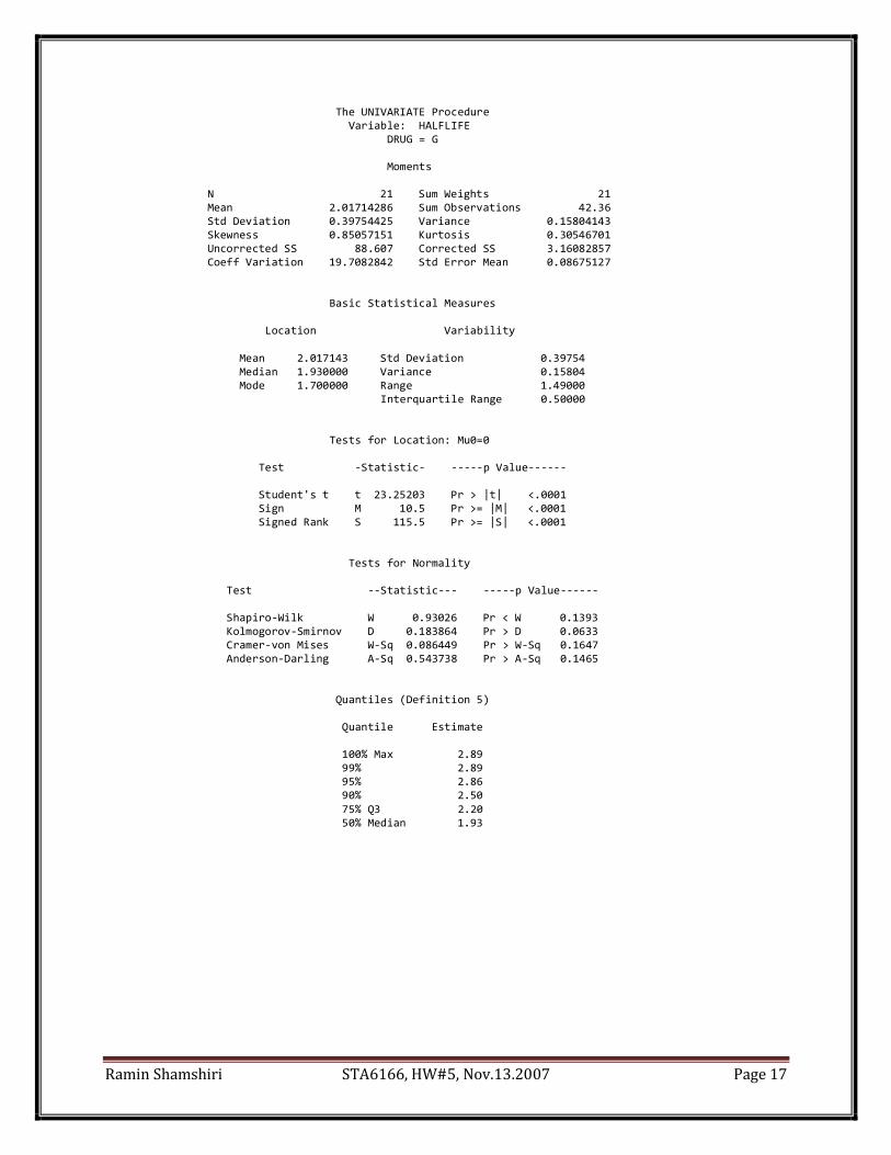
Ramin Shamshiri STA6166, HW#5, Nov.13.2007 Page 17
The UNIVARIATE Procedure Variable: HALFLIFE DRUG = G Moments N 21 Sum Weights 21 Mean 2.01714286 Sum Observations 42.36 Std Deviation 0.39754425 Variance 0.15804143 Skewness 0.85057151 Kurtosis 0.30546701 Uncorrected SS 88.607 Corrected SS 3.16082857 Coeff Variation 19.7082842 Std Error Mean 0.08675127 Basic Statistical Measures Location Variability Mean 2.017143 Std Deviation 0.39754 Median 1.930000 Variance 0.15804 Mode 1.700000 Range 1.49000 Interquartile Range 0.50000 Tests for Location: Mu0=0 Test -Statistic- -----p Value------ Student's t t 23.25203 Pr > |t| <.0001 Sign M 10.5 Pr >= |M| <.0001 Signed Rank S 115.5 Pr >= |S| <.0001 Tests for Normality Test --Statistic--- -----p Value------ Shapiro-Wilk W 0.93026 Pr < W 0.1393 Kolmogorov-Smirnov D 0.183864 Pr > D 0.0633 Cramer-von Mises W-Sq 0.086449 Pr > W-Sq 0.1647 Anderson-Darling A-Sq 0.543738 Pr > A-Sq 0.1465 Quantiles (Definition 5) Quantile Estimate 100% Max 2.89 99% 2.89 95% 2.86 90% 2.50 75% Q3 2.20 50% Median 1.93

Ramin Shamshiri STA6166, HW#5, Nov.13.2007 Page 18
The UNIVARIATE Procedure Variable: HALFLIFE DRUG = G Quantiles (Definition 5) Quantile Estimate 25% Q1 1.70 10% 1.60 5% 1.60 1% 1.40 0% Min 1.40 Extreme Observations ----Lowest---- ----Highest--- Value Obs Value Obs 1.4 39 2.30 4 1.6 33 2.40 36 1.6 1 2.50 10 1.7 37 2.86 17 1.7 32 2.89 25 Stem Leaf # Boxplot 28 69 2 | 26 | 24 00 2 | 22 000 3 +-----+ 20 00 2 | + | 18 000038 6 *-----* 16 00000 5 +-----+ 14 0 1 | ----+----+----+----+ Multiply Stem.Leaf by 10**-1 Normal Probability Plot 2.9+ * *+++++ | +++++ | *+*++ | **+*+ | ++*+* | **+*+** | * * *+++* 1.5+ * +++++ +----+----+----+----+----+----+----+----+----+----+ -2 -1 0 +1 +2

Ramin Shamshiri STA6166, HW#6, Nov.27.2007 Page 1
STA 6166, Section 8489, Fall 2007
Homework #6
Due 27 November 2007
RAMIN SHAMSHIRI UFID#: 9021-3353

Ramin Shamshiri STA6166, HW#6, Nov.27.2007 Page 2
Chapter6- Concept Questions- Indicate True or False. If False, specify what change will make the statement true. 1- If for two samples the conclusions from an ANOVA and t-test disagree, you should trust the t-test. Answer: False, In ANOVA we consider each group as a population. In t-test our assumption is that the difference of the two samples should be normally distributed, but in ANOVA each population should be normally distributed. So the ANOVA is stronger. (This answer is also checked with software package.) 2- A set of sample means is more likely to result in rejection of the hypothesis of equal population
means if the variability within the populations is smaller. Answer: True
Based on the ratio 𝐹 =𝑠𝐵2
𝑠𝑤2 , the smaller within group variance, the larger the F value which leads to the
smaller P-value, thus more likely to reject the Hypothesis of equality of population. 3- If the treatments in a CRD consist of numeric levels of input to a process, the LSD multiple
comparison procedure is the most appropriate test. Answer: False 4- If every observation is multiplied by 2, then the value of the F statistic in an ANOVA is multiplied by
4. Answer: False
Based on the ratio of 𝐹 =𝑠𝐵2
𝑠𝑤2 , if every observation is multiplied by 2, the variances will be each
multiplied by 4, but the ratio of F will still remain the same. 5- To use the F statistic to test the equality of two variances, the samples sizes must be equal. Answer: False The assumptions of the F statistic are equality of population variances, independency of samples and normally distribution of populations. thus, the sample sizes do not to be equal. 6- The logarithmic transformation is used when the variance is proportional to the Mean. Answer: True If σ is proportional to the Mean, we use the logarithm of the yij. 7- With the usual ANOVA assumptions, the ratio of two Mean squares whose expected values are the
same has an F distribution. Answer: 8- One purpose of randomization is to remove experimental error from the estimates. Answer: 9- To apply the F test in ANOVA, the sample size for each factor level (population) must be the same. Answer: False The size of each treatment does not need to be same.

Ramin Shamshiri STA6166, HW#6, Nov.27.2007 Page 3
10- To apply the F test for ANOVA, the sample standard deviations for all factor levels must be the same. Answer: False The variances of the populations must be equal. 11- To apply the F test for ANOVA, the population standard deviations for all factor levels must be the
same. Answer: True The variances of the populations must be equal. 12- An ANOVA table for a one-way experiment gives the following: Answer true or false for the following six arguments:
The null hypothesis is that all four means are equal. Answer: False , There are three groups
The calculated value of F is 1.125.
Answer: False because 𝐹 =𝑠𝐵2
𝑠𝑤2 =
810/2
720/8= 4.5
The critical value for F for 5% significance is 6.60. Answer: False, The critical value is 4.46 (from 0.05 table, F=4.5,dfN=2, dfDN=8 )
The null hypothesis can be rejected at 5% significance. Answer: True because the critical F value at 5% is 4.46 which is less than F value from test. It means that the P-value from test is less than the critical p-value 5%, thus we reject H0
The Null hypothesis cannot be rejected at 1% significance. Answer: TRUE, because the critical F-value at 1% is 8.86
There are 10 observations in the experiment. Answer: False, There are 11 observations in this experiment.
13- A statistically significant F in an ANOVA indicates that you have identified which levels of factors are
different from the others. Answer: False, the F value just tells if the levels of factor are different or not different, but it does not tell which ones are different from the others

Ramin Shamshiri STA6166, HW#6, Nov.27.2007 Page 4
Chapter 6- Exercises 4- A manufacturer of concrete bridge supports is interested in determining the effect of varying the sand content of concrete on the strength of the supports. Five supports are made for each of five different amounts of sand in the concrete mix and each support tested for compression resistance. The results are shown in table below:
Percent Sand Comparison Resistance (10,000 psi)
Support 1 Support 2 Support 3 Support 4 Support 5 A= 15 7 7 10 15 9 B= 20 17 12 11 18 19 C= 25 14 18 18 19 19 D= 30 20 24 22 19 23 E= 35 7 10 11 15 11
a- Perform the analysis to determine whether there is an effect due to changing the sand content. Answer: The factor is the Sand and the treatments are the five sand contents which have named as A,B,C,D and E. To determine whether there is a significant difference in the Means of each sand contents, we use ANOVA which requires checking the assumptions stated below. 1- The population from which the samples were obtained must be normally or approximately normally
distributed. 2- The samples must be independent. 3- The variances of the populations must be equal. Checking the Normality assumption: H0: the Population A: Sand=15% has a specified theoretical distribution H1: the distribution is not the theoretical distribution Moments N 5 Sum Weights 5 Mean 9.6 Sum Observations 48 Std Deviation 3.28633535 Variance 10.8 Skewness 1.43410896 Kurtosis 2.0936214 Uncorrected SS 504 Corrected SS 43.2 Coeff Variation 34.2326598 Std Error Mean 1.46969385
Tests for Normality Test --Statistic--- -----p Value------ Shapiro-Wilk W 0.844815 Pr < W 0.1787 Kolmogorov-Smirnov D 0.251562 Pr > D >0.1500 Cramer-von Mises W-Sq 0.067783 Pr > W-Sq 0.2467 Anderson-Darling A-Sq 0.420715 Pr > A-Sq 0.1932
H0: the Population B: Sand=20% has a specified theoretical distribution H1: the distribution is not the theoretical distribution Moments

Ramin Shamshiri STA6166, HW#6, Nov.27.2007 Page 5
N 5 Sum Weights 5 Mean 15.4 Sum Observations 77 Std Deviation 3.64691651 Variance 13.3 Skewness -0.4824345 Kurtosis -2.8509243 Uncorrected SS 1239 Corrected SS 53.2 Coeff Variation 23.681276 Std Error Mean 1.63095064 Tests for Normality Test --Statistic--- -----p Value------ Shapiro-Wilk W 0.860318 Pr < W 0.2294 Kolmogorov-Smirnov D 0.26957 Pr > D >0.1500 Cramer-von Mises W-Sq 0.068758 Pr > W-Sq 0.2404 Anderson-Darling A-Sq 0.398516 Pr > A-Sq 0.2235
H0: the Population C: Sand=25% has a specified theoretical distribution H1: the distribution is not the theoretical distribution Moments N 5 Sum Weights 5 Mean 17.6 Sum Observations 88 Std Deviation 2.07364414 Variance 4.3 Skewness -1.9177563 Kurtosis 3.87777177 Uncorrected SS 1566 Corrected SS 17.2 Coeff Variation 11.782069 Std Error Mean 0.92736185 Tests for Normality Test --Statistic--- -----p Value------ Shapiro-Wilk W 0.738725 Pr < W 0.0233 Kolmogorov-Smirnov D 0.37648 Pr > D 0.0201 Cramer-von Mises W-Sq 0.127365 Pr > W-Sq 0.0340 Anderson-Darling A-Sq 0.686044 Pr > A-Sq 0.0296
H0: the Population D: Sand=30% has a specified theoretical distribution H1: the distribution is not the theoretical distribution Moments N 5 Sum Weights 5 Mean 21.6 Sum Observations 108 Std Deviation 2.07364414 Variance 4.3 Skewness -0.2355139 Kurtosis -1.9632234 Uncorrected SS 2350 Corrected SS 17.2 Coeff Variation 9.60020433 Std Error Mean 0.92736185 Tests for Normality Test --Statistic--- -----p Value------ Shapiro-Wilk W 0.952351 Pr < W 0.7540 Kolmogorov-Smirnov D 0.179821 Pr > D >0.1500 Cramer-von Mises W-Sq 0.031987 Pr > W-Sq >0.2500 Anderson-Darling A-Sq 0.206799 Pr > A-Sq >0.2500
H0: the Population E: Sand=35% has a specified theoretical distribution H1: the distribution is not the theoretical distribution Moments N 5 Sum Weights 5 Mean 10.8 Sum Observations 54 Std Deviation 2.86356421 Variance 8.2 Skewness 0.33218026 Kurtosis 1.66864961 Uncorrected SS 616 Corrected SS 32.8 Coeff Variation 26.5144835 Std Error Mean 1.28062485 Tests for Normality
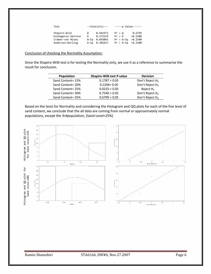
Ramin Shamshiri STA6166, HW#6, Nov.27.2007 Page 6
Test --Statistic--- -----p Value------ Shapiro-Wilk W 0.941971 Pr < W 0.6799 Kolmogorov-Smirnov D 0.272159 Pr > D >0.1500 Cramer-von Mises W-Sq 0.056065 Pr > W-Sq >0.2500 Anderson-Darling A-Sq 0.303417 Pr > A-Sq >0.2500
Conclusion of checking the Normality Assumption: Since the Shapiro-Wilk test is for testing the Normality only, we use it as a reference to summarize the result for conclusion.
Population Shapiro-Wilk test P-value Decision
Sand Content= 15% 0.1787 > 0.05 Don’t Reject H0 Sand Content= 20% 0.2294> 0.05 Don’t Reject H0 Sand Content= 25% 0.0233 < 0.05 Reject H0 Sand Content= 30% 0.7540 > 0.05 Don’t Reject H0 Sand Content= 35% 0.6799 > 0.05 Don’t Reject H0
Based on the tests for Normality and considering the Histogram and QQ plots for each of the five level of sand content, we conclude that the all data are coming from normal or approximately normal populations, except the 3rdpopulation, (Sand Level=25%)
Histogram and QQ-plot
for Sand level=15%
Histogram and QQ-plot for
Sand level=20%

Ramin Shamshiri STA6166, HW#6, Nov.27.2007 Page 7
Histogram and QQ-plot for
Sand level=25%
Histogram and QQ-plot for
Sand level=30%
Histogram and QQ-plot for
Sand level=35%
Checking the assumption of equality of Variance Testing the equality of Variance with Levene’s test: Levene's Test for Homogeneity of Y Variance ANOVA of Absolute Deviations from Group Means Sum of Mean Source DF Squares Square F Value Pr > F treatment 4 8.8320 2.2080 0.95 0.4573 Error 20 46.6080 2.3304 Covariance Parameter Estimates Cov Parm Group Estimate Residual treatment A 10.8000 Residual treatment B 13.3000 Residual treatment C 4.3000 Residual treatment D 4.3000 Residual treatment E 8.2000

Ramin Shamshiri STA6166, HW#6, Nov.27.2007 Page 8
Conclusion of checking the Normality Assumption: Do not reject the hypothesis of equality of variance since the P-value from the Levene’s test is greater than the common rejection p-value (0.05). Thus we conclude that the assumption of the homogeneity of variance is met. This conclusion can also be observed from the estimated variances listed above Now that we have our assumptions checked, we can continue performing the analysis to determine whether there is an effect due to changing the sand content. Our hypothesis is as below: H0: μA=μB= μC =μD =μE H1: At least one Mean is difference from the others Since we have more than two means, we cannot use the t-test (due to reasons mentioned in text) and we should use ANOVA for such comparison. If there is no difference in the Means, the between group variance estimate will be approximately equal to the within group variance estimate and the F-test value will be approximately equal to 1 and the null hypothesis will not be rejected. If the Means differs significantly, the between group variance will be much larger than the within group variance, thus the F-test will be significantly greater than 1 and the null hypothesis will be rejected. Using both SAS and Excel software packages, the ANOVA outputs are as below:
From SAS Sum of Source DF Squares Mean Square F Value Pr > F Model 4 486.4000000 121.6000000 14.87 <.0001 Error 20 163.6000000 8.1800000 Corrected Total 24 650.0000000
From Excel:
SUMMARY Groups Count Sum Average Variance
Row 1 5 48 9.6 10.8 Row 2 5 77 15.4 13.3 Row 3 5 88 17.6 4.3 Row 4 5 108 21.6 4.3 Row 5 5 54 10.8 8.2
ANOVA Source of
Variation SS df MS F P-value F crit
Between Groups 486.4 4 121.6 14.86553 8.65E-
06 2.866081
Within Groups 163.6 20 8.18
Total 650 24

Ramin Shamshiri STA6166, HW#6, Nov.27.2007 Page 9
Conclusion: The F-value of ANOVA is 14.87 which is much larger than the Critical value of F which is 2.87. In other words, since the P-value from ANOVA is much less than the critical p-value, we reject the Null hypothesis of equal means and conclude that there is not enough evidence that the Means of these 5 groups are equal. Figure.

Ramin Shamshiri STA6166, HW#6, Nov.27.2007 Page 10
b. Redo the analyses as a linear regression of compression resistance on sand content. Check the assumptions and if met, test whether the slope is not equal to 0.
Answer: From the ANOVA we have already concluded that there is not enough evidences that the Means of the five sand levels are equal. This is due to the fact the one or more pairs of the sand level Means are statistically not equal. In the other words, there is sufficient evidence that at least one of the sand level mean differs from the others. We first need to check the assumption first before analyzing the Means of the sand levels. The ANOVA can also be represented as the Linear model for several populations,
yij= μi+Єij i=1,2,…,t j=1,2,…,n
yij: jth observation sample value from the ith population
μi:Mean of the ith population Єij: Difference or deviation of the jth observed value from its respective population mean.
With the following assumptions: 1. The Єij‘s are normally distributed random variables with Mean=0 and Variance= σ2 2. The Єij‘s are independent in probability sense; that is the behavior of the Єij is not affected by the
behavior value of any other. Tests for Normality
Test --Statistic--- -----p Value------ Shapiro-Wilk W 0.967737 Pr < W 0.5884 Kolmogorov-Smirnov D 0.13053 Pr > D >0.1500 Cramer-von Mises W-Sq 0.055396 Pr > W-Sq >0.2500 Anderson-Darling A-Sq 0.326296 Pr > A-Sq >0.2500
Quantile Estimate 100% Max 5.4

Ramin Shamshiri STA6166, HW#6, Nov.27.2007 Page 11
99% 5.4 95% 4.2 90% 3.6 75% Q3 1.4
Extreme Observations ----Lowest---- ----Highest--- Value Obs Value Obs -4.4 8 2.4 17 -3.8 21 2.6 9 -3.6 11 3.6 10 -3.4 7 4.2 24 -2.6 19 5.4 4
Stem Leaf # Boxplot 5 4 1 | 4 2 1 | 3 6 1 | 2 46 2 | 1 4446 4 +-----+ 0 224444 6 *--+--* -0 86 2 | | -1 6 1 | | -2 666 3 +-----+ -3 864 3 | -4 4 1 | ----+----+----+----+
Variable: resid Normal Probability Plot 5.5+ *++ | *++++ | +*++ | +*+* | ***+* 0.5+ ***+** | **++ | ++*+ | ++** | *+*+* -4.5+ *++++ +----+----+----+----+----+----+----+----+----+----+ -2 -1 0 +1 +2

Ramin Shamshiri STA6166, HW#6, Nov.27.2007 Page 12
STRENGTH = 10. 7 +0. 172 SAND
N
25
Rsq
0. 0569
Adj Rsq
0. 0159
RMSE
5. 1627
5. 0
7. 5
10. 0
12. 5
15. 0
17. 5
20. 0
22. 5
25. 0
SAND
15. 0 17. 5 20. 0 22. 5 25. 0 27. 5 30. 0 32. 5 35. 0
STRENGTH = 10. 7 +0. 172 SAND
N
25
Rsq
0. 0569
Adj Rsq
0. 0159
RMSE
5. 1627
- 10. 0
- 7. 5
- 5. 0
- 2. 5
0. 0
2. 5
5. 0
7. 5
10. 0
Pr edi ct ed Val ue
13. 0 13. 5 14. 0 14. 5 15. 0 15. 5 16. 0 16. 5 17. 0

Ramin Shamshiri STA6166, HW#6, Nov.27.2007 Page 13
Testing whether the slope is equal to zero: H0: β1=0 H1: β1≠0 Parameter Estimates Parameter Standard Variable DF Estimate Error t Value Pr > |t| Intercept 1 10.70000 3.79376 2.82 0.0097 SAND 1 0.17200 0.14602 1.18 0.2509
Analysis of Variance Sum of Mean Source DF Squares Square F Value Pr > F Model 1 36.98000 36.98000 1.39 0.2509 Error 23 613.02000 26.65304 Corrected Total 24 650.00000 Root MSE 5.16266 R-Square 0.0569 Dependent Mean 15.00000 Adj R-Sq 0.0159 Coeff Var 34.41772
Conclusion: The t-value is equal to 1.18 and leads to p-value equal to 0.2509 which is larger than 0.05 significant level. The F-value is equal to 1.39 and leads to a same p-value which shows that there is not enough evidence to reject the null hypothesis that the Slope is equal to zero. In the other words, based on this test, we do not reject H0
A measure of the amount of “explained” variability is R-squared which is equal to 0.0569. This value is very close to zero and shows that there is almost no linear relationship between Y and X. From the residual plot, Histogram plot and QQ-plot of the Єij‘s, we can conclude that the errors are normally distributed random variables. Since the p-values from all of these tests are greater than the common critical P-value (0.05) they all show that there is not sufficient evidence to reject the null hypothesis of Normality, thus we conclude that the data are coming from normally distributed populations.

Ramin Shamshiri STA6166, HW#6, Nov.27.2007 Page 14
Comparing the Means of Sand Levels, we have 52 = 10 following hypothesizes:
H0: μA= μB H0: μA= μC H0: μA= μD H0: μA= μE H1: μA≠ μB H1: μA≠ μC H1: μA≠ μD H1: μA≠ μE H0: μB= μC H0: μB= μD H0: μB= μE H1: μB≠ μC H1: μB≠ μD H1: μB≠ μE H0: μC= μD H0: μC= μE H1: μC≠ μD H1: μC≠ μE H0: μD= μE H1: μD≠ μE The GLM Procedure Least Squares Means Adjustment for Multiple Comparisons: Tukey Sand_ resistance LSMEAN Level LSMEAN Number A 9.6000000 1 B 15.4000000 2 C 17.6000000 3 D 21.6000000 4 E 10.8000000 5
Protected Fisher’s LSD approach: Least Squares Means for effect Sand_Level Pr > |t| for H0: LSMean(i)=LSMean(j) Dependent Variable: resistance i/j 1 2 3 4 5 1 0.0044 0.0003 <.0001 0.5146 2 0.0044 0.2381 0.0027 0.0194 3 0.0003 0.2381 0.0388 0.0012 4 <.0001 0.0027 0.0388 <.0001 5 0.5146 0.0194 0.0012 <.0001

Ramin Shamshiri STA6166, HW#6, Nov.27.2007 Page 15
Tukey approach: Least Squares Means for effect Sand_Level Pr > |t| for H0: LSMean(i)=LSMean(j) Dependent Variable: resistance i/j 1 2 3 4 5 1 0.0320 0.0022 <.0001 0.9620 2 0.0320 0.7423 0.0200 0.1204 3 0.0022 0.7423 0.2159 0.0096 4 <.0001 0.0200 0.2159 <.0001 5 0.9620 0.1204 0.0096 <.0001
Decision summary based on Tukey approach i/j A B C D E
A 0.03<0.05 Reject
H0: μA= μB
0.002<0.05 Reject
H0: μA= μC
0.0001<0.05 Reject
H0: μA= μD
0.962>0.05 Do not Reject
H0: μA= μE
B 0.03<0.05 Reject
H0: μA= μB
0.7423>0.05 Do Not Reject
H0: μB= μC
0.02<0.05 Reject
H0: μB= μD
0.12>0.05 Do not Reject
H0: μB= μE
C 0.002<0.05 Reject
H0: μA= μC
0.7423>0.05 Do not Reject
H0: μB= μC
0.2159>0.05 Do not Reject
H0: μC= μD
0.0096<0.05 Reject
H0: μC= μE
D 0.0001<0.05 Reject
H0: μA= μD
0.02<0.05 Reject
H0: μB= μD
0.2159>0.05 Do not Reject
H0: μC= μD
0.0001<0.05 Reject
H0: μD= μE
E 0.962>0.05 Do not Reject
H0: μA= μE
0.12>0.05 Do not Reject
H0: μB= μE
0.0096<0.05 Reject
H0: μC= μE
0.0001<0.05 Reject
H0: μD= μE
Conclusion of Mean comparison: From the Least Squares Means, it is clear that the Means of Sand Level A and Sand Level E are very close together, (Mean A=9.6 and Mean E=10.8) which confirms rejecting the H0: μA= μE . It can also be found that the Sand Level B and sand Level C have close values of Means, (15.4 and 17.6). This is also confirmed from the Tukey comparison of Means, where we make the decision to reject the H0: μB= μC It should be noted that another conclusion may be made based on the Protected Fisher’s LSD approach. From the fit test, we see that the R-square, (R2) which is a measure of the amount of “explained” variability is equal to 0.748 implies that the regression relationship “explains” approximately 81% of the observed variability in Y (index). Fit Test: (R2), Grand Mean is 15.00 R-Square Coeff Var Root MSE Y Mean 0.748308 19.06713 2.860070 15.00000

Ramin Shamshiri STA6166, HW#6, Nov.27.2007 Page 16
12- For laboratory studies of an organism, it is important to provide a medium in which the organism flourishes. The data for this exercise shown in table below are from a completely randomized design with four samples for each of seven media. The response is the diameters of the colonies of fungus.
Medium Fungus colony Diameters
WA 4.5 4.1 4.4 4.0 RDA 7.1 6.8 7.2 6.9 PDA 7.8 7.9 7.6 7.6 CMA 6.5 6.2 6.0 6.4 TWA 5.1 5.0 5.4 5.2 PCA 6.1 6.2 6.2 6.0 NA 7.0 6.8 6.6 6.8
a. Perform an analysis of variance to determine whether there are different growth rates among the
media.
Dependent Variable: Y Sum of Source DF Squares Mean Square F Value Pr > F Model 6 32.75857143 5.45976190 168.61 <.0001 Error 21 0.68000000 0.03238095 Corrected Total 27 33.43857143 R-Square Coeff Var Root MSE Y Mean 0.979664 2.905720 0.179947 6.192857
ANOVA Source of
Variation SS df MS F P-value F crit
Between Groups 32.75857 6 5.459762 168.6103 1.19E-
16 2.572712 Within Groups 0.68 21 0.032381
Total 33.43857 27
Conclusion: The very big F-value leads to a very small P-value which rejects null hypothesis at any significant level. Therefore, we conclude that there are different growth rates among the media.

Ramin Shamshiri STA6166, HW#6, Nov.27.2007 Page 17
b. Is this exercise appropriate for preplanned or post hoc comparison? Perform the appropriate method and make recommendations.
Answer: This exercise is appropriate for Post-hoc comparison since the problem is to find a medium in which the organism flourishes. It means that we first need to test the medium if they are significantly difference. Then based on the result, we need a multiple comparison techniques which are of two general types: 1- Pre-planned comparison (generated prior to the experiment being conducted). Pre-planned
comparisons should be performed whenever possible because:
Pre-planned comparisons have more power.
A post-hoc comparison may not provide useful results. 2- Post-hoc comparison (use the result of the analysis to formulate the hypotheses) As mentioned, we use post-hoc comparison in which specific hypotheses are based on observed differences among the estimated factor level means. That is, the hypotheses are based on the sample data. Most post-hoc comparison procedures are restricted to testing contrasts that compare pairs of means, H0: μi=μj for all values of i≠j Here we can use the Tukey test after the analysis of variance has been completed to make pair wise comparisons between the groups which have the same sample size.
𝑞 =𝑋 𝑖 − 𝑋 𝑗
𝑠𝑤2 /𝑛
Where 𝑋 𝑖 and 𝑋 𝑗 are the Means of the samples being compared, n is the size of the samples and 𝑠𝑤2 is
the within group variance. When the absolute value of q is greater than the critical value for the Tukey test, there is a significant difference between the two means being compared. The GLM Procedure Least Squares Means Adjustment for Multiple Comparisons: Tukey LSMEAN MEDIUM DIAM LSMEAN Number CMA 6.27500000 1 NA 6.80000000 2 PCA 6.12500000 3 PDA 7.72500000 4 RDA 7.00000000 5 TWA 5.17500000 6 WA 4.25000000 7 Least Squares Means for effect MEDIUM Pr > |t| for H0: LSMean(i)=LSMean(j) Dependent Variable: DIAM

Ramin Shamshiri STA6166, HW#6, Nov.27.2007 Page 18
i/j 1 2 3 4 5 6 7 1 0.0074 0.8944 <.0001 0.0002 <.0001 <.0001 2 0.0074 0.0005 <.0001 0.7004 <.0001 <.0001 3 0.8944 0.0005 <.0001 <.0001 <.0001 <.0001 4 <.0001 <.0001 <.0001 0.0002 <.0001 <.0001 5 0.0002 0.7004 <.0001 0.0002 <.0001 <.0001 6 <.0001 <.0001 <.0001 <.0001 <.0001 <.0001 7 <.0001 <.0001 <.0001 <.0001 <.0001 <.0001
Conclusion of H0: μi=μj for all values of i≠j
Decision summary based on Tukey approach i/j 1 2 3 4 5 6 7
1 Reject Do not Reject Reject Reject Reject Reject
2 Reject Reject Reject Do not Reject Reject Reject
3 Do not Reject Reject Reject Reject Reject Reject
4 Reject Reject Reject Reject Reject Reject
5 Reject Do not Reject Reject Reject Reject Reject
6 Reject Reject Reject Reject Reject Reject
7 Reject Reject Reject Reject Reject Reject