1

I Can’t Smile Without You: Spousal Correlation in Life Satisfaction

Nattavudh Powdthavee

University of York

March, 2009

Forthcoming in the Journal of Economic Psychology

Abstract

This paper tests whether one partner’s happiness significantly influences the happiness of the other partner. Using ten waves of the British Household Panel Survey, it utilizes a panel-based GMM methodology to estimate a dynamic model of life satisfaction. The use of the GMM-system estimator corrects for correlated effects of partner’s life satisfaction and solves the problem of measurement error bias. The results show that, for both genders, there is a positive and statistically significant spillover effect of life satisfaction that runs from one partner to the other partner in a couple. The positive bias on the estimated spillover effect coming from assortative mating and shared social environment at cross-section is almost offset by the negative bias coming from systematic measurement errors in the way people report their life satisfaction. Moreover, consistent with the spillover effect model, couple dissolution at t+1 is negatively correlated with partners’ life satisfaction at t.

Key words: life satisfaction; assortative mating; spillover; marriage; happiness; GMM

JEL: D1, D62, D64, I0

2

“You see, I feel sad when you’re sad, I feel glad when you’re glad. If you only knew

what I’m going through, I just can’t smile without you.” - Barry Manilow

1. Introduction

The idea that married people care a great deal about the well-being of their partner is not new

to economists (Becker, 1973, 1974; Friedman, 1986). The past three decades have seen a

significant increase in the number of studies showing that people in marriage tend to behave

altruistically towards their partner (see, for example, Foster and Rosenzweig, 2001; Ermisch,

2003). However, while it may be possible to make some inferences about the degree of caring

between partners from their behaviour, the idea that there may be a direct spillover of well-

being from one partner to the other has rarely been tested empirically.

This paper aims to do just that. Using a long-run panel of nationally representative

randomly sampled married and cohabiting individuals, it examines the extent of spousal

correlation in subjective well-being data, particularly self-rated life satisfaction (LS). It

proposes that a positive correlation between partners’ LS may reflect three distinct processes.

First, individuals who are born happy or are born with innate predispositions that make them

happy may tend to marry those who are similar to them. In addition to this, people of the same

family background or life styles – in other words, same unobserved social factors – may also

tend to marry each other. This matching of fixed personal characteristics on the marriage

market is analogous to the concept of assortative mating (Becker, 1974). Manski (1995) refers

to such phenomena as correlated effects of social interactions.

Second, given that marriage allows individuals to share with their partner the kind of

physical and emotional resources that may not be available for each person to obtain outside

marriage (Waite and Gallagher, 2000), correlated effects may also arise from the shared social

3

environment (which can either be time-invariant or time-variant) that is simultaneously

affecting LS for both spouses.

Lastly, the observed correlation may be the result of a direct spillover of LS within the

couple. The idea is that, if a husband cares about his wife, then her LS becomes one of the

main determinants of his own LS, and vice versa. This generates a possibility that a husband

will be ceteris paribus happier when his wife is happier for whatever reasons that make her

happy but not him directly. Hence, we would expect an increase in one partner’s LS to be

positively correlated with the other partner’s LS even after allowing for all the factors that can

affect both partners’ LS at the same time. This phenomenon is likened to the endogenous

effects in Manski’s terminology, whereby the individual outcome is a function of group

achievement.

In addition to the above confounding influences which make it difficult for the true

relationship between partners’ well-being to be identified, the estimates of spousal correlation

in LS may also suffer from the negative measurement error bias. There may be, for example, a

tendency for individuals to misreport their true LS in surveys. The low signal-to-noise ratio

caused by misreporting can result in an estimated coefficient on partner LS that is biased

towards zero in a large sample. In short, because there are both positive (correlated effects)

and negative (measurement error) biases involved, the direction of bias is unclear on a priori

ground.

This paper uses ten waves of the British Household Panel Survey (BHPS) data to

examine the extent of spousal correlation in LS. In particular, it uses the “system GMM

estimator” proposed by Arellano and Bover (1995) and Blundell and Bond (1998) to estimate

the causal spillover effect that runs from one partner’s life satisfaction to the other partner’s

life satisfaction. The use of the GMM-system estimator, which is a unique approach in the

study of happiness, control for the correlated effects and solve the problem of measurement

4

error bias in self-rated life satisfaction through instrumentations and first-differencing. The

results show that there is strong evidence of a spillover effect of LS, which suggests that well-

being is transferable from one partner to the other. Consistent with the spillover effect model,

partners’ LS today are also associated with lower probabilities of partners separating or

divorcing one period into the future.

There are similarities in terms of research questions and analytic strategy between this

paper and previous studies that examined similarities in a husband’s and wife’s behaviour such

as smoking (Clark and Etile, 2006), their political preferences (Kan and Heath, 2006), and

their sporting activities (Farrell and Shields, 2002).

This article is organised as follows: Section 2 reviews relevant past research on

marriage and well-being. Section 3 addresses theoretical issues revolving around the various

interpretations of the correlation between partners’ LS. Section 4 describes how to implement

a test and the data set. Section 5 discusses the results, and Section 6 concludes.

2. Marriage, subjective well-being, and spillovers

Previous research on marital status and emotional well-being is clear on one point: married

persons are significantly happier and more satisfied with life than those who are divorced,

separated, widowed, or single, across various countries and time periods (Gove et al., 1983;

Mastekaasa, 1994; Marks and Lambert, 1998). The large psychological benefits of marriage

persist even when the selection of happy people into marriage is controlled for in the analysis

(Frey and Stutzer, 2006; Mastekaasa, 1992), and such advantages are sometimes shown to be

stronger for men than for women (see, for example, Gove et al., 1983). Both cross-sectional

and longitudinal studies confirm the overall psychological benefits of marriage (for a review,

see Oswald and Wilson, 2005).

5

There are several explanations for the protective effects of marriage. First, on the

grounds that two can live almost cheaply as one, marriage may work simply because it

provides higher real income per partner (Korenman and Neumark, 1991; Loh, 1996; Smock et

al., 1999). Second, marriage provides the couple with a source of constant emotional and

instrumental support, which may act as an important buffer against stress and depression for

the person who experiences negative shocks in life events (Berkman, 1988; Marks and

Lambert, 1998). In other words, the negative impacts of shocks in life events appear to be

significantly lower for married individuals than for those of other marital groups. Third,

marriage provides the couple with a sense of belonging and social reality, in which they are

the only two people living and operating in their own world. This shared sense of meaning can

be an important foundation for emotional well-being (Berger and Kellner, 1964; House et al.,

1982). Marriage also encourages people to engage less in risky activities and more in healthy

ones – perhaps for the sake of their partner. For example, married people smoke and drink

less, and such healthy behaviour may provide an important source of both physical and

emotional well-being for the couple. The results hold even when one allows for selection

effects into marriage (see Power et al., 1999).

What has received much less attention is whether one partner’s well-being is a function

of the other partner’s well-being (Becker, 1974). Previous studies on emotional spillover have

often focused on daily transmissions of only negative effects, such as measures of stress and

strain. One of the common findings in the literature is that stress experienced by one partner in

the workplace has the tendency to heighten the level of stress being experienced by the other

partner at home (see Bolger et al., 1989; Jones and Fletcher, 1993; Westman and Vinokur,

1998). Yet this is not a persuasive reason to believe that well-being is transferable within

couples. One reason for this is that there is evidence in the psychology literature that one

measure is not just a mirror of the other. For instance, whilst several studies have found a

6

moderate correlation between ill-being and well-being (Chamberlain, 1988; Michalos, 1991),

others have shown that these components appear to behave differently over time and to have

differing relationships with other variables (Liang, 1985; Stock et al., 1986; Huppert and

Whittington, 2003). Research into the validity of the two constructs has also shown that there

is a clear distinction in terms of determinants between measures of well-being and ill-being

(see Bradburn, 1969; Diener et al., 1999, Headey et al., 1993; Pavot and Diener, 1993).

Because measures of cognitive well-being such as LS frequently form a separate factor and

correlate with predictor variables in a unique way, it seems worthwhile to separately assess

this construct in the research.

Of the very few studies on the topic, Rose’s (1955) was one of the first to report cross-

sectional correlation between LS within marriage. The author showed that spouses may feel

something is wrong with their marriage when one or both feel unhappy with life. In that case,

even if there was nothing wrong with their marriage, low levels of happiness detected between

couples may have shattered their confidence and lead to separation and divorce. Argyle (1999)

made a conjecture in his study on the effect of marriage on subjective well-being that one

spouse’s happiness may encourage the happiness of the other in a marriage. More recently,

Anderson et al. (2003) found that people in early dating relationships, i.e. the first six months

of dating, tend to report similar levels of positive emotional experiences over time, such as

happiness, amusement, and pride. Plug and Van Praag (1998) found similarities in the reported

income satisfaction by members of the same household. In a similar study, Powdthavee and

Vignoles (2008) also found significant spillover effects in reported well-being between parents

and children.

To the best of my knowledge, the only paper that has conducted a longitudinal analysis

on whether there is a substantial long-term interdependent relationship between spouses’ LS

within marriage is the innovative work by Schimmack and Lucas (2006). Their methods and

7

dataset differ from those set out in this paper, and the respective projects were begun

independently. Using the German panel data and time-lagged cross-spouse correlation method,

they found that spousal correlation in LS is due mainly to the shared stable component of LS

within the couple, i.e. partners sharing similar traits and social environments. Little was

discussed in their paper, however, on the possibility that there may be a spillover effect of LS

from one partner to the other. This is the main difference between this paper’s analysis and

that adopted by Schimmack and Lucas (2006).

3. Theory

In this section, I will briefly discuss the three underlying mechanisms that may account for the

raw correlation between a husband’s and wife’s LS levels: assortative mating, shared social

environment, and spillover effect.

3.1 Assortative mating

The first explanation is that the observed spousal correlation in LS may have been the outcome

of a matching of unobserved personality traits and/or social factors on the marriage market

(Becker, 1974). Individuals may prefer partners who are phenotypically similar to them.

Hence, people who are born with innate predispositions that make them happy or come from

the same social backgrounds may tend to marry each other. One reason for this is that the

decision to marry somebody who is like us could make living with them easier, as the latter

may enjoy the same kind of lifestyle, such as leisure and sporting activities, whilst someone

else with a completely different set of personalities or have a different social background may

not. Such positive assortative mating or homogenous matching by personality traits and/or

8

social factors is supported by the evidence that a number of lifestyles are highly correlated

within a couple (Contoyannis and Jones, 2004). It is also consistent with the evidence of

positive assortative mating by education (Mare, 1991), professional backgrounds (Qian, 1998),

productivity traits and desires for public goods (Lam, 1998). An assortative mating market

may thus induce correlated effects in LS via correlation between respondent individual fixed

effects and partner’s LS.

Alternatively, correlated effects may result from partners sharing the same social

environment, as discussed below.

3.2 Shared social environment

The second explanation also views the observed correlation as a correlated effect; what

appears to be a direct spillover of LS from one partner to the other may be no more than the

result of partners sharing the same social environment that simultaneously influences the well-

being of them both. For example, a positive shock in one partner’s income (i.e. one partner

receiving a pay rise at work) can result in an increase in both spouses’ LS through an increase

in the family income. Moreover, under assortative mating, a couple with common lifestyles

characteristics may also experience common life cycle events. Two people in the same

occupation may be attracted to each other and as a result, they may experience the same cyclic

shocks to income. Likewise, couples may share the same health habits and given their

similarity in age and habits, they may also experience health shocks that are close in timing.

As a result, the observed spousal similarity in LS could thus be a spurious relationship

stemming from the fact that some life events either occur to both spouses simultaneously or

occur to one partner but due to the nature of partnership affect both spouses simultaneously.

9

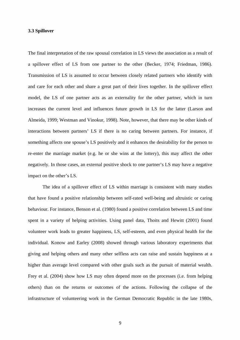
3.3 Spillover

The final interpretation of the raw spousal correlation in LS views the association as a result of

a spillover effect of LS from one partner to the other (Becker, 1974; Friedman, 1986).

Transmission of LS is assumed to occur between closely related partners who identify with

and care for each other and share a great part of their lives together. In the spillover effect

model, the LS of one partner acts as an externality for the other partner, which in turn

increases the current level and influences future growth in LS for the latter (Larson and

Almeida, 1999; Westman and Vinokur, 1998). Note, however, that there may be other kinds of

interactions between partners’ LS if there is no caring between partners. For instance, if

something affects one spouse’s LS positively and it enhances the desirability for the person to

re-enter the marriage market (e.g. he or she wins at the lottery), this may affect the other

negatively. In those cases, an external positive shock to one partner’s LS may have a negative

impact on the other’s LS.

The idea of a spillover effect of LS within marriage is consistent with many studies

that have found a positive relationship between self-rated well-being and altruistic or caring

behaviour. For instance, Benson et al. (1980) found a positive correlation between LS and time

spent in a variety of helping activities. Using panel data, Thoits and Hewitt (2001) found

volunteer work leads to greater happiness, LS, self-esteem, and even physical health for the

individual. Konow and Earley (2008) showed through various laboratory experiments that

giving and helping others and many other selfless acts can raise and sustain happiness at a

higher than average level compared with other goals such as the pursuit of material wealth.

Frey et al. (2004) show how LS may often depend more on the processes (i.e. from helping

others) than on the returns or outcomes of the actions. Following the collapse of the

infrastructure of volunteering work in the German Democratic Republic in the late 1980s,

10

Meier and Stutzer (2008) studied the causal impact of loss of volunteer work on happiness.

They found that a drop from volunteering monthly to less than monthly reduced LS by more

than 0.2 point in an 11-point-scale (one-half of the effect of separation from partner). More

closely related to this paper, in the German Panel data Schwarze and Winkelmann (2003) and

Bruhin and Winkelmann (2007) found some evidence of altruism. As well as showing that

predicted altruists are more likely to make transfer payments, they were able to demonstrate

that an exogenous increase in children’s LS can lead to an increase in LS for the parents.

4. Implementing a test

4.1 The utility model of couples

Consider first Gary Becker’s (1974) simple utility function of an individual i in a marriage to

individual j at any given time, which can be written as

)),(,( XUXUU ji = (1) where X is a vector of the consumption of commodities within the household, and jU is the

individual i’s partner’s utility. The individual’s utility is assumed to be increasing with X,

which is divisible and can be shared between the couple. An increase in X therefore raises the

individual’s utility both through a direct effect upon )(XU i and an indirect effect, acting

through a rise in the partner’s utility, )(XU j . The utility function is highly stylized and

abstracts from a number of issues that can be expected to be important, i.e. I assume no other

relations-specific investments in the household.

For a partnership between individual i and j, the empirical counterpart to equation (1),

with application to life satisfaction, is of the following form:

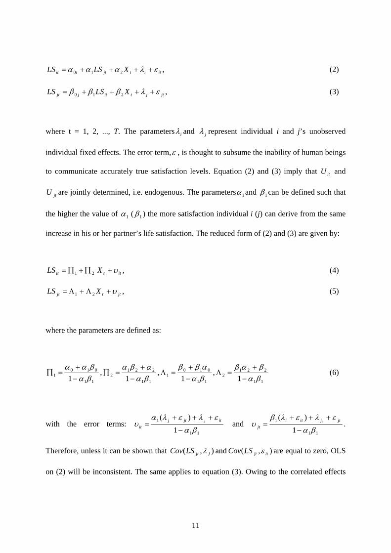
11

,210 ititjttit XLSLS ελααα ++++= (2)

,210 jtjtitjjt XLSLS ελβββ ++++= (3)

where t = 1, 2, ..., T. The parameters iλ and jλ represent individual i and j’s unobserved

individual fixed effects. The error term,ε , is thought to subsume the inability of human beings

to communicate accurately true satisfaction levels. Equation (2) and (3) imply that itU and

jtU are jointly determined, i.e. endogenous. The parameters 1α and 1β can be defined such that

the higher the value of 1α ( 1β ) the more satisfaction individual i (j) can derive from the same

increase in his or her partner’s life satisfaction. The reduced form of (2) and (3) are given by:

,21 ittit XLS υ+∏+∏= (4)

,21 jttjt XLS υ+Λ+Λ= (5)

where the parameters are defined as:

11

2212

11

0101

11

2212

11

0101 1

,1

,1

,1 βα

βαββααββ

βααβα

βαβαα

−+

=Λ−+

=Λ−

+=∏

−+

=∏ (6)

with the error terms: 11

1

1)(βα

ελελαυ

−

+++= itjtj

iti and

11

1

1)(βα

ελελβυ

−

+++= jtjiti

jti .

Therefore, unless it can be shown that ),( and ),( itjtjjt LSCovLSCov ελ are equal to zero, OLS

on (2) will be inconsistent. The same applies to equation (3). Owing to the correlated effects

12

mentioned in the previous section, it is likely however that the partner’s LS will be correlated

with both the respondent’s unobserved fixed effects and the time-varying error term.

4.2 A sketch of identification

The correlated effects due to assortative mating, i.e. ,0),( ≠jjtLSCov λ can be easily solved by

applying the first-differencing approach on the LS data. By contrast, the correlated effects due

to shared social environmental can be solved if there is a valid instrument that affects the

respondent’s partner’s LS directly but is not correlated with the respondent’s LS beyond its

impact on the endogenous regressor.

One such instrument for partner LS may be its own lagged variables. To illustrate, we

can incorporate the lagged variables of the respondent’s own LS in each equation in the

system. The inclusion of lagged LS is theoretically plausible as, according Graham and

Oswald (2006), past happiness can be thought of as a “hedonic capital” or investment for

future happiness. Assuming, for now, that the individual’s past LS only correlates with the

individual’s current LS but is not correlated with his partner’s LS, we can rewrite equations

(2) and (3) as:

,13210 itiittjttti LSXLSLS ελαααα +++++= − (2’)

,13210 jtjjttitjjt LSXLSLS ελββββ +++++= − (3’)

where the individual’s past LS is assumed to be correlated only with the individual’s current

realisation of LS and not his partner’s LS. It then follows that the reduced form of (2’) and

(3’), after first-differencing to eliminate the time-invariant parameterλ , are given by:

13

,141321 itjtittit LSLSXLS υ+∆∏+∆∏+∏+∏=∆ −− (4’)

,141321 jtjtittjt LSLSXLS υ+∆Λ+∆Λ+Λ+Λ=∆ −− (5’)

where ,1

,1

,1

,1 11

314

11

33

11

34

11

313 βα

αββα

ββα

αβα

βα−

=Λ−

=Λ−

=∏−

=∏ with the other

parameters have remained the same as defined in equation (6) and the error terms are now

defined as: 11

1

1 βαεεα

υ−

+= itjt

it and 11

1

1 βαεεβ

υ−

+= jtit

jt . We can now solve for 1α and 1β from the

structural equation that will give the true effects of partner LS on the respondent’s LS

,1

1 13

11

11

31

3

3 αβ

βαβα

βα=

−•

−=

Λ∏

(7)

.1

1 13

11

11

31

4

4 βα

βαβα

αβ=

−•

−=

Λ∏

(8)

In addition to this, provided that the lagged dependent variable is a valid instrument, i.e., it

does not correlate with the measurement error and the equation error (or, for individual

i, 0),( and 0),( 11 ≠= −− jtjtitjt LSLSCovLSCov ε ), the IV method will also correct for the

negative bias associated with the misreporting of LS by removing the variance-in-noise and

only use variance-in-signal to estimate the true well-being effects from one partner to the

other.

4.3 A dynamic GMM model of life satisfaction

The solutions obtained from equations (7) and (8) would be valid only if each partner’s lagged

LS is a valid instrument, i.e. 0),( 1 =− itjtLSCov ε , and vice versa. However, this may still be a

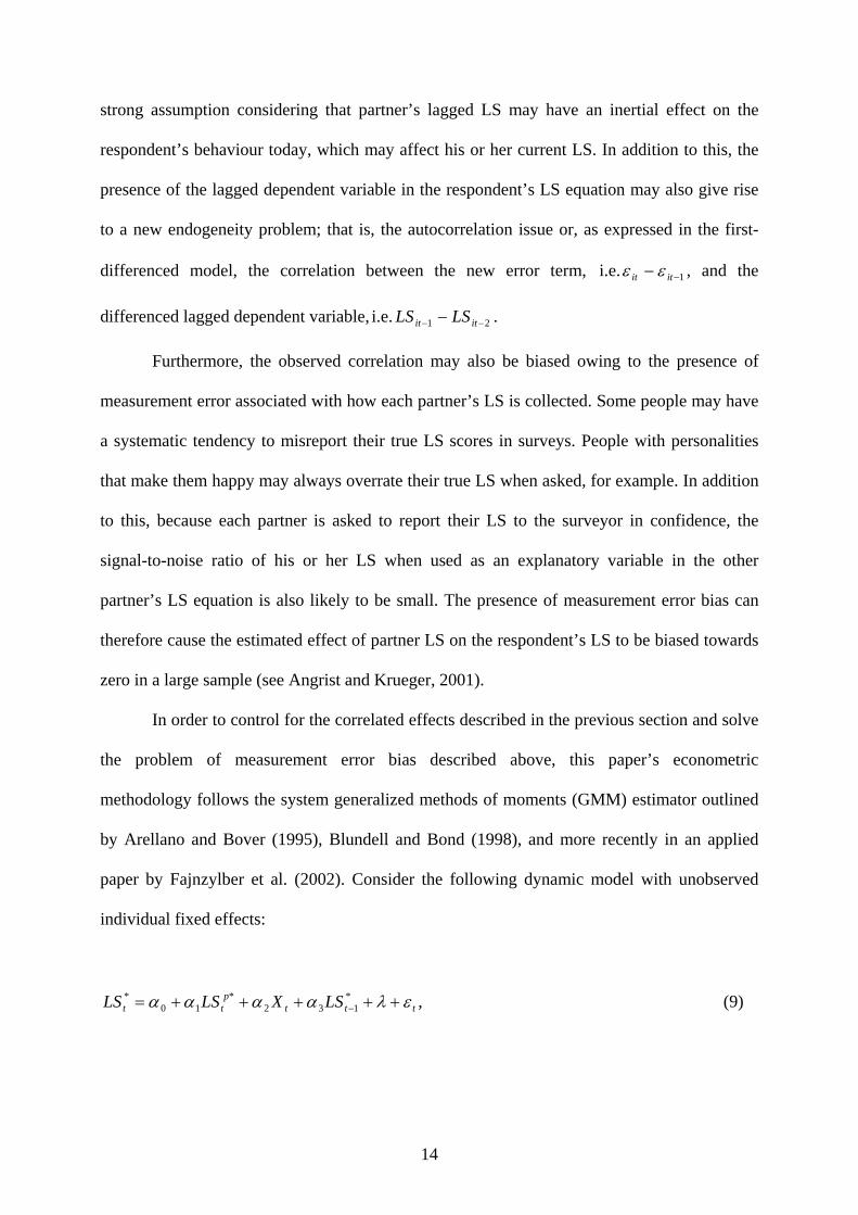
14

strong assumption considering that partner’s lagged LS may have an inertial effect on the

respondent’s behaviour today, which may affect his or her current LS. In addition to this, the

presence of the lagged dependent variable in the respondent’s LS equation may also give rise

to a new endogeneity problem; that is, the autocorrelation issue or, as expressed in the first-

differenced model, the correlation between the new error term, 1 i.e. −− itit εε , and the

differenced lagged dependent variable, 21 i.e. −− − itit LSLS .

Furthermore, the observed correlation may also be biased owing to the presence of

measurement error associated with how each partner’s LS is collected. Some people may have

a systematic tendency to misreport their true LS scores in surveys. People with personalities

that make them happy may always overrate their true LS when asked, for example. In addition

to this, because each partner is asked to report their LS to the surveyor in confidence, the

signal-to-noise ratio of his or her LS when used as an explanatory variable in the other

partner’s LS equation is also likely to be small. The presence of measurement error bias can

therefore cause the estimated effect of partner LS on the respondent’s LS to be biased towards

zero in a large sample (see Angrist and Krueger, 2001).

In order to control for the correlated effects described in the previous section and solve

the problem of measurement error bias described above, this paper’s econometric

methodology follows the system generalized methods of moments (GMM) estimator outlined

by Arellano and Bover (1995), Blundell and Bond (1998), and more recently in an applied

paper by Fajnzylber et al. (2002). Consider the following dynamic model with unobserved

individual fixed effects:

,*132

*10

*ttt

ptt LSXLSLS ελαααα +++++= − (9)

15

where the terms, *LS and *pLS , denote self-rated life satisfaction of the respondent and the

respondent’s partner, respectively. Assuming that there are systematic errors to how each

partner LS is measured and that this measurement error is being driven by (a) a fixed effect

and (b) a time-varying component:

,*ttt LSLS ωξ ++= (10)

.*t

pt

pt LSLS φη ++= (11)

Substituting (10) and (11) into (9)

],[])1([ 1313113210 −− −+−+−+−++++= tiitttp

tt LSXLSLS ωαωφαεξαηαλαααα

,13210 tttp

tt LSXLSLS νµαααα +++++= − (12)

Therefore the measurement error of each partner’s LS is subsumed in the unobserved

individual fixed effects and the error term in our model. Because there are two components to

the bias, i.e. assortative mating (+ve) and measurement error (-ve), the overall direction of bias

coming from unobserved individual fixed effects is unclear on a priori ground.

To estimate the dynamic model of life satisfaction with unobserved individual fixed

effects, I use the system GMM estimator mentioned above. The special feature of this dynamic

GMM estimator is that it joins in a single system the regression equation in differences and in

levels, each with its specific set of instrumental variables, thereby allowing both types of

endogeneity to be controlled for.

In the difference equation, the unobserved individual fixed effects, µ , are eliminated

from the model through first-differencing:

16

).()()()()(

1213

12111001

−−−

−−−−

−+−+−+−+−=−

tttt

ttp

tp

ttttt

LSLSXXLSLSLSLS

εεααααα

(13)

The use of instruments is required to deal with two issues. First, the endogeneity of the

explanatory variables – and in particular, the partner’s LS – which is reflected in the

correlation between these variables and the error term. The second is the correlation, by

construction, between the new error term, )( 1−− tt εε , and the differenced lagged dependent

variable, )( 21 −− − tt LSLS . Assuming, for now, that (a) the error term is not serially correlated,

and (b) the explanatory variables are weakly exogenous, i.e. they may be affected by past and

current realisations of the dependent variable (the respondent’s LS) but not by its future

innovations, the following moment conditions apply:

,,...,3 ,2for 0)]([ 1 TtsLSE ttst =≥=− −− εε (14)

,,...,3 ,2for 0)]([ 1 TtsLSE ititp

st =≥=− −− εε (15)

,,...,3 ,2for 0)]([ 1 TtsXE ttst =≥=− −− εε (16)

However, given that the partner’s LS is an endogenous variable, the natural candidate

instrument in the above equation would instead be the first-difference of the second lag of

partner LS rather than the first-difference of the first lag. This is simply because the second lag

is not correlated with the error term, while the first lag is. The same applies to other

explanatory variables which are endogenous to current realisations of the respondent’s LS. In

addition to this, given our lagged dependent variable model, the presence of time-varying

measurement error would make that the regression error follow a moving average of order 1.

In other words, as will be explained later in the results section, the error term will be serially

17

correlated and, thus, we could not use the most recent lags of the dependent variable as

instruments. Because the BHPS has 3≥T , the use of higher-order lagged dependent variable

as instruments in the GMM-system estimation is considered feasible. It will also, following

Arellano’s (2003, p.51) advice, help to solve the problem of time-varying measurement error

bias.

To improve the model’s efficiency, a second level equation is augmented to the first

difference equation. One reason for this is because sometimes the lagged dependent variables

are poor instruments for the first-differenced regressors, and by adding the second equation

additional instruments can be obtained. For the regression in levels, the unobserved individual

fixed effects are not eliminated but must be controlled for by the use of instrumental variables.

Assuming that there is no correlation between the differences of the explanatory variables and

the unobserved individual fixed effects, their values can be instrumented with their own first

differences. This assumption results from the following stationarity property:

],[][ imitilt LSELSE λλ ++ = (17)

],[][ imjtip

lt LSELSE λλ ++ = (18)

],[][ imitilt XEXE λλ ++ = (19)

for all l and m. Thus, the additional moment conditions for the second part of the system are

given by:

,1for 0)])([( 1 ==+− −−− sLSLSE tstst εµ (20)

,1for 0)])([( 1 ==+− −−− sLSLSE tp

stp

st εµ (21)

.1for 0)])([( 1 ==+− −−− sXXE tstst εµ (22)

18

Using the moment conditions (14-16) for the difference equation and (20-22) for the level

equation, I employ the system GMM estimator to generate consistent estimates for partner’s

LS on the respondent’s LS and their asymptotic variance-covariance (Arellano and Bond ,

1991; Arellano and Bover, 1995; Blundell and Bond, 1998). Because the impact of partner LS

on own LS may be different for men and for women, I conduct all statistical analysis by

gender.

A crucial assumption for the validity of GMM is that the instruments are exogenous.

There are two specification tests that we can use to check whether the lagged values of the

explanatory variables are valid instruments in the LS regression equation. The first is the

Hansen test of overidentification (Hansen, 1982), which tests the null hypothesis of overall

validity of the instruments by analysing the sample analogue of the moment conditions used in

the estimation process. Failure to reject the null hypothesis gives support to the model. Note

that the Hansen test is robust compared to Sargan test of overidentification but can be

weakened by having too many instruments, i.e. more instruments than the number of

individuals used in the estimation (Roodman, 2007). The second test examines the hypothesis

that the error term itε is not serially correlated. This is done by testing whether the differenced

error term (that is, the residual of the regression in differences) is first- or second-order serially

correlated. First-order serial correlation of the differenced error term is expected even if the

original error term (in levels) is uncorrelated, unless the latter follows random walk. Second-

order serial correlation of the differenced error term specifies that the original error term is

serially correlated and that the instruments are misspecified. By contrast, if we can accept the

null hypothesis of no second-order serial correlation then we can conclude that the original

error term is serially uncorrelated and the moment conditions are well-specified.

19

4.4 Data

The present investigation uses data from the BHPS. This is a nationally representative sample

of persons aged 16 and over in 1991, who have been interviewed every subsequent year. The

study interviewed separately all adult members of the household with respect to their income,

employment status, marital status, health, and attitudes. There is both entry into and exit from

the panel, leading to unbalanced data with an increasing number of individual interviews over

time. This is due to the inclusion of children from the original household sample who turn 16,

of refresher samples, and of new members of households formed by original panel members.

As well as questions on socio-economic status, individuals were also asked from Wave

6 onwards to indicate how satisfied they are with their life, from 1 (very dissatisfied with life)

to 7 (very satisfied with life). The LS question is located in a self-completed section of the

survey, which is strategically placed at the end of the questionnaire after individuals had been

asked about their household and individual characteristics.

I consider all married and cohabiting individuals (including same-sex partnership)

observed consecutively over two periods with information on own and partner lagged LS for

the years 1996–2007 (Waves 6-16). Couples who remained with the same partner are treated

the same way in the analysis as those who changed partners during the observed panel. Note

that Wave 11 is omitted from the analysis because of the omission of LS questions in that

survey year. The unbalanced panel with non-missing information on both on and partner LS

(not including lags) includes 38,161 female observations (7,468 individuals) and 38,311 male

observations (7,464 individuals). Of these observations, 6,493 of female observations, and

6,644 of male observations, are currently cohabiting. The average age for women is 46 and 48

for men. Around 51% of women and 59% of men are in full-time employment. Approximately

70% of households have at least one child under the age of 16 in the household.

20

4.5 Accounting for selection bias

Although I am interested only in live-in couples, there is likely some selection bias involved in

moving from other marital statuses (e.g. single, divorced, widowed, or separated) to being in a

relationship. One could imagine, for instance, that married or cohabiting individuals present

specific characteristics that influence the way they are affected by their partner’s well-being

compared to other non-married persons.

To correct for any selection bias in moving from non-married status to being in a

couple, I compute an inverse Mills ratio using a selection variable that equals 1 if the person is

either married or cohabiting and 0 otherwise. This couple equation is estimated on the whole

BHPS sample, as shown in Table A1 in the appendix, as a function of gender, age, age-

squared, number of young (aged 11 and under) and old children ( 18 age 12 <≤ ) in the

household, subjective health (5 dummies), log of real household income per capita, education

(2 dummies), employment status (3 dummies), wave dummies and the divorce rate of other

households within the region. This last variable is used to satisfy the exclusion restrictions,

which is possible as the divorce rate of other households within the region is correlated with

whether or not the respondent is married or cohabiting, but should not be correlated with how

each partner is affected by the other partner’s LS.

5. Results

5.1 Life satisfaction spillovers

Table 2 reports results from the GMM-system estimator described in the previous section. The

dependent variable is the respondent’s self-rated life satisfaction measured cardinally (on a

21

scale of 1 to 7)1. For comparative purposes, I also present results from the OLS estimator, as

well as the GMM-levels estimator, which does not control for individual fixed effects. In

contrast to the GMM-system, first-order serial correlation is a sign of misspecification in the

case of levels estimator. To prevent the case of having too many instruments that would lead

to an overfitting of the endogenous variables, I follow Roodman’s (2007) advice and

“collapse” instruments in all GMM regressions. Finally, it should also be noted that, in cases

where the lagged dependent variable is included as a right-hand side variable in the regression,

each estimated coefficient represents the short-run effect of the respective variable.

The first two columns of Table 2 report the OLS results for men and women,

respectively. Here, only partner LS, inverse Mills ratio, and the exogenous variables – namely

age, age-squared, and wave dummies – are included as the right-hand side variables in the LS

equation. As anticipated, partner LS enters the respondent LS equations in a positive and

statistically significant manner, i.e. there seems to be strong evidence that partners’ LS are

positively correlated at cross-section. The relationship appears to be moderate in size; an

increase of one life satisfaction score in partner LS is associated with approximately 25

percentage-points increase in respondent LS for men and 27 percentage-points for women.

However, as described in the previous section, this observed correlation between partners’

well-being is likely to be biased owing to either or both correlated effects and measurement

errors in the LS variables.

Treating partner LS as endogenous – i.e. using the second- rather than the first-lag of

partner LS as instruments, Columns 3 and 4 of Table 2 re-estimate the first two columns’

specification using the GMM-levels estimator. GMM-levels yields a positive coefficient on

partner LS for both men and women, although the relationship is statistically significant only

1 One objection is that measures of subjective well-being, such as happiness and life satisfaction, are ordinal rather than cardinal variables. However, many research papers have shown that it virtually makes no difference in the estimation whether one assumes ordinality or cardinality in the reported well-being data (see, e.g., Ferrer-i-Carbonell and Frijters, 2004).

22

in the male sub-sample regression; the coefficients on partner LS are 0.561 (S.E. = 0.205) for

men and 0.228 (S.E. = 0.188) for women. However, the model performs poorly; this

specification is rejected by the test of first-order serial correlation, which indicates that the

model is misspecified in the case of the levels estimator.

Columns 5 and 6 of Table 2 introduce a lag one of the dependent variable into the

model. Using the most recent lags of the dependent variable as instruments, the lagged

respondent LS variable is positive and statistically significant at the 1% level for both men and

women, which is consistent with the hedonic capital theory, i.e. our happiness today is

determined by how happy we were in the past (Graham and Oswald, 2006). Yet the inclusion

of the lagged dependent variable has now made the partner LS variable insignificant in both

male and female sub-sample regressions. Furthermore, this specification is also rejected by the

tests of serial correlation for both men and women, as well as the Hansen test of

overidentification in the case of male sub-sample regression. In other words, we may still have

(a) omitted variables that are correlated with both respondent and partner LS, which can either

be time-varying or relatively stable over-time, and/or (b) serial correlations in the error term

caused by the presence of time-varying measurement error bias.

To solve the problem of unobserved heterogeneity, the next two columns use the

GMM-system estimator to control for unobserved individual fixed effects that are potentially

correlated with the explanatory variables. As described in the previous section, the presence of

unobserved individual fixed effects can bias the estimated coefficients on partner LS through

assortative mating and shared social environment with high over-time persistence (+ve) and

measurement errors (-ve), although the extent of each bias on the estimated correlation

between partners’ LS is unknown on a priori ground.

The GMM-system estimator generates coefficients on partner LS that are notably

larger than the ones obtained by the GMM-levels estimator; a one-satisfaction-point increase

23

in partner LS is now associated with approximately 0.58 increase in the respondent’s LS for

men and 0.75 for women. What this implies is that, in regressions where unobserved

individual effects are ignored, the negative bias stemming from the relatively stable

component of the measurement error is larger compared to the positive bias coming from

assortative mating and shared social environment with high over-time persistence.

Nevertheless, the estimates are still poorly defined, considering that the specification is

rejected by both the Hansen test of overidentification and the tests of serial correlation. As

mentioned earlier, a rejection of the second-order serial correlation in the case of the GMM-

system estimator implies that the original error term is serial correlated. This serial correlation

is expected, however, as we have yet to correct for the measurement error term that varies over

time.

To solve the problem of time-varying measurement error bias, Columns 9 and 10 drop

the most recent lags of the dependent variable from the instrument list and use only the

second-lag and beyond as instruments in the GMM-system estimation. The specification is

now supported by the tests of serial correlation, i.e. we can now accept the null hypothesis of

no second-order serial correlation with the use of higher-order lags of the dependent variable

as instruments. This is the case for both men and women. However, this specification is still

rejected in the female sub-sample regression by the Hansen test of overidentification. In

addition to this, the process also increases the size of the estimated coefficients on the lagged

dependent variable; the estimated coefficients on respondent lagged LS are 0.13 and 0.09 for

men and women, respectively. This supports the way we modelled the measurement error term

as having a time-varying component as well as a fixed effect. However, this specification also

produces large standard errors for the estimated lagged dependent variable. By contrast, the

The last two columns (Columns 11 and 12) control for a number of household and

individual characteristics known in the literature to be important LS predictors (see, e.g.,

24

Oswald and Powdthavee, 2008), adding log of real household income per capita, employment

status, a dummy of whether the respondent is cohabiting, number of years stayed together as a

couple in the BHPS (maximum of 16 years), number of children, education, and subjective

health status, all of which are treated as endogenous variables in the GMM-system estimation.

The estimated coefficients on these control variables are presented in Table A2 in the

appendix.

In this specification, we can see that for both men and women the p-values for the

Hansen test are now, according to Roodman (2007), sufficiently high and within the

recommended range ( 25.01.0 <≤ p ). This confirms that important time-varying components

has been omitted in the previous specifications and by controlling for them in the estimation,

the models are now well-specified. With a full set of controls, the point estimates on the

partner LS variable are reduced to 0.278 (S.E. = 0.047) for men and 0.329 (S.E. = 0.057) for

women, which are not that much different to the point estimates obtained in the OLS

estimation (see Columns 1 and 2). What this implies is that there is almost a full offsetting

effect between omitted variables (i.e. unobserved individual fixed effects, time-varying

variables, and dynamic effects coming from the lagged dependent variable) and the

measurement error bias on the estimated correlation between partners’ LS at cross-section.

With respect to Table 2’s other results, there is a U-shaped relationship between age

and LS for both partners, minimizing at around early 40s. The negative and statistically

significant inverse Mills ratio indicates that the selection into partnership and LS is correlated.

Interestingly, household income is negatively correlated with LS in the GMM-system

estimation. Better health is found to be highly correlated with higher LS levels for both

genders. Nonetheless, while almost all of the other estimated coefficients have the correct

signs, they are also estimated with large standard errors.

25

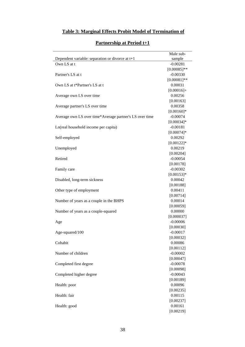
5.2 Termination of partnership

Up to this point, this paper has concentrated on the estimation of causal effect of partner LS on

respondent LS. Such an approach seems to be of some worth in its own right. However, in

order to make further justification on the importance of the previous spillover effect model

presented in the last section, I now estimate a marital dissolution equation.

Of the married and cohabiting individuals, there were approximately 621 couples

(roughly 1% of the sample) who moved from being married or cohabiting with a partner at

period t to separation or divorce at t+1. The key hypothesis to be tested here is that there is a

short-run association between partners’ LS and their decision to stay together. More

specifically, couples with higher LS levels at t are less likely to be separated or divorced at

t+1.

Table 3 presents marginal effects (reported in percentages) obtained from a probit

model on whether the couple terminates their relationship at period t+1. The model controls

for a number of household and personal characteristics, including age, age-squared, cohabiting

dummy, income, employment status, education, health, number of years stayed as a couple in

the panel, selection into a couple (i.e. inverse Mills ratio), number of children, regional and

wave dummies. It also includes as the variables of interest (a) LS measured at t and (b)

average LS over time for male and female partners in a couple. Following one of the referees’

advice, I also introduce variables for the interaction between partners’ LS at t and the same

interaction for the average LS levels. The probit is estimated on the male sub-sample, although

the female sub-sample regression produces qualitatively similar results.

Controlling for household and personal characteristics, as well as the average LS levels

of both partners, we can see that both partners’ LS at t are associated negatively and

statistically significantly with separation and divorce at t+1. A unit increase in either partner

26

LS at t is associated with approximately 0.3 percentage-point decrease in the probability of

separation or divorce at t+1. This is a large effect, considering that only 1% of the sample

made a transition from being married/cohabiting at t to being separated or divorced at t+1.

Interestingly, the interaction term between partners’ LS at t is positive and statistically

significant at the 10% level; the negative effect of each partner’s LS on the couple’s

propensity to separate or divorce is smaller in the case when both partners’ LS at t are high

compared to when they are both low.

By contrast, the mean values of both partners’ LS are positively correlated with the

probability of separation or divorce at t+1. This is somewhat consistent with the notion that

there may be important peak-end effects in the marriage market, whereby the decision to

separate/divorce depends positively on past variation in LS, i.e. the difference between current

LS and some reference level that would be proxied by the averaged LS levels (see, e.g.,

Kahneman, 1999; Clark and Georgellis, 2004). Furthermore, the peak-end theory is supported

by the negative interaction effect between the average LS levels, which is statistically

significant at the 5% level.

In short, the link between partners’ decision to end partnership at t+1 and their LS at t

is consistent with the spillover effect model, whereby changes in either partner’s LS today

influence the decision of whether or not to stay together as a couple in the next period.

Finally, Table 3’s other results are also interesting in their own right. Income this

period is associated negatively with the probability that the couple will split one period into

the future, whilst people who are self-employed at t are more likely than those in full-time

employment to end their relationship at t+1. Interestingly, being a housewife (or look after

home) this year lowers the probability of couple dissolution in the subsequent year by

approximately 3 percentage-points. This is perhaps due to the fact that at least one partner is

27

always home when the other partner is back from work, something which can be considered as

good for the relationship.

6. Conclusion

This paper has used ten waves of BHPS data to study intra-spousal correlations in self-

reported life satisfaction data. Its primary objective was to determine whether the observed

correlation is due largely to partners’ fixed traits are similar through assortative mating by

personality traits on the marriage market, partners sharing the same social environment that

simultaneously affects their well-being, or a spillover effect of life satisfaction from one

partner to the other.

A simple OLS model reveals that there is indeed a positive and statistically significant

correlation between partners’ LS. This correlation persists even when the GMM-system

estimator is used to estimate the model, i.e. partners’ LS remain positively and statistically

significantly correlated even after controlling for the presence of measurement error bias and

unobserved heterogeneity and allowing partner LS to be instrumented by the first-differences

of its lags. In other words, there seems to be strong evidence of a causal spillover effect of

well-being that runs from one partner to the other in a couple. This conclusion is also

supported by the evidence that partners’ LS can be used to predict observable behaviours:

there is a negative and statistically significant association between partners’ life satisfaction

this year and the likelihood of couple dissolution in the subsequent year. These results are

consistent with models of spillover effects within couples. The findings thus provide strong

statistical support in terms of validity for many economic models that were built around the

assumption that utility is interdependently related between members of the same household

28

(Becker, 1974). It is also consistent with studies that found evidence of caring preferences

between partners within marriage (Foster and Rosenzweig, 2001; Ermisch, 2003).

More generally, the empirical approach of this paper can be extended and applied to

distinguish between various explanations of other types of similarity in couples’ behaviours

and characteristics that are not specific to a partner’s subjective well-being.

29

Acknowledgement

I am grateful to Andrew Oswald, Andrew Clark, Paul Dolan, Ian Walker, Robin Naylor, Geeta

Kingdon, Rainer Winkelmann, Ulrich Schimmack, Nateecha Ratanadilok Na Bhuket, Anthony

Fielding, participants at the Royal Economic Society at Nottingham and the Economics of

Happiness Symposium at the University of Southern California in March, 2006, and two

anonymous referees for their valuable comments. The British Household Panel Survey data

were made available through the UK Data Archive. The data were originally collected by the

ESRC Research Centre on Micro-social Change at the University of Essex, now incorporated

within the Institute for Social and Economic Research. Neither the original collectors of the

data nor the Archive bears responsibility for the analyses or interpretations presented here.

30

REFERENCES

Angrist, J.D., and Krueger, A.B. (2001). Instrumental variables and the search for

identification: From supply and demand to natural experiments. Journal of Economic

Perspectives, 15(4), 69-85.

Arellano, M. (2003). Panel Data Econometrics. Oxford University Press, UK.

Arellano, M., and Bond, S. (1991). Some tests of specification for panel data: Monte

Carlo evidence and application to employment equations. Review of Economic Studies, 58,

277-297.

Arellano, M., and Bover, O. (1995). Another look at the instrumental-variable

estimation of error-components models. Journal of Econometrics, 68, 29-52.

Anderson, C., Keltner, D., and John, O.P. (2003). Emotional convergence between

people over time. Journal of personality and social psychology, 84, 1054-1068.

Becker, G. S. (1973). A theory of marriage: Part I. Journal of Political Economy, 81,

813-846.

Becker, G.S. (1974). A theory of marriage: Part II. Journal of Political Economy, 82,

11-26.

Benson, P. L., et al., (1980). Intrapersonal correlates of nonspontaneous helping

behaviour, Journal of Social Psychology, 110, 87-95.

Berger, P., and Kellner, H. (1964). Marriage and the construction of reality: An

exercise in the microsociology of knowledge. Diogenes, 46, 1-25.

Berkman, L.F. (1988). The changing and heterogeneous nature of aging and longevity:

A social and biomedical perspective. Annual Reviews in Gerontology and Geriatrics, 8, 37-68.

Blundell, R., and Bond, S. (1998). Initial conditions and moment restrictions in

dynamic panel data models. Journal of Econometrics, 87, 115-143.

31

Bolger, N., DeLongis, A., Kessler, R.C., and Wethington, E. (1989). The contagion of

stress across multiple roles. Journal of Marriage and the Family, 51, 175-183.

Bradburn, N.M. (1969). The structure of psychological well-being. Aldine, Chicago.

Bruhin, A., and Winkelmann, R. (2007). Happiness function with preference

interdependence and heterogeneity: the case of altruism within family. Socioeconomic

Institute, University of Zurich, mimeo.

Chamberlain, K. (1988). On the structure of well-being. Social Indicators Research,

20, 581-604.

Clark, A.E., and Etile, F. (2006). Don’t give up on me baby: spousal correlation in

smoking behaviour. Journal of Health Economics, 25, 958-978.

Clark, A.E., and Georgellis, Y. (2004). Kahneman meets the quitters: peak-end

behaviour in the labour market. CNRS and DELTA, working paper.

Contoyannis, P., and Jones, A. (2004). Socio-economic status, health and lifestyle.

Journal of Health Economics, 23, 965-995.

Ermisch, J.F. (2003). An Economic Analysis of the Family. Princeton University Press.

Fajnzylber, P., Lederman, D., and Loayza, N. (2002). What causes violent crime?

European Economic Review, 46, 1323-1357.

Farrell, L., and Shields, M. (2002). Investigating the economic and demographic

determinants of sporting participation in England. Journal of Royal Statistical Society A, 165,

335-348.

Ferrer-i-Carbonell, A., and Frijters, P. (2004). How important is methodology for the

estimates of the determinants of happiness? Economic Journal, 114, 641-659.

Foster, A.D., and Rosenzweig, M.R. (2001). Imperfect commitment, altruism, and the

family: Evidence from transfer behaviour in low-income rural areas. Review of Economics and

Statistics, 83, 389-407.

32

Frey, B., and Stutzer, A. (2006). Does marriage make people happy, or do happy

people get married? Journal of Socio-Economics, 35(2), 326-347.

Frey, B., Benz, M., and Stutzer, A. (2004). Introducing procedural utility: not only

what, but also how matters. Journal of Theoretical Economics, 160(3), 377-401.

Friedman, D.D. (1986). Price theory: an intermediate text. South-Western College

Publishing.

Gove, W.R., Hughes, M., and Style, C.B. (1983). Does marriage have positive effects

on the psychological well-being of the individual? Journal of Health and Social Behavior, 24,

122-131.

Graham, L., and Oswald, A.J. (2006). Hedonic Capital. IZA Discussion Paper No.

2079.

Hansen, L. (1982). Large sample properties of generalised method of moments

estimator. Econometrica, 50, 1029-1054.

Headey, B.W., Kelley, J., and Wearing, A.J. (1993). Dimensions of mental health: life

satisfaction, positive affect, anxiety and depression. Social Indicators Research, 29, 68-83.

House, J.S., Robbins, C., and Metzner, H. (1982). The association of social

relationships and activities with mortality: prospective evidence from the Tecumseh

Community Health Study. American Journal of Epidemiology, 116, 123-140.

Huppert, F.A., and Whittington, J.E. (2003). Evidence for the independence of positive

and negative well-being: Implications for quality of life assessment. British Journal of Health

Psychology, 8, 107-122.

Kahneman, D. (1999). Objective happiness. In Kahneman, D., Diener, E., and

Schwarz, N. (eds.). Well-Being: The Foundation of Hedonic Psychology. New York: Russell

Sage, 3-25.

33

Kan, M.Y., and Heath, A. (2006). The political values and choices of husbands and

wives. Journal of Marriage and Family, 68, 70-86.

Konow, J., and Earley, J. (2008). The hedonistic paradox: is homo economicus

happier? Journal of Public Economics, 92, 1-33.

Korenman, S. and Neumark, D. (1991) Does marriage really make men more

productive? Journal of Human Resources, 26(2), 282-307.

Jones, E., and Fletcher, B. (1993). An empirical study of occupational stress

transmission in working couples. Human Relations, 46, 881-902.

Lam, D. (1988). Marriage markets and assortative mating with household public

goods: Theoretical results and empirical implications. Journal of Human Resources, 24, 462-

487.

Larson, R.W., and Almeida, D.M. (1999). Emotional transmission in the daily lives of

families: A new paradigm for studying family process. Journal of Marriage and the Family,

61, 5-20.

Liang, J. (1985). A structural integration of the affective balance scale and the life-

satisfaction Index A. Journal of Gerontology, 40, 552-561.

Loh, E.S. (1996). Productivity differences and the marriage wage premium for white

males. Journal of Human Resources, 31 (3), 566-589.

Manski, C. (1995). Identification problems in social sciences. Harvard University

Press, Cambridge, MA.

Mare, R. (1991). Five decades of educational assortative mating. American

Sociological Review, 56(1), 15-32.

Marks, N.F., and Lambert, J.D. (1998). Marital status continuity and change among

young and midlife adults: longitudinal effects on psychological well-being. Journal of Family

Issues, 19, 652-686.

34

Mastekaasa, A. (1992). Marriage and psychological well-being: some evidence on

selection into marriage. Journal of Marriage and the Family, 54, 901-911.

Mastekaasa, A. (1994). The subjective well-being of the previously married: the

importance of unmarried cohabitation and time since widowhood or divorce. Social Forces,

73, 665-692.

Meier, S., and Stutzer, A. (2008). Is volunteering rewarding in itself? Economica, 75,

39-59.

Michalos, A.C. (1991). Global report on student well-being. Life-satisfaction and

happiness, volume I. Springer: New York.

Oswald, A.J., and Powdthavee, N. (2008). Does happiness adapt? A longitudinal study

with implications for economists and judges. Journal of Public Economics, 92, 1061-1077.

Oswald, A.J., and Wilson, C.M. (2005). How does marriage affect physical and

psychological health? A survey of the longitudinal evidence. Paper presented at the

Department of Economics, University of Warwick.

Pavot, W., and Diener, E. (1993). Review of the satisfaction with life scale.

Psychological Assessment, 5(2), 164-172.

Plug, E.J.S., and Van Praag, B.M.S. (1998). Similarity in response behaviour between

household members: an application to income evaluation. Journal of Economic Psychology,

19, 497-513.

Powdthavee, N., and Vignoles, A. (2008). Mental Health of Parents and Life

Satisfaction of Children: A Within-Family Analysis of Intergenerational Transmission of

Well-Being. Social Indicators Research, 88(3), 397-422.

Power, C., Rodgers, B., and Hope, S. (1999). Heavy alcohol consumption and marital

status: disentangling the relationship in a National Study of Young Adults. Addiction, 94,

1477-1487.

35

Qian, Z. (1998). Changes in assortative mating: The impact of age and education,

1970-1990. Demography, 35(3), 279-292.

Roodman, D. (2007). A short note on the theme of too many instruments. Centre for

Global Development, Working Paper No. 125.

Rose, A.M. (1955). Factors associated with the life satisfaction of middle-class, middle

aged persons. Marriage and Family Living, 17, 15-19.

Schwarze, J., and Winkelmann, R. (2005). What can happiness research tell us about

altruism? Evidence from the German Socio-economic Panel. Institute for the Study of Labour

(IZA), discussion paper: No. 1487.

Schimmack, U., and Lucas, R.E. (2006). Marriage matters: spousal similarity in life

satisfaction. German Institute for Economic Research, discussion paper, 623.

Smock, P.J., Manning, W.D., and Gupta, S. (1999). The effect of marriage and divorce

on economic well-being. American Sociological Review, 64, 794-812.

Stock, W.A., Okun, M.A., and Benin, M. (1986). Structure of subjective well-being

among the elderly. Psychology and Aging, 1, 91-102.

Thoits, P.A., and Hewitt, L.N. (2001). Volunteer work and well-being. Journal of

Health and Social Behaviour, 42(2), 115-131.

Waite, L.J., and Gallagher, M. (2000). The case for marriage: why married people are

happier, healthier, and better off financially, Broadway Books: New York

Westman, M., and Vinokur, A.D. (1998). Unravelling the relationship of distress

levels within couples: common stressors, emphatic reactions, or crossover via social

interaction? Human Relations, 51(2), 137-156.

36

Table 1: Descriptive Statistics of the Variables used in the GMM estimation, BHPS 1996-2006

Variables Men Women

Life satisfaction 5.300 (1.196)

5.347 (1.250)

Partner Life satisfaction 5.347 (1.249)

5.299 (1.197)

Age 48.039 (15.422)

45.695 (14.826)

Age-squared/100 25.456 (15.855)

23.161 (14.826)

Inverse Mills ratio 0.377 (0.281)

0.483 (0.326)

Ln(real household income per capita) 9.570 (0.628)

9.569 (0.628)

Self-employed 0.127 (0.333)

0.042 (0.201)

Unemployed 0.031 (0.174)

0.017 (0.130)

Retired 0.195 (0.396)

0.170 (0.376)

Maternity leave 0.000 (0.011)

0.011 (0.107)

Family care 0.005 (0.074)

0.159 (0.366)

Full-time student 0.004 (0.067)

0.008 (0.093)

Disabled, long-term sickness 0.044 (0.206)

0.035 (0.185)

Government training scheme 0.000 (0.022)

0.000 (0.016)

Other type of employment 0.003 (0.056)

0.004 (0.065)

Number of years as a couple in the BHPS 11.381 (4.660)

11.430 (4.636)

Number of years as a couple-squared 151.269 (99.379)

152.156 (99.406)

Cohabit 0.173 (0.378)

0.170 (0.375)

Number of children (aged<16) 0.714 (1.036)

0.721 (1.040)

Completed first degree 0.105 (0.307)

0.102 (0.303)

Completed higher degree 0.033 (0.179)

0.022 (0.147)

Health: poor 0.073 (0.261)

0.086 (0.281)

Health: fair 0.212 (0.409)

0.224 (0.417)

Health: good 0.452 (0.497)

0.453 (0.497)

Health: excellent 0.241 (0.427)

0.211 (0.408)

N 38135 37985 Note: Standard deviations are in parentheses.

37

Table 2: OLS and Dynamic GMM estimates of life satisfaction, BHPS 1996-2007

OLS GMM-levels

GMM-levels, Instrument from

first-lag dependent variable

GMM-system, Instrument from

first-lag dependent variable

GMM-system, Instrument from

second-lag dependent variable

GMM-system with full controls and instrument from

second-lag dependent variable

Men Women Men Women Men Women Men Women Men Women Men Women Dependent variable: Own LS at t (1) (2) (3) (4) (5) (6) (7) (8) (9) (10) (11) (12) Partner LS at t 0.245 0.270 0.561 0.228 0.069 0.164 0.575 0.749 0.543 0.765 0.278 0.329 [0.008]** [0.009]** [0.205]** [0.188] [0.136] [0.113] [0.094]** [0.117]** [0.116]** [0.129]** [0.047]** [0.057]** Own lagged LS (t-1) 0.668 0.448 0.064 0.064 0.130 0.093 0.018 -0.038 [0.098]** [0.115]** [0.017]** [0.017]** [0.121] [0.121] [0.045] [0.049] Age -0.067 -0.055 -0.044 -0.074 -0.022 -0.043 -0.026 -0.024 -0.025 -0.022 -0.039 -0.035 [0.006]** [0.006]** [0.027] [0.020]** [0.017] [0.015]** [0.012]* [0.012]+ [0.012]* [0.013]+ [0.017]* [0.019]+ Age-squared/100 0.073 0.062 0.048 0.083 0.024 0.047 0.030 0.026 0.029 0.024 0.047 0.044 [0.006]** [0.007]** [0.029]+ [0.022]** [0.018] [0.016]** [0.012]* [0.013]* [0.012]* [0.013]+ [0.017]** [0.019]* Inverse Mills ratio -0.504 -0.336 -0.340 -0.526 -0.216 -0.316 -0.202 -0.116 -0.211 -0.116 -0.456 -0.379 [0.054]** [0.045]** [0.263] [0.171]** [0.165] [0.130]* [0.129] [0.119] [0.126]+ [0.120] [0.176]** [0.200]+ Constant 5.541 5.121 3.326 5.835 1.941 3.094 2.468 1.554 2.292 1.295 3.595 5.731 [0.173]** [0.171]** [1.670]* [1.355]** [0.999]+ [0.950]** [0.635]** [0.718]* [0.666]** [0.805] [1.023]** [1.530]** Observations 38135 37985 38135 37985 27520 27659 27520 27659 27520 27659 27518 27655 Number of individuals 7438 7442 6432 6494 6432 6494 6432 6494 6432 6494 Number of instruments 34 34 41 41 47 47 46 46 357 358 Wave dummies Yes Yes Yes Yes Yes Yes Yes Yes Yes Yes Yes Yes - Hansen test of overidentification 0.243 0.936 0.036 0.271 0.153 0.028 0.190 0.040 0.235 0.144 - First order serial correlation 0.000 0.000 0.000 0.000 0.000 0.000 0.000 0.000 0.000 0.000 - Second order serial correlation 0.288 0.503 0.000 0.001 0.006 0.014 0.186 0.243 0.299 0.792 Note: + < 10%; * < 5%; ** < 1%. Standard errors are in parentheses. Life satisfaction is recorded on a 7-point-scale, with 1 = very dissatisfied and 7 = very satisfied. All explanatory variables whenever they are appeared in the model – except for age, age-squared, and year dummies – are treated as endogenous variables, i.e. used as GMM-type instruments. Age, age-squared, and year dummies are treated as exogenous variables orthogonal to the individual fixed effects, i.e. their levels are used as instruments the level equations. Control variables in the last two columns include log of real household income per capita, employment status, a dummy of whether the respondent is cohabiting, number of years stayed together as a couple in the panel, number of children, education, and subjective health status, all of which are treated as endogenous variables in the GMM-system estimation.

38

Table 3: Marginal Effects Probit Model of Termination of

Partnership at Period t+1

Dependent variable: separation or divorce at t+1 Male sub-

sample Own LS at t -0.00281 [0.00085]** Partner's LS at t -0.00330 [0.00081]** Own LS at t*Partner's LS at t 0.00031 [0.00016]+ Average own LS over time 0.00256 [0.00163] Average partner's LS over time 0.00358 [0.00160]* Average own LS over time*Average partner's LS over time -0.00074 [0.00034]* Ln(real household income per capita) -0.00181 [0.00074]* Self-employed 0.00292 [0.00122]* Unemployed 0.00219 [0.00204] Retired -0.00054 [0.00178] Family care -0.00302 [0.00153]* Disabled, long-term sickness 0.00042 [0.00188] Other type of employment 0.00411 [0.00714] Number of years as a couple in the BHPS 0.00014 [0.00059] Number of years as a couple-squared 0.00000 [0.000037] Age -0.00006 [0.00030] Age-squared/100 -0.00017 [0.00032] Cohabit 0.00086 [0.00112] Number of children -0.00002 [0.00047] Completed first degree -0.00078 [0.00098] Completed higher degree -0.00043 [0.00189] Health: poor 0.00096 [0.00235] Health: fair 0.00115 [0.00237] Health: good 0.00161 [0.00219]

39

Health: excellent 0.00183 [0.00258] Inverse Mills ratio -0.00810 [0.00265]** Regional dummies Yes Wave dummies Yes Observations 32356 Pseudo R-squared 0.1118 Log-likelihood -1557.9151

Note: + < 10%; * < 5%; ** < 1%. Standard errors are in parentheses. Reference groups include in full-time employment, married, education level less than first degree, health: very poor.

40

Table A1: Instrumental regression for selection bias

Dependent variable: In a couple = 1, 0 otherwise β

Divorce rate of other households within the region (in %) -0.055 [0.009]** Male 0.218 [0.017]** Age 0.166 [0.002]** Age-squared/100 -0.152 [0.003]** Number of younger children (aged under 12) 0.577 [0.020]** Number of older children (12 <= age < 18) -0.018 [0.017] Health: poor 0.059 [0.030]+ Health: fair 0.066 [0.033]* Health: good 0.071 [0.034]* Health: excellent 0.041 [0.036] Log of real household income per capita 0.389 [0.013]** Completed first degree -0.124 [0.030]** Completed higher degree -0.208 [0.063]** In full-time employment 0.100 [0.017]** Unemployed -0.229 [0.027]** Disabled -0.377 [0.034]** Constant -7.033 [0.147]** Wave dummies Yes Observations 204845 Log likelihood -101618.8

Note: + < 10%; * < 5%; ** < 1%. Standard errors are in parentheses. Reference groups include women, not in full-time employment (e.g. self-employed, retired, family care, student, in government training, maternity leave, and other type of employment), education level less than first degree, and health: very poor.

41

Table A2: Estimated GMM-system coefficients on the control variables

(Columns 11 and 12, Table 2)

GMM-system with full controls

Dependent variable: Own LS at t Men Women Ln(real household income per capita) -0.043 -0.215 [0.046] [0.094]* Self-employed 0.162 0.068 [0.116] [0.194] Unemployed 0.130 -0.350 [0.248] [0.370] Retired 0.226 0.102 [0.144] [0.165] Maternity leave 3.677 0.508 [5.896] [0.340] Family care -0.272 0.097 [0.502] [0.126] Full-time student 0.253 -0.506 [0.417] [0.336] Disabled, long-term sickness -0.173 -0.332 [0.289] [0.291] Government training scheme -2.076 -0.026 [2.595] [2.507] Other type of employment 0.489 -0.264 [0.576] [0.700] Number of years as a couple in the panel -0.061 0.009 [0.100] [0.106] Number of years as a couple-squared 0.002 -0.002 [0.005] [0.005] Cohabit 0.063 0.018 [0.064] [0.092] Number of children (aged<16) -0.015 -0.051 [0.042] [0.061] Completed first degree 0.154 0.177 [0.159] [0.141] Completed higher degree -0.213 -0.235 [0.207] [0.250] Health: poor 0.970 0.213 [0.395]* [0.379] Health: fair 1.363 0.680 [0.369]** [0.355]+ Health: good 1.763 1.257 [0.366]** [0.351]** Health: excellent 2.125 1.443 [0.383]** [0.368]**

Note: + < 10%; * < 5%; ** < 1%. Standard errors are in parentheses. Reference groups include in full-time employment, married, education level less than first degree, health: very poor.