Spectroscopic properties from hybrid QM, MM molecular dynamics simulation
140
1.61.2 Spectroscopic Properties from Hybrid QM/MM Molecular Dynamics Simulation Dissertation zur Erlangung des Grades ”Doktor der Naturwissenschaften” dem Fachbereich Chemie, Pharmazie und Geowissenschaften der Johannes Gutenberg-Universit¨at Mainz vorgelegt von Sittipong Komin geboren in Khonkaen, Thailand Mainz 2009 1
-
Upload
independent -
Category
Documents
-
view
0 -
download
0
Transcript of Spectroscopic properties from hybrid QM, MM molecular dynamics simulation

1.61.2
Spectroscopic Properties from Hybrid QM/MM
Molecular Dynamics Simulation
Dissertation
zur Erlangung des Grades
”Doktor der Naturwissenschaften”
dem Fachbereich Chemie, Pharmazie und Geowissenschaften
der Johannes Gutenberg-Universitat Mainz
vorgelegt von
Sittipong Komin
geboren in Khonkaen, Thailand
Mainz 2009
1

I would like to dedicate this thesis to my loving parents ...

Contents
1 Introduction 7
1.1 Thesis Overview . . . . . . . . . . . . . . . . . . . . . . . . . . . . 12
2 Theory 13
2.1 General . . . . . . . . . . . . . . . . . . . . . . . . . . . . . . . . 13
2.2 Density Functional Theory . . . . . . . . . . . . . . . . . . . . . . 14
2.2.1 Born-Oppenheimer approximation . . . . . . . . . . . . . . 14
2.2.2 Many-body electronic wave function . . . . . . . . . . . . . 16
2.2.3 Hohenberg-Kohn and Kohn-Sham formalism . . . . . . . . 20
2.2.4 Exchange-correlation functionals . . . . . . . . . . . . . . . 25
2.3 Pseudopotential approximation . . . . . . . . . . . . . . . . . . . 28
2.4 Plane wave representation . . . . . . . . . . . . . . . . . . . . . . 30
2.5 Molecular Dynamics . . . . . . . . . . . . . . . . . . . . . . . . . 32
2.5.1 Equations of motion . . . . . . . . . . . . . . . . . . . . . 33
2.5.2 Car-Parrinello molecular dynamics (CPMD) . . . . . . . . 35
2.5.3 Empirical Force-Fields . . . . . . . . . . . . . . . . . . . . 37
2.6 Realization of MD in Statistical Ensembles . . . . . . . . . . . . . 41
2.7 Hybrid DFT-QM/MM Simulations . . . . . . . . . . . . . . . . . 43
2.7.1 The QM/MM Approach to Complex Systems . . . . . . . 44
2.7.2 The partitioning of the system . . . . . . . . . . . . . . . . 45
3

CONTENTS
2.7.3 Non-bonded QM/MM interactions . . . . . . . . . . . . . 48
2.7.4 The bonded QM-MM interactions . . . . . . . . . . . . . . 52
2.8 NMR chemical shifts . . . . . . . . . . . . . . . . . . . . . . . . . 54
2.8.1 Magnetic perturbation theory . . . . . . . . . . . . . . . . 56
2.8.2 Electronic current density . . . . . . . . . . . . . . . . . . 59
2.8.3 Induced field, susceptibility and shielding . . . . . . . . . . 60
2.8.4 Effect of pseudopotentials on NMR chemical shifts . . . . . 62
2.8.5 Combination of NMR and QM/MM . . . . . . . . . . . . . 63
3 NMR solvent shifts of adenine in aqueous solution from hybrid
QM/MM molecular dynamics simulations 65
3.1 Introduction . . . . . . . . . . . . . . . . . . . . . . . . . . . . . . 65
3.1.1 Hybrid quantum-classical (QM/MM) molecular dynamics
simulations . . . . . . . . . . . . . . . . . . . . . . . . . . 68
3.1.2 QM/MM NMR chemical shift calculations . . . . . . . . . 69
3.2 QM/MM NMR benchmark calculations on hydrogen bonded molec-
ular dimers . . . . . . . . . . . . . . . . . . . . . . . . . . . . . . 73
3.2.1 Water dimer . . . . . . . . . . . . . . . . . . . . . . . . . . 73
3.2.2 Methanol dimer . . . . . . . . . . . . . . . . . . . . . . . . 77
3.3 Adenine solvated in water . . . . . . . . . . . . . . . . . . . . . . 80
3.3.1 Hydrogen bonding structure from radial distribution func-
tions . . . . . . . . . . . . . . . . . . . . . . . . . . . . . . 80
3.3.2 Solvent effect in the 1H NMR chemical shift spectrum . . . 82
3.3.3 Dynamical evolution of the proton shifts . . . . . . . . . . 84
3.3.4 Solvent effect in the 15N NMR chemical shift spectrum . . 86
3.4 Conclusion . . . . . . . . . . . . . . . . . . . . . . . . . . . . . . . 91
4

CONTENTS
4 Optimization of capping potentials in hybrid QM/MM calcula-
tions 92
4.1 Introduction . . . . . . . . . . . . . . . . . . . . . . . . . . . . . . 92
4.2 Methods and computational details . . . . . . . . . . . . . . . . . 97
4.2.1 Goal of the optimization . . . . . . . . . . . . . . . . . . . 97
4.2.2 Functional form of the dummy potential . . . . . . . . . . 99
4.2.3 Optimization scheme . . . . . . . . . . . . . . . . . . . . . 99
4.2.4 Computational details . . . . . . . . . . . . . . . . . . . . 100
4.3 Results and Discussion . . . . . . . . . . . . . . . . . . . . . . . . 102
4.3.1 Dummy potentials in the reference molecule . . . . . . . . 102
4.3.2 Improvement of electronic densities with Dopti . . . . . . . 103
4.3.3 NMR chemical shifts of the dummy-substituted ethane . . 105
4.3.4 Energetic and Geometric properties of the D-C bonds . . . 106
4.3.5 Application of the capping dummy potential to histidine . 108
4.3.6 Application of the capping dummy potential to lysine . . . 111
4.4 Conclusion . . . . . . . . . . . . . . . . . . . . . . . . . . . . . . . 114
5 Conclusion 115
References 132
5

CONTENTS
List of abbreviations
BLYP: Becke Lee Yang Parr
BO: Born-Oppenheimer
CPMD: Car Parrinello molecular dynamics
CSGT: continuous set of gauge transformations
DFT: density functional theory
DFPT: density functional perturbation theory
GC: gradient correction
GIAO: gauge-including atomic orbital
HK: Hohenberg-Kohn
IGLO: individual gauges for localized orbitals
KS: Kohn-Sham
LDA: local density approximation
QM/MM: hybrid quantum mechanics / molecular mechanics methods
NMR: nuclear magnetic resonance
ppm: parts per million
PW: plane wave
PBE: Perdew-Burke-Ernzerhoff
PCM: polarized continuum model
Ry: Rydberg
TMS: tetramethylsilane
SCRF: Self-Consistent Reaction Field
6

Chapter 1
Introduction
The determination of the detailed microscopic structure and dynamics of complex
supramolecular systems is still a challenge for modern physics and chemistry. The
interplay of intramolecular (often covalent) and intermolecular (non-covalent)
interactions is crucial for a broad range of chemical, biological, and physical
processes that occur in nature (1; 2; 3; 4).
With the recent advances in computational methodology as well as computer
hardware, the first-principles prediction of such non-covalent effects on structure
and experimentally observable spectra has come into reach for many systems of
technological and fundamental scientific interest (5; 6; 7). Several methods ex-
ist to incorporate the influence of the chemical environment into such electronic
structure calculations. The explicit consideration of a large number of neighbor-
ing molecules is in principle most accurate, but computationally very demanding
and thus only applicable in simple cases (8; 9; 10).
The most accurate and generally applicable methods in computational physics
and chemistry are those based on quantum mechanics, which solve partially sim-
plified the Schrodinger equation using different numerical schemes and approx-
imations. Density functional theory (DFT) (11; 12; 13; 14) is based on the
7

solution of the Kohn Sham equations, which are derived from Schrodinger equa-
tion and it employs a strategy by avoiding the calculation of the many-electron
wave function. Due to its accuracy for a wide range of compounds and because
the computational effort is in general lower than that of wave function based
methods, DFT has become the method of choice for many practical applications.
However, DFT relies on the use of an approximate functional for the exchange-
correlation energy (13; 15; 16; 17; 18), and the accuracy of DFT calculations is
limited by the quality of this approximate functional.
Besides quantum chemical methods, there are the molecular mechanics (MM)
methods, which are based on classical force fields obtained from fitting to exper-
imental data or to the results of quantum chemical calculations. MM methods
are computationally inexpensive, and can be applied to very large systems. How-
ever, the applicability of the available force fields is limited to those of molecules
for which the force field has been designed, and chemical reactions could not be
modelled reliably.
As this short overview shows, the methods available in computational physics
and chemistry differ significantly in their applicability, their accuracy and the
computational effort that is required. As a rule of thumb, more accurate methods
are in general computationally more expensive, and usually show a less favourable
scaling of the computational effort with the size of the system. Calculations using
the most accurate methods are generally limited to small molecules in the gas
phase, while calculations on larger systems are only feasible with less accurate
methods.
One of the biggest challenges for computational physics and chemistry is the
realistic description of large systems such as biological systems (e.g., reactions
catalyzed by enzymes) or of molecules in solution. Such a description requires
not only the calculation of large systems, but also that the dynamics of the system
8

at finite temperature is accounted for. This means that long time scales have to be
considered by performing calculations for a large number of different structures.
Therefore, such calculations which are of the focus of this work are only within
reach if one tries to apply suitably simplified quantum chemical methods.
On the experimental side, the primary output of all theoretical methods and
tools is structural data. The latter, however, is often not directly accessible ex-
perimentally . The predominant way to analyze complex supramolecular systems
is via their spectroscopic fingerprints. Nuclear magnetic resonance (NMR) is a
widespread analysis tool in many areas of chemistry and biology. One of the
key quantities in this context are NMR chemical shifts spectra, which allow the
characterization of the chemical environment of individual atoms, in particular re-
garding hydrogen bond strength (19). A special advantage of magnetic resonance
is that the quantitative determination of many structural properties is possible
for systems which are only ordered locally. No long-range order is required, in
contrast to conventional diffraction and scattering methods. In exchange, the
data obtained from NMR experiments does not directly provide the ensemble of
three-dimensional atomic coordinates (as do many diffraction techniques), but
only a set of distance and angle constraints, including packing effects such as
hydrogen bonding structure and aromatic π-electron interactions. Nevertheless,
magnetic resonance techniques are able to reveal details about structure and
dynamics of complex supramolecular systems (20; 21; 22).
On the level of computational chemistry, the corresponding electronic struc-
ture based calculation of nuclear shielding tensors is nowadays well-established (23;
24; 25; 26). These approaches, developed in the framework of density functional
theory (DFT) (13; 27) or explicitly correlated post-Hartree-Fock theory (28; 29)
have enabled an accurate analysis of NMR chemical shifts in many systems of high
chemical and biological relevance, be it isolated molecules and clusters (22; 30),
9

crystalline solids (31; 32; 33), nanotubes (34; 35), molecular liquids (8; 36), or
solutions (9).
In many cases, the calculation of NMR chemical shifts or other properties of
a large system is not only prohibitively expensive, but also not particularly inter-
esting. For instance, in enzymes focus can be placed on the active center, where
the reaction of interest takes place, while the protein environment is important
for stabilizing this active center, but in general does not take part in the reaction
itself. In the case of solvent effects, the main interest lies usually on properties
of the solute molecule, while the surrounding solvent molecules are only impor-
tant because of their effect on the solute. Therefore, it is often not necessary to
treat the whole system at the same level, but instead to apply methods in which
different parts of the system are described using different approximation. Usu-
ally, one combines a high-level method for the important part of the system (the
subsystem of interest) with a low-level method for the environment. This allows
to focus on the important parts, while not wasting computational effort on parts
of the system were an accurate description is not essential. In such cases, only
this sub-system merits the computationally intensive treatment with quantum
mechanical methods (QM) whereas the large remaining part of the system can
be described with less accurate empirical molecular mechanics (MM) approaches.
In this way, the advantages of both types of simulation can be combined.
There are a number of different embedding schemes available, that can be dis-
tinguished by the methods that are combined and by their treatment of the cou-
pling between these different methods. In this context, a hybrid QM/MM method
is often adopted which splits the total system into a larger and a smaller part. A
variety of methods to accomplish this task have been presented in the last decades.
Fundamental work in this field is given in (37; 38; 39; 40; 41; 42; 43; 44; 45). A
novel implementation of the QM/MM idea has been presented (45), which com-
10

bines a classical force field (in this case from the GROMOS96 (46) or AMBER
codes (47)) with a Car-Parrinello Molecular Dynamics package (CPMD (48; 49)).
The CPMD package is based on a pseudopotential plane-wave scheme within den-
sity functional theory (DFT) under periodic boundary conditions. This hybrid
QM/MM combination allows an efficient simulation of picosecond dynamics of
extended systems like solvated macromolecules or liquids, keeping the accuracy
and flexibility of DFT while incorporating the ability to simulate explicitly all
degrees of freedom of thousands of atoms.
This thesis focuses on improving the methods for the calculation of NMR
chemical shifts within the QM/MM framework. In particular, a realistic system
in the condensed phase will be considered whose NMR chemical shifts of the
atoms at the border of the QM subsystem are computed. The NMR lines of
those atoms which are close or in direct contact with the classical part of the
system are likely to be more difficult to describe. Their electrons see the QM
fragment on one side, while the other side consists of a distribution of point
charges, thus lacking any quantum-mechanical effects (e.g. chemical bonds, Pauli
repulsion). To this purpose, the approach is pushed to its limits by investigating
the case that only a single molecule is treated quantum mechanically, surrounded
by a solvent, described on the molecular mechanics level.
Handling the boundary between the QM and MM regions need extreme cau-
tion, because wrong assumptions can easily lead to unphysical results. The prob-
lem in such a setup is the cut between QM and MM system since the valence
shell of the QM atom, which is part of a mixed QM/MM bond is not saturated.
A popular choice is to cap all boundary bonds by hydrogens. However, this of-
ten leads to a distortion of the electronic density. For this purpose, a special
“dummy” pseudopotential is used to connect the QM and MM parts in a more
physical way, in order to preserve important chemical properties like bond lengths
11
1.1 Thesis Overview
and vibrational frequencies. The specific aim of the present thesis work is to tune
this peudopotential such as to reproduce the electronic structure of the quantum
region as similar as possible to a full QM calculation.
1.1 Thesis Overview
The topic of this thesis is the methodological improvement and the application
of the existing QM/MM implementation, based on the computer codes CPMD (
Car-Parrinello Molecular Dynamics, for the QM part) and Gromos (force field,
for the MM part).
This thesis work is organized in two introductory chapters in which the gen-
eral motivation and the fundamental theoretical concepts are outlined (chapters
1 and 2), followed by an application to adenine in aqueous solution (chapter 3)
and the central methodological development, the QM/MM capping potentials
(chapter 4). The introduction and general theory parts draw in parts on review
papers and previously published work (41; 45; 50; 51; 52; 53; 54; 55) while the
original research development (an automatized scheme that is able to systemati-
cally optimize QM/MM capping potentials) and the application project (solvent
effects on adenine NMR chemical shifts from QM/MM calculations) have been
published in the framework of this thesis (56; 57). An additional project that has
been carried out during this doctoral work has been published separately (58),
but is not included in this thesis, as it was performed in a separate collaboration
outside the specific QM/MM context, and thus does not fit the scope of this
dissertation.
12

Chapter 2
Theory
2.1 General
In the following sections, the general theory for the quantum mechanical descrip-
tion of matter that is used in this work will be presented. Physical and chemical
intuition can suggest the use of several approximations, which render numerical
calculations affordable. When it comes to the actual calculation of the prop-
erties of matter through a numerical description of the atoms and electrons, a
theoretical framework is needed to represent them in a suitable way.
To investigate the properties of matter, a combination of a variety of compu-
tational methods will be employed. In this work, a hybrid of quantum mechanics
and molecular mechanics (QM/MM) calculations based on density functional the-
ory (DFT) is chosen. This allows the efficient calculation of large systems and,
in combination with molecular dynamics, good statistical sampling. It consti-
tutes the fundamental concept underlying all the calculations done lateron, thus
justifying that it be described in detail in this section.
The starting point is the basic equation of quantum theory, the Schrodinger
equation, which is then transformed to simplified formulations that can be treated
13

2.2 Density Functional Theory
by computer programs. Then, several additional approximations are introduced,
which need to be used in order to lower the consumption of computational re-
sources. Finally, the division of the system into a quantum and a classical part
forms the core of hybrid QM/MM calculations is presented, which form the basis
of this scheme and combination with NMR calculations that is the topic of this
thesis.
In the following sections, a brief overview will be given of the theories un-
derlying the quantum mechanical description of matter used throughout this
work. Both general aspects of the density functional theory (DFT) approach
in combination with gradient corrected exchange correlation energy function-
als (11; 12; 13; 14; 51; 52) and an introduction to hybrid QM/MM molecular
dynamics calculations (41; 45; 50; 52; 53; 54; 55) will be discussed.
2.2 Density Functional Theory
2.2.1 Born-Oppenheimer approximation
The Schrodinger equation for a system containing n electrons and N nuclei has
the form of an eigenvalue problem:
HΨ(r1, .., rn,R1, ..RN) = EΨ(r1, .., rn,R1, ..RN), (2.1)
The many body Hamiltonian operator H can be written in dimensionless form:
H =∑
i
−1
2∇2
i +∑
I
− 1
2MI
∇2I +
1
2
∑
i6=j
1
|ri − rj| +
1
2
∑
I 6=J
QIQJ
|RI −RJ | −∑iI
QI
|ri −RI | . (2.2)
14

2.2 Density Functional Theory
by atomic units transformation:
r → r
a; E → E
Ea
(2.3)
where
a =4πε0~2
mee2; Ea =
~2
mea2(2.4)
The Bohr radius a = 0.529A ≡ 1bohr and Hartree energy Ea = 27.212eV ≡1Hartree are the new units for a length and an energy respectively. Here, e
and me are the electronic charge and mass, ~ is Planck’s constant divided by 2π,
and ε0 is the permittivity of vacuum. In Hamiltonian 2.2, ri and RI designate
the dimensionless position operators acting on the electrons i and the nuclei I,
respectively. MI and QI are the masses and charges of the nuclei in atomic units.
The Born-Oppenheimer (BO) approximation (14; 59) is based on the fact that
the mass of the ions is much larger than the mass of the electrons. This implies
that the typical electronic velocities are much larger than the ionic ones, and
that by consequence, the dynamical evolution can be decoupled. Energetically,
the decoupling corresponds to a separation of the spectra in such a way that in
practice the electrons are always in their instantaneous ground state. The total
wavefunction is therefore written as the product of the nuclear and electronic
parts:
Ψ(r1, . . . , rn,R1, . . . ,RN) = ΨelR1,...,RN
(r1, . . . , rn)Ψi(R1, . . . ,RN) (2.5)
where the electronic wavefunction ΨelR1,...,RN
(r1, . . . , rn)depends only parametri-
cally on the ionic position variables. In most cases, this approximation turns
out to be justified. This adiabatic behaviour leads to separating the Schrodinger
15

2.2 Density Functional Theory
equation (2.1) into two decoupled ones: the Schrodinger equation for the elec-
trons in the electrostatic field of the fixed nuclei, and the other one for the nuclei,
in which the potential function is given by the electronic energy eigenvalue for the
corresponding nuclear positions. A further approximation is to treat the nuclei
like classical particles, so that in the end, the nuclear position operators can all
be turned into position variables. The quantum effects are then limited to the
electronic wavefunctions, which obey a simpler Schrodinger equation:
HelΨelR1,...,RN
(r1, . . . , rn) = EelR1,...,RN
ΨelR1,...,RN
(r1, . . . , rn) (2.6)
with
Hel =∑
i
−1
2∇2
i +1
2
∑
i 6=j
1
|ri − rj| −∑iI
QI
|ri −RI | . (2.7)
In the following sections, one of the currently most popular theories will be
described in detail. Its main idea is to take the electronic density instead of the
wavefunction as the fundamental variable, thus reducing the degrees of freedom
drastically.
2.2.2 Many-body electronic wave function
The exact quantum mechanical treatment of systems consisting of nuclei and
electrons is not possible at present, even within the BO approximation, and
independently of the system size. A simple analysis of the complexity of the
problem shows that its computational requirements are prohibitive. Also in the
foreseeable future, such calculations will very probably be impossible.
One of the simplest systems that one can assume to be a representative exam-
ple for a practical calculation is a single isolated atom, for instance the neon atom.
16

2.2 Density Functional Theory
As a first simplification, only the electronic wavefunction shall be described as a
system of ten particles. The electronic wavefunction has the form
Ψ(r1, r2, . . . , r10) (2.8)
where ri are the position variables of the electrons. For simplicity, this wave-
function shall be described on a real space grid of only ten points per axis, and
the values of Ψ on this mesh are assumed to be representable by numbers requir-
ing ten bytes of storage capacity. The various simplifications that can be made
thanks to the symmetry of this particular system shall not be taken into account,
as these symmetries can easily be broken.
The storage requirements of the wavefunction for this isolated system are then
10bytes
point×
(10
points
axis
)3axis×10particles
= 1031 bytes. (2.9)
This number of bytes needs to be stored in order to represent the wavefunction
of the ten electrons. Assuming heuristically that a DVD disc has a theoretical
storage capacity of 10 Gigabytes = 1010 bytes, one needs a total of 1021 DVD
discs for the storage. With a weight of ten grams per DVD, the total weight of
those discs is 1016 tons. A heavy truck can carry less than 100 tons of weight, so
that more than 1014 trucks are needed to carry the DVDs to the computer that is
responsible for the calculation. If these trucks are ten meters long, the distance
of 1015m or 1012km is equivalent to ten thousand times the distance between the
sun and the planet on which this work has been done.
This little example makes evident that an exact solution of the quantum many
body problem is not feasible. Therefore, many concepts have been developed to
overcome the complexity of the problem and to introduce physically reasonable
17

2.2 Density Functional Theory
simplifications.
Fortunately, it turns out that the use of several approximations still repro-
duces the experimental results with a good accuracy. Only these approximations
make numerical calculations affordable. In this chapter, one of the currently most
popular theories shall be described in detail. It basically consists of taking the
electronic density instead of the wavefunction as the fundamental variable, thus
reducing the degrees of freedom drastically.
The BO approximation provides a way to separate the ionic degrees of freedom
from the electronic ones. The additional simplifications and approximations are
necessary to describe the electrons numerically therefore concern the Schrodinger
equation (2.1) only.
Quantum chemical methods are based on the fact that any antisymmetric
many-electron wavefunction can be written as a sum of Slater determinants of
atomic basis functions. The simplest method is just to take one determinant,
built from the occupied states of the atom. This is called the Hartree-Fock
wavefunction.
When not only considering occupied, but also unoccupied or virtual atomic
orbitals, one can increase the accuracy of the method. The size of the set of atomic
orbitals used in the determinants characterizes the level of precision of these
methods: configuration interaction (60), multi-configuration Hartree-Fock (61),
multi-reference configuration interaction (62) and the coupled cluster methods
(63; 64; 65) belong to this category and are nowadays routinely used to calculate
molecular properties. Their accuracy is very high, and especially the coupled
cluster approach can actually compete with experiment.
In the configuration interaction method, the wavefunction is a linear com-
bination of Slater determinants constructed from occupied and virtual atomic
basis functions, and the linear coefficients are varied to find the minimum of
18

2.2 Density Functional Theory
the total energy. In the limit of a complete atomic basis, the configuration in-
teraction approaches yield the correct solution of the Schrodinger equation. In
practice, the basis set is truncated after a few excited states. In the multi con-
figuration configuration interaction method, not only the linear coefficients of
the determinants, but also the orbital coefficients of the underlying atomic basis
orbitals within each determinant are varied to find the minimum energy. This
procedure basically speeds up the convergence with respect to the simple con-
figuration interaction scheme. Another approach is the so-called Møller-Plesset
perturbation theory (MP2), where the wavefunction contributions from excited
states are taken into account through a perturbation theory calculation, starting
with the standard Hartree-Fock determinants.
The disadvantage common to all these approaches is that they have a rela-
tively high computational cost and are therefore restricted to small systems. The
definition of small changes in time, but the scaling of these methods with the
system size is such that at a reasonable expense, only systems with less than
roughly hundred atoms can be treated.
Density functional theory (DFT) is conceptually different from the previ-
ous approaches. In this method, the large-dimensional many body problem of
interacting electrons is transformed into a system of equations of independent
electrons. This method is described in detail in the following sections. It shall be
noted here that in the following, DFT will be used as a synonym for ground state
DFT. It has turned out that DFT is able to treat excited states as well (14), even
though its results need to be used with more care. However, in this work, only
the electronic ground state shall be considered.
19

2.2 Density Functional Theory
2.2.3 Hohenberg-Kohn and Kohn-Sham formalism
Density functional theory is based primarily on two theorems by Hohenberg and
Kohn (11). The first one states:
The all electron many body ground state wavefunction Ψ(r1, . . . , rn)
of a system of n interacting electrons is a unique functional of the
electronic density n(r).
Ψ(r1, . . . , rn) = Ψ[n(r)](r1, . . . , rn) (2.10)
n(r) =
∫d3r2
∫d3r3 ...
∫d3rn |Ψ(r1, . . . , rn)|2(2.11)
The immediate consequence of this theorem is that all physically measurable
quantities based on the electronic structure are in fact unique functionals of the
electronic ground state density alone. Note that in general, there is no closed
expression for these functionals.
The proof of this theorem is based on the variational Ritz principle: The
wavefunction which minimizes the energy functional, i.e. the expectation value
of the Hamiltonian, is the ground state solution of the Schrodinger equation.
In Eq. (2.7), the electronic Hamiltonian is completely determined by the
Coulomb potential of the nuclei, which can be generalized to a universal ex-
ternal potential v(r). The all electron wavefunction being well defined through
the variational principle from this fixed Hamiltonian, it follows that this wave-
function is a functional of this external potential. Thus, the Hohenberg Kohn
theorem as stated above is equivalent to saying that the ground state electronic
density determines the external potential. It shall be noted here that this ex-
ternal potential has nothing to do with the Coulomb potential the electronic
density creates by itself, this interaction is taken into account by the second term
20

2.2 Density Functional Theory
in Eq. (2.7). Assume there were two external potentials v and v′ differing by
more than a constant and leading to the same ground state density n. This
density would be obtained through the solutions Ψ and Ψ′ determined from the
variational principle of the corresponding Hamiltonians H and H′, respectively.
Then, the following inequalities hold:
E0 = 〈Ψ|H|Ψ〉 < 〈Ψ′|H|Ψ′〉 (2.12)
E ′0 = 〈Ψ′|H′|Ψ′〉 < 〈Ψ|H′|Ψ〉 (2.13)
Adding Eq. (2.12) to Eq. (2.13) yields
E0 + E ′0 < 〈Ψ′|H|Ψ′〉+ 〈Ψ|H′|Ψ〉
= 〈Ψ′|H′|Ψ′〉+ 〈Ψ′|H −H′|Ψ′〉
+〈Ψ|H|Ψ〉+ 〈Ψ|H′ −H|Ψ〉
0 < 〈Ψ′|H −H′|Ψ′〉+ 〈Ψ|H′ −H|Ψ〉. (2.14)
But since the difference of the two Hamiltonians in Eq. (2.14) is equal to the
difference of their external potentials, this becomes:
0 < 〈Ψ′|v − v′|Ψ′〉+ 〈Ψ|v′ − v|Ψ〉. (2.15)
This external potential, however, is a local operator, so that it can be expressed
as a simple integral:
0 <
∫d3r [v(r)− v′(r)] |Ψ′|2(r) + [v′(r)− v(r)] |Ψ|2(r). (2.16)
But since the two solutions Ψ and Ψ′ were supposed to give the same electronic
density, |Ψ′|2(r) = |Ψ|2(r) and the right hand side of Eq. (2.16) vanishes and the
21

2.2 Density Functional Theory
inequality results in a contradiction
0 < 0. (2.17)
Therefore, there cannot be two external potentials that yield the same electronic
density. Or, in other words, a given electronic density can be uniquely assigned
to one external potential.
In this theorem, it is important to note that it can not be applied to any
arbitrary density. Only densities that result from the solution Ψ of the true
Schrodinger equation by Eq. 2.11) can be assigned to the originating external
potential. If a density can be obtained this way, it is said to be v-representable.
The second Hohenberg-Kohn theorem is essentially a minimum principle for
the density. In contrast to the ordinary variational principle, which is formulated
only with respect to the wavefunctions in combination with the energy functional,
it states:
For all v-representable densities n, the one that minimizes the energy
functional with a given external potential is the ground state density,
i.e. the density which corresponds to the solution of the Schrodinger
equation.
The Hohenberg Kohn theorems show that it is possible in principle to calculate all
quantities of physical interest from the electronic density alone. The remaining
problem, how to find this density in practice, is more involved than it seems at
first glance. In terms of wavefunctions, the total electronic energy is given by the
expectation value of the Hamiltonian, Eq. (2.7):
Eel = Etot[Ψ] =
⟨Ψ
∣∣∣∣∣∑
i
−1
2∇2
i +1
2
∑
i 6=j
1
|ri − rj| +∑
i
vext(ri)
∣∣∣∣∣ Ψ
⟩.(2.18)
22

2.2 Density Functional Theory
Here and in the following, calligraphic letters indicate a functional, whereas arabic
ones designate a scalar quantity.
There are no closed expressions to calculate the first two parts of the total
energy directly from the electronic density only, because the involved operators
∇i and 1|ri−rj | act on individual orbitals. In order to turn DFT into a practical
tool for real calculations, Kohn and Sham (12) proposed an indirect approach to
this functional by introducing a fictitious system of independent, non interacting
electrons. Their goal was to tune the electrical potential of this fictitious system in
such a way that will eventually lead to the same electronic density as for the true
system. The idea is to define a new functional subtracting from Eq. (2.18) several
terms calculated from the wave function of a non interacting gas of electrons with
the same density as would have the exact solution of interacting particles. Let
|ϕi〉 be the single particle wavefunctions of the independent electron gas. Its
kinetic energy and density are:
T[ϕ] = −1
2
∑i
〈ϕi|∇2|ϕi〉 (2.19)
n(r) =∑
i
|ϕi(r)|2. (2.20)
This density is by construction equal to the one of the interacting electrons. If
the density were a classical charge distribution, its interaction energy would be:
EH[n] =1
2
∫d3r
∫d3r′
n(r)n(r′)|r− r′| . (2.21)
EH [n] is called the Hartree energy of the system. Finally, the interaction with
the external potential remains:
Eext[n] =
∫d3r vext(r)n(r) (2.22)
23

2.2 Density Functional Theory
Thus, the Kohn Sham energy functional of the fictitious non interacting system
is:
EKS[n] = T[ϕ[n(r)]] + EH[n] + Eext[n]. (2.23)
Substitution of T, EH and Eext in the energy functional of the interacting sys-
tem introduces an error even when assuming identical electronic densities. The
error contains all many body effects which cannot be treated in an exact way.
This difference between the correct functional and the one which can be com-
puted, EKS, shall be compensated by the exchange-correlation functional Exc of
the system, which still needs to be defined. Formally, it is given by the difference
between Eq. (2.18) and Eq. (2.23):
Exc[n] = Etot[n]− EKS[n]. (2.24)
If this functional is known, one is able to compute the ground state density of
interacting system by minimizing the total energy EKS +Exc. However, no closed
expression has been found up to date for this. Several approximations for Exc
proposed in literature are discussed in the next section.
The minimization of the total electronic energy functional must be done re-
quiring the electronic wavefunctions be orthonormal to each other:
〈ϕi|ϕj〉 = δij ∀i, j. (2.25)
This is achieved by a Lagrange multiplier method (66) in combination with
the stationarity condition for the energy functional:
δ
δϕi(r)(EKS + Exc) = 0. (2.26)
24

2.2 Density Functional Theory
This technique yields the Kohn Sham equations, which read:
[−1
2∇2 + vH(r) + vxc(r) + vext(r)
]ϕi(r) = εi ϕi(r). (2.27)
Here, εi are the eigenvalues of the KS Hamiltonian and the potentials are the
derivatives of the corresponding energy functionals with respect to the density:
vH(r) =δ
δn(r)EH[n] =
∫d3r′
n(r′)|r− r′| (2.28)
vxc(r) =δ
δn(r)Exc[n] (2.29)
vext(r) =δ
δn(r)Eext[n] =
∑I
QI
|r−RI | (2.30)
Since these potentials still depend on the density, Eq. (2.27) has to be solved
self-consistently. For a density computed from a set of trial wavefunctions, the
potentials are calculated, and inserted in (2.27). Then, a better set of trial
wavefunctions is obtained and the procedure is repeated until the changes in the
orbitals and the density are neglegible according to a chosen convergence criterion.
At first sight, this single particle formulation due to Kohn and Sham has some
similarity with a mean-field approach: the independent electrons move in the
electrostatic field created by themselves and by the nuclei. However, the many
body effects are taken into account through the exchange-correlation functional,
even if there is no straightforward way to write it down.
2.2.4 Exchange-correlation functionals
As already mentioned, DFT is formally an exact theory, but the difficulties related
to the many body nature of the Schrodinger equation have only been reformu-
25

2.2 Density Functional Theory
lated in the exchange-correlation energy functional. To proceed to a practical
calculation, an approximation has to be found for this expression. Even if nowa-
days, where there is a tendency towards more elaborate theories, a very popular
one is the local density approximation (LDA) which yields good results in a large
number of systems and which is still used in ab initio calculations (13; 15).
In this approximation, the exchange-correlation energy functional is chosen
to have the same formal expression as the one of a uniform electron gas with the
same density:
ELDAxc =
∫d3r εxc(n(r)) n(r), (2.31)
where the function εxc(n(r)) depends locally on the density at the position r.
This function has been calculated through a Monte Carlo simulation (67), pro-
viding the total energy of the ground state of a homogeneous interacting electron
gas. This data, which was obtained for several densities, has been parametrized
(68), yielding a function usable in Eq. (2.31). Considering the way this approx-
imation has been obtained, it is obvious that for a uniform system, it is exact.
Furthermore, it is expected to be still valid for a slowly varying electronic density.
In other cases, its behaviour is not well controlled. It is used anyhow, mainly
because of its ability to reproduce experimental ground state properties of many
systems. Although there is no direct proof why it works correctly, it turns out
that LDA can successfully deal with atoms, molecules, clusters, surfaces and in-
terfaces. Even for dynamical processes like the phonon dispersion, it has been
shown to yield good results (69; 70). However, in the course of time, many sys-
tems have been found that are incorrectly described by LDA. The most popular
examples of this class are dielectric constants and related quantities, as well as
weak bonds, in particular hydrogen bonds. In the field of metals, the ground
26

2.2 Density Functional Theory
state structure of crystalline iron is predicted to be paramagnetic fcc instead of
ferromagnetic bcc (71).
Various corrections have been introduced in the course of the years to improve
the local density approximation, but none of them has yet been generally accepted
as being ’the best’. The class of gradient-corrected (GC) functionals can in many
situations significantly increase the accuracy of DFT. These functionals assume
that the exchange correlation energy does not only depend on the density, but
also on its spatial derivative:
Exc[n,∇n] =
∫d3r εxc[n(r),∇n(r)] n(r) (2.32)
Among the GC schemes two of the popular ones, also used in this work, are
the Perdew-Burke-Ernzerhoff (PBE) (16) functional and the BLYP functional,
which is constructed from the exchange functional of Becke (17) and the corre-
lation functional of Lee, Yang, and Parr (18). For illustration, the the exchange-
correlation function for the BLYP functional is given below:
εxc = εxc[n(r),∇n(r)]
= −(
CX + βx[n]2
1 + 6β sinh−1 x[n]
)n1/3
−a1 + b n−5/3
[CF n5/3 − 21
9tW [n] + 1
18∇2n
]e−c n−1/3
1 + d n−1/3(2.33)
x[n] =|∇n|n4/3
(2.34)
tW [n] =1
8
|∇n|2n
− 1
8∇2n (2.35)
where for simplicity, an implicit dependence n ≡ n(r) is assumed. The parameters
CX , CF , β, a, b, c, d are chosen in such a way that to fit the known exchange-
27

2.3 Pseudopotential approximation
correlation energy of selected atoms in their ground state.
2.3 Pseudopotential approximation
The Kohn Sham equations, Eq. (2.18), can be solved expanding the KS orbitals
in a complete set of known basis functions. Among the various existing possi-
bilities, only the plane wave (PW) basis set shall be discussed in further detail.
When describing a periodic system, they have invaluable numerical advantages,
besides their conceptual simplicity. PWs allow a simple integration of the Pois-
son equation for the calculation of the Hartree potential, Eq. (2.21), and for the
calculation of the kinetic energy expression, Eq. (2.19).
Due to the large oscillations of the core orbitals in the neighborhood of
the atoms, plane waves cannot be used directly in the Kohn Sham formalism,
Eq. (2.27). These oscillations would require an enormous basis set size to be
described with acceptable resolution. However, the total energies associated with
the core orbitals are several orders of magnitude larger than those of the valence
band wavefunctions. Further, chemical reactions involve exclusively the valence
electrons which are relatively far away from the nuclei. In contrast to this, the
core electrons remain almost unaffected by the chemical bonding situation. They
can be approximated to be “frozen” in their core configurations. This approxi-
mation considerably simplifies the task of solving the Kohn Sham equations, by
eliminating all the degrees of freedom related to the core orbitals.
This process of mapping the core electrons out of Eq. (2.27) is done by the
introduction of pseudopotentials. In the Hamiltonian, the nuclear potential is
replaced by a new one, whose lowest energies coincide with the energies of the
valence electrons in an all-electron calculation. In addition, this pseudopoten-
tial is required to reproduce the shape of the valence wavefunctions in regions
28

2.3 Pseudopotential approximation
sufficiently far from the nucleus. Close to the nucleus, the strong oscillations of
the valence orbitals due to orthogonality requirements in the all-electron case are
smoothed out.
In a typical pseudopotential, there is an attractive Coulomb term, whose
charge is given by the atomic valence, as well as a short-ranged term, which
is supposed to reproduce the effects of core-valence orthogonality, core-valence
Coulomb interaction, exchange and correlation between core and valence. In a
practical pseudopotential, these requirements are only partially satisfied. Nev-
ertheless, it turns out that pseudopotentials allow the description of the valence
properties up to a very good accuracy with a reasonable number of plane waves.
Common pseudopotentials are mostly norm-conserving. This means that in
addition to reproducing the all-electron valence wavefunctions outside a certain
core radius, the charge of the pseudo-wavefunction inside this core region is re-
quired to be identical to the corresponding charge in an all-electron calculation.
This can be achieved through non-local pseudopotentials of the form:
VI(r) = V locI (r) +
lmax∑
l=0
V nlI,l(r) Pl (2.36)
where Pl is a projector on the angular momentum l:
Pl =m=+l∑
m=−l
|l, m〉〈l,m| (2.37)
with the spherical harmonics |l, m〉, the eigenfunctions of the angular momentum
operator (L2, L3). The functions V locI (r) and V nl
I,l(r) are the local and nonlocal
radial parts of the pseudopotential, respectively, and their concrete forms vary.
These functions are optimized numerically in such a way that the criteria men-
tioned above are best satisfied. Several expressions have been proposed for V locI (r)
29

2.4 Plane wave representation
and V nlI,l(r) (72; 73; 74; 75; 76).
In general, it turns out that by means of pseudopotentials, the number of plane
waves necessary to obtain physically meaningful valence orbitals is drastically
reduced.
2.4 Plane wave representation
The Kohn Sham orbitals can be obtained from an expansion in a complete set
of known basis functions and solving the KS equations self-consistently. There
are several basis sets introduced in computational chemistry. However, since for
this thesis, mostly plane waves have been used, they will be refered as basis.
Apart for their intuitive concept, plane waves are more suited for calculations
of periodic solids, as they naturally have the desired periodicity. They have a
striking conceptual simplicity, and the kinetic energy and Coulomb interaction
expressions between them are straightforward to implement. In addition, plane
waves are not attached to the ions, so that moving the latter during a simulation
does not give rise to any Pulay forces (77). To obtain the electronic density
n(r) =∑
i |ϕi(r)|2 from an electronic state, they have to be transferred to direct
space or R-space. This can be done very efficiently by using the Fast Fourier
Transformations technique (78).
One of their drawbacks is that fast oscillations in R-space cannot be rep-
resented easily. Nevertheless, adopting the pseudopotential approximation in-
roduced above the plane wave description is sufficiently accurate and provides
an efficient method to analyze extended systems, in particular under periodic
boundary conditions.
The electronic orbitals in a periodic system can be written according to
30

2.4 Plane wave representation
Bloch’s theorem (59):
ψn,k(r) = ϕn,k(r) exp[ik · r], (2.38)
with a wavevector k, a band index n and a function ϕn,k(r) which is periodic in
space, with the periodicity of the primitive cell:
ϕn,k(r + R) = ϕn,k(r) (2.39)
for any lattice vector R. In the plane wave representation, this periodic function
can therefore be expanded as:
ϕn,k(r) =1√Ω
∑G
cn,k,G exp[iG · r], (2.40)
where Ω is the volume of the primitive cell and G are the reciprocal space vectors.
These vectors are characterized through
1
2π|G ·R| ∈ IN (2.41)
with IN representing the set of integer numbers and R being any lattice vector.
Thus, Eq. (2.39) is automatically satisfied. In fact, Eq. (2.40) is a discrete complex
Fourier series development of the wavefunction ϕn,k. The coefficients can be
obtained by means of the inverse transformation:
cn,k,G =1√Ω
∫
Ω
d3r ϕn,k(r) exp[−iG · r]. (2.42)
In practice, the wavefunction ϕn,k(r) is not known for all points r in space, but
rather on a finite mesh. Thus, the integral in Eq. (2.42) must be transformed
31

2.5 Molecular Dynamics
into a discrete sum.
In the reciprocal space representation, the kinetic energy of an orbital can be
simply written as
Tn = −1
2〈ϕn,k| ∇2 |ϕn,k〉 (2.43)
=1
2Ω
∑G
|k + G|2 |cn,k|2. (2.44)
The accuracy of a calculation is determined by the number of plane waves in the
series (2.40). In practice, this is commonly controlled through a maximum value
for the contribution to the kinetic energy expression, Eq. (2.44), called cut-off
energy Ec. Only those vectors G are taken into account which satisfy
1
2|k + G|2 ≤ Ec. (2.45)
2.5 Molecular Dynamics
One important achievement of computational chemistry is the possibility of simu-
lating the time evolution of a system. This allows efficient scanning of the config-
urational space, as compared with geometry optimization procedures which can
easily be trapped in local minima which may differ from the correct equilibrium
geometry (this is especially true for large molecules like proteins). Furthermore, it
makes possible to observe chemically relevant events, compute activation barriers
or thermochemical properties.
Depending on the desired timescale and the phenomena one is interested in,
different approaches are available. For large systems or long timescales, the least
computationally demanding approach is based on classical molecular mechanics
(MM). For a more accurate description and to allow for chemical reactions, ab
32

2.5 Molecular Dynamics
initio molecular dynamics is the method of choice, but the latter is also much
more expensive in terms of computational time.
In the following, we will briefly illustrate the principle of the classical molec-
ular dynamics and the Car Parrinello Molecular Dynamics method. Finally, for
large systems of which only a small part requires an accurate quantum descrip-
tion, the two previously mentioned methods can be combined into a so-called
hybrid QM/MM scheme which will be presented in section 2.7.
2.5.1 Equations of motion
The starting point for the solution of the equation of motion for a system of N
particles interacting via a potential Φ is the Lagrangian equation of the motion
(79):
d
dt
∂L
∂Rk
− ∂L
∂Rk
= 0, (k = 1, ..., 3N) (2.46)
where the Lagrangian L(R, R) is a function of the generalized coordinates Rk
and their time derivatives Rk. Such a Lagrangian is defined in terms of kinetic
and potential energies:
L = T − Φ. (2.47)
If we consider now a system of atoms, with Cartesian coordinates rI and mass
MI , then the kinetic energy reads:
T =N∑
I=1
1
2MI R2
I (2.48)
and the potential energy:
Φ = V (R1, ...,RN). (2.49)
33

2.5 Molecular Dynamics
Using these definitions, Eq.(2.46) becomes:
MI RI = FI , (2.50)
and
FI = −∇RIV, (2.51)
is the force on the atom I. The equation of motion (2.50) can be integrated
numerically. The simplest method of integration is the Verlet algorithm (80),
which is a direct solution of Eq. (2.50) using a finite-difference representation of
the time derivative.
R(t + δt) = 2R(t)−R(t− δt) +δt2FI(t)
MI
. (2.52)
In this approach velocities do not appear at all. The velocities are not needed to
compute the trajectories, but they are useful for estimating the kinetic energy.
They may be obtained using finite differences:
R(t + δt) =R(t + δt)−R(t− δt)
2δt. (2.53)
Whereas Eq.(2.52) is correct to order δt4 the velocities from Eq.(2.53) are subject
to errors of order δt2(81). In order to solve this problem, several algorithms were
introduced. The one used in the calculations presented in this thesis is called
“velocity Verlet” (82) and reads:
R(t + δt) = R(t) + δtR(t) +δt2FI(t)
MI
, (2.54)
and
R(t + δt) = R(t) +1
2MI
δt[FI(t) + FI(t + δt)]. (2.55)
34

2.5 Molecular Dynamics
The explicit treatment of the velocities not only gives a more accurate integration
scheme, but also allows the time step to be changed during the run and to control
the temperature by simple velocity scaling (83).
2.5.2 Car-Parrinello molecular dynamics (CPMD)
The molecular dynamics technique requires the calculation of the atomic forces
FI from the knowledge of the positions of the atoms. In the ab-initio molecu-
lar dynamics approach, these forces are directly computed from the electronic
orbitals of the system. This can be achieved by a regular solution of the elec-
tronic Schrodinger or Kohn-Sham equations for each atomic conformation, which
is commonly called Born-Oppenheimer molecular dynamics. The Car-Parrinello
approach which is outlined below and used throughout this thesis work is another
specific ab-initio molecular dynamics method, which allows the calculation of the
atomic forces ”on the fly”, meaning that the electronic orbitals are propagated
in time on the same footing as the atomic coordinates.
In Born-Oppenheimer MD the static electronic structure problem is straight-
forwardly solved, given in each molecular dynamics step the set of fixed nuclear
positions at that instance of time. The instantaneous forces on the nuclei are
obtained as gradients of the computed total electronic energy with respect to
nuclear positions. After the nuclei have been moved according to these forces
substituted into the classical Newtonian equations of motion, the new forces are
then obtained by re-solving the KS-equations 2.27 under the new external poten-
tial. The advantage of the scheme is a relatively big time step for the integration
of molecular dynamic equations, since no electronic dynamics is involved in the
time-depended equations of motion for the nuclei, i.e. they can be integrated on
the time scale given by nuclear motion. However, this means that the electronic
35

2.5 Molecular Dynamics
density has to be fully optimized self-consistently for every timestep.
An alternative approach for ab-initio MD simulations which has turned out to
be more efficient in many cases was introduced by Car and Parrinello in 1985 (48).
This scheme has been used extensively since then for simulating real materials
previously inaccessible for such studies. The forces acting on the classical nuclear
degrees of freedom are calculated from the appropriate electronic ground state
along the trajectory. This involves adiabatically evolving of the ground-state
electronic wavefunction along with the nuclear motion by introducing a fictitious
classical dynamics on the electronic degrees of freedom, ( the KS orbitals). Car
and Parrinello postulated the following extended Lagrangian:
L(RI , RI , ϕi, ϕi) =∑
I
1
2MIR
2I +
∑i
1
2µi〈ϕi|ϕi〉 − Eel(RI , n(r))−
∑i,j
Λij(〈ϕi|ϕj〉 − δij). (2.56)
Here, MI are the masses of the nuclei and µi (= µ) are the fictitious masses or
inertia parameters associated with the electronic degrees of freedom. RI are the
position vectors of the nuclei. The last term represents orthonormality require-
ments for the wavefunctions with associated Lagrangian multipliers Λij.
The physical total energy of the system, which is a sum of Eel and the kinetic
energy of nuclei, remains always close to the exact Born-Oppenheimer surface,
with fluctuations of a magnitude comparable to the fictitious kinetic energy of
electronic orbitals, the second term in 2.56. In the adiabatic limit, where elec-
tronic and nuclear degrees of freedom are decoupled, the Car-Parrinello approach
yields accurate nuclear trajectories. Proper adiabaticity is ensured by the appro-
priate choice of the fictitious electron mass µ (84). While a small value necessi-
tates a short timestep for the integration of the equations of motions, too large
36

2.5 Molecular Dynamics
of a value will increase the coupling of the nuclear and electronic subsystems. An
optimal range for the fictitious electron mass turns out to be from 200 up to 900
a.u. depending on the system under consideration. Also the available computer
resources play a role, since smaller µ leads to faster fictitious electronic dynamics
and hence requires a smaller time step, which in turn means more MD steps for
the same simulation time.
The Car-Parrinello forces deviate at most instants of time from the exact
Born-Oppenheimer force. However, this does not disturb the physical time evo-
lution due to the intrinsic averaging effect of small-amplitude high-frequency os-
cillations within a few molecular dynamics time steps, i.e. on the sub-femtosecond
time scale which is irrelevant for nuclear dynamics.
2.5.3 Empirical Force-Fields
In Molecular mechanics calculations, the interactions between particles are mod-
eled using empirical force fields insead of energy expression based on electronic
structure calculations. The approach of molecular mechanics is much more radi-
cal, assuming a simple empirical ”ball-and-spring” model of molecular structure.
Atoms (balls) are connected by springs (bonds) that can be stretched or com-
pressed by intra or intermolecular forces. Hence, the basis of molecular mechanics
is that a good estimate of the geometry of a molecule can be obtained by taking
into account all the forces between the atoms, calculated using a mechanical ap-
proach. For example, bonded atoms are treated as if they are held together by
forces that behave as mechanical springs, and non-bonded interactions are taken
to be made up of attractive and repulsive forces that together produce the typi-
cal van der Waals curve. The parameters that define the strength of the springs
or the steepness of the van der Waals curves are derived, in the first instance,
37

2.5 Molecular Dynamics
from experimental observables such as infrared vibrational frequencies and gas
compressibility data. However, the parameters are normally modified empirically
to enhance the reproduction of experimentally determined values as geometries
or thermodynamic stabilities. To optimize the geometry of a molecule, the total
energy that arises from these forces or stresses, is minimized by computational
methods. The minimized total energy is taken to be an indication of the strain
present in the molecule. It is related to the molecule’s potential energy and
stability.
Some of the potential energy functions used to calculate the total strain energy
of a molecule are similar to the functions used in the analysis of vibrational
spectra. Because the parameters used to derive the strain energies from these
functions are fitted quantities, which are based on experimental data (for example
X-ray structures). The quality of such calculations is strongly dependent on the
reliability of potential energy functions and the corresponding parameters (the
force field). Thus, the selection of experimental data to fit the force field is one
of the most important steps in a molecular mechanics study. An empirical force
field calculation is in essence a method where the structure and the strain energy
of an unknown molecule are interpolated from a series of similar molecules with
known structures and properties.
The basic idea of classical molecular dynamics approach is to represent every
atom (or group of atoms) by an interaction site associated with an unpolarizable
point charge, and to compute forces from an empirical force field designed to fit
experimental data like geometries and vibrational frequencies for example. The
classical equations of motion derived from these forces can then be integrated
over time. The AMBER force field (47), which was used in this work, has the
38

2.5 Molecular Dynamics
following functional form:
E =∑
bonds
Kr(r − req)2 +
∑
angles
Kθ(θ − θeq)2
+∑
dihedrals,n
Vn
2[1 + cos(nφ− γ)] +
∑i<j
Aij
R12ij
− Bij
R6ij
+∑i<j
qiqj
εRij
(2.57)
The two first terms describe the potential energy due to bond and angle distor-
tions by a simple harmonic potential. Dihedral angles are treated by a sum of
2πn
periodic functions to represent the rotational barrier(s) encountered during
a complete rotation around the corresponding bond. The Van der Waals inter-
actions are modelled by a function with an attractive part decreasing with 1R6
and a repulsive part decreasing more rapidly with 1R12 . The potential energy
contribution arising from this function is very high for small distances, gets to a
minimum and then tends to 0 as the distance increases. Finally, the electrostatic
interactions are taken into account by a simple Coulomb potential. It has to be
mentioned that beyond a cutoff radius, non-bonded interactions are not treated
explicitely. Van der Waals interactions are estimated by a continuum model, and
electrostatic interactions by the particle-mesh Ewald summation method (79).
Classical methods are well suited for studying large systems – like proteins –
for which quantum calculations are impossible up to now. They are also a useful
tool for studying compounds in solution, by using a periodically repeated box of
solvent. They allow calculations on long timescales (several ns), and make it pos-
sible to observe, for example, diffusion or solvent molecule exchange. The main
limitation of these models is that they do not take the electronic structure of the
molecules explicitely into account. Therefore, they cannot simulate events like
chemical reactions, where bonds are broken or formed, photoexcitation or elec-
tron transfer. Furthermore, they cannot accurately represent any molecule. The
force fields are developed to fit experimental data for a certain type of molecules,
39

2.5 Molecular Dynamics
and cannot be transferred to very different ones. For example, one cannot expect
a good representation of small strained organic molecules or metal-ligand coor-
dination from a force field which has been developed for proteins without adding
ad-hoc parameters, or even changes in the functional form.
Despite its overwhelming success, the bias that is necessarily introduced when
the interatomic interactions are described through empirical potentials implies
serious drawbacks. Apart from a lack of description of changes in chemical bond-
ing, the transferability of the force field parameters can often be questioned.
Moreover, induced polarization and charge transfer effects are difficult to imple-
ment and are currently neglected in most MD studies. As a rule of thumb, a
first-principles description is necessary when the chemistry of the system plays
an important role, e.g. when there is making and breaking of chemical bonds,
changing environments, variable coordination, etc. If this is not the case, then it
is better to use classical MD, which allows for much longer simulations of much
larger samples, leading to a significant improvement in the statistics required to
estimate thermodynamic quantities.
Force-field optimization. Force field parameters are fitted to reproduce
chemical-physical properties of a class of model compounds representative of the
biomolecules of interest. To this end quantum mechanics geometry optimizations
are used to obtain bond and valence angle equilibrium constants and the dihedral
phase and multiplicity, whereas vibrational spectra calculations are used to adjust
force constants. Lennard-Jones parameters are fitted to reproduce observable
such as enthalpies of vaporization, free energies of solvation and densities of
molecular liquids. Atomic charges are optimized to reproduce the QM-determined
electrostatic potential (ESP) on a grid surrounding the molecule. As ESP charges
tend to be undetermined, a widely used approach is to use restraints during fitting
(usually to Hirshfeld charges), a method referred as Restrained ESP (RESP) (85).
40

2.6 Realization of MD in Statistical Ensembles
Of course gas-phase calculations do no properly represent some of the condensed
phase properties, thus a further refinement based on available experimental data
is necessary.
2.6 Realization of MD in Statistical Ensembles
The idea behind MD simulations echoes the way real-life experiments are per-
formed. The equilibrium behavior of a complex system is studied by following its
time evolution in the absence of external impulses and thermodynamic properties
are calculated from averages over a sufficient long trajectory. Such a procedure
is well founded only for the so-called ergodic systems, which are assumed to
fully sample the accessible phase space during the observation (i.e. simulation)
time. The ergodic hypothesis for a system is described by the microcanonical
distribution (NVE). The dynamics of such system follows the Hamiltonan (or
the equivalent Newtonian) laws of motion:
Ri =pi
mi
(2.58)
pi = Fi (2.59)
However, the conditions of constant volume V , number of particles N and
total energy E do not fit those in which experiments are usually made. Thus,
it is necessary to define schemes allowing for the evolution of systems under
conditions of constant volume and temperature (NV T ), or constant pressure
and temperature (NPT ), corresponding to typical real-life situations.
There are several methods for obtaining such an ensemble in a MD simulation.
Anderson has proposed to include stochastic “collisions” of the particles, i.e. at
41

2.6 Realization of MD in Statistical Ensembles
intervals some or all of the velocities are resampled according to the Boltzmann
distribution (86). This method has the disadvantage that it does not yield a con-
tinuous trajectory with well defined conserved quantities anymore. The approach
used in this work has been developed based on the extended Lagrangian formal-
ism, originally proposed by Nose (87), then extended by Nose-Hoover (87; 88)
and finally brought to its final form by Tuckerman and Martyna (83). It is based
on the introduction of new, unphysical degrees of freedom that represent the
coupling to the heat bath. The equations of motion are defined as follows:
Ri =pi
m(2.60)
pi = Fi − pη
Qpi (2.61)
η =pη
Q(2.62)
pη =3N∑i=1
p2i
mi
−NkT (2.63)
where Ri, pi are coordinates and and momenta of the N particles with
masses mi, the forces Fi are derived from the N -particle potential. The two
nonphysical variables η and pη in Eq. 2.63 regulate the fluctuations in the total
kinetic energy of the physical variables, and can be thus regarded as an effective
“thermostat” for the physical system. The parameter Q controls the strength
of the coupling to the thermostat: high values result into a low coupling and
viceversa.
Additionally, the equation for η helps with the interpretation of the parameter
Q. It can be considered the mass of the new, fictitious particle. This mass has
to be chosen in a way, that the coupling between the thermostat and the real
degrees of freedom is optimal. Often, the fastest vibrational frequency of the
42

2.7 Hybrid DFT-QM/MM Simulations
real system is taken as a good reference for Q. Eq. (2.62) reveals, that the
momentum pη acts as a friction term for the momenta pi. It is increased, if the
kinetic energy of the real system is greater than NkT , decreased if the energy
is smaller. These equations of motion are supposed to reproduce the desired
Boltzmann distribution for the canonical ensemble.
Unfortunately it turns out, that even for the harmonic oscillator this is not
the case. However, the problem can be cured, if not only a single thermostat, but
a chain of thermostat is used. That means, that the thermostat η itself is coupled
to a second thermostat, which is coupled to a third one, and so on. Tuckerman
and Martyna showed, that a chain of length 3 is sufficient to yield almost perfect
agreement with the theoretical distribution. The equations of motion for the
general case can be found in (83). Finally, it should be noted that within this
extended system approach, the conserved quantity is not the total energy of the
real system but the extended Hamiltonian below:
H′ = V (R) +3N∑i=1
p2i
2mi
+p2
η
2Q+ NkTη . (2.64)
Therefore, this quantity needs to be monitored during the simulation and is a
measure for the quality of the MD run. A good conservation of H′ lends credence
to the choices of the parameters used.
2.7 Hybrid DFT-QM/MM Simulations
is the realistic description of large systems such as biological systems (e.g., reac-
tions catalyzed by enzymes) or of molecules in solution.
In many cases, the realistic description of large systems such as biological
systems (e.g., reactions catalyzed by enzymes) or of molecules in solution is not
43

2.7 Hybrid DFT-QM/MM Simulations
only prohibitively expensive, but also not particularly interesting. Often, the
chemically or biologically relevant parts are located in a small region, as in the
case of a molecule in solution or the active site of an enzyme. In such cases, only
this sub-system merits the computationally intensive treatment with quantum
mechanical methods (QM) whereas the large remaining part of the system can
be described with less accurate empirical molecular mechanics (MM) approaches.
For this class of problems the so-called quantum mechanical/molecular mechan-
ical (QM/MM) approach offers a satisfactory compromise between accuracy and
computational efficiency.
2.7.1 The QM/MM Approach to Complex Systems
Pure Quantum calculations are today restricted to the treatment of at most a
few hundreds of atoms. Classical Molecular Mechanics, on the other hand, can
deal with systems containing 105 - 106 atoms, but cannot take into account the
quantum nature of chemical bonds. Since most of times the relevant chemistry
of a biological process is restricted to a small subset of atoms, hybrid schemes
have been developed that model different parts of the system at a different level
of modeling. These schemes allow to evaluate the effect of the biological environ-
ment on chemical processes, and represents thus an improvement over a quantum
calculation in vacuo. In particular a widely adopted approach is to partition the
system into two regions and to treat one at Quantum Mechanics and the other at
Molecular Mechanics levels. Such approach, as implemented in the CPMD (49)
code, has been used in the works reported in this thesis, and is based on a single
hybrid Hamiltonian:
H = HQM + HMM + HQM/MM (2.65)
44

2.7 Hybrid DFT-QM/MM Simulations
where HQM is the quantum Hamiltonian, HMM is the Molecular Mechanics
Hamiltonian and HQM/MM is the Hamiltonian describing the interaction between
the two subsystems. This section partly follows the work by J. VandeVondele
(45; 50; 89).
2.7.2 The partitioning of the system
A central decision in the modelling of any system within a QM/MM approach
is the partitioning into QM subsystem and MM environment. A larger QM
model increases the accuracy and predictive power of the simulation, however,
the computational cost of a QM/MM simulation is almost completely determined
by the size of the QM subsystem, which for a typical plane wave based DFT
implementation, scales in general with roughly the third power of the system
size. An appropriate partitioning strongly depends on the system under study,
and on the quality of both the MM model and the quantum mechanical interaction
potential. With increasing accuracy of either of the two facets, more challenging
problems can be studied with eventually smaller sizes of the QM system. An
adequate QM method will be needed to describe all the chemical and physical
aspects of molecular interactions that are not taken into account by the MM
model. Given the current limitations of classical force fields in describing reactive
events such as bond breaking, charge transfer or polarisation, a minimal QM
model should at least contain the parts of the system that undergo significant
changes in their electronic structure. One of the simplest examples (see figure 2.1)
for a possible choice of QM/MM partitioning is a typical solute/solvent system
in which the former is treated quantum mechanically and the latter classical. In
this specific case, the interactions between the two subsystems do not involve any
chemical bonds and the two zones are perfectly differentiated, that can be taken
45

2.7 Hybrid DFT-QM/MM Simulations
QM
MM QM/MM
Figure 2.1: Schematic representation of the separation of the total system intotwo subsystem used in the QM/MM model.
into account as described in Section 2.7.3
A very important issue related to QM/MM calculations is the treatment of the
QM/MM boundary region. For solvent effects on organic molecules, the division
in a QM and a MM system is straightforward and does not cause any problems.
However, for a protein this no longer holds; in order to make a division in a QM
and a MM system, one has to cut through covalent bonds (see figure 2.2).
For instance, in Retinyl palmitate structure, if the first residue of this amino
Figure 2.2: An illustration of the QM/MM partitioning of Retinyl palmitatestructure. The active part of the system is treated with a QM method while therest of the protein is the MM part. The QM model is shown with the solid linesrepresentation, while the MM part is represented using thin lines. The carbonatom labeled with “P“ indicates the link-atom or a pseudopotential that is neededto describe the boundary between the QM and the MM fragments of the totalmolecules.
46

2.7 Hybrid DFT-QM/MM Simulations
acid (consisting of Retinol) is supposed to be put in the QM system due to their
highly complex electronic properties and their directional nature of bonding, and
the rest residues in the MM system, residue 1 is left with dangling bonds. In this
case the way to link the QM and MM part is not straightforward. A problem
occurs at this frontier because the electron from QM part involved in the covalent
bond with the rest MM is not paired with any other electron because in molecular
mechanics the electrons of MM part are not explicitly represented. This unpaired
electron would give a radical character in the QM part that would change all the
chemistry. For the MM system this poses no problem, as the interaction with the
QM system is treated on a MM level in which the QM system can be treated as
if it were a MM system.
Several options are available to circumvent the problem with the dangling
bonds of the QM system. One option, that is preferred if one uses plane-wave
basissets, is to use pseudo potentials. However, for regular QM calculations
with atomic basisfunctions this is less straightforward to implement. Another
solution is to use localized orbitals, but the most commonly chosen way to solve
the problem is to use link atoms. In this method, capping (link) atoms are
added to the QM system in order to fulfil the valency of the system, which are
normally chosen to be hydrogens. The QM calculation is then performed on the
capped QM system, while the capping atoms are not involved in the interaction
between the QM and MM systems. We will describe in detail in Section 2.7.4
how a covalent bond can be ’cut’ and ’terminated’, so that the influence of the
QM/MM boundary can be kept minimal.
47

2.7 Hybrid DFT-QM/MM Simulations
2.7.3 Non-bonded QM/MM interactions
So far the partitioning of the MM and QM system has been described. The next
step is the detailed interaction between the QM and the MM system, focusing on
the non-bonded interaction terms. These non-bonded interactions are of primary
importance since they can impose additional steric constraints on the QM sub-
systems, and can significantly stabilise certain states by electrostatic interactions.
Different QM/MM techniques are available in the literature (90; 91; 92; 93;
94; 95; 96; 97), which differ for instance in how the interface between the MM and
QM parts is treated and or in how the environment is simulated. The non-bonded
interactions between the MM and the QM parts are modelled as:
HNB =∑
i∈MM
qi
∫
Ω
d3rρ(r)
|r− ri| +∑
i∈MM, j∈QM
vvdW (rij) (2.66)
where ρ(r) is the density of the electrons and the nuclei of the QM system,
qi are the MM partial charges at positions ri , and vvdW is the van der Waals
interactions between the MM-atom i and the QM-atom j.
The use of this expression is however problematic if the QM system is close
to some positively charged MM atoms since the electrons will be attracted by
the MM charges and the density overpolarized. This so-called spill-out effect is
non physical and is particularly severe when a plane-wave basis is used as in the
CPMD(49) code. To avoid this problem, a screening term is introduced for the
point charges which are in proximity of the QM system. The electrostatic interac-
tion of electrons with the close MM atoms (NN) in the non-bonded Hamiltonian
is rewritten as
48

2.7 Hybrid DFT-QM/MM Simulations
HNB−SR =∑
i∈MM
qi
∫
Ω
d3r ρ(r) vi(|r− ri|) (2.67)
In this definition vi(r) is a function which goes to 1r
for large values of r and
to a constant for small r, preventing a too strong attractive interaction between
the electronic density ρ and positive qi at short range. It takes the following
functional form:
vi(r) =rnci − rn
rn+1ci − rn+1
, (2.68)
with n = 4 and rci the covalent radius of atom i.
This functional form resembles that obtained by smearing the MM point
charges into Gaussian charge distributions of finite width. In the context of
plane-waves, the QM/MM scheme devised above cannot be used for practical
purposes without an additional approximation. Indeed, the quantum charge dis-
tribution is distributed on a grid of Nr ∼ 1003 points, so that an exact evaluation
of EQM/MM would involve Nr × NMM operations, with NMM ≥ 105. There-
fore, this interaction term is split into a short and a long-range part, in a way
reminishent of the Ewald method (79). The direct evaluation of the integral in
Eq. (2.67) is done only for a subset (NN) of MM atoms. The latter is defined in
such a way as to include all non neutral atoms belonging to charge groups with
at least one atom inside a shell of thickness Rc around any QM atom. The rest
of MM atoms belong to the second shell. For those, the electrostatic interaction
with the QM system is calculated using for the charge density of the QM system
a multipolar expansion around the geometrical center of the quantum system
rα = 1/NQM
∑J rJ up to the quadrupole order. In particular, the electrostatic
49

2.7 Hybrid DFT-QM/MM Simulations
interaction Hamiltonian can be expressed as:
HNB =∑
i∈NN
qi
∫
Ω
d3r ρ(r) vi(|r− ri|) + HNB−LR (2.69)
where HNB−LR is defined as:
HNB−LR = C∑
i/∈NN
qi
τi
+∑
α
Dα∑
i/∈NN
qi
τ 3i
ταi +
1
2
∑
αβ
Qαβ∑
i/∈NN
qi
τ 5i
ταi τβ
i (2.70)
C =
∫drρ (r) (2.71)
Dα =
∫drρ (r) (rα − rα) (2.72)
Qαβ =
∫drρ (r)
[3 (rα − rα)
(rβ − rβ
)− δαβ |r − r|2] (2.73)
where ταi = rα
i − rαi ; This long range electrostatic scheme is based on a
multipole expansion of the QM density and effectively couples the monopole
(C), dipole (Dα) and quadrupole (Qαβ) of the electronic charge distribution with
the far MM atoms (LR).
This two level coupling scheme can also be refined introducing an intermediate
third layer in which the charge density of the QM system is replaced by variational
D-RESP charges (89). These charges are obtained by a fit to the electrostatic
field at the classical atoms close to the QM-region (i ∈ NN) and restrained to
50

2.7 Hybrid DFT-QM/MM Simulations
the corresponding Hirshfeld charges with a quadratic penalty function. Thus, the
charges will reproduce the electrostatic potential due to the QM-charge density,
which is polarized by the MM-part including thus automatically polarization
effects. Furthermore, since they are evaluated at every MD-step, fluctuations
during the MD can be monitored easily.
In order to evaluate the electrostatic interactions within the first shell, the
potential at each MM-atom in this part has to be calculated according to Eq. (2.74
and thus at each MM-atom the electrostatic potential Vi is given by:
Vi =
∫
Ω
d3r ρ(r) vi(|r− ri|) (2.74)
The D-RESP charges are then obtained by minimizing the norm of the fol-
lowing restraining function by a least squares fit:
E =∑
i∈NN
(∑
j∈QM
qDj /rij − Vi)
2 + W (qDj ) (2.75)
where W is a restraining function, which makes use of the Hirshfeld charges
and is of the form:
W (qDj ) = wq
∑
k∈QM
(qDk − qH
k ) (2.76)
where wq is an adjustable parameter and the Hirshfeld charges are given by:
51

2.7 Hybrid DFT-QM/MM Simulations
qHk =
∫drρel(r)
ρatk (|r − rk|)∑i ρ
ati (|r − ri|) (2.77)
where ρatk is the atomic (pseudo) valence charge density of the atom k and Zk =
∫drρat
k is its valence. The Hirshfeld charges provide a physically sound restraining
set, since they are directly related to the charge distribution of the system and
therefore more physical than a restraint to neutral charges.
One limitation of this method is that it still needs a fixed van der Waals
parameter for the QM/MM interactions. QM atoms that undergo a significant
change in van der Waals radius cannot be described with a time-independent,
classical van der Waals radius. In principle, a pseudopotential that takes into
account the van der Waals repulsion could be parametrized for all the MM atom
types, as was done in (98) for water. If the pseudopotential is local, and has a
simple analytical form, this could be included in the code without a significant
increase of computational cost.
2.7.4 The bonded QM-MM interactions
In this section, the treatment of bonded QM-MM interactions is described, i.e.
how a chemical bond through the QM-MM interface is treated in this approach.
This is an important question, and several approaches exist in the literature (99;
100; 101; 102; 103; 104). A good strategy is to design the cut in such a way that
the MM and QM system have, as computed based on the force field charges, an
integer charge, since otherwise artifacts in the electrostatic interactions will be
introduced. The most tricky part is the cut between QM and MM system since
the valence shell of the QM atom, which is part of a mixed QM-MM bond is not
saturated, therefore the cut between QM and MM system has to be treated in
52

2.7 Hybrid DFT-QM/MM Simulations
special ways. An unsaturated bond of the QM system is a strong perturbation
of the electronic structure. Therefore the valence has to be saturated in such a
way as to make this perturbation as small as possible. The simplest solution is to
cap this bond with an atom or a group that makes a single covalent bond, e.g. a
hydrogen, a fluorine or a methyl group. If a cut through a single, non-polar bond
that is far away from the reactive center can be made the effect of those different
substituents will be small and the effect of the capping can be understood. If
the cut is close to the reactive center, through a conjugated system or a highly
polar bond, the effect will be larger. In that case, a careful consideration of the
minimum number of unpertubed bonds between the reactive center and the cut
will be necessary.
There exist several ways to remedy this problem, such as the link-atom ap-
proach, the frozen orbitals or monovalent pseudopotentials. In the first approach,
the last QM-atom is saturated by additional hydrogen atoms that is not present
in the real system, and that is located in an unphysical location, e.g. a hydrogen
between the C and P atom in figure 2.2. It should be pointed out that this strat-
egy introduces additional artifacts and a correction for the interactions between
the ghost atoms and the classical environment is required. The correct treatment
of this additional atom is problematic in the electrostatic coupling approach. The
QM-charge density will however be perturbed due to the presence of additional
hydrogen atoms.
The second consists of the use of a monovalent pseudopotential that replaces
one of the physical atoms situated at the position of the MM involved in the
bond crossing the QM/MM interface. The pseudopotential is empirical and has
only one valence electron. The parametrisation is such that it reproduces binding
properties typically found in a generic C-C apolar bond. As shown in figure 2.2,
we remark that from the partitioning point of view, the P boundary atom should
53

2.8 NMR chemical shifts
be considered a quantum atom.
The advantages of this approach are that no additional degrees of freedom
are introduced and that more accurate pseudopotentials can be parametrized for
specific situations. E.g. a boundary P can be parametrized to have electronic
properties that resemble more those of the backbone than those of a methyl group.
It can be checked that the HOMO, LUMO, electronic gap, proton affinities of the
QM/MM system reproduce as good as possible these properties of a reference
full QM system.
In the boundary pseudopotential approach, the binding geometry over the in-
terface can be kept by the standard bonded terms of the force field. These terms,
i.e. bonds, angles, dihedrals, and exclusions are introduced, as soon as one of the
atoms involved in these terms belongs to the classical partition. Note that these
classical terms have not been parametrized to describe chemical reactions and
might have limited accuracy in cases where this boundary is strongly distorted.
Rearrangements of the QM system should not be hindered by these boundary
terms that might, as in the case of dihedral (1-4) interactions, extend quite far
into the quantum region. In Chapter 4, a new capping model is presented that
does not have this unwanted behavior; furthermore, the introduction of the new
parameters of capping atom is corrected for afterwards, and in principle its in-
troduction however be modelled accurately.
2.8 NMR chemical shifts
Knowledge of the electronic density (or electronic orbitals) is only one of the goals
of computational chemistry. In itself, the electronic density has only a limited
value, but many important physical and chemical quantities can be derived from
it. The most prominent ones are the equilibrium geometries and corresponding
54

2.8 NMR chemical shifts
molecular energies, as well as atomic forces and dynamical conformations at finite
temperatures. Another very important class of quantities are response proper-
ties, like IR-, UV-, Raman and nuclear magnetic resonance (NMR) frequencies,
which can provide direct comparison of the computed spectroscopic parameters
with measured spectra. They can also be used for an indirect validation of com-
putational results obtained for properties which are not easily accessible from
experiment, like structural properties of low-ordered systems or the character of
an H-bond network. Being included in the same computational framework, the
calculation of spectroscopic parameters is a tool to enable the dialogue between
theory and experiment.
The NMR chemical shift is derived from the Larmor frequency of the nuclear
spin of an atom, which describes the precession of the spin when the system is
placed in a magnetic field. Since the electrons also react to the external field,
the total magnetic field responsible for this precession is the superposition of
the external field and the field induced by the electronic response. The latter
is heterogeneous field created by local ring currents of electronic orbitals. The
interaction of electron spins with external magnetic field is not considered here,
since for the closed-shell system the total electron spin is equal to zero. Hence,
non-equivalent atoms feel different total magnetic fields, and their nuclear spins
therefore have different energy levels. The nuclear shielding tensor is defined as
a proportionality matrix between the induced field at the position of a nucleus
and the externally applied field:
σ(R) =∂Bind(R)
∂Bext. (2.78)
In order to obtain this tensor numerically, the impact of the magnetic field on the
55
2.8 NMR chemical shifts
electronic orbitals has to be calculated. It acts through a vector potential A(r)
in the Hamiltonian of the electronic system, whose effect on the orbitals is usu-
ally calculated by perturbation theory. The outline of the theoretical framework
described in detail in (105; 106) will be presented in the next sections.
2.8.1 Magnetic perturbation theory
According to the Maxwell’s equation, a magnetic field B is divergence-free and
therefore can be represented by a vector potential A which has to satisfy the
relation
B = ∇×A(r) (2.79)
The vector potential is an auxiliary quantity, it has no direct physical meaning.
For a given magnetic field, a whole class of vector potentials exist which fulfill
the constituting equation 2.79.
It contains a degree of freedom in form of an arbitrary scalar function Φg(r)
whose gradient may be added to A(r) without affecting the resulting magnetic
field:
A(r) 7→ A′(r) = A(r) +∇Φg(r) (2.80)
B′ = ∇× (A(r) +∇Φg(r)) = ∇×A(r) = B. (2.81)
Φg(r) is called the gauge function, and its choice should not affect any physi-
cal results (gauge invariance). A typical choice for A in the case of a desired
homogeneous magnetic field B is
A(r) = −1
2(r−Rg)×B (2.82)
56

2.8 NMR chemical shifts
where a particular class of gauge functions was taken. It obviously satisfies
eq. (2.79). A cyclic variable Rg is called the gauge origin of the vector potential
A and describes a translation of the origin of the coordinate system by Rg. This
gauge origin does not change the physics of the system, but furthermore it will
be shown that a careful choice of the gauge function is essential for ensuring good
numerical accuracy.
The incorporation of the magnetic field into the system’s Hamiltonian is done
by replacing the standard momentum operator by its generalized expression in
the presence of a magnetic field (107):
p 7→ πππ = p− eA(r) (2.83)
This generalized momentum replaces the standard momentum operator p in the
Hamiltonian. Developing the latter in powers of the magnetic field (i.e. in powers
of A), this yields a linear and a quadratic term:
H(1) = − e
mp ·A(r) (2.84)
H(2) = − e2
2mA(r) ·A(r). (2.85)
with the momentum operator p, and the charge e and mass m of the electron.
These modifications of the field-free Hamiltonian are treated within perturbation
theory and represent the first and second order perturbation Hamiltonians.
Density functional perturbation theory (DFPT), also known as the coupled
perturbed Kohn-Sham (KS) method (105; 106) provides the electronic linear
response |ϕ(1)i 〉 to the magnetic field.
The DFT energy functional in the Kohn-Sham (KS) scheme denoted by EKS,
is modified by an additional term EB which describes the effect of an external
57

2.8 NMR chemical shifts
magnetic field B. The additional contribution is very small compared to EKS
and can therefore be treated perturbatively:
EKS 7→ EKS + EB. (2.86)
Eq. (2.86) is expanded in powers of the perturbation, i.e. in the strength B of
the magnetic field:
EKS + EB = E(0) + B E(1) +1
2B2 E(2) + . . . (2.87)
The variational principle is applied to all orders that arise from the expan-
sion (106). At zero order, this formalism yields the usual Kohn-Sham equations:
H(0) |ϕ(0)i 〉 = εi |ϕ(0)
i 〉 (2.88)
with the KS-Hamiltonian H(0), its energy eigenvalues εi and the corresponding
unperturbed Kohn-Sham orbitals ϕ(0)i . The expansion of the Hamiltonian and
the orbitals is done in complete analogy to Eq. (2.87):
H = H(0) + BH(1) +1
2B2H(2) (2.89)
|ϕi〉 = |ϕ(0)i 〉+ B|ϕi
(1)〉+1
2B2|ϕ(2)
i 〉+ . . . (2.90)
The second order expansion of the energy functional results in a linear equation
(Eq. (34) of (105)) for the wavefunction components ϕi(1) which are first order in
the magnetic field:
∑j
(H(0) δij − εij
) |ϕj(1)〉 = −H(1) |ϕ(0)
i 〉 (2.91)
εij = 〈ϕ(0)j | H(0) |ϕ(0)
i 〉 (2.92)
58

2.8 NMR chemical shifts
where H(1) is the perturbation Hamiltonian. In the original formulation of
ref. (106), H(1)|ϕ(0)i 〉 was written as the derivative of a perturbation functional
EB with respect to the KS orbitals. In the case of a finite molecular system, it is
given by Eq. (2.84)
2.8.2 Electronic current density
The electronic current density at a position r′ is defined as the expectation value
of the current operator:
jr′ =e
2m
[πππ|r′〉〈r′|+ |r′〉〈r′|πππ
]. (2.93)
Using first order perturbation theory, one can show (105) that the first non-
vanishing term in the expansion of the expectation value for the induced electronic
current density is given by:
j(1)(r′) =e
2m
∑j
〈ϕ(0)j |
(p|r′〉〈r′|+ |r′〉〈r′|p
)|ϕ(1)
j 〉+ c.c.
−e2
m
∑j
A(r′) 〈ϕ(0)j |r′〉〈r′|ϕ(0)
j 〉 (2.94)
The two terms of the expression 2.94 are called para– and diamagnetic current
densities, respectively. Both contributions individually depend on the gauge,
whereas the total current j = j(1)(r′) is gauge-independent. However, the two
contributions are large numbers and have opposite signs. For the choice of the
vector potential given in eq. 2.82, A(r) is linear in the gauge origin Rg. There-
fore, the diamagnetic current also grows linearly in Rg, and paramagnetic term
must compensate this in order to fulfill the invariance of the total current. Thus,
for large distances |r − Rg|, the current density j results from the cancellation
59

2.8 NMR chemical shifts
of two large terms, making the actual calculation rather challenging. In a com-
puter simulation using a finite basis set, the gauge invariance of Rg is no longer
numerically verified.
To circumvent the problem, the so-called “Rg = r”–variant of the continuous
set of gauge transformations (CSGT method (108)) is used (105) . In this ap-
proach, for each point r′ in space at which the current density is calculated, the
gauge origin Rg is set to r′. Thus, the last term of eq. 2.94 vanishes analytically
and the cancellations of large numbers no longer occur.
In a QM/MM framework, the gauge is not affected by the presence of the
external potential of the MM atoms. From the view of the magnetic linear re-
sponse calculation, the only effect of the MM system is the change in the local
electrostatic potential.
2.8.3 Induced field, susceptibility and shielding
Once the induced electronic current density 2.94 is properly defined and can be
computed numerically, the induced inhomogeneous magnetic field can be obtained
by the Biot-Savart law:
Bind(r) =µ0
4π
∫d3r′
r′ − r
|r′ − r|3 × j(r′), (2.95)
where µ0 is the permeability of the vacuum. The integral in eq. (2.95) is well-
known as the solution of the Poisson equation for the electrostatic field. Since
the system is treated under periodic boundary conditions, the current density
j(r) is periodic and can be represented in reciprocal space. The difficulty lies in
the point that 1|r′−r| is not periodic. Under periodic boundary conditions, the
convergence of eq. (2.95) in reciprocal space is not assured generally; but with
the exception of the G = 0 component. In this case, its Fourier transform can
60

2.8 NMR chemical shifts
be computed in a straightforward way (81) and reads:
Bind(G 6= 0) = µ0 iG
|G|2 × j(G). (2.96)
where the j(G) denote the vectors of Fourier coefficients, defined in analogy to
equation 2.42. The G = 0 component of the field depends on the bulk magnetic
susceptibility tensor, χ, and the shape of the sample. In general, it is expressed
as:
Bind0 = κ χ Bext (2.97)
with the macroscopic bulk susceptibility χ and a prefactor which describes the
dependence on the macroscopic geometry of the system. The bulk susceptibility
χ can be expressed (105) as a function of the orbital electronic current:
χ =µ0
2Ω
∂
∂Bext
∫
Ω
d3r r× j(r), (2.98)
where the integral is done over one unit cell of volume Ω. In the case of a spherical
system, κ is given by κ = 2/3 (105).
As we already discussed above, the chemical shift tensor, one of the main
physical observables calculated in this work, is defined as the proportionality fac-
tor between the induced and the externally applied magnetic field at the positions
of the nuclei:
σ(R) =∂Bind(R)
∂Bext. (2.99)
Hence, it can be straightforwardly calculated since the induced magnetic field is
known.
61

2.8 NMR chemical shifts
In experiment, this shielding tensor is measured and quoted relative to a
reference material, e.g. for hydrogen commonly tetramethylsilane (TMS). This
yields the chemical shift tensor:
δ(R) = σref (R)− σ(R) (2.100)
The trace of this tensor is the central quantity measured in NMR spectroscopy.
2.8.4 Effect of pseudopotentials on NMR chemical shifts
A special note has to be devoted to the use of pseudopotentials in combination
with the nuclear shielding calculations. In the analysis of chemical bonding, this
frozen core approximation has been shown to work reliably, since only changes
in the valence region are of interest. The chemical shift, however, is extremely
sensitive to the core region, because the interaction between nuclear spin and
electronic current is proportional to 1/r2. Thus, it is not clear a priori whether
a pseudopotential implementation can give meaningful results at all.
The normconserving pseudopotentials which have been used in the context
of the calculations are used to represent the ionic core and the inner electrons
for non-hydrogen atoms. Therefore, these computed nuclear shieldings do not
account for the effect of core electrons, which is a matter of recent discussions,
especially for very heavy atoms (109; 110).
For first-row atoms, there is a variety of studies in which the performance of
the pseudopotential approximation was generally found to be acceptable (5; 31;
32; 105; 111; 112; 113; 114). The absolute values of NMR chemical shifts for first-
row atoms may not be as accurate as in all-electron calculations (115). It turns
out that often, the contribution of the core orbitals to the chemical shift is almost
constant with respect to the chemical environment of the atom: however, It is
62

2.8 NMR chemical shifts
believed that the trends for phenomena such as solvation are well reproduced
and reliable (22; 34; 116). There is a reconstruction scheme of Pickard and
Mauri (115) which permits a significant reduction of this error, but in this work,
the aim is to focus on the effects of solvation on the hydrogen NMR chemical
shifts, which are not significantly affected by this problem.
2.8.5 Combination of NMR and QM/MM
In the previous section, the theoretical description of combining spectroscopic
properties and QM/MM method which are of particular interest in this work
have been outlined. In most QM/MM schemes, the interaction of the classical
atoms with the quantum part is described by means of an external field that is
added to the quantum Hamiltonian. In this approach, this field represents the
effects of point charges placed at the positions of the classical atoms. The imple-
mentation of the QM/MM interaction Hamiltonian into an electronic structure
calculation scheme has the effect of polarizing the quantum system by means
of the electrostatic field of the classical point charges. Both the ground state
Kohn-Sham orbitals as well as the spectroscopic properties of the system will be
affected by this polarization.
It follows from the Hohenberg-Kohn theorem that the change in the electro-
static potential due to the additional classical field will result in new KS orbitals
and a different electronic density. Together with a suitable interaction scheme
for the QM/MM interface region, this is the basic ingredient for the total energy
calculation (45).
In addition, the perturbation theory equations themselves are modified. Both
the unperturbed Hamiltonian H(0), its matrix elements Eq.(2.92) and the unper-
turbed KS-orbitals |ϕ(0)〉 must be replaced by those of the QM/MM calculation.
63

2.8 NMR chemical shifts
After substitution into Eq. (2.91), the new linear response orbitals |ϕ(1)〉 can
readily be inserted into the formula for the induced current density, Eq. (2.94).
Finally, the induced magnetic field is given by Eq. (2.95), yielding the NMR
chemical shielding tensors, Eq. (2.99), within the QM/MM framework.
64

Chapter 3
NMR solvent shifts of adenine in
aqueous solution from hybrid
QM/MM molecular dynamics
simulations
3.1 Introduction
The focus of this this chapter is the calculation of NMR properties of Adenine
in aqueous solution. The solvation of such molecules is of crucial importance in
biological systems, where highly important structural information, such as proto-
nation states, can be obtained and verified with the combination of experimental
NMR (117; 118; 119) and first principles calculations (120; 121; 122). The in-
fluence of the aqueous environment on the NMR chemical shift is called solvent
shift, a well known phenomenon in magnetic resonance spectroscopy.
When modeling extended liquid systems, and in particular for molecules in
aqueous solution, the highly fluctuating dynamical structure of the molecules
65

3.1 Introduction
of the liquid must be dealt in an appropriate way. In many cases, molecular
dynamics simulations within an all-atom scheme of the solvent molecules can
yield a suitable description of the relevant effects, providing an atomistic time-
dependent picture of the molecular structure (123).
In biology and biochemistry, the solvation of hydrophilic species is normally
not specifically investigated, although it represents a highly relevant issue in
most biological environments. Also in the area of quantum chemistry, calcula-
tions of solvent shifts and related phenomena based on realistic molecular dy-
namics simulations at ambient conditions are rare in literature, in spite of their
great importance. Most electronic structure based studies rely on more simpli-
fied embedding schemes, such as continuum approaches (90; 91; 92; 93) or other
models (94; 95; 96; 97). Further, many static cluster calculations of a set of
molecular configurations with a few specifically placed solvent molecules exist in
literature. However, the most realistic description of spectroscopic solvent effects
via Car-Parrinello (48) and QM/MM molecular dynamics simulations (124) in
combination with an adequate sampling of the resulting trajectories is still an
exception in literature. Such calculations are especially valuable in non-standard
environments, where predictions based on interaction scheme are difficult to ap-
ply.
The present chapter deals with molecular dynamics simulations based on a
hybrid quantum mechanical/mechanical modeling (QM/MM) approach, which is
capable of describing atomistic details of solvation, using density functional the-
ory for the description of the electronic structure of the solute (37; 45; 124). The
solvent is represented by classical (non-quantum) point charges, interacting elec-
trostatically and sterically with the solute molecule. This approach is combined
with the QM/MM calculation of NMR chemical shifts, which enables a direct
comparison of the results to existing spectroscopic experiments (44; 55; 125; 126).
66

3.1 Introduction
The particular feature of this present implementation (55; 105; 114) is that how
to define a special repulsive potential between the classical atoms and the quan-
tum electrons, which is meant to mimic the Pauli repulsion due to the “classical
electrons”, which are not present in the molecular mechanics description of the
classical atoms.
Besides a benchmark study on a series of molecular dimers, intended to verify
this approach, to gauge its accuracy and to understand its capabilities and lim-
its, my focus lies on the study of the adenine molecule in aqueous solution (see
fig. 3.1). The electronic structure as well as the NMR spectrum of an isolated
adenine molecule have already been calculated on various levels of theory (119).
However, the complex interplay of the structure and dynamics of hydrogen bond-
ing networks – leading to the solvation effects mentioned above – in a solvated
Figure 3.1: Illustration of the adenine molecule in aqueous solution. The num-bering scheme is also shown.
67

3.1 Introduction
biomolecule system can not yet be computed by accurate ab-initio calculations
at correlated levels of theory. While Møller-Plesset (MP2) and coupled-cluster
(CC) calculations are highly precise (24; 26; 127; 128; 129), they are still compu-
tationally too expensive to be applied to dynamical problems involving a large
number of atoms. Hence, in this chapter, the writer relied on Kohn-Sham density
functional theory for the quantum-mechanical part (13; 27), and the Amber force
field for the classical surroundings (47).
3.1.1 Hybrid quantum-classical (QM/MM) molecular dy-
namics simulations
Car-Parrinello molecular dynamics (MD) simulations have been performed of an
adenine molecule solvated in water, using the CPMD simulation package (49;
81; 130) and applying a quantum mechanical/mechanical modeling (QM/MM)
Hamiltonian coupling scheme (45) for the description of the solvent.
The QM part is based on Kohn-Sham density functional theory (DFT (13)),
relying on the BLYP exchange-correlation functional (17; 18) and a plane-wave
basis set with a 70 Ry kinetic energy cutoff for the valence orbitals. Martins-
Troullier pseudopotentials (74) were used to describe the interaction of the valence
shell electrons with the nuclei and their core electrons. The QM part contained
only the solute molecule and was placed inside a cubic simulation box of 12A lat-
tice parameter. The interaction with the periodic images was removed using the
Tuckerman solver for the Poisson equation (83).
The classical atoms of the solvent were modeled with a modified version of
the GROMOS96 simulation library (46), using the TIP3P water model (131).
The solute was solvated by 826 water molecules in a cubic box of (30A)3 size.
This lattice parameter was obtained from the average box size in an initial NPT
68

3.1 Introduction
molecular dynamics equilibration run at P=1bar. A cutoff distance of Ewald
sums at 10A was used for the classical nonbonded interactions, while the bonds
involving hydrogen atoms were kept constrained via the SHAKE algorithm (132).
The inclusion of the QM/MM interaction Hamiltonian into an electronic struc-
ture calculation scheme has the effect of polarizing the quantum system by means
of the electrostatic field of the classical point charges. Both the ground-state
Kohn- Sham orbitals as well as the spectroscopic properties of the system are
affected by this polarization, because the electrostatic field from the MM charges
is present in the unperturbed KS-Hamiltonian.
For the solvated molecules, an initial equilibration run was performed using
purely classical MD at T=300K. The overall simulation length was 1 ns, using
an integration time step of 1.5fs. The QM/MM Car-Parrinello simulations were
started from the last frame of the classical simulation. The overall duration
of the CP-MD-QM/MM simulations was 12ps with a time step of 4 a.u.(∼0.1
fs). In both the classical and the QM/MM molecular dynamics simulations, the
temperature was held constant by a chain of Nose-Hoover thermostats at T=300K
with a coupling frequency of 2000 cm−1.
3.1.2 QM/MM NMR chemical shift calculations
As the basis for study of spectroscopic calculations, trajectories obtained pre-
viously via canonical QM/MM Car-Parrinello molecular dynamics simulations
were used, in the spirit of ref. (8). For consistency, the computational setup in
the calculation of the spectroscopic parameters was the same as in the QM/MM
MD simulations. The NMR chemical shifts were calculated via density functional
perturbation theory (106; 133) for 40 snapshots extracted from the aqueous solu-
tion. The set of computed nuclear shieldings was subsequently time-averaged, as
69

3.1 Introduction
indicated by 〈〉 brackets in eq. (3.2). This averaging yields single numerical val-
ues compatible with experiment, where the same averaging process takes place,
since the experimental measurement process has a finite duration (of the order
of microseconds).
In this respect, it is also important to verify that within the relatively short
simulation time of 12ps, all relevant relaxation processes have taken place, and
that the statistical averages of our spectroscopic parameters are accurate and
well converged. In order to verify this point, standard deviations of the proton
chemical shifts have been computed during the MD run.
Following the experimental convention, chemical shifts are quoted relative to
computed nuclear shieldings of standard reference systems. As for the bulk sus-
ceptibility correction, a sample with spherical shape was assumed (105; 112). The
hydrogen and nitrogen shifts are given with respect to the computed shieldings
of tetramethylsilane (TMS) and nitromethane, respectively:
δH(X) =1
3
⟨Tr
[σH(Si(CH3)4)− σH(X)
] ⟩(3.1)
δN(X) =1
3
⟨Tr
[σN(NO2CH3)− σN(X)
] ⟩. (3.2)
For the solvated adenine, the NMR chemical shifts have been computed from
about 40 snapshots, all taken from a QM/MM molecular dynamics trajectory
of a total duration of 12ps. The nuclear shieldings have been calculated at five
different levels regarding the treatment of the solvating water environment:
1. As a reference, an isolated adenine molecule was optimized within the com-
putational setup used for the QM/MM simulations, but with no solvent.
2. To estimate the purely geometrical effect of the solvent, the snapshots from
the QM/MM run were taken without the classical water molecules. In
70

3.1 Introduction
other words, the adenines were computed as isolated molecules, but in the
geometries extracted from the QM/MM run.
3. The polarization effect of the solvent was obtained by including the classical
point charges from the QM/MM model (45) into the ground-state Hamilto-
nian in the NMR calculation. This involves a Coulomb interaction between
the classical point charges and the electrons, which needs to be smoothened
in order to remove the 1/r singularity:
vQM/MM(r) =∑
R
qR|r−R|4 − r4
c
|r−R|5 − r5c
. (3.3)
Here, qR and R are the charges and positions of the classical particles,
and rc is a cutoff radius, which is set equal to the covalent radius of the
respective atom.
4. Using the same computational QM/MM setup, further chemical shift cal-
culations were performed with an additional repulsive potential according
to ref. (55). This potential is intended to represent the (missing) Pauli-type
repulsion effect of the electrons from the classically treated atoms onto the
actual electrons in the QM region (134). It has the following form:
vext(r) = v0 exp
[−1
2
(r−RI
RcovI
)2]
(3.4)
where RI are the atomic positions, RcovI the corresponding covalent radii,
and v0 is a global amplitude for the potential. This empirical potential of
Gaussian shape was originally designed for 1H NMR chemical shift calcula-
tions of liquid water. Here, the transferability of this empirical potential is
investigated via extend to the 1H and 15N shifts of a more complex system.
This computational setup is denoted QM/MM+REP in the following.
71

3.1 Introduction
5. Finally, NMR calculations have been performed using an implicit treat-
ment of the solvent within the PCM model (135; 136). To this purpose, an
isolated adenine has been geometry optimized at B3LYP/6-311+G(2d,p)
level, surrounding the molecule with the SCRF-IEFPCM polarized contin-
uum model (137). In this model, a self-consistent reaction field technique
is employed, using a solvent cavity which is defined by a set of overlapping
spheres. For the dielectric constant the value of εr=78.39 (for water at
T=300K) was chosen. The proton and nitrogen NMR chemical shifts were
calculated with the same computational setup, with and without solvent.
All calculations used the Gaussian 03 code (138).
In this way, we can separate out the contributions of the aqueous solvation from
the geometry of the solute, the polarisation of the electronic orbitals and the
influence of an additional repulsion potentional in the QM/MM scheme.
The NMR chemical shifts calculations which have been done in the context
of this chapter are based on a plane-wave pseudopotential implementation. The
chemical shift, however, is extremely sensitive to the core region. This prob-
lem has been further investigated, by comparing also 13C NMR chemical shifts
between the pseudopotential and all-electron implementations, which have been
summarized in table 3.1. The nuclear shieldings were referenced to those of ben-
zene computed under the same computational setup and then corrected with the
experimental TMS-shift of benzene:
δTMS(X) = σcalc(C6H6)− σcalc(X) + δTMSexp (C6H6) (3.5)
It turns out that there are sizeable deviations in the chemical shift anisotropy,
which is due to the somewhat smaller spread of the chemical shift eigenvalues
72

3.2 QM/MM NMR benchmark calculations on hydrogen bondedmolecular dimers
scheme: isolated isolatedgeometry: G03 CPMD
C(1) 162.9(151.8) 161.8(101.8)C(2) 126.7(123.3) 122.9( 77.0)C(3) 142.6(107.6) 143.4( 73.2)C(4) 159.5(142.4) 157.6(101.3)C(5) 164.7(139.6) 164.1( 92.6)
Table 3.1: Calculated values of the 13C NMR chemical shifts of adenine relative toTMS obtained with a quantum chemistry code relying on localized basis sets (138)and with the CPMD code. The nuclear shieldings were referenced to those of ben-zene computed under the same computational setup and then corrected with theexperimental TMS-shift of benzene: δTMS
(x) = σcalc(C6H6)−σcalc(x)+δTMS(exp) (C6H6)
in a pseudopotential calculation. However, the anisotropies are not very large
on the absolute scale. This leads to a good mutual agreement for the isotropic
carbon chemical shifts which in turn confirms the principal validity of the present
approach.
3.2 QM/MM NMR benchmark calculations on
hydrogen bonded molecular dimers
3.2.1 Water dimer
In this section, the accuracy of this present QM/MM NMR implementation is
gauged by applying it to a series of hydrogen-bonded molecular dimers. The
NMR parameters of these systems can easily be computed in a standard QM
fashion, in order to obtain a reference for the QM/MM calculations. In this way,
the performance of the QM/MM NMR approach will be illustrated, i.e. explore
its capabilities, but also learn about its limits. To this purpose, the chemical shift
changes upon variation of the oxygen-oxygen distances have been computed .
73

3.2 QM/MM NMR benchmark calculations on hydrogen bondedmolecular dimers
The first system, a water dimer, is shown in figure 3.2 (top). The 1H NMR
chemical shifts of the H-bond donor and acceptor protons as a function of the
dimer separation (ROO) are investigated. In the QM/MM prescription, this re-
quires two different calculations, one with the donor molecule in the quantum part
(the acceptor water being treated with the classical point charge model TIP3P),
and another one with the inverse repartitioning.
ROO
ROO
Figure 3.2: Illustration of the two benchmark systems: The water dimer and themethanol dimer. For all systems, NMR chemical shift dependences as a functionof the oxygen-oxygen distance have been computed. The three configurationshave been considered: (i) both molecules quantum-mechanically (QM), (ii) theH-bond donor molecule as QM and the acceptor molecule classically (MM), and(iii) the H-bond acceptor molecule as QM with the donor as MM. The geometriesof the clusters were not re-optimized for the different distances.
74

3.2 QM/MM NMR benchmark calculations on hydrogen bondedmolecular dimers
Figure 3.3: Distance dependence of the 1H NMR chemical shift of the donor andacceptor protons in a water dimer as illustrated in fig. 3.2, using a full QM, thestandard QM/MM, and QM/MM+REP treatment of the different components.The calculation in which the donor molecule is treated quantum-mechanicallyis shown using solid lines, and the results for the quantum-mechanical acceptorare represented by dotted lines. The shifts are referenced to the correspondingisolated molecule.
The results for the 1H NMR chemical shifts are presented in figure 3.3. While
the standard QM/MM implementation, represented by crosses (×) performs quite
well for a medium and large separation of the two waters, its performance is poor
for the strongly hydrogen bonded dimer at close distance (below ROO ≤3A).
Especially for the donating proton, the QM/MM shifts show large deviations
from the full-QM results. However, the inclusion of the additional repulsive
potential between MM atoms and electrons yields a significantly better agreement
in this case, as shown using square symbols (¤) in fig. 3.3. The QM/MM+REP
75

3.2 QM/MM NMR benchmark calculations on hydrogen bondedmolecular dimers
shifts of the donor hydrogen differ from the full-QM reference results by less
than 0.4ppm. The same value holds for the acceptor proton, although here, the
repulsive potential does not yield an improvement with respect to the QM/MM
calculation. A problem of this kind had already been found in an earlier study (44)
and mentioned in the previous work (55). The Pauli-mimiking potential is not
able to represent the full characteristics of a strong hydrogen bond for the acceptor
molecule. So far, no solution to this issue is known.
Figure 3.4: Distance dependence of the 17O NMR chemical shifts of the donorand acceptor protons in a water dimer as illustrated in fig. 3.2 (left), using afull QM, the standard QM/MM, and QM/MM+REP treatment of the differentcomponents. The shifts are referenced to the corresponding isolated molecule.
A similar problem is observed for the oxygen chemical shifts, shown in fig-
ure 3.4. While the standard QM/MM scheme leads to a shift dependence of the
correct shape, the QM/MM+REP values are actually further off with respect to
the full-QM reference shifts. Only at comparably large separation, the long-range
76

3.2 QM/MM NMR benchmark calculations on hydrogen bondedmolecular dimers
dipolar character dominates the water-water interaction. There, the point charge
model performs well and the three approaches converge to the same dependence.
The attribute of these discrepancies mainly to the way the repulsive poten-
tial is constructed. Its functional form is meant to mimic a Pauli-like repulsion,
which the electrons of the acceptor-oxygen have on the donor hydrogen, in the
configuration donor=QM/acceptor=MM. The polarizing function of the donor-
hydrogen on the lone pairs of the acceptor-oxygen in the configuration accep-
tor=QM/donor=MM are more difficult to model with such a simple potential.
Probably, more elaborate techniques must be used here, such as specially designed
pseudopotentials on the classical atoms, along the lines of refs. (54; 134; 139; 140).
In comparison with similar calculations from the Karplus group (44),the
hydrogen-oxygen distance ROH is used instead of ROO, the present results show
the same general trends. The variation of the shift of the donor proton in the
standard QM/MM scheme is less pronounced in this calculation; it is believed
that this effect is due to the slightly different electrostatic QM/MM interaction
potential, which is smoother (see eq. (3.3)) compared to the one used by Karplus.
For the H-bond donor molecule, our additional repulsive potential can slightly
improve the quality of the NMR parameters.
3.2.2 Methanol dimer
As an additional benchmark system, the methanol dimer has been looked at in
detail, as illustrated in the bottom of fig. 3.2. Also for this dimer, the 1H NMR
chemical shift variation has been analyzed as a function of the O–O distance .
In this system, a picture similar to the case of the water dimer emerges,
although now, both the H-bond donor and acceptors are alcoholic OH groups.
The shift of the donor proton changes considerably, with a magnitude comparable
77

3.2 QM/MM NMR benchmark calculations on hydrogen bondedmolecular dimers
to that of the water dimer, while the acceptor proton shift is almost unaffected
by the hydrogen bond. The amplitude of the chemical shift dependence with
OO-distance is slightly weaker (see fig. 3.5), but the effect is relatively small.
As in the case of the water dimer discussed above, the standard QM/MM
interaction scheme via the smoothened Coulomb potential from eq. (3.3) does
not appear to be suitable for a quantitative representation of the shift variation.
Again, the weaker performance of the present conventional QM/MM calculation
is attributed to a somewhat too strong smoothing of the Coulomb potential by
Figure 3.5: Dependence of the 1H NMR chemical shifts of the donor and acceptorprotons in a methanol dimer on the oxygen-oxygen distance. The moleculargeometry is illustrated in fig. 3.2. The NMR chemical shifts of the full QMcalculation, the standard QM/MM scheme, and QM/MM+REP treatment areshown. The line coding is the same as for the water dimer (fig. 3.3). Again, theshifts are referenced to the corresponding isolated molecule.
78

3.2 QM/MM NMR benchmark calculations on hydrogen bondedmolecular dimers
the potential form of eq. (3.3). Only when the additional term from eq. (3.4)
is added, the distance dependence is reproduced in agreement with the full QM
calculation (× symbols in fig. 3.5). The NMR resonance of the donor proton
is well reproduced, while the acceptor proton is not improved. However, the
absolute value of its variation with dOO is even smaller than in the case of the
water-water cluster.
In conclusion, the optimization of the interactions in the QM/MM inter-
face region is the central problem in hybrid quantum–classical calculations. The
benchmark results indicate that the short-range interactions of the solvent are
not easy to model adequately (on a quantitative level) in point-charge based
QM/MM schemes. Already in the original paper describing the QM/MM inter-
action Hamiltonian, the sensitivity of geometric data (RDFs) on the choice of
the smoothing radius (rc in eq. (3.3) had been observed. Similar results have
been reported by other authors (124). In these studies, it was shown that albeit
the QM/MM approach does not yield quantitative agreement with correspond-
ing all-quantum calculations, it does have a good predictive power for trends and
environmental effects in NMR shieldings. It is believed that for an optimal treat-
ment of the quantum-classical interface, more sophisticated effective potentials
need to be generated (54; 134; 139; 140).
79

3.3 Adenine solvated in water
3.3 Adenine solvated in water
3.3.1 Hydrogen bonding structure from radial distribu-
tion functions
The adenine molecule with its atom numbering scheme is shown in figure 3.1.
The radial distribution functions (RDF) of the acceptor nitrogens of adenine and
the water hydrogens are shown in figures 3.6 and 3.7, together with the RDFs of
the donor C–H protons and the aqueous oxygens.
The first peak of the RDF(dN,Haq) in figure 3.6, located at 2A, is similar
for all unprotonated nitrogen atoms (N(1),N(3),N(7)). Nevertheless, there is a
Figure 3.6: The radial pair distribution functions (RDF) computed for the dis-tance between adenine nitrogens and water protons. The distribution functionshave been smoothened by applying running averages to the raw data.
80

3.3 Adenine solvated in water
Figure 3.7: The radial pair distribution functions of the distances between aro-matic carbon protons (of adenine) and water oxygens. As in fig. 3.6, runningaverages have been applied.
81

3.3 Adenine solvated in water
small difference in their nucleophilicity, in which N(7) is the strongest, followed
by N(3) and N(1). A substantially smaller first peak is associated to the amino
group (N(6)), which is sterically protected by its two protons. In most cases,
the accessibility of the free electron pair towards the water is clearly visible in
the peak at 2A. The only exception concerns N(9), which is not accepting any
hydrogen bonds, resulting in a practically vanishing RDF.
The amino moiety (N(6)) exhibits a comparably strong peak at 3A, which we
attribute to the protons of the water molecules whose oxygens accept H-bonds
from the amino protons. The same holds for N(9), which has its first maximum
at 3.5A.
Concerning the two aromatic C–H protons of adenine (figure 3.7), their affinity
with regard to the oxygens of the water is significantly different. The RDF of the
H(8) proton does not show a clear structure, and the features around 2.3A and
2.9A are difficult to distinguish from the statistical noise. In contrast to this, the
H(2) has a clear peak at 3.1A and the corresponding minimum at 4.2A. Thus,
both C–H protons have no direct hydrogen bonds to the solvent.
It is believed that the stronger structure of H(2) is a consequence of the two
H-bond acceptor sites (N(1) and N(3)), which attract more water oxygens to the
neighborhood of H(2) than the single acceptor site (N(7)) of H(8). In addition to
this, the amino protons on N(6) could attract the water molecules binding to N(7)
and hence lower the oxygen density around H(8) further.
3.3.2 Solvent effect in the 1H NMR chemical shift spec-
trum
In experiment, the hydrogens attached to nitrogen atoms exchange on a fast
timescale (relative to the timescale of the NMR experiment) with those of water.
82

3.3 Adenine solvated in water
Hence, their NMR resonances are not visible in the proton NMR spectrum. The
experimentally visible carbon protons, however, are usually not directly involved
in hydrogen bonding to an aqueous solvent, due to the nonpolar C–H bond.
Nevertheless, the H-bond acceptor sites on N(1), N(3) and N(7) are quite close to
these C–H moieties, which could allow for a measurable solvent effect despite
their non-polar character.
The 1H NMR chemical shift spectra of protons H(2) and H(8) are shown in
figure 3.8, for the four computational setups as described in section 3.1.2. In the
optimized isolated adenine, the resonance lines are separated by ∼0.4ppm, with
Figure 3.8: 1H NMR chemical shifts of the two aromatic C–H protons in adenineunder the various computational conditions as mentioned in the text. For thenumerical shift values, see table 3.2.
83

3.3 Adenine solvated in water
H(8) at higher frequency. A similar picture (∆δ ≈0.5ppm, with H(8) less shielded)
is obtained for isolated adenine, when only its molecular geometry is extracted
from the QM/MM simulations (ignoring the solvent).
A dramatic change is observed upon inclusion of the classical point charges of
the surrounding water. The polarization due to the solvent inverts the order of
the protons, leaving H(8) at lower frequency, and reducing their shift difference to
∼0.2ppm. When comparing to the experimental results, only the full QM/MM
calculations yield the correct assignment of the NMR chemical shift lines. From
the isolated adenines, the inverse order of the resonances is obtained.
A slightly smaller difference (∼0.15ppm) is obtained when including the ad-
ditional repulsive potential; this change, however, is clearly below our statistical
and systematic errors. However, there is space for improvement on the level of
the functional form and the numerical parameters of the repulsive interaction.
The significance of the repulsive potential is presently being investigated in our
group.
The proton solvent shifts have also been computed at the PCM level of theory
(see table 3.3). Compared to the isolated molecule, the polarizable continuum is
able to improve the relative shifts of the aromatic protons considerably. However,
the inversion of the 1H NMR resonances is not observed, the shift difference
becomes +0.28ppm in the PCM as opposed to -0.04ppm in experiment.
3.3.3 Dynamical evolution of the proton shifts
The dynamical evolution of the 1H NMR chemical shifts of the aromatic C–H
protons during the QM/MM molecular dynamics simulation is shown in figure 3.9.
The results have been plotted from the full QM/MM NMR calculations as well
as the evolution of the isolated adenine molecules in the conformations extracted
84

3.3 Adenine solvated in water
from the QM/MM trajectory, in order to see directly the effect of the polarization
due to the solvent molecules. As expected, the dynamical trends with and without
the point charges closely follow each other for both protons, which shows that
most of the microscopic oscillations in the instantaneous NMR values are due to
the atomic motion of the molecule (geometric effect).
The oscillations of the two protons show no mutual correlation. Neither the
amplitude of the oscillations nor the (partially averaged) chemical shifts them-
selves show any drift in the 12ps timescale considered here. However, the standard
deviation of H(2) is about twice as large (∼0.4ppm) as that of H(8) (∼0.2ppm). In
Figure 3.9: Evolution of the 1H NMR chemical shifts of the two aromatic C–H protons in adenine during the QM/MM molecular dynamics trajectory. Theshifts were obtained with and without inclusion of the QM/MM point charges inthe linear response calculations.
85

3.3 Adenine solvated in water
both cases, the statistical error keeps in the range of the systematic one (in the
order of 0.3. . . 0.4ppm). Further, there is a dramatic change in the influence of the
polarization from the solvent: While H(2) is almost unaffected and its chemical
shift trends are essentially congruent with and without solvation, the solvent shift
of H(8) manifests itself as a shift offset (of ∼0.5ppm), which is almost constant
during the entire simulation.
Surprisingly, this finding has no straightforward correlation with the radial
distribution functions of H(2) and H(8) (figure 3.7). The proton with the more
structured oxygen distribution (H(2)) exhibits a smaller solvent shift than H(8)
which appears to have the water oxygens distributed more homogeneously around
itself. However, since in both cases, the solvent oxygens do not actually form
hydrogen bonds – the RDFs vanish for distances below 2.1A – we attribute the
different responses of the two C–H protons to indirect effects, e.g. the polarization
of the neighboring nitrogens and the interaction of the aromatic electrons with
the solvent field. Those effects are difficult to predict from simple concepts.
3.3.4 Solvent effect in the 15N NMR chemical shift spec-
trum
The 15N NMR chemical shift spectra of the five nitrogen atoms in adenine are
shown in figure 3.10, referenced to isolated nitromethane (NO2CH3). For all
computational models, the spectra shows three main features: At low frequency
(-280. . . -300ppm) appears the amino group, at medium frequency (≈-210ppm),
the secondary aromatic amino moiety is found, and the remaining unprotonated
nitrogens are located at high frequency around -150. . . -175ppm.
Again the fully optimized molecule and the isolated adenine configurations
from the QM/MM trajectory are similar, although there is a global high-frequency
86

3.3 Adenine solvated in water
Figure 3.10: 15N NMR chemical shifts of all nitrogen atoms in adenine under thevarious computational conditions as mentioned in the text. For the numericalshift values, see table 3.2.
shift of about 5ppm when including the geometric effect from the condensed-phase
molecular dynamics simulation. It is important to note that N(3) and N(7) are
almost undistinguishable, while N(1) is about 10ppm less shielded.
The picture remains qualitatively the same when incorporating the solvation
via the QM/MM point charges. However, N(3) and N(7) separate and δ(N(3)) ap-
proaches the N(1) shift, both for the standard QM/MM interaction scheme as well
as with the additional repulsive potential. As in the case of the proton chemical
shifts, this effect of the aqueous environment brings the shape of the calculated
15N spectra closer to the experimental results. Hence, a unique assignement of
87

3.3 Adenine solvated in water
the experimental NMR chemical shift lines is only possible by means of the full
QM/MM NMR calculations.
Still, the agreement with experiment is not perfect, especially for the amino
group. This is probably a consequence of the use of pseudopotentials, which have
certain transferability errors between differently hybridized atoms. In this case,
the chemical shift reference is an sp2 hybridized nitrogen (in NO2CH3), which
typically results in a better experimental agreement with atoms of the same or
similar hybridization state. The amino nitrogen, however, is in an sp3 state,
which causes a deterioration of the relative shifts when using an sp2 shielding
reference.
A part of this problem can be attributed to very large variations of the chemi-
cal shift anisotropy as shown in table 3.2 and table 3.3, which in adenine range up
to 400ppm in the all-electron calculation, and only up to 280ppm in the pseudopo-
tential calculation. This discrepancy shows that the pseudopotential approach is
indeed not capable of reproducing the true spread in the NMR eigenvalues ex-
actly, which in turn will also lead to larger errors in the isotropic chemical shifts.
Hence, the good agreement (for the 15N shifts) with experiment in the pseudopo-
tential scheme is probably partly fortuitous. However, it is believed that the
changes due to the chemical environment are more reliable and do reflect the
physics of solvation.
Another source of error is the actual description of the hybridization state of
N(6) in the QM/MM molecular dynamics simulation, which has been monitored
by means of the degree of planarity of NH2. It has been observed that in the MD
runs, the nature of N(6) appears to vary between sp2 and sp3 on short timescales
(∼50fs). This effect is due to changes in the momentaneous hydrogen bonding
state of these protons, which results in large-amplidute deformations of the NH2
group from its planar equilibrium geometry. However, it is not clear how accurate
88

3.3 Adenine solvated in water
scheme: isolated isolated QM/MM QM/MM+REP exp.geometry: optimized MD MD MD
H(2) 8.07 8.21 7.99 7.98 8.07H(8) 7.65 7.74 8.22 8.17 8.11N(1) -151.8(241.2) -144.8 -162.3 -158.5 -157.3N(3) -159.1(254.1) -154.3 -166.7 -162.6 -158.2N(6) -271.1( 54.3) -264.8 -268.8 -273.9 -304.0N(7) -160.9(248.8) -154.1 -180.6 -174.3 -166.8N(9) -213.0( 50.2) -213.9 -209.0 -211.1 -209.9
Table 3.2: Calculated and experimental values of the 1H and 15N NMR chemicalshifts of adenine with the CPMD code. “MD” means that an ensemble of config-urations has been extracted from the QM/MM molecular dynamics simulations.While the third and fourth significant digits of hydrogen and nitrogen shifts arebelow the numerical accurancy, they are given here to illustrate trends betweenthe computational models. Values in parentheses are anisotropies of the chemicalshifts tensor.
these conformational fluctuations are modeled within the QM/MM scheme, which
can not provide the same quality in terms of energetics and structural features
as in a full QM description.
The results of the PCM model are shown in table 3.3. With respect to the
isolated molecule, most chemical shifts improve considerably, albeit they do not
reach a quantitative agreement with experiment. For all nitrogens except N(6), the
changes due to solvation are similar when compared to our QM/MM calculations
(table 3.2). The absolute values, however, are a bit less satisfactory. However, this
might also be a fortituous agreement of the pseudopotential-based calculations,
which are usually expected to underperform all-electron based approaches.
89

3.3 Adenine solvated in water
scheme: isolated PCM exp.geometry: optimized optimized
H(2) 8.61 8.63 8.07H(8) 7.79 8.35 8.11N(1) -112.3(374.4) -124.6 -157.3N(3) -121.0(392.3) -132.8 -158.2N(6) -295.3( 79.5) -290.1 -304.0N(7) -103.6(394.1) -119.9 -166.8N(9) -212.7( 92.7) -203.4 -209.9
Table 3.3: Calculated and experimental values of the 1H and 15N NMR chemicalshifts of adenine. The geometry optimizations and shielding calculations weredone using localized basis sets (138). Values in parentheses are anisotropies ofthe chemical shifts tensor.
90

3.4 Conclusion
3.4 Conclusion
In this chapter, hybrid quantum/classical (QM/MM) calculations of the aqueous
solvation of adenine have been presented, in particular regarding the 1H and 15N
NMR resonance lines and their solvent shifts. The NMR calculations are based
on a QM/MM Car-Parrinello molecular dynamics simulation, under full consid-
eration of the QM/MM solute/solvent interaction. The results show that the
adequate incorporation of electrostatic effects is crucial for a correct assignment
of the experimental NMR resonances, and that QM/MM scheme presented in
this work, is indeed suitable for a reliable description of such effects.
An investigation has been shown that in QM/MM calculations, the – fre-
quently ignored – effect of the electron clouds of the solvent molecules is often
significant for the electronic structure and the spectroscopic parameters of solute
atoms which are in direct contact with the solvent. The additional repulsive
potential, which mimics the incorporation of the Pauli exclusion principle, is ca-
pable of modeling a part of this effect (55). However, there is still a need for
improvement, in particular in the direction of pseudopotentials specifically opti-
mized for this Pauli interaction, along the lines of refs. (54; 139; 140). Work in
this direction is in progress and will be presented in a forthcoming publication.
91

Chapter 4
Optimization of capping
potentials in hybrid QM/MM
calculations
4.1 Introduction
One of the difficulties of such a hybrid quantum mechanical/mechanical modeling
(QM/MM) approach is the transition region between the two different parts.
Often, chemical bonds are “broken”, i.e. one of the atoms involved in the covalent
bond is in the quantum (QM) part, the other in the classical (MM) one. This
situation is sketched in figure 4.1. Similar problems arise when MM atoms are
located near a QM region, because the QM and MM descriptions are not genuinely
compatible. Thus, a suitable interface has to be used, which can mutually couple
the two schemes in a realistic way.
In this chapter, the perturbing effect of a bond cleavage is discussed that
occurs if a part of a given molecule is treated using quantum mechanics and
another part is modeled classically (figure 4.1). There are several approaches for
92

4.1 Introduction
tackling such a situation, where most commonly a carbon-carbon bond is cut.
In the following, the resulting pseudo-atom will be referred as “dummy atom”
or capping potential synonymously (the “D” atom in fig. 4.1). There are many
implementations of QM/MM molecular dynamics simulation methods already
available in quantum chemistry software packages; many groups have further
developed specific improvements to the QM/MM idea (38; 39; 40; 41; 42; 43;
45; 96; 99; 141). In particular, there are several approaches to tackle the bond
saturation problem arising from a bond cleavage by the QM/MM repartitioning
as mentioned above. Among them are:
• Hydrogen capping: The dummy atom in figure 4.1 is represented by a
regular hydrogen atom (142). This relatively straightforward solution has
known disadvantages, but it is nevertheless used very often. Obviously, the
CH bond length is shorter than the original CC bond, and the vibrational
frequencies are different. The smaller electronegativity of the hydrogen
furthermore changes the electronic structure of the quantum subsystem in
the vicinity of the border region considerably. This perturbation can reach
over several CC bonds in the QM subsystem.
• Fluorine capping: The saturation of the dangling bond is done via a seven-
valent termination atom, for instance a fluorine, instead of a hydrogen.
While this solution, which was originally developed as a pseudo-bond ap-
proach (99), provides a better bond distance agreement (dC−F ≈ dC−C),
the electronegativity of fluorine is significantly higher than that of carbon.
Thus, the electronic subsystem can be perturbed somewhat stronger com-
pared to hydrogen capping.
• Frozen orbitals: An alternative method relies on pre-computed atomic or-
bitals that are placed at the link atom in order to ensure an adequate elec-
93

4.1 Introduction
trostatic interaction and an accurate orthogonality of the terminal chemical
bond of the QM subsystem (143). This frozen-orbital scheme has also been
employed for the calculation of NMR shielding constants (144). A related
approach has been developed by the Truhlar group, where auxiliary hybrid
orbitals are used to provide an optimal directionality of the termination
of the last QM bond (145). While this class of approaches is one of the
more accurate ones, it involves a higher coding effort for the incorporation
of the frozen orbitals, even though they are excluded from the actual SCF
optimization.
• Effective fragment potential: Originally designed as a discrete solvation ap-
proach to treat chemical reactions in solution (146), it has been extended
to study covalently bound clusters and bulk properties (147; 148; 149; 150).
In this method, the total system is divided into a QM region and the en-
vironment (the fragment) which interacts with the QM region via a set of
one-electron potentials. All important physical interactions between the
two fragments (which can be either covalently or non-covalently bonded)
are considered explicitly, in particular electrostatic interactions, charge pen-
etration and polarization effects. Also the effect of exchange repulsion can
be incorporated into the scheme. While this effective fragment potential
provides a highly accurate description of the original quantum-mechanical
interactions, it is not designed to be transferable between different types of
fragments. Furthermore, it requires a considerable additional effort both for
the design and implementation of the fragment potentials, and it increases
the computational effort at runtime compared to conventional QM/MM ap-
proaches based on empirical force fields for the MM part. A method that has
similar characteristics is known as the effective group potentials (151; 152),
94

4.1 Introduction
but has been used less frequently than the original effective fragment po-
tential approach.
• Field-adapted adjustable density matrix assembler (FA-ADMA): A related
technique exists in which the target macromolecule is divided into fragments
for which conventional quantum chemical calculations are performed (153;
154; 155). Both the fragment and its local environment up to a certain
distance are included in these calculations, and the rest of the macro-
molecule is incorporated via point charges. This approach is hence a regular
QM/MM method, with the difference that the QM region is made some-
what larger than really necessary to remove the problems related to the
QM/MM boundary region.
• Quantum capping potentials: The saturation of dangling bonds with effec-
tive potentials has already been attempted by DiLabio et al. (100; 101; 102;
103; 104) in an approach that is similar to the one proposed in this work.
A conventional pseudopotential is used to truncate the quantum region,
using a local part and nonlocal angular-momentum-dependent projectors.
These effective capping potentials, however, are not specifically tuned to
reproduce the full-QM spectroscopic properties in the QM/MM calcula-
tions. Instead, they are built in analogy to the generation of regular atomic
pseudopotentials, focusing on the capping atom’s orbitals and their energy
levels.
The aim of this work wants to go one step beyond the QM/MM capping ap-
proaches presented above, by using specially designed capping potentials. The
results of an optimization scheme designed to improve such special potentials
within a density functional theory based approach are presented. Specifically,
this work is based on analytical effective core potentials (pseudopotentials) of
95

4.1 Introduction
C
HH
R1R2
D
R1R2
MM
QM
Figure 4.1: General principle of the repartitioning scheme for a QM/MM cal-culation in which a chemical bond (here: C-R2) crosses the QM/MM borderand is hence cleaved. The link atom that saturates the resulting dangling bond(·R2) is denoted D. Also shown is the ethane molecule, which serves as the refer-ence molecule for optimizing the parameters of the pseudopotential by which thedummy atoms is implemented.
Goedecker type (75; 156), in line with previous QM/MM studies (45; 157; 158).
The goal is to optimize the pseudopotential parameters in such a way that the
change of the electronic density in the quantum part of a QM/MM calculation is
minimal with respect to a ”full-QM” calculation. In this way, it also be ensured
that structural parameters and spectroscopic properties in the direct neighbor-
hood of a QM/MM bond cleavage are modeled with a high degree of reliability.
To achieve this aim, a penalty functional that quantifies the deviation of the
electronic density in a molecular fragment from the corresponding density in
the complete molecule is defined, while simultaneously penalizing changes in the
equilibrium bond distance and frequency. The penalty functional is minimized
iteratively by varying the coefficients of the capping potential placed at the bond
cleavage site. This approach is similar to the recently developed heptavalent
potential (54), where effective atom centered potentials were variationally opti-
mized to describe the methyl group in acetic acid. However, it was found that
this potential is not optimally reproducing the spectroscopic parameters of the
full molecule. In this paper, the writer modifies this approach by creating novel
design dummy atoms which are conceptually similar and easy to employ, without
96

4.2 Methods and computational details
significant code modifications. The capping potentials, presented in this thesis,
can be used as link atoms replacing a carbon, and involve no further external ge-
ometry constraints. They also give reasonable results for potential energy surfaces
of the C-C bond. The perturbative effect of the bond cleavage is characterized
by means of NMR chemical shifts, which are known to be particularly sensitive
to both the intra-molecular electronic structure and intermolecular effects such
as hydrogen bonding (19; 25; 30; 159; 160). Hence, the direct perturbing effect of
the cleaved bond on the electronic structure of the remaining part of a molecule
can not be only gauged, but also quantitatively describe how strongly its response
properties are tainted by the QM/MM bond cleavage.
4.2 Methods and computational details
4.2.1 Goal of the optimization
The purpose of dummy atoms in QM/MM calculations is to enable a saturation
of the last covalent bond of the quantum region, i.e. the bond which is cleaved
by the QM/MM repartitioning. The central difficulty regarding the quantum
region is that the true character of the bond cannot be reproduced easily by a
simple terminal atom. Especially spectroscopic parameters react very sensitively
to small deviations in the electronic structure around the cleaved bond.
The aim of the optimization scheme is to provide a tool which allows to tune
the properties of the terminal “dummy” atom in such a way as to make the
electronic density in the QM part of the molecule (ρD) as similar as possible to
the reference electron density (ρQM), i.e. the density when the entire molecule
is treated quantum-mechanically. This will eventually lead to an improvement
in the spectroscopic properties of the system in the QM/MM description. The
97

4.2 Methods and computational details
investigation further aim at preserving the C-C equilibrium bond length in the
dummy calculation, in order to allow an easy coupling of the “first” classical MM
atom and to avoid the need for additional geometric constraints.
To this aim, a penalty functional is defined, which expresses the deviation of
these properties from their target values obtained in a full-QM calculation via:
P =
∫
Ω
d3r [ρQM(r)− ρD(r)]2 +
Ngeom∑J
wF
Nions∑I
[FQM
I (RJ)− FDI (RJ)
]2
+
wE
[∆EQM(RJ)−∆ED(RJ)
]2
(4.1)
The integration volume Ω is used to restrict the penalization region to areas in
which an improvement is physically meaningful. In that case, this volume corre-
sponds to the union of spheres of 1A radius around all atoms except the carbon
which immediately follows the dummy atom. This definition ensures that the
covalent dummy-carbon bond is not included in the penalty integration volume,
while all other bonds of the first carbon are fully incorporated. The wF and
wE are weighting factors chosen such as to ensure adequate relative importance
is given to deviations of the electronic density, the forces and the total energy.
It turned out that in atomic units, both weighting factors can be set to unity.
Severel different molecular geometries (here Ngeom=3) are incorporated in the
force and energy terms of eq. (4.1), in order to ensure that not only the equilib-
rium configuration of the molecule is taken into account. Specifically, the three
geometries correspond to a stretching and shortening of the CC-bond by ±0.1A.
98

4.2 Methods and computational details
4.2.2 Functional form of the dummy potential
The capping potentials are represented in the form of analytical effective core
potentials of Goedecker type (54; 156), consisting of a local and a nonlocal part.
For a carbon atom, the local potential reads
Vloc(r) =−Zion
|r| erf [%] + e−%2 (C1 + C2 %2
)(4.2)
with the reduced radius % = |r|/√2rloc and the valence charge Zion, which would
be Zion = 4e for a regular carbon pseudopotential. The local radius rloc charac-
terizes both the Gaussian smearing of the nuclear charge density resulting in the
error function and the decay of the local potential in eq. (4.2). The nonlocal part
of the carbon capping potential consists of one s-type and one p-type projector:
Vnl(r, r′) = hs
1
2π2 r3s
exp
(−r2 + r′2
2r2s
)+
hp32
225 π
r r′
r5p
exp
(−r2 + r′2
2r2p
) ∑m=0,±1
Y m1 (r)Y m
1 (r′) (4.3)
with additional characteristic radii rs, rp and the amplitudes hs, hp of one s and p-
type projector respectively. The starting point for the optimization of the capping
potential parameters (C1, C2, rloc, rs, hs) was the regular carbon pseudopotential
with an adjusted valence charge (Zion = 1).
4.2.3 Optimization scheme
Common effective core potentials are often generated by means of a direct inver-
sion of the electronic Schrodinger equation for an isolated atom, with the help
of its all-electron orbitals (161). An alternative approach consists in iteratively
minimizing a penalty functional that expresses the deviations of the pseudo wave
99
4.2 Methods and computational details
function from its all-electron counterpart; this method is commonly used for an-
alytic potentials of Goedecker type (75; 156).
In analogy to this concept, the writer optimizes the potentials by an itera-
tive Nelder-Mead downhill simplex minimization (78) of the penalty function in
eq. (4.1). All seven parameters of the analytic expression in eqs. (4.2) and (4.3)
are varied until the penalty functional becomes stationary. While the derivative
of the force and energy terms of the penalty functional with respect to the cap-
ping parameters is done via a three-point finite difference, the derivative of the
density deviation is done analytically via perturbation theory. This part can be
obtained by means of a perturbation theory calculation. On the example of the
radius of the s-channel of the potential, this can be achieved according to
dP
drs
= 2
∫
Ω
d3r [ρQM(r)− ρD(r)]dρD(r)
drs
+ . . . (4.4)
in which the term dρD(r)drs
is computed as the first order density response of the
system with respect to the “perturbation” that is induced by varying the s-
channel radius rs in the capping potential. In this context, H(1) = dVnl
d rsrepresents
a perturbation Hamiltonian, as would be an external electric or magnetic field in
the case of ab external perturbation (105; 106; 162).
4.2.4 Computational details
The calculations were done within density functional theory (11; 12; 13) using
the BLYP (17; 18) exchange-correlation functional, as implemented in the CPMD
package (49; 130). Standard norm-conserving pseudopotentials (75; 156) were
used and a 70 Ry energy cutoff for the plane-wave expansion of the Kohn-Sham
orbitals. In order to simplify the problem of the bond cleavage and to eliminate
the corresponding degrees of freedom, any point charges to the atoms in the
100

4.2 Methods and computational details
classical fragments have not been assigned
The calculation of magnetic resonance properties (NMR chemical shifts) were
done within density functional perturbation theory as implemented in the CPMD
package (105; 106; 114). Following the experimental convention, chemical shifts
were quoted relative to computed nuclear shieldings of standard reference systems
tetramethylsilane and nitromethane for 13C, 1H and 15N according to eq. (4.5); all
sp2-hybridized carbons are actually referenced indirectly to TMS via the exper-
imental shift and the computed shieldings of benzene (δexp(C6H6)=128.4ppm (163))
according to eq. (4.6):
δcalc(X) =
1
3Tr
[σcalc
(TMS/NMe) − σcalc(X)
](4.5)
δcalc(X) = δexp
(C6H6) +1
3Tr
[σcalc
(C6H6) − σcalc(X)
]. (4.6)
101

4.3 Results and Discussion
4.3 Results and Discussion
4.3.1 Dummy potentials in the reference molecule
The ethane molecule was chosen for the optimization of the pseudopotential pa-
rameters of the carbon dummy atom, because C-C bonds are very common within
biomolecules, and thus a controllable way of cutting is highly desirable. Fig. 4.2
shows the evaluation of the parameters rloc, rs and rp during the simultaneous
optimization.
0 0.2 0.4 0.6 0.8 1 1.2 1.4 1.6 1.8 2Radial Parametric Distance (a.u.)
0.0
6.0×10⁻⁵
1.2×10⁻⁴
1.8×10⁻⁴
2.4×10⁻⁴
3.0×10⁻⁴
3.6×10⁻⁴
4.2×10⁻⁴
4.8×10⁻⁴
Pen
alty
Fu
nct
ion
al
rLocalrSrP
Figure 4.2: History of the penalty function depend on rloc, rs and rp.
The results for the potential parameters (see eq. (4.2) and eq.(4.3) for the
form of the potential) are shown in table 4.1. The results for rloc, rs and hs are
comparable to the original values of the regular carbon pseudopotential (75; 156).
102

4.3 Results and Discussion
rloc indicates that the range of the Gaussian ionic charge distribution is increased.
C1 is responsible for an attracting potential that is strengthened by about 20%
in the capping atom, while the repulsive term C2 is decreased by about 75%.
This results in an overall stronger electron affinity of the capping atom, which
can be seen as a partial compensation of the change in core charge with respect
to the original pseudopotential from Zv=4 to Zv = 1. An additional p-type
projector is used for introducing a small perturbation in order to allow for a
stronger repulsion.
4.3.2 Improvement of electronic densities with Dopti
In figure 4.3, the improvements obtained due to the optimization process for
ethane are illustrated in terms of electron density differences. The density in
the full molecule have been compared to the density of the dummy-substituted
one, using the initial values for the pseudopotential (Dini) and the optimized
dummy parameters (Dopti). It can be recalled that the initial values are the
pseudopotential parameters for a regular carbon atom (except for the valence
charge, which is reduced to one). Finally, a direct comparison of D − CH3
between the initial and optimized dummy link atom D is shown in figure 4.3,
along with its projection in 2D.
The effect of the optimization is obvious. For the unoptimized dummy Di,
rloc C1 C2 rs hs rp hp
regular C 0.3376 -9.1285 1.4251 0.3025 9.6507 - -DC 0.3593 -11.5399 0.3408 0.2786 9.5771 1.5677 0.0968
Table 4.1: Pseudopotenial parameters of the regular carbon atom and the opti-mized dummy capping potential. DC represent the capping potentials optimizedfor a C-C bond, rloc, rs, rp are given in units of Bohr, C1, C2, hs and hp in Hartree.
103

4.3 Results and Discussion
Fig
ure
4.3:
Isos
urf
aces
ofth
eel
ectr
onden
sity
diff
eren
ceplo
tat
the
0.00
1a.
u.
valu
esfo
rth
edum
my-s
ubst
itute
det
han
em
olec
ule
.Fro
mle
ftto
righ
t:ρ
Din
i−C
H3−
ρH
3C−C
H3;ρ
Dopti−C
H3−
ρH
3C−C
H3;ρ
Dopti−C
H3−
ρD
ini−
CH
3.
104
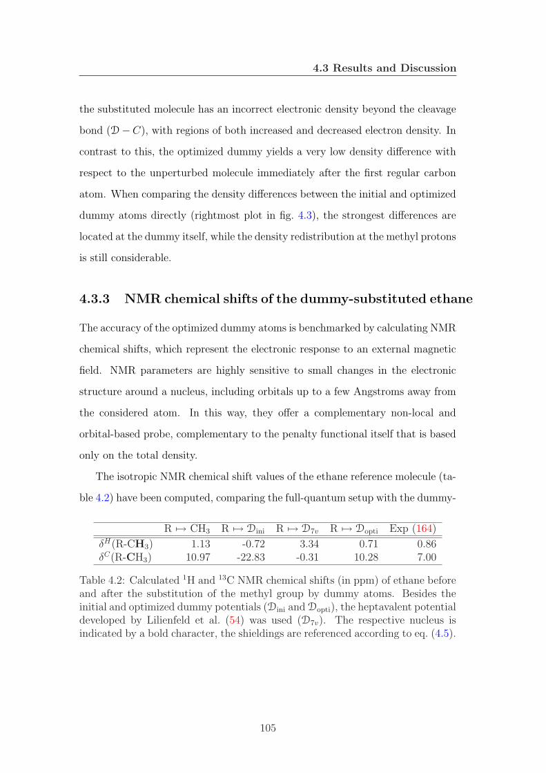
4.3 Results and Discussion
the substituted molecule has an incorrect electronic density beyond the cleavage
bond (D−C), with regions of both increased and decreased electron density. In
contrast to this, the optimized dummy yields a very low density difference with
respect to the unperturbed molecule immediately after the first regular carbon
atom. When comparing the density differences between the initial and optimized
dummy atoms directly (rightmost plot in fig. 4.3), the strongest differences are
located at the dummy itself, while the density redistribution at the methyl protons
is still considerable.
4.3.3 NMR chemical shifts of the dummy-substituted ethane
The accuracy of the optimized dummy atoms is benchmarked by calculating NMR
chemical shifts, which represent the electronic response to an external magnetic
field. NMR parameters are highly sensitive to small changes in the electronic
structure around a nucleus, including orbitals up to a few Angstroms away from
the considered atom. In this way, they offer a complementary non-local and
orbital-based probe, complementary to the penalty functional itself that is based
only on the total density.
The isotropic NMR chemical shift values of the ethane reference molecule (ta-
ble 4.2) have been computed, comparing the full-quantum setup with the dummy-
R 7→ CH3 R 7→ Dini R 7→ D7v R 7→ Dopti Exp (164)
δH(R-CH3) 1.13 -0.72 3.34 0.71 0.86δC(R-CH3) 10.97 -22.83 -0.31 10.28 7.00
Table 4.2: Calculated 1H and 13C NMR chemical shifts (in ppm) of ethane beforeand after the substitution of the methyl group by dummy atoms. Besides theinitial and optimized dummy potentials (Dini and Dopti), the heptavalent potentialdeveloped by Lilienfeld et al. (54) was used (D7v). The respective nucleus isindicated by a bold character, the shieldings are referenced according to eq. (4.5).
105

4.3 Results and Discussion
substituted molecule. For the latter, the optimized (Dopti) and the unoptimized
(Dini) monovalent dummy potentials are used, as well as the seven-valent one
(D7v) developed by Lilienfeld et al. (54), which was developed to reproduce the
electronic density in acetic acid.
It turns out (see table 4.2) that the chemical shifts from the optimized capping
atom are generally in better agreement with the all-QM calculation than for the
initial (Dini) and seven-valent (D7v) capping potentials. The initial potential
results in significantly lower chemical shifts, while the heptavalent dummy greatly
overestimates them. Only the optimized monovalent substitution yields values
close to the all-quantum calculation. A similar picture emerges for carbon, where
both the unoptimized monovalent and the heptavalent dummies yield incorrect
results. Deviations of 0.4ppm for the protons and 0.7ppm for carbon (as obtained
for Dopti) are probably unavoidable for the heteroatom directly connected to the
dummy, but errors of 30ppm and 10ppm (for Dini and D7v, respectively) are
clearly more than what would normally be deemed acceptable. In conclusion,
the NMR resonances of the dummy-substituted ethane show indeed a very good
agreement with the corresponding full-quantum calculations, even for the atom
directly connected to the bond cleavage.
4.3.4 Energetic and Geometric properties of the D-C bonds
The geometry of the reference ethane has been optimized with the methyl group
substituted by the optimized dummy atom. The results for selected distances and
angles are shown in table 4.3. The equilibrium geometry of the initial potential
exhibits somewhat elongated bonds, but the situation improves significantly with
the optimized dummy atom. Comparing the equilibrium bond distances to the
heptavalent dummy (D7v), an investigation find a clear improvement, which is
106

4.3 Results and Discussion
R 7→ CH3 R 7→ Dini R 7→ Dopti R 7→ D7v
d(R-C) [A] 1.54 1.68 1.52 2.04d(C-H) [A] 1.10 1.10 1.10 1.09θH−C−C [deg] 111.3 110.3 111.9 106.8θH−C−H [deg] 107.6 108.6 106.9 112.0
Table 4.3: Optimized bond lengths in the ethane reference molecule, before andafter substitution of the methyl group by a dummy. The bond lengths are re-ported both for the initial capping potential (parameters of the regular carbonpseudopotential) as well as for the optimized dummy.
most likely due to the incorporation of the atomic forces into the penalty func-
tional.
Figure 4.4: Potential energy curve for rigid stretching/compression of the C-Cbond in ethane and D-CH3 with the original and the optimized pseudopotentials.
Figure 4.4 shows the potential energy profile of ethane as a function of the C-C
107

4.3 Results and Discussion
bond length. The equilibrium bond length of Dini-CH3 is somewhat longer than
the full QM value. The optimized capping potential Dopti, in turn, improved
this distance considerably. However, it does so at the expense of a somewhat
lower curvature, corresponding to a reduced harmonic stretch frequency of this
bond. The reason for this is that the parameters C1 and C2 in the local poten-
tial, eq. (4.2), which are both more negative after the optimization. A qualitative
analysis showed that this results in a less repulsive D − C potential. The opti-
mization for both the electronic structure in the equilibrium geometry and the
vibrational properties did not suceed simultaneously, which illustrates the limits
of the monovalent capping with respect to other techniques. Nevertheless, for
the analysis of structural and electronic response properties, the vibrational fre-
quencies play only a minor role. Increased weighting factors wF and wE for the
geometry-related term in the penalty potential might help to reduce this bond
strength problem.
4.3.5 Application of the capping dummy potential to his-
tidine
The good agreement obtained in the previous section might be fortituous, as the
dummy potentials were optimized for the very specific molecules that were sub-
sequently benchmarked there. Thus, the transferability of the dummy potentials
has been checked by applying them to a different molecule, namely histidine.
Table 4.4 shows the NMR chemical shifts of the full histidine molecule and its
imidazole fragment within a QM/MM description. As expected, the strongest
deviations are observed for the carbon C(2) directly involved in the bond cleav-
age. Here, the dummy optimization scheme results in the reduction of the error
by almost an order of magnitude compared to the unoptimized capping atom.
108

4.3 Results and Discussion
QM
Figure 4.5: Atom numbering and bond cutting scheme for histidine molecule. Theupper part (outside the “QM” region) is being replaced by the dummy cappingpotential (“D”).
Similarly, a considerable improvement is obtained for the next carbons C(3) and
C(6), as well as the nitrogen N(7). In all these cases, the optimized monovalent
potential also performs better than the heptavalent dummy atom. For C(9) and
N(8), which are further away from the bond cleavage, the situation is less drastic,
and all three choices yield similar –yet small– discrepancies with respect to the
full-QM calculation.
The hydrogens exhibit smaller absolute deviations, which is because their
NMR chemical shift spectrum spans a range that is about an order of magnitude
smaller than that of C and N nuclei. Nevertheless, the shifts of the hydrogens
adjacent to the bond cut (H(4) and H(5)) are considerably be better. The problem
109

4.3 Results and Discussion
Full-QM R 7→ Dopti R 7→ Dini R 7→ D7v Exp (164)
C(2) 32.46 25.67 -2.72 11.11 30.78C(3) 136.90 138.35 142.05 141.54 134.67C(6) 137.37 136.69 132.52 135.03 119.55C(9) 138.05 137.16 135.96 137.37 138.97N(7) -202.97 -201.98 -200.70 -204.79 -N(8) -138.91 -137.87 -139.60 -139.60 -H(4) 3.40 4.18 2.62 5.99 3.12H(5) 3.56 3.60 2.03 5.26 3.23H(10) 7.60 6.89 6.56 7.28 7.06H(11) 9.93 9.80 9.66 9.93 -H(12) 7.33 7.19 7.09 7.20 7.80
Table 4.4: Calculated 1H, 13C and 15N NMR chemical shifts (in ppm) of histidineand its dummy-substituted fragment (for the atom numbering, see fig. 4.5). Datafor both the initial and optimized dummy potentials (Dini and Dopti) as well asthe heptavalent one (D7v) (54) are shown. R represents the remaining fragmentsin the classical regions.
Full-QM R 7→ Dini R 7→ Dopti
∆E [kcal/mol] 238.1 245.8 239.8rD−C2 [A] 1.57 1.69 1.55rC2−C3 [A] 1.51 1.49 1.50
Table 4.5: Computed and experimental proton affinities ∆E = EDFT(Hist) −EDFT(Hist-H+) as well as geometric data for histidine and its dummy-substitutedfragment (for the atom numbering, see fig. 4.5). Data for both our initial and op-timized dummy potentials (Dini and Dopti) are shown. R represents the remainingfragments in the classical regions.
for H(4) might be due to the effect of the lone electron pairs of the nearby nitrogen,
which are missing entirely when the left fragment is replaced by the dummy
potential. It may be noted that that the same phenomenon applies to H(10)
which is in somewhat better agreement after the optimization. The deviations of
H(11) and H(12) are quite small and do not obviously correlate to the choice of the
capping potential. In most cases, the monovalent capping potential outperforms
the heptavalent one.
110

4.3 Results and Discussion
In addition to the NMR chemical shifts, the optimized capping potential has
been used to compute the protonation energy (N(8) is the protonation site), and
structural parameters for comparison with the initial capping potential and full
QM results. Geometry optimizations of both protonated and non-protonated
form were carried out. The energy differences between these neutral and charged
histidine molecules (see table 4.5) from the Dopti capping model are fairly accurate
when compared to full-QM results. Using Dopti allow for reducing the error from
the full QM deprotonation energy ∆E by 1.7 kcal/mol, while the Dini yields an
error of 7.6 kcal/mol. Also for the D − C2 bond length, the optimized Dopti
yields the smallest deviations from the full-QM values, whereas the equilibrium
geometry of the Dini − C2 bonds is more elongated, in analogy to the situation
observed for ethane.
4.3.6 Application of the capping dummy potential to ly-
sine
Full-QM R 7→ Dini R 7→ Dopti Exp (164)
C(1) 37.54 7.33 36.27 32.60C(2) 28.81 30.88 29.98 24.13C(3) 35.27 43.81 37.39 29.11C(4) 48.10 48.27 47.96 41.75N(5) -293.21 -292.82 -292.95 -H(6,7) 2.25 1.13 2.13 1.9H(8,9) 2.25 2.13 2.18 1.5H(10,11) 2.10 1.99 1.91 1.7H(12,13) 3.72 3.59 3.65 3.0H(14) 1.95 1.88 1.90 -H(15) 2.78 2.70 2.74 -
Table 4.6: Calculated 1H, 13C and 15N NMR chemical shifts (in ppm) of lysineand its dummy-substituted fragment (for the atom numbering, see fig. 4.6). Datafor both the initial and optimized dummy potentials (Dini and Dopti) are shown.R represents the remaining fragments in the classical regions.
111

4.3 Results and Discussion
QM
Figure 4.6: Atom numbering and bond cutting scheme for the lysine molecule.The upper part (outside the “QM” region) is being replaced by the dummycapping potential (“D”).
The second QM/MM application of the capping potential is the amino acid
lysine, which was split into QM/MM fragments as illustrated in fig. 4.6. In
this present setup, the amino group was replaced by the initial and optimized
dummy potentials; note that the Dopti parameters were obtained from the ethane
molecule without any further change, in order to benchmark the transferability
of this capping scheme presented in this chapter.
112

4.3 Results and Discussion
The NMR chemical shifts obtained via the full-QM and QM/MM calculations
are summarized in Table 4.6. It turns out that the results for the Dopti capping
potential are in much better agreement with the full-QM values than that those
from the unoptimized dummy Dini. The deviation of the C(1) chemical shift is
decreased from 30 to 1.2 ppm, and for H(6) and H(7), it is reduced from 1.1 to 0.1
ppm. This suggests that the nonoptimized dummy potential leads to a seriously
flawed representation of the electron density when the C1 −D bond is broken in
the QM/MM setup. Inspecting the shifts of C(2), C(3) and C(4), it is found that
the influence of the bond cleavage is not negligible even for the atoms located
several bonds away from the QM/MM border. The Dopti instead agrees quite
well with the full-QM calculations for all atoms.
A geometry optimization of the lysine molecule was furthermore performed
within the QM/MM framework using the initial and optimized capping potentials
Dini and Dopti. The resulting C-C bond lengths for the two bonds closest to the
MM region are shown in table 4.7. While the C1−C2 bond is not affected by the
bond cleavage, the D − C1 bond length is notably different for the unoptimized
capping potential. The same is observed for the proton affinity of lysine, which
is considerably better for the optimized link atom than for the initial one.
Full-QM R 7→ Dini R 7→ Dopti
∆E [kcal/mol] 225.6 232.8 228.6rD−C1 [A] 1.56 1.69 1.56rC1−C2 [A] 1.55 1.55 1.55
Table 4.7: Computed and experimental proton affinities ∆E = EDFT(Lys) −EDFT(Lys-H+) as well as geometric data for lysine and its dummy-substitutedfragment, using both the initial and optimized capping potentials.
113

4.4 Conclusion
4.4 Conclusion
A new monovalent capping potential has been presented for hybrid QM/MM cal-
culations within density functional theory. The parameters of analytic effective
pseudopotentials were optimized such as to reproduce electronic density, proton
affinities, atomic forces and geometries as closely as possible with respect to the
corresponding full-QM quantities. Particular focus was put on the reliability of
NMR chemical shifts as highly sensitive probes of the ground state and response
properties of the electronic orbitals. The resulting analytic capping potentials
were shown to have a high transferability for different molecules. An important
advantage resulting from the improved electronic structure of the optimized cap-
ping potentials is that our Dopti can help to reduce the QM box size significantly,
since the perturbation of the QM/MM bond cleavage is essential undetectable in
the QM region beyond one single chemical bond.
114

Chapter 5
Conclusion
The central aim of this thesis work is the application and further development of a
hybrid quantum mechanical/molecular mechanics (QM/MM) based approach to
compute spectroscopic properties of molecules in complex chemical environments.
While the method is suitable and intended for biomolecules such as proteins,
the focus of the present work was mainly on conceptual aspects. Therefore,
the chemical complexity was reduced by considering rather small molecules in
contact with a simple solvent (water), while nevertheless retaining all physical
interactions as in the case of a complex biochemical system.
In the framework of this thesis, the existing density functional theory im-
plementation of the QM/MM approach was first used to calculate the nuclear
magnetic resonance (NMR) solvent shifts of an adenine molecule in aqueous so-
lution (chapter 3). In order to obtain a realistic picture of this situation, a large
number of solvent molecules was incorporated into the calculations, and a molec-
ular dynamics trajectory was sampled with NMR calculations in order to obtain
a suitable ensemble averaging. Both the generation of the molecular dynam-
ics trajectory and the calculation of NMR chemical shifts were done within the
QM/MM scheme, in which only the adenine molecule was treated quantum me-
chanically; all the surrounding water solvent was modeled via conventional point
115

charges (the so-called TIP3P all-atom force field). The findings show that the
aqueous solvation with its strongly fluctuating hydrogen bond network leads to
specific changes in the NMR resonance lines. Besides the absolute values, also
the ordering of the NMR lines changes under the influence of the solvating water
molecules. Without the QM/MM scheme, a quantum chemical calculation could
have led to an incorrect assignment of these lines. While the agreement of the
computed QM/MM NMR chemical shifts is not perfect, the overall agreement
with respect to experimental values is very good for the 1H and reasonably good
for the 15N chemical shifts.
The second part of this thesis describes a methodological improvement of the
QM/MM method that is designed for cases in which a covalent chemical bond
crosses the QM/MM boundary. The development consists in an automatized
protocol to optimize the so-called capping potential that saturates the electronic
subsystem in the QM region. While capping potentials are commonly used in
QM/MM calculations since many years, their quality turned out to be insufficient
to predict spectroscopic parameters with the desired accuracy. The optimization
scheme presented in chapter 4 is capable of tuning the parameters of generalized
capping potentials (for which analytical pseudopotentials with a small number of
parameter are used) in such a way that the deviations of the electronic orbitals
between the regular and the truncated (and ”capped”) molecule are minimized.
This in turn results in a considerable improvement of the spectroscopic parame-
ters computed with the new optimized capping potential.
In the present thesis, this optimization scheme is applied and benchmarked on
the example of truncated carbon-carbon bonds in a set of small test molecules. It
turns out that the optimized capping potentials yield an excellent agreement of
NMR chemical shifts and protonation energies with respect to the corresponding
full molecules. These first results are very promising, so that the application to
116

larger biological complexes will significantly improve the reliability of the predic-
tion of the related spectroscopic properties.
117

References
[1] J.-M. Lehn. Reports on Progress in Physics, 2004, 67, 249–265. 7
[2] P. M. Tolstoy, P. Schah-Mohammedi, S. N. Smirnov, N. S. Golubev, G. S.
Denisov and H. H. Limbach. J. Am. Chem. Soc., 2004, 126, 5621–5634. 7
[3] S. Meng, L. F. Xu, E. G. Wang and S. Gao. Phys. Rev. Lett., 2002, 89,
176104. 7
[4] B. Chen, I. Ivanov, M. L. Klein and M. Parrinello. Phys. Rev. Lett., 2003,
91, 215503. 7
[5] C. Gervais, R. Dupree, K. J. Pike, C. Bonhomme, M. Profeta, C. J. Pickard
and F. Mauri. J. Phys. Chem. A, 2005, 109, 6960–6969. 7, 62
[6] T. Murakhtina, L. Delle Site and D. Sebastiani. ChemPhysChem, 2006, 7,
1215–1219. 7
[7] S. Sekharan, O. Weingart and V. Buss. Biophysical Journal, 2006, 91,
L07–L09. 7
[8] D. Sebastiani and M. Parrinello. ChemPhysChem, 2002, 3, 675. 7, 10, 69
[9] T. Murakhtina, J. Heuft, J.-E. Meijer and D. Sebastiani. ChemPhysChem,
2006, 7, 2578–2584. 7, 10
118

REFERENCES
[10] M. Buhl, S. Grigoleit, H. Kabrede and F. T. Mauschick. Chem. Eur. J.,
2006, 12, 477–488. 7
[11] P. Hohenberg and W. Kohn. Phys. Rev., 1964, 136, B864. 7, 14, 20, 100
[12] W. Kohn and L. J. Sham. Phys. Rev., 1965, 140, A1133. 7, 14, 23, 100
[13] R. O. Jones and O. Gunnarsson. Rev. Mod. Phys., 1989, 61, 689–746. 7,
8, 9, 14, 26, 68, 100
[14] R. G. Parr and W. Yang. Density functional theory of atoms and molecules.
Oxford Science Publications, 1989. 7, 14, 15, 19
[15] S. Lundqvist and N. H. March, Eds. Theory of the inhomogeneous electron
gas. Plenum Press, New York, 1983. 8, 26
[16] K. B. J. Perdew and M.Ernzerhof. Phys. Rev. Lett., 1996, 77, 3865. 8, 27
[17] A. D. Becke. Phys. Rev. A, 1988, 38, 3098. 8, 27, 68, 100
[18] C. Lee, W. Yang and R. G. Parr. Phys. Rev. B, 1988, 37, 785–789. 8, 27,
68, 100
[19] S. P. Brown and H. W. Spiess. Chem. Rev., 2001, 101, 4125. 9, 97
[20] H. W. Spiess. J. Polymer Sci. Part A, 2004, 42, 5031–5044. 9
[21] H. W. Spiess. J. Polym. Sci., 2004, A 42, 5031–5044. 9
[22] D. Sebastiani. Mod. Phys. Lett. B, 2003, 17, 1301–1319. 9, 63
[23] M. Buhl, M. Kaupp, O. L. Malkina and V. Malkin. J. Comput. Chem.,
1999, 20, 91–105. 9
[24] J. Gauss. Chem. Phys. Lett., 1992, 191, 614–620. 9, 68
119

REFERENCES
[25] M. Schulz-Dobrick, T. Metzroth, H. W. Spiess, J. Gauss and I. Schnell.
ChemPhysChem, 2005, 6, 315–327. 9, 97
[26] A. A. Auer, J. Gauss and J. F. Stanton. J. Chem. Phys., 2003, 118, 10407.
9, 68
[27] R. M. Martin. Electronic Structure: Basic Theory and Practical Methods.
Cambridge University Press, 2004. 9, 68
[28] P. Knowles, M. Schutz and H.-J. Werner. in Modern Methods and Algo-
rithms of Quantum Chemistry, J. Grotendorst, Ed., pp 97–179. John von
Neumann Institute for Computing, Julich, NIC Series, Vol. 3, 2000. 9
[29] A. Szabo and N. S. Ostlund. Modern Quantum Chemistry. Dover Publica-
tions Inc., Mineola, New York, 1996. 9
[30] C. Ochsenfeld, S. P. Brown, I. Schnell, J. Gauss and H. W. Spiess. J. Am.
Chem. Soc., 2001, 123, 2597–2606. 9, 97
[31] F. Mauri, B. Pfrommer and S. Louie. Phys. Rev. Lett., 1997, 79, 2340. 10,
62
[32] Y. Yoon, B. Pfrommer, F. Mauri and S. Louie. Phys. Rev. Lett., 1998, 80,
3388. 10, 62
[33] J. Schmidt, A. Hoffmann, H. W. Spiess and D. Sebastiani. J. Phys. Chem.
B, 2006, 110, 23204–23210. 10
[34] A. Hoffmann, D. Sebastiani, E. Sugiono, K. S. Kim, H. W. Spiess and
I. Schnell. Chem. Phys. Lett., 2004, 388, 164–169. 10, 63
[35] D. Sebastiani. ChemPhysChem, 2006, 7, 164–175. 10
120

REFERENCES
[36] B. Pfrommer, F. Mauri and S. Louie. J. Am. Chem. Soc., 2000, 122,
123–129. 10
[37] P. Sherwood. in Modern Methods and Algorithms of Quantum Chemistry,
J. Grotendorst, Ed., pp 257–277. John von Neumann Institute for Com-
puting, Julich, NIC Series, Vol. 1, 2000. 10, 66
[38] R. Z. Deng, G. J. Martyna and M. L. Klein. Phys. Rev. Lett., 1993, 71,
267. 10, 93
[39] D. Wei and D. Salahub. Chem. Phys. Lett., 1994, 224, 291. 10, 93
[40] R. V. Stanton, L. R. Little and K. M. Merz. J. Phys. Chem., 1996, 99,
11266. 10, 93
[41] M. Eichinger, P. Tavan, J. Hutter and M. Parrinello. J. Chem. Phys., 1999,
21, 10452. 10, 12, 14, 93
[42] P. Lyne, M. Hodosceck and M. Karplus. J. Phys. Chem. A, 1999, 103,
3462. 10, 93
[43] M. J. Field, P. A. Bash and M. Karplus. J. Comp. Chem., 1990, 11, 700.
10, 93
[44] Q. Cui and M. Karplus. J. Phys. Chem. B, 2000, 104, 3721–3743. 10, 66,
76, 77
[45] A. Laio, J. VandeVondele and U. Roethlisberger. J. Chem. Phys., 2002,
116, 6941. 10, 12, 14, 45, 63, 66, 68, 71, 93, 96
[46] W. van Gunsteren and H. Berendsen. Computer code GROMOS96. Copy-
right BIOMOS b.v., Biomolecular Software, ETH-Zurich. 11, 68
121
REFERENCES
[47] D. A. Case, D. A. Pearlman, J. W. Caldwell, T. E. Cheatham, J. Wang,
W. S. Ross, C. Simmerling, T. Darden, K. M. Merz, R. V. Stanton,
A. Cheng, J. J. Vincent, M. Crowley, V. Tsui, H. Gohlke, R. Radmer,
Y. Duan, J. Pitera, I. Massova, G. L. Seibel, U. C. Singh, P. Weiner and
P. A. Kollman. Computer code Amber. Copyright University of California.
11, 38, 68
[48] R. Car and M. Parrinello. Phys. Rev. Lett., 1985, 55, 2471. 11, 36, 66
[49] J. Hutter et al. Computer code CPMD, version 3.12, 1990-2005. Copyright
IBM Corp. and MPI-FKF Stuttgart, http://www.cpmd.org. 11, 44, 48,
68, 100
[50] J. VandeVondele. Extending length and time scales of ab initio molecular
dynamics simulations. PhD thesis, Swiss Federal Institute of Technology
Zurich, 2001. 12, 14, 45
[51] D. Sebastiani. Development of a new ab-initio method for NMR chemical
shifts in periodic systems. PhD thesis, Max-Planck-Institut fur Festkorper-
forschung Stuttgart, 2001. 12, 14
[52] T. Murakhtina. Spectroscopic Signatures from First Principles Calcula-
tions: from surface adsorbates to liquids and polymers. PhD thesis, Jo-
hannes Gutenberg-University Mainz, 2007. 12, 14
[53] J. Schmidt. Quantum Effects and Dynamics in Hydrogen-Bonded Systems:
A First-Principles Approach to Spectroscopic Experiments. PhD thesis,
Johannes Gutenberg-University Mainz, 2007. 12, 14
[54] A. von Lilienfeld-Toal, I. Tavernelli, U. Rothlisberger and D. Sebastiani. J.
122

REFERENCES
Chem. Phys., 2005, 122, 014113. 12, 14, 77, 79, 91, 96, 99, 105, 106, 110,
134
[55] D. Sebastiani and U. Rothlisberger. J. Phys. Chem. B, 2004, 108, 2807.
12, 14, 66, 67, 71, 76, 91
[56] S. Komin, C. Gossens, I. Tavernelli, U. Rothlisberger and D. Sebastiani. J.
Phys. Chem. B, 2007, 111, 5225–5232. 12
[57] S. Komin and D. Sebastiani. J. Chem. Theory Comp., 2009. submitted.
12
[58] R. Acosta, S. Komin, L. Agulles, D. Sebastiani, H. W. Spiess and
P. Blumler. Phys. Chem. Chem. Phys., 2006, 8, 4182–4188. 12
[59] N. W. Ashcroft. Solid state physics. Saunders, Philadelphia, 1976. 15, 31
[60] I. Shavitt. in Modern Theoretical Chemistry, H. F. Schaefer, Ed. Plenum
Press, New York, 1977. 18
[61] A. C. Wahl and G. Das. in Modern Theoretical Chemistry, H. F. Schaefer,
Ed. Plenum Press, New York, 1977. 18
[62] H. J. Werner. in Ab Initio Methods in Quantum Chemistry, K. Lawley, Ed.
John Wiley, Chichester, 1987. 18
[63] J. Cızek. J. Chem. Phys., 1966, 45. 18
[64] J. Cızek. Adv. Chem. Phys., 1969, 14. 18
[65] J. Cızek. Int. J. Quantum Chem., 1971, 5. 18
[66] E. E. Pickett. Comput. Phys. Reports, 1989, 9, 115. 24
[67] D. M. Ceperley and B. J. Alder. Phys. Rev. Lett., 1980, 45, 566. 26
123

REFERENCES
[68] J. Perdew and A. Zunger. Phys. Rev. B, 1981, 23, 5048. 26
[69] P. Giannozzi, S. de Gironcoli, P. Pavone and S. Baroni. Phys. Rev. B, 1991,
43, 7231. 26
[70] X. Gonze, D. C. Allan and M. P. Teter. Phys. Rev. Lett., 1992, 68, 3603.
26
[71] C. S. Wang, B. M. Klein and H. Krakauer. Phys. Rev. Lett., 1985, 54,
1852. 27
[72] D. R. Hamann, M. Schluter and C. Chiang. Phys. Rev. Lett., 1979, 43,
1494. 30
[73] G. B. Bachelet, D. R. Hamann and M. Schluter. Phys. Rev. B, 1982, 26,
4199. 30
[74] N. Troullier and J. L. Martins. Phys. Rev. B, 1991, 43, 1993. 30, 68
[75] S. Goedecker, M. Teter and J. Hutter. Phys. Rev. B, 1996, 54, 1703. 30,
96, 100, 102
[76] L. Kleinman and D. M. Bylander. Phys. Rev. Lett., 1982, 48, 1425. 30
[77] P. Pulay. Mol. Phys., 1969, 17, 197. 30
[78] W. H. Press, S. A. Teukoldky, W. T. Vetterling and B. P. Flannery. Nu-
merical recipes. Cambridge University Press, 2 edition, 1992. 30, 100
[79] M. P. Allen and D. J. Tildesley. Computer Simulation of Liquids. Oxford
University Press, Oxford, 2nd edition, 1994. 33, 39, 49
[80] L. Verlet. Phys. Rev., 1968, 165, 201–214. 34
124

REFERENCES
[81] D. Marx and J. Hutter. in Modern Methods and Algorithms in Quantum
Chemistry, volume 1 of NIC Series, pp 301–449. Forschungzentrum Juelich,
2000. 34, 61, 68
[82] W. C. Swope, H. C. Andersen, P. H. Berens and K. R. Wilson. The Journal
of Chemical Physics, 1982, 76, 637–649. 34
[83] G. Martyna and M. Tuckerman. J. Chem. Phys., 1999, 110, 2810. 35, 42,
43, 68
[84] J. C. Grossman, E. Schwegler, E. W. Draeger, F. Gygi and G. Galli. J.
Chem. Phys., 2003, 120, 300–311. 36
[85] C. I. Bayly, P. Cieplak, W. D. Cornell and P. A. Kollman. J. Phys. Chem.,
1993, 97, 10269. 40
[86] H. C. Anderson. J. Chem. Phys., 1980, 72, 2384. 42
[87] S. Nose. Mol. Phys., 1984, 5, 255. 42
[88] W. G. Hoover. Phys. Rev. A, 1985, 31, 1695. 42
[89] A. Laio, J. VandeVondele and U. Rothlisberger. Journal of Physical Chem-
istry B, 2002, 106, 7300–7307. 45, 50
[90] R. A. Klein, B. Mennucci and J. Tomasi. J. Phys. Chem. A, 2004, 108,
5851–5863. 48, 66
[91] C. Amovilli and B. Mennucci. J. Phys. Chem. B, 1997, 101, 1051–1057.
48, 66
[92] R. A. Klein, B. Mennucci and J. Tomasi. J. Phys. Chem. A, 2004, 108,
5851–5863. 48, 66
125

REFERENCES
[93] J.-L. Fattebert and F. Gygi. Int. J. Quantum Chem., 2003, 93, 139. 48,
66
[94] M. S. Gordon, M. A. Freitag, P. Bandyopadhyay, J. H. Jensen, V. Kairys
and W. J. Stevens. J. Phys. Chem. A, 2001, 105, 293–307. 48, 66
[95] N. Di Fiori, A. Orendt, M. C. Caputo, M. B. Ferraro and J. C. Facelli.
Magn. Reson. Chem., 2004, 42, S41–S47. 48, 66
[96] Q. Cui. J. Chem. Phys., 2002, 117, 4720–4728. 48, 66, 93
[97] A. Klamt and G. Schuurmann. J. Chem. Soc. Perkin Trans., 1993, 2,
799–805. 48, 66
[98] S. Chalmet and M. F. Ruiz-Lopez. Chemical Physics Letters, 2000, 329,
154–159. 52
[99] Y. Zhang, T.-S. Lee and W. Yang. J. Phys. Chem., 1999, 110, 46–54. 52,
93
[100] N. Jardilliera and A. Goursot. Chem. Phys. Lett., 2008, 454, 65–69. 52, 95
[101] A. Mallik, D. E. Taylor, K. Runge and J. W. Dufty. Int. J. Quantum
Chem., 2004, 100, 1019–1025. 52, 95
[102] G. A. DiLabio, R. A. Wolkow and E. R. Johnson. J. Chem. Phys., 2005,
122, 044708. 52, 95
[103] P. Slavicek and T. J. Martinez. J. Chem. Phys., 2006, 124, 084107. 52, 95
[104] G. A. DiLabio, M. M. Hurley and P. A. Christiansen. J. Chem. Phys.,
2002, 116, 9578–9584. 52, 95
126

REFERENCES
[105] D. Sebastiani and M. Parrinello. J. Phys. Chem. A, 2001, 105, 1951. 56,
57, 58, 59, 60, 61, 62, 67, 70, 100, 101
[106] A. Putrino, D. Sebastiani and M. Parrinello. J. Chem. Phys., 2000, 113,
7102–7109. 56, 57, 58, 59, 69, 100, 101
[107] H. Goldstein. Classical mechanics. Addison-Wesley, 1980. 57
[108] T. A. Keith and R. F. W. Bader. Chem. Phys. Lett., 1993, 210, 223. 60
[109] G. Schreckenbach, S. K. Wolff and T. Ziegler. J. Phys. Chem. A, 2000,
104, 8244–8255. 62
[110] M. Straka and M. Kaupp. Chem. Phys. Lett., 2005, 311, 45–56. 62
[111] F. Mauri and S. Louie. Phys. Rev. Lett., 1996, 76, 4246–4249. 62
[112] F. Mauri, B. Pfrommer and S. Louie. Phys. Rev. Lett., 1996, 77, 5300–
5303. 62, 70
[113] F. Mauri, N. Vast and C. J. Pickard. Phys. Rev. Lett., 2001, 88, 085506.
62
[114] D. Sebastiani, G. Goward, I. Schnell and H. W. Spiess. J. Mol. Struct.
(THEOCHEM), 2003, 625, 283–288. 62, 67, 101
[115] C. J. Pickard and F. Mauri. Phys. Rev. B, 2001, 63, 245101. 62, 63
[116] D. Sebastiani. Int. J. Quantum Chem., 2005, 101, 849–853. 63
[117] A. Sulkowska and A. Michnik. J. Mol. Struct. (THEOCHEM), 1997, 410,
27–29. 65
127

REFERENCES
[118] N. C. Gonnella, H. Nakanishi, J. B. Holtwick, D. S. Horowitz, K. Kanamori,
N. J. Leonard and J. D. Roberts. J. Am. Chem. Soc., 1983, 105, 2050–2055.
65
[119] M. Schindler. J. Am. Chem. Soc., 1988, 110, 6623–6630. 65, 67
[120] S. Piana, D. Sebastiani, P. Carloni and M. Parrinello. J. Am. Chem. Soc.,
2001, 122, 123. 65
[121] P. Vidossich, S. Piana, A. Miani and P. Carloni. J. Am. Chem. Soc., 2006,
128, 7215–7221. 65
[122] D. Sebastiani and U. Rothlisberger. Advances in Density Functional Based
Modelling Techniques: Recent Extensions of the Car-Parrinello Approach,
volume 88 of Methods and Principles in Medicinal Chemistry, Series Edi-
tors: R. Mannhold, H. Kubiny, G. Folkers. Wiley-VCH, Weinheim, Ger-
many, 2003. 65
[123] R. Iftimie, P. Minary and M. Tuckerman. Proc. Natl. Acad. Sci. USA,
2005, 102, 6654–6659. 66
[124] Q. Cui and M. Karplus. J. Chem. Phys., 2000, 112, 1133. 66, 79
[125] B. Wang and K. M. Merz. J. Chem. Theory Comp., 2006, 2, 209–215. 66
[126] T. C. Ramalho, E. F. F. da Cunha and R. B. de Alencastro. J. Phys. Cond.
Matter, 2004, 16, 6159–6170. 66
[127] J. Gauss. J. Chem. Phys., 1993, 99, 3629–3643. 68
[128] J. Gauss and J. Stanton. J. Chem. Phys., 1995, 102, 251–253. 68
[129] J. Gauss and J. Stanton. J. Chem. Phys., 1995, 103, 3561–3577. 68
128

REFERENCES
[130] J. Hutter and A. Curioni. ChemPhysChem, 2005, 6, 1788–1793. 68, 100
[131] W. L. Jorgensen, J. Chandrasekhar, J. D. Madura, R. W. Impey and M. L.
Klein. J. Chem. Phys., 1983, 79, 926–935. 68
[132] J. P. Ryckaert, G. Ciccotti and H. J. C. Berendsen. J. Comp. Phys., 1977,
23, 327–341. 69
[133] S. Baroni, S. de Gironcoli, A. del Corso and P. Giannozzi. Rev. Mod. Phys.,
2001, 73, 515. 69
[134] P. N. Day, J. H. Jensen, M. S. Gordon, S. P. Webb, W. J. Stevens,
M. Krauss, D. Garmer, H. Basch and D. Cohen. J. Chem. Phys., 1996,
105, 1968. 71, 77, 79
[135] M. Cossi, V. Barone, R. Cammi and J. Tomasi. Chem. Phys. Lett., 1996,
255, 327–335. 72
[136] C. Amovilli, V. Barone, R. Cammi, E. Cances, M. Cossi, B. Mennucci,
C. Pomelli and J. Tomasi. Adv. Quant. Chem., 1999, 32, 227–261. 72
[137] J. Tomasi, B. Mennucci and E. Cances. J. Mol. Struct. (THEOCHEM),
1999, 464, 211–226. 72
[138] M. J. Frisch, G. W. Trucks, H. B. Schlegel, G. E. Scuseria, M. A. Robb, J. R.
Cheeseman, J. A. Montgomery, Jr., T. Vreven, K. N. Kudin, J. C. Burant,
J. M. Millam, S. S. Iyengar, J. Tomasi, V. Barone, B. Mennucci, M. Cossi,
G. Scalmani, N. Rega, G. A. Petersson, H. Nakatsuji, M. Hada, M. Ehara,
K. Toyota, R. Fukuda, J. Hasegawa, M. Ishida, T. Nakajima, Y. Honda,
O. Kitao, H. Nakai, M. Klene, X. Li, J. E. Knox, H. P. Hratchian, J. B.
Cross, C. Adamo, J. Jaramillo, R. Gomperts, R. E. Stratmann, O. Yazyev,
129

REFERENCES
A. J. Austin, R. Cammi, C. Pomelli, J. W. Ochterski, P. Y. Ayala, K. Mo-
rokuma, G. A. Voth, P. Salvador, J. J. Dannenberg, V. G. Zakrzewski,
S. Dapprich, A. D. Daniels, M. C. Strain, O. Farkas, D. K. Malick, A. D.
Rabuck, K. Raghavachari, J. B. Foresman, J. V. Ortiz, Q. Cui, A. G.
Baboul, S. Clifford, J. Cioslowski, B. B. Stefanov, G. Liu, A. Liashenko,
P. Piskorz, I. Komaromi, R. L. Martin, D. J. Fox, T. Keith, M. A. Al-
Laham, C. Y. Peng, A. Nanayakkara, M. Challacombe, P. M. W. Gill,
B. Johnson, W. Chen, M. W. Wong, C. Gonzalez and J. A. Pople. Com-
puter code Gaussian 03, Revision B.03, 2003. 72, 73, 90, 133
[139] A. von Lilienfeld-Toal, I. Tavernelli, U. Rothlisberger and D. Sebastiani.
Phys. Rev. B, 2005, 71, 195119. 77, 79, 91
[140] N. Reuter, A. Dejaegere, B. Maigret and M. Karplus. J. Phys. Chem. A,
2000, 104, 1720–1735. 77, 79, 91
[141] G. Brancato, N. Rega and V. Barone. J. Chem. Phys., 2008, 128, 144501.
93
[142] U. C. Singh and P. A. Kollman. J. Comp. Chem., 1986, 7, 718. 93
[143] X. Assfeld and J.-L. Rivail. Chem. Phys. Lett., 1996, 263, 100–106. 94
[144] C. R. Jacob and L. Visscher. J. Chem. Phys., 2006, 125, 194104. 94
[145] J. Jung, C. H. Choi, Y. Sugita and S. Ten-no. J. Chem. Phys., 2007, 127,
204102. 94
[146] K. Ohta, Y. Yoshioka, K. Morokuma and K. Kitaura. Chem. Phys. Lett.,
1983, 101, 12–17. 94
[147] P. N. Day, J. H. Jensen, M. S. Gordon, S. P. Webb, W. J. Stevens, M. Krauss
and D. Garmer. J. Chem. Phys., 1996, 105, 1968. 94
130

REFERENCES
[148] I. Adamovic, M. A. Freitag and M. S. Gordon. J. Chem. Phys., 2003, 118,
6725–6732. 94
[149] H. M. Netzloff and M. S. Gordon. J. Chem. Phys., 2004, 121, 2711–2714.
94
[150] I. Adamovic and M. S. Gordon. J. Phys. Chem. A, 2006, 110, 10267–10273.
94
[151] R. Poteau, I. Ortega, F. Alary, A. R. Solis, J.-C. Barthelat and J.-P.
Daudey. J. Phys. Chem. A, 2001, 105, 198–205. 94
[152] R. Poteau, F. Alary, H. A. E. Makarim, J.-L. Heully, J.-C. Barthelat and
J.-P. Daudey. J. Phys. Chem. A, 2001, 105, 206–214. 94
[153] T. E. Exner and P. G. Mezey. J. Comp. Chem., 2003, 24, 1980–1986. 95
[154] T. E. Exner and P. G. Mezey. Phys. Chem. Chem. Phys., 2005, 24, 4061–
4069. 95
[155] S. Eckard and T. E. Exner. Z. Phys. Chem., 2006, 220, 927–944. 95
[156] C. Hartwigsen, S. Goedecker and J. Hutter. Phys. Rev. B, 1998, 58, 3641.
96, 99, 100, 102
[157] U. Rohrig, L. Guidoni, A. Laio, I. Frank and U. Rothlisberger. J. Am.
Chem. Soc., 2004, 126, 15328–15329. 96
[158] U. F. Rohrig and D. Sebastiani. J. Phys. Chem. B, 2008, 112, 1267–1274.
96
[159] H. W. Spiess. Macromol. Chem. Phys., 2003, 204, 340–346. 97
131

REFERENCES
[160] M. Buhl, H. Kabrede, R. Diss and G. Wipff. J. Am. Chem. Soc., 2006,
128, 6357–6368. 97
[161] W. E. Pickett. Comp. Phys. Rep., 1989, 9, 115–198. 99
[162] A. Putrino and M. Parrinello. Phys. Rev. Lett., 2002, 88, 176401. 100
[163] H. E. Gottlieb, V. Kotlyar and A. Nudelman. J. Org. Chem., 1997, 62,
7512–7515. 101
[164] E. L. Ulrich, H. Akutsu, J. F. Doreleijers, Y. Harano, Y. E. Ioannidis, J. Lin,
M. Livny, S. Mading, D. Maziuk, Z. Miller, E. Nakatani, C. F. Schulte, D. E.
Tolmie, R. K. Wenger, H. Yao and J. L. Markley. Biological magnetic res-
onance data bank. http://www.bmrb.wisc.edu; doi: 10.1093/nar/gkm957,
2007. 105, 110, 111
132

List of Tables
3.1 Calculated values of the 13C NMR chemical shifts of adenine rela-
tive to TMS obtained with a quantum chemistry code relying on
localized basis sets (138) and with the CPMD code. The nuclear
shieldings were referenced to those of benzene computed under
the same computational setup and then corrected with the exper-
imental TMS-shift of benzene: δTMS(x) = σcalc(C6H6) − σcalc(x) +
δTMS(exp) (C6H6) . . . . . . . . . . . . . . . . . . . . . . . . . . . . . 73
3.2 Calculated and experimental values of the 1H and 15N NMR chem-
ical shifts of adenine with the CPMD code. “MD” means that an
ensemble of configurations has been extracted from the QM/MM
molecular dynamics simulations. While the third and fourth sig-
nificant digits of hydrogen and nitrogen shifts are below the nu-
merical accurancy, they are given here to illustrate trends between
the computational models. Values in parentheses are anisotropies
of the chemical shifts tensor. . . . . . . . . . . . . . . . . . . . . 89
3.3 Calculated and experimental values of the 1H and 15N NMR chem-
ical shifts of adenine. The geometry optimizations and shielding
calculations were done using localized basis sets (138). Values in
parentheses are anisotropies of the chemical shifts tensor. . . . . 90
133

LIST OF TABLES
4.1 Pseudopotenial parameters of the regular carbon atom and the
optimized dummy capping potential. DC represent the capping
potentials optimized for a C-C bond, rloc, rs, rp are given in units
of Bohr, C1, C2, hs and hp in Hartree. . . . . . . . . . . . . . . . 103
4.2 Calculated 1H and 13C NMR chemical shifts (in ppm) of ethane
before and after the substitution of the methyl group by dummy
atoms. Besides the initial and optimized dummy potentials (Dini
and Dopti), the heptavalent potential developed by Lilienfeld et
al. (54) was used (D7v). The respective nucleus is indicated by a
bold character, the shieldings are referenced according to eq. (4.5). 105
4.3 Optimized bond lengths in the ethane reference molecule, before
and after substitution of the methyl group by a dummy. The
bond lengths are reported both for the initial capping potential
(parameters of the regular carbon pseudopotential) as well as for
the optimized dummy. . . . . . . . . . . . . . . . . . . . . . . . . 107
4.4 Calculated 1H, 13C and 15N NMR chemical shifts (in ppm) of his-
tidine and its dummy-substituted fragment (for the atom number-
ing, see fig. 4.5). Data for both the initial and optimized dummy
potentials (Dini and Dopti) as well as the heptavalent one (D7v) (54)
are shown. R represents the remaining fragments in the classical
regions. . . . . . . . . . . . . . . . . . . . . . . . . . . . . . . . . 110
4.5 Computed and experimental proton affinities ∆E = EDFT(Hist)−EDFT(Hist-H+) as well as geometric data for histidine and its
dummy-substituted fragment (for the atom numbering, see fig. 4.5).
Data for both our initial and optimized dummy potentials (Dini
and Dopti) are shown. R represents the remaining fragments in
the classical regions. . . . . . . . . . . . . . . . . . . . . . . . . . 110
134

LIST OF TABLES
4.6 Calculated 1H, 13C and 15N NMR chemical shifts (in ppm) of lysine
and its dummy-substituted fragment (for the atom numbering, see
fig. 4.6). Data for both the initial and optimized dummy potentials
(Dini and Dopti) are shown. R represents the remaining fragments
in the classical regions. . . . . . . . . . . . . . . . . . . . . . . . 111
4.7 Computed and experimental proton affinities ∆E = EDFT(Lys)−EDFT(Lys-H+) as well as geometric data for lysine and its dummy-
substituted fragment, using both the initial and optimized capping
potentials. . . . . . . . . . . . . . . . . . . . . . . . . . . . . . . 113
135

List of Figures
2.1 Schematic representation of the separation of the total system into
two subsystem used in the QM/MM model. . . . . . . . . . . . . 46
2.2 An illustration of the QM/MM partitioning of Retinyl palmitate
structure. The active part of the system is treated with a QM
method while the rest of the protein is the MM part. The QM
model is shown with the solid lines representation, while the MM
part is represented using thin lines. The carbon atom labeled with
“P“ indicates the link-atom or a pseudopotential that is needed to
describe the boundary between the QM and the MM fragments of
the total molecules. . . . . . . . . . . . . . . . . . . . . . . . . . 46
3.1 Illustration of the adenine molecule in aqueous solution. The num-
bering scheme is also shown. . . . . . . . . . . . . . . . . . . . . 67
136

LIST OF FIGURES
3.2 Illustration of the two benchmark systems: The water dimer and
the methanol dimer. For all systems, NMR chemical shift de-
pendences as a function of the oxygen-oxygen distance have been
computed. The three configurations have been considered: (i) both
molecules quantum-mechanically (QM), (ii) the H-bond donor molecule
as QM and the acceptor molecule classically (MM), and (iii) the
H-bond acceptor molecule as QM with the donor as MM. The
geometries of the clusters were not re-optimized for the different
distances. . . . . . . . . . . . . . . . . . . . . . . . . . . . . . . . 74
3.3 Distance dependence of the 1H NMR chemical shift of the donor
and acceptor protons in a water dimer as illustrated in fig. 3.2, us-
ing a full QM, the standard QM/MM, and QM/MM+REP treat-
ment of the different components. The calculation in which the
donor molecule is treated quantum-mechanically is shown using
solid lines, and the results for the quantum-mechanical acceptor
are represented by dotted lines. The shifts are referenced to the
corresponding isolated molecule. . . . . . . . . . . . . . . . . . . 75
3.4 Distance dependence of the 17O NMR chemical shifts of the donor
and acceptor protons in a water dimer as illustrated in fig. 3.2
(left), using a full QM, the standard QM/MM, and QM/MM+REP
treatment of the different components. The shifts are referenced
to the corresponding isolated molecule. . . . . . . . . . . . . . . . 76
137

LIST OF FIGURES
3.5 Dependence of the 1H NMR chemical shifts of the donor and ac-
ceptor protons in a methanol dimer on the oxygen-oxygen dis-
tance. The molecular geometry is illustrated in fig. 3.2. The NMR
chemical shifts of the full QM calculation, the standard QM/MM
scheme, and QM/MM+REP treatment are shown. The line cod-
ing is the same as for the water dimer (fig. 3.3). Again, the shifts
are referenced to the corresponding isolated molecule. . . . . . . 78
3.6 The radial pair distribution functions (RDF) computed for the
distance between adenine nitrogens and water protons. The dis-
tribution functions have been smoothened by applying running
averages to the raw data. . . . . . . . . . . . . . . . . . . . . . . 80
3.7 The radial pair distribution functions of the distances between
aromatic carbon protons (of adenine) and water oxygens. As in
fig. 3.6, running averages have been applied. . . . . . . . . . . . . 81
3.8 1H NMR chemical shifts of the two aromatic C–H protons in ade-
nine under the various computational conditions as mentioned in
the text. For the numerical shift values, see table 3.2. . . . . . . 83
3.9 Evolution of the 1H NMR chemical shifts of the two aromatic C–
H protons in adenine during the QM/MM molecular dynamics
trajectory. The shifts were obtained with and without inclusion of
the QM/MM point charges in the linear response calculations. . 85
3.10 15N NMR chemical shifts of all nitrogen atoms in adenine under
the various computational conditions as mentioned in the text. For
the numerical shift values, see table 3.2. . . . . . . . . . . . . . . 87
138

LIST OF FIGURES
4.1 General principle of the repartitioning scheme for a QM/MM cal-
culation in which a chemical bond (here: C-R2) crosses the QM/MM
border and is hence cleaved. The link atom that saturates the re-
sulting dangling bond (·R2) is denoted D. Also shown is the ethane
molecule, which serves as the reference molecule for optimizing the
parameters of the pseudopotential by which the dummy atoms is
implemented. . . . . . . . . . . . . . . . . . . . . . . . . . . . . . 96
4.2 History of the penalty function depend on rloc, rs and rp. . . . . 102
4.3 Isosurfaces of the electron density difference plot at the 0.001 a.u.
values for the dummy-substituted ethane molecule. From left to
right: ρDini−CH3 − ρH3C−CH3 ; ρDopti−CH3 − ρH3C−CH3 ; ρDopti−CH3 −ρDini−CH3 . . . . . . . . . . . . . . . . . . . . . . . . . . . . . . . . 104
4.4 Potential energy curve for rigid stretching/compression of the C-C
bond in ethane and D-CH3 with the original and the optimized
pseudopotentials. . . . . . . . . . . . . . . . . . . . . . . . . . . . 107
4.5 Atom numbering and bond cutting scheme for histidine molecule.
The upper part (outside the “QM” region) is being replaced by
the dummy capping potential (“D”). . . . . . . . . . . . . . . . . 109
4.6 Atom numbering and bond cutting scheme for the lysine molecule.
The upper part (outside the “QM” region) is being replaced by
the dummy capping potential (“D”). . . . . . . . . . . . . . . . . 112
139

Sittipong KominEmail: [email protected]
Max-Planck-Institute fur PolymerforschungAckermannweg 10 · 55128 Mainz
Tel: +49-6131-379-217 · Fax: +49-6131-379-100
Curriculum Vitae
Personal Data
Date of birth: 04.05.1976
Place of birth: Khonkaen (Thailand)
Nationality: Thai
Education and Academic Curriculum
2004 – present: PhD student at the Max-Planck Institute for Polymer Research,
Mainz. Thesis title: Spectroscopic Properties from Hybrid QM/MM
Molecular Dynamics Simulation
2004 Three-month reasearch stay at the Swiss Federal Institute of
Technology EPF Lausanne, Swizerland in the group of Prof.
Ursula Rothlisberger
2001-2003 Physics studies at Chiangmai University. M.Sc. in Physics with
”Chemical Shifts Calculation of the Carbon Atom by INDO/S
- SOS Method” master thesis.
since 1999: Lecturer; Computational Physics and Material Science in Physics
Department, Faculty of Science, Ubonratchathani University,
Thailand
1994 – 1998: Physics studies at Khonkaen University. B.Sc.(honors) in Physics.
Topic: Computer simulation of Solar Cell.
1992 – 1994: Science studies program in maths, physics, chemistry, biology,
english at Kannakorn Wittayalai school Thailand.
cxl