Theoretical Computer Science 353 (2006) 228–248www.elsevier.com/locate/tcs

Specification, testing and implementation relations forsymbolic-probabilistic systems�

Natalia López, Manuel Núñez∗, Ismael RodríguezDept. Sistemas Informáticos y Programación, Facultad de Informática, Universidad Complutense de Madrid, E-28040 Madrid, Spain

Received 1 March 2005; received in revised form 6 October 2005; accepted 10 October 2005

Communicated by R. Gorrieri

Abstract

We consider the specification and testing of systems where probabilistic information is not given by means of fixed values but asintervals of probabilities. We will use an extension of the finite state machines model where choices among transitions labelled bythe same input action are probabilistically resolved. We will introduce our notion of test and we will define how tests are applied toimplementations under test. We will also present implementation relations to assess the conformance, up to a level of confidence, ofan implementation to a specification. In order to define these relations we will take finite samples of executions of the implementationand compare them with the probabilistic constraints imposed by the specification. Finally, we will give an algorithm for derivingsound and complete test suites.© 2005 Elsevier B.V. All rights reserved.

Keywords: Symbolic-probabilistic finite state machines; Conformance testing; Test derivation and application

1. Introduction

Formal methods try to keep a balanced trade-off between expressivity of the considered language and complexityof the underlying semantic framework. During the last years we have seen an evolution in the kind of systems thatformal methods are dealing with. In the beginning, they mainly concentrated on the functional behavior of systems,that is, on what a system could/should do. In this regard, and considering specification formalism, we may mention the(original) notions of process algebras, Petri nets, and Moore/Mealy machines. Once the roots were well consolidatedother considerations were taken into account. The next step was to deal with quantitative information such as the timeunderlying the performance of systems or the probabilities resolving the non-deterministic choices that a system mayundertake. These characteristics gave raise to new models where time and/or probabilities were included (for example,[1,4,5,10,12–14,18,19,23,27] among many others).

� This paper represents an extended, revised, and improved version of [15]. This research has been partially supported by the Spanish MCyTproject MASTER (TIC2003-07848-C02-01), the Junta de Castilla-La Mancha project DISMEF (PAC-03-001), and the Marie Curie project TAROT(MRTN-CT-2003-505121).

∗ Corresponding author. Tel.: +34 91 3947628.E-mail addresses: natalia@sip.ucm.es (N. López), mn@sip.ucm.es (M. Núñez), isrodrig@sip.ucm.es (I. Rodríguez).

0304-3975/$ - see front matter © 2005 Elsevier B.V. All rights reserved.doi:10.1016/j.tcs.2005.10.047

N. López et al. / Theoretical Computer Science 353 (2006) 228 –248 229

One of the main criticisms about formal models including probabilistic information is the inability, in general, toaccurately determine the actual values of the involved probabilities. In fact, using a process algebraic notation, the usual

inclusion of probabilistic information is given by processes such as P = a + 13b. Intuitively, the process P indicates

that if the choice between a and b must be resolved then a has probability 13 of being chosen while b has probability

23 . However, there are situations where it is rather difficult to be so precise when specifying a probability. A very goodexample is the specification of faulty channels (e.g. the classical ABP [2]). These protocols contain information suchas “the probability of losing the message is equal to 0.05.” However, two questions may be immediately raised. First,why would one like to specify the exact probability of losing a message? Second, how can the specifier be sure that thisis in fact the probability? In other words, to know the exact value seems as a very strong requirement. It would be moreappropriate to say “the probability of losing the message is smaller than 0.05.” Such a statement can be interpretedas “we know that the probability is low but we do not know the exact value.” Moreover, this kind of probabilisticinformation, that we call symbolic probabilities, allows us to refine the model. For example, let us suppose that afterexperimentation with the system we have detected that some messages are lost, so that we can discard that the probabilityof losing a message is equal to zero, but not many messages were lost. By using the appropriate statistics machinery,mainly hypothesis contrasts and the Tchebyshev inequality, we may infer information such as “with probability 0.95the real probability of losing the message belongs to the interval [0.01, 0.03].”

In order to specify probabilistic systems dealing with symbolic probabilities we will consider a probabilistic extensionof finite state machines introduced in [16]. Intuitively, transitions in finite state machines indicate that if the machineis in a state s and receives an input i then it will produce an output o and it will change its state to s′. An appropriate

notation for such a transition could be si/o−−→ s′. If we consider a probabilistic extension of finite state machines, a

transition such as si/o−−→ p s′ indicates that the probability with which the previous sequence of events happens is

equal to p. By using symbolic probabilities we go one step further. A transition such as si/o−−→ p̄ s′ indicates that the

probability with which the corresponding transition is performed belongs to the range given by p̄. For instance, p̄ maybe the interval [ 1

4 , 34 ] while the real probability is in fact 0.53.

An important issue when dealing with probabilities consists in fixing how different actions/transitions are proba-bilistically related. We consider a variant of the reactive interpretation of probabilities (see for example [13]) sinceit is the most suitable for our framework. Intuitively, a reactive interpretation imposes a probabilistic relation amongtransitions labelled by the same action. In contrast, choices between different actions are not quantified. In our settingwe are able to express probabilistic relations between transitions outgoing from a given state and having the same inputaction (while the output action may vary). In the following example we illustrate this notion (a formal definition willbe given in the next section).

Example 1.1. Let us consider that the unique transitions from a state s are

t1 = si1/o1−−−→ p̄1 s1, t2 = s

i1/o2−−−→ p̄2 s2, t3 = si1/o3−−−→ p̄3 s2,

t4 = si2/o1−−−→ p̄4 s3, t5 = s

i2/o3−−−→ p̄5 s1.

If the environment offers the input action i1 then the choice between t1, t2, and t3 will be resolved according to someprobabilities fulfilling the conditions p̄1, p̄2, and p̄3. All we know about these values is that they are within the imposedranges, that they are non-negative, and that the sum of them equals 1. Something similar happens for the transitions t4and t5. However, there does not exist any probabilistic relation between transitions labelled with different input actions(e.g. t1 and t4).

Let us remark that, according to this framework, probabilistic information should not be the same for specifications ofsystems as for the systems themselves. In the first case, we allow the specifier to use symbolic probabilities. In contrast,implementations will have fixed probabilities governing their behavior. For example, we may specify a not-very-unfaircoin as a coin such that the probability of obtaining tails belongs to the interval [0.4, 0.6] (and the same for faces).Given a real coin (i.e. an implementation) the probability pt of obtaining tails (resp. pf for faces) will be a fixed number

230 N. López et al. / Theoretical Computer Science 353 (2006) 228 –248

(possibly unknown, but fixed). If pt, pc ∈ [0.4, 0.6] and pt + pc = 1 then we will consider that the implementationconforms to the specification.

After introducing a proper formalism to deal with these concepts we will present a testing methodology. It follows ablack-box testing approach (see e.g. [3,17]). That is, if we apply an input to an implementation under test (IUT) then wewill observe an output and we may continue the testing procedure according to the observed result. However, we willnot be able to see the probabilities that the IUT has assigned to each of the choices. Thus, even though implementationswill behave according to fixed probabilities we will not be able to read their values. In order to compute the probabilitiesassociated with each choice of the implementation we will apply the same test several times and analyze the obtainedresponses. The set of tests used to check the suitability of an implementation will be constructed by using the givenspecification. By collecting the observations and comparing them with the symbolic probabilities of the specification,we will be able to assess the validity of the IUT. This comparison will be performed by using hypothesis contrasts.Hypothesis contrasts allow to (probabilistically) decide whether an observed sample follows the pattern given by arandom variable. For example, even if we do not know the exact probabilities governing a coin under test, if we tossthe coin 1000 times and we get 502 faces and 498 tails then we can infer, with a big probability, that the coin conformswith the specification of a not-very-unfair coin.

In addition to our testing methodology we will also introduce new implementation relations. First, we give two imple-mentation relations where we require that the probabilities governing the implementation belong to the correspondingintervals of the specification. Unfortunately, these notions are useful only from a theoretical point of view. This is sobecause it is not possible to check, by using a finite number of observations, the correctness of the probabilistic behaviorof an implementation with respect to a specification. Alternatively, we define implementation relations by followingthe ideas underlying our testing methodology. Intuitively, we do not request that the probabilities of the implementationbelong to the corresponding intervals of the specification but that this fact happens up to a certain probability.

There is already significant work on testing preorders and equivalences for probabilistic processes [5–7,19,20,24,27].However, most of these proposals follow the de Nicola and Hennessy’s style [9,11], that is, the interaction betweentests and processes is given by their concurrent execution, synchronizing on a set of actions. For example, we may saythat two processes are equivalent if for any test T , out of a set of tests T , the application of T to each of the processesreturns an equivalent result. These frameworks are not very related to ours since our main task is to determine whetheran implementation conforms to a specification. Even though some of the aforementioned preorders can be used for thispurpose, our approach is more based on pushing buttons: The test applies an input to the IUT and we check whether thereturned output is expected by the specification. Moreover, none of these papers use the kind of statistical testing thatwe use, that is, applying the same test several times and extracting conclusions about the probabilities governing theimplementation. In this sense, the work closest to ours is reported in [22,25]. In fact, we take the statistical machineryfrom [22], where a testing framework to deal with systems presenting time information given by stochastic time isintroduced. In [25], the authors present a testing scenario for a notion of probabilistic automata. In order to replicatethe same experiment several times they introduce a reset button. Since this button is the only way to influence thebehavior of the IUT, they can only capture trace-like semantics. Actually, their equivalence coincides with a certainnotion of trace distribution equivalence. In our case we can capture branching-like behavior since different tests canguide the IUT through different paths. Finally, it is worth to mention that all of the previous approaches use fixedprobabilities.

The rest of the paper is organized as follows. In Section 2, we present the probabilistic finite state machines model.In Section 3, we introduce our first implementation relations and show that, regardless of their elegant definition, theyare not adequate from the practical point of view. Some basic concepts about hypothesis contrasts that will be neededin the rest of the paper will be presented in Section 4. For the sake of readability, the definition of a specific hypothesiscontrast mechanism will be presented in the appendix of the paper. In Section 5, we present the notion of test anddefine how they are applied to implementations. In Section 6, we introduce implementation relations based on samples.The underlying idea is that a hypothesis contrast is used to assess whether the observed behavior corresponds, up to acertain confidence, to the probabilistic behavior defined in the specification. In Section 7, we present an algorithm toderive sound and complete test suites with respect to two of the relations presented in the previous section. In fact, wecannot properly use the term completeness; we should use the most accurate expression completeness up to a certainconfidence level. In Section 8, we present our conclusions. Finally, in the appendix of this paper we give some basicstatistical concepts that are (abstractly) used along the paper, including a full definition of a specific hypothesis contrastmechanism.

N. López et al. / Theoretical Computer Science 353 (2006) 228 –248 231

2. Probabilistic finite state machines

In this section, we introduce our notion of probabilistic finite state machines. As we have previously mentioned,probabilistic information will not be given by fixed values of probabilities but by introducing certain constraints onthe considered probabilities. By taking into account the inherent nature of probabilities we will consider that theseconstraints are given by intervals contained in (0, 1] ⊆ R.

Definition 2.1. We define the set of symbolic probabilities, denoted by simbP, as the following set of intervals:

simbP =⎧⎨⎩$p1, p2&

∣∣∣∣∣∣p1, p2 ∈ [0, 1] ∧ p1 �p2 ∧$ ∈ { (, [ } ∧ & ∈ { ), ] } ∧0 /∈ $p1, p2& ∧ $p1, p2& �= ∅

⎫⎬⎭ .

If we have a symbolic probability such as [p, p], with 0 < p�1, we simply write p.Let p1, . . . , pn ∈ simbP be symbolic probabilities such that for all 1� i�n we have pi = $ipi, qi&i , with

$i ∈ { (, [ } and &i ∈ { ), ] }. We define the product of p1, . . . , pn, denoted by∏

pi , as the symbolic probability$

∏pi,

∏qi&. The limits of the interval are defined as:

$ ={

( if ∃1� i�n : $i = (,

[ otherwise ,& =

{) if ∃1� i�n : &i =),

] otherwise .

We define the addition of p1, . . . , pn, denoted by∑

pi , as the symbolic probability $∑

pi, min{1,∑

qi}&. Thelimits of the interval are defined as before.

The previous definition expresses that a symbolic probability p is any non-empty (open or closed) interval containedin (0, 1]. In particular, we will not allow transitions with probability 0 because this value would complicate (evenmore) our model since we would have to deal with priorities. 1 We have also defined how to multiply and add symbolicprobabilities. The maximal (resp. minimal) bound of the resulting interval is obtained by operating over the maximal(resp. minimal) bounds of the considered intervals. In the case of addition of symbolic probabilities the maximal boundof the interval is set to the minimum between 1 and the addition of the maximal bounds because this last numbercould be greater than 1. Multiplication of symbolic probabilities will be used to compute the symbolic probability ofhaving several consecutive events. Intuitively, if p1 ∈ p1 and p2 ∈ p2, that is, p1 and p2 are possible values that twosymbolic probabilities can have, then p1 · p2 ∈ ∏

pi . Addition of symbolic probabilities will be used to ensure that1 is a possible probability when considering all the transitions fulfilling certain conditions. Let us remark that otherpossibilities to develop a model of symbolic probabilities can be taken just by modifying the previous definition andkeeping the rest of the theory as it is. For example, in order to consider fix non-symbolic probabilities it is enough to setsimbP = (0, 1], while a more elaborated notion of symbolic probabilities (e.g. sets of probabilities) would need thatthe new set simbP is close with respect to the corresponding notions of addition and multiplication. In the followingdefinition we introduce our notion of probabilistic finite state machine. We assume that | X | denotes the cardinalityof the set X.

Definition 2.2. A probabilistic finite state machine, in short PFSM, is a tuple M = (S, I, O, �, s0) where

• S is a finite set of states,• I and O denote the sets of input and output actions, respectively,• � ⊆ S × I × O × simbP× S is the set of transitions, and• s0 is the initial state.

For all state s ∈ S and input action i ∈ I , we consider that the set

�s,i ={s

i/o−−→p s′ | ∃ o ∈ O, p ∈ simbP, s′ ∈ S : si/o−−→p s′ ∈ �

}

1 The interested reader can check [8] where different approaches for introducing priorities are reviewed.

232 N. López et al. / Theoretical Computer Science 353 (2006) 228 –248

1 2

3 4

i1/o1

i2 /o1

i1/o1i1/o3

i1/o3

i1/o2 i1/o2

i1/o3

i1/o3

i1/o1

i2 /o1

i2 /o1

i2 /o3

i1/o2i1/o1

i1/o1

i2 /o2

i2 /o2

i2 /o2

i2 /o1

M1 M2M3

1

2

1

2 3

i2 /o2

Fig. 1. Examples of PFSM.

fulfills the following two conditions:

• If | �s,i | > 1 then for all si/o−−→p s′ ∈ �s,i we have that 1 /∈ p and

• 1 ∈ ∑ {p | ∃ o ∈ O, s′ ∈ S : si/o−−→p s′ ∈ �s,i}.

We will usually denote transitions as (s, i, o, p, s′) by si/o−−→p s′. Intuitively, a transition s

i/o−−→p s′ indicates that ifthe machine is in state s and receives the input i then, with a probability belonging to the interval p, the machine emitsthe output o and evolves into s′. Let us comment the restrictions introduced at the end of the previous definition. The first

constraint indicates that a symbolic probability such as p = $p, 1] can appear in a transition si/o−−→p s′ ∈ � only if it is

the unique transition for s and i. Let us note that if there would exist two transitions si/o−−→p s′, s i/o′−−→p′ s′′ ∈ � and the

probability of one of them (say p) includes 1, the only situation that makes sense is that the probability associated to theother transition (that is, p′) includes 0, which is forbidden. Regarding the second condition, since the real probabilitiesfor each state s ∈ S and for each input i ∈ I should add 1, then 1 must be within the lower and upper bounds of theassociated symbolic probabilities.

Next we define some additional properties that our state machines will sometimes fulfill.

Definition 2.3. Let M = (S, I, O, �, s0) be a PFSM. We say that M is input-enabled if for all s ∈ S and i ∈ I thereexist s′ ∈ S, o ∈ O, and p ∈ simbP such that (s, i, o, p, s′) ∈ �. We say that M is deterministically observable if forall s ∈ S, i ∈ I , and o ∈ O there do not exist two different transitions (s, i, o, p1, s1), (s, i, o, p2, s2) ∈ �.

First, let us remark that the previous concepts are independent of the probabilistic information appearing in statemachines. Besides, the notion of deterministically observable is different from the more restricted notion of deterministicfinite state machine. In particular, we allow transitions from the same state labelled by the same input action, as far asthe outputs are different.

Example 2.4. Let us consider the (probabilistic) finite state machines depicted in Fig. 1. For the sake of clarity we havenot included probabilistic information in the graphs. Let M3 = ({1, 2, 3}, {i1, i2}, {o1, o2, o3}, �, 1). Next we define theset of transitions �. For the first state we suppose the transitions (1, i1, o1, 1, 2), (1, i2, o1, p1, 1), and (1, i2, o2, p2, 3),where p1 = (0, 1

2 ], p2 = [ 13 , 1). Let us remind that we denote the interval [1, 1] simply by 1. We also know that the real

probabilities associated with the last two transitions, say p1 and p2, are such that p1 + p2 = 1. A similar assignmentof symbolic probabilities can be done to the rest of transitions appearing in the graph.

Regarding the notions of input-enabling and deterministically observable, we have that M1 fulfills the first of theproperties but not the second one (there are two transitions outgoing from the state 3 labelled by i1/o3). The firstproperty does not hold in M2 (there is no outgoing transition labelled by i2 from the state 2) while the second one does.Finally, M3 fulfills both properties.

N. López et al. / Theoretical Computer Science 353 (2006) 228 –248 233

As usual, we need to consider not only single evolutions of a PFSM but also sequences of transitions. Thus, weintroduce the notion of (probabilistic) trace. We will associate probabilities to traces. The probability of a trace will beobtained by multiplying the probabilities of all transitions involved in the trace.

Definition 2.5. Let M = (S, I, O, �, s0) be a PFSM. Let s, s′ ∈ S, i1, . . . , in ∈ I , o1, . . . , on ∈ O, and p ∈ simbP.

We write s(i1/o1,...,in/on)================⇒p s′ if there exist s1, . . . , sn−1 ∈ S and p1, . . . , pn ∈ simbP such that

si1/o1−−−→p1

s1i2/o2−−−→p2

s2 · · · sn−1in/on−−−→pn

s′

and p = ∏pi .

We say that � = (i1/o1, . . . , in/on) is a non-probabilistic trace, or simply a trace, of M if there exist s′ ∈ S and

p ∈ simbP such that s0�=⇒p s′.

Let � = (i1/o1, . . . , in/on) and p ∈ simbP. We say that � = (�, p) is a probabilistic trace of M if there exists

s′ ∈ S such that s0�=⇒p s′.

We denote by Traces(M) and pTraces(M) the sets of non-probabilistic and probabilistic traces of M , respec-tively.

3. Probabilistic implementation relations

In this section, we introduce our first two implementation relations. We will consider that both specifications andimplementations are given by deterministically observable PFSMs. Moreover, we will assume that PFSMs representingimplementations are input-enabled. The idea is that an implementation should not be able to refuse an input providedby a test. As we have commented before, we assume that IUTs are black boxes. Thus, no information can be knownabout their internal behavior/structure: We may only apply inputs and observe the returned outputs. In addition, letus remark that the symbolic probabilities appearing in implementations follow the pattern [p, p] (or simply p), forsome p ∈ (0, 1]. That is, they are indeed fixed probabilities. While specifications are abstract entities where symbolicprobabilities allow us to represent different scenarios (one for each probability within the intervals) in a compactfashion, implementations represent concrete machines. Hence, even though observations will not give us the actualprobability associated to a transition in an implementation, we may rely on the fact that the probability is indeed fixed.

Regarding the performance of actions, our implementation relations follow the classical pattern of formal confor-mance relations defined in systems distinguishing between inputs and outputs (see e.g. [26]). That is, an IUT conformsto a specification S if for any possible evolution of S the outputs that the IUT may perform after a given input are asubset of those for the specification. Besides, the first relation will require that the probability of any trace of the IUTis within the corresponding (symbolic) probability of the specification for this trace.

Definition 3.1. Let S and I be PFSMs. We say that I non-probabilistically conforms to S, denoted by I conf S, iffor all � = (i1/o1, . . . , in/on) ∈ Traces(S), with n�1, we have

�′ = (i1/o1, . . . , in−1/on−1, in/o′n) ∈ Traces(I) implies �′ ∈ Traces(S)

We say that I probabilistically conforms to S considering traces, denoted by I confp S, if I conf S and for each� = (�, p) ∈ pTraces(I) we have

� ∈ Traces(S) implies ∃ q ∈ simbP : (�, q) ∈ pTraces(S) ∧ p ∈ q.

Intuitively, the idea underlying the definition of the non-probabilistic conformance relation conf is that the im-plementation I does not invent anything for those inputs that are specified in the specification (this notion has beenpreviously used in the context of finite state machines in [21,22]). This condition is also required in the probabilisticcase: We check probabilistic traces only if they can be performed by the specification.

The problem behind the previous implementation relation is that we have no access to the probabilities governing thetransitions of the IUT. So, we are not able to check whether a given IUT probabilistically conforms to a specification.However, we may get approximations of the probabilities controlling the IUT by applying a test several times and

234 N. López et al. / Theoretical Computer Science 353 (2006) 228 –248

computing the empirical ratio associated with the different decision points of the IUT. This is the purpose of the nextsections. However, before introducing these new relations, that we call based on samples, we would like to discuss thecomplexity underlying the checking of implementation relations based on confp.

As we have previously mentioned, the probabilistic features of implementations will be estimated on the basis ofobserved samples. Thus, we will need to perform a high amount of experimental samples to obtain good estimations.Actually, collecting useful samples to estimate the probability of a given trace becomes harder as its length grows. Thisis so because the probability of following a given path decays with the number of probabilistic decisions. So, if wehave to obtain enough samples to infer reliable probabilistic information about a trace, the number of experiments willincrease with the length of the trace. However, this problem could be bypassed if we assume the following hypothesisabout implementations:

In the case that the non-probabilistic requirements are fulfilled then we assume that the IUT is implemented by aPFSM equal to that of the specification, up to probabilistic information.

Let us denote the previous hypothesis by Hyp (a formal presentation of this requirement is presented in Definition 3.2).Given the fact that we are assuming non-probabilistic conformance, this condition is slightly stronger than the com-bination of the two usual conditions in testing: The IUT has not redundant states and the number of states of the IUTis not greater than that of the specification. Intuitively, if this hypothesis is assumed then a second implementationrelation can be informally formulated as

The IUT conforms to the specification if the non-probabilistic requirements are fulfilled and the probabilitydistributions, one for each input action, associated with each state of the implementation match the ones of theequivalent state in the specification.

Thus, the samples collected by stimulating the implementation will be used to collect information about the state of theimplementation that matches the corresponding state in the specification. Clearly, the efficiency of the experimentalsamples is dramatically boosted since all the samples, for all the traces, will collaborate together to estimate theprobabilities associated with each state of the implementation.

Let us remark that the assumption of the previous hypothesis, when the IUT does not fulfill it, could result in mixingprobabilistic information of the implementation that actually cannot be mixed. For instance, a loop in the specificationcould not appear in the implementation. Thus, it would be incorrect to add the experimental samples to the same stateof the implementation every time a trace completes a new round according to the states of the specification.

Definition 3.2. Let S = (S, I, O, �, s0) and I = (V , I, O, �′, v0) be PFSMs. We say that the hypothesis Hyp holds ifI conf S and there exists a bijection cSt : S −→ V such that (s1, i, o, s2) ∈ � iff (cSt(s1), i, o,cSt(s2)) ∈ �′. Inthis case we say that, for each state s ∈ S, cSt(s) ∈ V is the state corresponding to s in the implementation.

We say that I probabilistically conforms to S considering Hyp, denoted by I confHypp S, if I confS and for eachstate s ∈ S, i ∈ I , and o ∈ O we have that if there exist s′ ∈ S and p ∈ simbP, with (s, i, o, p, s′) ∈ �, then thereexists p′ ∈ (0..1] such that (cSt(s), i, o, p′,cSt(s′)) ∈ �′ and p′ ∈ p.

Let us remark that this new notion presents the same problem as the previous one: It cannot be checked in practice.However, as we will show in the next sections, by following its pattern we will have a better confidence in the estimationof the probabilities controlling the IUT. The following result relates both implementation relations.

Lemma 3.3. Let S = (S, I, O, �, s0) and I = (V , I, O, �′, v0) be PFSMs and let us assume that Hyp holds. We havethat I conf

Hypp S implies I confp S.

Proof. Let us prove the implication by contrapositive. Let us suppose that I confp S does not hold. We have twopossibilities: Either I conf S is false or the probabilistic conditions imposed by confp do not hold. In the first case,

we have that I confHypp S does not hold, in contrast with our assumption, since I conf S is also a requirement

for I confHypp S. In the second case, let us assume I conf S and let us suppose that there exists a probabilistic

trace � = (�, q) ∈ pTraces(I) such that � ∈ Traces(S) but there does not exist a probabilistic trace (�, p) ∈pTraces(S) with q ∈ p. Since Hyp holds, there exists (�, p′) ∈ pTraces(S) with q /∈ p′. Let us consider the trace

N. López et al. / Theoretical Computer Science 353 (2006) 228 –248 235

� = (i1/o1, . . . , in/on), where

s0i1/o1−−−→p1

s1 · · · sn−1in/on−−−→pn

sn,

v0i1/o1−−−→ q1 cSt(s1) · · · cSt(sn−1)

in/on−−−→ qn cSt(sn)

with p′ = ∏pi and q = ∏

qi . If for all 1�j �n we have qj ∈ pj then q ∈ p′, which represents a contra-diction. Hence, there exists 1�k�n such that qk /∈ pk . So, we have two transitions (sk−1, ik, ok, pk, sk) ∈ � and(cSt(sk−1), ik, ok, qk,cSt(sk)) ∈ �′ such that qk /∈ pk . Since both S and I are deterministically observable we canconclude that there do not exist two transitions (sk−1, ik, ok, p

′k, s

′′) ∈ � and (cSt(sk−1), ik, ok, q′k,cSt(s′′)) ∈ �′

with q ′k ∈ p′

k . Thus, I confHypp S does not hold and we obtain a contradiction. �

It is worth to point out that the reverse implication is false, that is, I confp S does not imply I confHypp S.

This is because the effect of the deviation of the probability of a single transition in a trace may be compensated byother transitions of the trace. Hence, the relation conf

Hypp is stronger than the relation confp. Next, we present a

counterexample for this reverse implication.

Example 3.4. Let S = (S, I, O, �, s0) and I = (V , I, O, �′, v0), where I = {a}, O = {b, c, d}, S = {s0, s1, s2},V = {v0, v1, v2}, and

� ={s0

a/b−−→[0.2,0.6] s1, s0a/d−−→[0.3,0.7] s2, s1

a/b−−→[0.4,0.6] s2, s1a/d−−→[0.3,0.8] s2

},

�′ ={v0

a/b−−→ 0.5 v1, v0a/d−−→ 0.5 v2, v1

a/b−−→ 0.2 v2, v1a/d−−→ 0.8 v2

}.

It is immediate to establish a bijection between states of I and states of S such that the availability of transitions ineach pair is the same. As a result, it is clear that I conf S. The probabilistic traces of S are

((a/b), [0.2, 0.6]), ((a/d), [0.3, 0.7]), ((a/b, a/b), [0.08, 0.36]) and((a/b, a/d), [0.06, 0.48])

while the probabilistic traces of I are

((a/b), 0.5), ((a/d), 0.5), ((a/b, a/b), 0.1) and ((a/b, a/d), 0.4).

Since the probability of any trace in I fits into the symbolic probability of the corresponding trace in S, we have that

I confp S. Let us note that the transition s1a/b−−→ [0.4,0.6] s2 of S requires that the probability of the corresponding

transition in I is between 0.4 and 0.6. However, that transition in I is v1a/b−−→ 0.2 v2. So, I confHypp S does not hold.

4. Hypothesis contrasts

In this section, we introduce some notation related to hypothesis contrasts. These concepts and definitions will beused along the rest of the paper. Hypothesis contrasts will be presented abstractly, that is, we will not consider thespecific operations needed to perform a hypothesis contrast but we will focus only on using their output. Additionally,an operational definition of these concepts will be given in the appendix of this paper.

In the following definition, we present some concepts that are independent from the peculiarities of our framework.These concepts will be particularized to our framework later, in Definition 4.2. We call event to any reaction we candetect from a system or environment. A sample contains information about the number of times we have detected eachevent along a set of observations. Besides, we associate a random variable with each set of events. Its purpose is toprovide the theoretical (a priori) probability of each event in the set. In our framework, these random variables willbe inferred from the PFSMs denoting the (ideal) probabilistic behavior of systems, while samples will be collected byinteracting with the implementation under test. We will consider a variant of random variable allowing to deal withsymbolic probabilities. Besides, we provide a function that returns the confidence we have that a sample of events hasbeen produced according to a given random variable. This function encapsulates the subjacent hypothesis contrast.

236 N. López et al. / Theoretical Computer Science 353 (2006) 228 –248

Definition 4.1. Let A = {�1, . . . , �n} be a set of events. A sample of A is a set J = {(�1, m1), . . . , (�n, mn)} wherefor all 1� i�n we have that mi ∈ N+ represents the number of times the event �i has been observed.

Let � : A → simbP be a function such that 1 ∈ ∑�∈A �(�). We say that � is a symbolic random variable for the

set of events A. We denote the set of symbolic random variables for the set of events A by RV(A). We denote the setof symbolic random variables for any set of events by RV .

Given the symbolic random variable � and the sample J we denote the confidence of � on J by �(�, J ).

We assume that �(�, J ) takes values in the interval [0, 1]. Intuitively, bigger values of �(�, J ) denote that the observedsample J is more likely to be produced by the symbolic random variable �. There exist several hypothesis contraststo compute these confidence levels. In the appendix of this paper, we show one of them to indicate how the notion ofconfidence may be formally defined.

In the next definition, we particularize the previous notions in the context of our framework. Basically, we will considertwo different ways to collect samples from a system. They will follow the ideas underlying the two implementationrelations defined in the previous section, that is, they will associate samples to either traces or inputs leaving eachstate, respectively. In the first case, given a sequence of inputs we consider the sequence of outputs that the systemcan return. Hence, the set of events are those sequences of outputs that could be produced in response. The randomvariable to denote the theoretical probability of each event is computed by considering the symbolic probability of thecorresponding trace in the specification. Alternatively, by using our second approach, in order to collect samples wemay observe the outputs produced by the system from a state in response to a single input. In this case, the randomvariable is constructed by considering the corresponding state and input in the specification.

Definition 4.2. Let M = (S, I, O, �, s0) be a PFSM and � = (i1, . . . , in) be a sequence of inputs. The set of traceevents associated to M with respect to �, denoted by TraceEvents(M, �), is defined as

TraceEvents(M, �)={(o1, . . . , on)|(i1/o1, . . . , in/on) ∈ Traces(M)}.The symbolic random variable associated to the previous events, denoted by ��

M , fulfills that for all sequence (o1, . . . , on)

∈ TraceEvents(M, �) we have ��M(o1, . . . , on) = p, being ((i1/o1, . . . , in/on), p) ∈ pTraces(M).

Let s ∈ S and i ∈ I . The set of state events associated to M , starting from s by using input i, denoted byStateEvents(M, s, i), is defined as

StateEvents(M, s, i) ={o | ∃ o ∈ O, s′ ∈ S : s

i/o−−→p s′ ∈ �

}.

The symbolic random variable associated to the previous events, denoted by �s,iM , fulfills that for all o ∈

StateEvents(M, s, i) we have �s,iM (o) = p, where s

i/o−−→p s′ ∈ �.

5. Testing probabilistic systems

In this section, we introduce the notion of test and we present how they are applied to implementations. We willfollow the two approaches introduced in Section 3 to define implementation relations, that is, to consider either tracesor the behavior in each state. In our context, to test an IUT consists in applying a sequence of inputs to the IUT. Afteran input is offered to the IUT by the test, an output is received. We check whether the output belongs to the set ofexpected ones. If this is the case, either a pass signal is emitted (indicating successful termination) or the testing processcontinues by applying another input. Otherwise, a fail signal is produced, the testing process stops, and we concludethat the implementation does not conform to the specification.

As we indicated in Section 1, the methodology to guess the probabilities associated with each output action inresponse to some input action consists in applying several times the same test. If we are testing an IUT with input andoutput sets I and O, respectively, tests are deterministic acyclic I/O labelled transition systems (i.e. trees) with a strictalternation between an input action and the whole set of output actions. A branch labelled by an output action can befollowed by a leaf or by another input action. Moreover, leaves of the tree represent either successful or failure states.We will collect a sample of successes and failures of the test (one for each test execution) and, in the successful case, the

N. López et al. / Theoretical Computer Science 353 (2006) 228 –248 237

T1

i2

fail

o2

o2

o2

o1

o1

o1

i2

pass i1

pass pass

fail fail

fail

fail fail

pass

o3

o3

o3

o2 o1 o3 o1 o2o3

o1o2 o3

o1 o2o3

T2

i1

pass i1 pass

T3

i2

fail fail i3

pass pass pass

Fig. 2. Examples of tests.

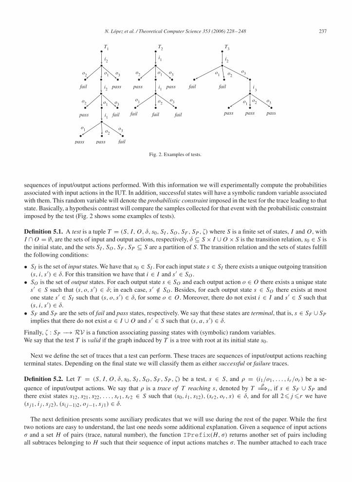
sequences of input/output actions performed. With this information we will experimentally compute the probabilitiesassociated with input actions in the IUT. In addition, successful states will have a symbolic random variable associatedwith them. This random variable will denote the probabilistic constraint imposed in the test for the trace leading to thatstate. Basically, a hypothesis contrast will compare the samples collected for that event with the probabilistic constraintimposed by the test (Fig. 2 shows some examples of tests).

Definition 5.1. A test is a tuple T = (S, I, O, �, s0, SI , SO, SF , SP , �) where S is a finite set of states, I and O, withI ∩ O = ∅, are the sets of input and output actions, respectively, � ⊆ S × I ∪ O × S is the transition relation, s0 ∈ S isthe initial state, and the sets SI , SO, SF , SP ⊆ S are a partition of S. The transition relation and the sets of states fulfillthe following conditions:

• SI is the set of input states. We have that s0 ∈ SI . For each input state s ∈ SI there exists a unique outgoing transition(s, i, s′) ∈ �. For this transition we have that i ∈ I and s′ ∈ SO .

• SO is the set of output states. For each output state s ∈ SO and each output action o ∈ O there exists a unique states′ ∈ S such that (s, o, s′) ∈ �; in each case, s′ /∈ SO . Besides, for each output state s ∈ SO there exists at mostone state s′ ∈ SI such that (s, o, s′) ∈ �, for some o ∈ O. Moreover, there do not exist i ∈ I and s′ ∈ S such that(s, i, s′) ∈ �.

• SF and SP are the sets of fail and pass states, respectively. We say that these states are terminal, that is, s ∈ SF ∪ SP

implies that there do not exist a ∈ I ∪ O and s′ ∈ S such that (s, a, s′) ∈ �.

Finally, � : SP −→ RV is a function associating passing states with (symbolic) random variables.We say that the test T is valid if the graph induced by T is a tree with root at its initial state s0.

Next we define the set of traces that a test can perform. These traces are sequences of input/output actions reachingterminal states. Depending on the final state we will classify them as either successful or failure traces.

Definition 5.2. Let T = (S, I, O, �, s0, SI , SO, SF , SP , �) be a test, s ∈ S, and � = (i1/o1, . . . , ir/or) be a se-

quence of input/output actions. We say that � is a trace of T reaching s, denoted by T� ⇒s , if s ∈ SF ∪ SP and

there exist states s12, s21, s22, . . . , sr1, sr2 ∈ S such that (s0, i1, s12), (sr2, or , s) ∈ �, and for all 2�j �r we have(sj1, ij , sj2), (s(j−1)2, oj−1, sj1) ∈ �.

The next definition presents some auxiliary predicates that we will use during the rest of the paper. While the firsttwo notions are easy to understand, the last one needs some additional explanation. Given a sequence of input actions� and a set H of pairs (trace, natural number), the function IPrefix(H, �) returns another set of pairs includingall subtraces belonging to H such that their sequence of input actions matches �. The number attached to each trace

238 N. López et al. / Theoretical Computer Science 353 (2006) 228 –248

corresponds to the number of traces belonging to H beginning with the given sequence of inputs �. Before definingthis concept, we present a simple example to show how this function works.

Example 5.3. Let us consider the sequence of input actions � = (i1) and the set

H ={

((i1/o1, i2/o1), 1), ((i1/o2, i1/o2), 2),

((i1/o2, i2/o1), 3), ((i2/o1, i2/o2), 4)

}.

The application of the function IPrefix(H, �) returns the set of pairs H ′ = {((i1/o1), 1), ((i1/o2), 5)}.

Given a sample of executions from an implementation, we will use this function to compute the number of times thatthe implementation has performed each sequence of outputs in response to some sequence of inputs. Let us note thatif the sequence of outputs (o1, . . . , on) has been produced in response to the sequence of inputs (i1, . . . , in) then, forall j �n, we know that the sequence of outputs (o1, . . . , oj ) has been produced in response to (i1, . . . , ij ). Hence, theobservation of a trace is useful to compute the number of instances of its prefixes. In the next definition, the symbols{| and |} are used to denote multisets.

Definition 5.4. Let � = (u1, . . . , un) and �′ = (u′1, . . . , u

′m) be two sequences. We say that � is a prefix of �′, denoted

by Prefix(�, �′), if n�m and for all 1� i�n we have ui = u′i .

Let � = (i1/o1, . . . , im/om) be a sequence of input/output actions. We define the input actions of the sequence �,denoted byinputs(�), as the sequence (i1, . . . , im) and the output actions of the sequence �, denoted byoutputs(�),as the sequence (o1, . . . , om). We denote the set of all sequences of output actions by .

Let H = {(�1, r1), . . . , (�m, rm)} be a set of pairs (trace, natural number) and � = (i1, . . . , in) be a sequence ofinput actions. The set of input prefixes of � in H , denoted by IPrefix(H, �), is defined as

IPrefix(H, �)={(�′, r ′)

∣∣∣∣� = inputs(�′) ∧ r ′ > 0 ∧r ′ =∑{|r ′′ | (�′′, r ′′) ∈ H ∧ Prefix(�′, �′′)|}

}.

Next we present the notions that we will use to denote that a given event has been detected in an IUT. We will alsocompute the sequences of actions that the implementation performs when a test is applied.

Definition 5.5. Let I = (S, I, O, �, s0) be a PFSM representing an IUT. We say that (i1/o1, . . . , in/on) is an executionof I if the sequence (i1/o1, . . . , in/on) can be performed by I. Let �1, . . . , �n be executions of I and r1, . . . , rn ∈ N.We say that the set H = {(�1, r1), . . . , (�n, rn)} is an execution sample of I.

Let T = (S′, I, O, �′, s′0, SI , SO, SF , SP , �) be a valid test. We say that H = {(�1, r1), . . . , (�n, rn)} is an execution

sample of I under the test T if H is an execution sample of I and for all (�, r) ∈ H we have that T� ⇒ s,

with s ∈ S′.Let = {T1, . . . , Tn} be a test suite and H1, . . . , Hn be sets such that each Hi is an execution sample of I under

Ti . We say that H = {(�1, r1), . . . , (�n, rn)} is an execution sample of I under the test suite if for all (�, r) ∈ H

we have that r = ∑i{|r ′ | (�, r ′) ∈ Hi |}.

In the definition of execution sample under a test we have that each number r , with (�, r) ∈ H , denotes the numberof times we have observed the execution � in I under the repeated application of T .

5.1. Passing a test on the basis of the behavior in traces

In this section, we introduce a notion of passing a test where the behavior of traces is concerned. A different notion,concerning the behavior of states, will be presented in the next section. Passing a test consists in fulfilling two constraints.First, we require that the test never reaches a failure state as a result of its interaction with the implementation. Thiscondition concerns what is possible. Second, we require that the random variables attached to successful states conformto the samples collected during the repeated application of the test to the IUT. This condition concerns what is probable.We will consider that the set of executions analyzed to pass a test does not only include those executions obtained byapplying that test, but also the executions obtained by applying other tests. Let us remark that the very same traces that

N. López et al. / Theoretical Computer Science 353 (2006) 228 –248 239

are available in a test could be part of other tests as well. Let us also note that the validity of any hypothesis contrastincreases with the number of samples. Hence, it would not be efficient to apply each hypothesis contrast to the limitedcollection of samples obtained by a single test. On the contrary, samples collected from the application of differenttests will be shared so that our statistical information grows and the hypothesis contrast procedure improves. Thus,this testing methodology represents a real novelty with respect to usual techniques where the application of each testis independent from the application of other tests.

Definition 5.6. Let I be an IUT, H be an execution sample of I under the test suite , 0���1, and T = (S′, I, O,

�′, s′0, SI , SO, SF , SP , �) ∈ be a test. We say that I (�, H)-passes the test T if for all trace � ∈ Traces(I), with

T� ⇒ s, we have that s /∈ SF and if s ∈ SP then �(�(s), R) > �, where

R = {(outputs(�′), r) | (�′, r) ∈ IPrefix(H,inputs(�))}.We say that I (�, H)-passes the test suite is for all test T ∈ we have I (�, H)-passes T .

Let us remark that the previous definition can be applied only if for each test T the function � associating randomvariables to passing states returns the random variables appearing in the first part of Definition 4.2, that is, we considertrace events. If events described by these random variables denote state events then they would not fit into the kind ofsamples considered in the previous relation.

5.2. Passing tests on the basis of the behavior in states

As we pointed out in Section 3, it is possible to check the correctness of an implementation by means of its reactions ineach state. This new framework requires to assume the additional hypothesis Hyp indicating that the graph underlyingthe IUT is isomorphic, up to probabilities, to the one representing the specification. Equivalently, we may assumethat we can see the internal ramification of the model of the implementation, that is, we may consider that a functionprovides us the state of the implementation after observing a given trace. This function will be used to convert ourtrace-oriented samples into state-oriented ones. Finally, we still assume that both specifications and implementationsare given by deterministically observable PFSMs.

Definition 5.7. Let � = (i0/o0, . . . , in/on) and �′ = (i′0/o′0, . . . , i

′m/o′

m) be two sequences of input/output actions.We define the concatenation of � and �′, denoted by � ◦ �′, as (i0/o0, . . . , in/on, i

′0/o

′0, . . . , i

′m/o′

m).Let I = (S, I, O, �, s0) be a PFSM. The function GI : Traces(I) −→ S fulfills that for any � ∈ Traces(I) we

have s0� ⇒ s implies GI(�) = s. We say that GI is the guiding function of I.

Let H = {(�1, r1), . . . , (�n, rn)} be an execution sample of I under a test suite . The states execution sample ofH for I, denoted by SSample(H, I), is defined as the set{(

(s, i, o), r ′) ∣∣∣∣ r ′ =∑ {

r

∣∣∣∣ ∃ �, �′ : Prefix(�′ ◦ i/o, �) ∧GI(�′) = s ∧ (�, r) ∈ H

}> 0

}.

Let us comment on the previous definition. In order to generate information concerning states from informationconcerning traces, we have to consider all the times that each trace belonging to the sample has arrived at each states ∈ S and has produced an output o ∈ O in response to an input i ∈ I . This is done by taking into account thosetraces appearing in the sample as well as their prefixes. Let us suppose that a prefix of a trace reaches s and it is still aprefix of that trace after adding i/o. Then, all the observations of that prefix are in fact observations of events wherethe implementation was in the state s and produced o after receiving i. Let us remark that a single trace could performthe pair i/o from the state s several times if that trace reaches a state s several times. In this case, different prefixes ofthe trace would fulfill the previous condition. Each time one of these prefixes does so, the number of observations ofthat trace will be added again to the number of repetitions of that event.

Next we introduce our second definition of passing a test. In this case, acceptance states of the test will be providedwith random variables describing the ideal probabilistic behavior concerning the last transition of the actual executionof the implementation and the test. For each trace leading the test to a passing state, the hypothesis contrast is applied

240 N. López et al. / Theoretical Computer Science 353 (2006) 228 –248

to the state the implementation stayed before the last input/output pair of the trace was performed. In fact, this is thestate where the decision of performing that output in response to that input was taken.

Definition 5.8. Let I be an IUT, H be an execution sample of I under the test suite , 0���1, and T = (S′, I,O, �′, s′

0, SI , SO, SF , SP , �) ∈ be a test. We say that the implementation I (�, H)st -passes the test T for states if

for all trace � ∈ Traces(I), with T� ⇒ s, we have that s /∈ SF and if s ∈ SP then �(�(s), R) > �, where

• � = �′ ◦ i′/o′ with GI(�′) = s′, and• R = {(o, r) | ((s′, i′, o), r) ∈ SSample(H, I)}.We say that I (�, H)st -passes for states the test suite if for any T ∈ we have I (�, H)st -passes T for states.

Let us remark that the previous definition can be applied only if the functions associating random variables to passingstates in tests concern state events (see Definition 4.2).

5.3. Relating notions of passing tests

In this section, we show how the notions of passing tests introduced in Definitions 5.6 and 5.8 are related. The nextdefinition introduces a simple method to convert a test where random variables concern trace events into a new testwhere random variables concern state events. Unfortunately, random variables in passing states do not provide enoughprobabilistic information to perform that conversion. In order to obtain this additional information, the transformationwill be supported by a PFSM which will be supposed to be the model of the test. When a passing state is reached in thetest after performing a trace, the random variable in that passing state will be constructed according to the symbolicprobability of that trace in the referenced PFSM. In the following definition, let us remind that denotes the set of allsequences of output actions (see Definition 5.4).

Definition 5.9. Let T = (S, I, O, �, s0, SI , SO, SF , SP , �) be a test for a certain function � : S → ( → simbP). Let

S be a PFSM. We say that the test T fits into S if for any s ∈ SP , with T� ⇒ s, we have that �(s)(outputs(�)) = p,

where (�, p) ∈ pTraces(S).If T fits into S then the conversion to states of T with respect to S, which is denoted by ConvToSt(T , S), is a

test T ′ = (S, I, O, �, s0, SI , SO, SF , SP , �′), for a certain function � : S → (O → simbP) where for any s ∈ SP ,

with T� ⇒ s, and � = (i1/o1, . . . , in/on) we have that �′(s)(on) = p′′, where ((i1/o1, . . . , in−1/on−1), p

′), (�, p) ∈pTraces(S) and p = p′ · p′′.

The following property shows that the notions of passing a test suite given in Definitions 5.6 and 5.8 are quitedifferent. In particular, neither of them implies the other. Intuitively, the relation based on traces is not contained in therelation based on states because, as we pointed out in Example 3.4, an unexpected probabilistic behavior in a transitioncould be compensated by the traces where it is included. On the other hand, the relation based on states is not containedin the relation based on traces because a correct probabilistic behavior in a state could be the result of some traceswhose behavior is unexpected. This could happen if the empirical bias of each of them balance in the overall in thatstate.

Lemma 5.10. Let T1, . . . , Tn be tests fitting into a PFSM S. Let I be an implementation under test, H be an executionsample of I under the test suite {T1, . . . , Tn}, and 0���1. We have that I (�, H)-passes for traces {T1, . . . , Tn}does not imply that I (�, H)st -passes for states the test suite {ConvToSt(T1, S), . . . ,ConvToSt(Tn, S)}, neitherthe reverse is true.

Proof. To prove that the first implication is false it is enough to create a counterexample inspired in Example 3.4.Let us take a test suite = {T1, T2}, where T1 and T2 are depicted in Fig. 3. In both tests, the passing states reachedafter (a/d) will be endowed with a random variable �1 such that �1(b) = [0.2, 0.6] and �1(d) = [0.3, 0.7]. In T2, thepassing state reached after executing (a/b) will be equipped with the same random variable. Besides, states reachedin T1 after performing the sequences (a/b, a/b) and (a/b, a/d) will be equipped with a random variable �2 such that

N. López et al. / Theoretical Computer Science 353 (2006) 228 –248 241

T1

a

pass

d b

a

pass

d

pass

b c

fail

fail

fail fail fail fail fail

failfail

c

T2

a

pass

d

pass

b c

T3

a

d b

a

d

pass

b

pass

c

c

T4

e

b d

a

d

pass

b

pass

c

c

Fig. 3. Tests to be used in Lemma 5.10.

�2(b, b) = [0.08, 0.36] and �2(b, d) = [0.06, 0.48]. Tests T1 and T2 fit into S (see Example 3.4). To convert these testsinto new tests that concern state events (according to S) it is enough to change the previous random variables by �′

1 and�′

2 respectively, where �′1(b) = [0.2, 0.6], �′

1(d) = [0.3, 0.7], �′2(b) = [0.4, 0.6], and �′

2(d) = [0.3, 0.8]. Besides, letus suppose that H , the execution sample of I under , is the set H = {((a/d), 5), ((a/b, a/b), 1), ((a/b, a/d), 4)}.Finally, the confidence function � : (A → simbP) × ((A × N) × . . . (A × N)) → R is defined such that

�(V, ((�1, r1), . . . , (�k, rk))) =⎧⎨⎩ 1 if for all �i ∈ A : ri∑

rj∈ V(�i ),

0 otherwise ,

where the type of V is given by V : A → simbP. Let us consider 0 < ��1. Under these conditions, we have that I(�, H)-passes for traces {T1, T2} holds because all observed ratios fit into the probabilistic constraints. Let us remindthat the observed ratio of (a/b) is 0.5, because it has been detected 1 + 4 times out of 10. On the other hand, we havethat I (�, H)st -passes for states {ConvToSt(T1, S),ConvToSt(T2, S)} is false because the observed ratio of outputb in response to input a after (a/b) has been performed is 0.2, which does not belong to the interval [0.4, 0.6].

In order to show that the opposite implication is also false, we need to give a new counterexample. Let S =(S, I, O, �, s0), where I = {a, e}, O = {b, c, d}, S = {s0, s1, s2}, and the set of transitions is given by

� ={s0

a/b−−−→1 s1, s0e/d−−−→1 s1, s1

a/b−−−→ 0.5 s2, s1a/c−−−→ 0.5 s2

}.

Let us remind that an interval [p, p] is denoted simply by p. Let us consider a test suite = {T3, T4}, where T3 andT4 are depicted in Fig. 3. In T3, the passing states reached after (a/b, a/b) and (a/b, a/c) will be endowed with thesame random variable, �1, taking values �1(b) = 0.5 and �1(c) = 0.5. Besides, states reached in T4 after (e/d, a/b)

and (e/d, a/c) will be also equipped with the same random variable �1.In order to transform these tests into new tests that concern trace events and fit into S, we substitute the previous

random variable �1 by the random variables �′1 (in T3) and �′

2 (in T4). These new variables are defined by �′1(b, b) =

�′1(b, c) = �′

2(d, b) = �′2(d, c) = 0.5. Let T ′

3 and T ′4 be these new tests. Besides, let us suppose that the execution

sample of I under is H = {((a/b, a/b), 1), ((e/d, a/c), 1)}. Finally, let us suppose that the confidence function� is defined as before, and let 0 < ��1. Under these conditions we have that I (�, H)st -passes for states {T1, T2}holds. Since Hyp is assumed in this relation, both samples in H reach the same implementation state after (a/b) and(e/d), respectively. At this state, after the input a is received, half of the times the output b is produced, while the otherhalf the output c is produced. This fits into the probabilistic constraint given in both tests for that state. However, I(�, H)-passes for traces {T1, T2} does not hold. Let us note that the empirical ratio of the trace (a/b, a/b) when thesequence of inputs (a, a) is produced is equal to 1, while it should be equal to 0.5. �

6. Implementation relations based on samples

In Section 3, we presented two implementation relations that clearly expressed the probabilistic constraints an imple-mentation must fulfill to conform to a specification. Unfortunately, these notions are useful only from a theoretical pointof view since it cannot be tested, by using a finite number of test executions, the correctness, in this sense, of the proba-bilistic behavior of an implementation with respect to a specification. In this section, we introduce new implementation

242 N. López et al. / Theoretical Computer Science 353 (2006) 228 –248

relations that take into account the practical limitations to collect probabilistic information from an implementation.These new relations allow us to claim the accurateness of the probabilistic behavior of an implementation with respectto a specification up to a given confidence level. Given a set of execution samples, we will apply a hypothesis contrastto check whether the probabilistic choices taken by the implementation follow the patterns given by the specification.

Our new implementation relations follow again the classical pattern. Regarding input/output actions, the constraintsimposed by these implementation relations are given by the relation conf (see Definition 3.1). This condition over thesequences that the implementation may perform could be rewritten in probabilistic terms as follows: The confidencewe have on the fact that the implementation will not perform forbidden behaviors is 1 (i.e. complete). However, sinceno hypothesis contrast can provide full confidence, it is preferable to keep the constraints over actions separated fromthe probabilistic constraints. In fact, the reverse is not true: We cannot claim that the implementation is correct even ifno forbidden behavior is detected after a finite number of interactions with it.

Regarding the probabilistic constraints of the specification, the new relations will express them in a different way tothe one used in Definitions 5.6 and 5.8. In the first two relations (forthcoming Definitions 6.1 and 6.2) we put togetherall the observations of the implementation. Then, the set of samples corresponding to each trace of the specificationwill be generated by taking all the observations such that the trace is a prefix of them. By doing so, we will be ableto compare the number of times the implementation has performed the chosen trace with the number of times theimplementation has performed any other behavior. We will use hypothesis contrasts to decide whether the probabilisticchoices of the implementation conform to the probabilistic constraints imposed by the specification. In particular, ahypothesis contrast will be applied to each sequence of inputs considered by the specification. This contrast will checkwhether the different sequences of outputs associated with these inputs are distributed according to the probabilitydistribution of the random variable associated with that sequence of inputs in the specification.

Definition 6.1. Let S be a specification, I be an IUT, H be an execution sample of I, and 0���1. We say that I(�, H)-probabilistically conforms to S, denoted by I confp(�,H) S, if I confS and for all � ∈ Traces(S) we have�(��

S , R) > �, where � = inputs(�) and

R = {(outputs(�′), r) | (�′, r) ∈ IPrefix(H, �)}.

In the previous relation, ��S denotes the symbolic random variable associated with the sequence of input actions �

for the PFSM S (see Definition 4.2). Intuitively, each trace observed in the implementation will add one instance to theaccounting of its prefixes. We could consider an alternative procedure where traces are independently accounted andeach observed trace does not affect the number of instances of other traces being prefix of it. However, this methodwould lose valuable information that might negatively affect the quality of the hypothesis contrasts. Let us remind thatthe reliability of any hypothesis contrasts increases with the number of instances included in the samples. Besides, as wesaid before, an observation where (o1, . . . , on) has been produced in response to (i1, . . . , in) is indeed an observationwhere, for all 1�j �n, (o1, . . . , oj ) has been produced in response to (i1, . . . , ij ). So, by joining prefixes we properlyincrease the number of instances processed by hypothesis contrasts, which makes them more precise (as well as theprobabilistic implementation relation that takes them into account).

The previous idea induces the definition of a refinement of the previous implementation relation. Let us note thatthe probability of observing a given trace decreases, in general, as the length of the trace increases. This is so becausemore probabilistic choices are taken in long traces. Besides, taking prefixes into account increases the number ofinstances of short traces. Thus, it is likely that the number of short traces applied to the hypothesis contrasts of theprevious relation will outnumber that of longer traces. Let us note that statistical noise effects are higher when smallersets of samples are considered. Moreover, if we consider extremely long traces we could obtain a few instances, oreven none, in each class of events to be considered by a hypothesis contrast. This fact would ruin the result of such acontrast. Taking these factors into account, in the next definition we introduce a new implementation relation wherethe confidence requirement is relaxed as the length of the trace grows. This reduction is defined by a non-increasingfunction associating confidence levels to the length of traces.

Definition 6.2. Let f : N → [0, 1] be a strictly non-increasing function, S be a specification, I be an implementation,and H be an execution sample of I. We say that I (f, H)-probabilistically conforms to S, denoted by Iconfp(f,H) S,if I conf S and for all trace � ∈ Traces(S) we have �(��

S , R) > f (l), where � = inputs(�), l is the length of �,

N. López et al. / Theoretical Computer Science 353 (2006) 228 –248 243

and

R = {(outputs(�′), r) | (�′, r) ∈ IPrefix(H, �)}.

It is straightforward to see that when the function f of the previous definition is defined as f (i) = �, for all i ∈ N,then we have confp(�,H) = confp(f,H).

Next, we will define the relation based on samples for states. This relation works under the additional implementationhypothesis Hyp explained in Section 3. This hypothesis allows us to collect the probabilistic behavior of each state ofthe implementation by considering all the implementation observations whose trace would traverse the correspondingstate in the specification. Thus, each time that the interaction between a test and the IUT produces a trace that wouldreach a given state, a new sample is added to the probabilistic information corresponding to that state. Hence, for eachstate of the implementation and each input, a different set of samples is created. Each of these sets provides the numberof times each output was performed in that state in response to that input. By taking into account these samples, wecan check the probabilistic constraint of the second implementation relation. It forces the sets of samples to match theprobabilities given in the specification for the corresponding states and inputs.

Definition 6.3. Let S = (S, I, O, �, s0) and I = (S′, I, O, �′, s′0) be a specification and an IUT, respectively, H be an

execution sample of I, and 0���1. Let us suppose that Hyp holds. We say that I (�, H)-probabilistically conforms

to S considering states, denoted by I confp(�,H)Hyp S, if I confS and for each s ∈ S and i ∈ I we have �(�s,i

S , R) > �,where

R = {(o′, r) | ((s′, i, o′), r) ∈ SSample(H, I) ∧ cSt(s) = s′},where for each state s ∈ S, cSt(s) denotes the corresponding state in S′.

Let us remind that �s,iS is a random variable constructed from the specification S (see Definition 4.2). In the following

result, we show the relation between the implementation relations confp(�,H) and confp(�,H)Hyp . Let us note that,

similarly to the relations presented in Section 5, both relations are based on the idea of sampling. Hence, the reasonsconsidered when we related the notion of passing a test suite for traces and the concept of passing it for states,shown in Lemma 5.10, apply also to the implementation relations confp(�,H) and confp(�,H)

Hyp . In fact, to adapt thecounterexamples presented in Lemma 5.10 to the context of these relations is easy. In particular, let us note that samplesin confp(�,H) and in the relation introduced in Definition 5.6 are grouped in the same way. Similarly, samples aredealt in the same manner in confp(�,H)

Hyp and in the relation presented in Definition 5.8. Moreover, in both cases theconfidence function is applied to the execution sample in the same way.

Lemma 6.4. confp(�,H) does not imply confp(�,H)Hyp , neither the reverse implication holds.

Besides, the relations presented in this section cannot be related with those introduced in Section 3. In particular,computing these relations on the basis on samples would require to collect infinite samples, which is not feasible. Hence,the relations presented in this section can be seen as a way to put in practice the concepts presented in Section 3.

7. Test derivation

In this section, we provide an algorithm to derive test suites from specifications. We will show that the derived testsuites are complete with respect to two of the conformance relations introduced in the previous section. As usually,the idea consists in traversing the specification to get all the possible traces in the adequate way. Thus, each test isgenerated to focus on chasing a concrete trace of the specification. Test cases will also contain probabilistic constraintsso that they can detect faulty probabilistic behaviors in the IUT. The probabilistic constraints of the specification willbe encoded in the tests. Specifically, passing states will have attached symbolic random variables that impose someconstraints concerning either the trace executed so far in the test or the transition taken from the previous state of thetest. This choice will depend on whether we want to test implementations with respect to traces or states, respectively.First, we introduce some auxiliary functions.

244 N. López et al. / Theoretical Computer Science 353 (2006) 228 –248

Input: M = (S, I, O, �, s0).Output: T = (S′, I, O, �′, s′

0, SI , SO, SF , SP , �).Initialization:

• S′ := {s′0}, �′ := SI := SO := SF := SP := ∅.

• Saux := {(s0, s′0, ( ), Nothing)}.

Inductive Cases: Apply one of the following two possibilities until Saux = ∅.(1) If (sM, sT , �, sprev) ∈ Saux then perform the following steps:

(a) Saux := Saux − {(sM, sT , �, sprev)}.(b) SP := SP ∪ {sT }.(c) Let � = �′ ◦ i. If we wish to check conformance considering traces, do

• �(sT ) := ��M

else, if we wish to check conformance considering states, do• �(sT ) := �sprev,i

M,st

(2) If Saux = {(sM, sT , �, sprev)} is a unitary set and there exists i ∈ I

such that out(sM, i) �= ∅ then perform the following steps:(a) Saux := ∅.(b) Choose i such that out(sM, i) �= ∅.(c) Create a fresh state s′ /∈ S′ and perform S′ := S′ ∪ {s′}.(d) SI := SI ∪ {sT }; SO := SO ∪ {s′}; �′ := �′ ∪ {(sT , i, s′)}.(e) For each o /∈ out(sM, i) do

• Create a fresh state s′′ /∈ S′ and perform S′ := S′ ∪ {s′′}.• SF := SF ∪ {s′′}; �′ := �′ ∪ {(s′, o, s′′)}.

(f) For each o ∈ out(sM, i) do• Create a fresh state s′′ /∈ S′ and perform S′ := S′ ∪ {s′′}.• �′ := �′ ∪ {(s′, o, s′′)}.• sM

1 := after(sM, i, o).• Let (sM, i, o, p, sM

1 ) ∈ �.Saux := Saux ∪ {(sM

1 , s′′, � ◦ i, sM)}.Fig. 4. Test derivation algorithm.

Definition 7.1. Let M = (S, I, O, �, s0) be a PFSM. We define the set of possible outputs in state s after input i,denoted by out(s, i), as the set out(s, i) = {o | ∃s′ : (s, i, o, p, s′) ∈ �}. For each transition (s, i, o, p, s′) ∈ � wewrite after(s, i, o) = s′.

Let us remark that, due to the assumption that PFSMs are deterministically observable, after(s, i, o) is uniquelydetermined.

Our derivation algorithm is presented in Fig. 4. This is a non-deterministic algorithm that, given a specification,returns a single test case. However, by considering the tests returned by the algorithm for each possible combination ofnon-deterministic choices, we get the (possible infinite) set of tests extracted from the specification M . In this algorithmthe set of pending states Saux keeps track of the states of the test whose definition has not been finished yet. A tuple(sM, sT , �, sprev) ∈ Saux indicates that the current state in the traversal of the specification is sM , that we did notconclude yet the description of the state sT in the test, that the sequence of inputs traversed from s0 to sT is �, and thatthe state before sM in the traversal of the specification was sprev. The set Saux initially contains a tuple with the initialstates (of both specification and test), an empty sequence of inputs, and a symbol denoting that there does not exista previous state yet. For each tuple in Saux we may choose between two different choices. It is important to remarkthat possibility (2) is applied at most to one of the possible tuples. Thus, our derived tests correspond to valid tests asintroduced in Definition 5.2.

The possibility (1) simply indicates that the state of the test becomes a passing state. In this case, we attach asymbolic random variable to the passing state. On the one hand, if we are developing the test suite to check conformance

N. López et al. / Theoretical Computer Science 353 (2006) 228 –248 245

considering traces (see Definition 5.6) then this random variable must encode the probability distribution, according tothe specification, for all possible traces containing the sequence of inputs �. In this case we denote by tests(M) thederived test suite. On the other hand, if we have to check conformance considering states (see Definition 5.8) then therandom variable will encode the probability of performing each output in response to the last input from the last statevisited in the specification. In this case we denote by testsst(M) the derived test suite.

The possibility (2) of the algorithm takes an input and generates a transition in the test labelled by this input. Then,the whole sets of outputs is considered. If the output is not expected by the implementation then a transition leading toa failing state is created. This could be simulated by a single branch in the test, labelled by else, leading to a failingstate (in the algorithm we suppose that all the possible outputs appear in the test). For the rest of outputs, we create atransition with the corresponding output and add the appropriate tuple to the set Saux.

Finally, let us remark that finite test cases are constructed simply by considering a step where the second inductivecase is not applied.

The next result states that, for a given specification S, the test suites tests(S) and testsst(S) can be usedto distinguish those (and only those) implementations conforming with respect to confp or confpHyp, respec-tively. However, we cannot properly say that the test suite is complete since both passing tests and the consid-ered implementation relation have a probabilistic component. So, we can speak about completeness up to a certainconfidence level.

Theorem 7.2. Let S and I be PFSMs. For any 0���1 and execution sample H of I we have

(a) I confp(�,H) S iff I (�, H)-passes tests(S).(b) I confp(�,H)

Hyp S iff I (�, H)st -passes testsst(S).

Proof. We will prove the statement (a); the proof of (b) is similar.First, let us show that I (�, H)-passes the test suite tests(S) implies that we also have I confp(�,H) S. In

order to do that, we will use contrapositive, that is, we assume that I confp(�,H) S does not hold and we show thatI (�, H)-passes the test suite tests(S) is false as well. First, let us suppose that I confp(�,H) S is false becauseIconfS does not hold. This means that there exist two non-probabilistic traces � = (i1/o1, . . . , ir−1/or−1, ir/or) and�′ = (i1/o1, . . . , ir−1/or−1, ir/o

′r ), with r �1, such that � ∈ Traces(S), �′ ∈ Traces(I), and �′ /∈ Traces(S).

Let us show that if � ∈ Traces(S) then there exists a test T = (S, I, O, �′, s, SI , SO, SF , SP , �) ∈ tests(S) such

that T� ⇒ s and s ∈ SP . That test is built by applying the algorithm presented in Fig. 4 in such a way that we resolve

the non-determinism as follows.

for 1�j �r doapply inductive case (2) for input ij

apply inductive case (1) for all (sS , sT , �, sprev) ∈ Saux obtainedby processing an output different from oj

endapply inductive case (1) for the last (sS , sT , �, sprev) ∈ Saux

Intuitively, the generated test T traverses all inputs ij and outputs oj as specified in trace �. We have that the test T

is such that T�′ ⇒ u, with u ∈ SF . This is because the last application of the inductive case (2) deals with the output o′

r

in step (e), since we have �′ /∈ Traces(S). Due to the fact that �′ ∈ Traces(I), we have that I (�, H)-passes thetest T does not hold. Since T ∈ tests(S), we conclude that I (�, H)-passes the test suite tests(S) does not hold.

Let us suppose now that I confp(�,H) S is false because there exists a trace � ∈ Traces(S) such that�(��

S , R)��, where we have � = inputs(�) and R = {(outputs(�′), r) | (�′, r) ∈ IPrefix(H, �)}. Then,

there exists a test T = (S, I, O, �′, s, SI , SO, SF , SP , �) ∈ tests(S) such that T� ⇒ s, with s ∈ SP and �(s) = ��

S .We have that �(�(s), R)��. So, I (�, H)-passes the test T does not hold. Thus, we conclude that neither I (�, H)-passesthe test suite tests(S) holds.

Let us prove now that I confp(�,H) S implies I (�, H)-passes tests(S). In order to do that, we assumethat I (�, H)-passes the test suite tests(S) is not true and we show that I confp(�,H) S is also false. First,let us suppose that I (�, H)-passes the test suite tests(S) does not hold because there exist T ∈ tests(S),

246 N. López et al. / Theoretical Computer Science 353 (2006) 228 –248

�′ = (i1/o1, . . . , ir−1/or−1, ir/o′r ) ∈ Traces(I), and a state s such that T

�′ ⇒ s and s ∈ SF . According toour test derivation algorithm, a branch of a test leads to a failure state only if the associated output cannot be performedin the specification. Thus, �′ /∈ Traces(S). Let us note that our algorithm only allows to create a failure state if it isthe result of the application of the inductive case (2). A requirement to perform this case is out(sS , i) �= ∅, that is, thespecification must produce some output after the reception of the chosen input. Therefore, there exist an output or and anon-probabilistic trace � = (i1/o1, . . . , ir−1/or−1, ir/or) such that � ∈ Traces(S). Since we have �′ ∈ Traces(I),�′ /∈ Traces(S) and � ∈ Traces(S), the predicate I conf S does not hold. Thus, I confp(�,H) S is false.

Finally, let us suppose that I (�, H)-passes tests(S) does not hold because there exist T = (S, I, O, �′, s, SI , SO,

SF , SP , �) ∈ tests(S) and � ∈ Traces(I) such that I (�, H)-passes T does not hold, T� ⇒ s, with s ∈ SP ,

inputs(�) = �, and �(�(s), R)��, where R = {(outputs(�′), r) | (�′, r) ∈ IPrefix(H, �)}. According tothe test derivation algorithm we know that if s ∈ SP then � ∈ Traces(S). Besides, we have �(s) = ��

S . Then,�(��

S , R)��. Thus, we conclude that I confp(�,H) S does not hold. �

8. Conclusions

In this paper, we have presented a testing methodology to check whether an implementation properly followsthe behavior described by a given specification. The particularity of our framework is that specifications can explicitlyexpress the desired propensity of each option in each non-deterministic choice of the system. This propensity is denotedin terms of probabilities. Moreover, in order to improve the expressivity of specifications, symbolic probabilities areintroduced. Let us note that, in several situations, it is not desirable or feasible to impose that the probability of an eventis some fix value. Symbolic probabilities help to overcome this problem.

We have presented a testing methodology for these kind of systems. The necessity of assessing the probabilisticbehavior of a system increases the complexity of the methodology, as it is impossible to infer the actual probabilitiesassociated with implementations from a set of interaction samples. In order to cope with this problem, the probabilisticbehavior of the implementation is probabilistically assessed on the basis of a finite set of samples, which is obtainedby applying tests several times. Hypothesis contrasts allow to obtain a (probabilistic) diagnosis result by comparingthe set of samples with the ideal probabilistic requirements.

We have explored several possibilities to apply this methodology. In particular, we have studied the practical dif-ferences between associating probabilistic constraints to traces and associating them to the transitions leaving eachstate. Finally, we have presented a test derivation algorithm. The resulting test suite is sound and complete with respectto our implementation relations, that is, the test suite is passed if and only if the corresponding implementationrelation holds.

9. Acknowledgments

We would like to thank the anonymous referees of this paper for their suggestions and valuable comments.

Appendix. Statistics background: hypothesis contrasts

In this appendix, we introduce one of the standard ways to measure the confidence that a certain sample has beengenerated by a given random variable. In order to do so we present a methodology to perform hypothesis contrasts.Intuitively, a sample will be rejected if the probability of observing that sample from a given random variable is low.In practice, we will check whether the probability to observe a discrepancy lower than or equal to the one that we havedetected is low enough. We will present Pearson’s �2 contrast. This contrast can be applied both to continuous anddiscrete random variables. The mechanism is the following. Once we have collected a sample of size n we perform thefollowing steps:

• We split the sample into k classes covering all the possible range of values. We denote by Oi the observed frequencyin class i (i.e. the number of elements belonging to the class i).

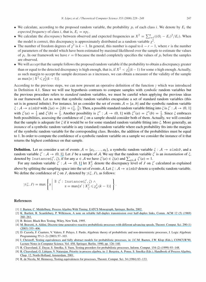
N. López et al. / Theoretical Computer Science 353 (2006) 228 –248 247

• We calculate, according to the proposed random variable, the probability pi of each class i. We denote by Ei theexpected frequency of class i, that is, Ei = npi .

• We calculate the discrepancy between observed and expected frequencies as X2 = ∑ni=1((Oi − Ei)

2/Ei). When

the model is correct, this discrepancy is approximately distributed as a random variable �2.• The number of freedom degrees of �2 is k − 1. In general, this number is equal to k − r − 1, where r is the number

of parameters of the model which have been estimated by maximal likelihood over the sample to estimate the valuesof pi . In our framework we have r = 0 because the model completely specifies the values of pi before the samplesare observed.

• We will accept that the sample follows the proposed random variable if the probability to obtain a discrepancy greater

than or equal to the detected discrepancy is high enough, that is, if X2 < �2�(k−1) for some � high enough. Actually,

as such margin to accept the sample decreases as � increases, we can obtain a measure of the validity of the sampleas max{� | X2 ��2

�(k − 1)}.According to the previous steps, we can now present an operative definition of the function � which was introducedin Definition 4.1. Since we will use hypothesis contrasts to compare samples with symbolic random variables butthe previous procedure refers to standard random variables, we must be careful when applying the previous ideasin our framework. Let us note that symbolic random variables encapsulate a set of standard random variables (thisset is in general infinite). For instance, let us consider the set of events A = {a, b} and the symbolic random variable� : A → simbPwith �(a) = �(b) = ( 1

4 , 34 ). Then, a possible standard random variable fitting into � is �′ : A → (0, 1]

with �′(a) = 13 and �′(b) = 2

3 . Another possibility is �′′ : A → (0, 1] with �′′(a) = �′′(b) = 12 . Since � embraces

both possibilities, assessing the confidence of � on a sample should consider both of them. Actually, we will considerthat the sample is adequate for � if it would be so for some standard random variable fitting into �. More generally, aninstance of a symbolic random variable is any (standard) random variable where each probability fits into the marginsof the symbolic random variable for the corresponding class. Besides, the addition of the probabilities must be equalto 1. In order to compute the confidence of a symbolic random variable on a sample we consider the instance of it thatreturns the highest confidence on that sample.

Definition. Let us consider a set of events A = {a1, . . . , ak}, a symbolic random variable � : A → simbP, and arandom variable �′ : A → (0, 1]. Let J be a sample of A. We say that the random variable �′ is an instantiation of �,denoted by Instance(�′, �), if for any a ∈ A we have �′(a) ∈ �(a) and

∑a∈A �′(a) = 1.

For any random variable �′ : A → (0, 1] let X2�′ denote the discrepancy level of J on �′ calculated as explained

above by splitting the sampling space into the set of events A. Let � : A → simbP denote a symbolic random variable.We define the confidence of � on J , denoted by �(�, J ), as follows:

�(�, J ) = max

{�

∣∣∣∣∣ ∃ �′ : Instance(�′, �) ∧� = max{�′ | X2

�′ ��2�′(k − 1)}

}.

References

[1] J. Baeten, C. Middelburg, Process Algebra With Timing, EATCS Monograph, Springer, Berlin, 2002.[2] K. Bartlett, R. Scantlebury, P. Wilkinson, A note on reliable full-duplex transmission over half-duplex links, Comm. ACM 12 (5) (1969)

260–261.[3] B. Beizer, Black Box Testing, Wiley, New York, 1995.[4] M. Bravetti, A. Aldini, Discrete time generative-reactive probabilistic processes with different advancing speeds, Theoret. Comput. Sci. 290 (1)

(2003) 355–406.[5] D. Cazorla, F. Cuartero, V. Valero, F. Pelayo, J. Pardo, Algebraic theory of probabilistic and non-deterministic processes, J. Logic Algebraic

Programming 55 (1–2) (2003) 57–103.[6] I. Christoff, Testing equivalences and fully abstract models for probabilistic processes, in: J.C.M. Baeten, J.W. Klop (Eds.), CONCUR’90,

Lecture Notes in Computer Science, Vol. 458, Springer, Berlin, 1990, pp. 126–140.[7] R. Cleaveland, Z. Dayar, S. Smolka, S. Yuen, Testing preorders for probabilistic processes, Inform. Comput. 154 (2) (1999) 93–148.[8] R. Cleaveland, G. Lüttgen, V. Natarajan, Priority in process algebra, in: J. Bergstra, A. Ponse, S. Smolka (Eds.), Handbook of Process Algebra,

Chap. 12, North-Holland, Amsterdam, 2001.[9] R. de Nicola, M. Hennessy, Testing equivalences for processes, Theoret. Comput. Sci. 34 (1984) 83–133.

248 N. López et al. / Theoretical Computer Science 353 (2006) 228 –248

[10] R.v. Glabbeek, S. Smolka, B. Steffen, Reactive, generative and stratified models of probabilistic processes, Inform. Comput. 121 (1) (1995)59–80.

[11] M. Hennessy, Algebraic Theory of Processes, MIT Press, Cambridge, MA, 1988.[12] B. Jonsson, W. Yi, K. Larsen, Probabilistic extensions of process algebras, in: J. Bergstra, A. Ponse, S. Smolka (Eds.), Handbook of Process

Algebra, Chap. 11, North-Holland, Amsterdam, 2001.[13] K. Larsen, A. Skou, Bisimulation through probabilistic testing, Inform. Comput. 94 (1) (1991) 1–28.[14] N. López, M. Núñez, An overview of probabilistic process algebras and their equivalences, in: C. Baier, B.R. Haverkort, H. Hermanns, J.-P.

Katoen, M. Siegle (Eds.), Validation of Stochastic Systems, Lecture Notes in Computer Science, Vol. 2925, Springer, Berlin, 2004, pp. 89–123.[15] N. López, M. Núñez, I. Rodríguez, Testing of symbolic-probabilistic systems, in: J. Grabowski, B. Nielsen (Eds.), Fourth Internat. Workshop

on Formal Approaches to Testing of Software (FATES 2004), Lecture Notes in Computer Science, Vol. 3395, Springer, Berlin, 2004, pp. 49–63.[16] N. López, M. Núñez, I. Rodríguez, Formal specification of symbolic-probabilistic systems, in: M. Núñez, Z. Maamar, F.L. Pelayo, K. Pousttchi,

F. Rubio (Eds.), European Performance Engineering Workshop (EPEW’04), Lecture Notes in Computer Science, Vol. 3236, Springer, Berlin,2004, pp. 114–127.

[17] G. Myers, The Art of Software Testing, Wiley, New York, 1979.[18] X. Nicollin, J. Sifakis, An overview and synthesis on timed process algebras, in: K.G. Larsen, A. Skou (Eds.), Computer Aided Verification’91,

Lecture Notes in Computer Science, Vol. 575, Springer, Berlin, 1991, pp. 376–398.[19] M. Núñez, Algebraic theory of probabilistic processes, J. Logic Algebraic Programming 56 (1–2) (2003) 117–177.[20] M. Núñez, D. de Frutos, Testing semantics for probabilistic LOTOS, in: G. von Bochmann, R. Dssouli, O. Rafiq (Eds.), Formal Description

Techniques VIII, Chapman & Hall, London, 1995, pp. 365–380.[21] M. Núñez, I. Rodríguez, Encoding PAMR into (timed) EFSMs, in: D. Peled, M.Y. Vardi (Eds.), FORTE 2002, Lecture Notes in Computer

Science, Vol. 2529, Springer, Berlin, 2002, pp. 1–16.[22] M. Núñez, I. Rodríguez, Towards testing stochastic timed systems, in: H. König, M. Heiner, A. Wolisz (Eds.), FORTE 2003, Lecture Notes in

Computer Science, Vol. 2767, Springer, Berlin, 2003, pp. 335–350.[23] G. Reed, A. Roscoe, A timed model for communicating sequential processes, Theoret. Comput. Sci. 58 (1988) 249–261.[24] R. Segala, Testing probabilistic automata, in: U. Montanari, V. Sassone (Eds.), CONCUR’96, Lecture Notes in Computer Science, Vol. 1119,

Springer, Berlin, 1996, pp. 299–314.[25] M. Stoelinga, F. Vaandrager, A testing scenario for probabilistic automata, in: J.C.M. Baeten, J.K. Lenstra, J. Parrow, G.J. Woeginger (Eds.),

ICALP 2003, Lecture Notes in Computer Science, Vol. 2719, Springer, Berlin, 2003, pp. 464–477.[26] J. Tretmans, Test generation with inputs, outputs and repetitive quiescence, Software—Concepts Tools 17 (3) (1996) 103–120.[27] W. Yi, K. Larsen, Testing probabilistic and nondeterministic processes, in: R.J. Linn Jr., M. Ümit Uyar (Eds.), Protocol Specification, Testing

and Verification XII, North-Holland, Amsterdam, 1992, pp. 47–61.