SPECIALIZED MAPPINGS ARCHITECTURE WITH ...

BOSTON UNIVERSITY

GRADUATE SCHOOL OF ARTS AND SCIENCES

Dissertation

SPECIALIZED MAPPINGS ARCHITECTURE

WITH APPLICATIONS TO VISION-BASED ESTIMATION

OF ARTICULATED BODY POSE

by

R�OMER E. ROSALES-DEL-MORAL

B.Eng., Universidad Centroccidental Lisandro Alvarado, 1995.M.A., Boston University, 2000

Submitted in partial ful�llment of the

requirements for the degree of

Doctor of Philosophy

2002

Approved by

First Reader

Stanley Sclaro�, Ph.D.Associate Professor of Computer ScienceBoston University

Second Reader

Matthew Brand, Ph.D.Research ScientistMitsubishi Electric Research Laboratories

Third Reader

David Hogg, Ph.D.Professor of Computer Scienceand University Pro-Vice-ChancellorUniversity of Leeds

SPECIALIZED MAPPINGS ARCHITECTURE,

WITH APPLICATIONS TO VISION-BASED ESTIMATION

OF ARTICULATED BODY POSE

(Order No. )

ROMER E. ROSALES-DEL-MORAL

Boston University Graduate School of Arts and Sciences, 2002

Major Professor: Stan Sclaro�, Associate Professor of Computer Science

ABSTRACT

A fundamental task of vision systems is to infer the state of the world given some

form of visual observations. From a computational perspective, this often involves

facing an ill-posed problem; e.g., information is lost via projection of the 3D world

into a 2D image. Solution of an ill-posed problem requires additional information,

usually provided as a model of the underlying process. It is important that the model

be both computationally feasible as well as theoretically well-founded. In this thesis,

a probabilistic, nonlinear supervised computational learning model is proposed: the

Specialized Mappings Architecture (SMA). The SMA framework is demonstrated in a

computer vision system that can estimate the articulated pose parameters of a human

body or human hands, given images obtained via one or more uncalibrated cameras.

The SMA consists of several specialized forward mapping functions that are

estimated automatically from training data, and a possibly known feedback func-

tion. Each specialized function maps certain domains of the input space (e.g., image

features) onto the output space (e.g., articulated body parameters). A probabilistic

model for the architecture is �rst formalized. Solutions to key algorithmic problems

are then derived: simultaneous learning of the specialized domains along with the

mapping functions, as well as performing inference given inputs and a feedback

function. The SMA employs a variant of the Expectation-Maximization algorithm

and approximate inference. The approach allows the use of alternative conditional in-

dependence assumptions for learning and inference, which are derived from a forward

model and a feedback model.

Experimental validation of the proposed approach is conducted in the task of

estimating articulated body pose from image silhouettes. Accuracy and stability of

the SMA framework is tested using arti�cial data sets, as well as synthetic and real

video sequences of human bodies and hands.

Contents

1 Introduction 1

1.1 An Everyday Example . . . . . . . . . . . . . . . . . . . . . . . . . . 3

1.2 General Elements and Properties of the Problem . . . . . . . . . . . . 4

1.3 General Problem De�nition in the Context of Theory of Function

Approximation . . . . . . . . . . . . . . . . . . . . . . . . . . . . . . 11

1.3.1 Articulated Body Pose from Visual Features . . . . . . . . . . 14

1.4 Contributions . . . . . . . . . . . . . . . . . . . . . . . . . . . . . . . 16

1.5 Structure of The Thesis . . . . . . . . . . . . . . . . . . . . . . . . . 17

2 Background and Related Work 20

2.1 Related Machine Learning Models . . . . . . . . . . . . . . . . . . . . 20

2.1.1 Divide-and-Conquer . . . . . . . . . . . . . . . . . . . . . . . 21

2.1.2 Feedback Models . . . . . . . . . . . . . . . . . . . . . . . . . 25

2.2 Representation in Articulated Pose Estimation . . . . . . . . . . . . . 27

2.2.1 Taxonomy According to Input Representation . . . . . . . . . 28

2.2.2 Taxonomy According to Output Representation . . . . . . . . 32

v

2.3 Articulated Body Pose Estimation Approaches . . . . . . . . . . . . . 38

2.3.1 Tracking vs. Non-Tracking Approaches . . . . . . . . . . . . . 38

2.3.2 Models and Exemplars . . . . . . . . . . . . . . . . . . . . . . 41

2.4 On Visual Ambiguities in Articulated Objects . . . . . . . . . . . . . 44

2.5 Summary . . . . . . . . . . . . . . . . . . . . . . . . . . . . . . . . . 48

3 Specialized Mappings Architecture 51

3.1 Introduction . . . . . . . . . . . . . . . . . . . . . . . . . . . . . . . . 51

3.2 Specialized Maps . . . . . . . . . . . . . . . . . . . . . . . . . . . . . 52

3.3 Probabilistic Model . . . . . . . . . . . . . . . . . . . . . . . . . . . . 53

3.4 Likelihood Choices . . . . . . . . . . . . . . . . . . . . . . . . . . . . 55

3.5 Learning . . . . . . . . . . . . . . . . . . . . . . . . . . . . . . . . . . 56

3.5.1 Case (1) . . . . . . . . . . . . . . . . . . . . . . . . . . . . . . 56

3.5.2 Case (2) . . . . . . . . . . . . . . . . . . . . . . . . . . . . . . 57

3.6 Stochastic Learning . . . . . . . . . . . . . . . . . . . . . . . . . . . . 58

3.7 Inference in SMA's . . . . . . . . . . . . . . . . . . . . . . . . . . . . 59

3.7.1 Standard Maximum A Posteriori Inference . . . . . . . . . . . 59

3.7.2 Maximum A Posteriori Estimation by Using the Inverse Map � 61

3.8 Optimal Inference Using � . . . . . . . . . . . . . . . . . . . . . . . . 62

3.9 Multiple Sampling (MS) and Mean Output (MO) Algorithms: Approx-

imate Inference using � . . . . . . . . . . . . . . . . . . . . . . . . . . 64

3.9.1 Kernel Approximations . . . . . . . . . . . . . . . . . . . . . . 64

3.9.2 Bayesian Inference: Solutions Given By Probability Distributions 68

3.10 On the Feed-back Mapping Function � . . . . . . . . . . . . . . . . . 69

3.10.1 Exact vs. Estimated � . . . . . . . . . . . . . . . . . . . . . . 70

3.10.2 The Function Estimation Case . . . . . . . . . . . . . . . . . . 71

3.10.3 The Computer Graphics Rendering Case . . . . . . . . . . . . 72

4 Applications 74

4.1 Introduction . . . . . . . . . . . . . . . . . . . . . . . . . . . . . . . . 74

4.2 Basic Approximation to SMA Applied to 2D Body Pose Estimation . 75

4.2.1 Overview: Supervised Learning of Body Pose . . . . . . . . . 75

4.2.2 Modeling the Con�guration Space . . . . . . . . . . . . . . . . 78

4.2.3 Inference: Synthesizing Body Con�gurations . . . . . . . . . . 81

4.2.4 Preliminary Approach Summary . . . . . . . . . . . . . . . . . 83

4.2.5 Discussion . . . . . . . . . . . . . . . . . . . . . . . . . . . . . 84

4.2.6 Justifying this Approximation to SMA . . . . . . . . . . . . . 85

4.2.7 Basic Approximation and General SMA approach . . . . . . . 86

4.3 3D Hand Pose Estimation . . . . . . . . . . . . . . . . . . . . . . . . 88

4.3.1 General problem . . . . . . . . . . . . . . . . . . . . . . . . . 88

4.3.2 Hand Model . . . . . . . . . . . . . . . . . . . . . . . . . . . . 89

4.3.3 3D Hand Data-Set . . . . . . . . . . . . . . . . . . . . . . . . 90

4.3.4 Hand Detection and Segmentation . . . . . . . . . . . . . . . 94

4.3.5 System Overview . . . . . . . . . . . . . . . . . . . . . . . . . 94

4.4 2D Human body pose Estimation . . . . . . . . . . . . . . . . . . . . 96

4.4.1 General Problem . . . . . . . . . . . . . . . . . . . . . . . . . 97

4.4.2 Human Body Model . . . . . . . . . . . . . . . . . . . . . . . 97

4.4.3 Human Pose Data Set . . . . . . . . . . . . . . . . . . . . . . 98

4.4.4 Detection and Segmentation . . . . . . . . . . . . . . . . . . . 100

5 Multiple View Formulation of the Specialized Mappings Architec-

ture 101

5.1 Introduction . . . . . . . . . . . . . . . . . . . . . . . . . . . . . . . . 101

5.2 The Basic Idea . . . . . . . . . . . . . . . . . . . . . . . . . . . . . . 102

5.2.1 Visual Features to 2D Pose . . . . . . . . . . . . . . . . . . . . 104

5.2.2 3D Structure and Camera Estimation from Multiple Pose Hy-

potheses . . . . . . . . . . . . . . . . . . . . . . . . . . . . . . 106

5.3 Probabilistic 3D Reconstruction . . . . . . . . . . . . . . . . . . . . . 107

5.4 EM Algorithm for Estimating 3D Body Pose and Virtual Cameras . . 108

5.4.1 General M-step . . . . . . . . . . . . . . . . . . . . . . . . . . 109

5.4.2 M-Step for Orthographic Case . . . . . . . . . . . . . . . . . . 111

5.4.3 Multiple Frames . . . . . . . . . . . . . . . . . . . . . . . . . . 114

5.5 Multiple-View Body Pose Estimation Application: Implementation

Remarks . . . . . . . . . . . . . . . . . . . . . . . . . . . . . . . . . . 114

6 Experimental Results 116

6.1 A 1D Estimation Task . . . . . . . . . . . . . . . . . . . . . . . . . . 117

6.1.1 Dataset . . . . . . . . . . . . . . . . . . . . . . . . . . . . . . 117

6.1.2 Model . . . . . . . . . . . . . . . . . . . . . . . . . . . . . . . 119

6.1.3 Experiments and Discussion . . . . . . . . . . . . . . . . . . . 119

6.2 Results from Initial SMA Approximation - 2D Body Pose Estimation 121

6.2.1 Model . . . . . . . . . . . . . . . . . . . . . . . . . . . . . . . 121

6.2.2 Experiments with Synthetic Human Bodies . . . . . . . . . . . 122

6.2.3 Experiments using Real Visual Cues . . . . . . . . . . . . . . 123

6.3 Fixed Camera Viewpoint Hand Pose Estimation . . . . . . . . . . . . 138

6.3.1 Model and Experiment Data . . . . . . . . . . . . . . . . . . . 138

6.3.2 Quantitative Experiments . . . . . . . . . . . . . . . . . . . . 140

6.3.3 Experiments with Real Images . . . . . . . . . . . . . . . . . . 151

6.4 3D Hand Pose Reconstruction From Unrestricted Camera Viewpoint . 156



6.4.3 Experiments with Real Images . . . . . . . . . . . . . . . . . . 175

6.5 2D Human Body Pose using SMA . . . . . . . . . . . . . . . . . . . . 182



6.6 Multi View Pose and Camera Calibration . . . . . . . . . . . . . . . 187

6.6.1 Model . . . . . . . . . . . . . . . . . . . . . . . . . . . . . . . 187

6.6.2 Quantitative Experiments . . . . . . . . . . . . . . . . . . . . 187

6.6.3 Experiments with Real Sequences . . . . . . . . . . . . . . . . 188

6.7 Gaussian Error Assumption . . . . . . . . . . . . . . . . . . . . . . . 193

6.8 Experiments on Feature Properties . . . . . . . . . . . . . . . . . . . 199

6.8.1 Error in Visual Feature Space . . . . . . . . . . . . . . . . . . 199

6.8.2 Error Sensitivity Analysis . . . . . . . . . . . . . . . . . . . . 207

7 Conclusions and Future Work 210

7.1 SMA Summary and Relation to Other Learning Models . . . . . . . . 211

7.2 Applications . . . . . . . . . . . . . . . . . . . . . . . . . . . . . . . . 214

7.2.1 Choice of Visual Features and the E�ect of Occlusions . . . . 219

7.3 Multiple-View SMA . . . . . . . . . . . . . . . . . . . . . . . . . . . . 221

7.4 Open Questions and Future Work . . . . . . . . . . . . . . . . . . . . 223

List of Tables

6.1 1D tests results using di�erent SMA structures . . . . . . . . . . . . . 124

xi

List of Figures

1.1 Basic system diagram of example application . . . . . . . . . . . . . . 5

1.2 A hypothetical human pose estimation system . . . . . . . . . . . . . 6

1.3 Example points from input and output spaces . . . . . . . . . . . . . 7

1.4 Ambiguities generalize beyond points to regions . . . . . . . . . . . . 8

1.5 Ambiguities generalize beyond points . . . . . . . . . . . . . . . . . . 9

1.6 The inverse map: from output space to input space . . . . . . . . . . 10

2.1 Input body pose representations. . . . . . . . . . . . . . . . . . . . . 30

2.2 Output body pose representations . . . . . . . . . . . . . . . . . . . . 37

2.3 Ambiguity analysis diagram . . . . . . . . . . . . . . . . . . . . . . . . 46

3.1 Diagram illustrating an already learned SMA model . . . . . . . . . . 53

3.2 Diagram illustrating the inference process in SMA . . . . . . . . . . . 59

4.1 Example training data . . . . . . . . . . . . . . . . . . . . . . . . . . 77

4.2 Cluster means obtained after performing unsupervised clustering of the

data points in 2D marker space . . . . . . . . . . . . . . . . . . . . . 80

4.3 Diagram of rendered hand images given a 3D hand pose and viewpoint 91

xii

4.4 Hand pose estimation, system overview . . . . . . . . . . . . . . . . . 95

4.5 Human body model with 20 markers . . . . . . . . . . . . . . . . . . 98

4.6 Example motion capture body suit . . . . . . . . . . . . . . . . . . . 99

5.1 Silhouettes segmented from real camera views and 2D joint estimates

in the corresponding virtual cameras . . . . . . . . . . . . . . . . . . 102

5.2 Pose hypothesis generation diagram for multiple cameras . . . . . . . 104

5.3 Diagram of structure from motion algorithm . . . . . . . . . . . . . . 105

5.4 Four hypotheses generated for three cameras views of the same body

pose . . . . . . . . . . . . . . . . . . . . . . . . . . . . . . . . . . . . 108

6.1 Underlying functions for 1D multiple approximation . . . . . . . . . . 118

6.2 Function approximation using two specialized functions with three and

�ve hidden units . . . . . . . . . . . . . . . . . . . . . . . . . . . . . 125

6.3 Function approximation using two specialized functions with seven and

nine hidden units . . . . . . . . . . . . . . . . . . . . . . . . . . . . . 126

6.4 Function approximation using three specialized functions with three

and �ve hidden units . . . . . . . . . . . . . . . . . . . . . . . . . . . 127

6.5 Function approximation using three specialized functions with seven

and nine hidden units . . . . . . . . . . . . . . . . . . . . . . . . . . . 128

6.6 Function approximation using �ve specialized functions with three and

�ve hidden units . . . . . . . . . . . . . . . . . . . . . . . . . . . . . 129

6.7 Function approximation using �ve specialized functions with seven and

nine hidden units . . . . . . . . . . . . . . . . . . . . . . . . . . . . . 130

6.8 Function approximation using seven specialized functions with three

and �ve hidden units . . . . . . . . . . . . . . . . . . . . . . . . . . . 131

6.9 Function approximation using seven specialized functions with seven

and nine hidden units . . . . . . . . . . . . . . . . . . . . . . . . . . . 132

6.10 Log-likelihood evolution using two and three specialized functions . . 133

6.11 Log-likelihood evolution using �ve and seven specialized functions . . 134

6.12 Synthetic body pose estimation using the destroy sequence . . . . . . 135

6.13 Example reconstruction of a sequence of a walking person . . . . . . . 135

6.14 Body pose reconstruction for two action sequences . . . . . . . . . . . 136

6.15 Body pose reconstruction for sinle action sequence . . . . . . . . . . . 137

6.16 Estimated hand poses using mean output algorithm and � . . . . . . 145

6.17 Estimated hand poses using multiple sampling algorithm and � . . . . 146


6.19 Estimated hand poses using mean output algorithm and � . . . . . . 148


6.21 Maps found by the SMA in the �xed orientation hand dataset . . . . 150

6.22 Hand pose estimates in real sequences using mean output algorithm

and � . . . . . . . . . . . . . . . . . . . . . . . . . . . . . . . . . . . . 153

6.23 Hand pose estimates in real sequences using multiple sampling algo-

rithm and � . . . . . . . . . . . . . . . . . . . . . . . . . . . . . . . . 154

6.24 Hand pose estimates in real sequences using mean output algorithm

and � . . . . . . . . . . . . . . . . . . . . . . . . . . . . . . . . . . . . 155

6.25 Estimated hand poses from unrestricted views using mean output al-

gorithm and � . . . . . . . . . . . . . . . . . . . . . . . . . . . . . . . 162

6.26 Estimated hand poses from unrestricted views using multiple sampling

algorithm and � . . . . . . . . . . . . . . . . . . . . . . . . . . . . . . 163


algorithm and � . . . . . . . . . . . . . . . . . . . . . . . . . . . . . . 164

6.28 Estimated hand pose from 26 viewpoints . . . . . . . . . . . . . . . . 165

6.29 Unrestricted view model performance using mean output and � . . . 166

6.30 Unrestricted view model performance using multiple sampling and � . 167

6.31 Maps found by SMA for the unrestricted hand pose dataset . . . . . 168

6.32 Estimated hand poses using mean output algorithm and CG rendering �169


algorithm and � . . . . . . . . . . . . . . . . . . . . . . . . . . . . . . 170


algorithm and � . . . . . . . . . . . . . . . . . . . . . . . . . . . . . . 171

6.35 Estimated hand pose at 26 viewpoints using � . . . . . . . . . . . . . 172

6.36 Unrestricted view model performance using mean output and � . . . 173

6.37 Unrestricted view model performance using multiple sampling and � . 174

6.38 Estimated hand poses from real sequences using mean output algo-

rithm and � . . . . . . . . . . . . . . . . . . . . . . . . . . . . . . . . 178

6.39 Estimated hand poses from real sequences using multiple sampling

algorithm and � . . . . . . . . . . . . . . . . . . . . . . . . . . . . . . 179

6.40 Estimated hand poses from real sequences using mean output algo-

rithm and � . . . . . . . . . . . . . . . . . . . . . . . . . . . . . . . . 180

6.41 Estimated hand poses from real sequences using multiple sampling

algorithm and � . . . . . . . . . . . . . . . . . . . . . . . . . . . . . . 181

6.42 Reconstruction of several arti�cial human body sequences . . . . . . . 184

6.43 Human body pose RMSE and standard deviation per camera viewpoint 185

6.44 SMA reconstruction obtained from observing a human subject . . . . 186

6.45 Normalized correlation between ground-truth and estimated 3D poses 190

6.46 3D reconstruction of a human body using multiple view SMA . . . . 191

6.47 Multiple view SMA human body pose reconstruction using real video 192

6.48 Multiple view SMA reconstruction using real video . . . . . . . . . . 192

6.49 Skewness and kurtosis of the error random variable � using dataset

Hand-Single-View . . . . . . . . . . . . . . . . . . . . . . . . . . . . . 197

6.50 Skewness and kurtosis of the error random variable � using dataset

Hand-All-Views . . . . . . . . . . . . . . . . . . . . . . . . . . . . . . 198

6.51 SMA estimation error in input (visual feature) space using Alt moments204

6.52 SMA estimation error in input (visual feature) space using Hu moments205

6.53 Example visual feature ambiguities . . . . . . . . . . . . . . . . . . . 206

6.54 Sensitivity of the error with respect to additive white Gaussian noise

using the best MS sample . . . . . . . . . . . . . . . . . . . . . . . . 208

6.55 Sensitivity of the error with respect to white Gaussian noise using the

best 20 MS samples . . . . . . . . . . . . . . . . . . . . . . . . . . . . 209

List of Abbreviations

ART Adaptive Resonance Theory

ASL American Sign Language

BP Belief Propagation

BN Bayes Network

BM Boltzmann Machine

CARS Classi�cation and Regression Trees

CG Computer Graphics

DOF Degrees of Freedom

EM Expectation Maximization

GLIM Generalized Linear Model

HCE Hierarchical Community of Experts

HM Helmholtz Machine

HME Hierarchical Mixture of Experts

HMM Hidden Markov Model

HN Hidden Neuron

IEEE Institute of Electrical and Electronics Engineers

HSV Hue-Saturation-Value

MAP Maximum A Posteriori Probability

MARS Multivariate Adaptive Regression Splines

MFA Multiple Function Approximation

ME Mixture of Experts

MEI Motion Energy Image

MHI Motion History Image

ML Maximum Likelihood

MLP Multiple Layer Perceptron

MO Mean Output

MRF Markov Random Field

MS Multiple Sampling

NN Neural Network

PCA Principal Components Analysis

PDF Probability Density Function

RGB Red-Green-Blue

SMA Specialized Mappings Architecture

Chapter 1

Introduction

The increasingly ubiquitous role of computers in many human tasks is perhaps among

the main distinguishing characteristics of current society. These tasks are varied and

complex. In this thesis, we are mainly concerned with systems that gather perceptual

stimuli (or some form of possibly noisy data), and create internal representations with

the goal of performing a given task. Informally speaking, this can be cast as the

general problem that learning algorithms try to solve.

The above describes a very broad setting, associated with it there is a great

number of exceptionally interesting research problems. We will direct our attention,

in particular, to vision guided systems that can infer particular object con�gurations

(e.g., a hand or a human body) given an image of that class of object. The complexity

of such a task could be extremely high and many factors are responsible for this

complexity; for example, the object can be perceived from an unknown viewpoint,

the con�guration space may be embedded in a high dimensional space (this is almost

purely of computational concern), the image may have undergone the e�ect of non-

linear noise, there might be several interpretations (poses) for the observed visual

2

features (i.e., non-uniqueness), the object itself can present variations of its intrinsic

characteristics, such as size, length, etc.

In their everyday life, humans are able to easily estimate body part locations

or structure (body pose) from relatively low-resolution images of the projected 3D

environment (e.g., when viewing a photograph or watching a video). However, body

pose estimation still represents an unsolved computer vision problem.

Body pose estimation methods did not su�ciently solve the problem to allow

widespread use in vision applications. Articulated body pose estimation presents a

crucial problem because a great number of applications could bene�t from solutions

to it: human-computer interfaces, video coding, computer graphics animation, visual

surveillance, human motion recognition, ergonomics, video indexing/retrieval, etc.

In this thesis articulated body pose is de�ned in two ways: (1) as the locations of

a set of prede�ned body joints or (2) as the relative orientation angles de�ned by the

segments connecting the joints in this set. There are other ways to represent body

pose. The representation of body pose is an important aspect; however, in this thesis

we will not study this issue in depth.

Despite research attention, only in very well controlled situations have researchers

been able to obtain relatively satisfactory results in the problem of recovering artic-

ulated pose from images. In this thesis, we are interested in creating theoretically

sound models that are, at the same time, computationally tractable.

The approaches described in this thesis are general and not con�ned to any of

these particular vision areas. In fact, the Specialized Mappings Architecture (SMA),

the main concept developed in this thesis, is a more general non-linear supervised

3

learning algorithm1. SMA's can therefore be used in a wide variety of machine

learning modeling tasks that satisfy certain properties.

1.1 An Everyday Example

Imagine watching a dancer behind a semi-opaque curtain, so that you can only

perceive her silhouette. If body part relationships projected on the curtain lacked

any structure, as if they could be located (projected) at random on the curtain, it

would be very hard to tell the 3D body pose behind. It would even be very di�cult

to identify body parts on the given 2D silhouette.

On the contrary, if there were some knowledge of human body con�gurations, like

those that humans could obtain while watching others, this task could be made much

easier. Given this, consider how a computer might learn the underlying structure of

these con�gurations and infer body pose from the projected silhouette.

This is an example of a very common task faced by all higher level organisms, yet

neuroscientists, psychologists, psychophysicists, mathematicians, computer scientists,

and others have not been able to give a de�nitive explanation of the underlying

processes for solving such tasks. Therefore, the question of how these organisms

can perform this task, as it relates to this thesis topic, and how this task could be

reproduced by arti�cial systems, remains a puzzle. Our goal is not to give a de�nitive

answer to this very general problem. We instead present a computationally tractable

model which achieves a simpli�ed version of those tasks described above.

In other words, for us to have any hope of solving this problem, it is necessary

1It also �ts in the de�nition of self-supervised learning models, mainly because SMA can auto-

matically generate inputs from outputs.

4

that the output (the unobserved random variables) have some structure. In our case,

this refers to some structure given the input (observed random variables). If we do

not assume that at least some structure exists, then this problem is essentially ill-

posed. Therefore, our task is to encode an assumed structure (or model), and develop

tractable algorithms for learning the parameters of this structure and performing

inference (i.e., providing an output given an input). There is usually a balance

between tractability and model expressiveness (modeling power). In developing an

e�cient solution, we will try to exploit the structure of the speci�c vision problems

at hand.

1.2 General Elements and Properties of the Prob-

lem

In this section, we will extend the above example and introduce, in an intuitive

way, some general elements and properties of the problem. We will also discuss

some basic di�culties that can be encountered in this class of problems. We will

use a speci�c example problem. This problem was chosen given its relation to the

framework of this thesis: human body pose estimation from a single image.

Our task consists of looking at a picture of a person (this is our input) and

creating a description of the person's pose in 3D or 2D (this is our desired output).

One can think of many forms of descriptions, but to be concrete, let us consider only

formal descriptions, for example a description in terms of the person's joint locations

in space (3D) or in the image (2D). We can just pick a �xed set of joints to make this

description more concrete (e.g., elbows, knees, ankles, etc.). As argued in the above

5

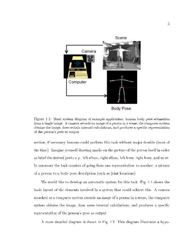
Figure 1.1: Basic system diagram of example application: human body pose estimationfrom a single image. A camera records an image of a person in a scene, the computer systemobtains the image, does certain internal calculations, and produces a speci�c representationof the person's pose as output.

section, if necessary humans could perform this task without major trouble (most of

the time). Imagine yourself drawing marks on the picture of the person itself in order

to label the desired joints e.g., left elbow, right elbow, left knee, right knee, and so on.

In summary the task consists of going from one representation to another: a picture

of a person to a body pose description (such as joint locations).

We would like to develop an automatic system for this task. Fig. 1.1 shows the

basic layout of the elements involved in a system that could achieve this. A camera

attached to a computer system records an image of a person in a scene, the computer

system obtains the image, does some internal calculations, and produces a speci�c

representation of the person's pose as output.

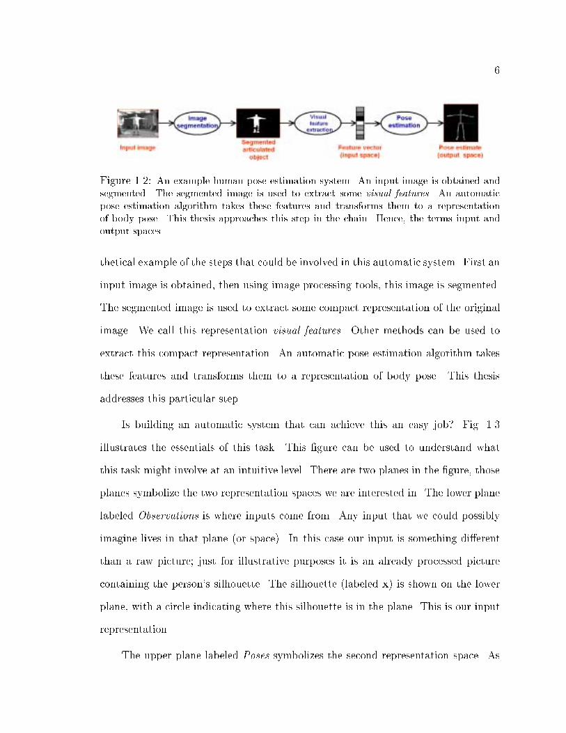
A more detailed diagram is shown in Fig. 1.2. This diagram illustrates a hypo-

6

Figure 1.2: An example human pose estimation system. An input image is obtained andsegmented. The segmented image is used to extract some visual features. An automaticpose estimation algorithm takes these features and transforms them to a representationof body pose. This thesis approaches this step in the chain. Hence, the terms input andoutput spaces.

thetical example of the steps that could be involved in this automatic system. First an

input image is obtained, then using image processing tools, this image is segmented.

The segmented image is used to extract some compact representation of the original

image. We call this representation visual features. Other methods can be used to

extract this compact representation. An automatic pose estimation algorithm takes

these features and transforms them to a representation of body pose. This thesis

addresses this particular step.

Is building an automatic system that can achieve this an easy job? Fig. 1.3

illustrates the essentials of this task. This �gure can be used to understand what

this task might involve at an intuitive level. There are two planes in the �gure, those

planes symbolize the two representation spaces we are interested in. The lower plane

labeled Observations is where inputs come from. Any input that we could possibly

imagine lives in that plane (or space). In this case our input is something di�erent

than a raw picture; just for illustrative purposes it is an already processed picture

containing the person's silhouette. The silhouette (labeled x) is shown on the lower

plane, with a circle indicating where this silhouette is in the plane. This is our input

representation.

The upper plane labeled Poses symbolizes the second representation space. As

7

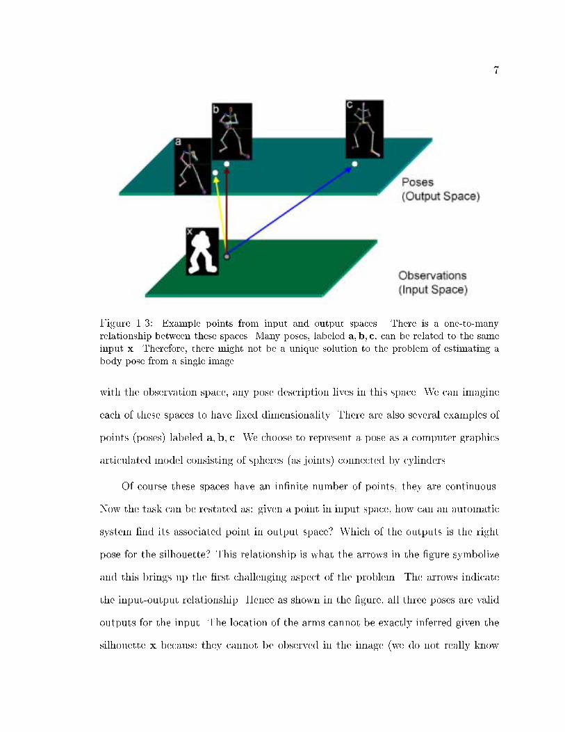
Figure 1.3: Example points from input and output spaces. There is a one-to-manyrelationship between these spaces. Many poses, labeled a;b; c, can be related to the sameinput x. Therefore, there might not be a unique solution to the problem of estimating abody pose from a single image.

with the observation space, any pose description lives in this space. We can imagine

each of these spaces to have �xed dimensionality. There are also several examples of

points (poses) labeled a;b; c. We choose to represent a pose as a computer graphics

articulated model consisting of spheres (as joints) connected by cylinders.

Of course these spaces have an in�nite number of points, they are continuous.

Now the task can be restated as: given a point in input space, how can an automatic

system �nd its associated point in output space? Which of the outputs is the right

pose for the silhouette? This relationship is what the arrows in the �gure symbolize

and this brings up the �rst challenging aspect of the problem. The arrows indicate

the input-output relationship. Hence as shown in the �gure, all three poses are valid

outputs for the input. The location of the arms cannot be exactly inferred given the

silhouette x because they cannot be observed in the image (we do not really know

8

where they are). Therefore a and b are both possible. As for c, this pose is the

re ection of b (it is the same pose but left and right sides of the body have been

swapped and the camera now looks at the posterior rather than at the frontal part of

the body). The joints are swapped with respect to b. In summary, there is nothing

in our observation (the silhouette x) that help us discriminate between these three

possible poses.

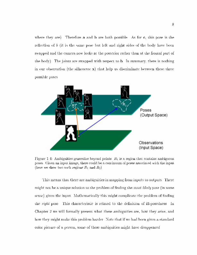
Figure 1.4: Ambiguities generalize beyond points. R1 is a region that contains ambiguousposes. Given an input image, there could be a continuum of poses associated with the input(here we show two such regions R1 and R2).

This means that there are ambiguities in mapping from inputs to outputs. There

might not be a unique solution to the problem of �nding the most-likely pose (in some

sense) given the input. Mathematically this might complicate the problem of �nding

the right pose. This characteristic is related to the de�nition of ill-posedness. In

Chapter 2 we will formally present what these ambiguities are, how they arise, and

how they might make this problem harder. Note that if we had been given a standard

color picture of a person, some of these ambiguities might have disappeared.

9

The ambiguity problem can be more general. Given an input, ambiguities might

extend in a continuum of the output space. Therefore, we could have entire regions

that are valid poses associated with the silhouette. This is shown in Fig. 1.4. In this

�gure we have drawn a region R1 where all poses are valid poses given the observation.

Thus, there might be an in�nite number of ambiguous poses for an input. There can

be many disconnected regions, we have drawn R2 to symbolize a region similar to R1

but for posterior side poses.

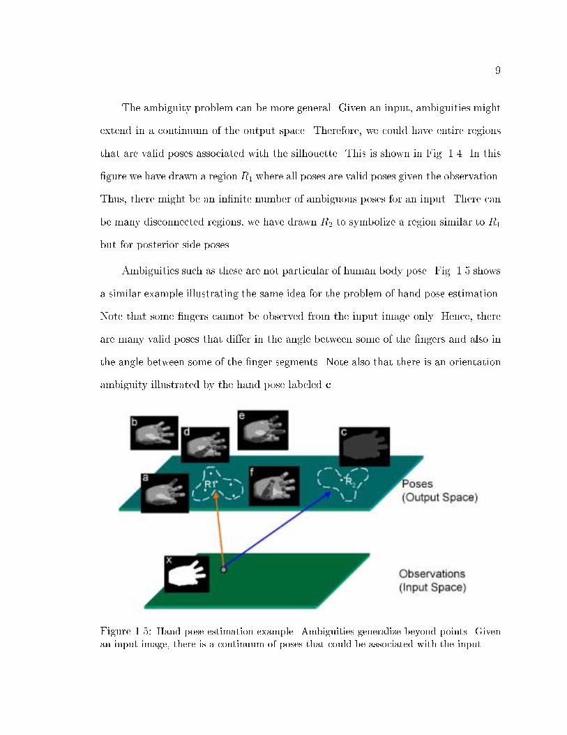
Ambiguities such as these are not particular of human body pose. Fig. 1.5 shows

a similar example illustrating the same idea for the problem of hand pose estimation.

Note that some �ngers cannot be observed from the input image only. Hence, there

are many valid poses that di�er in the angle between some of the �ngers and also in

the angle between some of the �nger segments. Note also that there is an orientation

ambiguity illustrated by the hand pose labeled c.

Figure 1.5: Hand pose estimation example. Ambiguities generalize beyond points. Givenan input image, there is a continuum of poses that could be associated with the input.

10

Before continuing, note that these regions represent a space of valid poses. There

can be many meanings attached to the word valid. A pose could be geometrically

correct in the sense that a projection (in geometric terms) of that pose into an image

would produce a silhouette with features x. However, this pose might not be a valid

human pose. For example a human being cannot twist his arms and shoulders in

certain ways. Hence, given that we are observing a human, not all geometrically

possible poses are probable human poses. This probabilistic aspect of the problem

can be exploited if we want to disambiguate poses.

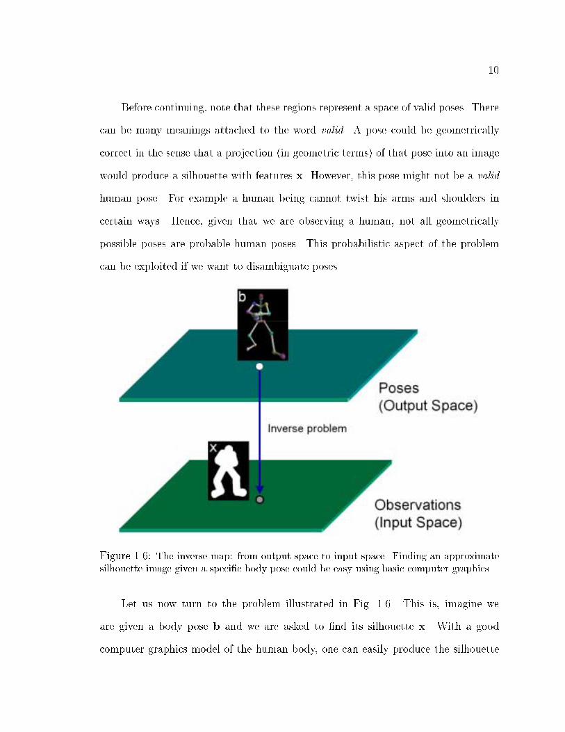
Figure 1.6: The inverse map: from output space to input space. Finding an approximatesilhouette image given a speci�c body pose could be easy using basic computer graphics.

Let us now turn to the problem illustrated in Fig. 1.6. This is, imagine we

are given a body pose b and we are asked to �nd its silhouette x. With a good

computer graphics model of the human body, one can easily produce the silhouette

11

x. Therefore it seems the inverse problem is easy. Thus, perhaps we could use the

fact that the inverse problem is easy in order to help solving our initial problem. Our

initial problem will also be called the forward problem2.

Many real world problems share the property that their inverse problem is simpler

(e.g., speech recognition). In fact, this property is a key part of our problem de�nition

and will play an important role in developing the framework presented in this thesis.

1.3 General Problem De�nition in the Context of

Theory of Function Approximation

Given the above informal introduction, we know may have a notion of the input

and output spaces, the forward and inverse relationships associated with them, and

a few basic di�culties that can arise in the context of our example application. Let

us now de�ne more formally and generally the problem addressed in this thesis.

A common problem in many disciplines is the task of approximating a function,

given a collection of points. Function approximation, regression, and statistical

learning are all similar concepts used in mathematics, statistics, and computer science,

respectively.

We have already mentioned our main application, the problem of obtaining

articulated pose from visual features. However, this problem and many others will be

viewed here as an instance of the more general problem of estimating a function that

2Given this de�nition, one should not confuse this term with the term forward kinematics.

Forward kinematics is another expression (used in robotics) for the function de�ned by our inverse

problem.

12

maps elements of a given (cue / observation) space to another (target / estimation)

space from data. In applications such as vision-based articulated body pose estima-

tion, this function seems to be highly complex, and the mapping is many-to-many;

e.g., the same visual features can represent di�erent body pose con�gurations and

the same body con�gurations can generate di�erent visual features due to clothing,

view-point, etc.

Let us de�ne � <t to be the set of sample data points from the target (or

output) space and � � <c, with the same cardinality as , to be the set of sample

data points from the cue space (or input). Let us assume that for each element i 2

we know its counterpart �i 2 � (i.e., the data is labeled), or that there is a way to

generate �i, for example �i = �( i), for some �. Note that if � is many-to-one, its

inverse does not exist. In function approximation problems, � is not considered part

of the formulation.

Given this, the problem is to approximate a relation (which could be a function),

that we will call � : <c ! <t (not necessarily the inverse of �) that when given

x 2 <c, such that �(y) = x, with x possibly not in �, �(x) estimates y 2 <t such

that y is close to y or x is close to �(y), according to some distance measures.

This problem can be approached in terms of minimizing:

�� = argmin�

lXi=1

�(�(�i)� i); (1.1)

or more commonly using an instance of the previous equation:

�� = argmin�

lXi=1

(�(�i)� i)2; (1.2)

where l is the cardinality of or � [45, 10, 73], and � is an error function, for

example a robust error norm [39]. If � is a function, this is the standard formulation

13

the function approximation problem. The problem of function approximation from

sparse data, sometimes regarded as the general machine learning problem, is known

to be ill-posed [45, 10] if no further constraints are added. For example one can

constrain the function space of � (e.g., if � is constrained to be linear, a unique

solution may exist).

Our problem has two key properties beyond those found in standard function

approximation problems. First, � is one-to-many; one input can be associated with

more than one output. Therefore, this precludes the use of many supervised learning

algorithms that �t a function to the data to uncover the input-output map. Second,

we have access to the inverse map, or a stochastic version thereof. We denote this

map � : <t ! <c. By a stochastic map we mean that in a more general sense, we can

de�ne a probability distribution p(xjh) with h 2 <t and x 2 <c that probabilistically

maps outputs to inputs. We will see that it makes sense to de�ne this distribution

using the deterministic �det, for example p(xjh) = p(xj�deth).

Moreover, this probabilistic notion can also be applied to the relation �. There-

fore, we can generalize our problem to �nding a probabilistic relationship between

inputs x and outputs h, represented by p(hjx). This must be done according to

some probabilistic cost function (i.e., a model). Algorithms for �nding both the

deterministic and probabilistic versions of � will be developed in this thesis. Also,

several ways of constructing and using � will be studied. For ease of notation, both

the deterministic and probabilistic inverse maps will be denoted by � in the rest of

this chapter.

14

1.3.1 Articulated Body Pose from Visual Features

The problem of estimating articulated body pose from visual features can be

cast as an instance of the more general problem de�ned above. By articulated body

we mean a 3D or 2D object composed of a set of rigid parts. 3D marker positions

and orientation of the given object could be obtained using current technology; e.g.,

motion capture, magnetic wearable devices, etc). Following a similar notation to the

one used above, this set is denoted 3d, with 3d � <t.

The visual features generated by the three-dimensional object can be obtained

using a video camera pointed towards the given object. It is clear that these visual

features depend on the camera's intrinsic and extrinsic parameters (e.g., focal length,

skew, camera orientation, location, etc). Alternatively, a computer graphics model of

the 3D object (in our example a human body) can be used to render a set of images.

These images represent the visual appearance of the object in question, given pose

and camera parameters. We call the rendering function R : <t ! I, where I is set

of images at a given resolution. Let us assume, for now, that the camera position

and orientation are �xed. Note that this rendering function (e.g., the computer

graphics rendering of the model) may vary in complexity. Images are an intermediate

representation from which we can extract visual features using a function we denote

by V : I ! <c. Following the de�nitions above, we have:

�( ) = V (R( )); � : <t ! <c; (1.3)

The set �3d � <c is formed by the visual features extracted from the images

of 3d, using �; i.e., the visual features of the projections of the articulated model

viewed from the given camera position. Our goal is to estimate the function denoted

�, as de�ned above. Throughout this thesis, we will usually refer to � directly, rather

15

than to the speci�c V or R functions.

An alternative problem is to recover 2D marker positions, instead of 3D marker

positions, from image features. The 2D projections of the markers can be obtained

from 3d to generate a data set 2d;� � <s of all frames viewed from camera

orientation �, and a distance to the object.

As in the 3D case, we can render 2D marker positions to form an image. This

rendering function will be denoted R : <s ! I, which is a 2D approximation of R.

Note that having the set 3d from which 2d;� was generated, we can obtain a

more accurate rendering by using R on 3d at the appropriate orientation �. When

this is possible, it is reasonable to use R instead of R. To generate visual features

from images, we can proceed as before, using V . In either case, it is always possible

to generate the set �2d;� � <c, which contains the visual features corresponding to

the rendering of the set 2d;�. For notational convenience, we de�ne:

2d =[�

2d;�; (1.4)

�2d can be de�ned similarly. We also have:

�2d( ) = V (R( )); � : <s ! <c; (1.5)

with 2 2d. The problem is to approximate �2d from data. In other words, given

visual features, we want to �nd the 2D marker projections that generated them.

As before, this can be viewed from a probabilistic viewpoint. In this sense, our

problem generalizes to that of not just �nding the marker positions given visual fea-

tures, but that of �nding a distribution over marker positions given visual features. In

fact, if the underlying relationship is one-to-many, a deterministic � would potentially

do a very bad job at mapping inputs to outputs.

16

Also, any of the � functions can be viewed probabilistically. In such a case, given a

body pose, the visual features generated (by using a rendering function for example)

would have a probabilistic nature. In this thesis, we will focus on a probabilistic

problem formulation. Special cases of deterministic (or point) estimate of � and �

will follow from this more general view of the problem.

1.4 Contributions

Original contributions presented in this thesis are in both the �eld of computer

vision and the �eld of machine learning:

� A novel non-linear supervised learning model, named the Specialized Mappings

Architecture (SMA) is presented. The development of this model is given from

a probabilistic perspective.

� Various algorithms for learning and inference in SMA's are developed and tested

using several arti�cial and real data sets of articulated body and hand pose.

� A general probabilistic approach for estimation of articulated body pose from

low level visual features is presented. This approach is di�erent from standard

computer vision approaches for body pose estimation based on the tracking

methodology. The proposed framework models the distribution of body poses

given the input image. Thus, this approach allows the use of single frames and

avoids the need of manual model initialization.

� An approach for multiple-camera articulated pose estimation and self-calibration

is introduced. This formulation introduces the concept of virtual cameras and

17

a probabilistic formulation of the structure from motion problem under articu-

lated pose estimation.

1.5 Structure of The Thesis

In this chapter we introduced the main focus of this thesis. We motivated

and de�ned the problems to be addressed. An illustrative introductory example

is presented in the context of a computer vision problem: body pose estimation from

single images. Some basic elements and properties of the problem were presented in

an informal way. We also provided a more formal general formulation of the problem

addressed in this thesis. This was done in the context of function approximation

and its relation to this thesis. To conclude, the main contributions of this work were

enumerated.

The rest of the thesis is organized as follows: in Chapter 2 we survey the relevant

literature in supervised learning, articulated body representations, and estimation

algorithms, and relate them to this thesis' ideas. We also provide a formulation to

the problem as related to the general function approximation paradigm. In order to

complete the background we give a formal analysis of the kinematic ambiguities in

estimating articulated pose from visual observations, and extend it to the goals of

this thesis.

In Chapter 3 we present the general formulation of the Specialized Mappings

Architecture (SMA). Because of the generality of SMA's, this chapter is written from

a more general supervised learning viewpoint. Almost no reference is made to speci�c

applications or data sets. Applications of this formulation are explained in detail in

Chapter 4. Issues derived from speci�cs of the implementation are also discussed.

18

Chapter 5 extends SMA to handle multiple views. This chapter addresses a

particular vision problem: 3D articulated pose recovery and partial camera self-

calibration given multiple views. A formulation and solution for this problem based

on SMA's is presented. We propose a mechanism to recover 3D pose from a set of 2D

pose hypotheses via multiple-view geometry and alternating minimization algorithms.

Results from chosen SMA applications and other arti�cial data sets along with

quantitative experimental evaluations are described in Chapter 6. Experimental

results for the multiple-view pose estimation problem are also considered. Discussions

of these are provided for each application and experiment.

Chapter 7 provides an overall discussion of the ideas presented in the thesis and

suggests implications and directions for future work.

Parts of the work described in this thesis appear in the following papers:

� R. Rosales and S. Sclaro�. Inferring body pose without tracking body parts.

In Proceedings IEEE Computer Vision and Pattern Recognition, 2000.

� R. Rosales and S. Sclaro�. Specialized mappings and the estimation of body

pose from a single image. In Proceedings IEEE Human Motion Workshop, 2000.

� R. Rosales, V. Athitsos, L. Sigal, and S. Sclaro�. 3D hand pose estimation

using specialized mappings. In Proceedings IEEE International Conference on

Computer Vision, 2001.

� R. Rosales, M. Siddiqui, J. Alon, and S. Sclaro�. Estimating 3D body pose

using uncalibrated cameras. In Proceedings IEEE Computer Vision and Pattern

Recognition, 2001.

19

� R. Rosales and S. Sclaro�. Learning body pose using specialized maps. To

appear in Neural Information Processing Systems 14, 2002.

� R. Rosales and S. Sclaro�. Approximate inference algorithms in specialized

maps. In review, 2002.

Chapter 2

Background and Related Work

In this chapter, we survey the relevant literature. As a supervised learning ar-

chitecture, SMA is related to a series of machine learning approaches. These are

reviewed and related to SMA's in Sec. 2.1. The visual understanding of articulated

body motion and con�guration has been a long-standing goal in computer vision.

Secs. 2.2 and 2.3 survey the most relevant approaches related to those presented

in this thesis. This survey is conducted from a representation and an algorithmic

perspective, respectively. Concluding this chapter, Sec. 2.4 presents a formal analysis

of the problem of articulated pose estimation from a computer vision viewpoint. In

this section, we derive a set of mathematical conditions under which it is possible to

uniquely recover articulated body pose from single images.

2.1 Related Machine Learning Models

In this section we review models related to our proposed architecture for non-

linear supervised learning. A discussion of their di�erences and similarities to our

21

approach will also be presented. A technical summary is given further in Sec. 7.1

once relevant concepts have been introduced. Here we present a general overview of

the related models.

2.1.1 Divide-and-Conquer

SMA's are related to machine learning models [66, 50, 42, 104] that use the

principle of divide-and-conquer to reduce the complexity of the learning problem.

Generally, each of these probably simpler problems is approached using specialized

functions that act as simpler problem solvers.

In general, these algorithms try to �t surfaces to the observed data by (1) splitting

the input space into several regions, and (2) approximating simpler functions to �t

the input-output relationship inside these regions. Sometimes these functions can

be constants, and the regions may be recursively subdivided creating a hierarchy of

functions. Convergence if some divide and conquer algorithms has been reported to

be generally faster than gradient-based neural network optimization algorithms [66].

Notwithstanding the wide applicability of the divide-and-conquer principle. In

supervised learning, the divide process may create a new challenge: how to optimally

partition the problem such that we obtain several sub-problems that can be solved

using the speci�c solver capabilities. These capabilities are related to the form of

mapping functions.

In this sense we can consider [104] as a simpli�cation of our approach, where

the splitting is done at once without considering neither the descriptive power or

characteristics of the mapping functions nor the input-output relationship in the

training set. This gives rise to two independent optimization problems in which input

22

regions are formed and a mapping function is estimated for each region, causing

sub-optimality. In this thesis we generalize these underlying ideas and present a

probabilistic interpretation along with an estimation framework that simultaneously

optimizes both problems. Moreover, we provide a formal justi�cation of this seemingly

ad-hoc method.

In MARS (Multivariate Adaptive Regression Splines) [42] and in CART (Clas-

si�cation and Regression Trees) [23], surfaces are �tted to the data by explicitly

subdividing the input space into nested regions. Once the space is subdivided, simple

surfaces are �tted within the regions. In these approaches, sets of data points are

split to form a partition so that each data point is assigned to one subset. MARS and

CART fall into the so called non-parametric class of function approximation methods.

In both approaches recursive partitioning is the fundamental idea, however an

advantage of MARS is that it produces continuous models with continuous derivatives.

The continuity e�ect is a product of using spline basis functions (truncated power

splines) rather than the standard step functions. This is, in part, responsible for the

increased computational complexity of �tting MARS relative to recursive partitioning.

Although a thought provoking idea, and an interesting step beyond recursive

partitioning, MARS has several main disadvantages. (1) It has bad scalability prop-

erties to higher dimensions. Usually in high dimensional spaces, very large sets of

basis functions are required to capture simple functional relationships in the data.

(2) It is coordinate dependent since cuts cannot be formed at arbitrary orientations

in the input space. (3) It is not designed to model ambiguous inputs or one-to-many

relationships between independent-dependent variables or input-output vectors. This

is a disadvantage that is clearly task dependent. (4) Hard splits, as pointed out by

23

[66], tend to increase the variance of the estimator.

Hierarchical Mixture of Experts (HME)[62, 66] are tree-structure architectures

designed for supervised learning. Similar to the above general description, they

involve dividing the input space into several regions and �tting simple surfaces to

the data in each region. Their hierarchical structure resembles CART [23]. Unlike

CART, the underlying statistical model is a hierarchical mixture, involving mixture

coe�cients and mixture components.

In contrast to MARS and CART, the optimization process of this parametric

model involves soft splits of the data. This is similar to allowing the data to lie

simultaneously in various sub-regions.

The models used for coe�cients and components in HME, are generalized linear

models (GLIM's). The mixture coe�cients are provided by the so called gating net-

works located at the nonterminal nodes of the tree. The components are determined

by the expert networks, located at the leaves. Each region is approximated by an

expert network, implementing a linear model that works as a local regression surface

[66] 1. In summary, given an input x, the gating networks probabilistically determine

what expert network should be used to generate the output. The output is in turn

also probabilistically generated by the experts.

An interesting extension of HME's was presented in [50], the Hierarchical Com-

munity of Experts (HCE). Following the terminology of HME's, an HCE consists of

gating and expert units (called linear units in the HCE terminology), and a hidden

unit layer incorporated between input and output layers. In a generative top-down

view, gating units gate linear units at each layer, but also in uence, probabilistically,

1Partially addressing a concern related to the high variance of this type of architectures [66].

24

the output of all the gating units in the layer below. There is a direct dependency

between gating units in neighboring layers. In HME's gating units at di�erent layers

are conditionally independent with respect to each other.

The main idea is to use a distributed representation of the data points, in which

the outputs are generated by not just one expert unit as in HME's, but by an arbitrary

combination of expert units. MCE incorporates a non-linear selection process that

picks subsets of experts. In an application involving images [50], an image can be

modeled by several experts, each of them producing a given object in the image, while

higher-level experts model interactions or redundancies between image parts.

Note that nothing prevents HME from generating images that consist of several

objects. However, HME's are highly ine�cient at modeling this type of image.

Intuitively, by using HME's a separate expert is required for each combination of

objects.

However, among the drawbacks of HCE, it is no longer feasible to compute

posterior probabilities over hidden nodes in the architecture. In order to address this,

Gibbs sampling was used instead to generate samples from these probabilities [50].

It is clear that a HCE obtains an e�cient compact representation in images with

approximately independently appearing or disappearing objects as in the example

above. However, it is not clear how accurate learning mechanisms could be for this

architecture. In addition, it is not clear how advantageous this architecture (over

HME's for example) is when the structure of the data is not so obviously convenient

for this model, such as the image example.

Several other approaches underlying the divide-and-conquer principle include [22,

49]. Non-linear surfaces are estimated from data in [22]. The surface is approximated

25

by a set of local linear patches. These patches are initially determined using PCA

on point subsets obtained using K-means clustering, and later re�ned using the EM

algorithm.

This work [22] did not provide a statistical basis to justify the approach taken.

It turns out that a well founded procedure for achieving this approach is formally

justi�ed by assuming the data is distributed with a mixture of Gaussians probability

density function.

A similar approach was taken in this case by [49], to model hand-written digits.

A mixture of linear sub-models is learned for each digit. Recognition is performed

by choosing the digit class with the highest probability given an input image. This

was a supervised classi�cation task in which each class is trained independently of

the others. Regression was not considered in this work.

2.1.2 Feedback Models

In Chapter 3 we will see that the model presented here cannot be simply for-

malized as a purely forward or unidirectional generative model. These models are

more generally called Bayes Networks [90]. Feedback models are those in which

there are two interacting processes, one relating inputs to outputs, and another one

relating output to inputs. This interaction can be at any scale, thus the model

behavior depends on both processes. A related idea in neuroscience is analysis by

synthesis [83, 33], in which it is thought that the visual cortex may have a generative

model of the world, and recognition involves inverting that model. Other related and

antagonistic theories have also been proposed, for example those based more heavily

on 2D representations [24, 115, 40] and more generally [111, 28, 84].

26

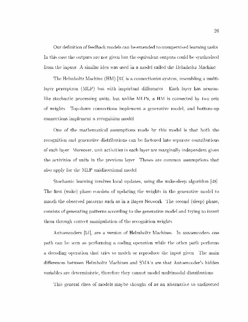
Our de�nition of feedback models can be extended to unsupervised learning tasks.

In this case the outputs are not given but the equivalent outputs could be synthesized

from the inputs. A similar idea was used in a model called the Helmholtz Machine.

The Helmholtz Machine (HM) [33] is a connectionist system, resembling a multi-

layer perceptron (MLP) but with important di�erences. Each layer has neuron-

like stochastic processing units, but unlike MLPs, a HM is connected by two sets

of weights. Top-down connections implement a generative model, and bottom-up

connections implement a recognition model.

One of the mathematical assumptions made by this model is that both the

recognition and generative distributions can be factored into separate contributions

of each layer. Moreover, unit activities in each layer are marginally independent given

the activities of units in the previous layer. Theses are common assumptions that

also apply for the MLP unidirectional model.

Stochastic learning involves local updates, using the wake-sleep algorithm [48].

The �rst (wake) phase consists of updating the weights in the generative model to

match the observed patterns such as in a Bayes Network. The second (sleep) phase,

consists of generating patterns according to the generative model and trying to invert

them through correct manipulation of the recognition weights.

Autoencoders [51], are a version of Helmholtz Machines. In autoencoders one

path can be seen as performing a coding operation while the other path performs

a decoding operation that tries to match or reproduce the input given. The main

di�erences between Helmholtz Machines and SMA's are that Autoencoder's hidden

variables are deterministic, therefore they cannot model multimodal distributions.

This general class of models maybe thought of as an alternative to undirected

27

models or Markov random �elds (MRF), such as the Boltzmann Machine [1].

Given the existence of Boltzmann Machines, one may ask, why not use a Boltz-

mann Machine instead of conceiving these directed models? There are problems

with Boltzmann Machines since need to apply sampling methods for learning and

inference. Sampling is usually a delicate task because one usually does not know

when it is enough [79]. The update learning rule may not be accurate also in many

cases [33]. Therefore, a motivation for two-way unidirectional models comes from

the fact that formulating this explicit path separation makes these models simpler

computationally, over similarly structured MRFs.

Another related approach is the Adaptive Resonance Theory (ART) Networks

[25]. In ART, usually two layers of neurons are connected by two sets of bottom-up

and top-down weights. Units in the input layer receive activations from the input

vectors as well as feedback from the second layer. The units in the second layer can

interact among themselves. The task of each network is very similar to a nearest

neighbor classi�cation algorithm using correlation as distance function. The goal is

to classify the input pattern into one of a series of self-organized categories. This

number of categories can increase depending on the patterns presented and other

parameters of the network. A key di�erence with our proposed approach is that the

ART approach does not consider learning as a statistical problem.

2.2 Representation in Articulated Pose Estimation

We now direct our attention to related work in the computer vision literature.

Visual tracking of articulated bodies has received a great deal of research attention

in the computer vision community [7, 101, 76, 119, 58, 69, 43, 91, 97, 67, 94, 21] and

28

more recently in machine learning [89, 85, 19, 76, 101]

Approaches vary from tracking rough body position on the image plane (for

example as a blob, recovering center of mass or bounding contour), to estimating

body pose as represented by each body part in 3D. Tracking human bodies and hands

has been the main focus of attention due to the great number of applications derived.

In order to place this work in a more general context, we classify the approaches

undertaken in this area in several groups taking into account, representational di�er-

ences in both input and output signals; and di�erences in the underlying algorithms

employed.

2.2.1 Taxonomy According to Input Representation

An intuitive way to group related approaches is by describing the visual input

characteristics on which they are based. We have divided the visual input representa-

tions commonly used into three major groups: binary features, textured-based, and

high-level inputs. Fig. 2.1 shows several of the input representations discussed next.

In this context, it is adequate to explain the notion of blobs in computer vision,

an intermediate representation derived from images. In general, blobs are regarded

as a collection of neighboring pixels that share a common property that di�erentiates

them from their surrounding pixels (e.g., color, contrast, texture, motion, etc). Blobs

are easy to understand at an intuitive level, perhaps because their properties can be

related to standard physical properties of everyday objects, such as area, volume,

width, etc, although some other properties such as moments (e.g., Hu moments

[55]) do not have an intuitive physical analogue. In our taxonomy, blobs have close

connection with binary and texture-based image features.

29

Common binary features include silhouettes, contours, edges, blob maps (i.e.,

binary blobs), and other representations derived from them e.g., low-order statistics,

distance transforms, moments, contour curvature, etc. Binary features or functions

thereof are low-level visual descriptors that involve (probably as an intermediate step)

assigning a binary value to each pixel in the image. They are usually obtained after

processing the original color or gray image to produce a binary image, sub-image,

or other binary descriptor. Once this binary representation is obtained then features

are extracted; but keep in mind that the binary image itself could be the feature

representation intended. In our taxonomy, they are usually the easiest to extract

from images.

Binary blobs and their features were used in [96, 101, 92, 52, 7, 32, 59, 119], for

example for detection [104, 19, 7, 119, 59, 92], as shown in Fig. 2.1(a), and matching

[101, 52, 57, 118], shown in Fig. 2.1(a)(b)(c)). As for edges and image contours, they

have been incorporated as a front-end for basic tracking and matching [44, 56, 36], as

in Fig. 2.1(d), for learned motion models [61, 16], Fig. 2.1(e), and 3D pose estimation

of body parts [46, 68] or the full body [43].

The main disadvantages of binary descriptors include the seemingly low informa-

tion content. The descriptors may convey little about variables such as 3D body pose

or motion classes. The process that assigns a binary value to pixels may potentially

discard a lot of useful information about the random variable of study. However, such

low-level representations have proven to be useful for simple detection and matching

tasks.

An alternative class of input representations is texture-based; such as optical

ow, texture regions, and many forms of �lter response outputs. Texture-based

30

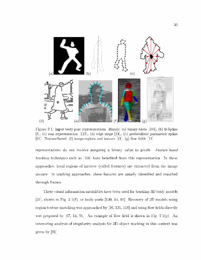
(a) (b) (c)

(d) (e) (f) (g)

Figure 2.1: Input body pose representations. Binary: (a) binary blobs [104], (b) B-Spline[8], (c) star representation [119], (d) edge maps [44], (e) probabilistic parametric spline

[61]. Texture-based: (f) image-regions and texture [21], (g) ow �elds [13].

representations do not involve assigning a binary value to pixels. Feature-based

tracking techniques such as [106] have bene�ted from this representation. In these

approaches, local regions of interest (called features) are extracted from the image

texture. In tracking approaches, these features are usually identi�ed and matched

through frames.

These visual information modalities have been used for tracking 3D body models

[21], shown in Fig. 2.1(f), or body parts [120, 94, 91]. Recovery of 2D models using

region texture matching was approached by [26, 121, 118] and using ow �elds directly

was proposed by [67, 14, 91]. An example of ow �eld is shown in Fig. 2.1(g). An

interesting analysis of singularity analysis for 3D object tracking in this context was

given by [81].

31

Texture-based inputs are, in general, more informative about 3D body pose or

motion. In most cases binary features can be deterministically obtained from texture-

based inputs. However, a limitation of approaches that employ texture-based visual

inputs is that manual initialization or model placement is required. Also, texture-

based methods rely heavily on the constant brightness assumption, which does not

make them well-suited for tracking or detecting articulated objects. Also, image ow

is di�cult to obtain at low resolution or for fast moving objects. In summary, in

texture-based methods, the increase of information content in the observed variable

comes at a cost. This cost is related mainly to two aspects: (1) the assumptions

about the image that are necessary to make (e.g., constant brightness assumption)

and (2) the usually higher complexity and lower accuracy of the algorithms required to

extract these features relative to extracting binary features. An important aspect from

a modeling perspective is that it is usually harder to (1) �nd suitable mathematical

models for texture-based feature variables or (2) relate them to the desired output

(i.e., extract the important information).

The third class of input representation is that of higher-level inputs. The key

distinguishing characteristic of this input class is that it is no longer a low-level vision

representation. Speci�cally, this input representation cannot be associated directly

to general image properties (e.g., such as image motion, texture, edges, and others

studied above), but potentially to image properties that are speci�c of the problem

of study. Obtaining these representations usually involves the use of new algorithms.

However, sometimes vision problems are formulated assuming this input was already

obtained.

Higher-level features are even harder to obtain by automatic systems in general

(relative to those representations mentioned above). They may include information

32

about locations of speci�c body parts. Such an input representation was �rst studied

in psychophysical experiments [63], where moving lights were attached to human body

parts. In these experiments human observers could infer a higher-level representation

of body pose, and even identify known motions.

Computer vision approaches that include higher-level representations include [54]

which used 2D joint locations found by another tracking system to produce 3D joint

con�gurations of a human body; ambiguities in body pose were circumvented by

using a learned mapping of 2D motion to 3D human body con�guration. For 3D pose

estimation (up to scale) from static images, [5, 112, 75] used a series of user-positioned

feature points; these points were located at several prede�ned body joints.

Higher-level features such as those described are very informative about 3D body

pose. Moreover, they are designed to encode only the relevant information about the

problem. However, they limit the usability of the approach because such features

cannot be extracted automatically in general.

Note that in this review we do not consider the problem of feature selection.

This is a research problem per se. See [72, 71, 29] for interesting related discussions.

2.2.2 Taxonomy According to Output Representation

After reviewing the di�erent classes of input representations, we now study

classes of output representations. A useful classi�cation of vision-based articulated

pose estimation systems can be made in terms of the descriptive level of the repre-

sentation that they intend to achieve. In this context, we simply classify approaches

into low-, mid-, and high-level description approaches. For clarity, it is good to point

out that in the approach presented in this thesis, body pose is de�ned via a high-

33

level description of the articulated object/body (e.g., in terms of joint locations).

However, for generality we consider and brie y review approaches that produce low-

level and mid-level descriptions of body pose. Fig. 2.2 shows some of the common

representations used for modeling body pose.

As its name suggests, low-level description approaches represent a body pose in

terms of low-level visual features or functions of these features. Example low-level

visual features commonly used include contours, silhouettes, and low order statistics

thereof; for example mean, principal axis, etc.

Some approaches in this category include [57, 100, 18, 53], as shown in Fig. 2.2(a),

where blobs corresponding to humans are segmented and tracked. These methods

rely on standard image processing tools, plus some heuristics or simple statistical

models on image brightness (e.g., for background subtraction or blob matching among

frames), or on object shape. Other low-level output descriptions include [60, 15], as

shown in Fig. 2.2(b) where slightly more complex statistical models based on contours

were employed in learning distributions of motion classes. These distributions then

form a prior used in tracking. Even at the lowest-level of representation, pose

estimation is still considered a di�cult task in partly constrained environments.

Mid-level descriptions tend to be view-based. They provide motion information

without necessarily indicating or discovering body part location, or joint con�gura-

tions. For example, in [92] recognition of repetitive body motion was achieved via

bottom-up processing, without identifying speci�c parts or classifying the object. In

order to recognize the motion, a feature vector of motion magnitudes directly mea-

sured on an image grid was computed and compared with stored patterns. A exible

model representation of the human body [8], as shown in Fig. 2.2(c) was obtained by

34

using a basic segmentation procedure consisting of background subtraction and then

�tting a B-spline to the segmented blob.

Other models of deformation, in this case a�ne models, were used in [14], by

considering motions at di�erent prede�ned locations on the object. Another view-

based technique for representing and recognizing human actions was proposed in [32],

where temporal templates called Motion History Images (MHI) and Motion Energy

Images (MEI) were employed. Other examples of mid-level descriptions are proposed

in [13, 14].

Mid-level descriptions tend to be coarse, and are therefore unsuitable for our

goals. They involve recognition of a �nite number of motion classes. Even though

recognizing a given motion is an important problem, it has severe limitations. One

of them is its ill-suitability for synthesis, for example for character animation. In

this thesis, we are interested in more detailed body pose such as the one provided by

high-level descriptions.

High-level descriptions of body pose are those based on labeled articulated body

joint information or body part representations such as joint angles, joint locations, or

body part labeling, either in 2D or 3D.

Starting at the coarsest level, in the representation used by [119], blobs were

designed to represent rough body part location, as shown in Fig. 2.2(d). These blobs

were tracked given the segmented images. In general, most high-level representations

are model-based. These models are generally articulated bodies comprised of 2D or

3D primitives. The 2D models include the prismatic model in [26], which incorporates

a length and orientation parameter per limb, as shown in Fig. 2.2(e). Another repre-

sentation in this category includes the cardboard model used in [67], that assumes a

35

at human body, as shown in Fig. 2.2(f). A description in terms of eleven 2D joint

locations was presented in [104], as in the example shown in Fig. 2.2(g); even though

there are more degrees of freedom (DOF) in a human body, these eleven DOF were

used for their descriptive representation of body pose and for numerical convenience.

Other high-level output representations employ 3D solid primitives, i.e., articu-

lated models of a rather complete human body such as [85, 37, 19, 54, 21, 118, 43],

as illustrated in Fig. 2.2(h)(i). These representations include information about joint

locations or joint angles, as well as some parameters that control the volume of

the solids used. Volume is determined usually by cylinders [85, 21, 52, 96] and

superquadrics [68, 43]). The volume parameter is sometimes set in advance according

to the expected volume of the tracked object.

Interestingly, several models based on joint location or joint angles do not require

these volume parameters [102, 19, 54, 109], because they use di�erent approaches to

pose estimation (Sec. 2.3.1). Examples of such models are shown in Fig. 2.2(g)(h),.

A key distinguishing representational and moreover numerical issue in [21] was the

use of exponential maps for representing joint angles.

Similar articulated hand models have been used by [99, 122, 107, 47, 94] for pose

estimation, and in [117, 77] for recognition. Moreover, body parts such as arms have

been modeled in similar ways [69].

In order to avoid the so called curse of dimensionality [9]2, these high-dimensional

spaces are sometimes reduced to lower dimensions through some form of dimension-

ality reduction, most commonly Principal Components Analysis (PCA) [78, 64].

2This term is used to express the fact that an exponentially increasing number of data points are

needed to densely populate Euclidean spaces of increasing dimension.

36

The main advantages of high-level representations are: (1) they provide strong

constraints for image matching during tracking; (2) they can sometimes account for

self-occlusion due to the strong structure prior provided by the model; (3) they can

provide a simple representation of rough object appearance. However, the main

disadvantages are (1) the need for manual initialization, because it is hard to auto-

matically place the model in the required accurate way; (2) the matching of the model

to the image usually requires non-linear optimization; (3) the model is designed for

a speci�c object class, and even within the same class, it cannot account for within

class variations (such as limb proportions, volume, etc.).

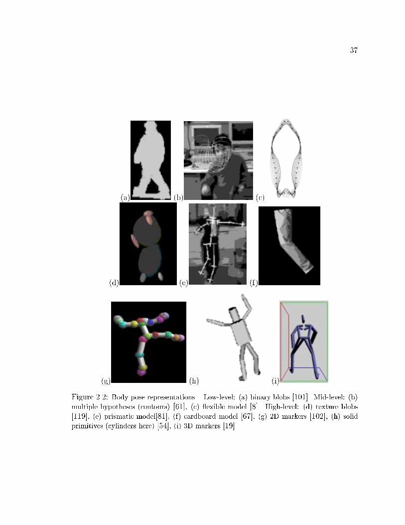
37

(a) (b) (c)

(d) (e) (f)

(g) (h) (i)

Figure 2.2: Body pose representations. Low-level: (a) binary blobs [101]. Mid-level: (b)

multiple hypotheses (contours) [61], (c) exible model [8]. High-level: (d) texture blobs

[119], (e) prismatic model[81], (f) cardboard model [67], (g) 2D markers [102], (h) solidprimitives (cylinders here) [54], (i) 3D markers [19].

38

2.3 Articulated Body Pose Estimation Approaches

In the previous section, we focussed on the input and output representations

employed in articulated body pose estimation systems. In both cases, the resulting

taxonomy ranged from low to high-level. We will now concentrate on approaches that

recover high-level representations of body pose since these are most closely related to

the framework proposed in this thesis. High-level representations are usually at the

level of joint or part con�gurations.

2.3.1 Tracking vs. Non-Tracking Approaches

To Track...

In computer vision, the task of recovering articulated body pose from images is

usually posed as a tracking problem (e.g., [4]). Tracking of motion in image sequences

is a well-established area of computer vision. Articulated body tracking is typically

approached by using models comprised of 2D or 3D geometric primitives. As discussed

above, these models are composed of a series of parts representing the high-level

structure of the object.

These models are object dependent, in the sense that they are designed for

tracking a speci�c class of articulated bodies [85, 37, 21, 94]. At each frame, these

models are �tted to the image to optimize some cost function that favors the overlap

of model and associated image regions (or motion). In other words, image motion is

explained by the parameterized motion of the 3D articulated model. In this form,

image motion is constrained to lie on the manifold of permissible model motions.

Other forms of constraining image motion during tracking include [13, 14]. In

39

this set of approaches, a motion subspace is learned from a set of examples. These

examples and the model (usually linear) are hoped to be su�cient to span the set of

possible motions that may be seen during tracking.

In these models, careful manual placement of the model on the �rst frame

is required, and tracking in subsequent frames tends to be sensitive to errors in

initialization and numerical drift.

Generally, these systems cannot recover from tracking errors in the middle of a

sequence. To address these weaknesses, more complex dynamic models have been

proposed [89, 85, 26, 60]; these methods learn a prior over some speci�c motion,

such as walking. This strong prior however, substantially limits the generality of the

motions that can be tracked.

... Or Not To Track

The main di�erence in our proposed approach with respect to the model-based

techniques mentioned above is that we do not try to match a body model directly to

the image. In our approach, we avoid matching image features from frame to frame

(e.g., image regions, points, articulated models). Therefore, we do not refer to our

approach as tracking.

There is a series of approaches that also depart from the aforementioned tracking

paradigm. In [54] a statistical approach was employed in reconstructing the three-

dimensional motions of a human �gure. It consisted of building a Gaussian probability

model for short human motion sequences. This method assumes that 2D tracking of

joints in the image is given; however, this assumption implicitly incurs the restrictions

also found in all tracking approaches.

40

In [109] dynamic programming was used to calculate the best global labeling of

image points to prede�ned body joints according to the learned joint probability

density function of the position and velocity of body features. The probability

function was de�ned by a triangulated acyclic graph. This representation was key

to making inference feasible 3 [90, 65]. Still, in this approach, the image points and

model initialization must be provided by hand or through some other method.

In [19], the manifold of human body dynamics was modeled via a hidden Markov

model and learned via entropic minimization. Once the states are inferred from

observations, a quadratic cost function is used to generate a path in con�guration

space.

In all of these non-tracking approaches, models of motion were estimated from

data. Although the approach presented in this thesis can be used to model dynamics,

we argue that when general human motion dynamics are to be learned, the amount

of training data, model complexity, and computational resources required are im-

practical. As a consequence, models with unacceptably large priors towards speci�c

motions are generated; the most common motions are walking and single gestures.

Even though by not modeling the dynamics we are ignoring information (i.e.,

the motion component) that can be useful for constraining the reconstruction process,

there are some bene�ts. A model for inferring body pose that does not model

dynamics provides invariance with respect to speed (i.e., sampling di�erences) and

direction in which motions are performed. This happens simply because this model

treats con�gurations as temporally independent of each other.

In this thesis, a single image has been used along with prede�ned three-dimensional

3Exact inference is feasible in triangulated acyclic graphs because of the running intersection

property [65].

41

body models in the estimation of human body pose. Because of the use of a single

image, no tracking nor dynamics modeling is involved. Approaches using this idea

include [5, 112, 75, 86]; however, most of these methods also require that projected

joint locations be given as input.

In our approach, we learn to map visual features to likely body con�gurations.

Following a machine learning paradigm, functions that map visual features to pose

parameters are approximated from training data. A very distinctive aspect of our

approach is also the feedback (forward kinematics) matching process used. This

process transforms the reconstructed con�gurations back to the visual observation

space to choose among a set of reconstruction hypotheses. Our approach avoids the

need for manual initialization and tracking per se, and therefore avoids the subsequent

disadvantages of tracking.

2.3.2 Models and Exemplars

As with many other computer vision approaches or machine learning in general

one can divide previous articulated body pose estimation approaches into model-

based and an exemplar based-approaches. Sometimes these approaches are regarded

also as parametric and non-parametric models.

From this stand-point, model-based approaches are those that form a repre-

sentation of the world (the body pose world in our case) with an underlying prior

on what the world looks like. This prior can be represented as a functional form.

For example, a family of probability distributions (e.g., the exponential family) for

statistical models, a neural network topology for function approximation models, a

Markov random �eld compatibility matrix or neighborhood system for a statistical

42

physics representation, etc.

At the other end of the spectrum, there are purely exemplar-based approaches.

This class of approaches is built solely on the exemplars it has seen during training

and no prior underlying structure of the space is incorporated in the process (however,

there is a way to see exemplar-based approaches as an extreme form of model-based

approaches). For example an exemplar representation can be formed simply by a

subset of the training examples seen. As a consequence, this representation lacks

continuous structure. A simple general example is the standard form of the K-nearest

neighbors representation.

Standard algorithms exist for estimating the parameters of both types of models.

Model-based algorithms can use the advantages of continuous space representations.

Exemplar-based models cannot since estimation is tied more closely to discrete opti-

mization algorithms.

Model-based approaches can model many samples in a very e�cient sparse man-

ner if these samples agree with the underlying functional form chosen. Exemplar-

based approaches need to represent all these examples explicitly; therefore the de-

scription length for a representation that encodes the same articulated bodies can be

considerably bigger than that needed in a model-based approach. However, model-

based approaches require the choice of their functional form (what the world should

look like). Some assumptions can be made; for example, we live in a smooth con-

tinuous world. Physically-based models are common because of this. However, it is

usually hard to go further and try to automatically �nd the structure of the world.

This was in fact proven to be an NP-hard problem [31]. Many approaches have tried

to deal with this issue, e.g., [27, 31, 20, 80, 110].

43

For spaces whose underlying structure is almost completely unknown, or believed

to be complicated, then exemplar-based representations o�er an alternative because

they can represent highly non-linear manifolds. In body pose estimation, exemplar-

based representations avoid the use of explicit models to describe the body poses

given the observations and the priors on poses. In this case a model-based approach

would use, for example, a 3D articulated model or would de�ne a form on the prior

distribution of poses.

In body pose estimation, examples of model-based representations include most

of the model-based tracking approaches already discussed [89, 85, 102, 26, 19]. All

of these models are based on some form of functional prior, e.g., a linear dynamical

system, a speci�ed form of probability model, speci�ed physical laws, etc.

Classic examples of exemplar-based representations include the pedestrian detec-

tion system of [44]. In this approach, an image with potential pedestrians is compared

with stored templates of pedestrians built at di�erent scales and locations. The

problem reduces to that of �nding a prototype which is close enough to the observed

image. In [32] human motion is compared with prototypes stored in a database in

order to classify the type of motion. In addition, the body tracking approach of

[114] can be thought of as model-based even though some components (the pose

transformations) are speci�ed from a continuous set. This approach presented an

interesting formalization of the problem of exemplar-based tracking.

Not all articulated body pose approaches are easily classi�ed as either model-

based or exemplar-based. For example, in [60] a probability distribution of the model

state is represented by exemplars, but the underlying dynamical model is continuous.

Another example is [19], where mean poses given by the HMM states during inference

44

can be thought of as exemplars that are to be blended to construct a trajectory in

body con�guration-velocity space. The methods proposed in this thesis tend towards

the side of model-based approaches during learning. However, this model is then used

to compute exemplars used in pose inference.

2.4 On Visual Ambiguities in Articulated Objects

So far we have studied di�erent approaches and representations for estimating

articulated body pose. However, we have not yet studied when it is possible to

achieve the goal of uniquely estimating 2D or 3D body pose from visual features.

In this section, based on [81], we start from the basic idea that kinematics provides

a fundamental constraint in the motion of articulated bodies (e.g., [68, 94, 52]).

Therefore, it is worthwhile to analyze the singularities of the kinematic models used

to constrain the visually perceived motion. We can then generalize to cases in which

tracking is not involved explicitly.

One can think of kinematics as a way to specify the mapping between body pose

and visual features (<t and <c respectively). This is one of the central topics of this

thesis. However, in kinematic models normally used in vision, this map is de�ned

� = V � R : <t ! <c, with V : I ! <c and R : <t ! I. This notation was

already introduced in Sec. 1.3.1. In order to facilitate our analysis in this section, we

further de�ne R as R = PG. This is, we have made our rendering R function to be

the product of the kinematics function G and the projection matrix P . The reasons

for this more detailed de�nition are the separation of the contributions of these two

elements of R, and will be clear in the next equation.

In this thesis, even though � is incorporated in the formulation, we devote most

45

of our e�ort to �nding the inverse: one or more maps � : <c ! <t.

In this section we study some of the theoretical properties of the map � under

the kinematics model G. Using G, most kinematics based approaches for body pose

estimation de�ne a cost function over <t and minimize it. This cost function normally

represents the residual error when registering the model with the visual features (e.g.,

ow, edges, etc). For example,

Dj(q) = Ij(q)� Ij (2.1)

Ij(q) = I(PG(q;pj)) (2.2)

where Dj is the residual at pixel j, q 2 <t, Ij(q) is the model pixel j given a q,

Ij is the input image at j, P is the camera projection matrix, G is the non-linear

kinematics model. The function G takes a pose q and a point in 3D (relative to

the link) and tells what point in 3D (with respect the camera coordinate system, for

example) it represents. Therefore, pj is the 3D point related to pixel Ij. This is

shown in Fig. 2.3.

Tracking methods usually minimize the squared error E(q) = D>D, with D =

D1; :::; DP , using gradient information. Now, let's say we are at q0. The residual

gradient for pixel j is:

_Dj(q0) = [@Dj

@q(q0)] _q = Jj _q (2.3)

Jj =@Dj

@q= (rIj)

>P@G

@q(q0;pj) (2.4)

We see that if a given residual change is in _r 2 N (J>) (the left null space) then

that residual will never be produced by changes in a pose (from q0). This yields a

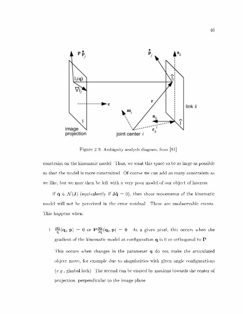
46

Figure 2.3: Ambiguity analysis diagram, from [81].

constraint on the kinematic model. Thus, we want this space to be as large as possible

so that the model is more constrained. Of course we can add as many constraints as

we like, but we may then be left with a very poor model of our object of interest.

If _q 2 N (J) (equivalently if J _q = 0), then those movements of the kinematic

model will not be perceived in the error residual. These are unobservable events.

This happens when:

1. @Gq(q0;p) = 0 or P@G

@q(q0;p) = 0. At a given pixel, this occurs when the

gradient of the kinematic model at con�guration q is 0 or orthogonal to P.

This occurs when changes in the parameter q do not make the articulated

object move, for example due to singularities with given angle con�gurations

(e.g., gimbal lock). The second can be caused by motions towards the center of

projection, perpendicular to the image plane.

47

2. (rI)> and P @Gq(q0;p) are orthogonal. This occurs when the gradient ofG does

not provide a constraint related to the image features (e.g., due to the aperture

problem).

In the case when the gradient of the residual error is not used to infer the body

pose (e.g., in non-tracking approaches) we can derive from the above that two poses

q1 and q2 cannot be distinguished if (q1 � q2) 2 N (J) or:

1. P (Gq1 � Gq2) = 0; when a pose can be described by two di�erent sets of

parameters or when projections of these poses are equal.

2. (rI)> and P (q1 � q2) are orthogonal; when two di�erent poses project to an

image that produces the same image features. For example, when poses di�er

in parts that cannot be seen in the image under the current view-point. Any

form of occlusion under the given visual feature would su�ce for this to happen.

Note that these poses may produce di�erent images and same features. This

gives us a theoretical insight into the role of the feature space.

48

2.5 Summary

Tracking is normally seen as the problem of matching, from frame to frame,

image features to the geometric model of interest (e.g., an articulated object model).

There are many methods for performing tracking in this sense. However, in general

these methods (1) require manual initialization or model placement, (2) tend to rely

on iterative nonlinear optimization or sampling techniques at every frame, (3) are

object-dependent (i.e., we have to build speci�c constraints for each class of artic-

ulated object that we desire to track), and (4) tend to be sensitive to the accuracy

at all frames, and therefore not robust to errors in the middle of a sequence. In

addition, most models are based on simple heuristics, or based only on camera ge-

ometry concepts that exclude probabilistic interpretations of the underlying process.

Probabilistic models are normally easier to study because: (1) it is simpler to identify

the assumptions or approximations made; one consequence of this is that it is easier to

predict the behavior of a system, or at least there exists a framework for its analysis;

and more importantly (2) the nature of the observed signal is almost always of a

probabilistic nature.

Probabilistic models for performing tracking have also been proposed. Most of

them have concentrated on modeling the dynamics of motion. For given applications

they are more realistic than those that only model the con�guration space (static

con�gurations). However, most of these models tend to form too strong priors that

favor speci�c motions (training sequences). Even though they are realistic models,

in practice their modeling power of the con�guration space is considerably limited.

They are therefore not general enough, and their usage is constrained to a smaller

set of situations. They are limited by the fact that in theory, one needs an exponen-

49

tially higher number of data points to model a higher-dimensional space. Moreover,

there are many cases in which one can only observe single images, not a continuous

sequence of them. In this thesis, we do not model dynamics, and claim that there is

enough structure in the static con�gurations given the observations for the problem

of articulated pose estimation to be solved. There are previous methods that use a

single image to perform pose estimation; however, they usually require considerable

user interaction, and are therefore not fully-automatic.

We have also reviewed many previous supervised learning methods. Something

common in these methods is that they try to discover the process that generated the

training outputs given the inputs. However, these methods do not incorporate the

structure of the visual tracking problem at hand. Speci�cally, they do not incorporate

the fact that the inverse map, or an approximate version thereof, can be computed

easily for this class of problems. In this thesis, we will see that this can at least reduce

model complexity and ease inference. Also, some other supervised learning models

cannot uncover one-to-many mappings. Given that visual estimation of body pose is

inherently ambiguous, we are required to be able to model one-to-many mappings.

Introducing a fully probabilistic approach in this context, under these requirements,

is achieved in this thesis.

As for uniqueness of the estimated body pose, the analysis presented in Sec. 2.4

tells us that there exist certain visual ambiguities. Because of these ambiguities,

certain body poses cannot be distinguished from others given the observed visual

features. In this thesis, we provide solutions for body pose estimation in which this

issue is addressed probabilistically.

Learning in the Specialized Mappings Architecture (SMA) follows the path of

50

latent variable models, preserving the probabilistic properties of this framework. The

SMA is developed on general (e.g., non-linear) forms of conditional distributions

under this model. The SMA also allows the use of alternative forms of the model's

joint probability distribution, which are derived from the availability of the inverse

map. The inverse map allows us to de�ne a di�erent set of conditional independence

assumptions. Such conditional independence assumptions can simplify the model

complexity; e.g., structure and number of parameters. Inference is based on the

use of the inverse map, and therefore it can make use of a new set of probabilistic

dependences as well. These dependencies are used to simplify the computations and

tend to make the model estimates more accurate.

Chapter 3

Specialized Mappings Architecture

3.1 Introduction

In this section we present the general formulation of a nonlinear supervised

learning model that we have called the Specialized Mappings Architecture (SMA). We

will start by de�ning characteristics of the problem at hand. A probabilistic model

for the architecture will then be formalized along with a mechanism for learning its

parameters. The SMA consists of several specialized forward mapping functions that

are estimated automatically from training data. Each function maps certain domains

of the input space (image features) onto the output space (body pose parameters).

The �rst key algorithmic issue is learning the specialized domains and mapping

functions in an optimal way. The solution to this learning problem employs a variant

of the Expectation-Maximization algorithm. The second key issue is formulating the

inference process in a way that takes advantage of the characteristics of the problem1.

1A condensed version of this material was presented in [103, 102].

52

3.2 Specialized Maps

There at least two key characteristics of the problem we are trying to solve which

make it di�erent from other supervised learning problems. First, we have access to

the inverse map. We are trying to learn unknown probabilistic maps from inputs

to outputs space, but we have access to the map from outputs to inputs. In our

pose estimation problem, it is easy to see how we can arti�cially produce some visual

features (e.g., body silhouettes) given joint positions (forward kinematics), using

computer graphics (CG). Second, it is one-to-many: one input can be associated

with more than one output. Features obtained from silhouettes (and many other

visual features) are ambiguous. Consider an occluded arm, or the re ective ambiguity

generated by symmetric poses. This last observation precludes the use of standard

algorithms for supervised learning that �t a single mapping function to the data.

Given input and output spaces <c and <t, and the inverse function � : <t ! <c,

we describe a solution for these supervised learning problems 2. Our approach consists

of generating a series of m functions �k : <c ! <t. Each of these functions is

specialized to map only certain inputs (for a specialized sub-domain) better than

others. For example, each sub-domain can be a region of the input space. However,

the specialized sub-domain of �k can be more general than just a connected region in

the input space.

Several other learning models use a similar concept of �tting surfaces to the

observed data by splitting the input space into subregions and approximating simpler

2Thus, � is a computer graphics rendering. Some readers may note that camera parameters,

body morphology, etc, are also needed. We will consider these known for now. In the experiments

we explain how we can allow camera viewpoint to vary.

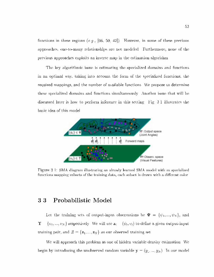
53

functions in these regions (e.g., [66, 50, 42]). However, in some of these previous

approaches, one-to-many relationships are not modeled. Furthermore, none of the

previous approaches exploits an inverse map in the estimation algorithm.

The key algorithmic issue is estimating the specialized domains and functions

in an optimal way, taking into account the form of the specialized functions, the

required mappings, and the number of available functions. We propose to determine

these specialized domains and functions simultaneously. Another issue that will be

discussed later is how to perform inference in this setting. Fig. 3.1 illustrates the

basic idea of this model.

Figure 3.1: SMA diagram illustrating an already learned SMA model with m specializedfunctions mapping subsets of the training data, each subset is drawn with a di�erent color.

3.3 Probabilistic Model

Let the training sets of output-input observations be = f 1; :::; Ng, and

� = f�1; :::; �Ng respectively. We will use zi = ( i; �i) to de�ne a given output-input

training pair, and Z = fz1; :::; zNg as our observed training set.

We will approach this problem as one of hidden variable density estimation. We

begin by introducing the unobserved random variable y = (y1; :::; yN). In our model

54

any yi has as its domain the discrete set C = f1; :::;Mg of labels for the specialized

functions, and can be thought of as the function number used to map data point i.

Thus M is the number of specialized mapping functions. Our model uses parameters

� = (�1; :::; �M ; �), where �k represents the parameters of the mapping function k,

and � = (�1; :::; �M), where �k represent P (yi = kj�): the prior probability that the

mapping function with label k will be used to map the i-th data point. As an example,

P (yijzi; �) represents the probability that function number yi generated data point

number number i.

Using Bayes' rule and assuming independence of observations given �, we have

the log-probability of our data log p(Zj�), which we want to maximize:

argmax�

log p(Zj�) (3.1)

= argmax�

Xi

log p(zij�) (3.2)

= argmax�

Xi

logXk

p(zijyi = k; �)P (yi = kj�) (3.3)

= argmax�

Xi

logXk

p( ij�i; yi = k; �)P (yi = kj�)p(�i); (3.4)

where we used the independence assumption p(�j�) = p(�). Note that because �i

does not depend on the model parameters we can ignore its distribution when �nding

the optimal parameter settings.

Because of the log-sum encountered, this problem is intractable in general. How-

ever, there exist practical approximate optimization procedures, one of them, based on

alternating minimizations [30] is Expectation Maximization (EM) [35, 82]. Learning

will be discussed in detail in the following sections.

55

3.4 Likelihood Choices

Note that we have been very general with our formulation so far. In particular,

in the above formulation (e.g., Eq. 3.4) the probability p( ij�i; yi = k; �) has not

been de�ned yet. It turned out that a key question in instantiating the architecture

is: what is p( j�; y; �)? This is, the probability that output was generated using

the mapping function y and the input � assuming a certain setting of the model

parameters �. In this thesis we analyze the following possible cases:

1. A Gaussian joint distribution of input-output vectors:

p( ; �jy; �) = N (( ; �);�y;�y) (3.5)

2. A Gaussian distribution with mean de�ned by the error incurred in using the

possibly non-linear function indexed by �y as a mapping function, and a �xed,

given variance �y:

p( j�; y; �) = N ( ;�y(�; �);�y) (3.6)

One way to interpret this choice is to think that the error cost in estimating

once we know the specialized function to use, is a Gaussian distribution whose

mean is the output of the specialized function and whose covariance is map-

dependent.

Of course, the SMA formulation is general enough to accept other forms of

likelihood functions. This will be discussed at the end of this thesis.

56

3.5 Learning

The EM algorithm is well known [35, 3, 82], therefore here we only provide the

derivations speci�c to SMA's. The E-step consists of �nding P (y = kjz; �) = ~P (y).

Note that the variables yi are assumed independent (given zi). Thus, factorizing

~P (y):

~P (y) =Yi

~P (t)(yi) =Yi

[(�yip( ij�i; yi; �))=(Xk2C

�kp( ij�i; yi = k; �))] (3.7)

The M-step consists of �nding �(t) = argmax� E ~P (t)[log p(Z;yj�)]. In all of our

cases we can show that this is equivalent to �nding:

�(t) = argmax�

Xi

Xyi2C

~P (t)(yi)[logP (zijyi; �) + logP (yij�)]: (3.8)

It is important to mention that this is valid if P (zij�) depends on yi and not on

yj, for any j 6= i. Note that for the distributions discussed above, this is true. We

present solutions for the cases described above.

3.5.1 Case (1)

In case (1) we have:

p( �jy; �) = N (�y;�y) = N (

2664��

�

3775 ;2664

��

�>� � ;

3775)y (3.9)

In this case, we can show that the SMA parameter learning problem is reduced to a

mixture of Gaussian estimation, for which it is straightforward to estimate � using

57

EM. Moreover, the Bayesian estimate of the conditional distribution (the conditional

distribution is of major importance because we must estimate given that we observe

�) is also Gaussian:

P ( j�; y; �) = N (� + �>

� ��1�� (� � ��);� � �>

� ��1�� )y (3.10)

Therefore in case (1), each specialized function �k is just the mean of the condi-

tional distribution (conditioned on the observation �i and the function index):

�k(�; �) = � + �>

� ��1�� (� � ��): (3.11)

Moreover, we have an expression for the con�dence of this estimate given by

the variance (� � �>� �

�1�� )y above. However, this expression does not depend

on the input, a sometimes undesirable consequence of the given model. Thus, each

functions �k is linear in the input vector from <c.

3.5.2 Case (2)

In case (2) we have:

@E

@�k=

Xi

~P (t)(yi = k)@

@�klogP (yi = kj�) (3.12)

@E

@�k=

Xi

~Pi(t)(yi = k)

@

@�klogP ( ijyi = k; �i; �k) (3.13)

@E

@�k=

Xi

~Pi(t)(yi = k)

[(@

@�k�k(�i; �k))

>��1k ( i � �k(�i; �k))]; (3.14)

where E is the cost function found in Eq. 3.8.

This gives the following update rules for �k and �k (where Lagrange multipliers

58

were used to incorporate the constraint that the sum of the �k's is 1.

�k =1

n

Xi

P (yi = kjzi; �) (3.15)

�k =

Pi~P (t)(yi = k)( i � �k(�i; �k))( i � �k(�i; �k))

>

Pi~P (t)(yi = k)

(3.16)

To keep the formulation general, we have not yet de�ned the form of the special-

ized functions �k. Whether or not we can �nd a closed form solution for the update

of �k depends on the form of �k. For example if �k is a non-linear function, we may

have to use iterative optimization to �nd �(t)k . If �k yields a quadratic form, then a

closed form update exists.

3.6 Stochastic Learning

The optimization equations for learning described above are useful to �nd a local

minimum given the initial values of the parameters. In order to improve this process,

and avoid some of the local minima that inevitably arise, we use an annealing schedule

on the ~Pi(t)

probabilities during the M-step. In this way, we rede�ne:

~Pi(t)(yi = j) =

elog(~Pi(t)

(yi=j))=T (t)

Pk2C elog(

~Pi(t)

(yi=k))=T (t)(3.17)

In our experiments, the temperature parameter T decays exponentially. This step

not only helps in avoiding local minima, but it also creates two desirable e�ects. It

forces ~Pi(t)(yi = j) to be binary (either 1 or 0) at low temperatures; as a consequence

each point will tend to be mapped by only one specialized function at the end of

optimization. Moreover, it makes ~Pi(t)(yi = k) (k = 1; 2; :::; m) be fairly uniform at

high temperatures, making the optimization less dependent on initialization.

Note that in some cases, there is no closed-form solution for the M-step. In

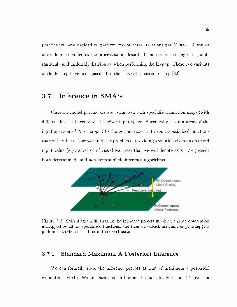
59

practice we have decided to perform two or three iterations per M-step. A source

of randomness added to the process so far described consists in choosing data points

randomly and uniformly distributed when performing the M-step. These two variants

of the M-step have been justi�ed in the sense of a partial M-step [82].

3.7 Inference in SMA's

Once the model parameters are estimated, each specialized function maps (with

di�erent levels of accuracy) the whole input space. Speci�cally, certain areas of the

input space are better mapped to the output space with some specialized functions

than with others. Now we study the problem of providing a solution given an observed

input value (e.g., a vector of visual features) that we will denote as x. We present

both deterministic and non-deterministic inference algorithms.

Figure 3.2: SMA diagram illustrating the inference process in which a given observationis mapped by all the specialized functions, and then a feedback matching step, using �, isperformed to choose the best of the m estimates.

3.7.1 Standard Maximum A Posteriori Inference

We can formally state the inference process as that of maximum a posteriori

estimation (MAP). We are interested in �nding the most likely output h� given an

60

input con�guration x:

h� = argmaxh

p(hjx) (3.18)

= argmaxh

Zp(hjy;x)P (yjx)dy: (3.19)

We will use an integral operator in general and later specialize it to a sum operator

in the case of discrete random variables. Because P (yjx) = P (y) in this model (this

is in fact one of our conditional independence assumptions), we have:

h� = argmaxh

Zp(hjy;x)P (y)dy (3.20)

Any further treatment depends on the properties of the probability distributions

involved.

In both of the cases considered in previous sections ( Case (1) and Case (2)),

we can write p(hjx; y) = N (h;�y(x);�y). In Case (2), by de�nition this is exactly

the form of the conditional distribution. In Case (1), we can make �y = (� �

�>� �

�1�� )y and obtain the given expression for p(hjx; y). Also recall that y is

discrete. Therefore, in any case we have:

h� = argmaxh

Xy

N (h;�y(x);�y)P (y): (3.21)

This is a mixture of Gaussians; hence in general there could be many maxima in

this distribution.

61

3.7.2 Maximum A Posteriori Estimation by Using the In-

verse Map �

Note that the mixing factors do not depend on the input x. In fact, �y is always

the same, for any input. This makes sense in terms of the information we have

incorporated into the inference problem so far, e.g., P (yjx) = P (y).

This is related to the key modeling choice of Mixture of Experts (ME) [62, 66].

In ME P (yjx) is no longer P (y) because the related independence assumption was

removed from the model. In its place, it was assumed that P (yjx) has a certain form.

This is called the gating network; there are M gating networks. In [62, 66] this was

modeled by a logit linear model, learned from data.

Here, a di�erent approach is used, based on the fact that we have access to a

forward kinematics function �, which we call here the inverse function or inverse map

(the input-output map is called the forward map).

We are interested in �nding an optimal h� given an input x (e.g., an optimal body

pose given features taken from an image). This can be formulated as the following

continuous optimization problem:

h� = argmaxh

p(hjx) (3.22)

= argmaxh

p(xjh)p(h)

p(x)(3.23)

= argmaxh

p(xjh)R R

p(h;x; y)dxdy

p(x)(3.24)

simply by Bayes' rule, and marginalizing over all variables except h.

Since x is observed, say x = xo,Rp(h;x; y)dx = �(x�xo)p(h;x; y) we can simply

rewrite Eq. 3.24:

62

= argmaxh

p(xjh)R R

p(h; y; jx)p(x)dxdy

p(x)(3.25)

= argmaxh

p(xjh)p(x)Rp(h; yjx)dy

p(x)(3.26)

= argmaxh

p(xjh)Zp(h; yjx)dy (3.27)

= argmaxh

p(xjh)Zp(hjy;x)P (y)dy; (3.28)

where we have taken into account P (y) = P (yjx), from our conditional independence

assumptions 3.

In summary, we described the inference process involved in SMA's. Under

the MAP approach, this derivation is completely general. We did not make any

assumptions on the form of the distributions or algorithms used.

3.8 Optimal Inference Using �

In this section, we derive the optimal analytical solution for the inference problem

given in Sec. 3.7.2. This problem is given by the optimization of Eq. 3.28.

h� = argmaxh

p(xjh)Zp(hjy;x)P (y)dy (3.29)

= argmaxh

EI(h): (3.30)

Using the optimality condition @ logEI(h)@h

= 0, we can �nd possible solutions for

h�, assuming that our inverse function is not fully deterministic, (i.e., there is a

probability distribution on generating the output of �). In this section, it is assumed

that p(xjh) = N (x; �(h);��).

3We assumed p(h;x; y) factorizes into p(hjx; y)p(x)P (y) .

63

Therefore, we can write:

@

@hlogEI(h) =

@

@hlog p(xjh) +

@

@hlog

Xy2C

p(hjy;x)P (y) (3.31)

= �1

2

@

@h(x� �(h))>��1

� (x� �(h)) +@@h

Py2C p(hjy;x)P (y)P

y2C p(hjy;x)P (y)(3.32)

=@

@h�(h)>��1

� (x� �(h)) +

Py2C

@@hp(hjy;x)P (y)P

y2C p(hjy;x)P (y)(3.33)

=@

@h�(h)>��1

� (x� �(h))

+

Py2C p(hjy;x)P (y)

@@hlog p(hjy;x)P

y2C p(hjy;x)P (y); (3.34)

where the last equality is valid in the more general case of any p(hjy;x) in the

exponential family. After some basic algebra, this gives us:

@ logEI(h)

@h=

@

@h�(h)>��1

� (x� �(h))�

Py2C y�

�1y (h� �y(x; �))Py2C y

; (3.35)

with y = p(hjy;x)P (y).

Recall that � is usually highly non-linear, h is continuous, and y is discrete. It

is probably not easy to �nd the values of h that satisfy @ logEI(h)@h

= 0. In fact, given

the form of Eq. 3.35, it is easy to show that in general, there might be several values

of h for which this condition is satis�ed.

A valid alternative is to use Eq. 3.35 and use an iterative optimization method to

�nd a local minimum. Each of the values �y(x) are potential choices for initial con-

ditions of h. In the following sections, we show alternative approximation algorithms

to obtain one or more good estimates for h�.

64

3.9 Multiple Sampling (MS) andMean Output (MO)

Algorithms: Approximate Inference using �

In this section, our interest is to �nd approximate solutions to Eq. 3.28, to

approximately maximize p(hjx) in our general problem settings. We present two

possible approximate inference algorithms. One is deterministic and the other is

non-deterministic.

3.9.1 Kernel Approximations

Let us assume that we can approximateRp(hjy;x)P (y)dy by a set of samples

generated according to p(hjy;x)P (y) and a kernel function K(h;hs). Denote the set

of samples HSpl = fhsgs=1:::S. An approximate toRp(hjy;x)P (y)dy is formally built

by:

Zp(hjy;x)P (y)dy �

1

S

SXs=1

K(h;hs); (3.36)

with the normalizing conditionRK(h;hs)dh = 1 for any given hs.

We will focus on several cases for the choice of K.

� If K(h;hs) = �(h� hs), we have

h = argmaxh

p(xjh)SXs=1

�(h� hs): (3.37)

After some simple manipulations, this can be reduced to the following equivalent

discrete optimization problem whose goal is to �nd the most likely sample s�:

s� = argmaxsp(xjhs) (3.38)

65

s� = argmins(x� �(hs))

>��(x� �(hs)); (3.39)

where the last equation uses the assumption p(xjh) = N (x; �(h);��). Using

Eq. 3.39 to �nd h = hs� will be called the multiple sampling solution (MS).

This procedure is non-deterministic.

� If K(h;hs) = N (h;hs;�Spl), we have

h = argmaxh

p(xjh)SXs=1

N (h;hs;�Spl): (3.40)

This case is hard to solve, because contrary to the case above (Eq. 3.39), in

general, there is no guarantee that the optimal h is among the samples.

A Deterministic Approximation based on the Functions Mean Output

The structure of the inference in SMA, and the choice of probabilities p(hjx; y)allows

us to construct a newer approximation that is considerably less expensive to compute,

and moreover it is deterministic. Notwithstanding the speed gain, this approximation

is still useful in practice, as will be demonstrated in the experiments. Furthermore,

it can be formally justi�ed as explained in the rest of this section.

The idea is straightforward. Intuitively it consists of asking each of the specialized

functions �k what their most likely estimate for h is, given the observed input x.

The opinions of each of these specialized functions are then evaluated using our

distribution p(xjh), in the same way as was done in (Eq. 3.39). The computational

gain results from the fact that sampling is no longer needed. The computational gain

is on the order O(S=M), relative to the solution given by Eq. 3.39, where S is the

number of samples and M the number of specialized functions.

This can be justi�ed by the observation that the probability of the mean is

66

maximal in a Gaussian distribution (i.e., it is the most-likely value). Formally,

in our case p(E[hjy;x; �]) > p(h0jy;x; �), for any h0. Consider again the set of

samples HSpl = fhsgs=1:::S generated according to p(hjy;x)P (y) = �y(x; �)�y. We

can arti�cially build a set of samples H� = fh�sgs=1:::S that has the property:

8y;maxsp(h�s jy;x) > max

sp(hsjy;x); (3.41)

this is just the set given by setting h�s = �s(x; �). Thus, this approximate solution,

called the mean output solution (MO) relies on the observation: by considering the

means �s(x), we would be considering the most likely output of each specialized

function, given the input. The expression to be minimized is the same as that given

in Eq. 3.39, except for the use of the M means instead of the S samples s. This is

a convenient approximation. The source of the approximation is the fact that the

underlying kernel form does not take into account the full information given by the

forward probabilities; i.e., p(hjy;x; �).

We use Fig. 3.2 to illustrate this approximate inference process. When generating

an estimate of body pose, denoted h, given an input x (the gray point with a dark

contour in the lower plane), the SMA generates a series of output hypotheses H� =

fh�kgk obtained using hk = �k(x), with k 2 C (illustrated by each of the points

pointed to by the arrows).

Given the set H�, the most accurate hypothesis under the MO criteria is the one

that minimizes the function:

k� = argmaxk2C

p(xjh�k) (3.42)

k� = argmink(x� �(h�k))

>��(x� �(h�k)); (3.43)

where in the last equation we have assumed p(xjh) is Gaussian. In Fig. 3.2 we can

see that each of the points in the output space is mapped back to the input space.

67

Once in this space, these points can be compared to the novel input (using a given

cost function e.g., Eq. 3.43). The form of the cost function could of course vary under

the conditions speci�ed above speci�ed. Note that unlike multiple sampling (MS) the

mean output (MO) approximation is deterministic.

Why the Mean Output Approach Cannot be Used if � is Ignored

One can imagine that the MO simple approach could be used even if � is not

incorporated. Using the same ideas developed in the MO approach, given a specialized

function k and an input x, we now have:

log p(hjy = k;x) = � log j�yj �1

2(h� �y(x))

>��1y (h� �y(x)) + �y: (3.44)

Let us note the properties of the second term in Eq. 3.44. First, it cannot be

smaller than zero because ��1y is positive de�nite4. Second, for a given y, the second

term in Eq. 3.44 is zero only when h = �y(x).

As a consequence, the optimal h� needs to be the output of one of the specialized

functions �y (i.e., the mean of the distribution). We can then restrict our search by

only considering the M (total number of specialized functions) hypotheses denoted

H = fhkg, with hk = �k(x).

Given this set, the answer to the initial continuous optimization problem now

involves solving a very simple discrete optimization task with O(M). This task's goal

is to �nd the optimal element of the set H, in the sense of Eq. 3.44. The index y� of

the optimal hypothesis can be chosen by considering the rest of the terms in Eq. 3.44.

4Assuming ��1y

is full rank.

68

Given that the second term is zero, we now have:

y� = argmaxy� log j�yj+ log�y (3.45)

= argminy

logj�yj

�y(3.46)

This is in fact a very pleasing answer because it agrees with our intuition that in

the absence of other information, to map x we should choose the specialized function

that has the least uncertainty or lowest entropy. This is, in the case of a Gaussian

distribution, that Gaussian with a sharper peak or smaller covariance �. If a prior

P (y) is given, then the higher the prior on y, the smaller the ratio in Eq.3.46; thus

there is a higher chance for y to be the index of the optimal specialized function or

the optimal hypothesis.

Even though Eq. 3.46 is technically correct, the best estimate does not depend

on the input. Thus, if � is not incorporated, this algorithm would always use the

same specialized function to infer the best output.

3.9.2 Bayesian Inference: Solutions Given By Probability

Distributions

Note that in many cases, there may not be any need to simply provide a point

estimate, in terms of a most likely output h. In fact we could instead use the whole

distribution found in the inference process. This is the Bayesian inference approach.

In our case this distribution is given by:

p(hjx) = p(xjh)Zp(hjy;x)P (y)dy; (3.47)

In reference to the above kernel choices, we could also have approximates to this

69

distribution. Assuming p(hjx) is Gaussian.

� If K(h;hs) = �(h� hs), it is easy to show that

p(hjx) =1

S

SXs=1

N (x; �(hs);��); (3.48)

� If K(h;hs) = N (h;hs;�Spl), we have

p(hjx) = N (x; �(h);��)SXs=1

N (h;hs;�Spl) (3.49)

Note that in general this approximations are particularly useful in the context of

dynamic probabilistic models. In such case the resulting time-dependent distributions

are not likely to be representable in closed-form, but we can obtain estimates (e.g.,

to p(htjxt;ht�1)) using for example, particle �ltering. As a consequence, we could

express our solution using a set of pairs f(hi; �i)g with �i the associated posterior

probability of sample hi. Thus, given this representation our method can be easily

extended to dynamical models (e.g., [60]) and any form of the distribution p(xjh).

Even though, for the sake of simplicity, we chose a form for p(xjh), the latter holds

true for all approximations developed in this section.

3.10 On the Feed-back Mapping Function �

In the previous sections we have made reference to the inverse or feedback

function denoted �. There are at least two ways to de�ne this function. In one

hand, � could be a computer graphics rendering model. Given the body pose vector

70

h this model is able to produce the image of the object in the given con�guration. On

the other hand, we can approximate � given a set of output-input examples (probably

obtained using the same computer graphics model). For this we need to assume a

functional form for the approximating function �. Thus, once the function has been

estimated, when a body pose vector h is given, we just need to evaluate the estimated

function, therefore no rendering is required.

In this section we study the di�erences in the use of a estimated � or a graphics

rendering � feedback function. The choice of what function to use can be constrained

by practical limitations. For example, it is usually faster to (1) compute a (pre-

estimated) function � that maps an element from the output space (e.g., a 22 DOF

vector for the case of the hand pose estimation application) to an element from the

input space (e.g., a seven dimensional vector such as the Hu moments); than to (2)

render the given object and compute the visual features of choices given the resulting

image. This of course depends on the object modeling, rendering, and visual features,

but in general we believe that using a pre-estimated function is faster. For example,

for a real time application, one may be required to use �. It is then interesting to

theoretically study the advantages of using either feedback function (aside from the

usual speed di�erences).

3.10.1 Exact vs. Estimated �

The possibility of using a computer graphics function � during inference (and

learning) is appealing. A computer graphics rendering function seems to provide a

more exact calculation of visual features given the body pose hypothesis. Unlike its

counterpart, the function approximation approach (where � is estimated from data to

71

approximate �), the former involves estimating the function parameters given a �nite

set of examples. In almost all cases the map built is a limited approximation whose

form is chosen from the family of functions that share a given functional form. Using

a computer graphics rendering function seems to give us a more accurate mapping

power. However, in practice, there are other considerations one has to take into

account.

In real applications, one does not usually work in the spaces where the data

originally comes (e.g., in our 60 DOF body pose, we use PCA encode them with 9

DOF with the hope that they encode the rest accurately enough). For the purpose of

our discussion5, denote <t0

the space where the original data (output con�gurations)

lies, and the usual <t to be the space where our numerical algorithms work, with

t0 > t. Equivalently, denote <c0

and <c the input data, with c0 > c.

Let us consider the case in which h = Ah0, with h 2 <t and h0 2 <t0

. This is,

h and h0 are related by a linear transformation represented by the matrix A, with

t0 rows and t columns. Assume, without loss of generality there is no dimensionality

reduction performed in the input space, i.e., <c0

= <c. Given this, in the following

sections we will study the properties and di�erences between this two ways to de�ne

the inverse function.

3.10.2 The Function Estimation Case

When a function is estimated in a supervised learning fashion to map elements

of <t to <t, we have:

5This notation is in agreement with the rest used in this thesis.

72

x = �NN(h) (3.50)

= �NN(Ah0); (3.51)

therefore the components of h0 in the direction of the null space of A, N (A) are lost

in the transformation to h. In other words, we �nd a function �NN : <t ! <c that

approximates only the mapping from the row space of the pose con�gurations to the

corresponding visual features.

Denote Hr � to be a set of output space con�gurations that share the same

row space representation hr, and �r to be the set of input samples associated with the

elements inHr. Then in general, the map we are trying to estimate with function �NN

unfortunately becomes many-to-one. This cannot be approximated by a function.

In practice one makes the assumption that this function estimate is still accurate.

Technically, one is really making the assumption that �r is convex in the limit of

in�nite number of points in Hr. In practice, one also wants �r to span a relatively

small area of the input space (in the best case, this is just a point), or that in the

training set, there is only one element in each set Hr (for all r at a given resolution).

In information theoretic terms, one expects that there is no loss (or little loss) of

information when transforming the random variable H 0 into H of poses (in <t0

and

<t respectively) about X (in <c).

3.10.3 The Computer Graphics Rendering Case

Following the notation introduced above, we now explore the implications of

using a computer graphics (CG) rendering function �CG as inverse mapping.

73

Let h 2 <t denote a single output hypothesis, provided by any of the specialized

functions in out architecture. In order to use �CG : <t0

! <c0

, we need to transform h

back to its original space <t0

(because this is the domain of �CG). This transformation

has as range the row space of A, therefore it cannot reach pose con�guration com-

ponents in N (A) (there are some poses that cannot be reached, it does not matter

what the h is).

Thus, for a setHr, the function �CG will produce the visual features �CG(hr) (with

hr as above). This means that the CG mapping is not exact given the hypothesis.

In summary, the CG rendering function maps a given pose hypothesis to the visual

features of the hypothesis' components that are in the row space of A.

In conclusion, the two varieties are an approximation, and there is no guarantee

which will perform better under any data set. Because performance is data set

dependent, we can state: in cases where the underlying output to input map is many-

to-one (in the original spaces), then a function approximation framework cannot form

an accurate map. Conversely, if the sets �r are convex, and span a small area, then

the overhead of extra computations needed to use a CG rendering may not justify

its use. In any case, an important issue not addressed in this section is how the

functional form chosen �NN , can approximate the relations between the output and

input data sets. In order to simplify notation, in the rest of this thesis, we will use

the following notational convention : �:= �NN and �

:= �CG.

Chapter 4

Applications

4.1 Introduction

This chapter describes the applications in which we will test the Specialized

Mappings Architecture. The implementation details speci�c to each application are

explained. The applications developed are in the area of vision-based estimation of

articulated body pose from low-level features. In these applications, it is possible to

obtain (or approximate) a feedback function from pose space to feature space.

In general, applications of SMA do not have to be limited to the vision domain.

As a simple example, one could apply the SMA approach in speech recognition

problems, where the input space is given by features computed on acoustic signals

(e.g., cepstral coe�cients), and the output space could be the space of phonemes.

It is possible to compute acoustic features of given phonemes by simply acoustically

rendering them to obtain their acoustic realization, where features could then be

computed.

75

4.2 Basic Approximation to SMA Applied to 2D

Body Pose Estimation

This application was the �rst developed. In some sense it motivated a number

of the ideas later generalized as the Specialized Mappings Architecture framework

presented throughout this thesis. Thus, we have chosen to include this application

to relate general SMA elements with the speci�cs of the human pose estimation

application. Many simpli�cations are made and the underlying ideas are presented in

the context of the basic example task: 2D body pose estimation. The reader familiar

with the problem may choose to skip this section. However, in Sec. 4.2.6 a formal

justi�cation for the basic approach presented in this section will be given within the

more general context of the SMA.

4.2.1 Overview: Supervised Learning of Body Pose

Generally speaking, in supervised learning tasks, the goal is to discover the input-

output relationship of an unknown process, or to discover the process that generated

the outputs given the inputs. Sometimes we know something about this input-output

relationship, and this is usually incorporated into the problem. These elements vary

because they are usually problem dependent. However, in supervised learning, it is

assumed that there is a series of example input-output pairs, generated by the process

in which we are interested1. This is usually referred as the data.

1There are more general views about supervised learning. For example, the training examples

may come not from the generating process, but from another process that is somehow related; i.e.,

one that can provide information about the generating process.

76

In this thesis, we see the pose estimation problem as an instance of supervised

learning, where we are interested in �nding the mapping between low-level image fea-

tures and body con�gurations. This mapping is highly complex and ambiguous. The

di�culty stems from many elements, for example, the number of degrees of freedom

in the human body, the complex underlying probability distribution of body poses,

ambiguities in the projection of human pose onto the image plane, self-occlusion,

insu�cient temporal or spatial resolution, etc.

In this section, we introduce many of these concepts with an approach for

estimation of human body pose given a single image or a monocular image sequence

containing a single body. Human pose is de�ned as the instantaneous two dimensional

con�guration (i.e., the projection onto the image plane) of a single articulated body

in terms of the position of a predetermined set of joints.

The underlying idea is that given a set of body motion sequences for training, a

set of clusters is built in which each has statistically similar con�gurations according

to a given measure and model. Then, for each of the clusters, a function that maps

visual features to body pose is built. We use machine learning concepts to build this

function using a set of training data.

During inference, given new visual features, a mapping from each cluster is

performed providing a set of possible poses. From this set, we extract the most

likely pose given the learned probability distribution and the visual feature similarity

between hypothesis and input.

Our approach will learn how speci�c body classes (e.g., human bodies) are con-

strained to be con�gured. This is done by observing examples of body con�gurations.

Because body con�gurations have some underlying structure, this can considerably

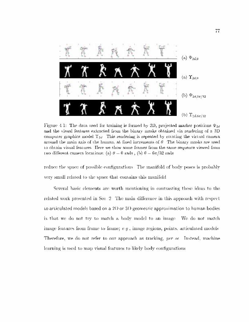
77

(a) 2d;0

(a) �2d;0

(b) 2d;6�=32

(b) �2d;6�=32

Figure 4.1: The data used for training is formed by 2D, projected marker positions 2d

and the visual features extracted from the binary masks obtained via rendering of a 3Dcomputer graphics model �2d. This rendering is repeated by rotating the virtual cameraaround the main axis of the human, at �xed increments of �. The binary masks are usedto obtain visual features. Here we show some frames from the same sequence viewed fromtwo di�erent camera locations: (a) � = 0 rads., (b) � = 6�=32 rads .

reduce the space of possible con�gurations. The manifold of body poses is probably

very small related to the space that contains this manifold.

Several basic elements are worth mentioning in contrasting these ideas to the

related work presented in Sec. 2. The main di�erence in this approach with respect

to articulated models based on a 2D or 3D geometric approximation to human bodies

is that we do not try to match a body model to an image. We do not match

image features from frame to frame; e.g., image regions, points, articulated models.

Therefore, we do not refer to our approach as tracking, per se. Instead, machine

learning is used to map visual features to likely body con�gurations.

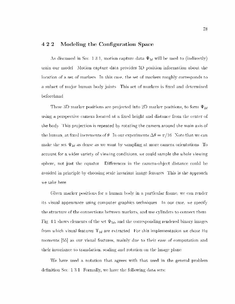
78

4.2.2 Modeling the Con�guration Space

As discussed in Sec. 1.3.1, motion capture data 3d will be used to (indirectly)

train our model. Motion capture data provides 3D position information about the

location of a set of markers. In this case, the set of markers roughly corresponds to

a subset of major human body joints. This set of markers is �xed and determined

beforehand.

These 3D marker positions are projected into 2D marker positions, to form 2d

using a perspective camera located at a �xed height and distance from the center of

the body. This projection is repeated by rotating the camera around the main axis of

the human, at �xed increments of �. In our experiments �� = �=16. Note that we can

make the set 2d as dense as we want by sampling at more camera orientations. To

account for a wider variety of viewing conditions, we could sample the whole viewing

sphere, not just the equator. Di�erences in the camera-object distance could be

avoided in principle by choosing scale invariant image features. This is the approach

we take here.

Given marker positions for a human body in a particular frame, we can render

its visual appearance using computer graphics techniques. In our case, we specify

the structure of the connections between markers, and use cylinders to connect them.

Fig. 4.1 shows elements of the set 2d, and the corresponding rendered binary images

from which visual features �2d are extracted. For this implementation we chose Hu

moments [55] as our visual features, mainly due to their ease of computation and

their invariance to translation, scaling and rotation on the image plane.

We have used a notation that agrees with that used in the general problem

de�nition Sec. 1.3.1. Formally, we have the following data sets:

79

1. 3d is the set of 3D body con�gurations expressed in marker positions, obtained

using motion capture.

2. 2d = f 2d 2 <sjC( 3d; �) = 2dg, with � varying from 0 to 2� using a �xed

increment, and C the transformation that projects spatial coordinates to the

image plane, using viewpoint �.

3. �2d = f�2d 2 <cj�( 3d; �) = �2dg, with � = V �R, mapping 3D marker positions

to image features.

Clustering body con�gurations

It would be ideal if the mapping from �2d to 2d were simple. Unfortunately

this mapping is highly ambiguous. For example, if moments of binary images (e.g.,

body silhouettes) are used as visual features, a person facing forward would generate

very similar image moments to another facing backwards. Image moments provide

a descriptor that does not encode many of the degrees of freedom of 2D markers.

Therefore, it is possible that drastically di�erent body con�gurations have similar

image moments.

In this introductory example, the way we approach the problems mentioned

above is by �rst creating clusters of statistically homogeneous data points in the

marker space2. We used 2D projected markers to try to generate clusters that can be

described by a Gaussian probability distribution. This is an unsupervised clustering

task, for which we use the EM algorithm.

Let us denote �i = (�i;�i) to be the learned distribution parameters for cluster

2This idea will be further generalized in the next applications

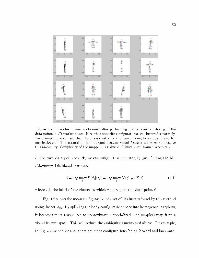
80

Figure 4.2: The cluster means obtained after performing unsupervised clustering of thedata points in 2D marker space. Note that opposite con�gurations are clustered separately.For example, one can see that there is a cluster for the �gure facing forward, and anotherone backward. This separation is important because visual features alone cannot resolvethis ambiguity. Complexity of the mapping is reduced if clusters are trained separately.

i. For each data point 2 , we can assign it to a cluster, by just �nding the ML

(Maximum Likelihood) estimate.

i = argmaxj(P (�jj )) = argmax

j(N ( ; �j;�j)); (4.1)

where i is the label of the cluster to which we assigned this data point .

Fig. 4.2 shows the mean con�guration of a set of 15 clusters found by this method

using the set 2d. By splitting the body con�guration space into homogeneous regions,

it becomes more reasonable to approximate a specialized (and simpler) map from a

visual feature space. This will reduce the ambiguities mentioned above. For example,

in Fig. 4.2 we can see that there are mean con�gurations facing forward and backward.

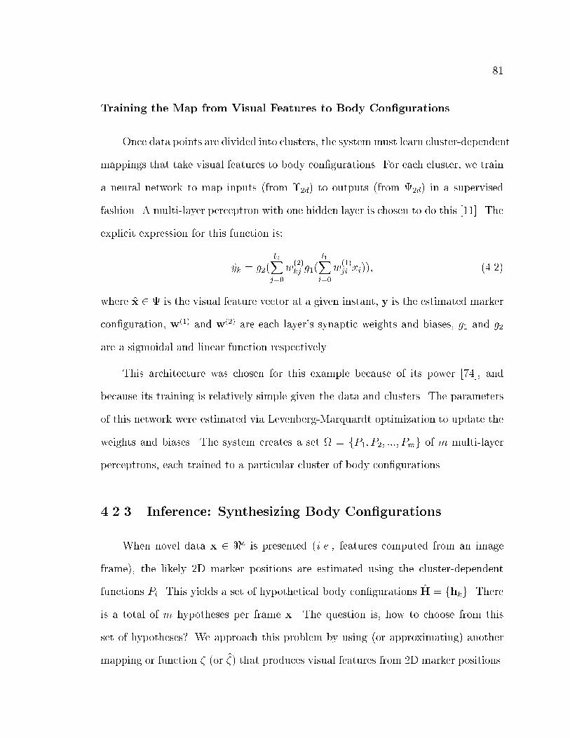
81

Training the Map from Visual Features to Body Con�gurations

Once data points are divided into clusters, the system must learn cluster-dependent

mappings that take visual features to body con�gurations. For each cluster, we train

a neural network to map inputs (from �2d) to outputs (from 2d) in a supervised

fashion. A multi-layer perceptron with one hidden layer is chosen to do this [11]. The

explicit expression for this function is:

yk = g2(l2Xj=0

w(2)kj g1(

l1Xi=0

w(1)ji xi)); (4.2)

where x 2 is the visual feature vector at a given instant, y is the estimated marker

con�guration, w(1) and w(2) are each layer's synaptic weights and biases, g1 and g2

are a sigmoidal and linear function respectively.

This architecture was chosen for this example because of its power [74], and

because its training is relatively simple given the data and clusters. The parameters

of this network were estimated via Levenberg-Marquardt optimization to update the

weights and biases. The system creates a set = fP1; P2; :::; Pmg of m multi-layer

perceptrons, each trained to a particular cluster of body con�gurations.

4.2.3 Inference: Synthesizing Body Con�gurations

When novel data x 2 <c is presented (i.e., features computed from an image

frame), the likely 2D marker positions are estimated using the cluster-dependent

functions Pi. This yields a set of hypothetical body con�gurations H = fhkg. There

is a total of m hypotheses per frame x. The question is, how to choose from this

set of hypotheses? We approach this problem by using (or approximating) another

mapping or function � (or �) that produces visual features from 2D marker positions.

82

There are di�erent alternatives for doing this (some exact and some approximate).

We experiment with both cases in further sections.

One approach is to simply use each hk to render an image using � = V � R, i.e.,

use computer graphics to render and then �nd the image visual features via V (V

may �nd Hu moments for example). Recall that R is a 2D approximation of the 3D

rendering function R. It is an approximation because the object to be rendered is

three-dimensional, and here the hypotheses H are 2D markers.

Another alternative is to �nd an approximate function � from data (i.e., �2d and

2d). That is, we could estimate the parameters of � using the approach outlined in

Sec. 4.2.2. Then given hk, we can obtain an estimate xk = �(hk). This function �

would avoid the need of a probably expensive rendering of the m hypotheses.

In this example system, we chose the second alternative. This was done using

the sets �2d and 2d. Because this mapping uses data rendered with knowledge

of 3D information, it is very likely to have accuracy advantages over the simpler

transformation R.

Given the set H of hypotheses about the body con�guration, we �nd the most

accurate hypothesis by minimizing:

i = argminj(�(hj)� xj)

>��1� (�(hj)� xj); (4.3)

where �� is the covariance matrix of the elements in the set �2d and i is the neural

network label that best matched the visual feature observed.

Even though intuitively the cost function above makes sense, one may wonder

about the existence of a formal justi�cation for its use. It turns out that there are

several ways to view inference in this model, one of them is Eq. 4.3. This approach

is what we called the mean output algorithm.

83

We will not focus on dynamical systems here, but as a side note we will mention

that a further re�nement step was used here. Because neighboring frames are gener-

ally from similar con�gurations, we obtained slightly better performance if consistency

in time is enforced. Therefore, after we obtain the best hk to use for a given frame, if

this network di�ers from that chosen in the previous frame, we wait for the next frames

to arrive (generally two or three) to decide whether to use this new hj. If within this

window the new frames are consistent with the change (involve the same hj), then

the new hj is used; if not, then the previous network is used instead3. Although a

probabilistic dynamical model would be advantageous in certain cases, this proved to

be an e�ective culling mechanism to avoid spurious individual reconstructed frames.

4.2.4 Preliminary Approach Summary

We very brie y enumerate every step of the preliminary approach we just pre-

sented:

1. A set of motion 3D capture sequences is obtained, 3d � <t. A set of visual

features �3d is computed from images that the 3D body generated (using a

computer graphics rendering function or simply captured by a video camera).

By projecting the elements of 3d onto the image plane over a given number of

views, we obtain as set of 2D marker positions 2d.

2. The set 2d is partitioned into several exclusive subsets via unsupervised clus-

tering. This yields a set of m clusters. Each cluster corresponds to a group

of similar pose parameters.

3This can be formally justi�ed by assuming these transitions are governed by a second or third

order Markov model. However, we will not expand on this here.

84

3. Given 2d and �2d, for each cluster i, we approximate a mapping function �i.

By clustering our target space, the mapping can be approximated with simple

functions, each responsible for a subset of the domain.

4. Novel data is presented in the form of human silhouettes. For each frame, visual

features are extracted using V : I ! <c. Then, using Pi, a set of m projected

marker positions per frame are estimated.

5. The series of possible m solutions provided for each frame is transformed back

to the input space using � to obtain the visual features of these m hypotheses.

The best match with respect to the presented data can then be found via the

maximum likelihood criterion. As an optional step, consistency in time can be

enforced by observing some frames ahead.

4.2.5 Discussion

The simple approach just described was described in [104]. Additional results

with this approach are given in Sec. 6.2.

This section's goal is to introduce basic ideas of the more general framework we

will use in the next applications. We use as an example, a technique that allows for

the reconstruction of human body con�guration from raw low-level visual features.

The proposed approach seems both simple and powerful. Also due to the framework

generality, it can be used for learning mappings to other non-rigid or articulated

objects.

Human pose reconstruction is a particularly hard problem because the relation-

ship input-output is highly ambiguous. To approach this di�culty, the basic concept

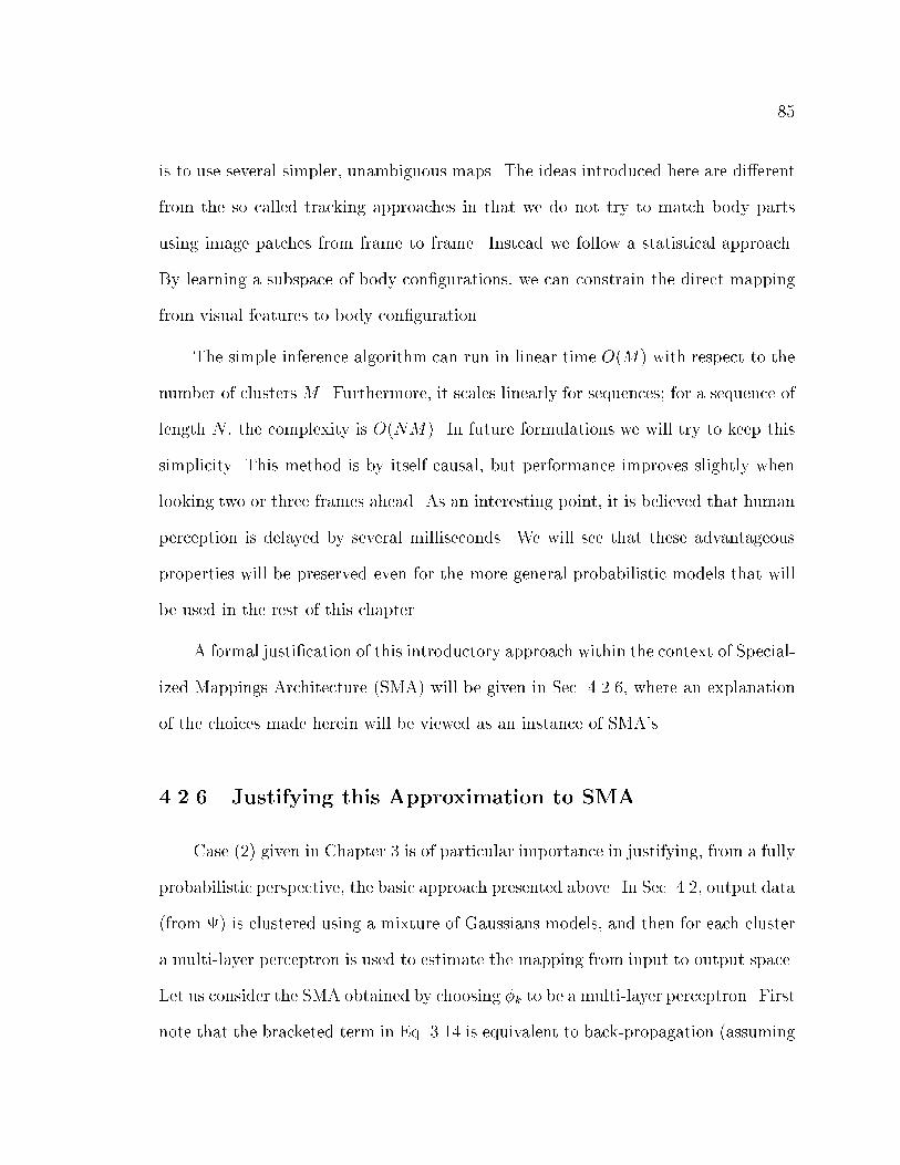
85

is to use several simpler, unambiguous maps. The ideas introduced here are di�erent

from the so called tracking approaches in that we do not try to match body parts

using image patches from frame to frame. Instead we follow a statistical approach.

By learning a subspace of body con�gurations, we can constrain the direct mapping

from visual features to body con�guration.

The simple inference algorithm can run in linear time O(M) with respect to the

number of clusters M . Furthermore, it scales linearly for sequences; for a sequence of

length N , the complexity is O(NM). In future formulations we will try to keep this

simplicity. This method is by itself causal, but performance improves slightly when

looking two or three frames ahead. As an interesting point, it is believed that human

perception is delayed by several milliseconds. We will see that these advantageous

properties will be preserved even for the more general probabilistic models that will

be used in the rest of this chapter.

A formal justi�cation of this introductory approach within the context of Special-

ized Mappings Architecture (SMA) will be given in Sec. 4.2.6, where an explanation

of the choices made herein will be viewed as an instance of SMA's

4.2.6 Justifying this Approximation to SMA

Case (2) given in Chapter 3 is of particular importance in justifying, from a fully

probabilistic perspective, the basic approach presented above. In Sec. 4.2, output data

(from ) is clustered using a mixture of Gaussians models, and then for each cluster

a multi-layer perceptron is used to estimate the mapping from input to output space.

Let us consider the SMA obtained by choosing �k to be a multi-layer perceptron. First

note that the bracketed term in Eq. 3.14 is equivalent to back-propagation (assuming

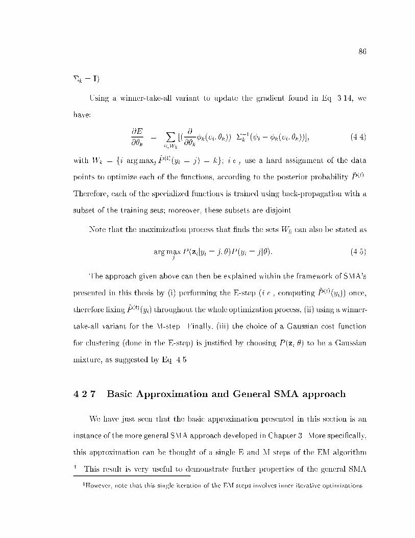
86

�k = I).

Using a winner-take-all variant to update the gradient found in Eq. 3.14, we

have:

@E

@�k=

Xi2Wk

[(@

@�k�k(�i; �k))

>��1k ( i � �k(�i; �k))]; (4.4)

with Wk = fij argmaxj ~P(t)(yi = j) = kg; i.e., use a hard assignment of the data

points to optimize each of the functions, according to the posterior probability ~P (t).

Therefore, each of the specialized functions is trained using back-propagation with a

subset of the training sets; moreover, these subsets are disjoint.

Note that the maximization process that �nds the sets Wk can also be stated as

argmaxjP (zijyi = j; �)P (yi = jj�): (4.5)

The approach given above can then be explained within the framework of SMA's

presented in this thesis by (i) performing the E-step (i.e., computing ~P (t)(yi)) once,

therefore �xing ~P (t)(yi) throughout the whole optimization process, (ii) using a winner-

take-all variant for the M-step. Finally, (iii) the choice of a Gaussian cost function

for clustering (done in the E-step) is justi�ed by choosing P (zij�) to be a Gaussian

mixture, as suggested by Eq. 4.5.

4.2.7 Basic Approximation and General SMA approach

We have just seen that the basic approximation presented in this section is an

instance of the more general SMA approach developed in Chapter 3. More speci�cally,

this approximation can be thought of a single E and M steps of the EM algorithm

4. This result is very useful to demonstrate further properties of the general SMA

4However, note that this single iteration of the EM steps involves inner iterative optimizations.

87

approach and its relation to this initial approximation.

One of the EM algorithm properties is that at each iteration of the E and M steps,

the log-likelihood of the training data is guaranteed to increase. This was proven in

[35]. Given the convergence properties of the EM algorithm, we can show that this

approximate model can be easily improved using the EM algorithm. By saying that

it can be improved we formally mean that the log-likelihood of the training data can

be increased.

Recall that the EM algorithm guarantees that the log-likelihood of the data does

not decrease with an extra E and M steps [35, 30]. Thus, in order to improve the one-

step approximation in question, we just need to compute the E and M steps once more

as described in the general SMA formulation. Unless the solution found using the

initial approximation is already a local optimum of the log-likelihood function (this

is rarely the case), the log-likelihood of the data will increase with this new iteration.

Thus, in summary the general SMA approach is more likely to �nd a con�guration in

the SMA parameter space that has higher likelihood than the approximation shown

here. Moreover, for any model computed using the initial approximation, we can

�nd another model that is at least as good using the more general SMA learning

equations.

The initial approximation was useful in order to illustrate the basic SMA ideas.

In the future, we will concentrate in the more general approach. We will test the

general SMA framework derived in Chapter 3 using the applications to be described

in the remainder of this chapter.

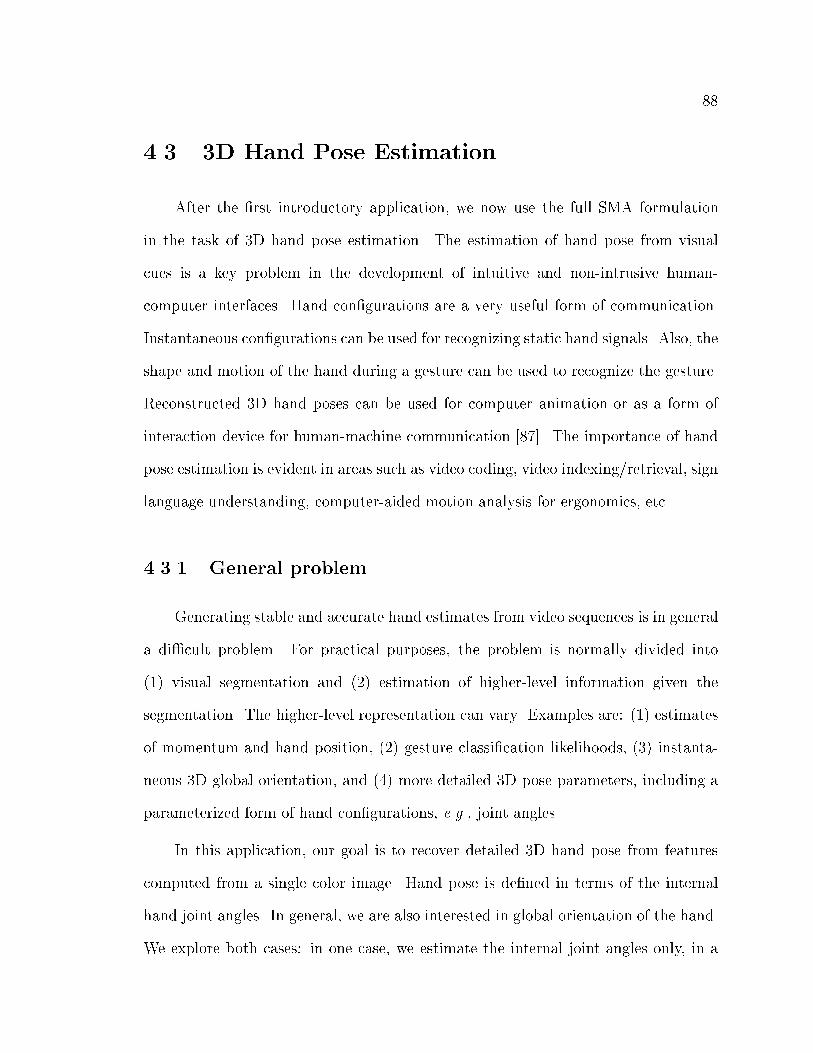
88

4.3 3D Hand Pose Estimation

After the �rst introductory application, we now use the full SMA formulation

in the task of 3D hand pose estimation. The estimation of hand pose from visual

cues is a key problem in the development of intuitive and non-intrusive human-

computer interfaces. Hand con�gurations are a very useful form of communication.

Instantaneous con�gurations can be used for recognizing static hand signals. Also, the

shape and motion of the hand during a gesture can be used to recognize the gesture.

Reconstructed 3D hand poses can be used for computer animation or as a form of

interaction device for human-machine communication [87]. The importance of hand

pose estimation is evident in areas such as video coding, video indexing/retrieval, sign

language understanding, computer-aided motion analysis for ergonomics, etc.

4.3.1 General problem

Generating stable and accurate hand estimates from video sequences is in general

a di�cult problem. For practical purposes, the problem is normally divided into

(1) visual segmentation and (2) estimation of higher-level information given the

segmentation. The higher-level representation can vary. Examples are: (1) estimates

of momentum and hand position, (2) gesture classi�cation likelihoods, (3) instanta-

neous 3D global orientation, and (4) more detailed 3D pose parameters, including a

parameterized form of hand con�gurations, e.g., joint angles.

In this application, our goal is to recover detailed 3D hand pose from features

computed from a single color image. Hand pose is de�ned in terms of the internal

hand joint angles. In general, we are also interested in global orientation of the hand.

We explore both cases: in one case, we estimate the internal joint angles only, in a

89

second case, we estimate both internal joint angles and global orientation of the hand.

We will use the specialized mappings architecture (SMA), to map image features

obtained from other computer vision tools (e.g., [108]) to likely 3D hand poses5. The

SMA is used to perform the estimation once features are obtained. The forward SMA

functions are estimated directly from training data, which in our case are examples of

hand joint con�gurations (outputs) and their corresponding visual features (inputs).

The feedback function can be estimated from data or can be obtained by rendering

a computer graphics hand model. In the next sections we will explain the details of

this formulation.

4.3.2 Hand Model

The hand model we use is implemented in the VirtualHand programming library

[116]. The parameters of the model are 22 joint angles. For the index, middle, ring

and pinky �nger, there is an angle for each of the distal, proximal and metacarpopha-

langeal joints. For the thumb, there is an inner joint angle, an outer joint angle and

two angles for the trapeziometacarpal joint. There are also abduction angles between

the following pairs of successive �ngers: index/middle, middle/ring and ring/pinky.

Finally, there is an angle for the palm arch, an angle measuring wrist exion and an

angle measuring the wrist bending towards the pinky �nger. However, because the

former two wrist angles also encode global orientation, we decided not to model them

in our hand pose applications. Hence, ignoring these two angles, our model has 20

DOF for the internal hand con�guration.

All of these 20 angles are relative to two global orientation angles. These two

5Currently, the systems for detection [108] and reconstruction work independently.

90

angles will encode the camera viewpoint or alternatively hand 3D rotation. In the

future, we will refer to these angles as the camera viewpoint. Imagine a sphere

surrounding the hand model (i.e., a �xed hand center point is at the center of the

sphere). For ease of reference, we will employ the widely used latitude and longitude

notions. The �rst angle �1 represents the latitude from which we are looking at the

hand, the second angle �2 represents the longitude. We have de�ned �1 2 [0; �], with

zero and � being the imaginary poles of the sphere and �2 2 [0; 2�). In summary our

full hand model contains 22 DOF.

Even though the camera location is unrestricted, we assume that the camera is

always pointing to the center of the sphere. However, the camera up vector is also

unrestricted.

4.3.3 3D Hand Data-Set

Using a CyberGlove6, we collected approximately 9,000 examples of 3D hand

poses (parameterized as vectors containing the hand 22 DOF). The data consisted of

hand con�gurations from American Sign Language (ASL) and other hand con�gura-

tions informally determined by several members of our research group.

The VirtualHand library provides tools that can render an arti�cial hand from

an arbitrary viewpoint (de�ned by a pair (�1; �2)), given values for the 22 angles.

We built a training set of all the hand con�gurations initially collected, and rendered

from 86 viewpoints. These viewpoints were chosen to approximately sample the

sphere surface in an uniform way.

Therefore, the hand data set has approximately 9,000 x 86 con�gurations with

6Cyberglove was manufactured by VirtualTechnologies.

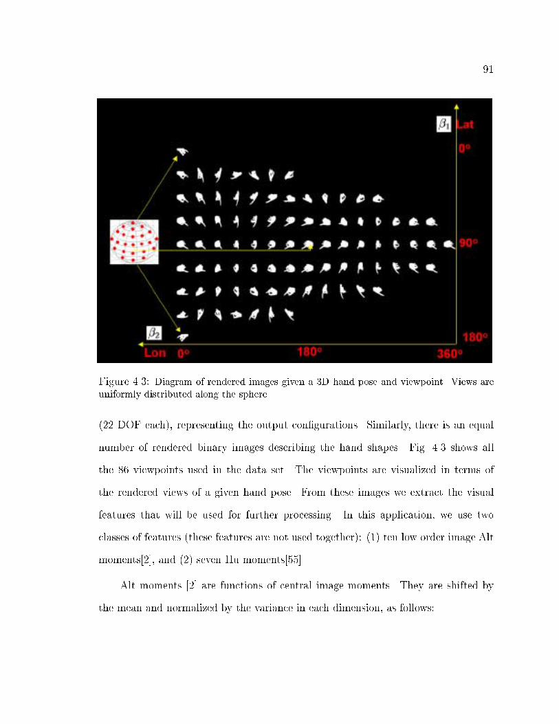
91

Figure 4.3: Diagram of rendered images given a 3D hand pose and viewpoint. Views areuniformly distributed along the sphere.

(22 DOF each), representing the output con�gurations. Similarly, there is an equal

number of rendered binary images describing the hand shapes. Fig. 4.3 shows all

the 86 viewpoints used in the data set. The viewpoints are visualized in terms of

the rendered views of a given hand pose. From these images we extract the visual

features that will be used for further processing. In this application, we use two

classes of features (these features are not used together): (1) ten low order image Alt

moments[2], and (2) seven Hu moments[55].

Alt moments [2] are functions of central image moments. They are shifted by

the mean and normalized by the variance in each dimension, as follows:

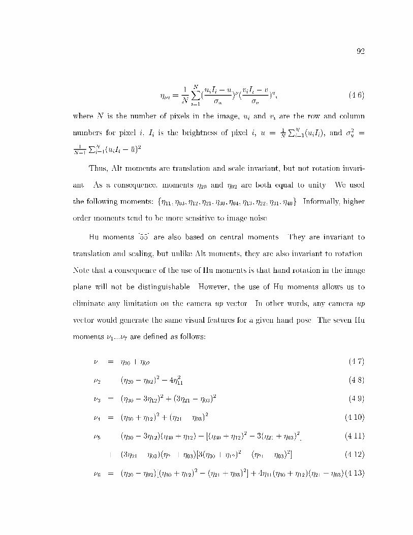
92

�pq =1

N

NXi=1

(uiIi � �u

�u)p(

viIi � �v

�v)q; (4.6)

where N is the number of pixels in the image, ui and vi are the row and column

numbers for pixel i, Ii is the brightness of pixel i, �u = 1N

PNi=1(uiIi), and �2u =

1N�1

PNi=1(uiIi � �u)2.

Thus, Alt moments are translation and scale invariant, but not rotation invari-

ant. As a consequence, moments �20 and �02 are both equal to unity. We used

the following moments: f�11; �03; �12; �21; �30; �04; �13; �22; �31; �40g. Informally, higher

order moments tend to be more sensitive to image noise.

Hu moments [55] are also based on central moments. They are invariant to

translation and scaling, but unlike Alt moments, they are also invariant to rotation.

Note that a consequence of the use of Hu moments is that hand rotation in the image

plane will not be distinguishable. However, the use of Hu moments allows us to

eliminate any limitation on the camera up vector. In other words, any camera up

vector would generate the same visual features for a given hand pose. The seven Hu

moments �1:::�7 are de�ned as follows:

�1 = �20 + �02 (4.7)

�2 = (�20 � �02)2 + 4�211 (4.8)

�3 = (�30 � 3�12)2 + (3�21 � �03)

2 (4.9)

�4 = (�30 + �12)2 + (�21 � �03)

2 (4.10)

�5 = (�30 � 3�12)(�30 + �12) + [(�30 + �12)2 � 3(�21 + �03)

2] (4.11)

+ (3�21 � �03)(�21 + �03)[3(�30 + �12)2 � (�21 + �03)

2] (4.12)

�6 = (�20 � �02)[(�30 + �12)2 � (�21 + �03)

2] + 4�11(�30 + �12)(�21 + �03)(4.13)

93

�7 = (3�21 � �03)(�30 + �12)[(�30 + �12)2 � 3(�21 + �03)

2] (4.14)

� (�30 � �12)(�21 + �03)[3(�30 + �12)2 � (�21 + �03)

2] (4.15)

In summary, Hu moments allow us to simplify the estimation process by reducing

the amount of data required to cover the input space. However, they make certain

con�gurations indistinguishable from each other. Alt moments improve the number

of distinguishable con�gurations, but make it impractical to create a good training

set.

In view of this, let us de�ne two data sets. (1) The Hand-Single-View dataset,

containing the input-output pairs (approximately 9,000) where outputs consist of

only the camera viewpoint that renders a view of the hand palm (�1 = �=2, �2 = 0),

and features (input) are computed using the Alt moments. (2) The Hand-All-Views

dataset, containing the input-output pairs (approximately 9,000 x 86), where outputs

are all 9,000 di�erent con�gurations with all the 86 prede�ned orientations (camera

viewpoints), and features are computed using Hu moments. In Chapter 6 we will

conduct experiments with both data sets.

There are many other possible feature choices beyond Hu and Alt moments;

however, the intention of this thesis is not to study feature selection. The purpose of

a feature set in this application is to reduce the dimensionality of the problem and

incorporate useful invariances, such as translation and scaling. These invariances ease

the observation process; e.g., we do not need to be concerned about where and how

large the hand appears in the image.

94

4.3.4 Hand Detection and Segmentation

We will use video sequences collected with a color digital camera. These se-

quences have a static background, only one person is present, and the person is

facing towards the camera. Our system tracks both hands of the user automatically

using a skin color tracker.

This tracker uses an estimated probability distribution of skin color. For esti-

mating this distribution, we used labeled samples of regions where skin color was

present. Thus, at every pixel we can measure how likely it is that the pixel belongs

to a skin-colored object. For a detailed explanation, readers are referred to [99, 108].

Our simple hand detection and tracking algorithm would not work at any frame

where the hands overlap with each other or with the face. In our video sequences

we took care to avoid such situations. Our system could be made more general by

including modules to predict occlusion of an object by another and to detect when

those objects are separated again. A similar approach has been successfully applied

in the domain of multiple person tracking with occlusion handling [100].

4.3.5 System Overview

An overview of our approach for unrestricted view hand pose estimation can be

seen in Fig. 4.4. First, a number J � 9; 000 of example hand joint con�gurations

are acquired using a CyberGlove (at approx. 15 Hz). The CyberGlove measures 22

angular DOF of the hand. However, we took only 20 of those DOF (for the reasons

discussed in Sec. 4.3.3). Computer graphics software can be used to render a shaded

view of any hand con�guration captured by the CyberGlove. Using this computer

graphics rendering function, we can generate a uniform sampling (with size S = 86)

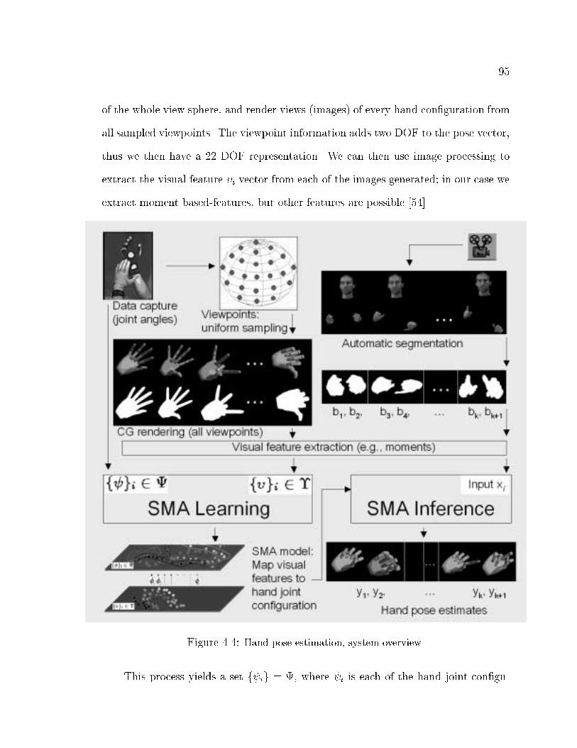
95

of the whole view sphere, and render views (images) of every hand con�guration from

all sampled viewpoints. The viewpoint information adds two DOF to the pose vector,

thus we then have a 22 DOF representation. We can then use image processing to

extract the visual feature �i vector from each of the images generated; in our case we

extract moment based-features, but other features are possible [54].

Figure 4.4: Hand pose estimation, system overview.

This process yields a set f ig = , where i is each of the hand joint con�gu-

96

rations from each viewpoint7, and f�ig = �, where �i is a vector of visual features

corresponding to each i.

The sets and � constitute samples from the input-output relationship that we

will attempt to learn using our architecture. Given a new image of a hand, we will

compute its visual feature vector x. We then compute the mapping from x to the

most likely 22 DOF hand con�guration. This con�guration includes 20 DOF joint

angles and 2 DOF associated with the camera viewpoint or alternatively the hand

spatial orientation.

The SMA tries to learn a multiple mapping so that, when performing inference,

given a vector of visual features x, an output in the output space of hand con�g-

urations can be provided. The right column of Fig. 4.4 shows a diagram of the

inference process. First, video input is obtained, then using a segmentation module,

regions with high likelihood of being skin colored are found. From these regions we

extract visual features (e.g., moments). Then the given vector of visual features x is

presented to SMA, which generates several output estimates, one of which is chosen

using a de�ned cost function.

4.4 2D Human body pose Estimation

The second application domain that will be used to test SMA is the estimation

of 2D human pose from visual features. As explained before, this is an intensely

studied application in computer vision. The methodology followed is very similar to

the estimation of hand pose. We are mainly concerned with the estimation of body

7This vector is then composed of 20 internal pose parameters plus two global orientation

parameters.

97

pose, once features have been extracted. In the following sections we describe the

implementation details of this application.

4.4.1 General Problem

The goal of this application is to estimate human body posture from a single

image. The problem de�nition and related work in this area is thoroughly described

in Chapter 2. Human pose is de�ned as the instantaneous con�guration of a single

articulated body in terms of the position of a predetermined set of joints. Note

that these positions automatically determine body orientation. First, statistical

segmentation of the human bodies from the background is performed [52, 101, 119],

then low-level visual features are found given the segmented body shape. Our goal is

to be able to map these, generally low-level, visual features to body con�gurations.

4.4.2 Human Body Model

The human body model used in this application is de�ned in terms of 20 marker

positions. Unlike the 3D hand model, we do not use joint angle representations.

Therefore a 3D body pose consists of 60 DOFs.

The 20 markers are distributed as follows: three markers for the head, three

markers for the hip - back bone articulation, two markers for shoulders, two markers

for elbows, two markers for wrists, two markers for hands, two markers for knees, two

markers for ankles, and two markers for the feet.

For rendering, the body model is de�ned as being composed of cylinders of equal

width. The cylinders connect the de�ned markers to form the standard human body

structure. The thorax was modeled using a wider cylinder. Because in this application

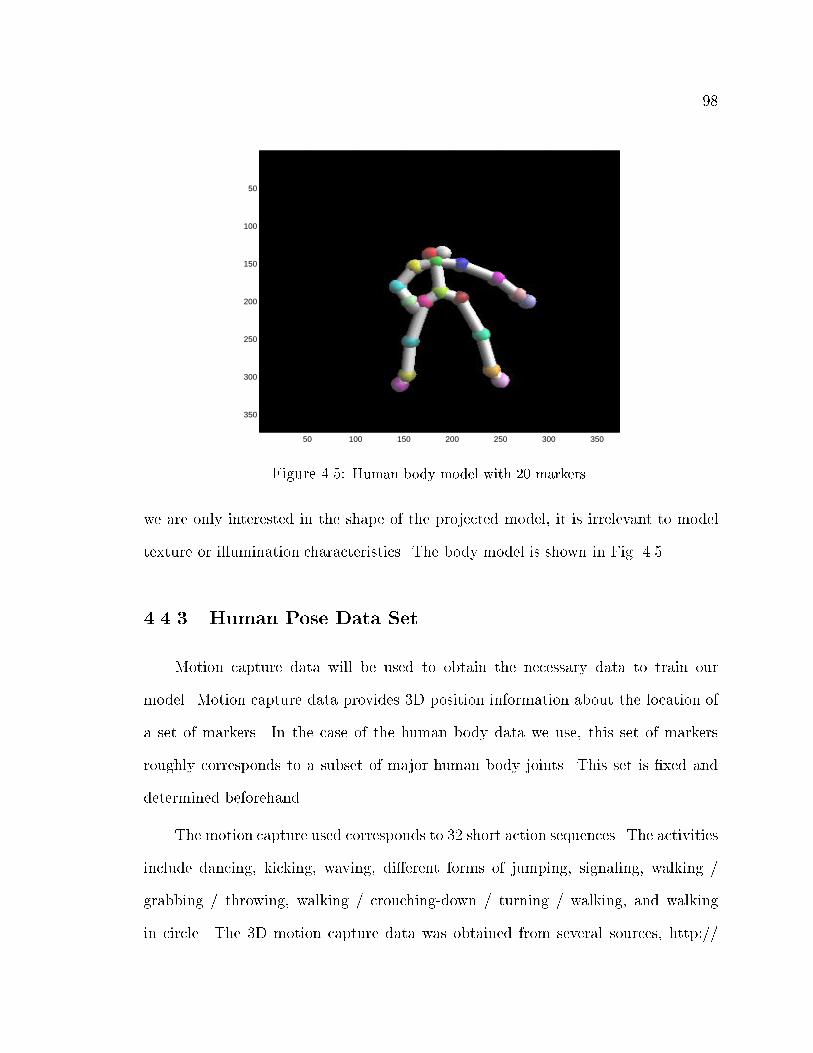
98

50 100 150 200 250 300 350

50

100

150

200

250

300

350

Figure 4.5: Human body model with 20 markers.

we are only interested in the shape of the projected model, it is irrelevant to model

texture or illumination characteristics. The body model is shown in Fig. 4.5.

4.4.3 Human Pose Data Set

Motion capture data will be used to obtain the necessary data to train our

model. Motion capture data provides 3D position information about the location of

a set of markers. In the case of the human body data we use, this set of markers

roughly corresponds to a subset of major human body joints. This set is �xed and

determined beforehand.

The motion capture used corresponds to 32 short action sequences. The activities

include dancing, kicking, waving, di�erent forms of jumping, signaling, walking /

grabbing / throwing, walking / crouching-down / turning / walking, and walking

in circle. The 3D motion capture data was obtained from several sources, http://

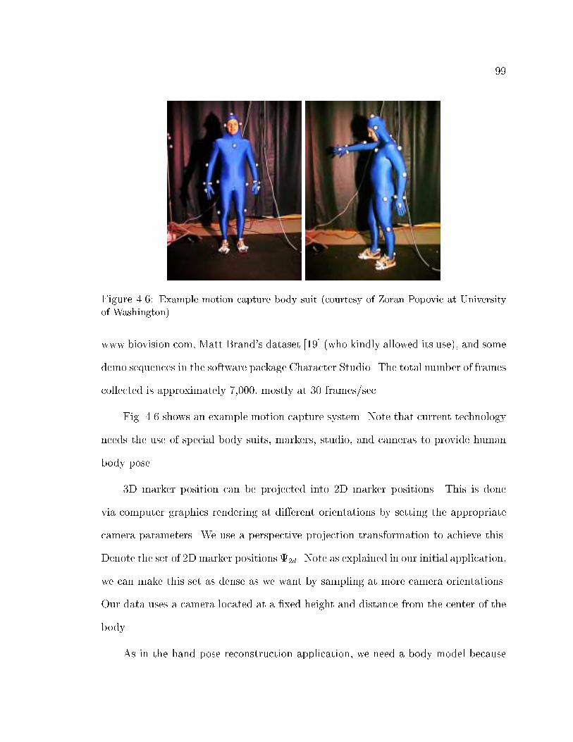
99

Figure 4.6: Example motion capture body suit (courtesy of Zoran Popovic at Universityof Washington).

www.biovision.com, Matt Brand's dataset [19] (who kindly allowed its use), and some

demo sequences in the software package Character Studio. The total number of frames

collected is approximately 7,000, mostly at 30 frames/sec.

Fig. 4.6 shows an example motion capture system. Note that current technology

needs the use of special body suits, markers, studio, and cameras to provide human

body pose.

3D marker position can be projected into 2D marker positions. This is done

via computer graphics rendering at di�erent orientations by setting the appropriate

camera parameters. We use a perspective projection transformation to achieve this.

Denote the set of 2Dmarker positions 2d. Note as explained in our initial application,

we can make this set as dense as we want by sampling at more camera orientations.

Our data uses a camera located at a �xed height and distance from the center of the

body.

As in the hand pose reconstruction application, we need a body model because

100

our approach must model how the articulated model looks from di�erent viewing

angles, not just the angle in which the data was captured (i.e., 0 rads.). In other

words, the system needs to be prepared to estimate poses at any orientation. This

approach could also account for a wider variety of viewing conditions, for example,

we could sample the whole viewing sphere. Di�erences in the camera-object distance

could be avoided in principle by choosing scale invariant image features.

By having knowledge of the body structure, we can render its visual appearance.

As before, we can also obtain the visual appearance of the body by rendering in 3D

using the 3D marker positions. In any case, we obtain the set of visual features �2d,

whose elements are in one-to-one correspondence with the elements of 2d.

For this application, we have chosen image Alt moments [2] as our visual features,

mainly due to their ease of computation and invariances to translation and scaling

on the image plane. We call the dataset formed by the pairs (�i 2 �2d; i 2 2d)ni=1

the Body-All-Views-Alt dataset.

4.4.4 Detection and Segmentation

When processing real sequences we use a very basic and widely used human

body pose segmentation scheme [52, 101, 119]. Assuming a static camera and back-

ground, the technique depends on statistical learning of the background appearance,

assuming each pixel is independent of each other, and their color (luminance) is

distributed according to a Gaussian distribution. Segmentation is then approached

in a maximum-likelihood fashion, where we classify each pixel as belonging to one of

two classes: background or foreground (human body). For a complete and detailed

discussion on this topic, readers are referred to [98].

Chapter 5

Multiple View Formulation of the

Specialized Mappings Architecture

5.1 Introduction

The estimation of 3D human body structure from multiple, simultaneous views

is an important problem faced by computer vision. A related problem, the automatic

calibration of multiple cameras from video, has also been the subject of considerable

research. Here, we provide a solution to both of these problems in the context of

SMA.

In this chapter, we introduce a framework for 3D articulated pose recovery, given

multiple uncalibrated views1. The map from visual features to body joint locations

is obtained via Specialized Mappings Architecture (SMA) of Chapter 3. The SMA

provides several pose hypotheses, each one with correspondences of 2D joint locations

1A previous version of this material was presented in [105]. This chapter describes joint work

with Matheen Siddiqui and Joni Alon.

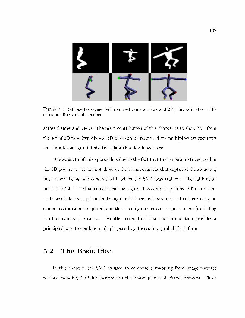
102

Figure 5.1: Silhouettes segmented from real camera views and 2D joint estimates in thecorresponding virtual cameras.

across frames and views. The main contribution of this chapter is to show how from

the set of 2D pose hypotheses, 3D pose can be recovered via multiple-view geometry

and an alternating minimization algorithm developed here.

One strength of this approach is due to the fact that the camera matrices used in

the 3D pose recovery are not those of the actual cameras that captured the sequence,

but rather the virtual cameras with which the SMA was trained. The calibration

matrices of these virtual cameras can be regarded as completely known; furthermore,

their pose is known up to a single angular displacement parameter. In other words, no

camera calibration is required, and there is only one parameter per camera (excluding

the �rst camera) to recover. Another strength is that our formulation provides a

principled way to combine multiple pose hypotheses in a probabilistic form.

5.2 The Basic Idea

In this chapter, the SMA is used to compute a mapping from image features

to corresponding 2D joint locations in the image planes of virtual cameras. These

103

virtual camera views are a direct consequence of our use of image features that are

invariant to translation, scaling, and rotation on the image plane. This is evident from

Fig.5.1. Note that these estimates are insensitive to image translation, scaling and

rotation. Also note the overall vertical orientation of the skeleton. This is from the

SMA mappings being trained with concentric cameras, where each camera's principal

axis passes through the circles' center, and all cameras have coinciding up-vectors; in

other words, the virtual image scan lines should ideally match across views.

Given correspondences of the most likely 2D joint locations in multiple, virtual

camera views obtained from the SMA inference procedure, 3D body pose can be re-

covered with an algorithm related to structure from motion. Moreover, given multiple

hypotheses per camera (as presented here) we formalize a generalized probabilistic

structure from motion technique and provide an algorithm for the special virtual

camera case.

An overview of our approach is shown in Figs.5.2{5.3. Our goal is to produce a

reconstruction of body pose X (3D joint locations) and the relative orientations of

the real cameras. First images obtained by each camera c are segmented to extract

image features xc. Each camera is assumed to capture images of the whole body,

camera parameters are otherwise unconstrained.

In order to be more speci�c, in this chapter, visual features refer to image

moments of the binary image of the segmented body pose. We use Hu moments

[55], shape descriptors based on central moments. The crucial characteristic to notice

about these features is their invariance to translation, scaling, and rotation in the

image plane. These invariances originate the name Virtual Cameras. Our cameras

cannot perceive changes in the image associated with the referred invariances, thus

104

Figure 5.2: Overview of pose hypothesis generation. Cameras capture the scene, human�gures are segmented, and a vector of visual features xc is computed per camera. The SMAproduces several body pose hypotheses per camera,.

they are not real cameras. Further, we will see that this special characteristic would

lead to more tractable algorithms for computing 3D structure.

5.2.1 Visual Features to 2D Pose

The front-end of our approach consists of a Specialized Mapping Architecture

(SMA) developed in Chapter 3. In this chapter, an SMA may be regarded as a

set of functions � = f�kg that have been trained to map inputs to outputs. The

SMA mapping functions have been precomputed via a supervised learning procedure.

Training data for the SMA is generated via computer graphic renderings of 3D motion

capture data. As shown in Fig. 5.2, each function �k transforms (maps) a vector of

visual features x into a 2D body pose hypotheses, H:k.

Given a silhouette for the human extracted in C camera views, each yielding

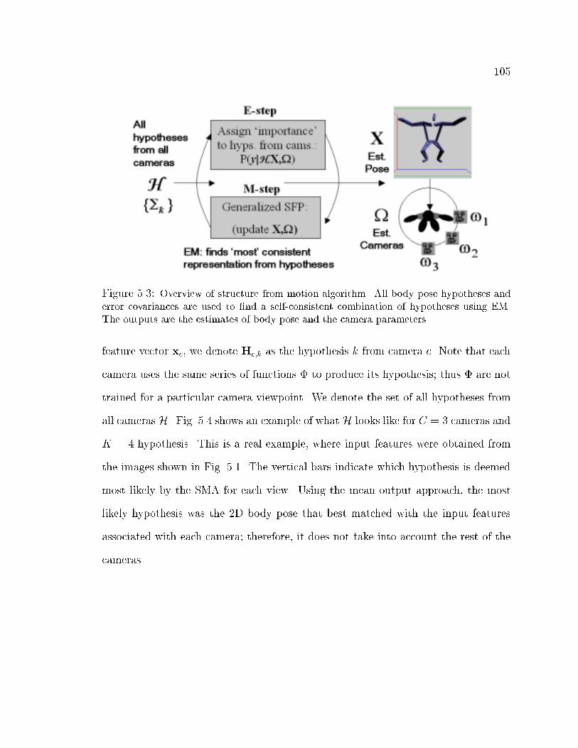
105

Figure 5.3: Overview of structure from motion algorithm. All body pose hypotheses anderror covariances are used to �nd a self-consistent combination of hypotheses using EM.The outputs are the estimates of body pose and the camera parameters.

feature vector xc, we denote Hc;k as the hypothesis k from camera c. Note that each

camera uses the same series of functions � to produce its hypothesis; thus � are not

trained for a particular camera viewpoint. We denote the set of all hypotheses from

all cameras H. Fig. 5.4 shows an example of what H looks like for C = 3 cameras and

K = 4 hypothesis. This is a real example, where input features were obtained from

the images shown in Fig. 5.1. The vertical bars indicate which hypothesis is deemed

most likely by the SMA for each view. Using the mean output approach, the most

likely hypothesis was the 2D body pose that best matched with the input features

associated with each camera; therefore, it does not take into account the rest of the

cameras.

106

5.2.2 3D Structure and Camera Estimation from Multiple

Pose Hypotheses

The individual best con�gurations shown in Fig. 5.4 (marked with a bar) are

not guaranteed to be self-consistent, i.e., they may not agree. A 3D reconstruction

algorithm needs to account for this inconsistency of the observations. To accomplish

this, 3D estimation can be posed as a maximum likelihood (ML) estimation problem

that tries to �nd the best estimates for X and given the set of all hypotheses from

all cameras H = fHc;kg. As shown in Fig. 5.3 we try to �nd a 3D body pose and

cameras that generate the most consistent combination of 2D hypotheses from each

camera.

In the remainder of this chapter, we formulate this problem and show its exact

solution is intractable. We then present an Expectation Maximization (EM) algo-

rithm that approximates a solution to the initial problem. In order to prepare the

reader for the next sections, we will anticipate that the form of the EM algorithm

requires solving a generalized form of the Structure from Motion problem at each

iteration of the M-step. This is related in some sense to the recent work of [34], but

di�ers in the following key aspects: 1.) our method handles multiple hypotheses per

camera, 2.) our method uses a full covariance matrix weighting for the hypotheses

in the solution, and 3.) sampling methods are not required because our problem is

posed in a tractable form.

107

5.3 Probabilistic 3D Reconstruction

Reconstruction will be formulated as a stochastic optimization problem. The

goal is to maximize the log-likelihood of the 3D body pose X and camera parameters

:

�;X� = argmaxX;

log p(HjX;); (5.1)

where X 2 <p, with p = 3 � (number of joints) and = (!1; ::!C). Assuming that

the hypotheses presented by each camera are conditionally independent given the

model parameters X and , we have:

�;X� = argmaxX;

logCYc=1

p(HcjX;): (5.2)

This assumption is reasonable because by knowing X and , we do not gain any

information about a given view if we know about another view. Introducing a latent

random variable yc 2 f1:::Kg representing the choice of hypothesis for camera c we

obtain:

�;X� = argmaxX;

CXc=1

log(KcXk=1

p(Hcjyc = k;X;)P (yc = kjX;)): (5.3)

Intuitively, p(Hcjyc = k;X;) is how probable the k � th hypothesis of camera c is,

given the model parameters X;. It is important to note that the probability of a set

of hypotheses from several cameras can be factorized into a product of probabilities of

hypotheses from each camera (because of our conditional independence assumption).

Thus, combinatorial complexity is avoided.

If we consider P (yc = kjX;) as uniform, then we face the following stochastic

optimization problem:

�;X� = argmaxX;

CXc=1

log(KcXk=1

p(Hcjyc = k;X;)): (5.4)

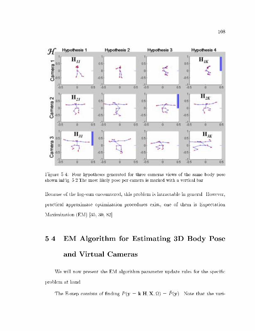
108

Figure 5.4: Four hypotheses generated for three cameras views of the same body poseshown inFig. 5.2.The most likely pose per camera is marked with a vertical bar.

Because of the log-sum encountered, this problem is intractable in general. However,

practical approximate optimization procedures exist, one of them is Expectation

Maximization (EM) [35, 30, 82].

5.4 EM Algorithm for Estimating 3D Body Pose

and Virtual Cameras

We will now present the EM algorithm parameter update rules for the speci�c

problem at hand.

The E-step consists of �nding P (y = kjH;X;) = ~P (y). Note that the vari-

109

ables yc are independent (it follows from our conditional independence assumption in

Sec. 5.3). Therefore, we can factorize ~P (y) =Qc~P (yc). Assuming a uniform prior

over the specialized functions of any camera, i.e., P (yc = kjX;) = � (in a bounded

domain), it can be shown that:

~P (yc) =p(Hcjyc = k;X;)Pj p(Hcjyc = j;X;)

(5.5)

However, note that p(Hcjyc = k;X;) is still unde�ned. We can use:

p(Hcjyc = k;X;) = N (Hc;k;R(X;c);�k); (5.6)

with Hc;k the k-th hypothesis of camera c, c the parameters of the camera c, and

�k the covariance error of the specialized function k.

One way to interpret this choice is to simply think that the error cost in the

projection of the current estimate is a Gaussian distribution. This seems a natural

choice, and leads to tractable further derivations. The distribution is shaped according

to �k to represent our degree of con�dence in the hypotheses generated by the SMA.

5.4.1 General M-step

The M-step consists of �nding

(;X)(t) = argmax;X

E ~P (t)[log p(H;yj;X)]: (5.7)

In our case we can show that this is equivalent to:

argmax;X

Xc

E ~P(t)c

[log p(Hc; ycj;X)] =

argmin;X

Xc

Xk

~P (t)(yc = k)(Hc;k � R(X;c))>��1

k (Hc;k �R(X;c)) (5.8)

Very interestingly, Eq. 5.8 corresponds to a generalized version of the Structure

from Motion problem [41]. In the standard structure from motion problem, �k is

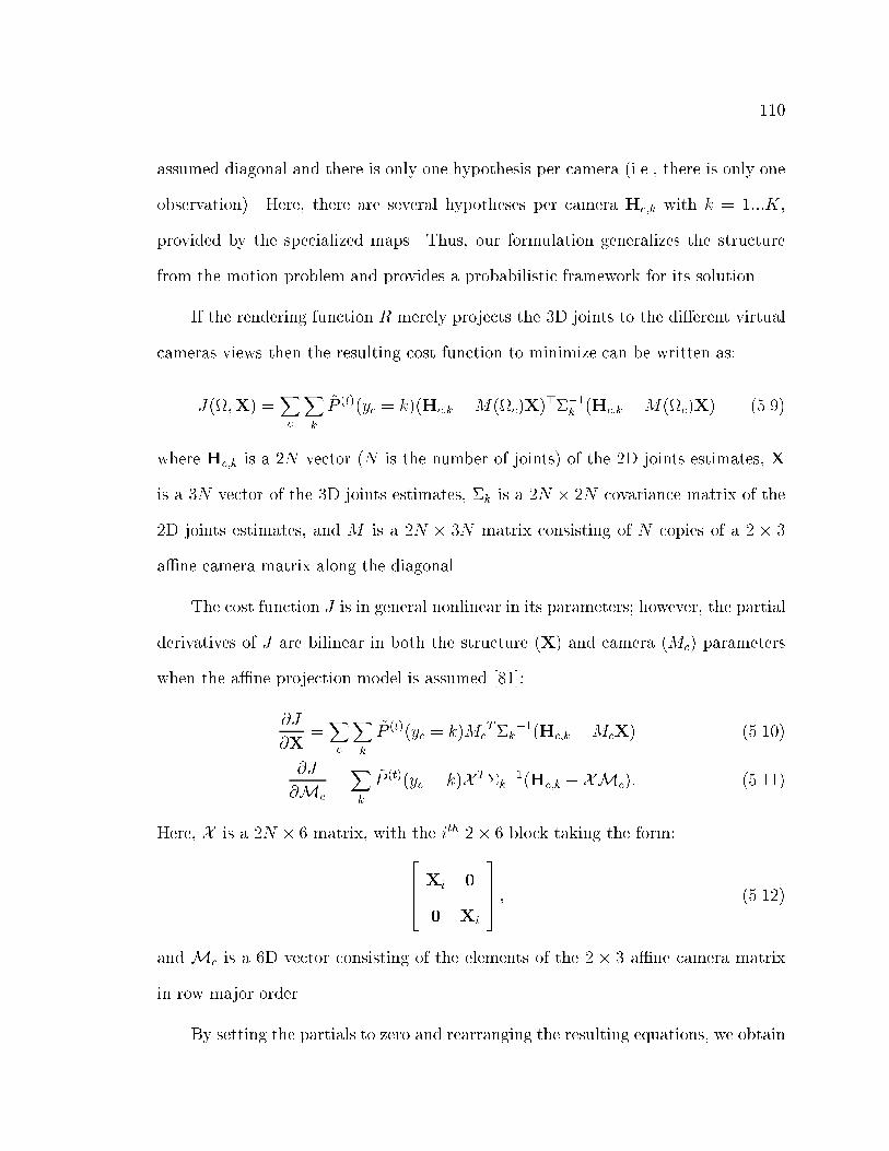
110

assumed diagonal and there is only one hypothesis per camera (i.e., there is only one

observation). Here, there are several hypotheses per camera Hc;k with k = 1:::K,

provided by the specialized maps. Thus, our formulation generalizes the structure

from the motion problem and provides a probabilistic framework for its solution.

If the rendering function R merely projects the 3D joints to the di�erent virtual

cameras views then the resulting cost function to minimize can be written as:

J(;X) =Xc

Xk

~P (t)(yc = k)(Hc;k �M(c)X)>��1

k (Hc;k �M(c)X) (5.9)

where Hc;k is a 2N vector (N is the number of joints) of the 2D joints estimates, X

is a 3N vector of the 3D joints estimates, �k is a 2N � 2N covariance matrix of the

2D joints estimates, and M is a 2N � 3N matrix consisting of N copies of a 2 � 3

a�ne camera matrix along the diagonal.

The cost function J is in general nonlinear in its parameters; however, the partial

derivatives of J are bilinear in both the structure (X) and camera (Mc) parameters

when the a�ne projection model is assumed [81]:

@J

@X=Xc

Xk

~P (t)(yc = k)McT�k

�1(Hc;k �McX) (5.10)

@J

@Mc

=Xk

~P (t)(yc = k)X T�k�1(Hc;k � XMc): (5.11)

Here, X is a 2N � 6 matrix, with the ith 2� 6 block taking the form:

2664Xi 0

0 Xi

3775 ; (5.12)

and Mc is a 6D vector consisting of the elements of the 2 � 3 a�ne camera matrix

in row major order.

By setting the partials to zero and rearranging the resulting equations, we obtain

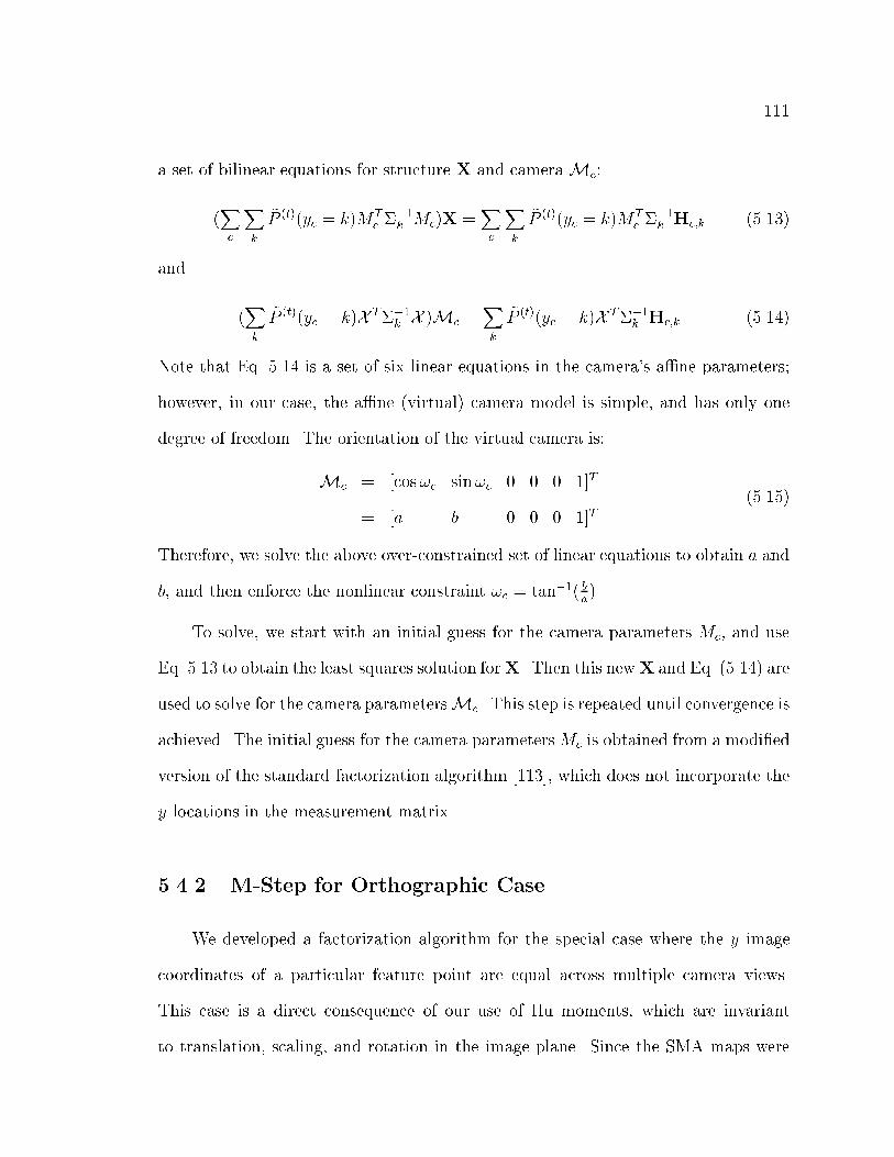
111

a set of bilinear equations for structure X and camera Mc:

(Xc

Xk

~P (t)(yc = k)MTc �

�1k Mc)X =

Xc

Xk

~P (t)(yc = k)MTc �

�1k Hc;k (5.13)

and

(Xk

~P (t)(yc = k)X T��1k X )Mc =

Xk

~P (t)(yc = k)X T��1k Hc;k (5.14)

Note that Eq. 5.14 is a set of six linear equations in the camera's a�ne parameters;

however, in our case, the a�ne (virtual) camera model is simple, and has only one

degree of freedom. The orientation of the virtual camera is:

Mc = [cos!c sin!c 0 0 0 1]T

= [a b 0 0 0 1]T(5.15)

Therefore, we solve the above over-constrained set of linear equations to obtain a and

b, and then enforce the nonlinear constraint !c = tan�1( ba).

To solve, we start with an initial guess for the camera parameters Mc, and use

Eq. 5.13 to obtain the least squares solution forX. Then this newX and Eq. (5.14) are

used to solve for the camera parametersMc. This step is repeated until convergence is

achieved. The initial guess for the camera parametersMc is obtained from a modi�ed

version of the standard factorization algorithm [113], which does not incorporate the

y locations in the measurement matrix.

5.4.2 M-Step for Orthographic Case

We developed a factorization algorithm for the special case where the y image

coordinates of a particular feature point are equal across multiple camera views.

This case is a direct consequence of our use of Hu moments, which are invariant

to translation, scaling, and rotation in the image plane. Since the SMA maps were

112

trained with cameras with coinciding up-vectors, the v coordinates of the 2D estimates

of a particular joint obtained from the inference are expected to be equal across

multiple views.

The inputs to the algorithm are 2D joint location estimates in the di�erent virtual

camera views obtained from the SMA inference. The outputs are estimates of the

camera's orientation and 3D joint estimates. The algorithm consists of the following

steps:

Step 0: Normalize the data: (i) subtract the coccyx (tail bone) joint from all

other joints. (ii) isotropically scale all but the �rst virtual camera view so that image

scan lines match across all camera views.

Step 1: Construct the measurement matrix W :

W =

266666666664

u11 u12 : : : u1N

u21 u22 : : : u2N...

......

...

uC1 uC2 : : : uCN

377777777775; (5.16)

where uci is the u image coordinate of feature point i in camera view c, and compute

the singular value decomposition W = USV T .

Step 2: The a�ne camera and structure reconstruction are:

Pca =

2664Uc1 0 Uc2

0 1 0

3775 (5.17)

�xia zi

a

�= S 0 �

�Vi1 Vi2

�; (5.18)

where S 0 is the 2 � 2 major of S. Note that yia can be set to the average of the v

coordinates of feature point i across all camera views.

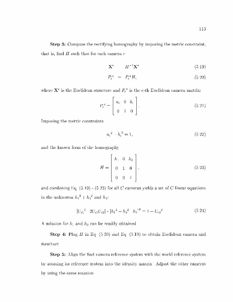
113

Step 3: Compute the rectifying homography by imposing the metric constraint,

that is, �nd H such that for each camera c

Xe = H�1Xa (5.19)

Pce = Pc

aH; (5.20)

where Xe is the Euclidean structure and Pce is the c-th Euclidean camera matrix:

Pce =

2664ac 0 bc

0 1 0

3775 : (5.21)

Imposing the metric constraints

ac2 + bc

2 = 1; (5.22)

and the known form of the homography

H =

26666664

h1 0 h3

0 1 0

0 0 1

37777775; (5.23)

and combining Eq. (5.19) - (5.23) for all C cameras yields a set of C linear equations

in the unknowns h12 + h3

2 and h3:

[Uc12 2Uc1Uc2] � [h1

2 + h32 h3]

T = 1� Uc22 (5.24)

A solution for h1 and h3 can be readily obtained.

Step 4: Plug H in Eq. (5.20) and Eq. (5.19) to obtain Euclidean camera and

structure.

Step 5: Align the �rst camera reference system with the world reference system

by rotating its reference system into the identity matrix. Adjust the other cameras

by using the same rotation.

114

5.4.3 Multiple Frames

For the sake of simplicity, our formulation was derived for a single time frame

only. In our implementation, we extended it to multiple frames. A straightforward

way to do this is to assume that frames are conditionally independent over time:

p(H1; :::;HT jX1; :::;XT ;) =TYt=1

p(HtjXt;); (5.25)

with t indicating the frame number.

This is di�erent than just several single frame estimations in that is not time

dependent, and therefore more evidence from multi-frames should tend in theory to

provide a more robust estimate. An equivalent to Eqs. 5.13 and 5.14 was derived

with just an additional summation over time t in each side. Note also that these total

independence assumptions can be relaxed easily to obtain, for example, Markov-

like models of a given order. In these cases, inference is not as e�cient and good

approximations to the solution may be harder to formulate.

5.5 Multiple-View Body Pose Estimation Applica-

tion: Implementation Remarks

This chapter is self-contained at describing the use of this approach in vision.

However this section brie y explains some of the application details that were initially

left out or not described in detail.

The goal is to estimate 3D body pose and camera relative location from multiple,

uncalibrated views. First, a mapping from image features to 2D body joint locations

is computed using SMA which yields a set of several body pose hypotheses. Given

115

pose hypotheses obtained in the multiple virtual camera views, the recovery of 3D

body pose and camera relative orientations is formulated as a stochastic optimization

problem. Similarly, as with the other applications we described, the performance of

the approach is evaluated with synthetic sequences as well as real video sequences of

general human motion in Chapter 6.

The human body model, data set and segmentation details are explained in

Sec. 4.4 (dataset Body-All-Views-Alt). The only di�erence is that for visual features,

we use Hu moments instead of Alt moments. Hence, we call this data set: Body-All-

Views-Hu. Hu moments were chosen because our task requires rotation invariant

features. The other di�erence regarding the data utilized is related to the real

sequences. For this set, the data was gathered using a system composed of four

synchronized cameras. These cameras work happen to work at a frame rate of up

to 60 frames/sec. However this sampling rate is not a requirement for our approach,

and lower frame rates are acceptable.

Chapter 6

Experimental Results

In this section, we present experimental results obtained by using the SMA in a variety

of problems. First, the SMA is tested in the arti�cial task of approximating several

functions that share the same domain (i.e., a one-to-many estimation task). We

then present results on real vision problems: single and multiple viewpoint hand pose

estimation, 2D human body pose estimation, and 3D human body pose estimation

from multiple uncalibrated cameras. Detailed experimental results are presented in all

cases. However, we emphasize our experimental evaluation on the most general and

complex problem of hand pose estimation, where camera viewpoints are completely

unrestricted. A formal description of the approaches undertaken in these tasks can

be found in Secs. 3 and 5 (for the multiple camera case); therefore, we will not

concentrate on this aspect here. Our focus in this chapter is on the experimental

evaluation. Therefore, the speci�cs of the experimental settings in each case are

described in the corresponding sections1.

1Results on 2D and 3D body pose estimation shown here were presented �rst in [103, 105]

respectively.

117

6.1 A 1D Estimation Task

In these initial illustrative experiments, the performance of the SMA learning

and forward inference algorithms will be tested in a one-dimensional multiple function

approximation (1D-MFA) task. Inputs and outputs are one-dimensional, but there

is no one-to-one relationship between them. This dataset consists of data points

generated from sampling three di�erent functions in the interval [0,1].

6.1.1 Dataset

The functions were obtained by combinations of cosine functions with di�erent

amplitudes and frequencies; e.g., f1(x) = 0:2397[cos(20x) � cos(5x)] + 0:4377. The

other two functions, f2 and f3 are similar to f1 but we have varied the amplitude and

frequency parameters. Thus in theory they should all have the same descriptional

complexity using an amplitude-frequency representation. This functional form was

chosen as a simple example task to illustrate the properties of the SMA when faced

with a 1D one-to-many mapping task. Moreover, representing these functions is

not a straightforward problem when using other representations di�erent from their

Fourier transform. This is the case for the SMA model. Fig. 6.1 shows the three

underlying functions that generated the data. Let us denote each of the functions fk,

the generating process was as follows:

1. The training set Z is initially empty.

2. One of the functions fk was chosen at random with uniform probability.

3. A point �i was generated uniformly at random in the interval [0,1].

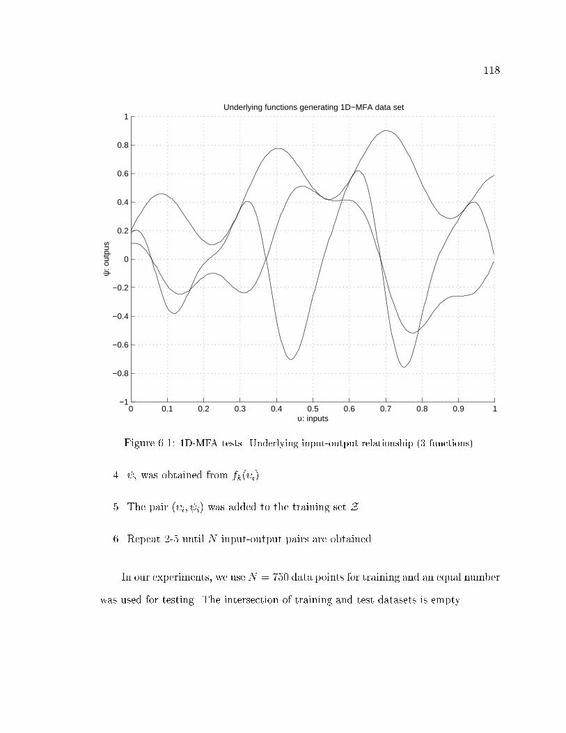
118

0 0.1 0.2 0.3 0.4 0.5 0.6 0.7 0.8 0.9 1−1

−0.8

−0.6

−0.4

−0.2

0

0.2

0.4

0.6

0.8

1

υ: inputs

ψ: o

utpu

sUnderlying functions generating 1D−MFA data set

Figure 6.1: 1D-MFA tests. Underlying input-output relationship (3 functions).

4. i was obtained from fk(�i).

5. The pair (�i; i) was added to the training set Z.

6. Repeat 2-5 until N input-output pairs are obtained.

In our experiments, we use N = 750 data points for training and an equal number

was used for testing. The intersection of training and test datasets is empty.

119

6.1.2 Model

We used the SMA with specialized functions whose mean is the output of a one-

hidden layer perceptron (MLP). This corresponds to case (2) described in Chapter

3; thus the update equations for the model parameters are as described in Eqs. 3.14,

3.15, and 3.16.

Early stopping was used, taking into account several factors"

� Training data: stop if the log-likelihood changes in less than 0.5% averaged over

the last ten iterations.

� Held out data: stop if the held out data log-likelihood average change is negative

over the last ten iterations. Held out data was chosen in the same way as the

training and test data.

� Number of iterations: stop if a maximum of 200 iterations is reached.

6.1.3 Experiments and Discussion

The general model was tested with various structural choices. More speci�cally,

the number of nodes in the MLP hidden layer and the number of specialized functions

were varied as shown in Table 6.1.

From Table 6.1 we can observe the basic behavior of the SMA in this simple

task. The training and test errors almost always decrease with an increase in the

complexity of the model (however this is clearly not true in general). In this sense,

complexity can be roughly thought of as the logarithm of the number of parameters

in the model. Also note that training and test error did not behave in this way when

we used �ve or seven maps and a high number of hidden neurons to approximate the

120

data.

This behavior can be due to several reasons. First, a more complex model is

relatively harder to estimate due to its increased number of local minima. Thus,

roughly speaking, there is an increased probability that our optimization algorithm

will fall into one of these local minima. Second, the increased test error could have

been a consequence of the well-known over�tting phenomenon. Over�tting generally

implies that the model �ts the training data so well that generalization is poor for

other datasets [38].

We experimentally found the number of hidden neurons necessary to approximate

a single function to be nine. This explains why and when over�tting occurs: the upper

bound on the number of parameters that are necessary to �t each of the curves is

nine, thus more parameters would be unnecessary in theory. This agrees with the

results in Table 6.1.

Figs. 6.2 - 6.8 show the maps found by the di�erent SMA con�gurations. It is

now easy to see the e�ect of an increased architecture complexity. Similarly, Figs. 6.10

and 6.11 show the evolution of the log-likelihood logP (�;j�) for each case studied.

An interesting element can also be observed here. Even though it is easy to think

that given the number of parameters required to �t a single function, an e�cient

learning algorithm would probably require triple that number to approximate three

di�erent functions. In our case, it is obvious that if these three underlying functions

are not the same, at least three mapping functions are required. The interesting point

is that as Fig. 6.7(top) shows, we needed three mapping functions with only seven

hidden nodes to approximate the three underlying functions for this example.

This happens when in a given domain, one function can be explained with the

121

same model parameters estimated to �t another function in a di�erent domain. This

is the case for this dataset. This result re ects one of the main reasons why multiple

functions are such an appealing alternative in many problems, even if the underlying

mapping tends to be one-to-one.

6.2 Results from Initial SMA Approximation - 2D

Body Pose Estimation

In this section we test the performance of our initial approach for recovering

2D pose described as an introduction in Sec. 4.2, and later justi�ed within the SMA

framework in Sec. 4.2.6.

6.2.1 Model

Using a subset of the dataset Body-All-Views-Hu (1.000 motion capture frames),

we performed clustering and training as described in Sec. 4.2.2. The view-points for

generating the 2D data set were chosen to be 32 equally spaced locations on the view-

sphere equator. Thus, this gives us 32,000 2D body poses and their corresponding

visual features. We took 5,000 of them for training and the rest for testing. The

model architecture consisted of 15 clusters and 15 single hidden layer perceptrons

with 15 hidden units each. We used the MDL principle [95] to obtain this parameter

choice. In order to apply the MDL principle we varied the number of clusters and

the number of hidden units.

In this task, the output consisted of 11 marker locations (a subset of the original

20 markers), encoded using Principal Components Analysis (PCA) to eight dimen-

122

sions. The input consisted of seven Hu moments.

6.2.2 Experiments with Synthetic Human Bodies

In order to evaluate the performance of our approach, we conducted experiments

in which we had knowledge of the ground-truth.

Fig. 6.12 shows the reconstruction obtained by our approach when images of the

destroy sequence were shown. This sequence exhibits very challenging con�gurations

and orientations. The view angles used were 0 and 12�=32 radians respectively.

Reconstruction and ground-truth agree for all sequences. Note that for self-occluding

con�gurations, reconstruction is harder, but the estimate is close. The error is mainly

due to the inadequacy of the feature and image representation to correctly separate

con�gurations that are di�erent in the marker space, but similar in feature space, and

even in image space.

In order to formally characterize the performance of our system, using the train-

ing and testing procedure described above, we measured the average marker error

measured as the distance between reconstructed and ground-truth projected marker

position. After testing all the sequences, the mean and variance marker displacement

was 17.2% and 33.4% of the average body height. This is a good result given that

choosing a random con�guration from the training set for each test input pattern

would give 47.7% marker displacement error.

We also measured the average marker error per body orientation. For this we

have to rotate the 3D �gures so that their orientation corresponds to the orientation

tested. Recall that in the original sequences, bodies are not always facing a �xed

point. Angles were sampled every 6�=32 radians. The results indicate that the error

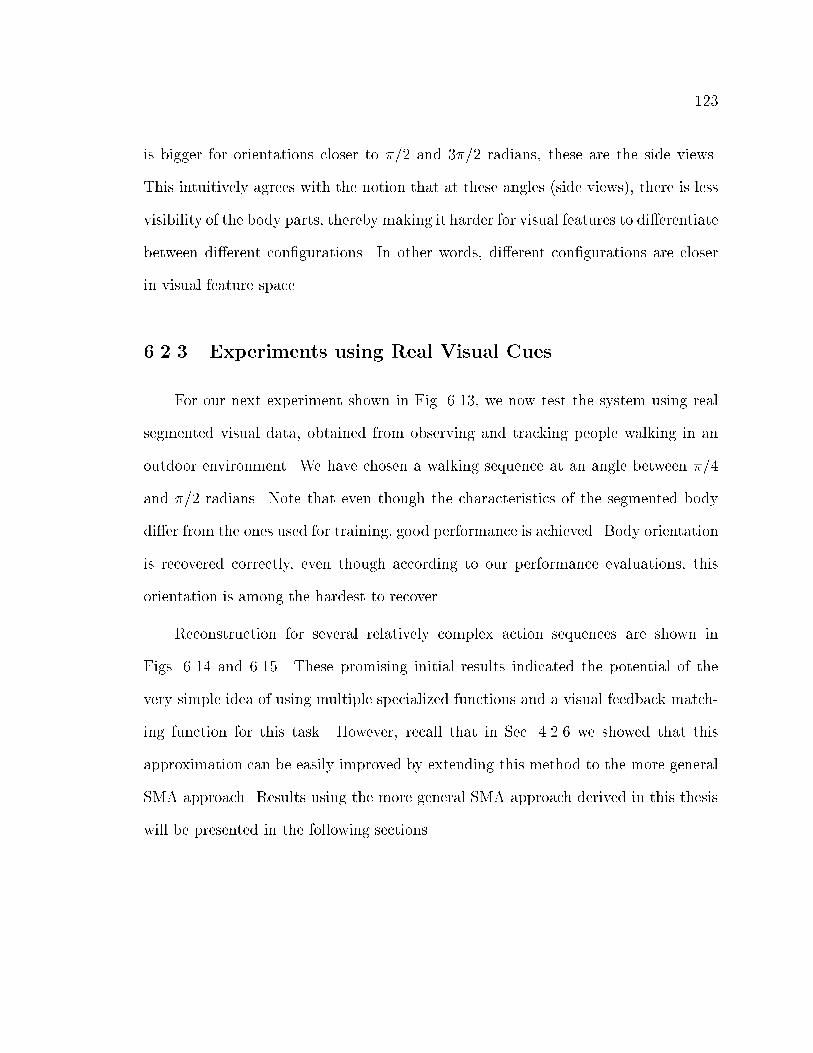
123

is bigger for orientations closer to �=2 and 3�=2 radians, these are the side views.

This intuitively agrees with the notion that at these angles (side views), there is less

visibility of the body parts, thereby making it harder for visual features to di�erentiate

between di�erent con�gurations. In other words, di�erent con�gurations are closer

in visual feature space.

6.2.3 Experiments using Real Visual Cues

For our next experiment shown in Fig. 6.13, we now test the system using real

segmented visual data, obtained from observing and tracking people walking in an

outdoor environment. We have chosen a walking sequence at an angle between �=4

and �=2 radians. Note that even though the characteristics of the segmented body

di�er from the ones used for training, good performance is achieved. Body orientation

is recovered correctly, even though according to our performance evaluations, this

orientation is among the hardest to recover.

Reconstruction for several relatively complex action sequences are shown in

Figs. 6.14 and 6.15. These promising initial results indicated the potential of the

very simple idea of using multiple specialized functions and a visual feedback match-

ing function for this task. However, recall that in Sec. 4.2.6 we showed that this

approximation can be easily improved by extending this method to the more general

SMA approach. Results using the more general SMA approach derived in this thesis

will be presented in the following sections.

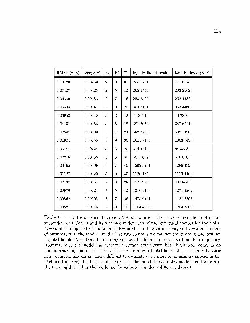
124

RMSE (test) Var(test) M W T log-likelihood (train) log-likelihood (test)

0.10420 0.00969 2 3 8 -22.7608 -23.1797

0.07427 0.00423 2 5 12 205.2554 203.9562

0.06800 0.00488 2 7 16 253.5520 252.4582

0.06333 0.00547 2 9 20 353.6191 353.4460

0.06953 0.00440 3 3 12 71.3124 70.2870

0.04451 0.00356 3 5 18 391.3656 387.6724

0.02597 0.00089 3 7 24 682.3730 682.1476

0.01804 0.00050 3 9 30 1015.7185 1003.9430

0.03481 0.00224 5 3 20 314.4416 68.3333

0.02216 0.00138 5 5 30 681.5077 676.8507

0.00765 0.00006 5 7 40 1292.3291 1286.3995

0.01127 0.00020 5 9 50 1126.1854 1119.4162

0.02137 0.00061 7 3 28 457.5999 437.8045

0.00870 0.00024 7 5 42 1310.9443 1271.9262

0.00562 0.00005 7 7 56 1475.0451 1421.2703

0.00881 0.00016 7 9 70 1264.4790 1204.3509

Table 6.1: 1D tests using di�erent SMA structures. The table shows the root-mean-squared-error (RMSE) and its variance under each of the structural choices for the SMA.M=number of specialized functions, W=number of hidden neurons, and T=total numberof parameters in the model. In the last two columns we can see the training and test setlog-likelihoods. Note that the training and test likelihoods increase with model complexity.However, once the model has reached a certain complexity, both likelihood measures donot increase any more. In the case of the training set likelihood, this is usually becausemore complex models are more di�cult to estimate (i.e., more local minima appear in thelikelihood surface). In the case of the test set likelihood, too complex models tend to over�tthe training data, thus the model performs poorly under a di�erent dataset.

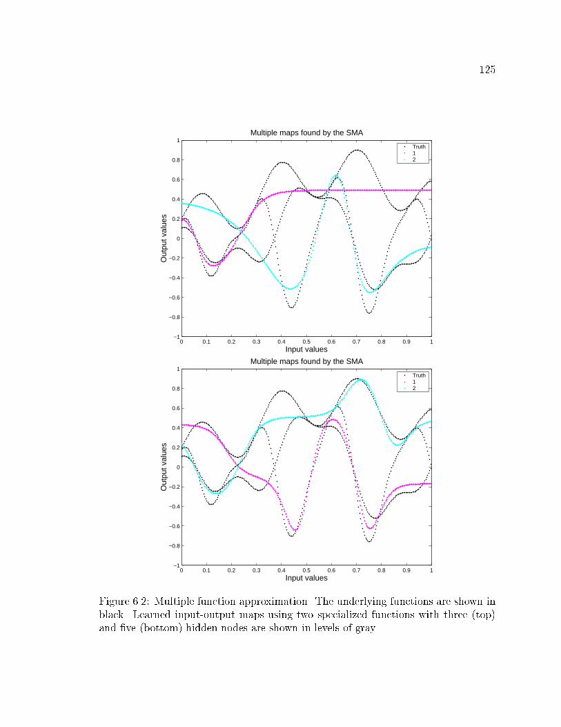
125

0 0.1 0.2 0.3 0.4 0.5 0.6 0.7 0.8 0.9 1−1

−0.8

−0.6

−0.4

−0.2

0

0.2

0.4

0.6

0.8

1

Input values

Out

put v

alue

s

Multiple maps found by the SMA

Truth1 2

0 0.1 0.2 0.3 0.4 0.5 0.6 0.7 0.8 0.9 1−1

−0.8

−0.6

−0.4

−0.2

0

0.2

0.4

0.6

0.8

1

Input values

Out

put v

alue

s


Truth1 2

Figure 6.2: Multiple function approximation. The underlying functions are shown inblack. Learned input-output maps using two specialized functions with three (top)and �ve (bottom) hidden nodes are shown in levels of gray.

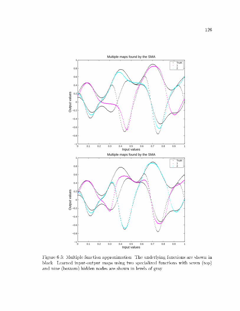
126

0 0.1 0.2 0.3 0.4 0.5 0.6 0.7 0.8 0.9 1−1

−0.8

−0.6

−0.4

−0.2

0

0.2

0.4

0.6

0.8

1

Input values

Out

put v

alue

s


Truth1 2

0 0.1 0.2 0.3 0.4 0.5 0.6 0.7 0.8 0.9 1−1

−0.8

−0.6

−0.4

−0.2

0

0.2

0.4

0.6

0.8

1

Input values

Out

put v

alue

s


Truth1 2

Figure 6.3: Multiple function approximation. The underlying functions are shown inblack. Learned input-output maps using two specialized functions with seven (top)and nine (bottom) hidden nodes are shown in levels of gray.

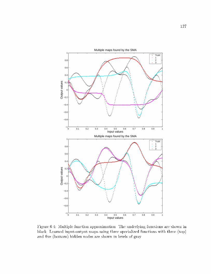
127

0 0.1 0.2 0.3 0.4 0.5 0.6 0.7 0.8 0.9 1−1

−0.8

−0.6

−0.4

−0.2

0

0.2

0.4

0.6

0.8

1

Input values

Out

put v

alue

s


Truth1 2 3

0 0.1 0.2 0.3 0.4 0.5 0.6 0.7 0.8 0.9 1−1

−0.8

−0.6

−0.4

−0.2

0

0.2

0.4

0.6

0.8

1

Input values

Out

put v

alue

s


Truth1 2 3

Figure 6.4: Multiple function approximation. The underlying functions are shown inblack. Learned input-output maps using three specialized functions with three (top)and �ve (bottom) hidden nodes are shown in levels of gray.

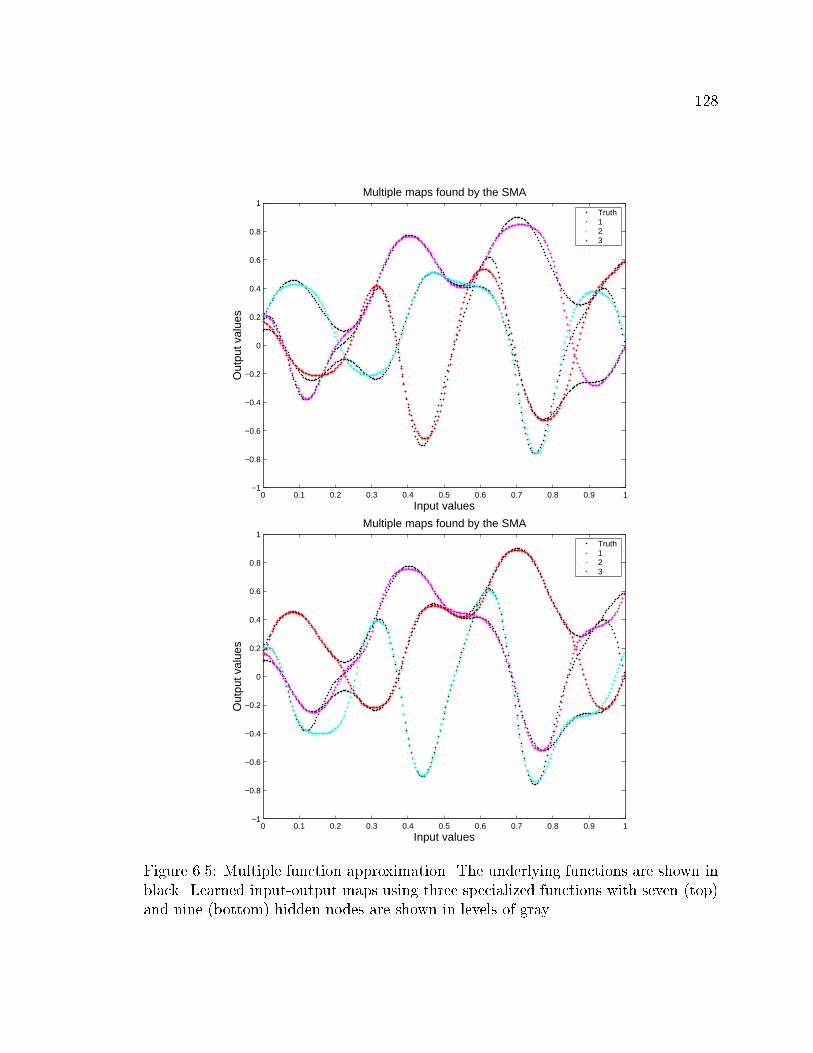
128

0 0.1 0.2 0.3 0.4 0.5 0.6 0.7 0.8 0.9 1−1

−0.8

−0.6

−0.4

−0.2

0

0.2

0.4

0.6

0.8

1

Input values

Out

put v

alue

s


Truth1 2 3

0 0.1 0.2 0.3 0.4 0.5 0.6 0.7 0.8 0.9 1−1

−0.8

−0.6

−0.4

−0.2

0

0.2

0.4

0.6

0.8

1

Input values

Out

put v

alue

s


Truth1 2 3

Figure 6.5: Multiple function approximation. The underlying functions are shown inblack. Learned input-output maps using three specialized functions with seven (top)and nine (bottom) hidden nodes are shown in levels of gray.

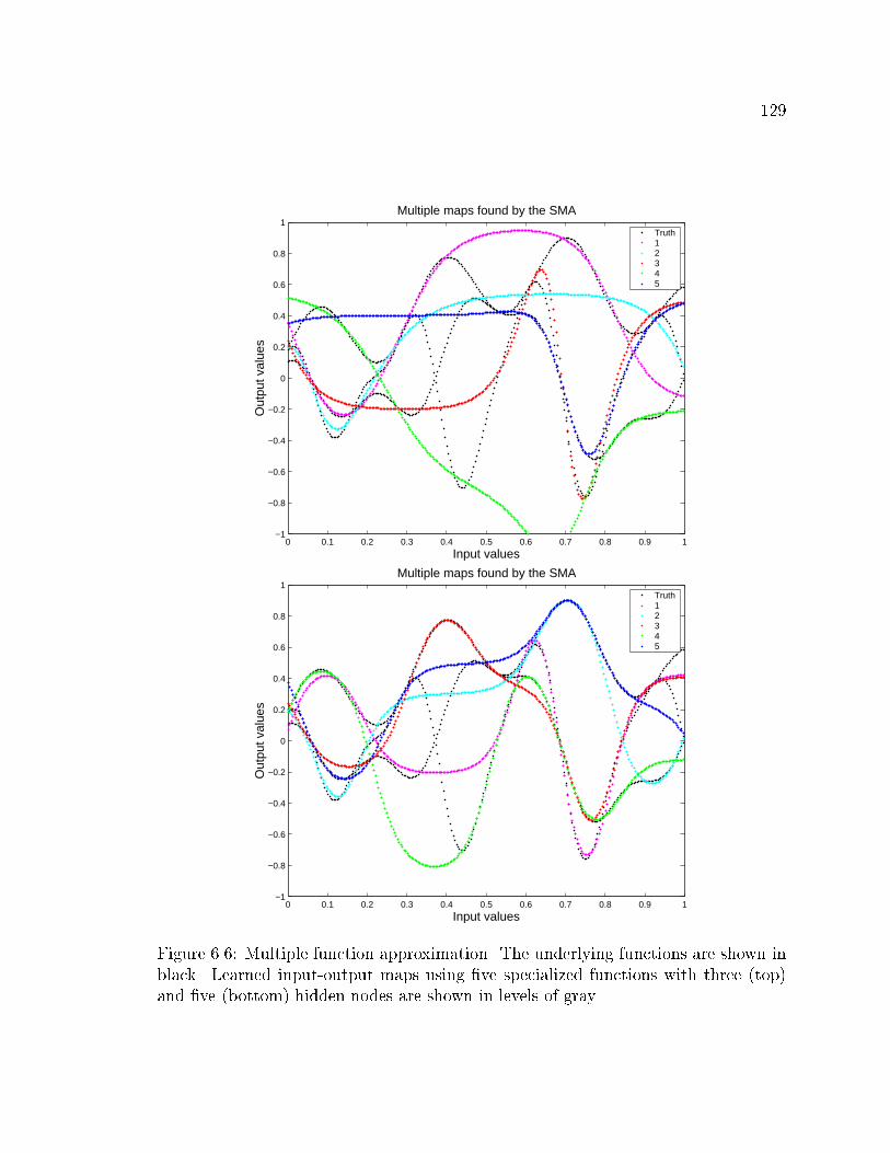
129

0 0.1 0.2 0.3 0.4 0.5 0.6 0.7 0.8 0.9 1−1

−0.8

−0.6

−0.4

−0.2

0

0.2

0.4

0.6

0.8

1

Input values

Out

put v

alue

s


Truth1 2 3 4 5

0 0.1 0.2 0.3 0.4 0.5 0.6 0.7 0.8 0.9 1−1

−0.8

−0.6

−0.4

−0.2

0

0.2

0.4

0.6

0.8

1

Input values

Out

put v

alue

s


Truth1 2 3 4 5

Figure 6.6: Multiple function approximation. The underlying functions are shown inblack. Learned input-output maps using �ve specialized functions with three (top)and �ve (bottom) hidden nodes are shown in levels of gray.

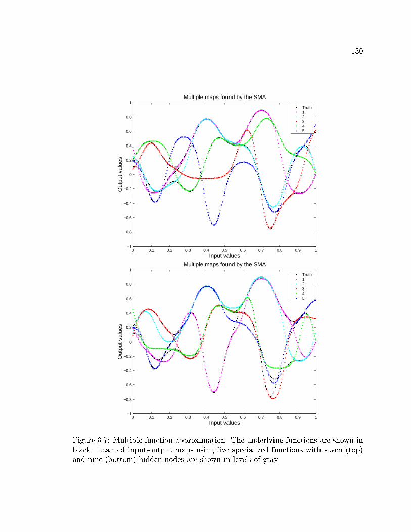
130

0 0.1 0.2 0.3 0.4 0.5 0.6 0.7 0.8 0.9 1−1

−0.8

−0.6

−0.4

−0.2

0

0.2

0.4

0.6

0.8

1

Input values

Out

put v

alue

s


Truth1 2 3 4 5

0 0.1 0.2 0.3 0.4 0.5 0.6 0.7 0.8 0.9 1−1

−0.8

−0.6

−0.4

−0.2

0

0.2

0.4

0.6

0.8

1

Input values

Out

put v

alue

s


Truth1 2 3 4 5

Figure 6.7: Multiple function approximation. The underlying functions are shown inblack. Learned input-output maps using �ve specialized functions with seven (top)and nine (bottom) hidden nodes are shown in levels of gray.

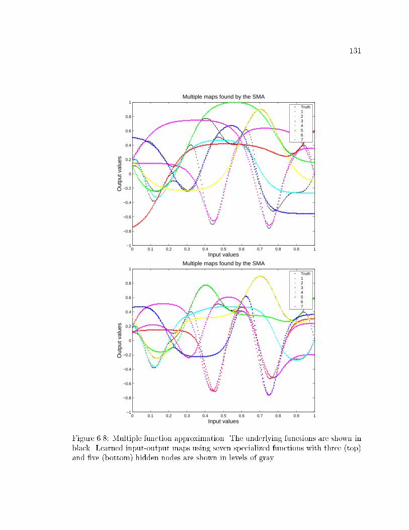
131

0 0.1 0.2 0.3 0.4 0.5 0.6 0.7 0.8 0.9 1−1

−0.8

−0.6

−0.4

−0.2

0

0.2

0.4

0.6

0.8

1

Input values

Out

put v

alue

s


Truth1 2 3 4 5 6 7

0 0.1 0.2 0.3 0.4 0.5 0.6 0.7 0.8 0.9 1−1

−0.8

−0.6

−0.4

−0.2

0

0.2

0.4

0.6

0.8

1

Input values

Out

put v

alue

s


Truth1 2 3 4 5 6 7

Figure 6.8: Multiple function approximation. The underlying functions are shown inblack. Learned input-output maps using seven specialized functions with three (top)and �ve (bottom) hidden nodes are shown in levels of gray.

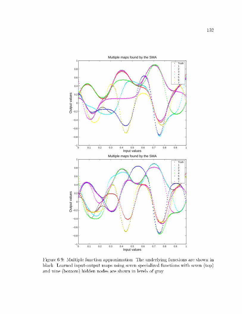
132

0 0.1 0.2 0.3 0.4 0.5 0.6 0.7 0.8 0.9 1−1

−0.8

−0.6

−0.4

−0.2

0

0.2

0.4

0.6

0.8

1

Input values

Out

put v

alue

s


Truth1 2 3 4 5 6 7

0 0.1 0.2 0.3 0.4 0.5 0.6 0.7 0.8 0.9 1−1

−0.8

−0.6

−0.4

−0.2

0

0.2

0.4

0.6

0.8

1

Input values

Out

put v

alue

s


Truth1 2 3 4 5 6 7

Figure 6.9: Multiple function approximation. The underlying functions are shown inblack. Learned input-output maps using seven specialized functions with seven (top)and nine (bottom) hidden nodes are shown in levels of gray.

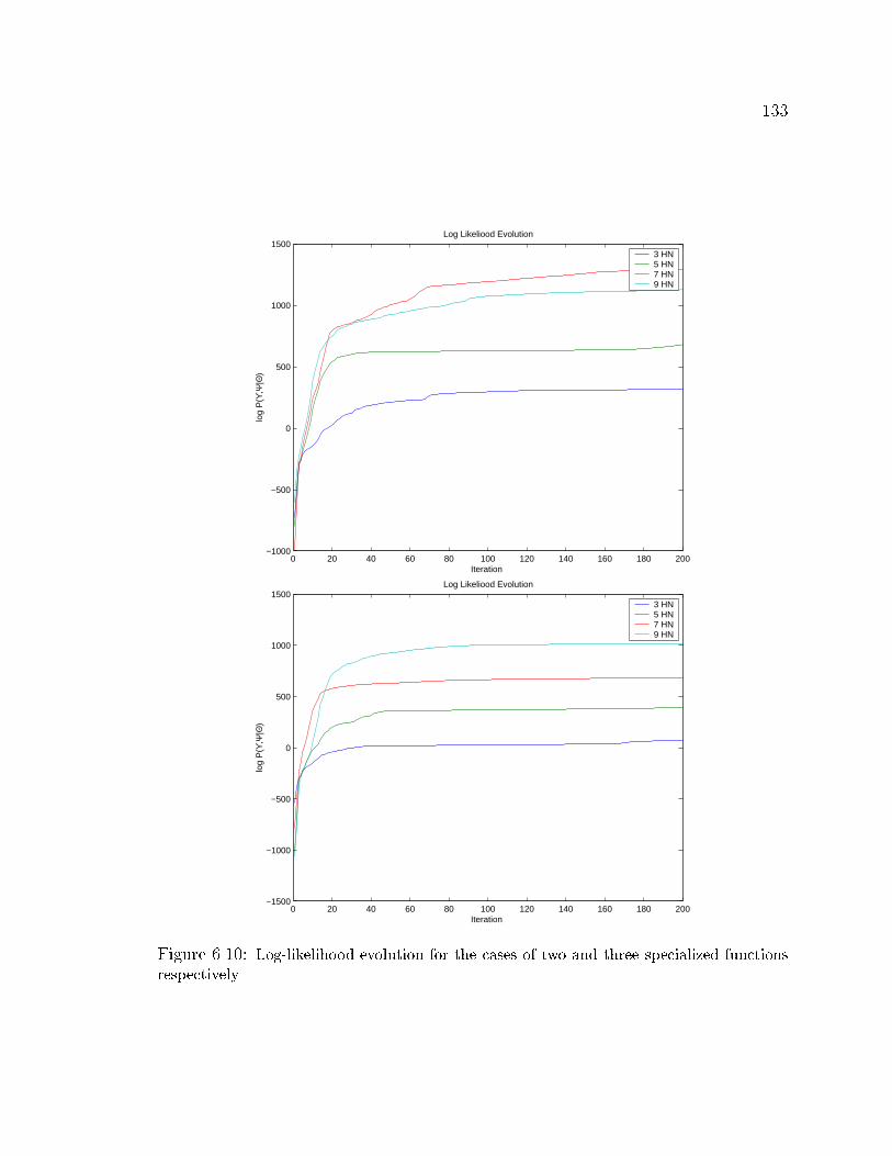
133

0 20 40 60 80 100 120 140 160 180 200−1000

−500

0

500

1000

1500Log Likeliood Evolution

Iteration

log

P(ϒ

,Ψ|Θ

)3 HN5 HN7 HN9 HN

0 20 40 60 80 100 120 140 160 180 200−1500

−1000

−500

0

500

1000


Iteration

log

P(ϒ

,Ψ|Θ

)

3 HN5 HN7 HN9 HN

Figure 6.10: Log-likelihood evolution for the cases of two and three specialized functionsrespectively.

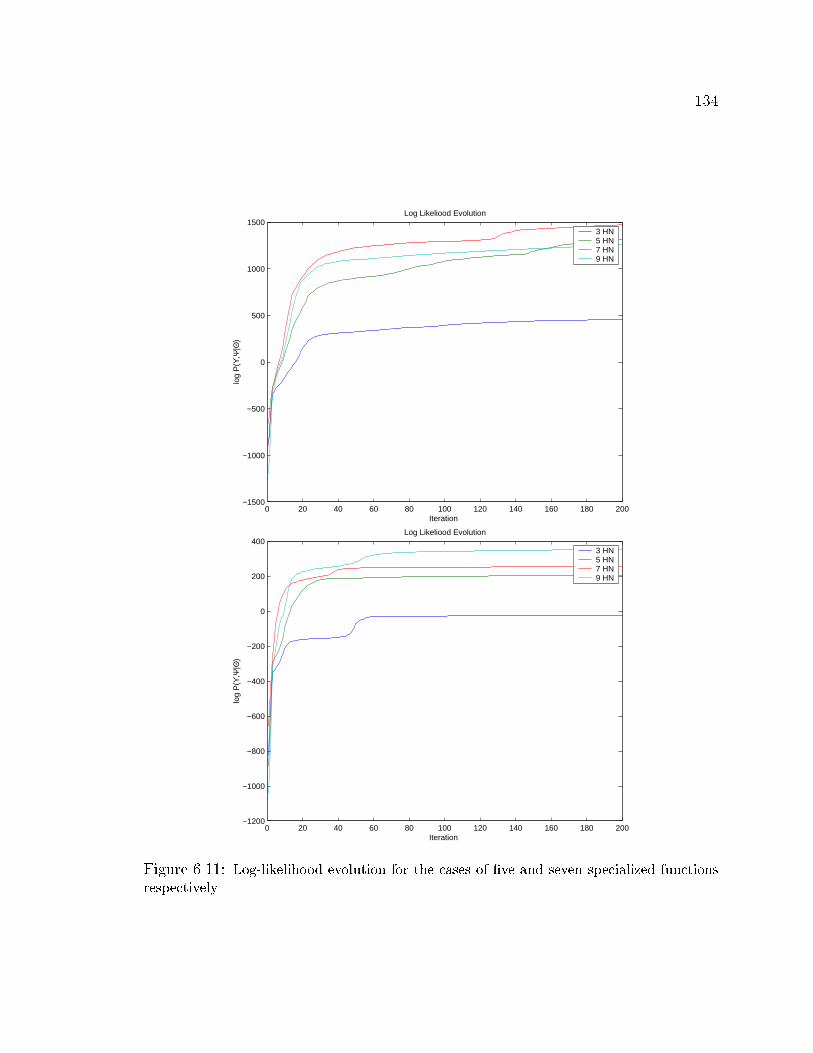
134

0 20 40 60 80 100 120 140 160 180 200−1500

−1000

−500

0

500

1000


Iteration

log

P(ϒ

,Ψ|Θ

)3 HN5 HN7 HN9 HN

0 20 40 60 80 100 120 140 160 180 200−1200

−1000

−800

−600

−400

−200

0

200


Iteration

log

P(ϒ

,Ψ|Θ

)

3 HN5 HN7 HN9 HN

Figure 6.11: Log-likelihood evolution for the cases of �ve and seven specialized functionsrespectively.

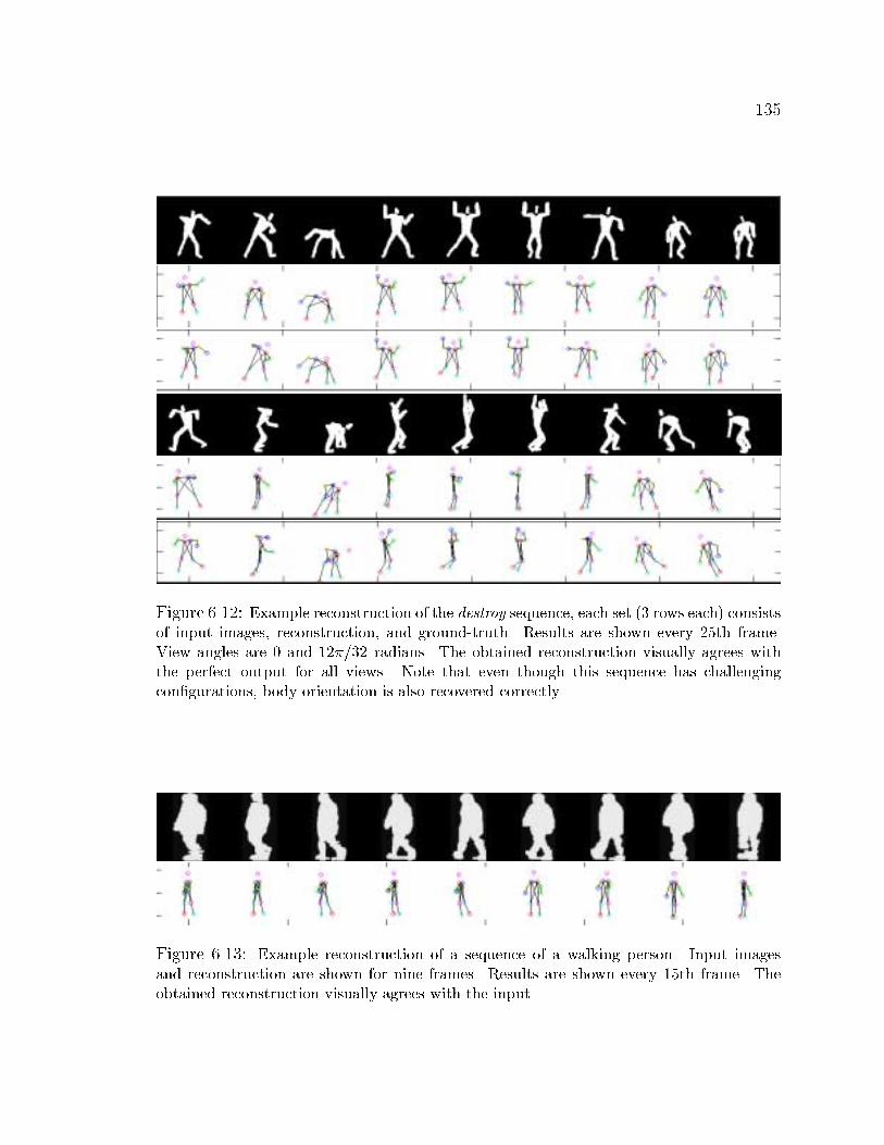
135

Figure 6.12: Example reconstruction of the destroy sequence, each set (3 rows each) consistsof input images, reconstruction, and ground-truth. Results are shown every 25th frame.View angles are 0 and 12�=32 radians. The obtained reconstruction visually agrees withthe perfect output for all views. Note that even though this sequence has challengingcon�gurations, body orientation is also recovered correctly.

Figure 6.13: Example reconstruction of a sequence of a walking person. Input imagesand reconstruction are shown for nine frames. Results are shown every 15th frame. Theobtained reconstruction visually agrees with the input.

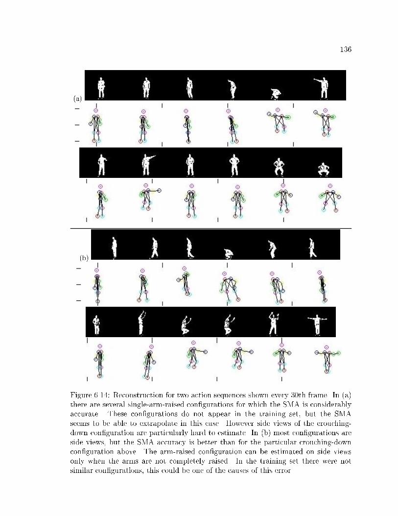
136

(a)

(b)

Figure 6.14: Reconstruction for two action sequences shown every 30th frame. In (a)there are several single-arm-raised con�gurations for which the SMA is considerablyaccurate. These con�gurations do not appear in the training set, but the SMAseems to be able to extrapolate in this case. However side views of the crouching-down con�guration are particularly hard to estimate. In (b) most con�gurations areside views, but the SMA accuracy is better than for the particular crouching-downcon�guration above. The arm-raised con�guration can be estimated on side viewsonly when the arms are not completely raised. In the training set there were notsimilar con�gurations, this could be one of the causes of this error.

137

Figure 6.15: Body pose estimation experiments (continued). Reconstruction for anaction sequence shown every 30th frame. In the �gure, most con�gurations are frontalviews. In this case the SMA performs well in most cases. However, note that thereis also an arm-raised con�guration for which a good estimate could not be provided.

138

6.3 Fixed Camera Viewpoint Hand Pose Estima-

tion

In these experiments, the modeling capabilities of SMA's are tested in the task

of recovering 3D human hand pose at a �xed hand/camera orientation given observed

low-level visual features 2

A similar task was studied in Sec. 6.2 using our simple approximation to the

SMA. In such approximation, each data point was assigned to a specialized function

using a clustering approach. Once clusters were de�ned, function parameters were

optimized in a standard fashion to �t these functions to the data.

In the general SMA formulation used in the following experiments, clusters

and function parameters are found simultaneously using an alternating optimization

procedure such as the EM algorithm explained in Chapter 3. Moreover, cluster

ownership is determined probabilistically rather than deterministically as in our initial

approximation. We saw in Sec. 4.2.6 that the initial approximation is in fact an

instance of the more general SMA framework, and that the model obtained can be

improved in the maximum likelihood sense in the way described in Sec. 4.2.7.

6.3.1 Model and Experiment Data

The model structure chosen for this dataset was as follows. The output consisted

of 20 joint angles of a human hand linearly encoded by nine real values using Principal

Component Analysis (PCA). The input consisted of 10 real-valued Alt moments [2]

2Hand sequences used in these experiments were collected in collaboration with Vassilis Athitsos

at the Boston University American Sign Language Laboratory.

139

computed on synthetically generated silhouettes of the hand (see Chapter 4 for a

detailed explanation). In this case each silhouette is the result of rendering the 3D

articulated hand from what we will call the canonical view.

The canonical view is de�ned to be the viewpoint pair �1 = �=2 and �2 = 0; i.e.,

on the view sphere equator at longitude 0 radians. This is a view towards the palm

of the hand. As an illustration, Fig. 4.3 shows the resulting appearance of the hand

as seen from di�erent viewpoints. The synthetic binary images obtained in this way

were used for training and testing as described in Chapter 4.

For training, we used the Hand-Single-View dataset, with approximately 9,000

examples. Of these, 3,000 were used for training and the rest for testing. All experi-

ments were performed on a test set with no common con�gurations with respect to the

training set. We used cross-validation for early stopping (stop the iterative training

algorithm) and to avoid over�tting, as explained in Sec. 6.1.2. In the experimental

results shown here, the number of specialized functions was set to 20. This number

was also found using the MDL principle [95]. Each of these functions was a one hidden

layer, feed-forward network (a MLP) with seven hidden neurons. We carried out two

major classes of experiments: (1) synthetically generated hands (where we know the

ground-truth) were used to quantitatively evaluate the model performance, (2) real

hand sequences captured using a single uncalibrated camera were used to test the

model generalization to real data. These experiments are described in the following

sections.

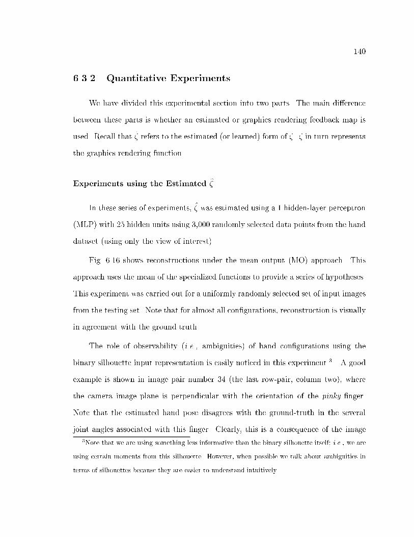
140

6.3.2 Quantitative Experiments

We have divided this experimental section into two parts. The main di�erence

between these parts is whether an estimated or graphics rendering feedback map is

used. Recall that � refers to the estimated (or learned) form of �. � in turn represents

the graphics rendering function.

Experiments using the Estimated �

In these series of experiments, � was estimated using a 1 hidden-layer perceptron

(MLP) with 25 hidden units using 3,000 randomly selected data points from the hand

dataset (using only the view of interest).

Fig. 6.16 shows reconstructions under the mean output (MO) approach. This

approach uses the mean of the specialized functions to provide a series of hypotheses.

This experiment was carried out for a uniformly randomly selected set of input images

from the testing set. Note that for almost all con�gurations, reconstruction is visually

in agreement with the ground truth.

The role of observability (i.e., ambiguities) of hand con�gurations using the

binary silhouette input representation is easily noticed in this experiment 3 . A good

example is shown in image pair number 34 (the last row-pair, column two), where

the camera image plane is perpendicular with the orientation of the pinky �nger.

Note that the estimated hand pose disagrees with the ground-truth in the several

joint angles associated with this �nger. Clearly, this is a consequence of the image

3Note that we are using something less informative than the binary silhouette itself; i.e., we are

using certain moments from this silhouette. However, when possible we talk about ambiguities in

terms of silhouettes because they are easier to understand intuitively.

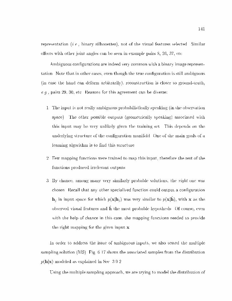
141

representation (i.e., binary silhouettes), not of the visual features selected. Similar

e�ects with other joint angles can be seen in example pairs 8, 26, 37, etc.

Ambiguous con�gurations are indeed very common with a binary image represen-

tation. Note that in other cases, even though the true con�guration is still ambiguous

(in case the hand can deform arbitrarily), reconstruction is closer to ground-truth,

e.g., pairs 29, 30, etc. Reasons for this agreement can be diverse:

1. The input is not really ambiguous probabilistically speaking (in the observation

space). The other possible outputs (geometrically speaking) associated with

this input may be very unlikely given the training set. This depends on the

underlying structure of the con�guration manifold. One of the main goals of a

learning algorithm is to �nd this structure.

2. Few mapping functions were trained to map this input, therefore the rest of the

functions produced irrelevant outputs.

3. By chance, among many very similarly probable solutions, the right one was

chosen. Recall that any other specialized function could output a con�guration

hj in input space for which p(xjhj) was very similar to p(xjh), with x as the

observed visual features and h the most probable hypothesis. Of course, even

with the help of chance in this case, the mapping functions needed to provide

the right mapping for the given input x.

In order to address the issue of ambiguous inputs, we also tested the multiple

sampling solution (MS). Fig. 6.17 shows the associated samples from the distribution

p(hjx) modeled as explained in Sec. 3.9.2.

Using the multiple sampling approach, we are trying to model the distribution of

142

outputs given the input x. In Fig. 6.17 we can see excellent examples of the advantages

of giving an answer in terms of a distribution (approximated by samples) rather than

in terms of a single best result. Note that for all ambiguous inputs, several possible

outputs were generated. For example, the �rst row shows di�erent hand poses that

can be inferred when a binary silhouette of the ground-truth image is analyzed. Row

number seven of the �gure clearly demonstrate this phenomenon. In this case, note

that estimated �nger con�gurations vary so as to be consistent with the input, but

are still plausible hand con�gurations from a camera-geometry perspective.

Less ambiguous hand con�gurations can also be observed. Examples of them are

shown in Fig. 6.17 rows number two, �ve, etc. Note in these cases, almost all samples

are very similar, indicating that the posterior distribution is peaked at a given output

con�guration. Many other examples can be seen in Fig. 6.18.

Quantitatively, in the mean output approach (MO), the average L2 error between

reconstruction and ground-truth over approximately 4,000 randomly chosen frames

was 0:1863 rads. (approximately 10o), with variance 0:0185. These error estimates

are averaged over joint angles. In the MS inference approach, also using approxi-

mately 4; 000 randomly chosen test examples, the mean L2 error of the most likely

sample to the ground-truth is 0:2202 with variance 0:02284. The average mean and

variance from the best 20 samples are 0:308 and 0:3023 respectively. Thus, these

experiments con�rmed that our mean output (MO) inference approach from Sec. 3.9

seems to be a reasonable approximation, at least in this dataset. Recall that this

approximation was based on the premise that the most-likely reconstruction given by

each specialized function provides a good approximation to the best solution given

by the full probability distribution.

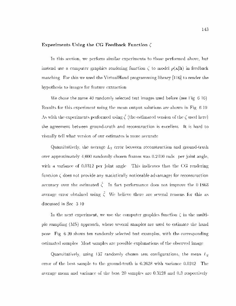
143

Experiments Using the CG Feedback Function �

In this section, we perform similar experiments to those performed above, but

instead use a computer graphics rendering function � to model p(xjh) in feedback

matching. For this we used the VirtualHand programming library [116] to render the

hypothesis to images for feature extraction.

We chose the same 40 randomly selected test images used before (see Fig. 6.16).

Results for this experiment using the mean output solutions are shown in Fig. 6.19.

As with the experiments performed using � (the estimated version of the � used here)

the agreement between ground-truth and reconstruction is excellent. It is hard to

visually tell what version of our estimates is more accurate.

Quantitatively, the average L2 error between reconstruction and ground-truth

over approximately 4,000 randomly chosen frames was 0:2410 rads. per joint angle,

with a variance of 0:0312 per joint angle. This indicates that the CG rendering

function � does not provide any statistically noticeable advantages for reconstruction

accuracy over the estimated �. In fact performance does not improve the 0.1863

average error obtained using � .We believe there are several reasons for this as

discussed in Sec. 3.10.

In the next experiment, we use the computer graphics function � in the multi-

ple sampling (MS) approach, where several samples are used to estimate the hand

pose. Fig. 6.20 shows ten randomly selected test examples, with the corresponding

estimated samples. Most samples are possible explanations of the observed image.

Quantitatively, using 137 randomly chosen test con�gurations, the mean L2

error of the best sample to the ground-truth is 0:2628 with variance 0:0242. The

average mean and variance of the best 20 samples are 0:3128 and 0:3 respectively.

144

Note that even though the multiple sample approach does not provide a statistically

di�erent overall error (when the most likely sample is compared to the mean output

reconstruction), it does allow for the use of multiple valid hypotheses. It is possible

to see from the numerical results that on average, these hypotheses seem reasonably

good, given the low mean error obtained. Another observation derived from these

results is that even in the multiple sample case, using an estimated and graphics

rendering function seems to make no di�erence in terms of performance in this task.

Fig. 6.21 provides an alternative to look at the high-dimensional maps formed

by the SMA model under the �xed view-point hand data. Note that even though this

is a high dimensional space (thus harder to visualize), we can still see that the data

points grouped by preferred specialized functions form clusters with non-Gaussian

shapes. These clusters are not even required to be connected, as seen in the �gure.

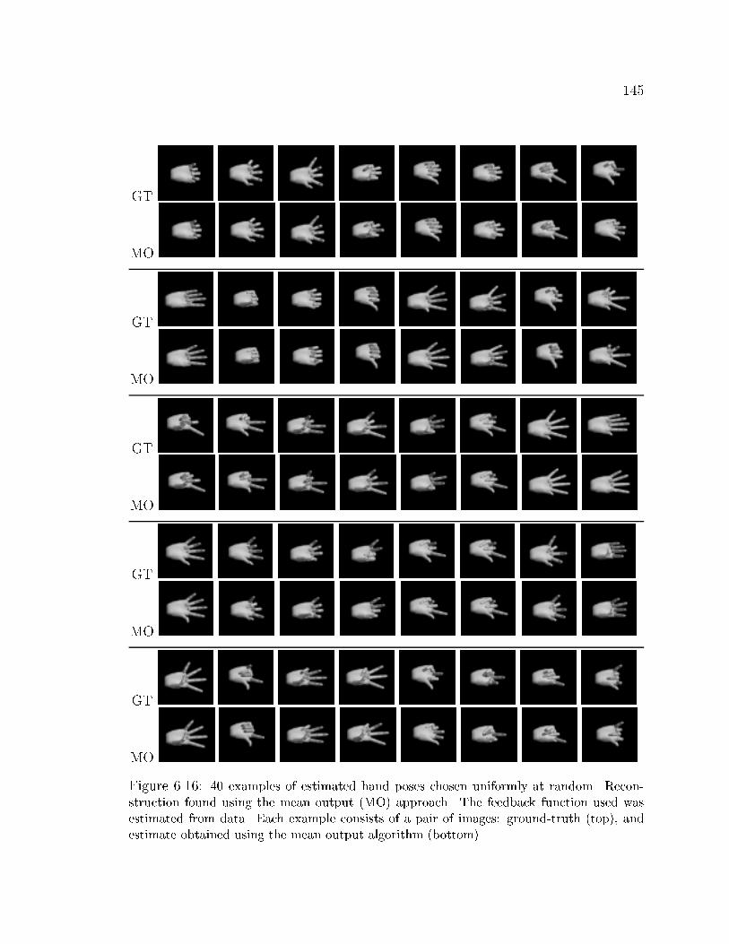
145

GT

MO

GT

MO

GT

MO

GT

MO

GT

MO

Figure 6.16: 40 examples of estimated hand poses chosen uniformly at random. Recon-struction found using the mean output (MO) approach. The feedback function used wasestimated from data. Each example consists of a pair of images: ground-truth (top), andestimate obtained using the mean output algorithm (bottom).

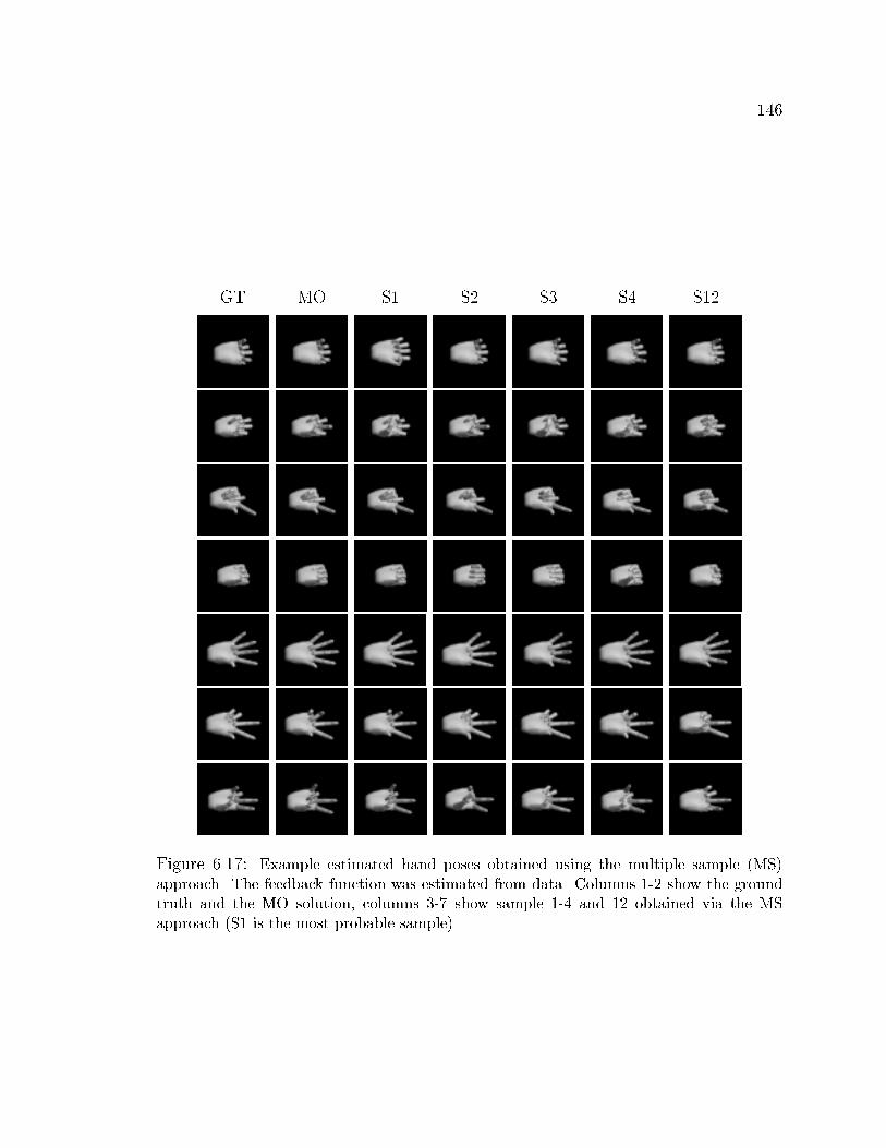
146

GT MO S1 S2 S3 S4 S12

Figure 6.17: Example estimated hand poses obtained using the multiple sample (MS)approach. The feedback function was estimated from data. Columns 1-2 show the groundtruth and the MO solution, columns 3-7 show sample 1-4 and 12 obtained via the MSapproach (S1 is the most probable sample).

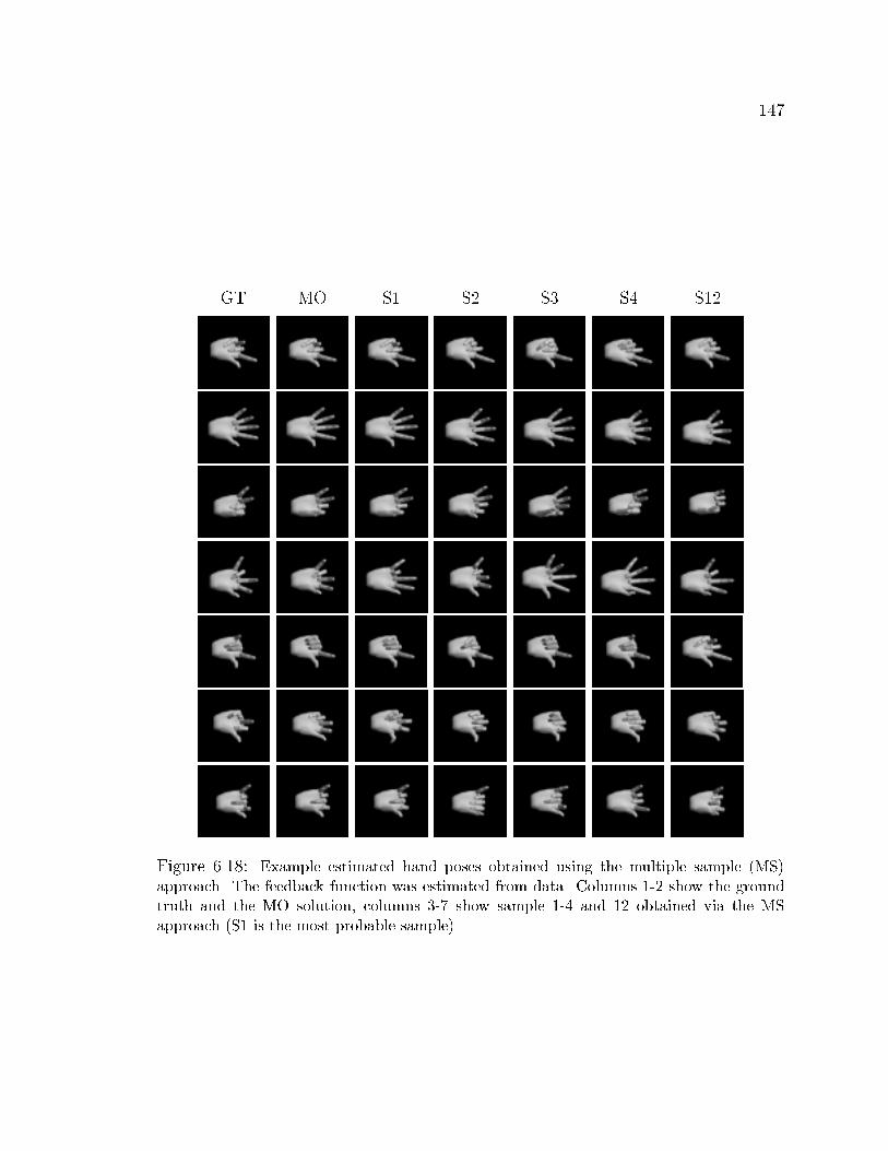
147


Figure 6.18: Example estimated hand poses obtained using the multiple sample (MS)approach. The feedback function was estimated from data. Columns 1-2 show the groundtruth and the MO solution, columns 3-7 show sample 1-4 and 12 obtained via the MSapproach (S1 is the most probable sample).

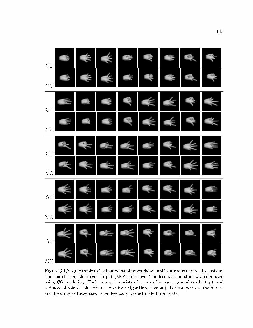
148

GT

MO

GT

MO

GT

MO

GT

MO

GT

MO

Figure 6.19: 40 examples of estimated hand poses chosen uniformly at random. Reconstruc-tion found using the mean output (MO) approach. The feedback function was computedusing CG rendering. Each example consists of a pair of images: ground-truth (top), andestimate obtained using the mean output algorithm (bottom). For comparison, the framesare the same as those used when feedback was estimated from data.

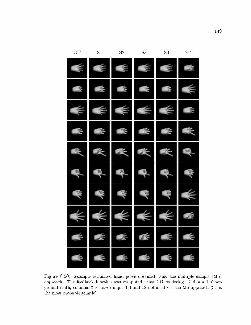
149

GT S1 S2 S3 S4 S12

Figure 6.20: Example estimated hand poses obtained using the multiple sample (MS)approach. The feedback function was computed using CG rendering. Column 1 showsground truth, columns 2-6 show sample 1-4 and 12 obtained via the MS approach (S1 isthe most probable sample).

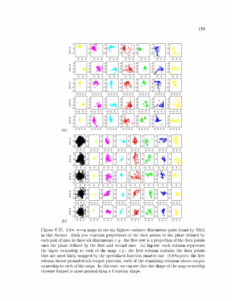
150

(a)

0 2 4

−2

0

2

d=1−

2

0 2 4

−2

0

2

0 2 4

−2

0

2

0 2 4

−2

0

2

0 2 4

−2

0

2

0 2 4

−2

0

2

0 2 4

−2

0

2

−2 0 2

−2024

d=2−

3

−2 0 2

−2024

−2 0 2

−2024

−2 0 2

−2024

−2 0 2

−2024

−2 0 2

−2024

−2 0 2

−2024

−2 0 2 4−4

−2

0

2

d=3−

4

−2 0 2 4−4

−2

0

2

−2 0 2 4−4

−2

0

2

−2 0 2 4−4

−2

0

2

−2 0 2 4−4

−2

0

2

−2 0 2 4−4

−2

0

2

−2 0 2 4−4

−2

0

2

−4 −2 0 2−2

024

d=4−

5

−4 −2 0 2−2

024

−4 −2 0 2−2

024

−4 −2 0 2−2

024

−4 −2 0 2−2

024

−4 −2 0 2−2

024

−4 −2 0 2−2

024

−2 0 2 4−4−2

02

d=5−

6

−2 0 2 4−4−2

02

−2 0 2 4−4−2

02

−2 0 2 4−4−2

02

−2 0 2 4−4−2

02

−2 0 2 4−4−2

02

−2 0 2 4−4−2

02

(b)

−2 0 2

−2

0

2

d=1−

2

−2 0 2

−2

0

2

−2 0 2

−2

0

2

−2 0 2

−2

0

2

−2 0 2

−2

0

2

−2 0 2

−2

0

2

−2 0 2

−2

0

2

−2 0 2

−2

0

2

−2 0 2−2

0

2

d=2−

3

−2 0 2−2

0

2

−2 0 2−2

0

2

−2 0 2−2

0

2

−2 0 2−2

0

2

−2 0 2−2

0

2

−2 0 2−2

0

2

−2 0 2−2

0

2

−2 0 2−2−1

01

d=3−

4

−2 0 2−2−1

01

−2 0 2−2−1

01

−2 0 2−2−1

01

−2 0 2−2−1

01

−2 0 2−2−1

01

−2 0 2−2−1

01

−2 0 2−2−1

01

−2−1 0 1

−1

0

1

d=4−

5

−2−1 0 1

−1

0

1

−2−1 0 1

−1

0

1

−2−1 0 1

−1

0

1

−2−1 0 1

−1

0

1

−2−1 0 1

−1

0

1

−2−1 0 1

−1

0

1

−2−1 0 1

−1

0

1

−1 0 1

−1

0

1

d=5−

6

−1 0 1

−1

0

1

−1 0 1

−1

0

1

−1 0 1

−1

0

1

−1 0 1

−1

0

1

−1 0 1

−1

0

1

−1 0 1

−1

0

1

−1 0 1

−1

0

1

Figure 6.21: First seven maps in the six highest-variance dimensions pairs found by SMAin this dataset. Each row contains projections of the data points to the plane de�ned byeach pair of axes in these six dimensions; e.g., the �rst row is a projection of the data pointsonto the plane de�ned by the �rst and second axes. (a) Inputs: each column representsthe input ownership to each of the map; e.g., the �rst column contains the data pointsthat are most likely mapped by the specialized function number one. (b)Outputs: the �rstcolumn shows ground-truth output patterns, each of the remaining columns shows outputownership to each of the maps. In this case, we can see that the shape of the map ownershipclusters formed is more general than a Gaussian shape.

151

6.3.3 Experiments with Real Images

We now test our approach using data collected from a single uncalibrated camera.

The sequences used in these experiments were obtained using a camera pointing

towards the palm of a person's hand. Of course, this is done because the model in

this section was trained with a �xed hand/camera orientation (i.e., the orientation

corresponding to a view of the hand palm). However this constraint is not satis�ed

perfectly; the hand con�gurations are usually not in the same orientation as those

used for training.

The capture system obtained frames at 60Hz. Recall that we use single images;

therefore, we do not need to take advantage of this sampling rate. However, this rate

usually prevents motion blur. On average, the hand occupied an area of approximately

200x200 pixels on the screen. For these experiments observation inputs were obtained

by simply tracking skin color distribution [108].

The SMA model was the same as the one used for the synthetic data experiments

above. We again compare the performance of SMA's using (1) an estimate from data

(�) and (2) a graphics rendering (�) feedback function. In both cases, we tested SMA

using both mean output (MO) and multiple-sample (MS) inference algorithms.

For a fairer comparison, the estimated � was set the same as that used for the

synthetic data experiments above. In the �rst experiment we use the mean output

(MO)inference approach to obtain a single best estimate for each segmented hand.

Estimates of 40 frames (taken 0.9 secs apart) are shown in Fig. 6.22. The silhouettes

from which features are computed and resulting pose estimates are shown. Visually we

can notice that in most cases the estimate is a possible explanation of the segmented

silhouette. However, there are also some inaccurate reconstructions, as shown in the

152

fourth row of the �gure.

It is expected that the model cannot perform well in all con�gurations due to

the following issues:

1. Recall that learning is the result of optimizing an expected or average error.

2. Synthetic and real hand features are similar but not the same.

3. Even the best model would fail in some con�gurations. Information theory tells

us that this is always the case except when the information in the features about

the con�gurations is equal to the entropy of the body pose con�gurations; in

other words, when features tell us everything needed about the con�guration.

This is usually not the case, and clearly not the case even in �xed hand orien-

tations, where there might be multiple explanations for a given visual feature

vector.

In order to test the ability of the system to provide these multiple explanations,

we tested the multiple sampling (MS) approach. Fig. 6.23 shows the corresponding

estimates. They can be interpreted as possible hypotheses of hand con�gurations

given the silhouettes. The frames shown were taken approximately every 0.9 secs.

Now we test the performance of the model using a computer graphics rendering

function. For visual comparison, we chose to display the same frames shown in

Fig. 6.22. Fig. 6.24 shows results obtained when using the MO algorithm. The

resulting quality is comparable to that obtained in experiments using the estimated

�. The synthetic experiments' quantitative results also showed similar performance

between inference using � and �.

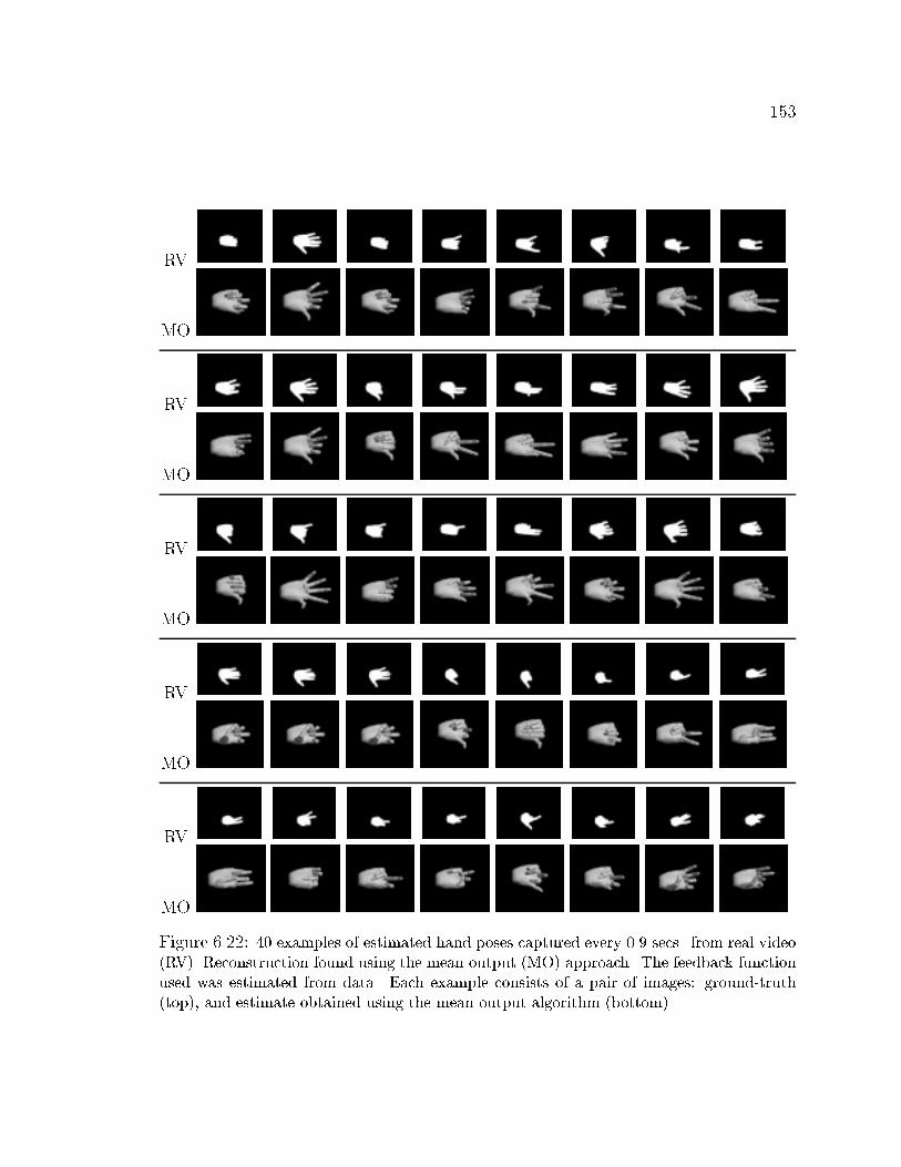
153

RV

MO

RV

MO

RV

MO

RV

MO

RV

MO

Figure 6.22: 40 examples of estimated hand poses captured every 0.9 secs. from real video(RV). Reconstruction found using the mean output (MO) approach. The feedback functionused was estimated from data. Each example consists of a pair of images: ground-truth(top), and estimate obtained using the mean output algorithm (bottom).

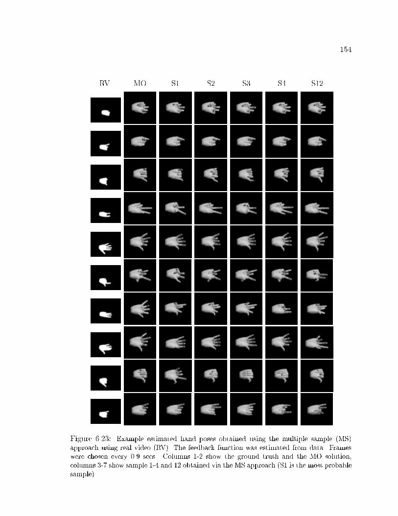
154

RV MO S1 S2 S3 S4 S12

Figure 6.23: Example estimated hand poses obtained using the multiple sample (MS)approach using real video (RV). The feedback function was estimated from data. Frameswere chosen every 0.9 secs. Columns 1-2 show the ground truth and the MO solution,columns 3-7 show sample 1-4 and 12 obtained via the MS approach (S1 is the most probablesample).

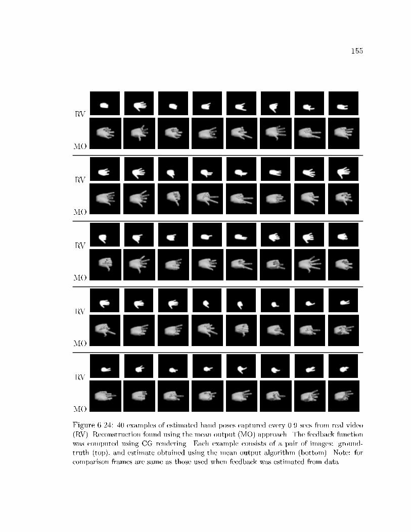
155

RV

MO

RV

MO

RV

MO

RV

MO

RV

MO

Figure 6.24: 40 examples of estimated hand poses captured every 0.9 secs from real video(RV). Reconstruction found using the mean output (MO) approach. The feedback functionwas computed using CG rendering. Each example consists of a pair of images: ground-truth (top), and estimate obtained using the mean output algorithm (bottom). Note: forcomparison frames are same as those used when feedback was estimated from data.

156

6.4 3D Hand Pose Reconstruction From Unrestricted

Camera Viewpoint

In this section, the SMA is tested on the task of recovering 3D human hand pose

from an unknown orientation using the observed low-level visual features4.


The model characteristics chosen for this dataset were similar to the single view

case above. However, here we consider global orientation (or camera viewpoint). The

output consisted of 20 internal joint angles of a human hand and two orientation

angles. This 22 DOF representation was linearly encoded by nine real values us-

ing Principal Component Analysis (PCA). The input consisted of seven real-valued

Hu moments [55] computed on synthetically generated silhouettes of the hand (see

Chapter 4 for a detailed explanation).

We will use the dataset Hand-All-Views, with approximately 750,000 input-

output pairs. Of these, 18,000 were used for training and the rest for testing. As

before we use the training procedure described in Sec. 6.1.2. In the experiments

shown, the number of specialized functions was set to 45. Each of these functions was

a one hidden layer, feed-forward network with seven hidden nodes. This setting was

obtaining using the MDL principle on a number of architectures.

4A di�erent version of these results were �rst presented in [99].

157


As in previous experimental sections, we compare the performance of SMA's

using (1) an estimated and (2) a graphics rendering feedback function.

Experiments using the Estimated Feedback Function �

In these experiments, � was estimated using a 1 hidden-layer perceptron with

35 hidden units using 19,000 data points from the hand dataset. Approximately

220 poses were chosen uniformly at random, but along with them we also chose

the remaining 85 views of the given pose. The rest (approximately 730,000 hand

con�gurations) were used for testing.

In order to illustrate the performance of our model, we chose 40 con�gurations

uniformly at random. The view was therefore randomly chosen also. Fig. 6.25

shows the reconstructions under the mean output (MO) approach. For these 40

con�gurations. Even though the di�culty of this task is higher than that for single

hand orientation, estimates are also close to ground-truth.

As expected, ambiguities of the hand con�gurations are more abundant here than

in the single view experiments. The reason for this is that besides the ambiguities

caused by internal joint angles, there are now ambiguities also caused by camera view-

point. However, the reasons for the performance given in the single view experiments

are also valid in this experiment. In addition, bear in mind that Hu moments as

features are not able to distinguish two di�erent hand poses whose appearance di�ers

only by a rotation in the image plane. Given that we can provide a large variety of

quantitative performance, these will be shown later in Fig. 6.29.

Results using the multiple sampling solution (MS) are shown in Figs. 6.26 and

158

6.27 where random test samples were used to generate a series of likely hand pose

reconstructions. These samples are from the distribution p(hjx) (where h is the pose

reconstruction, and x is the input vector of image features) as explained in Sec. 3.9.2.

Note that there are hand reconstructions which seem to di�er from the ground-truth

by just a rotation (on the image plane). This is the expected behavior given the

features employed. There are other cases where the projection of the reconstruction

may have very likely come from the input binary silhouette (not shown here, but

could be easily imagined if we think of the silhouette of the ground truth image).

These ambiguities are due to the image representation and the projective ambiguities

studied in Sec. 2.4.

In our next experiment, we took one random test con�guration and all the

associated images corresponding to 26 di�erent viewpoints. The goal is to compare

the reconstructions of the same pose across di�erent viewpoints. The 26 viewpoints

chosen span the view-sphere approximately uniformly.

The �rst viewpoint corresponds to one of the poles (latitude 0 rads. i.e., �1 = 0).

We systematically traverse the sphere by changing the latitude, and then the longi-

tude. Fig. 6.28 shows the results of this test for a randomly chosen hand con�guration.

Visually, we can see that reconstructions and ground-truth match; however, it is

hard to visually judge the quality of the reconstruction across views. Therefore,

we computed the L2 error and quantitatively compared it across views. These

comparisons are presented in Fig. 6.29 for the mean output approach, and in Fig. 6.30

for the multiple sampling approach.

Fig. 6.29 shows the error of the best sample. The best sample was found using

the MO approach, according to the value of the posterior distribution on the samples.

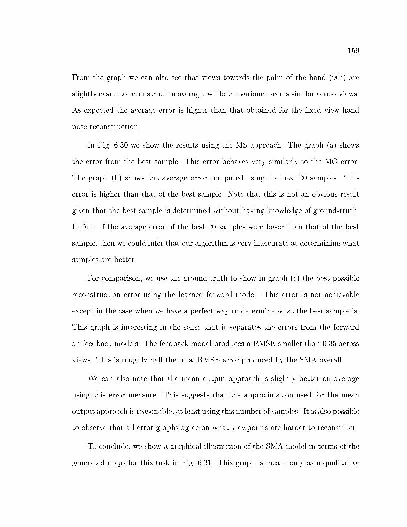
159

From the graph we can also see that views towards the palm of the hand (90�) are

slightly easier to reconstruct in average, while the variance seems similar across views.

As expected the average error is higher than that obtained for the �xed view hand

pose reconstruction.

In Fig. 6.30 we show the results using the MS approach. The graph (a) shows

the error from the best sample. This error behaves very similarly to the MO error.

The graph (b) shows the average error computed using the best 20 samples. This

error is higher than that of the best sample. Note that this is not an obvious result

given that the best sample is determined without having knowledge of ground-truth.

In fact, if the average error of the best 20 samples were lower than that of the best

sample, then we could infer that our algorithm is very inaccurate at determining what

samples are better.

For comparison, we use the ground-truth to show in graph (c) the best possible

reconstruction error using the learned forward model. This error is not achievable

except in the case when we have a perfect way to determine what the best sample is.

This graph is interesting in the sense that it separates the errors from the forward

an feedback models. The feedback model produces a RMSE smaller than 0.35 across

views. This is roughly half the total RMSE error produced by the SMA overall.

We can also note that the mean output approach is slightly better on average

using this error measure. This suggests that the approximation used for the mean

output approach is reasonable, at least using this number of samples. It is also possible

to observe that all error graphs agree on what viewpoints are harder to reconstruct.

To conclude, we show a graphical illustration of the SMA model in terms of the

generated maps for this task in Fig. 6.31. This graph is meant only as a qualitative

160

illustration of the specialized function ownership formed in this dataset.

Given that the input and output spaces are highly dimensional, we have com-

puted many two dimensional views of the data. Each of these views are projections

onto the plane de�ned by two data axes. The axes are chosen to be those that

provide most of the variance of the data. The group of points shown in each graph

can be considered a cluster. Note that we obtain clusters with shapes that are more

general than Gaussian distributions. This happens because there is no constraint in

the SMA that obligate the clusters to have a Gaussian shape. Clusters are formed

automatically depending on what function better maps a data point from input to

output space. In this sense, the SMA can be considered a clustering method.

Experiments using the CG Feedback Function �

In this section, we perform similar experiments as those in the section above. In

this case, we will use �, the computer graphics based feedback function, to render the

hypotheses as previously described.

Following the same methodology presented in previous sections, we chose the

same 40 randomly selected test images used before (see Fig. 6.25). Results for this

experiment using the mean output solutions are shown in Fig. 6.25.

In the next experiment, we use the computer graphics function � and the multiple

sampling (MS) approach, where several samples are used to estimate a distribution

over the hand pose. Fig. 6.33 shows ten randomly selected test examples, with the

corresponding estimated samples. Most samples are possible explanations of the given

silhouette image of the ground-truth. Fig. 6.34 shows other randomly selected test

examples.

161

We performed another experiment where only one test sample was chosen at

random, and many of its views are presented to the SMA to further reconstruction.

We chose 26 di�erent viewpoints uniformly distributed on the view-sphere, results

are shown in Fig. 6.35. For comparison the same frame as in Fig. 6.28 was used.

Finally, in order to quantitatively measure the accuracy of this approach as a

whole and across views, using 1; 000 randomly chosen samples, we produced the

graphs shown in Figs. 6.36 and 6.37. This is the equivalent to Figs. 6.29 and 6.30,

when � was used for feedback.

A behavior similar to the case when � was used is observed here, in the sense

that the mean output approach is still slightly better in average. This suggests again

that the mean output approximation is satisfactory in practice.

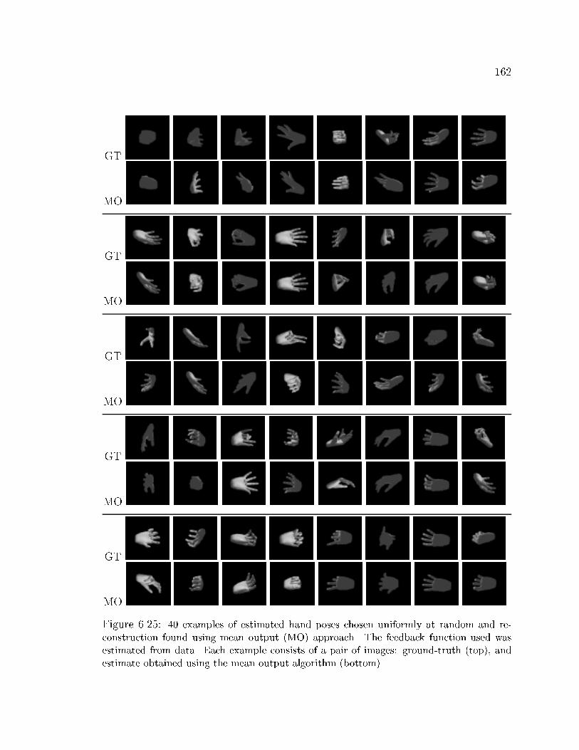
162

GT

MO

GT

MO

GT

MO

GT

MO

GT

MO

Figure 6.25: 40 examples of estimated hand poses chosen uniformly at random and re-construction found using mean output (MO) approach. The feedback function used wasestimated from data. Each example consists of a pair of images: ground-truth (top), andestimate obtained using the mean output algorithm (bottom).

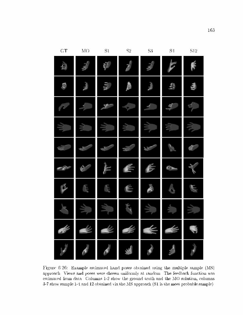
163


Figure 6.26: Example estimated hand poses obtained using the multiple sample (MS)approach. Views and poses were chosen uniformly at random. The feedback function wasestimated from data. Columns 1-2 show the ground truth and the MO solution, columns3-7 show sample 1-4 and 12 obtained via the MS approach (S1 is the most probable sample).

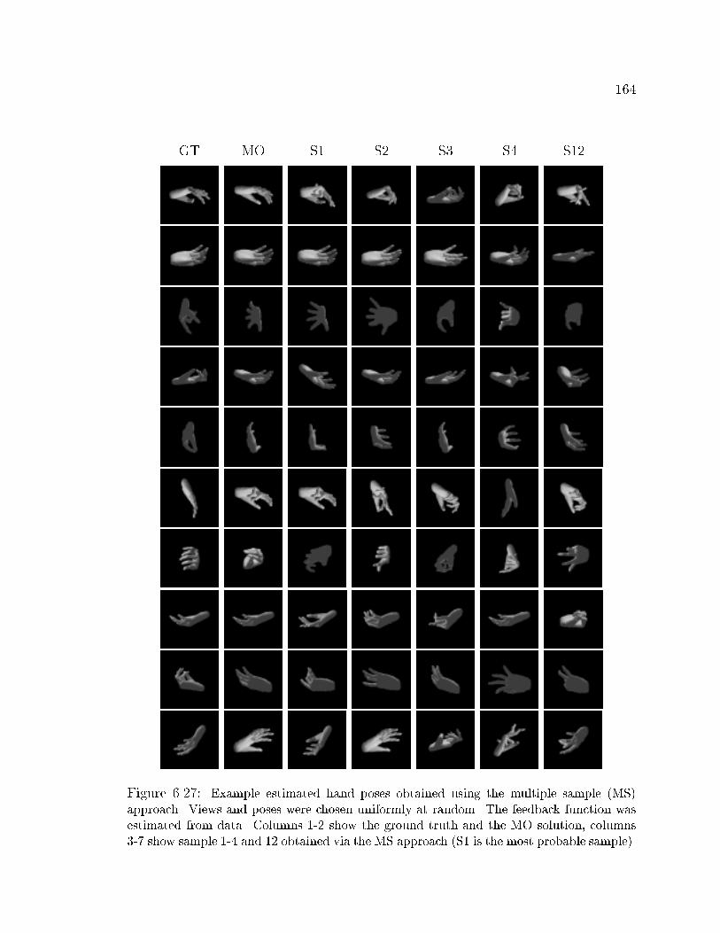
164


Figure 6.27: Example estimated hand poses obtained using the multiple sample (MS)approach. Views and poses were chosen uniformly at random. The feedback function wasestimated from data. Columns 1-2 show the ground truth and the MO solution, columns3-7 show sample 1-4 and 12 obtained via the MS approach (S1 is the most probable sample).

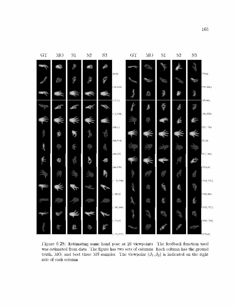
165

GT MO S1 S2 S3 GT MO S1 S2 S3

(0,0) (23,0)

(23,103) (23,206)

(45,0) (45,90)

(45,180) (45,270)

(68,0) (68,120)

(68,240) (90,0)

(90,90) (90,180)

(90,270) (113,0)

(113,120) (113,240)

(135,0) (135,90)

(135,180) (135,270)

(158,0) (158,103)

(158,257) (180,0)

Figure 6.28: Estimating same hand pose at 26 viewpoints. The feedback function usedwas estimated from data. The �gure has two sets of columns. Each column has the groundtruth, MO, and best three MS samples. The viewpoint (�1; �2) is indicated on the rightside of each column.

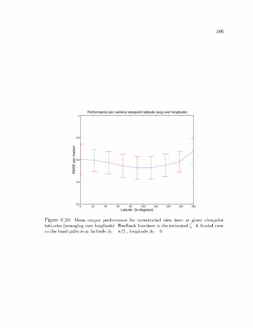
166

0 20 40 60 80 100 120 140 160 1800.2

0.4

0.6

0.8

1

Latiude (in degrees)

RM

SE

per

mar

ker

Performance per camera viewpoint latitude (avg over longitude)

Figure 6.29: Mean output performance for unrestricted view tests at given viewpointlatitudes (averaging over longitude). Feedback functions is the estimated �. A frontal viewto the hand palm is at latitude �1 = �=2 , longitude �2 = 0.

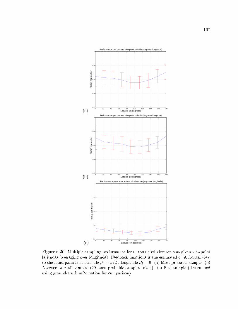
167

(a)0 20 40 60 80 100 120 140 160 180

0.2

0.4

0.6

0.8

1


RM

SE

per

mar

ker


(b)0 20 40 60 80 100 120 140 160 180

0.2

0.4

0.6

0.8

1


RM

SE

per

mar

ker


(c)0 20 40 60 80 100 120 140 160 180

0.2

0.4

0.6

0.8

1


RM

SE

per

mar

ker


Figure 6.30: Multiple sampling performance for unrestricted view tests at given viewpointlatitudes (averaging over longitude). Feedback functions is the estimated �. A frontal viewto the hand palm is at latitude �1 = �=2 , longitude �2 = 0. (a) Most probable sample. (b)Average over all samples (20 most probable samples taken). (c) Best sample (determinedusing ground-truth information for comparison).

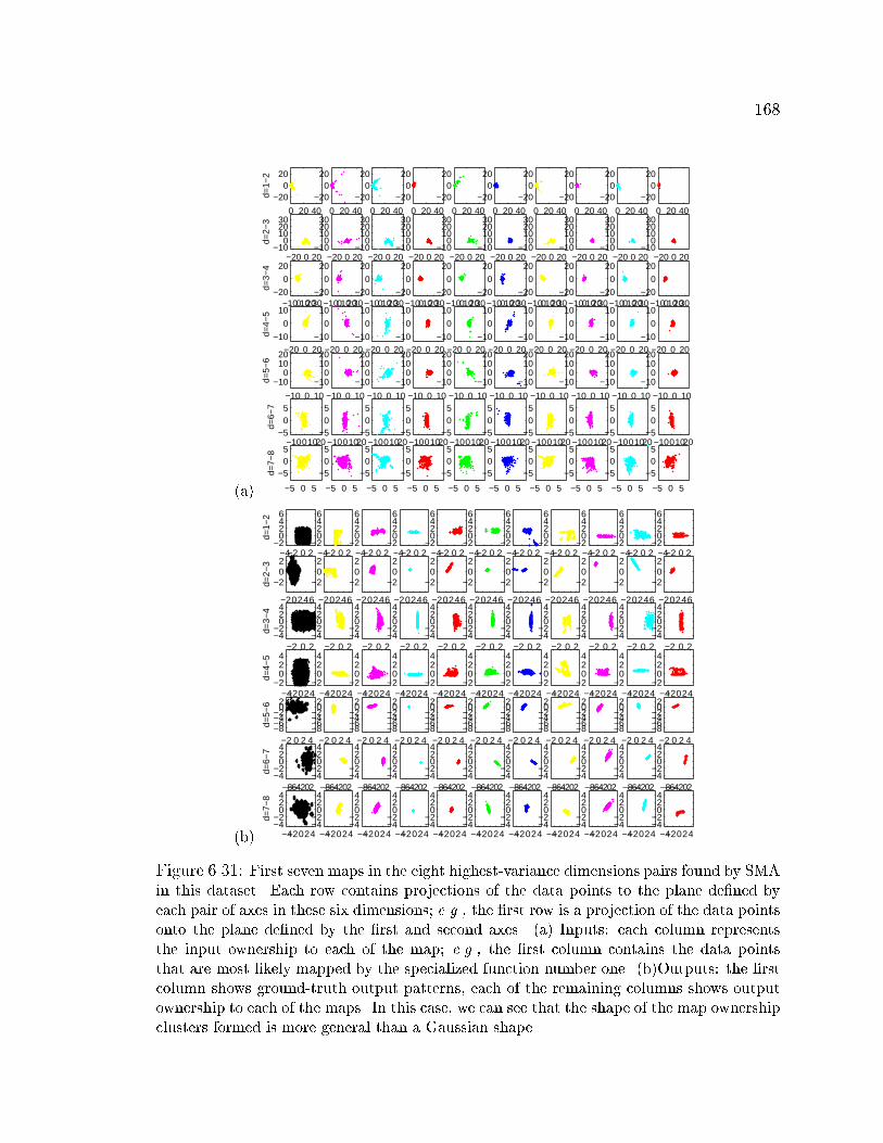
168

(a)

0 20 40

−200

20

d=1−

2

0 20 40

−200

20

0 20 40

−200

20

0 20 40

−200

20

0 20 40

−200

20

0 20 40

−200

20

0 20 40

−200

20

0 20 40

−200

20

0 20 40

−200

20

0 20 40

−200

20

−20 0 20−10

0102030

d=2−

3−20 0 20

−100

102030

−20 0 20−10

0102030

−20 0 20−10

0102030

−20 0 20−10

0102030

−20 0 20−10

0102030

−20 0 20−10

0102030

−20 0 20−10

0102030

−20 0 20−10

0102030

−20 0 20−10

0102030

−100102030−20

0

20d=

3−4

−100102030−20

0

20

−100102030−20

0

20

−100102030−20

0

20

−100102030−20

0

20

−100102030−20

0

20

−100102030−20

0

20

−100102030−20

0

20

−100102030−20

0

20

−100102030−20

0

20

−20 0 20−10

0

10

d=4−

5

−20 0 20−10

0

10

−20 0 20−10

0

10

−20 0 20−10

0

10

−20 0 20−10

0

10

−20 0 20−10

0

10

−20 0 20−10

0

10

−20 0 20−10

0

10

−20 0 20−10

0

10

−20 0 20−10

0

10

−10 0 10

−100

1020

d=5−

6

−10 0 10

−100

1020

−10 0 10

−100

1020

−10 0 10

−100

1020

−10 0 10

−100

1020

−10 0 10

−100

1020

−10 0 10

−100

1020

−10 0 10

−100

1020

−10 0 10

−100

1020

−10 0 10

−100

1020

−1001020−5

05

d=6−

7

−1001020−5

05

−1001020−5

05

−1001020−5

05

−1001020−5

05

−1001020−5

05

−1001020−5

05

−1001020−5

05

−1001020−5

05

−1001020−5

05

−5 0 5

−505

d=7−

8

−5 0 5

−505

−5 0 5

−505

−5 0 5

−505

−5 0 5

−505

−5 0 5

−505

−5 0 5

−505

−5 0 5

−505

−5 0 5

−505

−5 0 5

−505

(b)

−4−2 0 2−2

0246

d=1−

2

−4−2 0 2−2

0246

−4−2 0 2−2

0246

−4−2 0 2−2

0246

−4−2 0 2−2

0246

−4−2 0 2−2

0246

−4−2 0 2−2

0246

−4−2 0 2−2

0246

−4−2 0 2−2

0246

−4−2 0 2−2

0246

−4−2 0 2−2

0246

−20246

−202

d=2−

3

−20246

−202

−20246

−202

−20246

−202

−20246

−202

−20246

−202

−20246

−202

−20246

−202

−20246

−202

−20246

−202

−20246

−202

−2 0 2−4−2

024

d=3−

4

−2 0 2−4−2

024

−2 0 2−4−2

024

−2 0 2−4−2

024

−2 0 2−4−2

024

−2 0 2−4−2

024

−2 0 2−4−2

024

−2 0 2−4−2

024

−2 0 2−4−2

024

−2 0 2−4−2

024

−2 0 2−4−2

024

−4−2024−2

024

d=4−

5

−4−2024−2

024

−4−2024−2

024

−4−2024−2

024

−4−2024−2

024

−4−2024−2

024

−4−2024−2

024

−4−2024−2

024

−4−2024−2

024

−4−2024−2

024

−4−2024−2

024

−2 0 2 4−8−6−4−2

02

d=5−

6

−2 0 2 4−8−6−4−2

02

−2 0 2 4−8−6−4−2

02

−2 0 2 4−8−6−4−2

02

−2 0 2 4−8−6−4−2

02

−2 0 2 4−8−6−4−2

02

−2 0 2 4−8−6−4−2

02

−2 0 2 4−8−6−4−2

02

−2 0 2 4−8−6−4−2

02

−2 0 2 4−8−6−4−2

02

−2 0 2 4−8−6−4−2

02

−8−6−4−202−4−2

024

d=6−

7

−8−6−4−202−4−2

024

−8−6−4−202−4−2

024

−8−6−4−202−4−2

024

−8−6−4−202−4−2

024

−8−6−4−202−4−2

024

−8−6−4−202−4−2

024

−8−6−4−202−4−2

024

−8−6−4−202−4−2

024

−8−6−4−202−4−2

024

−8−6−4−202−4−2

024

−4−2024−4−2

024

d=7−

8

−4−2024−4−2

024

−4−2024−4−2

024

−4−2024−4−2

024

−4−2024−4−2

024

−4−2024−4−2

024

−4−2024−4−2

024

−4−2024−4−2

024

−4−2024−4−2

024

−4−2024−4−2

024

−4−2024−4−2

024

Figure 6.31: First seven maps in the eight highest-variance dimensions pairs found by SMAin this dataset. Each row contains projections of the data points to the plane de�ned byeach pair of axes in these six dimensions; e.g., the �rst row is a projection of the data pointsonto the plane de�ned by the �rst and second axes. (a) Inputs: each column representsthe input ownership to each of the map; e.g., the �rst column contains the data pointsthat are most likely mapped by the specialized function number one. (b)Outputs: the �rstcolumn shows ground-truth output patterns, each of the remaining columns shows outputownership to each of the maps. In this case, we can see that the shape of the map ownershipclusters formed is more general than a Gaussian shape.

169

GT

MO

GT

MO

GT

MO

GT

MO

GT

MO

Figure 6.32: 40 examples of estimated hand poses chosen uniformly at random and recon-struction found using mean output (MO) approach. The feedback function was computedusing CG rendering. Each example consists of a pair of images: ground-truth (top), andestimate obtained using the mean output algorithm (bottom). Note: for comparison framesare same as those used when feedback was estimated from data.

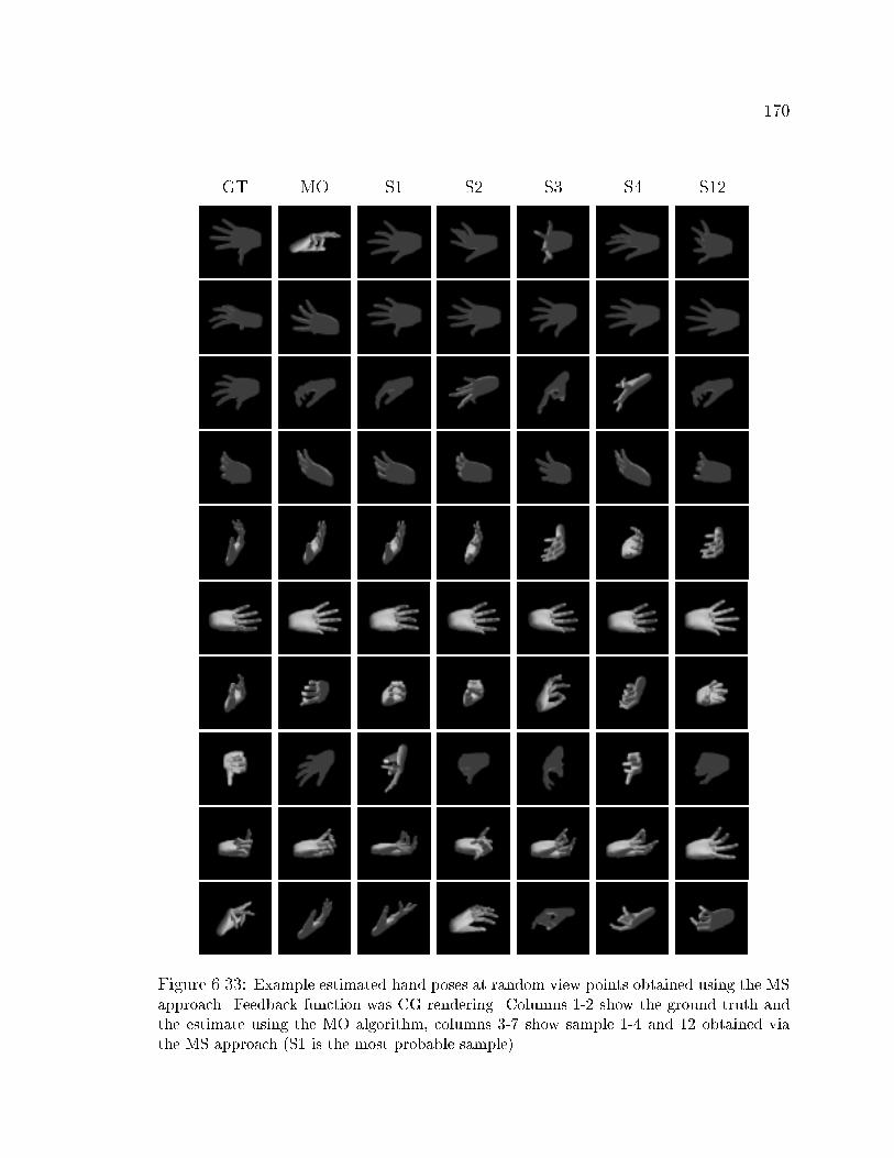
170


Figure 6.33: Example estimated hand poses at random view points obtained using the MSapproach. Feedback function was CG rendering. Columns 1-2 show the ground truth andthe estimate using the MO algorithm, columns 3-7 show sample 1-4 and 12 obtained viathe MS approach (S1 is the most probable sample).

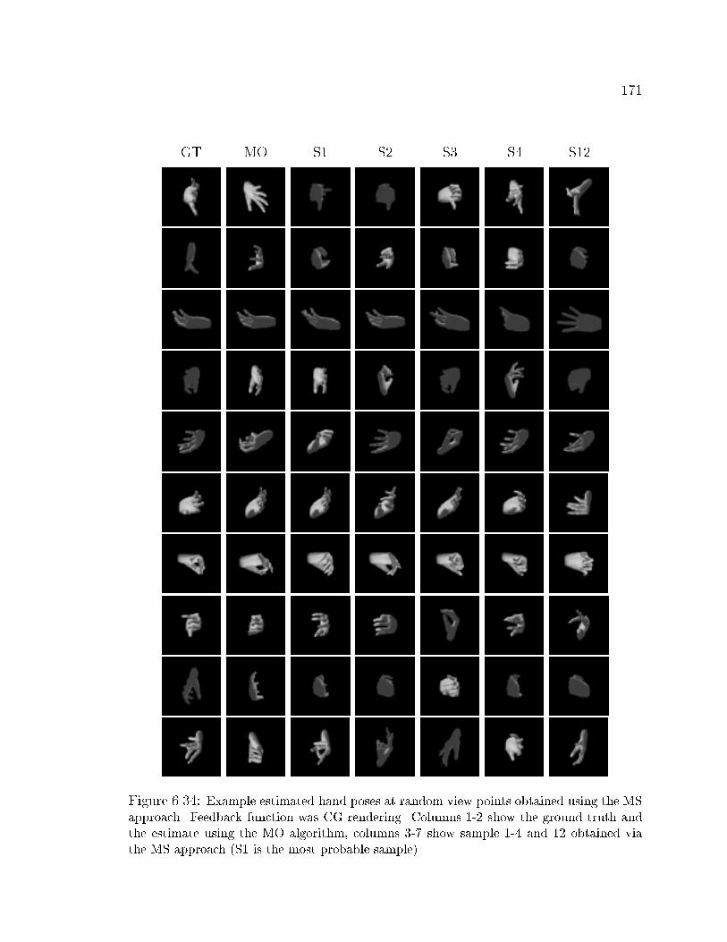
171


Figure 6.34: Example estimated hand poses at random view points obtained using the MSapproach. Feedback function was CG rendering. Columns 1-2 show the ground truth andthe estimate using the MO algorithm, columns 3-7 show sample 1-4 and 12 obtained viathe MS approach (S1 is the most probable sample).

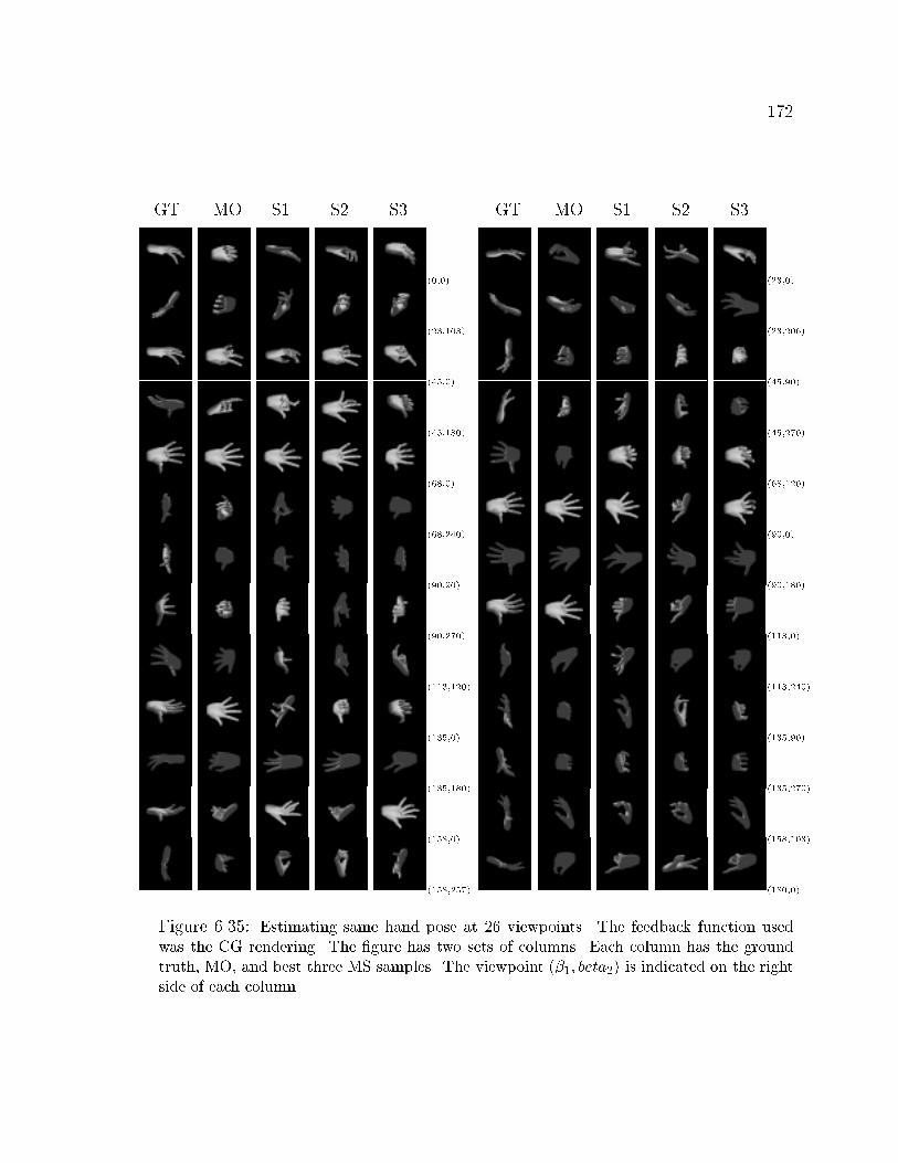
172

GT MO S1 S2 S3 GT MO S1 S2 S3

(0,0) (23,0)

(23,103) (23,206)

(45,0) (45,90)

(45,180) (45,270)

(68,0) (68,120)

(68,240) (90,0)

(90,90) (90,180)

(90,270) (113,0)

(113,120) (113,240)

(135,0) (135,90)

(135,180) (135,270)

(158,0) (158,103)

(158,257) (180,0)

Figure 6.35: Estimating same hand pose at 26 viewpoints. The feedback function usedwas the CG rendering. The �gure has two sets of columns. Each column has the groundtruth, MO, and best three MS samples. The viewpoint (�1; beta2) is indicated on the rightside of each column.

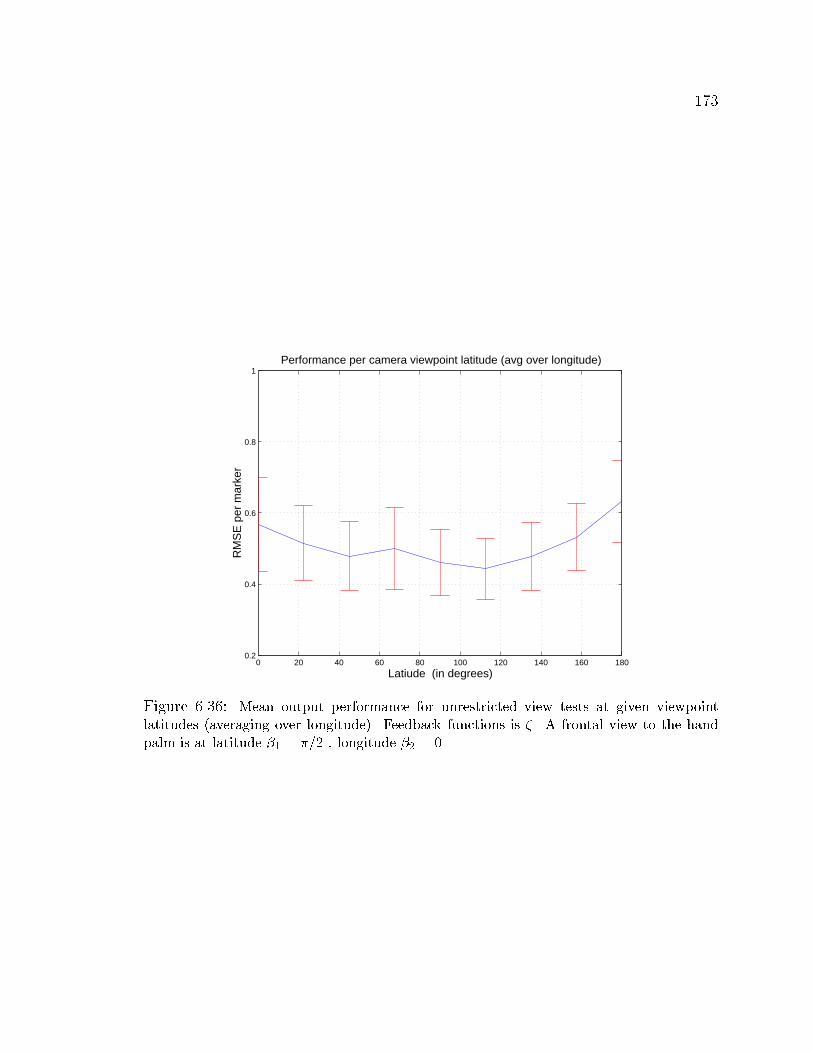
173

0 20 40 60 80 100 120 140 160 1800.2

0.4

0.6

0.8

1


RM

SE

per

mar

ker


Figure 6.36: Mean output performance for unrestricted view tests at given viewpointlatitudes (averaging over longitude). Feedback functions is �. A frontal view to the handpalm is at latitude �1 = �=2 , longitude �2 = 0.

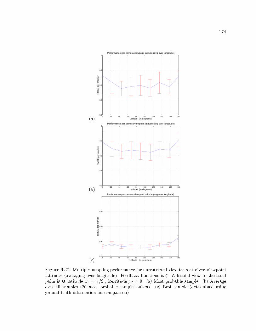
174

(a)0 20 40 60 80 100 120 140 160 180

0.2

0.4

0.6

0.8

1


RM

SE

per

mar

ker


(b)0 20 40 60 80 100 120 140 160 180

0.2

0.4

0.6

0.8

1


RM

SE

per

mar

ker


(c)0 20 40 60 80 100 120 140 160 180

0.2

0.4

0.6

0.8

1


RM

SE

per

mar

ker


Figure 6.37: Multiple sampling performance for unrestricted view tests at given viewpointlatitudes (averaging over longitude). Feedback functions is �. A frontal view to the handpalm is at latitude �1 = �=2 , longitude �2 = 0. (a) Most probable sample. (b) Averageover all samples (20 most probable samples taken). (c) Best sample (determined usingground-truth information for comparison).

175

6.4.3 Experiments with Real Images

As before (see Sec. 6.3.3), we now test our approach using data collected from a

single uncalibrated camera. However, the sequences used here consists of a person's

hand under unrestricted motion (i.e., the subject was not ask to limit his hand motion

to speci�c con�gurations or orientations). As before the image sampling rate was

60Hz and the hand occupies an area of approximately 200x200 pixels on the screen.

For these experiments, observation inputs were obtained simply tracking skin color

distributions (e.g., [108]).

Following a similar methodology as in Sec. 6.4.3, the SMA model was the same as

the one used for the unrestricted view synthetic-data experiments above. We again

compare the performance of SMA's using a feedback function (1) estimated from

data (�) and (2) provided by CG rendering (�) . In both cases, we tested SMA using

both mean output (MO) and multiple-sample (MS) inference algorithms described in

Chapter 3.

Experiments using the Estimated Feedback Function �

First we use �, estimated from data (we made it a 1 hidden layer perceptron

with 35 units). The estimated � used here is the same used in the synthetic-data

experiments. In the �rst experiment we use the mean output (MO)inference approach

to obtain a best estimate for each segmented hand. Estimates from 40 frames (taken

every 0.9 secs apart) using MO are shown in Fig. 6.38.

Note that there are wrongly segmented hands in these sequence. We decided to

leave them to avoid frame rearrangements (and lose the uniform frame sampling),

to show that segmentation does not always work correctly, and to show that this

176

approach is inherently robust to extreme errors such as entire frames badly segmented.

In this experiment, there was usually visual agreement between reconstruction and

estimate as seen in the �gures. This is one way to measure how good the system

worked. Note that even for a human observer, looking at the segmented silhouettes

in the �gure, reconstruction is not straightforward (moreover, there are many ambi-

guities). There are also con�gurations for which the system did not perform correctly.

In the second test we use the MS approach to perform inference. Fig. 6.39 shows

the corresponding estimates. The frames shown were taken approximately every 0.9

secs. In the sixth row, we can see some e�ects of the feature properties. From this

example, it is possible to see that a horizontal and vertical hand orientation are very

similar in feature space. This is a reason why these apparently di�erent hypothesis

are actually close to each other in terms of their probability, given the features e.g.,

p(hjx). The same e�ect repeats clearly in the eighth row and second row and not so

clearly in other rows.

We can avoid this by considering features with less invariances. At an extreme we

can consider the full silhouette as a feature. Of course there are important trade-o�s

to take into account when considering di�erent features.

Experiments using the CG Feedback Function �

Now we test the performance of the model using a computer graphics rendering

function. We also chose to display the same frames shown in Fig. 6.38 (to ease

comparisons among approaches). Fig. 6.40 shows results obtained when using the MO

algorithm. Result quality is comparable to those using the estimated �. However,

we believe reconstructions tend to agree slightly more with the underlying silhou-

177

ettes. Sec. 3.10 presents a discussion on comparing the use of an estimated or a

graphics-based feedback function. In our next test, we used the MS approach and

the CG rendering function to perform inference. Fig. 6.41 shows example frames of

reconstructions in this case.

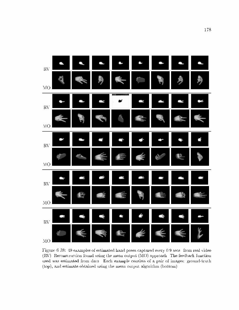
178

RV

MO

RV

MO

RV

MO

RV

MO

RV

MO

Figure 6.38: 40 examples of estimated hand poses captured every 0.9 secs. from real video(RV). Reconstruction found using the mean output (MO) approach. The feedback functionused was estimated from data. Each example consists of a pair of images: ground-truth(top), and estimate obtained using the mean output algorithm (bottom).

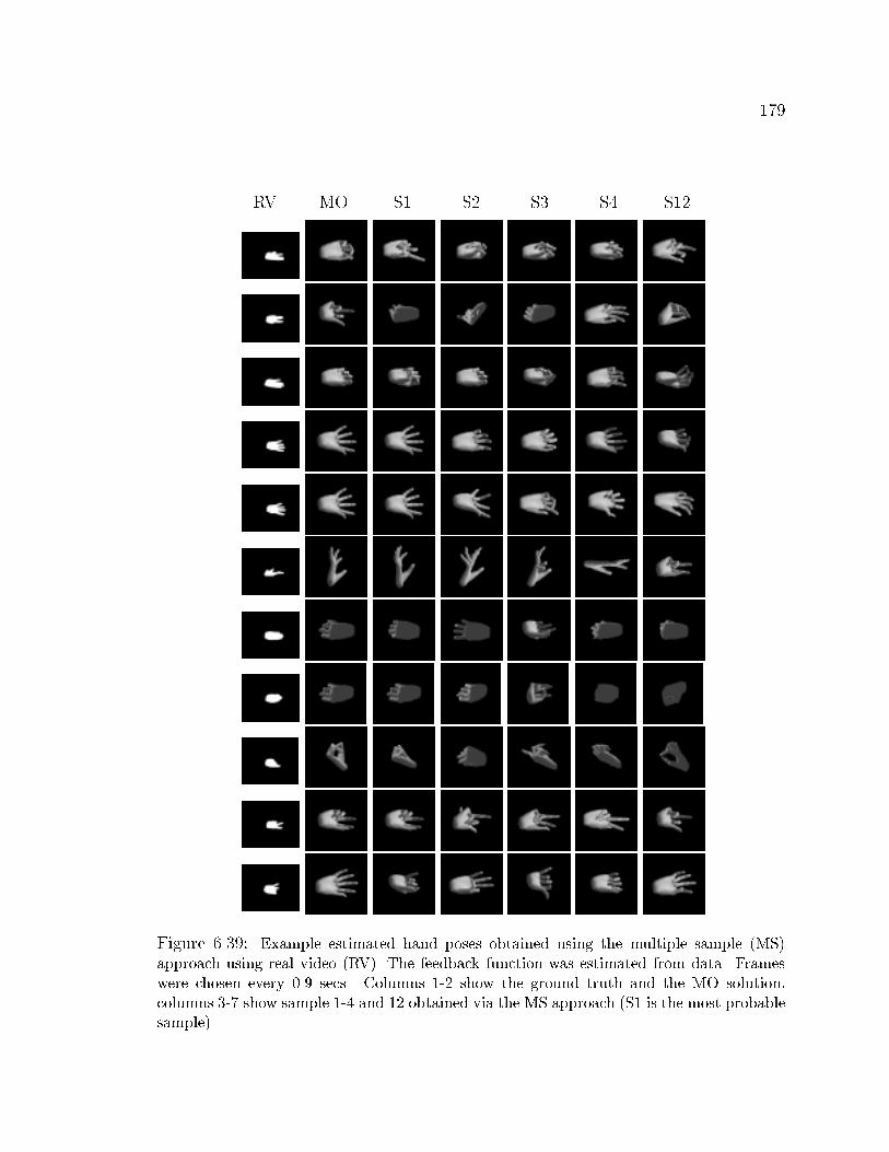
179


Figure 6.39: Example estimated hand poses obtained using the multiple sample (MS)approach using real video (RV). The feedback function was estimated from data. Frameswere chosen every 0.9 secs. Columns 1-2 show the ground truth and the MO solution,columns 3-7 show sample 1-4 and 12 obtained via the MS approach (S1 is the most probablesample).

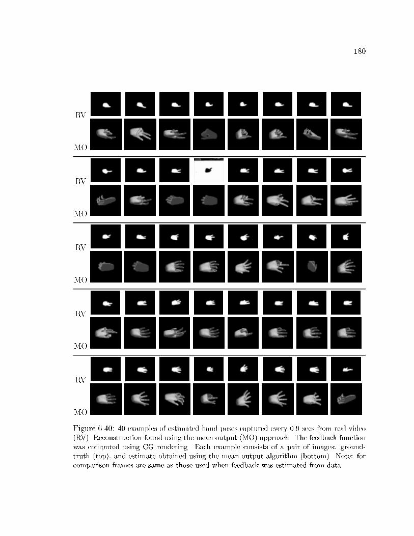
180

RV

MO

RV

MO

RV

MO

RV

MO

RV

MO

Figure 6.40: 40 examples of estimated hand poses captured every 0.9 secs from real video(RV). Reconstruction found using the mean output (MO) approach. The feedback functionwas computed using CG rendering. Each example consists of a pair of images: ground-truth (top), and estimate obtained using the mean output algorithm (bottom). Note: forcomparison frames are same as those used when feedback was estimated from data.

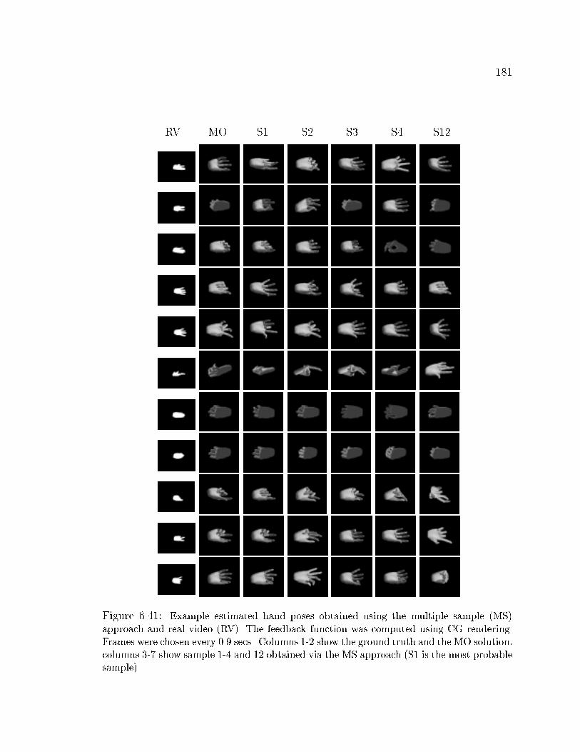
181


Figure 6.41: Example estimated hand poses obtained using the multiple sample (MS)approach and real video (RV). The feedback function was computed using CG rendering.Frames were chosen every 0.9 secs. Columns 1-2 show the ground truth and the MO solution,columns 3-7 show sample 1-4 and 12 obtained via the MS approach (S1 is the most probablesample).

182

6.5 2D Human Body Pose using SMA

We now test the SMA on a di�erent dataset and use a di�erent output represen-

tation. The goal is to estimate 2D human body pose from low level visual features

from a single image. The same problem was studied in Sec. 6.2. In that case using our

simple approximation to the SMA. However, in Sec. 4.2.6 we showed that the initial

approximation is an instance of the SMA framework and that that approximation

can be improved in the maximum likelihood sense as described in Sec. 4.2.7. Hence,

in theory the following experiments should provide more accurate estimates relative

to those obtained using the initial SMA approximation.


In these experiments, the training dataset consisted of approximately 7,000

frames of human body poses obtained through motion capture, as described in Sec. 4.4.

The output consisted of 20 2D marker positions: 3D markers projected to the image

plane using a perspective model. These were linearly encoded by eight real values

using Principal Component Analysis (PCA). The input (visual features) consisted of

10 real-valued Alt moments computed on synthetically generated silhouettes of the

articulated �gure. For training/testing we generated 100,000 data points. Our 3D

poses from motion capture were projected to 16 views along the view-sphere equator.

We took 8,000 2D poses for training and the rest for testing. The only free parameters

in this test, related to the given SMA, were the number of specialized functions used:

15, and the number of hidden nodes in the multi-layer perceptron: 7. For choosing

these numbers we used MDL [95].

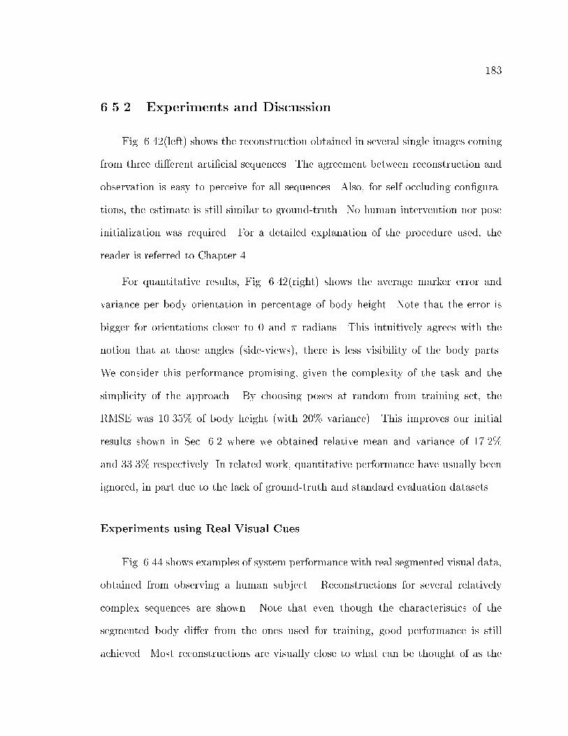
183


Fig. 6.42(left) shows the reconstruction obtained in several single images coming

from three di�erent arti�cial sequences. The agreement between reconstruction and

observation is easy to perceive for all sequences. Also, for self-occluding con�gura-

tions, the estimate is still similar to ground-truth. No human intervention nor pose

initialization was required. For a detailed explanation of the procedure used, the

reader is referred to Chapter 4.

For quantitative results, Fig. 6.42(right) shows the average marker error and

variance per body orientation in percentage of body height. Note that the error is

bigger for orientations closer to 0 and � radians. This intuitively agrees with the

notion that at those angles (side-views), there is less visibility of the body parts.

We consider this performance promising, given the complexity of the task and the

simplicity of the approach. By choosing poses at random from training set, the

RMSE was 10.35% of body height (with 20% variance). This improves our initial

results shown in Sec. 6.2 where we obtained relative mean and variance of 17.2%

and 33.3% respectively. In related work, quantitative performance have usually been

ignored, in part due to the lack of ground-truth and standard evaluation datasets.

Experiments using Real Visual Cues

Fig. 6.44 shows examples of system performance with real segmented visual data,

obtained from observing a human subject. Reconstructions for several relatively

complex sequences are shown. Note that even though the characteristics of the

segmented body di�er from the ones used for training, good performance is still

achieved. Most reconstructions are visually close to what can be thought of as the

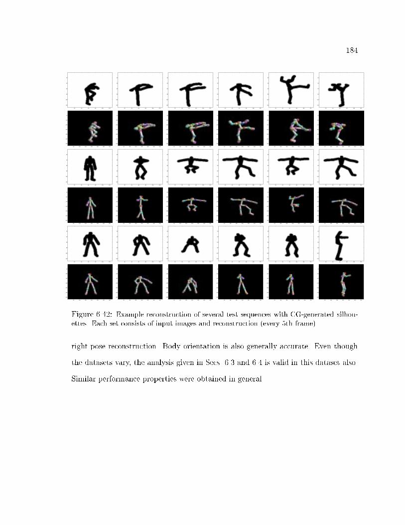
184

20 40 60 80 100 120

20

40

60

80

100

120

20 40 60 80 100 120

20

40

60

80

100

120

20 40 60 80 100 120

20

40

60

80

100

120

20 40 60 80 100 120

20

40

60

80

100

120

20 40 60 80 100 120

20

40

60

80

100

120

20 40 60 80 100 120

20

40

60

80

100

120

50 100 150 200 250 300 350

50

100

150

200

250

300

350

50 100 150 200 250 300 350

50

100

150

200

250

300

350

50 100 150 200 250 300 350

50

100

150

200

250

300

350

50 100 150 200 250 300 350

50

100

150

200

250

300

350

50 100 150 200 250 300 350

50

100

150

200

250

300

350

50 100 150 200 250 300 350

50

100

150

200

250

300

350

20 40 60 80 100 120

20

40

60

80

100

120

20 40 60 80 100 120

20

40

60

80

100

120

20 40 60 80 100 120

20

40

60

80

100

120

20 40 60 80 100 120

20

40

60

80

100

120

20 40 60 80 100 120

20

40

60

80

100

120

20 40 60 80 100 120

20

40

60

80

100

120

50 100 150 200 250 300 350

50

100

150

200

250

300

350

50 100 150 200 250 300 350

50

100

150

200

250

300

350

50 100 150 200 250 300 350

50

100

150

200

250

300

350

50 100 150 200 250 300 350

50

100

150

200

250

300

350

50 100 150 200 250 300 350

50

100

150

200

250

300

350

50 100 150 200 250 300 350

50

100

150

200

250

300

350

20 40 60 80 100 120

20

40

60

80

100

120

20 40 60 80 100 120

20

40

60

80

100

120

20 40 60 80 100 120

20

40

60

80

100

120

20 40 60 80 100 120

20

40

60

80

100

120

20 40 60 80 100 120

20

40

60

80

100

120

20 40 60 80 100 120

20

40

60

80

100

120

50 100 150 200 250 300 350

50

100

150

200

250

300

350

50 100 150 200 250 300 350

50

100

150

200

250

300

350

50 100 150 200 250 300 350

50

100

150

200

250

300

350

50 100 150 200 250 300 350

50

100

150

200

250

300

350

50 100 150 200 250 300 350

50

100

150

200

250

300

350

50 100 150 200 250 300 350

50

100

150

200

250

300

350

Figure 6.42: Example reconstruction of several test sequences with CG-generated silhou-ettes. Each set consists of input images and reconstruction (every 5th frame).

right pose reconstruction. Body orientation is also generally accurate. Even though

the datasets vary, the analysis given in Secs. 6.3 and 6.4 is valid in this dataset also.

Similar performance properties were obtained in general.

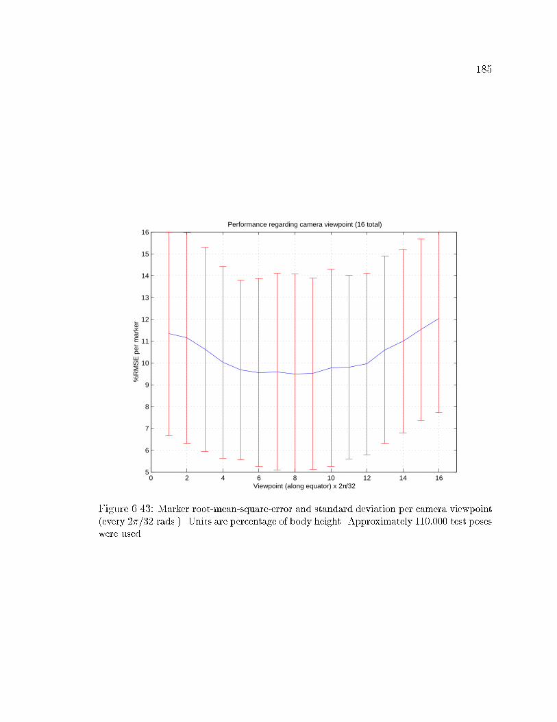
185

0 2 4 6 8 10 12 14 165

6

7

8

9

10

11

12

13

14

15

16

%R

MS

E p

er m

arke

r

Viewpoint (along equator) x 2π/32

Performance regarding camera viewpoint (16 total)

Figure 6.43: Marker root-mean-square-error and standard deviation per camera viewpoint(every 2�=32 rads.). Units are percentage of body height. Approximately 110,000 test poseswere used.

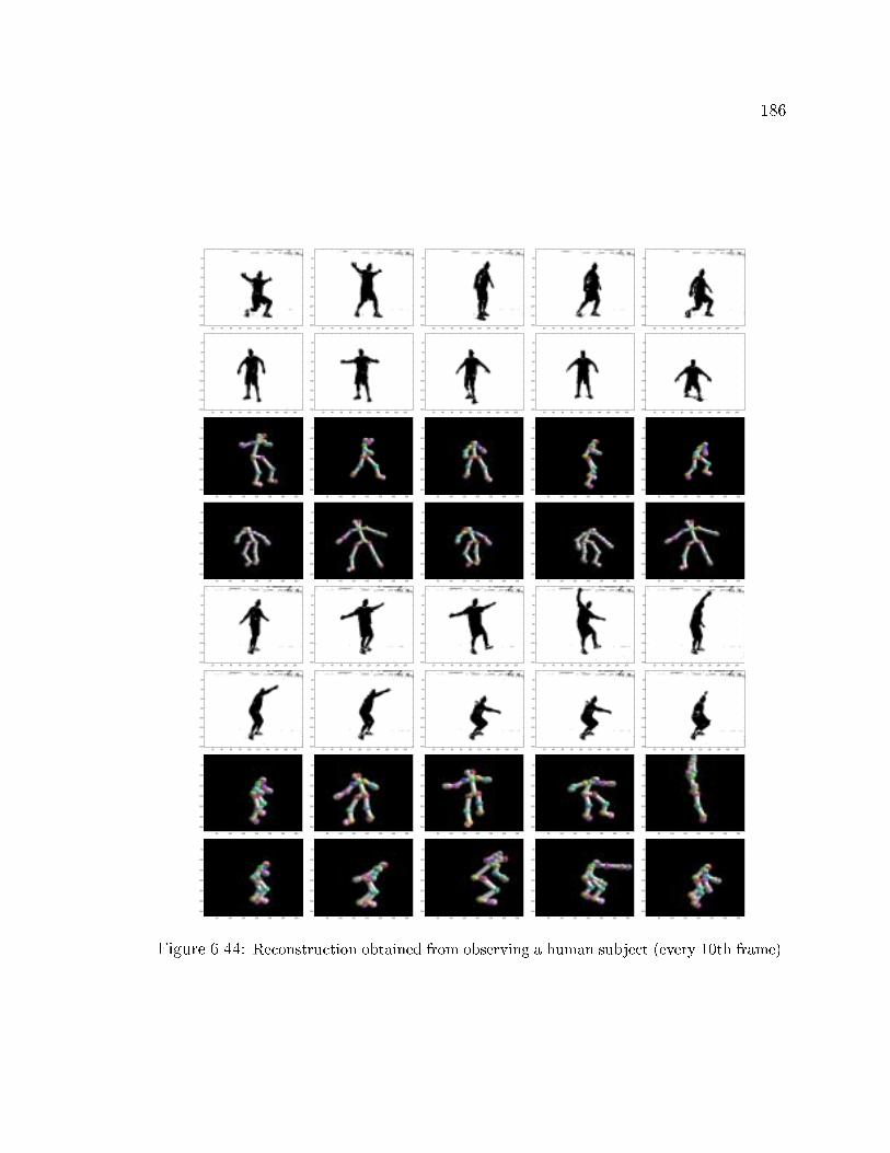
186

20 40 60 80 100 120 140 160 180 200

20

40

60

80

100

120

140

16020 40 60 80 100 120 140 160 180 200

20

40

60

80

100

120

140

16020 40 60 80 100 120 140 160 180 200

20

40

60

80

100

120

140

16020 40 60 80 100 120 140 160 180 200

20

40

60

80

100

120

140

16020 40 60 80 100 120 140 160 180 200

20

40

60

80

100

120

140

160

20 40 60 80 100 120 140 160 180 200

20

40

60

80

100

120

140

16020 40 60 80 100 120 140 160 180 200

20

40

60

80

100

120

140

16020 40 60 80 100 120 140 160 180 200

20

40

60

80

100

120

140

16020 40 60 80 100 120 140 160 180 200

20

40

60

80

100

120

140

16020 40 60 80 100 120 140 160 180 200

20

40

60

80

100

120

140

160

50 100 150 200 250 300 350

50

100

150

200

250

300

350

50 100 150 200 250 300 350

50

100

150

200

250

300

350

50 100 150 200 250 300 350

50

100

150

200

250

300

350

50 100 150 200 250 300 350

50

100

150

200

250

300

350

50 100 150 200 250 300 350

50

100

150

200

250

300

350

50 100 150 200 250 300 350

50

100

150

200

250

300

350

50 100 150 200 250 300 350

50

100

150

200

250

300

350

50 100 150 200 250 300 350

50

100

150

200

250

300

350

50 100 150 200 250 300 350

50

100

150

200

250

300

350

50 100 150 200 250 300 350

50

100

150

200

250

300

350

20 40 60 80 100 120 140 160 180 200

20

40

60

80

100

120

140

16020 40 60 80 100 120 140 160 180 200

20

40

60

80

100

120

140

16020 40 60 80 100 120 140 160 180 200

20

40

60

80

100

120

140

16020 40 60 80 100 120 140 160 180 200

20

40

60

80

100

120

140

16020 40 60 80 100 120 140 160 180 200

20

40

60

80

100

120

140

160

20 40 60 80 100 120 140 160 180 200

20

40

60

80

100

120

140

16020 40 60 80 100 120 140 160 180 200

20

40

60

80

100

120

140

16020 40 60 80 100 120 140 160 180 200

20

40

60

80

100

120

140

16020 40 60 80 100 120 140 160 180 200

20

40

60

80

100

120

140

16020 40 60 80 100 120 140 160 180 200

20

40

60

80

100

120

140

160

50 100 150 200 250 300 350

50

100

150

200

250

300

350

50 100 150 200 250 300 350

50

100

150

200

250

300

350

50 100 150 200 250 300 350

50

100

150

200

250

300

350

50 100 150 200 250 300 350

50

100

150

200

250

300

350

50 100 150 200 250 300 350

50

100

150

200

250

300

350

50 100 150 200 250 300 350

50

100

150

200

250

300

350

50 100 150 200 250 300 350

50

100

150

200

250

300

350

50 100 150 200 250 300 350

50

100

150

200

250

300

350

50 100 150 200 250 300 350

50

100

150

200

250

300

350

50 100 150 200 250 300 350

50

100

150

200

250

300

350

Figure 6.44: Reconstruction obtained from observing a human subject (every 10th frame).

187

6.6 Multi View Pose and Camera Calibration

In these experiments, we test our approach for determining 3D human body pose

and camera relative location as presented in Chapter 5.

6.6.1 Model

The training dataset was described in Sec. 5.5; i.e., we will use the Body-All-

Views-Hu dataset. Experiments were conducted using real video sequences, and

synthetic sequences that were not used in training the SMA. For the experiments

with real video sequences, observation inputs were obtained using simple background

subtraction, as described in Chapter 4. In the following three performance experi-

ments, unless otherwise stated, three cameras are used to capture the test sequences.

6.6.2 Quantitative Experiments

The �rst experiment tested the sensitivity of the system to the change in the

angular displacement between the cameras, or equivalently the baseline between pairs

of cameras. The result of 100 reconstruction trials with 50 randomly chosen frames

is each depicted in Fig. 6.45(a). As seen in the graph, the normalized correlation

between ground-truth and estimated 3D pose improves as the baseline increases. A

wider baseline in other approaches results in a major feature correspondence problem.

Our approach does not su�er from this shortcoming because the mapping between

silhouette features and the 2D joint locations provides correspondence across frames

and disparate views.

The second experiment measured the average performance of our approach with

188

respect to the number of cameras used. The angular displacement was set to �=8

rads (22.5 degrees) and the number of cameras varied from two to six. The number

of trials and performance measures are as in the �rst experiment. A graph showing

results of this experiment is shown in Fig. 6.45(b). It was noted that there is a major

increase in reconstruction accuracy when the number of cameras increases from two

to three.

Fig. 6.46 shows several example reconstructions taken from our test sequences.

Frames were taken evenly spaced (every 50-th at 30 frames/sec) from a novel motion

capture sequence. Estimates and ground-truth are on the left and right hand side

respectively. The visual agreement between the estimates and ground-truth can be

observed.

6.6.3 Experiments with Real Sequences

Real sequences of a single human subject were captured by a setup of three

synchronized cameras for which neither calibration nor pose was known. In Fig. 6.47

we can see the result of standard background subtraction applied to the original

images to obtain the initial silhouettes shown (only those obtained by the �rst camera

are shown). Seven Hu moments were computed for each silhouette and then the SMA

inference procedure described in Chapter 5 was carried out to obtain estimates of

2D joint locations; 3D reconstruction was obtained as shown in the bottom rows of

Fig. 6.47. The �gure shows every 15-th frame from the sequence. A similar procedure

was used to obtain the results in Fig. 6.48. Cameras were located at roughly mid-

body height and their relative angular displacement was approximately 0, 30, and 90

degrees.

189

We used a sequence of 50 frames at a time to obtain the poses shown. The

estimates of camera angular displacements were 0, 25, and 83 degrees on average. In

these sequences, pose accuracy varies over frames, but rough body pose is, for the

most part, visually accurate. Given the complexity of the body con�gurations, the

lack of knowledge about the cameras, and no manual initial placement of the human

body model, this is a very di�cult task. The main source of inaccuracy when using

real data is the statistical di�erences between the visual features generated by a real

person and the computer graphics model used in training the SMA.

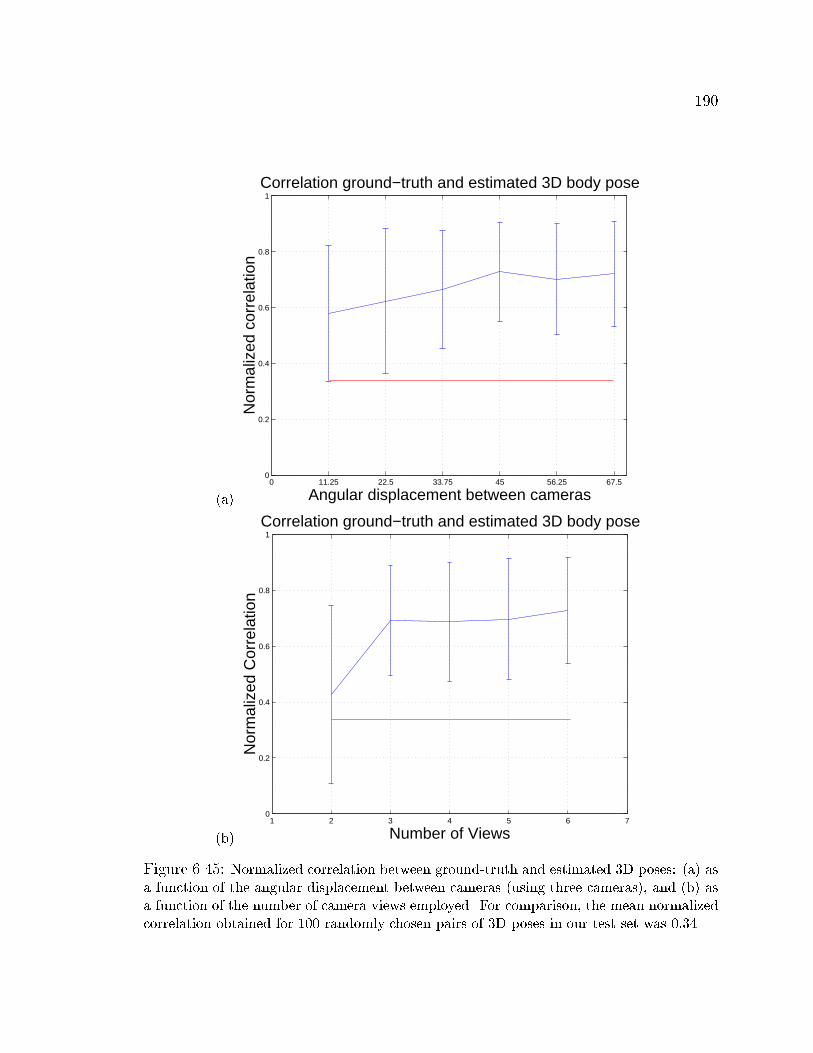
190

(a)

0 11.25 22.5 33.75 45 56.25 67.50

0.2

0.4

0.6

0.8

1

Angular displacement between cameras

Nor

mal

ized

cor

rela

tion

Correlation ground−truth and estimated 3D body pose

(b)

1 2 3 4 5 6 70

0.2

0.4

0.6

0.8

1

Number of Views

Nor

mal

ized

Cor

rela

tion

Correlation ground−truth and estimated 3D body pose

Figure 6.45: Normalized correlation between ground-truth and estimated 3D poses: (a) asa function of the angular displacement between cameras (using three cameras), and (b) asa function of the number of camera views employed. For comparison, the mean normalizedcorrelation obtained for 100 randomly chosen pairs of 3D poses in our test set was 0:34.

191

−1

−0.5

0

0.5

1

−1

−0.5

0

0.5

1

−1

−0.5

0

0.5

1

−1

−0.5

0

0.5

1

−1

−0.5

0

0.5

1

−1

−0.5

0

0.5

1

−1

−0.5

0

0.5

1

−1

−0.5

0

0.5

1

−1

−0.5

0

0.5

1

−1

−0.5

0

0.5

1

−1

−0.5

0

0.5

1

−1

−0.5

0

0.5

1

−1

−0.5

0

0.5

1

−1

−0.5

0

0.5

1

−1

−0.5

0

0.5

1

−1

−0.5

0

0.5

1

−1

−0.5

0

0.5

1

−1

−0.5

0

0.5

1

−1

−0.5

0

0.5

1

−1

−0.5

0

0.5

1

−1

−0.5

0

0.5

1

−1

−0.5

0

0.5

1

−1

−0.5

0

0.5

1

−1

−0.5

0

0.5

1

−1

−0.5

0

0.5

1

−1

−0.5

0

0.5

1

−1

−0.5

0

0.5

1

Figure 6.46: Example reconstruction of a test sequence (every 50-th frame at 30frames/sec). In each 3D graph, pose estimates are drawn on the left side and ground-truthone the right.

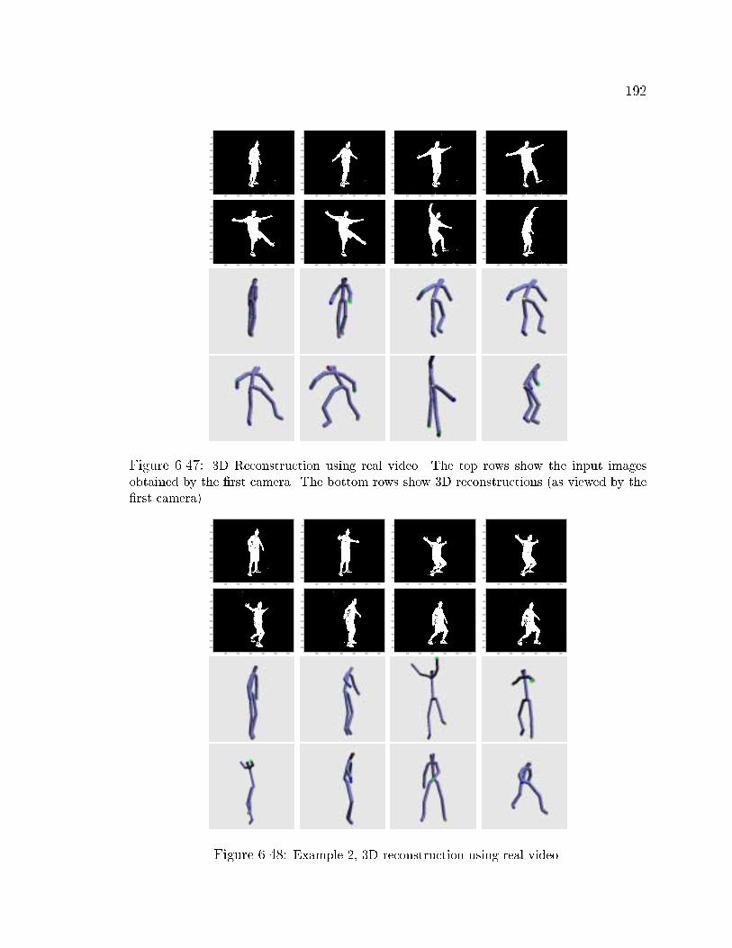
192

100 200 300 400 500 600

50

100

150

200

250

300

350

400

450

100 200 300 400 500 600

50

100

150

200

250

300

350

400

450

100 200 300 400 500 600

50

100

150

200

250

300

350

400

450

100 200 300 400 500 600

50

100

150

200

250

300

350

400

450

100 200 300 400 500 600

50

100

150

200

250

300

350

400

450

100 200 300 400 500 600

50

100

150

200

250

300

350

400

450

100 200 300 400 500 600

50

100

150

200

250

300

350

400

450

100 200 300 400 500 600

50

100

150

200

250

300

350

400

450

Figure 6.47: 3D Reconstruction using real video. The top rows show the input imagesobtained by the �rst camera. The bottom rows show 3D reconstructions (as viewed by the�rst camera).

100 200 300 400 500 600

50

100

150

200

250

300

350

400

450

100 200 300 400 500 600

50

100

150

200

250

300

350

400

450

100 200 300 400 500 600

50

100

150

200

250

300

350

400

450

100 200 300 400 500 600

50

100

150

200

250

300

350

400

450

100 200 300 400 500 600

50

100

150

200

250

300

350

400

450

100 200 300 400 500 600

50

100

150

200

250

300

350

400

450

100 200 300 400 500 600

50

100

150

200

250

300

350

400

450

100 200 300 400 500 600

50

100

150

200

250

300

350

400

450

Figure 6.48: Example 2, 3D reconstruction using real video.

193

6.7 Gaussian Error Assumption

In the above experiments, we have used the assumption that the error in ap-

proximating and output body pose using a speci�c specialized function and an input

pattern is distributed according to a Gaussian distribution. Formally, this can be

written:

p( j�; y; �) = N ( ;�y(�; �y);�y); (6.1)

with the output (e.g., body pose), � the input (e.g., visual features), � the special-

ized function, y the function index, � the SMA specialized function parameters, and

� the covariance of this distribution.

In addition to the fact that a Gaussian distribution seems a natural choice for

approximating the error distribution, this assumption was also used because it allows

us to obtain feasible learning and inference algorithms. In order to test the overall

validity of this assumption, we use the standard skewness and kurtosis statistics.

Skewness is a measure of the symmetry of the distribution. A negative or positive

skewness indicates that the distribution has more mass towards the negative or

positive side of the random variable mean. Hence, a truly Gaussian random variable

will have zero skewness.

Kurtosis is the classical measure of Gaussianity. The kurtosis of a truly Gaus-

sian random variable is equal to three. Random variables with lower kurtosis are

called sub-Gaussian, and those higher kurtosis are called super-Gaussian. The terms

platykurtic and leptokurtic are also used. Super-Gaussian random variables usually

have a spiky density function with heavy tails.

Skewness is the third central moment of the data divided by the cube of the

194

standard deviation. Similarly, kurtosis is the fourth order moment divided by the

fourth power of the standard deviation.

In the SMA, the skewness and kurtosis of the error � = � �k(�; �) when using

specialized function y = k are:

skewk(�j) =

Pi~P (y(i) = k)(�

(i)j � ��j)

3=Pi~P (y(i) = k)

[Pi~P (y(i) = k)(�

(i)j � ��j)2=

Pi~P (y(i) = k)]3=2

(6.2)

and

kurtk(�j) =

Pi~P (y(i) = k)(�(i)j � ��j)

4=Pi~P (y(i) = k)

[Pi~P (y(i) = k)(�

(i)j � ��j)2=

Pi~P (y(i) = k)]2

(6.3)

respectively. With ~P (y(i) = k) = P (yi = kj�i; i; �), �(i) and y(i) the error and the

specialized function label (respectively) associated with the i � th data point, and ��

the weighted population mean:

�� =

Pi P (y

(i) = k)�(i)Pi~P (y(i) = k)

(6.4)

Note that these equations de�ne the skewness and kurtosis of a particular com-

ponent of the error random variable �. Using these de�nitions, we will compute the

skewness and kurtosis of the error random variable for each specialized function in

each component (dimension).

First, we will test our Gaussian error assumption using as population 6,000

test con�gurations from the Hand-Single-View dataset using the model computed

in Sec. 6.3. This model has 20 specialized functions and an output dimension of nine.

195

Hence, we computed 180 instances of the skewness and kurtosis statistics (one for

each dimension and one for each specialized function).

Fig. 6.49 shows two histograms illustrating skewness and kurtosis respectively.

Note that the skewness histogram is strongly peaked at zero and decreases very rapidly

so that it is rare to observe distributions with skewness considerably far from zero.

This indicates that our error distribution is in general symmetric.

The kurtosis histogram has most of its probability mass around a kurtosis value

equal to three. Hence, this indicates that the error distributions are in general close

to a Gaussian distribution using fourth order statistics. Recall that the kurtosis of

a Gaussian random variable is equal to three. It is possible to observe also that

this histogram is biased towards values bigger than three (it is not symmetric).

This indicates that when the error is not a Gaussian random variable, it is instead

more sharply peaked than a Gaussian random variable (i.e., the error tends to be

leptokurtic). Note also that there are few instances of very high kurtosis, indicating

that in these few cases the distribution fourth order statistics might be far from the

Gaussian statistics.

In our next experiment, we will use the dataset Hand-All-Views to also test

the Gaussianity of the error random variable. We used approximately 200,000 test

examples as our population and the SMA model obtained in Sec. 6.4. This model

uses 45 specialized and an output dimension equal to nine, thus we performed 405

kurtosis and skewness tests.

Fig. 6.50 shows the two histograms illustrating these results. On the �rst graph

we can observe instances of skewness values. As before, skewness is usually zero or

close to zero. This agrees with the skewness of a Gaussian random variable. However,

196

in few cases the error distribution seems very asymmetric. There seems to be a slight

preference of the error to be positive as compared with negative.

The second graph in Fig. 6.50 shows the kurtosis histogram. Very similarly to

the previous experiment, kurtosis is usually that of a Gaussian random variable, with

few cases for which kurtosis is considerably higher.

In both cases, our experiments indicate that the distribution of the error random

variable can be approximated reasonably well by a Gaussian distribution, with very

few exceptions for which a super-Gaussian random variable seems to provide a better

�t. In those instances, a Laplace distribution, for example, seems a good candidate

for approximation.

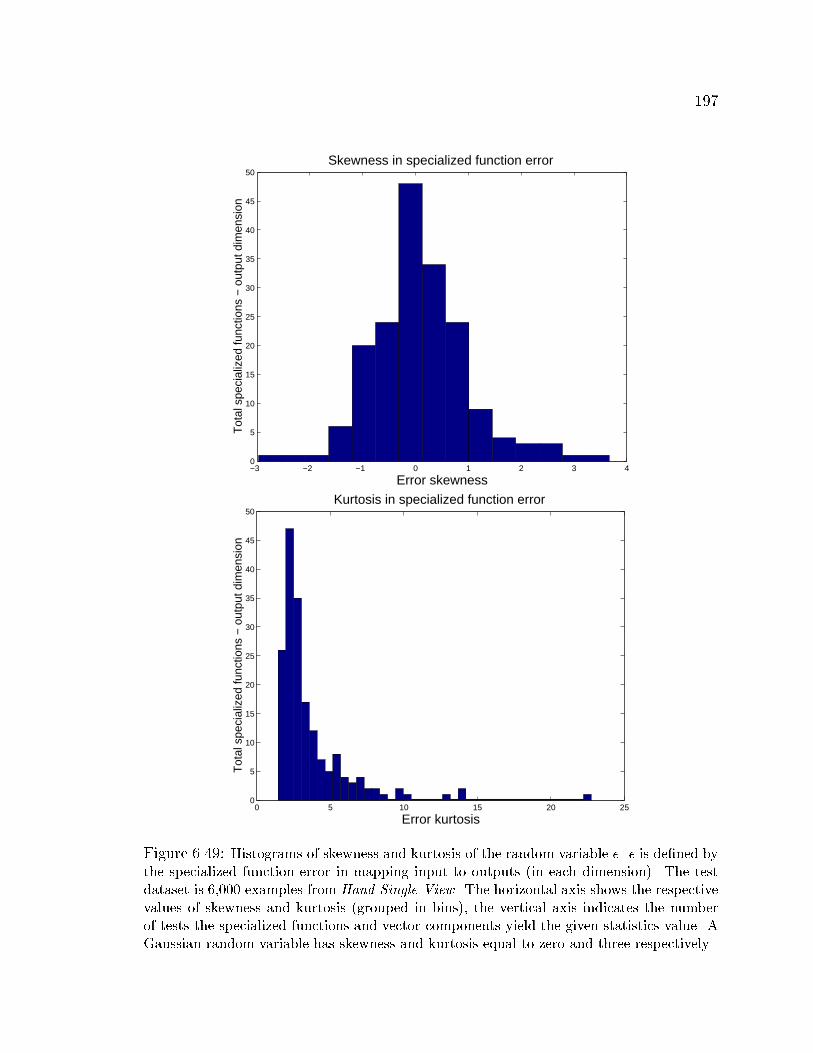
197

−3 −2 −1 0 1 2 3 40

5

10

15

20

25

30

35

40

45

50

Error skewness

Tot

al s

peci

aliz

ed fu

nctio

ns −

out

put d

imen

sion

Skewness in specialized function error

0 5 10 15 20 250

5

10

15

20

25

30

35

40

45

50

Error kurtosis

Tot

al s

peci

aliz

ed fu

nctio

ns −

out

put d

imen

sion

Kurtosis in specialized function error

Figure 6.49: Histograms of skewness and kurtosis of the random variable �. � is de�ned bythe specialized function error in mapping input to outputs (in each dimension). The testdataset is 6,000 examples from Hand-Single-View. The horizontal axis shows the respectivevalues of skewness and kurtosis (grouped in bins), the vertical axis indicates the numberof tests the specialized functions and vector components yield the given statistics value. AGaussian random variable has skewness and kurtosis equal to zero and three respectively.

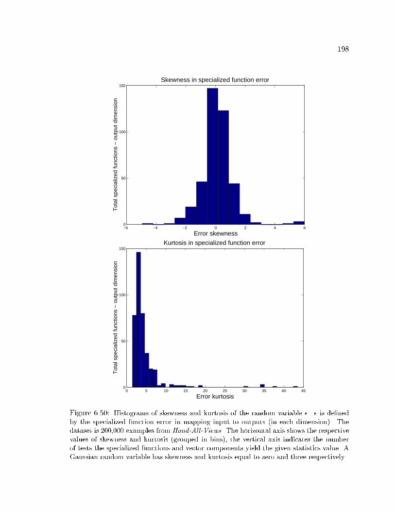
198

−6 −4 −2 0 2 4 60

50

100

150

Error skewness

Tot

al s

peci

aliz

ed fu

nctio

ns −

out

put d

imen

sion

Skewness in specialized function error

0 5 10 15 20 25 30 35 40 450

50

100

150

Error kurtosis

Tot

al s

peci

aliz

ed fu

nctio

ns −

out

put d

imen

sion

Kurtosis in specialized function error

Figure 6.50: Histograms of skewness and kurtosis of the random variable �. � is de�nedby the specialized function error in mapping input to outputs (in each dimension). Thedataset is 200,000 examples from Hand-All-Views. The horizontal axis shows the respectivevalues of skewness and kurtosis (grouped in bins), the vertical axis indicates the numberof tests the specialized functions and vector components yield the given statistics value. AGaussian random variable has skewness and kurtosis equal to zero and three respectively.

199

6.8 Experiments on Feature Properties

The following experiments are intended to test the impact of the visual features

used throughout this thesis: Alt and Hu moments. This impact will be studied from

two perspectives: the in uence of the discriminating power of visual features and the

sensitivity of the error estimate to perturbation in visual features.

6.8.1 Error in Visual Feature Space

In these experiments we test whether the error in the output estimates has any

relation to the visual feature properties (e.g., lack of discriminating power) or it is

caused by a potential unsuitability of the underlying architecture (SMA). For this,

we will compute the SMA error in the visual feature space between input observation

and the input (visual features) computed from the SMA output estimate.

Recall that in the SMA, roughly speaking the feedback probabilistic model is

used to evaluate the hypotheses generated by the forward model. This is done using

the input space. If the elements of the input space are not discriminative enough

with respect to the elements of the output space, the overall performance of the SMA

would be poor. This would be true even if the SMA forward model is very accurate.

If our experiments show quantitatively that using the SMA, the error in the

visual feature space is high, then the SMA is not performing its job and is probably

not useful for this task. On the contrary if the error in input feature space is low,

then the SMA is performing the right task, and the estimation error could be more

likely associated with other aspects. Among other things, poor performance could be

associated with the underlying lack of discriminating power in the visual features.

200

A factor that needs to be considered is that the error in the input feature space

may depend on the choice of the feedback function (e.g., � or �). Because of this, we

will perform experiments using both cases of feedback functions. In each case we will

also test both the mean output (MO) and the multiple sampling (MS) algorithms.

In the following experiments, we test the error in visual feature space when the

SMA pose estimates are used to compute the associated visual features. The visual

features are computed using the inverse function � or �. This error is then compared

with chance; i.e., for the case when we use a random sample from our training set as

the estimate for a given input from the test set.

First, we will use 6,000 test con�gurations from the Hand-Single-View dataset

and the model computed in Sec. 6.3 for �xed view hand pose estimation. Thus, we

will be using Alt-moment features. Fig. 6.51 shows the results of this test.

Both graphs in this �gure indicate the root mean square error and standard

deviation in visual feature space. The distribution of the inputs has zero mean and

unit variance in each dimension (a consequence of using PCA). In the �gure, the

hypotheses are labeled in the x axis. In each graph the error for the mean output

algorithm is represented by the error bar corresponding to hypothesis zero. Similarly,

the error associated to the multiple sampling algorithm is represented by the �rst to

the twentieth hypothesis error bars. The MS hypotheses have been sorted according

to their likelihood as done throughout all the previous experiments. The horizontal

line formed by long segments represents the mean of the baseline performance.

The �rst graph uses � as feedback function and the second graph uses �. Note

that there are no major di�erences in both cases. More importantly, note that the

SMA performs considerably better than the baseline solution. For the multiple sample

201

approach we took ten samples per function. Even using this low number of samples,

the twentieth overall best sample is still much better than the baseline. We can

also observe that the mean output solution is usually as good as the best hypotheses

generated by the multiple sampling approach.

In our next experiment, we will use 200,000 test con�gurations from the Hand-

All-Views dataset and the model created in Sec. 6.4 for unrestricted-view hand pose

estimation. The features involved in this test are the seven Hu moments. This test's

results are shown in Fig. 6.52.

This �gure is equivalent to Fig. 6.51, but the test is performed on a di�erent

dataset. The �rst graph uses � as feedback function and the second graph uses

�. As before, there are no major di�erences in performance when using � or �.

The performance of the SMA is better than that of the baseline. The di�erences

in performance in this test are greater than in the previous experiment. This can

be explained by noting that the dataset for the unrestricted hand pose has greater

variability than that used in the task of �xed hand pose estimation.

Given the results obtained in all experiments, we can conclude that for these

tasks, the SMA is a reasonable probabilistic model. The SMA seems to be �nding

the underlying input-output mappings. The extent to which this task is accurately

performed depends on how well the SMA re ects the true structure of the process

that generated the data. Unless we have knowledge of the true process, we can only

evaluate the SMA performance experimentally.

Given the performance observed when measuring the error in the input space

and the known lack of disambiguating power of the visual features, it is likely that

the error in the estimates are in a bigger extent related to feature weaknesses than

202

to an unsuitability of the SMA as a probabilistic model for this task.

In order to con�rm these results, we used the Hand-All-Views dataset to test

if there were input-output pair instances with very similar visual features but very

di�erent poses. It is clear that due to the feature invariance to rotation, translation,

and scaling, it is easy to �nd such examples. However, given that pose estimate errors

due to these feature properties are relatively easy to determine, we only considered

cases for which the source of error was not directly associated with these invariances.

In order to do this, we discarded from the dataset con�gurations that were merely a

rotation in image plane of another con�guration in the dataset.

Using a nearest neighbor algorithm, for each test input, we found the closest

con�guration in the training set using an Euclidean distance in the input space

(RMSE). Fig. 6.53 shows 30 example best matches found using a nearest neighbor.

The ground-truth pose is shown in the top row, and estimated pose is shown in the

bottom row. The average root-mean-squared-error (RMSE) of these examples (in

input feature space) is 0.272, which is approximately �ve times better than the SMA

average RMSE (as seen in Fig. 6.52). However, it is easy to observe major di�erences

between estimates and ground truth. These di�erences are due to the discriminating

power of visual features. In other words, the information content in the visual features

about the object pose does not provide all the reduction in uncertainty necessary to

achieve perfect performance, even with a perfect probabilistic model.

In summary, we have tested the accuracy of SMA in the visual feature space.

This was done to partially discard the e�ect of non-discriminative visual features and

evaluate the SMA performance when partially reducing the e�ect of visual feature

ambiguities. Examples of the discriminative problems faced by the visual features

203

were illustrated in Fig.. 6.53

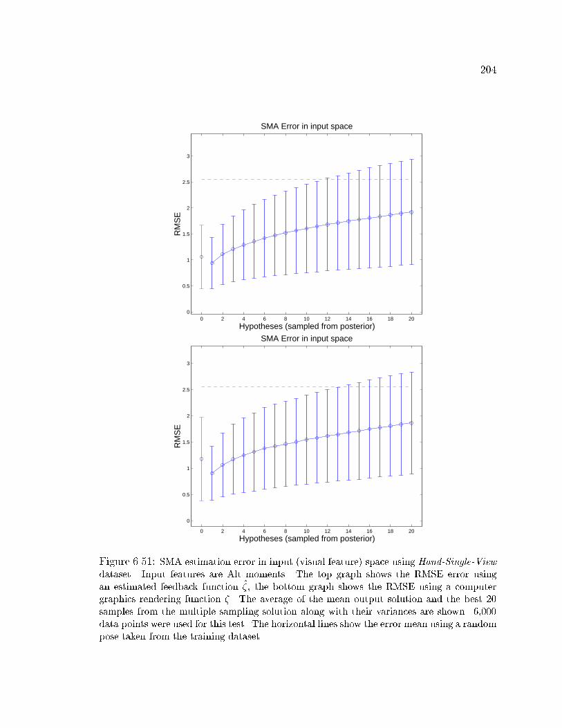
204

0 2 4 6 8 10 12 14 16 18 200

0.5

1

1.5

2

2.5

3

Hypotheses (sampled from posterior)

RM

SE

SMA Error in input space

0 2 4 6 8 10 12 14 16 18 20

0

0.5

1

1.5

2

2.5

3


RM

SE


Figure 6.51: SMA estimation error in input (visual feature) space using Hand-Single-View

dataset. Input features are Alt moments. The top graph shows the RMSE error usingan estimated feedback function �, the bottom graph shows the RMSE using a computergraphics rendering function �. The average of the mean output solution and the best 20samples from the multiple sampling solution along with their variances are shown. 6,000data points were used for this test. The horizontal lines show the error mean using a randompose taken from the training dataset.

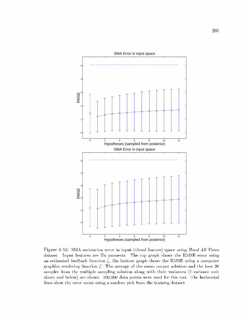
205

0 2 4 6 8 10 12

0

1

2

3

4

5


RM

SE


0 2 4 6 8 10 12

0

1

2

3

4

5


RM

SE


Figure 6.52: SMA estimation error in input (visual feature) space using Hand-All-Views

dataset. Input features are Hu moments. The top graph shows the RMSE error usingan estimated feedback function �, the bottom graph shows the RMSE using a computergraphics rendering function �. The average of the mean output solution and the best 20samples from the multiple sampling solution along with their variances (1-variance unitabove and below) are shown. 200,000 data points were used for this test. The horizontallines show the error mean using a random pick from the training dataset.

206

Figure 6.53: Example visual feature ambiguities. Each of the �ve pairs of rows contain sixexamples. The visual feature di�erence between any pair (top and bottom) is at most �vetimes lower than the average SMA error in visual feature space, however pose is considerablydi�erent in each case.

207

6.8.2 Error Sensitivity Analysis

In the previous section, we studied the SMA estimation error in input space

using the speci�c feature choice and its relation to the visual ambiguities generated

by such features. In this section we will further analyze the relation between SMA

performance and visual features by studying how sensitive the estimation error is with

respect to perturbations in the input observation (i.e., the vector of visual features).

In these experiments, we took 6,000 test examples from the Hand-Single-View

dataset and the model obtained in Sec. 6.3 to perform pose estimation. This test

set was perturbed with di�erent levels of Gaussian white noise: ! � N (!; 0; �2I),

with ! the noise random variable. The di�erent levels of noise had variance �2 =

f0:0; 0:2; 0:4; 0:6; 0:8; 1:0; 1:2; 1:4; 1:6; 1:8; 2:0g. Recall that the input observation ran-

dom variable x also has a Gaussian distribution given by x � N (x; 0; I). Hence, the

noise levels added are su�ciently high given the input random variable distribution.

The new input vector is thus de�ned by x! = x+ !.

Now, instead of using x, we will use x! with di�erent levels of variance. First, we

observe the error in the estimate given by the most likely sample using the multiple

sampling algorithm. Fig. 6.54 shows the mean and variance of the estimate error at

all the di�erent noise levels. Note that the curve is smooth and the variance increases

with the higher levels of noise as expected. Thus the algorithm seems well-behaved in

the case of the most-likely estimate. A similar graph was obtained also for the mean

output algorithm.

To further con�rm these results, Fig. 6.55 illustrates results using a similar

performance measure for the rest of the most-likely samples (20 in total). In this

graph, the di�erent curves indicate the di�erent noise levels. The bottom curve

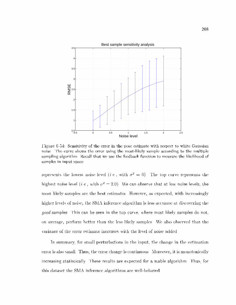
208

−0.5 0 0.5 1 1.5 2 2.50.5

1

1.5

2

2.5

3

3.5

4

4.5

Noise level

RM

SE

Best sample sensitivity analysis

Figure 6.54: Sensitivity of the error in the pose estimate with respect to white Gaussiannoise. The curve shows the error using the most-likely sample according to the multiplesampling algorithm. Recall that we use the feedback function to measure the likelihood ofsamples in input space.

represents the lowest noise level (i.e., with �2 = 0). The top curve represents the

highest noise level (i.e., with �2 = 2:0). We can observe that at low noise levels, the

most likely samples are the best estimates. However, as expected, with increasingly

higher levels of noise, the SMA inference algorithm is less accurate at discovering the

good samples. This can be seen in the top curve, where most-likely samples do not,

on average, perform better than the less likely samples. We also observed that the

variance of the error estimate increases with the level of noise added.

In summary, for small perturbations in the input, the change in the estimation

error is also small. Thus, the error change is continuous. Moreover, it is monotonically

increasing statistically. These results are expected for a stable algorithm. Thus, for

this dataset the SMA inference algorithms are well-behaved.

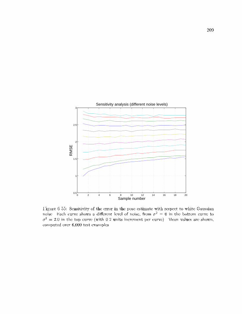
209

0 2 4 6 8 10 12 14 16 18 200.5

1

1.5

2

2.5

3

Sample number

RM

SE

Sensitivity analysis (different noise levels)

Figure 6.55: Sensitivity of the error in the pose estimate with respect to white Gaussiannoise. Each curve shows a di�erent level of noise, from �2 = 0 in the bottom curve to�2 = 2:0 in the top curve (with 0.2 units increment per curve). Mean values are shown,computed over 6,000 test examples.

Chapter 7

Conclusions and Future Work

This thesis developed a probabilistic model of non-linear supervised learning called the

Specialized Mappings Architecture (SMA). The SMA model is directed to problems

in which it is possible to obtain an inverse mapping � from outputs to inputs. The

SMA also allows for modeling domains whose underlying input-output relationship

is inherently one-to-many. In this thesis we studied applications in the area of

vision-based estimation of articulated body pose. We also formulated a multiple-

view approach that combines the probabilistic aspects of the SMA and the multi-view

geometry framework employed in vision to approach structure-from-motion problems.

We evaluated this approach in the context of 3D hand and body pose estimation.

Algorithms for learning (parameter estimation) and inference (�nding posterior

distributions over unobserved variables) in the SMA were developed. This was done

within the context of maximum likelihood (ML) estimation, maximum a posteriori

(MAP), and Bayesian inference. Two classes of algorithms for inference, one prob-

abilistic and one deterministic were presented. The SMA is related to several other

probabilistic learning models; however, the SMA is distinguished in a number of ways

211

as explained in the next section.

7.1 SMA Summary and Relation to Other Learn-

ing Models

The SMA relies on the use of alternative forms of the joint probability distribution

of the problem random variables. This distribution represents the relationship among

these random variables. Each distribution form de�nes a di�erent set of conditional

independence assumptions. The availability of the inverse map � played a major role

in deriving these alternative forms.

These alternatives are advantageous because in some cases it is more convenient

(computationally and mathematically) to choose one set of these independences over

another, as seen throughout Chapter 3. Also, the forward model assumes that the

mixing factors are independent of the input, as seen in Sec. 3.7.1. This limits the

expressibility of the architecture. In SMA the use of several independence assumptions

eliminates this independence. This issue brings up a discussion about the relation

between the SMA and another class of probabilistic models.

One may think that this independence between mixing factors and inputs is

because the forward model in the SMA is like a mixture model. There are other

models in which the mixing factors depend explicitly on the inputs. Examples of such

models include the mixture of experts (ME) [62] and the community of experts (CE)

[50] model, where this distribution (of mixing factors given the inputs) is represented

by what is called the gating networks. However, given that we have access to �, we

do not need to increase the complexity of our model by making the mixing factors

212

depend on the inputs, as in ME and CE. In other words, � provides an alternative that

avoids increasing the model complexity. We argue that estimating the parameters of

our simpler probabilistic forward model is likely to be easier than estimating the

parameters of probabilistic models such as ME or CE. Note that the use of � does

not limit the possibility of having multi-modal posteriors. In applications such as

those presented in this thesis, � incorporates information about the structure of the

problem. In general it is advantageous to exploit such information if it is available.

Learning in the SMA is based on latent variable model ideas [12, 6], where there

may be a non-linear conditional relationship p(hjy;x; �) between the inputs x and

the outputs h (given the latent variable y). Hence, this is more general than their

counterpart in the mixture of experts (ME) architecture, called the expert networks

[62]. In general, the forward model in the SMA can be seen as a (non-linear) mixture

model. Note that the form of the conditional distribution is not required to be in the

exponential family [3]. The logarithm of the form provided in Chapter 3, Case (2) is

non-linear in the parameters (in contrast with the log-linear form of the exponential

family). Of course, this comes at a cost and we pay by requiring iterative M-steps in

the Expectation Maximization algorithm used for learning.

The SMA's philosophy relies on the use of two complementary probabilistic

models: (1) a forward model that obtains observations and tries to synthesize or

imagine what generated them (e.g., outputs or body poses), and (2) a feedback

model that knows how those outputs (e.g., body poses) generate the inputs (e.g.,

body silhouettes). This philosophy is shared with the Helmholtz Machines (HM)

[33], which is perhaps one of the most closely related architectures. HM's use of

recognition and generative models is conceptually related to the SMA's utilization of

forward and feedback models. The basic philosophy of this approach can be traced

213

back to the analysis by synthesis theory of cognitive psychology [83].

There are key di�erences between the SMA and HM. In learning, the HM tries

to alternatively correct the forward and feedback models. In the SMA we do not need

to correct the feedback model based on the forward model because we know how the

observations or inputs should look given the output. This is the case in the class

of vision problems that we have investigated. This di�erence considerably reduces

the training complexity of the SMA relative to the HM, since learning in HM's is

an approximate process. As for inference, HM's concentrate on a di�erent kind of

problem, where the equivalent for inputs and outputs belong to the same space. What

we call an output in the SMA would be just an intermediate representation generated

by the HM. This intermediate representation is not part of the training set as in

our case. This representation is the body pose representation in the SMA example

applications.

Other not so closely related ideas such as MARS [42] and also the manifold

learning (MLA) approach of [22] use the divide and conquer principle. However the

probabilistic model is very di�erent. In particular, MARS cannot generate one-to-

many relationships, nor can the MLA. While in MARS and in the MLA inference uses

a deterministic version of the SMA forward model, there is no equivalent to SMA's

feedback.

We can also analyze the SMA from the more general perspective of graphical

models [90, 65]. In learning, the SMA structure is �xed in a manner that is similar

to a mixture model. In the SMA graph structure, there is a non-linear relationship

between children and parent nodes (the parents are discrete as usual). The SMA

learning involves using an approximation to maximum-likelihood (ML) estimation,

214

where the approximation comes from the use of a non-exact M-step. Partial M-step

ideas, equivalent to ours, have been justi�ed in e.g., [82]. Inference in SMA, unlike

other probabilistic models, involves using a di�erent graph structure. This graph

structure is provided by our knowledge of the feedback function. The idea is that

given an output distribution, we have an alternative way to infer inputs, in a simpler

form (very likely considerably more exact) than using belief propagation on the old

graph structure.

7.2 Applications

The use of SMA was demonstrated in a variety of applications. In this thesis

we are mainly interested in vision-based estimation of articulated body pose from

low-level visual features.

Why is SMA a good model for these vision problems? There are various reasons.

It is relatively easy render body poses or con�gurations via computer graphics. This

allows us to satisfy the requirement of a feedback function �. The relationship

between visual features and articulated body con�gurations is ambiguous. The SMA

gets around this problem by creating several simpler maps, each of them hopefully

responsible of uncovering locally non-ambiguous relationships. Hence, there is the

need for several mapping functions.

The SMA was also used in-vision based estimation of human body pose in 2D. As

can be seen in the experiments, we emphasize its use in recovering 3D articulated hand

pose from visual features. We performed experiments with a �xed global orientation

(Sec. 6.3), and unrestricted hand orientation (Sec. 6.4). As expected, the SMA

performed better in the former problem, but still could model the essentially more

215

ambiguous input-output relationship under unrestricted hand orientation.

We use a function of the object binary silhouette (moment based features) to

represent our observations. These features are less informative than the silhouette

they come from. Note (e.g., in Sec. 6.4) that even by observing the object's silhouette,

many con�gurations are still very hard to estimate by humans. Although it is an

important element of this problem, we do not address the issue of feature selection in

this thesis (see Sec. 7.2.1 for a further discussion).

Many previous tracking approaches work by trying to �nd an optimum of a non-

linear cost function at each step. This cost function in general is optimized when the

articulated model matches the image data. These optimization approaches use initial

conditions that are given by a dynamics model (e.g., [88]) or simply by the previous

pose estimate (e.g., [21]). The SMA forward model provides a prior on the body poses

that is dependent on the visual features observed at the current time step. Samples

from this prior distribution are then evaluated using a feedback distribution that in

some cases resembles the cost function used for optimization by tracking systems.

Tracking systems in general do not have a way to obtain estimates of the current

pose that use the observed visual features. Thus, tracking systems have not used the

potential reduction in the search space provided by a forward model such as that of

SMA. They mostly rely on previous estimates or manual initialization to initialize

this search. Further constraints based on observed visual features are not exploited

to reduce the complexity of the optimization problem.

This framework used by most tracking systems is also used by particle-�ltering-

based tracking [60]. However samples instead of an analytic distribution are used

to maintain the state of the system. Besides the reduction in the volume of the

216

solution space, the posterior distribution or the multiple samples provided by SMA

can be directly used to initialize or bootstrap these systems given that the SMA only

requires a single image. Note also that if a further pose re�nement is desired, the

pose estimates provided by the SMA could also be used as initial conditions for the

standard non-linear optimization step used by most tracking systems.

In summary, for articulated body pose applications, the SMA's main advantages

include:

1. Single frame pose estimation or automatic model initialization.

2. No need for visual tracking; i.e., no need to match an articulated model to the

image from frame to frame.

3. General camera viewpoint formulation without increased inference computa-

tional complexity.

4. Incorporation of a prior distribution on the pose parameters that takes into

account the observed visual features to constraint the search of the current

pose estimate.

5. Non-iterative inference algorithms.

6. Inference based on multiple-hypothesis and on approximate multi-modal prob-

ability distributions rather than on a single point estimate.

7. Fully probabilistic development and interpretation of the single and multi-

camera cases of the problem.

Notwithstanding the advantages of the SMA in pose estimation tasks, there are

217

still certain elements that introduce errors in the estimate. We believe the source of

error in these applications is mainly due to the following reasons:

1. Insu�cient/lack of data to account for given con�gurations that cannot be

accounted for by the local properties of the model.

2. Possible need for more clusters or approximating functions with more specialized

domains.

3. Di�erences in body characteristics used for training/testing.

4. Little discriminative power of the chosen image features (which reduces the

image interpretation to a seven or ten dimensional vector.

5. Di�culties in segmentation and lack of highly accurate segmentation algorithms.

The main weaknesses of the SMA in the studied applications are:

1. Segmentation is required.

2. Estimates tend to be coarse.

3. A representative training dataset is necessary.

4. There exist some camera-viewpoint limitations. For example, in the human

body pose application, the camera is required to be located on the view-sphere

equator.

However, we believe the aforementioned weaknesses are relatively mild:

1. Most state-of-the-art pose estimation systems assume that a very good local-

ization of the body is given, this is almost always done manually.

218

2. Coarse estimates could be re�ned using any standard pose-to-image alignment

algorithms; e.g., those used by most tracking systems. Note that tracking

systems will generally not be able to achieve these coarse initial estimates by

their own. This is a reason why initialization is done manually.

3. A reasonable requirement of most leaning algorithms is the availability of rep-

resentative training data.

4. Camera-view point restrictions could be approached by a similar approach than

that used by the hand pose estimation application. In this application, the full

view-sphere was sampled. However this creates a larger learning task. Hence the

requirements on amount of training data will also increase. Amount of training

data requirements usually increase exponentially with the dimensionality of the

data space.

SMA ideas can be used in di�erent tasks as well. Speech is perhaps one of

the easiest to consider. Feedback functions can be de�ned to map phonemes to an

acoustic signal. In other words, we can render a phoneme to produce voice. Speech

features (e.g., cepstral coe�cients) could then be computed from the acoustic signal.

An extension of SMA, based on multiple-view geometry was used in estimating 3D

human body pose and camera relative location. This is explained in Sec. 7.3.

An existing C++ implementation of the SMA mean output inference algorithm

runs at 5 fps in a 1 GHz Intel Pentium 3, using unoptimized code and the Multiple

Document Interface (MDI) architecture by Microsoft Visual Studio. However, only

approximately 1=10-th of this processing time involves computations related to the

SMA. The rest of the time is spent in frame grabbing, segmentation, and rendering

of the estimate.

219

7.2.1 Choice of Visual Features and the E�ect of Occlusions

One aspect that clearly a�ects the performance of the SMA is the choice of the

input space or features to be used. In this thesis, the main focus of research was not

on feature selection. This is a major research problem on its own. For interesting

reviews and related topics, see [72, 71, 29].

The extent to which the SMA performance is related to the features employed

is a di�cult question. In this thesis, we performed several experiments evaluating

performance and visual features used. In Sec. 6.8.1 we tested how well the SMA

performs if the error measure is computed in the input feature space. These tests

allowed us to partially separate the error associated with feature properties and

the error incorporated by using the SMA as a probabilistic model for the given

task. Clearly the SMA performance still depends on the type of visual features

employed, as these are used to compute the forward functions. Results indicate that

the SMA inference algorithms perform considerably better than an estimator that

picks a random solution from the training set. We also studied example non-trivial

ambiguities arising from the visual feature choice. From these experiments it was

clear that using Hu and Alt moments, very di�erent con�gurations are very close in

visual feature space.

Further tests were also performed in Sec. 6.8.2 to evaluate the sensitivity of the

estimates when inputs are perturbed with Gaussian noise. The SMA estimates were

in general well-behaved. We observed small changes in the SMA estimate when the

input vector underwent small perturbations. A smooth continuous increase in the

estimate error with an increase in the added noise was also observed for the sample

estimates computed using the multiple sampling algorithm.

220

The discriminating power of visual features is closely related to the notion of

image occlusion. One can think of occlusions as a lack of discriminating power of the

image as visual feature itself. Hence, a similar analysis applies. Two poses cannot

be discriminated given a pair of images if the poses vary only in the occluded parts.

The image can be thought of as the most informative feature space for purely vision

applications. However, this similar analysis has its limits given that occlusions have

very speci�c statistical properties.

In general, there are many di�culties associated to evaluating the robustness of

a probabilistic model in the presence of occlusions. One of the main reasons for this is

that occlusions are a structured process. In order to evaluate the model performance

with respect to occlusions, we need to count with a way to generate visual features

of occluded images that resembles the way they occur in reality. Because occlusions

are a structured process, it is usually the case that the probability distribution of

the inputs under the e�ect of occlusion cannot be modeled easily. For example, the

probability distribution of the image features given that some occlusion is present

cannot be simply modeled with an additive white Gaussian noise model. Moreover,

the characteristics of this structured process depends on the articulated object being

studied and on the speci�c application enviroment. Thus, in a general setting, we

cannot guarantee the SMA performance under occlusions. As an alternative to this

problem, local visual features could be incorporated instead of global ones.

On the other hand, this simple Gaussian noise model is usually considered an

acceptable approximation to other elements that a�ect the quality of the image (e.g.,

sensor noise and its consequences in segmentation error). In fact, this simple Gaussian

noise model was used to evaluate the sensitivity of the system with respect to small

perturbations of the input.

221

At an intuitive level, the can SMA handle occlusions or feature ambiguities in

general as follows. In the training phase, the SMA observes examples of occlusions

and tries to associate the right output (e.g., articulated body pose). This is possible

at training phase because we have access to the ground-truth. In inference, if a

similar occluded image is presented, then in theory this image is associated with the

occluded output. However, because of the occlusion, many other poses that vary in

the occluded part con�guration can be associated to this input image too. This was

observed very often throughout our experiments. The multiple sampling approach in

many cases produces samples that are valid poses for the given occluded image. Thus,

the SMA provides a form of multiple-hypothesis solution well-suited for the case of

occlusions. The likelihood of these multiple hypotheses is in uenced by the limited

information provided by the input due to occlusions. In theory two con�gurations

that vary only in occluded parts should have similar likelihood. Clearly, this is a

theoretical, best case analysis. In practice the process of modeling occlusions is

in uenced by several aspects such as the number of occluded examples, visual feature

similarity among these examples, similarity to the rest of the training examples,

output similarity, speci�c properties of the information conveyed by the visual features

about the outputs, and expressiveness of the probabilistic model.

7.3 Multiple-View SMA

The SMA can be very useful for reconstructing 3D body pose using views from

multiple uncalibrated cameras. Moreover, it is possible to recover a subset of the

camera parameters without imposing major restrictions on the scene. In Chapter 5,

we presented a novel approach for estimating 3D body pose from image sequences

222

based on SMA. We introduced the notion of \virtual cameras" and the formulation

of a probabilistic, multiple hypothesis Structure from Motion framework along with

an approximate, practical algorithm for solving it.

There are several advantages to the proposed approach. (1) It does not require

any camera calibration nor manual initialization as required by previous approaches

(e.g., [43, 21]) that use multiple-camera setups. (2) The approach exploits the

invariances of Hu moments and the concept of \virtual cameras" to obtain good 3D

structure estimates and a more tractable algorithm for solving this problem. (3) The

approach allows for the use of large baselines for better 3D reconstruction without

the nettlesome issue of feature correspondence. (4) It is relatively e�cient; it runs at

around 5 frames/sec. when computing with one frame at a time.

The approach provides approximate estimates of 3D body pose. In these con-

ditions obtaining high accuracy estimates of human body pose is a very ambitious

problem in computer vision. Our estimates can be improved by employing kinematic

and dynamic constraints, as initial experiments suggest (not included in this thesis).

Note that as in testing SMA, we have not addressed the image segmentation problem,

segmentation is assumed to be reasonably good.

Even though in theory we could use the SMA to map directly to 3D pose, the

increased dimensionality of the problem makes the SMA training problem computa-

tionally less accurate, time consuming and the amount of data required for training

increases. In our approach, we explored the idea that a more complex SMA model

might not be required for 3D estimation if camera geometry is incorporated in the

solution. In other words, we pursued the idea of combining geometric and statistical

constraints in a single framework. As was evident in the experiments, this approxi-

223

mate approach yields quite satisfactory results.

7.4 Open Questions and Future Work

Extensions to the formulation presented here include the e�cient incorporation

of dynamics in the SMA. This could be done in several ways. One way is to learn

a forward model that includes some form of time dependence on the specialized

functions, for example as in a Markov process. We then may assume a model for

p(ytjyt�1) (instead of assuming independence, as in the current SMA), while leaving

the feedback model as it is, without any dependence on previous con�gurations. The

reasons for this are explained next.

In the applications presented here, it makes sense to leave the feedback model as

it is since it is reasonably accurate at reproducing the underlying process. It is simple

to obtain visual features given a single pose, but it may not be as simple to e�ciently

and accurately represent features from multiple frames. An example probabilistic

model with these properties could be one in which the forward model is made similar

in structure to an input-output HMM. Therefore, the discrete random variable that

represents the function label may become the standard HMM state label; however,

there are other possibilities.

Another way is to learn conditional probabilities not on the function labels,

but on the outputs (poses) themselves. In other words, we may incorporate time

dependence using a distribution p(htjht�1; y;x; �). This would be a distribution on

continuous random variables. There are interesting options for articulated body pose

applications. For example one could use basic physics principles or control models

to represent these distributions. These physics or control based frameworks have

224

been explored in the computer animation and robotics; e.g., [93, 70]. However, their

incorporation into the SMA framework involves further research.

Learning and inference procedures would need to be explored in this class of mod-

els. However, given a learned model in which p(htjht�1; y;x; �) is already known, we

can in general use sampling techniques such as particle �ltering to perform inference.

This can be very easily implemented in our framework using the multiple sample

inference algorithm at each step. These samples are then assigned a probability

given the dynamics p(htjht�1; y;x; �). At each time step, all that is required is to

keep enough of these samples as necessary depending on the task and distribution

properties (deciding how many samples to use may not be an easy task in general).

A more complex extension would be to consider our initially suggested input-

output HMM-like model and let the output dynamics be in uenced also by, for

example, Newtonian physics. Maybe we can call this probabilistic model an input-

output mixed-state dynamic network. In the standard mixed-state models, inference

and learning are in general approximate.

Alternatively to these ideas, one could model the conditional dependences in the

input space across time. For example, one can derive models by taking into account

the time dependence directly in the feedback function. One idea is to build visual

features or representations that depend on time (e.g., motion energy images [17]).

Thus feedback matching would involve matching not just the output con�guration

(e.g., a pose) at an instant but matching a motion. However, the complexity of such

models needs to be studied further.

Can we discover how many specialized functions a data set may need?. In

this thesis we use a minimum description length (MDL) approach [95] to choose

225

the SMA complexity. The general structure learning problem seems to be an open

and challenging area in probabilistic machine learning [27, 20, 80, 31].

Can the multiple sampling (MS) algorithm be made more e�cient? It seems

it is possible to bias the number of samples per specialized function by looking at

the samples already generated and their match with the observed visual features x.

It makes sense to favor specialized functions that generate samples whose feedback

match is closer to the observed x. We could use the computational savings to generate

more samples that are more likely to be useful samples.

One of the main sources of inaccuracies in the SMA when applied to vision

applications is sometimes the low similarity between the object appearance used for

training (i.e., the CG model) and real objects. Clearly these appearance di�erences

in general result in di�erences in visual features too. Can this source of inaccuracy

be reduced? One idea is to possibly learn the relationship between real object

appearances and synthetic object appearances. This could be done in a supervised

fashion where the real object (e.g., a hand) may be required to perform certain

prede�ned poses before the SMA can start estimating its con�gurations.

Another interesting extension is to use an active vision inference approach to

obtain body poses using the current SMA framework. In this case, the goal is to

query image properties or feature properties actively. The queries must be such to

provide the most information according to the already discovered information about

the body pose. Given that the SMA is a probabilistic model, an information theoretic

approach seems to provide the right direction for further research in this topic.

In computer vision, one of the most important challenges is to �nd theoretically

well founded methods that are at the same time computationally feasible. Many

226

researchers have tried in numerous ways to use camera geometry to perform pose

estimation, resulting in iterative procedures that require careful choice of initial

conditions (model placement). As we have seen, we do not always have to perform

expensive iterative optimizations or to manually initialize an articulated model to

estimate articulated body pose.

The use of statistical methods in computer vision remains a fertile area for

further research. Many vision problems have a rich structure that could be used

to make statistical methods tractable. Also, statistical methods provide a formal way

to incorporate prior knowledge that is speci�c to the tasks to be performed. In this

area, there are many vision problems waiting for people to explore and new algorithms

waiting to be discovered.

Bibliography

[1] D. H. Ackley, G. E. Hinton, and T. J. Sejnowski. A learning algorithm for

Boltzmann machines. Cognitive Science, 9:147{169, 1985.

[2] F.L. Alt. Digital pattern recognition by moments. Journal of the Association

for Computing Machinery, 9(2):240-258, April 1962.

[3] S. I. Amari. Information geometry of the EM and em algorithms for neural

networks. Neural Networks, 8(9):1379{1408, 1995.

[4] Y. Bar-Shalom and T. Fortmann. Tracking and Data Association. Academic

Press, 1988.

[5] C. Barron and I. Kakadiaris. Estimating anthropometry and pose from a single

image. In Proceedings Computer Vision and Pattern Recognition, 2000.

[6] D. Bartholomew and Martin Knott. Latent Variable Models and Factor Anal-

ysis. Edward Arnold, 1999.

[7] A Baumberg and D Hogg. Learning exible models from image sequences. In

European Conference on Computer Vision, volume 1, pages 299{308, May 1994.

[8] A Baumberg and D Hogg. An adaptive eigenshape model. In D Pycock, editor,

British Machine Vision Conference, volume 1, pages 87{96, 1995.

227

228

[9] R. E. Bellman. Adaptive Control Processes. Princeton University Press, Prince-

ton, NJ, 1961.

[10] M. Bertero, T. Poggio, and V. Torre. Ill-posed problems in early vision. Pro-

ceedings of the IEEE, (76) 869-889, 1988.

[11] C. Bishop. Neural networks for pattern recognition. Oxford University Press,

1995.

[12] C. Bishop, M. Svens�en, and C. Williams. EM optimization of latent-variable

density models. In David S. Touretzky, Michael C. Mozer, and Michael E.

Hasselmo, editors, Neural Information Processing Systems, volume 8. MIT

Press, 1995.

[13] M. Black and A. Jepson. A probabilitic framework for matching temporal

trajectories: Condensation-based recognition of gestures and expressions. In

Proceedings European Conference on Computer Vision, 1998.

[14] M. Black and Y Yacoob. Tracking and recognizing rigid and non-rigid facial

motion using local parametric models of image motion. In Proceedings Inter-

national Conference on Computer Vision, 1995.

[15] A. Blake, R. Curwen, , and A. Zisserman. A framework for spatiotemporal

control in the tracking of visual contours. International Journal of Computer

Vision, 11(2):127-145, 1991.

[16] A. Blake, M. Isard, and D. Reynard. Learning to track the visual motion of

contours. Arti�cial Intelligence, 78(1{2):179{212, 1995.

229

[17] A. Bobick and J. Davis. The representation and recognition of action using

temporal templates. Pattern Analysis and Machine Intelligence, 23(3)257-267,

2001.

[18] A. F. Bobick and R. C. Bolles. The representation space paradigm of concur-

rent evolving object descriptions. IEEE Transactions on Pattern Analysis and

machine Intelligence, 14(2):146{156, February 1992.

[19] M. Brand. Shadow puppetry. In Proceedings International Conference on

Computer Vision, 1999.

[20] M. Brand. Structure learning in conditional probability models via an entropic

prior and parameter extinction. Neural Computation, 11(5):1155{1182, 1999.

[21] C. Bregler. Tracking people with twists and exponential maps. In Proceedings

Computer Vision and Pattern Recognition, 1998.

[22] C. Bregler and S. Omohundro. Nonlinear image interpolation using manifold

learning. In G. Tesauro, D. Touretzky, and T. Leen, editors, Advances in Neural

Information Processing Systems, volume 7, pages 973{980. The MIT Press,

1995.

[23] L. Breiman, J. H. Friedman, R. A. Olshen, and C. J. Stone. Classi�cation and

Regression Trees. Statistics/Probability Series. Wadsworth Publishing Com-

pany, Belmont, California, U.S.A., 1984.

[24] H. H. B�ultho� and S. Edelman. Psychophysical support for a 2-D view inter-

polation theory of object recognition. Proceedings of the National Academy of

Science, 89:60{64, 1992.

230

[25] G. Carpenter and S. Grossberg. A massively parallel architecture for a self-

organizing neural pattern recognition machine. Computer Vision, Graphics,

and Image Processing, 37(1):54{115, January 1987.

[26] T.J. Cham and J. Rehg. A multiple hypothesis approach to �gure tracking. In

Proceedings Computer Vision and Pattern Recognition, 1999.

[27] C. Chow and C. Liu. Approximating discrete probabilities with dependence

trees. IEEE Transactions on Information Theory, 14(3):462{467, 1968.

[28] P. Churchland. Neurophilosophy: Toward A Uni�ed Science of the Mind/Brain.

MIT Press, 1986.

[29] T. Cover and J. Thomas. Elements of Information Theory. Wiley Series in

Telecommunications. John Wiley & Sons, New York, NY, USA, 1991.

[30] I. Csiszar and G. Tusnady. Information geometry and alternating minimization

procedures. Statistics and Decisions, 1:205{237, 1984.

[31] P. Dagum and M. Luby. Approximating probabilistic inference in bayesian

belief networks is NP-hard. Arti�cial Intelligence, 60(1):141{153, 1993.

[32] J. Davis and A. F. Bobick. The representation and recognition of human

movement using temporal templates. In Proceedings Computer Vision and

Pattern Recognition, 1997.

[33] P. Dayan, G. Hinton, R. Neal, and Richard S. Zemel. The Helmholtz machine.

Neural Computation, 7(5):889{904, 1995.

231

[34] F. Dellaert, S. Seitz, C. Thorpe, and S. Thrun. Structure from motion without

correspondence. In Proceedings of the IEEE Conference on Computer Vision

and Pattern Recognition, pages 557{564, Los Alamitos, June 13{15 2000. IEEE.

[35] A. Dempster, N. Laird, and D. Rubin. Maximum likelihood estimation from

incomplete data. Journal of the Royal Statistical Society (B), 39(1), 1977.

[36] R. Deriche and O. Fagueras. Tracking line segments. In Proceedings European

Conference on Computer Vision, 1990.

[37] J. Deutscher, A. Blake, and I. Reid. Articulated body motion capture by

annealed particle �ltering. In Proceedings Computer Vision and Pattern Recog-

nition, 2000.

[38] R. Duda, P. Hart, and D. Stork. Pattern Classi�cation. John Wiley and Sons,

New York, 2001.

[39] R. Dutter and P. Huber. Numerical methods for the non-linear robust regression

problem. Journal of Statistical Computer Simulation, 13(2):79-113, 1981.

[40] S. Edelman and T. Poggio. Models of object recognition. Current Opinion in

Neurobiology, 1, 270-273, 1991.

[41] O. Faugeras. Three-Dimensional Computer Vision. MIT Press, 1993.

[42] J.H. Friedman. Multivatiate adaptive regression splines. The Annals of Statis-

tics, 19,1-141, 1991.

[43] D. Gavrila and L. Davis. Tracking of humans in action: a 3-d model-based

approac. In Proceedings ARPA Image Understanding Workshop, Palm Springs,

1996.

232

[44] D. Gavrila and V. Philomin. Real-time object detection for \smart\ vehicles. In

Proceedings International Conference on Computer Vision, pages 87{93, 1999.

[45] F. Girosi, M. Jones, and T. Poggio. Regularization theory and neural network

architectures. Neural Computation, (7) 219-269, 1995.

[46] L. Goncalves, E.D. Bernardo, E. Ursella, and P. Perona. Monocular tracking of

the human arm in 3d. In ICCV95, pages 764{770, 1995.

[47] T. Heap and D. Hogg. Towards 3d hand tracking using a deformable model. In

Proceedings International Conference on Automatic Face and Gesture Recogni-

tion, pages 140{145, 1996.

[48] G. Hinton, P. Dayan, B. Frey, and Radford M. Neal. The wake-sleep algorithm

for unsupervised neural networks. Science, 268:1158{1161, 1995.

[49] G. Hinton, P. Dayan, and M. Revow. Modeling the manifolds of images of

handwritten digits. IEEE Transactions on Neural Networks, 8 65-74, 1997.

[50] G. Hinton, B. Sallans, and Z. Ghahramani. A hierarchical community of experts.

Learning in Graphical Models, M. Jordan (editor), 1998.

[51] G. Hinton and R. Zemel. Autoencoders, minimum description length and

Helmholtz free energy. In Jack D. Cowan, Gerald Tesauro, and Joshua Al-

spector, editors, Advances in Neural Information Processing Systems, volume 6,

pages 3{10. Morgan Kaufmann Publishers, Inc., 1994.

[52] D. Hogg. Model-based vision: A paradigm to see a walking person. Image and

Vision Computing, 1(1), 1983.

233

[53] D. Hogg. Interpreting Images of a Known Moving Object. PhD thesis, University

of Sussex, 1984.

[54] N. Howe, M. Leventon, and B. Freeman. Bayesian reconstruction of 3d human

motion from single-camera video. In Neural Information Processing Systems,

1999.

[55] M. K. Hu. Visual pattern recognition by moment invariants. IRE Transactions

Information Theory, IT(8), 1962.

[56] D. Huttenlocher, P. Noh, J. Jae, and J. Willian. Tracking non-rigid objects in

complex scenes. In Proceedings International Conference on Computer Vision,

1994.

[57] L. Davis I. Haritaoglu, D. Harwood. W4s: A realtime system for detecting

and tracking people in 2.5d. In Proceedings European Conference on Computer

Vision, 1998.

[58] L. Davis I. Haritaouglu, D. Harwood. Ghost: A human body part labeling

system using silhouettes. In International Conference on Pattern Recognition,

1998.

[59] S. Intille and A. F. Bobick. Real time close world tracking. In Proceedings


[60] M. Isard and A. Blake. Contour tracking by stochastic propagation of condi-

tional density. In Proceedings European Conference on Computer Vision, 1996.

234

[61] M. Isard and A. Blake. Icondensation: Unifying low-level and high-level tracking

in a stochastic framework. In Proceedings European Conference on Computer

Vision, 1998.

[62] R. Jacobs, M. Jordan, S. Nowlan, and G. E. Hinton. Adaptive mixtures of local

experts. Neural Computation, 3(1):79{87, 1991.

[63] G. Johansson. Visual perception of biological motion and a model for its

analysis. Perception and Psychophysics, 14(2): 210-211, 1973.

[64] I. T. Jolli�e. Principal Component Analysis. Series in Statistics. Springer-

Verlag, 1986.

[65] M. Jordan. Learning in graphical models. Kluwer Academic, The Netherlands,

1999.

[66] M. Jordan and R. Jacobs. Hierarchical mixtures of experts and the EM algo-

rithm. Neural Computation, 6, 181-214, 1994.

[67] S. Ju, M. Black, and Y. Yacoob. Cardboard people: A parameterized model of

articulated image motion. In Proceedings Gesture Recognition, 1996.

[68] I. Kakadiaris. Shape and motion estimation of complex multi-part objects:

Application to human body tracking. Thesis, University of Pennsylvania, De-

partment of Computer Science, 1996.

[69] I. Kakadiaris, D. Metaxas, and R. Bajcsy. Active part-decomposition, shape

and motion estimation of articulated objects: A physics-based approach. In


235

[70] M. Kalisiak and M. van de Panne. A grasp-based motion planning algorithm for

character animation. In N. Thalman-Magnenat, D. Thalman, and B. Arnaldi,

editors, Proceedings of the Eurographics Workshop on Computer Animation and

Simulation (EGCAS-00), pages 43{58, Wien-NY, August 21{22 2000. Springer.

[71] R. Kohavi. Wrappers for performance enhancements and oblivious decision

graphs. Thesis CS-TR-95-1560, Stanford University, Department of Computer

Science, September 1995.

[72] Daphne Koller and Mehran Sahami. Toward optimal feature selection. In

Proceedings of ICML-96, 13th International Conference on Machine Learning,

pages 284{292, Bari, IT, 1996.

[73] N. Kolmogorov and S.V. Fomine. Elements of the Theory of Functions and

Functional Analysis. Dover, 1975.

[74] A. Lapedes and R Farber. How neural nets work. Neural Information Processing

Systems, 442-456, 1988.

[75] H. Lee and Z. Chen. Determination of 3d human body posture from a single-

view. Image Understanding, 30:148{168, 1985.

[76] M. Leventon and W. Freeman. Bayesian estimation of 3-d human motion.

Technical Report TR 98-06, Mitsubishi Electric Research Labs, 1998.

[77] R. Liang and M. Ouhyoung. A real-time continuous gesture recognition system

for sign language. In Proceedings International Conference on Automatic Face

and Gesture Recognition, pages 558{567, 1998.

[78] M. Lo�eve. Probability Theory. Van Nostrand, Princeton, New Jersey, 1955.

236

[79] D. Mackay. Introduction to monte carlo methods. Learning in Graphical Models,

M. Jordan (editor), 1998.

[80] M. Meila. Learning with mixtures of trees. PhD thesis, Massachusetts Institute

of Technology, 1999.

[81] D. Morris and J. Rehg. Singularity analysis for articulated object tracking. In


[82] R. Neal and G. Hinton. A view of the em algorithm that justi�es incremental,

sparse, and other variants. Learning in Graphical Models, M. Jordan (editor),

1998.

[83] U. Neisser. Cognitive Psychology. New York, Appleton-Century-Crofts, 1967.

[84] B. Olshausen, C. Anderson, and D. C. Van Essen. A neurobiological model of

visual attention and invariant pattern recognition based on dynamic routing of

information. The Journal of Neuroscience, 13(11):4700{4719, November 1993.

[85] D. Ormoneit, H. Sidenbladh, M. Black, and T. Hastie. Learning and tracking

cyclic human motion. In Neural Information Processing Systems 13, 2001.

[86] J. O'Rourke and N. Badler. Model-based image analysis of human motion using

constraint propagation. IEEE Transactions on PAMI, Nov. 1980, PAMI-2(6),

1980.

[87] V. Pavlovi�c. Dymanic Bayesian Networks for Information Fusion with Applica-

tions to Human Computer Interfaces. PhD thesis, University of Illinois, 1999.

[88] V. Pavlovi�c, J. Rehg, T. Cham, and K. Murphy. A dynamic bayesian network

approach to �gure tracking using learned dynamic models. In Proceedings

237

International Conference on Computer Vision, volume I, pages 94{101, Los

Alamitos, CA, September 20{27 1999. IEEE.

[89] V. Pavlovi�c, J. Rehg, and J. MacCormick. Learning switching linear models of

human motion. In Neural Information Processing Systems 13, 2001.

[90] J. Pearl. Probabilistic Reasoning in Intelligent Systems. Morgan-Kaufman,

1988.

[91] A. Pentland and B. Horowitz. Recovery of non-rigid motion and structure.

PAMI, 13(7):730{742, 1991.

[92] R. Polana and R. Nelson. Low level recognition of human motion. In Proceedings

IEEE Workshop on Nonrigid and Articulate Motion, 1994.

[93] M. Raibert. Legged robots. Communications of the ACM, June 1986, 9(6),

1986.

[94] J. M. Rehg and T. Kanade. Model-based tracking of self-occluding articulated

objects. In Proceedings International Conference on Computer Vision, 1995.

[95] J. Rissanen. Stochastic complexity and modeling. Annals of Statistics, 14,1080-

1100, 1986.

[96] K. Rohr. Incremental recognition of pedestrians from image sequences. In


[97] K. Rohr. Towards model-based recognition of human movements in image

sequences. Image Understanding, 59(1):94-115, 1994.

238

[98] R. Rosales. Improved tracking of multiple humans with trajectory prediction,

oclussion modeling, and motion analysis. Master's thesis, Boston University,

2000.

[99] R. Rosales, V. Athitsos, and S. Sclaro�. 3d hand pose estimation using special-

ized mappings. In Proceedings International Conference on Computer Vision,

2001.

[100] R. Rosales and S. Sclaro�. Improved tracking of multiple humans with tra-

jectory prediction and occlusion modeling. In IEEE CVPR Workshop on the

Interpretation of Visual Motion, 1998.

[101] R. Rosales and S. Sclaro�. 3d trajectory recovery for tracking multiple objects

and trajectory guided recognition of actions. In Proceedings Computer Vision

and Pattern Recognition, 1999.

[102] R. Rosales and S. Sclaro�. Specialized mappings and the estimation of body

pose from a single image. In IEEE Human Motion Workshop. Austin, TX,

2000.

[103] R. Rosales and S. Sclaro�. Learning body pose using specialized maps. In

Neural Information Processing Systems 14, 2001.

[104] R. Rosales and Stan Sclaro�. Inferring body pose without tracking body parts.

In Proceedings Computer Vision and Pattern Recognition, 2000.

[105] R. Rosales, M. Siddiqui, J. Alon, and S. Sclaro�. Estimating 3d body pose

using uncalibrated cameras. In Proceedings Computer Vision and Pattern

Recognition, 2001.

239

[106] J. Shi and C. Tomasi. Good features to track. Technical Report TR93-1399,

Cornell University, Computer Science Department, November 1993.

[107] N. Shimada, Y. Shirai, Y. Kuno, and J. Miura. Hand gesture estimation and

model re�nement using monocular camera - ambiguity limitation by inequality

constraints. In Proceedings International Conference on Automatic Face and

Gesture Recognition, pages 268{273, 1998.

[108] L. Sigal, S. Sclaro�, and V. Athitsos. Estimation and prediction of evolving color

distributions for skin segmentation under varying illumination. In Proceedings


[109] Y. Song, Xiaoling Feng, and P. Perona. Towards detection of human motion.

In Proceedings Computer Vision and Pattern Recognition, 2000.

[110] N. Srebro. Maximum likelihood bounded tree-width markov networks. In

Proceedings Uncertainty in Arti�cial Intelligence, 2001.

[111] M. Tarr. Rotating objects to recognize them: A case study on the role of

viewpoint dependency in the recognition of three-dimensional objects. Psy-

chonometry Bulleting, 2:55{82, 1995.

[112] C. J. Taylor. Reconstruction of articulated objects from point correspondences

in a single uncalibrated image. In Proceedings Computer Vision and Pattern

Recognition, 2000.

[113] C. Tomasi and T. Kanade. Shape and motion from image streams: a fac-

torization method: Full report on the orthographic case. Technical Report

TR92-1270, Cornell University, Computer Science Department, March 1992.

240

[114] K. Toyama and A. Blake. Probabilistic tracking in a metric space. In Proceedings

International Conference on Computer Vision, 2001.

[115] T. Vetter, A. Hurlbert, and T. Poggio. View-based models of 3d object recog-

nition: Invariance to imaging transformations. Cerebral Cortex, (5)3,261-269,

1995.

[116] Virtual Technologies, Inc., Palo Alto, CA. VirtualHand Software Library Ref-

erence Manual, August 1998.

[117] C. Vogler and D. Metaxas. Toward scalability in asl recognition: Breaking down

signs into phonemes. In Proceedings of the Gesture Workshop, 1999.

[118] S. Wachter and H.-H. Nagel. Tracking of persons in monocular image sequences.

In Proceedings IEEE Nonrigid and Articulated Motion Workshop, 1997.

[119] C. Wren, A. Azarbayejani, T. Darrell, and A. Pentland. P�nder: Real time

tracking of the human body. PAMI, 19(7), 1997.

[120] M. Yamamoto and K. Koshikawa. Human motion analysis based on a robot

arm model. In Proceedings Computer Vision and Pattern Recognition, pages

664{665, 1991.

[121] M. Yang and N. Ahuja. Recognizing hand gesture using motion trajectories. In

Proceedings Computer Vision and Pattern Recognition, volume 1, pages 466{

472, 1999.

[122] Y.Wu and T. Huang. A co-inference approach to robust visual tracking. In

Proceedings International Conference on Computer Vision, 2001.

SPECIALIZED MAPPINGS ARCHITECTURE WITH ...

Documents

Transcript of SPECIALIZED MAPPINGS ARCHITECTURE WITH ...