Memory optimization strategies for linear mappings and ...
237
HAL Id: tel-01746222 https://tel.archives-ouvertes.fr/tel-01746222v3 Submitted on 24 Apr 2012 HAL is a multi-disciplinary open access archive for the deposit and dissemination of sci- entific research documents, whether they are pub- lished or not. The documents may come from teaching and research institutions in France or abroad, or from public or private research centers. L’archive ouverte pluridisciplinaire HAL, est destinée au dépôt et à la diffusion de documents scientifiques de niveau recherche, publiés ou non, émanant des établissements d’enseignement et de recherche français ou étrangers, des laboratoires publics ou privés. Memory optimization strategies for linear mappings and indexation-based shared documents Mumtaz Ahmad To cite this version: Mumtaz Ahmad. Memory optimization strategies for linear mappings and indexation-based shared documents. Discrete Mathematics [cs.DM]. Université Henri Poincaré - Nancy 1, 2011. English. tel-01746222v3
-
Upload
khangminh22 -
Category
Documents
-
view
3 -
download
0
Transcript of Memory optimization strategies for linear mappings and ...

HAL Id: tel-01746222https://tel.archives-ouvertes.fr/tel-01746222v3
Submitted on 24 Apr 2012
HAL is a multi-disciplinary open accessarchive for the deposit and dissemination of sci-entific research documents, whether they are pub-lished or not. The documents may come fromteaching and research institutions in France orabroad, or from public or private research centers.
L’archive ouverte pluridisciplinaire HAL, estdestinée au dépôt et à la diffusion de documentsscientifiques de niveau recherche, publiés ou non,émanant des établissements d’enseignement et derecherche français ou étrangers, des laboratoirespublics ou privés.
Memory optimization strategies for linear mappings andindexation-based shared documents
Mumtaz Ahmad
To cite this version:Mumtaz Ahmad. Memory optimization strategies for linear mappings and indexation-based shareddocuments. Discrete Mathematics [cs.DM]. Université Henri Poincaré - Nancy 1, 2011. English.�tel-01746222v3�

Université Henri Poincaré
Departement de formation doctorale en informatique Ecole doctorale IAEM Lorraine
UFR STMIA
Memory optimization strategies forlinear mappings and indexation-based
shared documents
THESE
presentee et soutenue publiquement le November 14, 2011
pour l’obtention du
Doctorat de l’universite Henri Poincare – Nancy 1
(specialite informatique)
par
M. Mumtaz AHMAD
Composition du jury
Rapporteurs : Denis LUGIEZ Professeur, Universite de Provence, Marseille, FR
Miki (Nicolas) HERMANN CR (CNRS), Ecole Polytechnique, Paris, FR
Examinateurs : Eugeniusz Adam CICHON Professeur, Universite Henri Poincare, Nancy, FR
Siva ANANTHARAMAN Professeur, Universite d’Orleans, Orleans, FR
Lhouari NOURINE Professeur, Universite Blaise Pascal, Aubiere, FR
Nacer BOUDJLIDA Professeur, Universite Henri Poincare, Nancy, FR
Serge BURCKEL Maıtre de conferences, Universite de la Reunion, FR
Abdessamad IMINE Maıtre de conferences, Universite Nancy 2, FR
Laboratoire Lorrain de Recherche en Informatique et ses Applications — UMR 7503


Acknowledgments
I would like to thank to everyone who helped me with this thesis:
to ones who know they did (my special thanks to CRT)
and to ones who do not know.
i

ii

I dedicate this thesisto my
benefactors
iii

iv

INRIA Research Laboratories
INRIA (Institut national de recherche en informatique et en automatique) is aFrench national research institution focusing mainly on applied mathematics,computer science and control theory. It was created in August 25, 1967 atRocquencourt near Paris, part of Plan Calcul project. Its first site was thehistorical premises of SHAPE (central command of NATO military forces).INRIA is a public scientific and technical research establishment (EPST) underthe double supervision of the French ministry of national education, advancedinstruction and research, and ministry of economy, finance and industry.
Firmly rooted in local industrial and academic ecosystems, INRIA is pur-suing an increasing involvement in the European Research Area. With a res-olutely international outlook, it is contributing to the global profile of com-putational sciences. Convinced that the future of our societies lies in digitaltechnology, INRIA is tackling research subjects crucial to the social issues oftoday. More than half of INRIA project-teams are involved in the EuropeanFramework Programs for Research and Development (FPRD).
The European Commission ranks INRIA in the top ten contributing organi-zations. After CERN (European Organization for Nuclear Research), Genève,Switzerland, INRIA is at top of all European research centres (see for reference,April 2012, (http://research.webometrics.info)). INRIA is strengthening anddiversifying its partnerships with other scientific disciplines and the businessworld (strategic partnerships), in France and in Europe, in the USA and withemerging countries (China, India, South America, Africa).
INRIA is organized around five fields of research
1. Applied Mathematics, Computation and Simulation
2. Algorithmic, Programming, Software and Architecture
3. Networks, Systems and Services, Distributed Computing
4. Perception, Cognition, Interaction
v

INRIA Research Laboratories
5. Computational Sciences for Biology, Medicine and the Environment
Figure 1: INRIA-Nancy Research center
INRIA employs 3800 people including 1300 researchers, 1000 Ph.D. studentsand 500 post-doctorates. INRIA has 8 research centers in different cities (Bor-deaux, Grenoble, Lille, Rennes, Saclay, Rocquencourt-Paris, Nancy and SophiaAntipolis) of France.
Figure 2: INRIA-Nancy Research center
INRIA Research center Nancy, is hosted at LORIA, Lorraine laboratory ofresearch. LORIA is a high level security research laboratory of Lorraine regionof France and is mixed unite of research (UMR 7503) hosting INRIA, and is
vi

associated with University of Henri Poincaré (Université de Lorraine, since2012), CNRS (Centre National de la Recherche Scientifique). INPL (InstitutNational Polytechnique de Lorraine), Université Nancy 2 and is a member ofthe Charles Hermite Federation. Currently, 27 research teams and 500 research
Figure 3: INRIA-Nancy Research center
scientists work at the LORIA research center.
Figure 4: INRIA-Nancy Research center
vii

INRIA Research Laboratories
viii

Contents
General Introduction xix
Chapter 1Introduction 1
1.1 Sequential Break-down of Operations . . . . . . . . . . . . . 11.1.1 Optimization Context . . . . . . . . . . . . . . . . . 3
1.2 Decentralized Collaborative Editing . . . . . . . . . . . . . . 41.2.1 Collaborative Editing Context . . . . . . . . . . . . . 61.2.2 Approach by Weiss et al. . . . . . . . . . . . . . . . . 71.2.3 Approach by Preguiça et al. . . . . . . . . . . . . . . 12
1.3 Contributions . . . . . . . . . . . . . . . . . . . . . . . . . . 151.4 Overview and structure . . . . . . . . . . . . . . . . . . . . 16
Part I Sequential Break-Down of Operations 19
ix

Contents
Chapter 2Compiler, Processor Optimization (A quick overview)
2.1 Compilers . . . . . . . . . . . . . . . . . . . . . . . . . . . . 222.1.1 Compiler Optimization . . . . . . . . . . . . . . . . . 23
2.2 Processors . . . . . . . . . . . . . . . . . . . . . . . . . . . . 242.2.1 Processor Optimization . . . . . . . . . . . . . . . . 26
2.3 Applications . . . . . . . . . . . . . . . . . . . . . . . . . . . 262.4 Motivations and Objectives . . . . . . . . . . . . . . . . . . 27
Chapter 3In Situ Design of Computation for Linear Mappings overFields
3.1 Sequential Computation . . . . . . . . . . . . . . . . . . . . 303.1.1 In Situ Design of Computation (IDC) . . . . . . . . 31
3.2 Existence of IDC for Linear Mappings over Fields . . . . . . 333.2.1 Case-I . . . . . . . . . . . . . . . . . . . . . . . . . . 353.2.2 Case-II . . . . . . . . . . . . . . . . . . . . . . . . . 383.2.3 Computing Inverse Mapping . . . . . . . . . . . . . . 393.2.4 Case-III . . . . . . . . . . . . . . . . . . . . . . . . . 393.2.5 Possibility of Computing Inverse Mappings . . . . . . 41
3.3 Novel approach using Bézout’s Identity . . . . . . . . . . . . 413.3.1 Case-I . . . . . . . . . . . . . . . . . . . . . . . . . . 433.3.2 Case-II . . . . . . . . . . . . . . . . . . . . . . . . . 433.3.3 Computing Inverse Mappings: . . . . . . . . . . . . . 45
Chapter 4In Situ Design of Computation for Linear Mappings overRings
4.1 Existence of IDC for Linear Mappings over Rings . . . . . . 484.1.1 Assignment Matrices . . . . . . . . . . . . . . . . . . 48
4.2 Explanation and Construction . . . . . . . . . . . . . . . . . 504.2.1 Case-I . . . . . . . . . . . . . . . . . . . . . . . . . . 504.2.2 Case-II . . . . . . . . . . . . . . . . . . . . . . . . . 52
4.3 Computing Inverse Mappings . . . . . . . . . . . . . . . . . 54
x

4.3.1 Possibility of computing Inverse mappings . . . . . . 55
Chapter 5In Situ Design of Computation for Linear Mappings overIntegers
5.1 Existence of IDC for Linear Mappings over Integers . . . . . 585.1.1 Modifications: . . . . . . . . . . . . . . . . . . . . . . 605.1.2 Explanation and construction of assignments: . . . . 60
5.2 Investigating bounds for the number of assignments: . . . . 685.2.1 An approach based on Fibonacci numbers . . . . . . 715.2.2 Identity (coefficient linkage): . . . . . . . . . . . . . . 74
Chapter 6In Situ Design of Computation for Boolean Mappings
6.1 Boolean Mappings . . . . . . . . . . . . . . . . . . . . . . . 786.2 Computing Bijective Boolean Mappings . . . . . . . . . . . 79
6.2.1 Explanation . . . . . . . . . . . . . . . . . . . . . . . 816.2.2 Linearity Property . . . . . . . . . . . . . . . . . . . 83
6.3 Computing General Boolean Mappings . . . . . . . . . . . . 846.3.1 Simple Mappings . . . . . . . . . . . . . . . . . . . . 856.3.2 Decomposing general boolean mappings . . . . . . . 86
6.4 IDC for Polynomials over GF(2) . . . . . . . . . . . . . . . . 916.4.1 A First Tool . . . . . . . . . . . . . . . . . . . . . . . 926.4.2 Explanation and Construction . . . . . . . . . . . . . 95
Part II Decentralized Collaborative Editing 101
Chapter 7Collaborative Editing System
7.1 Introduction . . . . . . . . . . . . . . . . . . . . . . . . . . . 103
xi

Contents
7.1.1 A Collaborative Editing Scenario . . . . . . . . . . . 1047.1.2 Pessimistic Concurrency Control . . . . . . . . . . . 1057.1.3 Optimistic Concurrency Control . . . . . . . . . . . . 1067.1.4 Group Communication . . . . . . . . . . . . . . . . . 1067.1.5 Centralized collaborative editing systems . . . . . . . 1067.1.6 Decentralized collaborative editing systems . . . . . . 108
7.2 DCE Model . . . . . . . . . . . . . . . . . . . . . . . . . . . 1117.2.1 Framework Description . . . . . . . . . . . . . . . . . 1137.2.2 Editing a Document . . . . . . . . . . . . . . . . . . 1147.2.3 Modifying a Document . . . . . . . . . . . . . . . . . 1157.2.4 Mapping between elements and Identifiers . . . . . . 115
Chapter 8Generating Identifiers
8.1 Creating Unique Identifiers . . . . . . . . . . . . . . . . . . 1188.1.1 Precision Control Technique . . . . . . . . . . . . . . 1188.1.2 Generating user/site identifiers (USIDs) . . . . . . . 1208.1.3 The Procedure . . . . . . . . . . . . . . . . . . . . . 1218.1.4 Explanation . . . . . . . . . . . . . . . . . . . . . . . 1248.1.5 Uniqueness of line/character identifiers (LCIDs) . . . 1258.1.6 Verifying uniqueness . . . . . . . . . . . . . . . . . . 127
8.2 Computing cardinality . . . . . . . . . . . . . . . . . . . . . 1278.2.1 Local cardinality . . . . . . . . . . . . . . . . . . . . 1288.2.2 Global cardinality . . . . . . . . . . . . . . . . . . . 128
Chapter 9Properties and Analysis
9.1 Properties . . . . . . . . . . . . . . . . . . . . . . . . . . . . 1329.1.1 Bijection property . . . . . . . . . . . . . . . . . . . 1329.1.2 Closure properties . . . . . . . . . . . . . . . . . . . 133
9.2 Analysis . . . . . . . . . . . . . . . . . . . . . . . . . . . . . 1379.2.1 Comparison under Rounding Conditions . . . . . . . 1379.2.2 Comparison without Rounding Conditions . . . . . . 1389.2.3 Comparison under floating-point arithmetics . . . . . 1389.2.4 Effect of different rounding conditions . . . . . . . . 139
xii
9.2.5 Assuring order preservation . . . . . . . . . . . . . . 147
Chapter 10Exchange of points and variation in global cardinality
10.1 Delayed exchange of points . . . . . . . . . . . . . . . . . . 15010.1.1 Random Participation . . . . . . . . . . . . . . . . . 15010.1.2 Ordered Participation . . . . . . . . . . . . . . . . . 154
10.2 Real time exchange of points . . . . . . . . . . . . . . . . . 15810.2.1 Computing Instant Global Cardinality . . . . . . . . 15910.2.2 Comparison . . . . . . . . . . . . . . . . . . . . . . . 160
Part III Evaluation 161
Chapter 11Further work and conclusion
11.1 Further work . . . . . . . . . . . . . . . . . . . . . . . . . . 16311.1.1 Dispersion . . . . . . . . . . . . . . . . . . . . . . . . 16311.1.2 One of the possible situations . . . . . . . . . . . . . 16511.1.3 Case-1 . . . . . . . . . . . . . . . . . . . . . . . . . . 16511.1.4 Case-2 . . . . . . . . . . . . . . . . . . . . . . . . . . 16511.1.5 Modifications and extensions of IDC . . . . . . . . . 166
11.2 Conclusion . . . . . . . . . . . . . . . . . . . . . . . . . . . 167
Appendixes
Appendix AExperimentation Frame Work
A.1 Exchange of points (an experiment with 900 Users) . . . . . 169A.1.1 Delayed exchange of points with random participation169A.1.2 Delayed exchange of points with ordered participation180
xiii

Contents
Appendix BImplementation Framework
B.1 Algorithm . . . . . . . . . . . . . . . . . . . . . . . . . . . . 191
Glossary 195
Index 197
Bibliography 199
xiv

List of Figures
1 INRIA-Nancy Research center . . . . . . . . . . . . . . . . . . . vi2 INRIA-Nancy Research center . . . . . . . . . . . . . . . . . . . vi3 INRIA-Nancy Research center . . . . . . . . . . . . . . . . . . . vii4 INRIA-Nancy Research center . . . . . . . . . . . . . . . . . . . vii
1.1 Identifiers exchange scenario . . . . . . . . . . . . . . . . . . . . 91.2 Redundancy of Identifiers . . . . . . . . . . . . . . . . . . . . . 111.3 Generating POSID . . . . . . . . . . . . . . . . . . . . . . . . . 14
2.1 Compiler Interaction . . . . . . . . . . . . . . . . . . . . . . . . 222.2 Microprocessor . . . . . . . . . . . . . . . . . . . . . . . . . . . 252.3 IntelrCoreTM i7 processor . . . . . . . . . . . . . . . . . . . . . 27
3.1 Sequential break-down of operations . . . . . . . . . . . . . . . . 313.2 Interpreting linear assignment . . . . . . . . . . . . . . . . . . . 323.3 Reference value of linear assignment . . . . . . . . . . . . . . . . 33
6.1 Interpretation of ”A First Tool” . . . . . . . . . . . . . . . . . . 95
7.1 A collaborative editing scenario . . . . . . . . . . . . . . . . . . 1047.2 An example of collaborative editing . . . . . . . . . . . . . . . 1057.3 Wrong Integration . . . . . . . . . . . . . . . . . . . . . . . . . 1097.4 Correct Integration . . . . . . . . . . . . . . . . . . . . . . . . . 1107.5 Model . . . . . . . . . . . . . . . . . . . . . . . . . . . . . . . . 1117.6 Inserting single character . . . . . . . . . . . . . . . . . . . . . . 112
8.1 Precision control principle . . . . . . . . . . . . . . . . . . . . . 1198.2 Position of an identifier in the interval . . . . . . . . . . . . . . 1228.3 Insertion of points by single user . . . . . . . . . . . . . . . . . . 124
9.1 A scenario of three users . . . . . . . . . . . . . . . . . . . . . . 148
10.1 Users participation . . . . . . . . . . . . . . . . . . . . . . . . . 15310.2 Number of users vs global cardinality . . . . . . . . . . . . . . . 153
xv

List of Figures
10.3 Users participation . . . . . . . . . . . . . . . . . . . . . . . . . 15710.4 Number of users vs global cardinality . . . . . . . . . . . . . . . 157
11.1 General diagram for dispersion problem . . . . . . . . . . . . . . 164
A.1 A view of users participation . . . . . . . . . . . . . . . . . . . . 179A.2 Updates in global cardinality . . . . . . . . . . . . . . . . . . . . 180A.3 Updates in global cardinality . . . . . . . . . . . . . . . . . . . . 190A.4 A users participation curve . . . . . . . . . . . . . . . . . . . . . 190
xvi

List of Algorithms
1 Function (How to generate new Line Identifier) . . . . . . . . . . 82 Function (How to Construct new ID) . . . . . . . . . . . . . . . . 83 Function (Generating POSID) . . . . . . . . . . . . . . . . . . . 13
4 Boolean Compatible Decomposition . . . . . . . . . . . . . . . . 90
5 Function (Round a value) . . . . . . . . . . . . . . . . . . . . . . 1196 How to generate USIDs . . . . . . . . . . . . . . . . . . . . . . . 1207 Function middle(How to compute new identifier) . . . . . . . . . 1228 How to generate a set of LCIDs . . . . . . . . . . . . . . . . . . . 1239 . . . . . . . . . . . . . . . . . . . . . . . . . . . . . . . . . . . . 127
10 How to exchange points in Batch Mode . . . . . . . . . . . . . . 15111 Batch Mode Ordered Participation . . . . . . . . . . . . . . . . . 155
xvii

LIST OF ALGORITHMS
xviii

General Introduction
xix


« Mathematical discoveries, small or great arenever born of spontaneous generation. They alwayspresuppose a soil seeded with preliminary knowledgeand well prepared by labour, both conscious and sub-conscious ».
Henri Poincaré (1854 - 1912)
xxi

xxii

Chapter 1Introduction
Contents1.1 Sequential Break-down of Operations . . . . . 1
1.1.1 Optimization Context . . . . . . . . . . . . . . . 3
1.2 Decentralized Collaborative Editing . . . . . . 41.2.1 Collaborative Editing Context . . . . . . . . . . 6
1.2.2 Approach by Weiss et al. . . . . . . . . . . . . . 7
1.2.3 Approach by Preguiça et al. . . . . . . . . . . . 12
1.3 Contributions . . . . . . . . . . . . . . . . . . . 151.4 Overview and structure . . . . . . . . . . . . . 16
1.1 Sequential Break-down of OperationsThe rapid growth in the use of modern computer technology has increased thedemand for higher performance in all areas of computing. This demand forever greater performance led to growth in hardware performance and archi-tecture evolution that resulted in a stress on compiler technology and researchcommunities. Since a high-performance microprocessor is at the heart of everygeneral-purpose computer, from servers, to desktop and laptop PCs, to cell-phone platforms such as the iPhone. Therefore, increasing the performanceis considered to be a permanent challenge in computer science. Since a 32bit processor performs operations on 32 bits. Therefore, any transformationof data structure required decomposition in successive operations on 32 bits.A well-known technique used in exchanging contents of registers is to makecopies of the initial data. However, it is possible that, dealing with large datastructure, such technique may generates some memory errors and slow downthe performance of computations. Moreover, to perform such operations, anumber of registers in a micro-processor, through compiler or an electronic
1

Chapter 1. Introduction
circuit, are involved, and to complete such operations, it requires to makecopies of contents of registers in the cache memory or in RAM or alternatively,it requires signal duplication in the chip design. In both cases, it causes, a lossof speed or an extra power consumption [BGT09].
O ”One of the possible approaches to this issue is the sequentialbreak down of operations in such a way that it does not re-
quire any extra variable other than the variables available as input.Ultimately, it results in requiring no extra writing memory, there-fore, such computations find applications in program optimizationand chip design”.
Moreover, such "In Situ Design of Computation (IDC)" enables to improveperformance of calculations and to calculate an operation related to n registersby a sequence of assignments using only these n registers [SCT].
Such in situ computation are applied in computing mappings from a set Snto itself by performing a sequence of operations (assignments). Therefore, themapping E : Sn −→ Sn can be interpreted as the parallel computation of nassignment mappings of the form Sn −→ S. These mappings (n assignments)compute mapping E, either by mapping n input component variables onto noutput component variables separately, or by modifying n component variablessimultaneously. Such way of computation is termed as "In Situ Design ofComputation (IDC)". The idea of such type of computations is explained bythe following preliminary example.
Example 1. Let E : {0, 1}2 −→ {0, 1}2 be a mapping defined as E(x1, x2) =(x2, x1) that actually, exchanges two boolean variables. A basic program thatcompletes the required task is: x0 := x1, x1 := x2, x2 := x0, whereas, an insitu program that computes mapping E is x1 := f1(x1, x2), x2 := f2(x1, x2),x1 := g1(x1, x2). The in situ program avoids using extra variable x0, withf1(x1, x2) = f2(x1, x2) = g1(x1, x2) = x1 ⊕ x2.
As further interpretations, the mapping Sn −→ Sn (for S = {0, 1}) in-terprets boolean networks that have been vastly studied for their theoreti-cal interest in computer science as for their potential applications in nature(genetic networks [Kum96], neuron networks, etc) or in the social sciences[Kel96]. In the context of chip design, such approaches (like in situ) areconsidered to be important and are discussed in electronic oriented papers(see for example [RAS97]). In (MINs) multistage interconnection networks[Agr83, BFJM89, Tom67], mappings Sn −→ S (assignments) can be inter-preted as set of edges that form bipartite graph between the set Sn and Sn. Forall most 40 years, multistage interconnection networks (MINs) is considered tobe an active research area. Many investigations exist about MINs consideringvarious applications, for instance [Jur01, TM03, TH97, WT00, YW02, ZA02].The technique for in situ computations can be viewed in the context of MINs,
2

1.1. Sequential Break-down of Operations
due to the fact that, making successive modifications of consecutive compo-nents of a transformation in Sn is equivalent to routing a butterfly networkwhen S = {0, 1}, or a generalized butterfly network with greater degree for anarbitrary finite set S [BGT09]. It has been proved that such in situ computa-tion exists for linear mapping on binary field and some combinatorial resultshave also been discussed [Mir01].
1.1.1 Optimization ContextIn recent years, many computer scientists investigated the area of optimiza-tion including compiler optimization, processor optimization, code optimiza-tion [BDGR06], algorithm optimization etc. The optimization of specific lin-ear algebra problems has been discussed on a large scale because such type ofoptimizations have significant effect on processor performance. Whaley andDongarra discuss optimizing the widely used Basic Linear Algebra Subroutines(BLAS) in [WD98]. Chatterjee et al. discuss layout optimizations for a suiteof dense matrix kernels in [CJL+99]. Park et al. discuss dynamic data remap-ping to improve cache performance for the DFT in [PKBP00]. Frigo et al. in[FLP+99], discusses the cache performance of cache oblivious algorithms forthe matrix transpose, FFT, and sorting. Optimizing blocked algorithms hasbeen extensively studied [LRW91].
A “An important optimization, affecting the performance of com-piler code, is register allocation. Register allocation has been
studied extensively in compilation and is a NP-complete problem.In 1981, Chaitin et al. [Cha82, CAC+81] modeled the problem ofassigning temporary variables to k machine registers as the problemof coloring, with k colors the interference graph associated to thevariables”.
In general, register access is faster than memory access. Hence it is preferableto use register than memory whenever it is possible. When it is not possi-ble to use register then some variables must be transferred to memory. Thisload/store operation has its cost. To avoid this cost, some classical approacheshave been introduced like in graph coloring algorithms [BDGR06]. An iter-ated register coalescing algorithm, proposed by Appel and George [GA96] is amodified version of previous developments by Chaitin et al. [Cha82, CAC+81]and Briggs et al. [BCT94]. In these heuristics, spilling, coalescing (removingregister-to-register moves), and coloring (assigning variables to registers) aredone in the same framework. These techniques are very useful in compileroptimization but still have to be revised to get better results. Burckel et al.[BG08] proposed methods to compute mapping sequentially (by designing pro-grams/electronic circuits), for performing operation on k registers of any sizesin a processor, in such a way that it does not requires extra working memory(such as other registers or external memories). These methods are directly con-nected with processor and compiler optimization in the sense of applications.
3
Chapter 1. Introduction
Moreover, it is proved that any mapping on {0, 1}n can be computed by suchan in situ program and three types of assignments are sufficient to completethese operations [Bur96, BM00]. A boolean linear mapping of dimension n iscomputed with a sequence of 2n − 1 linear assignments [BM04a, BM04b]. Itis also proved that every mapping E on Sn can be computed by an in situprogram of length 5n− 4 whereas 4n− 3 assignments are required when |S| isa power of 2. Moreover, the maximal length of the program is 2n − 1, if themappings are bijective [BG08, BGT09].
1.2 Decentralized Collaborative EditingThe expanding mobile technology and the ability to build connection be-tween devices leads towards further extension of existing applications intonew realms, so that mobile device users could communicate, process andpresent information. The rapid development of computer network inspiredthe advancement of real-time collaborative editing in which users are notbound to be in the same location, they can be at different sites that aregeographically dispersed. Collaborative editing is a part of Computer Sup-ported Collaborative Work (CSCW) [EGR91], and is a major research areain computer science for over two decades. Collaborative editing systems areused to allow physically dispersed people to edit a shared textual document[EG89, KP93, RNRGa96a, MO92, SJZ+98, SM96], to draw a shared graphstructure [GM94, KBL93], to record ideas during a brainstorming meeting[HO92], or to hold a design meeting [OOSC92]. These documents could bearticles, wiki pages and programming source code. A real time collaborativeeditor can be considered as a shared software application that makes it possiblefor several people to modify a shared document, provided they are connectedto each other by any suitable network system.
Although being distributed applications, Real-time collaborative editors (R-CE) are specific in the sense that they must consider human factors. So, theyare characterized by the following requirements [Imi09]:
• High local responsiveness: the system has to be as responsive as itssingle-user editors [EG89, SJZ+98, SXS+06];
• High concurrency: the users must be able to concurrently and freelymodify any part of the shared document at any time [EG89, SJZ+98];
• Consistency: the users must eventually be able to see a converged viewof all copies [EG89, SJZ+98];
• Decentralized coordination: all concurrent updates must be synchronizedin a decentralized fashion in order to avoid a single point of failure;
4

1.2. Decentralized Collaborative Editing
• Scalability: a group must be dynamic in the sense that users may joinor leave the group at any time.
A real-time collaboration editor can be based on a centralized or a replicatedarchitecture.
“In a centralized architecture, a central server is responsible to keep theshared document and to manage various aspects of the collaboration, i.e., theconsistency, ordering of updates, resolving conflicts and the session member-ship. It requires that every user propagates his/her action to the central server,then the server will apply these changes to the document to ensure the intendeddocument state [Cit07, CMR07] ”.
“In a decentralized or replicated architecture, there is no central server tohold the shared document. Each participating site holds a copy of the shareddocument (replica) to work on separately. Each participant requires to broad-cast its actions/updates to all participating sites so that each site can updatetheir replicas accordingly. As compared to centralized architecture, decentral-ized architecture is more attractive specifically in wireless and ad-hoc networks.The absence of central server enables user to continue his/her work even incase of disconnection. The collaboration is managed by individual devices inthe absence of central server [Cit07, CMR07]”.
This issue presents challenges in implementing collaborative editors in areplicated architecture, especially in a mobile network which is characterizedby limited resource reliability and availability. One of the main technical chal-lenges in real time collaborative editing can be explained in the following ex-ample.
Example 2. Suppose that two users U1 and U2 edit/modify a shared documentthat contains, word “Hear”. Let user U1 deletes character ’H’, then insertscharacter ’N’, so that word changes into “Near”. Let user U2, before he receiveseither edit from U1, deletes character ’a’ so that the original word changes into“Her”. Both of the users U1 and U2 then receive updates that were applied toversions of the document that never existed on their own machines. Still itis a challenge to figure out how to apply edits from remote users, which wereoriginally created in versions of the document that never existed locally, andwhich may conflict with the user’s own local edits (explained with more detailin part II, chapter 7, section 7.1.6).
Moreover, since users make conflicting modifications to their copies, thesemultiple copies of the same document can cause confusion. The conflictingmodifications must be integrated into a coherent document. When users stopworking on different versions of a document, i.e, following delivery delays, the
5

Chapter 1. Introduction
problem of integration becomes even more complex. To address such issues,indexing the content of shared documents seems to be the basic requirement.
O “one of the possible approaches is that the shared document be mappedto an interval I = [a, b] (where, 0 ≤ a < b and a, b ∈ R) such that
each character/line or object contained in the document is associated with aunique identifier in the interval I. For this purpose, we introduce a precisioncontrol indexing method that generates these identifiers such that the identifiersare real. We start in computing these identifiers using midpoint formula withparticular modification and rounding conditions. It makes sure that each useris able to insert elements (character, line, etc) with different identifiers inthe same interval and is able to knows his local as well as global cardinalitycorresponding to the set of identifiers”.
1.2.1 Collaborative Editing ContextA comparison of several approaches to the problem of collaboratively editingshared text has been proposed by Ignat et al. [IOM+07]. A number of col-laborative applications are based on operational transformation (OT) [EG89,LL04a, LL04b, SE98, SJZ+98] but OT considers collaborative editing basedon non-commutative operations and it transforms the arguments of remoteoperations to take into account the effects of concurrent executions. In fact,OT needs two conditions of correctness [RNRä96]. The transformation mustenables concurrent operations so that the execution should be in order, and thetransformation functions themselves should commute. The second conditionis more complex than the first one [PMSL09]. It has proven that all previouslyproposed transformations don’t ensure these properties [IMOR03, IROM06].Moreover, the solutions proposed later [LL07, OMUI06, SS06] are complex,and their correctness can not be easily verified.
“All the OT-based algorithms [EG89, LL07, Ost06, RNRGA96b, SJZ+98]belong to the logical level approach. The logical-level approach needs to main-tain and scan historical log to decide right transformation paths for remote up-date operations. The transformation procedure becomes expensive under heavyworkloads. Furthermore, operations defined on the logical view lose their cor-rect position indexes as the document is edited, which creates difficulties forundo operations. OT-algorithm [Ost06] also introduces ”tomb stone” as partof their data structure. But the purpose is to resolve transforming ambiguitieson operations that update the same portion of a document.”.
Oster et al. [OUMI06] proposed WOOT algorithm to manage cooperativeediting and to support insert and delete operations . The proposed algo-rithm WOOT, is also identified as a CRDT (Commutative Replicated DataTypes) [PMSL09]. In WOOT, each character assigned a unique identifier, andmaintains the identifiers of the previous and following characters at the initial
6

1.2. Decentralized Collaborative Editing
execution time. Moreover, data structure grows indefinitely, due to the reasonthat there is no garbage collection or restructuring [SPBZ11].
The WOOT [OUMI06] algorithm and the technique used in the editor TeN-DaX [LHWBD06] belongs to the physical-level approach. The WOOT algo-rithm defines a pair (site identifier, local counter) to create a unique identifierfor each character. The site identifier is unique to each site. The local counter isincremented each time a new operation is executed. In TeNDax, each characteris assigned a unique integral identifier by a central server. In both approaches,character identifiers are indexed (such as hash-tables or B-trees) so that theycan be quickly searched to determine data dependencies between operations.The major problem in their approaches is that the identifiers do not carryordering information. Therefore, characters that are logically consecutive maynot be stored physically consecutive on disk [QC09].
Recently, Weiss et al. proposed the Logoot CRDT [WUM09] where theyintroduce identifiers as tuple 〈i, s, c〉 with ‘i’ a digit, ‘s’ a peer identifier
and ‘c’ a clock. While, an approach consists of Treedoc’s dense binary tree isproposed by Nuno et al. [PMSL09]. Weiss et al. introduced a position iden-tifier as a list of (long) unique identifiers, and Logoot does not flatten. Ascompared to Treedoc technique, Logoot has a high overhead. Another techniqueto ensure consistency is executing operations in the same order at all copy(replicas) [Lam78]. To make sure that an edit position has the same meaningat all replicas needs either operating replicas in lock-step, or operational trans-formation [SE98]. In the Treedoc design proposed by Nuno et al. [PMSL09],common edit operations execute optimistically, without a latency and replicassynchronize only in the background.
However, we noticed that both of the algorithms [PMSL09, WUM09] forgenerating unique line and position identifiers do not support some criti-
cal situations. we discuss these problems by quoting examples, constructed byusing original algorithms.
1.2.2 Approach by Weiss et al.
In this section, we describe, in detail, the algorithm for generating identifiers,proposed by Weiss et al. [WUM10]. The algorithm (proposed by Weiss et al.)consists in two parts, Function 1 and Function 2. The authors, consider anedit of a shared document as a set of operations, called patch. So performinga set of operations (patch) results in insertion of lines that are contiguous orgrouped by contiguous blocks. In Function 1, N presents the size of a block.So between two lines indexed by two line identifiers p and q, N denotes thenumber of identifiers, that are to be generated on site s.
7

Chapter 1. Introduction
The boundary use to limit the distance between two successive line iden-tifiers so that the constructed line identifiers can be apportioned. Therefore,boundary helps in grouping line identifiers so that the space can be created fornext subsequent insertion. Within chosen boundary the identifiers can be ap-portioned randomly and is called random strategy. The function prefix(p, i)
Function 1:(How to generate new Line Identifier)Function: generateLineIdInput: (p, q, N, boundary, site)
1 begin2 let list := π3 index := 04 interval := 05 while (interval < N) do6 index++7 interval := prefix(q, index)− prefix(p, index)− 18 end9 Let step := min(interval/N, boundary)
10 r := prefix(p, index)11 for j:=1 to N do12 list.add(constructId(r + Random(1, step), p, q, site))13 r :=r + step14 end15 return list16 end
(see line 10, Function 1) returns a number in base-BASE. The second part
Function 2:(How to Construct new ID)Function: constructIdInput: (r, p, q, site)
1 begin2 let id:={}3 for i := 1 to |r| do4 d:=ith digit of r5 if d = pi.digit then6 s := pi.siteid7 c := pi.clock8 else if d = qi.digit then9 s := qi.siteid
10 c := qi.clock11 else12 s := site.identifier13 c := site.clock + +14 end15 end16 end17 id := id.〈d, s, c〉18 return id19 end20 end
of the algorithm [WUM10] (Function 2) constructs identifiers and is executedthrough Function 1. In fact, Function 1 finds a place for N lines between theshortest possible prefixes of identifiers p and q. After selecting the shortestpossible prefixes for N , Function 2 returns N identifiers.
8

1.2. Decentralized Collaborative Editing
We analyse capabilities of Functions (1 and 2) in the context of identifiersexchange scenario which is explained below.
Identifiers Exchange Scenario
For the sake of simplicity, we take two users U1 and U2 at site 1 and site 2 (seeFigure 1.1) and empty document with initial and final identifiers. Suppose that
Site 1
Id1: Identifier created at site 1
Id1 Id2
Site 2
Id2 Id1
Id2: Identifier created at site 2
Figure 1.1: Identifiers exchange scenario
two identifiers are generated at site 1 and site 2 respectively corresponding tothe insertion of two characters "a" and "b".
Suppose that updates are executed and identifiers are exchanged such thateach user sees two identifiers. Our investigation is that, if any of two usersinserts a new character between "a" and "b" then new identifier lies betweenidentifiers corresponding to characters "a" and "b" or not? Let us observe“Approach by Weiss et al.” under identifier exchange scenario. According tothis approach, for empty document, we take the initial and final identifiers〈0, NA, NA〉 and 〈MAX, NA, NA〉 respectively, where MAX = BASE− 1.After exchanging identifiers by two users, each user can have some of theidentifiers of the form
〈i, sj, cj〉, for j = 1, 2, . . . , and i = 0, 1, . . . ,MAX
9

Chapter 1. Introduction
Suppose that these two identifiers are
〈i, s1, c1〉 and 〈i, s2, c2〉
s1 < s2 or s1 = s2 and c1 < c2
Suppose that user U1 intends to insert new character between the twos that arealready there. We detect some drawbacks in Algorithm (consists of functions1 and 2) that are given below.
Infinite Iteration: For two identifiers with same values of i, Algorithm (con-sists of Function 1 and Function 2) does not generate any new identifierdue to the fact that the value ”interval = −1” (see line 7, Function 1).It runs the loop for an infinite iteration.
Now, suppose that we exit from infinite iteration by defining some extra con-ditions for the Algorithm then still there is order preservation problem asdiscussed below.
Order Alteration: To insert one identifier, we can take the value N = 1.Since selecting value for boundary is optional so it can be taken as“boundary = 1” then for two identifiers
p = 〈0, s, c〉 and q = 〈0, s, c〉
with p < q (say), the algorithm returns values as given below
step = min(1, 1) = 1 (see line 9, Function 1)
and
prefix(p, index) = 0 =⇒ r = 0 (see line 10, Function 1)
After execution of Function 1 for these values, Function 2 returns newidentifier as
id = 〈1, s, c〉 (see line 17, Function 2)
To preserve our desired order, computed identifiers should follow
p = 〈0, s, c〉 < 〈1, s, c〉 < 〈0, s, c〉 = q
which is not true because 1 /∈ [0, 0].
Formula failure: The formula proposed (by Weiss et al.) to compute numberof identifiers between two identifiers does not support some cases. Forexample, suppose two lines are identified by the identifiers
p = 〈k1, 4, 7〉〈k2, 9, 5〉 and q = 〈k3, 5, 3〉〈k4, 3, 6〉〈k5, 3, 9〉
10

1.2. Decentralized Collaborative Editing
with assumption that BASE = 100, boundary = 10 and
Suppose that k1 = k2 = k3 = k4 = k5 = k
Suppose that we are interested to insert N lines between two lines iden-tified by the identifiers p and q, then to compute number of identifiersusing the formula we proceed as follows
prefix(q, 1)− prefix(p, 1)− 1 ={−1 if k3 = k10 if k3 = k1 + 1
Thus, formula does not work in this case, moreover, it does not workto compute cardinality of the identifiers for sizes 2, 3 and so on, for thevalues as prescribed above.
Redundancy of Identifiers: We explain redundancy of identifiers by propos-ing the following scenario (see figure 1.2). Suppose that two users at twodifferent sites site 1 and site 2 have an empty shared document (see figure1.2) with initial and final points
user 2
site 2
(id1, x)
(id2, y)
Delete (id1, x)
user 1
site 1
Insert (id1, x)
Insert (id2, y)
Delete (id1, x)
p=<9, 1, 1>
q
Figure 1.2: Redundancy of Identifiers
lb =< 0, NA, NA > and le =< 10, NA, NA >
respectively.The operations labelled in the figure 1.2 perform the following tasks.
1. Insert (id1, x), inserts character "x" with an identifier "id1".2. Delete (id1, x), deletes character "x" with an identifier "id1".
11

Chapter 1. Introduction
3. Insert (id2, y), inserts character "y" with an identifier "id2".
Let first user (user 1, with assumptions, s = 1 and initial clock c = 0)inserts a character "x" (we take N = 1, for insertion of single character)and an identifier p (say) is created that, according to the algorithm (con-sists of Function 1, Function 2), takes the value p =< 9, 1, 1 > (see line4 to line 17, Function 2). We get the value p =< 9, 1, 1 > for the reasonsthat any value can be chosen for boundary, therefore, it is possible that(see for details, line 4 to line 9, Function 1)
boundary ≥ interval/N
In this case the following may holds
step=min(interval/N, boundary)=interval/N
It permits thatfor N = 1, step=9
Thus, algorithm will return identifier p =< 9, 1, 1 > such that
{lb, p, le} = {< 0, NA, NA >, < 9, 1, 1 >, < 10, NA, NA >}
Let user 1 inserts another character "y" after "x" and an identifier q (say)between
p =< 9, 1, 1 > and le =< 10, NA, NA >
is created. We observed that, this new identifier q generated by algorithm(Function 1, Function 2) could be equal to p or le. Let q = p, but sincethe contents of p and q are not necessarily the same. Therefore, let thecontent of p be "x" and content of q be "y". The updates are sent touser 2 at site 2 and suppose that user 2 intends to perform operation“Delete (id1, x)” and send update to user 1. The execution of “Delete”operation at site 2 (because of redundant identifiers) does not guaranteethe desired result and may leads to divergence.
1.2.3 Approach by Preguiça et al.Nuno preguiça et al. [PMSL09] proposed an approach to construct uniqueposition identifiers in which they introduce unique disambiguators. They calledthis approach as UDIS approach. The proposed algorithm (Function 3) isdescribed as below. We analyse Function 3 also, under “Identifiers ExchangeScenario” described in Section 1.2.2 (Figure 1.1).
12

1.2. Decentralized Collaborative Editing
Function 3:(Generating POSID)Result: newPosID (PosIDp, PosIDf )
1 // d: new disambiguator.;2 Require: PosIDp < PosIDf ∧ @atom x such that PosIDp < PosIDx < PosIDf ;
3 begin4 if PosIDp/
+PosIDf then5 Let PosIDf = c1 � . . .� (pn : un);6 end7 return c1 � . . .� pn � (0 : d);8 else if PosIDf/
+PosIDp then9 Let PosIDp = c1 � . . .� (pn : un);
10 end11 return c1 � . . .� pn � (1 : d);12 else if MiniSibling(PosIDp, PosIDf ∨ ∃PosIDm > PosIDp
13 : MiniSibling(PosIDp, PosIDm ∧ PosIDm/+PosIDf then
14 Let PosIDp = c1 � . . .� (pn : un);15 end16 return PosIDp � (1 : d)17 end
Order Alteration Suppose that an empty document is marked with initialand final identifiers (0, d0), and (1, d1) respectively. Let two users A andB edit/modify the document and exchange the corresponding identifiers(for example, PosIDa, PosIDb) by executing updates.
(PosIDa) A
++VVVVVVVVVVVVVVVVVVVVB (PosIDb)
sshhhhhhhhhhhhhhhhhhhh
(PosIDb) (PosIDa)
After performing updates and exchange of identifiers, each user will seetwo identifiers. Now, suppose that user B intends to create new identifierbetween two identifiers (already computed, one of them is sent by otheruser). Let us compute this new identifier according to Function 3 andexplain the problem with more detail using Figure 1.3.
Figure 1.3 presents an empty shared document with initial and finalpoint marked as ’Beg’ and ’End’ respectively. Now any new positionidentifier must be the right child of the node ’Beg’ or the left child of thenode ’End’. Let user A wants to insert a character "a" and user B wantsto insert a character "c" at the same position. Suppose that dA and dB
13

Chapter 1. Introduction
Beg
End ca
dBdA
A B
[1(0:dA)(1:dB)]
[1(0:dA)(1:dA)]
End
1
0Disambiguator
Identifier
Identifier
Document
Figure 1.3: Generating POSID
denote the disambiguators for users A and B such that dA < dB thenaccording to the first “if condition” (see lines 4 to 6) of Function 3
PosIDa = [1(0 : dA)] and PosIDc = [1(0 : dB)]
Now two nodes marked as "a" and "c" are the siblings. Let user B isinterested in insertion of a new character "a1" between "a" and "c" thenhe/she/it must has to create new identifier according to “if condition”(see lines 12 to 15) of Function 3, that returns
PosIDa1 = [1(0 : dA)(1 : dB)]
LetdA = (counter, siteID) = (1, 1)
anddB = (counter, siteID) = (1, 2)
thenPosIDa = [1(0 : (1, 1))]
andPosIDc = [1(0 : (1, 2))]
Now, identifier for character "a1" is computed as
PosIDa1 = [1(0 : (1, 1))(1 : (1, 2))]
14

1.3. Contributions
Following the definition as prescribed by Nuno preguiça et al. [PMSL09],it gives
PosIDa < PosIDa1 and PosIDc < PosIDa1
i.e., PosIDa1 /∈ [PosIDa, PosIDc]
We focus to deal with such kind of problems that pose restriction to the users,we intend to provide an environment where the identifiers follow a strict orderand can be seen like an ordered set. It will provide an open option for theparticipants to start, whereas, the set of identifiers will be a finite ordered setthat preserves a strict order.
1.3 Contributions
We aim to extend the idea of sequential break down of operations appliedin computing mappings from a set Sn to itself by sequence of assign-
ments that does not require any extra variable other than the variables avail-able as input variables. Such computations contribute in improving the perfor-mance of calculations and to calculate operations related to n (say) registersthrough sequence of assignments that involves the same number of registers.Such type of contributions provide motivations and inspired us to look forwardin this area of research. The existence of such in situ computations over fields,rings and for the boolean case has already been proved [Bur07, BGT09].
We start in explaining the existence of these computations over fields andrings with different examples to provide a strong foundation. Then, we inves-tigate the possibility of computing inverse mapping E−1 (say) by sequence ofassignments (keeping coefficients in fields or rings) generated by correspondingsequence of assignments that computes mapping E and provide counter exam-ples. For the fields, we propose an alternate simple technique using Bézout’sIdentity. For the rings, we design algorithm and implemented the idea suc-cessfully. We prove the existence of such computation over the set of integersand investigated bound over the minimum number of assignments (requiredto compute mappings) by developing relations between mappings keeping Fi-bonacci numbers as coefficients. We established relation between determinantof matrix (that expresses coefficients of corresponding mapping) and the coef-ficients of assignments that combine to compute mappings sequentially. Thisidentity provides quick reply in investigating the sequence that can computeinverse mappings. In boolean case, it has already noticed that, every assign-ment xi (say) performed in an in situ program to compute a boolean bijectivemapping must be linear in xi [BGT09]. Based on this linearity property, weextend investigation and proposed a technique to compute bijective mappingwith respect to set of its components (boolean mappings) through constructionof boolean polynomials.
15

Chapter 1. Introduction
In contributing to Collaborative Editing Systems.
We aim to design a decentralized collaborative editing system (DCES),focusing into the existing limitations and to contribute in the required
perfections so that the system could be able to deal with the modern and newlylaunched applications based on the collaborative editing. Some of the issues(e.g, high concurrency, correct integration of updates) require proper indexingof characters/lines or objects that comprise a shared document. For properindexing, it needs to create identifiers for each character/line or object. Sometechniques are available to generate these identifiers, see for instance [PMSL09,WUM10]. These techniques avoid to use real numbers due to the precision issueand the proposed algorithms don’t deal all cases of preserving order for theseidentifiers, specifically during the remote computation and exchange of points.
”We introduce a precision control indexing method to generate a set of uniqueidentifiers such that these identifiers can be used for indexing characters/linesor objects. These identifiers are still real numbers with a specific controlledpattern of precision. The set of these identifiers is finite that enables us tocompute local as well as global cardinality. To generate a new identifier, onlythe information about two neighboring identifiers is required. From an identi-fier, the site, where it has been generated, can be identified immediately. Westart in indexing shared document, initially, with an interval I = [a, b] with0 ≤ a < b for a, b ∈ R and new identifiers lie within the interval I. Wesuppose a collaborative editing system as a network ℵ of n (n ∈ N) users/sitesor peers such that each site/peer also assigned an identifier generated underspecific precision. We implement the idea successfully by designing algorithmthat guarantees order preservation for the set of identifiers as well as over thesubsets ”.
1.4 Overview and structureAn overview of this thesis is outlined below.
Part I illustrates the existing strategies and contributes in developing newstrategies for sequential break-down of operations.
? Chapter 2, gives a quick overview about compiler/processor opti-mization and provides motivations in the area of research underdiscussion.
? Chapter 3, starts in providing the basic concept of "In Situ Designof Computation (IDC)" for mappings, explains its existence overfields, gives alternate strategy and illustrates with examples.
? Chapter 4, verifies the existence of "IDC" for mappings over rings,explains and discuss the case of inverse linear mappings.
16

1.4. Overview and structure
? Chapter 5, proves the existence of "IDC" for mappings over in-tegers, develops relations to determine bound over the number ofassignments and makes connection between matrices (presenting co-efficients of mappings) and the coefficients of assignments involvein computing mappings.
? Chapter 6, illustrates in more simple ways "IDC" for bijective andgeneral boolean mappings and provides foundation to develop "IDC"through polynomials over GF(2).
Part II provides foundation to design decentralized collaborative editing sys-tem based on precision control indexing method.
? Chapter 7, presents fundamental concepts related to collaborativeediting systems and provides a model for decentralized collaborativeediting system.
? Chapter 8, provides precision control indexing strategy, illustratesits implementation in generating identifiers used for indexation incollaborative editing systems, proves the uniqueness of identifiersand provides method to compute cardinality of these identifiers.
? Chapter 9, presents some important properties of identifiers gener-ated under precision control strategy, analysis of the algorithm thatgenerates identifiers, and comparisons of the output of the strategyunder certain conditions.
? Chapter 10, provides different models for exchanging points acrossthe network and computing new points based on remote points, andestimates the effect on cardinality of identifiers through experimen-tations.
Part III Presents an evaluation.
? Chapter 11, describes future research directions and presents con-clusion.
Annexes 11.2 .
1. Annex A, provides an extensive experiment that helps in observingthe effect on cardinality during the exchange of points (see for detail,chapter 10).
2. Annex B, provides Maple algorithm that implements the idea of insitu computation over rings (see for detail, chapter 4).
17

Chapter 1. Introduction
18

Part I
Sequential Break-Down ofOperations
19


Chapter 2Compiler, Processor Optimization (Aquick overview)
Contents2.1 Compilers . . . . . . . . . . . . . . . . . . . . . . 22
2.1.1 Compiler Optimization . . . . . . . . . . . . . . 23
2.2 Processors . . . . . . . . . . . . . . . . . . . . . 24
2.2.1 Processor Optimization . . . . . . . . . . . . . . 26
2.3 Applications . . . . . . . . . . . . . . . . . . . . 26
2.4 Motivations and Objectives . . . . . . . . . . . 27
Relatively, in a short time, computers evolved from huge mainframes tosmall and elegant computers including ultra-portable hand-held devices. Withpassage of time the size of computers became smaller but computers becamefaster. The first commercial computer (UNIVAC I), occupied 943 cubic feetspace and was able to perform 1, 905 operations per second. Now, a processorequipped in an electronic shaver is able to perform the basic job. A processorinterprets sequences of particular instructions, while a computer program iswritten using a high-level programming language. The program text must beconverted into suitable sequence of instructions so that it can be processed byprocessor, this task is performed by compilers.
In this chapter, we take a brief look at the basic concepts of compilers,processors and their applications. Section 2.1 discusses compilers, compileroptimization and the techniques of compiler optimization. Section 2.2 de-scribes processors and processor optimization. Applications are described insection 2.3, whereas, section 2.4 gives motivations and objectives.
21

Chapter 2. Compiler, Processor Optimization (A quick overview)
2.1 CompilersThe main purpose to execute relatively simple commands is, to reduce thecomplexity of building and designing computers. A program readable for acomputer must be developed by combining such kind of very simple com-mands into a program in what is called machine language. Machine languagesare the languages that computers understand but are almost impossible forhumans to use because they are entirely based on numbers. Therefore, pro-grammers, use either a high level programming language or an assembly lan-guage. High level languages (for example, C++, Java, etc.) could be verydifferent from the language that a computer can execute. A high level lan-guage must be converted to a language that a processor can understand, there-fore, some measures are required to bridge the gap and compiler is actuallythe mean to do this task. Compilers were introduced in the early 1950′s[ABE+97, CD97, Ghu, gM10, Wir96].
A compiler (more generally, translator) is a software application that trans-lates (compiles, converts) a program (code) written in a high-level program-ming language that is suitable for human programmers into the low-level ma-chine language that is required by computers. In addition, compilers also pointout the obvious programmer’s mistakes. A cross compiler is the compiler thatgenerates code for a computer different from the one that executes the com-piler.
Programmer's Code(High-Level Language)
Programmer can understand
Compiler using
Optimization
Optimized Code(Machine Language)
Computer can understand
Code Compiler Interpreter
Figure 2.1: Compiler Interaction
Many compilers are available for the same language, for instance, a list ofFORTRAN compilers is shown in the Table 2.1. Besides Table 2.1, there isa number of compilers. For example, C Compilers, C++ Compilers, ALGOLCompilers, Haskell Compilers etc. The first compiler was constructed for thelanguage Fortran (formula translator) around 1956, the success was consideredas a daring step because it was not sure to achieve the goal. Almost 18 years
22

2.1. Compilers
Compiler Author Windows Unix-likeAbsoft Pro Fortran Absoft Yes Linux and Mac OS X
FTN95 Silverfrost Yes NoG95 Andy Vaught Yes Yes
gfortran GNU Yes YesIntel Fortran Compiler Intel Yes Linux and Mac OS X
Lathey Fortran Lathey Computer Systems, Inc. yes Linux onlyNAG Fortran Compiler Numerical Algorithm Group Yes Yes
Open64 Google, HP, Intel, Nvidia, PathScale, Yes YesTsinghua University and others
Table 2.1: Fortran Compilers
of effort were involved in developing the first compiler, that is why the projectwas remarked as one of the largest programming project of the time.
Selecting a well defined and well structured source language helps in improv-ing the quality and reducing the complexity of the translation process. Algol60, first time, has introduced the technical foundations of compiler design.
Now, the translation process is guided by the structure of the analyzed text.According to the syntax, the text is decomposed into its components. However,the meaning of the source text is preserved by the translation.
The output of two different pieces of code in assembly language could beequivalent, but they may perform the task using different sequence of steps.As an example, there are different ways to add three numbers 1, 2 and 3, thecomputer could execute this. One of the possible ways would be to add 1 and2 together and then add 3 to that result (1 + 2) + 3. Another way to addthe three numbers would be to add 2 and 3 together, and then add 1 to thatresult (2 + 3) + 1. A compiler has options in which specific implementation ofassembly language it will choose in making the translation from the high-levelprogramming language [Mir01, Wir96].
2.1.1 Compiler Optimization
Generally, the optimization aims at finding set of instructions that make a par-ticular pattern (sequence of instructions) so that this pattern can be replacedby another set of instructions. Compiler optimization enables computer pro-grams to be more efficient and ultimately the whole process helps to increasethe speed for compilation. In addition, it aims to minimize the usage of mem-ory storage and power consumption.
Usually three types of optimizations are considered:
23

Chapter 2. Compiler, Processor Optimization (A quick overview)
1. Global optimization: It seeks to reorder the sequencing of a program inorder to eliminate redundant computations (for example, moving invari-ant operations outside loop bodies, collapsing loops, etc.).
2. Register optimization: It adjusts the allocation of machine registers tovariables and intermediate quantities in such a way as to minimize thenumber of a register has to be stored and later reloaded.
3. Local (time) optimization: It seeks to adapt the code to exploit particularfeatures of the machine architecture and to remove local mishandlingsuch as loading a register with a value that it already contains.
Compiler Optimization Techniques
Compiler optimization techniques are categorized as, machine dependent, ar-chitecture dependent and independent. Machine dependent techniques de-scribe the instruction level sensitivities of a compiler. Architecture dependenttechniques describe the parts of programs that relate to the general hardwareimplementation, but not to a specific machine. Architecture independent tech-niques describe the aspects of program formulation that do not depend on aparticular computer system or even on a type of implementation (e.g. pipelineprocessing). Until now, manufacturers focus on machine dependent techniques.
Programming techniques take advantage of the optimizing compilers andthe system architecture, e.g., BLAS (a library of Basic Linear Algebra Sub-routines). The subroutines included in this library are able to provide sig-nificant enhancement in the performance of a program that is numericallyintensive. ESSL (Engineering Scientific Subroutine Library) is an extensionof BLAS library and includes high-performance mathematical routines forchemistry, engineering, and physics. Several run-time techniques have beenintroduced by computer architects based on the hardware. This enabled theprocessor that it can run any ready instruction from an instruction window[Cen, Kel96, Kum96, MO56, Sch73, Tom67].
2.2 ProcessorsProcessor, also known as microprocessor (designed for microcomputers andmicro controllers) or CPU (Central Processing Unit), is a complete compu-tation engine that is integrated in a single chip. In fact, it is an integratedcircuit, containing the arithmetic, logic, and control circuitry, and is used tointerpret and execute instructions from a computer program. This integratedcircuit, in combination with other integrated circuits that provide memory tostore and execute the program, form a chip. Microprocessor registers used tohold temporary results, when the computation is being performed. Since theseregisters and microprocessors are made by the same technology, therefore there
24

2.2. Processors
is no speed disparity between them. Moreover, these registers act as processormemory.
To improve the performance of microprocessor a small memory has beenintroduced between microprocessor and main memory. This small memory iscalled cache memory, it is expensive but fast and is first time introduced inIBM 360/85 computer. The first microprocessor was the Intel 4004, introduced
Figure 2.2: Microprocessor
in 1971. It was able to perform only subtraction and addition up to 4 bits at atime but everything was first time on a single chip. The microprocessors canbe classified based on:
• the semiconductor technology of their design, (e.g., TTL, CMOS orECL).
• the width of the data format (4, 8, 16, 32, 64-bit) they process.
• their instruction set, (e.g., CISC or RISC).
Due to low power consumption, CMOS (complementary-metal-oxide semi-conductor) technology is preferred to use in portable computers and in otherdevices that use batteries while TTL (transistor-transistor logic) is commonlyused. When high performance is needed, the ECL (emitter-coupled logic) isused. Older high-end mainframe computers, like the Enterprise System/9000use ECL but current IBM mainframes use CMOS [BEM+92]. Four-bit devicesare good for simple control applications and they are not so costly. CISC,
25

Chapter 2. Compiler, Processor Optimization (A quick overview)
(complex-instruction-set computer) processors, which have 70 to several hun-dred instructions, are easier to program than RISC, (reduced-instruction-setcomputer) processors, but are slower and more expensive [ACP+08, IR87,SRAC91, Sla92].
2.2.1 Processor OptimizationHow efficiently and effectively the processor executes instructions (provided inthe form of a program designed by using some high level language) is deter-mined by its internal design, also called its architecture. A processor can beconsidered as a combination of small blocks that organize to make a system.To optimize the design space, a model is required that can predict the per-formance of a processor as a function of the delays of the underlying blocks.With such a model, one can evaluate how a change in the delay of a givenmodule will affect the system’s performance and can use this information tooptimize a design. Because the design space is complicated, therefore, it maybe difficult to know how changing the delay of a module will affect the overallperformance of a processor [ACP+08].
Processor architects continue their efforts to improve the performance ofprocessor every year. Some of the major techniques used by processor ar-chitects are the use of wider data buses and registers, floating point units,pipe lining and super scale architecture. As processor speed continues to in-crease faster than memory speed, optimization to use the memory hierarchyefficiently become ever more important. Blocking [GL89] or tiling [Wol89] is awell-known technique that improves the data locality of numerical algorithms.The improvement obtained from tiling can be far greater. Tiling can be usedfor different levels of memory hierarchy such as physical memory, caches andregisters. Multi-level tiling can be used to achieve locality in multiple lev-els of the memory hierarchy simultaneously [AS78, JDD90, KGS87, MSLW91,MC69, WM91].
2.3 ApplicationsA fast computer program (as a result of compiler optimization) is not onlyuseful for computer scientist and computer architecture, it affects the generalpublic as well. Compiler optimization helps to increase the efficiency and ca-pabilities of not only the sophisticated software but also increase the demandof newly introduced computer based devices. Ultimately, compiler optimiza-tion directly affect the computer based technology used in particular as wellas in common life. For example, an improvement in computer programs forthe medical community can affect all communities. An improved resolution ofimages obtained through scanning process has a direct affect on doctors andpatients. An optimization may turn life of the public to an ease. A number
26

2.4. Motivations and Objectives
of soft wares are being used only for the purpose of research to observe theoutput of different results. A maple program can take more than a week toproduce the output of a program, but if the same program yields the resultwithin one hour or less, imagine, how fast will be the conclusions based onthese results.
Microprocessors are the result of the semiconductor industry’s ability toplace an ever-greater number of transistors in a single integrated circuit. Op-timized processors at the heart of mobile products enable communications,computing, and multimedia functions to be efficiently executed. Microproces-sors also play supporting role within larger computers as smart controllers forgraphics displays, storage devices, and high-speed printers.
A vast majority of microprocessors are used to control everything from con-sumer appliances to smart weapons. Microprocessors are the main reason tohave inexpensive hand-held electronic calculators, digital wristwatches, and theelectronic games. They are also used to control consumer electronic devices,such as the programmable microwave oven and DVD player, to
Figure 2.3: IntelrCoreTM i7 proces-sor
regulate gasoline consumption and antilock brakes in auto mobiles, to moni-tor alarm systems, and to operate auto-matic tracking and targeting systems inaircraft, tanks, and missiles and to con-trol radar arrays that track and iden-tify aircraft, among other defense ap-plications. IntelrCoreTM i7 processor isthe most ever advanced desktop proces-sor, introduced by Intel corporation re-cently in 2008. The Core i7 processor(as shown in the Figure 2.3) is the firstmember of a new family of Nehalemprocessor designs and is the most so-phisticated ever built, with new tech-nologies that boost performance on demand and maximize data throughput.The Core i7 processor speeds video editing, immersion games and other pop-ular Internet and computer activities by up to 40 percent without increasingpower consumption.
2.4 Motivations and ObjectivesMulti-core processors bring an evolution in computing technology. Almost, allmodern computers are equipped with multi-core processors. Multi-core pro-cessors offer performance and productivity benefits beyond the capabilities of
27

Chapter 2. Compiler, Processor Optimization (A quick overview)
today’s single-core processors. This new trend of multi-core processors de-manding new modifications in compilers so that they could be able to dealwith new challenges. Modern compilers are introduced with a significant num-ber of optimization that have different effect on quality and size of code, timetaken and energy consumption etc. The code of the program that is to be com-piled influenced the optimization as well and code optimization introduced newtrend both in hardwares and softwares [HE08, Sar08, Sar09].
Current architectures contain one or more processors that are equipped withrelatively small number of registers. The number of registers available on aprocessor and the operations that can be performed using those registers havesignificant impact on the quality of code generated by optimizing compilers.These registers are constantly requested in the operations, however, it is ad-visable to minimize the use of registers. It is proved that it is possible tocalculate an operation related to n registers by a sequence of assignments us-ing only these n registers. Moreover, if this operation is linear or bijective,the number of assignments is at most 2n. In the general case, this number ofassignments is at most 4n.
It is a fact that current computer architectures reach their theoretical limitsof performance. However, it is still possible to gain performance of calculationsby performing calculations in a new way. Such type of calculations, actually,generalize the traditional principle of the exchange of two numbers A, B bythe sequence:
A := A+B
B := A−BA := A−B
We aim to study these methods and focus to improve these techniques ofcomputations, especially to develop methods and efficient heuristic algorithmsto find these decompositions and implement these methods. We are interestedin improving the bounds over these computations, to obtain new methods ofcomputations for particular cases and implementing these methods in a com-piler with an aim of optimizing code in machine language. This implemen-tation can be provided in hardware through the design of new processors, inthe software, by optimizing compilers upstream (pre-level language compilers)and downstream (post-machine language compilers).
28

Chapter 3In Situ Design of Computation forLinear Mappings over Fields
Contents3.1 Sequential Computation . . . . . . . . . . . . . 30
3.1.1 In Situ Design of Computation (IDC) . . . . . . 313.2 Existence of IDC for Linear Mappings over
Fields . . . . . . . . . . . . . . . . . . . . . . . . 333.2.1 Case-I . . . . . . . . . . . . . . . . . . . . . . . . 353.2.2 Case-II . . . . . . . . . . . . . . . . . . . . . . . 383.2.3 Computing Inverse Mapping . . . . . . . . . . . 393.2.4 Case-III . . . . . . . . . . . . . . . . . . . . . . . 393.2.5 Possibility of Computing Inverse Mappings . . . 41
3.3 Novel approach using Bézout’s Identity . . . . 413.3.1 Case-I . . . . . . . . . . . . . . . . . . . . . . . . 433.3.2 Case-II . . . . . . . . . . . . . . . . . . . . . . . 433.3.3 Computing Inverse Mappings: . . . . . . . . . . 45
Sequential computation of linear mappings in such a way that it requiresno extra variables other than the variables available as input, is an approachtowards optimization (for instance, processor, compiler, memory, code). Afundamental step in this approach is investigating the existence of such com-putations over fields, i.e., whether the coefficients of linear assignments (involvein computing the given mapping) belong to a field or not.
In this chapter, we aim to discuss in detail, the existence of such compu-tations over fields (has already been proved by Burckel et al [Bur07]). Weillustrate the corresponding assertion in section 3.2 and provides examples
29

Chapter 3. In Situ Design of Computation for Linear Mappings over Fields
that explain, how to construct a sequence of linear assignments that com-pute the given mapping and how to construct a sequence of assignments thatcompute inverse mapping. We investigate the possibility of computing inversemapping and provide counter example. In section 3.3, we introduce an alter-native approach using Bézout’s Identity, and give examples that explain thisapproach.
3.1 Sequential Computation
Conversion of input into output under well defined sequence of basic computa-tional steps leads towards the theory of sequential computations. A sequentialprogram implements mathematical function that maps a set of inputs to a setof outputs. These mathematical functions are well defined and the notion ofcomputable functions has been introduced earlier by Church, Kleene and Tur-ing. These functions are frequently used in untyped lambda calculus, recursivefunctions, and Turing machines [Chu36, Kle36, Tur37].These basic models help in designing and reasoning for programming lan-guages, domain theory and denotational semantics introduced by Scott andStrachey, and provide a global mathematical setting for sequential computa-tion, building on top of the foundational theories [SS71]. This advancementinterconnects different programming languages and makes connection with themathematical world of algebra, topology, and logic. It inspires the program-ming languages, type disciplines, and reasoning methods.
“An in-place algorithm converts data structure using a minimal constantextra storage space. When such algorithms run, the input is overwritten by theoutput. For example, heap sort is an in-place sorting algorithm ”.
“ An operation is said to be an in-place operation if it does not alter thenormal state of the system like a file backup can be stored over a runningsystem without altering the speed of the system, while an in-place operationdepends on the sophistication of the system”.
In order to improve cache performance, an algorithm or application shouldincrease data reuse, decrease cache conflicts, and decrease cache pollution,because a large amount of cache pollution increases the bandwidth requirementof the application, even though the application is not using more data [MPP02].
The technique, we use, is based on the principle of reusing, only, the availableset of input variables in computing a mapping sequentially.
30

3.1. Sequential Computation
3.1.1 In Situ Design of Computation (IDC)In this section, we explain the concept of "In Situ Design of Computation(IDC)" and interpret a linear assignment.
Burckel et al. (see for instance [BGT09]) introduce a technique to computemappings by sequence of linear assignments that are still linear mappings.This sequence of linear mappings reuses the available set of input variablesand does not use any extra variable. This method of computation is knownas "In Situ Design of Computation (IDC)" of mappings. An ultimate effect ofthis technique results in sequential break down of operations.
It starts in constructing the first assignment from matrix that representscoefficients of the given mapping, then compute its reference value that usein the next assignments where ever it needed to be referenced. Each linearassignment, involved in the sequence, is restricted to have maximum numberof variables, not more than as available in the initial set of input variables. Eachassignment is constructed in such a way that its reference can be computed andthe computed reference is used in next assignments involved in the sequence,if it is required there.
Assignment Reference Value
Assignment
Assignment Reference Value
Assignment Reference Value
Reference Value
Reference Value
Reference Value
Reference Value
Process continues
Evaluating assignments performs the desired operation
continuing
Using reference values of the previous assignments
MAPPING
Matrix of coefficients
Desired operation
Figure 3.1: Sequential break-down of operations
31

Chapter 3. In Situ Design of Computation for Linear Mappings over Fields
An interpretation of the technique is shown in the Figure 3.1, where, as-signments are shown by green bars and their corresponding reference valuesare presented with blue bars. When the references of previous assignments areused in the current assignments, it yields current transformation of mappingaccording to current values. In fact a single operation (computing mapping)is performed through sequence of assignments.
Interpreting a linear assignment
To interpret a linear assignment, a diagram is shown in Figure 3.2. Supposethat ‘SOIV’ denotes the set of input variables and ‘v’ denotes an ith variableof the set of input variables (SOIV). Delta contains elements of the set ’SOIV’but it does not depend on ith variable ’v’, and ’alpha’ (acts as coefficient foran assignment) denotes an element of field (say for instance) and it must benon-zero for an assignment to be invertible. A linear assignment consists inthese parameters, is presented by green bar in the Figure 3.2. A small whitegap in the dark brown block makes difference between ’SOIV’ and ’Delta’.
SOIV
V alpha V Delta+*
FIELD
V
Arithmetic Operation
Set of Input Variables
Set of Input Variablesexcluding variable 'V'
Figure 3.2: Interpreting linear assignment
How to compute reference value of a single assignment involving in sequenceof assignments, is interpreted in Figure 3.3. In this Figure 3.3, ’beta’ denotesthe inverse value of ’alpha’ that multiply with pink colored block of assign-ments, where, ’v’ is the updated value of ith variable that could be used asreference value, if it is needed, in the next assignments involve in the sequenceof assignments that compute a given mapping.
As an example, suppose that
SOIV = {x1, x2, x3, . . . , xi−1, xi, xi+1, . . . , xn}
32

3.2. Existence of IDC for Linear Mappings over Fields
SOIV
V beta V Delta*
FIELD
V
Arithmetic Operation
Set of Input Variables
Set of Input Variablesexcluding variable 'V'
_
Figure 3.3: Reference value of linear assignment
For an ith variable xi ∈ SOIV, an assignment is
xi := alpha(xi) +Delta
where,Delta = {x1, x2, x3, . . . , xi−1, xi+1, . . . , xn}
The reference value is computed as
xi := beta(xi −Delta)
where,beta = alpha−1 6= 0
Next, we explain the existence of (IDC) for linear mappings over fields.
3.2 Existence of IDC for Linear Mappings overFields
In this section, we explain that sequential computation of mappings by se-quence of linear assignments (In Situ Design of Computation), such that thecoefficients of these linear assignments belong to the field, exist. We explainthe assertion (see [Bur07]) as follows.
Theorem 1. Let E be a linear mapping on Kn, where K is a field and n is apositive integer. Then there exists a sequence f1, f2, . . . , fn−1, fn, gn−1, . . . , g2, g1
33

Chapter 3. In Situ Design of Computation for Linear Mappings over Fields
of linear mappings (assignments) from Kn to K such that the program :
x1 := f1(x1, x2, . . . , xn)x2 := f2(x1, x2, . . . , xn)... := ... ... ... ...
xn−1 := fn−1(x1, x2, . . . , xn)xn := fn(x1, x2, . . . , xn)
xn−1 := gn−1(x1, x2, . . . , xn)... := ... ... ... ...x2 := g2(x1, x2, . . . , xn)x1 := g1(x1, x2, . . . , xn)
performs the operation X := E(X) for any X = (x1, x2, . . . , xn) in Kn .Moreover:For any i, gi will be xi or xi + xj for some j > i.E will be bijective ⇐⇒ fi[i] 6= 0 for any i.For any i, if fi[i] = 0 then gi = xi and fj[i] = 0 for any j ≥ i.
Proof. For aji ∈ K, let A = [aji], (i, j = 1, 2, . . . , n) be the matrix suchthat AX presents mapping E in a way that each row of matrix AX is thecomponent of mapping E at current values of the variables (x1, x2, . . . , xn).For example, the jth row aj1x1 +aj2x2 +aj3x3 + · · ·+ajnxn, of matrix AX willbe the Ej component of mapping E. These linear mappings are denoted byFi for i = 1, 2, . . . , n and the integers ri are introduced to manage the secondsequence. The first sequence fi is computed by an iterative process as follows:For i from 1 to n, the following steps will be performed keeping ri = i at thebeginning.
Case 1: If aii = α 6= 0, then fi := Fi, and xi will be modified toxi := αxi + ∆, where ∆ does not depend on xi. For any aji 6= 0, j > i,the reference α−1(xi −∆) is used to compute next mappings.
Case 2: If aji = α = 0, ∀j ≥ i, then fi := Fi, and xi := ∆.
Case 3: If aii = α = 0, and aji 6= 0, for some j > i, then select aji = βsuch that β 6= 0. and perform operation Fi := Fi − Fj, i.e., subtract jthrow from ith row so that α = −β 6= 0, where α denotes the new value ofα. It leads to be again in case 1 and by the hypothesis the value Ei−Ejwill be assigned to xi.The operation Fi := Fi − Fj will introduce an assignment to the secondsequence that can be obtained by adding Ej to xi with ri := j.
Computation of the second sequence:The integers ri, that are introduced, will be used to build the second se-
quence of assignments.Therefore, from i = n to 1, the following steps will be performed iteratively.
34

3.2. Existence of IDC for Linear Mappings over Fields
Step 1: If ri = i, then xi will be assigned in the first sequence and nothingto do more.
Step 2: If ri = j such that j > i. Then because it results by the operationFi := Fi − Fj, therefore gi := xi + xj, but for i = n, this situation willnot exist.
The mapping E will not be injective in the case 2 of the computation offirst sequence but if aii 6= 0 for any i, then one can compute E−1 by writingassignments, obtained, from last to first.Compute xi := α−1(xi−∆) from xi := αxi+∆, (α 6= 0) and use these referencesin the next assignments to compute E−1.
Next, we explain Theorem 1 and the construction of sequence of linear as-signments in detail.
3.2.1 Case-IIn this section, we illustrate, by the following example, how to construct se-quence of linear assignments that involves in computing mapping sequentially.
Example 3. Let E be a linear mapping defined as
E (x1, x2, x3) −→ (3x1 + 7x2 + 5x3, 8x1 + 4x2 + 9x3, 2x1 + x2 + 6x3)
Then for X := (x1, x2, x3), the mapping E can be expressed as AX, where Adenotes matrix of coefficients as given below.
A =
3 7 58 4 92 1 6
Now, since α = 3 6= 0, therefore, we are in the case-1. So we proceed inconstructing the first assignment directly from the first row of the matrix A. Itgives
x1 := 3x1 + 7x2 + 5x3 (3.1)To use the reference value of assignment 3.1 in the next computation, we com-pute the value for x1 as given below.
13(x1 − 7x2 − 5x3)
Now, for β = 8, we perform the operation
x2 := x2 − βx1 + β{α−1 (x1 −∆)
}on second row of the matrix A andfor β = 2, we perform the operation
x3 := x3 − βx1 + β{α−1 (x1 −∆)
}35

Chapter 3. In Situ Design of Computation for Linear Mappings over Fields
on third row of matrix A.It gives,
x2 := 8x1 + 4x2 + 9x3 − 8x1 + 8{1
3(x1 − 7x2 − 5x3)}
x2 := 83x1 −
443 x2 −
133 x3 (3.2)
Similarly,x3 := 2x1 + x2 + 6x3 − 2x1 + 2
3 (x1 − 7x2 − 5x3)
x3 := 23x1 −
113 x2 + 8
3x3
After performing these operations the matrix A takes the form
A =
3 7 583 −44
3 −133
23 −11
383
Now, the reference value x2 for assignment 3.2, is given below,
844x1 −
344x2 −
1344x3
To compute third assignment, we proceed as follows.For, α = −44
3 and β = −113 , perform the following operation:
x3 := x3 − βx2 + β{α−1 (x2 −∆)
}
x3 := 23x1 −
113 x2 + 8
3x3 + 113 x2 −
113
{ 844x1 −
344x2 −
1344x3)
}It gives
x3 := 14x2 + 15
4 x3 (3.3)
Combining (3.1), (3.2) and (3.3), we get the sequence of linear assignments,that compute the given mapping
x1 := 3x1 + 7x2 + 5x3
x2 := 83x1 −
443 x2 −
133 x3
x3 := 14x2 + 15
4 x3
36
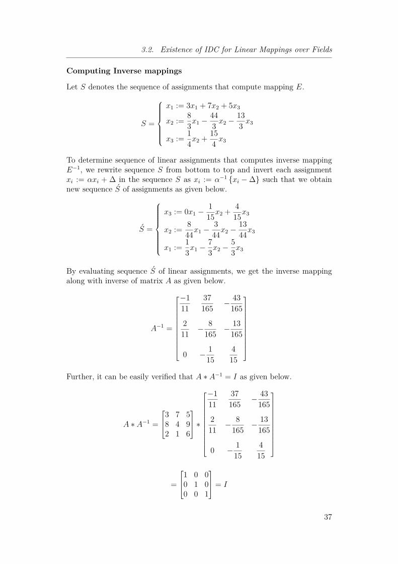
3.2. Existence of IDC for Linear Mappings over Fields
Computing Inverse mappings
Let S denotes the sequence of assignments that compute mapping E.
S =
x1 := 3x1 + 7x2 + 5x3
x2 := 83x1 −
443 x2 −
133 x3
x3 := 14x2 + 15
4 x3
To determine sequence of linear assignments that computes inverse mappingE−1, we rewrite sequence S from bottom to top and invert each assignmentxi := αxi + ∆ in the sequence S as xi := α−1 {xi −∆} such that we obtainnew sequence S of assignments as given below.
S =
x3 := 0x1 −115x2 + 4
15x3
x2 := 844x1 −
344x2 −
1344x3
x1 := 13x1 −
73x2 −
53x3
By evaluating sequence S of linear assignments, we get the inverse mappingalong with inverse of matrix A as given below.
A−1 =
−111
37165 − 43
165
211 − 8
165 − 13165
0 − 115
415
Further, it can be easily verified that A ∗ A−1 = I as given below.
A ∗ A−1 =
3 7 58 4 92 1 6
∗
−111
37165 − 43
165
211 − 8
165 − 13165
0 − 115
415
=
1 0 00 1 00 0 1
= I
37

Chapter 3. In Situ Design of Computation for Linear Mappings over Fields
3.2.2 Case-IIIn this section, we focus in explaining that, how to construct sequence ofassignments when matrix of coefficients has not some non-zero entries at theposition as described in Theorem 1 under case 2. We discuss this situationwith the following example.
Example 4. Consider a linear mapping
E (x1, x2, x3) −→ (5x2 + 7x3, x2 + 4x3, 3x1 + 2x3)
Given mapping E can be written as X := AX for a vector X := (x1, x2, x3)and a matrix A of coefficients, given as under
A =
0 5 70 1 43 0 2
Since a11 = 0 = α. But a13 = 3 = β. Therefore we have to subtract third rowof matrix A from first row. The operation will be R1 := R1 −R3.After the completion of this operation, the matrix A will take the form:
A =
−3 5 50 1 43 0 2
Now the first assignment will be of the form:
x1 := −3x1 + 5x2 + 5x3 (3.4)
The initial value of x1 will be
13(−x1 + 5x2 + 5x3)
Now, we will perform the operation
x2 := x2 − βx1 + β{α−1 (x1 −∆)
}and
x3 := x3 − βx1 + β{α−1 (x1 −∆)
}The matrix A will take the form
A =
−3 5 50 1 4−1 5 7
The second assignment will be
x2 := x2 + 4x3 (3.5)
38

3.2. Existence of IDC for Linear Mappings over Fields
Now, the initial value of second assignment, x2 will be
x2 − 4x3
and for the computation of third assignment:For, α = 1 and β = 5, We perform the following operation:
x3 := x3 − βx2 + β{α−1 (x2 −∆)
}We get the third assignment as
x3 := −x1 + 5x2 − 13x3 (3.6)
The first assignment of second sequence that is obtained by the operation R1 :=R1 −R3 will be.
x1 := x1 + x3
Hence the required sequence of assignments is
Sequence of assignments→
x1 := −3x1 + 5x2 + 5x3
x2 := x2 + 4x3
x3 := −x1 + 5x2 − 13x3x1 := x1 + x3
3.2.3 Computing Inverse MappingThe inverse mapping is computed by applying the same technique as describedin section 3.2.1, i.e., by inverting the assignments and rewriting from bottomto top.
Sequence of assignments→
x1 := x1 − x3
x3 := 113 (−x1 + 5x2 − x3)
x2 := 413x1 −
713x2
x1 := 13 (−x1 + 5x2 + 5x3)
3.2.4 Case-IIIFollowing example illustrates, how to construct sequence of assignments whenthe matrix of coefficients has not some non-zero entries at the position asdescribed in Theorem 1 under case 3. As compared to the previous two cases,case 3 is easier.
Example 5. Let E be a linear mapping defined as
E (x1, x2, x3) −→ (3x1 + 5x2 + 7x3, x2 + 4x3, 2x3)
39

Chapter 3. In Situ Design of Computation for Linear Mappings over Fields
The mapping E is expressed as X := AX, where X := (x1, x2, x3), is a vectorand A is a matrix of coefficients as given below
A =
3 5 70 1 40 0 2
Since a11 = 3 6= 0 = α. Therefore the first assignment will be of the form:
x1 := 3x1 + 5x2 + 7x3 (3.7)
The initial value of x1 will be13(x1 − 5x2 − 7x3)
Since β = 0 both for second and third row, therefore, Matrix A will remainunchanged, and no reference of x1 is used to compute the second assignment.The second assignment will be
x2 := x2 + 4x3 (3.8)
In computation of third assignment, we also do not need to use any referenceof first or second assignment.
x3 := 2x3 (3.9)Therefore, for such type of mappings (as defined in the Example 5) the sequenceof assignments can be written directly from the given mapping. Hence therequired assignments are
Sequence of Assignments→
x1 := 3x1 + 5x2 + 7x3
x2 := x2 + 4x3
x3 := 2x3
Computing Inverse Mapping
Sequence of three assignments that computes the inverse mapping is given be-low.
Computing Inverse Mapping→
x3 := 12x3
x2 := x2 − 4x3
x1 = 13(x1 − 5x2 − 7x3)
The inverse of matrix A is as follows.
A−1 =
13 −5
3136
0 1 −2
0 0 12
40

3.3. Novel approach using Bézout’s Identity
3.2.5 Possibility of Computing Inverse MappingsThere exist some of the mappings for which a sequence of linear assignmentsthat computes corresponding inverse mapping does not exist. We prove by giv-ing the following example that to compute inverse mapping, each assignmentmust be invertible.
Example 6. Consider a linear mapping
E (x1, x2, x3) −→ (5x2 + 7x3, x2 + 4x3, 2x3)
For a vector X := (x1, x2, x3), the mapping E takes the form as X := AX,where A is a matrix of coefficients as given below.
A =
0 5 70 1 40 0 2
Since a11 = 0 = α and β = 0, for all other cases, therefore we do not needto perform any operation, and we construct the required assignments directlyfrom matrix A as given below.
Sequence of assignnments→
x1 := 5x2 + 7x3
x2 := x2 + 4x3
x3 := 2x3
“Now, to compute inverse mapping, each assignment must be invertible”.
Notice that one of the assignments (given above) is not invertible, and isgiven below.
x1 := 5x2 + 7x3
Therefore, we cannot compute inverse mapping. Moreover, the matrix “A” isa singular matrix.
3.3 Novel approach using Bézout’s IdentityIn this section, we introduce an alternative approach (that use Bézout’s Iden-tity) for constructing a sequence of linear assignments that computes the givenlinear mapping. We prove it, here, for two dimensional linear mappings.
Definition 1. Bézout’s identity states that, if two integers a and b are rela-tively prime then there exists u, v ∈ Z such that au + bv = 1.
Theorem 2. Every linear mapping E: (x, y) −→ (mx + ny, px + qy), wherem, n, p, q ∈ Z, can be computed by a sequence of at most 3 linear assignmentswith rational coefficients.
41

Chapter 3. In Situ Design of Computation for Linear Mappings over Fields
Proof. Suppose that the given mapping E is computed with a sequence ofthree linear assignments as given below
Three linear Assignnments→
x := ax+ byy := cx+ dyx := ex+ fy
(S)
with rational coefficients a, b, c, d, e, and f . The sequence of linear assign-ments S (after evaluating sequentially) takes the form:
x := ax+ by
y := cax+ (cb+ d)yx := (ea+ fca)x+ (eb+ fcb+ fd)y
Coefficients of given Linear mapping E(x, y) −→ (mx + ny, px + qy), can beexpressed as a matrix of order 2× 2 as given below.[
m np q
]= A(say)
Determinant (A) = mq − np (3.10)We establish a system of four equations as given below:
m = ea+ fcan = eb+ fcb+ fdp = caq = bc+ d
(SOE)
By the equality 3.10 and the system of equations SOE, we have
mq − pn = aed
It yields that, the product of three variables a, e and d must be equal todeterminant of matrix A. Now, the general solution of the system of equationsSOE is as given below.
a = −fp−me
, b = −fq − ne
, c = − pe
fp−m, d = −mq − np
fp−m(3.11)
To find particular solution, we modify matrix A using Bézout’s identity. Sup-pose that m and p are relatively prime, then we find u, v ∈ Z such thatum + vp = 1 and modify matrix A by multiplying its rows by u and v respec-tively. New matrix will satisfy conditions 3.11 and yields values for coefficients.To return back to the original matrix, we perform the following operations.
y := y(1v
) and x := x( 1u
)
If m and p are not co-prime, then we make them co-prime by extracting theirGCD and solve the mapping as, for co-prime case and finally assign the GCDto the coefficient a.
42

3.3. Novel approach using Bézout’s Identity
Next, we explain, Theorem 2 in detail, by examples.
3.3.1 Case-IIn this section, we discuss the case when the GCD of entries of first column ofthe matrix (that represents coefficients of mapping), equals 1.
Example 7. Let E be a linear mapping as defined below
E : (x, y) −→ (55x + 89y, 34x + 21y)
such that matrix A represents the coefficients.
A =[m np q
]=[55 8934 21
]
The values corresponding to the entriesm and p are co-prime, i.e., GCD(55, 34) =1. Therefore, we apply Bézout’s identity to find integers u and v such that55u + 89v = 1A number of values are possible for u and v. Two of them are u = 13,v = −21.Multiply first row of matrix A by u and second by v, it gives
A =[um unvp vq
]=[
715 1157−714 −441
]
Using
a = −fp−me
, b = −fq − ne
, c = − pe
fp−m, d = −mq − np
fp−m(3.12)
we find the values a = 1, b = 716, c = −714, d = 510783, e = 1, f = −1Therefore, the sequence of assignments is as given below:
x := x+ 716y
y := 113 (−714x+ 510783y)
x := − 121 (x− y)
Next, we give another example to explain the case, when the entries of thefirst column of matrix A are not co-prime
3.3.2 Case-IIIn this section, we discuss the case when the GCD of entries of the first columnof matrix (that represent coefficients of mapping), is not equals 1.
43

Chapter 3. In Situ Design of Computation for Linear Mappings over Fields
Example 8. Consider the mapping E: (x, y) −→ (25x + 13y, 35x + 21y),whose coefficients are expressed by matrix A as given below.
A =[m np q
]=[25 1335 21
]
Notice that GCD(m, p) = GCD(25, 35) = 5 6= 1. We extract GCD to makeentries of the column co-prime
B =[m np q
]=[5 137 21
]
Now GCD(5, 7) = 1, so solving Bézout’s identity 5u + 7v = 1, one of thepossible solutions is u = −4, v = 3. Multiply first row of the matrix B with uand second row with v, It gives
B =[um unvp vq
]=[−20 −5221 63
]
For matrix B, the system of equations SOE takes the form
−20 = ea+ fca−52 = eb+ fcb+ fd21 = ca63 = bc+ d
(SOE-1)
Solving the system of equations SOE-1, we find the values
a = 1, b = 11, c = 21d = −168, e = 1, f = −1
The sequence of assignments for a = 1, is given below.
x := x+ 11y
y := −14 (21x− 168y)
x := 13 (x− y)
Now, replace a = 5, and the required sequence of assignments for a = 5, is asunder
x := 5x+ 11y
y := −14 (21x− 168y)
x := 13 (x− y)
44

3.3. Novel approach using Bézout’s Identity
3.3.3 Computing Inverse Mappings:In this section, we show by example, how to compute inverse mappings.
Example 9. The intermediate sequence of assignments that compute mappingE, in Example 7, whose coefficients are represented by matrix
A =[
715 1157−714 −441
]
is given as under x := x+ 716yy := −714x+ 510783yx := x− y
(SOA)
We construct the sequence of assignments that compute inverse mapping, byinverting and rewriting the sequence of assignments SOA, as given below.
x := x+ y
y := 1510783 {714x+ y}
x := x− 716y
and the inverse matrix A−1 is obtained by evaluating the sequence of assign-ments that compute inverse mapping.
A−1 =
− 21
24323 − 8939291
3424323
5539291
We compute A−1 by making some changes in the above sequence of assign-ments, i.e., we multiply the first column of A−1 by u and second by v. Thesequence of assignments that compute A−1 is given below:
x := u ∗ x+ v ∗ y
y := 1510783 {714x+ v ∗ y}
x := x− 716y
The matrix A−1 corresponding to matrix A is given below:
A−1 =
− 21
187189
187134
1871 − 551871
45

Chapter 3. In Situ Design of Computation for Linear Mappings over Fields
46

Chapter 4In Situ Design of Computation forLinear Mappings over Rings
Contents4.1 Existence of IDC for Linear Mappings over
Rings . . . . . . . . . . . . . . . . . . . . . . . . 48
4.1.1 Assignment Matrices . . . . . . . . . . . . . . . 48
4.2 Explanation and Construction . . . . . . . . . 50
4.2.1 Case-I . . . . . . . . . . . . . . . . . . . . . . . . 50
4.2.2 Case-II . . . . . . . . . . . . . . . . . . . . . . . 52
4.3 Computing Inverse Mappings . . . . . . . . . . 54
4.3.1 Possibility of computing Inverse mappings . . . 55
Investigating the existence of "In Situ Design of Computation (IDC)" forlinear mappings over rings consists, actually, in finding whether the coefficientsof such "In Situ Design of Computation (IDC)" belong to rings or not. Theexistence of IDC of linear mappings over rings is proved in [BGT09]. Weare interested to verify and implement the existence of "In Situ Design ofComputation (IDC)" over rings.
In this chapter, we explain the existence of "In Situ Design of Computation(IDC)" for linear mappings over rings. We design algorithm (given in annexB) to verify and implement the idea. Section 4.1 consists in explaining theexistence of such type of computations over rings, in detail. How a matrix isdecomposed into assignment matrices and how the corresponding assignmentscan be constructed, is described in section 4.2. We discuss the possibility ofconstructing sequence of assignments that compute inverse mappings in section4.3 and provide counter example.
47

Chapter 4. In Situ Design of Computation for Linear Mappings over Rings
4.1 Existence of IDC for Linear Mappings overRings
It is proved (see [BGT09]) that "In Situ Design of Computation (IDC)" forlinear mappings such that the coefficients of these linear mappings belong torings, exist. In this section we explain the idea for the ring Z/NZ.
Lemma 1 ([BGT09]). Suppose that x1, · · · , xn be co-prime integers and Nbe an integer. Then, there exists integers λ2, · · · , λn such that x1 + Σiλixi ∈(Z/NZ)∗, where (Z/NZ)∗ denotes the group of invertible elements.
Proof. Suppose that N be a prime power pv. It is given that integers xi areco-prime, therefore there exists an integer i0 (say) such that xi0 is co-prime top. If x1 is itself co-prime to p, then one can select i0 = 1. If x1 is not co-primeto p, i.e., if x1 is divisible by p, then x1 + xi0 is co-prime to p. So the resultholds when N = pv . For each prime power dividing N , we can thereforeconstruct n integers λp
v
1 , · · · , λpv
n such that
λpv
1 = 1 and Σi(λi)pv
xi ∈ (Z/pvZ)∗
Applying Chinese Remainder Theorem, these vectors combine to form a globalsolution
(1, λ2, · · · , λN)
satisfying the required property.
4.1.1 Assignment MatricesIn this section, we explain the basic idea of assignment matrices and the pos-sibility of decomposing a matrix into assignment matrices under “modulo”operation. An assignment matrix is actually the modified form of identitymatrix with a row different from identity matrix as defined below.
Definition 2. A matrix A is said to be an assignment matrix, if there existsan integer i0 such that for all row and column indices (i, j), one has eitheri = i0 or Ai,j = δji .
By definition 2, for a square matrix A, A−I has at most one non-zero row,where I denotes the identity matrix.
Example 10. Let A be the square matrix as given below:
A =
2 3 54 7 15 6 7
48

4.1. Existence of IDC for Linear Mappings over Rings
Performing operation with “modulo 8”, the given matrix A is decomposed intofour assignment matrices as given below.
A1 :=
7 1 40 1 00 0 1
, A2 :=
1 0 04 3 10 0 1
A3 :=
1 0 00 1 07 1 2
, A4 :=
1 0 70 1 00 0 1
such that
A4 ∗ A3 ∗ A2 ∗ A1 = A (modulo 8)
Next, we explain the assertion regarding existence of "In Situ Design ofComputation (IDC)" over rings.
Proposition 1 (see [BGT09]). Let N be an integer. Any n × n matrix over(Z/NZ) can be written as the product of at most 2n− 1 assignment matrices.
Proof. The result can be easily proved by the help of induction on the numberof rows (representing by n) of the given matrix. Therefore if n = 1, the resultis obvious.For n > 1, we can proceed as follows. Consider the first column of the givenmatrix “A” (say). Suppose that the entry a11 of the matrix “A” is not aninvertible element under modulo N . Let ‘g’ denotes GCD of the first column,i.e., g = (a11, a21, · · · , an1). We construct an invertible element using Lemma1 and we apply it to make a combination of the coefficients of this columnequal to g times an invertible element of (Z/NZ), with the constraint that thiscombination has its first multiplier equal to 1. This implies that the n × nmatrix T defined by ti, j = δji for i > 1, and t1, j = λj , where the multipliers1, λ2, · · · , λn are obtained from Lemma 1. Clearly, matrix T is an invertibleassignment matrix, and the product T ∗ A has a coefficient at position (1, 1)which is equal to g times an invertible element modulo N . Now assumingthat a1, 1 ∈ g(Z/NZ)∗ . Let n′ be the number of columns of A . Let G =diag(g, 1, · · · , 1), and let A′ be the integer matrix AG−1 (A′ has coefficientsin Z because g is the GCD of the first column). We have a′1, 1 ∈ (Z/NZ∗). We form an n′ × n′ assignment matrix U defined by ui, j = δji for i > 1,and u1, j = a′1, j . The matrix U is invertible modulo N (its determinant isa′1, 1 ). The first row of the matrix A′′ = A′ ∗ U−1 is equal to (1, 0, · · · , 0).Notice further that UG is an assignment matrix as well (even though notinvertible modulo N). Putting together the different results we have thatA = T ×A′′× (UG), where the matrix T may be omitted. Applying the resultinductively on A′′ completes the proof.
Next, we explain Proposition 1 in detail and describe method for construct-ing the sequence of linear assignments.
49

Chapter 4. In Situ Design of Computation for Linear Mappings over Rings
4.2 Explanation and ConstructionThis section consists in explaining, how to implement Proposition 1 in con-structing sequence of assignments.
Let “A” be the matrix that represents coefficients of the given mapping.Now, there are two cases, whether the entry “a1, 1” of matrix “A” is invertibleunder chosen value of modulo or not.
If the entry “a1,1” of the matrix “A” is invertible under chosen value of themodulo then matrix T will be the identity matrix of the same order as ofmatrix A and A′ = AG−1.
Otherwise, we construct matrix T as defined below
tij = δij for i > 1 and t1,j = λj
By definition, first row of the matrix T will consist of the multipliers 1, λ1, · · · , λn,obtained by Lemma 1. It is noted that matrix T could be single matrix orT = T1 · T2, · · · , Tn depending on number of prime factors of N .An invertible matrix L can be constructed by solving the system TL = A.i.e.
L1 = T1A, L2 = T2A, · · · , Ln = TnA
andA = (T1 ∗ T2, · · · , Tn)Ln
where “g” denotes GCD of the first column of matrix Li obtained after Titransformation. So if
A = (T1 ∗ T2, · · · , Tn)Lfthen A′ = LfG
−1, where Lf denotes the final invertible matrix after Ti, 1 ≤i ≤ n transformation.
Matrix A will finally satisfy the relation A = (T1 ∗ T2, · · · , Tn)A′′UG.
Next, we show by examples, how these assignment matrices can be con-structed.
4.2.1 Case-IIn this section, we explain the construction of sequence of linear assignments,when N is the product of single integer.
Example 11. Consider a mapping E : (x1, x2) −→ (2x1 + 3x2, 5x1 + 7x2).The coefficients can be represented by a square matrix
M =[2 35 7
]
50

4.2. Explanation and Construction
Suppose that N = 8 = 23.For pv = 2, (2, 2) 6= 1,=⇒ m1,1 is not invertible.Since λ2 = 1, therefore matrix
T =[1 10 1
]
Now, solving the system as given below[1 10 1
] [a bc d
]=[2 35 7
]
We have values for coefficients a, b, c, and d as given below.
a = −3 = 5 (mod 8)
b = −4 = 4 (mod 8)
c = 5, d = 7
Now we construct matrix M as
M =[5 45 7
]
Further,
G =[5 00 1
]where,
G−1 = 5−1[1 00 5
]=[5 00 1
](mod 8)
M ′ = MG−1 =[5 45 7
] [5 00 1
]
=[25 425 7
]=[1 41 7
](mod 8)
U =[1 40 1
]
U−1 =[1 −40 1
]
UG =[1 40 1
] [5 00 1
]=[5 40 1
]
M ′′ = M ′U−1 =[1 41 7
] [1 −40 1
]=[1 01 3
]
51

Chapter 4. In Situ Design of Computation for Linear Mappings over Rings
Notice that matrix M is decomposed into three assignment matrices T , M ′′
and UG such that
TM ′′UG =[10 115 7
]=[2 35 7
](mod 8)
These three assignment matrices yield the sequence of linear assignments thatcompute the given mapping E and is given below
Sequence of assignments→
a := 5a+ 4bb := a+ 3ba := a+ b
4.2.2 Case-IIIn this section, we explain the construction of sequence of linear assignments,when N is not the product of single integer.
Example 12. Consider a mapping E : (x1, x2) −→ (2x1 +3x2, 5x1 +x2). Thecoefficients can be represented by a square matrix
M =[2 35 1
]and N = 6 = 21 ∗ 31
m1, 1 is not invertible with respect to pv = 2, (2, 2) 6= 1λ1 = 1, and λ2 = 1,
T1 =[λ1 λ20 1
]=[1 10 1
]Now, by solving the following system[
1 10 1
] [a bc d
]=[2 35 1
]
We have values for coefficients a, b, c, and d as given below.
a = −3 = 3 (mod 6)
b = 2, c = 5, and d = 1Then we proceed by constructing matrix
L1 =[3 25 1
]
Observe that entry l1, 1 is not invertible, For pv = 3, (3, 3) 6= 1λ1 = 1, and λ2 = 1,
T2 =[1 20 1
]
52

4.2. Explanation and Construction
Again, solving the system [1 20 1
] [a bc d
]=[3 25 1
]We have values for coefficients a, b, c, and d as given below.
a = −7 = 5 (mod 6)b = 0, c = 5, and d = 1
Now matrixL2 =
[5 05 1
]
G =[5 00 1
]where,
G−1 = 5−1[1 00 5
]= 5
[1 00 5
]
=[5 00 1
](mod 6)
M ′ = MG−1 =[5 05 1
] [5 00 1
]
=[25 025 1
]=[1 01 1
](mod 6)
Now,
U =[1 00 1
]
U−1 =[1 00 1
]
UG =[5 00 1
]
M ′′ = M ′U−1 =[1 01 1
]Thus, the matrix M is decomposed into three assignment matrices T = T1 ∗T2,M ′′ and UG such that
T1T2M′′UG =
[20 35 1
]=[2 35 1
](mod 6)
From these assignment matrices, the sequence of linear assignments (that com-putes the given mapping) is constructed and is given below:
Sequence of assignments→
a := 5ab := a+ ba := a+ 3b
53

Chapter 4. In Situ Design of Computation for Linear Mappings over Rings
4.3 Computing Inverse MappingsIn this section, we show, by examples, how to construct a sequence of linear as-signments that computes inverse mapping, by a sequence of linear assignmentsover the ring Z/NZ.
Example 13. Let E be a linear mapping defined as follows
E (x1, x2, x3) −→ (2x1 + 8x2 + 6x3, 3x1 + 13x2 + 7x3, 5x1 + 5x2 + x3)
and “A” be the matrix expressing coefficients of mapping E, given as under
A =
2 8 63 13 75 5 1
Suppose that we are to perform operations under “modulo 9”. Then
A =
2 8 63 4 75 5 1
(modulo 9)
We construct the sequence of linear assignments that compute mapping E,under “modulo 9” operation, and is given below
x1 := 2x1 + 8x2 + 6x3x2 := 6x1 + x2 + 7x3x3 := 7x1 + 3x2 + x3
(modulo 9) (S-1)
We are interested in computing a sequence of linear assignments under “modulo9” that compute inverse mapping E−1. We obtain this sequence of assignmentsby inverting and rewriting each assignment of the Sequence S-1 (from bottomto top) that computes the given mapping E.
Sequence of assignments→
x3 := x3 − 7x1 − 3x2x2 := x2 − 6x1 − 7x3x1 := 2−1 (x1 − 8x2 − 6x3)
(S’-1)
Replacing “2−1” in the last assignment of the Sequence S’-1 of assignments byits inverse “modulo 9”, we obtain the required sequence of assignments.
x3 := x3 − 7x1 − 3x2x2 := x2 − 6x1 − 7x3x1 := 5 (x1 − 8x2 − 6x3)
modulo 9
that computes inverse mapping. By, evaluating above sequence of linear as-signments, we get the inverse of matrix A as given below.
A−1 =
7 2 77 4 22 6 1
54

4.3. Computing Inverse Mappings
Verifying the product of assignment matrices
The matrix
A =
2 8 63 13 75 5 1
is decomposed into three assignment matrices under modulo 9 operation, thesematrices are as given below:
A1 =
2 8 60 1 00 0 1
A2 =
1 0 03 13 70 0 1
A3 =
1 0 00 1 05 5 1
The product of matrices is A3 ∗ A2 ∗ A1 = A.
4.3.1 Possibility of computing Inverse mappingsIn this section, we provide example which proves that constructing a sequenceof linear assignments that computes the inverse mapping of a given mappingmay not exist.
Definition 3. A modular inverse of an integer “a” (modulo k) is the integer“a−1“ such that
aa−1 ≡ 1 mod k
i.e, an integer ”a” has an inverse (modulo k) if and only if GCD(a, k) = 1.If ”p” is a prime number, then for each a 6≡ 0 (modulo p), there exists amultiplicative inverse mod p.
It is not always true that an integer “a” with a 6≡ 0 (mod k) has an inversemod k.
Consider, for instance, 2 6≡ 0 (mod 4) does not have modular inverse be-cause of
2× 2 = 4 ≡ 0 mod 4
Thus (2 mod 4) has no modular inverse, otherwise, we could multiply bothsides of
2× 2 ≡ 0 mod 4
by the inverse of 2 and get the false result 2 ≡ 0 mod 4.
Next, we give an example to show that there may not exist a sequence oflinear assignments that required to compute inverse mapping.
Example 14. Let E be the linear mapping defined as under.
E (x1, x2, x3) −→ (2x1 + 8x2 + 6x3, 3x1 + 13x2 + 7x3, 5x1 + 5x2 + x3)
55

Chapter 4. In Situ Design of Computation for Linear Mappings over Rings
The mapping E has already discussed in Example 13 with “modulo 9”. Supposethat we want to construct the sequence of linear assignments keeping operationunder “modulo 12”. Then the required sequence of assignments is given below
Sequence of assignments→
x1 := 5x1 + 5x2 + 9x3x2 := 3x1 + 10x2 + 4x3x3 := x1 + 4x3x1 := x1 + 3x2
To construct sequence of assignments that computes inverse mapping E−1, weneed to invert each assignment and to rewrite the above sequence of assignmentsfrom bottom to top. Performing this technique, we get sequence of assignmentsas given below.
Sequence of assignments→
x1 := x1 − 3x2x3 := 4−1 (x3 − x1)x2 := 10−1 (x2 − 3x1 − 4x3)x1 := 5−1 (x1 − 5x2 − 9x3)
Observe that, the second and third assignment of the above sequence is notinvertible due to the reason that integers 4 and 10 have not their modularinverses under “modulo 12” operation.
Similarly, the inverse of the matrix (that presents coefficients of the mappingE) does not have its inverse under “modulo 12” because the determinant ofmatrix A
|A| =
∣∣∣∣∣∣∣2 8 63 13 75 5 1
∣∣∣∣∣∣∣ = 248
is not invertible under “modulo 12” operation.
“Therefore, to compute inverse mapping for a mapping, each linear assign-ment in the sequence of linear assignments (that compute the mapping) mustbe invertible”.
56

Chapter 5In Situ Design of Computation forLinear Mappings over Integers
Contents5.1 Existence of IDC for Linear Mappings over
Integers . . . . . . . . . . . . . . . . . . . . . . . 58
5.1.1 Modifications: . . . . . . . . . . . . . . . . . . . 60
5.1.2 Explanation and construction of assignments: . 60
5.2 Investigating bounds for the number of assign-ments: . . . . . . . . . . . . . . . . . . . . . . . . 68
5.2.1 An approach based on Fibonacci numbers . . . . 71
5.2.2 Identity (coefficient linkage): . . . . . . . . . . . 74
Proving the existence of "In Situ Design of Computation (IDC)" over theset of integers (to compute mappings) leads to perform these operations inmore simple way as compared to IDC for mappings over fields and rings. Inthis chapter, (following the ideas of Serge Burckel), we prove the existence of"In Situ Design of Computation (IDC)" over the set of integers (to computemappings sequentially). Section 5.1 describes the existence of "In Situ De-sign of Computation (IDC)" for linear mappings over the set of integers andexplains the construction of assignments involve in IDC. Section 5.2 consistsin investigating bound over the number of assignments required to computemappings by IDC. An approach with Fibonacci numbers is attempted in thesame section. At the end of this section, we prove an identity that relates thedeterminant of matrices (presenting coefficients of mappings) to the productof coefficients of assignments involve in computing the given mappings.
57

Chapter 5. In Situ Design of Computation for Linear Mappings over Integers
5.1 Existence of IDC for Linear Mappings overIntegers
In this section, following the ideas of Serge Burckel, we provide the existenceof "In Situ Design of Computation (IDC)" for linear mappings over integers.The assertion is proved as the following theorem.
Theorem 3. Let E be a linear mapping on Zn. There exists a finite sequenceof linear assignments of the form:
xp1 := xp1 + fp1(x1, . . . , xp1−1, xp1+1, . . . , xn)xp2 := xp2 + fp2(x1, . . . , xp2−1, xp2+1, . . . , xn)... := ... ... ... ... ... ... ... ... ... ...
xpm := xpm + fpm(x1, . . . , xpm−1, xpm+1, . . . , xn)xn := gn(x1, x2, . . . , xn)... := ... ... ... ...x2 := g2(x1, x2, . . . , xn)x1 := g1(x1, x2, . . . , xn)
that computes the mapping E, where p1, . . . , pm ∈ {1, 2, . . . , n} m, n ∈ Z.
Proof. The given mapping E can be expressed as AX, where A is a squarematrix of integer coefficients (i.e., for A = [aij], aij ∈ Z, i, j = 1, 2, . . . , n),such that each row of the matrix AX represents a component of the mappingE at current values of the variables (x1, x2, . . . , xn) and is a linear mapping.We construct the sequence of linear assignments by considering the followingfour different cases:
Case 1: If aij < 0, for i ≥ j, then multiply jth column by −1, sothat aij > 0 and construct the corresponding linear assignment xj asxj := −xj.
Case 2: If aii > aij, for j > i, then perform the operation Ci := Ci−Cj,and the corresponding linear assignment xj will be of the form xj :=xj + f , where f does not depend on xj and Ci is the ith column ofmatrix A.
Case 3: If aii ≤ aij, for j > i, then perform the operation Cj := Cj−Ci,and corresponding linear assignment xi will take the form xi := xi + f .
Case 4: If aii = 0, then we perform the operation Ci := Ci − Cj, and xjwill take the form xj := xj + f .
58

5.1. Existence of IDC for Linear Mappings over Integers
Performing this procedure iteratively, we transform the square matrix A intotriangular matrix L (say) as given below.
L :=
l11 0 0 . . . 0 0 0l21 l22 0 . . . 0 0 0l31 l32 l33 . . . 0 0 0... ... ... . . . ... ... ...
ln−2,1 ln−2,2 ln−2,3 . . . ln−2,n−2 0 0ln−1,1 ln−1,2 ln−1,3 . . . ln−1,n−2 ln−1,n−1 0ln1 ln2 ln3 . . . ln,n−2 ln,n−1 lnn
We construct the second sequence of linear assignments directly from matrixL as follows:
xn := ln1x1 + ln2x2 + ln3x3 + . . .+ ln,n−2xn−2 + ln,n−1xn−1 + lnnxn
xn−1 := ln−1,1x1 + ln−1,2x2 + . . .+ ln−1,n−2xn−2 + ln−1,n−1xn−1
xn−2 := ln−2,1x1 + ln−2,2x2 + ln−2,3x3 + . . .+ ln−2,n−2xn−2... . . . . . . . . . . . . . . . . . . . . . . . .
... . . . . . . . . . . . . . . . . . . . . . . . .
... . . . . . . . . . . . . . . . . . . . . . . . .
x3 := l31x1 + l32x2 + l33x3
x2 := l21x1 + l22x2
x1 := l11x1
Now, let A and V denote the modified form of the matrix A and vector V (ofvariables) after performing any operation. Then, after each operation, it mustpreserve and compute the original mapping effectively i.e.
AV = AV
If T denotes the transformation matrix then
A = AT
V = T−1V
=⇒ AV = A(TT−1)V = AV
We notice that, an assignment xi := αxi + f , repeated k times can bewritten as a single assignment of the form.
xi := αkxi + f(αk−1 + αk−2 + . . .+ α2 + α1 + α0
), α = 1
It enables us to modify the algorithm to avoid from repeated similar assign-ments. So, we introduce the following modifications.
59

Chapter 5. In Situ Design of Computation for Linear Mappings over Integers
5.1.1 Modifications:Case 2: If aii > aij, for j > i, then the program will perform the opera-tion Ci := Ci − β1Cj, and xj will be modified to xj := αxj + β1f , wheref does not depend on xj. Ci denotes the ith column of matrix A andβ1 = trunc(aii/aij). The function trunc returns integer quotient.
Case 3: If aij ≥ aii, for j > i, then the program will perform the opera-tion Cj := Cj − β2Ci, and xi will be modified to xi := αxi + β2f , wheref does not depend on xi and β1 = trunc(aij/aii). The case aij = 0, canbe handled by taking β2 = 1
“We estimate an upper bound over the number of assignments with the helpof famous result presented by Gabriel Lamé [Lam44]”.
Suppose that γ denotes the total number of assignments involve in comput-ing linear mapping E, then γ ≤ 5(n− 1)d+ n, where d denotes the number ofdigits in the entry a(i, j) of the matrix A such that i ≤ j, but i 6= n, MatrixA is the matrix of coefficients of mapping E.
5.1.2 Explanation and construction of assignments:We explain the construction of assignments by the following Example 15 andwill discuss step by step in Example 16.
Example 15. Suppose that E be the mapping with integer coefficients as de-fined by
E (x1, x2) −→ (13x1 + 21x2, 21x1 + 34x2)Let the matrix Mc represents the coefficients of mapping E.
Mc :=[13 2121 34
]
We generate sequence of linear assignments by performing column/row opera-tions on matrix Mc in such a way that it results with integer entries (excludingdivision operation). In fact, the square matrix Mc is transformed into triangu-lar matrix, at the completion of all operations. In Table 5.1, we show the stepsinvolve in generating sequence of linear assignments, that involve in computinglinear mapping E.
60

5.1. Existence of IDC for Linear Mappings over Integers
Table 5.1: Example 15
Generating linear assignmentsMatrix(input) Operation Assignment Matrix(output)[
13 2121 34
]C2 − C1 x1 := x1 + x2
[13 821 13
][13 821 13
]C1 − C2 x2 := x1 + x2
[5 88 13
][5 88 13
]C2 − C1 x1 := x1 + x2
[5 38 5
][5 38 5
]C1 − C2 x2 := x1 + x2
[2 33 5
][2 33 5
]C2 − C1 x1 := x1 + x2
[2 13 2
][2 13 2
]C1 − C2 x2 := x1 + x2
[1 11 2
][1 11 2
]C2 − C1 x1 := x1 + x2
[1 01 1
]
In Table 5.1, first column presents input matrices and second column presentscolumn operations performed on these matrices. The corresponding assign-ments constructed are in third column while matrices (modified) after perform-ing operations are presented in last column of the table. Instead of columnoperations, row operations could be performed and assignments could be con-structed accordingly.
We terminate the operations, when square matrix Mc is transformed intotriangular matrix, and we generate, the next part of sequence of assignments,directly from triangular matrix, writing from last row to first as given below.[
1 01 1
]−→
{x2 := x1 + x2x1 := x1
If we ignore the last assignment, it will not affect the computation and we willhave a sequence of eight linear assignments in total.
Computing inverse mappings:
Generate the set of linear assignments that compute inverse mapping E−1, di-rectly from the set of linear assignments that computes mapping E, by invertingand rewriting from the last assignment to the first as given below.
61

Chapter 5. In Situ Design of Computation for Linear Mappings over Integers
Table 5.2: Example 15
Generating linear assignments for E−1
Input Inverted Evaluated Coefficients
x2 := x1 + x2 x2 := −x1 + x2 x2 := −x1 + x2[−1 1
]
x1 := x1 + x2 x1 := x1 − x2 x1 := 2x1 − x2[2 −1
]
x2 := x1 + x2 x2 := −x1 + x2 x2 := −3x1 + 2x2[−3 2
]
x1 := x1 + x2 x1 := x1 − x2 x1 := 5x1 − 3x2[5 −3
]
x2 := x1 + x2 x2 := −x1 + x2 x2 := −8x1 + 5x2[−8 5
]
x1 := x1 + x2 x1 := x1 − x2 x1 := 13x1 − 8x2[13 −8
]
x2 := x1 + x2 x2 := −x1 + x2 x2 := −21x1 + 13x2[−21 13
]
x1 := x1 + x2 x1 := x1 − x2 x1 := 34x1 − 21x2[34 −21
]
Second column of the Table 5.2 presents set of linear assignments that computethe inverse mapping E−1 of E defined by
E−1 (x1, x2) −→ (34x1 − 21x2, −21x1 + 13x2)
Consequently, we obtain inverse of matrix A as given below.
A−1 :=[
34 −21−21 13
]
A ∗ A−1 =[13 2121 34
]∗[
34 −21−21 13
]=[1 00 1
]
Next, we give another example that explains the process of construction ofassignments step by step.
Example 16. Consider a linear mapping defined as
E (x1, x2, x3) −→ (5x1 − 3x2 + 5x3, 3x1 − 7x3, 4x1 + 8x2 + 13x3)
62

5.1. Existence of IDC for Linear Mappings over Integers
We are interested to compute the given mapping by sequence of linear assign-ments such that the coefficients of these assignments are integers. Let matrix’A’ presents coefficients of given mapping E.
A :=
5 −3 53 0 −74 8 13
We compute mapping E by applying the procedure, keeping in mind differentcases, as described in Theorem 3.
Now, notice that a12 < 0, therefore, we are in the first case and we per-form the operation C2 := −C2. The linear assignment corresponding to thisoperation is
x2 := −x2
and matrix A will be modified to the form
A :=
5 3 53 0 −74 −8 13
Now, because a11 = 5 > a12 = 3, therefore, we are in the second case and weperform the operation C1 := C1 −C2. The linear assignment corresponding tothis operation is
x2 := x1 + x2
and the matrix A will be modified.
A :=
2 3 53 0 −712 −8 13
Now, observe that a12 = 3 ≥ a11 = 2 therefore, we are in the third case and weperform the operation C2 := C2 −C1. The linear assignment corresponding tothis operation is
x1 := x1 + x2
and the matrix A will be modified.
A :=
2 1 53 −3 −712 −20 13
Since a11 = 2 > a12 = 1, therefore, we perform the operation C1 := C1 − C2.The linear assignment corresponding to this operation is x2 := x1 +x2 and thematrix A will be modified.
A :=
1 1 56 −3 −732 −20 13
63

Chapter 5. In Situ Design of Computation for Linear Mappings over Integers
Since a12 = 1 ≥ a11 = 1, therefore, we perform the operation C2 := C2 − C1.The linear assignment corresponding to this operation is x1 := x1 +x2 and thematrix A will be modified.
A :=
1 0 56 −9 −732 −52 13
Observe that a12 became zero, We will continue this process until a13 = 0.Since a13 = 5 ≥ a11 = 1, we perform the operation C3 := C3 − C1. The linearassignment corresponding to this operation is x1 := x1 +x3. The matrix A willbe modified.
A :=
1 0 46 −9 −1332 −52 −19
Since a13 = 4 ≥ a11 = 1, we perform the operation C3 := C3 − C1. The linearassignment corresponding to this operation is x1 := x1 +x3. The matrix A willbe modified.
A :=
1 0 36 −9 −1932 −52 −51
Since a13 = 3 ≥ a11 = 1, we perform the operation C3 := C3 − C1. The linearassignment corresponding to this operation is x1 := x1 +x3. The matrix A willbe modified.
A :=
1 0 26 −9 −2532 −52 −83
Since a13 = 2 ≥ a11 = 1, we perform the operation C3 := C3 − C1. The linearassignment corresponding to this operation is x1 := x1 +x3. The matrix A willbe modified.
A :=
1 0 16 −9 −3132 −52 −115
Since a13 = 1 ≥ a11 = 1, we perform the operation C3 := C3 − C1. The linearassignment corresponding to this operation is x1 := x1 +x3. The matrix A willbe modified.
A :=
1 0 06 −9 −3732 −52 −147
Now the first column will remain unchanged throughout the next operations,we will focus on second diagonal entry.Since a23 = −37 < 0, we perform the operation C3 := −C3. The linear
64

5.1. Existence of IDC for Linear Mappings over Integers
assignment corresponding to this operation is x3 := −x3. The matrix A willbe modified.
A :=
1 0 06 −9 3732 −52 147
Since a22 = −9 < 0, we perform the operation C2 := −C2. The linear as-signment corresponding to this operation is x2 := −x2. The matrix A will bemodified.
A :=
1 0 06 9 3732 52 147
Since a23 = 37 ≥ a22 = 9, we perform the operation C3 := C3−C2. The linearassignment corresponding to this operation is x2 := x2 +x3. The matrix A willbe modified.
A :=
1 0 06 9 2832 52 95
since a23 = 28 ≥ a22 = 9, we perform the operation C3 := C3−C2. The linearassignment corresponding to this operation is x2 := x2 +x3. The matrix A willbe modified.
A :=
1 0 06 9 1932 52 43
Since a23 = 19 ≥ a22 = 9, we perform the operation C3 := C3−C2. The linearassignment corresponding to this operation is x2 := x2 +x3. The matrix A willbe modified.
A :=
1 0 06 9 1032 52 −9
Since a23 = 10 ≥ a22 = 9, we perform the operation C3 := C3−C2. The linearassignment corresponding to this operation is x2 := x2 +x3. The matrix A willbe modified.
A :=
1 0 06 9 132 52 −61
Since a22 = 9 > a23 = 1, we perform the operation C2 := C2 − C3. The linearassignment corresponding to this operation is x3 := x2 +x3. The matrix A willbe modified.
A :=
1 0 06 8 132 113 −61
65

Chapter 5. In Situ Design of Computation for Linear Mappings over Integers
Since a22 = 8 > a23 = 1, we perform the operation C2 := C2 − C3. The linearassignment corresponding to this operation is x3 := x2 +x3. The matrix A willbe modified.
A :=
1 0 06 7 132 174 −61
Since a22 = 7 > a23 = 1, we perform the operation C2 := C2 − C3. The linearassignment corresponding to this operation is x3 := x2 +x3. The matrix A willbe modified.
A :=
1 0 06 6 132 235 −61
Since a22 = 6 > a23 = 1, we perform the operation C2 := C2 − C3. The linearassignment corresponding to this operation is x3 := x2 +x3. The matrix A willbe modified.
A :=
1 0 06 5 132 296 −61
Since a22 = 5 > a23 = 1, we perform the operation C2 := C2 − C3. The linearassignment corresponding to this operation is x3 := x2 +x3. The matrix A willbe modified.
A :=
1 0 06 4 132 357 −61
Since a22 = 4 > a23 = 1, we perform the operation C2 := C2 − C3. The linearassignment corresponding to this operation is x3 := x2 +x3. The matrix A willbe modified.
A :=
1 0 06 3 132 418 −61
Since a22 = 3 > a23 = 1, we perform the operation C2 := C2 − C3. The linearassignment corresponding to this operation is x3 := x2 +x3. The matrix A willbe modified.
A :=
1 0 06 2 132 479 −61
Since a22 = 2 > a23 = 1, we perform the operation C2 := C2 − C3. The linearassignment corresponding to this operation is x3 := x2 +x3. The matrix A willbe modified.
A :=
1 0 06 1 132 540 −61
66

5.1. Existence of IDC for Linear Mappings over Integers
Since a23 = 1 ≥ a22 = 1, we perform the operation C3 := C3 − C2. The linearassignment corresponding to this operation is x2 := x2 +x3. The matrix A willbe modified.
A :=
1 0 06 1 032 540 −601
The matrix A is converted into lower triangular matrix and the last three as-signments will be written directly from this lower triangular matrix. Thesethree assignments are:
x3 := 32x1 + 540x2 − 601x3x2 := 6x1 + x2x1 := x1
Possibility of computing inverse mappings:
IDC for inverse mappings over integers is not always possible. We illustratethis by the following example
Example 17. Consider a mapping E
E (x1, x2, x3) −→ (2x1 + 3x2 + 5x3, 3x1 + 4x2 − 7x3, 8x2 + 13x3)
The mapping E can be computed by the following sequence of assignments.
Assignments
x1 := x1 + x2x2 := 2x1 + x2x2 := x1 + x2x1 := −x1x1 := x1 + x2x1 := x1 + 5x3x3 := −x3x2 := x2 + 7x3x3 := 24x1 − 16x2 + 219x3x2 := x2x1 := x1
The matrix of coefficients A for the mapping E can be written as
A :=
2 3 53 4 −70 8 13
and
A−1 := 1219
108 1 −41−39 26 2924 −16 −1
67

Chapter 5. In Situ Design of Computation for Linear Mappings over Integers
Notice that 1219 /∈ Z and the assignment
x3 := 24x1 − 16x2 + 219x3
is not invertible. Hence, the inverse mapping E−1 is not always computableby inverting and rewriting the sequence of assignments that computes mappingE.
5.2 Investigating bounds for the number of as-signments:
We are interested in determining the minimum number of assignments requiredto compute given mapping by "In Situ Design of Computation (IDC)" withinteger coefficients. We proceed by developing relations between mappingsthat help to find minimum number of assignments and investigate by findingdifferent counter examples. Based on, one of such counter examples, we providethe following theorem.
Theorem 4. There exists a linear mapping
E : (x, y) −→ (mx + ny, px + qy)
with m, n, p, q ∈ Z, that cannot be computed by a sequence of at most 6 linearassignments
x := ax+ byy := cx+ dyx := ex+ fyy := gx+ hyx := ix+ jyy := kx+ ly
where a, b, c, d, e, f, g, h, i, j, k, and l ∈ Z.
Proof. Let E be a linear mapping E(x, y) −→ (461x + 286y, 353x + 219y),whose coefficients can be viewed as a matrix given below.[
461 286353 219
]= A(say)
We establish a system of four equations (by evaluating assignments), as givenbelow:
461 = a(ie+ ifc+ jge+ jgfc+ jhc)286 = ieb+ ifcb+ ifd+ jgeb+ jgfcb+ jgfd+ jhcb+ jhd353 = 461k + lgea+ lgfca+ lhca219 = 286k + lgeb+ lgfcb+ lgfd+ lhcb+ lhd
(2)
68

5.2. Investigating bounds for the number of assignments:
determinant (A) = mq − pn = aedihl
=⇒ The product of variables a, d, e, h, i, and l must be equal to determinantof matrix A. Since, determinant of matrix A is equal to 1. Therefore,
a ∗ e ∗ d ∗ h ∗ i ∗ l = 1
and each of six variables take values from the set {1, −1}. Notice that, thereare
P (6, 2) + 2 = 32cases of assigning values to a, d, e, h, i, and l.
Let us start by considering the case with values
a = 1, e = 1, d = 1, h = 1, i = 1, l = 1
It gives a set of equations:460 = fc+ jg + jgfc+ jc286 = 461b+ f + jgf + j353 = 461k + g + gfc+ c218 = 286k + 353b− 461bk + gf
(3)
We observe that there are three general solutions for system 3 of equations:First possible solution is of the form:
c = 461j, j = j, f = f, b = − 1
461j + 286461
k = 1461−460j + 461f + 353j2
j2 , g = −1j
(first)
Second possible solution is of the form:
j = j, g = 460j, k = 1
461−460 + 353j
j
b = −f − 1461j + 286
461 , f = f, c = 0
(second)
The third possible solution is of the form:
j = j, g = g, k = − 1461
461g + c− 353− 353jg1 + jg
c = c, b = 1461
jg − 460 + 286cc
, f = −−460 + jg + jc
c(1 + jg)
(third)
Consider the first possible solution:
Let g = −1j∈ Z =⇒ j = 1 or − 1
Now, If j = 1 then
g = −1 ∈ Z, but b = − 1461 + 286
461 = 285461 /∈ Z
69
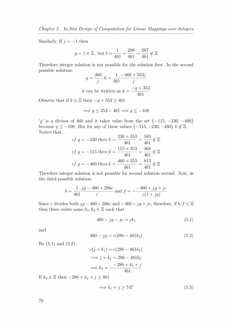
Chapter 5. In Situ Design of Computation for Linear Mappings over Integers
Similarly, If j = −1 then
g = 1 ∈ Z, but b = 1461 + 286
461 = 287461 /∈ Z
Therefore integer solution is not possible for the solution first. In the secondpossible solution:
g = 460j, k = 1
461−460 + 353j
j
k can be written as k = −g + 353461
Observe that if k ∈ Z then −g + 353 ≥ 461
=⇒ g ≤ 353− 461 =⇒ g ≤ −108
’g’ is a divisor of 460 and it takes value from the set {−115, −230, −460}because g ≤ −108. But for any of these values {−115,−230,−460} k /∈ Z.Notice that,
if g = −230 then k = 230 + 353461 = 583
461 /∈ Z
if g = −115 then k = 115 + 353461 = 468
461 /∈ Z
if g = −460 then k = 460 + 353461 = 813
461 /∈ Z
Therefore integer solution is not possible for second solution second. Now, inthe third possible solution:
b = 1461
jg − 460 + 286cc
and f = −−460 + jg + jc
c(1 + jg)
Since c divides both jg− 460 + 286c and −460 + jg+ jc, therefore, if b, f ∈ Zthen there exists some k1, k2 ∈ Z such that
460− jg − jc = ck1 (5.1)
and460− jg = c(286− 461k2) (5.2)
By (5.1) and (5.2)c(j + k1) = c(286− 461k2)=⇒ j + k1 = 286− 461k2
=⇒ k2 = −−286 + k1 + j
461If k2 ∈ Z then −286 + k1 + j ≥ 461
=⇒ k1 + j ≥ 747 (5.3)
70

5.2. Investigating bounds for the number of assignments:
c = 460− jgj + k1
by equation (5.1)
and if c ∈ Z thenj + k1 ≤ 460− jg (5.4)
By (5.3) and (5.4), we can write
460− jg = 747 =⇒ jg = −287
=⇒ For j and g to be integers, they must be factors of 287 and the possiblefactors of 287 are
{±1, ±7, ±41, ±287}Let, for example, g = −287 then j = 1
=⇒ k1 = 746 =⇒ k2 = −1 =⇒ c = 1
But, then, f = −−460− 287 + 11− 287 = −34
13 /∈ Z
Thus, for all divisors of 287, f /∈ Z. In a similar way, it can be proved for other31 possibilities of assigning values {1, −1} to variables a, d, e, h, i, and l.
5.2.1 An approach based on Fibonacci numbersTo investigate the minimum number of assignments required to perform "InSitu Design of Computation (IDC)" for mappings over integers, we establishrelations, keeping Fibonacci numbers, as coefficients of the mapping.
Definition 4. We define a Fibonacci-like sequence as
Fn = Fn−1 + Fn−2
where F0 = F1 = 1.
Definition 5. We define a Fibonacci-like matrix to be a matrix of the form[Fn−1 FnFn Fn+1
]
and the following relations.
R1 :[0 11 1
]n+1
=[Fn−1 FnFn Fn+1
]
R2 :[F2 F3F3 F4
]∗[F4n+1 F4n+2F4n+2 F4n+3
]=[F4n+4 F4n+5F4n+5 F4n+6
]
Theorem 5. Let En : (x, y) −→ (Fn−1x + Fny, Fnx + Fn+1y) be the map-ping on Z2, where Fn is the Fibonacci number. Then the mapping E4k+2 iscomputed with 2k + 2 number of assignments, where k = 0, 1, 2, · · · , n.
71

Chapter 5. In Situ Design of Computation for Linear Mappings over Integers
Proof. For n = 2, E2 = (F1x+F2y, F2x+F3y) and the matrix of coefficientsis
A2 =[1 22 3
]
The assignments for A2 →{x := x+ 2yy := 2x− y
A3 =[2 33 5
]
The assignments for A3 →
x := x+ 2yy := 3x− yx := −x+ y
Now,
A3 =[2 33 5
]∗ A2 =
[1 22 3
]= A6 =
[8 1313 21
]by R2.
We obtain sequence of assignments required to compute E6 as follows. In fact,we pack together the assignments require to compute E3 and the assignmentsrequire to compute E2.
The assignments for A6 →
x := x+ 2yy := 3x− yx := −x+ yx := x+ 2yy := 2x− y
→
x := x+ 2yy := 3x− yx := −x+ 3yy := 2x− y
Similarly, since A3 =[2 33 5
]∗ A6 =
[8 1313 21
]=[55 8989 144
]= A10
Therefore,
The assignments for A10 →
x := x+ 2yy := 3x− yx := −x+ yx := x+ 2yy := 3x− yx := −x+ 3yy := 2x− y
→
x := x+ 2yy := 3x− yx := −x+ 3yy := 3x− yx := −x+ 3yy := 2x− y
Continuing in this way, we have, A3 ∗ A4k+2 = A4k+6
72
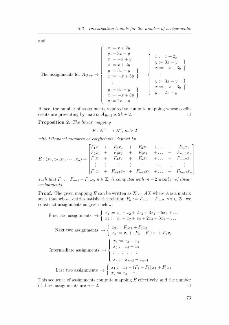
5.2. Investigating bounds for the number of assignments:
and
The assignments for A4k+6 →
x := x+ 2yy := 3x− yx := −x+ yx := x+ 2yy := 3x− yx := −x+ 3y
}...
y := 3x− yx := −x+ 3y
}y := 2x− y
=
x := x+ 2yy := 3x− yx := −x+ 3y
}...
y := 3x− yx := −x+ 3y
}y := 2x− y
Hence, the number of assignments required to compute mapping whose coeffi-cients are presenting by matrix A4k+2 is 2k + 2.Proposition 2. The linear mapping
E : Zm −→ Zm, m > 2
with Fibonacci numbers as coefficients, defined by
E : (x1, x2, x3, · · · , xn) =
F1x1 + F2x2 + F3x3 + . . . + FmxnF2x1 + F3x2 + F4x3 + . . . + Fm+1xnF3x1 + F4x2 + F5x3 + . . . + Fm+2xn... ... ... ... ... . . . . . . ...
Fnx1 + Fn+1x2 + Fn+2x3 + . . . + F2n−1xn
such that Fn := Fn−1 + Fn−2, n ∈ Z, is computed with m+ 2 number of linearassignments.
Proof. The given mapping E can be written as X := AX where A is a matrixsuch that whose entries satisfy the relation Fn := Fn−1 + Fn−2, ∀n ∈ Z. weconstruct assignments as given below:
First two assignments →{x1 := x1 + x2 + 2x3 + 3x4 + 5x5 + . . .x2 := x1 + x2 + x3 + 2x4 + 3x5 + . . .
Next two assignments →{x3 := F1x1 + F2x2x4 := x3 + (F2 − F1)x1 + F1x2
Intermediate assignments →
x5 := x3 + x4x6 := x4 + x5... ... ... ... ... ... .xn := xn−2 + xn−1
Last two assignments →{x1 := x3 − (F2 − F1)x1 + F1x2x2 := x3 − x1
This sequence of assignments compute mapping E effectively, and the numberof these assignments are n+ 2.
73

Chapter 5. In Situ Design of Computation for Linear Mappings over Integers
Next, we prove an identity that relates determinant of matrix of coefficientsto product of coefficients of assignments.
5.2.2 Identity (coefficient linkage):The sequence of linear assignments (with integer coefficients) that computemapping E has an interesting property to compute determinant of matrix Mc
corresponding to mapping E. To explore this property, we prove the followingidentity.
Theorem 6. Let E : Z2 −→ Z2 be a linear mapping defined as
E(x, y) −→ (mx+ ny, px+ qy)
with integral coefficients m, n, p, q ∈ Z. Let E be computable by a sequence oflinear assignments
x := a1x+ b1yy := b′1x+ a′1yx := a2x+ b2yy := b′2x+ a′2y... := ... ...x := akx+ bkyy := b′kx+ a′ky
where ai, a′i, bi, b′i ∈ Z are integral coefficients for each i = 1, . . . , k. Then theidentity
mq − pn = a1a′1 . . . aka
′k holds. (5.5)
Proof. Proof by induction on k.Base: For k = 1 we have x = a1x + b1y and y = a1b
′1x + (b1b
′1 + a′1)y, where
m = a1, n = b1, p = a1b′1, and q = b1b
′1 + a′1.
Hence we have mq − pn = a1(b1b′1 + a′1) − a1b1b
′1 = a1a
′1, that satisfies the
required identity 5.5. Step: Let the identity 5.5 holds for some k − 1, we willprove it for k.We have E(x, y) −→ (mx + ny, px + qy) computed by the aforementionedlinear assignment sequence of length k − 1. To this we apply the step k withx := akx + bky followed by y := b′kx + a′ky. After substitution we obtainx = akx+ bky and y = akb
′kx+ (bkb′k + a′k)y. We substitute x := mx+ ny and
y := px+ qy respectively in the right-hand sides, and obtain after some simplemanipulation, we have
x = (akm+ bkp)x+ (akn+ bkq)y = m′x+ n′y
y = (akb′km+ bkb′kp+ a′kp)x+ (akb′kn+ bkb
′kq + a′kq)y = p′x+ q′y.
Now we have new values for the coefficients m, n, p and q denoted by m′, n′, p′and q′ which are equal to m′ = akm+bkp, n′ = akn+bkq, p′ = akb
′km+bkb
′kp+
a′kp, q′ = akb′kn + bkb
′kq + a′kq. The expression m′q′ − p′n′, after a long and
74

5.2. Investigating bounds for the number of assignments:
tedious multiplication and elimination calculus, is equal to (mq− pn)aka′k. Byassumption hypothesis we have mq − pn = a1a
′1 . . . ak−1a
′k−1, what proves the
required identity.
Example 18. Let E : Z2 −→ Z2 be a linear mapping defined as
E(x, y) −→ (33x+ 307y, 103x+ 610y)
The coefficients of mapping can be represented by matrix as given below.
A =[
33 307103 610
]
determinant (A) = −11491 (5.6)Mapping E can be computed by the following sequence of linear assignments
Assignments
x := x+ 9yy := 3x+ yx := x+ 3yy := 2x+ yx := x+ yy := 8012x− 11491y
Product of coefficients ais = −11491 (5.7)
The identity (Theorem 6) helps in determining whether a sequence (of linearassignments) that computes the inverse mapping, exists or not. For example,for the mapping E : Z2 −→ Z2, a sequence that computes E−1, exists if R.H.Sof identity 5.5 becomes numerically equal to 1.
75

Chapter 5. In Situ Design of Computation for Linear Mappings over Integers
76

Chapter 6In Situ Design of Computation forBoolean Mappings
Contents6.1 Boolean Mappings . . . . . . . . . . . . . . . . . 78
6.2 Computing Bijective Boolean Mappings . . . 79
6.2.1 Explanation . . . . . . . . . . . . . . . . . . . . 81
6.2.2 Linearity Property . . . . . . . . . . . . . . . . . 83
6.3 Computing General Boolean Mappings . . . . 84
6.3.1 Simple Mappings . . . . . . . . . . . . . . . . . 85
6.3.2 Decomposing general boolean mappings . . . . . 86
6.4 IDC for Polynomials over GF(2) . . . . . . . . 91
6.4.1 A First Tool . . . . . . . . . . . . . . . . . . . . 92
6.4.2 Explanation and Construction . . . . . . . . . . 95
Decomposition of boolean functions is considered as an important problemin the design of logic circuits and the area of research is considered as old as thearea of digital circuit engineering. Boolean polynomials occur either directly oras a tool in the problem of decomposing boolean functions. The extensive useof integrated circuits that includes “modulo 2 adders”, in electronics, drawsattention towards the representation of boolean functions in the form of poly-nomials. Expressing boolean functions as boolean polynomials is consideredan extensive method in boolean algebra. Boolean polynomials have a largenumber of applications in various fields including graph theory, law, medicine,operations research and spectroscopy [Bei93, CH08, Leo98, MS77, Rud04].Polynomial methods have been employed extensively in circuit complexityand the boolean polynomials have variety of applications, e.g., they used inReed-Muller codes (error correcting codes). Besides a number of applications
77

Chapter 6. In Situ Design of Computation for Boolean Mappings
including text mining, knowledge discovery, role engineering, sequential com-putation of boolean mappings also leads to decomposition of boolean matricesand directed graphs. Burckel et al. [Bur96, BGT09, BM04b] proposed in situcomputation for boolean mappings and proved combinatorial results for thenumber of assignments involved. We illustrate these results in section 6.2 and6.3 as related work to provide general background. Section 6.1 gives basicconcept about boolean mappings whereas we propose strategy to develop se-quence of assignments that computes boolean mappings (through constructionof boolean polynomials) sequentially, in section 6.4.
6.1 Boolean MappingsBoolean mappings describe how to determine boolean valued output basedon some logical combinations from boolean inputs. These mappings can berepresented in propositional logic, or as multivariate polynomials over GF (2).These mappings are important in the theory of complexity as well as in thedesign of circuits/chips for digital computers. Besides, a number of applica-tions exist in different other areas including artificial intelligence, propositionallogic, electrical engineering, game theory, reliability theory and combinatorics.The properties of boolean mappings play a crucial role in cryptography, par-ticularly in the design of symmetric key algorithms (a class of algorithms forcryptography that use boolean function keys for both decryption and encryp-tion), e.g., two fish, Serpent, Blowfish, CAST5, RC4, TDES, and IDEA.Definition 6. A boolean mapping ‘f ’ is defined as
f : {0, 1}n −→ {0, 1}The set {0, 1}n, of all n-tuples (x1, · · · , xn), where each xi is either 0 or 1, isthe domain for ‘f ’. There are 22n, n-ary functions for every n.Example 19. Let E(y1, y2, y3) be the boolean mapping from {0, 1}3 to {0, 1}such that
y1 = x1 + x2 ∗ x3
y2 = x1 + x2 + x1 ∗ x3 + x1 ∗ x2 + x2 ∗ x3
y3 = x3 + x1 ∗ x2 + x2 ∗ x3
Components (y1, y2, y3) of the mapping E are expressed in the table 6.1 thathelps in verifying that the mapping E is bijective.
Definition 7. An in situ program that computes boolean mappings of the formE : {0, 1}n −→ {0, 1}n
consists in a sequence of assignments of one bit component defined as belowxj := fj (x1, · · · , xn)
where fj : {0, 1}n −→ {0, 1} is a linear mapping and j is the index for inputvariables.
78

6.2. Computing Bijective Boolean Mappings
x1 x2 x3 y1 y2 y30 0 0 0 0 00 0 1 0 0 10 1 0 0 1 00 1 1 1 0 01 0 0 1 1 01 0 1 1 0 11 1 0 1 1 11 1 1 0 1 1
Table 6.1: Boolean mapping
6.2 Computing Bijective Boolean MappingsBurckel et al. [BGT09] proved that a bijective mapping on the set Sn iscomputed by an in situ program involving 2n − 1 number of assignmentsprovided that n is the number of variables in the set of input variables. In thissection, we illustrate this result for the case S = {0, 1} in detail to provide afoundation for further work.
Theorem 7. A bijective mapping E defined over {0, 1}n can be computed byan in situ program of the form.
fn, fn−1, · · · , f3, f2, f1, g2, g3, · · · , gn−1, gn
with 2n− 1 number of assignments involved in the program.
Proof. For n = 1, the in situ program takes the form x1 := f1(x1). To provethat the statement is true for n > 1, bipartite graph is used. Suppose that G =(X, Y, A) be the bipartite multi-edges graph defined by X = Y = {0, 1}n−1,and (x, y) ∈ X × Y is in A with the label xnyn, for xnyn ∈ {0, 1} if and onlyif E(x, xn) = (y, yn).The degree of vertices of graph G will be exactly 2 due to the bijection Eand graph G will be the union of disjoint even cycles due to the reason thatit is 2-color-able regular bipartite graph. Therefore, by definition, graph Gis 2-color-able [Hav07]. This is a particular case of a general result by Königon regular graphs [Kön16], from which this proof can be generalized to anymapping on a finite set. Now, color the edges of G with elements of {0, 1}and define two mappings E0, E1 on {0, 1}n−1 and two mappings fn, gn from{0, 1}n to {0, 1} as follows.For each color i ∈ {0, 1} and every edge (x, y) with color i and labeled xnyn,define
Ei(x) = y
fn(x, xn) = i
gn(y, i) = yn
79

Chapter 6. In Situ Design of Computation for Boolean Mappings
By construction, any mapping Ei is bijective on {0, 1}n−1. Then under induc-tion hypothesis, each Ei admits an in situ program of the form:
f in−1, · · · , f i2, f i1, gi2, · · · , gin−1
Define, for every i ∈ {0, 1} and x ∈ {0, 1}n−1.
fj(x, i) = f ij(x) for j = n− 1, · · · , 1
gj(x, i) = gij(x) for j = 2, · · · , n− 1In other words,
fj(x, xn) = xn.f1j (x) + (1 + xn).f 0
j (x) for j = n− 1, · · · , 1
gj(x, xn) = xn.g1j (x) + (1 + xn).g0
j (x) for j = n− 1, · · · , 1By construction, for the bijective boolean mapping E, we obtain an in situprogram of length
2(n− 1)− 1 + 2 = 2n− 1as given below
xn := fn(x1, · · · , xn)xn−1 := fn−1(x1, · · · , xn) = f in−1(x1, · · · , xn−1)xn−2 := fn−2(x1, · · · , xn) = f in−2(x1, · · · , xn−1)
... ... ... ...x2 := f2(x1, · · · , xn) = f i2(x1, · · · , xn−1)x1 := f1(x1, · · · , xn) = f i1(x1, · · · , xn−1)x2 := g2(x1, · · · , xn) = gi2(x1, · · · , xn−1)... ... ... ...
xn−2 := gn−2(x1, · · · , xn) = gin−2(x1, · · · , xn−1)xn−1 := gn−1(x1, · · · , xn) = gin−1(x1, · · · , xn−1)xn := gn(x1, · · · , xn) = gn(y1, · · · , yn−1, i)
In other words at the first step, the component xn equals a color i, Then
Ei(x1, · · · , xn−1)
is computed by induction in 2(n − 1) − 1 steps. At the step before last, wehave
(x1, · · · , xn−1) = (y1, · · · , yn−1)At the last step we have xn = yn.
Next, we explain Theorem 7 by giving two different examples.
80

6.2. Computing Bijective Boolean Mappings
6.2.1 ExplanationThis section explains theorem 7 by examples.
Example 20. Suppose that E1 is a bijective boolean mapping defined over{0, 1}3 and is represented by the truth table 6.2. Mapping E1 can be computed
x1 x2 x30 0 00 0 10 1 00 1 11 0 01 0 11 1 01 1 1
E1−→
x1 x2 x30 0 01 1 10 0 10 1 11 0 10 1 01 0 01 1 0
Table 6.2: Table for mapping E1
by performing a sequence of operations, as given below.
x1 := 1 + x2 + x1x3 (f ′1)x2 := 1 + x1 + x2 + x1x3 + x2x3 + x1x2 (f ′2)x3 := x1 + x2 + x3 + x2x3 (f ′3)x2 := x1 + x2 + x1x3 (g′2)x1 := 1 + x1 + x2 + x3 + x2x3 (g′1)
Sequence of operations consists in two sub-sequences. After performing the firstthree operations f ′1, f ′2, f ′3, the mapping E1 transforms into another booleanmapping that is still bijective then we perform the second sequence of opera-tions g′2, g′1, and compute the mapping E1. Table 6.3 explains, how the givenmapping go through transformation process under the sequence of operations.The Intermediate truth table presents the given mapping after performing the
x1 x2 x30 0 00 0 10 1 00 1 11 0 01 0 11 1 01 1 1
f ′1, f
′2, f
′3−−−−−→
x1 x2 x31 1 01 1 10 0 10 1 11 0 10 1 00 0 01 0 0
g′2, g
′1−−−→
x1 x2 x30 0 01 1 10 0 10 1 11 0 10 1 01 0 01 1 0
Table 6.3: Transformation process
81

Chapter 6. In Situ Design of Computation for Boolean Mappings
sequence of first three operations. The final truth table shows the transfor-mation obtained after performing the sequence of next two operations on theintermediate truth table.
Next, we describe a second example to explain all steps involve in the com-putation of boolean bijective mappings.
Example 21. Let E2 be a bijective boolean mapping over {0, 1}3 as describedin the Table 6.4. Given bijective mapping E2 can be computed by performing
x1 x2 x30 0 00 0 10 1 00 1 11 0 01 0 11 1 01 1 1
E2−→
x1 x2 x31 1 10 1 11 1 00 0 10 0 01 0 11 0 00 1 0
Table 6.4: Bijective boolean mapping (example)
the following sequence of operations.
x1 := 1 + x1 + x2 + x3 + x2x3 (f ′1)x2 := x1 + x2 + x1x3 (f ′2)x3 := x3 + x1x2 (f ′3)x2 := x2 + x3 + x1x3 (g′2)x1 := x1 + x2 + x2x3 (g′1)
We illustrate step by step the transformation of bijective mapping E2 by apply-ing the above sequence of operations.
x1 x2 x30 0 00 0 10 1 00 1 11 0 01 0 11 1 01 1 1
f ′1−→
x1 x2 x31 0 00 0 10 1 00 1 10 0 01 0 11 1 01 1 1
f ′2−→
x1 x2 x31 1 00 0 10 1 00 1 10 0 01 0 11 0 01 1 1
Table 6.5: First Two Operations
82
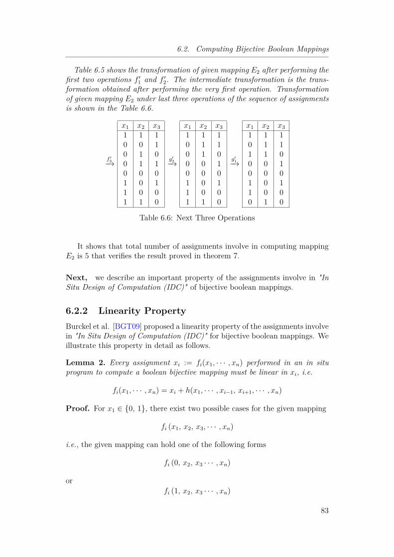
6.2. Computing Bijective Boolean Mappings
Table 6.5 shows the transformation of given mapping E2 after performing thefirst two operations f ′1 and f ′2. The intermediate transformation is the trans-formation obtained after performing the very first operation. Transformationof given mapping E2 under last three operations of the sequence of assignmentsis shown in the Table 6.6.
f ′3−→
x1 x2 x31 1 10 0 10 1 00 1 10 0 01 0 11 0 01 1 0
g′2−→
x1 x2 x31 1 10 1 10 1 00 0 10 0 01 0 11 0 01 1 0
g′1−→
x1 x2 x31 1 10 1 11 1 00 0 10 0 01 0 11 0 00 1 0
Table 6.6: Next Three Operations
It shows that total number of assignments involve in computing mappingE2 is 5 that verifies the result proved in theorem 7.
Next, we describe an important property of the assignments involve in "InSitu Design of Computation (IDC)" of bijective boolean mappings.
6.2.2 Linearity PropertyBurckel et al. [BGT09] proposed a linearity property of the assignments involvein "In Situ Design of Computation (IDC)" for bijective boolean mappings. Weillustrate this property in detail as follows.
Lemma 2. Every assignment xi := fi(x1, · · · , xn) performed in an in situprogram to compute a boolean bijective mapping must be linear in xi, i.e.
fi(x1, · · · , xn) = xi + h(x1, · · · , xi−1, xi+1, · · · , xn)
Proof. For x1 ∈ {0, 1}, there exist two possible cases for the given mapping
fi (x1, x2, x3, · · · , xn)
i.e., the given mapping can hold one of the following forms
fi (0, x2, x3 · · · , xn)
orfi (1, x2, x3 · · · , xn)
83

Chapter 6. In Situ Design of Computation for Boolean Mappings
For each of these cases, there exists two possibilities for the output value, thesepossibilities are as given below.
fi (0, x2, x3, · · · , xn) = 0 (a)fi (0, x2, x3, · · · , xn) = 1 (b)fi (1, x2, x3, · · · , xn) = 0 (c)fi (1, x2, x3, · · · , xn) = 1 (d)
In the computation of bijection, exactly, one of the equations from the pair (a,b) and one of the equations from the pair (c, d) will hold. Since the pairs ofequations (a, c) and (b, d) cannot hold simultaneously due to the bijection,therefore, the only two possible pairs of equations (a, d) and (b, c) will hold.But the pair (a, d) will define the mapping
fi (x1, x2, x3, · · · , xn) = x1
and the pair (b, c) defines
fi (x1, x2, x3, · · · , xn) = x1 + 1
Therefore for all cases
fi(x1, · · · , xn) = x1 + h(x2, · · · , xn)
where
h(x2, · · · , xn) =
0 for the pair (a, d)
and1 for the pair (b, c)
Hence for the ith component, we have
fi(x1, · · · , xn) = xi + h(x1, · · · , xi−1, xi+1, · · · , xn)
In the next section, we discuss the "In Situ Design of Computation (IDC)"for the case of general boolean mappings.
6.3 Computing General Boolean MappingsThe results included in this section have been proposed by Burckel et al. (seefor instance [BGT09] and related work). We are interested to illustrate theseresults (concerning general boolean mappings over {0, 1}n) in detail so that afoundation could be provided to proceed further. In general boolean mappings,it is possible that two different vectors may have the same image that is notthe case for bijective mappings. We start with the following definition.
84

6.3. Computing General Boolean Mappings
Definition 8. A mapping ‘f ‘ on the set {0, . . . ,M}, where, M > 0, is calleda step mapping if
0 ≤ f(y)− f(x) ≤ y − x
such that0 ≤ x ≤ y ≤M
In particular one can have the following
f(x) ≤ f(x+ 1) ≤ f(x) + 1
Next, we discuss simple mappings.
6.3.1 Simple MappingsSimple mapping can be defined by making use of definition 8 and the mapping
φ : {0, 1}n −→ {2n}
defined as given below
φ(x1, x2, x3, . . . , xn) = 2n−1.xn + . . .+ 22.x3 + 2.x2 + x1, ∀ n > 0
Definition 9. A mapping E on {0, 1}n is called a simple mapping if
E(x) = y ⇔ E ′(φ(x)) = φ(y)
is a step mapping, where, E ′ is a mapping on [2n].
Proposition 3. A simple mapping E on {0, 1}n, ∀ n > 0, can be computedby an in situ program of the form
p1, p2, . . . , pn
with a length of ‘n’ assignments.In brief, for E(x1, x2, x3, . . . , xn) = y1, y2, y3, . . . , yn and for each i = 1, 2, . . . n
pi(y1, . . . , yi−1, xi, . . . , xn) = yi
Proof. Since the minimum number of assignments for n input variables is n.Therefore each function pi must return its correct final value to each of itscorresponding component xi. This method for in situ computation of simplemapping is unique possible. However the correctness of this method is stillremains to prove due to the fact that the mappings being computed are simple.
Next, we describe the "In Situ Design of Computation (IDC)" for the generalboolean mappings.
85

Chapter 6. In Situ Design of Computation for Boolean Mappings
6.3.2 Decomposing general boolean mappingsIn this section, we explain "In Situ Design of Computation (IDC)" of generalboolean mappings. The idea consists in decomposing the mapping E of {0, 1}nin F ◦ P ◦G where F and G are bijective and P is simple.
Definition 10. Suppose that E be a mapping on {0, 1}n. A triple (F, P, G)on {0, 1}n, with n > 0, of mappings is called a decomposition of the mapping’E’ if
E = F ◦ P ◦G
where, F and G are bijective mappings and P is a simple mapping.
Procedure
Suppose that E be the mapping on {0, 1}n, the decomposition procedurefor the mapping E consists in the following steps.
Step 1. In the first step, vectors with the same images are grouped via a bijectivemapping G that gives intermediary consecutive images in lexicographicalorder to vectors with same final images. This will actually maps the setsE−1(x) for x ∈ {0, 1}n onto consecutive intervals of [2n] via φ ◦G.
Step 2. The second step consists in the identification of vectors with the samefinal image via a simple mapping P such that φ◦P ◦φ−1 maps consecutiveintervals of [2n] on consecutive values of [2n].
Step 3. The third step consists in the attribution of the correct final image valueto each vector obtained by P ◦G via another bijective mapping F , thatis F (P (G(x))) = E(x). Then F is completed arbitrarily to a bijectivemapping on {0, 1}n.
Next, we explain the result regarding an upper bound of the program thatcompute general boolean mappings.
Corollary 1 (see [BGT09] for more general case). Every mapping E on {0, 1}ncan be computed by an in situ program of the form
f1, . . . , fn, gn−1, . . . , g1, p2, . . . , pn−1, f′n, . . . , f
′1, g
′2, . . . , g
′n
such that the number of assignments (involve in the program) is 5n− 4.
Proof. The procedure (6.3.2) of decomposition (given above) is used in con-structing the proof. Suppose that E = F ◦ P ◦G, i.e., the triple (F, P, G) bethe decomposition of E, with F and G are bijective mappings and P is a simplemapping. Both of the mappings F and G can be computed by a sequence of2n−1 number of assignments (see Theorem 7). Similarly, the simple mapping
86
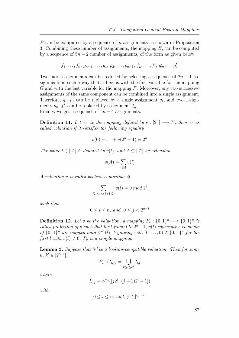
6.3. Computing General Boolean Mappings
P can be computed by a sequence of n assignments as shown in Proposition3. Combining these number of assignments, the mapping E, can be computedby a sequence of 5n− 2 number of assignments, of the form as given below
f1, . . . , fn, gn−1, . . . , g1, p2, . . . , pn−1, f′n, . . . , f
′1, g
′2, . . . , g
′n
Two more assignments can be reduced by selecting a sequence of 2n − 1 as-signments in such a way that it begins with the first variable for the mappingG and with the last variable for the mapping F . Moreover, any two successiveassignments of the same component can be combined into a single assignment.Therefore, g1, p1 can be replaced by a single assignment g1, and two assign-ments pn, f ′n can be replaced by assignment f ′n.Finally, we get a sequence of 5n− 4 assignments.
Definition 11. Let ‘v’ be the mapping defined by v : [2n] −→ N, then ‘v’ iscalled valuation if it satisfies the following equality
v(0) + . . .+ v(2n − 1) = 2n
The value l ∈ [2n] is denoted by v(l), and A ⊆ [2n] by extension
v(A) =∑l∈A
v(l)
A valuation v is called boolean compatible if∑j2i≤l<(j+1)2i
v(l) = 0 mod 2i
such that0 ≤ i ≤ n, and, 0 ≤ j < 2n−i
Definition 12. Let v be the valuation, a mapping Pv : {0, 1}n −→ {0, 1}n iscalled projection of v such that for l from 0 to 2n−1, v(l) consecutive elementsof {0, 1}n are mapped onto φ−1(l), beginning with (0, . . . , 0) ∈ {0, 1}n for thefirst l with v(l) 6= 0. Pv is a simple mapping.
Lemma 3. Suppose that ‘v’ be a boolean-compatible valuation. Then for somek, k′ ∈ [2n−i],
P−1v (Ii,j) =
⋃k≤l≤k′
Ii,l
whereIi, j = φ−1([j2i, (j + 1)2i − 1])
with0 ≤ i ≤ n, and, j ∈ [2n−i]
87

Chapter 6. In Situ Design of Computation for Boolean Mappings
Proof. Suppose that the interval of [2n] is the converse image of an intervalof {0, 1}n mapped by the mapping φ. Observe that, the converse image of aninterval {0, 1}n is also an interval of {0, 1}n mapped under the mapping Pv(due to the reason that Pv is a simple mapping). Therefore, by definition ofPv, it gives
|P−1v (Ii,j)| =
∑j2i≤l<(j+1)2i
v(l)
For all l ∈ φ(I, i, j), if v(l) = 0 then P−1v (Ii,j) may be empty and it is given
that v is a boolean compatible. Therefore, it gives∑j2i≤l<(j+1)2i
v(l) = 0 (mod 2i)
Thus|P−1v (Ii,j)| = 0 (mod 2i)
By induction on j and for a fixed i, the result can be proved. Thus, if j = 0then
|P−1v (Ii,0)| = k.2i, for some, k ∈ [2n−i]
Now, suppose that P−1v (Ii,0) is not empty, then by using definition of the
projection Pv, it is an interval of {0, 1}n containing (0, . . . , 0). The length ofthis interval is k.2i which is the multiple of the factor 2i, so, it is of the formas given below ⋃
0≤l≤kIi,l
Further, if the property is true for all l with 0 ≤ l < j, then
P−1v (
⋃0≤l<j
Ii,l) =⋃
0≤l<j′Ii,l
Since|P−1v Ii,j| = k.2i, for some k ∈ [2n−i]
we must haveP−1v (
⋃0≤l≤j
Ii,l) =⋃
0≤l≤j′+kIi,l
HenceP−1v (Ii,j) =
⋃j′<l≤j′+k′
Ii,l
Lemma 4. Suppose that v be a boolean compatible valuation and 1 ≤ i ≤ n.For a, b ∈ {0, 1}n and l ≥ i, if al = bl, then
Pv(a)l = Pv(b)l , ∀ l ≥ i
88

6.3. Computing General Boolean Mappings
Proof. Suppose that al = bl, for l ≥ i. Also, suppose that c ∈ Sn, where,S = {0, 1} is given as under
cn = an = bn, . . . , ci = ai = bi, ck−1 = 0, . . . , c1 = 0
It givesφ(c) = 0 (mod 2i−1)
Thus for j ∈ [2n−i+1]φ(c) = j.2i−1
Moreover, φ(a) and φ(b) are in the same interval [j.2i−1, (j + 1).2i−1 − 1]whose elements have same components for l ≥ i. It gives that a and b belongto Ii−1,j. Now, using Lemma 3, the inverse images of intervals of the form Ii−1,kby projection Pv are unions of such consecutive intervals. Hence the image ofan interval Ii−1,j by projection Pv is an interval contained in an interval Ii−1,kfor some k ∈ [2n−i+1].Hence for l ≥ i, Pv(a) and Pv(b) have the same components.
Proposition 4 ([BGT09]). Let E be a bijective mapping on {0, 1}n and iscomputable by an in situ program of the form f1, . . . , fn. Then the mappingE ◦ Pv (where v is a boolean compatible valuation) is computed by an in situprogram of the form p1, p2, . . . , pn. That is for E(x1, x2, . . . , xn) = (y1, . . . , yn)and for each i = 1, 2, . . . , n:
pi(y1, . . . , yi−1, xi, . . . , xn) = yi
Proof. To prove the assertion, the same argument is used as for the computa-tion of simple mappings, i.e., due to the fact that the number of assignmentsis minimal, necessarily each function pi must gives its correct final value toeach component xi. But the correctness of the method is still to be proved.On contrary basis, suppose that, at some step i, two different vectors x, x′become the same vector, say z, whereas their final images y = E ◦ Pv(x) andy′ = E ◦Pv(x′) are different. Because, now, they become the same vector, onehas
yi−1 = y′i−1 = zi−1, . . . , y1 = y′1 = z1
On the other side, one has
xn = x′n = zn, . . . , xi = x′i = zi
which implies, by Lemma 4
Pv(x)l = Pv(x′)l = z′l , ∀ l ≥ i
Now, suppose thatPv(x) 6= Pv(x′)
89

Chapter 6. In Situ Design of Computation for Boolean Mappings
Since E is bijective, therefore, the mapping E ′ programmed by the sequencef1, . . . , fi−1 is also bijective. But since E is programmed by f1, . . . , fn, where,each component is modified at most once, it gives
E ′(Pv(x)) = E ′(Pv(x′)) = (z′n, . . . , z′i, z′i−1, . . . , z1)
A contradiction. Hence Pv(x) = Pv(x′) and y = y′
Definition 13. A boolean compatible decomposition of E defined over {0, 1}nfor n > 0 is a triple of mappings (F, P, G) on {0, 1}n, such that E = F ◦P ◦Gwith F and G are bijective mappings and P is the projection Pv of a booleancompatible valuation v = v′ ◦σ, where v′(l) is the number of elements of whichimage by E is φ(l).
The construction of boolean compatible decomposition of a mapping isexplained by the following Algorithm.
Algorithm 4: Boolean Compatible DecompositionAlgorithm: How to build a boolean compatible decompositionDefine a valuation v by v(l) = |E−1(φ(l))|;Define a permutation σ such that v ◦ σ is boolean-compatible;Define a bijection G of {0, 1}n compatible with v ◦ σ;begin
Set i=0;for l from 0 to 2n − 1 do
for j from 1 to v ◦ σ(l) dofor every x ∈ {0, 1}n with E(x) = φ(l) do
G(x):=φ−1(i);i:=i+1;
endend
endDefine P = Pv;Define a bijection F of {0, 1}n such that E = F ◦ P ◦G;foreach element x ∈ {0, 1}n do F(P(G(x))):=E(x);
endComplete the definition of F, keeping F bijective.
Theorem 8 (see [BGT09] for more detail). Every mapping E on {0, 1}n iscomputed by an in situ program of the form as given below
f ′′1 , . . . , f′′n , g
′′n−1, . . . , g
′′2 , f1, . . . , fn, g
′n−1, . . . , g
′1
such that the number of assignments involve is 4n− 3.
90

6.4. IDC for Polynomials over GF(2)
Proof. Suppose that the triple (F, P, G) be boolean-compatible decomposi-tion (by definition 13) of the mapping E. Now, since, F and G are bijectivemappings, therefore, by Theorem 7, it requires 2n− 1 assignments to computemappings F and G. Let
f ′1, . . . , f′n, g
′n−1, . . . , g
′1
be the sequence of 2n− 1 assignments that compute mapping F and let
f ′′1 , . . . , f′′n , g
′′n−1, . . . , g
′′1
be the sequence of 2n− 1 assignments that compute mapping G respectively.Now, suppose that F ′ be the mapping on {0, 1}n computed by the sequence
f ′1, . . . , f′n
Then by Proposition (4), the mapping F ′ ◦ P is computed by a sequence of nassignments of the form
f1, . . . , fn
Thus, the given mapping E is computed by sequence of assignments as givenbelow
f ′′1 , . . . , f′′n , g
′′n−1, . . . , g
′′1 , f1, . . . , fn, g
′n−1, . . . , g
′1
such that the number of assignments is 4n− 2, and the indices are the indicesof the concerned variables. Notice that the assignments g′′1 , f1 can be replacedby a single assignment g1. It results that the required number of assignmentsis 4n− 3.
Next, we introduce method to construct IDC by constructing polynomialsover GF (2) with respect to set of boolean mappings.
6.4 IDC for Polynomials over GF(2)Investigating decomposition of functions with respect to a given system offunctions is a traditional problem of the theory of boolean functions. Decom-posing boolean function is an important problem that deals with answeringtheoretical questions of the theory of boolean functions as well as in technicalapplications [VP93]. Some discussions about the polynomial form of booleanfunctions and its applications are presented in [Fal99, Sch98]. In this section,in the context of lemma 2 and discussion in previous sections, we propose astrategy to develop sequence of assignments (via boolean polynomials) thatcomputes boolean bijective mappings. We start in constructing polynomialsover GF(2) with respect to set of boolean mappings
y1, y2, . . . , yi−1, yi, yi+1, . . . , yn
91

Chapter 6. In Situ Design of Computation for Boolean Mappings
and a set of their corresponding inverse mappings
x1, x2, . . . , xi−1, xi, xi+1, . . . , xn
linear both in yi and xi. Construction of such polynomials enables to develop’IDC’ for bijective boolean mappings. As preliminary, GF (2) (Galois field oftwo elements) is a finite field of elements 0 and 1 with the properties of additionand multiplication as given in the Table 6.7.
+ 0 10 0 11 1 0
and,∗ 0 10 0 01 0 1
Table 6.7: Properties of GF (2)
Next, we describe strategy that construct polynomials over GF (2) with re-spect to set of boolean mappings and termed as “A First Tool“.
6.4.1 A First ToolThis strategy consists in constructing polynomials over GF(2) with respect toset of boolean mappings such that the polynomials are linear with respect tothe ith (say) mapping and its corresponding inverse image. The strategy worksinductively and yields ’IDC’ to compute boolean bijective mappings. Let Ebe a bijective boolean mapping of dimension n such that
Set of booleanmappings→
y1 := f1 (x1, x2, x3, · · · , xn)y2 := f2 (x1, x2, x3, · · · , xn)y3 := f3 (x1, x2, x3, · · · , xn)... ... ... ... ... ... ... ...yi := fi (x1, x2, x3, · · · , xn)... ... ... ... ... ... ... ...yn−1 := fn−1 (x1, x2, x3, · · · , xn)yn := fn (x1, x2, x3, · · · , xn)
(SBM)
We are interested to compute polynomial linear with respect to mapping yiand its inverse mapping xi. For this purpose we proceed as follows.
Constructing Inverse Mappings
As a first step, we compute inverse images for each of the boolean mappings
y1, y2, . . . , yi−1, yi, yi+1, . . . , yn
92

6.4. IDC for Polynomials over GF(2)
Corresponding to the set of boolean mappings (SBM), we denote by (SIM),the set of inverse images, as given below
Set of inverseimages→
x1 := g1 (y1, y2, y3, · · · , yn)x2 := g2 (y1, y2, y3, · · · , yn)x3 := g3 (y1, y2, y3, · · · , yn)... ... ... ... ... ... ... ...xi := gi (y1, y2, y3, · · · , yn)... ... ... ... ... ... ... ...xn−1 := gn−1 (y1, y2, y3, · · · , yn)xn := gn (y1, y2, y3, · · · , yn)
(SIM)
Computing Possible Products
Compute all possible products of boolean mappings contained in the set (SBM),i.e., compute possible products of permutations of
y1, y2, . . . , yi−1, yi, yi+1, . . . , yn
These products are of the form as given below.
Possible products→
y1y2, y1y3, · · · , y1yny2y3, y2y4, · · · , y2yny3y4, y3y5, · · · , y3yn... ... ... ... ... ...y1y2y3, y1y2y4, · · · , y1y2yny1y3y4, y1y3y5, · · · , y1y3yn... ... ... ... ... ... ... ...y1y2y3y4, y1y2y3y5, · · · , y1y2y3yny1y2y3y4y5, y1y2y3y4y6, · · · , y1y2y3y4yn... ... ... ... ... ... ... ... ... ... ...
Computing Possible Products of Inverse Mappings
Compute all possible products for the set of mappings (SIM), i.e., computethe possible products of permutations of
x1, x2, . . . , xi−1, xi, xi+1, . . . , xn
93

Chapter 6. In Situ Design of Computation for Boolean Mappings
These products will be of the form as given below.
Possible products ofinverse mappings→
x1x2, x1x3, · · · , x1xnx2x3, x2x4, · · · , x2xnx3x4, x3x5, · · · , x3xn... ... ... ... ... ...x1x2x3, x1x2x4, · · · , x1x2xnx1x3x4, x1x3x5, · · · , x1x3xn... ... ... ... ... ... ... ...x1x2x3x4, x1x2x3x5, · · · , x1x2x3xnx1x2x3x4x5, x1x2x3x4x6, · · · , x1x2x3x4xn... ... ... ... ... ... ... ... ... ... ...
Require
For an ith mapping of the set (SBM) and the corresponding inverse mappingof the set (SIM), the following equality must be satisfied
yi + hi (y1, y2, . . . , yi−1, yi+1, . . . , yn) = xi + hi (x1, x2, . . . , xi−1, xi+1, . . . , xn)(6.1)
Establishing the System
To satisfy equality 6.1, establish a system of equations. For this purpose,introduce a set of coefficients
c1, c2, . . . , ci−1, ci+1, . . . , cn
and start in generating one side of the equality 6.1, for instance, for ith com-ponent, one of the possible expressions could be of the form
yi + a1y2 + a2y3 + a3y2y3 + . . . (6.2)
Then, compute values for the coefficients and evaluate the expression 6.2.Finally, one can get the required polynomial by substituting back the valuesof these coefficients and evaluating the corresponding expression.
A quick view of the procedure is given in the figure 6.1, where, ‘SBM’ de-notes the set of boolean mappings (corresponding to bijective mapping) and‘SIM’ denotes the set of inverse images corresponding to the set ‘SBM’. Yellowbar shows the process of establishing and evaluating the system of equations.Different steps included in the process are shown by arrows.
94

6.4. IDC for Polynomials over GF(2)
SBM FIELD SIM
Required Polynomial
Products
Set of Inverse mappings
Set of bijective mappings
Figure 6.1: Interpretation of ”A First Tool”
In this way, we develop basic step (as given below) that leads to constructIDC through polynomials over GF (2).
y1 + h1 (y2, y3, . . . , yi−1, yi, yi+1, . . . , yn) :=x1 + h1 (x2, x3, . . . , xi−1, xi, xi+1, . . . , xn)
}This polynomial (basic step) provides two assignments, the first assignmentand the last assignment, that are involve in computing bijective boolean map-pings.
6.4.2 Explanation and ConstructionIn this section, we explain method "A First Tool" by constructing the firstrequired polynomial over GF(2). Let E : (x1, x2, x3) → (y1, y2, y3) be abijective mapping (see table 6.8), such that
y1 := 1 + x2 + x1x3y2 := 1 + x1 + x2 + x1x2 + x2x3 + x1x3y3 := x1 + x2 + x3 + x2x3
(SB)
To compute polynomial linear both in y1 as well as in x1, we compute thepossible products as given below:
Possible products→
y1y2 := 1 + x1 + x2 + x1x2y1y3 := x1 + x3 + x1x2 + x2x3y2y3 := x3 + x1x3y1y2y3 := x3 + x2x3 + x1x3 + x1x2x3
Then, corresponding to the set of boolean mappings (SB), we compute a setof inverse mappings as shown below.
Set of inversemappings→
x1 := 1 + y1y3 + y2y1 + y3x2 := 1 + y1y3 + y2y3 + y2x3 := y1 + y2 + y1y3
(SI)
95

Chapter 6. In Situ Design of Computation for Boolean Mappings
x1 x2 x3 y1 y2 y30 0 0 1 1 00 0 1 1 1 10 1 0 0 0 10 1 1 0 1 11 0 0 1 0 11 0 1 0 1 01 1 0 0 0 01 1 1 1 0 0
Table 6.8: Bijective Mapping E
Then, we compute the possible products for the set of inverse mappings (SI),that are listed below
Possible products ofinverse mappings→
x1x2 := 1 + y2 + y3 + y2y3x1x3 := y1 + y2 + y1y3 + y2y3x2x3 := y1 + y2y3 + y1y3 + y2y1x1x2x3 := y1 + y1y3 + y2y1 + y1y3y2
Now, we introduce three coefficients, α, β and γ. To construct the requiredpolynomial, we need to make an expression of the form
y1 + αy2 + βy3 + γ(y2 ∗ y3) (6.3)
that gives
y1 + αy2 + βy3 + γ(y2 ∗ y3) =
(1 + x2 + x1x3)
+ α (1 + x1 + x2 + x1x2 + x2x3 + x1x3)+ β (x1 + x2 + x3 + x2x3)+ γ (x3 + x1x3)
Establish a system of equations by comparing the coefficients (in the aboveequality) of unwanted products, e.g., x1x3 etc. Therefore
1 + α + γ = 0 (comparing coefficients of x1x3)α = 0 (comparing coefficients of x1x2)α + β = 1 (comparing coefficients of x1)
It givesα = 0, β = 1, and γ = 1
Substituting these values of α, β and γ in (6.3), we get the required polynomial
x2x3 + x1 := 1 + y1 + y2y3 + y3 (6.4)
that is linear in y1 and x1. This is the basic step that leads to design sequenceof "In Situ Design of Computation (IDC)" for the boolean bijective mappingE.
96

6.4. IDC for Polynomials over GF(2)
Example 22. Let E : (x1, x2, x3)→ (y1, y2, y3) be boolean bijective mappingsuch that
y1 := x1 + x2x3 + x1x3y2 := x1 + x2 + x1x2 + x2x3y3 := x1 + x1x2 + x2x3 + x1x3 + x3
(Set of mappings)
where, table 6.9 presents boolean values that construct boolean bijective mappingE. Let A denotes polynomial over GF(2) linear both in y1 as well as in x1.
x1 x2 x3 y1 y2 y30 0 0 0 0 00 0 1 0 0 10 1 0 0 1 00 1 1 1 0 01 0 0 1 1 11 0 1 0 1 11 1 0 1 1 01 1 1 1 0 1
Table 6.9: Bijective Mapping E
There are two such polynomials for the set of mappings y1, y2 and y3. One ofthem is written as follows:
A := x2x3 + x1 + x2 + x3 = y1 + y2 + y3 (6.5)
Polynomial (6.5) leads to generate ’IDC’ for the mapping E by performing thefollowing steps:
• Construct first assignment by setting A equals x1 asx1 := x2x3 + x1 + x2 + x3 (6.6)
• Construct two mappings E1 and E2 by letting A = 0 and A = 1 respec-tively.
Table 6.10 presents mapping E1 and Table 6.11 presents mapping E2. Mappings
x2 x3 y2 y30 0 1 10 1 0 11 0 1 01 1 0 0
Table 6.10: Mapping E1
presenting table 6.10 are defined as
y2 = 1 + x3
y3 = 1 + x2
97

Chapter 6. In Situ Design of Computation for Boolean Mappings
• Construct polynomial linear in x2 and y2 and is given belowx2 + x3 = y2 + y3
Now, sequence of ’IDC’ that computes mapping E1 isx2 := x2 + x3x3 := 1 + x2 + x3x2 := x2 + x3
(IDC for E1)
x2 x3 y2 y30 0 0 00 1 1 11 0 1 01 1 0 1
Table 6.11: Mapping E2
Mappings presenting table 6.11 are defined asy2 = x2 + x3
y3 = x3
• Construct polynomial linear in x2 and y2 and that isx2 + x3 = y2
Now, sequence of ’IDC’ that computes mapping E2 isx2 := x2 + x3x3 := x3x2 := x2
(IDC for E2)
• Combine the sequence of IDC for E1 and the sequence of IDC for E2 asgiven below
x2 := (1 + x1)(x2 + x3) + x1(x2 + x3)x3 := (1 + x1)(x3) + x1(1 + x2 + x3)x2 := (1 + x1)(x2) + x1(x2 + x3)
It gives three intermediate assignments as given belowx2 := x2 + x3
x3 := x1 + x3 + x1x2
x2 := x2 + x1x3
• Construct the sequence of ’IDC’ that computes mapping E as follows:
x1 := x1 + x2 + x3 + x2x3x2 := x2 + x3x3 := x1 + x3 + x1x2x2 := x2 + x1x3x1 := x1 + x2 + x3
(IDC for E)
98

Conclusion of the part
The strategies for in situ computation of mappings provide a strong foundationto proceed further in this direction of research and to enhance the capabilities ofsequential computations. Along with, a quick glance of applications in matrixdecomposition, it motivates to implement the idea in circuit/chip design. Anumber of publications (see for instance [Pin99]) could be found for furthermotivations. The idea of in situ computation is a great effort in contributing tooptimization (for example processor/compiler/memory) and could be extendedfurther by finding real applications and implementations. But still there arelimitations that need attention to be resolved and the strategies need somemodifications to deal with such limitations.
To highlight these limitations, in chapter 3, we have explained the idea ofin situ computation for mappings over fields and provided counter examplethat leads towards the modifications of the existing approach. An alternateapproach (using Bézout’s Identity) to generate sequence of assignments thatperforms in situ computation for mappings with two dimensions has been dis-cussed but the idea needs its further extension for general case and it requiresto investigate the possibility for the case of integers.
Similar limitations are observed in the case of rings and are highlighted byproviding counter example in generating sequence of assignments (from thesequence of assignments that compute given mappings) to compute inversemappings. Thus, current approach requires modifications to deal with suchsituations and could be applied possibly in different way.
In case of integers, (chapter 5), the combinatorial results and counter ex-amples show that there are certain limitations for in situ strategies and itrequire improvements and modifications. For example, reducing the numberof assignments (involved in computation), providing the possibility to generatesequence of assignments that could compute inverse mapping and extendingthe approach for general case. Moreover, in reducing number of assignments,we have to deal carefully with some situations, e.g, packing similar assignments
99

Chapter 6. In Situ Design of Computation for Boolean Mappings
(involved in computation) may results in an assignment with a co-efficient tobe multiplied.
A tool for generating sequence of assignments (chapter 6) for in situ com-putation of bijective boolean mappings through construction of polynomialsover GF(2) is a basic attempt to develop the required strategy. But still, it re-mains to extend the idea for general case and to find some useful combinatorialresults.
100

Part II
Decentralized CollaborativeEditing
101


Chapter 7Collaborative Editing System
Contents7.1 Introduction . . . . . . . . . . . . . . . . . . . . 103
7.1.1 A Collaborative Editing Scenario . . . . . . . . 1047.1.2 Pessimistic Concurrency Control . . . . . . . . . 1057.1.3 Optimistic Concurrency Control . . . . . . . . . 1067.1.4 Group Communication . . . . . . . . . . . . . . 1067.1.5 Centralized collaborative editing systems . . . . 1067.1.6 Decentralized collaborative editing systems . . . 108
7.2 DCE Model . . . . . . . . . . . . . . . . . . . . . 1117.2.1 Framework Description . . . . . . . . . . . . . . 1137.2.2 Editing a Document . . . . . . . . . . . . . . . . 1147.2.3 Modifying a Document . . . . . . . . . . . . . . 1157.2.4 Mapping between elements and Identifiers . . . 115
7.1 IntroductionCollaborative Editing Systems (CES), provide environment to group of users,dispersed geographically, so that they can edit/modify the same data concur-rently. For this purpose, collaborative editing tools have been designed thatenable authorized users to edit/modify a shared document, to see who elseis working over the same document and to know in real time, the changesthat are being made by others. Wikis, on-line office suites and version controlsystems are the most popular collaborative editing tools [Cit07]. The shareddocuments are similar to wikis in the sense that a number of users can makemodification by adding or deleting the content. Some of the collaborativeediting tools facilitate users to communicate by instant messaging (like a chat
103

Chapter 7. Collaborative Editing System
session) as an addition to collaborative editing. As an example, Wikipedia isedited by 7.5 millions of users and got 10 millions of articles in only six years[WUM09].
7.1.1 A Collaborative Editing ScenarioTo understand, how the collaborative editing works, consider a collaborativeediting scenario as presented in the Figure 7.1.
Three users are participating in editing a shared document contained aninitial content ”behave”. The elapse of time is shown by vertical lines. Anoperation generated locally is presented by circle and is executed immediately.The propagation of local operations to other sites are presented by arrows.Suppose that user-1 inserts character “r“ at position 2 of the initial content,
behave behavebehave
brave brave brave
User 1 User 2 User 3
Site 1 Site 2 Site 3
Op1: Insert 'r' at pos 2
Op2: Delete 'e'
Op3: Delete 'h'
Op1 Op2
Op3
Figure 7.1: A collaborative editing scenario
and user-2 deletes character “e“ at position 2, simultaneously. Each replicais updated after the execution of operations “Op1“ and “Op2“ so that user-3has replica modified to “brhave“. Now user-3 performs operation “Op3“ anddeletes “h“ at position 3 of the modified copy of the initial content. Updatingthe document after executing operation ”Op3” results in containing the finalcontent as ”brave”.
Another simple example of collaborative editing is shown in Figure 7.2 (nextpage), where INRIA research centres are joined with each other. Suppose users
104

7.1. Introduction
at different centres participate in editing an INRIA Research Report. A welldefined collaborative editing system (for example, INRIA Gforge) makes itpossible that all users can write a common research report.
Research Report
Nancy Grand-Est
Rocquencourt-Paris
Rennes
Lille Grenoble
Bordeaux
Saclay
Sophia Antipolis
Replay Replication Stream
Forward Update Request
Figure 7.2: An example of collaborative editing
To make it possible that all participants in real time collaborative editing,edit and view the shared document, almost at the same time, some kind of syn-chronization strategies between the participants must be used. Traditionally,there exist two synchronization control approaches, in reaching this behavior[Pre07], they are pessimistic concurrency control (lock based) and optimisticconcurrency control (lock free).
7.1.2 Pessimistic Concurrency ControlPessimistic concurrency control (Lock based editing), is based on acquiringa lock before starting edition for a given object/document. When a lock isapplied to facilitate one user, all other participants have to wait until the lockis released. Therefore, only one user can edit a given object/document at atime, that in some ways limits the parallel nature of collaborative editing.Briefly, it can be described in the following three steps.
• Acquire the lock on the object “O“, given that it is not already acquired.
• Perform some edits to the object.
• Release the lock on the object ”O”.
Another relevant issue with lock based editing is when a participant activelyediting an object, it crashes or leaving the object locked forever.
105

Chapter 7. Collaborative Editing System
7.1.3 Optimistic Concurrency ControlA fast response and high degree of concurrency is the need of Real-time Ap-plications. Optimistic concurrency control has the properties of non-blockingand deadlock freedom, they are especially recommended to real-time trans-action processing [HCL90, HSRT91, JS92]. Lock free editing, or optimisticconcurrency control, allows participants to more freely modify an object in amore parallel nature. However, there are risks of conflicts that needs somekind of algorithms to resolve these conflicts automatically. Further, it mayresults in loss of data, when, for example, a user’s edits are overwritten duringthe conflict resolving [CMR07, JBC05].
Collaborative editing between more than two participants require somekind of group communication. However, different collaboration strategies re-quire different styles of group communication guarantees.
7.1.4 Group CommunicationGroup communication allows reliable messaging between senders and receiverscomprise a network. In the basic form of group communication, two userscommunicate with each other while others wait for their turn. Some of theproblems regarding group communication (for instance, reliability and order-ing) are addressed using different techniques but still there exist some otherproblems, when multi users are participating simultaneously. More difficultproblems occur in providing the reliability for transmission and ordering ofpackets etc [Å10].
Total Ordering
To maintain the consistency among the replicas, a total ordering on the up-dates must be provided. Total ordering within group communication guar-antees that all broadcast messages will be received in the same order, by allrecipients. Being able to totally order the events can be very useful in imple-menting distributed system. To see the importance of total ordering consideran example of two clients C1 and C2. Suppose these two clients send updatesfor a document “D” simultaneously, Suppose these updates are totally ordered,so the servers either S1 receive first the update from C1 and then the updatefrom C2 or S2 receive first the update from C2 and then the update from C1.In both cases, the replicas will remain consistent, since every server applies up-dates in the same order. If these updates are not totally ordered, the serverscan apply updates in different orders that will cause the consistency problem[Å10].
7.1.5 Centralized collaborative editing systemsIn centralized systems, the messages have to go through a round trip and userscannot see their own actions immediately. Therefore, local commands (includ-
106

7.1. Introduction
ing lock requests) are not of responsiveness. Existing collaborative editingsystems such as CVS, RCS or WIKIs are centralized and unanimously adoptthe client-server architecture. The server node holds a persistent copy of shareddocument. Each client node stores a copy of the shared document. A user at aclient node updates the shared document through the local copy. All updatesare synchronized to other users through the server node. Such systems cannotbe adapted to peer-to-peer networks [OUMI06].
Below, we discuss some collaborative editing systems keeping the order oftheir restrictiveness on collaboration.
RCS
RCS (Revision Control System) is a version control system where a single ormultiple users modify document through an explicit check-out step. In RCS,when user attempts to check in a new version whose modifications are basedon a state version, editing conflicts occur. To detect these editing conflicts,RCS uses a locking mechanism. It notifies impacted users through diagnosticmessages. Usually RCS is being used to handle source code in software de-velopment, however, it is also used to support wiki applications, e.g., Twiki[twi10].
MediaWiki
In MediaWiki, users are able to edit different parts of a document withoutinterference. If multi-user edit the same paragraph simultaneously, it causesediting conflicts. A user releases edits by clicking a button manually. Medi-aWiki uses diff3 [com10] to merge changes, automatically, that make by usersbut these changes should be made in different parts of the document, otherwise,impacted users are notified by diagnostic messages. MediaWiki is working asunderlying engine for the largest on-line encyclopedia, Wikipedia [kao10b].
Google Docs
Google Docs serves as collaborative tool and it combines, features of Writelyand Spreadsheets with a presentation program incorporating technology de-signed by Tonic Systems. Since, January 13, 2010, a data storage capacityof 1GB is introduced. Editing conflicts occur if more than one users simul-taneously update the same sentence. Versions of Google Docs for the iPhoneand Android include functionality for editing spreadsheets and viewing pre-sentations, along with an interface designed specifically for the device. Up-dates between users are automatically synchronized within seconds and tomerge changes from different users, it uses differential-synchronization algo-rithm [kao10a].
107

Chapter 7. Collaborative Editing System
Google Wave
Google Wave allows users to edit a shared document anywhere and anytimethat is why it considered as most liberal editing system. The system is ableto reconciles conflicts of edition, in all situations including, when users edit anoverlapping area simultaneously. Google Wave uses operational transforma-tion (OT) [EG89], a non-blocking distributed concurrency control algorithmto guarantee the data consistency. It also preserve the properties of conver-gence and causality. The causality preservation follows Lamport’s logical clock[Lam78], that needs all operations to be executed in their happened-before re-lationships.
The collaborative editing systems described above differ by the degree ofrestriction on collaboration and each of them uses different implementationtechniques. For instance, RCS (Revision Control System) uses locking mech-anism, whereas Google Wave uses operational transformation [EG89] to guar-antee the data consistency.
7.1.6 Decentralized collaborative editing systemsDecentralized collaborative systems provide environment in which a numberof users located at several sites are able to update common object (e.g., textdocument) independently. Each participant in the network has a separatereplica (i.e., local copy) of the document and he/she modifies his/her replica.Editing a shared text or document co-operatively, is considered to be a well-studied example. When users make any modifications locally, the replicasdiverge from one another. The operations performed on some sites propagateto other sites and are integrated or replayed there. Eventually, all sites executeevery action of users.
Collaborative systems based on the operational transformation approachcould be decentralized [EG89, SE98, WUM09]. The replicas might not con-verge if the users execute operations in different orders. For convergence, twobasic approaches can be found in the literature. One of them is the serializing,i.e., enforcing a total order of operations before execution [Lam78]. Secondapproach is operational transformation, i.e., modifying the parameters of op-erations to make them run in different orders [SE98]. The later approach isconsidered to be complex and error-prone, as evidenced by the errors found inpublished algorithms [OUMI05].
Consistency Issue
To maintain the consistency in a scalable and decentralized manner is a chal-lenging problem due to the replication and exchange of updates. Concurrencycontrol techniques, such as (pessimistic/optimistic) locking and serialization,are no more considered to be effective because they may ensure consistency atthe cost of responsiveness and loss of updates [EG89, LL04a, SJZ+98]. To illus-
108

7.1. Introduction
trate this problem, we present a scenario in Figure 7.3. where two users user-1
mutarz mutarz
mumtrz
Site 1
Op1: Insert 'm' at pos 3Op2: Delete 'r' at pos 5
Op1 Op2
mutazmumtarz
mumtaz
Site 2
Figure 7.3: Wrong Integration
and user-2 work on a shared document represented by sequence of characters.These characters are labeled by a sequence of natural numbers. Suppose that,both users, initially, have a sequence “mutarz“ of characters. Let user-1 ex-ecutes an operation “Op1“ and inserts a character “m“ at position 3, user-2performs operation “Op2“ and deletes character “r“ at position 5. Now, Op1is received at site 2 and after execution, it produces a sequence of characters“mumtaz“. But, at site 1, “Op2“ has not the same effect because it producesa different sequence “mumtrz“ as compared to the sequence produced at site2. In spite of it, that all sites execute operations in the same order followingthe requirement of serialization protocol [EG89], the final results are not thesame.
Operational Transformation
Operational transformation (OT) is basically invented for consistency mainte-nance and concurrency control in collaborative editing of plain text documents.In this approach, local operations are executed immediately after their gen-eration, while remote operations must be transformed regarding concurrentlyexecuted operations. To address the consistency issue, an OT approach hasbeen proposed in [EG89, Imi08]. Generally, it is an application-dependenttransformation algorithm, called IT, that works in a way that for every pos-sible pair of concurrent updates, the application programmer has to specify
109

Chapter 7. Collaborative Editing System
how to integrate these updates regardless of reception order. To see the effectof IT on previous example, consider the Figure 7.4. To have the same final
mutarz mutarz
mumtaz
Site 1
Op1: Insert 'm' at pos 3Op2: Delete 'r' at pos 5
Op1 Op2
mutazmumtarz
mumtaz
Site 2
IT1 IT2
IT1: Delete 'r' at pos 6
IT2: Insert 'm' at pos 3
Figure 7.4: Correct Integration
result, on site 1 and site 2, operation ”Op2” has to be operated in a way suchthat IT1(Op1, Op2)=Del(6). The operation IT1 includes the effect of bothoperations ”Op1” and ”Op2”. The main task of OT is to assure consistencyin a decentralized way without the requirement of any global order. OT facil-itates users in a way so that they can modify shared document concurrentlyand exchange updates in any order. But still most of the OT algorithms doesnot guarantee consistency, because there exist some bugs. The proposed OTenvironments dealt with a fixed number of users in collaborative session. More-over, scalability requirements are still needs attention from the OT researchcommunity [IMOR03].
We aim to design decentralized collaborative editing system that could beable to serve in a way better than the existing systems. In the next section,we propose a model and describe our idea in detail:
110

7.2. DCE Model
7.2 DCE ModelOur DCE (decentralized collaborative editing) model is based on precision con-trol indexing method that we will discuss later in detail. Our idea is applicableto all kind of documents that bear sequential structure but, here, for the sake ofsimplicity, we illustrate it by taking a shared text document. To edit the shareddocument, an Insert or Remove (delete) operation is followed by an Update tosynchronize the document replica (as shown in Figure 7.5). Insert operation,requires in collecting information of neighboring elements, and computing newidentifier for an entry to be inserted. Therefore, a Collect action collects the in
Collect ( Information about two neighboring characters )Comp ( new Identifier )
Insert
Update.................................
Collect ( Information about character to be removed )
Remove
Update....................................
Figure 7.5: Model
formation and Comp will computenew identifier. One of the ad-vantages of the technique is that,for an Insert operation, it needsthe informations only about twoidentifiers corresponding to charac-ters neighboring the insertion po-sition. For a Delete operation,it needs information exactly aboutthe identifier corresponding to el-ement (character, line, etc) to bedeleted. This is important becauseit avoids communication overheadfor moving data items between ma-chines given that Read operationsare frequent and may involve a largeamount of data items. Since alldocument replicas are updated ina global serialization order boththe convergence property and thecausality preservation property (seesection 7.2.1) are preserved. In thismodel, users update the shared document without any restriction. All editingconflicts are automatically reconciled. Our model can be treated as update-anywhere-anytime Model. Further, the model can be easily interpreted as anetwork ℵ of n (n ∈ N) users (sites or peers) that assigned a unique smallpositive real value ′′ε′′ (chosen from a set of such values {εi, i = 1, 2, · · ·n },generated under specific precision), to each user (site or peer) such that thesevalues act as identifiers for users (sites or peers). In our approach, a shareddocument is mapped to an interval I = [ a, b ], where, 0 ≤ a < b, for a, b ∈ Rand unique identifiers are computed over the interval I such that these uniqueidentifiers could be assigned to characters or lines (to be edited) in the shareddocument. Corresponding to the insertion or deletion of elements in the doc-ument, there exists insertion/deletion of identifiers inside the interval I. Theidea of associating identifiers resembles with the idea of shared sequential buffer
111

Chapter 7. Collaborative Editing System
where each buffer entry is identified by unique identifier [PMSL09]. In a shareddocument, an element may present a sequence of characters assigned a uniqueidentifier with the following properties:
1. Each element is assigned an identifier.
2. Two elements have two different identifiers.
3. The identifier once assigned does not change during the whole lifetimeof the document
4. There exists a total order on identifiers, < , consistent with the order ofelements.
5. For two identifiers ID1 < ID2, new identifier ID3 respects the inequalityID1 < ID3 < ID2.
At the completion of process of insertion/deletion, the final set of unique-identifiers will be an ordered set. In fact, an insertion of a point partitions theinterval I into further sub-intervals. Thus, an insertion of m ∈ N points in theinterval I takes the form
a = a0 < a1 < a2 < . . . < am−1 < am < am+1 = b
such thatam = am−1 + am+1 − am−1
2 − ε
respecting rounding and computation conditions introduced to the Algorithm8 (will be discussed in detail, later in chapter 8, section 8.1.3) used to createthese identifiers. Consider the Figure 7.6, a sequence of characters is indexed
00
x0.292
m0.392
y0.492
z0.992
b1
00
x0.292
y0.492
z0.992
b1
Algo
Insertion of 'm' betweentwo characters 'x' & 'y'indexed by identifiers
0.292 and 0.492
Characters
Identifiers
process Unit
Figure 7.6: Inserting single character
112

7.2. DCE Model
by a sequence of identifiers. The initial and final characters are marked with”0” and ”b”, whereas the initial and final points for the identifiers are markedwith ”0” and ”1”. A user is intended to insert a character ”m” between twoneighboring characters ”x” and ”y” indexed by two identifiers 0.292 and 0.492.These identifiers are calculated using precision control indexing method (willbe discussed in detail later in chapter 8). New identifier 0.392 that used toindex new character “m” can be computed by executing Algorithm 8 (will bediscussed in next chapter).
7.2.1 Framework DescriptionIt is supposed that all users in the network are capable to perform the sameactivities and the network could be structured or unstructured. Each user iscapable to send and receive points in the network and any local modificationby any user eventually received by all users in the network. Each user performsoperations on a separate replica (i.e., local copy) of the document. Operationsmay arrive and be executed at different sites in different orders, resulting indifferent final results. For the sake of efficiency and fault-tolerance, the contenton the network is supposed to be replicated. This replication can be eithertotal or partial in the sense that each user/peer can owns a replica partiallyor completely [WUM10]. A user can modify a replica at any time [Sun02]and it helps to attain high responsiveness and concurrency in the system.When a peer receives a modification, it replays it on its local replica. Thus,replicas are allowed to diverge in a short time. This kind of replication isknown as optimistic replication [SS05] (or lazy replication). A collaborativeediting system is considered to be correct [SJZ+98] if it satisfies the followingconditions:
1. Causality: On every replica, the operations ordered by a precedencerelation, in the sense of the Lamport’s happened-before relation [Lam78],are executed in the same order. This property ensures the consistencyof the execution orders of dependent operations during a cooperativeediting session.
2. Convergence: When the same set of operations have been executed atall sites, all copies of the shared document are identical. The systemconverges to a stable state, where all the replicas are consistent (con-verge), i.e., all replicas are up to date [PC04]. This property ensures theconsistency of the final results at the end of a cooperative editing session.
3. Intention preservation: For any operation φ, the effects of executing φ atall sites are the same as the intention of φ, and the effect of executing φdoes not change the effects of independent operations. the convergenceproperty ensures the consistency of the final results at the end of a coop-erative editing session. The following definition of operation intentionsfor textual documents is considered to be well-accepted:
113

Chapter 7. Collaborative Editing System
• delete: A deleted line (character) must not appear in the document unlessthe inverse operation is not executed.
• insert: A line (character) inserted by user must appear to every user.The order relation between the document lines (characters) and a newlyinserted line (character) must be preserved on every peer (as long asthese lines / characters exist) [LL07].
We are interested to build decentralized collaborative editing system respectingCCI consistency model and supporting P2P constraints such as:
• Scalability: The system must be capable to handle the addition of usersor objects without suffering a noticeable loss of performance [Neu94]. Itmeans the system may consist of a finite large number of users / peers.
• Churn: Any user can be an active or lazy user, i.e., a user can participateat any time.
• Unknown number of peers: The system must not subject to handle a fixnumber of users / peers, it should be compatible for unknown numberof users / peers.
• Failures: It is possible that any peer can crash at any time withoutwarning other peers. So the system must deal with this situation.
7.2.2 Editing a DocumentOur approach to edit a document can be viewed in the CRDT (CommutativeReplicated Data Type) framework [PMSL09] whose main idea is to providea genuine commutativity between concurrent operations. CRDTs guaranteeeventual consistency, provided that every site executes every operation in anorder consistent with happens-before, the final state of replicas is identical atall sites. When the data type is an ordered list, such as a text document,commutativity between insertions in the list can be obtained with unique andtotally ordered identifiers for each element. In our work, we consider a textdocument as a sequence of elements where an element can be a character, aline, a paragraph, etc.
Our approach is based on associating an identifier to each element. Theseidentifiers must be unique, dense, and totally ordered. Our method for creatingthese identifiers is based on precision control, that falls under the floatingpoint arithmetic environment and leads to an extension of the research in thisdirection. We prove the uniqueness of these identifiers and design algorithmto implement the idea of creation of these identifiers.
114

7.2. DCE Model
7.2.3 Modifying a DocumentIn the model that we proposed, users modify the shared document by insertingor deleting characters/lines. In performing this task, a creation or removal ofcorresponding identifiers occurs. Thousands of users are able to create millionsof points with epsilon assigned to it, and by changing precisions. Each user cancreate points locally as well as based on the remote points during the exchangeof points between the users in the network. All users in the network use thesame criteria to compute points.
7.2.4 Mapping between elements and IdentifiersFrom a user’s perspective, a document consists of a sequence of elements (char-acters, lines, etc.). If a new element is inserted, a portion of the sequence is tobe dispersed to create the space for the new element. Similarly, if a element isdeleted, a portion of the sequence is to be merged to reclaim the space. Theediting system keeps the elements of the document in a selected data structure.The editing operation can be mapped to the creation/removal of correspondingidentifiers.
• Insert a new element corresponds to the creation of new identifier.
• Delete an existing element corresponds to the removal of an identifier.
Therefore, if a user edits a document locally then an element corresponds tothe creation or removal of an identifier.
To maintain the ordering information, for each element, its before and afterelement’s identifiers need to be explicitly maintained. When reconstructing adocument’s content, the system has to follow these before and after identifiersiteratively and maps them into their corresponding elements. A set of totallyordered identifiers makes easy and efficient, the sequential reading and retriev-ing the elements. When reconstructing a document’s content, the system hasto follow these before and after identifiers iteratively and maps them into theircorresponding elements. Consequently, the mapping between elements andidentifiers impacts the performance of sequential reading of elements and theircorresponding identifiers.
115

Chapter 7. Collaborative Editing System
116

Chapter 8Generating Identifiers
Contents8.1 Creating Unique Identifiers . . . . . . . . . . . 118
8.1.1 Precision Control Technique . . . . . . . . . . . 1188.1.2 Generating user/site identifiers (USIDs) . . . . . 1208.1.3 The Procedure . . . . . . . . . . . . . . . . . . . 1218.1.4 Explanation . . . . . . . . . . . . . . . . . . . . 1248.1.5 Uniqueness of line/character identifiers (LCIDs) 1258.1.6 Verifying uniqueness . . . . . . . . . . . . . . . . 127
8.2 Computing cardinality . . . . . . . . . . . . . . 1278.2.1 Local cardinality . . . . . . . . . . . . . . . . . . 1288.2.2 Global cardinality . . . . . . . . . . . . . . . . . 128
In collaborative editing system (CES), due to concurrent editing conflicts,the communication must be carefully constructed to maintain data consistency.This leads towards the importance of generating unique identifiers that couldbe associated with characters or lines to be edited. From user’s perspectivea document is a sequence of characters. Therefore, a set of ephemeral keyswhich are prone to change with the modification of the document, is requiredto index the document. We address this issue by assigning immutable andordered identifiers to the data items of a document. We introduce a precisioncontrol technique capable to generate an ordered set of unique real identifiersof the same pattern. To the best of our knowledge, before this, it was notrecommended to use real number (see for instance [PMSL09]) as identifiersdue to infinite precision. In this chapter, we explain, in detail, how to generateunique identifiers and how to compute cardinality of a set of identifiers. Firstsection consists in explaining the precision control technique, rounding a value,generating user (site, peer) identifiers and line or character identifiers, relatedalgorithms and explanations. Section 2 explains, the concept of local as wellas global cardinality and computing the cardinalities.
117

Chapter 8. Generating Identifiers
8.1 Creating Unique IdentifiersIn this section, we explain, Precision Control Technique (PCT), that we useto generate unique element (line, character) identifiers (LCIDs). Then weillustrate algorithms to generate identifiers with examples and figures.
Definition 14. We define precision as the number of digits following the pointof a value (rounded to decimal places/to significant digits), e.g., the precisionof the values 12.34600 and 12.345 is 5 and 3 respectively.
8.1.1 Precision Control TechniqueTo reduce existing errors and to provide strong foundation for collaborativesystems, we introduce precision control technique (PCT) which is based on thefollowing assumptions.
• A1 : ′′pd ′′ denotes the default precision that commonly used by program-ming language over which we perform computations.For example, in Maple, the precision used is controlled by the globalvariable “Digits” which has 10 as its default value and floating pointarithmetic is done in decimal with rounding, so one can adjust de-fault precision.
• A2 : ′′pε ′′ denotes the precision taken for small positive real numbers ’ε’that acts as user/site identifiers (USIDs).
• A3 : ′′pr ′′ denotes the rounding precision and is kept less than both ofpε and pd.
Keeping in view, the above assumptions, we establish
pr < pε < pd (8.1)
inequality 8.1 and keep it as basic principle to generate unique identifiers(LCIDs) and to perform computations accordingly. Following (PCT), we as-sign a positive small real number ′′ε′′ to each user/site or peer (of the networkℵ) that acts as site identifier or user identifier (USID). To create identifiers,computation (calculation) are performed over the precision ′′p′′d presented bygray bar in the Figure 8.1. and then values are rounded over precision ′′p′′rpresented by green bar in the Figure 8.1. The yellow bar presents precision′′p′′ε taken to generate user/site identifiers (USIDs).
118

8.1. Creating Unique Identifiers
Default Precision
Rounding Precision
Precision for USIDs
Pd
pr
P€
Figure 8.1: Precision control principle
Rounding values
To perform computation according to the basic principle (Inequality 8.1), weintroduce Function 5 that rounds a given value according to definition 14.
Function 5:(Round a value)
Function: Round a valueInput: Value to be rounded, Desired precisionOutput: Rounded Value
1 begin2 Let dp := Desired precision;3 x := Value to be rounded;4 prec←− 10dp;
5 y = round(x ∗ prec)prec ;
6 Rounded value←− y;7 return Rounded value;8 end
The function ′′round(x)′′ (see line 5, Function 5) rounds an expression x tothe nearest integer and the function ′′Round a value(x, pr)′′ rounds the decimalpart of an expression to the prth decimal place, e.g., round(−2.4) returns −2and ′′Round a value(15.0766647, 4)′′ returns 15.0767 performing computationusing Maple 12. We denote ′′Round a value(x, pr)′′ by
∣∣∣x∣∣∣pr, i.e., value x
rounded over precision pr by the function ′′Round a value′′.
119

Chapter 8. Generating Identifiers
8.1.2 Generating user/site identifiers (USIDs)A number of choices available in selecting values that could be assigned asuser/site identifiers but we observed that (in the existing techniques) there isno computational link between these identifiers and that for indexing charac-ters/lines. We propose an approach to generate USIDs that are involved ingenerating line/character identifiers such that from an LCID, a USID could
Algorithm 6: How to generate USIDsAlgorithm: Generate USIDsResult: user/site identifiers (USIDs)
1 begin2 Let dp := Desired precision3 U := Set of USIDs4 w1 ←− dp+ 25 w2 ←− 10dp − 16 for i from 1 to w2 do7 w3 ←− blog10 (i)c8 w4 ←− − (w1 + w3)9 USID ←− i ∗ 10w4
10 if member(USID, U) = false then11 U := [ op(U), USID ]12 Arrange set U in an order13 end14 end15 return An Ordered Set of USIDs16 end
be computed. In fact, we assign each user/site an epsilon (ε), a small positivereal value that acts as user/site identifier and generate different USIDs of theform
ε = 0.00 . . . 0pr+1d1d2 . . . dpr
where pr ≥ 1, pε ≥ pr + µ, µ ≥ 2, µ ∈ N
Keeping this particular pattern makes it easy to deal with basic principle 8.1and computing cardinality for LCIDs. Following this approach (as prescribedabove), we can generate 9× 10w different epsilons with w = pr − 1. Note thatfor pr ≥ 1, the minimum value of epsilon is 1 × 10−(pr+2) and the maximumvalue is
ε = 0.00 . . . 0pr+199 . . . 9pr
A set of user/site identifiers generated by keeping pr = 1 is shown in the table8.1. To generate a set of different USIDs, we design Algorithm 6.
120
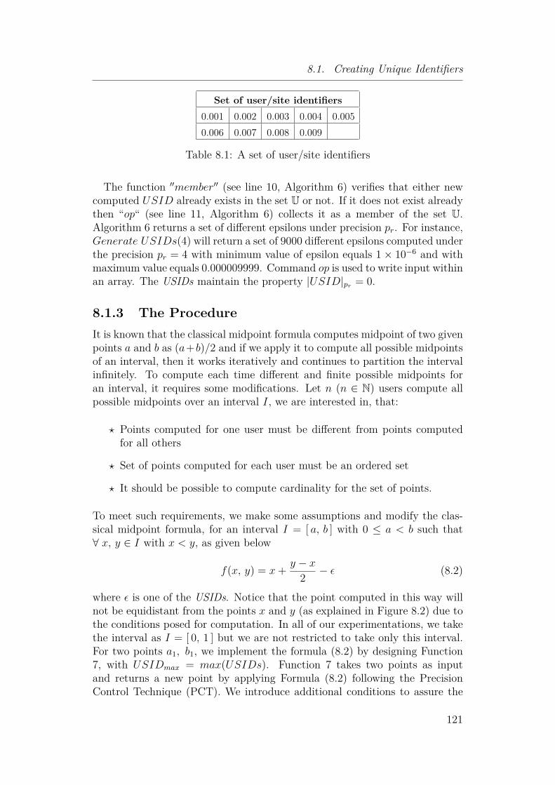
8.1. Creating Unique Identifiers
Set of user/site identifiers0.001 0.002 0.003 0.004 0.0050.006 0.007 0.008 0.009
Table 8.1: A set of user/site identifiers
The function ′′member′′ (see line 10, Algorithm 6) verifies that either newcomputed USID already exists in the set U or not. If it does not exist alreadythen “op“ (see line 11, Algorithm 6) collects it as a member of the set U.Algorithm 6 returns a set of different epsilons under precision pr. For instance,Generate USIDs(4) will return a set of 9000 different epsilons computed underthe precision pr = 4 with minimum value of epsilon equals 1× 10⁻⁶ and withmaximum value equals 0.000009999. Command op is used to write input withinan array. The USIDs maintain the property |USID|pr = 0.
8.1.3 The ProcedureIt is known that the classical midpoint formula computes midpoint of two givenpoints a and b as (a+b)/2 and if we apply it to compute all possible midpointsof an interval, then it works iteratively and continues to partition the intervalinfinitely. To compute each time different and finite possible midpoints foran interval, it requires some modifications. Let n (n ∈ N) users compute allpossible midpoints over an interval I, we are interested in, that:
? Points computed for one user must be different from points computedfor all others
? Set of points computed for each user must be an ordered set
? It should be possible to compute cardinality for the set of points.
To meet such requirements, we make some assumptions and modify the clas-sical midpoint formula, for an interval I = [ a, b ] with 0 ≤ a < b such that∀ x, y ∈ I with x < y, as given below
f(x, y) = x+ y − x2 − ε (8.2)
where ε is one of the USIDs. Notice that the point computed in this way willnot be equidistant from the points x and y (as explained in Figure 8.2) due tothe conditions posed for computation. In all of our experimentations, we takethe interval as I = [ 0, 1 ] but we are not restricted to take only this interval.For two points a1, b1, we implement the formula (8.2) by designing Function7, with USIDmax = max(USIDs). Function 7 takes two points as inputand returns a new point by applying Formula (8.2) following the PrecisionControl Technique (PCT). We introduce additional conditions to assure the
121

Chapter 8. Generating Identifiers
order preservation and to get the computed points in the form of an orderedset. For this purpose we design Algorithm 8 that contains Function 7 as a partof it. In the Algorithm 8, the function ′′nops′′ (see line 5, 6 and 10) computes
Function 7: middle(How to compute new identifier)Function: middleInput: I=[a1, b1], USID, USIDmax, Desired precisionOutput: LCID
1 begin2 Let dp := Desired precision;3 a←−
∣∣∣a1∣∣∣dp;
4 b←−∣∣∣b1∣∣∣dp;
5 ∇ :=∣∣∣∣b− a2
∣∣∣∣dp;
6 if ∇ > USIDmax then7 point :=
∣∣∣a+∇∣∣∣dp− (USID);
8 end9 return point;
10 end
number of elements in a set, for example, nops([ 5, 6, 7 ]) returns 3.
Interval
Point lies in this regionin case of
subtraction of a USID
classicalmidpoint
Point lies in this regionin case of
addition of a USID
Figure 8.2: Position of an identifier in the interval
122

8.1. Creating Unique Identifiers
Algorithm 8: How to generate a set of LCIDsAlgorithm: Generate LCIDsInput: Interval, USID, USIDmax, Desired precisionOutput: Set of unique identifiers (LCIDs)
1 begin2 Let res := Interval3 dp := Desired precision4 tempres := Set of LCIDs5 while nops(tempres) 6= nops(res) do6 if nops(tempres) 6= 0 then7 res←− tempres8 tempres←− φ
9 end10 for i←− 1 to nops(res)− 1 do11 LCID ←− middle(res[i], res[i+ 1], USID, USIDmax, dp)12 tempres := [ op(tempres), res[i] ]13 if (LCID 6= res[i] and LCID 6= res[i+ 1]) then14 verify that15 if (LCID < res[i+ 1] and LCID > res[i]) then16 tempres←− [ op(tempres), LCID ]17 end18 end19 end20 tempres←− [ op(tempres), res[nops(res)] ]21 end22 return Set of LCIDs23 end
Next, we summarize all steps that are performed above, in computing LCIDs,as follows.
Outlines
Let the interval I = [ a, b ], 0 ≤ a < b, presents an empty document or a andb are two LCIDs for two corresponding characters/lines. To compute a newLCID (say p) between a and b, we proceed as follows:
C1. Round a and b over the precision pr
C2. Evaluate ∇ = |b|pr−|a|pr
2 and round it over pr
C3. If ∇ > USIDmax then go to the next step
C4. p :=∣∣∣|a|pr +∇
∣∣∣pr− USID
123

Chapter 8. Generating Identifiers
C5. Verify that p � a and p � b.
8.1.4 ExplanationIn whole of our experimentation, it is supposed that an empty shared doc-ument is mapped to an interval I = [ 0, 1 ], as we stated before. Here, weexplain the procedure for computing unique identifiers LCIDs. Figure 8.3
ALGORITHM
SINGLE
USER
P1
EMPTY DOCUMENT
p3 p1 p2
p4 p3 p5 p1 p6 p2 p7
p p4 p p3 p p5 p p1 p p6 p p2 p p7 p
[B,...,p,p,p,...p1,...,p,p,p,...E]
updating
first point
Figure 8.3: Insertion of points by single user
presents an overview of, how a single user inserts points, corresponding tounique identifiers, starting with an empty document. p1 is the first identifiercomputed corresponding to first insertion by user. This first identifier parti-tion the corresponding interval into two sub-intervals. Now, user has choicesto insert new character on both sides of the first insertion. Therefore, let userinserted two more characters, one to the left side and other to the right sideof the first insertion. This operation results in creation of two identifiers p2and p3 to both sides of the first identifier p1. Two more partitions occurred inthe corresponding interval. After performing this operation, user inserted fourmore characters, each new character between each existing pair. This opera-
124

8.1. Creating Unique Identifiers
tion results in creation of four new corresponding identifiers p4, p5, p6 and p7and partition of interval into further sub-intervals. Notice that each time werequire the information only about the neighboring identifiers of new creation.This process continues and new points are presented by ps in the Figure 8.3whereas an update operation is marked with ’updating’.
Next, we give an example to show that LCIDs computed by Algorithm 8are different.
Example 23. Let pr = 1, and pε = 3. Consider a set of nine different USIDsas given below
ε1 = 0.001, ε2 = 0.002, ε3 = 0.003, ε4 = 0.004, ε5 = 0.005
ε6 = 0.006, ε7 = 0.007, ε8 = 0.008, ε9 = 0.009, ε = 0.009We compute all possible LCIDs for each user with different USIDs (by theAlgorithm 8) as listed in the Table 8.2, in such a way that first row presents thepoints computed by first user, second row presents points computed by seconduser and so on. Notice that there is no common point between any two rows
User Unique IdentifiersU1 0.099 0.199 0.299 0.399 0.499 0.599 0.699 0.799 0.899 0.999U2 0.098 0.198 0.298 0.398 0.498 0.598 0.698 0.798 0.898 0.998U3 0.097 0.197 0.297 0.397 0.497 0.597 0.697 0.797 0.897 0.997U4 0.096 0.196 0.296 0.396 0.496 0.596 0.696 0.796 0.896 0.996U5 0.095 0.195 0.295 0.395 0.495 0.595 0.695 0.795 0.895 0.995U6 0.094 0.194 0.294 0.394 0.494 0.594 0.694 0.794 0.894 0.994U7 0.093 0.193 0.293 0.393 0.493 0.593 0.693 0.793 0.893 0.993U8 0.092 0.192 0.292 0.392 0.492 0.592 0.692 0.792 0.892 0.992U9 0.091 0.191 0.291 0.391 0.491 0.591 0.691 0.791 0.891 0.991
Table 8.2: Set of unique identifiers
of the Table 8.2.
8.1.5 Uniqueness of line/character identifiers (LCIDs)In this section, we prove that the algorithm 8 generates different LCIDs fordifferent participants assigned with different identifiers.
Theorem 9. Let two participants are assigned with two different USIDs (εi,εj such that εi < εj, for 0 < i < j). Then for two operations performed bytwo participants respectively, two different LCIDs will be generated (over theinterval I = [ a, b ] with 0 ≤ a < b).
125

Chapter 8. Generating Identifiers
Proof. Suppose that U1 and U2 be the two users, assigned with two differentUSIDs, εi and εj, compute two LCIDs, p1 and p2 by executing algorithm 8.For xi, xj, yi, yj ∈ I = [ a, b ], and v = pr ∈ N, p1 and p2 can be written as
p1 =∣∣∣∣xi+|yi − xi2 |v
∣∣∣∣v− εi
p2 =∣∣∣∣xj+|yj − xj2 |v
∣∣∣∣v− εj
where xi =|xi|v, xj =|xj|v, xj =|xj|v, yj =|yj|v. For the sake of simplicity,suppose that
mi =∣∣∣∣xi+|yi − xi2 |v
∣∣∣∣v
mj =∣∣∣∣xj+|yj − xj2 |v
∣∣∣∣v
So, it is enough to prove that
|mi −mj|+ (εj − εi) 6= 0 (8.3)
Now, for u1, u2 ∈ Nεi = li.d
i1di2di3 . . . d
iu1
εj = lj.dj1dj2dj3 . . . d
ju1
εj − εi = lk.dk1d
k2d
k3 . . . d
kvd
kv+1 . . . d
ku2
εi 6= εj
∴ At least one of dkk1 6= 0, v < k1 ≤ u2 ≤ u1 (8.4)
Letα =|mi −mj| = lα.d
α1d
α2d
α3 . . . d
αv
and β = εj − εi = lβ.dβ1d
β2d
β3 . . . d
βvd
βv+1 . . . d
βu2
∵ v = pr < pε < pd (basic principle (8.1))
=⇒ pα < pβ =⇒ α 6= β
Also β 6= 0 by (8.4)
Hence α + β 6= 0 and (8.3) holds.
126

8.2. Computing cardinality
8.1.6 Verifying uniquenessTo generate unique line/character identifier one must have to keep our pro-posed specific pattern of user/site identifiers and precision control technique.In the theorem 9, we prove the uniqueness even keeping only one zero after
Algorithm 9:Algorithm: comparing different sets of LCIDsInput: Desired precision, IntervalOutput: LCIDs are unique
1 begin2 Let dp := Desired precision3 U := Set of USIDs4 I := Interval5 U←− GenerateUSIDs(dp)6 USIDmax:= Max. value of USID in the set U7 M:= No. of elements in the set U8 for kk ←− 1 to M do9 USID ←− U [kk]
10 d[kk]←− Generate LCIDs (I, USID, USIDmax, dp)11 end12 for i ←− 1 to M-1 do13 MM:=No. of elements in d[i]14 for j ←− 2 to MM-1 do15 for k ←− i+1 to M do16 if member(d[i][j], d[k]) = true then17 USIDi:= USID corresponding to the set d[i]18 USIDk:= USID corresponding to the set d[k]19 if USIDi 6= USIDj then20 d[i][j] is a common point between the sets d[i] and d[k]21 please verify the precision conditions22 end23 else24 No common points are there25 end26
27 end28 end29 end30 return No collision31 end
decimal point but in generating line/character identifiers we keep more thanone zero in that place. The reason is that, with only one zero, cardinalityformulation is complicated that could be observed by drawing graph for theline/character identifiers generated by keeping only one zero. In addition totheorem 9, we provide a simple algorithm that make a comparison betweenline/character identifiers generated (see line 16) for different users and alertsif there is any mistake in selecting specific pattern to generate such identifiers.
8.2 Computing cardinalityCardinality of a set is the "number of elements in the set". For example, theset A = {2, 4, 6} contains 3 elements, and therefore cardinality of set A is 3.
127

Chapter 8. Generating Identifiers
Under Precision Control Technique (PCT), it is possible to compute cardinalityof line/character identifiers LCIDs, generated by taking a particular precision.
Definition 15. The possible number of identifiers (LCIDs) that could be cre-ated for a user (site) under particular precision is called local cardinality andis denoted by Cl.
8.2.1 Local cardinalityLet γ denotes the length of the interval I = [ a, b ], 0 ≤ a < b then γ = |b− a|with γ > 0. For the precision pr, local cardinality for a single user can becomputed as
Cl =
γ × 10pr if b > a ≥ 0, for a, b ∈ N(γ1 × 10pr)− 1 if b > a > 0, for a, b ∈ R
and γ1 = |γ|pr
such thatpr < pε < pd
USIDs are of the pattern as explained in section 8.1.2.
Example 24. Suppose that I1 = [0, 1], pr = 3, USIDmin = 0.00001, andUSIDmax = 0.0000999. The local cardinality of a set of LCIDs, that a singleuser with USID = 0.0000439 can generate, is computed by Cl = 1∗103 = 1000.Now, let the same user wants to compute local cardinality of LCIDs betweentwo LCIDs (already computed by him). Let I2 = [0.7609561, 0.8139561] thenγ1 = 0.053 and Cl = (0.053 ∗ 103)− 1 = 52.
8.2.2 Global cardinalityWe define global cardinality as follows.
Definition 16. In a network of users/peers, the union of local cardinalitycomputed by/at each user/peer is called global cardinality and is denoted byCg.
Computing global cardinality of a network depends on the local cardinali-ties, insertion/deletion, sending/receiving and the ways of exchange of LCIDsby the participants. We compute, here, global cardinality for a simple sit-uation. Consider a network of n (n ∈ N) users/peers and assume that eachuser/peer generates LCIDs locally and send to others. Each user/peer can alsoremoves points that has already been created. Since two different users/peersgenerate different LCIDs (by Theorem 9), therefore, no duplication of LCIDsis possible during the exchange of elements between users/peers.
128

8.2. Computing cardinality
Bounds over cardinality
For a particular precision pr, we take zero as the lower bound over local car-dinality for a single user/peer and local cardinality computed by a single userfor an empty document is considered to be an upper bound over local car-dinality. We take local cardinality computed by a single user for an intervalI = [ a, b ], 0 ≤ a < b (as explained in section 8.2.1) as a lower bound forglobal cardinality of a network of n ∈ N users/peers. Similarly, we take anupper bound over global cardinality as
Cg =n∑i=1
Cli
that corresponds to an ideal situation in which each user/peer achieves anupper bound over local cardinality.
129

Chapter 8. Generating Identifiers
130

Chapter 9Properties and Analysis
Contents9.1 Properties . . . . . . . . . . . . . . . . . . . . . . 132
9.1.1 Bijection property . . . . . . . . . . . . . . . . . 132
9.1.2 Closure properties . . . . . . . . . . . . . . . . . 133
9.2 Analysis . . . . . . . . . . . . . . . . . . . . . . . 137
9.2.1 Comparison under Rounding Conditions . . . . 137
9.2.2 Comparison without Rounding Conditions . . . 138
9.2.3 Comparison under floating-point arithmetics . . 138
9.2.4 Effect of different rounding conditions . . . . . . 139
9.2.5 Assuring order preservation . . . . . . . . . . . . 147
Set of identifiers LCIDs generated by algorithm 8 (see chapter 8, section8.1.3) holds some important properties that show advantages of the precisioncontrol indexing method. These properties provide assurance in generatingidentifiers based on remote points. The existence of closure properties confirmthat there is no loss of identifier during exchange of points and all the identifiersgenerated don’t escape from the interval allocated for all users in the network.Similarly, an analysis of the function 8.2 helps in exploring the usefulness ofthe function with rounding conditions and explains its limitations.In this chapter, we prove some important properties that hold on the set ofidentifiers LCIDs generated by the algorithm 8. In section 9.2, we presentan analysis of function 8.2 by comparing it with classical midpoint formulaunder different situations. Section 9.2.4 presents effect of different roundingconditions over the function (function 8.2) used in algorithm 8. Section 9.2.5describes how our approach assure order preservation in exchange of pointsacross the network particularly when identifies are required to generate on thebasis of identifiers of remote points.
131

Chapter 9. Properties and Analysis
9.1 PropertiesIn this section, we prove that set of identifiers LCIDs holds bijection propertyas well as some closure properties.
9.1.1 Bijection propertyProposition 5. Let S ′ be the set defined over the interval I = [ a, b ], 0 ≤ a <b, as
S ′ = { n′
10pr| n′ ∈ N, a < n′ ≤ β, β = γ ∗ 10pr}
where γ is the length of the interval I with |γ|pr > 0. For 1 ≤ k ≤ n, n ∈ N,let εk be one of the USIDs then the function fk : S ′ −→ S ′′ defined by fk(x′) =x′ − εk, ∀x′ ∈ S ′, is a bijection.
Proof. The domain of the function fk is the set
S ′ = { n′
10pr| n′ ∈ N, a < n′ ≤ β, β = γ ∗ 10pr}
and the range of the function fk is the set
S ′′ = {x′ − εk | ∀ x′ ∈ S ′, pε ≥ pr + µ, µ ≥ 2}
Now, we have to prove that the given function fk is both injective and surjective
• InjectionSuppose that
x′1 6= x′2, ∀ x′1, x′2 ∈ S ′
thenfk(x′1) = x′1 − εk and fk(x′2) = x′2 − εk
Letfk(x′1) = fk(x′2)
=⇒ x′1 = x′2
A contradiction to the supposition that x′1 6= x′2. Thus
fk(x′1) 6= fk(x′2)
• Surjection
For surjection, we have to prove that
∃ x′ ∈ S ′, such that x′′ = fk(x′), ∀x′′ ∈ S ′′
∵ x′ = x′′ + εk
∴ fk(x′′ + εk) = x′′ + εk − εk = x′′
=⇒ fk is a surjective functionsHence for 1 ≤ k ≤ n, fk presents a family of bijective functions.
132

9.1. Properties
The bijection property as described in proposition 5 helps in verifying thecardinality formula proposed in previous chapters. Set S ′′ contains LCIDssimilar generated by the algorithm 8. For example, for the interval [0, 1], wecan generate values
[0.1, 0.2, 0.3, 0.4, 0.5, 0.6, 0.7, 0.8, 0.9, 1]
It generates LCIDs by subtracting corresponding USIDs, under chosen round-ing precision.
Definition 17. We denote, the set of USIDs computed by user Uk with USI-D (εk) over the interval [a, b], 0 ≤ a < b, by Sk, where 1 ≤ k ≤ n, n ∈ N.
Corollary 2. For the interval I = [ a, b ], 0 ≤ a < b, two sets S ′′ and Sk areequal.
Proof. For a USID = εk, the set Sk can be written as
Sk = {xk | xk = |xk|pr − εk}
Let xk ∈ Sk then xk = |xk|pr − εk. Now |xk|pr ∈ S, where
S ′ = { n′
10pr| n′ ∈ N, 1 ≤ n′ ≤ β, β = γ × 10pr}
But |xk|pr − εk ∈ S ′′ by Proposition 5.Therefore Sk and S ′′ are equal sets generated over the same interval.
9.1.2 Closure propertiesIn this section, we prove some important closure properties.
First Property
Lemma 5. Let for 1 ≤ k ≤ n, n ∈ N, εk ∈ {ε1, ε2, ε3, . . . , εn−1, εn} be theUSID for user Uk and Sk be the set of LCIDs generated for the user Uk overthe interval I = [ a, b ], 0 ≤ a < b. Then for x, y ∈ Sk, x < y,∣∣∣∣∣|x|pr +
∣∣∣∣ |y|pr − |x|pr
2
∣∣∣∣pr
∣∣∣∣∣pr
− εk ∈ Sk
Proof. Let x, y ∈ Sk then
x = |x|pr − εk, and |x|pr ∈ S
y = |y|pr − εk, and |y|pr ∈ S
whereS ′ = { n′
10pr| n′ ∈ N, 1 ≤ n′ ≤ β, β = γ × 10pr}
133

Chapter 9. Properties and Analysis
Suppose that∇ =
∣∣∣∣ |y|pr − |x|pr
2
∣∣∣∣pr
> (USID)max
That is, condition C5. (section 23) is satisfied. It gives ∇ ∈ S,Now
|x|pr <∣∣∣|x|pr +∇
∣∣∣ ≤ |y|pr
But ∣∣∣|x|pr +∇∣∣∣pr∈ S
Therefore, by definition 17. ∣∣∣|x|pr +∇∣∣∣pr− εk ∈ Sk
This property proves that over the set of identifiers generated for a user,any new identifier generated (for the same user) on the basis of two identifiersthat have already generated, this new identifier lies in the same set.
Second Property
Lemma 6. Let Si, Sj, andSk be the set of LCIDs generated for users Ui, Ujand Uk with USIDs, εi, εj and εk over the interval I = [ a, b ], 0 ≤ a < brespectively. Then for any two points x ∈ Si, y ∈ Sj, x < y and for εj < εk.∣∣∣∣∣|x|pr +
∣∣∣∣ |y|pr − |x|pr
2
∣∣∣∣pr
∣∣∣∣∣pr
− εk ∈ Sk
Proof. Let x ∈ Si and y ∈ Sj then
x = |x|pr − εi, and |x|pr ∈ S
y = |y|pr − εj, and |y|pr ∈ S
Also, the sets Si, Sj, andSk can be written as
Si = {x′ − εi | ∀ x′ ∈ S ′, pε ≥ pr + µ, µ ≥ 2}
Sj = {x′ − εj | ∀ x′ ∈ S ′, pε ≥ pr + µ, µ ≥ 2}Sk = {x′ − εk | ∀ x′ ∈ S ′, pε ≥ pr + µ, µ ≥ 2}
whereS ′ = { n′
10pr| n′ ∈ N, 1 ≤ n′ ≤ β, β = γ × 10pr}
Suppose that
∇ =∣∣∣∣ |y|pr − |x|pr
2
∣∣∣∣pr
> ε, with, ε = max(εi, εj, εk)
134

9.1. Properties
=⇒ |x|pr 6= |y|pr
Otherwise, condition C5. (section 23) does not hold.Now, let
p =∣∣∣|x|pr +∇
∣∣∣pr
then|x|pr < p ≤ |y|pr
Letp = |y|pr
thenp ∈ S
Now, sinceεj < εk
Therefore,p− εk < p− εj and p− εk ∈ Sk
This property proves that if an identifier is generated for first user andanother identifier is generated for second user, then an identifier generated forthird user lies within the set of identifier generated for third user.
Third Property
Lemma 7. Let Si be the set of LCIDs generated by user (or at site) Ui withUSID = εi over the interval I = [ a, b ], 0 ≤ a < b. Then for any two pointsx, y ∈ Si, x < y and for εi < εk.∣∣∣∣∣|x|pr +
∣∣∣∣ |y|pr − |x|pr
2
∣∣∣∣pr
∣∣∣∣∣pr
− εk ∈ Sk
Proof. Letpi,1 =
∣∣∣∣∣|x|pr +∣∣∣∣ |y|pr − |x|pr
2
∣∣∣∣pr
∣∣∣∣∣pr
be the first rounded value computed by user Ui over the interval I. Since, eachuser starts computing values over the same interval I keeping same conditionsof the algorithm. Therefore, for, 1 ≤ i ≤ n, we have
p1,1 = p2,1 = p3,1 = . . . = pi,1 = p(i+1),1 = . . . = pn,1
But by Theorem 9.
p1,1 − ε1 6= p2,1 − ε2 6= . . . 6= pi,1 − εi
6= p(i+1),1 − εi−1 6= . . . = pn,1 − εn
135

Chapter 9. Properties and Analysis
By definition 17,
p1,1 − ε1 ∈ S1, p2,1 − ε2 ∈ S2, . . . , pn,1 − εn ∈ SnHence ∣∣∣∣∣|x|pr +
∣∣∣∣ |y|pr − |x|pr
2
∣∣∣∣pr
∣∣∣∣∣pr
− εk ∈ Sk
This property proves that if a set of identifiers is generated for first userthen a new identifier generated for second user (based on the set of identifiersgenerated for first user), belongs to the set of identifiers generated for seconduser.
Fourth property
Lemma 8. For 1 ≤ k ≤ n, n ∈ N, let Uk be the set of users/sites and
S =n⋃k=1
Sk, with x < y be the set of USIDs generated by all Uk/sites then for
x, y ∈ S and εk ∈ {ε1, ε2, ε3, . . . , εn−1, εn}, the point∣∣∣∣∣|x|pr +∣∣∣∣ |y|pr − |x|pr
2
∣∣∣∣pr
∣∣∣∣∣pr
− εk ∈ Sk
Proof. Suppose that∇ =
∣∣∣∣ |y|pr − |x|pr
2
∣∣∣∣pr
> ε,
withUSIDmax = max(ε1, ε2, ε3, . . . , εn−1, εn)
Now, let x, y ∈ Sk then, by Lemma (5).∣∣∣∣∣|x|pr +∣∣∣∣ |y|pr − |x|pr
2
∣∣∣∣pr
∣∣∣∣∣pr
− εk ∈ Sk
Let x ∈ Si and y ∈ Sj then, by Lemma (6).∣∣∣∣∣|x|pr +∣∣∣∣ |y|pr − |x|pr
2
∣∣∣∣pr
∣∣∣∣∣pr
− εk ∈ Sk
Finally, let x, y ∈ Si then, by Lemma (7).∣∣∣∣∣|x|pr +∣∣∣∣ |y|pr − |x|pr
2
∣∣∣∣pr
∣∣∣∣∣pr
− εk ∈ Sk
Since Sk ⊆ S, therefore∣∣∣∣∣|x|pr +∣∣∣∣ |y|pr − |x|pr
2
∣∣∣∣pr
∣∣∣∣∣pr
− εk ∈ S
Hence the proof.
136

9.2. Analysis
9.2 AnalysisIn this section, we make an analysis for the function 8.2 to explore some of itsadvantages. The classical midpoint formula excludes condition C4. (see fordetail, chapter 8, section 8.1.3).
C4. p :=∣∣∣|a|pr +∇
∣∣∣pr− USID
and rounding restrictions described in Outlines (chapter 8, section 8.1.3). Wemake a comparison between two formulas as follows:
9.2.1 Comparison under Rounding ConditionsUnder rounding conditions formula 8.2 compute more points as compared tothe classical midpoint formula.
Example 25. Consider the interval I = [0, 0.001] with (user-identifier) =0.00001, epsilon = 0.00001 and pr = 3. We are able to insert one point insidethe interval I using formula 8.2 as given below,
I = [0, 0.00099, 0.001]
with ∇ = 0.0005 and ∇ > epsilon, but we cannot insert any point inside theinterval I using classical midpoint formula due to the fact that rounding ∇over pr = 3 returns ∇ = 0.001 which is the end point of the interval I.Similarly for the interval I = [0, 0.002], using formula 8.2, we can computeone more point over the interval I as compared to classical midpoint formula,with pr = 3, epsilon = 0.00001 and (user-identifier) = 0.00001.
[0, 0.00099, 0.00199, 0.002]
[0, 0.001, 0.002]
With different values of epsilons and rounding scheme (as we proposed inTheorem 9), formula 8.2 generate different points (see Table: 8.2), while theclassical midpoint formula does not do the same under the same environment(see Table: 9.1). Nine users assigned with different USIDs as given below:
ε1 = 0.0100, ε2 = 0.0200, ε3 = 0.0300, ε4 = 0.0400ε5 = 0.0500, ε6 = 0.0600, ε7 = 0.0700, ε8 = 0.0800ε9 = 0.0900, ε = 0.0900
participate. The identifiers are listed in table 9.1.
137

Chapter 9. Properties and Analysis
User Similar IdentifiersU1 0.1000 0.2000 0.3000 0.4000 0.5000 0.6000 0.7000 0.8000 0.9000U2 0.1000 0.2000 0.3000 0.4000 0.5000 0.6000 0.7000 0.8000 0.9000U3 0.1000 0.2000 0.3000 0.4000 0.5000 0.6000 0.7000 0.8000 0.9000U4 0.1000 0.2000 0.3000 0.4000 0.5000 0.6000 0.7000 0.8000 0.9000U5 0.1000 0.2000 0.3000 0.4000 0.5000 0.6000 0.7000 0.8000 0.9000U6 0.1000 0.2000 0.3000 0.4000 0.5000 0.6000 0.7000 0.8000 0.9000U7 0.1000 0.2000 0.3000 0.4000 0.5000 0.6000 0.7000 0.8000 0.9000U8 0.1000 0.2000 0.3000 0.4000 0.5000 0.6000 0.7000 0.8000 0.9000U9 0.1000 0.2000 0.3000 0.4000 0.5000 0.6000 0.7000 0.8000 0.9000
Table 9.1: Similar Identifiers
I pe εi ε Cd(fc) Cd(f1) Cd(f1)− Cd(fc)[0, 0.01] 3 0.003 0.003 3 33 30[0, 0.01] 4 0.0003 0.0003 33 243 210[0, 0.01] 5 0.00003 0.00003 257 2216 1959[0, 0.01] 6 0.000003 0.000003 2049 19380 17331
[0, 0.0001] 7 0.0000003 0.0000003 257 2216 1959[0, 0.0001] 8 0.00000003 0.00000003 2049 19580 17371[0, 0.0001] 9 0.000000003 0.000000003 32769 165039 132270
Table 9.2: Cardinality Comparison
9.2.2 Comparison without Rounding ConditionsLet Cd(f1) and Cd(fc) denotes the cardinality of points inserted by formula 8.2and classical formula respectively. With different values of epsilon and length ofthe interval I, we observe a notable difference in Cd(f1) and Cd(fc) as givenin the Table 9.2. We observed that, on increasing the precision of epsilons,the cardinality increases more for the points computed by the formula 8.2 ascompare to the cardinality computed by the classical formula.
9.2.3 Comparison under floating-point arithmeticsWe also prefer to use the fraction
xi + xi+1 − xi2 over xi+1 + xi
2due to the fact that midpoint computed by later one may not lies within theinterval under certain restriction on floating-point arithmetics. For example,for an interval I = [0.982, 0.987], if we are restricted to perform calculation ona machine with three decimal digit chopped floating point arithmetic, then
x+ y = 1.96 and x+ y
2 = 0.980 /∈ I
138

9.2. Analysis
9.2.4 Effect of different rounding conditionsIn this section, we analyse function 8.2 with different rounding conditions sothat the effect over the set of identifiers LCIDs can be observed. Consider asituation in which users/sites in the network participate in an order to computeLCIDs. Each user in the network computes LCIDs locally and sends it to allother users/sites. For a set of USIDs {ε1, ε2, ε3, . . . , εn−1, εn}, let USIDmin =min(εk), where 1 ≤ k ≤ n, for n ∈ N,To analyse function 8.2, we modify rounding conditions (see line 2 to line 4 inthe modified form of function 7 as given below).
Modification-I
Input: I=[a1, b1], USID, USIDmax, Precision(pr)1 begin2 a← a1;3 b← b1;4 ∇ :=
∣∣∣∣b− a2
∣∣∣∣pr
;
5 if ∇ > USIDmax then6 point := |a+∇|pr − (USID);7 end8 return point;9 end
We also exclude condition C5. of the outlines (section 8.1.3, page 123) tocompute LCIDs.We consider the following two situations.
1. If the set of USIDs is in ascending order
2. If the set of USIDs is in descending order
Computing LCIDs keeping USIDs in ascending order
In this environment, we suppose that the user (site) assigned with USIDminstarts computing and sends points to others such that the computation ofUSIDs occurs in a way that user Ui+1 starts computation after user Ui. In thiscase the set of USIDs is in ascending order, i.e. {ε1, ε2, ε3, . . . , εn−1, εn}. Weexplain the situation by the following example.Example 26. Suppose that I = [ 0.0, 0.02 ] be an interval and user U1 withUSID = 0.0001 starts computing LCIDs keeping precision pr = 2. Then theset of USIDs generated corresponding to the modifications performed by userU1 is given below.
S1 = [ 0.0, 0.0099, 0.0199, 0.02 ]
139

Chapter 9. Properties and Analysis
Now, U1 sends LCIDs to other users/sites so that updates are executed at eachsite of the network. Now, user U2 with USID = ε2 = 0.0002 has to computenew USIDs based on the points sent by U1. The set of USIDs computed by U2is
S2 = [ 0.0, 0.0099, 0.0198, 0.0199, 0.02 ]
U2 sends LCIDs to next users.Similarly, user U3 with USID = ε3 = 0.0003 has to compute USIDs based onthe points that it received. But U3 is not able to compute any point because the∇ condition is not valid. Consider, for example,
∇ =∣∣∣∣0.0198− 0.0099
2
∣∣∣∣2
=∣∣∣0.00495
∣∣∣2≯ USIDmax
Hence, for an interval I = [ 0, 1 ] and a set of nine users/sites assigned aset of USIDs as given below
[ 0.001, 0.002, 0.003, 0.004, 0.005, 0.006, 0.007, 0.008, 0.009 ]
User at site with USID = 0.001 computes 10 USIDs
[ 0, 0.099, 0.199, 0.299, 0.399, 0.499, 0.599, 0.699, 0.799, 0.899, 0.999, 1 ]
and sends to next users/sites. Now user U2 with USID = 0.002 computes 9more LCIDsbut any other user could not be able to increase the global cardinality that is
A final set after the participation of each user0.000 0.099 0.198 0.199 0.2980.299 0.398 0.399 0.498 0.4990.598 0.599 0.698 0.699 0.7980.799 0.898 0.899 0.998 0.999 1.000
Table 9.3: Set of Identifiers (LCIDs)
21 as shown in the Table 9.3 We observe that
• Only two users are able to compute the points but not all.
• Final set of USIDs is an ordered set and USIDs are in ascending order.
Computing LCIDs keeping USIDs in descending order
In this environment, the user (site) assigned with USIDmax starts comput-ing and sending points to others, in a way that user Ui starts computationafter user Ui+1. In this case the set of USIDs is in decreasing order, i.e.,{εn, εn−1, εn−2, . . . , ε2, ε1}.
140

9.2. Analysis
Example 27. For the precision pr = 2, consider a set of 90 users such thatuser U90 with USID = ε90 = 0.00099 starts computing points for the intervalI = [ 0, 0.02 ],
S90 = [ 0, 0.00901, 0.01901, 0.02 ]and U90 sends LCIDs to the next user U89 with USID = ε89 = 0.00098. UserU89 computes one point based on the points sent by U90
[ 0, 0.00901, 0.01902, 0.01901, 0.02 ]
and sends to next users. Now, user U88 with USID = ε88 = 0.00097 computesone point because the ∇ condition is valid. Consider two consecutive points,for instance,
[ 0.01902, 0.00901 ]
∇ =∣∣∣∣0.00901− 0.01902
2
∣∣∣∣2
= 0.01 > USIDmax
Therefore, next user can compute one more point as given below.
[ 0., 0.00901, 0.01903, 0.01902, 0.01901, 0.02 ]
Similarly, we observe that, all other users can compute LCIDs and gives theglobal cardinality as 93 including the end points of the interval.
Thus for an interval I = [ a, b ], and a set of nine users with a set of nineUSIDs as given below
[ 0.001, 0.002, 0.003, 0.004, 0.005, 0.006, 0.007, 0.008, 0.009 ]
User with USID = 0.009 will compute 10 points, while all other users compute9 points as given in the Table 9.4. Thus the global cardinality for the giveninterval is 84. We observe that
Similar Identifiers0.0 0.091 0.199 0.198 0.197 0.196 0.195 0.194 0.193 0.192
0.191 0.299 0.298 0.297 0.296 0.295 0.294 0.293 0.292 0.2910.399 0.398 0.397 0.396 0.395 0.394 0.393 0.392 0.3910.499 0.498 0.497 0.496 0.495 0.494 0.493 0.492 0.4910.599 0.598 0.597 0.596 0.595 0.594 0.593 0.592 0.5910.699 0.698 0.697 0.696 0.695 0.694 0.693 0.692 0.6910.799 0.798 0.797 0.796 0.795 0.794 0.793 0.792 0.7910.899 0.898 0.897 0.896 0.895 0.894 0.893 0.892 0.8910.999 0.998 0.997 0.996 0.995 0.994 0.993 0.992 0.991 1.0
Table 9.4:
• All users are able to compute the points.
• The final set of Inserted points is not in order.
141

Chapter 9. Properties and Analysis
Modification-II
To analyse function 8.2, we modify rounding conditions (see line 2 to line 6in the modified form of function 7 as given below). Here, we also exclude
Input: I=[a1, b1], USID, USIDmax, Precision(pr)1 begin2 a← a1;3 b← b1;
4 ∇ := b− a2 ;
5 if ∇ > USIDmax then6 point := |a+∇|pr − (USID);7 end8 return point;9 end
condition C5. of the outlines (section 8.1.3, page 123) to compute LCIDs.
Computing LCIDs keeping USIDs in Ascending Order
Consider the following example, to observe the effect of above modification ofthe Function 7.Example 28. Let I = [ 0, 0.3 ] be the interval and user U1 with USID = ε1 =0.001 starts computing USIDs under precision pr = 1, Then
S1 = [ 0, −0.001, 0.099, 0.199, 0.3 ]U1 sends LCIDs to the next user U2 with USID = ε2 = 0.002. User U2computes points based on the points sent by U1
S2 = [ 0, −0.001, −0.002, 0.099, 0.098, 0.199, 0.198, 0.3 ]and sends to next users. Now, user U3 with USID = ε3 = 0.003 computespoints because the ∇ Condition is valid.
[0.,−0.001,−0.002,−0.003, 0.099, 0.098, 0.097, 0.199, 0.198, 0.197, 0.3]At the completion of the process we have a set of 29 LCIDs as listed in theTable 9.5
Similarly, under precision pr = 1, for an interval I = [0, 1] and a set ofnine users as given below
[0.001, 0.002, 0.003, 0.004, 0.005, 0.006, 0.007, 0.008, 0.009]Each user is able to compute 10 points. So the global cardinality for the giveninterval will be 92 as shown in the Table 9.6. We observe that
• Each user is able to insert points due to the modified rounding scheme
• Each patch of USIDs is in decreasing order.
142

9.2. Analysis
A final set after the participation of each user0 −0.001 −0.002 −0.003 −0.004 −0.005
−0.006 −0.007 −0.008 −0.009 0.099 0.0980.097 0.096 0.095 0.094 0.093 0.0920.091 0.199 0.198 0.197 0.196 0.1950.194 0.193 0.192 0.191 0.3
Table 9.5: Set of Identifiers
A final set after the participation of each user0 −0.001 −0.002 −0.003 −0.004 −0.005 −0.006 −0.007 −0.008 −0.009
0.099 0.098 0.097 0.096 0.095 0.094 0.093 0.092 0.0910.199 0.198 0.197 0.196 0.195 0.194 0.193 0.192 0.1910.299 0.298 0.297 0.296 0.295 0.294 0.293 0.292 0.2910.399 0.398 0.397 0.396 0.395 0.394 0.393 0.392 0.3910.499 0.498 0.497 0.496 0.495 0.494 0.493 0.492 0.4910.599 0.598 0.597 0.596 0.595 0.594 0.593 0.592 0.5910.699 0.698 0.697 0.696 0.695 0.694 0.693 0.692 0.6910.799 0.798 0.797 0.796 0.795 0.794 0.793 0.792 0.7910.899 0.898 0.897 0.896 0.895 0.894 0.893 0.892 0.891 1
Table 9.6: Set of Identifiers
Computing LCIDs keeping USIDs in descending order
With a set of USIDs in decreasing order, consider the same interval I = [ 0, 0.3 ]and precision pr = 1, as taken in Example 28.
Example 29. Suppose pr = 1, user u1 at ε1 = 0.009 computes points for theinterval [0, 0.3],
[ 0, −0.009, 0.091, 0.191, 0.3 ]
and sends to the next user u2 at ε2 = 0.008. User u2 computes points on thebasis of points received from u1
[ 0, −0.009, −0.008, 0.091, 0.092, 0.191, 0.192, 0.3 ]
and sends to next users. Now, user u3 at ε3 = 0.007 computes points becausethe ∇ Condition is valid.
[ 0.0, −0.009, −0.008, −0.007, 0.091, 0.092, 0.093, 0.191, 0.192, 0.193, 0.3 ]
we compute the LCIDs as given in the Table 9.7.
143

Chapter 9. Properties and Analysis
A final set after the participation of each user0 −0.009 −0.008 −0.007 −0.006 −0.005
−0.004 −0.003 −0.002 −0.001 0.091 0.0920.093 0.094 0.095 0.096 0.097 0.0980.099 0.191 0.192 0.193 0.194 0.1950.196 0.197 0.198 0.199 0.3
Table 9.7: Set of Identifiers
Similarly for the interval I = [0, 1] with a set of nine users/sites assigneda set of USIDs as given below
[ 0.001, 0.002, 0.003, 0.004, 0.005, 0.006, 0.007, 0.008, 0.009 ]
User at epsilon = 0.009 will compute 10 points, and all other users also com-putes 10 points. So the global cardinality for the given interval will be 92 aslisted in the Table 9.8.
A final set after the participation of each user0 −0.009 −0.008 −0.007 −0.006 −0.005 −0.004 −0.003 −0.002 −0.001
0.091 0.092 0.093 0.094 0.095 0.096 0.097 0.098 0.0990.191 0.192 0.193 0.194 0.195 0.196 0.197 0.198 0.1990.291 0.292 0.293 0.294 0.295 0.296 0.297 0.298 0.2990.391 0.392 0.393 0.394 0.395 0.396 0.397 0.398 0.3990.491 0.492 0.493 0.494 0.495 0.496 0.497 0.498 0.4990.591 0.592 0.593 0.594 0.595 0.596 0.597 0.598 0.5990.691 0.692 0.693 0.694 0.695 0.696 0.697 0.698 0.6990.791 0.792 0.793 0.794 0.795 0.796 0.797 0.798 0.7990.891 0.892 0.893 0.894 0.895 0.896 0.897 0.898 0.899 1
Table 9.8: Set of Identifiers
• Notice that, if we ignore the negative values, the final set of USIDs willbe in order.
We observe that
• Each user is able to insert points due to the modified rounding scheme
• Negative values are not within the given interval.
Effect of condition C5.
Condition C5. (see for detail chapter 8, section 8.1.3) is introduced to strictlypreserve order of identifiers based on exchanged points. This order preservationproperty is implemented in Algorithm 8 from line 13 to line 18. Condition C5.
144

9.2. Analysis
is still flexible in some cases and can be excluded partially or fully. It mayaffect the global cardinality, particularly when identifiers are to be computed,based on exchanged identifiers and users are participating without keeping anyorder in participation. This section deals with observing the effect of conditionC5. in the outlines (section 8.1.3, page 123). For this purpose, we have notmade any change in function 7 but only exclude condition C5..
Computing LCIDs keeping USIDs in ascending Order
We perform the similar experiment as above.Example 30. Suppose pr = 1, user U1 with USID = ε1 = 0.001 computesLCIDs for the interval [ 0, 0.2 ] as given below
S1 = [ 0, 0.099, 0.199, 0.2 ]
Then U1 sends LCIDs to the next user U2 with USID = ε2 = 0.002. User U2computes one point based on the points sent by U1
S2 = [ 0, 0.098, 0.099, 0.198, 0.199, 0.2 ]
and sends to next users.Now, user U3 with USID = ε3 = 0.003 compute point because the ∇ Conditionis valid. For instance, for two points [ 0.099, 0.198 ]
∇ =∣∣∣∣∣∣∣∣0.198
∣∣∣1−∣∣∣0.099
∣∣∣1
2
∣∣∣∣∣1
= 0.1 > USIDmax
After the completion of process, final set of USIDs is listed in the Table 9.9
A final set after the participation of each user0 0.0910 0.0920 0.0930 0.0940
0.0950 0.0960 0.0970 0.0980 0.09900.191 0.192 0.193 0.194 0.1950.196 0.197 0.198 0.199 0.2
Table 9.9: Set of Identifiers
Similarly, for the interval [ 0, 1 ], and a set of nine users/sites assigned witha set of USIDs as given below
[0.001, 0.002, 0.003, 0.004, 0.005, 0.006, 0.007, 0.008, 0.009]
User with USID = 0.009 will compute 10 points, and all other users alsocomputes 10 points. So the global cardinality for the given interval is 92 asshown in the Table 9.10. We observe that
• All users are able to compute the points.
• Final set of LCIDs is an ordered set.
145

Chapter 9. Properties and Analysis
A final set after the participation of each user0 0.091 0.092 0.093 0.094 0.095 0.096 0.097 0.098 0.099
0.191 0.192 0.193 0.194 0.195 0.196 0.197 0.198 0.1990.291 0.292 0.293 0.294 0.295 0.296 0.297 0.298 0.2990.391 0.392 0.393 0.394 0.395 0.396 0.397 0.398 0.3990.491 0.492 0.493 0.494 0.495 0.496 0.497 0.498 0.4990.591 0.592 0.593 0.594 0.595 0.596 0.597 0.598 0.5990.691 0.692 0.693 0.694 0.695 0.696 0.697 0.698 0.6990.791 0.792 0.793 0.794 0.795 0.796 0.797 0.798 0.7990.891 0.892 0.893 0.894 0.895 0.896 0.897 0.898 0.8990.991 0.992 0.993 0.994 0.995 0.996 0.997 0.998 0.999 1
Table 9.10: Set of Identifiers
Computing LCIDs keeping USIDs in descending Order
Consider the following exampleExample 31. Suppose pr = 1, user U9 with USID = ε9 = 0.009 computespoints for the interval [ 0, 0.2 ],
[ 0, 0.091, 0.191, 0.2 ]and sends to the next user U8 with USID = ε8 = 0.008. User U8 computesone point based on the points sent by U9
[ 0, 0.092, 0.091, 0.192, 0.191, 0.2 ]and sends LCIDs to next users.Now, user U7 with USID = ε7 = 0.007 computes point because the∇ Conditionis valid. For instance, for two points 0.091 and 0.192
∇ =∣∣∣∣∣∣∣∣0.192
∣∣∣1−∣∣∣0.091
∣∣∣1
2
∣∣∣∣∣1
= 0.1 > USIDmax
User U6 compute points[ 0, 0.093, 0.092, 0.091, 0.193, 0.192, 0.191, 0.2 ]
Final set of USIDs computed is listed in the Table 9.11.Thus, for an interval I = [ 0, 1 ], and a set of nine users/sites with a set of
USIDs as given below[ 0.001, 0.002, 0.003, 0.004, 0.005, 0.006, 0.007, 0.008, 0.009 ]
User with USID = 0.009 computes 10 points, and each other user/site alsocompute 10 points. So the global cardinality for the given interval is 92 asshown in the Table 9.12. We observe that
• All users are able to compute the points.
• Each patch of USIDs is in decreasing order.
146

9.2. Analysis
A final set of USIDs0 0.099 0.098 0.097 0.096
0.095 0.094 0.093 0.092 0.0910.199 0.198 0.197 0.196 0.1950.194 0.193 0.192 0.191 0.2
Table 9.11: Set of Identifiers
A final set after the participation of each user0 0.099 0.098 0.097 0.096 0.095 0.094 0.093 0.092 0.091
0.199 0.198 0.197 0.196 0.195 0.194 0.193 0.192 0.1910.299 0.298 0.297 0.296 0.295 0.294 0.293 0.292 0.2910.399 0.398 0.397 0.396 0.395 0.394 0.393 0.392 0.3910.499 0.498 0.497 0.496 0.495 0.494 0.493 0.492 0.4910.599 0.598 0.597 0.596 0.595 0.594 0.593 0.592 0.5910.699 0.698 0.697 0.696 0.695 0.694 0.693 0.692 0.6910.799 0.798 0.797 0.796 0.795 0.794 0.793 0.792 0.7910.899 0.898 0.897 0.896 0.895 0.894 0.893 0.892 0.8910.999 0.998 0.997 0.996 0.995 0.994 0.993 0.992 0.991 1
Table 9.12: Set of Identifiers
9.2.5 Assuring order preservationGenerally, a midpoint, of two points, computed by classical midpoint formulalies within these two points but it may not true under certain environment asexplained in section 9.2.3, where a midpoint does not contained in the interval.
In generating identifiers, order preserving problem exist specifically duringthe exchange of updates and in computing identifiers based on remote points(identifiers), we have discussed this problem in detail in section 1.2.2 andsection 1.2.3. To deal with this issue, we pose condition C5. (see, outlines,section 8.1.3) so that the order preservation property can be assured.
Next, we present a scenario of shared document, where three users partici-pate in edition/modification, we explain, how the corresponding identifiers arecreated and order is preserved over them.
Multi-users scenario
We take a shared document marked with ’Beg’ and ’End’ (supposed to bemapped on an interval [0, 1]) as shown in Figure 9.1. Let with precisionpr = 1, three users U1 (assigned a user identifier 0.007), U2 (assigned a useridentifier 0.004) and U3 (assigned a user identifier 0.001) start editing the
147

Chapter 9. Properties and Analysis
U3
site 1
U1
site 3
U3
site 2
U2
user
updating
0.007 0.001
0.004
charactersidentifiers
EndBeg
0.499 10
A
EndBeg A B
10 0.499 0.799
X EndBBeg Y A
0.293 10.7990 0.296 0.499
X EndBTBeg Y S A
0.293 10.7990.6960 0.296 0.393 0.499
X EndBTBeg Y S
0.293 10.7990.6960 0.296 0.393
Figure 9.1: A scenario of three users
shared document at three different sites as shown in the Figure 9.1. Let userU3 inserts character ’A’ then the first associated identifier 0.499 is computed.User U3 inserts a second character ’B’ between ’A’ and ’End’ and the associatedidentifier between 0.499 and 1 is computed as 0.799. Now document is updatedand at each site sequence of characters ’AB’ is appeared. Now, user U1 anduser U2 concurrently inserted two characters ’X’ and ’Y’ between ’Beg’ and ’A’.Notice that identifiers for both characters are to be computed between 0 and0.499 and are 0.293 and 0.296 respectively. Again, updates are performed andeach user has sequence of characters ’XYAB’. Now, user U1 inserts character’S’ between ’Y’ and ’A’, identifier for ’S’, 0.393 is computed using neighboringidentifiers of characters ’Y’ and ’A’. Similar insertion of character ’T’ betweencharacters ’A’ and ’B’ by user U2 is attempted. Identifier for ’T’, 0.696 iscomputed using neighboring identifiers of characters ’A’ and ’B’. At the sametime user U3 removes character ’A’. Updates are executed and each site has asequence of characters ’XYSTB’. Notice that removal of ’A’ does not affect theinsertion by other users because each site has its own replicas.
148

Chapter 10Exchange of points and variation inglobal cardinality
Contents10.1 Delayed exchange of points . . . . . . . . . . . 150
10.1.1 Random Participation . . . . . . . . . . . . . . . 15010.1.2 Ordered Participation . . . . . . . . . . . . . . . 154
10.2 Real time exchange of points . . . . . . . . . . 15810.2.1 Computing Instant Global Cardinality . . . . . 15910.2.2 Comparison . . . . . . . . . . . . . . . . . . . . 160
In decentralized collaborative editing, to generate new identifiers based onremote points and updates, the information about identifiers of remote pointsis also required along with updates. This will facilitate in resolving conflictsduring edition/modification. We are interested in designing a model for anetwork of users/sites/peers in such a way that the global cardinality could bemaximized.
In this chapter, we present different models to observe the effect on globalcardinality during the exchange of points across the network. We provide acomparison of these models and explain the limitations of certain situations.We perform whole of experimentations with focusing in two different situations:
1. Delayed exchange of points
2. Real time exchange of points
Section 10.1 deals with the first situation whereas section 10.2 deals with thesecond situation in detail. For whole of the communication in the network,the identifiers are generated using the criteria (as explained in section 8.1.3,Outlines, page 123) respecting the posed precision conditions.
149

Chapter 10. Exchange of points and variation in global cardinality
10.1 Delayed exchange of pointsWe propose this environment based on the supposition that users edit/modifyshared document one after the other, for example, one of the users U1 (say)starts modifying/editing shared object/document and sends updates to allother users (say lazy), then a second (any one else) user starts computing, af-ter receiving the points from U1. After receiving updates, any user who wantsto compute points must have to verify the validity of the required conditions(section 8.1.3, Outlines, chapter 8) on the points including the points thathe/she has received. This environment may prevent global cardinality in ap-proaching to its upper bound. We explain this environment by considering twodifferent situations, firstly when users participate randomly and secondly whenthey participate in an order. We describe the first situation by a stochastic-likemodel and second by a deterministic-like model.
10.1.1 Random ParticipationThis section deals with random participations of participants and it allowsusers to participate several times independent of any order.
Model 1
We propose a model that deals with exchange of points in the network ℵ, thatis based on the following assumptions.
1. Each user in the network is assigned an identifier from an ordered set Uof user/site-identifiers (USIDs) generated under a chosen precision.
2. Any user participate in edition/modification of shared document ran-domly.
3. Users perform all possible operations and send these updates, at once,to others, i.e., packets of points are exchanged during the process.
4. All updates receive at all sites.
5. To generate new identifiers, it has to verify the validity of the requiredconditions (section 8.1.3, Outlines, chapter 8) on the points includingthe points received.
6. If a new identifier is generated then global cardinality will be updatedotherwise it remains unchanged.
7. Any user can participate more than once, however, insertion of pointsdepend on the validity of the required conditions.
150

10.1. Delayed exchange of points
We transform Model 1 in the form of an algorithm 10 and perform an experi-ment in which 90 users participate in editing a shared documents and exchangepoints across the network ℵ. Algorithm generates an ordered set of user iden-tifiers and take any identifier randomly from the set. Then it computes allpossible identifiers (under selected precision) for a user and send the set ofthese identifiers to all other users. Then algorithm take a second identifierrandomly from the set that has already generated and repeat the same pro-cess as it completed first time. In fact, after first iteration, algorithm verifyconditions over the identifiers including identifiers that received from previousiteration. It may create limitations in generating new identifiers due to thereason of validity of conditions of the basic criteria. Algorithm 10 provides aquick view of the Model 1 and helps to understand idea in a more simple way.
Algorithm 10: How to exchange points in Batch ModeAlgorithm: Batch Mode (Random Participation)Input: Interval I = [a1, b1], Desired precisionOutput: Set of USIDs after exchanges and global cardinality
1 begin2 Let dp := Desired precision3 U := Set of USIDs4 L := Set of LCIDs5 U←− Generate USIDs(dp)6 USIDmax:= Max. value of USID in the set U7 M:= No. of elements in the set U8 for j ←− 1 to M do9 USIDrand ←− USID randomly picked from set U
10 L←− Generate USIDs (L, USIDrand,11 USIDmax, dp)12 foreach USIDrand do13 Update Global Cardinality if14 new points are computed15 end16 end17 return Final Set of LCIDs along-with global cardinality18 end
Experiment
By taking rounding precision pr = 2, we perform an experiment for a set of 90users assigned with different USIDs and record global cardinality (correspond-ing to user-identifiers that participate in the experiment) in Table 10.1.
151

Chapter 10. Exchange of points and variation in global cardinality
Table 10.1: Cardinality observation with precision 2
An example with 90 users, participating randomlyuser-identifier 0.0001900 0.0004900 0.0007500 0.0009600 0.0002500cardinality 102 202 302 402 402user-identifier 0.0005200 0.0006200 0.0007000 0.0005600 0.0003700cardinality 402 402 402 402 402user-identifier 0.0008400 0.0001200 0.0001400 0.0002000 0.0004600cardinality 402 402 402 402 402user-identifier 0.0008400 0.0001300 0.0003100 0.0004900 0.0006700cardinality 402 402 402 402 402user-identifier 0.0002000 0.0003900 0.0001500 0.0004100 0.0004900cardinality 402 402 402 402 402user-identifier 0.0003300 0.0008900 0.0002000 0.0003200 0.0005000cardinality 402 402 402 402 402user-identifier 0.0006100 0.0006700 0.0007600 0.0009000 0.0007400cardinality 402 402 402 402 402user-identifier 0.0007800 0.0001100 0.0004500 0.0007000 0.0009300cardinality 402 402 402 402 402user-identifier 0.0004000 0.0009000 0.0004000 0.0006300 0.0007600cardinality 402 402 402 402 402user-identifier 0.0006800 0.0007500 0.0002100 0.0005800 0.0009900cardinality 402 402 402 402 502user-identifier 0.0004400 0.0002400 0.0003500 0.0003300 0.0001700cardinality 502 502 502 502 502user-identifier 0.0007200 0.0008700 0.0003200 0.0008200 0.0003100cardinality 502 502 502 502 502user-identifier 0.0004100 0.0001800 0.0006200 0.0001200 0.0007800cardinality 502 502 502 502 502user-identifier 0.0001200 0.0008200 0.0009700 0.0004600 0.0006900cardinality 502 502 502 502 502user-identifier 0.0006100 0.0002500 0.0003800 0.0006000 0.0001200cardinality 502 502 502 502 502user-identifier 0.0005400 0.0007600 0.0004900 0.0008000 0.0008300cardinality 502 502 502 502 502user-identifier 0.0005800 0.0006900 0.0007800 0.0004200 0.0003900cardinality 502 502 502 502 502user-identifier 0.0001000 0.0009200 0.0001800 0.0007300 0.0005200cardinality 502 502 502 502 502
We observe that two users with USID = 0.00049 and 0.00012 participate4 times in the experiment and is the maximum participation, highlighted by
152

10.1. Delayed exchange of points
light-gray color. We show the jumps in global cardinality by green color and themaximum cardinality achieved during this process, by pink color. A graphical
Figure 10.1: Users participation
observation is noted in Figure 10.1 that shows the participation of users inthe network ℵ. X-axis presents the number of users while y-axis presents theset of USIDs. It is easy to observe that who participates, how many times inthe experiment. There are 32 users out of 90 who did not participate in theexperiment.
Figure 10.2: Number of users vs global cardinality
Figure 10.2 shows updates in the global cardinality corresponding to usersin the network ℵ. X-axis presents the number of users while y-axis presentsglobal cardinality corresponding to USIDs. It is easy to observe that whichuser does not make an increment in the global cardinality.
Probability of maximum global cardinality
Suppose that Tu denotes the total number of users participate in the experi-ment of computing points, then the probability to get maximum global cardi-
153

Chapter 10. Exchange of points and variation in global cardinality
nality will be calculated by1T Tuu
Example 32. Let the precision pr = 2 and pε = 5, then we have a set of90 different users with different user-identifiers. If we perform the randomexperiments as one of them is shown in the table 10.1 then the probability tohave the maximum global cardinality is given by
1T Tuu
= 19090 = 1.312726192 ∗ 10−176
10.1.2 Ordered ParticipationIn last section we discussed random participation of the participants and notedthe effect on global cardinality. This section deals with the second situationin which participants participate one by one following an order.
Model 2
To deal with the second situation, we propose this model for the network ℵ ofusers keeping following assumptions.
1. Each user in the network is assigned an identifier from an ordered set Uof user/site-identifiers (USIDs) generated under a chosen precision.
2. Users participate in editing shared document keeping an order.
3. Users perform all possible operations and send these updates, at once,to others, i.e., packets of points are exchanged during the process.
4. All sites in the network are able to receive the points that sent by others.
5. To generate new identifiers, it has to verify the validity of the requiredconditions (section 8.1.3, Outlines, chapter 8) on the points includingthe points received.
6. If a user computes new points then global cardinality will be updatedotherwise it will remain unchanged.
7. A user can participate only once.
To notice the effect on global cardinality, we make small modification in al-gorithm 10 and named it algorithm 11. The modification can be seen in line9. This small modification makes it easy to perform an experiment keeping inview Model 2.
154

10.1. Delayed exchange of points
Algorithm 11: Batch Mode Ordered ParticipationAlgorithm: Exchange of pointsInput: Interval I = [a1, b1], Desired precisionOutput: Set of USIDs after exchanges and global cardinality
1 begin2 Let dp := Desired precision3 U := Set of USIDs4 L := Set of LCIDs5 U←− Generate USIDs(dp)6 USIDmax:= Max. value of USID in the set U7 M:= No. of elements in the set U8 for j ←− 1 to M do9 USIDj ←− Jth USID in the set U
10 L←− Generate USIDs (L, USIDj,11 USIDmax, dp)12 foreach USIDj do13 Update Global Cardinality if14 new points are computed15 end16 end17 return Final Set of LCIDs along-with global cardinality18 end
Experiment
Executing algorithm 11, we perform an experiment keeping rounding precisionpr = 2, with a set of 90 users assigned different USIDs. We record the globalcardinality corresponding to user-identifiers in the table 10.2.
Table 10.2: Cardinality observation with precision 2
An experiment with 90 users, participating randomlyuser-identifier 0.0001000 0.0001100 0.0001200 0.0001300 0.0001400cardinality 102 202 302 402 502user-identifier 0.0001500 0.0001600 0.0001700 0.0001800 0.0001900cardinality 602 702 802 902 1002user-identifier 0.0002000 0.0002100 0.0002200 0.0002300 0.0002400cardinality 1102 1202 1302 1402 1502user-identifier 0.0002500 0.0002600 0.0002700 0.0002800 0.0002900cardinality 1602 1702 1802 1902 2002user-identifier 0.0003000 0.0003100 0.0003200 0.0003300 0.0003400cardinality 2102 2202 2302 2402 2502
Continued on next page
155

Chapter 10. Exchange of points and variation in global cardinality
Table 10.2 – continued from previous pageAn experiment with 900 users, participating randomly
user-identifier 0.0003500 0.0003600 0.0003700 0.0003800 0.0003900cardinality 2602 2702 2802 2902 3002user-identifier 0.0004000 0.0004100 0.0004200 0.0004300 0.0004400cardinality 3102 3202 3302 3402 3502user-identifier 0.0004500 0.0004600 0.0004700 0.0004800 0.0004900cardinality 3602 3702 3802 3902 4002user-identifier 0.0005000 0.0005100 0.0005200 0.0005300 0.0005400cardinality 4102 4202 4302 4402 4502user-identifier 0.0005500 0.0005600 0.0005700 0.0005800 0.0005900cardinality 4602 4702 4802 4902 5002user-identifier 0.0006000 0.0006100 0.0006200 0.0006300 0.0006400cardinality 5102 5202 5302 5402 5502user-identifier 0.0006500 0.0006600 0.0006700 0.0006800 0.0006900cardinality 5602 5702 5802 5902 6002user-identifier 0.0007000 0.0007100 0.0007200 0.0007300 0.0007400cardinality 6102 6202 6302 6402 6502user-identifier 0.0007500 0.0007600 0.0007700 0.0007800 0.0007900cardinality 6602 6702 6802 6902 7002user-identifier 0.0008000 0.0008100 0.0008200 0.0008300 0.0008400cardinality 7102 7202 7302 7402 7502user-identifier 0.0008500 0.0008600 0.0008700 0.0008800 0.0008900cardinality 7602 7702 7802 7902 8002user-identifier 0.0009000 0.0009100 0.0009200 0.0009300 0.0009400cardinality 8102 8202 8302 8402 8502user-identifier 0.0009500 0.0009600 0.0009700 0.0009800 0.0009900cardinality 8602 8702 8802 8902 9002
For the above table 10.2, we can compute global cardinality for any user byknowing its USID and the local cardinality using the following formula.
lc+ 2 + 100((USID)− 0.0001) ∗ 105
where, lc denotes the local cardinality.As an example, for USID = 0.00088, the global cardinality is computed as
102 + 100 ∗ (0.00088− 0.0001) ∗ 105 = 7902
Figure 10.3 shows a contribution of each user in updating the global cardinal-ity during the experiment whereas Figure 10.4 shows participation of each userin the experiment. In both figures, x-axis presents the number of users par-ticipate in the experiment, where y-axis shows updates in cardinality and the
156

10.1. Delayed exchange of points
Figure 10.3: Users participation
Figure 10.4: Number of users vs global cardinality
set of user-identifiers respectively. Note that both figures present straight linesshowing equal participation of users in the experiment and equal contributionin updating the global cardinality.
When users participate keeping the set ofUSIDs in descending order
We keep the set of USIDs in decreasing order and modify condition ?? ofModel 2 as
??-b. From the set U, we pick any user/site-identifier in decreasing order, i.e.,next user participates in the process has USID smaller than the USIDhold by the previous user.
Suppose that user at USID = max(USIDs) starts computing points and sendto all other users in the network ℵ such that others are lazy and they start
157

Chapter 10. Exchange of points and variation in global cardinality
computing after receiving these points. We record the global cardinality versusUSID in the Table 10.3.
Table 10.3: Cardinality observation with precision 1
An experiment with 9 usersuser-identifier 0.009 0.008 0.007cardinality 12 12 12user-identifier 0.006 0.005 0.004cardinality 12 12 12user-identifier 0.003 0.002 0.001cardinality 12 12 12
It is clear by the Table 10.3, that only first user with USID = 0.0090000succeeded to insert points but not others in the network ℵ due to the reasonthat Condition C5. (outlines section 8.1.3, page 123) is not satisfied for otherusers.
Example 33. As shown in the Table 10.3, the user at USID = 0.009 computea set of LCIDs for the interval I = [ 0, 1 ] (as listed in the Table 10.4). and
Set of USIDs0 0.091 0.191 0.291
0.391 0.491 0.591 0.6910.791 0.891 0.991 1
Table 10.4: Example
send to all other users. Now user/site with USID = 0.008 computes the firstpoint 0.092 for the sub-interval [ 0.0, 0.091 ]. But due to Condition C5., thepoint 0.092 will not be accepted and it will leads to no update in the globalcardinality.
10.2 Real time exchange of pointsContrary to the environment discussed in section 10.1, we propose this en-vironment based on the assumptions as illustrated in Model 3. Under thisenvironment the identifiers are not essentially computed on the basis of re-mote points and all participants are supposed to be active. This environmenthas significant effect on global cardinality too. Real time exchange of pointsactually is an ideal situation to maximize the global cardinality. This situationcan be modeled in the following way.
158

10.2. Real time exchange of points
Model 3
This section deals to model the real time exchange of points (characters, iden-tifiers). We propose a model based on the following assumptions.
1. Each user in the network is assigned an identifier from an ordered set Uof user/site-identifiers (USIDs) generated under a chosen precision.
2. To edit/modify shared document, users are free to participate in a ran-dom way or in an ordered way.
3. Users perform all possible updates (and corresponding identifiers aregenerated following the criteria (outlines section 8.1.3, page 123)) andsend these updates immediately without any delay, to others, i.e., userssend updates to others before receiving identifiers from others.
4. All users in the network are able to receive the points that sent by others.
5. To generate new identifiers, it is not necessary to verify the validity ofthe required conditions (section 8.1.3, Outlines, chapter 8) on the pointsreceived.
6. If new identifiers are generated then global cardinality will be updatedotherwise it will remain unchanged.
7. A user can participate once.
Model 3 makes it possible to maximize the global cardinality. If we sort outthe set of user-identifiers and corresponding cardinality in an increasing orderthen we get a straight line inclined with horizontal line. From the straight line,it is easy to compute global cardinality at any time.
10.2.1 Computing Instant Global CardinalitySuppose that two users ui and uj at time ti and tj compute the global cardi-nality gci and gcj. Suppose uei and uej are the user-identifiers assigned to Uiand Uj then a third user uγ with ueγ can estimate the global cardinality attime tγ, (when uγ completes its turn), as follows
gcγ = gcj − gciuej − uei
(ueγ − uei) + gci
Due to validity of condition 3 (Model 3), each user is able to insert all thepoints that he/she can compute based on the computation criteria, so eachuser achieves his/her local cardinality. Due to the fact that each user sendpoints immediately to all others, ultimately, each user is able to complete theprocess of computation before receiving points from other users, as a result,the global cardinality for this modal is the union of the local cardinalities ofall users in the network and this is the upper-bound for global cardinality.
159

Chapter 10. Exchange of points and variation in global cardinality
10.2.2 ComparisonThis section presents a comparison of different situations that we have stud-ied in this chapter. In Model 1, all users are not able to update the globalcardinality due to the reason that Condition C5. is not valid for all users.For example, in the experiment performed under the scenario of Model 1, userwith USID = 0.00099 succeeded to insert 100 points and updates the globalcardinality from 402 to 502 but user with USID = 0.00044 did not succeed toinsert any point and ultimately, there is no update in the global cardinality isobserved.
Model 2, presents the situation of ordered participation and in the experi-ment performed a user with USID = 0.0001 starts edition/modification andsends updates to others. Since the users are assigned the USID in an in-creasing order and they follow this order in sending the points. ThereforeCriteria (outlines section 8.1.3, page 123) including Condition C5. both re-mains valid for each user in the network ℵ and each user succeed to makeedition/modification. It enables each user to achieve its local cardinality, ulti-mately, each user updates global cardinality.The most worst case is described in the table 10.3, where only one user isable to insert points but all others fail to update global cardinality. In thiscase, criteria (Outlines, section 8.1.3, chapter 8) is satisfied for all users butCondition C5. is not satisfied.
An ideal situation in maximizing the global cardinality achieved by imple-menting Model 3. The global cardinality achieved both in Model 2 and Model3 is similar. But in Model 2, the users have to follow the order imposed in com-puting and sending the points where as Model 3 (section 10.2) is independentof such restrictions.
160

Part III
Evaluation
161


Chapter 11Further work and conclusion
This thesis comprises the successful efforts in advancing the capabilities of se-quential computation and distributed systems through investigating, extend-ing and introducing strategies that facilitate "In Situ Design of Computation(IDC)" (part-I) and indexed communications in decentralized collaborativeediting systems (part-II). The key contributions aimed to focus at:
1. Sequential break-down of operations through in situ design of computa-tion (IDC).
2. Designing decentralized collaborative editing system based on precisioncontrol indexing technique (PCT).
This final chapter presents future work and further perspectives of the de-scribed results.
11.1 Further workWe begin by discussing possible future research directions and identifying openquestions that have emerged from this thesis.
11.1.1 Dispersion
In collaborative editing, the process of exchange of points corresponds to theinsertion/deletion of points during the edition/modification of shared docu-ment. The removal of point creates the possibility to insert new point. Buteach removal of point does not guarantee the insertion of new point as one candesire. We describe this problem as follows.
163

Chapter 11. Further work and conclusion
Problem Description
Suppose that an experiment is performed in which a shared document id edited.Let, for instance, there are nine points in the document (see figure 11.1) asgiven below.
[ p1, p2, p3, p4, p5, p6, p7, p8, p9 ]
Suppose that no more points can be added. Let one of the users attempted
p1
p2
p3
p4
p5
p6
p7
p8
p9
User/Site User/Site User/Site
update
p1
p2
p4
p5
p6
p8
p9
Rejected
Rejected
User/Site
Algorithm to generate LCIDs
Dispersion Mechanism
p1
p2
p4
p5
p6
p8
p9
APPLIED
p1
p2
mp4
mp5
mp6
p8
p9
User/Site
Accepted
One of the possible updates
This Time
Figure 11.1: General diagram for dispersion problem
to insert a point at the position between points p4 and p5 and Algorithm 8 isexecuted to perform the task, but the request is not accepted. Next, supposethat one/two user/site/users/sites removes/remove two points p3 and p7 andupdates are executed. A different/same user/site again attempted the insertionof a point at the position between the points p4 and p5. But still the requestis not accepted by the Algorithm 8 because of the failure of conditions.Suppose that there is a dispersion mechanism that can displace the points insuch a way that available space/memory can be fully utilized. Now, apply thedispersion mechanism to create the space to facilitate the intension of user/site.
164

11.1. Further work
After the execution of updates, the points mp4, mp5 and mp6 are the modifiedpoints.Notice that, a user/site attempted the insertion of point at the same positionand the request is now accepted by the Algorithm 8.In fact, we are interested to design a comprehensive “Dispersion Mechanism“,that enables to recover empty spaces (or memory slots).
Next, we explain one of the possible situations and propose one of the pos-sible algorithms that could be helpful to understand the dispersion problem.
11.1.2 One of the possible situationsSuppose that there are two users U1 and U2, assigned with USIDs, ε1 and ε2such that
USIDmax = max(ε1, ε2), compute, and let two sets S1 and S2 of LCIDs are computed such that
S1 ∪ S2 = S (say)
Letpj, 1 ≤ j ≤ CdS
denotes position of points in the set S, where CdS denotes number of elementsin the set S. Let users U1, U2 are not allowed to remove points at positionspj, for j = 1 and/or j = CdS.Let nr denotes number of points removed and nin denotes number of pointsthat user can insert then nin = nr. Now, let U1/U2 remove nr consecutivepoints at position pj,
n1 ≤ j ≤ n2
for some n1, n2 ∈ N.
11.1.3 Case-1Let U1/U2 wants to insert points at the same position pj,
n1 ≤ j ≤ n2
In this case, due to the closure property, users U1/U2 will recompute the pointsthat has already been removed by U1/U2.
11.1.4 Case-2Let U1/U2 wants to insert points at the position different than pj,
n1 ≤ j ≤ n2, n1 > 1, n2 < CdS
then users U1/U2 will insert points nin = nr at position pj, for
n0 ≤ j < n1, or, n2 < j ≤ n3, n2 > 1, n3 < CdS, n0 > 1
165

Chapter 11. Further work and conclusion
• Let pj, n0 ≤ j < n1, n0 > 1 and nin = nr. In this case, we have twooptions.
1. We add δ ∗nr to all the points at position pj, n1 ≤ j ≤ n2 and pushthem towards right-hand to create space before inserting points nr,where δ = 1× 10−pr .
2. We add δ to all the points at position pj, n1 ≤ j ≤ n2 each timebefore inserting each point and shift them towards right-hand tocreate space, and perform this process recursively.
• Let pj, n2 < j ≤ n3, and nin = nr. In this case, we repeat any oneof the above two options and subtract δ from the points at position pj,n1 ≤ j ≤ n2 to shift them towards left.
We generalize this procedure in the form of an algorithm as follows:Let CdSR denotes cardinality of the set S after removing some points.
Algorithm
1. If CdSR = CdS, then no insertion is possible.
2. If CdSR 6= CdS, then execute the Algorithm 8
(a) If conditions of Algorithm 8 are satisfied then insert the point/points,otherwise go to next step
(b) Let user desires to insert a point between positions pj and pj+1 thenlocate the empty positions in both directions, to the left of the pjand to the right of the pj+1.Suppose that pj+q1 or pj−q2 is empty position for some q1, q2 ∈ Nthen
• Add δ to point (points) at position (positions) pi, for, j + 1 ≤i ≤ j + q1, OR,
• Subtract δ to point (points) at position (positions) pi, for, j −q2 ≤ i ≤ j, OR,
• One can perform both operations simultaneously.
(c) Insert the point if it is different from s, ∀s ∈ S, where
S =⋃Si
3. Continue the process until the condition CdSR 6= CdS holds.
11.1.5 Modifications and extensions of IDCWe observed limitations in the IDC strategies (designed to deal with sequentialbreak down of operations) that need attention to be resolved and the strategiesneed some modifications to deal with such limitations.
166

11.2. Conclusion
To highlighted these limitations for the fields and provided counter examplethat leads towards the modifications of the existing approach. An alternateapproach (using Bézout’s Identity) to generate sequence of assignments thatperforms in situ computation for mappings with two dimensions has been dis-cussed but the idea needs its further extension for general case and it requiresto investigate the possibility for the case of integers.
Similar limitations are observed in the case of rings and are highlighted byproviding counter example in generating sequence of assignments (from thesequence of assignments that compute given mappings) to compute inversemappings. Thus, current approach requires modifications to deal with suchsituations and could be applied possibly in different way.
In case of integers, the combinatorial results and counter examples showthat there are certain limitations for in situ strategies and it require improve-ments and modifications. For example, reducing the number of assignments(involved in computation), providing the possibility to generate sequence ofassignments that could compute inverse mapping and extending the approachfor general case. Moreover, in reducing number of assignments, we have to dealcarefully with some situations, e.g, packing similar assignments (involved incomputation) may results in an assignment with a co-efficient to be multiplied.
A tool for generating sequence of assignments for in situ computation ofbijective boolean mappings through construction of polynomials over GF(2)is a basic attempt to develop the required strategy. But still, it remains toextend the idea for general case and to find some useful combinatorial results.Throughout part I, investigation mostly remains limited to deal with linearmappings. It is still remain to investigate for the more general case.
11.2 ConclusionThis thesis aims at developing strategies to enhance the power of sequentialcomputation and distributed systems particularly it deals with sequential breakdown of operations and decentralized collaborative editing systems. Our con-tributions lead to design decentralized collaborative editing system based onprecision control indexing method introduced in Part II. Along with evaluationof some existing techniques, it explore algorithms, applications and experimen-tation performed to verify the results. Such indexed communication betweendistributed system ensures the reduction of conflicts. Since the uniquenessof identifiers for indexing is proved, therefore, there is no chance of conflictsin ordered or random exchange of points. A prescribed pattern of generatedidentifiers allowed to pack them in allocated space, set or table, from where,they are easy to access. Dealing with sequential break down of operations, weexplore limitations of the existing strategies, extended the idea by introducing
167

Chapter 11. Further work and conclusion
new strategies. These strategies lead towards optimization (processor, com-piler, memory, code). This style of decomposition attracts research communityfor further investigation and practical implementation that could lead towardsdesigning an arithmetic unit.
168

Appendix AExperimentation Frame Work
ContentsA.1 Exchange of points (an experiment with 900
Users) . . . . . . . . . . . . . . . . . . . . . . . . 169A.1.1 Delayed exchange of points with random partic-
ipation . . . . . . . . . . . . . . . . . . . . . . . 169A.1.2 Delayed exchange of points with ordered partic-
ipation . . . . . . . . . . . . . . . . . . . . . . . 180
In this chapter we describe experiments performed in the context of decen-tralized collaborative editing system.
A.1 Exchange of points (an experiment with900 Users)
We discuss two situations, section A.1.1 describes delayed exchange of pointswith random participation, whereas, section A.1.2 describes delayed exchangeof points with ordered participation.
A.1.1 Delayed exchange of points with random partici-pation
We generate an ordered set U of 900 unique user-identifiers, with initial valueof 0.00001 and final value of 0.0000999 keeping precision pr = 3 and pε > 3.Our algorithm picks random identifier from the set U and computes cardinality,then picks another value from set U and compute the cardinality, if the lateruser adds in the cardinality then it updates the global cardinality otherwise itremains unchanged. We continue this process and record the values in TableA.1.
169

Appendix A. Experimentation Frame Work
Table A.1: Cardinality observation with precision 3
An experiment with 900 users, participating randomlyuser-eps 0.0000109 0.0000402 0.0000290 0.0000148 0.0000782cardinality 1002 2002 2002 2002 3002user-eps 0.0000916 0.0000371 0.0000304 0.0000966 0.0000124cardinality 4002 4002 4002 5002 5002user-eps 0.0000868 0.0000515 0.0000638 0.0000678 0.0000687cardinality 5002 5002 5002 5002 5002user-eps 0.0000712 0.0000659 0.0000120 0.0000745 0.0000355cardinality 5002 5002 5002 5002 5002user-eps 0.0000503 0.0000913 0.0000871 0.0000843 0.0000439cardinality 5002 5002 5002 5002 5002user-eps 0.0000701 0.0000373 0.0000861 0.0000691 0.0000801cardinality 5002 5002 5002 5002 5002user-eps 0.0000859 0.0000163 0.0000363 0.0000680 0.0000970cardinality 5002 5002 5002 5002 6002user-eps 0.0000951 0.0000761 0.0000704 0.0000426 0.0000756cardinality 6002 6002 6002 6002 6002user-eps 0.0000441 0.0000462 0.0000499 0.0000824 0.0000207cardinality 6002 6002 6002 6002 6002user-eps 0.0000580 0.0000331 0.0000448 0.0000673 0.0000451cardinality 6002 6002 6002 6002 6002user-eps 0.0000636 0.0000805 0.0000337 0.0000545 0.0000242cardinality 6002 6002 6002 6002 6002user-eps 0.0000828 0.0000238 0.0000451 0.0000129 0.0000247cardinality 6002 6002 6002 6002 6002user-eps 0.0000154 0.0000112 0.0000883 0.0000187 0.0000314cardinality 6002 6002 6002 6002 6002user-eps 0.0000103 0.0000675 0.0000506 0.0000361 0.0000320cardinality 6002 6002 6002 6002 6002user-eps 0.0000166 0.0000406 0.0000826 0.0000461 0.0000585cardinality 6002 6002 6002 6002 6002user-eps 0.0000555 0.0000564 0.0000922 0.0000283 0.0000769cardinality 6002 6002 6002 6002 6002user-eps 0.0000523 0.0000316 0.0000817 0.0000779 0.0000767cardinality 6002 6002 6002 6002 6002user-eps 0.0000381 0.0000950 0.0000386 0.0000134 0.0000198cardinality 6002 6002 6002 6002 6002user-eps 0.0000186 0.0000698 0.0000245 0.0000326 0.0000719cardinality 6002 6002 6002 6002 6002user-eps 0.0000793 0.0000771 0.0000941 0.0000472 0.0000992
Continued on next page
170

A.1. Exchange of points (an experiment with 900 Users)
Table A.1 – continued from previous pageAn experiment with 900 users, participating randomly
cardinality 6002 6002 6002 6002 7002user-eps 0.0000343 0.0000678 0.0000322 0.0000935 0.0000671cardinality 7002 7002 7002 7002 7002user-eps 0.0000942 0.0000409 0.0000618 0.0000372 0.0000184cardinality 7002 7002 7002 7002 7002user-eps 0.0000301 0.0000556 0.0000524 0.0000133 0.0000353cardinality 7002 7002 7002 7002 7002user-eps 0.0000317 0.0000813 0.0000234 0.0000270 0.0000145cardinality 7002 7002 7002 7002 7002user-eps 0.0000367 0.0000450 0.0000346 0.0000732 0.0000108cardinality 7002 7002 7002 7002 7002user-eps 0.0000932 0.0000790 0.0000657 0.0000373 0.0000243cardinality 7002 7002 7002 7002 7002user-eps 0.0000247 0.0000453 0.0000717 0.0000853 0.0000329cardinality 7002 7002 7002 7002 7002user-eps 0.0000169 0.0000514 0.0000992 0.0000661 0.0000640cardinality 7002 7002 7002 7002 7002user-eps 0.0000844 0.0000292 0.0000266 0.0000751 0.0000975cardinality 7002 7002 7002 7002 7002user-eps 0.0000706 0.0000657 0.0000242 0.0000600 0.0000384cardinality 7002 7002 7002 7002 7002user-eps 0.0000839 0.0000413 0.0000624 0.0000650 0.0000907cardinality 7002 7002 7002 7002 7002user-eps 0.0000251 0.0000537 0.0000124 0.0000357 0.0000333cardinality 7002 7002 7002 7002 7002user-eps 0.0000902 0.0000467 0.0000664 0.0000903 0.0000380cardinality 7002 7002 7002 7002 7002user-eps 0.0000264 0.0000758 0.0000215 0.0000927 0.0000187cardinality 7002 7002 7002 7002 7002user-eps 0.0000362 0.0000775 0.0000787 0.0000951 0.0000414cardinality 7002 7002 7002 7002 7002user-eps 0.0000941 0.0000360 0.0000365 0.0000485 0.0000852cardinality 7002 7002 7002 7002 7002user-eps 0.0000857 0.0000326 0.0000603 0.0000486 0.0000271cardinality 7002 7002 7002 7002 7002user-eps 0.0000967 0.0000134 0.0000774 0.0000107 0.0000673cardinality 7002 7002 7002 7002 7002user-eps 0.0000169 0.0000917 0.0000695 0.0000400 0.0000339cardinality 7002 7002 7002 7002 7002user-eps 0.0000567 0.0000515 0.0000345 0.0000744 0.0000848
Continued on next page
171

Appendix A. Experimentation Frame Work
Table A.1 – continued from previous pageAn experiment with 900 users, participating randomly
cardinality 7002 7002 7002 7002 7002user-eps 0.0000560 0.0000370 0.0000517 0.0000577 0.0000804cardinality 7002 7002 7002 7002 7002user-eps 0.0000895 0.0000497 0.0000215 0.0000145 0.0000314cardinality 7002 7002 7002 7002 7002user-eps 0.0000477 0.0000144 0.0000225 0.0000107 0.0000684cardinality 7002 7002 7002 7002 7002user-eps 0.0000413 0.0000572 0.0000612 0.0000467 0.0000325cardinality 7002 7002 7002 7002 7002user-eps 0.0000735 0.0000831 0.0000159 0.0000844 0.0000487cardinality 7002 7002 7002 7002 7002user-eps 0.0000419 0.0000529 0.0000541 0.0000148 0.0000603cardinality 7002 7002 7002 7002 7002user-eps 0.0000932 0.0000162 0.0000516 0.0000145 0.0000584cardinality 7002 7002 7002 7002 7002user-eps 0.0000572 0.0000537 0.0000952 0.0000507 0.0000157cardinality 7002 7002 7002 7002 7002user-eps 0.0000153 0.0000955 0.0000549 0.0000917 0.0000782cardinality 7002 7002 7002 7002 7002user-eps 0.0000431 0.0000882 0.0000217 0.0000220 0.0000111cardinality 7002 7002 7002 7002 7002user-eps 0.0000213 0.0000429 0.0000800 0.0000662 0.0000579cardinality 7002 7002 7002 7002 7002user-eps 0.0000294 0.0000869 0.0000881 0.0000895 0.0000285cardinality 7002 7002 7002 7002 7002user-eps 0.0000434 0.0000771 0.0000434 0.0000578 0.0000174cardinality 7002 7002 7002 7002 7002user-eps 0.0000101 0.0000547 0.0000390 0.0000837 0.0000628cardinality 7002 7002 7002 7002 7002user-eps 0.0000801 0.0000643 0.0000333 0.0000243 0.0000130cardinality 7002 7002 7002 7002 7002user-eps 0.0000110 0.0000518 0.0000956 0.0000960 0.0000536cardinality 7002 7002 7002 7002 7002user-eps 0.0000538 0.0000155 0.0000906 0.0000150 0.0000503cardinality 7002 7002 7002 7002 7002user-eps 0.0000621 0.0000758 0.0000843 0.0000538 0.0000614cardinality 7002 7002 7002 7002 7002user-eps 0.0000563 0.0000722 0.0000223 0.0000307 0.0000763cardinality 7002 7002 7002 7002 7002user-eps 0.0000621 0.0000235 0.0000493 0.0000486 0.0000428
Continued on next page
172

A.1. Exchange of points (an experiment with 900 Users)
Table A.1 – continued from previous pageAn experiment with 900 users, participating randomly
cardinality 7002 7002 7002 7002 7002user-eps 0.0000226 0.0000793 0.0000916 0.0000168 0.0000181cardinality 7002 7002 7002 7002 7002user-eps 0.0000102 0.0000485 0.0000188 0.0000676 0.0000976cardinality 7002 7002 7002 7002 7002user-eps 0.0000485 0.0000785 0.0000613 0.0000901 0.0000959cardinality 7002 7002 7002 7002 7002user-eps 0.0000581 0.0000329 0.0000652 0.0000559 0.0000761cardinality 7002 7002 7002 7002 7002user-eps 0.0000272 0.0000853 0.0000655 0.0000675 0.0000141cardinality 7002 7002 7002 7002 7002user-eps 0.0000252 0.0000635 0.0000554 0.0000207 0.0000407cardinality 7002 7002 7002 7002 7002user-eps 0.0000789 0.0000161 0.0000991 0.0000706 0.0000847cardinality 7002 7002 7002 7002 7002user-eps 0.0000974 0.0000539 0.0000183 0.0000758 0.0000553cardinality 7002 7002 7002 7002 7002user-eps 0.0000949 0.0000563 0.0000527 0.0000213 0.0000132cardinality 7002 7002 7002 7002 7002user-eps 0.0000354 0.0000516 0.0000944 0.0000269 0.0000882cardinality 7002 7002 7002 7002 7002user-eps 0.0000559 0.0000677 0.0000442 0.0000882 0.0000527cardinality 7002 7002 7002 7002 7002user-eps 0.0000628 0.0000845 0.0000256 0.0000989 0.0000415cardinality 7002 7002 7002 7002 7002user-eps 0.0000246 0.0000293 0.0000975 0.0000705 0.0000907cardinality 7002 7002 7002 7002 7002user-eps 0.0000202 0.0000361 0.0000479 0.0000782 0.0000642cardinality 7002 7002 7002 7002 7002user-eps 0.0000263 0.0000269 0.0000585 0.0000679 0.0000409cardinality 7002 7002 7002 7002 7002user-eps 0.0000372 0.0000356 0.0000824 0.0000989 0.0000630cardinality 7002 7002 7002 7002 7002user-eps 0.0000165 0.0000131 0.0000984 0.0000413 0.0000829cardinality 7002 7002 7002 7002 7002user-eps 0.0000654 0.0000142 0.0000217 0.0000609 0.0000383cardinality 7002 7002 7002 7002 7002user-eps 0.0000448 0.0000131 0.0000734 0.0000190 0.0000160cardinality 7002 7002 7002 7002 7002user-eps 0.0000790 0.0000356 0.0000156 0.0000782 0.0000601
Continued on next page
173

Appendix A. Experimentation Frame Work
Table A.1 – continued from previous pageAn experiment with 900 users, participating randomly
cardinality 7002 7002 7002 7002 7002user-eps 0.0000411 0.0000567 0.0000437 0.0000434 0.0000640cardinality 7002 7002 7002 7002 7002user-eps 0.0000852 0.0000535 0.0000866 0.0000383 0.0000129cardinality 7002 7002 7002 7002 7002user-eps 0.0000884 0.0000909 0.0000449 0.0000376 0.0000736cardinality 7002 7002 7002 7002 7002user-eps 0.0000159 0.0000923 0.0000988 0.0000317 0.0000276cardinality 7002 7002 7002 7002 7002user-eps 0.0000603 0.0000459 0.0000495 0.0000373 0.0000833cardinality 7002 7002 7002 7002 7002user-eps 0.0000810 0.0000385 0.0000998 0.0000643 0.0000420cardinality 7002 7002 8002 8002 8002user-eps 0.0000446 0.0000112 0.0000491 0.0000292 0.0000430cardinality 8002 8002 8002 8002 8002user-eps 0.0000474 0.0000521 0.0000429 0.0000242 0.0000310cardinality 8002 8002 8002 8002 8002user-eps 0.0000592 0.0000821 0.0000848 0.0000636 0.0000688cardinality 8002 8002 8002 8002 8002user-eps 0.0000217 0.0000759 0.0000593 0.0000997 0.0000357cardinality 8002 8002 8002 8002 8002user-eps 0.0000436 0.0000317 0.0000613 0.0000905 0.0000960cardinality 8002 8002 8002 8002 8002user-eps 0.0000182 0.0000904 0.0000469 0.0000695 0.0000662cardinality 8002 8002 8002 8002 8002user-eps 0.0000234 0.0000310 0.0000744 0.0000582 0.0000681cardinality 8002 8002 8002 8002 8002user-eps 0.0000449 0.0000819 0.0000395 0.0000185 0.0000580cardinality 8002 8002 8002 8002 8002user-eps 0.0000643 0.0000178 0.0000698 0.0000289 0.0000392cardinality 8002 8002 8002 8002 8002user-eps 0.0000501 0.0000581 0.0000157 0.0000702 0.0000465cardinality 8002 8002 8002 8002 8002user-eps 0.0000502 0.0000560 0.0000252 0.0000394 0.0000588cardinality 8002 8002 8002 8002 8002user-eps 0.0000573 0.0000657 0.0000511 0.0000838 0.0000671cardinality 8002 8002 8002 8002 8002user-eps 0.0000979 0.0000753 0.0000817 0.0000788 0.0000925cardinality 8002 8002 8002 8002 8002user-eps 0.0000416 0.0000983 0.0000507 0.0000662 0.0000420
Continued on next page
174

A.1. Exchange of points (an experiment with 900 Users)
Table A.1 – continued from previous pageAn experiment with 900 users, participating randomly
cardinality 8002 8002 8002 8002 8002user-eps 0.0000470 0.0000227 0.0000922 0.0000244 0.0000345cardinality 8002 8002 8002 8002 8002user-eps 0.0000709 0.0000762 0.0000355 0.0000576 0.0000930cardinality 8002 8002 8002 8002 8002user-eps 0.0000333 0.0000394 0.0000168 0.0000198 0.0000369cardinality 8002 8002 8002 8002 8002user-eps 0.0000838 0.0000244 0.0000161 0.0000628 0.0000246cardinality 8002 8002 8002 8002 8002user-eps 0.0000450 0.0000424 0.0000670 0.0000628 0.0000234cardinality 8002 8002 8002 8002 8002user-eps 0.0000637 0.0000556 0.0000846 0.0000157 0.0000686cardinality 8002 8002 8002 8002 8002user-eps 0.0000376 0.0000556 0.0000648 0.0000652 0.0000766cardinality 8002 8002 8002 8002 8002user-eps 0.0000885 0.0000571 0.0000649 0.0000237 0.0000987cardinality 8002 8002 8002 8002 8002user-eps 0.0000331 0.0000143 0.0000924 0.0000832 0.0000687cardinality 8002 8002 8002 8002 8002user-eps 0.0000105 0.0000319 0.0000714 0.0000430 0.0000445cardinality 8002 8002 8002 8002 8002user-eps 0.0000440 0.0000598 0.0000840 0.0000328 0.0000213cardinality 8002 8002 8002 8002 8002user-eps 0.0000759 0.0000282 0.0000736 0.0000890 0.0000584cardinality 8002 8002 8002 8002 8002user-eps 0.0000337 0.0000893 0.0000500 0.0000772 0.0000416cardinality 8002 8002 8002 8002 8002user-eps 0.0000866 0.0000357 0.0000535 0.0000534 0.0000480cardinality 8002 8002 8002 8002 8002user-eps 0.0000665 0.0000965 0.0000203 0.0000946 0.0000356cardinality 8002 8002 8002 8002 8002user-eps 0.0000726 0.0000542 0.0000201 0.0000442 0.0000510cardinality 8002 8002 8002 8002 8002user-eps 0.0000897 0.0000921 0.0000414 0.0000145 0.0000105cardinality 8002 8002 8002 8002 8002user-eps 0.0000390 0.0000560 0.0000938 0.0000312 0.0000394cardinality 8002 8002 8002 8002 8002user-eps 0.0000188 0.0000765 0.0000976 0.0000369 0.0000643cardinality 8002 8002 8002 8002 8002user-eps 0.0000132 0.0000256 0.0000557 0.0000762 0.0000208
Continued on next page
175

Appendix A. Experimentation Frame Work
Table A.1 – continued from previous pageAn experiment with 900 users, participating randomly
cardinality 8002 8002 8002 8002 8002user-eps 0.0000161 0.0000913 0.0000375 0.0000177 0.0000138cardinality 8002 8002 8002 8002 8002user-eps 0.0000239 0.0000894 0.0000100 0.0000568 0.0000982cardinality 8002 8002 8002 8002 8002user-eps 0.0000605 0.0000965 0.0000692 0.0000234 0.0000269cardinality 8002 8002 8002 8002 8002user-eps 0.0000496 0.0000934 0.0000741 0.0000472 0.0000420cardinality 8002 8002 8002 8002 8002user-eps 0.0000368 0.0000507 0.0000143 0.0000960 0.0000313cardinality 8002 8002 8002 8002 8002user-eps 0.0000438 0.0000422 0.0000897 0.0000447 0.0000871cardinality 8002 8002 8002 8002 8002user-eps 0.0000511 0.0000715 0.0000245 0.0000841 0.0000179cardinality 8002 8002 8002 8002 8002user-eps 0.0000627 0.0000496 0.0000529 0.0000436 0.0000449cardinality 8002 8002 8002 8002 8002user-eps 0.0000263 0.0000702 0.0000211 0.0000325 0.0000206cardinality 8002 8002 8002 8002 8002user-eps 0.0000329 0.0000723 0.0000152 0.0000308 0.0000849cardinality 8002 8002 8002 8002 8002user-eps 0.0000121 0.0000468 0.0000518 0.0000665 0.0000756cardinality 8002 8002 8002 8002 8002user-eps 0.0000174 0.0000471 0.0000939 0.0000614 0.0000291cardinality 8002 8002 8002 8002 8002user-eps 0.0000450 0.0000502 0.0000180 0.0000220 0.0000935cardinality 8002 8002 8002 8002 8002user-eps 0.0000250 0.0000418 0.0000275 0.0000294 0.0000792cardinality 8002 8002 8002 8002 8002user-eps 0.0000959 0.0000240 0.0000683 0.0000606 0.0000187cardinality 8002 8002 8002 8002 8002user-eps 0.0000485 0.0000691 0.0000685 0.0000725 0.0000807cardinality 8002 8002 8002 8002 8002user-eps 0.0000221 0.0000737 0.0000417 0.0000913 0.0000469cardinality 8002 8002 8002 8002 8002user-eps 0.0000848 0.0000329 0.0000487 0.0000945 0.0000511cardinality 8002 8002 8002 8002 8002user-eps 0.0000361 0.0000817 0.0000387 0.0000255 0.0000406cardinality 8002 8002 8002 8002 8002user-eps 0.0000857 0.0000853 0.0000742 0.0000453 0.0000502
Continued on next page
176

A.1. Exchange of points (an experiment with 900 Users)
Table A.1 – continued from previous pageAn experiment with 900 users, participating randomly
cardinality 8002 8002 8002 8002 8002user-eps 0.0000429 0.0000953 0.0000918 0.0000823 0.0000256cardinality 8002 8002 8002 8002 8002user-eps 0.0000605 0.0000810 0.0000653 0.0000465 0.0000104cardinality 8002 8002 8002 8002 8002user-eps 0.0000277 0.0000672 0.0000493 0.0000546 0.0000656cardinality 8002 8002 8002 8002 8002user-eps 0.0000642 0.0000329 0.0000920 0.0000527 0.0000187cardinality 8002 8002 8002 8002 8002user-eps 0.0000329 0.0000424 0.0000729 0.0000765 0.0000397cardinality 8002 8002 8002 8002 8002user-eps 0.0000204 0.0000170 0.0000849 0.0000257 0.0000662cardinality 8002 8002 8002 8002 8002user-eps 0.0000693 0.0000620 0.0000750 0.0000688 0.0000892cardinality 8002 8002 8002 8002 8002user-eps 0.0000454 0.0000738 0.0000344 0.0000532 0.0000403cardinality 8002 8002 8002 8002 8002user-eps 0.0000382 0.0000512 0.0000206 0.0000659 0.0000667cardinality 8002 8002 8002 8002 8002user-eps 0.0000711 0.0000176 0.0000206 0.0000839 0.0000967cardinality 8002 8002 8002 8002 8002user-eps 0.0000702 0.0000234 0.0000179 0.0000262 0.0000375cardinality 8002 8002 8002 8002 8002user-eps 0.0000754 0.0000686 0.0000732 0.0000657 0.0000560cardinality 8002 8002 8002 8002 8002user-eps 0.0000734 0.0000998 0.0000212 0.0000335 0.0000227cardinality 8002 8002 8002 8002 8002user-eps 0.0000231 0.0000715 0.0000697 0.0000467 0.0000915cardinality 8002 8002 8002 8002 8002user-eps 0.0000324 0.0000529 0.0000382 0.0000958 0.0000746cardinality 8002 8002 8002 8002 8002user-eps 0.0000301 0.0000828 0.0000612 0.0000190 0.0000147cardinality 8002 8002 8002 8002 8002user-eps 0.0000872 0.0000596 0.0000994 0.0000960 0.0000708cardinality 8002 8002 8002 8002 8002user-eps 0.0000676 0.0000303 0.0000406 0.0000880 0.0000393cardinality 8002 8002 8002 8002 8002user-eps 0.0000930 0.0000283 0.0000218 0.0000923 0.0000684cardinality 8002 8002 8002 8002 8002user-eps 0.0000436 0.0000570 0.0000612 0.0000550 0.0000998
Continued on next page
177

Appendix A. Experimentation Frame Work
Table A.1 – continued from previous pageAn experiment with 900 users, participating randomly
cardinality 8002 8002 8002 8002 8002user-eps 0.0000806 0.0000833 0.0000558 0.0000354 0.0000613cardinality 8002 8002 8002 8002 8002user-eps 0.0000468 0.0000259 0.0000320 0.0000550 0.0000756cardinality 8002 8002 8002 8002 8002user-eps 0.0000956 0.0000734 0.0000546 0.0000196 0.0000741cardinality 8002 8002 8002 8002 8002user-eps 0.0000817 0.0000781 0.0000703 0.0000812 0.0000824cardinality 8002 8002 8002 8002 8002user-eps 0.0000577 0.0000754 0.0000978 0.0000212 0.0000479cardinality 8002 8002 8002 8002 8002user-eps 0.0000223 0.0000195 0.0000746 0.0000585 0.0000220cardinality 8002 8002 8002 8002 8002user-eps 0.0000405 0.0000664 0.0000621 0.0000486 0.0000237cardinality 8002 8002 8002 8002 8002user-eps 0.0000249 0.0000643 0.0000721 0.0000831 0.0000564cardinality 8002 8002 8002 8002 8002user-eps 0.0000550 0.0000833 0.0000359 0.0000921 0.0000625cardinality 8002 8002 8002 8002 8002user-eps 0.0000772 0.0000190 0.0000567 0.0000320 0.0000854cardinality 8002 8002 8002 8002 8002user-eps 0.0000235 0.0000187 0.0000651 0.0000516 0.0000683cardinality 8002 8002 8002 8002 8002user-eps 0.0000330 0.0000855 0.0000915 0.0000471 0.0000405cardinality 8002 8002 8002 8002 8002user-eps 0.0000379 0.0000290 0.0000552 0.0000779 0.0000358cardinality 8002 8002 8002 8002 8002user-eps 0.0000788 0.0000986 0.0000309 0.0000861 0.0000657cardinality 8002 8002 8002 8002 8002user-eps 0.0000928 0.0000286 0.0000240 0.0000360 0.0000167cardinality 8002 8002 8002 8002 8002user-eps 0.0000379 0.0000692 0.0000433 0.0000358 0.0000523cardinality 8002 8002 8002 8002 8002user-eps 0.0000992 0.0000172 0.0000332 0.0000500 0.0000339cardinality 8002 8002 8002 8002 8002user-eps 0.0000498 0.0000417 0.0000520 0.0000334 0.0000689cardinality 8002 8002 8002 8002 8002user-eps 0.0000205 0.0000402 0.0000713 0.0000248 0.0000749cardinality 8002 8002 8002 8002 8002user-eps 0.0000337 0.0000755 0.0000447 0.0000579 0.0000276
Continued on next page
178

A.1. Exchange of points (an experiment with 900 Users)
Table A.1 – continued from previous pageAn experiment with 900 users, participating randomly
cardinality 8002 8002 8002 8002 8002
In, Figure A.1, a set of 900 users presented along x-axis and a set of corre-sponding 900 user-identifiers is presented along y-axis. It is noted that, the
Figure A.1: A view of users participation
user with user-identifier = 0.00001, 0.00004, 0.00006 and 0.00008 participateonly one time and a user with user-identifier = 0.00005 participates 2 times inthe experiment, whereas users with user-identifier = 0.00002, 0.00003, 0.00007and 0.00009 don’t participate in the process. The first user who start comput-ing the points is user with user-identifier = 0.0000109 and the last user whoparticipates in the process is with user-identifier = 0.0000276 and it partici-pated 2 times. The maximum value of the user-identifier participated in theexperiment is 0.0000998 and this user participated 3 times. A total numberof 8000 points are inserted in the interval [0, 1] (supposed to be a an emptydocument) during this process. Updates, at each step, in global cardinality ispresented in Figure A.2.
Notice that Table A.1 and Figure A.1 shows that user with user-identifier= 0.0000329 participates 6 times in the process and it is the maximum par-ticipation of any of the 900 users, this maximum participation is highlightedby gray color in the Table A.1. We observe that 331 users participate 1 time,173 users participate 2 times, 55 users participate 3 times, 8 users participate4 times and there are 4 users who participate 5 times in the experiment. Intotal, there are 572 users who have participated in this process and out of 900,
179

Appendix A. Experimentation Frame Work
Figure A.2: Updates in global cardinality
there are 328 users who did not take part in this experiment. Green cells in theTable A.1 present an update in the global cardinality whereas pink cell showsthe maximum global cardinality achieved at the completion of this experiment.A yellow cell shows the minimum and maximum value of the user-identifierparticipated in the experiment.
A.1.2 Delayed exchange of points with ordered partici-pation
We design a similar algorithm as described in section A.1.1, with a modificationthat it does not picks random identifier from the set U but in an increasingorder and compute cardinality, then picks next value from set U and computethe cardinality, if the later user adds in the cardinality then it updates theglobal cardinality otherwise it remains unchanged. We continue this processand record the values in the Table A.2.
Table A.2: Cardinality observation with precision 3
An experiment with 900 users, participating randomlyuser-identifier 0.0000100 0.0000200 0.0000300 0.0000400 0.0000500cardinality 1002 2002 3002 4002 5002user-identifier 0.0000600 0.0000700 0.0000800 0.0000900 0.0000110cardinality 6002 7002 8002 9002 9002user-identifier 0.0000120 0.0000130 0.0000140 0.0000150 0.0000160cardinality 9002 9002 9002 9002 9002user-identifier 0.0000170 0.0000180 0.0000190 0.0000210 0.0000220cardinality 9002 9002 9002 9002 9002user-identifier 0.0000230 0.0000240 0.0000250 0.0000260 0.0000270cardinality 9002 9002 9002 9002 9002user-identifier 0.0000280 0.0000290 0.0000310 0.0000320 0.0000330cardinality 9002 9002 9002 9002 9002
Continued on next page
180

A.1. Exchange of points (an experiment with 900 Users)
Table A.2 – continued from previous pageAn experiment with 900 users, participating randomly
user-identifier 0.0000340 0.0000350 0.0000360 0.0000370 0.0000380cardinality 9002 9002 9002 9002 9002user-identifier 0.0000390 0.0000410 0.0000420 0.0000430 0.0000440cardinality 9002 9002 9002 9002 9002user-identifier 0.0000450 0.0000460 0.0000470 0.0000480 0.0000490cardinality 9002 9002 9002 9002 9002user-identifier 0.0000510 0.0000520 0.0000530 0.0000540 0.0000550cardinality 9002 9002 9002 9002 9002user-identifier 0.0000560 0.0000570 0.0000580 0.0000590 0.0000610cardinality 9002 9002 9002 9002 9002user-identifier 0.0000620 0.0000630 0.0000640 0.0000650 0.0000660cardinality 9002 9002 9002 9002 9002user-identifier 0.0000670 0.0000680 0.0000690 0.0000710 0.0000720cardinality 9002 9002 9002 9002 9002user-identifier 0.0000730 0.0000740 0.0000750 0.0000760 0.0000770cardinality 9002 9002 9002 9002 9002user-identifier 0.0000780 0.0000790 0.0000810 0.0000820 0.0000830cardinality 9002 9002 9002 9002 9002user-identifier 0.0000840 0.0000850 0.0000860 0.0000870 0.0000880cardinality 9002 9002 9002 9002 9002user-identifier 0.0000890 0.0000910 0.0000920 0.0000930 0.0000940cardinality 9002 10002 11002 12002 13002user-identifier 0.0000950 0.0000960 0.0000970 0.0000980 0.0000990cardinality 14002 15002 16002 17002 18002user-identifier 0.0000101 0.0000102 0.0000103 0.0000104 0.0000105cardinality 18002 18002 18002 18002 18002user-identifier 0.0000106 0.0000107 0.0000108 0.0000109 0.0000111cardinality 18002 18002 18002 18002 18002user-identifier 0.0000112 0.0000113 0.0000114 0.0000115 0.0000116cardinality 18002 18002 18002 18002 18002user-identifier 0.0000117 0.0000118 0.0000119 0.0000121 0.0000122cardinality 18002 18002 18002 18002 18002user-identifier 0.0000123 0.0000124 0.0000125 0.0000126 0.0000127cardinality 18002 18002 18002 18002 18002user-identifier 0.0000128 0.0000129 0.0000131 0.0000132 0.0000133cardinality 18002 18002 18002 18002 18002user-identifier 0.0000134 0.0000135 0.0000136 0.0000137 0.0000138cardinality 18002 18002 18002 18002 18002user-identifier 0.0000139 0.0000141 0.0000142 0.0000143 0.0000144cardinality 18002 18002 18002 18002 18002
Continued on next page
181

Appendix A. Experimentation Frame Work
Table A.2 – continued from previous pageAn experiment with 900 users, participating randomly
user-identifier 0.0000145 0.0000146 0.0000147 0.0000148 0.0000149cardinality 18002 18002 18002 18002 18002user-identifier 0.0000151 0.0000152 0.0000153 0.0000154 0.0000155cardinality 18002 18002 18002 18002 18002user-identifier 0.0000156 0.0000157 0.0000158 0.0000159 0.0000161cardinality 18002 18002 18002 18002 18002user-identifier 0.0000162 0.0000163 0.0000164 0.0000165 0.0000166cardinality 18002 18002 18002 18002 18002user-identifier 0.0000167 0.0000168 0.0000169 0.0000171 0.0000172cardinality 18002 18002 18002 18002 18002user-identifier 0.0000173 0.0000174 0.0000175 0.0000176 0.0000177cardinality 18002 18002 18002 18002 18002user-identifier 0.0000178 0.0000179 0.0000181 0.0000182 0.0000183cardinality 18002 18002 18002 18002 18002user-identifier 0.0000184 0.0000185 0.0000186 0.0000187 0.0000188cardinality 18002 18002 18002 18002 18002user-identifier 0.0000189 0.0000191 0.0000192 0.0000193 0.0000194cardinality 18002 18002 18002 18002 18002user-identifier 0.0000195 0.0000196 0.0000197 0.0000198 0.0000199cardinality 18002 18002 18002 18002 18002user-identifier 0.0000201 0.0000202 0.0000203 0.0000204 0.0000205cardinality 18002 18002 18002 18002 18002user-identifier 0.0000206 0.0000207 0.0000208 0.0000209 0.0000211cardinality 18002 18002 18002 18002 18002user-identifier 0.0000212 0.0000213 0.0000214 0.0000215 0.0000216cardinality 18002 18002 18002 18002 18002user-identifier 0.0000217 0.0000218 0.0000219 0.0000221 0.0000222cardinality 18002 18002 18002 18002 18002user-identifier 0.0000223 0.0000224 0.0000225 0.0000226 0.0000227cardinality 18002 18002 18002 18002 18002user-identifier 0.0000228 0.0000229 0.0000231 0.0000232 0.0000233cardinality 18002 18002 18002 18002 18002user-identifier 0.0000234 0.0000235 0.0000236 0.0000237 0.0000238cardinality 18002 18002 18002 18002 18002user-identifier 0.0000239 0.0000241 0.0000242 0.0000243 0.0000244cardinality 18002 18002 18002 18002 18002user-identifier 0.0000245 0.0000246 0.0000247 0.0000248 0.0000249cardinality 18002 18002 18002 18002 18002user-identifier 0.0000251 0.0000252 0.0000253 0.0000254 0.0000255cardinality 18002 18002 18002 18002 18002
Continued on next page
182

A.1. Exchange of points (an experiment with 900 Users)
Table A.2 – continued from previous pageAn experiment with 900 users, participating randomly
user-identifier 0.0000256 0.0000257 0.0000258 0.0000259 0.0000261cardinality 18002 18002 18002 18002 18002user-identifier 0.0000262 0.0000263 0.0000264 0.0000265 0.0000266cardinality 18002 18002 18002 18002 18002user-identifier 0.0000267 0.0000268 0.0000269 0.0000271 0.0000272cardinality 18002 18002 18002 18002 18002user-identifier 0.0000273 0.0000274 0.0000275 0.0000276 0.0000277cardinality 18002 18002 18002 18002 18002user-identifier 0.0000278 0.0000279 0.0000281 0.0000282 0.0000283cardinality 18002 18002 18002 18002 18002user-identifier 0.0000284 0.0000285 0.0000286 0.0000287 0.0000288cardinality 18002 18002 18002 18002 18002user-identifier 0.0000289 0.0000291 0.0000292 0.0000293 0.0000294cardinality 18002 18002 18002 18002 18002user-identifier 0.0000295 0.0000296 0.0000297 0.0000298 0.0000299cardinality 18002 18002 18002 18002 18002user-identifier 0.0000301 0.0000302 0.0000303 0.0000304 0.0000305cardinality 18002 18002 18002 18002 18002user-identifier 0.0000306 0.0000307 0.0000308 0.0000309 0.0000311cardinality 18002 18002 18002 18002 18002user-identifier 0.0000312 0.0000313 0.0000314 0.0000315 0.0000316cardinality 18002 18002 18002 18002 18002user-identifier 0.0000317 0.0000318 0.0000319 0.0000321 0.0000322cardinality 18002 18002 18002 18002 18002user-identifier 0.0000323 0.0000324 0.0000325 0.0000326 0.0000327cardinality 18002 18002 18002 18002 18002user-identifier 0.0000328 0.0000329 0.0000331 0.0000332 0.0000333cardinality 18002 18002 18002 18002 18002user-identifier 0.0000334 0.0000335 0.0000336 0.0000337 0.0000338cardinality 18002 18002 18002 18002 18002user-identifier 0.0000339 0.0000341 0.0000342 0.0000343 0.0000344cardinality 18002 18002 18002 18002 18002user-identifier 0.0000345 0.0000346 0.0000347 0.0000348 0.0000349cardinality 18002 18002 18002 18002 18002user-identifier 0.0000351 0.0000352 0.0000353 0.0000354 0.0000355cardinality 18002 18002 18002 18002 18002user-identifier 0.0000356 0.0000357 0.0000358 0.0000359 0.0000361cardinality 18002 18002 18002 18002 18002user-identifier 0.0000362 0.0000363 0.0000364 0.0000365 0.0000366cardinality 18002 18002 18002 18002 18002
Continued on next page
183

Appendix A. Experimentation Frame Work
Table A.2 – continued from previous pageAn experiment with 900 users, participating randomly
user-identifier 0.0000367 0.0000368 0.0000369 0.0000371 0.0000372cardinality 18002 18002 18002 18002 18002user-identifier 0.0000373 0.0000374 0.0000375 0.0000376 0.0000377cardinality 18002 18002 18002 18002 18002user-identifier 0.0000378 0.0000379 0.0000381 0.0000382 0.0000383cardinality 18002 18002 18002 18002 18002user-identifier 0.0000384 0.0000385 0.0000386 0.0000387 0.0000388cardinality 18002 18002 18002 18002 18002user-identifier 0.0000389 0.0000391 0.0000392 0.0000393 0.0000394cardinality 18002 18002 18002 18002 18002user-identifier 0.0000395 0.0000396 0.0000397 0.0000398 0.0000399cardinality 18002 18002 18002 18002 18002user-identifier 0.0000401 0.0000402 0.0000403 0.0000404 0.0000405cardinality 18002 18002 18002 18002 18002user-identifier 0.0000406 0.0000407 0.0000408 0.0000409 0.0000411cardinality 18002 18002 18002 18002 18002user-identifier 0.0000412 0.0000413 0.0000414 0.0000415 0.0000416cardinality 18002 18002 18002 18002 18002user-identifier 0.0000417 0.0000418 0.0000419 0.0000421 0.0000422cardinality 18002 18002 18002 18002 18002user-identifier 0.0000423 0.0000424 0.0000425 0.0000426 0.0000427cardinality 18002 18002 18002 18002 18002user-identifier 0.0000428 0.0000429 0.0000431 0.0000432 0.0000433cardinality 18002 18002 18002 18002 18002user-identifier 0.0000434 0.0000435 0.0000436 0.0000437 0.0000438cardinality 18002 18002 18002 18002 18002user-identifier 0.0000439 0.0000441 0.0000442 0.0000443 0.0000444cardinality 18002 18002 18002 18002 18002user-identifier 0.0000445 0.0000446 0.0000447 0.0000448 0.0000449cardinality 18002 18002 18002 18002 18002user-identifier 0.0000451 0.0000452 0.0000453 0.0000454 0.0000455cardinality 18002 18002 18002 18002 18002user-identifier 0.0000456 0.0000457 0.0000458 0.0000459 0.0000461cardinality 18002 18002 18002 18002 18002user-identifier 0.0000462 0.0000463 0.0000464 0.0000465 0.0000466cardinality 18002 18002 18002 18002 18002user-identifier 0.0000467 0.0000468 0.0000469 0.0000471 0.0000472cardinality 18002 18002 18002 18002 18002user-identifier 0.0000473 0.0000474 0.0000475 0.0000476 0.0000477cardinality 18002 18002 18002 18002 18002
Continued on next page
184

A.1. Exchange of points (an experiment with 900 Users)
Table A.2 – continued from previous pageAn experiment with 900 users, participating randomly
user-identifier 0.0000478 0.0000479 0.0000481 0.0000482 0.0000483cardinality 18002 18002 18002 18002 18002user-identifier 0.0000484 0.0000485 0.0000486 0.0000487 0.0000488cardinality 18002 18002 18002 18002 18002user-identifier 0.0000489 0.0000491 0.0000492 0.0000493 0.0000494cardinality 18002 18002 18002 18002 18002user-identifier 0.0000495 0.0000496 0.0000497 0.0000498 0.0000499cardinality 18002 18002 18002 18002 18002user-identifier 0.0000501 0.0000502 0.0000503 0.0000504 0.0000505cardinality 18002 18002 18002 18002 18002user-identifier 0.0000506 0.0000507 0.0000508 0.0000509 0.0000511cardinality 18002 18002 18002 18002 18002user-identifier 0.0000512 0.0000513 0.0000514 0.0000515 0.0000516cardinality 18002 18002 18002 18002 18002user-identifier 0.0000517 0.0000518 0.0000519 0.0000521 0.0000522cardinality 18002 18002 18002 18002 18002user-identifier 0.0000523 0.0000524 0.0000525 0.0000526 0.0000527cardinality 18002 18002 18002 18002 18002user-identifier 0.0000528 0.0000529 0.0000531 0.0000532 0.0000533cardinality 18002 18002 18002 18002 18002user-identifier 0.0000534 0.0000535 0.0000536 0.0000537 0.0000538cardinality 18002 18002 18002 18002 18002user-identifier 0.0000539 0.0000541 0.0000542 0.0000543 0.0000544cardinality 18002 18002 18002 18002 18002user-identifier 0.0000545 0.0000546 0.0000547 0.0000548 0.0000549cardinality 18002 18002 18002 18002 18002user-identifier 0.0000551 0.0000552 0.0000553 0.0000554 0.0000555cardinality 18002 18002 18002 18002 18002user-identifier 0.0000556 0.0000557 0.0000558 0.0000559 0.0000561cardinality 18002 18002 18002 18002 18002user-identifier 0.0000562 0.0000563 0.0000564 0.0000565 0.0000566cardinality 18002 18002 18002 18002 18002user-identifier 0.0000567 0.0000568 0.0000569 0.0000571 0.0000572cardinality 18002 18002 18002 18002 18002user-identifier 0.0000573 0.0000574 0.0000575 0.0000576 0.0000577cardinality 18002 18002 18002 18002 18002user-identifier 0.0000578 0.0000579 0.0000581 0.0000582 0.0000583cardinality 18002 18002 18002 18002 18002user-identifier 0.0000584 0.0000585 0.0000586 0.0000587 0.0000588cardinality 18002 18002 18002 18002 18002
Continued on next page
185

Appendix A. Experimentation Frame Work
Table A.2 – continued from previous pageAn experiment with 900 users, participating randomly
user-identifier 0.0000589 0.0000591 0.0000592 0.0000593 0.0000594cardinality 18002 18002 18002 18002 18002user-identifier 0.0000595 0.0000596 0.0000597 0.0000598 0.0000599cardinality 18002 18002 18002 18002 18002user-identifier 0.0000601 0.0000602 0.0000603 0.0000604 0.0000605cardinality 18002 18002 18002 18002 18002user-identifier 0.0000606 0.0000607 0.0000608 0.0000609 0.0000611cardinality 18002 18002 18002 18002 18002user-identifier 0.0000612 0.0000613 0.0000614 0.0000615 0.0000616cardinality 18002 18002 18002 18002 18002user-identifier 0.0000617 0.0000618 0.0000619 0.0000621 0.0000622cardinality 18002 18002 18002 18002 18002user-identifier 0.0000623 0.0000624 0.0000625 0.0000626 0.0000627cardinality 18002 18002 18002 18002 18002user-identifier 0.0000628 0.0000629 0.0000631 0.0000632 0.0000633cardinality 18002 18002 18002 18002 18002user-identifier 0.0000634 0.0000635 0.0000636 0.0000637 0.0000638cardinality 18002 18002 18002 18002 18002user-identifier 0.0000639 0.0000641 0.0000642 0.0000643 0.0000644cardinality 18002 18002 18002 18002 18002user-identifier 0.0000645 0.0000646 0.0000647 0.0000648 0.0000649cardinality 18002 18002 18002 18002 18002user-identifier 0.0000651 0.0000652 0.0000653 0.0000654 0.0000655cardinality 18002 18002 18002 18002 18002user-identifier 0.0000656 0.0000657 0.0000658 0.0000659 0.0000661cardinality 18002 18002 18002 18002 18002user-identifier 0.0000662 0.0000663 0.0000664 0.0000665 0.0000666cardinality 18002 18002 18002 18002 18002user-identifier 0.0000667 0.0000668 0.0000669 0.0000671 0.0000672cardinality 18002 18002 18002 18002 18002user-identifier 0.0000673 0.0000674 0.0000675 0.0000676 0.0000677cardinality 18002 18002 18002 18002 18002user-identifier 0.0000678 0.0000679 0.0000681 0.0000682 0.0000683cardinality 18002 18002 18002 18002 18002user-identifier 0.0000684 0.0000685 0.0000686 0.0000687 0.0000688cardinality 18002 18002 18002 18002 18002user-identifier 0.0000689 0.0000691 0.0000692 0.0000693 0.0000694cardinality 18002 18002 18002 18002 18002user-identifier 0.0000695 0.0000696 0.0000697 0.0000698 0.0000699cardinality 18002 18002 18002 18002 18002
Continued on next page
186

A.1. Exchange of points (an experiment with 900 Users)
Table A.2 – continued from previous pageAn experiment with 900 users, participating randomly
user-identifier 0.0000701 0.0000702 0.0000703 0.0000704 0.0000705cardinality 18002 18002 18002 18002 18002user-identifier 0.0000706 0.0000707 0.0000708 0.0000709 0.0000711cardinality 18002 18002 18002 18002 18002user-identifier 0.0000712 0.0000713 0.0000714 0.0000715 0.0000716cardinality 18002 18002 18002 18002 18002user-identifier 0.0000717 0.0000718 0.0000719 0.0000721 0.0000722cardinality 18002 18002 18002 18002 18002user-identifier 0.0000723 0.0000724 0.0000725 0.0000726 0.0000727cardinality 18002 18002 18002 18002 18002user-identifier 0.0000728 0.0000729 0.0000731 0.0000732 0.0000733cardinality 18002 18002 18002 18002 18002user-identifier 0.0000734 0.0000735 0.0000736 0.0000737 0.0000738cardinality 18002 18002 18002 18002 18002user-identifier 0.0000739 0.0000741 0.0000742 0.0000743 0.0000744cardinality 18002 18002 18002 18002 18002user-identifier 0.0000745 0.0000746 0.0000747 0.0000748 0.0000749cardinality 18002 18002 18002 18002 18002user-identifier 0.0000751 0.0000752 0.0000753 0.0000754 0.0000755cardinality 18002 18002 18002 18002 18002user-identifier 0.0000756 0.0000757 0.0000758 0.0000759 0.0000761cardinality 18002 18002 18002 18002 18002user-identifier 0.0000762 0.0000763 0.0000764 0.0000765 0.0000766cardinality 18002 18002 18002 18002 18002user-identifier 0.0000767 0.0000768 0.0000769 0.0000771 0.0000772cardinality 18002 18002 18002 18002 18002user-identifier 0.0000773 0.0000774 0.0000775 0.0000776 0.0000777cardinality 18002 18002 18002 18002 18002user-identifier 0.0000778 0.0000779 0.0000781 0.0000782 0.0000783cardinality 18002 18002 18002 18002 18002user-identifier 0.0000784 0.0000785 0.0000786 0.0000787 0.0000788cardinality 18002 18002 18002 18002 18002user-identifier 0.0000789 0.0000791 0.0000792 0.0000793 0.0000794cardinality 18002 18002 18002 18002 18002user-identifier 0.0000795 0.0000796 0.0000797 0.0000798 0.0000799cardinality 18002 18002 18002 18002 18002user-identifier 0.0000801 0.0000802 0.0000803 0.0000804 0.0000805cardinality 18002 18002 18002 18002 18002user-identifier 0.0000806 0.0000807 0.0000808 0.0000809 0.0000811cardinality 18002 18002 18002 18002 18002
Continued on next page
187

Appendix A. Experimentation Frame Work
Table A.2 – continued from previous pageAn experiment with 900 users, participating randomly
user-identifier 0.0000812 0.0000813 0.0000814 0.0000815 0.0000816cardinality 18002 18002 18002 18002 18002user-identifier 0.0000817 0.0000818 0.0000819 0.0000821 0.0000822cardinality 18002 18002 18002 18002 18002user-identifier 0.0000823 0.0000824 0.0000825 0.0000826 0.0000827cardinality 18002 18002 18002 18002 18002user-identifier 0.0000828 0.0000829 0.0000831 0.0000832 0.0000833cardinality 18002 18002 18002 18002 18002user-identifier 0.0000834 0.0000835 0.0000836 0.0000837 0.0000838cardinality 18002 18002 18002 18002 18002user-identifier 0.0000839 0.0000841 0.0000842 0.0000843 0.0000844cardinality 18002 18002 18002 18002 18002user-identifier 0.0000845 0.0000846 0.0000847 0.0000848 0.0000849cardinality 18002 18002 18002 18002 18002user-identifier 0.0000851 0.0000852 0.0000853 0.0000854 0.0000855cardinality 18002 18002 18002 18002 18002user-identifier 0.0000856 0.0000857 0.0000858 0.0000859 0.0000861cardinality 18002 18002 18002 18002 18002user-identifier 0.0000862 0.0000863 0.0000864 0.0000865 0.0000866cardinality 18002 18002 18002 18002 18002user-identifier 0.0000867 0.0000868 0.0000869 0.0000871 0.0000872cardinality 18002 18002 18002 18002 18002user-identifier 0.0000873 0.0000874 0.0000875 0.0000876 0.0000877cardinality 18002 18002 18002 18002 18002user-identifier 0.0000878 0.0000879 0.0000881 0.0000882 0.0000883cardinality 18002 18002 18002 18002 18002user-identifier 0.0000884 0.0000885 0.0000886 0.0000887 0.0000888cardinality 18002 18002 18002 18002 18002user-identifier 0.0000889 0.0000891 0.0000892 0.0000893 0.0000894cardinality 18002 18002 18002 18002 18002user-identifier 0.0000895 0.0000896 0.0000897 0.0000898 0.0000899cardinality 18002 18002 18002 18002 18002user-identifier 0.0000901 0.0000902 0.0000903 0.0000904 0.0000905cardinality 18002 18002 18002 18002 18002user-identifier 0.0000906 0.0000907 0.0000908 0.0000909 0.0000911cardinality 18002 18002 18002 18002 18002user-identifier 0.0000912 0.0000913 0.0000914 0.0000915 0.0000916cardinality 18002 18002 18002 18002 18002user-identifier 0.0000917 0.0000918 0.0000919 0.0000921 0.0000922cardinality 18002 18002 18002 18002 18002
Continued on next page
188

A.1. Exchange of points (an experiment with 900 Users)
Table A.2 – continued from previous pageAn experiment with 900 users, participating randomly
user-identifier 0.0000923 0.0000924 0.0000925 0.0000926 0.0000927cardinality 18002 18002 18002 18002 18002user-identifier 0.0000928 0.0000929 0.0000931 0.0000932 0.0000933cardinality 18002 18002 18002 18002 18002user-identifier 0.0000934 0.0000935 0.0000936 0.0000937 0.0000938cardinality 18002 18002 18002 18002 18002user-identifier 0.0000939 0.0000941 0.0000942 0.0000943 0.0000944cardinality 18002 18002 18002 18002 18002user-identifier 0.0000945 0.0000946 0.0000947 0.0000948 0.0000949cardinality 18002 18002 18002 18002 18002user-identifier 0.0000951 0.0000952 0.0000953 0.0000954 0.0000955cardinality 18002 18002 18002 18002 18002user-identifier 0.0000956 0.0000957 0.0000958 0.0000959 0.0000961cardinality 18002 18002 18002 18002 18002user-identifier 0.0000962 0.0000963 0.0000964 0.0000965 0.0000966cardinality 18002 18002 18002 18002 18002user-identifier 0.0000967 0.0000968 0.0000969 0.0000971 0.0000972cardinality 18002 18002 18002 18002 18002user-identifier 0.0000973 0.0000974 0.0000975 0.0000976 0.0000977cardinality 18002 18002 18002 18002 18002user-identifier 0.0000978 0.0000979 0.0000981 0.0000982 0.0000983cardinality 18002 18002 18002 18002 18002user-identifier 0.0000984 0.0000985 0.0000986 0.0000987 0.0000988cardinality 18002 18002 18002 18002 18002user-identifier 0.0000989 0.0000991 0.0000992 0.0000993 0.0000994cardinality 18002 19002 20002 21002 22002user-identifier 0.0000995 0.0000996 0.0000997 0.0000998 0.0000999cardinality 23002 24002 25002 26002 27002
Figure A.3 shows that a total number of 27000 points are inserted in the in-terval [0, 1] (supposed to be a an empty document) during this process. Thestraight horizontal line shows that there is no update in the global cardinality.In, Figure A.4, a set of 900 users presented along x-axis and a set of corre-sponding 900 user-identifiers is presented along y-axis. We have also observedthat if we perform the experiment A.1.2 by keeping set U in decreasing orderi.e. the user at highest value of user-identifier starts computing the points,then the global cardinality is only 1000 points. It is observed by the TableA.2 and Figure A.4 that each user in the network participates only one time.Green cells in the Table A.2 present an update in the global cardinality whilethe pink cell shows the maximum global cardinality achieved during this pro-
189

Appendix A. Experimentation Frame Work
Figure A.3: Updates in global cardinality
Figure A.4: A users participation curve
cess. A yellow cell shows the minimum value of the user-identifier participatedin the process.
A comparison of the experiment A.1.1 and A.1.2
Comparing two experiments A.1.1 and A.1.2, a significant increment in thecardinality has been observed in the experiment A.1.2 as compared to theexperiment A.1.1, but still there are 873 users out of 900 who did not insertpoints during the process. Since the global cardinality increased in experimentA.1.2 more than 3 times of the experiment A.1.2, therefore, clearly experimentA.1.2 is better than experiment A.1.1.
190

Appendix BImplementation Framework
ContentsB.1 Algorithm . . . . . . . . . . . . . . . . . . . . . . 191
Mostly, we implemented our ideas using Maple and performed an extensiveexperimentations that, sometimes, took a number of days but here we provideone of the algorithms that implements the idea of in situ computation overrings.
B.1 Algorithmwith(LinearAlgebra):
gcd_multipliers := proc(x::list, alpha::integer, i::integer)local tmp , fac, projections,l,j,k,mres:fac := ifactors(alpha)[2]:projections := []:
for k from 1 to nops(fac) do
l := [seq(0, j=1..nops(x))]:l[i] := 1:
if igcd(x[i], fac[k][1]) <> 1 then
for j from 1 to nops(x) do
if igcd(x[j], fac[k][1]) = 1 then
l[j] := 1:break:
fi:
191

Appendix B. Implementation Framework
od:fi:
projections := [op(projections), l]:od:
tmp := [seq(fac[k,1]^fac[k,2], k=1..nops(fac))]:mres := []:mres :=[op(mres), chrem(projections, tmp)][]:
end:isone := proc(M::Matrix)local i, j:for i from 1 to RowDimension(M) do
for j from 1 to ColumnDimension(M) doif M[i,j] != 1 then
return false:fi:
od:od:return true:end:creatematrix := proc(d::integer)local M, i:M := Matrix(d,d,0):for i from 1 to d do
M[i,i] := 1:od:return M:end:with(ListTools):matrixop := proc(Ma::Matrix, N::integer)local i,j,k,nr,nc, left, right,g,l,T,G,M, U, final, F:M := copy(Ma):left := []: right := []:nr := RowDimension(M):nc := ColumnDimension(M):
for k from 1 to min(nr, nc) dog:= igcd ( seq(M[i,k], i=1..nr) ):
if g = 1 thencontinue:
fi:
if igcd( M[k,k]/g, N) <> 1 then
192

B.1. Algorithm
l := gcd_multipliers([seq(M[i,k]/g, i=1..nr)], N, k):
T := creatematrix(nr)mod N:
for j from 1 to nr doT[k,j] := l[j]:
od:
M := Multiply(T , M)mod N:left := [op(left), MatrixInverse(T)mod N]:
fi:G:= creatematrix(nc):
G[k,k] := M[k,k]:M := Multiply(M , MatrixInverse(G))mod N:U := creatematrix(nc):
for j from 1 to nc doU[k,j] := M[k,j]:
od:
M := Multiply(M , MatrixInverse(U))mod N:right := [op(right), Multiply(U , G)mod N ]:
od:
final := []:for i from 1 to nops(left) do
if isone(left[i]) = false thenfinal := [op(final), left[i] ]:
fi:od:
for i from nops(right) to 1 by -1 doif isone(right[i]) = false then
final :=[op(final), right[i]]:fi:
od:
Reverse(final):
end:
193

Appendix B. Implementation Framework
194

Glossary
CSCW : CSCW abbreviated for Com-puter Supported CollaborativeWork
DCE : DCE stands for decentralizedcollaborative editing, where usersare dispersed geographically.
DCE Model : A decentralized col-laborative editing model basedon precision control indexingmethod.
Dispersion Mechanism : A possiblestrategy that enables to uti-lize existing memory in such away that maximum cardinal-ity could be obtained.
Elements : Elements describe char-acters, lines, objects etc. thatcould be modified during theprocess of collaborative edit-ing.
First Tool : A method to constructpolynomial over GF(2) so thatIDC can be constructed for booleanmappings.
IDC : IDC denotes In Situ Design ofComputation, A sequential com-putation that use no extra vari-ables other than the variablesavailable as input.
LCID : LCID denotes identifiers thatwe assign to lines or characters
in editing a shared documentcollaboratively.
Local Cardinality : The possible num-ber of identifiers USIDs thatcould be created for a user/siteunder particular precision is calledlocal cardinality and is denotedby Cl.
Notation (ℵ) : Notation ℵ used todenote a network comprises n(n ∈ N) users, sites or peers,
PCT : Precision control technique thatenables to create unique realidentifiers.
Points : Points describe identifiers aswell as elements because ex-change of elements cause ex-change of identifiers too.
POSID : POSID denotes position iden-tifiers created to associate withcharacters (lines) in collabora-tive editing.
Precision : number of digits follow-ing the point of a value (roundedto decimal places/to significantdigits), e.g., the precision ofthe values 12.34600 and 12.345is 5 and 3 respectively.
Precision (pε) : is a notation for pre-cision taken to create identi-fiers USID.
RCE : Real-time Collaborative Edi-
195

Glossary
tors enable group of users toedit simultaneously shared doc-ument from physically dispersedsites that are interconnected bycomputer network.
Round a value : A function thatrounds value according to def-inition of Precision.
USID : USID denotes identifiers thatwe assign to users or sites par-ticipating in editing a shareddocument collaboratively.
196

Index
assignment matrix, 48
Bézout’s identity, 41bijection property, 132boolean compatible, 91boolean mapping, 78bounds, 129
causality, 113CCI, 114CES, 117churn, 114closure properties, 133collaborative editing, 6, 104
centralized, 106decentralized, 4
compatible, 87compiler, 22conclusion, 99, 167concurrency control, 105consistency, 108convergence, 113CRDT, 6, 114cross compiler, 22
DCE model, 111framework description, 113
delayed exchange, 150dispersion, 163
Fibonacci numbers, 71
general boolean mappings, 84global cardinality, 128
IDC, 31
limitations, 167linear assignment, 32linearity Property, 83local cardinality, 128
ordered participation, 154OT, 109outlines, 123
PCT, 118procedure, 86, 121processor, 24
microprocessor, 27processor optimization, 26
random participation, 150experiment, 151
rapid exchange, 158redundancy, 11rounding a value, 119
scalability, 114simple mapping, 85step mapping, 85
total ordering, 106
uniqueness of identifiers, 125user identifiers, 120
valuation, 87
197

Index
198

Bibliography
[Å10] Jonas Ådahl. Shared resource for collaborative editing over awireless network. Master’s thesis, Chalmers University of Tech-nology, Gothenburg, Sweden, December 2010.
[ABE+97] Sarita V. Adve, Doug Burger, Rudolf Eigenmann, Alasdair Raw-sthorne, Michael D. Smith, Catherine H. Gebotys, Mahmut T.Kandemir, David J. Lilja, Alok N. Choudhary, Jesse Z. Fang,and Pen-Chung Yew. Changing interaction of compiler and ar-chitecture. Computer, 30:51–58, December 1997.
[ACP+08] O. Azizi, J. Collins, D. Patil, Hong Wang, and M. Horowitz.Processor Performance Modeling using Symbolic Simulation.ISPASS 2008, IEEE International Symposium on PerformanceAnalysis of Systems and software, pages 127–138, April 2008.
[Agr83] D.P. Agrawal. Graph theoretical analysis and design of multi-stage interconnection networks. Computers, IEEE Transactionson, C-32(7):637 –648, july 1983.
[AS78] W. Abu-Sufah. Improving the Performance of Virtual Mem-ory Computers. PhD thesis, University of Illinois at Urbana-Champaign, Nov 1978.
[BCT94] Preston Briggs, Keith D. Cooper, and Linda Torczon. Improve-ments to graph coloring register allocation. ACM Trans. Pro-gram. Lang. Syst., 16(3):428–455, 1994.
[BDGR06] Florent Bouchez, Alain Darte, Christophe Guillon, and FabriceRastello. Register Allocation: What does the NP-completenessProof of Chaitin et al. Really Prove? In Fifth Annual Workshopon Duplicating, Deconstructing and Debunking (WDDD2006)(at ISCA-33), June 2006. http://perso.ens-lyon.fr/fabrice.rastello/Biblio_Perso/Articles/WDDD06.pdf.
199

Bibliography
[Bei93] Richard Beigel. The polynomial method in circuit complexity. InStructure in Complexity Theory Conference, pages 82–95, 1993.
[BEM+92] A. E. Brown, J. P. Eckhardt, M. D. Mayo, W. A. Svarczkopf,and S. P. Gaur. Improved performance of IBM Enterprise Sys-tem/9000 bipolar logic chips. IBM J. Res. Dev., 36(5):829–834,1992.
[BFJM89] Jean Claude Bermond, Jean Michel Fourneau, and Alain Jean-Marie. A graph theoretical approach to equivalence of multi-stage interconnection networks. Discrete Appl. Math., 22:201–214, March 1989.
[BG08] Serge Burckel and E. Gioan. In situ design of register operations.In Proceedings of ISVLSI’08, pages 287–292, 2008.
[BGT09] Serge Burckel, Emeric Gioan, and Emmanuel Thomé. Mappingcomputation with no memory. In Proceedings of the 8th Inter-national Conference on Unconventional Computation, UC ’09,pages 85–97, Berlin, Heidelberg, 2009. Springer-Verlag.
[BM00] Serge Burckel and M. Morillon. Three Generators for MinimalWriting-Space Computations. In Theoretical Informatics andApplication, volume 34, pages 131–138, 2000.
[BM04a] Serge Burckel and M. Morillon. Quadratic Sequential Compu-tations of Boolean Mappings. In Theory of Computing Systems.37(4), pages 519–525, 2004.
[BM04b] Serge Burckel and M. Morillon. Sequential computation of lin-ear boolean mappings. In Theoretical Computer Science, (314),pages 287–292. Springer, 2004.
[Bur96] Serge Burckel. Closed Iterative Calculus. In Theoretical Com-puter Science, pages 371–378, 1996.
[Bur07] Serge Burckel. The parallel-sequential duality : Matrices andgraphs. CoRR, abs/0709.4397, 2007.
[CAC+81] Gregory J. Chaitin, Marc A. Auslander, Ashok K. Chandra,John Cocke, Martin E. Hopkins, and Peter W. Markstein. Reg-ister allocation via coloring. Comput. Lang., 6(1):47–57, 1981.
[CD97] James Cohoon and Jack Davidson. C++ Program Design: AnIntroduction to Programming and Object-Oriented Design. IrwinMcGraw-Hill, Boston, Massachusetts, 1997.
200

[Cen] IBM Systems Information Center. Compiler optimizationtechniques. http://publib.boulder.ibm.com/infocenter/systems.
[CH08] Y. Crama and Peter L. Hammer. Boolean Functions - Theory,Algorithms, and Applications. In preparation, December 02,2008.
[Cha82] G. J. Chaitin. Register allocation & spilling via graph coloring.In SIGPLAN ’82: Proceedings of the 1982 SIGPLAN sympo-sium on Compiler construction, pages 98–105, New York, NY,USA, 1982. ACM.
[Chu36] A. Church. An unsolvable problem in elementary number the-ory. American Journal of Mathematics, 58:356–363, 1936.
[Cit07] Sandy Citro. A Framework for Real Time Collaborative Edit-ing in a Mobile Replicated Architectur. PhD thesis, School ofComputer Science and Information technology, RMIT Univer-sity, Melbourne, Victoria, Australia, June 2007.
[CJL+99] Siddhartha Chatterjee, Vibhor V. Jain, Alvin R. Lebeck, ShyamMundhra, and Mithuna Thottethodi. Nonlinear array layoutsfor hierarchical memory systems. In Proceedings of the 1999ACM International Conference on Supercomputing, pages 444–453, 1999.
[CMR07] Sandy Citro, Jim McGovern, and Caspar Ryan. Conflict man-agement for real-time collaborative editing in mobile replicatedarchitectures. In Gillian Dobbie, editor, Thirtieth AustralasianComputer Science Conference (ACSC2007), volume 62 of CR-PIT, pages 115–124, Ballarat Australia, 2007. ACS.
[com10] Comparing and merging files. available at: http://www.gnu.org/software/diffutils/manual/html_mono/diff.html,2010.
[EG89] Clarence A. Ellis and Simon J. Gibbs. Concurrency Controlin Groupware Systems. In Proceedings of the ACM SIGMODConference on the Management of Data - SIGMOD’89, pages399–407, Portland, Oregon, USA, May 1989. ACM Press.
[EGR91] Clarence A. Ellis, Simon J. Gibbs, and Gail Rein. Groupware:some issues and experiences. Commun. ACM, 34:39–58, January1991.
[Fal99] Bogdan J. Falkowski. A note on the polynomial form of booleanfunctions and related topics. IEEE Trans. Comput., 48:860–864,August 1999.
201

Bibliography
[FLP+99] Matteo Frigo, Charles E. Leiserson, Harald Prokop, Sridhar Ra-machandran, and Z W(l. Cache-oblivious algorithms (extendedabstract). In Proceedings of 40th Annual Symposium on Foun-dations of Computer Science, pages 285–397. IEEE ComputerSociety Press, 1999.
[GA96] Lal George and Andrew W. Appel. Iterated register coalescing.ACM Trans. Program. Lang. Syst., 18(3):300–324, 1996.
[Ghu] Abdulaziz Ghuloum. An Incremental Approach to CompilerConstruction. In Scheme and Functional Programming 2006.
[GL89] G. H. Golub and C. F. Van Loan. Matrix Computations. JohnsHopkins University Press, 1989.
[GM94] Saul Greenberg and David Marwood. Real time groupware asa distributed system: concurrency control and its effect on theinterface. In Proceedings of the 1994 ACM conference on Com-puter supported cooperative work, CSCW ’94, pages 207–217,New York, NY, USA, 1994. ACM.
[gM10] Torben Ægidius Mogensen. Basics of Compiler Design. DIKU,DK-2100 Copenhagen, DENMARK, August 2010.
[Hav07] F. Havet. Graph colouring and applications. Habilitation àdiriger des recherches, Université de Nice-Sophia Antipolis, De-cember 12 2007.
[HCL90] Jayant R. Haritsa, Michael J. Carey, and Miron Livny. Dynamicreal-time optimistic concurrency control. Technical report, Uni-versity of Wisconsin-Madison, 1990.
[HE08] K. Hoste and L. Eeckhout. Cole: Compiler optimization levelexploration. In the International Symposium on Code Genera-tion and Optimization (CGO), 2008.
[HO92] Charles McLaughlin Hymes and Gary M. Olson. Unblockingbrainstorming through the use of a simple group editor. In Pro-ceedings of the 1992 ACM conference on Computer-supportedcooperative work, CSCW ’92, pages 99–106, New York, NY,USA, 1992. ACM.
[HSRT91] Jiandong Huang, John A. Stankovic, Krithi Ramamritham, andDonald F. Towsley. Experimental evaluation of real-time opti-mistic concurrency control schemes. In Proceedings of the 17thInternational Conference on Very Large Data Bases, VLDB ’91,pages 35–46, San Francisco, CA, USA, 1991. Morgan KaufmannPublishers Inc.
202

[Imi08] Abdessamad Imine. Decentralized concurrency control for real-time collaborative editors. In Proceedings of the 8th interna-tional conference on New technologies in distributed systems,NOTERE ’08, pages 41:1–41:9, New York, NY, USA, 2008.ACM.
[Imi09] Abdessamad Imine. Coordination model for real-time collabo-rative editors. In John Field and Vasco Thudichum Vasconce-los, editors, COORDINATION, volume 5521 of Lecture Notesin Computer Science, pages 225–246. Springer, 2009.
[IMOR03] Abdessamad Imine, Pascal Molli, Gérald Oster, and MichaëlRusinowitch. Proving correctness of transformation functionsin real-time groupware. In Kari Kuutti, Eija Helena Karsten,Geraldine Fitzpatrick, Paul Dourish, and Kjeld Schmidt, edi-tors, ECSCW, pages 277–293. Springer, 2003.
[IOM+07] Claudia-Lavinia Ignat, Gérald Oster, Pascal Molli, MichèleCart, Jean Ferrié, Anne-Marie Kermarrec, Pierre Sutra, MarcShapiro, Lamia Benmouffok, Jean-Michel Busca, and RachidGuerraoui. A comparison of optimistic approaches to collab-orative editing of Wiki pages. In Collaborative Comp.: Net-working, Apps. and Worksharing (CollaborateCom), number 3,White Plains, NY, USA, November 2007.
[IR87] R. Ismail and V.M. Rooney. Microprocessor Hardware and Soft-ware Concepts. Macmillan, Collier Macmillan, New York, Lon-don, 1987.
[IROM06] Abdessamad Imine, Michaël Rusinowitch, Gérald Oster, andPascal Molli. Formal design and verification of operationaltransformation algorithms for copies convergence. Theor. Com-put. Sci., 351(2):167–183, 2006.
[JBC05] Bo Jiang, Jiajun Bu, and Chun Chen. Preserving consistency indistributed embedded collaborative editing systems. In Zhao-hui Wu, Chun Chen, Minyi Guo, and Jiajun Bu, editors, Em-bedded Software and Systems, volume 3605 of Lecture Notes inComputer Science, pages 601–606. Springer Berlin / Heidelberg,2005.
[JDD90] S. Hammarling J. Dongarra, J. Du Croz and I. Duff. A set oflevel 3 basic linear algebra subprograms. ACM Transactions onMathematical Software, pages 1–17, March 1990.
[JS92] H. V. Jagadish and Jagadish Oded Shmueli. A proclamation-based model for cooperating transactions. In Proceedings of the
203

Bibliography
eighteenth International Conference on Very Large Databases,pages 265–276, 1992.
[Jur01] Michael Jurczyk. Performance comparison of wormhole-routingpriority switch architectures. In Proceedings of the internationalconference on parallel and distributed processing techniques andapplications 2001 (PDPTA’01), pages 1834–1840, Las Vegas,USA, 2001.
[kao10a] Differential synchronization overview. available at: http://neil.fraser.name/writing/sync/, 2010.
[kao10b] Wikipedia: a free, web-based, collaborative, multilingual ency-clopedia. http://en.wikipedia.org/wiki/Wikipedia, 2010.
[KBL93] A. Karsenty and M. Beaudouin-Lafon. An algorithm for dis-tributed groupware applications. In Distributed Computing Sys-tems, 1993., Proceedings of the 13th International Conferenceon, pages 195–202, May 1993.
[Kel96] J. Keller. The 21264: a superscalar alpha processor with out-of-order execution. 9th Annual Microprocessor Forum, 1996.
[KGS87] U. Meier K. Gallivan, W. Jrdby and A. Sameh. The impact ofhierarchical memory systems on linear algebra algorithm design.Technical Report, University of Illinios, 1987.
[Kle36] S. C. Kleene. λ-definability and recursiveness. Duke Mathemat-ical Journal, 2:340–353, 1936.
[Kön16] D. König. Über Graphen und ihre Anwendung auf Determinan-tentheorie und Mengenlehre. Mathematische Annalen, 77:453–465, 1916.
[KP93] Michael Knister and Atul Prakash. Issues in the design of atoolkit for supporting multiple group editors. Computing Sys-tems – The Journal of the Usenix Association, 6:135–166, 1993.
[Kum96] A. Kumar. The HP PA-8000 RISC CPU: A high performanceout-of-order processor. In Hot Chips VIII, 1996.
[Lam44] Gabriel Lamé. Note sur la limite du nombre des divisions dansla recherche du plus grand commun diviseur entre deux nombresentiers. volume 19, pages 867–870, Paris, 1844. Comptes Rendusde l’Académie des sciences.
[Lam78] Leslie Lamport. Time, Clocks, and the Ordering of events in aDistributed System. Communications of the ACM, 21(7):558–565, July 1978.
204

[Leo98] V. K. Leont’ev. Certain problems associated with boolean poly-nomials. Computing Center, Russian academy of Sciences, ul.Vavilova 40, Moscow, GSP-1, 117967 Russia, September 11,1998.
[LHWBD06] Stefania Leone, Thomas B. Hodel-Widmer, Michael H. Böhlen,and Klaus R. Dittrich. Tendax, a collaborative database-basedreal-time editor system. In Yannis E. Ioannidis, Marc H. Scholl,Joachim W. Schmidt, Florian Matthes, Michael Hatzopoulos,Klemens Böhm, Alfons Kemper, Torsten Grust, and ChristianBöhm, editors, EDBT, volume 3896 of Lecture Notes in Com-puter Science, pages 1135–1138. Springer, 2006.
[LL04a] Du Li and Rui Li. Ensuring content and intention consistencyin real-time group editors. In ICDCS, pages 748–755. IEEEComputer Society, 2004.
[LL04b] Du Li and Rui Li. Preserving operation effects relation in groupeditors. In James D. Herbsleb and Gary M. Olson, editors,CSCW, pages 457–466. ACM, 2004.
[LL07] Rui Li and Du Li. A new operational transformation frameworkfor real-time group editors. IEEE Trans. Parallel Distrib. Syst.,18:307–319, March 2007.
[LRW91] Monica S. Lam, Edward E. Rothberg, and Michael E. Wolf. Thecache performance and optimizations of blocked algorithms. InProceedings of the Fourth International Conference on Architec-tural Support for Programming Languages and Operating Sys-tems, pages 63–74, 1991.
[MC69] A. C. McKeller and E. G. Coffman. The organization of matricesand matrix operations in a paged multi-programming environ-ment. CACM, 12(3):153–165, 1969.
[Mir01] John Miranda. The Usage of Compiler Optimization by Pro-grammers. In Thesis, School of Engineering and Applied ScienceUniversity of Virginia, 2001.
[MO56] R.C. Miller and B. J. Oldfield. Producing Computer Instruc-tions for the PACT I Compiler. Journal of the ACM, 1956.
[MO92] L. McGuffin and G. Olson. Shredit: A shared electronicworkspace. Technical report, Cognitive Science and MachineIntelligence Laboratory, University of Michigan, 1992.
[MPP02] Joon-Sang Park Michael, Michael Penner, and Viktor KPrasanna. Optimizing graph algorithms for improved cache
205

Bibliography
performance. In Proc. Int’l Parallel and Distributed Process-ing Symp. (IPDPS 2002), Fort Lauderdale, FL, pages 769–782,2002.
[MS77] F. J. MacWilliams and N. J. A. Sloane. The theory of errorcorrecting codes / F.J. MacWilliams, N.J.A. Sloane. North-Holland Pub. Co. ; sole distributors for the U.S.A. and Canada,Elsevier/North-Holland, Amsterdam ; New York : New York :,1977.
[MSLW91] E. E. Rothberg M. S. Lam and M. E. Wolf. The cache per-formance and optimization of blocked algorithms. In The SixthInternational Conference on Architectural Support for Program-ming Languages and Operating Systems, April 1991.
[Neu94] B. Clifford Neuman. Scale in distributed systems. In Read-ings in Distributed Computing Systems, pages 463–489. IEEEComputer Society Press, 1994.
[OMUI06] Gérald Oster, Pascal Molli, Pascal Urso, and AbdessamadImine. Tombstone Transformation Functions for Ensuring Con-sistency in Collaborative Editing Systems. In IEEE Confer-ence on Collaborative Computing: Networking, Applications andWorksharing - CollaborateCom 2006 Collaborative Computing:Networking, Applications and Worksharing, 2006. Collaborate-Com 2006. International Conference on, pages 1–10, Atlanta,Georgia, USA, 11 2006. IEEE. http://ieeexplore.ieee.org/.
[OOSC92] Judith S. Olson, Gary M. Olson, Marianne Storrøsten, andMark Carter. How a group-editor changes the character of adesign meeting as well as its outcome. In Proceedings of the1992 ACM conference on Computer-supported cooperative work,CSCW ’92, pages 91–98, New York, NY, USA, 1992. ACM.
[Ost06] Gérald Oster. Tombstone transformation functions for ensuringconsistency in collaborative editing systems. In Proceedings ofthe 2nd International Conference on Collaborative Computing:Networking, Applications and Worksharing. IEEE Press, 2006.
[OUMI05] Gérald Oster, Pascal Urso, Pascal Molli, and AbdessamadImine. Proving correctness of transformation functions in col-laborative editing systems. Research Report RR-5795, INRIA,2005.
[OUMI06] Gérald Oster, Pascal Urso, Pascal Molli, and AbdessamadImine. Data consistency for p2p collaborative editing. In
206

Pamela J. Hinds and David Martin, editors, CSCW, pages 259–268. ACM, 2006.
[PC04] Franjo Plavec and Tomasz Czajkowski. Distributed file replica-tion system based on freepastry dht, 2004.
[Pin99] Tomasz Pinkiewicz. Design of a 32-bit Arithmetic Unit based onComposite Arithmetic and its Implementation on a Field Pro-grammable Gate Array. Honours, University of Tasmania, 1999.
[PKBP00] Neungsoo Park, Dongsoo Kang, Kiran Bondalapati, and Vik-tor K. Prasanna. Dynamic data layouts for cache-consciousfactorization of dft. In Proc. of International Parallel and Dis-tributed Processing Symposium, pages 693–701, 2000.
[PMSL09] Nuno Preguiça, Joan Manuel Marquès, Marc Shapiro, and Mi-hai Leţia. A commutative replicated data type for cooperativeediting. Distributed Computing Systems, International Confer-ence on, 0:395–403, 2009.
[Pre07] Jon A. Preston. Rethinking Consistency Management in Real-Time Collaborative Editing Systems. PhD thesis, College of Artsand Sciences, Georgia State University, 2007.
[QC09] Wu Qinyi and Pu Calton. Consistency in real-time collaborativeediting systems based on partial persistent sequences. Techni-cal Report CERCS ; GIT-CERCS-09-07, Georgia Institute ofTechnology, 2009.
[RAS97] C. P. Ravikumar, R. Aggarwal, and C. Sharma. A graph-theoretic approach for register file based synthesis. In Pro-ceedings of the Tenth International Conference on VLSI De-sign: VLSI in Multimedia Applications, VLSID ’97, pages 118–,Washington, DC, USA, 1997. IEEE Computer Society.
[RNRä96] Matthias Ressel, Doris Nitsche-Ruhland, and Rul Gunzenhäuser. An integrating, transformation-oriented approach to con-currency control and undo in group editors. In CSCW, pages288–297, 1996.
[RNRGa96a] Matthias Ressel, Doris Nitsche-Ruhland, and Rul Gun-zenh äuser. An integrating, transformation-oriented approachto concurrency control and undo in group editors. In Proceedingsof the 1996 ACM conference on Computer supported cooperativework, CSCW ’96, pages 288–297, New York, NY, USA, 1996.ACM.
207

Bibliography
[RNRGA96b] Matthias Ressel, Doris Nitsche-Ruhland, Rul Gunzenhäuser,and Rul Gunzenh Auser. An integrating, transformation-oriented approach to concurrency control and undo in groupeditors. pages 288–297. ACM Press, 1996.
[Rud04] S. Rudeanu. On the decomposition of boolean functions viaboolean equations. j-jucs, 10(9):1294–1301, 2004. http://www.jucs.org/jucs_10_9/on_the_decomposition_of.
[Sar08] Vivek Sarkar. Code optimization of parallel programs: evolu-tionary vs. revolutionary approaches. In CGO ’08: Proceed-ings of the sixth annual IEEE/ACM international symposiumon Code generation and optimization, pages 1–1, New York,NY, USA, 2008. ACM.
[Sar09] Vivek Sarkar. Challenges in code optimization of parallel pro-grams. In CC, page 1, 2009.
[Sch73] P. B. Schneck. A Survey of Compiler Optimization Techniques.In Proceedings of ACM Conference, pages 106–113, 1973.
[Sch98] W.G. Schneeweiss. On the polynomial form of boolean func-tions: derivations and applications. Computers, IEEE Transac-tions on, 47(2):217 –221, feb 1998.
[SCT] K. S. McKinley S. Carr and C. Tseng. Compiler optimizationfor improving data locality. Proceedings of the Sixth Interna-tional Conference on Architectural Support for ProgrammingLanguages and Operating Systems.
[SE98] Chengzheng Sun and Clarence Ellis. Operational transforma-tion in real-time group editors: issues, algorithms, and achieve-ments. In CSCW ’98: Proceedings of the 1998 ACM confer-ence on Computer supported cooperative work, pages 59–68, NewYork, NY, USA, 1998. ACM.
[SJZ+98] Chengzheng Sun, Xiaohua Jia, Yanchun Zhang, Yun Yang, andDavid Chen. Achieving convergence, causality preservation, andintention preservation in real-time cooperative editing systems.ACM Trans. Comput.-Hum. Interact., 5:63–108, March 1998.
[Sla92] Michael Slater, editor. A guide to RISC microprocessors. Aca-demic Press Professional, Inc., San Diego, CA, USA, 1992.
[SM96] Chengzheng Sun and P. Maheshwari. An efficient distributedsingle-phase protocol for total and causal ordering of group op-erations. In Proceedings of the Third International Conferenceon High-Performance Computing (HiPC ’96), HIPC ’96, page295, Washington, DC, USA, 1996. IEEE Computer Society.
208

[SPBZ11] Marc Shapiro, Nuno Preguiça, Carlos Baquero, and Marek Za-wirski. A comprehensive study of Convergent and CommutativeReplicated Data Types. Technical Report 7506, January 2011.http://hal.archives-ouvertes.fr/inria-00555588/.
[SRAC91] Ian L. Sayers, Adrian P. Robson, Alan E. Adams, and E. GraemeChester. Principles of microprocessors. CRC Press, Inc., BocaRaton, FL, USA, 1991.
[SS71] D. S. Scott and C. Strachey. Towards a mathematical semanticsfor computer languages. 1971.
[SS05] Yasushi Saito and Marc Shapiro. Optimistic replication. Com-puting Surveys, 37(1):42–81, March 2005.
[SS06] David Sun and Chengzheng Sun. Operation context andcontext-based operational transformation. In Proceedings of the2006 20th anniversary conference on Computer supported coop-erative work, CSCW ’06, pages 279–288, New York, NY, USA,2006. ACM.
[Sun02] Chengzheng Sun. Optional and responsive fine-grain locking ininternet-based collaborative systems. Parallel and DistributedSystems, IEEE Transactions on, 13(9):994 – 1008, September2002.
[SXS+06] Chengzheng Sun, Steven Xia, David Sun, David Chen, HaifengShen, and Wentong Cai. Transparent adaptation of single-userapplications for multi-user real-time collaboration. ACM Trans.Comput.-Hum. Interact., 13(4):531–582, December 2006.
[TH97] Dietmar Tutsch and Guenter Hommel. Performance of bufferedmultistage interconnection networks in case of packet multicas-ting. In Proceedings of the 1997 Advances in Parallel and Dis-tributed Computing Conference (APDC ’97), APDC ’97, pages50–, Washington, DC, USA, 1997. IEEE Computer Society.
[TM03] Jonathan S. Turner and Riccardo Melen. Multirate clos net-works. IEEE Communications Magazine, 41:38–44, 2003.
[Tom67] R. M Tomasulo. An efficient algorithm for exploiting multiplearithmetic units. IBM Journal of Research and Development,pages 25–233, 1967.
[Tur37] A. Turing. Computability and λ-definability. Journal of Sym-bolic Logic, 2:153–163, 1937.
[twi10] Twiki system requirements. available at: http://twiki.org/cgi-bin/view/TWiki/TWikiSystemRequirements, 2010.
209

Bibliography
[VP93] S. F. Vinokurov and N. A. Peryazev. A polynomial decompo-sition of boolean functions. Mathematical Notes, 53:130–133,1993. 10.1007/BF01208315.
[WD98] R. Clint Whaley and Jack J. Dongarra. Automatically tunedlinear algebra software. In Supercomputing ’98: Proceedings ofthe 1998 ACM/IEEE conference on Supercomputing (CDROM),pages 1–27, Washington, DC, USA, 1998. IEEE Computer So-ciety.
[Wir96] Niklaus Wirth. Compiler construction. International computerscience series. Addison-Wesley, 1996.
[WM91] M. E. Wolf and S. Lam. M. A data locality optimizing algorithm.In The SIGPLAN’91 Conference on Programing Language De-sign and Implementation, pages 30–44, June 1991.
[Wol89] M. J. Wolfe. More iteration space tiling. In Supercomputing’89,November 1989.
[WT00] Tilman Wolf and Jonathan S. Turner. Design issues for highperformance active routers. In Proc. of the InternationalZurich Seminar on Broadband Communications, pages 199–205,Zurich, Switzerland, February 2000.
[WUM09] Stéphane Weiss, Pascal Urso, and Pascal Molli. Logoot: A scal-able optimistic replication algorithm for collaborative editingon p2p networks. In ICDCS, pages 404–412. IEEE ComputerSociety, 2009.
[WUM10] Stéphane Weiss, Pascal Urso, and Pascal Molli. Logoot-undo:Distributed collaborative editing system on p2p networks. IEEETransactions on Parallel and Distributed Systems, 21:1162–1174, 2010.
[YW02] Yuanyuan Yang and Jianchao Wang. A class of multistageconference switching networks for group communication. InProceedings of the 2002 International Conference on ParallelProcessing, ICPP ’02, pages 73–, Washington, DC, USA, 2002.IEEE Computer Society.
[ZA02] B. Zhou and M. Atiquzzaman. A performance comparison offour buffering schemes for multistage interconnection networks,2002.
210

AbstractThis thesis aims at developing strategies to advance the capabilities of
sequential computations and distributed systems, particularly, it deals withsequential break down of operations and decentralized collaborative editingsystems. In this thesis, we introduced precision control indexing method thatgenerates unique identifiers which are used for indexed communication in dis-tributed systems, particularly, in decentralized collaborative editing systems.These identifiers are still real numbers with a specific controlled pattern ofprecision. The set of identifiers is finite that facilitates in computing local aswell as global cardinality. This property plays important role in dealing withindexed communication. In addition, we proved some other properties includ-ing order preservation. The indexing method is tested and verified throughexperimentation successfully and the method leads to design decentralizedcollaborative editing system. Dealing with sequential break down of opera-tions, we explore limitations of the existing strategies, extended the idea byintroducing new strategies. These strategies lead towards optimization (pro-cessor, compiler, memory, code). This style of decomposition attracts researchcommunities for further investigation and practical implementation that couldlead towards designing an arithmetic unit.
Keywords: High performnace processors, discrete mathematics, linear al-gebra, chip/circuit design, distributed replicated architecture, combinatorialoptimization, security on distributed systems, collaborative publishing, logicand computation
RésuméCette thèse vise à développer des stratégies permettant d’augmenter la puis-sance du calcul séquentiel et des systèmes distribués, elle traite en particulier,la décomposition séquentielle des opérations ainsi que des systèmes d’éditioncollaboratifs décentralisés. Nous introduisons, une méthode d’indexage avecprécision contrôlée. Celle-ci permet la génération d’identifiants uniques util-isés dans l’indexage des communications dans les systèmes distribués, plusparticulièrement dans les systèmes d’édition collaboratifs décentralisés. Cesidentifiants sont des nombres réels avec un motif de précision contrôlé. Unensemble fini d’identifiants est conservé pour permettre le calcul de cardinal-ités locales et globales. Cette propriété joue un rôle prépondérant dans lagestion des communications indexées. De plus, d’autres propriétés incluant lapréservation de l’ordre sont observées. La méthode d’indexage a été testée et
211

vérifiée avec succès. Ceci a permis la conception d’un système d’édition col-laboratif décentralisé. Aussi, nous explorons les stratégies existantes, relativesa la décomposition séquentielle d’opérations, que nous étendons à de nouvellesstratégies. Ces stratégies mènent à une optimisation (processeur, compilateur,mémoire, code). Ces styles de décomposition portent un intérêt majeur à lacommunauté scientifique. Des recherches et des implémentations de plus enplus rapides résultent de la conception d’unité arithmétique.
Mots-clés: Processeurs à hautes performances, algorithmes optimaux, edi-teurs collaboratifs, sécurité sur les systèmes distribués, algèbre linéaire, ar-chitecture décentralisée, réplication optimiste, algorithmes, optimisation de lamémoire, la logique et de calcul, la conception de circuits
212