ECOSYSTEMS AND SUSTAINABILITY

Spatiotemporal patterns of marine mammal distributionin coastal waters of Galicia, NW Spain

Evangelos Spyrakos • Tania C. Santos-Diniz •

Gema Martinez-Iglesias • Jesus

M. Torres-Palenzuela • Graham J. Pierce

Published online: 6 May 2011

� Springer Science+Business Media B.V. 2011

Abstract The spatial and seasonal distribution of

cetaceans and possible links with environmental

conditions were studied at the Galician continental

shelf. Data were collected between February–August

2001 and June–September 2003 during opportunistic

surveys onboard fishing boats. Seven species of

cetaceans were identified from 250 sightings of 6,846

individuals. The common dolphin (Delphinus delphis)

was by far the most frequently sighted and the most

widely distributed species. Spatiotemporal trends in

cetacean distribution and abundance, and their rela-

tionships with environmental parameters (sea depth,

SST and chlorophyll-a) were quantified using gener-

alised additive models (GAMs). Results for all

cetaceans were essentially the same as for common

dolphins alone. Modelling results indicated that the

number of common dolphin sightings per unit effort

was higher further south. The number of individual

common dolphins seen per sighting of this species (i.e.

group size) was however higher in the north and west of

the study area, higher later in the year and higher in

2001 than in 2003. In contrast, the number of common

dolphin calves seen (per sighting of this species) was

higher in the south. Models including environmental

variables indicated larger common dolphin group sizes

in deeper waters and at higher chlorophyll concentra-

tions (i.e. in more productive areas). There was also a

positive relationship between survey effort and group

size, which is probably an artefact of the tendency of

the survey platforms (fishing boats) to spend most time

in areas of high fish abundance. Numbers of common

dolphin calves per sighting were found to be higher in

shallower waters. The results are consistent with

common dolphins foraging mainly in deeper waters

of the Galician continental shelf, while more southern

inshore waters may represent a nursery area.

Keywords Cetaceans sighting � GAMs � GIS �Galician waters

Introduction

Defining geographical ranges and distribution limits

for highly mobile marine species such as cetaceans is

Guest editors: Graham J. Pierce, Vasilis D. Valavanis,

M. Begona Santos & Julio M. Portela / Marine Ecosystems

and Sustainability

E. Spyrakos � T. C. Santos-Diniz � G. Martinez-Iglesias �J. M. Torres-Palenzuela (&)

Remote Sensing and GIS Laboratory, Department of

Applied Physics, Sciences Faculty, University of Vigo,

Campus Lagoas Marcosende, Vigo, Spain

e-mail: jesu@uvigo.es

G. J. Pierce

School of Biological Sciences (Zoology), University

of Aberdeen, Aberdeen, UK

G. J. Pierce

Instituto Espanol de Oceanografıa, Centro Oceanografico

de Vigo, Vigo, Spain

123

Hydrobiologia (2011) 670:87–109

DOI 10.1007/s10750-011-0722-4

intrinsically difficult. Nevertheless, many studies

have shown that the distribution of cetaceans (espe-

cially in relation to foraging areas) is linked to

environmental features, both physiographic (e.g.

water depth) and oceanographic (such as temperature

and chlorophyll-a (chl-a) concentrations) at various

scales (e.g. Evans, 1987; Baumgartner et al., 2001;

Murase et al., 2002; Tynan et al., 2005; Marubini

et al., 2009; Scott et al., 2010). Such relationships

may be either direct or indirect. Thus, temperature

may have direct and indirect effects on cetacean

distribution, for example through its effects on the

energetic costs of thermoregulation (MacLeod et al.,

2009) and on the distribution of fish, cephalopod and

zooplankton prey (Rubın, 1994; Baumgartner, 1997;

Davis et al., 1998; Murase et al., 2002; Tynan et al.,

2005). As evident from recent interest in defining

characteristics of Essential Fish Habitat (e.g. Valav-

anis, 2008), the distributions of fish and cephalopods

have been found to be related to numerous oceano-

graphic and environmental features, including depth

(Gil de Sola, 1993), upwelling (Guerra, 1992; Rubın,

1997) and fronts, which create hotspots of primary

and secondary production (Rubın, 1994).

The horizontal and vertical mobility of the prey of

cetaceans, combined with temporal variability, make

it difficult to predict habitat use of cetaceans over

small spatial and temporal scales. In general, it is

easier to measure environmental parameters accu-

rately than fine-scale prey distribution. According to

Torres et al. (2008), environmental parameters can

generate better models of cetacean habitat prefer-

ences than models derived from prey distribution

data, due to the difficulty of accurately measuring the

latter at an appropriate scale.

Understanding the relationships between cetacean

distribution and environmental factors is necessary to

identify cetacean habitat requirements, to predict

their distribution and provide insights into their

feeding habits. In turn, this provides valuable infor-

mation to underpin conservation measures directed at

cetaceans, for example identifying areas suitable for

designation as Special Areas of Conservation (as

required under the EU ‘Habitats Directive’, Directive

92/43/EEC, in relation to bottlenose dolphins and

harbour porpoises) and mitigating impacts of anthro-

pogenic threats such as naval sonar trials, collisions

with ships and fishery by-catch (e.g. Redfern et al.,

2006). In addition, implementation of the Ecosystem

Approach to Fisheries Management (EAFM) and the

Marine Strategy Framework Directive (MSFD)

require collection of data on the status of all

ecosystem components, including top predators.

Over the last two decades, most studies on

cetacean ecology and conservation in the coastal

waters of Galicia (NW Spain), e.g. on interactions

with fisheries (Lopez et al., 2003), have been carried

out by or based on data and samples provided by the

non-governmental organisation Coordinadora para o

Estudio dos Mamıferos Marinos (CEMMA, see

Lopez et al., 2002). Diets of common and bottlenose

dolphins along the Galician coast have been

described in several previous studies (e.g. Gonzalez

et al., 1994; Santos et al., 2004, 2007). The most

important prey of common dolphins in Galician

waters are blue whiting (Micromesistius poutassou)

and sardine (Sardina pilchardus) (Santos et al., 2004)

while the most important prey of bottlenose dolphin

are blue whiting and hake (Merluccius merluccius).

The majority of the main prey species of these

cetaceans are of high commercial importance in

Galician waters. Although there considerable overlap

in the diets of the three main cetacean species in these

waters (e.g. the generally high importance of blue

whiting), dietary differences may reflect different

habitat preferences.

Geographical Information Systems (GIS) offer a

powerful tool in ecosystem studies, facilitating map-

ping of species occurrence and abundance in relation

to a range of environmental variables, construction of

empirical habitat preference models and suggesting

hypotheses about mechanisms that determine species

distribution (e.g. Meaden & Do Chi, 1996; Sakurai

et al., 2000; Eastwood et al., 2001; Wang et al., 2003;

Koubbi et al., 2006). Among the statistical tools

available for constructing habitat models, General-

ised Additive Models (GAMs), first proposed by

Hastie & Tibshirani (1990), are particularly appro-

priate. GAM is a non-parametric generalisation of

linear regression, allowing non-normal distributions

and non-linear relationships between an independent

variable and multiple predictors. In the context of

variation of species abundance along ecological

gradients, non-linear relationships are more common

than linear relationships (Oksanen & Minchin, 2002),

while the capability to use non-normal distributions

permits the use of presence–absence (bionomial) or

count (e.g. Poisson or negative binomial) data as

88 Hydrobiologia (2011) 670:87–109

123

response variables. GAMs have been regularly used

to analyse distributions of commercially exploited

marine species in relation to geographical and

environmental variables (e.g. Swartzman et al.,

1992; Daskalov 1999; Bellido et al., 2001; Marave-

lias & Papaconstantinou, 2003; Valavanis et al.,

2008) and there are increasing numbers of applica-

tions to marine mammal habitat use (see Redfern

et al., 2006 for a review).

A frequent problem in studies of marine mammal

distribution is that dedicated surveys are time-

consuming and expensive. An alternative is to use

opportunistically collected sightings data, e.g. from

observers place on ferries or fishing boats. Clearly,

this tends to result in imperfect survey designs, with

non-random distribution of survey effort, so that

variation in survey effort must be taken into account

in the model-building process. In addition, when data

are collected by fishery observers, the efficiency of

detection of marine mammals is inevitably reduced

(especially when the catch is being sampled), and the

reliability of absence records may therefore be

doubtful.

There are few published studies about marine

mammal distribution in Galician waters. Lopez et al.

(2004) summarised results on cetacean distribution

and relative abundance from opportunistic boat-

based surveys in Galician waters during 1998 and

1999. Pierce et al. (2010) reported on spatiotemporal

and environmental trends in land-based sightings of

cetaceans along the Galician coast and identified

some broad-scale relationships between local ceta-

cean occurrence and productivity. However, there

have been no similar studies on relationships

between at-sea cetacean occurrence and oceano-

graphic parameters (e.g. SST and chl-a concentra-

tion) in this area.

The present study utilises GIS and statistical

modelling to analyse data collected by fishery

observers during 2001 and 2003 and aims to

(a) describe spatiotemporal (geographical, seasonal,

between-year) trends in distribution of different

cetacean species in Galician continental shelf waters,

(b) test whether relative local abundance is dependent

on environmental conditions, specifically, depth, SST

and chl-a concentration, (c) for the most common

cetacean species (common dolphin), to identify

potential ‘nursery areas’ (i.e. where calves were

present) and determine their characteristics.

Methodology

Study area

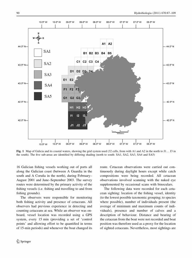
Galicia (NW Spain) has a coastline of about

1,200 km (Fig. 1). It has a relatively narrow conti-

nental shelf with a total surface area of approximately

15,000 km2 (Farina et al., 1997). The Galician

continental shelf and the Galician rıas (coastal fjords

according to Vidal-Romanı, 1984) lie at the northern

edge of one of the major upwelling areas in the world,

the eastern boundary system off NW Africa and SW

Europe (Wooster et al., 1976). The frequent upwell-

ing of cold and dense North Atlantic Central Water

(NACW) results in nutrient enrichment of the area

(Blanton et al., 1984) and this area is among the most

productive oceanic regions of the world. Upwelling

reaches its highest intensity during summer (April to

September) (Fraga, 1981; Prego & Bao, 1997). Up to

300 species of fish (Solorzano et al., 1988) and

around 80 species of cephalopods (Guerra, 1992)

have been recorded in Galician coastal waters. The

area constitutes an important nursery ground for

several commercially important fish species, e.g.

hake, Merluccius merluccius (Pereiro et al., 1980;

Farina et al., 1985). The broad-scale distribution of

fish assemblages over the continental shelf area is

mainly determined by depth and hydrographic struc-

ture and, in general, density, biomass and species

richness all decrease with increasing depth (Farina

et al., 1997), reflecting the general phenomenon that

species with more restricted depth ranges tend to

occur in the shallowest waters (Smith & Brown,

2002). Galician waters are also an important area for

marine mammals, including 16 cetacean and four

pinniped species. Resident cetaceans in Galicia

include the common dolphin (Delphinus delphis),

the bottlenose dolphin (Tursiops truncatus) and the

harbour porpoise (Phocoena phocoena). These three

species are seen all along the Galician coast, although

with different geographical patterns of local abun-

dance (Lopez et al., 2004; Pierce et al., 2010), and are

listed as vulnerable in Spain’s National Endangered

Species Act (Canadas et al., 2002).

Data collection and processing

Cetacean sightings data were collected from Galician

coastal waters by four observers on-board a total of

Hydrobiologia (2011) 670:87–109 89

123

16 Galician fishing vessels working out of ports all

along the Galician coast (between A Guardia in the

south and A Coruna in the north), during February–

August 2001 and June–September 2003. The survey

routes were determined by the primary activity of the

fishing vessels (i.e. fishing and travelling to and from

fishing grounds).

The observers were responsible for monitoring

both fishing activity and presence of cetaceans. All

observers had previous experience in detecting and

counting cetaceans at sea. While an observer was on-

board, vessel location was recorded using a GPS

system, every 15 min (providing a set of ‘control

points’ and allowing effort to be quantified in terms

of 15-min periods) and whenever the boat changed its

route. Cetacean observations were carried out con-

tinuously during daylight hours except while catch

compositions were being recorded. All cetacean

observations involved scanning with the naked eye

supplemented by occasional scans with binoculars.

The following data were recorded for each ceta-

cean sighting: location of the fishing vessel, identity

(to the lowest possible taxonomic grouping; to species

where possible), number of individuals present (the

average of minimum and maximum counts of indi-

viduals), presence and number of calves and a

description of behaviour. Distance and bearing of

the cetacean from the boat were not recorded and boat

position was therefore used as a proxy for the location

of sighted cetaceans. Nevertheless, most sightings are

Fig. 1 Map of Galicia and its coastal waters, showing the grid system used (32 cells, from with A1 and A2 in the north to J1… J3 in

the south). The five sub-areas are identified by differing shading (north to south: SA1, SA2, SA3, SA4 and SA5)

90 Hydrobiologia (2011) 670:87–109

123

thought to have been within 1 km of the position of

the boat and in any case the final analysis uses a

coarser-scale (grid cell) spatial resolution.

The study area was divided into a base-grid of 32

cells of dimensions 1401200 longitude and 1404200

latitude (area approximately 530 km2), which cov-

ered the area of Galician coastal waters between

latitudes 41� to 45�N and longitudes 7� to 12�W. This

grid size was a compromise between the aim of

determining environmental relationships and the need

to avoid the majority of cells having no sightings (this

being a function of the amount of survey effort). A

grid-based approach also reduces potential problems

with autocorrelation in the data. Five sub-areas were

also defined along the north–south axis (Fig. 1).

Survey routes and sightings positions data were

imported into GIS (MapInfo; Idrisi Taiga). The

system used included detailed bathymetry data.

Satellite-derived sea surface temperature (SST)

data were sourced from Plymouth Marine Laboratory

(Natural Environment Research Council, UK). All

level-2 images used in this study were geo-referenced

and masked out manually in black for clouds, land

and sun-glint. The SST images were from the

AVHRR (Advanced Very High Resolution Radiom-

eter) sensor onboard the NOAA satellite series.

Satellite-derived images of chl-a concentration were

from the SeaWIFS (Sea Viewing Wide Field-of-View

Sensor) colour sensor. Treatment of SeaWIFS images

included application of nearest neighbour interpola-

tion. Raster data were extracted on a standard digital

0–255 colour or grey-scale value for each pixel.

Chl-a concentration is calculated based to the reflec-

tance ratio between 490 and 555 nm (McClain,

1997). Both satellite sensors provide data with a

1.1 km on-ground resolution in nadir.

The conversion from the standard Digital Number

(DN) 0–255 scale integer value stored in the image,

to obtain the real-world SST values (8C), used

the AVHRR Oceans Pathfinder SST algorithm

(Walton, 1988; Walton et al., 1990): SST = DN 9 0.1 ?

5.0. Conversion from DN to real values of Chl-a

(mg/m3) used the following equation: Chl-a =

10ðð0:015�DNÞþlog10ð0:01ÞÞ.Information on calendar day, depth (m) and asso-

ciated effort was available for all cetacean observa-

tions. In addition, depth (minimum, maximum and

average) and total effort were derived for each grid

cell. Satellite-derived data for SST and chl-a were

available for slightly over half of the sightings

records (missing values are due to cloud cover).

Data analysis

Data were analysed at two levels of temporal resolu-

tion, by cell over the whole study period and by cell per

day. The former provides a coarse-scale view of

distribution without the possibility to examine temporal

trends but avoids problems of temporal autocorrelation.

The latter is potentially more powerful but the daily by-

cell sightings data included a very high proportion of

zero values, making model fitting difficult and with a

high likelihood of significant temporal (or spatial)

autocorrelation. In addition, at present, satellite data

have not been obtained for all the absence records.

Therefore, fine-scale analysis was restricted to an

analysis of trends in cetacean abundance among the

subset of presence records. Note that a further option

for analysing the data would have been to use (15 min)

survey legs as the basic unit of data. However, this

suffers similar limitations to the by cell by day analysis.

Daily survey effort within a grid cell was

estimated from the number of GPS positions recorded

within the cell, counting only the ‘control point’

position records, i.e. those taken at 15-min intervals.

To generate summary statistics we expressed total

survey effort per cell as a percentage of the total

number of control points over the whole study area

and period (N = 2,002 within the study grid). Thus, a

figure of 1% represents approximately 5 h of obser-

vation time (2,002 9 0.25 h/100).

To provide overall indices of relative abundance,

totals for sightings and survey effort were extracted

by grid cell, and two measures of sighting rate were

derived: sightings per unit effort (SPUE, i.e. number

of sightings per 15 min search effort) and individuals

per unit effort (IPUE, number of individuals per

15 min search effort).

The environmental characteristics of locations at

which each species was seen were summarised:

although absolute values may be biased due to

uneven distribution of effort, comparisons between

species are potentially informative.

Generalised additive models were used to deter-

mine environmental relationships for (a) cetacean

sightings rate per cell over the study period and

Hydrobiologia (2011) 670:87–109 91

123

(b) for the subset of cetacean sightings records,

variation in numbers of cetaceans (given presence).

In the latter case, search effort for the relevant grid

cell, day and year combination was used as one of the

explanatory variables. Since common dolphins were

by far the most frequently recorded species, both

analyses were repeated for common dolphin sightings

only. Finally, the analysis of numbers given presence

was also repeated for common dolphin calves.

Between-cell variation in abundance

The overall cetacean SPUE by cell and common

dolphin SPUE by cell were modeled as a function of

grid cell location (as northing and easting, i.e.

equivalent to latitude and longitude) and average

sea depth. Since all three explanatory variables are

continuous variables they were fitted as smoothers.

SPUE was assumed to be normally distributed and an

identity link function was used. The assumption of

normality was validated by examining the distribu-

tion of model residuals. Separate GAMS were not

fitted for any other cetacean species since there were

insufficient non-zero records.

Abundance given presence

For this analysis, each sighting was treated as a

separate data point, with the response variables being

(a) number of cetaceans sighted, (b) number of

common dolphins sighted and (c) number of common

dolphin calves sighted. The suite of explanatory

variables tested was: grid cell location (as northing

and easting), year, calendar day, depth, effort (for the

cell and day) and satellite image-derived values for

SST and chl-a. Since some of the available explan-

atory variables potentially explain the same variation

in abundance, three types of models were fitted:

(1) models with only effort, time and location used

as explanatory variables, i.e. models describing

spatiotemporal variation in abundance;

(2) models with environmental variables used in

place of the time and location variables, i.e.

models to test the proportion of spatiotemporal

variation that can be ascribed to environmental

conditions;

(3) models using all available explanatory vari-

ables, thus allowing both ‘environmental’ and

‘non-environmental’ components of spatiotem-

poral patterns to be included (although the latter

may of course be a consequence of environ-

mental variables not included in the analysis).

Since SST was significantly correlated with

calendar day (r = 0.69), we derived residual SST

from a Gaussian GAM model of SST in relation to

calendar day for use in models which included both

calendar day and SST. Thus, the seasonal compo-

nent of SST variation will be contained within the

variable ‘calendar day’ while residual variation in

SST is included as a separate explanatory variable.

Chl-a values showed a complex and non-linear

relationship with bathymetry, in that both the

highest values and the widest range of values were

found in shallow waters. Data on SST and

chl-a were not available for all sightings, mainly

due to high cloud cover on some days. Therefore,

for those models which included ‘environmental’

variables, we separately tested use of (i) depth alone

and (ii) depth, SST and chl-a.

Initial GAM fits using a Poisson distribution for

abundance data indicated substantial overdispersion

of the response variable. Adult numbers were mark-

edly more overdispersed than those for calves so a

negative binomial distribution was used for the

former and quasi-Poisson for the latter, in both cases

using a log-link function. Abundance of other ceta-

cean species was too low to fit separate models.

For all GAMs, the final model was selected on the

basis of the AIC, individual significance of explan-

atory variables and examination of diagnostic plots

(e.g. residual plots, hat values, etc.). To avoid

overfitting, the maximum value of k (knots, i.e. a

measure of the maximum complexity of the fitted

curve) was set at 4 for all explanatory variables. Note

that, since we used grid cells as spatial units, there

were few unique values of latitude and longitude and

higher k values could not have been used for these

variables. F tests were used to compare the nested

models (Zuur et al., 2007). Significance of smooth

terms is reported along with an indication of the

estimated degrees of freedom, a measure of the

complexity of the curve, where edf = 1 indicates a

linear fit and higher values indicate curves. Brodgar

software (www.brodgar.com), a menu-based inter-

face for R (R Core Development Team, 2006), was

used for fitting GAMs.

92 Hydrobiologia (2011) 670:87–109

123

Results

Survey effort

Surveys took place during 119 non-consecutive days

over 2 years, with observers present on-board Gali-

cian fishing vessels during February–August 2001

(85 days) and June–September 2003 (34 days). A

total of 136 observer-days at sea was achieved (102

and 34, in 2001 and 2003, respectively), with 2,116

control points acquired over a broad area within

Galician coastal waters, 2,002 of which fell within

the grid. There was considerable variation in the

survey coverage within each grid-square, mainly due

to the routes and preferred fishing areas of the fishing

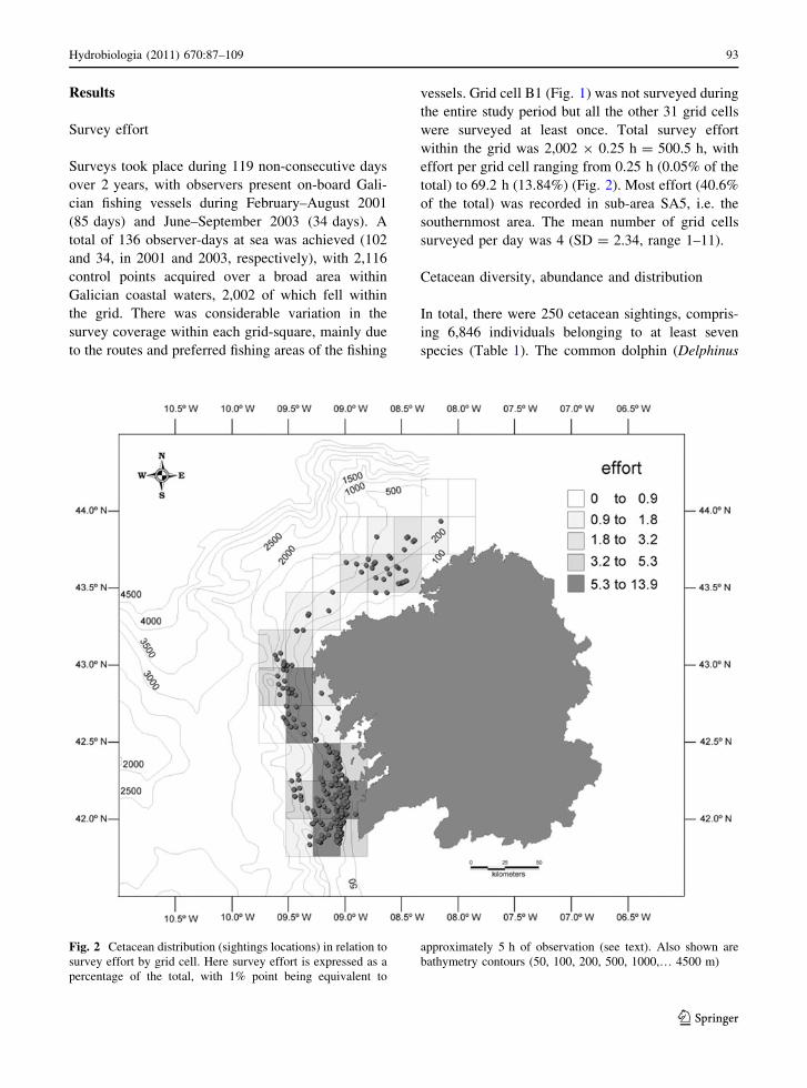
vessels. Grid cell B1 (Fig. 1) was not surveyed during

the entire study period but all the other 31 grid cells

were surveyed at least once. Total survey effort

within the grid was 2,002 9 0.25 h = 500.5 h, with

effort per grid cell ranging from 0.25 h (0.05% of the

total) to 69.2 h (13.84%) (Fig. 2). Most effort (40.6%

of the total) was recorded in sub-area SA5, i.e. the

southernmost area. The mean number of grid cells

surveyed per day was 4 (SD = 2.34, range 1–11).

Cetacean diversity, abundance and distribution

In total, there were 250 cetacean sightings, compris-

ing 6,846 individuals belonging to at least seven

species (Table 1). The common dolphin (Delphinus

Fig. 2 Cetacean distribution (sightings locations) in relation to

survey effort by grid cell. Here survey effort is expressed as a

percentage of the total, with 1% point being equivalent to

approximately 5 h of observation (see text). Also shown are

bathymetry contours (50, 100, 200, 500, 1000,… 4500 m)

Hydrobiologia (2011) 670:87–109 93

123

delphis) was by far the most frequently sighted

species (205 sightings, 82.4% of the all-species total).

The other species recorded were long-finned pilot

whale (Globicephala melas) (13 sightings), bottle-

nose dolphin (Tursiops truncatus) (9), Risso’s dol-

phin (Grampus griseus) (6), harbour porpoise

(Phocoena phocoena) (5), striped dolphin (Stenella

coeruleoalba) (4) and fin whale (Balaenoptera phys-

alus) (1). In addition, there were two sightings of

unidentified Delphinidae and five sightings of uniden-

tified mysticetes. For further analysis, the unidentified

mysticetes and the fin whale were grouped as

mysticetes.

Delphinus delphis was also the most abundant

species in the study area, accounting for 93.3% of

individual cetaceans seen. G. melas was the second

most abundant species (3.5%), followed by

T. truncatus (1.3%) and G. griseus (1.1%). Common

dolphins tended to be seen in large groups while

mysticetes were seen alone or in very small groups.

Calves were recorded during 60 sightings (24% of

the total), with numbers ranging from 1 (21 sightings)

to 18 (1 sighting) individuals. Calves of five species

were recorded: D. delphis (158 individuals from 48

sightings), G. melas (18 individuals, 8 sightings);

T. truncatus (2 individuals, 2 sightings); G. griseus

(2 individuals, 1 sighting) P. phocoena (1 individual,

1 sighting).

Two sightings of T. truncatus were outside the pre-

defined study area and therefore excluded from further

analysis. Of the remaining 248 sightings, the highest

percentages were recorded in sub-areas SA5 (40.6% of

sightings) and SA3 (20.2%, Fig. 2). Most sightings in

SA5 occurred between the 100 and 200 m isobaths

although further north there appear to be fewer

sightings in such shallow waters. Taking into account

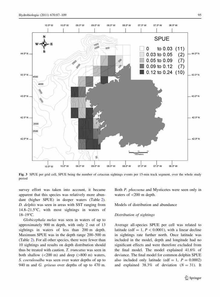
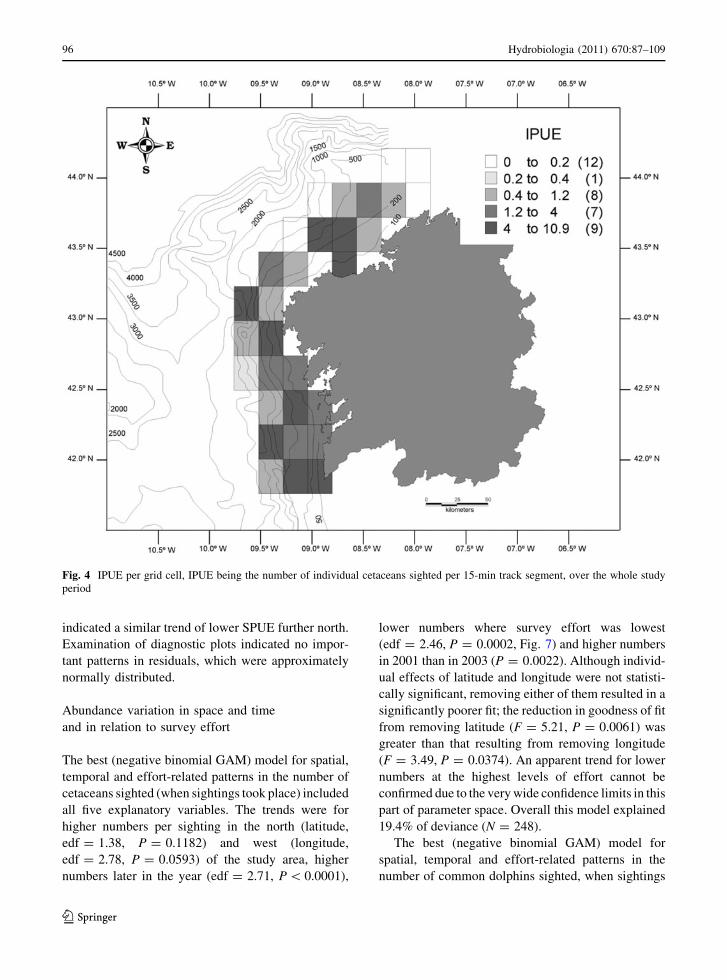
survey effort, overall the sightings rate (SPUE) per grid

cell was generally higher in the south (Fig. 3) while the

spatial pattern in abundance (IPUE) is less clear

(Fig. 4). The highest values of both SPUE (0.24) and

IPUE (10.86) were seen in SA5.

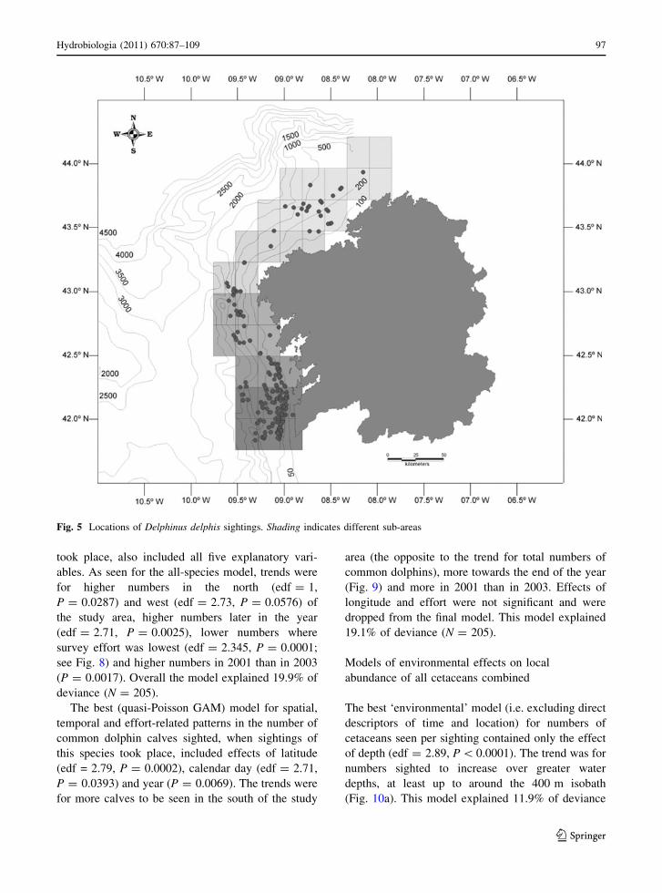
Delphinus delphis was the most widely distributed

cetacean and was present in all sub-areas, although

over half of the sightings (51.3%) were in SA5

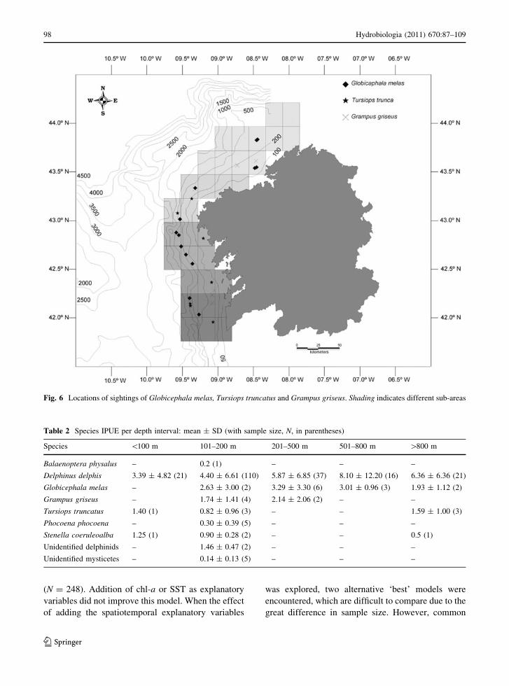
(Fig. 5), G. melas was present all along the coast but

mostly seen in SA3 and SA1 (38.5 and 30.8%,

respectively) and generally not close to the shore

(Fig. 6). For the other species, the small number of

sightings precludes any firm conclusions about dis-

tribution, although T. truncatus was most often

sighted in SA5 (40%) and P. phocoena was only

sighted in SA5.

Delphinus delphis was sighted mainly in May to

August, although it should be noted that the months

June to August were the only months sampled in both

years. The second most frequently sighted species,

G. melas (N = 13) was seen most often in May.

Cetacean distribution and abundance in relation

to environmental parameters

Cetacean sightings were recorded in water depths

ranging from 7–1,432 m. The majority of D. delphis

sightings were in waters of less than 200 m depth,

although it was also the only species sighted in waters

over 1,050 m depth (11 out of 205 sightings). Once

Table 1 Number of cetaceans recorded during surveys, by species: number of sightings, sums of minimum, maximum and mean

counts, total number of groups seen and mean group size

Species Sightings Minimum Maximum Mean Number of groups Mean group size

Delphinus delphis 205 5410 7368 6389 252 25.4

Globicephala melas 13 208 265 236.5 20 11.8

Tursiops truncatus 7 69 90 79.5 9 8.8

Grampus griseus 6 61 86 73.5 6 12.3

Phocoena phocoena 5 8 8 8 5 1.6

Stenella coeruleoalba 4 25 30 27.5 4 6.9

Balaenoptera physalis 1 1 1 1 1 1

Unidentified mysticeti 5 6 6 6 5 1.2

Unidentified delphinid 2 18 25 21.5 2 10.8

94 Hydrobiologia (2011) 670:87–109

123

survey effort was taken into account, it became

apparent that this species was relatively more abun-

dant (higher SPUE) in deeper waters (Table 2).

D. delphis was seen in areas with SST ranging from

14.8–21.5�C, with most sightings in waters of

18–19�C.

Globicephala melas was seen in waters of up to

approximately 900 m depth, with only 2 out of 13

sightings in waters of less than 200 m depth.

Maximum SPUE was in the depth range 200–500 m

(Table 2). For all other species, there were fewer than

10 sightings and results on depth distribution should

thus be treated with caution. T. truncatus was seen in

both shallow (\200 m) and deep ([800 m) waters,

S. coeruleoalba was seen over water depths of up to

940 m and G. griseus over depths of up to 470 m.

Both P. phocoena and Mysticetes were seen only in

waters of \200 m depth.

Models of distribution and abundance

Distribution of sightings

Average all-species SPUE per cell was related to

latitude (edf = 1, P \ 0.0001), with a linear decline

in sightings rate further north. Once latitude was

included in the model, depth and longitude had no

significant effects and were therefore excluded from

the final model. The model explained 41.6% of

deviance. The final model for common dolphin SPUE

also included only latitude (edf = 1, P = 0.0002)

and explained 38.3% of deviation (N = 31). It

Fig. 3 SPUE per grid cell, SPUE being the number of cetacean sightings events per 15-min track segment, over the whole study

period

Hydrobiologia (2011) 670:87–109 95

123

indicated a similar trend of lower SPUE further north.

Examination of diagnostic plots indicated no impor-

tant patterns in residuals, which were approximately

normally distributed.

Abundance variation in space and time

and in relation to survey effort

The best (negative binomial GAM) model for spatial,

temporal and effort-related patterns in the number of

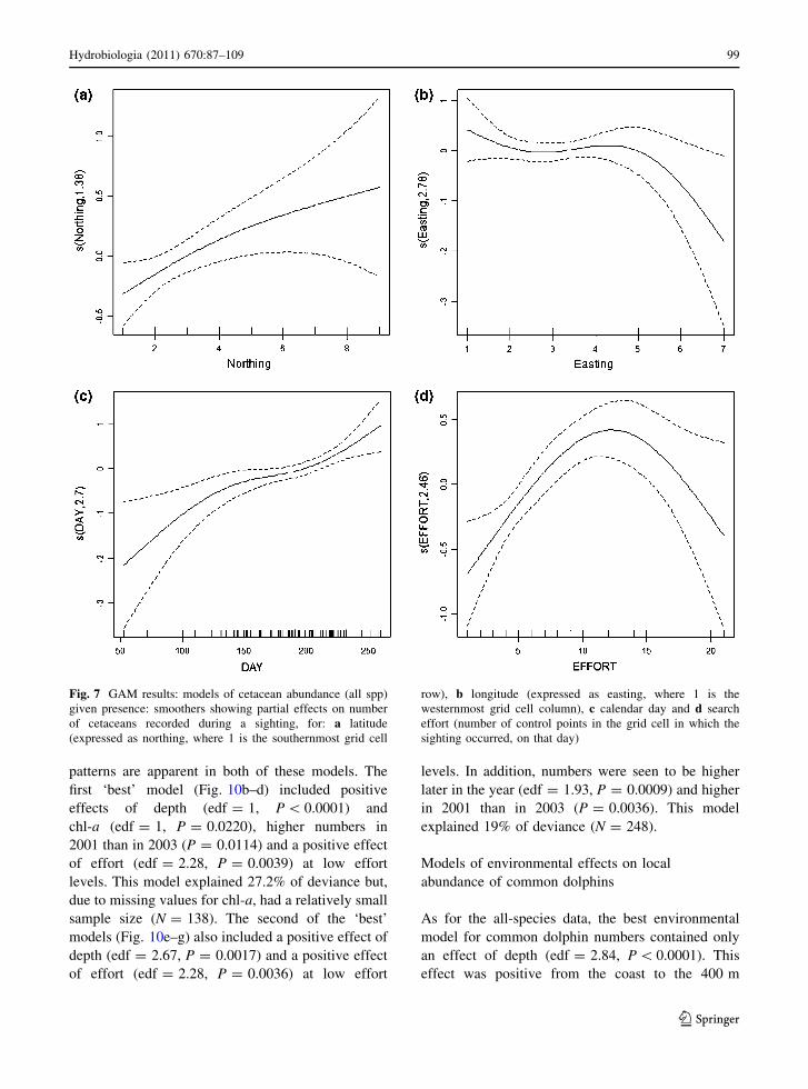
cetaceans sighted (when sightings took place) included

all five explanatory variables. The trends were for

higher numbers per sighting in the north (latitude,

edf = 1.38, P = 0.1182) and west (longitude,

edf = 2.78, P = 0.0593) of the study area, higher

numbers later in the year (edf = 2.71, P \ 0.0001),

lower numbers where survey effort was lowest

(edf = 2.46, P = 0.0002, Fig. 7) and higher numbers

in 2001 than in 2003 (P = 0.0022). Although individ-

ual effects of latitude and longitude were not statisti-

cally significant, removing either of them resulted in a

significantly poorer fit; the reduction in goodness of fit

from removing latitude (F = 5.21, P = 0.0061) was

greater than that resulting from removing longitude

(F = 3.49, P = 0.0374). An apparent trend for lower

numbers at the highest levels of effort cannot be

confirmed due to the very wide confidence limits in this

part of parameter space. Overall this model explained

19.4% of deviance (N = 248).

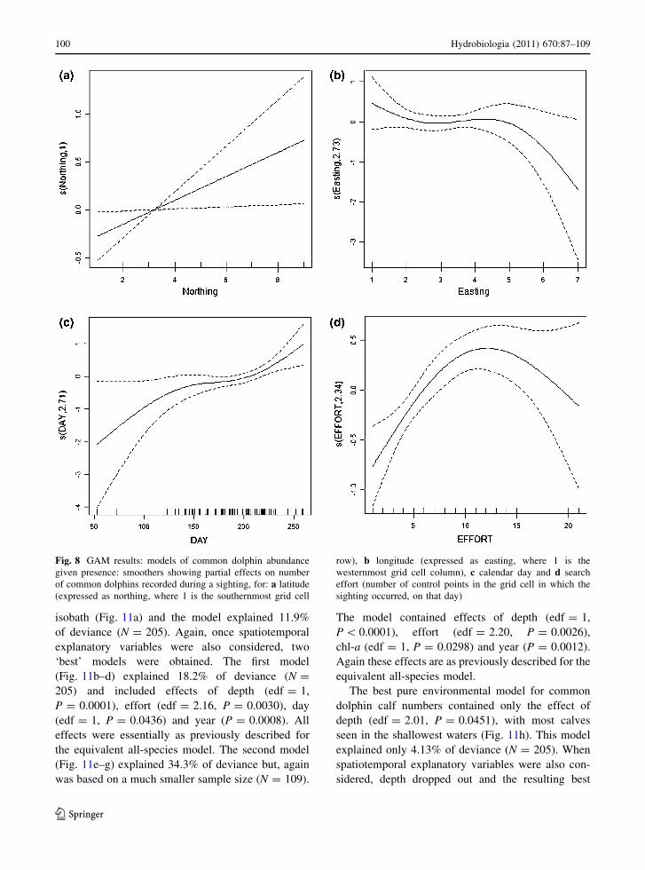
The best (negative binomial GAM) model for

spatial, temporal and effort-related patterns in the

number of common dolphins sighted, when sightings

Fig. 4 IPUE per grid cell, IPUE being the number of individual cetaceans sighted per 15-min track segment, over the whole study

period

96 Hydrobiologia (2011) 670:87–109

123

took place, also included all five explanatory vari-

ables. As seen for the all-species model, trends were

for higher numbers in the north (edf = 1,

P = 0.0287) and west (edf = 2.73, P = 0.0576) of

the study area, higher numbers later in the year

(edf = 2.71, P = 0.0025), lower numbers where

survey effort was lowest (edf = 2.345, P = 0.0001;

see Fig. 8) and higher numbers in 2001 than in 2003

(P = 0.0017). Overall the model explained 19.9% of

deviance (N = 205).

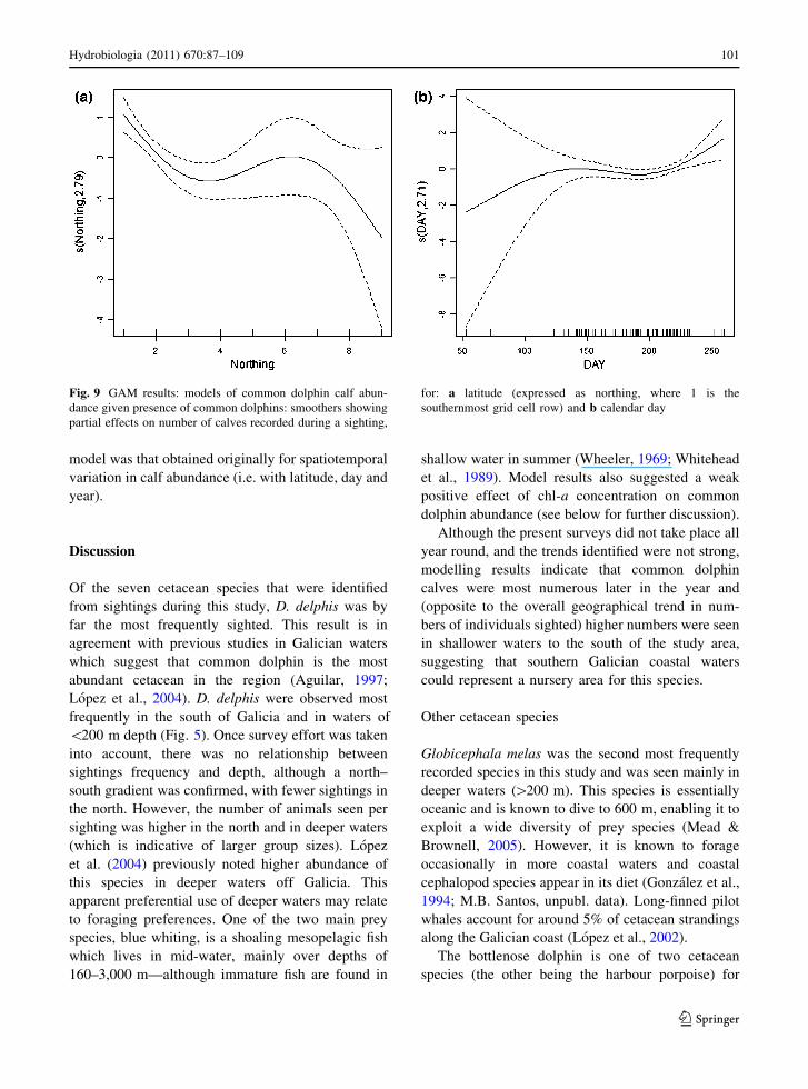
The best (quasi-Poisson GAM) model for spatial,

temporal and effort-related patterns in the number of

common dolphin calves sighted, when sightings of

this species took place, included effects of latitude

(edf = 2.79, P = 0.0002), calendar day (edf = 2.71,

P = 0.0393) and year (P = 0.0069). The trends were

for more calves to be seen in the south of the study

area (the opposite to the trend for total numbers of

common dolphins), more towards the end of the year

(Fig. 9) and more in 2001 than in 2003. Effects of

longitude and effort were not significant and were

dropped from the final model. This model explained

19.1% of deviance (N = 205).

Models of environmental effects on local

abundance of all cetaceans combined

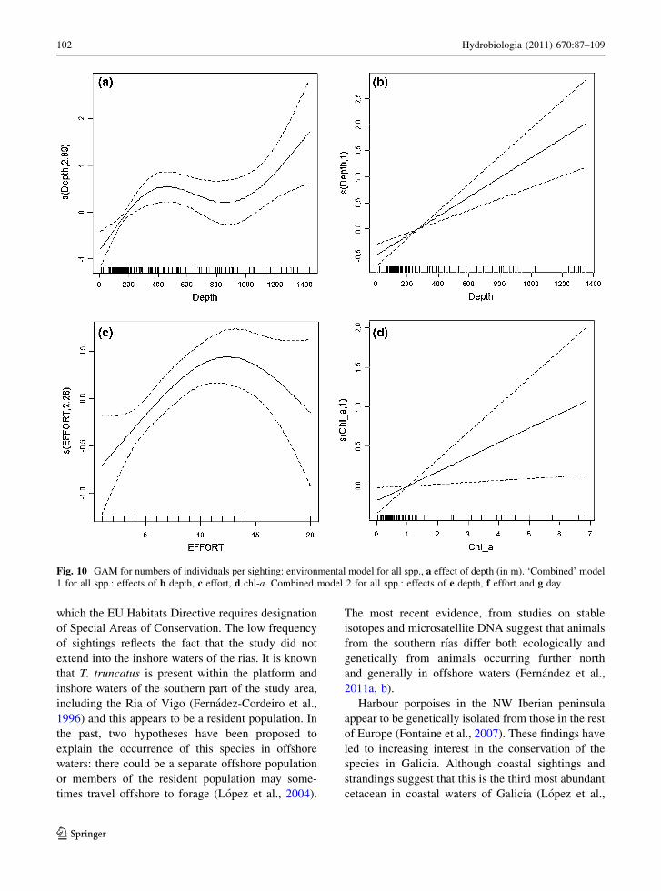
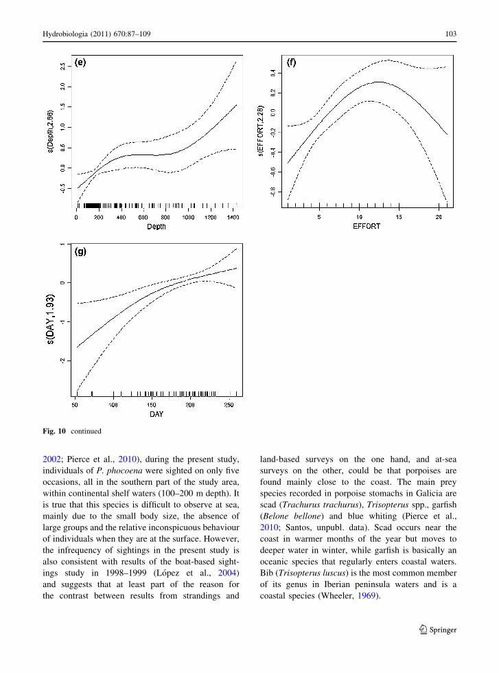
The best ‘environmental’ model (i.e. excluding direct

descriptors of time and location) for numbers of

cetaceans seen per sighting contained only the effect

of depth (edf = 2.89, P \ 0.0001). The trend was for

numbers sighted to increase over greater water

depths, at least up to around the 400 m isobath

(Fig. 10a). This model explained 11.9% of deviance

Fig. 5 Locations of Delphinus delphis sightings. Shading indicates different sub-areas

Hydrobiologia (2011) 670:87–109 97

123

(N = 248). Addition of chl-a or SST as explanatory

variables did not improve this model. When the effect

of adding the spatiotemporal explanatory variables

was explored, two alternative ‘best’ models were

encountered, which are difficult to compare due to the

great difference in sample size. However, common

Fig. 6 Locations of sightings of Globicephala melas, Tursiops truncatus and Grampus griseus. Shading indicates different sub-areas

Table 2 Species IPUE per depth interval: mean ± SD (with sample size, N, in parentheses)

Species \100 m 101–200 m 201–500 m 501–800 m [800 m

Balaenoptera physalus – 0.2 (1) – – –

Delphinus delphis 3.39 ± 4.82 (21) 4.40 ± 6.61 (110) 5.87 ± 6.85 (37) 8.10 ± 12.20 (16) 6.36 ± 6.36 (21)

Globicephala melas – 2.63 ± 3.00 (2) 3.29 ± 3.30 (6) 3.01 ± 0.96 (3) 1.93 ± 1.12 (2)

Grampus griseus – 1.74 ± 1.41 (4) 2.14 ± 2.06 (2) – –

Tursiops truncatus 1.40 (1) 0.82 ± 0.96 (3) – – 1.59 ± 1.00 (3)

Phocoena phocoena – 0.30 ± 0.39 (5) – – –

Stenella coeruleoalba 1.25 (1) 0.90 ± 0.28 (2) – – 0.5 (1)

Unidentified delphinids – 1.46 ± 0.47 (2) – – –

Unidentified mysticetes – 0.14 ± 0.13 (5) – – –

98 Hydrobiologia (2011) 670:87–109

123

patterns are apparent in both of these models. The

first ‘best’ model (Fig. 10b–d) included positive

effects of depth (edf = 1, P \ 0.0001) and

chl-a (edf = 1, P = 0.0220), higher numbers in

2001 than in 2003 (P = 0.0114) and a positive effect

of effort (edf = 2.28, P = 0.0039) at low effort

levels. This model explained 27.2% of deviance but,

due to missing values for chl-a, had a relatively small

sample size (N = 138). The second of the ‘best’

models (Fig. 10e–g) also included a positive effect of

depth (edf = 2.67, P = 0.0017) and a positive effect

of effort (edf = 2.28, P = 0.0036) at low effort

levels. In addition, numbers were seen to be higher

later in the year (edf = 1.93, P = 0.0009) and higher

in 2001 than in 2003 (P = 0.0036). This model

explained 19% of deviance (N = 248).

Models of environmental effects on local

abundance of common dolphins

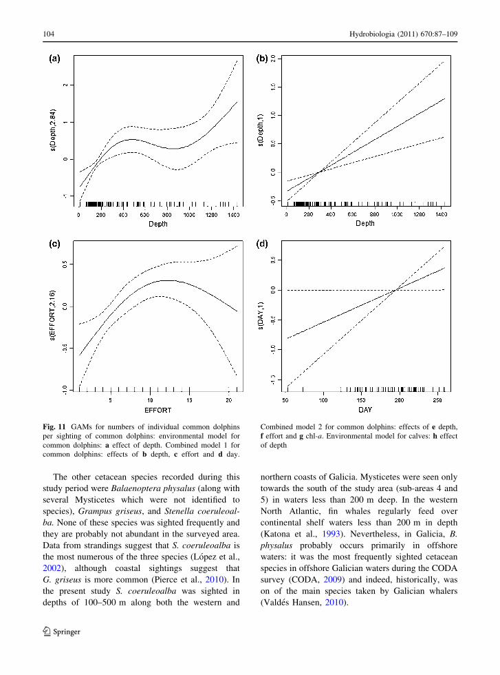
As for the all-species data, the best environmental

model for common dolphin numbers contained only

an effect of depth (edf = 2.84, P \ 0.0001). This

effect was positive from the coast to the 400 m

Fig. 7 GAM results: models of cetacean abundance (all spp)

given presence: smoothers showing partial effects on number

of cetaceans recorded during a sighting, for: a latitude

(expressed as northing, where 1 is the southernmost grid cell

row), b longitude (expressed as easting, where 1 is the

westernmost grid cell column), c calendar day and d search

effort (number of control points in the grid cell in which the

sighting occurred, on that day)

Hydrobiologia (2011) 670:87–109 99

123

isobath (Fig. 11a) and the model explained 11.9%

of deviance (N = 205). Again, once spatiotemporal

explanatory variables were also considered, two

‘best’ models were obtained. The first model

(Fig. 11b–d) explained 18.2% of deviance (N =

205) and included effects of depth (edf = 1,

P = 0.0001), effort (edf = 2.16, P = 0.0030), day

(edf = 1, P = 0.0436) and year (P = 0.0008). All

effects were essentially as previously described for

the equivalent all-species model. The second model

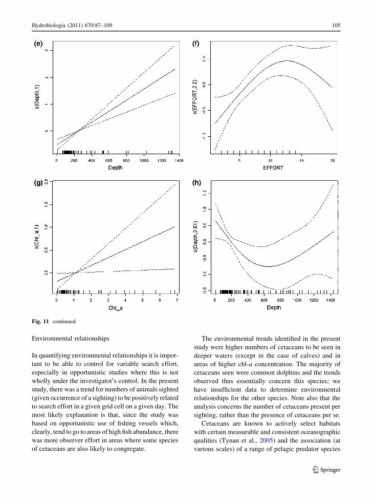
(Fig. 11e–g) explained 34.3% of deviance but, again

was based on a much smaller sample size (N = 109).

The model contained effects of depth (edf = 1,

P \ 0.0001), effort (edf = 2.20, P = 0.0026),

chl-a (edf = 1, P = 0.0298) and year (P = 0.0012).

Again these effects are as previously described for the

equivalent all-species model.

The best pure environmental model for common

dolphin calf numbers contained only the effect of

depth (edf = 2.01, P = 0.0451), with most calves

seen in the shallowest waters (Fig. 11h). This model

explained only 4.13% of deviance (N = 205). When

spatiotemporal explanatory variables were also con-

sidered, depth dropped out and the resulting best

Fig. 8 GAM results: models of common dolphin abundance

given presence: smoothers showing partial effects on number

of common dolphins recorded during a sighting, for: a latitude

(expressed as northing, where 1 is the southernmost grid cell

row), b longitude (expressed as easting, where 1 is the

westernmost grid cell column), c calendar day and d search

effort (number of control points in the grid cell in which the

sighting occurred, on that day)

100 Hydrobiologia (2011) 670:87–109

123

model was that obtained originally for spatiotemporal

variation in calf abundance (i.e. with latitude, day and

year).

Discussion

Of the seven cetacean species that were identified

from sightings during this study, D. delphis was by

far the most frequently sighted. This result is in

agreement with previous studies in Galician waters

which suggest that common dolphin is the most

abundant cetacean in the region (Aguilar, 1997;

Lopez et al., 2004). D. delphis were observed most

frequently in the south of Galicia and in waters of

\200 m depth (Fig. 5). Once survey effort was taken

into account, there was no relationship between

sightings frequency and depth, although a north–

south gradient was confirmed, with fewer sightings in

the north. However, the number of animals seen per

sighting was higher in the north and in deeper waters

(which is indicative of larger group sizes). Lopez

et al. (2004) previously noted higher abundance of

this species in deeper waters off Galicia. This

apparent preferential use of deeper waters may relate

to foraging preferences. One of the two main prey

species, blue whiting, is a shoaling mesopelagic fish

which lives in mid-water, mainly over depths of

160–3,000 m—although immature fish are found in

shallow water in summer (Wheeler, 1969; Whitehead

et al., 1989). Model results also suggested a weak

positive effect of chl-a concentration on common

dolphin abundance (see below for further discussion).

Although the present surveys did not take place all

year round, and the trends identified were not strong,

modelling results indicate that common dolphin

calves were most numerous later in the year and

(opposite to the overall geographical trend in num-

bers of individuals sighted) higher numbers were seen

in shallower waters to the south of the study area,

suggesting that southern Galician coastal waters

could represent a nursery area for this species.

Other cetacean species

Globicephala melas was the second most frequently

recorded species in this study and was seen mainly in

deeper waters ([200 m). This species is essentially

oceanic and is known to dive to 600 m, enabling it to

exploit a wide diversity of prey species (Mead &

Brownell, 2005). However, it is known to forage

occasionally in more coastal waters and coastal

cephalopod species appear in its diet (Gonzalez et al.,

1994; M.B. Santos, unpubl. data). Long-finned pilot

whales account for around 5% of cetacean strandings

along the Galician coast (Lopez et al., 2002).

The bottlenose dolphin is one of two cetacean

species (the other being the harbour porpoise) for

Fig. 9 GAM results: models of common dolphin calf abun-

dance given presence of common dolphins: smoothers showing

partial effects on number of calves recorded during a sighting,

for: a latitude (expressed as northing, where 1 is the

southernmost grid cell row) and b calendar day

Hydrobiologia (2011) 670:87–109 101

123

which the EU Habitats Directive requires designation

of Special Areas of Conservation. The low frequency

of sightings reflects the fact that the study did not

extend into the inshore waters of the rias. It is known

that T. truncatus is present within the platform and

inshore waters of the southern part of the study area,

including the Ria of Vigo (Fernadez-Cordeiro et al.,

1996) and this appears to be a resident population. In

the past, two hypotheses have been proposed to

explain the occurrence of this species in offshore

waters: there could be a separate offshore population

or members of the resident population may some-

times travel offshore to forage (Lopez et al., 2004).

The most recent evidence, from studies on stable

isotopes and microsatellite DNA suggest that animals

from the southern rıas differ both ecologically and

genetically from animals occurring further north

and generally in offshore waters (Fernandez et al.,

2011a, b).

Harbour porpoises in the NW Iberian peninsula

appear to be genetically isolated from those in the rest

of Europe (Fontaine et al., 2007). These findings have

led to increasing interest in the conservation of the

species in Galicia. Although coastal sightings and

strandings suggest that this is the third most abundant

cetacean in coastal waters of Galicia (Lopez et al.,

Fig. 10 GAM for numbers of individuals per sighting: environmental model for all spp., a effect of depth (in m). ‘Combined’ model

1 for all spp.: effects of b depth, c effort, d chl-a. Combined model 2 for all spp.: effects of e depth, f effort and g day

102 Hydrobiologia (2011) 670:87–109

123

2002; Pierce et al., 2010), during the present study,

individuals of P. phocoena were sighted on only five

occasions, all in the southern part of the study area,

within continental shelf waters (100–200 m depth). It

is true that this species is difficult to observe at sea,

mainly due to the small body size, the absence of

large groups and the relative inconspicuous behaviour

of individuals when they are at the surface. However,

the infrequency of sightings in the present study is

also consistent with results of the boat-based sight-

ings study in 1998–1999 (Lopez et al., 2004)

and suggests that at least part of the reason for

the contrast between results from strandings and

land-based surveys on the one hand, and at-sea

surveys on the other, could be that porpoises are

found mainly close to the coast. The main prey

species recorded in porpoise stomachs in Galicia are

scad (Trachurus trachurus), Trisopterus spp., garfish

(Belone bellone) and blue whiting (Pierce et al.,

2010; Santos, unpubl. data). Scad occurs near the

coast in warmer months of the year but moves to

deeper water in winter, while garfish is basically an

oceanic species that regularly enters coastal waters.

Bib (Trisopterus luscus) is the most common member

of its genus in Iberian peninsula waters and is a

coastal species (Wheeler, 1969).

Fig. 10 continued

Hydrobiologia (2011) 670:87–109 103

123

The other cetacean species recorded during this

study period were Balaenoptera physalus (along with

several Mysticetes which were not identified to

species), Grampus griseus, and Stenella coeruleoal-

ba. None of these species was sighted frequently and

they are probably not abundant in the surveyed area.

Data from strandings suggest that S. coeruleoalba is

the most numerous of the three species (Lopez et al.,

2002), although coastal sightings suggest that

G. griseus is more common (Pierce et al., 2010). In

the present study S. coeruleoalba was sighted in

depths of 100–500 m along both the western and

northern coasts of Galicia. Mysticetes were seen only

towards the south of the study area (sub-areas 4 and

5) in waters less than 200 m deep. In the western

North Atlantic, fin whales regularly feed over

continental shelf waters less than 200 m in depth

(Katona et al., 1993). Nevertheless, in Galicia, B.

physalus probably occurs primarily in offshore

waters: it was the most frequently sighted cetacean

species in offshore Galician waters during the CODA

survey (CODA, 2009) and indeed, historically, was

on of the main species taken by Galician whalers

(Valdes Hansen, 2010).

Fig. 11 GAMs for numbers of individual common dolphins

per sighting of common dolphins: environmental model for

common dolphins: a effect of depth. Combined model 1 for

common dolphins: effects of b depth, c effort and d day.

Combined model 2 for common dolphins: effects of e depth,

f effort and g chl-a. Environmental model for calves: h effect

of depth

104 Hydrobiologia (2011) 670:87–109

123

Environmental relationships

In quantifying environmental relationships it is impor-

tant to be able to control for variable search effort,

especially in opportunistic studies where this is not

wholly under the investigator0s control. In the present

study, there was a trend for numbers of animals sighted

(given occurrence of a sighting) to be positively related

to search effort in a given grid cell on a given day. The

most likely explanation is that, since the study was

based on opportunistic use of fishing vessels which,

clearly, tend to go to areas of high fish abundance, there

was more observer effort in areas where some species

of cetaceans are also likely to congregate.

The environmental trends identified in the present

study were higher numbers of cetaceans to be seen in

deeper waters (except in the case of calves) and in

areas of higher chl-a concentration. The majority of

cetaceans seen were common dolphins and the trends

observed thus essentially concern this species; we

have insufficient data to determine environmental

relationships for the other species. Note also that the

analysis concerns the number of cetaceans present per

sighting, rather than the presence of cetaceans per se.

Cetaceans are known to actively select habitats

with certain measurable and consistent oceanographic

qualities (Tynan et al., 2005) and the association (at

various scales) of a range of pelagic predator species

Fig. 11 continued

Hydrobiologia (2011) 670:87–109 105

123

in areas of high productivity (including meso-scale

fronts and upwelling areas) is well-documented (e.g.

Jaquet & Whitehead, 1996; Zainuddin et al., 2006).

Thus, the association of higher cetacean numbers

with higher chlorophyll concentrations is not unex-

pected. Higher numbers of common dolphins were

seen over deeper waters, although the survey did not

extend beyond the shelf waters used by the fishing

fleet. Oceanic cetaceans may undertake feeding

excursions into coastal waters, congregating in areas

where there is high abundance of prey, thus feeding at

relatively shallow depths (Katona et al., 1993). This

is likely in the Atlantic (western) area of Galician

waters, where the effect of coastal upwelling (during

April–September) is known to be more intense

(Fraga, 1981; Blanton et al., 1984; Castro et al.,

1994) and prey availability would be higher than in

offshore waters (FAO, 1987; Farina et al., 1997;

Canadas et al., 2002; Smith & Brown, 2002).

Understanding the spatiotemporal relationships

linking oceanographic variables such as SST and

chl-a to diversity and abundance of cetaceans is not

straightforward, e.g. due to questions about the

appropriate scale at which relationships will be seen.

Hotspots of primary production resulting from ocean-

ographic phenomena are often localised in both space

and time. In addition, as pointed out by Gremillet

et al. (2008), we tend to forget that top predators do

not consume phytoplankton and the relationship

between primary production and the presence of

cetaceans may involve significant time-lags (e.g.

several weeks) and/or spatial displacement (e.g. tens

of kilometres) (e.g. Brown & Winn, 1989; Littaye

et al., 2004; Walker, 2005). Without good knowledge

of local oceanography and current systems and of the

ecology of the cetaceans, such relationships can

easily be missed. An additional logistical issue

associated with fine-scale studies is the availability

of cloud-free satellite images for the desired area and

time-window.

Although the present study provides some useful

preliminary indications of habitat preferences and

environmental relationships in Galician cetaceans,

further studies on cetacean habitat preferences in the

area are needed and would benefit from use of on-

board CTD, permitting measurement of additional

oceanographic variables and providing the further

benefit of allowing whole water column profiles to be

constructed (Scott et al., 2010).

Acknowledgments We gratefully acknowledge the input of

the four observers, who were funded by the European

Commission’s Directorate General for Fisheries under Study

Project 00/027, ‘Pelagic fisheries in Scotland and (UK) and

Galicia (Spain): observer studies to collect fishery data and

monitor by-catches of small cetaceans’ (2001) and the Xunta

de Galicia under project PGIDIT02MA00702CT, 2002–2005,

‘Predictive system of fishing efforts for the Galician artisan

fleet’). TCSD, ES and GMI would like to acknowledge funding

from EU Marie Curie project 20501 ‘ECOsystem approach to

Sustainable Management of the Marine Environment and its

living Resources’—ECOSUMMER. GJP was funded by a

Marie Curie excellence grant (MEXC-CT-2006-042337,

‘Anthropogenic Impacts on the Atlantic marine Ecosystems

of the Iberian Peninsula’—ANIMATE). We also thank Ruth

Fernandez and Begona Santos for comments on the

manuscript.

References

Aguilar, A., 1997. Inventario de los cetaceos de las aguas at-

lanticas peninsulares: aplicacion de la directiva 92/43/

CEE. Memoria Final. Departamento de Biologıa Animal

(Vert.), Facultad de Biologıa, Universitat de Barcelona,

Spain.

Baumgartner, M. F., 1997. The distribution of Risso’s dolphins

(Grampus griseus) in relation to the physiography of the

northern Gulf of Mexico. Marine Mammal Science 13:

614–638.

Baumgartner, M. F., K. D. Mullin, L. N. May & T. D. Leming,

2001. Cetacean habitats in the northern Gulf of Mexico.

Fishery Bulletin 99: 219–239.

Bellido, J. M., G. J. Pierce & J. Wang, 2001. Modelling intra

annual variation of squid Loligo forbesi in Scottish waters

using generalized additive models. Fisheries Research 52:

23–39.

Blanton, J. O., L. P. Atkinson, C. F. Fernandez & A. Lavin,

1984. Coastal upwelling off the Rıas Baixas, Galicia

Northwest Spain. I: hydrographic studies. Rapp. P.-V

Reun. Const. int. Explor. Mer 183: 79–90.

Brown, C. W. & H. E. Winn, 1989. Relationship between the

distribution pattern of right whales, Eubalaena glacialis, and

satellite-derived sea surface thermal structure in the Great

South Channel. Continental Shelf Research 9: 247–260.

Canadas, A., R. Sagarminada & S. Garcıa-Tiscar, 2002.

Cetacean distribution related with depth and slope in the

Mediterranean waters of Southern Spain. Deep-Sea

Research I 49: 2053–2073.

Castro, C. G., F. F. Perez, X. A. Alvarez-Salgado, G. Roson &

A. F. Rıos, 1994. Hydrographic conditions associated with the

relaxation process o fan upwelling event off Galicia coast

(NW Spain). Journal of Geophysical Research 99: 5135–5147.

CODA, 2009. Cetacean Offshore Distribution and Abundance.

Final Report. Available from SMRU, Gatty Marine Lab-

oratory, University of St Andrews, St Andrews, Fife,

KY16 8LB, UK.

Daskalov, G., 1999. Relating fish recruitment to stock biomass

and physical environment in the Black Sea using gen-

eralized additive models. Fisheries Research 41: 1–23.

106 Hydrobiologia (2011) 670:87–109

123

Davis, R. W., G. S. Fargion, N. May, T. D. Leming, M.

Baumgartner, W. E. Evans, L. J. Hansen & K. Mullin,

1998. Physical habitat of cetacean along the continental

slope in the north-central and western Gulf of Mexico.

Marine Mammal Science 14: 490–507.

Eastwood, P. D., G. J. Meaden & A. Grioche, 2001. Modelling

spatial variations in spawning habitat suitability for the

sole Solea solea using regression quantiles and GIS pro-

cedures. Marine Ecological Progress Series 224: 251–266.

Evans, P. G. H., 1987. The natural history of whales and dol-

phins. Christopher Helm Beckenham, London.

FAO, 1987. Fiches FAO d’identification des especes pour les

besoins de la peche. Mediterranee et Mer Noire. Zone de

Peche 37. Revision 1. Vol. II: Vertebres. FAO, Rome.

Farina, A. C., F. J. Pereiro & A. Fernandez, 1985. Peces de los

fondos de arrastre de la plataforma continental de Galicia.

Boletın del Instituto Espanol de Oceanografıa 2: 89–98.

Farina, A. C., J. Freire & E. Gonzalez-Gurriaran, 1997.

Demersal fish assemblages in the Galician continental

shelf and upper slope (NW Spain): spatial structure and

long-term changes. Estuarine and Coastal Shelf Science

44: 435–454.

Fernandez, R., S. Garcıa-Tiscar, M. B. Santos, A. Lopez,

J. A. Martınez-Cedeira, J. Newton & G. J. Pierce, 2011a.

Stable isotope analysis in two sympatric populations of

bottlenose dolphins Tursiops truncatus: evidence of

resource partitioning? Marine Biology 158: 1043–1055.

Fernandez, R., M. B. Santos, G. J. Pierce, A. Llavona,

A. Lopez, M. A. Silva, M. Ferreira, M. Carrillo,

P. Cermeno, S. Lens & S. Piertney, 2011b. Fine scale

genetic structure of bottlenose dolphins (Tursiops trunc-atus) off Atlantic waters of the Iberian Peninsula. Hyd-

robiologia (this volume).

Fernandez-Cordeiro, A. F. Torrado-Fernandez, R. Perez-Pin-

tos, M. Garci-Blanco & A. Rodrıguez-Folgar, 1996. The

bottlenose dolphin, Tursiops truncatus, along the Galician

coast, with special reference to the rıa de Vigo herd.

European Research on Cetaceans 10: 213–216.

Fontaine, M. C., S. J. E. Baird, S. Piry, N. Ray, K. A. Tolley,

S. Duke, A. Birkun, M. Ferreira, T. Jauniaux, A. Llavona,

B. Ozturk, A. A. Ozturk, V. Ridoux, E. Rogan,

M. Sequeira, U. Siebert, G. A. Vikingsson, J. M.

Bouquegneau & J. R. Michaux, 2007. Rise of oceano-

graphic barriers in continuous populations of a cetacean:

the genetic structure of harbour porpoises in Old World

waters. BMC Biology 5: 30–46.

Fraga, F., 1981. Upwelling of the Galician coast, Northwest

Spain. In Richards, F. (ed.), Coastal Upwelling. American

Geophysical Union Washington, DC: 176–182.

Gremillet, D. Lewis, S. Drapeau, L. van Der, C. D. Lingen,

J. A. Huggett, J. C. Coetzee, H. M. Verheye, F. Daunt,

S. Wanless & P. G. Ryan, 2008. Spatial match-mismatch

in the Benguela upwelling zone: should we expect chlo-

rophyll and sea-surface temperature to predict marine

predator distributions? Journal of Applied Ecology 45:

610–621.

Guerra, A., 1992. Mollusca, Cephalopoda. Fauna Iberica, Vol.

1. Museo Nacional de Ciencias Naturales, Madrid.

Gil de Sola, L., 1993. Las pesquerıas demersales del Mar de

Alboran (Surmediterraneo iberico). Evolucion en los

ultimos decenios. Informes Tecnicos Instituto Espanol de

Oceanografıa.

Gonzalez, A. F., A. Lopez, A. Guerra & A. Barreiro, 1994.

Diets of marine mammals stranded on the northwestern

Spanish Atlantic coast with special reference to Cepha-

lopoda. Fisheries Research 21(1–2): 179–191.

Hastie, T. & R. Tibshirani, 1990. Generalized Additive Mod-

els. Chapman and Hall, London.

Jaquet, N. & H. Whitehead, 1996. Scale-dependent correlation

of sperm whale distribution with environmental features

and productivity in the South Pacific. Marine Ecology

progress Series 135: 1–9.

Katona, S. K., V. Rough & D. T. Richardson, 1993. A Field

Guide to Whales, Porpoises, and Seals from Cape Cod to

Newfoundland. Fourth Edition, Revised. Smithsonian

Institution Press, Washington DC.

Koubbi, P., C. Loots, G. Cotonnec, X. Harlay, A. Grioche,

S. Vaz, C. Martin, M. Walkey & A. Carpentier, 2006.

Spatial patterns andGIS habitat modelling of Solea solea,

Pleuronectes flesus and Limanda limanda fish larvae in

the eastern English Channel during the spring. Scientia

Marina 70: 147–157.

Littaye, A., A. Gannier, S. Laran & J. P. F. Wilson, 2004. The

relationship between summer aggregation of fin whales

and satellite-derived environmental conditions in the

northwestern Mediterranean Sea. Remote Sensing of

Environment 90: 44–52.

Lopez, A., M. B. Santos, G. J. Pierce, A. F. Gonzalez,

X. Valeiras & A. Guerra, 2002. Trends in strandings and

by-catch of marine mammals in north-west Spain during

the 1990s. Journal of the Marine Biological Association of

the United Kingdom 82(3): 513–521.

Lopez, A., G. J. Pierce, M. B. Santos, J. Gracia & A. Guerra,

2003. Fishery by-catches of marine mammals in Galician

waters: results from on-board observations and an interview

survey of fishermen. Biological Conservation 111: 25–40.

Lopez, A., G. J. Pierce, X. Valeiras, M. B. Santos & A. Guerra,

2004. Distribution patterns of small cetaceans in Galician

waters. Journal of the Marine Biological Association of

the United Kingdom 84: 283–294.

Macleod, C. D., C. R. Weir, M. B. Santos & T. E. Dunn, 2009.

Temperature-based summer habitat partitioning between

white-beaked and common dolphins around the United

Kingdom and Republic of Ireland. Journal of the Marine

Biological Association of the United Kingdom 88:

1193–1198.

Maravelias, C. & C. Papaconstantinou, 2003. Size-related

habitat use, aggregation patterns and abundance of ang-

lerfish (Lophius budegassa) in the Mediterranean Sea

determined by generalized additive modelling. Journal of

the Marine Biological Association of the United Kingdom

83: 1171–1178.

Marubini, F., A. Gimona, P. G. H. Evans, P. J. Wright &

G. J. Pierce, 2009. Habitat preferences and interannual

variability in occurrence of the harbour porpoise Phoco-ena phocoena off northwest Scotland. Marine Ecology

Progress Series 381: 297–310.

McClain, C., 1997. SeaWiFS Bio-Optical Algorithm Mini-

workshop (SeaBAM) Overview, SeaBAM Technical

Memo, NASA SeaWiFS Project.

Hydrobiologia (2011) 670:87–109 107

123

Mead, J. G. & R. L. Brownell Jr, 2005. Order Cetacea (pp.

723–743). In Wilson, D. E. & D. M. Reeder (eds),

Mammal Species of the World: A Taxonomic and Geo-

graphic Reference, 2 Vols. (3rd ed.). Johns Hopkins

University Press, Baltimore: 2142 pp.

Meaden, G.J. & T. Do Chi, 1996. Geographical Information

Systems: Applications to Marine Fisheries. FAO Fisheries

Technical Paper No. 356. FAO, Rome, Italy: 335 pp.

Murase, M., K. Matsuoka, T. Ichii & S. Nishiwaki, 2002.

Relationship between the distribution of euphausiids and

baleen whales in the Antarctic (35�E–145�W). Polar

Biology 25(2): 135–145.

Oksanen, J. & P. R. Minchin, 2002. Continuum theory revis-

ited: what shape are species responses along ecological

gradients? Ecological Modelling 157: 119–129.

Pereiro, F. J., A. Fernandez & S. Iglesias, S, 1980. Relation-

ships between depth and age, and recruitment indexes of

hake on Galicia and Portugal shelf. International Council

for the Exploration of the Sea (CM Papers and Reports),

CM 1980/G.32.

Pierce, G. J., M. Caldas, J. Cedeira, M. B. Santos, A. Llavona,

P. Covelo, G., Martinez, J. Torres, M. Sacau & A. Lopez,

2010. Trends in cetacean sightings along the Galician

coast, north-western Spain, 2003–2007, and inferences

about cetacean habitat preferences. Journal of the Marine

Biological Association of the United Kingdom.

Prego, R. & R. Bao, 1997. Upwelling influence on the Galician

coast: silicate in shelf water and underlying surface sed-

iments. Continental Shelf Research 17: 307–318.

R Development Core Team, 2006. R: a language and envi-

ronment for statistical computing. Vienna, Austria.

Available via http://www.R-project.org.

Redfern, J., M. C. Ferguson, E. A. Becker, K. D. Hyrenbach,

C. Good, J. Barlow, K. Kaschner, M. F. Baumgartner,

K. A. Forney, L. T. Ballance, P. Fauchald, P. Halpin,

T. Hamazaki, A. J. Pershing, S. S. Qian, A. Read,

S. B. Reilly, L. F. Torres & F. Werner, 2006. Techniques

for cetacean habitat modelling. Marine Ecology Progress

Series 310: 271–295.

Rubın, J. P., 1994. El ictioplacton y el medio marino en los

sectores norte y sur del mar de Alboran, en junio de, 1992.

Informe Tecnico del Instituto Espanol de Oceanografıa 146.

Rubin, J. P., 1997. La influencia de los procesos fisico-quim-

icos y biologicos en la composicion y distribucion del

ictioplacton estival en el mar de Alboran y estrecho de

Gibraltar. Informe Tecnico del Instituto Espanol de

Oceanografıa 24.

Sakurai, Y., H. Kiyofuji, S. Saitoh, T. Goto & Y. Hiyama,

2000. Changes in inferred spawning areas of Todarodespacificus (Cephalopoda: Ommastrephidae) due to chang-

ing environmental conditions. ICES Journal of Marine

Science 57: 24–30.

Santos, M. B., R. Fernandez, A. Lopez, J. A. Martınez &

G. J. Pierce, 2007. Variability in the diet of bottlenose

dolphin, Tursiops truncatus, in the Galician waters, north-

western Spain, 1990–2005. Journal of the Marine Bio-

logical Association of the United Kingdom 87: 231–241.

Santos, M. B., G. J. Pierce, R. J. Reid, H. M. Ross, I. A. P.

Patterson, D. G. Reid & K. Peach, 2004. Variability in the

diet of harbour porpoises (Phocoena phocoena) in

Scottish waters 1992-2003. Marine Mammal Science 20:

1–27.

Scott, B. E., J. Sharples, O. N. Ross, J. Wang, G. J. Pierce &

C. J. Camphuysen, 2010. Sub-surface hotspots in shallow

seas: fine-scale limited locations of marine top predator

foraging habitat indicated by tidal mixing and sub-sur-

face chlorophyll. Marine Ecology Progress Series 408:

207–226.

Smith, K. F. & J. H. Brown, 2002. Patterns of diversity, depth

range and body size among pelagic fishes along a gradient

of depth. Global Ecology and Biogeography 11(4):

313–322.

Solorzano, M. R., J. L. Rodrıguez, J. Iglesias, F. X. Pereiro &

F. Alvarez, 1988. Inventario dos peixes do litoral galego

(Pisces: Cyclostomata, Condrichthyes, Osteichthyes).

Cadernos da Area de Ciencias Biologicas. Seminarios de

Estudios Galegos.

Swartzman, G., C. Huang & S. Kaluzny, 1992. Spatial analysis

of Bering Sea groundfish survey data using generalized

additive models. Canadian Journal of Fisheries and

Aquatic Sciences 49(7): 1366–1378.

Torres, L. G., A. J. Read & P. Halpen, 2008. Fine-scale habitat

modeling of a top marine predator: do prey data improve

predictive capacity? Ecological Applications 18:

1702–1717.

Tynan, C. T., D. G. Ainley, J. A. Barth, T. J. Cowles,

S. D. Pierce & L. B. Spear, 2005. Cetacean distributions

relative to ocean processes in the northern California

Current system. Deep-Sea Research II 52: 145–167.

Valavanis, V. D. (ed.), 2008. Essential fish habitat mapping in

the Mediterranean. Hydrobiologia 612: 297–300.

Valavanis, V. D., G. J. Pierce, A. F. Zuur, A. Palialexis,

A. Saveliev, I. Katara & J. Wang, 2008. Modelling of

essential fish habitat based on remote sensing, spatial

analysis and GIS. Hydrobiologia 612: 5–20.

Valdes Hansen, F., 2010. Los balleneros en Galicia (siglos XIII

al XX). Collecion Galicia Historica. Fundacion Pedro

Barrie de la Maza, A Coruna: 591 pp.

Vidal-Romanı, J. R., 1984. A orixe das rias galegas: Estado da

cuestion (1886–1983). Cuadernos da Area de Ciencias

Marinas, Seminario de Estudios Galegos 1: 13–26.

Walker, D., 2005. Using Oceanographic Features to Predict

Areas of High Cetacean Diversity. MSc thesis, University

of Wales, Bangor, U.K.

Walton, C. C., 1988. Nonlinear multichannel algorithms for

estimating sea surface temperature with AVHRR satellite

data. Journal of Applied Meteorology 27: 115–124.

Walton, C. C., E. P. McClain & J. F. Sapper. 1990. Recent

changes in satellite based multichannel sea surface tem-

perature algorithms. Marine Technology Society Meeting,

MTS’ 90, Washington D.C, September 1990.

Wang, J., G. J. Pierce, P. B. Boyle, V. Denis, J. P. Robin &

J. M. Bellido, 2003. Spatial and temporal patterns of

cuttlefish (Sepia officinalis) abundance and environmental

influences: a case study using trawl fishery data in French

Atlantic coast, English Channel, and adjacent waters.

ICES Journal of Marine Science 60: 1149–1158.

Wheeler, A., 1969. The Fishes of the British Isles and North-

West Europe. Michigan State University Press, East

Lansing: 613 pp.

108 Hydrobiologia (2011) 670:87–109

123

Whitehead, P. J. P., M. -L. Bauchot, J.-C. Hureau, J. Nielsen &

E. Tortonese (eds), 1989. Fishes of the North-eastern

Atlantic and the Mediterranean. UNESCO, Paris:

1461 pp.

Wooster, W. S., A. Bakun & D. R. McLain, 1976. The seasonal

upwelling cycle along the eastern boundary of the North

Atlantic. Journal of Marine Research 34: 131–141.

Zainuddin, M., H. Kiyofuji, K. Saitoh & S. I. Saitoh, 2006.

Using multisensor satellite remote sensing and catch data

to detect ocean hot spots for albacore (Thunnus alalunga)

in the northwestern North Pacific. Deep-Sea Research Part

II 53: 419–431.

Zuur, A. F., E. N. Ieno & G. M. Smith, 2007. Analysing

Ecological Data. Springer, New York.

Hydrobiologia (2011) 670:87–109 109

123