Seediscussions,stats,andauthorprofilesforthispublicationat:http://www.researchgate.net/publication/273824976

Spatio-temporalestimationofconsumptivewateruseforassessmentofirrigationsystemperformanceandmanagementofwaterresourcesinirrigatedIndusBasin,Pakistan

ARTICLEinJOURNALOFHYDROLOGY·JANUARY2015

ImpactFactor:2.69·DOI:10.1016/j.jhydrol.2015.03.031

DOWNLOADS

86

VIEWS

67

1AUTHOR:

MuhammadUsman

TechnischeUniversitätDresden

15PUBLICATIONS18CITATIONS

SEEPROFILE

Availablefrom:MuhammadUsman

Retrievedon:12July2015

Journal of Hydrology 525 (2015) 26–41

Contents lists available at ScienceDirect

Journal of Hydrology

journal homepage: www.elsevier .com/locate / jhydrol

Spatio-temporal estimation of consumptive water use for assessmentof irrigation system performance and management of water resourcesin irrigated Indus Basin, Pakistan

http://dx.doi.org/10.1016/j.jhydrol.2015.03.0310022-1694/� 2015 Elsevier B.V. All rights reserved.

⇑ Corresponding author. Tel.: +49 351 46342551; fax: +49 351 46337288.E-mail address: musman@uaf.edu.pk (M. Usman).

1 Address: International Center for Agricultural Research in the Dry Areas (ICARDA),15 Khalid Abu Dalbouh St., Abdoon Eshamali, P.O. Box 950764, Amman, Jordan.

M. Usman a,⇑, R. Liedl a, U.K. Awan b,1

a Institute for Groundwater Management, TU Dresden, Bergstrasse 66, 01069 Dresden, Germanyb International Center for Agricultural Research in the Dry Areas, 950764 Amman, Jordan

a r t i c l e i n f o s u m m a r y

Article history:Received 17 October 2014Received in revised form 12 March 2015Accepted 14 March 2015Available online 21 March 2015This manuscript was handled byKonstantine P. Georgakakos, Editor-in-Chief,with the assistance of Venkat Lakshmi,Associate Editor

Keywords:Actual evapotranspirationConsumptive water useSEBALIrrigation performance indicatorsLand-use-land-cover-change-scenarios

Reallocation of water resources in any irrigation scheme is only possible by detailed assessment of cur-rent irrigation performance. The performance of the Lower Chenab Canal (LCC) irrigation system inPakistan was evaluated at large spatial and temporal scales. Evaporative Fraction (EF) representing thekey element to assess the three very important performance indicators of equity, adequacy and reliabil-ity, was determined by the Surface Energy Balance Algorithm (SEBAL) using Moderate Resolution ImagingSpectroradiometer (MODIS) images. Spatially based estimations were performed at irrigation subdivi-sions, lower and upper LCC and, whole LCC scales, while temporal scales covered months, seasons andyears for the study period from 2005 to 2012. Differences in consumptive water use between upperand lower LCC were estimated for different crops and possible water saving options were explored.The assessment of equitable water distribution indicates smaller coefficients of variation and hence lessinequity within each subdivision except Sagar (0.08) and Bhagat (0.10). Both adequacy and reliability ofwater resources are found lower during kharif as compared to rabi with variation from head to tailreaches. Reliability is quite low from July to September and in February/March. This is mainly attributedto seasonal rainfalls. Average consumptive water use estimations indicate almost doubled water use(546 mm) in kharif as compared to (274 mm) in rabi with significant variability for different croppingyears. Crop specific consumptive water use reveals rice and sugarcane as major water consumers withaverage values of 593 mm and 580 mm, respectively, for upper and lower LCC, followed by cotton andkharif fodder. The water uses for cotton are 555 mm and 528 mm. For kharif fodder, corresponding valuesare 525 mm and 494 mm for both regions. Based on the differences in consumptive water use, differentland use land cover change scenarios were evaluated with regard to savings of crop water. It is found thatsuch analyses need to be complemented at more fine spatial resolutions (i.e. irrigation subdivisions).

� 2015 Elsevier B.V. All rights reserved.

1. Introduction

Both land and water resources are considered to be finite andtheir management and judicious use is emerging as a big challengein the 21st century due to high population growth rates and associ-ated food security (Bos et al., 2005). Boelee et al. (2011) predictedan exponential increase in population in most of the South Asiancountries including Pakistan. As a consequence, these countriesneed to expand their land and water resources. As 93% of the landsuitable for agricultural practices has already been cultivated in the

region (Alexandratos and Bruinsma, 2012), it is challenging to fur-ther increase water resources availability to maximize production.This situation is generally faced in arid and semi-arid regionswhere operational use of water resources is close to its maximumand its further extension is slim (Navalawala, 1995). Therefore it isof paramount importance to maximize crop production with lim-ited water resources (Gowda et al., 2007). One of the options isto improve consumptive water use per yield for different crops inirrigated areas.

There are several ways to improve consumptive water use (e.g.,mulching, intelligent irrigation, etc.); however there are no tradi-tional ways to measure consumptive water use at high spatialand temporal resolution (Sari et al., 2013). The most commonmethod to measure consumptive water use is based on the cropspecific evapotranspiration concept described in detail in FAO

M. Usman et al. / Journal of Hydrology 525 (2015) 26–41 27

paper 56 (Allen et al., 1998). This concept involves the crop coeffi-cient and climatic parameters. However, water use by differentcrops under optimal growing conditions (idealized crop coefficient(Kc)) may be different due to heterogeneous irrigation conditions,especially under water shortage when stomata closure of plantleaves can reduce consumptive water use below potential (Allenet al., 2011). Therefore, quantification of consumptive water useover large irrigated areas is important for water resources planningand management, regulation of the irrigation system, mitigation ofimpacts of water flow (Allen et al., 2011), evaluation of any irriga-tion scheme and water use efficiency (Awan et al., 2011).

Irrigation system evaluation at field scale has been expandedover the last four decades. For example, modification of irrigationmethods based on classical irrigation efficiencies (Bos andNugteren, 1974; Jensen, 1977) and performance indicators (Boset al., 1994; Clemmens and Burt, 1997) usually allow the users toassess equity, adequacy, and reliability of an irrigation system onsmall spatial scales. Methods of water accounting and productivity(Molden, 1997) made it possible to evaluate the system at differentlevels ranging from field to basin scale. All these water accountingand productivity development frameworks demand integration ofpoint measurements with spatially distributed information(Awan et al., 2011).

Recent advancements in the field of remote sensing techniquesmade it possible to estimate consumptive water use/actual evapo-transpiration (ETa) (Usman et al., 2014; Sari et al., 2013). Based onETa, it has become possible to assess the equity, adequacy andreliability of water uses at large irrigation schemes both at largerspatial and temporal scales (Bos et al., 2005; Allen et al., 2007;Chowdary et al., 2009). There are numerous ways to estimate dif-ferent components of energy balance (EB) including the two-source model (TSM; Norman et al., 1995; Kustas and Norman,1997), the surface energy balance algorithm for land (SEBAL;Bastiaanssen et al., 1998), the surface energy balance index(SEBI; Menenti and Choudhury, 1993), the simplified surfaceenergy balance index (S-SEBI; Roerink et al., 2000), the surfaceenergy balance system (SEBS; Su, 2002) and the mapping of ETa

with internalized calibration (METRIC; Allen et al., 2005, 2007a).Particularly, SEBAL is well established and extensively used in dif-ferent climates for various land uses including USA, Europe, Egypt,Kenya, Sudan, Sri Lanka, Pakistan and Uzbekistan (Usman et al.,2014; Kongo et al., 2011; Awan et al., 2011).

The Lower Chenab Canal (LCC) irrigation system, the largest andone of the oldest irrigation schemes of the Indus Basin Irrigationsystem, experiences poor conditions of crop water productionmainly due to mismanagement of water resources (Usman et al.,2014; Sheikh and Abbas, 2007). LCC can therefore benefit fromthe remote sensing techniques to assess equity, reliability and ade-quacy of irrigation systems (WaterWatch, 2006). Apart fromestimating ETa, the relationship between ETa and crop types is ofprime importance (Liu and Hong, 2010) and must be described(Jewitt, 2006). The complex nature of mixed vegetation and landuse in irrigated basins makes it a very hard task (Kongo et al.,2011). This type of detailed analysis, which is missing in LCC, cansupport decision makers to review current land use practices andresultantly recommend possible changes (Elhag and Psilovikos,2011) for sustainability.

This paper is intended to demonstrate the usefulness of energybalance calculations in estimating consumptive water use based ondetailed spatio-temporal analysis in LCC. In particular, its integra-tion with different land cover types is quite unique for this studyregion where no such type of approach is known in literature.Both temporal and spatial analyses are performed at multiplescales. Temporal scales range from months to crop seasons andyears. Spatial scales range from irrigation subdivision levels, upperand lower LCC to overall LCC (basin scale). Most importantly, the

cumulative water use for each month of both kharif and rabi sea-sons is estimated which could be very useful for policy makers.In addition, the paper provides information about overall con-sumptive water use, irrigation performance of each irrigationsubdivision, monthly consumptive water use, and crop specificconsumptive water use which adds further knowledge on waterresources in the study region.

2. Study area

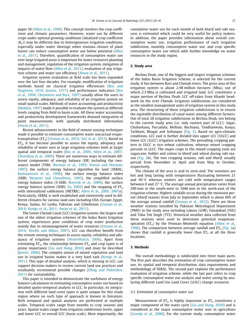
Rechna Doab, one of the biggest and largest irrigation schemesof the Indus Basin Irrigation Scheme, is selected for the currentstudy. It lies between Ravi and Chenab rivers. The gross area of thisirrigation system is about 2.98 million hectares (Mha), out ofwhich 2.3 Mha is cultivated and irrigated land. LCC constitutes amajor portion of Rechna Doab. LCC off-takes from Khanki head-work on the river Chenab. Irrigation subdivisions are consideredas the smallest management units of irrigation system in this studyarea. The structuring of these irrigation subdivisions is to ensurethe equitable distribution of canal water among different farmers.Out of total 28 irrigation subdivisions in Rechna Doab, ten belongto the current study area (i.e. only eastern part of LCC): Sagar,Chuharkana, Paccadala, Mohlan, Buchiana, Tandlianwala, Kanya,Tarkhani, Bhagat and Sultanpur (Fig. 1). Based on agro-climaticconditions, LCC east is further divided into upper LCC (ULCC) andlower LCC (LLCC) irrigation schemes. The prevailing cropping pat-tern in ULCC is rice–wheat cultivation, whereas mixed croppingprevails in LLCC. The major crops in the mixed cropping zone aresugarcane, fodder and cotton in kharif and wheat during rabi sea-son (Fig. 2b). The two cropping seasons, rabi and kharif, usuallyprevail from November to April and from May to October,respectively.

The climate of the area is arid to semi-arid. The summers arehot and long lasting with temperatures fluctuating between 21and 50 �C whereas winters are cold with temperature rangesbetween 0 and 27 �C. The average annual precipitation varies from290 mm in the south-west to 1046 mm in the north-east of theirrigation scheme. Highest rainfalls occur during the monsoon per-iod (kharif season) from July to September which is about 60% ofthe average annual rainfall (Usman et al., 2012). There are threeweather stations installed by Pakistan Metrological Department(PMD) in the study area including Lahore (LHR), Faisalabad (FSD)and Toba Tek Singh (TTS). Historical weather data collected fromthese stations were used to determine potential evapotran-spiration (ETo) by the Penman–Monteith equation (Allen et al.,1998). The comparison between average rainfall and ETo (Fig. 2a)shows that rainfall is generally lower than ETo at all the threelocations.

3. Methods

The overall methodology is subdivided into three main parts.The first part describes the estimation of crop consumptive wateruse, its spatial and temporal distribution, data requirements andmethodology of SEBAL. The second part explains the performanceevaluation of irrigation scheme, while the last part refers to cropspecific consumptive water use analysis and water saving by ana-lyzing different Land Use Land Cover (LULC) change scenarios.

3.1. Estimation of consumptive water use

Measurement of ETa is highly important as ETa constitutes amajor component of the water cycle (Liu and Hong, 2010) and isconsidered as the major consumptive water user in agriculture(Gowda et al., 2008). For the current study, consumptive water

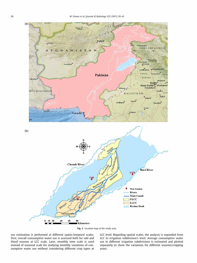
Fig. 1. Location map of the study area.

28 M. Usman et al. / Journal of Hydrology 525 (2015) 26–41

use estimation is performed at different spatio-temporal scales.First, overall consumptive water use is assessed both for rabi andkharif seasons at LCC scale. Later, monthly time scale is usedinstead of seasonal scale for studying monthly variations of con-sumptive water use without considering different crop types at

LCC level. Regarding spatial scales, the analysis is expanded fromLCC to irrigation subdivision’s level. Average consumptive wateruse in different irrigation subdivisions is estimated and plottedseparately to show the variations for different seasons/croppingyears.

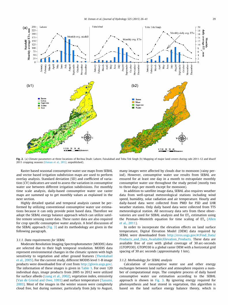
Fig. 2. (a) Climate parameters at three locations of Rechna Doab: Lahore, Faisalabad and Toba Tek Singh (b) Mapping of major land covers during rabi 2011-12 and kharif2011 cropping seasons (Usman et al., 2012, unpublished).

M. Usman et al. / Journal of Hydrology 525 (2015) 26–41 29

Raster based seasonal consumptive water use maps from SEBALand vector based irrigation subdivision maps are used to performoverlay analysis. Standard deviation (SD) and coefficient of varia-tion (CV) indicators are used to assess the variation in consumptivewater use between different irrigation subdivisions. For monthlytime scale analysis, daily-based consumptive water use rastermaps are summed up to get monthly values as explained in thenext section.

Highly detailed spatial and temporal analysis cannot be per-formed by utilizing conventional consumptive water use estima-tions because it can only provide point based data. Therefore weadopt the SEBAL energy balance approach which can utilize satel-lite remote sensing raster data. These raster data are also requiredfor crop specific consumptive water analysis. A brief discussion ofthe SEBAL approach (Fig. 3) and its methodology are given in thefollowing paragraph.

3.1.1. Data requirements for SEBALModerate Resolution Imaging Spectrophotometer (MODIS) data

are selected due to their high temporal resolution. MODIS datarepresent environmental changes in the climatic system with highsensitivity to vegetation and other ground features (Thenkabailet al., 2005). For the current study, different MODIS level 1-B imageproducts were downloaded free of cost from http://glovis.usgs.gov/.The information of these images is given in Table 1. For over 120individual days, image products from 2005 to 2012 were utilizedfor surface albedo (Liang et al., 2002), vegetation index, emissivity(Van de Griend and Owe, 1993) and surface temperature (Tasumi,2003). Most of the images in the winter season were completelycloud free, but during summer, particularly from July to August,

many images were affected by clouds due to monsoon (rainy per-iod). However, consumptive water use results from SEBAL areensured for at least one day in a month to extrapolate monthlyconsumptive water use throughout the study period (mostly twoto three days per month except for monsoon).

In addition to satellite image data, SEBAL also requires weatherdata from well-spread meteorological stations including windspeed, humidity, solar radiation and air temperature. Hourly anddaily-based data were collected from PMD for FSD and LHRweather stations. Only daily based data were collected from TTSmeteorological station. All necessary data sets from these obser-vatories are used for SEBAL analysis and for ETo estimation usingthe Penman–Monteith equation for time scaling of ETa (Allenet al., 2011).

In order to incorporate the elevation effects on land surfacetemperature, Digital Elevation Model (DEM) data required bySEBAL were downloaded from http://eros.usgs.gov/#/Find_Data/Products_and_Data_Available/Elevation_Products. These data areavailable free of cost with global coverage of 30 arc-seconds(GTOPO30). GTOPO30 is a global raster DEM with a horizontal gridspacing of 30 arc seconds (approximately 1 km).

3.1.2. Methodology for SEBAL analysisCalculation of consumptive water use and other energy

exchanges between land surface and atmosphere requires a num-ber of computational steps. The complete process of daily basedconsumptive water use estimation according to the SEBALapproach is shown in Fig. 3. By ignoring energy required forphotosynthesis and heat stored in vegetation, this algorithm isbased on the land surface energy balance theory, which is

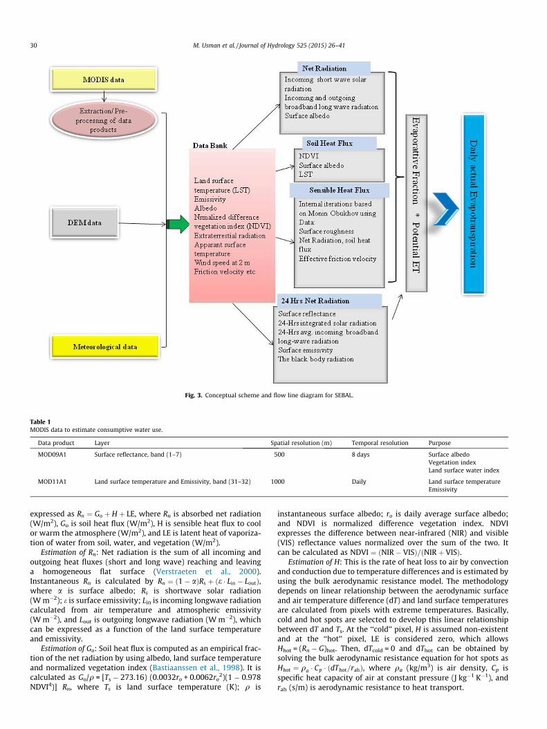
Fig. 3. Conceptual scheme and flow line diagram for SEBAL.

Table 1MODIS data to estimate consumptive water use.

Data product Layer Spatial resolution (m) Temporal resolution Purpose

MOD09A1 Surface reflectance, band (1–7) 500 8 days Surface albedoVegetation indexLand surface water index

MOD11A1 Land surface temperature and Emissivity, band (31–32) 1000 Daily Land surface temperatureEmissivity

30 M. Usman et al. / Journal of Hydrology 525 (2015) 26–41

expressed as Rn ¼ Go þ H þ LE, where Rn is absorbed net radiation(W/m2), Go is soil heat flux (W/m2), H is sensible heat flux to coolor warm the atmosphere (W/m2), and LE is latent heat of vaporiza-tion of water from soil, water, and vegetation (W/m2).

Estimation of Rn: Net radiation is the sum of all incoming andoutgoing heat fluxes (short and long wave) reaching and leavinga homogeneous flat surface (Verstraeten et al., 2000).Instantaneous Rn is calculated by Rn ¼ ð1� aÞRs þ ðe � Lin � LoutÞ,where a is surface albedo; Rs is shortwave solar radiation(W m�2); e is surface emissivity; Lin is incoming longwave radiationcalculated from air temperature and atmospheric emissivity(W m�2), and Lout is outgoing longwave radiation (W m�2), whichcan be expressed as a function of the land surface temperatureand emissivity.

Estimation of Go: Soil heat flux is computed as an empirical frac-tion of the net radiation by using albedo, land surface temperatureand normalized vegetation index (Bastiaanssen et al., 1998). It iscalculated as Go/q = [Ts � 273.16) (0.0032ro + 0.0062ro

2)(1 � 0.978NDVI4)] Rn, where Ts is land surface temperature (K); q is

instantaneous surface albedo; ro is daily average surface albedo;and NDVI is normalized difference vegetation index. NDVIexpresses the difference between near-infrared (NIR) and visible(VIS) reflectance values normalized over the sum of the two. Itcan be calculated as NDVI ¼ ðNIR � VISÞ=ðNIR þ VISÞ.

Estimation of H: This is the rate of heat loss to air by convectionand conduction due to temperature differences and is estimated byusing the bulk aerodynamic resistance model. The methodologydepends on linear relationship between the aerodynamic surfaceand air temperature difference (dT) and land surface temperaturesare calculated from pixels with extreme temperatures. Basically,cold and hot spots are selected to develop this linear relationshipbetween dT and Ts. At the ‘‘cold’’ pixel, H is assumed non-existentand at the ‘‘hot’’ pixel, LE is considered zero, which allowsHhot = (Rn � G)hot. Then, dTcold = 0 and dThot can be obtained bysolving the bulk aerodynamic resistance equation for hot spots asHhot ¼ qa � Cp � ðdThot=rahÞ, where qa (kg/m3) is air density, Cp isspecific heat capacity of air at constant pressure (J kg�1 K�1), andrah (s/m) is aerodynamic resistance to heat transport.

M. Usman et al. / Journal of Hydrology 525 (2015) 26–41 31

Estimation of LE: LE is the residual term of the calculated energybudget and represents the amount of energy required for ET. LE onpixel by pixel basis is obtained as LE ¼ Rn � H � Go. LE is used tocalculate the instantaneous evaporative fraction (EFins), which isthe ratio of the actual to the potential crop evaporative demandwhen the soil moisture conditions are in equilibrium with atmo-spheric moisture conditions. EFins is used to find daily valuesbecause it does not change considerably during daytime althoughGo and H vary considerably. The value of EFins at satellite overpasstime is slightly different from the 24 h integrated value of energybalance. This difference can be ignored (Akbari et al., 2007;Mutiga et al., 2010). Instantaneous EF is represented byEFins ¼ LE=ðRn � GÞ ¼ LE=ðLEþ HÞ ¼ EFday.

Estimation of daily ET (ET24): For the time scale of one day orlonger, Go can be neglected and (Rn–Go) reduces to Rn (Usmanet al., 2014; Kongo et al., 2011). ETa at daily time scale (ET24) iscomputed as ET24 ¼ ð86400�103Þ � EF � Rn24=ðk � qwÞ, where Rn24 is24 h averaged net radiation (W m�2), k is latent heat of vaporiza-tion (J kg�1), and qw is density of water (kg m�3).

Monthly or other interval ET (ETdt): The computation of ETdt

involves extrapolation of SEBAL ET24 values within a particularmonth or time period, in proportion to ETo, where the latter isderived from standard meteorological data. ETo from a specificpoint in the image does not reflect the actual condition at eachpixel. The procedure involves computing cumulative ETo betweensuccessive satellite images before computing the ratio (Km) ofcumulative to average ETo over the period. So, ETdt is computedas ETdt ¼ km �

Pni¼1ðETsebalÞi where ETsebal is ET24 image, Km is a mul-

tiplication factor for the representation period, and n is the numberof ET images processed during the period.

3.2. Performance evaluation of irrigation schemes

Operational performance of any irrigation scheme is judged byusing different performance indicators which can range from largescale (overall irrigation scheme) to small scale (on farm). The selec-tion of these indicators is based on the feasibility of taking mea-surements, accuracy and cost effectiveness (Bandara, 2003). Boset al. (2005) documented different approaches and challenges ofusing performance indicators which mainly cover the key aspectsof equity, adequacy, and reliability with which the water is deliv-ered to and used within the irrigation scheme. In the current study,we assess the performance of the irrigation scheme at irrigationsubdivision levels by using equity, adequacy and reliability asirrigation performance indicators. These indicators can describeand judge the overall irrigation system performance under actualfield conditions (Ahmad et al., 2009) and hence the improvementof the irrigation system in terms of water distribution and possiblereallocation. The description of each performance indicator isexplained as follows.

3.2.1. EquityAnalysis of equity was performed on irrigation subdivision

level. Generally, equity is calculated from the supply side, but forareas with water shortage like LCC, it is measured from the farm-er’s perspective. In the current study, equity addresses both, theequal water distribution in different parts of the study area andits distribution within each individual irrigation subdivision. Thedepth of water utilized in different irrigation subdivisions isassessed by coupling the annual consumptive water use maps withirrigation subdivision vector maps. Detailed results are presentedfor each cropping year starting from 2005–06 to 2011–2012 andevaluated using standard deviation (SD) and coefficient of variation(CV) to demonstrate the variation of water use in different irriga-tion subdivisions.

3.2.2. AdequacyAdequacy is an indicator used to assess the reduction in con-

sumptive water use and to evaluate the sufficiency of irrigationwater delivery to a selected command area (Perry, 1996). In thecurrent study, adequacy is described as the average seasonal evap-oration fraction (EF). Series of EF maps during a particular seasonare used to measure average seasonal EF which is then plottedfor each respective irrigation subdivision to assess the water avail-ability status in different parts of the study area. Kharif and rabi aretreated separately as separated maps are plotted for both seasonsto assess the water situation.

3.2.3. ReliabilityReliability describes the sufficient availability of water through-

out the season for crop use. It can also be measured using seasonalEF values like adequacy. In the current study, temporal CV of EFwas used to describe reliability (Bastiaanssen and Bos, 1999;Awan et al., 2011) for both kharif and rabi seasons separately.Apart from seasonal analysis, reliability was also assessed onmonthly time scale by plotting CV of monthly EF against monthlytime scale both for kharif and rabi. Higher values of CV representless reliable water supplies and vice versa.

3.3. Estimation of crop specific consumptive water use and watersaving

The methodology explained so far for consumptive water useanalyses does not consider the crop specific water consumption.Therefore, an attempt is made to correlate the water consumptionwith all main crops during different rabi and kharif seasons. Wheat,rabi fodder and sugarcane are selected for rabi. Rice, cotton, sugar-cane and kharif fodder are selected for each kharif season. The studyarea is split into two parts (i.e. ULCC and LLCC) for this type of analy-sis. The average depth of consumptive water use during a particularseason is assessed for each individual crop by overlaying seasonalconsumptive water use maps with LULC maps. LULC maps weredeveloped for each cropping season from 2005 to 2012. NDVI prod-ucts from MODIS are utilized to classify different land covers byadopting unsupervised classification technique. Different classifica-tion accuracies were estimated before finalizing maps with the aid ofground truthing crop data. The impact of land use change on waterresources is also assessed. Different types of LULC change scenariosare developed to study its impact on possible water saving.

4. Results and discussion

4.1. Validation of SEBAL results

The validation of SEBAL results is quite important for furtheranalysis. SEBAL has already been widely and successfully used inPakistan as reported in different studies (Ahmad et al., 2009;Kongo et al., 2011). Generally SEBAL results are compared withlysimeters but in the current study, SEBAL results are comparedwith the advection aridity method as no results from lysimetersor other methods are available. The advective aridity method hasbeen used intensively for validation of other methods of ETa

estimation (Hobbins and Ramirez, 2001; Liu et al., 2010) but thistechnique performs relatively better under cool environmentalconditions than under very hot. Similar types of results were foundfor the current study where quite high Nash Sutcliffe Efficiency(NSE = 0.92) and relatively low bias (�13.32) were found for rabiseasons. Values of NSE and bias for kharif seasons were 0.71 and�24.89, respectively (Usman et al., 2014). Moreover, detaileddescription of advective aridity method can be found fromUsman et al. (2015).

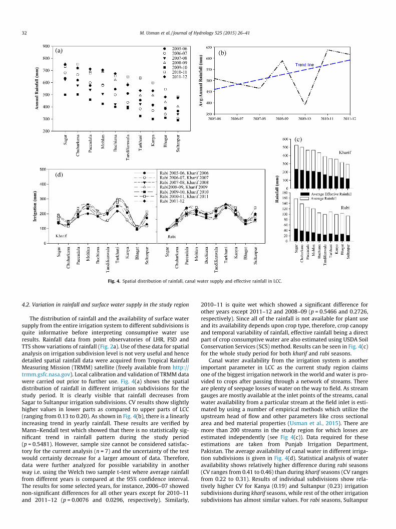
Fig. 4. Spatial distribution of rainfall, canal water supply and effective rainfall in LCC.

32 M. Usman et al. / Journal of Hydrology 525 (2015) 26–41

4.2. Variation in rainfall and surface water supply in the study region

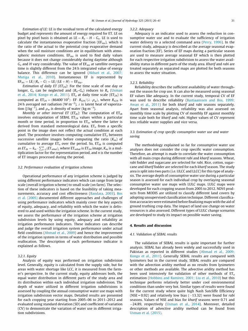
The distribution of rainfall and the availability of surface watersupply from the entire irrigation system to different subdivisions isquite informative before interpreting consumptive water useresults. Rainfall data from point observatories of LHR, FSD andTTS show variations of rainfall (Fig. 2a). Use of these data for spatialanalysis on irrigation subdivision level is not very useful and hencedetailed spatial rainfall data were acquired from Tropical RainfallMeasuring Mission (TRMM) satellite (freely available from http://trmm.gsfc.nasa.gov). Local calibration and validation of TRMM datawere carried out prior to further use. Fig. 4(a) shows the spatialdistribution of rainfall in different irrigation subdivisions for thestudy period. It is clearly visible that rainfall decreases fromSagar to Sultanpur irrigation subdivisions. CV results show slightlyhigher values in lower parts as compared to upper parts of LCC(ranging from 0.13 to 0.20). As shown in Fig. 4(b), there is a linearlyincreasing trend in yearly rainfall. These results are verified byMann–Kendall test which showed that there is no statistically sig-nificant trend in rainfall pattern during the study period(p = 0.5481). However, sample size cannot be considered satisfac-tory for the current analysis (n = 7) and the uncertainty of the testwould certainly decrease for a larger amount of data. Therefore,data were further analyzed for possible variability in anotherway i.e. using the Welch two sample t-test where average rainfallfrom different years is compared at the 95% confidence interval.The results for some selected years, for instance, 2006–07 showednon-significant differences for all other years except for 2010–11and 2011–12 (p = 0.0076 and 0.0296, respectively). Similarly,

2010–11 is quite wet which showed a significant difference forother years except 2011–12 and 2008–09 (p = 0.5466 and 0.2726,respectively). Since all of the rainfall is not available for plant useand its availability depends upon crop type, therefore, crop canopyand temporal variability of rainfall, effective rainfall being a directpart of crop consumptive water are also estimated using USDA SoilConservation Services (SCS) method. Results can be seen in Fig. 4(c)for the whole study period for both kharif and rabi seasons.

Canal water availability from the irrigation system is anotherimportant parameter in LCC as the current study region claimsone of the biggest irrigation network in the world and water is pro-vided to crops after passing through a network of streams. Thereare plenty of seepage losses of water on the way to field. As streamgauges are mostly available at the inlet points of the streams, canalwater availability from a particular stream at the field inlet is esti-mated by using a number of empirical methods which utilize theupstream head of flow and other parameters like cross sectionalarea and bed material properties (Usman et al., 2015). There aremore than 200 streams in the study region for which losses areestimated independently (see Fig 4(c)). Data required for theseestimations are taken from Punjab Irrigation Department,Pakistan. The average availability of canal water in different irriga-tion subdivisions is given in Fig. 4(d). Statistical analysis of wateravailability shows relatively higher difference during rabi seasons(CV ranges from 0.41 to 0.46) than during kharif seasons (CV rangesfrom 0.22 to 0.31). Results of individual subdivisions show rela-tively higher CV for Kanya (0.19) and Sultanpur (0.23) irrigationsubdivisions during kharif seasons, while rest of the other irrigationsubdivisions has almost similar values. For rabi seasons, Sultanpur

M. Usman et al. / Journal of Hydrology 525 (2015) 26–41 33

(0.32) and Tandlianwala (0.20) irrigation subdivisions exhibit rela-tively larger values of CV, while for other irrigation subdivisionsthe results are almost similar. The difference of water availabilityamong particular irrigation subdivisions can be high for specificseason, nevertheless groundwater is also one of the main sourcesof water for crops. Individual farmers own private tube wells fromwhich they can pump water uninterruptedly. According to Kazmiet al. (2012) the share of groundwater to agriculture in the studyarea is about half.

4.3. Spatio-temporal variability in consumptive water use

4.3.1. Monthly consumptive water use in LCC from 2005 to 2012Fig. 5 indicates the distribution of monthly water consumption

in each individual month for rabi and kharif seasons, respectively,from 2005 to 2012. The consumptive water use during kharif sea-sons (546.2 mm ± 47.50 mm) is almost two times higher than inrabi seasons (274 mm ± 20 mm). The main reason for this is highcrop water requirements of rice, cotton, and sugarcane which aretriggered by high temperatures. As opposed to this, wheat is culti-vated at larger areas along with fodder during rabi season. There isalso an indication of abrupt change in trends for kharif from midJuly to September due to higher availability of water as a resultof monsoon rainfalls and resultantly better vegetative growth forcrops. During rabi season, a relatively steep rise is observed fromend of February to end of March when temperature rises and suffi-cient soil moisture becomes available to crops after winter rainfall.

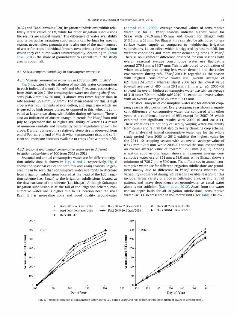
4.3.2. Seasonal and annual consumptive water use in differentirrigation subdivisions of LCC from 2005 to 2012

Seasonal and annual consumptive water use for different irriga-tion subdivisions is shown in Figs. 6 and 7, respectively. Fig. 6shows the seasonal values for both rabi and kharif seasons. In gen-eral, it can be seen that consumptive water use tends to decreasefrom irrigation subdivisions located at the head of the LCC irriga-tion scheme (i.e., Sagar) to the irrigation subdivisions located atthe downstreams of the scheme (i.e., Bhagat). Although Sultanpurirrigation subdivision is at the tail of the irrigation scheme, con-sumptive water use is higher due to its location near the riverRavi. It has non-saline soils and good quality groundwater

Fig. 5. Temporal variation of consumptive water use in LCC during kh

(Ahmad et al., 2009). Average seasonal values of consumptivewater use for all kharif seasons indicate highest value forSagar with 576.9 mm ± 35 mm and lowest for Bhagat with513.5 mm ± 57 mm. For Bhagat, this can also be attributed to lesssurface water supply as compared to neighboring irrigationsubdivisions, i.e. an effect which is triggered by less rainfall, hotweather conditions and more water demanding crops in kharif.There is no significant difference observed for rabi seasons withoverall seasonal average consumptive water use fluctuatingaround 276.1 mm ± 19.27 mm. This is attributed to cultivation ofwheat on a large area having less water demand and the coolerenvironment during rabi. Kharif 2011 is regarded as the seasonwith highest consumptive water use (overall average of621 mm ± 24.6 mm), whereas kharif 2006 has the lowest value(overall average of 485 mm ± 26.1 mm). Similarly, rabi 2005–06showed the overall highest consumptive water use with an averageof 310 mm ± 7.0 mm, while rabi 2010–11 exhibited lowest valueswith an overall average of 260 mm ± 9.13 mm.

Statistical analysis of consumptive water use for different crop-ping years is also performed. Every cropping year shows a signifi-cant difference of consumptive water use compared with otheryears at a confidence interval of 95% except for 2007–08 whichexhibited non-significant results with 2009–10 and 2010–11.These variations are not only caused by varying water availabilityfrom canals and rainfall but also by yearly changing crop scheme.

The analysis of annual consumptive water use for the wholestudy period from 2005 to 2012 exhibits the highest value forthe 2011–12 cropping season with an overall average value of873.7 mm ± 25.5 mm, while 2006–07 shows the smallest one withan overall average value of 750 mm ± 27.5 mm (Fig. 7). Amongirrigation subdivisions, Sagar shows a maximum average con-sumptive water use of 851 mm ± 58.0 mm, while Bhagat shows aminimum of 786.7 mm ± 50.0 mm. The differences in annual con-sumptive water use for different irrigation subdivisions are promi-nent mainly due to difference in kharif seasons whereas lessvariability is observed during rabi seasons. Possible reasons for thisinclude: larger variety of crops in cultivated area, erratic rainfallpattern, and heavy dependence on groundwater as canal wateralone is not sufficient (Kazmi et al., 2012). Apart from the wateruse on depth basis for all irrigation subdivisions, consumptivewater use is also presented in volumetric units (see Table 3 below).

arif and rabi season (Please note different scales of vertical axes).

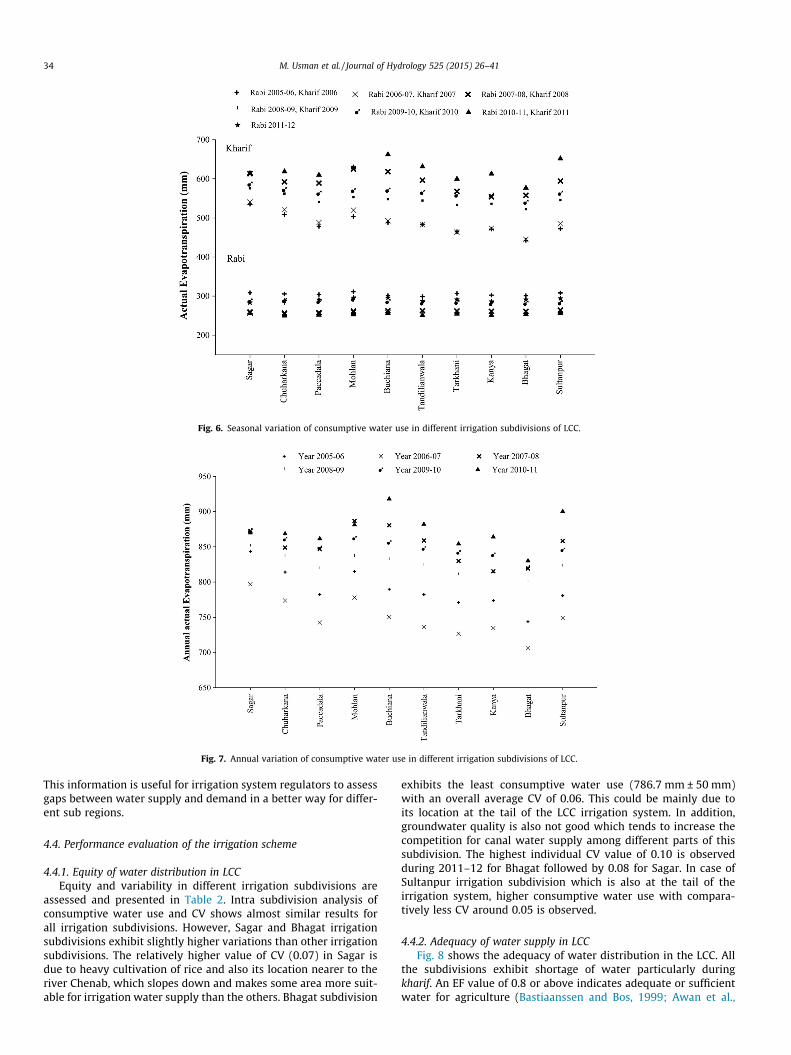
Fig. 6. Seasonal variation of consumptive water use in different irrigation subdivisions of LCC.

Fig. 7. Annual variation of consumptive water use in different irrigation subdivisions of LCC.

34 M. Usman et al. / Journal of Hydrology 525 (2015) 26–41

This information is useful for irrigation system regulators to assessgaps between water supply and demand in a better way for differ-ent sub regions.

4.4. Performance evaluation of the irrigation scheme

4.4.1. Equity of water distribution in LCCEquity and variability in different irrigation subdivisions are

assessed and presented in Table 2. Intra subdivision analysis ofconsumptive water use and CV shows almost similar results forall irrigation subdivisions. However, Sagar and Bhagat irrigationsubdivisions exhibit slightly higher variations than other irrigationsubdivisions. The relatively higher value of CV (0.07) in Sagar isdue to heavy cultivation of rice and also its location nearer to theriver Chenab, which slopes down and makes some area more suit-able for irrigation water supply than the others. Bhagat subdivision

exhibits the least consumptive water use (786.7 mm ± 50 mm)with an overall average CV of 0.06. This could be mainly due toits location at the tail of the LCC irrigation system. In addition,groundwater quality is also not good which tends to increase thecompetition for canal water supply among different parts of thissubdivision. The highest individual CV value of 0.10 is observedduring 2011–12 for Bhagat followed by 0.08 for Sagar. In case ofSultanpur irrigation subdivision which is also at the tail of theirrigation system, higher consumptive water use with compara-tively less CV around 0.05 is observed.

4.4.2. Adequacy of water supply in LCCFig. 8 shows the adequacy of water distribution in the LCC. All

the subdivisions exhibit shortage of water particularly duringkharif. An EF value of 0.8 or above indicates adequate or sufficientwater for agriculture (Bastiaanssen and Bos, 1999; Awan et al.,

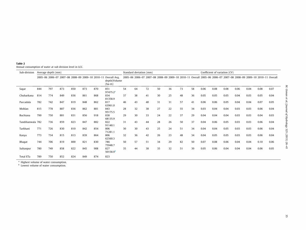
Table 2Annual consumption of water at sub division level in LCC.

Sub-division Average depth (mm) Standard deviation (mm) Coefficient of ariation (CV)

2005–06 2006–07 2007–08 2008–09 2009–10 2010–11 Overall Avg.depth/Volume(ha-m)

2005–06 2006–07 2007–08 2008–09 2009–10 2010–11 Overall 2005–06 200 –07 2007–08 2008–09 2009–10 2010–11 Overall

Sagar 844 797 873 850 873 870 851 54 64 72 50 36 73 58 0.06 0.0 0.08 0.06 0.04 0.08 0.0797475.2a

Chuharkana 814 774 849 836 861 868 834 37 38 41 30 25 48 36 0.05 0.0 0.05 0.04 0.03 0.05 0.0481358.9

Paccadala 782 742 847 819 848 862 817 46 43 40 31 31 57 41 0.06 0.0 0.05 0.04 0.04 0.07 0.0563961.0

Mohlan 815 778 887 836 862 881 843 28 32 38 27 22 55 34 0.03 0.0 0.04 0.03 0.03 0.06 0.0495175.5

Buchiana 790 750 881 831 856 918 838 29 30 33 24 22 37 29 0.04 0.0 0.04 0.03 0.03 0.04 0.0368135.9

Tandilianwala 782 736 859 823 847 882 822 31 43 44 28 26 50 37 0.04 0.0 0.05 0.03 0.03 0.06 0.0491140.1

Tarkhani 771 726 830 810 842 854 806 30 30 43 25 24 51 34 0.04 0.0 0.05 0.03 0.03 0.06 0.0471281.1

Kanya 773 734 815 813 839 864 806 32 36 42 26 23 48 34 0.04 0.0 0.05 0.03 0.03 0.06 0.0462560.3

Bhagat 744 706 819 800 821 830 786 50 57 51 34 29 82 50 0.07 0.0 0.06 0.04 0.04 0.10 0.0675948.7

Sultanpur 780 749 858 822 845 908 827 35 44 38 35 32 51 39 0.05 0.0 0.04 0.04 0.04 0.06 0.0550158.9b

Total ETa 789 750 852 824 849 874 823

a Highest volume of water consumption.b Lowest volume of water consumption.

M.U

sman

etal./Journal

ofH

ydrology525

(2015)26–

4135

v

6

8

5

6

4

4

6

4

5

8

6

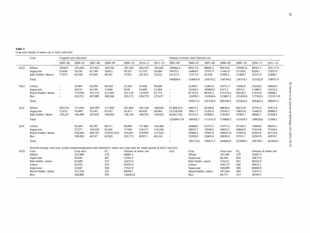
Table 3Crop-wise details of water use in ULCC and LLCC.

Crop Cropped area (hectare) Volume of water used (hectare-m)

2005–06 2006–07 2007–08 2008–09 2009–10 2010–11 2011–12 2005–06 2006–07 2007–08 2008–09 2009–10 2010–11 2011–12

ULCC Wheat 345827 379,204 337,025 340,766 365,769 349,163 356,045 106802.4 98517.0 88005.3 95676.8 105887.6 88561.7 103117.9Sugarcane 55,656 54,182 47,740 39,812 39,557 31,533 43,684 16970.5 14404.9 12797.9 11461.9 11338.6 8209.1 12955.9Rabi Fodder. Minors 77,073 45,920 93,500 98,591 75,931 101,012 79,232 23121.9 11571.9 23,936 27605.5 21488.5 25151.9 22898.1

Total 146894.8 124493.8 124739.2 134744.2 138714.7 121922.8 138971.9

ULCC Cotton – 43,803 26,038 40,544 27,263 41,466 96,498 21200.7 13461.6 24731.7 14585.8 23220.8 59924.9Sugarcane – 24,527 54,199 13,846 9338 19,490 21,684 – 12520.5 285864.1 9127.2 5291.6 11489.5 14152.2Kharif Fodder. Minor – 175,658 191,175 215,203 167,136 110,670 87,773 – 81153.9 88705.2 121374.5 84236.5 57216.4 50908.1Rice – 229,721 207,989 208,506 259,172 299,770 275,677 – 124702.1 116586.6 133867.2 151829.6 177565.5 1753311.9

Total – 239577.2 247339.9 289100.5 255943.5 269492.2 300297.2

LLCC Wheat 202,576 171,644 160,189 171,495 232,403 185,144 188,945 61,888,414 44831.5 42340.4 48830.6 66213.0 47755.3 55411.6Sugarcane 72,672 70,489 79,143 65,957 58,475 46,920 69,984 22,538,569 18917.7 21291.0 19199.7 16825.8 12482.0 20888.2Rabi Fodder. Minor 150,227 184,490 187,845 190,658 138,130 198,705 169,425 44,467,192 45753.5 47900.5 51858.9 37985.7 48682.7 47608.4

Total 128,894,174 109502.7 111531.8 119889.3 121024.5 108920.0 12398.2

LLCC Cotton 92,459 50,702 90,711 89,896 137,803 163,466 – 42808.6 23373.7 51977.2 47105.5 74964.8 98243.1Sugarcane 75,277 144,220 92,465 77,959 118,271 116,344 – 38033.7 73848.5 58925.5 44668.9 71414.0 75526.6Kharif Fodder. Minor 550,204 508,761 518,937,832 516,991 478,956 517,643 – 63080.3 79387.0 106951.8 77963.8 61051.9 45110.4Rice 106,965 44,767 42,929 102,772 49,073 66,124 – 52250.0 22862.4 26828.4 57951.1 29363.9 42978.7

Total – 196172.6 199471.7 244682.9 227689.2 236794.7 261858.7

Overall average crop area, actual evapotranspiration and volumetric water use crop-wise for study period in ULCC and LLCCULCC Crop Crop area ETa Volume of water use LLCC Crop Crop area ETa Volume of water use

Wheat 353,400 278 98081.2 Wheat 187,485 279 52467.3Sugarcane 44,595 281 12591.3 Sugarcane 66,234 284 18877.6Rabi fodder. minor 81,609 273 22253.4 Rabi fodder. minor 174,211 267 46322.4Cotton 45,935 555 26187.6 Cotton 104,173 528 56412.1Sugarcane 23,847 584 13527.9 Sugarcane 104,089 580 60402.9Kharif fodder. minor 157,936 525 80599.1 Kharif fodder. minor 147,656 494 72257.5Rice 246,806 593 146643.8 Rice 68,771 573 38705.7

36M

.Usm

anet

al./Journalof

Hydrology

525(2015)

26–41

Fig. 8. Intra and inter subdivision level variation in average seasonal evaporation fraction for kharif and rabi seasons.

Fig. 9. Intra and inter subdivision level temporal coefficient of variation (CV) in evaporative fraction and monthly ETa for kharif and rabi seasons.

M. Usman et al. / Journal of Hydrology 525 (2015) 26–41 37

2011), which is not met even for an individual kharif season duringthe study period. The average evaporation fraction line for thekharif season starts from 0.6 for the upper irrigation subdivisionsand tends to decline slightly in some lower irrigation subdivisionslike Tarkhani, Kanya and Bhagat. During rabi, the situation of wateravailability is relatively better as compared to kharif (EF valuearound 0.67). The possible reasons may be cool environment, lowerdemand for water by wheat. This is in accordance with the findingsof Ahmad et al. (2009), who report a better availability of water inthe upper Rechna Doab irrigation subdivisions compared to thelower ones.

4.4.3. Reliability of water supply in LCCThe reliability of water resources in LCC is studied using tem-

poral CV of EF (Fig. 9). The figure clearly indicates higher CV inkharif as compared to rabi. This advocates a lower reliability ofwater supplies during kharif. It is also important to note that duringkharif, temporal CV in higher irrigation subdivisions is around 0.20which becomes even higher at lower subdivisions (around 0.30),thus showing relatively low reliability of water resources at theselocations. For rabi, values of CV are relatively lower (around 0.10)as well as less variable among different irrigation subdivisionswhich indicates almost similar situations regarding reliability.

38 M. Usman et al. / Journal of Hydrology 525 (2015) 26–41

The analyses were further expanded to check the reliability of theirrigation system within any individual rabi or kharif season byplotting the CV of monthly consumptive water use with time(Fig. 8). This analysis is performed at LCC scale instead of irrigationsubdivision level. The results show that months with higher tem-perature and more heterogeneous rainfall (i.e. July–Septemberduring kharif and February and March during rabi) showed higherCV (from 0.3 to 0.36 for kharif and 0.15 to 0.165 for rabi) comparedto other months.

4.5. Analysis of crop specific consumptive water use

4.5.1. Land use and water resourcesTable 3 summarizes information concerning areas under dif-

ferent crops, average depth of consumptive water use and totalvolume of water consumed both for ULCC and LLCC.Volumetric water use is estimated by weighted average of differ-ent cropping years. The results for a particular crop cannot beconsidered to be exact as cropping dates for a particular cropmay vary in different regions. Duration of cropping seasons fordifferent crops was estimated using temporal trends of NDVI.NDVI does not classify different LULC directly; however time ser-ies NDVI patterns make it possible to discriminate differentclasses based on their unique behaviors in terms of its peaktrends and duration of phenological stages in various agro-ecosystems (Shi et al., 2013).

Fig. 10. Crop wise consumptive water use differen

Analysis for different crops indicates that sugarcane has thehighest value of water consumption with a value of 310.14 mmduring rabi 2005–06, while rabi fodder shows the lowest value of245 mm during rabi 2010–11, both in LLCC. Similarly, for kharifseasons, sugarcane shows the highest value of 659.2 mm duringkharif 2008 in ULCC and kharif fodder shows the lowest value of430 mm during kharif 2007 in LLCC. Consumptive water use perunit area of a particular crop indicates that rice is the major waterconsumer with a value of 593 mm followed by sugarcane, cottonand kharif fodder with values of 584 mm, 555 mm and 525 mm,respectively, in ULCC. In LLCC, sugarcane is the major consumerof water with a value of 580 mm followed by rice, cotton and khariffodder with values of 573 mm, 528 mm and 494 mm, respectively.Consumptive use of water for rabi crops is almost similar for bothregions. Since the area under rice and wheat crops is much largercompared with other crops grown in the study region, therefore,the volumetric consumptive water use is relatively higher for riceand wheat crops during kharif and rabi, respectively. Reporting ofthe volumetric water uses for different crops is helpful for irriga-tion water regulators as water is provided to different regions onvolumetric basis rather than on depth basis.

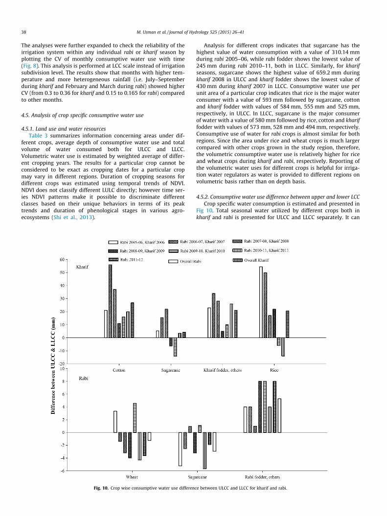
4.5.2. Consumptive water use difference between upper and lower LCCCrop specific water consumption is estimated and presented in

Fig 10. Total seasonal water utilized by different crops both inkharif and rabi is presented for ULCC and LLCC separately. It can

ce between ULCC and LLCC for kharif and rabi.

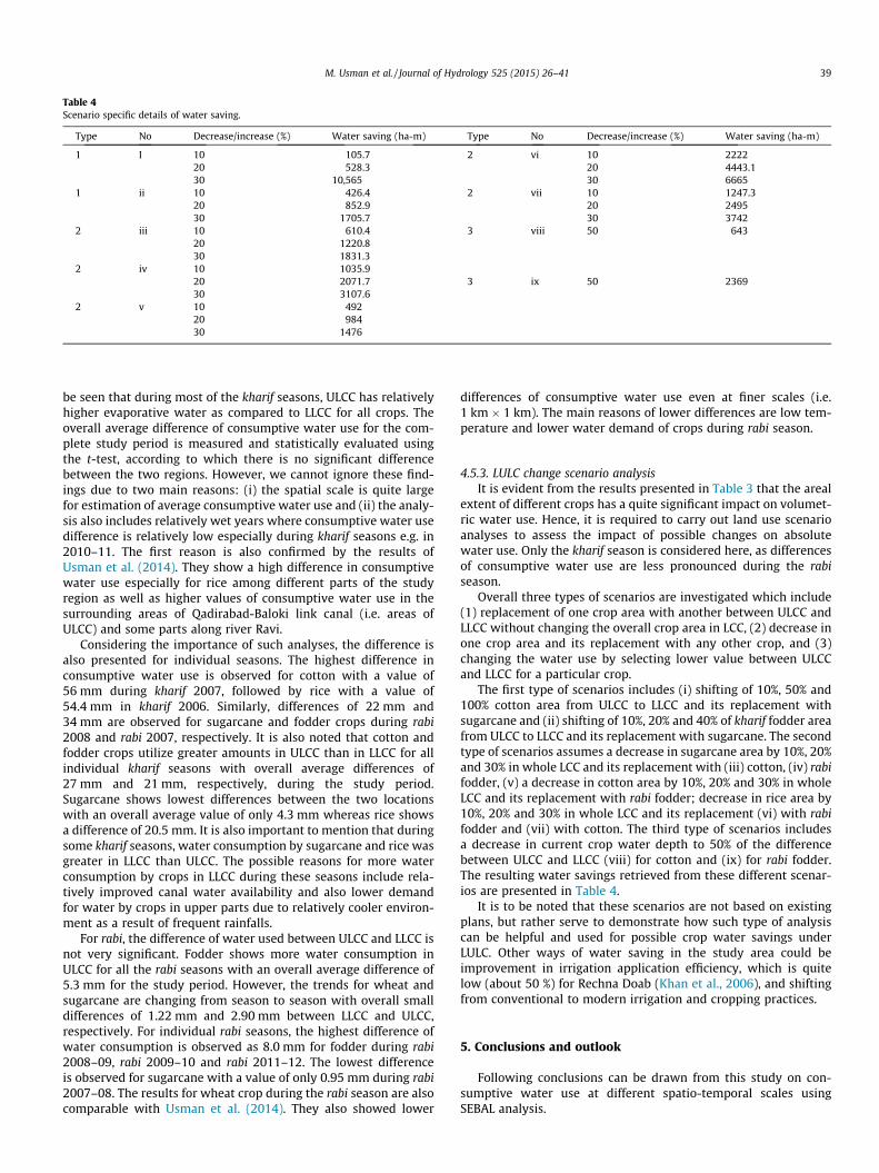
Table 4Scenario specific details of water saving.

Type No Decrease/increase (%) Water saving (ha-m) Type No Decrease/increase (%) Water saving (ha-m)

1 I 10 105.7 2 vi 10 222220 528.3 20 4443.130 10,565 30 6665

1 ii 10 426.4 2 vii 10 1247.320 852.9 20 249530 1705.7 30 3742

2 iii 10 610.4 3 viii 50 64320 1220.830 1831.3

2 iv 10 1035.920 2071.7 3 ix 50 236930 3107.6

2 v 10 49220 98430 1476

M. Usman et al. / Journal of Hydrology 525 (2015) 26–41 39

be seen that during most of the kharif seasons, ULCC has relativelyhigher evaporative water as compared to LLCC for all crops. Theoverall average difference of consumptive water use for the com-plete study period is measured and statistically evaluated usingthe t-test, according to which there is no significant differencebetween the two regions. However, we cannot ignore these find-ings due to two main reasons: (i) the spatial scale is quite largefor estimation of average consumptive water use and (ii) the analy-sis also includes relatively wet years where consumptive water usedifference is relatively low especially during kharif seasons e.g. in2010–11. The first reason is also confirmed by the results ofUsman et al. (2014). They show a high difference in consumptivewater use especially for rice among different parts of the studyregion as well as higher values of consumptive water use in thesurrounding areas of Qadirabad-Baloki link canal (i.e. areas ofULCC) and some parts along river Ravi.

Considering the importance of such analyses, the difference isalso presented for individual seasons. The highest difference inconsumptive water use is observed for cotton with a value of56 mm during kharif 2007, followed by rice with a value of54.4 mm in kharif 2006. Similarly, differences of 22 mm and34 mm are observed for sugarcane and fodder crops during rabi2008 and rabi 2007, respectively. It is also noted that cotton andfodder crops utilize greater amounts in ULCC than in LLCC for allindividual kharif seasons with overall average differences of27 mm and 21 mm, respectively, during the study period.Sugarcane shows lowest differences between the two locationswith an overall average value of only 4.3 mm whereas rice showsa difference of 20.5 mm. It is also important to mention that duringsome kharif seasons, water consumption by sugarcane and rice wasgreater in LLCC than ULCC. The possible reasons for more waterconsumption by crops in LLCC during these seasons include rela-tively improved canal water availability and also lower demandfor water by crops in upper parts due to relatively cooler environ-ment as a result of frequent rainfalls.

For rabi, the difference of water used between ULCC and LLCC isnot very significant. Fodder shows more water consumption inULCC for all the rabi seasons with an overall average difference of5.3 mm for the study period. However, the trends for wheat andsugarcane are changing from season to season with overall smalldifferences of 1.22 mm and 2.90 mm between LLCC and ULCC,respectively. For individual rabi seasons, the highest difference ofwater consumption is observed as 8.0 mm for fodder during rabi2008–09, rabi 2009–10 and rabi 2011–12. The lowest differenceis observed for sugarcane with a value of only 0.95 mm during rabi2007–08. The results for wheat crop during the rabi season are alsocomparable with Usman et al. (2014). They also showed lower

differences of consumptive water use even at finer scales (i.e.1 km � 1 km). The main reasons of lower differences are low tem-perature and lower water demand of crops during rabi season.

4.5.3. LULC change scenario analysisIt is evident from the results presented in Table 3 that the areal

extent of different crops has a quite significant impact on volumet-ric water use. Hence, it is required to carry out land use scenarioanalyses to assess the impact of possible changes on absolutewater use. Only the kharif season is considered here, as differencesof consumptive water use are less pronounced during the rabiseason.

Overall three types of scenarios are investigated which include(1) replacement of one crop area with another between ULCC andLLCC without changing the overall crop area in LCC, (2) decrease inone crop area and its replacement with any other crop, and (3)changing the water use by selecting lower value between ULCCand LLCC for a particular crop.

The first type of scenarios includes (i) shifting of 10%, 50% and100% cotton area from ULCC to LLCC and its replacement withsugarcane and (ii) shifting of 10%, 20% and 40% of kharif fodder areafrom ULCC to LLCC and its replacement with sugarcane. The secondtype of scenarios assumes a decrease in sugarcane area by 10%, 20%and 30% in whole LCC and its replacement with (iii) cotton, (iv) rabifodder, (v) a decrease in cotton area by 10%, 20% and 30% in wholeLCC and its replacement with rabi fodder; decrease in rice area by10%, 20% and 30% in whole LCC and its replacement (vi) with rabifodder and (vii) with cotton. The third type of scenarios includesa decrease in current crop water depth to 50% of the differencebetween ULCC and LLCC (viii) for cotton and (ix) for rabi fodder.The resulting water savings retrieved from these different scenar-ios are presented in Table 4.

It is to be noted that these scenarios are not based on existingplans, but rather serve to demonstrate how such type of analysiscan be helpful and used for possible crop water savings underLULC. Other ways of water saving in the study area could beimprovement in irrigation application efficiency, which is quitelow (about 50 %) for Rechna Doab (Khan et al., 2006), and shiftingfrom conventional to modern irrigation and cropping practices.

5. Conclusions and outlook

Following conclusions can be drawn from this study on con-sumptive water use at different spatio-temporal scales usingSEBAL analysis.

40 M. Usman et al. / Journal of Hydrology 525 (2015) 26–41

1. SEBAL results are comparable with advection aridity methodsas NSE is quite high both for rabi season values (0.92) and forkharif seasons values (0.71).

2. Analysis of rainfall data shows that there is no statistically sig-nificant increasing/decreasing trend during the study period.Years 2006–07 and 2010–11 are considered as relatively dryand wet years. Statistically, year 2006–07 shows non-signifi-cant difference for other years except the years 2010–11 and2011–12 with probability values of 0.0076 and 0.0296, respec-tively. Similarly, year 2010–11 shows significant differenceswith all other years except 2011–12 and 2008–09 (p = 0.5466and p = 0.2726, respectively) at 95% confidence interval.

3. The canal water supply during kharif and rabi seasons showsrelatively more variability for rabi seasons as compared to kharifseasons.

4. Monthly consumptive water use is almost double for kharif sea-sons than that for rabi seasons. Consumptive water usebecomes higher during monsoon in kharif season and after win-ter rains in rabi seasons due to higher water availability.

5. There is a generally decreasing trend in consumptive water usefrom upper irrigation subdivisions to lower irrigation subdivi-sions. The trend is more pronounced during kharif seasons thanrabi seasons. Highest and lowest average annual crop waterconsumptive uses are observed for years 2011–12 and 2006–07, respectively.

6. Intra subdivision analyses indicate lower differences in equityamong different areas except Sagar and Bhagat irrigationsubdivisions. Results of adequacy and reliability analyses forthe irrigation scheme show that neither adequacy nor reliabilityis high in LCC. Inadequacy is more pronounced during kharifseasons than during rabi seasons with average EF values of0.60 and 0.67, respectively. Similarly, reliability is relativelyhigh in upper subdivisions as compared to lower subdivisionswith CV values of 0.20 and 0.30 for kharif seasons.

7. Rice and wheat are major crops in LCC during kharif and rabiseasons, respectively. Crop specific consumptive water useanalysis ranks rice and sugarcane crops first with average val-ues of 593 mm and 580 mm, followed by cotton and kharif fod-der in ULCC and LLCC areas. The consumptive water use for rabicrops is almost similar throughout LCC. Considerable differ-ences in consumptive water use between ULCC and LLCC arealso observed for particular crops during some specific cropseasons.

8. Land use change scenarios indicate different options of watersaving in LCC. This analysis is based only on the average con-sumptive water use for different crops on spatial scales ofULCC and LLCC. According to the results, there is a potentialfor water saving between different parts of LCC for somecrops like cotton, sugarcane and rice. However, it is highlyrecommended to study these effects on finer spatial scales(i.e. at irrigation subdivision levels) as consumptive water usecould be highly variable for a particular crop among differentregions.

Acknowledgements

The authors are thankful to HEC, Pakistan, and DAAD, Germany,for providing funding to accomplish this study and to allorganizations which provided necessary data to achieve specificobjectives of the study. Special thanks to Departments ofIrrigation and Drainage and Agronomy, University of Agriculture,Faisalabad, Pakistan to provide all necessary technical and scienti-fic support.

References

Ahmad, M.D., Turral, H., Nazeer, A., 2009. Diagnosing irrigation performance andwater productivity through satellite remote sensing and secondary data in alarge irrigation system of Pakistan. Agric. Water Manag. 96, 551–564.

Akbari, M., Toomanian, N., Droogers, P., Bastiaanssen, W., Gieske, A., 2007.Monitoring irrigation performance in Esfahan, Iran, using NOAA satelliteimagery. Agric Water Manage. 88, 99–109.

Alexandratos, N., Bruinsma, J., 2012. World agriculture towards 2030/2050: the2012 revision. ESA Working Paper No 12-03. Rome, FAO.

Allen, R.G., Pereira, L.S., Raes, D., Smith, M., 1998. Crop evapotranspiration –guidelines for computing crop water requirements. FAO Irrigation and DrainagePaper, No. 56, FAO, Rome.

Allen, R.G., Tasumi, M., Morse, A., Kramber, W.J., Bastiaanssen, W.G.M., 2005.Computing and mapping evapotranspiration in U Aswathanarayana. Advancesin water science methodologies. Taylor & Francis, pp. 73–85.

Allen, R.G., Tasumi, M., Trezza, R., 2007. Satellite-based energy balance for mappingevapotranspiration with internalized calibration (METRIC) model. J. Irrig. DrainEng. 133, 380–394.

Allen, R., Irmak, A., Trezza, R., 2011. Satellite based ET estimation in agricultureusing SEBAL and METRIC. Hydrol. Process. http://dx.doi.org/10.1002/hyp.8408.

Awan, U., Tischbein, B., Conrad, C., 2011. Remote sensing and hydrologicalmeasurements for irrigation performance assessments in a water userassociation in the lower Amu Darya River Basin. Water Resour. Manage.http://dx.doi.org/10.1007/s11269-011-9821-2.

Bandara, K.M.P.S., 2003. Monitoring irrigation performance in Sri Lanka with high-frequency satellite measurements during the dry season. J. Agric. WaterManage. 58, 159–170.

Bastiaanssen, W.G.M., Bos, M.G., 1999. Irrigation performance indicators based onremotely sensed data: a review of literature. Irrig. Drain. Syst. 13, 291–311.

Bastiaanssen, W.G.M., Menenti, M., Feddes, R.A., Holtslag, A.A.M., 1998. A remotesensing surface energy balance algorithm for land (SEBAL) formulation. J.Hydrol. 212–213, 198–212.

Boelee, E., Atapattu, S., Amede, T., 2011. Ecosystems for water and food security.<http://www.iwmi.cgiar.org/Topics/Ecosystems/PPT/Ecosystems>.

Bos, M.G., Nugteren, J., 1974. On Farm Irrigation Efficiencies. International Institutefor Land Reclamation and Improvement (ILRI), Wageningen, The Netherlands,pp. 138.

Bos, M.G., Murray-Rust, D.H., Merrey, D.J., Johnson, H.G., Snellen, W.B., 1994.Methodologies for assessing performance of irrigation and drainagemanagement. Irrig. Drain. Syst. 7, 231–261.

Bos, M.G., Burton, M.A., Molden, D.J., 2005. Irrigation and Drainage PerformanceAssessment: Practical Guidelines. CABI Publishing, UK, pp. 158.

Chowdary, V.M., Srivastava, Y.K., Chandran, V., Jeyaram, A., 2009. Integrated waterresource development plan for sustainable management of Mayurakshiwatershed, India using remote sensing and GIS. Water Resour. Manage. 23,1581–1602.

Clemmens, A.J., Burt, C.M., 1997. Accuracy of irrigation efficiency estimates. J. Irrig.Drain. Eng. 123, 443–453.

Elhag, M., Psilovikos, A., 2011. Application of the SEBS water balance model inestimating daily evapotranspiration and evaporative fraction. doi: http://dx.doi.org/10.1007/s11269-011-9835-9.

Gowda, P., Chávez, J.L., Colaizzi, P.D., Evett, S.R., Howell, T.A., Tolk, J.A., 2007. Remotesensing based energy balance algorithms for mapping ET: current status andfuture challenges. Trans. ASABE 50, 1639–1644.

Gowda, P., Chavez, J., Colaizzi, P., 2008. ET mapping for agricultural watermanagement: present status and challenges. Irrig. Sci. 223–237. http://dx.doi.org/10.1007/s00271-007-0088-6.

Hobbins, M.T., Ramirez, J.A., 2001. The complementary relationship in estimation ofregional evapotranspiration: an enhanced advection-aridity model. WaterResour. Res. 37 (5), 1389–1403.

Jensen, M.E., 1977. Water Conservation and Irrigation Systems: Climate Tech. Sem.Proc., Columbia, MO.

Jewitt, G.P.W., 2006. Integrating blue and green water flows for water resourcesmanagement and planning. Phys. Chem. Earth 31, 753–762.

Kazmi, S.I., Ertsen, M.W., Asi, M.R., 2012. The impact of conjunctive use of canal andtubewell water in Lagar irrigated area, Pakistan. Phys. Chem. Earth 47–48, 86–98.

Khan, S., Tariq, R., Yuanlai, C., Blackwell, J., 2006. Can irrigation be sustainable?Agric. Water Manage. 80 (1–3), 87–99.

Kongo, M., Jewitt, G., Lorentz, S., 2011. Evaporative water use of different land usesin the upper-Thukela river basin assessed from satellite imagery. Agric. WaterManag. 98, 1727–1739.

Kustas, W.P., Norman, J.M., 1997. A two-source approach for estimating turbulentfluxes using multiple angle thermal infrared observations. Water Resour. Res.33, 1495–1508.

Liang, S.L., Fang, H.L., Chen, M.Z., Shuey, C.J., Walthall, C., Daughtry, C., Morisette, J.,Schaaf, C., Strahler, A., 2002. Validating MODIS land surface reflectance andalbedo products: methods and preliminary results. Remote Sens. Environ. 83,149–162.

Liu, W., Hong, Y., 2010. Actual evapotranspiration estimation for different land useand land cover in urban regions using Landsat 5 data. J. Appl. Remote Sens.http://dx.doi.org/10.1117/1.3525566.

Liu, S., Bai, J., Jia, Z., Jia, L., Zhou, H., Lu, L., 2010. Estimation of evapotranspiration inthe Mu Us sand land of China. Hydrol. Earth Syst. Sci. 14 (3), 573–584.

M. Usman et al. / Journal of Hydrology 525 (2015) 26–41 41

Menenti, M., Choudhury, B.J., 1993. Parameterization of land surfaceevapotranspiration using a location dependent potential evapotranspirationand surface temperature range. In: Bolle, H.J. et al. (Eds.), Exchange processes atthe land surface for a range of space and time scale, IAHS Publication No. 212,pp. 561–568.

Molden, D., 1997. Accounting for Water Use and Productivity SWIM Paper 1.International Irrigation Management Institute (IIMI), Colombo, Sri Lanka.

Mutiga, J.K., Su, Z., Woldai, T., 2010. Using satellite remote sensing to assessevapotranspiration: case study of the upper Ewaso Ngiro North Basin, Kenya.Int. J. Appl. Earth Observ. Geoinform.

Navalawala, B.N., 1995. Water Scenario in India. Yojana, October 5–11.Norman, J.M., Kustas, W.P., Humes, K.S., 1995. A two-source approach for estimating

soil and Vegetation energy fluxes from observations of directional radiometricsurface temperature. Agric. For. Meteorol. 77, 263–293.

Perry, C.J. 1996. Quantification and measurement of a minimum set of indicators ofthe performance of irrigation systems. International Irrigation ManagementInstitute, Colombo.

Roerink, G.J., Su, Z., Menenti, M., 2000. S-SEBI: a simple remote sensing algorithm toestimate the surface energy balance. Phys. Chem. Earth 25, 147–157.

Sari, D.K. et al., 2013. Estimation of water consumption of lowland rice in tropicalarea based on heterogeneous cropping calendar using remote sensingtechnology. Proc. Environ. Sci. 17, 298–307, http://dx.doi.org/doi.org/10.1016/j.proenv.2013.02.042.

Sheikh, A.D., Abbas, A., 2007. Barriers in efficient crop management in rice wheatcropping system of Punjab. Pakistan J. Agric. Sci. 44 (2).

Shi, J., Huang, J., Zhang, F., 2013. Multi-year monitoring of paddy rice planting areain northeast China using MODIS time series data. J. Zhejiang Univ. Sci. B 14 (10),934–946, http://dx.doi.org/10.1631/jzus.B1200352.

Su, Z., 2002. The surface energy balance system (SEBS) for estimation of turbulentheat fluxes. Hydrol. Earth Syst. Sci. 6, 85–100. http://dx.doi.org/10.5194/hess-6-85-2002.

Tasumi, M., 2003. Progress in operational estimation of regional evapotranspirationusing satellite imagery. Dissertation, University of Idaho.

Thenkabail, P.S., Schull, M., Turral, H., 2005. Ganges and Indus river basin landuse/land cover (LULC) and irrigated area mapping using continuous streams ofMODIS data. Remote Sens. Environ. 95, 24.

Usman, M., Kazmi, I., Khaliq, T., Ahmad, A., Saleem, M.F., Shabbir, A., 2012.Variability in water use, crop water productivity and profitability of rice andwheat in Rechna Doab, Punjab, Pakistan. J. Anim. Plant Sci. 22 (4), 998–1003,ISSN: 1018-7081.

Usman, M., Liedl, R., Shahid, M.A.M., 2014. Managing irrigation water by yield andwater productivity assessment of a rice-wheat system using remote sensing. J.Irrig. Drain. Eng. http://dx.doi.org/10.10061/(ASCE)IR.1943-4774.0000732.

Usman, M., Liedl, R., Kavousi, A., 2015. Estimation of distributed seasonal netrecharge by modern satellite data in irrigated agricultural regions of Pakistan. J.Environ. Earth Sci. 10. http://dx.doi.org/10.1007/s12665-015-4139-7.

Van de Griend, A.A., Owe, M., 1993. On the relationship between thermal emissivityand the normalized divergence vegetation index for natural surfaces. Int. J.Remote Sens. 14, 1119–1131.

Verstraeten, W.W., Veroustraete, F., Feyen, J., 2000. Estimating evapotranspirationof European Forests from NOAA-imagery at satellite overpass time: towards anoperational processing chain for integrated optical and thermal sensor dataproducts. Remote Sens. Environ. 96, 256–276.

WaterWatch, 2006. Combining remote sensing and economic analysis to assesswater productivity. A demonstration project in the Inkomati Basin. Projectreport. WaterWatch, The Netherlands.