W O R K R E P O R T

Institute for World Forestry

Spatial variation of crown condition of main European tree species

by

WALTER SEIDLING, VOLKER MUES and RICHARD FISCHER

Federal Research Centre for Forestry and Forest Products

Bundesforschungsanstalt für Forst- und Holzwirtschaft Hamburg (Federal Research Centre for Forestry and Forest Products)

Address: Leuschnerstr. 91, D-21031 Hamburg, Germany Postal address: P.O. Box: 80 02 09, D-21002 Hamburg, Germany

Phone: +40 / 73962-101

Fax: +40 / 73962-480 E-mail: weltforst@holz.uni-hamburg.de

Internet: http://www.bfafh.de

Institute for World Forestry

Spatial variation of crown condition of main European tree species

Work report of the Institute for World Forestry 2003 / 8

This work report was published in December 2000.

Hamburg, September 2003

Contents

PREFACE.............................................................................................................................................................. 1

1. INTRODUCTION............................................................................................................................................. 3

2. METHODS ........................................................................................................................................................ 4

2.1 GENERALIZED LINEAR MODELS .................................................................................................................... 4 2.2 GEOSTATISTICS.............................................................................................................................................. 5

3. RESULTS .......................................................................................................................................................... 7

3.1 GENERALIZED LINEAR MODELS FOR THE MAIN TREE SPECIES IN EUROPE ..................................................... 7 3.2 PICEA ABIES................................................................................................................................................... 8

3.2.1 Generalized Linear Models ................................................................................................................... 8 3.2.2 Spatial variation of preliminarily adjusted defoliation (PAD).............................................................. 9

3.3 PINUS SYLVESTRIS ....................................................................................................................................... 12 3.3.1 Generalized Linear Models ................................................................................................................. 12 3.3.2 Spatial variation of preliminarily adjusted defoliation (PAD)............................................................ 13

3.4 FAGUS SYLVATICA....................................................................................................................................... 16 3.4.1 Generalized Linear Models ................................................................................................................. 16 3.4.2 Spatial variation of preliminarily adjusted defoliation (PAD)............................................................ 17

3.5 QUERCUS ROBUR AND QUERCUS PETRAEA .................................................................................................. 20 3.5.1 Generalized Linear Models ................................................................................................................. 20 3.5.2 Spatial variation of preliminarily adjusted defoliation (PAD)............................................................ 21

3.6 PINUS PINASTER........................................................................................................................................... 24 3.6.1 Generalized Linear Models ................................................................................................................. 24 3.6.2 Spatial variation of preliminarily adjusted defoliation (PAD)............................................................ 25

3.7 QUERCUS ILEX............................................................................................................................................. 27 3.7.1 Generalized Linear Models ................................................................................................................. 27

4. REPRESENTATIVENESS OF LEVEL I PLOTS AND ACCURACY OF KRIGING ESTIMATES ... 29

4.1 REPRESENTATIVENESS................................................................................................................................. 29 4.1.1. Example for a frequency comparison: elevation of Pinus sylvestris plots ......................................... 29

4.2 ACCURACY OF KRIGING ESTIMATES............................................................................................................. 30

5. DISCUSSION .................................................................................................................................................. 31

5.1 Quality and Suitability of used Variables ............................................................................................ 31 5.2 Generalized Linear Models (GLM) ..................................................................................................... 31 5.3 Regionalized preliminarily adjusted defoliation (PAD) ...................................................................... 32

6. RECOMMENDATIONS................................................................................................................................ 34

7. REFERENCES................................................................................................................................................ 35

1

Preface Under the UNECE Convention on Long-range Transboundary Air Pollution the International Cooperative Programme on the Assessment and Monitoring of Air Pollution Effects on Forests (ICP Forests) is operated under the Lead of Germany with a participation of 39 countries. The Programme Co-ordinating Centre (PCC) of the ICP Forests is hosted by the Federal Research Centre for Forestry and Forest Products in Germany. The present report was prepared by PCC of ICP Forests under its contract (No. 96.60.CO.002) with the European Commission. It is the fifth in the series of Internal Reports of PCC to EC which documents the results of latest unpublished evaluations of the transnational (Level I) data on crown condition. These evaluations are intended to be a basis for the evaluations of the updated dataset of the year 2000 the results of which will then be included in the Draft Technical Report on Forest Condition of the coming year. The results presented in the series of Internal Reports until 2000 led to the following innovations in the Technical Report on Forest Condition: • A new time series starting in 1992 was introduced with the 1997 Technical Report in order to

track the development of defoliation, based on data from a number of countries larger than the one of the time series starting in 1988. Also, the respective graphs and maps were completely redesigned.

• Evaluations of identified damage types, such as insects, fungi, game, grazing, fire, action of man

etc. were streamlined from the 1997 Technical Report on. The occurrence of insects and the occurrence of fungi were found to be the parameters most completely assessed and tightest correlated with defoliation.

• The impact of different soil and humus types on the development of defoliation was studied in the

Technical Report of 1998. From that year on, also as a result of the Internal Reports, increasing emphasis was laid upon frequency distributions of defoliation, mean plot defoliation and the relevant descriptive statistics.

• Studies of large-scale relationships between crown condition of the most important tree species

and soil-pH revealed that regional stratification is indispensable and that acidification parameters other than pH should be considered in future reports.

• In the 1999 Technical Report it was demonstrated that there is no consistent time trend in the

mortality of the main tree species. However, there were clear differences in mean annual mortality of the species. In addition, the development of crown condition of severely damaged trees was analysed showing distinct differences in the regeneration between the species.

One of the main objectives of the monitoring at Level I is to “provide a periodic overview on the spatial and temporal variation in forest condition in relation to anthropogenic factors (in particular air pollution) as well as natural stress factors on an European and national large-scale systematic network”. In all reports until 2000 the spatial variation of a parameter (mostly defoliation and its change over time) was visualized only by means of the pattern of its plot values across Europe, with no information on the situation between the plots. Also, little could be concluded regarding the degree to which the variation of defoliation can be explained by country specific bias in the assessment and by stand age. The present report describes the assessment of country specific bias and stand age by means of a linear statistical model. A geostatistical model is used to derive area related defoliation from mean plot defoliation (“kriging”) and to visualize the unexplained part (residuals) of defoliation by maps of kriged residuals. In further steps the occurrence of insects and fungi is considered and statistical models with discoloration are tentatively elaborated. Finally, suggestions are made regarding the future adjustment for country bias prior to statistical evaluations as well as regarding the inclusion of further explanatory parameters, e.g. soil and foliage data. The presented work report is the unmodified version of the Internal Report 2000.

2

Richard Fischer is deputy Head of the Programme Co-ordinating Centre of ICP Forests hosted by the Institute for World Forestry. Dr. Walter Seidling was scientist at the same institute from 1998 until 2001. Dr. Volker Mues is scientist at the Institute for World Forestry.

3

1. Introduction According to the manual of ICP Forests (PCC/BFH, 1998) crown condition is assessed by the parameters defoliation and discoloration. From a statistical point of view there are several explanatory variables influencing the target variables defoliation and discoloration. Generally the explanatory variables can be grouped into (i) systematic methodological influences, into (ii) anthropogenic and (iii) natural factors. However, it has to be taken into account that single factors are interacting in many cases and that in addition variables often express influences from more than one of the mentioned categories. As an example the factor country which explains large parts of the variation of defoliation may on one side be determined by systematic methodological differences in the assessments of different participating countries. On the other side it may be determined by “real” differences in the crown condition of forest trees of different countries. Age as another important variable, may be regarded as an intrinsic natural factor (older trees having in general lighter crowns). In addition it may through cumulative effects be associated with increased stress (the older a tree is, the longer it might have been exposed to atmospheric pollution or adverse soil condition). Lastly age might contain methodical influences as some countries may take into account the stand age by using different reference trees in stands of different age, whereas other countries may use similar references for all ages. In order to trace relations between defoliation and discoloration as target variables on one side and natural and anthropogenic stress factors as explanatory variables on the other side, in a first step it is necessary to quantify the influences of systematic (e.g. country) and intrinsic natural factors (e.g. age). In the presented study this is done by the use of generalised linear models (GLM). In a second step the influence of the stress factors on the target variables is analysed. This is performed by the inclusion of stress parameters into the statistical models. In parallel, geostatistics are used to cover the spatial aspects of defoliation. Following this approach, residuals between assessed defoliation and modelled values are calculated and interpolated by the geostatistic method kriging. Thus the spatial analyses of the unexplained part of the variance of the target variable may reveal further relations that can be interpreted against the background of known cause-effect relationships. Assuming a model with country and age as variables explaining the systematic part of the variance of mean defoliation, the kriged residuals can in a simplified way be interpreted as the spatial variation of the species-specific crown condition in Europe cleared from country and age effects.

4

2. Methods

2.1 Generalized Linear Models Generalized linear models (GLM, SAS 1990) are used to parameterise the most important statistical relationships concerning crown condition in Europe. The evaluated tree species are Pinus sylvestris, Picea abies, Pinus pinaster, Fagus sylvatica, Quercus robur et petraea, and Quercus ilex. Only plots which were annually assessed from 1994 to 1999 and contained more than 2 trees of the respective species were taken into consideration. As dependent (target) variable the medium-term mean defoliation averaged over the annual plot means from 1994 to 1999 are used. In addition, models with medium-term means of discoloration over the same period as target variable are evaluated. Several explanatory variables are used within the statistical models. Since methodological differences between countries are highly probable (e.g. KLAP et al. 1997, 2000) country is introduced as a discrete classification variable into the general linear models. The most important continuous (numeric) variable used as a covariate within the models is stand age. Stand age classes given in the Level I data base were transformed into mean ages of the respective classes beforehand. Further covariates used in additional runs are indices for the infestation rate by insects or fungi. They were calculated as the averages of the annual share of trees per plot which were observed to be infested by insects or fungi respectively. GLM allows a mixed approach, including class variables and continuous variables. The model of the basic form y = f(C1, X1) (1) used in this approach, is an analysis-of-covariance model, where "y" denotes the dependent (target) variable (e.g. mean defoliation), "C1" a class variable (e.g. country), and "X1" a continuos numeric variable (e.g. age). This type of evaluation combines features of regression analysis and analysis of variance. A linear regression model describes the relationship between the target variable and explaining metric variables (predictors) as a linear function:

yi = β0 + β1 X1i + β2 X2i + . . . + ri (2) The mean crown condition "y" of the plot "i" can be explained by the model with the error "ri", the so called residuum. This residuum can be used as a basis for further analyses. The intercept "β0" gives the value of the target variable (defoliation) for the statistical age value of 0. The regression coefficients " β1", "β2" ... accomplish the statistical model. Categorical variables "C1" like country are added according to equation (3): yij = β0 + C1j + β1 X1i + β2 X2i + . . . + ri (3) The value "C1j" of a categorical variable describes the differences between the target variable level of the plots of country "j" and the mean of a system selected reference country. The next step of the analysis considers the so-called interactions between the class variable country (C1) and the numeric variable age (X1). The specific model with country and age reads: yij = β0 + C1j + β1 X1i + (X1*C1)j X1i + ri (4) with "X1*C1" expressing an interaction term of country "j". The inclusion of numeric parameters for the occurrences of insect and fungi (X2, X3) and its interactions with country is done in the same way. The modelled mean level of defoliation is mapped for each country taking 90 years for age. In regions without any plot for the particular tree species a model value would not be as meaningful as it

5

is in regions with a high density of sample plots. Therefore the model is graphically only presented in a radius up to 100 km around the plots.

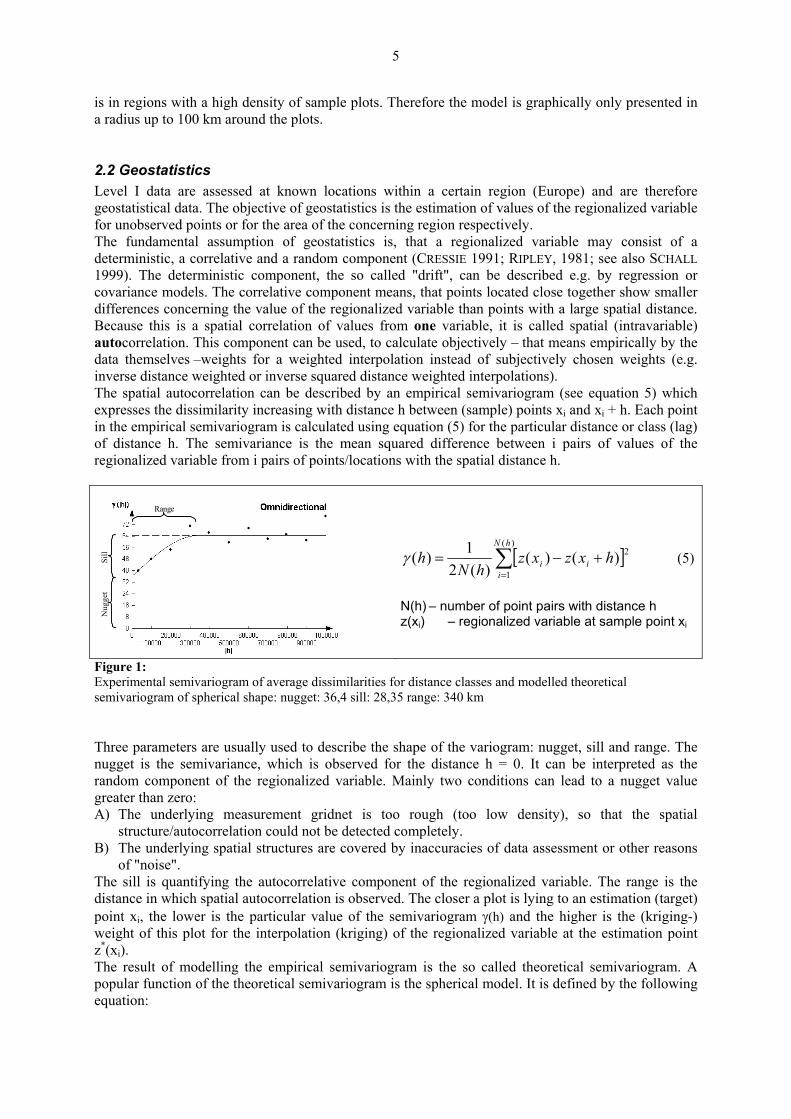
2.2 Geostatistics Level I data are assessed at known locations within a certain region (Europe) and are therefore geostatistical data. The objective of geostatistics is the estimation of values of the regionalized variable for unobserved points or for the area of the concerning region respectively. The fundamental assumption of geostatistics is, that a regionalized variable may consist of a deterministic, a correlative and a random component (CRESSIE 1991; RIPLEY, 1981; see also SCHALL 1999). The deterministic component, the so called "drift", can be described e.g. by regression or covariance models. The correlative component means, that points located close together show smaller differences concerning the value of the regionalized variable than points with a large spatial distance. Because this is a spatial correlation of values from one variable, it is called spatial (intravariable) autocorrelation. This component can be used, to calculate objectively – that means empirically by the data themselves –weights for a weighted interpolation instead of subjectively chosen weights (e.g. inverse distance weighted or inverse squared distance weighted interpolations). The spatial autocorrelation can be described by an empirical semivariogram (see equation 5) which expresses the dissimilarity increasing with distance h between (sample) points xi and xi + h. Each point in the empirical semivariogram is calculated using equation (5) for the particular distance or class (lag) of distance h. The semivariance is the mean squared difference between i pairs of values of the regionalized variable from i pairs of points/locations with the spatial distance h.

Nug

get

Si

ll

Range

[ ]∑=

+−=)(

1

2)()()(2

1)(hN

iii hxzxz

hNhγ (5)

N(h) – number of point pairs with distance h z(xi) – regionalized variable at sample point xi

Figure 1: Experimental semivariogram of average dissimilarities for distance classes and modelled theoretical semivariogram of spherical shape: nugget: 36,4 sill: 28,35 range: 340 km Three parameters are usually used to describe the shape of the variogram: nugget, sill and range. The nugget is the semivariance, which is observed for the distance h = 0. It can be interpreted as the random component of the regionalized variable. Mainly two conditions can lead to a nugget value greater than zero: A) The underlying measurement gridnet is too rough (too low density), so that the spatial

structure/autocorrelation could not be detected completely. B) The underlying spatial structures are covered by inaccuracies of data assessment or other reasons

of "noise". The sill is quantifying the autocorrelative component of the regionalized variable. The range is the distance in which spatial autocorrelation is observed. The closer a plot is lying to an estimation (target) point xi, the lower is the particular value of the semivariogram γ(h) and the higher is the (kriging-) weight of this plot for the interpolation (kriging) of the regionalized variable at the estimation point z*(xi). The result of modelling the empirical semivariogram is the so called theoretical semivariogram. A popular function of the theoretical semivariogram is the spherical model. It is defined by the following equation:

6

( )

≥+

−

•+=

ngera h ; sillnugget

range < h < 0 ; range

h0,5range

h1,5sillnugget

h = 0 ; nugget

hγ3

(6)

Spherical semivariograms are used in the presented study due to their good interpretability and in order to increase the comparability between the examined tree species. Better adapted models are mentioned in the particular chapters. Geostatistics and particularly semivariography are used for a spatial analysis of the residuals from a model, in which age, country and their interaction term age*country are used for a statistical explanation of the variance of mean defoliation. This model is assumed to explain most of the systematical part of the deterministic component of the variance of defoliation. Thus the residuals – here the regionalized variables – roughly quantify the defoliation, corrected for systematical differences between the countries. The country correction is however preliminary due to missing objectively assessed correction factors. Thus the residuuals can be described as “preliminarily adjusted defoliation” (PAD). Using the kriging interpolation for the model residuals maps of preliminarily adjusted defoliation in Europe are produced. Inter-country relations should however be interpreted with care. Only for those points a value of the regionalized variable was estimated, for which at least 12 Level I plot values are available in a radius of 400 km and for which at least 4 plot values are available in a radius of 100 km. The latter precondition was defined in order to reduce the area of extrapolation beyond the sample area. For the calculation of the kriging values however plots within the 400 km radius were used. Another application of semivariography is the detection of outliers. Plots with residuals, which do not fit to the spatial pattern lead to very high variogram values and can easily be identified e.g. by calculating so called variogram clouds. Possible reasons for extremely high or low values or residuals respectively should be discussed with the particular National Focal Centres and can lead to the design of new explanatory variables.

7

3. Results

3.1 Generalized Linear Models for the main tree species in Europe Mean defoliation 1994-1999 Results from generalised linear models (GLM) are summarised in Table 1. For Scots pine (Pinus sylvestris) the largest number of plots was available, closely followed by Norway spruce (Picea abies). Both, common beech (Fagus sylvatica) and pedunculate and sessile oak (Quercus robur et petraea), are represented with approximately 500 plots, while for each of the Mediterranean species holm oak (Quercus ilex) and maritime pine (Pinus pinaster) only about 150 plots could be evaluated. The mean defoliation of the investigated tree species is influenced to a different extend by effects related to country. With 47% of explained variance Pinus sylvestris shows by far the highest influence of country, while for Quercus ilex no country effect at all could be detected. The models that in addition include age and its interaction with country, denote Picea abies as the species for which defoliation is explained best, closely followed by Pinus sylvestris. For Norway spruce the enclosure of age and its interaction with country has more than doubled the amount of the explained variance. For the deciduous tree species the increase in the explained variance due to the inclusion of age amounts to approximately 10% while for Pinus pinaster the increase is comparatively poor. In Querus ilex also a small age effect was found, but the model in total explains only a very small amount of the variance. If the medium-term mean occurrence of insects and fungi is added to the model for some of the tree species another distinct increase in explained variance can be detected. This increase is most obvious for Pinus pinaster and the two deciduous tree species. For Pinus sylvestris and Picea abies the influence of insects and fungi including their interactions with country improve the statistical model only to minor degrees. For Quercus ilex there is almost no effect. In all, the models show distinct influences of country, age, insects, and fungi as these factors explain 41% to 61% of the spatial variation of defoliation. Only in the case of Quercus ilex the model remains quite poor with respect to the explained variance. Table 1: Matrix of basic statistical relationships in terms of explained variance (R2) evaluated by generalised linear models (GLM) for crown condition parameters of the main tree species. Predicting variables Picea

abies Pinus sylvestris

Pinus pinaster

Fagus sylvatica

Quercus robur et petraea

Quercus ilex

number of plots

1115 1399 154 526 499 156

Country

0.26 0.47 0.34 0.22 0.31 0.01

Country, age1) 0.59 0.57 0.39 0.33 0.40 0.06

mean defoliation 1994-1999

Country, age1), insect1), fungi1)

0.61 0.61 0.50 0.41 0.50 0.07

Country 0.20 0.35 0.36 0.37 0.31 0.00 Country, age1) 0.28 0.38 0.38 0.42 0.34 0.02

mean discoloration 1994-1999 Country, age1),

insect1), fungi1) 0.31 0.47 0.47 0.55 0.54 0.04

age: stand age class transformed into stand age [y] country: class variable describing all peculiarities related to single countries fungi: medium-term mean share of trees infested by fungi [%] insect: medium-term mean share of trees infested by insects [%]. 1) additionally interaction with country included. Mean discoloration 1994-1999 Like for defoliation distinct country effects show up for discoloration. Expressed as R2 values, they range between 20% (Picea abies) and 37% (Fagus sylvatica). Again, as in defoliation, Quercus ilex shows no country specific peculiarities at all. The inclusion of age and its interaction with country reveals a considerable increase in the explained variance for Picea abies. For all other tree species it only reveals an increase of up to 5%. If the mean influence of insects and fungi and their interactions with country are included in the generalised linear model, a remarkable increase in the explained

8

variance is achieved in Quercus robur et petraea, reflecting its outstanding receptivity to a large number of biotic agents. Also for Fagus sylvatica a distinct influence of insects or fungi can be supposed. For both deciduous species the models concerning discoloration reveal higher degrees of explained variance than the models for defoliation. Both Pinus species also show distinct influences of biotic agents. Only for Picea abies the model on discoloration is distinctively worse than the model for defoliation. Like in defoliation, discoloration of the wintergreen holm oak (Quercus ilex) is not influenced by any of the introduced parameters. The following subchapters specify the presented overview through species and country specific details and supplement the model calculations by geostatistical analyses.

3.2 Picea abies

3.2.1 Generalized Linear Models According to the selection criteria 1115 Picea abies plots are available for statistical evaluations. They are located in 24 countries. The general distribution pattern is roughly congruent with the phytogeographic features of Norway spruce. For Picea abies the class variable country explains 26% of the variance of mean defoliation (Tab. 1), which is the smallest amount among the coniferous species. The intercepts found for the different countries vary between -5.64% (Norway) and 29.35% (Czech Republic) (Tab. 2). 123.72% for Luxembourg or 35.47% for Croatia must be considered as statistical artefacts due to very low numbers of plots. Those countries with sufficiently large numbers of plots reveal positive coefficients for the influence of age onto the state of defoliation. Norway and Finland for example show an average increase in defoliation per age class (20 years) of 6,4% and 5.8% respectively. Negative coefficients may largely depend on random effects due to low plot numbers or effects not regarded yet (e.g. Luxembourg with two plots and a strong negative slope for age of -0.983%). Another explanation might be the fact that some countries include the natural age trend into their reference tree system (PCC/BFH 1998), whereas other countries use similar reference trees for all age classes. Further, in countries with limited variation of age, only very low amounts of variance can potentially be explained by this variable.

9

Table 2: Model for medium-term mean defoliation [%] for Picea abies in Europe, 1994-1999; listed according to the country specific mean defoliation.

n mean defol. [%]

intercept [%]

age trend [% defol./a]

Spain 1 5.278 4.809 0.047 France 38 5.738 -2.597 0.147 Austria 67 7.494 1.453 0.067 Estonia 31 12.676 1.767 0.2 Bulgaria 5 14.511 26.659 -0.148 Italy 15 14.870 15.296 -0.005 UK 11 16.237 10.701 0.086 Denmark 9 16.696 7.193 0.276 Ireland 4 18.135 20.724 -0.092 Latvia 38 18.209 15.395 0.047 Sweden 163 18.397 4.648 0.186 Finland 156 19.944 -2.594 0.292 Germany 181 20.141 2.317 0.231 Switzerland 25 21.833 12.847 0.077 Belgium 7 21.870 26.466 -0.063 Lithuania 25 21.981 10.506 0.185 Norway 131 22.271 -5.635 0.322 Slovenia 21 22.295 17.749 0.054 Romania 33 22.390 14.032 0.126 Luxembourg 2 25.451 123.716 -0.983 Czech Rep. 82 31.981 29.346 0.029 Slovak Rep. 44 32.217 25.604 0.083 Poland 26 32.418 26.548 0.07 Croatia 1 40.625 35.465 0.047 The model values for defoliation adjusted for an age of 90 years show distinct differences in the evaluated areas of Europe (Fig. 2). Whereas the mean defoliation values in Scandinavia are rather homogeneously , the model values in Central Europe vary between <10% (Austria) and <40% (Denmark, Luxembourg, Czech Republik, Slovakia, parts of Poland and Italy). The sharp borders between areas with such different mean defoliation values underlines the existence of methodological differences in the assessment methods.

3.2.2 Spatial variation of preliminarily adjusted defoliation (PAD) The theoretical semivariogram is described by a very high nugget effect of 54,4 and a low sill of 9,6. (Fig. 3).

Figure 3: Empirical variogram (dots) and modelled spherical variogram (line) for the residuals of the mean defoliation model of Picea abies, including age, country and the interaction of both variables as explanatory variables; h = distance in meters; nugget 54.4 sill 9.6 range 960 km.

10

Figure 2: Evaluated Level I plots and modelled mean level of defoliation in a radius of 100 km, Picea abies. The analyses of the high variogram values show, that all high dissimilarities for distances h < 200 km and 450 km < h < 900 km are related to either one plot in Germany or to one of several plots in Norway (north of Trondheim), all showing very high defoliation values. Whereas the German plot shows very high insect and fungi indices there are no similar indications for the high defoliation at the plots in Norway.

11

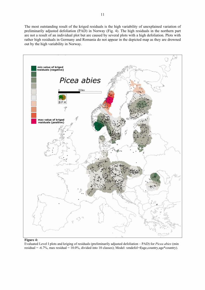
The most outstanding result of the kriged residuals is the high variability of unexplained variation of preliminarily adjusted defoliation (PAD) in Norway (Fig. 4). The high residuals in the northern part are not a result of an individual plot but are caused by several plots with a high defoliation. Plots with rather high residuals in Germany and Romania do not appear in the depicted map as they are drowned out by the high variability in Norway.

Figure 4: Evaluated Level I plots and kriging of residuals (preliminarily adjusted defoliation – PAD) for Picea abies (min residual = -6.7%, max residual = 10.0%, divided into 10 classes); Model: xmdefol=f(age,country,age*country).

12

3.3 Pinus sylvestris

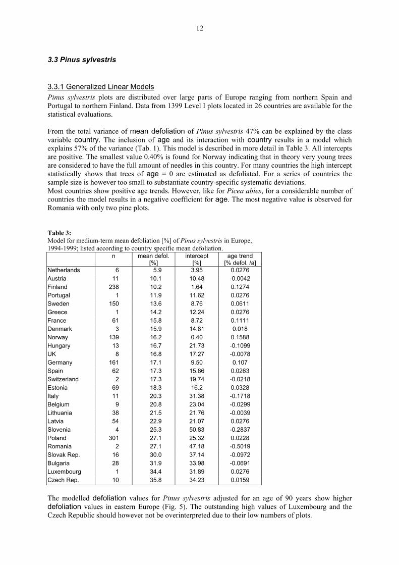
3.3.1 Generalized Linear Models Pinus sylvestris plots are distributed over large parts of Europe ranging from northern Spain and Portugal to northern Finland. Data from 1399 Level I plots located in 26 countries are available for the statistical evaluations. From the total variance of mean defoliation of Pinus sylvestris 47% can be explained by the class variable country. The inclusion of age and its interaction with country results in a model which explains 57% of the variance (Tab. 1). This model is described in more detail in Table 3. All intercepts are positive. The smallest value 0.40% is found for Norway indicating that in theory very young trees are considered to have the full amount of needles in this country. For many countries the high intercept statistically shows that trees of age = 0 are estimated as defoliated. For a series of countries the sample size is however too small to substantiate country-specific systematic deviations. Most countries show positive age trends. However, like for Picea abies, for a considerable number of countries the model results in a negative coefficient for age. The most negative value is observed for Romania with only two pine plots. Table 3: Model for medium-term mean defoliation [%] of Pinus sylvestris in Europe, 1994-1999; listed according to country specific mean defoliation.

n mean defol. [%]

intercept [%]

age trend [% defol. /a]

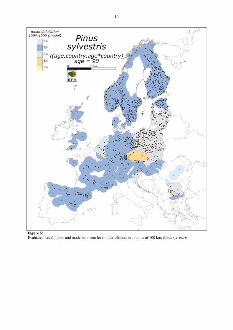
Netherlands 6 5.9 3.95 0.0276 Austria 11 10.1 10.48 -0.0042 Finland 238 10.2 1.64 0.1274 Portugal 1 11.9 11.62 0.0276 Sweden 150 13.6 8.76 0.0611 Greece 1 14.2 12.24 0.0276 France 61 15.8 8.72 0.1111 Denmark 3 15.9 14.81 0.018 Norway 139 16.2 0.40 0.1588 Hungary 13 16.7 21.73 -0.1099 UK 8 16.8 17.27 -0.0078 Germany 161 17.1 9.50 0.107 Spain 62 17.3 15.86 0.0263 Switzerland 2 17.3 19.74 -0.0218 Estonia 69 18.3 16.2 0.0328 Italy 11 20.3 31.38 -0.1718 Belgium 9 20.8 23.04 -0.0299 Lithuania 38 21.5 21.76 -0.0039 Latvia 54 22.9 21.07 0.0276 Slovenia 4 25.3 50.83 -0.2837 Poland 301 27.1 25.32 0.0228 Romania 2 27.1 47.18 -0.5019 Slovak Rep. 16 30.0 37.14 -0.0972 Bulgaria 28 31.9 33.98 -0.0691 Luxembourg 1 34.4 31.89 0.0276 Czech Rep. 10 35.8 34.23 0.0159 The modelled defoliation values for Pinus sylvestris adjusted for an age of 90 years show higher defoliation values in eastern Europe (Fig. 5). The outstanding high values of Luxembourg and the Czech Republic should however not be overinterpreted due to their low numbers of plots.

13

3.3.2 Spatial variation of preliminarily adjusted defoliation (PAD) A spherical model was fitted to the empirical semivariogram of Pinus sylvestris residuals (Fig. 6). Remarkable is the high nugget value of 27.7 showing a high amount of unexplained variance. The low sill of 10,15 shows, that only a low spatial autocorrelation can be found for the residuals which however can be traced up to a range of 1 300 km. The high variogram values at distances between 300 and 500 km can be explained by some outliers. In addition a power model was fitted to the empirical variogram (Fig. 7). Even though the power function is closer to the depicted residuals the spherical model was chosen as a basis for the interpolation due to an easier interpretation especially in relation to other tree species and better characteristics concerning the theory of geostatistics.

Figure 6: Empirical variogram (dots) and modelled spherical variogram (line) for the residuals of the mean defoliation model of Pinus sylvestris, including age, country and the interaction of both as explanatory variables; h = distance in meters; nugget 27,7; sill 10,15; range 1.300 km

Figure 7: Empirical variogram (dots) and modelled power variogram (line) for the residuals of the mean defoliation model of Pinus sylvestris, including age, country and the interaction of both as explanatory variables; h = distance in meters; nugget 27,7; power 1,02; slope 7.8e-06

For some areas a distinct spatial trend in the kriged residuals (preliminarily adjusted defoliation, PAD) is observed (Fig. 8). The most obvious one is the spatial pattern of the PAD in Poland. Whereas the low residuals in the northern and especially the north western regions are an indication for better crown condition defoliation residuals are high in the south in relation to the mean of the country. Similar observations can be made for the north west of Estonia, France – in the south east – and in the east of Spain. Germany, Norway and Finland show spots of less remarkable high residuals. Some of the red spots are directly related to the high variogram values of the empirical semivariogram (Figs. 6; 7). Namely four plots in Finland, Poland, France and Spain show very high dissimilarities compared with plots in a distance between 300 and 500 km. The reasons for their high mean defoliation values have to be discussed further on.

14

Figure 5: Evaluated Level I plots and modelled mean level of defoliation in a radius of 100 km, Pinus sylvestris.

15

Figure 8: Evaluated Level I plots and kriging of residuals (preliminarily adjusted defoliation – PAD) for Pinus sylvestris (min residual = -6.2%, max residual = 11.1%, divided into 10 classes); Model: xmdefol=f(age,country,age*country).

16

3.4 Fagus sylvatica

3.4.1 Generalized Linear Models Plots stocked with Fagus sylvatica are mainly located in central Europe as well as in mountainous regions of the northern Mediterranean zone and south-eastern Europe. 526 plots from 20 countries are included in the evaluations. The results of the model are given in Table 4. Negative intercepts as observed for Belgium, Austria and Sweden, are due to random effects mainly based on small numbers of plots per country. For most countries the model results in positive relationships between age and defoliation. For Germany, the country with the most Fagus plots, an increase in defoliation of 3.16% per age class (20 years) is calculated. France with the second most plots shows a similar result with 1.76% increase in defoliation per age class. Table 4: Model for medium-term mean defoliation [%] of Fagus sylvatica in Europe, 1994-1999; listed according to country specific mean defoliation.

n mean defol. [%]

intercept [%]

age trend [% defol. /a]

Hungary 5 4.42 1.337 0.041 Austria 12 6.374 -1.469 0.084 Greece 5 7.11 6.754 0.003 Croatia 22 10.01 5.431 0.065 France 88 14.264 7.099 0.088 Belgium 8 15.379 -43.692 0.513 UK 12 15.772 12.83 0.031 Slovenia 18 16.436 11.132 0.059 Romania 88 18.472 15.707 0.037 Spain 8 19.034 15.74 0.055 Italy 36 19.074 17.908 0.023 Sweden 7 19.557 -0.513 0.187 Switzerland 13 19.952 13.149 0.065 Slovak Rep. 51 20.18 20.769 -0.008 Czech Rep. 2 20.775 7.794 0.13 Germany 114 21.672 7.841 0.158 Bulgaria 14 23.918 24.817 -0.016 Denmark 6 25.331 5.569 0.169 Poland 17 26.73 20.479 0.072 Luxembourg 1 27.652 29.383 -0.016

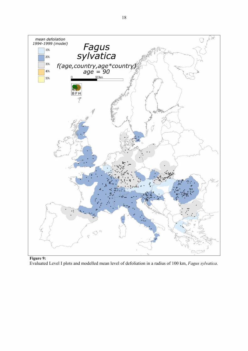
The model values for defoliation of Fagus sylvatica adjusted for the age of 90 years are below 30% in all countries. In Greece, Belgium, Czech Republic and Slovakia they are lowest with values below 10% defoliation.

17

3.4.2 Spatial variation of preliminarily adjusted defoliation (PAD) Figure 10 shows the empirical semivariogram. It was fitted by a theoretical semivariogram of spherical type with the following parameters: nugget 36.04 sill 16.96 range 221 km. The high variogram values at distances (h) of c. 350 km can mainly be explained by four plots with high defoliation, and particular high residual values located in Germany, Romania and France. For these plots the mean defoliation values are underestimated by the age-country-model with residuals between 30 and 34%. With the exception of a single German plot these extreme values can be explained by the conspicuous appearance of insects in the observed period. An analysis of the plots in the neighbourhood of these conspicuous plots shows that they are no single extraordinary observations but extreme values in a region of relatively high defoliation values.

Figure 10: Empirical variogram (dots) and modelled spherical variogram (line) for the residuals of the mean defoliation model of Fagus sylvatica, including age, country and the interaction of both variables as explanatory variables; h = distance in meters; nugget 36.04 sill 16.96 range 221 km

The map of the preliminarily adjusted defoliation (PAD) shows a strong variation of relative crown condition throughout Europe (Fig. 11). The areas in central Germany and southern Romania do not only show high residuals and defoliation values for Fagus sylvatica, they also attract the attention through high residuals of oak species (Chapt. 3.5). For the particular plots in Romania a high occurrence of insects and fungi is observed.

18

Figure 9: Evaluated Level I plots and modelled mean level of defoliation in a radius of 100 km, Fagus sylvatica.

19

Figure 11 Evaluated Level I plots and kriging of residuals (preliminarily adjusted defoliation – PAD) for Fagus sylvatica (min residual = -9.2%, max residual = 9.3%, divided into 10 classes); Model: xmdefol=f(age,country,age*country).

20

3.5 Quercus robur and Quercus petraea

3.5.1 Generalized Linear Models The two oak species (Quercus robur, Q. petraea) can be found on 499 plots spread over large parts of Europe reaching from the belt of nemoral woodlands in north-western Spain to eastern Bulgaria and Moldova. The total sample contains plots from 24 countries, however by far the most of the oak plots are located in France. Apart from Austria with an outstandingly low mean defoliation of only 1.13%, depending however on one plot only, most of the countries do have high defoliation values with averages above 20% or even above 30% (Tab. 5). The age trends vary considerably. France with its 189 Quercus plots reveals an average increase of 2% per age class (20 years). Similar coefficients are found for many countries, especially for those with higher numbers of plots. In countries with only a few plots often negative coefficients are found, mainly due to random effects. Table 5: Model for medium-term mean defoliation [%] of Quercus robur and Quercus petraea in Europe, 1994-1999; listed according to country specific mean defoliation.

n mean defol. [%]

intercept [%]

age trend [% defol. /a]

Austria 1 1.125 12.286 -0.223 Portugal 1 13.333 33.423 -0.223 Netherlands 4 14.573 25.073 -0.15 Belgium 11 15.088 6.961 0.078 Spain 15 17.879 22.723 -0.087 France 189 19.606 12.079 0.102 Hungary 17 20.295 16.703 0.065 UK 15 20.463 18.841 0.014 Lithuania 3 20.907 4.038 0.203 Sweden 11 21.626 25.388 -0.042 Slovenia 7 21.724 35.668 -0.145 Croatia 23 25.337 18.642 0.091 Italy 16 26.178 22.272 0.08 Switzerland 2 26.461 62.325 -0.299 Germany 55 27.584 18.041 0.108 Greece 13 28.119 30.827 -0.056 Slovak Rep. 21 30.526 17.481 0.182 Romania 36 31.380 32.215 -0.014 Poland 35 31.532 23.679 0.1 Bulgaria 9 31.587 42.748 -0.223 Czech Rep. 2 31.914 38.38 -0.064 Moldova 6 32.170 30.776 0.025 Luxembourg 3 32.347 48.587 -0.212 Denmark 4 35.217 29.226 0.057 Country-wise modelled defoliation values increase from the south-west (<10% in the north of Spain and Portugal) to the east where they mostly range between 30 and 40 % (Fig. 12). The only exceptions are Switzerland and Austria, however the model values of these two countries are based on a very few plots only.

21

3.5.2 Spatial variation of preliminarily adjusted defoliation (PAD) The empirical semivariogram for the residuals of the statistical model for the oak species Quercus robur and Qercus petraea shows a typical shape and thus can be modelled easily with a theoretical semivariogram of spherical type (Fig. 13). The range (256 km) is the second lowest (Fagus sylvatica: 221 km). Most characteristical is the very low sill (9.0) in relation to the high nugget value (44.4). Spatial autocorrelation is thus low compared with the random component of spatial variability.

Figure 13: Empirical variogram (dots) and modelled spherical variogram (line) for the residuals of the mean defoliation model of Quercus robur and Qercus petraea, including age, country and the interaction of both as explanatory variables; h = distance in meters; nugget 40.4 sill 9.0 range 256 km.

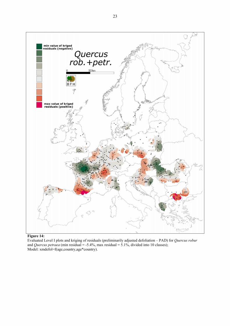
The mapping of the preliminarily adjusted defoliation (PAD) of the two Quercus species (Fig. 14) shows a very inhomogeneous structure. The patterns in Germany and Romania resemble to the map of the relative crown condition of Fagus sylvatica. An in-depth explanation of the spatial pattern is not possible without consultation through the National Focal Centres.

22

Figure 12: Evaluated Level I plots and modelled mean level of defoliation in a radius of 100 km, Quercus robur and Quercus petraea.

23

Figure 14: Evaluated Level I plots and kriging of residuals (preliminarily adjusted defoliation – PAD) for Quercus robur and Quercus petraea (min residual = -5.4%, max residual = 5.1%, divided into 10 classes); Model: xmdefol=f(age,country,age*country).

24

3.6 Pinus pinaster

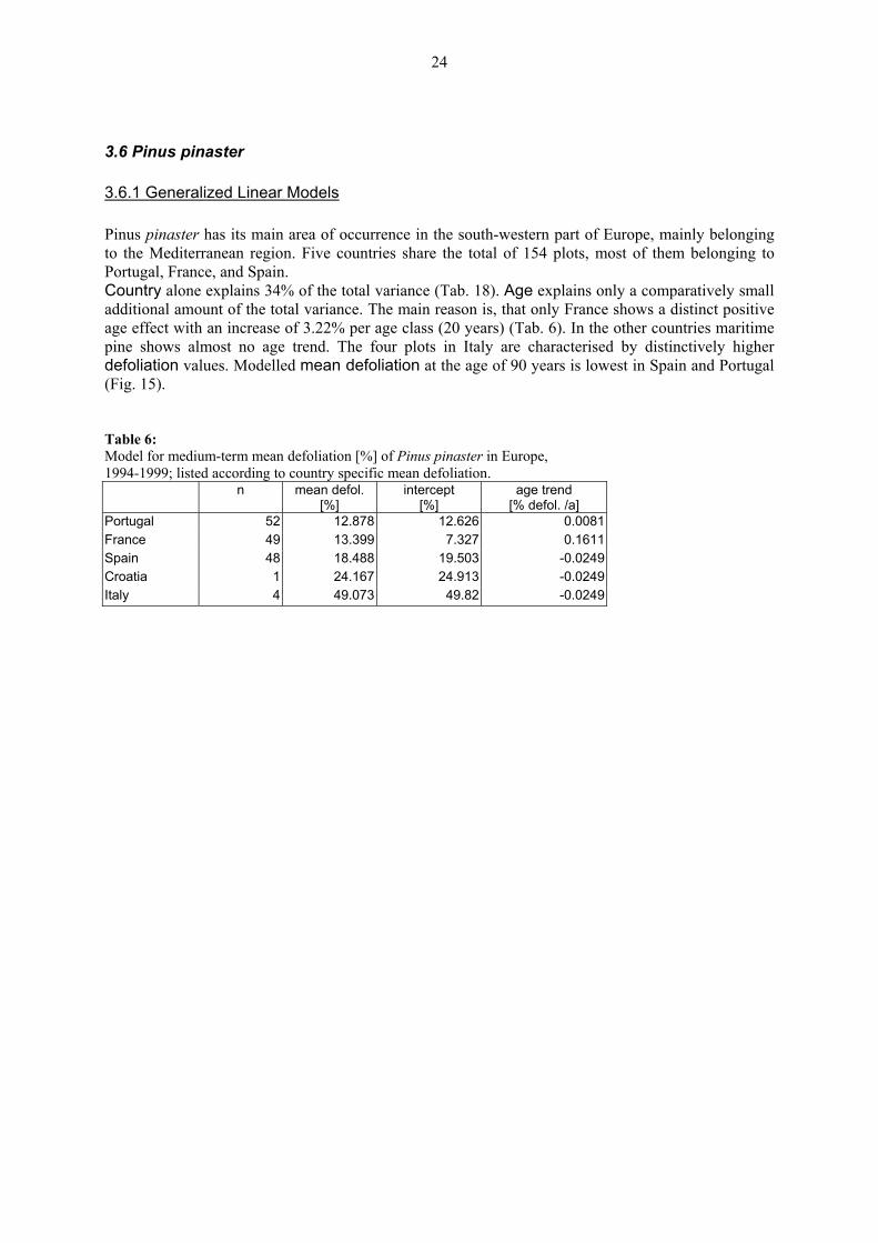
3.6.1 Generalized Linear Models Pinus pinaster has its main area of occurrence in the south-western part of Europe, mainly belonging to the Mediterranean region. Five countries share the total of 154 plots, most of them belonging to Portugal, France, and Spain. Country alone explains 34% of the total variance (Tab. 18). Age explains only a comparatively small additional amount of the total variance. The main reason is, that only France shows a distinct positive age effect with an increase of 3.22% per age class (20 years) (Tab. 6). In the other countries maritime pine shows almost no age trend. The four plots in Italy are characterised by distinctively higher defoliation values. Modelled mean defoliation at the age of 90 years is lowest in Spain and Portugal (Fig. 15). Table 6: Model for medium-term mean defoliation [%] of Pinus pinaster in Europe, 1994-1999; listed according to country specific mean defoliation.

n mean defol. [%]

intercept [%]

age trend [% defol. /a]

Portugal 52 12.878 12.626 0.0081France 49 13.399 7.327 0.1611Spain 48 18.488 19.503 -0.0249Croatia 1 24.167 24.913 -0.0249Italy 4 49.073 49.82 -0.0249

25

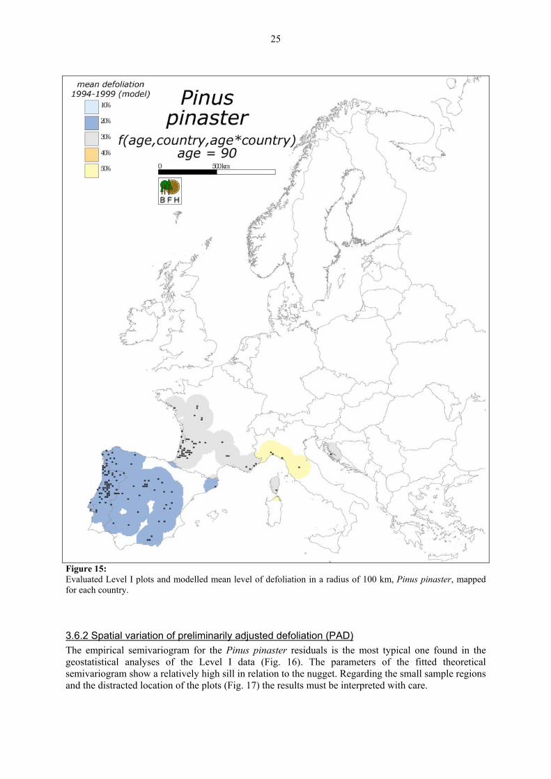
Figure 15: Evaluated Level I plots and modelled mean level of defoliation in a radius of 100 km, Pinus pinaster, mapped for each country.

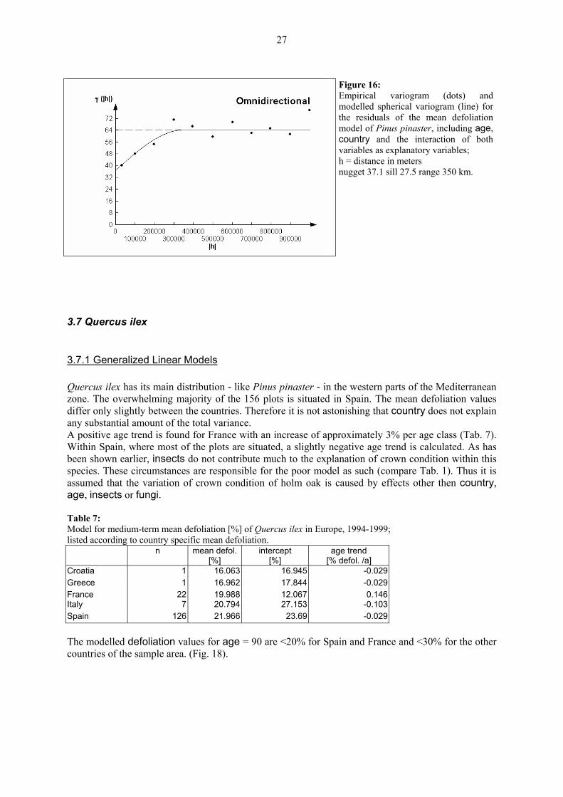
3.6.2 Spatial variation of preliminarily adjusted defoliation (PAD) The empirical semivariogram for the Pinus pinaster residuals is the most typical one found in the geostatistical analyses of the Level I data (Fig. 16). The parameters of the fitted theoretical semivariogram show a relatively high sill in relation to the nugget. Regarding the small sample regions and the distracted location of the plots (Fig. 17) the results must be interpreted with care.

26

Figure 17: Evaluated Level I plots and kriging of residuals (preliminarily adjusted defoliation, PAD) for Pinus pinaster (min residual = -5.6%, max residual = 8.8%, divided into 10 classes); Model: xmdefol=f(age,country,age*country). The spatial variation of the preliminarily adjusted defoliation (PAD) shows high residuals in south eastern France. Residuals are lowest in north eastern parts of the sample area in Spain and Portugal.

27

Figure 16: Empirical variogram (dots) and modelled spherical variogram (line) for the residuals of the mean defoliation model of Pinus pinaster, including age, country and the interaction of both variables as explanatory variables; h = distance in meters nugget 37.1 sill 27.5 range 350 km.

3.7 Quercus ilex

3.7.1 Generalized Linear Models Quercus ilex has its main distribution - like Pinus pinaster - in the western parts of the Mediterranean zone. The overwhelming majority of the 156 plots is situated in Spain. The mean defoliation values differ only slightly between the countries. Therefore it is not astonishing that country does not explain any substantial amount of the total variance. A positive age trend is found for France with an increase of approximately 3% per age class (Tab. 7). Within Spain, where most of the plots are situated, a slightly negative age trend is calculated. As has been shown earlier, insects do not contribute much to the explanation of crown condition within this species. These circumstances are responsible for the poor model as such (compare Tab. 1). Thus it is assumed that the variation of crown condition of holm oak is caused by effects other then country, age, insects or fungi. Table 7: Model for medium-term mean defoliation [%] of Quercus ilex in Europe, 1994-1999; listed according to country specific mean defoliation.

n mean defol. [%]

intercept [%]

age trend [% defol. /a]

Croatia 1 16.063 16.945 -0.029Greece 1 16.962 17.844 -0.029France 22 19.988 12.067 0.146Italy 7 20.794 27.153 -0.103Spain 126 21.966 23.69 -0.029 The modelled defoliation values for age = 90 are <20% for Spain and France and <30% for the other countries of the sample area. (Fig. 18).

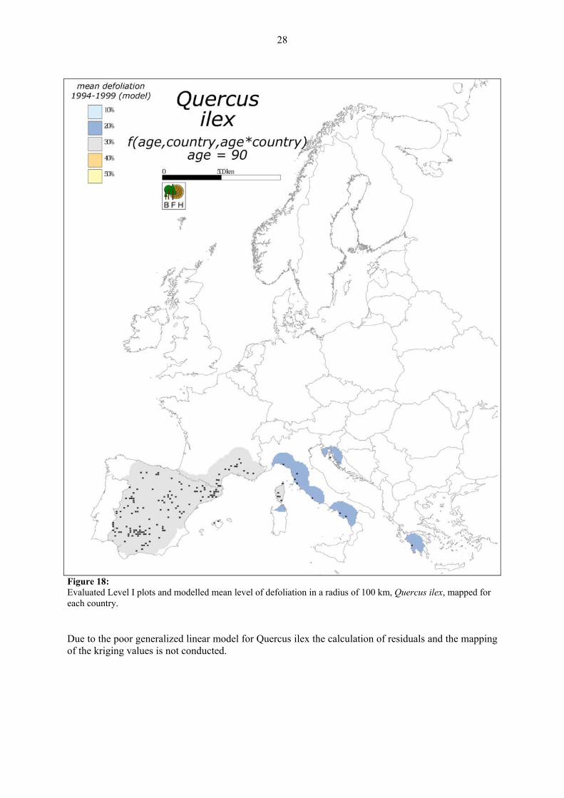
28

Figure 18: Evaluated Level I plots and modelled mean level of defoliation in a radius of 100 km, Quercus ilex, mapped for each country. Due to the poor generalized linear model for Quercus ilex the calculation of residuals and the mapping of the kriging values is not conducted.

29

4. Representativeness of Level I plots and accuracy of kriging estimates

4.1 Representativeness The Level I gridnet is designed to facilitate the projection of relations found for data of this and particular of the Level II gridnet to the sampled area. The data are taken at known locations within a certain region and are used as regionalized variables in the sense of geostatistics. For the estimation of a regionalized variable at locations where no data were taken it is important to know whether the sample data are representative for the target point or target area respectively. The representativeness can be tested by the use of a geographic information system (GIS). To perform such tests values of a certain parameter in the sample area are taken from a thematic map or grid layer respectively. The frequency distribution of the parameter is then compared to the frequency distribution of the same parameter as interpolated at the sample plots. The representativeness of Level I plots has to be checked with respect to the variables that are used in the models. As values of these variables are however in most cases not easily available for the total sample area, the method is in the following subchapter demonstrated using the elevation values of a digital elevation model for Europe. The task of further representativeness checks remains however.

4.1.1. Example for a frequency comparison: elevation of Pinus sylvestris plots As an example for a test of representativeness the relative frequency of elevation values at the co-ordinates of Pinus sylvestris Level I plots on one side are compared to the relative frequency of elevation values of the total sample area on the other side. The elevation values are derived from a digital elevation model (DEM). The cell size of the digital elevation model is 1000 m.

relative frequency of altitude

00.10.20.30.40.50.60.70.8

0 1000 2000 3000 4000 5000altitude [m]

rel.

freq

[%]

DEMLEVEL I

Figure 19: Relative frequencies of elevation values at co-ordinates of Level I Pinus sylvestris plots and of elevation values of the total sample area as derived from a digital elevation model (DEM).

In general the frequency distributions of the elevations at the co-ordinates of Level I plots and the elevations of the digital elevation model show similar shapes (Fig. 19). The most frequent elevation at Level I co-ordinates is 138 m. For 10 plots this elevation is calculated. These plots account for 0.71% of the evaluated 1399 Level I Pinus sylvestris plots. Within the DEM 1 m is an extreme value represented by 26196 cells accounting for 0,75% of the modelled area. Both distributions show highest frequencies below an elevation of 400 m. The highest calculated altitude of a Pinus sylvestris Level I plot is 2327 m followed by plots located at 1971 m and 1926 m respectively. Thus, up to an altitude of 2000 m the Level I plots are well representing the target area. Only 1.1% (39190 cells) of the DEM area are at higher elevations not represented by the Level I plots with respect to altitude.

30

4.2 Accuracy of kriging estimates For every plot location the assessed value is estimated by the kriging interpolation. Kriging therefore is an exact estimator. Within a crossvalidation the kriging estimator is calculated for every plot location without including the particular observed value of the regionalized variable at this location. As a result the kriging estimator z*(xi) for all plot locations as well as the difference to the true value of the regionalized variable z(xi) at the plot locations (Level I plots) is calculated and thus gives a measure for the deviation from the expected value. This deviation contains an information on the accuracy of the kriging estimation. Results show that standard deviation of differences between kriging estimates and residuals of the assessed defoliation values at Level I plots is for the main five tree species between 5% and 10% (Tab. 8). As these values are within the accuracy of the defoliation assessments (DOBBERTIN et al., 1997) it can be assumed that the kriged residuals provide a sufficient accurate estimation for relative crown condition. Table 8: Standard deviation of differences between calculated and true values of the regionalized variable at Level I plots. std(z*(xi) - z(xi))

[%] Fagus sylvatica 7.4 Picea abies 8.0 1) Pinus pinaster 7.7 Pinus sylvestris 5.5 1) Quercus robur et petraea 7.4 1) Due to restrictions of the programme GEO-EAS only 1000 observations are included in the calculations.

31

5. Discussion

5.1 Quality and Suitability of used Variables The target variables defoliation and discoloration are field estimates and therefore prone to comparatively high sampling errors (INNES 1988, DOBBERTIN et al. 1997), which are however assumed to be random. The use of medium-term averages of both crown condition parameters for the period of 1994 to 1999 should not only level off fluctuations due to annual meteorological extremes, but also short-term insect gradations, strong fruiting or other short-term influences. The medium-term target variables reflect medium-term and long-term causes for poor crown condition, such as adverse soil related processes like acidification, nutrient imbalances, or continuous direct impacts of air pollutants. The explaining variables used so far are the class variable country, stand age and estimates of infestations by insects and fungi. Stand age class respective its transformation mean age is available with an accuracy of ±10 years, which seems to be sufficient. However, stand age distribution and age-crown relationship are not uniform for the different countries. Therefore interaction terms between country and age cannot be neglected within the calculations. The estimates for crown damages caused by insects and fungi have to be considered rather critically. Sources of inaccuracies are: missing estimates in some countries, qualitative estimates with probably differing levels, different time-lags between field survey and activity of the biotic agent. Nevertheless, due to plot-wise and temporal averaging an estimate is gained, which seems to reflect at least some of the mean activities of these biotic agents at many monitoring plots. In the course of the statistical analysis it also turned out, that for both estimates country-specific differences exist. Therefore interactions with country was considered within the statistical models. The selection criteria for monitoring plots taken into consideration were largely set in accordance with former Technical Reports (e.g. LORENZ et al. 2000). However, plots with negative lower limits of the confidence interval were not excluded, in order to avoid systematic exclusion of plots with low mean defoliation values.

5.2 Generalized Linear Models (GLM) Generalized linear models offer the possibility of a combined analysis of class and numerical variables. As systematic differences between many participating countries can hardly be expressed by a numeric variable or dummy variables, this type of statistical model has been preferred over multiple linear regression models in order to take into account methodological differences between countries. It has already been stated earlier that Level I crown condition data are biased by country (INNES et al. 1993; KLAP et a. 1997, 2000, SEIDLING in prep.). The results from the statistical models presented above confirm these earlier findings by the use of data sets differing with respect to time spans and regions in Europe. Apart from Quercus ilex, which shows no significant country effect, the variance of the medium-term (1994-1999) mean defoliation explains 22% (Fagus sylvatica) to 47% (Pinus sylvestris) by country. It has however to be taken into account that this comparatively high amount of explained variance may not only be due to methodological differences, but may also be due to “real” differences in the crown condition between countries. Parts of it might thus be explainable by different natural or anthropogenic stress factors if models with more precise predictors are applied. Up to now, there are however no data sets with explanatory variables that allow for an exact quantification of methodological differences and natural or anthropogeneous stress factors that cause deviations of defoliation between countries. The consideration of country as a class variable is only a simplifying statistical approach in order to overcome this lack. For a more objective consideration of country, independent correction factors should be worked out according to the proposals made by FERRETTI (1999). Only the use of correction factors that quantify methodological differences between countries guaranties comparable defoliation and discoloration values throughout the sampling areas in Europe. The relationship between defoliation and age is also well known from international (KLAP et al. 1997, 2000) or national studies (e.g. INNES & BOSWELL 1988, HENDRIKS et al. 1994, RIEK & WOLFF 1999 and others, see SEIDLING 2000 for an overview). In the present study, for a first robust approach,

32

a simplified linear relationship between defoliation and age was assumed which might be refined in more sophisticated approaches in the future. Models with age and country and their interaction reveal a considerable amount of explained variance with a maximum of almost 60% for Picea abies and Pinus sylvestris. Again, Quercus ilex is an exception as it shows almost no correlation between age and crown condition. The detected country-specific differences of the age-defoliation relationship may be caused by (i) high random influences in countries with small numbers of plots, (ii) different treatment of tree age at the level of local or regional reference tree systems, and (iii) a limited variation of age in some countries. In order to minimize methodological differences between countries with respect to their consideration of age, the relationship between crown condition and age should also be parameterised at future intercalibration courses. Discoloration reveals, like defoliation, a considerable influence of country. SEIDLING (in prep.) also found a considerable amount of variation explained by country specific peculiarities. For Pinus pinaster and Fagus sylvatica the effect of country onto discoloration is even more pronounced than onto defoliation. This result calls for an elaboration of country specific correction factors also for this crown condition parameter. Since up to now discoloration has seldom been introduced into empirical statistical studies, merely any comparisons with results from other studies are possible and the potential value of this crown condition parameter is still rather unknown. The results above, contribute at least for some of the main tree species to a better general understanding of crown related processes.

5.3 Regionalized preliminarily adjusted defoliation (PAD) The residuals between the assessed medium-term mean defoliation and the generalized linear models based on country, age and their interaction have been used to describe the European-wide condition of tree crowns as preliminarily adjusted defoliation (PAD). Due to this procedure, country and age specific effects are eliminated and the defoliation of large areas without the influence of both variables becomes visible. Compared to the field assessments of defoliation, the PAD allows for an better inter-country comparability. As however not only methodological influences but also true country specific differences are eliminated, inter-country comparisons still have to be conducted cautiously. The interpretation of the maps of PAD always has to take into account the results of the underlying generalized linear models. Only for Quercus ilex, which shows neither significant country effects nor a significant influence of age, the original plot-wise means of medium-term averages of defoliation could in principal be directly be used for kriging and for further investigations as well. However the analysis of semivariance (semivariography) showed strong deviations from the underlying assumptions of second order stationarity or the intrinsic hypothesis (RIPLEY 1981). Thus, it was refrained to interpolate defoliation of Quercus ilex. The maps of PAD for the other evaluated tree species show very clear (red) hot spots of high defoliation. These spots and the green counterparts of regions with very low defoliation have to be interpreted as distinct deviations from the particular country mean defoliation. Thus, e.g. the very high variance of PAD for Picea abies in Norway (see also GHOSH et al. 1997) must not be interpreted as the highest and lowest defoliation within the total of Europe, but in Norway. Reasons for this very high intra country variation in Norway, and less pronounced in Finland, must be discussed with the respective National Focal Centres. If there weren't such high variances in both countries, the intra country variances of other countries became better visible. Several observations can be made over all tree species. Thus, in the centre of the German low-mountain region a hot spot is observed for all mapped tree species with exception of Pinus pinaster, which does not occur in this region. For Quercus robur et petraea as well as for Fagus sylvatica and – with reduced clarity – for Picea abies the data from Romania show high PAD values in the south and low values in the north. For Quercus robur et petraea and especially for Pinus sylvestris a distinct hot spot is interpolated in the south of Poland. The maps for Fagus sylvatica and Quercus robur et petraea on the one hand indicate a much higher spatial variability than that for Picea abies and Pinus sylvestris. Nevertheless, especially the range of

33

residual values for Quercus robur et petraea is lower (-5.4% to 5.1%) than that for both coniferous tree species (-6.7% to 10.0% and –6.2% to 11.1% respectively). A significant explanation for this observation can not be given yet. All the hot spots (and outliers) should be analysed and discussed with the National Focus Centres. This should in most cases confirm that hot spots are not only due to an unique observation but that they represent a region with higher defoliation values. Through the consultation process other explanations may be found that could improve the models by new explanatory variables. The coincidence of some hot spots in the PAD maps with high values for insect and fungi indices could already be demonstrated and is thus indicating the value of the preliminarily adjusted defoliation.

34

6. Recommendations From the work done so far the following recommendations can be drawn for future work: Selection criteria for the species specific evaluation of Level I plots, as defined in former Technical Reports (e.g. LORENZ et al. 2000), should not longer exclude plots with a negative lower limit of the confidence interval as the criteria causes a systematic exclusion of plots with low mean defoliation. International Intercalibration Courses for the assessment of crown condition should be redesigned. Two main tasks can be emphasised: - For a more objective consideration of methodological differences between countries, independent

correction factors should be worked out according to the proposals made by FERRETTI (1999). They are necessary as a basis for comparable defoliation values.

- The relationship between stand age and defoliation respectively discoloration should also be parameterised at the Intercalibration Courses.

The presented results concerning discoloration suggest an intensified evaluation of this target variable. The presented evaluations of crown condition at the European level have to be considered as a further step to understand tree responses towards different kinds of natural and anthropogeneous stress (Manion 1978). Apart from the inclusion of basic explaining variables, in later steps soil related parameters (co-operation with FSCC/Belgium), element concentrations of foliage (co-operation with FFCC/Austria) and data concerning deposition as well as medium-term meteorological characteristics of the plots (co-operation with ALTERRA, RIVM/The Netherlands, JRC/Italy and EMEP) should be introduced. Geomorphological items can be derived from the digital elevation model of National Geophysical Data Center (NGDC) of the National Oceanic and Atmospheric Administration (NOAA) of the U.S. Department of Commerce. Landuse information of the plot surroundings can be provided by the European Environmental Agency (EEA). Different types of data preparation like transformations and factor analyses should become part of those advanced approaches. Another important approach for the improvement of the statistical models are consultations with the National Focal Centers which might help to explain some of the extreme values of the observed preliminarily adjusted defoliation. The analysis of time trends of defoliation in combination with the relationship to age should be a further task within the ongoing integrating evaluations. The combination of temporal and spatial aspects should provide a dynamic picture of crown condition processes in Europe. It may in addition give insights into underlying environmental conditions.

35

7. References CRESSIE, N., 1991: Statistiscs for Spatial Data; Wiley, New York. DE VRIES, W., KLAP, J.M., ERISMAN, J.W., 2000a: Effects of environmental stress on forest crown

condition in Europe: Part I: hypotheses and approach to the study. Water, Air, and Soil Pollution 119: 317-333.

DOBBERTIN, M., LANDMANN, G., PIERRAT, J.C., MÜLLER-EDZARDS, C., 1997: Quality of crown condition data. In: MÜLLER-EDZARDS, C., DE VRIES, W., ERISMAN, J.W., (eds.): Ten years of monitoring forest condition in Europe. United Nations Economic Commission for Europe, European Commission, Brussels, Geneva, 7-22.

ENGLUND, E. and SPARKS, A., "Geo-EAS 1.2.1 User's Guide," EPA Report #600/8-91/008 EPA-EMSL, Las Vegas, NV, 1991.

FERRETTI, M., DOBBERTIN, M., DURRANT, D., HERKENDELL, J., LANDMANN, G., NAKOS, G., NEUMANN, M., SANCHEZ-PENA, G., 1999: Future international intercalibration courses (IICs) - developing a concept. Internal paper, unpublished.

GHOSH, S., LANDMANN, G., PIERRAT, J.C., MÜLLER-EDZARDS, C., 1997: Spatio-temporal variation in defoliation. In: MÜLLER-EDZARDS, C., DE VRIES, W., ERISMAN, J.W., (eds.): Ten years of monitoring forest condition in Europe. United Nations Economic Commission for Europe, European Commission, Brussels, Geneva, 35-50.

HENDRIKS, C.M.A., DE VRIES, W., VAN DEN BURG, J., 1994: Effects of acid deposition on 150 forest stands in the Netherlands. DLO WINAND STARING CENTRE FOR INTEGRATED LAND, SOIL AND WATER RESEARCH, Wageningen, Report 69.2, 55 p.

INNES, J.L., 1988: Forest health surveys: problems in assessing observer objectivity. Can. J. For. Res. 18: 560-565.

INNES, J.L., BOSWELL, R.C., 1988: Forest health surveys 1987. Part 2: analysis and interpretation. Forestry Commission Bulletin (HMSO, London) 79, 52 p.

INNES, J.L., LANDMANN, G. METTENDORF, B., 1993: Consistency of observation of Forestry Condition in Three European Countries. Environmental Monitoring and Assessment 25: 29-40.

KLAP, J., VOSHAAR, J.O., DE VRIES, W., ERISMAN, J.W., 1997: Relationships between crown condition and stress factors. In: MÜLLER-EDZARDS, C., DE VRIES, W., ERISMAN, J.W., (eds.): Ten years of monitoring forest condition in Europe. United Nations Economic Commission for Europe, European Commission, Brussels, Geneva, 277-302.

KLAP, J.M., VOSHAAR, J.H.O., DE VRIES, W., ERISMAN, J.W., 2000: Effects of environmental stress on forest crown condition in Europe. Part IV: statistical analysis of relationships. Water, Air, and Soil Pollution 119: 387-420.

LORENZ, M., BECHER, G., FISCHER, R., SEIDLING; W., 2000: Forest condition in Europe. Results of the 1999 crown condition survey. United Nations Economic Commission for Europe, European Commission, Geneva, Brussels, 86 p. + Annexes.

MANION, P.D., 1981: Tree disease concepts. Englewood Cliffs, N.Y., 367 p. PANNATIER, Y., "VARIOWIN: Software for Spatial Data Analysis in 2D," Springer-Verlag, New

York, NY, 1996. ISBN 0-387-94679-9 PEBESMA, E., 1997: GSTAT User’s Manual. Dept. of Physical Geography, UtrechtUniversity. PCC/BFH (Programme Coordinating Centre/Federal Research Centre for Forestry and Forestry

Products, ed.), 1998: Manual on methods and criteria for harmonized sampling, assessment, monitoring and analysis of the effects of air pollution on forests. Part 2 Visual Assessment of crown condition and submanumal on visual assessment of crown condition on intensive monitoring plots. United Nations Economic Commission for Europe, Hamburg.

RIEK, W., WOLFF, B., 1999b: Integrierende Auswertung bundesweiter Waldzustandsdaten. Abschlußbericht. Institut für Forstökologie und Walderfassung Eberswalde. 137 p. + annex, not publ.

RIPLEY, B.D., 1981: Spatial Statistics. Wiley & Sons, New York. SAS INSTITUTE INC., 1990: SAS/STAT User's Guide, Version 6, 4th Ed., SAS Institute Inc., Cary

(USA), 1668 p. SCHALL, P., 1999: Proposal for extrapolation of relationships identified for Level II plots with

available data at Level I plots. Internal paper, unpubl.

36

SEIDLING, W., 2000: Multivariate statistics within integrated studies on tree crown condition in Europe - an overview. United Nations Economic Commission for Europe, European Commission, Gent, Brussels, Geneva, 56 p + annexes.

SEIDLING, W., in prep.: Integrative studies on forest ecosystem conditions: Multivariate evaluations on tree crown condition for two area with distinct deposition gradients. United Nations Economic Commission for Europe, European Commission, Flemish Government, Geneva, Brussels, Gent, 86 p.