Spatial variability of salinity and alkalinity of a field having salination risk in semi-arid...

Environ Monit Assess (2007) 127:55–65

DOI 10.1007/s10661-006-9258-x

O R I G I N A L A R T I C L E

Spatial variability of salinity and alkalinity of a field havingsalination risk in semi-arid climate in northern TurkeyKenan Kılıc · Sinan Kılıc

Received: 26 September 2005 / Accepted: 13 April 2006 / Published online: 23 August 2006C© Springer Science + Business Media B.V. 2006

Abstract Spatial variability of salinity and alkalinity

is important for site-specific management since they

are the most important factors influencing soil qual-

ity and agricultural production. The objectives of this

study were to analyze spatial variability in salinity and

alkalinity and some soil properties affecting salinity

and alkalinity, using classical statistics and geostatis-

tical methods, in an irrigated field with low-quality ir-

rigation water diverted from drainage canals. A field

of 5 da was divided into 10 m × 10 m grids (5 lines

in the east-west direction and 10 lines in the north-

south direction). The soil samples were collected from

three depths (0–30, 30–60 and 60–90 cm) at each grid

corner. The variation coefficients of OM and sand con-

tents were higher than other soil properties. OM had

the maximum variability, with a mean of 1.63% at 0–

30 cm depth and 0.71% at 30–60 cm depth. Significant

correlations occurred between ESP, EC and each of Ca,

Mg, K and CaCO3 contents of the soils (p < 0.01). Ex-

perimental semivariograms were fitted to spherical and

gaussian models. All geostatistical range values were

greater than 36 m. The soil properties had spatial vari-

ability at small distances at 60–90 cm depth. EC was

variable within short distances at 30–60 cm depth. The

nugget effect of ESP increased with soil depth. Kriged

Kenan Kılıc (�) · Sinan KılıcDepartment of Soil Science, Faculty of Agriculture,University of Gaziosmanpasa, Taslıciftlik, 60250, Tokat,Turkeye-mail: [email protected]

contour maps revealed that soils had a salinisation and

alkalisation tendency at 60–90 cm depth based on spa-

tial variance structure of the EC and ESP values. Spatial

variability in EC and ESP can depend on ground water

level, quality of irrigation water, and textural differ-

ences.

Keywords Salinity . Alkalinity . Geostatistics .

Spatial variability . Turkey

1 Introduction

Salinity (EC) and alkalinity (ESP) are the two of the

most important problems on agricultural production

in arid and semi-arid regions and are threatening for

sustainable agricultural management (Ceuppens et al.,1997; Boivin et al., 2002). The amount of agricultural

lands having salinity and alkalinity problems increase

continuously as related to climate, topography, ground-

water level and quality of irrigation water (Postel, 1989;

Ayers and Westcot, 1989). About 400 million hectares

of agricultural lands are under salinity in the world are.

The most common reasons of salinity and alkalinity

are low precipitation, high evapotranspiration, and low

quality of irrigation water. Saline soils contain soluble

salts in sufficient quantities to interfere the growth of

most crop plants but they do not contain enough ex-

changeable sodium to alter soil characteristics (Seatz

and Peterson, 1965). However, alkali soils include

Springer

56 Environ Monit Assess (2007) 127:55–65

exchangeable sodium in a sufficient quantity to inter-

fere the growth of most crops (Bohn et al., 1985).

There is a close relationship between soil properties

and salinity and alkalinity (Kachanoski et al., 1988).

When clay content is low, EC is affected by volumet-

ric water content, and EC increased with increasing

water content (Kachanoski et al., 1988). There was a

significant relationship between EC and the depth of

claypan in the soil profile, and EC was determined to

increase with increasing the depth of claypan (Doolittle

et al., 1994; Sudduth et al., 1999). The claypan formed

in the agricultural lands complicates water movement

through soil profile due to low pore size (Rhoades

et al., 1992).

Soil properties may show both vertical and horizon-

tal variability along a field. The structure of variability

in soil properties showed differences according to sam-

pling spacing, soil properties, and method used in the

study (Trangmar et al., 1985). Miyamoto et al. (2005)

reported that soil sampling for salinity appraisal was

the most problematic in Entisols, but could be made

simply if a detailed soil map was available. Soil sam-

pling of Entisols can be made based on the soil type

distributions (Miyamoto et al., 2005). Several methods

are available to evaluate soil salinity and determine the

effects of soil management systems on salinity and al-

kalinity. Some researchers (Kelleners and Chaudhry,

1998; Sharma and Rao, 1998; Miyamoto and Chacon,

2005), used conventional statistics to evaluate extent of

soil salinity and many others used geostatistical meth-

ods (Nielsen et al., 1983; Miyamoto and Cruz, 1987;

Utset et al., 1998; Miyamoto et al., 2005).

Soil properties are continuous variables and values

at any location can vary according to direction and dis-

tance of separation from neighboring samples (Burgess

and Webster, 1980). Salinity and alkalinity exhibit spa-

tial dependence within some localized region. The clas-

sical statistic is insufficient for interpolation of spatial

dependent variables, because it supposes random vari-

ation and does not takes into consideration of spatial

correlation, distance of sampling and location of sam-

ples (Trangmar et al., 1985).

Management practices in the study area have caused

to salinity and alkalinity in the subsurface layers, espe-

cially in 60–90 cm depth. Salinity and alkalinity have

been increased dramatically with soil management sys-

tems such as irrigated cultivation of the soils, existing

farm irrigation management, high groundwater level,

and applying poor quality water. The soils in Kazova

of Tokat Province in the middle Black sea region of

Turkey are commonly surface irrigated, with low qual-

ity of irrigation water having 980 μS cm−1 EC and

SAR value of 1.28 (Saltalı et al., 1999).

The soils of the study area (Aquic Ustifluvent) have

high variability in short distances as they formed on

alluvial materials. This property of the soils can com-

plicate to analysis of spatial variability in soil proper-

ties. However, assessment of spatial variability in salin-

ity and alkalinity will play an important role for site-

specific management. The objectives of this study were

to (i) assess relationships between some soil proper-

ties and EC and ESP values; and (ii) evaluate spatial

variability of EC and ESP for the purpose of identi-

fying the possible trends in soil salinity and alkalin-

ity to avoid further deterioration in soil quality in the

region.

2 Material and Methods

2.1 Study area

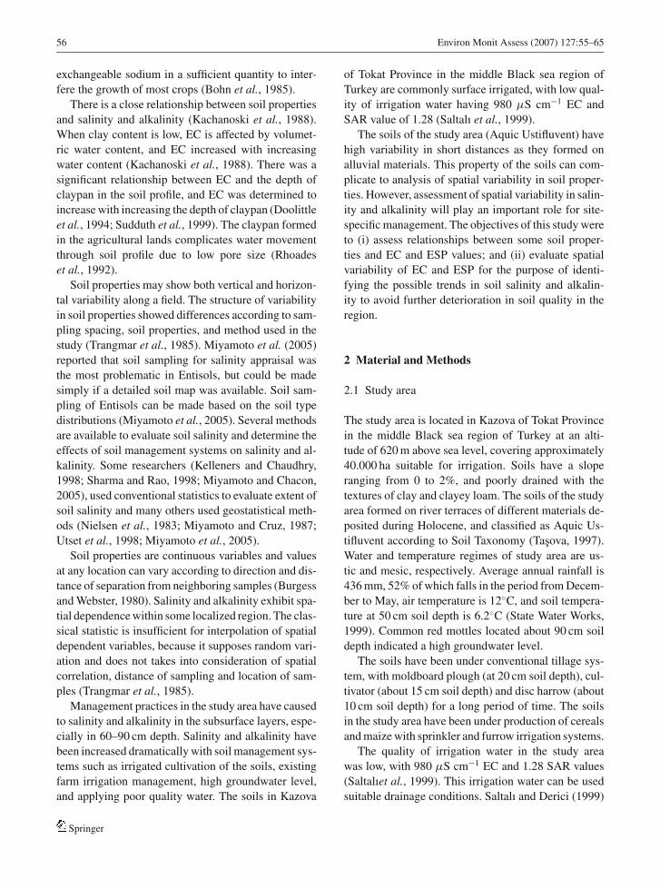
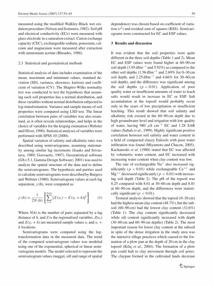
The study area is located in Kazova of Tokat Province

in the middle Black sea region of Turkey at an alti-

tude of 620 m above sea level, covering approximately

40.000 ha suitable for irrigation. Soils have a slope

ranging from 0 to 2%, and poorly drained with the

textures of clay and clayey loam. The soils of the study

area formed on river terraces of different materials de-

posited during Holocene, and classified as Aquic Us-

tifluvent according to Soil Taxonomy (Tasova, 1997).

Water and temperature regimes of study area are us-

tic and mesic, respectively. Average annual rainfall is

436 mm, 52% of which falls in the period from Decem-

ber to May, air temperature is 12◦C, and soil tempera-

ture at 50 cm soil depth is 6.2◦C (State Water Works,

1999). Common red mottles located about 90 cm soil

depth indicated a high groundwater level.

The soils have been under conventional tillage sys-

tem, with moldboard plough (at 20 cm soil depth), cul-

tivator (about 15 cm soil depth) and disc harrow (about

10 cm soil depth) for a long period of time. The soils

in the study area have been under production of cereals

and maize with sprinkler and furrow irrigation systems.

The quality of irrigation water in the study area

was low, with 980 μS cm−1 EC and 1.28 SAR values

(Saltalıet al., 1999). This irrigation water can be used

suitable drainage conditions. Saltalı and Derici (1999)

Springer

Environ Monit Assess (2007) 127:55–65 57

Fig. 1 Location of the study area in Turkey, topography map of the experimental field and the sampling sites (dots). The mean sea levelaltitudes of the contours are in meters. Each contour is 0.1 cm.

pointed out that salt content of soils in the study area

changed temporally depending on growing plant vari-

ety. Upward movement of salts was the highest when

cereals are produced as compared to the other produc-

ing plants such as sunflower, watermelon and sugar

beets. Percent salt content in the topsoil was higher in

October than June (Saltalı and Derici, 1999). The soils

are regularly flooded even after the installation of the

irrigation scheme. These floods caused leaching of eas-

ily soluble salts in spite of the poor quality of irrigation

water. The grayish-blue reduction matrix colors and the

presence of abundant iron mottling below 60 cm depth

Springer


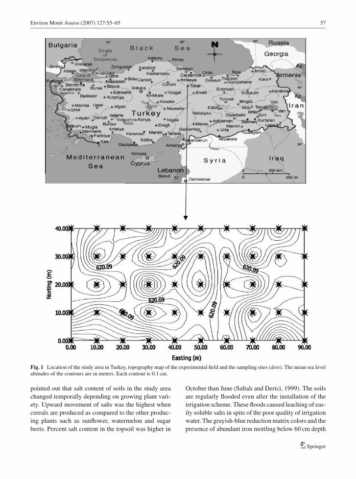
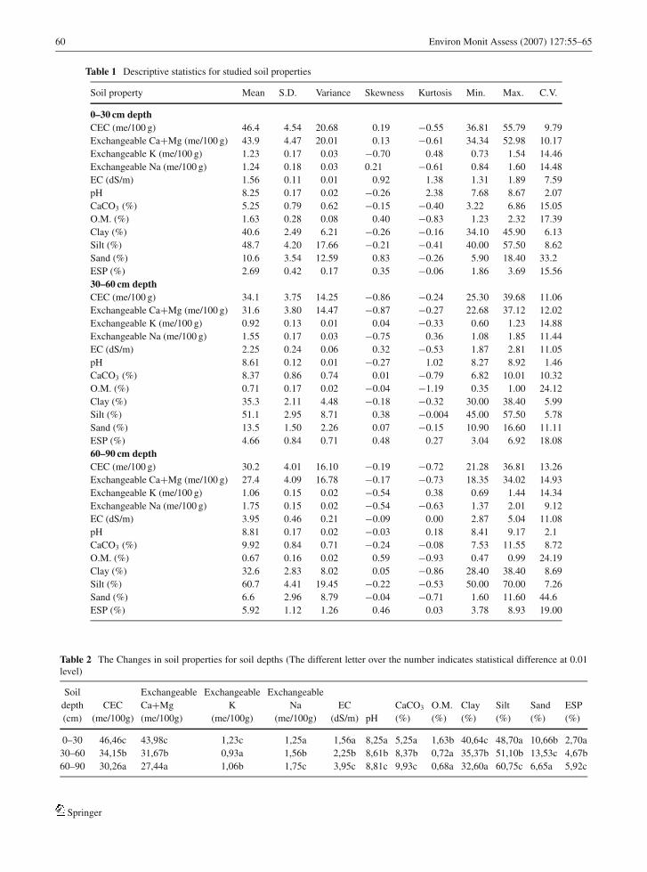
Fig. 2 Spatial pattern of soil EC for each soil depth

Fig. 3 Spatial pattern of soil ESP for each soil depth

suggested that the groundwater level showed large an-

nual fluctuations.

2.2 Soil sampling and analysis

The study area (100 m × 50 m) was divided into10 m

× 10 m grids (10 lines in the north-south direction and

5 lines in the east-west direction). Total 50 grid points

were obtained and soil samples were collected at these

points from three depths (0–30, 30–60 and 60–90 cm)

in August 2003. At the sampling time, maize was sown

in the field.

The soil samples were air-dried and passed through

a 2-mm sieve. The particle-size distribution was de-

termined by Bouyoucos hydrometer method (Gee

and Bouder, 1986). Soil organic matter content was

Springer


measured using the modified Walkley-Black wet oxi-

dation procedure (Nelson and Sommers, 1982). Soil pH

and electrical conductivity (ECe) were measured with

glass electrode in a saturation extract. Cation exchange

capacity (CEC), exchangeable sodium, potassium, cal-

cium and magnesium were measured after extraction

with ammonium acetate (Rhoades, 1986).

2.3 Statistical and geostatistical methods

Statistical analysis of data includes examination of the

mean, maximum and minimum values, standard de-

viation (SD), variance, skewness, kurtosis and coeffi-

cient of variation (CV). The Shapiro-Wilks normality

test was conducted to test the hypothesis that assum-

ing each soil properties has a normal distribution, and

these variables without normal distribution subjected to

log-transformation. Variance and sample means of soil

properties were compared using LSD test. The linear

correlation between pairs of variables was also exam-

ined, as it often reveals relationships, and helps in the

choice of variables for the kriging estimation (Webster

and Oliver, 1990). Statistical analyses of variables were

performed with SPSS 10 (2000).

Spatial variation of salinity and alkalinity rates was

described using semivariograms, assuming stationar-

ity among similar lag increments (Isaaks and Srivas-

tava, 1989; Goovaerts, 1997). Geostatistical software

(GS+5.1, Gamma Design Software; 2001) was used to

analyze the spatial structure of the data and to define

the semivariograms. The hypothesis and parities used

to calculate semivariograms were described by Burgess

and Webster (1980). Semivariogram values at each lag

separation, γ (h), were computed as:

γ (h) = 1

2N (h)

{N (h)∑i=1

[Z (xi ) − Z (xi + h)]2

}(1)

Where N(h) is the number of pairs separated by a lag

distance of h, and Z is the regionalized variables, Z(xi )

and Z (xi + h) are measured sample values xi and xi +h locations.

Semivariograms were computed using the log-

transformation data in the measured data. The trend

of the computed semivariogram values was modeled

using one of the exponential, spherical or linear semi-

variogram models. The model selected to represent the

semivariogram values (nugget, sill and range of spatial

dependence) was chosen based on coefficient of varia-

tion (r2) and residual sum of squares (RSS). Semivari-

ograms were constructed for EC and ESP values.

3 Results and discussion

It was evident that the soil properties were quite

different in the three soil depths (Table 1 and 2). Mean

EC and ESP values were found higher at 60–90 cm

soil depth (3.95 dSm−1 and 5.92%) as compared to the

other soil depths (1.56 dSm−1 and 2.69% for 0–30 cm

soil depth, and 2.25 dSm−1 and 4.66% for 30–60 cm

soil depth), and the difference was significant among

the soil depths (p < 0.01). Application of poor

quality water or insufficient amounts of water to leach

salts would result in increase in EC or ESP. Salt

accumulation at the topsoil would probably occur

only in the years of low precipitation or insufficient

leaching. This result showed that soil salinity and

alkalinity risk existed in the 60–90 cm depth due to

high groundwater level and irrigation with low quality

of water, having 980 μS cm−1 EC and 1.28 SAR

values (Saltalı et al., 1999). Highly significant positive

correlation between soil salinity and water content in

a field of compacted clayey Entisols with poor water

infiltration was found (Miyamoto and Chacon, 2005).

Kachanoski et al. (1988) stated that EC was affected

by volumetric water content, and EC increased with

increasing water content when clay content was low.

The rate of exchangeable Na+ also increased sig-

nificantly (p < 0.01) while exchangeable Ca++ and

Mg++ decreased significantly (p < 0.01) with increas-

ing soil depth (Table 2). The pH of the topsoil was

8.25 compared with 8.61 at 30–60 cm depth and 8.81

at 60–90 cm depth, and the differences were statisti-

cally significant (p < 0.01).

Textural analysis showed that the topsoil (0–30 cm)

had the highest mean clay content (48.7%), but the sub-

soil (60–90 cm) had the lowest clay content (32.6%)

(Table 1). The clay content significantly decreased

while silt content significantly increased with depth

(30–60 cm and 60–90 cm depths) (Table 2). The most

important reason for lower clay content at the subsoil

in spite of the dense irrigation in the study area was

the intensive tillage practices which caused to the for-

mation of a plow pan at the depth of 20 cm in the clay

topsoil (Kılıc et al., 2004). The formation of a plow

pan could halt to clay movement through soil pores.

The claypan formed in the cultivated lands decrease

Springer


Table 1 Descriptive statistics for studied soil properties

Soil property Mean S.D. Variance Skewness Kurtosis Min. Max. C.V.

0–30 cm depthCEC (me/100 g) 46.4 4.54 20.68 0.19 −0.55 36.81 55.79 9.79

Exchangeable Ca+Mg (me/100 g) 43.9 4.47 20.01 0.13 −0.61 34.34 52.98 10.17

Exchangeable K (me/100 g) 1.23 0.17 0.03 −0.70 0.48 0.73 1.54 14.46

Exchangeable Na (me/100 g) 1.24 0.18 0.03 0.21 −0.61 0.84 1.60 14.48

EC (dS/m) 1.56 0.11 0.01 0.92 1.38 1.31 1.89 7.59

pH 8.25 0.17 0.02 −0.26 2.38 7.68 8.67 2.07

CaCO3 (%) 5.25 0.79 0.62 −0.15 −0.40 3.22 6.86 15.05

O.M. (%) 1.63 0.28 0.08 0.40 −0.83 1.23 2.32 17.39

Clay (%) 40.6 2.49 6.21 −0.26 −0.16 34.10 45.90 6.13

Silt (%) 48.7 4.20 17.66 −0.21 −0.41 40.00 57.50 8.62

Sand (%) 10.6 3.54 12.59 0.83 −0.26 5.90 18.40 33.2

ESP (%) 2.69 0.42 0.17 0.35 −0.06 1.86 3.69 15.56

30–60 cm depthCEC (me/100 g) 34.1 3.75 14.25 −0.86 −0.24 25.30 39.68 11.06

Exchangeable Ca+Mg (me/100 g) 31.6 3.80 14.47 −0.87 −0.27 22.68 37.12 12.02

Exchangeable K (me/100 g) 0.92 0.13 0.01 0.04 −0.33 0.60 1.23 14.88

Exchangeable Na (me/100 g) 1.55 0.17 0.03 −0.75 0.36 1.08 1.85 11.44

EC (dS/m) 2.25 0.24 0.06 0.32 −0.53 1.87 2.81 11.05

pH 8.61 0.12 0.01 −0.27 1.02 8.27 8.92 1.46

CaCO3 (%) 8.37 0.86 0.74 0.01 −0.79 6.82 10.01 10.32

O.M. (%) 0.71 0.17 0.02 −0.04 −1.19 0.35 1.00 24.12

Clay (%) 35.3 2.11 4.48 −0.18 −0.32 30.00 38.40 5.99

Silt (%) 51.1 2.95 8.71 0.38 −0.004 45.00 57.50 5.78

Sand (%) 13.5 1.50 2.26 0.07 −0.15 10.90 16.60 11.11

ESP (%) 4.66 0.84 0.71 0.48 0.27 3.04 6.92 18.08

60–90 cm depthCEC (me/100 g) 30.2 4.01 16.10 −0.19 −0.72 21.28 36.81 13.26

Exchangeable Ca+Mg (me/100 g) 27.4 4.09 16.78 −0.17 −0.73 18.35 34.02 14.93

Exchangeable K (me/100 g) 1.06 0.15 0.02 −0.54 0.38 0.69 1.44 14.34

Exchangeable Na (me/100 g) 1.75 0.15 0.02 −0.54 −0.63 1.37 2.01 9.12

EC (dS/m) 3.95 0.46 0.21 −0.09 0.00 2.87 5.04 11.08

pH 8.81 0.17 0.02 −0.03 0.18 8.41 9.17 2.1

CaCO3 (%) 9.92 0.84 0.71 −0.24 −0.08 7.53 11.55 8.72

O.M. (%) 0.67 0.16 0.02 0.59 −0.93 0.47 0.99 24.19

Clay (%) 32.6 2.83 8.02 0.05 −0.86 28.40 38.40 8.69

Silt (%) 60.7 4.41 19.45 −0.22 −0.53 50.00 70.00 7.26

Sand (%) 6.6 2.96 8.79 −0.04 −0.71 1.60 11.60 44.6

ESP (%) 5.92 1.12 1.26 0.46 0.03 3.78 8.93 19.00

Table 2 The Changes in soil properties for soil depths (The different letter over the number indicates statistical difference at 0.01level)

Soil Exchangeable Exchangeable Exchangeable

depth CEC Ca+Mg K Na EC CaCO3 O.M. Clay Silt Sand ESP

(cm) (me/100g) (me/100g) (me/100g) (me/100g) (dS/m) pH (%) (%) (%) (%) (%) (%)

0–30 46,46c 43,98c 1,23c 1,25a 1,56a 8,25a 5,25a 1,63b 40,64c 48,70a 10,66b 2,70a

30–60 34,15b 31,67b 0,93a 1,56b 2,25b 8,61b 8,37b 0,72a 35,37b 51,10b 13,53c 4,67b

60–90 30,26a 27,44a 1,06b 1,75c 3,95c 8,81c 9,93c 0,68a 32,60a 60,75c 6,65a 5,92c

Springer


water movement through soil profile due to little pore

size (Rhoades et al., 1992).

CEC differed significantly in all the soil depths

(p < 0.01), with a mean of 46.46 me100 g−1 CEC

for 0–30 cm, 34.15 me100 g−1 CEC for 30–60 cm,

and 30.26 me100 g−1 CEC for 60–90 cm depth. CEC

decreased with soil depth due to the decreases of

clay content. OM content of 0–30 cm differed signifi-

cantly from those of 30–60 and 60–90 cm (p < 0.01;

Tables 1 and 2).

Soil pH CV had a lower variation as compared to

the other soil properties (Table 1). The OM had the

maximum variability with a mean of 1.63% at 0–30 cm

and 0.71% at 30–60 cm depths (Table 1). In general,

the CV for the soil properties increased with soil depth

except for Na+ and silt contents. The soil properties

had the highest CV values at the 60–90 cm depth. The

coefficients of skewness and kurtosis indicated that

most of the soil properties had normal distributions ex-

cept OM and sand content for 0–30 cm depth; CEC,

exchangeable Ca++, Mg++ and Na+ for 30–60 cm;

and exchangeable Na+ and OM for 60–90 cm

(Table 1). The values of salinity and alkalinity (EC and

ESP) had coefficients of skewness that was very close

to zero except for EC at 0–30 cm (0.92).

The linear correlation matrix between pairs of vari-

ables was shown in Table 3 for all depths. EC and ESP

values were much higher and significant at 60–90 cm

depth than the other depths. At the 30–60 cm depth,

the correlation coefficients between EC and CaCO3,

CEC and exchangeable Ca++ and Mg++ were signif-

icant (p < 0.05), while there was not significant rela-

tionship between EC and ESP and other soil properties

at the 0–30 cm depth. The relationships between ESP,

EC and K values were reciprocally associated (p < 0.01

and p < 0.05, respectively) at 60–90 cm depth; on the

other hand, a significant positive relationship occurred

between ESP and CaCO3 (p < 0.05). Significant re-

lationships were found between EC and Exchangeable

Ca++, Mg++ and K+ and CaCO3 contents at 60–90 cm

depth (p < 0.05), but these relationships were neg-

atively significant except for exchangeable K+. Van

Asten et al. (2003) pointed out that EC and alkalinity

increased when CEC, Mg++ and Ca++ decreased in

the soil solution.

Soil properties showed differences in spatial depen-

dence as showed by semivariance (Table 4). Exponen-

tial, spherical and linear isotropic models were used

to define the most of soil variables except for some

of the soil properties at 30–60 cm depth. Semivari-

ance increased with distance to a constant value at a

given separation distance for exponential, gaussian and

spherical models. The linear model has a slope that is

close to zero, and total variance was equal to the nugget

variance, and the variables are not spatially correlated

(Isaaks and Srivastava, 1989). In this study, soil vari-

ables for linear models were spatially correlated in the

distances greater than the minimum grid spacing at all

lag distances.

Nugget effect was generally higher at 60–90 cm

depth as compared to the other depths. This indicated

that soil properties had spatial variability at small dis-

tances at 60–90 cm depth (Table 4). Nugget effect is

related to the spatial variability at smaller distances

than the lowest separation distance between measure-

ments (Webster, 1985; Warrick et al., 1986). Nugget ef-

fect for EC increased considerably from soil surface to

60 cm depth, but it decreased below 60 cm depth. Utset

et al. (1998) reported a similar result in a hydromorpfic

Vertisol within a 500 by 600 m field. They showed that

nugget effects for EC values were higher at the soil sur-

face as compared to the subsurface. EC was variable

within short distances at 30–60 cm depth. The nugget

effect of ESP increased with soil depth, indicating that

ESP had high spatial variability at smaller distances

than the lowest separation distance at 60–90 cm depth.

Nevertheless, according to the difference between sill

and nuggets, a weaker spatial structure was found at

0–30 and 30–60 cm depths, with almost a pure nugget

effect and a stronger spatial structure at 60–90 cm depth

with a higher nugget effect (Table 4). Therefore, spatial

structure of ESP increased with depth.

The ranges of EC values ranged from 48 m to 169 m.

The EC values were spatially dependent over a dis-

tance of 48 m (Table 4). The geostatistical range of val-

ues calculated for EC in the present study was smaller

than that calculated by Utset et al. (1998). The EC

values at the topsoil might be dependent higher dis-

tances than maximum lag distance due to intensive irri-

gation and plow pan occurred about 20 cm depth (Kılıc

et al., 2004). On the contrary, the ranges of ESP values

increased with depth, between 62 m and 210 m. The

ranges of isotropic semivariograms for ESP (210 m)

were found higher for greater distances between mea-

surements at 60–90 cm depth, indicating that ESP val-

ues had a homogeneous variability in spite of higher

spatial variability at smaller distances than the lowest

separation distance and a spatially dependent over a

Springer


Tabl

e3

Co

rrel

atio

nb

etw

een

soil

pro

per

ties

and

EC

and

ES

Pfo

rea

chso

ild

epth

So

ilP

rop

erty

CE

CE

xch

ang

eab

leC

a+M

gE

xch

ang

eab

leK

Ex

chan

gea

ble

Na

EC

pH

CaC

O3

O.M

.C

lay

Sil

tS

and

0–30

cmde

pth

CE

C1

,00

0

Ca+

+ +M

g++

0,99

9∗∗

1,0

00

K+

0,1

67

0,1

30

1,0

00

Na+

0,28

4∗0

,24

80

,00

41

,00

0

EC

0,2

47

0,2

51

−0,0

12

0,0

01

1,0

00

pH

−0,5

22∗∗

−0,5

13∗∗

0,0

15

−0,4

74∗∗

−0,2

44

1,0

00

CaC

O3

0,0

82

0,0

79

0,0

38

0,0

81

0,1

87

−0,1

94

1,0

00

O.M

.0

,01

40

,01

50

,09

8−0

,11

4−0

,14

80

,13

5−0

,12

01

,00

0

Cla

y0

,00

4−0

,00

40

,14

40

,05

5−0

,04

40

,21

80

,05

0−0

,10

31

,00

0

Sil

t0

,02

30

,02

3−0

,07

70

,08

50

,12

8−0

,13

1−0

,07

00

,05

0−0

,539

∗∗1

,00

0

San

d−0

,03

0−0

,02

5−0

,01

0−0

,14

0−0

,12

10

,00

20

,04

80

,01

3−0

,06

5−0

,80

6∗∗

1,0

00

ES

P−0

,06

3−0

,07

80

,20

30

,14

60

,03

5−0

,00

5−0

,09

90

,21

8−0

,04

4−0

,02

00

,05

5

30–6

0cm

dept

hC

EC

1,0

00

Ca+

+ +M

g++

0,99

8∗∗

1,0

00

K+

0,0

62

0,0

13

1,0

00

Na+

−0,1

66

−0,2

21

0,2

69

1,0

00

EC

−0,1

20

−0,1

24

−0,0

35

0,1

27

1,0

00

pH

−0,2

36

−0,2

28

−0,1

19

−0,0

33

0,1

32

1,0

00

CaC

O3

−0,2

09

−0,2

02

−0,0

31

−0,1

04

0,35

1∗0

,21

71

,00

0

O.M

.−0

,03

0−0

,03

20

,10

0−0

,03

90

,05

80

,21

6−0

,04

31

,00

0

Cla

y−0

,22

0−0

,20

8−0

,12

3−0

,13

7−0

,00

70

,19

00

,01

80

,15

61

,00

0

Sil

t0,

291∗

0,28

4∗0

,03

10

,08

0−0

,01

6−0

,17

9−0

,08

4−0

,22

6−0

,875

∗∗1

,00

0

San

d−0

,26

1−0

,26

50

,11

30

,03

70

,04

00

,08

30

,13

90

,22

40,

308∗

−0,7

31∗∗

1,0

00

ES

P−0

,302

∗−0

,306

∗0

,03

50

,10

8−0

,05

80

,20

7−0

,07

1−0

,11

1−0

,05

30

,12

7−0

,17

4

60–9

0cm

dept

hC

EC

1,0

00

Ca+

+ +M

g++

0,99

8∗∗

1,0

00

K+

−0,1

65

−0,2

05

1,0

00

Na+

−0,3

33∗

−0,3

71∗∗

0,1

66

1,0

00

EC

−0,3

54∗

−0,3

61∗

0,33

7∗0

,02

21

,00

0

pH

−0,0

28

−0,0

50

0,2

61

0,34

6∗−0

,06

61

,00

0

CaC

O3

−0,0

62

−0,0

59

−0,2

06

0,1

69

−0,3

15∗

−0,2

10

1,0

00

O.M

.−0

,02

7−0

,02

4−0

,08

40

,01

10

,02

4−0

,10

60

,08

71

,00

0

Cla

y−0

,10

3−0

,10

60

,09

50

,04

0−0

,16

7−0

,05

40

,09

9−0

,24

41

,00

0

Sil

t0

,06

90

,07

5−0

,15

1−0

,04

30

,11

60

,04

2−0

,09

70

,25

7−0

,748

∗∗1

,00

0

San

d−0

,00

4−0

,01

00

,13

40

,02

5−0

,01

3−0

,01

00

,05

1−0

,14

80

,15

7−0

,773

∗∗1

,00

0

ES

P−0

,17

5−0

,16

3−0

,360

∗0

,13

4−0

,400

∗∗−0

,19

20,

322∗

0,1

11

0,1

26

−0,0

65

−0,0

24

Springer


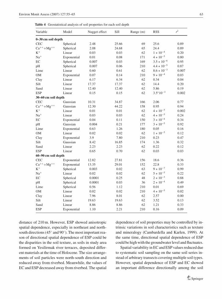
Table 4 Geostatistical analysis of soil properties for each soil depth

Variable Model Nugget effect Sill Range (m) RSS r2

0–30 cm soil depthCEC Spherical 2.48 25.66 69 25.6 0.89

Ca+++Mg++ Spherical 2.08 24.68 65 24.4 0.89

K+ Linear 0.03 0.03 62 1 ∗ 10−4 0.20

Na+ Exponential 0.01 0.08 171 4 ∗ 10−5 0.80

EC Spherical 0.007 0.03 169 3.5 ∗ 10−6 0.95

pH Spherical 0.007 0.06 210 4.4 ∗ 10−5 0.87

Lime Linear 0.60 0.61 62 8.6 ∗ 10−3 0.007

OM Exponential 0.07 0.14 210 9 ∗ 10−4 0.03

Clay Linear 6.17 6.34 62 0.34 0.04

Silt Linear 17.37 17.37 62 14.4 0.20

Sand Linear 12.40 12.40 62 5.86 0.19

ESP Linear 0.15 0.15 62 3.5∗10−3 0.002

30–60 cm soil depthCEC Gaussian 10.31 34.87 166 2.06 0.77

Ca+++Mg++ Gaussian 12.30 44.22 158 0.95 0.94

K+ Linear 0.01 0.01 62 4 ∗ 10−5 0.002

Na+ Linear 0.03 0.03 62 4 ∗ 10−5 0.24

EC Exponential 0.04 0.11 150 3 ∗ 10−4 0.34

pH Gaussian 0.004 0.21 177 3 ∗ 10−5 0.92

Lime Exponential 0.63 1.26 180 0.05 0.16

OM Linear 0.02 0.02 62 1 ∗ 10−5 0.12

Clay Exponential 3.9 7.80 210 0.23 0.47

Silt Gaussian 8.42 16.85 174 1.36 0.32

Sand Linear 2.23 2.23 62 0.22 0.12

ESP Linear 0.65 0.70 62 0.03 0.03

60–90 cm soil depthCEC Exponential 12.82 27.81 156 18.6 0.36

Ca+++Mg++ Exponential 13.35 29.01 152 22.8 0.33

K+ Spherical 0.003 0.02 63 9 ∗ 10−7 0.99

Na+ Linear 0.02 0.02 62 5 ∗ 10−5 0.22

EC Spherical 0.0001 0.25 48 2 ∗ 10−3 0.88

pH Spherical 0.0001 0.03 36 2 ∗ 10−4 0.49

Lime Spherical 0.56 1.12 210 0.01 0.69

OM Linear 0.02 0.02 210 4 ∗ 10−5 0.02

Clay Linear 7.96 8.01 62 2.57 0.00

Silt Linear 19.63 19.63 62 3.52 0.13

Sand Linear 8.86 8.86 62 1.21 0.33

ESP Exponential 1.10 2.21 210 0.16 0.09

distance of 210 m. However, ESP showed anisotropic

spatial dependence, especially in northeast and north-

south directions (45◦ and 90◦). The most important rea-

son of directional spatial dependence of ESP could be

the disparities in the soil texture, as soils in study area

formed on Yesilirmak river terraces, deposited differ-

ent materials at the time of Holocene. The size arrange-

ments of soil particles were north-south direction and

reduced away from riverbed. Meanwhile, the values of

EC and ESP decreased away from riverbed. The spatial

dependence of soil properties may be controlled by in-

trinsic variations in soil characteristics such as texture

and mineralogy (Cambardella and Karlen, 1999). At

the same time, directional spatial dependence of ESP

could be high with the groundwater level and fluctuates.

Spatial variability in EC and ESP values reduced due

to systematic soil sampling on the same soil series in-

stead of arbitrary transects covering multiple soil types.

However, spatial dependence of ESP and EC showed

an important difference directionally among the soil

Springer


depths, especially in 60–90 cm. The variability in soil

properties at the soil series level is often caused by small

changes in topography that affect movement and stor-

age of water across and within the soil profile (Mulla

and McBratney, 2000). Because of the same landscape

positions of the study area, the main reason for dif-

ferences in spatial dependence could be the textural

difference and plow pan at 20 cm, which affects water

intake and percolation.

4 Conclusions

Spatial variability of salinity and alkalinity of a field

having salination risk was assessed. The observations

on spatial variability and correlation coefficients calcu-

lated among the variables indicated that the changes in

salinity and alkalinity varied depending on soil depths.

The results showed that topsoil did not have a risk of

salinity and alkalinity, but subsoil (60–90 cm depth)

had salinity and alkalinity problem. This study sug-

gested that spatial variability of salinity and alkalinity

had an important role for site-specific management.

Differences in EC and ESP were significant by soil

depth, and were higher for 60–90 cm. The semivari-

ograms fitted to the data showed that EC and ESP values

were spatially dependent over the geostatistical range

of distances from 48 to 210 m, and ESP had directional

dependence at 30–60 cm and 60–90 cm depths, with an

angle of 90. Consequently, soil sampling distance of

salinity and alkalinity for practical sampling purposes

could be taken as 48 m. Salinity data maps developed

using the kriging estimations showed that EC values at

60–90 cm depth slightly increased (EC ∼= 4 dS m−1).

The main reason of salinity in subsoil was upward

movement of salts during evaporation from high

groundwater due to recharged water from high lands

and irrigation with low-quality water diverted from

drainage channels. The most important reasons of low

salt concentration in topsoil could be the soil manage-

ment practices such as intensive irrigation, crop variety

(maize production) and soil tillage (a plow pan forma-

tion) applied in the study area.

The topsoil in study area occurred free of the risks

of salinity and alkalinity under current irrigation. How-

ever, if low-quality irrigation water is used it may cause

some problems of salinity and alkalinity. Meanwhile,

salts may rise until the plant root zone if dryland agri-

culture is practiced in these soils. The land should be

used for agriculture production with the rotation of ir-

rigated plants and non-irrigated plants. However, the

level of groundwater table should be under monitored

continuously to avoid high levels of groundwater.

Acknowledgements The authors thank the Research Funds Ac-countancy of Gaziosmanpasa University providing the financialsupport for this study (Project No: 2003/34). We also acknowl-edge the authorities at Kazova Farm for their permitting us un-restricted access to collect the soil samples.

References

Ayers, R.S. & Westcot, D.W. (1989). Water Quality for Agricul-ture. FAO Irrigation and Drainage. Paper no: 29, pp. 1–174,Rome.

Bohn, H.L., McNeal, B.L. & O’Connor, G.A. (1985). Soil chem-istry (329 pp). New York: Wiley.

Boivin, P., Favre, F., Hammecker, C., Maeght, J.L., Delariviere,J., Poussin, J.C., & Wopereis, M. C. S. (2002). Processesdriving soil solution chemistry in a flooded rice-croppedvertisol: analysis of long-time monitoring data. Geoderma,110, 87–107.

Burgess, T.M. & Webster, R. (1980). Optimal interpolationand isarithmic mapping of soil properties. I. The semi-variogram and punctual kriging. Journal of Soil Science,31, 315–331.

Cambardella, C.A. & Karlen, D.L. (1999). Spatial analy-sis of soil fertility parameters. Precision Agriculture 1,5–14.

Ceuppens, J., Wopereis, M.C.S. & Miezan, K.M. (1997). Soilsalinization processes in rice irrigation schemes in the Sene-gal River delta. Soil Science Society of American Journal,61(4), 1122–1130.

Dolittle, J.A., Sudduth, K.A., Kitchen, N.R., & Indorante, S.J.(1994). Estimating depth to claypans using electromagneticinduction methods. Journal of Soil Water Conservaton, 49,572–575.

Gee, G.W. & Bouder, J.W. (1986). Particle size analysis. In:Klute, A. (Ed.), Methods of soil analysis. Part 1. Physicaland mineralogical methods (2nd ed., pp. 825–844) Madi-son, WI: Agronomy monography no: 9, ASA and SSSA.

Goovaerts, R. (1997). Geostatistics for natural resources evalu-ation (483 pp). New York: Oxford University Press.

GS+5.1. (2001). Gamma design software. MI, USA.: Plainwell.Isaaks, E.H. & Srivastava, R.M. (1989). An introduction to ap-

plied geostatistics (561 pp). New York: Oxford Uni. Press,Inc.

Kachanoski, R.G., Gregorich, E.G., & Van Wesenbeck, I. J.(1988). Estimating spatial variations of soil water contentusing non-containing electromagnetic inductive methods.Canadian Soil Science, 68, 715–722.

Kelleners, T.J. & Chaudhry, M.R. (1998). Drainage water salinityof tube wells and pipe drains: A case study from Pakistan.Agriculture Water Management 37, 41–53.

Kılıc, K., Ozgoz, E., & Akbas, F. (2004). Assessment of spatialvariability in penetration resistance as related to some soilphysical properties of two Fluvents in Turkey. Soil & TillageResearch, 76, 1–11.

Springer


Miyamoto, S., Chacon, A., Hossain, M., & Martinez, I. (2005).Soil salinity of urban turf areas irrigated with saline water:I. Spatial variability. Landscape and Urban Planning, 71,233–241.

Miyamoto, S. & Chacon, A. (2005). Soil salinity of urban turfareas irrigated with saline water: II. Soil factors. Landscapeand Urban Planning. (in Press)

Miyamoto, S. & Cruz, I. (1987). Spatial variability of soil salin-ity in furrow-irrigated torrifluvents. Soil Science Society ofAmerican Journal, 51, 1019–1025.

Mulla, D.J. & McBratney, A.B. (2000). Soil spatial variability(pp. A-321–A-352). In: M.E. Sumner (Ed.), Handbook ofsoil science. Boca Raton, FL, USA.: CRC Press.

Nelson, D.W. & Sommers, l.E. (1982). Total carbon, organiccarbon and organic matter. In: Page, A. L., et al., (Eds.).Part 2. Methods of soil analysis (2nd ed., pp. 539–577).Madison, WI: ASA Publ. Vol. 9 ASA and SSSA.

Nielsen, D.R., Tillotson, P.M., & Vieira, S.R. (1983). Analyz-ing field-measured soil-water properties. Agricultural Wa-ter Management 6, 93–109.

Postel, R. (1989). Water of agriculture: Facing the limits, world-watch paper. Washington D.C.: 93 Worldwatch Ins.

Rhoades, J.D. (1986). Cation exchange capacity. In C. A. Franciset al. (ed.) Methods of soil analysis (pp. 149–158). Madi-son, WI.: Part 2. 2nd ed. Agron. Monogr. 9. ASA andSSSA,

Rhoades, J.D., Kandioh, A.P., & Mashali, A.M. (1992). The Useof Saline Waters for Crop Production. FAO irrigation andDrainage Paper 48, Food and Agricultural Organization ofThe United Nations, Rome Italy.

Saltalı, K. & Derici, M.R. (1999). Salinity status and seasonalmovement of salts in Kazova soils of Tokat in Turkey.Gaziosmanpasa University of Agricultur Faculty Journal,16, 203–215.

Saltalı , K., Kılıc, K., Durak, A., & Kılıc, M. (1999). The deter-mination of water quality of some drainage channels at KazLake of Tokat province in Turkey. Gaziosmanpasa Univer-sity of Agricultur Faculty Journal, 16, 193–203.

Seatz, L.F. & Peterson, H.B. (1965). Acid, alkaline, saline, andsodic soils. In: Bear, F. E. (Ed.), Chemistry of the soil (pp.292–319). New York: Reinhold Pub.

Sharma, D.P. & Rao, K.V.G.K. (1998). Strategy for long term useof saline drainage water for irrigation in semi-arid regions.Soil&Tillage Research, 48, 287–295.

SPSS (2000). SPSS for Windows. Student Version. USA.: Release10.0.9. SPSS Inc.

State Water Works. (1999). The detailed land classification anddrainage reports in Kazova Province in Turkey. UpperYesilirmak Project, 2, 17–790. Ankara, Turkey.

Sudduth, K.A., Kitchen, N.R., & Drummond, S.T. (1999). Soilconductivity sensing on claypan soils: Comparison of elec-tromagnetic induction and direct methods. In: P. C. Robert,R. H. Rust, & W. E. Larson (Eds.), Proceedings of the 4thInt. Conference On Precision Agriculture (pp. 979–990).St. Paul, MN, July 19–22 1998. Madison, WI: ASA-CSSA-SSSA.

Tasova, H. (1997). Classification, survey and mapping of soilsin the kazova agriculture working. Gaziosmanpasa Uni.Grad. Sch. Nat. App. Sci., Dept. Soil Sci., PhD Thesis,187 pp.

Trangmar, B.B., Yost,R.S., & Uehara, G. (1985). Application ofgeostatistics to spatial stu-dies of soil properties. Advance-ment in Agronomy, 38, 45–94.

Utset, A., Ruiz, M.E., Herrera, J. & de Leon, D.P. (1998). Ageostatistical method for soil salinity sample site spacing.Geoderma, 86, 143–151.

van Asten, P.J.A., Barbiero, L., Wopereis, M.C.S., Maeght, J.L.& van der Zee, S.E.A.T.M. (2003). Actual and potentialsalt-related soil degradation in an irrigated rice scheme inthe Sahelian zone of Mauritania. Agricultural Water Man-agement, 60, 13–32.

Warrick, A.W., Myers, D.E. & Nielsen, D.R. (1986). Geosta-tistical methods applied to soil science. SSSA, AgronomyMonograph no. 9.

Webster, R. (1985). Quantitative Spatial Analysis of Soil in TheField. Advancement in Soil Science, 3, 1–70.

Webster, R., (2001). Statistics to support soil research and theirpresentation. European Journal of Soil Science, 52, 331–340.

Webster, R. & Oliver, M.A. (1990). Statistical methods insoil and land resource survey (316 pp). Oxford Univ.Press.

Springer

Spatial variability of salinity and alkalinity of a field having salination risk in semi-arid...

Documents

Transcript of Spatial variability of salinity and alkalinity of a field having salination risk in semi-arid...