Modelling Objects Having Quadric SurfacesIncorporating Geometric ConstraintsNaoufel Werghi, Robert Fisher, Craig Robertson, and Anthony AshbrookDepartment of Arti�cial Intelligence,University of Edinburgh5 Forrest Hill, EH1 2QL Edinburgh, UKemail:fnaoufelw, rbf, craigr, anthonya g@dai.ed.ac.ukAbstract. This paper deals with the constrained shape reconstructionof objects having quadric patches. The incorporation of geometric con-straints in object reconstruction was used �rst by Porrill [10]. His ap-proach combined the Kalman �lter equations with linearized constraintequations. This technique was improved by De Geeter et al [5] to reducethe e�ects of linearization error. The nature and the speci�city of thistechnique make it limited in scope and application.In their approach for 3-D object pose estimation, Bolle et al [2] con-strained some quadrics to have a certain shape (circular cylinder andsphere) by using a speci�c representation for these particular surfaces.Our work uses a new approach to global shape improvement based onfeature coincidence, position and shape constraints. The key idea is toincorporate user speci�c geometric constraints into the reconstructionprocess. The constraints are designed to �x some feature relationships(such as parallel surface separations, or cylindrical surface axis relation-ships) and then use least squares �tting to �x the remaining parameters.An optimization procedure is used to solve the reconstruction problem.In this paper, constraints for planar and general quadric surface classesare given. Results with quadric surfaces show much improvement inshape reconstruction for both constrained and unconstrained relation-ships. The proposed approach avoids the drawbacks of linearization andallows a larger category of geometric constraints. To our knowledge thiswork is the �rst to give such a large framework for the integration ofgeometric relationships in object modelling.The technique is expected to have a great impact in reverse engineeringapplications and manufactured object modelling where the majority ofparts are designed with intended feature relationships.1 IntroductionThere has been a recent urry of e�ort on reconstructing 3D geometric modelsof objects from single [3, 6, 8] or multiple [2, 4, 12, 11, 13] range images, in partmotivated by improved range sensors, and in part by demand for geometricmodels in the CAD and Virtual Reality (VR) application areas. However, animportant aspect which has not been fully investigated is the exploitation of the

geometric constraints de�ning the spatial or topological relationships betweenobject features.The work presented in this paper investigates reverse engineering, namelythe combination of manufacturing knowledge of standard object shapes withthe surface position information provided by range sensors.The �rst motivation behind this work is that models needed by industry aregenerally designed with intended feature relationships so this aspect should beexploited rather than ignored. The consideration of these relationships is actuallynecessary because some attributes of the object would have no sense if the objectmodelling scheme did not take into account these constraints. For example, takethe case when we want to estimate the distance between two parallel planes: ifthe plane �tting results gave two planes which are not parallel, then the distancemeasured between them would have no signi�cance.The second motivation is to see whether exploiting the available known re-lationships would be useful for reducing the e�ects of registration errors andmis-calibration. Thus improving the accuracy of estimated part features' para-meters and consequently the quality of the modelling or the object localization.In previous work [14] we have shown that this is quite possible for planarobjects. A general incremental framework was presented whereby geometric re-lationships can be added and integrated in the model reconstruction process.The objects treated were polyhedral and the data was taken from single viewsonly. An overview of the technique is given in Section 3.In this paper we study the case of parts having quadric surfaces. Two typesof quadric are treated here, cylinders and cones. Both single view data andregistered multiple view data data have been used.Section.2 discuss the related work and the originality of our contribution.In Section.3, we summarize the technique. More details can be found in [14].Section.4 gives some mathematical preliminaries about quadrics in general andcylinders and cones in particular. Section.5 demonstrates the process on severaltest objects.2 Related workThe main problem encountered in the incorporation of geometric relationshipsin object modelling is how to integrate these constraints in the shape �ttingprocess. The problem is particularly crucial in the case of geometric constraintsmany of which are non-linear. In his pioneering work, Porrill [10] suggested alinearization of the nonlinear constraints and their combination with a Kalman�lter applied to wire frame model construction. Porrill's method takes advantageof the recursive linear estimation of the KF, but it guarantees satisfaction of theconstraints only to linearized �rst order. Additional iterations are needed at eachstep if more accuracy is required. This last condition has been taken into accountin the work of De Geeter et al [5] by de�ning a \Smoothly Constrained KalmanFilter". The key idea of their approach is to replace a nonlinear constraint by aset of linear constraints applied iteratively and updated by new measurements in

order to reduce the linearization error. However, the characteristics of Kalman�ltering makes these methods essentially adapted for iteratively acquired dataand many data samples. Moreover, there was no mechanism for determining howsuccessfully the constraints have been satis�ed. Besides, only lines and planeswere considered in both of the above works.The constraints considered by Bolle et al [2] in their approach to 3D objectposition covers only the shape of the surfaces. They chose a speci�c representa-tion for the treated features: plane, cylinder and sphere.Compared to Porrill's and De Geeter's work, our approach avoids the draw-backs of linearization, since the constraints are completely implemented. Besidesour approach covers a larger category of feature shapes. Regarding the work ofBolles, the type of constraints which can be held by our approach go beyondthe restricted set of surface shapes and cover also the geometric relationshipsbetween object features. To our knowledge the work appears the �rst to givesuch a large framework for the integration of geometric relationships in objectmodelling.3 The optimization techniqueGiven sets of 3D measurement points representing surfaces belonging to a cer-tain object, we want to estimate the di�erent surfaces' parameters, taking intoaccount the geometric constraints between these surfaces.A state vector p is associated to the object, which includes the set of paramet-ers related to the patches. The vector p has to best �t the data while satisfyingthe constraints. So, the problem that we are dealing with is a constrained optim-ization problem to which an optimal solution may be provided by minimizingthe following function: E(p) = F (p) + C(p) (1)where F (p) is the objective function de�ning the relationship between the set ofdata and the parameters and C(p) is the constraint function. F (p) could be thelikelihood of the range data given the parameters (with a negative sign since wewant to minimize) or the least squares error function. The likelihood functionhas the advantage of considering the statistical aspect of the measurements. Ina �rst step, we have chosen the least squares function as the integration of thedata noise characteristics into the LS function can be done afterwards with noparticular di�culty, leading to the same estimation of the likelihood function inthe case of the Gaussian distribution.GivenM geometric constraints, the constraint function is represented by thefollowing equation: C(p) = MXk=1 �kCk(p) (2)where Ck(p) is a vector function associated to constraint k. �k are weightingcoe�cients used to control the contribution of the constraints in the parameters'estimation. Each function is required to be convex since many robust techniques

for minimizing convex functions are available in the literature. The objectivefunction F (p) is convex by de�nition, so therefore E(p) is also convex.Figure 1 shows the optimization algorithm that we have used, which has beensimpli�ed so that a single � is associated to all the constraints. The algorithmstarts with an initial parameter vector p [0] that satis�es the least squares func-tion. Then we iteratively increase � and solve for a new optimal parameter p [n+1]using the previous p [n]. The new optimal vector is found by means of the stand-ard Levenberg-Marquardt algorithm. The algorithm stops when the constraintsare satis�ed to the desired degree or when the parameter vector remains stablefor a certain number of iterations. The initial value �0 has to be large enough toavoid the trivial null solution and to give the constraints a certain initial weight.A convenient value for the initial � is : �0 = F (p [0])=C(p [0])Σ

kk(p)C

p0

= 1..Kkk(p)C

initialise p

C(p) =

update p

While

λ C(p)find p mimizing F(p) +

p λ λ0

and λ

λ λ + ∆ λkτ>

Fig. 1. The optimization algorithm optim4 PreliminariesThis section give a brief overview about constraining quadrics and some partic-ular shapes. A full treatment of these surfaces can be found in [1]. While thematerial contained here is largely elementary geometry, we present it in orderto make clear how the set of constraints used for each surface type and relation-ship relate to the parameters of the generic quadric. The generic quadric form isused because it is easy to generate a least squares surface �t using the algebraicdistance.A general quadric surface is represented by the following quadratic equation:f(x; y; z) = ax2+by2+cz2+2hxy+2gxz+2fyz+2ux+2vy+2wz+d= 0 (3)

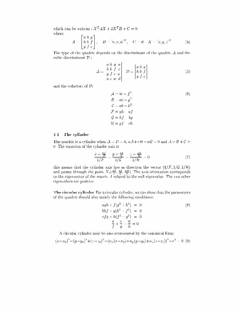
which can be written : XTAX + 2XTB + C = 0where A = 24 a h gh b fg f c 35 ; B = [u; v; w]T ; C = d; X = [x; y; z]T (4)The type of the quadric depends on the discriminant of the quadric � and thecubic discriminant D : � = �������� a h g uh b f vg f c wu v w d �������� D = ������ a h gh b fg f c ������ (5)and the cofactors of D: A = bc� f2 (6)B = ac� g2C = ab� h2F = gh� afG = hf � bgH = gf � ch4.1 The cylinderThe quadric is a cylinder when � = D = 0, uA+vH+wG = 0 and A+ B + C >0. The equation of the cylinder axis isx� ufF1=F = y � vgG1=G = z � whH1=H = 0 (7)this means that the cylinder axis has as direction the vector (1=F ; 1=G; 1=H)and passes through the point Xo(ufF ; vgG ; whH ). The axis orientation correspondsto the eigenvector of the matrix A related to the null eigenvalue. The two othereigenvalues are positive.The circular cylinder For a circular cylinder, we can show that the parametersof the quadric should also satisfy the following conditions:agh+ f(g2 + h2) = 0 (8)bhf + g(h2 + f2) = 0cfg + h(f2 + g2) = 0uf + vg + wh = 0A circular cylinder may be also represented by the canonical form:(x�x0)2+(y�y0)2+(z�z0)2�(nx(x�x0)+ny(y�y0)+nz(z�zo))2�r2 = 0 (9)

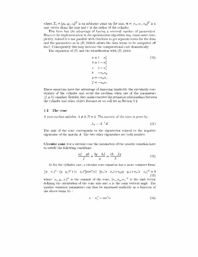
where Xo = [x0; y0; z0]T is an arbitrary point on the axis, n = [nx; nz; ny]T is aunit vector along the axis and r is the radius of the cylinder.This form has the advantage of having a minimal number of parameters.However its implementation in the optimization algorithm may cause some com-plexity, indeed it is not possible with this form to get separate terms for the dataand the parameters as in (3) (which allows the data terms to be computed o�line). Consequently this may increase the computational cost dramatically.The expansion of (9) and the identi�cation with (3) yieldsa = 1� n2x (10)b = 1� n2yc = 1� n2zh = �nxnyg = �nxnzf = �nynzThese equations have the advantage of imposing implicitly the circularity con-straints of the cylinder and avoid the problem when one of the parameters(f; g; h) vanishes. Besides, they make concrete the geometric relationships betweenthe cylinder and other object features as we will see in Section 5.2.4.2 The coneA cone surface satis�es � 6= 0;D = 0. The summit of the cone is given by:Xo = A�1B (11)The axis of the cone corresponds to the eigenvector related to the negativeeigenvalue of the matrix A. The two other eigenvalues are both positive.Circular cone For a circular cone the parameters of the quadric equation haveto satisfy the following conditionsaf � ghf = bg � hfg = ch� fgh (12)As for the cylinder case, a circular cone equation has a more compact form:[(x�xo)2+(y�yo)2+(z�zo)2]cos2(�)�[nx(x�xo)+ny(y�yo)+nz(z�zo)]2 = 0(13)where [xo; yo; zo]T is the summit of the cone, [nx; ny; nz]T is the unit vectorde�ning the orientation of the cone axis and � is the semi-vertical angle. Thequadric equation parameters can thus be expressed explicitly as a function ofthe above terms by : a = n2x � cos2� (14)

b = n2y � cos2�c = n2z � cos2�h = nxnyg = nxnzf = nynzFor the same reasons mentioned in the cylinder case the compact form of the coneequation is not adequate for the optimization algorithm. Nevertheless it is usefulto implicitly impose the conic constraints by means of equations (14) Instead of(12). Indeed in this form all the parameters (f; g; h) need to be di�erent of zero.4.3 PlanesA plane surface can be represented by this following equation:nxx+ nyy + nzz + d = 0; (15)where n = [nx; ny; nz]T is unit normal vector (knk = 1) to the plane and d isthe distance to the origin.5 Application on some test objectsThe objects treated in this section are real parts. The data was acquired with a3D triangulation range sensor. The range measurements were already segmentedinto groups associated with features by means of the rangeseg [7] program.5.1 NotationFor the rest of the paper we need the following notations:ir is a vector which all the elements are null except the rth element which isequal to 1.j(r;s) is a vector which all the elements are null except the rth and the sthelements which are equal to 1 and �1 respectively.M(r;s) is a diagonal matrix which all the elements are null except the rth andthe sth elements which are equal to 1 and �1 respectively.U(r;s) is a diagonal matrix de�ned byU(r;s) = �U(i; i) = 1 if r � i � sU(i; i) = 0 otherwiseL(r;s;p) a symmetric matrix de�ned byL(r;s;p) = �L(i; j) = L(j; i) = 1=2 if i = r + t; j = s+ t 0 � t � pL(i; j) = L(j; i) = 0 otherwise

5.2 The half cylinderThis object is composed of four surfaces. Three patches S1, S2 and S3 havebeen extracted from two views represented in Figure 2(a,c). These surfaces cor-respond respectively to the base plane S2, lateral plane S1 and the cylindricalsurface S3 (Figure 2.b). The parameter vector is p = [p1T ;p2T ;p3T ]T , wherep1 = [n1T ; d1]T , p2 = [n2T ; d2]T and p3 = [a; b; c; h; g; f; u; v; w; d]T . The leastsquares error function is given by:F (p) = pTHp; H = 24 H1 O(4;4) O(4;10)O(4;4) H2 O(4;10)OT(4;10) OT(4;10) H3 35 (16)where H1, H2, H3 are the data matrices related respectively to S1, S2, S3:Hi =Xj (X ij)(X ij)T for X ij belonging to surface SiThis object has the following constraints1. S1 and S2 are perpendicular,2. the cylinder axis is parallel to S1's normal,3. the cylinder axis lies on the surface S2,4. the cylinder is circular.Constraint 1 is expressed by the following conditionCang(p) = (n1Tn2)2 = (pTL(1;5;2)p)2 = 0; (17)Constraint 2 is satis�ed by equating the unit vector n in (9) to S1's normaln1. Constraint 3 is represented by two conditions: axis vector n is orthogonalto S2's normal n2, and one point of the axis satis�es S2's equation. The �rsthalf cylinder

S3

1

2

n

nn

S2

S1(a) (b) (c)Fig. 2. Two views of the half cylinder and the extracted surfaces

condition is guaranteed by constraint 2 since n2 is orthogonal to n1. For thesecond condition the point Xo in Section 4.1 has to satisfy the equation:Caxe(p) = (XTo n2 + d2)2 = (�[u; v; w]Tn2 + d2)2 = (i8Tp� pTL(5;15;2)p)2 = 0(18)using equations (6) and (10).The cylinder circularity constraint is implicitly de�ned by the equations (10).From these equations we extract the following constraints on the parametervector p: Ccirc1(p) = (i9Tp+ pTU(1;1)p� 1)2 = 0 (19)Ccirc2(p) = (i10Tp+ pTU(2;2)p� 1)2 = 0Ccirc3(p) = (i11Tp+ pTU(3;3)p� 1)2 = 0Ccirc4(p) = (i12Tp+ pTL(1;2;0)p)2 = 0Ccirc5(p) = (i13Tp+ pTL(1;3;0)p)2 = 0Ccirc6(p) = (i14Tp+ pTL(2;3;0)p)2 = 0We group then all the above constraints in a single oneCcirc(p) = 6Xk=1Ccirck (p) = 0 (20)Finally the normals n1 and n2 have to be unit. This is represented by:Cunit(p) = (pTU(1;3)p� 1)2 + (pTU(5;7)p� 1)2 = 0 (21)The constraint function is thenC(p) = Cunit(p) + Cang(p) + Caxe(p) + Ccirc(p) (22)and optimisation function isE(p) = pTHp+ �(Cunit(p) + Cang(p) + Caxe(p) + Ccirc(p)) (23)Experiments In the �rst test, the algorithm optim has been applied to dataextracted from a single view (Figure 2.c). The behaviour of the constraints(17),(18),(20) and (21) during the optinization have been mapped as a functionof � as well as the least squares residual (16) and the constraint function (22).The �gures show a linear logarithmic decrease of the constraints with respect to�. It is also noticed that at the end of the optimization all the constraints arehighly satis�ed. The least squares error converges to a stable value and the con-straint function vanishes at the end of the optimization. The �gures also showthat it is possible to continue the optimization further until a higher toleranceis reached, however this is limited by the computing capacity of the machine.We have noticed that beyond a certain value of � some numerical instabilitiesoccurred.

8 9 10 11 12 13 14−20

−18

−16

−14

−12

−10

−8

log10

(λ)

log 10

(con

stra

int e

rror)

angle constraint

8 9 10 11 12 13 14−12

−11

−10

−9

−8

−7

−6

−5

log10

(λ)

log 10

(|erro

r con

stra

int|)

unit constraint

(a): Cang (b):Cunit8 9 10 11 12 13 14

−22

−20

−18

−16

−14

−12

−10

log10

(λ)

log 10

(con

stra

int e

rror)

cylinder axis constraint

8 9 10 11 12 13 14−14

−13

−12

−11

−10

−9

−8

−7

−6

−5

log10

(λ)

log 10

(con

stra

int e

rror)

cylinder circularity constraint

(c): Caxe (d): Ccirc8 9 10 11 12 13 14

5.2

5.3

5.4

5.5

5.6

5.7

5.8

5.9

log10

(λ)

log10

(ls fu

nctio

n)

ls function

8 9 10 11 12 13 14−12

−11

−10

−9

−8

−7

−6

−5

−4

log10

(λ)

log 10

(con

stra

int f

unct

ion)

constraint function

(e): LS error (f):C(p)Fig. 3. (a),(b),(c),(d): decrease of the di�erent constraints with respect to �. (e),(f):variation of least squares function and the constraint function with respect to �.

In the second test, registered data from view1 (Figure 2.a) and view2 (Figure2.c) have been used. The registration was carried out by hand. Results similarto the �rst test have been obtained for the constraints.Tables 1 and 2 represent the values of some object characteristics obtainedfrom an estimation without considering the constraints and from the presentedoptimization algorithm. These are shown for the �rst and second test respect-ively.The characteristics examined are the angle between plane S1 and plane S2,the distance between the cylinder axis's point Xo (see (4.1) and (9)) and theplane S2 and the radius of the cylinder. The comparison of the tables' valuesfor the two approaches show the clear improvement carried by the proposedtechnique. This is noticed in particular for the radius which the actual value is30mm, although the extracted surface covers considerably less than a half of acylinder. As we constrained the angle and distance relations, we expect these tobe satis�ed, as they are to almost an arbitrarily high tolerance, as seen in Fig.3.The radius was not constrained, but the other constraints on the cylinder haveallowed the least squares �tting of the unconstrained parameters to achieve amuch more accurate estimation of the cylinder radius in both cases.view2 angle(S1; S2)(degree) distance(Xo; S2)(mm) radius(mm)without constraints 90.84 6.32 26.98with constraints 90 0 29.68actual values 90 0 30Table 1. Improvement in shape and placement parameters with and without con-straints from data from single view.registered view1 and view2 angle(S1; S2)(degree) distance(Xo; S2)(mm) radius(mm)without constraints 89.28 2.23 30.81with constraints 90 0 30.06actual values 90 0 30Table 2. Improvement in shape and placement parameters with and without con-straints from data merged from two views.5.3 The cone objectThis object contain two surfaces: a plane (S1) and a cone patch (S2) (Figure4(c,d).Two views have been taken for this object (Figure4(a,b)

(a) (b)(c) (d)Fig. 4. (a,d): Two views of part , (c,d): extracted patchesThe parameter vector is p = [p1T ;p2T ]T , where p1 = [n1T ; d1]T and p2 =[a; b; c; h; g; f; u; v; w; d]T . The least squares error function is given by:F (p) = pTHp; H = � H1 O(4;10)OT(4;10) H2 � (24)whereH1 andH2 are the data matrices related to S1 and S2. This object involvesthe following constraints: 1) the cone axis is parallel to S1, 2) the cone is circularConstraint 1 is imposed if S1's normal is equated to the unit vector n of thecone axis. Eliminating cos2� from the the cone circularity equations (14) andtaking into consideration constraint 1, the circularity constraints are formulatedas : a� b = n21x � n21y (25)a� c = n21x � n21zb� c = n21y � n21zh = n1xn1yg = n1xn1zf = n1yn1zA matrix formulation of these equations as a function of the parameter vector pis: Ccirc1(p) = (j(5;6)Tp� pTM(1;2)p)2 = 0 (26)Ccirc2(p) = (j(5;7)Tp� pTM(1;3)p)2 = 0Ccirc3(p) = (j(6;7)Tp� pTM(2;3)p)2 = 0Ccirc4(p) = (i8Tp� pTL(1;2;0)p)2 = 0Ccirc5(p) = (i9Tp� pTL(1;3;0)p)2 = 0Ccirc6(p) = (i10Tp� pTL(2;3;0)p)2 = 0

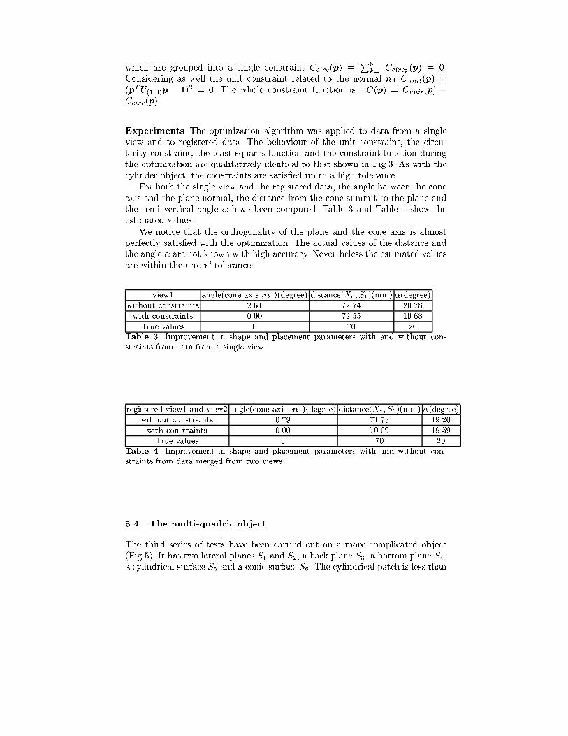
which are grouped into a single constraint Ccirc(p) = P6k=1 Ccirck(p) = 0.Considering as well the unit constraint related to the normal n1 Cunit(p) =(pTU(1;3)p � 1)2 = 0. The whole constraint function is : C(p) = Cunit(p) +Ccirc(p).Experiments The optimization algorithm was applied to data from a singleview and to registered data. The behaviour of the unit constraint, the circu-larity constraint, the least squares function and the constraint function duringthe optimization are qualitatively identical to that shown in Fig.3. As with thecylinder object, the constraints are satis�ed up to a high tolerance.For both the single view and the registered data, the angle between the coneaxis and the plane normal, the distance from the cone summit to the plane andthe semi vertical angle � have been computed. Table 3 and Table 4 show theestimated values.We notice that the orthogonality of the plane and the cone axis is almostperfectly satis�ed with the optimization. The actual values of the distance andthe angle � are not known with high accuracy. Nevertheless the estimated valuesare within the errors' tolerances.view1 angle(cone axis ,n1)(degree) distance(Xo; S1)(mm) �(degree)without constraints 2.61 72.74 20.78with constraints 0.00 72.55 19.68True values 0 70 20Table 3. Improvement in shape and placement parameters with and without con-straints from data from a single view.registered view1 and view2 angle(cone axis ,n1)(degree) distance(Xo; S1)(mm) �(degree)without constraints 0.79 71.73 19.20with constraints 0.00 70.09 19.59True values 0 70 20Table 4. Improvement in shape and placement parameters with and without con-straints from data merged from two views.5.4 The multi-quadric objectThe third series of tests have been carried out on a more complicated object(Fig.5). It has two lateral planes S1 and S2, a back plane S3, a bottom plane S4,a cylindrical surface S5 and a conic surface S6. The cylindrical patch is less than

(a)(b)

(c) (d)

lateral plane

S1cylinder patch

S2cone patch

S5

S6

back planeS3

bottom plane

S4

lateral plane

Fig. 5. four views of the multi-quadric objecta half cylinder (40% arc), the conic patch occupies a small area of the wholecone (less then 30%)The vector parameter associated to this object is then pT = [p1T ;p2T ;p3T ;p4T ;p5T ;p6T ]where pi is the parameter vector associated to the surface Si.The considered surfaces of the object have the following constraints1. S1 makes an angle of 120o1 with S22. S1 and S2 are perpendicular to S33. S1 and S2 make an angle of 120o with S44. S3 is perpendicular to S45. the axis of the cylindrical patch S5 is parallel to S3's normal6. the axis of the cone patch S6 is parallel to S4's normal7. the cylindrical patch is circular8. the cone patch is circularThese constraints are then represented in the same manner as in Section 5.2and Section 5.3.Experiments Since the surfaces can not be recovered from a single view, fourviews (Fig.5) have been registered by hand. The results regarding the algorithmconvergence are qualitatively identical to those shown in Fig.3. All the constraintfunctions vanish and are highly satis�ed.In order to check the robustness and the stability of the technique, we havecarried out 100 optimizations, in each of them 50% of the surfaces' points are1 We consider the angle between normals.

angle (S1; S2) (S1; S3) (S1; S4) (S2; S3) (S2; S4) (S3; S4)without constraints 119.76 92.08 121.01 87.45 119.20 90.39with constraints 120.00 90.00 120.00 90.00 120.00 90.00actual values 120 90 120 90 120 90Table 5. Improvement of the surface's angle estimation.selected randomly. The results shown below are the average of this tests. Our�rst intention was to compare the constrained approach with an object estima-tion method which does not consider constraints, in this case the least squarestechnique applied to each surface separately.In Table 5 the angles between the di�erent planes are mapped, we noticethat all the angles converge to the actual values. Table 6 and Table 7 containthe estimated values of some attributes of the cylinder and the cone. The valuesshow that each of the axis constraints are perfectly satis�ed, the estimated radiusand the cone half angle � are quite close to the actual ones. We notice the goodshape improvement of improvement, relative to the unconstrained least squaresmethod, given by reduction of bias of about 12mm and 3O respectively in theradius and the half angle estimation. The standard deviation of the estimationshave also been reduced.The radius estimation is within the hoped tolerances, a systematic errorof about 0:5mm is quite nice. However the cone half angle estimation seems toinvolve a larger systematic error (about 1:8o). Two factors may contribute to thisfact: 1) the registration error may be too large since it was made by hand and 2)the area of the cone patch covers less than 30 % of the whole cone. It is knownthat when a quadric patch does not contain enough information concerning thecurvature, the estimation is very biased, even when robust techniques are applied,because it is not possible to predict the variation of the surface curvature.cylinder parameters angle( axis ,S3's normal) radius standard deviationwithout constraints 2.34 37.81 0.63with constraints 0.00 59.65 0.08actual values 0 60 0Table 6. Improvement of the cylinder characteristic estimates.cone parameters angle( axis ,S4's normal) � standard deviationwithout constraints 6.0866 26.0108 0.3024with constraints 0 31.8389 0.1337actual values 0 30 0Table 7. Improvement of the cone characteristic estimates.

angle (S1; S2) (S1; S3) (S1; S4) (S2; S3) (S2; S4) (S3; S4)without constraints 119.76 92.08 121.48 87.45 119.20 90.39with constraints 119.99 90.33 120.00 90.00 120.00 90.00actual values 120 90 120 90 120 90Table 8. Improvement of non-constrained angle estimates.We have also investigated whether leaving some features unconstrained willa�ect the estimation since one can say that the satisfaction of the other con-straints may push the unconstrained surfaces away from their actual positions.To test this, we have left the angles between the pair of planes (S1; S2) and(S1; S3) unconstrained. The results in Table 8 show that the estimated uncon-strained angles are still close to the actual ones and the accuracy is improvedcompared to the non-constrained method. The computation time for this objectin Matlab was 48s on a 200Mhz sun Ultrasparc workstation.6 ConclusionIf we consider the objectives stated in the introduction which are : object shapereconstruction which satis�es the constraints and improves the estimation ac-curacy, we can say that these objectives have been reached. The experimentsshow that parameter optimization search does produce shape �tting that almostperfectly satis�ed the constraints. The comparison of the results with the non-constrained �tting con�rms that the proposed approach improves the qualityof the �tting accuracy to a high degree. For the two objects having cylinderpatches, the radius error is less then 0:5mm. Results for the cone are reasonablebut less satisfactory. This is mainly due to the relatively small area of the conicpatch. Actually, we intentionally chose to work with small patches because it isthe case when non-constrained �tting surface techniques fail to give reasonableestimation even with the robust algorithms. This is due to the \poorness" of theinformation embodied in the patch. However we intend to investigate a morerobust form for the objective function which involves the data noise statistics.Regarding the constraint representation, it is noticed that some constraintsinvolve a large number of equations, in particular for the circularity constraint.One solution is to implicitly impose this constraints through the representationof the quadric equation ((X�Xo)T (I�nnT )(X�Xo)�r2 = 0 ) for the cylinderand ((X �Xo)T (nnT � cos2(�))(X �Xo) = 0) for the cone. The main problemencountered with this representation is the complexity of the related objectivefunction and the di�culty of separating the data terms from the parameterterms, but we are working on this issue. It will be also worthwhile to investigatesome topological constraints between surfaces which have a common intersection.The adequate formulation of this type of constraints is the main problem to solve.We are starting to investigate is how one might identify inter-surface rela-tionships that can have a constraint applied. In manufacturing objects, simple

angular and spatial relationships are given by design. It should be straightfor-ward to de�ne Mahalanobis distance tests for standard feature relationships,subject to the feature's statistical position distribution. With this analysis, acomputer program could propose a variety of constraints that a human couldeither accept or reject, after which shape reconstruction could occur.We have also investigated [14] an approach where constraints are increment-ally added, for example by a human reverse engineer, but have found no essentialdi�erence in results. The batch satisfaction of all constraints as presented heretakes very little computing time, so we no longer use the incremental algorithm.2References1. R.J.Bell An elementary treatise on coordinate geometry. McMillan and Co,London, 1910.2. R.M.Bolle, D.B.Cooper On Optimally Combining Pieces of Information, with Ap-plication to Estimating 3-D Complex-Object Position from Range Data. IEEETrans. PAMI, Vol.8, No.5, pp.619-638, September 1986.3. K.L.Boyer, M.J.Mirza, G.Ganguly The Robust Sequential Estimator. IEEE Trans.PAMI, Vol.16, No.10, pp.987-1001 October 1994.4. Y.Chen, G.Medioni Object Modelling by Registration of Multiple Range Images.Proc. IEEE Int. Conf. Robotics and Automation, Vol.2 pp.724-729, April, 1991.5. J.De Geeter, H.V.Brussel, J.De Schutter, M. Decreton A Smoothly ConstrainedKalman Filter. IEEE Trans. PAMI pp.1171-1177, No.10, Vol.19, October 1997.6. P.J.Flynn, A.K.Jain Surface Classi�cation: Hypothesizing and Parameter Estima-tion. Proc. IEEE Comp. Soc. CVPR, pp. 261-267. June 1988.7. A. Hoover, G. Jean-Baptiste, X. Jiang, P. J. Flynn, H. Bunke, D. Goldgof, K.Bowyer, D. Eggert, A. Fitzgibbon, R. Fisher An Experimental Comparison ofRange Segmentation Algorithms. IEEE Trans. PAMI, Vol.18, No.7, pp.673-689,July 1996.8. S.Kumar, S.Han, D.Goldgof, K.Boyer On Recovering Hyperquadrics from Rangedata. IEEE Trans. PAMI, Vol.17, No.11, pp.1079-1083, November 1995.9. S.L.S. Jacoby, J.S Kowalik, J.T.Pizzo Iterative Methods for Nonlinear OptimizationProblems. Prentice-Hall, Inc. Englewood Cli�s, New Jersey, 1972.10. J.Porrill Optimal Combination and Constraints for Geometrical Sensor Data. In-ternational Journal of Robotics Research, Vol.7, No.6, pp.66-78, 1988.11. M.Soucy, D.Laurendo Surface Modelling from Dynamic Integration of MultipleRange Views. Proc 11th Int. Conf. Pattern Recognition, pp.449-452, 1992.12. H.Y.Shun, K.Ikeuchi, R.Reddy Principal Component Analysis with Missing Dataand its Application to Polyhedral Object Modelling. IEEE Trans. PAMI, Vol.17,No.9, pp.855-867.13. B.C.Vemuri, J.K Aggrawal 3D Model Construction from Multiple Views UsingRange and Intensity Data. Proc. CVPR, pp.435-437, 1986.14. N.Werghi, R.B.Fisher, A.Ashbrook, C.Robertson Improving Model Shape Acquis-ition by Incorporating Geometric Constraints. Proc. BMVC, pp.530-539 Essex,September 1997.2 Acknowledgements: the work presented in this paper was funded by UK EPSRCgrant GR /L25110.