Spatial Stability for Mixed Convection Boundary Layer over a Heated Horizontal Plate
35
sapm˙355 SAM.cls July 19, 2006 14:17 Spatial Stability for Mixed Convection Boundary Layer over a Heated Horizontal Plate By T. K. Sengupta and K. Venkata Subbaiah The spatial stability properties of a mixed convection boundary layer developing over a heated horizontal plate is studied here under linear and quasi-parallel flow assumption. The main aim of the present work is to find out if there is a critical buoyancy parameter that would indicate the importance of heat transfer in destabilizing mixed convection boundary layers, when the buoyancy effect is given by Boussinesq approximation. The undisturbed flow used here is that given by the similarity solution of [1] that implies the wall temperature to vary as the inverse square root of the distance from the leading edge of the plate. The stability of this flow has been investigated by using the compound matrix method (CMM)—that allows finding all the modes in the chosen range in the complex wave number plane for spatial stability analysis. Presented neutral curves for mixed convection boundary layer show the existence of two types of disturbances present simultaneously, for large buoyancy parameter. One notices very unstable high-frequency mode when the buoyancy parameter exceeds the above-mentioned critical value. This unstable thermal mode is in addition to the hydrodynamic mode of isothermal flow given by corresponding similarity profile. The calculated critical buoyancy parameter is shown to qualitatively match with experimental results. Address for correspondence: T. K. Sengupta, Department of Aerospace Engineering, I.I.T. Kanpur, U.P. 208016, India; e-mail: [email protected] STUDIES IN APPLIED MATHEMATICS 117:265–298 265 C 2006 by the Massachusetts Institute of Technology Published by Blackwell Publishing, 350 Main Street, Malden, MA 02148, USA, and 9600 Garsington Road, Oxford, OX4 2DQ, UK.
Transcript of Spatial Stability for Mixed Convection Boundary Layer over a Heated Horizontal Plate

sapm˙355 SAM.cls July 19, 2006 14:17
Spatial Stability for Mixed Convection BoundaryLayer over a Heated Horizontal Plate
By T. K. Sengupta and K. Venkata Subbaiah
The spatial stability properties of a mixed convection boundary layer developingover a heated horizontal plate is studied here under linear and quasi-parallelflow assumption. The main aim of the present work is to find out if there is acritical buoyancy parameter that would indicate the importance of heat transferin destabilizing mixed convection boundary layers, when the buoyancy effectis given by Boussinesq approximation. The undisturbed flow used here is thatgiven by the similarity solution of [1] that implies the wall temperature tovary as the inverse square root of the distance from the leading edge of theplate. The stability of this flow has been investigated by using the compoundmatrix method (CMM)—that allows finding all the modes in the chosen rangein the complex wave number plane for spatial stability analysis. Presentedneutral curves for mixed convection boundary layer show the existence of twotypes of disturbances present simultaneously, for large buoyancy parameter.One notices very unstable high-frequency mode when the buoyancy parameterexceeds the above-mentioned critical value. This unstable thermal mode is inaddition to the hydrodynamic mode of isothermal flow given by correspondingsimilarity profile. The calculated critical buoyancy parameter is shown toqualitatively match with experimental results.
Address for correspondence: T. K. Sengupta, Department of Aerospace Engineering, I.I.T. Kanpur, U.P.208016, India; e-mail: [email protected]
STUDIES IN APPLIED MATHEMATICS 117:265–298 265C© 2006 by the Massachusetts Institute of TechnologyPublished by Blackwell Publishing, 350 Main Street, Malden, MA 02148, USA, and 9600 GarsingtonRoad, Oxford, OX4 2DQ, UK.

sapm˙355 SAM.cls July 19, 2006 14:17
266 T. K. Sengupta and K. V. Subbaiah
1. Introduction
Mixed convection flows are important as they are found in many practicalsituations- in nature and man-made devices. For problems of the continuumthey are as relevant for atmospheric dynamics at planetary scale to that forelectronic devices at micro-scale. Mixed convection differs from isothermalflow due to the induced buoyancy effects via heat transfer. It has been noted [2]that in natural convection and in mixed regime, the instability is due to growthof small disturbances. For natural convection this is a narrow-band phenomenonwhile for forced convection boundary layers the unstable frequency-bandis wider. Buoyancy forces—even when they are small—cannot be neglectedwhen the convection velocities are small or the temperature differencebetween the surface and the ambient is large. A comprehensive review ofthe heat transfer aspect of mixed convection can be found in [3]. For someflows the induced body forces are either parallel or anti-parallel to the meanconvection direction—as in the case of mixed convection flow past verticalplates.
However, the flow and heat transfer properties are more complicated whenmixed convection flows are considered past inclined or horizontal plates. This isdue to the fact that the buoyancy forces induce a longitudinal pressure gradientthat will directly alter flow and heat transfer rates. This is readily evidentby looking at Equations (8) and (9) describing the mean flow. Additionally,such imposed pressure gradient also alters the instability pattern. For example,it has been shown [4] that transition to turbulence for natural convectionproblem follows the instability of small disturbances. For natural convectionpast inclined flat plates, generation of an array of longitudinal vortices havebeen reported [5]. Instability of flow past inclined plate have been reported [6,7], that indicated the presence of two modes depending on the inclinationangle of the plate. When the inclination angle with respect to the vertical isless than 14o then the authors reported wave-like instability. Such wavelikeinstability has also been studied in [8]. For inclination angles greater than17o—for the natural convection problem—it is noted experimentally that thedisturbance field is dominated by vortices and is often termed as vortexinstability. This vortex mode of instability is present for both the horizontaland inclined plates. This has been variously studied in [9–14] among manyother such studies. In an alternate viewpoint [15], classify instability offorced-convection boundary layers over horizontal heated plates in terms of thetwo prototypical instabilities: Rayleigh–Benard type that is usually describedfor closed convection system heated from below and Tollmien–Schlichtingtype that is typical of isothermal open flows- as in wall-bounded shear layerstriggered by viscous instability. In their theoretical analysis [15], simultaneouspresence of both the modes that coalesce in the small wave number limit wasreported.
sapm˙355 SAM.cls July 19, 2006 14:17
Spatial Stability for Mixed Convection Boundary Layer 267
As the instability in mixed convection flows start off as growing smalldisturbances, linear stability is often used to analyze such flows. The analysishas been traditionally performed using temporal theory, as in [16] for mixedconvection flow along an isothermal vertical flat plate. The effect of buoyancywas studied by the temporal theory of a flow perturbed by small buoyancyinduced body force. The primary mean flow was obtained by local nonsimilaritymethod and they reported, for assisting flows, the buoyancy force to stabilizethe flow.
One should, however, note the critique of various nonsimilar flow descriptionsused in instability studies given in [2]. All the nonsimilar methods used forstability studies are local in nature, with nonsimilar terms defined as the newvariables. The boundary layer equations are augmented by new equations thatare derived by differentiating the transformed boundary layer equation withrespect to the new variables. This process actually leads to another equation thatis again nonsimilar. If the previous process of creating augmented equations isrepeated the system never closes—unless, at some level, nonsimilar terms areomitted. According to the authors, this measure makes the accuracy of localnonsimilarity method difficult to assess. Having realized this shortcoming, it isdecided that we would obtain the stability of mixed convection flow that isgiven by a similarity solution.
For an inclined plate the earliest instability study was reported in [8] andfor horizontal isothermal plate in [17]. Results of these studies indicated theflow along vertical and inclined plates to be more stable when the buoyancyforce aids external convection and stability decreased as the inclination angleapproached toward the horizontal. It was also noted for horizontal plates theflow to become more unstable when the buoyancy force is directed away fromthe surface.
However, experimental studies relate to spatial growth of disturbances asthe flow system is always excited by fixed frequency sources. Hence a spatialtheory is preferred to study the stability of nonisothermal flows. Despitethe distinction between temporal and spatial methods, the neutral curve,however, is identical. Results, using linear spatial theory and under parallelflow approximation, have been reported for free-convection flow past heated,inclined plates [18]. The spatial stability of natural convection flow on inclinedplates providing the eigenspectrum was reported in [19].
Here, we will investigate the stability property of mixed convection flow pasta heated horizontal plate, to provide the threshold buoyancy parameter thatalters the instability property qualitatively. Such a problem is of importancefor many engineering applications and in geophysical fluid dynamics. We alsonote that for mixed convection over a horizontal plate that is cooled to exhibitnonuniqueness and numerical instabilities for the corresponding boundarylayer equation [20]. However, such problems with analysis is absent when theplate is heated instead—as is the case that is studied here.

sapm˙355 SAM.cls July 19, 2006 14:17
268 T. K. Sengupta and K. V. Subbaiah
When Boussinesq approximation is adopted in full conservation equations,it is noted that the effect of buoyancy force appears in terms of Gr/Re2, whereGr is the Grashof number and Re is the Reynolds number defined in terms ofappropriate length, velocity and temperature scales. However, [21] and [22]have shown that the equivalent buoyancy parameter with the boundary layerassumption changes to K = Gr/Re5/2. Experimental investigations in [14] and[12] have also demonstrated the onset of instability to always occur at thesame value of K—underlying the importance of it as the relevant buoyancyparameter. We note that the similarity profile derived in [1] is given in terms of Konly.
Keeping all of the above in mind, we have used the similarity solution of [1]to study the stability of mixed convection flow past a horizontal plate, so thatstandard results for similarity profile is obtained by an accurate method. Thiswill be similar to what is available for isothermal flows using Blasius profile.Although it may be known that heat addition for flow past a horizontal platecan additionally destabilize the flow, it is the intention of the present study toprovide a quantification of the same. We are specifically interested to findingout a critical buoyancy effects, above which there is a sudden qualitativechange in the mixed convection regime. Wang [14] has reported a qualitativechange of heat transfer properties for flow past a horizontal plate that is kept ata constant temperature. It has also been noted in [23], with respect to heattransfer effects, significant buoyancy effects are encountered for Kx ≥ 0.05and Kx ≤ −0.03 for aiding and opposing flow past horizontal plate, whereK x = Grx/Re5/2
x . In studying the stability properties of flow over a heatedhorizontal plate, present work is kept within the limit given in [23].
As compared to the canonical problem of instability of flow past a platefor isothermal flow, the study becomes involved and complicated when heattransfer effects are introduced. It is known that the viscous action can bedestabilizing for isothermal flows, giving rise to Tollmien–Schlichting waves.For flow past a heated horizontal flat plate, buoyancy force is an additionalsource of destabilization and both these destabilizing effects can enhanceinstabilities.
Such effects have not been studied in great details due to numericalproblems. Addition of heat transfer effects necessitates incorporating theenergy equation—that requires solving sixth order stability equation, insteadof fourth order equations for isothermal flows. In reporting results in [17], theauthors have used Runge–Kutta integration scheme along with the Kaplanfiltering technique to avoid numerical difficulties. Tumin [19] has used bothChebyshev collocation and Runge–Kutta integration schemes to solve theninth order stability equation. In the collocation method 70 modes weretaken and Runge–Kutta method required Gram–Schmidt orthonormalizationprocedure to maintain linear independence of the components of fundamentalsolutions.
sapm˙355 SAM.cls July 19, 2006 14:17
Spatial Stability for Mixed Convection Boundary Layer 269
The major difficulty in studying instability is due to fundamental solutionsdisplaying variation of physical quantities at totally dissimilar rates—thewell-known problem of stiffness. This is variously tackled by special techniques ofsolving stability equations. The main three approaches in solving hydrodynamicstability problems are based on (see [24] and [25] for description): (i) matrixmethod using spectral or finite difference discretization; (ii) shooting methodsusing orthogonalization or orthonormalization and (iii) shooting method usingCompound Matrix Method (CMM). The Chebyshev collocation method belongsto the first category, while the Runge–Kutta method with orthonormalization orKaplan filter belongs to the second category. Bridges and Morris [26] have notedthat the matrix method leads to the appearance of “spurious” eigenvalues. Forplane Poiseuille flow, in [26] both stable and unstable spurious eigenvalues withlarge distinguishable magnitude have been reported. According to [27], suchspurious eigenvalues are created due to fracturing of the continuous spectrumfor problems in infinite domain. In [28], a QR algorithm based on Chebyshevpolynomials have been used for the spatio-temporal study of mixed convectionboundary layers developing over a vertical plate. It has also been noted in[27], that orthogonalization/orthonormalization procedure causes numericalsolution to be nonanalytic and on infinite domains there is the added problemthat asymptotically correct boundary conditions may not preserve analyticity.Kaplan filter-based method also suffers from this source of error. In contrast,CMM does not suffer from any of these problems. Basic ideas behind CMMare given in [29, 30] and [24]. CMM has been re-developed using exterioralgebra in a co-ordinate free context in [29]. CMM has been used in [31]for receptivity analysis and reporting the eigenspectrum of Blasius boundarylayer. Some problems of CMM have been identified and solved in [32] toobtain eigen functions correctly for high wave numbers. In [27], the stabilityproblem of Ekman boundary layer interacting with a compliant surface havebeen studied by solving a sixth-order system by CMM. In [30], CMM hasbeen developed for general fourth- and sixth-order systems.
Considering the strengths and limitations of different methods to solvestability equations, it is apparent that CMM has relative advantages. It avoidscreating spurious eigenvalues; retains analyticity of dispersion relation (as thecase is with orthogonalization) and mainly making a method available thatexploits the analytical structure of the solution to obtain the solution in a smallregion of the flow. In doing all these, major work is related at the formulationstage, while the solution is obtained by writing a simple Runge–Kutta solver,without requiring any special software.
The governing equations are given in the next section. The mean flow, whosestability will be studied, is given in Section 3. The stability equations andrelated numerical methods for CMM is given in Section 4. The results anddiscussion follow in Section 5. The paper closes with some comments andoutlook in Section 6.
sapm˙355 SAM.cls July 19, 2006 14:17
270 T. K. Sengupta and K. V. Subbaiah
2. The governing equations
We consider the laminar two-dimensional motion of fluid past a hot semi-infiniteplate, with the free stream velocity and temperature denoted by, U∞ andT∞. We will focus our attention on the top of the plate, for which thetemperature is Tw- that is greater than T∞, while assuming the leading edgeof the plate as the stagnation point. Governing equations are written indimensional form (indicated by the quantities with asterisk), along with theBoussinesq approximation to represent the buoyancy effect, for the velocityand temperature fields by [3],
∇∗ · �V ∗ = 0, (1)
D �V ∗
Dt∗ = g jβ(T ∗ − T∞) − 1
ρ∇ p∗ + ν∇2 �V ∗, (2)
DT ∗
Dt∗ = α∇∗2T ∗ + ν
C pφv + q
ρCv
, (3)
where DDt ∗ represents the substantive derivative and φv and q are the viscous
dissipation and the heat generation term in the energy equation. gj = [0, g, 0]T
is the gravity vector; α and ν are the thermal diffusivity and kinematic viscosityrespectively; β represents the volumetric thermal expansion coefficient. In ouranalysis we will neglect the viscous dissipation and the heat source term.
If we introduce a length scale (L), velocity scale (U∞), temperature scale(�T = T w − T ∞) and pressure scale (ρU 2
∞), then the above equations can berepresented in nondimensional form by,
∇ · �V = 0, (4)
D �VDt
= Gr
Re2T − ∇ p + 1
Re∇2 �V , (5)
DT
Dt= 1
RePr∇2T, (6)
where T = (T − T∞)/�T and Gr = gβ�TL3
ν2 ; Re = U∞Lν
and Pr = ν/α. In themomentum conservation equation, the quantity Gr/Re2 is also known as theRichardson number or Archimedes number. The Grashof number weighs inthe relative importance of buoyancy and viscous force terms and in the mixedconvection regime the Richardson number/Archimedes number is of order one.
sapm˙355 SAM.cls July 19, 2006 14:17
Spatial Stability for Mixed Convection Boundary Layer 271
3. Mean flow equations
The mean flow equations are obtained by invoking boundary layer approximationto the above conservation equations. For the two-dimensional steadyincompressible flow with constant properties and Boussinesq approximation, thenondimensional equations are written in a Cartesian co-ordinate system, fixedat the leading edge of the semi-infinite horizontal flat plate, as given in [1] by
∂U
∂X+ ∂V
∂Y= 0, (7)
U∂U
∂X+ V
∂U
∂Y= −∂P
∂X+ ∂2U
∂Y 2, (8)
0 = K θ − ∂P
∂Y, (9)
U∂θ
∂X+ V
∂θ
∂Y= 1
Pr
∂2θ
∂Y 2, (10)
where X = x/L; Y = y√
Re/L; U = u/U∞; V = √Rev/U∞; θ = T − T∞
Tw − T∞;
P = p/(ρ∞U 2∞); and K = Gr/Re5/2.
These equations are solved subject to boundary conditions at the wall (Y =0 and X > 0): U = V = 0 and θ = θw(X ); and at the free-stream (Y → ∞):U = 1 and θ = P = 0.
In the above set of equations, (7) is automatically satisfied if we introduce astream function (ψ). As P indicates an excess pressure over the free-streamvalue, then (9) can be integrated to P = − ∫ ∞
Y K θ dY . When these areintroduced in the x-momentum and the energy equation, one gets
ψY ψXY − ψXψYY − K
∫ ∞
YθX dY = ψYYY , (11)
ψY θX − ψXθY = 1
PrθYY . (12)
It is obvious that the buoyancy force creates a streamwise pressure gradientterm as given by the last term on the left-hand side of (11). This makes the meanflow to be nonsimilar. However, it is shown in [1] that the above formulationadmits similarity solution, if θw ∝ X −1/2 and for which the following similaritytransformations are introduced for the independent variable: η = YX −1/2
and for the dependent variables via: ψ = X 1/2g(η) and θ = θw�. Thesetransformations yield the following system of equations;
2g′′′ + gg′′ + Kη� = 0, (13)

sapm˙355 SAM.cls July 19, 2006 14:17
272 T. K. Sengupta and K. V. Subbaiah
2
Pr�′′ + g�′ + g′� = 0. (14)
In these equations a prime indicates a derivative with respect to theindependent variable, η. These equations have to be solved subject to theboundary conditions at η = 0: g = g′ = 0 and � = 1 and as η → ∞: g′ = 1and � = 0. The energy equation can be furthermore integrated analyticallyonce to obtain,
2
Pr�′ + g� = 0. (15)
Note that the solutions depend on Reynolds number, that is implicitlyincluded in the Y or η co-ordinate itself. The numerical results of these werepresented in [1] and an interesting feature of it was seen that the wall slope for� is equal to zero for all values of K—as seen from Equation (15) applied atthe wall, implying the solution to be given for an adiabatic wall condition.
4. Stability equations and numerical method
Here the stability equations for two-dimensional plane flows have been derived,by starting from the nondimensional equations (4)–(6) given by,
∂u
∂x+ ∂v
∂y= 0, (16)
∂u
∂t+ u
∂u
∂x+ v
∂u
∂y= −∂p
∂x+ 1
Re
(∂2u
∂x2+ ∂2u
∂y2
), (17)
∂v
∂t+ u
∂v
∂x+ v
∂v
∂y= Gr
Re2 T − ∂p
∂y+ 1
Re
(∂2v
∂x2+ ∂2v
∂y2
), (18)
∂T
∂t+ u
∂T
∂x+ v
∂T
∂y= 1
RePr
(∂2T
∂x2+ ∂2T
∂y2
). (19)
For the stability analysis, all the physical variables would be split into themean part, derived in Section 3, and a disturbance component indicated by acaret in the following:
u(x, y, t) = U (x, y) + εu(x, y, t),
v(x, y, t) = V (x, y) + εv(x, y, t),
p(x, y, t) = P(x, y) + ε p(x, y, t),
T (x, y, t) = T + εT (x, y, t).
sapm˙355 SAM.cls July 19, 2006 14:17
Spatial Stability for Mixed Convection Boundary Layer 273
The quantities with the over-bar are related to the mean flow solutions of theprevious section, via the appropriate transformations. The stability equations areobtained by making the additional parallel flow assumption, U = U (y), V = 0and T = T (y) so that a normal mode spatial instability analysis is possible bylooking for a solution of the linearized equations of the following form:
[u, v, p, T ] = [ f (y), φ(y), π (y), h(y)]ei(kx−ωt). (20)
After substituting (20) into (16) to (19), one can obtain the system ofequation governing the disturbance amplitude functions as,
i(kU − ω)(k2φ − φ′′) + ikU ′′φ = Gr
Re2 k2h − 1
Re(φiv − 2k2φ′′ + k4φ), (21)
i(kU − ω)h + T ′φ = 1
RePr(h′′ − k2h). (22)
These are the well-known Orr–Sommerfeld equations for mixed convectionflows, that show the disturbance normal velocity and the temperature fields tobe coupled, constituting a sixth-order differential system. Equations (21) and(22) are to be solved subject to the six boundary conditions:
at y = 0 : φ, φ′ = 0 and h = 0 (23)
as y → ∞ : φ, φ′, h → 0. (24)
The homogeneous boundary condition for h at the wall corresponds to theeigenvalue analysis, in contrast to receptivity analysis where h = h(x, t) isprescribed at the wall that represents a specific thermal input provided. It isshown in [31] that these two analyses are related through the disturbanceamplitude expression, described in the next subsection.
Indicated boundary conditions imply the disturbances to decay in the farstream (y → ∞). Equations (21)–(22), with the boundary conditions (23)–(24)reveal that the temperature field given by (22), decouples from the velocityfield in the free stream (y → ∞), as T ′ ≈ 0 there. The characteristic modes atfree stream are given by: λ5,6 = ∓S, where S = [k2 + iRePr(k − ω)]1/2.However, the disturbance momentum equation is not decoupled, as (21) at thefree stream simplifies (as U = 1 and all mean flow derivatives are zero) to
i(k − ω)(k2φ − φ′′) = Gr
Re2 k2h − 1
Re(φiv − 2k2φ′′ + k4φ). (25)
This equation for the disturbance amplitude of normal component of velocityrepresents a forced dynamics with the thermal field acting as the forcing. Thehomogeneous part of the solution is governed by the following characteristics,λ1,2 = ∓k and λ3,4 = ∓Q where Q2 = k2 + iRe(k − ω). Out of these sixcharacteristic values, we will discard those modes that grow with y. Let usidentify the admissible fundamental solution components by,
sapm˙355 SAM.cls July 19, 2006 14:17
274 T. K. Sengupta and K. V. Subbaiah
φ1 = e−ky; φ3 = e−Qy and φ5 = e−Sy, (26)
when the real part of k, Q and S are all positive. For this combination offundamental solutions, the particular solution is of the type φ p = Cne−Sy in
the free stream where, Cn = k2GrRe /[S 4 − 2k2S 2 + k4 + iRe(k − ω)(k2 − S 2)].
We will represent the governing stability equations as a set of six first-orderordinary differential equations by introducing the vector:
u(y, .) = [u1(y, .), u2(y, .), u3(y, .), u4(y, .), u5(y, .), u6(y, .)]T .
Where, u1 = φ, u2 = φ′, u3 = φ′′, u4 = φ′′′, u5 = h, and u6 = h′. Thegoverning system of equations given by (21) and (22) can be written as,
{u′j } = [A]{u j }. (27)
Thus, u is defined by u ∈ C 6 and where the matrix A is written as,
A =
0 1 0 0 0 0
0 0 1 0 0 0
0 0 0 1 0 0
−a 0 b 0 c 0
0 0 0 0 0 1
e 0 0 0 d 0
with, a = k4 + iRekU ′′ + iRek2(kU − ω); b = 2k2 + iRe(kU − ω); c =k2Gr/Re; d = k2 + iRePr(kU − ω); and e = RePr T ′.
The problem is to integrate (27) on C 6 that are defined on an intervaly ∈ [0, ∞] with three boundary conditions at y = 0—as defined by (23) andthree asymptotic boundary conditions applied at y = Y∞ for some Y∞ >
0—as defined by (24). The integration of (27) subject to boundary conditions(23) and (24) is not straightforward—due to the stiffness problem discussedin the Introduction. To remove the stiffness of the problem and integrate theODEs we will employ the CMM—as described in detail, in the Appendix.
4.1. Dispersion relation
To solve the stability problem one is required to solve the CMM Equations (A.3)starting from y = Y∞ using the initial condition given by Equation (A.4). Thedispersion relation can be obtained by satisfying the wall-boundary conditionas given by (23) in terms of disturbance velocity components and temperaturefield. In terms of the fundamental solution components, these conditions at thewall can be written as,
a1φ1 + a3φ3 + a5φ5 = 0, (28)
a1φ′1 + a3φ
′3 + a5φ
′5 = 0, (29)
h = 0. (30)
sapm˙355 SAM.cls July 19, 2006 14:17
Spatial Stability for Mixed Convection Boundary Layer 275
The condition given by (30) can be rewritten, using (21) and the fundamentalsolution components as
a1(φiv
1 + aφ1 − bφ′′1
) + a3(φiv
3 + aφ3 − bφ′′3
) + a5(φiv
5 + aφ5 − bφ′′5
) = h.
(31)
Thus, the dispersion relation can be obtained from the characteristicdeterminant of the linear system formed by (28), (29), and (31). Aftersimplification and using the definition of second compounds the dispersionrelation is obtained as
Dr + iDi = y3 − by1 = 0 at y = 0. (32)
The dispersion relation has an interesting physical and mathematicalinterpretation that can be understood in the context of spatio-temporal receptivityanalysis, as given in [31] for the excitation problem of a parallel shear layer. Forthe isothermal flow analyzed therein, if the fundamental decaying solutions areidentified as φ1 and φ3, then the disturbance stream function is shown as
ψ(x, y, t) = 1
(2π )2
∫ ∫φ′
1φ30 − φ3φ′10
φ′30φ10 − φ30φ
′10
BCwei(kx−ωt) dk dω, (33)
where the additional subscript “0” refers to the quantities evaluated at thewall and BCw is the excitation provided at the wall. For isothermal flow, thedenominator of the integrand on the right-hand side of the Fourier–Laplaceintegral is the dispersion relation of the corresponding eigenvalue problem.Thus, it is easy to see that the dispersion relation provides the poles for thereceptivity problem, that will yield the asymptotic solution obtained usingresidue theorem. In the context of the present problem, if one is interested in areceptivity analysis with respect to wall excitation, then in Equation (23) oneof the wall conditions would be inhomogeneous and identified with BCw in(33). Also, in (33) the denominator will have to be replaced by the dispersionrelation given by (32) and the numerator would change in terms of the threefundamental solutions, φ1, φ3, and φ5. However, we are only interested inthe corresponding eigenvalue problem and this discussion is for showing thephysical importance of the dispersion relation. Readers can look at [31] forfurther details on spatio-temporal receptivity analysis.
This completes the definition of the stability problem for the mixedconvection flow over the horizontal plate. For a given K and Re, one would berequired to solve (A.3), starting with the initial conditions (A.4) and satisfy(32) for particular combinations of the eigenvalues obtained as the complex kand ω. We will use the procedures adopted in [31] to obtain the eigenspectrumfor the mixed convection case, when the problem is analyzed by spatial theory.In the process, it is possible to scan for all the eigenvalues in the complexk-plane, without any problem of spurious eigenvalues.
sapm˙355 SAM.cls July 19, 2006 14:17
276 T. K. Sengupta and K. V. Subbaiah
4.2. Eigenfunction for the mixed convection problem
While Ng and Reid [30] have given the CMM for evaluating the eigenvalues,till to date there are no published literature on how to obtain eigenfunctionsusing CMM for sixth-order system. It is for this reason, we discuss how thiscan be evaluated using CMM.
Having obtained the eigenvalues, it is possible to obtain the eigenfunctionsby writing them in terms of the decaying fundamental modes as
φ = a1φ1 + a3φ3 + a5φ5. (34)
For the sixth-order system, one can form the auxiliary system of equationsby eliminating a1, a3, and a5 from the definition of the second compounds asprovided in the Appendix and
φ′ = a1φ′1 + a3φ
′3 + a5φ
′5, (35)
φ′′ = a1φ′′1 + a3φ
′′3 + a5φ
′′5 , (36)
φ′′′ = a1φ′′′1 + a3φ
′′′3 + a5φ
′′′5 , (37)
φiv = a1φiv1 + a3φ
iv3 + a5φ
iv5 , (38)
φv = a1φv1 + a3φ
v3 + a5φ
v5 . (39)
For example, using (34)–(36) and using the definition of the secondcompounds, one obtains the following auxiliary equation:
y1φ′′′ − y2φ
′′ + y5φ′ − y11φ = 0. (40)
If instead one uses (34), (35), and (37), the following auxiliary equation isobtained:
y1φiv − y3φ
′′ + y6φ′ − y12φ = 0. (41)
There are many other possible auxiliary equations that can be used inprinciple to obtain the eigenfunctions. In the context of fourth-order systems,multiplicity of such equations was considered a source of confusion (see[24]—that was resolved later in [32] by looking at the eigenfunction equationsfor their correct asymptotic behavior when y → Y∞. As the problem allowsonly three decaying modes for the present case, it is necessary to ensure thatthe chosen eigenfunction equation also displays same asymptotic decay. Forexample, (40) displays the correct decay rates of −k, −Q, and −S, while (41)has the asymptotic variation given by the characteristic exponents as −k, −Q,−S and (k + Q + S). Thus, (41) has a spurious, violently growing mode andcannot be used. As (40) already displays the correct solution behavior, we willnot look for any other auxiliary equations.
sapm˙355 SAM.cls July 19, 2006 14:17
Spatial Stability for Mixed Convection Boundary Layer 277
5. Results and discussion
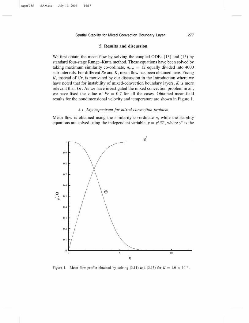
We first obtain the mean flow by solving the coupled ODEs (13) and (15) bystandard four-stage Runge–Kutta method. These equations have been solved bytaking maximum similarity co-ordinate, ηmax = 12 equally divided into 4000sub-intervals. For different Re and K, mean flow has been obtained here. FixingK, instead of Gr, is motivated by our discussion in the Introduction where wehave noted that for instability of mixed-convection boundary layers, K is morerelevant than Gr. As we have investigated the mixed convection problem in air,we have fixed the value of Pr = 0.7 for all the cases. Obtained mean-fieldresults for the nondimensional velocity and temperature are shown in Figure 1.
5.1. Eigenspectrum for mixed convection problem
Mean flow is obtained using the similarity co-ordinate η, while the stabilityequations are solved using the independent variable, y = y∗/δ∗, where y∗ is the
η
g′,Θ
0 5 100
0.1
0.2
0.3
0.4
0.5
0.6
0.7
0.8
0.9
1g′
Θ
Figure 1. Mean flow profile obtained by solving (3.11) and (3.13) for K = 1.0 × 10⁻⁵.
sapm˙355 SAM.cls July 19, 2006 14:17
278 T. K. Sengupta and K. V. Subbaiah
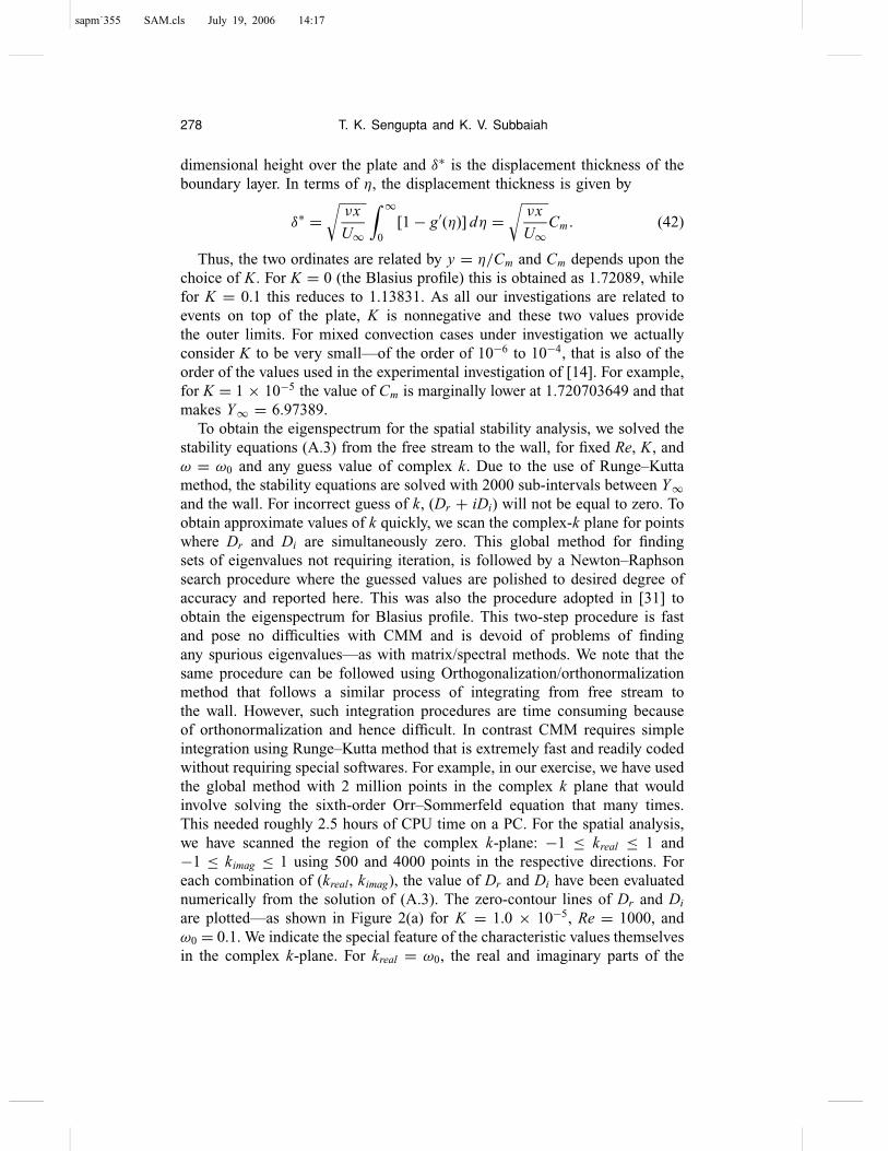
dimensional height over the plate and δ∗ is the displacement thickness of theboundary layer. In terms of η, the displacement thickness is given by
δ∗ =√
νx
U∞
∫ ∞
0[1 − g′(η)] dη =
√νx
U∞Cm . (42)
Thus, the two ordinates are related by y = η/Cm and Cm depends upon thechoice of K. For K = 0 (the Blasius profile) this is obtained as 1.72089, whilefor K = 0.1 this reduces to 1.13831. As all our investigations are related toevents on top of the plate, K is nonnegative and these two values providethe outer limits. For mixed convection cases under investigation we actuallyconsider K to be very small—of the order of 10−6 to 10−4, that is also of theorder of the values used in the experimental investigation of [14]. For example,for K = 1 × 10⁻⁵ the value of Cm is marginally lower at 1.720703649 and thatmakes Y∞ = 6.97389.
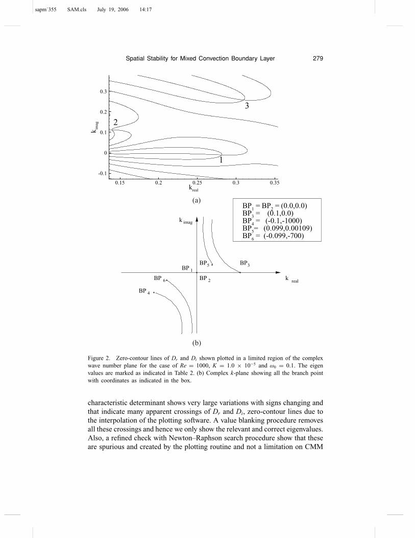
To obtain the eigenspectrum for the spatial stability analysis, we solved thestability equations (A.3) from the free stream to the wall, for fixed Re, K, andω = ω0 and any guess value of complex k. Due to the use of Runge–Kuttamethod, the stability equations are solved with 2000 sub-intervals between Y∞and the wall. For incorrect guess of k, (Dr + iDi) will not be equal to zero. Toobtain approximate values of k quickly, we scan the complex-k plane for pointswhere Dr and Di are simultaneously zero. This global method for findingsets of eigenvalues not requiring iteration, is followed by a Newton–Raphsonsearch procedure where the guessed values are polished to desired degree ofaccuracy and reported here. This was also the procedure adopted in [31] toobtain the eigenspectrum for Blasius profile. This two-step procedure is fastand pose no difficulties with CMM and is devoid of problems of findingany spurious eigenvalues—as with matrix/spectral methods. We note that thesame procedure can be followed using Orthogonalization/orthonormalizationmethod that follows a similar process of integrating from free stream tothe wall. However, such integration procedures are time consuming becauseof orthonormalization and hence difficult. In contrast CMM requires simpleintegration using Runge–Kutta method that is extremely fast and readily codedwithout requiring special softwares. For example, in our exercise, we have usedthe global method with 2 million points in the complex k plane that wouldinvolve solving the sixth-order Orr–Sommerfeld equation that many times.This needed roughly 2.5 hours of CPU time on a PC. For the spatial analysis,we have scanned the region of the complex k-plane: −1 ≤ kreal ≤ 1 and−1 ≤ kimag ≤ 1 using 500 and 4000 points in the respective directions. Foreach combination of (kreal, kimag), the value of Dr and Di have been evaluatednumerically from the solution of (A.3). The zero-contour lines of Dr and Di
are plotted—as shown in Figure 2(a) for K = 1.0 × 10⁻⁵, Re = 1000, andω0 = 0.1. We indicate the special feature of the characteristic values themselvesin the complex k-plane. For kreal = ω0, the real and imaginary parts of the
sapm˙355 SAM.cls July 19, 2006 14:17
Spatial Stability for Mixed Convection Boundary Layer 279
kreal
k imag
0.15 0.2 0.25 0.3 0.35
-0.1
0
0.1
0.2
0.3
1
2
3
BP1 = BP2 = (0.0,0.0)BP3 = (0.1,0.0)BP4 = (-0.1,-1000)BP5= (0.099,0.00109)BP6 = (-0.099,-700)
k
k imag
BP 1
BP 2BP 6
BP 4
BP5 BP3
real
(a)
(b)
Figure 2. Zero-contour lines of Dr and Di shown plotted in a limited region of the complexwave number plane for the case of Re = 1000, K = 1.0 × 10⁻⁵ and ω0 = 0.1. The eigenvalues are marked as indicated in Table 2. (b) Complex k-plane showing all the branch pointwith coordinates as indicated in the box.
characteristic determinant shows very large variations with signs changing andthat indicate many apparent crossings of Dr and Di, zero-contour lines due tothe interpolation of the plotting software. A value blanking procedure removesall these crossings and hence we only show the relevant and correct eigenvalues.Also, a refined check with Newton–Raphson search procedure show that theseare spurious and created by the plotting routine and not a limitation on CMM
sapm˙355 SAM.cls July 19, 2006 14:17
280 T. K. Sengupta and K. V. Subbaiah
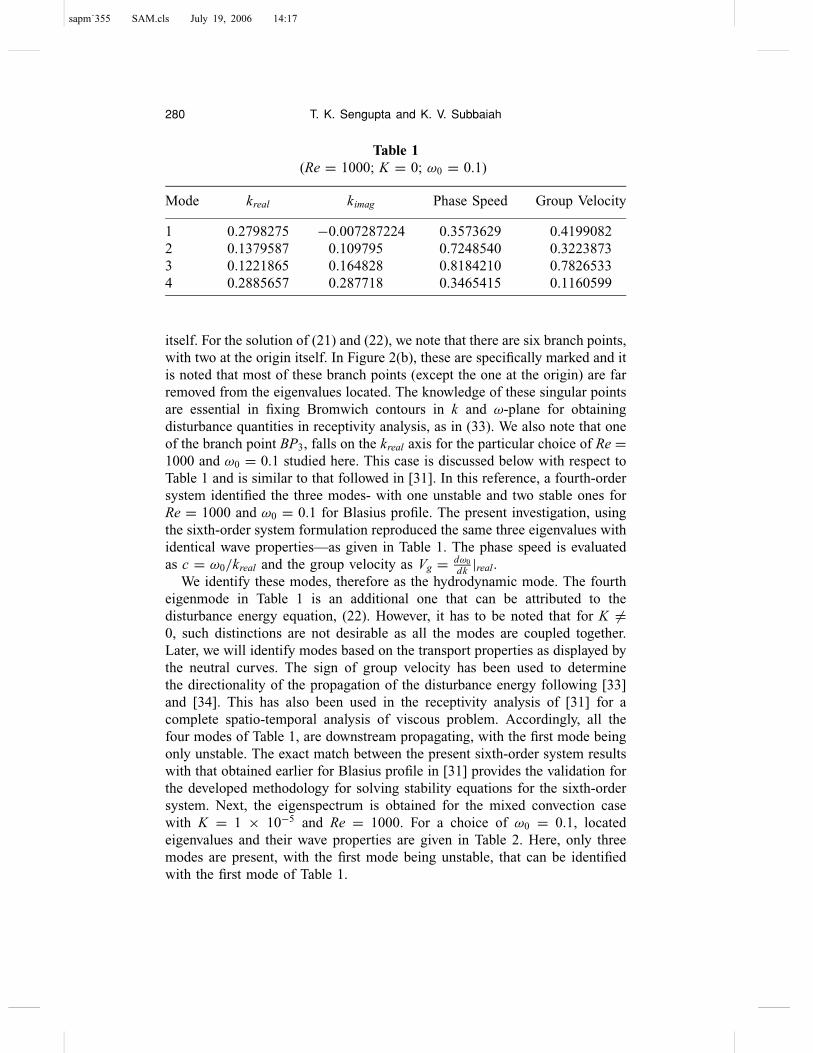
Table 1(Re = 1000; K = 0; ω0 = 0.1)
Mode kreal kimag Phase Speed Group Velocity
1 0.2798275 −0.007287224 0.3573629 0.41990822 0.1379587 0.109795 0.7248540 0.32238733 0.1221865 0.164828 0.8184210 0.78265334 0.2885657 0.287718 0.3465415 0.1160599
itself. For the solution of (21) and (22), we note that there are six branch points,with two at the origin itself. In Figure 2(b), these are specifically marked and itis noted that most of these branch points (except the one at the origin) are farremoved from the eigenvalues located. The knowledge of these singular pointsare essential in fixing Bromwich contours in k and ω-plane for obtainingdisturbance quantities in receptivity analysis, as in (33). We also note that oneof the branch point BP3, falls on the kreal axis for the particular choice of Re =1000 and ω0 = 0.1 studied here. This case is discussed below with respect toTable 1 and is similar to that followed in [31]. In this reference, a fourth-ordersystem identified the three modes- with one unstable and two stable ones forRe = 1000 and ω0 = 0.1 for Blasius profile. The present investigation, usingthe sixth-order system formulation reproduced the same three eigenvalues withidentical wave properties—as given in Table 1. The phase speed is evaluatedas c = ω0/kreal and the group velocity as Vg = dω0
dk |real.We identify these modes, therefore as the hydrodynamic mode. The fourth
eigenmode in Table 1 is an additional one that can be attributed to thedisturbance energy equation, (22). However, it has to be noted that for K �=0, such distinctions are not desirable as all the modes are coupled together.Later, we will identify modes based on the transport properties as displayed bythe neutral curves. The sign of group velocity has been used to determinethe directionality of the propagation of the disturbance energy following [33]and [34]. This has also been used in the receptivity analysis of [31] for acomplete spatio-temporal analysis of viscous problem. Accordingly, all thefour modes of Table 1, are downstream propagating, with the first mode beingonly unstable. The exact match between the present sixth-order system resultswith that obtained earlier for Blasius profile in [31] provides the validation forthe developed methodology for solving stability equations for the sixth-ordersystem. Next, the eigenspectrum is obtained for the mixed convection casewith K = 1 × 10⁻⁵ and Re = 1000. For a choice of ω0 = 0.1, locatedeigenvalues and their wave properties are given in Table 2. Here, only threemodes are present, with the first mode being unstable, that can be identifiedwith the first mode of Table 1.

sapm˙355 SAM.cls July 19, 2006 14:17
Spatial Stability for Mixed Convection Boundary Layer 281
Table 2(Re = 1000; K = 1.0 × 10⁻⁵; ω0 = 0.1)
Mode kreal kimag Phase Speed Group Velocity
1 0.2814215 −0.01035186 0.3553388 0.40252522 0.1397349 0.1118859 0.7156407 0.30761613 0.3095879 0.2579895 0.3230100 0.1498453
While the wavelength, phase speed and group velocity is similar for the firstmode in Tables 1 and 2, the spatial growth rate has increased significantly dueto added instability via buoyancy effect. The second mode of these two tablesare also similarly related, while the third mode of Table 1 has disappeared forthe case of mixed convection. Disappearance of modes has been identified in[35] as related to waves attaining phase speed equal to the free stream speed.The third mode of Table 2 can be seen related to the fourth mode of Table 1. Wenote that this mode propagate at smaller speed compared to the other modes.
In Table 3, eigenspectrum for a case is tabulated for K = 1 × 10⁻⁵, Re =1000 and ω0 = 0.65. This case, at a high circular frequency, is computedbecause such parameter combinations correspond to unstable modes occurringfor very small length-scale disturbances—as explained later. It is for thisreason, here the eigenspectrum is searched over a larger range of −2.5 ≤kreal ≤ 2.5, while the kimag search space is kept the same with same number ofpoints in both these directions.
The tabulated values display four eigenmodes with the first mode as aviolently unstable one that moves downstream. The growth rate is 40 timeshigher than the growth rate of most unstable mode for Blasius profile. Thesecond and the third mode in this table are similar to the damped modes withsmaller wave length and higher phase speeds for Blasius profile. The third modesends the associated disturbance energy at almost the speed of free stream.
Table 3(Re = 1000; K = 1.0 × 10⁻⁵; ω0 = 0.65)
Mode kreal kimag Phase Speed Group Velocity
1 2.1746912 −0.2976624 0.2988930 0.32066512 1.6960187 0.4214139 0.3832504 0.22759763 0.9495165 0.2522278 0.6845588 0.94057974 0.9101455 0.4832617 0.7141714 4.6808463
sapm˙355 SAM.cls July 19, 2006 14:17
282 T. K. Sengupta and K. V. Subbaiah
The fourth mode is also a damped mode, but for which the disturbance energytravels at more than four times the free-stream speed. Due to its high dampingrate and group velocity, this mode does not affect the dynamics significantly.
5.2. Neutral curves for mixed convection problem
One of the aim of any instability study is to relate it with the critical valuesof parameters that marks the onset of the instability. In the present context,one would therefore like to obtain the critical Reynolds number (Recr), thecorresponding circular frequency (ωcr). Additionally, one would also look forthe critical buoyancy parameter (Kcr), at which the instability properties changequalitatively, as well as quantitatively. In the previous subsection, we havenoted that for K = 0, an additional mode is triggered due to the couplingbetween the energy and momentum equations through convection process forincompressible flows even when the density change due to buoyancy effect iscompletely ignored. When the density change is included, as accounted bythe Boussinesq approximation, one is interested in finding Kcr that alters theinstability of the system dramatically. At a given K, it is possible that there canbe more than one unstable modes for a chosen Re due to the coupling ofmomentum and energy equations. This implies that the corresponding neutralcurves are multilobed. To investigate this and obtaining critical parameters,we obtain neutral curves for different cases of interest. Having obtained theeigenspectrum for different cases using CMM for the sixth-order system, it isstraightforward to obtain the spatial eigenvalues for any combinations of Reand ω0 using Newton–Raphson search procedure.
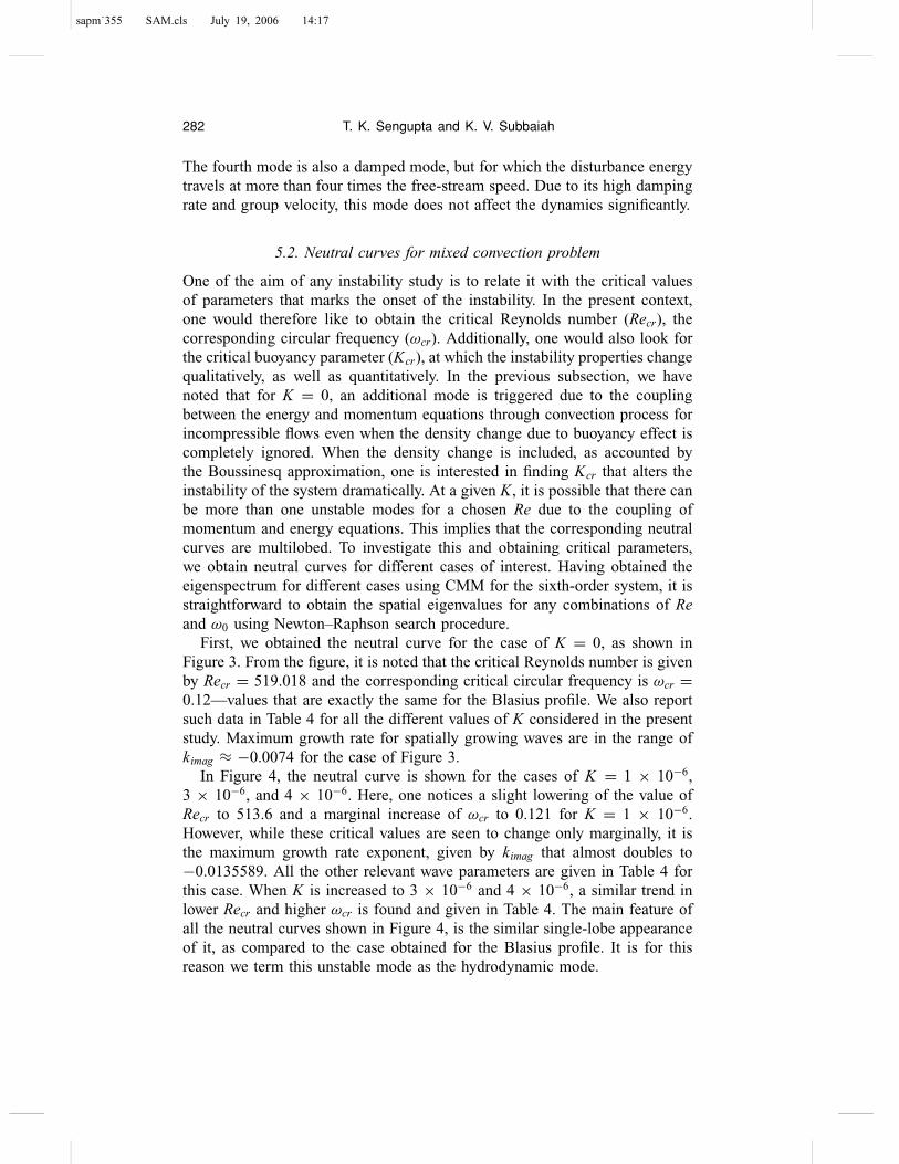
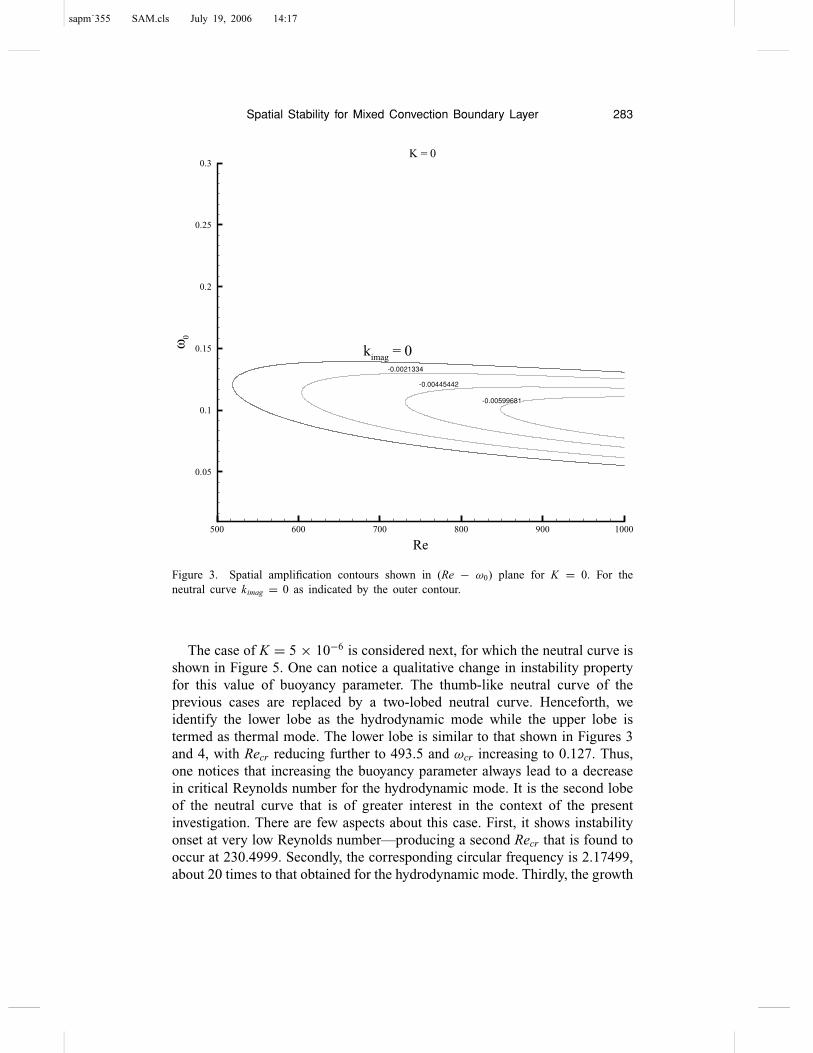
First, we obtained the neutral curve for the case of K = 0, as shown inFigure 3. From the figure, it is noted that the critical Reynolds number is givenby Recr = 519.018 and the corresponding critical circular frequency is ωcr =0.12—values that are exactly the same for the Blasius profile. We also reportsuch data in Table 4 for all the different values of K considered in the presentstudy. Maximum growth rate for spatially growing waves are in the range ofkimag ≈ −0.0074 for the case of Figure 3.
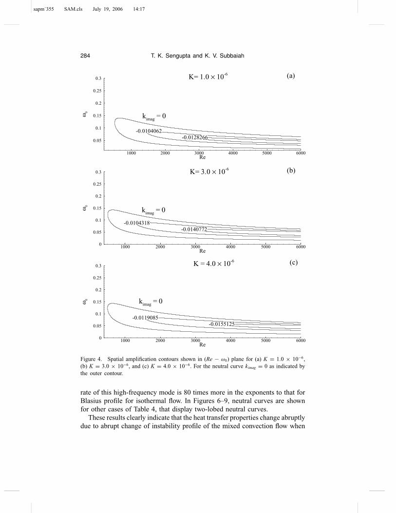
In Figure 4, the neutral curve is shown for the cases of K = 1 × 10−6,3 × 10−6, and 4 × 10⁻⁶. Here, one notices a slight lowering of the value ofRecr to 513.6 and a marginal increase of ωcr to 0.121 for K = 1 × 10⁻⁶.However, while these critical values are seen to change only marginally, it isthe maximum growth rate exponent, given by kimag that almost doubles to−0.0135589. All the other relevant wave parameters are given in Table 4 forthis case. When K is increased to 3 × 10⁻⁶ and 4 × 10⁻⁶, a similar trend inlower Recr and higher ωcr is found and given in Table 4. The main feature ofall the neutral curves shown in Figure 4, is the similar single-lobe appearanceof it, as compared to the case obtained for the Blasius profile. It is for thisreason we term this unstable mode as the hydrodynamic mode.
sapm˙355 SAM.cls July 19, 2006 14:17
Spatial Stability for Mixed Convection Boundary Layer 283
-0.0021334
-0.00445442
-0.00599681
Re
ω0
500 600 700 800 900 1000
0.05
0.1
0.15
0.2
0.25
0.3
kimag = 0
K = 0
Figure 3. Spatial amplification contours shown in (Re − ω0) plane for K = 0. For theneutral curve kimag = 0 as indicated by the outer contour.
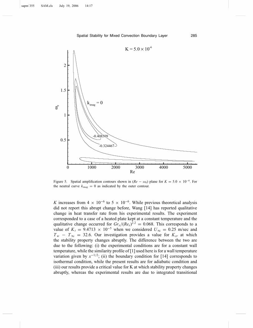
The case of K = 5 × 10⁻⁶ is considered next, for which the neutral curve isshown in Figure 5. One can notice a qualitative change in instability propertyfor this value of buoyancy parameter. The thumb-like neutral curve of theprevious cases are replaced by a two-lobed neutral curve. Henceforth, weidentify the lower lobe as the hydrodynamic mode while the upper lobe istermed as thermal mode. The lower lobe is similar to that shown in Figures 3and 4, with Recr reducing further to 493.5 and ωcr increasing to 0.127. Thus,one notices that increasing the buoyancy parameter always lead to a decreasein critical Reynolds number for the hydrodynamic mode. It is the second lobeof the neutral curve that is of greater interest in the context of the presentinvestigation. There are few aspects about this case. First, it shows instabilityonset at very low Reynolds number—producing a second Recr that is found tooccur at 230.4999. Secondly, the corresponding circular frequency is 2.17499,about 20 times to that obtained for the hydrodynamic mode. Thirdly, the growth
sapm˙355 SAM.cls July 19, 2006 14:17
284 T. K. Sengupta and K. V. Subbaiah
-0.0104062-0.0128266
Re
ω0
1000 2000 3000 4000 5000 6000
0.05
0.1
0.15
0.2
0.25
0.3
kimag = 0
K= 1.0 × 10⁻⁶ (a)
-0.0104318-0.0140772
Re
ω0
1000 2000 3000 4000 5000 60000
0.05
0.1
0.15
0.2
0.25
0.3
kimag = 0
K= 3.0 × 10⁻⁶ (b)
-0.0119085-0.0155125
Re
ω0
1000 2000 3000 4000 5000 60000
0.05
0.1
0.15
0.2
0.25
0.3
kimag = 0
K = 4.0 × 10⁻⁶ (c)
Figure 4. Spatial amplification contours shown in (Re − ω0) plane for (a) K = 1.0 × 10⁻⁶,(b) K = 3.0 × 10⁻⁶, and (c) K = 4.0 × 10⁻⁶. For the neutral curve kimag = 0 as indicated bythe outer contour.
rate of this high-frequency mode is 80 times more in the exponents to that forBlasius profile for isothermal flow. In Figures 6–9, neutral curves are shownfor other cases of Table 4, that display two-lobed neutral curves.
These results clearly indicate that the heat transfer properties change abruptlydue to abrupt change of instability profile of the mixed convection flow when
sapm˙355 SAM.cls July 19, 2006 14:17
Spatial Stability for Mixed Convection Boundary Layer 285
-0.408509
-0.324467
Re
ω0
0 1000 2000 3000 4000 5000
0.5
1
1.5
2
kimag = 0
K = 5.0 × 10⁻⁶
Figure 5. Spatial amplification contours shown in (Re − ω0) plane for K = 5.0 × 10⁻⁶. Forthe neutral curve kimag = 0 as indicated by the outer contour.
K increases from 4 × 10⁻⁶ to 5 × 10⁻⁶. While previous theoretical analysisdid not report this abrupt change before, Wang [14] has reported qualitativechange in heat transfer rate from his experimental results. The experimentcorresponded to a case of a heated plate kept at a constant temperature and thequalitative change occurred for Grx/(Rex)2.2 = 0.068. This corresponds to avalue of K t = 9.4713 × 10⁻⁵ when we considered U∞ = 0.25 m/sec andT w − T ∞ = 32.6. Our investigation provides a value for Kcr at whichthe stability property changes abruptly. The difference between the two aredue to the following: (i) the experimental conditions are for a constant walltemperature, while the similarity profile of [1] used here is for a wall temperaturevariation given by x−1/2; (ii) the boundary condition for [14] corresponds toisothermal condition, while the present results are for adiabatic condition and(iii) our results provide a critical value for K at which stability property changesabruptly, whereas the experimental results are due to integrated transitional
sapm˙355 SAM.cls July 19, 2006 14:17
286 T. K. Sengupta and K. V. Subbaiah
-0.433137
-0.262398
Re
ω0
0 1000 2000
0.5
1
1.5
2
kimag = 0
K = 1.0 × 10⁻⁵
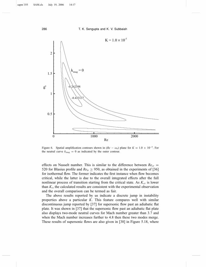
Figure 6. Spatial amplification contours shown in (Re − ω0) plane for K = 1.0 × 10⁻⁵. Forthe neutral curve kimag = 0 as indicated by the outer contour.
effects on Nusselt number. This is similar to the difference between Recr =520 for Blasius profile and Retr ≥ 950, as obtained in the experiments of [36]for isothermal flow. The former indicates the first instance when flow becomescritical, while the latter is due to the overall integrated effects after the fullnonlinear process of transition starting from the critical state. As Kcr is lowerthan Kt, the calculated results are consistent with the experimental observationand the overall comparison can be termed as fair.
The above results reported by us indicate a discrete jump in instabilityproperties above a particular K. This feature compares well with similardiscontinuous jump reported by [37] for supersonic flow past an adiabatic flatplate. It was shown in [37] that the supersonic flow past an adiabatic flat platealso displays two-mode neutral curves for Mach number greater than 3.7 andwhen the Mach number increases further to 4.8 then these two modes merge.These results of supersonic flows are also given in [38] in Figure 5.18, where
sapm˙355 SAM.cls July 19, 2006 14:17
Spatial Stability for Mixed Convection Boundary Layer 287
-0.241765
-0.362574
Re
ω0
0 500 1000 1500
0.5
1
1.5
2
kimag = 0
K = 1.5 × 10⁻⁵
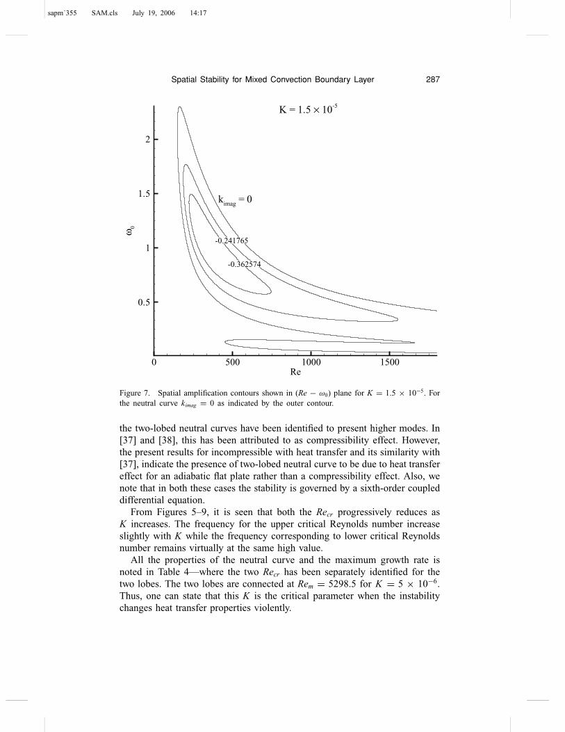
Figure 7. Spatial amplification contours shown in (Re − ω0) plane for K = 1.5 × 10⁻⁵. Forthe neutral curve kimag = 0 as indicated by the outer contour.
the two-lobed neutral curves have been identified to present higher modes. In[37] and [38], this has been attributed to as compressibility effect. However,the present results for incompressible with heat transfer and its similarity with[37], indicate the presence of two-lobed neutral curve to be due to heat transfereffect for an adiabatic flat plate rather than a compressibility effect. Also, wenote that in both these cases the stability is governed by a sixth-order coupleddifferential equation.
From Figures 5–9, it is seen that both the Recr progressively reduces asK increases. The frequency for the upper critical Reynolds number increaseslightly with K while the frequency corresponding to lower critical Reynoldsnumber remains virtually at the same high value.
All the properties of the neutral curve and the maximum growth rate isnoted in Table 4—where the two Recr has been separately identified for thetwo lobes. The two lobes are connected at Rem = 5298.5 for K = 5 × 10⁻⁶.Thus, one can state that this K is the critical parameter when the instabilitychanges heat transfer properties violently.
sapm˙355 SAM.cls July 19, 2006 14:17
288 T. K. Sengupta and K. V. Subbaiah
-0.28473
-0.337065
Re
ω0
0 500 1000
0.5
1
1.5
2
kimag = 0
K = 2.0 × 10⁻⁵
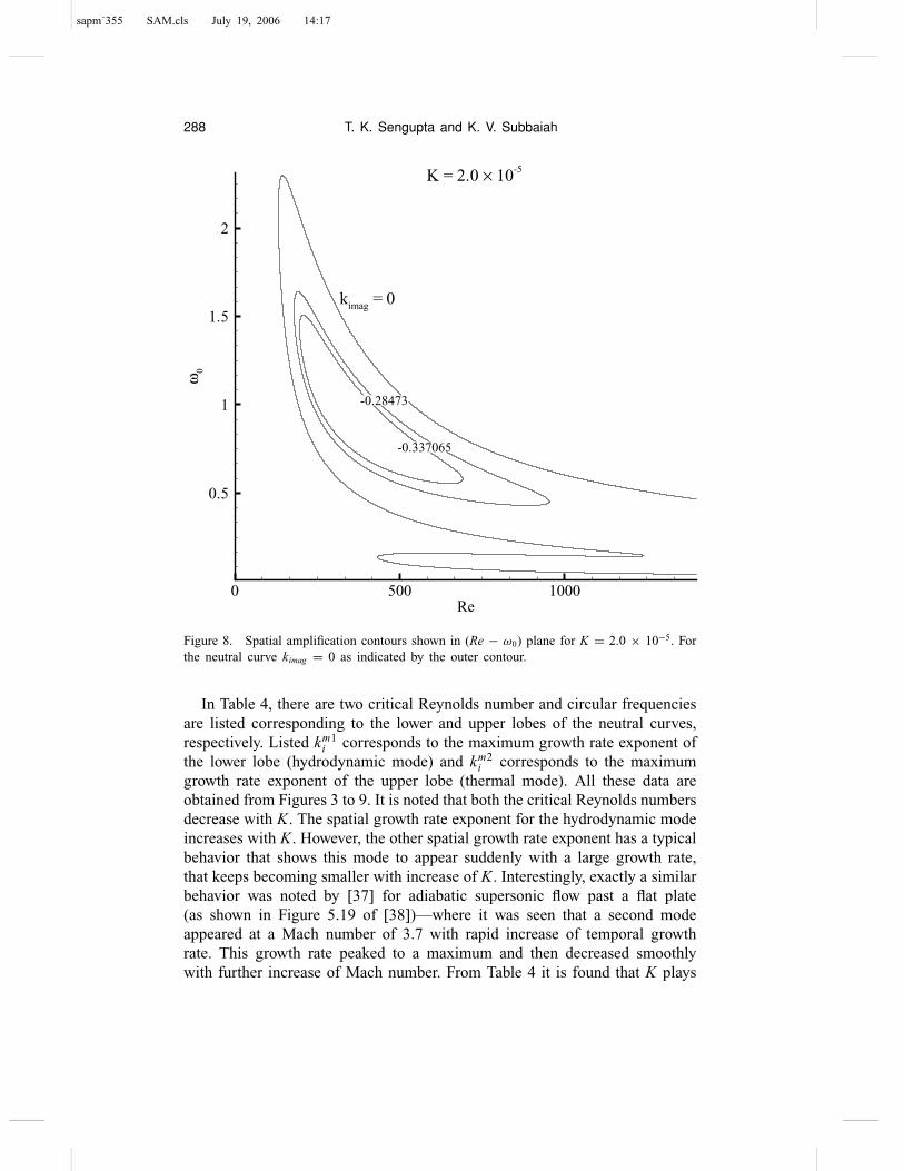
Figure 8. Spatial amplification contours shown in (Re − ω0) plane for K = 2.0 × 10⁻⁵. Forthe neutral curve kimag = 0 as indicated by the outer contour.
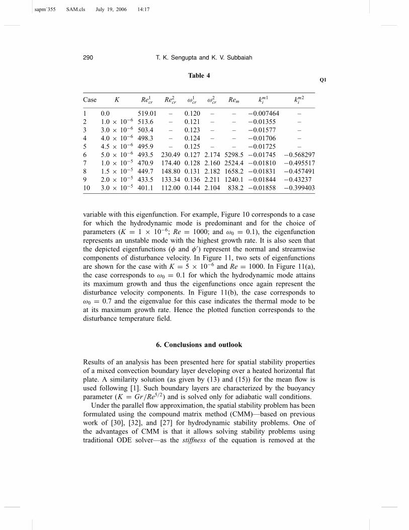
In Table 4, there are two critical Reynolds number and circular frequenciesare listed corresponding to the lower and upper lobes of the neutral curves,respectively. Listed km1
i corresponds to the maximum growth rate exponent ofthe lower lobe (hydrodynamic mode) and km2
i corresponds to the maximumgrowth rate exponent of the upper lobe (thermal mode). All these data areobtained from Figures 3 to 9. It is noted that both the critical Reynolds numbersdecrease with K. The spatial growth rate exponent for the hydrodynamic modeincreases with K. However, the other spatial growth rate exponent has a typicalbehavior that shows this mode to appear suddenly with a large growth rate,that keeps becoming smaller with increase of K. Interestingly, exactly a similarbehavior was noted by [37] for adiabatic supersonic flow past a flat plate(as shown in Figure 5.19 of [38])—where it was seen that a second modeappeared at a Mach number of 3.7 with rapid increase of temporal growthrate. This growth rate peaked to a maximum and then decreased smoothlywith further increase of Mach number. From Table 4 it is found that K plays
sapm˙355 SAM.cls July 19, 2006 14:17
Spatial Stability for Mixed Convection Boundary Layer 289
-0.183431
-0.283565
-0.363688
Re
ω0
200 400 600 800
0.5
1
1.5
2
kimag = 0
K= 3.0 × 10⁻⁵
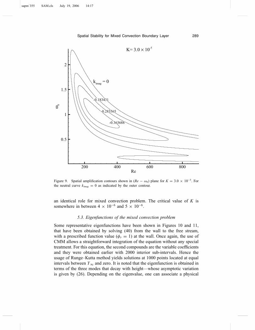
Figure 9. Spatial amplification contours shown in (Re − ω0) plane for K = 3.0 × 10⁻⁵. Forthe neutral curve kimag = 0 as indicated by the outer contour.
an identical role for mixed convection problem. The critical value of K issomewhere in between 4 × 10⁻⁶ and 5 × 10⁻⁶.
5.3. Eigenfunctions of the mixed convection problem
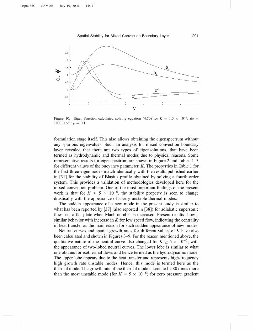
Some representative eigenfunctions have been shown in Figures 10 and 11,that have been obtained by solving (40) from the wall to the free stream,with a prescribed function value (φr = 1) at the wall. Once again, the use ofCMM allows a straightforward integration of the equation without any specialtreatment. For this equation, the second compounds are the variable coefficientsand they were obtained earlier with 2000 interior sub-intervals. Hence theusage of Runge–Kutta method yields solutions at 1000 points located at equalintervals between Y∞ and zero. It is noted that the eigenfunction is obtained interms of the three modes that decay with height—whose asymptotic variationis given by (26). Depending on the eigenvalue, one can associate a physical
sapm˙355 SAM.cls July 19, 2006 14:17
290 T. K. Sengupta and K. V. Subbaiah
Table 4Q1
Case K Re1cr Re2
cr ω1cr ω2
cr Rem km1i km2
i
1 0.0 519.01 – 0.120 – – −0.007464 –2 1.0 × 10⁻⁶ 513.6 – 0.121 – – −0.01355 –3 3.0 × 10⁻⁶ 503.4 – 0.123 – – −0.01577 –4 4.0 × 10⁻⁶ 498.3 – 0.124 – – −0.01706 –5 4.5 × 10⁻⁶ 495.9 – 0.125 – – −0.01725 –6 5.0 × 10⁻⁶ 493.5 230.49 0.127 2.174 5298.5 −0.01745 −0.5682977 1.0 × 10⁻⁵ 470.9 174.40 0.128 2.160 2524.4 −0.01810 −0.4955178 1.5 × 10⁻⁵ 449.7 148.80 0.131 2.182 1658.2 −0.01831 −0.4574919 2.0 × 10⁻⁵ 433.5 133.34 0.136 2.211 1240.1 −0.01844 −0.4323710 3.0 × 10⁻⁵ 401.1 112.00 0.144 2.104 838.2 −0.01858 −0.399403
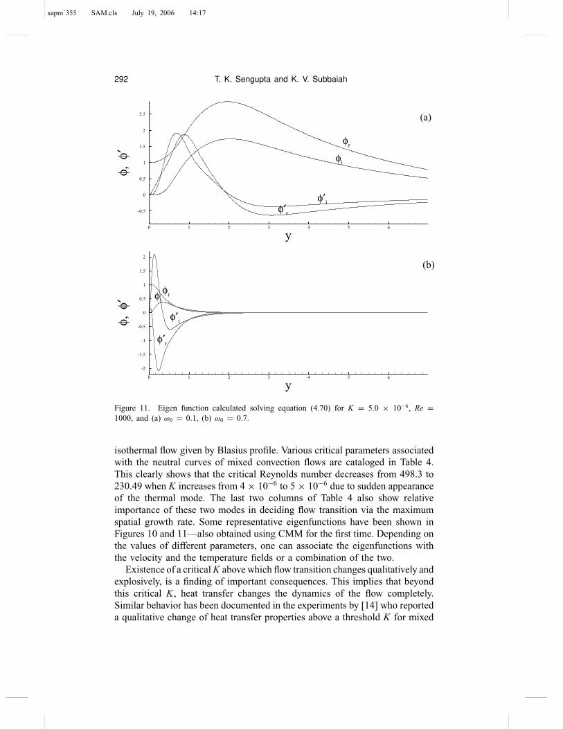
variable with this eigenfunction. For example, Figure 10 corresponds to a casefor which the hydrodynamic mode is predominant and for the choice ofparameters (K = 1 × 10⁻⁶; Re = 1000; and ω0 = 0.1), the eigenfunctionrepresents an unstable mode with the highest growth rate. It is also seen thatthe depicted eigenfunctions (φ and φ′) represent the normal and streamwisecomponents of disturbance velocity. In Figure 11, two sets of eigenfunctionsare shown for the case with K = 5 × 10⁻⁶ and Re = 1000. In Figure 11(a),the case corresponds to ω0 = 0.1 for which the hydrodynamic mode attainsits maximum growth and thus the eigenfunctions once again represent thedisturbance velocity components. In Figure 11(b), the case corresponds toω0 = 0.7 and the eigenvalue for this case indicates the thermal mode to beat its maximum growth rate. Hence the plotted function corresponds to thedisturbance temperature field.
6. Conclusions and outlook
Results of an analysis has been presented here for spatial stability propertiesof a mixed convection boundary layer developing over a heated horizontal flatplate. A similarity solution (as given by (13) and (15)) for the mean flow isused following [1]. Such boundary layers are characterized by the buoyancyparameter (K = Gr/Re5/2) and is solved only for adiabatic wall conditions.
Under the parallel flow approximation, the spatial stability problem has beenformulated using the compound matrix method (CMM)—based on previouswork of [30], [32], and [27] for hydrodynamic stability problems. One ofthe advantages of CMM is that it allows solving stability problems usingtraditional ODE solver—as the stiffness of the equation is removed at the
sapm˙355 SAM.cls July 19, 2006 14:17
Spatial Stability for Mixed Convection Boundary Layer 291
y
φ,φ′
0 1 2 3 4 5 6
-0.5
0
0.5
1
1.5
2
2.5
φr
φi
φ′rφ′i
Figure 10. Eigen function calculated solving equation (4.70) for K = 1.0 × 10⁻⁶, Re =1000, and ω0 = 0.1.
formulation stage itself. This also allows obtaining the eigenspectrum withoutany spurious eigenvalues. Such an analysis for mixed convection boundarylayer revealed that there are two types of eigensolutions, that have beentermed as hydrodynamic and thermal modes due to physical reasons. Somerepresentative results for eigenspectrum are shown in Figure 2 and Tables 1–3for different values of the buoyancy parameter, K. The properties in Table 1 forthe first three eigenmodes match identically with the results published earlierin [31] for the stability of Blasius profile obtained by solving a fourth-ordersystem. This provides a validation of methodologies developed here for themixed convection problem. One of the most important findings of the presentwork is that for K ≥ 5 × 10⁻⁶, the stability property is seen to changedrastically with the appearance of a very unstable thermal modes.
The sudden appearance of a new mode in the present study is similar towhat has been reported by [37] (also reported in [38]) for adiabatic supersonicflow past a flat plate when Mach number is increased. Present results show asimilar behavior with increase in K for low speed flow, indicating the centralityof heat transfer as the main reason for such sudden appearance of new modes.
Neutral curves and spatial growth rates for different values of K have alsobeen calculated and shown in Figures 3–9. For the reason mentioned above, thequalitative nature of the neutral curve also changed for K ≥ 5 × 10⁻⁶, withthe appearance of two-lobed neutral curves. The lower lobe is similar to whatone obtains for isothermal flows and hence termed as the hydrodynamic mode.The upper lobe appears due to the heat transfer and represents high-frequencyhigh growth rate unstable modes. Hence, this mode is termed here as thethermal mode. The growth rate of the thermal mode is seen to be 80 times morethan the most unstable mode (for K = 5 × 10⁻⁶) for zero pressure gradient
sapm˙355 SAM.cls July 19, 2006 14:17
292 T. K. Sengupta and K. V. Subbaiah
y
φ,φ′
0 1 2 3 4 5 6
-0.5
0
0.5
1
1.5
2
2.5
φr
φi
φ′rφ′i
(a)
y
φ,φ′
0 1 2 3 4 5 6
-2
-1.5
-1
-0.5
0
0.5
1
1.5
2
φrφi
φ′r
φ′i
(b)
Figure 11. Eigen function calculated solving equation (4.70) for K = 5.0 × 10⁻⁶, Re =1000, and (a) ω0 = 0.1, (b) ω0 = 0.7.
isothermal flow given by Blasius profile. Various critical parameters associatedwith the neutral curves of mixed convection flows are cataloged in Table 4.This clearly shows that the critical Reynolds number decreases from 498.3 to230.49 when K increases from 4 × 10⁻⁶ to 5 × 10⁻⁶ due to sudden appearanceof the thermal mode. The last two columns of Table 4 also show relativeimportance of these two modes in deciding flow transition via the maximumspatial growth rate. Some representative eigenfunctions have been shown inFigures 10 and 11—also obtained using CMM for the first time. Depending onthe values of different parameters, one can associate the eigenfunctions withthe velocity and the temperature fields or a combination of the two.
Existence of a critical K above which flow transition changes qualitatively andexplosively, is a finding of important consequences. This implies that beyondthis critical K, heat transfer changes the dynamics of the flow completely.Similar behavior has been documented in the experiments by [14] who reporteda qualitative change of heat transfer properties above a threshold K for mixed

sapm˙355 SAM.cls July 19, 2006 14:17
Spatial Stability for Mixed Convection Boundary Layer 293
convection flow over a hot isothermal plate. Our calculation reveals similarorder of value of K between the experiment and our calculated results. Thedifference is due to different boundary conditions required for the similarity tohold for the mean profile and the difference between the Kcr calculated herewith the corresponding integral property (Kt) of the experiment. The existenceof such Kcr would be of prime importance, whenever convective heat transferprocess is involved in fluid flow—as in atmospheric boundary layer. It wouldalso be interesting to investigate spatial stability properties of heat convectingflows past vertical and inclined plates. The existence of the violent thermalmode also shows the need to re-evaluate transition prediction methodologiesfor flow problems involving heat transfer—and these will be attempted in ourfuture investigations.
Appendix: Compound matrix method for mixed convection problem
The general methods for fourth- and sixth-order order system are as given in[30] and the specific formulation presented here is for the sixth-order systemfor mixed convection flow. In [29], other references are listed, where thecompound matrices have been used to integrate stiff linear system withoutrequiring any orthogonalization process. To our knowledge, CMM has notbeen used for the study of stability of mixed convection flow before—in [27],CMM is used for the sixth-order system defining a problem of hydrodynamicstability and the present study is similar in mathematical scope.
While the general method can be found in [30], [27], and [29], only theessential details are given here for the mixed convection instability problem.In this method an induced system is constructed, determined by the set ofasymptotic boundary conditions at y = Y∞ that in turn is governed by theanalytic nature of solution at y → ∞. This procedure converts the originalboundary value problem into an initial value problem, while removing thestiffness of the differential system. For the sixth-order system, this is equivalentto projecting the solution on a subspace of C 6, with the help of three decayingboundary conditions for y → Y∞, following the notations of [27], into�3(C 6). Similarly, the boundary conditions at y = 0 defines a secondthree-dimensional subspace of C 6. The problem is thus reduced to linkingthese two three-dimensional subspaces satisfying Equation (27). Any subspacespanned by three linearly independent vectors {φ1, φ3, φ5} (as defined inEquation (26)), is represented notationally as a point φ1�φ3�φ5, in the vectorspace �3(C 6), where � is the wedge product ([27]).
Let us introduce the following basis e1 = [φ1, φ3, φ5]; e2 = [φ1′, φ3
′, φ5′];
e3 = [φ1′′, φ3
′′, φ5′′]; e4 = [φ1
′′′, φ3′′′, φ5
′′′]; e5 = [φiv1 , φiv
3 , φiv5 ]; and e6 = [φv
1, φv3,
φv5 ] in C 6, then all the elements of ei�ej�ek form the basis for �3(C 6) with
the dimension 6!3!3! = 20. The solution matrix [φ1φ3φ5], thus has twenty (3 ×
3) minors—that are also called the second compound [30] denoted by
sapm˙355 SAM.cls July 19, 2006 14:17
294 T. K. Sengupta and K. V. Subbaiah
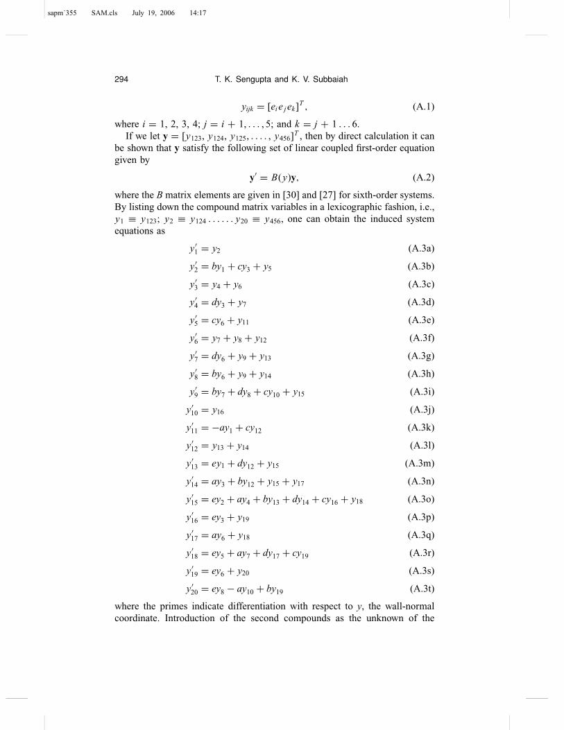
yijk = [ei e j ek]T , (A.1)
where i = 1, 2, 3, 4; j = i + 1, . . . , 5; and k = j + 1 . . . 6.If we let y = [y123, y124, y125, . . . . , y456]T , then by direct calculation it can
be shown that y satisfy the following set of linear coupled first-order equationgiven by
y′ = B(y)y, (A.2)
where the B matrix elements are given in [30] and [27] for sixth-order systems.By listing down the compound matrix variables in a lexicographic fashion, i.e.,y1 ≡ y123; y2 ≡ y124 . . . . . . y20 ≡ y456, one can obtain the induced systemequations as
y′1 = y2 (A.3a)
y′2 = by1 + cy3 + y5 (A.3b)
y′3 = y4 + y6 (A.3c)
y′4 = dy3 + y7 (A.3d)
y′5 = cy6 + y11 (A.3e)
y′6 = y7 + y8 + y12 (A.3f)
y′7 = dy6 + y9 + y13 (A.3g)
y′8 = by6 + y9 + y14 (A.3h)
y′9 = by7 + dy8 + cy10 + y15 (A.3i)
y′10 = y16 (A.3j)
y′11 = −ay1 + cy12 (A.3k)
y′12 = y13 + y14 (A.3l)
y′13 = ey1 + dy12 + y15 (A.3m)
y′14 = ay3 + by12 + y15 + y17 (A.3n)
y′15 = ey2 + ay4 + by13 + dy14 + cy16 + y18 (A.3o)
y′16 = ey3 + y19 (A.3p)
y′17 = ay6 + y18 (A.3q)
y′18 = ey5 + ay7 + dy17 + cy19 (A.3r)
y′19 = ey6 + y20 (A.3s)
y′20 = ey8 − ay10 + by19 (A.3t)
where the primes indicate differentiation with respect to y, the wall-normalcoordinate. Introduction of the second compounds as the unknown of the
sapm˙355 SAM.cls July 19, 2006 14:17
Spatial Stability for Mixed Convection Boundary Layer 295
problem, helps remove the stiffness of the problem, thereby allowing anystandard integration procedure to integrate (A.3). However, we have alsomentioned before that the usage of asymptotic boundary conditions at y →∞ allows us to convert the boundary value problem to an initial valueproblem—that is discussed next.
A.1. Initial conditions for the induced system
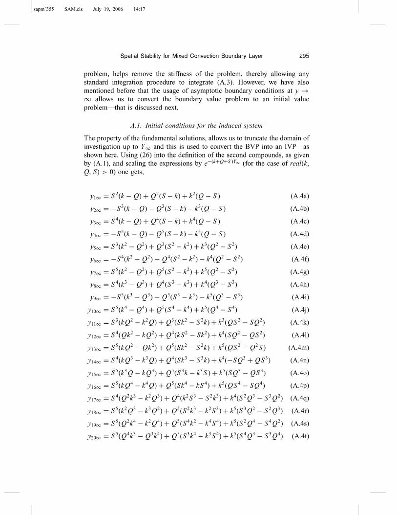
The property of the fundamental solutions, allows us to truncate the domain ofinvestigation up to Y∞ and this is used to convert the BVP into an IVP—asshown here. Using (26) into the definition of the second compounds, as givenby (A.1), and scaling the expressions by e−(k+Q+S )Y∞ (for the case of real(k,Q, S) > 0) one gets,
y1∞ = S 2(k − Q) + Q2(S − k) + k2(Q − S ) (A.4a)
y2∞ = −S 3(k − Q) − Q3(S − k) − k3(Q − S ) (A.4b)
y3∞ = S 4(k − Q) + Q4(S − k) + k4(Q − S ) (A.4c)
y4∞ = −S 5(k − Q) − Q5(S − k) − k5(Q − S ) (A.4d)
y5∞ = S 3(k2 − Q2) + Q3(S 2 − k2) + k3(Q2 − S 2) (A.4e)
y6∞ = −S 4(k2 − Q2) − Q4(S 2 − k2) − k4(Q2 − S 2) (A.4f)
y7∞ = S 5(k2 − Q2) + Q5(S 2 − k2) + k5(Q2 − S 2) (A.4g)
y8∞ = S 4(k3 − Q3) + Q4(S 3 − k3) + k4(Q3 − S 3) (A.4h)
y9∞ = −S 5(k3 − Q3) − Q5(S 3 − k3) − k5(Q3 − S 3) (A.4i)
y10∞ = S 5(k4 − Q4) + Q5(S 4 − k4) + k5(Q4 − S 4) (A.4j)
y11∞ = S 3(k Q2 − k2 Q) + Q3(Sk2 − S 2k) + k3(QS 2 − SQ2) (A.4k)
y12∞ = S 4(Qk2 − k Q2) + Q4(kS 2 − Sk2) + k4(SQ2 − QS 2) (A.4l)
y13∞ = S 5(k Q2 − Qk2) + Q5(Sk2 − S 2k) + k5(QS 2 − Q2S ) (A.4m)
y14∞ = S 4(k Q3 − k3 Q) + Q4(Sk3 − S 3k) + k4(−SQ3 + QS 3) (A.4n)
y15∞ = S 5(k3 Q − k Q3) + Q5(S 3k − k3S ) + k5(SQ3 − QS 3) (A.4o)
y16∞ = S 5(k Q4 − k4 Q) + Q5(Sk4 − kS 4) + k5(QS 4 − SQ4) (A.4p)
y17∞ = S 4(Q2k3 − k2 Q3) + Q4(k2S 3 − S 2k3) + k4(S 2 Q3 − S 3 Q2) (A.4q)
y18∞ = S 5(k2 Q3 − k3 Q2) + Q5(S 2k3 − k2S 3) + k5(S 3 Q2 − S 2 Q3) (A.4r)
y19∞ = S 5(Q2k4 − k2 Q4) + Q5(S 4k2 − k4S 4) + k5(S 2 Q4 − S 4 Q2) (A.4s)
y20∞ = S 5(Q4k3 − Q3k4) + Q5(S 3k4 − k3S 4) + k5(S 4 Q3 − S 3 Q4). (A.4t)
sapm˙355 SAM.cls July 19, 2006 14:17
296 T. K. Sengupta and K. V. Subbaiah
While evaluating Q and S one can always choose the mode with positive realpart, it is not necessarily so while obtaining the response field by integrating(A.2) along the Bromwich contour when real(k) < 0. In such instances, onecan develop similar initial conditions. It is now easy to see from above as tohow CMM avoids the stiffness of the original problem. While the individualcomponents of the fundamental solutions, as given by (26) decays with heightdifferently due to the disparate value of the characteristic exponents, the secondcompounds y, all have the same decay rate given by the exponent −(k + Q +S)—thereby removing the stiffness. It is for this reason (A.3) can be simplyintegrated as IVP from y = Y∞ to the wall (y = 0) by any ordinary integrator.We have used four-stage Runge–Kutta method for this purpose.
References
1. W. SCHNEIDER, A similarity solution for combined forced and free convection flow overa horizontal plate, Int. J. Heat Mass Transfer 22:1401–1406 (1979).
2. R. A. BREWSTAR and B. GEBHART, Instability and disturbance amplification in amixed-convection boundary layer, J. Fluid Mech. 229:115–133 (1991).
3. B. GEBHART, Y. JALURIA, R. L. MAHAJAN, and B. SAMMAKIA, Buoyancy-Induced Flowsand Transport, Hemisphere Publication, Washington DC, 1988.
4. E. R. G. ECKERT and E. SOEHNGEN, Interferometric studies on the stability and transitionto turbulence in a free-convection boundary-layer, Proc. Gen. Disc. Heat Transfer, ASMEand IME, London, pp. 321, 1951.
5. E. M. SPARROW and R. B. HUSAR, Longitudinal vortices in natural convection flow oninclined plates, J. Fluid Mech. 37:251–255 (1969).
6. J. R. LLOYD and E. M. SPARROW, On the instability of natural convection flow oninclined plates, J. Fluid Mech. 42:465–470 (1970).
7. E. J. ZUERCHER, J. W. JACOBS, and C. F. CHEN, Experimental study of thestability boundary-layer flow along a heated inclined plate, J. Fluid Mech. 367:1–25(1998).
8. T. S. CHEN and A. MOUTSOGLU, Wave instability of mixed convection flow on inclinedsurfaces, Num. Heat Transfer 2:497–509 (1979).
9. S. E. HAALAND and E. M. SPARROW, Vortex instability of natural convection flows oninclined surfaces, Int. J. Heat Mass Transfer 16:2355–2367 (1973).
10. R. S. WU and K. C. CHENG, Thermal instability of Blasius flow along horizontal plates,Int. J. Heat Mass Transfer 19:907–913 (1976).
11. H. SHAUKATULLAH and B. GEBHART, An experimental investigation of naturalconvection flow on an inclined surface, Int. J. Heat Mass Transfer 21:1481–1490(1978).
12. R. R. GILPIN, H. IMURA, and K. C. CHENG, Experiments on the onset of longitudinalvortices in horizontal Blasius flow heated from below, ASME J. Heat Transfer 100:71–77(1978).
13. A. MOUTSOGLU, T. S. CHEN, and K. C. CHENG, Vortex instability of mixedconvection flow over a horizontal flat plate, ASME J. Heat Transfer 103:257–261(1981).
sapm˙355 SAM.cls July 19, 2006 14:17
Spatial Stability for Mixed Convection Boundary Layer 297
14. X. A. WANG, An experimental study of mixed, forced, and free convection heat transferfrom a horizontal flat plate to air, ASME J. Heat Transfer 104:139–144 (1982).
15. P. HALL and H. MORRIS, On the instability of boundary layers on heated flat plates, J.Fluid Mech. 245:367–400 (1992).
16. A. MUCOGLU and T. S. CHEN, Wave instability of mixed convection flow along a verticalflat plate, Num. Heat Transfer 1:267 (1978). Q2
17. T. S. CHEN and A. MUCOGLU, Wave instability of mixed convection flow over a horizontalflat plate, Int. J. Heat Mass Transfer 22:185–196 (1979).
18. P. A. IYER and R. E. KELLY, The stability of the laminar free convection flow induced bya heated, inclined plate, Int. J. Heat Mass Transfer 17:517–525 (1974).
19. A. TUMIN, The spatial stability of natural convection flow on inclined plates, ASME J.Fluid Engg. 125:428–437 (2003).
20. H. STEINRUCK, Mixed convection over a cooled horizontal plate: Non-uniqueness andnumerical instabilities of the boundary layer equations, J. Fluid Mech. 278:251–265(1994).
21. G. E. ROBERTSON, J. H. SEINFELD, and L. G. LEAL, Combined forced and free convectionflow past a horizontal flat plate, AIChE Jour. 19(5):998–1008 (1973).
22. E. M. SPARROW and W. J. MINKOWYCZ, Buoyancy effects on horizontal boundary-layerflow and heat transfer, Int. J. Heat Mass Transfer 5:505 (1962).
23. T. S. CHEN, E. M. SPARROW, and A. MUCOGLU, Mixed convection in boundary layer flowon a horizontal plate, ASME J. Heat Transfer 99:66–71 (1977).
24. P. G. DRAZIN and W. H. REID, Hydrodynamic Stability, Cambridge University Press,Cambridge, U.K., 1981.
25. P. J. SCHMID and D. S. HENNINGSON, Stability and Transition in Shear Flows, SpringerVerlag, New York, USA, 2001.
26. T. J. BRIDGES and P. MORRIS, Differential eigenvalue problems in which the parametersappear nonlinearly, J. Comp. Phys. 55:437–460 (1984).
27. L. ALLEN and T. J. BRIDGES, Hydrodynamic stability of the Ekman boundary layerincluding interaction with a compliant surface: A numerical framework, European J.Mechanics B/Fluids 22:239–258 (2003).
28. P. MORESCO and J. J. HEALEY, Spatio-temporal instability in mixed convection boundarylayers, J. Fluid Mech. 402:89–107 (2000).
29. L. ALLEN and T. J. BRIDGES, Numerical exterior algebra and the compound matrixmethod, Numerische Mathematik 92:197–232 (2002).
30. B. S. NG and W. H. REID, The compound matrix method for ordinary differentialsystems, J. Comp. Phys. 58:209–228 (1985).
31. T. K. SENGUPTA, M. BALLAV, and S. NIJHAWAN, Generation of Tollmien-Schlichtingwaves by harmonic excitation, Phys. Fluids 6:1213–1222 (1994).
32. T. K. SENGUPTA, Solution of Orr-Sommerfeld equation for high wave numbers, ComputersFluids 21(2):301–303 (1992).
33. L. BRILLOUIN, Wave Propagation and Group Velocity, Academic Press, New York (USA),1960.
34. B. VANDER POL and H. BREMMER, Operational Calculus Based On Two-Sided LaplaceIntegral, Cambridge University Press, U.K., 1959.
35. T. K. SENGUPTA, M. T. NAIR, and V. RANA, Boundary layer excited by low frequencydisturbances-Klebanoff mode, J. Fluid Struct. 11:845–853 (1997).

sapm˙355 SAM.cls July 19, 2006 14:17
298 T. K. Sengupta and K. V. Subbaiah
36. G. B. SCHUBAUER and H. K. SKRAMSTAD, Laminar boundary layer oscillations and thestability of laminar flow, J. Aero. Sci. 14(2):69–78 (1947).
37. L. M. MACK, Boundary layer stability theory, Doc. 900-277, Rev. A Jet Prop. Lab,Pasadena, Calif, 1969.
38. F. M. WHITE, Viscous Fluid Flow, McGraw Hill Int. Edn., New York, USA, 1991.
INDIAN INSTITUTE OF TECHNOLOGY, KANPUR
(Received January 26, 2006)
sapm˙355 SAM.cls July 19, 2006 14:17
Queries
Q1 Author: Please provide the caption of Table 4.
Q2 Author: Please provide complete page range in references 16 and 22.
299