ORI GIN AL ARTICLE

Spatial Preference Modelling for equitableinfrastructure provision: an applicationof Sen’s Capability Approach

Arif Wismadi • Mark Zuidgeest • Mark Brussel •

Martin van Maarseveen

Received: 22 March 2012 / Accepted: 27 March 2013 / Published online: 21 April 2013

� Springer-Verlag Berlin Heidelberg 2013

Abstract To determine whether the inclusion of spatial neighbourhood compar-

ison factors in Preference Modelling allows spatial decision support systems

(SDSSs) to better address spatial equity, we introduce Spatial Preference Modelling

(SPM). To evaluate the effectiveness of this model in addressing equity, various

standardisation functions in both Non-Spatial Preference Modelling and SPM are

compared. The evaluation involves applying the model to a resource location-

allocation problem for transport infrastructure in the Special Province of Yogya-

karta in Indonesia. We apply Amartya Sen’s Capability Approach to define

opportunity to mobility as a non-income indicator. Using the extended Moran’s

I interpretation for spatial equity, we evaluate the distribution output regarding, first,

‘the spatial distribution patterns of priority targeting for allocation’ (SPT) and,

second, ‘the effect of new distribution patterns after location-allocation’ (ELA). The

Moran’s I index of the initial map and its comparison with six patterns for SPT as

well as ELA consistently indicates that the SPM is more effective for addressing

A. Wismadi (&) � M. Zuidgeest � M. Brussel � M. van Maarseveen

Faculty of Geo-Information Science and Earth Observation (ITC), University of Twente,

Hengelosestraat 99, P.O. Box 6, 7500 AA Enschede, The Netherlands

e-mail: wismadi@itc.nl; wismadi@yahoo.com; arif.wismadi@ugm.ac.id

URL: http://www.itc.nl

M. Zuidgeest

e-mail: m.h.p.zuidgeest@utwente.nl

M. Brussel

e-mail: m.j.g.brussel@utwente.nl

M. van Maarseveen

e-mail: m.f.a.m.vanmaarseveen@utwente.nl

A. Wismadi

Center for Transportation and Logistics Studies (PUSTRAL), Universitas Gadjah Mada,

Jl. Kemuning M-3, Sekip, Yogyakarta 55281, Indonesia

URL: http://www.pustral.ugm.ac.id

123

J Geogr Syst (2014) 16:19–48

DOI 10.1007/s10109-013-0185-4

spatial equity. We conclude that the inclusion of spatial neighbourhood comparison

factors in Preference Modelling improves the capability of SDSS to address spatial

equity. This study thus proposes a new formal method for SDSS with specific

attention on resource location-allocation to address spatial equity.

Keywords Capability Approach � Spatial and social equity � Location-allocation �Spatial Preference Modelling � Spatial decision support system

JEL Classification R53 � R58

1 Introduction

In 1968, the theory of social equity was developed as the third pillar of public

administration in addition to ‘economy’ and ‘efficiency’ (Frederickson 1990).

Social equity concerns fair access to resources and livelihood. One of the possible

means of governmental interventionism towards social equity is the distribution of

public services (e.g., infrastructure provision) based on characteristics such as the

age, health, wealth, sex, and geographical location of people (Chitwood 1974).

Typically, distributional patterns are evaluated in terms of social equity (achieving

equity over socio-economic groups of society) or spatial equity (achieving equity

over geographical locations).

Decisions leading to an inequitable distribution of public services can result in

social tensions. Following protests in Indonesia in 1997 and 1998, government

reforms were implemented and resulted in a more decentralised governmental

system. This trend of governance and fiscal decentralisation is currently occurring in

many other countries (Neyapti 2010). Surprisingly, although such resource

allocations for infrastructure investment in decentralising systems aim to better

accommodate local preferences, authors such as Neyapti (2010) and Kyriacou and

Roca-Sagales (2011) note that efficiency decreases in countries with local or

regional elections. These authors argue that decentralised systems in conjunction

with a system of local elections result in local politicians having decision biases in

the distribution of resources to their constituents.

Efforts to counter this decision bias are complicated by the absence of decision

support tools that allow for a more balanced allocation of resources in such a

decentralised context (bottom–up, reflecting local preferences) but that also

consider national processes and requirements (top–down, reflecting national pro-

poor, pro-growth, and pro-jobs policies, where pro-poor stands for the equity

objective). Without such tools, stakeholders cannot effectively evaluate how each

infrastructure project in their region or under their responsibility is expected to

contribute to equitable development.

Decision support systems (DSSs) generally incorporate so-called Preference

Modelling routines to transform preference values from stakeholders into sets of

priorities, such as for location–allocation decisions (Tsoukias 1991; Perny and Roy

1992; Benferhat et al. 2006; Piccolo and D’Elia 2008; Roberts and Tsoukias 2009).

Spatial decision support systems (SDSSs) aim to assist decision-making related to

20 A. Wismadi et al.

123

spatial issues such as land use decisions. However, although the priority settings in

SDSS are mostly presented in maps, the computations often disregard the spatial

equity aspect. For instance, a ‘standard’ Preference Modelling typically focuses on

making global comparisons, whereas, in real life, there may be significant local and

neighbourhood effects; for example, the sense of inequity of an individual is usually

stronger in local comparisons than in global comparisons. In addition, the sense of

inequity is supposed to decrease with a greater distance between two objects. The

implementation of global comparisons in Preference Modelling, which often

overlooks local and neighbourhood variations, might therefore negatively affect the

effectiveness of resource allocation.

Moreover, infrastructure resource allocation at lower administrative levels (e.g.,

the village level) requires special attention to the co-existence of infrastructures in a

location and infrastructures in its neighbouring areas. Infrastructure systems,

particularly networks of linear infrastructures, such as roads, typically exhibit high

levels of interconnectivity and therefore require neighbourhood-inclusive analysis

techniques in decision-making for resource allocation. Disregarding this connec-

tivity jeopardises the function of infrastructure systems in a society and may

therefore lead to inefficient location-allocation. Wismadi et al. (2012) previously

disclosed the importance of adding neighbourhood information to village-level

infrastructure–economy interaction modelling.

In the context of neighbourhood comparisons, the well-known statistical measure

of spatial autocorrelation enables quantification of the degree of difference among

values of the same variables of an object with other surrounding objects. One of such

measurements is Moran’s I index (Shortridge 2007). Although this approach has been

widely used to quantify spatial distributions (e.g., Overmars et al. 2003; Ping et al.

2004; Tsou et al. 2005; Tsai 2005), the inclusion of this concept within a resource

allocation mechanism to address social and spatial equity at a local level cannot be

found in the current literature. With the growing number of pro-poor programmes and

attention to equity issues, knowledge of equity-based resource allocation has become

critical, particularly in situations where priority setting typically faces efficiency–

equity trade-offs and/or budget constraint issues (Cho 1998; Bibi and Duclos 2007;

Cherchye et al. 2010). This budget allocation issue is even more complex in the

context of the recent decentralisation of administrations in Indonesia.

The purpose of this study is therefore to determine whether the inclusion of

spatial neighbourhood comparison factors in Preference Modelling, that is, Spatial

Preference Modelling, can improve the capability of SDSS in resource location-

allocation for addressing spatial equity. To this end, we compare Spatial Preference

Modelling (SPM) with the more common (Non-Spatial) Preference Modelling

(NSPM) approach. We develop SPM by extending the Moran’s I Scatter Plot

formulation and combine it with a linear scale transformation method that is

commonly applied in Preference Modelling. This SPM is expected to result in a

more equitable allocation. The comparison is performed for the allocation of

transport infrastructure resources in Yogyakarta, a region with 438 urban and rural

villages in Indonesia. This region is highly diverse in terms of topography, level of

urbanisation and modernity, road infrastructure, transport modes, and traffic

volumes.

An application of Sen’s Capability Approach 21

123

The paper is organised as follows: Sect. 2 discusses the methodology of

Preference Modelling, its formulation, the data requirements and the analytical

framework. Section 3 presents the results of each Preference Modelling approach.

Section 4 discusses the most important findings; conclusions and policy implica-

tions follow in Sect. 5.

2 Methodology

2.1 Research design

We compare two methods of Preference Modelling: First, NSPM, a more common

method that disregards spatial features and their neighbourhood effects, and second,

SPM, which includes spatial neighbouring objects in the equity measure.

For both methods, we investigate three possible ways for stakeholders to perceive

the gaps between object values. First, the gap is defined as the distance between the

values and zero as well as between the values and the maximum value within the

set. Second, the gap is defined as the interval between the lowest and the highest

values. Third, the gap is defined as the distance between the values and a set of pre-

determined policy goals. These gaps are operationalised through three common

standardisation procedures: maximum standardisation, interval standardisation and

goal standardisation (Beedasy and Whyatt 1999; Xiang 2001; Sharifi and van

Herwijnen 2001; Phua and Minowa 2005; Ananda and Herath 2009). As such, we

evaluate six preference models in terms of their effectiveness in addressing spatial

equity for a resource location-allocation problem.

The process is conducted in two stages; we evaluate, first, the effectiveness of the

models at addressing ‘the spatial distribution patterns of priority targeting for

allocation’ (SPT) and, second, their ‘effect on the new distribution patterns after

location-allocation’ (ELA). The evaluation is performed by comparing the Moran’s

I index of an initial map with the six mapped patterns from the SPT and ELA

analyses. The discussion then focuses on the interpretation of the results and the

policy implications with regard to a more equitable resource allocation.

For the case study, we develop and apply a resource location-allocation model for

transport infrastructure in the Special Province of Yogyakarta, Indonesia. Specif-

ically, the distributed allocation is framed in terms of ‘opportunity to mobility’

rather than monetary units or construction materials. This notion is derived from the

Amartya Sen’s Capability Approach, which is discussed in the next section.

2.2 Sen’s Capability Approach in preference modelling

To achieve an equitable distribution, it is important to define the concept of equity.

The notions of equality, equity and redistribution are linked concepts and are

strongly related to governmental interventionism. The concept of ‘equality’ in

particular denotes that everyone is at the same level. From an economic perspective,

the term implies that incomes are shared in a homogenous way (Garcia-Valinas

et al. 2005). To counter inequality, governments must intervene and reduce strong

22 A. Wismadi et al.

123

income differences. For ‘equality’, not only should poor people be less poor, but the

rich should also be less rich. A common ‘equality’ measurement is the Gini index.

Equality requires redistribution of resources among groups, which is often

problematic to implement. Therefore, the notion of ‘equity’ replaces the more

radical notion of equality. Equity represents fairness, or the equality of outcomes,

and involves attention to disadvantaged groups in the system towards accessing

equality of outcome. As an analogy, ‘equality’ involves a ‘floor’ and a ‘ceiling’,

whereas ‘equity’ only entails a minimum ‘floor’ (Garcia-Valinas et al. 2005). In

measuring poverty, the ‘floor’ is commonly known as the ‘poverty line’. As such,

the term ‘equity’ is more reasonable in a practical context. Equity is also very

relevant to infrastructure development, which aims to provide minimum service

levels so that people can access certain levels of economic opportunity.

In line with the concept of equity, Sen (1980) developed the Capability Approach,

which defines individual opportunity as the capability to achieve essential functioning.

The approach provides a general way of evaluating social arrangements and a particular

way of viewing assessments of equality and inequality (Sen 1992). Hence, one of the

central notions in the Capability Approach relates to equity aspects or the equality of

opportunity (Lelkes 2006; Cabrales and Calvo-Armengol 2008). In the Capability

Approach, the level of opportunity is measured not only by an income indicator but also

by non-income indicators. For example, the performance of transport infrastructure and

its services indicate the opportunity or capability of movement (Deneulin 2008).

Although the Capability Approach has been discussed widely in the literature

(e.g., Dworkin 1981a, b; Nussbaum 2003; Sen 2004; Sudgen 2006; Lelkes 2006;

Gasper 2007 and Qizilbash 2011), its implementation is still limited to social equity

assessment, particularly at national levels (e.g., in terms of the Human Development

Index). However, when addressing both social and spatial equity issues, a more

appropriate level of assessment is usually needed at the local level where

communities exist, for example, in terms of income-generating activities in a

village. This requirement can be illustrated by looking at national-level develop-

ment policies, in which a government such as Indonesia—or a politician during

election periods—declares a target economic growth of, for example, 10 %. This

10 % growth is cited as a ‘two-digit’ optimistic target (Yuan et al. 2008; Ohana

2010; Chen 2010) of national development. This target should then be pursued by

improving infrastructure performance (among other things), which enables people

to engage in economic activities. The distribution of the target growth, however, is

often overlooked at the disaggregate level, for example, the village level. In this

study, resource allocation thus refers to the distribution of (targeted) levels of

growth or increasing levels of opportunity in each village in the study area.

In addition to the above concept, this study introduces the Capability Approach

within Preference Modelling for the allocation of transport infrastructure resources

at the village level in Yogyakarta Special Province, Indonesia. Among other types

of infrastructure (e.g., water, electricity, telecommunication), transport infrastruc-

ture and services provide the opportunity for people to move, meet other people,

interact, and carry out transactions. Hence, for this research, we derive data on

travel time budgets and transport infrastructure performance as an indicator of

capability or opportunity for mobility.

An application of Sen’s Capability Approach 23

123

To operationalise Sen’s Capability Approach, we also include an opportunity

benchmark (e.g., a poverty line) in the model. In a standard Preference Modelling, a

benchmark is represented through a goal standardisation procedure. The benchmark is

also known as the policy achievement target that defines the ‘floor’ or basic capability

in the equity concept. Moreover, according to Sen (1980), the notion of the equality of

basic capability is very general, whereas any application of it must be culturally

dependent. In the field of infrastructure development, this issue of cultural

dependency is related to the capability of the community to properly adapt to an

increased capacity of new infrastructure, which often involves a new type of

technology. In a very diverse region, the idea of applying a single absolute benchmark

for the whole population might not be appropriate; therefore, specific benchmarks

with reference to each local condition should be introduced. In this research, SPM

captures the level of equity among neighbourhoods to define the relative benchmark.

Hence, we introduce two types of benchmarks, the absolute benchmark and the

relative benchmark. The absolute benchmark is the minimum level of opportunity

required as defined by the policy maker and applied to the whole region, whereas

the relative benchmark is derived from gaps in opportunity in relation to the level of

opportunities in neighbouring villages. There are two reasons for using the relative

benchmark. The first reason is to accommodate efficiency–equity trade-offs and

avoid an idle capacity of the provided infrastructure due to a lack of utilisation.

Comparison with only one absolute value of benchmark might result in an extreme

gap. This gap could result in an overinvestment or underutilised infrastructure.

Accordingly, the second reason for the use of the relative benchmark is related to

the issue of the adaptive capacity of the community. In an attempt to mend an

extreme gap, infrastructure of an inappropriate level may be introduced to which

communities will find themselves unable to adapt. This study intends to provide a

workable application to operationalise Sen’s Capability Approach for an equity-

based resource location-allocation problem. In the next section, we discuss the

implementation of the NSPM and SPM methods.

2.2.1 Standardisation without spatial neighbouring comparison features

Preference Models typically include a decision rule based on a difference of ranking

between two objects. To compare objects, the common method of linear scale

transformation is applied to convert the original criterion scores into standardised

scores of utility (Xiang 2001; Malczewski 2004; Ananda and Herath 2009). This

method uses two types of preference criteria: benefit criteria, which refer to a

stakeholder’s preference for the highest raw score (higher scores correspond to greater

preference), and cost criteria, which refer to a stakeholder’s preference to choose the

object with the lowest raw score (lower scores correspond to greater preference).

With NSPM, the three common sets of standardisation procedures, that is,

maximum, interval and goal standardisations, are considered (Beedasy and Whyatt

1999; Xiang 2001; Sharifi and van Herwijnen 2001; Phua and Minowa 2005;

Ananda and Herath 2009).

Maximum standardisation produces scores on a ratio scale with a linear function

between 0 and the highest absolute score. For the benefit criteria, the absolute

24 A. Wismadi et al.

123

highest score is standardised to 1, whereas for the cost criteria, the lowest score

becomes 1 (Eqs. 1, 2). The advantage of maximum standardisation is that the

standardised values are proportional to the original values. However, a small

difference between alternatives is not clearly visible.

The following notations are used in Eqs. 1–6:

Pi = the priority score for unit i; the unit is a spatial target for resource location-

allocation

xi = the score of unit i

max x = the highest absolute score in dataset x

min x = the lowest absolute score in dataset x

min G = a specific goal reference point to the lowest value of a user-specified

range

max G = a specific goal reference point to the highest value of a user-specified

range

The following equation provides the benefit criteria for maximum standardisation:

Pi ¼xi

max xð1Þ

The following equation provides the cost criteria for maximum standardisation:

Pi ¼ �xi �min x

max x

� �þ 1 ð2Þ

Interval standardisation produces a score that is normalised with a linear

function between the absolute lowest score and the highest score (Eqs. 3, 4). For a

benefit effect, the absolute highest score is indicated with a value of 1, and the

absolute lowest score is indicated with a value of 0. For the cost effect, the score

indications are opposite. This standardisation implies a relative scale and aims to

exaggerate differences.

The following equation provides the benefit criteria for interval standardisation:

Pi ¼xi �min x

max x�min xð3Þ

The following equation provides the cost criteria for interval standardisation:

Pi ¼ �xi �min x

max x�min x

� �þ 1 ð4Þ

Goal standardisation is similar to interval standardisation but assigns specific

reference points within the range of unit i scores (Eqs. 5, 6). The reference points

are an ideal or goal value and a minimum or maximum value that is acceptable for

decision makers. Goal standardisation also defines the range of values to

standardise, that is, the goal range G. A meaningful minimum value for G is often

the score in the no-action alternative or the score of the worst possible alternative.

This method produces a clear, real meaning that is independent of the alternatives

being evaluated.

An application of Sen’s Capability Approach 25

123

The following equation provides the benefit criteria for goal standardisation:

Pi ¼xi �min G

max G�min Gð5Þ

The following equation provides the cost criteria for goal standardisation:

Pi ¼ �xi �min G

max G�min G

� �þ 1 ð6Þ

For the NSPM calculations, only cost criteria are used, that is, areas with lower

scores (i.e., lower infrastructure performance) should be given preference in

allocating resources.

2.2.2 Standardisation including spatial neighbourhood comparison features

To include spatial neighbourhood comparison features in the Preference Modelling,

we extend the NSPM with a spatial autocorrelation feature, which is achieved

through an extension of Moran’s I Scatter Plot. Moran’s I can be interpreted as the

correlation between a spatial variable Xi and a spatial lag variable Xlagi, which is

formed by averaging all the values of neighbouring polygons of Xi. Xlagiis

calculated by using a neighbourhood connectivity rule for the weights Wij, which

represent the connectivity between neighbouring units of j; Wij equals 1 if locations

i and j are adjacent or connected and zero otherwise (in addition, Wii = 0 because a

region cannot be adjacent to itself). Two types of neighbourhood connectivity (e.g.,

Queen and Rook) are commonly applied in spatial statistics software (e.g., GeoDA).

A Queen weights matrix defines a location’s neighbours as those with either a

shared border or vertex (in contrast to a Rook weights matrix, which only includes

shared borders). In a regular grid, neighbours according to the Rook criterion would

be cells to the north, south, west and east but not those to the northwest or southeast.

In the context of Indonesia, the spatial forms of villages and their configurations are

more organic and irregular as opposed to the regular forms of rectangular or block

systems that are found in some other countries. Hence, we apply the Queen matrix

because it better represents the actual village neighbourhood connectivity than the

Rook matrix.

In the calculation, weights are row standardised accordingly (Bivand et al. 2009;

Feser and Sweeney 2006). A graphical explanation of the row standardisation

method is presented in Fig. 1 below.

Before implementing a linear scale transformation method, we standardise the

raw input values of x, xi into Xi and xlagiinto Xlagi

. For both xi and xlagi,

standardisations are based on the raw dataset of x; therefore, the mean and standard

deviation (SD) of x are applied to the following formulae, (Eq. 7) and (Eq. 8):

Xi ¼ ðxi � �xÞ=SDðxÞ ð7ÞXlagi¼ ðxlagi

� �xÞ=SDðxÞ ð8Þ

with the variables defined as follows: x = is a set of raw input values of x;

�x = mean of x; xi = x in the location of i; xlagi= xlag is the average of x values on

the neighbouring polygons of i; SD (x) = standard deviation of all x.

26 A. Wismadi et al.

123

Fig

.1

Exam

ple

of

the

row

stan

dar

diz

atio

nm

ethod

(So

urc

eF

eser

and

Sw

een

ey2

00

6)

An application of Sen’s Capability Approach 27

123

In the Moran’s Scatter Plot, a scatter diagram between X and Xlag (also denoted as

W_X in a Moran’s Scatter Plot) for all locations of i is generated, which is used to

obtain the Moran’s I index. In our model, we used these values as the spatial feature

to be included in the Preference Modelling. As such, the traditional NSPM

Preference Modelling becomes a Spatial Preference modelling (SPM). Specifically,

we defined the local inequity gi, or the gap values between a location i, as Xi, and its

neighbouring units as Xlagi(Eq. 9), where a positive gi indicates high local inequity,

0 indicates equity and a negative gi indicates that the location i has a better condition

and no priority for allocation.

gi ¼ Xlagi� Xi ð9Þ

We then apply a linear scale transformation method to the local inequity gi in

location i to obtain the preference for allocation. Three standardisation procedures

similar to NSPM (i.e., maximum, interval and goal standardisation) are applied as

discussed below.

Maximum standardisation in SPM produces a linear function between 0 and the

highest score in the neighbouring units (Eqs. 10, 11).

We define benefit criteria for maximum standardisation of SPM as follows:

Pi ¼ Wij

gi

max g_

� �ð10Þ

The cost criteria for maximum standardisation of SPM are defined as follows:

Pi ¼ Wij

min g^ð Þ � gi

max g_

þ 1

� �ð11Þ

with the variables defined as follows: Pi = the priority score for unit i; the unit is a

spatial target for resource location-allocation; Wij = the connectivity between i and

its neighbouring units of j, as in Fig. 1; min g^

= minimum value of g of neigh-

bouring units j; max g_

= maximum value of g of neighbouring units j. The symbols

‘\’ and ‘[’ indicate that the max and min values are only obtained for all g at all j

around the unit i, not for all g in the dataset.

Interval standardisation in SPM produces a normalised score with a linear

function between the absolute lowest score and the highest score in the

neighbouring units j (Eqs. 12, 13).

We define the benefit criteria of interval standardisation in SPM as follows:

Pi ¼ Wij

gi � min g_ð Þ

max g_

� �� min g

^� �

24

35 ð12Þ

The cost criteria of interval standardisation in SPM are defined as follows:

Pi ¼ Wij �gi � min g

^ð Þmax g

_� �

� min g^

� �0@

1Aþ 1

24

35 ð13Þ

28 A. Wismadi et al.

123

Goal standardisation in SPM implies putting a constraint on the location-

allocation process (Eqs. 14, 15). For example, the allocation may be restricted only

to locations under the poverty line or within the range of min G and max G. In the

spatial-lag based calculations, the allocation is restricted only to locations below the

average value of neighbouring units, which will act as the poverty line, or the so-

called local benchmark G. The expected result is that spatial inequity among units in

neighbouring groups will decrease.

We define the benefit criteria of goal standardisation in SPM:

Pi ¼WijðgiÞ �min G

max G�min Gð14Þ

The cost criteria of goal standardisation in SPM are defined as follows:

P ¼ � WijðgiÞ �min G

max G�min G

� �þ 1 ð15Þ

In our Preference Modelling, because the input for SPM is the gap calculation gi, we

apply the benefit criteria. Allocation is expected to target those areas with wider

gaps from the benchmark value. If, for example, we set G = 0, the objective is to

obtain a new value that is closer to the average of the neighbouring polygons.

In the next section, we perform six simulations for the different types of

Preference Modelling with the various standardisation methods. Table 1 describes

the simulations and their settings.

2.3 Case study

Attention to local-level resource allocation is common in a country with

decentralised fiscal and governance systems, such as Indonesia. To address spatial

equity, over the years, Indonesia has executed various infrastructure programmes

that target about 70,000 villages. These programmes aim to provide greater equality

in economic opportunity in the various regions of the country. The village is the

smallest spatial unit of administration in Indonesia.

Implementation of such a large national program that nonetheless targets the very

local setting of the village requires a method to reconcile the process and outcome

of detailed design of local infrastructure provision with national development

objectives. As such, for various rural infrastructure programs, the government of

Indonesia limits itself to national overviews of performance of infrastructure

provision at the village level; it allows communities to decide on the detailed level

of infrastructure planning, engineering and design. In practice, the government

allocates funding resources to villages to conduct community-based infrastructure

development programmes.

Several community-based infrastructure development programmes have been

implemented, the most important being the Kecamatan Development Programme

(KDP). The KDP, a community infrastructure programme financed by the World

Bank (USD 1.2 billion), started in 1998 and seeks to alleviate poverty and improve

local governance in rural communities. The programme, covering approximately

An application of Sen’s Capability Approach 29

123

Ta

ble

1S

eto

fsi

mu

lati

on

s

Gro

up

sN

on

-Sp

atia

l(N

S)

Pre

fere

nce

Mo

del

lin

gS

pat

ial

Pre

fere

nce

Mo

del

lin

gw

ith

Qu

een

(QN

)n

eig

hb

ourh

oo

d

con

nec

tiv

ity*

SIM

1:

NS

Max

SIM

2:

NS

Int

SIM

3:

NS

Go

al

SIM

4:

QN

Max

SIM

5:

QN

Int

SIM

6:

QN

Go

al

Sta

nd

ard

izat

ion

Max

imu

mIn

terv

alG

oal

Max

imu

mIn

terv

alG

oal

Inp

ut

xx

XS

tan

dar

dis

edX

lag–

XS

tand

ardi

sed

Xla

g–X

Sta

nd

ard

ised

Xla

g–

X

Ty

pe

of

crit

erio

n

Cost

Cost

Co

stB

enefi

tB

enefi

tB

enefi

t

Lo

cati

on

-

allo

cati

on

con

stra

int

No

loca

tion

con

stra

int,

dif

fere

nce

sp

rop

ort

ion

al

tosc

ore

No

loca

tion

con

stra

int,

dif

fere

nce

sw

ere

exag

ger

ated

All

oca

tio

n

on

lyin

loca

tio

ns

bel

ow

po

ver

tyli

ne

Zer

og

apas

the

low

est

pri

ori

ty,

no

allo

cati

on

to

loca

tio

nth

atb

ette

rth

at

its

nei

gh

bo

urh

oo

d

No

loca

tion

con

stra

int,

dif

fere

nce

sw

ere

exag

ger

ated

All

oca

tio

no

nly

in

loca

tio

ns

bel

ow

aver

age

val

ue

of

nei

gh

bo

uri

ng

po

lyg

on

Ben

chm

ark

Glo

bal

:ab

solu

teze

rov

alu

e

asth

em

ost

pri

ori

tize

d

wit

hm

axim

um

asth

e

low

est

pre

fere

nce

s

Glo

bal

:m

inim

um

val

ue

as

the

most

pri

ori

tize

dw

ith

max

imum

asth

elo

wes

t

pre

fere

nce

s

Glo

bal

:

po

ver

tyli

ne

asg

lob

al

ben

chm

ark

Glo

cal

Glo

bal

:st

andar

dd

evia

tio

n

(SD

)d

ista

nce

tom

ean

Lo

cal:

loca

lh

igh

est

(po

siti

ve)

SD

dis

tan

ceto

mea

nas

the

most

pri

ori

ty

Glo

cal

Glo

bal

:

max

imu

man

d

min

imu

mS

D

dis

tan

ceto

mea

n

Lo

cal:

Pri

ori

tyto

hig

hes

tlo

cal

SD

dis

tan

ceto

the

min

imu

m

Glo

cal

Glo

bal

:st

andar

d

dev

iati

on

(SD

)

dis

tan

ceto

mea

n

Lo

cal:

pri

ori

tyto

min

imis

eth

e

dif

fere

nce

sw

ith

its

nei

gh

bo

urh

oo

d

*Q

uee

n(Q

N)

refe

rsto

the

type

of

nei

gh

bo

uri

ng

con

nec

tiv

ity

inG

eoD

Aso

ftw

are

30 A. Wismadi et al.

123

28,000 villages, has resulted in infrastructure developments such as roads, bridges,

irrigation, drainage and clean water supplies. Kecamatan is the sub-district level of

administration in Indonesia. There are more than 4,000 sub-districts in the country.

On average, a sub-district contains some 20 villages and has a population of over

50,000 people. The KDP programme is among those that operate on the basis of a

direct transfer of funds from the national level to the targeted villages. This system

of transfer and disbursement in sub-district and village development plans has led to

the need for a robust resource allocation model that is able to handle the realisation

of policy objectives but maintain accountability.

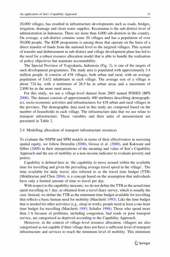
The Special Province of Yogyakarta, Indonesia (Fig. 2), is one of the targets of

such development programmes. The study area is populated with approximately 3.4

million people. It consists of 438 villages, both urban and rural, with an average

population of 5,632 inhabitants in each village. The average size of a village is

about 724 ha, with a minimum of 26.5 ha in urban areas and a maximum of

2,890 ha in the more rural areas.

For this study, we use a village-level dataset from 2005 named PODES (BPS

2006). The dataset consists of approximately 400 attributes describing demograph-

ics, socio-economic activities and infrastructures for 438 urban and rural villages in

the province. The demographic data used in this study are composed based on the

number of households in each village. The infrastructure data that we use relate to

transport infrastructure. These variables and their units of measurement are

presented in Table 2.

2.4 Modelling allocation of transport infrastructure resources

To evaluate the NSPM and SPM models in terms of their effectiveness in assessing

spatial equity, we follow Deneulin (2008), Grosse et al. (2008), and Kakwani and

Silber (2008) in their interpretations of the meaning and value of Sen’s Capability

Approach and the use of mobility as a non-income indicator to evaluate poverty and

justice.

Capability is defined here as ‘the capability to move around within the available

time for travelling and given the prevailing average travel speed in the village’. The

time available for daily travel, also referred to as the travel time budget (TTB)

(Mokhtarian and Chen 2004), is a concept based on the assumption that individuals

have only a limited amount of time to travel per day.

With respect to the capability measure, we do not define the TTB as the actual time

spent travelling in 1 day, as obtained from a travel diary survey, which is usually the

case. Instead, we define the TTB as the minimum time budget available for travelling

that reflects a basic human need for mobility (Marchetti 1993). Like the time budget

that is needed for other activities (e.g., sleep or work), people need at least a one-hour

time budget for travelling (Marchetti 1993; Schafer 1998). Those who spend more

than 1 h because of problems, including congestion, bad roads or poor transport

service, are categorised as deprived according to the Capability Approach.

Moreover, in the context of village-level resource allocation, villagers are also

categorised as not capable if their village does not have a sufficient level of transport

infrastructure and services to reach the minimum level of mobility. This minimum

An application of Sen’s Capability Approach 31

123

Fig

.2

Th

est

ud

yar

eais

loca

ted

inth

esp

ecia

lP

rovin

ceo

fY

og

yak

arta

,In

do

nes

ia,

wit

h4

38

urb

anan

dru

ral

vil

lag

es(S

ou

rce

bas

edo

nB

PS

20

06)

32 A. Wismadi et al.

123

level of mobility is defined here as a travelling distance that refers to the poverty

line of mobility and is calculated by multiplying the minimum travelling speed by

the available TTB. Villages residing under the poverty line can be labelled as

deprived and thus merit higher priority in allocating resources.

To define the poverty line, the minimum travelling speed was set at 25 (km/h).

The decision to use a 25 km/h minimum is based on a survey of expected speeds on

local roads in mountainous areas (TRB 2004). This figure is selected on the

assumption of minimum capability preferred by the community in the most difficult

topographic parts of the study area.

To measure travel speed in each village, we use the average travel speed from the

PODES database. Travel speed (km/h) for villagers is calculated by dividing the

stated distance by the stated travel time from the village centre to (a) the capital of

the sub-district, (b) the capital of the district and (c) the capital of the nearest district

outside their own district. Most facilities (e.g., education, market, entertainment and

administrative centres) are located in these capitals.

Again referring to the Capability Approach, to estimate the total opportunity of

mobility in a village, we assert that one person in each household should be capable

of movement for income-generating activities. This approach is in line with Golob

and McNally (1997) and Barrios (2008), who have already suggested that a travel

behaviour analysis of heads of household is important for measuring the impact of

transport infrastructure development in rural communities. For this reason, to

allocate resource, we use the number of households in the village as a weighting

factor. Figure 3 summarises the calculation procedure from the raw data into the

capability of mobility.

2.4.1 Procedure for location-allocation

To test both the SPM and NSPM models, in combination with the result of the

formulas in Sect. 2.2, we allocate an additional 10 % of total opportunity to mobility

Table 2 Variables and the data sources

Variables Unit of

measurement

for the model

Data sources Unit of

measurement in

the data source

Data conversion

Infrastructure

Transport Opportunity

to mobility

(personkm)

PODES code

9022, 9023

Travel Time

Budget (TTB)

study

Distances (KM),

travel time (Hour),

TTB (Hour)

Average travel speed to

facilities multiplied by

available Travel Time

Budget (9022/

9023*TTB)

Demographic

Population Number of

households

in the village

PODES code

401c

Number of

households

Number of HH (401c)

An application of Sen’s Capability Approach 33

123

(Mtot) as compared to the initial condition in the various locations in the study area.

A step-by-step procedure for location-allocation is explained below.

2.4.2 Calculation of total daily opportunity to mobility

The total daily opportunity to mobility is calculated on a household basis using the

following equation (Eq. 16):

Mtot ¼X

i

hi � �vi ��t ð16Þ

Mtot = total daily opportunity of distance to mobility in the study area (pers. km); ht

number of household in each village i from the PODES database; �vi = average

travel speed in village i (km) from the PODES database; �t = average daily travel

time budget TTB (hours).

2.4.3 Estimating the average travel speed

The total opportunity to mobility (Eq. 16) requires that an average travel speed be

calculated for each village (Eq. 17):

�vi ¼Pn

j¼1 ðtij=dijÞn

ð17Þ

Fig. 3 The calculation of raw data for Preference Modelling with mobility as a non-income indicator

34 A. Wismadi et al.

123

�vi = average travel speed in village i (km/h); tij = travel time in village i to facility

j from the PODES database (h); dij = distance from village i to facility j from the

PODES database (km); n = number of facilities calculated from the PODES

database (Unit).

2.4.4 Resources to be allocated

The amount of resources to be allocated is based on the percentage change or

growth (or target growth of T) in daily opportunity that is required (Eq. 18):

A ¼ T �Mtot ð18Þ

A = resources to be allocated (pers.km); T = percentage of expected target growth

from initial level of opportunity (%); Mtot = the total daily opportunity (pers.km).

2.4.5 Household weighted priority

To allocate resources, the number of households in each village is used to normalise

the scores that resulted from the preference modelling, (Eq. 19):

ai ¼Pi � HiPi Pi � Hi

ð19Þ

Pi = score of priority of village i from the Preference Modelling (0–1); obtained

with the formulas in Sect. 2.2; Hi = number of households in village i (hh);

ai = percentage of resources from the total available additional resources in the

region to be allocated in village i (%).

2.4.6 Location-allocation at the village level

Finally, the location-allocation for each village is calculated. The percentage of

allocation for village i (Eq. 20) is based on the household weighted priority from

Eq. 19:

Ai ¼ ai � A ð20Þ

Ai = allocated resources for village i (pers.km); ai = percentage of resource from

the total available additional resources in the region to be allocated in village i (%);

A = allocated resources for the region (pers.km).

2.5 Data analysis

2.5.1 Spatial equity analysis

Inequity is often subjective and can generate disputes among stakeholders;

therefore, a quantitative approach is required. To provide this quantitative

description of the level of spatial equity generated by NSPM and SPM, we apply

a spatial autocorrelation approach. Spatial autocorrelation analysis provides both

An application of Sen’s Capability Approach 35

123

location and attribute information and thus is a powerful analytical technique (Tsou

et al. 2005).

This quantitative description is provided with Moran’s I method, which is

commonly applied for evaluating spatial equity (Lorant et al. 2001; Tsou et al. 2005;

Grubesic 2008). Moran’s I is an estimate of Pearson’s correlation coefficient among

the values in location i or xi, with the average values of its neighbourhood (xlag) in a

Moran Scatter Plot with a horizontal axes of xi and a vertical axes of xlag. When all

the xi are equal to xlag, there is no spatial inequity.

Moran’s I provides a global index for spatial equity for the whole study area and

does not indicate spatial variation in the subset area. However, a map of Local

Indicators of Spatial Autocorrelation/Association (LISA) can be viewed as a direct

extension of the Moran Scatter Plot. The resulting map indicates how spatial

inequity varies over the study region. For example, a location with low values of xi

but high values of xlag indicates an inequitable situation where the poor are

surrounded by the rich. In this study, we use LISA maps to visualise where equity

changed as a result of a different allocation model.

2.5.2 Policy interpretation on Moran’s I

The levels of equity as calculated through Moran’s I in both the NSPM and SPM

models provide a basis for policy interpretation. The interpretation of Moran’s I is

provided for the distribution of priority scores, as well as for the effect of location-

allocation (Fig. 4).

Following Tsou et al. (2005), Moran’s I is positive when nearby objects tend to

be similar in attributes; a positive Moran’s I suggests an equitable distribution, with

Moran’s I = 1 being the best equitable distribution. By contrast, Moran’s I is

Fig. 4 Policy interpretation of simulation results

36 A. Wismadi et al.

123

negative when object values tend to be more dissimilar than what is normally

expected. With respect to the spatial equity of a public facility, a negative Moran’s

I suggests an inequitable distribution, with Moran’s I = -1 being the worst

distribution. Moran’s I = 0 when attribute values are arranged randomly and

independently in space (Tsou et al. 2005).

The interpretation of Moran’s I for spatial equity can be deducted from two

results of the simulation, that is, the intermediate and end results. The first is the

Spatial Priority Targeting (SPT), in which the models are used to prioritise the

locations of allocation, whereas in the second result, that is, the Effect of Location-

Allocation (ELA), the new state of equity for the area as a whole is investigated.

Both are further discussed below.

Spatial Priority Targeting (SPT) refers to the distribution of priority scores as

determined by the Preference Modelling. The distribution of Moran’s I scores can

be interpreted to create to two general types of distributional patterns.

1. Positive Moran’s I (towards ?1) of SPT implies a clustered allocation

distribution. Spatial priorities are more concentrated in certain areas. This type

of distribution provides a less equitable location-allocation in spatial terms.

2. Negative Moran’s I (towards -1) of SPT implies a dispersed allocation over the

region. The allocation is more spatially dispersed over the region. This type of

distribution provides a more equitable allocation in spatial terms.

The Effect of Location-Allocation (ELA) can also be studied using Moran’s I,

based on the new state of equity after the distribution of resources to the priority

locations.

1. Positive Moran’s I (towards ?1) of ELA implies a more equitable opportunity

distribution. Clusters of greater similarity have been generated in the region.

The equity among objects and their neighbourhoods is improved. Therefore, the

allocation provides better spatial equity. In line with the expected outcome of

the Capability Approach, the opportunity is more equally distributed in the

region.

2. Negative Moran’s I (towards -1) of ELA implies a cluster of dissimilarity.

Clusters of greater dissimilarity have been generated. Therefore, the inequity

among objects and their neighbourhoods is increased. The location-allocation

has reduced the spatial equity of opportunity to mobility in the region.

3 Results

We find some variations in spatial equity from the NSPM and SPM models for both

the Spatial Priority Targeting (SPT) and the Effect of Location-Allocation (ELA).

These variations are discussed below.

For NSPMs with maximum and interval standardisations, the Moran’s I values

for both SPT and ELA are identical to the distribution of the initial maps before the

allocation. All the values are identical, with Moran’s I = 0.4218, which is quite

surprising. This result therefore merits a more careful inspection and is further

An application of Sen’s Capability Approach 37

123

elaborated upon in the discussion section. The results of NSPM are presented in

Figs. 7 and 9. The ‘NS’ in NSMAX and NSINT means ‘non-spatial’, whereas

‘MAX’ and ‘INT’ represent the type of standardisation. The initial maps before

allocation are presented in Figs. 5 and 9 (Initial).

In the NSPM with goal standardisation, the Moran’s I of SPT increases, whereas

after allocation, that is, ELA, the Moran’s I decreases. This result indicates a cluster

of allocation priority in a certain part of the region and an increased level of cluster

of dissimilarity in the region after allocation. See Fig. 6 (PRNSGOAL) and 8 (Goal)

for the SPT of NSPM with goal standardisation. The ‘PR’ in PRNSGOAL means

‘priority’. Figure 6 shows that NSPMs with maximum and interval standardisations

have identical values to the initial map (0.4218) but different scatter plot patterns.

The ELA is presented in Figs. 7 (NSGOAL) and 9 (Non-Spatial, Goal).

With SPM, we find negative Moran’s I values on SPT for all standardisation

methods, as shown in Figs. 6 and 8 [(PRQNMAX, I = -0.05823), (PRQNINT,

I = -0.1950) and (PRQNGOAL, I = -0.05823)]. ‘PR’ means priority, whereas

‘QN’ represents the Queen neighbourhood connectivity with all adjacent (neigh-

bouring) polygons, as commonly applied in spatial statistics software. After

simulation (ELA), the Moran’s I values increase [see Figs. 7 (QNMAX, QNINT and

QNGOAL) and 9 (Spatial, Maximum: I = 0.05992, Interval: I = 0.4596 and Goal:

I = 0.05992)]. The ELA for NSPMs with maximum and interval standardisations

produce Moran’s I values (0.4218) that are identical to the initial map. For both

NSPM and SPM, the goal standardisations clearly present the changes of equity

status. We also find that the SPMs with maximum and goal standardisations produce

identical Moran’s I values (Fig. 6. PRQNMAX, PRQNGOAL).

Figures 8 and 9 present a direct extension of the Moran’s I Scatter Plot, which is

visualised as a LISA map and a map showing statistically significant relationships

with its neighbours. The map of statistical significance indicates how the

neighbourhood variation of a unit forms a cluster of similarity or dissimilarity

only for the clusters that are significant. These maps clearly demonstrate the

differences between NSPM and SPM and show that the NSPMs with maximum and

Fig. 5 Initial data before simulation

38 A. Wismadi et al.

123

Fig

.6

Sp

atia

lP

rio

rity

Tar

get

ing

,th

ed

istr

ibu

tio

no

fal

loca

tio

np

refe

ren

ces

inth

esi

mu

lati

on

s

An application of Sen’s Capability Approach 39

123

Fig

.7

Eff

ect

of

the

loca

tion

-all

oca

tio

n

40 A. Wismadi et al.

123

Fig

.8

LIS

Am

aps,

the

dis

trib

uti

on

of

Spat

ial

Pri

ori

tyT

arget

ing

An application of Sen’s Capability Approach 41

123

Fig

.9

LIS

Am

aps,

bef

ore

(in

itia

l)an

dth

eef

fect

of

loca

tion

-all

oca

tio

naf

ter

sim

ula

tio

n

42 A. Wismadi et al.

123

interval standardisations result in identical maps with Moran’s I equal to the initial

map.

In the maps of SPT (Fig. 8), we found that the NSPMs with maximum and

interval standardisations produce Moran’s I values that are identical to the initial

map but produce an inverted version of the initial map. As shown in Fig. 8, we also

found that the SPMs with maximum and goal standardisations produce identical

Moran’s I values as presented in Fig. 6 (PRQNMAX, PRQNGOAL). Moreover, the

SPMs produce more disbursed targeting over the region, as indicated by the

negative Moran’s I values.

Figure 9 clearly shows that the NSPMs with maximum and interval standardi-

sations produce identical maps and identical Moran’s I values compared with the

initial map. SPM produces more clusters of similarity with positive Moran’s

I values.

In general, we find that SPM and NSPM and their standardisation procedures

result in various degrees of equity, both in the SPT and ELA, and therefore, these

results need to be carefully interpreted in the following discussion.

4 Discussion

In this study, we demonstrate that a new type of Spatial Preference Modelling

(SPM) provides more spatially equitable resource allocations compared with a Non-

Spatial Preference Modelling (NSPM). This finding is evidenced by the inclusion of

a spatial autocorrelation approach within a Spatial Preference Modelling (SPM) that

results in a more equitable distribution, as indicated by Moran’s I values.

All the simulations with SPM, which include spatial neighbourhood compari-

sons, produce allocation priorities that are more equally distributed in the region.

This effect is indicated by negative Moran’s I values of Spatial Priority Targeting

(Fig. 8). As a result, the spatial equity of the new distribution also increases, as

indicated by increasing Moran’s I values in the Effect of Location-Allocation

(Fig. 9). The results systematically and consistently address equity, as indicated

quantitatively by the Moran’s I values.

The results also indicate that SPM complies well with the equity feature in Sen’s

Capability Approach. Our conclusion is based on the fact that by allocating the same

amount of additional resources, that is, 10 % of the initial condition, with SPM, the

Moran’s I changes towards a more equitable distribution (i.e., towards Moran’s

I = 1). Figure 8 shows clearly that the Moran’s I of the Effect of Location-

Allocation changes towards I = 1, from I = 0.4218 (Initial) to I = 0.5992 (SPM-

Maximum) and I = 0.4596 (SPM-Interval), providing evidence that SPM is able to

provide a more effective measure for spatial equity.

The Moran’s I of Spatial Priority Targeting (Fig. 8) strengthens this evidence. In

contrast to the Maximum and Interval NSPMs, which produce an inverted LISA

Map of SPT with Moran’s I values that are identical to the initial map and ELA, the

maximum and interval standardisations for SPM produce distinct Moran’s I and

LISA Maps from the initial map for both SPT and ELA. Those SPTs in SPMs with

negative I values (I = -0.05823 and -0.1950), which produce a dispersed

An application of Sen’s Capability Approach 43

123

allocation, provide additional evidence of the advantage of SPM in addressing

equity.

In addition to demonstrating the advantages of SPM over NSPM, we find an

unexpected result; it appears that the Maximum and Interval NSPMs are not

sensitive to Moran’s I. Figure 9 shows that for these NSPMs and 10 % additional

opportunity distributed in the region, the Moran’s I values of the SPT and ELA are

identical to the initial value (I = 0.4218), indicating that the 10 % allocation may

increase opportunity in a region but that it does not elevate opportunity to a level

that is equal to neighbouring communities. The NSPMs that do not consider local

inequity always prioritise allocation to the most deprived locations and set priorities

from highest to least. This behaviour explains why the SPT Moran’s I values are

identical to the initial value and why the resulting LISA maps are inverted compared

with the initial map. In the inverted maps, the highest score in SPT indicates the

lowest, or most deprived, location in the initial map. Figure 8 clearly reveals that the

LISA maps of ELA, both from the Maximum and Interval NSPMs, are inverted

versions of the initial map. The figure also demonstrates that the high-scoring

villages surrounded by high-scoring villages (High-High areas) have been inverted

into Low-Low areas, and vice versa, but these situations result in similar Moran’s

I values. This result also reveals that Moran’s I is not sensitive to the degree of

differences in allocation. Our findings imply a necessity to combine Moran’s I with

an additional measure of equity (e.g., a social equity measure) that is sensitive to the

degree of differences among units.

The NSPM with goal standardisation provides the only ELA result that is not

indicated by an inverted LISA map with an identical Moran’s I value

(I = 0.3795). This result is understandable given that goal standardisation

specifically aims to prioritise target groups below the poverty line. However,

the fact that the result provides a lower Moran’s I value than the initial value

(I = 0.4218) requires further interpretation. The lower I value of 0.3795 (Fig. 9,

Goal) provides evidence that the Goal NSPM, which applies a global comparison

and disregards local neighbourhood comparisons, can address social equity (the

deprived village under the poverty line), but it does not systematically resolve

spatial equity in the whole region.

The fact that Maximum and Goal SPMs provide identical results (Figs. 8 and 9)

can be explained. The Goal SPM aims to minimise the gap among neighbouring

units. Hence, we apply the gap to the mean rather than to the absolute poverty line.

This approach is mainly used to accommodate for the sense of differences among

neighbouring units as well as to obtain a sense of the differences within the study

region. Similarly, the Maximum SPM also uses the absolute 0 as the reference of

the goal, which produces the identical result between the Maximum and Goal

SPMs.

The better performance of SPM over NSPM suggests that combining a global

comparison with a local comparison in a so-called Glocal model is more effective

for addressing equity. As we applied standardised X and W_X scores in SPM

(Eq. 8), all the formulae for SPM have been applied to Glocal comparisons. This

approach enables us to address social equity and to systematically resolve spatial

equity. Moreover, this Glocal modelling actually represents one of the important

44 A. Wismadi et al.

123

aspects of the Capability Approach (Sen 1980). The Capability Approach requires

the accommodation of ideas of relative importance, which are related to the nature

of society. SPM with a Glocal benchmark, which captures relative equity among

neighbourhoods as well as the region as a whole, shows a workable application to

operationalising Sen’s Capability Approach for an equity-based resource location-

allocation problem.

An alternative approach that includes a local benchmark, rather than a Glocal or

Global one, can be used by applying Goal SPM with raw scores (x and W_x), instead

of standardised (X and W_X) scores. With the raw scores, we could apply the

average raw values of the neighbouring units as the benchmark in Goal SPM with

Benefit Criteria as max G (Eq. 14) and set the minimum value from neighbouring

units as min G (Eq. 14). This approach allows us to address both social equity and,

at the same time, to improve spatial equity in each neighbourhood. Moreover, the

effectiveness of SPM might be further evaluated with other types of neighbourhood

connectivity matrices (e.g., Rook). Selection of the type of connectivity should also

consider the appropriateness to local conditions. Implementation of these ideas and

their implication to spatial equity policy should be examined in future research.

We conclude that Spatial Preference Modelling is a reliable method for equitable

resource allocation. All the simulations in SPM, which include a spatial relationship

by taking into account not only global comparison but also local or neighbourhood

comparison, produce allocation priorities that give more equally distributed

resources in the region. Again, this deduction provides a basis for establishing a

new method for implementing Sen’s Capability Approach into equity-based

resource location-allocation.

5 Conclusions

We conclude that the inclusion of a neighbourhood comparison in Spatial

Preference Modelling (SPM) provides a more equitable resource location-allocation

than NSPM. The SPM also provides an alternative way to accommodate the need of

an efficiency-equity trade-off in a diverse region, such as the Special Province of

Yogyakarta in Indonesia. This approach allows public officials to apply social and

spatial equity criteria for decision-making.

Moreover, the derivation of Sen’s Capability Approach (CA) into a resource

location-allocation procedure provides a new way of addressing the spatial equity of

infrastructure provision. The CA in our case study provides the intermediate step

towards resource allocation in terms of monetary or fiscal units.

Therefore, this study provides a new systematic approach for resource allocation

that can be implemented in a GIS environment to support decision makers in

distributing limited resources in an equitable manner.

Acknowledgments This publication is part of the research activities funded through the Indonesia

Facility (INDF) of the Netherlands EVD agency to establish a new Master of Science Program on

Management of Infrastructure and Community Development—MICD (http://pipm.pasca.ugm.ac.id). The

project is a joint research activity between ITC the Netherlands, PUSTRAL UGM (The Centre for

An application of Sen’s Capability Approach 45

123

Transport and Logistics Studies—Gadjah Mada University) Indonesia, and Keypoint Consultancy BV the

Netherlands.

References

Ananda J, Herath G (2009) A critical review of multi-criteria decision making methods with special

reference to forest management and planning. Ecol Econ 68(10):2535–2548. doi:10.1016/j.ecolecon.

2009.05.010

Barrios E (2008) Infrastructure and rural development: household perceptions on rural development. Prog

Plann 70(1):1–44. doi:10.1016/j.progress.2008.04.001

Beedasy J, Whyatt D (1999) Diverting the tourists: a spatial decision-support system for tourism planning

on a developing island. Int J Appl Earth Obs Geoinf 1(3):163–174. doi:10.1016/S0303-2434(99)

85009-0

Benferhat S, Dubois D, Kaci S, Prade H (2006) Bipolar possibility theory in preference modelling:

representation, fusion and optimal solutions. Inffus 7(1):135–150. doi:10.1016/j.inffus.2005.04.001

Bibi S, Duclos J (2007) Equity and policy effectiveness with imperfect targeting. J Devel Econ

83(1):109–140. doi:10.1016/j.jdeveco.2005.12.001

Bivand R, Muller WG, Reder M (2009) Power calculations for global and local Moran’s I. Comput Stat

Data Anal 53(8):2859–2872. doi:10.1016/j.csda.2008.07.021

BPS (2006) PODES. BPS-Statistics Indonesia, Jakarta

Cabrales A, Calvo-Armengol A (2008) Interdependent preferences and segregating equilibria. J Econ

Theory 139(1):99–113. doi:10.1016/j.jet.2007.08.003

Chen A (2010) Reducing China’s regional disparities: is there a growth cost? China Econ Rev

21(1):2–13. doi:10.1016/j.chieco.2009.11.005

Cherchye L, De Witte K, Ooghe E, Nicaise I (2010) Efficiency and equity in private and public education:

a nonparametric comparison. Eur J Oper Res 202(2):563–573. doi:10.1016/j.ejor.2009.06.015

Chitwood SR (1974) Social equity and social service productivity. Public Admin Rev 34(1):29–35

Cho C (1998) An equity-efficiency trade-off model for the optimum location of medical care facilities.

Socio Econ Plan Sci 32(2):99–112. doi:10.1016/S0038-0121(97)00007-4

Deneulin S (2008) Beyond individual freedom and agency: structures of living together in the capability

approach. In: Comim F, Qizilbash M, Alkire S (eds) The capability approach concepts, measures

and applications. Cambridge University Press, Cambridge, pp 105–124

Dworkin R (1981a) What is equality? Part 1: equality of welfare. Philos Public Aff 10(3):185–246

Dworkin R (1981b) What is equality? Part 2: equality of resources. Philos Public Aff 10(4):283–345

Feser E, Sweeney S (2006) Regional industry cluster analysis using spatial concepts, space as indicator.

Pre-conference training, ACCRA 46th annual conference, 7 June 2006, Charlotte, NC. http://

www.urban.illinois.edu/faculty/feser/ESEBA/ESEBA_All.pdf. Accessed 18 March 2013

Frederickson HG (1990) Public administration and social equity. Public Admin Rev 50(2):228–237. doi:

10.2307/976870

Garcia-Valinas MA, Llera RF, Torgler B (2005) More income equality or not? An empirical analysis of

individuals’ preferences. CREMA working paper series, Center for Research in Economics,

Management and the Arts (CREMA), http://econpapers.repec.org/RePEc:cra:wpaper:2005-23.

Accessed 18 March 2013

Gasper D (2007) What is the capability approach? Its core, rationale, partners and dangers. J Socio-Econ

36(3):335–359. doi:10.1016/j.socec.2006.12.001

Golob TF, McNally MG (1997) A model of activity participation and travel interactions between

household heads. Transp Res B-Meth 31(3):177–194. doi:10.1016/S0191-2615(96)00027-6

Grosse M, Harttgen K, Klasen S (2008) Measuring pro-poor growth in non-income dimensions. World

Dev 36(6):1021–1047. doi:10.1016/j.worlddev.2007.10.009

Grubesic TH (2008) The spatial distribution of broadband providers in the United States: 1999–2004.

Telecommun Policy 32(3):212–233. doi:10.1016/j.telpol.2008.01.001

Kakwani N, Silber J (2008) Introduction: multidimensional poverty analysis: conceptual issues, empirical

illustrations and policy implications. World Dev 36(6):987–991. doi:10.1016/j.worlddev.2007.10.004

Kyriacou AP, Roca-Sagales O (2011) Fiscal decentralization and government quality in the OECD. Econ

Lett 111(3):191–193. doi:10.1016/j.econlet.2011.02.019

46 A. Wismadi et al.

123

Lelkes O (2006) Knowing what is good for you, Empirical analysis of personal preferences and the

‘‘objective good’’. J Socio-Econ 35(2):285–307. doi:10.1016/j.socec.2005.11.002

Lorant V, Thomas I, Delie‘ge D, Tonglet R (2001) Deprivation and mortality: the implications of spatial

autocorrelation for health resources allocation. Soc Sci Med 53(12):1711–1719. doi:10.1016/S0277-

9536(00)00456-1

Malczewski J (2004) GIS-based land-use suitability analysis: a critical overview. Prog Plann 62(1):3–65.

doi:10.1016/j.progress.2003.09.002

Marchetti C (1993) On mobility. Final status report, contract no. 4672-92-03 ED ISP A, International

Institute for Applied Systems Analysis (IIASA), Laxenburg, Austria. http://www.cge.uevora.pt/

energia/marchetti/MARCHETTI-057_Pt.1.pdf. Accessed 18 March 2013

Mokhtarian PL, Chen C (2004) TTB or not TTB, that is the question: a review and analysis of the

empirical literature on travel time (and money) budgets. Transport Res A-Pol 38(9/10):643–675.

doi:10.1016/j.tra.2003.12.004

Neyapti B (2010) Fiscal decentralization and deficits: international evidence. Eur J Polit Econ

26(2):155–166. doi:10.1016/j.ejpoleco.2010.01.001

Nussbaum M (2003) Capabilities as fundamental entitlements: Sen and social justice. Fem Econ 9(2/

3):33–59. doi:10.1080/1354570022000077926

Ohana S (2010) Modeling global and local dependence in a pair of commodity forward curves with

an application to the US natural gas and heating oil markets. Energ Econ 32(2):373–388. doi:

10.1016/j.eneco.2009.08.015

Overmars KP, de Koning GHJ, Veldkamp A (2003) Spatial autocorrelation in multi-scale land use

models. Ecol Model 164(2):257–270. doi:10.1016/S0304-3800(03)00070-X

Perny P, Roy B (1992) The use of fuzzy outranking relations in preference modelling. Fuzzy Set Syst

49(1):33–53. doi:10.1016/0165-0114(92)90108-G

Phua M, Minowa M (2005) A GIS-based multi-criteria decision making approach to forest conservation

planning at a landscape scale: a case study in the Kinabalu Area, Sabah, Malaysia. Landsc Urban

Plan 71(2/4):207–222. doi:10.1016/j.landurbplan.2004.03.004

Piccolo D, D’Elia A (2008) A new approach for modelling consumers’ preferences. Food Qual Prefer

19(3):247–259. doi:10.1016/j.foodqual.2007.07.002

Ping JL, Green CJ, Zartman RE, Bronson KF (2004) Exploring spatial dependence of cotton yield using

global and local autocorrelation statistics. Field Crop Res 89(2/3):219–236. doi:10.1016/j.fcr.2004.

02.009

Qizilbash M (2011) Sugden’s critique of the capability approach. Util 23(1):25–51. doi:10.1017/S095

3820810000439

Roberts F, Tsoukias A (2009) Voting theory and preference modelling. Math Soc Sci 57(3):289–291. doi:

10.1016/j.mathsocsci.2008.12.005

Schafer A (1998) The global demand for motorized mobility. Transport Res A-Pol 32(6):455–477. doi:

10.1016/S0965-8564(98)00004-4

Sen AK (1980) Equality of what. In: McMurrin SM (ed) The tanner lectures on human value. University

of Utah Press, Salt Lake City, pp 195–220

Sen AK (1992) Inequality reexamined. Oxford University Press, Oxford

Sen AK (2004) Capabilities, lists, and public reason: continuing the conversation. Fem Econ 10(3):77–80.

doi:10.1080/1354570042000315163

Sharifi A, van Herwijnen M (2001) Spatial decision support systems. International Institute for

Geoinformation Science and Earth Observation (ITC), Enschede

Shortridge A (2007) Practical limits of Moran’s autocorrelation index for raster class maps. Comput

Environ Urban Syst 31(3):362–371. doi:10.1016/j.compenvurbsys.2006.07.001

Sudgen R (2006) What we desire, what we have reason to desire, whatever we might desire: Mill and Sen

on the value of opportunity. Util 18(1):33–51. doi:10.1017/S0953820805001810

TRB (2004) Design speed, operating speed, and posted speed practices. TRB’s National Cooperative

Highway Research Program (NCHRP) report 504, Transportation Research Board of The National

Academies

Tsai Y (2005) Quantifying urban form: compactness versus ‘sprawl’. Urban Stud 42(1):141–161. doi:

10.1080/0042098042000309748

Tsou K, Hung Y, Chang Y (2005) An accessibility-based integrated measure of relative spatial equity in

urban public facilities. Cities 22(6):424–435. doi:10.1016/j.cities.2005.07.004

An application of Sen’s Capability Approach 47

123

Tsoukias A (1991) Preference modelling as a reasoning process: a new way to face uncertainty in

Multiple Criteria Decision Support Systems. Eur J Oper Res 55(3):309–318. doi:10.1016/0377-

2217(91)90201-6

Wismadi A, Brussel M, Zuidgeest M, Sutomo H, Nugroho LE, van Maarseveen M (2012) Effect of

neighbouring village conditions and infrastructure interdependency on economic opportunity: a case

study of the Yogyakarta region, Indonesia. Comput Environ Urban Syst 36(5):371–385. doi:

10.1016/j.compenvurbsys.2012.02.001

Xiang W (2001) Weighting-by-choosing: a weight elicitation method for maps overlays. Landsc Urban

Plan 56(1/2):61–73. doi:10.1016/S0169-2046(01)00169-4

Yuan J, Kang J, Zhao C, Hu Z (2008) Energy consumption and economic growth: evidence from China at

both aggregated and disaggregated levels. Energ Econ 30(6):3077–3094. doi:10.1016/j.eneco.

2008.03.007

48 A. Wismadi et al.

123