1 23

Theoretical and Applied Climatology ISSN 0177-798XVolume 106Combined 1-2 Theor Appl Climatol (2011) 106:139-152DOI 10.1007/s00704-011-0425-9

Spatial prediction of urban–ruraltemperatures using statistical methods

Jan Hjort, Juuso Suomi & Jukka Käyhkö

1 23

Your article is protected by copyright and

all rights are held exclusively by Springer-

Verlag. This e-offprint is for personal use only

and shall not be self-archived in electronic

repositories. If you wish to self-archive your

work, please use the accepted author’s

version for posting to your own website or

your institution’s repository. You may further

deposit the accepted author’s version on a

funder’s repository at a funder’s request,

provided it is not made publicly available until

12 months after publication.

ORIGINAL PAPER

Spatial prediction of urban–rural temperaturesusing statistical methods

Jan Hjort & Juuso Suomi & Jukka Käyhkö

Received: 17 December 2010 /Accepted: 22 February 2011 /Published online: 20 March 2011# Springer-Verlag 2011

Abstract Spatial information on climatic characteristics isbeneficial in e.g. regional planning, building constructionand urban ecology. The possibility to spatially predicturban–rural temperatures with statistical techniques andsmall sample sizes was investigated in Turku, SW Finland.Temperature observations from 36 stationary weatherstations over a period of 6 years were used in the analyses.Geographical information system (GIS) data on urban landuse, hydrology and topography served as explanatoryvariables. The utilized statistical techniques were general-ized linear model and boosted regression tree method. Theresults demonstrate that temperature variables can berobustly predicted with relatively small sample sizes (n≈20–40). The variability in the temperature data wasexplained satisfactorily with few accessible GIS variables.Statistically based spatial modelling provides a cost-efficient approach to predict temperature variables on aregional scale. Spatial modelling may aid also in gainingnovel insights into the causes and impacts of temperaturevariability in extensive urbanized areas.

1 Introduction

Howard’s (1818) investigation of the climate of London isoften considered a pioneer study in urban climatology.Howard pointed out that the city centre is warmer than the

surrounding countryside during the night. Ever since therelative warmness of urban areas, i.e. the urban heat island(UHI) phenomenon has been the focus of interest innumerous climatological studies (e.g. Sundborg 1950; Oke1981; Svensson et al. 2002; Balázs et al. 2009; Tan et al.2010). The UHI has several causes that are not all fullyunderstood, but the most central reasons for UHI aredifferences in solar heat storage, anthropogenic heat releaseand evaporation difference between urban and rural areas(Oke 1973; Landsberg 1981; Atkinson 2003). The thermalconductivity and heat capacity of the building materials inurban areas is often high in relation to land-use typescommon in rural regions. This enables large amounts of solarradiation to be stored in both street pavements and buildings indaytime. This stored heat is released to the air during eveningand night, being the focal reason for UHI in low latitudesthroughout the year, and in middle and high latitudes insummertime (Oke 1973; Landsberg 1981). The mostimportant sources of anthropogenic heat are traffic, industryand the heating of buildings. The role of anthropogenic heatin creating UHI is central in high latitudes in winter, when itsenergy amount often exceeds that of the solar radiation (e.g.Klysik 1996). Evaporation is in general lower in an urbanarea because of surface materials’ lower ability to absorbwater. Sewerage also transports surface waters effectivelyaway from urban areas. In rural areas, plants take moisturefrom deeper ground, which also enhances evaporation (Oke1987; Cotton and Pielke 1995). Due to the differences inevaporation, in urban areas the larger proportion of the heatis in sensible form (Cleugh and Oke 1986).

UHI has various relevant impacts. For example, theadditional warmth amplifies people’s heat stress leading tohigher mortality rates during heat waves (Conti et al. 2005;Johnson and Wilson 2009). Under climate change, theseheat waves may become more intense, more frequent and

J. Hjort (*)Department of Geography, University of Oulu,P.O. Box 3000, FI-90014 Oulu, Finlande-mail: jan.hjort@oulu.fi

J. Suomi : J. KäyhköDepartment of Geography and Geology, University of Turku,Turku FI-20014, Finland

Theor Appl Climatol (2011) 106:139–152DOI 10.1007/s00704-011-0425-9

Author's personal copy

longer lasting (Meehl and Tebaldi 2004). In contrast, theobvious benefit of relatively higher temperatures in cooland cold climate urban areas is lower heating energydemand in winter (Taha 1997). Due to the various aspectsof the UHI, knowledge on the intensities, frequencies andalso spatial dimensions of urban temperatures have boththeoretical and practical relevance in climatological studies(e.g. Oke 2006; Heisler and Brazel 2010). Because the heatstress poses an immediate threat to people’s health, majorityof the concrete UHI-related measures and applications havebeen concentrated on UHI mitigation. Partly for the samereason, the focus of the UHI research has been more insummer situations and in low- or mid-latitude cities (e.g.Steinecke 1999; Memon et al. 2007; Giridharan andKolokotroni 2009). On the contrary, the urban climate hasbeen the focus of relatively few studies in high latitudes(Magee et al. 1999; Steinecke 1999; Svensson and Eliasson2002; Eliasson and Svensson 2003; Hinkel et al. 2003).

Temperature data used to study various aspects of urbanclimate have traditionally been collected by stationarymeasurement networks or vehicle-based surveys (e.g.Hinkel et al. 2003; Hart and Sailor 2009). However, thecompilation of temperature data for extensive urban areasand long periods of time is often laborious and time-consuming task. Moreover, the data set gained is spatiallynon-continuous information that is difficult to relate to thespatially varying environmental factors controlling the UHI.Traditionally, different interpolation techniques have beenutilized to transform the point-based temperature data tospatially continuous form (Chapman and Thornes 2003;Dobech et al. 2007; Szymanowski and Kryza 2009). Thecentral problem with the interpolation methods is that theycannot satisfactorily extrapolate the information beyond thesurveyed area. The combination of multivariate statisticalmodelling, geographical information system (GIS) andremote sensing data is increasingly used as an efficientapproach to solve the “spatialization” problem in climato-logical studies (Unger et al. 2001; Svensson et al. 2002;Balázs et al. 2009; Hart and Sailor 2009; Rajasekar andWeng 2009; Szymanowski and Kryza 2009; Vicente-Serrano et al. 2010).

Basically, statistical modelling can be used to (1) simplifycomplex climatological relationships (model reduction), (2)provide understanding of UHI–environment relationships(explanatory models), and (3) predict UHI and relatedvariables across space, but also in time (predictive models).Model simplification approaches utilize variable reductiontechniques in the analytical phase and have as their goal amodel that explains and/or predicts the occurrence of, forexample UHI, with a restricted number of explanatoryvariables (e.g. Eliasson and Svensson 2003). Explanatorymodels seek to provide insights into the UHI and physicalconditions that determine it (e.g. Kim and Baik 2004). In

contrast, predictive models typically seek to provide the userwith a statistical relationship between the response and aseries of explanatory variable for use in predicting theclimatic conditions (e.g. Vicente-Serrano et al. 2010).

One potential problem occurs in that statistical methodsmay require from several tens to hundreds of observationsto reveal pattern between the studied phenomena andexplanatory variables, especially when modelling phenom-ena that vary geographically (Stockwell and Peterson 2002;Hjort and Marmion 2008). In studying urban climate, theestablishment of a stationary monitoring network withnumerous measurement stations is, however, often difficultdue to the time and financial constrains. Thus, it would behighly important to understand the possibilities as well asthe limitations to spatially predict urban temperatures withrelatively small data sets.

Suomi and Käyhkö (2011) studied diurnal and seasonalcharacteristics of spatial temperature differences and usedlinear regression to estimate the effects of environmentalfactors on spatial temperature variability in Turku, SWFinland. In this study, the main objectives are to: (1)investigate the possibility to spatially predict urban–ruraltemperatures with GIS data and small sample sizes, (2)compare the prediction abilities of traditional generalizationof linear regression technique (generalized linear model,GLM) and a novel machine learning-based ensemblemethod (boosted regression tree, BRT) that has shown tobe highly promising technique in various fields of earth andenvironmental sciences and (3) explore (a) the ability tomodel monthly mean, mean daily minimum, mean dailymaximum and mean diurnal temperature range in differentseasons and (b) which of the commonly used GIS variablesbest explain the variability in the data in the study area. Tofulfil our study aims, we utilized temperature data gatheredfrom 36 stationary temperature loggers in and around thecity of Turku in SW Finland over a period of 6 years(2002–2007). Using relatively long-term monitoring data,the ability to generalize the results is much higher than instudies using data on extreme weather conditions only.

2 Background: statistically based spatial modellingof climate variables

Reliable statistically based spatial modelling practiceshould include the following key steps (Hjort and Marmion2008): (1) establishment of a conceptual model, (2)compilation of response (e.g. temperature) and explanatory(e.g. GIS) variable data, (3) data exploration, (4) statisticalformulation, (5) model calibration, (6) model evaluationand (7) prediction and/or interpretation of the results.

First, conceptual model based on solid climatologicaltheory should be proposed before a statistical model is even

140 J. Hjort et al

Author's personal copy

considered. This is extremely important, as in addition tothe study problem, the conceptual framework outlines thefollowing steps in data collection and analysis. Second, thecompilation of response data and selection of appropriateexplanatory variables for the statistical analyses can be acomplicated and difficult task without a firm conceptualmodel. There are neither universal criteria nor widelyaccepted guidelines for the selection of explanatoryvariables and hence, the rationale of the study at hand willsteer the exact procedure. Commonly, the variables aregathered from field campaigns, remotely sensed data, plusGIS-based modelling and databases (Svensson et al. 2002;Hart and Sailor 2009; Vicente-Serrano et al. 2010).

Third, the adequacy of the data should be assessed usingexplorative analyses e.g., for distribution and spatial propertiesof the response data. Fourth, statistical formulation includes thechoice of an optimal statistical approach with regard to themodelling context and a suitable algorithm for modelling aparticular type of response variable and estimating the modelcoefficients. In addition to the explorative analysis, previousstudies and literature are used to guide this stage.

Fifth, the explanatory variables will be selected for thestatistical model which will be constructed (e.g. estima-tion and adjustment of model parameters) in modelcalibration. Traditionally, the model selection has beenbased on p values but recently, there has been a shifttowards the use of Akaike’s Information Criterion (orrelated information theories) and multimodel inference(Burnham and Anderson 1998). This shift has been seen tobe useful for reducing reliance on the “truth” of a modelselected by stepwise approaches and for understanding theerror tendencies of conventional selection approaches(Elith and Leathwick 2009).

Sixth, evaluation of the generated model is a vital step inthe model building process that is often overlooked (Balázset al. 2009). Evaluating the model includes the assessmentof the realism of fitted response functions and explanatoryvariables, the model’s fit to data, characteristics of residualsand predictive performance on test data. For predictivepurposes, it is advisable to assess the model performanceusing independent evaluation data. The final stage includesmapping predictions to geographical space and/or iteratingthe process to improve the model in light of knowledgegained throughout the process, or the modelling outcomescan directly be used to draw conclusions. All the abovestages are interconnected and ultimately controlled by theobjectives of the study.

3 Study area

The study area (~206 km2) consists of the city of Turku(175,000 inhabitants) and parts of its neighbouring munic-

ipality Kaarina (31,000 inhabitants). Turku is a coastal townlocated in south-western Finland at the mouth of river Aura(average discharge 7 m3/s). The coastline is very indented,exhibiting a large archipelago to the south-west of the city(Fig. 1). Therefore, the climate of Turku shows both coastaland continental characteristics. A factor affecting the localclimate in Turku is the spatiotemporal extent of the sea icecover, as a continuous sea ice eliminates heat and watervapour transfer from the sea and effectively makes theclimate more continental. The average duration of perma-nent ice cover in the inner archipelago is 2.5–3 months(1961–1990), although the extent and duration can varyconsiderably from year to year (Seinä and Peltola 1991;Seinä et al. 2006).

In Köppen’s (Peel et al. 2007) classification, Turkubelongs to the Hemiboreal and humid continental Dfb classtogether with southern parts of the Scandinavian Peninsula,the Baltic countries and much of Eastern Europe. At Turkuairport, 7 km to the north of the city centre, the meanannual air temperature is 5.2°C (1971–2000). On average,the coldest month is February with a mean temperature of−5.3°C, while July is the warmest with a mean temperatureof 16.9°C. The measured temperature extremes in 1971–2000 were −34.8°C (January 1987) and 32.0°C (June1977). Mean annual precipitation is 698 mm, of which30% falls as snow. The duration of permanent snow coveris 92 days (24 December–25 March). The wettest month istypically August, while May is the driest, with monthlyrainfalls of 79 and 35 mm, respectively. Winds are variablein speed (mean 3.5 m/s, highest in November, 3.8 m/s, andlowest in August, 3.0 m/s) and direction (dominant SWwith 17% proportion) due to cyclonic activity (Drebs et al.2002; FMI 2009).

The grid plan area of the Turku city centre isapproximately rectangular in its form with a spatial extentof 4 km (SW–NE) times 1.5 km (SE–NW). The marketsquare with a surrounding concentration of commercialbuildings sits in the middle of the city. Elsewhere, the gridplan area consists mainly of residential areas and parks.Most of the buildings are six to eight storey stone houseswith varying surface colours. River Aura flows across thecity centre, where its width varies between 50 and 100 m(City of Turku 2001). Most of the urban parks occupy smallbedrock hills on the south-eastern side of the river.Industrial areas (dock yard, light industry) lie scattered tothe west and north of the city centre. Outside the grid planarea, the land cover is a mosaic of suburbs, forests and cropfields. The largest sparsely populated areas are foundtowards the north of the city centre (Fig. 1).

Topographically, the grid plan area consists of flat clayground 5–10 m above the sea level (a.s.l.), frequentlybroken through by 30–50-m-high bedrock outcrops. Out-side the grid plan area hills alternate with flat areas and the

Spatial prediction of urban–rural temperatures 141

Author's personal copy

basic elevation rises gently towards the inland. The highestplaces of the study area reach 65 m a.s.l. (Fig. 1).

4 Data and methods

4.1 Response and explanatory variables

The response data consist of temperature observationscollected as part of the TURCLIM project (Turku UrbanClimate Research Project) of the Department of Geography

and Geology at the University of Turku. The explanatoryvariables, namely cover of urban land use and surface water(in percentage), building floor area (in square metres) andrelative elevation (in metres) were selected using aconceptual model (Oke 1973, 1987; Landsberg 1981).The spatial analyses were performed at a 100×100 m gridresolution (Vicente-Serrano et al. 2007). An advantage ofthe grid approach is the possibility to convert usuallyvacillating spatial variables to numeric form enablingnumerical analysis and the possibility to utilize GIS dataas a source of explanatory variables (Svensson et al. 2002;

Fig. 1 The location of Turku and its surroundings on the SW coast ofFinland (a) with the limits of the study area (b) and principal land useforms (c) plus topography (d). The 36 temperature logger sites are

marked with star symbols in c. The “other” land use consists mainlyof forests and fields. In d, the loggers are identified, andcorresponding logger site information is included in Table 1

142 J. Hjort et al

Author's personal copy

Vicente-Serrano et al. 2007; Hart and Sailor 2009; Vicente-Serrano et al. 2010).

The TURCLIM project has altogether 63 Hobo H8 Protemperature loggers set up to record temperature at 30-minintervals. The manufacturer-proclaimed accuracy of theinstrument is ±0.2°C at 0–50°C, while the resolution is0.02°C. Loggers are placed at 3 m elevation above theimmediately surrounding ground. In this study, only loggerswith an uninterrupted observation period from 2002 to

2007 were included in the calculations, resulting to 36devices (Fig. 1; Table 1). Using this data set, a total of 16temperature variables were computed: mean, mean dailyminimum, mean daily maximum and mean diurnal temper-ature range in January, April, July and October.

The main objective in the temperature variable selectionwas to take into account the typical diurnal and seasonaldifferences in the UHI behaviour. UHI is often strongest atnight, while during daytime the city centre can be colder

Table 1 Basic information of the logger sites

Logger number Site description Elevation (m) a.s.l. Distance from the city centre (km) Land cover in the surroundings

1 Rural 2.4 9.8 Forest, gravel road

2 Semi-urban 4.9 7.1 Forest, field

3 Rural 34.7 6.2 Forest, gravel road

4 Semi-urban 9.3 6.0 Gravel field, 2-storey building

5 Rural 15.1 6.2 Forest, gravel road

6 Rural 1.5 5.2 Field, meadow

7 Semi-urban 5.8 4.6 Parking lot, 2-storey building

8 Rural 0.6 5.1 Field, forest

9 Semi-urban 0.0 3.2 Gravel field, high grassland

10 Urban 4.6 2.8 Grassland, different-sized buildings

11 Urban 18.5 1.9 Block of flats, gravel field

12 Semi-urban 5.8 2.9 Forest, asphalt road

13 Semi-urban 19.9 1.3 Detached house, park

14 Urban 10.3 1.0 Park, asphalt road

15 Semi-urban 26.2 3.0 Parking lot, field

16 Semi-urban 30.0 1.7 Park, 2-storey building

17 Urban 7.4 0.7 Asphalt road, block of flats

18 Urban (market place) 8.6 0.1 Asphalt road, block of flats

19 Semi-urban 36.8 4.2 Block of flats, 2-storey building

20 Urban 30.8 0.7 Block of flats, park

21 Rural 41.2 2.6 Forest, landfill

22 Semi-urban 20.0 1.2 Detached houses, gravel road

23 Semi-urban 19.9 1.8 Industrial, asphalt road

24 Urban 22.9 1.0 Block of flats, asphalt road

25 Urban 20.7 1.3 Park, asphalt road

26 Semi-urban 15.0 3.8 Allotment garden houses, forest

27 Urban park 20.0 1.6 Park, leisure time areas

28 Semi-urban 25.1 3.4 Forest, graveyard

29 Semi-urban 49.9 3.9 Block of flats, row house

30 Rural 20.0 5.2 Landfill, forest

31 Rural 12.7 4.2 Field, forest

32 Rural 34.6 9.9 Field, forest

33 Rural 21.5 7.5 Field, forest

34 Semi-urban 56.4 11.1 Block of flats, asphalt road

35 Rural 32.4 9.9 Forest, meadow

36 Semi-urban 38.7 6.3 Detached house, lake

Distance from the city centre is measured from the centre point of the market place. Land cover includes two most common land cover typesinside 100-m radius

Spatial prediction of urban–rural temperatures 143

Author's personal copy

than the surrounding countryside (e.g. Steinecke 1999;Eliasson and Svensson 2003; Suomi and Käyhkö 2011).Such daily fluctuation is clearest in summer, when thestorage and release of solar heat energy is the main agent inUHI formation. In high latitude winter, the anthropogenicheat release is the main factor behind the UHI development,and the daily rhythm is somewhat blurred (Ekholm 1981;Miara et al. 1987; Klysik 1996; Magee et al. 1999;Giridharan and Kolokotroni 2009). To reflect the diurnaltemperature variation, the mean daily minimum tempera-ture, mean daily maximum temperature and mean diurnaltemperature range were selected for response variables. Inaddition, mean temperature was selected to reflect theaverage conditions.

The principal factors behind seasonal differences of UHIbehaviour include variations in anthropogenic heat releaseand solar radiation (Klysik and Fortuniak 1999; Magee etal. 1999). In Turku, the seasonally fluctuating sea watertemperature is a further component affecting the localclimate. We selected months that would best reflect theinfluencing climatic factors, namely January, April, Julyand October. January was considered to best represent themaximum anthropogenic heat release, which is the mainagent behind the UHI in winter. Although solar radiationhas its minimum in December, the sea may still releaseremnant heat from the preceding summer, which is whyJanuary was selected. July reflects high solar heat input andrelease, and similarly to winter, the lag in sea temperaturefluctuation made us prefer July to June. In order to reflectboth the seasonal cooling and warming effect of the sea,April and October, respectively, were selected.

The spatial variation of the heat storage capacity of variousurban land cover types and the subsequent spatial temperaturedifferences were investigated using the SLICES (2010) land-use classification with a grid size of 10×10 m. The SLICESclassification consists of 45 land-use classes in eightcategories: A=residential and leisure areas, B=business,administrative and industrial areas, C=supporting activityareas, D=rock and soil extraction areas, E=agricultural land,F=forestry land, G=other land, and H=water areas. Suomiand Käyhkö (2011) created an “urban land use” class basedon the temperature correlations of the SLICES’ original land-use classes. The urban class was formed from five SLICESclasses (roads, office buildings, blocks of flats, publicbuildings, commercial buildings) that showed a statisticallysignificant positive Pearson’s correlation coefficient withmean, minimum and maximum temperatures of 2002–2007.The coverage (in percentage) of urban land use inside the100×100 m grid cells was used as one explanatory variable.The building floor area (in square metres) inside 100×100 mcells was used as another urban-type explanatory variable(City of Turku 2010). The variable acted as a surrogate forvolume of buildings. Thus, the floor area variable was

thought to complete the information given by the SLICES-based variable by taking more accurately account thequantity of anthropogenic heat release and the solar heatstorage capacity of different-sized buildings.

In urban climate studies, the impact of surface waters hasoften been assessed based on the distance between logger andcoastline (e.g. Eliasson and Svensson 2003; Giridharan et al.2006). However, as the seashore around Turku is highlyirregular with numerous islands, capes and coves, a plaindistance from the nearest water body was not considered tobe a satisfactory variable reflecting the climatic effect of thewater (see Fig. 1; Suomi and Käyhkö 2011). Therefore, abuffer analysis was considered to be more justifiable forwater body detection in the area. The large specific heatcapacity of the water, the relatively thick layer of heatstorage plus effective latent heat transport by humid airabove the water suggest a large sphere of influence aroundwater bodies. Therefore, a buffer of 1-km radius aroundevery 100×100 m grid cell was estimated to be appropriatefor the water body analyses. All “wet” land-use classes in theSLICES database, i.e. sea areas, lakes and rivers, weremerged into a single surface water class, whose proportionswere calculated inside every buffer.

A digital elevation model with a grid cell size of 25×25 m and a height value resolution of 0.1 m was used tocompute the variable indicating the variability in relativeelevations. The influence of topography on temperatureswas determined as the susceptibility of logger sites to relief-induced cold air drainage. For this, the relative elevation ofeach logger was determined by comparing the averageelevation (a.s.l.) of the 100×100 m logger grid cell to theaverage elevation of a surrounding 400-m-radius buffer.The relative elevation value (in metres) equals logger cellelevation minus buffer elevation. The radius of 400 m was abest estimate that was considered appropriate in view of thesize of topographic features in the study area. Thecorrelation (Spearman’s rank correlation coefficient) be-tween the compiled explanatory variables was below 0.7,which is a liberal limit to reduce the multicollinearity (i.e.intercorrelation of the explanatory variables) problem inmultivariate analysis (e.g. Zimmermann et al. 2007).

4.2 Statistical modelling

Based on the explorative analysis, GLM and a BRT wereselected as the statistical modelling techniques. GLM ismore flexible and better suited for analysing environmentalrelationships than the linear least square regression methodthat has implicit statistical assumptions (Sokal and Rohlf1995). Technically, GLMs are relatively close to linearregressions and thus relatively easy to utilize. GLMs aremathematical extensions of linear models that do not forcedata into unnatural scales; they allow for non-linearity and

144 J. Hjort et al

Author's personal copy

non-constant variance (heteroscedasticity) structures in thedata (McCullagh and Nelder 1989). GLMs have threecomponents: (1) the response variables Y1, Y2, …, Yn, whichare assumed to share the same distribution from theexponential family, (2) a set of parameters α and β andexplanatory variables and (3) a monotone link function g,which allows transformation to linearity and the predictionsto be maintained within the range of coherent values for theresponse variable (McCullagh and Nelder 1989).

For GLMs we have data (Yi, xi) (i=1,2,.., n) where n isthe number of observations and xi=(xi1, xi2,.., xip)

T is avector of p explanatory variables. The mean of the responsevariable at X=x, namely, μi=μi (x)=E(Yi), is related to thecovariate information by

g mð Þ ¼ a þ b Tx ¼ a þXp

j¼1

b j x j ð1Þ

where α is the constant (i.e. intercept) and β=(β1, β2,…,βp)T

is a vector of regression coefficients.In GLMs, the model is optimised through deviance

reduction that is comparable to least square models variancereduction. However, the regression coefficients of themodel cannot be estimated with the ordinary least squaremethod. Instead, maximum likelihood techniques, wherethe estimation method maximises the log-likelihood func-tion, are used to calculate these parameters (McCullagh andNelder 1989).

A novel statistical method BRT was used as a compar-ative method (cf. Hart and Sailor 2009). The BRT is anensemble method for fitting statistical models that differsfundamentally from conventional techniques that aim to fita single parsimonious model (Friedman et al. 2000). Theboosting method has no need for prior data transformationor elimination of outliers, can fit complex nonlinearrelationships and automatically handles interaction effectsbetween variables. The BRT has shown to be a verypromising analysis and predictive technique for use indifferent fields of physical geography (e.g. Brown et al.2006; Elith et al. 2008; Hjort and Marmion 2009).

BRT combines the strengths of two algorithms: regres-sion trees and boosting (Friedman et al. 2000). BRT utilizesa numerical optimization technique for minimizing a lossfunction (like deviance) by adding a new tree at each step.Predictor variables are input into a first regression tree,which reduces the loss function to a minimum. It should benoted that each consecutive tree is built for the predictionresiduals of an independently drawn random sample. Theintroduction of a certain degree of randomness into theboosted model usually improves accuracy and speed andreduces over-fitting (Friedman 2002). Thus, a second tree isfitted to the residuals of the first and the model is updatedto contain two trees, and the residuals from these are then

calculated. This residual is then inputted into another tree toimprove the classification. The sequence is then repeatedfor as long as necessary. The process is stagewise, notstepwise because existing trees are left unchanged as themodel is enlarged. The final BRT model is a linearcombination of many trees (often hundreds to thousands)that can be thought of as a regression model where eachterm is a tree. Further information about the boosting andBRT method can be found from Friedman et al. (2000),Hastie et al. (2001) and Friedman (2002).

In this study, modelling was performed utilizing thestatistical package R version 2.11.1 (R Development CoreTeam 2010). The modelling included three stages: (1) modelcalibration, (2) model evaluation and (3) model extrapola-tion. First, the GLMs and BRTs were calibrated using datafrom 26 randomly selected data loggers (e.g. Vicente-Serrano et al. 2007). The GLMs were fitted with standardglm function and BRT using gbm package version 1.6–3(Ridgeway 2007) plus custom code (see Elith et al. 2008).All the response variables were normally distributed. Thus, anormal distribution of errors was assumed in the modelcalibration. In GLM, the variables to the final models wereselected using a step-wise approach and Akaike’s Informa-tion Criterion (Akaike 1974; Burnham and Anderson 1998).

To optimise the BRTs, various combinations of learningrate and tree complexity were tested (for details see Elith etal. 2008). The learning rate determines the contribution ofeach tree to the growing model, whereas the tree complex-ity controls whether interactions are fitted. For example, atree complexity of one fits an additive model and a treecomplexity of two fits a model with up to two-wayinteractions. In addition to the learning rate and treecomplexity, bag fraction can be controlled during thecalibration of BRTs. The bag fraction is a “stochasticityparameter” that usually improves accuracy and speed andreduces over-fitting by introducing randomness into aboosted model (Friedman 2002). More precisely, bagfraction specifies the proportion of data to be selected ateach step. Due to the small number of observation, a bagfraction of 0.95 was mandatory in this study (Elith et al.2008). The percentage of deviance explained (D2) [(nulldeviance−residual deviance/null deviance)×100] was cal-culated for the final models to gain an overall picture of thesuccess of the fitting. Moreover, residuals were used toassess the success of the calibrations and the appropriate-ness of the selected probability distributions used for theresponses in the modelling.

Second, the models were evaluated with data from ten dataloggers not used in the model calibration (independent modelevaluation). Third, the GLMs and BRTs were calibrated withall the available observations (n=36) and the calibratedmodels were extrapolated to a larger area (n=20,625) tovisualize the modelling results at a regional scale.

Spatial prediction of urban–rural temperatures 145

Author's personal copy

5 Results

The results of the model calibration are presented inTable 2. A total of 14 GLMs and 13 BRTs were calibratedwith the calibration data (n=26). According to the residualplots, the assumption of normal errors was appropriate.Models for mean daily maximum temperature of Januaryand October could not be calibrated due to the weakrelationships between the response and explanatory varia-bles. Moreover, BRT failed to calibrate the model with themean diurnal temperature range of July variable. GLMs(mean D2=41%) explained slightly more of the deviancechange in the data when compared with BRTs (mean D2=35%). The highest explanation abilities (D2≥60%) weregained with GLM when modelling the mean and meandaily maximum temperature of April, mean daily maximumtemperature of July and mean diurnal temperature range ofJanuary. Urban land use and surface water cover variableswere clearly the best predictors. Of the 14 calibrated GLMs,urban land-use variable occurred in 13, surface water

variable in 11 and relative elevation variable in just twomodels. The floor area variable was not included in anyGLMs. According to the BRTs, a similar pattern wasdetected with relative contributions of 71%, 16%, 7% and6% for the cover of urban land use, cover of surface water,relative elevation and floor area, respectively.

In general, the directions of the effects of explanatoryvariables were as expected. For example, the effect of urbanland use increased the mean, minimum and maximumtemperatures and decreased temperature ranges. The impactof water cover was negative in April and positive inOctober. Water cover also decreased the mean dailymaximum temperature of July. Relative elevation was oftena suppressing factor for mean diurnal temperature ranges.However, it had a minor positive effect on mean dailyminimum temperatures of April and July based on BRTs.Floor area had from weak to moderate effect in five BRTs.

The results of the model evaluation are presented inTable 3. Taking into account the small sample size forcalibration (n=26) and evaluation (n=10), the calibration

Table 2 Results of model calibration (see text for details)

GLM BRT

Temperaturevariables

Urban landuse

Floorarea

Relativeelevation

Surfacewater

D2

(%)Urban landuse

Floorarea

Relativeelevation

Surfacewater

D2

(%)

Mean

January +/ 00 13 +/68 +/28 21

April +/*** −/** 63 +/98 59

July +/*** 42 +/98 45

October +/* +/* 27 +/40 +57 25

Maximum

January n.m. n.m.

April +/* −/*** 66 +/82 +/10 −/6 35

July +/*** −/** 65 +/88 +/10 55

October n.m. n.m.

Minimum

January +/*** +/ 00 39 +/89 +/6 30

April +/*** 48 +/89 +/6 54

July +/** 31 +/88 +/8 32

October +/ 0 8 −/26 +/68 40

Range

January −/*** −/* −/ 00 60 −/64 −/6 −/21 −/7 49

April −/** −/* 33 −/69 −/7 −/17 −/6 18

July −/* −/* 26 n.m.

October −/** −/* −/** 56 −/43 −/30 −/24 31

The relative contributions of explanatory variables (%) are shown for BRTs. If the contribution was less than 5%, neither the direction of the effectnor the amount of contribution is shown

Direction of effect of the explanatory variables: + positive, − negative

D2 explained change in deviance, n.m. no model

***p<0.001, **p<0.01, *p<0.05, 00p<0.1, 0p>0.1. For GLMs, the p-values of the selected variables based on Akaike’s Information Criterion(AIC) are indicated

146 J. Hjort et al

Author's personal copy

models predicted the temperature values rather well in theevaluation setting. The highest Pearson’s correlation coeffi-cient (r≥0.7) between predicted and observed temperaturevalues were obtained with mean temperatures of April andJuly (GLM and BRT), mean daily minimum temperature ofApril (GLM) and mean diurnal temperature ranges of Januaryand October (GLM; Table 3). The prediction ability of GLMshowed to be higher when compared with BRT. According toa Student’s paired t test, the difference was statisticallysignificant at 5% risk level (p=0.03). Visualizations of thethird stage of modelling, the model extrapolation appears inFigure 2 and 3. In general, the temperature maps facilitate theinterpretation of the spatial differences of the modellingresults. For example, in addition to the significance of urbanland use, the effects of surface water cover and topographyare highlighted at the regional scale.

6 Discussion

The integration ofmultivariate statistical modelling techniquesand GIS data is a highly cost-efficient approach to gain deeper

understanding of factors affecting the variability of climaticconditions and furthermore, to spatially predict climateparameters at local and regional scales (e.g. Eliasson andSvensson 2003; Balázs et al. 2009; Hart and Sailor 2009;Vicente-Serrano et al. 2010). In prediction, the utilization ofstatistical method enables not only interpolation but alsoextrapolation of the climate variables. Thus, statisticallybased spatial modelling approach provides a concrete toolfor both theoretical and applied climatological studies atmicro- and mesoscales (Mills 2009; Heisler and Brazel2010). For example, the spatial temperature predictionsbased on long-term observations could be utilized inlandscape and urban planning (Svensson and Eliasson2002; Svensson et al. 2002; Eliasson and Svensson 2003;Hart and Sailor 2009). In high latitudes and cool climates,the clearest benefit is connected with winter time energyefficiency; heating costs could be reduced by building intorelatively warm areas. On the contrary, relatively coldareas would be ideal for, e.g. winter sport activities suchas outdoor ice rinks and ski tracks, as the active seasonwould be longer. The temperature predictions togetherwith land-use patterns could also be used in trafficplanning by assessing and mapping slippery-sensitiveareas. In addition to spatial planning, knowledge onclimate of built-up areas has relevance in urban plantand animal ecology (Kent et al. 1999; Godefroid andKoedam 2007).

In the context of urban and regional planning, our resultshighlight the great potential of statistically based spatialmodelling approach with moderate data gathering costs. Inother words, the number of observations i.e. measurementstations does not necessarily have to be very high (>30–100)to build robust spatial models to support decision-making atscales usable in urban planning (e.g. Svensson and Eliasson2002). According to Szymanowski and Kryza (2009), somekriging-based approaches could provide more accuratepredictions when compared with traditional regression-based techniques. However, it should be noted that thesample size used in Szymanowski and Kryza (2009) waseight times larger than the one used on this study (n=206 vs.n=26). The density of the stations does not have to be asdense as in this study either, although, in order to formulatereliable models, the station network should cover the fullrange of environmental conditions in the study area.

In urban climatology, neural networks have been utilizedclearly more frequently when compared with othermachine-learning techniques (e.g. Mihalakakou et al.2002). Also, other learning algorithms such as randomforests, bagging and boosting have received considerableattention in spatial analysis (Hastie et al. 2001). Of these,boosting has been considered to offer a major improvementin statistical modelling (Friedman et al. 2000). In general,boosting is used for two reasons: firstly, to improve the

Table 3 Model evaluation results (Pearson’s correlation coefficient)between predicted and observed temperature values in the evaluation data

Temperature variables GLM BRT

Mean

January 0.55 0.52

April 0.76 0.77

July 0.78 0.81

October 0.68 0.30

Maximum

January n.m. n.m.

April 0.32 −0.16July 0.48 0.23

October n.m. n.m.

Minimum

January 0.69 0.53

April 0.70 0.68

July 0.67 0.65

October 0.16 0.15

Range

January 0.77 0.69

April 0.62 0.64

July 0.54 n.m.

October 0.76 0.62

The highest (r≥0.7) and lowest (r≤0.3) coefficients are shown in boldand italics, respectively

n=10

n.m. no model

Spatial prediction of urban–rural temperatures 147

Author's personal copy

performance of models calibrated using traditional statisti-cal methods and secondly, to overcome problems related tomore conventional modelling techniques (Sokal and Rohlf1995; Friedman et al. 2000; Elith et al. 2008).

In various fields of geo- and biosciences, boosting methodshave been among the most powerful techniques for predictinggeographical distributions (Elith et al. 2006; Hjort andMarmion 2009). For example, in soil (Brown et al. 2006)and ecological (Leathwick et al. 2006) studies boostingprovided superior predictions compared with conventionalregression-based techniques. Somewhat contrastingly, ourresults do not support the general trend of better performanceof boosting. The reasons for this can be related to the studiedphenomena itself, the sample size or both. Firstly, parametrictechniques with strong mathematical basis may be bettersuited to predict physically based variables such as temper-ature (cf. Vicente-Serrano et al. 2010). For example, theperformance of parametric and non-parametric methods hasoften been rather equal in geological and geomorphologicalcontext, especially for frost-related processes (Hjort andMarmion 2008, 2009). On the contrary, non-parametricmachine-learning techniques seem to work better whencomplex phenomena such as biogeographical variables are

under investigation (Elith et al. 2006, 2008; Leathwick et al.2006). Consequently, there may be a continuum of predictionability in relation to the complexity of response variable (e.g.physical–biotic phenomena). Secondly, the number ofobservations used in this study may be too small forboosting method to reach the level of optimum prediction,i.e. the level where the increase of observations does notincrease the prediction ability. For example, Hjort andMarmion (2008) demonstrated that BRT needs several tensof observations just to calibrate the models and the level ofoptimum prediction was reached only with 100–200 obser-vations. Moreover, the modelling resolution and the buffersizes in the computation of explanatory variable can alsoaffect the performance of the models (Luoto and Hjort 2006;Hjort et al. 2010).

The ability to predict temperature conditions in urban areashas great relevance (e.g. Meehl and Tebaldi 2004; Heisler andBrazel 2010). At low latitudes, summer conditions are in acentral role due to heat stress to people as well as to buildingmaterials and transport infrastructure. On the contrary, inregions with cool and cold climate, understanding tempera-ture conditions during the heating season are important (Taha1997; Martinaitis 1998). Based on our study, the perfor-

Fig. 2 Predicted monthlymean temperatures in January(a), April (b), July (c) andOctober (d) using the generalizedlinear model (GLM) at100-m grid resolution. TheGLMs were calibrated with allavailable observation sites(n=36) and the calibratedmodels were extrapolated tothe whole study area (n=20,625 grids)

148 J. Hjort et al

Author's personal copy

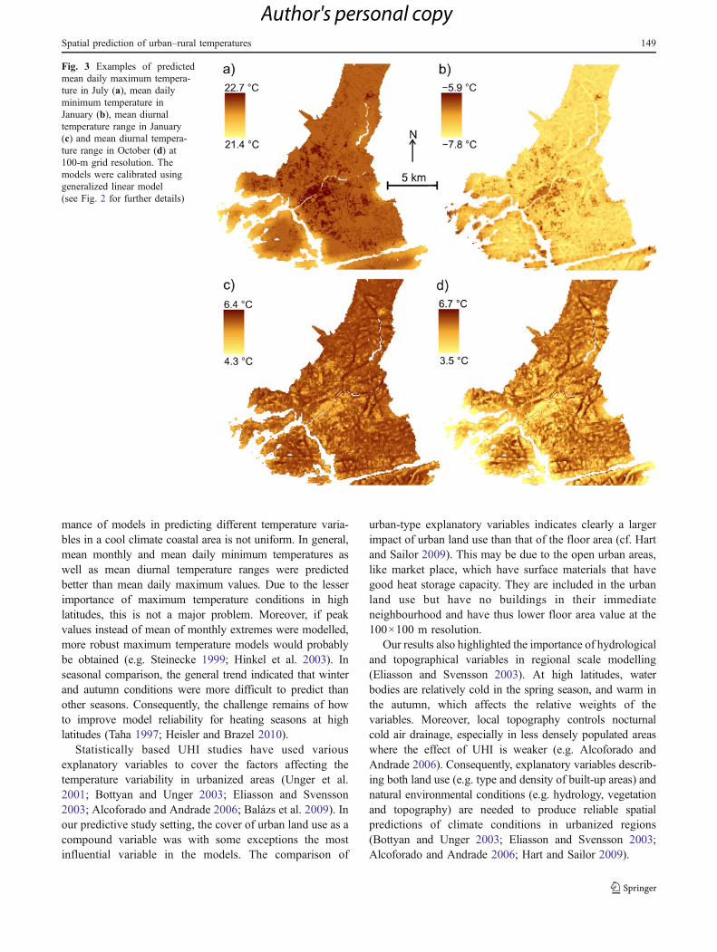
mance of models in predicting different temperature varia-bles in a cool climate coastal area is not uniform. In general,mean monthly and mean daily minimum temperatures aswell as mean diurnal temperature ranges were predictedbetter than mean daily maximum values. Due to the lesserimportance of maximum temperature conditions in highlatitudes, this is not a major problem. Moreover, if peakvalues instead of mean of monthly extremes were modelled,more robust maximum temperature models would probablybe obtained (e.g. Steinecke 1999; Hinkel et al. 2003). Inseasonal comparison, the general trend indicated that winterand autumn conditions were more difficult to predict thanother seasons. Consequently, the challenge remains of howto improve model reliability for heating seasons at highlatitudes (Taha 1997; Heisler and Brazel 2010).

Statistically based UHI studies have used variousexplanatory variables to cover the factors affecting thetemperature variability in urbanized areas (Unger et al.2001; Bottyan and Unger 2003; Eliasson and Svensson2003; Alcoforado and Andrade 2006; Balázs et al. 2009). Inour predictive study setting, the cover of urban land use as acompound variable was with some exceptions the mostinfluential variable in the models. The comparison of

urban-type explanatory variables indicates clearly a largerimpact of urban land use than that of the floor area (cf. Hartand Sailor 2009). This may be due to the open urban areas,like market place, which have surface materials that havegood heat storage capacity. They are included in the urbanland use but have no buildings in their immediateneighbourhood and have thus lower floor area value at the100×100 m resolution.

Our results also highlighted the importance of hydrologicaland topographical variables in regional scale modelling(Eliasson and Svensson 2003). At high latitudes, waterbodies are relatively cold in the spring season, and warm inthe autumn, which affects the relative weights of thevariables. Moreover, local topography controls nocturnalcold air drainage, especially in less densely populated areaswhere the effect of UHI is weaker (e.g. Alcoforado andAndrade 2006). Consequently, explanatory variables describ-ing both land use (e.g. type and density of built-up areas) andnatural environmental conditions (e.g. hydrology, vegetationand topography) are needed to produce reliable spatialpredictions of climate conditions in urbanized regions(Bottyan and Unger 2003; Eliasson and Svensson 2003;Alcoforado and Andrade 2006; Hart and Sailor 2009).

Fig. 3 Examples of predictedmean daily maximum tempera-ture in July (a), mean dailyminimum temperature inJanuary (b), mean diurnaltemperature range in January(c) and mean diurnal tempera-ture range in October (d) at100-m grid resolution. Themodels were calibrated usinggeneralized linear model(see Fig. 2 for further details)

Spatial prediction of urban–rural temperatures 149

Author's personal copy

7 Conclusions

We explored (1) the possibility to spatially predicttemperature variables using GIS data and small samplesize (calibration n=26) in urbanized region, (2) theperformance of two different statistical techniques (gener-alized linear model and boosted regression tree) and (3) theability to model monthly temperature values in differentseasons. The study area was located in cool climate coastalregion, in SW Finland. Based on the study results, we drawthree main conclusions:

& Monthly temperature variables (mean, mean dailyminimum, mean daily maximum and mean diurnaltemperature range) were robustly predicted with rela-tively small samples sizes (n≈20–40). For small samplesizes, parametric statistical techniques should be pre-ferred over non-parametric methods.

& On average, the temperature variables (mean, minimumand maximum) of spring and summer months werepredicted better than autumn and winter months. Thepredominant weather conditions probably overrule localaffecting factors more frequently in the autumn andwinter complicating the spatial modelling. Thus, chal-lenges remain to develop more reliable models forheating seasons, for the benefit of urban planning.

& Variability in the temperature data was explainedsatisfactorily with the employed GIS-based explana-tory variables. Regarding variable comparison, urbanland use and surface water cover were clearly thestrongest affecting factors in the study area in coolcoastal setting.

Consequently, the combination of multivariate statisticaltechniques and GIS data provides a cost-efficient approachto predict and analyze climate conditions at regional scales.The utilization of statistically based spatial modelling mayaid in gaining novel insights into the causes and impacts oftemperature variability in extensive urbanized areas.

Acknowledgements We express our gratitude to three anonymousreviewers for the critical and helpful comments which improved themanuscript. JS was funded by the Finnish Cultural Foundation’sVarsinais-Suomi Regional Fund and the Emil Aaltonen Foundation.TURCLIM project is maintained in collaboration with the TurkuEnvironmental and City Planning Department, whose assistance isgreatly acknowledged. The long-term reference weather data used inthis study is provided by the Finnish Meteorological Institute.

References

Akaike H (1974) A new look at the statistical identification model.IEEE Trans Autom Contr 19:716–723

Alcoforado MJ, Andrade H (2006) Nocturnal urban heat island inLisbon (Portugal): main features and modelling attempts. TheorAppl Climatol 84:151–159. doi:10.1007/s00704-005-0152-1

Atkinson BW (2003) Numerical modelling of urban heat island intensity.Bound LayMeteorol 109:285–310. doi:10.1023/A:1025820326672

Balázs B, Unger J, Gál T, Sümeghy Z, Geiger J, Szegedi S (2009)Simulation of the mean urban heat island using 2D surfaceparameters: empirical modelling, verification and extension.Meteorol Appl 16:275–287. doi:10.1002/met.116

Bottyan Z, Unger J (2003) A multiple linear statistical model forestimating the mean maximum urban heat island. Theor ApplClimatol 75:233–243. doi:10.1007/s00704-003-0735-7

Brown DJ, Shepherd KD, Walsh MG, Mays MD, Reinsch TG (2006)Global soil characterization with VNIR diffuse reflectance spectros-copy. Geoderma 132:273–290. doi:10.1016/j.geoderma.2005.04.025

Burnham KP, Anderson DR (1998) Model selection and inference: apractical information-theoretic approach. Springer, New York

Chapman L, Thornes JE (2003) The use of geographical informationsystems in climatology and meteorology. Prog Phys Geogr27:313–330. doi:10.1191/030913303767888464

City of Turku (2001) Turku Master Plan 2020. Environmental andCity Planning Office, Turku

City of Turku (2010) Floor area of the buildings. Real EstateDepartment, Turku

Cleugh HA, Oke TR (1986) Suburban-rural energy balance comparisonsin summer for Vancouver, B.C. Bound-Lay Meteorol 36:351–369.doi:10.1007/BF00118337

Conti S, Meli P, Minelli G, Solmini R, Toccaceli V, Vichi M, BeltranoC, Perini L (2005) Epidemologic study of mortality during thesummer 2003 heat wave in Italy. Environ Res 98:390–399.doi:10.1016/j.envres.2004.10.009

Cotton WR, Pielke RA (1995) Human impacts on weather andclimate. Cambridge University Press, Cambridge

Dobech H, Dumolard P, Dyras I (eds) (2007) Spatial interpolation ofclimate data. The use of GIS in climatology and meteorology.ISTE, London

Drebs A, Nordlund A, Karlsson P, Helminen J, Rissanen P (2002)Climatological statistics of Finland 1971–2000. Clim Stat Finland2002:1–99

Ekholm J (1981) Joensuun paikallisilmasto. Terra 93:145–154Eliasson I, Svensson MK (2003) Spatial air temperature variations and

urban land use—a statistical approach. Meteorol Appl 10:135–149. doi:10.1017/S1350482703002056

Elith J, Leathwick J (2009) Species distribution models: ecologicalexplanation and prediction across space and time. Ann Rev EcolEvol Syst 40:677–697. doi:10.1146/annurev.ecolsys.110308.120159

Elith J, Graham CH, Anderson RP et al (2006) Novel methods improveprediction of species’ distributions from occurrence data. Ecography29:129–151. doi:10.1111/j.2006.0906-7590.04596.x

Elith J, Leathwick JR, Hastie T (2008) A working guide to boostedregression trees. J Anim Ecol 77:802–813. doi:10.1111/j.1365-2656.2008.01390.x

FMI (2009) Climate service. Telephone customer service. FinnishMeteorological Institute

Friedman J (2002) Stochastic gradient boosting. Comp Stat Data Anal38:367–378. doi:10.1016/S0167-9473(01)00065-2

Friedman J, Hastie T, Tibshirani R (2000) Additive logistic regression:a statistical view of boosting. Ann Stat 38:337–374. doi:10.1214/aos/1016218223

Giridharan R, Kolokotroni M (2009) Urban heat island characteristicsin London during winter. Sol Energy 83:1668–1682.doi:10.1016/j.solener.2009.06.007

Giridharan R, Lau SSY, Ganesan S, Givoni B (2006) Urban designfactors influencing urban heat island intensity in high rise highdensity environments of Hong Kong. Build Environ 42:3669–3684. doi:10.1016/j.buildenv.2006.09.011

150 J. Hjort et al

Author's personal copy

Godefroid S, Koedam N (2007) Urban plant species patterns are highlydriven by density and function of built-up areas. Landscape Ecol22:1227–1239. doi:10.1007/s10980-007-9102-x

Hart MA, Sailor DJ (2009) Quantifying the influence of landuse andsurface characteristics on spatial variability in the urban heatisland. Theor Appl Climatol 95:397–406. doi:10.1007/s00704-008-0017-5

Hastie T, Tibshirani R, Friedman J (2001) The elements of statisticallearning: data mining, inference and prediction. Springer, NewYork

Heisler GM, Brazel AJ (2010) The urban physical environment:temperature and urban heat islands. In: Aitkenhead-Peterson J,Volder A (eds) Urban ecosystem ecology. American Society ofAgronomy, Crop Science Society of America, Soil Science,Society of America, Madison, pp 29–56

Hinkel KM, Nelson FE, Klene AE, Bell JH (2003) The urban heatisland in winter at Barrow, Alaska. Int J Clim 23:1889–1905.doi:10.1002/joc.971

Hjort J, Marmion M (2008) Effects of sample size on the accuracy ofgeomorphological models. Geomorph 102:341–350. doi:10.1016/j.geomorph.2008.04.006

Hjort J, Marmion M (2009) Periglacial distribution modelling with aboosting method. Permafr Periglac Process 20:15–25. doi:10.1002/ppp.629

Hjort J, Etzelmüller B, Tolgensbakk J (2010) Effects of scale and datasource in periglacial distribution modelling in a High Arcticenvironment, western Svalbard. Permafr Periglac Process21:345–354. doi:10.1002/ppp.705

Howard L (1818) Climate of London. Harvey and Darton, LondonJohnson DP, Wilson JS (2009) The socio-spatial dynamics of extreme

urban heat events: the case of heat-related deaths in Philadelphia.Appl Geogr 29:419–434. doi:10.1016/j.appgeog.2008.11.004

Kent M, Stevens RA, Zhang L (1999) Urban plant ecology patternsand processes:a case study of the flora of the City of Plymouth,Devon, UK. J Biogeogr 26:1281–1298. doi:10.1046/j.1365-2699.1999.00350.x

Kim Y, Baik J (2004) Daily maximum urban heat island intensity inlarge cities of Korea. Theor Appl Climatol 79:151–164.doi:10.1007/s00704-004-0070-7

Klysik K (1996) Spatial and seasonal distribution of anthropogenicheat emissions in Lodz, Poland. Atmos Environ 30:3397–3404.doi:10.1016/1352-2010(96)00043-X

Klysik K, Fortuniak K (1999) Temporal and spatial characteristics ofthe urban heat island of Lodz, Poland. Atmos Environ 33:3885–3895. doi:10.1016/S1352-2310(99)00131-4

Landsberg HE (1981) The urban climate. Academic, LondonLeathwick JR, Elith J, Francis MP, Hastie T, Taylor P (2006) Variation

in demersal fish species richness in the oceans surrounding NewZealand: an analysis using boosted regression trees. Mar EcolProg Ser 321:267–281

Luoto M, Hjort J (2006) Scale matters—a multi-resolution study of thedeterminants of patterned ground activity in subarctic Finland.Geomorph 80:282–294. doi:10.1016/j.geomorph.2006.03.001

Magee N, Curtis J, Wendler G (1999) The urban heat island effect atFairbanks, Alaska. Theor Appl Climatol 64:39–47. doi:10.1007/s007040050109

Martinaitis V (1998) Analytic calculation of degree-days for theregulated heating season. Energy Build 28(2):185–189

McCullagh P, Nelder JA (1989) Generalized linear models, 2nd edn.Chapman and Hall, London

Meehl GA, Tebaldi C (2004) More intense, more frequent, and longerlasting heat waves in the 21st century. Science 305:994–997.doi:10.1126/science.1098704

Memon RA, Leung DYC, Chunho L (2007) A review on the generation,determination and mitigation of Urban Heat Island. J Environ Sci 20(1):120–128. doi:10.1016/S1001-0742(08)60019-4

Miara K, Paszyfiski J, Grzybowski J (1987) Zrózniicowanie przestrz-enne bilansu promieniowania na obszarze Polski. PrzegledGeogr. t. LIX, z. 4

Mihalakakou HA, Flocas M, Santamouris HCG (2002) Application ofneural networks to the simulation of the heat island over Athens,Greece, using synoptic types as a predictor. J Appl Meteorol 41:519–527. doi:10.1175/1520-0450(2002)041<0519:AONNTT>2.0.CO;2

Mills G (2009) Micro- and mesoclimatology. Prog Phys Geogr33:711–717. doi:10.1177/0309133309345933

Oke TR (1973) City size and the urban heat island. Atmos Environ7:769–779. doi:10.1016/0004-6981(73)90140-6

Oke TR (1981) Canyon geometry and the urban heat island:comparison of scale model and field observations. Int J Climatol1:237–254. doi:10.1002/joc.3370010304

Oke TR (1987) Boundary layer climates, 2nd edn. Routledge, LondonOke TR (2006) Initial guidance to obtain representative meteorological

observations at urban sites. Instruments and observing methodsreport No. 81. World Meteorological Organization, Geneva

Peel MC, Finlayson BM, McMahon TA (2007) Updated world map ofthe Köppen-Geiger climate classification. Hydrol Earth Syst Sci11:1633–1644

R Development Core Team (2010) R: a language and environment forstatistical computing. R Foundation for Statistical Computing.http://www.R-project.org. Accessed 24 June 2010

Rajasekar U, Weng Q (2009) Urban heat island monitoring andanalysis using a non-parametric model: a case study of Indian-apolis. ISPRS J PhotogrammRemote Sens 64:86–96. doi:10.1016/j.isprsjprs.2008.05.002

Ridgeway G (2007) Generalized boosted regression models. Docu-mentation on the R Package ‘gbm’, version 1.6–3. http://cran.r-project.org/web/packages/gbm/gbm.pdf. Accessed 24 June 2010

Seinä A, Peltola J (1991) Duration of the ice season and statistics offast ice thickness along the Finnish coast 1961–1990. Finn MarRes 258:1–46

Seinä A, Eriksson P, Kalliosaari S, Vainio J (2006) Ice seasons 2001–2005 in Finnish sea areas. Rep Ser Finn Inst Mar Res 57:1–94

SLICES (2010) National Land Survey of Finland. http://www.slices.nls.fi/. Accessed 13 June 2010

Sokal RR, Rohlf F (1995) Biometry. WH Freeman, New YorkSteinecke K (1999) Urban climatological studies in Reykjavik

surbarctic environment, Iceland. Atmos Environ 33:4157–4162.doi:10.1016/S1352-2310(99)00158-2

Stockwell DRB, Peterson AT (2002) Effects of sample size onaccuracy of species distribution models. Ecol Mod 148:1–13.doi:10.1016/S0304-3800(01)00388-X

Sundborg Å (1950) Local climatological studies of the temperatureconditions in an urban area. Tellus 2:222–232. doi:10.1111/j.2153-3490.1950.tb00333.x

Suomi J, Käyhkö J (2011) The impact of environmental factors onurban temperature variability in the coastal city of Turku SWFinland. Int J Climatol. doi:10.1002/joc.227

Svensson MK, Eliasson I (2002) Diurnal air temperatures in built-upareas in relation to urban planning. Landscape Urban Plan 61:37–54. doi:10.1016/S0169-2046(02)00076-2

Svensson M, Eliasson I, Holmer B (2002) A GIS based empiricalmodel to simulate air temperature variations in the Göteborgurban area during the night. Clim Res 22:215–226

Szymanowski M, Kryza M (2009) GIS-based techniques for urbanheat island spatialization. Clim Res 38:171–187

Taha H (1997) Urban climates and heat islands: albedo, evapotrans-piration, and anthropogenic heat. Energy Build 25:99–103.doi:10.1016/S0378-7788(96)00999-1

Tan J, Zheng Y, Tang X, Guo C, Li L, Song G, Zhen X, Yuan D,Kalkstein AL, Li F, Chen H (2010) The urban heat island and itsimpact on heat waves and human health in Shanghai. Int JBiometeorol 54:75–84. doi:10.1007/s00484-009-0256-x

Spatial prediction of urban–rural temperatures 151

Author's personal copy

Unger J, Sümeghy Z, Gulyás Á, Bottyán Z, Mucsi L (2001) Land-useand meteorological aspects of the urban heat island. MeteorolAppl 8:189–194. doi:10.1017/S1350482701002067

Vicente-Serrano SM, Lanjeri S, López-Moreno JI (2007) Compar-ison of different procedures to map reference evapotranspira-tion using geographical information systems and regression-based techniques. Int J Climatol 27:1103–1118. doi:10.1002/joc.1460

Vicente-Serrano SM, López-Moreno JI, Vega-Rodríguez MI, Beguería S,Cuadrat JM (2010) Comparison of regression techniques formapping fog frequency: application to the Aragón region (northeastSpain). Int J Climatol 30:935–945. doi:10.1002/joc.1935

Zimmermann NE, Edwards TC, Moisen GG, Frescino TS, Blackard JA(2007) Remote sensing-based predictors improve distribution mod-els of rare, early successional and broadleaf tree species in Utah. JAppl Ecol 44:1057–1067. doi:10.1111/j.1365-2664.2007.01348.x

152 J. Hjort et al

Author's personal copy