land

Article

Spatial Interactions in Business and Housing Location Models

Katarzyna Kopczewska * , Mateusz Kopyt and Piotr Cwiakowski

�����������������

Citation: Kopczewska, K.; Kopyt, M.;

Cwiakowski, P. Spatial Interactions in

Business and Housing Location

Models. Land 2021, 10, 1348. https://

doi.org/10.3390/land10121348

Academic Editors: Shiliang Su,

Shenjing He and Monika Kuffer

Received: 9 October 2021

Accepted: 5 December 2021

Published: 7 December 2021

Publisher’s Note: MDPI stays neutral

with regard to jurisdictional claims in

published maps and institutional affil-

iations.

Copyright: © 2021 by the authors.

Licensee MDPI, Basel, Switzerland.

This article is an open access article

distributed under the terms and

conditions of the Creative Commons

Attribution (CC BY) license (https://

creativecommons.org/licenses/by/

4.0/).

Faculty of Economic Sciences, University of Warsaw, 00-927 Warszawa, Poland; mkopyt@wne.uw.edu.pl (M.K.);pcwiakowski@wne.uw.edu.pl (P.C.)* Correspondence: kkopczewska@wne.uw.edu.pl

Abstract: The paper combines theoretical models of housing and business locations and shows thatthey have the same determinants. It evidences that classical, behavioural, new economic geography,evolutionary and co-evolutionary frameworks apply simultaneously, and one should consider themjointly when explaining urban structure. We use quantitative tools in a theory-guided factorsinduction approach to show the complexity of location models. The paper discusses and measuresspatial phenomena as distance-decaying gradients, spatial discontinuities, densities, spillovers,spatial interactions, agglomerations, and as multimodal processes. We illustrate the theoreticaldiscussion with an empirical case of interacting point-patterns for business, housing, and population.The analysis reveals strong links between housing valuation and business location and profitability,accompanied by the related spatial phenomena. It also shows that assumptions concerning unimodalspatial urban structure, the existence of rational maximisers, distance-decaying externalities, and asingle pattern of behaviour, do not hold. Instead, the reality entails consideration of multimodality,a mixture of maximisers and satisfiers, incomplete information, appearance of spatial interactions,feed-back loops, as well as the existence of persistence of behaviour, with slow and costly adjustmentsof location.

Keywords: business location; housing valuation; density; multimodality; urban structure

1. Introduction

Despite the immensely large range of theories and empirical evidence in regionaland urban studies, there are still very few explanations of the links between businessand residential location within cities, with particular insight into firms’ profitability andhousing valuation. Existing theories of the location of both business and housing, togetherwith their inherent agglomeration and spatial externalities effects, have, in fact, the samedrivers and deserve to be considered jointly. Location factors affect where households andbusinesses decide where to live and locate a firm, respectively. Independent of the adoptedresearch perspective and the decision-makers’ internal motivations, the final outcomesare the densities of business and housing and the spatial distribution of economic activityreflected in the prices of real estate and the profitability of businesses.

The intersection of both streams, business and housing location and valuation, liesin their similar spatial determinants, and the spatial consequences of both processes interms of clustering, density, agglomeration externalities, central business district (CBD)location, rural vs. urban sites, accessibility, proximity to important neighbours, quality andusefulness of neighbourhoods, absolute and relative locations, local and global perspectives,spatial segregation, etc. Both processes are interconnected. Real estate prices are a costto businesses that impact their profitability. Conversely, prestigious neighbourhoods ofwell-performing companies increase the price of real estate.

An overview of the literature shows that both business and housing location and valu-ation models follow the same mainstream theoretical influences, from classical, behavioural,new economic geography (NEG), to evolutionary and co-evolutionary. However, their

Land 2021, 10, 1348. https://doi.org/10.3390/land10121348 https://www.mdpi.com/journal/land

Land 2021, 10, 1348 2 of 25

developmental trajectory has been different—in business location theories, scholars aban-doned the old concepts when shifting to new ones, while in housing, they have added newcomponents to a classical base. This asymmetry in development has caused current modelsto be poorly integrated because of fundamental differences in assumptions. Secondly, boththeoretical streams do not fine-tune their assumptions on spatial patterns, for examplewith respect to spatial interactions between agents, a mixture of maximisers, satisfiers andrandom decision takers, discontinuities in distance-decaying gradients, spatial interactionsin determinants of processes or polycentric urban structures.

The remainder of the paper is structured as follows: In Section 2 this paper comparesbusiness and housing location theories and provides a unique insight into the spatialcontext to highlight common elements. We propose the following hypotheses: first, that thetheoretical spatial assumptions of location models are mostly not fulfilled, and second, thatneither of the models is out-of-date. At the same time, their joint application may shed somenew light on occurring interactions. We suggest that regional theory requires an integratingumbrella across the agents and mechanisms involved. We show that localisation modelsin classical, behavioural, new economic geography, evolutionary and co-evolutionaryframeworks, should be considered jointly, as they each account for different phenomenaincluded in the von Thünen, Loesch, Weber, Alchian, Alonso, Tiebout, Webber, Krugman,Boschma and Gong and Hassink models. In Section 3, we discuss spatial issues of locationtheories including location changes, agglomeration effects, economies of density, bid-rentcurves, spatial interactions, spatial externalities, a rationality-based mixture of satisfiers andoptimisers, multimodality, and feed-back loops. Section 4 presents quantitative methods tocapture these effects. In the empirical component (Section 5), we use spatial quantitativemethods to verify existing relationships between business location and profitability andhousing valuation. We hypothesise that there are visible links and spatial interactionsbetween both spatial patterns. In an empirical illustration, we use geo-located point datafor firms and real estate in Warsaw, Poland. We close the paper with conclusions anddiscussion (Section 6). An appendix provides empirical and technical details of the study.

2. Location of Business and Real Estate—Determinants and Decision Processes2.1. Theories on Firms’ Location

Over the last 200 years, beginning with the first business location model by vonThünen [1], many concepts have been proposed and many studies undertaken on howfirms choose their location. The oldest, classical, approach was based on entirely rationaloptimisation, i.e., when selecting a place, firms seek to maximise their profit or minimisetheir costs. The models of districts by von Thünen [1] indicate that the location chosendepends on the activity type and proximity to the city centre. Later models, such asthose of Alfred Weber [2], Loesch [3] and Moses [4], imply that choice is determined bymaximisation of profit or sales with regard to raw-material markets and transportationcosts. The Hotelling model [5], and its development from line to circle location by Salop [6],considers the relationship between the location and a companies’ pricing policy. However,in these models, companies do not take advantage of differences in product characteristics—they compete and assess the products only in the geographic dimension and treat productsas perfect substitutes.

Though classical models have been justified from a micro-economic perspective andrationality paradigm, they have been widely criticised. Webber [7], in his critique in thelate 1960s, listed several categories of problem. The “error criticism” emphasizes thatnon-economic factors, such as prestige, persistent social networks, costly and imperfectinformation about alternatives, personal motivations, etc., may play a significant role inchoosing and changing location. Simonian bounded rationality, driven by the impossibilityof obtaining complete information and uncertainty about the future, causes agents to strivefor a satisfactory level of profit or utility but not for a maximal one. The “deterministiccriticism” implies that stochastic models will perform better than deterministic ones, mainlybecause of the inclusion of risk, unknown variables, and future uncertainty. Interestingly,

Land 2021, 10, 1348 3 of 25

some current models still assume a maximisation mechanism regarding location, whichsuggests that there are doubts over the criticisms levelled above [8].

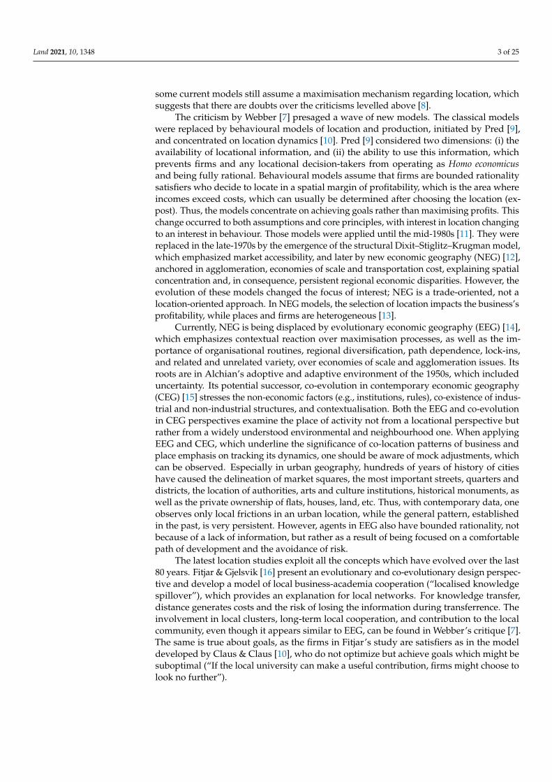
The criticism by Webber [7] presaged a wave of new models. The classical modelswere replaced by behavioural models of location and production, initiated by Pred [9],and concentrated on location dynamics [10]. Pred [9] considered two dimensions: (i) theavailability of locational information, and (ii) the ability to use this information, whichprevents firms and any locational decision-takers from operating as Homo economicusand being fully rational. Behavioural models assume that firms are bounded rationalitysatisfiers who decide to locate in a spatial margin of profitability, which is the area whereincomes exceed costs, which can usually be determined after choosing the location (ex-post). Thus, the models concentrate on achieving goals rather than maximising profits. Thischange occurred to both assumptions and core principles, with interest in location changingto an interest in behaviour. Those models were applied until the mid-1980s [11]. They werereplaced in the late-1970s by the emergence of the structural Dixit–Stiglitz–Krugman model,which emphasized market accessibility, and later by new economic geography (NEG) [12],anchored in agglomeration, economies of scale and transportation cost, explaining spatialconcentration and, in consequence, persistent regional economic disparities. However, theevolution of these models changed the focus of interest; NEG is a trade-oriented, not alocation-oriented approach. In NEG models, the selection of location impacts the business’sprofitability, while places and firms are heterogeneous [13].

Currently, NEG is being displaced by evolutionary economic geography (EEG) [14],which emphasizes contextual reaction over maximisation processes, as well as the im-portance of organisational routines, regional diversification, path dependence, lock-ins,and related and unrelated variety, over economies of scale and agglomeration issues. Itsroots are in Alchian’s adoptive and adaptive environment of the 1950s, which includeduncertainty. Its potential successor, co-evolution in contemporary economic geography(CEG) [15] stresses the non-economic factors (e.g., institutions, rules), co-existence of indus-trial and non-industrial structures, and contextualisation. Both the EEG and co-evolutionin CEG perspectives examine the place of activity not from a locational perspective butrather from a widely understood environmental and neighbourhood one. When applyingEEG and CEG, which underline the significance of co-location patterns of business andplace emphasis on tracking its dynamics, one should be aware of mock adjustments, whichcan be observed. Especially in urban geography, hundreds of years of history of citieshave caused the delineation of market squares, the most important streets, quarters anddistricts, the location of authorities, arts and culture institutions, historical monuments, aswell as the private ownership of flats, houses, land, etc. Thus, with contemporary data, oneobserves only local frictions in an urban location, while the general pattern, establishedin the past, is very persistent. However, agents in EEG also have bounded rationality, notbecause of a lack of information, but rather as a result of being focused on a comfortablepath of development and the avoidance of risk.

The latest location studies exploit all the concepts which have evolved over the last80 years. Fitjar & Gjelsvik [16] present an evolutionary and co-evolutionary design perspec-tive and develop a model of local business-academia cooperation (“localised knowledgespillover”), which provides an explanation for local networks. For knowledge transfer,distance generates costs and the risk of losing the information during transferrence. Theinvolvement in local clusters, long-term local cooperation, and contribution to the localcommunity, even though it appears similar to EEG, can be found in Webber’s critique [7].The same is true about goals, as the firms in Fitjar’s study are satisfiers as in the modeldeveloped by Claus & Claus [10], who do not optimize but achieve goals which might besuboptimal (“If the local university can make a useful contribution, firms might choose tolook no further”).

Land 2021, 10, 1348 4 of 25

2.2. Theories on Real Estate Location

Similar to business location theory, which commenced with the profit-optimisation ap-proach, the housing location theory introduced by Alonso [17] was based on differentiatedbid-rent curves for specific land-use types (e.g., housing, commercial, and industry) withinthe city. Alonso claimed that different actors, such as households, industries, commercialestablishments, etc., compete for locations within the city. They maximise utility from quickaccessibility to the city centre with respect to available budget constraints. He assumed thatcentrally located land is more expensive than peripheral land, businesses can pay more forland than households, that rich people need less quick access to the city centre, and thathigh utility from accessibility is the concern of the poor. His urban-land-use segregationmodel is fundamental for job-housing balancing [18], assuming that people will be willingto live near to work if they can afford it. As summarised by Straszhem [19], residentiallocation decisions are correlated with housing prices. In general, they are the function ofurban spatial structure, including city size, population density, rent gradient, and housinglocation and business, as well as the budget constraints of households. Demand for realestate fluctuates because of the gentrification process and the rent gap, which appears alsoto be a driver [20,21].

Housing models have evolved somewhat differently than business location models.In contrast to business location models, they have never rejected the classical principles ofoptimisation formulated by Alonso. The new generations of theoretical models of locationhave only added new elements to the fundaments of the classical theory.

Behavioural housing models, as developed by Wheaton [22], imply that the Alonsomodel may not work if factors other than accessibility, such as income, taxation, the so-cial composition of the neighbourhood, etc., impact the utility of housing location anddrive settlement decisions. They have been extended into non-spatial models (such as theDiPasquale–Wheaton model) and explain housing demand with a depreciation rate of stockor rental price [23,24]. However, current behavioural models [25] optimise the residentiallocation choice combined with transportation networks and still assume that endogenousneighbourhood characteristics determine it. In the behavioural approach [26], locationdecision is optimised with respect to housing prices and personal income; the neighbour-hoods are assumed heterogeneous, while the primary decision driver is aspiration level.Inequality of income is the driver of spatial segregation of inhabitants.

NEG models [27] deal with competition between housing and business, which isstrongly affected by pollution effects and includes agglomeration effects, which conse-quently establish industrial and residential clusters. Within the group of NEG models,Partridge et al. [28] tested urban cost-gradients, typical for distance-decay optimisationmodels, but under assumptions of hierarchical urban structure and different sourcesof agglomeration spillovers. Glaeser [29] built a complex NEG model of urban spatialequilibrium with three actors—firms, inhabitants, and developers—adding to it issues ofagglomeration, wages, and transportation, and merging it with the Alonso–Muth–Millsmodel. Suedekum [30] extended Krugman’s NEG model by incorporating the home goodssector and living costs.

Co-evolutionary models, such as [31], consider the relationship of the Alonso modelto neighbourhood quality, primarily the Tiebout-model-driven quality of schools. Eventhough formally the EEG and CEG approaches appeared in the early 2000s, the old defini-tion by Papageorgiou [32] that the “city is a complex system of spatial interdependencebetween its constituent elements: households, businesses, industries, and public insti-tutions” created the opening for them, treating the other drivers of location as spatialexternalities [33]. Taking a life-cycle perspective, household activity demand and accessibil-ity to activities, such as employment, education, shopping, or medical services, may impacthousing prices in urban spaces. However, an example provided by Beijing [34] showedthat employment accessibility was the primary determinant of price and confirmed thathousing and business locations were strongly connected. There is, further, a vast literatureon location and neighbourhood quality in housing consumption from the perspective of

Land 2021, 10, 1348 5 of 25

economic and socio-cultural changes in urban and metropolitan housing market areas [35].Current studies [36] have confirmed the positive value of cultural amenities for housingmarkets when studied jointly with the effects produced by green areas, public transport,and university proximity. The complexity of the problem shifts the interest from urbanlandscape elements to well-being in cities as well. Though studies have confirmed thespatial nature of neighbourhood well-being and significance [37], they are inconclusive.They cannot explain why living in the city centre does not produce full happiness [38].

3. Spatial Issues in the Revision of Business and Housing Location Theories

The selection of business location in any location theory is inseparably linked to thelocation changes. In consequence, the classical optimisation approach implies that firmsshould move, preferably from worse to better locations. This can be found in Tiebout’s [39]“voting with feet” concept for firms. His work on business location is not far conceptuallyfrom the much better-known idea of optimisation for taxpayers who benefit from publicservices [40]. Tiebout [39] links the place of business with its profitability and argues infavour of classical maximisation-based models. Even in cases of the random selection oflocations by industry, the market competition mechanism will eliminate inferior firms fromthe market, which means that only well-located firms will survive.

Consequently, this causes the emergence of the profit-maximising agglomerativespatial pattern of location. However, this easy portability of business is in contradictionto the “sticky location” approach proposed by Webber [7], who claims that a businesswill prefer to stay in its location because of social and business links, knowledge of themarket, suppliers, and customers, etc. Later models and studies have treated the stickinessof location differently, most often including it together with other assumptions and rarelyconsidering the mechanisms.

Amongst well-established drivers of location changes are agglomeration forces. In fact,all location models, from von Thünen circles to the co-evolution economic geography (EG)approach, refer explicitly or implicitly to agglomeration effects, which are operationalisedfurther by distance and density. Different mechanisms have been proposed for agglomer-ation: in the von Thünen model, it results from urban economies; in NEG it stems fromtransport costs and firm-level scale economies [41]; while in EEG it is the “endogenousco-evolution of agglomeration of industries and local formal and informal institutions,that are specific to certain industries and places” [15], and its existence is simply assumed.The well-established division into Marshallian specialisation and Jacobian diversificationagglomeration externalities has been tested and discussed [42], and case-based evidencehas been produced [43,44].

The latest studies shift the key issue of agglomeration phenomenon from productionstructure to economies of density, with greater emphasis on the spatial dimension in theurban context. As in [8], the seller maximises the profit through the “exploitation of theeconomies of density”. The importance of density and urbanisation for agglomerationexternalities find confirmation in study of [45], which showed that, “the threshold ofurbanisation at which diversity, density and competition agglomeration externalities allgenerate positive effects was 33%”. With more of an EEG flavour, the study by de Matteiset al. [46] found that for exporting firms, independently from internal features of thebusiness, the most crucial factor for export was the local environment, including distancefrom foreign markets, the level of social capital, the efficiency of the public sector, the degreeof financial development and the extent of agglomeration economies. The same regionalagglomeration economies were confirmed by [47], which showed that these economiesdo not depend on the firm’s characteristics. The first consequence of agglomeration areclusters, which have been well-studied since Porter [48] and developed by McCann [49].The latest studies confirm that the optimal location for a business results from being part ofa local cluster. This adherence may increase survival chances in times of crisis [50].

The above-presented overview shows that each of the mentioned streams, e.g.,optimisation-based classical models, behavioural models, agglomeration-driven NEG, and

Land 2021, 10, 1348 6 of 25

neighbourhood-driven EEG and CEG, are partly right but only shed light on some aspects ofthis complex phenomenon. Integration of these models could explain the spatial pattern oflocation more comprehensively.

The same problems occurring with business location models have been examinedin housing models. Urban agglomeration effects are primarily modelled for firms, andhousing appears as an extra component explaining the costs of living [30] or wage premium,or by adding an “Alonso” component for land consumption [41], all contained within theNEG framework. Agglomeration externalities traditionally arise from the central businessdistrict (CBD) issue, while new studies in the USA suggest that sub-centres may alsobecome their source [51]. This can be optimised by defining new cores in a polycentricurban structure [52].

Change of location is mostly modelled with residential location choice, which isoperationalised by binary-choice or multi-choice econometric models with respect to land-use and transportation, accessibility and commuting issues [53,54]. This approach wasinitiated by McFaden [55] and assumes a rational consumer, who “will choose a residentiallocation by weighing the attributes of each available alternative and by selecting thealternative that maximises utility”. In fact, it is based on gradients and Alonso’s vision ofthe utility of households. The classical issue of bid-rent curves has been analysed by testingurban accessibility. The intra-city accessibility and its relation with housing prices andhousehold income may be modelled in many ways [56]. Gutiérrez-i-Puigarnau et al. [57]found that the richer the household, the closer the residential location to Denmark’sworkplace. There are also many studies on the role of transportation in real estate valuationand household preferences [58,59]. Wong and Ho [60] proposed a housing location choicemodel considering a continuous transportation system for a city of arbitrary shape.

In general, the spatial behaviour of agents (people or firms) can be modelled the-oretically using spatial interactions and spatial externalities. Both concepts previouslyappeared in Tobler’s theory [61], e.g., “Everything is related to everything else, but nearthings are more related than distant things”. However, it does not distinguish whetherobjects behave interactively (spatial interactions) or whether some are passive and simplyinfluenced by other agents (spatial externalities). The theory of spatial externalities byPapageorgiou [62,63] does not assume interactions between agents. However, such effectsdecay with distance. There exist two surfaces: the population surface, where each agentis exerting and being influenced by some effects, and the externality surface, which isthe total effect of all effecting agents over space, depending on the agents’ distribution.Spatial externalities are, in fact, a kind of multiplier of benefits and costs for distance effectsin the process of utility maximisation. The reaction of agents to change in location maydiffer, depending on stationarity or movability of the impact emitting point, but withrespect to their own situation only and without insight into others’ utility. A differentapproach, where absorption of externalities changes an agent’s behaviour, was introducedby Papageorgiou [64]. It assumes that social interactions, including communication andconstant comparison (re-assessment) of the spatial distribution of welfare opportunities,induce agents to move, and more specifically, to agglomerate. Both approaches to spatialinteractions and externalities assume that agents, independent of interactions, are max-imisers. Furthermore, spillovers are distance-decaying, while the urban spatial structure isunimodal. These are strong assumptions, which, when relaxed, may give different results.

The above-mentioned spatial issues generate three major problems. The first problemof spatial externalities and spatial interactions is the case of satisfiers, agents with Simonianbounded rationality and targeted to achieve a given level of wealth (as in Webber’s [7]critique), instead of continuous maximisation as in Papageorgiou’s models. They are affectedby discontinuity over space and with a permanent steady state because some agents simplystop reacting after having achieved an internal goal. Agglomeration in neo-classical models isthe effect of permanent spatial adjustments and re-location patterns and appears as the agentscontinuously look for more. When agents lose their motivation for permanent improvement,they stabilise. This was confirmed in knowledge-diffusion studies [65]. A variety of possible

Land 2021, 10, 1348 7 of 25

behaviours can be observed in the whole population. Thus, theoretical and empirical studiesshould assume some proportion of utility optimisers and include satisfiers as well as randomand undecided agents. This will cause a discontinuity in the spatial distribution of preference.Simultaneously, the break in a distance–decay function may be the reason for random spatialallocation, which depends on past positions, as in EEG.

The second problem in the explicit modelling of distance-decaying spatial effects is themultimodality of urban spatial structures. Even though the literature already addresses theissue of the existence of more than one core within the city (since Fujita & Ogawa [66], laterin [67]), most models still explicitly or implicitly assume that there is only one urban core,in which the externalities start and spillover smoothly over space in a linear or negativelyexponential way. The current models applied to multimodal urban structures are notas conclusive as for unimodal structures. Multimodality, and potentially reducing theunimodal spatial urban structure, is a safer starting point than the opposite strategy. Inconsequence, for multi-cores modelling, the distance–decay function might be stepped, notstrictly decreasing. However, all patterns may be biased with spatial discontinuity, whichis understood here as a limitation of the pure geographic patterns that deregulate gradientsor distance–decay. It may be caused by administrative borders, by the non-linearity ofprocesses, as well as by the non-optimising behaviour of agents (i.e., Simonian boundedrationality) and the overlap of the effects of gradients from different spatial processes.

The third problem is the iterative reaction of agents on the observed situation, i.e., afeed-back loop. Interactions by Papageogiou [64] are simply the possibility of comparingagents with others. Here there is no feed-back effect which would change the level of exter-nal effects emitted because of a change in some other agent’s position. Papageorgiou’s [64]model concerns direct impacts only, where feedback does not transfer between agents.However, many studies have observed, both for firms and real estate, the existence of anindirect effect, which allows for the transfer of feedback among agents. Although for a realestate market, the modelling of indirect effects is a standard [68], this is not represented inbusiness location models. The existence of a feedback loop implies an inter-dependence inspace. Spatial interactions can be observed at the level of persons and units, while theycan also appear between markets as joint distributions. Many spatial econometric studiesusing spatial Durbin models [69] have convincingly shown that spatial inter-dependenceof phenomena is often observed, and that direct and indirect spillover effects should beincluded in modelling.

Spatial analysis requires an integrated approach, both for individuals and aggregates,at a micro and macro scale, as a result of the diversity of agents [70]. Somewhat naïvely, butconvenient for quantitative studies, the assumption is made that discovering the empiricalshape of rent gradients and patterns of spatial accessibility with different modes of transportwill allow for tracking of the trade-off between transport costs and housing price [70]. This,of course, follows from assumptions on unaffected, regular spatial distance-decay or cost-decay patterns, both for place attractiveness and human preferences. However, an overviewof city housing and business location theories suggests that this simplification may gotoo far. Both spatial discontinuities and the spatial inter-dependence and agglomerationforces prevent us from assuming that spatial distributions are unimodal. Consequently,it is necessary to consider the multimodality of spatial patterns, together with the multi-surface problem, as in Papageorgiou’s surfaces. Discovering composite spatial patterns,varying between subgroups, entailing the composition of different spatial layers withextreme values and discontinuities, is a complex task and should be based on a mixtureof neoclassical, behavioural, institutional, and evolutionary approaches. Additionally,the issue of MAUPs (modifiable areal unit problems) should be considered, along withdata aggregation and global and local perspectives, as well as the conditionality (vs. theunconditionality) of processes.

Land 2021, 10, 1348 8 of 25

4. Spatial Methods to Verify the Spatial Mechanisms4.1. Spatial Variables Included in the Modelling

Our research approach is that of “theory-guided factors induction” being midwaybetween purely inductive and deductive modelling [71]. The explanatory variables aretheory-connected, selected critically as potential candidates, however in an unstructuredway and without specification of possible interactions. In this approach, less significantvariables cannot simply be dropped, as they are anticipated to contribute to theory andshould be considered [71].

We discuss the general types of spatial variables included in modelling. Each of themhas its roots in theories discussed in Section 2 or Section 3. The kinds of spatial variablesmentioned below apply to three separate datasets of geo-located point-data: for business,housing, and population. Typical pure point data are supplemented with additional spatialinformation, including values in a neighbourhood, distance to the core, and density around.

Value in the neighbourhood of a point is the average of values calculated within agiven radius of the analysed point (firm location or real estate location) or the existence offirms from a given sector. We have calculated nearby profitability (ROA_around), nearbyhousing prices (price_sqm_around), and, as a dummy variable, the existence of firms from agiven sector in close surrounding (sec_XXX for 28 sectors). They differ among the modelsin values and interpretations. ROA_around, in the model for ROA_individual, representsthe average value of ROA in the surroundings of a given firm, and it becomes a spatial lagvariable to measure spatial spillover. However, ROA_around in the model for price_sqmbecomes an ROA average in the surrounding of real estate and tests the inter-dependenceof local spatial distributions. The same applies to price_sqm_around.

Distance from a point to core location (as CBD) reflects gradients and the spatialdistance-decay of phenomena. In the case of multi-core spatial organisation, the modelsshould include distances to all cores. As in spatial interaction models, distance can be linear,multinomial, or logarithmic. The inclusion of multinomial distance allows for non-linearityto be dealt with flexibly. In this study, we measured the distances to two identified cores(clust1 and clust2, derived with DBSCAN, described further) and applied the first, secondand third power (ˆ1, ˆ2, ˆ3) of those distances, which produced six variables (dist_clust1ˆ1,dist_clust1ˆ2, dist_clus1ˆ3, dist_clust2ˆ1, dist_clust2ˆ2, dist_clust2ˆ3).

The neighbourhood density can be expressed by a number of points within a radiusof a point. Diverse local densities indicate agglomeration patterns and can detect cores ofthe city. Business density can be general (e.g., for all business units around), or sectoral(e.g., for a number of firms from a given or own sector). We included the followingvariables, which always represent a specific number of points within the analysed radius:knn_business_density (number of firms around), knn_own_sector (number of firms from thesame sector around), knn_BusinessServices (number of firms from the business servicessector around), knn_Wholesale (number of firms from the wholesale sector around). Wehave also included the local density of the population (popul_around) and the intensity ofhousing transactions (no_of_trans_around).

Beyond these individual data, the overall agglomeration within the territory can betested with density functions based on points as well as on the entropy of the tessellatedpoint-pattern (details in Appendix A, part 3). The areas of high density can be detectedwith the DBSCAN algorithm.

4.2. Data Used in Modelling

The empirical study was based on data for Warsaw, the capital city of Poland. We haveintegrated three datasets. The dataset on firms was collected from the AMADEUS/ORBISdatabase for 2016 and included approximately 24,000 geo-located point observations withinformation on ROA indicator (return on assets) and the business sector. A dataset forreal housing transactions between 2012 and 2016 (a period of stable prices) was collectedfrom the official register from the mayor’s office and included approximately 36,000 geo-located point observations with information on price per sqm and general real estate

Land 2021, 10, 1348 9 of 25

characteristics included in official documents (e.g., floor space, number of rooms, separatekitchen, balcony, cellar). The dataset for the population was released by Statistics Poland(https://geo.stat.gov.pl/inspire, 15 November 2021) as a 1 km × 1 km grid for 2011 withdetailed data for number of inhabitants.

The original datasets were extended. For each observation of business data, we havecalculated, within a radius of 500 m, the average profitability of firms, and the followingdensity variables: the number of business units around, the number of firms from thesame sector as an analysed firm, and the number of firms from the two most frequentlyappearing sectors, business services and wholesale. For each firm, we have also calculated,within that radius, the average transactional sqm price on the real estate market and thenumber of sales transactions, which creates the connection between these two datasets.We also transformed the gridded population into a point pattern by sampling within each1 km × 1 km grid cell the points reflecting the population (1 point for 100 people). Wehave integrated this point pattern with business data by calculating the number of points(people) within a 500 m radius of each firm. The core locations of business were detectedwith the DBSCAN algorithm by searching a minimum of 1100 firms within a radius of ca.150 m. Using this procedure, we have obtained two main density clusters (see Figure 1a).We calculated distances between each firm and the core of each cluster. All calculationswere performed using R software (details in Appendix A, part 1). Descriptive statistics forthe datasets are presented in Appendix B.

Land 2021, 10, x FOR PEER REVIEW 9 of 25

4.2. Data Used in Modelling The empirical study was based on data for Warsaw, the capital city of Poland. We

have integrated three datasets. The dataset on firms was collected from the AMADEUS/ORBIS database for 2016 and included approximately 24,000 geo-located point observations with information on ROA indicator (return on assets) and the business sector. A dataset for real housing transactions between 2012 and 2016 (a period of stable prices) was collected from the official register from the mayor’s office and included ap-proximately 36,000 geo-located point observations with information on price per sqm and general real estate characteristics included in official documents (e.g., floor space, number of rooms, separate kitchen, balcony, cellar). The dataset for the population was released by Statistics Poland (https://geo.stat.gov.pl/inspire, 15 November 2021) as a 1km x 1km grid for 2011 with detailed data for number of inhabitants.

The original datasets were extended. For each observation of business data, we have calculated, within a radius of 500 m, the average profitability of firms, and the following density variables: the number of business units around, the number of firms from the same sector as an analysed firm, and the number of firms from the two most frequently appearing sectors, business services and wholesale. For each firm, we have also calculated, within that radius, the average transactional sqm price on the real estate market and the number of sales transactions, which creates the connection between these two datasets. We also transformed the gridded population into a point pattern by sampling within each 1km x 1km grid cell the points reflecting the population (1 point for 100 people). We have integrated this point pattern with business data by calculating the number of points (peo-ple) within a 500 m radius of each firm. The core locations of business were detected with the DBSCAN algorithm by searching a minimum of 1100 firms within a radius of ca. 150 m. Using this procedure, we have obtained two main density clusters (see Figure 1a). We calculated distances between each firm and the core of each cluster. All calculations were performed using R software (details in Appendix A, part 1). Descriptive statistics for the datasets are presented in Appendix B.

(a) (b)

Figure 1. Business locations: (a) dense clusters of firms from DBSCAN to assess the multimodality of urban structure; (b) median values of ROA by city districts to assess the business profitability by locations.

Integration and comparison of point patterns require statistical solutions, which pro-vide common references. For plotting, we used the rasterisation method, visible in Figure

Figure 1. Business locations: (a) dense clusters of firms from DBSCAN to assess the multimodality of urban structure;(b) median values of ROA by city districts to assess the business profitability by locations.

Integration and comparison of point patterns require statistical solutions, whichprovide common references. For plotting, we used the rasterisation method, visible inFigure 3a,b. As conventionally required, the correlations of variables were also analysedto avoid multicollinearity in the model. In the case of geo-located data, this involvedanalysing the similarity of values of variables in similar locations. Typical correlationmeasurement was not effective in this case as it did not deal with space, while we operatedwith three geo-located datasets which included different observations. Therefore, we rana more sophisticated algorithm based on the Rand Index (Figure 2b). Raw data (eachvariable individually) were clustered with k-means into 10 clusters, minimising within-cluster distances, and maximising between-cluster separation and group similar values.

Land 2021, 10, 1348 10 of 25

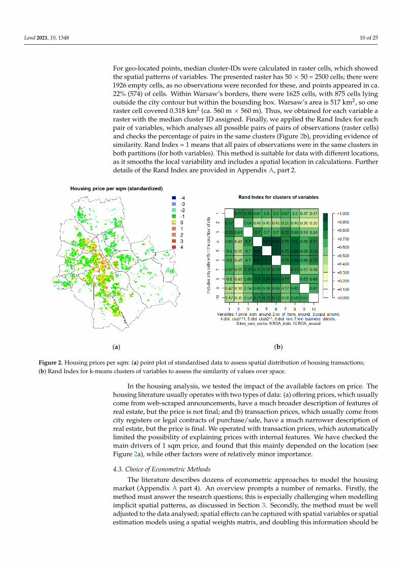
For geo-located points, median cluster-IDs were calculated in raster cells, which showedthe spatial patterns of variables. The presented raster has 50 × 50 = 2500 cells; there were1926 empty cells, as no observations were recorded for these, and points appeared in ca.22% (574) of cells. Within Warsaw’s borders, there were 1625 cells, with 875 cells lyingoutside the city contour but within the bounding box. Warsaw’s area is 517 km2, so oneraster cell covered 0.318 km2 (ca. 560 m × 560 m). Thus, we obtained for each variable araster with the median cluster ID assigned. Finally, we applied the Rand Index for eachpair of variables, which analyses all possible pairs of pairs of observations (raster cells)and checks the percentage of pairs in the same clusters (Figure 2b), providing evidence ofsimilarity. Rand Index = 1 means that all pairs of observations were in the same clusters inboth partitions (for both variables). This method is suitable for data with different locations,as it smooths the local variability and includes a spatial location in calculations. Furtherdetails of the Rand Index are provided in Appendix A, part 2.

Land 2021, 10, x FOR PEER REVIEW 10 of 25

3a,b. As conventionally required, the correlations of variables were also analysed to avoid multicollinearity in the model. In the case of geo-located data, this involved analysing the similarity of values of variables in similar locations. Typical correlation measurement was not effective in this case as it did not deal with space, while we operated with three geo-located datasets which included different observations. Therefore, we ran a more sophis-ticated algorithm based on the Rand Index (Figure 2b). Raw data (each variable individu-ally) were clustered with k-means into 10 clusters, minimising within-cluster distances, and maximising between-cluster separation and group similar values. For geo-located points, median cluster-IDs were calculated in raster cells, which showed the spatial pat-terns of variables. The presented raster has 50 × 50 = 2500 cells; there were 1926 empty cells, as no observations were recorded for these, and points appeared in ca. 22% (574) of cells. Within Warsaw’s borders, there were 1625 cells, with 875 cells lying outside the city contour but within the bounding box. Warsaw’s area is 517 km2, so one raster cell covered 0.318 km2 (ca. 560 m × 560 m). Thus, we obtained for each variable a raster with the median cluster ID assigned. Finally, we applied the Rand Index for each pair of variables, which analyses all possible pairs of pairs of observations (raster cells) and checks the percentage of pairs in the same clusters (Figure 2b), providing evidence of similarity. Rand Index = 1 means that all pairs of observations were in the same clusters in both partitions (for both variables). This method is suitable for data with different locations, as it smooths the local variability and includes a spatial location in calculations. Further details of the Rand Index are provided in Appendix A, part 2.

(a) (b)

Figure 2. Housing prices per sqm: (a) point plot of standardised data to assess spatial distribution of housing transactions; (b) Rand Index for k-means clusters of variables to assess the similarity of values over space.

In the housing analysis, we tested the impact of the available factors on price. The housing literature usually operates with two types of data: (a) offering prices, which usu-ally come from web-scraped announcements, have a much broader description of features of real estate, but the price is not final; and (b) transaction prices, which usually come from city registers or legal contracts of purchase/sale, have a much narrower description of real estate, but the price is final. We operated with transaction prices, which automatically limited the possibility of explaining prices with internal features. We have checked the main drivers of 1 sqm price, and found that this mainly depended on the location (see Figure 2a), while other factors were of relatively minor importance.

Figure 2. Housing prices per sqm: (a) point plot of standardised data to assess spatial distribution of housing transactions;(b) Rand Index for k-means clusters of variables to assess the similarity of values over space.

In the housing analysis, we tested the impact of the available factors on price. Thehousing literature usually operates with two types of data: (a) offering prices, which usuallycome from web-scraped announcements, have a much broader description of features ofreal estate, but the price is not final; and (b) transaction prices, which usually come fromcity registers or legal contracts of purchase/sale, have a much narrower description ofreal estate, but the price is final. We operated with transaction prices, which automaticallylimited the possibility of explaining prices with internal features. We have checked themain drivers of 1 sqm price, and found that this mainly depended on the location (seeFigure 2a), while other factors were of relatively minor importance.

4.3. Choice of Econometric Methods

The literature describes dozens of econometric approaches to model the housingmarket (Appendix A part 4). An overview prompts a number of remarks. Firstly, themethod must answer the research questions; this is especially challenging when modellingimplicit spatial patterns, as discussed in Section 3. Secondly, the method must be welladjusted to the data analysed; spatial effects can be captured with spatial variables or spatialestimation models using a spatial weights matrix, and doubling this information should be

Land 2021, 10, 1348 11 of 25

avoided. Thirdly, explanatory econometric models (as in this paper) have different rulesand problems than predictive models [72]. This relates especially to over-specification,goodness-of-fit, relation to theory, selection of variables, model selection and retention ofinsignificant covariates. The decision as to whether the model is intended to explain orpredict impacts the econometric standards applied [72].

Below, we use econometric modelling to test mutual relations between housing valua-tion and business profitability in terms of the inter-dependence of the spatial distributionsof these two processes. The modelling design allows for studying gradient issues (due tothe polynomial distances), multimodality (due to the two cores), agglomeration patterns(due to the local densities), spillovers (due to the situation in the neighbourhood), andsectoral effects (due to the sectoral dummies). The central assumption is that of a feed-backloop and mutual relations between business, housing, and population. For that reason, webuilt several econometric models, for which the general form is as in Equation (1), whilethey differ in the dependent variable y, selected from the set of analysed variables:

Y = β0 + βi · business.profits + βj · business.density + βk ·housing.market ++ βl · population + βm · distances.to.cores + βn · sectoral.dummies + ε

(1)

We estimated six models, with the following dependent variables: (1) transaction priceof sqm of real estate (price_sqm); (2) profitability of a given firm (ROA_indiv);(3) average profitability of firms in the neighbourhood (ROA_around); (4) distance tofirst cluster (dist_clust1); (5) distance to second cluster (dist_clust2); and (6) local busi-ness density (business_density). All the models used a similar set of covariates, includingbusiness profits, ROA_indiv and ROA_around; business density (number of neighbour-ing firms within radius) knn_business_density; number of neighbouring firms from thesame sector, knn_own_sector; number of neighbouring firms from business services andwholesale sectors, knn_BusinessServices, knn_Wholesale; housing market (average price ofhousing in neighbourhood), price_sqm_around; intensity of transactions in neighbourhood,no_of_trans_around; population (number of people living in neighbourhood), popul_around;distances to cores (polynomials of distance to core1 and core2), dist_clust1ˆ1, dist_clust1ˆ2,dist_clus1ˆ3, dist_clust2ˆ1, dist_clust2ˆ2, dist_clust2ˆ3); and sectoral dummies, to control if afirm from a given sector was in the nearby area (sec_XXX).

In the estimation procedure, we considered a-spatial (e.g., OLS, ordinary least squares)and spatial models. To assure the comparability of the six models and avoid doublingthe information from the neighbourhoods, we needed to eliminate spatial lag models.Specification of the model already included spatial components including spatial lagsas variables for the surrounding area and as distance to clusters variables. Thus, weconsidered OLS, a spatial Durbin error model (SDEM), and a spatial error model (SEM). Asthe data were geo-located points, the spatial weights matrix could be k nearest neighbours(knn) or inverse distance. We opted for knn = 5, as this often provides the best fit and/orlowest bias [73]. In the estimation procedure for three competing models, spatial models,due to the spatial variables included, were over-specified; the spatial parameters (theta,lambda) were negative, which means that they balanced the already captured spatialeffect. AIC was similar in the spatial and OLS models. The spatial models also had farfewer significant variables than OLS. The OLS model was free from spatial autocorrelationof residuals (tested with Moran’s I). On this basis, we concluded that the OLS modelsperformed the best, and we selected these models for interpretation. The R2 value of thefinal models (Supplementary Materials) varied, with the highest values (ca. 0.97–0.99)for equations explaining distance to core and business density, lower values (ca. 0.26) forhousing prices, and the lowest values (ca. 0.05–0.1) for business profitability. This reflectedthe strength of the spatial patterns readable from the data. The R2 value does not conditiona good model in two situations: when the model is explanatory, not predictive [72], andwhen the analysis is conducted on populations, not random samples. In this study, wetreated the model as explanatory, and we analysed the population having all registeredhousing transactions; this makes even low R2 values acceptable. The adjusted R2 (Adj.Rˆ2

Land 2021, 10, 1348 12 of 25

= 1 − [(1 − R2)(n − 1)/(n − k − 1)]) was very similar to R2, so for the sample size n, thecorrection due to the number of variables k was not necessary. For the same reason, theinclusion of many variables, insignificant in some models, did not lower the quality of themodels [72] since the purpose was to ensure comparability and allow the model to follow“theory-guided factors induction” [71]. Due to comparability issues, we did not includereal estate features in the model for housing price. This finds its justification in housingstudies, which confirm that relative and absolute location are primary drivers of price,while internal real-estate features only fine-tune location-based valuations [74].

5. Interpretation of Results5.1. Interpretation of Spatial Phenomena

The results of the regressions (Supplementary Materials) and visualisations (Figures 1–4)confirmed the existence of several spatial patterns, which we discuss below.

Land 2021, 10, x FOR PEER REVIEW 12 of 25

models (Supplementary Materials) varied, with the highest values (ca. 0.97–0.99) for equa-tions explaining distance to core and business density, lower values (ca. 0.26) for housing prices, and the lowest values (ca. 0.05–0.1) for business profitability. This reflected the strength of the spatial patterns readable from the data. The R2 value does not condition a good model in two situations: when the model is explanatory, not predictive [72], and when the analysis is conducted on populations, not random samples. In this study, we treated the model as explanatory, and we analysed the population having all registered housing transactions; this makes even low R2 values acceptable. The adjusted R2 (Adj.R^2 = 1 − [(1 − R2)(n − 1)/(n − k − 1)]) was very similar to R2, so for the sample size n, the correc-tion due to the number of variables k was not necessary. For the same reason, the inclusion of many variables, insignificant in some models, did not lower the quality of the models [72] since the purpose was to ensure comparability and allow the model to follow “theory-guided factors induction” [71]. Due to comparability issues, we did not include real estate features in the model for housing price. This finds its justification in housing studies, which confirm that relative and absolute location are primary drivers of price, while in-ternal real-estate features only fine-tune location-based valuations [74].

5. Interpretation of Results 5.1. Interpretation of Spatial Phenomena

The results of the regressions (Supplementary Materials) and visualisations (Figures 1–4) confirmed the existence of several spatial patterns, which we discuss below.

(a) (b)

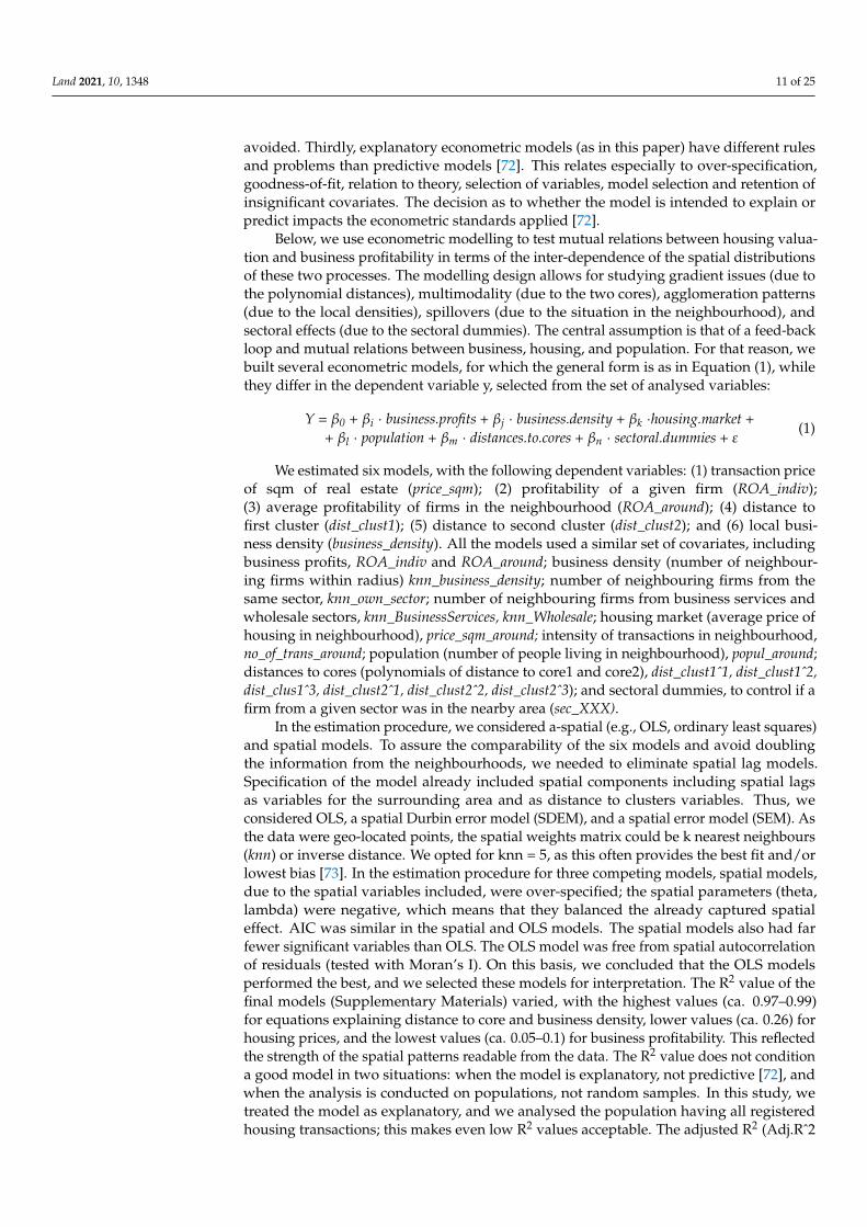
Figure 3. Spatial distribution of transactions by values: (a) below 1 mln PLN, (b) above 1 mln PLN to assess the spatial distribution of transactions and premium submarket location. Figure 3. Spatial distribution of transactions by values: (a) below 1 mln PLN, (b) above 1 mln PLN to assess the spatialdistribution of transactions and premium submarket location.

The existence of mutual relations between housing valuation and business profitabilitywas evident from mutually significant coefficients of regression, e.g., β for housing valua-tion in model_3 explaining ROA_around, and β for ROA_around in model_1, explainingthe sqm price of real estate. They also confirmed the strong inter-dependence of spatialdistributions (considered above, x and y are average values in the neighbourhood), wherethe relation was negative. This implies that higher business profitability (ROA) coincideswith lower prices of flats. This is confirmed by Figure 1b, where higher ROA is relativelyperipheral, and Figure 3a,b, where higher flat prices are in the center. This relationshipwas also visible in the models for distance to clusters (model_4 and model_5) and forbusiness density (model_6), where profitability and housing valuation showed a mutuallysignificant relationship.

There was also a mutual relationship between housing valuation and business location.A significant regression coefficient was observed in model_1 (for housing valuation) withdensity of business (positive β at knn_business_density) and for distances to cores (somesignificant β, positive and negative). In contrast, β for housing price in the neighbourhood(price_sqm_around) was significant in models explaining business density (model_6) and

Land 2021, 10, 1348 13 of 25

distance to cluster1 (model_4) and cluster2 (model_5). This implies that the higher pricedflats were in dense business locations, especially in cluster 2.

Land 2021, 10, x FOR PEER REVIEW 13 of 25

Figure 4. Tessellated business and population locations in the urban area of Warsaw to assess the degree of agglomeration.

The existence of mutual relations between housing valuation and business profita-bility was evident from mutually significant coefficients of regression, e.g., β for housing valuation in model_3 explaining ROA_around, and β for ROA_around in model_1, explain-ing the sqm price of real estate. They also confirmed the strong inter-dependence of spatial distributions (considered above, x and y are average values in the neighbourhood), where the relation was negative. This implies that higher business profitability (ROA) coincides with lower prices of flats. This is confirmed by Figure 1b, where higher ROA is relatively peripheral, and Figure 3a,b, where higher flat prices are in the center. This relationship was also visible in the models for distance to clusters (model_4 and model_5) and for business density (model_6), where profitability and housing valuation showed a mutually significant relationship.

There was also a mutual relationship between housing valuation and business loca-tion. A significant regression coefficient was observed in model_1 (for housing valuation) with density of business (positive β at knn_business_density) and for distances to cores (some significant β, positive and negative). In contrast, β for housing price in the neigh-bourhood (price_sqm_around) was significant in models explaining business density (model_6) and distance to cluster1 (model_4) and cluster2 (model_5). This implies that the higher priced flats were in dense business locations, especially in cluster 2.

Business location in the city reflects multimodality. Statistically, it was confirmed us-ing a DBSCAN search for density clusters (Figure 1a). We found two significant and stable clusters: cluster1, located to the south, in a new business district, and cluster2, situated in the city center, next to the Old Town. Cluster2 was much broader than cluster1 and cov-ered government buildings, major avenues, and so-called prestigious addresses. Distance to clusters was a significant factor in housing valuation and ROA in the neighbourhood; however, each cluster impacted differently, mostly because of the cluster characteristics. Both clusters had different business densities, which was evident from the DBSCAN sta-tistics and diverse β coefficients for distances in model_6. Moreover, the clusters did not impact linearly, rather as the second and third power of distance in models.

The existence of clusters and diverse local densities result in the agglomeration phe-nomenon. In statistical analysis (Figure 4), the degrees of agglomeration of business and population were very similar and significant; the relative entropy relH of both point pat-terns equalled 0.89 (relH = 1 for uniform spatial distribution). The determinants of ag-glomeration were tested in model _6 for business density with many significant predictive

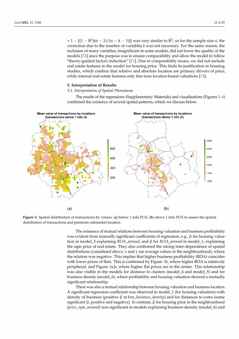
Figure 4. Tessellated business and population locations in the urban area of Warsaw to assess the degree of agglomeration.

Business location in the city reflects multimodality. Statistically, it was confirmed usinga DBSCAN search for density clusters (Figure 1a). We found two significant and stableclusters: cluster1, located to the south, in a new business district, and cluster2, situated inthe city center, next to the Old Town. Cluster2 was much broader than cluster1 and coveredgovernment buildings, major avenues, and so-called prestigious addresses. Distance toclusters was a significant factor in housing valuation and ROA in the neighbourhood;however, each cluster impacted differently, mostly because of the cluster characteristics.Both clusters had different business densities, which was evident from the DBSCANstatistics and diverse β coefficients for distances in model_6. Moreover, the clusters did notimpact linearly, rather as the second and third power of distance in models.

The existence of clusters and diverse local densities result in the agglomeration phe-nomenon. In statistical analysis (Figure 4), the degrees of agglomeration of businessand population were very similar and significant; the relative entropy relH of both pointpatterns equalled 0.89 (relH = 1 for uniform spatial distribution). The determinants ofagglomeration were tested in model _6 for business density with many significant pre-dictive variables. This phenomenon had spatial nature (significant β for distances), andwas related to population, housing valuation and business profitability. However, whilepopulation density was associated with housing valuation (negatively), and businessdensity (positively, business clusters were densely populated), it was not associated withbusiness profitability. Agglomeration was also linked to sectoral effects: firms from thebusiness services sector and wholesale sector preferred to locate more distantly from denseareas. A wider study of agglomeration, measured with entropy for tessellated point-patterns, presented in Figure 4, is available in [75]. Details of this method are presented inAppendix A, part 3.

The importance of distance means that a gradients and distance-decay pattern exist.Firstly, distance is significant for clusters in the business profitability model (model_3) andhousing valuation model (model_1). As the β coefficients differ between clusters, thereare no symmetric reactions over space, and distance-decay patterns vary in strength. Theinsignificance of some distance coefficients may also be considered as spatial discontinuity.Secondly, significant variables in model_4 and model_5 may be understood as gradientsfor clusters 1 and 2. The spatial patterns differ between those two clusters. For cluster2 (centrally located, “old” business cluster), the closer to this cluster, the higher the flatprices, business, and population density, but the lower the ROA in the surrounding sectoral(business services and wholesale) density and the number of flat sales transactions. How-

Land 2021, 10, 1348 14 of 25

ever, for cluster 1 (southern location, new business cluster), the closer to this cluster thehigher the business and population density, but also the higher the ROA in surroundingand sectoral (business services and wholesale) density, and the lower the prices of flatsand the number of transactions. Cluster 1 attracted, and cluster 2 repelled, the most densesectors; the significant sectoral dummies in models 4 and 5 show which sectors tendedtoward which cluster. Interestingly, most industries were distributed in a mixed fashion,not around a given cluster.

The sectoral effects were visibly broader. The neighbourhood of three sectors (i.e.,transportation, freight and storage, retail and metal production) lowered the housingvaluation significantly by 3–4%, i.e., by comparing significant β coefficients (ca. −359,−293, −296 PLN) with a mean (8707 PLN) and median (8622 PLN) housing sqm price.The profitability of sectors was mostly well-diversified, with some positive effects in somesectors (e.g., business services, chemicals, food and tobacco, public administration) of2.7 to 3.1 p.p. (for example, a negative impact in the utilities sector of 2.9 p.p.). Cluster1 attracted sectors such as industrial, electrical and electronic products, metal products,and miscellaneous and utilities manufacturers (significant sectoral dummies in model_4).In contrast, cluster 2 attracted firms from the chemical and petroleum sectors, as well aswaste management.

Finally, spillover effects could be observed when point observations were connectedto their neighbourhoods. This was visible in business profitability where individual ROAwas well-linked to ROA in the neighbourhood (model_2). This was also evident for thehousing market, where higher prices were linked to a higher number of transactions.

5.2. Interpretation in the Light of Location Theories

The profitability of firms tended to cluster visibly. The spatial distribution was non-random, relative location mattered, and ROA in neighbourhoods was spatially correlated(β for ROA.around in model_2). In classical theory, optimisation of location with respectto gradients would be predicted to cause similar profitability of firms located next toeach other. The spatial independence of profit indicates that classical gradient theoryworks well. In behavioural theory, information on the location is known, companieshave different capabilities to relocate, and there should be a supply of the “best” places.Where neighbourhood dependence in profitability exists, (a) companies use the availableinformation, or (b) there is the flexibility of mobility, or (c) there are over-profitable locationsand the place of doing business is relevant. Firms and places are heterogeneous in the NEGapproach, while a business’s success depends on location and other internal factors. Highprofitability may be linked to location or agglomeration externalities. In the evolutionaryapproach, there is both a visible neighbourhood outlook and a contextual reaction to ROA(further information is provided in Appendix A, part 6). This implies that all theories canbe applied to explain this phenomenon.

In general, sectoral profitability did not differ, as the sectoral β coefficients in model_2and model_3 were mostly insignificant. This supports the viewpoint of classical theory thatall companies are homogeneous. There is no basis for creating spatial clusters and optimalbusiness territories from a behavioural perspective if there are no industry patterns. Inthe NEG approach, the importance of transport costs and market access should diversifysector profitability. This did not happen, with the limited exceptions of business services,chemicals, food and tobacco, and public administration. Thus, in general, the NEG fails, orthe spatial scale necessary for these factors to differentiate business was too narrow. TheEEG’s flow of experience and tacit knowledge, strengthened with industry predispositions,would be predicted to create better-performing sectors, which was observable in only afew sectors. It appears that the assumptions of classical theory best fit the scenario. Thismethod can approximate behavioural persistence, with adjustments to location being slowand costly.

The aggregated data indicated a slight difference in ROA by city district (Figure 1b).Surprisingly, the median and mean of ROA in core locations and CBD were lower than

Land 2021, 10, 1348 15 of 25

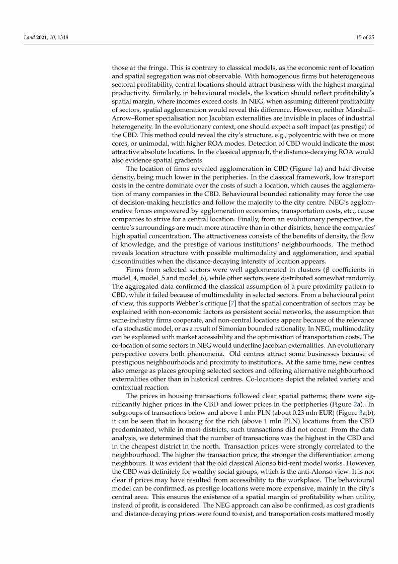
those at the fringe. This is contrary to classical models, as the economic rent of locationand spatial segregation was not observable. With homogenous firms but heterogeneoussectoral profitability, central locations should attract business with the highest marginalproductivity. Similarly, in behavioural models, the location should reflect profitability’sspatial margin, where incomes exceed costs. In NEG, when assuming different profitabilityof sectors, spatial agglomeration would reveal this difference. However, neither Marshall–Arrow–Romer specialisation nor Jacobian externalities are invisible in places of industrialheterogeneity. In the evolutionary context, one should expect a soft impact (as prestige) ofthe CBD. This method could reveal the city’s structure, e.g., polycentric with two or morecores, or unimodal, with higher ROA modes. Detection of CBD would indicate the mostattractive absolute locations. In the classical approach, the distance-decaying ROA wouldalso evidence spatial gradients.

The location of firms revealed agglomeration in CBD (Figure 1a) and had diversedensity, being much lower in the peripheries. In the classical framework, low transportcosts in the centre dominate over the costs of such a location, which causes the agglomera-tion of many companies in the CBD. Behavioural bounded rationality may force the useof decision-making heuristics and follow the majority to the city centre. NEG’s agglom-erative forces empowered by agglomeration economies, transportation costs, etc., causecompanies to strive for a central location. Finally, from an evolutionary perspective, thecentre’s surroundings are much more attractive than in other districts, hence the companies’high spatial concentration. The attractiveness consists of the benefits of density, the flowof knowledge, and the prestige of various institutions’ neighbourhoods. The methodreveals location structure with possible multimodality and agglomeration, and spatialdiscontinuities when the distance-decaying intensity of location appears.

Firms from selected sectors were well agglomerated in clusters (β coefficients inmodel_4, model_5 and model_6), while other sectors were distributed somewhat randomly.The aggregated data confirmed the classical assumption of a pure proximity pattern toCBD, while it failed because of multimodality in selected sectors. From a behavioural pointof view, this supports Webber’s critique [7] that the spatial concentration of sectors may beexplained with non-economic factors as persistent social networks, the assumption thatsame-industry firms cooperate, and non-central locations appear because of the relevanceof a stochastic model, or as a result of Simonian bounded rationality. In NEG, multimodalitycan be explained with market accessibility and the optimisation of transportation costs. Theco-location of some sectors in NEG would underline Jacobian externalities. An evolutionaryperspective covers both phenomena. Old centres attract some businesses because ofprestigious neighbourhoods and proximity to institutions. At the same time, new centresalso emerge as places grouping selected sectors and offering alternative neighbourhoodexternalities other than in historical centres. Co-locations depict the related variety andcontextual reaction.

The prices in housing transactions followed clear spatial patterns; there were sig-nificantly higher prices in the CBD and lower prices in the peripheries (Figure 2a). Insubgroups of transactions below and above 1 mln PLN (about 0.23 mln EUR) (Figure 3a,b),it can be seen that in housing for the rich (above 1 mln PLN) locations from the CBDpredominated, while in most districts, such transactions did not occur. From the dataanalysis, we determined that the number of transactions was the highest in the CBD andin the cheapest district in the north. Transaction prices were strongly correlated to theneighbourhood. The higher the transaction price, the stronger the differentiation amongneighbours. It was evident that the old classical Alonso bid-rent model works. However,the CBD was definitely for wealthy social groups, which is the anti-Alonso view. It is notclear if prices may have resulted from accessibility to the workplace. The behaviouralmodel can be confirmed, as prestige locations were more expensive, mainly in the city’scentral area. This ensures the existence of a spatial margin of profitability when utility,instead of profit, is considered. The NEG approach can also be confirmed, as cost gradientsand distance-decaying prices were found to exist, and transportation costs mattered mostly

Land 2021, 10, 1348 16 of 25

for the rich. In an evolutionary context, the neighbourhoods, local networks, and prestigewere evidenced, and the surrounding areas generated clustering. Significantly higher pricesin the three districts suggest a polycentric structure and the impact of absolute location.

5.3. Discussion of the Results

This paper presents one of the first trials to quantitatively operationalise the compar-ison of location theories and their spatial effects as inter-dependence of different spatialdistributions, studying gradients, multimodality, agglomeration patterns, spillovers, andsectoral effects. We deal with issues that have not been addressed until now and arechallenging. However, we believe that many important aspects of business and housinglocation models have been revealed.

We have not sought to solve all issues in business and housing location but insteadto shed some light on spatial aspects. Typically, economic or land-use models are simpli-fications, as the enormous complexity of reality is almost impossible to grasp in a singlestudy. Secondly, we designed our research as “theory-guided factors induction”, whichmeans our approach was more theory-based than data-mining-based. For that reason, wehave omitted many issues which are often included in popular deductive models, e.g.,commuting, transport infrastructure, etc.

We also wished to underline the heterogeneity of economic agents, and especially theirdifferent attitudes to wealth and utility. Many economic models assume, for simplification,neo-classical full rationality and maximisation of utility. However, non-classical modelsstress the existence of bounded rationality and the co-existence of optimisers (i.e., rationalagents) and satisfiers (i.e., those who reach a satisfactory level and stop improving theirsituation). Spatial gradients work well in mono-centric cities with rational maximisers asinhabitants. In mixtures with satisfiers and/or next to the urban core, the non-linearitiesand discontinuities appear. There are no studies on these aspects, while our approach candetect the appearance of these issues, e.g., through polynomial distances, multi-cores, andthe insignificance of some variables. We feel that it is an important part of regional scienceworth studying.

6. Conclusions

This study has shown that theoretical approaches to business and housing location,even if they are related in reality, should be treated separately in analyses. The approach tothe analysis of problems started with a classical framework, then behavioural, new eco-nomic geography, evolutionary and co-evolutionary models were applied, and, due to theirrelative independence, business and housing theories evolved in different directions. In thebusiness location context, it is apparent that abandoned old concepts have taken on newerones. Conversely, in housing location, new theoretical waves have been successfully addedto strong classical foundations. Housing location models seem not to be subject to Webber’scritique, which has though led to very different approaches in contemporary analyses inrelation to business localisation models. This may indicate that the consequences of thiscritique were not as important as business location researchers thought. There is also animbalance in existing studies: firms’ location (with respect to profitability) has receivedmore theoretical consideration, while empirical studies are less represented; converselyin housing location and valuation, empirical studies have dominated (especially hedonicmodels and residential location choice approaches), while theoretical studies are limited.

Secondly, both research areas have inherited spatial components, for which assump-tions are rarely fulfilled, and as a result, models do not work as predicted. Reality demon-strates that assumptions on unimodal spatial urban structure, the existence of rationalmaximisers, distance-decaying externalities, and a single pattern of behaviour, do nothold. Instead, situations involve multimodality, a mixture of maximisers and satisfiers,incomplete information, the appearance of spatial interactions, feedback loops, as well asthe existence of persistence of behaviour with slow and costly adjustments of location.

Land 2021, 10, 1348 17 of 25

Thirdly, our paper’s empirical approach has evidenced that none of the theories wereentirely wrong but that none of these concepts could be taken as comprehensive. There is aneed for at least five theoretical approaches (classical, behavioural, NEG, evolutionary, andco-evolutionary) to explain the location mechanisms in a complementary way.

Fourthly, in our empirical example, we have shown that there exist links betweenhousing valuation and business location and profitability. We have confirmed the exis-tence of all the highlighted spatial phenomena including agglomeration, gradients, spatialdiscontinuities, the impact of density, and multimodality.

We conclude that regional science would profit from integrating both processes andfamilies of models. Housing valuation and business location have similar spatial patterns,and their determinants and mechanisms can also be congruent. We argue that none ofthe single theoretical models can work because of their high complexity. An “umbrella”theory is required that integrates all available concepts. In addition, there is a strong needto rethink spatial components and fine-tune them to observed mechanisms to discover alldimensions of spatial patterns.

Supplementary Materials: The following are available online at https://www.mdpi.com/article/10.3390/land10121348/s1. Table S1: Estimation of models.

Author Contributions: Conceptualisation, K.K.; methodology, K.K.; software, K.K., P.C., M.K.;validation, K.K.; formal analysis, K.K.; investigation, K.K.; resources, K.K., P.C., M.K.; data curation,K.K., P.C., M.K.; writing—original draft preparation, K.K.; writing—review and editing, K.K., P.C.,M.K.; visualisation, K.K.; supervision, K.K.; project administration, K.K.; funding acquisition, K.K.All authors have read and agreed to the published version of the manuscript.

Funding: This research was a part of a project titled “Spatial econometric models with fixed andchanging structure of neighbourhood. Applications to real estate valuation and business location”funded by the National Science Center Poland (Krakow, Poland) [OPUS 12 call, grant numberUMO-2016/23/B/HS4/02363].

Institutional Review Board Statement: Not applicable.

Informed Consent Statement: Not applicable.

Data Availability Statement: Due to formal restrictions data are not publicly available.

Conflicts of Interest: The authors declare no conflict of interest.

Appendix A

1. Technical details of estimation in R

We used the following R packages: sp, spdep, rgeos, spatstat, raster, ggplot2, ggmap,plot.matrix, RColorBrewer, fossil. For efficient analysis of surroundings, we used spatialgeometry–rings (rgeos::gBuffer()), which were overlaid on point pattern (sp::over()) to indi-cate with dummy if the point was covered with geometry. Dummies were used to derivestatistics of the neighbourhood–number of points or their features. Figure 1a was generatedwith ggplot2:: and ggmap::, we used as a background map a Google watercolour map ofWarsaw in stamen format (using ggmap() and getmap()), on which we added point-patternof business locations (using geom_point()), the administrative contour of Warsaw city (usinggeom_polygon()) and density layer of business (using stat_density2d()). Figure 1b was gener-ated with plot(), and counts the median value of points overlaid (with sp::over()) on spatialpolygons of Warsaw districts. Figure 2a used plot() and findInterval() to visualise valuesof points. Figure 2b was plotted with plot.matrix::plot.matrix(), while the Rand Index wascalculated with fossil::adj.rand.index(), colours were derived with RColorBrewer::brewer.pal()and k-means clusters were found with stats::kmeans(). For Figure 3 we rasterised valueswith raster::rasterize(). On Figure 4, we show point-pattern, which was converted withspatstat::ppp() and tessellated with spatstat::dirichlet(), while entropy was derived as alge-braic computation of areas computed with spatstat::tile.areas(). Core locations were derivedwith dbscan() and hullplot() from dbscan::. Distances between points and cores were cal-

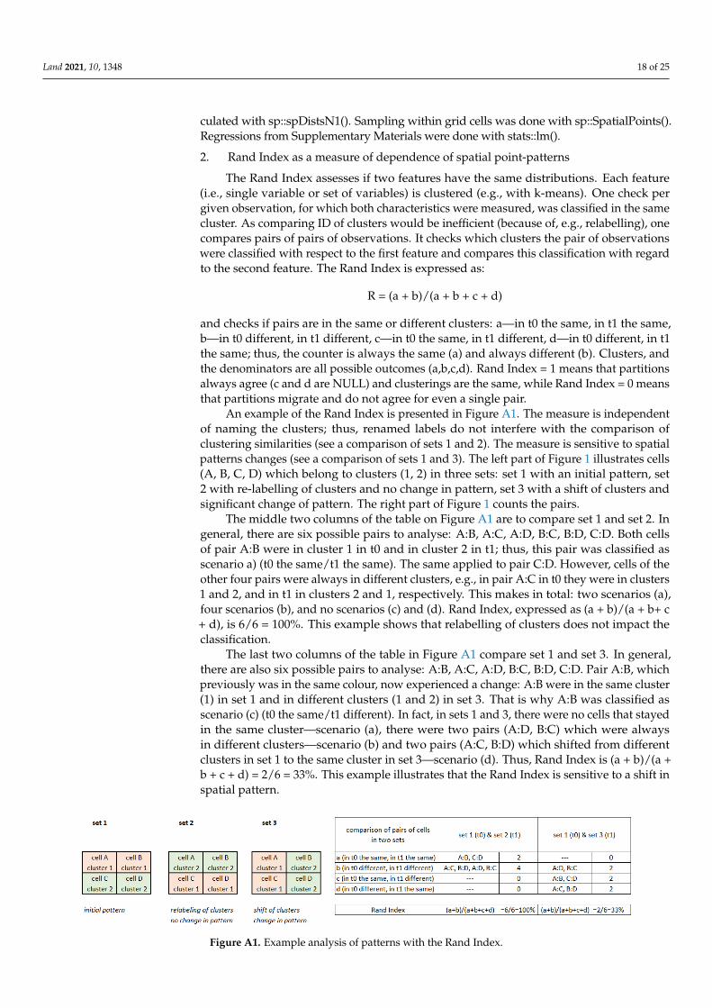
Land 2021, 10, 1348 18 of 25

culated with sp::spDistsN1(). Sampling within grid cells was done with sp::SpatialPoints().Regressions from Supplementary Materials were done with stats::lm().

2. Rand Index as a measure of dependence of spatial point-patterns

The Rand Index assesses if two features have the same distributions. Each feature(i.e., single variable or set of variables) is clustered (e.g., with k-means). One check pergiven observation, for which both characteristics were measured, was classified in the samecluster. As comparing ID of clusters would be inefficient (because of, e.g., relabelling), onecompares pairs of pairs of observations. It checks which clusters the pair of observationswere classified with respect to the first feature and compares this classification with regardto the second feature. The Rand Index is expressed as:

R = (a + b)/(a + b + c + d)

and checks if pairs are in the same or different clusters: a—in t0 the same, in t1 the same,b—in t0 different, in t1 different, c—in t0 the same, in t1 different, d—in t0 different, in t1the same; thus, the counter is always the same (a) and always different (b). Clusters, andthe denominators are all possible outcomes (a,b,c,d). Rand Index = 1 means that partitionsalways agree (c and d are NULL) and clusterings are the same, while Rand Index = 0 meansthat partitions migrate and do not agree for even a single pair.

An example of the Rand Index is presented in Figure A1. The measure is independentof naming the clusters; thus, renamed labels do not interfere with the comparison ofclustering similarities (see a comparison of sets 1 and 2). The measure is sensitive to spatialpatterns changes (see a comparison of sets 1 and 3). The left part of Figure 1 illustrates cells(A, B, C, D) which belong to clusters (1, 2) in three sets: set 1 with an initial pattern, set2 with re-labelling of clusters and no change in pattern, set 3 with a shift of clusters andsignificant change of pattern. The right part of Figure 1 counts the pairs.

The middle two columns of the table on Figure A1 are to compare set 1 and set 2. Ingeneral, there are six possible pairs to analyse: A:B, A:C, A:D, B:C, B:D, C:D. Both cellsof pair A:B were in cluster 1 in t0 and in cluster 2 in t1; thus, this pair was classified asscenario a) (t0 the same/t1 the same). The same applied to pair C:D. However, cells of theother four pairs were always in different clusters, e.g., in pair A:C in t0 they were in clusters1 and 2, and in t1 in clusters 2 and 1, respectively. This makes in total: two scenarios (a),four scenarios (b), and no scenarios (c) and (d). Rand Index, expressed as (a + b)/(a + b+ c+ d), is 6/6 = 100%. This example shows that relabelling of clusters does not impact theclassification.

The last two columns of the table in Figure A1 compare set 1 and set 3. In general,there are also six possible pairs to analyse: A:B, A:C, A:D, B:C, B:D, C:D. Pair A:B, whichpreviously was in the same colour, now experienced a change: A:B were in the same cluster(1) in set 1 and in different clusters (1 and 2) in set 3. That is why A:B was classified asscenario (c) (t0 the same/t1 different). In fact, in sets 1 and 3, there were no cells that stayedin the same cluster—scenario (a), there were two pairs (A:D, B:C) which were alwaysin different clusters—scenario (b) and two pairs (A:C, B:D) which shifted from differentclusters in set 1 to the same cluster in set 3—scenario (d). Thus, Rand Index is (a + b)/(a +b + c + d) = 2/6 = 33%. This example illustrates that the Rand Index is sensitive to a shift inspatial pattern.

Land 2021, 10, x FOR PEER REVIEW 19 of 25

b+ c + d), is 6/6 = 100%. This example shows that relabelling of clusters does not impact the classification.

The last two columns of the table in Figure A1 compare set 1 and set 3. In general, there are also six possible pairs to analyse: A:B, A:C, A:D, B:C, B:D, C:D. Pair A:B, which previously was in the same colour, now experienced a change: A:B were in the same clus-ter (1) in set 1 and in different clusters (1 and 2) in set 3. That is why A:B was classified as scenario (c) (t0 the same/t1 different). In fact, in sets 1 and 3, there were no cells that stayed in the same cluster—scenario (a), there were two pairs (A:D, B:C) which were always in different clusters—scenario (b) and two pairs (A:C, B:D) which shifted from different clus-ters in set 1 to the same cluster in set 3—scenario (d). Thus, Rand Index is (a + b)/(a + b + c + d) = 2/6 = 33%. This example illustrates that the Rand Index is sensitive to a shift in spatial pattern.

Figure A1. Example analysis of patterns with the Rand Index.

3. Agglomeration measure based on the entropy of tessellated point-pattern Measuring agglomeration degree with the entropy of tessellated point-pattern was

originated by Lews [76] and developed by Kopczewska [75]. The idea behind this is that in the case of no agglomeration, points are distributed equally on the surface, which makes the reference point for this measure. Any empirical point pattern can be tessellated with Voronoi’s polygons, which divides the area continuously into non-overlapping tiles. Tessellation tiles are limited by lines located precisely halfway between two neighbouring points. Each tile has its area, and a total of all tiles’ areas equals the area of the bounding region. Shares s of areas in the total area become a percentage measure, which is an input into entropy measure H. 𝐻 = − 𝑠 ∙ log 𝑠

In the case of equally distributed points, all tiles’ areas are equal, and entropy equals Hmax. 𝐻 = − 𝑠 ∙ log 𝑠

A convenient measure to compare empirical and maximum entropy is relative en-tropy expressed as the ratio of both: 𝑟𝑒𝑙𝐻 = 𝐻𝐻 = 𝐻ln 𝑛

Thus, in the case of equally distributed points, without agglomeration pattern, rela-tive H equals 1. Agglomeration is detected when relative H < 1. 4. Econometric methods in verification of location choice

Most existing studies use econometrics for the verification of theories on location choice. The popular hedonic model by Rosen [77] was in previous decades expanded and

Figure A1. Example analysis of patterns with the Rand Index.

Land 2021, 10, 1348 19 of 25

3. Agglomeration measure based on the entropy of tessellated point-pattern

Measuring agglomeration degree with the entropy of tessellated point-pattern wasoriginated by Lews [76] and developed by Kopczewska [75]. The idea behind this isthat in the case of no agglomeration, points are distributed equally on the surface, whichmakes the reference point for this measure. Any empirical point pattern can be tessellatedwith Voronoi’s polygons, which divides the area continuously into non-overlapping tiles.Tessellation tiles are limited by lines located precisely halfway between two neighbouringpoints. Each tile has its area, and a total of all tiles’ areas equals the area of the boundingregion. Shares s of areas in the total area become a percentage measure, which is an inputinto entropy measure H.

H = −N

∑n=1

s· log s

In the case of equally distributed points, all tiles’ areas are equal, and entropy equalsHmax.

Hmax = −N

∑n=1

s· log s

A convenient measure to compare empirical and maximum entropy is relative entropyexpressed as the ratio of both:

relH =Hempir

Hmax=

Hempir

ln n

Thus, in the case of equally distributed points, without agglomeration pattern, relativeH equals 1. Agglomeration is detected when relative H < 1.

4. Econometric methods in verification of location choice

Most existing studies use econometrics for the verification of theories on locationchoice. The popular hedonic model by Rosen [77] was in previous decades expanded andfine-tuned in terms of explanatory variables and estimation methods [78] (see Appendix A,part 5). This model allows for the valuation of characteristics of real estate and whenspatial components are added, as a spatial weights matrix, spatial coordinates of a location,dummy for CDB, etc., measures the spillover effects of the studied phenomena and itsdeterminants [79,80]. The key attribute of company or real estate location data is thatthey are geo-referenced, which means that their locations are related to the site and maydepend on the features of the nearest areas [81]. The spatial distribution of companiesand housing is by no means homogeneous, and a spatial approach helps differentiatethe groups. In addition, the lack of consideration of spatial effects may contradict thetheoretical assumptions, as in new economic geography, where agglomeration economiesoften appear mainly at the local level [82]. However, its popularity has meant that they arebased on a plethora of determinants but do not produce the same conclusions. Meta-studieson hedonic models, such as [83], using OLS and quantile regression, seek to find the generalrules on the sign and volume of marginal effect coefficients in models determining the realestate price.

The choice of residential location can be measured, following McFadden [55], withbinominal or multinomial choice models for alternatives or their aggregates. The modelweights the features of possible options and maximises the utility by choosing the bestalternative. Kohlhase and Ju [84] tested, using a discrete-choice model, the firm-locationassuming a polycentric city [85]. One can also apply multinomial mixed logit to modelthe housing choice and urban location parallel with respect to differences between in-dividuals [86]. In the catalogue of non-spatial methods, the multiple criteria complexproportional assessment (COPRAS) can also be found based on weighted preferences. Ithas been applied to real estate’s utility degree and market value determinants using experts’assessments of preference decisions on competing alternatives [87]. There is also a streamof multi-agent systems to model location optimisation’s urban dynamics [88].

Land 2021, 10, 1348 20 of 25

The last decade has brought the application of machine learning methods to loca-tion problems, e.g., the artificial neural network (ANN) [89], genetic algorithms [90], k-nearest neighbour smoothing [91], fuzzy logic [92], boosted trees, support vector regressionand CART [93].

5. Hedonic models for housing valuation

Parallel to residential location models, a stream of hedonic models was originatedby Rosen [77]. They incorporate the different factors of real estate itself as well as ofneighbourhood and spatial externalities on housing valuation. Originally, the hedonicmodel was based on the Alonso approach and designed as an operationalisation in searchof market equilibrium with respect to budget constraints. Thousands of citations havedemonstrated its enormous potential for empirical research on real estate. Current hedonicmodels [94] include economic factors (i.e., in relation to income and price or government taxpolicy), intrinsic factors (e.g., ownership, type of premises, size, age, condition, additionalsurface, floor, etc.), as well as socio-cultural issues (e.g., distance to relatives, job and publicservices, the reputation of the place, noise, crime, etc.). There are also models referring togovernment (e.g., urban, locational, housing) policy [95,96], ecological issues, or variationsin prices and interest rates [97]. Geographical issues are included as the characteristicsof local markets [98], existing land use patterns [99] or topography and proximity tonetworks [100], as well as the distance to the city centre or place of work.

6. Links between the business location and its profitability

A separate issue in the literature on business is to link firm location with its profitabil-ity, measured by return on investment (ROI), on assets (ROA), on sales (ROS), and onequity (ROE). Profitability and location are often linked with other internal and externalorganisational factors, such as ownership, management, age, innovations, acquisitions, andassociated management turnover [101], worker representation in unions and works coun-cils [102], technological capability to profit on knowledge externalities [103], and capitalstructure [104]. SME surveys [105] have shown that firms located in cities are more likely tobe profitable than those located in smaller towns or rural areas. Comprehensive empiricalstudies evidence that entrepreneurs consider many factors when establishing a new firm,which varies over space, e.g., economic policy, scope of product sales, industrial structure ofcountries and regions, distance to capital city, location of resources, demographic variables,localisation patterns, local demand and supply linkages, taxes and zoning system, sectorsand segmentation, economic growth rates, per capita income, government policy, marketsize, institutional stability and the degree of economic freedom, infrastructure, institutionalissues, the importance of market access and factor endowments, innovation capacity, clus-tering and agglomeration issues, consulting, territorial distribution of economic activity,etc. However, agglomeration externalities and elusive “good” locations do not guaranteehigh firm profitability [106]. Current applied studies on location show that explanationof business location within the framework of a single theory only is impossible. There isalso the plethora of factors that “the probability of a plant start-up is more strongly relatedto increases in local market size and labour force qualification, lower labour costs, anda more diversified economic environment” [107], which, in fact, refers to all streams oftheory. Long-term decisions depend on budget, costs, opportunity cost, and utility/profit.

Somewhat different is the integrated model of residential and employment location(IMREL), which considers where to locate new real estate from an optimisation pointof view based on random utility theory with fixed travel costs. It was formulated andapplied as a policy analysis tool in the Stockholm region [108,109]. IMREL uses a heuristicapproach; the location choice model was solved sequentially with a user-optimal routechoice model (i.e., trip assignment) to determine the location and travel choices of allworkers in the Stockholm region. These choice patterns were then used to investigate thewelfare maximising location of housing supply [110].

Land 2021, 10, 1348 21 of 25

Appendix B

Table A1. Descriptive statistics of the analysed dataset.

VARIABLES Min Q1 Median Mean Q3 Max

lat 52.104 52.196 52.227 52.221 52.239 52.363

lon 20.856 20.985 21.007 21.011 21.031 21.254

ROA_indiv −29.950 −4.120 1.040 1.320 7.690 29.990

ROA_around −27.730 0.032 1.006 1.338 2.592 28.210

knn_business_density 1.000 23.000 60.000 130.473 201.000 888.000

knn_BusinessServices 0.000 4.000 13.000 29.948 45.000 234.000

knn_Wholesale 0.000 3.000 9.000 17.031 24.000 104.000

knn_own_sector 1.000 2.000 7.000 18.037 21.000 234.000

popul_around 0.000 8.000 19.000 18.212 26.000 58.000

price_sqm_around 2528.845 7709.940 8621.766 8707.044 9543.100 20,208.349

no_of_trans_around 0.000 3.000 30.000 53.285 87.000 526.000

dist_clust1ˆ1 0.147 4.714 5.986 6.503 8.015 20.607

dist_clust2ˆ1 0.086 1.461 4.073 4.598 6.771 18.291

sec_Bank_Insur_FinServ 0.000 0.000 0.000 0.046 0.000 1.000

sec_Biotech_and_LifeScien 0.000 0.000 0.000 0.006 0.000 1.000

sec_BusinessServ 0.000 0.000 0.000 0.212 0.000 1.000

sec_Chemic_Petr_Rubber_Plast 0.000 0.000 0.000 0.011 0.000 1.000

sec_Communicat 0.000 0.000 0.000 0.010 0.000 1.000

sec_CompHard 0.000 0.000 0.000 0.001 0.000 1.000

sec_CompSoft 0.000 0.000 0.000 0.042 0.000 1.000

sec_Constr 0.000 0.000 0.000 0.112 0.000 1.000

sec_Food_Tobacco_Manuf 0.000 0.000 0.000 0.010 0.000 1.000

sec_Industr_Electric_Electro 0.000 0.000 0.000 0.014 0.000 1.000

sec_InformServ 0.000 0.000 0.000 0.001 0.000 1.000

sec_Leather_Stone_Clay_Glass 0.000 0.000 0.000 0.003 0.000 1.000

sec_Media_Broadcast 0.000 0.000 0.000 0.026 0.000 1.000

sec_Metals_MetalProd 0.000 0.000 0.000 0.007 0.000 1.000

sec_MiningExtr 0.000 0.000 0.000 0.003 0.000 1.000

sec_Misc_Manuf 0.000 0.000 0.000 0.002 0.000 1.000

sec_Print_Publish 0.000 0.000 0.000 0.018 0.000 1.000

sec_PropertyServ 0.000 0.000 0.000 0.110 0.000 1.000

sec_Publ_Adm_Edu_Health_SocServ 0.000 0.000 0.000 0.046 0.000 1.000

sec_Retail 0.000 0.000 0.000 0.046 0.000 1.000

sec_Textiles_Cloth 0.000 0.000 0.000 0.003 0.000 1.000

sec_Transp_Manuf 0.000 0.000 0.000 0.002 0.000 1.000

sec_Transp_Freight_Storage 0.000 0.000 0.000 0.025 0.000 1.000

sec_Travel_Pers_Leisure 0.000 0.000 0.000 0.051 0.000 1.000

sec_Utilities 0.000 0.000 0.000 0.019 0.000 1.000

sec_Waste_Manag_Treat 0.000 0.000 0.000 0.005 0.000 1.000

sec_Wholesale 0.000 0.000 0.000 0.158 0.000 1.000

sec_Wood_Furnit_Paper_Manuf 0.000 0.000 0.000 0.006 0.000 1.000

Land 2021, 10, 1348 22 of 25

References1. Thünen, J.V. Der isolierte Staat. Beziehung auf Landwirtschaft und Nationalökonomie; Perthes: Hamburg, Germany, 1826.2. Weber, A.; Friedrich, C.J. Alfred Weber’s Theory of the Location of Industries; University of Chicago Press: Chicago, IL, USA, 1929.3. Lösch, A. The Spatial Organization of the Economy; Encyclopædia Britannica: London, UK, 1940.4. Moses, L.N. Location and the theory of production. Q. J. Econ. 1958, 72, 259–272. [CrossRef]5. Hotelling, H. Stability in Competition. Econ. J. 1929, 39, 41–57. [CrossRef]6. Salop, S.C. Monopolistic Competititon with Outside Goods. Bell J. Econ. 1979, 10, 141–156. [CrossRef]7. Webber, M.J. Sub-optimal behaviour and the concept of maximum profits in location theory. Aust. Geogr. Stud. 1969, 7, 1–8.

[CrossRef]8. Cocco, L.; Deidda, M.; Marchesi, M.; Pigliaru, F. Insularity and economies of density: Analysing the efficiency of a logistic

network using an econometric simulation-based approach. Reg. Stud. 2018, 53, 900–911. [CrossRef]9. Pred, A. Behaviour and location: Foundations for a geographic and dynamic location theory, part 1. Lund Stud. Geogr. 1967, 27,

128.10. Claus, R.J.; Claus, K.E. Behavioural location theory: A review and discussion of Pred’s dynamic location model. Aust. Geogr.

1971, 11, 522–530. [CrossRef]11. Karlson, S.H. Modeling location and production: An application to US fully-integrated steel plants. Rev. Econ. Stat. 1983, 65,

41–50. [CrossRef]12. Krugman, P. Geography and Trade; MIT Press: Cambridge, MA, USA, 1991.13. Ottaviano, G.I. ‘New’new economic geography: Firm heterogeneity and agglomeration economies. J. Econ. Geogr. 2010, 11,

231–240. [CrossRef]14. Boschma, R. Evolutionary economic geography and its implications for regional innovation policy. Pap. Evol. Econ. Geogr. 2009, 9,

1–33.15. Gong, H.; Hassink, R. Co-evolution in contemporary economic geography: Towards a theoretical framework. Reg. Stud. 2018, 53,

1344–1355. [CrossRef]16. Fitjar, R.D.; Gjelsvik, M. Why do firms collaborate with local universities? Reg. Stud. 2018, 52, 1525–1536. [CrossRef]17. Alonso, W. Location and Land Use: Toward a General Theory of Land Rent; Harvard University Press: Cambridge, MA, USA, 1964.18. Levine, J. Rethinking accessibility and jobs-housing balance. J. Am. Plan. Assoc. 1998, 64, 133. [CrossRef]19. Straszhem, M. The theory of urban residential location. In Handbook of Regional and Urban Economics; Elsevier: Amsterdam, The

Netherlands, 1987; Volume 2, pp. 717–757.20. Smith, N. Toward a theory of gentrification a back to the city movement by capital, not people. J. Am. Plan. Assoc. 1979, 45,

538–548. [CrossRef]21. Diappi, L.; Bolchi, P. Smith’s rent gap theory and local real estate dynamics: A multi-agent model. Computers. Environ. Urban Syst.

2008, 32, 6–18. [CrossRef]22. Wheaton, W.C. Income and urban residence: An analysis of consumer demand for location. Am. Econ. Rev. 1977, 67, 620–631.23. DiPasquale, D.; Wheaton, W.C. The markets for real estate assets and space: A conceptual framework. Real Estate Econ. 1992, 20,

181–198. [CrossRef]24. DeSalvo, J.S. Teaching the DiPasquale-Wheaton Model. J. Real Estate Pract. Educ. 2017, 20, 1–25. [CrossRef]25. Bravo, M.; Briceño, L.; Cominetti, R.; Cortés, C.E.; Martínez, F. An integrated behavioral model of the land-use and transport

systems with network congestion and location externalities. Transp. Res. Part B Methodol. 2010, 44, 584–596. [CrossRef]26. Pangallo, M.; Nadal, J.P.; Vignes, A. Residential income segregation: A behavioral model of the housing market. J. Econ. Behav.

Organ. 2019, 159, 15–35. [CrossRef]27. Kyriakopoulou, E.; Xepapadeas, A. Spatial location decisions under environmental policy and housing externalities. Environ.

Econ. Policy Stud. 2011, 13, 195. [CrossRef]28. Partridge, M.D.; Rickman, D.S.; Ali, K.; Olfert, M.R. Agglomeration spillovers and wage and housing cost gradients across the

urban hierarchy. J. Int. Econ. 2009, 78, 126–140. [CrossRef]29. Glaeser, E.L. Cities, Agglomeration, and Spatial Equilibrium; Oxford University Press: Oxford, UK, 2008.30. Suedekum, J. Agglomeration and regional costs of living. J. Reg. Sci. 2006, 46, 529–543. [CrossRef]31. Hanushek, E.; Yilmaz, K. The complementarity of Tiebout and Alonso. J. Hous. Econ. 2007, 16, 243–261. [CrossRef]32. Papageorgiou, Y.Y. Externality diffusion. Syst. Urban 1982, 4, 17–39.33. Werczberger, E. Endogenous spatial externalities in residential location theory. In Regional Science; Springer: Berlin/Heidelberg,

Germany, 1991; pp. 79–96.34. Niu, F.; Liu, W. Modeling urban housing price: The perspective of household activity demand. J. Geogr. Sci. 2017, 27, 619–630.

Available online: https://www.researchgate.net/publication/316551331_Modeling_urban_housing_price_The_perspective_of_household_activity_demand (accessed on 15 November 2021). [CrossRef]

35. Kauko, T. What makes a location attractive for the housing consumer? Preliminary findings from metropolitan Helsinki andRandstad Holland using the analytical hierarchy process. J. Hous. Built Environ. 2006, 21, 159–176. [CrossRef]

36. Borgoni, R.; Michelangeli, A.; Pontarollo, N. The value of culture to urban housing markets. Reg. Stud. 2018, 52, 1672–1683.[CrossRef]

37. Ala-Mantila, S.; Heinonen, J.; Junnila, S.; Saarsalmi, P. Spatial nature of urban well-being. Reg. Stud. 2018, 52, 959–973. [CrossRef]

Land 2021, 10, 1348 23 of 25

38. Morrison, P.S.; Weckroth, M. Human values, subjective well-being and the metropolitan region. Reg. Stud. 2018, 52, 325–337.[CrossRef]

39. Tiebout, C.M. Location theory, empirical evidence, and economic evolution. Pap. Reg. Sci. 1957, 3, 74–86. [CrossRef]40. Tiebout, C.M. A pure theory of local expenditures. J. Political Econ. 1956, 64, 416–424. [CrossRef]41. Tabuchi, T. Urban agglomeration and dispersion: A synthesis of Alonso and Krugman. J. Urban Econ. 1998, 44, 333–351. [CrossRef]42. Van der Panne, G. Agglomeration externalities: Marshall versus Jacobs. J. Evol. Econ. 2004, 14, 593–604. [CrossRef]43. Daskalopoulou, I.; Liargovas, P. Regional determinants of manufacturing start-ups in Greece: Evidence on the effect of agglomer-

ation economies. Appl. Econ. Lett. 2010, 17, 1841–1844. [CrossRef]44. Mion, G. Spatial externalities and empirical analysis: The case of Italy. J. Urban Econ. 2004, 56, 97–118. [CrossRef]45. Guevara-Rosero, G.C.; Riou, S.; Autant-Bernard, C. Agglomeration externalities in Ecuador: Do urbanisation and tertiarisation

matter? Reg. Stud. 2018, 53, 706–719. [CrossRef]46. de Matteis, P.; Pietrovito, F.; Pozzolo, A.F. Local context and exports: An analysis with a matched sample of firm–province data.

Reg. Stud. 2019, 53, 550–561. [CrossRef]47. Hervas-Oliver, J.L.; Belussi, F. Cluster Advantage and Firm Performance: A Shift into the Future! In Agglomeration and Firm Performance;

Springer: Cham, Switzerland, 2018; pp. 1–7.48. Porter, M.E. Clusters and the New Economics of Competition; Harvard Business Review: Boston, MA, USA, 1998; Volume 76, pp.

77–90.49. McCann, P. Rethinking the economics of location and agglomeration. Urban Stud. 1995, 32, 563–577. [CrossRef]50. Cainelli, G.; Giannini, V.; Iacobucci, D. Agglomeration, networking and the Great Recession. Reg. Stud. 2018, 53, 951–962.

[CrossRef]51. Yang, T.; Pan, H.; Hewings, G.; Jin, Y. Understanding urban sub-centers with heterogeneity in agglomeration economies—Where

do emerging commercial establishments locate? Cities 2019, 86, 25–36. [CrossRef]52. Boussauw, K.; Sansen, J.; van Meeteren, M.; Meijers, E.; Louw, E.; Storme, T.; Derudder, B.; Witlox, F. Planning for agglomeration

economies in a polycentric region: Envisioning an efficient metropolitan core area in Flanders. Eur. J. Spat. Dev. 2018, 2018, 1–26.[CrossRef]

53. White, M.J. A model of residential location choice and commuting by men and women workers. J. Reg. Sci. 1977, 17, 41–52.[CrossRef]

54. Guo, J.Y.; Bhat, C.R. Operationalising the concept of neighborhood: Application to residential location choice analysis. J. Transp.Geogr. 2007, 15, 31–45. [CrossRef]

55. McFadden, D. Modeling the choice of residential location. Transp. Res. Rec. 1978, 673, 72–77.56. Kwon, Y. Rent-Commuting Cost Function Versus Rent-Distance Function. J. Reg. Sci. 2002, 42, 773–791. [CrossRef]57. Gutiérrez-i-Puigarnau, E.; Mulalic, I.; van Ommeren, J.N. Do rich households live farther away from their workplaces? J. Econ.

Geogr. 2014, 16, 177–201. [CrossRef]58. Berechman, J.; Small, K.A. Modeling land use and transportation: An interpretive review for growth areas. Environ. Plan. A 1988,

20, 1285–1309. [CrossRef]59. Heldt, B.; Gade, K.; Heinrichs, D. Determination of Attributes Reflecting Household Preferences in Location Choice Models.

Transp. Res. Procedia 2016, 19, 119–134. [CrossRef]60. Wong, S.C.; Ho, H.W. A combined model of housing location and traffic equilibrium problems in a continuous transportation

system. In Transportation and Traffic Theory. Flow, Dynamics and Human Interaction, Proceedings of the 16th International Symposium onTransportation and Traffic Theory, College Park, MD, USA, 19–21 July 2005; Elsevier: New York, NY, USA, 2005; pp. 761–779.

61. Tobler, W.R. A computer movie simulating urban growth in the Detroit region. Econ. Geogr. 1970, 46 (Suppl. 1), 234–240.[CrossRef]

62. Papageorgiou, G.J. Spatial externalities I: Theory. Ann. Assoc. Am. Geogr. 1978, 68, 465–476. [CrossRef]63. Papageorgiou, G.J. Spatial externalities II: Applications. Ann. Assoc. Am. Geogr. 1978, 68, 477–492. [CrossRef]64. Papageorgiou, Y.Y.; Smith, T.R. Agglomeration as local instability of spatially uniform steady-states. Econom. J. Econom. Soc. 1983,

51, 1109–1119. [CrossRef]65. Döring, T.; Schnellenbach, J. What do we know about geographical knowledge spillovers and regional growth?: A survey of the

literature. Reg. Stud. 2006, 40, 375–395. [CrossRef]66. Fujita, M.; Ogawa, H. Multiple equilibria and structural transition of non-monocentric urban configurations. Reg. Sci. Urban Econ.

1982, 12, 161–196. [CrossRef]67. Vasanen, A. Functional polycentricity: Examining metropolitan spatial structure through the connectivity of urban sub-centres.

Urban Stud. 2012, 49, 3627–3644. [CrossRef]68. Mussa, A.; Nwaogu, U.G.; Pozo, S. Immigration and housing: A spatial econometric analysis. J. Hous. Econ. 2017, 35, 13–25.

[CrossRef]69. Montero, J.M.; Mínguez, R.; Fernández-Avilés, G. Housing price prediction: Parametric versus semi-parametric spatial hedonic

models. J. Geogr. Syst. 2018, 20, 27–55. [CrossRef]70. Golledge, R.G.; Stimson, R. Spatial Behavior: A Geographic Perspective; Guilford Press: New York, NY, USA, 1997.71. Overmars, K.P.; de Groot, W.; Huigen, M. Comparing Inductive and Deductive Modeling of Land Use Decisions: Principles, a

Model and an Illustration from the Philippines. Hum. Ecol. 2007, 35, 439–445. [CrossRef]

Land 2021, 10, 1348 24 of 25

72. Shmueli, G. To explain or to predict? Stat. Sci. 2010, 25, 289–310. [CrossRef]73. Comber, A.; Brunsdon, C.; Charlton, M.; Dong, G.; Harris, R.; Lu, B.; Lu, Y.; Murakami, D.; Nakaya, T.; Wang, Y.; et al. The GWR

route map: A guide to the informed application of Geographically Weighted Regression. arXiv 2020, arXiv:2004.06070.74. Hill, R. Hedonic Price Indexes for Housing; OECD Statistics Working Papers, No. 2011/01; OECD Publishing: Paris, France, 2011.

[CrossRef]75. Kopczewska, K. Entropy as a measure of agglomeration, In Handbook on Entropy, Complexity, and Spatial Dynamics: The Rebirth of

Theory? Reggiani, A., Schintler, L., Czamanski, D., Patuelli, R., Eds.; Edward Elgar: Cheltenham, UK, 2021.76. Lews, R. Redundancy as an index of change in point pattern analysis. Geogr. Anal. 1979, 11, 374–388. [CrossRef]77. Rosen, S. Hedonic prices and implicit markets: Product differentiation in pure competition. J. Political Econ. 1974, 82, 34–55.

[CrossRef]78. Helbich, M.; Griffith, D.A. Spatially varying coefficient models in real estate: Eigenvector spatial filtering and alternative

approaches. Comput. Environ. Urban Syst. 2016, 57, 1–11. [CrossRef]79. Osland, L. An application of spatial econometrics in relation to hedonic house price modeling. J. Real Estate Res. 2010, 32, 289–320.

[CrossRef]80. Chrostek, K.; Kopczewska, K. Spatial Prediction Models for Real Estate Market Analysis. Ekonomia 2013, 35, 25–43.81. Bhat, C.R.; Paleti, R.; Singh, P. A Spatial Multivariate Count Model for Firm Location Decisions. J. Reg. Sci. 2014, 54, 462–502.

[CrossRef]82. Li, Y.; Zhu, K. Spatial dependence and heterogeneity in the location processes of new high-tech firms in Nanjing, China. Pap. Reg.

Sci. 2015, 96, 519–535. [CrossRef]83. Sirmans, G.S.; Macpherson, D.A.; Zietz, E.N. The composition of hedonic pricing models. J. Real Estate Lit. 2005, 13, 3–46.

[CrossRef]84. Kohlhase, J.E.; Ju, X. Firm location in a polycentric city: The effects of taxes and agglomeration economies on location decisions.

Environ. Plan. C Gov. Policy 2007, 25, 671–691. [CrossRef]85. Mori, T. Monocentric versus polycentric models in urban economics. New Palgrave Dict. Econ. 2016, 1–4.86. Barrios Garcia, J.A.; Rodriguez Hernandez, J.E. Housing and urban location decisions in Spain: An econometric analysis with

unobserved heterogeneity. Urban Stud. 2007, 44, 1657–1676. [CrossRef]87. Kaklauskas, A.; Zavadskas, E.K.; Banaitis, A.; Šatkauskas, G. Defining the utility and market value of a real estate: A multiple

criteria approach. Int. J. Strateg. Prop. Manag. 2007, 11, 107–120. [CrossRef]88. Arentze, T.; Timmermans, H. Modeling agglomeration forces in urban dynamics: A multi-agent system approach. Int. J. Urban

Sci. 2003, 7, 1–13. [CrossRef]89. Selim, H. Determinants of house prices in Turkey: Hedonic regression versus artificial neural network. Expert Syst. Appl. 2009, 36,

2843–2852. [CrossRef]90. Morano, P.; Tajani, F.; Locurcio, M. Land use, economic welfare and property values: An analysis of the interdependencies of the

real-estate market with zonal and socio-economic variables in the municipalities of Apulia region (Italy). Int. J. Agric. Environ. Inf.Syst. 2015, 6, 16–39. [CrossRef]

91. Pavlov, A.D. Space-varying regression coefficients: A semi-parametric approach applied to real estate markets. Real Estate Econ.2000, 28, 249–283. [CrossRef]

92. Bagnoli, C.; Smith, H. The theory of fuzz logic and its application to real estate valuation. J. Real Estate Res. 1998, 16, 169–200.[CrossRef]

93. Özsoy, O.; Sahin, H. Housing price determinants in Istanbul, Turkey: An application of the classification and regression treemodel. Int. J. Hous. Mark. Anal. 2009, 2, 167–178. [CrossRef]

94. Poulhes, M. From Latin Quarter to Montmartre: Investigating Parisian Real Estate Prices. Ann. Econ. Stat. 2018, 130, 39–68.[CrossRef]

95. Fingleton, B. Housing supply, housing demand, and affordability. Urban Stud. 2008, 45, 1545–1563. [CrossRef]96. Dachis, B.; Duranton, G.; Turner, M.A. The effects of land transfer taxes on real estate markets: Evidence from a natural experiment

in Toronto. J. Econ. Geogr. 2011, 12, 327–354. [CrossRef]97. Arrazola, M.; de Hevia, J.; Romero-Jordán, D.; Sanz-Sanz, J.F. Long-run Supply and Demand Elasticities in the Spanish Housing

Market. J. Real Estate Res. 2015, 37, 371–404. [CrossRef]98. Saiz, A. The geographic determinants of housing supply. Q. J. Econ. 2010, 125, 1253–1296. [CrossRef]99. Meen, G.; Nygaard, C. Local housing supply and the impact of history and geography. Urban Stud. 2011, 48, 3107–3124. [CrossRef]100. Portnov, B.A.; Schwartz, M. On the relativity of urban location. Reg. Stud. 2008, 42, 605–615. [CrossRef]101. Braguinsky, S.; Ohyama, A.; Okazaki, T.; Syverson, C. Acquisitions, productivity, and profitability: Evidence from the Japanese

cotton spinning industry. Am. Econ. Rev. 2015, 105, 2086–2119. [CrossRef]102. Addison, J.T. The determinants of firm performance: Unions, works councils, and employee involvement/high-performance

work practices. Scott. J. Political Econ. 2005, 52, 406–450. [CrossRef]103. Jo, Y.; Lee, C.Y. Technological capability, agglomeration economies and firm location choice. Reg. Stud. 2014, 48, 1337–1352.

[CrossRef]104. El-Sayed Ebaid, I. The impact of capital-structure choice on firm performance: Empirical evidence from Egypt. J. Risk Financ.

2009, 10, 477–487. [CrossRef]

Land 2021, 10, 1348 25 of 25

105. SME Survey. 2014. Available online: https://www.smesurvey.co.za/reports/SME%20Survey%20summary%202014.pdf (accessedon 15 November 2021).

106. Stavropoulos, S.; Skuras, D. Firm profitability and agglomeration economies: An elusive relationship. Tijdschr. Voor Econ. En Soc.Geogr. 2016, 107, 66–80. [CrossRef]

107. Holl, A. Start-ups and re-locations: Manufacturing plant location in Portugal. Pap. Reg. Sci. 2004, 83, 649–668.108. Anderstig, C.; Mattsson, L.G. An integrated model of residential and employment location in a metropolitan region. Pap. Reg. Sci.

1991, 70, 167–184. [CrossRef]109. Anderstig, C.; Mattsson, L.G. Modelling land-use and transport interaction: Policy analyses using the IMREL model. In Network

Infrastructure and the Urban Environment; Springer: Berlin/Heidelberg, Germany, 1998; pp. 308–328.110. Boyce, D.; Mattsson, L.G. Modeling residential location choice in relation to housing location and road tolls on congested urban

highway networks. Transp. Res. Part B Methodol. 1999, 33, 581–591. [CrossRef]