This article appeared in a journal published by Elsevier. The attachedcopy is furnished to the author for internal non-commercial researchand education use, including for instruction at the authors institution

and sharing with colleagues.

Other uses, including reproduction and distribution, or selling orlicensing copies, or posting to personal, institutional or third party

websites are prohibited.

In most cases authors are permitted to post their version of thearticle (e.g. in Word or Tex form) to their personal website orinstitutional repository. Authors requiring further information

regarding Elsevier’s archiving and manuscript policies areencouraged to visit:

http://www.elsevier.com/copyright

Author's personal copy

Spatial concentration and plant-level productivity in France

Philippe Martin a, Thierry Mayer b,⇑, Florian Mayneris c

a Sciences-Po and CEPR, Franceb Sciences-Po, CEPII and CEPR, Francec IRES and CORE, Université catholique de Louvain, Belgium

a r t i c l e i n f o

Article history:Received 6 January 2009Revised 8 September 2010Available online 3 December 2010

JEL classification:C23R10R11R12R15

Keywords:ClustersLocalization economiesSpatial concentrationProductivity

a b s t r a c t

This paper analyzes empirically the effect of spatial agglomeration of activities on plant-level productiv-ity, using French firm and plant-level data from 1996 to 2004. We exploit short-run variations of vari-ables by making use of GMM estimation. This allows us to control for endogeneity biases that theestimation of agglomeration economies typically encounters. This means that our paper focuses on a sub-set of agglomeration economies, the short-run ones. Our results show that French plants benefit fromlocalization economies, but we find very little – if any – evidence of urbanization economies. We alsoshow that those localization benefits are relatively well internalized by firms in their location choice:we find very little difference between the geography that would maximize productivity gains in theshort-run and the geography actually observed.

� 2010 Elsevier Inc. All rights reserved.

1. Introduction

Aside from its academic interest, the analysis of agglomerationeconomies has potentially important policy implications. Since the1980s, agglomeration economies have been used to justify clusterpolicies by national and local governments in Germany, Brazil,Japan, Southern Korea, Spanish Basque country or more recentlyin France. Some of those policies are very costly. For example, 1.5billions euros have been devoted to the ‘‘Competitiveness clusters’’policy by the French government from 2005 to 2008, and againfor the 2009–2011 period. Two separate questions deserve atten-tion. First, how large are the gains from agglomeration? In partic-ular, how much does the productivity of a firm increase whenother firms from the same sector or from another sector decideto locate nearby? Second, how much do firms internalize thesegains when deciding where to locate? The answer to the first ques-tion should help understand how much economic gains can be ex-pected from clusters. The answer to the second question shouldhelp understand whether there is a strong case for public interven-tion in favor of industrial clusters.1

Rosenthal and Strange (2004) survey this literature, and reportthat the elasticity of productivity with respect to the size of the cityor to the size of the industry generally lies between 3% and 8%. Thissurvey and another recent work in the literature by Combes et al.(2010) for instance also emphasize that until recently, estimatesof agglomeration externalities suffered from serious endogeneityproblems. From a technical point of view, the estimation of geo-graphical externalities is subject to two main sources of endogene-ity: unobserved heterogeneity and simultaneity bias.

Ciccone and Hall (1996) are the first to address directly andcarefully these endogeneity issues. They study the impact ofcounty employment density on American states’ labor productiv-ity. The authors insist that if there are unmeasured and/or unob-served differences in the determinants of productivity acrossstates, and if these determinants are correlated with countiesemployment density within states, the measure of the returns todensity by simple OLS may be spurious. They take the exampleof climate or transportation infrastructures which will both en-hance workers’ productivity and the attractiveness of the place.They consequently resort to an instrumental variables approach.Also controlling for the average level of education within the stateor the county, the authors find that a doubling of local employmentdensity increases labor productivity by 5–6%.

Ciccone and Hall’s article represents an important step in theempirical approach of agglomeration externalities. Nevertheless,

0094-1190/$ - see front matter � 2010 Elsevier Inc. All rights reserved.doi:10.1016/j.jue.2010.09.002

⇑ Corresponding author.E-mail addresses: philippe.martin@sciences-po.fr (P. Martin), thierry.mayer@

sciences-po.fr (T. Mayer), florian.mayneris@uclouvain.be (F. Mayneris).1 See Duranton et al. (forthcoming) for more detail about this.

Journal of Urban Economics 69 (2011) 182–195

Contents lists available at ScienceDirect

Journal of Urban Economics

www.elsevier .com/locate / jue

Author's personal copy

their work relies on an aggregate measure of labor productivity. Inthe present paper, the use of firms and plants panel data allows acareful treatment of endogeneity issues and a measurement ofagglomeration externalities which is very close to the micro theo-ries. As far as we know, Henderson (2003) was the first paper touse plant-level data for such an analysis and is the closest to thepresent paper. His data is available at five years intervals from1972 to 1992. He estimates a plant-level production function fortwo broad sectors, machinery industries and high-tech industries,and measures the elasticity of TFP to the number of other plantsof the same industry in the county. Using industry-time andplant-location fixed effects, he finds a positive and significant elas-ticity of 8% in the high-tech industry only.2 He does not find evi-dence of gains arising from agglomeration of firms belonging todifferent industries . The use of fixed effects accounts for a large partof unobserved heterogeneity. Henderson also addresses the questionof simultaneity bias by adding location-time fixed effects.

Our paper goes further than Henderson (2003) in several direc-tions. We use French firms and plants panel data, for all manufac-turing sectors, with yearly observations from 1996 to 2004. Oursample is therefore larger and more complete than Henderson’sone which allows us to deal with simultaneity bias and instrumen-tation more directly. We adopt a two-step estimation strategy. Wefirst estimate plant-level production functions for each two-digitindustry. Using those coefficients, we then compute individual pro-ductivities and estimate agglomeration economies through a GMMspecification, decomposing carefully the agglomeration effects intoown industry (localization)/other industries (urbanization) exter-nalities, as well as diversity and competition effects. We also dis-cuss spatial selection of firms. In this paper, we find that thegains from clustering do exist: our benchmark regression showsthat a 10% increase of employment in neighboring plants of thesame industry increases a plant’s productivity by around 0.55%.As stated above, these estimates are based on yearly variations inTFP and are therefore best interpreted as short-run gains fromagglomeration, which has important implications in particular forthe source of the effects we are estimating. Since our paper focuseson agglomeration economies that take place over a short period oftime, we believe that we capture externalities on the labor and in-put markets, rather than technological spillovers or human capitalexternalities that should take more time to realize.

The second consequence has to do with urbanization econo-mies, which take probably even longer to implement. That we donot find evidence of urbanization economies should probably beinterpreted as the fact that they are better captured by cross-sectional analysis than by the short-term analysis we conduct here.Another way to understand our method is that it tries to purge pro-ductivity from any firm-level component that is constant over timeto deal with endogeneity. But doing so, it also purges the analysisfrom a large part of the long-term agglomeration economies ‘‘cap-italized’’ in this fixed firm-level component. Consequently, we con-sider our paper to complement existing research that relies moreheavily on cross-sectional variations and which thus captures long-er-term agglomeration gains.

Finally, using a non-linear specification, we can estimate thegeography that maximizes short-run productivity gains from clus-tering and compare it to the observed geography. A disturbing fea-ture of the existing empirical literature is that one would betempted to conclude from the results usually obtained that more

agglomeration is always better because it increases the productiv-ity of plants. This does not look very plausible as congestion costsmust necessarily appear and dominate at a certain level of agglom-eration. If this was not so, one should also conclude that theobserved geography (where all plants of the same sector are notlocated in the same region) is vastly suboptimal. Another impor-tant contribution of this paper is that we find the relation betweenproductivity gains and agglomeration to be bell-shaped. Previouspapers have failed to exhibit such a non-linear relationship be-cause they were mostly based on long-run analysis; the presenceof ‘‘suboptimal’’ observations in the data, necessary to estimate abell-shaped curve, is indeed more plausible in the short-run. Whenusing a non-linear specification, we are able to estimate the peakagglomeration that maximizes the productivity gains.3 We findthat a plant that would move (with its time-invariant idiosyncraticcharacteristics and for a given level of employment and capital) froma location with no other workers to a location with 1150 employeesin the same sector (the peak of the observed distribution in France)would gain 53.8% in TFP. However, going to an ‘‘over-crowded’’ area(with more than 9000 employees) would eliminate these TFP gains.Hence, geography matters a lot for French plants and they are awareof it: French plants seem to take into account the TFP gains in theirlocation choice. Indeed, when we compare the geography that max-imizes productivity gains and the observed geography, we find verylittle difference between the two. From this point of view, our papersuggests that the short term gains of cluster policies which aim is toincrease the size of clusters, should be very modest.

The remainder of the paper is as follows. Section 2 details ourempirical strategy, Section 3 then proceeds to a description ofthe data used, while Section 4 presents basic results and Section 5goes further in the comprehension of short-run agglomerationeconomies and assesses in particular the existence of non-linearities.

2. Estimating agglomeration externalities: empirical strategy

2.1. The model

Agglomeration economies are generally assumed to improvetotal factor productivity (TFP) of plants through localizationeconomies (externalities on inputs markets, on labor markets orknowledge externalities, following the classification proposed byMarshall (1890)) and urbanization economies (cross fertilizationsof different industries on a given territory, as emphasized by JaneJacobs). When plant-level data is available, this suggests a naturalempirical strategy, based on the estimation of a Cobb–Douglas pro-duction function4:

Yit ¼ AitKaitL

bit ð1Þ

where Yit is value-added of plant i at time t, Ait is TFP, Kit the capitalstock and Lit the labor-force (in terms of employees) of plant i attime t. We then assume that TFP of plant i depends on a plant-level

2 In regressions not reported here but available upon request, we also ran theanalysis separately for low-tech and medium low-tech industries on the one hand,and high-tech and medium high-tech industries on the other hand. Agglomerationeconomies are significant for low-tech and medium low-tech industries only.However, instruments do not pass the validity tests for high-tech and mediumhigh-tech industries.

3 Au and Henderson (2006) analyze this question for Chinese cities and also find abell-shaped curve.

4 Combes et al. (2008a) (among many others) estimate agglomeration economiesusing wages as a dependent variable. An advantage of using wages for the evaluationof agglomeration economies is that wages are measured more precisely than TFP. Themeasurement of TFP involves a variety of estimation procedures, which all have theirown issues or implementation problems. On the other hand, we do not knowprecisely how agglomeration gains are distributed among production factors. If thegains are not distributed in proportion to the share of each factor in value-added,using wages could bias the estimation of agglomeration effects on productivity.Therefore, we stick to the more direct method using TFP as a dependent variable here(see Chapter 11 of Combes et al. (2008b) for the theoretical relationship between thetwo methods).

P. Martin et al. / Journal of Urban Economics 69 (2011) 182–195 183

Author's personal copy

component, Uit, but also on its immediate environment in terms oflocalization and urbanization economies:

Ait ¼ LOCszit

� �d URBszit

� �cUit; ð2Þ

where LOCszit is a measure of localization economies and URBsz

it is ameasure of urbanization economies for plant i, which belongs tosector s and area z, at time t. Log-linearizing expressions (1) and(2), one obtains:

yit ¼ akit þ blit þ ait; ð3Þ

and

ait ¼ dlocszit þ curbsz

it þ uit ; ð4Þ

where lower-case letters denotes the log of upper-case variables inEqs. (1) and (2).

Our strategy consists first in estimating Eq. (3) at the two-digitindustry level, used to calculate ait. We then estimate Eq. (4). Themodel can be estimated by simple Ordinary Least Squares (OLS)regressions if all the independent variables are observable and atleast weakly exogenous, but this hypothesis is rarely valid. Conse-quently, several estimation issues arise that we now detail.

2.2. Estimation issues

Two main issues arise when estimating production functionsand agglomeration economies: unobserved heterogeneity andsimultaneity. Several estimation procedures of production func-tions have been developed since the mid-1990s in order to copewith these issues. We follow Levinsohn and Petrin’s (2003) approach.We obtain standard estimates for inputs elasticities, rangingapproximately from 0.6 to 0.85 for labor and from 0.07 to 0.35for capital. Most of the results presented in this paper are robustwhen using an OLS estimate for TFP. In the following, we detailsuccessively unobserved heterogeneity and simultaneity issuesfor the estimation of agglomeration economies and we proposemethods to solve them.

2.2.1. Unobserved heterogeneitySome characteristics, unobserved by the econometrician, can be

related to both plant-level TFP and some of the explanatory vari-ables. In this case, uit is correlated with the independent variables;consequently, the OLS estimates of the coefficients are potentiallybiased, since the endogenous variables will partly capture theeffect of unobserved characteristics. This issue is better known asthe ‘‘unobserved heterogeneity’’ problem. In our specification,locsz

it and urbszit are both likely to be correlated with uit: Local cli-

mate, transportation infrastructures, natural resources or publicservices to plants can in many ways increase the TFP of a plant.In the same time, a region richly endowed with those environmen-tal elements will be more attractive for firms. There is a positivecorrelation between unobserved (or unmeasured) plant’s environ-mental variables and localization and/or urbanization indiceswhich potentially biases the estimation of d and c.

The first estimations of agglomeration economies were oftenbased on aggregate and cross-sectional data (as Shefer (1973) orSveikauskas (1975) for example) that could not take into accountthe potential biases just mentioned. The use of plant-level paneldata enables us to address directly these questions.

If we consider plants that do not change industry or regionacross time, the plant-level environmental unobserved characteris-tics can be appropriately dealt with using plants’ fixed effects,which will take into account all plants’ specific characteristics thatare invariant across time, whether or not those characteristics areobservable. This amounts to assuming that uit = /i + �it:

ait ¼ dlocszit þ curbsz

it þ /i þ �it; ð5Þ

where the remaining error term �it is now assumed to have the re-quired properties, and in particular not to be correlated withexplanatory variables.

Combes et al. (2007, 2008a) have shown the spatial sorting ofworkers to be important. That spatial sorting must be reflected inplants’ TFP but we do not have information about the skills mixwithin plants. If skills composition of plants’ workforce does notchange over the period, plant-level fixed effect will also take intoaccount the heterogeneous quality of labor among plants.

Using a panel of firms over several years, one can use standardfixed effects techniques, which involve the introduction of a set ofplant dummies, or equivalently mean-differencing expression (5).Alternatively, one can ‘‘eliminate’’ /i using a time differencingapproach. The estimated equation is in this case:

Dait ¼ dDlocszit þ cDurbsz

it þ D�it: ð6Þ

However, unobserved heterogeneity is not the only source of endo-geneity affecting agglomeration effects estimation.

2.2.2. Simultaneity biasEstimating agglomeration economies raises simultaneity issues:

as a consequence of the negative (or positive) economic shock inthe region or in the industry, other firms may close (open) or layoff (hire) employees. �it, locsz

it and urbszit are possibly correlated

and the estimations of d and c may be spurious.To address the simultaneity issue, we adopt a GMM approach.

The method follows Bond (2002): we start by first-differencingeach variable, as in (6) to address the unobserved heterogeneityissue. We then instrument first-differenced independent variablesby their level at time t � 2, following a GMM procedure. The eco-nomic rationale to use lagged levels as instruments is convergence:for each variable, we expect first-differences to be negatively cor-related to the past level of variables. The underlying econometricassumption is that the idiosyncratic shock at time t � 2 is orthog-onal to D�it, which makes the instruments exogenous.

At this stage, several remarks are in order about the type ofagglomeration economies that one can capture with a GMMestimation.

2.3. What can we learn about agglomeration economies from GMM?

Glaeser and Mare (2001), followed by Combes et al. (2008a)among others estimate the impact of agglomeration on wagesexploiting workers who move as a source of variation; such a strat-egy is hard to replicate for plants since those are less mobile.5 Wefocus our analysis on plants that do not change area nor sector overthe time period under study and we exploit short-run variationsof agglomeration variables by resorting to fixed effects or first-differences estimations. This is very different from exploiting cross-sectional variations like in Combes et al. (2007) or Barbesol andBriant (2008). Indeed, estimation strategies based on cross-sectionalvariations capture the impact of agglomeration economies accumu-lated during all the years that precede the year of observation ofdata. Such analyses consequently address the issue of the impactof spatial agglomeration in the long-run. On the contrary, our esti-mation strategy, based on yearly variations in the data, will captureshort-run effects of spatial agglomeration. Our focus is thus differentfrom previous papers and some of our results, such as the absenceof urbanization economies and the non-linearity of localization

5 In fact, it is even hard from a statistical point of view to systematically detectmovements of producing units inside France. The identification number of eachproducing unit is supposed to be location-dependent and should therefore changewhen the unit is re-located.

184 P. Martin et al. / Journal of Urban Economics 69 (2011) 182–195

Author's personal copy

economies, may be specific to this short-run approach. Conse-quently, they should not be seen as conflicting with previous resultsobtained in the literature but as complementary. This focus on theshort-run raises some important conceptual and theoretical issuesabout agglomeration economies:

1. The type of agglomeration economies: The literature has distin-guished intra-industry (localization) from inter-industry(urbanization) agglomeration economies. It seems reasonableto expect urbanization economies to take place over a longertime period, and therefore be captured by the fixed firm-levelcomponent that we difference out with our methodology. Fail-ure to find important short-run urbanization economies doesnot mean that they do not exist in the longer run.

2. The channels of agglomeration economies: We think that ourstrategy may hardly capture technological/knowledge spill-overs, since a long time is probably needed for new ideas tocirculate and be implemented in neighboring firms.6 Neverthe-less, knowledge spillovers are only one of the sources ofagglomeration economies, and according to Rosenthal andStrange (2001) and Ellison et al. (2010), they would not bethe main one. Agglomeration economies on the labor andinputs’ markets are more direct externalities and their impactcould thus be more rapidly detected. The opening of new plantsor the growth of existing plants in a given sector-area couldmake it profitable for public authorities to propose specifictrainings that could improve workers’ efficiency. It could alsobecome profitable for some transport companies to serve thefirms in the area which would decrease the production coststhere. We believe that we capture that kind of externalities byusing short-term variations.

3. Local infrastructures and the bell-shaped curve: Previous studiesfound a monotonic effect of agglomeration economies. This isto some extent puzzling since theory in economic geographyand urban economics suggests that besides positive agglomer-ation externalities, congestion effects exist and could, all elseequal, offset agglomeration economies above a certain thresh-old. In this respect, it might be argued that short-run varia-tions are the relevant focus point to detect non-linearagglomeration economies, since rational profit-maximizingfirms should all be located in optimal places in the long-run.Moreover, it is possible that gains from agglomeration arebell-shaped in the short-run but less so in the longer run.Indeed, in the medium-run or in the long-run, public authori-ties should provide the necessary local public services andinfrastructure to avoid congestion effects. The estimation ofagglomeration effects in the long-run could thus consist inthe estimation of an envelop curve corresponding to theincreasing segments of successive bell-shaped curves. Thiswould explain why papers based on cross-sectional variationsusually find a linear effect of agglomeration, unable to captureshort-run non-linearities.

Finally, from an empirical point of view, we show in Section 4.1that even though plant-level TFP is largely explained by time-invariant elements, the within dimension is not negligible and ishighly correlated with département–industry–year fixed effects.Consequently, the investigation of short-run agglomeration econo-mies is worth scientific scrutiny. We do not provide in this paper acomplete theoretical framework to deal with the temporal scope ofagglomeration economies and the provision of local infrastruc-tures, but it could be a fruitful direction for future theoreticalresearch.

3. Data and variables

We present in this section the data we use, the way we buildour sample and some issues about the construction of ourvariables.

3.1. The French annual business surveys: data and selection issues

We use French annual business surveys7 data, provided by theFrench Ministry of Industry. We have information at the firm andat the plant level. The data set covers all the firms with more than20 employees, or some smaller firms with sales higher than 5 mil-lions euros, and all the plants of those firms over the 1996–2004period.

At the firm-level, we have all balance-sheet data (production,value-added, employment, capital, exports, aggregate wages etc.)and information about the firm’s location, industry classificationand structure (number of plants, etc.). At the plant-level, data areless exhaustive; they mainly contain plant location, plant industryclassification, number of employees and information about thefirm the plant belongs to. Capital and value-added data are avail-able at the firm level only, which is a problem for multi-plant firms.However, estimating agglomeration economies for multi-plantfirms is also a problem since the definition of the relevant geo-graphic environment for a firm that would have a plant in Parisand another one in Marseille is not straightforward. To cope withthese issues, we decide to run our analysis at the plant-level, allo-cating firm-level value-added and capital among plants accordingto their respective share in firm’s total employment. We are awarethat this strategy is not without raising concerns. This is why weshow in Section 5.3 that the main result of the paper, the one onthe bell-shaped curve, holds for different samples that are not sub-ject to this capital and value-added allocation rule.

Annual business surveys cover firms larger than 20 employees.There is consequently a selection of firms in our sample accordingto their size. Theoretical work (Melitz and Ottaviano, 2008; Baldwinand Okubo, 2006) has shown that there might be spatial selec-tion of firms, the most productive ones being predominantlylocated in denser areas. Yet, we know that bigger firms are moreproductive. The incompleteness of our sample could consequentlybe a problem. In this respect, note first that we run the analysis atthe plant-level which allows us to consider entities smaller than 20employees (i.e., plants smaller than 20 employees belonging tofirms bigger than 20 employees), which does not solve entirelythe problem of representativeness of our sample, but hopefullyreduces it.8 Moreover, if the unobserved efficiency parameter is fixedover time, it is adequately taken into account by a plant-level fixedeffect or by first-differences. Note that since we keep in the sampleplants that do not change industry nor area over the period, thisstrategy also controls for the quality of local infrastructure and pub-lic services. Nevertheless, it is true that we base our estimation on alarge time-span (9 years): the quality of local transport infrastruc-ture and public services might change over the period. If thesechanges are correlated with changes in agglomeration variables,estimation will be spurious in spite of plant-level fixed effects. Theresort to first-differences has here a great advantage: it allows usto control for all characteristics that do not change at the plant-levelover two consecutive years, and not only over the entire period. Inthat sense, first-differences are less restrictive in terms of fixed char-acteristics that are taken into account. There still remains a problemfor the years in which changes occur. This is why we instrument

6 The same is probably true for human capital externalities.

7 Called in French ‘‘Enquêtes annuelles d’entreprises’’.8 We focus on plants bigger than 10 employees, since the estimation of production

functions is made difficult by the small sample of very small firms. Plants between 10and 20 employees represent 10% of the sample.

P. Martin et al. / Journal of Urban Economics 69 (2011) 182–195 185

Author's personal copy

first-differenced variables by their level in (t � 2). Given reportedtests, we are confident that our estimation strategy deals adequatelywith this spatial selection issue.

3.2. The variables

Firm value-added, employees and capital (measured at thebeginning of the year) are directly available in the annual businesssurveys. The creation of agglomeration variables is more elaborate.First of all, the geographical and the sectoral level of aggregationcould have an impact on our measure of agglomeration econo-mies.9 This is why we decided to focus on two geographical entities,the départements, which are administrative entities (there are 100départements in France, of which 4 are overseas départements)and the employment areas, which are economic entities defined onthe basis of workers’ commuting (there are 348 employment areasin metropolitan France). From a sectoral point of view, we considerthe French sectoral classification (Naf) at both the three and two-digit levels. Consequently, we create our agglomeration variables atfour levels: département/Naf 3-digit, employment area/Naf 3-digit,département/Naf 2-digit and employment area/Naf 2-digit. The def-inition of our variables follows:

� Localization economies: to deal with intra-industry externalities,we compute, for each plant, the number of other employeesworking in the same industry and in the same area. Concretely,we use the annual business surveys at the plant-level and calcu-late the number of workers by year, industry and area. For planti, in industry s, area z and time t, we then define our localizationeconomies variable as:

locszit ¼ ln employeessz

t � employeesszit þ 1

� �:

� Urbanization economies: we use two variables to capture urban-ization economies. The first one is the number of workers inother industries on the territory z where plant i is located.10

Using the same notation, we have:

urbszt ¼ ln employeesz

t � employeesszt þ 1

� �:

We also add an industrial diversity index

divszt ¼ ln

1Hsz

t

� �;

faced by plants of industry s, territory z and time t, with Hszt defined

as follows:

Hszt ¼

Xs0–s

employeess0zt

employeeszt � employeessz

t

!2

:

We introduce a last variable to control for local strength of com-petitive pressure. The use of such a variable aims to test MichaelPorter’s idea about competition and agglomeration: competitionwhips up innovation so that more intense competition within clus-ters improves firms’ performance (Porter, 1998). We therefore usean Herfindahl index of employment concentration inside industry sand area z:

Herf szt ¼

Xj2Ssz

t

employeesszjt

employeesszt

!2

;

where Sszt is the set of firms belonging to industry s on territory z at

time t.11 The variable

compszt ¼ ln

1Herf sz

t

!

measures the degree of competition a plant of sector s faces on ter-ritory z at time t. This gives us the relation we want to bring to data:

ait ¼ dlocszit þ curbsz

it þ ldivszt þ kcompsz

t þ /i þ �it: ð7Þ

3.3. Construction of the sample

We create four samples, crossing the two territorial and the twosectoral levels mentioned in the previous section, and proceed toseveral ‘‘cleaning’’ procedures. From a geographical point of view,we drop all plants located in Corsica and in overseas départements.Consequently, our sample covers the 94 and the 341 continentalFrench départements and employment areas respectively. Indus-try-wise, we keep in the sample plants that belong to manufactur-ing sectors only. Plants in the food-processing sector have beendropped, since the information related to those plants come froma different survey, not entirely compatible with the rest of manu-facturing. The sample we use in our estimations spans over nine-teen 2-digit and eighty-eight 3-digit industrial sectors.12

For each sample, we drop all plants that changed geographicalunit or industrial sector during the period.13 Indeed, we do notknow if such information reflects true relocation or errors in report-ing. Our effects are consequently not identified on ‘‘movers’’ but, fora given plant, on the growth of agglomeration variables across time.We also make simple error checks; among other things, we drop allobservations for which value-added, employment or capital aremissing, negative or null. We deflate value-added data by an indus-try-level price index and capital data by a national investment priceindex.

Finally we clean up our sample from large outliers, dropping the1% extreme values for the following variables: capital intensity,yearly mean capital intensity growth rate, yearly capital growthrate, yearly employment growth rate.

3.4. Summary statistics

In this section, we present summary statistics for the Départe-ment/Naf 3-digit sample, on which we will focus most of ourempirical analysis.

Table 1Temporal composition of the sample Département/Naf 3-digit.

Year Observations Percent Cum. percent

1996 25,469 11.77 11.771997 24,458 11.31 23.081998 24,287 11.23 34.311999 24,093 11.14 45.452000 23,993 11.09 56.542001 23,973 11.08 67.622002 23,709 10.96 78.582003 23,504 10.86 89.442004 22,854 10.56 100.00

Total 216,340 100.00

9 For more details about the impact of spatial zoning on economic geographyestimations, see Briant et al. (2010).

10 From the point of view of the plant, the variables lit ; locszit and urbsz

t operate anexhaustive tripartition of local employment in manufacturing.

11 We assume that plants from the same firm are not direct competitors. Weconstruct Herf sz

t from plant-level data, so that employeesszjt is really the number of

employees working in plants of firm j on territory z at time t.12 In the French 2-digit classification, manufacturing sectors correspond to sector 17

(textile) to sector 36 (miscellaneous), sector 23 (refining) excluded.13 At the Départements/Naf 3-digit level, they represent around 5% of the

observations.

186 P. Martin et al. / Journal of Urban Economics 69 (2011) 182–195

Author's personal copy

Table 1 shows how our sample exhibits temporal attrition. Thisis due to the fact that during the recent period, manufacturingindustry has been losing, in France as in other industrial countries,many firms and employees.

Table 2 shows the usual descriptive statistics of our variables.First note that most variables exhibit strong variability, as shownby the large values of standard deviations respective to their mean.

The minimum value for the localization economies variable (interms of employees and of plants) is zero: some plants are the solerepresentative of their industry in their département. For thoseplants, there are consequently no localization economies.14

Note that the minimum value of plants’ number of employees is11; we focus on plants bigger than 10 employees because the esti-mation of production functions for smaller plants is difficult due tomore measurement errors and less observations for such plants.

Table 12 in the Appendix displays between and within varia-tions of log variables for the sample used in the GMM estimation.Even if between variations account for a large part of heterogene-ity, within standard-deviation is not negligible (above 10% for allvariables except the urbanization economies one). Hence, our iden-tification strategy based on short-run variations appears valid (ex-cept maybe, as stated earlier, for urbanization economies).

4. How large are agglomeration economies?

As analyzed in Section 2.2, estimates of agglomeration econo-mies suffer from two main biases, unobserved heterogeneity andsimultaneity. We address those two problems through a fixedeffects approach first (for unobserved heterogeneity), and thenthrough a GMM approach. Before presenting empirical results,we perform a variance decomposition analysis in order to assessthe extent to which agglomeration economies can explain short-run variations of plant-level productivity.

4.1. Variance decomposition analysis

Variance decomposition is a useful exercise since it allows us toassess how much of plant-level TFP observed variations we canhope to explain by exploiting short-run variations. We first regressplant-level TFP, obtained through the estimation of Levinsohn andPetrin (2003) production functions at the two-digit level, on yeardummies and plant fixed effects. Not surprisingly, as shown inTable 3, plant fixed effects capture most of plant-level TFP variations.We then regress in Table 4 the plant fixed effects on the averagenumber of employees in the other plants from the same industry-département (localization economies) and in the plants from theother industries of the département (urbanization economies).Table 4 shows that both localization and urbanization economiesexplain significantly the time-invariant element of plant-levelTFP, with coefficients that are close to those obtained by Combes

et al. (2008a) or Barbesol and Briant (2008), even though dataand methodologies differ. However, Table 3 shows that the time-varying dimension contained in the residuals, even though muchless important, is not null and is positively correlated with plant-level TFP. In addition, if we regress plant-level TFP net of plantfixed effects (the plant residual) on département–industry–yeardummies, we can see in the bottom part of Table 3 that the stan-dard-deviation of département–industry–year fixed effects is equalto half of the standard-deviation of plant-level time-varying TFP.These département–industry–year fixed are moreover highly cor-related with time-varying component of plant-level TFP.

To sum up, plant-level TFP is largely explained by time-invariantelements, among which average localization and urbanizationeconomies over the period. However, the variance decompositionshows that the within dimension is not negligible and that it ishighly correlated with département–industry–year fixed effects.In the investigation of the effect of agglomeration economies onplant-level TFP, the time dimension is important.

4.2. Measuring agglomeration economies taking into accountunobserved heterogeneity

We now turn to actual regressions. As stated in Section 2, allexplanatory variables in our regressions are potentially correlated

Table 2Summary statistics Département/Naf 3-digit.

Variable Mean Std. dev. Min Max

Value-added 5104.56 18357.77 1.43 1,440,578Plant’s employment 93.41 256.86 11 19,385Plant’s capital 6554.73 39285.63 10.85 4,283,886# Employees, other plants, same industry–area 1762.04 3205.69 0 24,475# Other plants, same industry–area 33.48 76.01 0 874# Other employees, other industries–same area 44337.15 30867.67 357 135,657# Other plants, other industries–same area 665.30 509.11 12 2873

Note: Number of observations: 216,340 in all rows. Value-added and capital are expressed in thousands of real euros.

Table 3Summary statistics variance decomposition of TFP (Levinsohn–Petrin).

Std. dev. Corr. with plant TFP

Plant TFP 0.600 1.000Plant fixed effect 0.559 0.935Plant residual (TFP – fixed effect) 0.210 0.350

Corr. with plant residual(TFP – fixed effect)

Plant residual (TFP – fixed effect) 0.210 1.000Département–industry–year

fixed effects0.101 0.482

Table 4Local determinants of plant fixed effects, Département/Naf 3-digit.

Dep. var.: Plant fixed effect

Average ln(# employees, other plants,same industry–area + 1)

0.016a

(0.004)Average ln(# employees, other industries, same area) 0.038a

(0.005)

Industry fixed effects Yes

N 46,855R2 0.526

Note: Standard errors in parentheses. Standard errors are corrected to take intoaccount autocorrelation at the industry-département level.

a Significance at the 1% level.b Significance at 5% level.c Significance at 10% level.

14 Since locszit ¼ lnðemployeessz

t � employeesszit þ 1Þ; locsz

it ¼ 0 when employeesszt �

employeesszit ¼ 0.

P. Martin et al. / Journal of Urban Economics 69 (2011) 182–195 187

Author's personal copy

with omitted time-invariant variables. To capture these, we addplant fixed effects to the simple OLS regression. To capture shockswhich affect all firms of the sample in a given year, we also useyear fixed effects. Results are presented in Table 5.

The first two regressions concentrate on localization and urban-ization economies. According to the simple OLS regression of col-umn (1), increasing by 10% the number of other workers of thesame industry–area, keeping the size of the other sectors in thearea constant, increases the TFP of a plant by 0.24%. Consideringthe other variable, increasing the size of the other sectors in thearea by 10%, increases the TFP of a plant, all else equal, by 0.54%.Those results would indicate a domination of urbanization econo-mies at the firm-level. The estimation of agglomeration economiesmust however deal with the spatial selection of plants. Column (2)controls for this issue by integrating plant fixed effects. Doing so,we exploit the variance over time of different variables. Since wefocus on plants that do not change industry or area over the period,these fixed effects also control for differences in terms of localendowments or industrial specificities that are fixed over time.Localization economies are now the only ones to be significant,with a small, but highly significant coefficient. Controlling for localcompetition and sectoral diversity does not affect the results. Com-petition appears to have a positive impact on plant-level TFP in theshort-run, but the coefficient is only weakly significant. However,controlling for plant fixed effects does not solve potential simulta-neity issues. We now refine our first results with an instrumentalvariables approach.

4.3. Measuring agglomeration economies taking into account bothunobserved heterogeneity and simultaneity

In order to correct the simultaneity bias, we resort, as explainedabove, to a GMM approach. Such a method reduces drastically thesize of the sample, since an observation is included if and only if,for the same plant, the two preceding observations are also avail-able. Consequently, the first two years of the sample, 1996 and1997, are dropped and only plants that survive long enough areconsidered. This may be an issue if agglomeration affects firm sur-vival. Three cases must be distinguished:

� Plants in agglomerated areas have higher survival rates due to bet-ter unobserved characteristics: this should not be a problem,since plant-level characteristics that are fixed over time arepurged by first-differences.

� Agglomeration has a positive effect on survival rate through a pro-ductivity channel: in that case, not controlling for exit could leadto underestimating agglomeration economies. However, ourestimation strategy still captures the evolution of productivityfor years preceding the exit, and thus measures part of the effectfor disappearing firms.� Agglomeration has a negative effect on survival rate through a

competition effect: not taking this into account could lead to anoverestimation of agglomeration economies. However, Combeset al. (2009) show that this is not the case for French firms:differences in terms of productivity between areas are mainlyexplained by local externalities and not by selection. Consis-tently with this result, in unreported regressions, we estimatea logit and we show that conditioning on firm-level size, pro-ductivity, wages, industry fixed effects and area fixed effects,local variables (size of the industry, size of other industries,competition and diversity) have a less important impact onplant-level survival than internal variables, either in terms ofstatistical significance or in terms of marginal effect.

We thus conclude that survival bias is unlikely to be a majorissue for our estimation.

Regressions (1) and (3) of Table 6 are OLS on first-differencedvariables. In regressions (2) and (4), we instrument first-differencedvariables by levels in t � 2 and use the GMM option. Standarderrors are clustered at the area–industry–year level. Indeed,Moulton (1990) showed that when not doing so, regressing indi-vidual variables on aggregate variables could induce a downwardbias in the standard errors. First-stage regressions are presentedin an online Appendix. For all variables, the first difference isnegatively and significantly affected by the level in t � 2. SinceCragg–Donald and Stock and Yogo tests are not strictly valid inthe presence of heteroskedasticity, we refer to the often used ‘‘ruleof thumb’’ to test for the presence of weak instruments: For eachfirst-stage regression, the F-statistic is at least equal to 10 so thatthere is no evidence of weak instruments problem. We also presentthe Kleinbergen–Paap weak-identification test, that is valid inthe presence of heteroskedasticity. In all cases (except at theDépartement-Naf 2-digit level, see below), the test is passed.

Our results show that there are positive and significant localiza-tion economies in the short-run: for a plant, all other things beingequal, a 10% increase from one year to the other in the number ofworkers of the industry in the rest of the employment area in-creases the value-added produced by that firm by around 0.5–0.6%.

Table 5Fixed effects approach, Département/Naf 3-digit.

Dep. var.: ln Levinsohn–Petrin TFP

Model (1) (2) (3) (4)

ln(# employees, other plants, same industry–area + 1) 0.024a 0.008a 0.037a 0.007a

(0.002) (0.002) (0.002) (0.002)ln(# employees, other industries, same area) 0.054a 0.017 0.066a 0.018

(0.004) (0.019) (0.004) (0.020)Competition �0.038a 0.008c

(0.004) (0.005)Sectoral diversity �0.072a 0.003

(0.007) (0.011)

Time fixed effect Yes Yes Yes YesPlant fixed effects No Yes No Yes

N 216,340 216,340 216,340 216,340# Plants 46,855 46,855 46,855 46,855R2 0.028 0.018 0.032 0.018

Note: Standard errors in parentheses. Standard errors are corrected to take into account individual autocorrelation.a Significance at the 1% level.b Significance at the 5% level.c Significance at the 10% level.

188 P. Martin et al. / Journal of Urban Economics 69 (2011) 182–195

Author's personal copy

The number of employees in the other sectors of the area, compe-tition and sectoral diversity have no significant impact. Moreover,our specification is robust to the Sargan–Hansen test of joint valid-ity of instruments. The economic rationale which underlies ourempirical strategy is therefore not invalidated. Again, these effectsare based on yearly variations and should thus be interpreted asshort-run effects.

We note that the estimated coefficient on localization variableis larger compared to the fixed effects estimation and very closeto the estimates in the existing literature (see Rosenthal andStrange (2004)). While we expected a positive correlation betweenshocks and the agglomeration variables locsz

it and urbszit , this sug-

gests that the correlation was rather negative. A first explanationis the presence of measurement errors in the agglomeration vari-ables, which would cause a downward bias in the fixed effects esti-mates. A second explanation is linked to an argument made byCingano and Schivardi (2004). They suggest that there is a possiblenegative impact of an increase of productivity on employment. In-deed, if demand is sufficiently inelastic, a positive productivityshock may negatively affect employment. The macroeconomic lit-erature (see Gali (1999) for example) corroborates the idea that inthe short-run, a positive technology shock reduces employment.Our instrumentation strategy may enable us to correct for thisproblem which was biasing downwards our non-instrumentedregressions.

To sum up, for French firms and in the short-run, no evidence ofJacobs’ urbanization economies is detected: ceteris paribus, sec-toral diversity and the scale of activities in other sectors have nosignificant effect on firms’ TFP. When exploiting annual variationsof the data, the only source of agglomeration economies are local-ization externalities, with a positive and significant coefficientindicating that a 10% increase of employment in neighboring firmsof the same industry increases a firm productivity by around 0.5–0.6%.

The results in the literature regarding the strength of localiza-tion vs urbanization economies are mixed. Henderson (2003) orRosenthal and Strange (2003) show the domination of localizationeconomies on US data, while Combes et al. (2007) or Barbesol andBriant (2008) show the reverse on French data. Our results cantherefore be seen as complementing the conclusions reached bythe two papers on French firm-level data. Recall that we measure

the impact of agglomeration economies on short-run variationsof plant-level TFP, while these two papers focus on cross-sectional,and thus long-run variations. One interpretation, which can helpreconcile conflicting results in the literature, is that the nature ofagglomeration economies varies with time.

4.4. Marginal effects and explanatory power of localization economies

In this section, we analyze the impact of the choice of classifica-tion on the intensity of localization economies; we then study theexplanatory power of localization economies.

4.4.1. Different intensities for localization economies or modifiableareal unit problem?

We reproduce the same analysis for the other three levels ofsectoral and geographical aggregation. The results of GMM regres-sions are presented in Tables 15 and 16 in the appendix. Localizationeconomies are significant in all cases except at the Employmentarea/Naf 3-digit industry when competition and diversity areaccounted for. The coefficient at the Département/Naf 2-digitlevel is strikingly high. The Kleinbergen–Paap and Sargan–Hansenstatistics show that GMM perform poorly at this level of aggregationmaking those results unreliable. Since diversity and competitionare never significant, we always ignore these variables in thefollowing.

As we can see in Table 7, the impact of a doubling of the local-ization economies variable on productivity varies according to theaggregation level.15 They are in particular much smaller at theEmployment area/Naf 3-digit level. Two explanations are possible:localization economies really vary according to the spatial and theindustrial level of aggregation, or the different intensities are onlydue to statistical noise (this problem is also known as ModifiableAreal Unit Problem (MAUP), see Briant et al. (2010)). At this stage,we cannot distinguish between those two effects.

4.4.2. Explanatory power of localization economiesThe explanatory power of a variable depends both on the value

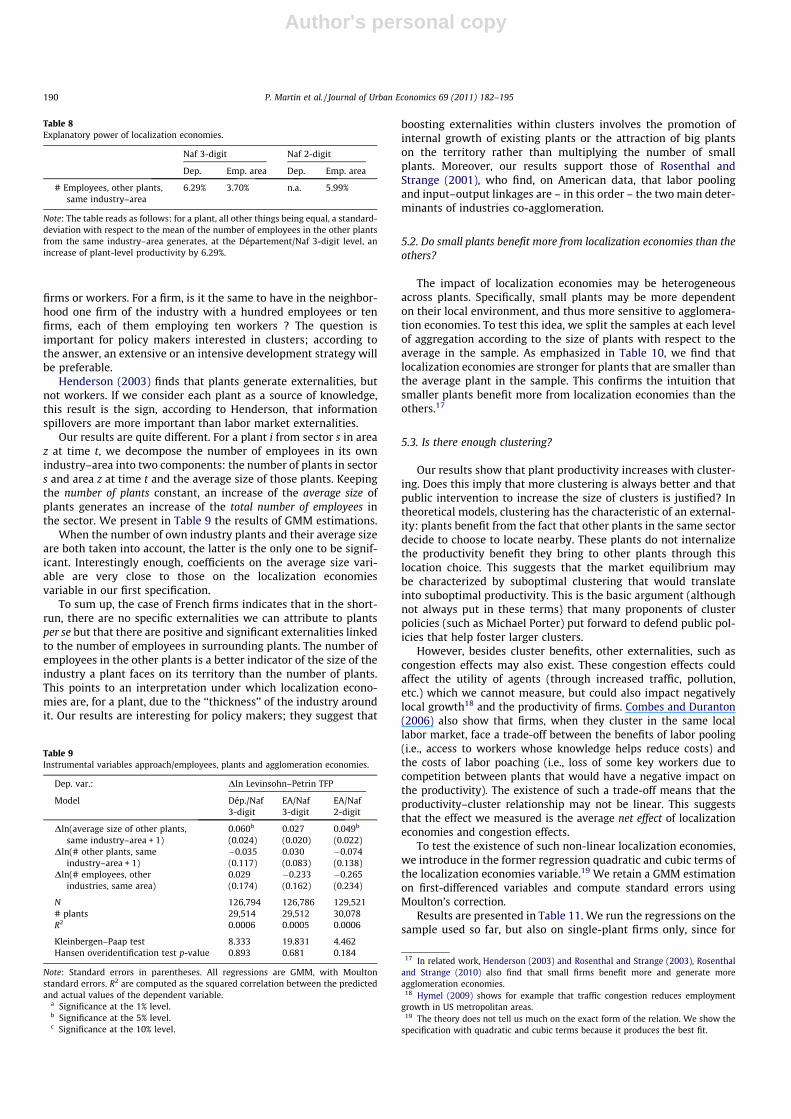
of the coefficient attached to it and on its variability. If a variablehas a very low variance, its explanatory power will be small, evenif it has a large coefficient. The explanatory power of an indepen-dent variable is strong if, all other things being equal, a standard-deviation of that variable implies a large variation of the dependentvariable.16 We consequently calculated the explanatory power oflocalization economies. The results are presented in Table 8. Theexplanatory power of localization economies variables appears smallbut non negligible.

5. Robustness checks and further issues

5.1. Who generates externalities: plants or employees?

Theory offers several possible channels for localization econo-mies. A notable alternative is whether externalities transit through

Table 6Instrumental variables approach, Département/Naf 3-digit.

Dep. var.: Dln Levinsohn–Petrin TFP

Model (1) (2) (3) (4)

Dln(# employees, other plants,same industry–area + 1)

�0.002 0.059b �0.002 0.055c

(0.002) (0.028) (0.002) (0.029)Dln(# employees, other

industries, same area)�0.005 �0.060 0.003 �0.005(0.021) (0.149) (0.022) (0.206)

Dln(sectoral diversity) 0.013 �0.056(0.012) (0.130)

Dln(competition) 0.002 0.057(0.005) (0.047)

N 126,794 126,794 126,794 126,794# Plants 29,514 29,514 29,514 29,514R2 0.003 0.0006 0.003 0.0004

Kleinbergen–Paap test 60.581 15.158Hansen overidentification test

p-value0.402 0.130

Note: Standard errors in parentheses. (1) and (3) simple OLS, (2) and (4) are GMM,with standard errors clustered at the area–industry–year level. For columns (2) and(4), R2 are computed as the squared correlation between the predicted and actualvalues of the dependent variable.

a Significance at the 1% level.b Significance at the 5% level.c Significance at the 10% level.

Table 7Results across aggregation levels.

Dép./Naf 3-digit EA/Naf 3-digit Dép./Naf 2-digit EA/Naf 2-digit

4.17% 1.96% n.a. 3.89%

Note: Each column gives the percentage increase in productivity following a dou-bling of the localization economies for each sample.

15 If lny = alnx, y increases in percentage by (2a � 1) � 100 when x is doubled.16 If ln y = aln x, we define the explanatory power of x as ½expða lnð1þ rx

�x ÞÞ � 1� �100 = ½ð1þ rx

�x Þa � 1� � 100, where rx and x are the standard deviation and the mean

of x respectively.

P. Martin et al. / Journal of Urban Economics 69 (2011) 182–195 189

Author's personal copy

firms or workers. For a firm, is it the same to have in the neighbor-hood one firm of the industry with a hundred employees or tenfirms, each of them employing ten workers ? The question isimportant for policy makers interested in clusters; according tothe answer, an extensive or an intensive development strategy willbe preferable.

Henderson (2003) finds that plants generate externalities, butnot workers. If we consider each plant as a source of knowledge,this result is the sign, according to Henderson, that informationspillovers are more important than labor market externalities.

Our results are quite different. For a plant i from sector s in areaz at time t, we decompose the number of employees in its ownindustry–area into two components: the number of plants in sectors and area z at time t and the average size of those plants. Keepingthe number of plants constant, an increase of the average size ofplants generates an increase of the total number of employees inthe sector. We present in Table 9 the results of GMM estimations.

When the number of own industry plants and their average sizeare both taken into account, the latter is the only one to be signif-icant. Interestingly enough, coefficients on the average size vari-able are very close to those on the localization economiesvariable in our first specification.

To sum up, the case of French firms indicates that in the short-run, there are no specific externalities we can attribute to plantsper se but that there are positive and significant externalities linkedto the number of employees in surrounding plants. The number ofemployees in the other plants is a better indicator of the size of theindustry a plant faces on its territory than the number of plants.This points to an interpretation under which localization econo-mies are, for a plant, due to the ‘‘thickness’’ of the industry aroundit. Our results are interesting for policy makers; they suggest that

boosting externalities within clusters involves the promotion ofinternal growth of existing plants or the attraction of big plantson the territory rather than multiplying the number of smallplants. Moreover, our results support those of Rosenthal andStrange (2001), who find, on American data, that labor poolingand input–output linkages are – in this order – the two main deter-minants of industries co-agglomeration.

5.2. Do small plants benefit more from localization economies than theothers?

The impact of localization economies may be heterogeneousacross plants. Specifically, small plants may be more dependenton their local environment, and thus more sensitive to agglomera-tion economies. To test this idea, we split the samples at each levelof aggregation according to the size of plants with respect to theaverage in the sample. As emphasized in Table 10, we find thatlocalization economies are stronger for plants that are smaller thanthe average plant in the sample. This confirms the intuition thatsmaller plants benefit more from localization economies than theothers.17

5.3. Is there enough clustering?

Our results show that plant productivity increases with cluster-ing. Does this imply that more clustering is always better and thatpublic intervention to increase the size of clusters is justified? Intheoretical models, clustering has the characteristic of an external-ity: plants benefit from the fact that other plants in the same sectordecide to choose to locate nearby. These plants do not internalizethe productivity benefit they bring to other plants through thislocation choice. This suggests that the market equilibrium maybe characterized by suboptimal clustering that would translateinto suboptimal productivity. This is the basic argument (althoughnot always put in these terms) that many proponents of clusterpolicies (such as Michael Porter) put forward to defend public pol-icies that help foster larger clusters.

However, besides cluster benefits, other externalities, such ascongestion effects may also exist. These congestion effects couldaffect the utility of agents (through increased traffic, pollution,etc.) which we cannot measure, but could also impact negativelylocal growth18 and the productivity of firms. Combes and Duranton(2006) also show that firms, when they cluster in the same locallabor market, face a trade-off between the benefits of labor pooling(i.e., access to workers whose knowledge helps reduce costs) andthe costs of labor poaching (i.e., loss of some key workers due tocompetition between plants that would have a negative impact onthe productivity). The existence of such a trade-off means that theproductivity–cluster relationship may not be linear. This suggeststhat the effect we measured is the average net effect of localizationeconomies and congestion effects.

To test the existence of such non-linear localization economies,we introduce in the former regression quadratic and cubic terms ofthe localization economies variable.19 We retain a GMM estimationon first-differenced variables and compute standard errors usingMoulton’s correction.

Results are presented in Table 11. We run the regressions on thesample used so far, but also on single-plant firms only, since for

Table 8Explanatory power of localization economies.

Naf 3-digit Naf 2-digit

Dep. Emp. area Dep. Emp. area

# Employees, other plants,same industry–area

6.29% 3.70% n.a. 5.99%

Note: The table reads as follows: for a plant, all other things being equal, a standard-deviation with respect to the mean of the number of employees in the other plantsfrom the same industry–area generates, at the Département/Naf 3-digit level, anincrease of plant-level productivity by 6.29%.

Table 9Instrumental variables approach/employees, plants and agglomeration economies.

Dep. var.: Dln Levinsohn–Petrin TFP

Model Dép./Naf3-digit

EA/Naf3-digit

EA/Naf2-digit

Dln(average size of other plants,same industry–area + 1)

0.060b 0.027 0.049b

(0.024) (0.020) (0.022)Dln(# other plants, same

industry–area + 1)�0.035 0.030 �0.074(0.117) (0.083) (0.138)

Dln(# employees, otherindustries, same area)

0.029 �0.233 �0.265(0.174) (0.162) (0.234)

N 126,794 126,786 129,521# plants 29,514 29,512 30,078R2 0.0006 0.0005 0.0006

Kleinbergen–Paap test 8.333 19.831 4.462Hansen overidentification test p-value 0.893 0.681 0.184

Note: Standard errors in parentheses. All regressions are GMM, with Moultonstandard errors. R2 are computed as the squared correlation between the predictedand actual values of the dependent variable.

a Significance at the 1% level.b Significance at the 5% level.c Significance at the 10% level.

17 In related work, Henderson (2003) and Rosenthal and Strange (2003), Rosenthaland Strange (2010) also find that small firms benefit more and generate moreagglomeration economies.

18 Hymel (2009) shows for example that traffic congestion reduces employmentgrowth in US metropolitan areas.

19 The theory does not tell us much on the exact form of the relation. We show thespecification with quadratic and cubic terms because it produces the best fit.

190 P. Martin et al. / Journal of Urban Economics 69 (2011) 182–195

Author's personal copy

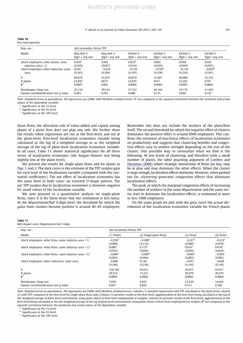
those firms, the allocation rule of value-added and capital amongplants of a given firm does not play any role. We further showthe results when regressions are run at the firm-level, and not atthe plant-level, firm-level localization economies variable beingcalculated as the log of a weighted average or as the weightedaverage of the log of plant-level localization economies variable.In all cases, Table 11 shows statistical significance for all threeterms of localization economies (the Sargan–Hansen test beingslightly low at the plant-level).

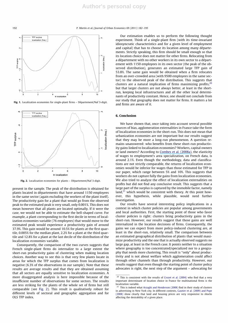
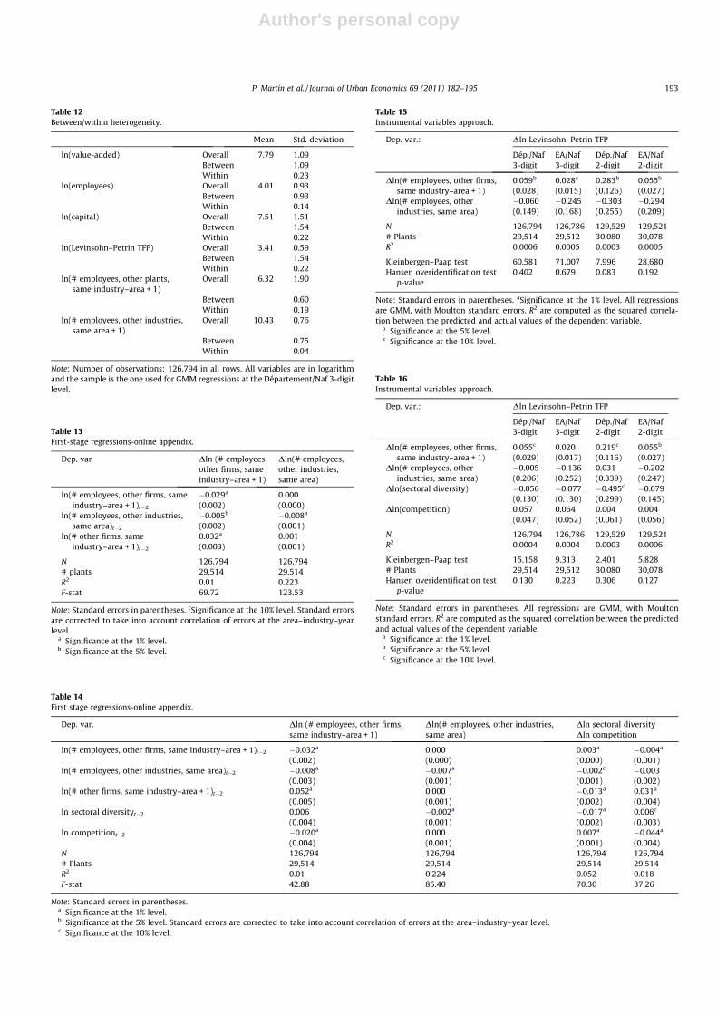
We present the results for single-plant firms and for plants inFigs. 1 and 2. The dark curve is the estimate of the TFP surplus gainfor each level of the localization variable (computed with the esti-mated coefficients). The net effect of localization economies hasthe same form in both cases: an inverted U-shape pattern. Thenet TFP surplus due to localization economies is however negativefor small values of the localization variable.

We now proceed to a quantitative analysis on single-plantfirms, since it is for those firms that our estimation is less noisy.At the département/Naf 3-digit level, the threshold for which thegains from clusters become positive is around 40–45 employees.

Remember this does not include the workers of the plant/firmitself. The second threshold for which the negative effect of clustersdominates the positive effect is around 9500 employees. This con-firms the existence of non-linear effects of localization economieson productivity and suggests that clustering benefits and conges-tion effects vary in relative strength depending on the size of thecluster. One possible way to rationalize what we find is thefollowing. At low levels of clustering, and therefore with a smallnumber of plants, the labor poaching argument of Combes andDuranton (2006) where strategic interactions of firms are key, maybe at play and may dominate the other effects. When the clusteris large enough, localization effects dominate. However, when pushedtoo far, clustering generates congestion effects that dominatelocalization effects.

The peak, at which the marginal congestion effects of increasingthe number of workers in the same département and the same sec-tor start to dominate the localization effects, is estimated at moreor less 1000 employees.

On the same graph we plot with the grey curve the actual dis-tribution of the localization economies variable for French plants

Table 10Size heterogeneity.

Dep. var.: Dln Levinsohn–Petrin TFP

Model Dép./Naf 3-digit 6 avg size

Dép./Naf 3-digit > avg size

EA/Naf 3-digit 6 avg size

EA/Naf 3-digit > avg size

EA/Naf 2-digit 6 avg size

EA/Naf 2-digit > avg size

Dln(# employees, other plants, sameindustry–area + 1)

0.050c 0.042 0.033b 0.003 0.050c 0.035(0.029) (0.057) (0.016) (0.029) (0.029) (0.055)

Dln(# employees, other industries, samearea)

0.036 �0.419 �0.126 �0.769b �0.119 �0.859b

(0.163) (0.299) (0.183) (0.328) (0.224) (0.361)

N 94,879 31,915 94,879 31,907 96,989 32,532# plants 22,835 6679 22,835 6677 23,287 6791R2 0.0007 0.001 0.0004 0.0004 0.0007 0.0003

Kleinbergen–Paap test 47.120 20.514 57.332 46.104 19.772 21.503Hansen overidentification test p-value 0.493 0.025 0.489 0.151 0.669 0.147

Note: Standard errors in parentheses. All regressions are GMM, with Moulton standard errors. R2 are computed as the squared correlation between the predicted and actualvalues of the dependent variable.

a Significance at the 1% level.b Significance at the 5% level.c Significance at the 10% level.

Table 11Bell-shaped curve Département-Naf 3-digit.

Dep. var.: Dln Levinsohn–Petrin TFP

Model (1) Plants (2) Single plant firms (3) Firms (4) Firms

Dln(# employees, other firms, same industry–area + 1) �0.256a �0.298a �0.227a �0.223a

(0.088) (0.114) (0.080) (0.078)Dln(# employees, other firms, same industry–area + 1)2 0.086b 0.113b 0.076a 0.074b

(0.034) (0.044) (0.029) (0.029)Dln(# employees, other firms, same industry–area + 1)3 �0.006c �0.009b �0.005b �0.005c

(0.003) (0.004) (0.003) (0.002)Dln(# employees, other industries, same area) �0.046 0.144 �0.051 �0.044

(0.184) (0.238) (0.145) (0.149)

N 126,794 63,675 95,077 95,077# plants 29,514 15,221 20,479 20,479R2 0.0005 0.0002 0.0005 0.0004

Kleinbergen–Paap test 7.829 6.832 12.329 14.443Hansen overidentification test p-value 0.047 0.692 0.311 0.366

Note: Standard errors in parentheses. All regressions are GMM, with Moulton standard errors. Column (1) presents regressions with TFP calculated at the plant-level, column(2) with TFP computed at the firm-level for single-plant firms only. Column (3) presents results at the firm-level, agglomeration at the firm-level being calculated as the log ofthe weighted average of plant-level environment, using plant-shares in firm-level employment as weights. Column (4) presents results at the firm-level, agglomeration at thefirm-level being calculated as the the weighted average of the log of plant-level environment, using plant-shares in firm-level employment as weights. R2 are computed as thesquared correlation between the predicted and actual values of the dependent variable.

a Significance at the 1% level.b Significance at the 5% level.c Significance at the 10% level.

P. Martin et al. / Journal of Urban Economics 69 (2011) 182–195 191

Author's personal copy

present in the sample. The peak of the distribution is obtained forplants located in départements that have around 1150 employeesin the same sector (again excluding the workers of the plant itself).The productivity gain for a plant that would go from the observedpeak to the estimated peak is very small, only 0.001%. This does notmean however that all plants are located optimally. If it were thecase, we would not be able to estimate the bell-shaped curve. Forexample, a plant corresponding to the first decile in terms of local-ization economies variable (76 employees) that would move to theestimated peak would experience a productivity gain of around37.9%. This gain would be around 10.5% for plants at the first quar-tile, 0.005% for the median plant, 2.2% for a plant at the third quar-tile and 12.8% for a plant at the last decile of the distribution of thelocalization economies variable.

Consequently, the comparison of the two curves suggests thatFrench single-plant firms do internalize to a large extent theshort-run productivity gains of clustering when making locationchoices. Another way to see this is that very few plants locate inareas for which the TFP surplus that comes from localization isnegative (6.3% of the observations in our sample). Note that theseresults are average results and that they are obtained assumingthat all sectors are equally sensitive to localization economies. Amore disaggregated analysis is here impossible because of theinsufficient number of observations for some sectors. The resultsare less striking for the plants of the whole set of firms but stillcomparable (see Fig. 2). This result is qualitatively robust fordifferent levels of sectoral and geographic aggregation and forOLS TFP index.

Our estimation enables us to perform the following thoughtexperiment. Think of a single-plant firm (with its time-invariantidiosyncratic characteristics and for a given level of employmentand capital) that has to choose its location among many départe-ments. Strictly speaking, this firm should be small enough so thatits location choice does not matter for other firms. Relocating froma département with no other workers in its own sector to a départ-ement with 1150 employees in its own sector (the peak of the ob-served distribution), generates an estimated large TFP gain of53.8%. The same gain would be obtained when a firm relocatesfrom an over-crowded area (with 9500 employees in the same sec-tor) to the observed peak of the distribution. This suggests thatclusters are a natural implication of firms maximizing profits,20

but that larger clusters are not always better, at least in the short-run, keeping local infrastructures and all the other local determi-nants of productivity constant. Hence, one should not conclude fromour study that geography does not matter for firms. It matters a lotand firms are aware of it.

6. Conclusion

We have shown that, once taking into account several possiblesources of bias, agglomeration externalities in France take the formof localization economies in the short-run. This does not mean thaturbanization economies are not important but our results suggestthat they may be more a long-run phenomenon. A question re-mains unanswered: who benefits from these short-run productiv-ity gains linked to localization economies? Workers, capital ownersor land owners? According to Combes et al. (2008a), the elasticityof wages to employment’s area specialization, on French data, isaround 2.1%. Even though the methodology, data and classifica-tions are not strictly comparable, the returns of localization econ-omies would be inferior for wages than those estimated for TFP inour paper, which range between 5% and 10%. This suggests thatworkers do not capture fully the gains from localization economies.We also tried to analyze the effect of localization externalities onprofits but did not find any conclusive result. This suggests that alarge part of the surplus is captured by the immobile factor, namelyland,21 which would be consistent with theory. At this point how-ever, this hypothesis, while plausible, would need furtherinvestigation.

Our results have several interesting policy implications in acontext in which cluster policies are popular among governmentsand local authorities. First, the starting point of those who favorcluster policies is right: clusters bring productivity gains in theshort-run. However, our results suggest that those gains are wellinternalized in the location decisions of firms. Consequently, thegains we can expect from more policy-induced clustering are, atleast in the short-run, relatively small. The comparison betweenan estimated geographical distribution of plants that would maxi-mize productivity and the one that is actually observed suggests nolarge gap, at least in the French case. It points neither to a situationwhere geography is too concentrated/specialized nor to a geogra-phy that needs more clustering. This result is ‘‘only’’ about produc-tivity and is not about welfare which agglomeration could affectthrough other channels than through productivity. However, ourresults suggest that even though the starting point of cluster policyadvocates is right, the next step of the argument – advocating for

Fig. 1. Localization economies for single-plant firms – Département/Naf 3-digit.

Fig. 2. Localization economies for plants – Département/Naf 3-digit.

20 This is consistent with the results of Crozet et al. (2004) who find that a veryimportant determinant of location choice in France for multinational firms is thelocalization variable.

21 This is indeed what Arzaghi and Henderson (2008) find in their study of clustersin advertising in New York city. In different contexts, Gautier et al. (2009) and Pope(2008) show clearly that land and housing prices are very responsive to shocksaffecting the desirability of a given place.

192 P. Martin et al. / Journal of Urban Economics 69 (2011) 182–195

Author's personal copy

Table 12Between/within heterogeneity.

Mean Std. deviation

ln(value-added) Overall 7.79 1.09Between 1.09Within 0.23

ln(employees) Overall 4.01 0.93Between 0.93Within 0.14

ln(capital) Overall 7.51 1.51Between 1.54Within 0.22

ln(Levinsohn–Petrin TFP) Overall 3.41 0.59Between 1.54Within 0.22

ln(# employees, other plants,same industry–area + 1)

Overall 6.32 1.90

Between 0.60Within 0.19

ln(# employees, other industries,same area + 1)

Overall 10.43 0.76

Between 0.75Within 0.04

Note: Number of observations: 126,794 in all rows. All variables are in logarithmand the sample is the one used for GMM regressions at the Département/Naf 3-digitlevel.

Table 13First-stage regressions-online appendix.

Dep. var Dln (# employees,other firms, sameindustry–area + 1)

Dln(# employees,other industries,same area)

ln(# employees, other firms, sameindustry–area + 1)t�2

�0.029a 0.000(0.002) (0.000)

ln(# employees, other industries,same area)t�2

�0.005b �0.008a

(0.002) (0.001)ln(# other firms, same

industry–area + 1)t�2

0.032a 0.001(0.003) (0.001)

N 126,794 126,794# plants 29,514 29,514R2 0.01 0.223F-stat 69.72 123.53

Note: Standard errors in parentheses. cSignificance at the 10% level. Standard errorsare corrected to take into account correlation of errors at the area–industry–yearlevel.

a Significance at the 1% level.b Significance at the 5% level.

Table 15Instrumental variables approach.

Dep. var.: Dln Levinsohn–Petrin TFP

Dép./Naf3-digit

EA/Naf3-digit

Dép./Naf2-digit

EA/Naf2-digit

Dln(# employees, other firms,same industry–area + 1)

0.059b 0.028c 0.283b 0.055b

(0.028) (0.015) (0.126) (0.027)Dln(# employees, other

industries, same area)�0.060 �0.245 �0.303 �0.294(0.149) (0.168) (0.255) (0.209)

N 126,794 126,786 129,529 129,521# Plants 29,514 29,512 30,080 30,078R2 0.0006 0.0005 0.0003 0.0005

Kleinbergen–Paap test 60.581 71.007 7.996 28.680Hansen overidentification test

p-value0.402 0.679 0.083 0.192

Note: Standard errors in parentheses. aSignificance at the 1% level. All regressionsare GMM, with Moulton standard errors. R2 are computed as the squared correla-tion between the predicted and actual values of the dependent variable.

b Significance at the 5% level.c Significance at the 10% level.

Table 16Instrumental variables approach.

Dep. var.: Dln Levinsohn–Petrin TFP

Dép./Naf3-digit

EA/Naf3-digit

Dép./Naf2-digit

EA/Naf2-digit

Dln(# employees, other firms,same industry–area + 1)

0.055c 0.020 0.219c 0.055b

(0.029) (0.017) (0.116) (0.027)Dln(# employees, other

industries, same area)�0.005 �0.136 0.031 �0.202(0.206) (0.252) (0.339) (0.247)

Dln(sectoral diversity) �0.056 �0.077 �0.495c �0.079(0.130) (0.130) (0.299) (0.145)

Dln(competition) 0.057 0.064 0.004 0.004(0.047) (0.052) (0.061) (0.056)

N 126,794 126,786 129,529 129,521R2 0.0004 0.0004 0.0003 0.0006

Kleinbergen–Paap test 15.158 9.313 2.401 5.828# Plants 29,514 29,512 30,080 30,078Hansen overidentification test

p-value0.130 0.223 0.306 0.127

Note: Standard errors in parentheses. All regressions are GMM, with Moultonstandard errors. R2 are computed as the squared correlation between the predictedand actual values of the dependent variable.

a Significance at the 1% level.b Significance at the 5% level.c Significance at the 10% level.

Table 14First stage regressions-online appendix.

Dep. var. Dln (# employees, other firms,same industry–area + 1)

Dln(# employees, other industries,same area)

Dln sectoral diversityDln competition

ln(# employees, other firms, same industry–area + 1)t�2 �0.032a 0.000 0.003a �0.004a

(0.002) (0.000) (0.000) (0.001)ln(# employees, other industries, same area)t�2 �0.008a �0.007a �0.002c �0.003

(0.003) (0.001) (0.001) (0.002)ln(# other firms, same industry–area + 1)t�2 0.052a 0.000 �0.013a 0.031a

(0.005) (0.001) (0.002) (0.004)ln sectoral diversityt�2 0.006 �0.002a �0.017a 0.006c

(0.004) (0.001) (0.002) (0.003)ln competitiont�2 �0.020a 0.000 0.007a �0.044a

(0.004) (0.001) (0.001) (0.004)N 126,794 126,794 126,794 126,794# Plants 29,514 29,514 29,514 29,514R2 0.01 0.224 0.052 0.018F-stat 42.88 85.40 70.30 37.26

Note: Standard errors in parentheses.a Significance at the 1% level.b Significance at the 5% level. Standard errors are corrected to take into account correlation of errors at the area–industry–year level.c Significance at the 10% level.

P. Martin et al. / Journal of Urban Economics 69 (2011) 182–195 193

Author's personal copy

costly public intervention in favor of clusters – is not supported bythe French evidence. In a related paper, Martin et al. (2009), usingthe same dataset as in this paper, we find no evidence that a Frenchcluster policy, the ‘‘Systèmes Productifs Locaux’’, had any effect onfirms’ productivity.

Acknowledgments

We thank two anonymous referees, Anthony Briant, Pierre-Philippe Combes and Gilles Duranton for helpful comments on earlyversions. We also thank William Strange for his insightful discus-sion of this paper at the 2008 RSAI conference in New York, andhis numerous advices and comments as an editor. Participants ofthe GSIE lunch seminar of the Paris School of Economics, theJournées d’économie spatiale in Saint-Etienne, the workshops ineconomic geography in Barcelona and Passau, the EEA conferencein Milano and the conference on the ‘‘dynamics of firm evolution’’in Pisa, also gave helpful comments. We thank CEPREMAP for fund-ing this research, and the French Ministry of Industry for providingthe necessary data.

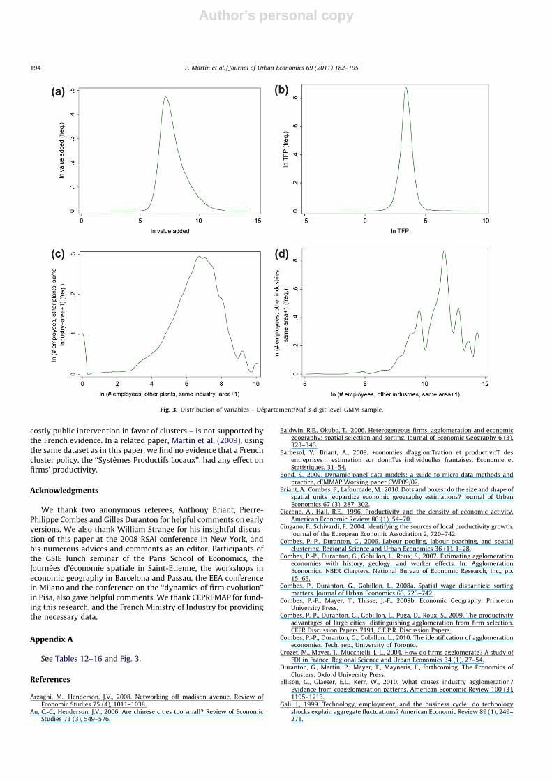
Appendix A

See Tables 12–16 and Fig. 3.

References

Arzaghi, M., Henderson, J.V., 2008. Networking off madison avenue. Review ofEconomic Studies 75 (4), 1011–1038.

Au, C.-C., Henderson, J.V., 2006. Are chinese cities too small? Review of EconomicStudies 73 (3), 549–576.

Baldwin, R.E., Okubo, T., 2006. Heterogeneous firms, agglomeration and economicgeography: spatial selection and sorting. Journal of Economic Geography 6 (3),323–346.

Barbesol, Y., Briant, A., 2008. +conomies d’agglomTration et productivitT desentreprises : estimation sur donnTes individuelles frantaises. Economie etStatistiques, 31–54.

Bond, S., 2002. Dynamic panel data models: a guide to micro data methods andpractice, cEMMAP Working paper CWP09/02.

Briant, A., Combes, P., Lafourcade, M., 2010. Dots and boxes: do the size and shape ofspatial units jeopardize economic geography estimations? Journal of UrbanEconomics 67 (3), 287–302.

Ciccone, A., Hall, R.E., 1996. Productivity and the density of economic activity.American Economic Review 86 (1), 54–70.

Cingano, F., Schivardi, F., 2004. Identifying the sources of local productivity growth.Journal of the European Economic Association 2, 720–742.

Combes, P.-P., Duranton, G., 2006. Labour pooling, labour poaching, and spatialclustering. Regional Science and Urban Economics 36 (1), 1–28.

Combes, P.-P., Duranton, G., Gobillon, L., Roux, S., 2007. Estimating agglomerationeconomies with history, geology, and worker effects. In: AgglomerationEconomics. NBER Chapters. National Bureau of Economic Research, Inc., pp.15–65.

Combes, P., Duranton, G., Gobillon, L., 2008a. Spatial wage disparities: sortingmatters. Journal of Urban Economics 63, 723–742.

Combes, P.-P., Mayer, T., Thisse, J.-F., 2008b. Economic Geography. PrincetonUniversity Press.

Combes, P.-P., Duranton, G., Gobillon, L., Puga, D., Roux, S., 2009. The productivityadvantages of large cities: distinguishing agglomeration from firm selection.CEPR Discussion Papers 7191, C.E.P.R. Discussion Papers.

Combes, P.-P., Duranton, G., Gobillon, L., 2010. The identification of agglomerationeconomies. Tech. rep., University of Toronto.

Crozet, M., Mayer, T., Mucchielli, J.-L., 2004. How do firms agglomerate? A study ofFDI in France. Regional Science and Urban Economics 34 (1), 27–54.

Duranton, G., Martin, P., Mayer, T., Mayneris, F., forthcoming. The Economics ofClusters. Oxford University Press.

Ellison, G., Glaeser, E.L., Kerr, W., 2010. What causes industry agglomeration?Evidence from coagglomeration patterns. American Economic Review 100 (3),1195–1213.

Gali, J., 1999. Technology, employment, and the business cycle: do technologyshocks explain aggregate fluctuations? American Economic Review 89 (1), 249–271.

Fig. 3. Distribution of variables – Département/Naf 3-digit level-GMM sample.

194 P. Martin et al. / Journal of Urban Economics 69 (2011) 182–195

Author's personal copy

Gautier, P.A., Siegmann, A., Van Vuuren, A., 2009. Terrorism and attitudes towardsminorities: the effect of the Theo van Gogh murder on house prices inAmsterdam. Journal of Urban Economics 65 (2), 113–126.

Glaeser, E.L., Mare, D.C., 2001. Cities and skills. Journal of Labor Economics 19 (2),316–342.

Henderson, V., 2003. Marshall’s scale economies. Journal of Urban Economics 53 (1),1–28.

Hymel, K., 2009. Does traffic congestion reduce employment growth? Journal ofUrban Economics 65 (2), 127–135.

Levinsohn, J., Petrin, A., 2003. Estimating production functions using inputs tocontrol for unobservables. Review of Economic Studies 70 (2), 317–342.

Marshall, A., 1890. Principles of Economics. Macmillan, London.Martin, P., Mayer, T., Mayneris, F., 2009. Public support to clusters: a case study on

French local productive systems, 1996–2004. Regional Science and UrbanEconomics, forthcoming.

Melitz, M.J., Ottaviano, G.I.P., 2008. Market size, trade, and productivity. Review ofEconomic Studies 75 (1), 295–316.

Moulton, B.R., 1990. An illustration of a pitfall in estimating the effects of aggregatevariables on micro unit. The Review of Economics and Statistics 72 (2), 334–338.

Pope, J.C., 2008. Fear of crime and housing prices: household reactions to sexoffender registries. Journal of Urban Economics 64 (3), 601–614.

Porter, M., 1998. Clusters and competition: new agendas for companies,governments, and institutions. In: On Competition. Harvard Business SchoolPress.

Rosenthal, S.S., Strange, W.C., 2001. The determinants of agglomeration. Journal ofUrban Economics 50 (2), 191–229.

Rosenthal, S.S., Strange, W.C., 2003. Geography, industrial organization, andagglomeration. The Review of Economics and Statistics 85 (2), 377–393.

Rosenthal, S.S., Strange, W.C., 2004. Evidence on the nature and sources ofagglomeration economies. In: Henderson, J.V., Thisse, J.F. (Eds.), Handbook ofRegional and Urban Economics, Handbook of Regional and Urban Economics,vol. 4. Elsevier, pp. 2119–2171 (Chapter 49).

Rosenthal, S.S., Strange, W.C., 2010. Small establishments/big effects: agglomeration,industrial organization and entrepreneurship. In: Agglomeration Economics.NBER Chapters. National Bureau of Economic Research, Inc., pp. 277–302.

Shefer, D., 1973. Localization economies in sma’s: a production function analysis.Journal of Urban Economics 13 (1), 55–64.

Sveikauskas, L.A., 1975. The productivity of cities. Quarterly Journal of Economics 89(3), 393–413.

P. Martin et al. / Journal of Urban Economics 69 (2011) 182–195 195