Spatial biodiversity patterns of bacterio- and picoplankton

communities in Arctic fjords

Bachelorarbeit im Studiengang

B. Sc. Biologie

Vorgelegt von

Pauline Thomé

Geb. in Berlin

Angefertigt am

Alfred-Wegener-Institut, Helmholtz-Zentrum für Polar- und

Meeresforschung, Bremerhaven

und an der

Fakultät für Biologie und Psychologie der Georg-August-Universität

zu Göttingen

Abgabe im SoSe 2020

Erstbetreuer: Prof. Thomas Friedl

Zweitbetreuer: Dr. Uwe John

Göttingen, 29. Mai 2020

Contents

List of Figures .......................................................................................................................................... i

List of Tables ........................................................................................................................................... ii

1 Summary ......................................................................................................................................... 1

2 Introduction ..................................................................................................................................... 2

3 Outline of the Thesis ....................................................................................................................... 7

4 Materials and Methods .................................................................................................................... 9

4.1 Study Area ............................................................................................................................... 9

4.1.1 North Norway ................................................................................................................ 10

4.1.2 South Norway ................................................................................................................ 10

4.1.3 Svalbard ......................................................................................................................... 11

4.1.4 Iceland ........................................................................................................................... 12

4.1.5 East Greenland .............................................................................................................. 12

4.1.6 West Greenland ............................................................................................................. 13

4.2 Sampling ................................................................................................................................ 14

4.3 DNA Extraction and Quantification ...................................................................................... 14

4.3.1 DNA extraction ............................................................................................................. 14

4.3.2 DNA Quantification with Spectrophotometry ............................................................... 14

4.3.3 DNA quantification with gel electrophoresis ................................................................ 15

4.4 Library Preparation and Sequencing ..................................................................................... 16

4.4.1 Amplicon PCR .............................................................................................................. 16

4.4.2 Index PCR and Quantification ....................................................................................... 17

4.5 Sequencing ............................................................................................................................ 18

4.6 ASV Table ............................................................................................................................. 18

4.7 Rarefaction ............................................................................................................................ 19

4.8 Diversity Measures and Nutrient Concentrations .................................................................. 19

4.9 T-Test .................................................................................................................................... 20

4.10 Dissimilarity Calculations and Mantel Test .......................................................................... 20

4.11 NMDS Analysis .................................................................................................................... 20

5 Results ........................................................................................................................................... 21

5.1 Alpha Diversity ..................................................................................................................... 21

5.1.1 Alpha Diversity across regions: Richness ..................................................................... 21

5.1.2 Alpha Diversity across regions: Diversity ..................................................................... 23

5.1.3 Alpha Diversity across prokaryotes and eukaryotes: co-variation ................................ 26

5.2 Beta Diversity ........................................................................................................................ 28

5.2.1 Beta Diversity across regions ........................................................................................ 28

5.2.2 Beta Diversity across regions: Drivers .......................................................................... 30

5.2.3 Beta Diversity within regions: North Norway ............................................................... 32

5.2.4 Beta Diversity within regions: Svalbard ........................................................................ 34

5.2.5 Beta Diversity across tip and mouth stations: fjords and glaciers ................................. 36

6 Discussion ..................................................................................................................................... 38

6.1 Methodological Approach ..................................................................................................... 38

6.2 Alpha Diversity ..................................................................................................................... 39

6.2.1 Alpha Diversity across regions: Richness ..................................................................... 39

6.2.2 Alpha Diversity across regions: Diversity ..................................................................... 40

6.2.3 Alpha Diversity across prokaryotes and eukaryotes: co-variation ................................ 41

6.3 Beta Diversity ........................................................................................................................ 43

6.3.1 Beta Diversity across regions ........................................................................................ 43

6.3.2 Beta Diversity within regions ........................................................................................ 46

6.3.3 Beta Diversity: Influences of fjord structures and glaciers ........................................... 48

7 Conclusion ..................................................................................................................................... 49

8 Outlook .......................................................................................................................................... 51

References ............................................................................................................................................. 51

Acknowledgement ................................................................................................................................. 59

Supplement ............................................................................................................................................... I

i

List of Figures

Fig. 1: Study area. ................................................................................................................................... 9 Fig. 2: Sampled stations of North Norway. ........................................................................................... 10 Fig. 3: Sampled stations of South Norway. ............................................................................................ 11 Fig. 4: Sampled stations of Svalbard. .................................................................................................... 11 Fig. 5: Sampled stations of Iceland. ...................................................................................................... 12 Fig. 6: Sampled stations in East Greenland. ......................................................................................... 13 Fig. 7: Sampled stations of West Greenland. ........................................................................................ 13 Fig. 8: Spectrophotometric absorption curves, DNA concentration and purity ratios.......................... 15 Fig. 9: Gel bands of the extracted DNA. ............................................................................................... 16 Fig. 10: Gel bands of Amplicon PCR products ..................................................................................... 17 Fig. 11: Ranges in ASV richness of pro- and eukaryotic communities per region. ............................... 22 Fig. 12: Temperature versus eukaryotic and prokaryotic richness. ...................................................... 22 Fig. 13: Phosphate concentration versus eukaryotic and prokaryotic richness. ................................... 23 Fig. 14: Nitrate concentration versus eukaryotic and prokaryotic richness ......................................... 23 Fig. 15: Ranges of the Inverse Simpson index for prokaryotes and eukaryotes per region .................. 24 Fig. 16: Prokaryotic Simpson diversity versus richness without North Norway. .................................. 24 Fig. 17: Eukaryotic Simpson diversity versus richness. ........................................................................ 25 Fig. 18: Temperature versus eukaryotic and prokaryotic Inverse Simpson. ......................................... 25 Fig. 19: Phosphate versus eukaryotic and prokaryotic Inverse Simpson. ............................................. 26 Fig. 20: Eukaryotic versus prokaryotic richness without North Norway. ............................................. 27 Fig. 21: Eukaryotic versus prokaryotic Inverse Simpson in North Norway. ......................................... 27 Fig. 22: NMDS of the a) prokaryotic and b) eukaryotic samples across all regions. ........................... 29 Fig. 23: Proportions of unique a) prokaryotic and b) eukaryotic ASVs per region. ............................. 30 Fig. 24: Pairwise a) prokaryotic and b) eukaryotic Bray-Curtis-Dissimilarity versus environmental

dissimilarity. .......................................................................................................................................... 31 Fig. 25: Pairwise a) prokaryotic and b) eukaryotic Bray-Curtis-Dissimilarity versus geographic

distance. ................................................................................................................................................. 32 Fig. 26: NMDS of the a) prokaryotic and b) eukaryotic samples of North Norway. ............................. 33 Fig. 27: Proportions of unique a) prokaryotic and b) eukaryotic ASVs per fjord in North Norway ..... 34 Fig. 28: NMDS of the a) prokaryotic and b)eukaryotic samples of Svalbard. ...................................... 35 Fig. 29: Proportions of unique a) prokaryotic and b) eukaryotic ASVs per fjord within Svalbard. ..... 36 Fig. 30: NMDS of the a) prokaryotic and b) eukaryotic tip and mouth stations. .................................. 37 Fig. 31: Proportions of unique a) prokaryotic and b) eukaryotic ASVs for tip and mouth stations with

and without glacial influence. ............................................................................................................... 38 Fig. 32: Synthesis figure. ....................................................................................................................... 50 Fig. 33: Typical absorbance curves of pure DNA. ................................................................................... I Fig. 34: Gel electrophoresis of the extracted DNA of HE533 samples 1-20. ........................................ IV Fig. 35: Gel electrophoresis of the extracted DNA of HE533 samples 21-60. ...................................... IV Fig. 36: Gel electrophoresis of the extracted DNA of HE533 samples 61-80. ...................................... IV Fig. 37: Forward and reverse primer. .................................................................................................... V Fig. 38: Gel electrophoresis of a test 18S Amplicon PCR. ..................................................................... V Fig. 39: Gel electrophoresis of the 18S Amplicon PCR products of the HE533 stations 2-6. ................ V Fig. 40: Gel electrophoresis of the 18S Amplicon PCR products of the HE533 stations 17-28........... VI Fig. 41: Gel electrophoresis of the 18S Amplicon PCR products of HE431 and MSM21/3. ................ VI Fig. 42: Gel electrophoresis of the 16S Amplicon PCR products of HE431 and MSM21/3. ............... VII Fig. 43: Gel electrophoresis of the 16S Amplicon PCR products of MSM21/3 and MSM56. .............. VII Fig. 44: Verification of successful index attachment during the Index PCR. ....................................... XII Fig. 45: Rarefaction curves for all eukaryotic North Norwegian samples. .......................................... XII Fig. 46: Rarefaction curves for eukaryotic North Norwegian samples without HE533_20C. ........... XIII

Fig. 47: Rarefaction curves for eukaryotic South Norwegian samples. ............................................. XIII Fig. 48: Rarefaction curves for eukaryotic Svalbard samples. ........................................................... XIII Fig. 49: Rarefaction curves for eukaryotic Iceland samples. ............................................................. XIV Fig. 50: Rarefaction curves for eukaryotic East Greenland samples. ................................................ XIV Fig. 51: Rarefaction curves for eukaryotic West Greenland samples. ............................................... XIV Fig. 52: Rarefaction curves for prokaryotic North Norwegian samples. ............................................. XV Fig. 53: Rarefaction curves for prokaryotic South Norwegian samples. ............................................. XV Fig. 54: Rarefaction curves for prokaryotic Svalbard samples. ........................................................... XV Fig. 55: Rarefaction curves for prokaryotic Iceland samples. ........................................................... XVI Fig. 56: Rarefaction curves for prokaryotic East Greenland samples. .............................................. XVI Fig. 57: Rarefaction curves for prokaryotic West Greenland samples. ............................................. XVI Fig. 58: Ranges in Shannon diversity of the pro- and eukaryotic communities per region.............. XVIII Fig. 59: Sites in Kongsfjord, Svalbard.............................................................................................. XVIII Fig. 60: Salinity versus prokaryotic and eukaryotic richness. ........................................................... XIX Fig. 61 Silicate concentration versus prokaryotic and eukaryotic richness. ...................................... XIX Fig. 62: Salinity versus prokaryotic and eukaryotic Simpson diversity. .............................................. XX Fig. 63: Nitrate concentration versus prokaryotic and eukaryotic Simpson diversity. ........................ XX Fig. 64: Silicate versus prokaryotic and eukaryotic Simpson diversity. ............................................. XXI Fig. 65: Prokaryotic Simpson diversity versus richness. .................................................................... XXI Fig. 66: Eukaryotic versus prokaryotic richness in North Norway. .................................................. XXII Fig. 67: Eukaryotic versus prokaryotic Simpson diversity without North Norway. .......................... XXII Fig. 68: NMDS of all eukaryotic samples per region. ...................................................................... XXIII Fig. 69: Influence of environmental dissimilarity on prokaryotic ASV turnover in North Norway. XXIII Fig. 70: Influence of environmental dissimilarity on eukaryotic ASV turnover in North Norway. . XXIV Fig. 71: Influence of geographic distance on prokaryotic ASV turnover in North Norway. ........... XXIV Fig. 72: Influence of geographic distance on eukaryotic ASV turnover in North Norway. ............... XXV Fig. 73: Ranges in nitrate concentration per region. ........................................................................ XXV Fig. 74: Prokaryotic Simpson Diversity versus richness in North Norway. .................................... XXVI Fig. 75: Eukaryotic Simpson Diversity versus richness in North Norway. ..................................... XXVI Fig. 76: Salinity in Kongsfjord, Svalbard. ...................................................................................... XXVII Fig. 77: Temperature in Kongsfjord, Svalbard. ............................................................................. XXVII Fig. 78: Salinity in the Lofoten, Norway. ....................................................................................... XXVIII Fig. 79: Temperature in the Lofoten, Norway. .............................................................................. XXVIII

List of Tables

Table 1: DNA concentrations measured with spectrophotometry of all HE533 samples. ....................... I Table 2: LabChip® quantification. ...................................................................................................... VII Table 3: T-test results of eukaryotic alpha diversity measures. ......................................................... XVI Table 4: T-Test result of prokaryotic alpha diversity measures. ....................................................... XVII Table 5: T-Test result of pro- and eukaryotic alpha diversity measures. .......................................... XVII

1

1 Summary

Marine microbial plankton drive global biogeochemical cycles and are therefore pivotal to the

ecosystem functioning of the biosphere. In particular marine picoplankton harbour a vast biodiversity

on which their community dynamics and functioning are based. Because they function collectively as a

community, it is crucial to understand the underlying diversity patterns of microbial assemblages and

identify their drivers. The data set I investigated here allows insights into surface water bacterio- and

picoplankton communities of Arctic and subarctic coastal waters and fjord systems. To infer their

diversity with a metabarcoding approach, I amplified and sequenced the V4 regions of the prokaryotic

16S and eukaryotic 18S ribosomal DNA which serve as molecular markers. The resulting amplicons

were arranged into amplicon sequence variants (ASVs) which I used as a substitute for species. In

comparing prokaryotic and picoeukaryotic alpha and beta diversity across space, I unveiled profound

differences between the domains, the investigated regions and the respective drivers. Picoeukaryotes

appeared to vastly exceed prokaryotes in their richness and are thus hypothesized to comprise a large

rare biosphere ensuring community stability. They are more strongly influenced by fjord structures and

glaciers than prokaryotes and I found spring bloom conditions to induce a drastic decrease in

picoeukaryotic richness. Prokaryotes appeared to be more strongly influenced by nutrient availability

and environmental conditions than picoeukaryotes, resulting in a higher spatial turnover through more

efficient taxa sorting. I found no distance-decay relationship in prokaryotic and picoeukaryotic

communities on the scales observed here. I assume a functional coupling and mutual dependence of the

prokaryotic and eukaryotic communities based on co-varying alpha diversity measures, which were

fundamentally restructured by spring bloom conditions. I observed a pronounced compositional

turnover in both space and time. Seasonal succession and change across years appeared to shape

picoplankton communities equally strong as spatially differing influences, stressing the need to control

for time in future spatial analyses. In contributing to a better understanding of the basic patterns and

their drivers underlying picoplankton diversity, this study may also contribute to a better understanding

of the impact climate change will have on the planet. Spatial dynamics across environmentally differing

sites can deliver indications to the influence of environmental changes in time. Thus, they allow to

anticipate changes in microbial plankton dynamics and therefore the functioning of the global biosphere

in the face of climate change.

2

2 Introduction

Oceans are the cradle of evolution which created the biodiversity on earth we know today. It harbours

the vast diversity of marine microbial plankton, who drive carbon and nutrient cycles and provide half

of the global primary production (Field et al., 1998). Because of their huge abundances and large genetic

biodiversity, those minute organisms impact processes on a global scale and are flexible in their response

to fluctuating environmental conditions. Not only the evolutionary roots of the contemporary global

biodiversity, but its vast majority in the sense of a genetic diversity can be found in the as of yet largely

unexplored microbial world.

Microbes comprise organisms of all domains of life – prokaryotes, i. e. bacteria and archaea and

unicellular eukaryotes (protists) – which possess different traits and functions. However, all of them

have the following features in common which distinguish microorganisms sharply from

macroorganisms: Being unicellular, characterized by small cell sizes, short life cycles and generally

large population sizes. These features evoke the need for different concepts to study their diversity and

distribution patterns. Common approaches to assess the biodiversity and distribution of terrestrial

macrobial life, which is shaped by dispersal barriers leading to biological speciation (Mayr, 1948),

endemism and extinction, cannot be applied so easily to microbial life. Even more so, if the marine

biosphere is addressed: At first sight, the world´s oceans appear to be a continuous space, lacking

physical dispersal barriers and being globally connected by freely flowing ocean currents. Because of

their size, microbes are passively and widely dispersed within them (Finlay & Clarke, 1999) – the

passive dispersal in fact is the feature plankton is defined by. Therefore, it has long been thought that in

principle “everything is everywhere” and through selection by environmental factors certain species

dominate distinct ecological regions (Baas Becking, 1934). However, the limitless dispersal of all

marine microbial species in the absence of dispersal barriers as proposed by Baas Becking has

increasingly been doubted (Martiny et al., 2006; Spatharis et al., 2019). Despite the occurrence of widely

distributed, diluted microbes (Farooq Azam & Malfatti, 2007), global sampling efforts have been

revealing clearly differing community compositions across spatial and temporal scales (e. g. Galand et

al., 2009; Massana et al., 2015). These findings indicate that marine microbial species, just as all other

organisms, exhibit a distinct biogeography that is shaped by both historical contingencies, i. e. dispersal

limitations, as well as by current environmental influences (Martiny et al., 2006). Density differences

between water masses for example can act as physical boundaries restricting distribution (Galand et al.,

2009).

With the knowledge we have today, the notion of a cosmopolitan distribution of all marine microbial

species solely shaped by environmental selection seems highly unlikely as a universal rule. All the more

interesting it becomes to address the patterns of local marine diversity.

In contrast to the concept of biodiversity, which refers to the entirety of contemporary species, i. e. the

global gene pool, the term diversity describes the local selection of taxa of a specific region or site

(Margalef, 1994). Global microbial biodiversity can only be roughly estimated, while the local diversity

of one community or region can be tackled more easily. In order to characterize diversity, it can be

partitioned into two subcommunities: 1) the few abundant and 2) the many rare taxa constituting every

microbial community, which have substantially different characteristics. Usually, taxa with abundances

>1% are considered abundant species and taxa with abundances <0.01% rare (Galand et al., 2009;

Logares et al., 2014).

The abundant subcommunity comprises few species but most individuals. They are abundant because

the environmental conditions in that time and place are well suited for them, resulting in increased

3

growth rates and abundances. At the same time, they suffer high losses from predation and viral lysis,

thus contributing to the carbon and energy flow of the respective ecosystem (Pedrós-Alió, 2006).

The proposed rare biosphere (Sogin et al., 2011) consists of a number of taxa vastly exceeding that of

the abundant community, while being present at extremely low abundances. Its members are defined

solely by their abundance at a given time and place under specific environmental conditions, in fact, it

is an ever changing assortment. Low abundance protects microbes from predation, competition and viral

lysis, which is one of the aspects fundamentally distinguishing micro- from macroorganisms:

competitively superior taxa can never completely extinguish inferior taxa in the microbial world,

because they survive even at almost undetectable abundances. In the case of the rare biosphere, this is a

great advantage to the functioning of the whole community, because they serve as a seed bank (Campbell

et al., 2011). Most rare species are thought to be functionally redundant, but in the current environmental

regime competitively inferior. However, because of the short microbial life cycles, they can quickly

increase in number in response to environmental changes in favour of their optima, replacing former

abundant taxa and providing the same ecological functions. Thus, flexible and constant taxonomic

reassembles are thought to maintain stable ecological processes such as nutrient cycling and carbon flow

on the community level over a broad range of environmental changes (Caron & Countway, 2009).

However, being rare doesn´t necessarily mean being inactive. While some taxa switch between being

rare and abundant, that is active and inactive, in accordance to the surrounding conditions, others

permanently remain rare while being metabolic active (Campbell et al., 2011). Among prokaryotes,

dormancy and low metabolic activity is comparatively more common than among protists (Massana &

Logares, 2013), but for both activity can even increase with decreasing abundance (Logares et al., 2014).

The composition and richness of the rare biosphere can strongly influence an ecosystems and a

communitys robustness and resilience, i. e. their ability to recover from and maintain their functions

despite of disturbances or changes. The more genetically divers the rare community is, the more possible

responses it contains and the wider the range of change it can buffer (Caron & Countway, 2009). Both

the rare and the abundant marine subcommunities can differ greatly in community composition in time

and space and thus show a clear biogeography (Galand et al., 2009; Logares et al., 2014). These findings

argue once more against a ubiquitous distribution of marine microbes, because otherwise the rare

biosphere would be the same wherever investigated. While the species composition of both the rare and

abundant communities are subject to strong fluctuations, they were observed to have strikingly similar

and temporally constant relative proportions and species turnover, i. e. beta-diversity, across sites,

indicating self-perpetuation possibly linked to interactions across the two spheres (Logares et al., 2014).

Despite being the most ancient forms of life, quantifying microbial diversity remains a challenging task

to accomplish. Traditional approaches to assign individuals to species or genus are deficient for pro- and

eukaryotic unicellular organisms, who can hardly be distinguished according to their shape or other

morphological features. The scarcity of sexual reproduction among unicellular eukaryotes and the

absence among prokaryotes make Ernst Mayrs biological species concept (1948) challenging or even

unfeasible for microbes. What is more, in order to be assigned to a species, microbes need to be

cultivated and described first. Present cultivation methods manage to cultivate only a small percentage

of microbial taxa which creates the need for a different approach to group individuals into biological

entities (Amann et al., 1995). Nowadays, improved DNA sequencing methods allow an additional

approach that is often applied in combination with cultivation efforts (e. g. Siegesmund et al., 2008).

Molecular analyses for species identification are based on the comparison of specific genomic regions.

These regions serve as molecular markers who reveal genetic variation among different individuals. The

most widely used markers in microbial research are the ubiquitous gene of the small subunit (SSU) of

the ribosomal RNA, the 16S for prokaryotes and 18S for eukaryotes. While the whole marker is used

for clonal and culture characterisation, only a specific variable region (e. g. V4 or V9) is used for bulk

4

or field sample analyses (e. g. in Massana et al., 2015). These specific regions within the SSU are chosen

to simultaneously amplify and parallel sequence the molecular marker for all organisms in one

community sample, resulting in so called metabarcode amplicons. When resolving these amplicons into

exact sequences, nucleotide polymorphism allows clustering them into so called operational taxonomic

units (OTUs) or arranging them into amplicon sequence variants (ASVs; Callahan et al., 2017), i. e.

groups of individuals with a similar genetic code. ASVs are less biased than OTUs because reads are

not fit into a predefined pattern, but rather sorted according to the genetic variation among them. Still,

they are no equivalent to species, as they only represent molecules. However, they can serve as

“phylospecies” to tackle ecological questions such as describing the environmental distribution of

microorganisms. It is a powerful approach that facilitates exploring the temporal and spatial patterns of

marine microbial diversity (e. g. Vargas et al., 2015).

Diversity lacks a clear definition but rather is a broad concept composed of several different components

that can be weighted and interpreted according to purpose (Swingland, 2001). The most intuitive

component is species richness, which refers to the total number of different species within a given

sample. However, species richness is prone to the sampling problem. Observing only species richness

might lead to underestimation of the correct number of species, due to insufficient sampling effort that

overlooks in particular rare species. Moreover, species richness masks the different proportions of the

species present. Another parameter of biodiversity is therefore species evenness, which describes how

evenly the individuals are distributed across the different species. In order to combine both components

of diversity and express them quantitatively, they are used to calculate diversity indices which allow

comparison on a spatial or temporal scale. These diversity indices are (1) the Shannon index, which

quantifies the uncertainty of predicting the identity of a given organism in a sample and (2) the Simpson

index, which describes the probability that two individuals chosen randomly from a community belong

to the same species or ASV. However, these two indices are (unlike species richness) non-linearly

connected to diversity and rather a measure for the entropy within a community from which the effective

number of species can be deduced (Jost, 2006). The effective number of species indicates the number

of equally common species in a community that would result in the same index value and is provided

by the Hill Numbers (Chao et al., 2014; Hill, 1973). The Hill Numbers calculate the Shannon entropy

and the Simpson concentration instead of the raw indices, thus using the information given by the indices

while effectively tackling the abundance and the sampling problem mentioned above. Hill Numbers are

a class of diversity measures varying in their order q. They include species richness (q = 0), the Shannon

entropy (q = 1, the exponential of the Shannon index) and the Simpson concentration (q = 2, the Simpson

index subtracted from unity and taken its reciprocal). They value species evenness proportionally higher

than species richness the higher their order q, and with increasing q samples become less susceptive to

the sampling problem. While the Shannon entropy, like any other index of order one, weighs each

species according to its abundance and therefore reflects the diversity of typical species, the Simpson

concentration can be thought of as the diversity of the dominant species since, as an index of order two,

it is mostly based on species evenness and little on species richness. Species richness itself, in turn,

disproportionately reflects rare species by neglecting frequencies altogether. A comprehensive

acquisition of the diversity of a community can only be achieved in incorporating these different aspects

into the analysis.

The presented indices describe the alpha diversity of a community and can be used to measure the

difference in alpha diversity between sites by comparing its magnitude and statistical significance.

Across multiple samples, diversity can furthermore be explored by assessing species compositional

similarity. This level of diversity is called beta diversity, a term first introduced by Whittaker (1960),

which describes dissimilarity in community composition between samples on a spatial or temporal scale.

It is shaped by two different processes: (1) species replacement, i. e. species turnover, and (2) species

5

gain or loss, resulting in richness difference (Legendre, 2014). The latter can also lead to nestedness of

communities, meaning the community of one site is a subset of another. The spatial turnover and

nestedness components of beta diversity are additive (Baselga, 2010) and in combination provide

indications on how ecological processes differ across sites and along environmental gradients and hence

shape community assemblage (Loiseau et al., 2017). A changing environment, similar to a spatial

environmental gradient, may be reflected in species turnover and hence in a changing beta diversity

(Hillebrand et al., 2010).

Taken together, the different components of alpha- and beta-diversity constitute fundamental descriptors

of ecology since they form the basis for further exploration of the ecological factors shaping species

distribution. They allow insights into interactions between individuals, because the more evenly

individuals are distributed across species, the higher the possible variety of interactions among different

individuals. Furthermore, high evenness generally indicates an improved resistance to environmental

changes and thus a higher stability of ecosystems (Shade et al., 2012). A larger variety of functionally

redundant species allows to buffer changes by maintaining overall community functions, despite

structural changes. Keeping this in mind it becomes clear why understanding the ecological potential

of the manifold pro- and eukaryotic microbial interactions can only be approached through an

understanding of the underlying patterns of diversity.

Microbial interactions, functions and diversity patterns are strongly influenced by the surrounding

environmental regime. The Arctic coastal waters are a unique habitat characterized by the formation of

sea ice during winter, the resulting low light availability during the periods of ice cover, and strong

stratification resulting from meltwater, i. e. fresh water, input during summer. Temperature, the primary

metabolic rate driver, is known to significantly influence both microbial communities (Sunagawa et al.,

2015; Ward et al., 2017) and diversity (Fuhrman et al., 2008) as well. Therefore, global warming in the

course of climate change affects the spatial distribution of microbes and thereon the functioning of

ecosystems all over the world (Thomas et al., 2012). Specifically, it impacts the polar regions more

severely than any other part of the planet because of an accelerated warming rate (IPCC, 2014). Sea ice

diminishment (Screen & Simmonds, 2010) and surface water warming (Steele et al., 2008) will alter

Arctic ecosystems profoundly, as will thawing of permafrost and glaciers (Garcia-Lopez et al., 2019;

Müller et al., 2018).

Arctic fjords are influenced by glaciers and permafrost in their inside, especially in their tips, and by the

open ocean in their mouth regions. The freshwater input from permafrost and glacier runoffs creates an

environmental gradient along the fjord with lower salinity and an additional nutrient input in the tips of

the fjords, as well as an increased stratification of the water column. Melting glaciers transport terrestrial

and englacial organic matter and nutrients along their runoffs into the fjords (Kim et al., 2020; Müller

et al., 2018). Additionally, it acts as a vehicle for glacier inhabiting microbes, thus shaping the fjord

microbial communities (Garcia-Lopez et al., 2019). Tidewater glaciers, who terminate at the ocean

margin, discharge freshwater at depth which upwells along with entrained fjord water, pumping

nutrients from the depth to the surface (Cape et al., 2019). If tidewater glaciers decline because of global

warming, so does the nutrient input and its turnover. At the same time, the increased freshwater inflow

into the Arctic Ocean surface waters via runoffs of melting glaciers leads to increased stratification,

which even more diminishes nutrient input into surface waters through upwelling. While intensifying

the vertical stratification of the ocean surface, melting glaciers and permafrost are not the only cause for

this global phenomenon. Freshening of the surface caused by increased precipitation in higher latitudes

is another cause associated with climate change (Sarmiento et al., 1998).

Microbes can rapidly respond to changing environmental conditions due to their short generation time

and large population sizes and thus both indicate and amplify change (Vincent, 2010). Thus, the

6

warming climate has been observed to alter microbial community structure in general and favour smaller

microbes in marine surface waters in particular (Li et al., 2009), especially picoeukaryotes and

bacterioplankton.

Picoplankton consists of both pico-sized eukaryotes, who have cell sizes of 0.2 to 3 μm, and prokaryotes.

Due to their minuteness, picoplankton is characterized by an even higher dispersal potential, larger

abundances and a higher specific activity than the microbial world in general (Massana & Logares,

2013). Their large surface-to-volume-ratio allows them to deal better with low nutrient availability, such

as nitrogen (Li et al., 2009), and some of them may be more efficient in absorbing radiant energy (Fogg,

1986; González-Olalla et al., 2017), which makes them suited for life in polar regions. Despite belonging

to different domains of life, picoeukaryotes and prokaryotes share those size-specific features. The

surface communities remain in the upper ocean layer because they sink extremely slowly and they have

a limited variability in abundance as a community, unlike bigger protists (Massana & Logares, 2013).

Thus, they form a stable global ocean veil (Smetacek, 2002). Among picoeukaryotes, an unexpected

diversity is increasingly being discovered (Farrant et al., 2016; Moon-Van Der Staay et al., 2001). In

fact, they have repeatedly been found to be not only more abundant, but also more diverse than bigger

sized protists (Elferink et al., 2017; Fenchel & Finlay, 2004; Vargas et al., 2015). Also, they appear to

be more ubiquitously distributed across seas than eukaryotes of larger size fractions, so contemporary

environmental conditions may indeed shape their biogeography more than historical events do (Massana

& Logares, 2013), as originally proposed by Baas Becking (1934) for microbes in general.

Thus, picoplankton may be of special significance when observing the response of marine ecosystems

to environmental changes. Shifts in the size structure of microbial communities in favour of

picoplankton are particularly interesting to observe because of their metabolic interactions which

influence ecosystem functions.

Picoplanktonic communities form a major part of the marine microbial loop, a system of production and

recycling of organic matter (F. Azam et al., 1983; Pomeroy et al., 2007). The microbial loop is vital for

biomass production, its turn-over and biogeochemical cycling. Phytoplankton, which comprises

photoautotrophic eukaryotes and prokaryotes, fix dissolved inorganic carbon from the atmosphere via

photosynthesis, produce organic material and form hence the base of the marine food web. They release

dissolved organic matter (DOM; e. g. carbon, lipids and amino acids) into the ocean via different

processes such as passive leakage along a concentration gradient or active exudation of info chemicals

(Thornton, 2014). The DOM released by phytoplankton constitutes a major energy source for the

heterotrophic picoplankton community. Other sources of DOM include sloppy feeding by zooplankton

grazing on protists (Møller et al., 2003), phagotrophy, microbial cell lysis through lytic viral infections

as well as excretion of waste products on all levels of the trophic food web during the carbon flux

towards larger organisms. DOM production occurs directly or via an intermediate stage of particulate

organic matter (POM), i. e. organic matter of a bigger size fraction, that results from the same sources

via the same processes. POM is either dissolved by bacterial enzymes to DOM or exported to the deep

sea via the biological carbon pump for long term storage facilitated by its higher sinking ability

compared to dissolved matter (Buchan et al., 2014).

The outlined production of DOM is the first part and the driver of the microbial loop – the

reincorporation into the food web by heterotrophic bacteria the second. During secondary production,

the largest fraction of the available organic matter is rapidly respired and thereby turned into bacterial

biomass or released as CO2 back into the atmosphere. The carbon uptake during this process is an

important step of the global carbon cycle (Azam & Malfatti, 2007). While DOM itself is not accessible

by most eukaryotic marine organisms, after incorporation into bacterial biomass the organic matter can

be returned into the marine food web, following the classic food chain: eukaryotic grazers such as

7

mixotrophic and heterotrophic flagellates and microzooplankton who prey on bacteria are in turn grazed

upon by larger zooplankton, which eventually feeds fish and marine mammals. Phagotrophic eukaryotes

who ingest bacteria and phytoplankton are another effective channel for the products from the base of

the food web to reach higher trophic levels (Sherr & Sherr, 2002). The microbial loop therefore is a self-

sustained cycle with high significance especially in the global carbon cycle (Kirchman et al., 2009).

Within the microbial loop, the cycling of organic matter is tightly coupled with the flow of mineral

nutrients (Pomeroy et al., 2007). Nutrients such as nitrogen, phosphorus and silicate are remineralized

by bacteria and thereby kept within the upper mixed layer of the ocean where it remains available for

reusage by phytoplankton (Sigman & Hain, 2012). Phytoplankton rely on the bacterial nutrient supply

for growth because bacteria can recapture nutrients from various sources, more efficiently and from

lower concentrations due to their unique metabolic potential resulting from a high surface to volume

ratio (Pomeroy et al., 2007).

Besides nutrient supply, bacteria also affect the amount and composition of the DOM released and thus

the phytoplanktonic community composition. Phytoplankton in turn influences the bacterial community

composition, drives secondary production via DOM release and determines their numbers and biomass

through the rate of primary productivity (Bell et al., 1974; Thornton, 2014). The complex coupling of

the communities constituting the microbial loop is furthermore shaped by higher levels of the food web

as well as by abiotic environmental influences: Mixotrophic and heterotrophic flagellates and

microzooplankton control the bacterial densities by feeding on them. Through POM and DOM release

while sloppy feeding, protist grazing on bacteria provides the very basis their prey subsists on (Sherr &

Sherr, 2002). The more complex the described interactions are, the more ecological niches are created

and the more divers microbial communities tend to be. A niche for heterotrophic bacteria, for example,

can be determined by the algal release of specific organic carbon (Sarmento & Gasol, 2012) while for

protists, competition for nutrients and other resources influences diversity. Pro- and eukaryotes are also

interlinked in their diversities through the food web: The richness and evenness of heterotrophic and

mixotrophic protists can be influenced by their prey´s richness, while heterotrophic bacterial

productivity and richness can be influenced by their predator´s abundance (Saleem et al., 2013).

The partitioning of prokaryotic and eukaryotic marine microbes is not only visible in their respective

functions within the microbial loop and biogeochemical cycles, but these distinctions led to the

development of different strategies of complexity during evolution: eukaryotes display a large array of

morphological diversity resulting in a wide variety regarding structure and behaviour, such as

locomotion, feeding and reproduction. They show a higher phenotypic plasticity (Keeling & Campo,

2017). Bacteria have been evolving a complexity on the level of molecules, which is visible in an

unprecedented metabolic diversity. Because of their different strategies to occupy ecological niches,

prokaryotic and eukaryotic microbes develop diversity at different levels (Keeling & Campo, 2017).

3 Outline of the Thesis

1.1 Diversity can be understood as a combination of species richness and evenness. To quantify and

compare the alpha diversity across the study area, I infer the Hill Numbers of the Shannon und Simpson

Indices and taxonomic richness of the prokaryotic and picoeukaryotic communities for each sample. I

distinguish between the samples taken from the six regions North Norway, South Norway (including

one Swedish fjord), Svalbard, Iceland, East Greenland and West Greenland and between the prokaryotic

and picoeukaryotic communities. I depict the indices clustered per region to observe differences between

the ecologically distinct regions of the study areas and use the Student´s t-test to evaluate the significance

8

of the differences between them. For the same six regions, I compare the main oceanographic parameters

temperature and salinity and the nutrient concentrations of nitrate, phosphate and silicate to observe

possible links to alpha diversity.

Across all investigated samples, I expect alpha diversity to differ among the main regions. Since they

are distinct in latitudinal position, ice influence and water mass history, I expect them to have different

pro- and eukaryotic diversities in adaption to different water temperatures, stratification and nutrient

availability. Furthermore, I expect eukaryotic and prokaryotic diversities to co-vary, because they are

ecologically strongly coupled, e. g. via the microbial loop, and provide ecological niches for each other.

1.2 I observe both geographical distance and dissimilarity of environmental parameters as potential

drivers of community dissimilarity among samples (beta diversity). I will perform a pairwise Mantel

test to evaluate the correlations between the pro- and eukaryotic ASV variance (genetic divergence as

provided by Bray-Curtis-dissimilarity), the environmental variance (differences in temperature and

salinity) and the spatial variance (geographic distance), and plot the respective distances.

I hypothesize that geographical distance is the dominant parameter influencing prokaryotic and

eukaryotic ASV turnover among the main areas, while environmental parameters have comparatively

less influence on this scale. Despite their high dispersal ability, I expect community turnover to increase

with distance, especially since fjords provide habitats that are less well connected with each other than

the open ocean.

2.1 On a regional scale, within the main regions, I also assess the influence of environmental parameters

and geographical distance on beta diversity. To examine this relationship, I run a pairwise Mantel test

as described in 1.2 and plot the respective dissimilarities with the samples of each region separately,

both for prokaryotes and picoeukaryotes.

On this smaller spatial scale, I expect environmental dissimilarities to have a stronger influence on beta

diversity than geographical distance. Nutrient concentrations and oceanographic parameters can vary

widely across spatially close sites due to the characteristics of different fjords, e. g. regarding glacial

influence. Glaciers shape sea surface temperatures, stratification and upwelling processes within fjords.

As a consequence, nutrient availability will also vary along with these parameters. For instance, I expect

that within the Svalbard region, the more Atlantic Water influenced west fjords will differ from the

rather polar northern fjords.

2.2 I furthermore want to explore if the species turnover, i. e. beta diversity, is higher across or within

the different regions. I implement non-metric multidimensional scaling (NMDS) analysis, which allows

to depict the variance in diversity (based on Bray-Curtis-dissimilarity) across and within regions for

prokaryotes and picoeukaryotes, respectively. The resulting ordination plots visualize the extent of

compositional difference among all samples in relation to each other.

I expect that samples from the different regions will cluster together and be distinct from each other.

Beta diversity reflects differences in the environmental regimes. Picoplankton in particular can flexibly

and rapidly respond to even minor differences in the environmental regime because of their short

generation time and large population sizes. The samples from the ecologically distinct regions observed

here might therefore be reflected in the degree of taxonomic turnover. For example, the temperate

climate of southern Norway may be separated by a higher ASV turnover from the polar influenced fjord

waters of Greenland and Svalbard.

9

3.1 Finally, I will explore the beta diversity across the tip and mouth fjord communities of the different

regions. By employing NMDS analysis, as described in 2.2, I visualize how the different samples cluster

together in their compositional similarity.

Among the stations inside of each fjord, I expect the community turnover to be higher than among the

stations outside (in its mouth). Along the mouth regions of the fjords, ocean streams mix water masses

more effectively than in fjord tips. Furthermore, the environmental conditions inside of each fjord are

more unique than in the fjord mouth regions, dependent on possible glacial or anthropogenic influence.

I presume that fjords with glacier estuaries in their tips will show more pronounced biodiversity

differences between tip and outer station compared with fjords without glaciers.

4 Materials and Methods

4.1 Study Area

The samples analysed in my study were taken during five expeditions in Arctic and subarctic coastal

waters and fjord waters in the Arctic and northern hemisphere spring and summer. The expeditions took

place between 2012 and 2019 with the research vessels RV Maria S. Merian (MSM) and RV Heincke

(HE). These studied areas provide a habitat shaped by a strong seasonality: ice cover and low light

availability during winter and freshwater influence from thawing glaciers and permafrost and the

resulting strong stratification during summer. Two main water masses influence most sampled locations:

cold and low salinity polar water and warmer and more saline Atlantic Water. The samples cluster

together in six spatially and ecologically distinct regions: North Norway, South Norway, Svalbard,

Iceland, East Greenland and West Greenland (Fig. 1). In my analysis I will investigate differences and

similarities between these regions and their different fjord systems. In the following, I will introduce

each region individually.

Fig. 1: Study area, partitioned into regions, sites marked blue. Regions are indicated

with red boxes and labelled accordingly.

10

4.1.1 North Norway

The studied field of North Norway includes the five fjords Balsfjord, Lyngenfjord, Porsangerfjord,

Laksefjord and Tanafjord as well as the Lofoten archipelago (Fig. 2). The fjords are subglacial with no

glaciers in their tips, but receive surface freshwater input from rivers and freeze during the winter period.

The fjords are largely influenced by the Barents Sea and partly by the Norwegian Sea. The three

northernmost fjords have the strongest polar influence from the Barents Sea within North Norway. The

Lofoten are not a fjord system, but open towards the ocean and strongest influenced by the Norwegian

Sea. They have a more temperate climate and higher water temperatures than the fjords in this region.

Because of the different environmental settings within North Norway, it serves as an interesting example

to explore the diversity of prokaryotes and picoeukaryotes in a (compared to all samples) spatially close

but environmentally differing location. North Norway was sampled on the expedition HE533 between

23.05.2019 and 04.06.2019. The Lofoten were additionally sampled on the expedition HE431 between

24. and 25.08.2014.

Fig. 2: Sampled stations of North Norway. Samples are indicated by blue

dots and fjords are labelled accordingly.

4.1.2 South Norway

To the South Norwegian fjords Nordfjord, Sognefjord and Boknafjord and the Swedish Orust-Tjörn

fjord system sampled, I will collectively refer to as South Norway hereafter (Fig. 3). The fjords in this

region are characterized by a temperate climate and a moderate seasonality, climatically resembling the

Lofoten. Nordfjord and Sognefjord have a clear fjord structure and are the deepest fjord systems within

this study. Including this region into this comparative analysis might highlight the typical polar features

of the Arctic and subarctic regions in this study. Furthermore, it allows to reveal the influence on

diversity the fjord structure itself has, independently from the climatic setting. South Norway was

sampled on the expedition HE431 between 28.08.2014 and 06.09.2014

11

Fig. 3: Sampled stations of South Norway. Samples are indicated by blue

dots and fjords are labelled accordingly.

4.1.3 Svalbard

Within the Svalbard archipelago, Van Mijen Fjord, Isfjord, Kongsfjord, Woodfjord and Wijdefjord were

sampled (Fig. 4). Among the regions investigated in this data set, Svalbard comprises the most northern

and most strongly polar-influenced fjords. The fjords are influenced by melting sea ice and melting and

calving glaciers at their tips in summer, creating surface stratification but also upwelling through

subglacial freshwater discharge (Svendsen et al., 2002). Along the western coast of Svalbard, Atlantic

(West Spitsbergen Current) and Arctic Water flow. In the course of the summer, Atlantic Water

increasingly intrudes into the fjords (Cottier et al., 2005). Among the different fjords of Svalbard, the

northern Woodfjord and Wijdefjord are stronger influenced by Arctic Water than the western

Kongsfjord, Isfjord and Wijdefjord. Svalbard serves in this analysis as a typical Arctic habitat, with

more and less polar influenced fjords within it. Samples were taken on the expedition HE492 between

03.08.2017 and 16.08.2017. The Kongsfjord was additionally sampled on the expedition MSM56 on 03.

and 04.07.2016.

Fig. 4: Sampled stations of Svalbard. Samples are indicated by blue dots

and fjords are labelled accordingly.

12

4.1.4 Iceland

In Iceland, samples were taken in Arnarfjörður, Breiðafjörður and Faxaflóe (Fig. 5). The coastal

structure of Iceland is very open and thus resembles more the Lofoten area of North Norway than other

northern regions of this study. The investigated fjords are open towards the open ocean and strongly

influenced by Atlantic currents flowing northwards. Therefore, the water temperature and salinity is

most similar to the South Norwegian region, despite being located almost on the polar circle. Iceland

was sampled on the expedition MSM21/3 between 05. and 08.08.2012.

Fig. 5: Sampled stations of Iceland. Samples are indicated by blue dots and

fjords are labelled accordingly.

4.1.5 East Greenland

In my study, only one fjord in eastern Greenland, the Nordvestfjord within Scoresby Sund, was sampled

(Fig. 6). The Scoresby Sund fjord system is the largest in the northern hemisphere. The Nordvestfjord

receives large amounts of meltwater from the inland glaciers, both into the surface and through

subglacial discharge. From the open ocean both Atlantic and polar water intrude into the fjord system.

East Greenland was sampled on board MSM56 between 12. and 17.07.2016.

13

Fig. 6: Sampled stations in East Greenland. Samples are indicated by blue

dots and fjords are labelled accordingly.

4.1.6 West Greenland

In West Greenland, samples were taken in Disko Bay, Sullorsuaq Strait and Baffin Bay (Fig. 7). The

sampled waters surrounding Disko Island are strongly influenced by meltwater from the Greenland ice

shield, especially from the Ilulissiat glacier (Meire et al., 2017), and due to their exposure to the open

ocean also by Atlantic and polar waters. The Ilulissiat glacier is a tidewater glacier terminating into these

coastal waters. It is probably the most active polar glacier on the planet, causing strong upwelling and

thus turning the Disko Bay waters into a very productive area supporting huge fish, bird and whale

populations. West Greenland was sampled on board MSM21/3 on 27. and 28.07.2012.

Fig. 7: Sampled stations of West Greenland. Samples are indicated by

blue dots and fjords are labelled accordingly.

14

4.2 Sampling

Samples were taken during five different expeditions between 2012 and 2019. Sea surface water (3m to

30m below surface) was pooled, a depth corresponding to the photosynthetically active layer. On the

expedition HE533 water from 0m - 40m below surface was used. Water samples were filtered with a

peristaltic pump through a 3μm sized filter comprising a total volume of 20 L during expedition HE492,

15 L during expedition MSM56 and 12 L during expeditions HE431 and HE533, respectively. All water

samples followed a second filtration step through a 0,2 μm filter to obtain the picoplankton biomass.

The filters were then immersed into lysis buffer and ceramic beads from the DNA extraction kit (see

below) were added. After being treated with liquid nitrogen for a few seconds, the samples were stored

at -80 °C until further processing. The samples taken on the expedition HE533 in North Norway were

taken as triplicates which were treated as independent samples in all subsequent processing and analyses.

Overall, 149 prokaryotic and 156 eukaryotic samples were analysed, including the triplicates.

4.3 DNA Extraction and Quantification

4.3.1 DNA extraction

To analyse the genetic diversity within the samples, the DNA has to be isolated from the filters first.

This is done during the DNA extraction. I performed the DNA extraction only for prokaryotes and

eukaryotes of the expedition HE533, since for all other samples DNA extracts or already sequenced

samples were provided. For DNA extraction, I used the „Genomic DNA from soil“ (NucleoSpin® Soil)

kit following the manufacturer´s protocol

(https://github.com/CoraHoerstmann/Arctic_picos/blob/master/DNA_extraction_protokoll.pdf) with

minor modifications. For the sample lysis step I didn´t deploy a vortexer for breaking up the cells with

the beads, but used a bead beater (MagNA Lyser, Roche).

During the silica based extraction procedure, the cells were (1) eluted from the filters and broken up

with ceramic beads to access the DNA. (2) The nucleic acid component was bound to a silica membrane

by adding chaotrophic salts, which remove the hydrate shell of the DNA molecules. This allows the

sugar phosphate backbone of the DNA to bind to the silica membrane instead. (3) With the DNA

securely attached to the membrane, non-nucleic-acid components such as proteins, polysaccharides and

PCR inhibitors (e.g. humic acids) can be removed from the sample. The purification is done in several

washing steps in the presence of salt and alcohol, who prevent the reformation of the hydrate shell and

hence the DNA from being washed off the membrane. (4) Then the alcohol is removed as to not interfere

with the subsequent processing and the isolated and purified DNA is eluted off the silica membrane

under low salt conditions.

4.3.2 DNA Quantification with Spectrophotometry

I quantified the extracted DNA in the samples regarding purity and concentration with a NanoDrop™

1000 UV-VIS spectrophotometer, which measures the light absorbance of a given sample. If the

measured absorbance curve shows an absorption maximum at 260 nm and an absorption minimum at

230 nm, which is typical for pure DNA, the presence of DNA in the sample can be verified (Supplement

Fig. 33). If the absorbance spectrum differs, like in my analysis, the samples may be contaminated with

proteins or humic acids, indicating an insufficient purification during the extraction (Fig. 8). Also, the

DNA concentration may be too low to be detected by the device. The NanoDrop measures the DNA

concentration in ng/μl based on the absorbance at 260 nm. Naturally, this calculation will deliver

misleading results if contaminants contribute to a higher absorbance at this wavelength than the pure

15

DNA would show. The NanoDrop therefore calculates two purity ratios. (1) The A260/230 value is above

2 for pure DNA. If the sample is contaminated, there is no absorption minimum at 230 nm, thus the

A260/230 value is too low and it can be assumed that the DNA concentration measured by the NanoDrop

is likely higher than it actually is. (2) The A260/280 purity ratio indicates protein contamination if below

1.8, since proteins absorb at 280 nm.

According to the concentrations measured by the NanoDrop (Supplement Table 1), I normalized all

samples to DNA concentrations of 5ng/µl. Since the absorption curves and purity ratios in my analysis

suggested very low DNA concentrations and possible contaminations (Fig. 8), I decided to verify the

presence and estimate the yield of DNA additionally with agarose gel electrophoresis.

Fig. 8: Spectrophotometric absorption curves, DNA concentration and purity ratios of five

exemplary samples, as measured by the NanoDrop. Ratios and final concentration are

indicated with a red box.

4.3.3 DNA quantification with gel electrophoresis

I ran the extracted DNA on a 1% agarose gel to validate the successful extraction (Supplement Fig. 34-

36), an exemplary result is depicted in Fig. 9. During the process, an electric field is applied to the gel

which causes the slightly negative charged DNA fragments to move through the gel towards the cathode.

Thereby, the DNA fragments are being sorted according to their length, since shorter fragments move

faster through the pores of the gel than larger ones. To assess the size spectrum of the DNA in the

sample, a mix of fragments of known length, i. e. a “ladder”, is run alongside the samples. As loading

dye, ethidium bromide was added to the gel which intercalates in the DNA molecules and makes the

bands visible by fluorescing in UV-light afterwards.

For observing the gel electrophoresis results, I used a gel electrophoresis documentation system with an

integrated camera (type B-1393-3U7N), which didn´t function properly and didn’t reliably deliver good

pictures. Later on, I preferred looking at the gels on a transillumination UV-table, taking pictures with

a smartphone camera. Since neither technique provided adequate pictures, I only relied on the notes in

my lab book for further processing, where I classified every band as either “no”, “weak” or “yes”.

Therefore, the pictures shown here are not complete and may not always conform to the actual results,

since weak bands were often undetectable.

16

Fig. 9: Gel bands of the extracted DNA of 19 exemplary samples of the HE533 cruise.

The “L” indicates the ladder.

4.4 Library Preparation and Sequencing

To determine the genetic diversity of the different samples, I targeted specific regions of the extracted

gene sequences as molecular markers. These amplicons allow the comparison of different sites regarding

their compositional diversity. Here, I use the hypervariable V4 region in the gene of the small subunit

of the 16S ribosomal RNA for prokaryotes and 18S ribosomal RNA for eukaryotes. The V4 region has

highly evolutionary conserved parts and can be targeted with the same primers in most taxa, but also

includes highly variable sections allowing a high taxonomic differentiation and resolution. To unravel

the taxonomic diversity within an environmental sample, the V4 region of all present genetic material

is selected with specific primers, isolated and amplified during the library preparation for sequencing to

obtain the exact genetic code of the amplicons. I did the library preparation for prokaryotes of the

expeditions MSM21/3, MSM56, HE431 and HE533 and for eukaryotes of the expeditions MSM21/3,

HE431 and HE533.

Library preparation for both 16S and 18S rDNA was conducted using the manual „Metagenomic

sequencing library preparation. Preparing 16S Ribosomal RNA Gene Amplicons for the Illumina MiSeq

System“ (Illumina Technology,

https://support.illumina.com/documents/documentation/chemistry_documentation/16s/16s-

metagenomic-library-prep-guide-15044223-b.pdf) using the following primers to obtain both

prokaryotic and eukaryotic V4 amplicon libraries: Primers were chosen in accordance with the Earth

Microbiome Project (https://earthmicrobiome.org/) to ensure comparability of my results with the

results of other studies. I used the primers M5-V4_806R-1 (Apprill et al., 2015) and M5-V4_515F-N

(Parada et al., 2016) for the 16S library and V4R and V4F for the 18S library (Stoeck et al., 2010) with

slight modifications (Supplement Fig. 37, Geisen et al., 2019; Piredda et al., 2017)

The library preparation consists of two polymerase chain reaction (PCR) steps. In the first PCR the

prokaryotic and eukaryotic V4 regions are targeted by specific primers and amplified. In the second

PCR sample specific indices are attached to the amplicons while amplification to tag sample origination

and attach illumina specific primers. The prepared 16S and 18S rDNA libraries are ready for sequencing.

4.4.1 Amplicon PCR

The aim of the Amplicon PCR is the isolation and amplification of the V4 regions of the 16S and 18S

rDNA, respectively, resulting in the so-called amplicons. During the PCR, the sequences of the primers

tailored to complement the forward and reverse strands bordering the desired region bind to all V4 gene

17

sequences present in the sample to mark the segments to be amplified. Attached to the 5´ end of the

primer sequences are overhang adaptor sequences that will be needed during the Index PCR.

For the Amplicon PCR I used the undiluted extracted DNA, after all, because a first test Amplicon PCR

with samples diluted according to the concentration measured by the NanoDrop in step 3.3.2 showed

positive amplification as indicated by a gel electrophoresis result only in 2 out of 6 samples (Supplement

Fig. 38). The NanoDrop is known to measure samples with a concentration below 50 ng/µl inaccurately

which is why I presumably ended up with falsely normalized aliquots. From now on, samples with

NanoDrop concentrations above 50 ng/µl were diluted 1:5 to exclude inhibitors and avoid a rapid decline

in primer and dNTP concentration during PCR. Samples with NanoDrop concentrations below 50ng/µl

were used undiluted. Now the Amplicon PCR worked well. All PCR products were checked on a gel to

ensure a positive result (Supplement Fig. 39-43), as is exemplarily depicted in Fig. 10. For the samples

without a PCR result, I repeated the amplification with 30 cycles instead of the 25 cycles as suggested

in the protocol and used the undiluted samples in addition to a PCR with an aliquot diluted 1:10 to reduce

the concentration of inhibitors, resulting in successful amplification (Fig. 10). The PCR products were

cleaned up according to the protocol, using magnetic beads (AMPure XP beads), to remove the PCR

reactants.

The PCR has an inherent bias that can distort the result. The performance of the PCR depends strongly

on primer choice, since most primers don´t amplify all taxonomic groups equally readily, resulting in

over- or underrepresentation of some groups (Parada et al., 2016). For example, the primers used here

were found to underrepresent haptophytes in their original form and were modified accordingly (Geisen

et al., 2019).

Fig. 10: Gel bands of Amplicon PCR products of 18S and 16S samples. The ladder (L),

the PCR negative control (PCR neg.) and the gel electrophoresis negative control (Gel

neg.) are indicated. Each sample was PCR amplified twice: undiluted and * diluted

1:10.

4.4.2 Index PCR and Quantification

During the Index PCR, multiplexing indices are attached to the overhang adapter sequences on the

primers enclosing the amplicons. Thus, the fragments of each sample are tagged differently (Supplement

Table 2). The indices are sequenced along with the amplicon, so each amplicon sequence can later be

18

assigned to the sample it originated from. I completed the Index PCR according to the protocol, followed

by another clean-up step to remove the PCR reactants.

In preparation for the final pooling step, DNA concentration was determined in [ng/µl] with LabChip®

GX Touch HT™ (Perkin Elmer. Supplement Table 2). The LabChip® also identifies the average length

of the DNA fragments, which was 600 base pairs for the 18S amplicons and 463 base pairs for the 16S

amplicons, including the overhang adapters and multiplexing indices. I verified the successful index

PCR by comparing for six exemplary samples the fragment length of the Index PCR product to the

fragment length of the Amplicon PCR product. It clearly displayed a difference in fragment length

before and after the Index PCR, thus with and without indices (Supplement Fig. 44).

For sequencing, the samples of a library need to be pooled into one sample so they can be sequenced

simultaneously. To make the samples and the read proportions within them comparable afterwards, they

have to be normalized to equal DNA concentrations before being pooled. I prepared 4nM aliquots based

on the DNA concentrations in [nM], which were calculated with the following formula:

𝐷𝑁𝐴 𝑐𝑜𝑛𝑐. [𝑛𝑔/µl]

660𝑔𝑚𝑜𝑙

∗ 𝑓𝑟𝑎𝑔𝑚𝑒𝑛𝑡 𝑙𝑒𝑛𝑔𝑡ℎ [𝑏𝑝]∗ 106 = 𝐷𝑁𝐴 𝑐𝑜𝑛𝑐. [𝑛𝑀]

To calculate the sample volume needed to arrive at 20 µl aliquots with a concentration of 4 nM, I used

the following formula:

4 [𝑛𝑀] ∗ 20[µ𝑙]

𝐷𝑁𝐴 𝑐𝑜𝑛. [𝑛𝑀]= 𝑠𝑎𝑚𝑝𝑙𝑒 𝑣𝑜𝑙𝑢𝑚𝑒 [µl]

10µl of the 4nM aliquots were combined to a prokaryotic and a eukaryotic pool, respectively.

4.5 Sequencing

The amplicon libraries were sequenced using a MiSeq Sequencer (Illumina). The 16S rDNA amplicon

libraries were sequenced at the Alfred-Wegener-Institute in Bremerhaven, Germany, and 18S rDNA

PCR products were sequenced at the Leibniz Institute on Aging (FLI) in Jena, Germany using the MiSeq

Reagent Kit v3 (600-cycle) MS-102-3003, respectively. They were sequenced with the paired-end

approach, meaning that each amplicon is sequenced from both ends simultaneously. The forward and

reverse reads generated for each amplicon are later aligned and allow a more precise result than in single

read sequencing. In each direction, 300 base pairs are sequenced which includes an overlap of

approximately 100 bp in eukaryotes and 40 bp in prokaryotes. Raw sequences will be submitted along

with the metadata to https://www.ebi.ac.uk/ena.

4.6 ASV Table

From here on, all subsequent analyses are conducted in RStudio (R Core Team, 2019; version 3.6.2,

RStudio version 1.2.5033). Code is deposited at https://github.com/CoraHoerstmann/Arctic_picos.git.

Samples were demultiplexed, i. e. the reads belonging to one sample sorted according to their indices,

and transferred into fasta files. For each independent sequencing run (including previously sequenced

16S samples from the expeditions HE492, MSM21/3, MSM56 and HE431 expeditions and samples

from the MSM56 and HE492 expeditions for eukaryotes, respectively), sequencing runs were

individually processed as follows.

19

The raw reads were quality filtered to remove non-DNA characters such as primer sequences, adapters

and PCR artefacts. Primers were removed using Cutadapt version 1.18 (Martin, 2011). Sequence reads

were dereplicated and forward and reverse reads were merged with a minimum overlap of 20 bp. ASV

tables were constructed and potential chimeras were de-novo identified (removeBimeraDenovo

command) and removed. For prokaryotes and eukaryotes, ASV tables from different expeditions were

merged using the mergeSequencetable command, resulting in single ASV tables for 16S and 18S,

respectively, with ASVs as rows and samples as columns.

4.7 Rarefaction

As part of a quality control of sample sequencing, I made rarefaction curves for all sites using the

rarecurve function in the package vegan (Oksanen et al., 2019). Rarefaction curves show if enough

reads were sequenced to retrieve the majority or all taxa present, i. e. if the sequencing depth was

sufficient to be representative of the microbial community. The sample size based curve displays the

number of detected taxa as it grows with growing sample size. Ideally, it eventually reaches an

asymptote when taking into account more reads doesn´t anymore deliver new taxa or, in this case, ASVs.

Comparisons between samples or groups of samples are only meaningful, if similar proportions of the

microbial community are taken into account. Most samples of my data set showed a sufficient

sequencing depth to deliver relevant results in the further analyses (Supplement Fig. 45-57). Exceptions

(eukaryotic sample HE533_13B and prokaryotic samples MSM21_540, HE431_15, HE431_24 because

of insufficient sampling depth) were removed from the analysis.

4.8 Diversity Measures and Nutrient Concentrations

I aim to compare the alpha diversity, i. e. species richness and evenness, of the pro- and eukaryotic

communities in the investigated regions. To make it comparable, diversity can be quantified by

calculating certain indices that reflect different aspects of community structure. To characterize the

communities and regions in my study, I chose richness, i. e. total ASV numbers, the Shannon index and

the Inverse Simpson index. These diversity measures can be expressed by the corresponding Hill

numbers qD of different orders of q: ASV richness (q = 0), Shannon diversity (q = 1, effective number

of common species) and the reciprocal of the Simpson index (q = 2, the effective number of dominant

species).

𝐷𝑞

= (∑ 𝑝𝑖𝑞𝑆

𝑖=1 )1/(1−𝑞)

(Hsieh et al., 2016).

I calculated the Hill numbers with the R package iNEXT (Hsieh & Chao, 2020) Hereafter, I will use the

richness estimates and the Inverse Simpson for further analysis and supply the Shannon diversity

supplementary. To depict the variation of the alpha diversity measures among regions, I plotted them

with the function ggplot (Wickham, 2009) in R.

The nutrient concentrations and environmental parameters were provided from the cruise reports and

the corresponding PANGEA depositories. To compare them among regions and observe correlations

with the diversity measures, I plotted them with the function ggplot (Wickham, 2009) in R and with

Microsoft Excel 2003.

20

4.9 T-Test

To determine if the difference in alpha diversity between regions and between prokaryotes and

eukaryotes is statistically significant, I implemented the independent two group t-test, i. e. Student´s t-

test. It compares the means of the diversity measures of two groups. The Student´s t-test is the statistical

test of choice, if the two groups compared are unrelated and all samples only belong to either group,

which applies to my data. The hypothesis H0 was that there is no effective difference between the

respective two groups tested. The H0 can be rejected, i. e. a significant difference between groups can

be assumed, if the p-value calculated by the t-test is below 0.05. To run the test, I used the function t.test

in R. The results can be found in the Supplement Table 3-5.

4.10 Dissimilarity Calculations and Mantel Test

To determine what influences beta diversity, i. e. ASV turnover, between sites and regions, I aimed to

compare differences in compositional variance, geographical distances and environmental dissimilarity.

Before testing for statistical correlation between those dissimilarities, they have to be quantified.

ASV turnover refers to the differences in community composition between two sites, including addition

and removal of species and changes in the absolute species number and relative abundances. The Bray-

Curtis-Dissimilarity coefficient takes these aspects into account and calculates for a given pair of sites

a value between 0 (identical composition) and 1 (no shared taxa). It is based on raw abundance data,

that is absolute counts. For each ASV it adds up the differences between its counts in each site and

divides it by its overall count sum (Goslee, 2010). The resulting value can be used to compare the

turnover between multiple pairs of sites and to compare compositional turnover with changes in other

parameters between sites. I calculated Bray-Curtis-Dissimilarities in R with the function vegdist in the

package vegan (Oksanen et al., 2019).

The environmental dissimilarity is metric and can therefore be calculated as Euclidean distance between

all pairs of sites with the vegdist function of the package vegan (Oksanen et al., 2019). For the geographic

distance, I used the function geodist in the package geodist (Padgham, 2019). It transforms the

geographic coordinates of the sites into geodesic distances that represent distances on the Earth´s surface

taking into account its curvature.

The derived distance matrices can be tested for correlations between them with the Mantel test. The

Mantel test uses the Pearson product-moment correlation to assess the statistical significance of the

correlation. It permutes rows and columns of the distance matrices to calculate how well the given

variables fit a linear regression when plotted against each other. It expresses the correlation with the

Pearson correlation coefficient r which ranges between 0 (no association between the variables) and 1

(perfect fit) and delivers a p-value.

4.11 NMDS Analysis

Nonmetric-multidimensional scaling (NMDS) visualizes beta diversity among sites. It ranks each site

according to its compositional similarity in relation to all other sites. Unlike the multidimensional

arrangement when theoretically considering the relationships between all sites at the same time, the

calculated rank orders can be collapsed into a two-dimensional space, where sites cluster closer together

the more similar their taxonomic composition is. The technique only visualizes ordinations of variables

and no true distances of a particular unit.

21

Before visualizing the samples´ compositional similarity with NMDS, I normalized the abundance data

with the Hellinger transformation to account for compositionality of sequencing data (Gloor et al.,

2017). The transformation prepares the ASV counts for ordination by changing each total count to the

percentage of the overall counts of the respective ASV it presents. Then, the square root is taken for

each value. Thus, less weight is given to rare ASVs which prevents the result from being distorted by

samples whose rare proportion has been retrieved less thoroughly. As a cut off for low abundance ASVs,

a row sum of 5 was chosen for prokaryotes, and 1 for eukaryotes, respectively. A higher cut off for

eukaryotes made the NMDS plot meaningless (and the stress too low), because they have more rare

species that account for a significant proportion of the overall counts and can´t be left out of the analysis.

I performed NMDS with the transformed abundance data using the function metaMDS from the package

vegan (Oksanen et al., 2019) in R. The analysis is based on Bray-Curtis-Distances which are calculated

during the process. The function then calculates different configurations in multiple runs to fit the rank

ordinations in a two dimensional space until the stress is minimized, i. e. the solution best preserving

the original rank orders is reached.

5 Results

5.1 Alpha Diversity

Alpha diversity is determined by species richness and evenness. To assess the variation of alpha diversity

across regions, I depicted ASV richness, i. e. total ASV numbers per sample, and the Inverse Simpson

index as boxplots for comparison and used the Student´s t-test to assess if the differences are statistically

significant. Additionally, the Shannon index is supplied (Supplement Fig. 58), but not included into the

analysis since the aim is to relate the total ASV numbers to the heterogeneity of dominant ASVs, which

is best covered by richness and the Inverse Simpson.

5.1.1 Alpha Diversity across regions: Richness

Richness clearly varies in total ASV numbers and in its range among regions and among prokaryotes

and eukaryotes (Fig. 11). Among eukaryotes, the North Norway and West Greenland samples have an

overall lower richness that is significantly different from all other regions (Student´s t-test, p < 0.05),

but not from each other (Fig. 11). South Norway eukaryotes have a significantly higher richness than all

regions but Iceland (Student´s t-test, p < 0.05). Eukaryotic richness ranges from numbers as low as 15

in North Norway up to 1224 in South Norway. Among prokaryotes, all Norwegian samples have a

significantly higher prokaryotic richness than the other regions (Student´s t-test, p < 0.05) and the

Svalbard prokaryotic richness is the lowest among all samples, though not statistically significantly

different (Fig. 11).

Within North Norway and Svalbard there are sites that differ fundamentally from the majority in ASV

richness: In Svalbard, where prokaryotic richness is lowest of all regions, most samples differ only

slightly within a particularly narrow range (183-332), especially considering the high number of stations.

However, I found an exceptionally high prokaryotic richness in the Kongsfjord stations sampled on the

expedition MSM56 (Supplement Fig. 59) compared to the Kongsfjord samples taken on the expedition

HE492 (shown as outliers in Fig. 59). In North Norway, I identified outliers in eukaryotic richness within

four stations of the Lofoten showing exceptionally high eukaryotic ASV numbers of up to 1062, thus

ranging among the richness observed in South Norway (visible as outliers in Fig. 11). An exceptionally

low eukaryotic richness (<30 different ASVs) is observed in one station inside Balsfjord and two of the

stations in the coastal archipelago outside Lyngenfjord (visible as outliers in Fig. 11).

22

Fig. 11: Ranges in ASV richness of pro- and eukaryotic communities per region. Lower case

letters and orange colouring mark prokaryotic and capital letters and blue colouring mark

eukaryotic results. *The letters indicate to which other boxplot the respective boxplot is

statistically significantly different, as calculated with the Student´s t-test.

To explore possible determinants of ASV richness, I related ASV richness to the environmental

parameters temperature and salinity and to the nutrient concentrations of phosphate, silicate and nitrate

and performed a regression analysis. For salinity, nitrate and silicate no or minor correlations to richness

were observed (Fig. 14, Supplement Fig. 60-61). Temperature correlates significantly with eukaryotic

(regression analysis, R2 = 0.38) and prokaryotic richness (regression analysis, R2 = 0.25, Fig. 12).

Phosphate also correlates significantly, though weaker than temperature, with prokaryotic richness

(regression analysis, R2 = 0.37, Fig. 13). Nitrate correlates significantly with prokaryotic richness

(regression analysis, R2 = 0.23, Fig. 14).

Fig. 12: Temperature versus eukaryotic and prokaryotic richness. R2 and p-value are

indicated.

23

Fig. 13: Phosphate concentration versus eukaryotic and prokaryotic richness. R2 and

p-value are indicated.

Fig. 14: Nitrate concentration versus eukaryotic and prokaryotic richness. R2 and p-

value are indicated.

5.1.2 Alpha Diversity across regions: Diversity

To further characterize the regions regarding their alpha diversity, I calculated the Inverse Simpson

index, which is strongly influenced by ASV evenness. I depicted the values as boxplots for comparison

and used the Student´s t-test to assess if the differences are statistically significant.

Not only richness, but also Simpson index values vary across regions (Fig. 15). Among eukaryotes,

Iceland has the highest evenness (up to a value of 127), which is significantly distinct from North

Norway, Svalbard and East Greenland (Student´s t-test, p < 0.05). These three regions in turn showed

the lowest Inverse Simpson. Iceland displayed the widest range in eukaryotic Inverse Simpson (28-270),

despite the low number of samples included, while East Greenland has the most narrow range (5-33;

Fig. 15). Among prokaryotes, South Norway, which also has the highest richness, has the highest

evenness (up to 85) and is significantly distinct from all other regions except Iceland (Student´s t-test,

24

p < 0.05). The Greenland regions have the lowest Inverse Simpson. North Norway has the highest

variability of Inverse Simpson and West Greenland the most narrow range (Fig. 15).

Fig. 15: Ranges of the Inverse Simpson index for prokaryotes and eukaryotes per region,

respectively. Lower case letters and orange colouring mark prokaryotic and capital letters and

blue colouring mark eukaryotic results. *The letters indicate to which other boxplot the

respective boxplot is statistically significantly different, as calculated with the Student´s t-test.

To explore possible influences on the Inverse Simpson, I performed a regression analysis of richness

and Inverse Simpson within prokaryotes and eukaryotes, respectively (Supplement Fig. 65 and Fig. 17).

The correlation is significant in both prokaryotes and eukaryotes (regression analysis, p < 0.05), though

it becomes much stronger in prokaryotes when excluding North Norway from the analysis (Fig. 16).

Fig. 16: Prokaryotic Simpson diversity versus richness without North Norway. R2 and

p-value are indicated.

25

Fig. 17: Eukaryotic Simpson diversity versus richness. R2 and p-value are indicated.

To explore further determinants of the Inverse Simpson, I related it to the environmental parameters

temperature and salinity and to the nutrient concentrations of phosphate, silicate and nitrate. For salinity,

silicate and nitrate I observed no or minor correlations to the Inverse Simpson (Supplement Fig. 62-64).

Temperature correlates significantly with the eukaryotic (regression analysis, R2 = 0.30) and prokaryotic

Inverse Simpson index (regression analysis, R2 = 0.25, Fig. 18). Phosphate also correlates significantly,

though weaker than temperature, with eukaryotic (regression analysis, R2 = 0.12) and prokaryotic

Inverse Simpson index (regression analysis, R2 = 0.18, Fig. 19).

Fig. 18: Temperature versus eukaryotic and prokaryotic Inverse Simpson. R2 and p-

value are indicated.

26

Fig. 19: Phosphate versus eukaryotic and prokaryotic Inverse Simpson. R2 and p-value

are indicated.

My results so far indicate a co-variation of as well as differences between prokaryotes and eukaryotes

in alpha diversity (Fig. 11 and Fig. 15). However, North Norway is distinct from the general pattern

observed between the other regions. To resolve differences in diversity patterns, I continued with

analysing North Norway and all other regions independently.

5.1.3 Alpha Diversity across prokaryotes and eukaryotes: co-variation

To observe possible correlations between pro- and eukaryotic alpha diversity, I performed a regression

analysis with the richness and Inverse Simpson across the prokaryotic and eukaryotic communities,

respectively. It appeared, that eukaryotic richness is positively correlated to prokaryotic richness in all

regions, excluding North Norway (regression analysis, R2 = 0.38, p < 0.05; Fig. 20, Supplement Fig.

66). In contrast, eukaryotic Inverse Simpson was only within North Norway positively correlated to

prokaryotic evenness (regression analysis, R2 = 0.62, p < 0.05; Fig. 21, Supplement Fig. 67).

27

Fig. 20: Eukaryotic versus prokaryotic richness without North Norway. R2 and p-value

are indicated.

Fig. 21: Eukaryotic versus prokaryotic Inverse Simpson in North Norway. R2 and p-

value are indicated.

Despite the presented co-variations of prokaryotic and eukaryotic alpha-diversity, there are also

pronounced differences. Except in the North Norwegian samples, the eukaryotic richness is significantly

higher in absolute numbers than the prokaryotic richness within all regions (Student´s t-test, p < 0.05,

Fig. 11). In North Norway, in contrast, the prokaryotic even significantly exceeds the eukaryotic richness

(Student´s t-test, p < 0.05, Fig. 11). In prokaryotes, richness within each region varies within a smaller

range than among eukaryotes.

As an overall tendency, the more evenness is weighed in the Hill numbers, the higher the diversity

measure for prokaryotes compared to eukaryotes (Fig. 11, Fig. 15, Supplement Fig. 58). While

eukaryotes (except in North Norway) exceed prokaryotes vastly in ASV richness, the prokaryotic

Simpson diversity is significantly (South Norway) or slightly (East Greenland) higher than the

eukaryotic (Student´s t-test, p < 0.05, respectively) or at least there is no obvious difference anymore

28

between the communities (Iceland, West Greenland, Fig. 15). In North Norway, however, prokaryotes

display both higher richness and Inverse Simpson than prokaryotes (Student´s t-test, p < 0.05,

respectively).

Overall, eukaryotic Simpson diversity is positively correlated with prokaryotic Simpson diversity in

North Norway. Everywhere else, prokaryotic and eukaryotic richness are significantly correlated.

Eukaryotic richness is significantly higher than prokaryotic richness. In prokaryotes, richness within

each region varies within a smaller range than among eukaryotes.

5.2 Beta Diversity

5.2.1 Beta Diversity across regions

Furthermore, I explored the spatial diversity patterns of the pro- and eukaryotic communities in the

investigated regions by means of beta diversity, i. e. ASV turnover. I evaluated if the ASV turnover is

higher across or within the different regions and how it is structured within regions and their fjords. I

approached the beta diversity investigation with two different methods that look from different angles

on ASV turnover: NMDS ordination plots rank all sites based on their compositional similarity without

indicating total counts or percentages, thus providing an overall degree of similarity. “Upset”-plots

depict total numbers of ASVs that are shared between or unique to different sites, thus allowing first

insights into what causes the similarity.

The turnover across regions is larger than within regions in prokaryotes and eukaryotes, indicated by

the clustering of sites per region (Fig. 22). An exception are the Lofoten samples taken on a different

expedition than the other North Norway samples and the Kongsfjord samples taken on a different

expedition than the other Svalbard samples. For better visualization, they are coloured separately Fig.

22). Among eukaryotes, some North Norway stations who clustered far apart from all others had to be

removed first, because they distorted the image (Supplement Fig. 68).

Among prokaryotes, the samples mostly cluster together per region (Fig. 22). Only the two Greenland

regions are not entirely distinct from each other. North Norway and Svalbard are visually separated

according to the two different expeditions they were sampled on, because they cluster separately.

Clustering per region can be observed as a tendency among eukaryotes as well, though if sampled at

different expeditions, the samples cluster according to expedition instead of region. Among eukaryotes,

West Greenland and North Norway were arranged with an overlap during the scaling process while in

prokaryotes, the two Greenland regions cluster together and are distinct from North Norway.

29

Fig. 22: NMDS of the a) prokaryotic and b) eukaryotic samples across all regions, as

they cluster together according to their compositional similarity. The samples are

coloured per region of origin. North Norway and Svalbard are additionally separated

into the two expeditions they were sampled on.

Among prokaryotes and eukaryotes, most ASVs are either unique to one region or shared among all

(Fig. 23). Among prokaryotes, North Norway, South Norway and Svalbard have the biggest proportions

of unique ASVs with North Norway vastly exceeding the other two. Among eukaryotes, the same three

regions have the highest number of unique ASVs, though more evenly distributed among them. The

proportions shared between respectively two of these three regions also are substantial. The number of

ASVs ubiquitously distributed across all regions is considerable, too, in prokaryotes and eukaryotes. In

general, the more ASVs are present in a region in total, the more ASVs are unique to that region.

30

Fig. 23: Proportions of unique a) prokaryotic and b) eukaryotic ASVs per region and the

number of ASVs shared by multiple regions, as indicated by the intersection size. The set

size depicts the number of different ASVs each region comprises in total.

5.2.2 Beta Diversity across regions: Drivers

I aimed to determine spatial distance and environmental dissimilarity, as indicated by temperature and

salinity, as possible drivers of ASV turnover across regions. I calculated distance matrices regarding

these variables between all sites paired with all other sites and depicted the distance measures for all

pairs of sites between regions. To assess statistical significant correlations, I performed Mantel tests

using the Pearson product-moment correlation.

Environmental and compositional dissimilarity of both prokaryotic (Pearson, R2 = 0.52, p < 0.05) and

eukaryotic (Pearson, R2= 0.1, p < 0.05) communities are positively correlated, though stronger in

prokaryotes (Fig. 24). The pairs of stations with low environmental dissimilarity include pairs with all

levels of ASV variance. With growing environmental dissimilarity between stations, there are fewer up

to no pairs of stations with a small turnover. The described trend is more marked in prokaryotes which

31

show all ranges of ASV variance at a low environmental dissimilarity, but display a steady decrease in

station pairs with low ASV turnover with growing environmental dissimilarity. The decrease in pairs of

stations with a small turnover described for prokaryotes can be observed for eukaryotes as well, though

less pronounced. ASV turnover plateaus above a value of environmental dissimilarity of approximately

9.

Fig. 24: Pairwise a) prokaryotic and b) eukaryotic Bray-Curtis-Dissimilarity versus

environmental dissimilarity. The number pairs indicate pairs of regions and are

coloured accordingly. The results of the Mantel test (Pearson) are indicated.

I observed a minor distance-decay of similarity in prokaryotic (Pearson, R2 = 0.59, p < 0.05) and slightly

less pronounced in eukaryotic (Pearson, R2 = 0.23, p < 0.05) communities (Fig. 25). Within all

magnitudes of distance, a high variance in community similarity is apparent. Only among the station

pairs that are farthest away from each other there are fewer pairs with a low turnover. Among eukaryotes,

some station pairs from within North Norway showed a turnover of nearly 100% (Fig. 24 and Fig. 25).

These are pairs between stations comprising less than 100 individuals.

32

Fig. 25: Pairwise a) prokaryotic and b) eukaryotic Bray-Curtis-Dissimilarity versus

geographic distance. The number pairs indicate pairs of regions and are coloured

accordingly. The results of the Mantel test (Pearson) are indicated.

5.2.3 Beta Diversity within regions: North Norway

To assess beta diversity within regions, I deployed the same methods as for the beta diversity analysis

across regions. I exemplary analysed North Norway and Svalbard, since these regions include many

sampled fjords and fjords with distinct environmental influences.

In North Norway the fjords cluster in the ordination plots according to three groups that can be assigned

to the influence of three different water masses: the Barents Sea influenced fjords Tanafjord, Laksefjord

and Porsangerfjord cluster as one group, Lyngenfjord and Balsfjord, who are less influenced by the

Barents Sea and more by the Norwegian Sea and are well in the Tromsø archipelagic fjord system cluster

together, and the Norwegian Sea influenced Lofoten without a pronounced fjord structure cluster

separately and are additionally separated by expedition (Fig. 26). This pattern is more pronounced

among prokaryotes. Among eukaryotes, Lyngenfjord shows no clear distance to any group.

33

Fig. 26: NMDS of the a) prokaryotic and b) eukaryotic samples of North Norway, as

they cluster together according to their compositional similarity. The samples are

coloured per fjord, except for the Lofoten, which are additionally separated into the two

expeditions they were sampled on.

The influence of environmental dissimilarity and geographic distance within North Norway is similar

to the influence on all samples: the environmental influence is stronger than geographic distance and

both act stronger on prokaryotes than eukaryotes (Supplement Fig. 69-72).

Analogous to the division across all regions, most ASVs within North Norway are either unique to one

fjord or shared among all (Fig. 27). The Lofoten show the highest proportion of unique ASVs in

prokaryotes and eukaryotes, in eukaryotes only exceeded by Porsangerfjord. Especially in prokaryotes,

the numbers of unique ASVs is similar between fjords.

34

Fig. 27: Proportions of unique a) prokaryotic and b) eukaryotic ASVs per fjord in North

Norway and the number of ASVs shared by multiple fjords, as indicated by the intersection

size. The Lofoten were sampled on two different expeditions and are depicted accordingly.

The set size depicts the number of different ASVs each fjord comprises in total.

5.2.4 Beta Diversity within regions: Svalbard

The Svalbard fjords cluster more distinct per fjord than the North Norwegian fjords (Fig. 28). Woodfjord

and Wijdefjord cluster together in both prokaryotes and eukaryotes, though stronger in eukaryotes. For

Kongsfjord, the samples taken on different expeditions cluster far apart. Within the fjords, a gradual

differentiation of eukaryotic communities along the fjords transects is visible as lined up data points

(Fig. 28).

35

Fig. 28: NMDS of the a) prokaryotic and b)eukaryotic samples of Svalbard, as they

cluster together according to their compositional similarity. The samples are coloured

per fjord, except for the Kongsford, who is additionally separated into the two

expeditions it was sampled on.

Svalbard shows the same pattern as it was visible across all regions and in North Norway (Fig. 29): the

vast majority of ASVs is either unique to one fjord or shared between all. Among prokaryotes, the

positive correlation of set size and unique ASVs per fjord or sampling campaign is particularly

pronounced.

36

Fig. 29: Proportions of unique a) prokaryotic and b) eukaryotic ASVs per fjord within

Svalbard and the number of ASVs shared by multiple fjords, as indicated by the

intersection size. Kongsfjord was sampled on two different expeditions and is depicted

accordingly. The set size depicts the number of different ASVs each fjord comprises in

total.

5.2.5 Beta Diversity across tip and mouth stations: fjords and glaciers

Furthermore, I investigated if beta diversity is higher across inner than across outer fjord stations,

distinguishing fjords with and without glacial influence.

I observed a clear distinction in eukaryotes between the tip and mouth stations, which is almost absent

in prokaryotes (Fig. 30). Mouth stations cluster closer together, indicating a more similar community

composition, while tip stations cluster far apart from each other. Furthermore, eukaryotic samples from

fjords with and without glacial influence are very clearly separated and more similar within groups.

Prokaryotes cluster strongly per region and not according to the parameters investigated here.

37

Fig. 30: NMDS of the a) prokaryotic and b) eukaryotic tip and mouth stations of fjords

with and without glacial influence, as they cluster together according to their

compositional similarity. Each stations location within the fjord is indicated by shape

and the glacial influence by colour.

Shared and unique ASVs are displayed for the four groups tip station with and without glacial influence

and mouth stations with and without glacial influence (Fig. 31). Among eukaryotes most ASVs found

in these groups are unique to only one group or shared by all, with mouth stations having a larger number

of unique ASVs than tip stations. Among prokaryotes, most ASVs are unique to the groups without

glacial influence, shared by only these two or shared among all groups (Fig. 31). Glacial influenced

fjords display a rather small number of unique prokaryotic ASVs, regardless whether tip or mouth.

38

Fig. 31: Proportions of unique a) prokaryotic and b) eukaryotic ASVs for tip and mouth

stations with and without glacial influence. The plot also shows the number of ASVs shared

by multiple groups, as indicated by the intersection size. The set size depicts the number

of different ASVs each fjord comprises in total.

6 Discussion

The aim of my project was to explore the spatial diversity patterns of picoplankton inhabiting Arctic

Ocean surface waters and investigate the differences they reveal between prokaryotic and picoeukaryotic

communities. I show differences in alpha diversity, i. e. taxonomic richness and evenness, and beta

diversity, i. e. species turnover, across and within the different regions and their respective fjords. I

evaluate differences in diversity in relation to geographical distance between microbial communities

and the prevailing environmental parameters, particularly with regard to fjords and glaciers.

6.1 Methodological Approach

In this study, I use amplicon sequence variants (ASVs) as a substitute for species. ASVs allow the least

artificial delineation of taxonomic units while there is no unified species concept for microorganisms.

In order to define microbial species, cultivation experiments are necessary, since they reveal the specific

features and characteristics based on which species can be defined. Considering the magnitude of

39

microbial biodiversity, only a small proportion of the presumed species has been described as such

(Pedrós-Alió, 2016). The proportion is even smaller among extremophiles, such as microbes inhabiting

polar environments, since it is more difficult to culture them (García-López et al., 2016). To assess

diversity patterns of whole communities, like in my study, an amplicon sequencing approach using

genetic markers is least biased by our current ability to identify species based on proceeding culturing

efforts. The spatial or temporal distribution of molecular markers delivers indications on overarching

diversity patterns and allows comparisons between sites in space and time, making it a suitable tool to

approach my research questions. From here on, I will use the technical term “ASV” and “taxon”

interchangeable, since ASV is a proxy for a taxonomic unit of yet unknown classification.

6.2 Alpha Diversity

6.2.1 Alpha Diversity across regions: Richness

One aim of this study was to evaluate differences in picoplankton alpha diversity across different regions

in Arctic and subarctic waters. Species richness is an important component of alpha diversity to explore

if the studied regions differ in their diversity. I compared regional species richness as measured in total

ASV numbers per sample. When related to abiotic environmental parameters, such as temperature,

salinity and nutrient concentrations, differences in richness across regions can indicate how the

environment shapes microbial assemblages. Thus, it can be an indicator for the number and the range of

available ecological niches, as created by biotic and abiotic factors. Biotic factors are mostly species

interactions and will be discussed below. Abiotic factor shaping niches are for example environmental

gradients of oceanographic parameters or nutrients who select for a specific range of optima in

organisms towards these parameters. In addition to quantity, the quality, i. e. the kind of source for

nutrients, can favour differently specialised species. The more diverse the composition of organic and

inorganic matter and the wider the range of environmental parameters is within the regions, the more

niches are provided and the higher the observed richness (Passow, 2002).

I found a variation in richness across regions (Fig. 11) and a positive correlation between microbial

richness and water temperature (Fig. 12). In particular, South Norwegian prokaryotic and eukaryotic

richness as well as the Lofoten outliers of the North Norwegian eukaryotic richness were associated

with higher temperatures (Fig. 11). Temperature has repeatedly been found to be positively related to

taxa richness (Gran-Stadniczeñko, 2018, Sunagawa, 2015), as is also reflected in a proposed (Fuhrman

et al., 2008), though controversial (Ghiglione et al., 2012; Ladau et al., 2013), latitudinal microbial

diversity gradient. A warmer environment increases the metabolic rate in living organisms, which

influences the pace of reproduction, mutation, speciation, interactions and productivity (Thomas et al.,

2012). With increasing productivity larger populations can be sustained, which creates more niches

through more possible interspecific interactions and, consequently, could lead to a higher taxa richness,

as was vividly rephrased by Fuhrman et al. (2008) as ‘‘the larger pie can be divided into more pieces”.

Yet, the observed correlation could also be a result of autocorrelation with different environmental

parameters such as oxygen concentration or other unmeasured water mass characteristics.

Similarly, prokaryotic richness was high in South Norway, despite much lower water temperatures. A

common feature South and North Norway share, but is absent in the other regions, is a high level of

human impact (Halpern et al., 2008) due to e. g. pollution, commercial fishing and tourism (e. g. cruise

ships). High human caused perturbation was repeatedly linked to an elevated bacterial richness (Ladau

et al., 2013; Nogales et al., 2011) which may be reflected in my data as well.

Among nutrient concentrations, I found a positive correlation of taxa richness with phosphate

40

concentration. This observation is in agreement with the findings of (Ladau et al., 2013) and (Elferink

et al., 2017), whose studies included polar and subpolar regions. Sunagawa et al. (2015), in contrast,

analysed a global sampling campaign that did not include the polar regions and found no correlation

between phosphate concentration and taxa richness. My observation and the literature indicate that

phosphorus plays a more important role as a limiting nutrient in the coastal waters of polar regions than

in oceans of lower latitude. Prokaryotic richness was furthermore influenced by nitrate, indicating

nutrient availability to more strongly shape prokaryotic and picoeukaryotic richness.

The observed richness may not reflect the actual number of available niches, if the community harbours

a large number of taxa in the rare biosphere, i. e. in the part of the microbial community that is composed

of many different taxa at very low abundances (Pedrós-Alió, 2007). Furthermore, the pro- and

eukaryotic communities may harbour different proportions of rare taxa. Thus, from their richness alone

it is not possible to draw conclusions about the number of niches available to compare both communities

in this regard. Among the rare biosphere, some taxa may be resting stages only rising in abundance if

environmental conditions become favourable, i. e. niches become available. Until then they contribute

to the richness measure without being an active part of the community. Other members of the rare

biosphere may be specialists that are active despite being rare. Hence it is important to include other

measures of diversity into the analysis before being able to compare the pro- and eukaryotic microbial

communities of the different regions investigated.

6.2.2 Alpha Diversity across regions: Diversity

To reveal differences in diversity across regions, I furthermore compared species diversity, considering

both species richness and species evenness as another descriptor of alpha diversity. As a measure of

diversity I decided to use the Inverse Simpson because its value is strongly shaped by taxa evenness.

Although it reflects both richness and evenness, I will use the term Inverse Simpson interchangeable

with evenness as it serves here to compare richness and evenness as revealed by Inverse Simpson. When

related to environmental parameters, differences in community evenness across regions can indicate

how the environment shapes microbial assemblages and provide indications on community stability.

Generally, I found a positive coupling of richness and evenness within prokaryotes and eukaryotes,

respectively, with the exception of prokaryotic communities in North Norway (Fig. 16 and Fig. 17). The

positive coupling of richness and evenness as a general pattern is in agreement with other studies (e. g.

Pommier et al., 2010). If more different taxa are present and if the seed bank constituted by the rare

biosphere is large, a community has larger pool of ecotypes and can occupy more provided niches. It

thus becomes more divers and more abundant, i. e. more competition and top down control (e. g. via

grazing and coupling through the microbial loop) is exerted (Prowe et al., 2012). For instance,

functionally redundant taxa inhabiting slightly different niches may control each other through

competition. This prevents numerical domination of few taxa but instead leads to an increased evenness.

A high evenness, in turn, leads to more possible interactions between taxa. The more different and the

more complex interactions there are, the more ecological niches are created and the more divers

microbial communities tend to be. Evenness and richness are therefore tightly coupled and generally co-

vary, which is reflected in my data.

Similar as for taxa richness, evenness was influenced by temperature and phosphate availability ( Fig.

18 and Fig. 19). The fact that most abiotic parameters explained no or small proportions of alpha

diversity measures indicates that biotic factors, i. e. interactions between organisms, may strongly define

the complexity of available niches, as proposed by (Connell & Orias, 1964) and Piredda et al. (2017).

41

• I found a coupling of community richness and evenness within prokaryotes and

eukaryotes, respectively, indicating that more niches are created in more diverse

communities.

• I found prokaryotic and picoeukaryotic diversity to be positively influenced by

temperature and phosphate concentration. In referring my observations to literature, I

assume phosphorus to play an increased role as limiting nutrient in polar environments

and human impact to elevate prokaryotic richness.

6.2.3 Alpha Diversity across prokaryotes and eukaryotes: co-variation

The main objective of this study is to evaluate similarities and differences between the prokaryotic and

eukaryotic diversity of picoplankton communities. Not only abiotic influences shape spatial diversity

patterns, but also biotic factors, i. e. species interactions. By testing for correlations between prokaryotic

and eukaryotic alpha diversity measures across the different regions, possible co-variations and

dependencies can be revealed.

I observed a significant difference between prokaryotic and eukaryotic richness within all regions (Fig.

11), except in North Norway. In North Norway, picoeukaryotes vastly exceed prokaryotes in their taxa

numbers, which supports the presumed existence of a vast undiscovered picoeukaryotic diversity

(Farrant et al., 2016; Moon-Van Der Staay et al., 2001). Thus, either in the investigated habitats at the

time of sampling more niches were available to picoeukaryotes than to prokaryotes or eukaryotes can

divide into more taxa due to their larger and more complex genomes (Lynch & Conery, 2003) and hence

are intrinsically able to occupy more niches. Eukaryotes evolutionary developed diversity at a structural

and behavioural level including a high phenotypic plasticity (Keeling & Campo, 2017). Higher plasticity

proves to be an advantage over the prokaryotic metabolic diversity in occupying a wider niche space

(Poole et al., 2003). For example, while a prokaryotic taxon might already have disappeared at an

environmentally changing site when conditions become unfavourable, eukaryotic taxa from the former

might still be present in the current environmental regime, resulting in a higher observed richness

(Massana & Logares, 2013). The prokaryotic may thus rise disproportionately more than the eukaryotic

richness when observed over time, as it is strongly influenced by e. g. season (Wilson et al., 2017).

In North Norway, the pattern of a higher eukaryotic than prokaryotic richness was reversed. This may

be explained by the season of sampling: while in all other regions the sampling took place between July

and September, North Norway was sampled at the end of May / beginning of June. In the Lofoten,

Balsfjord, Lyngenfjord and Tanafjord indications to a beginning or ongoing spring bloom were evident.

Sørensen et al. (2011) could relate a significant decrease in picoeukaryotic richness to high productivity

and Linacre et al. (2010) observed a decreased contribution of picoautotrophs to total phytoplankton

biomass during high productivity. While having an advantage over larger cells under low nutrient

conditions because of their high surface to volume ratio, upwelling events and blooms seem to lead to

decreased richness and abundance in pico-sized eukaryotes, as opposed to larger eukaryotes and

prokaryotes (Sørensen et al., 2011).

Three of the four upper Lofoten outliers of eukaryotic richness in North Norway (Fig. 11) were sampled

on the expedition HE431 in August 2014, corresponding with both the elevated temperatures in the

42

Lofoten in late summer compared to spring and with post spring bloom sampling. Increased productivity

might not only explain the low eukaryotic richness in North Norway, but also in West Greenland (Fig.

11), which is a highly productive area with strong upwelling because of marine terminating glaciers

(Meire et al., 2017). The higher nitrate concentrations in North Norway and West Greenland compared

to most other regions (Supplement Fig. 73) support the assumption of high productivity in these regions

at the time of sampling. A decreased richness during periods of high primary production was also

observed for marine bacteria by Storesund et al. (2015) and Hodges et al. (2005). However, I didn´t find

these patterns in my study. It also contradicts the observed increase in bacterial richness in areas with

high human impact (Ladau et al., 2013; Nogales et al., 2011) which is usually accompanied by an

elevated nutrient input.

Prokaryotes comprise overall fewer taxa, but they occur similarly (Iceland and both Greenland regions)

or significantly more (Svalbard and Norwegian regions) evenly distributed in their respective

abundances within sites as indicated by a higher Simpson diversity (Fig. 15). A higher evenness may

indicate a higher resistance to environmental changes and thus a higher stability within the prokaryotic

communities of Norway and Svalbard compared to eukaryotes (Shade et al., 2012). A higher initial

evenness in bacterial communities was found to improve quick responses to perturbations or

environmental changes (Wittebolle et al., 2009). The equal or higher evenness in prokaryotes may also

suggest that among eukaryotes, fewer dominant taxa are needed to maintain ecosystem functions than

among prokaryotes (Vargas et al., 2015). This could be traced back to the high specificity of prokaryotic

metabolism, so more taxa are needed to perform all required nutrient and organic matter turnover.

However, considering the greater picoeukaryotic richness, a lower evenness in eukaryotes may still

result in the same total number of dominant taxa while the rare biosphere is large. Within the scope of

this study it is not possible to draw further conclusions.

Notably, the otherwise observed coupling between richness and evenness was only minor within

prokaryotes in North Norway (Supplement Fig. 74), but strong in eukaryotes (Supplement Fig. 75).

Considering the wide range of Inverse Simpson for prokaryotes in North Norway (Fig. 15), this may

indicate a current transition in community structure related to the spring bloom situation that was

progressing everywhere except in Porsangerfjord and Laksefjord, where it had not even started. At the

time of sampling, the prokaryotic communities may have been at different stages of the process of

restructuring their communities according to differing stages of bloom in different fjords (Sørensen et

al., 2011). A wide range in evenness as an indicator for structural changes can also be observed in the

eukaryotic communities of Iceland and West Greenland. Both regions have open coastal structures,

where different water masses meet in contrast to the fjord systems in the other regions. Eukaryotic

communities may therefore be constantly reassembling due to immigration of new eukaryotic taxa or in

response to the immigration of new prokaryotic taxa from the currents. This is also reflected in a high

range in eukaryotic richness within Iceland, especially considering the low number of stations. Apart

from the exceptions discussed above, prokaryotes generally show a narrower range in richness and

evenness. They seem to maintain a more stable community structure than eukaryotes (Curtis & Sloan,

2004). This may be because of their narrower ecological niche space, so the environment more quickly

selects for a well-adapted community .

A mutual dependence of pro- and eukaryotes, reflected in co-variation of alpha diversity patterns, can

generally be explained by their tight coupling of metabolic and predator-prey interactions. For instance,

bacterial communities can be shaped according to their substrate preferences by specific exometabolites

(Baran et al., 2015). Saleem et al. (2013) found, that increased bacterial prey richness can enhance

evenness and production of bacteriovorous eukaryotes. Through various interactions like these,

prokaryotic and eukaryotic communities provide niches for each other. An increased richness and

43

evenness in one community leads to more possible interspecific interactions and thus to an elevated

richness and evenness in the other community. However, the different patterns in North Norway and the

other regions indicate a fundamentally different structuring of prokaryotic and eukaryotic interactions

during these two distinct phases. During the onset and process of spring blooms, i. e. as represented by

North Norway in this study, the evenness of the prokaryotic diversity is coupled to the evenness of the

eukaryotic communities (Fig. 21). Later in plankton succession, a positive correlation can be found

between prokaryotic and eukaryotic richness, as represented by the other regions (Fig. 20). As described

above, picoeukaryotes decrease in richness and abundance during spring blooms (Sørensen et al., 2011).

This may lead to a greater importance of a more even structure of the remaining community and in

response also in the prokaryotic community to maintain their interaction based functions. Perhaps the

transition from a coupled richness to a coupled evenness during spring bloom buffers the effect of the

eukaryotic taxon loss.

• I found a greater richness in picoeukaryotes than prokaryotes, except during spring

bloom, indicating that picoeukaryotic community stability may be based on a larger

rare biosphere. I found a narrower range in richness within regions and a narrower

range in evenness across regions in prokaryotes than eukaryotes, indicating a higher

stability through more efficient taxa sorting.

• I found spring blooms/high productivity to profoundly decrease richness in

picoeukaryotes and restructure prokaryotic communities as well as induce a

transition from positively coupled richness to evenness across domains.

6.3 Beta Diversity

6.3.1 Beta Diversity across regions

I aimed to assess how prokaryotic and eukaryotic community composition changes across regions and

what drives the turnover by means of beta diversity measures. Beta diversity, i. e. species turnover,

extends the structural description of a community as provided by alpha diversity to a description of

compositional dissimilarity across communities in space or time. By comparing community

dissimilarities to geographic distance and differences in temperature and salinity between sites, I

assessed possible drivers of species turnover.

Across all sites, taxa turnover is greater between regions than within them in both prokaryotes and

eukaryotes, as indicated by the partitioning of sites according to their respective regions in the ordination

plots (Fig. 22). This pattern is supported by Fig. 23, which reveals that most taxa are unique to only one

region, if not ubiquitously dispersed among all. Geographic distance between the regions is likely not

the reason for the partitioning according to regions, since a distance-decay relationship was almost

imperceptible in prokaryotes and eukaryotes, though slightly higher in prokaryotes (Fig. 25). My

findings contrast with those of Logares et al. (2018), who observed a distance-decay in both prokaryotes

and picoeukaryotes. However, these findings result from a global sampling campaign, highlighting the

influence of spatial scale on the observed patterns. My study indicates that within a spatial range like

the one investigated here, distance may not be of great importance for community turnover. This is in

44

accordance with Sunagawa et al. (2015), who only found a minor influence of distance on prokaryotic

communities below 5000 km. The absence of a distance-decay may reflect a high connectivity of the

investigated regions via ocean currents or the dominance of environmental influences who overrule the

effect of distance.

Indeed, I found environmental conditions to be strong drivers of taxa turnover (Fig. 24). A strong

influence of environmental conditions on community turnover was also observed by Milici et al. (2016)

and Pinhassi et al. (2003). It may be even enhanced in polar environments, where strong seasonal

changes in the environmental conditions shape microbial assemblages (Wilson et al., 2017). The great

differences in the influence of ice cover (temperature), meltwater (salinity) and solar radiation create

environmental fluctuations within the year that may have an even stronger effect on community

composition than in lower latitudes, where microbial communities are exposed to less strong

environmental fluctuation. The extremely high picoplankton turnover described here is further

supported by the observation, that a high taxa turnover was equally observed across all magnitudes of

spatial distance and environmental dissimilarity, while the influence of environmental dissimilarity was

only evident by a decrease in low turnover.

Furthermore, the separation per region appears to be even more pronounced in prokaryotes than in

eukaryotes, whose regional clusters partly overlap (Fig. 22). This observation may be explained by the

higher correlation of environmental dissimilarity with prokaryotic than with eukaryotic community

dissimilarity. Additionally, the slightly bigger impact of distance on prokaryotes than eukaryotes may

contribute to this effect. In contrast to my findings, Logares et al. (2018) didn´t only find a distance-

decay in prokaryotic and picoeukaryotic community composition, but also a higher dispersal limitation

among picoeukaryotes than prokaryotes. Despite their similar size based characteristics when compared

to the whole microbial biosphere, the dispersal potential of prokaryotes was presumed to be even higher

than of picoeukaryotes because of their even smaller cell sizes and the believed higher capacity for

dormancy and resting stages in eukaryotic microbes (Jones & Lennon, 2010). My data, however, shows

no indication to a more restricted dispersal in picoeukaryotes compared to prokaryotes but rather the

opposite tendency, since there are more compositionally similar stations across regions among

eukaryotes than prokaryotes (Fig. 22). The environmental influences obviously overrule potential effects

of distance or dispersal limitations in my study, a phenomenon also observed by Milici et al. (2016).

While prokaryotic community composition varies more, their evenness varies less strongly across

regions then in eukaryotes (Fig. 15). This indicates a higher structural stability in prokaryotic than in

picoeukaryotic diversity in response to environmental pressures. On the other hand, having a higher

richness implies a bigger rare biosphere among eukaryotes, which may result in more resilience to

change through different processes. For example, taxa for whom conditions become unfavourable can

be substituted with functionally redundant taxa from the rare biosphere which is serving as a seed bank,

thus maintaining functions over a broader range of environmental conditions.

Among eukaryotes, some regions cluster together in the NMDS plot (Fig. 22) which can be explained

either by many shared taxa or by similar degrees of alpha diversity. The overlap between Norway and

West Greenland eukaryotic communities, for example, may reflect the similar and low eukaryotic

richness (Fig. 11). West Greenland has the lowest number of total eukaryotic taxa and few shared with

North Norway (Fig. 23), so compositional similarity does not seem to set these regions apart from the

others. Therefore, the structural difference in response to the high productivity in these regions at the

time of sampling, as described above, may cause the close rank orders.

A temporal influence is evidently not only exerted via season, but also across years. Within Svalbard,

the Kongsfjord samples taken in July 2016 on the expedition MSM56 and the samples taken in August

2017 on the expedition HE492 differ greatly in their compositional dissimilarity. Similarly, the Lofoten

45

samples of North Norway taken in August 2014 on the expedition HE431 and the samples taken in May

2019 on the expedition HE533 cluster separately. Among eukaryotes, samples cluster even stronger per

expedition than per region, while among prokaryotes, all groups cluster equally according to region and

expedition (Fig. 22). The observed pattern indicates to a strong seasonality changing on an at least

monthly basis as well as largely differing environmental conditions between years. The temporal aspect

seems to select stronger on eukaryotes than environmental differences, which in turn influence

prokaryotic turnover equally strong as the time of sampling. An extreme seasonality in Arctic microbial

eukaryotic communities was also observed by Marquardt et al. (2016). In Svalbard, in the course of the

summer, sea ice and glaciers melt increase so a continuous input of fresh water stratifies the water

column. The surface water temperatures rise during summer through solar radiation. What is more, the

amount of sea ice, the duration of ice cover and the time of melting in spring can differ greatly between

years (Belchansky et al., 2004). This influences the succession of changes in environmental conditions,

for example, at what time of the year the Atlantic current starts intruding into the west Svalbard fjords.

The higher temperature and lower salinity measured in August 2017 compared to July 2016 (Supplement

Fig. 76-77) indicate a larger amount of Atlantic water present in August 2017. Within the Lofoten it is

mainly the temperature difference distinguishing the seasons while salinity is less distinct between the

sampling times (Supplement Fig. 78-79). It is evident, that meaningful comparisons between fjords or

regions should ideally be based on samples taken at the same time. Even then, they would only allow

insights into the specific patterns prevailing at that time of the year and cannot be extrapolated to other

seasons.

Besides the observed high turnover across regions and the large number of taxa that are unique to each

region, there is a considerable proportion of taxa found in all regions (Fig. 23). The observed strong

environmental influence on community composition makes this rather big proportion even more

noteworthy. Hence, this study supports the proposition of Massana & Logares (2013), who suggested

that marine picoplankton may to some extend conform to the dogma of a ubiquitously dispersed species

pool on which the environment selects (Baas Becking, 1934). The high numbers of unique taxa per

region, on the other hand, support the assumed biogeography for marine microbes (Pommier et al., 2007;

Whitaker et al., 2003). My study thus supports the proposition of Van Der Gucht et al. (2007), who

assumed that both ubiquitous dispersal as well as biogeographical patterns shape marine microbial

communities. This may be explained by different processes such as selection, drift, dispersal and

mutation acting differently on different phylogenetic groups (Hanson et al., 2012). This in turn further

highlights the need to not treat microorganisms as one uniform group, but distinguish within them

(Keeling & Campo, 2017). This may lead to more meaningful conclusions, if additionally done on the

basis of traits or phylogenetic groups than merely on the basis of size fractions.

• I found a higher spatial turnover across than within regions in both prokaryotes and

eukaryotes and identified environmental dissimilarities as the main driver of

turnover. Geographic distance had a negligible influence. In referring my

observations to literature, I assume distance-decay to depend on spatial scale.

• I found most taxa to be unique to only one region or ubiquitously dispersed among

all, indicating that both wide dispersal as well as biogeographical patterns driven

by environmental influences shape picoplankton communities.

46

• I found prokaryotes to cluster more distinctly per region than eukaryotes,

highlighting the stronger influence of environment and distance on prokaryotes that

may overrule potential size based differences in dispersal ability.

• I observed strong seasonality and heterogeneity in community composition across

years that are particularly pronounced in picoeukaryotes, stressing the importance

of controlling for time in spatial comparisons.

6.3.2 Beta Diversity within regions

I aimed to evaluate, if community turnover within regions is shaped by different processes than across

regions. Comparing prokaryotic and eukaryotic taxa turnover within and across the fjords of Svalbard

and North Norway allowed insights into geographic distance and dissimilarity in temperature and

salinity as possible drivers of compositional differences.

Like across regions, I also observed a pronounced influence of the environmental parameters

temperature and salinity as drivers of community turnover within North Norway. It is much stronger

than the influence of geographic distance and affects prokaryotes more than eukaryotes. With the

exception of the eukaryotic community in Lyngenfjord, the fjords cluster in the ordination plots

according to three groups that can be assigned to the influence of three different water masses.

Furthermore, the three northern fjords are covered by sea ice during winter and have thus a stronger

seasonality than the other North Norwegian fjords and the Lofoten. A strong influence of water mass on

differences in community composition was also observed by Galand et al. (2009) and is reflected in the

positive coupling of salinity and eukaryotic richness (Supplement Fig. 60). Microbes may travel with

currents that don´t mix because of density differences. Being passively dispersed organisms, plankton

may thus stick with their water mass of origin over large distances (Kalenitchenko et al., 2019).

Within the areas sampled on two different expedition (Lofoten and Kongsfjord), eukaryotes clustered

across regions stronger per expedition than prokaryotes did, which is similarly visible in this smaller

spatial scale within North Norway. The eukaryotic Lofoten samples from May 2019 cluster together

with the Lyngenfjord and Balsfjord samples from the same cruise. With increasing distance and

environmental dissimilarity to the northern fjords, however, the effect seems to level off. The northern

fjords are distinct in both the progress of the spring bloom, which had mostly not yet started, and the

influencing ocean currents, which is mainly the Barents Sea, and the sea ice coverage during winter.

Among prokaryotes, the Lofoten are equally separated by fjord and time of sampling. Apparently, the

time of sampling influences the retrieved picoeukaryotic community more than the prokaryotic on both

spatial scales observed in this study. Within eukaryotes, the temporal effect decreases with increasing

distance and environmental dissimilarity.

Svalbard reveals some distinct characteristics in its beta diversity pattern. Here, samples cluster strongly

per fjord and expedition in prokaryotes and eukaryotes equally, except for the eukaryotic communities

of Woodfjord and Wijdefjord who are not distinct from each other. The observation that eukaryotes are

mainly separated per expedition in North Norway and across all regions, but per expedition and fjord

within Svalbard, may be explained by the glacial and sea ice influence in Svalbard. As described above,

the strong fluctuations across years in the seasonal succession of sea ice coverage, sea ice and glacier

melting and the intrusion of Atlantic water into the western Svalbard fjords make the environmental

fluctuations in the Svalbard region more intense than in the subarctic region of North Norway. This is

47

reflected in an exceptionally high community turnover in Kongsfjord across years, since the samples

taken in July 2016 cluster particularly far apart from the samples in August 2017 (Fig. 28).

What is more, the polar Svalbard fjords seem to strongly select for a gradual community turnover along

the environmental gradients unfolding within the fjords. The Kongsfjord stations, though separated per

expedition, show the same differentiation within each cluster. The same pattern was vaguely indicated

in eukaryotes in the mostly temperate North Norway fjords, but only clearly expressed in the Svalbard

eukaryotes and will be discussed below.

Notably, sampling the same area at different times evidently brings as many new taxa to light as

sampling different areas at the same time. The extreme compositional variability over time is further

highlighted by a surprisingly small proportion of taxa shared between samples of the same location at

different times. This seconds Nolte et al. (2010), who observed 25% unique eukaryotic OTUs in each

of the observed samples that were taken in three weeks intervals. The effect may be enhanced in my

study because the different expeditions sampling Kongsfjord and the Lofoten didn´t always sample the

exact same stations. The high spatial turnover is emphasized by the fact that the vast majority of taxa is

unique to only one fjord (or ubiquitously dispersed among all) and samples belonging to one fjord

sometimes cluster farther apart from each other than between fjords. The high number of taxa unique to

each region and fjord explains, why across and within regions the number of unique taxa is related to

set size. While sampling depth in my study appeared to be sufficient to cover the majority of taxa present

at that time and place, expanding the sampling effort even slightly in space or time would evidently

bring many more taxa to light.

While the environmental conditions observed here explain taxa turnover to some extent, there obviously

have to be additional factors selecting on community composition that change more intensely across

space and time. Similarly, I found few limiting nutrients influencing alpha diversity, ruling them out as

main niche provider for the observed vast taxa diversity. Huisman & Welssing (1999) suggested internal

community dynamics based on competition as multiplier of niche space. Constant oscillations of

abundances among taxa caused by competitive interactions may lead to chaotic and unpredictable

reassembling of microbial communities, independent of the environmental conditions. This model may

explain the vast diversity and the extreme turnover in space and time observed here better than the

different environmental settings of the studied area.

• I found environmental and temporal influences to shape community dissimilarity within

North Norway and Svalbard. Glacier influence evidently causes a higher taxa turnover

across fjords and within fjords across years, than fjord structure alone.

• I found most taxa within regions to be unique to only one fjord or ubiquitously dispersed

among all, repeating the pattern observed on a larger spatial scale across regions.

• I suggest niches created by community intrinsic chaotic fluctuations of taxa abundances

across time to partly explain the observed diversity patterns, in addition to the

predictable external influences observed in this study.

48

6.3.3 Beta Diversity: Influences of fjord structures and glaciers

Finally, I was interested in how fjords as habitats shape microbial diversity, especially if they are

influenced by glaciers. I compared tip and mouth stations of all fjords regarding their community

turnover, expecting a higher turnover across tip station than across mouth station. In distinguishing

glacial influenced fjords from not glacial influenced fjords, the influence of fjord structures themselves

and of glaciers can be disentangled.

A compositional partitioning along fjord transects in eukaryotes became already apparent in Svalbard

and North Norway highlighting fjords as strongly structuring habitats. This is supported by the higher

community turnover across tip than across mouth stations in eukaryotes, though not in prokaryotes (Fig.

30). While I found that temperature and salinity generally shape the community turnover of prokaryotic

stronger than the turnover of eukaryotic communities, there are evidently gradients along fjord transects

that create a pronounced differentiation only in picoeukaryotic communities. One possible gradient may

be created by the meltwater of thawing glaciers and permafrost and the water of rivers terminating into

the fjord tips. They release terrestrial derived organic matter into the fjord tips, which can alter microbial

community composition (Garcia-Lopez et al., 2019; Sipler et al., 2017). They furthermore transport

microorganisms into the fjords (Garcia-Lopez et al., 2019), which may lead to distinct tip and mouth

communities as well. The capability of eukaryotes to occupy a wider niche space, as assumed above,

may explain why prokaryotes appear only separated by region, while eukaryotes are markedly

partitioned by tip and mouth samples. The eukaryotes originating from glaciers and rivers may still be

viable in the fjords, thus altering the local community composition, while a more efficient taxa sorting

selects the prokaryotic community quickly according to their more narrow environmental optima,

resulting in more homogenous communities within fjords.

The turnover across tip stations is higher than across mouth stations (Fig. 30). This may be caused by

stronger mixing of the mouth stations who are connected by water currents flowing along the coast lines.

More unique communities can develop in the tips according to the distinct characteristics of each fjord.

For example, tidewater glaciers that terminate with a calving front into the ocean differ in the amount

and composition of the organic matter they release from glaciers that terminate inland and release

meltwater via river runoffs into the fjords (Garcia-Lopez et al., 2019). Additionally, different rivers and

glaciers discharge different microorganisms into the fjords. The response of community composition to

different environmental settings is furthermore visible in the clear partitioning of glacial and non-glacial

influenced fjords (Fig. 30).

The pronounced pattern of most taxa being unique to only one spatial unit or dispersed among all is also

visible when grouping stations according to qualitative feature, i. e. the mouth and tip stations with and

without glacial influence, though stronger pronounced in eukaryotes (Fig. 31). This suggests that a

considerable number of taxa may be even unique to each station.

• I found picoeukaryotic communities to be partitioned along fjord transects, suggesting

environmental gradients within fjords as drivers. Based on literature research, I

propose organic matter and microorganism input from rivers and meltwater into the

fjord tips as possible influences.

• The turnover across mouth stations is higher than across tip stations, suggesting unique

conditions inside the fjord tips and mixing along the coast line.

49

7 Conclusion

In my study, I found similarities as well as pronounced differences in microbial picoplankton diversity

between regions and between prokaryotic and eukaryotic communities and identified possible drivers.

Picoplankton communities changed both in spatial and temporal scales in Arctic and subarctic surface

waters, while at the same time, a considerable proportion of the pro- and eukaryotic communities was

ubiquitously dispersed across the studied areas. This suggests both a wide dispersal ability and selection

by environmental conditions, both across and within regions, thus rejecting the hypothesized stronger

influence of distance on the diversity patterns across regions.

I found picoeukaryotes to vastly exceed prokaryotes in their richness, which may reflect inherent

differences between the two domains of life. I suggest a larger rare biosphere as driver of community

stability in eukaryotes, while prokaryotic communities may be stabilized through more efficient taxa

sorting by the environment, as indicated by a higher evenness despite a higher taxa turnover across space

than eukaryotes.

The picoeukaryotic community was stronger influenced by the time of sampling, while prokaryotes were

stronger influenced by environmental parameters and geographic distance (Fig. 32), resulting in a higher

spatial turnover. Among environmental influences, temperature was a strong driver of alpha and beta

diversity and phosphorus and nitrogen appeared to be weakly limiting nutrients influencing prokaryotes

(Fig. 32). Fjord structures – and even more so glacial influence – appeared to strongly shape

picoeukaryotic communities along fjord transects, thus confirming the hypothesized difference between

the tip and mouth communities for picoeukaryotes (Fig. 32). I observed seasonal succession to strongly

influence community composition, for instance spring blooms progression, which affected particularly

the picoeukaryotic richness and induced shifts in community structures of both prokaryotes and

picoeukaryotes (Fig. 32). Furthermore, communities from the same location sampled in different years

showed little resemblance, highlighting the need to eliminate time as a confounding factor in future

analyses of the marine microbial biosphere. While I could identify some environmental factors shaping

picoplankton communities, a large proportion of variance and turnover in community composition

remains unexplained and may be shaped by as of yet unpredictable community intrinsic dynamics.

In conclusion, my study contributes to a better understanding of the general patterns and their drivers

underlying picoplankton community dynamic across different scales and fjord systems in Arctic and

subarctic surface waters. My findings can be used as groundwork for urgently needed future explorations

of microbial community successions across space and time. Given their vital contribution to global

biogeochemical cycles, advancing our understanding of marine microbial community dynamics is

pivotal to assess the impact of climate change on the planet and its biodiversity.

50

Fig. 32: Synthesis figure. a) Alpha diversity: Depicted as arrows is the influence of

phosphate and temperature on pro- and eukaryotic richness and Inverse Simpson,

respectively. The intersection of the curves with the arrows indicates the strength of the

influence on pro- in relation to eukaryotic alpha diversity measures. Depicted is also the

coupling of richness and Inverse Simpson across domains as they change during spring

bloom, along with the relation of prokaryotic to eukaryotic richness. b) Beta diversity:

The environmental parameters geographic distance, temperature/salinity, time and

fjords/glaciers are depicted, their influence increases along the arrows. The intersection

of the curves with the arrows indicates the influence on pro- in relation to eukaryotic

community turnover, respectively.

51

8 Outlook

In my study I only scratched the surface of the taxonomic analyses that would be possible with the data

set at hand. It may be interesting to extend the structural diversity analysis I did to a qualitative analysis.

Resolving the picoplankton communities not only by domain but also by phylogenetic group, i. e. on

the phylum or class level, may provide further insights into the stability of prokaryotic and

picoeukaryotic communities. Resistance to environmental changes, for example, may be based on

community stability within higher taxonomic levels, masked in my study by the high turnover on ASV

level.

Using the same approach, the pro- and eukaryotic communities could be grouped by trophic mode, i. e.

autotrophs, heterotrophs and mixotrophs. It could be explored, if the relative proportions of and the

spatial turnover within trophic groups differs between prokaryotes and eukaryotes. This may allow

insights into their functional coupling. i. e. within the microbial loop, in different environmental

conditions. It could also be explored, if different environmental parameters shape the trophic groups

differently. This may reveal indications on how community functions may change in the course of the

climate change, using differences in environmental conditions in space as a proxy for change in time.

Furthermore, the data used here allows investigations of the rare biosphere to observe spatial community

turnover and its drivers in more detail. Partitioning the pro- and picoeukaryotic communities into their

rare and abundant subcommunities may reveal, if concepts such as the distance-decay relationship apply

differently to the rare and abundant community proportion. In comparing their respective spatial

turnover it could furthermore be explored, if the ubiquitously distributed and the subcommunity

underlying high turnover rates, as observed in this study, comprise different proportions of the rare

biosphere. This may reveal further insights into community stability.

The observed pronounced changes of microbial diversity with time indicate, that controlling for time

would increase the significance of spatial comparisons. Furthermore, universal conclusions about

microbial communities can evidently only be derived from exploration across both space and time. If

setting up a new sampling campaign, samples would therefore ideally be all taken at the same time and

the same stations would be sampled at multiple times per year and at the same times of the year across

different years. A thus derived data set, though hardly feasible in reality, may allow to disentangle

community intrinsic chaotic oscillations in abundance from diversity patterns reflecting different

environmental settings, seasons or inherent differences between prokaryotes and eukaryotes. With this

knowledge, it would be possible to further anticipate changes in the marine microbial biosphere and its

ecosystem functions in the face of climate change.

References

Amann, R. I., Ludwig, W., & Schleifer, K. H. (1995). Phylogenetic identification and in situ detection

of individual microbial cells without cultivation. Microbiological Reviews, 59(1), 143–169.

https://doi.org/10.1128/mmbr.59.1.143-169.1995

Apprill, A., Mcnally, S., Parsons, R., & Weber, L. (2015). Minor revision to V4 region SSU rRNA 806R

gene primer greatly increases detection of SAR11 bacterioplankton. Aquatic Microbial Ecology,

75(2), 129–137. https://doi.org/10.3354/ame01753

52

Azam, F., Fenchel, T., Field, J. G., Gray, J. S., Meyer-Reil, L. A., & Thingstad, F. (1983). The Ecological

Role of Water-Column Microbes in the Sea. MARINE ECOLOGY - PROGRESS SERIES, 10, 257–

263. https://doi.org/10.1021/acs.joc.6b00938

Azam, Farooq, & Malfatti, F. (2007). Microbial structuring of marine ecosystems. Nature Reviews

Microbiology, 5(10), 782–791. https://doi.org/10.1038/nrmicro1747

Baran, R., Brodie, E. L., Mayberry-Lewis, J., Hummel, E., Da Rocha, U. N., Chakraborty, R., Bowen,

B. P., Karaoz, U., Cadillo-Quiroz, H., Garcia-Pichel, F., & Northen, T. R. (2015). Exometabolite

niche partitioning among sympatric soil bacteria. Nature Communications, 6.

https://doi.org/10.1038/ncomms9289

Baselga, A. (2010). Partitioning the turnover and nestedness components of beta diversity. Global

Ecology and Biogeography, 19(1), 134–143. https://doi.org/10.1111/j.1466-8238.2009.00490.x

Becking, B., L.G.M. (1934) Geobiologie of inleiding tot de milieukunde. The Hague, The 96

Netherlands (In Dutch): W.P. van Stockum & Zoon.

Belchansky, G. I., Douglas, D. C., & Platonov, N. G. (2004). Duration of the Arctic sea ice melt season:

Regional and interannual variability, 1979-2001. Journal of Climate, 17(1), 67–80.

https://doi.org/10.1175/1520-0442(2004)017<0067:DOTASI>2.0.CO;2

Bell, W. H., Lang, J. M., & Mitchell, R. (1974). Selective stimulation of marine bacteria by algal

extracellular products. Limnology and Oceanography, 19(5), 833–839.

https://doi.org/10.4319/lo.1974.19.5.0833

Buchan, A., LeCleir, G. R., Gulvik, C. A., & González, J. M. (2014). Master recyclers: features and

functions of bacteria associated with phytoplankton blooms. Nature Reviews. Microbiology,

12(10), 686–698. https://doi.org/10.1038/nrmicro3326

Callahan, B. J., McMurdie, P. J., & Holmes, S. P. (2017). Exact sequence variants should replace

operational taxonomic units in marker-gene data analysis. ISME Journal, 11(12), 2639–2643.

https://doi.org/10.1038/ismej.2017.119

Campbell, B. J., Yu, L., Heidelberg, J. F., & Kirchman, D. L. (2011). Activity of abundant and rare

bacteria in a coastal ocean. Proceedings of the National Academy of Sciences of the United States

of America, 108(31), 12776–12781. https://doi.org/10.1073/pnas.1101405108

Cape, M. R., Straneo, F., Beaird, N., Bundy, R. M., & Charette, M. A. (2019). Nutrient release to oceans

from buoyancy-driven upwelling at Greenland tidewater glaciers. Nature Geoscience, 12(1), 34–

39. https://doi.org/10.1038/s41561-018-0268-4

Caron, D. A., & Countway, P. D. (2009). Hypotheses on the role of the protistan rare biosphere in a

changing world. Aquatic Microbial Ecology, 57(3), 227–238. https://doi.org/10.3354/ame01352

Chao, A., Gotelli, N. J., Hsieh, T. C., Sander, E. L., Ma, K. H., Colwell, R. K., & Ellison, A. M. (2014).

Rarefaction and extrapolation with Hill numbers: A framework for sampling and estimation in

species diversity studies. Ecological Monographs, 84(1), 45–67. https://doi.org/10.1890/13-

0133.1

Connell, J. H., & Orias, E. (1964). The Ecological Regulation of Species Diversity. The American

Naturalist, 98(903), 399–414. https://doi.org/10.1086/282335

Cottier, F., Tverberg, V., Inall, M., Svendsen, H., Nilsen, F., & Griffiths, C. (2005). Water mass

modification in an Arctic fjord through cross-shelf exchange: The seasonal hydrography of

Kongsfjorden, Svalbard. Journal of Geophysical Research: Oceans, 110(12), 1–18.

https://doi.org/10.1029/2004JC002757

Curtis, T. P., & Sloan, W. T. (2004). Prokaryotic diversity and its limits: Microbial community structure

in nature and implications for microbial ecology. Current Opinion in Microbiology, 7(3), 221–

226. https://doi.org/10.1016/j.mib.2004.04.010

53

Elferink, S., Neuhaus, S., Wohlrab, S., Toebe, K., Voß, D., Gottschling, M., Lundholm, N., Krock, B.,

Koch, B. P., Zielinski, O., Cembella, A., & John, U. (2017). Molecular diversity patterns among

various phytoplankton size-fractions in West Greenland in late summer. Deep-Sea Research Part

I: Oceanographic Research Papers, 121(February 2016), 54–69.

https://doi.org/10.1016/j.dsr.2016.11.002

Farrant, G. K., Doré, H., Cornejo-Castillo, F. M., Partensky, F., Ratin, M., Ostrowski, M., Pitt, F. D.,

Wincker, P., Scanlan, D. J., Iudicone, D., Acinas, S. G., & Garczarek, L. (2016). Delineating

ecologically significant taxonomic units from global patterns of marine picocyanobacteria.

Proceedings of the National Academy of Sciences of the United States of America, 113(24),

E3365–E3374. https://doi.org/10.1073/pnas.1524865113

Fenchel, T., & Finlay, B. J. (2004). The Ubiquity of Small Species: Patterns of Local and Global

Diversity. BioScience, 54(8), 777. https://doi.org/10.1641/0006-

3568(2004)054[0777:tuossp]2.0.co;2

Field, C. B., Behrenfeld, M. J., Randerson, J. T., & Falkowski, P. (1998). Primary production of the

biosphere: Integrating terrestrial and oceanic components. Science, 281(5374), 237–240.

https://doi.org/10.1126/science.281.5374.237

Finlay, B. J., & Clarke, K. J. (1999). Ubiquitous dispersal of microbial species [6]. Nature, 400(6747),

828. https://doi.org/10.1038/23616

Fogg, G. E. (1986). Review Lecture-Picoplankton. Proceedings of the Royal Society of London,

228(June), 1–30.

Fuhrman, J. A., Steele, J. A., Hewson, I., Schwalbach, M. S., Brown, M. V., Green, J. L., & Brown, J.

H. (2008). A latitudinal diversity gradient in planktonic marine bacteria. Proceedings of the

National Academy of Sciences of the United States of America, 105(22), 7774–7778.

https://doi.org/10.1073/pnas.0803070105

Galand, P. E., Casamayor, E. O., Kirchman, D. L., & Lovejoy, C. (2009). Ecology of the rare microbial

biosphere of the Arctic Ocean. Proceedings of the National Academy of Sciences of the United

States of America, 106(52), 22427–22432. https://doi.org/10.1073/pnas.0908284106

García-López, E., Alcázar, P., Postigo, M., & Cid, C. (2016). The effect of climate change on microbial

communities from glaciers. Glaciers: Formation, Climate Change and Their Effects, April, 71–

88.

Garcia-Lopez, E., Rodriguez-Lorente, I., Alcazar, P., & Cid, C. (2019). Microbial communities in

coastal glaciers and tidewater tongues of Svalbard archipelago, Norway. Frontiers in Marine

Science, 5(JAN). https://doi.org/10.3389/fmars.2018.00512

Geisen, S., Vaulot, D., Mahé, F., Lara, E., Vargas, C. de, & Bass, D. (2019). A user guide to

environmental protistology: primers, metabarcoding, sequencing, and analyses. BioRxiv, 850610.

https://doi.org/10.1101/850610

Ghiglione, J. F., Galand, P. E., Pommier, T., Pedrós-Alió, C., Maas, E. W., Bakker, K., Bertilson, S.,

Kirchman, D. L., Lovejoy, C., Yager, P. L., & Murray, A. E. (2012). Pole-to-pole biogeography

of surface and deep marine bacterial communities. Proceedings of the National Academy of

Sciences of the United States of America, 109(43), 17633–17638.

https://doi.org/10.1073/pnas.1208160109

Gloor, G. B., Macklaim, J. M., Pawlowsky-Glahn, V., & Egozcue, J. J. (2017). Microbiome datasets are

compositional: And this is not optional. Frontiers in Microbiology, 8(NOV), 1–6.

https://doi.org/10.3389/fmicb.2017.02224

González-Olalla, J. M., Medina-Sánchez, J. M., Cabrerizo, M. J., Villar-Argáiz, M., Sánchez-Castillo,

P. M., & Carrillo, P. (2017). Contrasting effect of Saharan dust and UVR on autotrophic

picoplankton in nearshore versus offshore waters of Mediterranean Sea. Journal of Geophysical

54

Research: Biogeosciences, 122(8), 2085–2103. https://doi.org/10.1002/2017JG003834

Goslee, S. C. (2010). Correlation analysis of dissimilarity matrices. Plant Ecology, 206(2), 279–286.

https://doi.org/10.1007/s11258-009-9641-0

Halpern, B. S., Walbridge, S., Selkoe, K. A., Kappel, C. V., Micheli, F., D´Agrosa, C., Bruno, J. F.,

Casey, K. S., Ebert, C., Fox, H. E., Fujita, R., Heinemann, D., Lenihan, H. S., Madin, E. M. P.,

Perry, M. T., Selig, E. R., Spalding, M., Steneck, R., & Watson, R. (2008). A global map of human

impact on marine ecosystems. In Science (Vol. 321, Issue 5895, pp. 948–953).

https://doi.org/10.1126/science.1157390

Hanson, C. A., Fuhrman, J. A., Horner-Devine, M. C., & Martiny, J. B. H. (2012). Beyond

biogeographic patterns: Processes shaping the microbial landscape. Nature Reviews Microbiology,

10(7), 497–506. https://doi.org/10.1038/nrmicro2795

Hill, M. O. (1973). Diversity and Evenness: A Unifying Notation and Its Consequences. Ecology, 54(2),

427–432. https://doi.org/10.2307/1934352

Hillebrand, H., Soininen, J., & Snoeijs, P. (2010). Warming leads to higher species turnover in a coastal

ecosystem. Global Change Biology, 16(4), 1181–1193. https://doi.org/10.1111/j.1365-

2486.2009.02045.x

Hodges, L. R., Bano, N., Hollibaugh, J. T., & Yager, P. L. (2005). Illustrating the importance of

particulate organic matter to pelagic microbial abundance and community structure - An Arctic

case study. Aquatic Microbial Ecology, 40(3), 217–227. https://doi.org/10.3354/ame040217

Hsieh, T. C., Ma, K. H., & Chao, A. (2016). iNEXT: an R package for rarefaction and extrapolation of

species diversity (Hill numbers). Methods in Ecology and Evolution, 7(12), 1451–1456.

https://doi.org/10.1111/2041-210X.12613

Huisman, J., & Welssing, F. J. (1999). Biodiversity of plankton by species oscillations and chaos.

Nature, 402(6760), 407–410. https://doi.org/10.1038/46540

IPCC (2014) Climate Change 2014: Synthesis Report. Contribution of Working Groups I, II and III to

the Fifth Assessment Report of the Intergovernmental Panel on Climate Change [Core Writing

Team, R.K. Pachauri and L.A. Meyer (eds.)]. Geneva, Switzerland.

Jones, S. E., & Lennon, J. T. (2010). Dormancy contributes to the maintenance of microbial diversity.

Proceedings of the National Academy of Sciences of the United States of America, 107(13), 5881–

5886. https://doi.org/10.1073/pnas.0912765107

Jost, L. (2006). Entropy And Diversity. https://doi.org/10.1111/j.2006.0030-1299.14714.x

Kalenitchenko, D., Joli, N., Potvin, M., Tremblay, J. éric, & Lovejoy, C. (2019). Biodiversity and

species change in the Arctic Ocean: A view through the lens of Nares Strait. Frontiers in Marine

Science, 6(JUL), 1–17. https://doi.org/10.3389/fmars.2019.00479

Keeling, P. J., & Campo, J. del. (2017). Marine Protists Are Not Just Big Bacteria. Current Biology,

27(11), R541–R549. https://doi.org/10.1016/j.cub.2017.03.075

Kim, H., Kwon, S. Y., Lee, K., Lim, D., Han, S., & Kim, T. (2020). Input of terrestrial organic matter

linked to deglaciation increased mercury transport to the Svalbard fjords. 1–11.

https://doi.org/10.1038/s41598-020-60261-6

Kirchman, D. L., Morán, X. A. G., & Ducklow, H. (2009). Microbial growth in the polar oceans - Role

of temperature and potential impact of climate change. Nature Reviews Microbiology, 7(6), 451–

459. https://doi.org/10.1038/nrmicro2115

Ladau, J., Sharpton, T. J., Finucane, M. M., Jospin, G., Kembel, S. W., O’Dwyer, J., Koeppel, A. F.,

Green, J. L., & Pollard, K. S. (2013). Global marine bacterial diversity peaks at high latitudes in

winter. ISME Journal, 7(9), 1669–1677. https://doi.org/10.1038/ismej.2013.37

55

Legendre, P. (2014). Interpreting the replacement and richness difference components of beta diversity.

Global Ecology and Biogeography, 23(11), 1324–1334. https://doi.org/10.1111/geb.12207

Li, W. K. W., McLaughlin, F. A., Lovejoy, C., & Carmack, E. C. (2009). Smallest algae thrive as the

arctic ocean freshens. Science, 326(5952), 539. https://doi.org/10.1126/science.1179798

Linacre, L. P., Landry, M. R., Lara-Lara, J. R., Hernández-Ayón, J. M., & Bazán-Guzmán, C. (2010).

Picoplankton dynamics during contrasting seasonal oceanographic conditions at a coastal

upwelling station off Northern Baja California, México. Journal of Plankton Research, 32(4), 539–

557. https://doi.org/10.1093/plankt/fbp148

Logares, R., Audic, S., Bass, D., Bittner, L., Boutte, C., Christen, R., Claverie, J. M., Decelle, J., Dolan,

J. R., Dunthorn, M., Edvardsen, B., Gobet, A., Kooistra, W. H. C. F., Mahé, F., Not, F., Ogata, H.,

Pawlowski, J., Pernice, M. C., Romac, S., Shalchian-Tabrizi, K., Simon, N., Stoeck, T., Santini,

S., Siano, R., Wincker, P., Zingone, A., Richards, T. A., Vargas, C. de, Massana, R. (2014).

Patterns of rare and abundant marine microbial eukaryotes. Current Biology, 24(8), 813–821.

https://doi.org/10.1016/j.cub.2014.02.050

Logares, R., Deutschmann, I. M., Giner, C. R., & Krabberød, A. K. (2018). Different processes shape

prokaryotic and picoeukaryotic assemblages in the sunlit ocean microbiome. Icm, 37–49.

https://doi.org/doi.org/10.1101/374298

Loiseau, N., Legras, G., Kulbicki, M., Mérigot, B., Harmelin-Vivien, M., Mazouni, N., Galzin, R., &

Gaertner, J. C. (2017). Multi-component β-diversity approach reveals conservation dilemma

between species and functions of coral reef fishes. Journal of Biogeography, 44(3), 537–547.

https://doi.org/10.1111/jbi.12844

Lynch, M., & Conery, J. S. (2003). The Origins of Genome Complexity. Science, 302(5649), 1401–

1404. https://doi.org/10.1126/science.1089370

Margalef, R. (1994). Dynamic aspects of diversity. Journal of Vegetation Science, 5(4), 451–456.

https://doi.org/10.2307/3235970

Marquardt, M., Vader, A., Stübner, E. I., Reigstad, M., & Gabrielsen, T. M. (2016). Strong Seasonality

of Marine Microbial Eukaryotes in a High-Arctic. Applied and Environmental Microbiology,

82(6), 1868–1880. https://doi.org/10.1128/AEM.03208-15.Editor

Martin, M. (2011). Cutadapt removes adapter sequences from high-throughput sequencing reads.

EMBnet.Journal, 17(1), 10–12.

Martiny, J. B. H., Bohannan, B. J. M., Brown, J. H., Colwell, R. K., Fuhrman, J. A., Green, J. L., Horner-

Devine, M. C., Kane, M., Krumins, J. A., Kuske, C. R., Morin, P. J., Naeem, S., Øvreås, L.,

Reysenbach, A. L., Smith, V. H., & Staley, J. T. (2006). Microbial biogeography: Putting

microorganisms on the map. Nature Reviews Microbiology, 4(2), 102–112.

https://doi.org/10.1038/nrmicro1341

Massana, R., Gobet, A., Audic, S., Bass, D., Bittner, L., Boutte, C., Chambouvet, A., Christen, R.,

Claverie, J. M., Decelle, J., Dolan, J. R., Dunthorn, M., Edvardsen, B., Forn, I., Forster, D., Guillou,

L., Jaillon, O., Kooistra, W. H. C. F., Logares, R., Mahé, F., Not, F., Ogata, H., Pawlowski, J.,

Pernice, M. O., Probert, I., Romac, S., Richards, T., Santini, S., Shalchian-Tabrizi, K., Siano, R.,

Simon, N., Stoeck, T., Vaulot, D., Zingone, Al., de Vargas, C. (2015). Marine protist diversity in

European coastal waters and sediments as revealed by high-throughput sequencing. Environmental

Microbiology, 17(10), 4035–4049. https://doi.org/10.1111/1462-2920.12955

Massana, R., & Logares, R. (2013). Eukaryotic versus prokaryotic marine picoplankton ecology.

Environmental Microbiology, 15(5), 1254–1261. https://doi.org/10.1111/1462-2920.12043

Mayr, E. (1948). The Bearing of the New Systematics on Genetical Problems The Nature of Species.

Advances in Genetics, 2(C), 205–237. https://doi.org/10.1016/S0065-2660(08)60469-1

56

Meire, L., Mortensen, J., Meire, P., Juul-Pedersen, T., Sejr, M. K., Rysgaard, S., Nygaard, R.,

Huybrechts, P., & Meysman, F. J. R. (2017). Marine-terminating glaciers sustain high productivity

in Greenland fjords. Global Change Biology, 23(12), 5344–5357.

https://doi.org/10.1111/gcb.13801

Milici, M., Tomasch, J., Wos-Oxley, M. L., Decelle, J., Jáuregui, R., Wang, H., Deng, Z. L., Plumeier,

I., Giebel, H. A., Badewien, T. H., Wurst, M., Pieper, D. H., Simon, M., & Wagner-Döbler, I.

(2016). Bacterioplankton biogeography of the Atlantic ocean: A case study of the distance-decay

relationship. Frontiers in Microbiology, 7(APR), 1–15. https://doi.org/10.3389/fmicb.2016.00590

Møller, E. F., Thor, P., & Nielsen, T. G. (2003). Production of DOC by Calanus finmarchicus, C.

glacialis and C. hyperboreus through sloppy feeding and leakage from fecal pellets. Marine

Ecology Progress Series, 262, 185–191. https://doi.org/10.3354/meps262185

Moon-Van Der Staay, S. Y., De Wachter, R., & Vaulot, D. (2001). Oceanic 18S rDNA sequences from

picoplankton reveal unsuspected eukaryotic diversity. Nature, 409(6820), 607–610.

https://doi.org/10.1038/35054541

Müller, O., Seuthe, L., Bratbak, G., & Paulsen, M. L. (2018). Bacterial response to permafrost derived

organic matter input in an Arctic Fjord. Frontiers in Marine Science, 5(AUG).

https://doi.org/10.3389/fmars.2018.00263

Nogales, B., Lanfranconi, M. P., Piña-Villalonga, J. M., & Bosch, R. (2011). Anthropogenic

perturbations in marine microbial communities. FEMS Microbiology Reviews, 35(2), 275–298.

https://doi.org/10.1111/j.1574-6976.2010.00248.x

Nolte, V., Pandey, R. V., Jost, S., Medinger, R., Ottenwälder, B., Boenigk, J., & Schlötterer, C. (2010).

Contrasting seasonal niche separation between rare and abundant taxa conceals the extent of protist

diversity. Molecular Ecology, 19(14), 2908–2915. https://doi.org/10.1111/j.1365-

294X.2010.04669.x

Oksanen, J., Blanchet, F. G., Friendly, M., Kindt, R., Legendre, P., Mcglinn, D., Minchin, P. R., O’hara,

R. B., Simpson, G. L., Solymos, P., Henry, M., Stevens, H., Szoecs, E., & Maintainer, H. W.

(2019). Package “vegan” Title Community Ecology Package. Community Ecology Package, 2(9),

1–297. https://cran.r-project.org/web/packages/vegan/vegan.pdf

Padgham, M. and Sumner, M. D. (2019). geodist: Fast, Dependency-Free Geodesic Distance

Calculations. R package version 0.0.3. https://CRAN.R-project.org/package=geodist

Parada, A. E., Needham, D. M., & Fuhrman, J. A. (2016). Every base matters: Assessing small subunit

rRNA primers for marine microbiomes with mock communities, time series and global field

samples. Environmental Microbiology, 18(5), 1403–1414. https://doi.org/10.1111/1462-

2920.13023

Passow, U. (2002). Transparent exopolymer particles (TEP) in aquatic environments. Progress in

Oceanography, 55(3–4), 287–333. https://doi.org/10.1016/S0079-6611(02)00138-6

Pedrós-Alió, C. (2006). Marine microbial diversity: can it be determined? Trends in Microbiology,

14(6), 257–263. https://doi.org/10.1016/j.tim.2006.04.007

Pedrós-Alió, C. (2007). Dipping into the rare biosphere. Science, 315(5809), 192–193.

https://doi.org/10.1126/science.1135933

Pinhassi, J., Winding, A., Binnerup, S. J., Zweifel, U. L., Riemann, B., & Hagström, Å. (2003). Spatial

variability in bacterioplankton community composition at the Skagerrak-Kattegat front. Marine

Ecology Progress Series, 255, 1–13. https://doi.org/10.3354/meps255001

Piredda, R., Tomasino, M. P., D’Erchia, A. M., Manzari, C., Pesole, G., Montresor, M., Kooistra, W.

H. C. F., Sarno, D., & Zingone, A. (2017). Diversity and temporal patterns of planktonic protist

assemblages at a Mediterranean Long Term Ecological Research site. FEMS Microbiology

Ecology, 93(1), 1–14. https://doi.org/10.1093/femsec/fiw200

57

Pomeroy, L. R., Williams, P. J. I., Azam, F., & Hobbie, J. e. (2007). The Microbial Loop.

Oceanography, 20(9), 28–33. https://doi.org/10.1017/CBO9781107415324.004

Pommier, T., Canbäck, B., Riemann, L., Boström, K. H., Simu, K., Lundberg, P., Tunlid, A., &

Hagström, Å. (2007). Global patterns of diversity and community structure in marine

bacterioplankton. Molecular Ecology, 16(4), 867–880. https://doi.org/10.1111/j.1365-

294X.2006.03189.x

Pommier, Thomas, Neal, P. R., Gasol, J. M., Coll, M., Acinas, S. G., & Pedrós-Alió, C. (2010). Spatial

patterns of bacterial richness and evenness in the NW Mediterranean Sea explored by

pyrosequencing of the 16S rRNA. Aquatic Microbial Ecology, 61(3), 221–233.

https://doi.org/10.3354/ame01484

Poole, A. M., Phillips, M. J., & Penny, D. (2003). Prokaryote and eukaryote evolvability. BioSystems,

69(2–3), 163–185. https://doi.org/10.1016/S0303-2647(02)00131-4

Prowe, A. E. F., Pahlow, M., Dutkiewicz, S., Follows, M., & Oschlies, A. (2012). Top-down control of

marine phytoplankton diversity in a global ecosystem model. Progress in Oceanography, 101(1),

1–13. https://doi.org/10.1016/j.pocean.2011.11.016

Saleem, M., Fetzer, I., Harms, H., & Chatzinotas, A. (2013). Diversity of protists and bacteria

determines predation performance and stability. ISME Journal, 7(10), 1912–1921.

https://doi.org/10.1038/ismej.2013.95

Sarmento, H., & Gasol, J. M. (2012). Use of phytoplankton-derived dissolved organic carbon by

different types of bacterioplankton. Environmental Microbiology, 14(9), 2348–2360.

https://doi.org/10.1111/j.1462-2920.2012.02787.x

Sarmiento, J. L., Hughes, T. M. C., Stouffer, R. J., & Manabe, S. (1998). Simulated response of

theoceancarboncycle to anthropogenic climatewarming. Nature, 393(May), 1–2.

Screen, J. A., & Simmonds, I. (2010). The central role of diminishing sea ice in recent Arctic temperature

amplification. Nature, 464(7293), 1334–1337. https://doi.org/10.1038/nature09051

Shade, A., Peter, H., Allison, S. D., Baho, D. L., Berga, M., Bürgmann, H., Huber, D. H., Langenheder,

S., Lennon, J. T., Martiny, J. B. H., Matulich, K. L., Schmidt, T. M., & Handelsman, J. (2012).

Fundamentals of microbial community resistance and resilience. 3(December), 1–19.

https://doi.org/10.3389/fmicb.2012.00417

Sherr, E. B., & Sherr, B. F. (2002). Significance of predation by protists in aquatic microbial food webs.

Antonie van Leeuwenhoek, International Journal of General and Molecular Microbiology, 81(1–

4), 293–308. https://doi.org/10.1023/A:1020591307260

Siegesmund, M. A., Johansen, J. R., Karsten, U., & Friedl, T. (2008). Coleofasciculus gen. nov.

(Cyanobacteria): Morphological and molecular criteria for revision of the genus Microcoleus

Gomont. Journal of Phycology, 44(6), 1572–1585. https://doi.org/10.1111/j.1529-

8817.2008.00604.x

Sigman, D. M., & Hain, M. P. (2012). The Biological Productivity of the Ocean | Learn Science at

Scitable. Nature Education Knowledge, October.

https://www.nature.com/scitable/knowledge/library/the-biological-productivity-of-the-ocean-

70631104/

Sipler, R. E., Kellogg, C. T. E., Connelly, T. L., Roberts, Q. N., Yager, P. L., & Bronk, D. A. (2017).

Microbial community response to terrestrially derived dissolved organic matter in the coastal

Arctic. Frontiers in Microbiology, 8(JUN), 1–19. https://doi.org/10.3389/fmicb.2017.01018

Smetacek, V. (2002). The ocean’s veil. Nature, 419(6907), 565. https://doi.org/10.1038/419565a

Sogin, M. L., Morrison, H. G., Huber, J. A., Welch, D. M., Huse, S. M., Neal, P. R., Arrieta, J. M., &

Herndl, G. J. (2011). Microbial Diversity in the Deep Sea and the Underexplored “Rare

58

Biosphere.” Handbook of Molecular Microbial Ecology II: Metagenomics in Different Habitats,

30, 243–252. https://doi.org/10.1002/9781118010549.ch24

Sørensen, N., Daugbjerg, N., & Gabrielsen, T. M. (2011). Molecular diversity and temporal variation of

picoeukaryotes in two Arctic fjords, Svalbard. Polar Biology, 35(4), 519–533.

https://doi.org/10.1007/s00300-011-1097-8

Spatharis, S., Lamprinou, V., Meziti, A., Kormas, K. A., Danielidis, D. D., Smeti, E., Roelke, D. L.,

Mancy, R., & Tsirtsis, G. (2019). Everything is not everywhere: Can marine compartments shape

phytoplankton assemblages? Proceedings of the Royal Society B: Biological Sciences, 286(1914),

1–10. https://doi.org/10.1098/rspb.2019.1890

Steele, M., Ermold, W., & Zhang, J. (2008). Arctic Ocean surface warming trends over the past 100

years. Geophysical Research Letters, 35(2), 1–6. https://doi.org/10.1029/2007GL031651

Stoeck, T., Bass, D., Nebel, M., Christen, R., Jones, M. D. M., Breiner, H. W., & Richards, T. A. (2010).

Multiple marker parallel tag environmental DNA sequencing reveals a highly complex eukaryotic

community in marine anoxic water. Molecular Ecology, 19(SUPPL. 1), 21–31.

https://doi.org/10.1111/j.1365-294X.2009.04480.x

Storesund, J. E., Erga, S. R., Ray, J. L., Thingstad, T. F., & Sandaa, R. A. (2015). Top-down and bottom-

up control on bacterial diversity in a western Norwegian deep-silled fjord. FEMS Microbiology

Ecology, 91(7), 1–10. https://doi.org/10.1093/femsec/fiv076

Sunagawa, S., Coelho, L. P., Chaffron, S., Kultima, J. R., Labadie, K., Salazar, G., Djahanschiri, B.,

Zeller, G., Mende, D. R., Alberti, A., Cornejo-Castillo, F. M., Costea, P. I., Cruaud, C., D’Ovidio,

F., Engelen, S., Ferrera, I., Gasol, J. M., Guidi, L., Hildebrand, F., Kokoszka, F., Lepoivre, C.,

Lima-Mendez, G., Poulain, J., Poulos, B. T., Royo-Llonch, M., Sarmento, H., Vieira-Silva, S.,

Dimier, C., Picheral, M., Searson, S., Kandels-Lewis, S., Bowler, C., de Vargas, C., Gorsky, G.,

Grimsley, N., Hingamp, P., Iudicone, D., Jaillon, O., Not, F., Ogata, H., Pesant, S., Speich, S.,

Stemmann, L., Sullivan, M. B., Weissenbach, J., Bork, P. (2015). Structure and function of the

global ocean microbiome. Science, 348(6237), 1–10. https://doi.org/10.1126/science.1261359

Svendsen, H., Beszczynska-Møller, A., Hagen, J. O., Lefauconnier, B., Tverberg, V., Gerland, S.,

Ørbøk, J. B., Bischof, K., Papucci, C., Zajaczkowski, M., Azzolini, R., Bruland, O., Wiencke, C.,

Winther, J. G., & Dallmann, W. (2002). The physical environment of Kongsfjorden-Krossfjorden,

and Arctic fjord system in Svalbard. Polar Research, 21(1), 133–166.

https://doi.org/10.1111/j.1751-8369.2002.tb00072.x

Swingland, I. R. (2001). Biodiversity, Definition of. Encyclopedia of Biodiversity, November, 377–391.

https://doi.org/10.1016/b0-12-226865-2/00027-4

Thomas, M. K., Kremer, C. T., Klausmeier, C. A., & Litchman, E. (2012). A global pattern of thermal

adaptation in marine phytoplankton. Science, 338(6110), 1085–1088.

https://doi.org/10.1126/science.1224836

Thornton, D. C. O. (2014). Dissolved organic matter (DOM) release by phytoplankton in the

contemporary and future ocean. European Journal of Phycology, 49(1), 20–46.

https://doi.org/10.1080/09670262.2013.875596

Van Der Gucht, K., Cottenie, K., Muylaert, K., Vloemans, N., Cousin, S., Declerck, S., Jeppesen, E.,

Conde-Porcuna, J. M., Schwenk, K., Zwart, G., Degans, H., Vyverman, W., & De Meester, L.

(2007). The power of species sorting: Local factors drive bacterial community composition over a

wide range of spatial scales. Proceedings of the National Academy of Sciences of the United States

of America, 104(51), 20404–20409. https://doi.org/10.1073/pnas.0707200104

Vargas, C., Engelen, S., Hingamp, P., Sieracki, M., Audic, S., Henry, N., Decelle, J., Mahé, F., Logares,

R., Lara, E., Berney, C., Bescot, N., Probert, I., Carmichael, M., Poulain, J., & Romac, S. (2015).

Eukaryotic plankton diversity in the sunlit ocean. Science, 348(6237), 1261605-1/11.

https://doi.org/10.1007/s13398-014-0173-7.2

59

Vincent, W. F. (2010). Microbial ecosystem responses to rapid climate change in the Arctic. ISME

Journal, 4(9), 1089–1091. https://doi.org/10.1038/ismej.2010.108

Ward, C. S., Yung, C. M., Davis, K. M., Blinebry, S. K., Williams, T. C., Johnson, Z. I., & Hunt, D. E.

(2017). Annual community patterns are driven by seasonal switching between closely related

marine bacteria. ISME Journal, 11(6), 1412–1422. https://doi.org/10.1038/ismej.2017.4

Whitaker, R. J., Grogan, D. W., & Taylor, J. W. (2003). Hyperthermophilic Archaea. Science,

301(August), 2002–2004. https://doi.org/10.1126/science.1086909

Whittaker. (1960). The Effect of o‐Salicylate upon Pentose Phosphate Pathway Activity in Normal and

G6PD‐Deficient Red Cells. British Journal of Haematology, 30(2), 225–231.

https://doi.org/10.1111/j.1365-2141.1975.tb00536.x

Wickham, H. ggplot2: Elegant Graphics for Data Analysis. Springer-Verlag New York, 2016.

Wilson, B., Müller, O., Nordmann, E. L., Seuthe, L., Bratbak, G., & Øvreås, L. (2017). Changes in

marine prokaryote composition with season and depth over an Arctic polar year. Frontiers in

Marine Science, 4(APR), 1–17. https://doi.org/10.3389/fmars.2017.00095

Wittebolle, L., Marzorati, M., Clement, L., Balloi, A., Daffonchio, D., Heylen, K., De Vos, P.,

Verstraete, W., & Boon, N. (2009). Initial community evenness favours functionality under

selective stress. Nature, 458(7238), 623–626. https://doi.org/10.1038/nature07840

Acknowledgement

I thank first and foremost my supervisor Dr. Uwe John and Cora Hörstmann for giving me this

opportunity and for the great supervision. I learned a lot from you! Cora, I am so grateful you took me

on Polarstern in the first place… I thank my supervisor Prof. Thomas Friedl. I thank the whole

workgroup on Marine Protists for answering my questions and helping me. I am in particular grateful to

Nancy Kühne for helping me in the lab and to Stephanie Elferink for helping me to work out the

statistical methods. Thank you to my patient family and friends. And finally, I am very grateful to my

partner Philippe Ackermann for backing me up during the past months – thank you so much for

everything!

I

Supplement

Fig. 33: Typical absorbance curves of pure DNA, as measured with spectrophotometry. Exemplary

depicted for two samples

Table 1: DNA concentrations measured with spectrophotometry of all HE533 samples.

Station replicate depth Nanodrop_conc

HE533_2 A surface_pooled 40.43

HE533_2 B surface_pooled 19.18

HE533_2 C surface_pooled 12.76

HE533_2 deep deep 16.9

HE533_3 A surface_pooled 8.56

HE533_3 B surface_pooled 32.5

HE533_3 C surface_pooled 13.68

HE533_3 deep deep 29.4

HE533_4 A surface_pooled 26.86

HE533_4 B surface_pooled 16.93

HE533_4 C surface_pooled 11.05

HE533_4 deep deep 19.9

HE533_5 A surface_pooled 10.07

HE533_5 B surface_pooled 26.29

HE533_5 C surface_pooled 9.66

HE533_5 deep deep 19.25

HE533_6 A surface_pooled 66.25

HE533_6 B surface_pooled 43.48

HE533_6 C surface_pooled 6.31

II

HE533_6 deep deep 86.71

HE533_7 A surface_pooled 36.77

HE533_7 B surface_pooled 50.67

HE533_7 C surface_pooled 18.54

HE533_7 deep deep 17.55

HE533_8 A surface_pooled 20.63

HE533_8 B surface_pooled 60.24

HE533_8 C surface_pooled 8.13

HE533_8 deep deep 9.08

HE533_9 A surface_pooled 2.8

HE533_9 B surface_pooled 2.53

HE533_9 C surface_pooled 6.56

HE533_9 deep deep 61.04

HE533_10 A surface_pooled 11.89

HE533_10 B surface_pooled 39.15

HE533_10 C surface_pooled 1.43

HE533_10 deep deep 37.29

HE533_11 A surface_pooled 16.01

HE533_11 B surface_pooled 14.91

HE533_11 C surface_pooled 6.14

HE533_11 deep deep 9.81

HE533_12 A surface_pooled 12.77

HE533_12 B surface_pooled 6.69

HE533_12 C surface_pooled 12.08

HE533_12 deep deep 10.44

HE533_13 A surface_pooled 39.89

HE533_13 B surface_pooled 71.21

HE533_13 C surface_pooled 40.63

HE533_13 deep deep 7.39

HE533_14 A surface_pooled 38.13

HE533_14 B surface_pooled 49.09

HE533_14 C surface_pooled 10.82

HE533_14 deep deep 78.47

HE533_15 A surface_pooled 12.88

HE533_15 B surface_pooled 10.82

HE533_15 C surface_pooled 39.89

HE533_15 deep deep 96.13

HE533_16 A surface_pooled 58.53

HE533_16 B surface_pooled 133.73

HE533_16 C surface_pooled 40.22

HE533_16 deep deep 23.72

HE533_17 A surface_pooled 62.71

HE533_17 B surface_pooled 37.59

HE533_17 C surface_pooled 44.61

HE533_17 deep deep 18.19

HE533_18 A surface_pooled 27.18

III

HE533_18 B surface_pooled 65.53

HE533_18 C surface_pooled 31.77

HE533_18 deep deep 25.17

HE533_19 A surface_pooled 74.26

HE533_19 B surface_pooled 27.24

HE533_19 C surface_pooled 46.93

HE533_19 deep deep 34.47

HE533_20 A surface_pooled 28.97

HE533_20 B surface_pooled 12.07

HE533_20 C surface_pooled 36.18

HE533_20 deep deep 29.18

HE533_21 A surface_pooled 3.21

HE533_21 B surface_pooled 66.48

HE533_21 C surface_pooled 17.39

HE533_21 deep deep 16.59

HE533_22 A surface_pooled 26.23

HE533_22 B surface_pooled 87.57

HE533_22 C surface_pooled 119.23

HE533_22 deep deep 11.54

HE533_23 A surface_pooled 33.51

HE533_23 B surface_pooled 9.64

HE533_23 C surface_pooled 22.77

HE533_23 deep deep 133.39

HE533_25 A surface_pooled 12.5

HE533_25 B surface_pooled 32.89

HE533_25 C surface_pooled 3.1

HE533_25 deep deep 8.97

HE533_26 A surface_pooled 8.01

HE533_26 B surface_pooled 71.37

HE533_26 C surface_pooled 43.33

HE533_26 deep deep 51.48

HE533_27 A surface_pooled 16.11

HE533_27 B surface_pooled 32.01

HE533_27 C surface_pooled 12.08

HE533_27 deep deep 41.92

HE533_28 A surface_pooled 16.92

HE533_28 B surface_pooled 16.16

HE533_28 C surface_pooled 10.41

HE533_28 deep deep 47.37

IV

Fig. 34: Gel electrophoresis of the extracted DNA of HE533 samples 1-20. The samples include non-

surface (“deep”) samples that were not analysed in the scope of this study.

Fig. 35: Gel electrophoresis of the extracted DNA of HE533 samples 21-60. The samples include non-

surface (“deep”) samples that were not analysed in the scope of this study.

Fig. 36: Gel electrophoresis of the extracted DNA of HE533 samples 61-80. The samples include non-

surface (“deep”) samples that were not analysed in the scope of this study.

V

Fig. 37: Forward and reverse primer for 16S and 18S rDNA to target the V4 region during the

Amplicon PCR..

Fig. 38: Gel electrophoresis of a test 18S Amplicon PCR. Indicated are the ladder (L), the tested

samples 1-6 and the positive and negative control (“pos” and “neg”).

Fig. 39: Gel electrophoresis of the 18S Amplicon PCR products of the HE533 stations 2-6. The ladder

(L) and the negative control (neg.) are indicated.

pos. neg 1

2

3

4

5

6

L

VI

Fig. 40: Gel electrophoresis of the 18S Amplicon PCR products of the HE533 stations 17-28 (not all

are visible in the picture due to technical difficulties). The ladder is indicated (L).

Fig. 41: Gel electrophoresis of the 18S Amplicon PCR products of HE431 and MSM21/3. The ladder

(L), the PCR negative control (PCR neg.) and the gel electrophoresis negative control (Gel neg.) are

indicated.

VII

Fig. 42: Gel electrophoresis of the 16S Amplicon PCR products of HE431 and MSM21/3. The ladder

(L) is indicated.

Fig. 43: Gel electrophoresis of the 16S Amplicon PCR products of MSM21/3 and MSM56. The ladder

(L) and the negative control (neg.) are indicated.

Table 2: LabChip® quantification. Illumina indices, peak counts, DNA concentrations and average

fragment length as calculated by the LabChip®

Sample name Indices

Peak

Count

Total Conc.

(ng/μl)

LabChip_con

c

average_length

[bp]

HE533_Euk_F02_2A

S502

N701 12 2.095492472 41.90984944 600

HE533_Euk_F02_2B

S502

N702 11 1.019900727 20.39801453 600

HE533_Euk_F02_2C

S502

N703 3 0.764007598 15.28015197 600

HE533_Euk_F02_3A

S502

N704 3 0.434655458 8.693109151 600

HE533_Euk_F02_3B

S502

N705 13 2.254696727 45.09393453 600

VIII

HE533_Euk_F02_3C

S502

N706 3 0.55483203 11.09664059 600

HE533_Euk_F02_2A_A

mp control 1 0.446184101 8.923682025

HE533_Euk_F02_2B_A

mp control 1 0.329304507 6.586090135

HE533_Euk_F02_2C_A

mp control 2 0.069154649 1.383092983

HE533_Euk_F02_3A_A

mp control 1 0.140504062 2.810081235

HE533_Euk_F02_3B_A

mp control 5 0.496479378 9.92958757

HE533_Euk_F02_3C_A

mp control 1 0.069723953 1.394479057

HE533_Euk_F02_04A

S502

N707 4 0.410727133 8.214542666 600

HE533_Euk_F02_04B

S502

N710 4 0.349679385 6.993587702 600

HE533_Euk_F02_04C

S502

N711 6 1.542269323 30.84538646 600

HE533_Euk_F02_05A

S502

N712 9 4.704753888 94.09507776 600

HE533_Euk_F02_05B

S502

N714 1 0.394677941 7.893558819 600

HE533_Euk_F02_05C

S502

N715 18 5.724880056 114.4976011 600

HE533_Euk_F02_06A

S503

N701 3 0.710797719 14.21595438 600

HE533_Euk_F02_06B

S503

N702 15 2.090936362 41.81872724 600

HE533_Euk_F02_06C

S503

N703 5 1.695685678 33.91371357 600

HE533_Euk_F02_07A

S503

N704 3 0.243319116 4.866382315 600

HE533_Euk_F02_07B

S503

N705 4 0.020470603 0.40941206 600

HE533_Euk_F02_07C

S503

N706 1 0.141415141 2.828302813 600

HE533_Euk_F02_08A

S503

N707 3 0.280412494 5.608249886 600

HE533_Euk_F02_08B

S503

N710 0 0 0 600

HE533_Euk_F02_08C

S503

N711 3 0.051250723 1.025014456 600

HE533_Euk_F02_09A

S503

N712 3 0.041566935 0.831338696 600

HE533_Euk_F02_09B

S503

N714 2 0.017244179 0.344883585 600

HE533_Euk_F02_09C

S503

N715 2 0.170292116 3.405842325 600

HE533_Euk_F02_10A

S505

N701 2 0.080851138 1.617022755 600

HE533_Euk_F02_10B

S505

N702 7 0.295263723 5.905274459 600

IX

HE533_Euk_F02_10C

S505

N703 2 0.041516774 0.830335473 600

HE533_Euk_F02_11A

S505

N704 2 0.051123013 1.02246025 600

HE533_Euk_F02_11B

S505

N705 2 0.052512009 1.050240174 600

HE533_Euk_F02_11C

S505

N706 3 0.041674623 0.833492455 600

HE533_Euk_F02_12A

S505

N707 4 0.349277003 6.985540058 600

HE533_Euk_F02_12B

S505

N710 3 0.016978669 0.339573375 600

HE533_Euk_F02_12C

S505

N711 2 0.041230728 0.824614566 600

HE533_Euk_F02_13A

S505

N712 4 0.334366276 6.687325513 600

HE533_Euk_F02_13B

S505

N714 0 0 0 600

HE533_Euk_F02_13C

S505

N715 24 3.032303598 60.64607196 600

HE533_Euk_F02_14A

S506

N701 5 0.394748761 7.894975227 600

HE533_Euk_F02_14B

S506

N702 2 0.055362049 1.107240972 600

HE533_Euk_F02_14C

S506

N703 7 1.402371998 28.04743997 600

HE533_Euk_F02_15A

S506

N704 5 0.328142022 6.562840431 600

HE533_Euk_F02_15B

S506

N705 3 0.121233797 2.42467595 600

HE533_Euk_F02_15C

S506

N706 3 0.305434413 6.108688262 600

HE533_Euk_F02_16A

S506

N707 2 0.024595971 0.491919413 600

HE533_Euk_F02_16B

S506

N710 2 0.150119765 3.002395292 600

HE533_Euk_F02_16C

S506

N711 2 0.368540527 7.370810538 600

HE533_Euk_F02_17A

S506

N712 17 5.895427872 117.9085574 600

HE533_Euk_F02_17B

S506

N714 2 0.767113203 15.34226405 600

HE533_Euk_F02_17C

S506

N715 2 0.421633098 8.432661963 600

HE533_Euk_F02_18A

S507

N701 15 3.790947338 75.81894677 600

HE533_Euk_F02_18B

S507

N702 5 0.891712418 17.83424837 600

HE533_Euk_F02_18C

S507

N703 5 1.007626663 20.15253326 600

HE533_Euk_F02_19A

S507

N704 9 1.213062083 24.26124165 600

HE533_Euk_F02_19B

S507

N705 10 1.566627492 31.33254985 600

X

HE533_Euk_F02_19C

S507

N706 16 4.994617246 99.89234493 600

HE533_Euk_F02_20A

S507

N707 4 0.895956923 17.91913846 600

HE533_Euk_F02_20B

S507

N710 5 0.453222087 9.064441748 600

HE533_Euk_F02_20C

S507

N711 15 3.256386408 65.12772817 600

HE533_Euk_F02_21A

S507

N712 4 0.603068843 12.06137686 600

HE533_Euk_F02_21B

S507

N714 4 0.254956754 5.099135074 600

HE533_Euk_F02_21C

S507

N715 2 0.738348407 14.76696815 600

HE533_Euk_F02_22A

S508

N701 4 0.827950678 16.55901356 600

HE533_Euk_F02_22B

S508

N702 5 0.302166634 6.043332686 600

HE533_Euk_F02_22C

S508

N703 2 0.060724811 1.214496213 600

HE533_Euk_F02_23A

S508

N704 2 0.167900027 3.358000549 600

HE533_Euk_F02_23B

S508

N705 2 0.23812998 4.762599604 600

HE533_Euk_F02_23C

S508

N706 4 0.937523717 18.75047435 600

HE533_Euk_F02_25A

S508

N707 5 1.578311051 31.56622102 600

HE533_Euk_F02_25B

S508

N710 5 0.507821034 10.15642069 600

HE533_Euk_F02_25C

S508

N711 5 0.565838716 11.31677432 600

HE533_Euk_F02_26A

S510

N701 3 0.542089612 10.84179225 600

HE533_Euk_F02_26B

S510

N702 6 0.442591897 8.85183794 600

HE533_Euk_F02_26C

S510

N703 5 0.529914611 10.59829223 600

HE533_Euk_F02_27A

S510

N704 3 0.507496262 10.14992524 600

HE533_Euk_F02_27B

S510

N705 4 1.028449751 20.56899501 600

HE533_Euk_F02_27C

S510

N706 2 0.905897707 18.11795413 600

HE533_Euk_F02_28A

S510

N707 10 1.609973257 32.19946513 600

HE533_Euk_F02_28B

S510

N710 3 0.536833637 10.73667275 600

HE533_Euk_F02_28C

S510

N711 10 1.778061221 35.56122441 600

HE431_Euk_F02_01

S510

N712 9 1.003871038 20.07742075 600

HE431_Euk_F02_02

S510

N714 18 9.239288975 184.7857795 600

XI

HE431_Euk_F02_03

S510

N715 18 3.565563753 71.31127506 600

HE431_Euk_F02_04

S511

N701 9 1.725557723 34.51115446 600

HE431_Euk_F02_05

S511

N702 16 1.222251076 24.44502153 600

HE431_Euk_F02_06

S511

N703 12 4.661070734 93.22141467 600

HE431_Euk_F02_07

S511

N704 3 0.336638903 6.732778064 600

HE431_Euk_F02_08

S511

N705 16 2.137785976 42.75571953 600

HE431_Euk_F02_09

S511

N706 1 0.352147288 7.042945761 600

HE431_Euk_F02_13

S511

N707 5 0.681369284 13.62738567 600

HE431_Euk_F02_14

S511

N710 21 1.766168296 35.32336593 600

HE431_Euk_F02_15

S511

N711 3 0.972400061 19.44800121 600

HE431_Euk_F02_16

S511

N712 20 2.304591142 46.09182284 600

HE431_Euk_F02_17

S511

N714 6 0.733053001 14.66106001 600

HE431_Euk_F02_18

S511

N715 16 2.456129581 49.12259163 600

HE431_Euk_F02_19

S502

N716 16 3.152081747 63.04163494 600

HE431_Euk_F02_20

S502

N718 14 1.580808596 31.61617192 600

HE431_Euk_F02_21

S502

N719 17 4.711180105 94.2236021 600

HE431_Euk_F02_22

S502

N720 29 6.193839921 123.8767984 600

HE431_Euk_F02_23

S502

N721 14 4.194289717 83.88579435 600

HE431_Euk_F02_24

S502

N722 19 8.192771039 163.8554208 600

HE431_Euk_F02_25

S502

N723 21 3.855225275 77.10450551 600

HE431_Euk_F02_26

S502

N724 15 2.07987514 41.5975028 600

HE431_Euk_F02_27

S502

N726 16 2.599431641 51.98863281 600

HE431_Euk_F02_28

S502

N727 23 2.088194686 41.76389372 600

HE431_Euk_F02_29

S502

N728 17 1.449627642 28.99255285 600

HE431_Euk_F02_30

S502

N729 9 0.666072727 13.32145454 600

HE431_Euk_F02_31

S503

N716 16 5.175194961 103.5038992 600

MSM21_Euk_F02_503

S503

N718 19 2.028934661 40.57869323 600

XII

MSM21_Euk_F02_511

S503

N719 5 0.767640852 15.35281703 600

MSM21_Euk_F02_512

S503

N720 8 1.156533503 23.13067006 600

MSM21_Euk_F02_514

S503

N721 16 4.181239431 83.62478862 600

MSM21_Euk_F02_515

S503

N722 17 3.0757171 61.51434201 600

MSM21_Euk_F02_516

S503

N723 14 1.075135794 21.50271589 600

MSM21_Euk_F02_527

S503

N724 6 1.017228834 20.34457669 600

MSM21_Euk_F02_530

S503

N726 8 0.895405543 17.90811086 600

MSM21_Euk_F02_532

S503

N727 5 0.804013768 16.08027537 600

MSM21_Euk_F02_540

S503

N728 19 1.516537026 30.33074052 600

Fig. 44: Verification of successful index attachment during the Index PCR for six exemplary samples.

Fig. 45: Rarefaction curves for all eukaryotic North Norwegian samples.

Index PCR products of 6 samples (1-6a)

Amplicon PCR products of the same 6

samples (1-6b). They moved further in the

gel.

→

1a 2a 3a 4a 5a 6a 1b 2b 3b 4b 5 6b

Figure 1: Exemplary LabChip gel result of 6 samples.

XIII

Fig. 46: Rarefaction curves for eukaryotic North Norwegian samples without HE533_20C, which

distorted the image.

Fig. 47: Rarefaction curves for eukaryotic South Norwegian samples.

Fig. 48: Rarefaction curves for eukaryotic Svalbard samples.

XIV

Fig. 49: Rarefaction curves for eukaryotic Iceland samples.

Fig. 50: Rarefaction curves for eukaryotic East Greenland samples.

Fig. 51: Rarefaction curves for eukaryotic West Greenland samples.

XV

Fig. 52: Rarefaction curves for prokaryotic North Norwegian samples.

Fig. 53: Rarefaction curves for prokaryotic South Norwegian samples.

Fig. 54: Rarefaction curves for prokaryotic Svalbard samples.

XVI

Fig. 55: Rarefaction curves for prokaryotic Iceland samples.

Fig. 56: Rarefaction curves for prokaryotic East Greenland samples.

Fig. 57: Rarefaction curves for prokaryotic West Greenland samples.

Table 3: T-test results of eukaryotic alpha diversity measures, compared across regions.

EUK Richness Shannon Simpson

t-test t p t p t p

XVII

nnor-snor -8.72 -5.03 <0.05 -3.13 <0.05

nnor-sval -6.02 <0.05 -0.42 0.6 0.17 0.8

nnor-ice -3.51 <0.05 -4.14 <0.05 -4.47 <0.05

nnor-egreen -3.19 <0.05 0.28 0.7 1.04 0.3

nnor-wgreen -0.48 0.6 -1.04 0.3 -0.97 0.3

snor-sval 4.98 <0.05 5.12 <0.05 3.4 <0.05

snor-ice 1.88 0.07 -0.74 0.4 -1.9 0.06

snor-egreen 3.84 <0.05 3.55 <0.05 2.77 <0.05

snor-wgreen 5.83 <0.05 2.09 <0.05 0.96 0.3

sval-ice -0.95 0.3 -4.5 <0.05 -4.84 <0.05

sval-egreen 0.54 0.5 0.6 0.5 1.06 0.2

sval-wgreen 3.6 <0.05 -0.97 0.3 -1.1 0.2

ice-egreen 1.5 0.1 3.6 <0.05 3.4 <0.05

ice-wgreen 4.6 <0.05 2.28 <0.05 1.9 0.07

egreen-

wgreen 5.02 <0.05 -1.68 0.1 -1.8 0.09

Table 4: T-Test result of prokaryotic alpha diversity measures compared across regions.

Table 5: T-Test result of pro- and eukaryotic alpha diversity measures compared across regions and

domains.

PROK Richness Shannon Simpson

t-test t p t p t p

nnor-snor -0.3 0.7 -5.2 <0.05 -3.8 <0.05

nnor-sval 20.04 <0.05 2.9 <0.05 -0.26 0.7

nnor-ice 6.21 <0.05 0.4 0.6 -0.07 0.9

nnor-egreen 7.9 <0.05 2.5 <0.05 2.19 <0.05

nnor-wgreen 8.5 <0.05 2.2 <0.05 1.7 0.09

snor-sval 11.9 <0.05 10.12 <0.05 7.5 <0.05

snor-ice 3.3 <0.05 3.03 <0.05 1.6 0.1

snor-egreen 4.3 <0.05 5.7 <0.05 4.01 <0.05

snor-wgreen 4.7 <0.05 5.5 <0.05 3.9 <0.05

sval-ice -1.7 0.08 -1.01 0.3 0.02 0.9

sval-egreen -1.1 0.2 2.6 <0.05 4.89 <0.05

sval-wgreen -1.8 0.06 1.4 0.1 2.37 <0.05

ice-egreen 0.8 0.4 1.8 0.1 1.6 0.1

ice-wgreen 0.19 0.8 1.03 0.3 1.2 0.2

egreen-wgreen -0.3 0.7 -0.6 0.5 -0.7 0.4

tip vs. mouth 0.71 0.4 0.13 0.8 -0.4 0.7

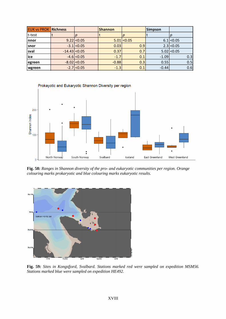
XVIII

Fig. 58: Ranges in Shannon diversity of the pro- and eukaryotic communities per region. Orange

colouring marks prokaryotic and blue colouring marks eukaryotic results.

Fig. 59: Sites in Kongsfjord, Svalbard. Stations marked red were sampled on expedition MSM56.

Stations marked blue were sampled on expedition HE492.

EUK vs PROK Richness Shannon Simpson

t-test t p t p t p

nnor 9.22 <0.05 5.01 <0.05 6.1 <0.05

snor -3.1 <0.05 0.03 0.9 2.3 <0.05

sval -14.43 <0.05 0.37 0.7 5.02 <0.05

ice -4.6 <0.05 -1.7 0.1 -1.09 0.3

egreen -8.02 <0.05 -0.88 0.3 0.55 0.5

wgreen -2.7 <0.05 -1.3 0.1 -0.44 0.6

tip + mouth 16.2 <0.05 12.5 <0.05 10.8 <0.05

tip 11.03 <0.05 7.8 <0.05 6.4 <0.05

mouth 11.84 <0.05 10.11 <0.05 9.31 <0.05

XIX

Fig. 60: Salinity versus prokaryotic and eukaryotic richness. R2 and p-value are indicated.

Fig. 61 Silicate concentration versus prokaryotic and eukaryotic richness. R2 and p-value are indicated.

XX

Fig. 62: Salinity versus prokaryotic and eukaryotic Simpson diversity. R2 and p-value are indicated.

Fig. 63: Nitrate concentration versus prokaryotic and eukaryotic Simpson diversity. R2 and p-value are

indicated.

XXI

Fig. 64: Silicate versus prokaryotic and eukaryotic Simpson diversity. R2 and p-value are indicated.

Fig. 65: Prokaryotic Simpson diversity versus richness. R2 and p-value are indicated.

XXII

Fig. 66: Eukaryotic versus prokaryotic richness in North Norway. R2 and p-value are indicated.

Fig. 67: Eukaryotic versus prokaryotic Simpson diversity without North Norway. R2 and p-value are

indicated.

XXIII

Fig. 68: NMDS of all eukaryotic samples per region.

Fig. 69: Influence of environmental dissimilarity on prokaryotic ASV turnover in North Norway. All

data points that represent pairs of sites from the same two fjords are coloured accordingly. The results

of the Mantel test (Pearson) are indicated.

XXIV

Fig. 70: Influence of environmental dissimilarity on eukaryotic ASV turnover in North Norway. All data

points that represent pairs of sites from the same two fjords are coloured accordingly. The results of the

Mantel test (Pearson) are indicated.

Fig. 71: Influence of geographic distance on prokaryotic ASV turnover in North Norway. All data

points that represent pairs of sites from the same two fjords are coloured accordingly. The results of

the Mantel test (Pearson) are indicated.

XXV

Fig. 72: Influence of geographic distance on eukaryotic ASV turnover in North Norway. All data

points that represent pairs of sites from the same two fjords are coloured accordingly. The results of

the Mantel test (Pearson) are indicated.

Fig. 73: Ranges in nitrate concentration per region.

XXVI

Fig. 74: Prokaryotic Simpson Diversity versus richness in North Norway. R2 and p-value are indicated.

Fig. 75: Eukaryotic Simpson Diversity versus richness in North Norway. R2 and p-value are indicated.

XXVII

Fig. 76: Salinity in Kongsfjord, Svalbard, as measured on two different expeditions.

Fig. 77: Temperature in Kongsfjord, Svalbard, as measured on two different expeditions.

XXVIII

Fig. 78: Salinity in the Lofoten, Norway, as measured on two different expeditions.

Fig. 79: Temperature in the Lofoten, Norway, as measured on two different expeditions.