Dynamics of land use patterns in biodiversity rich farming systems of ...
87
Dynamics of land use patterns in biodiversity rich farming systems of India Von der Wirtschaftswissenschaftlichen Fakultät der Gottfried Wilhelm Leibniz Universität Hannover zur Erlangung des akademischen Grades Doktor der Wirtschaftswissenschaften —Doctor rerum politicarum— genehmigte Dissertation von M.Sc Monish Jose geboren am 20.04.1983 in Mulamkunathukave, Kerala, Indien 2016
-
Upload
khangminh22 -
Category
Documents
-
view
1 -
download
0
Transcript of Dynamics of land use patterns in biodiversity rich farming systems of ...
Dynamics of land use patterns in biodiversityrich farming systems of India
Von der Wirtschaftswissenschaftlichen Fakultät derGottfried Wilhelm Leibniz Universität Hannover
zur Erlangung des akademischen Grades
Doktor der Wirtschaftswissenschaften—Doctor rerum politicarum—
genehmigte Dissertationvon
M.Sc Monish Josegeboren am 20.04.1983 in Mulamkunathukave, Kerala, Indien
2016
Erstgutachter: Prof. Dr. Ulrike Grote
Institut für Umweltökonomik und Welthandel
Wirtschaftswissenschaftliche Fakultät
Gottfried Wilhelm Leibniz Universität Hannover
Zweitgutachter: Prof. Dr. Martina Padmanabhan
Lehrstuhl für Vergleichende Entwicklungs- und Kulturforschung
Fachbereich Südostasienkunde
Philosophische Fakultät
Universität Passau
Tag der Promotion: 18.07.2016
ACKNOWLEDGEMENTS
It is my pleasure to glance back and recall the path travelled during the days of hard work
and perseverance. Interdependence is definitely more valuable than independence. This
thesis is the result of years of work whereby I have been accompanied, supported and
guided by many people.
Major part of this thesis is compiled as part of the BioDiva project (http://www.
uni-passau.de/en/biodiva/home/). I duly acknowledge FONA – Social-Ecological Research,
BMBF (Federal Ministry of Education and Research, Germany) (Grant 01UU0908) for
funding this project.
I extend reverence and deep sense of gratitude to my promoter, Prof. Dr. Ulrike Grote
for her sustained interest and generous assistance at every stage of my work. Her invaluable
comments and guidance during my research period have been a constant motivation for
the successful completion of my dissertation.
I profoundly thank my co-supervisor and mentor, Prof. Dr. Martina Padmanabhan for
giving me the opportunity to work as a part of the BioDiva research team. I immensely
owe her for all the support and guidance during my research endeavour.
My sincere thanks to the farmers of Wayanad, M.S Swaminathan Research Foundation
and the Community Agrobiodiversity Centre, Wayanad, for the collaboration during the
field study in Kerala, India.
I acknowledge the support and critical comments given by all researchers in Team
BioDIVA, Institute for Environmental Economics and World Trade and Institute for Devel-
opment and Agricultural Economics.
I would like to thank the Almighty, my family, friends and colleagues who provided
support, and encouragement though this journey of mine.
ZUSAMMENFASSUNG
Der Trend der Diversifizierung des Anbaus von Grundnahrungsmitteln wie Reis zu hochw-
ertigen Marktfrüchten (high value crops, HVCs), wie beispielsweise Obst und Gemüse,
kann in allen großen Reis produzierenden Ländern Asiens beobachtet werden. Aktuelle
Literatur zeigt, dass der Anteil von HVCs in Indien sowohl in Bezug auf die Anbaufläche
als auch auf den Gesamtwert der Produktion steigt. Diversifizierung hin zu HVCs wird,
vor allem für Kleinbauern und in Indien, als armutsbekämpfend und einkommenssteigernd
betrachtet. Jedoch ist der Wechsel von Nahrungspflanzen zu Marktfrüchten kein rei-
bungsloser Prozess und hat signifikante ökologische Folgen. FAO Prognosen zeigen, dass
der steigende Bedarf der wachsenden Bevölkerung der asiatischen Länder in Zukunft
nicht durch selbstversorgenden Grundnahrungsmittelanbau zu decken sein wird. Darüber
hinaus ist die Produktion von HVCs durch mangelhafte Marktstrukturen und fehlende
infrastrukturelle Unterstützung zu einem riskanten Unterfangen geworden. Ein hoher
Anteil der HVC Produzenten, vor allem Kleinbauern, haben sich verschuldet. Kerala in
Südindien hat den höchsten Nahrungsmittel zu Nicht-Nahrungsmittel Diversifizierungsin-
dex in Indien. In Kerala wandelt sich die landwirtschaftliche Landnutzung vor allem
von Reisanbausystemen zu Marktfrüchten, wie beispielsweise Kautschuk, Bananen oder
Kokosnüssen. Dies führte zu einer alarmierenden Nahrungsmittelknappheit in Kerala, da
die derzeitige Produktion nur 15% der benötigten Grundnahrungsmittel abdeckt. Trotz
verschiedener Versuche der Regierung Keralas, die Reisproduktion anzukurbeln, nahm
diese noch ab. Zudem gibt es einen landwirtschaftlichen Notstand in Kerala, und zwar
vornehmlich unter den Bauern, die HVCs kultivieren.
Das übergeordnete Ziel dieser Dissertation ist es, die Dynamiken und Auswirkungen
der sich ändernden Landnutzungsmuster von Kleinbauern am Beispiel von Kerala zu
analysieren. Konkrete Forschungsziele sind folgende: 1) Untersuchung der Makroanreize
(exogen zu den Haushalten) der Landtransformation von Reisanbau hin zu HVCs, 2)
Abschätzung der kurz- und langfristigen Reisflächenallokation als Reaktion auf temporäre
Änderungen in Preis und Nicht-Preis Faktoren, 3) Analyse der Determinanten, die die
HVC-Einführung unter landwirtschaftlichen Haushalten beeinflussen, 4) Abschätzung der
Wohlfahrtswirkung von HVC-Adoption durch kleine und marginale landwirtschaftliche
Haushalte, und 5) Analyse der Wirkung von Methanemissionssteuern auf die Produktion
von Rohreis.
Die Dissertation ist eingebettet in ein größeres Projekt (BioDivA), das auf die nach-
haltige Landnutzung und den Erhalt von Biodiversität im Wayanad District in Kerala
abzielt. Fokusgruppendiskussionen, partizipative Bewertungen im ländlichen Raum, und
Workshops mit Interessenvertretern wurden zwischen 2010-2013 durchgeführt, um Hin-
weise auf Muster der Landnutzungsveränderung zu sammeln. Die Ergebnisse dieser
Diskussionen, nebst Daten auf Staats- bzw. Distriktebene, die den Zeitraum von 1983-2011
abdecken, sind Grundlagen für die Analyse der politischen und soziodemografischen
Ursachen der Landnutzungs-veränderungen. Die Ergebnisse zeigen, dass unbeabsichtigte
Effekte von Politik, Politikkonflikte und inadäquate sektorale Integration von Politik die
Hauptmakroanreize für den Wandel der Landnutzung weg von Nahrungsmitteln sind.
Die geringe Wirtschaftlichkeit des Rohreisanbaus, der Mangel an Arbeitskräften in der
Landwirtschaft und der Bevölkerungsdruck auf dem Land wurden als die hauptsächlichen
sozioökonomischen Ursachen für den Landnutzungswandel identifiziert.
Um ein tieferes Verständnis von Landnutzungsdynamiken zu erhalten, wird die Beziehung
zwischen der Flächenverteilung für Reis in Wayanad und den zeitlichen Veränderungen
von Preisen, Löhnen und Regenfall analysiert. Dafür werden Daten von 1987-2009 zu-
grunde gelegt. Mit Hilfe des ,Auto Regressive Distributive Lags‘ (ARDL) Ansatzes zur
Ko-Integration und der Bounds Testing Methode werden die Kurz- und Langzeitelastiz-
itäten der Verteilung von Flächen für den Reisanbau geschätzt. Die Ergebnisse zeigen, dass
Kleinbauern positiv auf Preis- und negativ auf Lohnfaktoren reagieren, und zwar sowohl
kurz- als auch langfristig. Interventionen wie eine Erhöhung der Preise, die die Bauern
für Rohreis erhalten, und Arbeitsreformen zur Lohnerhöhung könnten die Versorgung
von Rohreis in Wayanad verbessern. Die endogenen Faktoren, die die Entscheidung
des Haushalts beeinflussen, HVCs statt Reis anzubauen, werden mit Hilfe eines Multi-
iii
nomialen Logit Regressions-Modells überprüft. Die heterogenen Wohlfahrtseffekte von
HVC-Adoption werden mit der Multinomialen Endogenen Switching Regression geschätzt.
Die Basis dieser Analysen ist ein Querschnittsdatensatz von Haushalten in Wayanad Dis-
trikt von 2011. Insgesamt wurden 304 rurale Haushalte zufällig ausgewählt und interviewt.
Die Ergebnisse zeigen, dass der Zugang von Transportmitteln zur Farm, die Anzahl von
Feldern, auf denen der Haushalt etwas anbaut, die Entfernung vom Wohnhaus zur Farm
und die Betriebsgröße Faktoren sind, die die Entscheidung, HVC einzuführen, beeinflussen.
Das Ergebnis der Folgenabschätzung von HVC Adoption auf die Wohlfahrt weist nach,
dass die Adoption von HVCs einen positiven Effekt auf das Haushaltseinkommen und die
Ausgaben hat. Außerdem zeigt sich, dass die Haushalte, die HVC nur teilweise eingeführt
haben, einen größeren Wohlfahrtseffekt erreicht haben als die Haushalte, die ihren Anbau
komplett auf HVC umgestellt haben.
Die Wirkung von Methanemissionssteuern als ein Verminderungsmechanismus für
Treibhausgase (GHG) im Reissektor wurde untersucht basierend auf Reisproduktions-
und Methanemissionsdaten auf nationaler Ebene. Das Ergebnis des iso-elastischen
Angebotsmodells zeigt, dass Emissionssteuern auf Reis einen negativen Effekt auf die
Reisproduktion und die Produzentenwohlfahrt haben könnte. Für eine erfolgreiche Im-
plementierung von Emissionssteuern ist die Entwicklung von kosteneffektiven GHG-
Verminderungsmaßnahmen auf Betriebsebene nötig, die die Wohlfahrtsverluste ausgle-
ichen.
Schlüsselwörter: Landnutzungswandel, Adoption, hochwertige Marktfrüchte, Wohlfahrt-
seffekt, Reisanbau, Emissionen, Indien
iv
ABSTRACT
The trend of diversification from staple food, rice, to high value crops (HVCs), such
as, fruits and vegetables has been observed in major rice producing countries of Asia.
Recent literature shows that the share of HVCs in India is increasing both in terms of
area cropped and total value of the output. Diversification to HVCs is largely regarded
as poverty reducing and income increasing particularly for small and marginal farmers in
India. However, transition from food crops to commercial crops is not a frictionless process
and has significant environmental consequences. FAO projections show that the thin line
of self sufficiency in food grain production of Asian countries may not hold true in the
future due to the inability of the countries to meet the increasing demand of the burgeoning
population. In addition, the existing market imperfections and lack of infrastructural
support mainly for perishables, such as, high value fruits and vegetables, have made the
production of HVCs a riskier enterprise in India. A high degree of indebtedness is observed
among the HVC growers, especially, the small and marginal growers. The state of Kerala
in Southern India has the highest food crop to non-food crop diversification index in India.
Specifically, the agricultural land use is changing from wetland paddy system to cash crops,
such as, rubber, banana and coconut in Kerala. This has resulted in alarming levels of food
deficit in the state, as the state currently produces only 15 per cent of its required food
grain demand. Despite various efforts from the state government, the rice production has
not picked up any pace, but is declining. On the other hand, there is an increasing rate of
agrarian distress in the state, more prevalent among the farmers who adopted HVCs.
The overall objective of this dissertation is to analyse the dynamics of land use pattern
of small and marginal farmers and its impacts using the example of Kerala. Specific
research objectives are outlined as below: 1) To examine the macro drivers (exogenous
to the household) influencing land transformation from paddy farming to HVCs. 2) To
estimate the short-run and long-run paddy area allocation in response to temporal changes
in price and non-price factors. 3) To analyse the household determinants influencing
HVC adoption among agricultural households. 4) To estimate the welfare impacts of
HVC adoption by small and marginal farming households and 5) To analyse the impact of
methane emission taxes on paddy production.
The dissertation is embedded in the framework of a larger project (BioDiva), which
is aimed at sustainable land use and biodiversity conservation in Wayanad district of
Kerala. Focus group discussions, participatory rural appraisals and stakeholder workshops
were conducted during the period of 2010-2013 to gather evidence on land use change
pattern. Outputs from these discussions, along with state and district level data, covering
a period of 1983-2011, are used to analyse the policy and socio-demographic causes of
land use transitions. The results reveal unintended policy idiosyncrasies, policy conflicts
and inadequate sectoral integration of policies as the major macro drivers causing change
in land use from food crops. Low economic viability of paddy farming, shortage of
agricultural labour and population pressure on land are identified as major socio-economic
causes behind agricultural land use change.
In order to gain deeper understanding of the land use dynamics, the relationship
between the area allocation of rice in Wayanad and the temporal changes in prices, wages
and rainfall is analysed. Data covering a period of 1987-2009 is used for this purpose.
Auto Regressive Distributive Lags Approach (ARDL) of co-integration and bounds testing
method are used to estimate the short- and long-run elasticities of rice area allocation.
The model results reveal that farmers respond positively to price and negatively to wage
factors in the short as well as in the long run. Interventions to improve the price received
by farmers for paddy and labour reforms to address higher wage rates might improve
the supply response of paddy in Wayanad. The factors endogenous to the household
that influence the household decision to adopt HVCs over rice are studied by using a
multinomial logit regression model. The heterogeneous welfare impacts of HVC adoption
are also assessed by multinomial endogenous switching regression. The data basis of these
analyses is a cross sectional household survey conducted in the year of 2011 in Wayanad
district. A total of 304 agricultural households were randomly selected and interviewed.
The results showed that transport access to farm, number of sub-plots the household
vi
cultivated, distance to farm from dwelling and farm size as the factors determining the
HVC adoption decision. The result of the welfare impacts of HVC adoption proved that
adoption has a positive impact on household income and expenditure. Furthermore, the
households that partially adopted HVCs had higher welfare than those that entirely adopted
HVCs.
The impact of methane emission taxes as a greenhouse gas (GHG) mitigation mech-
anism in rice is studied based on the production price and methane emissions data at
national level. The outcome of iso-elastic supply model reveals that emission taxes on rice
might have negative impact on the rice production and producer’s welfare. For successful
implementation of emission taxes, development of cost-effective mitigation measures at
the farm level offsetting the welfare losses of small holders is essential.
Keywords: land use change, adoption, high value crops, welfare impact, paddy farming,
emissions.
vii
CONTENTS
Acknowledgements i
Zusammenfassung ii
Abstract v
List of Abbreviations x
1 Introduction 1
1.1 Background and problem statement . . . . . . . . . . . . . . . . . . . . 1
1.2 Research objectives . . . . . . . . . . . . . . . . . . . . . . . . . . . . . 5
1.3 Conceptual framework of the dissertation . . . . . . . . . . . . . . . . . 5
1.4 Synthesis of the thesis . . . . . . . . . . . . . . . . . . . . . . . . . . . . 8
References . . . . . . . . . . . . . . . . . . . . . . . . . . . . . . . . . . 10
2 Dynamics of agricultural land use change in Kerala: A policy and social-ecological perspective 14
3 Impact of price and non-price factors on paddy acreage response in Wayanaddistrict of Southern India 15
Abstract . . . . . . . . . . . . . . . . . . . . . . . . . . . . . . . . . . . . . . 15
3.1 Introduction . . . . . . . . . . . . . . . . . . . . . . . . . . . . . . . . . 16
3.2 Previous studies on farmers’ response . . . . . . . . . . . . . . . . . . . 18
3.3 Study location . . . . . . . . . . . . . . . . . . . . . . . . . . . . . . . . 20
3.4 Theoretical framework . . . . . . . . . . . . . . . . . . . . . . . . . . . 21
3.4.1 Basic model . . . . . . . . . . . . . . . . . . . . . . . . . . . . . 21
3.4.2 Analytical developments . . . . . . . . . . . . . . . . . . . . . . 22
Contents
3.5 Methodology . . . . . . . . . . . . . . . . . . . . . . . . . . . . . . . . 24
3.5.1 Data . . . . . . . . . . . . . . . . . . . . . . . . . . . . . . . . . 24
3.5.2 Empirical estimation . . . . . . . . . . . . . . . . . . . . . . . . 25
3.6 Results . . . . . . . . . . . . . . . . . . . . . . . . . . . . . . . . . . . . 28
3.7 Discussion and policy implications . . . . . . . . . . . . . . . . . . . . . 32
3.8 Conclusion . . . . . . . . . . . . . . . . . . . . . . . . . . . . . . . . . 34
References . . . . . . . . . . . . . . . . . . . . . . . . . . . . . . . . . . 35
4 Assessing the household welfare impacts of high value crop adoption in awetland paddy system of southern India 40
Abstract . . . . . . . . . . . . . . . . . . . . . . . . . . . . . . . . . . . . . . 40
4.1 Introduction . . . . . . . . . . . . . . . . . . . . . . . . . . . . . . . . . 41
4.2 Literature review and conceptual framework . . . . . . . . . . . . . . . . 43
4.2.1 Determinants of adoption . . . . . . . . . . . . . . . . . . . . . 43
4.2.2 Impacts of adoption . . . . . . . . . . . . . . . . . . . . . . . . . 45
4.2.3 Conceptual framework . . . . . . . . . . . . . . . . . . . . . . . 46
4.3 Data and methdology . . . . . . . . . . . . . . . . . . . . . . . . . . . . 48
4.3.1 Study area . . . . . . . . . . . . . . . . . . . . . . . . . . . . . . 48
4.3.2 Survey data and questionnaire . . . . . . . . . . . . . . . . . . . 50
4.3.3 Estimation strategy . . . . . . . . . . . . . . . . . . . . . . . . . 51
4.4 Results and discussion . . . . . . . . . . . . . . . . . . . . . . . . . . . 56
4.4.1 Descriptive statistics . . . . . . . . . . . . . . . . . . . . . . . . 56
4.4.2 Determinants of HVC adoption . . . . . . . . . . . . . . . . . . 58
4.4.3 Welfare impacts of heterogeneous adoption . . . . . . . . . . . . 60
4.5 Conclusion . . . . . . . . . . . . . . . . . . . . . . . . . . . . . . . . . 63
References . . . . . . . . . . . . . . . . . . . . . . . . . . . . . . . . . . 64
5 Emission taxes as a GHG mitigation mechanism in Agriculture: Effects onrice production of India 71
Appendix A 72
ix
LIST OF ABBREVIATIONS
Acronyms / Abbreviations
| Indian Rupee
AAY Antyodaya Anna Yojana
APL Above Poverty Line
ARDL Auto Regressive Distributive Lag
BPL Below Poverty Line
CDM Clean Development Mechanism
CER Certified Emission Reduction
DES Directorate of Economics and Statistics
FAO Food and Agriculture Organisation of the United Nations
FAOSTAT Food and Agriculture Organisation of the United Nations Statistics
GHG Green House Gas
GWP Global Warming Potential
HDI Human Development Index
HVC High Value Crop
IAAE International Association of Agricultural Economists
IMR Inverse Mills Ratio
IPCC Intergovernmental Panel on Climate Change
MGNREGA The Mahatma Gandhi National Rural Employment Guarantee Act
Mha Million hectare
MPC Market Price of Carbon
MSP Minimum Support Price
Mt Million tonne
x
List of Abbreviations
SBIC Schwarz’s Bayesian Information Criterion
SHG Self Help Groups
SPC Shadow Price of Carbon
TPDS Targeted Public Distribution System
t tonne
UEC Unrestricted Error Correction
UNESCO United Nations Educational, Scientific and Cultural Organization
UNFCCC United Nations Framework Convention on Climate Change
US$ US Dollar
WPI Wholesale Price Index
xi

Chapter 1
INTRODUCTION
1.1 Background and problem statement
Rice plays a pivotal role in Indian agriculture. India is the world’s second largest rice
producer and exporter of rice (FAOSTAT, 2012). Rice is cultivated on 44 million ha
(35% of total area under food grains) contributing to around 40% of the total food grain
production in India (Government of India, 2015), thus making rice the most important food
crop of the country. However, the Indian agricultural sector has undergone considerable
changes since the 1990s. Lately, it is observed that agriculture is under transition from
food crops towards high value crops (HVCs) and livestock products (Rada, 2016). During
the past two decades, the area under HVCs in India has increased (Kumar & Gupta,
2015; Mittal & Hariharan, 2016). As argued by MacRae (2016), “Indian agriculture is
now poised between two futures—one of increasing technology-driven intensification and
integration into national and global markets—the other [. . . .] ecologically based forms of
small-farming producing for more local consumption”.
Rice paddies play an important role in shaping the food and agricultural sector of Asia.
It is not only the major staple food of Asia but is also an important source of income
and employment for many resource poor rural farming households. Over 90% of the
production and consumption of rice is concentrated in Asia and the Asia-Pacific region
(Papademetriou, Dent, & Herath, 2000). Rice accounts for 23% of world’s total cropped
area and 29% of total grain output (Mew, Brar, Peng, Dawe, & Hardy, 2003). Since the
era of Green revolution, the production of rice has kept pace with the consumption levels.
1
Chapter 1. Introduction
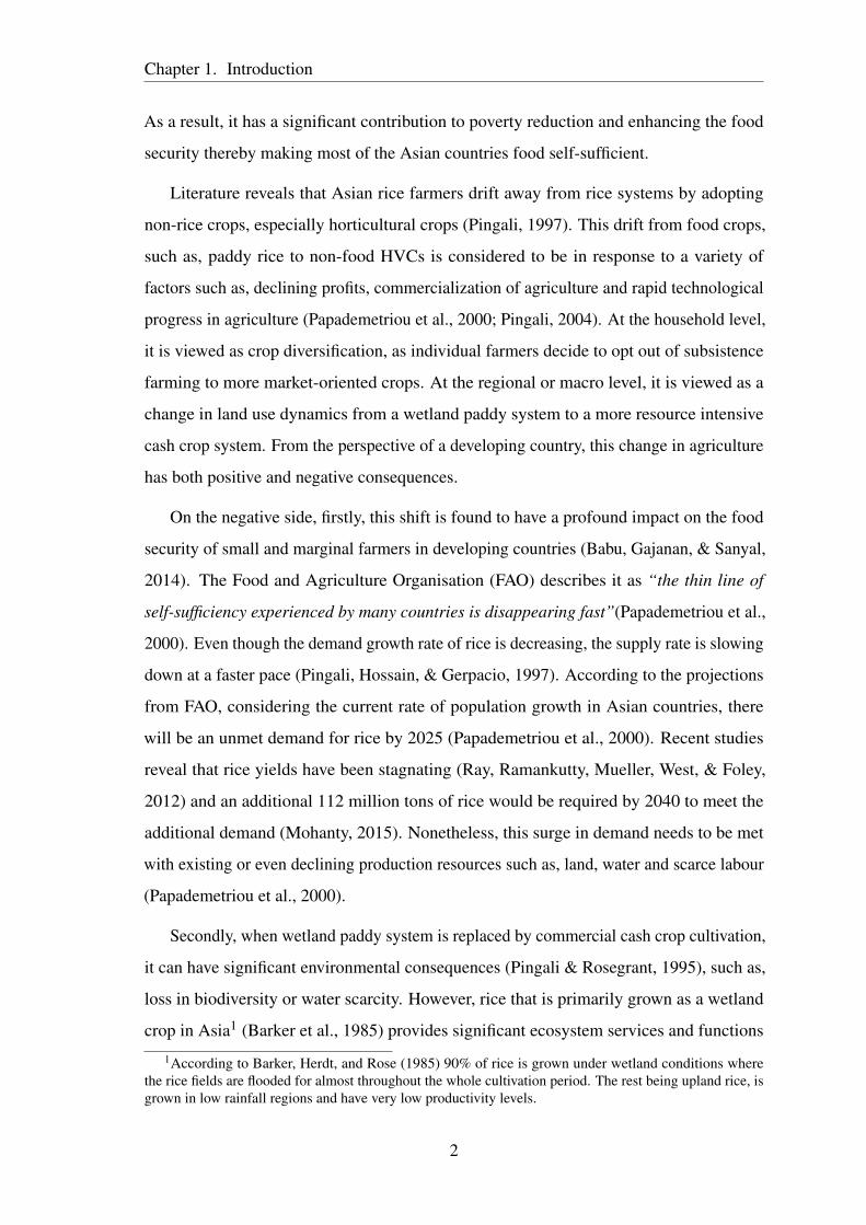
As a result, it has a significant contribution to poverty reduction and enhancing the food
security thereby making most of the Asian countries food self-sufficient.
Literature reveals that Asian rice farmers drift away from rice systems by adopting
non-rice crops, especially horticultural crops (Pingali, 1997). This drift from food crops,
such as, paddy rice to non-food HVCs is considered to be in response to a variety of
factors such as, declining profits, commercialization of agriculture and rapid technological
progress in agriculture (Papademetriou et al., 2000; Pingali, 2004). At the household level,
it is viewed as crop diversification, as individual farmers decide to opt out of subsistence
farming to more market-oriented crops. At the regional or macro level, it is viewed as a
change in land use dynamics from a wetland paddy system to a more resource intensive
cash crop system. From the perspective of a developing country, this change in agriculture
has both positive and negative consequences.
On the negative side, firstly, this shift is found to have a profound impact on the food
security of small and marginal farmers in developing countries (Babu, Gajanan, & Sanyal,
2014). The Food and Agriculture Organisation (FAO) describes it as “the thin line of
self-sufficiency experienced by many countries is disappearing fast”(Papademetriou et al.,
2000). Even though the demand growth rate of rice is decreasing, the supply rate is slowing
down at a faster pace (Pingali, Hossain, & Gerpacio, 1997). According to the projections
from FAO, considering the current rate of population growth in Asian countries, there
will be an unmet demand for rice by 2025 (Papademetriou et al., 2000). Recent studies
reveal that rice yields have been stagnating (Ray, Ramankutty, Mueller, West, & Foley,
2012) and an additional 112 million tons of rice would be required by 2040 to meet the
additional demand (Mohanty, 2015). Nonetheless, this surge in demand needs to be met
with existing or even declining production resources such as, land, water and scarce labour
(Papademetriou et al., 2000).
Secondly, when wetland paddy system is replaced by commercial cash crop cultivation,
it can have significant environmental consequences (Pingali & Rosegrant, 1995), such as,
loss in biodiversity or water scarcity. However, rice that is primarily grown as a wetland
crop in Asia1 (Barker et al., 1985) provides significant ecosystem services and functions
1According to Barker, Herdt, and Rose (1985) 90% of rice is grown under wetland conditions wherethe rice fields are flooded for almost throughout the whole cultivation period. The rest being upland rice, isgrown in low rainfall regions and have very low productivity levels.
2

Chapter 1. Introduction
(Natuhara, 2013). The Ramsar Convention classifies rice paddy fields as human made
wetlands that constitute for about 18% of the total global wetlands. They play a major
role in regulating the rainfall pattern, maintaining the floral and faunal diversity and in
providing climatic stability (Ambastha, Hussain, & Badola, 2007). The wise use of paddy
wetland can partially compensate for the loss of natural wetlands (Yoon, 2009).
On the positive side, diversification to HVCs can be an important strategy to augment
income and reduce poverty (Birthal, Roy, & Negi, 2015) of rice farmers in a developing
country. As argued by Mew et al.(2003), many of these rice farmers in developing countries
remain poor. Agriculture in developing countries is characterised by large numbers of
such small and marginal farmers with less than 2 ha of land (Conway, 2011). The steady
decline in profit from rice farming is one of the major reasons for these farmers to remain
poor. High levels of production achieved from the green revolution technologies have
kept the world market prices of rice low, thus affecting the livelihood of the rice farmers.
Nonetheless, most of the major rice producing countries have consumer-friendly policies
that keep the prices of rice stable and within the reach of the purchasing power of low
income consumers, all at the cost of the producers (Mew et al., 2003).
Other major deterrents for rice production are economic growth and industrialization
in major rice producing countries that have caused a reduction in the agricultural labour
supply and an increase in the wage rate. It has resulted in lowering the profitability of rice
cultivation. Also, continuous monocropping of rice has degraded the soil and reduced the
factor productivity. These reasons act as catalysts for both the farmers and policy-makers
to seek alternative income sources for the resource poor farmers. From the perspective of a
developing country, government and policy-makers view the shift from paddy to high value
crops as an important approach to increase the agricultural income of small and marginal
farmers, increase in off farm employment opportunities, thus reducing the incidence of
poverty and stimulating overall economic growth.
Among the states of India, Kerala recorded the highest degree of crop diversification
among food crops (Kumar & Gupta, 2015). The wetland paddy in Kerala has been
subsequently replaced by high value crops, namely, rubber and coconut (Viswanathan,
2014). The share of area under food crops reduced from 35% in 1960 to 9% of the total
cropped area in 2010-11 (Andrews, 2013). This has resulted in a situation where Kerala has
3
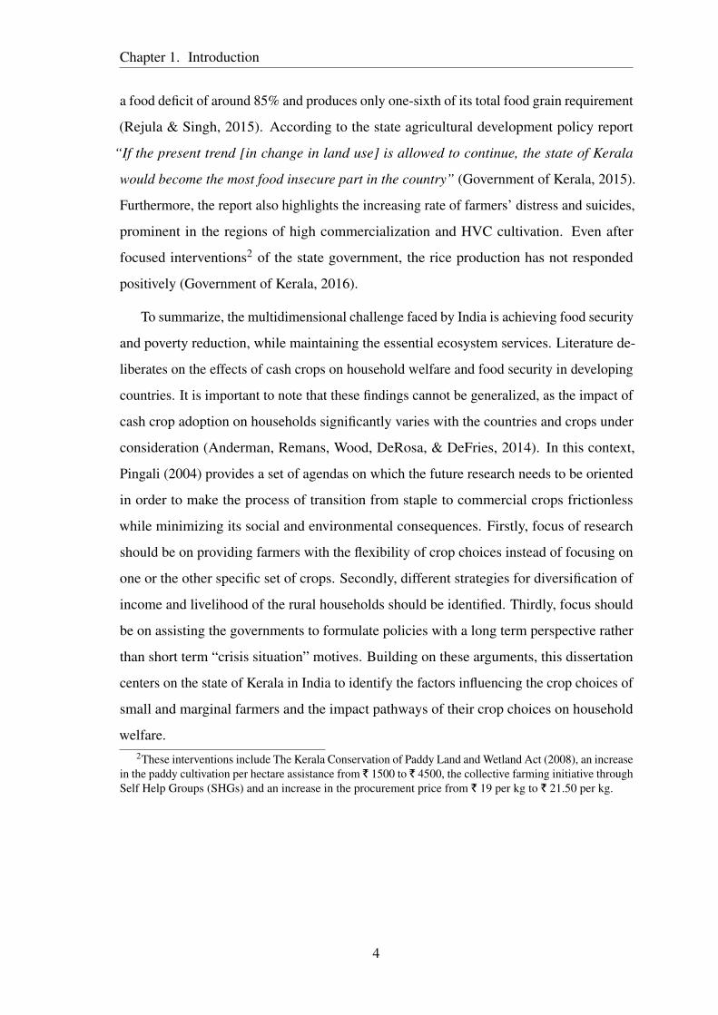
Chapter 1. Introduction
a food deficit of around 85% and produces only one-sixth of its total food grain requirement
(Rejula & Singh, 2015). According to the state agricultural development policy report
“If the present trend [in change in land use] is allowed to continue, the state of Kerala
would become the most food insecure part in the country” (Government of Kerala, 2015).
Furthermore, the report also highlights the increasing rate of farmers’ distress and suicides,
prominent in the regions of high commercialization and HVC cultivation. Even after
focused interventions2 of the state government, the rice production has not responded
positively (Government of Kerala, 2016).
To summarize, the multidimensional challenge faced by India is achieving food security
and poverty reduction, while maintaining the essential ecosystem services. Literature de-
liberates on the effects of cash crops on household welfare and food security in developing
countries. It is important to note that these findings cannot be generalized, as the impact of
cash crop adoption on households significantly varies with the countries and crops under
consideration (Anderman, Remans, Wood, DeRosa, & DeFries, 2014). In this context,
Pingali (2004) provides a set of agendas on which the future research needs to be oriented
in order to make the process of transition from staple to commercial crops frictionless
while minimizing its social and environmental consequences. Firstly, focus of research
should be on providing farmers with the flexibility of crop choices instead of focusing on
one or the other specific set of crops. Secondly, different strategies for diversification of
income and livelihood of the rural households should be identified. Thirdly, focus should
be on assisting the governments to formulate policies with a long term perspective rather
than short term “crisis situation” motives. Building on these arguments, this dissertation
centers on the state of Kerala in India to identify the factors influencing the crop choices of
small and marginal farmers and the impact pathways of their crop choices on household
welfare.2These interventions include The Kerala Conservation of Paddy Land and Wetland Act (2008), an increase
in the paddy cultivation per hectare assistance from | 1500 to | 4500, the collective farming initiative throughSelf Help Groups (SHGs) and an increase in the procurement price from | 19 per kg to | 21.50 per kg.
4
Chapter 1. Introduction
1.2 Research objectives
The overall objective of this dissertation is to analyse the land use dynamics of small and
marginal farmers and the subsequent impacts using the case of paddy farmers in Kerala,
southern India. Specific research objectives are outlined as below:
1. To examine the macro drivers (exogenous to the household) influencing land trans-
formation from paddy farming to a market-oriented system.
2. To estimate the short-run and long-run paddy area allocation in response to temporal
changes in price and non-price factors.
3. To analyse the household determinants influencing HVC adoption among agricultural
households.
4. To estimate the welfare impacts of HVC adoption by small and marginal farming
households.
5. To analyse the impact of methane emission taxes on paddy production.
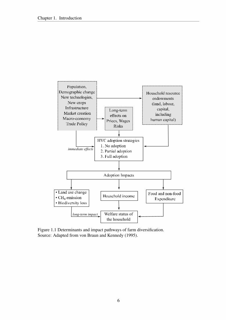
1.3 Conceptual framework of the dissertation
Household adoption decision is a complex process that depends not only on the household
preferences but also on the macroeconomic and agricultural policies, which influence
the production conditions (Babu, Gajanan & Sanyal, 2014). In order to understand the
dynamics of decision-making behaviour, it is essential to conceptualize the agricultural
situation, its components and their interrelationships. With this view, to analyse the causes
and impacts of adoption, this work uses a modified version of a conceptual framework
(Figure 1.1) developed by von Braun (1995).
The framework focuses on the farm households’ decision-making behaviour on HVC
adoption. In order to simplify the analysis from a household perspective, this framework
separates out the exogenous factors influencing decision-making from the endogenous
factors. These two sets of factors act at macro and household levels, respectively. Three
potential pathways that influence farmers’ decision to adopt are identified. The first
5
Chapter 1. Introduction
Welfare status of
the household
immediate effects
long-term impact
• Land use change
• CH4 emission
• Biodiversity loss
Figure 1.1 Determinants and impact pathways of farm diversification.Source: Adapted from von Braun and Kennedy (1995).
6
Chapter 1. Introduction
possible pathway is the influence of the macro-level (district, state) factors, such as,
agricultural policies, technological progress, population and demographic pressure, and
institutional infrastructure on the adoption decision. The influence of these factors on
adoption are analysed in chapter 1 of the dissertation by using district and state level
data. Second pathway is the influence of long-term changes in wages, prices and risk
associated with agricultural production process on the adoption decision. The adoption
decision can be viewed as farmers’ response to relative price signals and changes in agro-
climatic conditions (Mukherjee, 2010). It is, hence, important to capture the temporal
dimension of these macro drivers to clearly understand the adoption process. Chapter 2
addresses this pathway by analysing the short–run and long–run area allocation of farmers
in response to the temporal changes in the price and non-price factors. The third potential
pathway comprises of different micro-level determinants acting at the household level.
The household resource endowments such as land, labour, and human capital and their
allocation can play an important role in the crop choice decision in this respect (Babu et
al., 2014).
On the impact side, two pathways are analysed. First, the household decision on the
choice can have endogenous consequences on the household income and expenditure of the
household (von Braun & Kennedy, 1994). Increase in household income and expenditure
can improve the overall welfare status of the households. On the other hand, if the choice
of crop is towards low labour-intensive farming system, the households depending on
the farm labour as their major source of income will be adversely affected. The second
impact pathway is concerning the environmental consequences of crop choices. This can
be considered more crop management specific and depends on government policies that
encourage the production of certain crops (Barbier, 1989). There can be different ways
in which the choice of crop can affect the environment, for example, loss in biodiversity
and soil degradation. One particular pathway, which is addressed in this dissertation, is
the methane emission from rice fields. The choice of this pathway is motivated by the fact
that there is lack of literature addressing the relationship between measures for mitigating
methane emission from rice fields and its impacts on farmers’ welfare in India. While the
environmental consequences of cash crop adoption in paddy fields are well studied, e.g.
7
Chapter 1. Introduction
by Gopikuttan and Kurup (2004), Karunakaran (2014) and Nair and Menon (2007), the
implications of methane emissions for rice fields in particular remain unexplored.
1.4 Synthesis of the thesis
The dissertation is divided into five chapters. Chapter 1 gives the general introduction to
the overall dissertation and to the rest of the papers. The overview of the articles included
in the dissertation is presented in Table 1.1.
Chapter 2 presents the trends and patterns in agricultural land use changes in the state
of Kerala and in Wayanad district. The chapter also focuses on identifying the macro
level (exogenous to the household) drivers determining the land use transformation in
paddy farming. It uses data from multiple sources, which include, focus group discussions,
participatory rural appraisals, and stakeholders’ workshops conducted during the period of
2010-2013 coupled with state and district level data for the period 1983-2011. The analysis
reveals low profitability of paddy farming, labour shortage, and demographic pressure as
the major macro level causes of paddy land use change. Even though land use changes
are the consequences of farmers’ livelihood responses to these changing macro drivers, at
a more fundamental level, it reflects the unintended policy conflicts and lack of sectoral
policy integration and implementation strategies.
Farmers’ crop choice responses and the magnitude of their response also depend
largely on the long-term volatility in the agricultural commodity prices and climatic factors.
Chapter 3 analyses this response as the impact of price and non-price factors on acreage
allocation of paddy growers. It uses time series data covering the period 1987-2009 on the
prices of paddy, and competing crops along with other macro variables, such as, rainfall
and wages to quantify the elasticity of response of these variables to the acreage allocation
of paddy in Wayanad. The chapter uses unit root testing to avoid spurious regression.
Autoregressive Distributed Lag Approach (ARDL) for co-integration is used along with
bounds testing to estimate the short- and long-run elasticities of paddy area allocation. The
results imply that farmers respond positively to paddy price and negatively to female wage
rate in the long-run as well as in the short-run. However, there was no significant impact
of rainfall and the price of competing crops on the area allocation decision of the farmers.
8
Chapter 1. Introduction
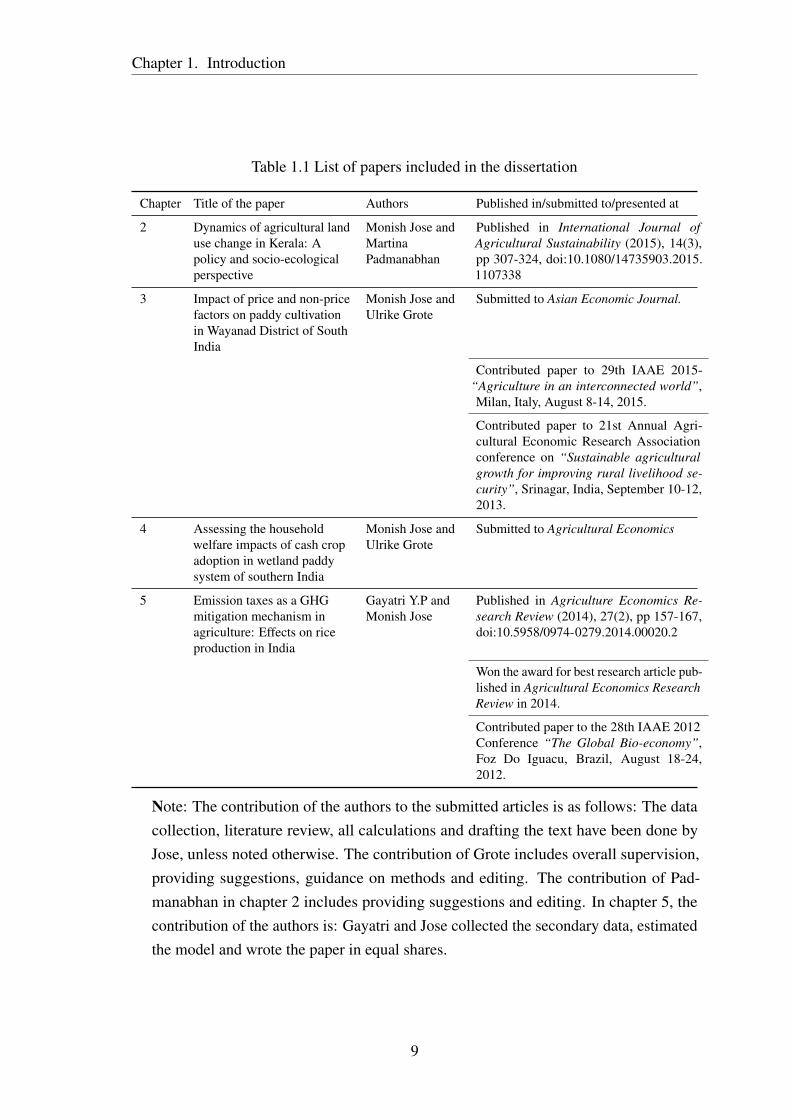
Table 1.1 List of papers included in the dissertation
Chapter Title of the paper Authors Published in/submitted to/presented at
2 Dynamics of agricultural landuse change in Kerala: Apolicy and socio-ecologicalperspective
Monish Jose andMartinaPadmanabhan
Published in International Journal ofAgricultural Sustainability (2015), 14(3),pp 307-324, doi:10.1080/14735903.2015.1107338
3 Impact of price and non-pricefactors on paddy cultivationin Wayanad District of SouthIndia
Monish Jose andUlrike Grote
Submitted to Asian Economic Journal.
Contributed paper to 29th IAAE 2015-“Agriculture in an interconnected world”,Milan, Italy, August 8-14, 2015.
Contributed paper to 21st Annual Agri-cultural Economic Research Associationconference on “Sustainable agriculturalgrowth for improving rural livelihood se-curity”, Srinagar, India, September 10-12,2013.
4 Assessing the householdwelfare impacts of cash cropadoption in wetland paddysystem of southern India
Monish Jose andUlrike Grote
Submitted to Agricultural Economics
5 Emission taxes as a GHGmitigation mechanism inagriculture: Effects on riceproduction in India
Gayatri Y.P andMonish Jose
Published in Agriculture Economics Re-search Review (2014), 27(2), pp 157-167,doi:10.5958/0974-0279.2014.00020.2
Won the award for best research article pub-lished in Agricultural Economics ResearchReview in 2014.
Contributed paper to the 28th IAAE 2012Conference “The Global Bio-economy”,Foz Do Iguacu, Brazil, August 18-24,2012.
Note: The contribution of the authors to the submitted articles is as follows: The datacollection, literature review, all calculations and drafting the text have been done byJose, unless noted otherwise. The contribution of Grote includes overall supervision,providing suggestions, guidance on methods and editing. The contribution of Pad-manabhan in chapter 2 includes providing suggestions and editing. In chapter 5, thecontribution of the authors is: Gayatri and Jose collected the secondary data, estimatedthe model and wrote the paper in equal shares.
9
Chapter 1. Introduction
Chapter 4 determines the drivers of HVC adoption among paddy farmers and their
impact on the welfare of small and marginal households. It uses cross-section data collected
during 2011 from 304 small and marginal households in Wayanad. Household income
and expenditure are used to measure the welfare. In order to control for self-selection
bias and possible endogeneity, an endogenous switching regression model is used. The
welfare impacts of a heterogeneous HVC adoption decision are discussed in detail. It was
found that land characteristics, such as, farm size, access to transport, number of plots
and distance to farm from dwelling influence the decision-making behaviour. The results
also indicate that cash crop adopters are better-off when compared to the non-adopters.
The heterogeneous adoption impact reveals that the farmers who chose to partially adopt
cash crops in combination with paddy have higher welfare than farmers who exclusively
adopted cash crops.
Chapter 5 focuses on the impact of emission tax on paddy production of India. Emission
tax as a Greenhouse Gas (GHG) mitigation mechanism can lead to an increase in the cost
of production and shift from rice to other crops subsequently inducing land use change
especially among smallholders. The concept of an iso-elastic supply function and a shift
parameter are used to estimate the shift in supply and demand of rice production at national
level. Shadow price of carbon and market price of carbon are used as hypothetical emission
tax levels to estimate the shift parameter. The result indicates that emission taxes on paddy
production would have negative impacts on farmers’ welfare.
References
Ambastha, K., Hussain, S. A., & Badola, R. (2007). Resource dependence and attitudesof local people toward conservation of Kabartal wetland: A case study from the Indo-Gangetic plains. Wetlands Ecology and Management, 15(4), 287–302. doi:10.1007/s11273-006-9029-z
Anderman, T. L., Remans, R., Wood, S. A., DeRosa, K., & DeFries, R. S. (2014). Synergiesand trade-offs between cash crop production and food security: A case study in ruralGhana. Food Security, 6(4), 541–554. doi:10.1007/s12571-014-0360-6
Andrews, S. (2013). Dynamics of cropping pattern shifts in Kerala: Sources and determi-nants. Agricultural Situation in India, 70(6), 15–24.
10

Chapter 1. Introduction
Babu, S. C., Gajanan, S. N., & Sanyal, P. (2014). Effects of commercialization of agri-culture (shift from traditional crop to cash crop) on food consumption and nutrition:Application of Chi-square statistic. In S. C. Babu, S. N. Gajanan, & P. Sanyal (Eds.),Food Security, Poverty and Nutrition Policy Analysis (pp. 63–91). San Diego: Elsevier.
Barbier, E. B. (1989). Cash crops, food crops, and sustainability: The case of Indonesia.World Development, 17(6), 879–895. doi:10.1016/0305-750X(89)90009-0
Barker, R., Herdt, R. W., & Rose, B. (1985). The rice economy of Asia. Washington, D.C.:International Rice Research Institute.
Birthal, P. S., Roy, D., & Negi, D. S. (2015). Assessing the impact of crop diversificationon farm poverty in India. World Development, 72, 70–92. doi:10.1016/j.worlddev.2015.02.015
Conway, G. (2011). On being a smallholder. In Conference on New Directions forSmallholder Agriculture (pp. 75–90). International Fund for Agricultural Development(IFAD), 24-25 January 2011, Rome, Italy.
FAOSTAT. (2012). Food and Agricultural commodities production. Retrieved from Foodand Agriculture Organization of the United Nations (FAO) website: http://faostat.fao.org/site/339/default.aspx
Gopikuttan, G., & Kurup, K. P. (2004). Paddy land conversion in Kerala: An inquiry intoecological and economic aspects in a midland watershed region. Final Report, KeralaResearch Programme on Local Level Development. Thiruvananthapuram: Centre forDevelopment Studies.
Government of India. (2015). Agricultural statistics at a glance 2014 (First edition). NewDelhi India: Oxford University Press.
Government of Kerala. (2015). Agricultural development policy. Thiruvananthapuram,Kerala. Retrieved from Department of Agriculture Development and Farmers’ Welfarewebsite: http://www.keralaagriculture.gov.in/pdf/kn_2015.pdf
Government of Kerala. (2016). Economic review 2015. Kerala State Planning Board,Thiruvanathapuram, Kerala. Retrieved from Kerala State Planning Board website:http://spb.kerala.gov.in/images/er/er15/index.html
Karunakaran, N. (2014). Crop diversification and environmental conflicts in KasaragodDistrict of Kerala. Agricultural Economics Research Review, 27(2), 299-308. doi:10.5958/0974-0279.2014.00033.0
Kumar, S., & Gupta, S. (2015). Crop diversification towards high-value crops in India:A state level empirical analysis. Agricultural Economics Research Review, 28(2),339-350. doi:10.5958/0974-0279.2016.00012.4
11

Chapter 1. Introduction
MacRae, G. (2016). Beyond Basmati: Two approaches to the challenge of agriculturaldevelopment in the ‘New India’. In S. Venkateswar & S. Bandyopadhyay (Eds.),Globalisation and the challenges of development in contemporary India (pp. 107–129).Singapore: Springer Singapore.
Mew, T. W., Brar, D. S., Peng, S., Dawe, D., & Hardy, B. (Eds.) 2003. Rice science:Innovations and impact for livelihood. Beijing, China: International Rice ResearchInstitute, Chinese Academy of Engineering and Chinese Academy of AgriculturalSciences.
Mittal, S., & Hariharan, V. K. (2016). Crop diversification by agro-climatic zones of India:Trends and drivers. Indian Journal of Economics and Development, 12(1), 123–132.doi:10.5958/2322-0430.2016.00014.7
Mohanty, S. (2015). Trends in global rice trade. Rice Today (IRRI), 14(1), 40-42. Re-trieved from International Rice Research Institute website http://books.irri.org/RT14_1_content.pdf
Mukherjee, S. (2010). Crop diversification and risk: An empirical analysis of Indian states(MPRA Paper No. 35947). Retrieved from https://mpra.ub.uni-muenchen.de/35947/
Nair, K. N. & Menon, V. (2007). Agrarian distress and livelihood strategies: A study inPulpalli panchayat, Wayanad District, Kerala (CDS working paper No. 396). Thiru-vanathapuram, Kerala: Centre for Development Studies.
Natuhara, Y. (2013). Ecosystem services by paddy fields as substitutes of natural wetlandsin Japan. Ecological Engineering, 56, 97–106. doi:10.1016/j.ecoleng.2012.04.026
Papademetriou, M. K., Dent, F. J., & Herath, E. M. (Eds.). (2000). Bridging the rice yieldgap in the Asia-Pacific region (2000/16). Bangkok, Thailand: FAO Regional Office forAsia and the Pacific.
Pingali, P. (2004). Agricultural diversification in Asia: Opportunities and constraints. Riceis life: Proceedings of the FAO Rice Conference. Food and Agricultural Organizationof United Nations, 12-13 February, Rome, Italy.
Pingali, P. L. (1997). From subsistence to commercial production systems: The trans-formation of Asian agriculture. American Journal of Agricultural Economics, 79(2),628–634.
Pingali, P. L., Hossain, M., & Gerpacio, R. V. (1997). Asian rice bowls: The returningcrisis? United Kingdom: C.A.B. International.
Pingali, P. L., & Rosegrant, M. W. (1995). Agricultural commercialization and diversifica-tion: Processes and policies. Food Policy, 20(3), 171–185. doi:10.1016/0306-9192(95)00012-4
12
Chapter 1. Introduction
Rada, N. (2016). India’s post-green-revolution agricultural performance: What is drivinggrowth? Agricultural Economics, 47(3), 341–350. doi:10.1111/agec.12234
Ray, D. K., Ramankutty, N., Mueller, N. D., West, P. C., & Foley, J. A. (2012). Recentpatterns of crop yield growth and stagnation. Nature Communications, 3(Articlenr.1293), 1–7. doi:10.1038/ncomms2296
Rejula, K., & Singh, R. (2015). An analysis of changing land use pattern and croppingpattern in a scenario of increasing food insecurity in Kerala state. Economic Affairs,60(1), 123-129. doi:10.5958/0976-4666.2015.00017.0
Viswanathan, P. K. (2014). The rationalization of agriculture in Kerala: Implications forthe natural environment, agro-ecosystems and livelihoods. Agrarian South: Journal ofPolitical Economy, 3(1), 63–107. doi:10.1177/227797601453023
von Braun, J. (1995). Agricultural commercialization: Impacts on income and nutritionand implications for policy. Food Policy, 20(3), 187–202. doi:10.1016/0306-9192(95)00013-5
von Braun, J., & Kennedy, E. (1994). Agricultural commercialization, economic develop-ment, and nutrition. Baltimore, London: Published for the International Food PolicyResearch Institute [by] Johns Hopkins University Press.
Yoon, C. G. (2009). Wise use of paddy rice fields to partially compensate for the lossof natural wetlands. Paddy and Water Environment, 7(4), 357–366. doi:10.1007/s10333-009-0178-6
13
Chapter 2
DYNAMICS OF AGRICULTURAL LAND USE CHANGE IN KERALA: A
POLICY AND SOCIAL-ECOLOGICAL PERSPECTIVE
This chapter is published as:
Jose, M., & Padmanabhan, M. (2015). Dynamics of Agricultural Land Use Change in
Kerala: A Policy and Social-ecological Perspective. International Journal of Agricultural
Sustainability, 14(3), 307-324. doi:10.1080/14735903.2015.1107338
Downloadable at: http://dx.doi.org/10.1080/14735903.2015.1107338
14
Chapter 3
IMPACT OF PRICE AND NON-PRICE FACTORS ON PADDY ACREAGE
RESPONSE IN WAYANAD DISTRICT OF SOUTHERN INDIA
This chapter is a version of: Monish Jose & Ulrike Grote (2015), “Impact of price and
non-price factors on paddy cultivation in Wayanad District of South India”, Contributed
paper to 29th IAAE conference- “Agriculture in an interconnected world”, Milan, Italy,
8-14 August 2015.
Abstract
Despite the efforts from the government, the land use change from wetland paddy to
other cash crops and non-agricultural use is on rapid rise in Kerala. We explore the case
of Wayanad in Kerala, which is home to traditional as well as geographical indicator
varieties of paddy, where drastic decline in the area under paddy production is witnessed.
This study attempts to estimate the impact of price and non-price factors on the acreage
response of paddy farmers so that appropriate policies are formulated to promote paddy
cultivation. The study uses bounds testing approach to co-integration to estimate short
run and long run estimates. The results reveal that farmers respond positively to price
of paddy and negatively to increase in female wage rate in both long and short run. The
study recommends interventions to improve the price of paddy received by the farmers
and labour reforms to improve the utilization of female labour work force in agriculture to
increase area under paddy cultivation.
Keywords: Area response, paddy cultivation, co-integration, land use change.
15
Chapter 3. Impact of price and non-price factors on paddy cultivation
3.1 Introduction
Agricultural land use and agricultural policy instruments play an important role in shaping
the economy of developing countries as majority of the rural population depends on
agriculture for their livelihood. Agricultural policies influence the farmers’ decision in the
allocation of resources, such as land, labour and capital, among crops. It can also influence
the allocation between agricultural and non-agricultural land uses, where agricultural
land has an alternative use value. The land use decisions have a significant impact on
the supply of the agricultural commodities and environmental outcomes (Claassen &
Tegene, 1999).The success of these agricultural policies, such as, economic incentives to
the economy largely relies on the responsiveness of the farmers to such policy interventions.
Acreage response can be used as an effective evaluation technique to assess the agricultural
policies and land allocation changes. Reliable estimates of response function provide
crucial information for the policy makers to formulate effective agricultural and land use
policies or to make amendments to the existing policies in order to achieve sustainable
land use systems and agricultural growth.
The performance of agriculture is critical to achieve overall economic growth in a
developing country like India. Even though agricultural contribution to India’s total GDP
decreased from 51% in 1950’s to 17% by 2014, the sector provides 50% of the total
employment (Planning Commission, 2014). Recent studies show that the agriculture in
India is experiencing crisis with lower growth rate and productivity (Siddiqui, 2014). As
argued by Tripathi (2008) and Olayiwola (2013), even after government initiatives, such as,
increase in minimum support price (MSP), improved market, irrigation and credit facilities,
the literature on Indian agriculture has shown that the farmers are less responsive. Despite
the success of green revolution in late 1960’s and liberalization of economy in early 1990’s,
the response of Indian farmers remains weak (Mythili, 2008). The reason behind the lower
responsiveness to policy instruments, as per Mythili (2008), could be 1) sensitiveness of
the response to the nature and specification of the methods used in the previous studies. 2)
ineffectiveness of existing polices to identify and target the constraints faced by the farmers.
The current literature is thus inconclusive on the responsiveness of Indian agriculture as
well as limited in the selection of estimation methods. According to Olayiwola (2013),
16
Chapter 3. Impact of price and non-price factors on paddy cultivation
there are no recent reliable estimates to see if the response has improved in India after
the introduction of economic reforms in early 90’s. In the light of these issues, there is a
need to re-examine the responses of agricultural supply if an effective overall agricultural
policy has to be implemented. Hence, the objective of this paper is to estimate the acreage
response of Indian farmers by applying recent approaches in econometric literature, which
are less restrictive and relatively robust than earlier used methods. Specifically, we aim
at estimating the short run and long run elasticities of acreage response, by taking the
example of the staple food crop, rice in the Kerala state of South India.
Tripathi (2008) gives a brief overview of the previous studies on the supply/acreage
response of Indian farmers; most of which use Nerlovian restrictive adaptive expectation
model or partial adjustment model (Nerlove, 1971). It is argued that the Nerlove model is
limited in its abilities to capture the full dynamics of agricultural supply (Muchapondwa,
2009; Thiele, 2000). The regression results of these models can also be spurious raising
doubts on the validity of the estimates (Ozkan & Karaman, 2011). Autoregressive Dis-
tributive Lag (ARDL) (Pesaran & Pesaran, 2010; Pesaran & Shin, 1998; Pesaran, Shin,
& Smith, 2001) has better small sample properties and methodological advantages over
previous techniques. This study uses ARDL approach to estimate supply elasticities and to
contribute to the literature by improvised estimation technique over previous approaches.
The details on the development and issues associated with different supply response models
are discussed in section 3.4.2
Past literature addressing the farmers’ responsiveness in India, by and large, used time
series data aggregated at country level. This approach even though has a broader scope for
policy intervention inferences,the approach fails to capture the inter-state variability and
state-specific characteristics. Especially for countries with wide agro-ecological diversity,
such as, India, location specific study inferences can provide better information and can
advocate targeted policy interventions. In addition, the recent decentralization and local
governance system of India have made the grass-root level institutions (gram panchayats1
and zilla panchayats2 ) more powerful to exercise greater control over the implementation
of rural development programs. Considering this, we explore the responsiveness of farmers
using a district level data. Specifically, we focus on the Wayanad district of Kerala state
1Politically elected village level self-governance body2District level self-governance body
17
Chapter 3. Impact of price and non-price factors on paddy cultivation
in Southern India, where agricultural land use is in a stage of transition from paddy
farming to non-food crops or even to non-agricultural land uses in spite of multiple revival
efforts from the Government (Government of Kerala, 2016). The agricultural policies and
interventions advocated without prior empirical support might produce unintended results
(Muchapondwa, 2009). Our paper seeks to provide empirical evidence on the relationship
between the acreage allocation decision and the price and non-price factors among the
paddy farmers in Wayanad district of Kerala. Thus, this study would assist policy makers
to identify the major factors that determine the acreage allocation by the farmers and to
formulate effective policies to encourage paddy cultivation.
The rest of the paper is organized as follows; the next section briefs about the data and
the study region followed by research framework and methodology. Then, we present the
results in section three, discussion in section four and finally, the conclusion in the last
section.
3.2 Previous studies on farmers’ response
One of the pioneering works on the supply response of farmers from an Indian context
was done by Krishna (1963) using Nerlovian adjustment model on undivided Punjab data,
where they estimated the rice acreage response elasticities of 0.31 and 0.59 for short-run
and long-run respectively. The importance of non-price factors in measuring the acreage
response is asserted by Krishna (1963), where the author argues that the net effect of price
variables can be properly measured only if the non-price variables determining supply are
well specified. The argument on the importance of non-price factors was also supported
by a study that followed, using distributive lag analysis (Parikh, 1971). However, most of
the studies on supply response of Indian agriculture use data from pre independence to
1970’s and are mainly based on the Nerlove approach or production function framework
(Cummings, 1975; Herdt, 1970; Krishna, 1963; Krishna & Raychaudhuri, 1980; Lambert
& Narain, 1968; Madhavan, 1972). Cummings (1975) reviewed the past studies on supply
response from pre-independence to mid 1970s and ascertained a large variation in supply
response elasticities across studies.
18
Chapter 3. Impact of price and non-price factors on paddy cultivation
With the development of more robust time series econometric techniques, recent work
on the supply response, greatly involve either auto-regressive integrated moving average
(ARIMA) or a superior approach, co-integration techniques along with error correction
(Hallam & Zanoli, 1993). Narayana and Parikh (1981) critiqued the Nerlove-model for
specification error in the formulation of price expectation function and recommend the
identification of stationary and random components in the series and used ARIMA in
formulating the expectation functions.
The studies on supply response during the pre-liberalization period, with varying
methodological approach show high variability in the range of estimated price elasticities
of rice. Gulati and Kelley (2001) analysed supply using pooled data for 23 crop zones of
India for the period 1970-1991 using pooled cross section panel data and corroborated the
importance of non-price factors in explaining the shift in cropping pattern. Their analysis
concluded that the paddy area was responsive to prices in only few zones with a very
narrow elasticity range of 0.06-0.17. On the other hand, as compared to the earlier studies,
Surekha (2005) established a larger value of 1.9 for long run elasticity using a two stage
Bayesian estimator and 0.54 using ordinary least square (OLS) method for the period
1953-1986 . The authors attributed the relatively lower elasticity estimates found in many
of the earlier studies to the sensitiveness of the method adopted and, developed non-linear
autoregressive distributed lag model to study the supply response. Acreage response
elasticity for rice estimated by Kumar and Rosegrant (1997) for the period 1970-71 to
1987-88 was low, ranging between 0.019 in the short run and 0.12 in the long run.
Studies on supply response for post liberalization era are limited (eg., Kanwar,2006;
Kanwar and Sadoulet,2008; Mythili, 2008; and Tripathi and Prasad,2009). Mythili (2008)
and Kanwar (2006) using Arellano-Bond estimator detected a slower adjustment for rice
acreage (0.12 and 0.32 respectively). The low adjustment coefficient is attributed to the
fact that farmers are reluctant in making larger adjustments for major cereals used for
self-consumption. Mythili (2008) found no significant difference between the supply
elasticities for rice before and after liberalization. This study also indicated that farmers
increasingly respond better through non-acreage inputs than shifting the acreage. In
general, post-liberalization period studies conclude that rice acreage elasticity remained
low with slow area adjustment coefficient. Common conclusion which can be drawn from
19
Chapter 3. Impact of price and non-price factors on paddy cultivation
the past literature on farmers supply response in India are the following; low acreage
response was reported in most of the studies. The reported range for both long run and
short elasticities are very broad and inconclusive, the differences being attributed to the
underlying method used in estimation. Vast majority of studies relied on Nerlove model
and OLS estimation that are not likely to capture the full dynamics of the agriculture
response.
3.3 Study location
The state of Kerala witnessed drastic reduction in area under paddy cultivation during the
past few decades. Farmers replaced paddy with either cash crops or, left their land fallow
for years (Raj & Azeez, 2009) for future non-agricultural use. Wayanad district, located
in north-east of Kerala (Figure 3.1) also witnessed 70 percent decrease in its paddy area
since 1980’s. Majority of the paddy area is replaced by cash crops, such as, banana and
later put to non-agricultural use. Conservation and promotion of paddy cultivation in this
region is important, because Wayanad is a part of ‘Western Ghats’, which is one of the
global biodiversity hot spots (Myers, Mittermeier, Mittermeier, da Fonseca, & Kent, 2000)
and UNESCO recognized world heritage sites. According to the literature, paddy fields in
Wayanad support numerous species of plants and animals of use value that also include
medicinal plant species (Lockie & Carpenter, 2010). In addition, the region is very well
known for traditional and special varieties of paddy. Studies show that Wayanad was home
to more than 75 varieties of paddy (Girigan, Kumar, & Nambi, 2004), which include two
paddy varieties that have a status of geographical indication. Even though the government
has initiated several steps to promote paddy cultivation in Wayanad, the area under paddy
continues to decrease.
20

Chapter 3. Impact of price and non-price factors on paddy cultivation
Figure 3.1 Geographical location of Wayanad district, Kerala.
3.4 Theoretical framework
3.4.1 Basic model
In the basic Nerlove framework (Nerlove, 1958) the acreage response function in log form
can be written as a function of expected price,
Y ∗t = β0P∗β1
t
Y ∗t = β0 +β1P∗
t (3.1)
Y ∗t is the desired cultivated area for the period t, P∗
t is the price expectations which are
latent. The model can be extended with other exogenous non-price factors, such as, climatic
variables and wage which are hypothesised to influence the expected area allocation.
Assuming that the price expectations are adaptive, for instance, the farmers’ expectation
is a function of the proportion of deviations from his or her earlier price expectation and
21
Chapter 3. Impact of price and non-price factors on paddy cultivation
actual price, then
P∗t −P∗
t−1 = δ (Pt−1 −P∗t−1)
P∗t = δPt−1 +(1−δ )P∗
t−1 (3.2)
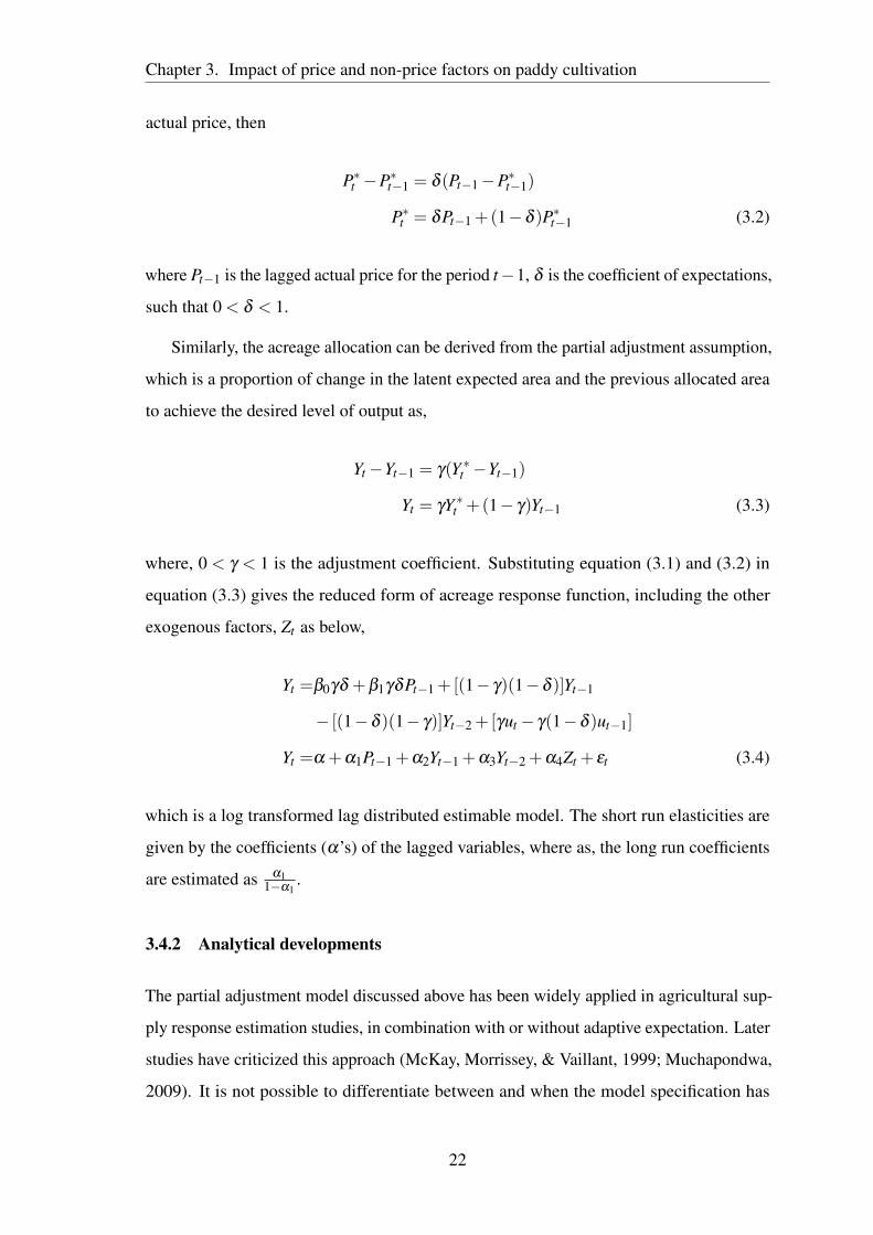
where Pt−1 is the lagged actual price for the period t−1, δ is the coefficient of expectations,
such that 0 < δ < 1.
Similarly, the acreage allocation can be derived from the partial adjustment assumption,
which is a proportion of change in the latent expected area and the previous allocated area
to achieve the desired level of output as,
Yt −Yt−1 = γ(Y ∗t −Yt−1)
Yt = γY ∗t +(1− γ)Yt−1 (3.3)
where, 0 < γ < 1 is the adjustment coefficient. Substituting equation (3.1) and (3.2) in
equation (3.3) gives the reduced form of acreage response function, including the other
exogenous factors, Zt as below,
Yt =β0γδ +β1γδPt−1 +[(1− γ)(1−δ )]Yt−1
− [(1−δ )(1− γ)]Yt−2 +[γut − γ(1−δ )ut−1]
Yt =α +α1Pt−1 +α2Yt−1 +α3Yt−2 +α4Zt + εt (3.4)
which is a log transformed lag distributed estimable model. The short run elasticities are
given by the coefficients (α’s) of the lagged variables, where as, the long run coefficients
are estimated as α11−α1
.
3.4.2 Analytical developments
The partial adjustment model discussed above has been widely applied in agricultural sup-
ply response estimation studies, in combination with or without adaptive expectation. Later
studies have criticized this approach (McKay, Morrissey, & Vaillant, 1999; Muchapondwa,
2009). It is not possible to differentiate between and when the model specification has
22
Chapter 3. Impact of price and non-price factors on paddy cultivation
both adaptive expectation as well as partial adjustment. This implies that unless arbitrary
assumptions are imposed on the model specification, either as adaptive expectation or as
partial adjustment, estimation of long run elasticity is not possible. From the estimation
equation (3.4), it is clear that the model can involve both partial adjustment and adaptive
expectation in the same dynamic specification. Further, as noted by McKay et al. (1999)
and Thiele (2000), the theoretical assumptions used in the model are considered to be
inadequate can result in downward bias in the estimated elasticities and hence the Nerlovian
model cannot capture the full dynamics of the response of the farmers (Muchapondwa,
2009).
Furthermore, the OLS estimation approach used in Nerlovian-model studies, assumes
that the underlying time series data is stationary. However, it has been observed that most of
the agricultural time series data are non-stationary at levels. Using OLS on non-stationary
data can result in spurious regression estimates (Granger & Newbold, 1974). Therefore,
the studies employing the Nerlovian partial adjustment model have constantly produced
low and biased estimates of the price elasticity for developing countries from different
regions (Thiele, 2000). To overcome restrictive dynamic specification of the Nerlove-
model, co-integration analysis, which is based on long run co-movement of the variables,
can be conducted as it does not impose any restrictions on the short-run behaviour of
prices and quantities. In combination with error correction model (ECM), co-integration
analysis can be used to obtain consistent estimates of short and long run elasticities. The
ECM with co-integration using stationary variables can overcome the problem of spurious
correlations which may occur in OLS regressions of the Nerlove-model if variables are
non-stationary (Thiele, 2000), and hence, is a superior alternative to partial adjustment
model both theoretically and empirically (Hallam & Zanoli, 1993).
A range of co-integration approaches exist in the time series literature, such as, the
most commonly used Engle and Granger (1987) method, Johansen (1991) and Johansen
and Juselius (1990). All these methods have their own merits and limitations. Engel-
Granger approach ignores short-run dynamics while estimating the co-integrating vector
thus resulting in biased estimates of long-run coefficients especially in finite samples with
complex short-run dynamics, where as the Johansen method requires large data samples
for validity, strongly relies on the unit root test and assumes that the order of integration
23
Chapter 3. Impact of price and non-price factors on paddy cultivation
of all the variables is same and known with certainty (Muchapondwa, 2009). The Auto
Regressive Distributive Lag (ARDL) co-integration approach has numerous advantages
in comparison with other co-integration methods (Odhiambo, 2009; Ozturk & Acaravci,
2010). ARDL is relatively a recent approach to co-integration proposed by Pesaran and
Shin (1998) and extended by Pesaran et al. (2001) using bounds testing to overcome the
problems of Johansen estimation procedure and Engle-Granger procedure in co-integration
techniques (Getnet, Verbeke, & Viaene, 2005). This approach tests for the existence of
a non-spurious long term co-integration relationship among the variables involved. It
also captures long-run equilibrium and short run dynamics for the testing co-integration
relationship (Pesaran et al., 2001). ARDL method also allows the estimation of long run
co-integration relationship even when the variables are I(0), I(1) or a combination of both.
This approach avoids the pre-testing of unit roots using conventional unit root testing
mechanism on the time series and overcomes the uncertainties of lower statistical power
associated with these unit root tests (Getnet et al., 2005). ARDL approach is efficient even
when the sample size is small while other co-integration techniques are sensitive to the
size of the sample (Odhiambo, 2009). This approach allows different optimal lag length
for different variables as opposed to same lag length in Johansen’s method. This method is
also less sensitive to endogenous regressors in the model and generally provides unbiased
long run estimates (Odhiambo, 2009). Previous studies using bounds testing ARDL model
for supply response include Muchapondwa (2009), Binuomote, Ajetomobi, and Omodunbi
(2012), Boansi (2014), Ogundari (2016) and Getnet et al. (2005).
3.5 Methodology
3.5.1 Data
The data for estimating the acreage response of Wayanad farmers is compiled from publica-
tions, such as, Agricultural Statistics and Statistics for Planning, published by Directorate
of Economics and Statistics, Kerala. The district of Wayanad was administratively formed
in 1980, but consistent and regular data on variables, such as, area and prices from Wayanad
is only available from 1987. Hence, a time period of 1987-2009 is selected for the study.
24
Chapter 3. Impact of price and non-price factors on paddy cultivation
The choice of appropriate dependent variable to measure supply response is often
debated in supply response literature (Narayana & Parikh, 1981) and is inconclusive among
price, output or area. Mythili (2008) argues that output is subject to more fluctuation than
area because of uncertain random factors, namely, temperature and rainfall, and area
is a more appropriate variable especially when response is confined to changes in area
allocation than total area under cultivation. Hence, we use absolute paddy area of winter
(LPA) in hectare for this study. Other studies using area to measure response include
Lambert and Narain (1968) and Krishna (1963). The variables used in the study are price
of paddy (LPP) in Rupees/quintal, price of banana (LBP) in Rupees/quintal, female wage
rate of agricultural workers (LFW) in Rupees/day of Wayanad district. Price and wage
data are deflated to 2010 real prices using the WPI (Wholesale Price Index) for agricultural
commodities to account for inflation. The importance of rainfall as a relevant variable
in determining the supply response is supported by several studies (Narayana & Parikh,
1981; Imai, Gaiha, & Thapa, 2011; Kanwar, 2006; Mythili, 2008; Tripathi & Prasad, 2009).
The data on rainfall of Wayanad was extracted from western grid rainfall data from Indian
meteorological department. Rainfall as a weather parameter is difficult to incorporate in
the analysis, because, average total rainfall in a crop season, rainfall in the pre-sowing
period and absolute deviation from normal rainfall can have different impacts on the paddy
cultivation. According to Mythili (2008), there is no satisfactory measure of rainfall in
the area or supply response literature. However, the current study uses the average daily
rainfall in mm (LRF) for the months of May, June, July and August as they include the
pre-monsoon and monsoon season, which coincides with the land preparation, sowing and
transplanting of paddy in Wayanad. Therefore, rainfall during these months is more likely
to have an influence on the area allocation. All the variables are converted to their natural
logarithms for the empirical analysis.
3.5.2 Empirical estimation
Empirical estimation of ARDL modelling technique to co-integration consists of four
steps: 1) unit root testing for identifying the right order of integration of variables involved;
2) establishing the existence of long run co-integration relationship among the variables
using bounds testing; 3) estimation of the ARDL model to obtain short run and long run
25
Chapter 3. Impact of price and non-price factors on paddy cultivation
coefficients; finally, testing the stability of the model and the coefficients using various
diagnostic tests. In the next few paragraphs we will be covering these steps in detail.
The hypothesized functional relationship between acreage allocation and the dependent
variables are modelled as,
pat = α0 +α1 ppt +α2bpt +α3 f wt +α4r ft + vt (3.5)
Before testing the model for co-integration, the order of integration of individual
variables are tested using conventional Augmented Dickey-fuller (ADF) and Philips-
Perron (PP) test. Unit root tests are conducted to ensure that the variables are integrated
of order less than two (Abbott, Darnell, & Evans, 2001) as the ARDL approach requires
the integration of the variables I(0), I(0) or a mix of both. PP unit root test is also
conducted due to its robustness to auto-correlation as it allows the presence of unknown
forms of correlation in time series and conditional heteroscedasticity in the error term
(Muchapondwa, 2009). The optimal lags for the ADF tests are selected based on Schwarz’s
Bayesian Information Criterion (SBIC). The ADRL modeling approach involves the
estimation of the following unrestricted (conditional) error correction model (UEC) by
ordinary least square method in order to test for one or more co-integration relationships
among the variables:
∆pat =β0 +p
∑i=1
β1i∆pat−i +q1
∑i=0
β2i∆ppt−i +q2
∑i=0
β3i∆bpt−i +q3
∑i=0
β4i∆ f wt−i
+q4
∑i=0
β5i∆r ft−i + γ0 pat−1 + γ1 ppt−1 + γ2bpt−1 + γ3 f wt−1 + γ4r ft−1 + εt (3.6)
where ∆ is the difference operator, εit is the white noise error term and other variables as
defined earlier. After the estimation of the above model the presence of co-integration
can be tested using the bounds testing approach. Accordingly, in order to test the long
run relationship among the variables, F-test is conducted for testing the joint significance
of coefficients of the lagged levels of the variables with the null hypothesis that they are
jointly equal to zero.
i.e,
H0 : γ0 = γ1 = γ2 = γ3 = γ4 = 0
26
Chapter 3. Impact of price and non-price factors on paddy cultivation
as against the alternative hypothesis;
HA : γ0 ̸= γ1 ̸= γ2 ̸= γ3 ̸= γ4 ̸= 0
A pair of asymptotic critical value bounds for the F-statistic is generated by Pesaran et
al. (2001), where the independent variables are I(d). The lower bound corresponds to a
situation when the regressor variables are I(0) and a upper bound value corresponding
to situation when the regressors are I(1). If the calculated F-statistic is outside these
critical boundaries, a conclusion regarding co-integration of the regressors can be derived
regardless of the degree of integration of the regressors. If the computed F-statistic is lower
than the lower bound value, then there is no long run co-integrating relationship among the
variables, thus accepting the hypothesis. On the contrary, if it lies above the upper bound
critical value, the hypothesis of non-existence of co-integrating relationship can be safely
rejected. But, if the F-statistic lie within the bounds of the critical values then the results
are inconclusive.
In the next step, once when a co-integration relationship is established, a conditional
ARDL (m, n, o, p, q) long run model is specified of the following form;
pat = α0 +m
∑i=1
β1i pat−i +n
∑i=0
β2i ppt−i +o
∑i=0
β3i f wt−i +p
∑i=0
β4ibpt−i
+q
∑i=0
β5ir ft−i + εt (3.7)
where, all the variables are defined earlier. The lag length in the ARDL is selected based
on SBIC selection criteria. In the third step, the short run dynamic elasticities are estimated
by using the error correction model (ECM), as described below,
∆pat = δ0 +m
∑i=1
δ1i∆pat−i +n
∑i=0
δ2i∆ppt−i +o
∑i=0
δ3i∆ f wt−i +p
∑i=0
δ4i∆bpt−i
+q
∑i=0
δ5i∆r ft−i +λECMt−1 +µt (3.8)
27
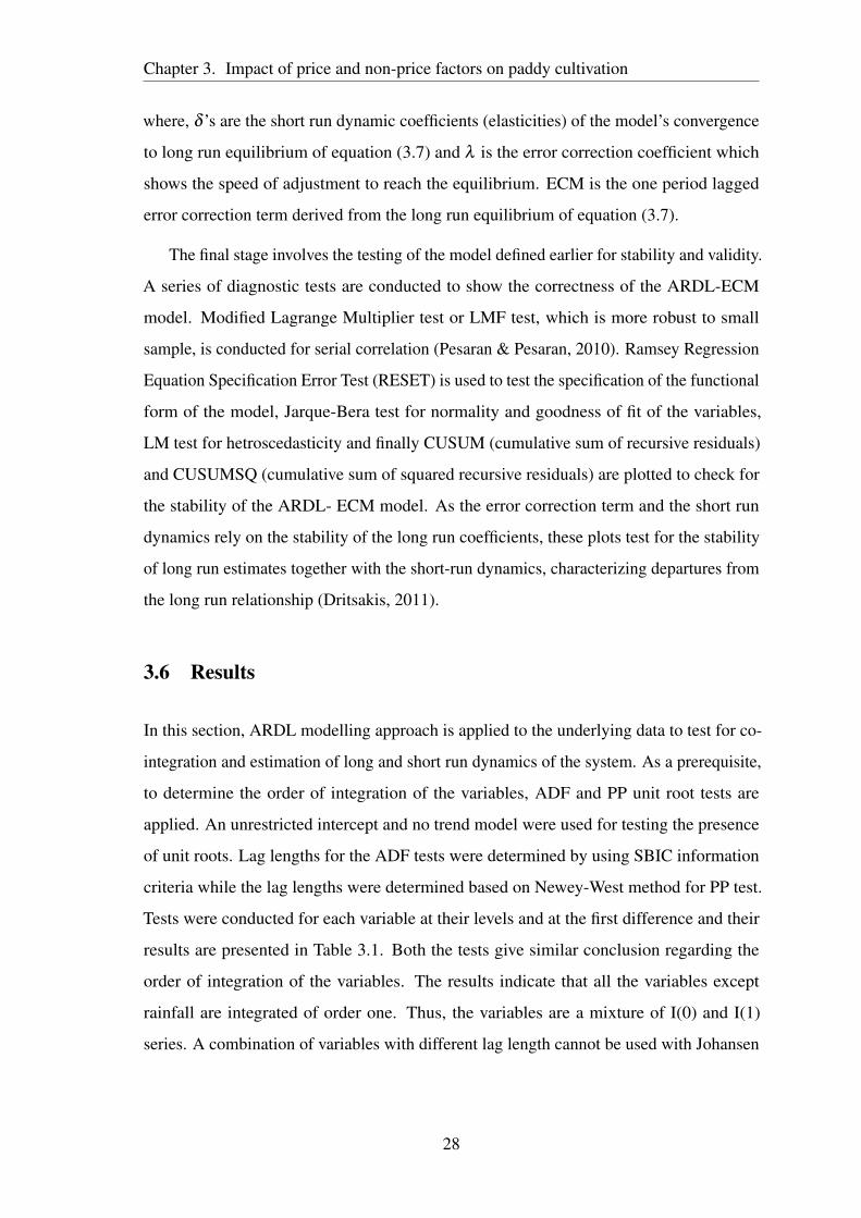
Chapter 3. Impact of price and non-price factors on paddy cultivation
where, δ ’s are the short run dynamic coefficients (elasticities) of the model’s convergence
to long run equilibrium of equation (3.7) and λ is the error correction coefficient which
shows the speed of adjustment to reach the equilibrium. ECM is the one period lagged
error correction term derived from the long run equilibrium of equation (3.7).
The final stage involves the testing of the model defined earlier for stability and validity.
A series of diagnostic tests are conducted to show the correctness of the ARDL-ECM
model. Modified Lagrange Multiplier test or LMF test, which is more robust to small
sample, is conducted for serial correlation (Pesaran & Pesaran, 2010). Ramsey Regression
Equation Specification Error Test (RESET) is used to test the specification of the functional
form of the model, Jarque-Bera test for normality and goodness of fit of the variables,
LM test for hetroscedasticity and finally CUSUM (cumulative sum of recursive residuals)
and CUSUMSQ (cumulative sum of squared recursive residuals) are plotted to check for
the stability of the ARDL- ECM model. As the error correction term and the short run
dynamics rely on the stability of the long run coefficients, these plots test for the stability
of long run estimates together with the short-run dynamics, characterizing departures from
the long run relationship (Dritsakis, 2011).
3.6 Results
In this section, ARDL modelling approach is applied to the underlying data to test for co-
integration and estimation of long and short run dynamics of the system. As a prerequisite,
to determine the order of integration of the variables, ADF and PP unit root tests are
applied. An unrestricted intercept and no trend model were used for testing the presence
of unit roots. Lag lengths for the ADF tests were determined by using SBIC information
criteria while the lag lengths were determined based on Newey-West method for PP test.
Tests were conducted for each variable at their levels and at the first difference and their
results are presented in Table 3.1. Both the tests give similar conclusion regarding the
order of integration of the variables. The results indicate that all the variables except
rainfall are integrated of order one. Thus, the variables are a mixture of I(0) and I(1)
series. A combination of variables with different lag length cannot be used with Johansen
28
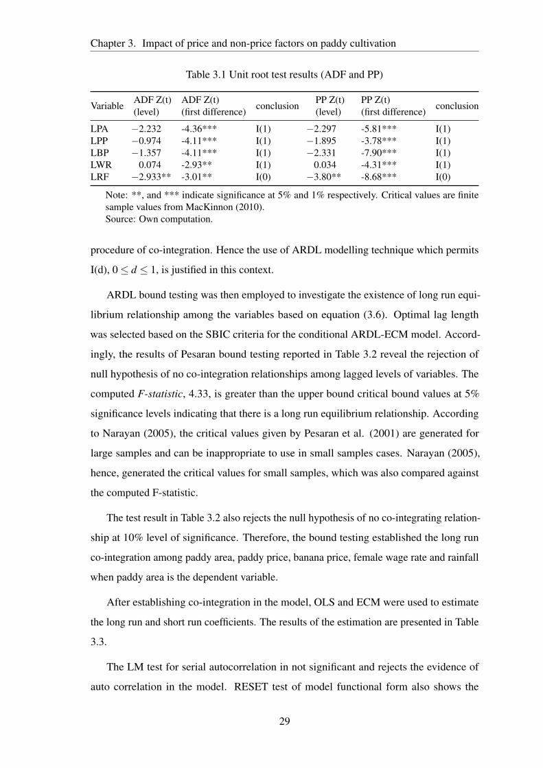
Chapter 3. Impact of price and non-price factors on paddy cultivation
Table 3.1 Unit root test results (ADF and PP)
VariableADF Z(t)(level)
ADF Z(t)(first difference) conclusion
PP Z(t)(level)
PP Z(t)(first difference) conclusion
LPA −2.232 -4.36*** I(1) −2.297 -5.81*** I(1)LPP −0.974 -4.11*** I(1) −1.895 -3.78*** I(1)LBP −1.357 -4.11*** I(1) −2.331 -7.90*** I(1)LWR 0.074 -2.93** I(1) 0.034 -4.31*** I(1)LRF −2.933** -3.01** I(0) −3.80** -8.68*** I(0)
Note: **, and *** indicate significance at 5% and 1% respectively. Critical values are finitesample values from MacKinnon (2010).Source: Own computation.
procedure of co-integration. Hence the use of ARDL modelling technique which permits
I(d), 0 ≤ d ≤ 1, is justified in this context.
ARDL bound testing was then employed to investigate the existence of long run equi-
librium relationship among the variables based on equation (3.6). Optimal lag length
was selected based on the SBIC criteria for the conditional ARDL-ECM model. Accord-
ingly, the results of Pesaran bound testing reported in Table 3.2 reveal the rejection of
null hypothesis of no co-integration relationships among lagged levels of variables. The
computed F-statistic, 4.33, is greater than the upper bound critical bound values at 5%
significance levels indicating that there is a long run equilibrium relationship. According
to Narayan (2005), the critical values given by Pesaran et al. (2001) are generated for
large samples and can be inappropriate to use in small samples cases. Narayan (2005),
hence, generated the critical values for small samples, which was also compared against
the computed F-statistic.
The test result in Table 3.2 also rejects the null hypothesis of no co-integrating relation-
ship at 10% level of significance. Therefore, the bound testing established the long run
co-integration among paddy area, paddy price, banana price, female wage rate and rainfall
when paddy area is the dependent variable.
After establishing co-integration in the model, OLS and ECM were used to estimate
the long run and short run coefficients. The results of the estimation are presented in Table
3.3.
The LM test for serial autocorrelation in not significant and rejects the evidence of
auto correlation in the model. RESET test of model functional form also shows the
29
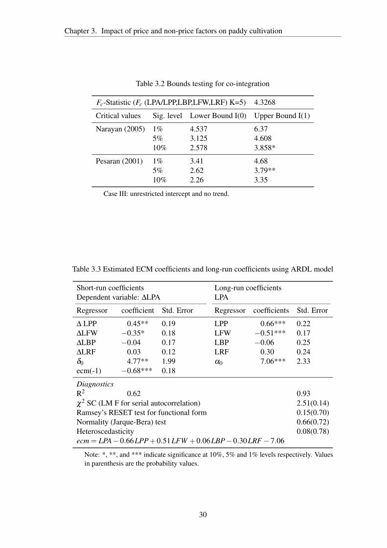
Chapter 3. Impact of price and non-price factors on paddy cultivation
Table 3.2 Bounds testing for co-integration
Fc-Statistic (Fc (LPA/LPP,LBP,LFW,LRF) K=5) 4.3268
Critical values Sig. level Lower Bound I(0) Upper Bound I(1)
Narayan (2005) 1% 4.537 6.375% 3.125 4.60810% 2.578 3.858*
Pesaran (2001) 1% 3.41 4.685% 2.62 3.79**10% 2.26 3.35
Case III: unrestricted intercept and no trend.
Table 3.3 Estimated ECM coefficients and long-run coefficients using ARDL model
Short-run coefficients Long-run coefficientsDependent variable: ∆LPA LPA
Regressor coefficient Std. Error Regressor coefficients Std. Error
∆ LPP 0.45** 0.19 LPP 0.66*** 0.22∆LFW −0.35* 0.18 LFW −0.51*** 0.17∆LBP −0.04 0.17 LBP −0.06 0.25∆LRF 0.03 0.12 LRF 0.30 0.24δ0 4.77** 1.99 α0 7.06*** 2.33ecm(-1) −0.68*** 0.18
DiagnosticsR2 0.62 0.93χ2 SC (LM F for serial autocorrelation) 2.51(0.14)Ramsey’s RESET test for functional form 0.15(0.70)Normality (Jarque-Bera) test 0.66(0.72)Heteroscedasticity 0.08(0.78)ecm = LPA−0.66LPP+0.51LFW +0.06LBP−0.30LRF −7.06
Note: *, **, and *** indicate significance at 10%, 5% and 1% levels respectively. Valuesin parenthesis are the probability values.
30
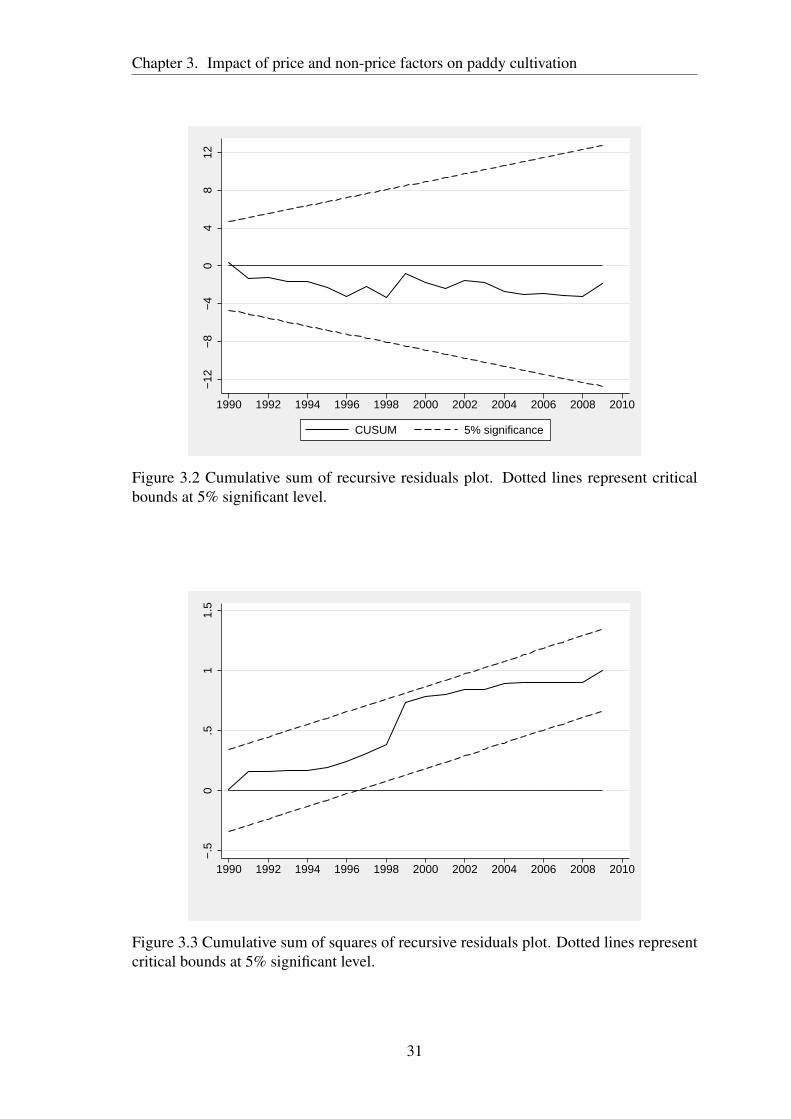
Chapter 3. Impact of price and non-price factors on paddy cultivation
−12
−8
−4
04
812
1990 1992 1994 1996 1998 2000 2002 2004 2006 2008 2010
CUSUM 5% significance
Figure 3.2 Cumulative sum of recursive residuals plot. Dotted lines represent criticalbounds at 5% significant level.
−.5
0.5
11.
5
1990 1992 1994 1996 1998 2000 2002 2004 2006 2008 2010
Figure 3.3 Cumulative sum of squares of recursive residuals plot. Dotted lines representcritical bounds at 5% significant level.
31
Chapter 3. Impact of price and non-price factors on paddy cultivation
correctness of the model form specification. Jarque-Bera statistics for the test of normality
in the distribution of the errors show that the errors are normally distributed. Test for
heteroscedasticity in the error process of the model is also statistically insignificant. R2
values explain about 93% of the variations in the long run equation and 62% of the variation
in the short run equation suggesting the goodness of fit of the model. Finally, the CUSUM
and CUSUM of squares of residuals are plotted and the result shows that the plot remains
within the 5% statistical significance boundary (Figure 3.2 and Figure 3.3). It can be
concluded from the various tests mentioned above that the model is well formulated and
estimated. It also confirms the statistical stability of the estimated coefficients for a valid
policy discussion.
All estimated coefficients in the error correction model have their expected sign.
The negative coefficient of the error correction term is in the range of -1 and 0 and is
significant at 1% level. This again supports the co-integration and the long term equilibrium
relationship between the dependent and independent variables in the model (Getnet et al.,
2005). Coefficient of the error correction term (-0.68) indicates high speed of adjustment
towards long run equilibrium as 68% of the deviation in previous period paddy area from
the long run equilibrium is corrected in the current period. In short run, the coefficients of
both paddy price and female wage rate are statistically significant.
In the short run, price of paddy influences the allocation of paddy area positively,
whereas female wage rate has a negative impact. The most important limiting factor for
agriculture, rainfall, though insignificant has a positive sign and holds a direct relationship
with paddy acreage in the long run as well as in the short run. Similarly, price of banana,
which is considered as the main competing crop for paddy in Wayanad has a negative
coefficient even though statistically insignificant in the long and short run.
3.7 Discussion and policy implications
When interpreting the results of acreage responsiveness of farmers, we have to consider
land as a resource that is virtually fixed in total quantity at any point in time (Shi, Phipps,
& Colyer, 1997). Conventionally, agricultural land is considered as a fixed resource in
short run but as a variable resource in long run (Raju & Rao, 1990). Field experience from
32
Chapter 3. Impact of price and non-price factors on paddy cultivation
Wayanad show that farmers cultivate banana and ginger as a rotation or alternative crop in
paddy fields (Kunze, Betz, Parameswaran, & Suma, 2011). This explains the changes in
area allocation of paddy in the short run as well as in the long run.
Mythili (2008) compared the price responsiveness to paddy acreage in India from
various studies and reported that the price elasticity estimates for rice range from 0.06
to 0.12 in the short run and from 0.15 to 0.93 in the long run. The deviation of the price
response estimates in the current study, from the past studies can be attributed to the
difference in the time period considered for the analysis, difference in estimation technique
used and also the location specificity of the current study. The high sensitiveness of
estimates to the estimation techniques is also confirmed by previous studies (Surekha,
2005). Our finding of area equations supports the argument that the farmers of Wayanad
are moderately and highly responsive to paddy price changes in the short run and long run
respectively. As a result, measures on price reforms might prove effective in promoting
paddy cultivation in the district. It is also advisable for the government to intervene with
formal market interventions, such as, government procurement centres for paddy with a
guaranteed better price for the producer. Promoting development of markets for special
and local varieties of paddy from Wayanad might prove effective so that the farmers can
realize higher price for these varieties.
High acreage responsiveness of paddy to female wage rate in the long and short run
in the current study can be explained by the following; 1) The female labour requirement
in paddy is about 70% of the total labour (Narayanan, 2006); 2) Labour contribution to
the operational cost of paddy cultivation in Kerala is 60% (DES, 2012); 3) Kerala has the
highest average daily wage rate in all agricultural operations throughout the year when
compared to the all India average wage rate. Female labour force, hence, form an important
factor in the land allocation decision of paddy, thus adding strength to the result of female
labour wage rate being a major factor in the paddy acreage response. Women participation
in MGNREGA3 scheme in the district was about 84% during the year 2010-11, which
has considerably influenced the agricultural labour supply. Thadathil & Mohandas (2012)
indicated an increase in the agricultural wage rate due to the MGNREGA scheme in the
3MGNREGA stands for Mahatma Gandhi National Rural Employment Guarantee Act, 2005, whichguarantee the right to work in rural area by providing 100 days of volunteer wage employment in everyfinancial year to all adult citizens.
33
Chapter 3. Impact of price and non-price factors on paddy cultivation
district, where the wage fixed by the MGNREGA serves as the unofficial minimum wage
rate for agriculture.
According to our results, the increase in wage rate would have a long and short term
negative impact on the paddy area cultivated in Wayanad. Further, discussions with the
farmers in Wayanad revealed that MGNREGA, if, extended to the paddy field could be
very effective in reducing the labour cost involved in the cultivation of paddy. The finding,
high negative responsiveness of paddy acreages to female wage rates, of this study supports
reforms to include paddy cultivation under the purview of MGNREGA work force so that
it would facilitate in the improvement of the area under of paddy cultivation in Wayanad
district of Kerala. Our results hence imply the importance of intervention to remove the
constraints of labour supply to agriculture in order to strengthen the area response of paddy.
The results also necessitate the need for labour cost reduction initiatives, such as, adequate
investment support for farm mechanization that are suitable for smallholders in order to
improve the paddy acreage response.
3.8 Conclusion
We estimated the area allocation response of farmers in Wayanad district of Kerala in
Southern India. Considering the methodological issues in the earlier literature, ARDL
approach of co-integration using bounds testing and error correction technique were
employed. The short-run and long-run relationship between the area allocated by the
farmers and various price and non-price factors was estimated. Price of paddy and price of
competing crop (banana) as the price factors, rainfall as a non-price factor and wage rate
as an input factor, were used in estimating the acreage response.
The results of the analysis suggest that relative to the non-price factors, price factors
and input factors play a major role in determining the acreage allocation to paddy. The
estimated short run and long run coefficients indicate that the acreage response of paddy
towards paddy price is positive and significant. Hence, agricultural price reforms in
paddy sector can promote cultivation of paddy in Wayanad. Market interventions like
formal market infrastructure and direct procurement mechanism that can improve the price
received by the producer are also recommended. Developing local markets for special and
34
Chapter 3. Impact of price and non-price factors on paddy cultivation
paddy varieties from Wayanad might improve the acreage response of paddy. The potential
for labelling these varieties to assure a premium price needs to be further studied. The
responsiveness of farmers towards female wage rate in the long run and short run suggests
reforms in existing labour policies like MGNREGA favouring paddy farmers. Initiatives
on farm mechanization that are labour saving are also suggested to improve the paddy
acreage response in Wayanad.
References
Abbott, A., Darnell, A.C., & Evans, L. (2001). The influence of exchange rate vari-ability on UK exports. Applied Economics Letters, 8(1), 47–49. doi:10.1080/135048501750041286
Binuomote, S.O., Ajetomobi, J.O., & Omodunbi, C.O. (2012). Application of autoregres-sive distributed lags (ARDL) modelling approach to co-integration in econometricestimation of wheat imports demand in Nigeria (1970-2008). Advances in Arts, SocialSciences and Education Research, 2(5), 168–176.
Boansi, D. (2014). Yield response of rice in Nigeria: A co-integration analysis. AmericanJournal of Agriculture and Forestry, 2(2), 15–24.
Claassen, R., & Tegene, A. (1999). Agricultural land use choice: A discrete choiceapproach. Agricultural and Resource Economics Review, 28(1), 26–36.
Cummings, J.T. (1975). The Supply responsiveness of Indian farmers in the post-independenceperiod: Major cereal and cash crops. Indian Journal of Agricultural Economics, 30(1),25–40.
DES. (2012). Cost of Cultivation / Production & Related Data. New Delhi. Retrieved fromDirectorate of Economics and Statistics, Ministry of Agriculture, Government of Indiawebsite: http://eands.dacnet.nic.in/Cost_of_Cultivation.htm
Dritsakis, N. (2011). Demand for money in Hungary: An ARDL Approach. Review ofEconomics and Finance, 1(11), 1–16.
Engle, R.F., & Granger, C.W.J. (1987). Co-integration and error correction: Representation,estimation, and testing. Econometrica, 55(2), 251–276.
Getnet, K., Verbeke, W., & Viaene, J. (2005). Modelling spatial price transmission inthe grain markets of Ethiopia with an application of ARDL approach to white teff.Agricultural Economics, 33(s3), 491–502.
35
Chapter 3. Impact of price and non-price factors on paddy cultivation
Government of Kerala. (2016). Economic review 2015. Kerala State Planning Board,Thiruvanathapuram, Kerala. Retrieved from Kerala State Planning Board website:http://spb.kerala.gov.in/images/er/er15/index.html.
Girigan, G., Kumar, N.A., & Nambi, V.A. (2004). Vayals: A traditional classification ofagricultural landscapes. LEISA India-Farming with Nature, 6(4), 27–28.
Granger, C.W.J., & Newbold, P. (1974). Spurious regressions in econometrics. Journal ofeconometrics, 2(2), 111–120.
Gulati, A., & Kelley, T. (2001). Trade liberalization and Indian agriculture: Croppingpattern changes and efficiency gains in semi-arid tropics. Delhi, Oxford: OxfordUniversity Press.
Hallam, D., & Zanoli, R. (1993). Error correction models and agricultural supply response.European Review of Agricultural Economics, 20(2), 151–166.
Herdt, R.W. (1970). A Disaggregate approach to aggregate supply. American Journal ofAgricultural Economics, 52(4), 512–520. doi:10.2307/1237258
Imai, K.S., Gaiha, R., & Thapa, G. (2011). Supply response to changes in agriculturalcommodity prices in Asian countries. Journal of Asian Economics, 22(1), 61–75.doi:10.1016/j.asieco.2010.08.002
Johansen, S. (1991). Estimation and hypothesis testing of cointegration vectors in Gaussianvector autoregressive models. Econometrica, 59(6), 1551–1580.
Johansen, S., & Juselius, K. (1990). Maximum likelihood estimation and inference oncointegration with applications to the demand for money. Oxford Bulletin of Economicsand Statistics, 52(2), 169–210. doi:10.1111/j.1468-0084.1990.mp52002003.x
Kanwar, S. (2006). Relative profitability, supply shifters and dynamic output response,in a developing economy. Journal of Policy Modeling, 28(1), 67–88. doi:10.1016/j.jpolmod.2005.06.014
Kanwar, S., & Sadoulet, E. (2008). Dynamic output response revisited: The Indian cashcrops. The Developing Economies, 46(3), 217–241. doi:10.1111/j.1746-1049.2008.00064.x
Krishna, R. (1963). Farm supply response in India-Pakistan: A case study of the Punjabregion. The Economic Journal, 73(291), 477–487. doi:10.2307/2228581
Krishna, R., & Raychaudhuri, G.S. (1980). Some aspects of wheat and rice price policy inIndia. Washington D.C : World Bank.
Kumar, P., & Rosegrant, M. (1997). Dynamic supply response of cereals and supplyprojections: A 2020 Vision. Agricultural Economic Research Review, 10(1).
36
Chapter 3. Impact of price and non-price factors on paddy cultivation
Kunze, I., Betz, L., Parameswaran, P., & Suma, T. (2011). (No) Future for rice inWayanad: exploring the social-ecological transformation processes and its impacts onmarginalised farmers in South India. In proceeding of Annual Conference on Tropicaland Subtropical Agricultural and Natural (Tropentag): Development on the margin,October 5-7, Bonn, Germany.
Lambert, D., & Narain, D. (1968).The Impact of price movements on areas under selectedcrops in India, 1900-1939 (Vol. 19). Cambridge [England]: Cambridge UniversityPress.
Lockie, S., & Carpenter, D. (Eds.). (2010). Agriculture, biodiversity and markets: Liveli-hoods and agroecology in comparative perspective. London: Earthscan.
MacKinnon, J.G. (2010). Critical values for cointegration tests (Queen’s EconomicsDepartment Working PaperNo. 1227). Retrieved from website: http://akson.sgh.waw.pl/~ewams/MacKinnon_Critical_values_for_cointegration_tests_qed_wp_1227.pdf
Madhavan, M.C. (1972). Acreage response of Indian farmers: A case study of Tamil Nadu.Indian Journal of Agricultural Economics, 27(1), 67–87.
McKay, A., Morrissey, O., & Vaillant, C. (1999). Aggregate supply response in Tanzanianagriculture. The Journal of International Trade & Economic Development, 8(1),107–123. doi:10.1080/09638199900000008
Muchapondwa, E. (2009). Supply response of Zimbabwean agriculture: 1970–1999.African Journal of Agricultural and Resource Economics, 3(1), 28–42.
Myers, N., Mittermeier, R.A., Mittermeier, C.G., da Fonseca, G.A.B., & Kent, J. (2000).Biodiversity hotspots for conservation priorities.Nature, 403(6772), 853–858. doi:10.1038/35002501
Mythili, G. (2008). Acreage and yield response for major crops in the pre- and post- reformperiods in India: A dynamic panel data approach [Report prepared for IGIDR – ERS/USDA Project: Agricultural Markets and Policy]. Retrieved from http://www.igidr.ac.in/pdf/publication/PP-061.pdf
Narayan, P.K. (2005). The saving and investment nexus for China: evidence from cointegra-tion tests. Applied Economics, 37(17), 1979–1990. doi:10.1080/00036840500278103
Narayana, N.S.S., & Parikh, K.S. (1981). Estimation of farm supply response and acreageallocation: A case study of Indian agriculture (No. Research report RR-81-1). Laxen-burg, Austria: International Institute for Systems Analysis.
Narayanan, N. (2006). For and against grain land use: Politics of rice in Kerala, India. Inter-national Journal of Rural Management, 2(1), 123–144. doi:10.1177/097300520500200107
37
Chapter 3. Impact of price and non-price factors on paddy cultivation
Nerlove, M. (1958). The dynamics of supply: Estimation of farmers response to price.The Johns Hopkins University studies in historical and political science: ser. 76, no.2.Baltimore, MD: Johns Hopkins University Press.
Nerlove, M. (1971). Further evidence on the estimation of dynamic economic relationsfrom a time series of cross sections.Econometrica, 39(2), 359–382.
Odhiambo, N.M. (2009). Energy consumption and economic growth nexus in Tanzania:An ARDL bounds testing approach. Energy Policy, 37(2), 617–622. doi:10.1016/j.enpol.2008.09.077
Ogundari, K. (2016). Maize supply response to price and nonprice determinants inNigeria: Bounds testing approach. International Transactions in Operational Research.doi:10.1111/itor.12284
Olayiwola, O.O. (2013). Review on methodology for supply responses of agriculturalcrops. Journal of Research in Management and Technology, 2(11), 1–10.
Ozkan, B., & Karaman, S. (2011). Acreage response for cotton regions in Turkey: an appli-cation of the bounds testing approach to cointegration. New Medit: A Mediterraneanjournal of economics, agriculture and environment, 10(2), 42–50.
Ozturk, I., & Acaravci, A. (2010). The causal relationship between energy consumption andGDP in Albania, Bulgaria, Hungary and Romania: Evidence from ARDL bound testingapproach. Applied Energy, 87(6), 1938–1943. doi:10.1016/j.apenergy.2009.10.010
Parikh, A. (1971). Farm supply response: A distributed lag analysis. Bulletin of the OxfordUniversity Institute of Economics & Statistics, 33(1), 57–72. doi:10.1111/j.1468-0084.1971.mp33001004.x
Pesaran, B., & Pesaran, M.H. (2010). Time Series Econometrics Using Microfit 5.0: AUser’s Manual. Oxford University Press, Inc.
Pesaran, M.H., & Shin, Y. (1998). An autoregressive distributed-lag modelling approachto cointegration analysis.Econometric Society Monographs, 31, 371–413.
Pesaran, M.H., Shin, Y., & Smith, R.J. (2001). Bounds testing approaches to the analysisof level relationships.Journal of Applied Econometrics, 16(3), 289–326. doi:10.1002/jae.616http://dx.doi.org/10.1002/jae.616
Planning Commission. (2014). Data and statistics: Data book. Retrieved from Govern-ment of India Planning Commission webstie: http://planningcommission.nic.in/data/datatable/
Raj, P.P.N., & Azeez, P.A. (2009).Real estate and agricultural wetlands in Kerala.Economicand Political Weekly, 44(5), 63–66. doi:10.2307/40278461
38
Chapter 3. Impact of price and non-price factors on paddy cultivation
Raju, V.T., & Rao, D.V.S. (1990). Economics of farm production and Management. NewDelhi: Oxford & IBH Publishing Co. Pvt. Ltd.
Shi, Y.J., Phipps, T.T., & Colyer, D. (1997). Agricultural land values under urbanizinginfluences.Land Economics, 73(1), 90–100.
Siddiqui, K. (2014). Growth and crisis in India’s political economy from 1991 to 2013.In-ternational Journal of Social and Economic Research, 4(2), 84.doi:10.5958/2249-6270.2014.00487.5
Surekha, K. (2005). Modeling nonlinear autoregressive distributed lag models: A NewApproach. Journal of Quantitative Economics, 3(1), 101–114.
Thadathil, M.S., & Mohandas, V. (2012).Impact of MGNREGS on labour supply toagricultural sector of Wayanad district in Kerala. Agricultural Economics ResearchReview, 25(1), 151–155.
Thiele, R. (2000). Estimating the aggregate agricultural supply response: A survey oftechniques and results for developing countries (No. 1016). Kiel. Retrieved from KielInstitute for the World Economy website: http://hdl.handle.net/10419/2516
Tripathi, A., & Prasad, A.R. (2009). Estimation of agricultural supply response usingcointegration technique.The Indian Economic Journal, 57(1), 106–131.
Tripathi, A. (2008). Estimation of agricultural supply response using cointegration Ap-proach. Retrieved from http://works.bepress.com/amarnath_tripathi/4/
39
Chapter 4
ASSESSING THE HOUSEHOLD WELFARE IMPACTS OF HIGH VALUE
CROP ADOPTION IN A WETLAND PADDY SYSTEM OF SOUTHERN IN-
DIA
Abstract
The impact of High Value Crop (HVC) adoption on smallholders’ welfare remains unex-
plored especially in climate vulnerable and less resilient areas. The study aims to examine
the heterogeneous impacts of HVC adoption on household welfare in the ecologically
sensitive and biodiversity rich Western Ghats region of South India. We use data of 303
small and marginal farming households having either fully, partly or not adopted HVCs.
Per capita annual consumption expenditure and income are chosen as measures of welfare
status of the households. Multinomial logit regression reveal that land characteristics, such
as, farm size, access to transport, number of plots and distance to farm from dwelling
influences the HVC adoption decision of the household. The results of the multinomial
endogenous switching regression approach suggest that adoption has a positive and signifi-
cant impact on the welfare of smallholder households but partial adopters are found to be
better-off than full adopters and non-adopters.
Keywords: commercialization, impact assessment, multinomial switching regression,
Kerala.
40
Chapter 4. Assessing the household welfare impacts of high value crop adoption
4.1 Introduction
Over the past four decades, agriculture in developing countries has experienced gradual
transition from subsistence to an input intensive commercial system (Altieri & Nicholis,
2005). Globalization, rapid urbanization and accelerating pace of technological progress
have increased the agro-export competition in the international market (Hall, Dixon,
Gibbon, & Gulliver, 2001). The pressure on the small landholders to increase their per
unit value of output has subsequently resulted in shifting the focus of production systems
from food crops to high value crops (HVC) (Pingali, 1997). Policy-makers promote HVC
adoption as a general strategy to move the small and marginal landholders out of poverty.
Also agencies, such as, the World Bank or the Department for International Development
(DFID) identified it as an important source of poverty reduction and a tool to reverse the
declining investment trend in agriculture (Babu, Gajanan, & Sanyal, 2014; Pingali, 1997).
In India, policy-makers actively discuss HVC promotion (Birthal, Roy, & Negi, 2015)
and encourage its use through their agricultural policies1 (Birthal, Joshi, Roy, & Thorat,
2013). The reason for this is the pro-poor nature of the HVCs and the overwhelming
number of smallholders in the country. Small and marginal farmers with less than 2 ha
occupying 85% of total operational holdings dominate the agricultural sector in India
(Ministry of Agriculture, 2015). Among the smallholders, HVC cultivation is considered
to enhance farm income, increase employment opportunities and reduce the incidence of
poverty (Birthal et al., 2013; Joshi, Joshi, & Birthal, 2006). On the consumption side, the
demand for HVCs, such as, fruits and vegetables in the country is expected to increase
threefold by 2030 (Birthal et al., 2015). As a result, India has seen an increase in area
under HVC as well as share of HVC in total value of agricultural output (Kumar & Gupta,
2015; Rada, 2016).
However, the transition process from food crops to commercial crops is not a fric-
tionless process and has significant environmental consequences (Pingali & Rosegrant,
1995). Commercial crop adoption can lead to unsustainable land use changes and loss in
biodiversity leading to significant alteration in the environment and its natural resources
1For example, the Mission for Integration Development of Horticulture was launched in 2015 by theMinistry of Agriculture and Farmers’ Welfare, Government of India with a mandate of promoting productionand processing of fruits and vegetables (http://midh.gov.in).
41
Chapter 4. Assessing the household welfare impacts of high value crop adoption
(Aragona & Orr, 2011; Barbier, 1989; Garcia-Yi, 2014; Matson, Parton, Power, & Swift,
1997; Su, Yang, Hu, Luo, & Wang, 2014). In developing countries, the livelihoods of low
income rural households depend on the environmental resources and services (Nguyen, Do,
Bühler, Hartje, & Grote, 2015). Degradation of this environmental resource base might
subsequently reduce the household welfare of smallholders by making them vulnerable
to climate risks and food insecurity (King, Siddick, Gopi, & Kav, 2014). Evidence from
marginalized and climate vulnerable areas shows that the households which adopted im-
proved technology can have lower welfare than the non-adopters (Coromaldi, Pallante, &
Savastano, 2015). In the South Indian state of Kerala, the adoption of high value crops
over paddy, the staple food, has resulted in a decline in the ratio of food crop to non-food
crop from 64:36 in 1960-61 to 13:87 in 2013-14 (Government of Kerala, 2015). This
has posed a serious threat to the food security of the state and exacerbated the loss of
biodiversity and local rice cultivars, soil erosion, crop pests and diseases resulting in the
reduction in agricultural productivity posing indebtedness, climate and food security risks
(Karunakaran, 2014; Kennedy & King, 2014; Rejula & Singh, 2015; Shanavas, Sumesh, &
Haris, 2016). HVC adoption is also found to have a positive correlation with the increasing
rates of suicides among marginal farmers in Kerala (J. George & Krishnaprasad, 2006;
Kennedy & King, 2014).
This empirical evidence clearly indicates that even though HVC adoption among
smallholders is primarily considered welfare enhancing, the results cannot be generalized.
Therefore, there exist ambiguities regarding HVC adoption behavior and its impact. This
leads us to some issues, which need to be further explored. Firstly, HVC adoption and
its impacts on the household welfare are location-specific that depend on the production
and ecological conditions and the socio-economic state of the households. Therefore, it
is important to garner more micro-level empirical evidence on the adoption behaviour of
the farmers especially from less resilient, climate vulnerable and biodiversity rich areas.
Secondly, to meet the future climatic and food requirement challenges, it is necessary to
make agriculture more productive, stable and resilient while minimizing the environmental
impacts (Bommarco, Kleijn, & Potts, 2013). Hence, there is a need to focus on how the
welfare benefits can be maximized while minimizing the negative social and environmental
42
Chapter 4. Assessing the household welfare impacts of high value crop adoption
impacts so that an ecologically and socially sustainable agricultural land use system can be
developed (Banik, Edmonds, & Fuwa, 2014).
To understand the relationship between welfare and adoption, we examine the case
of a marginalized and climate vulnerable region in the biodiversity rich Western Ghats,
namely Wayanad in Kerala, South India. Specifically, we i) identify the determinants of
HVC adoption at the household level, and ii) analyse the smallholders’ welfare impacts of
HVC adoption. The study provides useful information to policy-makers to design effective
regional and crop-specific agro-environmental programs that can safeguard the livelihood
interests of small and marginal farmers while maintaining the environmental balance.
Our paper is also an attempt to augment the emerging body of literature, addressing
adoption not only as a binary decision but also as a polychotomous one. Econometrically,
evaluating the impact of adoption on household welfare poses the challenge of a self-
selection bias (Asfaw, Shiferaw, Simtowe, & Lipper, 2012). We control for selection bias
and estimate separate welfare functions that allow us to assess the heterogeneous impacts
of the HVC adoption process using the multinomial endogenous switching regression
approach. To our best knowledge, there is hardly any study that aims at establishing a
strong empirical link between HVC adoption and its impact on household welfare in highly
agro-biodiverse zones. Finally, there is a dearth of literature on robust impact assessments
of HVC adoption in India. Most of the existing empirical studies use farm cost-benefit
analyses and descriptive analyses to evaluate the impacts of adoption.
The paper is organized as follows; the next section provides a brief literature review
followed by the conceptual framework for this research. Section 3 describes the study
area, the data and the analytical methods used. Section 4 presents and discusses the results.
Section 5 concludes and highlights some implications.
4.2 Literature review and conceptual framework
4.2.1 Determinants of adoption
What influences the decision-making behaviour of farmers to adopt new crops or technolo-
gies? This question has been long debated in the literature. The most comprehensive and
43
Chapter 4. Assessing the household welfare impacts of high value crop adoption
established review on the adoption of agricultural technologies in developing countries
by Feder and Umali (1993) identifies two broad perspectives of viewing determinants of
adoptions: one at the household or micro-level, and one at the macro level.
From a macro perspective, adoption is influenced by infrastructure, policy framework
and demographic changes. There is an overall consensus over the macro factors such as,
government policy in addressing adoption and commercialization. For instance, appropriate
policies facilitate the households to overcome constraints in adoption such as, lack of credit
access, market information and rural infrastructure while assuring the food security needs
and reducing the possible environmental consequences (Feder, Just, & Zilberman, 1985;
Pingali & Rosegrant, 1995).
From a micro perspective, the individual and farm specific characteristics influence the
farmers’ individual decision of adoption. At the household level, these can be categorized
as 1) biophysical factors (farm and soil characteristics, irrigation), 2) economic factors
(land, labor, capital and other household endowments, such as, non-farm income and
asset ownership), 3) social factors (group membership, access to information and cultural
values) and 4) cognitive factors (environmental preferences, risk preferences, and weather
perceptions) (Jain, Naeem, Orlove, Modi, & DeFries, 2015).
However, conflicting conclusions on the various micro level determinants and their
influence on adoption decisions emerge from studies on adoption in India. For example,
Sharma and Singh (2015) studied the adoption of modern agricultural technologies by
farm households and indicated that farm size is an important positive factor in determining
the adoption. Results from Birthal et al. (2013) on high value fruits and vegetable
diversification indicate a negative relationship between farm size and adoption. However,
Matuschke and Qaim (2009), in their study on adoption of improved hybrid wheat varieties,
concluded that farm size has no significant influence on the probability of adoption.
It is also crucial to consider the heterogeneity in farmers’ adoption decisions while
examining the factors influencing adoption. Most earlier studies modeled farmers’ deci-
sions as a binary choice between adoption and non-adoption (Asfaw, Shiferaw, et al., 2012;
Khonje, Manda, Alene, & Kassie, 2015). However, adoption in agriculture cannot be
adequately represented by a dichotomous choice variable (Feder & Umali, 1993); instead,
it is often considered as a sequential process. The farmers may adopt a certain HVC first on
44
Chapter 4. Assessing the household welfare impacts of high value crop adoption
a small part of their land before further expanding (Smale, 2005). They may assume that
temporal profits from adoption increase as more experience is gained (Sunding & Zilber-
man, 2001). Interestingly, in Wayanad, the majority of households remain partial adopters
of HVCs. Results from past studies in Kerala show that HVC adoption on rice fields
have posed challenges to the environment and soil fertility resulting in the reduction of
agricultural production (Abdussalam, Aslam, Jyothi, Azeez, & Girijan, 2011; Karunakaran,
2014). Thus, farmers tend to examine the expected profit before taking up partial or full
adoption. Therefore, it is logical to assume that the partial and full adopters might have
intrinsic differences in their characteristics and preferences, subsequently having different
production functions. As a result, partial adoption must be treated as a separate adoption
strategy and separate welfare outcomes need to be estimated for non-adopters, partial
adopters and full adopters.
4.2.2 Impacts of adoption
A decent level of research attempts to understand the relationship between adoption and
household welfare. Most of the related literature exists for African agriculture. These
studies show that the adoption of new crop varieties have a positive impact on household
welfare and reduce the incidence of poverty. Amare, Asfaw, and Shiferaw (2012) demon-
strated that maize and pigeon pea adoption in Tanzania have a positive and significant
impact on income and consumption expenditure. Shiferaw, Kassie, Jaleta, and Yirga (2014)
found that adoption increase food security and food consumption expenditure among
Ethiopian farmers. Likewise, Kassie, Shiferaw, and Muricho (2011) from Uganda, (Asfaw,
Kassie, Simtowe, & Lipper, 2012) from rural Tanzania and Kabunga, Dubois, and Qaim
(2014) from Kenya studied farmers’ adoption and found a similar positive relationship
between adoption and household welfare. Evidence from India also suggested a strong
positive link between adoption of HVC and poverty reduction (Birthal et al., 2015). Sharma
and Singh (2015) followed suit to conclude that agricultural technology adoption has a
significant positive impact on the consumption expenditure. However, Coromaldi et al.
(2015) studied the impact of adoption on welfare and biodiversity in marginalized and
climatic vulnerable areas in Uganda. Their study in one of the global biodiversity hotspots
45
Chapter 4. Assessing the household welfare impacts of high value crop adoption
supporting rich land races, reported that the income and per capita food expenditure of
adopters of modern varieties would have been higher if they had not adopted.
Effective policy interventions to promote smooth transition from food crops to com-
mercial crops require more micro level evidence on adoption (Feder & Umali, 1993).
The majority of studies assessing the impact of HVC adoption in Kerala focus on the
regional magnitude of the area decline under food crops due to HVC adoption (Rejula
& Singh, 2015; Shaharban & Shabana, 2015). These studies reveal an increasing trend
of HVC adoption and a shift from food crops to non-food crops. However, they provide
limited evidence on the households’ adoption behaviour and its welfare impacts. Simi-
larly, other available literature is confined to the macro level analysis of shifts in land use
due to HVC adoption. For instance, P. S. George and Chattopadhyay (2001) studied the
exogenous factors influencing land use change from a policy perspective and indicated
that taxation policies and poor policy enforcement are the major determinants. Spatial
analysis conducted in Wayanad report that the adoption of HVC has a detrimental impact
on the traditional land use practices and calls for a multi-level transdisciplinary approach to
understand agricultural transformation (Nagabhatla et al., 2015). While the environmental
externalities associated with the adoption induced land use changes are well researched
(Abdussalam et al., 2011; Gopikuttan & Kurup, 2004; Karunakaran, 2014; Nadesapan-
icker, Gopi, & Parameswaran, 2011), the household welfare impacts and socio-economic
implications remain unexplored.
4.2.3 Conceptual framework
Smale, Just, and Leathers (1994) summarize the different theories put forward to explain
the incomplete adoption of an agricultural technology; these relate to input rationing, risk
and uncertainty, market imperfections and farmers’ learning. In a developing country
context, combinations of these theoretical explanations rather than a single explanation
that can best explain the farmers’ adoption behaviour (Smale et al., 1994). Thus, on the
one hand, a risk averse farmer may choose to grow both a food crop and an HVC whereas
a risk neutral farmer may grow only HVCs. Likewise, a migrant farmer who is better
skilled in growing HVCs may choose to allocate more area to HVCs than to paddy. On
the other hand, an indigenous farmer who is traditionally and culturally attached to paddy
46
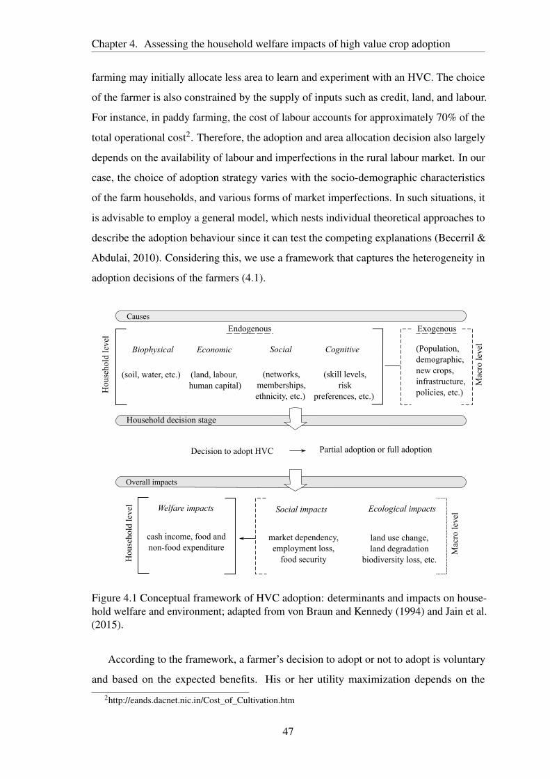
Chapter 4. Assessing the household welfare impacts of high value crop adoption
farming may initially allocate less area to learn and experiment with an HVC. The choice
of the farmer is also constrained by the supply of inputs such as credit, land, and labour.
For instance, in paddy farming, the cost of labour accounts for approximately 70% of the
total operational cost2. Therefore, the adoption and area allocation decision also largely
depends on the availability of labour and imperfections in the rural labour market. In our
case, the choice of adoption strategy varies with the socio-demographic characteristics
of the farm households, and various forms of market imperfections. In such situations, it
is advisable to employ a general model, which nests individual theoretical approaches to
describe the adoption behaviour since it can test the competing explanations (Becerril &
Abdulai, 2010). Considering this, we use a framework that captures the heterogeneity in
adoption decisions of the farmers (4.1).
Causes
Household decision stage
House
hold
lev
el
Endogenous
Biophysical
(soil, water, etc.)
Economic
(land, labour,
human capital)
Social
(networks,
memberships,
ethnicity, etc.)
Cognitive
(skill levels,
risk
preferences, etc.)
Exogenous
(Population,
demographic,
new crops,
infrastructure,
policies, etc.)
Mac
ro l
evel
Decision to adopt HVC Partial adoption or full adoption
Overall impacts
House
hold
lev
el Welfare impacts Social impacts Ecological impacts
cash income, food and
non-food expenditure
market dependency,
employment loss,
food security
land use change,
land degradation
biodiversity loss, etc.
Mac
ro l
evel
Figure 4.1 Conceptual framework of HVC adoption: determinants and impacts on house-hold welfare and environment; adapted from von Braun and Kennedy (1994) and Jain et al.(2015).
According to the framework, a farmer’s decision to adopt or not to adopt is voluntary
and based on the expected benefits. His or her utility maximization depends on the
2http://eands.dacnet.nic.in/Cost_of_Cultivation.htm
47
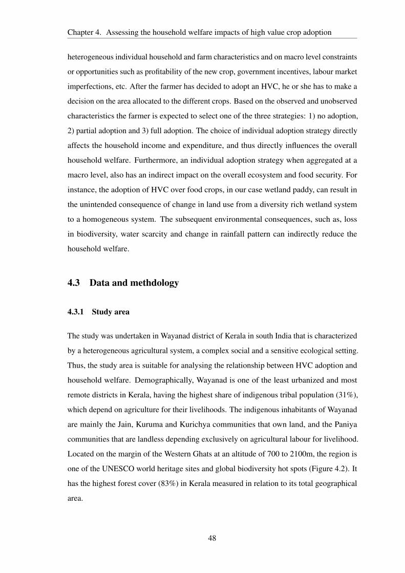
Chapter 4. Assessing the household welfare impacts of high value crop adoption
heterogeneous individual household and farm characteristics and on macro level constraints
or opportunities such as profitability of the new crop, government incentives, labour market
imperfections, etc. After the farmer has decided to adopt an HVC, he or she has to make a
decision on the area allocated to the different crops. Based on the observed and unobserved
characteristics the farmer is expected to select one of the three strategies: 1) no adoption,
2) partial adoption and 3) full adoption. The choice of individual adoption strategy directly
affects the household income and expenditure, and thus directly influences the overall
household welfare. Furthermore, an individual adoption strategy when aggregated at a
macro level, also has an indirect impact on the overall ecosystem and food security. For
instance, the adoption of HVC over food crops, in our case wetland paddy, can result in
the unintended consequence of change in land use from a diversity rich wetland system
to a homogeneous system. The subsequent environmental consequences, such as, loss
in biodiversity, water scarcity and change in rainfall pattern can indirectly reduce the
household welfare.
4.3 Data and methdology
4.3.1 Study area
The study was undertaken in Wayanad district of Kerala in south India that is characterized
by a heterogeneous agricultural system, a complex social and a sensitive ecological setting.
Thus, the study area is suitable for analysing the relationship between HVC adoption and
household welfare. Demographically, Wayanad is one of the least urbanized and most
remote districts in Kerala, having the highest share of indigenous tribal population (31%),
which depend on agriculture for their livelihoods. The indigenous inhabitants of Wayanad
are mainly the Jain, Kuruma and Kurichya communities that own land, and the Paniya
communities that are landless depending exclusively on agricultural labour for livelihood.
Located on the margin of the Western Ghats at an altitude of 700 to 2100m, the region is
one of the UNESCO world heritage sites and global biodiversity hot spots (Figure 4.2). It
has the highest forest cover (83%) in Kerala measured in relation to its total geographical
area.
48

Chapter 4. Assessing the household welfare impacts of high value crop adoption
The agricultural landscape of Wayanad traditionally consisted of high value plantations
(coffee, pepper, cardamom and tea) in the highland and paddy cultivation in the valley. The
average size of a land holding is 0.44 ha and 89% of these holdings are marginal farms
with less than one hectare. Wayanad harbours rich agro-biodiversity especially associated
with the wetland paddy fields (Parameswaran, Narayanan, & Kumar, 2014) and is home to
more than 75 local rice cultivars, including two rice cultivars with geographical indicator
status.
Thirunelli
MananthavadiThavinjal
Thondernadu
Edavaka
Vellamunda
Panamaram
Poothadi
Mullankolly
Pulpally
Kaniyambetta
Padinjarethara
Thariyode
Kottathara
Vengapally
Pozhuthana
Vythiri
Kalpetta
Muttil
Meenangadi
MeppadiMoopainade
Ambalavayal
Nenmeni
Noolpuzha
Sulthanbathery
Wayanad
Mananthavadi (ST)
Kalpetta
Sulthanbathery (ST)
Western ghats
Kerala
Wayanad
Vellamaunda
Panamaram
Edawaka
INDIA
Figure 4.2 Map showing the sampling locations of Wayanad district, Kerala in south India
Paddy cultivation has a strong cultural meaning, particularly among the indigenous
communities, as, rice being their staple food is essential to maintain food security (Kunze
& Momsen, 2015). Wayanad is classified as highly vulnerable to climate change due
to climate sensitive agriculture and forestry, and high dependence of marginalized tribal
communities on these sectors (Nanadakumar, 2014). The economic value of functions
and services lost in the region due to paddy-land adoption was estimated to be between
| 78,020 and | 97,646 per hectare in the year 2000 (Gopikuttan & Kurup, 2004). The
importance of paddy farming in the region, its richness in biodiversity and local rice
49
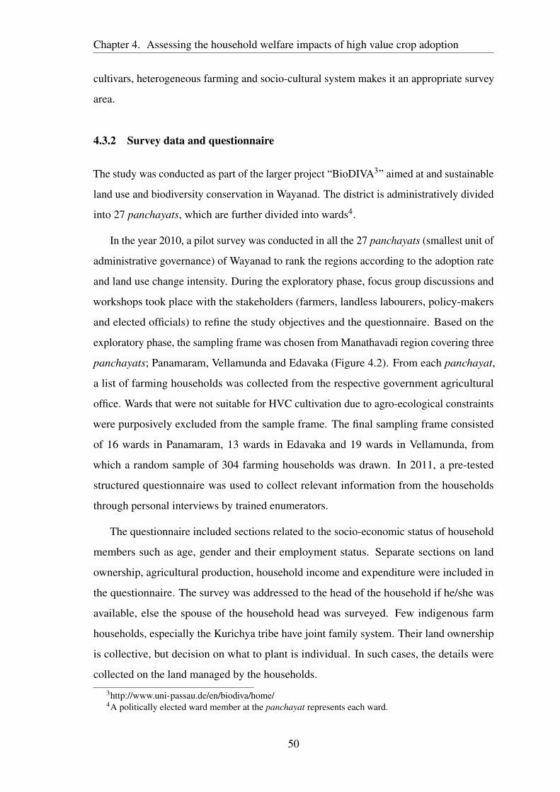
Chapter 4. Assessing the household welfare impacts of high value crop adoption
cultivars, heterogeneous farming and socio-cultural system makes it an appropriate survey
area.
4.3.2 Survey data and questionnaire
The study was conducted as part of the larger project “BioDIVA3” aimed at and sustainable
land use and biodiversity conservation in Wayanad. The district is administratively divided
into 27 panchayats, which are further divided into wards4.
In the year 2010, a pilot survey was conducted in all the 27 panchayats (smallest unit of
administrative governance) of Wayanad to rank the regions according to the adoption rate
and land use change intensity. During the exploratory phase, focus group discussions and
workshops took place with the stakeholders (farmers, landless labourers, policy-makers
and elected officials) to refine the study objectives and the questionnaire. Based on the
exploratory phase, the sampling frame was chosen from Manathavadi region covering three
panchayats; Panamaram, Vellamunda and Edavaka (Figure 4.2). From each panchayat,
a list of farming households was collected from the respective government agricultural
office. Wards that were not suitable for HVC cultivation due to agro-ecological constraints
were purposively excluded from the sample frame. The final sampling frame consisted
of 16 wards in Panamaram, 13 wards in Edavaka and 19 wards in Vellamunda, from
which a random sample of 304 farming households was drawn. In 2011, a pre-tested
structured questionnaire was used to collect relevant information from the households
through personal interviews by trained enumerators.
The questionnaire included sections related to the socio-economic status of household
members such as age, gender and their employment status. Separate sections on land
ownership, agricultural production, household income and expenditure were included in
the questionnaire. The survey was addressed to the head of the household if he/she was
available, else the spouse of the household head was surveyed. Few indigenous farm
households, especially the Kurichya tribe have joint family system. Their land ownership
is collective, but decision on what to plant is individual. In such cases, the details were
collected on the land managed by the households.
3http://www.uni-passau.de/en/biodiva/home/4A politically elected ward member at the panchayat represents each ward.
50
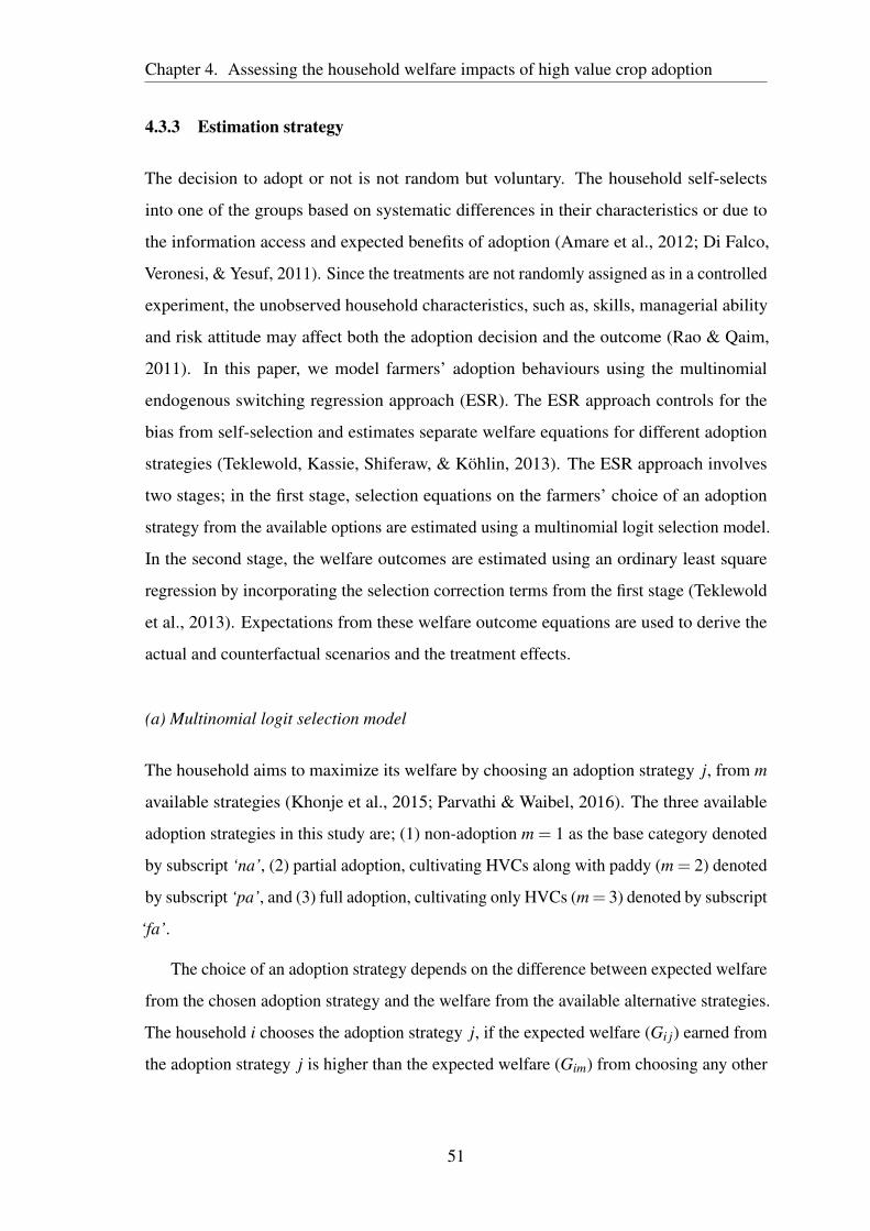
Chapter 4. Assessing the household welfare impacts of high value crop adoption
4.3.3 Estimation strategy
The decision to adopt or not is not random but voluntary. The household self-selects
into one of the groups based on systematic differences in their characteristics or due to
the information access and expected benefits of adoption (Amare et al., 2012; Di Falco,
Veronesi, & Yesuf, 2011). Since the treatments are not randomly assigned as in a controlled
experiment, the unobserved household characteristics, such as, skills, managerial ability
and risk attitude may affect both the adoption decision and the outcome (Rao & Qaim,
2011). In this paper, we model farmers’ adoption behaviours using the multinomial
endogenous switching regression approach (ESR). The ESR approach controls for the
bias from self-selection and estimates separate welfare equations for different adoption
strategies (Teklewold, Kassie, Shiferaw, & Köhlin, 2013). The ESR approach involves
two stages; in the first stage, selection equations on the farmers’ choice of an adoption
strategy from the available options are estimated using a multinomial logit selection model.
In the second stage, the welfare outcomes are estimated using an ordinary least square
regression by incorporating the selection correction terms from the first stage (Teklewold
et al., 2013). Expectations from these welfare outcome equations are used to derive the
actual and counterfactual scenarios and the treatment effects.
(a) Multinomial logit selection model
The household aims to maximize its welfare by choosing an adoption strategy j, from m
available strategies (Khonje et al., 2015; Parvathi & Waibel, 2016). The three available
adoption strategies in this study are; (1) non-adoption m = 1 as the base category denoted
by subscript ‘na’, (2) partial adoption, cultivating HVCs along with paddy (m = 2) denoted
by subscript ‘pa’, and (3) full adoption, cultivating only HVCs (m= 3) denoted by subscript
‘fa’.
The choice of an adoption strategy depends on the difference between expected welfare
from the chosen adoption strategy and the welfare from the available alternative strategies.
The household i chooses the adoption strategy j, if the expected welfare (Gi j) earned from
the adoption strategy j is higher than the expected welfare (Gim) from choosing any other
51
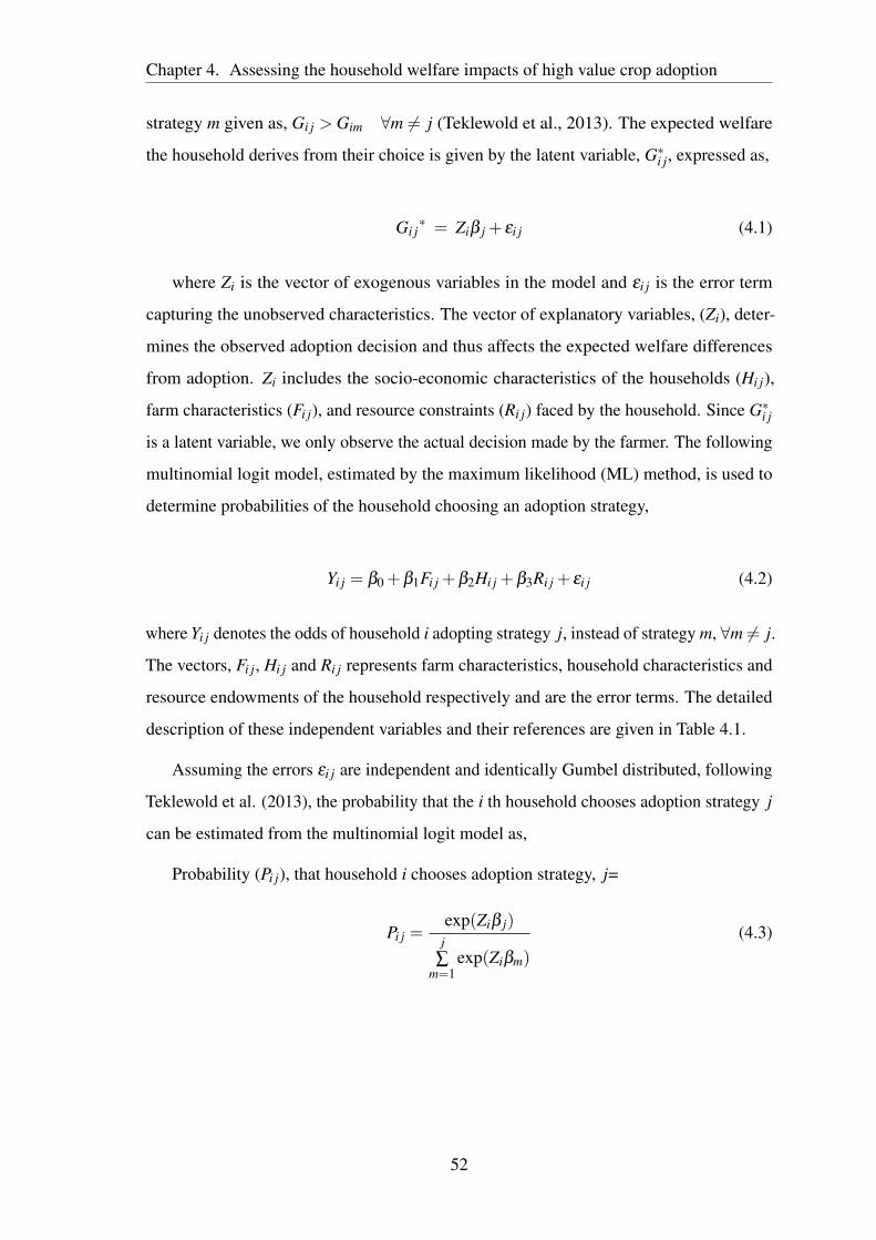
Chapter 4. Assessing the household welfare impacts of high value crop adoption
strategy m given as, Gi j > Gim ∀m ̸= j (Teklewold et al., 2013). The expected welfare
the household derives from their choice is given by the latent variable, G∗i j, expressed as,
Gi j∗ = Ziβ j + εi j (4.1)
where Zi is the vector of exogenous variables in the model and εi j is the error term
capturing the unobserved characteristics. The vector of explanatory variables, (Zi), deter-
mines the observed adoption decision and thus affects the expected welfare differences
from adoption. Zi includes the socio-economic characteristics of the households (Hi j),
farm characteristics (Fi j), and resource constraints (Ri j) faced by the household. Since G∗i j
is a latent variable, we only observe the actual decision made by the farmer. The following
multinomial logit model, estimated by the maximum likelihood (ML) method, is used to
determine probabilities of the household choosing an adoption strategy,
Yi j = β0 +β1Fi j +β2Hi j +β3Ri j + εi j (4.2)
where Yi j denotes the odds of household i adopting strategy j, instead of strategy m, ∀m ̸= j.
The vectors, Fi j, Hi j and Ri j represents farm characteristics, household characteristics and
resource endowments of the household respectively and are the error terms. The detailed
description of these independent variables and their references are given in Table 4.1.
Assuming the errors εi j are independent and identically Gumbel distributed, following
Teklewold et al. (2013), the probability that the i th household chooses adoption strategy j
can be estimated from the multinomial logit model as,
Probability (Pi j), that household i chooses adoption strategy, j=
Pi j =exp(Ziβ j)
j∑
m=1exp(Ziβm)
(4.3)
52
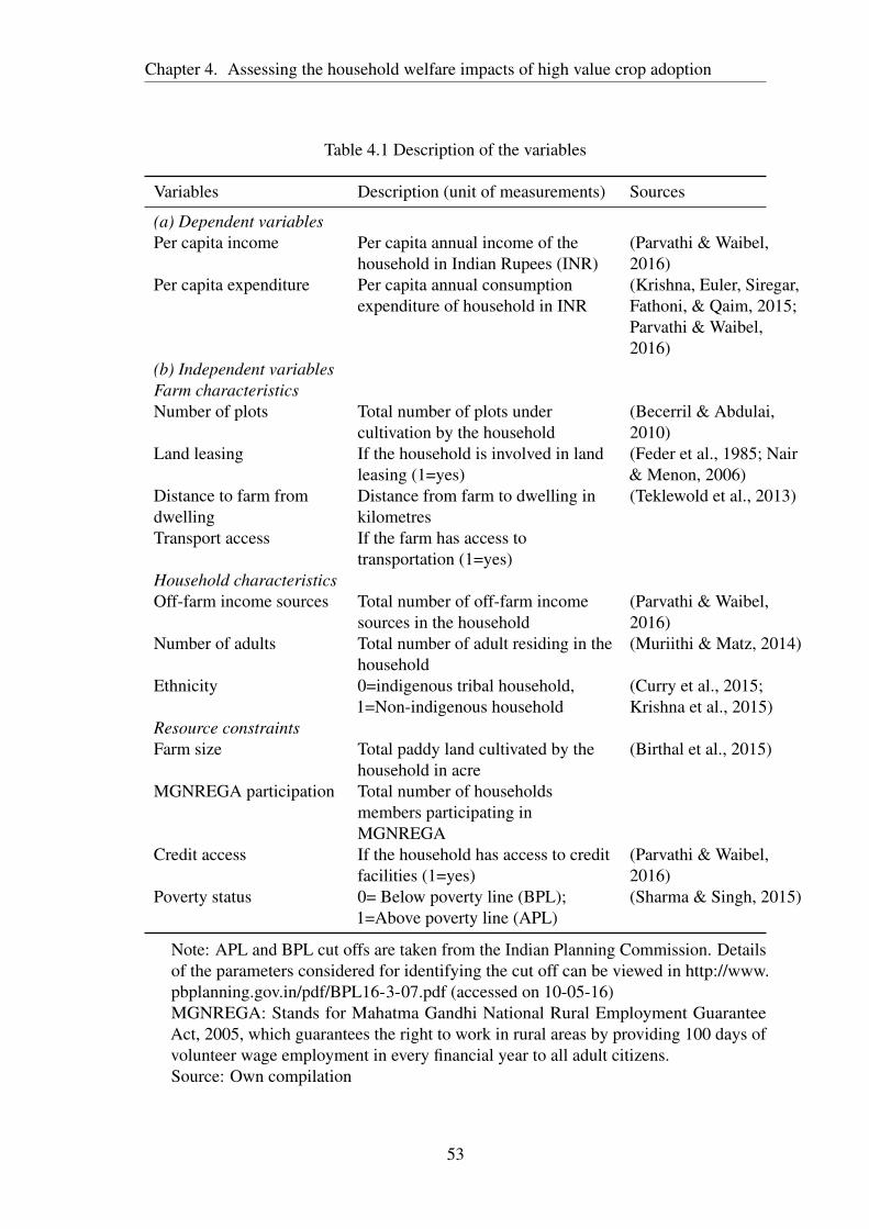
Chapter 4. Assessing the household welfare impacts of high value crop adoption
Table 4.1 Description of the variables
Variables Description (unit of measurements) Sources
(a) Dependent variablesPer capita income Per capita annual income of the
household in Indian Rupees (INR)(Parvathi & Waibel,2016)
Per capita expenditure Per capita annual consumptionexpenditure of household in INR
(Krishna, Euler, Siregar,Fathoni, & Qaim, 2015;Parvathi & Waibel,2016)
(b) Independent variablesFarm characteristicsNumber of plots Total number of plots under
cultivation by the household(Becerril & Abdulai,2010)
Land leasing If the household is involved in landleasing (1=yes)
(Feder et al., 1985; Nair& Menon, 2006)
Distance to farm fromdwelling
Distance from farm to dwelling inkilometres
(Teklewold et al., 2013)
Transport access If the farm has access totransportation (1=yes)
Household characteristicsOff-farm income sources Total number of off-farm income
sources in the household(Parvathi & Waibel,2016)
Number of adults Total number of adult residing in thehousehold
(Muriithi & Matz, 2014)
Ethnicity 0=indigenous tribal household,1=Non-indigenous household
(Curry et al., 2015;Krishna et al., 2015)
Resource constraintsFarm size Total paddy land cultivated by the
household in acre(Birthal et al., 2015)
MGNREGA participation Total number of householdsmembers participating inMGNREGA
Credit access If the household has access to creditfacilities (1=yes)
(Parvathi & Waibel,2016)
Poverty status 0= Below poverty line (BPL);1=Above poverty line (APL)
(Sharma & Singh, 2015)
Note: APL and BPL cut offs are taken from the Indian Planning Commission. Detailsof the parameters considered for identifying the cut off can be viewed in http://www.pbplanning.gov.in/pdf/BPL16-3-07.pdf (accessed on 10-05-16)MGNREGA: Stands for Mahatma Gandhi National Rural Employment GuaranteeAct, 2005, which guarantees the right to work in rural areas by providing 100 days ofvolunteer wage employment in every financial year to all adult citizens.Source: Own compilation
53
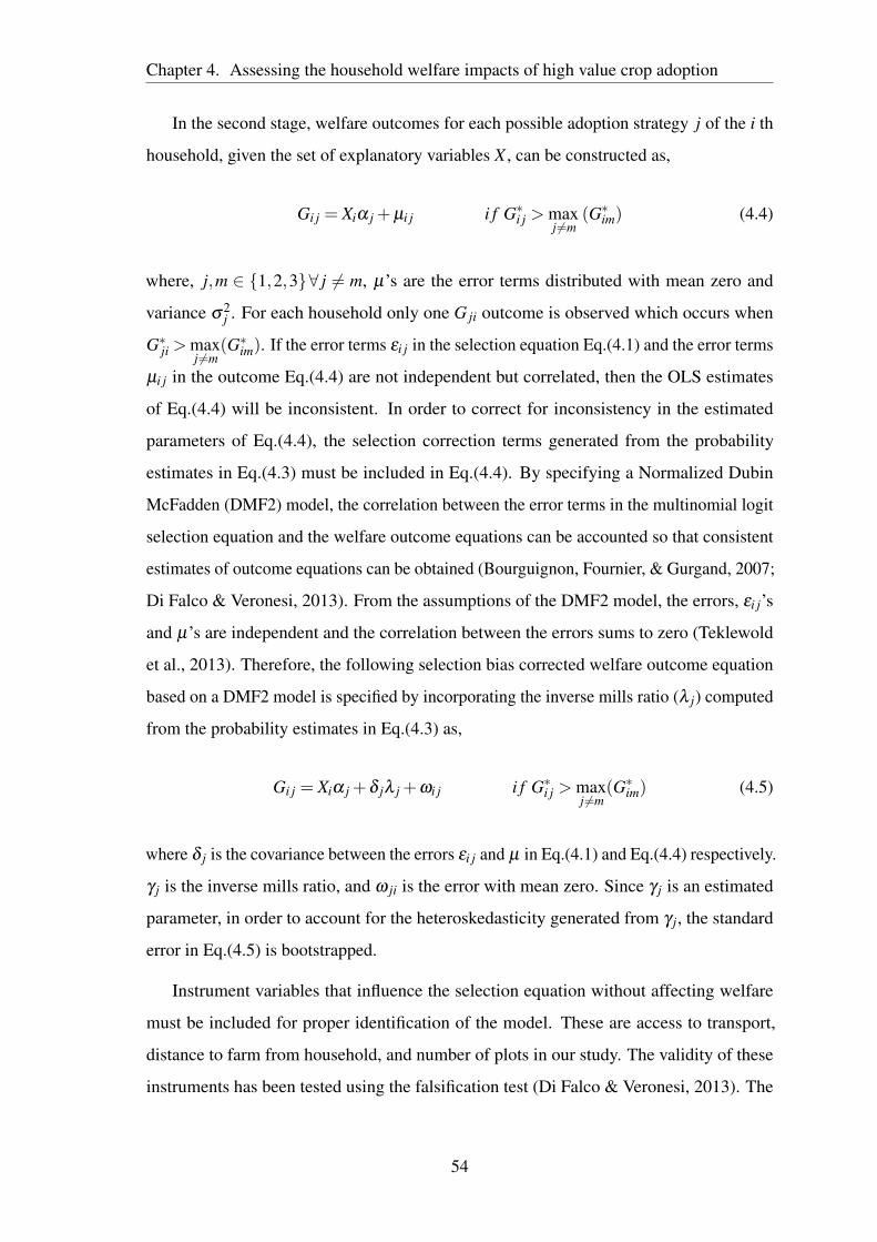
Chapter 4. Assessing the household welfare impacts of high value crop adoption
In the second stage, welfare outcomes for each possible adoption strategy j of the i th
household, given the set of explanatory variables X , can be constructed as,
Gi j = Xiα j +µi j i f G∗i j > max
j ̸=m(G∗
im) (4.4)
where, j,m ∈ {1,2,3}∀ j ̸= m, µ’s are the error terms distributed with mean zero and
variance σ2j . For each household only one G ji outcome is observed which occurs when
G∗ji > max
j ̸=m(G∗
im). If the error terms εi j in the selection equation Eq.(4.1) and the error terms
µi j in the outcome Eq.(4.4) are not independent but correlated, then the OLS estimates
of Eq.(4.4) will be inconsistent. In order to correct for inconsistency in the estimated
parameters of Eq.(4.4), the selection correction terms generated from the probability
estimates in Eq.(4.3) must be included in Eq.(4.4). By specifying a Normalized Dubin
McFadden (DMF2) model, the correlation between the error terms in the multinomial logit
selection equation and the welfare outcome equations can be accounted so that consistent
estimates of outcome equations can be obtained (Bourguignon, Fournier, & Gurgand, 2007;
Di Falco & Veronesi, 2013). From the assumptions of the DMF2 model, the errors, εi j’s
and µ’s are independent and the correlation between the errors sums to zero (Teklewold
et al., 2013). Therefore, the following selection bias corrected welfare outcome equation
based on a DMF2 model is specified by incorporating the inverse mills ratio (λ j) computed
from the probability estimates in Eq.(4.3) as,
Gi j = Xiα j +δ jλ j +ωi j i f G∗i j > max
j ̸=m(G∗
im) (4.5)
where δ j is the covariance between the errors εi j and µ in Eq.(4.1) and Eq.(4.4) respectively.
γ j is the inverse mills ratio, and ω ji is the error with mean zero. Since γ j is an estimated
parameter, in order to account for the heteroskedasticity generated from γ j, the standard
error in Eq.(4.5) is bootstrapped.
Instrument variables that influence the selection equation without affecting welfare
must be included for proper identification of the model. These are access to transport,
distance to farm from household, and number of plots in our study. The validity of these
instruments has been tested using the falsification test (Di Falco & Veronesi, 2013). The
54
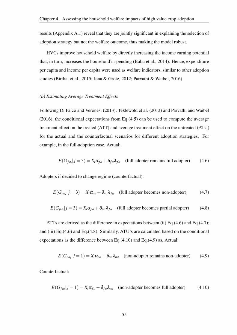
Chapter 4. Assessing the household welfare impacts of high value crop adoption
results (Appendix A.1) reveal that they are jointly significant in explaining the selection of
adoption strategy but not the welfare outcome, thus making the model robust.
HVCs improve household welfare by directly increasing the income earning potential
that, in turn, increases the household’s spending (Babu et al., 2014). Hence, expenditure
per capita and income per capita were used as welfare indicators, similar to other adoption
studies (Birthal et al., 2015; Jena & Grote, 2012; Parvathi & Waibel, 2016)
(b) Estimating Average Treatment Effects
Following Di Falco and Veronesi (2013); Teklewold et al. (2013) and Parvathi and Waibel
(2016), the conditional expectations from Eq.(4.5) can be used to compute the average
treatment effect on the treated (ATT) and average treatment effect on the untreated (ATU)
for the actual and the counterfactual scenarios for different adoption strategies. For
example, in the full-adoption case, Actual:
E(G f ai| j = 3) = Xiα f a +δ f aλ f a (full adopter remains full adopter) (4.6)
Adopters if decided to change regime (counterfactual):
E(Gnai| j = 3) = Xiαna +δnaλ f a (full adopter becomes non-adopter) (4.7)
E(Gpai| j = 3) = Xiαpa +δpaλ f a (full adopter becomes partial adopter) (4.8)
ATTs are derived as the difference in expectations between (ii) Eq.(4.6) and Eq.(4.7);
and (iii) Eq.(4.6) and Eq.(4.8). Similarly, ATU’s are calculated based on the conditional
expectations as the difference between Eq.(4.10) and Eq.(4.9) as, Actual:
E(Gnai| j = 1) = Xiαna +δnaλna (non-adopter remains non-adopter) (4.9)
Counterfactual:
E(G f ai| j = 1) = Xiα f a +δ f aλna (non-adopter becomes full adopter) (4.10)
55
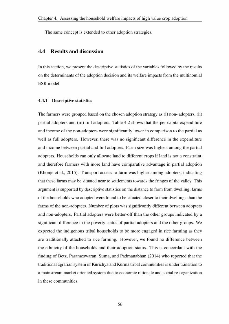
Chapter 4. Assessing the household welfare impacts of high value crop adoption
The same concept is extended to other adoption strategies.
4.4 Results and discussion
In this section, we present the descriptive statistics of the variables followed by the results
on the determinants of the adoption decision and its welfare impacts from the multinomial
ESR model.
4.4.1 Descriptive statistics
The farmers were grouped based on the chosen adoption strategy as (i) non- adopters, (ii)
partial adopters and (iii) full adopters. Table 4.2 shows that the per capita expenditure
and income of the non-adopters were significantly lower in comparison to the partial as
well as full adopters. However, there was no significant difference in the expenditure
and income between partial and full adopters. Farm size was highest among the partial
adopters. Households can only allocate land to different crops if land is not a constraint,
and therefore farmers with more land have comparative advantage in partial adoption
(Khonje et al., 2015). Transport access to farm was higher among adopters, indicating
that these farms may be situated near to settlements towards the fringes of the valley. This
argument is supported by descriptive statistics on the distance to farm from dwelling; farms
of the households who adopted were found to be situated closer to their dwellings than the
farms of the non-adopters. Number of plots was significantly different between adopters
and non-adopters. Partial adopters were better-off than the other groups indicated by a
significant difference in the poverty status of partial adopters and the other groups. We
expected the indigenous tribal households to be more engaged in rice farming as they
are traditionally attached to rice farming. However, we found no difference between
the ethnicity of the households and their adoption status. This is concordant with the
finding of Betz, Parameswaran, Suma, and Padmanabhan (2014) who reported that the
traditional agrarian system of Kurichya and Kurma tribal communities is under transition to
a mainstream market oriented system due to economic rationale and social re-organization
in these communities.
56
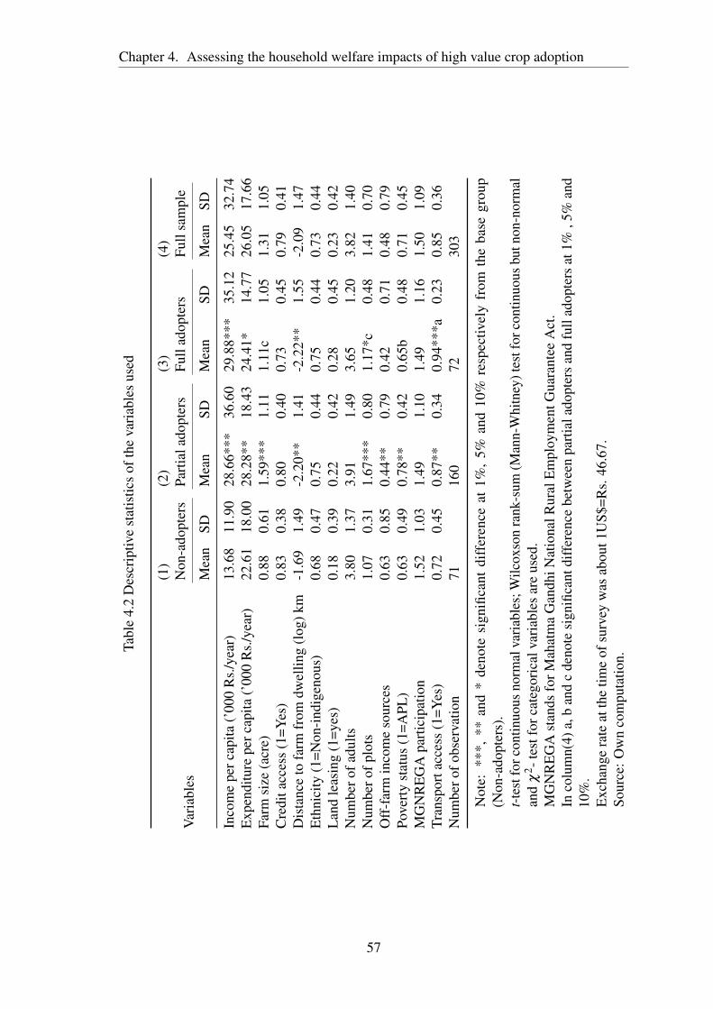
Chapter 4. Assessing the household welfare impacts of high value crop adoption
Tabl
e4.
2D
escr
iptiv
est
atis
tics
ofth
eva
riab
les
used
(1)
(2)
(3)
(4)
Var
iabl
esN
on-a
dopt
ers
Part
iala
dopt
ers
Full
adop
ters
Full
sam
ple
Mea
nSD
Mea
nSD
Mea
nSD
Mea
nSD
Inco
me
perc
apita
(’00
0R
s./y
ear)
13.6
811
.90
28.6
6***
36.6
029
.88*
**35
.12
25.4
532
.74
Exp
endi
ture
perc
apita
(’00
0R
s./y
ear)
22.6
118
.00
28.2
8**
18.4
324
.41*
14.7
726
.05
17.6
6Fa
rmsi
ze(a
cre)
0.88
0.61
1.59
***
1.11
1.11
c1.
051.
311.
05C
redi
tacc
ess
(1=Y
es)
0.83
0.38
0.80
0.40
0.73
0.45
0.79
0.41
Dis
tanc
eto
farm
from
dwel
ling
(log
)km
-1.6
91.
49-2
.20*
*1.
41-2
.22*
*1.
55-2
.09
1.47
Eth
nici
ty(1
=Non
-ind
igen
ous)
0.68
0.47
0.75
0.44
0.75
0.44
0.73
0.44
Lan
dle
asin
g(1
=yes
)0.
180.
390.
220.
420.
280.
450.
230.
42N
umbe
rofa
dults
3.80
1.37
3.91
1.49
3.65
1.20
3.82
1.40
Num
bero
fplo
ts1.
070.
311.
67**
*0.
801.
17*c
0.48
1.41
0.70
Off
-far
min
com
eso
urce
s0.
630.
850.
44**
0.79
0.42
0.71
0.48
0.79
Pove
rty
stat
us(1
=APL
)0.
630.
490.
78**
0.42
0.65
b0.
480.
710.
45M
GN
RE
GA
part
icip
atio
n1.
521.
031.
491.
101.
491.
161.
501.
09Tr
ansp
orta
cces
s(1
=Yes
)0.
720.
450.
87**
0.34
0.94
***a
0.23
0.85
0.36
Num
bero
fobs
erva
tion
7116
072
303
Not
e:**
*,**
and
*de
note
sign
ifica
ntdi
ffer
ence
at1%
,5%
and
10%
resp
ectiv
ely
from
the
base
grou
p(N
on-a
dopt
ers)
.t-t
estf
orco
ntin
uous
norm
alva
riabl
es;W
ilcox
son
rank
-sum
(Man
n-W
hitn
ey)t
estf
orco
ntin
uous
butn
on-n
orm
alan
dχ
2 -tes
tfor
cate
gori
calv
aria
bles
are
used
.M
GN
RE
GA
stan
dsfo
rMah
atm
aG
andh
iNat
iona
lRur
alE
mpl
oym
entG
uara
ntee
Act
.In
colu
mn(
4)a,
ban
dc
deno
tesi
gnifi
cant
diff
eren
cebe
twee
npa
rtia
lado
pter
san
dfu
llad
opte
rsat
1%,5
%an
d10
%.
Exc
hang
era
teat
the
time
ofsu
rvey
was
abou
t1U
S$=R
s.46
.67.
Sour
ce:O
wn
com
puta
tion.
57
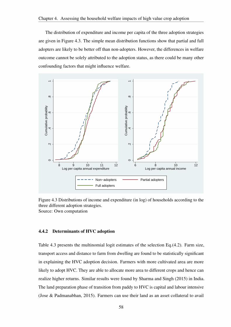
Chapter 4. Assessing the household welfare impacts of high value crop adoption
The distribution of expenditure and income per capita of the three adoption strategies
are given in Figure 4.3. The simple mean distribution functions show that partial and full
adopters are likely to be better off than non-adopters. However, the differences in welfare
outcome cannot be solely attributed to the adoption status, as there could be many other
confounding factors that might influence welfare.
0.2
.4.6
.81
Cum
ulat
ive
prob
ablit
y
8 9 10 11 12Log per capita annual expenditure
0.2
.4.6
.81
Cum
ulat
ive
prob
ablit
y
6 8 10 12Log per capita annual income
Non−adopters Partial adopters
Full adopters
Figure 4.3 Distributions of income and expenditure (in log) of households according to thethree different adoption strategies.Source: Own computation
4.4.2 Determinants of HVC adoption
Table 4.3 presents the multinomial logit estimates of the selection Eq.(4.2). Farm size,
transport access and distance to farm from dwelling are found to be statistically significant
in explaining the HVC adoption decision. Farmers with more cultivated area are more
likely to adopt HVC. They are able to allocate more area to different crops and hence can
realize higher returns. Similar results were found by Sharma and Singh (2015) in India.
The land preparation phase of transition from paddy to HVC is capital and labour intensive
(Jose & Padmanabhan, 2015). Farmers can use their land as an asset collateral to avail
58
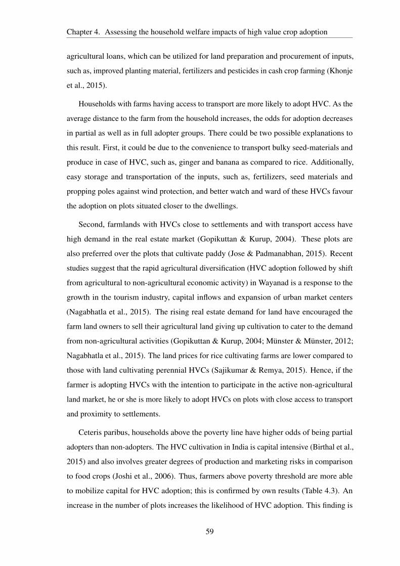
Chapter 4. Assessing the household welfare impacts of high value crop adoption
agricultural loans, which can be utilized for land preparation and procurement of inputs,
such as, improved planting material, fertilizers and pesticides in cash crop farming (Khonje
et al., 2015).
Households with farms having access to transport are more likely to adopt HVC. As the
average distance to the farm from the household increases, the odds for adoption decreases
in partial as well as in full adopter groups. There could be two possible explanations to
this result. First, it could be due to the convenience to transport bulky seed-materials and
produce in case of HVC, such as, ginger and banana as compared to rice. Additionally,
easy storage and transportation of the inputs, such as, fertilizers, seed materials and
propping poles against wind protection, and better watch and ward of these HVCs favour
the adoption on plots situated closer to the dwellings.
Second, farmlands with HVCs close to settlements and with transport access have
high demand in the real estate market (Gopikuttan & Kurup, 2004). These plots are
also preferred over the plots that cultivate paddy (Jose & Padmanabhan, 2015). Recent
studies suggest that the rapid agricultural diversification (HVC adoption followed by shift
from agricultural to non-agricultural economic activity) in Wayanad is a response to the
growth in the tourism industry, capital inflows and expansion of urban market centers
(Nagabhatla et al., 2015). The rising real estate demand for land have encouraged the
farm land owners to sell their agricultural land giving up cultivation to cater to the demand
from non-agricultural activities (Gopikuttan & Kurup, 2004; Münster & Münster, 2012;
Nagabhatla et al., 2015). The land prices for rice cultivating farms are lower compared to
those with land cultivating perennial HVCs (Sajikumar & Remya, 2015). Hence, if the
farmer is adopting HVCs with the intention to participate in the active non-agricultural
land market, he or she is more likely to adopt HVCs on plots with close access to transport
and proximity to settlements.
Ceteris paribus, households above the poverty line have higher odds of being partial
adopters than non-adopters. The HVC cultivation in India is capital intensive (Birthal et al.,
2015) and also involves greater degrees of production and marketing risks in comparison
to food crops (Joshi et al., 2006). Thus, farmers above poverty threshold are more able
to mobilize capital for HVC adoption; this is confirmed by own results (Table 4.3). An
increase in the number of plots increases the likelihood of HVC adoption. This finding is
59
Chapter 4. Assessing the household welfare impacts of high value crop adoption
Table 4.3 Multinomial logit results (selection equation)
VariablesPartial
adoptersSE
Full
adoptersSE
Transport access(1=Yes) 1.002** (0.426) 1.985*** (0.615)
Distance to farm from dwelling (log) -0.264** (0.116) -0.321** (0.130)
Number of plots 2.225*** (0.535) 0.525 (0.592)
Number of adults 0.087 (0.135) -0.107 (0.150)
Credit access (1=Yes) -0.543 (0.443) -0.750 (0.473)
Poverty status (1=APL) 0.963* (0.546) -0.013 (0.537)
Farm size (acre) 0.790*** (0.245) 0.512** (0.226)
Land leasing (1=yes) -0.725 (0.483) 0.315 (0.483)
Ethnicity (1=Non-indigenous) -0.185 (0.531) 0.735 (0.564)
Off-farm income sources -0.327 (0.230) -0.297 (0.256)
MGNREGA participation -0.032 (0.172) -0.002 (0.189)
Constant -4.291*** -2.888**
Chi-square 117.746***
Pseudo R2 0.191
N 303
Note: Robust standard errors in parentheses; ***, significant at 1%; **, signifi-cant at 5%; *, significant at 10%Base category: Non-adopters.Source: Own computation.
supported by Guillerme et al. (2011) where the authors argue land fragmentation, as the
cause of land use intensification and monoculture of commercial crops in Kerala.
4.4.3 Welfare impacts of heterogeneous adoption
The welfare outcome variables, income per capita and expenditure per capita were right-
skewed and hence were transformed into logarithms to obtain a more symmetric distri-
bution. The second stage coefficient estimates of multinomial endogenous switching
regression are given in Appendix A.2. These results are not discussed in detail, as in this
section we focus on the impact of different levels of adoption on the welfare outcome.
60
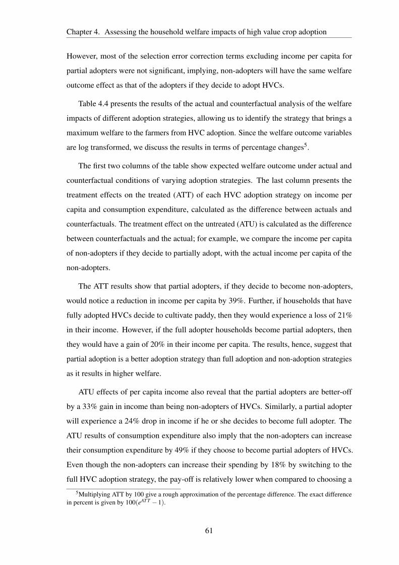
Chapter 4. Assessing the household welfare impacts of high value crop adoption
However, most of the selection error correction terms excluding income per capita for
partial adopters were not significant, implying, non-adopters will have the same welfare
outcome effect as that of the adopters if they decide to adopt HVCs.
Table 4.4 presents the results of the actual and counterfactual analysis of the welfare
impacts of different adoption strategies, allowing us to identify the strategy that brings a
maximum welfare to the farmers from HVC adoption. Since the welfare outcome variables
are log transformed, we discuss the results in terms of percentage changes5.
The first two columns of the table show expected welfare outcome under actual and
counterfactual conditions of varying adoption strategies. The last column presents the
treatment effects on the treated (ATT) of each HVC adoption strategy on income per
capita and consumption expenditure, calculated as the difference between actuals and
counterfactuals. The treatment effect on the untreated (ATU) is calculated as the difference
between counterfactuals and the actual; for example, we compare the income per capita
of non-adopters if they decide to partially adopt, with the actual income per capita of the
non-adopters.
The ATT results show that partial adopters, if they decide to become non-adopters,
would notice a reduction in income per capita by 39%. Further, if households that have
fully adopted HVCs decide to cultivate paddy, then they would experience a loss of 21%
in their income. However, if the full adopter households become partial adopters, then
they would have a gain of 20% in their income per capita. The results, hence, suggest that
partial adoption is a better adoption strategy than full adoption and non-adoption strategies
as it results in higher welfare.
ATU effects of per capita income also reveal that the partial adopters are better-off
by a 33% gain in income than being non-adopters of HVCs. Similarly, a partial adopter
will experience a 24% drop in income if he or she decides to become full adopter. The
ATU results of consumption expenditure also imply that the non-adopters can increase
their consumption expenditure by 49% if they choose to become partial adopters of HVCs.
Even though the non-adopters can increase their spending by 18% by switching to the
full HVC adoption strategy, the pay-off is relatively lower when compared to choosing a
5Multiplying ATT by 100 give a rough approximation of the percentage difference. The exact differencein percent is given by 100(eAT T −1).
61
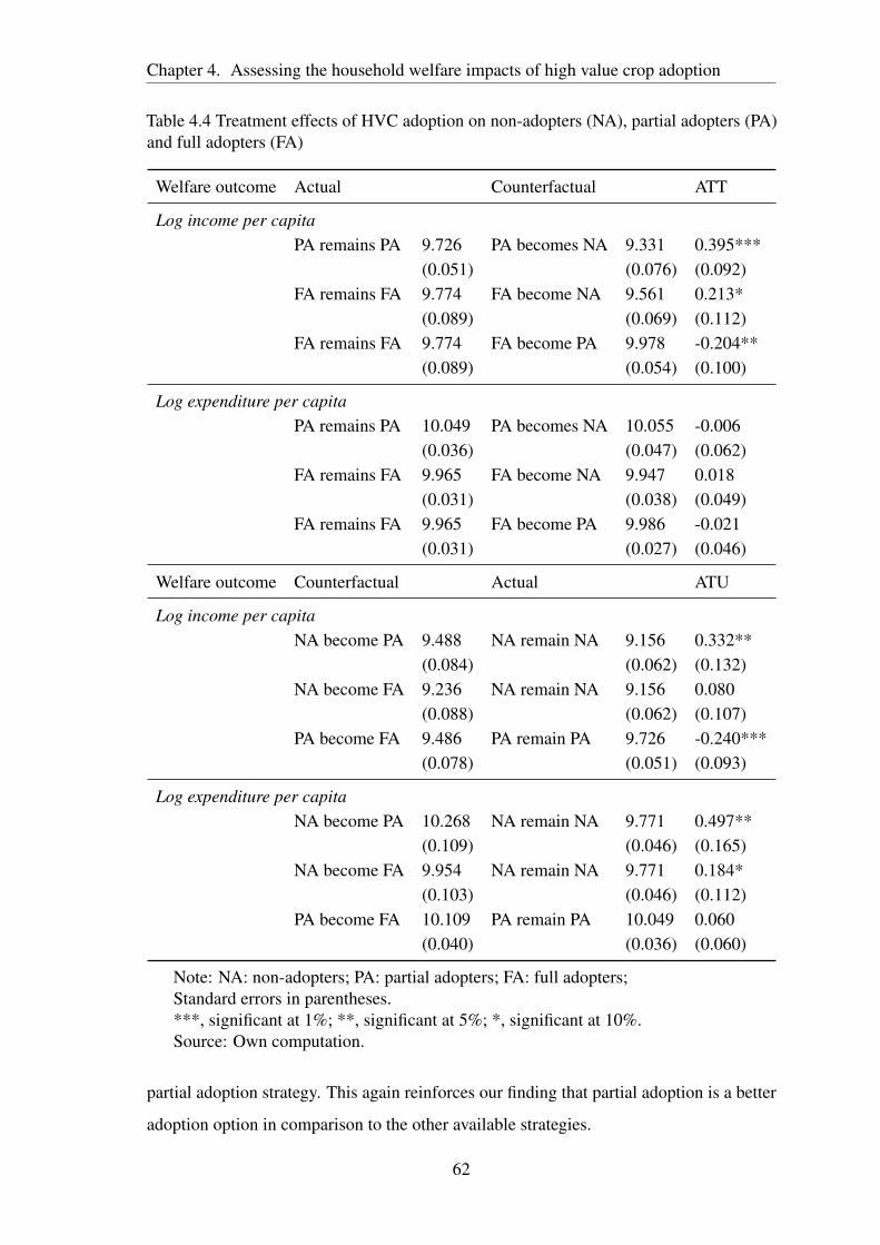
Chapter 4. Assessing the household welfare impacts of high value crop adoption
Table 4.4 Treatment effects of HVC adoption on non-adopters (NA), partial adopters (PA)and full adopters (FA)
Welfare outcome Actual Counterfactual ATT
Log income per capitaPA remains PA 9.726 PA becomes NA 9.331 0.395***
(0.051) (0.076) (0.092)FA remains FA 9.774 FA become NA 9.561 0.213*
(0.089) (0.069) (0.112)FA remains FA 9.774 FA become PA 9.978 -0.204**
(0.089) (0.054) (0.100)
Log expenditure per capitaPA remains PA 10.049 PA becomes NA 10.055 -0.006
(0.036) (0.047) (0.062)FA remains FA 9.965 FA become NA 9.947 0.018
(0.031) (0.038) (0.049)FA remains FA 9.965 FA become PA 9.986 -0.021
(0.031) (0.027) (0.046)
Welfare outcome Counterfactual Actual ATU
Log income per capitaNA become PA 9.488 NA remain NA 9.156 0.332**
(0.084) (0.062) (0.132)NA become FA 9.236 NA remain NA 9.156 0.080
(0.088) (0.062) (0.107)PA become FA 9.486 PA remain PA 9.726 -0.240***
(0.078) (0.051) (0.093)
Log expenditure per capitaNA become PA 10.268 NA remain NA 9.771 0.497**
(0.109) (0.046) (0.165)NA become FA 9.954 NA remain NA 9.771 0.184*
(0.103) (0.046) (0.112)PA become FA 10.109 PA remain PA 10.049 0.060
(0.040) (0.036) (0.060)
Note: NA: non-adopters; PA: partial adopters; FA: full adopters;Standard errors in parentheses.***, significant at 1%; **, significant at 5%; *, significant at 10%.Source: Own computation.
partial adoption strategy. This again reinforces our finding that partial adoption is a better
adoption option in comparison to the other available strategies.
62
Chapter 4. Assessing the household welfare impacts of high value crop adoption
In other words, from the analysis of counterfactuals of income and expenditure, even
though HVC adoption results in increased welfare outcome, we find statistical evidence to
infer that the household welfare can be maximized by following the most effective strategy
of growing HVC in combination with paddy. Our results are corroborated by Birthal
et al. (2015), where the odds of reducing the poverty for smallholders in India remain
unchanged when the intensity of HVC adoption was above 60% of the total cultivated
area, suggesting that further expansion of area under HVCs beyond the threshold might
not increase farmers’ welfare.
4.5 Conclusion
The objectives of the paper were to analyse the determinants of HVC adoption and the
impact of adoption on the household welfare, especially, of small and medium farmers
in India. The study uses cross sectional household data from 303 farming households
collected in 2011 from Wayanad district of Kerala, South India. This is a region, which
is ecologically sensitive and rich in biodiversity, and where agriculture is in a transition
stage from subsistence paddy farming to HVC, such as, banana and ginger. Annual per
capita income and per capita consumption expenditure were used as proxies for measuring
household welfare. Multinomial endogenous switching regression model with selection
bias correction was applied to assess the impact of heterogeneous adoption decision on
household welfare.
The analysis of the determinants of adoption showed that the adoption of HVC is
significantly related to the landholding size, distance to farm from dwelling, transport
access and number of cultivated plots. Overall, our findings support the hypothesis that
the adoption of HVCs increases the welfare of farmers. The analysis of the counterfactual
estimates indicates that the non-adopters can realize an increase in their income and
spending if they adopt HVC. The estimates of heterogeneous impacts of levels of adoption
reveal that the households which grow both HVC and paddy rice, meaning, that they have
at least allocated a proportion of their cultivable area to food crops, are found to have higher
income and consumption expenditure than the non-adopters and full adopters. Therefore,
the question arises, as to what explains the positive impact on the household welfare of
63

Chapter 4. Assessing the household welfare impacts of high value crop adoption
partial adopters. First, in case of full adopters due to the long growing duration of HVCs
such as ginger, banana and areca nut, by allocating their entire land to HVCs the food
supply and household income might be negatively affected, thus reducing their welfare in
the short and medium term (Babu et al., 2014). Second, the agricultural intensification and
incorrect cultivation practices associated with HVCs have resulted in negative ecological
consequences leading to the degradation of land and reduction in productivity of HVCs
(Nair & Menon, 2006). By allocating a certain proportion of their farm land to paddy,
the partial adopters are able to reduce the intensity of land degradation thus restoring
the ecological balance and minimize the risk arising from production. Our argument is
also supported by Parameswaran et al. (2014) who noted that paddy fields and associated
diversity play a significant role in controlling and restoring the agro-ecological balance of
the wetland system.
Commercial crop adoption is seen as an irreversible phenomenon that is triggered
by economic growth (Pingali, 2004) and is aimed at the improvement of the rural living
conditions. At the same time, it is seen as a major threat to the environment and biodiversity
(Nadesapanicker et al., 2011). In view of this, the government of Kerala has taken
an initiative to preserve the wetland paddy in the state, the most important ones being
the Kerala Conservation of Paddy Land and Wetland Act of 2008 and the scheme for
comprehensive development of rice. Our findings will facilitate the policy-makers in
developing more targeted policies and implementation plans for such initiatives, which
would not only aim at improving the welfare of farmers but also maintain the ecological
balance and overall sustainability of the system. The intrinsic differences among the
groups of households and heterogeneity in the welfare impact suggest for policy measures
and incentive programs addressing HVC adoption that are not generalized, but effectively
targeted in consideration with the socioeconomic conditions and welfare differentials
across the target groups.
References
Abdussalam, A. K., Aslam, M. M. A., Jyothi, P. V., Azeez, K., & Girijan, G. (2011).Ecological impact of changing cultivation on the biodiversity of Wayanad, Kerala,India. Millennium Zoology, 12(1), 44–49.
64

Chapter 4. Assessing the household welfare impacts of high value crop adoption
Altieri, M. A., & Nicholis, C. I. (2005). Agroecology and the search for a truly sustain-able agriculture. Mexico D.F., Mexico: United Nations Environmental Programme,Environmental Training Network for Latin America and the Caribbean.
Amare, M., Asfaw, S., & Shiferaw, B. (2012). Welfare impacts of maize-pigeonpeaintensification in Tanzania. Agricultural Economics, 43(1), 27–43. doi:10.1111/j.1574-0862.2011.00563.x
Aragona, F. B., & Orr, B. (2011). Agricultural Intensification, Monocultures, and EconomicFailure: The Case of Onion Production in the Tipajara Watershed on the EasternSlope of the Bolivian Andes. Journal of Sustainable Agriculture, 35(5), 467–492.doi:10.1080/10440046.2011.579832
Asfaw, S., Kassie, M., Simtowe, F., & Lipper, L. (2012). Poverty reduction effects ofagricultural technology adoption: A micro-evidence from rural Tanzania. The Journalof Development Studies, 48(9), 1288–1305. doi:10.1080/00220388.2012.671475
Asfaw, S., Shiferaw, B., Simtowe, F., & Lipper, L. (2012). Impact of modern agriculturaltechnologies on smallholder welfare: Evidence from Tanzania and Ethiopia. FoodPolicy, 37(3), 283–295. doi:10.1016/j.foodpol.2012.02.013
Babu, S. C., Gajanan, S. N., & Sanyal, P. (2014). Effects of commercialization of agri-culture (shift from traditional crop to cash crop) on food consumption and nutrition:Application of Chi-square statistic. In S. C. Babu, S. N. Gajanan, & P. Sanyal (Eds.),Food Security, Poverty and Nutrition Policy Analysis (Second Edition ed., pp. 63–91).San Diego: Elsevier.
Banik, P., Edmonds, C., & Fuwa, N. (2014). Sustainability implications of the evolutionof rice farming amid rural poverty: The case of the Chhotanagpur Plateau in EasternIndia. Journal of Sustainable Development, 7(4), 282-297. doi:10.5539/jsd.v7n4p282
Barbier, E. B. (1989). Cash crops, food crops, and sustainability: The case of Indonesia.World Development, 17(6), 879–895. doi:10.1016/0305-750x(89)90009-0
Becerril, J., & Abdulai, A. (2010). The Impact of Improved Maize Varieties on Povertyin Mexico: A Propensity Score-Matching Approach. World Development, 38(7),1024–1035. doi:10.1016/j.worlddev.2009.11.017
Betz, L., Parameswaran, P., Suma, T. R., & Padmanabhan, M. (2014). The social–ecologicalweb: A bridging concept for transdisciplinary research. Current Science, 107(4),572–579.
Birthal, P. S., Joshi, P. K., Roy, D., & Thorat, A. (2013). Diversification in Indianagriculture toward High-Value Crops: The role of small farmers. Canadian Journalof Agricultural Economics/Revue canadienne d’agroeconomie, 61(1), 61–91. doi:10.1111/j.1744-7976.2012.01258.x
65
Chapter 4. Assessing the household welfare impacts of high value crop adoption
Birthal, P. S., Roy, D., & Negi, D. S. (2015). Assessing the impact of crop diversificationon farm poverty in India. World Development, 72, 70–92. doi:10.1016/j.worlddev.2015.02.015
Bommarco, R., Kleijn, D., & Potts, S. G. (2013). Ecological intensification: Harnessingecosystem services for food security. Trends in Ecology & Evolution, 28(4), 230–238.doi:10.1016/j.tree.2012.10.012
Coromaldi, M., Pallante, G., & Savastano, S. (2015). Adoption of modern varieties,farmers’ welfare and crop biodiversity: Evidence from Uganda. Ecological Economics,119, 346–358. doi:10.1016/j.ecolecon.2015.09.004
Curry, G. N., Koczberski, G., Lummani, J., Nailina, R., Peter, E., McNally, G., & Kuaimba,O. (2015). A bridge too far?: The influence of socio-cultural values on the adaptation re-sponses of smallholders to a devastating pest outbreak in cocoa. Global EnvironmentalChange, 35, 1–11. doi:10.1016/j.gloenvcha.2015.07.012
Di Falco, S., & Veronesi, M. (2013). How can African agriculture adapt to climatechange?: A counterfactual analysis from Ethiopia. Land Economics, 89(4), 743–766.doi:10.3368/le.89.4.743
Di Falco, S., Veronesi, M., & Yesuf, M. (2011). Does adaptation to climate change providefood security?: A micro-perspective from Ethiopia. American Journal of AgriculturalEconomics, 93(3), 829–846. doi:10.1093/ajae/aar006
Feder, G., Just, R. E., & Zilberman, D. (1985). Adoption of agricultural innovations indeveloping countries: A survey. Economic Development and Cultural Change, 33(2),255–298.
Feder, G., & Umali, D. L. (1993). The adoption of agricultural innovations: A review. Tech-nological Forecasting and Social Change, 43(3), 215–239. doi:10.1016/0040-1625(93)90053-a
Garcia-Yi, J. (2014). Market Participation and Agro-Biodiversity Loss: The Case ofNative Chili Varieties in the Amazon Rainforest of Peru. Sustainability, 6(2), 615–630.doi:10.3390/su6020615
George, J., & Krishnaprasad, P. (2006). Agrarian distress and farmers’ suicides in the tribaldistrict of Wayanad. Social Scientist, 34(7/8), 70–85.
George, P. S., & Chattopadhyay, S. (2001). Population and land use in Kerala. In P.National Academy (Ed.), Growing populations, changing landscapes (pp. 79–106).Washington; D.C: National Academy Press.
Gopikuttan, G., & Kurup, K. N. P. (2004). Paddy land conversion in Kerala: An inquiry intoecological and economic aspects in a midland watershed region. Research Programme
66
Chapter 4. Assessing the household welfare impacts of high value crop adoption
on Local Level Development, Centre for Development Studies. Thiruvanathapuram,Kerala.
Government of Kerala. (2015). Agricultural development policy. Department of Agricul-ture Development and Farmers’ Welfare. Thiruvananthapuram, Kerala. Retrieved fromhttp://www.keralaagriculture.gov.in/pdf/kn_2015.pdf
Guillerme, S., Kumar, B. M., Menon, A., Hinnewinkel, C., Maire, E., & Santhoshkumar,A. V. (2011). Impacts of public policies and farmer preferences on agroforestrypractices in Kerala, India. Environmental Management, 48(2), 351–364. doi:10.1007/s00267-011-9628-1
Hall, M., Dixon, J., Gibbon, D. P., & Gulliver, A. (2001). Farming systems and poverty :Improving farmers’ livelihoods in a changing world. Rome: FAO and World Bank.
Jain, M., Naeem, S., Orlove, B., Modi, V., & DeFries, R. S. (2015). Understandingthe causes and consequences of differential decision-making in adaptation research:Adapting to a delayed monsoon onset in Gujarat, India. Global Environmental Change,31, 98–109. doi:10.1016/j.gloenvcha.2014.12.008
Jena, P. R., & Grote, U. (2012). Impact evaluation of traditional basmati rice cultivation inUttarakhand State of Northern India: What implications does it hold for geographicalindications? World Development, 40(9), 1895–1907. doi:10.1016/j.worlddev.2012.04.004
Jose, M., & Padmanabhan, M. (2015). Dynamics of agricultural land use change in Kerala:A policy and social-ecological perspective. International Journal of AgriculturalSustainability, 1–18. doi:10.1080/14735903.2015.1107338
Joshi, P. K., Joshi, L., & Birthal, P. S. (2006). Diversification and its impact on smallholders:evidence from a study on vegetable production. Agricultural Economics ResearchReview, 19(2), 219–236.
Kabunga, N. S., Dubois, T., & Qaim, M. (2014). Impact of tissue culture banana technologyon farm household income and food security in Kenya. Food Policy, 45, 25–34.doi:10.1016/j.foodpol.2013.12.009
Karunakaran, N. (2014). Crop diversification and environmental conflicts in KasaragodDistrict of Kerala. Agricultural Economics Research Review, 27(2), 299–308. doi:10.5958/0974-0279.2014.00033.0
Kassie, M., Shiferaw, B., & Muricho, G. (2011). Agricultural technology, crop income,and poverty alleviation in Uganda. World Development, 39(10), 1784–1795. doi:10.1016/j.worlddev.2011.04.023
67
Chapter 4. Assessing the household welfare impacts of high value crop adoption
Kennedy, J., & King, L. (2014). The political economy of farmers’ suicides in India:Indebted cash-crop farmers with marginal landholdings explain state-level variation insuicide rates. Globalization and health, 10(16), 1-9. doi:10.1186/1744-8603-10-16
Khonje, M., Manda, J., Alene, A. D., & Kassie, M. (2015). Analysis of adoption andimpacts of improved maize varieties in Eastern Zambia. World Development, 66,695–706. doi:10.1016/j.worlddev.2014.09.008
King, E. D. I. O., Siddick, S. A., Gopi, G., & Kav, N. (2014). Integrated agricultureenhances farm productivity and livelihoods in agro-biodiversity hotspots. Canada:International Development Research Centre.
Krishna, V. V., Euler, M., Siregar, H., Fathoni, Z., & Qaim, M. (2015). Farmer heterogene-ity and differential livelihood impacts of oil palm expansion among smallholders inSumatra, Indonesia. EFForTS Discussion Paper Series. Göttingen. Retrieved fromhttp://hdl.handle.net/10419/117325
Kumar, S., & Gupta, S. (2015). Crop diversification towards high-value crops in India:A state level empirical analysis. Agricultural Economics Research Review, 28(2),339-350. doi:10.5958/0974-0279.2016.00012.4
Kunze, I., & Momsen, J. (2015). Exploring gendered rural spaces of agrobiodiversitymanagement – a case study from Kerala, South India. In A. Coles, L. Gray, & J. H.Momsen (Eds.), The Routledge handbook of gender and development. New York:Routledge.
Matson, P. A., Parton, W. J., Power, A. G., & Swift, M. J. (1997). Agricultural intensifica-tion and ecosystem properties. Science, 277(5325), 504–509. doi:10.1126/science.277.5325.504
Matuschke, I., & Qaim, M. (2009). The impact of social networks on hybrid seed adoptionin India. Agricultural Economics, 40(5), 493–505. doi:10.1111/j.1574-0862.2009.00393.x
Ministry of Agriculture. (2015). Agricultural census 2010-2011. Government of India.Retrieved from http://agcensus.dacnet.nic.in/NL/natt1table2.aspx
Münster, D., & Münster, U. (2012). Consuming the forest in an environment of crisis: Na-ture tourism, forest conservation and neoliberal agriculture in south India. Developmentand Change, 43(1), 205–227. doi:10.1111/j.1467-7660.2012.01754.x
Muriithi, B. W., & Matz, J. A. (2014). Smallholder participation in the commercialisationof vegetables: Evidence from Kenyan panel data. Quarterly Journal of InternationalAgriculture, 53(2), 141–168.
Nadesapanicker, A. K., Gopi, G., & Parameswaran, P. (2011). Genetic erosion anddegradation of ecosystem services of wetland rice fields: A case study from Western
68
Chapter 4. Assessing the household welfare impacts of high value crop adoption
Ghats, India. In S. Lockie & D. Carpenter (Eds.), Agriculture, biodiversity and markets.London, UK; New York, NY: Earthscan.
Nagabhatla, N., Padmanabhan, M., Kühle, P., Vishnudas, S., Betz, L., & Niemeyer,B. (2015). LCLUC as an entry point for transdisciplinary research: Reflectionsfrom an agriculture land use change study in South Asia. Journal of EnvironmentalManagement, 148, 42–52. doi:10.1016/j.jenvman.2014.03.019
Nair, K. N., & Menon, V. (2006). Lease farming in Kerala: Findings from micro levelstudies. Economic and Political Weekly, 41(26), 2732–2738.
Nanadakumar, T. (2014, 20/04/2014). Four districts categorised as climate changehotspots. The Hindu. Retrieved from http://www.thehindu.com/news/national/kerala/four-districts-categorised-as-climate-change-hotspots/article5801125.ece
Nguyen, T. T., Do, T. L., Bühler, D., Hartje, R., & Grote, U. (2015). Rural livelihoodsand environmental resource dependence in Cambodia. Ecological Economics, 120,282–295. doi:10.1016/j.ecolecon.2015.11.001
Parameswaran, P., Narayanan, M. K. R., & Kumar, N. A. (2014). Diversity of vascularplants associated with wetland paddy fields (vayals) of Wayanad district in WesternGhats, India. Annals of Plant Sciences, 3(5), 704–714.
Parvathi, P., & Waibel, H. (2016). Organic agriculture and fair trade: A happy marriage? Acase study of certified smallholder black pepper farmers in India. World Development,77, 206–220. doi:10.1016/j.worlddev.2015.08.027
Pingali, P. L. (1997). From subsistence to commercial production systems: The trans-formation of Asian agriculture. American Journal of Agricultural Economics, 79(2),628–634.
Pingali, P. L. (2004). Agricultural diversification in Asia: Opportunities and constraints.Paper presented at the Rice is life: Proceedings of the FAO Rice Conference, Rome,Italy.
Pingali, P. L., & Rosegrant, M. W. (1995). Agricultural commercialization and diversifica-tion: Processes and policies. Food Policy, 20(3), 171–185. doi:10.1016/0306-9192(95)00012-4
Rada, N. (2016). India’s post-green-revolution agricultural performance: What is drivinggrowth? Agricultural Economics, 47(3), 341–350. doi:10.1111/agec.12234
Rao, E. J. O., & Qaim, M. (2011). Supermarkets, farm household income, and poverty:Insights from Kenya. World Development, 39(5), 784–796. doi:10.1016/j.worlddev.2010.09.005
69
Chapter 4. Assessing the household welfare impacts of high value crop adoption
Rejula, K., & Singh, R. (2015). An analysis of changing land use pattern and croppingpattern in a scenario of increasing food insecurity in Kerala state. Economic Affairs,60(1), 123–129. doi:10.5958/0976-4666.2015.00017.0
Sajikumar, N., & Remya, R. S. (2015). Impact of land cover and land use change on runoffcharacteristics. Journal of Environmental Management, 161, 460–468. doi:10.1016/j.jenvman.2014.12.041
Shaharban, K. P., & Shabana, T. P. (2015). Agricultural land decline in Kerala: Aninvestigation. International Journal of Scientific and Research Publication, 5(6), 1-3.
Shanavas, P. H., Sumesh, A. K., & Haris, P. M. (2016). Western Ghats - From Ecology ToEconomics. New Delhi: Educreation Publishing.
Sharma, R., & Singh, G. (2015). Access to modern agricultural technologies and farmerhousehold welfare: Evidence from India. Millennial Asia, 6(1), 19–43. doi:10.1177/0976399614563222
Shiferaw, B., Kassie, M., Jaleta, M., & Yirga, C. (2014). Adoption of improved wheatvarieties and impacts on household food security in Ethiopia. Food Policy, 44, 272–284.doi:10.1016/j.foodpol.2013.09.012
Smale, M. (2005). Issues facing agricultural technology adoption in developing countries:Discussion. American Journal of Agricultural Economics, 87(5), 1335–1336. doi:10.1111/j.1467-8276.2005.00827.x
Smale, M., Just, R. E., & Leathers, H. D. (1994). Land Allocation in HYV Adoption Mod-els: An Investigation of Alternative Explanations. American Journal of AgriculturalEconomics, 76(3), 535–546.
Su, S., Yang, C., Hu, Y., Luo, F., & Wang, Y. (2014). Progressive landscape fragmentationin relation to cash crop cultivation. Applied Geography, 53, 20–31. doi:10.1016/j.apgeog.2014.06.002
Sunding, D., & Zilberman, D. (2001). The agricultural innovation process: Research andtechnology adoption in a changing agricultural sector Agricultural Production (Vol. 1,Part A, pp. 207–261): Elsevier.
Teklewold, H., Kassie, M., Shiferaw, B., & Köhlin, G. (2013). Cropping system diversifica-tion, conservation tillage and modern seed adoption in Ethiopia: Impacts on householdincome, agrochemical use and demand for labour. Ecological Economics, 93, 85–93.doi:10.1016/j.ecolecon.2013.05.002
von Braun, J., & Kennedy, E. (1994). Agricultural commercialization, economic develop-ment, and nutrition. Baltimore; London: Published for the International Food PolicyResearch Institute [by] Johns Hopkins University Press.
70
Chapter 5
EMISSION TAXES AS A GHG MITIGATION MECHANISM IN AGRI-
CULTURE: EFFECTS ON RICE PRODUCTION OF INDIA
This chapter is published as:
Gayatri, Y.P., & Jose, M. (2014). Emission Taxes as a GHG Mitigation Mechanism in
Agriculture: Effects on Rice Production of India. Agricultural Economics Research Review,
27(2), 157–166. doi:10.5958/0974-0279.2014.00020.2
Downloadable at: http://dx.doi.org/10.5958/0974-0279.2014.00020.2
71

Appendix A
72
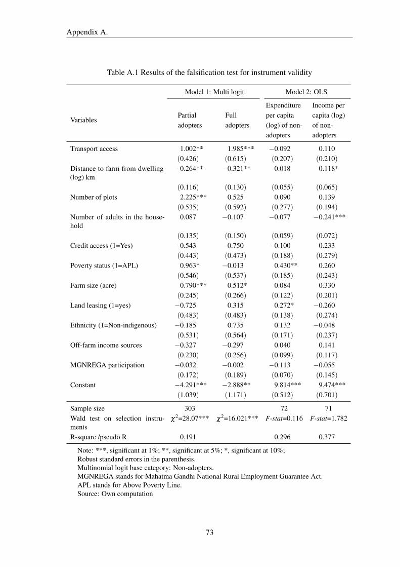
Appendix A.
Table A.1 Results of the falsification test for instrument validity
Model 1: Multi logit Model 2: OLS
VariablesPartialadopters
Fulladopters
Expenditureper capita(log) of non-adopters
Income percapita (log)of non-adopters
Transport access 1.002** 1.985*** −0.092 0.110(0.426) (0.615) (0.207) (0.210)
Distance to farm from dwelling(log) km
−0.264** −0.321** 0.018 0.118*
(0.116) (0.130) (0.055) (0.065)Number of plots 2.225*** 0.525 0.090 0.139
(0.535) (0.592) (0.277) (0.194)Number of adults in the house-hold
0.087 −0.107 −0.077 −0.241***
(0.135) (0.150) (0.059) (0.072)Credit access (1=Yes) −0.543 −0.750 −0.100 0.233
(0.443) (0.473) (0.188) (0.279)Poverty status (1=APL) 0.963* −0.013 0.430** 0.260
(0.546) (0.537) (0.185) (0.243)Farm size (acre) 0.790*** 0.512* 0.084 0.330
(0.245) (0.266) (0.122) (0.201)Land leasing (1=yes) −0.725 0.315 0.272* −0.260
(0.483) (0.483) (0.138) (0.274)Ethnicity (1=Non-indigenous) −0.185 0.735 0.132 −0.048
(0.531) (0.564) (0.171) (0.237)Off-farm income sources −0.327 −0.297 0.040 0.141
(0.230) (0.256) (0.099) (0.117)MGNREGA participation −0.032 −0.002 −0.113 −0.055
(0.172) (0.189) (0.070) (0.145)Constant −4.291*** −2.888** 9.814*** 9.474***
(1.039) (1.171) (0.512) (0.701)
Sample size 303 72 71Wald test on selection instru-ments
χ2=28.07*** χ2=16.021*** F-stat=0.116 F-stat=1.782
R-square /pseudo R 0.191 0.296 0.377
Note: ***, significant at 1%; **, significant at 5%; *, significant at 10%;Robust standard errors in the parenthesis.Multinomial logit base category: Non-adopters.MGNREGA stands for Mahatma Gandhi National Rural Employment Guarantee Act.APL stands for Above Poverty Line.Source: Own computation
73

Appendix A.
Tabl
eA
.2M
ultin
omia
lend
ogen
ous
switc
hing
regr
essi
onre
sults
(out
com
eeq
uatio
ns)
Inco
me
per-
capi
taE
xpen
ditu
rePe
r-ca
pita
Var
iabl
esN
on-
Ado
pter
sSE
Part
ial-
Ado
pter
sSE
Full-
Ado
pter
sSE
Non
-
Ado
pter
sSE
Part
ial-
Ado
pter
sSE
Full-
Ado
pter
sSE
Num
bero
fadu
ltsin
the
HH
-0.2
48**
*-0
.095
-0.2
75**
*-0
.053
-0.0
81-0
.125
-0.0
72-0
.077
-0.1
94**
*-0
.038
-0.1
20-0
.080
Cre
dita
cces
s0.
127
-0.3
990.
028
-0.2
09-0
.052
-0.3
76-0
.164
-0.2
42-0
.292
***
-0.0
99-0
.097
-0.1
67
Pove
rty
stat
us0.
358
-0.4
730.
374
-0.3
390.
953*
-0.5
230.
571*
*-0
.302
0.02
0-0
.204
-0.0
05-0
.264
Farm
size
(acr
e)0.
282
-0.2
640.
353*
**-0
.08
0.24
2-0
.214
0.12
7-0
.195
0.06
5-0
.055
0.02
6-0
.090
Lan
dle
asin
g-0
.188
-0.3
940.
504*
**-0
.195
1.01
0**
-0.4
060.
249
-0.2
47-0
.014
-0.0
910.
163
-0.1
94
Eth
nici
ty-0
.061
-0.4
440.
154
-0.3
44-0
.102
-0.6
030.
113
-0.2
660.
490*
*-0
.196
0.53
5**
-0.2
71
Off
-far
min
com
eso
urce
s0.
152
-0.1
500.
104
-0.1
05-0
.233
-0.2
330.
025
-0.1
140.
126*
-0.0
73-0
.065
-0.1
27
MG
NR
EG
Apa
rtic
ipan
ts-0
.046
-0.1
610.
076
-0.0
74-0
.029
-0.1
26-0
.118
-0.0
88-0
.044
-0.0
45-0
.054
-0.0
94
_m0
(δna
)0.
168
-0.8
61-1
.880
-1.2
610.
031
-1.8
490.
344
-0.6
79-0
.072
-0.8
3-0
.334
-0.7
94
_m1
(δpa
)0.
822
-2.3
46-1
.431
*-0
.86
0.13
9-1
.967
1.33
5-1
.987
0.10
4-0
.55
-0.0
35-0
.932
_m2
(δfa
)0.
467
-1.6
05-1
.071
-0.9
240.
141
-0.7
330.
759
-1.3
650.
140
-0.6
370.
230
-0.2
93
Con
stan
t9.
935*
**-1
.050
9.43
9***
-0.4
719.
090*
**-1
.388
10.2
93**
*-0
.743
10.5
50**
*-0
.276
9.77
6***
-0.6
09
Not
e:N
umbe
robs
erva
tion
is30
3;δ
na,δ
paan
dδ
faar
eth
ese
lect
ion
erro
rcor
rect
ion
term
sfr
omE
q.(4
.5).
Boo
tstr
appe
dst
anda
rder
rors
at20
0re
plic
atio
nsin
pare
nthe
ses.
***,
sign
ifica
ntat
1%;*
*,si
gnifi
cant
at5%
;*,s
igni
fican
tat1
0%.
74