JOINT INSTITUTE FOR AERONAUTICS AND ACOUSTICS

NASANational Aeronautics andSpace Administration

Ames Research Center Stanford University

JIAATR-20

ACOUSTIC RESONANCES AND SOUND SCATTERINGBY A SHEAR LAYER

S.P. Koutsoyannis, K. Karamcheti,and D.C. Galant

STANFORD UNIVERSITYDepartment of Aeronautics and Astronautics

Stanford, California 94305

SEPTEMBER 1979

JIAA TR - 20

ACOUSTIC RESONANCES AND SOUND SCATTERINGBY A SHEAR LAYER

S,P, KOUTSOYANNIS, K, KARAMC.HETI,

AND D,C, GALANT

SEPTEMBER 1979

The work here presented has been supported by theNational Aeronautics and Space Administration underNASA Grant 2233-6 and NASA 2308-1 to the JointInstitute for Aeronautics and Acoustics

TABLE OF CONTENTS

ABSTRACT 1

NOMENCLATURE 3

I. Introduction 5

II. The Expression for the Energy ReflectionCoefficient 6

III. Numerical Evaluation of the Energy ReflectionCoefficient R2 13

IV. Limiting Behavior of the ReflectionCoefficient 17

V. Resonances for the Finite Thickness ThinShear Layer 20

VI. Conclusions ."' 22

REFERENCES 25

APPENDIX A A-l

A.I Representation of the VelocityPotentials in the Regions A-l

i. Velocity Potential <(>£ for the LowerRegion z £ 0 A-l

ii. Velocity Potential <J>U in the UpperRegion z j> z, A-2

A.2 Definition of the Energy ReflectionCoefficient A-5

A. 3 Acoustic Energy Conservation A-6

APPENDIX B B-l

11

ACKNOWLEDGEMENTS

The authors would like -to acknowledge, Mr. Ramji Digumarthi,

for helping in the calculations of the graphs and Miss Jill Izzarelli

for her expert typing of the manuscript.

ACOUSTIC RESONANCES AND SOUND SCATTERINGBY A SHEAR LAYER

S. P. Koutsoyannis and K. KaramchetiJoint Institute for Aeronautics and AcousticsDepartment of Aeronautics and Astronautics

Stanford University, Stanford, California 94305

and

D. C. GalantNational Aeronautics and Space Administration

Ames Research CenterMoffett Field, California 94035

ABSTRACT

We examine the reflection and transmission of plane waves by a

finite thickness shear layer having a linear velocity profile and

bounded by two otherwise uniform parallel flows. The pressure per-

turbation equation in the shear layer has been shown previously to

have exact solutions in terms of Whittaker M-functions. It is shown

that in addition to the angle of plane wave incidence and the relative

Mach number of the flows bounding the shear layer, the scattering

properties of the shear layer depend crucially on a parameter T in

such a manner that the case T -»• 0 characterizes the long wavelength

properties of the layer (with T = 0 being the vortex sheet) and the

case T ->• °° characterizes the short wavelength properties of the layer

(Geometrical Acoustics). We have evaluated numerically the relevant

Whittaker M-functions and using these values we have studied the

behavior of the energy reflection coefficient for a number of

cases (angle of incidence, Mach number and various values of the

parameter.T) at which the corresponding vortex sheet is known to

exhibit resonances (reflection coefficient -»• °°) and/or Brewster

angles (reflection coefficient •> 0) . We find that, unlike the vortex

sheet, the finite thickness shear layer has no resonances or Brewster

angles. Moreover we find that in general for T > 0.5 the amplified

reflection regime degenerates into the total reflection regime of

geometrical acoustics even in the cases in which the corresponding

vortex sheet has resonances. In contrast for the region of ordinary

reflection we find that in the cases in which the corresponding

vortex sheet does not have a Brewster angle the values of the reflec-

tion coefficient up to T = 1 follow quite closely those of the vortex

sheet whereas for the cases for which the corresponding vortex sheet

has a Brewster angle the magnitude of the reflection coefficient may

be quite sensitive even to small changes of T in certain cases,

contrary to some previous results of Graham and Graham1. The results

of the present studies indicate that caution should be exercised in

uncritically modeling a finite thickness shear layer by a correspond-

ing vortex sheet, a practice usually followed currently in noise

research and aeroacoustics.

NOMENCLATURE

a = (constant) sound speed

a. . = constant coefficients defined by eq. (12)

b = linear velocity profile slope [units: (time) ]

f, g = the two independent solutions (eq. (9)) of eq. (7)

k = wave vector of incident plane

k = x-component of wave vector kJ

m = -ri second index of the Whittaker M-functions.

p1 = pressure perturbation

p / P = linear combinations of f and g.-»•r = position vectorsgn = "sign of"t = time

w = z-component of velocity perturbation

x, z = coordinates

A, B, C, D = expressions defined by eq. (14)

H = heaviside function

M(z) = local Mach number

M, = upper fluid Mach numberi *

M-functions = Whittaker M-functions

2R = Energy reflection coefficient

R = R, ± iR, = Complex reflection coefficient for the perturbationvelocity potential.

T = TI ± iT2 = complex transmission coefficient for the perturbationvelocity potential.

R.P. = "Real Part of"

U(z) = local mean speed

n = non-dimensional variable defined by eq. (5)

0 = incident wave angle (see Fig. (1))

K = sin8

T = non-dimensional parameter defined by eq. (8)

0) = angular frequency of incident plane wave

$£, <f> u = perturbation velocity potentials for the lower andupper regions respectively.

I. Introduction

The shear layer with a linear velocity profile has been the object

of a number of studies. Kuchemann* considered the stability of the

boundary layer with a linear velocity profile. Pridmore-Brown3

studied rectangular duct modes in a duct with the basic flow having

a linear velocity profile. Graham and Graham1 studied plane wave

propagation through a linear veloicty profile shear layer. Goldstein

and Rice1* found an exact solution to the pressure perturbation equa-

tion in terms of linear combinations of parabolic cylinder functions

of different order. We have reported earlier (see Koutsoyannis5)

some preliminary results on sound propagation through a shear layer

with a linear velocity profile using essentially Whittaker M-functions

as the basic solutions of the pressure perturbation equation. Jones6

studied the stability of such a layer for subsonic basic flow using

our previous solution in terms of Whittaker M-functions. Recently

Scott7examined wave propagation through a linear shear layer using

the Goldstein and Rice1* unwieldy solution. With the exception of

Goldstein and Rice\ Koutsoyannis5, .Jones6 and Scott7 the other

investigators were concerned with either series or asymptotic solu-

tions of the pressure perturbation equation in the shear layer region.

In i.the present study we are concerned with the behavior of the

energy reflection coefficient for plane waves incident on a finite

thickness shear alyer with a linear velocity profile and bounded by

two uniform parallel flows. For that purpose we have evaluated

numerically the solutions of the pressure perturbation equation in

terms of Whittaker M-functions and with the aid of these we have

numerically evaluated the reflection coefficient for a number of

typical cases involving the relevant parameters, i.e., the angle of

incidence of the plane waves, the upper fluid Mach number and a

characteristic parameter T which represents a non-dimensional measure

of the disturbance Strouhal number with respect to the disturbance

Mach number in the mean flow direction (see Section IV.).

In section II below we shall derive the expression for the

reflection coefficient in terms of the two basic solutions of the pres-

sure perturbation equation (i.e., the Whittaker M-function solutions).

In section III we shall summarize and discuss our numerical results

on the variation of the reflection coefficient. In section IV we

shall discuss various limiting cases including the vortex sheet and

geometrical acoustics limits and in section V we shall give an

analytical proof for the absence of resonances for a thin shear

layer. The results of the present studies are then summarized in

the final section VI. At the end, in Appendix A we discuss the

representations of the perturbations in the three flow regions

(see Figure 1), and the definition of the energy reflection coefficient

as well as energy conservation and finally in Appendix B we give the

general outline of the numerical scheme used to evaluate the Whittaker

M-functions.

II. The Expression for the Energy Reflection Coefficient

Without loss of generality we may assume that the layer with the

linear velocity profile is bounded by two uniform flows, one of which

is at relative rest, as shown in Figure 1, i.e., we assume the

following two-dimensional {in the (x,z) plane] inviscid compressible

shear layer characterized by the mean continuous velocity flow field:

U(z) = 0 for z <_ 0

= bz for 0 <_ z <_ z, (1)

= bz for z, <_ z

Furthermore we assume a time-harmonic plane wave incident from the

z -£ 0 half space with wave vector k and wave number k = —. The entirea

unperturbed flow field is otherwise assumed to be homogeneous, i.e.

no variation for mean densities, temperatures and speeds of sound

are allowed.

The velocity potentials 4>0 and <(> in the lower and upper regionsX* XI

of uniform flow, respectively, bounding the shear layer of thickness

*z, may be taken to be (see for instance Graham and Graham or Miles ):

< J > 0 = R.P. < ± i - | e x p [±ik(xsin9 + zcos9 - at) 1 +( _ }

+R exp [±ik(xsin6 + zcosS - at) 1 I (

<f>u = R.P. < ±iT jexp f± ik (xs in9 ± ( z - z '

(2)for z < 0

sine |"\Al? - 1 - at ] 1 > for z > z (3)

*The representation of the perturbation fields expressed by equations(2), (3), (4) and (5) is essentially the one used by Graham and Graham1,although they did neither use the non-dimensional variable n nor theparameter T (see equations (5) and (8)). At any rate this representa-tion is consistent with the different ones used by Miles and Ribner8 .

In the above equations R.P. denotes "real part of"; the first term in

equation (2) represents the incident plane wave of unit amplitude

emanating from the half space z 0 having wave vector k that makes

an angle 6 with the z-axis as shown in figure 1, with - 5- <. 9 <, + •?•;

R and T are the complex reflection and transmission coefficients

for the velocity potentials <j>? and <J> respectively, i.e.:

R = R ± i R?(4)

T = T, ± i T2 ,

where R. and T. are real for the so-called ordinary and amplified

reflection regimes and complex in the region of total reflection.

In equations (2), (3) and (4) above the upper signs are

to be used for ru > 1 (ordinary reflection regime) , and the lower

signs for n-, < -1 (amplified reflection regime); ru is the non-

dimensional quantity ru = —• — 5- ~ Mn (see equation (5) below) withbz, X Sin9 1

M- = - being the upper fluid Mach number. This choice of signsJ_ Si

ensures that the radiation condition, as discussed by Miles7,

Ribner8 and Graham and Graham1 is satisfied.

In the shear layer region 0 £ z <. z, in which the mean flow

varies linearly with z (see equation (1)), it is convenient to use

the non-dimensional variable n (see Ref. 5)

bz 1 „/ \- M(z)sin6 a

where M(z) is the local Mach number of the mean flow in the shear

layer. If then one assumes that within the shear layer region the

pressure perturbation p1 (r,t) is of the form:

+ (cos) ,6)p'(r,t) = p(z)sin(k x-ut)

with k = k«e = — k sin9, one obtains the following ordinary differ-«t H d

ential equation for the z-dependent part p(z) of the pressure pertur-

bation p1 in terms of the nondimensional variable n defined by

equation (5) (see Koutsoyannis5) : :

with T ' being the parameter defined by:

4t = £ sine (8)

We have shown earlier (see Koutsoyannis5) that the two independent

solutions of equation (7) are:

g(n;T) J XL'-1U - (9)

which are real functions of the variable n and the parameter T for

real values of n and T. Using the above solutions f(n;T) g(n/T) one

may further write the following general expression for the pressure

perturbation p1(r,t) and the z-component w of the velocity perturba-

tion:

p ' ( r , t ) = p ^ ( n ; T ) s i n f k ( x s i n e - a t ) 1 + p( ' (n ;T)cos lk (xs in9-a t ) 1 (10)

10

(l;T)cos[k(xsine-at)j - p^2) (n; T.) sin[k (xsin6-at)w(n;T) =(11)

where p (r\) and p (ri) are linear combinations of the two inde-

pendent solutions f (n) and g(n) (given by equations (9)) of the

pressure perturbation equation (7), i.e.

(1)(n;T) = ai:Lf(n;T) + a12g(n;T), p(2)(n;T) = a21f(n;T) + a22g(n;T) (12)

with a.. constants.

Finally we apply the appropriate boundary conditions at the two

edges of the shear layer, at z = 0 and z = z, [or in terms of the

non-dimensional variable ri (equation (5)) at ri = —:—5- ando s in t/

n1 = . - Mn ] , namely continuity,of the pressure perturbation p1

A. S Xii 0 J_*

and of the z-component w of the velocity perturbation. Then using

equations (2), (3), (10), (11) and (12) one may obtain eight linear

algebraic equations for the determination of the eight unknowns a.•,

R. and T. appearing in these equations. After a somewhat tedious

*Specifically at z = 0 we set:

>p' (z = 0~) = -P - = p' (z = 0+)Q

w(z = 0~) - (V<j>,,). e, = w(z = 0x 2

and similarly at z = z, we set:

w(z = z,) = (Vtj) ) . e = w(z = z,)J- iZ Z X

with D/Dt designating the convective name operator in the upperfluid region of constant Mach number M...

11

but straightforward algebra we obtain the following expressions for

the square of the reflection coefficient:

(C±D)

(A+B)2 + (C+D)2

(13)

|R|2 = 1 , for |n]_| 1 1

where the expressions for A, B, C and D given below involve essentially

evaluation of the two independent solutions f(n) and g(n) of the

pressure perturbation given by equations (9) and of their first

derivatives at the two edges of the shear layer and are functions of

no ~ sine

and (8)).

1 1 *sine ' nl = sin6 ~ Ml and tne Parameter T (see equations (5)7

Using equations (4) for the definitions of the complex reflection andtransmission coefficients R and T, respectively, we easily obtain:

2 2 2R = R^ + R*2 2 , for ITU | ^ 1

T = T^ + T^

i.e. in the ordinary and amplified reflection regimes where R^ and T^are real. In the total reflection regime |ni| ^. I/ Ri and T^ arecomplex and it is al.so easily obtained that in such as case |R|2 =lRll2 + | R 2 l 2 = 1 ' T = 0 - The meaning of R2 follows from the inter-pretation:

2 _ Reflected Acoustic Energy Flux (Time-averaged over one cycle)~ Incident Acoustic Energy Flux (Time-averaged over one cycle).

and is discussed in Appendix A.

12

Explicitly :

A = fn(0)gn(1) - fn ( 1 ) 0 )

B =

C =

D =

(f(l)gn(0) - fn(0)g(l)]

|fn(l)g(0) - f(0)gn(l)j

The upper signs in equations (14) hold for n-, > 1 and the lower

signs for n, -^ -If in both cases | f|, | 2- I/ and we have used the

notation 0 and 1 in the arguments of f and g and their derivatives

with the understanding that 0 designates evaluation at

n = n = n _n = — : — 5- and 1 designates evaluation at n = nn = n I _j*~ u s in u j. z ~i --— , — g- - M.. i.e., at the two edges of the shear layer. Equation (13)

is valid for - -~ £. Q £. + •* wi-th the upper signs holding for the regime

of ordinary reflection (r), > 1 and R < 1) and the lower signs for

the regime of the so-called amplified reflection (r\. £ -1, R 2. 1) .O

(For the total reflection regime |R| = 1, -1 <, ru -£ +1*

- -^ 6 + -y. ) It is seen from equations (13) and (14) that we

recover the three reflection regimes:

For simplicity we have assumed sin 9 >_ 0 in the expressions for A, B,C and D given by equations (14) since for the geometry chosen inFigure 1 resonances and/or Brewster angles for the correspondingvortex sheet cases exist only for 0 <. 6 i ir/2. Equations (14) maybe made general, i.e. to apply for all values of the incidence angle0 (- ir/2 <. 9 <. + 7T/2) by multiplying B and C by sgn(sin8).

13

2L 1 » R £ 1: Ordinary Reflection Regime

2•1 £ n-, £ T! , R = 1: Total Reflection Regime

n, £ -1 / R 2l 1: Amplified Reflection Regime

which agree with the results of Graham and Graham1. Indeed these

regimes are the same as those found by Miles7 and Ribner8 for the

limiting case of the vortex sheet (T = 0).

2III. Numerical Evaluation of the Energy Reflection Coefficient R

We have evaluated numerically the Whittaker M-functions involved

in the two independent solutions f (TI;T) and g(n;T) of the pressure

perturbation equation given by equation (9) using the known series

representations of f and g as given by Koutsoyannis5 for relatively

small values of n and T whereas for large values of r\ and/or T we have

used a numerical technique outlined in Appendix B. Using these values

we have then evaluated the functions A, B, C and D given in equation2

(14) and then the expression for the energy reflection coefficient R

given by equation (13). In particular we have chosen ranges of the

relevant problem parameters, i.e., angle of incidence 6, upper fluid

Mach number M.. and Strouhal number T, for which the corresponding

vortex sheet (for the same 9 and MI) has one or two resonances and/or

one or no Brewster angle.

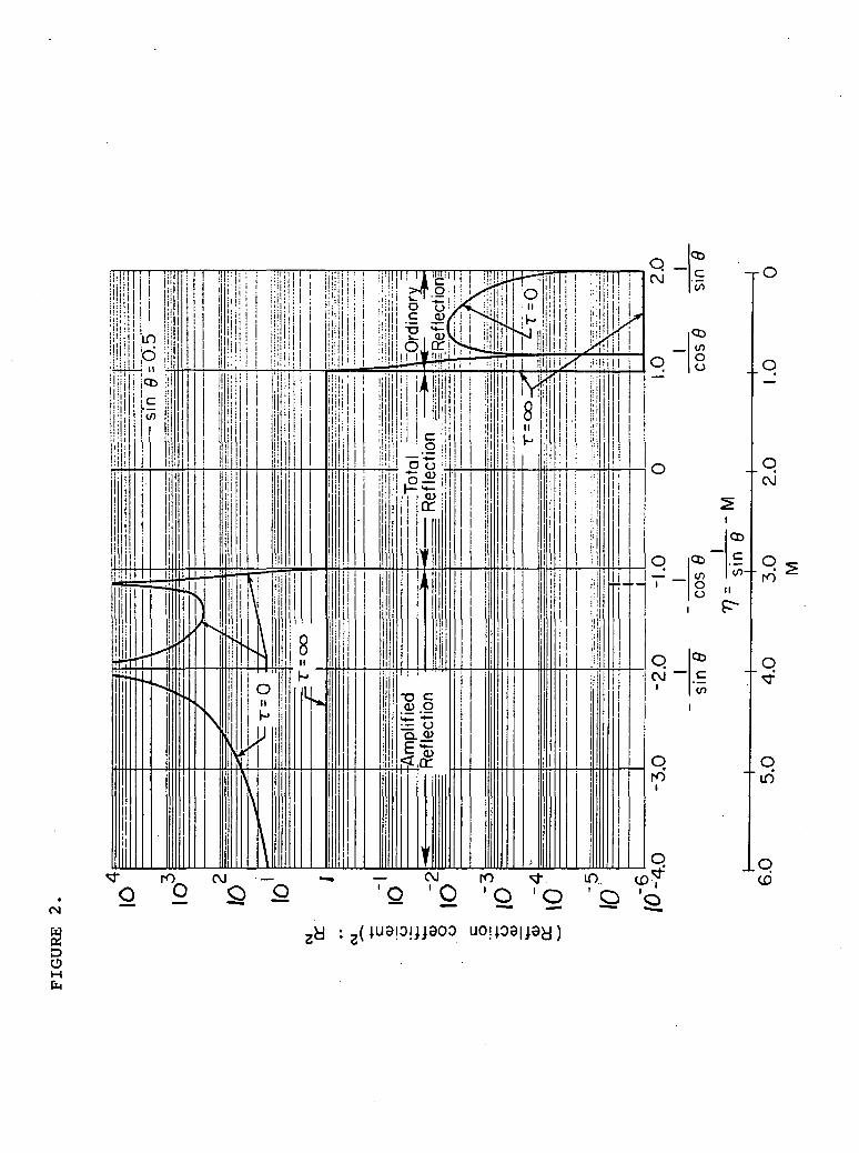
Figure 2 shows the behavior of "the energy reflection coefficient2

R for the limiting cases of the vortex sheet (T = 0) and geometrical

acoustics (T •*• °°) for a typical incidence angle 9 = 30°, as a function

14

of the variable n-, = —r=-Q - M.. = 2 - M, , or as a function of the

upper fluid Mach number M,. As is known (see Refs. 7 and 8) the

vortex sheet in this case has resonances at ru = - —=—^ and1 sinu

n1 = - cos9 'i*e< for Mi = 4 and a Brewster angle at ru = + COSQ'

i.e. at M =1.134. in the geometrical acoustics limit (T •* °°) the

2energy reflection coefficient R , as a function of ru/ degenerates '

2 2into the Heaviside-type step function R = 1 - H(l-ru)/ i.e. R =1

2for Tii < 1 and R = 0 for n, > 1.J. 1

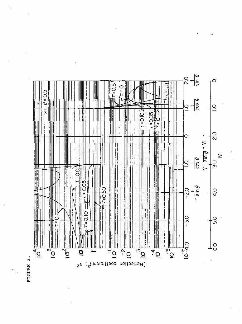
Figure 3 shows the variation of the reflection coefficient with

upper fluid Mach number M. for a number of values of the parameter f

for a fixed angle of incidence of 30°. For 30° angle of incidence :

the corresponding vortex sheet (T = 0) has two resonances, i.e.,

at -I/sin 30° and -I/cos 30° and one Brewster angle at +l/cos 30°.

It is seen from the figure that even for very small T (~0.01) the

resonances in the amplified reflection regime disappear and for

values of T 2. 0.5 the amplified reflection regime has degenerated2

into the total reflection one with R = 1. In the ordinary reflection

regime in which the corresponding vortex sheet has a Brewster angle

at r)i = +l/cos(30°) it is seen that even for low values of T ~ 0.05

the Brewster angle has disappeared and there is discernible variation

of the reflection coefficient with upper fluid Mach number up to the

value T = 1 that we have calculated.

Figure 4 shows the variation of the reflection coefficient with

upper fluid Mach number M, for a number of values of the parameter T

and for a fixed angle of incidence of 45°. This is the special case

in which the two resonances of the corresponding vortex sheet

coalesce and the same holds for the Brewster angles. As in the 30°

15

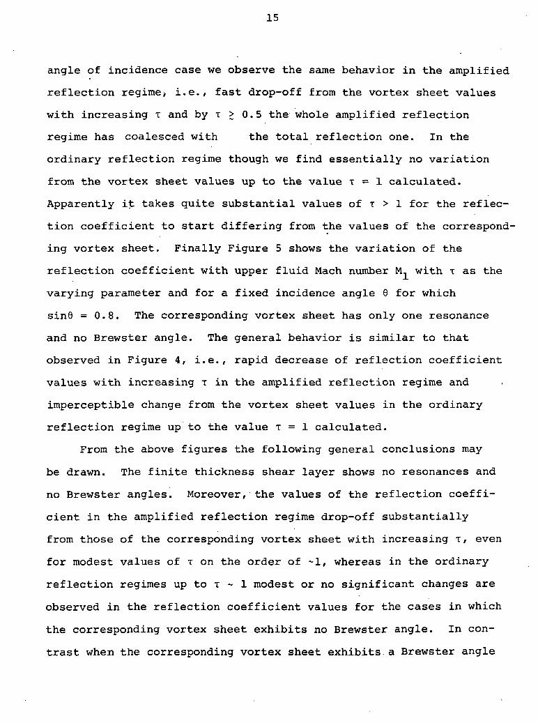
angle of incidence case we observe the same behavior in the amplified

reflection regime•, i.e., fast drop-off from the vortex sheet values

with increasing T and by T > 0.5 the whole amplified reflection

regime has coalesced with the total reflection one. In the

ordinary reflection regime though we find essentially no variation

from the vortex sheet values up to the value T = 1 calculated.

Apparently it takes quite substantial values of T > 1 for the reflec-

tion coefficient to start differing from the values of the correspond-

ing vortex sheet. Finally Figure 5 shows the variation of the

reflection coefficient with upper fluid Mach number M.. with T as the

varying parameter and for a fixed incidence angle 6 for which

sin6 = 0.8. The corresponding vortex sheet has only one resonance

and no Brewster angle. The general behavior is similar to that

observed in Figure 4, i.e., rapid decrease of reflection coefficient

values with increasing T in the amplified reflection regime and

imperceptible change from the vortex sheet values in the ordinary

reflection regime up to the value T = 1 calculated.

From the above figures the following general conclusions may

be drawn. The finite thickness shear layer shows no resonances and

no Brewster angles. Moreover, the values of the reflection coeffi-

cient in the amplified reflection regime drop-off substantially

from those of the corresponding vortex sheet with increasing T, even

for modest values of T on the order of ~1, whereas in the ordinary

reflection regimes up to T ~ 1 modest or no significant changes are

observed in the reflection coefficient values for the cases in which

the corresponding vortex sheet exhibits no Brewster angle. In con-

trast when the corresponding vortex sheet exhibits a Brewster angle

16

in the ordinary reflection regime the reflection (and transmission)

characteristics of the finite thickness shear layer, as may be

surmised from Figure 3, strongly depend on the value of the para-

meter T (in addition to the angle of incidence 6 and the upper fluid

Mach number MJ . This is in contrast to the results of Graham and

Graham1 who for the case of M. = 3 and sin8 = 0.2, that they examined

as a typical one for the ordinary reflection regime, they have calcu-

lated negligible effects due to the finite layer thickness as compared

with the corresponding vortex sheet results. The reason is, as may

be easily checked, that in their case the corresponding vortex sheet

has Brewster angle at n = ~ Q =1.1021, i.e. very close to 1 (see Fig.

2) and moreover they have evaluated the variation of R and T as a

function of the non-dimensional parameter*:

~™ z cos fa zShear Layer Thickness _ a 1 _ u ^ i ^ cos9

Wave Length 2ir b " a ' 2ir

w M cos6"™ L~ *?** ftb 1 27T

and they considered variations of this parameter from zero to less

than 0.2. This range corresponds to variation of our non-dimensional

parameter T from zero to less than 0.02 and since the value T = 0

characterizes the vortex sheet, it follows that the choice on the

*In actuality the parameter in Ref. 1 is:

2_ Shear Layer Thickness _ _ _ 1

(Incident wave vector component in the z-direction) , 1 w(2¥ a

17

above parameter in Ref. 1 has been an unfortunate one, and the

range of values of this parameter investigated by Graham and Graham1

is too close to the vortex sheet value T = 0.

<

IV. Limiting Behavior of the Reflection Coefficient

In this section we study analytically the limiting values and

2forms of the energy reflection coefficient R , as given by equation

(13), as the parameters T, 9 and M.. take extreme values by examining

the behavior of A, B, C and D in equations (14) for these limiting

values. In particular we will be interested in T ->• 0 or T •*• °°

corresponding to the vortex sheet and geometrical acoustics limits,

respectively (see Koutsoyannis5) , in 6 •*• 0 or 9 ->• ± ir/2 corresponding

to the normal and parallel incidence, respectively, and in M, -»• 0 or

M -»- oo, i.e., the low and high upper fluid Mach number limits,

respectively.

The vortex sheet limit T •*• 0 follows from the known properties

of the series solutions f(n) and g(n) in equation (9) and from

equations (14) (see Ref. 5). In this limit A •*• 0 and B + 0, whereas

3n2o/I - K

Since the parameter used in Ref._!_ does not contain the shear layerprofile slope b, one could have anticipated that it is not a suitablenon-dimensional parameter that adequately characterizes the scatteringcharacteristics of the shear layer. In contrast our non-dimensionalparameter T as given by equation(8)does characterize the essentialfeatures of the problem since it is the product of the Strouhal num-ber w/b and the sine of the angle of the incident wave vector withthe z-axis.(See also Ref. 5 for a detailed discussion on the'physicalmeaning and importance of the parameter T.)

18

and

and since K

-3ni '

= sine, ru = • 9 - M.. we obtain from equation (13)

R2 =C ± D

\C + D,

(1 - ± secS y(l - f^s - sin20

+ sec9 - sin29

(15)

where again M.. is the upper fluid Mach number and upper signs corre-

spond to ordinary and lower signs to amplified reflection. Equation

(15) is the equation for the vortex sheet and agrees with the corre-

sponding results obtained by Miles and Ribner8.

The limiting form of the reflection coefficient in the limit of

.(geometrical acoustics) may be obtained using the asymptotic

form of the solutions f (n) and g(n) in equation (9) as T -> °° (see

Ref. 5). Instead of using these forms we may argue as follows:

Since it has been shown that in the limit T -»• °° one recovers both

the amplitude and the phase function of geometrical acoustics (see2

Ref. 5) it follows that the reflection coefficient R in the limit

T •*• °° has the form consistent with geometrical acoustics, i.e.,

R2 = 0

= 1

for

for(16)

ru < 1

The limiting form for normal incidence, i.e., 9 = 0 is obtained

by observing that in this limit

n = —••—?o sinf -*• + 001

sinf

19

and also in equations (14)

A -»• 0 , B •> 0 and C -»• -D.

Consequently since only ordinary reflection is possible (TU > 1) the

reflection coefficient is zero.

The limiting form for parallel incidence 6 = ± ir/2 i.e.,2

sin 6 = 1 is obtained from equations (14) by observing that in

this limit

A -*• °° and C ->• °°

and the reflection coefficient

The limiting form for M -»• 0 is obtained again from equations

(14) by observing that in this limit

A -»• 0, B -»- 0 and C -> -D.

Consequently again only ordinary reflection is possible

(n, •*• n = "-'ne > 1) with the reflection coefficient being zero.

Finally the limiting form of the reflection coefficient for

M ->• °° is the same as that for the vortex sheet, equation (15) , i.e.o

R = 1 and since as M -»• « ru •*• - °° only the amplified reflection

regime applies.

We summarize the above limiting forms of the values of the

reflection coefficient together with the corresponding regimes

(Ordinary, Total or Amplified reflection) in the following table:

20

Reflection -Coefficient R

Reflection Regime

T

0

VortexSheet LimitEq. (14)

O. , T. , A.

oo

GeometricalAcousticsLimit

0. , T. , A.

9

0

0

O.

± TT/2

1

T. A.

Ml

0

0

O.

00

1

A.

In the above table in the bottom line 0., T. or A. stand, respectively,

for Ordinary, Total or Amplified reflection.

V. Resonances for the Finite Thickness Thin Shear Layer

In this section we present a proof for the nonexistence of

resonances for a nonzero but thin shear layer. It is seen from2

equation (13) for the reflection coefficient R that resonances

which may only exist in the amplifying reflection regime (r\, < -1)

imply that

A + B = 0 and C + D = 0 (17)

We found out in deriving equation (15) for the vortex sheet case

(T = 0) that, to the lowest order in T,A ->• 0 B -> 0 whereas C and D

are nonzero and yield the vortex sheet result. We next evaluate A

and B to lowest order in T as follows: We first insert in equations

(14) the values for the functions f(n) and g(n) from equation (9) to

the lowest order in T and then we evaluate A + B at the zeros of

C + D and we show that the two equations (17) are incompatible for

small but finite T, the only possibility remaining being that of

T = 0, i.e. the vortex sheet case.

21

For small T one may obtain from equation (9) (see Ref . 5) :

n + IL- + 0(T4)

5 7\ (18)T7T ~ TT/ + 0(T )

Inserting 'these values in equation (14) we obtain:

A = (4T) J3(n0 - n1)n0n1(l - n0n1

Observing that n - \\. is the upper fluid Mach number M. we see

from equation (19) that the condition A + B = 0 yields:

A + B = (4i) 3nnn,d - nftn,) + l/n« - 1 v/nf - i n" + nf + n.n, = o (20)

Equation (20) must be evaluated at the vortex sheet values of n r

i.e., where C + D = 0 , i.e. at the vortex sheet values of n and rii

Using the two known properties of the vortex sheet solution, i.e.

2 ^ 2 2 2no + ni = noni ' noni

Equation (20) yields:

A + B = - (4i)(2M?) = 0 (21)

We see that equation (21) is satisfied only if T = 0 or M. = 0 or

both and consequently the two equations (17) required for the

existence of resonances are incompatible to the lowest order in T;

22

it follows that the nonzero thickness thin shear layer has no resonances*

and no Brewster angles.

One may also prove, in general, on the basis of certain differential

properties of the quantities A, B, C and D, equaitcns (14), and the

Wronskian of the solutions f(n;T) and g(n;T) (equation (9)) of equation

(8), that not only the thin shear layer, but also the finite thickness

shear layer has no resonances or Brewster angles and'more over resonances

and Brewster angles are possible if and only if either T = 0 (the

vortex sheet case) or T -»• °° (the geometrical, acoustics limit (see.

figure 2).**

VI. Conclusions

We have evaluated numerically the energy reflection coefficient

for plane waves incident on a plane shear layer having a linear

velocity profile. The numerical computations were based on a

* 2The conditions for the existence of Brewster angles, i.e. R = 0,is the same as that for the existence for resonances, i.e. equations(17), except that in this case the ordinary reflection regime (m >1)is the relevant one and the proof follows as for the case of theresonances.**This is true not only for the linear shear layer (equation 1) but

also for a finite thickness shear layer of a generally continuousvelocity profile. This result and the corresponding studies willbe published in a separate following publication concerned with thescattering characteristics of finite thickness shear layers with acontinuous velocity profile a special case of which is the shearlayer with a linear mean velocity profile of the present study.

23

representation of the pressure perturbations in the shear layer region

in terms of Whittaker M-functions.

We have found that the shear layer exhibits no resonances and no

Brewster angles and a separate analytical proof for the nonzero

thickness but thin shear layer substantiates the absence of both

resonances and Brewster angles for a finite thickness layer. More-

over we have observed that, the behavior of the reflection coeffi-

cient depends crucially on the parameter T, which/as is seen from

equation (8)/represents a non-dimensional measure of the disturbance

Strouhal number with respect to the disturbance Mach number in the

mean flow direction. In particular for moderate values of T the

amplified reflection regime degenerates into the total reflection

one whereas in the ordinary reflection regime the variation of the

reflection coefficient with T depends on whether the corresponding

vortex sheet has a Brewster angle or not. In cases in which the

corresponding vortex sheet has a Brewster angle the reflection

coefficient is sensitive to changes in T even for moderate values of

T whereas in the cases in which the corresponding vortex sheet has

no Brewster angle the reflection coefficient for moderate values of

T follows rather closely the corresponding vortex sheet values.

The above results indicate that caution should be exercised in

modeling planar shear layers by vortex sheets uncritically even in

the ordinary reflection regime and even for subsonic relative flows

of the two regions bounding the shear layer, a practice customarily

followed in current research and applications in noise studies and

in aeroacoustics in general (see Ref. 9). Although it is well known

24

that/the directional characteristics of the reflected and transmitted

plane waves scattered by a finite thickness plane parallel

shear layer are independent of the details of the velocity profile

in the layer (provided that the profile is "smooth") (see for instance

Ref. 10), the amplitudes of the transmitted and reflected waves

crucially depend on the parameter T, in addition to the angle of

incidence 9 and the relative Mach number M of the two uniform flows

bounding the finite thickness shear layer, indeed we have shown that

for certain combinations of T, 6 and M, i.e. those for which the

corresponding vortex sheet has a Brewster angle (energy reflection

coefficient = 0) the scattering characteristics of a finite thickness

shear layer may drastically differ from those of the corresponding

vortex sheet (T = 0) even for modest (non-zero) values of T. Moreover

if one allows for different densities and temperatures in the three

flow regions (z i 0, 0 z <. z1 and z .> z,),a case of particular

interest to noise generation by and/or propogation through hot jets,

the difference between the scattering characteristics of a finite

thickness shear layer and the corresponding vortex sheet characteristics

becomes even more pronounced for certain ranges of values and/or

combination of the relevent parameters involved. The detailed calcu-

lations and the corresponding studies will be published in a following

separate publication concerned with the scattering characteristics of

a linear shear layer as examined in the present studies but allowing

for different densities p and speeds of sound in the three regions

of mean flow (see Figure 1).

25

REFERENCES

1. Graham, E.W. & Graham, B.B. Effect of a shear layer on plane

waves of sound in fluid. J. Acoust. Soc. Am., 46 (1), 1968,

pp. 369-375.

2. Kuchemann, D. Storungsbewegungen in einer Gastromung mit

Grenzschicht. Zeit. angew. Math. Mech, 18, 1938, pp. 207-222;

see also Gortler, H. ibid, 23, 1943, pp. 1

3. Pridmore-Brown, D.C. Sound propagation in a fluid flowing

through an attenuating duct. J.F.M. 4, 1958, pp. 393-406.

4. Goldstein, M. & Rice, E. Effect of shear on duct wall impedance.

J. Sound & Vibration, 30 (1), 1973, pp. 79-84.\

5. Koutsoyannis, S.P. Features of sound propagation through and

stability of a finite shear layer. Advances in Engineering Science,

NASA CP-2001, 3, 1976, pp. 851-860; see also 1977 JIAA TR-5, 1978

JIAA TR-12.

6. Jones, D.S. The scattering of sound by a simple shear layer.

Phil. Trans., 284A, 1977, pp. 287-328.

7. Scott, J.N. Propagation of sound waves through a linear

shear layer, AIAA Journal, 17, 1979, p. 237-244.

8. Miles, J.W. On the reflection of sound at an interface of relative

motion, J. Acoust. Soc. Am., 29, 1957, pp 226-228. See also

Miles, J.W. On the disturbed motion of a plane vortex sheet. J.

Fluid Mech 4, 1958, pp. 538-552.

Ribner, H.S. Reflection, transmission and amplification of sound

by a moving medium. J. Acoust. Soc. Am., 27 (4), 1957, p. 435.

9. Candel, S.M. Application of geometrical techniques to aeroacoustic

problems. AIAA paper, 1976, pp. 76-546, Palo Alto, CA.

10. Kornhauser, E.T. Ray theory for moving fluids. J. Acoust. Soc. Am.,

25 (5), 1953, pp. 945-951; see also Goldstein, M.E. Aeroacoustics

1974, NASA N74-35118.

26

11. Blokhintzev, D.I. Acoustics of a nonhomogeneous moving medium.

Tekhniko-Theoreticheskoi Literatury, Moskva, 1946, NACA TM 1399.

12. Candel, S.M. Acoustic Conservation principles and an application

to plane and model propagation in nozzles and diffusers. J.S.V.

41 (2), 1975, pp. 207-232.

13. Bretherton, F.P. and Garrett, C.J.R. Wavetrains in inhomogeneous

moving media, Proc. Roy. Soc. A302, 1969, pp. 529-554.

14. Buchholz, H. Die konfluente hypergeometrische funktion. Springer-

Verlag, Berlin-Gottingen-Heidelberg, 1953.

15. Schafke, F.W. Losengstypen von difference gleichungen und

surmnengleischungen in normierten abelchen gruppen. Math. Zeitschr.

88, 1965, pp. 61-104.

16. Olver, F.W.J. Numerical solution of second-order linear difference

equation. J. Res. Nat. Bur. Standards, Sec. B, 71, 1967, pp. 111-

129; see also Olver, F.W.J. and Sookne, D.J. Note on background

recurrence algorithms. J. Math. Comput. 26, 1972, 941-947.

A-l

APPENDIX A

A.I Representation of the Velocity Potentials in the Regions

z £ 0 and z _> z, .

(i) Velocity Potential <j>» for the Lower Region z £ 0.

Consider an incident plane wave which in coordinates

(x,z) fixed in the lower fluid, which is at rest, is a sine

wave with wavevector k making an angle 6 with the z-axis, i.e.

k.e = kcos0z

with -\ £ 9 <_ +1 .

The wave is an upcoming one with amplitude A and thus its

potential may be written as:

d>. = d>. ., . = A sin (k x +k z - cot).Yi Yincident x z

And since k = ksinS , k = kcos6 , k = —X y Si

we may further write:

<j>. = A sin J —(xsin9 + zcosG - at)i 1 a j

The reflected wave will in general have in phase and out of

phase case components; thus since the x-wave number is conserved

in this stratified medium we may write for the reflected wave

which is a downgoing wave:

d> = d> _- . j = A [Rnsin —(xsin9 - zcos6 - at) + R^cos —(xsin0 - zcosO -atr reflected l a 2 a

A-2

where R, and R2 are respectively the in-phase and out-of-phase

components of the reflection coefficient for the velocity

potential. Finally

<$>,, = Total Velocity Potential in the lower region z <_ 0

= A | sin — (xsin6 + zcos9 - at) +I I a I

-l- R,sin |-(xsin6 - zcos6 - at) 1 +J- I a I

+ R-cos — (xsinS - zcos6 - at) |

Defining by R = R, ± i R2/ the complex reflection coefficient

and taking the amplitude A to be real we may write in complex

notation:

= A R.P. |±i [e 'V + kzz - wt) + Re±(kxx - kzz - Wt)]|

= A R.P. ±i fcos(k x + k z - wt) ± isin (k x + k z - wt)|I I X Z X Z J

(R, ± iR~) fcos(k x - k z - wt) ± isin (k x - k z - wt) >1 2 I x z x z J J

= A 'sin(k x + k z - wt) + R, sin (k x - k z - wt) +( X Z i x z

+ R_sin (k x - k z - wt)&» I

irrespective of upper or lower signs.

(ii) Velocity Potential <(> in the Upper Region z >_ z,,

The upper medium is moving with uniform velocity

A-3

bzlU, = bz, ex, with M.. •= ——-, with respect to the (x,z) -

J_ J. J. a

coordinate system which is fixed in the lower fluid (which

is at rest).

Since again the x-wave number is conserved in the

stratified medium we may write for the velocity potential

of the transmitted wave:

<j>u = A j T^sin [kTxx + kT z (z-Z l ) - u)t) | +

[kTxX + kTz(zlzl> - Wt)l

where T, and T2 are the in-phase and out-of-phase components

of the transmitted wave. As before k is obtained from x-waveJ. iC

number conservation, i.e.:

kTx = kTsin/ = kix = ksin9 = £ sine,

where JS is the transmitted wave angle, but the z-wave number

k of the transmitted wave may only be uniquely specified byJ. Z ••' •" ~ •

applying the radiation condition as postulated by Miles [17].

Namely from geometrical considerations,

2 _ 2 2KTz ~ KT ~ *T

i.e., kTz = ± t/kT - kTx , and

k is then obtained from conservation of the frequency to,

i.e./ since^ is the angle that the transmitted wave vector

makes with the z-axis, then

co = ka = kTcT = kT(a +

A-4

which together with the x-wavenumber conservation, and

phase speed conservation,

sin9 sin

results in:

k

Finally:

T

= * V k2^1-14!kTz = * k^1-1431116) - k2sin26

= ± k |s ine |yn2 - i .

Which of the two signs in the expression for k .J. Z IS

to be taken, is determined by the radiation conditions as

postulated by Miles [7] i.e. + sign for n-, > I/ i.e. in the

so-called ordinary reflection regime and - sign for ru < -1

i.e. in the so-called amplifying reflection regime.

Finally writing

T = T, ± i T_

and substituting in the expression for <fu we obtain the

expression given by eq. ( 3} in terms of the complex trans-

misstion coefficient T.

A-5

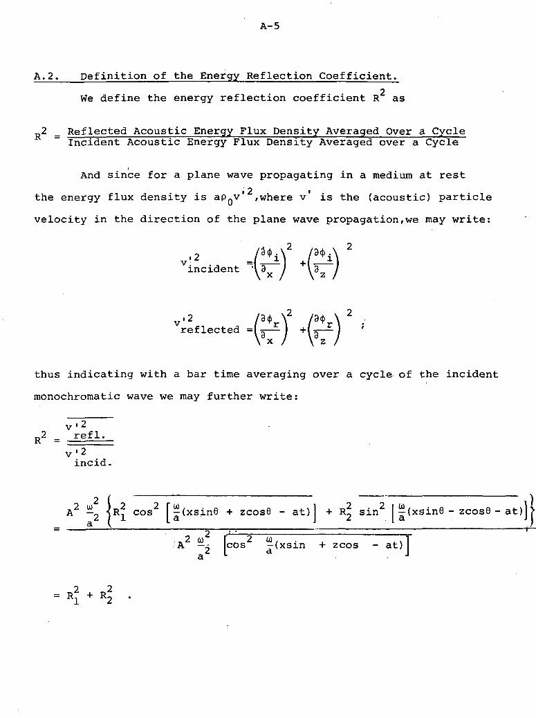
A. 2. Definition of the Energy Reflection Coefficient.2

We define the energy reflection coefficient R as

2 _ Reflected Acoustic Energy Flux Density Averaged Over a. Cycle~ Incident Acoustic Energy Flux Density Averaged over a Cycle

And since for a plane wave propagating in a medium at rest

the energy flux density is apQv" , where v is the (acoustic) particle

velocity in the direction of the plane wave propagation, we may write:

incident

2vreflected = U- +

Z

thus indicating with a bar time averaging over a cycle of the incident

monochromatic wave we may further write:

v'2refl.

v~incid.

*2 -2A —~ cos [-(xsinS + zcosS - at)l + R7, sin f-(xsin6 - zcos0 - at) >L a j ^ i a J j

A —x cos -(xsin 4- zcos - at)

= Rl

A-6

A. 3 Acoustic Energy Conservation.

Much confusion has resulted in the literature concerning the

precise expression and the meaning of acoustic energy conservation in

a stratified fluid since the original publication of Blokhintzev1s

work [11]. The confusion has been compounded by Ribner's [8]

analysis as well as by the more recent review by Candel [12]. It

is actually a very simple matter to show that in parallel flows what

is actually conserved is the time-averaged (Over one cycle) cross-flow

component of the energy flux density in a reference frame moving with9

the mean local speed, i.e. the conservation principle may be stated

as follows:

p'v'.n^——i—?— = const, (independant of z)',

where a)1 accounts for the usual Doppler factor relating w (in the

(x-z)-frame) and to1 (in the moving frame) and n, is the unit

normal to the parallel flow direction. The above relation relates

and compliments Bretherton and Garret's!13] action principle with the

essential difference that whereas the above principle is limited to

short wavelengths, our result in the above equation.although limited to a

statement concerning the time-averaged cross-flow part of the energy

density flux of a single monochromatic component, it is valid for

all frequencies.

Since the proof of the above statement has hot been given any-

where in the literature, we present Below a sketch of this proof,

with the details to be published elsewhere.

A-7

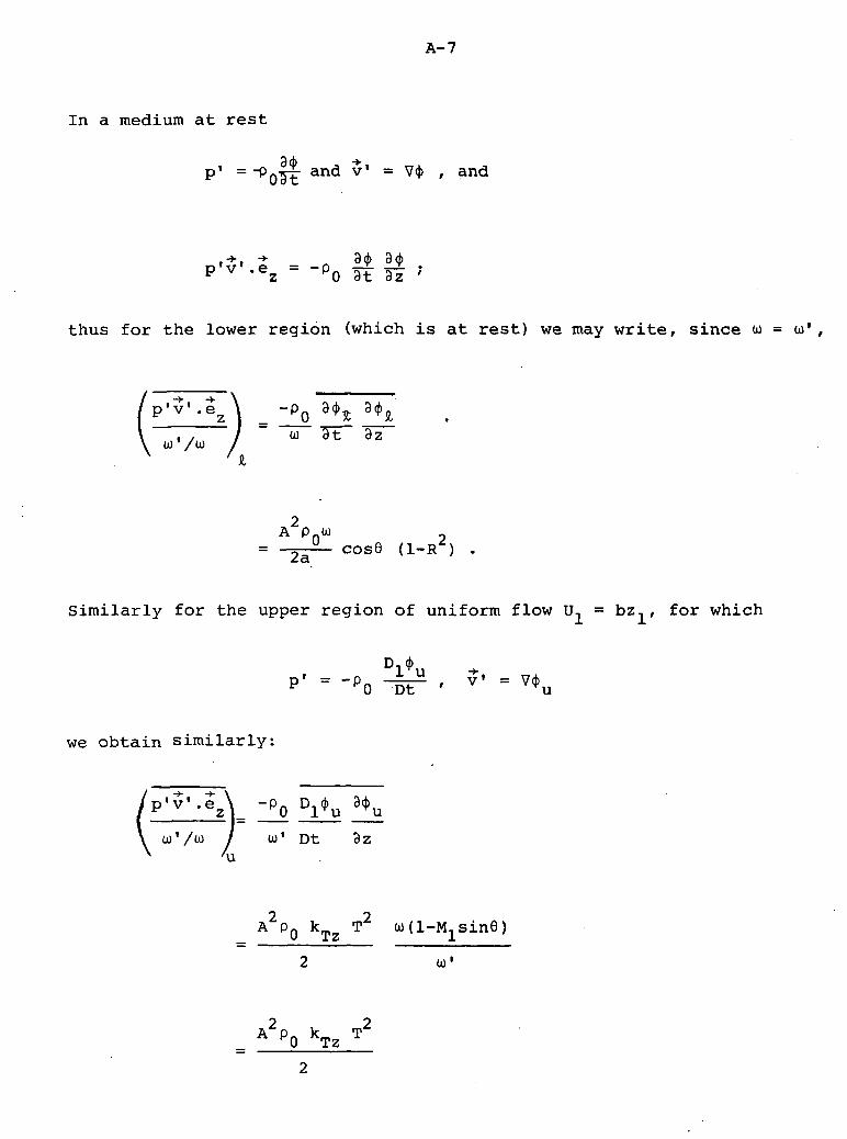
In a medium at rest

p' = ~

,-*•, -*• 3d> 3d>v -ez = -po 3?

thus for the lower region (which is at rest) we may write, since (0 =

P'v'-ez

A PW 2= 2a cose (i-R ) .

Similarly for the upper region of uniform flow U, = bz,, for which

we obtain similarly:

p'v'.e \ -Pn D.4-z 0 u

' Dt 3z

A2pQ kTz T2

0)'

A-8

Thus energy conservation follows,

d-R2) k.z = T2 kTz

where k. = kcos91Z

= ± J (1- siand k = ± (1-sinQ)2 - sin28

B-l

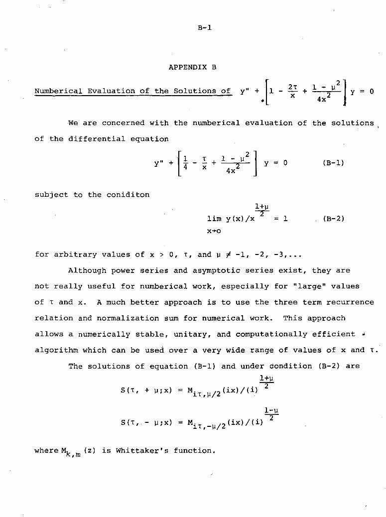
APPENDIX B

Numberical Evaluation of the Solutions of y" +M4x

We are concerned with the numberical evaluation of the solutions

of the differential equation

2y» + - V y = 0 (B-l)

subject to the coniditon

1+U

lim y(x)/x = 1

x+o

(B-2)

for arbitrary values of x > 0, T, and y ^ -1, -2, -3,...

Although power series and asymptotic series exist, they are

not really useful for numberical work, especially for "large" values

of T and x. A much better approach is to use the three term recurrence

relation and normalization sum for numerical work. This approach

allows a numerically stable, unitary, and computationally efficient *

algorithm which can be used over a very wide range of values of x and T,

The solutions of equation (B-l) and under condition (B-2) are

S(T, + y;x) = M.

,.- y;x) =

i-y• x 2

where M, (z) is Whittaker's function.

B-2

Using Buchholz [14] we can show that the functions

u. = S(T ,y + 2j;x)

satisfy the three term recurrence relation

(y + 2jy + j -- 1) (y

l+ 2j - 2)

!x

j+1

2T

(y + 2j - i) (y + 2j - 2)u .

2j2 2Z ^

(y + j) (y + 2j + 1) (y + 2j + 2) = 0

(B-4)

and are subject to the normalization relation

j=0

ux 1+y~2~ ~2~. (a)) u . = e x

The A . (w) are given by

(B-5)

(B-6)

The formulas (B-4), (B-5), (B-6) form the basis of the numerical

algorithm. Using the Perron-Kreuser theorem [15] , the solutions of

(B-4) behave asymptotically as

or

Using (B-5) and (B-6), we infer that the required solution has the

B-3

latter behavior; this solution is called the subdominant solution.

The actual numerical algorithm is based upon the algorithm of Olver

[16].

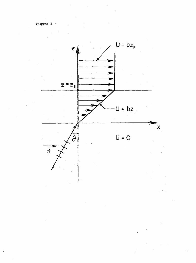
Figure 1

U = bz,

CM

-rO

CD

ro

'Q 'O 'O 'O

q'iri

qCD

OH

q'c\J

±-o " tS

o

o

o^

qIT)

q-*-(£>

~ ( o ' o • o 'o 'o

OH

-rO

O

OCM

Qro

o

OH

IT)

w

CE>

OO

C

CO

c.to

o o

'Q ' O ' O • O ' Q 'ouojpaipy)

-

o-cvi

q'ro

oin

UH