
Source Rocks Characterization in Benakat Gully, Limau, and ...
131
Proceedings of the 1 st International Conference on Energy and 7 th Indonesia – Malaysia Geoheritage Conference Yogyakarta, 20-21 November 2014 1 Source Rocks Characterization in Benakat Gully, Limau, and Jemakur-Tabuan Graben, North-South Palembang Sub-Basin, South Sumatra Basin M. Syaifudin 1,2,a , Eddy A. Subroto 2 , Dardji Noeradi 2 , Asep H.P.Kesumajana 2 1 Universitas Pembangunan Nasional “Veteran” Yogyakarta 2 Institut Teknologi Bandung a [email protected] ABSTRACT There are differences opinion among geochemistry expert about determining oil family in the South Sumatra Basin. The first opinion that only analyzing oil samples, argues that oils in this area are derived from fluvio-deltaic and lacustrine source rock, while the second opinion that analyzing source rocks and oils samples, argues that lacustrine oil is not found in this area. Research area is located at Benakat gully, Limau graben, and Jemakur-Tabuan graben which is considered as syn-rift basins, consist of syn-rift sediments. So, expected that source rock with lacustrine characterization could be found in this area. This paper emphasizes geochemistry methods. Source rock analysis, consist of 68 samples for carbon isotope and 76 samples for biomarker. Characterization has been based on qualitative and quantitative data. Qualitative data comprise evaluation based on chromatograms and mass-fragmentograms, whereas quantitative data consists of a series of cross-plots. The result from geochemistry analysis, concluded that Lemat Formation in Benakat Gully and Jemakur-Tabuan Graben is interpreted as source rock with estuarine characterization, while Lemat Formation in Limau graben interpreted as source rock with fluvio-deltaic characterization. Talangakar Formation in Benakat Gully, Limau Graben, and Jemakur-Tabuan Graben is interpreted as source rock with deltaic characterization. Based on geochemistry analysis, source rock in research area consist of estuarine, deltaic, and fluvio-deltaic source rocks. There is no source rock with lacustrine characterization in research area. Oil with lacustrine characterization in reseach area, considered generate by Lemat Formation from the deeper strata of stratigraphy, supported by Morley‟s Paleontology data but it need further exploration and analysis. There is also new interpretation of Lemat Formation‟s source rock in Benakat Gully and Jemakur-Tabuan Graben, which is part of it having tendency as marine influence, interpreted as source rock with estuarine characterization. Key words: biomarker, lacustrine, estuarine, fluvio-deltaic, deltaic. INTRODUCTION There are a number of sub-basins in the research area which is potential as the hydrocarbon kitchen but it isn‟t known with more certainty yet about the character of the source rock. There are two group‟s results of the source rock and oil research, there are: first group is Robinson (1987) and Suseno et al. (1992), researching source rock and oil samples, which is conclude that oil in the research area was generated from fluvio- deltaic source rock, while the second group is ten Haven and Schiefelbein (1995), Ginger and Fielding (2005), Noble et al. (2009), and Rashid et al. (1998), which only researching oil samples, conclude that the oil in the research area besides generated from fluvio- deltaic sediment, there are also generated from lacustrine sediment (Table 1). LOCATION OF RESEARCH AREA Research area located in Benakat Gully and Limau Graben, which are located in South Palembang Sub Basin, also in Jemakur- Tabuan Graben which is part of North Palembang Sub Basin, South Sumatra Basin.
-
Upload
khangminh22 -
Category
Documents
-
view
2 -
download
0
Transcript of Source Rocks Characterization in Benakat Gully, Limau, and ...

Proceedings of the 1st International Conference on Energy and
7th Indonesia – Malaysia Geoheritage Conference
Yogyakarta, 20-21 November 2014
1
Source Rocks Characterization
in Benakat Gully, Limau, and Jemakur-Tabuan Graben,
North-South Palembang Sub-Basin, South Sumatra Basin
M. Syaifudin1,2,a
, Eddy A. Subroto2, Dardji Noeradi
2, Asep H.P.Kesumajana
2
1Universitas Pembangunan Nasional “Veteran” Yogyakarta
2Institut Teknologi Bandung
ABSTRACT
There are differences opinion among geochemistry expert about determining oil family in the South
Sumatra Basin. The first opinion that only analyzing oil samples, argues that oils in this area are
derived from fluvio-deltaic and lacustrine source rock, while the second opinion that analyzing source
rocks and oils samples, argues that lacustrine oil is not found in this area. Research area is located at
Benakat gully, Limau graben, and Jemakur-Tabuan graben which is considered as syn-rift basins,
consist of syn-rift sediments. So, expected that source rock with lacustrine characterization could be
found in this area.
This paper emphasizes geochemistry methods. Source rock analysis, consist of 68 samples for carbon
isotope and 76 samples for biomarker. Characterization has been based on qualitative and quantitative
data. Qualitative data comprise evaluation based on chromatograms and mass-fragmentograms,
whereas quantitative data consists of a series of cross-plots.
The result from geochemistry analysis, concluded that Lemat Formation in Benakat Gully and
Jemakur-Tabuan Graben is interpreted as source rock with estuarine characterization, while Lemat
Formation in Limau graben interpreted as source rock with fluvio-deltaic characterization. Talangakar
Formation in Benakat Gully, Limau Graben, and Jemakur-Tabuan Graben is interpreted as source
rock with deltaic characterization. Based on geochemistry analysis, source rock in research area
consist of estuarine, deltaic, and fluvio-deltaic source rocks. There is no source rock with lacustrine
characterization in research area. Oil with lacustrine characterization in reseach area, considered
generate by Lemat Formation from the deeper strata of stratigraphy, supported by Morley‟s
Paleontology data but it need further exploration and analysis. There is also new interpretation of
Lemat Formation‟s source rock in Benakat Gully and Jemakur-Tabuan Graben, which is part of it
having tendency as marine influence, interpreted as source rock with estuarine characterization.
Key words: biomarker, lacustrine, estuarine, fluvio-deltaic, deltaic.
INTRODUCTION
There are a number of sub-basins in the
research area which is potential as the
hydrocarbon kitchen but it isn‟t known with
more certainty yet about the character of the
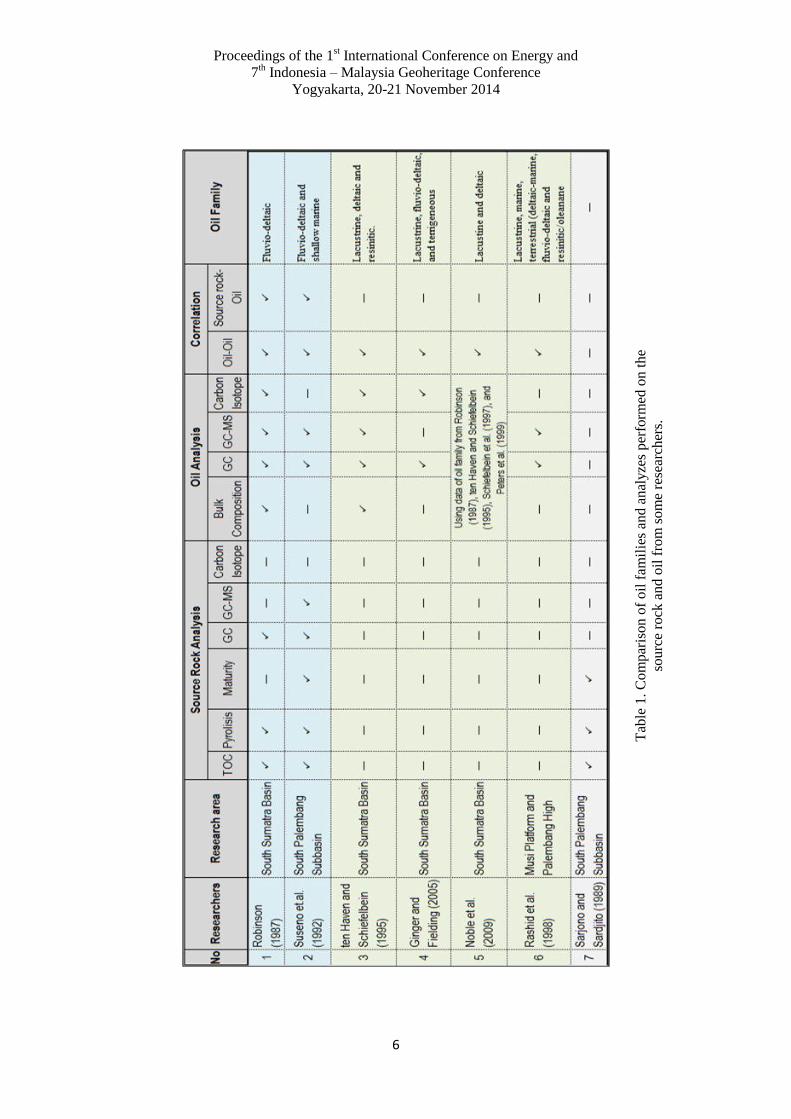
source rock. There are two group‟s results of
the source rock and oil research, there are: first
group is Robinson (1987) and Suseno et al.
(1992), researching source rock and oil
samples, which is conclude that oil in the
research area was generated from fluvio-
deltaic source rock, while the second group is
ten Haven and Schiefelbein (1995), Ginger
and Fielding (2005), Noble et al. (2009), and
Rashid et al. (1998), which only researching
oil samples, conclude that the oil in the
research area besides generated from fluvio-
deltaic sediment, there are also generated from
lacustrine sediment (Table 1).
LOCATION OF RESEARCH AREA
Research area located in Benakat Gully and
Limau Graben, which are located in South
Palembang Sub Basin, also in Jemakur-
Tabuan Graben which is part of North
Palembang Sub Basin, South Sumatra Basin.

Proceedings of the 1st International Conference on Energy and
7th Indonesia – Malaysia Geoheritage Conference
Yogyakarta, 20-21 November 2014
2
RESEARCH METHODS
This paper emphasizes geochemistry methods.
Source rock analysis, consist of 68 samples for
carbon isotope and 76 samples for biomarker.
Characterization has been based on qualitative
and quantitative data. Qualitative data
comprise evaluation based on chromatograms
and mass-fragmentograms, whereas
quantitative data consists of a series of cross-
plots, example: cross plot of carbon isotope
δ13
C saturates - aromatics, distribution of C27-
C28-C29 sterane, Pr/nC17-Ph/nC18, Pr/Ph-
Pr/nC17, carbon isotope δ13
C saturates-Pr/Ph,
Pr/Ph-total hopane/total sterane, and ratio of
C26/C25 (tricyclic).
The results of this study, expected could find
out the character of source rock in
hydrocarbon kitchen, including the possibility
of lacustrine source rock‟s existence.
REGIONAL STRUCTURAL GEOLOGY
OF SOUTH SUMATRA BASIN
Geological structures that control the regional
of South Sumatra (Figure 1) were influenced
by three tectonic phases (Pulunggono et al.,
1992):
Compression (Upper Jurassic – Lower
Cretaceous)
Tension (Upper Cretaceous – Lower
Tertiary)
Compression (Middle Miocene –
Recent)
The first phase: started in Upper Jurassic –
Lower Cretaceous, characterized with the
subduction of India-Australia plate as a
movement mechanism to yield primary stress
to the Sundaland trending N 30o
W. This
subduction resulted simple shear (N 300o E) as
strike slip fault that was actively moved
laterally. This was assumed as the cause of
linearity trending N-S as antithetic fault which
was inactive.
The second phase: commenced during Upper
Cretaceous-Lower Tertiary, characterized by
the change of the subduction trend of the
India-Australia plate into N-S. This event
resulted in the formation of some geological
structures (fractures) caused by tension force
as linearity with N-S direction. This
phenomenon caused the formation of grabens
and depressions, such as Benakat Gulley.
Initiation of graben filling with Tertiary
sediments was started.
The third phase: commenced in the Middle
Miocene-present, shown with, again, the
change of the subduction direction into N 6o E,
causing rejuvenation and inversion processes
on the paleostructures by Plio-Pleistocene (N
330o E) and the uplifting of the Barisan
Montains and also the formation of some
thrust faults with the Lematang fault pattern.
REGIONAL STRATIGRAPHY OF
SUMATRA BASIN
Based on the tectonostratigraphy framework,
Ryacudu (2008) divides Early Tertiary rock
units in the South Sumatra Basin as follows
(Figure 2):
Pre-rift sequences
This sequence consists of volcanic rock of
Kikim Formation and pre-Tertiary rocks.
Kikim Formation are the oldest Tertiary rocks
in the South Sumatra Basin, consist of
volcanic rocks such as volcanic breccia,
agglomerate, andesitic tuffs and igneous rocks
(as intrusions and lava flows). Age of Kikim
Formation based on dating K-Ar is 54-30 Ma
(Paleocene - Lower Oligocene, Ryacudu,
2008). The oldest age and the contact with pre-
Tertiary rocks are unknown, while the relation
with the formation above is unconformity.
Syn-rift sequences
Syn-rift sequence consists of Lahat Group
consisting of Lemat and Benakat Formations
with interfingering relations. The main
constituent of Lemat Formation are coarse
clastic rocks (sandstone) with Tuff Member
and conglomerate Member, while Benakat
Formations dominated by fine clastic rocks
(shale). The group does not contain fossils,
dating is determined by palinomorf
Meyeripollis naharkotensis in shale of Benakat
Formations indicating Upper Oligocene –
Lower Early Miocene. Sandstones of Lemat
Formation deposited in fluvial environment,
while conglomerate is interpreted as an
alluvial fan sediment. Shale of Benakat
Proceedings of the 1st International Conference on Energy and
7th Indonesia – Malaysia Geoheritage Conference
Yogyakarta, 20-21 November 2014
3
Formations interpreted as lake (lacustrine)
sediment.
Post-rift sequences
Tanjungbaru Formation, originally considered
a GRM (Gritsand Member) formerly known as
a member of the Talangakar Formation. This
unit is dominated by conglomeratic sandstone
deposition system as a result of braided river.
Unconformity contact with Lahat Group below
it. Member of the Formation Talangakar
commonly referred to as TRM (Transition
Member) proposed a Talangakar Formation.
This Formation consists of alternating
sandstones and shales, with thin coal
interbedded, deposited in the transition
environment, i.e : the delta system to shallow
marine, of Early Miocene. Baturaja Formation,
Early Miocene (N5-N6), composed of
limestone bioclastic, kalkarenit, bioclastic
sandy limestones and reefal bioherm with
interbedded of calcareous shale, deposited on
the carbonate platform. Gumai Formation,
Early Miocene to Middle Miocene, composed
by calcareous mudstone that contains fossil
planktonic foraminifera Globigerina and
shales napalan with glaukonitic quartz
sandstones. Deposited conformity over Gumai
Formation is Palembang Group, consist of Air
Benakat, Muara Enim, and Kasai Formation.
Furthermore, the marine condition is getting
shallower and then the Kasai Formation
deposited in fluviatil and terrestrial
environment.
SOURCE ROCKS
CHARACTERIZATION
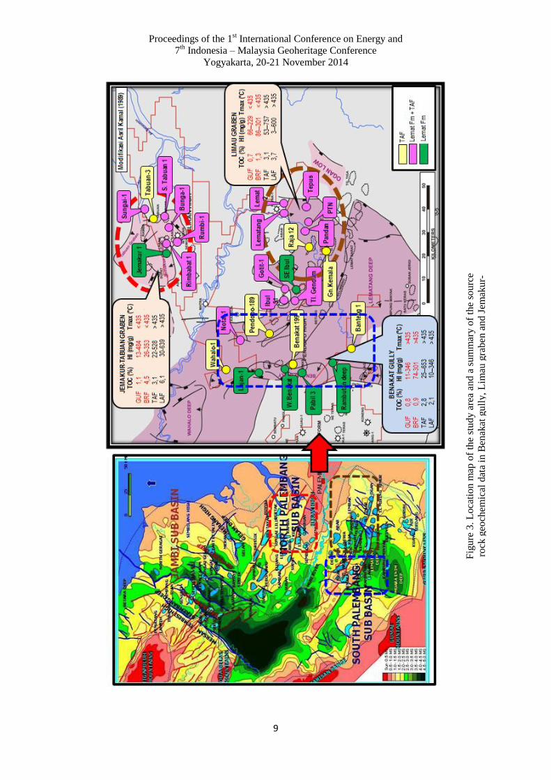
Figure 3 shows location map of the study area
and summary of the source rock geochemical
data in Benakat Gully, Limau Graben, and
Jemakur-Tabuan Graben.
Source Rocks Characterization in Benakat
Gully
Figure 4 shows sterane distribution curve of
C27,C28, dan C29 , cross plot of Pr/nC17-
Ph/nC18, Pr/Ph – Pr/nC17, Pr/Ph–
hopane/sterane, carbon isotope δ13
C saturates
– aromatics and carbon isotope δ13
C saturates -
Pr/Ph, Lemat and Talangakar Formation in
Benakat gully. This phenomenon shows Lemat
Formation was deposited in estuarine or
shallow lacustrine environment, whereas
Talangakar Formation was deposited in
estuarine or shallow lacustrine to terrestrial
environment. Lemat and Talangakar
Formation consists of humic and mixed
kerogen, but mostly humic kerogen, and
influenced by terrestrial material. Lemat
Formation mostly deposited in anoxic-suboxic,
and Talangakar Formation deposited in oxic
condition.
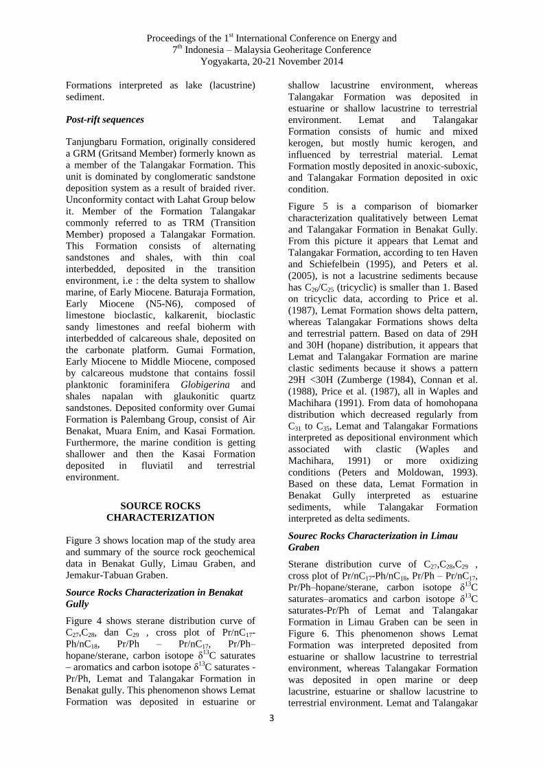
Figure 5 is a comparison of biomarker
characterization qualitatively between Lemat
and Talangakar Formation in Benakat Gully.
From this picture it appears that Lemat and
Talangakar Formation, according to ten Haven
and Schiefelbein (1995), and Peters et al.
(2005), is not a lacustrine sediments because
has C26/C25 (tricyclic) is smaller than 1. Based
on tricyclic data, according to Price et al.
(1987), Lemat Formation shows delta pattern,
whereas Talangakar Formations shows delta
and terrestrial pattern. Based on data of 29H
and 30H (hopane) distribution, it appears that
Lemat and Talangakar Formation are marine
clastic sediments because it shows a pattern
29H <30H (Zumberge (1984), Connan et al.
(1988), Price et al. (1987), all in Waples and
Machihara (1991). From data of homohopana
distribution which decreased regularly from
C31 to C35, Lemat and Talangakar Formations
interpreted as depositional environment which
associated with clastic (Waples and
Machihara, 1991) or more oxidizing
conditions (Peters and Moldowan, 1993).
Based on these data, Lemat Formation in
Benakat Gully interpreted as estuarine
sediments, while Talangakar Formation
interpreted as delta sediments.
Sourec Rocks Characterization in Limau
Graben
Sterane distribution curve of C27,C28,C29 ,
cross plot of Pr/nC17-Ph/nC18, Pr/Ph – Pr/nC17,
Pr/Ph–hopane/sterane, carbon isotope δ13
C
saturates–aromatics and carbon isotope δ13
C
saturates-Pr/Ph of Lemat and Talangakar
Formation in Limau Graben can be seen in
Figure 6. This phenomenon shows Lemat
Formation was interpreted deposited from
estuarine or shallow lacustrine to terrestrial
environment, whereas Talangakar Formation
was deposited in open marine or deep
lacustrine, estuarine or shallow lacustrine to
terrestrial environment. Lemat and Talangakar
Proceedings of the 1st International Conference on Energy and
7th Indonesia – Malaysia Geoheritage Conference
Yogyakarta, 20-21 November 2014
4
Formations consists of humic kerogen and
influenced by terrestrial material on anoxic-
suboxic to oxic condition but mostly found on
oxic condition. Lemat and Talangakar
Formations consist of terrigeneous material
and mixed source.
Figure 7 is a comparison of biomarker
characterization qualitatively between Lemat
and Talangakar Formations in Limau Graben.
From this picture, appears that Lemat and
Talangakar Formation in Limau Graben is not
a lacustrine sediments. Based on tricyclic data,
Lemat Formation shows terrestrial pattern,
whereas Talangakar Formations show
terrestrial and marine pattern. Based on data 29
H and 30
H (hopana) distribution, it appears
that Lemat Formation is marine clastic
sediments, while Talangakar Formation is
marine clastic and evaporates-carbonate
sediment. From data homohopana distribution,
Lemat and Talangakar Formations, interpreted
having depositional environment which
associated with clastic or more oxidizing
conditions. Based on these data, Lemat
Formation in Limau Graben interpreted as
fluvial sediments, while Talangakar Formation
interpreted having more marine
characterization as delta sediments.
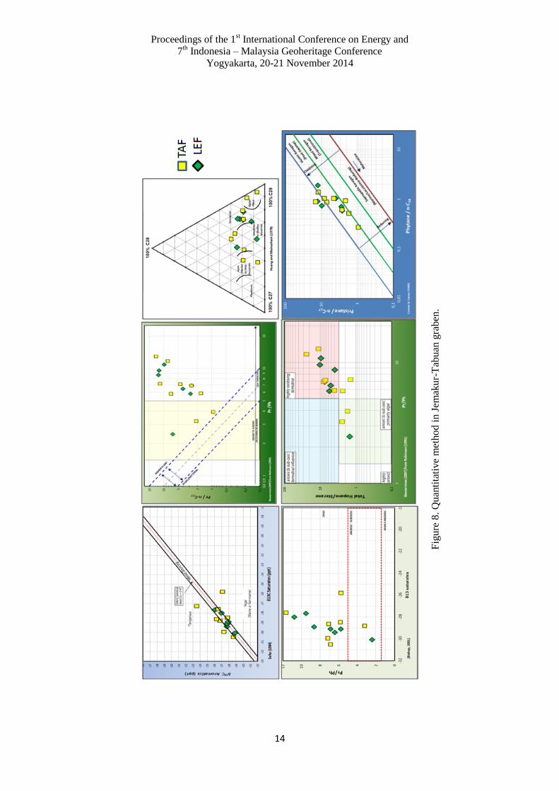
Sourec Rocks Characterization in Jemakur-
Tabuan Graben
Curve of sterane distribution C27, C28, and C29,
cross plots Pr/nC17-Ph/nC18, Pr/Ph – Pr/nC17,
and Pr/Ph–hopane/sterane, carbon isotope δ13
C
saturates–aromatics, and carbon isotope δ13
C
saturates-Pr/Ph of Lemat and Talangakar
Formations in Jemakur-Tabuan graben can be
seen in Figure 8. This figure shows Lemat
Formation interpreted deposited from
estuarine or shallow lacustrine to terrestrial
environments, whereas Talangakar Formations
deposited from marine or deep lacustrine,
estuarine or shallow lacustrine to terrestrial
environment. Lemat Formation consists of
humic kerogen while Talangakar Formation
consists of humic and mixed kerogen, but
most of the humic kerogen. Both of these
formations are influenced by terrestrial
material, with anoxic-suboxic to oxic
conditions, but mostly found on oxic
conditions. Lemat Formation consist of mixed
source, while Talangakar Formations consist
of algae, mixed source, and terrigeneous.
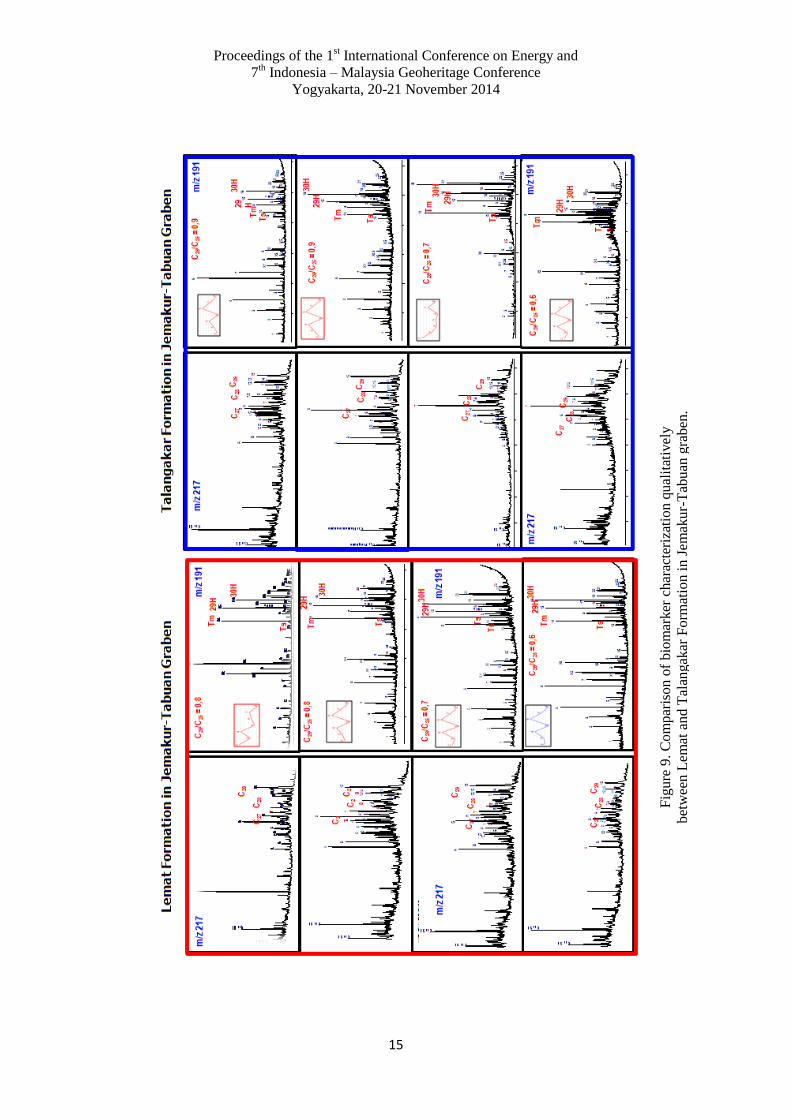
Figure 9 is a comparison of biomarker
characterization qualitatively between Lemat
and Talangakar Formations in Jemakur-
Tabuan Graben. From this picture it appears
that Lemat and Talangakar Formation in
Limau graben, is not a lacustrine sediments.
Based on tricyclic data, Lemat Formation
shows delta and marine pattern, whereas
Talangakar Formations show terrestrial, delta,
and marine pattern. Based on data of 29
H and 30
H (hopana) distribution, it appears that
Lemat and Talangakar Formation is marine
clastic and evaporates-carbonate sediment.
From data of homohopana distribution, Lemat
and Talangakar Formations interpreted having
depositional environment which associated
with clastic or more oxidizing conditions.
Based on these data, lemat Formation in
Limau graben is interpreted as estuarine
sediments, while Talangakar Formation is
interpreted as delta sediments.
CONCLUSION
Lemat and Talangakar Formations in Benakat
Gully mostly consist of humic kerogen and
influenced by terrestrial material. Lemat
Formation mostly found on anoxic-suboxic
conditions, whereas Talangakar Formation
largely found on oxic condition. Based on
tricyclic data, Lemat Formation shows delta
pattern, whereas Talangakar Formations show
delta and terrestrial pattern. Lemat Formation
in Benakat gully is interpreted not a lacustrine,
but estuarine sediments, and Talangakar
Formation is delta sediment. The existence of
lacustrine sediment is interpreted under
estuarine sediments.
Lemat and Talangakar Formations in Limau
Graben consists of humic kerogen and
influenced by terrestrial material in anoxic-
suboxik to oxic condition, but mostly oxic
condition. Based on tricyclic data, Lemat
Formation shows terrestrial pattern, whereas
Talangakar Formations show terrestrial and
marine pattern. Lemat Formations interpreted
not a lacustrine, but fluvio-deltaic sediments,
and Talangakar Formation is a delta sediment.
Lemat Formation in Jemakur-Tabuan graben
consists of humic kerogen while Talangakar
Formation consists of humic and mixed
kerogen, but most humic kerogen. Both of
these Formations are influenced by terrestrial

Proceedings of the 1st International Conference on Energy and
7th Indonesia – Malaysia Geoheritage Conference
Yogyakarta, 20-21 November 2014
5
material, with most oxic conditions. Lemat
Formation in Jemakur-Tabuan graben is
interpreted not a lacustrine but estuarine
sediments, and Talangakar Formation is delta
sediment.
ACKNOWLEDGEMENTS
We would like to thank the management of
Directorate General of Oil and Gas, Pertamina
EP, and Medco EP for their permission to
publish this paper.
REFFERENCES
Artono, E. and Tamtomo B. (2000): Pre
Tertiary reservoir as a hydrocarbon
prospecting opportunity in the South
Sumatra basin, Western Indonesia in the
third millennium, AAPG International
Conference & Exhibition, Bali, Indonesia.
Ginger, D. and Fielding, K. (2005): The
Petroleum systems and future potential of
the South Sumatra basin, Proceedings
Indonesian Petroleum Association, thirtieth
Annual Convention & Exhibition, Jakarta,
Indonesia, p. 67-89.
Morley, R.J. (2009): Sequence biostratigraphy
of Medco South Sumatra acreage, not
published, 85 pp.
Noble, R., Orange, D., Decker J., Teas P., and
Baillie, P. (2009): Oil and gas seeps in deep
marine sea floor cores as indicators of active
petroleum systems in Indonesia, Proceedings
Indonesia Petroleum Association, thirty third
IPA Annual Convention & Exhibition,
Jakarta, Indonesia.
Peters, K.E., and Moldowan, J.M. (1993): The
Biomarker guide “Interpreting molecular
fossils in petroleum and ancient sediments”,
Prentice Hall, Englewood Cliffs, New
Jersey, 363 pp.
Peters, K.E., Walters, C.C., and Moldowan
J.M. (2005), Volume 1, The Biomarker
guide, Cambridge University press, 474 pp.
Peters, K.E., Walters, C.C., and Moldowan
J.M. (2005), Volume 2, The Biomarker
guide, Cambridge University press, p. 475-
1155.
Price, P.L., Sullivan, T.O., and Alexander, R.
(1987): The Nature and occurrence of oil in
Seram, Indonesia, Proceedings Indonesia
Petroleum Association, sixteenth Annual
Convention, Jakarta, Indonesia.
Pulunggono, A., Agus, H. S. and Kosuma, C.
G. (1992): Pre-Tertiary and Tertiary fault
systems as a framework of the South
Sumatra basin; A Study of SAR maps.
Proceedings Indonesian Petroleum
Association, twenty first Annual Convention
& Exhibition, Jakarta, Indonesia, p. 339-360.
Rashid, H., Sosrowidjojo, I.B., and Widiarto,
F.X. (1998): Musi platform and Palembang
high: A New look at the petroleum system,
Proceedings, Indonesian Petroleum
Association, twenty-Sixth Annual
Convention, Jakarta, Indonesia, p. 265-276.
Robinson, K.M. (1987): An Overview of
source rocks and oils in Indonesia,
Proceedings Indonesian Petroleum
Association, sixteenth Annual Convention,
Jakarta, Indonesia, p. 97-122.
Ryacudu, R. (2008): Tinjauan stratigrafi
Paleogen Cekungan Sumatra Selatan,
Sumatra Stratigraphy Workshop, IAGI, p.
99-114.
Sarjono, S. and Sardjito (1989): Hydrocarbon
source rock identification in the South
Palembang subbasin, Proceedings
Indonesian Petroleum Association,
eighteenth Annual Convention, Jakarta,
Indonesia, p. 424-467.
Suseno, P.H., Zakaria, Mujahidin, N., and
Subroto, E.A. (1992): Contribution of Lahat
Formation as hydrocarbon source rock in
South Palembang area, South Sumatra,
Indonesia, Proceedings Indonesian
Petroleum Association, twenty first Annual
Convention, Jakarta, Indonesia, p. 325-337.
ten Haven and Schiefelbein (1995): The
petroleum systems of Indonesia,
Proceedings Indonesian Petroleum
Association, twenty fourth Annual
Convention, Jakarta, Indonesia, p. 443-459.
Waples, D.W. and Curiale J.A., (1999): Oil–
oil and oil–source rock correlations, Dalam
AAPG Treatise of Petroleum Geology, Hand
book of Petroleum Geology, Bab 8, ed.
Beaumont E.A., The American Association
of Petroleum Geologist, p. 8.3-8.71.
Proceedings of the 1st International Conference on Energy and
7th Indonesia – Malaysia Geoheritage Conference
Yogyakarta, 20-21 November 2014
6
Tab
le 1
. C
om
par
ison o
f oil
fam
ilie
s an
d a
nal
yze
s per
form
ed o
n t
he
sourc
e ro
ck a
nd o
il f
rom
som
e re
sear
cher
s.

Proceedings of the 1st International Conference on Energy and
7th Indonesia – Malaysia Geoheritage Conference
Yogyakarta, 20-21 November 2014
7
Fig
ure
1. T
ecto
nic
evolu
tion o
f th
e S
outh
Sum
atra
Bas
in f
rom
Up
per
Jura
ssic
-now
(P
ulu
nggono e
t al
., 1
992)

Proceedings of the 1st International Conference on Energy and
7th Indonesia – Malaysia Geoheritage Conference
Yogyakarta, 20-21 November 2014
8
Fig
ure
2. R
egio
nal
str
atig
raphy o
f th
e S
outh
Sum
atra
Bas
in (
mo
dif
ied
Ryac
udu,
2008).
Proceedings of the 1st International Conference on Energy and
7th Indonesia – Malaysia Geoheritage Conference
Yogyakarta, 20-21 November 2014
9
Fig
ure
3.
Loca
tion m
ap o
f th
e st
udy a
rea
and a
sum
mar
y o
f th
e so
urc
e
rock
geo
chem
ical
dat
a in
Ben
akat
gull
y,
Lim
au g
raben
and J
emak
ur-
Tab
uan
gra
ben
.

Proceedings of the 1st International Conference on Energy and
7th Indonesia – Malaysia Geoheritage Conference
Yogyakarta, 20-21 November 2014
10
Fig
ure
4.
Quan
tita
tive
met
hod i
n B
enak
at g
ull
y

Proceedings of the 1st International Conference on Energy and
7th Indonesia – Malaysia Geoheritage Conference
Yogyakarta, 20-21 November 2014
11
Fig
ure
5.
Com
par
ison o
f bio
mar
ker
char
acte
riza
tion q
ual
itat
ivel
y
bet
wee
n L
emat
and T
alan
gak
ar F
orm
atio
n i
n B
enak
at g
ull
y.

Proceedings of the 1st International Conference on Energy and
7th Indonesia – Malaysia Geoheritage Conference
Yogyakarta, 20-21 November 2014
12
Fig
ure
6.
Quan
tita
tive
met
hod i
n L
imau
gra
ben
.

Proceedings of the 1st International Conference on Energy and
7th Indonesia – Malaysia Geoheritage Conference
Yogyakarta, 20-21 November 2014
13
Fig
ure
7.
Com
par
ison o
f bio
mar
ker
char
acte
riza
tion q
ual
itat
ivel
y
bet
wee
n L
emat
and T
alan
gak
ar F
orm
atio
ns
in L
imau
Gra
ben
.
Proceedings of the 1st International Conference on Energy and
7th Indonesia – Malaysia Geoheritage Conference
Yogyakarta, 20-21 November 2014
14
Fig
ure
8.
Quan
tita
tive
met
hod i
n J
emak
ur-
Tab
uan
gra
ben
.
Proceedings of the 1st International Conference on Energy and
7th Indonesia – Malaysia Geoheritage Conference
Yogyakarta, 20-21 November 2014
15
Fig
ure
9.
Com
par
ison o
f bio
mar
ker
char
acte
riza
tion q
ual
itat
ivel
y
bet
wee
n L
emat
and T
alan
gak
ar F
orm
atio
n i
n J
emak
ur-
Tab
uan
gra
ben
.
Proceedings of the 1st International Conference on Energy and
7th Indonesia – Malaysia Geoheritage Conference
Yogyakarta, 20-21 November 2014
16
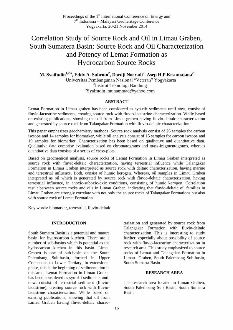
Correlation Study of Source Rock and Oil in Limau Graben,
South Sumatera Basin: Source Rock and Oil Characterization
and Potency of Lemat Formation as
Hydrocarbon Source Rocks
M. Syaifudin1,2,a
, Eddy A. Subroto2, Dardji Noeradi
2, Asep H.P.Kesumajana
2
1Universitas Pembangunan Nasional “Veteran” Yogyakarta
2Institut Teknologi Bandung
ABSTRACT
Lemat Formation in Limau graben has been considered as syn-rift sediments until now, consist of
fluvio-lacustrine sediments, creating source rock with fluvio-lacustrine characterization. While based
on existing publications, showing that oil from Limau graben having fluvio-deltaic characterization
and generated by source rock from Talangakar Formation with fluvio-deltaic characterization.
This paper emphasizes geochemistry methods. Source rock analysis consist of 26 samples for carbon
isotope and 14 samples for biomarker, while oil analysis consist of 15 samples for carbon isotope and
19 samples for biomarker. Characterization has been based on qualitative and quantitative data.
Qualitative data comprise evaluation based on chromatograms and mass-fragmentograms, whereas
quantitative data consists of a series of cross-plots.
Based on geochemical analysis, source rocks of Lemat Formation in Limau Graben interpreted as
source rock with fluvio-deltaic characterization, having terrestrial influence while Talangakar
Formation in Limau Graben interpreted as source rock with deltaic characterization, having marine
and terrestrial influence. Both, consist of humic kerogen. Whereas, oil samples in Limau Graben
interpreted as oil which is generated by source rock with fluvio-deltaic characterization, having
terrestrial influence, in anoxic-suboxic-oxic conditions, consisting of humic kerogen. Correlation
result between source rocks and oils in Limau Graben, indicating that fluvio-deltaic oil families in
Limau Graben are strongly correlate with not only the source rocks of Talangakar Formations but also
with source rock of Lemat Formation.
Key words: biomarker, terrestrial, fluvio-deltaic
INTRODUCTION
South Sumatra Basin is a potential and mature
basin for hydrocarbon kitchen. There are a
number of sub-basins which is potential as the
hydrocarbon kitchen in this basin. Limau
Graben is one of sub-basin on the South
Palembang Sub-basin, formed in Upper
Cretaceous to Lower Tertiary, in extensional
phase, this is the beginning of sedimentation in
this area. Lemat Formation in Limau Graben
has been considered as syn-rift sediments until
now, consist of terrestrial sediment (fluvio-
lacustrine), creating source rock with fluvio-
lacustrine characterization. While based on
existing publications, showing that oil from
Limau Graben having fluvio-deltaic charac-
terization and generated by source rock from
Talangakar Formation with fluvio-deltaic
characterization. This is interesting to study
further, especially about possibility of source
rock with fluvio-lacustrine characterization in
research area. This study emphasized to source
rocks of Lemat and Talangakar Formation in
Limau Graben, South Palembang Sub-basin,
South Sumatra Basin.
RESEARCH AREA
The research area located in Limau Graben,
South Palembang Sub Basin, South Sumatra
Basin.
Proceedings of the 1st International Conference on Energy and
7th Indonesia – Malaysia Geoheritage Conference
Yogyakarta, 20-21 November 2014
17
RESEARCH METHODS
This paper emphasizes geochemistry methods.
Source rock analysis, consist of 26 samples for
carbon isotope and 14 samples for biomarker,
while oil analysis, consist of 15 samples for
carbon isotope and 19 samples for biomarker.
Characterization has been based on qualitative
and quantitative data. Qualitative data
comprise evaluation based on chromatograms
and mass-fragmentograms, whereas
quantitative data consists of a series of cross-
plots, eg. cross plot of carbon isotope δ13
C
saturates - aromatics, distribution of C27-C28-
C29 sterane, Pr/nC17-Ph/nC18, Pr/Ph-Pr/nC17,
carbon isotope δ13
C saturates-Pr/Ph, Pr/Ph-
total hopane/total sterane, and ratio of C26/C25
(tricyclic).
The results of this study expected could
explain the character of source rocks and oil in
the Limau Graben, also to find out the
possibility of lacustrine source rock existence
and determine the correlation between source
rocks and oils in this area, so can be known
whether Lemat Formation source rocks also
have contributed to produce oil in this area or
not. In addition, to provide a new opportunity
in the exploration of hydrocarbons in the
Limau Graben which considered as a mature
and potential basin for hydrocarbon.
REGIONAL STRUCTURAL GEOLOGY
OF SOUTH SUMATRA BASIN
Geological structures that control the regional
of South Sumatra (Figure 1) were influenced
by three tectonic phases (Pulunggono et al.,
1992):
Compression (Upper Jurassic – Lower
Cretaceous)
Tension (Upper Cretaceous – Lower
Tertiary)
Compression (Middle Miocene –
Recent)
The first phase: started in Upper Jurassic –
Lower Cretaceous, characterized with the
subduction of India-Australia plate as a
movement mechanism to yield primary stress
to the Sundaland trending N 30o
W. This
subduction resulted simple shear (N 300o E) as
strike slip fault that was actively moved
laterally. This was assumed as the cause of
linearity trending N-S as antithetic fault which
was inactive.
The second phase: commenced during Upper
Cretaceous-Lower Tertiary, characterized by
the change of the subduction trend of the
India-Australia plate into N-S. This event
resulted in the formation of some geological
structures (fractures) caused by tension force
as linearity with N-S direction. This
phenomenon caused the formation of grabens
and depressions, such as Benakat Gulley.
Initiation of graben filling with Tertiary
sediments was started. In general faults and
grabens formed during this phase show N-S
and WNW-ESE directions.
The third phase: commenced in the Middle
Miocene-present, shown with, again, the
change of the subduction direction into N 6o E,
causing rejuvenation and inversion processes
on the paleostructures (N 300o E/N-S) by Plio-
Pleistocene (N 330o E) and the uplifting of the
Barisan Montains and also the formation of
some thrust faults with the Lematang fault
pattern. During this phase, the Lematang fault
pattern that initially acted as depocenter of the
Muara Enim Deep has been uplifted being
anticlinorium series of Pendopo-Limau
(Figure 2.5). Folding and thrust-faulting
processes caused by compression force
occurred in the back-arc basinal and floured
during Plio-Pleistocene.
REGIONAL STRATIGRAPHY OF
SUMATRA BASIN
Based on the tectonostratigraphy framework,
Ryacudu (2008) divides Early Tertiary rock
units in the South Sumatra Basin as follows
(Figure 2):
Pre-rift sequences
This sequence consists of volcanic rock of
Kikim Formations and pre-Tertiary rocks.
Kikim Formations are the oldest Tertiary rocks
in the South Sumatra Basin, consist of
volcanic rocks such as volcanic breccia,
agglomerate, andesitic tuffs and igneous rocks
(as intrusions and lava flows). Age of Kikim
Formation based on dating K-Ar is 54-30 Ma
(Paleocene - Lower Oligocene, Ryacudu,
2008). The oldest age and the contact with pre-

Proceedings of the 1st International Conference on Energy and
7th Indonesia – Malaysia Geoheritage Conference
Yogyakarta, 20-21 November 2014
18
Tertiary rocks are unknown, while the relation
with the Formation above is unconformity.
Syn-rift sequences
Syn-rift sequence consists of rock group of
Lahat Group consisting of Lemat and Benakat
Formation with interfingering relations. The
main constituent of Lemat Formation are
coarse clastic rocks (sandstone) with Tuff
Member and conglomerate Member, while
Benakat Formations dominated by fine clastic
rocks (shale). The group does not contain
fossils, dating is determined by palinomorf
Meyeripollis naharkotensis in shale of Benakat
Formations indicating Upper Oligocene –
Lower Early Miocene. The group has non-
conformity relationship with rock Formations
above and below it. Sandstones of Lemat
Formation deposited in fluvial environment,
while conglomerate is interpreted as an
alluvial fan sediment. Shale of Benakat
Formations interpreted as the result of
deposition in the lake system (lacustrine).
Post-rift sequences
This sequence consists of a rock from Telisa
group consisting Tanjungbaru, Talangakar,
Baturaja, and Gumai Formation. Tanjungbaru
Formation, originally considered a GRM
(Gritsand Member) formerly known as a
member of the Talangakar Formation. This
unit is dominated by conglomeratic sandstone
deposition system as a result of braided river.
Unconformity contact with Lahat Group below
it. Member of the Formation Talangakar
commonly referred to as TRM (Transition
Member) proposed a Talangakar Formation.
This Formation consists of alternating
sandstones and shales, with thin coal
interbedded, deposited in the transition
environment. Baturaja Formation, Early
Miocene (N5-N6), composed of limestone
bioclastic, kalkarenit, bioclastic sandy
limestones and reefal bioherm with
interbedded of calcareous shale, deposited on
the carbonate platform. Gumai Formation,
Early Miocene to Middle Miocene, composed
by calcareous mudstone that contains fossil
planktonic foraminifera Globigerina and
shales napalan with glaukonitic quartz
sandstones. The deposition of Gumai
Formation marked the peak transgression of
the South Sumatra Basin. Air Benakat
Formation, Middle Miocene, composed by the
dominance of shallow-marine mudstone with
sandstone interbedded which is thickening and
dominating upward. Sandstone at the top is a
quartz sandstone, tufaan and glaukonitic. The
presence of the tufa material in the Formation
marked the beginning of the influence of the
source sediments from the south or uplifting of
the Bukit Barisan Mountains. Furthermore, the
marine condition is getting shallower so that it
becomes transition environment, and then the
Formation Muaraenim deposited. Muara Enim
Formation, Middle Miocene to Late Miocene.
Consists of mudstone, shale, and sandstone
and coal interbedded deposited in the delta
system or transitional environment. Kasai
Formation, Pliocene. Is a volcaniclastic
sediment, consisting of mudstone and
sandstone's tufa interbedded deposited in
fluviatil and terrestrial environments.
CHARACTERIZATION OF SOURCE
ROCKS AND OILS IN LIMAU GRABEN
Figure 3 shows location map of research area
and data location of oil and source rocks in
Limau Graben. Figure 4 shows a cross plot
Pr/nC17-Ph/nC18 and Pr/Ph – Pr/nC17, source
rocks of lemat and Talangakar Formations,
and oils in Limau Graben. This image shows
both source rocks of Lemat and Talangakar
Formation and oils, consists of humic kerogen
in suboxic-anoxic until oxic conditions, but
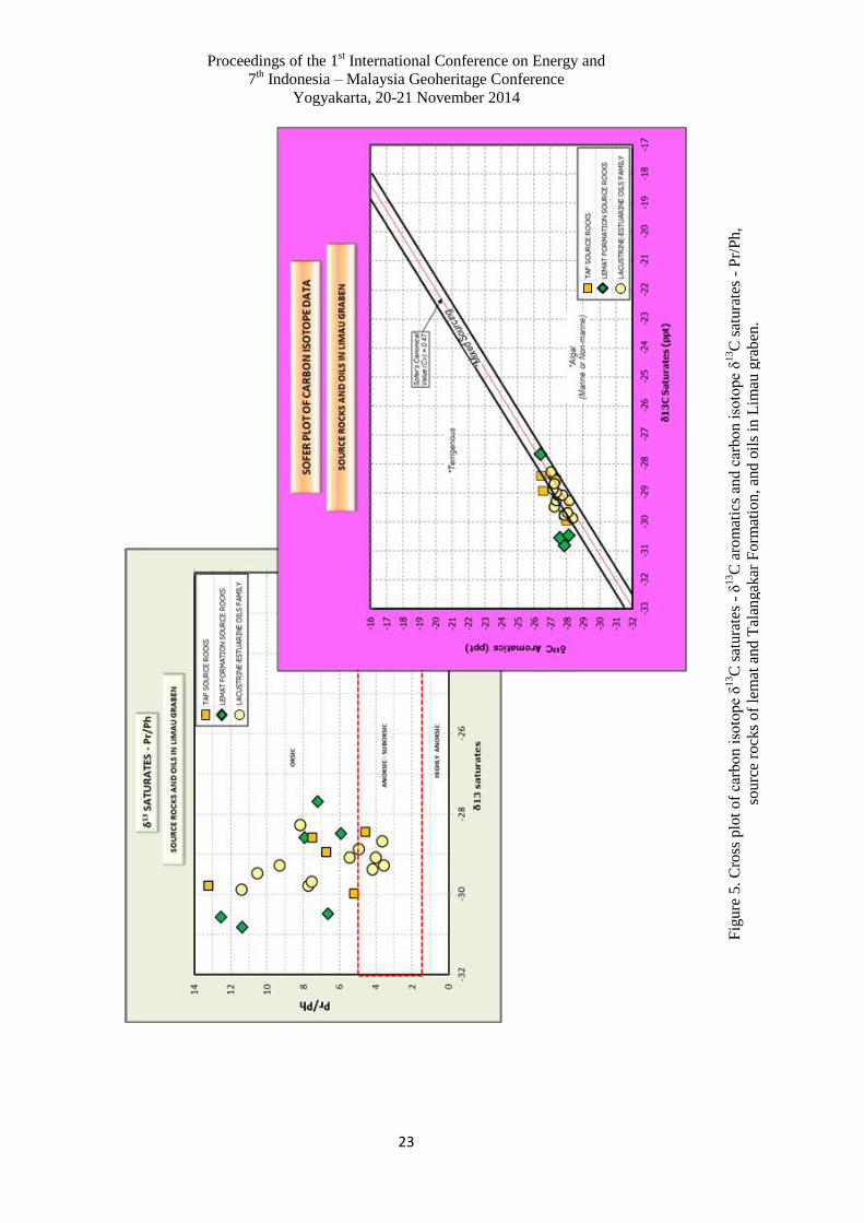
mostly in oxic conditions. Cross plot of carbon
isotope δ13
C saturates - δ13
C aromatics and
carbon isotope δ13
C saturates - Pr/Ph, source
rocks of Lemat and Talangakar Formations
and oils in Limau Graben shown in Figure 5.
This figure shows source rocks of Lemat and
Talangakar Formations and oils consists of
terrestrial and mixed material, in anoxic-
suboxic to oxic conditions, but mostly in oxic
conditions.
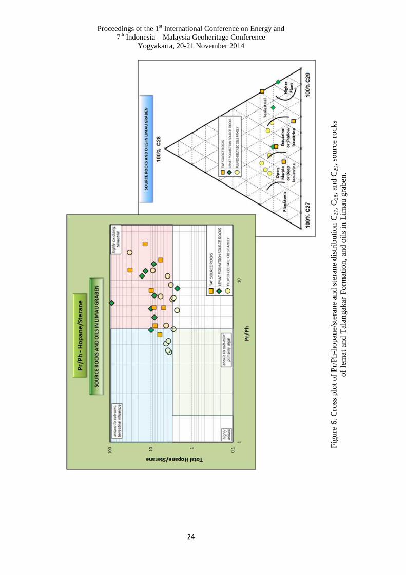
Figure 6 shows a cross plot of Pr/Ph-
hopane/sterane and sterane distribution C27,
C28, and C29, source rocks of Lemat and
Talangakar Formations and oils in Limau
Graben. From this picture it appears that the
source rocks of Lemat and Talangakar
Formations and oils affected by terrestrial
material in anoxic -suboxic until oxic
conditions, but mostly in high oxic conditions.
Besides, it also looks like Lemat Formations

Proceedings of the 1st International Conference on Energy and
7th Indonesia – Malaysia Geoheritage Conference
Yogyakarta, 20-21 November 2014
19
derived from estuarine or shallow lacustrine to
terrestrial environments, whereas Talangakar
Formation and oils derived from marine or
deep lacustrine, estuarine or shallow
lacustrine, and terrestrial environments.
Figure 7 is a comparison of biomarker
characterization qualitatively between source
rocks of Lemat and Talangakar Formation and
oils in Limau Graben. From this picture it
appears that source rocks of Lemat and
Talangakar Formations and oils, according to
ten Haven and Schiefelbein (1995), and Peters
et al. (2005), is not lacustrine sediments
because has C26/C25 (tricyclic) smaller than 1.
Based on tricyclic data, according to Price et
al. (1987), Lemat Formation and oils show
terrestrial pattern, whereas Talangakar
Formations show marine and terrestrial
pattern. These data indicate Lemat Formation
interpreted as fluvio-deltaic sediment, whereas
Talangakar Formation having more marine
characterization than Lemat Formation. Based
on data of 29
H and 30
H (hopane) distribution, it
appears that source rocks of Lemat Formation
and oils are marine clastic sediments because
it shows a pattern 29
H <30
H, while Talangakar
Formation not only show 29
H<30
H but also
show 29
H>30
H is evaporates-carbonate
sediment (Zumberge (1984); Connan et al.
(1988); Price et al. (1987), all in Waples and
Machihara (1991). From data of homohopana
distribution which decreased regularly from
C31 to C35, source rock of Lemat, Talangakar
Formations, and oils in Limau Graben
interpreted as depositional environment which
associated with clastic sediments (Waples and
Machihara, 1991) or more oxidizing
conditions (Peters and Moldowan, 1993).
Based on these data, oil in the Limau Graben
interpreted originated from fluvio-deltaic
source rocks and has a correlation with Lemat
and Talangakar Formations in Limau Graben.
CONCLUSION
Source rocks of Lemat and Talangakar
Formations and oils in Limau Graben consists
of humic kerogen and terrestrial and mixed
material. Source rocks of Lemat and
Talangakar Formations and oils in Limau
Graben, is not derived from a lacustrine
sediments, affected by terrestrial material in
anoxic -suboxic until oxic conditions, but
mostly on high oxic conditions. Besides, its
also looks like Lemat Formations derived from
estuarine or shallow lacustrine to terrestrial
environments, whereas Talangakar Formation
and oils in Limau Graben derived from marine
or deep lacustrine, estuarine or shallow
lacustrine, and terrestrial environments. Based
on tricyclic data, Lemat Formation and oils in
Limau Graben show terestrial pattern, whereas
Talangakar Formations show marine and
terrestrial pattern. These data indicate Lemat
Formation interpreted as fluvio-deltaic
sediment, whereas Talangakar Formation
having more marine characteriztion than
Lemat Formation. Oils in the Limau Graben
interpreted originated from fluvio-delta source
rocks, has a correlation with Lemat Formation
and Talangakar Formation in Limau graben.
ACKNOWLEDGEMENTS
We would like to thank the management of
Directorate General of Oil and Gas, Pertamina
EP, and Medco EP for their permission to
publish this paper.
REFERENCES
Artono, E. and Tamtomo B. (2000): Pre
Tertiary reservoir as a hydrocarbon
prospecting opportunity in the South
Sumatra basin, Western Indonesia in the
third millennium, AAPG International
Conference & Exhibition, Bali, Indonesia.
Doust, H. and Noble, R.A., (2008): Petroleum
system of Indonesia, Marine and Petroleum
Geology, Vol. 25, p. 103–129.
Ginger, D. and Fielding, K. (2005): The
Petroleum systems and future potential of
the South Sumatra basin, Proceedings
Indonesian Petroleum Association, thirtieth
Annual Convention & Exhibition, Jakarta,
Indonesia, p. 67-89.
Hall, R. and Morley, C.K. (2004): Sundaland
basins, In Continent–ocean interactions
within the East Asian marginal seas, ed.
Clift, P., Wang, P., Kuhnt, W., dan Hayes,
D.E., Geophysical Monograph, Vol. 149, p.
55–85.
Law, C.A. (1999): Evaluating source rocks, In
AAPG Treatise of Petroleum Geology, Hand
book of Petroleum Geology, Bab 6, ed.

Proceedings of the 1st International Conference on Energy and
7th Indonesia – Malaysia Geoheritage Conference
Yogyakarta, 20-21 November 2014
20
Beaumont E.A., The American Association
of Petroleum Geologist, p. 6.3-6.41.
Magoon, L.B., and Dow, W.G. (1994): The
Petroleum system-From source to trap:
American Association of Petroleum
Geologists Memoir 60, 655 pp.
Mello, M.R. and Maxwell, J.R. (1990):
Organic geochemical and biological marker
characterization of source rocks and oils
derived from Lacustrine environments in the
Brazilian continental margin, In Lacustrine
basin exploration, Case studies and modern
analogs, ed. Katz B.J., AAPG Memoir 50, p.
77-97.
Morley, R.J. (2009): Sequence biostratigraphy
of Medco South Sumatra acreage, not
published, 85 pp.
Noble, R., Orange, D., Decker J., Teas P., and
Baillie, P. (2009): Oil and gas seeps in deep
marine sea floor cores as indicators of active
petroleum systems in Indonesia, Proceedings
Indonesia Petroleum Association, thirty third
IPA Annual Convention & Exhibition,
Jakarta, Indonesia.
Peters, K.E., and Moldowan, J.M. (1993): The
Biomarker guide “Interpreting molecular
fossils in petroleum and ancient sediments”,
Prentice Hall, Englewood Cliffs, New
Jersey, 363 pp.
Peters, K.E., Walters, C.C., and Moldowan
J.M. (2005), Volume 1, The Biomarker
guide, Cambridge University press, 474 pp.
Peters, K.E., Walters, C.C., and Moldowan
J.M. (2005), Volume 2, The Biomarker
guide, Cambridge University press, p. 475-
1155.
Peters, K.E. and Cassa M.R. (1994): Applied
source rocks geochemistry, Dalam The
Petroleum system from source to trap, ed.
Magoon L.B. dan Dow W.G., AAPG
Memoir 60, p. 93-117.
Price, P.L., Sullivan, T.O., and Alexander, R.
(1987): The Nature and occurrence of oil in
Seram, Indonesia, Proceedings Indonesia
Petroleum Association, sixteenth Annual
Convention, Jakarta, Indonesia.
Pulunggono, A., Agus, H. S. and Kosuma, C.
G. (1992): Pre-Tertiary and Tertiary fault
systems as a framework of the South
Sumatra basin; A Study of SAR maps.
Proceedings Indonesian Petroleum
Association, twenty first Annual Convention
& Exhibition, Jakarta, Indonesia, p. 339-360.
Rashid, H., Sosrowidjojo, I.B., and Widiarto,
F.X. (1998): Musi platform and Palembang
high: A New look at the petroleum system,
Proceedings, Indonesian Petroleum
Association, twenty-Sixth Annual
Convention, Jakarta, Indonesia, p. 265-276.
Robinson, K.M. (1987): An Overview of
source rocks and oils in Indonesia,
Proceedings Indonesian Petroleum
Association, sixteenth Annual Convention,
Jakarta, Indonesia, p. 97-122.
Ryacudu, R. (2008): Tinjauan stratigrafi
Paleogen Cekungan Sumatra Selatan,
Sumatra Stratigraphy Workshop, IAGI, p.
99-114.
Sarjono, S. and Sardjito (1989): Hydrocarbon
source rock identification in the South
Palembang subbasin, Proceedings
Indonesian Petroleum Association,
eighteenth Annual Convention, Jakarta,
Indonesia, p. 424-467.
Suseno, P.H., Zakaria, Mujahidin, N., and
Subroto, E.A. (1992): Contribution of Lahat
Formation as hydrocarbon source rock in
South Palembang area, South Sumatra,
Indonesia, Proceedings Indonesian
Petroleum Association, twenty first Annual
Convention, Jakarta, Indonesia, p. 325-337.
ten Haven and Schiefelbein (1995): The
petroleum systems of Indonesia,
Proceedings Indonesian Petroleum
Association, twenty fourth Annual
Convention, Jakarta, Indonesia, p. 443-459.
Waples, D.W. and Curiale J.A., (1999): Oil–
oil and oil–source rock correlations, Dalam
AAPG Treatise of Petroleum Geology, Hand
book of Petroleum Geology, Bab 8, ed.
Beaumont E.A., The American Association
of Petroleum Geologist, p. 8.3-8.71.

Proceedings of the 1st International Conference on Energy and
7th Indonesia – Malaysia Geoheritage Conference
Yogyakarta, 20-21 November 2014
21
Fig
ure
3.
Loca
tion m
ap o
f th
e st
udy a
rea
and a
sum
mar
y o
f th
e so
urc
e
rock
geo
chem
ical
dat
a in
Lim
au g
raben
.

Proceedings of the 1st International Conference on Energy and
7th Indonesia – Malaysia Geoheritage Conference
Yogyakarta, 20-21 November 2014
22
Fig
ure
4.
Cro
ss p
lot
of
Pr/
nC
17-P
h/n
C1
8 a
nd P
r/P
h –
Pr/
nC
17,
sou
rce
rock
s
of
lem
at a
nd T
alan
gak
ar F
orm
atio
n,
and o
ils
in L
imau
gra
ben
.
Proceedings of the 1st International Conference on Energy and
7th Indonesia – Malaysia Geoheritage Conference
Yogyakarta, 20-21 November 2014
23
Fig
ure
5. C
ross
plo
t of
carb
on i
soto
pe
δ1
3C
sat
ura
tes
- δ
13C
aro
mat
ics
and
car
bo
n i
soto
pe
δ13C
sat
ura
tes
- P
r/P
h,
sourc
e ro
cks
of
lem
at a
nd T
alan
gak
ar F
orm
atio
n,
and
oil
s in
Lim
au g
rab
en.
Proceedings of the 1st International Conference on Energy and
7th Indonesia – Malaysia Geoheritage Conference
Yogyakarta, 20-21 November 2014
24
Fig
ure
6. C
ross
plo
t of
Pr/
Ph
-hopan
e/st
eran
e an
d s
tera
ne
dis
trib
uti
on C
27, C
28, an
d C
29, so
urc
e ro
cks
of
lem
at a
nd T
alan
gak
ar F
orm
atio
n, an
d o
ils
in L
imau
gra
ben
.

Proceedings of the 1st International Conference on Energy and
7th Indonesia – Malaysia Geoheritage Conference
Yogyakarta, 20-21 November 2014
25
Fig
ure
7.
Com
par
ison o
f bio
mar
ker
char
acte
riza
tion q
ual
itat
ivel
y b
etw
een
so
urc
e ro
cks
of
lem
at
and T
alan
gak
ar F
orm
atio
n, an
d o
ils
in L
imau
gra
ben

Proceedings of the 1st International Conference on Energy and
7th Indonesia – Malaysia Geoheritage Conference
Yogyakarta, 20-21 November 2014
26
Determination of Ancient Volcanic Eruption Centre
Based on Gravity Methods
in Gunungkidul Area Yogyakarta
Agus Santoso1,2,a
, Sismanto 3
, Ary Setiawan 4
, Subagyo Pramumijoyo 5
1Ph.D. Student, Physics Department, Gadjah Mada University, Indonesia
2Geophysical Engineering, UPN "Veteran" University, Yogyakarta, Indonesia
3Physics Department, FMIPA Gadjah Mada University, Indonesia
4Physics Department, FMIPA Gadjah Mada University, Indonesia
5Geology engineering Gadjah Mada University, Indonesia
[email protected]. (Corresponding author)
ABSTRACT
Ancient eruption centers can be determined by detecting the position of the ancient volcanic material,
it is important to understand the elements of ancient volcanic material by studying the area
geologically and prove the existence of an ancient volcanic eruption centers using geophysics gravity
method. The measuring instrument is Lacoste & Romberg gravimeter type 1115, the number of data
are 900 points. The area 60x40 kilometers, the modeling 2D software is reaching depth of 30 km at
the south of the island of Java subduction zone. It is suported by geological data in the field that are
found as the following:
1. Pyroclastic Fall which is a product of volcanic eruptions, and lapilli tuff with felsic mineral. 2.
Pyroclastic flow with Breccia, tuffaceous sandstone and tuff breccia. 3. Hot springs near
Parangwedang Parangtritis. 4. Igneous rock with scoria structure in Parang Kusumo, structured
amigdaloida which is the result of the eruption of lava/volcanic eruptions, and Pillow lava in the
shows the flowing lava into the sea.
Base on gravity anomaly shows that there are strong correlationship between those geological data to
the gravity anomaly. The 2D modeling shows the position of ancient of volcanic eruption in this area
clearly.
Keywords: Ancient Volcano, Gravity method. 2D program
INTRODUCTION
Theory of Gravity is proposed by Sir Isaac
Newton (1642-1727) states that the attraction
force of between two particles is proportional
to the multiplication of two masses and
inversely proportional to the square of the
distance between the two centers, so the
greater of the distance the second object, the
gravitational force is getting smaller, the
method is often used for the preliminary
survey on monitoring volcano. The research
location is in the area of Gunungkidul, Bantul
and Klaten, precisely located at geographic
coordinates of E 422000-472000, and S
9090000-9145000.[8].
GENERAL GEOLOGY
Southern Mountains zone [14] can be divided
into three subzona, namely Subzona
Baturagung, Subzona Wonosari and Subzona
Gunungsewu [2,6]. Subzona Baturagung
mainly located in the northern part, but
extends from the western (Mt. Sudimoro
altitude, ± 507 m, between Imogiri-Patuk), to
the north (Mt. Baturagung, ± 828 m), to the
east (Mt. Gajahmungkur, 737 ± m). In the east,
the Subzona Baturagung (± 706 m) and Mt.
Gajahmungkur (± 737 m). Subzona
Baturagung form the most rugged relief with
the high are between 100-700 meters and
almost entirely composed of volcanic rock
[11].
Proceedings of the 1st International Conference on Energy and
7th Indonesia – Malaysia Geoheritage Conference
Yogyakarta, 20-21 November 2014
27
Subzona Wonosari a plateau (± 190 m) located
in the central part of the Southern Mountains
Zone, namely Wonosari and surrounding area.
This plain is bounded by Subzona Baturagung
on the west and north side, while the south and
east side borders the mountain Subzona Sewu.
The main river in this area is K. Oyo that is
flowing to the west and merges with K. Opak.
The sediment surface in this area is black clay
and ancient lake sediments, whereas the rock
is essentially limestone.[9].
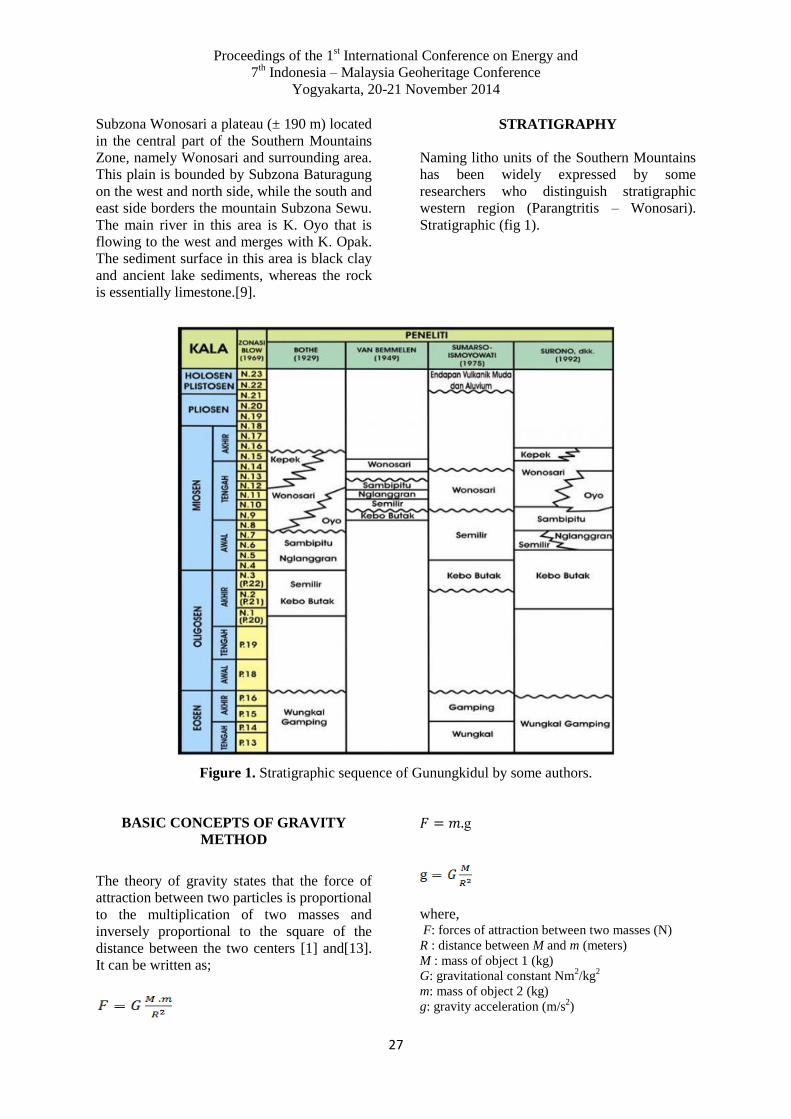
STRATIGRAPHY
Naming litho units of the Southern Mountains
has been widely expressed by some
researchers who distinguish stratigraphic
western region (Parangtritis – Wonosari).
Stratigraphic (fig 1).
Figure 1. Stratigraphic sequence of Gunungkidul by some authors.
BASIC CONCEPTS OF GRAVITY
METHOD
The theory of gravity states that the force of
attraction between two particles is proportional
to the multiplication of two masses and
inversely proportional to the square of the
distance between the two centers [1] and[13].
It can be written as;
g
where, F: forces of attraction between two masses (N)
R : distance between M and m (meters)
M : mass of object 1 (kg)
G: gravitational constant Nm2/kg
2
m: mass of object 2 (kg)
g: gravity acceleration (m/s2)

Proceedings of the 1st International Conference on Energy and
7th Indonesia – Malaysia Geoheritage Conference
Yogyakarta, 20-21 November 2014
28
The gravitational constant value G can be
derived from the experimental results [12],
i.e.,
G = 6.673 x 10⁻⁸
dyne cm2/g
2 = 6.673 x 10
-11
Nm2/kg
2.
The equation (1) shows that the magnitude of
gravity is directly proportional to the mass,
while the mass is directly proportional to the
mass density ρ and the volume of the object,
so that the magnitude of gravity measured,
reflecting both these quantities, the volume
would be related to the geometry of objects
[13]. The flowchart or the diagram of
processing gravity data is shown in Figure 2.
Figure 2. Flowchart of the processing data.
The standard by step correction concepts and
data processing see [8,13].
GRAVITY INTERPRETATION
In general, the interpretation of the gravity
data is divided into two type, i.e, quantitative
(Physical Modeling) and qualitative
interpretation (Geological Modeling).
Quantitative Interpretation (Physical
Modeling)
Quantitative interpretation is an indirect
method, the method of trial and error (trial-
error) using 2D modeling [12], The Talwani
modeling, basically is performed by varying
the form of polygons model in accordance
with the consideration of geological geometric
of model and sample that are taken from the
area of study, and then do a match or fitting of
the calculation gravity response of model
(anomaly) to the corrected observations.
Before calculations the response of the object
model, the separation of regional to local
effect have to be performed [4]. The regional
effect of the anomaly reflects the deep and
wide objects, while the local effect of anomaly
shows the shallow object [5]..
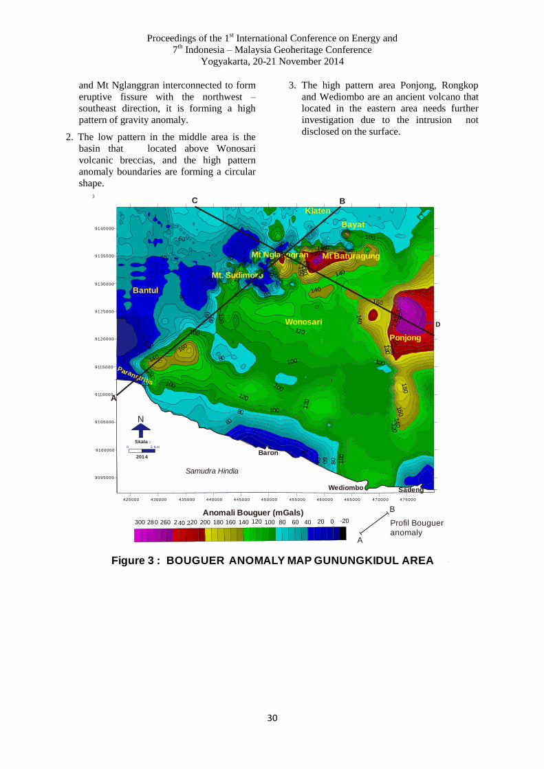
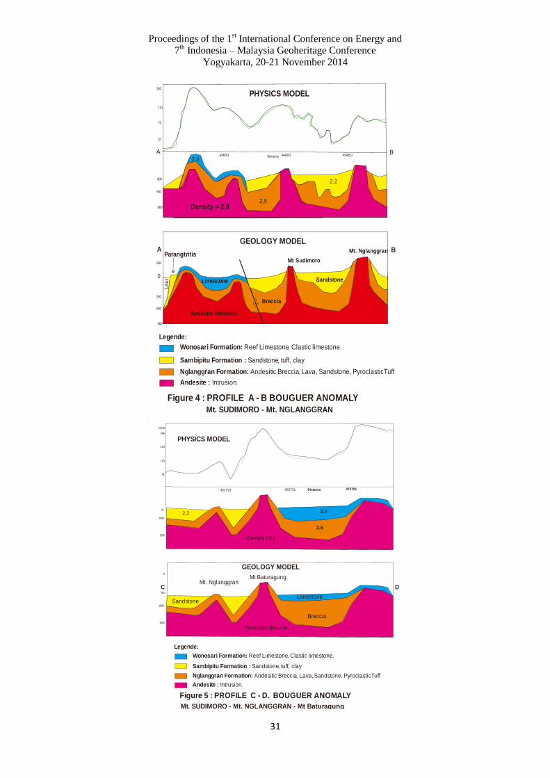
In general in figure 3, the Bouguer anomaly
reflect the effect of rock anomaly areas of
study; the general the high anomaly value
more than 100 mGal located at the edge of the
vicinity study area, i.e., Mt. Nglanggran, Mt.
Sudimoro, east of Mt. Nglanggran, until
Rongkop Ponjong area and surrounding of
cave Cerme near Parangtritis [7]. In figure 4
and figure 5, Mt. Pendul with anomalies of 81-
82 mGal shows that the depth of the rock is
about 600-2000 meters and the density
contrast of 0.2 kg/cm3. The 2.85 kg/cm
3
density areas in the basement is so low that
indicated the presence of anomalies around
60-70 mGal.
The polygon shape display from 2.85 to 2.9
kg/cm3 can be interpreted as igneous
intermediate as a basement [4] that these
rocks is the ocean crust rocks. According to
this model the mélange and oceanic rocks are
as revealed in Karangsambung [2]
Profile A – B, is a profile which extends from
Parangtritis Mt Sudimoro, Mt. Nglanggran
indicates that the rock has a density of 2.85
kg/cm3 is Andesite, density of 2.5 kg/cm
3 is
breccia and sandstone density is 2.2 kg/cm3
and 2.4 kg/cm3 is the density of coral
limestone (figure 4).
Profile C – D, figure 5 is a profile from the
Rongkop and Ponjong to Mt Nglanggran and
Gantiwarno Klaten shows that the gravity
anomaly pattern is also similar to the model of
Mt. Sudimoro to Mt. Nglanggran, where the
Calibration
Data acquisition and correction
Griding and Contouring
Separation anomaly Polynomial method
Residual anomaly Regional anomaly
2D MODELING
Qualyta tive Interpretation
Sub Surface Model
Quantitat ive Interpretation
CONCLUS ION

Proceedings of the 1st International Conference on Energy and
7th Indonesia – Malaysia Geoheritage Conference
Yogyakarta, 20-21 November 2014
29
density is 2.85 kg/cm3 at the bottom as an
igneous rock, density 2.5 kg/cm3 is breccia,
density is 2.2 kg/cm3 is and density 2.4
kg/cm3 is a reef limestone.]
From the quantitative analysis and contour
patterns of anomalies and patterns adapted to
the configuration of the object model, there are
some indications of geological structures such
as faults Opak that involve to rock groups with
a depth of 700 meters. It generally occupies
the western side of the area to the northern
side area.
Qualitative Interpretation (Geological
Modeling)
Geological modeling is a geological
interpretation based on the contour patterns of
gravity anomaly that resulting from the
distribution of density rock bodies of or the
subsurface geological structures. Further, the
anomalies gravitational interpreted are
produced by local geological information in
the form of distribution of objects with
different density contrasts or geological
structure, which is used as the basis of
estimation of the actual geological conditions.
To carry out the geological interpretation of
the subsurface is through several cross-
sectional approaches to gravity data with
surface geological data such as geological
structure pattern [9] The study area includes
the South Java that the value of gravity
anomaly is between 60 mGal to 240 mGal.
The variations of the shallow bedrock depths
are 500 - 1700 meters, at the perimeter of the
high Bouguer anomaly is relatively circular in
shape around the area of study. It is interpreted
as an ancient volcano. In geologically, this
area consists of Tertiary age rocks that are
covering Nglanggran Formation volcanic
breccia, formation Sambipitu (sandstone, clay,
calcareous sand, and tuff). and Wonosari
Formation which consists of coral limestone
and limestone layered. Those formations were
intruded by intrusive andesite into the surface
such as Mt. Nglanggran and Mt. Sudimoro.[3].
In briefly, the gravity models in this area
suggests that the possibility of the bedrock in
the study area is an igneous rock i.e., andesite
continental crust. The Formation rocks above
it may occur at the end of the Cretaceous era
[11]. However, geodynamics processes that
occur in Cretaceous is not known for a
moment. The gravity section shows a large
fault that extends along the river Opak to
Northwest – Southeast ward.
Bouguer anomaly map (figure 3), the basin
boundary is obtained by riffing deposited on
coral limestone formation known as Wonosari
that was located above the andesitic breccias.
TECTONIC PROCESSES
According to [4,6]. Geological interpretation
based on the contour patterns of anomalous
gravity field resulting from the distribution of
density anomalies bodies of rock or subsurface
geological structures. Further anomalies
interpreted gravitational field produced by
local geological information in the form of
distribution of objects with different density
contrasts or geological structure, which is used
as the basis of estimation of the actual
geological conditions [2].
GEOLOGICAL HISTORY
1. In the early - Middle Miocene [8, 10].:
The huge eruption of the volcano in
Gunungkidul areas produce materials
pyroclastic material spread out to 10-20
km radial.
2. Middle Miocene: because of the Huge
eruption of a great many times, and there
was wide graben caldera which the middle
is the city of Wonosari, this graben. Many
fault caused by the edge of the mountain
section contained around the caldera
3. In the Upper Miocene - Pliocene: the case
of transgression so surface mount caldera
sank below sea level, and the life of the
coral reef comes the mid section of the
caldera
4. Pliocene - Pleistocene: a process of
removal (tectonic) that Caldera was lifted
up in the earth's surface, the reef becomes
Wonosari Formation.
5. Recent : Erosion and denudation resulting
in the appearance of the topography and
morphology were present.
CONCLUSIONS
1. The existence of an ancient volcano is
andesite intrusion of igneous rocks that
form the lineament between Mt. Sudimoro
Proceedings of the 1st International Conference on Energy and
7th Indonesia – Malaysia Geoheritage Conference
Yogyakarta, 20-21 November 2014
30
and Mt Nglanggran interconnected to form
eruptive fissure with the northwest –
southeast direction, it is forming a high
pattern of gravity anomaly.
2. The low pattern in the middle area is the
basin that located above Wonosari
volcanic breccias, and the high pattern
anomaly boundaries are forming a circular
shape.
3. The high pattern area Ponjong, Rongkop
and Wediombo are an ancient volcano that
located in the eastern area needs further
investigation due to the intrusion not
disclosed on the surface.
0
20
20
20
40
40
40
40
40
40
40
40
60
60
60
60
60
60
60
60
60
80
80
8 0
80
80
80
80
10 0
100
100
100
100
100
10
0
100
100
100
120
120
120
120
120120
120
140
1 40
140
140
140
140
160
160
160
16
0
180
18
0
18
0
200
200
220
220
24
0
26
0
425000 430000 435000 440000 445000 450000 455000 460000 465000 470000 475000
9095000
9100000
9105000
9110000
9115000
9120000
9125000
9130000
9135000
9140000
-20020406080100120140160180200220240260280300
BOUGUER ANOMAL Figure 3 : Y MAP GUNUNGKIDUL AREA
Anomali Bouguer (mGals)
Baron
Parangtritis
Bantul
Mt. Sudimoro
Mt Nglanggran
Wediombo Sadeng
Wonosari
Bayat
Klaten
Samudra Hindia
N
Skala :0 5 Km
201 4
A
BC
D
Profil Bougueranomaly
A
B
Mt Baturagung
Ponjong
.
.
3
.
Proceedings of the 1st International Conference on Energy and
7th Indonesia – Malaysia Geoheritage Conference
Yogyakarta, 20-21 November 2014
31
Distance 444053434053
37
75
111
150
300
500
800
454053A B
PHYSICS MODEL
GEOLOGY MODEL
0
A B
300
500
800
200
Mt. Nglanggran
Mt SudimoroParangtritis
La
ut Limestone
Breccia
Andesite intrusion
Sandstone
Density = 2,82,5
2.2
2.4
Legend :e
Wonosari : Formation Reef Limestone Clastic limestone.,
Sambipitu : Formation Sandstone clay, tuff,
Nglanggran : Formation A ic Breccia Sandstone, Pyroclasticndesit , Lava, Tuff
Andesit : e Intrusion.
.
.
Mt Mt. SUDIMORO - . NGLANGGRAN
Figure 4 : PROFILE A - B BOUGUER ANOMALY
246
104
mGal
123
61
1000
1500
m
452791 462791 Distance 472791
Density = 2,8
2,5
2,42,2
500
1000
1500
m
C DMt. Nglanggran
Andesiteintrusion
Breccia
LimestoneSandstone
Legend :e
Wonosari : Formation Reef Limestone Clastic limestone.,
Sambipitu : Formation Sandstone clay, tuff,
Nglanggran : Formation A ic Breccia Sandstone, Pyroclasticndesit , Lava, Tuff
Andesit :e Intrusion.
GEOLOGY MODEL
PHYSICS MODEL
.
.Mt Mt - Mt Baturagung. SUDIMORO - . NGLANGGRAN
Figure 5 : PROFILE C - D. BOUGUER ANOMALY
Mt Baturagung

Proceedings of the 1st International Conference on Energy and
7th Indonesia – Malaysia Geoheritage Conference
Yogyakarta, 20-21 November 2014
32
3. Upper Miocene : Tectonic Processes, Transgresion (below sea level)
2. Middle Miocene : Eruption resulting the Formation of Caldera
1. Early - Middle Miocene : Eruption volcano in Gunungkidul
Sea Level
Magma
Pyroclastic rocks
Sea Level
Caldera
Sea Level
Caldera
Magma
Magma
Pyroclastic rocks
Pyroclastic rocks
Eruption
.
4. Upper Miocene - Pliocene : Coral reef was growing up formed Wonosari Formation (Limestone rocks)
Magma
Reef
Pyroclastic rocks
5. Pliocene - Pleistocene : Tectonic processes/regression followed by intrusion around the edge of the caldera.
Sea Level
Magma
Reef
Pyroclastic rocks
Sea Level
6. Recent : Erosion resulting in the Formation of current topography now
Limestone/Reef (Wonosari Formation)
Pyroclastic rocks : Breccia, Sandstone, Tuff(Semilir Formation & Nglanggran Formation)
Magma
Volcanic bedrock
Oceanic floor
Explanation
Magma
Reef
Pyroclastic rocks
Sea Level
.
.
.
Figure 7. Geological history of the formation the caldera

Proceedings of the 1st International Conference on Energy and
7th Indonesia – Malaysia Geoheritage Conference
Yogyakarta, 20-21 November 2014
33
REFERENCES
[1] Blakely, Richard.J, 1995, Potential Theory
in Gravity and Magnetic Application,
Cambridge Univ. Press.
[2] Bronto, S., Misdiyanta, P., Hartono, G.,
dan Sayudi, S., 1994. Penyelidikan Awal
Lava Bantal Watuadeg, Bayat dan
Karangsambung, Jawa Tengah, Kumpulan
Makalah Seminar: Geologi dan Geotektonik
Jawa, Sejak Akhir Mesozoik Hingga
Kuarter. Jur. Tek. Geologi, F. Teknik, UGM,
Yogyakarta, h. 123-130.
[3] Cas, R.A.F., dan Wright, J.V., 1987.
Volcanic Succession: Modern and Ancient,
Allen & Unwin, London, 534.
[4] Dobrin, M,B and Savit, CH 1988,
“Introduction to Geophysical Prospecting”,
Mc Graw Hill Co, Fourth edition, New
York, San Fransisco.
[5] Grant,F,S. & West,G,F, 1965,
“Interpretation Theory in Applied
Geophysics”, Mc Graw Hill Co, New York,
San Fransisco, Toronto, London, Sydney.
[6] Hartono, G. dan Syafri, I., 2007. Peranan
Merapi Untuk Mengidentifikasi Fosil
Gunung Api Pada “F. Andesit Tua”
[7] Macdonald, A.G., 1972. Volcanoes.
Prentice-Hall, Inc. Englewood Cliffs, New
Jersey, 510.
[8] Rahardjo, W., Sukandarrumidi dan Rosidi,
H. M. D., 1977. Peta Geologi Lembar
Jogjakarta, Jawa, skala 1 : 100.000.
Puslitbang Geologi, Bandung.
[9] Sartono, S., 1990. Extensive Slide Deposits
In Sunda Arc Geology, The Southern
Mountain of Java, Indonesia. Buletin
Geologi, Bandung, 20. 3-13.
[10] H.O. Seigel, 1995. A Guide To High
Precision Land Gravimeter Surveys.
Scintrex Limited 222 Snidercroft Road
Concord, Ontario. Canada.
[11] Soeria-Atmadja, R., Maury, R.C., Bellon,
H., Pringgoprawiro, H,. Polve, M., dan
Priadi, B., 1991. The Tertiary Magmatic
Belts in Java. Proceeidings of Silver Jubilee
Symposium On the Dynamics and Its
Products. Research and Development Center
for Geotechnology-LIPI; Yogyakarta,
September 17-19, h. 98-112.
[12] Talwani, M., J. L. Worzel, and M.
Landisman (1959), Rapid Gravity
Computations for two-Dimensional Bodies
with Application to the Mendocino
Submarine Fracture Zone, J. Geophys. Res.,
64(1), 49-59,
[13] Telford, W,M, Geldart,L.P, Sheriff,R,E &
Keys, D,A, 1976, “ Applied Geophysics”
second edition, Canbridge University Press,
New York, London Melbourne.
[14] Van Bemmelen, RW., 1949. The Geology
of Indonesia, Vol IA. Government Printing
Office, The Hague, 732.
Proceedings of the 1st International Conference on Energy and
7th Indonesia – Malaysia Geoheritage Conference
Yogyakarta, 20-21 November 2014
34
Stability Analysis of Single Slope on Soft Rock Using
Saptono‟s Chart Stability
S. Saptonoa
a) Mining Engineering Department
Pembangunan Nasional Veteran Yogyakarta University
Email: [email protected]
ABSTRACT
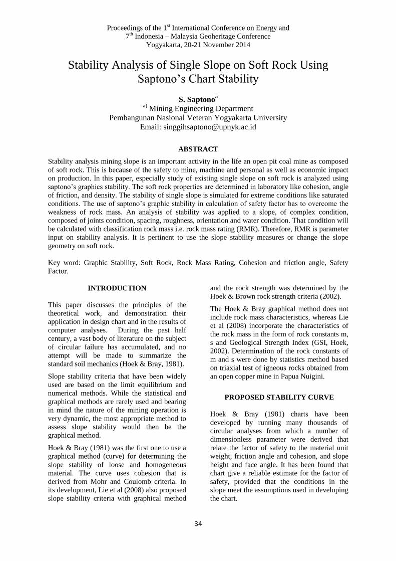
Stability analysis mining slope is an important activity in the life an open pit coal mine as composed
of soft rock. This is because of the safety to mine, machine and personal as well as economic impact
on production. In this paper, especially study of existing single slope on soft rock is analyzed using
saptono‟s graphics stability. The soft rock properties are determined in laboratory like cohesion, angle
of friction, and density. The stability of single slope is simulated for extreme conditions like saturated
conditions. The use of saptono‟s graphic stability in calculation of safety factor has to overcome the
weakness of rock mass. An analysis of stability was applied to a slope, of complex condition,
composed of joints condition, spacing, roughness, orientation and water condition. That condition will
be calculated with classification rock mass i.e. rock mass rating (RMR). Therefore, RMR is parameter
input on stability analysis. It is pertinent to use the slope stability measures or change the slope
geometry on soft rock.
Key word: Graphic Stability, Soft Rock, Rock Mass Rating, Cohesion and friction angle, Safety
Factor.
INTRODUCTION
This paper discusses the principles of the
theoretical work, and demonstration their
application in design chart and in the results of
computer analyses. During the past half
century, a vast body of literature on the subject
of circular failure has accumulated, and no
attempt will be made to summarize the
standard soil mechanics (Hoek & Bray, 1981).
Slope stability criteria that have been widely
used are based on the limit equilibrium and
numerical methods. While the statistical and
graphical methods are rarely used and bearing
in mind the nature of the mining operation is
very dynamic, the most appropriate method to
assess slope stability would then be the
graphical method.
Hoek & Bray (1981) was the first one to use a
graphical method (curve) for determining the
slope stability of loose and homogeneous
material. The curve uses cohesion that is
derived from Mohr and Coulomb criteria. In
its development, Lie et al (2008) also proposed
slope stability criteria with graphical method
and the rock strength was determined by the
Hoek & Brown rock strength criteria (2002).
The Hoek & Bray graphical method does not
include rock mass characteristics, whereas Lie
et al (2008) incorporate the characteristics of
the rock mass in the form of rock constants m,
s and Geological Strength Index (GSI, Hoek,
2002). Determination of the rock constants of
m and s were done by statistics method based
on triaxial test of igneous rocks obtained from
an open copper mine in Papua Nuigini.
PROPOSED STABILITY CURVE
Hoek & Bray (1981) charts have been
developed by running many thousands of
circular analyses from which a number of
dimensionless parameter were derived that
relate the factor of safety to the material unit
weight, friction angle and cohesion, and slope
height and face angle. It has been found that
chart give a reliable estimate for the factor of
safety, provided that the conditions in the
slope meet the assumptions used in developing
the chart.

Proceedings of the 1st International Conference on Energy and
7th Indonesia – Malaysia Geoheritage Conference
Yogyakarta, 20-21 November 2014
35
As mentioned before that the slope stability
curves of Hoek & Bray (1981) and Lie et al
(2008) include the cohesion of intact rock that
is obtained from direct shear test in laboratory
scale. Although the stability curve of Lie et al
uses rock mass constants such as m and s for
scaling up the cohesion to be representing rock
mass condition, it would have been better if
the cohesion and internal friction angle are
obtained from direct shear tests in the field
which take account scale effect (Kramadibrata
& Jones, 1993).
Hence, a series of slope stability curves is
proposed incorporating all parameters given in
that of Hoek & Bray and Lie at al. and by
taking account the scale effect and weathering
that lead to the strength deterioration. It is
expected that the proposed slope stability
curve will be well appropriate in the
application for assessing slope stability in
Indonesian as soft rock.
DERIVATION OFCIRCULAR FAILURE
CHARTS IN SOFT ROCK
Dimensional analysis has been extensively
used in solving complex engineering
problems. Its application is dependent on
listing of all the dimensional variables
affecting the problems.
It has been of immeasurable value in analyzing
complex engineering problems in many field
notably fluid mechanics and heat transfer. It
has also been used to establish the modeling
criteria for the scale model testing of coal-face
production system (Roxborough & Eskikaya,
1974), and more recently its use in subsidence
modelling was referred to by Whittaker &
Reddish (1989) and Kramadibrata (1996).
The authors therefore decided to apply this
technique to develop a rock slope stability
curve with the intention of deriving a set of
dimensionless groups which could thereafter
be used to correlate the experimental data and
develop appropriate functional relationships.
Application of the dimensional analysis for
slope stability analysis is to link 10 physical
quantities of which consists of a slope height
(h), specific weight of slope material (), water
content (w), slake durability (sd), uniaxial
compressive strength (UCS-c), cohesion (c),
friction angle (), area of shear plane (A), joint
frequency per meter (JF), and Rock Mass
Rating (RMR) with water surface condition is
saturated (Kramadibrata, 2011). In view of
that the rock formation is soft; allowing the
UCS varies from 1 MPa to 20 MPa, the
relationships between RMR and cohesion of
equation can therefore be generated as shown
in Figure 1 and 2.
DETERMINATION OF SLOPE
STABILITY
Slope Model
Illustration of slope model is shown in Figure
3 with height of h and slope of, and the
parameters used to represent the rock mass
properties constituting the slope are uniaxial
compressive strength (UCS or c), RMR and
specific weight (. The RMR is determined
using the data site rock characterization
(ISRM, 1981) and the slope is assumed as a
single slope, the slope stability calculation is
based on the limit equilibrium approach and
slope failure occurs at the toe of the slope.
Slope Stability Determination Procedure
The end result of establishing the soft rock
slope stability procedure is in form of three
curves, namely cohesion determination curve
(Figure 1), internal friction angle curve (Figure
2) and safety factor determination curve
(Figure 4).
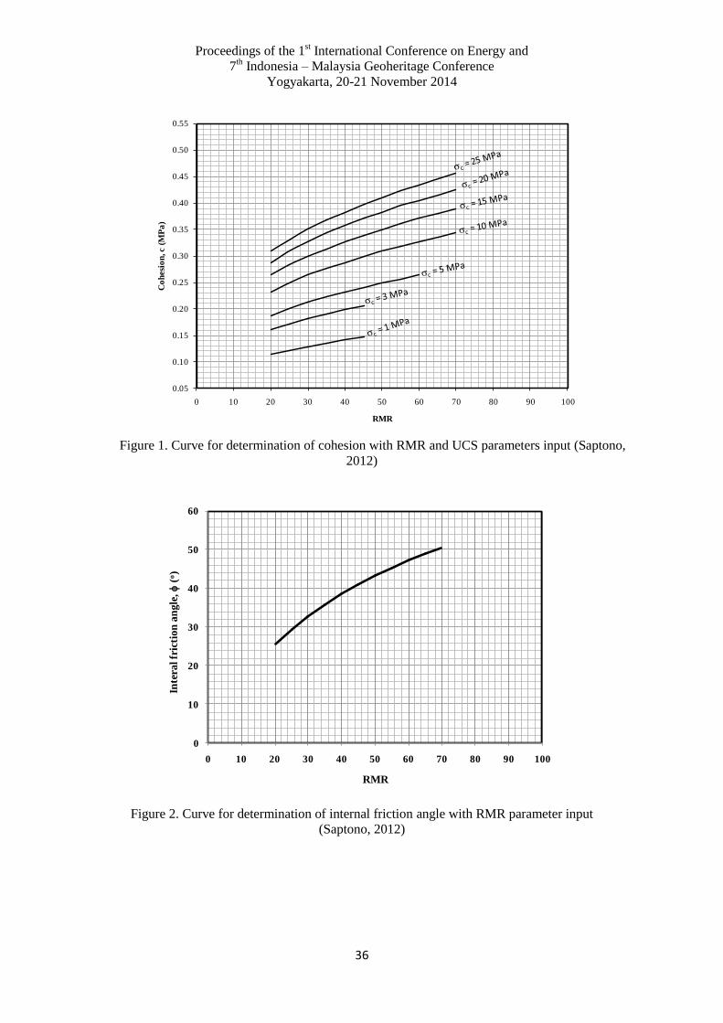
Proceedings of the 1st International Conference on Energy and
7th Indonesia – Malaysia Geoheritage Conference
Yogyakarta, 20-21 November 2014
36
Figure 1. Curve for determination of cohesion with RMR and UCS parameters input (Saptono,
2012)
Figure 2. Curve for determination of internal friction angle with RMR parameter input
(Saptono, 2012)
0.05
0.10
0.15
0.20
0.25
0.30
0.35
0.40
0.45
0.50
0.55
0 10 20 30 40 50 60 70 80 90 100
Co
hesi
on
, c (
MP
a)
RMR
0
10
20
30
40
50
60
0 10 20 30 40 50 60 70 80 90 100
Inte
ral fr
icti
on
an
gle
,
(o)
RMR

Proceedings of the 1st International Conference on Energy and
7th Indonesia – Malaysia Geoheritage Conference
Yogyakarta, 20-21 November 2014
37
Figure 3. Single Slope Model and rock properties parameters
Figure 4. The slope stability chart at different slope angles use of on soft rock (Saptono, 2012)
Use of the Failure Chart
In order to use the charts to determine the
factor of safety of a slope, the step outlined
here and shown in Figure 5 and 6 should be
followed.
Step 1: Decide upon rock characterization by
Rock Mass Rating (RMR) based on
Bieniawski (1989) and select rock
strength parameters appli-cation based
on uniaxial compr-essive strength
(UCS) and relation RMR and UCS for
determination of cohesion (Figure 1).
Step 2 : Determination of friction angle with
RMR parameter (Figure 2).
Step 3: Calculate the value of the dimen-
sionless ratio c/(H tan ) and find
this value on the x – coordinate scale
of this chart.
Step 4: Follow the vertical line from the value
found in step 3 to its intersection with
50o
RMR = 25, c = 3 MPa
12 m= 25 kN/m3
0.00
0.10
0.20
0.30
0.40
0.50
0.60
0.70
0.00 0.25 0.50 0.75 1.00 1.25 1.50 1.75 2.00 2.25 2.50
= 60o
= 50o
= 40o
= 30o
= 20o
h
c, , dan
= 15o

Proceedings of the 1st International Conference on Energy and
7th Indonesia – Malaysia Geoheritage Conference
Yogyakarta, 20-21 November 2014
38
the curve which corresponds to the
slope angle.
Step 5: Find the corresponding value of
tanFK, depending upon which is
more convenient, and calculate the
factor of safety.
Consider the following example:
A 12 m high cut with a slope face angle of
50o is to be excavated in soft rock with a
density = 25 kN/m2, with rock mass
characterization RMR = 25 and UCS = 3 MPa.
Find the factor of safety of slope.
Figure 6. Determination for cohesion and internal friction angle of slope on soft rock
0
10
20
30
40
50
60
0 10 20 30 40 50 60 70 80 90 100
Inte
ral f
rict
ion
an
gle
,
(o)
RMR
0.05
0.10
0.15
0.20
0.25
0.30
0.35
0.40
0.45
0.50
0 10 20 30 40 50 60 70 80 90 100
Co
hesi
on
, c (
MP
a)
RMR
Example Using Curve 1 & Curve 2
Stage 1:
Curve 1:
RMR = 25 and c = 3 MPa
c = 0,17 MPa,
Stage 2:
Curve 2:
RMR = 25
= 30o.
1
0,170
25
CU
RV
E 1
CU
RV
E 2
50o
RMR = 25, c = 3 MPa
12 m= 25 kN/m3
Example:
25

Proceedings of the 1st International Conference on Energy and
7th Indonesia – Malaysia Geoheritage Conference
Yogyakarta, 20-21 November 2014
39
Figure 6. Determination for factor of safety of slope on soft rock
CONCLUDING REMARKS
Determination of criteria and soft rock slope
stability analysis is proposed in the form of
charts based on: use of RMR and cohesion and
internal friction obtained from large-scale
direct shear test (scale effect). The all
parameters are obtained from coal bearing
strata that is located in the tropical region so
that rock strength deterioration due to
weathering. To develop a rock slope stability
curve with the intention of deriving a set of
dimensionless groups which could thereafter
be used to correlate the experimental data and
develop appropriate functional relationships.
This research is going to process towards the
application step.
ACKNOWLEDGEMENTS
Thanks to the Vice Rector for Research and
Innovation ITB which has approved this
research to be funded by the DIPA ITB Fiscal
Year 2010. Similarly, the authors would also
like to thank the Management of PT. Adaro
Indonesia, which continues to support the
research of rock mass characterization and
testing direct shear of large scale and would
you like to thank the students, laboratory staff
and technicians involved in this research.
REFERENCES
Bieniawski, Z.T., 1989. Engineering Rock
Mass Classifications, John-Wiley, New
York
Hoek, E. and Bray, J.W., 1981. Rock Slope
Engineering, Institution of Mining and
Metallurgy, London
Hoek, E., 2002. A Brief history of The
Development of The Hoek-Brown failure
Criterion, Accessed through the Program
RocLab.
Kramadibrata, S. and Jones, I.O., 1993. Size
Effect on Strength and Deformability of
Brittle Intact Rock, Scale Effects in Rock
Masses, Proc. of the Second International
Workshop on Scale Effects in Rock
Masses, Lisbon, Portugal, (ed. A. Pinto Da
Cunha), A.A. Balkema, Rotterdam.
Kramadibrata, S., 1996. The Influence of Rock
Mass and Intact Rock Properties on The
Design of Surface Mines with Particular
Reference to The Excavatability of Rock,
Ph. D. Thesis, Curtin University of
Technology.
Kramadibrata, S., Saptono, S., Wattimena,
RK., Simangunsong, GM., Sulistianto, S.,
2011. Developing a Slope Stability Curve
0.06
0.08
0.10
0.12
0.14
0.16
0.18
0.20
0.70 0.95 1.20 1.45 1.70 1.95
= 60o
= 50o
= 40o
= 30o
= 20o
h
c, , dan
h
c, , dan
= 15o
tan ϕ
FK
c
γhtanϕ
Example Using Curve Soft Rock Stability Analysis
Stage 3:
Curve 3:
= 50o
(c/ h tan ) = 0,98
(tan /FK) = 0,152
FK = (tan /0,152) = 3,798
2
0,152
0,98
CU
RV
E 3

Proceedings of the 1st International Conference on Energy and
7th Indonesia – Malaysia Geoheritage Conference
Yogyakarta, 20-21 November 2014
40
of Open Pit Coal Mine by Using
Dimensional Analysis Method, 12th ISRM
Congress, Beijing, China.
Lie, A.J., Merifield, R.S., Lyamin, A.V., 2008.
Stability Charts for Rock Slopes Based on
the Hoek-Brown Failure Criterion,
International Journal of Rock Mechanics &
Mining Science 45, 689 – 700.
Roxborough, F.F., and Eskikaya, S., 1974.
Dimensional considerations in the design
criteria of a scale model for coal-face
production system research. Int. J. Rock
Mech. Min Sci & Geomech. Abstr., Vol 11,
pp. 129-137.
Saptono, S., 2012. Pengembangan Metode
Analisis Stabilitas Lereng Berdasarkan
Karakterisasi Batuan di Tambang Terbuka
Batubara. Disertasi Doktor, Rekayasa
Pertambangan, Institut Teknologi Bandung.
Whittaker, B.N., and Reddish, D.J., 1989.
Subsidence occurrence prediction and
control. Developments in Geotechnical
Engineering, 56. Elsevier, pp. 437-473.

Proceedings of the 1st International Conference on Energy and
7th Indonesia – Malaysia Geoheritage Conference
Yogyakarta, 20-21 November 2014
41
Share Intrinsic Value Valuation Analysis of Company Mining
Sector: Study Empirical PT Bumi Resources Tbk (Bumi) in
Indonesia
Marlina Widiyanti* and Jatmika Setiawan
**
*) Finance Management Programme, Faculty Of Economic, Universitas Sriwijaya, Sumatera
Selatan, Indonesia
**) Geological Programme, Faculty of Mineral Technology, UPN “Veteran” Yogyakarta,
Indonesia
ABSTRACT
Focusing of this study is Share Intrinsic Value Valuation Analysis Of Company Mining Sector. Share
is known to high risk-high return characteristics. Because of that, investing in share needed share
valuation analysis to estimate how much intrinsic value is, for a share based on its fundamental data.
The purposes of the research were for getting intrinsic value of a share and knowing what the share
was in undervalued, overvalued or fairly price condition. The research used company object included
in mining sector, it was PT Bumi Resources Tbk (BUMI) in Indonesia. The analysis was done by
using top down approach that was begun from economy condition analysis, industry condition, and
company condition, then, it was continued by performing share valuation in using Model Discount
Dividend Approach and P/E Ratio. The result of the research showed intrinsic value of BUMI‟s share
with Model Discount Dividend Approach was Rp 601 mean while with P/E Ratio approach was Rp
608. If it was compared to market value per October 1st
, 2012 was Rp 750 so BUMI‟s share was
assessed overvalued (expensive), theoretically it was recommended to sell if it share had been owned
and to postpone the purchasing.
Keywords : Share Valuation, Dividend Discount Model, P/E Ratio (PER)
INTRODUCTION
Mining industry in Indonesia has a very bright
prospect and has been a boosting factor for
economy and social growth. One sector which
has rapidly developed is coal, where Indonesia
is the main actor in the world market, as since
2006, Indonesia has placed the second after
Australia as a coal exporter.
Coal in Indonesia is largely produced in
Kalimantan, Sumatera and some other places.
This rapidly growing coal industry is
supported by government policies which
introduce an aggressive foreign investment,
and is also propped up by abundant coal
reservoir. It can be concluded that firms which
produce coal still have good prospects.
PT Bumi Resources Tbk (BUMI) is one of the
firms covering exploration and exploitation of
coal content (including coal mining and
selling) and oil exploration. This firm went
public through IPO (initial Public Offering) in
1990, and is listed at Jakarta Share Exchange
(Bursa Efek Jakarta). The firm has several
subsidiaries, which include PT Kaltim Prima
Coal (KPC) and PT Arutmin Indonesia which
are coal producers as well as the biggest
income contributors to the firm. Both are the
biggest coal producers in Indonesia with a
market share of 26.6% (2009) and one of the
big three coal exporting countries in the world
with groos production in 2006 of 50.7 tons.
Below is the ratio of financial performance
and share trading activity in the last 5 years:
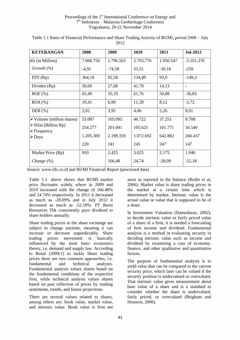
Proceedings of the 1st International Conference on Energy and
7th Indonesia – Malaysia Geoheritage Conference
Yogyakarta, 20-21 November 2014
42
Table 1.1 Ratio of Financial Performance and Share Trading Activity of BUMI, period 2008 – July
2012
KETERANGAN 2008 2009 2010 2011 Jul-2012
Net Profit (in Million)
Growth (%)
7.066.750
-4,91
1.796.503
-74,58
2.793.770
55,51
1.950.547
-30,18
-3.101.376
-259
EPS (Rp) 364,19 92,58 134,49 93,9 -149,3
Dividen (Rp) 50,60 27,68 41,78 14,13 -
ROE (%) 65,49 35,19 61,76 50,88 -36,83
ROA (%) 19,41 6,99 11,39 8,12 -3,72
DER (%) 2,02 3,95 4,06 5,26 8,91
Volume (million shares)
Nilai (Billion Rp)
Frequency
Days
53.087
254.277
1.205.300
220
105.095
201.041
2.198.359
241
46.722
105.625
1.072.692
245
37.251
101.771
642.882
247
9.708
16.540
266.437
147
Market Price (Rp)
Change (%)
910 2.425
166,48
3.025
24,74
2.175
-28,09
1.040
-52,18
Source: www.idx.co.id and BUMI Financial Report (processed data)
Table 1.1. above shows that BUMI market
price fluctuates widely where in 2009 and
2010 increased with the change of 166.48%
and 24.74% respectively. In 2011 it decreased
as much as -28.09% and in July 2012 it
decreased as much as -52.18%. PT Bumi
Resources Tbk consistently pays dividend to
share holders annually.
Share trading prices in the share exchange are
subject to change anytime, meaning it can
increase or decrease unpredictably. Share
trading prices movement is basically
influenced by the most basic economics
theory, i.e. demand and supply law. According
to Renal (2009:1) to tackle Share trading
prices there are two common approaches, i.e.
fundamental and technical analyses.
Fundamental analysis values shares based on
the fundamental conditions of the respective
firm, while technical analysis values shares
based on past reflection of prices by reading
sentiments, trends, and future projections.
There are several values related to shares,
among others are: book value, market value,
and intrinsic value. Book value is firm net
asset as reported in the balance (Bodie et al,
2006). Market value is share trading prices in
the market at a certain time which is
determined by market. Intrinsic value is the
actual value or value that is supposed to be of
a share.
In Investment Valuation (Damodaran, 2002),
to decide intrinsic value or fairly priced value
of a share of a firm, it is needed a forecasting
of firm income and dividend. Fundamental
analysis is a method in evaluating security in
deciding intrinsic value such as income and
dividend by examining a case of economy,
finance, and other qualitative and quantitative
factors.
The purpose of fundamental analysis is to
yield value that can be compared to the current
security price, which later can be valued if the
security position is undervalued or overvalued.
That intrinsic value gives measurement about
base value of a share and is a standard to
consider whether the share is undervalued,
fairly priced, or overvalued (Brigham and
Houston, 2006).

Proceedings of the 1st International Conference on Energy and
7th Indonesia – Malaysia Geoheritage Conference
Yogyakarta, 20-21 November 2014
43
Sehgal and Pandey (2010) also conducted a
research to estimate share prices in India share
exchange using Price Multiples. This research
used data from 1990 – 2007 with 145 samples
of firms consisting 13 sub-sector industries.
This research discovered that PER was the
best compared to PBV, P/S and P/CF. If
combination of the methods was used,
combination with P/S was very significant.
However, the use of PER alone was very good
if the comparison was by combining those
methods.
Research on share valuation had beforehand
been done by Supattarakul and Khanthavit
(2011) who conducted a research on firms in
Thailand. This research was done in two
periods in 1995 – 2004 to estimate share value
with Dividend Discount Model (DDM) and
Residual Income Model (RIM). The result of
this research stated that equity book value
gave stronger explanation compared to other
variables than DDM and RIM.
The author chose mining sector as the research
object to complete the previous research which
was about firm share in other industry sectors,
so the real condition can be generally better
described. Besides that, mining sector tends to
be corrected in line with the current global
economic crisis. This is a challenge for share
holders to judge whether their investment is
still worth holding on this mining sector or
whether they want to shift to other relatively
more stable sectors.
PT Bumi Resources Tbk consistently pays
dividend to share holders annually and is the
most owned share publicly and the most
favorite to investors. The share of BUMI is
currently listed on the LQ-45 index period
August 2012 – January 2013. This share once
yielded high gain when it underwent a
fantastic increase in 2007 – 2008, with the
highest historical price at Rp. 8,850 in June
2008. But starting from December 2011 –
October 2012, this share underwent a decrease
tendency, with the lowest historical price at
Rp. 650 on 4 September 2012. Below is the
movement of BUMI share period 30
December 2011 – 1 October 2012 (weekly):
Graph 1. Market Price Movement of Bumi Share Period 30 December 2011 – 1 October 2012
(Weekly). Source: finance.yahoo.com (data processed)
Based on graph 1.1 above the movement of
BUMI share underwent a very extreme
decrease and had a very high risk. During that
period, this share underwent a decrease of -
66.43%. With this steep price decline
phenomenon in a very short duration, it was
necessary to make a review on the fairness of
the price of PT Bumi Resources Tbk share,
whether this share was fairly priced or not.
Based on the above explanation, the author
meant to re estimate intrinsic value of the firm
on different industry sectors using present
value approach which discounts value of
future cash flow to be the present value that is
Dividend Discount Model and an approach
using firm earnings, that is Price Earning Ratio
(PER). The result of the estimation of the
fairness of the share price from each model
will then be compared to market prices.
To know the fair price of the share of PT Bumi
Resources Tbk, the author was interested to
take the title: “Valuation Analysis of Fair
Price of PT Bumi resources Tbk Share
(BUMI)”. With the problem formulation as
Rp- Rp500
Rp1.000 Rp1.500 Rp2.000 Rp2.500 Rp3.000
- 66,43%

Proceedings of the 1st International Conference on Energy and
7th Indonesia – Malaysia Geoheritage Conference
Yogyakarta, 20-21 November 2014
44
follows: what is the intrinsic value (fair price)
of the share of PPT Bumi Resources Tbk per 1
October 2012? And is the share price of PT
Bumi Resources Tbk undervalued or
overvalued if compared to its intrinsic value?
The purpose of this research is to find the
intrinsic value (fair price) of PT Bumi
Resources Tbk share if calculated using
Dividend Discount Model and P/E Ratio, also
to know if this share is undervalued or
overvalued from the intrinsic value if
compared to the share trading price.
THEORETICAL BASIS
Share
Bodie, Kane, and Marcus (2009) stated that
common shares, also known as equity
securities or equities, are the evidence of the
possession of some parts of a firm.
Furthermore, this means the share holders who
invest on the firm also own the firm since they
have the possession evidence.
Share Valuation
Every asset, be it financial or real asset possess
a value (Damodaran, 2002). Understanding the
value of an asset and the factors influencing
the asset value is a requirement in prudent
business decision making, such as choosing a
correct investment in a portfolio, determining
the fair price in selling or buying a firm or
shares, or in restructuring a firm.
Share analysis is aimed at estimating intrinsic
value of a share and then comparing it to the
market price of the share. Intrinsic Value (IV)
indicates cash flow present value expected of
the share. Below is what investors are to do in
response to the comparison:
1. If IV > P, the share is considered
undervalued and is therefore good to buy
or hold if already owned.
2. If IV<P, the share is considered
overvalued, and is therefore good to sell.
3. If IV=P, the share is fairly priced and in a
balanced condition.
Valuation Process
According to Tambunan (2008), there are
three important points that must be analyzed as
a part of valuation process before deciding to
invest:
1. Economic Condition
Monetary and fiscal policies launched by the
government of a country will affect the
country‟s global economy, which in turn will
affect whole industry activity and the firm.
Therefore it is advisable, before investing in a
country, to analyze deeply its economic
condition, such as fiscal policy, monetary
policy, inflation rate, and political situation.
2. Industry Condition
This is to identify industries experiencing
prosperity or poverty in the economic cycles.
Industries react in different ways to certain
business cycles. In this process, investors are
expected to deeply analyze industries having
bright prospect in the future. That way,
investors can choose which industry is worth
investing in.
3. Firm Condition
The next process is to analyze and compare
firm performance using financial ratios and
systematic risk. Financial ratio and risk which
can be used are liquidity ratio, solvability
ratio, and market ratio.
Ordinary Share Valuation
There are two approaches used to calculate
ordinary share intrinsic value, which are
(Jogiyanto, 2009:130) :
1. Present Value approach
This approach is based on arguments that the
value of a firm depends on that firm‟s prospect
in the future and this prospect is the ability of
the firm to produce future cash flow, therefore
firm value is determined by discounting future
cash flow to be present cash flow.
∑
Notes:
Po = present value of the firm
t = Period time of t=1 to t=∞
k = interest of discount or the
expected rate of return
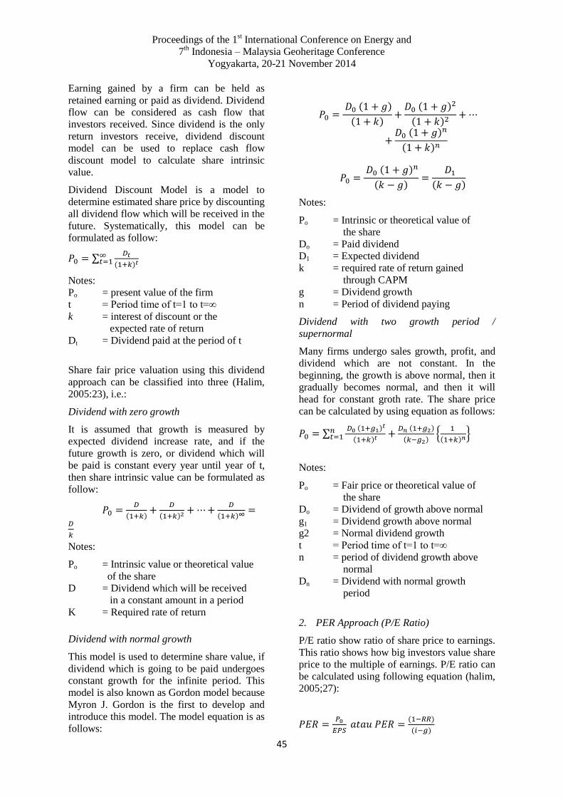
Proceedings of the 1st International Conference on Energy and
7th Indonesia – Malaysia Geoheritage Conference
Yogyakarta, 20-21 November 2014
45
Earning gained by a firm can be held as
retained earning or paid as dividend. Dividend
flow can be considered as cash flow that
investors received. Since dividend is the only
return investors receive, dividend discount
model can be used to replace cash flow
discount model to calculate share intrinsic
value.
Dividend Discount Model is a model to
determine estimated share price by discounting
all dividend flow which will be received in the
future. Systematically, this model can be
formulated as follow:
∑
Notes:
Po = present value of the firm
t = Period time of t=1 to t=∞
k = interest of discount or the
expected rate of return
Dt = Dividend paid at the period of t
Share fair price valuation using this dividend
approach can be classified into three (Halim,
2005:23), i.e.:
Dividend with zero growth
It is assumed that growth is measured by
expected dividend increase rate, and if the
future growth is zero, or dividend which will
be paid is constant every year until year of t,
then share intrinsic value can be formulated as
follow:
Notes:
Po = Intrinsic value or theoretical value
of the share
D = Dividend which will be received
in a constant amount in a period
K = Required rate of return
Dividend with normal growth
This model is used to determine share value, if
dividend which is going to be paid undergoes
constant growth for the infinite period. This
model is also known as Gordon model because
Myron J. Gordon is the first to develop and
introduce this model. The model equation is as
follows:
Notes:
Po = Intrinsic or theoretical value of
the share
Do = Paid dividend
D1 = Expected dividend
k = required rate of return gained
through CAPM
g = Dividend growth
n = Period of dividend paying
Dividend with two growth period /
supernormal
Many firms undergo sales growth, profit, and
dividend which are not constant. In the
beginning, the growth is above normal, then it
gradually becomes normal, and then it will
head for constant groth rate. The share price
can be calculated by using equation as follows:
∑
{
}
Notes:
Po = Fair price or theoretical value of
the share
Do = Dividend of growth above normal
g1 = Dividend growth above normal
g2 = Normal dividend growth
t = Period time of t=1 to t=∞
n = period of dividend growth above
normal
Dn = Dividend with normal growth
period
2. PER Approach (P/E Ratio)
P/E ratio show ratio of share price to earnings.
This ratio shows how big investors value share
price to the multiple of earnings. P/E ratio can
be calculated using following equation (halim,
2005;27):
Proceedings of the 1st International Conference on Energy and
7th Indonesia – Malaysia Geoheritage Conference
Yogyakarta, 20-21 November 2014
46
Notes:
Po = Fair price of the share
g = Dividend growth
RR = Retention Rate
i = Required rate of return
EPS = Earning per share = net profit
after tax / number of shares
Capital Asset Pricing Model (CAPM)
Capital Asset Pricing Mode (CAPM) was first
developed in 1960 by William F. Sharpe,
Lintner, and Mossin Brigham (2006) who
define CAPM as follows:
“A model based on the proposition that any
share’s required rate of return is equal to the
risk free of return plus a risk premium, where
risk reflect diversification”.
Which means CAPM is a model which relates
expected rate of return of asset with risk to the
risk of the asset in the balanced market.
According to the CAPM theory expected rate
of return of a security can be calculated using
equation (Halim, 2005:74):
Ks = Rf + β[E(Rm) - Rf]
Notes:
Ks= Expected rate of return of a security
β = Beta of asset I
E(Rm) = Expected rate of return from market
portfolio
[E(Rm) – Rf] = Risk premium
Beta (β)
Beta can be calculated using regression
technique. Regression technique to estimate
beta of a security can be assumed using
security return volatility as a dependent
variables and market return volatility as an
independent variable. The more risk an
investor is willing to take, the more aggressive
the shares one chooses (shares with more than
one beta).
Previous Researches
Some researches which studied the fairness of
share prices done by previous researchers are
among others: a research on share valuation
was once carried out by Supattarakul and
Khanthavit (2011) who carried out a research
on firms in Thailand. This research had a
period of research from 1995 -2004 to estimate
share value with Dividend Discount Method
(DDM) and Residual Income Model (RIM).
The result of this research stated that equity
book value gives stronger explanation than
other variables than DDM and RIM. Therefore
it is necessary to do a share valuation before
taking decision to invest. According to Halim
(2005:20) this makes firm intrinsic value a
very crucial measurement for investors to take
decisions in buying a firm‟s shares.
Sehgal and Pandey (2010) also did a research
to estimate share trading price at India Share
Exchange by using Price Multiples. This
research used data from 1990 – 2007 with 145
firm samples comprising of 13 industry sub
sector. This research found that PER was the
best method compared to PBV, P/S, and P/CF.
if a combination should be used, the very
significant one would be the combination with
P/S, but the use of PER alone was very good
compared to the combination of the method.
Andi Wijaya and Viliany (2008) did valuation
to the share of PT Indofood Sukses makmur
Tbk using Dividend Discount Model (DDM).
By using that method the price of the share
was overvalued. A similar research was one
carried out by Budi Erianda, et al (2011) on
the share of PT Teekomunikasi Indonesia Tbk,
using Gordon Growth Model approach. It was
found out that the share of PT Telekomunikasi
Indonesia Tbk was undervalued. In that
condition, investors may well buy the share.
Thought Frame
Based on the above-mentioned explanations at
the basis of the theory, it can be compiled a
thought that describes the fair price valuation
of BUMI as Graph. 2.
Hypothesis
1. H1 : Share trading price of PT Bumi
Resources with Dividend Discount Model
and P/E Ratio was considered unfair.
2. H2 : Fair intrinsic value of PT Bumi
Resources Tbk share is smaller compared
to share trading price per 1 October 2012,
meaning it was overvalued.
RESEARCH METHOD
Research Coverage
The coverage of this research is to calculate
the fair price of the share of PT Bumi
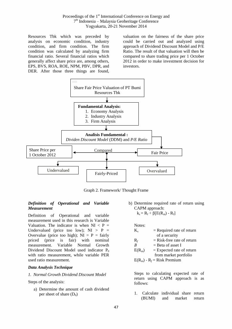
Proceedings of the 1st International Conference on Energy and
7th Indonesia – Malaysia Geoheritage Conference
Yogyakarta, 20-21 November 2014
47
Compared
Resources Tbk which was preceded by
analysis on economic condition, industry
condition, and firm condition. The firm
condition was calculated by analyzing firm
financial ratio. Several financial ratios which
generally affect share price are, among others,
EPS, BVS, ROA, ROE, NPM, PBV, DPR, and
DER. After those three things are found,
valuation on the fairness of the share price
could be carried out and analyzed using
approach of Dividend Discount Model and P/E
Ratio. The result of that valuation will then be
compared to share trading price per 1 October
2012 in order to make investment decision for
investors.
Graph 2. Framework/ Thought Frame
Definition of Operational and Variable
Measurement
Definition of Operational and variable
measurement used in this research is Variable
Valuation. The indicator is when NI < P =
Undervalued (price too low); NI > P =
Overvalue (price too high); NI = P = fairly
priced (price is fair) with nominal
measurement. Variable Normal Growth
Dividend Discount Model used indicator P0
with ratio measurement, while variable PER
used ratio measurement.
Data Analysis Technique
1. Normal Growth Dividend Discount Model
Steps of the analysis:
a) Determine the amount of cash dividend
per sheet of share (D0)
b) Determine required rate of return using
CAPM approach:
ks = Rf + β[E(Rm) - Rf]
Notes:
Ks = Required rate of return
of a security
Rf = Risk-free rate of return
Β = Beta of asset I
E(Rm) = Expected rate of return
from market portfolio
E(Rm) - Rf = Risk Premium
Steps to calculating expected rate of
return using CAPM approach is as
follows:
1. Calculate individual share return
(BUMI) and market return
Fundamental Analysis:
1. Economy Analysis
2. Industry Analysis
3. Firm Analysis
Share Fair Price Valuation of PT Bumi
Resources Tbk
Analisis Fundamental :
Dividen Discount Model (DDM) and P/E Ratio
Undervalued Fairly-Priced
Overvalued
Fair Price Share Price per
1 October 2012

Proceedings of the 1st International Conference on Energy and
7th Indonesia – Malaysia Geoheritage Conference
Yogyakarta, 20-21 November 2014
48
(JCI=Jakarta Composite Index
(IHSG)) using daily data:
Notes:
a. t= Index of price/price of
share period t
b. t-1= Index of price/price of
share period t-1
2. Determine Beta (β)
Beta (β) is calculated using
regression technique with security
return volatility (BUMI) as a
dependent variable and market
return volatility (JCI) as an
independent variable.
3. Determine risk-free interest (Rf)
Rf uses free-risk interest of Central
Bank Certificate (SBI = Setifikat
Bank Indonesia) year 2012.
4. Determine E(RM) which is the
expected return of rate from market
portfolio. E(RM) uses JCI market
return period 30 December 2011 – 1
October 2012.
c) Estimate future dividend growth rate:
g = (1-d) (ROE)
= RR x ROE
Notes:
1. d= Dividend pay out ratio =
dividend per share / earning
per share
2. RR= Retention Rate
3. ROE= Return on Equity
d) Value fair price of a share using
Normal Growth Dividend Discount
Model:
Notes:
Po = Intrinsic value or share
theoretical value
Do = Paid dividend
D1 = Expected dividend
k = Required rate of return of
share produced through
CAPM
g = Dividend growth
n = Period of dividend paying
2. P/E Ratio (PER)
Steps of this analysis are as follows:
1. Calculate average PER of BUMI share
for the last five years.
2. Calculate average growth of EPS of
BUMI share
3. Calculate next year‟s EPS projection
(Eo)
Eo = EPS + (1+g)
4. Calculate share‟s fair price with P/E
Ratio:
P = PER X Eo
ANALYSIS AND EXPLANATION
Fundamental Factor Analysis
Fundamental Factor Analysis in this research
was done by analyzing economic condition
with other factors which can influence firm‟s
performance and condition to strengthen
assumptions used in valuation so it can
describe the firm‟s real condition.
1. Economic Condition
Indonesian economic prospect in 2012 is
predicted to be still strong, although risk
coming from global economy weakening is
still high. National economy in 2012 is
predicted to grow 6.3% - 6.7% and inflation is
predicted to range the target of 4.5% ± 1%.
Below is the inflation growth graph in
Indonesia period April 2011 – October 2012:

Proceedings of the 1st International Conference on Energy and
7th Indonesia – Malaysia Geoheritage Conference
Yogyakarta, 20-21 November 2014
49
Graph 3. Indonesia‟s Inflation Rate Movement. Source: www.tradingeconomics.com and Indonesian
Central Bureau of Statistics.
Based on the graph above, we can see that
inflation in 2011 was able to be slowed down
to 3.79%, much lower than 2010‟s inflation
which was 6.96%. This low inflation
realization was reached while the national
economy growth condition increased to be
6.5% in 2011 from 6.1% in 2010. Inflation
growth in Indonesia was recorded 4.31% in
September 2012. Historically, from 1997 to
2012, Indonesia‟s inflation rate was 12.1%.
But this low inflation was not followed by the
strengthening of Rupiah towards US Dollar, as
since the early 2012 Rupiah had undergone
depreciation. Below is the graph of Rupiah
movement against US Dollar period January
2011 – October 2012:
Graph 4. The Movement of Rupiah against US Dollar. Source: www.tradingeconomics.com and
Indonesian Central Bureau of Statistics.
Based on the graph, the weakening of Rupiah
exchange rate which had happened since early
2012 negatively contributed to the whole
macro stability. This was the impact of the
worsening of the global economy which was
started by the Greek‟s Failure to pay crisis.
Meanwhile, banking response to the decrease
of Central Bank Rate was still limited, as seen
from credit growth and the decrease of interest
which was still not as expected. Below is the
graph of the decrease of Central Bank rate
period January 2011 – October 2012:

Proceedings of the 1st International Conference on Energy and
7th Indonesia – Malaysia Geoheritage Conference
Yogyakarta, 20-21 November 2014
50
Graph 5. Central Bank Rate Movement. Source: www.tradingeconomics.com and Indonesian Central
Bureau of Statistics.
Based on the graph, Central Bank rate was last
announced to be 5.75%. As the rate was
decreased, it was expected that investors
would be more interested to invest on shares
than to deposit the fund in the banks. Positive
sentiment to world‟s economy and gradual
recovery of liquidity tightening at global
monetary market had encourages the flow of
fund to Indonesia. This condition had positive
impact on the increase of JCI. Below is the
movement graph of JCI period January 2011 –
October 2012:
Graph 6. Movement of JCI. Source: www.tradingeconomics.com and Indonesian Central Bureau of
Statistics.
Based on the graph, it can be seen that JCI had
positive performance in the last 2 months, with
the highest achievement to be Rp 4311 in
October 2012. JCI gained 54 points or 1.28%
in the last 30 days. This indicated that trading
at Indonesia Share Exchange (IDX) got to
normalcy after the impact of global crisis
which indirectly also gave negative impact on
Indonesia‟s capital market.
2. Industrial Condition
Coal has become a very promising business
choice in a coal industry. Up to now, coal has
not only gotten domestic market, but also a
huge export. Below is the graph of production
of coal:
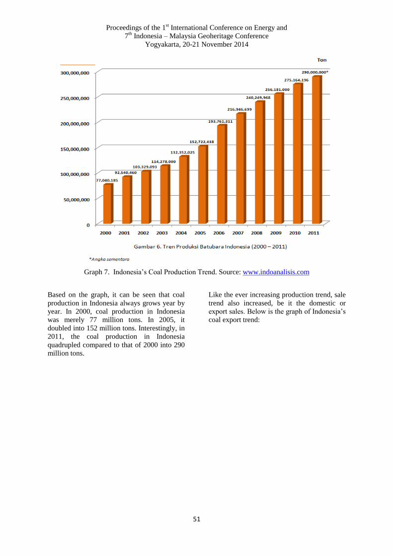
Proceedings of the 1st International Conference on Energy and
7th Indonesia – Malaysia Geoheritage Conference
Yogyakarta, 20-21 November 2014
51
Graph 7. Indonesia‟s Coal Production Trend. Source: www.indoanalisis.com
Based on the graph, it can be seen that coal
production in Indonesia always grows year by
year. In 2000, coal production in Indonesia
was merely 77 million tons. In 2005, it
doubled into 152 million tons. Interestingly, in
2011, the coal production in Indonesia
quadrupled compared to that of 2000 into 290
million tons.
Like the ever increasing production trend, sale
trend also increased, be it the domestic or
export sales. Below is the graph of Indonesia‟s
coal export trend:
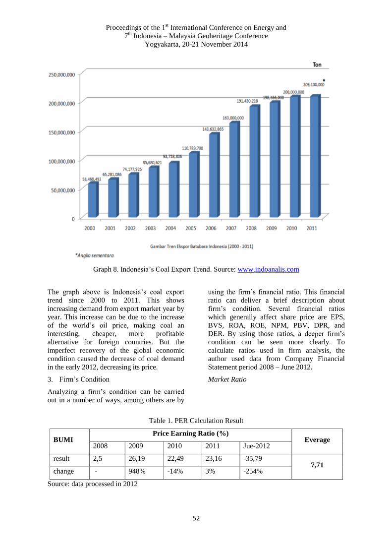
Proceedings of the 1st International Conference on Energy and
7th Indonesia – Malaysia Geoheritage Conference
Yogyakarta, 20-21 November 2014
52
Graph 8. Indonesia‟s Coal Export Trend. Source: www.indoanalis.com
The graph above is Indonesia‟s coal export
trend since 2000 to 2011. This shows
increasing demand from export market year by
year. This increase can be due to the increase
of the world‟s oil price, making coal an
interesting, cheaper, more profitable
alternative for foreign countries. But the
imperfect recovery of the global economic
condition caused the decrease of coal demand
in the early 2012, decreasing its price.
3. Firm‟s Condition
Analyzing a firm‟s condition can be carried
out in a number of ways, among others are by
using the firm‟s financial ratio. This financial
ratio can deliver a brief description about
firm‟s condition. Several financial ratios
which generally affect share price are EPS,
BVS, ROA, ROE, NPM, PBV, DPR, and
DER. By using those ratios, a deeper firm‟s
condition can be seen more clearly. To
calculate ratios used in firm analysis, the
author used data from Company Financial
Statement period 2008 – June 2012.
Market Ratio
Table 1. PER Calculation Result
BUMI Price Earning Ratio (%)
Everage 2008 2009 2010 2011 Jue-2012
result 2,5 26,19 22,49 23,16 -35,79 7,71
change - 948% -14% 3% -254%
Source: data processed in 2012

Proceedings of the 1st International Conference on Energy and
7th Indonesia – Malaysia Geoheritage Conference
Yogyakarta, 20-21 November 2014
53
Base on PER calculation as seen in table 4.1
above, average PER of BUMI was 7.71%.
Price Earning Ratio indicates market
appreciation toward firm‟s ability to earn
profit. To investors, the lower the PER of a
share, the better it is because the share is
categorized as cheap.
Table 2. PBV Calculation Result
BUMI Price To Book Value Ratio (X)
Everage 2008 2009 2010 2011 June-2012
Result 1,02 3,39 4,33 4,24 1,56 2,91
change 232% 28% -2% -63%
Source: data processed in 2012
Based on PBV Ratio calculation seen in table
4.2, average PBV of BUMI was 2.91 times.
PBV indicates how much market appreciates
firm‟s share book value.
Table 3. DPR Calculation Result
BUMI Dividen Payout Ratio (%)
Everage 2008 2009 2010 2011 June-2012
Result 13,89 29,9 31,07 15,24 - 18,02
change 115% 4% -51% -
Source: data processed in 2012
DPR is a ration calculating comparison of
dividend to firm‟s profit. Based on the DPR
Ratio calculation seen in table 4.3 above, DPR
average value of MUNI was 18.02%, which
means 18.02% from firm‟s net profit was
divided as cash dividend, while the rest
81.98% was used as additional equity.
Table 4. EPS Calculation Result
BUMI
Earning Per Share (Rp)
Everage 2008 2009 2010 2011
June-
2012
Result 364,19 92,58 134,49 93,9 -
149,3 107,173
change - -74% 45,3% -
30,18
-
259%
Source: data processed in 2012
Based on EPS calculation result as seen in
table 4.4 above, EPS average value of BUMI
was Rp 107.17, meaning for each sheet of
share there was average profit of Rp 107.13.
The higher the EPS, the higher the capital
return per sheet of share is.

Proceedings of the 1st International Conference on Energy and
7th Indonesia – Malaysia Geoheritage Conference
Yogyakarta, 20-21 November 2014
54
Table 5. BVS Calculation Result
BUMI Book Value Per Share (Rp)
Everage 2008 2009 2010 2011 June-2012
Resulr 889,87 715,09 699,16 513,52 333,67 630,26
change -20% -2% -27% -35%
Source: data processed in 2012
Based on BVS calculation result seen in table
4.5 above, BVS average value of BUMI was
630.26. Book Value per Share indicates net
asset owned by share holders by owning a
sheet of share. The higher the BVS, the higher
the net asset owned by share holders owning
per sheet of share.
Profitability Ratio
Table 6. NPM Calculation Result
BUMI Net Profit Margin (%)
Everage 2008 2009 2010 2011 June-2012
Result 19,1 5,92 7,12 5,38 -16,81 4,14
change -69% 20% -24% -412%
Source: data processed in 2012
This ratio calculates profit per rupiah sale.
Based on NPM calculation as seen in table 4.6
above, NPM average value of BUMI was
4.14%, meaning per one hundred rupiah sale
there was net profit of Rp. 4.14. This low
profit margin was caused by the high number
of debt use.
Tabel 7. Hasil Perhitungan ROA
BUMI Return On Total Asset (%)
Everage 2008 2009 2010 2011 June-2012
Result 19,41 6,99 11,39 8,12 -3,72 8,44
change
-64% 63% -29% -146%
Source: data processed in 2012
This ratio indicates firm‟s ability to produce
profit from each rupiah used, and shows
management effectiveness in using asset to
gain income. Based on ROA calculation seen
in table 4.7 above, ROA average of BUMI was
8.44%, meaning for each hundred rupiah
owned by the firm, it gained profit of Rp 8.44.
Table 8. ROE Calculation Result
BUMI Return On Equity (%)
Everage 2008 2009 2010 2011 June-2012
Result 65,49 35,19 61,76 50,88 -36,83 35,3
change -46% 76% -18% -172%
Source: data processed in 2012
Proceedings of the 1st International Conference on Energy and
7th Indonesia – Malaysia Geoheritage Conference
Yogyakarta, 20-21 November 2014
55
ased on ROE calculation result in table 4.8
above, ROE value of BUMI was 35.3%,
meaning for every one hundred rupiah of
firm‟s capital, it gained profit of Rp 35.3. ROE
is used to measure firm‟s ability to produce
profit on its capital. The higher the ROE, the
better the firm‟s performance in utilizing its
capital to produce profit.
Solvability Ratio
Table 9. DER Calculation Ratio
BUMI Debt To Equity Ratio (X)
Everage 2008 2009 2010 2011 Juni-2012
Result 2,02 3,95 4,06 5,25 8,91 4,84
change 96% 3% 29% 70%
Source: data processed in 2012
DER Ratio is a ratio measuring how big a debt
can be paid by its own capital. The higher the
DER, the lower the funding by share holders.
Based on table 4.9, DER of BUMI was 4.84
times, meaning that BUMI‟s debt was 4.84
times its capital.
Analisis Valuasi Saham PT Bumi Resources
Tbk
1. Fair Price Valuation Analysis with
Normal Growth DDM
Below are steps in calculating BUMI‟s fair
share price using normal growth Dividend
Discount Model:
a) Determine cash Dividend per sheet of
share (Do)\ Cash Dividend in 2011 which
was just paid was Rp. 14.31 and was
considered base year (Do). This dividend
distribution was decided in General
Meeting of Shareholders (GMS) in 2011.
b) Determine required rate of return.
Valuation of share fair price of PT Bumi
Resources Tbk can be done if required rate
of return is previously calculated using
Capital Asset Pricing Model (CAPM),
which is:
ks = Rf + β[E(Rm) – Rf]
Beta (β) can be calculated using regression
technique using security return volatility
(BUMI) as a dependent variable and market
return volatility (JCI) as an independent
variable. Beta value for BUMI share period 30
December 2011 – 27 September 2012 was
2.38. The beta of BUMI share which was
bigger than 1 (β > 1) meant that BUMI had
high risk, higher than average market risk or
security return higher than market return and
that share was categorized as aggressive share.
With Beta value (β) figured out, required rate
of return can be calculated. The result of
required rate of return calculation of the share
can be seen from table 4.10 below:
Table 10. Required Rate of Return (Ks) BUMI share in 2012
Year Rf Beta (β) E(RM) (E(RM) - Rf) Required Rate of
Return (ks)
2012 5,75% 2,38 11% 5,25% 18,25%
Source: Data processed in 2012.
c) Estimate future dividend growth rate.
One of the important parts when we carry out
share valuation is to estimate growth rate used
as the basis to project revenue and earning.
Growth estimation is used to keep dividend
growth received the same as estimated.
Growth estimation is very sensitive, because if
it is misestimated, share‟s fair price will
mismatch or far from market price. Growth
estimation can be calculated as follows:

Proceedings of the 1st International Conference on Energy and
7th Indonesia – Malaysia Geoheritage Conference
Yogyakarta, 20-21 November 2014
56
g = (1-d) (ROE)
g = RR x ROE
d =
x 100% = 15,24%
RR = 1 - 15,24% = 84,76%
g = 0,8476 x 18,28 = 0,1549 or 15,49%
Expected growth rate gained from the
calculation was 15.49%. With the growth as
big as 15.49%, meaning PT Bumi Resources
Tbk can yield growth rate 15.49% every year.
d) Carry out share‟s fair price using normal
growth Dividend Discount Model.
Fair price of the share of PT Bumi Resources
Tbk calculated by using Dividend Discount
Model method was Rp. 601/share sheet. That
was the estimation for 2012. This fair price
had assumption of dividend growth rate of
15.49% and required rate of return of 18.25%.
2. Fair Price of the Share Valuation
Analysis Using P/E Ratio
On of the indicators which are very often used
in fundamental analysis is Price Earning Ratio
(PER). Below are steps to calculating fair
price of BUMI share with P/E Ratio method of
PER.
Step 1: Calculate average PER of BUMI share
period 2008 – June 2012
Table 11. Average PER Calculation of BUMI share
Ratio 2008 2009 2010 2011 June-2012 Average
Price 910 2.425 3.025 2.175 1.040
7,71 EPS 364,19 92,58 134,49 93,90 -149,3
PER 2,5 26,19 22,49 23,16 -35,79
Source: www.idx.co.id (October 2012, processed)
After average PER was found to be 7.71, next
was to count EPS average growth period 2007
– 2011 to gain the projection of the following
year‟s EPS (Eo).
Step 2: Calculate EPS average growth of
BUMI share.
Table 12. EPS Average Growth Calculation
Period 2007 – 2011
Year EPS Change
2007 382,99 -
2008 364,19 -5%
2009 92,58 -75%
2010 134,49 45%
2011 93,9 -30%
Average Growth -16%
Source: www.idx.co.id (October 2012,
processed)
Based on table 4.12 above, EPS average
growth was -16%, then EPS projection for the
following year (Eo) can be calculated.
Step 3: Calculate EPS projection for the
following year (Eo) (2012)
Eo = EPS + (1 + g)
Eo = Rp 93.9 + (1 + (-16%)) = Rp 78.88
Step 4: Calculate share‟s fair price (Po)
Based on the data, fair price of BUMI share
was as follows:
Po = PER average X Eo
Po = 7.71 X Rp 78.88
Po = Rp 607.55 or Rp 608/sheet of share
The fair price of share of PR Bumi Resources
Tbk by using P/E Ratio was Rp 608/sheet of
share. It was the estimation for 2012. This fair
price, which was Rp 608/sheet of share, had an
assumption of EPS growth rate of -16% and
average PER of 7.71.
Discussion
Assessment of Fairness of BUMI Share Price
with Normal Growth DDM
The main goal of fair price analysis is to find
firms with undervalued share price (fair price
> market price), overvalued (fair price <

Proceedings of the 1st International Conference on Energy and
7th Indonesia – Malaysia Geoheritage Conference
Yogyakarta, 20-21 November 2014
57
market price), and fairly priced (fair price =
market price).
Table 13. Comparison of Fair Price of BUMI
Share to Market Price Using Normal Growth
DDM Approach
Share Fair
Price
Share
Market
Price
1 October
2012
Comparison
Result
Rp 601 Rp 750 Overvalued
Source: Processed data of 2012
From the table above, it can be seen that share
fair price < share market price, meaning that
the share was overvalued. This was matched
with the hypothesis, meaning the share value
was lower than its market price, so this share
was considered expensive and it was advisable
not to buy this kind of share.
The best strategy for this kind of share was
selling, because the share price for that year
was very fluctuating and tended to decrease
than increase.
BUMI Share Price Fairness Assessment with
P/E Ratio
P/E Ratio is a quite simple model and it can be
used to do quick estimation.
Table 14. Comparison of Fair Price of BUMI
Share to Share Market Price with P/E Rati
Approach
Share Fair
Price
Share
Market
Price
1 October
2012
Comparison
Result
Rp 608 Rp 750 Overvalued
Source: Data in 2012, processed
From the calculation result above, it can be
seen that share fair price < share market price,
so it can be concluded that the price of BUMI
share was overvalued to its fair price. The
good strategy for BUMI share was selling, like
the one stated by (Tambunan, 2007) by selling
overvalued share.
Comparison of Normal Growth Dividend
Discount Model with P/E Ratio
The purpose of valuation with normal growth
Dividend Discount Model is to give
assessment whether the share is fairly priced
(undervalued) or not fairly priced (overvalued)
so investors are expected o be able to make
correct decisions in applying the selling and
buying strategies. While the purpose of
comparison of these two models is just to find
out the result of the two models, not to
determine which is better. Below is the
valuation result comparison with normal
growth Dividend Discount model and P/E
Ratio:
Table 15. Comparison of BUMI Share Fair
Price to Share Market Price for Normal
Growth DDM Model and P/E Ratio Model
Assessme
nt Model
Share
Fair
Price
Share
Market
Price
1
October
2012
Compari
son
Result
Normal
Growth
DDM
Rp
601 Rp 750
Overvalu
ed
P/E Ratio Rp
608
Overvalu
ed
Source: Data in 2012, processed
There was similarity between these two
models, i.e. BUMI share price as overvalued.
Based BUMI share market price in the early
2012 which was Rp 2,175/sheet, and if
compared to share fair price obtained from
those two models above, which were Rp
601/sheet and 608/sheet, there was a huge loss
and it can be said that investors buying the
share then were irrational.
CONCLUSION
Based on the research and explanation above,
it can be concluded as such:
1. Intrinsic value (fair price) of BUMI share
per 1 October 2012, calculate by using
Dividend Discount Model method was Rp
601. While if counted using P/E Ratio was
Rp 608.
2. If compared to BUMI share market price
per 1 October which was Rp 750, BUMI

Proceedings of the 1st International Conference on Energy and
7th Indonesia – Malaysia Geoheritage Conference
Yogyakarta, 20-21 November 2014
58
share was overvalued, meaning that BUMI
share market price was too expensive for
the share fair price. Therefore, BUMI
share was supposed to be sold by investors
owning the share.
3. BUMI share intrinsic value based on
Dividend Discount Model method which
was Rp 601/sheet was influenced by
several factors namely:
a. Cash dividend in 2011 which was just
distributed on the 6th July 2012 which
was Rp 14.31.
b. Future firm growth rate which was
15.49%.
c. Required rate of return which was
gained using Capital Asset Pricing
Model (CAPM) approach which was
18.25%.
4. BUMI share intrinsic value based on P/E
Ratio (PER) which was Rp 608/share
sheet was influence by several factors
namely:
a. EPS average growth rate for the last
five years which was -16%.
b. Firm average PER period 2008 – June
2012 which was 7.71 times.
5. Taking into account economic condition,
industrial condition, and firm condition,
there are several conside-rations that
should be looked upon, among others are:
a. World‟s economic growth slowing
down, especially in coal-consuming
countries like China and India which
caused the decrease of the demand
of coal in those countries, which
resulted in the decrease in the coal
price.
b. Actually coal industry prospect in
the future is quite promising,
especially domestically because, in
the list of coal consumption,
Indonesia only ranks the 14th, which
is still low, giving advantage to coal
industry sector as prominent
commodity in Indonesia.
c. Seen from the performance through
ratio analysis against firm financial
statement period 2008 – June 2012,
profitability rate, that is return on
equity (ROE) of BUMI in June 2012
was 36.83%, meaning BUMI would
have to work really hard to gain
profit for its expansion. While the
solvability ratio rate, that is debt
equity ratio (DER) of BUMI in June
2012 reached 8.91, meaning that its
debt was already 8.91 times its
capital.
6. Intrinsic value (fair) of PT Bumi
Resources Tbk share obtained using
Dividend Discount Model method was Rp
601 and P/E Ratio (PER) was Rp 608,
indicating that share valuation before
buying it was very important. After
finding the fair price of BUMI share using
those two methods, it was almost certain
that investors would not buy it since it was
overvalued, so they could avoid
investment loss.
SUGGESTION AND IMPLICATION OF
THE RESEARCH RESULT
The author wishes to convey suggestions as
follows:
a. This research only used Dividend
Discount Model method and P/E Ratio
(PER) together with fundamental factor
analysis. It is suggested that in the next
research other methods should be used,
such as Free Cash Flow To Equity (FCFE)
which indicates whole net cash flow to all
share holders and not only dividend with
the purpose to complete the previous
research, so they can all describe the real
condition. Baurens (2010) stated that it
was not possible to say one method was
the best or the worst (incorrect).
b. It is highly advisable that the firm should
not have any more debt because, seen
from comparison between debt and BUMI
equity in June 2012 which was 8.91 times,
the firm‟s debt was already so high and
this huge debt will put more interest
burden which will in turn decrease the
firm‟s profit and the dividend, from the
profit, distributed to the share holders will
decrease.
REFERENCES
Baurens, Svetlana. 2010. Valuation of Metals
and Mining Companies. Working Paper

Proceedings of the 1st International Conference on Energy and
7th Indonesia – Malaysia Geoheritage Conference
Yogyakarta, 20-21 November 2014
59
Swiss Banking Institute, University of
Zurich.
Bodie, Zvi, Alex Kane, and Allan J. Marcus.
2006. “Invesment”. 6th
Edition, Jakarta:
Salemba Empat.
Brigham & Houston. 2006. Dasar-Dasar
Manajemen Keuangan. Edisi Kesepuluh.
Jakarta: Salemba Empat.
Damodaran, Aswath. 2002. Investment
Valuation. 2nd
Edition, New York: John
Wiley & Sons Inc.
Drake, P. (2010). Financial ratio analysis.
Farrell, Jr. L, James. 1985. “The Dividend
Discount Model : A Primer”. Financial
Analysts Journal, Vol. 41, No 6 (Nov-Dec
1985) pp 16-19+22-25.
Frase, L., & Ormiston, A. (2004).
Understanding Financial Statements. New
Jersey: Pearson Prentice Hall.
Khairi, Sherly Emita. 2010. Valuasi Harga
Wajar Saham Sektor Perbankan yang Go
Public di BEI. Skripsi, USU, Medan.
Laporan dividend announcement tahun 2008 –
2011”. http://www.idx.co.id, diakses 23
September 2012.
Laporan keuangan PT Bumi Resources Tbk
tahun 2008 - Jun 2012”.
http://www.bumiresources.com, diakses 2
November 2012.
Laporan tingkat suku bunga Bank Indonesia
(BI rate) tahun 2012”. http://www.bi.go.id,
diakses 14 November 2012.
Manurung, Andrian Lorand. 2008. Valuasi
Harga Wajar Saham PT Telekomunikasi
Indonesia, Tbk. Skripsi, USU, Medan.
Olweny, Tobias. 2011. “The Reliability of
Dividend Discount Model in Valuation of
Common Stock at the Nairobi Stock
Exchange”. International Journal of
Business and Social Science, April 2011 pp
127-141.
Sehgal, Sanjay and Asheesh Pandey. 2010.
Equity Valuation Using Price Multiples:
Evidence From India. Asian Academy of
Management Journal of Accounting and
Finance. Vol. 6, No. 1 pp. 89 108.
Supattarakul, Somchai and Anya Khanthavit.
2011. Empirical Evidence on Equity
Valuation of Thai Firms. World Academy of
Science, Engineering and Technology, Vol.
77; pp. 597 – 606.
Tambunan, Andy Porman. 2007. Menilai
Harga Wajar Saham. Jakarta: PT Elex
Media Komputindo.
Wijaya, Andi & Viliany. 2008. Estimasi Nilai
Intrinsik Saham PT Indofood Sukses
Makmur Tbk Dengan Menggunakan
Dividend Discount Model. Jurnal
Manajemen, No.1 pp 1-12.

Proceedings of the 1st International Conference on Energy and
7th Indonesia – Malaysia Geoheritage Conference
Yogyakarta, 20-21 November 2014
60
Gondang Dam Inspection
Puji Pratiknyo
Department of Geological Engineering, Universitas Pembangunan Nasional “Veteran” Yogyakarta
ABSTRACT
Gondang dam is the one of dams in Bengawan Solo River Region. The dam site in Gondang Lor
village, Sugio district, Lamongan regency, East Java Province. The Gondang dam is water reservoir to
supply water at adjacent dam area.The dam must be keep in save condition. One of inspection works
to know the dam condition is geotechnical research. The aim of geotechnical research si to get data
about physical and mechanical of dam material. The data of dam material is used to evaluate the dam
savety.The conclusion of geotehnical reserach result is the dam material is proper to earth dam
material.
Key words: dam, save, material, proper.
INTRODUCTION
Bengawan Solo river area, is an area with
potential water resources. Water resources
management (WRM) aims to supply a variety
of needs in the community, in addition to
anticipate impending water scarcity in the dry
season for the long term, it is one of the
strategies that will be done by storing runoff
and rainwater through building dams or other
water reservoir that serves to recharges
groundwater in an effort to conserve the water
resources. Gondang Dam is one of the dams in
the region of the Solo River in Gondang Lor
village, Sugio sub-district, Lamongan regency,
East Java. Need some inspection to determine
the condition of the dam. One inspection on
Gondang Dam is a geotechnical investigation.
Geotechnical investigation was to obtain data
of the physical and mechanical properties of
soil or rock dam material. The goal is to get
the parameters that are used for dam safety
evaluation in accordance with the geological
conditions and physical properties of soil or
rock.
METHODOLOGY
This investigation using methods such as
drilling in the core zone or impermeable dam
body and laboratory testing of soil samples,
with the following details:
a. Drilling
3-point core drilling: BG-1 with a depth
of 25 meters, BG-2 with a depth of 30
meters and BG-3 with a depth of 20
meters.
Standard penetration test
Field permeability test
Undisturb sample
b. Laboratory tests that includes :
Index Test for embankment material :
Natural Water content
Unit Weight
Specific Grvity
Grain Size Analysis
Atteberg Limit
Mechanical Properties for embank-ment
material :
Triaxial CU Test
Consolidation Test
Permeability Test
LOCATION
Gondang Dam is located in Gondang Lor
village, Sugio sub-district, Lamongan regency,
East Java Province. Access to this dam can be
reached from the junction of UNISDA
Sukodadi then turn to the south about 8
kilometers until the end of the T-junction.
From the T-junction then turn to the west
approximately 10 kilometers. Along this path,
there is a boundary between Sukodadi sub-
district and Sugio sub-district. There are signs
that direct way to Gondang Dam (turn to the
south). From signs about 3 kilometers to the
end of the T-junction and then turn to the west
about 1 kilometer.
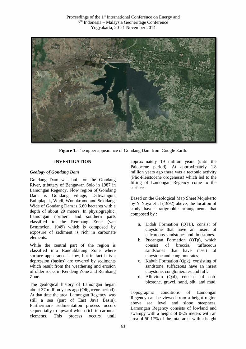
Proceedings of the 1st International Conference on Energy and
7th Indonesia – Malaysia Geoheritage Conference
Yogyakarta, 20-21 November 2014
61
Figure 1. The upper appearance of Gondang Dam from Google Earth.
INVESTIGATION
Geology of Gondang Dam
Gondang Dam was built on the Gondang
River, tributary of Bengawan Solo in 1987 in
Lamongan Regency. Flow region of Gondang
Dam is Gondang village, Daliwangun,
Buluplapak, Wudi, Wonokromo and Sekidang.
Wide of Gondang Dam is 6.60 hectares with a
depth of about 29 meters. In physiographic,
Lamongan northern and southern parts
classified to the Rembang Zone (van
Bemmelen, 1949) which is composed by
exposure of sediment is rich in carbonate
elements.
While the central part of the region is
classified into Randublatung Zone where
surface appearance is low, but in fact it is a
depression (basins) are covered by sediments
which result from the weathering and erosion
of older rocks in Kendeng Zone and Rembang
Zone.
The geological history of Lamongan began
about 37 million years ago (Oligocene period).
At that time the area, Lamongan Regency, was
still a sea (part of East Java Basin).
Furthermore sedimentation process occurs
sequentially to upward which rich in carbonat
elements. This process occurs until
approximately 19 million years (until the
Paleocene period). At approximately 1.8
million years ago there was a tectonic activity
(Plio-Pleistocene orogenesis) which led to the
lifting of Lamongan Regency come to the
surface.
Based on the Geological Map Sheet Mojokerto
by Y Noya et al (1992) above, the location of
study have stratigraphic arrangements that
composed by :
a. Lidah Formation (QTL), consist of
claystone that have an insert of
calcareous sandstones and limestones.
b. Pucangan Formation (QTp), which
consist of breccia, tuffaceous
sandstones that have insert of
claystone and conglomerates.
c. Kabuh Formation (Qpk), consisting of
sandstone, tuffaceous have an insert
claystone, conglomerates and tuff.
d. Alluvium (Qal), consists of cob-
blestone, gravel, sand, silt, and mud.
Topographic conditions of Lamongan
Regency can be viewed from a height region
above sea level and slope steepness.
Lamongan Regency consists of lowland and
swampy with a height of 0-25 meters with an
area of 50.17% of the total area, with a height

Proceedings of the 1st International Conference on Energy and
7th Indonesia – Malaysia Geoheritage Conference
Yogyakarta, 20-21 November 2014
62
of 25-100 meters land area of 45.68% and the
remaining, 4.15%, is land with a height of over
100 meters from the surface sea water.
Gondang Dam itself, including to area with
low topography.
The geological history of Lamongan began
about 37 million years ago (Oligocene period).
At that time the area, Lamongan Regency, was
still a sea (part of East Java Basin).
Furthermore sedimentation process occurs
sequentially to upward which rich in carbonat
elements. This process occurs until
approximately 19 million years (until the
Paleocene period). At approximately 1.8
million years ago there was a tectonic activity
(Plio-Pleistocene orogenesis) which led to the
lifting of Lamongan Regency come to the
surface.
Based on the Geological Map Sheet Mojokerto
by Y Noya et al (1992) above, the location of
study have stratigraphic arrangements that
composed by:
a. Lidah Formation (QTL), consist of
claystone that have an insert of calcareous
sandstones and limestones.
b. Pucangan Formation (QTp), which consist
of breccia, tuffaceous sandstones that have
insert of claystone and conglomerates.
c. Kabuh Formation (Qpk), consisting of
sandstone, tuffaceous have an insert
claystone, conglomerates and tuff.
d. Alluvium (Qal), consists of cobblestone,
gravel, sand, silt, and mud.
Topographic conditions of Lamongan
Regency can be viewed from a height region
above sea level and slope steepness.
Lamongan Regency consists of lowland and
swampy with a height of 0-25 meters with an
area of 50.17% of the total area, with a height
of 25-100 meters land area of 45.68% and the
remaining, 4.15%, is land with a height of over
100 meters from the surface sea water.
Gondang Dam itself, including to area with
low topography.
Result of Drilling
Drilling conducted at 3 points, there are BG-1
with a depth of 25 meters, BG-2 with a depth
of 30 meters, and BG-3 with a depth of 20
meters. The location of each drilling point in
Gondang Dam depicted in Figure 3.
Based on the drilling results in 3 points of
Gondang Dam ( BG-1, BG-2, and BG-3), it
can be seen the type of soil or rock as follows:
BG – 1
00.00 – 01.40 m Sand, loose, gray.
01.40 – 10.00 m Sandy clay (silt), stiff to very
stiff, greyish-brown, the value of N (SPT)
= 12-17.
10.00 – 16.00 m Clay, stiff to very stiff, gray-
brown there is little sand, the value of N
(SPT) = 16 - 18.
16.00 – 25.00 m Claystone, dense, gray-brown,
the value of N (SPT) = 24 – 35
BG – 2
00.00 – 01.60 m Sand, loose, gray.
01.60 – 03.00 m Sandy clay (silt), stiff gray-
brown, the value of N (SPT) = 15.
03.00 – 03.40 m Cobbly sand, stiff, brownish
gray.
03.40 –06.45 m Sandy clay (silt), stiff,
brownish gray, the value of N (SPT) = 15 -
20.
06.45 – 27.00 m Clay, stiff-very stiff, gray-
brown depths of 18-19, soft-stiff, the value
of N (SPT) = 15 - 19.
27.00 – 30.00 m Claystone, dense, gray-brown,
the value of N (SPT) = 31 - 34.
BG – 3
00.00 – 01.60 m Sand, solid half-off, greyish
at a depth of 0 to 0.3 m are soil filler, and
asphalt residua.
01.60 – 12.00 m Clay, gray-brown, stiff-very
stiff, there is a little sand, the value of N
(SPT) = 14-19.
12.00 – 20.00 m Claystone, dense, gray-brown,
the value of N (SPT) = 20-34.
The correlation between BG-1, BG-2, and BG
3, can be seen on Figure 5.
Test Laboratory
Soil mechanics laboratory tests of Gondang
dam performed on 3 point drill, drill point BG-
1 with a depth of 25 meters, BG-2 with a depth
of 30 meters and BG-3 with a depth of 20
meters.
On laboratory analysis, the index test
properties consisting of water content, unit
weight, the specific gravity, grain size and

Proceedings of the 1st International Conference on Energy and
7th Indonesia – Malaysia Geoheritage Conference
Yogyakarta, 20-21 November 2014
63
atterberg, also mechanical properties
consisting of Triaxial CU, Consolidation and
permeability tests. Laboratory test results can
be seen in Figure 6.
CONCLUSION
From the foregoing description can be
summarized as follows:
1. Gondang Dam is a earthdam, Zonal Dam
type, Dam Core Vertical. At the core
(impermeable zone) consists of silt and
clay, including fine-grained soil. On the
outside (pass zone) consists of a pile of
limestone fragments.
2. Results of field investigation in the form
of drilling, SPT, and permeability testing,
soil / rock in Gondang Dam consists of :
The core of dam body
A fill of soil material, from top to the
bottom, on BG-1 to a depth of 24 meters, the
BG-2 to a depth of 27 meters, and the BG-3
to a depth of 12 meters, composed of:
Depth, on the BG-1: 0 - 1.4m; BG-2: 0
- 1.6 m; BG-3: 0 - 1.6 m: in the form
of sand, gray, are off.
Depth, on BG-1 : 1,4 – 10 m; BG-2 :
1,6 -6,4 m : in the form of silt,
brownish-gray colored, stiff to very
stiff, the value of N (SPT) = 12-17.
Depth, on BG-1 10 – 16 m; BG-2 6,4
– 27 m; BG-3 1,6 – 12 m : in the form
of clay, brownish-gray colored, stiff
to very stiff, there is a little sand, the
value of N (SPT) = 16-18.
Bedrock palm of dams (BG-1 at a
depth of 16-25 m ; BG-2 at a depth of
27-30 m ; BG-3 at a depth of 12-20 m)
in the form:
Claystone, gray brown, hard, the value
of N (SPT) = 24-35.
Core permeability coefficient dam
body (soil embankment) ranged
2,34E-05 cm / sec - 5,49E-05 cm / sec,
palms dam bedrock ranges 4,69E-05
cm / sec - 6,51E-05 cm / sec.
3. Based on the grain size, permeability
values and the results of laboratory
analysis of soil samples filler, it can be
seen that the soil filler in dam core is still
appropriate when applied as a soil filler
material for impermeable zone on earth
dam type.
REFERENCES:
Ir. Shirley LH, 1987, Penuntun Praktis
Geoteknik dan Mekanika Tanah
(Penyelidikan Lapangan dan Laboratorium),
NOVA – Bandung.
Ir. Suyono Sosrodarsono dan Kazuto
Nakazawa, 1988, Mekanika Tanah & Teknik
Pondasi, Cetakan 4, Pradnya Paramita, ,
Jakarta.
Ir. I.W. Nortier & Ir. F. Vink, 1980, Ilmu
Konstruksi Untuk Ahli Bangunan dan Ahli
Bangunan Air, Jilid 2, Bhratara Karya
Aksara, Jakarta.

Proceedings of the 1st International Conference on Energy and
7th Indonesia – Malaysia Geoheritage Conference
Yogyakarta, 20-21 November 2014
64
Figure 2. Geological Maps of Gondang Dam, Lamongan (Source : the Geological Map Sheet Mojokerto by Y Noya et al (1992)
Location of Gondang Dam

Proceedings of the 1st International Conference on Energy and
7th Indonesia – Malaysia Geoheritage Conference
Yogyakarta, 20-21 November 2014
65
Intake tower
Outlet
Spillway weir
BG-1 (25 m)
BG-3 (20 m) BG-2 (30m)
Bore hole location Geotechnicaly Investigation
BG- : Bore hole.
Distance among bore holes :
Conduit ~ BG-1 = 180 m
BG-1 ~ BG-2 =
180 m
Figure 3. Layout Drilling Point of Gondang Dam

Proceedings of the 1st International Conference on Energy and
7th Indonesia – Malaysia Geoheritage Conference
Yogyakarta, 20-21 November 2014
66
Figure 4. Transverse pieces of Gondang Dam
BG-2 (30 m)
+ 12.00
Explanation :
1) Clay filler 2) Filter 3) Limestone filler 4) Random material
As dam
Static groundwater level
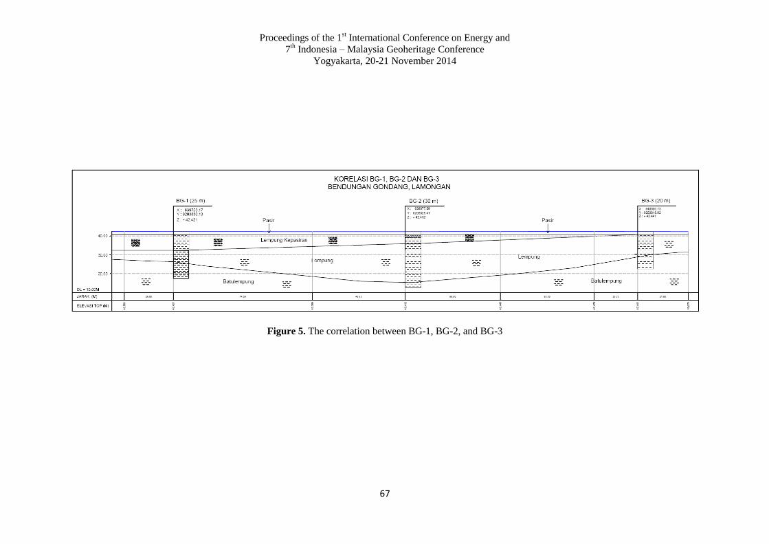
Proceedings of the 1st International Conference on Energy and
7th Indonesia – Malaysia Geoheritage Conference
Yogyakarta, 20-21 November 2014
67
Figure 5. The correlation between BG-1, BG-2, and BG-3
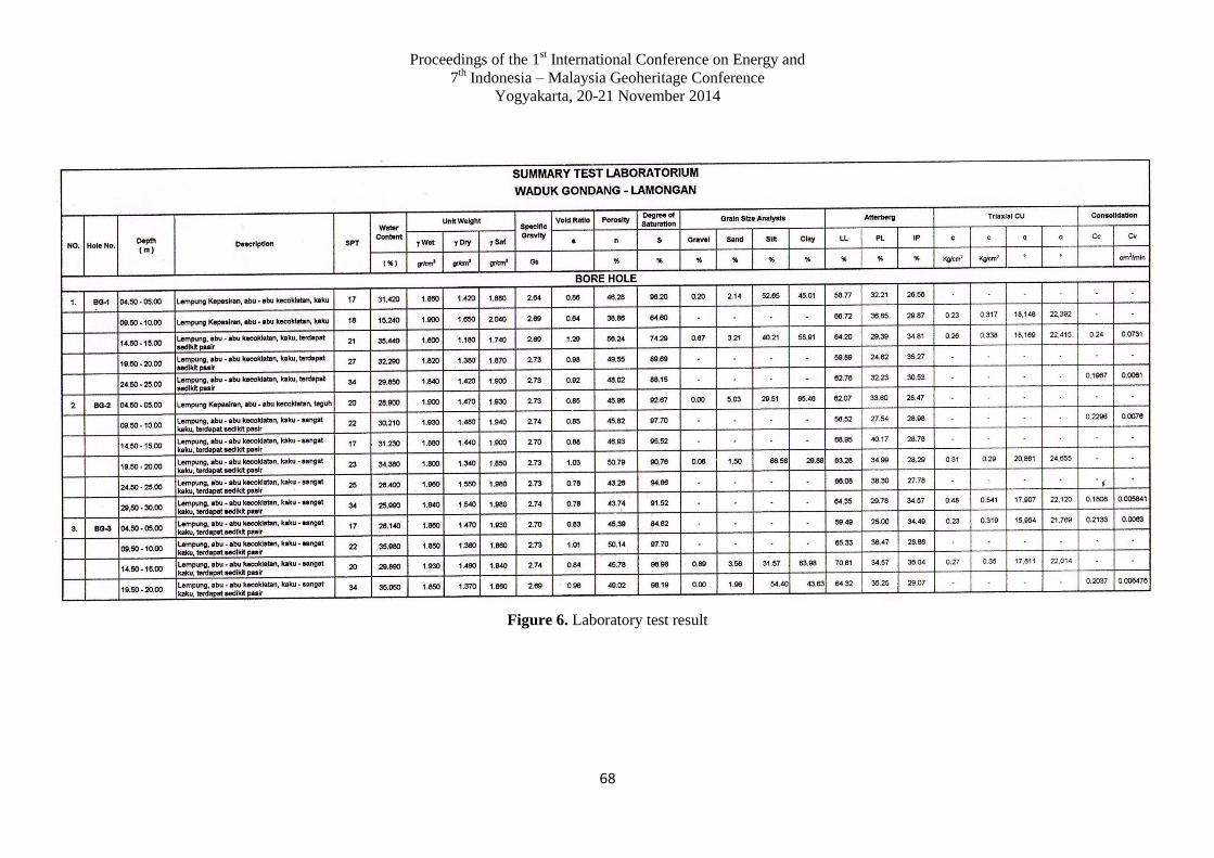
Proceedings of the 1st International Conference on Energy and
7th Indonesia – Malaysia Geoheritage Conference
Yogyakarta, 20-21 November 2014
68
Figure 6. Laboratory test result

Proceedings of the 1st International Conference on Energy and
7th Indonesia – Malaysia Geoheritage Conference
Yogyakarta, 20-21 November 2014
69
Petrophysical Analysis and Modeling, and Dynamic
Simulation in Development of “Victory” Low Resistivity Play
in “Papa” Field, Kutai Basin, East Kalimantan
Edo Pratama
Petroleum Engineering Department, UPN “Veteran” Yogyakarta
Jl. SWK 104 (Lingkar Utara) Condongcatur Depok Sleman DIY, 55283
E-mail: [email protected]
ABSTRACT
Low resistivity reservoir is an unique reservoir where generally low resistive formation whichis
identified as water bearing zone, but water free hydrocarbon are produced. It is of crucialimportance
to identify, evaluate, and develop of low resistivity reservoir where nowadays oil and gas industry is
facing decline of production, a certain case that will be happened. Thus, development of low
resistivity reservoir could be an alternative solution to answer this challenge.
This paper focuses on identifying, evaluating, and developing a low resistivity reservoir of The
“Victory” Play in “Papa” Field, Kutai Basin, East Kalimantan. Low resistivity reservoir in “Papa”
Field is a sandstone formation, where previous petrophysical interpretations yield high estimates of
water saturation. A new workflow in petrophysical analysis is conducted to get petrophysical
properties accurately, i.e. shale volume, porosity, and water saturation. Therefore, petrophysical
model could be built to generate reservoir models and dynamic simulation is conducted by making
development scenario.
According to 5 development scenario conducted in “Victory” Low Resistivity Play, Scenario IV
(Base Case + 1 Horizontal Drilling) is the best scenario which is resulting cumulative oil production
of 3,420,109 STB (RF = 21.61%) at end of prediction.
Keywords: Low resistivity reservoir, petrophysical analysis, dynamic simulation.
INTRODUCTION
Geographically, “Papa” Field is an offshore
field which is located on East Kalimantan, and
geologically is located on Kutai Basin. This
field was discovered by 1973 and started
produced by April 1975. “Papa” Field
stratigraphy is consisted by 6 sequences are
Maruat Formation, Yakin Formation, Deltaic
Sequence, Upper Carbonate Sequence, Low
Resistive Sequence, and Shallow Sequence
(Figure 1).
Generally, mainly reservoirs in “Papa” Field
are sandstone at interval of Middle Deltaic,
Lower Deltaic, and Upper Yakin Formation.
The reservoir characteristic has deep reservoir
with oil characteristic is light oil. “Papa” Field
has total wells of 38 wells with oil rate per
April 2014 up to 7.65 MBOPD and 15.18
BCFD gas. “Papa” Field reached peak of
production by February 1991 with 26,335
BOPD and 53,567 MCFD from 15 wells of
natural flow and 15 gas lift wells. After that,
trend of production was decline and there is no
further development until now.
According to this condition, it is needed a
further development in “Papa” Field to
increase production where one of alternative
solution by developing low resistive sequence.

Proceedings of the 1st International Conference on Energy and
7th Indonesia – Malaysia Geoheritage Conference
Yogyakarta, 20-21 November 2014
70
Statistically, resistivity values in this sequence
about 2 – 5 ohm-m and Gamma Ray respons
were warm (40-90 API) as shown in Well EP-
4 at zone-10 to zone-13 (Figure 2). From
previous petrophysical interpretations yield
high water saturation estimation and from
chart log generally indicated there is no
hydrocarbon, but it was proven there is
hydrocarbon in some of zones based on test
data. Thus, a comprehensive study is needed in
log interpretation, a suitable method for water
saturation calculation, and to get petrophysical
properties accurately, i.e. shale volume,
porosity, and water saturation. Therefore,
petrophysical model
could be built to generate reservoir models and
dynamic simulation is conducted by making
development scenario.
METHODOLOGY
Methods implemented for the petrophysical
interpretation of well logs as wells as in
conducting static and dynamic models
consisted of the following sequential steps:
Petrophysical analysis
The petrophysical analysis was built to
explicitly determine reservoir quality which
can be used to build petrophysical model. A
new workflow in petrophysical analysis was
conducted as shown in Figure 3. As in all
petrophysical analysis, the three basic
attributes determined are:
Shale volume: Volumetric shale fraction
was calculated using GR log where
previously shale distribution model
determined using Thomas Stieber
crossplot analysis.
Effective porosity: Neutron-density logs
were used to calculate non-shale
porosity whenever they were available
Water saturation: Determining accu-rate
water saturation values was challenging
and important for identifying
hydrocarbon distribution in “Papa”
Field.
Petrophysical modeling
Sequential Gaussian Simulation method was
used to buid petrophysical model where
previously well log scale-up and variogram
analysis were conducted.
Inplace calculation
Initial oil inplace was calculated using
volumetric method where properties that were
used from petrophysical model results and
fluid contacts were determined based on
gradient test.
Dynamic simulation
Sequential steps in planning and applying a
dynamic simulation as following below:
Defined the objectives
Prepared, analyzed, and processed
data (geology, geophysics,
petrophysics, reservoir, production,
and so on)
Made a geology – reservoir model and
its characteristic
Matched hydrocarbon inplace
(initialization) and matched reservoir
model performance with historical
production (history matching)
Conducted a reservoir forecasting with
development scenarios
RESULTS AND DISCUSSIONS
Petrophysical Analysis
Shale distribution model in sandstone
formation was analyzed by using Thomas
Stieber crossplot analysis, where it will be
known distribution model whether structural,
laminated, or dispersed clay. Analysis was
conducted at 4 wells in “Papa” Field, i.e. EP-4,
DWP-2RD2, NEL-3, and NEL-5RD. Based on
the results, shale distribution model in
sandstone of “Papa”
Field was laminated-dispersed shale (Figure
4).
Proceedings of the 1st International Conference on Energy and
7th Indonesia – Malaysia Geoheritage Conference
Yogyakarta, 20-21 November 2014
71
Due to shale distribution model in sandstone
of “Papa” Field was laminated-dispersed
shale, thus Vshale is not equivalent with
gamma ray index (Ish) or we cannot used
linier equation. In this study, we used Larinov
(for tertiary rock) method to calculate shale
volume where GRmax and GRmin were
determine for each markers.
Neutron-density logs were used to calculate
non-shale porosity whenever they were
available. Then, porosity values from log
interpretation were validated with available
core data. Table 1 shows tabulation of porosity
log validation with porosity log and Figure 5
shows the crossplot where a good match was
obtained.
Water saturation was tried to calculate by
using Dual Water, Indonesia, and Simandoux
methods. A suitable method was choosen to
calculate water saturation after compared to
core data and make a crossplot from difference
methods. According to Sw calculation at 4
wells with available core interval data, Dual
Water method resulted smaller error (Table 2).
Then, it was also done crossplot between
water saturation calculation using Dual Water
and water
saturation calculation using Indonesia and
Simandoux method (Figure 6 and 7). The
results show that Simandoux and Indonesia
methods resulted over estimation in water
saturation calculation compared to Dual Water
Method. Thus, Dual Water is a suitable
method to calculate water saturation in low
resistive sequence of “Papa” Field. Table 3
shows tabulation of Sw log validation with
available core data and Figure 8 shows
relationship between Sw from log
interpretation and Sw from available core data
for each wells.
Identifying proper petrophysical cut-off
parameter was required to determine
producible hydrocarbon volume and establish
an economical reserve estimate. Cut-off values
were determined according to test data for
each markers. Porosity and shale volume cut-
off were determined by doing crossplot both of
them and picked the higher Vshale value and
the lower porosity as cut-off values, also
higher water saturation as the Sw cut-off.
Petrophysical Modeling and Volumetric
Calculation
Petrophysical modeling was started by
interpretating well log data as data preparation,
where 9 wells were interpreted to get
petrophysical properties. Figure 9 shows wells
location in “Papa” Field. After petrophysical
properties were obtained, it is done well log
scale-up and variogram analysis as inputing
data for petrophysical modeling as well as
used stochastic method namely sequential
gaussian simulation. Figure 10 shows an
example of petrophysical modeling steps for
Vshale modeling in “Victory” Low Resistivity
Play.
Based on the models were built, it was
obtained petrophysical properties distribution
in “Victory” Low Resistivity. From the results,
“Victory” Low Resistivity Play has average
Sw distribution of 72%, average Vshale
distribution of 40%, average porosity
distribution of 13.07%. And for permeability
modeling, it was conducted using property
calculator by making an empirical equation
from porosity-permeability relationship.
Figure 11 shows
permeability modeling using empirical
equation in “Victory” Low Resistivity Play.
From permeability modeling, “Victory” Low
Resistivity Play has average permeability
distribution of 87.7 mD.
Initial oil inplace calculation by using
volumetric method was bounded using
polygon, so that inplace calculation was
focussed based on area which has well data
and inplace calculation was not being over
estimation. Figure 12 shows initial oil inplace
distribution map in “Victory” Low Resistivity
Play with total inplace of 35.47 MMSTB.
Dynamic Simulation
To conduct development scenarios with
dynamic simulation, it is needed a reservoir
model which is representating the actual
reservoir condition. The reservoir model was
generated from “Victory” Low Resistivity
Play in EP area due to this area has biggest
initial oil inplace and good petrophysical
properties distribution. Required data in
building the reservoir model were geological

Proceedings of the 1st International Conference on Energy and
7th Indonesia – Malaysia Geoheritage Conference
Yogyakarta, 20-21 November 2014
72
model, rock and fluid properties data, and
production and pressure data. Figure 13 shows
process in building “Victory” low resistivity
reservoir model.
After all of geological and reservoir data were
generated in simulator, it was needed to
conduct some of validation procedures, an
initial model validation was initialization, a
process to match initial oil inplace from
reservoir model towards to initial oil inplace
from volumetric calculation and to match
initial reservoir pressure. Initialization process
is shown in Figure 14. Initial oil inplace that
was obtained from volumetric calculation if
compared to initial oil inplace of the model
was not significantly difference. The
differences of both of them were 3.09% and
the differences between initial reservoir
pressure model and data of
0.027%.
After initial oil inplace and initial reservoir
pressure have matched, the next step is history
matching process of production data. In this
step, the previous model that was obtained
from initialization step was validated with
production data, by seeing production
performance resulted from the model and
comparing to field historical production data.
History matching process is shown in Figure
15, where reservoir pressure and production
data from start of
production till end of history have matched.
Thus, reservoir model that conducted by
dynamic simulation is valid.
Development of “Victory” low resistivity play
was conducted by making some of
development scenarios, consists of five
scenarios are Scenario I of base case
(existing), Scenario II of base case and two
workover wells, Scenario III of base case and
one infill drilling (vertical well), Scenario IV
of base case and one lateral drilling (horizontal
well), and Scenario V of base case and two
workover wells as well as one infill drilling
(vertical well). Prediction or forecasting step is
set till October 2018. Figure 16 shows
prediction results and comparison of
development scenarios. According to five
development scenarios conducted in EP Area
of “Victory” Low Resistivity Play, Scenario
IV (Base Case + 1 Horizontal Drilling) is the
best scenario which is resulting cumulative oil
production of 3,420,109 STB (RF = 21.61%)
at end of prediction.
CONCLUSIONS AND
RECOMMENDATIONS
Conclusions
1. Dual Water Method is a suitable method
for estimating water saturation in “Papa”
Low Resistive Pay Zones
2. Initial oil inplace in “Victory” Low
Resistivity Play is estimated about 35.47
MMSTB and it has petrophysical
properties distribution with average
Vshale distribution of 40%, average
porosity distribution of 13.07%, average
permeability distribution of 87.7 mD, and
average water saturation distribution of
72%.
3. According to 5 development scenario
conducted in EP Area of “Victory” Low
Resistivity Play, Scenario IV (Base Case +
1 Horizontal Drilling) is the best scenario
which is resulting cumulative oil
production of 3,420,109 STB (RF =
21.61%) at end of prediction.
Recommendations
1. It is fully recommended to develop low
resistivity reservoir in “Papa” Field due to
these reservoirs have a good potential to
be developed based on volumetric
calculation and petrophysical properties
distribution.
2. An economic analysis is needed for further
study to determine a suitable development
scenario in EP Area of “Victory” Low
Resistivity Play.
REFERENCES
A. Krygowski, Daniel. 2003. “Guide to
Petrophysical Interpretation”. Austin, Texas,
USA
Amyx, J. W., Jr , Bass, M.D., “Petroleum
Reservoir Engineering” , Mc Graw Hill
Book Company , New York , London ,
1960.

Proceedings of the 1st International Conference on Energy and
7th Indonesia – Malaysia Geoheritage Conference
Yogyakarta, 20-21 November 2014
73
Bowen, D.G. 2003. “Formation Evaluation
and Petrophysics”. Core Laboratories,
Jakarta, Indonesia
Claverie, Michel, et. al., “A New Look at
Low-Resistivity and Low-Contrast (LRLC)
Pay in Clastic Reservoirs”, SPE Annual
Technical Conference and Exhibition, 19-22
September 2010.
Ekwere, J.Peters, ”Petrophysics”, Department
of Petroleum & Geosystems Engineering
The University of Texas at Austin.
Gandhi, Ankur, et.al., “Low Resistivity
Petrophysical Mapping Expands The Terry
(Sussex) Play In Wattenberg Field,
Colorado“, SPWLA 52nd Annual Logging
Symposium, May 14-18, 2011.
Hamada, G.M. and Al-Awad, M.N.J,
“Petrophysical Evaluation of Low
Resistivity Sandstone Reservoirs”, Journal
of Canadian Petroleum Technology, July
2000, Volume 39, No. 7.
Schlumberger. 2008. “Petrel Introduction
Course: Seismic to Simulation Software”.
Tudge, Joanne.“Low Resistivity Pay; The Role
of Chlorite in Controlling Resistivity
Responses”. Thesis. University of Leicester.
APPENDIX
Table 1. Tabulation of porosity log validated with available core data
Table 2. Determination of Sw calculation method compared to available core data
Table 3. Tabulation of Sw log validated with available core data

Proceedings of the 1st International Conference on Energy and
7th Indonesia – Malaysia Geoheritage Conference
Yogyakarta, 20-21 November 2014
74
Figure 1. Stratigraphy of “Papa” Field

Proceedings of the 1st International Conference on Energy and
7th Indonesia – Malaysia Geoheritage Conference
Yogyakarta, 20-21 November 2014
75
Figure 2. Chart log in Well EP-4 (zone-10 to zone-13)
Figure 3. Petrophysical analysis workflow

Proceedings of the 1st International Conference on Energy and
7th Indonesia – Malaysia Geoheritage Conference
Yogyakarta, 20-21 November 2014
76
Figure 4. Thomas Stieber crossplot analysis
Figure 5. Porosity log validation with available core data

Proceedings of the 1st International Conference on Energy and
7th Indonesia – Malaysia Geoheritage Conference
Yogyakarta, 20-21 November 2014
77
Figure 6. A comparison of water saturation calculation using Dual Water equation and
Simandoux equation
Figure 7. A comparison of water saturation calculation using Dual Water equation and
Indonesia equation

Proceedings of the 1st International Conference on Energy and
7th Indonesia – Malaysia Geoheritage Conference
Yogyakarta, 20-21 November 2014
78
Figure 8. Sw log validation with available core data
Figure 9. Wells location in “Victory” Low Resistivity of “Papa” Field

Proceedings of the 1st International Conference on Energy and
7th Indonesia – Malaysia Geoheritage Conference
Yogyakarta, 20-21 November 2014
79
Figure 10. Vshale modeling in “Victory” Low Resistivity Play
Figure 11. Permeability modeling in “Victory” Low Resistivity Play

Proceedings of the 1st International Conference on Energy and
7th Indonesia – Malaysia Geoheritage Conference
Yogyakarta, 20-21 November 2014
80
Figure 12. Initial oil inplace distribution of “Victory” Low Resistivity Play in “Papa” Field
Figure 13. “Victory” Low Resistivity Reservoir model in EP Area

Proceedings of the 1st International Conference on Energy and
7th Indonesia – Malaysia Geoheritage Conference
Yogyakarta, 20-21 November 2014
81
Figure 14. Initialization process (OOIP and initial reservoir pressure)
Figure 15. History matching process (pressure and production)

Proceedings of the 1st International Conference on Energy and
7th Indonesia – Malaysia Geoheritage Conference
Yogyakarta, 20-21 November 2014
82
Figure 16. A comparison of prediction results for each development scenarios in EP Area of
“Victory” Low Resistivity Play

Proceedings of the 1st International Conference on Energy and
7th Indonesia – Malaysia Geoheritage Conference
Yogyakarta, 20-21 November 2014
83
Biozoning on Planktonic Foraminifera of Ngrayong, Bulu,
Wonocolo, Ledok, and Mundu Formation, Kecamatan
Tambakboyo and the Sorrounding Area, Kabupaten Tuban,
Provinsi Jawa Timur
M. Sultan Maulanasyah1, Mahap Maha
1, Achmad Subandrio
1
1Program studi Teknik Geologi UPN “Veteran” Yogyakarta
Email: [email protected], [email protected]
ABSTRACT
The research area is located in Tambakboyo district and Jatirogo district, Tuban Regency, East Java
Province. The research Area is included in the Mandala Rembang Zone, North East Java Basin. The
preparation of bio-datum and manufacture of bio-zonation (bio-stratigraphic zone) based on the
presence and distribution of taxon identifier of Planktonic Foraminifera fossil in rock sample on
surface measure stratigraphic section‟s line across Ngrayong Formation, Bulu Formation, Wonocolo
Formation, Ledok Formation and Mundu Formation in research area.
The biozonation that has been obtained from the biostratigraphy analysis, from older to younger
sedimentary rock layers (Ngrayong Formation- Mundu Formation) are 2 Partial Zone and 5 Interval
Zone, ie: Globorotalia menardii (N12) Partial Zone, Globorotalia menardii-Globorotalia
pseudomiocenica (N13) Interval Zone, Globorotalia pseudomiocenica- Globigerina bulloides (N14-
N15) Interval Zone, Globigerina bulloides-Globorotalia plesiotumida (N16) Interval Zone,
Globorotalia plesiotumida-Globorotalia tumida (N17) Interval Zone,Globorotalia tumida-
Globorotalia plesiotumida(N18) Interval Zone, Globorotalia plesiotumida (N19)Partial Zone.
From Bio-stratigraphic analysis in this research area, the conclusion is the sedimentation in research
area is younger than the Regional Geology Mandala Rembang Zone.
Key Words : Biozonation, Foraminifera Plankton, Miocen-Pliocen, Geology of Rembang Zone.
PREFACE
The law of Superposition (Steno,1669) is a
fundamental law of geology, it is explaining
about the sedimentary rock in the lower layer
is older than the upper one. However, at the
present time (Recent) the sedimentary layers
have been folded or faulted due to the tectonic
deformation of the earth. At the deposition
stage of sedimentary rocks, there is possibility
of sea level changes which causes the changes
of lithology of sediment layers that which
indicate a change in depositional environment.
It takes a variety of methods to solve these
problems, especially in the determination of
the age of deposition of sedimentary rocks,
one of them through a biological approach to
the sediment layer with Biostratigraphic
methods. Biostratigraphy is the branch of
stratigraphy, the studies about the distribution
of fossils in the stratigraphic record, and
classify the rock layers into units based on the
fossil content therein. This science utilizes the
Chronostratigraphy range of various species of
fossils to correlate stratigraphic cross-section,
especially the distribution of planktonic
foraminifera fossils are used for determining
the age of sedimentary rocks as datum planes
or in this case is bio-datum.
According to the research results of previous
researchers, North East Java Basin Mandala
Rembang Zone is a dynamic in term of
tectonic and a basin that has a good
composition of carbonate sedimentary rock.
So, it is very possible to do research in the
field of biostratigraphy. For the scientific
terms or in terms of industry.

Proceedings of the 1st International Conference on Energy and
7th Indonesia – Malaysia Geoheritage Conference
Yogyakarta, 20-21 November 2014
84
The research area is administratively located
in the District Tambakboyo, and District
Jatirogo, Tuban, East Java Province (Figure
1). Located on 49S zone, UTM coordinates
580000 mE - 586 000 mN mE and 9242000 -
9237500 mN.
The main objective of this study was to
determines and arrange the biodatum and
biostratigraphic zones based on taxon
identifier of planktonic foraminifera that found
on research area, and determine the age of
rocks or rock units of measurement
stratigraphic cross-section.
The research methods used was the analysis of
microfossils Foraminifera Plankton in each
sample taken at the track of measurement
stratigraphic cross-section from the geological
surface observation on research area. Then
distributing fossil analysis results in a
stratigraphic cross-section, and classify the the
rock layers into units based on fossil content
therein.
Figure 1. Map of Location Research Areas in East Java Province (Source: Bakorsurtanal / BPN Prov.
East Java).
REGIONAL GEOLOGY
Based on Java physiographic zones created by
Van Bemmelen (1949) (Figure 2.), the study
area includes in the Antiklinorium Rembang-
Madura Zone. This zone extends from the
northern boundary of Java and the western is
separated by Lusi Depression of Randublatung
Zone. This zone is characterized by the
presence of Antiklinorium Rembang that is the
lines of anticline that overlap each other
(superimposed). The Sediments at Rembang
zone are showing the rocks with a high sand
content in addition to the presence of
carbonate rocks and the absence of pyroclastic
sediments. The sediments are interpreted that
deposited on the sea not far from the beach,
the sea bottom are diverse in terms of depth
due to the giant faults (block faulting). The
Rembang zone commonly consists of a
sequence of Eocene-Pliocene sediments which
include shallow marine clastic and carbonate
sediments are widespread. The Rembang zone
basement rock is dominated by various types
of Cretaceous metamorphic rocks such as slate
stone, filit, and Diorite igneous rock diorit
(Prasetyadi, 2007). Even though no firm but
the boundary is interpreted by unconformity
with Ngimbang Formation were deposited on
top of it. The sediment sequence above Pre-
Ngimbang Formation and Ngimbang
Formation are dominated by carbonate
sediment of Kujung Formation and Prupuh
Formation which is an Oligocene sediment.
And the sequence stratigraphy above Kujung
Formation according to Pringgoprawiro(1983)
(Figure 3.) are Tuban Formation, Tawun
Formation, Ngrayong Formation, Bulu
Formation, Wonocolo Formation, Ledok
Formation, and Mundu Formation which are
sedimentary rocks deposited in conformity
state at Miocene to Pleistocene in the shallow

Proceedings of the 1st International Conference on Energy and
7th Indonesia – Malaysia Geoheritage Conference
Yogyakarta, 20-21 November 2014
85
marine area with the composition of carbonate
as the dominant.
Based on field data and laboratory analysis
and confirmed and be compared to the results
of previous research, the stratigraphy of the
study area (Figure 4.) sequentially from the
older to the younger, ie:
Ngrayong sandstones Unit.
Consists of quartz sandstone with claystone
and Orbitoid limestone inserts. The age
Ngrayong sandstone unit ranges from N12-
N15 zones or the Middle Miocene -Late
Miocene, depositional environment on neritik
bank - central neritik influenced by tidal sea
water on transgression phase.
Bulu limestones Unit.
Bulu limestone unit has a lithology
characteristic form of orbitoid limestone, with
inserts calcareous sandstones in several parts.
The age is N15-N16 (Late Miocene), from thin
section appears genus Lepidocyclina and
Cycloclypeus which also can be used as a
determination of the age that is the middle
Miocene - late Miocene (Tf). It deposited on
edge of neritic until the transition environment
(tidal) on transgression phase.
Wonocolo sandy marl Unit.
This rock unit is composed by sandy marl, and
calcarenit (sandy limestone) inserts. The
thickness of this unit is 75.25 meters. The age
ranged between N16-N17 zones or Late
Miocene. Based on the presence of
foraminifera bentonik present is Anomalina
colligera, Uvigerina scwageri, Hyperam-mina
cylindris, Turbinella funalis deposited at the
central neritik zone until upper bathial
according to Barker‟s classification (1960).
Ledok limestones Unit
This unit has lithological characteristics are
sandy marl and calcarenite (sandy limestones)
are repeated, with slight inserts calcareous
sandstones. The thickness of this unit is 112
meters. The age ranged between N17-N19
(Late Miocene-early Pliocene). It deposited at
the central neritik – upper bathial on sea level
drop phase, it supported by the presence of
sedimentary structures mega-crossbeding and
ichnofossil cruziana.
Mundu marl unit.
This unit has massive marl as its lithological
characteristics. From the result of calcimetri
analysis, it obtained CaCO3 content of Mundu
marl unit is 28-29% and named as marl-clay
(Petijohn, 1957). The Age range are N19-N21
(early Pliocene), it identified by the presence
of Globorotalia tumida (without Globorotalia
merotumida and Globorotalia plesiotumida). It
deposited on outer neritic- lower bathial in sea
level rise phase.
LITHO-STRATIGRAPHIC ON THE
RESEARCH AREA
Based on field data and laboratory analysis
and confirmed and be compared to the results
of previous research, the stratigraphy of the
study area (Figure 4.) sequentially from the
older to the younger, ie:
Ngrayong sandstones Unit.
Consists of quartz sandstone with claystone
and Orbitoid limestone inserts. The age
Ngrayong sandstone unit ranges from N12-
N15 zones or the Middle Miocene -Late
Miocene, depositional environment on neritik
bank - central neritik influenced by tidal sea
water on transgression phase.
Bulu limestones Unit.
Bulu limestone unit has a lithology
characteristic form of orbitoid limestone, with
inserts calcareous sandstones in several parts.
The age is N15-N16 (Late Miocene), from thin
section appears genus Lepidocyclina and
Cycloclypeus which also can be used as a
determination of the age that is the middle
Miocene - late Miocene (Tf). It deposited on
edge of neritic until the transition environment
(tidal) on transgression phase.
Wonocolo sandy marl Unit.
This rock unit is composed by sandy marl, and
calcarenit (sandy limestone) inserts. The
thickness of this unit is 75.25 meters. The age
ranged between N16-N17 zones or Late
Miocene. Based on the presence of

Proceedings of the 1st International Conference on Energy and
7th Indonesia – Malaysia Geoheritage Conference
Yogyakarta, 20-21 November 2014
86
foraminifera bentonik present is Anomalina
colligera, Uvigerina scwageri, Hyperammina
cylindris, Turbinella funalis deposited at the
central neritik zone until upper bathial
according to Barker‟s classification (1960).
Ledok limestones Unit
This unit has lithological characteristics are
sandy marl and calcarenite (sandy limestones)
are repeated, with slight inserts calcareous
sandstones. The thickness of this unit is 112
meters. The age ranged between N17-N19
(Late Miocene-early Pliocene). It deposited at
the central neritik – upper bathial on sea level
drop phase, it supported by the presence of
sedimentary structures mega-crossbeding and
ichnofossil cruziana.
Mundu marl unit.
This unit has massive marl as its lithological
characteristics. From the result of calcimetri
analysis, it obtained CaCO3 content of Mundu
marl unit is 28-29% and named as marl-clay
(Petijohn, 1957). The Age range are N19-N21
(early Pliocene), it identified by the presence
of Globorotalia tumida (without Globorotalia
merotumida and Globorotalia plesiotumida). It
deposited on outer neritic- lower bathial in sea
level rise phase.
Figure 2. Physiographic of Java (Van Bemmelen, 1949). Research
areas included in the Antiklinorium Rembang-Madura.

Proceedings of the 1st International Conference on Energy and
7th Indonesia – Malaysia Geoheritage Conference
Yogyakarta, 20-21 November 2014
87
Figure 3. Stratigraphy of Rembang Zone (Pringgoprawiro, 1983).

Proceedings of the 1st International Conference on Energy and
7th Indonesia – Malaysia Geoheritage Conference
Yogyakarta, 20-21 November 2014
88
Figure 4. Stratigraphic of Reasearch area (Maulanasyah, 2014).
BIOSTRTIGRAPHIC REASEARCH
AREA
Biodatum of Foraminifera Plankton
Biodatum that found by Biostratigraphy
analysis of sedimentary rock samples in
stratigraphic measured sections in the study
area sequentially from the older to younger,
include:
1. Globorotalia menardii biodatum (First
Appearance)
Globorotalia menardii„s range age is N13-N23
(Mid. Miocene- Pliocene). This fossil is used
for an identifier fossil for bottom of Ngrayong
Sandstone Unit in study area. Therefor the
writer picked the first appearance of
Globorotalia menardii as a bio-horizon line of
the last N12 and first N13. The biozonation‟s
boundary is in point bios 2.
2. Globorotalia pseudomiocenica bioda-tum
(First Appearance)
Globorotalia pseudomiocenica‟s range age is
N14-N23 (Mid. Miocene- Pliocene). This
fossil is used for an identifier fossil in body of
Ngrayong Sandstone Unit in study area.
Therefor the writer picked the first appearance
of Globorotalia menardii as a bio-horizon line
of the last N13 and first N14. The
biozonation‟s boundary is in point bios 9.
3. Globigerina bulloides biodatum (First
Appearance)
This fossil‟s range age is N16-N23 (Last
Miocene- Pleistocene). The first appearance of
Globigerina bulloides is used for an identifier
fossil as a bio-horizon line of last N15 and first
N16 in body of Bulu limestone Unit. The
biozonation‟s boundary is in point bios 15.
4. Globorotalia plesiotumida biodatum (First
Appearance)
This fossil‟s range age is N17-N18 (Last
Miocene- Lower Pliocene). The first

Proceedings of the 1st International Conference on Energy and
7th Indonesia – Malaysia Geoheritage Conference
Yogyakarta, 20-21 November 2014
89
appearance of Globorotalia plesiotumida is
used for an identifier fossil as a bio-horizon
line of last N16 and first N17 in body of
Wonocolo sandy-marl Unit. The biozonation‟s
boundary is in point bios 18.
5. Globorotalia tumida biodatum (First
Appearance)
Globorotalia tumida‟s range age is N18-N23
(Last Miocene- Lower Pliocene). The first
appearance of Globorotalia tumida is used for
an identifier fossil as a bio-horizon line of last
N17 and first N18 in body of Ledok limestone
Unit. The biozonation‟s boundary is in point
bios 24.
6. Globorotalia plesiotumida biodatum (Last
Appearance)
This fossil‟s range age is N17-N18 (Last
Miocene- Lower Pliocene). The last
appearance of Globorotalia plesiotumida is
used for an identifier fossil as a bio-horizon
line of last N18 and first N19 in top of Ledok
limestone Unit. The biozonation‟s boundary is
in point bios 27.
Biozonation of Foraminifera Plankton
Base on Biostratigraphic analysis from
stratigraphic measured section in research
area, it can be divided into two zones that is
Interval Zone and Partial Zone (Table 1.). The
Interval zones and Partial zones were made by
bio-horizons that have been arranged before.
The foraminifera planktonic‟s biozonations
sequentially from the older to the younger are:
1. Globorotalia menardii Partial zone as
indicator of N12 (Mid. Miocene) in
Ngrayong sandstone Unit.
2. Globorotalia menardii - Globorotalia
pseudomiocenica Interval zone as
indicator of N13 (Mid. Miocene)in
Ngrayong sandstone Unit.
3. Globorotalia pseudomiocenica –
Globigerina bulloides Interval zone as
indicator of N14-N15 (Mid. Miocene- last
Miocene) in Ngrayong sandstone Unit to
Bulu limestone Unit.
4. Globigerina bulloides - Globorotalia
plesiotumida Interval zone as indicator of
N16 (Last Miocene) in Bulu limestone
Unit to Wonocolo sandy-marl Unit.
5. Globorotalia plesiotumida - Globorotalia
tumida Interval zone as indicator of N17
(Last Miocene) in Wonocolo sandy-marl
Unit to Ledok limestone Unit.
6. Globorotalia tumida - Globorotalia
plesiotumida Interval zone as indicator of
N18 (Last Miocene- Early Miocene)in
Ledok limestone Unit.
7. Globorotalia plesiotumida Partial zone as
indicator of N19 (Last Miocene- Early
Miocene)in Ledok limestone Unit to
Mundu marl Unit.
CONCLUSSIONS
Age‟s plane : Globorotalia menardii (N13),
Age‟s plane Globorotalia pseudomiocenica
(N14), Age‟s plane Globigerina bulloides
(N16), Age‟s plane Globorotalia plesiotumida
(N17), Age‟s plane Globorotalia tumida
(N18).
The biozonation that has been found are 2
Partial zone (P.Z.), dan 5 Interval zone (I.Z.),
yaitu Globorotalia menardii P.Z. (N12),
Globorotalia menardii - Globorotalia
pseudomiocenica I.Z. (N13), Globorotalia
pseudomiocenica - Globigerina bulloides I.Z.
(N14-N15), Globigerina bulloides -
Globorotalia plesiotumida I.Z. (N16),
Globorotalia plesiotumida - Globorotalia
tumida (N17), Globorotalia tumida -
Globorotalia plesiotumida I.Z. (N18),
Globorotalia plesiotumida P.Z.(N19).
Base on biostratigraphic analysis‟s result on
research area, Sedimentary rocks in research
area deposited at younger age than the regional
geology reference of Mandala Rembang Zone
(1983).
REFERENCE
Allan, W. H. Bé, 1977. An Ecological,
"Oceanic Micropaleontology", Volume 1,
Proceedings of the 1st International Conference on Energy and
7th Indonesia – Malaysia Geoheritage Conference
Yogyakarta, 20-21 November 2014
90
Zoogeographic and Taxonomic Review of
Recent Planktonic Foraminifera, pp. 1-100.
Bandy, O. L., 1960. The geologic significance
of coiling rations in the foraminifer
Globigerina pachyderma (Ehrenberg). J.
Paleont.
Banner, F.T., and Blow, W.H., 1965. Two new
taxa of the Globorotaliinae (Globigerinacea,
Foraminfera) assisting determination of the
late Miocene / middle Miocene boundary.
Nature Vol. 207.
Barker R. W., 1960, Taxonomic Note. Society
of economic paleontologist and
mineralogist. The Collegiaten Press George
Santa Company, INC, Mekasha,
Wisconsin, U.S.A.
Blow, W.H., 1969. Late Middle Eocene to
Recent Planktonik Foraminifera
Biostratigrafi Cont, Planktonic Microfosil,
Geneva, 1967, Pro. Leiden, E.j.Bull, v.1.
Bolli, H., 1950. The direction of coiling in the
evolution of some Globorotaliidae. Reprint
from contributions from the Cush. Found.
Foram. Res., vol. 1, parts 3 and 4.
Dunham, R. J., 1962. Classification of
Carbonate Rock According to Depositional
Texture, In Han, W. E. (ed) 1962,
Classification of Carbonate Rock, AAPG,
Bull. Men 1, h. 108 – 121.
IAGI., 1996. Sandi Stratigrafi Indonesia
(Revisi SSI 1973). Komisi Sandi Stratigrafi
Indonesia, Ikatan Ahli Geologi Indonesia.
Jakarta.
Maha, M., 1995. Biozonasi Paleobathimetri
Dan Pemerian Sistematis Foraminifera
Kecil Sumur TO-04, Sumur TO-08 dan
Sumur-95 Daerah Cepu dan Sekitarnya
Cekungan Jawa Timur Utara. Thesis S2
Teknik Geologi,ITB, Bandung, h.10. Tidak
dipublikasikan.
Phleger, F.B., 1951. Ecology of foraminifera.
Elsevier Publishing company, Amsterdam,
p.420.
Postuma J.A., 1971, Manual Planktonic
Foraminifera. Elsevier Publishing
Company, Amsterdam, P. 420.
Prasetyadi, C., 2007. Evolusi tektonik
Paleogen Jawa bagian timur, Disertasi ITB,
tidak dipublikasikan
Pringgoprawiro, H., 1983, Biostratigrafi dan
Paleografi Cekungan Jawa Timur suatu
pendekatan baru, Thesis Doktor, ITB,
Bandung, Tidak dipublikasikan.
Smyth, H., Hall, R., Hamilton, J., dan Kinny,
P., 2005. East Java: Cenozoic basins,
volcanoes, and ancient basement,
Proceedings 30th Indonesian Petroleum
Association Annual Convention and
Exhibition, Jakarta
Tipsword, H.I., Setzer, F.M. Smith, Jr, F.L.,
1956. Introduction of Depositional
Environment in Gulf Coast Petroleum
Exploration From Paleontology and Related
Stratigraphy, Houston.
Van Bemmelen, R.W. 1949. The Geology of
Indonesia, Vol. 1A, General Geology.
Martinus Nijhoff, The Hague. The
Netherlands.
Verstappen, H. Th., 1985. Applied
Geomorphological Survey and Natural
Hazard Zoning. Enschede: ITC.
Wenworth, C.K., 1922. A Scale of grade class
term for clastic sediments. Journ. Geology,
30:337–392.
Williams, H., Turner, F.J. and Gilbert, C.M.,
1954. Petrography; An Introduction to the
Study of Rock in Thin Sections. W.H.
Freeman and Co., San Francisco.
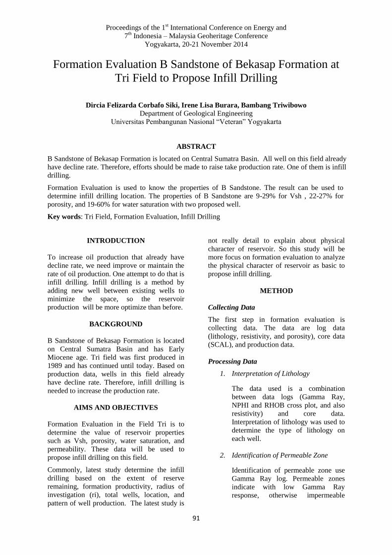
Proceedings of the 1st International Conference on Energy and
7th Indonesia – Malaysia Geoheritage Conference
Yogyakarta, 20-21 November 2014
91
Formation Evaluation B Sandstone of Bekasap Formation at
Tri Field to Propose Infill Drilling
Dircia Felizarda Corbafo Siki, Irene Lisa Burara, Bambang Triwibowo
Department of Geological Engineering
Universitas Pembangunan Nasional “Veteran” Yogyakarta
ABSTRACT
B Sandstone of Bekasap Formation is located on Central Sumatra Basin. All well on this field already
have decline rate. Therefore, efforts should be made to raise take production rate. One of them is infill
drilling.
Formation Evaluation is used to know the properties of B Sandstone. The result can be used to
determine infill drilling location. The properties of B Sandstone are 9-29% for Vsh , 22-27% for
porosity, and 19-60% for water saturation with two proposed well.
Key words: Tri Field, Formation Evaluation, Infill Drilling
INTRODUCTION
To increase oil production that already have
decline rate, we need improve or maintain the
rate of oil production. One attempt to do that is
infill drilling. Infill drilling is a method by
adding new well between existing wells to
minimize the space, so the reservoir
production will be more optimize than before.
BACKGROUND
B Sandstone of Bekasap Formation is located
on Central Sumatra Basin and has Early
Miocene age. Tri field was first produced in
1989 and has continued until today. Based on
production data, wells in this field already
have decline rate. Therefore, infill drilling is
needed to increase the production rate.
AIMS AND OBJECTIVES
Formation Evaluation in the Field Tri is to
determine the value of reservoir properties
such as Vsh, porosity, water saturation, and
permeability. These data will be used to
propose infill drilling on this field.
Commonly, latest study determine the infill
drilling based on the extent of reserve
remaining, formation productivity, radius of
investigation (ri), total wells, location, and
pattern of well production. The latest study is
not really detail to explain about physical
character of reservoir. So this study will be
more focus on formation evaluation to analyze
the physical character of reservoir as basic to
propose infill drilling.
METHOD
Collecting Data
The first step in formation evaluation is
collecting data. The data are log data
(lithology, resistivity, and porosity), core data
(SCAL), and production data.
Processing Data
1. Interpretation of Lithology
The data used is a combination
between data logs (Gamma Ray,
NPHI and RHOB cross plot, and also
resistivity) and core data.
Interpretation of lithology was used to
determine the type of lithology on
each well.
2. Identification of Permeable Zone
Identification of permeable zone use
Gamma Ray log. Permeable zones
indicate with low Gamma Ray
response, otherwise impermeable
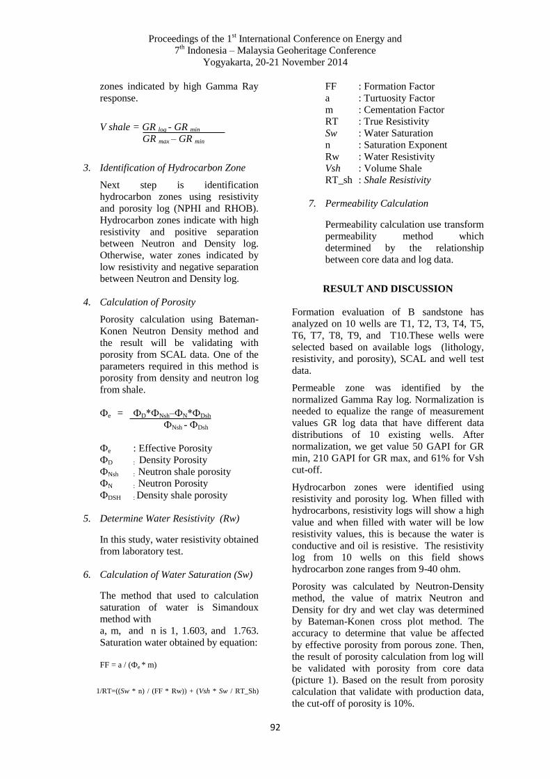
Proceedings of the 1st International Conference on Energy and
7th Indonesia – Malaysia Geoheritage Conference
Yogyakarta, 20-21 November 2014
92
zones indicated by high Gamma Ray
response.
V shale = GR log - GR min
GR max – GR min
3. Identification of Hydrocarbon Zone
Next step is identification
hydrocarbon zones using resistivity
and porosity log (NPHI and RHOB).
Hydrocarbon zones indicate with high
resistivity and positive separation
between Neutron and Density log.
Otherwise, water zones indicated by
low resistivity and negative separation
between Neutron and Density log.
4. Calculation of Porosity
Porosity calculation using Bateman-
Konen Neutron Density method and
the result will be validating with
porosity from SCAL data. One of the
parameters required in this method is
porosity from density and neutron log
from shale.
Фe = ФD*ФNsh–ФN*ФDsh
ФNsh - ФDsh
Фe : Effective Porosity
ФD : Density Porosity
ФNsh : Neutron shale porosity
ФN : Neutron Porosity
ФDSH : Density shale porosity
5. Determine Water Resistivity (Rw)
In this study, water resistivity obtained
from laboratory test.
6. Calculation of Water Saturation (Sw)
The method that used to calculation
saturation of water is Simandoux
method with
a, m, and n is 1, 1.603, and 1.763.
Saturation water obtained by equation:
FF = a / (Фe * m)
1/RT=((Sw * n) / (FF * Rw)) + (Vsh * Sw / RT_Sh)
FF : Formation Factor
a : Turtuosity Factor
m : Cementation Factor
RT : True Resistivity
Sw : Water Saturation
n : Saturation Exponent
Rw : Water Resistivity
Vsh : Volume Shale
RT_sh : Shale Resistivity
7. Permeability Calculation
Permeability calculation use transform
permeability method which
determined by the relationship
between core data and log data.
RESULT AND DISCUSSION
Formation evaluation of B sandstone has
analyzed on 10 wells are T1, T2, T3, T4, T5,
T6, T7, T8, T9, and T10.These wells were
selected based on available logs (lithology,
resistivity, and porosity), SCAL and well test
data.
Permeable zone was identified by the
normalized Gamma Ray log. Normalization is
needed to equalize the range of measurement
values GR log data that have different data
distributions of 10 existing wells. After
normalization, we get value 50 GAPI for GR
min, 210 GAPI for GR max, and 61% for Vsh
cut-off.
Hydrocarbon zones were identified using
resistivity and porosity log. When filled with
hydrocarbons, resistivity logs will show a high
value and when filled with water will be low
resistivity values, this is because the water is
conductive and oil is resistive. The resistivity
log from 10 wells on this field shows
hydrocarbon zone ranges from 9-40 ohm.
Porosity was calculated by Neutron-Density
method, the value of matrix Neutron and
Density for dry and wet clay was determined
by Bateman-Konen cross plot method. The
accuracy to determine that value be affected
by effective porosity from porous zone. Then,
the result of porosity calculation from log will
be validated with porosity from core data
(picture 1). Based on the result from porosity
calculation that validate with production data,
the cut-off of porosity is 10%.

Proceedings of the 1st International Conference on Energy and
7th Indonesia – Malaysia Geoheritage Conference
Yogyakarta, 20-21 November 2014
93
Figure 1. Validation between Porosity Log and
Porosity Core
Water saturation was calculated by Simandoux
method in equations (2) and (3) with a = 1, m
= 1.603 and n = 1.763. This method is very
effective to use on shally sand model such as
B Sandstone to give the best result. The cut-off
of water saturation is 60%.
Permeability value at Tri Field obtained using
transform permeability method. It is
determined based on equation from
relationship between core data and log data.
That equation can used to other wells which
don't have core data and also to make
permeability model. The permeability of B
sandstone from lowest to highest is 240 – 6799
mD. This indicates that B sandstone has a
good permeability.
Each property at 10 wells has been cut-off and
give very good result (Table 1). From this
table, we get 9-29% for Vsh, 22-27% for
porosity and 19-60% for water saturation.
Table 1. Property of Reservoir at 10 Wells
No Well Vsh
(%)
Porosity
(%)
Sw
(%)
1 T1 19 26 32
2 T2 11 25 19
3 T3 12 27 35
4 T4 14 27 23
5 T5 9 24 38
6 T6 9 27 22
7 T7 17 25 50
8 T8 27 23 52
9 T9 19 23 42
10 T10 29 22 60
Based on the evaluation result of Vsh,
porosity, water saturation and support by
production data, well location, and the
distance of wells, there are two infill drillings
that will be proposed. Well-I is located
between T2 well and T4 well with coordinate
x: 861600 and y: 106300. Top Structure Map
of B sandstone shows that the distance
between T2 well and T4 well is 350 m, and T4
well have a higher surface than T2 well
(Figure 2). Well-II is located between T5 well
and T6 well with coordinate x: 861240 and y:
106820. The distance between T5 well and T6
well is 350 m, and T6 well have a higher
surface than T5 well (Figure 2).
Geology Cross section on Figure 3.a shows
lateral continuity of B sandstone between T2-
T4 wells and has relative same values of Vsh
and porosity with low water saturation (Figure
3.b and 3.c).
Geology cross section on Figure 4.a shows
lateral continuity of B sandstone between T5-
T6 wells and has relative same values of Vsh
and porosity with low water saturation (Figure
4.b and 4.c).

Proceedings of the 1st International Conference on Energy and
7th Indonesia – Malaysia Geoheritage Conference
Yogyakarta, 20-21 November 2014
94
Figure 2. Top Structure Map of B Sandstone and Infill Drilling Proposed Location
Figure 3. (a) Geology cross section between T4 and T2 wells, (b) Petrophysical Result of T4 well, (c)
Petrophysical Result of T2 well
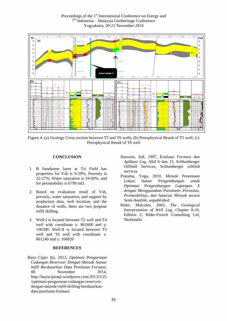
Proceedings of the 1st International Conference on Energy and
7th Indonesia – Malaysia Geoheritage Conference
Yogyakarta, 20-21 November 2014
95
Figure 4. (a) Geology Cross section between T5 and T6 wells, (b) Petrophysical Result of T5 well, (c)
Petrophysical Result of T6 well
CONCLUSION
1. B Sandstone layer at Tri Field has
properties for Vsh is 9-29%, Porosity is
22-27%, Water saturation is 19-60%, and
for permeability is 6799 mD.
2. Based on evaluation result of Vsh,
porosity, water saturation, and support by
production data, well location, and the
distance of wells, there are two propose
infill drilling.
3. Well-I is located between T2 well and T4
well with coordinate x: 861600 and y:
106300. Well-II is located between T5
well and T6 well with coordinate x:
861240 and y: 106820
REFERENCES
Bayu Cipto Aji, 2013, Optimasi Pengurasan
Cadangan Reservoir Dengan Metode Sumur
Infill Berdasarkan Data Penilaian Formasi,
08 November 2014,
http://bayuciptoaji.wordpress.com/2013/5/25
/optimasi-pengurasan-cadangan-reservoir-
dengan-metode-infill-drilling-berdasarkan-
data-penilaian-formasi/
Harsono, Adi, 1997, Evaluasi Formasi dan
Aplikasi Log, Jilid 6 dan 15, Schlumberger
Oilfield Services, Schlumberger oilfield
services
Pratama, Yoga, 2010, Metode Penentuan
Lokasi Sumur Pengembangan untuk
Optimasi Pengembangan Lapangan X
dengan Menggunakan Parameter Porositas,
Permeabilitas, dan Saturasi Minyak secara
Semi-Analitik, unpublished
Rider, Malcolm, 2002, The Geological
Interpretation of Well Log, Chapter 8-10,
Edition 2, Rider-French Consulting Ltd,
Skotlandia

Proceedings of the 1st International Conference on Energy and
7th Indonesia – Malaysia Geoheritage Conference
Yogyakarta, 20-21 November 2014
96
Assessment of Aquifer Type on Hydrogeologic System on the
Ngoro, Mojokerto District and Gempol, Pasuruan District
Gunawan Nusanto and Suyono
Faculty of Mineral Technology
University of National Development "Veteran" Yogyakarta
[email protected] or [email protected]
ABSTRACT
Ngoro and Gempol District located on the northern of Penanggungan Mount, in East Java. This area
there are a lot of stonesandy minings to support infrastructure development in East Java. Mining
Industry is closely related to the hydrogeological system. In order for the mining activities do not
interfere with the ground water, then the District of Ngoro and Gempol necessary hydrogeological
assessment system
Research area found two types of aquifer that is unconfined aquifer are estimated in area of
Wotanmasjedong Village, KunjorowesiVillage, ManduromanggunggajahVillage and Lolawang
Village. The confined aquifer found in Jeruk PurutVillage area to western of Bulusari to Gedangsari
Village. Caprock is claysandystone and andesitestone.The condition of the aquifers which in turn will
be used as the pit bottom level of the mine.
Keywods: aquifers type, pit bottom level
INTRODUCTION
Ngoro and Gempol district located on the
northern of Penanggungan Mount, and the
border area between Pasuruan and Mojokerto
regency. This area there are deposits of
stonesandy potential to mine, which until now
has been used for the embankment of Lapindo
Mud Project and construction of toll roads,
increasingly dangerous to the carriying
capacity environment.
The decision of the Governor of East Java
number : 123, year of 1997 on the closure
Industry Minerals Mining Area in District
Gempol, Pasuruan regency and district in
District Ngoro, District Mojokerto regency,
The rule decision has been revoked. While to
date the legislation governing the permitted
mining area boundary and not allowed to be
mined in accordance with the rules of good
mining and correct and environmentally
sound, has not been published. This is what
sparked the miners without permission or
licensed to mine in the area tend to be the
origin of mining without considering the
hydrogeological system. The second concern,
the impact caused by mining is subsidence of
land surface water (wells), which is based
from 2003 until 2009, decreased water level
reaches 9 meters (Nusanto Gunawan, 2009).
The thing that is important is the sustainability
of the management of post-mining.
The aim is formulated based mining limits the
carrying capacity of the environment which
includes the parameters of lithology,
hydrogeology and geotechnical. The result of
this formula further disseminated so that
people open their knowledge and
understanding of disasters that may occur and
how mitigation.
Review of the literature shows the study area
has the potential area contained water that can
be used at any time, but also a difficult area of
water in the dry season. Libraries are:
1. Bemmelen R.W. Van, (1949), stating that
the local stratigraphy Ngoro, Gempol and
Trawas consists of three rock units are units
that irreducibly volcanic rocks (pyroclastic
deposits), the unit of andesite-basalt lava
rocks and alluvial deposits. The
composition of bedrock and overburden
from the young to the elderly can be sorted
Proceedings of the 1st International Conference on Energy and
7th Indonesia – Malaysia Geoheritage Conference
Yogyakarta, 20-21 November 2014
97
along with the following physical
properties:
a. The units of andesite-basalt lava rock
Physical properties owned on this unit is
color - gray-black, fine grained -
medium, hard, jointly, decaying low -
medium and medium graduation - high
and dug hard and hold on steep slopes.
b. Pyroclastic deposits
Generally lithologies blackish gray,
somewhat compact, low decay, high
graduation, rather easy-difficult
excavated and somewhat resistant to the
steep slope. Soil cover is generally in
the form of yellowish brown silty sand,
soft, fine-coarse grained, gravel, low
plasticity and passing water-moderate
medium-high and thin soil between 0.50
to 1.00 meters.
2. Nusanto Gunawan, 2009, in the study area
on the slopes of the mountain is quite steep
with slope> 15 degrees until the top of the
mountain is the catchment rainy areas. For
District Ngoro is located at the southern
part of Mount jacks, Genting Mountain,
Mount Gajahmungkur, Mount Kemuncup
and at Mount Penanggungan as a parent. As
for the District of Gempol there is in the
southern part of Mount Penganggungan,
Mount Kemuncup, Mount Wangi, Mount
Welirang, Mount Prahu and Mount Arjuna.
3. Gunawan Nusanto 2009, another area that
is very possible to be a source of water for
the dry season in the surrounding area is
Mount Prau. Mount Prau is elongated hill
which has an area of approximately 900
hectares, located on the edge of the
highway Gempol - Mojosari. With the
repeal the decision of the Governor of East
Java, concerning in allowing no new
mining licenses in the region and Gempol
Ngoro, then Mount Prau is an area of great
potential and is a target for miners.
4. Down C (2001), Djauhari Noor (2005),
stating the change of landscape from
mining will affect the decline in the face of
the ground water. The observation
Gunawan Nusanto 2009, showed that the
water level of the wells in the study area of
9 meters (data PODES, 2009), then in
2009, the decline in ground water level
reaches 18 meters, so the decrease in depth
of 9 meters.
METHODS
The research methodology will be
implemented in the study of mining by basing
arrangement and management of post-mining
hydrogeology include a series of good work in
the field, the laboratory and in the studio
which includes: preparation of the study,
review the survey, mapping, geophysics,
aquifer distribution pattern, analysis and
formulation of results research, and
conclusions.
Hydrogeological studies
Hydrogeological study intended to determine
the model of the aquifer that are in the area,
which is then used as a reference in
determining the limits or boundaries vertical
feasibility depth of pi bottom level. Besides,
this study aimed to determine the function of
the area in relation to the carrying capacity of
the environment as a function of recharge area.
Geological observations made to determine the
condition of the local geology, structure
bedding, bedrock and deployment model of
sand, stone and gravel based on existing data.
Geological mapping carried out by making the
lines in accordance with the conditions of
observation lithology, structure and geological
processes that develop in these areas, and
based on the research that has been done
before.
Mapping and geoelectric resistivity
Investigations of geoelectric resistivity method
will provide an overview of rock properties
and rock containing water is based on
resistivity value of the electric current is
delivered to the underground. To know the
difference and spread each layer resistivity
subsurface rocks both vertically and
horizontally as outlined in the geological
cross-sectional shape of the detainees kind. In
this investigation have been according to the
rules of the Schlumberger electrode
arrangement with a distance AB / 2 and MN/2,
Voltage difference, current electricity. The
parameters are calculated apparent resistivity
Proceedings of the 1st International Conference on Energy and
7th Indonesia – Malaysia Geoheritage Conference
Yogyakarta, 20-21 November 2014
98
and geometry factors . Due to the state of
geometric factors that are always changing the
magnitude of apparent resistivity (Pa) can be
calculated by formula is:
V (AB² - MN²)
a = ----------------------
I (MN)
where:
a = apparent resistivity (Ohm m)
V = voltage difference (volts)
AB = distance between the two current
electrodes (m)
MN = distance between the electrode
potential (m)
I = current electricity (amperes)
The interpretation of the data field resistivity
method is done by connecting the physical
properties of rock conditions.
RESULTS AND DISCUSSION
Characteristics of aquifers.
Layers and aquifers in the District Ngoro
Gempol largely a porous aquifers composed of
sandstone that are local. Groundwater level is
the fluid pressure in the pores of a porous
medium is equal to the atmospheric pressure is
defined as the groundwater level in the
unconfined aquifer (Kodoatie, 2012). High
groundwater level is equal to the water level in
the well. Based on the height of groundwater
level, the aquifers in the District Ngoro and
Gempol classified as not depressed or
unconfined aquifer. But in some areas there is
a confined aquifer.
a. The village area Lolawang
Description of the results of the geoelectric
data interpretation above attributed to regional
geology order to obtain the results of further
analysis that found in the village of Lolawang
possibility of groundwater, the shallow aquifer
with low potential. Shallow depths and
dimensions are not great with low potential.
The depth of the aquifer is 8.36 to 23 m with
the type of silty sand lithology, aquifer
thickness of 14.6 m.
b. The village area Wotanmasjedong
This area there is a point of local aquifers with
shallow depth and dimension that is not great
with low potential. Aquifer is relatively
shallow depth of 5.18 to 6.08 m with a silty
sand lithology type, thickness is relatively thin
aquifer that is 0.9 m. So low groundwater
potential and is not a deep aquifer.
c. The village area Manduromanggunggajah
Aquifer is relatively shallow depth of 4.46 m
with 2,7- lithology types silty sand, is
relatively thin aquifer thickness is 1.76 m. On
top of a layer of silty sand, in this area there
are andesite, so here is confined aquifer. The
aquifer is evidenced by the presence in the
village artesian Manduromanggunggajah ini.
So, groundwater potential in this area is
relatively large.
d. The village area Wonosonyo
The depth of the first relatively shallow
aquifer is 2.19 to 5.21 m with a silty sand
lithology types, relatively thin aquifer
thickness is 3.02 m. Then the second aquifer is
relatively deep, ie at a depth of 11.7 to 23 m
with a thickness of the aquifer is relatively
thick and 11.3 m. Potential groundwater in the
second aquifer is relatively large but the
condition inside.
e. The Village area Sumber Tetek
Aquifer has sufficient depth and dimension in
the large, but the potential is small. Relatively
shallow depth of the aquifer is 9.15 to 16.9 m
with a silty sand lithology type, thickness is
relatively thin aquifer that is 7,75 m. With the
potential for groundwater in this area is
relatively small.
The condition can be interpreted visual field
area affixes, loose or discharge area, the area
with the type of unconfined aquifer, and
confined aquifer. Areas affixes expected in the
area over the hillside with a slope of> 25% is
in Mount Bekel, Mount Genting, Mount
Gajahmungkur, Mount Kemuncup and at
Mount Penanggungan as its parent. As for the
District of Gempol there is in the southern part
of Mount Penganggungan, Mount Kemuncup,
Mount Wangi, Mount Welirang, Mount Prahu
and Mount Arjuna. Aquifer is estimated in the
confined eastern Gempol. This is indicated by
the expanse of andesite in the northern part of
which is the cap rock. While in the west or
east area Ngoro an unconfined aquifer.

Proceedings of the 1st International Conference on Energy and
7th Indonesia – Malaysia Geoheritage Conference
Yogyakarta, 20-21 November 2014
99
Analysis of Water Quality
The potential level of Quality Criteria in
District Ngoro by comparing the spread of
element content of Fe, Mn and acidity level
(pH). The dissemination of the content of
other elements or compounds such as: Cl,
NO3, NO2, SO4, and TDS concentrations are
not increased or is still below a predetermined
threshold.
Groundwater quality conditions are taken at
UTM coordinates 49 MN 9.16119 million; E
0685075 (Ngoro) and N 9.16049 million; E
0684226 (Gempol), indicating that the
physical, chemical and biological remains
below the threshold of PP 82001 for drinking
water quality class II.
CONCLUSION
From the results of the study while it can be
concluded that:
1. The study area, there are two types of
aquifers, namely:
a. Confined aquifer layer, ie at a depth of
8-10 m, from the surface of the
surrounding land is located in the
District of Gempol east, precisely
Bulusari village, the village of Jeruk
Purut, District Gempol. Aquifer
thickness ranges from 5-10 m.
b. Unconfined aquifer layer is at a depth
of 2.9 m with a thickness of 11.7 m.
Aquifer layers are generally composed
of a layer of Sandstone and Sand Clay.
2. Areas affixes expected in the area on the
hillside with a slope of> 25% is in Mount
Bekel, Mount Genting, Mount
Gajahmungkur, Mount Kemuncup and at
Mount Penanggungan as a parent. As for
the District of Gempol there is in the
southern part of Mount Penganggungan,
Mount Kemuncup, Mount Wangi, Mount
Welirang, Mount Prahu and Mount Arjuna.
3. From the analysis of water samples, water
quality in the study area including the
second quality and deemed to be used as
drinking water.
REFERENCES
Bemmelen R.W. Van, (1949) The Geology of
Indonesia, Vol IA, Martinus Nijhoff, The
Hague.
Down C,. Stocks, 2001, Environtmental
Impact of Mining, Applied Science
Publishers, London.
Djauhari Noor., 2005, Environmental
Geology, Graha Science, Yogyakarta
Gunawan Nusanto, 2009, Technical and
Environmental Evaluation of Stonesandy
Mining, PT Karya Mitra Sejati, Ngoro,
Mojokerto.
Gunawan Nusanto, 2009, Evaluation of
Technical and Environmental Stonesandy
Mining, PT Imasco, Gempol, Pasuruan.
ACKNOWLEDGEMENTS
1. DP2M-Higher Education that has funded
research grants in this competition.
2. Fendy and Ferry which helps a lot of work
in the field.
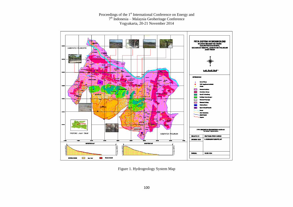
Proceedings of the 1st International Conference on Energy and
7th Indonesia – Malaysia Geoheritage Conference
Yogyakarta, 20-21 November 2014
100
Figure 1. Hydrogeology System Map

Proceedings of the 1st International Conference on Energy and
7th Indonesia – Malaysia Geoheritage Conference
Yogyakarta, 20-21 November 2014
101
Figure 2. Landuse Map

Proceedings of the 1st International Conference on Energy and
7th Indonesia – Malaysia Geoheritage Conference
Yogyakarta, 20-21 November 2014
102
Figure 3. A-A‟ Profile

Proceedings of the 1st International Conference on Energy and
7th Indonesia – Malaysia Geoheritage Conference
Yogyakarta, 20-21 November 2014
103
Figure 4. B-B‟ Profile
Proceedings of the 1st International Conference on Energy and
7th Indonesia – Malaysia Geoheritage Conference
Yogyakarta, 20-21 November 2014
104
Application of Geomagnetic Method to Identify the
Distribution of Dacite Igneous Rock in Mount Siwareng,
Sleman Regency, Special Region of Yogyakarta
Cimby Wicaksono Rezeki Nur Alam, Ahmad Nur Fauzi, Wahyu Hidayat
Student of Geophysical Engineering
University of Pembangunan Nasional “Veteran” Yogyakarta
Jalan SWK 104 Condongcatur Yogyakarta
ABSTRACT
The geological map of Godean area in Yogyakarta region consists of volcanic rocks of Oligocene-
Miocene age. A number of igneous rock outcrops are found in this area, specifically in Mount
Siwareng, Dusun Margodadi, Desa Sayegan area, where an intrusion of dacite igneous rock can be
found. This kind of rock tends to have higher value of magnetic property compared to its surrounding
rocks, hence to identify the distribution of dacite igneous rock, the geomagnetic method is applied.
The geomagnetic method is a passive geophysical method typically used to understand the condition
of underground rock according to the susceptibility value of the rock. Susceptibility is a measure of
the extent to which a medium may be magnetized in relation to the lithology and mineral composition.
Data sampling was conducted in the area with the coordinates of X=420330-420530 and Y= 9144166-
9144489. Data processing was done using the software Excel and Geosoft Oasis Montaj, and 3-D
modeling was done using the software Magblox, Bloxer and Rockwork. According to Total Magnetic
Field Intensity map, it appears that dacite igneous rock has relatively higher value than its surrounding
rocks, which ranges from 140 to 240 nanoTesla, and is located on the northwest side of the research
site in radial pattern. According to Reduce to Pole map interpretation, the center of intrusion is located
approximately on the west side of the research site. Based on the 3-D modelling, dacite rock has
susceptibility value of about 0.5 (SI), and the surrounding rocks (sedimentary rocks) susceptibility
value of about 0.0005 (SI). The dacite rock is located on the west side of the research site, spreading
to the north. The dacite distribution is roughly 160 meters wide in diameter and about 90 meters deep
below ground level.
Keywords: geomagnetic, susceptibility, 3-D modelling, dacite
INTRODUCTION
Outcrops of dacite igneous rock intrusion of
approximately Oligocene-Miocene age can be
found in Mount Siwareng, Dusun Margodadi,
Desa Sayegan, Kecamatan Godean, Kabupaten
Sleman, Yogyakarta. To identify this rock
intrusion, a geophysical survey is done using
geomagnetic method. The geomagnetic
method is a geophysical method typically used
for early survey in exploration of oil and other
valuable minerals. Data collected on field
produce graphs and magnetic field anomaly
map. Magnetic field anomaly is caused by the
result of a magnetic force oscillating with
Earth's magnetic field. Magnetic induction
anomaly is the result of external magnetic
induction in an iron sulfide by Earth's magnetic
field. The shape, dimensions and amplitude of
an induction anomaly is a function of
orientation, geometry, size, depth and magnetic
susceptibility of a material as well as the
intensity and inclination of the Earth's
magnetic field on the surveyed area. In other
words, this method is applied in accordance to
the susceptibility of the rock.

Proceedings of the 1st International Conference on Energy and
7th Indonesia – Malaysia Geoheritage Conference
Yogyakarta, 20-21 November 2014
105
GEOLOGICAL BACKGROUND
The local geology of the research site is
generally dominated by young volcanic
sediments (Wartano Raharjo, 1995). An
isolated mountain (Figure I) can be found in
this area, which consists of volcanic rocks of
Oligoene-Miocene age. Volcanic rocks are
dacite rocks (Figure II) presumably intruding
from Nanggulan Formation, which is mostly
composed of sedimentary rocks.
Figure I. Research site
Figure II. Dacite outcrop
LITERATURE REVIEW
Magnetic Force
In magnetics, there are two types of charges,
positive charge and negative charge. These
charges fulfill Coulomb Law. Opposite
charges attract each other, and like charges
repel each other with force F. Magnetic
method is based on Coulomb Force (Figure
III) between two magnetic poles q1 and q2
having distance r in the form of
rr
qqF ˆ
2
21
where μ is the magnetic permeability, which
values 4 x 10⁻⁷
w / A.m in vacuum. F is
Coulomb Force (N), q1 and q2 are magnetic
pole magnitudes (A/m), and r is the distance
between the two poles (m).
q1 q2Fr
Figure III. Magnetic force between two
particles of mass q1 and q2
Magnetic susceptibility
The parameter used in this method is
susceptibility. Susceptibility is a measure of
the extent to which a medium may be
magnetized. This value increases as more
magnetic minerals are found in the rock.
Factors affecting the value of susceptibility
include
Rock lithology
Mineral composition of the rock
Figure IV. Elements of Earth's magnetic field
Earth's magnetic field is characterized by
physical parameters, named magnetic field
elements (Figure IV) having quantitative

Proceedings of the 1st International Conference on Energy and
7th Indonesia – Malaysia Geoheritage Conference
Yogyakarta, 20-21 November 2014
106
properties such as the direction and magnetic
intensity. Those parameters include:
Declination (D) - the angle between
magnetic north and horizontal component
measured from north to east.
Inclination (I) - the angle between total
magnetic field and horizontal plane
measured from horizontal plane to vertical
plane downwards.
Horizontal Intensity (H) - the total
magnitude of horizontal magnetic field.
Total Magnetic Field (F) - the total
magnitude of magnetic field vector.
Data Correction
To obtain the survey target, i.e magnetic field
anomaly, the previously sampled magnetic
field data must be corrected from the effects of
other magnetic fields. General methods of
correction used in magnetic survey include:
Daily correction (H var)
the correction to remove the influence
of external magnetic field (of the sun
and moon) from measured magnetic
data (H).
IGRF correction (Ho)
the correction to remove the influence
of Earth's main magnetic field from
measured magnetic field data.
The value of magnetic anomaly (∆H) in a
rock's magnetic field intensity can therefore be
expressed as:
∆H = H - Ho – Hvar
Data Processing Filter
Reduce To Pole (RTP)
The total magnetic field data are then
reduced to pole so that the maximum
magnetic field anomaly is located exactly
above the body of the source of anomaly
(anomaly is monopole).
Figure V. Reduce to Pole
Upward Continuation
A process of converting the measured
potential field data to higher surface level
than the location of measurement. This
process is done for easier interpretation by
reducing the effect of noise.
Figure IV. Upward Continuation Filter
METHODOLOGY
Figure VII. Data Processing Flowchart

Proceedings of the 1st International Conference on Energy and
7th Indonesia – Malaysia Geoheritage Conference
Yogyakarta, 20-21 November 2014
107
The research was conducted on May 24-25,
2014 at 07.00-15.00 WIB in Mount Siwareng
area, Dusun Margodadi, Desa Sayegan,
Kecamatan Godean, Kabupaten Sleman, DIY.
The tool used is PPM G-856. The first step of
magnetic data collecting is data acquisition.
Data acquisition began with getting geology
information in the form of survey design to
determine the point and length to measure.
The software Excel was used in data
processing to calculate the value of Ha. The
obtained value of X, Y and Ha are then
processed using the software Geosoft Oasis
Montaj to produce total magnetic field map,
reduction to pole, and regional continuity map
50 meter upwards. Three-dimensional model
was processed using Magblox and displayed
using Rockwork15. The result is re-modeled in
case the result produced does not match. The
produced maps and model are then analyzed
with the help of geology data of research site
to draw the conclusion.
RESULT AND DISCUSSION
Total Magnetic Intensity Map
Figure VIII shows the distribution of magnetic
intensity in Mount Siwareng area. Igneous
rock intrusion is predicted to have medium to
high magnetic anomaly value, as its mineral
composition has higher magnetic property than
the surrounding rocks. These surrounding
rocks are presumed to be sedimentary rocks
which have lower intensity since the mineral
composition has lower magnetic property. A
high range closure of 140-240 nanoTesla can
be seen on southwest side (marked in circle)
on the map indicating distribution of igneous
rock intrusion. Nevertheless, this map is still
affected by dipole characteristic of Earth's
magnetic field; its central location still cannot
be interpreted.
Reduce to Pole Map
After filtering the data by changing dipole
effect into monopole, so that the position of
anomaly is exactly above its maximum
anomaly magnetic field. According to the map
(Figure IX), the central location of intrusion is
indicated to be on the west side of research site
(marked in circle) and spreading relatively to
the north.
Regional Upward Continuation 50 m Map
The above map (Figure X) shows that by
rising regional map by 50 meters, the effects
of local anomaly and noise are relatively
removed. In this map, the value of magnetic
intensity having depth profile in research site
can be seen. Two closures of high value can be
found on the west side of research site
(marked in circle) and one closure of low
value can be found on the southeast. This
justifies that the center of igneous rock
intrusion is located on the west side of
research site as its magnetic property is higher
than its surrounding rocks'.
Figure VIII. Total Magnetic Intensity Map

Proceedings of the 1st International Conference on Energy and
7th Indonesia – Malaysia Geoheritage Conference
Yogyakarta, 20-21 November 2014
108
Figure IX. Reduce to Pole Map
Figure X. Regional Upward Continuation 50
m Map
The above map (Figure X) shows that by
rising regional map by 50 meters, the effects
of local anomaly and noise are relatively
removed. In this map, the value of magnetic
intensity having depth profile in research site
can be seen. Two closures of high value can be
found on the west side of research site
(marked in circle) and one closure of low
value can be found on the southeast. This
justifies that the center of igneous rock
intrusion is located on the west side of
research site as its magnetic property is higher
than its surrounding rocks'.
3-D Modeling
Figure XI. Three-dimensional modeling of
dacite igneous rock and sedimentary rock
Figure XII. Three-dimensional modeling of
dacite igneous rock
The model above is formed based on the
susceptibility parameter of the rock (figure XI
and XII). Dacite igneous rock has
susceptibility value of about 0.5 (SI), and the
surrounding rocks (sedimentary rocks)

Proceedings of the 1st International Conference on Energy and
7th Indonesia – Malaysia Geoheritage Conference
Yogyakarta, 20-21 November 2014
109
susceptibility value of about 0.0005 (SI).
These values are classified by the Telford table
(1979). The dacite rock is located on the west
side of the research site, spreading to the
north. The dacite distribution is approximated
to be about 160 meters wide in diameter and
about 90 meters deep below ground level.
CONCLUSION
Based on the research conducted in Mount
Siwareng area, Godean, DIY, it can be
concluded that the intrusion has radial shape,
spreading on the southwest side of research
site. The intrusion has magnetic anomaly value
ranging from 140 to 240 nT and susceptibility
value of approximately 0.5 (SI). The center of
intrusion is on the west side of research site,
roughly 160 meters wide in diameter and
spreading up to 90 meters deep below ground
level.
REFERENCES
[1] Billim, F., and Ates A, Analytic signal
inferred from reduced from pole data:
Jornal of Balkan Geophysical Society, 6
(2), 66-74. 2003.
[2] Telford, W. M., Geldart, L.P., and Sheriff,
R.E, 1979, Applied Geophysics, Cambridge
University Press, Cambridge.
[3] Wartono Raharjo, Peta Geologi Lembar
Yogyakarta Jawa, Pusat Penelitian dan
Pengembangan Geologi, 1995.
[4] Yopanz, 2007, Metode-Metode Ge-
ofisika,http://yopanz.blogspot.com[online
access April,5 2013]

Proceedings of the 1st International Conference on Energy and
7th Indonesia – Malaysia Geoheritage Conference
Yogyakarta, 20-21 November 2014
110
Application of Geology in Studying Groundwater System
Beneath Gunung Kendil and Umbul Ponjong in Ponjong
District, Gunungkidul
Jatmika Setiawan Prodi Teknik Geologi, Fakultas Teknologi Mineral, UPN “Veteran” Yogyakarta
ABSTRACT
Gunung Kendil is one of the karst hills located in the district of Ponjong, Gunung Kidul regency
(8o00‟56.64”S, 110
o44‟18.32”E). This hill is situated approximately 400 meters north of Ponjong
District and about 20 km east of Yogyakarta.
Gunung Kendil is composed of bedded-limestone in the bottom part, chalky limestone, massive
limestone with conduits, and reef limestone at the top. These rocks are included in Wonosari
Formation, which is formed in Middle Miocene age (10-16 million years).
Groundwater system beneath Gunung Kendil is controlled by fractures, faults and bedding. The
normal faults below Gunung Kendil are northeast-southwest trending almost facing each other
forming a large subsidence. Cross cutting of the two normal faults and the bedding that is gently
sloping to the north beneath Gunung Kendil form an underground river flowing toward the southwest
and out as springs at the front of the Village Ponjong, called Umbul Ponjong (Sumbergiri)
(7o58‟34.39”S, 110
o44‟06.89”E).
The spring is very beneficial to people's lives in the village of Ponjong. At this time Umbul Ponjong
already managed by the Regional Government of Gunung Kidul as a unique and interesting tourist
area and geological heritage.
Key words: Gunung Kendil, groundwater system, fault, Umbul Ponjong.
RESEARCH BACKGROUND
Gunung Kendil is one of the karst hills located
in the district of Ponjong, Gunung Kidul
regency (8o00‟56.64”S, 110
o44‟18.32”E). This
hill is situated approximately 400 meters north
of Ponjong District and about 20 km east of
Yogyakarta (Figure 1).
Gunung Kendil is composed of bedded-
limestone in the bottom part, chalky limestone,
massive limestone with conduits, and reef
limestone at the top. These rocks are part of
Wonosari Formation, formed in Middle
Miocene age (10-16 million years).
Ground water in Gunungkidul, specifically in
Gunung Kedil is generally hard to find,
especially in long dry season. Therefore, it is
necessary to discover groundwater channels to
help the people of Gunung Kendil, Desa
Ponjong, Kecamatan Ponjong, Kabupaten
Gunung Kidul. This is needed for drilling so
that the water can be utilized by its people.
Groundwater system beneath Gunung Kendil
is controlled by fractures, faults and bedding.
The normal faults below Gunung Kendil that
are northeast-southwest trending almost facing
each other forming a large subsidence. Cross
cutting of the two normal faults and the
bedding that is gently sloping to the north
beneath Gunung Kendil form an underground
river flowing toward the southwest and out as
springs at the front of the Village Ponjong,
called Umbul Ponjong (Sumbergiri)
(7o58‟34.39”S, 110
o44-‟06.89”E).
The spring is very beneficial to people's lives
in the village of Ponjong. At this time Umbul
Ponjong already managed by the Regional
Government of Gunung Kidul as a unique and
interesting tourist area and geological heritage.

Proceedings of the 1st International Conference on Energy and
7th Indonesia – Malaysia Geoheritage Conference
Yogyakarta, 20-21 November 2014
111
Figure 1. Location of Ponjong District, Gunungkidul
OBJECTIVES
The goal of this research is as follows:
1. To study the groundwater system
beneath Gunung Kendil
2. To determine drilling location of well
3. To help developing Gunung Kendil
area as a Tourism Village
LITERATURE REVIEW
Gunungsewu
Gunungsewu is the largest tropical karst
landscape in Northeast Asia. This area is part
of East Java Southern Mountains, in
Gunungkidul Regency (DIY), Wonogiri and
Pacitan Regency (Central Java).
Geographically, Gunungsewu is situated
between 6o 10‟ to 6
o 30‟ LS and 99
o 35‟ to
100o BT, approximately 25 km southeast of
Yogyakarta, 109 km north-northwest of
Pacitan, and 20 km southwest of Wonogiri.
Gunungsewu has a total area of approximately
800 km2. This area can be easily accessed
from Yogyakarta-Wonosari, Wonogiri and
Pacitan, and also established as one of tourism
destinations, by Regional Government of DIY
as well as Central Java (Figure 2).
Gunungsewu area has an interesting geological
phenomenon, a beautiful karst
geomorphology, a unique hydrogeology, a
breathtaking view, and also a number of
geology heritage sites supporting a geopark
area. This is what encourages this paper to be
written, based on the research supported by
LPPM UPN “Veteran” Yogyakarta, to
understand the groundwater system
specifically in Gunung Kendil, and generally
in Southern Mountains.
GEOLOGY OF GUNUNGSEWU
According to van bemmelen's physio-
graphical map (1949), gunung sewu is part of
east java southern mountains, which is divided
into baturagung, panggung, and plopoh in the
north, wonosari in the middle, and
gunungsewu in the south (figure 3).
Geology of gunungsewu is generally
composed of volcanic rocks at the lower part
and carbonate rocks at the upper part, formed
in tertiary period. Geological map of
gunungsewu is shown in figure 4.

Proceedings of the 1st International Conference on Energy and
7th Indonesia – Malaysia Geoheritage Conference
Yogyakarta, 20-21 November 2014
112
Figure 2. Gunungsewu Location Map
Figure 3. East Java Physiography Map (Van Bemmelen, 1949)

Proceedings of the 1st International Conference on Energy and
7th Indonesia – Malaysia Geoheritage Conference
Yogyakarta, 20-21 November 2014
113
Figure 4. Geological Map of Gunungsewu (Kusumayudha, 2000, 2005)
Stratigraphy
Stratigraphy of Southern Mountains in DIY
according to Toha et al (1994) and Suyoto
(1994), from the oldest to the youngest is as
follows:
Semilir Formation: Semilir Formation is
composed of dasitic tuff, sandstone, tufaceous
sandstone, glass volcanic, aglomerate,
claystone, siltstone, shale, and breccia Semilir
Formation is formed in Oligocene to Early
Miocene period.
Nglanggran Formation: Nglanggran
Formation has conformity at the top, or
interfingering with the upper part of Semilir
Formation, composed of volcanic andesitic
breccia, lava, aglomerate, polimic breccia, ang
tufaceous sandstone. This Formation is
deposited in Oligomiocene to Middle Miocene
Period.
Sambipitu Formation: Sambipitu Formation
is composed by intercalation of marl, claystne,
carbonate sandstone, tufaceous sandstone
above Nglanggran Formation. Except in some
places, where interfingering with Nglanggran
Formation can be found. This Formation is
formed in Middle Miocene.
Oyo Formation: Oyo Formation is composed
of sandy carbonate, calcarenite, carbonate
sandstone, and tufaceous sandstone.
According to Suyoto (1994), its contact to
Sambipitu Formation is unconformity. Oyo
Formation, with its type location in Oyo River,
is formed in Middle Miocene to Mio-Pliocene.
Wonosari Formation: Wonosari Formation is
composed of carbonate, massive carconate,
and reefThis Formation sometimes shows
conformity and different facies with Oyo
Formation. An unconformity can even be
found in Semin area, formed in Middle
Miocene to Pliocene.
Kepek Formation: Kepek Formation is
mainly composed interbedded of claystone,
marl, and carconate, which is deposited in
isolated shallow-sea environment, in Late
Pliocene to Pleistocene period.
Terarosa Sediment and Merapi Sediment:
Terarosa sediment, alluvial and Merapi
sediment is the youngest lithology of
Gunungsewu. Alluvial sediment is composed
of dark clay, siltstone, sand, gravel and part of
plant, whereas Merapi sediment is composed
of sand and volcanic ash. Terrarosa is formed
of molded limestone, combined with volcanic
ash.
Geological Structure

Proceedings of the 1st International Conference on Energy and
7th Indonesia – Malaysia Geoheritage Conference
Yogyakarta, 20-21 November 2014
114
The Southern Mountains area is regionally a
high zone. A sincline trending in N75oE -
N255-E (northeast - southwest) direction can
be found in Wonosari Plato, with the slope
angle of its wings is less than 10o. In
Baturagung and Gunungsewu, the bedding
structure generally forms a slanted homoclinal
to the south. In Gunungsewu, the slope of
bedding ranges from 5o to 15
o. Fault structure
of Gunungsewu is trending in northwest-
southeast direction. Gunungsewu area is
divided into several blocks, separated by
faults. These faults also control the
hydrogeologic system in Gunungsewu.
Gunung Kendil
Gunung Kendil is located in Ponjong District,
approximately 500m from Regional
Govenrment office. Gunung Kendil site began
to be managed by its owner (Mbah Moyo) for
tourism object, bathing area, fishing area, and
health therapy as well as
geology/hydrogeology nature laboratory.
At the peak of Gunung Kendil, wells have
been drilled in two places, producing water
with relatively high pressure. The source of
the water is an underground river beneath
Gunung Kendil. This water fulfills drinking
water quality, and has been used in drinking
water production, as well as bathing area and
health therapy. The groundwater system
beneath Gunung Kendil is presumably
controlled by fractures, faults, and bedding.
Normal faults under Gunung Kendil trending
northeast-southwest face each other, forming a
large subsidence.
RESEARCH METHOD
Location and Time of Research
This research will be conducted in Gunung
Kendil, Ponjong Village, Ponjong District,
Gunungkidul Regency. The hill is located
approximately 400 m north of Ponjong
District, about 20 km east of Yogyakarta City.
The research is planned to start from June until
October 2014.
RESEARCH METHOD
This research will use Field Detail Mapping
Method and Laboratory Analysis Method.
Field Mapping Method
Field detail mapping in Gunung Kendil is done
using tools as follows:
- Geological compass
- Geologist hammer
- GPS
- Base Map
- Clipboard
- Protractor
- Geological field book
- Measuring tape
The data recorded in detail mapping include:
- Lithology/rock types
- Developing geology structure type
- Measurements of layers position and
geological structures (fractures, faults,
bedding)
- Hillside slope
- Surface situation data and settlement
- Rock samples for laboratory analysis
- Water samples
Laboratory Method
This method is done to analyze rock samples,
structure type and water sample.
TIME OF RESEARCH
One day of each week from June to October is
allocated for detail research, as seen in Table
1.

Proceedings of the 1st International Conference on Energy and
7th Indonesia – Malaysia Geoheritage Conference
Yogyakarta, 20-21 November 2014
115
Table 1. Field Research Activity Time
No Activity JUNE JULY AUG SEPT OCT
1. Proposal
2. Proposal Presentation
3. Field 1
4. Field 2
5. Field 3
6. Field 4
7. Analysis
8. Report Writing
9. Final Presentation
10. Final Report Submission
FIELD DATA
Field data obtained include rock type data,
fracture data, fault data, morphology data, rock
samples, and water samples. Those data is
organized as shown below.
Gunung Kendil and Umbul Ponjong
Morphology
Gunung Kendil is one of the hills in Gunung
Sewu scattered in Southern Mountains of
Yogyakarta Special Region, located 400 m
north of Ponjong District Government office
and 30 km east of Yogyakarta City. It lies in
coordinates 8o00‟56.64”S, 110
o44‟18.32”E
(Figure 5). A large spring can be found at the
southwest side of Regional Government
office, its water is collected in two large ponds
named Umbul Ponjong (Figure 6).
Figure 5. A photograph of Gunung Kendil taken from west direction.

Proceedings of the 1st International Conference on Energy and
7th Indonesia – Malaysia Geoheritage Conference
Yogyakarta, 20-21 November 2014
116
Figure 6. Tuk Umbul Ponjong taken from northwest direction
Geology of Gunung Kendil
Gunung Kendil is composed of bedded-
limestone in the bottom part, chalky limestone
in the middle (Figure 8), massive limestone
with conduits, and reef limestone at the top
(Figure 9). These rocks are part of Wonosari
Formation, formed in Middle Miocene age
(10-16 million years).
Figure 7. Bedded-limestone in the bottom part of Wonosari Formation

Proceedings of the 1st International Conference on Energy and
7th Indonesia – Malaysia Geoheritage Conference
Yogyakarta, 20-21 November 2014
117
Figure 8. Chalky limestone in the middle
Figure 9. Massive limestone with conduits and reef limestone
at the top part of Wonosari Formation

Proceedings of the 1st International Conference on Energy and
7th Indonesia – Malaysia Geoheritage Conference
Yogyakarta, 20-21 November 2014
118
Geological Structure
Measurements of fractures and faults done in
Gunung Kendil to understand ground water
flow pattern resulted in flow pattern following
structure pattern as seen in Figure 10.
Figure 10. Structure pattern controlling water flow beneath Gunung Kendil up to Umbul Ponjong
Ground Water beneath Gunung Kendil and
Sumber Ponjong Spring
At the peak of Gunung Kendil, wells have
been drilled in two places for approximately
60 m deep. It connected to an underground
river, forming artesian water as seen in Figure
10 and 11.
DISCUSSION
Underground river system beneath Gunung
Kendil is controlled by normal faults trending
nearly north northwest-south southwest
slanted in west-northwest direction with an
angle of 75-80 degrees meets with limestone
bedding of n20e/15 and fracture of n31e/75.
This activated dissolution caused by
infiltration of groundwater passing the meeting
point of fault, fracture, and fault, forming an
underground river trending nearly north-south.
The drilled Mbah Moyo 2 Well penetrates this
system in 66 meters deep.
This system meets the underground river
flowing southwest, controlled by two normal
faults trending northeast-southwest which
form a grabben. This underground river flows
out, forming a spring named tuk umbul smber
panjong.
The drilled well mbah moyo 1, 66 meters
deep, with coordinates 110 43‟141,467e and 7
58‟490,798s exactly cut through the
underground river flowing to tuk umbul
sumber ponjong.
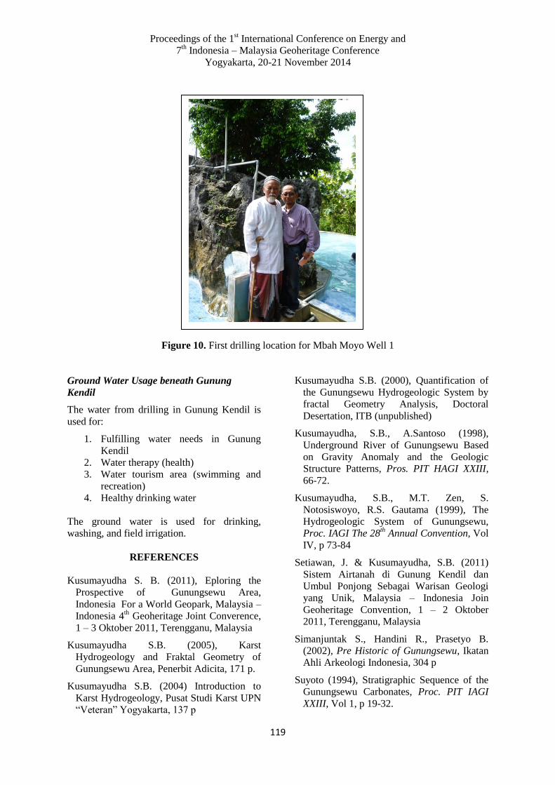
Proceedings of the 1st International Conference on Energy and
7th Indonesia – Malaysia Geoheritage Conference
Yogyakarta, 20-21 November 2014
119
Figure 10. First drilling location for Mbah Moyo Well 1
Ground Water Usage beneath Gunung
Kendil
The water from drilling in Gunung Kendil is
used for:
1. Fulfilling water needs in Gunung
Kendil
2. Water therapy (health)
3. Water tourism area (swimming and
recreation)
4. Healthy drinking water
The ground water is used for drinking,
washing, and field irrigation.
REFERENCES
Kusumayudha S. B. (2011), Eploring the
Prospective of Gunungsewu Area,
Indonesia For a World Geopark, Malaysia –
Indonesia 4th Geoheritage Joint Converence,
1 – 3 Oktober 2011, Terengganu, Malaysia
Kusumayudha S.B. (2005), Karst
Hydrogeology and Fraktal Geometry of
Gunungsewu Area, Penerbit Adicita, 171 p.
Kusumayudha S.B. (2004) Introduction to
Karst Hydrogeology, Pusat Studi Karst UPN
“Veteran” Yogyakarta, 137 p
Kusumayudha S.B. (2000), Quantification of
the Gunungsewu Hydrogeologic System by
fractal Geometry Analysis, Doctoral
Desertation, ITB (unpublished)
Kusumayudha, S.B., A.Santoso (1998),
Underground River of Gunungsewu Based
on Gravity Anomaly and the Geologic
Structure Patterns, Pros. PIT HAGI XXIII,
66-72.
Kusumayudha, S.B., M.T. Zen, S.
Notosiswoyo, R.S. Gautama (1999), The
Hydrogeologic System of Gunungsewu,
Proc. IAGI The 28th Annual Convention, Vol
IV, p 73-84
Setiawan, J. & Kusumayudha, S.B. (2011)
Sistem Airtanah di Gunung Kendil dan
Umbul Ponjong Sebagai Warisan Geologi
yang Unik, Malaysia – Indonesia Join
Geoheritage Convention, 1 – 2 Oktober
2011, Terengganu, Malaysia
Simanjuntak S., Handini R., Prasetyo B.
(2002), Pre Historic of Gunungsewu, Ikatan
Ahli Arkeologi Indonesia, 304 p
Suyoto (1994), Stratigraphic Sequence of the
Gunungsewu Carbonates, Proc. PIT IAGI
XXIII, Vol 1, p 19-32.

Proceedings of the 1st International Conference on Energy and
7th Indonesia – Malaysia Geoheritage Conference
Yogyakarta, 20-21 November 2014
120
Van Bemmelen, R.W. (1949), The Geology of
Indonesia, Vol IA, Martinus Nijhoff, The
Hague, 792 p.
White, W.B. (1988), Geomorphology and
Hydrology of Karst Terrains, Oxford
University Press, New York, 464 p.

Proceedings of the 1
st International Conference on Energy and
7th Indonesia – Malaysia Geoheritage Conference
Yogyakarta, 20-21 November 2014
121
Geology and Reservoir 4160 3D Modeling
of "X" Layer, "Y" Field in Bekasap Formation,
Central Sumatra Basin
Nur Arief Nugroho *)
,Jatmika Setiawan *)
, Deddy Kristanto**)
, Haryadi**)
* )Prodi Teknik Geologi, FTM, UPN "Veteran" Yogyakarta
**)Prodi Teknik Perminyakan, FTM, UPN “Veteran” Yogyakarta
ABSTRACT
Object of the research is Geology and 3D Modeling Reservoir Layers "X" Field "Y". Field "Y" is
located in the Central Sumatra Basin. Based on well data analysis, Layer "X" is included in Bekasap
Formation, sandstones were prepared on lithology, mudstone, and coal, Bekasap Formation was
deposited in fluvio deltaic environment to transitional deltaic, layer thickness "X" has an average of
20 ft. In the Field "Y" there is a growing fault, where the fault consists of the first period and the
second period fault. Faulting the first period in the form of the right horizontal fault ride-SSE trending
NNW, and second period down and reverse fault is a fault backthrusting of the first period trending
NE-SW.
Crease structures that develop in the Field "Y" in the form of folds that form the saddle, this anticline
trending folds in the form of a general northwest-south southeast North (NNW-SSE), this was folds
reverse fault on the east and westward-shaped asymmetry. These folds formed during the compression
that occurs sharpness Piosen until now.
3D modeling consists prepared on the framework, property distribution, and calculation of OOIP layer
"X". Property facies, vshale, PHIE and Sw using geostatistical variogram analysis as well as
population data distribution method using the SIS for facies and SGS for vshale, PHIE and Sw, while
the distribution of K using the equation results Perm vs Core crossplot of log. Based on calculation of
volumetric OOIP basis Layers "X" obtained Bulk Volume: 21.017 acre.ft, Net Volume: 20.798 acre.ft,
Pore Volume: 4.363 acre.ft, HCPV Oil: 2,542 acre.ft, OOIP: 17.93 MMSTB.
Keywords: Modeling, Geostatistic, Variogram
INTRODUCTION
"Y" field is located in Central Sumatra Basin,
one of hydrocarbon-producing basins (Figure
1). Geologically, this basin is also called
Neogene Convergent Back Arc Basin and is
classified as hydrocarbon-producing
sedimentary basin. The Central Sumatra Basin
has an area of about 103,500 km2, mainly
consists of land.
"X" layer is part of Bekasap Formation, one of
hydrocarbon-producing formations. Bekasap
formation is composed of sandstone lithology,
shale, and some coal parting, deposited in
fluvio deltaic to transitional deltaic
environment.
Reservoir 3D modeling on "X" layer is a
research study to learn the condition of a
reservoir, by integrating seismic and well data
to understand the developing structure pattern
as well as detailed reservoir property
distribution vertically and laterally.
The goal of this research is to make a
geological concept and 3D reservoir modeling,
in addition to distribute reservoir property in
3D and calculate OOIP volumetrically.
GEOLOGY AND REGIONAL
STRATIGRAPHY
The "Y" field is part of Central Sumatra Basin.
This basin is historically called as Neogene
Convergent Back Arc Basin and is classified
as hydrocarbon-producing sedimentary basin,

Proceedings of the 1
st International Conference on Energy and
7th Indonesia – Malaysia Geoheritage Conference
Yogyakarta, 20-21 November 2014
122
having an area of about 103,500 km2 of mainly
land. Geographically, this basin lies between
longitudes 90oE-103
oE and latitudes 1
oS-4
oS.
Central Sumatra Basin is separated from North
Sumatra Basin by Tinggian Asahan on the
north, and separated from South Sumatra
Basin by Tigapuluh mountain area.
Central Sumatra Basin is one of the three
hydrocarbon-producing basins in Eastern
Sumatra, developing as a sedimentary basin
behind a volcanic arc. Its border is marked by
basement rock outcrop, weight anomaly
pattern, isopach with cut-off 1,000m and
Tinggian.
Central Sumatra Basin is mostly formed of
two structure patterns, oriented in North-South
direction and Northwest-Southeast direction
(Heidrick & Aulia, 1993). The North-South
structure is relatively older, being formed in
Paleogen (Martono & Nayoan, 1974; De
Coster, 1975 in Heidrick & Aulia, 1993).
According to Eubank and Makki (1987), those
two structures were active in Tertiary period.
Heidrick & Aulia (1993) categorize the
Tectonic Development of Central Sumatra
Basin into four episodes based on poly-phase
tectonic terminology of Mc-Clay (1996), i.e.
F0, F1, F2, and F3 (Figure 2).
Eubank and Makki (1981), Yarmanto and
Aulia (1988), as well as Heidrick and Aulia
(1993) divide the regional stratigraphy of
Central Sumatra Basin from Paleogene to
Pliocene and Quaternary period into five
groups/formations, namely Pematang
Formation, Sihapas Group, Telisa Formation,
Petani Formation and Minas (Alluvial)
Formation. Whereas Heidrick and Aulia
(1996) divide the regional stratigraphy of
Central Sumatra Basin into Pre-Tertiary
Basement Rock, Paleogene Sedimentary Rock,
Neogene Sedimentary Rock, and Pleistocene
Sedimentary Rock (Figure 3).
Pre-Tertiary Basement Rocks
This rock is composed of three different micro
plate (Eubank and Makki, 1981), namely
quartzite terrain (Eubank and Makki, 1981),
also called Malacca Microplate (Pulunggono
& Cameron, 1984), and also called Mutus
Assemblage and Greywacke Terrain (Eubank
and Makki, 1981), or Megui Microplate
(Pulunggono & Cameron, 1984). According to
Pulunggono and Cameron (1984), Mergui
Microplate is formed of quartzite, granite, and
limestone of Paleozoic age. Mergui Microplate
is formed of Permo-Carbon rocks consisting of
greywacke, quartzite, argillite, and granite
intrusion. Mutus Assemblage is formed of
argilite, red shale, tuff, and basalt, also chlorite
schist of Triassic-Jurassic age.
Pematang Eosen-Oligosen Group
Deposition of tertiary rock is initially formed
of non-marine sediment of Pematang Group in
the north-south basin, caused by Eocene-
Oligocene Rifting (Yarmanto & Aulia, 1993),
or in F1 Deformation period (Heidrick &
Aulia, 1993). This Pematang Group is
unconformities above Pre-Tertiary Basement
Rocks.
Early Miocene Sihapas Group
This Sihapas Group is unconformity above
Pematang Group in Early Miocene Period.
This group is composed of Menggala
Formation at the base, followed by Bango
Formation, Bekasap Formation, Duri
Formation and Telisa Formation at the
topmost.
Middle Miocene-Late Miocene Petani
Formation
This formation in conformity above Sihapas
Group in Middle Miocene-Late Miocene
Period. Petani Formation is formed of grey
silt, shale, aluvial deposite coally silt, and
sandstone.
Plestocene Minas Formation
Minas Formation is unconformty above
Pleistocene-aged Petani Formation, in the form
of Alluvial rocks which consists of non-
consolidated rocks, i.e. gravel, sand, and clay.
Petroleum System of Central Sumatra Basin
Source Rock
One possible source rock is the lacustrin
sediment of Brown Shale facies of Pematang
Formation. In this formation, there are two
Brown Shale organis facies, namely algal-
amarphous facies (type-I and I-II) and
carbonaceous facies (type-III and II-III).
Algal-amarphous facies belongs to oil prone
facies, appearing at the upper part of Brown
Shale in Tinggian Aman, Ranggau, balam and
Bengkalis. Other possible source rocks are the

Proceedings of the 1
st International Conference on Energy and
7th Indonesia – Malaysia Geoheritage Conference
Yogyakarta, 20-21 November 2014
123
shale in Bangko Formation, Telisa Formation,
Duri Formation or Petani Formation.
Reservoir Rocks
The reservoir rock in Central Sumatra Basin is
a Post-Rift sedimentary rock. Sihapas Group is
the main group of reservoir rocks in Central
Sumatra Basin. This group is formed of five
rock formations, namely menggala Formation,
Bango Formation, Bekasap Formation, Duri
Formation and Telisa Formation.
Trap and Seal Rock
The series of structure episodes in Central
Sumatra Basin is categorized into genetic
groups of F1, F2, and F3. These genetic
groups are classified toward the developing
structure regime, regionally controlled by a
number of faults extending north-south in the
form of wrench fault.
Migration and Maturity
The source rocks, i.e. brown shale in Pematang
Formation, shale in Bangko Formation, shale
in Telisa Formation, shale in Duri Formation
and shale in Petani Formation mature in Late
Miocene Period and migrated to be trapping
in Plio-Pleistocene period until now.
METHODOLOGY
To reach the goal of this research, a number of
research methods were used, including:
Geology and Geophysical Analysis: the
analysis of geologic structure based on seismic
data supported by geologic concepts, and
correlation of well data that will be used as the
input in picking horizone.
3D Geomodeling Analysis: the making of 3D
model using parameters resulted from the
geology and geophysical evaluation, as well as
distributing reservoir property and calculating
OOIP.
DISCUSSION
Geology and Geophysical Analysis
The expanding fault in "Y" Field is formed of
first period fault and second period fault. The
first period fault is a right reverse slip fault
trending in NNW-SSE direction, whereas the
second period fault is formed of Normal fault
and thrust fault in the form of backthrusting of
the first period fault trending in NE-SW
direction.
First Period Fault in "Y" Field
The first period fault expanding in Field "Y" is
formerly a normal fault in the basement rock,
extending NNW-SSE, of Oligo-Miocene age.
This fault is the one controlling Butun Field.
In Late Miocene to Plio-Pleistocene period,
stress changed into a strong compression,
trending in N-S direction up to NNE-SSW
direction, changing the former normal fault
into right reverse slip fault moving upwards to
WSW-ENE involving Sihapas Group
(menggala Formation, Bangko Formation,
Bekasap Formation, Telisa Formation and
Duri Formation).
Second Period Fault in "Y" Field
The second period fault expanding in "Y"
Field can be divided into two blocks, namely
anticline block (in the east side of thrust fault,
and sincline block in the west side. The
anticline block developing in the east, there
expand second period faults in the form of
backthrusting, extending NE-SW. Whereas
faults expanding in the west side are normal
faults trending in NE-SW direction. This is
caused by a large compression in Plio-
Pleistocene period after the first period fault
happened and the large compression persists,
making the front part of the fault moved
upwards, extending in WNW-SSE direction --
parallel to the main fault, which resulted in
normal faults (Figure 4 and Figure 5).
Fold Structure of "Y" Field
The expanding Fold structure in "Y" Field is a
fold forming a saddle, resulting in a closure.
This anticline fold is generally trending in
NNW-SSE direction. The fold is located on
the east side of the thrust fault,
asymmetrically shaped which extends to the
west. This fold was formed when compression
from Pliocene period until now. The structure
of the fold is the main trap in "Y" Field
(Figure 4 and Figure 5).
Stratigraphy

Proceedings of the 1
st International Conference on Energy and
7th Indonesia – Malaysia Geoheritage Conference
Yogyakarta, 20-21 November 2014
124
Based on drilling in "Y" Field, the deepest
well only reached up to Pematang Formation,
specifically well A-01. The local stratigraphy,
from oldest to youngest, is as follows (Figure
6):
Pematang Group
Sihapas Group (Bekasap Formation, Upper
Sihapas Formation, and Telisa Group)
The researched layer is located in Bekasap
Formation, composed of sandstone lithology,
shale, and some coal parting, deposited in
fluvio deltaic to transitional deltaic
environment.
Geomodeling (Static Model)
Structural Modeling
Mapping
Mapping marker was done to marker Top of
"X" layer, using output map of 3D seismic
interpretation which has been corrected by
marker resulted from well correlation.
Fault Modeling
The "Y" Field is a NW-SE trending anticline,
with a large fault on the west side of Butun
Field. The fault structure pattern of Butun
Field is obtained from 3D seismic
interpretation, where the main fault is
relatively trending in North-South direction.
Pillar Gridding& Segmentasi
The size of the grid used is 50m x 50m, based
on the closest distance between wells and size
of research area. The "Y" Field is divided into
six Compartments: A, B, C, D, E, and F from
north to south consecutively.
Make Horizons
Horizon done in "X" Layer modeling, where
the map used has been corrected concerning
the well data.
Layering
Layering is done to make thinner and detailed
layers in each reservoir zone, where "X" layer
is proportionally divided into 22 zones.
Determining Fluid Contacts
The fluid contact used is Lowest Known Oil
(LKO), which is decided based on well data
that actually produce oil. The LKO value of
"X" Layer is -4190 ft-TVDSS (ref. A-19) dan
-4171 ft-TVDSS (ref. A-03).
Figure 7 shows Structural modeling.
Property Modeling
Scale Up Well Logs
This process is done to input data properties of
wells into 3D Grid, which will then be
distributed to all grids using Property
Modeling process. Scale up is done for
LogVShale, PHIE and Facies. The result of
scale up well logs is then validated by
considering differences between original log
data histogram and the scale up result (Figure
8).
Data Analysis
The method used in analyzing tendency in
direction of spatially distributing data is
geostatistic variogram analysis, laterally and
vertically. The main direction of the variogram
axis conforms to sediment direction.
Parameters resulted from the variogram
analysis include major range, minor range,
vertical range, nugget effect and major range
direction. The analysed properties include
Facies, VShale, and PHIE (Figure 9).
Facies dan Property Modeling
Facies analysis makes use of lithology
differences between sandstone and shale,
supported by cut off resulted from petrophysic.
Facies modeling is done using SIS (Sequential
Indicator Simulation) method by making
probability map beforehand, according to well
data resulted from well log scale-up. VShale
and PHIE properties modeling is done using
SGS (sequential Gaussian simulation)
geostatictic method guided by for each sand
according to parameters resulted from data
analysis. To validate the result of property
distribution from 3D Grid, histogram of scale
up well logs result data is compared to the
histogram of properties resulted from
modeling (Figure 10).
Permeability Calculation

Proceedings of the 1
st International Conference on Energy and
7th Indonesia – Malaysia Geoheritage Conference
Yogyakarta, 20-21 November 2014
125
Permeability distribution makes use of
equation resulted from permeability-porosity
crossplot from core data, which will then be
distributed according to PHIE model (Figure
11).
Water Saturation (Sw) Calculation
Sw calculation used the distribution of logs
drilled at earlier time and have complete data,
namely well A-01, A-03, A-04, A-05, A-06,
A-07, A-08, and A-09. The distribution used
the same method as VShale and PHIE, except
that its distribution will be controlled by
VShale distribution. (Figure 12).
OOIP (Original Oil In Place) Calculation
OOIP Calculation is done using Volumetric
method. Data needed for OOIP calculation
include porosity (PHIE) 3D model, NTG, Sw,
with cutoff done according to petrophysical
analysis, as well as fluid contacts and value of
Boi. The value of Boi is obtained from PVT
analysis, having value of 1.1 RB/STB. Results
of volumetric calculations are as follows:
Bulk Volume : 21,017 acre.ft
Net Volume : 20,798 acre.ft
Pore Volume : 4,363 acre.ft
HCPV Oil : 2,542 acre.ft
OOIP : 17.93 MMSTB
CONCLUSIONS
1. The expanding fault in "Y" Field is formed
of first period fault and second period
fault. The first period fault is a right
reverse slip fault trending in NNW-SSE
direction, whereas the second period fault
is formed of normal fault and thrust fault
in the form of backthrusting of the first
period fault trending in NE-SW direction.
2. The Fold structure developing in "Y" Field
is a fold forming a saddle, resulting in a
closure. This anticline fold is generally
trending in NNW-SSE direction. The fold
is located on the east side of the thrust
fault, asymmetrically shaped which
extends to the west. This fold was formed
when compression from Pliocene period
until now.
3. The researched layer is located in "Y"
Field, "X" Layer, part of Central Sumatra
Basin, Bekasap Formation, which is
composed of sandstone lithology, shale,
and some coal parting, deposited in fluvio
deltaic to transitional deltaic environment.
4. Trapping expanding in Field "Y" is
classified as structural type.
5. The 3D modeling of "X" layer was done
by distributing properties including facies,
vshale, PHIE, K, Sw, where geostatistic
variogram analysis was used for facies,
vshale, PHIE and Sw as data population
using SIS & SGS as distribution method,
whereas Perm vs log Core crossplot result
equation was used for K distribution.
6. The OOIP calculations using volumetric
method resulted in: Bulk Volume : 21,017
acre.ft, Net Volume : 20,798 acre.ft, Pore
Volume : 4,363 acre.ft, HCPV Oil : 2,542
acre.ft, OOIP : 17.93 MMSTB
REFERENCES
Edward H. Isaaks, R. Mohan Srivastava, 1989,
An Introduction to Applied Geostatistics.
Eubank, R.T. and Makki, A.C., 1981.
Structural Geology of the Central Sumatera
Basin. Proceeding IPA, 10th Annual
Convention, p. 285-317
Heidrick, T.L., and Aulia, K.A., 1993,
Structural and Tectonic Model of the Costal
Plains Block, Central Sumatera Basin
Indonesia. Proceeding IPA 22nd Annual
Convention, P. 285-317.
Kelkar, Mohan and Godofreo Perez, Applied
Geostatistics for Reservoir Characterization.
Satyana, et al.,2005, Petroleum Geology of
Indonesia: Current Concep

Proceedings of the 1
st International Conference on Energy and
7th Indonesia – Malaysia Geoheritage Conference
Yogyakarta, 20-21 November 2014
126
Figure 1. Location of “Y” Field
Figure 2. Structure pattern of “Y” Field

Proceedings of the 1
st International Conference on Energy and
7th Indonesia – Malaysia Geoheritage Conference
Yogyakarta, 20-21 November 2014
127
Figure 3. Regional Stratigraphy of Central Sumatra Basin
Figure 4. Structure Forming of “Y” Field
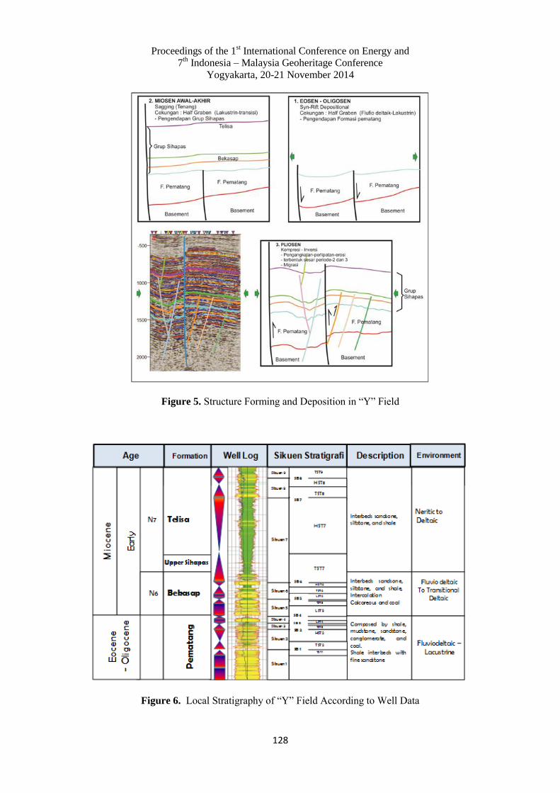
Proceedings of the 1
st International Conference on Energy and
7th Indonesia – Malaysia Geoheritage Conference
Yogyakarta, 20-21 November 2014
128
Figure 5. Structure Forming and Deposition in “Y” Field
Figure 6. Local Stratigraphy of “Y” Field According to Well Data

Proceedings of the 1
st International Conference on Energy and
7th Indonesia – Malaysia Geoheritage Conference
Yogyakarta, 20-21 November 2014
129
Figure 7. Structural Modeling
Figure 8. Scale Up Well Logs
VShale
PHIE
Fasies
0 : Shale
1 : Sand
Name Type Min Max Delta N Mean Std Var Sum
Upscaled Disc. 0 1 1 416 1 0 0 377
Well logs Disc. 0 1 1 1889 1 0 0 1709
Name Type Min Max Delta N Mean Std Var Sum
Upscaled Cont. 0.04 0.68 0.64 398 0.32 0.13 0.02 128.61
Well logs Cont. 0.01 0.73 0.72 2040 0.32 0.13 0.02 651.72
Name Type Min Max Delta N Mean Std Var Sum
Upscaled Cont. 0.04 0.29 0.26 380 0.18 0.05 0 69.08
Well logs Cont. 0 0.3 0.3 1969 0.18 0.05 0 359.25
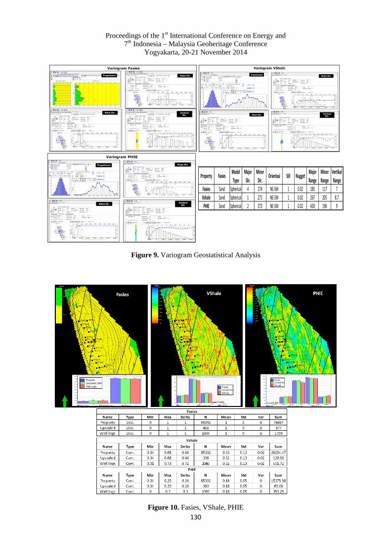
Proceedings of the 1
st International Conference on Energy and
7th Indonesia – Malaysia Geoheritage Conference
Yogyakarta, 20-21 November 2014
130
Figure 9. Variogram Geostatistical Analysis
Figure 10. Fasies, VShale, PHIE
Property FasiesModel
Type
Major
Dir.
Minor
Dir.Orientasi Sill Nugget
Major
Range
Minor
Range
Vertikal
Range
Fasies Sand Spherical 4 274 NE-SW 1 0.02 185 117 7
Vshale Sand Spherical 1 271 NE-SW 1 0.02 267 205 8.7
PHIE Sand Spherical 2 272 NE-SW 1 0.02 430 196 9
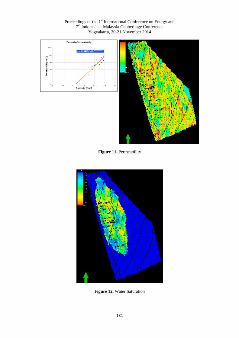
Proceedings of the 1
st International Conference on Energy and
7th Indonesia – Malaysia Geoheritage Conference
Yogyakarta, 20-21 November 2014
131
Figure 11. Permeability
Figure 12. Water Saturation


![Rocks and Minerals.ppt [Read-Only]](https://static.fdokumen.com/doc/165x107/633751f86fd2e64f8d0df5b5/rocks-and-mineralsppt-read-only.jpg)