Journal of Consulting and Clinical Psychology1993, Vol. 61, No. 6, 920-928

Copyright 1993 by the American Psychological Association, Inc.0022-006X/93/J3.00

Some Problems and Solutions in the Study of Change:Significant Patterns in Client Resistance

Mike Stoolmiller, Terry Duncan, Lew Bank, and Gerald R. Patterson

Latent growth curve methodology was applied to the study of patterns of change in client resistanceduring parent training therapy. The clinical sample consisted of 68 mothers of children, 52 boys and16 girls, ages 5 through 12 years, with confirmed conduct problems. Simple linear and linear splinegrowth models were fit to the three repeated observational measures of maternal resistance duringtherapy and found inadequate. Instead, a quadratic growth model was used. Pretherapy maternalcharacteristics of inept discipline and antisocial behavior predicted chronically high levels of resis-tance. Maternal depressed mood predicted less negative quadratic curvature. No significant predic-tors of overall change in resistance were detected. Lack of negative curvature of the resistance growthcurves predicted child court offenses during a 2-year posttermination follow-up. Results are dis-cussed with reference to the struggle-and-working-through hypothesis of client resistance.

Statistical methods and evaluative designs well suited to thestudy of change are of central interest to clinicians and psychol-ogists in general. The analysis of change is not, however, asstraightforward as investigators may wish. In this article, we dis-cuss and illustrate some of the problems in analyzing and inter-preting change data, and we present in detail a clinical data setwith one approach to analyzing change within the therapy mi-lieu.

Change over a specified time interval is of interest to clini-cians, who must demonstrate the effectiveness of a particulartreatment regimen from data collected at two or more timepoints. The pretest-posttest design has, perhaps, been the main-stay of clinical research. As an alternative, passive, noninterven-tive, longitudinal approaches involving responses collected overtwo or more time points are also frequently used. Regardless ofwhether the design is of a true, quasi-, or nonexperimental na-ture, variables that involve correlated observations pose severalunique problems for the investigator interested in demonstrat-ing change in behavior over time. It is, therefore, useful to con-sider all designs with two data collection points as generally sim-ilar longitudinal designs.

Longitudinal designs with only two waves of data, however,may address some research questions rather poorly. For exam-ple, although two observations collected over time does allowfor the estimation of the amount of change, it is not possible to

Mike Stoolmiller, Terry Duncan, Lew Bank, and Gerald R. Patterson,Oregon Social Learning Center, Eugene, Oregon.

Preparation of this article was supported in part by Grant MH 46690from the Prevention Research Branch, National Institute of MentalHealth (NIMH), U.S. Public Health Service (USPHS); Grant MH37940 from the Center for Studies of Antisocial and Violent Behavior,NIMH, USPHS; Grant MH 38318 from the Mood, Anxiety, and Per-sonality Disorders Research Branch, NIMH, USPHS; and Grant DA07031 from the National Institute on Drug Abuse, USPHS.

Correspondence concerning this article should be addressed to MikeStoolmiller, Oregon Social Learning Center, 207 East 5th Avenue, Suite202, Eugene, Oregon 97401.

study the shape of the developmental trajectory or the rate ofchange in the individual. This raises a key issue for studies ofclinical change. Is the shape of the developmental path that anindividual follows between two time points a key theoreticalquantity as an outcome or a predictor? Alternatively, is theamount of change between two points or the final level of someattribute the important theoretical quantity? Two-points-in-time designs do not allow the testing of both these alternatives.In general, they are only adequate if the intervening growth pro-cess is considered irrelevant or known to be linear.

When curvilinear growth is occurring, focusing on theamount of change between two points can be misleading. Ro-gosa (1988) has demonstrated, at least theoretically, that whenthere are individual differences in the shape of curvilineargrowth trajectories, the rank order of individuals on amount ofchange between any two points within the growth interval canvary tremendously depending on the choice of points. The im-plication is that if pre- and postmeasures were obtained on sucha growth process, inferences about predictors of change andchange as a predictor would depend on where in time the twopoints were located within the growth process. Two investiga-tors studying the same process in the same sample could reachopposite conclusions concerning some predictor of growth orsome outcome of growth merely because they chose differenttime points for assessment! The apparent solution to this di-lemma is to collect more information than just the pre- andposttests.

Using Growth Curve Methodology to Study Change

Heuristically, growth curve methodology can be thought of asconsisting of two stages. The first stage is focused on accuratelydescribing and summarizing individual differences in growthtrajectories if they exist. The accuracy of the description can beassessed by testing various growth form models (e.g., straightline versus quadratic growth) for goodness of fit. Summariza-tion is accomplished by focusing on the parameters of thegrowth curves rather than the original measures. As an example

920

SPECIAL SECTION: PATTERNS OF CLIENT RESISTANCE 921

of the first stage, let us assume six repeated measures on someattribute fell more or less on a straight line when plotted overtime for each individual in a sample. The six repeated measuresfor any individual could be accurately and much more com-pactly summarized by the slope and intercept of a custom fittedstraight line. The slope parameter for an individual would indexthe rate of change per unit time on the attribute for that indi-vidual. In the second stage, the parameters for an individual'scustom fit curve become the focus of the analysis rather thanthe original measures. Questions and hypotheses about deter-minants and outcomes of growth could be addressed by focus-ing on predictors of slope scores and slopes scores as predictors.

Using growth curve methodology to study change dependscrucially on the assumption that change is systematically re-lated to the passage of time, at least over the time interval ofinterest (Burchinal & Appelbaum, 1991). Change that is sys-tematically related to time is often thought of as development orgrowth. Because change over time is not always a systematicfunction of time, growth curve methodology is not a generalstrategy for the analysis of change. If change is not systemati-cally related to time, growth curve methodology is not appro-priate and may even be misleading. In this case, one alternativestrategy for the analysis of repeated measures is the longitudinalregression model of Zeger and Liang (1986).

In this article, statistical models for growth curves will betested using commercially available structural equation model-ing (SEM) software, EQS (Rentier, 1989). This approach, re-ferred to as latent growth curve modeling (LGC), is explainedin more technical detail in Meredith and Tisak (1990). A lesstechnical introduction is found in Stoolmiller (in press). Appli-cations of LGC may be found in Duncan and Duncan (1991),McArdle and Epstein (1987), and McArdle (1988). BecauseLGC is carried out using SEM methodology, it shares manyof the same strengths and weaknesses with regard to statisticalmethodology. Some of the strengths of the LGC approach in-clude the ability to test the adequacy of the hypothesized growthform, the ability to incorporate time varying covariates, and theability to use the growth parameters as predictors of later out-comes. Some of the limitations of the LGC approach includethe necessity for large samples, the necessity for multinormallydistributed variables, and the restriction to growth that can bedescribed by a general linear model. In particular, one weaknessof LGC that deserves mention is the restrictive requirement thatthe number and spacing of assessments be the same for all indi-viduals. For less restrictive, alternative techniques see Bryk andRaudenbush (1987) or Willet, Ayoub, and Robinson (1991).

Resistance in Parent Training Therapy

There has been relatively little data collected on client resis-tance, despite general agreement in the field that client resis-tance is a critical phenomenon. Previous work at the OregonSocial Learning Center (OSLC) has suggested that client resis-tance forms a curvilinear growth process through therapy(Chamberlain, Patterson, Reid, Kavanagh, & Forgatch, 1984).Recently, Patterson and Chamberlain (in press) articulated astruggle-and-working-through hypothesis to describe the devel-opment of resistance over the course of therapy. When the ther-apist begins to teach parenting skills and demands that the client

use these skills, client resistance occurs (Patterson & Forgatch,1985). Because this usually begins some time after the first fewsessions, the first half of the struggle-and-working-through hy-pothesis predicts that resistance increases from the baseline oftherapy to the midpoint; the second half suggests that if therapyis ultimately going to be successful, the level of resistance willfall off from midpoint to termination. If, however, the parent isunsuccessful in learning or applying the skills for whatever rea-son and the therapist continues to demand change, the struggle-working-through hypothesis suggests that levels of resistancewill not drop very much or will even increase. Finally, from co-ercion theory (Patterson, 1982), if the parent fails to learn andapply new skills, the behavior problems of the child are not ex-pected to improve.

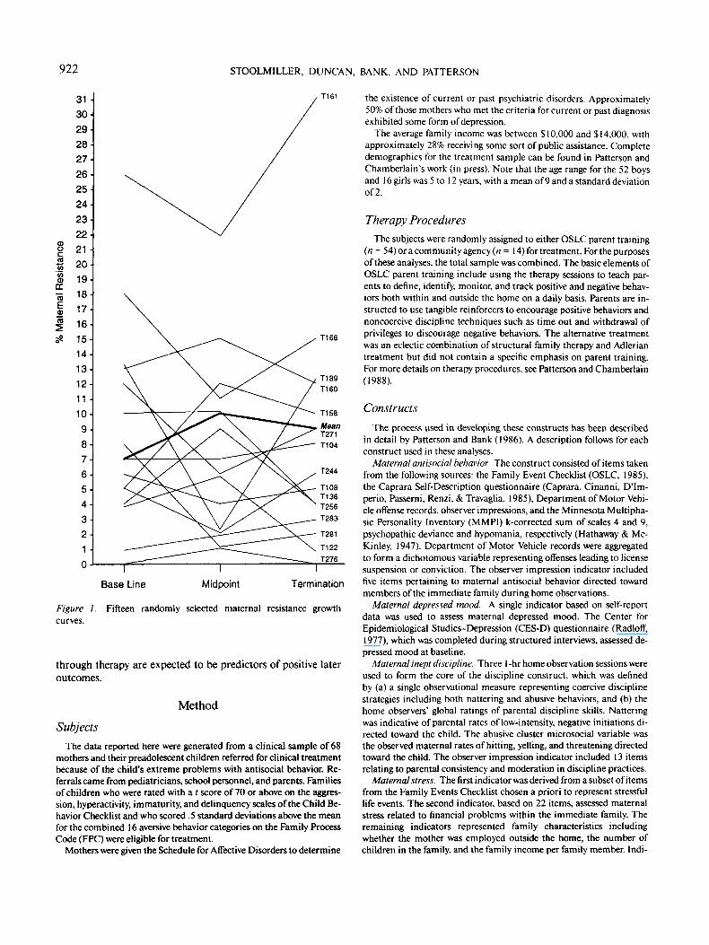
The struggle-and-working-through hypothesis lends itselfwell to growth curve analyses. Changes in parent resistance arehypothesized to depend systematically on the passage of timewhere time in this case is indexed by the phase of therapy: base-line, midpoint, and termination. Furthermore, the struggle-and-working-through hypothesis leads to the prediction of qua-dratic trajectories. The degree of success of therapy should berelated to the extent that resistance climbs from baseline tomidpoint and then falls off from midpoint to termination whichis indexed by a quadratic curvature score. Successful casesshould prototypically show negative curvature and resemble aninverted V. An example of a successful case is family T256,shown in Figure 1. Unsuccessful cases should prototypicallyshow less negative, and in some cases even positive, curvature.An example of a failure case is family T166, shown in Figure 1.However, with only three time points, a quadratic model willperfectly reproduce all the observed trajectories. This is a sim-ple extension of the principle that two points determine astraight line. When models use up all degrees of freedom andhence fit the data perfectly, as in this case, they are referred toas completely saturated. The overall fit of the quadratic modelcannot be meaningfully tested because it is saturated. However,simpler models such as straight-line growth could fit just as well,and if so, this would tend to disconfirm the struggle-and-work-ing-through hypothesis.

Chronically high levels of resistance are hypothesized to bedetrimental also, but only secondarily to the failure of workingthrough the resistance indexed by lack of negative curvature.This implies that even parents who are initially or chronicallyvery resistant can still succeed in parent training therapy.

On the basis of previous work, baseline differences in parentcharacteristics such as inept discipline skills, depressed mood,stress, and antisocial behavior, (Patterson & Chamberlain, inpress) are hypothesized to account for individual differences inthe growth parameters of resistance. In turn, individual patternsof resistance are hypothesized to account for posttherapy out-comes for the target child.

No specific hypotheses were advanced about the overallamount of change in resistance from baseline to termination.The overall amount of change as noted earlier is less meaningfulwhen dealing with curvilinear growth forms. Although it will beincluded in the analyses, the amount of change in client resis-tance is expected to be an unreliable determinant of postther-apy outcomes, whereas the presence of struggle and workingthrough behavior and chronically low levels of resistance

922 STOOLMILLER, DUNCAN, BANK, AND PATTERSON

§<o»in0)cr

~a

01

313029-28-27-26

252423222120191817

16-15-14-

131211

10987-6 -54- j32-1 •

0

T161

T166

I

Base Line

IMidpoint

I

Termination

Figure 1. Fifteen randomly selected maternal resistance growthcurves.

through therapy are expected to be predictors of positive lateroutcomes.

Method

Subjects

The data reported here were generated from a clinical sample of 68mothers and their preadolescent children referred for clinical treatmentbecause of the child's extreme problems with antisocial behavior. Re-ferrals came from pediatricians, school personnel, and parents. Familiesof children who were rated with a t score of 70 or above on the aggres-sion, hyperactivity, immaturity, and delinquency scales of the Child Be-havior Checklist and who scored .5 standard deviations above the meanfor the combined 16 aversive behavior categories on the Family ProcessCode (FPC) were eligible for treatment.

Mothers were given the Schedule for Affective Disorders to determine

the existence of current or past psychiatric disorders. Approximately50% of those mothers who met the criteria for current or past diagnosisexhibited some form of depression.

The average family income was between $10,000 and $14,000, withapproximately 28% receiving some sort of public assistance. Completedemographics for the treatment sample can be found in Patterson andChamberlain's work (in press). Note that the age range for the 52 boysand 16 girls was 5 to 12 years, with a mean of 9 and a standard deviationo(2.

Therapy Procedures

The subjects were randomly assigned to either OSLC parent training(n = 54) or a community agency (n= 14) for treatment. For the purposesof these analyses, the total sample was combined. The basic elements ofOSLC parent training include using the therapy sessions to teach par-ents to define, identify, monitor, and track positive and negative behav-iors both within and outside the home on a daily basis. Parents are in-structed to use tangible reinforcers to encourage positive behaviors andnoncoercive discipline techniques such as time out and withdrawal ofprivileges to discourage negative behaviors. The alternative treatmentwas an eclectic combination of structural family therapy and Adleriantreatment but did not contain a specific emphasis on parent training.For more details on therapy procedures, see Patterson and Chamberlain(1988).

Constructs

The process used in developing these constructs has been describedin detail by Patterson and Bank (1986). A description follows for eachconstruct used in these analyses.

Maternal antisocial behavior. The construct consisted of items takenfrom the following sources: the Family Event Checklist (OSLC, 1985),the Caprara Self-Description questionnaire (Caprara, Cinanni, DTm-perio, Passerni, Renzi, & Travaglia, 1985), Department of Motor Vehi-cle offense records, observer impressions, and the Minnesota Multipha-sic Personality Inventory (MMPI) k-corrected sum of scales 4 and 9,psychopathic deviance and hypomania, respectively (Hathaway & Mc-Kinley, 1947). Department of Motor Vehicle records were aggregatedto form a dichotomous variable representing offenses leading to licensesuspension or conviction. The observer impression indicator includedfive items pertaining to maternal antisocial behavior directed towardmembers of the immediate family during home observations.

Maternal depressed mood. A single indicator based on self-reportdata was used to assess maternal depressed mood. The Center forEpidemiological Studies-Depression (CES-D) questionnaire (Radloff,1977), which was completed during structured interviews, assessed de-pressed mood at baseline.

Maternal inept discipline. Three 1 -hr home observation sessions wereused to form the core of the discipline construct, which was definedby (a) a single observational measure representing coercive disciplinestrategies including both nattering and abusive behaviors, and (b) thehome observers' global ratings of parental discipline skills. Natteringwas indicative of parental rates of low-intensity, negative initiations di-rected toward the child. The abusive cluster microsocial variable wasthe observed maternal rates of hitting, yelling, and threatening directedtoward the child. The observer impression indicator included 13 itemsrelating to parental consistency and moderation in discipline practices.

Maternal stress. The first indicator was derived from a subset of itemsfrom the Family Events Checklist chosen a priori to represent stressfullife events. The second indicator, based on 22 items, assessed maternalstress related to financial problems within the immediate family. Theremaining indicators represented family characteristics includingwhether the mother was employed outside the home, the number ofchildren in the family, and the family income per family member. Indi-

SPECIAL SECTION: PATTERNS OF CLIENT RESISTANCE 923

cators were dichotomized using a median split and were summed torepresent level of maternal stress at baseline.

Child antisocial difference score. The teacher indicator was based onan a priori scale consisting of 16 items (e.g., argues a lot, disrupts classdiscipline, lies, tardy, etc.) from the Teacher Child Behavior Checklist(Achenbach & Edelbrock, 1986). The parent indicator was based onovert and covert antisocial scales formed by averaging across 21 antiso-cial behavior items from the Overt Covert Antisocial Questionnaire.The third indicator consisted of five items answered by trained observ-ers reflecting the level of the child's antisocial behavior observed duringhome observations.

Arrest. Juvenile court record searches were conducted locally for allchildren. When families moved to other communities, the local author-ities were contacted for permission to conduct record searches in theirjurisdiction. Contacts for reasons other than delinquency (i.e., abuse orneglect of the target child) were excluded from the analyses. Juvenilecourt contacts generated by the child during the 2-year period followingtreatment termination were used as a measure of subsequent arrests inthis study. For simplicity, the court contact variable was scored dichot-omously (1 for any contact and 0 for no contact) and reseated bymultiplying by 10 for computational convenience.

Maternal resistance. Maternal resistance to therapy was coded atbaseline, midtherapy, and termination using the Therapy Process Cod-ing System (Chamberlain et al., 1984). The process codes used to rep-resent resistance in our sample included seven categories describing theclients' verbalizations: (a) confront or challenge the therapist; (b) hope-less or blame; (c) defend self or other family member; (d) sidetrack orown agenda; (e) answer for other family member; (f) not answering; and(g) contradict own previous statement. The maternal resistance scorerepresents the proportion of total behaviors that were resistant. The pro-portions were rescaled to range from 0 to 100 for computational conve-nience.

To determine levels of interobserver agreement, two independentobservers coded 86 sessions. With a 6-s window, the average percentagreement was 79% (range, 66% to 88%), whereas the average kappa was.73 (range, .57 to .83; Chamberlain & Ray, 1988).

All sessions were coded, but for these analyses, only a subset of thesessions were used to create resistance scores. The baseline scores areaverages from the first two sessions. The midpoint and termination oftherapy were determined after therapy was terminated so that the totalnumber of sessions was known. The midpoint scores are averages fromthe middle two sessions. The termination scores are averages from thelast quarter of sessions.

Scoring resistance in this fashion standardizes the underlying timemetric for the development of maternal resistance so that families re-ceiving different numbers of sessions can be compared. The underlyingtime metric for growth curve analysis is then assumed to be the phaseof therapy, and for simplicity, baseline is assumed to be time = 1, mid-point is time = 2, and termination is time = 3. This procedure greatlysimplifies the analyses, but it does so at the expense of any informationrelevant to the development of maternal resistance over the course oftherapy carried by the number of sessions. However, Patterson andChamberlain (in press), found for this data set that the number of ses-sions was unrelated to the resistance measures. Also, in preliminaryanalyses on this project, no significant relations were found between thenumber of sessions and individual differences in maternal resistancegrowth curve parameters. For an interesting example of growth curveanalysis when the number of therapy sessions varies across families, seeWilletetal. (1991).

Results

In all, 21 missing data points, or 3%, out of 612, were esti-mated either by regression or by mean substitution. Six missing

values for maternal antisocial behavior were estimated using theother three mother variables as predictors. Four missing valuesfor maternal stress were estimated using the other three mothervariables as predictors. Mean substitution was used to replace11 missing values for the child antisocial change score.

Figure 1 shows 15 randomly selected resistance trajectoriesand the mean trajectory. The mean curve shows moderate neg-ative curvature and, according to the struggle-and-working-through hypothesis, is prototypical of a moderate success inparent-training therapy. Figure 1 also illustrates considerableindividual differences in trajectory around the mean trajectory.Also evident is the considerable degree of curvature both nega-tive and positive for a substantial number of the trajectories.

Univariate descriptive statistics, correlations and Mardia'smultivariate kurtosis statistic (Mardia, 1970) are shown in Ta-ble 1. Several features of these statistics are noteworthy. First,the means for resistance indicate that 6.96%, 9.99%, and 9.33%of all behaviors at baseline, midpoint, and termination, respec-tively, were resistant. The mean of 2.46 for the rescaled, dichot-omous arrest variable indicates that 24.6% of the sample hadbeen arrested by the end of a 2-year follow-up period after ter-mination of treatment.

Three observations were deleted because they were identifiedboth as multivariate outliers by EQS (Bentler, 1989) and ashighly influential outliers by standard regression influence di-agnostics. For the remaining sample of 65, measures of univar-iate skewness and kurtosis were minimal, and Mardia'a multi-variate kurtosis measure was not significant. The assumptionof multivariate normality is therefore reasonable, justifying theuse of maximum likelihood estimation techniques.

Turning now to the correlations, both maternal inept disci-pline and maternal antisocial behavior were correlated with re-sistance at all three time points. However, maternal depressedmood shows a curious pattern of being related to the first andthird resistance measures but not the second. Maternal stresswas only related to the initial resistance measure. Perhaps evenmore puzzling is the pattern of relations for both arrest and thechild antisocial change score with the resistance measures. Bothchild outcome variables correlated negatively with the secondresistance measure but positively with the first and last mea-sures. These patterns of correlations illustrate the confusionthat can arise if the nature of the underlying growth process isnot explicitly modeled.

Stage 1: Growth Models

The first stage in an LGC analysis is to compare the goodnessof fit of the competing, hypothesized growth functions. Thegrowth function that best fits the actual individual trajectoriesis then used in the second stage when covariates of change aretested. The effect sizes for covariates obtained in the secondstage can be highly dependent on the choice of a growth func-tion in the first stage. Stoolmiller (in press) provided an exampleof the misspecification bias that can occur when a poorly fittinggrowth form is used. A strength of the LGC approach is theavailability of a formal statistical test of the adequacy of thegrowth form used in the first stage.

Because only three assessments of resistance are available,only three basic growth forms can be tested. The first model is a

924 STOOLMILLER, DUNCAN, BANK, AND PATTERSON

Table 1Univariate Descriptive Statistics, Correlations, and Multivariate Kurtosis

Item

1. Child arrest2. Child antisocial3. Maternal inept discipline4. Maternal antisocial5. Maternal depressed mood6. Maternal stress7. Maternal resistance: Time 18. Maternal resistance: Time 29. Maternal resistance: Time 3

MSDSkewnessKurtosis

1

.03

.12

.00

.14

.14

.26*-.11

. 1 1

2.464.341.21

-0.56

2

.15

.02

.10

.24

.16-.07

.02

-0.673.221.333.24

3

.01

.18-.02

.23

.33*

.30*

0.228.91

-0.68-0.10

4

.47*

.40*

.34*

.18

.20

1.330.370.59

-0.05

Item

5

.40*

.39*

.05

.33*

19.2212.680.53

-0.41

6

.30*-.05

.10

2.411.360.06

-0.76

7 8

.29* —

.53* .70*

6.96 9.995.12 6.681.16 0.681.91 0.15

9

9.336.361.331.86

Note. N = 65. Multivariate kurtosis = 4.59, ns.* p < .05.

two-factor, simple linear (SL) growth model. The second modelis a two-factor, unspecified linear spline (US) model (Meredith& Tisak, 1990). The third model is a three-factor quadraticmodel (QU). The basic nature of the SL and QU models hasalready been explained, but the US model needs additional ex-plication.

A linear spline is a "crooked line," a piecewise linear curve.A concrete example of a linear spline would be obtained if themeans of the three resistance measures were plotted andstraight lines drawn from one mean value to the next. The USmodel can be quite useful and powerful because it is capable ofapproximating quadratic and other curvilinear trajectories butonly under special circumstances. It confounds the shape of thelinear spline with the general linear trend. This may describe theactual trajectories well. If the US model proved to be capable ofreproducing the observed trajectories, it could be preferred overthe QU model on the basis of parsimony (one less factor re-quired). The US model with three time points uses up all avail-able degrees of freedom, (i.e., it is completely saturated) and,therefore, fits the data perfectly. It is, however, rejectable onother grounds such as producing nonsensical, out-of-boundsparameter estimates, such as negative variances or correlationsover 1. Example applications and more details on the US modelcan be found in works by Meredith and Tisak (1990), McArdle(1988), Duncan and Duncan (1991) and Stoolmiller (in press).

With only three time points, the QU model can only be esti-mated by imposing some additional constraints on the basicgrowth model. The sizes of the error variances for the observedmeasures of resistance are natural candidates for providingfixed values because prior information concerning observeragreement is available. Chamberlain and Ray (1988) reportedthe percent agreement between observers to be 79% for the ther-apy process code, so 20% error variance is a reasonable esti-mate. Once the error terms are provided, the model is estimablebut still completely saturated. Because the model is saturatedand the estimated error variances fixed, the QU model is onlytrivially rejectable in the sense that the provided error variance

estimates could be set too large, leading to overcorrection formeasurement error and correlations over 1. With one additionalassessment of resistance, the error terms could be estimatedfrom the data within the QU model, and a more meaningful testof the overall model could be obtained.

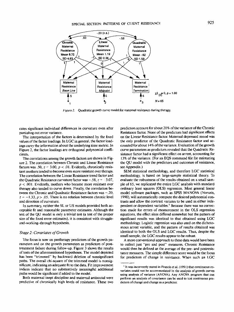
As expected, the SL model clearly does not fit the data, x2( 1,N = 65) = 6.91, p = .009, and also produces a nonsensical neg-ative variance estimate. The US model also produces a negativeerror estimate, and so it too is rejected. The QU model, shownin Figure 2, with the variance of the error terms fixed at 20% ofthe variance of the Time 1 resistance measure produces reason-able parameter estimates. The pattern of results obtained is thesame if the error terms are fixed at zero, a very conservativevalue.

In Figure 2, the first factor, labeled Chronic Resistance, rep-resents individual differences in average or chronic levels of re-sistance over therapy. If the estimate of the factor variance (orequivalently the standard deviation) is significant, it is indicativeof significant individual differences in chronic levels of resis-tance. The estimated standard deviation of Chronic Resistancewas 4.83%, z = 5.28, p < .001. This indicates significant indi-vidual differences (variance) in chronic levels of resistance evenafter partialing out error variance. The mean of 8.75%, z =14.01, p < .001, indicates that on the average, the chronic levelof resistance throughout therapy was 8.75% of all behaviors.

The second factor, labeled Linear Resistance, represents in-dividual differences in the linear trends of the resistance growthcurves over therapy. The mean was 1.19%, z = 3.34, p < .001,indicating that on the average, the amount of resistance went upfrom the start to the end of therapy. The standard deviation was2.36%, z = 3.90, p < .001. This indicates significant individualdifferences in linear trends even after partialing out error vari-ance. The third factor, labeled Quadratic Resistance, representsindividual differences in the curvature of the resistance growthcurves. The mean was -.62, z = -2.69, p < .01, indicating thaton average, the resistance growth curves tended to curve down.The standard deviation was 1.59, z = 4.25, p < .001. This indi-

SPECIAL SECTION: PATTERNS OF CLIENT RESISTANCE 925

LinearMaternal

ResistanceMean 1.19

SD 2.36

ChroniMaternal

ResistanceMean 8.75

SD 4.8

QuadraticMaternal

ResistanceMean -.62SD1.59

1

Figure 2. Quadratic growth curve model for maternal resistance during therapy.

cates significant individual differences in curvature even afterpartialing out error variance.

The interpretation of the factors is determined by the fixedvalues of the factor loadings. In LGC in general, the factor load-ings carry the information about the underlying time metric. InFigure 2, the factor loadings are orthogonal polynomial coeffi-cients.

The correlations among the growth factors are shown in Fig-ure 2. The correlation between Chronic and Linear Resistancefactors was .50, z = 3.00, p < .01. Evidently, chronically resis-tant mothers tended to become even more resistant over therapy.The correlation between the Linear Resistance trend factor andthe Quadratic Resistance curvature factor was -.58, z = -3.07,p < .001. Evidently, mothers who became more resistant overtherapy also tended to curve down. Finally, the correlation be-tween the Chronic and Quadratic Resistance factors was -.20,z = — 1.33, p > .05. There is no relation between chronic leveland direction of curvature.

In summary, neither the SL or US models provided both ac-ceptable fit and reasonable parameter estimates. Although thetest of the QU model is only a trivial test (a test of the propersize of the fixed error estimates), it is consistent with struggle-and-working-through hypothesis.

Stage 2: Covariates of Growth

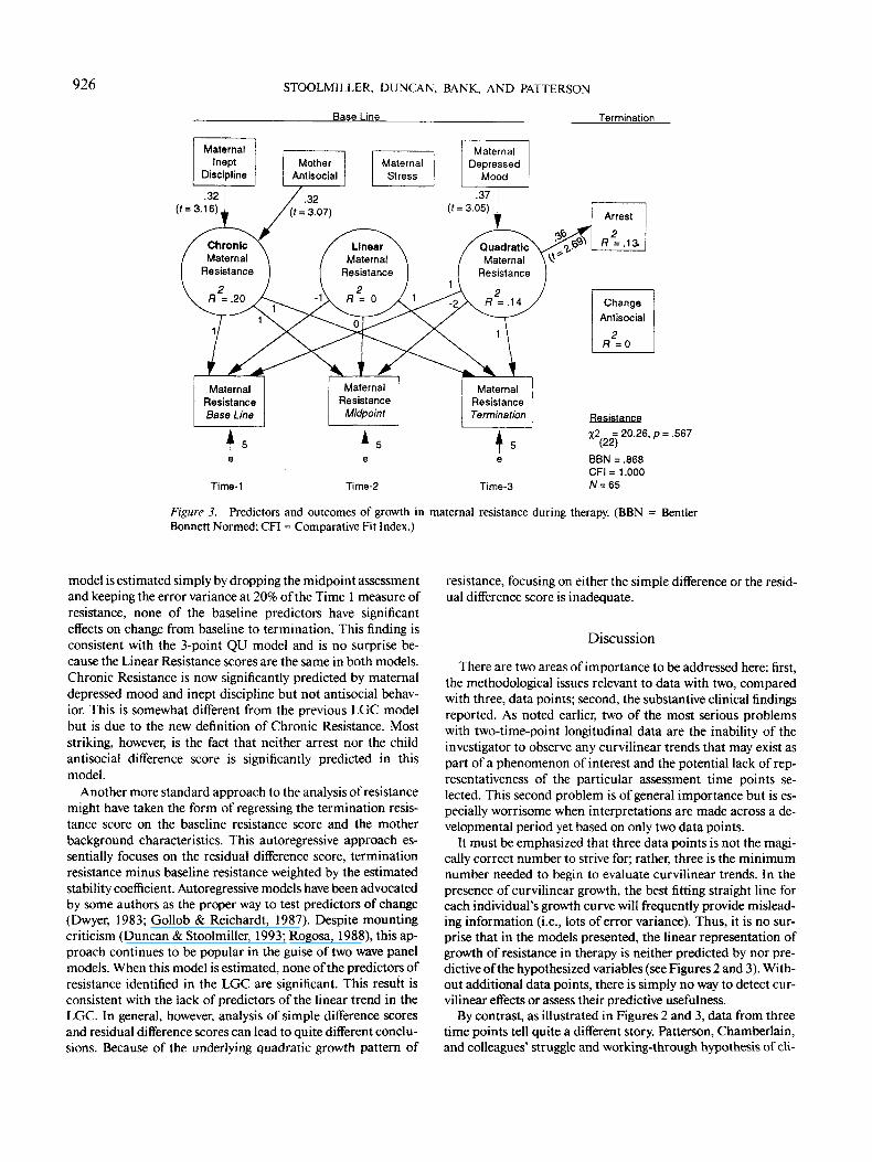
The focus is now on pretherapy predictors of the growth pa-rameters and on the growth parameters as predictors of post-treatment failure during follow-up. Figure 3 shows the resultsof tests of the aforementioned hypotheses. The model depictedhas been "trimmed" by backward deletion of nonsignificantpaths. The overall chi-square of the trimmed model is nonsig-nificant, indicating an adequate fit to the data. Fit improvementindices indicate that no substantively meaningful additionalpaths would be significant if added to the model.

Both maternal inept discipline and maternal antisocial werepredictive of chronically high levels of resistance. These two

predictors account for about 20% of the variance of the ChronicResistance factor. None of the predictors had significant effectson the Linear Resistance factor. Maternal depressed mood wasthe only predictor of the Quadratic Resistance factor and ac-counted for about 14% of the variance. Evaluation of the growthcurve parameters as predictors revealed that the Quadratic Re-sistance factor had a significant effect on arrest, accounting for13% of the variance. (For an EQS command file for estimatingthe QU model with the predictors and outcomes of resistance,see Appendix.)

SEM statistical methodology, and therefore LGC statisticalmethodology, is based on large-sample statistical theory. Toevaluate the robustness of the results obtained on a small sam-ple of 65, we replicated the entire LGC analysis with standardordinary least squares (OLS) regression. Most general linearmodel software packages, such as SPSS MANCAA (Norusis,1990), will automatically compute the desired polynomial con-trasts and allow the contrast variates to be used as either inde-pendent or dependent variables.' Because there was no correc-tion made for errors of measurement in the OLS regressionequations, the effect sizes differed somewhat but the pattern ofsignificant results was identical to that obtained using LGCmethodology. Logistic regression was also used on the dichoto-mous arrest variable, and the pattern of results obtained wasidentical to both the OLS and LGC results. Thus, despite thesmall sample, the LGC results appear to be robust.

A more conventional approach to these data would have beento collect just "pre and post" measures. Chronic Resistancewould then be defined as the average of the pre- and postresis-tance measures. The simple difference score would be the focusfor predictors of change in resistance. When such an LGC

1 It was incorrectly stated in Francis et al. (1991) that continuous co-variates could not be accommodated in the analysis of growth curvesusing analysis of variance (ANOVA). Any ANOV\ program that canperform an analysis of covariance can be used to test continuous pre-dictors of change and change as a predictor.

926 STOOLMILLER, DUNCAN, BANK, AND PATTERSON

Base Line Termination

MaternalInept

Disc

.323.16)

aline

r

MaternalStress

(' =

MaternalDepressed

Mood

.37!

3.05) I

Time-3

QuadraticMaternal

Resistance

%2 = 20.26, p = .567(22)

BBN = .868CFI = 1.000N = 65

Figure 3. Predictors and outcomes of growth in maternal resistance during therapy. (BBN = BentlerBennett Normed; CFI = Comparative Fit Index.)

model is estimated simply by dropping the midpoint assessmentand keeping the error variance at 20% of the Time 1 measure ofresistance, none of the baseline predictors have significanteffects on change from baseline to termination. This finding isconsistent with the 3-point QU model and is no surprise be-cause the Linear Resistance scores are the same in both models.Chronic Resistance is now significantly predicted by maternaldepressed mood and inept discipline but not antisocial behav-ior. This is somewhat different from the previous LGC modelbut is due to the new definition of Chronic Resistance. Moststriking, however, is the fact that neither arrest nor the childantisocial difference score is significantly predicted in thismodel.

Another more standard approach to the analysis of resistancemight have taken the form of regressing the termination resis-tance score on the baseline resistance score and the motherbackground characteristics. This autoregressive approach es-sentially focuses on the residual difference score, terminationresistance minus baseline resistance weighted by the estimatedstability coefficient. Autoregressive models have been advocatedby some authors as the proper way to test predictors of change(Dwyer, 1983; Gollob & Reichardt, 1987). Despite mountingcriticism (Duncan & Stoolmiller, 1993; Rogosa, 1988), this ap-proach continues to be popular in the guise of two wave panelmodels. When this model is estimated, none of the predictors ofresistance identified in the LGC are significant. This result isconsistent with the lack of predictors of the linear trend in theLGC. In general, however, analysis of simple difference scoresand residual difference scores can lead to quite different conclu-sions. Because of the underlying quadratic growth pattern of

resistance, focusing on either the simple difference or the resid-ual difference score is inadequate.

Discussion

There are two areas of importance to be addressed here: first,the methodological issues relevant to data with two, comparedwith three, data points; second, the substantive clinical findingsreported. As noted earlier, two of the most serious problemswith two-time-point longitudinal data are the inability of theinvestigator to observe any curvilinear trends that may exist aspart of a phenomenon of interest and the potential lack of rep-resentativeness of the particular assessment time points se-lected. This second problem is of general importance but is es-pecially worrisome when interpretations are made across a de-velopmental period yet based on only two data points.

It must be emphasized that three data points is not the magi-cally correct number to strive for; rather, three is the minimumnumber needed to begin to evaluate curvilinear trends. In thepresence of curvilinear growth, the best fitting straight line foreach individual's growth curve will frequently provide mislead-ing information (i.e., lots of error variance). Thus, it is no sur-prise that in the models presented, the linear representation ofgrowth of resistance in therapy is neither predicted by nor pre-dictive of the hypothesized variables (see Figures 2 and 3). With-out additional data points, there is simply no way to detect cur-vilinear effects or assess their predictive usefulness.

By contrast, as illustrated in Figures 2 and 3, data from threetime points tell quite a different story. Patterson, Chamberlain,and colleagues' struggle and working-through hypothesis of cli-

SPECIAL SECTION: PATTERNS OF CLIENT RESISTANCE 927

ent resistance over the course of parent training therapy is sup-ported quite well. The latent growth curve QU provides accept-able estimates for all parameters in the model. The alternativeSL and US models described by Meredith and Tisak (1990)were rejected because of inadequate fit or unacceptable out-of-bound parameter estimates or both. Furthermore, within theQU model, (a) chronically high maternal resistance during ther-apy was predicted by inept discipline strategies and by antiso-cial behavior assessed before the start of therapy, (b) the failureto struggle and work through resistance across the therapy pro-cess was predicted by mothers' depressed mood assessed beforethe start of therapy, and (c) the failure to struggle and workthrough resistance issues in therapy significantly predicted post-therapy child arrests over the 2-year period following therapytermination. These findings cannot be obtained from the verysame data set when only pre- and postassessment points for re-sistance are used.

These findings have powerful implications for clinical theoryand practice. As this study is a replication of the earlier Cham-berlain et al. (1984) and Patterson and Chamberlain (in press)papers, more confidence can be placed in the notion that thestruggle-and-working-through resistance pattern is critical forsuccessful parent-training therapy with families of antisocialchildren; that is, what goes on in the therapy process appears tohave better predictive validity than the assessed therapy end-point or overall change from therapy initiation to therapy ter-mination. This notion may be counterintuitive to many clini-cians, but it has held in two independent samples thus far.Clearly, families with accelerating and chronically high levels ofresistance are likely failure cases, but families that show lowlevels of resistance from baseline to termination also appear un-likely to benefit. The families who are likely to succeed are thosefamilies who struggle with the therapist and show increasingresistance over the course of therapy and who are then able toresolve or work through their resistance with ample time to putwhat they have learned into effect in their families with the con-tinuing support of their therapist. Those are the negative curva-ture families depicted in Figure 1.

It will be of interest to many clinicians that these results areconsistent with the psychodynamic notion of positive transfer-ence. Although this was not tested in our study, the critical pe-riod for the transference is likely to occur at the point in therapywhen resistance gives way to resolution and working through inthe client-therapist process. Articles by Patterson, Chamber-lain, and their colleagues describe their therapy observationcode (Chamberlain et al., 1984) and the development of theirstruggle-and-working-through hypotheses (Patterson & Cham-berlain, in press). This work demonstrates new avenues for thescientific investigation of resistance, transference, and otherpsychoanalytic constructs and hypotheses.

Avenues for future research and possible limitations to thisstudy must be stated. First, the therapists involved in this studywere typically at least master's degree level with considerableparent-training therapy experience, and they received weeklysupervision for all cases. Second, the pattern of the resistanceprocess for parent-training therapy with families of antisocialchildren may, of course, not generalize to therapy with othertechniques and for different populations. In fact, other criticalvariables such as the child's age and gender are known to in-

teract with the therapeutic interventions and will have to bemore specifically addressed in future work. Finally, althoughthe QU model worked well and none of the alternative modelswere acceptable, the overall adequacy of fit for the QU modelcould not be assessed with only three data points (i.e., it is bydefinition, saturated). A fourth data point would begin to allowfor that test. Indeed, it is recommended that three data pointsbe collected as an absolute minimum in the investigation ofclinical change. In the end, however, the exact number of assess-ments used to represent the course of possible curvilineartrends must be based on an understanding of the underlying psy-chological processes under investigation.

References

Achenbach, T. M., & Edelbrook, C. S. (1986). Manual for the teacher'sreport form and teacher version of the child behavior profile. (Availablefrom the Department of Child Psychiatry, University of Vermont, 1South Prospect Street, Burlington, VT 05401.)

Rentier, P. M. (1989). EQS structural equations program manual. LosAngeles: BMDP Statistical Software.

Bryk, A. S., & Raudenbush, S. W. (1987). Application of hierarchicallinear models to assessing change. Psychological Bulletin, 101, 147-158.

Burchinal, M., & Appelbaum, M. I. (1991). Estimating individual de-velopmental functions: Methods and their assumptions. Child Devel-opment, 62, 23-43.

Caprara, G. V., Cinanni, V., D'Imperio, G., Passerni, S., Renzi, P., &Travaglia, G. (1985). Indicators of impulsive aggression: Present sta-tus of research on irritability and emotional susceptibility scales. Per-sonality and Individual Differences, 6, 665-674.

Chamberlain, P., Patterson, G. R., Reid, J. B., Kavanagh, K.., & For-gatch, M. S. (1984). Observation of client resistance. Behavior Ther-apy, 15, 144-155.

Chamberlain, P., & Ray, J. (1988). The therapy process code: A multi-dimensional system for observing therapist and client interactions infamily treatment. In R. J. Prinz (Ed.), Advances in behavioral assess-ment of children and families (Vol. 4, pp. 189-217). Greenwich, CT:JAI Press.

Duncan, T. E., & Duncan, S. C. (1991). A latent growth curve approachto investigating developmental dynamics and correlates of change inchildren's perceptions of physical competence. Research Quarterlyfor Exercise and Sport, 62, 390-398.

Duncan, T. E., & Stoolmiller, M. L. (1993). Modeling social and psy-chological determinants of exercise behaviors via structural equationsystems. Research Quarterly for Exercise and Sport, 64, 1-16.

Dwyer, J. H. (1983). Statistical models for the social and behavioralsciences. New York: Oxford University Press.

Francis, D. J., Fletcher, J. M., Stuebing, K. K., Davidson, K. C., &Thompson, N. M. (1991). Analysis of change: Modeling individualgrowth. Journal of Consulting and Clinical Psychology, 59, 27-37.

Gollob, H. F., & Reichardt, C. S. (1987). Taking account of time lags incausal models. Child Development, 58, 80-92.

Hathaway, S. R., & McKinley, J. C. (1967). Minnesota Multiphasic Per-sonality Inventory manual. New York: Psychological Corporation.

Mardia, K. V. (1970). Measures of multivariate skewness and kurtosiswith applications. Biomelrika, 57, 519-530.

McArdle, J. J. (1988). Dynamic but structural equation modeling ofrepeated measures data. In R. B. Cattel & J. Nesselroade (Eds.),Handbook of multivariate experimental psychology (2nd ed., pp.561-614). New York: Plenum Press.

McArdle, J. J., & Epstein, D. (1987). Latent growth curves within de-velopmental structural equation models. Child Development, 58,110-133.

928 STOOLMILLER, DUNCAN, BANK, AND PATTERSON

Meredith, W., & Tisak, J. (1990). Latent curve analysis. Psychometrika,55, 107-122.

Norusis, M. J. (1990). SPSS/PC+ Advanced statistics 4.0. Chicago:SPSS Inc.

Oregon Social Learning Center. (1985). Family Event Checklist. (Tech.Rep. Available from Oregon Social Learning Center, 207 East 5thAvenue, Suite 202, Eugene, OR 97401.)

Patterson, G. R. (1982). Coercive family process. Eugene, OR: Castalia.Patterson, G. R., & Bank, L. (1986). Bootstrapping your way in the

nomological thicket. Behavioral Assessment, 8, 49-73.Patterson, G. R., & Chamberlain, P. (1988). Treatment process: A prob-

lem at three levels. In L. C. Wynne (Ed.), The state of the art in familytherapy research: Controversies and recommendations (pp. 189-226).New \brk: Family Process Press.

Patterson, G. R., & Chamberlain, P. (in press). A functional analysis ofresistance: A neobehavioral perspective. In H. Arkowitz (Ed.), Whydon 'l people change? New perspectives on resistance and noncompli-ance. New York: Guilford Press.

Patterson, G. R., & Forgatch, M. S. (1985). Therapist behavior as a de-

terminant of client noncompliance: A paradox for the behavior mod-ifier. Journal of Consulting and Clinical Psychology, 53, 846-851.

Radloff, L. S. (1977). The CES-D Scale: A self-report depression scalefor research in the general population. Applied Psychological Mea-surement, L 385-401.

Rogosa, D. (1988). Myths about longitudinal research. In K. W. Schaie,R. T. Campbell, W. Meredith, & S. C. Rawlings (Eds.), Methodologi-cal issues in aging research (pp. 171-210). New \brk: Springer-Ver-lag.

Stoolmiller, M. S. (in press). Using latent growth curve models to studydevelopmental processes. In J. M. Gottman & G. Sackett (Eds.) Theanalysis of change.

Willett, J. B., Ayoub, C. C., & Robinson, D. (1991). Using growth mod-eling to examine systematic differences in growth: An example ofchange in the functioning of families at risk of maladaptive parenting,child abuse, or neglect. Journal of Consulting and Clinical Psychol-ogy, 59, 38-47.

Zeger, S. L., & Liang, K. (1986). Longitudinal data analysis for discreteand continuous outcomes. Biometrics, 42, 121-130.

Appendix

EQS Command File

/titlegrowth model of resistance during therapy for mothers./specscases = 68; vars = 9; analysis = moment; matrix = raw;data_file = 'rxno3.asc'; delete = 3,38,41;/equationsvl = 2*v999 + 0*fe + el;v2 = 0*v999 + e2;v3 = .5*v999 + e3;v4= 1.3*v999 + e4;v5 = 19*v999 + e5;v6 = 2.3*v999 + e6;v7 = fl - I f 2 + I f3 + e7v8 = f 1 + Of2 - 2f3 + e8;v9 = fl + I f2+ 1O +e9;fl = 7*v999 + 0*v3 + 0*v4 + dl;K = 2*v999 + d2;f3 = 0*v999 + 0*v5 + d3;/variances

dl = *;d2 = *;d3 = *;el toe6 = *;/co variancesdl ,d2 = *;dl,d3 = *;d2,d3 = *;e3toe6 = *;el,e2 = *;/wtestapriori = (fl, v3), (fl , v4), (f3, v5), (vl, f3);/Imtestapriori = (vl , v3), (vl , v4), (vl , v5), (vl , v6), (v2, v3), (v2, v4), (v2, v5),

(v2, v6);set = bvf, bfv, bvv;/labelsvl = ARREST; v2 = DANTIS; v3 = MDISC2A; v4 = MPANT2R;

v5 = MCESDD2;v6 = MSTRS2A; v7 = MPRSIST1; v8 = MPRSIST2;

v9 = MPRSIST3;fl = resavg; f2 = reslin; f3 = resqud;/printparameters = yes; correlations = yes;/end

Received May 14, 1992Revision received September 4, 1992

Accepted April 2, 1993