This article appeared in a journal published by Elsevier. The attachedcopy is furnished to the author for internal non-commercial researchand education use, including for instruction at the authors institution

and sharing with colleagues.

Other uses, including reproduction and distribution, or selling orlicensing copies, or posting to personal, institutional or third party

websites are prohibited.

In most cases authors are permitted to post their version of thearticle (e.g. in Word or Tex form) to their personal website orinstitutional repository. Authors requiring further information

regarding Elsevier’s archiving and manuscript policies areencouraged to visit:

http://www.elsevier.com/copyright

Author's personal copy

Some insights into structure instability and the second-order work criterion

François Nicot a,⇑, Noël Challamel b, Jean Lerbet c, Florent Prunier d, Félix Darve e

a Cemagref, ETNA – Geomechanics Group, Grenoble, Franceb Université de Bretagne Sud, LIMATB, Lorient, Francec Université d’Evry Val d’Essonne, UFR Sciences et Technologie, Evry, Franced INSA, Lyon, Francee Laboratoire Sols Solides Structures, UJF-INPG-CNRS, Grenoble, France

a r t i c l e i n f o

Article history:Received 8 January 2011Received in revised form 13 July 2011Available online 24 September 2011

Keywords:BifurcationUniquenessInstabilitySecond-order workLoading parametersFailureCollapseStructuresNonconservative loading

a b s t r a c t

This paper is an attempt to extend the approach of the second-order work criterion to the analysis ofstructural system instability. Elastic structural systems with a finite number of freedoms and subjectedto a given loading are considered. It is shown that a general equation, relating the second-order timederivative of the kinetic energy to the second-order work, can be derived for kinetic perturbations. Thecase of constant, nonconservative loadings are then investigated, putting forward the role of the spectralproperties of the symmetric part of the tangent stiffness matrix in the occurrence of instability. As anillustration, the case of the generalized Ziegler column is considered and the case of aircraft wings sub-jected to aeroelastic effects is investigated. In the both cases, the consequences of additional kinematicconstraints are discussed.

� 2011 Elsevier Ltd. All rights reserved.

1. Introduction

Structure stability is one of the key issues that deserve attentionfor both engineering and academic purposes. In particular, the sta-bility of elastic structures has been abundantly investigated sincethe 1960s, extending to nonconservative loading (Bolotin, 1963;Ziegler, 1968; Nguyen, 2000). Inspired by the work in soil mechan-ics, the influence of additional kinematic constraints on the stabil-ity of nonconservative elastic systems constitutes a novel field thathas been insufficiently considered until now (Challamel et al.,2009, 2010). In soil mechanics, an equilibrium configuration of agiven soil body subjected to a given external loading is stable ifan incremental displacement field exists, associated with a strictlypositive value of the second time derivative of the kinetic energy.Formally, the following basic equation holds: Ëc = B2 �W2, whereB2 is a second-order boundary term involving both incrementaldisplacements and incremental external forces applied to theboundary of the system, and W2 is referred to as the second-orderwork involving both incremental stress and strain fields actingwithin the soil body (Hill, 1958).

Existence of stress–strain incremental fields that ensure thatthe quantity B2 �W2 is strictly positive has been broadly discussedin soil mechanics, especially when the boundary term is nil. Thishas shed light on the basic role played by the second-order workand leads to an investigation of the vanishing of the second-orderwork (see for instance Bigoni and Hueckel, 1991; Petryk, 1993;Bazant and Cedolin, 2003; Darve et al., 2004; Nicot and Darve,2007; Nicot et al., 2007, 2009; Prunier et al., 2009a,b; Sibilleet al., 2007a,b). This approach was applied to a variety of engineer-ing purposes, such as the analysis of landslides occurring alongvery gentle slopes (Lignon et al., 2009).

This paper aims at extending this approach to the context ofstructural systems with a finite number of freedoms, subjected tononconservative loadings. Application of a nonconservative loadmakes the tangent stiffness matrix nonsymmetric, even thoughthe constitutive behavior of the structure is reversible (elastic).As the second-order work is a quadratic form associated with thetangent stiffness matrix, this matrix’s loss of symmetry was shownto be a basic ingredient in the occurrence of instability in soilmechanics (Nicot et al., 2011).

The second section of this manuscript develops a theoreticalframework to derive the general second-order relation Ëc = B2 �W2 in the context of structural systems. The incidence of the spec-tral properties of the symmetric part of the tangent stiffness matrixon the occurrence of instability is thoroughly considered. Then the

0020-7683/$ - see front matter � 2011 Elsevier Ltd. All rights reserved.doi:10.1016/j.ijsolstr.2011.09.017

⇑ Corresponding author.E-mail address: francois.nicot@cemagref.fr (F. Nicot).

International Journal of Solids and Structures 49 (2012) 132–142

Contents lists available at SciVerse ScienceDirect

International Journal of Solids and Structures

journal homepage: www.elsevier .com/locate / i jsolst r

Author's personal copy

third section revisits the well-known Ziegler column in the contextof this approach. Finally, the case of a rigid plate (modeling an air-craft wing) with aeroelastic effects is considered.

Throughout the paper, two-order tensors are denoted A,whereas vectors are denoted X. The summation convention onrepeated indices will be employed. For any (one- or two-order)tensor A,tA denotes the transpose tensor. The notation ~dY is usedin the variational principle, where virtual variations of the variableY are considered.

2. From a quasistatic to a dynamical regime

2.1. Existence of multiple equilibrium configurations

Let a material system be considered, subjected to an externalloading characterized by a distribution of M forces Fp, withp = 1, . . . ,M. Any coordinate of Fp is denoted Fp

q, with q = 1, . . . ,3.In what follows, for the sake of simplicity, Fk will denote any termFp

q, with k = 1, . . . ,3M. Any geometrical configuration {x} of the sys-tem is assumed to be described by a finite set of N kinematicalparameters xi, with i = 1, . . . ,N. Terms xi stand indifferently as posi-tions or angles. By extension, x will denote the vector composed ofthe N coordinates xi.

Equilibrium configurations are determined using the virtualwork theorem, according to the following variational equation:

~dWext � ~dWint ¼ 0 ð1Þ

which must be verified for any admissible variational field ~dxi,where Wint and Wext denote, respectively, the internal and the exter-nal work.

Let {x⁄} be an equilibrium configuration composed of coordi-nates x�i . The question of the existence of other equilibrium config-urations {x} in a neighboring {x⁄} may arise: k{x} � {x⁄}k � L,where L is a characteristic length of the system.

Assuming an elastic behavior for the system considered yields:

~dWint � ~dUel ¼ 0 ð2Þ

where Ue x�i� �

denotes the elastic energy of the system in the equi-librium configuration {x⁄}. From Eq. (2), it can be written:

~dWint ¼@Uel

@xi

~dxi ¼ fiðxjÞ ~dxi ð3Þ

where fi is a function of the current geometrical configuration {x}and elastic stiffness parameters.

Denoting Dxi ¼ xi � x�i and making use of a first-order Taylorexpansion of fi(xj) around the equilibrium configuration {x⁄}, gives:

~dWint ¼ fi x�j� �

~dxi þ@fi

@xjx�j� �

Dxj~dxi ð4Þ

It should be emphasized that the stiffness tensor F, of the general

term Fij ¼ @fi@xj

x�j� �

, is symmetric in cases of an elastic behavior: With

the Schwarz theorem, the Hessian matrix @2Uel@xi@xj

is symmetric, which

gives, according to Eq. (3), @fi@xj¼ @fj

@xi. When constitutive irreversibility

develops (not considered in this paper), the tensor F is no longersymmetric.

Similarly, the external work can be expressed as a function ofthe geometrical configuration and the external loading coordinatesFk:

~dWext ¼ giðxj; FkÞ~dxi ¼ hi;kðxjÞ Fk~dxi ð5Þ

where gi is a function of both the current geometrical configuration{x} and the external forces Fk, and hi,k is a function of the currentgeometrical configuration {x}.

Likewise, making use of a first-order Taylor expansion of hi,k (xj)around the equilibrium configuration {x⁄}, gives:

~dWext ¼ hi;k x�j� �

Fk~dxi þ

@hi;k

@xjx�j� �

Fk Dxj~dxi ð6Þ

By combining Eqs. (2), (4) and (6), it can be written:

hi;k x�j� �

Fk � fi x�j� �� �

~dxi þ@hi;k

@xjx�j� �

Fk �@fi

@xjx�j� �� �

Dxj~dxi ¼ 0

ð7Þ

Eq. (7) holds for any admissible variational field f~dxg.Moreover, as {x⁄} is an equilibrium configuration, then:

hi;k x�j� �

Fk � fi x�j� �

¼ 0 ð8Þ

Thus, combining Eqs. (7) and (8) shows that the existence of severalequilibrium configurations {x} in a neighborhood of {x⁄} is related tothe existence of a non trivial solution {Dx} for the algebraic system:

@hi;k

@xjx�j� �

Fk �@fi

@xjx�j� �� �

Dxj ¼ 0 with i ¼ 1; . . . ;3N ð9Þ

It is worth noting that Eq. (9) introduces the so-called stiffness ma-

trix K, with Kij ¼@hi;k@xj

x�j� �

Fk � @fi@xj

x�j� �

, which depends explicitly on

the equilibrium configuration {x⁄} and incorporates the externalforces required for this equilibrium configuration to exist. Interest-ingly, it must be noted that Kij is composed of two terms:

– A first term @hi;k@xj

x�j� �

Fk accounts for the external loading. Forconservative loadings, hi,k is associated with a potential func-

tion, so that @hi;k@xj¼ @hj;k

@xi. In the general case, where the loading

depends on the current geometrical configuration (following

forces, for example), the term @hi;k@xj

x�j� �

Fk is nonsymmetric.

– A second term @fi@xj

x�j� �

is related to the constitutive behavior ofthe system. For an elastic behavior, as considered in this paper,this term is symmetric.

As a result, in the general case of a nonconservative system, thestiffness matrix K is nonsymmetric.

Eq. (9) admits a nontrivial solution if and only if the matrix K issingular, that is if K admits at least one nil eigenvalue. Thus, thesolution Dx is the related eigenvector, belonging to the kernel of,whose norm can be chosen as small as possible. In this case, a basicquestion is the following: starting from the initial equilibrium con-figuration {x⁄}, how does the system evolve toward another neigh-boring equilibrium configuration {x} satisfying Eq. (9)? Is thetransition irreversible? Is the equilibrium configuration {x⁄}stable?

2.2. Stability of equilibrium configurations

The notion of stability is intimately related to that of perturba-tion. Thus, the perturbation class considered must be specified.This issue is far from trivial, because of the large number of pertur-bation classes. Basically, for a material system made up of anassembly of rigid bodies, the perturbation can apply to the initialpositions, the initial velocities, the forces applied, or the mechani-cal properties. Throughout this paper, the perturbation is assumedto apply to the initial velocities.

Investigating the stability of an equilibrium configuration {x⁄} ofthe system requires analyzing how the kinetic energy of the sys-tem can evolve from this equilibrium configuration at a given timet⁄. Taking advantage of the approach developed in the general con-text of solid mechanics (Nicot and Darve, 2007; Nicot et al., 2007,2009), it can be written:

F. Nicot et al. / International Journal of Solids and Structures 49 (2012) 132–142 133

Author's personal copy

_EcðtÞ ¼ _Wext � _Wint ð10Þ

where _Ec represents the kinetic energy rate. It should be empha-sized that Eq. (10) does not correspond to the virtual work theorem.

Let us assume that the system at a time t P t⁄ is in a configura-tion {x}:x(t) = x⁄ + Dx(t) with kDxk � L. At time t⁄, Dx = 0 andx(t⁄) = x⁄. In what follows, for the sake of readability and whenno confusion is possible, terms x(t) and Dx(t) will be denoted xand Dx. Thus,

_WintðtÞ ¼ fiðxjÞ _xi ¼ fi x�j� �

_xi þ@fi

@xjx�j� �

Dxj _xi ð11Þ

Likewise,

_WextðtÞ ¼ hi;kðxjÞFk _xi ¼ hi;k x�j� �

Fk _xi þ@hi;k

@xjx�j� �

Fk Dxj _xi ð12Þ

Combining Eqs. (10)–(12) yields:

_EcðtÞ ¼ hi;k x�j� �

Fk _xi þ@hi;k

@xjx�j� �

Fk Dxj _xi � fi x�j� �

_xi

� @fi

@xjx�j� �

Dxj _xi ð13Þ

It must be noted that derivatives @fi@xj

x�j� �

and @hi;k@xj

x�j� �

, valuated at

points x⁄, do not vary over time. Thus, the time differentiation ofEq. (13) produces:

€EcðtÞ ¼ hi;k x�j� �

Fk €xi þ@hi;k

@xjx�j� �

Fk Dxj €xi � fi x�j� �

€xi

� @fi

@xjx�j� �

Dxj €xi þ@hi;k

@xjx�j� �

FkdðDxjÞ

dt_xi

� @fi

@xjx�j� � dðDxjÞ

dt_xi þ hi;k x�j

� �_Fk _xi þ

@hi;k

@xj

_Fk Dxj _xi ð14Þ

Furthermore, it can be noted that:

_xj ¼d x�j þ Dxj

� �dt

¼ dðDxjÞdt

ð15Þ

After rearranging the terms, Eq. (14) can therefore be rewritten attime t⁄ as:

€Ecðt�Þ ¼ hi;k x�j� �

Fkðt�Þ � fi x�j� �� �

€xiðt�Þ

þ @hi;k

@xjx�j� �

Fkðt�Þ �@fi

@xjx�j� �� �

Dxjðt�Þ €xiðt�Þ

þ @hi;k

@xjx�j� �

Fkðt�Þ �@fi

@xjx�j� �� �

_xiðt�Þ _xjðt�Þ

þ hi;k x�j� �

þ @hi;k

@xjx�j� �

Dxjðt�Þ� �

_Fkðt�Þ _xiðt�Þ ð16Þ

As {x⁄} is an equilibrium configuration, Eq. (8) holds. A kinetic per-turbation is envisaged, i.e., D _xðt�Þ – 0. Moreover, Eq. (16) holds attime t⁄. At that time, Dx(t⁄) = 0 and Eq. (16) can be expressed as:

€Ecðt�Þ ¼ hi;k x�j� �

_Fkðt�Þ _xiðt�Þ � Kij _xiðt�Þ _xjðt�Þ

¼ hi;k x�j� �

_F�k _x�i � Kij _x�i _x�j ð17Þ

In Eq. (17), velocities _x�i actually correspond to the disturbance ap-plied to the equilibrium configuration at time t⁄, responsible for theinitial kinetic energy Ec (t⁄) > 0.

In addition, the two-order Taylor expansion of kinetic energyreads:

Ecðt� þ DtÞ ¼ Ecðt�Þ þ Dt _Ecðt�Þ þðDtÞ2

2€Ecðt�Þ þ oðDtÞ3ð8 DtÞ ð18Þ

Since the system is in an equilibrium state at time t⁄, _Ecðt�Þ ¼ 0. Eq.(18) therefore reads:

€Ecðt�Þ ¼ 2Ecðt� þ DtÞ � Ecðt�Þ

ðDtÞ2þ oðDtÞ ð19Þ

Ignoring o(Dt) terms, it follows that:

Ecðt� þ DtÞ � Ecðt�Þ ¼ðDtÞ2

2hi;k x�j� �

_F�k _x�i � Kij _x�i _x�j� �

ð20Þ

Thus, Eq. (20) establishes that the evolution of the kinetic energy ofthe system at the subsequent time t + Dt, and after a kinetic pertur-bation, depends on the sign of the second-order quantity

hi;k x�j� �

_F�k _x�i � Kij _x�i _x�j .

The term Kij _x�i _x�j is the quadratic form associated with thesymmetric part Ks of the tensor K evaluated at time t⁄. It thereforecorresponds to the second-order work and will be denoted hereaf-ter W2 (Nicot et al., 2009):

W2 ¼ Kij _x�i _x�j ð21Þ

A different conclusion would be reached after a kinematic perturba-tion Dx(t⁄) – 0. The analogy should be noted between the expres-sion of the second-order work given in Eq. (21) and that obtainedfor the material point (Nicot et al., 2007), and for deformable mate-rials in finite element analysis: W2 = KijDuiDuj, where K is the glo-bal (assembled) tangent stiffness matrix and Du is the incrementof the global displacement vector (Prunier et al., 2009).

For nonconservative systems, K is nonsymmetric. Tensors Ks

and K are therefore different. However, it is useful to recall thatKij _xi _xj ¼ Ks

ij _xi _xj.Eq. (20) is the fundamental equation that relates the kinetic en-

ergy of the system to the second-order work. It should be empha-sized that Eq. (20) holds only when the system is in an equilibriumstate at time t⁄. Eq. (20) shows that the difference in kinetic energybetween times t⁄ and t⁄ + Dt appears as the difference between an

external loading term, B2 ¼ hi;k x�j� �

_F�k _x�i , involving the incremen-

tal external forces applied to the system, and the second-orderwork W2 that takes mainly the system’s material and geometricalproperties into account:

Ecðt� þ DtÞ � Ecðt�Þ ¼ðDtÞ2

2ðB2 �W2Þ ð22Þ

An interesting situation is obtained when external forces are main-tained constant after time t⁄. In that case, B2 = 0 and Eq. (22) simpli-fies to:

Ecðt� þ DtÞ � Ecðt�Þ ¼ �ðDtÞ2

2W2 ð23Þ

If no velocity disturbance is applied to the equilibrium configura-tion at time t⁄, i.e., for Dxðt�Þ ¼ D _xðt�Þ ¼ 0, then the system doesnot evolve and remains at rest: for any coordinate, _x�i ¼ 0 andEc(t⁄ + Dt) = Ec(t⁄) = 0.

If a disturbance characterized by the velocity field _x� is appliedat time t⁄, then Ec(t⁄) > 0, and the immediate change in the kineticenergy of the system is governed by Eq. (23).

Definition. The equilibrium configuration is reputed locally stableat time t⁄, if for any velocity disturbance Dt > 0 exists such that thekinetic energy decreases over the small time range [t⁄, t⁄ + Dt].Otherwise, the equilibrium configuration is reputed locally unstableat time t⁄.

Herein, the notion of local (temporal) stability at time t⁄

contrasts with that of Lyapunov stability or the notion of asymp-totic stability, in that only the time range [t⁄, t⁄ + Dt] is consideredfrom an equilibrium configuration.

134 F. Nicot et al. / International Journal of Solids and Structures 49 (2012) 132–142

Author's personal copy

2.3. Spectral analysis of tensors K and Ks

According to Eq. (23), the modifications in the system requirethat a velocity fields _x exist ensuring that W2 is negative. In thatcase, the equilibrium configuration {x⁄} is reputed locally unstable.On the contrary, if W2 is positive whatever the velocity field _x is,then the equilibrium configuration {x⁄} is reputed stable with re-spect to a velocity disturbance class.

The sign of the second-order work W2 is closely related to thespectral properties of the symmetric part of the tangent stiffnessmatrix Ks. If Ks is definitely positive, then for any velocity field _x,W2 is always positive. No increase in the system’s kinetic energyis therefore possible from the equilibrium configuration {x⁄}, underdead loads, if velocity disturbances are applied. The equilibriumconfiguration {x⁄} is reputed locally stable. If the symmetric partKs of the stiffness matrix admits at least one strictly negative eigen-value, then a velocity field _x exists, which ensures that W2 is neg-ative. In this case, the system’s kinetic energy may increase,depending on a certain velocity disturbance. The equilibrium con-figuration {x⁄} is reputed locally unstable.

The transition between the two situations (locally stable orunstable equilibrium states) corresponds to the existence of a nileigenvalue for Ks, all other eigenvalues being strictly positive. Inthat case, for velocity fields _x belonging to the kernel of Ks, the sec-ond-order work is nil, and the kinetic energy remains constant.

Coming back to Eq. (9), it was established that other equilib-rium configurations {x} exist if the matrix K is singular, that is ifK admits at least one nil eigenvalue. Taking advantage of the Brom-wich theorem (Ishaq, 1955; Iordache and Willam, 1998), statingthat the smallest eigenvalue of the symmetric part As of any squarematrix A is lower than any real part of the eigenvalues of A (theinequality is strict when A is nonsymmetric), it follows that fornonconservative systems the determinant of Ks always vanishesbefore that of K. In that case, when the determinant of K is zero,the equilibrium configuration {x⁄} is not unique: all the positionsx = x⁄ + Dx, where Dx is the solution of Eq. (9), are equilibriumstates. Moreover, at least one eigenvalue of Ks is strictly negative.The equilibrium configurations {x⁄ + Dx} are therefore locallyunstable.

2.4. Kinematically constrained systems

In the previous section, the spectral properties of the matrix Ks

were shown to play a basic role in the status of equilibrium config-uration {x⁄}. This configuration is reputed locally unstable when avelocity field _x exists, such that Ks

ij_xi _xj < 0, which requires that Ks

admit at least one negative eigenvalue k. The set of the direction ofsuch vectors _x is denoted I�. This set is not equipped with a vecto-rial space structure. I� can be regarded as a generalization of theisotropic cone structure, associated with a nil value of the sec-ond-order work. However, I� contains vectorial subspaces. Forexample, I� contains the eigen subspace associated with the nega-tive eigenvalue k:

A1i _x1 þ � � � þ ANi _xN ¼ 0 i ¼ 1; . . . ;p ð24Þ

where N � p denotes the dimension of the subspace (or, equiva-lently, the multiplicity of the negative eigenvalue). If the multiplic-ity of the eigenvalue is equal to 1, the eigen subspace associated is avector line described by p = N � 1 equations like Eq. (24). The desta-bilization of the system from an equilibrium configuration requiresthat the velocities _xi, acting as the disturbance, satisfy thesep = N � 1 equations. It should be emphasized that the probabilityof having a disturbance ð _x1; . . . ; _xNÞ such that the direction of _x be-longs to I� is very small, particularly if the dimension of the system(N) is large.

Kinematically constrained systems consist in systems subjectedto a set of p additional specific constraints, such as B1i x1 + � � � + B-Ni xN = 0 (Nicot et al., 2011). The dimension of the system is then re-duced to N � p. An interesting situation is obtained when thecoefficients Bij are chosen equal to the coefficients Aij. In that case,for any velocity _x ¼ ð _x1; . . . ; _xNÞ, the constraint B1i _x1 þ � � � þBNi _xN ¼ 0 applies. Whatever velocity disturbance is applied, Eq.(24) are met. The vector _x belongs to I�, which ensures thatKs

ij _xi _xj is strictly negative. In fact, contrary to what one could firstintuit, the system may become more prone to destabilization if aspecific kinematical constraint is applied (Challamel et al., 2009).

Interestingly, the uniqueness of the solution of a system KX = 0such as that given in Eq. (9) can be investigated for the case wherean additional constraint is prescribed (Challamel et al., 2010). Thisleads to analyzing the uniqueness of an equilibrium configurationfor the constrained system. More generally, a set of p independentconstraints is imposed, like Eq. (24).

In this case, the constrained system can be described by intro-ducing a set of p Lagrangian parameters ki, depending on the time,as follows:

K X þ A k ¼ 0 ð25aÞtA X ¼ 0 ð25bÞ

where A is a (n � p) matrix and k = (k1, . . . ,kp).Eqs. (25a) and (25b) can be merged into a single matricial equa-

tion, as follows:

K AtA 0

" #X

k

� ¼ 0 ð26Þ

where eK ¼ K AtA 0

� is a ((n + p) � (n + p)) block matrix.

For Eq. (26), the existence of another solution that is differentfrom the trivial solution (X = 0 and k = 0) requires that the determi-nant of eK vanish. When this condition is met, the constrained prob-lem admits different solutions that satisfy Eq. (26). It was shown(Challamel et al., 2010; Nicot et al., 2011) that the vanishing ofthe determinant of eK implies that the symmetric part Ks admitstwo eigenvalues of opposite signs, the equation of the eigen sub-space associated with the negative one corresponding to Eq. (25b).

As a consequence, as far as the constrained problem is con-cerned, it should be emphasized that when the uniqueness of thisproblem is lost, any related equilibrium configuration is locallyunstable. In that case, at least one velocity disturbance exists thatentails an immediate increase in the system’s kinetic energy.

To illustrate this, a very simple two-degree-of-freedom oscilla-tor is considered. Any geometrical configuration of the system isdefined by the variables x1 and x2, and it evolves according to thedynamical equation:

M €X þ K X ¼ 0 ð27Þ

with X = (x1,x2). In addition, the following kinematical constraint isprescribed to the system:

a1 x1 þ a2 x2 ¼ 0 ð28Þ

Both Eqs. (27) and (28) can be merged into the following system, byintroducing a Lagrangian parameter k:

M11 €x1 þ K11 x1 þ K12 x2 þ k a1 ¼ 0M22 €x2 þ K21 x1 þ K22 x2 þ k a2 ¼ 0a1 x1 þ a2 x2 ¼ 0

8><>: ð29Þ

Eliminating parameter k between the first two Eq. (29) gives:

M11 a2 €x1 �M22 a1 €x2 þ ðK11 a2 �K21 a1Þx1 þ ðK12 a2 �K22 a1Þx1 ¼ 0

ð30Þ

F. Nicot et al. / International Journal of Solids and Structures 49 (2012) 132–142 135

Author's personal copy

Combined with the third Eqs. (29), (30) can be expressed as:

M11 a22 þM22 a2

1

� �€x1 þ K11 a2

2 � ðK12 þ K21Þa1 a2 þ K22 a21

� �x1 ¼ 0

ð31Þ

Noting that:

M11 a22 þM22 a2

1 ¼ tða2; �a1ÞMða2;�a1Þ ð32Þ

and

K11 a22 � ðK12 þ K21Þa1 a2 þ K22 a2

1 ¼ tða2;�a1ÞKs ða2;�a1Þ ð33Þ

finally yields:

tða2;�a1Þ Mða2;�a1Þ€x1 þ tða2;�a1ÞKsða2;�a1Þx1 ¼ 0

x2 ¼ � a1a2

x1

(ð34Þ

Eq. (34) stands as the system’s governing equation, describing howthe geometrical configuration X = (x1,x2) evolves over time from theinitial state Xo = (x1o,x2o) = (0,0), when for example a velocity dis-turbance _Xo ¼ ð _x1o; _x2oÞ is applied. In this case, it is worth noting thatthe coordinates _x1o and _x2o have to meet the kinematic constraint(28), so that both vector _Xo and A = (a2,�a1) are collinear.

As the mass term t(a2,�a1)M (a2,�a1) is always strictly positive,the nature of the dynamical response of the system depends onlyon the sign of the quantity t(a2,�a1)Ks(a2,�a1).

If the two eigenvalues of Ks are strictly positive, t(a2,�a1)Ks(a2,� a1) is strictly positive as well, whatever kinematical constraint ispresent (28). The evolution of the system is given by:

x1ðtÞ ¼ _x1ox sinðx tÞ

x2ðtÞ ¼ _x2ox sinðx tÞ

(ð35Þ

where x ¼ffiffiffiffiffiffiffiffiffiffiffiffiffiffiffiffiffiffiffiffiffiffiffiffiffiffiffiffiffiffit ða2 ;�a1ÞKsða2 ;�a1Þt ða2 ;�a1ÞMða2 ;�a1Þ

r. The amplitude of the divergence of the

system from the initial position Xo remains bounded by the quantity

1x

ffiffiffiffiffiffiffiffiffiffiffiffiffiffiffiffiffiffiffi_x2

1o þ _x22o

q¼ _x1o

x

ffiffiffiffiffiffiffiffiffiffiffiffiffiffiffiffiffiffiffiffi1þ a1

a2

� �2r

, which tends toward zero when the

amplitude of the perturbation tends toward zero. The initial equilib-rium position is therefore stable (stable in the Lyapunov sense). Forthis linear system, stability does not depend on the initial condi-tions, since stability holds in this case whatever perturbations areconsidered.

If Ks admits one nil eigenvalue, and if the vector A = (a2,�a1) (orequivalently, if the perturbation _Xo ¼ ð _x1o; _x2oÞÞ is chosen withinthe kernel of Ks, then the system diverges:

x1ðtÞ ¼ _x1o t

x2ðtÞ ¼ _x2o t

�ð36Þ

The initial equilibrium position is therefore unstable regarding thisclass of disturbance.

If Ks admits at least one negative eigenvalue, let I�(Ks) denote

the set of vectors (x1,x2) ensuring that the quantity t(x1,x2)Ks(x1,x2)

is negative. If the vector A = (a2,�a1) (or equivalently, if the pertur-

bation _Xo ¼ ð _x1o; _x2oÞÞ is chosen within I�(Ks), then the evolution ofthe system is given by:

x1ðtÞ ¼ _x1ox sinhðx tÞ

x2ðtÞ ¼ _x2ox sinhðx tÞ

(ð37Þ

where x ¼ffiffiffiffiffiffiffiffiffiffiffiffiffiffiffiffiffiffiffiffiffiffiffiffiffiffiffiffiffiffiffiffiffiffi�

t ða2 ;�a1ÞKsða2 ;�a1Þt ða2 ;�a1ÞMða2 ;�a1Þ

r. Given any e > 0 and any L > 0, the

amplitudeffiffiffiffiffiffiffiffiffiffiffiffiffiffiffix2

1 þ x22

qof the system’s divergence from the initial po-

sition Xo exceeds L for any time higher than T ¼ 1x sinh�1 Lx

e

� �, when

the amplitude _x1o

ffiffiffiffiffiffiffiffiffiffiffiffiffiffiffiffiffiffiffiffi1þ a1

a2

� �2r

of the disturbance is smaller than e.

The initial equilibrium state is therefore unstable.The general conclusions previously drawn for the constrained

problem are therefore perfectly retrieved with this simple exam-ple: if Ks admits at least one negative eigenvalue, and if the kine-matic constraint is chosen such that the vector A = (a2,�a1)belongs to I� (Ks), then the equilibrium position Xo is unstable forthe constrained problem, and a certain velocity disturbance existsthat provokes the divergence of the system.

In the next sections, the theoretical results derived in Section 2are applied to a meaningful academic case (the generalized Zieglercolumn problem in Section 3), and then to a practical case (aircraftwings with aeroelastic effects in Section 4).

3. Application to the generalized Ziegler column problem

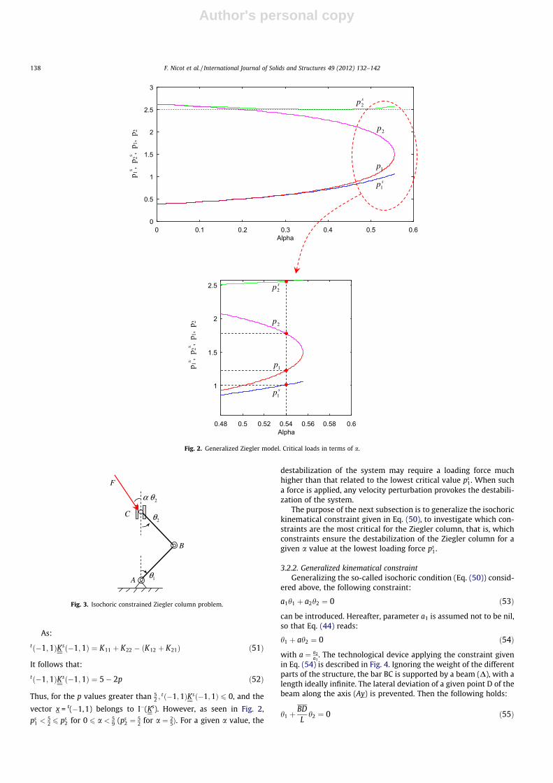
3.1. The generalized Ziegler column problem

An illustrating example is given with the nonconservativegeneralized Ziegler column, loaded by a partial follower load(Hermann and Bungay, 1964; Leipholz, 1987). The structure iscomposed of two bars AB and BC of length L, articulated on extrem-ities A and B with a torque bending k. A force F is imposed atextremity C, with an angle ah2 with the vertical direction y. Therotation of each bar is described with angles h1 and h2 (Fig. 1).Henceforth, the range of a is restricted to [0,1].

Given a force F with an inclination ah2, the question of the exis-tence of other geometrical configurations in the vicinity of the triv-ial solution h1 = 0 and h2 = 0, corresponding to the structureequilibrium, arises. This geometrical configuration is defined withangles h1 and h2. Assuming that both angles h1 and h2 are smallwith respect to 1, Eq. (9) yields:

2� p ap� 1�1 1� ð1� aÞp

� �h1

h2

� �¼

00

� �ð38Þ

where p ¼ FLk . K ¼ 2� p ap� 1

�1 1� ð1� aÞp

� �is the stiffness matrix. The

existence of another solution h�1; h�2

� �different from the trivial solu-

tion (0,0) requires that the determinant of K vanish, that is:

ð1� aÞp2 � 3ð1� aÞpþ 1 ¼ 0 ð39Þ

For a given value of a, Eq. (39) admits p-solutions if and only if a 6 59.

In that case, the two positive solutions p1 and p2 are:

p1 ¼32�

ffiffiffiffiffiffiffiffiffiffiffiffiffiffiffiffiffiffiffiffiffi94� 1

1� a

rand p2 ¼

32þ

ffiffiffiffiffiffiffiffiffiffiffiffiffiffiffiffiffiffiffiffiffi94� 1

1� a

rð40Þ

If 59 < a < 1;det K never vanishes and is strictly positive.

A

B

C

F

2θ

1θ

2θα

y

Fig. 1. Generalized Ziegler model subjected to partial follower load.

136 F. Nicot et al. / International Journal of Solids and Structures 49 (2012) 132–142

Author's personal copy

When a < 59, the two solutions correspond to the configurations

defined by the relation:

ð2� pÞh�1 þ ðap� 1Þh�2 ¼ 0 ð41Þ

where p 2 {p1,p2}. Only the ratio between angles h�1 and h�2 isdefined, not h�1 and h�2. According to the conclusions drawn in subSection 2.3, these configurations correspond to undifferentiatedequilibrium states, and whether the equilibrium configurationh�1; h

�2

� �is unstable will be investigated hereafter.

The stability analysis developed in Section 2 can be applied tothe generalized Ziegler column. At time t�; h1ðt�Þ ¼ h�1 and h2ðt�Þ ¼h�2. At any subsequent time t = t⁄ + D t, assuming that jh1(t)j =jh1j < < 1 and jh2(t)j = jh2j � 1, external and internal work ratesare expressed as:

_WextðtÞ ¼ FLðh1_h1 þ h2

_h2Þ � FLah2ð _h1 þ _h2Þ ð42Þ_WintðtÞ ¼ kðh1 � h2Þð _h1 � _h2Þ þ kh1

_h1 ð43Þ

After differentiation of Eqs. (42) and (43), it follows that:

€EcðtÞ ¼ k€h1ð�2h1 þ ph1 þ h2 � pah2Þ þ k€h2ðh1 � h2 þ ph2

� pah2Þ � kðð _h1Þ2ð2� pÞ þ ðpa� 2Þ _h1_h2 þ ð _h2Þ2ð1� p

þ paÞÞ þ _FLðh1_h1 þ h2

_h2Þ � _FLah2ð _h1 þ _h2Þ ð44Þ

Eq. (44) reads, at time t⁄:

€Ecðt�Þ ¼ k€h�1 �2h�1 þ ph�1 þ h�2 � pah�2� �

þ k€h�2 h�1 � h�2 þ ph�2 � pah�2� �

� k _h�1

� �2ð2� pÞ þ ðpa� 2Þ _h�1 _h�2 þ _h�2

� �2ð1� pþ paÞ

� �þ _F�L h�1 _h�1 þ h�2 _h�2

� �� _FLah�2 _h�1 þ _h�2

� �ð45Þ

As the configuration considered at time t⁄ defined with both anglesh�1 and h�2 corresponds to an equilibrium state, Eq. (38) holds, sothat:

�2h�1 þ ph�1 þ h�2 � pah�2 ¼ 0 and h�1 � h�2 þ ph�2 � pah�2 ¼ 0 ð46Þ

Prescribing the loading parameter F to remain constant from time t⁄

leads to _F ¼ 0.Moreover, the quadratic term _h�1

� �2ð2� pÞ þ ðpa� 2Þ _h�1 _h�2þ

_h�2

� �2ð1� pþ paÞ is associated with the symmetric part Ks ¼

2� p ap�22

ap�22 1� ð1� aÞp

!of matrix K. Finally, taking Eq. (19) into

account, and ignoring o(Dt) terms, a kinetic perturbation wouldgenerate an amount of kinetic energy calculated from Eq. (45) thatsimplifies to:

Ecðt þ DtÞ ¼ � ðDtÞ2

2t _h�1; _h�2

� �Ks _h�1; _h�2

� �ð47Þ

The quadratic term t _h�1;_h�2

� �Ks _h�1;

_h�2

� �corresponds to the second-

order work, defined in Eqs. (21), and (47) corresponds to the generalEq. (23) applied to the specific context of the Ziegler column.

When Ks admits negative eigenvalues, a velocity direction_h�1;

_h�2

� �exists that leads to negative values of the quadratic term

t _h�1; _h�2� �

Ks _h�1; _h�2� �

, that is, to positive values of Ec(t + Dt). Assuming

that a 6 59, the vanishing of det Ks is obtained for the critical values

ps1 ¼

3ð1�aÞ�ffiffiffiffiffiffiffiffiffiffiffiffiffiffiffiffiffiffiffiffi10a2�14aþ5p

2 1�a�a24

� � and ps2 ¼

3ð1�aÞþffiffiffiffiffiffiffiffiffiffiffiffiffiffiffiffiffiffiffiffi10a2�14aþ5p

2 1�a�a24

� � (the subscript ‘s’

indicates that the term refers to Ks). When p < ps1, all eigenvalues

of Ks are positive; when ps1 < p < ps

2;Ks admits one negative eigen-

value and one positive eigenvalue; when p > ps2, all eigenvalues of

Ks are negative. As shown in Fig. 2, both values p1 and p2 are be-tween ps

1 and ps2 (Challamel et al., 2009).

When p ¼ ps1;det Ks ¼ 0, and undifferentiated equilibrium con-

figurations _h�1;_h�2

� �exist that satisfy the relation:

ð2� pÞh�1 þap� 2

2h�2 ¼ 0 ð48Þ

For p ranging between ps1 and p1, det Ks < 0. Ks admits one negative

eigenvalue k and one positive eigenvalue. A velocity disturbance_h�1;

_h�2

� �exists that entails an increase in the kinetic energy of the

system:

ð2� p� kÞ _h�1 þap� 2

2_h�2 ¼ 0 ð49Þ

The unique equilibrium configuration h�1 ¼ 0; h�2 ¼ 0� �

is thereby lo-cally unstable.

When the load p is equal to p1, the equilibrium configurationðh�1 ¼ 0; h�2 ¼ 0Þ is no longer unique. All the configurations h�1; h

�2

� �with ð2� pÞh�1 þ ðap� 1Þh�2 ¼ 0 are equilibrium configurations.

When the load p is higher than p1 and lower than p2, both K andKs admit one negative eigenvalue and one positive eigenvalue.There is no loss of uniqueness of the equilibrium solution of thestatic problem. The unique equilibrium solution h�1 ¼ 0; h�2 ¼ 0

� �is locally unstable. A certain velocity disturbance applied to h1

and h2 provokes an increase in the system’s kinetic energy.When the load p is higher than p2 and lower than ps

2, K admitstwo negative eigenvalues, and Ks admits one negative eigenvalueand one positive eigenvalue. As in the previous case, there is noloss of uniqueness of the equilibrium solution of the static prob-lem. The unique equilibrium solution h�1 ¼ 0; h�2 ¼ 0

� �is locally

unstable. A certain velocity disturbance applied to h1 and h2 pro-vokes an increase in the kinetic energy of the system.

When the load p is higher than ps2, both K and Ks admit two neg-

ative eigenvalues. Whatever the vector x is, the quantity tx K x isnegative. The unique equilibrium solution h�1 ¼ 0; h�2 ¼ 0

� �is locally

unstable, and any velocity disturbance applied to h1 and h2 pro-vokes an increase in the kinetic energy of the system.

The next subsection investigates the fundamental role playedby external constraints in the local destabilization of the system.

3.2. Instability with constraints

3.2.1. The isochoric conditionThe generalized Ziegler column problem is considered by

henceforth preventing the lateral deviation of point C (Fig. 3). Thisconstraint reads:

h1 þ h2 ¼ 0 ð50Þ

Interestingly, Eq. (50) corresponds to a so-called isochoric condi-tion, like that used in soil mechanics for the standard undrained tri-axial test: an axial loading is applied to the soil specimen, while theisochoric condition (the volume is maintained constant) _e1 þ 2 _e3 ¼0 is prescribed ( _e2 ¼ _e3 for axisymmetric reasons).

Assume that the system is initially loaded so that p > ps1. The

equilibrium configuration ðh�1 ¼ 0; h�2 ¼ 0Þ is locally unstable. Thedestabilization of the system requires that a certain velocity distur-

bance _h�1;_h�2

� �be applied, verifying t _h�1;

_h�2

� �Ks _h�1;

_h�2

� �< 0 (the vec-

tor x ¼ t _h�1;_h�2

� �belongs to I� (Ks)).

The question that arises is whether the isochoric constraint gi-ven in Eq. (50) can destabilize the system: does the vectorx = t(�1,1) belong to I� (Ks)?

F. Nicot et al. / International Journal of Solids and Structures 49 (2012) 132–142 137

Author's personal copy

As:

tð�1;1ÞKsð�1;1Þ ¼ K11 þ K22 � ðK12 þ K21Þ ð51Þ

It follows that:

tð�1;1ÞKsð�1;1Þ ¼ 5� 2p ð52Þ

Thus, for the p values greater than 52 ;

tð�1;1ÞKsð�1;1Þ 6 0, and the

vector x = t(�1,1) belongs to I�(Ks). However, as seen in Fig. 2,

ps1 <

52 6 ps

2 for 0 6 a < 59 (ps

2 ¼ 52 for a ¼ 2

5Þ. For a given a value, the

destabilization of the system may require a loading force muchhigher than that related to the lowest critical value ps

1. When sucha force is applied, any velocity perturbation provokes the destabili-zation of the system.

The purpose of the next subsection is to generalize the isochorickinematical constraint given in Eq. (50), to investigate which con-straints are the most critical for the Ziegler column, that is, whichconstraints ensure the destabilization of the Ziegler column for agiven a value at the lowest loading force ps

1.

3.2.2. Generalized kinematical constraintGeneralizing the so-called isochoric condition (Eq. (50)) consid-

ered above, the following constraint:

a1h1 þ a2h2 ¼ 0 ð53Þ

can be introduced. Hereafter, parameter a1 is assumed not to be nil,so that Eq. (44) reads:

h1 þ ah2 ¼ 0 ð54Þ

with a ¼ a2a1

. The technological device applying the constraint givenin Eq. (54) is described in Fig. 4. Ignoring the weight of the differentparts of the structure, the bar BC is supported by a beam (D), with alength ideally infinite. The lateral deviation of a given point D of thebeam along the axis (Ay) is prevented. Then the following holds:

h1 þBDL

h2 ¼ 0 ð55Þ

0

0.5

1

1.5

2

2.5

3

0 0.1 0.2 0.3 0.4 0.5 0.6Alpha

p 1s ,

p 2s ,

p 1,

p 2

1

1.5

2

2.5

0.48 0.5 0.52 0.54 0.56 0.58 0.6Alpha

1p

sp1

2p

sp2

p 1s ,

p 2s ,

p 1,

p 2

1p

2p

sp2

sp1

Fig. 2. Generalized Ziegler model. Critical loads in terms of a.

A

B

C

F

2θ

1θ

2θα

Fig. 3. Isochoric constrained Ziegler column problem.

138 F. Nicot et al. / International Journal of Solids and Structures 49 (2012) 132–142

Author's personal copy

where the algebraic quantity a ¼ BDL can take positive or negative

values, its absolute value being less or greater than 1, accordingto the relative position of point D with respect to the segment [BC].

For the p values within the range ps1; p

s2

� , the set I� gathering all

vectors x ensuring that the quantity tx Ksx is negative is not reducedto the nil vector. The parameter a ¼ BD

L must therefore be determinedso that each vector x ¼ tð _h1; _h2Þ, satisfying Eq. (55), also belongs to I�.This requirement is fulfilled when the vector t(a,�1) belongs to I�.When p > ps

2, the vector t(a,�1) belongs to I� regardless the valueof a, because both eigenvalues of Ks are strictly negative.

Let the quadratic form vðaÞ ¼ tða;�1ÞKsða;�1Þ ¼ K11a2�ðK12 þ K21Þaþ K22 be considered. The sign of the quadratic formv depends upon the sign of the discriminant, equal to �4 det Ks.

When p < ps1;det Ks > 0, and v(a) is of the sign of K11 = 2 � p; as

p < ps1 < 2, it follows that v is positive, and whatever the value of a,

the vector t(a,�1) does not belong to I�.When ps

1 < p < ps2;det Ks < 0. As K11 = 2 � p, then:

– If ps1 < p < 2, the vector t(a,�1) belongs to I� for a 2 ]a1,a2]

– If 2 < p < ps2, the vector t(a,�1) belongs to I� for

a 2 ] �1 ;a2] [ ]a1;+1]

with a1 ¼K12þK21�2

ffiffiffiffiffiffiffiffiffiffiffiffi�det Ksp

2K11and a2 ¼

K12þK21þ2ffiffiffiffiffiffiffiffiffiffiffiffi�det Ksp

2K11.

It is worth noting that a1 !p!2��1 and a1 !

p!2þþ1, whereas

a2 !p!2

2K22K12þK21

¼ 2a�1a�1 .

When p > ps2;det Ks > 0; the discriminant of v(a) is therefore

negative, and v(a) is of the sign of K11 = 2 � p. Recalling thatps

2 P 2, it follows that v is strictly negative. Whatever the valueof a, the vector t(a,�1) belongs to I�.

As a consequence, the value of a ensuring that the vector t(a,�1)belongs to I� strongly depends on both parameters p and a. Thecritical loading for the constrained Ziegler column corresponds tothe first value vanishing det Ks, that is, to p ¼ ps

1. Under the corre-sponding loading force, the system is at a bifurcation point: thestate h�1 ¼ 0; h�2 ¼ 0

� �corresponds to an undifferentiated equilib-

rium, the transition between a stable state and a locally unstablestate. The related kinematical constraint is obtained for

a ¼ K12 þ K21

2K11¼

ffiffiffiffiffiffiffiffiK22

K11

s¼ aps

1 � 22 2� ps

1

� � ;with ps

1 ¼3ð1� aÞ �

ffiffiffiffiffiffiffiffiffiffiffiffiffiffiffiffiffiffiffiffiffiffiffiffiffiffiffiffiffiffiffiffiffiffi10a2 � 14aþ 5p

2 1� a� a2

4

� � :

4. Instability of rigid plates with aeroelastic effects

4.1. Physical system

Let the stability of a massive rigid plate of unit width and spe-cific mass l per unit length be considered. The plate is suspended

on springs of stiffness C1 and C2 as shown in Fig. 5. Initially in a hor-izontal position of static equilibrium, the plate is loaded by wind ofvelocity v, characterized by the wind force resultant F = nv2h actingat a distance a ahead of the downwind end of the plate. n is a con-stant parameter and h is the rotation of the plate. The foregoingdefinition of F is valid only for very slow oscillations. The locationof the resultant of the aerodynamic forces on the plate is called theaerodynamic center in aeroelasticity. For two-dimensional incom-pressible flow, this center is located at a = 3b/4, while for super-sonic flow it is located at a = b/2 (Bazant and Cedolin, 2003).

Denoting the deflection from the static equilibrium position atmidpoint as w, the dynamics equations of vertical forces and mo-ments around the center of the plate are written as:

M€xþ Kx ¼ 0 with x ¼w

h

� �;M ¼

lb 0

0 lb3

12

!

and K ¼k11 k12

k21 k22

� �ð56Þ

The stiffness matrix is detailed below:

k11 ¼ C1 þ C2

k12 ¼ b C1�C22 � nv2

k21 ¼ b C1�C22

k22 ¼ b2

4 ðC1 þ C2Þ � nv2 a� b2

� �

8>>>><>>>>: ð57Þ

Using a normalization procedure for the mass matrix, the differen-tial equations can also be presented in an equivalent way:

1€xþ eKx¼ 0 with x¼w

h

� �;1¼

1 00 1

� �and eK ¼ ~k11

~k12

~k21~k22

!ð58Þ

where the modified stiffness matrix is now given by:

~k11 ¼ C1þC2lb

~k12 ¼ C1�C22l �

nv2

lb

~k21 ¼ 6 C1�C2

lb2

~k22 ¼ 3lb ðC1 þ C2Þ � 12nv2

lb3 a� b2

� �

8>>>>>>><>>>>>>>:ð59Þ

The flutter condition is written as:

ð~k11 � ~k22Þ2 þ 4~k12~k21 ¼ 0 ð60Þ

whereas the divergence criterion det (K) = 0 is reduced to:

~k11~k22 ¼ ~k12

~k21 ð61Þ

Fig. 5. Elastically supported rigid plate under aerodynamic forces.

( )Δ

D

y

A

BC

F

2θ

1θ

2θα

Fig. 4. Generalized constrained Ziegler column problem.

F. Nicot et al. / International Journal of Solids and Structures 49 (2012) 132–142 139

Author's personal copy

It can be shown that flutter can appear only if C1 > C2 (see Bazantand Cedolin, 2003).

4.2. Divergence instability of the free system

It is possible to express the stiffness matrix K in a dimensionalformat, according to the equivalence equality:

Kx ¼ ðC1 þ C2Þkw

bh

� �with

k ¼1 c

2� vc2

14� v a

b� 12

� � !and

c ¼ C1�C2C1þC2

v ¼ nv2

bðC1þC2Þ

8<: ð62Þ

The dimensionless stiffness matrix k only depends on three dimen-sionless parameters, namely the dimensionless loading parameterv, the a/b ratio equal to 1/2 or 3/4 depending on the analysis con-sidered, and the stiffness ratio parameter c. This last parameter cmeasures the level of stiffness asymmetry in the mechanical sys-tem. The parameter c is vanishing for symmetrical stiffness connec-tions C1 = C2. The divergence criterion of the free systemcorresponds to the vanishing of the dimensionless stiffness matrix,det k = 0, which gives:

v ¼ c2 � 12 c � 2 a

bþ 1� � ð63Þ

Fig. 6 shows the dimensionless buckling load parameter v versusthe dimensionless stiffness parameter c.

4.3. The constrained system

Now the constrained system is shown in Fig. 7, where the twokinematic parameters are linked by a mechanism parameterizedby a fixed polar value x0. This mechanism models the connectionof the wing to the aircraft body.

As shown in Fig. 7, we have:

tan h ¼ wx0 þ b=2

ð64Þ

leading to the linearized additional constraint for a fixed value ofx0:

w� h x0 þb2

� �¼ 0 ð65Þ

More generally, let the general additional kinematic relationship beconsidered:

a1wþ a2hb ¼ 0 ð66Þ

Comparing Eqs. (65) and (66), it follows that:

a ¼a1

a2

� �¼

1� 1

2þx0b

� � !ð67Þ

The symmetric part of the (dimensionless) tangent stiffness matrixreads:

ks ¼1 1

2 ðc � vÞ12 ðc � vÞ 1

4� v ab� 1

2

� � !ð68Þ

The eigenvalues of ks are plotted in Fig. 8, for different values of theparameter v, in the case where c = 0 and a/b = 1/2 or a/b = 3/4. Theeigenvalue k1 decreases from positive values to negative values,when the loading parameter v increases.

Thus, the basic question is whether the kinematic constraint en-sures that the vector (a2,�a1) belongs to the negative isotropiccone I�(ks), when k1 takes negative values.

The negative isotropic cone I�(ks) gathers all the vectors

x ¼ wbh

� �such that ks

ijxixj 6 0. Asks

ijxixj

ðC1þC2Þb2h2 ¼ wbh

� �2 þ ðc � vÞ wbhþ

14� a� 1

2

� �v

� �, the negative isotropic cone I� (ks) can also be consid-

ered as a subset of R, with respect to the scalar w/bh. In this case,

I�(ks) coincides with the segment [A,B], where:

0

0.5

1

1.5

2

2.5

3

-2 -1.5 -1 -0.5 0 0.5 1 1.5 2

a/b = 0.5 a/b = 0.75c

χ

Fig. 6. Divergence instability load versus dimensionless connection parameter forthe free system.

Fig. 7. Elastically supported rigid plate under aerodynamic forces for the constrained system.

140 F. Nicot et al. / International Journal of Solids and Structures 49 (2012) 132–142

Author's personal copy

A ¼v� c �

ffiffiffiffiffiffiffiffiffiffiffiffiffiffiffiffiffiffiffiffiffiffiffiffiffiffiffiffiffiffiffiffiffiffiffiffiffiffiffiffiffiffiffiffiffiffiffiffiffiffiffiffiðc � vÞ2 � 1þ 4 a� 1

2

� �v

q2

ð69Þ

B ¼v� c þ

ffiffiffiffiffiffiffiffiffiffiffiffiffiffiffiffiffiffiffiffiffiffiffiffiffiffiffiffiffiffiffiffiffiffiffiffiffiffiffiffiffiffiffiffiffiffiffiffiffiffiffiffiðc � vÞ2 � 1þ 4 a� 1

2

� �v

q2

ð70Þ

The kinematic constraint belongs to the negative isotropic coneI�(ks) if �a2 /a1 = 1/2 + x0/b belongs to the segment [A,B].

The evolution of A and B in terms of the loading parameter v isgiven in Fig. 9, in the case in which a/b = 1/2, for v P 1 (k1 vanishesfor v = 1). It can be shown that A decreases from 0.5 (v = 1) to zero(v tends toward +1) and B increases from 0.5 (v = 1) to +1 (vtends toward +1). As a consequence, for any positive value of�a2/a1 = 1/2 + x0/b, a critical value vc exists such that for any valuev larger than vc, A < 1/2 + x0/b < B.

As a consequence, the equilibrium configuration (w = 0,h = 0) isunstable for the constrained problem under loading that verifiesthe condition v > vc. A certain velocity disturbance exists that pro-vokes the divergence of the system.

It is worth noting that when xo = 0, the kinematic constraint en-sures that the vector (a2,�a1) belongs to the negative isotropiccone I�(ks) for any value v P 1.

5. Concluding remarks

This paper has investigated the occurrence of instability forstructural systems subjected to nonconservative loadings. Extend-ing the approach developed in soil mechanics, a general equationrelating both the second-order time derivative of the kinetic en-

ergy and the second-order work was recovered. This equationspecifies in which conditions, under a constant loading, the sys-tem’s kinetic energy may increase under proper velocity distur-bances. As in soil mechanics, the second-order work is shown toplay a basic role.

As a quadratic form, the spectral properties of the symmetricpart of the associated (tangent stiffness) matrix entirely determinethe existence of velocity disturbances directing a nil or negative va-lue of the second-order work: when the symmetric part of the tan-gent stiffness matrix admits at least one negative eigenvalue, thenvelocity disturbances directing a nil or negative value of the sec-ond-order work exist.

Then kinematically constrained structures were examined. Thestructure is subjected to a set of constraints, as linear combinationsof the kinematic variables. As a result, these constraints reduce thekinematic degrees of freedom. Each constraint is described by theequation of a hyperplane. In cases where the symmetric part of thetangent stiffness matrix admits one negative eigenvalue, it isshown that the structure is more prone to destabilize when theassociated eigen subspace is included within the hyperplanedescribing each constraint. The critical case is obtained when theintersection of all the hyperplanes corresponds to the eigen sub-space associated with a negative eigenvalue. Then any velocity dis-turbance applied to the structure will entail an increase in thekinetic energy of the structure.

These results were applied to the case of the generalized Zieglercolumn, loaded by a partial follower force. It is shown how specifickinematic constraints have to be chosen in order to minimize theloading force leading to an instability situation.

Finally, the case of an aircraft wing with aeroelastic effects wasconsidered. It is shown that the introduction of specific kinematicconstraints (modeling the connection of the wing with the aircraftbody) can destabilize the unconstrained system.

Acknowledgments

The French Federative Research Structure VOR (Natural Hazardsand Structure Vulnerability) is gratefully acknowledged by theauthors. The European project LESSLOSS, and the French national(ANR) SIGMA, STABROCK and Snow-White projects also supportedthis research.

References

Bazant, Z., Cedolin, L., 2003. Stability of Structures. Dover Edition Publication, Inc.,New-York.

Bigoni, D., Hueckel, T., 1991. Uniqueness and localization, I. Associative and non-associative elastoplasticity. Int. J. Solids Struct. 28 (2), 197–213.

-3

-2

-1

0

1

2

3

4

0 1 2 3 4 5χ

λ 1, λ

2

λ1, a/b=3/4

λ1, a/b=1/2

λ2, a/b=1/2

λ2, a/b=3/4

Fig. 8. Eigenvalues of the symmetric part of the stiffness matrix over the loading parameter.

0

0.20.4

0.60.8

1

1.21.4

1.61.8

2

1 1.2 1.4 1.6 1.8 2

A, B

χ

A

B

Fig. 9. Negative isotropic cone over the loading parameter; a/b = 1/2.

F. Nicot et al. / International Journal of Solids and Structures 49 (2012) 132–142 141

Author's personal copy

Bolotin, V.V., 1963. Nonconservative Problems of the Theory of Elastic Stability.Pergamon Press, New-York.

Challamel, N., Nicot, F., Lerbet, J., Darve, F., 2009. On the stability of non-conservative elastic systems under mixed perturbations. EJECE 13 (3), 347–367.

Challamel, N., Nicot, F., Lerbet, J., Darve, F., 2010. Stability of non-conservativeelastic structures under additional kinematics constraints. Eng. Struct. 32,3086–3092.

Darve, F., Servant, G., Laouafa, F., Khoa, H.D.V., 2004. Failure in geomaterials,continuous and discrete analyses. Comput. Methods Appl. Mech. Eng. 193,3057–3085.

Hermann, G., Bungay, R.W., 1964. On the stability of elastic systems subjected tononconservative forces. J. Appl. Mech. 86, 435–440.

Hill, R., 1958. A general theory of uniqueness and stability in elastic–plastic solids. J.Mech. Phys. Solids 6, 236–249.

Iordache, M.M., Willam, K.J., 1998. Localized failure analysis in elastoplasticCosserat continua. Comput. Methods Appl. Mech. Eng. 151 (3-4), 559–586.

Ishaq, M., 1955. Sur les spectres des matrices. Séminaire Dubreuil, Algèbre etthéorie des nombres, vol. 9, pp. 1–14.VV.

Leipholz, H., 1987. Stability Theory. John Wiley Publication, New-York.Lignon, S., Laouafa, F., Prunier, F., Khoa, H.D.V., Darve, F., 2009. Hydromechanical

modelling of landslides with a material instability criterion. Geotechnique 59(6), 513–524.

Nguyen, Q.S., 2000. Stabilité et mécanique non linéaire. Hermès SciencesPublication, p. 461.

Nicot, F., Darve, F., 2007. A micro-mechanical investigation of bifurcation ingranular materials. Int. J. Solids Struct. 44, 6630–6652.

Nicot, F., Darve, F., Khoa, H.D.V., 2007. Bifurcation and second-order work ingeomaterials. Int. J. Numer. Anal. Methods Geomech. 31, 1007–1032.

Nicot, F., Sibille, L., Darve, F., 2009. Bifurcation in granular materials: an attempt at aunified framework. Int. J. Solids Struct. 46, 3938–3947.

Nicot, F., Challamel, N., Lerbet, J., Prunier, F., Darve, F., 2011. Mixed loadingconditions, revisiting the question of stability in geomechanics. Int. J. Num.Anal. Methods Geomech. 35 (3), 1409–1431.

Petryk, H., 1993. Theory of bifurcation and instability in time-independentplasticity. In: Nguyen, Q.S. (Ed.), Bifurcation and stability of dissipativesystems, CISM Courses and Lecturers, vol. 327. Springer, pp. 95–152.

Prunier, F., Nicot, F., Darve, F., Laouafa, F., Lignon, S., 2009a. 3D multiscalebifurcation analysis of granular media. J. Eng. Mech (ASCE) 135 (6), 1–17.

Prunier, F., Laouafa, F., Lignon, S., Darve, F., 2009b. Bifurcation modeling ingeomaterials: from the second-order work criterion to spectral analyses. Int.J. Numer. Anal. Methods Geomech. 33 (9), 1169–1202.

Sibille, L., Nicot, F., Donze, F., Darve, F., 2007a. Material instability in granularassemblies from fundamentally different models. Int. J. Numer. Anal. MethodsGeomech. 31, 457–481.

Sibille, L., Donzé, F., Nicot, F., Chareyre, B., Darve, F., 2007b. Bifurcation detectionand catastrophic failure. Acta Geotec. 3 (1), 14–24.

Ziegler, H., 1968. Principles of Structural Stability. Blaisdell Publishing Company.

142 F. Nicot et al. / International Journal of Solids and Structures 49 (2012) 132–142