SOLUTION OF THE MULTIGROUP ANALYTIC NODAL DIFFUSION EQUATIONS IN

3-DIMENSIONAL CYLINDRICAL GEOMETRY

N A N H. PRINSLOO

Dissertation submitted in partial fulfillment of the requirements for the degree Magister Scientiae in Reactor Science at North-West

University, Potchefstroom campus.

Supervisor: Prof. H. Moraal Co-supervisor: Dr. D.I. TomaSeviE

December 2006

Abstract.

I'iodal diffusion met.hods have been used estensively in nuclear react.or calculat io~~s: specifi-

cally for their performance advantage, but. also their superior accuracy. In this work a nodal

diffusion method is developed for three-dimensional c~lindrical geometry. Recent develop-

nlcnts in t,he Pebble Bed Modular React.or (PBMR) project have sparked renewed interest

in the application of different. modeling 1net.hods t.o it,s design, and riaturally included in t.his

effort is a nodal met.hod for cylindrical geomet.ry. More spccificall~, the Anal5t . i~ Yodale

Met.hod ( A Y M ) has been applied to numerous reactor problems with much success. The

m u l t i - p u p ASM is applied to Cartesian geometry in the Xecsa developed OSCAR-3 code

syst.em used for the calcuiat.ion of VTR and PWR tFpe nuclear reactors. Hnwever: in support.

of the PBMR prosect., a need has arisen t.o include the AS14 in cylindrical geonletry.

The -4Nhl is based on a transverse irltegratiom principle, result,itlg in a set, of one-

dimensional equat.ions containing inhomogeneo~~s sources. The issue of applying this met,hod

t,o 3D cylindrical geometry has never been sat.isfactorily addressed, due to difficulties in per-

forming the trans\.erse int,egration, and a proposed solution entails t.he use of confornlal

mapping in order t.o circumvent. these difficulties. This approach should 1,ieid a set. of ID

equat.ions 1vit.h an est.ra, geometrically dependent., "ghost." source. This t.hesis describes t,he

mat.hematica1 development of t.he conformal mapping approach, as well as t . 1 ~ numerical

alralysis via a developed FORTR.AX test code. The code is applied t.o a series of test prob-

lems, ranging from idealized const.ruct.ions to rea1ist.i~ PBMR 400 h11V designs. Results show

t,hat the nlet.hod is viable and yields much improved ;sccuracy and perfctrmaric:e, similar to

what, may be expected from nodal methods.

Xodalc difl'usit..metodcs curd ekst-ensief gebruik in kernreaktorborelte~~irige. spesifiek vir dic

spvcd- en i;ikliuraatt~eidsvc,ordelc. wat hulle bied, In hiedip vurhandeling word 'n nodale dif-

f'wie~netnde ontcikkel vir die gebruik i n meer-grcrrep, drie-di~nensioncle silindriese geomet.rie.

Die onlangse venvikkeIinge rakende die ICorrelbedrcak~orprojek het 'n nune inspuiting aan

berekcninpsrnet.odes vir sulke reaktore gesee en die silindriese notiale diffusicrnetode is 'ri

belan~rike bousteen van so 'n berekeningst.else1. Die Analitiese Yodale l ietode (.-2SlI) word

met g o o t sukses i n hierdie veld van globale reaktorber-ekeninge gebruik. Hierdie met.odc. is

ten volle ~~irnplementeer in ICart.esiese geometric in die Secsa-ontwiklielde OSC-4K bereken-

ingstelsel. llet. die oog op die ondersteuning van die Korrelbedreaktorprojek. her die behoefte

ont,staan om 'n silindriew oplossings~net~ode by hierdie ~ist.eem te voeg.

Die AXM word b s e e r op die beginsel van t.ranswrsale int.egrz4e, vat 'n reeks een-

dirnensionele vergelykings tot gevolg het. Elk lpan hierclic vergdykings bevar 'n s ~ c l nie-

homogene bronne en kan anczlities opgelos word. Die toepassing van hierdie rne~odiek op

silindriese georne.t.rie is nog nie in die verlede suksesvol aangespreek nie, aangesien d a ~

n i s k u n d i ~ ~ strriikelblokke in die t,ransverse integ~asie proses is. In hierdie 1.w-handcling word

'n moont.like oplossing, via die gebruik can die konforme afbeeldingst.egniek: bespreek. Hi-

erdie metode bchoort. ook 'n stel een-dirnrnsionele rergelykings t.e produseer: maar i ~ i hierdic

geval met 'n ekstra. nie-homogene? geornetriesafttanklike bron. Die wiskundige ont.nikkelil~g

en n u r n e r i ~ s ~ evaluasie van hierdie met.ode (via 'n ~ n t t ~ i k k ~ l d e FORTR.45 toetskode) word

i r ~ hierdie \t.erk beskr!-f. en resultate worcl verskaf vir beide geidealiseelde opstellings ell re-

alist.iese korrelbedprobiemc. Resultate dui danrop dat, die metodc aao die t.ipiese st.andaarde

1.an nodalc n-iet.odes voldoen.

Xarly palties and spccial indi~iduals have co~it.ributed d u r i ~ ~ g t.lie development of t.his work.

First mid forexnost I would like t,o ttmili Dr. D~ordje I. TornaSevici for his endles.s, unselfish

guidance and support throughout t.he spar] of t,his work. Furtlwrrnore! t.o t . 1 ~ rest. of' the

Radiation and Rmct,or Theory (RRT) Dcpart.ment I wish t.o extend a sincere ivoi-d of g a t . -

itude for t,heir ini.aluahle support during the past. three years. as well as t.o Secsa for t.he

oppor tuni t t.o work on this int.erest.ing t.opic. Specific ~nent.ion a1.w has t,o be n-lade of Dr.

Wessel Joubert. and Frederik Reitsma from PB3.IR for their. continuous input and feedbad.;.

-4 turt,her spccial word of t.hanks 1.0 Prof. Harm lioraal from Sor th-5esr 1'niversit.y (as

well as Hantie Labuschagne from RRT) for man:- hours of reading, checking, corrections and

su~ .~ps t ions during the writing of this thesis.

On a personal level! I wish 1.0 est.end special appreciat.ion t.o all m. farnil. and friends,

especially to my fat.her Hennie and fiance Chanelle, for their unselfish, patient support,.

Finall?, to nl!. Hea~.enl~. Father for the ample opportunities He has provided me with: and

the special people He has blessed me with.

1 ~ T R O D U C T I O ~ 9

. . . . 1 . I Reactor calctll:.*t icmal rnc?rhods and the South ."l rican nuclear industv- 9

. . . . . . . . . . . . . . . . . 1 Core solut.ion methods in cylindrical geometry 10 . . . . . . . . . . . . . . . . . . . . . . . . . . . . . . . . 1.3 PB\. IR background 12

. . . . . . . . . . . . . . . . . . . . . . . . . . . . . . . . . . 1 . 4 >-odd met.hods 15

. . . . . . . . . . . . . . . . . . . . . . . . . . . . . . . . 1 . Goals of this thesis l S

. . . . . . . . . . . . . . . . . . . . . . . . . . . . . . . . 1.6 La~.out of thc: thesis 19

2 DEVEL. OPS4ENT OF A 3D FINITE-DIFFERESCE. SOLVER 2 1

2.1 1nt.rodurt.ion. . . . . . . . . . . . . . . . . . . . . . . . . . . . . . . . . . . . '71 9 7 . . . . . . . . . . . . . . . . . . . . . . . . . . . . . . 2.2 C;eometric description --

. . . . . . . . . . . . 2.3 Finite-diKel-enc~ equations in 3D c?~Iindsical coordinates 24

. . . . . . . . . . . . . . . . . . . 2 .1 3D solution process - the T-point equations 25

. . . . . . . . . . . . . . . . . 2.4.1 Xumerical implementation of solution 33

. . . . . . . . . . . . . . . . . . . . . . . . 2.3 Code implernentat.ion arid ksting 35 . . . . . . . . . . . . . . . . . . . . . . . . . . . . . . . . . . . . 6 Conclusion 41

3 DER.IVATIOX OF A3-ALYTIC XOD.4 L METHOD IN CYLISDRICAL

GEOMETRY 4 2

3.1 Introduction 42 . . . . . . . . . . . . . . . . . . . . . . . . . . . . . . . . . . . .

. . . . . . . . . . . . . . . . . . . . . . 3.2 Balance equat. ion in three di~nensions 43

. . . . . . . . . . . . . . . . . . . . . . . . . . . . . . . 3.3 C'.orifonnal mapping 46

. . . . . . . 3 . 1 Rcl~tionshiy bct.n.eeri mapped and u ~ m a p p e d quantities 50

. . . . . . . . . . . . . . . . . . 3.4 'Trans-erse integratior~ of mapped equat.ions 53

. . . . . . . . . . . . . 3.4.1 Transverse integration o l w z: : the il-equa~ion 5.3 7 - . . . . . . . . . . . . . 3.4.2 Tsansl:erw ii~tegration mrer u : the 1. - equation a:>

. . . . . . . . . . . 3.4.3 'Transverw ini.egration uver (1. . ( I ) - t h c -,-er.~ualir!n 61

3.4 .4 Suniniar~ . . . . . . . . . . . . . . . . . . . . . . . . . . . . . . . . . . G:3

. . . . . . . . . . . . . . . . . . . 3.5 Sol~.itiori to t.he one-tlimension:il u-ec(uat.icm

. . . . . . . . . . . . . . . . . . . . . . . . . 3.3.1 Calrulat ion of moments

. . . . . . . . . . . . . . . . . . . . . . . 3.rJ.2 Current and flus expressions

. . . . . . . . . . . . . . . . . . . . . . . . . . . . . . 3.3.3 Tensorid source

. . . . . . . . . . . . . . . . . . . 3.6 Solution to t. he one-dimemiod c-equatic-~n

. . . . . . . . . . . . . . . . . . . . 3.6.1 Det.ermination of source moments

. . . . . . . . . . . . . . . . . . . . . . . 3.6.2 Ciment and flus expressions '3 ' . . . . . . . . . . . . . . . . . . . . . . . . . . . . . . .,. 6.3 Tensorial source

. . . . . . . . . . . . . . . . . . . 3.7 Solutiorl to the on?-din-lensiond z-equat ion

3.7.1 Determination of source moments . . . . . . . . . . . . . . . . . . . . . . . . . . . . . . . . . . . . . . . . . . . 3.7.2 Current and f lus espres.sions

. . . . . . . . . . . . . . . . . . . . . . . . . . . . . . 3.7.3 Tensol-ial source

. . . . . . . . . . . . . . . . . . . . . . . . . . . . . . . . . 3.8 Ealance equat.ion

. . . . . . . . . . . . . . . . . . . . . . . . 3.9 Transverse leakage approsirnat.ion

. . . . . . . . . . . . . . . . . . . . . . . . . . . . . . . . . . . . . 3.10 Conclusion

4 F13TE-41ESH L I l U T

4.1 1nt.roduction . . . . . . . . . . . . . . . . . . . . . . . . . . . . . . . . . . . . . . . . . . . . . . . . . . . . . . . . . . . . . . . . . . . . . . 4.2 Axial dire-ct ion

. . . . . . . . . . . . . . . . . . . . . . . . . . . . . . . . . . 4.3 Radial direction

. . . . . . . . . . . . . . . . . . . . . . . . . . . . . . . . 4.4 . 4zinlu t.l~al direct.ion

. . . . . . . . . . . . . . . . . . . . . . . 4 .5 Fine-mesh ~spressions in the center

. . . . . . . . . . . . . . . . . . . . . . . . . . . . . . . . . . . . . 4.6 Conclusion

5 NODAL CODE VALIDITY . . . . . . . . . . . . . . . . . . . . . . . . . . . . . . . . . . . . 5 . 1 Int roducr ion

. . . . . . . . . . . . . . . . . . . . . . . . . . . . . . . 5.2 Test code descsiption

. . . . . . . . . . . . . . . . . . . . . . . . . . . . . 3.3 H o l l o ~ . cylinder problem

. . . . . . . . . . . . . . . . . . . . . . . . . . . . . . 3.1 "Striped" (r.0) problem

6 RESULTS AKD DISCUSSIO3- . . . . . . . . . . . . . . . . . . . . . . . . . . 6.1 Dodds' bench~nark application

. . . . . . . . . . . . . . . . . . . . . . . . . . . . . . . . 6. 2 PBlIR application

. . . . . . . . . . . . . . . . . . . . . . . . . 6 .3 I.4E.4 c!:lindric~al 3D benrhn-lark

7 CONCLUSIOXS AXD FUTURE WORK . . . . . . . . . . . . . . . . . . . . . . . . . . . . . . . . . . . ; . I IntrocIuct.ion

- I .t> Gmeral conclusions . . . . . . . . . . . . . . . . . . . . . . . . . . . . . . . 143 - 1 . 3 Flituw i w k . . . . . . . . . . . . . . . . . . . . . . . . . . . . . . . . . . . . 146

7 .3 Firial ct?~isidrratiuns . . . . . . . . . . . . . . . . . . . . . . . . . . . . . . . . 146

A TEST CODE USER M4TiCTAL 148

B DODDS BESCHMARK PROBLEM 161

C TEST CODE INPUT EXAMPLES 163

D IAEA BENCHMART< DESCRIPTIOS (CYLTKDRICAL) 168

E RECURRESCE RELATIOSSHIPS FOR FLUX h*IO;\,IESTS 173

E. l Flus moments . . . . . . . . . . . . . . . . . . . . . . . . . . . . . . . . . I73

E.2 liapped flux momcnts . . . . . . . . . . . . . . . . . . . . . . . . . 173

F EXPANSIONS FOR DOUBLE LEGENDRE IXTEGRALS 177

G TRAXSVERSE LEAKAGE QLJADRATIC FIT 181

List of Figures

313 cylindrical discret. ization scheme . . . . . . . . . . . . . . . . . . . . . . . I I

PBMR 400 1IIY schematic core layout . . . . . . . . . . . . . . . . . . . . . I 4

PBMR fuel design . . . . . . . . . . . . . . . . . . . . . . . . . . . . . . . . . 13

.\mi's ( 7 . . Z) fixed source benchmark problem i l lu~~rat iu t i . . . . . . . . . 37

DODDS' benchmark rnodel in IT. 2'1 gwn~etry . . . . . . . . . . . . . . . . . 39

Gonforr~ial mapping . q.lindrical to recmngular mapping . . . . . . . . . . . 45

. . . Infinite cylinder flus and eigemdue error trends . 2nd order expansio~ 113

(1.0) "Striped" problem geometric description . . . . . . . . . . . . . . . . . . 115

Rdwence solutio~l for t. he "St. riped" problem . . . . . . . . . . . . . . . . . . 116

. . . . . . . . . "Striped" problem flus error (radial profile) along source zone 118

. . . . . . . "Scriyed" problem flus error (radial profile) along absorber zone 118

Dodds 2D ( r . 2 ) . radial profile (axially-averaged) . . . . . . . . . . . . . . . 121

Dodds 2D ( 7 ... z ) . axial profile (radiall>..a~.el.aged) . . . . . . . . . . . . . . . 122

F'BXiR 21) ( I - : t j material la*oub . . . . . . . . . . . . . . . . . . . . . . . . . 123

3D P B N R 400 . ( 1 .. U j projection (not tcr S C Z ~ C ) . . . . . . . . . . . . . . . . . 12.3

FD convergence error v s performance (calculat. ional time) . . . . . . . . . . . 126

. . . . . PI3.\.fR benchmark radial multi-group flus profiles {asiall!.-a~deraged) 127

PElIR be~ichrnark axial niulti-group flus profiles (radially-a\.eragcd) . . . . . 128

3D FD con\:ergcnce error vs performanccl (calcuiationaI time) . . . . . . . . . I29

PB1LR: R. adial profile through and adjacent t.o cont.rnl . . . . . . . . . . . . 130

6.111 PBl iR: Group fluxes through control . azimuthal prufile . . . . . . . . . . . 131

6.11 I.4E.i ( T - : ::) layout . azimuthal cut at 45 deg,rse as . . . . . . . . . . . . . . . . 1.32

6.12 I.4E.A ( I .. z ) layout . azimuthal cul a! CL degrees . . . . . . . . . . . . . . . . 133

6.13 I.AE.4 ( 7 .. 0) la!.out . - r.op ~ i e n . . . . . . . . . . . . . . . . . . . . . . . . . . . 133

. . . . 6.14 IAL-\ eigem . :due estrapoIation - 2nd order fit for uniform refinement .,. J

. . . 6.13 I.AE.4 ( 1 . . z ) thermal flus errors - (a) quadratic leakage (b) fiat leakage 136

6.16 I.4E.4 ( r . 8) t lwr~r~al Aus errors . (a) quadratic leakiigc (1)) Har 1cal;agc . . . 137

6.17 I.4E.4 thermal profiles . . . . . . . . . . . . . . . . . . . . . . . . . . . . . . 138

6.18 I.-lE.4 radial t l -~e~mal prnfilc t. hrough axial t. vp of' core . . . . . . . . . . . . . 138

6.19 I.4E.A thermal flus error5 for the mixed IcaBagcx approsir.twt.ion . . . . . . . 1.10

6.20 I.AE.-\nod.tl asptlct ratios . . . . . . . . . . . . . . . . . . . . . . . . . . . . . 141

E.1 DODDS' benr:hmarB model i n ( r . z ) geometry . . . . . . . . . . . . . . . . . 1G1

D.1 I.4E.4 ( i .. t j l a o u t - azirnutl-~al cut at 45 c l e p x s . . . . . . . . . . . . . . . . 1FS

D.2 LAEA ( T , z ) lqmt - azirnut.1ial cut at 0 dcglws . . . . . . . . . . . . . . . . 169

U . 3 I.AE.4 (I. .U) l a v u t - t. up \.ieiv . . . . . . . . . . . . . . . . . . . . . . . . . . 169

D.4 I.AE.4 Soda1 mesh . bot. tom ref lecm and bottom core wgions . . . . . . . . 170

D.3 1.4E.I\ Soda1 mesh . toy core and top reHect.or regions . . . . . . . . . . . . . 171

List of Tables

2.1 Description ant1 result of' an infinite hol-nogeneous ct.linder . . . . . . . . . . 36

. . . . . . . . . . . . . . . . . 2.2 . 4zrni's fised source (.r . 2 ) verificat.ion problem 35 . . . . . . . . . . . . . . . . . . . 2 . 3 DODDS' benchmark descript.ion and results 40

. . . . . . . . . . . . . . . . . . . . 5.1 Soda1 results for hello\ s. q-linder problem 112

. . . . . . . . . . . . . . . . . . . . . . . . . .. 5.2 Stripecl" problem global results 117

. . . . . . . . . . . . . 6.1 Eipnvalue results for 2D Dodds' benchmark psoblcrn 120

. . . . . . . . . . . . . . . . . . . . . 6.2 2D PBMR global results (nodal \.s FD) 126

. . . . . . . . . . . . . . . . . . . . . 6 . 3 313 PBIIR global result. s (nadal vs FD) 129

. . . . . . . . . . . . . . 6.4 Eigenvalue results for 3D I.\E:4 benchmark problem 1334

. . . 6.5 Eiynvalue results for I.4E.I benchr~~ark - mixed l ~ a k a . 5 ~ approsimacion 1111

. . . . . . . . . . . . . . . . . B.l DODDS' benchmark cross-section description 162

Chapter 1

INTRODUCTION

1.1 Rea.ctor calcula~tional methods a.nd the South 14frica.n

nuc1ea.r industry

The nuclear industry is carefully emerging from an era it 1:ould best forget. For many

!.ears! partljl due t,o int.ernationa1 politics and partly due to acciden~s .such as Chernobjrl

and Three Mile Island. the nuclear landscape vas bleak and empty, with very fe\: count.ric-s

act.ively developing new twhnolo@es: and building new reactors. In the more recent past.

the mornenturn has built up once again in this industr~., and pockets of n w and existing

technolnq development have opened up in various countries.

S0ur.h Airica has played an acti1.e part in this resurgence! largely in the Smn of the

P e h h l ~ Bed Modular Reactor (PBSIR) initiative - a generat.ion I!' reactor concept b a d

upon older German technology. It would be a blatant ~lnderstaten~ent to sa!- t.hat the d e s i p

and creation of a nuclear power plant is a complex process, and many specialized disciplines

ha\-e t,o merge and o\wlap s!-nergisticall!? iu a field ~vith carefull!: controlled margins. .4t t.hp

heart of such de1-elop~nent. surel~, ~vould lir the design of' thc nuclear reactor core: and would

cnt.ail specialist areas such as neutronic design. thcrnial hydraulic design: reactor kinetics

and s!.stcm d~xamics .

\\'ithin t.hese fields t.he prirriary focus is on safety. and r.o this end computer simulat,ions

h a w beco~nc an in\-aIuahle tool. The ahi1it.y to predict accurat.el!. quantities such as neutron

and temperature distribut,iori during o p c r a h g . as \wll as accident conditions, dose le\.els

during mainr.cnarlce. and operat.iona1 pararnct.ers such as criticalit!.. c ~ d e length and ponw

lel-els a r r central t.o t.he design arid operation of nuclear reactors.

This t.hesis fd ls within t.hp domai~l of nc.ut,ro~iic a~~aI!*sis and presents a n-~erliod for

dcterniining thc flus dist,ribut.ion throughout. the reactor core in an accurate and efficient

nlanner. Typically. such a f lus dimibution is ohaincd in t w r phases:

1 . De~ailed neur.mIl t.ransport. cnlculation.~ in fine encrg- groups to produce accurate Hus-

; i ~ l c l volunie u'eight.ed crws-.~eci.ioils for each macerial region in t . h ~ row. This cal-

culat.ion is independently performed for each material region. and cross-sctctions are

t.~.picall~. t.ahulated against relevant. state parameters. This is a once-off process and

results in a library o l ' a w r q e crwis-sxrions in broad energ! groups and large homog-

enized n-iat.eria1 regions.

2. The average cross-sections obtained in t.he prcvious step are used as input data for

glokal core difiusion calculat.ions. These calculations result i n core wideflus and power

profiles. Diffusion met.hods are derived as an approsimat.ion t.o neutron transport and

are IhereSore less accurate: but prmide a subst.antial performance increase. Severt.he-

lws. t.hese calculations are run very often. both within the realm of' st.ead?-state and

time-dependent solutions. and require even fulrher performance improvements. This

point. approaches the subject of t.his thesis! arid to be more specific, as it is btpplied to

c\.lindricnl reactor core designs.

This two step process is described in more detail in 131.

1.2 Core solution methods in cylindrical geometry

In t.hk w r k we will restrict ourselves to full core calculat.ional flux solutioris for n-hich reginn-

homogenized cross-sect.ions have been apprc)priat,el~ prepared. IS we furt.her assume that such

s!-stems are adequately described b. t,he neut.ron diffusion equat.ion: (which qualitat,ii.ely

assumes that. the angular neutron flus is liuearly anisotropic)? we may proc-eed t.o describc

t,he flus dist.ribut,ion within an annular cylindrical reactor GJ, writing t,he three-dimensional

difusinn equation in cj~lindrical geornr-tr?. \Ire. presern t.he steady-statc form of this equat.ion

here puwly for illust.rat.ion. and will a t ~ a c k i t in a more rigid mathematical sense mudl 1at.er.

Here Dyjr? ;,8j denotes the diflusion coefficient., and @'.'"" ir, 2. 8) t.he effwt.ii.e removal

C C O P G S F C ~ ~ C S ~ . IIJ eq. (1.1) QJ( r , z , 0) represents both the fission ant1 scat.t,ering . Eq. (1.1)

is the probIcm we n.ill later need to solve in order t.o obl.air1 the crit.ic.alit> level of t.hp row,

as we11 as the position and encrg. dependent dist.ributioli of t,hc flux. \,Ye may at,tcnipt to

rewrite this equation in a mow quantit.ativc and understandable manner. by reshaping i t as

an equatiou for atrerage fluxes and currents. If we di\.idc thc syst.eIn ir1t.o n zones (ncrtles).

as in Figure 1.1 below: integrat.~! the diffusion equation over each zone and then divide the

equation by node volume. we ill obtain a set of coupled 3D balance cquat.ions o t w all nodes

1-1. The det.ails of this process will be described 1at.e~ and are not important here. \!;hat is

of in-~port ,anc~, is t.hat we 1ial.c divided the heterogeneous syst,em illto a discret.ized sct of

Ilomc~ge~ieous zones. or nodes.

LJJ-, -

Figure 1.1: 3D cylindrical discretization scheme

- In eq. (1.2) (b,, represents the node-a~waged f l u s and /,,, the side averaged met current.

from node 17 to neighbour j . The surface-to-volume ratio f'or each bounding surface is den0t.e.d

by aE3. This representatio~~i of t.he diffusion problem is ~nuch more intuit.ive, and allows one

to view the nodal equat.ion as a balance of currents leaking out of all six sides of the node

(t.erm I ) , removals from the node aud energ;). group (term 2 ) : and sources adding neut.rons t.o

the nodc and energ. group in t.he form of' fission or in-scat.tering (right, hand side term), In

writing eq. (1.1) in this forxn, we have also accept,ed t,hat. we are onl:. int.erestcd in average

quant.ities for each node, and since this is t,he case, eq. (1.2) also t.akes t,lw form of t . 1 ~

equation we at.t.unlpt to solve in t.his thesis. Bcfore we can solve eq. (1 .2) , which is one

eq11at.ion with rnult.ipIe unknowus, we need a furt.her relationship Ijetween node-merased

flux and side-averaged currents in each direct.ion. Iu att.ernpt.ing t.o fiud such a relationship.

suitable to the given problem and, as irnportant.ly, find it in an effect,ive and efficient manner,

we require some special considerations.

The performance of any given discret.ized solut,iorl is defined by bot.11 the number of uodes

in t.he system, and the cost of each intra-node calculation. The indi\idual node volumes.

and t,herefore number of nodes in the system, are influerlced by the following fxtoss:

1. R.egions of' constant, hon~ogenized cross-sect.ion. This corsideration is complex in rra-

t urel but. in t.he case of light. wat,er reactor calculations, is typically chosen t.o be in the

order of a fuel assenibly. \Vit.hin e.g. t.he PBNR reactor, this concept is not a priori

defined because of t.he absenco of fixed fuel assemblies with well-defined dirrmsions.

This consideration typically set,s t.he nlasimum diffusion node size.

2. h4at.erial int.erfaces: which influence the magnitude of f l u s gradients within the reactor.

3. Accuracy of solution method: The greater the anall-tic accuracy of each intra-node so-

lution, t.he larger t.he node size can be in order to recoiw t.he dehiled reference solution

within the node. If t.herefore, wit.h t.his in mind, we obt.ain t.he missing relat,ionship in

eq. (1.2) via a finite-difference (FD) approsimat.ion (described in Chapte.r 2)! the nodc

size is typically limited to the order of a diffusion lcngt.1-I ir l each part of t.he s?.st.em.

I11 the case of nodal methods, and specificallj, the ANh3: the relationship used involves

an ana1yt.i~ solut,ion of t.he int.ra-node flus (described in Chapt,er 3) , and hence can ac-

commodat.e much larger nodes (3-8 diffusion 1engt.h~). 'This constit.utes an important

pot.ent.ia1 for performance increase.

These considerations are at play when the required efficiency (referring t,o t.lie combinat,ion

of accuracy and performance) of a solut.ion algorit.hm is to be det,ermined. If we ret-urn t.o

the issue of solving eq. (1.2), t.hese fact.ors are to be carefully considered when choosing a

solut,ion method, and in this case? in defining the nodeaveraged flus t.o side-averaged current.

relationship. Xevenheles, what,e\i.er t,he out.come may be, it. is clear from the above con-

siderat.ions that nodal methods p>t.ent.ially provide an import.ant, performance improvement

and in Section 1.4 we will present a brief discussion of nodal methods in general, and t,he

Anal?+t.ic Soda1 h,Iet.hod (AYM) in pahcular . However. we first. give a short description of

the South African PBMR, the industrial applicatio~~ area of t-he work in t.his t.hesis.

PBMR background

The application of t,his thesis does not. lie solely nit-11 t . 1 ~ PB1,IR: hut, with any react,or

defina1)lt. hy areas of ronst.ant! cylindricall!, discretized. homogenized regions. Nevertheless.

the current South African PBMR project signifies a direct applicatiou for this work and

therefore deserves some att.ent,ion. The fullowing estract. regarding its tackground is t.aken

from [ 181.

"Gas-cooled react.ors have had a long and varied hist.ory clat,ing back t.o t.he very early days

of the developrrlent. of nuclear energ . The developrnerrt proceeded along an evolutionary

path toget.her with significant advances in supporting technologies, and in So11t.h -4fric.a

has culminat.cd in t,he design of the Pebble Bed l~lodular- Reactor (PB5,IR). The PBMR is

expected t.o achieve t.he goals of safe, efficient: unr;iro~imetitall~- acceptable ancl economic

prcrduct.ion of energy a[. high t,emperat,ure for the generat.ion of eleciricity and industrial

process heat. applicat,ions. The PBXR power conversion is based on a single loop direct.

Brayton t.hermodynamic cycle, with a helium-cooled and graphite-muderat.edite-mdeae nuc-lear core

assernbl!. as heat source. The coolant gas transfers heat from t.he core directly to t.he power

conversion syst.em, consist.ing of gas turbo-machinery! a gener,zt.or, gas coolers ancl heat

excha~lgers.!'

The design of t.hc reactor core is g i ~ m briefly in Figure 1.2: and highlights some of the

major features important. to the safety and efficiency of the design.

Figure 1.2: PBMR. 400 M Y schematic core layout.

The reactor exhibits some interest.ir~g charact,eristics, such as on-line fuel loading (mini-

mizing excess rext.ivir.y), a fixed irmer seflect.or, and cnnt,roI rods placed within borings in

t.he side reflector. Fuel elerrler~ts are in t.he form of g~aphi te fuel spheres os pebbles: con-

r.aini11g fine ker~iels of low enriched Uranium. At, any given time t.he core will bc filled by

approximat.ely 400 000 fuel spheres! each containing about. 13 000 fuel kernels. Tlie fuel

design is shown in Figure 1.3.

It is clrar that tile typical calc111ational npprowh of choosing fiiel asscmblirs (in this case

individual pebbles) as Iiornogcui~ation xorivs wo~lld not he fc*asiblr. and tllcrrfore PDMR calculatiorw are pcrforrnect on llon~ogcllixittioll Lolies dcfinccl b l o ~ h e r facton such ;is rtgior~il

burllttp. changes it1 flux spectra, mtl drastic cha1qy.s in nlaterid para~rieters. Thcw issues,

although riot the topic. of this thcsis. p l y ;in i~nport ant rolc regarding t llc* cdcrrlat ional

chficic~lcy. as rcfmretl to by thr argu~rwnts ill Section 1.2.

1.4 Nodal methods

General characteristics

The class of nodal ~net.hodb, as applied to full reactor core diffusion problems, has grown into

a rnature and trusted technique in recent tirnes. Xodd for~nalisrns have gained much f~wour

due to tbc~ir increased performance a11t1 accuracy, m d mostly sharc three charactcristics 1131.

1. Cr~linonrr~s are defined iri terms of volnme-avenlged fluxes and s1rrfi1ce-avcragcc1 net or

partial currents.

2, Thc vol~rme (node) averaged fluses and surface-avcragct1 currents arc related through

ausiliary relationsliips. S~lcll relationslliys. in thcl case of 1nodcr11 nodal metIiocls, arc

often obtai~rrd via a transvcrsr ir~tqration procedure. In older classcs of r~odal ~nttth-

ods. tcrrnetl r~odaI silmilators. these reIationships wcrc tq~irally ob ta i~~ed via auxiliary

finc-rrlesh finitc-tlilference calcuIations.

3. Transverse leakage t.erms appear due to t,he transverse int.egrat.ion proc.edure, and these

are appoximat.ed in somc way. Typical approaches would include the "flat. leakage"

approsirnatiou, and the 'quadratk leakage" approsimation. The lat.ter int.roduces a

t.hree node quadrat.ic fit. for t.he t.ransversc leakage term in the t.ransverse1~7 iut.egrat.ed

equations and has beconle t-he illdustry standard ill Cart.esian geometr:.

Beyoncl these similarities, rnct,hods differ largely in the form of t.he intra-node solut,ion. Two

classes of rnet.hods, which are most often utilized, are t.he ana1gt.i~ nodal met-hod (.4Slij, and t.he polynomial method. I n the c a e of t.he ana1yt.i~ method, the intm-node flus shape

is solved directly from the one-dimensional t,ransversely inkgrated difl'usion equations in

each direction, This approach requires no approsimal.ions othcr than the t.ransverse leakage

approsimation in point. three above. In one dimension, therefore, the analyric met.hoc1 is

exac-t. X full description concerning the Analytic Nodal 14ethod may be found in [ l l ] and

Chapter 3 contains a detailed description of this approach.

In the case of the polynomial met.hods, the int-ra-node one-dimensional flus is approxi-

~rlated as an .nfh order polynomial on some set of basis functions. Espansion coefficients may

be determined in various nays, and the transverse leakage approsimation is, of course! still

required. It may be noted that, in the case of these polynomial methods, the one-dimensional

f fus , and ttherefore bot.h the scattering and fision sources in the one-dimensional equations.

are approsimated. Further details concerning the polynomial method may be found in [Is].

The pros and cons of these methods do not. lea-d to any clear preference in selection,

but, some arguments [13] suggest. that. the AKhl does exhibit both slight. performance and

accuracy advantages over its polynomial counterpart. Ot.her classes of nodal methods, which

do not require t.ransverse int,e~ration! also esist and may be soli.ei1 via various approaches

such as direct polynomial expansion, anal!;t.ic solut.ion! response mat.rix fornlalism and plane

wave approsimation.

Cy lindrica-l geometry

In this development., the focus nil1 be placed upon t,he Analytic Nodal Met,hod. The ASh3 in

Cartesian geometry has been implemented and used wit,hin t.he Kecsa developed OSCAR

code system for some years, and est,ended t.o a full mu1 t.i-group A X M forrnalisrn [lLf]. Given

the views in Sect,ion 1,1? the need has been ident.ified to extend t.he CISCXR syst.em to

include the XSki in cylindrical geomet.ry, for possible applicat.ion within t.he arena of

PBBlR design, safet.y and core-follow calculations. It is import.ant to esamine the landscape

uf nodal ~net.hods in cylindrical geometry prior to such a development. effort. arid be aware

of the pot,ent.ial pit.falls and suc.cesses wit,hin t.his ilornain.

1 . The 4511 is based on a transverse integration principle. rasulllng in a set of one-

dimensional equations containing inhomn,pneous sources. TIIP issw of applying this

method to 3D cylindrical gmrnetrg has never beer! sarkfxtorilj. adclrmed Ougouag

(121 showed thar the traditional transverse integration fails i n producin~ n one-dimensional equation in the 8-direcrion. Inst.ead. he propasccl a tw-dirn~nsional: solution in r and

0. This yields a set of rquationt; that is anal?ticall~- rather complex and difficult to

inlplemenr practically, and that is. at the time or this mitirig. still undcr de~.elopment.

2 . The polynomial class of rnct.hads has beer1 applied to 3D q-lindrical qmnct.ry. arr

example of which may he icrilnd i n the 5E1I (Xodal Expansion Method) code syswm.

J'ery limited 3D results are available.

3. il'ithin the c l a~s of analytic1 fur~ct~ion expansion methods, Cho (191 sugqests a solution

utilizing a set of ana l~ t i c b e s ~ functions for a direct 3D solution This approach shows

some pronlise. but some closer efFic.iency evaluathon is necmsary due to the large number

of unknowns per node.

4. Implementation of a nodal int.egra1 method for 2D ( r , z ) geomet l has been developed

161,

5. U'ithin the PEMR project, so called core-follon- calculations are currently performed

with the CITATIOY [9] code [or adaptation t.hereof)? utilizing a finite-difference solu-

tion met hod.

6. In the implementat.ion of the ASS1 in hexagonal geometry. which also suffers from

analytic difficulties. an approach was suggested b!. Chao 2161 which entails the use of

conforn~d mapping t o simplify the p m e t r y or the problem.

From tbe abor-e perspwtives. t h ~ develuprnmt of the .AN11 i n 3D q4indrical gpcsrnetr?. is an

out5tandin~ issue. sp~r=lficalIy within the contest or the South XTr-ican nuclear industry and

thc PB?rlR proj~ct . In thls work. the development of the .J,I'II in cylindnca2 Aeametry is

undrrtaken. utilizing the technique of conformal mapping to circumvent the trans\.erse inte-

pation d~ficulties ~xperienccd in a straight-forward application of the AYSI This approach

could potentiall? circumvent the h u e in (1) above.

1.5 Goa.ls of this thesis

SOITW l_~ai:lcgrlsund surrounding the area of concern h a s hwn sketched, and a more concise

furrnulixtion of the problem is now possible. The aim of this work, therefore, m a bt~ stated

as a n ~ d co draw relevant conclusions regardirig two main issues:

1. Does the proposed conformal mapping t,echnique allow, for the first h e , the formula-

t,ion and implementation of an -4nalytic Xodal >lethod in cj-lindrical geometrj,? Thc

msulnptions within the nodal formalisnl, and furtherrnore wit.hin the coriformal map-

ping approach [as suggeste.d in this work), are difficult t.o quantif~. anal!.ticall~., and

some aspects of t.hese conclusions will have to be d r a w from numerical arguments.

The method will ha1.e to adhere to t.he leveIs uf performance and accuraq. espect.ed

from t.hc A X I I .

2. Is the proposed solutior~ applicable to the PBAIR design. and can such a de\.eloprnent

add value to the reactor calculations within the PBhIR project? This questlor1 is not

dlrecily analogous to point ( I ) abo\.e, due to the consideration mentioned in Section

1.2. The PBJIR leacior design is sufficiently different from typical light water reactors

fLilTt) to inlalidate. or substantially influence, much of the experience gained fiom

~ppIying nodal methods to LNXs.

In the course of addr~ssing these issues, a series of papers has been produced, each signibing

an important milest.one within the n-ork. These. papers are listed and described below.

1. R i m H. Prinsloo, Djordje I. Torna3evIi.. "Dewlopment of t.he .4nalytic Nodal Method in

Cylindrical Geometry," Proceedings of llathernatics and Computation. Supercomyut-

ing. Re~ct.or Physics and Kuclear m d Biological Application 2005. Avignon, France,

Sept.enlber 2005 on CD (2005). This publication describes t h ~ mathematical method

development, and illustrates its basic viabilit!. ~ i a simplified idealized numerical es-

arnples. The paper received an invitation for publication in the JournaT lor Yuclear

Science and Enginwring (ME).

2. Rian H. Prinsloo. et a1 . ',Appl~cation of SP2 and the Spatially Continuous SP2-P1

Equations to the PBhIR Reactor," Proceedings of hlathematics and Computation. Su-

pcrmniyuting. Reactor Physics and Kuclear and Biological Appljratinn 2003. .4vignon,

France. September 200.5 on CD (2005). In the course of this work, some interrstmg

I r i n p topics of potential future importance to PBIIR modeling methods w r e explored.

This paper siqnihes one such inwstigation. but one which falls wme~vhat outside rhr scope of t h i s thesis.

TIP reader is reminded that the wurk is ~ventuall!. intended Tor application within an

a l r ~ a d ~ (leveloped industrial code system 1221. and will be placed within the appropriat~

infrastructure upon succr~sful proof of concept demonstration. in which this thesis pIap an

important part.

A foundation ha$ now been laid. on top of which the technical description ti31 be built,

and the p r o w s starts in the ncxt chapter with the development and verification of the finite-

difference k t code, SciFi. which will be used to validate the proposed nodal method. The

name refers to t h ~ obvious application of the code. namely SCllindrical FInite diffcrencc, but

hopefully also conveJrs the underlving attrachn within any nncl all scientific development:

The visinn to transform SCIencf Flction into science fact,..

DEVELOPMENT OF A 3D

FINITE-DIFFERENCE SOLVER

2.1 Introduction

Before proceeding with t he development of a nodal method. we must a d d r m the question

of a relerence or benchmark against which the succes5 or failure of the nodal method may

be masured. Such a measure will be with respect 2 0 b t h accurRc). and speed. one option

may entail urilizing a n off-the-shelf cylindrical finite-difference calculationaf code, and one

ma . nle~~t ion the CITe4T103 191 finite-differencr code as an example, which is currentIy used

by PBIIR and was n o t ~ d in Section 1.4, This finite-d~fference solution scheme utilized by

PRhIR results in very long calcularional times. and in some w e 5 reduced accuracy in order

ro make such ralculations practical.

The approach to use such an c s i s t i n ~ code, llke CIT.4TTOS. a? reference for the nodal

met.hodology to come, could accelerate the initial development of this nork, but cl price ma!.

be paid in the latter stages due t.0 R lack of flexibility. For thls reason: the derision wm made to begin the work ~v i th t h r development and implen~entation of a custorri 3D cylindrical

h i te-difference solver. Such a development har the following advanta~~s:

Opport.unity to customize the functiondi ty according t.0 project requirenlents. and to allow updates during t h e project development.

Establishment of both a mathematical and a coding skeleton for the nodal de~doprnent .

since man!; concepts are analogous wi thin the finite-diflerence and nodal formalisms.

r Introduction of rnatl~ematical notation within a less ccorriples environment

The potential to obt air1 relevant timing comparisons benveen nodal and finitedifference

codes. since similar accelerat.ion schenies will be built i n ~ u both C ~ C T

The current chapter. therefore, is co~icerrred with deriving and implementing thc finite-

difference approsimatim [I]. as applied to the multi-group neutron diffusion equation in

cylindrical coordinates. The derivation is carried out in three dimensional ( r z 8) Emmetry

and n-ilI culrninatr in the development of a FOIUR.4K b a w l nunlerical code. The chapter

will follow rile approach of solving the within-group problem (diffusion equation for a s i n q l ~

e n e r p prup) . Tn such an approach each within-group diffusion equation would contain a

generic rnn1t.i-gr;rotq~ source term, built up from a co~nbiuation of a fixed, a scattering and

a fission source (as the problem requires). These murces (non-linear in the c a w of rr~ulti-

group scattering and fis6ion sourcec) may h~ resolved via an iteratiw proem. The domain

is aswmed to be discretizable into cylindrical segments. with material paramet era constant

and appropsiatel! averaged within each zone.

Thr dptivation presented in the remairder of this chapter does not constitute new work.

and finire-differcncebwed solutions for the neutron diffusion equation in three dimensional

c_vlindrical geometry represent a standard (although inefficient) approach. Some alternatives

within such a lormalisrn map be found in 121, including the mesh centered scheme chosen

within this chapter Severtheless. the finlte-difference equations are developed in this chapter

in some cletall due to the reasom just presented.

2.2 Geometric description

Before we construct the. finite-dlfl~rence equations required to implement a reference cylin-

drical .solver, Ire introduce the fdloning notation in order to discretize the donlain in r . z

and @ coordinate direct ions:

r = r . , ,,, rl, ... r,j: describes the radial mesh boundaries, ivit.h ro at the center - enumerat.ed

by indts .5 : 0,1,2.. .iY.

rn Further definc the radial mwh width A r , = P+I - T ~ .

B = Q0 8,, . . .BP describes the azimu t ha1 mesh boundaries, with 0, as the 0 degree angle

(counter-clockwise rotation) - enurneratt by index ,r : @,I . 2.. . P with Po = f l p .

Furrller define the azimuthal mesh nidt.h as AQu = 8,,1 - 8,.

z = to, 23,. .=.JI describes the radial h m h boundaries, r i t h zo at the bottom - enumcr-

ated by indes t : 0 . 1 , 2 ..., 1f.

rn Further define t.he axial mesh width Az, = - i t .

Tlrp folloning notational constructs arr adopted for the remainder of this chapter. IYhere

appropriate thcse constructs will remain in use for all subs~puent derivations, bu t in some cas- a different notation will he introdilcd within the nodal formalism in Chapter 3.

0 Fluxes are defined at. mesh centers, denoted bj+ Q*,,., v,+ithin the region r, 5 r 5 v. , $+I. .r, < sr 5 8, 5 (I < PI,+ L. Xote that mesh-edge fluxes could j11.5t ac; well have

I,eerl chosen at this point, and ~ m l d not impact on the accuracy, or computational

ef ic i~nrv of the nlethod.

- (11, ,, denotes the mesh-averaged flux (note that this is d i f fe r~n~ to the m ~ s h centered

flus above, although the msumption v:ill shortly be made that these qquant.ities are

equal for sufficientl~ mal l meshes).

J:,t,,,i denotes the side-avwqed net current (in the direction of the outward unit

normal) for each m ~ s h ( s , t . 1 1 ) at the right (-) or left (-) side in the git.en directinn

2. =; {r, e, ,).

D,.!, denims the diffusion coefficient. within mesh j , ~ , t , u'j and Q,,,,,, the source term

within the m ~ s h Is, f , N). Qsat,, will he expanded upon later i n the text, b u t wpresents

a combination of d l possible sources for the current energ. group.

- 0 D:%,%:,,, denotes the a.rreragp mesh-edge diffusion coefficient of niesh l .5, +. u) on the r igh

[ -) or left (-) side in direct.ion r4 = {r. 8, z ) .

3'' %7,r,t.= denotes bhe cylindrical sur!acf: area of mesh I:,r;, I! rt'! on right ( - j or left (-) side in direction 7' = {r- 0. z )

r I,>,-,.+ denot~s t.he leakage from mesh I s . f , t t ) a c r m right IT) or lefr (-) surface in

direction t - = {t, Q, 2 )

2.3 Finite-difference equations in 3D cylindrica,l coordi-

nates

We return to the problem formulation in Section 1.2, and recall that, t,he diffusion eq. (1.1)

was inte-r_pted over each m s h to yield tl~e neutron balance equation (eq. (1.2)). M7e begin

b ~ . esamir~ing this process in more detail.

The balance equation

Let us st.art again ~ i t h t.he nvit.hin-goup difTusion e q u a t h . but, in t.his case corisider a

system 1vit.h cross-sections and diffusion coefficient. which are spatiall!. const.ant n.it.hin a

given discretized mesh (s: t.>u) (as compared t.o eq. (1.1))

Now that t.he group index g is not present., arid eq. (2.1) represent, the within-group neut.ron

diffusion equat.io11. If n e integrat.e eq. ('2.1) over mesh ( s : f , u ) ? t.he following balance relation

for mesh (s, t , u j is obtained:

Based upon eq. (2.2), we may define:

- -D[.?u,,lT rn @(r, r , @)I. denoted by .I;, , .- +, as the n ~ t , current in the direction of the

outward pointing unit normal vector 3. across each stlrfacr .$: , .,, bounding volume

I:,, ,. Xote that due t o the application of the dlwrgenr~ thenrenl to eq. (2.1), thprp is

a spccific need for a surface-aver ad difiusion coeffici~ni 5: ,,,, ,.. -

- JS< %,,,~l; vG!~., ;J)]d-$i ,,,.. +, as the leakage t?,,,,, , acrms each surface . t.h .r,

3: ,,.,,, hrtndinf volume \ ',,:,,, .

5' J J , J - as the mesh-edpc diffusion coefficimt on the surfaw. which still remain> TO

h~ defined. Diffusion crdlicicnts are supplied and are constant within each mesh. Rut some approximate inter-mesh averaged edge diffusion coefficient will have t n be defined

for use in eq. (2.2).

1 G C; ;?I<!! c,:.,, = q*.r.z ' - b ' x ch~;. ; ih: , , t as she mesh sourre term.

hf.I b=] k-- l.i.#::

which will be handled as consrant within the in-group problem, and later toupled ria

an iteration scheme. The terms nirhilf this source term definition assume their usual

meaning within the dornair~ of reacror analysis methods, and the readcr is referrccl to

13) for i u r t h ~ r description.

3 Kote t.hat the assumpt.ion has now also been made that [.he m e s h - a r c r ~ g d flus is equal

t,o the mesh-cenwred flus. Thus:

From h i s point onwards we will denot.e the mesh-averazed flux by rI)s,,,,l. Rewriting eq.

(2.2). n-e obtain:

Eq. (2.3) describes the sources and sinks for neutxons for a given mesh js, f , i l l . The

su~nmation term refers t.o the net currents crossing the sis s u r f a r ~ s of the mesh; the s~cond

t.errrl to the removal of neutarons through absorption or scattwin:: t o a different group and

the si&t hand side to the source twm. potentially consisting of in-scatter in^, fission and possible fised sources wit.hin the mesh

Application of the finite-difference approximation

Esanlining eq. (2.4) we notice that a further relationship is required between the ruesh-

a\.erayd flus and the net current. and in this chapter we choose t o resolvc this issue by

approximating the current by A finite-difference appro~imat~ion. The finite-difference ap-

proximation is u.wd to discretize the continuous gradien~ opra tor in tq . ('2.2). Therefore.

starting with our esprrlssion for 1eaka;c in eq. (2 .2) . applying the finite-diff~rence npprosi-

mation and explicitly writing i t for the outer radial boundary of mesh (s, t . u ) as illustration,

vie find

In t h ~ sRme way the net currents on both sides 111 all directions may be appro~i rna td by

such a finite-difference expmsinn. Xlthorlgh PEL.;!: rcr i n i p l ~ m m t , such an approach does limit

r11e mesh sizc quite s ~ w r e l ~ due to the nature of the grad~cnt approximation. It is further

also dea r from eq. (2.2) that the mesh-erlq diffusion coefficient musr still be defined I\-e - must dpterniinp the edge diffusion coefficient. G.:., ,;,,. 2: = {r. 0. z ) , so that flus and current

conlinuit!. are maintained within the finit<e-difkrence approximation. Ta solve this problem,

wc introduce redundant sick ~IUXPS a,,.,,,, and $:.,,. ~chich refer to fluxw at left and right

mesh-edgrs If we use t h e e fluscs to express continuity of currents at the right radial sut f w ~

uT mesh ( 5 . t , r r 5 , and lcft radial surfam of mesh (s - 1. t . u!. w e find:

Xote that n.e have alread!. enforced flux continui~y b>- s ~ t t i n g Q,L.,u = Q:,,, and that the

mesh-cent>ered diffusion coefficients D:, , . a are used within this finite diff'erenw approximation

By solving For the redundant flus, nnd replacing the solution in to eq. (2 .6) . we find the

current expres5ion to be

If we espl ic i t l~ write the full expression for the awraged diffusion coefficient

we find that the mesh-edge diffusion coefficient, takes the Form of the itarrnonic ayerag? of

neighbouring mesh diffusion co~ffrcients. For the generic coordiriatc directions za eq. 12.8)

bwostles f01 t1 = T . 2. B and i = s, t . ?J respecri~dy: - 2 . q i f L , = - . .- a;' + d;,,

11'~ ma? now insert t bc new f~rniulation of JTt..*,_ {I' = r, z or 8 ) into eq. (2.4). taking

care to npply the process of eqs. 12.5 -2.12j to each surface surmunding mesh [s. i. 11 'I, namely

two wrfaces in the axial direction (hot tom and top;. two in thc azimuthal direction (left

and riphtl a r ~ d t.wo in the radial direction (inner and oufpri. If we esplicitl!. esparld the

esprcssions, and for the moment. dexribe only interior points. we obtain

The equat.ion we obtained h ~ r e 1s the discretized ficite-difference form of eq. (2.4). This

equation is rather t~dious . but when expressed in terms of the surface areas

and finite-difference b ~ ~ w l surface-averased currents

- - SdnU,L - -d?,l,lJ.+!ol.l-~ '- - Q ' J , T I U 1

we reconnect with the notation or eq. (Z.1), n m with currents defined as finitp-difkence

relations) :

nit.11 c = { r , 8 . 2 ) . ]Ye are now ready f.o reforlnulate t.he diffusion e q u a h n as a set of c.oupled linear equat.ions, which may be solved via either direr:: inversion or standard mat.rix iterative

rnet hods.

2.4 3D solution process - the ?-point equations

Reformulating eq. (2.13) and grouping like flus terms, the following 7-point. equat iuris (linear syst ern of equations, each n-it h seI.er1 coupled unknowns) are obtained:

The (:\' - 2 ) x j.11 - 21 x (P - 3) equations (2.16) in (:\' x :\I x Pj unknowns r p p r w r r t

an open, ~ i n w l t ~ a n ~ u u r set. and require appropriate boundary conditions t.o clow.

Boundary conditions

Boundary condit.ions \rill h~ forrnulatcd in a general wa!., using diagonal albedo mat,rices to

allow u . ~ definable boundary conditions. To facilitate int.egration of the boundaq: conditions

into t h ~ misting quat ion structure. the domain ri l l be enlarged ti;) (liZ: - l j radial and Af

axial nlcshw. The albedo boundary condition will not be applied in tlw cmte r of t.he c ~ l i n d e r

[ r a t l i ~ zero net current. conditior~ at z = O), a.nd t.herefore t.he radial domain is only enlarged

at thc UILWT boundar~: U ~ d i c lmundary condithms will bc used i11 the azirnur.hal direction.

The enlargcrnenr, or the domain will allow- fictitious 8:,,,,, T I = r , r or 0 and valiie~ to bp

defined in these ourer zones, maintaining t.he existing equatim stzucture h r a more: g~neric

implementation. We rrmld then be able t o extend t h e indes ranges of s. t, and 11 in equation

(2.16) nnd close t t i e set.. SOW: Zero-flus boundary conditions can not he formulated using

an albedo approach, and these have bwn implemented by adjusting coupling coefficients

explicitly in the boundar~. meshes.

Radial boundary conditions

By using the definition of albedo ct =%, whew JZ refer to partial currents on a particular

outer surface. as well as applying cont.inuit?< of flux- and current at mesh boundaries, outer

radial boundary conditions in t h p fictitious outer zone ma!. be formulated, as described in

detail in Ill, as:

Havirrg defined these unknowns in the boundary zones. eq. (2.11) may be used to estend

rhe radial index in eq. (2.16) to run frurn 1 t o (N - 1). For implementation of t.he r = 0

zero ncr current condit.ion, inspehon of eqfi. (2.13) and (2.16) shows t,hat smt.ing a,,.,, = 0

in (2.16) will suffice. This a1lon.s t.he radial index s tu furt.hcr be extended to run lnsm 0 t.0

(A' - 1). In the case cr1 ZCTO-fiux hundary conditions: set,ting the flus to zero at the 0ut.m

boundary i s equivalent. t,o set,tir~g q"v-l , t . , , = O and adding 'w to hsLl . , , in eq. (2.16). - ,

Azirnu thal boundary conditions (Cyclic)

For irnpl~mentat~ion of t h ~ cyclic boundary condirions in the azimuthal direction, the folloiv-

ing definitions are applied:

Starting angle boundary condition:

%.1!1 = @ s . f . ~ - l

Final angle boundary condjtion:

t'sing t h m definitions, and eq. (2.11). the index u in eq. (2.16) may be e s t ~ n d d t.o run

from 0 to jP- 1)

Axial boundary conditions

Similar to the out.er radial boundary, the following boundary conditions are applied in t he

top and bo6tan.r fictitious asial zones:

Tup zone:

Bottom 7 ~ n e :

Ctiliting thecp definitions. eq (2 11) may be used lo extend the axial index r of eq. (2.16)

t o run from 0 t u J l - I. In the case of zero-flus boundar.v coriditions, setting the flux to

zero at the outer boundaries is equivalent to setting:

1D,.o ., 0 r i , , [ , , = I) and addin!; - -.. ., to in (2.16) for the bottom boundary.

b*,,,,,;: = 0 and adding 'I-: - - 3: to h5,r\l,,, in (2.16) for the t.op boundar!..

Final form of 'I-point equations

\Vith the fictitious I~oundary fluxes and rnedwrlg-17 diffusion coefficients defined, PI-1. (2. lfi!

may now b: P S I P ~ ~ ~ in its rurrent form t o i r lc lud~ tlw entire domain, arid form a .c.los~d ~ f ' t :

with:

This resyrewnr,? a cor~sist~nt fortriulat.ion of the 7-point equations. s i r w ~ internal and bound-

arJ- niwlrw are trcarvd similarl~~.

2.4.1 Numerical implement,at.ion of solut.ion

The set of equations preserlt,ed i n eq. (2,17). along ~ i t h the descrit~cri boundary cnnditlons.

can be written in matrix noration. Star~dard Iinriir iterative methods mfiy b~ applied to solie

t h e cystem of (-1' x :If x P ) equations, simp t h e nlatris is sparse, and direct rnethnds would

hr hishly ineficient. Ordering t h ~ unknows lesico,~aph~colly, (bv traversing the problem

domain azimuthelly. then rididly and finfilly axiall.) PC]. (2.17) ma? be writren as:

w i th IV representing r h r I!Y x -11 x P. A' x M x P; rn~ficienr matrix. f referring to t h ~

ordered [.Y x J i x Pj wctor of unknown fluxes. a ~ ~ d r representing the source vector j P , , i , , in eq, (2,17)). T ~ P rriarrir produced wilt bc sparse and diagonall~ dorn~nrtnt. Eq. (2.18) n ill

be s d ~ + e d using a Gauss-Seidel iteration scheme, described belov;.

From eq (2.17). the flus in r n ~ ~ l ~ 13, ?, a ) may he esptfiwrl as follows:

1 1 s r , 2 .

Since the f l u x ~ 5 011 the right hand side are not known, the solution will be an iterative

one. starting with an initial estimate for all fluses and continuing until conwrgmce criteria

are reni3itl.d. In our casP. c u n v q m c e ~ 3 1 be measured by:

where I denotw the iteration counter, and d the required nurnl-IW of sjsntlirant d~gttr;

in the allonahlc r4ative error. A further important factor tu note is that the Gam-%idel

iteration ~ c h ~ r n e makvs use of new fluses as they become available. Hence eq. (2.1g) hwi~rnes:

h , L L

Startmg with an initiijl gues for @!,, ,,. cqs. (2.207 and (2.21) fully descsibc thp Gauss-

SeiM Ltthrat Ion scheme. Further acc~leration can h+ achieved by applying the Succesiii-e

Oter Relasat lo11 .\lethad. In this caw the flux is estirnatd as FL w i ~ h t e d avera:P Ijetwen

the pre\,ious ((Fa,,,,) and current (@i+,.lu:~ - > iteration solution. arid u t , i l i z ~ a fiwd relaxation

pa rmr t e r LC. ( ~ Y I J U P t:picalI> in the order of 1.3). \\'e therefore redefin~ d$lIl in eq. (2 21) l+ :

ttq lllc intemedmte quantit!. Q>,,,:, and define the accelrrawd estinlatio~~ of ~ki;', as:

Power Iteration scheme - eigenvalue probPenl solutions

The equatiorrs and solution methods d~scrilwd i n this ctuqxer are charact~ri& as a within-

group problem. For the SAP of a multi-group problem, t h w equations ~vill be extended to ir~cludcl a zroup indes g. T ~ P solution wdl march through rhc groups. starting with the first

fast energy group g = 1 and p r o p s s i n a up to a specified final thermal energv g~n11p index

G. A n eigenvalne problem ~ 1 1 1 be solved to include fissionable mnt,erial within the source

Q. using a power iteration scheme. This scheme map be described as fol lo~s:

Chnoac a normalization for the total fission source F: (: r"o:9?,,d'r = J,, Fd3r = -, 1, = I

frl in other words norlnalize the fission source over the entire domain to the volume of

the domain.

Be,~in with an initial guess for k, and F;,,,. s~tizfj-ing t h ~ chosen normali7a t.ion, (TI

representc the new outer iteration counter VS. I which defines the inner Gauss Seidel

iteration counr.~.r?~

h , ~ l + ~ , Solve the fixed source problem of eg. (1.2) as described in Section 2.3 to obtain a,,,,, -

G

OVPT all groups /i = 1 t o G, using F;:f,i, for th$+:,,, in eq. (1.2). h = l

Calculate

5. Calculate

r . Continue [.he process until convergence criteria arc met for f:, ss well as conwrgcnce

for thc flus or fission source. In other words:

and

where J:r 11 derinws rhe rmgnitude of a quantity.

For a pra21lern with no upscattering. such a solution method only iterates wer the fi~sion

source. If upxaf t er from lower thermal groups iu included, nested GaussSeide t iterations

on t h ~ scan~r ing sourcti are i i s~d .

2.5 Code implementation and testing

The procedure d~sr r i 1 -d above was implmenred by the author in a stand-alone Fr3RTRAS code narnd SciFi. SciFi (neglecting the o h r i o u ~ acrcinyrnic dwcriptior~j is a 3D c;rlindrical,

finite-diff~renc~.. multi-group. eigwrvalue and fixed source solution imp l~n~en t~ t ion . making

use of macroscnpic crow-section input. SciFi solves eq. 12.171, utilizing the numerical

itemion schemes in Section 2.4.1. The mast important results obtained from the cod? is the

thrcc-dimensional multi-group flux distribution, as well as the system multiplicatinn factor

or kc,(. . .

Yo explicit syrnnlet ry h;t- been built into the code, and input musr alwayp Iw given ;A if

for an r, 2. fl,! problem. In order to perform ID and 2D calculations at least one zone in the

untwd dimensions musc still be defined and surrounded by fitting boundary ronditinns. E.g

if a n infinitr cylinder calculation is 10 be done. at lest one axial zone has t o be specified, and

m o c i a t ~ d zero net current (reflective) boundary conditions used. The code dow I~owever

allow for perforrninp an azimuthal segment calculation, since periodic boundary conditions

are implement4 in the azimuthal direction. Thv full input manual specification of SciFi is

giwn in .Appendix 4

TIlp SciFi mrlr- w;15 further ~xtended to include SP2 1201 and contirlliour PI-SP2 1211

transpnrt corrections. .Although these additions f d l outsde the s m p ~ of this thcsis. the

twrk is nnvd and ivaq published in 1241.

7-ht. SciFl codp h s l m n verified against 1,arious problems, and the r~snltq arp s u n ~ r n ~ r i z d

in this w t i o n . Cnmparisons were done and r~sults cnmparcd with:

An analytic infinite cylinder ~igenvalue solution.

r a fised source problem defined in 161,

r all p igrnva lu~ problem defined in 171 and fully dewibed i n Appendix B.

Analytic infinite cylinder solution

The flus sdution of a cri t ical (k,!, = 1). axially infinite, homo~eneous cylinder rna) be

calculated nnalvtically and wit.ten in terms of a m o t h order besqcl function of the first

kind in the followinq way:

\r.here the gconletric dimension

RS described in 1.31. to maintain

is det.ermined by equating material ;+nd genrnetric buckhg!

the critical condition !A+,:! = 1) for the cylinder:

Symbols have their usual meaning with R referring to the outer radius of the cylinder and

a(, to the first zero of the Bessd function zz 2.404825136. In comparison. SciFi wi.;~r run using

the Iollowing criteria. and produced the correct k,{; v n l u ~ to within an accuracy of 0.2 pcm (1 pcm = ?lo-5) :

(:"ross-spc t ions Diffusion coetEcien1 I D. * . ) I 0.33 cm I

Azirnu~hal rr~esl~es 1

E n e r c ,goups I 1

I , ,. I

Sel f Scatt.er (em'T:f ' I I 0.50 .' crn 1

h d i n l dirn~nsioa Top and b u t t om boundaries

Outer radial boundar!. Converp,enc~ crikria

I . .. .. ,, , I

I K-eff from SciFi 1 1 .O000016 10.2 vcm error)

2.-lIJ4P2S.X crn l3eR~cti.i.e Zercl-Flus 1 x 10-' I

Tal~le 2.1: Description and result. of an infinit,e honmgeneons cylinder

36

111 tllc casr of t.his vcrification problern we w r e not, i~it.iwsted in t.he full flus solut.iot~.

but purely in the vcrification of the analytic: cigenwluc soltrtio~i (reproducing kCf = 1). 1121

conclude t.hat the result obt.ained ill Table 2.1, naluel~r an c?igeiivalue accuracy within 0.2

pcm. shows that. the power iteration scheme withiu StriFi is correctly irnp1ernent.d. For a

more detailed flus solutiorl verification, we proceed to t.hc nest comparison. srd specifically

with t . 1 ~ fixed sourcc! problem described in [GI.

Fixed source benchmark

Thc sccond cornparison was done wit.t-I a publisl~crl onegroup fised source benchmark prob-

leni 161. whirh hlcludcs resu1t.s from the Ext.crn~ina~or I1 finite-difttre~~ce code srst.cm. This

out-group ( r . t) problem is georliet.ricxl1; specified below ( t h results are compared t,o cs-

t rapolated f i n i t . e - d i f l r c results):

Figure 2.1: .+\mii's (1.. ,-) fixed source beli~hrniuk problerrl illustration

This cylinciricnl prol~lc~.rn is specificti with asial and outcr radial Z C S O - ~ ~ U S t)ou~l(iary con-

ditions. Figurcl 2.1 represents a finite. four zone, inl~o~nogeneous cylindcr (t.1le y-axis refers

to the. asial- and the s-asis to t,hr ratlid coortlinatej! with the origin a t its centcr. The

figure prcsents an asial t,op-half symmetry st!gnicrtt, of the prol~lem; and I I ~ + * t.hcrefore be

int.erpreted as four cylinders within each ot.t~er. 'I'at~Ie 2.2 furt.her tlcscribes t . 1 ~ pr'oblcrn

by providi~~g cross-sections for each zone (1 to 4): as wcll as by comparing results fur t.he

vo1u1-ne-averaged fluxes i n each zone.

Table 2.2: Azmi's fixed source (T ! z ) verification problem

iffu us ion (mm) 1

1 Axial hleshi~~l;. .4xirnuthal _\hshing

ltadial Dirnenxions (crn j

\Ve may conclude t.hat. [.he obt,airied agreement between SciFi and both the CITATIOY

and extrapolated published resu1t.s' are within acceptable margins (less than 1% in zone

averaged flus), and that, t,he fised source functior~ali t in Sc.iFi is correctly implemented.

I 0.0 Source (n~utr.uns: 'cn~')

2 Group eigenvalue solution - DODDS' benchmark

1.0

The T)ODT)S7 benchniark is a fised cross-sect,ion ( r : 2 ) cj-lindrical reactor (heavy-water mod-

erated) core model, with t,op and bot.t.orn reflector and blanket region in the outer radial

zones. The problem is illust.rat.ed i n Figure 2.2 below. biit a detailed problem descript,io~~ is

provided i n Appendis E.

1 0.0

Radial Meshin~. 10 1

1 0.0

10 l a i lil

0.23

2.43E-OG 2 42E-06

2 . ~ i 2 ~ - 1 1 6

3 . 3 3 7 ~ : q 3.331 E-:-0!5

1 ti 1

111 1

T <1

10

1 -

-4si:~l dmensions (cm I RcmIts

Average Flux - es t r a p o h t d reference

0.22 -- - 0.23 -

0.2#5

1.98E-03

0.23 0.2,5 --

1 Radial Leakage - rrtmpolated ref

Radial Leaka~e - SciFi

0.25 0.25

Av~rage Flux - SciFi (4Ox40j ; 1.99E-09 2.68E-04 2.&3E-I14

I 1.014E-04

I, I 1 . 0 2 2 ~ X l

I Awrage Flux - ClTATIO.'i

m X ? c L e a k a ~ e - extrapolated ref r

a ,Axial Leakage - SCIFI

2.04E-03 2.03E-175

1.99E-03 1 2.62E-04 I 2.03E-0.5

I -

k'igure 2.2: DODDS' be~~ch~nark motlol irr ( I - , z) geomet.ry

An iriticpelitlently publislietl spccificar.iori of t,he problem may br found in 171. Tlir pul.)-

lisl~ed results art. cornpared t.o the SciFi code wing t tw input spc~ification given in hppcndis

A. The resu1t.s i l l Table 2.3 refer to coarse-ruesh and fine-tnrsir solutions. Coarsc-;wsh ill-

dicat,cs t.hc berichruark ~licshing of IS radial x 28 axial mcshes. arid fine-u1c41 refers to a

four-tirne refinement of thc roarst! rrieshing. 111 co1npariso1.1, SciFi \\xs run using tlw follo\ving

criteria, a r~d prodncitig thc following results:

Pararnrt~r I l ' a l u ~ I Radial rncshe~ (qui- volume^ 1 R

- X si al meshes i 29

.kimuthnl 117e-5h~ I 1 i

Out r r radial boundxrv I Zem-Flus I

Energ. groups Radial dimemian .L~ial dimension

I Convergence cri t ~ r ion I x i (

2 235.6 c n ~

524.Ri crt~ Top and I~ottonl boundaries i Z&n-Flux '

The dimensions and discretizat.ion of DODDS! benchmark as listed i n [TI (and in Figure

2.2 ahove) are not consistent with the results within that publication. Please refer to

181 for the correct material and dimensioning data. hlaterial zone definitions were kept

as arp round in [TI. but scaled to fit outer dimensions from 131.

Nuniber or material types Kumber of material regions

I- Rt*su1t15

I;.r, fronl Benchmark (coarse-mesh) ---- kFJ + from SciFi (coarse-mesh )

- -- -

XI,, from SclFj r l i u e - ~ n t ~ i h - eqiii-~it3tnnl..j

i., . . horn ~ a ~ T f i n e - r n ~ s h - equi-wlurn~ I

I . , r i from CIT.\TIOS (coarse-mesh) .-

0 There is an error in the cross-section data as giver1 in IT ] . Thc diffusion coefficient in

region 16 is 1.299;. and not 12.997 as indicated.

9 ?

16 I

0.867053_1

~.llti7053 j 17,813t34GT I

-- iMi64fiS

0.867005

0 All mentioned co~,rections are su~nrnarized in Appendix B.

Table 2.3: DODDS' benchmark des~ript~ion and result.9

From Table 2 3, we crtnclude that SciFi exactly reprocluces the teferenre k,,, result horn

this problcnl (0 867053). This result is obtained with the exact cimae-mest1 structurt? used

in the benchmark probIem. It is important to note t.hat the true fine-~nrsh f i n i t ~ diffwmce

solntion is somewhat different from this coarse mesh discretization result (400 pcm), a n d

tlw* fine-mesh resnlts are given Ior t\vn SciFi c a w . namel! equi-distant a d ~qui-volume

sub-mpsh refinement. As independant confirmation of thp hcnchmark X P S U ~ ~ , the mnlmercial

CIT.4TION codc is applied to the problem. and praduc~s a r ~ w l t of O.86TWJ.5 (diff~rence of

5 pcm) This small discrepancy is most prohabl!. nssociat~d with a snmewhat non-standard

implementation of zero-flus boundary coriditians in CITATi13)S and is not further elaborated

upon h e .

The input hlc Tor the DODDS' benchmark problem. ur i l~z ing a rad tally equi-distant

meshing, is i nc ludd in -4ppendix C for illustration or the u s a p nf the code.

2.6 Conclusion

SriFi showed good agreement. specifically eigenvaltle accuracy within 1 pcnl and flux accu-

racy within 1%,, as compared to the chosen published results. Some components of the code

Wstern were not tested within the sropo of the above benchmarks. These lncl~jde a ~ i m u t h a l

dependence. as well as multi-group u p s c a t t ~ r i n ~ problems. Examples featurir~rr thew re-

quirements will be evalrlated as part of rhe resi11ts and discussions in Chapter 6. This brings

to an end the d~i.elopment or a cylindrical finite-differenw test code for use as reference for

the nodal test code to come, This q.lindrica1 nodal r r ~ t h o d B I I ~ msociated code drvelop ment, described in the next chapter, forms the backbone of this t hrsjs. and s i p i f i e s a new

d~veluprnent within the field of full core reactor calculations.

Chapter 3

DERIVATION OF ANALYTIC NODAL

METHOD IN CYLINDRICAL

GEOMETRY

3.1 Introduction

Soda1 diffusion methods [I31 [lo1 haw been used extensively in nuclear react,or core cal-

culation.~, ~pecifically for their petformame advantage, but also for their superior accuracF.

More specifically, t,he .L\nalytsic Xodal Ilet.hod (XYbI) [ I l l utilizing ?he transverse int.eg-ratinn

principle? has been applied to numerous reactor problerrr~ with much success 1221. Recent,

derelop~nents in t he PBVR react.or project have sparked renewed interest in t.he applicaaion

of diffmnf modeling methods to its design, and nat.uraIly included in this effort is a nodal

method for cylindrical .pmetr_rV.

Thp ASII is based on a t.ramrerse integration principle. resulting in a set of one-

di~nensional equations'~oneaining inhomogmeous sources. The issue o l applying this method

to 3D cylindrical qmmetry has never been satjsfactr~riIy addremd. Ougouag showed that

the traditional transvem integrat- on process fails in producing a O~P-dimensional ?quation

in the 8-direction 1121. Instead: he s r i q e s t ~ d a two-~limensional solrrt.ion in T and 8. This

yields a set of equat.ions that are a n a l + x = ~ l l y rather complex. and difficult t o iniptement.

practically. In this chapter. a solut.ion is proposed which ent.ails the use of conformal map-

pin^ to circumvent thew difficulties. This approach should !=ielcl n wt d one-dimensional,

eguat.ions with an a d j u a ~ e d ~ geometrically dependent, inhornqmeous source. The concept

of applying conformal mapping to simplify gwmetric coniplesit~ has hcen used wit.h much

success It! Chao [I61 to apply the AK3.I t.o hesagonal .q.comctr)-, and t h ~ development in this

chapter sipifits the Erst such eHort. w9t.h regard t o cylindrical..~mm~~t~ry reactor cores.

Ilh will procc~d bj- defiling t h ~ nodal diffusion balance equation we iaish to sol^^. and

spend t.llr grpat.er part, of this chapter on fornlulahg t,he rrlissirlg nude-avera,oed flus 1.0 sid+

averaged current relat.ionshig~ needed within t.his b a h n c ~ oqult tion. The lat t.er part DC t.he

r:hapter will deal with represent.ing t.he obtained relationships in a nia~iageable h r rn for nse

in a Fort.ran test code.

3.2 Ba.lance equation in three dimensions

[n order t.o sketch the problem we need t.o solve, we b e ~ i n once more with t.he diffusion

equation In three dimensions, and allow s:mbols to den0t.e the same quantit.ies as in Chapt,er

2 (eq. 2.1);

with

for a fixed source problem. or

in the case when the problem has tnulti-group scattering and,'cbr fission source contributions,

l \ e will however, solve t h ~ s equation as a withi~r-group problem. and the~efore neglwt

the group indes g in the cornin3 derivat-ion. In order to obtain a nodal balance relation.

we i n t y r ~ t p eq (3.1) over each volume element n. denntp t h ~ node number by subscript

71. and node boundan~s between node 71 and n ~ d ~ j by subscript n j . lve once more ohtain

the nodal balance relation. similar to eq. (2.2). but i11 this case maintaining the functional

dependence in the intra-nodal flus cB(r, 8.2 I:

- n*here FT., is the surface area between node 11 and node j : J,, is the surCac&ar-~rng~d net

currenr nn surface n j in the direct.in.n of the outward unit, rmrrrial and 5, is t.he nndwveragerl

f lus or node TI..

i4,'e prntwd to divide eq. (3.2) with I.:, to yield:

with

Xote that the surfxe ta volume ratios are different on opposite radial surfaces of nobe n.

!I+ reiterate that the description of the balance equation in eq. (3.6) is equivalent to the

halancp equation in Chapter 2 (eq. 12.211, with the exceptions that all quantities in eq. (3.6)

are divided bu node volume, and that the intra-nodal flux and boundary currents have not

been approximated.

Surnn~ative description of proposed solution

In eq. (3.6) we see t h a t the surface-averaged currents and volume-averaged fluxes are the

primaly u n k n o n n s . \Ye therefore need a further reIat.ionship to create a complete equation

set, In order to find such a relationship we will apply a transverse in tq ra t ion procedure.

\Ye will int,egrat~ eq. (3 1) over all directions transwrse to a chosen direction, to yield

a one-di~ncnsiona! equation in each of the co~rd i r~a tc diretiom. From each of these one-

dinlensional equations we ma! then obtain an a n a l ~ ~ i c solution for the transverse integrated

flux. and from there determine a relationship between volume-a~wqed ffux ~ n d surface-

averagd net currents in the chosen direction Substituting t hrsr turrent-zwflux relationships

back into the balance ~ q - (3.6) will yield a dosed set of discretized equatio~~s.

This method of transverse integration works well in Cartesian coordinates 1111 and can

be directly applied in c>lindrical geometry to obtain a one-dimensional equation in the 2-

directim. Some insurnrountable difficulties, however, are esperienced ~ h i l e performing the

t ransvem integration pracedur~ to obtain z one-dinwnsiuna1 0 equation. This mat hemat ical

impasse is wry clearly esplained by Orrgmnq in [12]. .;In eserciscr! in writing out. t . 1 ~ rransverse

ir l tr~rated one-dinlerlsio~lal equations quickly show an inconsistmcy in defining t.tansv~~scly-

averaged fluscs. T h e derails hereof are referred to later in Sectmion 3.4.2. 3'0 cir-culnverrr

~ k m e difficulties. we int.roduce an extra step in order tn obtain one-din~ensional equations

in the r and 0-directions. We first.1~. integrate the rliK~~sion erpat.ion over the t dirwtion

19 nbtain a two-dimensions! equation in the (r, P) plane. Before w'e perlorm the second

t.ransverse intee;rat,ion: we. will use conformal rmppir~g t.0 locally map a discretized cylindrical

quadrilateral area element. (or node) in thc (7.. Pj plane into a rect.;ingular area elernent. in t h

(u! 71) plane, and t h ~ transversely integrat.e t.he resulting r~odal equation in the reit.arrg111nr

wordinat e.

The question must be asked why this t.ranslor~nat.ion alone mannqps to circul-nvent t-hr

transwrw int~gratinn problem encount.ered in the original (T, 0') coordinai.~ sysr.em. In n r d ~ r

to circumvent. r.he t r a n s ~ e m int.egrat.ion difficu1t.y we will apply a .xeparation of t-ariablw"

techniqur in t lw mapped Cartpsian coordinate system. .4lthough such an approsimat.ior1 is

extremely restrictive within the original c!:lindrical cnr~rdinate system ithe solution of the

[r . 8'1 diffusior~ equation is not separable), it. is p r o p o ~ d that the penalty is much less swere

\vit.hin the mapped Cart.esian coordinate szqstem. This stat.ement, will be proved numeri-

cally in this work: hur future work may include a more riqorous ana1yt.i~ approach to this

stat.ernent.

\Ye proceed t.o solve the one-dimensional equations in each mapped direction. and obt.ain

the needed surface-averaged current to node-8recag.d flw relationship in mapped coordi-

nates. W e transform the named relarionship back to original cylindriml F;eometrlP before

inserting the expressinns for current hack into t.he balance equat.ion (eq. (3.6)).

i1.e continue t.o solve the baIance rquation in cylindrical geometry, and obtain a solution

in the oriyinal coordinal~~ system. This conformal mapping technique is described in the

nest sect.ion. There is. of course, a penalt.. t-o pay for the simplification of the transvers~

integration process with conformal mapping. .As will be swn. this penalty arises in t.he shape

of an estra inho~nogeneous "glmf' source inrroduwd on the right hand side of f he diflusio~l

equation in both mapped direct.ions. Later in this chapter some t.ime will be spent. on dealing

with t h ~ s e -host sourrw.

Thp apprcmh \.cry briefly described here sketches the flow crf this chapter. end su~nrnar iz~s

t.he id~i1.9 behind t h t . which is rim* in t.his n-ork. The chapter will e1abor;tt.~ in quite some

detail upon each of the abcw paragraphs by

0 performing the cmforrnal mapping.

r relat.ing the original and mapped coordinate sytwns.

a performing t tb transverse in t~gra t ion and handling the transvene leakag~ r.erms.

0 solving the nlapped one-dimensional equations and

solvinq the cyLindrical balance equetion.

3.3 Conformal ma.pping

Mapping function

The technique of conformal mapping is a well-known matter arising from cc~mples analysis

and the reader is referred to 151 for a general overview of the topic and i ts properties. For the

purpose of this application, the most important pr~pert~ies r~lat inq to conforrrlal mapping

are:

the LapIacian operator in eq. (3.1) is invariant under conforn~al mapping.

a The mapping function from a cylindrical element to a rectarigulrtr elernent is given by a

straicht-lorward analytic function. This is an advantace, since no numerical evaluation

of the mapping function is required.

In this section we ~ j l l apply the conformal mapping strategy to a local cylindrical area

clement in the complex plane 2 (Z = s l ~y = T P ' " ' ~ , m d map it to a. rect.angular element

in the complex plane I.{' (1.1' = v i- i7'). The mappine function which performs such a

transforrnation is given b y

14' = Lnp[Z)

Equating components in eq. (3.7) yields:

and

Node scaling

\\*e u r t ~ n d to locally map the dlscretized domain d 4 r d by O .- I- 2 R,,,,!,, and fl 5 d c: '2;.

\Ye will, however. be forced to exclude t hc centw point at r = 0 from thc mappin?,. since the

lngaritl~mic function eshibits a sin.gular.ity at I - = 0. Our apprm< h to this exclusion will be

ro drfine a small ring at R,,,,. and nclrmalize the domain t o tha t point. thus ~sc lud ing the

zero point from our mapping. .4 boundary condition shall be placed at R,,,,,,. [or at 1 after

nor1uali7ation wi th Rt,,,,,l. The mapping domain is tlrerefore:

\I% will we the conformal mappinr technique to locally map a discret.ized cylindrical area

element.. in order to 01xajn B transversely integrated solutiori within that local node. Such a

local area elernent is defined a follo~-s:

41 5 0 < 4.q Applying eq. (3.7) to such a node will ~ i e l d a trandormed node with coord ina t .~~ :

and clirnensions {?zUl h.,);

Frorr~ eq. 3.12 and onward we drop the radial superscript norm- Sote that the radial

coordinate is now d i m e n s i o n l ~ ~ , sinw it was dividcd by t IW i n n ~ r radius of the system. For

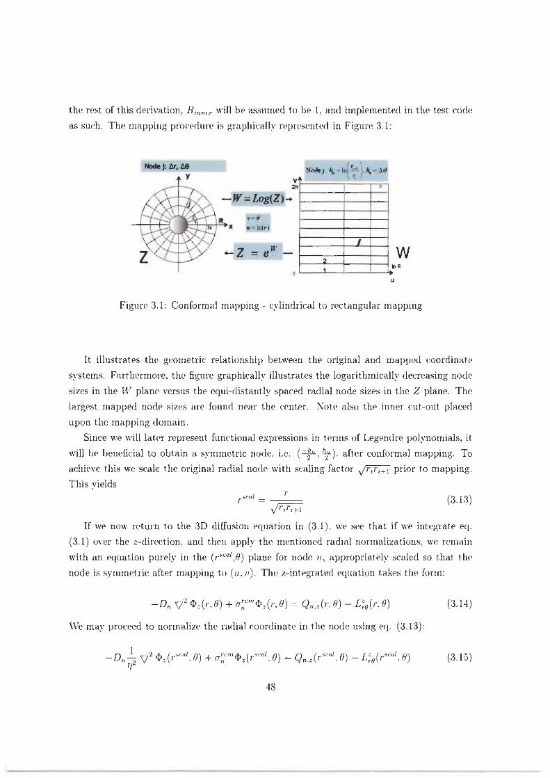
tho rest of this derivation. R,,,,, , will be assurned to be 1. ar~cl implelrlented in the test cock

as such The mappirig proccdurc. is graphically reprcsentcd in Figure 3.1:

Figure 3.1: Confornral mapping - cylindrical to rectangular mapping

It, il1nstrat.e~ t.hc geo~net,ric relationship between the origird a~rd rnappcxi coordinat.~

syst.ems. F~~rtherrnorc, tllc figure graphic all^? i1lustrat.e~ the logarith~nically clecreasing 110th

sixes in the I+' plane versus the cqui-distantly spaced radial node sizes in t,hc! % plane. The

largest mapped uode sizes arc: found near the ccnter. Note also the inner cut.-out. placed

upon thc mapping (1011-lain.

Since we will latw represent functional espsessions in tc!r~rrs of Legendre polpomials, it.

will he beneficial to obtain a symmet.ric node, i.e. (+. %). aft,er conformal mapping. To

achieve this we scale t . h origirral radial nocl~ with scaling factor d m prior to mapping.

This yields I' p - n l - (3.13)

d- If we now rcturu t.o the 4D diffusion equation in (3.1). we scv that if we int.egat.e eq.

(3.1) over t.he 2-direct.iori, a rd tl.leu apply t . 1 ~ rrlel~tio~ed radial norn~alizat.ions, we ren-laill

u4t.h an equat.iol1 purely in t.he (r"""',~) plane for ~~odc! n! appropriat.ely scaled so t . 1 ~ the

node is syrnrnet.ric after mapping to (u. 1 ~ ) . The z-integrated eqitation takes the form:

-D,, v%;(r, 8 ) + 07"'@~(7., 0) = C) ,,., ( I - , 8) - L:~(J. . 8 )

I\+ may I,roceed t.o norrnelixe the radial coordinatc in the uode using eq. (3.13):

I?, repr-ents the node size i n z - direction

In order to transform this equation w j c h conformal mapping. we need to transform the difl'er~nt id opsrat or as well and oht am:

n.i t h

p[ . rc ) ' = F ' ~ and denrlt,c.s the area mapping function.

The resulting mapped node is rectanrular and its siza is:

3.3.1 Relationship between mapped and unmapped quantities

Thr concrpt of the coordinate transkormation, or mapping. is now defined and we t ~ q i n .

in t h k ~ection, by delrlcsping some critical relatior~ships betwwn important quantitie. in

original q.lindrica1 and mapped Cartpsian coordinat~s.

The mapped rusrrdinar~ system, as mentioned abor.e, will only be osed ta perform t h ~

transyme intryation pxwrss and obtain the required node-averapxl flux to 4+awraped

currenr r~lationstiip. This relationship must then be mapped hack to the original coordinate

s p t e m and reinserted into the halance equation. To facilitate this '.unn~apping". two primary

quantitirs, ~ ia rnc i~ the node-averag~d flus and the side-atraped currents. must b~ rclated

bptneen (he two courd~nate sxstrms. Let us therefore b q i n nlth this end in mind, arid prior

1 r 1 w r n p l ~ r i rig the trans\-erse i n t e p t ion process, definr the* critical r ~ l a t ionships he rwen

tbrm (r , 81 and (11 1:; coordinate yasterns.

Node-averaged flux definit.ion

The dehnition of node-awmgcd flux in the original coordinat.~ system may be written in

terms of a surface integral over the z-almayed flus (which was obtained in eq. ( 3 . 1 3 ) ) :

If we a p p l the radial scaling prior to mapping. then

The node-averxgcd f lus in original and scaled coordinates are of course equal. Kov.. applying

the conformal mapping to this integral. ie.:

yields

Kotice tha: if we express the mapped nodc-avera~rd flux direct.1. in terms of the ( u , 2 )

c0ordinat.e system. as per definition of a surface-averapd quantity. x-e would fi~d that:

\Ye call t h i s quantity the mapped node-a\ e r a g ~ d flus or sirnpl!. the average one-dimensional

flus. and strive to relatr it to the node-a\-era~rd f l u s i n the original coordinate ~ ! ~ c t lam ( r e l a t ~

eqs. 3 21 ar~d 3.22)

Relationship bet.ween node-averaged flux and averaged one-dimensional flux (mapped average)

Eqs. (3.21) and (3.22) s u g ~ ~ s t s that a relationship lxtween one-dimensional airrraEp and

original node-averaged flus may h~ found. M'e perform the v-integration and rescale the u

I-asiable to (-1.1) via f = II, in equation (3.21). The node-averayd flus is then written as

where

kJlr~,r,-l K = (interpreted a5 ratio between s c a l ~ d and mapped area) (3.24)

52

with

\I7ithin this coordinate q , s t m , eq. (3 2'7 I for rhe one-dimensional average fl~ix may also be

writ t.eu. per defint,ion, as:

If we expr~:ss~ in eq. (3.23). t.he one-dimensional flux (a,, (<)) and t h ~ mapping function

ir2'l in terms of a Legendrt. polynomial expansion. w e find:

c2< = g I f l 19 and Q),, (( j = x.f;'fl{<) with

Here we ha\? t,runcattrI infinite wms LO a finite number of terms L EmpIoying f ! m ~ defini-

tions. 1i.e express the node-al6ern,yod Hux as:

Eq. (3.28) is an important resulr ! since i t ellon3 a clean espmssjon for the node-averapd flux

in t e r m of the mapped avorape A i l s (one-dimensional average) obtained fi.0111 the t r a r ~ w e r s e l ~

inregated rqiiations. This relat,ionship is t h ~ first of two which we need to relate the original

and mapped coordinat P syswm.

Side-averaged current. definition

A second wry important quantity whirl1 we will have to map between coordinate systpms

is t h ~ surface-averaged currenr. Using rhe net current definltlnns before and afth mapping.

we ma!. relate mapped and unmapped currents on radial and azimuthal surfaces by:

T ~ P ahavp r~lationships in the 0-dirwticm assume that the net currents across azimuthal sur-

laws h a w been appropriat.eIy averaged d o n s the radial direct ion. This a w r a ~ n g p r o d u r ~ ~

the (5 factor which would otherwise not be espected. since the azimuthal c~ord ina t~e is not .I

transformed during the mapping proced~ire.

3.4 Tra4nsverse integration of mapped equations

The bfiw for this approach has nov; been laid, and in order to proceed we have to develop

the auxiliary one-dimensional equations in each direction. and sohe them analytically to

cnnstruct a balancr relation which can be solved (in other words eq. (3.6) witten in t m n s

of node-av~rqed flus only). The ASAI in Cartesian cmrdinatw naturally makes use uf the

transv~rse intpqration process in order to obtain the ausi l iar~ one-dirnensionaI equations

and this prncm, a4 applied to Cartesian prometry. is fully described by Smith in Ill].

Severthelws. due to the application of conformal mapping, some further compIesities arise

in the application of transverse integration to the mapped Cart csian pmrnet ry, and therefore

this proc-s is full) described here up until the end of Section 3.8.

\\'e will nov perrorrn the first strp of the transverse integration -firstly by integratinq eq.

(3 16) over v to find a one-dimensional equation in c , and thereafter over u to yield a one-

dimensional equcstion in 1:. \Ye also obtain a one-dimensional quat ti on in the z-direction by

transvmely integrating the cylindrical diffusion equation (3.1 I over r and O directions. lye

then solve t h ~ e one-dimensional equations in u. LI and z analytically to obtain the required

relationships between volume-averaged flux and surface-averaged currents in each direction.

3.4.1 Transverse integration over .L. : the wequation

W e begin by intearating equation (3.16) over v. we apply the integral:

and find

\\ye move the inlmmogeneatts components to the sight hand side and find:

where

Eq. 13.29) is now an ordinary inhomngeneous linear difkrrmtial equation. which may be s o l t ~ I anal~tically (assuming that we know the right hand side)

Summary term analysis of the u-equation

In order to solve eq. (3.29) we espres the inhomogeneous sources on the right hand side in

terms of Legendrc pol!mornial expansions. The details of the one-dimensional solution, and

exart formulation of these expansions will be described in Section 3.5. but, for completenw

some notation and formalism will be introduced here.

1. L i , , , ( u ) and Lx.,(u) reprwnt the transverse leakage terms and will be expressed a~ L Zu

L e g d m poly~on~ials: L,?,.(rr) = /;P,(-;I. Thme expandons arp developed in 1=0 h ,'

% c r m 3.9.

L 2 u 2. s,.i~r j = 1 1 -giu12!a~'"' j , ( u ) = $'PI{-). These moments will be espr~ssed a s hvo

L ld., h"

terms:

T ~ P first integral term will he classified as flux mornents, the second as mapped flux moments. These expressions will be developed i n Section 3.5.1.

~ O I ~ W ' I . but will further rsquire rnornenrs of thp n l a p p i n ~ hlnction. These espremions

are also de~elopcd in Srrrtion 3.5.1.

Using these espansions we may express t h e right: hand side of eq. (3.29) i n terms of Legerrdre

polynomrals:

3.4.2 Transverse integration over u : the v-equation

We prore~d in a similar fashion b!. integratin equation 13.16) over u. Ilk apyIy the integral

This process yields

I t is irnport.ant t o notice that we deal, in this equation, with a t .roublw111~ issue. Fitst ly

we find tiva different definitions for t.he 11-avera,wd flux. namely ? ~ , . , ( t l l and f , l u \ . which

rcprrwnt the ou~-din~ensional flus in original and mapped coordinates. rwpwtively. This is a similar "impxw" found by Ougiruag in [14. ivith thp difference that we face this problem

from the perspective of the one-dimensional diffusion q u a t ion in Cartesian. and no longer

cylindrical, geometry. In order t-13 circumvenc this ism?, we firstly perform the following

manipulation of the one-dinlensional flus hy expandin? the mapping function onto a Legendre

polynomid base:

1 2v ' e u , F ! ~ i ; ) b [ u . Y)L'V Q ~ , J ~ ! J = - ~ u g [ ~ ~ ~ ~ 2 @ z ( u s ~ l d z = - h., h u * L i,;,

Here we defined the Leaendre moments of the mapping function w

The same npproach is used for the two-dimensional source term definition by writing

h7tah t.hese expansions terminatvd at some fised order L, eq. (3.31) may be rewritten as:

Here we have rnan-nyd to succersfully complete the Lranswrse i n t ep t jnn , and group the

problematic functiorlal forms into the right-hand-side sourcps. speci5cnIly

and

This fornlulation is the first important rnllestone in circumventing I ~ P transwrah int~graticm

problem described b!. 0 u ~ ; o n a g in 1121. The problem has now I w n reduced to handling the

non-linear source terms in r'rp (3.33; and (3.31)

The higher. order terms in exprrviions (3.33) and (3.34) require some special t r ~ ~ t ~ n e n t ,

and in thew casrs the assumption of separation of ~anahles leads to relatively manageahlo

constructions. The \.alidity of t h w est~rnptions XI-P nor obvious, and will he nurnmirally

evaIu;.ctd in later chapters. .Assuming such an approach. two choices are available. Thm concern the f~mm of the separ~tion of variables. either as a sum or a product, of two one-

dimensional solutions. The nest four 5ections dwelop t h ~ w approaches.

Summed variable separation - inhomogeneous source

In th i s instance, variable separat.ion is assumed in t.he following form:

This approximation is nrcessaqr in order to cornplet-e the trans] erse i n t~pa t ion proce-

dure. 111 short. the motivation is based upon the fact tha t the solutiorl of the hnmo~eneous

diffusion equar inn in Cart~sian coordinates is separable, 'but not so in c~lindrical coordinates.

It is reiterfird that this approximation will be evaluat.ed nurnericall!: arld future work will

include a rigorous analysis of the error inherent, to this approach. .Applying this approach to

the i n h o ~ n n , p n ~ ~ u s sourw rwm s,irlj (q. 3.33) yields-

Xotice t.hat. the contributions lrorn the jf, (.;?) and 7 terms are zero. since the summation

counts from 1. Thus: the esprwsinn for the inhornogeneous source t . t r m may be reduced as

~ O I ~ W S :

where we define the L~gendre moments 01 the one-di~nensional flux in u-direction as follon-s:

Sote tha t this exprassion is actually constant in z;, and this [act.

separation approximation.

results from the surnmative

Summative variable separation - standard source term

1Ve.also approximate the standard (fission and scattering) source tern1 in t.he same way b!.

writing

Vsing the sarnr arguments as for the inhornogeneous source: we may neglect the source

term contribution from Q, [I:) and Q. The resulting contribution is expanded into L~gendre

polynomials as before,

with

The source term Q,(ll) g i ~ m in eq. (3.34) ma?. then be expressed as:

This exprpsr;ior~ concains some in! ~ r w t i n g characteristics. The source term in the u-direction

is glven as two components. The first w the standard one-diniensional source q, ( 1 1 i scaled

by the mapped node size ratio K, and the second as a contribution of higher order source

moments from the radial direction. The mapped azimuthal source term carries a radial

contribution.

Factored variable separation - inhomogeneous geometric source

On the other hand, if we assume the following approsirnation lor the twodimensional flus:

and substitute it inlo eq. (3.331, we find:

Furthernwre. we espanding bot.11 the u and r one-dimensional flux in L q m d r e polynomials:

IVe notice that , using the factored separation, the inhonmgfmcous source in the 7 . rlirectiori

rna i r~ tn ins some functional dependence on v, with an averace value ~ q u a l to that of the

s u n m a t i w wparation a,s.wmptiou in the pr~vious section.

Factored variable separation - standard source t,errn

\Ye apply variabl~ se~arat~ion to the t.~vo-dimensional Iiource term in product form and define:

Q m (y) = - qn't" - ' -. 1 2 glp:(E.)Q:(Ti: t!.)du = qn'l"' - ' qni7"lu $g~f '~( l l )Q7, tu)dn A- ' h d hk

-I---

Q h ,

Utilizing one-dimensional source moments in u and c direction, this equation ma!. he reduced

to:

Summary t,errn analysis for r-equation

The four alternatiws described above, namely the factored or summed approach applicd

to bot,h t . h ~ standard and i~~honlogeneous c-dependent sours&, all provide the means of

conlplet inp the t.ransverse intepation over u. For t h e sake of this work. the sli,~htl>. simpler

surnrned approach will be applied to both sources. and the impact, of the ddi t ional higher

order t.errrls from the lacoored variable separation will LP left a5 future work.

To canclude the formulation of the one-diniensional u-equation. a summary of t.he required

espansions is given.

1. L:, , I :.) and L;., ( 1 4 ) will be express4 in terms of Legendre polynomial as L , ,.O+) =

27' I;fi(-). Thew ~xpansions are drsuribed in Secrion 3.9.

, - ,='I

h,

L 2, . ~ ~ [ y j = -rTV"' 1;s This expression requires, once spin- moments of the mapping -.

!=l function as w l i as flux moments in t l ~ u direction. T h w expansions are developed

in Section 3.5.1,

L

-3. q,, ( r r ) = ' C n 3 i i i I:-, ' Kotice here tha t the source i n c. direction is dcyendent

I= 1 upon the higher drder source moments in u direction. Since t,he surnrnative variable

approximation Is to he initially implemented into t h ~ I Y W cude. it is only stated in the

summary.

Final Form

lf ' i th all the terms exprc-sscd os Legendre polynomids, we may merge the source terms of eq. (3.31):

9;" 6;'= -I' + - for I > 0 K

3.4.3 Transverse integration over (r,F)) - t.he.2-equatkn

The proce.~ tn find a one-dimensional equation in thc z-dirwt.ion is much more analogous to

that of pure Cartesian Emmetry transverse integration [l I]. llt begin with the cylindrical

diffusion equation in three dimensions (eq. (3.1) j and transverselv integrate and a\.er;lKe over r find B to obtain:

\\'P transfer the first term of eq. (3.13) to the right hand side applying the diwrgence t . h ~ n r m

in order to express transversp Ieakap in terrns of transverse currents (as was done in the u

and u directions):

Summary term analysis of z-equation

In order t o sdve equation (3.46) we need to calculate the following inhomogeneous terms

(expressrd in t.erms of L ~ ~ e n d r e polynomials). The detailed farnr of t h ~ solution is given in

Section 3.7,

1. Lk,, i 1 1 and S t , [:I - t h w arp handled in Section 3.9. but will be ~spressed in terms

This gives the right hand side of eq. (3.46) in terms of Legendre polpomials:

Onr-dimensional. auxilial-y diffusion equations now brm dewloped in all three direc-

tions (5ertions 3.4.1, 3.4 2 and 3.4.3). with t4he r ~ q w t i v e source terms i r k P R C ~ direction

~spanded upon a Legendre polynomial base. T h w equations m e in the form of ordinary,

1ine.v. inhomogeneous differential equations. and may be solved anal!-tically. T'hp fnllow-

irlg sect ion will addreqs the isup of developing a onedimen..;iond solution t t ~ ~ a c h of thesir

~quations, and to USP it to obtain the elusive node-avwpd flux to side-averaged current

relationships required to close the system or nodal balance equations (eq. 3.2).

3.5 Solution t o the one-dirnensiona.1 u-eqmtion

The conformal mapping technique, applied to the diffusion equation in cylindrical ge-

ometry. allows us to solve the diffusion problem via the Analytic Sodal Method (ANiiI) in Cartesian geornelrv [ll]. ln the following sections, this fact is exploited, since we now romplete the solution of the one-dimensional equations in mapped Cartesian geometry. The

only price to pal- for the coordinate mapping manifests in the form of the additional inhomo-

ynPouq SouL'ces. a s w l l as the additional mapping funrt ion and scaling factors introduced

in Section 3.3 \\"e may rmrltp ~ q . (3 29'1 in term? of a normalizd variable u4 = !?. Thiq step is useful.

since i t transforms the nodp onto a local coordinate ranging from i-1, I]. and simplilies gome

of the algebraic expressions to follow. The transversely integrated one-dimensional diffusion

equation in ul then takes the form:

where

Here L is defined as the order of the source term mpansion. In eq. (3.48) the moments of

t.iie one-dimensional source. dr ! are as ~ e t unknown. They will be deveioped shortly, If we

Sssunle for the nlornent that they are kn0v.m: the anal~t ic solution of eq. (3.48) for node n

may then be witt.en in the rorrn:

N'e define

bl: as the moments of the particular solution

where once more (as described in Section 3.3)

j - . j-. Zf and Z-represents the side values of the flus and the particular solution

Sote hprp that ;?'. refers to the one-group buckling term for node n, atid r, and r,,,

r4er to the original inner and outer radial coordinatw of r a d i ~ l zone r ? , respectively. Some clarificarion is needed here, since the compound superscript index mu. coupled with subscript

n, refers to the v d u ~ of

neighbour in t.he cllrrezl!

t.he variable lor node n in the direction rnn where node 777 is the

direction of investi~ation - in this case directirm u . Dpnote further:

It is possible. by utilizing the ort.hogonality properties o i Ltprndre pol:.norninlsl to espress

the morncnls d t.he particular solution d i r d y i n tm-ms of the source 1noment.s. The par-

ticular so1ut.io11 ma!- be obtained directly from the sourcsl term b!. the follo\ving rwursive

relat.ionship:

2 1 t l - = 7 i l +- (-l}"+m) h 1 m L 1) - / [ j T 1); (3.56)

Thpw b, ro~fficients are used in obtaining the expressions for ,?"and 2- in eq. (3.49).

\I? dar, denote the side flues as node interface fIuses

.f- =

Here ciyTl,, refers t.o t.he side flus in direction mn on th~f surface bet.ween n o d ~ s 11 - 1 and n ,

Determination of source moments

The rcn~aininc: i s w in conlpl4~ting t.he so11-ittion in the u-direction is conmuc t ing the Legendre

expansion moments for t.he sourc~ tterm in t.he radial dirertion. Th? smrce i.5 constr~~ctpd

in n lappd u. coordinates in eq. (3,57j, and represents the surnmat.ion of the regulxr ( fision

and scat terina). in homogeneous and t%ransverse leakage sourcps:

\\.k rewrite t . h w ~spressions in terms of normalized u: coordinates t,o yield

and inhomogeneous source

and the regidar nodal source

dl = 4; ., q; +. sj' (3.59)

Some investigation of the definition of the required moments, will show that some support

quantities. to h r termed flux rn0ment.s and mapped flux moments, occur often and can

be independ~ntl? calculated. These flux moments are used t u construct t l ~ c required source

mornem. i.e. fission saurce, scatterinz sourrc and inhomogeneous source. These expansions

are devell~ped in the next section largely as recurrence relationships tn r;tcilit.ate variable

espansion order calculations,

3.5.1 Calculation of moments

A. significant component of this work is the efficient representahn 01 non-linear s o u r m in

the on4 imens iona l equat.ions, and as such; t.he calculat.ion for higher order expressions for

the one-dinlensional flux. These expressions are developed in this sect,ion, so far possible to

arbi trap- pol~ornia l order.

Flux Moments

Thc flux mommts are calculated via recurrence relationship alld some esplicit integrals.

Expressions for the one-dirnenwmal ff u s moments will allow the ralculatlon d sonip or the

components of dl in esp. ( 3 59). lye will p r a c ~ d in order to find L e g d r e ~ s p n n s i n n

coeffici~nts for t hc exprmion:

~ l n d t e r m t.he coef3icient.s /: flux moments. Using the analytic solut.ion (3.49), we ha^^

where we define thc h~perbolic cosine moments

and hyperbolic sine moments

These moments are calculated via derived recurrence relations and are given in Appendix E.

Mapped Flux moments

I\ also come across expwssions of the followinp form. and t.erm the moments of this espres-

sion mapped flux moments:

Lsing ana1yt.i~ solut.ion (3.49), we have

where wr defined the mapped hyperbolic cosine moments

and the mapped hyperbolic sine moments

These mapped moments arp calculated via recurrence reIationships derived in Appendix E. There are ho~vever dificulties in deriving a recurrence relationship for the particular solution

part of the one-dimensional flus. as ,chis term forms a double Lcmndrc - esponrntial integral:

Thew integrals are calculatrd espIicitly (15 in total s i n c ~ t h ~ y are q-rnmetxir: fourth ordcr in-

t q r a l ~ ) with the support of t h ~ suftmre y a c k a ~ Xlatl~eniatica 141. T ~ P expr~~s ions for t h e s ~

intcpals , in the form ol Goth their analytic and Taylor series fornms (rcqrtir~il t o eliminate

pntrntial round-off errors'[, are given in .Ilpyendix F.

Moments of t.he mapping function

Finally wr need to define an exprwion for moments of the rnapying function.

with

Using recurrence relation (E. I ) wr espress:

2 s i ~ ~ h ~ h u ) I,, = -.viilr (h,) I II =

h , h ,

Final form of source moments

Thr rmstructions i n the previous section allow us to describe: in a clt.ar form. all sources

within the one-dirnensinnal u-equation. These exprrmions. now develnped up to an arbitrary

order, are presented in t h i ~ swrion.

Scattering source moments

G

Fission source moment,^

Inhomogeneous Source moment expression

\Ye ma!; now put eqs, (3.61) and (3.63) together to yield the following e x p r ~ s ~ i o n for the

inhoniogeneous source moments in the mapped u direct ion:

Fixed source moment expression

The moments for the fised source term may he e s p r ~ s w d in terms of the mapping runction

moments defined i n eq. (3.67):

Transverse leakage moment expression

The trarwersc. leakage monlents are defined across multiple nodes. and their t rPat.nwnt is left

for Sectilm 3.9 hen all t h r w one-dimensional equation solut.ions have h e n zppropriately

fcrrrlulat~d.

3.5.2 Current and flux expressions

From the one-dimensional solution (3.49). we can derive the expression For both t h ~ surhce-

averapd currenl, as well as the espresion for side-averaged fluxes. T h ~ w solutions are

d~rived from a r.onstruct.ed two-node problem, and are consistent with the fornlalism or the

standard ASXI a_s implemented in the Kecsa based JIGR.4C code [22). lye ohtain

werp w e haw defined the "tenmrial source" as:

Using equation (3.49) o w two neighboaring nod^<, and applying f l u s and current conci-

nuity conditions at the interface. expressions (i3r the one-dimensional side-awra~ed current

may be obtained ia terms or the node-averapd quantities.

where

The side fluxes ca1culated in eq. (3.72) are nPmwtr!q in order to define the constant4 C1 and C: of the one-dimensional solution. A n i rnpor~nnt difference from the standard

AShl is that t h r currents obtained in this formulation are defined as currents within the

mapped L( direction, and have to be rerJ~fined per ~q 13-27) prior to lna~rting them into the

balance relation (3.2). I\-e therefore pre-wnt esprr4-m (3.74) as an important result from

this section:

wi th

where T,,, is the radial boundar? herween mesh m and mesh n. Stating for c1arit.r. the

relationship between mapped and unmapped currents:

Only t w ~FSIIF.~ remain before reinserting eq. (3.74) into the balance equation /3.2), having

then obtained the nwrssary information from the auxiliary one-dimensional u equation.

The quantity defined as the "tensorial source" must be exprewd in terms of ca1cul;~te~I

moments. ]Ye use the term "tensorial" because this source has different values at the

left and the right surfaces of the node.

The earlier defined relationship be twen the original coordinate system node-averaqed

flus and one-dimensional average flus (eq. 3.26) must be uced to adjust eq. (3.74) in

such a wax that the side-averapd current is expressed in terms of the node-averaged

flus in stead of one-dimensicma1 averay. This will be done by rdefining the tensorial

source quantity.

Both the above two points are addressed in the following section in \i<hich the Lensor~al slsurce

is described.

3.5.3 Tensorial source

H a v i n ~ obtained all moments related to the Legendr~ ~xpansinn for the source term in eq.

(3.731, we may proceed to caiculate the t~nsorial sourcp 2,,. The tensorial source is used in

the calculation of surface-a~leraqed net currents, and carrips thr source terms Iron1 iteration

to ~teration (along with the moments of the particular scrluth-m t~sed to cnlc~~late the one-

dimensional solution constarits) \\'e express

Here JW'' and 1;'" refer t a the quant.ities defined in eqs. (3.62) and (3.63) respectively. After

some sirnplifimtinn, expressions for the tensorial sourc-e may he wit,ten as:

Mapping impact; on tensorial definkion

The coordinate transformation implies a certain relationship between node-averaped flux

and one-di~nensional a\.erages in the u and v direction. This relatkmship was de\doped

and presented in eq. (3.26). Within a purely Cartesian framework, onp-dimensional averatcc

Buses are equal to nodeaveraged flus. and abviates this discussion. In our case, due to

th~1 11-dependent mapping function. and the separation of variable approsimation. a distinct

relationship between one-dimensional u and v-averagei and node-a~~ragsd fl uses: exist. The separation of variable approsimation. and the definition of node-averaged flus are once more

stated helm-:

remembering that the area elemen! rdrdf l ivas mapped onto g( t i ) zdudc during conformal

mapping Furthermore,

since

and

It is important to t,hen appl! the relationship berween rind s,, since the side-a\wxr:~d

cunent to node-averaged flus relationship ran only be found if i t is known. As stated in eq.

(3.74). we have:

\\:rt nerd to (after solving a two node problem to obtain this relationship) exprey this rela-

tionship in terms of node-averaged flux, and not putel? in term.: of one-dimensional averagp.

\\'e therefore need:

can, due to (3.811, only consider the relationship between one-dimensional average in u

and nodeaveraged flux (will be the same in z:-direction). T h e obtained node-averaged ff ux

to one-dimensional average in u is (restated here for easy reference):

Redefinit.ion of tensorial source

Using ey. (3.86) we may, as an initial sugystion. redefine the tensorial quant i ty as follons;

and remain with

- J 171 ?t =C'L,nf*3 - ~ ~ Z ~ , , ) - C ~ ~ I ' ~

This approach will do and we have obtained the all

node-avernpd current relationship. Ner~ertheles, esy.

important side-avrlra,crd current to

(3.58) may yield initial nurneriral

instabiliti*, sirrr+ eq. (331) i c only guaranteed to be valid upon svstern convergenw. It would be preferable to include the node-averaged flus in the definition crftwwirial in n sli+h.

rnorr sleqant ktrhion The fol1ov;ing approach is presented here yurel: s5 an alr~rnative when

and if such ronv.rrence problems arise.

Con?ider t h e cont.ributiol~ c ~ f the u-direction inhornog~neous wurw to the t.ensoria1 quan-

tity (define the remaining snurce contribution as ZLy i t . P.,,, = Z;:;' A P:S;'):

U'e may ident.if~ the first. of these integrals as possessing two components:

defining the remaining integral as:

Replacing t,his definition within eq. (3.531. yields:

Tlv remaining component o l the inhomogeneous source n e d s to be calculat.ed, and ret-olves

around the quantity:

which may be written i n terms of previously defined rnomcnts a$:

Definition (3.91) allows the definition of s i d e - a v ~ ~ f i ~ ~ d currents in terms of node-avera,ryd

. ff uxes hy limiting 1-he cont.ribut.ion of t.he inhonlnaeneous source to the censorial, and further

limits the numerical dependence of the t . m codt on calculated flus moments, which in turn

depmds, in the initial st.aEcs of calculatinn, on put.ential disrupt,ive initial yuer;st2.. Xkhougl-1

t.1- is rn~t.hod is more elegant, t.he striicture of thc test code is such that, the appropriate

relationship between one-dimensional average and nodeaveraged flux is maintained during

a11 iterat.ion levels For this reason the approach as dewribed in eq. (3.87) is implemented.

3.6 Solution to the one-dimensional v-equation

Thin same analysis and development that had bcen performed in t he previous wcfion to

formuhrr a node-averaged flus t o side-averaqrd current relationship is now repwted for the

t.-direction. The proccss is briefly restated. and i~sues particular to the solution in the 2:-

d i r~c t ion are highli~$ted. The transwrsely intergrated one-dimensional diffusion equation in

r1 is given as

R,, 1: v v

The arlalyrical solut.ion of equation (3.94) nit.h u. = !L.. for node n nlB! he n.rit.t.cn in the

form:

and let furt.her:

The part,icu!ar solution is obtained directly from the source term b:. the foliowing recursive

relationship:

with

Thesc bl coefficients are used in obtaining the exprwions for C1 and C? in eqs. (3.103) and

( 3 1 O f ) .

3.6.1 Determination of source moments

Thr issue once again is constructing the L ~ g m d r ~ ~spansion mtments for the source te rm

in the azi~nuthal direction The source is constructed from thp following terms, here defined

in mapped r-coordinat.5. The expressions for s, , l ts i and Q,(r) haw been expanded and

simplified ac described in Sect ion 3.4.2.

t 3u

Qn(1!! = - q p + - ) Q ; ( I L v i d u 1 fr, h a

11% may rewrite t.hesr? exprewions for the normalized dirnensinnlm coordinate u 4 = Ff. and

dmore the normalized u direction dimenzinnlrrc variable with tr , = ?:

The source tprm in t l~c z. -direction contains contributions from higher order terms in the

u-dtrmion Ewn though this contribution appeared due to the application of variable

separation, it is consistent, with the cenzraI issue in sglindricaI g~urne t ry that the solution in

the 0-equation is dependent upon r. This derivation aas given in Section 3.4.2.

CaIcuIation of moments

In rhe PI-direction only moments of the one-dimensional flux are required, and only for use in

the tision end scattering sources (the ir~hornogeneous sourcp in the r-direction is constant

in 2,. The d ~ f i n i t i m and recurrence relat.ions r~qriired are analopous to the developmen1 in

the u-dir~crion in Swt ion 3 .51 , and will not be rederitwl here. FIux moments arp expressed

as.

,.sin with 4i,".C"%and . r , recursively ca lcu las~d as in Section 3.3.1

Final form of source monlei~t~s

For the sakc of cay reference. the various SCWCP rPrms rel~vant to the solution in I ~ P r -

dimtion are I i s t ~ d in this section.

Inhomogene~us source moment expression

The expression for A,. 11-hirh is const.anr in UI, is C R I C I ~ ~ H I P ~ a i n ~ eq. (3.109). This expression

o s ~ c the su~nmatil+*l variable separation technique as d i sc l l s~d in Section 3 .42 . \Ye refer to

eq. (3.3Fj and restate

with

and

?;oi P that 1;:'' and g~ are calculated fro111 Sect.ion 3.5.1.

Scattering source moments

Fission source moments

Fixed source moment expression

The mornents for the fixed sourcc rwnl may IM ~ s p r m ~ d as:

Tramverse leakage moment expression

The transverse lealcagp moments are defined across nmultiple nodes, find their t.reatment is left

for Scct.ion 3.9 whem all thrw one-dimensional equation solut.ions have been appropriat.ely

f'orrnulated.

Total source moment in v-direction

The total v-dependent source. including t h ~ contribution from the u-direction. is r iven by:

In the case of fission and scattering s o u r c ~ , a series of higher order terms fr0m the u-direct ion

will contribute to the source term in t h v-direct inn.

3.6.2 Current and flux expressions

Once ~ g a i r ~ . analogoue to the dei.eloprnent in the u-direction, but this time in the 1.-direction.

t.he expressions for s ide -avera~d current and side-averaged flux are presented:

with

These expr~ssions culminate int.o a surface-averaged current to node-averaged flux re-

lationship, taking care t.o scale them appropriately 1.0 yield the side-meraped current in

original coordini~ter: (utilizing definitions from Sect.ion 3.3.1). Once more (m r a s t hc caw in

t h ~ u - d i r x ~ i m ) we obtain an inipvrtant result in this s~ct,ion as we define the net current

expressions in the 1.-direction:

i b t ~ that the side-averaged currenrs in the azimuthal dirertion have been radially avera~ed, F hence t h t - t.~m. U T . .

3.13.3 Tensorial source

Thc expressions obt.ained for the tensorial saurce in the c-dire tioii are identical to t.huee in

the u-direction. with a11 parameters assuming their corresponding values in the r-direction.

Impact of variable separation on tensorial definition

\l'e face here the identical situation as in t h ~ TI-direction. needing to relate the o~ie-dlrnensionaI

averapl flus in 8 to the node-avera~eci h x . \\'e p r o w 4 similarly. \!'I= restate t . h ~ relevant

~lrfinitions;

iVe ut.ilize the relationship bet-~veen 7 and s,, sirm t.he side-ave.r;cged current to node

a\?eraped flux relationship can onl). be found if it is known. As stated in eq. (3.1171, we

h a w

Redefinition of t.ensoria1 source

I.:sing eqs. (3.86 I and 13.81) we redefine the tensorial quantity ;t5 we did in !.he 11-

direction w follows:

and remain a.it.h

This approach would once again s u c c ~ ~ f u l 1 ~ - express the side-averag~? current in terms of

nod?-at-erapd flux, but is dependmt upon thc fact t har the one-dimensional averages in u

and r 8 directions are equal. This rnigh~, not be true at the start of the solution iteration

prows<. On the other hand, if we once again consider the approach of separating the

inhornugmc~us source contribution (but n t s ~ in t.-direction) from the tensorial quantity

in the c-direction, we may n-rite:

M Q may ident.if>* the first of these integrals as:

defining t.he remaining int.egra1 as:

Replacing t,his definition within q. (3.122). yields (onw again denntitig the tenr;orial con-

tribur,ion from other sources by Pzr i . ~ . 2,,1p1 = 2';;;; - z;?::):

4 J ** = r,':tn (5" - ( Z:,! j I - c:", 1 Tm - ( T::; 82 -L ZvPJ7l -*I 1 1 (3.129)

Relation (3.129'1 allows the definition of s ide-a \~ t .a~~cl currents in tetms uf no+-al.era,ped

fluses I>!- limiting thc mntr iht ion of the inho~~~ogencous source t o the I-ensorial, and further

limits the deyr~ldence of the numerical solution on calculat~d flux moments fe~pcc ia l l~ from

t h ~ moments in u-direction). which in turn depend. in the initial stag= of ralcdation. on

potentially disruptive initial guesses. The remaining component of the inhornq~ne-nus source

n w - b to be calculated. and evolves around the quantity:

which ma?- t.>e witt.en in t.erms of defined moments as:

3.7 Solution to the one-dimensional z-equa.tion

The solut.ion of the one-dimens~onal equation in the z-direction is identical to that of Carte- sian coordina~es as described in Ill]. The one-dirnensional, trans\srsely int~grat.ed equation

in the z-direction takes the form.

and

The arial!.tic solut.ion to equation (3.13'2) is given by:

The particular solrltion was obtained directly from the source term by t,he following recursi1.e

with

Thew tli coefficients are used in obtaining the expressions for cl and c2 in eq. (3.134)

3.7.1 Determination of source moments

Tltc total sourrlh urorncnt, in t h r z-tliructinn is thus d v e n as.

Calculation of moments

In rllr z-direction only rnornent,~ of the one-dimensional flus is required. and only for usp

in the fission and scattering source.. The definition and recurrence relritions required are

analopous to the development for the ti-direction in Section 3.5.1. and will not be r e d ~ r i v ~ d

here. Flux moments in the z-direction may then b~ pxpressd as:

Final form of source moments

Scattering source momenta

Fission source moments

Fixed source moment expression

The moments for the h e d source t ~ r m may h p ~ s p r e n ~ d as

Transverse leakage moment expression

T ~ P t.rcznsverse l e a k a ~ p moments are dpfined across rnultiple nodes, and their treatment 1s

left for Section 3.9.

3.7.2 Current and flux expressions

Vsing the one-dimensional analytic solution over multiple nodes, two important expressions

are obtained. The first for surface-averaged current! end the x~cond an expression fur deter-

mining sidc-fluxes:

These expressions culminate into the required surface-averag~d current to nude-avernpd flus

relationship in the z-direction:

Stittin; tliv relationship between scaled and unscaled currents for clarity:

3.7.3 Tensorial source

T h p espressions obtained for the tensorial source: in the z-direc~ion are identical to t.hose in

the u-direction. with all paramet.en def in~d as they are in the equations for z .

3.8 Balance equation

After quite wrne alg~braic dTm-t we h a l t derived xurfacp-averaged net currmt to nodr-

a v e r a p l flus relationships fr~r a11 three directions. In the case of r and 8 clirwtions, thp

rslationship was indirwtly obtained via t.he conformal mapping technique. while for z the

approach was as ~t is normally done within the Anal!-tic Xodal _\.lethod .4ll six reJ~tiunship

are finally in~erted into the balance equation (eq. 3.2). Eq. (3.156; presents the final form of

the balance equation for each node n. Kote that the surfac~s jnl = 1.2 .6) are numbered as

radral (inner, outer), azimuthal\rigl~t. left) and asial(bottoni. top). Therefow, for esarnyl~.

Czar would refer to the outer rad~al coupling coefficient of node n, and was defined in eq.

(3.74).

3.9 Tkansverse lmkage approximation

Il'e conclude this chapter b!- formulatir~a expressions lor the transvelw leakage terms in

all thwe directions. The transverse leakare terms appeared as sourcey in all three one-

dimensiond equations, and espreslons have to be developed for each of these. This section

is handled here. a t the conclusion of the chapter, since it require4 developed net current

expressions for a11 three directions. In this sertion both R flat and quadratic approximation

will be developed, with the latter symbolizing a new contribution for nodal methods in cylindrical geometry. IYithin equation (3.57), (3.105) and (3.143) we face expressions

for the txansversp leakage for respectively u . ~ and z directions. In each of these caws we

require one-dimensional currents on "top" and "bottom" surfaces in each transverse direction.

which we d o not have expressions for horn the nodal solution. I!-e d o however have surface-

averaged net currents on all transverse surfaces, and these currents can be used to coristruct

a one-dimensional transverse leakage representation in an approximate way. Once a one-

dimensional transverse leakage term is found, the ana1yt.i~ solution of the one-dimensional

~quat.ions may be written in terms of thcw functions.

z-direction

Let 11s start by consider in^ the equation in the z-direction (eq. 3.46) If we assume that radial

and aziniuthal currents arr constant in the r-direction within each node, we can calculate

the average transverse 1eakag-p in the z direction as

M'e knon- the quantities on the right hand side by assuming that the one-dimensional

equations in the t r ans lem directions w r e solved. i t is important to note that n.hat we

calculate a% rurrents from f h~ solutions in the t rans~wse directions iwr not directly radial and

azimuthal currents, but u and zq currents - therefore they are the currents in the mapped u and

dlrcctions. \\it are thus required to map t h ~ s e currents back int 13 ; R I ~ 0- directions before

usmg them to exprecs 1 he avcragc transwrw leakace in the z-direction The ~ s p r e s i n n s for

current in the one-dimensional solutions. as well as the mapping of t h w currents back mtv

r and 8. were aiwn In Section 3.3.1.

From this point ollv-ardq. two approaches are possible. The first to be dismssml consti-

tutes the simplest and mosr approximate solution. namely the "flat leakarrc approximat ion".

Tlrerdtcr . the rnlm accurate, but slightiy more instabilit~.-prone"quadratic l e a b ~ e appros-

imation" wi l l be discusrd.

Flat leakage approximation

The Rat I~akage ~pprosimation maintains the averaqe trans\.erse le&p from each transverse

direction, and uses only information irom the n d e under consideration Eq. (3.159) gives

the expressiun for t.he average transverse leakage. The expresions on the ri,ght hand side are

known and constitute the r and 8-currents in the original ~oordinat~e svstem. Therefore we

e s p r m

Quadratic leakage approximation

In t.he case of t4he quadratic leakage approximatZion? we use esprevion (3.157) to calculate

the averepp transverse leakage in each of the three neighbouring n o d s in the z-direction,

and m i l m e a quadratic pol:-nomial shape over these three nodes.

11-FI s01t.e lor q;,,, q:,, axid q;,? llsing t.hc fdlon5ng cIosed SP! of equatiow. ~ i n c e we now know

the averagp lenkaps on the right hand side from eq. (3-157):

The det.ailed solution expressions for the quadratic f i t ma!' be found in .4ppendix Gt and

we find an exprmion h r the one-dimensional transverw l e a k a ~ ~ source in terms of node

sizes i n t h ~ Z-djre~.tion. BS well as awrage leakages in the r and &directions. \ \e appl:. this

transverse l e a h g ~ shape L( r ) onlap to ncrde n. This rnethod is clearl?, an approsirnation, sirrc~ it is not. certain that a second-order polynomial udl phpsir~lly repreenr t h ~ t ranswrse

leakage function. I t is convenient to express the 4 u t i n n s of L I Z ] in t m n s of Legendre

pol!-nonlials; (for consist en^?^ with other one-dimensional sources). Therefore we would like:

k = 3

Equat,ing coefficients n-i th eq. (3.159) we find:

The prGt!W is similar in the 11 and vdirections. taking care to handle the currents from

mapped and unnlapped coordinates ro~rectl?~. The transverse leakage term in the ry-equation:

We obtain h e average transverse leakage in the u-direct ion (analogous to the z-direction

transverse leakap);

The term & JL,>, y(u12J,(u. u . -t%)dudu presents a problem and carelul consideration of

the term is r~quii-ed. Sor.ice fiistly that if we try to esprm the z-direction current in terms

d mapped coordinates. we find:

n1it.h I\' defined aa i n eq. (3.24). The manipulation allows us to w r i t e

Therefore we ma! rewrite the expression for the awrage transverse leakage in c.-direction as:

Flat leakage approximation

Once again the flat leakage approximation entails t l . 1~ calculation of only the averRge trans-

verse \ e a k ~ ~ ~ per node, and using that as a constant source term on the right hand side of t.he one-dimensional r-equation. IVe express:

Quadratic lec&age approximation

The transverse currents on the right hand side are once again k n o w from the solution or

the one-dimensional equations in the u and t-directions. From here the procesr; is identical

in nature to the ,--direction t.reatment, ending with an esprmion of the one-dimensional

transwrw leakage in terms of Legendre polynomials. 11-e approximate as before:

and apply

and e q u a t ~ c.aefficientn as in exp~w~.r;sion (3.160) to write (coefficients once again solved ac-

cording to solution in -4ppendix G) :

u-direc tion

The solution in h e u-direction is slightly different. The inhornogveous scaling function

9tr:)' doe5 not in t+pa t .e our. in t.he .u-dirccrion, and we have the following expression for t,he

t.ransversc leakage (from eq . (3 .2~ ) ) :

In this case we may approximate the transverse leakage component. in the axial direction in

three ways, and will presenr the first and third approaches in this wcion. \Ye may aim to:

1. Cse the flat. leakage ~pprosimation.

2. Approximate, wit.h a quadi-at.ic polynomial, the "tra-nsformed axial component of the J=~u.% ' ~ + J ~ i u , - % :% t.ransverse leakage!':

h, .- . This approach could potentially generate higher

order terms, but will add complexitv which might not add t.o t.he computat,ional ac-

curacy. The evaluation of this approach will not. be further investigated within this

chesis. and i t is left. as potent.ia1 future work.

3. Approximate, with a quadratic polynomial, the '.original axial component of the trans- ,* ? I[~,L , + j z ~ f i -L'I

verv l ea lap: g(u I - " ' A t --. This is the preferred implenlentation of quadratic

leakage in the u-direction, and will be further developed in this wction.

We proceed by obbaining axrerag@ t.ranslrerse leakages in t.he u-direction:

and wite analogously to 3,163:

Flat leakage approsirnation

This is once again t,l.ie simplest. c m . utilizing only the averace of mch trans\wse dirwtion's

contribution to the u-direct inn. Note that, thch r-ont.ribution fmrn t t.n zl is identical to t.he

awrage contribn~.km h-om 2 to as found in the previous .sect.inn. 13-P mat. write:

Quadratic leakage (original axial component)

In t.his a.pyroac11 we would approsimme the one-dimensional transverse I ~ a h g e shape! namely:

with L , . lr!) fitted in the normal way to conserve the averap transverse I B R I ~ P . Suh4tut ing

eq. (3.168) frsr the average transverse leakap in the u-direction into the W, below, and solving

thc srf of equations once asain as described in Appendix G:

After obtaining t h e q, , coefficients, we can express them as Leaendre polynonlial espansiori

coefficients usinp (3.160) for node TI:

3.10 Conclusion

T h ~ s concludw the discussion on the det-eluymenr. of the conlorma1 mappin? ~pproach t.n

the Analytic Sadal Xfet hod. T h chapter follow~d the derivation to the point of expressing

all terms in t h e within-group diffusion balance equation in terms of t h p primary unknown,

namely n o d e - m w ~ q ~ d flux. Utilizing appropriate boundary conditions. the set of equations

are c lwd mcl may b~ so l~ed nnlnerically. The major obstacle. of not beinrr xblp to c ; . h t a ~ ~ ~ the

nesewry ausiliar? one-dimensional 0-equation in cylindrical pometry . was clrcumvent~d b: prforming the tranwrrse inteesnt.ion in rriapped ( t r , 1 - 1 Cartesian gvornetr!. Sonw assurup-

tions were introduced in this process. such as the separation of virriabl~s for the sake of consrructiri~ the sources t e r m in the v-equation. or the truncation of the L ~ ~ ' f - ' n d r e source

expansions after L terms (in practice to be implemented h~ 4 for the sake of thr test code).

The* i issus will be nunwricali~ emluated in the upcmning results c h a p t r ~ , and further

conclusioc~ re~ard inq their reler+ance will be d r a w .

This chaprw serws as the basis for the development of a numerical FORTRAS code to

demonstratr the viability of this approach. and servrc t ~ q a prototype for a possible future

implementation into the Kersa de~,eloped OSCAR code system 1221. Before ciecribing the

developed test code (Chapter 3) the nest, chapter will m t ~ h l i s h whether an important re-

quiremenr of nodal methods is met by the ronforrnal mapping approach. name1:- whether

or not a fine-mesh limit exists for t.he e x p r ~ ~ i o n s obtained in this chapter. This propert!.

is important, and directly r e l a t ~ the numerical stability of t h e solution algorithm to be implemented

Chapter 4

FINE-MESH LIMIT

4.1 Introduction

The previous chapter concluded the development of the analytic nodal method in cylindrisxl

gmnetry Prior to that. in Chapter 2, the dewloprnent of thc finitedifference solution

method was described We now proceed to i l lust . ra t~ an important link between these two

developn~ents, by derivinn the fine-mesh limiting e x p r ~ s i o n s for the analytic nodal method

A necessary and important requirement of nodal methods in general is the esistence of snch

a fine-mesh limit, which specifically refers to the property of equivalenw of nodal equations

and finitdifference equations in the limit of fine nodal meshes. This propcrty is esprcially

important for nunwrical stability o l the nodal solution method and the .4KM in Cartesian

coordinates exhibits this property 1111. This chapter a d d r c s ~ ~ the qumtion as to wt l~rher or not the confornial mapping adjustments to the AS11 maintains the firl~-mesh Iimit prop4rt.c..

4 given nodal method may be said to exhibit a fine-mesh limit if the balance equation.

and hence node-averaged flus o l u t i o n , is equivalent to the finicp-difference solution on the

sam+ suffirientl~ fine rnrsh. Therefore. we must show that all terms in eq. (3.136) reduce to

corrwpondinr term in eq. (2.14) in the limit of a fine-mesh, for one to be able to conclude

that thr conformal mapping approach to the a n a l tic no{!id method does eshibit a fine-mesh

hmit. In order to more clparl!. define r he problem. we begn by at ter~lptirig to restatp thew equat inns in reconriled not at ion

The nodal balance equation, as derived in the previous chapter (eq. (3 1SGj 1 is ~ i v e n as:

If we subst.itut,e the expression for side-averaged

3.124 and 3.74) back into eq. (4.11, and multiply

h=l.?*g

net current in all three directions (3.152.

the equation by node volume, we ohain:

- 1 TI,, s.., - 0, 1 '. 6:'"@,, I.; = 0 (4.2) J = l

with the expression for net current in each direction restated for clarity:

7 - - Jm, , = q n m n - q-,,,,) - CJRm - qm\ -LI - - Jmn = C'kn t4>n - %hh\ - C'tm ( +,., - Z;:,71 I (3.3) -.. - - J,, = C,&, l(Pn - ZL F-T 1 - C&, - Z;,,.J

We find thal "q. (4.2) is of course identical t.0 the halance equation for the finite-difference

development (eq. (2.14)). with the exception thar the net current expressions within the finite-drfference formalism have the following form (from eq. (2 14)):

- JA* = d;,.,pn - +",I - J,", = d:,l% - @,J (4.4) - J,', = d',, l cp, - a,, ]

\l'e rnal now formulate the requirement for R fine-mesh limit. \\'e have tn show that eq.

14.3) reduces to eq. (4.4) in the limit of a small r n e h size. 11-e therefore aim to show that

as 11,. -+ U:

Xodal coupling coefficients tend to finite-difference mupling coefficients: C,!:, = C,": = - dEm .

Tensorial r.ontribut.ions tend to 0: Z:;', = 0

for all directinns rr4 -- { r , Q, 2)

In the corninc sections, WP show that points 1. and 2. above are satisfied Tor all directions

concerned. Howe\er, from the nature of the logarithmic mapping function the developed

discretization schenw is not defined in the roordinplt.~ origin. This was clear from Section

3.3. arid hence we may expect that a fine-mesh limit does riot eskf in the coordinate orit,in

(or arbitrarily clost. r o it j. This is in fact the case. and we will illust ratAe this fact nem the end

of the chapter. The arciirnents yrmented in Sections 4.2, 4 .3 and 4.4 are therefore derived

for all rprmnq escludinp the center of the system.

4.2 ,4xial direction

In 0rder.t.o den1onstrat.e that nodal coupling coeficients limit to finite-differenc~ co~fficients.

we invest.igate the form of the nodal coupling coefficients. wit1 consider each directinn in

t u n : and h q i n with the axial direction, sime no nzappi~~g or scaling fact.ots are ir~troduced in

the iixial d i r ~ c l i ~ n . ac is the cmCt in radial and azimuthal directions. As st.at.~d. wc are assured

t.hat- a fine-rnesh limit d i j s exist in Cartesian coordinat~s! aud hence we are reasonably

assured thac the asial nodal equatinris tvould limit to their finite-difference counterparts.

Coupling coefficients

The nodal axial coupling coefficients on the inkrfacr betwe~n node TI and node m w r e given.

in Section 3.7. as

Considering eq. (4.3), the following may he deduced as ?a, - 0:

M'r ma:' therefore d~dure that the asial nodal coupling coefTiclents correctly limit t$n finite-

difference ccr~pling coefficients.

Tensorial source

In order to determine the loadir~g order t,~rrn in t,he cav uf il fine-m~sh limit for the t . ~ ~ ~ s o r i a l

c!uant.ir. its expression will be expanded in a Tatl~r series and examined. Thr a'tripjnal

e rp r+s ion of the axial tcnsorinl quant.ity mas (eq. (3.154)):

In order to invwtigarre t h r behm-iour of this quantity for a limitinp mesh size, we espand the

caslrle rerm [I!-hich contains node sise a< a n aurgumen~) in a Taylor seriw as follows:

\\-c may subsiitutr expression ( 4 . 7 into eq. (1.61, and

The calculation of the Akl terms are not important here. hut rather the fact that the espres-

sion or Z:.., ha.: as minimu~n lcadinp order term a quantit!. of order h? 1 . 4 ~ ~ terms ;ire all of ordcr 1 or hirher orders of h j . Therefow

lim ZX,,, = 0 !Fit; h:-O

From t h ~ above esprfision we may dedwe that , since t.he leading order term in t.he expansion

is of order 11" ,.he censorial quantity in axial direct.ion doe5 approach zclra in t.he limit. of the

fine-mesh, and furthermore does so according t o thc square of the mesh size.

This conclud~s the fine-me41 limit requirement for the equations in t . h ~ asial directinn,

since t,hp coupling coefficients limit to t.heir finite-difference count.erparts and t.enmria1 quan-

t.itir.5 1imit.s to zero. The result in this section is by no means unespected, since the solut.io11

in axial direction IS ident.ical 10 that in Cartesian coordinat.es, where a fine-mesh limit es-

kts for all directions Ill]. l\'e may prure~d to inv~stigate both the radial and azimuthal

direcl ions.

4.3 Radial direction

U P will lolIo\r. an rtr~r-rlupc>n~ approach LL in Sertion 4.2. in~estigating thp Fdmriour of cou-

pling ccr~fficients and te~lsrrrid sources. but in this instance associated with t h ~ radial di-

trrtion. I\'e reiterare here that r is finite and non-7ero. and henw this secriou relates to

obt.aining a finhmwh limit in all regions of the system e s c l u d i n ~ tho mordina t~ origin.

Coupling coefficiei~ts

TIE nodal radial cnupling coefficient.^ on t h ~ i n t d x e l ~ c t w ~ n node t~ and node m were

given. i n Stmion 3.5, as:

irhere

a.nd

\Ye need to evaluate the behaviour of the coupling roelficients ns Ar - 0. and we begin by

inws t l~a t ing the buckling tertn 3Cm.

Tho a l s ~ v c limit is clearly zero when 7; is non-zero. \\'e will invest iga1.c t l w rpsult as rr.,

approaches zero in Section 4.5. Furtl~errnore. if we consider thr h~hat-iour of the mapped

node size as it appears in the espression for the coupl in~ coefficient? we haw

(4.12) in mind, we may deduce that as Ar - 0:

2 gL -?:: - - - , I .:.'F 3. CL, and CL, -- nx = d;,, (ser definition of finite-diflerenw radial coupling

& r , ; -.n

c.uefficients in eq. (3.11))

\Ik may therefore. deduce that, the radial nodal coupling coefficient^ correctly limit to finite-

difference coupling coefficients.

Tensorial source

In order to determine the leading order t e r n in t . h ~ case ot' a fincmesh limit for the radial tensnrial quantity we follmv an analogous approach to the tensorial in the axial dnect ion.

1-114- original espression of the radial tensorial guanticy is:

Y e employ an ider~tical espansion s in eq. (4.7), arrd suhstit.ute it into eq. (4.14) to obt.ain;

The quantity q2h:< does limit to zero (from eq. (4.12)). and hence we are sure that the

tensorial vanishes for snlall mesh siws. Therefore

Fronl the abnw ~spression ive ma:. deduce that. since the leading order term in the expansion

is of order h" the tensorial q u ~ n t i t v in radial direction does approach zero in the limit of the fine-mwlr. This ronclud~s the fine-n~esli limit requirernet~t for the equations in thv radial

direct ion. since the couplinq coefficients limit to their finit~diKerence count pryarts and the

tnensorinl quantity limits to zero.

4.4 Azimuthal direction

Once more we follon an a~lalagous approach as in Secthn 4.2. ~ n d investigte t.he behaviour

af azin~uthal coupling coefficients and tensorial sources.

Coupling coefficients

The nodal azimuthal coupling coefficients on the interrace between node n and node 777 were

given. in Section 3.6, as:

KOW that the esprwions in t h ~ ~ i ~ n u t h a l direction d ~ p c n d not only upon node size in the

azimuthal clir~ction, but are a1scI relatcd to radial nodesize. t\'e should begin by in\wtigatirig

the coupling coefficimt scaling term _I ,. within the limit ( o n r ~ again to reirerate that this

argument is valid for all regions escludin; the center of the sjstrnl):

1 'AT, A , A ] ? )) = lim -1n (1 +- + (1 + [%, - + ...

.,I 7-0 At, - 27,

W e mat- t.herefore deduce tha t 3s A0 -+ 0 and Or -. 0:

R 2&2% -&I-

4. c,, and C,, -- =+- d ~ - ~ ~ = $:, ( w e definition of finite-differ roc^ radial coupling . . a n T d ' . T

coefir-ients in eq. (2.1 11)

13-e may th~refore deduce that thc azimuthal nodal coupling coefficient.s rorrectly limit t.11

finite-diff~rence coupling coefficients.

Tensorial source

In ~ r d ~ r to determine the leading order term in the CEO of a fine-mwh limit for the azimuthal

tensorial quantitg. we follow an analagouq approach to the tensorial in the radial direct~on.

The original expression of the azimuthal tensorial quantity is:

\\'e employ an identical expansion as in eq. (4.7). and snl>st.itute i t into eq. (4.20) t.n obt.ain:

We may therefore once more deduce that

From the abow expression we may deduce that : sinc.e the leading order term in the expansion

is of order h2 , the tensorial quantity in azimuthal direction does approach zero in t he limit

of t h ~ fine-m~sh. This concludes the fine-mesh limit rfquirement for the equations in the

azimut ha1 direction. since the coupling coefficients limit to their finite-differerlce count.erparts

and tensorial quantities limit to zero.

4.5 Fine-mesh expressions in the center

Radial direct ion

If we consider t h ~ behaviour of t.he radial direction coupling coefficient expressions arbitrarily

close to and in the CI-)ordinate origin, we have to begin by investi,ynr ing he behsviour of

both the blrckling and node size terms in the c a w when T , also approach^+ zero (analogor:~

to equations (1.12) and (4.13) , and the problem may then bp formu1a1,ed as:

Imding US t.0 t.hree distinct ctws:

r 07- aPProaches zero facrpr than r,, and the limit is clr-arly zero.

A.r approachw ZPTO at the same rate .as r , , and the limit remains zero.

P., nppt.o~che.5 zero faster than Ar, and since & :- 1. the probleni reduces to: I

Consider

t\'e apply C'Hospital's theorem to this expr~ssion. Firstly we note:

and the.refore find

The h i t of espression (4.12) is once q z i n zero. ltb ma? then conclude that the limit of

espressiors (4.12) 1s zero for all caws. and hence:

On the other hand, if we consider the node sire t:errn

AT. A? lim h, = lim [ I n f I - - I = lim - - - D if and only i f T O (1.24)

A--0 ,L7--ri r Ar-0 T

From eq. (1.24) we deduce that t.he coupling coeficients do not h i t correctly t.o their

finite-difference countprparts in the center of the system, and as expected we do not achieve

a fine-nmh limit, for the net. current. expressions in the radial direction.

Azimuthal direction

If we cotlsider the limiting expression for azimuthal couphng coefficients in the rputer of the

systrm. we have to inrwtigate thr ~spression as both Lr and r, approach zero (analagous

to espression (4. lQj \ :

[n order to evaluate this limit, let T : = (Art,)\ E E 0. and consider the follow in^, thrw caws:

fur'?) I = lim - - -

Lr-?.-,-ll Am

1 1 r

I = lim - 1 - L , } z lim 1- 'I- = x ~ q - 1 2 r,4n LT,, hr-1.8 r,-T' ' t r , '

Hence I - x as both T,. Ar -- 0. 11% once again have to conclude that n fine-rrmh limlt

for the coupling ctlcfIicients doe9 not exist in the center for the azimuthal equations.

4.6 Conclusion

This chapter addressed t h ~ existence of a fine-mesh limit for the nodal equations, or more

precisely, the property of the nodal equations to yield fi~~ite-difference equivalent espmsions

for limiting mesh sizes. Two major conclusions may be drawn from this discussion:

The nodal balance equation reduc~s to the finite-difference balance equation for small

mesh sizrs in all regions of the system escludmg the center (or arbitrardy rlwc to

it.). This result is important, since we m a subdivide calculational meshes in the

system and be sure that the accuracy would improve. The exclusion 01 the cmter

is due to. and concistent with. the fact t h a t t l ~ mapping function is not defined in

the coordiriate origin. Furrher~nore, some heuristic guidelines as to the distribution

of inner mesh sim may be deduced from the discusions in Section 4.5. In that inner

mesh size (remembering that extra inner mwhm a w required due to nature of rhcl

inhomagcreneous sourre! shoiild be of the order 01 the absolute radial roordmat.e of the

m s h (P.R. ey. (4 .29)) to avoid porential numencd instabilities.

The point above constitutm some further motivation concerning special treatment

of the central region. In Chapter 3 the possibility of a central cut-out region. in

order to exclude t . h ~ lnrrarithmic singularity in the mapping function. was introduced.

ResuIt~ from the cur rmt chapter support such a sucgestion, but provides another potmtial solution, in the forrn of n hybrid finite-differenc~ nodal solution method. A

poesihk application of such an approach would be the use nf finite-difference coupling

coefficients w a r thy center (within a couple of neutron parh lm[~thsj . and the develcrped

nodal solution method for the remainder of t h ~ syst.eni. Results furt .h~r show that

finite-difference coupling cclclfficients for such a rmtral hybrid approach may hale 1r1

be used explicitly sinw the nodal coupling coefficients do not limit correc11y to their

fini te-differ~nc-P counterparts srhitrarily close to the center

Chapter 5

NODAL CODE VALIDITY

5.1 Introduction

TWJ test codes were develaped based upon the d ~ r m e d equations in Chapt~rz 2 and 3,

and the current chapter introduces the first numerical solutions utiIizing t h r s ~ codes. The

development of the proposed nodal method. and subsequent nodal test code. contain some

models a-nd assumptions which wiI1 ha1 e to be numerica1l.t- justified. In this regard we r n q

consider the approximation of the inhomogeneous m ~ p p i n g source by a Lqendre pol~momial

expansion. and the inner cut-out approximation to avoid the singularity in the coordinate

origin In order to investigate the domain of applicability of these approximations, two test.

problenls are defined and calculated. ~ h i c h respectively rrprewnt the ideal and worst rasp

scenario for thc proposed conformal mapping approach. The firsr, is a homogeneor~s hollow

c~ l inder problem, and the second a two-dimensional "str ipd" [r, 0) prob lm (see Figure

5.2). The definition and reasoning behind these problems are discussed lat.er in this chapter,

However, utilizing t h e v problems. we are able to investigate the domain of reltivanr? of

the proposed method, and make some decisions regarding areas o i practical application and

potential areas of future work. This chapter therefore serves as initial tpstine; of the SoRTHZ code. C'alldation will thus begin IIJ- considering.

r the code precision. referring tn m r r e r t n w of implenlentation. The solution of the

NoRTHZ code should, e.?., be exact for a hollow infinite cylinder problem. since no

removal of thc logarithmic s~ngularitp is npcessar? in this cast=. The current impl~men-

tation places a snlall cut-out in the center of the system, with a reflective boundaq

condition placed on the edge of the c u t s u t reson. The hollow cylinder problem should

therefor? he preciwlv and ~curat . e ly calculated by hot h the nodal and finite-diKeiaence

codes. and an anal~.tic solution in t ~ m s of Besel functions may be rvritteri to confirm

the code accuracy, referring to applicability and relevancy of ~ s ~ u m p t i o n s Hcre rt.?

~ & r to issues which may degrade the quality of t h ~ wlution, such as the inner rut-out

approxi~nation. accuracy of solutiori n r w the center due to !loth a large inhornop

ncuus source uo~itrihution and,'or azimuthal inhomogeneity npar the writer. Central azimuthal inhomogenrrty, or anv corner ~nsterial disrw~tinuit!. within a system. poses

a challenge t o both the nodal and finite-differenc~ approwh~s . due to the corner sin-

gularity proldeni within the neutron d i f u s i ~ n mjuatim. The ar ia l~t ic solution to this

problenn described by Cacuci 1231, is rathw complex. and rekttes to the unbounded

spatial derivatij-e in the corncr point. Here it is sufficient to notP t h a ~ even though

a fine-mesh finite-difference solution will be inaccurate in the center 01 a s).stern. t*he

logarithmic siny~larit? in the spatial derivative is mild in nature. and a reasonable

result may still be expected.

M'e continue with a short description of the test codes which were develcqwd in the course

of this work, and which serve the purpose of nunlerica!ly evaluating the proposed conforrrd

mapping technique.

5.2 Test code description

Scipi is a 3D cylindrical multi-group mesh-centered finite-difference code with mesh

refinement. Ko out,er acceleration is built into the code and limited inner accelera-

t.ion exists (Gauss Seidel with relaxation). Results horn SciFi ~ v i l l be c.onsidered a

reference. The implcrrlented solution proceeds in a group-by-group fashion, and herm

upscattering iterations are implemented. hlore detail regarding the implementation

was given in Chapter 2.

N o R T ~ is a SI? q.lindricrt4 nodal (.4Kbl) code. implementinp t . 1 ~ conlormal map-

ping technique and represents and nurnerical~. describes the bulk of t-he developments

in Chapter 3. The code performs both fixed source and multi-group e i g e ~ ~ v a l u ~ cal-

culations. Furthermore. Goth flat and quadratic leakage approsirnations have b e ~ n

implemented. The qroup-by-group wlu t ion is also implenlented. and fission scattering

and i n h ~ m i ~ , ~ ~ ~ n ~ . o ~ ~ s source terms are expanded in L%endre pol! nomial series (up to

the fourth order) Since the mapping approach forces an exclusion of the conrdlnate

o r ig i~~ . a small cut-ou t (1 cm) in the citw of NoRTHZ is pIaced about t h p renter The

flus in this region then has to be calculated via an alternative method T1r-o rudi-

mentary nietbods are built into SoRTHZ. namely t o approsimate the renter flux: as

an azimut hall- weighted arerase of first radial rina averag? fluses, or .an azirnut.b;llly

weighted axrerange of the f i r s t radial ring inner side fluxes ((thew ai-e a t ~ i l a l ~ l ~ from e . g

eq. (3.72) fnr tllr 11 side fluses). JIore advanced methods are consicked as future

development,. -4 final note r e p d i n g the implementation should reIat+ t a neqt.inp of it.eration levels. The ~t~anctard nesting scheme r~garding this class of nodal n~et,hods

would contain (from inner to ourer) flus solut,ion iterations, t;hp m e r m group loop, up-

scat.t.ering s o u r v iterations, utlter e i ,~~nva lue it.erat.iuns R I I ~ finally feedback iteratims

in the caw nherc intra-nodal crus~-section feedhack is ut.ilized (not imple~nented in

YoRTHZj. In the c a v of the conformal mapping approach, a f u r t h ~ r non-linear source

needs tn he evaluated, namely the inhomneenmus geo~netric source which appears

clue t o the geometric t,ranslnrniation. There hre many options ; l ~ to rhlr- placement of

t,his it.erat.ion level. but for the sake of the test code an estra iteration level has been

added ourside of ihp inner flux it~rat.ions. This approach might nor lend to optimized

performance. but seems to improve stability.

Acwlwation schcmes within NoRTHZ are equivalent to those in SciFi, and hence valid timing

comparisons betwwn the two codes could be made. Absolute times reported in this work may realistically be reduc~d b:. a further Cactor of at leaqt 20 when the met,hods arc h i l t inta an

appropriately accelerated code. -4ppropriat~ scheme$ w ~ u l d include Chebeshev C\ clic Semi

Iterative (CCST) for inner iterations and Wielandt shift acceleration for e i g e r d u e itrerat ions.

Confirming realistic calculational time is impo~t~an t and therefore the cylindrical AN11 will

be inlplempnted into the Secsa developed MGR.4C code [22] for this purpose.

5.3 Hollow cylinder problem

In order to validate the basic conformnl mapping approach, we begirl with a very simple

hdlow, infinite cylinder. Prnhlem 1 represents a 13 cm radius, radially homogrneous, as-

ially infinite cylinder, with a 1 cm cut-out in the center for t,he nodal calculation ( r r - =

0.5 m - l . D = 1 cm. valr = 0.5 cm-I). Three c1axm of independerlt results are produced

(the r e l a t i r ~ convergence criterion is set to 10-Vn flus):

r Refer~nce Finitediffercnce solution. n i t h a 1 crn cut-ont and accornpanging internal

boundary condition (zero current) at the edge of the cu t-out. This r ~ s u l t should match

the nodal solution: since i t is the precise problem s o l ~ ~ d by NoRTH2. This result may

be used to investig4t.e the accuriiq. of the inhomopnec~us Fcurce near t IIE center of the

system. This solution set; tvi thin Table 5.1 below. is termed FD - CUT.

Fine-mesh finite-difference solutiorr for a 12 cm ystern without a center cut-our - t-herefnre a full axially infinite cylinder problem. This problem S P ~ U P S to q~~ant i f r - thc

error in introducing the cut-out, a r~d defines a r ~ i e r ~ n c ~ cut-out flux. This solution set

is termed FD - FULL.

hlultiple sets of nodal solutions, ut.ilizing three n ~ e s h s . The first mesh is fixed at 1

cm for the inner cut-out., while t l ~ sizes of mesh6 two and three (zones 2 and 3 I11

the tablr) are parametrical1~- laried. This solution set is t.ertned N(a,b), where ( a h )

refers t o the sizes of m ~ ~ h e s 2 and 3 respect.ii,el.. As example, X(1,10) refers to a nodal

discret.ization with node sizes 1, 4 and 10 cnl to coi,er [.he 1.3 crn system.

The malysis of t.hese results aim to quantif). the following:

How sm-prp is t,he 1 cm cut-out approsirnation for a problem which is m a l l and homo-

geneous about the center, and do the implemented methods of estirnatiny the cut-out

zune flus produw reasonable results In Table Z.1, I n n m F'11.17 1 refers to t h ~ cut-out

zone flus based upon the node-averaged flux method. and . h ~ r F h x Q r o the method

based upon inner side Ruse. These txo approaches were described i n Section Z.2.

\Vhich cnnstraints apply 1.0 the choice of inner mesh sizes, given the fact that the

inhornogeneous source is largest where the ratio of consecutive radial meshes is greatest.,

Results of applying both the SciFi and KoRTHZ codes ro the hollow cylinder problem are

surnniarizecl in Table 5 . I, . In the table, FD-CUT serves a.; reference for the nodal calculat ion

for the 6 , r r . Z o n ~ 2 en- and Zone 3 err fluxes. and the referenc~ solution for both I m e r f l u ~

1 and Svrr~r ,I% 2 is piwn by the FD-FULL solution. .\I1 percentages in the table refer t o

relatnv percentay differences between the nodal and appropriatc finite-differenc~ solution.

The final tn-o entri& in the table refer to nodal calculations with multiple nodes (four and

fifteen nodes respectiwly~ .

Table 3.1: Nodal results for hollow cy1inde.r problem

Some immediate conclusions ma!. be drawn from the &,able above.

rn Eigenvalues match between FD-CUT and all the nodal discretizations (sub-pcm er-

rors). This indicat.es that the basic nodal methodoIogy performs as expected.

An eigenvalue comparison between FD-CLT (or nodal) and FD-FCLL shows an error

of 45 pcm due to the cut-out. Given that this is a neutronically small rexcror problem.

such a difference wilt become progressivel~ smaller as the problem approaches realistic

reactor sizes. This will be further illustrated in Chapter 6. Problems eshibiting inner

azin~uthal inhomqcneitp may produce larger errors, and such a problem is invest.ipatd

in Section 5.4.

The inner f l u s approsinlation, utilizing the s i d ~ flux rncihod ('qnner Flus 2" i n table), is more accurate in reproducing the cu t-out-zone flux, especially when the i r m r mesh

size grows. This is as e q w : i ~ d , since the flux shape within thr second mesh is t,aken

into account.

The ~ i g ~ n j d r ~ e and tone flux errors for the given problem, with a fourth order expansion

in the inhomogeneous source, are very small and i t may b~ difficult to extract useful trends

from the data. In order to draw conclusions concerning possible rest-rictions upon the inner

meshing sche~ne. the above calculation is repeated j n t h rhe inhomogeneous source ex-

pansion limited t,o the secorid order. Such a calculation nmdd sevrrrly over emphasize

any liniitat.ions d u ~ t o the inhomopneous source, or more directl:,. due to the conformal

mnpping approach. and hence allojs as an heuristic erduation of the behaciour of KoRTHZ.

Althougli holluw cyIjndiwprobh . .. '6:i'velry. sEtnp!e conscrudon, . j a d h s us to i n x ~ bq&ted # u u n ~ . o l the method. Tha dudi ion Is d r p ~ th&preLOtid problems xdght r q u k m o ~ imm Cacululwd meshes than lee materid distaihtim dcmaad~md &t

care must be t.aken in the choice of inner n m h sizes. We may consider some options in the

choice of such inner meshing schemes:

r Equi-distant radial spacing. Such an approach would lead to an inner rnesh of approx-

irnatel- 7 cm.

Equi-volume r d i d spacing. This approach would lead to an inner mesh size of a p

proximately 10.6 cm.

Equi-logarithmic radial spacing. This would yield ewn sized meshes in mapped coor-

dinates. and lead to an inner mesh choice of approxinlately 3.9 cm.

An investigation into the presented resuits in Figure 5.1 leads ns to believe that the last

option is preferable, since equi-logarithmic spacing (3.9 cm) is nearest to minimizing flux

and eigenvalue errors. Such a conclusion is expected, since it would minimize the size of the average inhomogeneous source in the system; large inhomogeneous sources could expose

truncation errors in the fourth order expansions implemented for these sources.

"Striped" (r ,B) problem

The problem in this section can be described as a pot.entia1 worst-case formulation for this

method, and will test the implementation much more severely. The problem will test the

mapping approach in multidimensional (T, 8 ) coordinates, addressing issues such as azimuthal

inhomogeneitv in the center, as well as the importance of quadratic transverse leakage within

cylindrical geometry. The (r,B) "striped" problem is illustrated in Figure 5.2 below. This problem ainis to:

Apply the conformal mapping approach to a multidin~ensional ( r , 0) problem. Figure

5.2 cont.ains azimuthally alternabing fuel (vLTj = 0.3 cm, u,=0.2 crn, D=l/cm) and

absorber (ar=0.5 cm, D=l/cm) regions.

I~ivestigate the accuracy of the flus distribution and cut-out zone flux approximation

for a problem mith azimuthal inhornogen~it~*, taking into account that the problem

contains severe inhom0geneit.y in t . h ~ coordinate origin.

Test the flat and quadratic transverse leakage options developed within SoRTHZ.

Figure 5.2: (t$) *S'~ttiysd" pmbfem g w m c h r k ' d ~ i o d

Figure 5 3 Reference soh t,ion fur the "Striped". probIem

We proceed and apply the XoWNZ t:ide to this problem. The cut-orit i r~dic~ted in Figure 3.2 is used within the SoRTHZ code: and the inr~cr flux is approsiruatcd via the

"inner side flux" method. Table 5.2 below preseuts global results for the yroblcm. and shows

eigenvalues and inner flux results for the following four casm:

1. FD (ref): The reference finite-diflercrice solutiori contains no cut-out.

2. Nodal (flat): SoRTHZ caIculation uti1ixlng t.he flat leakage approximation

3. Nodal (quad): KoRTHZ calculat.ion u tilixing the quadratic leakage approximation

4. FD (cut-out): The finitc-tlifference calculation for the problem which contains a cut-

out. This rcmlt is added to provicle some measure of the error introduced by adding

tlw cutmt (this may be seen by comparing FD (ref) to FD (cut-out)) . No ii~tier flux

result. is of COURC available in this set..

Nodal results are calculated with the cut-out plus five radial (sizes of 1, 3, 5, 5 and 5 cm),

and twelve zrziniuthal meshes (30 degrees per uode). Finite-difference reference results are

30 tirnes rcfined in bot,h directions, as compared to the nodal sizes.

Table 5.2: "Striped" problem global resuIts

Res.ult k-eff

Inner flux

The following global trends are observed:

The accuracy of the nodal solution improves significantIy with the use of qoadratic

leakage (8lM pcrri t o 138 pcm), but a n error of 138 pcrn remains due t.o the inner

in homogeneity

FD (ref)

1,21999 11.36714

rn Although the eigenvalue improws significantly with quadratic leakage, the azimuthally-

averaged inner flux approximation becomes worse (14% error in inner zone averaty).

This is an expected result due to the impact of the reflective boundary condition at I crn (from the solution in Figure 5.3 the flus b clearly not constant at 1 cm), which

would distort thr three-node radial transverse Ieakage fit from its true shape. A note

is required h ~ r e . The quadratic leakage approximation requires three nodes in order to

complete the fit [Section 3.9), which are of course not available for boundary nodes. .4t these positions, and in this cast? for the zero net current (reflective) boundary condition

in the center, an identical fictitious outer node is assumed to complete the fit.. Such

an assumption is consistent wi th the boundary condition, but prop~gates the error

introduced by the inner boundary condition (which is non-phpical) some distance into

the system.

In order to investigate this further, F~gures 5,4 and 5.5 show the radial profiles of the percent-

age flux error for both sourcc and absorber azimut.ha1 zones. The error is plotted for both the quadratic and flat leakage approsimations. In Figurm 5,4 and 5.5, m o w are given by

comparing nodal flwes with reference finite-difference averages owr the same nodal re,' vion~-

Nodal (flat)

1.22975 (800 pcm) 12.16053 (7%)

Nodal (quad) 1.22167 (138 pcm)

13.03466 I14'%)

FD (cut-out) 1 1.22018 (13 pcrn)

N A

. . . .. AB: "S~pod" problem flux e m (~d'1d pd i l i j do2 .baorbm WE

the solution in two distinct ways, namely by homogenizing the central disc, and secondly by

forcing a zero net current boundary condition a t the edge of the central disc. In sit.uations

where these assumptions are violated and where the size of the inner disc is significant in

comparison to the size of the system (as is the case in this problem), the method does lack

in accuracy. In these -es improved methods for approximating the solution in the center

have to be developed, Such approaches could include,

a An analytic solution for a homogenized cent,ral disc. Such an approach would still re- quire srrlearing the azimuthal inhomogeneity, but would improve upon the flux profile

vs. the zero net current boundary coudition at the edge of the cut-out. A confor-

mal mapping approach by mapping a circle into a rectangle would yield a similar

solution. The simplest approach to yield a homogeneous solution tnight be a hybrid

finite-difference / nodal formalism, utilizing a finite-difference approximation within

the central disc, and applying appropriate intadace conditions between finite-difference

and nodal currents at. the edge of the disc.

.r .A rigorous (analytically correct) (r, 8) solution, as proposed in 1121 or 1231, applied

only to the center region. Although t h e e sohbion methods me complex to implement,

and may degrade performance, their limited USE in the center of the system might, be

viable.

The results from this problem conclude this chapter on initial verification and investigation of

the SoRTHZ code. Results were as espect~ed Tor the two test problems and the implemented

quadratic leakage approximation yields a dramatic improvement in eigenvalue, and similarly

in node-averaged fluxes. The following chapter applies the SoRTHZ code to realistic reactor

problems, and will show that, the approximations in the development are not as limiting in

these caqes. Three react*or benchmark problems will be considered, and conclusions regarding

accuracy and performance will be drawn.

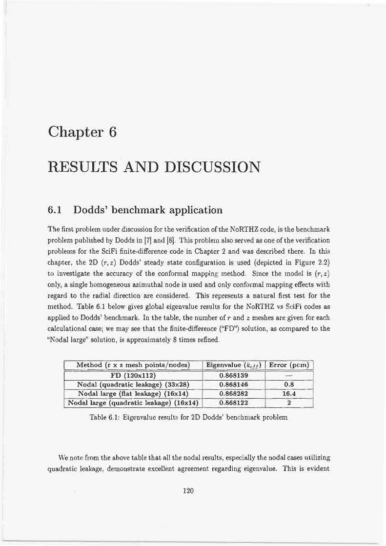
Chapter 6

RESULTS AND DISCUSSION

6.1 Dodds' benchmark application

The first problem under discussion for the verification of the NoRTHZ code, is the benchmark

problem published by Dodds in 171 and 181. This problem also served as one of the verification

problen~s for the SciFi finite-difference code in Chapter 2 and was described there. In this

chapter. the 2D (r , r ) Dodds' steady stat.e configuration is used (depicted in Figure 2.2)

to investigate the accuracy of the conformal mapping method. Since the model is ( r , z ) o n l ~ , a single homogeneous azimuthal node is used and only conformal mapping effects with

regard to the radial direction are considered. This represents a natural first tat. for the method. Table 6.1 below gives global eigenvalue results for the KoRTHZ vs SciFi codes as

applied to Dodds' benchmark. In the table, the numbr of r and z meshes are given for each calculational caw; we may see that the finite-difference ("FD") solution, as compared to the

"Kodal large" solution, is approximateIy 6 times refined.

1 Nodal large (quadratic leakage) (16x14) 1 0.868122 2 1 Table 6.1: Eigenvalue results for 2D Dodds' bencbnlark problem

Method (r x z mesh pints/nodes)

FD (120x112) Nodal (quadratic leakage) (33x28) Nodal large (flat leakage) (16x14)

We note from the above table that. all the nodal results, especialljt the nodal cases utilizing quadratic leakage. den~onstrate escellent. agreement regarding eigenvalue. This is evident

Eigenvalue (kcrf)IE.ror(pcm~] - 0.868139 0.868146 0.868282 '

- 0.8 16.4

6.2 PBMR application

PBMR was idonrihd ss one of the primary apylic~btion areas, and primary gods, of rbe work ID thi dismtation k % i m 1.5). The cham jmblarn for such an applicatioa b the 400

.The.2D p m b h . . Is gmphIc81ly rcpr~etlted below. The z-axis ~ b ~ ~ . b h e radial wrBIn,a%e (r) ~d tbb .pabris d s p i e ~ the d toordinate (r); Both ads m labeled wjth cmwec&m

cross-section) are in the order of F 4 diffusion lengths. The cross-section region sizes in this

PBMR pcobl~m, which are in the order of a single diffusion Iength, could therefore limit the

theoretical performance advantaee which nodal nlethods may provide. This statement will

be further investigated in the subsequent sections.

The problem is implemented as described in the benchmark specification, with one ex-

ception regarding the modeling of void regions. Void regions (indicated in the above figure)

are modeled in the PBMR benchmark with zero rernmal cross-sections. Although this is not

an in herent problem for the nodal method, special numerical expansions are required which

are not yet implemented within tbe current test code. For the purpose of this comparison.

the void region will be replaced with reflector material.

Three-dimensional description

The 3D problem description superimposes the (r. 8) layout in Figure 6.4 onto the (r, z j layout

in Figure 6.3. Notice from Figure 6.4 that the only azimrithal inhomogeneity occurs in the

vicinity of the control rods. Xote further that this figure represer~cs the (r, 8) cut of the

roded region of the core only, ~ ~ i t h the 'tRod" cross-sections replaced with reflector material

e~erywhere below the level of the rod insertion.

- I Cdcuhtion k-eff (error) T

FD RRference 70

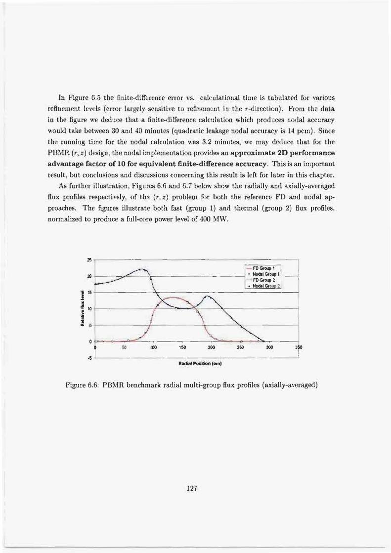
m f Cwlcdatron 1 k-eE lerrorl I Time Iminl 1 I I \ I 1 . I I

FD Reference (extrapolated) I 0.999652 -

lhbls 6.8: 3D PBM R global rcsulbs (nod4 vs ED)

''I-

6.3 IAEA cylindrical 3D benchmark

Tim find n u r n ~ ~ prob!m'addre& in thia itle&, k a "cyli.kdri$izd" arsion d Uiie 3D fAE.4 PWR bendmark pmblam degcribed in 17.1. For the sake of this work, the bewbrnark has b n adaptad to cylindrical eoordJnsres by c!oeely matching the vnluriie of fuel, control arid tpflecbr makrial,.and bum pmrvlng the niktun-f the'Elw gadientsk the pwbhrn. Tbis. pwbla hodd tsst the conforrnd mapping & p p m d h u g h l y , since it .exhibits severe material inhornogewjtles in all three d i m ~ ~ i o u a ~ The dctaiied d+mript.ion of the

The aim of applying t.he KoFYTHZ code to t.his probleln is two-fold:

Evaluate the accuracy of the method lor such a severely inhomogeneous neut.ro11ic

design.

* Identify deficiencies in the proposed method and define future improvements.

Global results

Eigensalue calcu1at.ions were performed with both SciFi and KoRTHZ for the above configu-

ration, and global. results are listed in Table 6.4. The nodal calculation was perfbrmed upon

a mesh with average axial- and radial sizes of approximately 20 cm, and the finite-difference refmement factors upon this mesh are listed in Table 6.4. The final two columns, named

"RZ" and "RP! list the maximum and the average .power error from two perspectives. The

"RY-column gives the (average and maximum) azimuthally-averaged ( T ~ z ) errors, and the

"RP-column gives the (average and maximum) axially-averaged (r, 0) error;. " R P may be

int.erpreted as the traditional assembly averaged powers for each axial channel. These def-

initions are introdnced in order to represent a very Iarge number of results as concisely tls

possible. The aeerase and maximum power errors reported in the table are for fuel regions in G

the system and the power in any node n is given by P, = ~ u ~ o ~ , , , , 9 ~ where w * represents g= 1

the energt releami per fission. The mesh on which these results are generated is described

in Appendix D.

Method (RxZxTh)

Extrapolated

FD(12x12x12)

F D (8x8~8)

F D ( 6 ~ 6 x 6 )

F D (4~4x4)

I Nodal - flat leakage 1 1.02483 1 9.2 rnin 1 62 pcm 1 0.84% (6.4%) 1 0.8% '02.6%) 1

k, r: 1.02420

1.02410

F D ( 2 x 2 ~ 2 )

FD (lxlxl)

1 Nodal - quad leakage [ 1.02424 ] 10.2 mjn 1 4 pcm ( 0.5% (6.9%) ( 0.5% (2.8%)

1.02398

1.02388

1.02378

Table 6.4: Eigenvalue results for 3D IAEA benchmark problem

Time \ kt!! Error - - I -

- .

34378 min 1 10 pcm

1.02468

1.02955

6202 rnin

2105 mjn

242 min

RZ(Ave,Mcoc) -

1% (3%)

lW(Ave,Max)

- 1% (1.7%)

21 pcnl

31 pcnl

41 pcm

6.5% (20.2%) 1 5.6% (12.8%)

6.1% (29.6%) 1 6.6% (22J%)

7.2 rnin

0.1 min 47 pcm

552 pcm

2% (6.2%)

3% (9.4%)

2% (3.5%)

3% (5-4s) 4.8% (15%) ' 4.6% (8.7%)

The reference flus results were obtained via extrapolation using results Gom the (6 ~ 6 x 6 ) ~

(8 x 8x8) and (12x 12x 12) finite-difference calculations as listed in Table 6.4. An extrapo-

l a t d solution was also obtained for the system eicenvalue (k,,,). This estrapolatiori fumction,

utilizing results from the same refinement levels as for the flux: and assuming a quadratic

approach to convergence, is found to be

and is plot.ted in i n Figure 6.14. From this function the extrapdated value for kc,, is found for a 0 'lA7eight.ed refinement factor" and has a value of 1.02420. This approach is consistent

with the procedure followed in 171 for t,he Cartesian equivalent of this problem, and is not

further described here.

1 + Un#orm reRemenl(6.8.12) - Poly. (Unilotm refinement (6.8.1 2)) 1

Figure 6.14: IAEA eigenvalue extrapolation - 2nd order fit for uniform refinement.

Firstly we notice: from Table 6.4, that t h ~ nodal solution is estremely accurate in eigen-

value (within 4 pcm of the ~xtrapolated resdt). M'e may further utilize Table 6.4 to estimate

the performance advantage factor for khe proposed nodal method over finite-difference re-

sults. \Ire notice a much larger improvernent in relative calculational time as compared to

the PBhfR in the previous section and an estimation of the performance advantage factor

Flux profile .comparisons

la order to inmstiggte the -nature- d the averaged nodal power errors, Figures 6.16 and 6.16 iltustrate erromin the.therrna1 Hux within. the core. Nodal flux errors, as wrnpared to extrapolated finite-difference, are presented Bratty as an (r ,zj contour plot and secondly aa an [r, 0) contour plat (the. mntout plob are, giveo lor both flat and quadratic leakage approximations), Once again {r, r) rmults are azJruuthdy-averaged and ('r+@) results me

dally-averqed. -

F i g w 6.16; IAEA (~~12) tbwmd flux errom--- .. . ().cparlr&ic 3-e [b) 8bt j&akqp

Figurn BJ7: ,JAW tbrmal profiles

In Figure 6.18 the adherence of the nodal solution to the inner boundary condition at

1 cm is visible, but does not signify a physical characterist.ic of the flux solut.ion. In the previous section. the PBMR model did not exhibit t . lh problern, since the ff ux solution was

near corr.stant in the center of the system. E'urt.herrnore, this effect is conipounded by the use of the quadratic leakage approximation near t.he cent.er, since this approacki makes use 0f .a

t.hrce node fit to approximate t.he trar~sverse leakage terms. The error therefore propagates

sorne dist,ance into Ihe systern. This rcsult higl-diglrts the nwd t.o include t,he inner zone

within the solrition proms, even if this is done in an appro.xhate manner.

Sorne i l l ture suggest ions in this regard include:

1. A hybrid leakage approximation, making usc of the flat approxirnat.ion near the center,

and dl+! quwdrat.ic approximat.ion t.hroughout. the rest of the system. This approach

wou1d avoid using the inner zone in leakage approximations near t,he center,

2. .4 hybrid fini t.e-difference / nodal solution in t.he ce~it~er of t,he system. Such an approach

would make use of the fact t.he the cerltral cut-out, region is small (in the order of 1

cm for t.he sake of current implen~ent.ation), and therefore do not require marly finite-

difference meshes to reproduce a reasonable result. Thus, such a solution would not

significantly affect t.he performa-nw.

3. A representative energy dependent albedo boundary condition st the edge of the cut-

out, updated during the calculational procedure. Such an update may be based upon

the intm-nodal s o h t ion within the neighbouring mesh.

4. -4 rigorous analytic solution for the inner homogeneous disc. Such an approach would

be more accurate, but may incur complexity not justified by the improvemeut .

Inner radial quadratic leakage contamination

These prior four c?dditions fall. in general, ontside the scope of the current thesis. Never-

theless, point 1 above has been implernel~tetl into t l ~ c test code and is termed the mixed

leakage approximation. This approach entails using the fiat (single node) transverse

leakage approximation within the first few radial meshes, and thereafter apply the quadratic

leakage aapproxirrlation to the rest of the systc~n. The motivation lies therein that the error

causd by the inner cut-out should not h~ ~IIowecl to propagate into the rest of the systcm.

Global results are p r ~ s ~ u t e d in Table 6.5 arid contour plots in Figure 6.19 ((r, z) and (r. 8)).

F i 6-10: IAEA thartnd ff LIX WFUW .far the mixed leakage oppra%imat;ion

Nodal aspect ratios

The quadtatIic leakage appm;uimatbn provida hpor.tmt imprwementa in results, and sped& i d l y in cases where aodd aqect ratios (measure of nodal skewness) are not excesgively large (typically lm than a factor ol10). Figure 6.20 indicates n d a l eYp~cla r&im r'w the system. Note t b t , sinm dl axial zone5 w e 20 cm in size, the x : r and z : 8 aspect mtiw a d only be &en for a single {r, B ) plane.

hand, the benchmark problem is also sufficient.ly difficult to highlight some short.con~ine of the approach, specifically associated with the ceot,er cut-out approximation and the u s a p of

the quadratic leakage approximation in this area These factors lead to larger flus errors on

the periphery of the system In these low flux areas, care must also be taken to implement

appropriate Tavlor series expansions to eliminate possible round-ofi errors, specifically in

the cxlculation of higher order Bus moments. These espansions are considered an important

future addition to the solution method as well as a coupled finite-difference/nodaI soh t ion

for the inner disc. A more consistently defined h ~ b r i d of the Bat and quadratic leahge

approximation is also foreseen, since this approach reduced errors in asially integrated powers

to within acceptable leveIs for nodal methods.

Final remarks regarding results

Three problems were investigated in this chapter, all of which relate to published bench-

mark problems. The problems represent various degrees of difficdtj-, and the YoRTHZ

code performed well in all cases. It may be concluded that the needed assumptions in the

development, such as (a) the inner cut-out approximation (Section 3.3) (b) the variable s ep

aration for the one-dimensional azimuthal source terms (Section 3-42), and (c) the fourth

order polynomial approximation to the inhomogeneous geometric sources (Section 5.2), are

numerically justified in both accuracy and performance, although some small outstanding

issues remain. The final chapter now follona, and gives general conclusions concerning the

ent<ire scope of this di~sert~ation ss well as potential future work.

Chapter 7

CONCLUSIONS AND FUTURE WORK

7.1 Introduction

The development, test implementation and verification of the conformal mapping approach

to the analytic nodal method. as described in this dissertation. signify some progress in the

field of method and code developm~nt for HTR reactors. The decision regarding the usa%e

of this method in dail?. PBNR d~s ign calculations is srill under discussion. but r~ su l t s in this

thesis will. go some way in supporting that obje~t~ive, This chapter w r w s t o summarize the major conclusions gathered during the development of t h ~ s work and supplies, at a glance,

the advanrages and shvrtcorninga of this approach. The dwelopment of this m r k has Iead

tn four international, refereed conference publications, received an award For best paper by

a young researcher. and has been nominated for publication in the SucI~ar Engineering and

Design journal (suhnlission in %larch 2007). These publicat.ions are listed below:

1. Rian H. Prinsloo. Djordje I TomaSeviC, "Development of the .?\nalytic ?;odal 3Iethc1d in

Cylindrical Geometr!". Prcxwdings of Blathematics and Computation. Superromput-

ing. Reactor Phyws and Suc lwr and Biological Application 20155. .4vignon, Franc?,

September 2003 on CD (2005).

2. R i m H Psinsluo. et al.. "Application of SP2 and the Spatially Continuously SPZP1

Equations to the PB\IR reactor ". Proc~edings of I I a thema t~cs and Computation. Su- p~rcornputing, Reactor Physim and Xuclear and Einlogical Application 2005 , At ignon,

Franre. Scptenlbcr 2005 on CD (1200;).

3. R i m H. Prinsloo. Djordje I. TomaSevit! '-Development of the Anal?t.ic Kodal 1Iet.hod

in Cylindrical Geometry for PBMR .4pplicstioll", 3rd Inrernational Topical SIerting

on High Tempcrat tire Reactor Technology (HTR 2006). Johannesburg-, South Africa. October 2006 on CD (2006).

4. Rim H. Prinsloo, Djordje I. TomaSevif, "!4pprmch t.r~ Singular Reeions in the Con-

formall Xlapped .4nalvtic S o d d l lethod in Cylindrical Geometry". Submitted and

acr~pted for publication at Jhitheruatiw and Computat.ion. Supercorr~puting. Reactor

Ph~sics and Nuclear and Riological .!pplicat ion 'lfl~7. Mon tcrey, California. US-4. April

2007 on CD (20071.

The major stepping stones of this work are discussed thrcli~phout these publications. In

the following sectkm. a more global perspective upon the work. its conchsions. releimt

cont rib11 rims and future work are presented.

7.2 General conclusions

I. Da>.-to-day design calculations for the South African PRhfR reactor are largely per-

formed with legacy code systems, and man! ad~ances in the field of method and code

development have not bem incorporated into thew systems. Onp such improvement

relaces to the usc of nodal methods for the sake of fulI core neutronic, diflusion solu-

tions.

2. The diffusion equation in cylindrical geometry poses problems during transvme inte-

gration within the Analfiic Soda1 Method. A proposed solution to circunlvent these

difficulties is 7.0 apply conformal mapping, to locaI1y map a node in cylindrical co-

ordinates into a rectangular one. and then apply transwrse int~grfition in Cartmian

coordinates. The important nude-averapcl flus to surface-averagpd current relation-

ship is obtained in mapped coordinates and findt: mapped back tcr or i~ ina l qlindrical

coordinati.~ Tor insertion inro the balance equation. Care must howver be raken in

the polynomial order of the approximat ion of the exponential mapping function This

deirlopment i s descrjb~d i n Chapter 3.

3. The equations derived in Chapter 3, based on [,he conformal mapping apprnarh. are

practical and manaq~able, both for the s a k ~ of implementation and efficiency. The

final equations arr similar in nature to nodal met hods with intra-node rwiduel s o l ~ r c ~ s

[r.g int.ro-node c~ms-s~ct.ion feedbzck), and were .mccr~fnlly iniplemenred in a 5tan-

dalone FORTR-4N code for numerical evaluation 01 the appraarh. A FORTR.43 based

f initwliffcr~nre solver. based upon the rnethodnloq described in Chapter 2. was r r l w

dev~loped to servc as a reference solution gencramr for the nodal test code.

4. -4s shown in Chapter 1. the derivrd equations exhibit a fine-mesh limit. which is an

important characteristic for the ~tnhility and accuraq. of the method. Due to the nature of the conforrnal mapping approach. the derived fine-mesh limit is not valid in

the center of the system.

5 . Comparison with finite-diff~rrnce results in Chapter 6 strongly supports the view that,

for the first time, successfnl transverse integration has indeed been achieved via con-

formal n ~ a p p i n ~ . Detailed flux profiles and global values of reactivity. for a variety

of test problems. sho\i- that the implemented conformal mapping technique works a

expected. Accuracy in eigenvalue. for the chosen s ~ t of test problems, is consistently

at. the order of 10 p c n ~ zs compared ta reference finite-difference solutions.

6. For the first time, as far as the author was aware at the time of rr riting. the quadratic

I w k ~ g j * approsirnation has successfully been applied to the .\?;>I in cylindrical Re-

ametry. This addition provides a marked improvement in the quality of results for

multidimensional problerns. and based on the results in Chapter 6, may be seen as a nccwsity for practical react.or calculations,

7. I t was shown in Chapter 6 that, although limited b ~ . PBIIR desirn factors, the .4Nhl still provida n 3D performance advantage factor of the order of 20 for x given accuracy,

when compared to a finite-diference approach. In the case of a mow typical LjI-R reactGr, a in the case of the 1.4E.A benchmark problem. the perfo~niance advantage

facttor is well in e x e s of 500.

S. -4s is visihIe from both Chapters 4 and .j, the conforrnal mapping approach does induce

a mild singularity in the center of the system, and this ma! b~ RF'PTI as a shortcomin~ uf

the m ~ t h o d . Due to this. a homogeneods cut-out is necessary in t1-1~ center. making use

of some form of coupled auxiliary solutions for the cut-out r~gion. A further impact

of the approach relates t o some meshing restrictions near the centrr of the system.

requiring typically two or three more nodal niesh~s near the center than some material

distributions would require.

9. The inner cwt-out approximation does not pose anj. difficultics for the PBSIR reactor

design. but \\.ill need an irnproi-ed formulation in the caw of larger central inhomogene-

it!. The imposrrl zero net current boundary condition placed a t the edcr of the cut-out

disc distorts the quadratic leakage approximation in ca.ws where the flux profilc near

the center is not constant In such c a s e hybrid solutions b e t w ~ n flat and quadratic

Icxkage. and fo r a coupled finitedifference, nodal w!utions may provide substantial irn-

trrovernents. Thew issues were d~scuswd and shon-11 in Srrtion 6.3.

10. All the abmv i:lsnsidered. nodal mrthods in general. ~ n d the rlcveloped conformal

mapping approach to the Analjtic Nodal XIethod in particular, certainl!. have a place

in t h ~ arena of PBSIR core calrulational methods. Son~e improvements may still hp

required for the method to become fully pract ~ c a l for ba! -to-da!. calcnlat ions, and some

of t h ~ w identified requirements are listed in the nest section.

7.3 Future work

During the development of this work, further developments outside the scope of the t h ~ s i .

were identified as natural next st.ep5. T h w are:

1. The method will be implernenkd in the Xecsa developed OSCAR code system 1221.

which uti l iz~s qtandard acceleration scherxm. This will allow realistic ralculational

times (improvement by approsimatel?. a factor of 20) to be obtained. and support

derisions to be made regarding the inclusim of the m e t h d in PBUR cdula t iona l

schemes.

2. Improved methods for the solution of the honmceneous central disc, and potentially

for the soIution of an azimuthally inhomo,aeneous central disc.

3. Taylor series expansions for small argument? are required in the case O F flus nmment

calculations. These are of specific use in problerns with larpc reflector nodes where t h e

flux reaches relatively lo\:. le~mels near s p t m boundark . Furthermore, such espansions

would allow incresed flexibility, such as the calrulatmn of void regions needed in

Section 6.2.

4. The PBhIR desim raiws inter~sting potential improvement nwds wit.hin the nodal

formalism. such as intra-node homogenization techniques to masinliw the nodal per-

formance a d v 8 n t . a ~ ~ . and non-st~ndatd or variable azimuthal discretitations applied t . ~

Iocalized azimuthal dependencies.

7.4 Final considerations

The succesiul int.tyration of the proposed met,hod into an industrial code syst.ern will require

furt.hrr twt,ing, develop men^, verification and validation. Furthermore. the optimal applica-

tion of the mcthnd n-111 requiw new methods. and adaptation of existing onw, in o t h ~ r :Ireas

of the reactor calr.uIationa1 path. Thew adjustments and extensions it41 take some time and

focuwd effort. Severthele~s. this work providps a solid foundation for further de~*eloprnent.

Other nodal solution methods, many of which were mentioned in the o p ~ n i n g rhapt~r .

may provide the final solution to the PBhIR core, diffusion problern. Decision m a k m in

this rward will make these choices at the appropriate time. but in the vrl? lcast, t.he South

-4lrlcan developed Cylindrical Analytic Kodal Method has now b ~ e n added to this list.

Appendix A

TEST CODE USER MANUAL

The input. rnanilnls for both SciFi and SoRTHZ are very similar, and hence. as ilIustration.

only the SciFi input manual is full!. desribed in this appendix.

SciFi user manual

SciFi input is CARD tvpe. with each card preceded with a cornpulsor~ comment field. The

data specification is free format and follons below. \\-hen multiple ent.rws are requ i r~d per

line, the description will be separated by a semicolon.

Version Card

a COAlSlEST: STRIXG I25S)

I'ERSIOK: STR14Cr [255j

Example input:

r '* CO3.IS.IENT'

'SciFi V1.00'

Tit,le Card

0 COXIME,3'T: STRIKG 12351

TITLE: STRIKG (255]

Example input.:

Description Card

a COJISIEKT: STRISG [255]

DESCRIPTIO?;: STRIYG 12351

Esample input:

'This problem is run as au input teqt'

Output. file name Card

CO>IhIEh'T: STRISG 12551

r OUTPL'T FILEY.AI\lE: STRISC: 125.51

Iteration Card

CO3l>lEKT: STRISG [255]

\ lax outer iterations: INT; M a x h e r iterations: INT; R ~ ~ ~ x i r t i o r i pnranwtrr: RE.iL(Gj ,F lu s

eonr-rxtmcr r~ i t~er i i~ : RE:lIJ{8) ; P o w r 1 \ '~1rmal i~~t ion Factor: r~nllP'I: DEBUG PRIST-

OL'T: IST: SP? calcu1ation:IKT; SP'2-P1 paranle~~r*REXLIBi

Sows;

\\'hen the debug option -: - 0. o n 1 standard output is w i t ten to the output file, c .hw

grea7t.r to I. incrementally more d~bugging information is written to t b ~ output file.

Energy Group Card

4 COllhlEST: STRING 1'2351

rn Number of Groups: IST ; First thermal group: IST

Example input:

30tes

XI1 thermal groups are automatically used in upscatter caIculations. [if the crasscct,ions

aIlow)

Fission Spectm Card

COXlhlENT: STRING [%5]

4 Fissiori neutron iraament per group for (1 .. SCII-GROUPS): real!?: .

EsarnpIe input:

a '* C03151EhTm

CalcuIational Mesh discretization Card

COkI.\IEST: STRIKG (23ZJ

Snmber of calculations! Radial m~shes: 1ST ; Xsial. IST : Azimuthal INT

Example input:

Calculational Mesh Refinement Card

r CO\I3lEST: STlUSG [235]

Y r s h refinenlent fact.or: Radial: 1ST ; Axial: 14T; .4zimutl1al: IKT

Example input:

Outer RadiaI boundary condition

a COMlIEYT: STRISG 1255)

ALBEnO Value(l..G): real(S}

Esample input.:

a '* COhlSIEXT - allledu ior two group problem'

. 1.0 1.0

Sot es:

A n Xlbeclo ~.alue of 1 indicate? r~flectivc boundary conditions.0 indicatw Zero Ir~cominy,

Currrnt. and -1.0 is used for Zero-flus condition. .Any value between O and I may be used for qxcifir: albedo value.

Bottom axial boundary condition

CC)\IXIEXT: S'TRISG (25.31

Example input:

3 o t . w

A n Albedo value of I indicates r e k t i v e boundar!- conditions,O indicorw Zero Incoming

Current.. and -1.0 is used for Z e r ~ f l u s condition. .An!. value between 0 and 1 n l q be used

for specific albe-do value.

Top axial boundary condition

a CO\I3lENl': STRING 12353

0 ALBEDO \hlue(l . .G): real(8);

'" COMXIEXT - albedo for two group problem'

X o t w

An Albedo value of 1 indicates reflecti~,~ boundar~ conditions. 0 indicatc~ Zero Incoming

Current.. and -1.0 is used for Zero-flus condition. Any \+slue lwt\veen O and 1 may be used

for specific albedo value.

~Mesll and Source options

0 COa.lh1ENT: STRIKG [255]

IIESH OPTIOY: TXT ; FIXED SOI'RCE FL.AG: IKT

Example input.:

sotm:

IlESEI OPTIOS = O indicatps ~splicit mesh division input in card 14. MESH OPTICIS= 1

ind~catcs uniform. equi-distant mesh distribution d~fined in card 1.5. and MESH OPT'IOS=3

ini l icat~s cqui-volume r e n d i n g described in card 16.

The FIXED SOURCE FL.X indicar PF the presenw of fixed sources in sornc! meqh rrgions,

and will be d~scribed in C?IRD 21

Explicit mesh definition (only given if MESH OPTIOX = 0 )

rn COLlZ\lEYT: STRIKG 12551

Radial Mesh Sizes (l..Radial Meshes 1: real(8)

Axial Mesh Siz,miT ..Axial Mesh~e): real(8)

.4zimuthal Mesh Sizes ( I ...A zimut.hal Meshes): realj8)

Esanlpl~ input.:

Uniform (equi-distant) mesh definition (only given if h4ESH OPTIOS = 1 )

COlIXIEKT: STRIXG [2351

Radial Mesh Size: redl S ) ; Axial liesh Size: tealis)

Example input:

Equi-Volume mesh defmition (only given if MESH OPTION = 2 )

COh,lllEST: STRIxG 123ST

r Xumber of C'oan~! R4j .d Regions to Renmh : IST

Boundaries for m a r w rrcgions(1 ..Sum-r~gi~-ms;-l): IST:

Example input.:

3-0t.m

XIESI-I OPTIOS = 2 r~quires an ini t id default mesh size to provid~ a ref~renre for

coarw-mesh boundaries The course r n ~ s h regions will be remeshed within thclr boundaries

spwified in this r ~ r d accordins to an equi-volurn~ radial condition (the total number of

me.shes will remain constant).

Material specification options

COSI>IES'I! STRIFG [253]

Kurnlwr of hlaterials: IST : Material specifici~tiun method (hlSIl) - 0 or 1: IXT

Example input:

Sot.6:

3I~t.wial Sperificlztion met hod llC3hf) = O indicntrr.~ explicit material ident.if cat.ion for

e ~ r h radial. axial and aaimuthal zone and is r lwcrih~d in CARD 18 kelow. MSJl=l ind1cat.e~

con-rl~inational n ~ a t ~ r i a l pl; le~~nent, allou-in,g for simultaneou5 wsirnment of a rnatrria! t.o

rntdtiple indices and is dewrihd in C.4RD 19 below.

Explicit Material assignment (only given if MShlI=O)

r C04lMEST: STRIXG [2%]

0 II*4TERI:4L ID SUMBER (1..Z.CIas.l..RB~Ia~~1.~~4rc~~~Ias): INT

E x a m p l ~ input:

o " CO.ZIZ1EKT'

Sotes:

The abovc input describes a 2 asial layer cylinder with 3 radial zones and 3 azimuthal

zones. 1la:ttria.l 1 is placed everywhere in axial zone 1, material 2 everywhere in axial zone

2. except the out,er radial zone has material 3 in all azimuthal zones.

Combinational Material assignment. (only given if h/ISM=l)

COlI3,IEKT: STRIYG [2531

0 Zone name: STRIFC[253]

Kumber of radial zones filled tty single material: 1KT

Example input:

The foilowing example d w r i b e s the same core x used for example in C.IRD 1s. (The

extracts in parenthesis wrves for explanation. and are not ccrn~pulsory input).

a '" COX~I.ClEST~

a 'BOTTO31 L.4YER'

a 1 (one asial layer)

3 (3 radicil layers)

a 1 (material number l!

a 'TOP AXI.4L L:!YER"

1 (one axial layer j

a 2 (first two radial layers)

a 7 (Matwial number .2)

a I font more rad id layer - Last, radial layetj

a 3 (liaterial number 3)

iiotes:

T'hc code will stop reading records when all asial and radial layers are fiiled. Please notc

that azimuthal dependence is not catered for in th is input specification, but still to be added

in the form or material specification method = 3.

a Repeat the follo?mtg TE~CCIITI , f o ~ each m n i m d lypc i:l!nfrum number oJ tivw.7)

a Material Kame: String1255l

a Removal cross-sections (l..G): real[8)

a Diffusion cross~ct , ions (1 ..G): real (8)

a Kufission cross-swtidns [l..G): real(S)l

a Power r r ~ ~ c a e c t . i o n s (l. .G): real(8)

a !katt.er Matrix (l..G,l..G): real(S)

Example input:

r 'Top.Bot Ref 1'

'FUEL r.ype 1'

P I e w note that the absorption cross-section specified should be removal cross-swtion,

Fixed Source specification (only given if FIXED SOURCE FLAG in CARD 13==1)

r Xumber of source zones: INT

r The iollo\rins, one line record is repeated "Xurnbcr of Sourcc zone" times

0 !-TART GROUP. INT : ETD GR(3UP:IST; ST.4RT RADI.4L:IKT: ESD R.ADI.\L:I?iT : START AXIAL: r n ; EXD PWAL: INT ; START . - ~ Z I ~ - T H A L : IXT : E?;D AZ- ISIUTH.-\L: I5-P : SOURCE: STRESGTH; real {S)

Example input:

Kotes:

The above input dwcr'ibes a source of density 1.5 in group 1. placed in radial z o w s 1 to

3. on av id layer ~ 4 , lor firs1 4 azimuthal zones,

Results requirement specification

r COM?.IESTr STRIXG 12,551

a Surnher of result sets requested: IST

a The foIloninq one line record is repeated "Xumber of Result set" limes

Primary results category: STRIYG 12531

8 ST.4RT GROUP: IST : END GROL-P:INT: START R.\DI=\L:INT; ESD R.%DI.\L:IST : START XXI.4L: INT: EKD .-lSI.4L: IKT ; ST-ART .4ZIhIUTH.4L: IKT ; EXD '42- IlIUTHi4L: INT

Esampic input:

'LIST'

Sot.es:

T ~ I P a13w-~ input requests a list of Ruses in group 1, placer1 in radial ZUIWS 1 to 4. 01.1 axial

layer 6. for first 4 azimuthal zones. .hiilable results reque~ts include:

Primary: 'FLUS'

Swondary:

'.A\'ER.\GEt- volume-averapd flus for region

'R,41yERi4GE'-sxiall and azimuthally-avemg~d (volume) A I L Y ~ S for radial regions

'X.\\'ER.c\GE'-radia11:y and azimuthally-avera~~c1jvolume) ff uxes for asial regions

';1,ZI.4\'ERACE' - radially and axially-avera~ed(vo1ume) fluxes for a~ imutha l r q i o n s

'RZ.%\-ERAGE' - Map of radially s axial Fluses averaged azimuthally

'RTHA\'ERAGE+ - Map of radiall!: s azimur.hal1 fluxes averaged a s i a l l ~

'LIST'

r '.417ER.4GE'- volume-averag~d power for rc~itinn

'R.4\'ERIJIGE'-asiall!.-a\-eraged po\vrr~ lis~ecl for radial and azimuthal region

'.4.4~'ER.4GE'-radially-avctn~d powrs list.~d for asial and azimuthal r e ~ i o n

Primary: 'SS' - crw-sect ions

Serondar!.:

Primary: 'COEFF' - finitc-diflermw coeficients

S~conclary :

Appendix B

DODDS BENCHMARK PROBLEM

The (r, r ) published ([7] and (81) 2-gronp DODDS' benchmark problem is fitlly described

in this appendix. We first present the general materia1 l v o u t of this Iwo-group eigenvalue

proldern.

Figure B.1: DODDS' beuchmark modal in ( r , z) geometry

Zero-flus boundary condit.ions are r~sed on all outer bouniling surfaces, as (described in

[S]. Cross-sectior~s associat.ecl with each zone are listed in t,11e t,uble L)elow.

TEST CODE INPUT EXAMPLES

SciFi input example (Dodds benchmark problem)

'* 1:ER.SIOX1 'SclFi \.'I .DO'

" TITLE'

'DODDS for corr-xted pmrnetr~~ RZ COX,IPARISOS' '* DATE' y 11at .2El[)4'

'* DESrnPTIOS"; '

'Compare Cylindrical m!ution with ASL BEXCH1;lARK' " PRISTOGT FILE' 'DODDS- bench.PRT' '* M.%S OUTER ITER, 1\,lAS INNER ITER, OUTER EPSILO?;, Extra POKER SORJIALIZATIOY

FACTOR, DEBUG PRIXTOUT'?' 21:0 50 U.17Lu:WOlDCI I 0

" YU.:.\,lBER OF GROUPS. FIRST THERMAL GROUP' 2 2 'I Chi - fission spcctrurn distribut.ion per enerr? group.'

1.DDO O.ODiJ

" Kurnher sFRadial. Axial and Atimnthal m&es'

1g ?R I

' ' .-'ilbebo lw~atdary wluw (in nlitar r d k l hw~ndary for group (-1 for zcrefjnx br-~undary condit.ion)'

-1.nDD -1,ODO

" :I lbedn boundan. di.~~.~ on bo: tom axial bilundary Tor ,pprlp> '

-1.ono -1.0~0 " A l k d n boundary valtics on top axial borladary for gilup '

-1 .OD0 -1.ODO '*I' ~tifornl mwh'?. Fixed E ~ Y ~ T C ~ ! .qwr i f i c3 th~~1 '

1 0

Appendix D

I U A . -'. =.,.-- .LA. BENCHMARK DESCRIPTION (CYLINDRICAL)

Figure D.4: IAEA Ncdal mesh - botm reHector md bottom care mgions

Appendix E

RECURRENCE RELATIONSHIPS

FOR FLUX MOMENTS

E l Flux moments

R e first derive recurrmce relationship for integrals of ~sponential-polynomial form.

Utilizing the relationships

1 .;3 1 S O H ~ ! j.) = - ( C - e-") and ~ i n h ( 3 ) = - (6' - cd3)

2 2 moments done-dimensional flux ar t spparately calculated in their cosir. s m h and particular

sohtion ccmponer~ts. Let us firstly define the hperbolic cosine moments, which exist only

for 1 elm:

lor

Similarly define:

fur

.I = 1.3.5 ,......

E.2 Mapped flux ~noments

In this i n s r m c ~ we may utilize eq. (E.1) by I$-riting

Developin? a similar recurrence re!atmnr-;hip a~ in eq. (E.?), r w may define:

Appendix F

EXPANSIONS FOR DOUBLE

LEGENDRE INTEGRALS

In this appendix. Taylor m i - expansions for the moments of double Legendre inr~grals are

developed. T h ~ w quantitiw ran not be naturally derived h r n recurrence relatinnships. and are irnplenlcnted as explicit expansions as listed below. The armlyric espansiom are listed.

and t8hmaf tw their Taylor series rountprparts. In the expressions below, 1 and n r e p r ~ e n t

the individual orders of Legendre pol:nomials, and c represents the mapped mesh s i z ~ h,,

Thecr mpresions arc prone to round-off error, and hence, if exprrssed in terms of Taylor

series espan,rions, become:

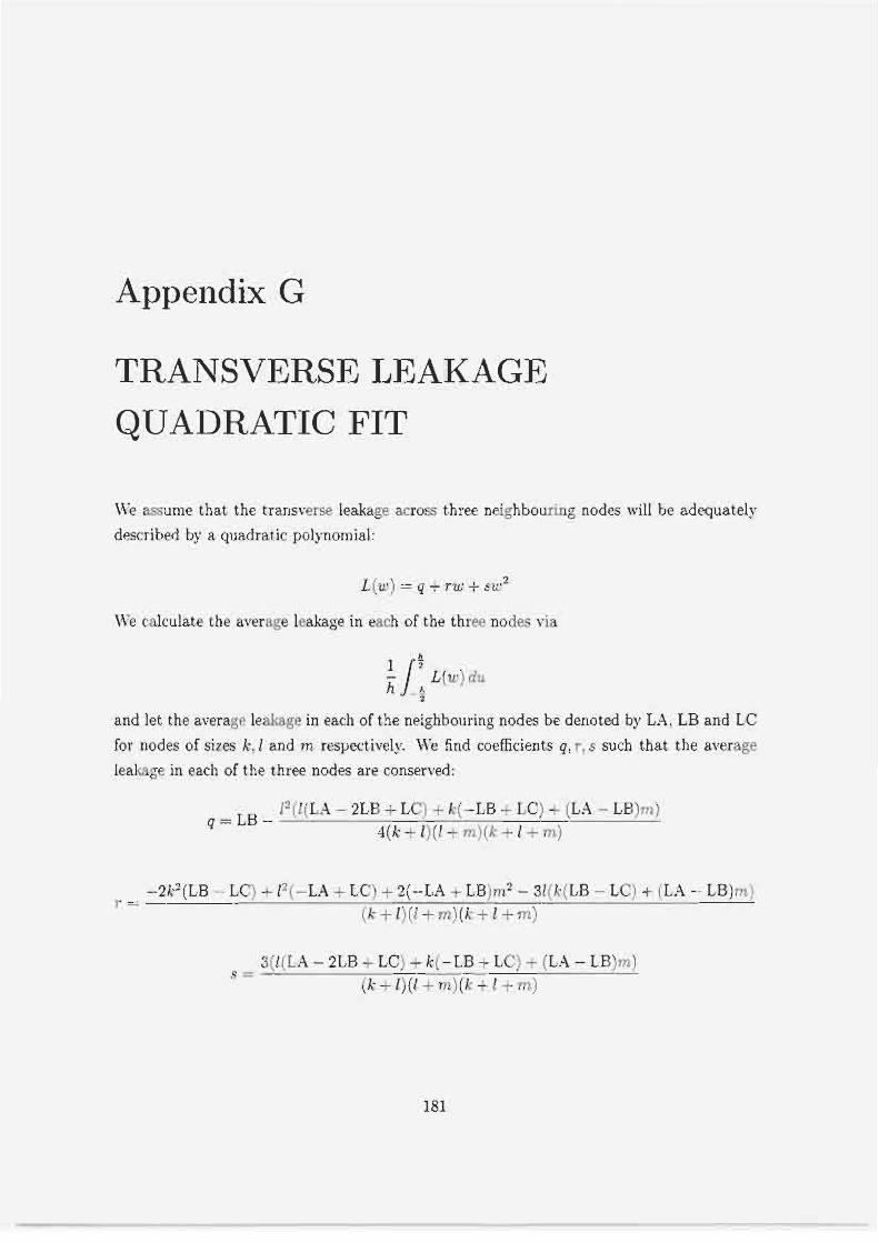
Appendix G

TRANSVERSE LEAKAGE

QUADRATIC FIT

\\k zwume that, the transverse leakay across three neightrowing nodes will be adequately

described by a quadratic polynomial:

\Ye calculate the atwage leakage in each of the t h r w nodes via

and let the averagv leakage in each of the neighbouring nodes be denoted by L.4. LB and LC

for nodes of sizes k . 1 and rn respectively. \\'e find coefficients q, r , s such that the a v e r q y

leakage in each of the three nodes are conserved:

Bibliography

Ilj R. J -1. ST:!13XI'LER and 1.1 I . -4BB.4TE. "IIlIethods of Steady St.ate Reactor Physics in Nuclear Design." Chap, 3, Academic Press, Grwt Brit.ain (1983).

121 H. GREE,NSP.U, C. S . KELBER and D. OIiRFST. "Con~putational Methods in

Reactor Ph?sics.l C h a p t ~ r s 1 and 2, Gordon and Breach, Kew k'orl; (1968).

[3] J. DUDERST.4DT and L. NXXIILTO3. "Kuclear Reactor Analysis." Chapters 4. 5. 7 and 10, J o h n \l'lle~- k Sons. Kew York (1976).

(41 S. \ \~~LFR.VII . "The Mathematics Book," IVolfram Media and Camhridy 1-nicer-

sit! P r p ~ (1999).

(31 D. TRIII; "Complex Analysis and its Applications:!' Chapter 7, P\33 Publishing

Company (ITP), Bostor, (l99G).

161 Y. .4ZMY, ".A Sodal Int.egra1 Method for the Seutron DifTusion Equation in Qlindrical

Geometry:" T m ~ j s . An-ler. ilturl. Soc., 54, p. 183 (1987).

171 R. R . LEE. "-kgunna Code C'rnter: Benchmark ProbIem Book," -4NL-7416, Suppl. 2,

ASL (1977j

(Bj H. L. DoDnS, *'.\ccuracy of the Quasistatic Jlethod for Two-din~ensional Thermal

Reartor Transients with Feedback." ~V~tc i . Sci. Ltjy., 59, p. 271 (1976)

191 t, B. FO\ITLER, et al.. "Suclear Reactor Ana1ysi.c Code: CIT=\TIOP!." ORSL-TSI-2496. RPV, 2 (197'2).

[101 R. D. LA\\'REXCE. "Prnyres in Sodal Slethods for the Solution of the Seutron Diffu- sion and Transport Equatims," P r m p s s ~n n ' t : c h ; E ~ L F . ~ Q ~ . 17, p. 371 (19%).

1111 K, S. SNITH, ;'.An .4nal!.tic Sodal hfethod for Solring T\:-wqoup. 1~3ult.idimensinnal

Transient and St.at,ic Kwt.ron Diffusion Equat.ions." Sucl. Eng. Thesis, Depart.n~ent of

Yucl. Ens., M1T (19793.

1121 .4 11 OUGOU-SG. er a1 , .'.4nal!tic Solution of the Seutron Diffusion Equation In

3D C!,lindrical Gmnlctry for Application in a Kodal llethod," Procwcli?vp of !'irtirI~nr

M12 t h x n!rcr~/ arrd C u ~ p ~ t a ! ~ i r ? i a I SCLV~I EN (XLilC 2OOT) . Gat.lirhurg, Tennrcsw, April

6-1 I , on C'D (2003).

1141 D. L. I'OGEL and Z J. IVEISS. '*.4 General >lult,i-group Formulation of thc -4nalytic

Soda1 1Iethod." Pwr: o j the Top?cal Mr4tng: A d r ~ n r ~ v ~ ~ ~ 7 r Reactor Phy.s?cs. 1, p. -197.

CLnrlesto~l. SC', >larch 8-1 1 (1992).

1151 H. FISSE.\I.AS, F. RESXC\\ITZ and 31. R.. I Y - G I E K . "Interface Current Technique.;

for hlulridimensional Reactor Calculations," AIovI:em~neqm'r. 30, p. 123 (1977)

[IF! 1'. -4. CI-(AO? 'TYnifying via Conformal )lapping Coarse-m~sh Yeutron Diffrlsio~l Cab- lations in Carte~ian and Mexagmal Geometries," J o : m u i o,f Co~rryxfn!imuI and A p y , b ~ d

Mathrrnntm? 63. p. 44.9 (1993).

11 T ] F. REITSIIi4: et a]., "The OECDi'SE:2 ..'KSC Coupled 3eut.ronics . ' T h ~ . r m d Hydraulics

Transient Benchmark: PBhIR 400 Core Design,!' Proc~~dirsyr: o,! Topicot Medang dn

.4dvar1ce~ in Reactor P h y . + c ~ (PHYSOR 2006), \hncoww, BC, Canada. September

10-13, on CD (2006).

1181 D, hlATZXER, "PBRIR Project Status and the t \ *a~ ' .4head,'! 2nd l n l ~ r n n i l o n a l Tnp-icol

Mcct,ng o n High Tmpvmfare Reactor Tcchvoiq~/. Beijing, China, September 22-24, on

CD (2004).

1191 X. Z. CHO. e t al.. 'The AFES Method in Cylindrical (r.0.z) Geometry for Pebble Bed

Re~ctors - Exteusion to I\Iultigroup Form and Treatnlent sf I'oids.'' Tn2n.c. r lmrt. !Yucl.

Soc.. 94. p. 553. June (2006'1

1201 D. I. TOII.&~IC and E.lJ-. L-4RSEN. ' T h e Simplified P2 Approsirnation." tl'tici. 5,;.

Eryc., 122. p. 309 (1996).

1211 P. S . BRAhTLEY. "Spatially Continuaus W-PI Solutions for Planar Geometry." Tvr~s.

Amer Ir:u.cl. Soc., 91, p. 14.5 (2004).

1231 D. G. C.\CUCI, ei al.!'T~~-o-Din~e~E;ion~l Geometrical Corner Sin,plarities in Neutron

Diffusion." J'ucl. Sci. Eng., 128, p. 1 (19881

12.11 R. H, PRTYSLOO, et 81.. ".;\pplir~~icln of SP2 and the Spatially Continuous SP2-P1 Equations to the PBhIR Reactor." P I - o c w L ! ~ ~ ~ ~ ~ of Jfnthernot~r..: nnd Cornputuiion, 5 ' ~ -

p ~ ~ c v n ~ p f r r r g , R ~ n c t m Phy~!'l:.s and i\'uclmr and 6t.dogicfll' A p p l ~ c d a t ~ ~ t 200.5, .4\ ipnm.

France. September 12-15. on CD (200.5).