Order of convergence for polynomial and analytical nodal methods

J. Appl. Math. & Computing Vol. 21(2006), No. 1 - 2, pp. 411 - 429

Website: http://jamc.net

ORDER OF CONVERGENCE FOR POLYNOMIAL ANDANALYTICAL NODAL METHODS

NAJIB GUESSOUS AND FOUZIA HADFAT∗

Abstract. In [6] we analyzed the direct analytical nodal methods (ANM)of index l and show that the corresponding mathematical methods areequivalent to the physical ones when the components of the matrices arecalculated by generalized Radau reduced integration. In this article weextend the theorem 8 of [7] to the polynomial nodal methods (PNM) (exactcalculation of moments) which are thus the order of O(hl+3−δl0 ). We alsoshow that the analytical nodal methods are only the order of O(hl+2). Forl = 0 our numerical results confirm our theoretical results.

AMS Mathematics Subject Classification : 74S30.Key words and phrases : Partial differential equations of elliptic type, nu-merical analysis, diffusion equations, finite element methods.

1. Introduction

Broadly speaking, nodal methods are fast and accurate methods which com-bine attractive features of the finite element method (f.m.e.) [3] as well as of thefinite difference method (f.d.m.) [9]. With the f.e.m., they share the fact thatthe unknown function is approximated over a given coarse mesh by a piecewisecontinuous function, usually a polynomial one. As with the f.d.m., the resultingsystems of algebraic equations are quite sparse and well structured, essentiallybecause the basic parameters are cell and edge moments of the unknown func-tion, which connect at most two adjacent cells. These methods were developedin the late 1970s for numerically solving partial differential equations (PDEs) ingeneral, especially in relation with static and dynamic nuclear reactor calcula-tion. Classical references are Finnemann and al. [4], Langenbuch et al. [10,11],Shober et al [13], Frohlich [5], Dorning [2] and Wagner and Kobke [14]. In §2,we present the analytical nodal methods (ANM) with transverse integration [7].

Received April 11, 2005. ∗Corresponding author.

c© 2006 Korean Society for Computational & Applied Mathematics and Korean SIGCAM.

411

412 Najib Guessous and Fouzia Hadfat

In §3, We recall the Theorem 8 of [7]: with the mathematical ANM, momentsare obtained exactly. We extend this result to the polynomial nodal methods(PNM). In §3 we analyze the direct procedure of ANM introduced in [7] and weshow that the corresponding mathematical ANM are equivalent to the physicalones when components of the matrices are calculated by generalized Radau re-duced integration [6]. In §4 we show that the PNM are of order of O(hl+3−δl0)whereas the ANM are only the order of O(hl+2). For l=0 our numerical resultsconfirm our theoretical results

In §5 our numerical results (with l = 0) confirm the theorem 8 of [7] as goodfor PNM that for ANM and show that the direct procedure is more fast andprecise that the procedure of the transverse integration.

2. Analytical nodal methods with transverse integration

Let us consider the elliptic PDE

−∇ · p∇u + qu = f, ∀ r ∈ Ω ⊂ Rn (1)

where p = p(r) > 0 while q = q(r) ≥ 0. Moreover u is subject to boundaryconditions on Γ = ∂Ω, that we shall take of the Dirichlet type for the sake ofsimplicity, namely

u = 0 on Γ (2)

In typical neutronics applications, u would be the neutron flux, while p andq would be the diffusion coefficient and the removal cross section, respectively,usually assumed to be piecewise constant. To make things easier to visualize,we shall take n = 2 and assume that Ω is of the “union of rectangles” type.Ω can be completely covered by I vertical and J horizontal slices. The basicanalytical nodal formalism consists first in “ transverse-integrating” (1) over (n−1) dimensions. This is done successively and leads to n 1D equations in thedifferent directions (here x and y). Assume that Ω is the union of rectangularcells Cij of size h × k (or more generally hi × kj) belonging to the intersectionof the ith vertical and jth horizontal slices mentioned above. Now write (1) overon such node in dimensionless variables (x and y again) as

− 4h2

(pux)x − 4k2

(puy)y + qu = f, ∀(x, y) ∈ C = [−1, 1]2 (3)

Let us now introduce some notation which will be quite useful in the followingfor the ith-order vertical moment of a function w of x and y, which is thus stilla function of x, namely:

miy(w; x) =

1Ni

∫ 1

−1

Pi(y)w(x, y)dy,

and similarly:

mix(w; y) =

1Ni

∫ 1

−1

Pi(x)w(x, y)dx

Order of convergence for polynomial and analytical nodal methods 413

Pi will be the normalized Legendre polynomial of degree i on [−1, 1] with thewell known properties:

Pi(+1) = 1 ,

Pi(−1) = (−1)i,

Pi(−x) = (−1)iPi(x),∫ 1

−1

Pi(x)Pj (x)dx = δijNi,

Pij(x, y) = Pi(x)Pj (y) .

Ni is a convenient normalization factor:

Ni =2

2i + 1

In particular, we shall define the following edge moments of w:

miL(w) = mi

y(w; x = −1),

miR(w) = mi

y(w; x = +1),

miB(w) = mi

x(w; y = −1),

miT (w) = mi

x(w; y = +1),

where L, R, B and T stand for Left, Right, Bottom and Top respectively. Cellmoments of w can also be defined as

mijC (w) =

1NiNj

∫ 1

−1

∫ 1

−1

Pi(x)Pj(y)w(x, y)dx dy. (4)

In the following, we shall frequently refer to some basic spaces of polynomials in2D, namely

℘i = xayb/ 0 ≤ a + b ≤ i i ∈ N,Qi,j = xayb/ 0 ≤ a ≤ i 0 ≤ b ≤ j i, j ∈ N ,

Qi ≡ Qi,i .

Multiplying (3) by Pi(y) and dividing by Ni (i = 0, . . . , l), we obtain aftertransverse integration in the y direction

−4h2

d

dx

(p

d

dxmi

y(u, x))

+ qmiy(u, x) = mi

y(f, x) +4k2

liy(u, x) i = 0, . . . , l(5)

where liy(u, x) is a transverse leakage depending on u (and x) at the top andbottom of the cell Cij :

liy(u, x) = miy

(d

dy

(p

d

dyu(x, y)

))i = 0, . . . , l


A similar equation can be obtained by transverse integrating in the x direction,namely

− 4k2

d

dy

(p

d

dymi

x(u, x))

+ qmix(u, y) = mi

x(f, y) +4h2

lix(u, y) i = 0, . . . , l(6)

with

lix(u, y) = mix

(d

dx

(p

d

dxu(x, y)

))i = 0, . . . , l

and clearly compatibility conditions must be satisfied, requiring that mix and

mjy commute

mix(mj

y(w; x)) = mjy(mi

x(w; y)) = mijC (w) i, j = 0, . . . , l.

The numerical solution of (5) for the J horizontal slices and of (6) for the Ivertical ones is then intended as follows. To simplify the exposition, we shallfirst consider that each of them reduces to the following canonical form

− d

dx

(p

d

dx

)u + qu = f, ∀x ∈ [a, b]. (7)

On the corresponding slice, where both p and q are piecewise constant and thatdue to (2), u is zero at the extremities of the slice

u(a) = u(b) = 0

. Equation (7) is first replaced by a “weak” form obtained by multiplying it bysome test function v(x) and integrating it over [a, b]. As with standard finiteelement methods, the original problem is equivalent to the following problem:

Find u ∈ H10 [a, b] such that a(u, v) = f(v) for all v ∈ H1

0 [a, b] (8)

where

a(u, v) =∫ b

a

(pdu

dx

dv

dx+ quv

)dx, f(v) =

∫ b

a

fv dx. (9)

Some discretization must be introduced, namely a finite dimensional subspaceSh of H1

0 [a, b] is defined and (8) is replaced by:Find uh ∈ Sh ⊂ H1

0 [a, b] such that

a(uh, vh) = f(vh), ∀vh ∈ Sh ⊂ H10 [a, b]. (10)

In our description of ANM, the basis aspects of standard f.e.m.’s will all bepreserved, except that the definition of Dl and Sl will be slightly different:

Dl = mL,mR,miC , i = 0, . . . , l, l ∈ N. (11)

If the particular element Ii = [xi−1, xi] of size hi is mapped onto the referenceinterval C ≡ [−1, 1], equation (7) becomes in reduced variables [7]

−uxx + λ2i u = f, ∀x ∈ [−1, 1] (12)


where λ2i =

h2i qi

4pi, while f stands now for f =

h2i fi

4pi.

Over I , we thus have (with λ = λi)

Sl = exp(λx), exp(−λx), 1, . . . , xl, l ∈ N (13)

and we havedim Sl = dim Dl = l + 3.

Remark 1. Another choice of Sl leading to PNM [8] consists to replace Sl by

℘l = 1, x, . . . ., xl+2, l ∈ N. (14)

Thus we have

Sl+2 = ℘l ⊕ e−λx, eλx. (15)

If w ∈ Sl+2, then there exist

w1 ∈ ℘l and w2 ∈ e−λx, eλxsuch that

w = w1 + w2.

i.e., there exist two constants a and b such that

w2 = ae−λx + beλx. (16)

If w ∈ Sl+2 is the solution to the equation (12), we have

Lw1 + Lw2 = f (17)

but

Lw2 = −λ2(ae−λx + beλx) + λ2(ae−λx + beλx) ≡ 0. (18)

Using Lax Milgram lemma,w = w1

andw2 ≡ 0.

Theorem 1. Dl is Sl(resp ℘l) unisolvent [1].

Proof. With card Dl = dim Sl (resp ℘l), it is sufficient to exhibit the corre-sponding basis functions:

1. Let us call

Qi(x) = Pi(x), i = 0, . . . , l, (19)

Ql+1(x) =

cosh∗

l (λx) l is oddsin h∗

l (λx) l is even,

Ql+2(x) =

sin h∗

l (λx) l is oddcosh∗

l (λx) l is even,


where the star (*) indicates that the corresponding functions are normalized to+1 when x=1. Equivalently

Ql+i(x) =expl(λx) + (−1)l+i+1 expl(−λx)expl(λ) + (−1)l+i+1 expl(−λ)

i = 1, 2 (20)

where

expl(λx) = exp(λx) −l∑

i=0

1Ni

∫ 1

−1

Pi(x) exp(λx)dx. (21)

The analytical basis functions are [7],

uL(x) = −12(−1)l+1(Ql+2(x) − Ql+1(x)), (22)

uR(x) = +12(Ql+2(x) + Ql+1(x)), (23)

uiC(x) = Qi(x) − Ql+m(i)(x) i = 0, . . . , l (24)

where m(i) = 1 or 2 is such that i and l + m(i) have the same party.2. The polynomial basis functions are [8],

uL(x) = −12(−1)l+1(Pl+2(x) − Pl+1(x)), (25)

uR(x) = +12(Pl+2(x) + Pl+1(x)), (26)

uiC(x) = Pi(x) − Pl+m(i)(x) i = 0, . . . , l. (27)

3. Direct analytical nodal methods

In correspondence with PNM of index l [8], the analytical analog schemes hasbeen introduced by Hennart [7]. Let us define

Dl ≡miL, mi

R, miB , mi

T , i = 0, . . . , l; mijC , i, j = 0, . . . , l, (28)

Sl =Ql,l⊕ < expl(+λx)Pi(y), expl(−λx)Pi(y), Pi(x)expl(+λy), (29)Pi(x) expl(−λy), i = 0, . . . , l, (30)

cardDl =dim Sl. (31)

Theorem 2. Dl is Sl unisolvent [1].

Proof. The basis functions are

uiL(x, y) = −1

2(−1)l+1(Ql+2,i(x, y) − Ql+1,i(x, y)), i = 0, . . . , l, (32)

uiR(x, y) = +

12(Ql+2,i(x, y) + Ql+1,i(x, y)), i = 0, . . . , l, (33)


uiB(y, x) = −

12(−1)l+1(Qi,l+2(x, y) − Qi,l+1(x, y)) i = 0, . . . , l, (34)

uiT (y, x) = +

12(Qi,l+2(x, y) + Qi,l+1(x, y)) i = 0, . . . , l, (35)

uijC (x, y) = Qij(x, y) − Ql+m(i),j(x, y) − Qi,l+m(j)(x, y) i, j = 0, . . . , l (36)

where

Ql+m(i),j(x, y) = Ql+m(i)(x)Pj(y), (37)Qi,l+m(j)(x, y) = Pi(x)Ql+m(j)(y) i, j = 0, . . . , l. (38)

In [13], ANM were developed which relied on more physical arguments. Theywill be called in the following physical ANM (§3.1) in contrast with the mathe-matical ANM (§3.2).

3.1. Physical analytical nodal method

In most papers dealing with nodal methods, the final nodal equations arederived in agreement with the physics of the problem. Using the same basisfunctions as above, but where the equations are derived through more physicalarguments, namely:- Cell balance equations: the first moments of the equation Pij, i, j = 0, . . . , lover a cell are zero∫

K∈Th

Pi(x)Pj (y)[Luh − f ]dr = 0, i, j = 0, . . . , l. (39)

-Current continuity conditions: with the basis functions defined above, the first(l + 1) moments of the function uh are automatically continuous from one cellto its neighbors, the current continuity conditions simply ensure that the corre-sponding moments of p∇u are continuous through cell interfaces∫

K1∩K2

Pi[p∇uh|K1 − p∇uh|K2 ].1nds = 0, i = 0, . . . , l (40)

where 1n is some arbitrary unit normal to Γ12 = K1 ∩ K2.

3.2. Mathematical analytical nodal method

A mathematical way to approximate the solution of the problem at handconsists in considering the weak form of (1). In other words, u ∈ H1

0 (Ω) is lookedfor such that

a(u, v) = f(v), ∀v ∈ H10 (Ω)

where a(., .) and f(.) are the usual bilinear and linear forms

a(u, v) =∫

Ω

(p∇u∇v + quv)dx, f(v) =∫

Ω

fv dx


In standard, i.e., conforming situations, a finite-dimenional Sh subspace of H10 (Ω)

is considered and a discretized form of the above problem is to find uh ∈ Sh suchthat

a(uh, vh) = f(vh), ∀vh ∈ Sh (41)

if we choose to approximate H10 (Ω) by the finite-dimensional space Sh (or Sl

element by element defined here above, Sh 6⊂ H10 (Ω) because uh is not continuous

through the faces of K (only moments of order up to l are). We are thus in anonconforming situation, where the discrete equations (41) can still be usedprovided a(., .) is replaced by ah(., .) where

ah(u, v) =∑

K∈Th

∫

K

(p∇u∇v + quv)dx (42)

since a(u, v) would have no meaning for u, v ∈ Sh.The convergence of this approximate solution depends on two components: thefirst one has to do with the approximation properties available in Sh globallyor rather in Sl element by element. These approximation properties depend onthe interpolation capablilities of Sl, and these in term rely on the highest indexi such that ℘i ⊂ Sl. The second component in the L2 error is a consistencyerror due to the nonconformity of Sh. More precisely, if ℘l+1 ⊂ Sl ∀l ∈ N andthat moreover moments of order up to l are common between two neighboringcells so that a Patch Test of order l is passed, the non-conforming schemes exibitconvergence of O(hl+2) in norme L2.

3.3. General properties of the corresponding nonconformingschemes [6]

3.3.1. Basis functions associated to boundary values

Let us consider for instance the basis functions ujL(x, y) associated to the left

(x = −1) boundary values mjL, j = 0, . . . , l. By (19), uj

L(x, y) = 0 as soon as xis one of the (l+2) generalized right Radau points xRR

i , i = 1, . . . , l+2 includingx = +1 [7], or y is one of the j (assuming j > 0) Gauss yG

m m = 1, . . . , j [8].

3.3.2. Basis functions associated to cell values

Let us consider basis functions associated to cell values. By (36) we have

uijC (x, y) = Pij(x, y) − Ql+m(i)(x)Pj (y) + Pij(x, y)

− Pi(x)Ql+m(j)(y) − Pij(x, y).(43)

Combining (24) and (43), we obtain

uijC (x, y) = ui

C(x)Pj(y) + Pi(x)ujC(y) − Pij(x, y) . (44)

For example we have

uijC (x, +1) = ui

C(x) − Pi(x). (45)



uijC (x, +1) = −Ql+m(i)(x). (46)

Denote T0 as follows:

T0(x) = −((−1)iuL(x) + uR(x)). (47)


T0(x) = −12[−(−1)l+i+1(Ql+2(x) − Ql+1(x)) + (Ql+2(x) + Ql+1(x))]

(48)

and then

T0(x) =

−Ql+1(x) if l + i + 1 is even−Ql+2(x) if l + i + 1 is odd.

In other words,

T0(x) = −Ql+m(i)(x). (49)

Combining (91), (47) and (49) we have

uijC (x, +1) = −((−1)iuL(x) + uR(x)). (50)

Similarly, we have

uijC (x,−1) = (−1)iuL(x) + uR(x), (51)

uijC (+1, y) = −((−1)juB(y) + uT (y)), (52)

uijC (−1, y) = (−1)juB(y) + uT (y), (53)

3.3.3. Relationships between the boundary and cell basis functions

Denote T1 and T2 as follows:

T1(x, y) = (−1)iujL(x, y) + uj

R(x, y), (54)

T2(x, y) = (−1)juiB(x, y) + ui

T (x, y). (55)

By (19) and (33)

T1(x, y) = ((−1)iuL(x) + uR(x))Pj(y) (56)

Combining (91), (56) we have

T1(x, y) = Pj(y)Ql+m(i)(x). (57)

Similarly,

T2(x, y) = Pi(x)Ql+m(j)(y). (58)

Using (94)-(96) and the definition of the boundary and cell basis functions, weobtain the following relationships

Pij(x, y) = (−1)iujL(x, y) + uj

R(x, y) + (−1)juiB(x, y)

+ uiT (x, y) + uij

C (x, y), i, j = 0, . . . , l.(59)


Elementary mass and stiffness matrices : Let us introduce the elementarymass and stiffness matrices Me and Ke of order N as

Me = (meij), Ke = (ke

ij)

where

meij =

∫

[−1,1]2ui(x, y)uj(x, y)dx dy, (60)

keij =

∫

[−1,1]2∇ui(x, y)∇uj(x, y)dxdy. (61)

Assume now that the vector tu = [u1, . . . , uN ] of basis functions is partitionedas

tu = [tuHtuC

tuV ]where

tuH = [u0L, . . . , ul

L, u0R, . . . , ul

R], (62)tuC = [u00

C , u10C , . . . , ull

C ], (63)tuV = [u0

B , . . . , ulB, u0

T , . . . , ulT ] (64)

with Me partitioned accordingly. We have for instance

Me =

Me

HH MeHC Me

HV

MeCH Me

CC MeCV

MeV H Me

V C MeV V

. (65)

If the matrix elements are evaluated exactly, it is easy to realize that

MeHV = Me

V H = KeHV = Ke

V H = 0

so that the coupling between the H (for horizontal) and V (for vertical) compo-nents is only via the cell parameters. The mass matrix can be greatly simplifiedif generalized reduced integration is used, each time a boundary basis functionuE where E is L, R, B or T appears, the corresponding Radau rule should havesampling abscissae or ordinates xRR, xRL, yRB or yRT respectively. As a resultthe elementary mass matrix Me only has nonzero entries in Me

CC , we have thenthanks to (59)

(uijC , ukm

C ) =4δikδjm

(2i + 1)(2j + 1). (66)

We obtain a similar result for Ke, indeed : with ui = uiE(E = L, R, B, T )

and uj = ujG(G = L, R, B, T, C),∇ui

E is proportional to Pi(i = 1, . . . , l) or to(Qk+1 ± Qk+2)(x or y ). In the first case, ∇uE is orthogonal to ∇uj

G ; in thesecond case we use the generalized Radau reduced integration.

Theorem 3. Assuming that p and q are cellwise constant, the physical ANM isequivalent to the mathematical ANM with generalized Radau reduced integration[6].


Proof. a. The mathematical ANM consists of finding uh ∈ Sh 6⊂ H10 (Ω),

ah(uh, vh) = f(vh) ∀vh ∈ Sh 6⊂ H10 (Ω). (67)

Let us take the cell basis functions uijC , i, j = 0, . . . , l associated to some element

K. Equation (67) becomes:∫

K

(p∇uTh∇uij

C + quhuijC − fuij

C )dr = 0 (68)

or equivalently∫

∂K

uijC (p∇uh.1n)ds +

∫

K

uijC (Lu − f)dr = 0 (69)

where 1n is some arbitrary unit normal to ∂K. If K = [−1, 1]2, then∫

∂K

uijC (p∇uh.1n)ds

= p

∫ 1

−1

uijC (1, y)

duh

dx

∣∣x=1

dy − p

∫ 1

−1

uijC (−1, y)

duh

dx

∣∣x=−1

dy

p

∫ 1

−1

uijC (x, 1)

duh

dy

∣∣y=1

dx − p

∫ 1

−1

uijC (x,−1)

duh

dy

∣∣x=−1

dx.

(70)

By (78) we have

p

∫ 1

−1

uijC (1, y)

duh

dx

∣∣x=1

dy

= −p

∫ 1

−1

uB(y)duh

dx

∣∣x=1

dy − p(−1)j

∫ 1

−1

uT (y)duh

dx

∣∣x=1

dy

(71)

and then, thanks to the quadrature rule based on the (l+2) zero yiBR (resp yi

TR)(i = 1, . . . , l + 2) of uB(y) (resp uT (y)) in [−1, 1]

p

∫ 1

−1

uijC (1, y)

duh

dx

∣∣x=1

dy = 0. (72)

Thus, it is easy to verify that the boundary term disappears in (69) with gener-alized Radau reduced integration. By (59) we have

uijC (x, y) = Pij(x, y) − (−1)iuj

L(x, y) − ujR(x, y) − (−1)jui

B(x, y) − uiT (x, y)

(73)

where i, j = 0, . . . , l. Equation (68) under generalized Radau reduced integrationfinally becomes

∫

K

Pij(x, y)(∇(p∇uh) + quh − f)dr = 0, i, j = 0, . . . , l. (74)


b. Let us now take vh the boundary basis functions uiE , i = 0, . . . , l where

E = L, R, B or T . For simplicity, let us consider

uiE =

ui

R on K1

uiL on K2

where Γ12 = K1 ∩ K2. Then (67) becomes∫

K1

(p∇uTh∇ui

R + quhuiR − f ui

R)dr

+∫

K2

(p∇uTh∇ui

L + quhuiL − f ui

L)dr = 0(75)

or equivalently, after generalized Radau reduced integration∫

∂K1

uiR(p∇uh.1n1)ds +

∫

∂K2

uiL(p∇uh.1n2)ds = 0. (76)

Because of generalized Radau reduced integration, (76) reduces to current con-tinuity conditions on Γ12,∫

Γ12

Pi(y)(p∇uh|K1 − p∇uh|K2).1nds = 0, i = 0, . . . , l. (77)

4. Error estimate

The above nodal schemes, either in their mathematical or physical form, ex-hibit convergence of O(hl+2) in L2 norm for all l ∈ N [7], [8].

Theorem 4. If we solve (7) following (10), where Sh in each interval Ii reducesto Sl [7] (resp ℘l) , then mL, mR and mk

C , k = 0, . . . , l are obtained exactly andindependently of the second member f .

Proof. Since mL(uh) and mR(uh) over Ii are in fact uh(xi−1) and uh(xi), thefirst part of the theorem implies

uh(xi) = u(xi), ∀i. (78)

We are assuming for the sake of maximum simplicity smoothness of u. From theweak form (8) and its discretized version (10), we easily deduce that

a(ε, vh) ≡ a(u − uh, vh) = 0, ∀ vh ∈ H10 [a, b] (79)

where ε is the error u − uh. Since G(.|ξ) is the Green’s function solution of(1)-(2) when f(x) = δ(x − ξ), then we have

a(G(.|ξ), v) = f(v) =∫ b

a

δ(x − ξ)v(x)dx = v(ξ), ∀v ∈ H10 [a, b].

(80)


Since ε ∈ H10 [a, b], with v = ε, we shall in particular have

a(G(.|ξ), ε) = ε(ξ). (81)

Combining (79) and (81), we shall in particular have

ε(ξ) = a(G(.|ξ) − vh, ε), ∀vh ∈ Sh. (82)

The Green’s function G(.|ξ) is continuous and satisfies G(a|ξ) = G(b|ξ) = 0 sothat it is in H1

0 [a, b]. At each material interface xi, its first order derivativepresents the same kind of discontinuity as u and it is only in the interval Ii towhich ξ belongs that it is not very regular (only of class C0). Considering therestriction G(.|ξ)|Ii of G(.|ξ) to the interval Ii (of size hi), let Gi(x) be its localH1 projection into Sh|Ii = Sl defined as follows

Gi(xi−1) = G(xi−1|ξ), (83)Gi(xi) = G(xi|ξ), (84)∫ xi

xi−1

d

dx[Gi(x) − G(x|ξ)]dvh

dxdx = 0, ∀vh ∈ Sl (85)

and such that vh(xi−1) = vh(xi) = 0, in other words, vh = u0C(x), . . . , ul

C(x).From approximation theory, if ξ = xj , for all j, we have

∥∥∥ d

dx(G(.|xj) − Gi)

∥∥∥0,Ii

≤ Chl+2i ‖G(l+3)(.|xj)‖0,Ii , ∀j. (86)

Here and in the following C will be a generic constant. Taking

wh =l∑

i=1

G0i where G0

i =

Gi if x ∈ Ii

0 otherwise,(87)

we shall have

‖G(.|xj) − wh‖1 ≤ Chl+2, ∀j (88)

where h = maxi hi. Going back to (82) we have:

|ε(ξ)| ≤ C‖G(.|ξ) − wh‖1‖ε‖1, ∀ξ ∈ [a, b], ∀wh ∈ Sh. (89)

Combining (86) and (89) and the fact that (from approximation theory again)

‖ε‖1 ≤ chl+2‖u‖l+3, (90)

we obtain

|ε(xj)| ≤ ch2(l+2)‖u‖l+3, ∀j. (91)

With the analytical (13)(resp because of remark 4, polynomial) nodal schemes,we can choose wh (an arbitrary) element of Sh identical to G(.|xj), ∀j so that(89) gives us

ε(xj) = 0, j = 1, . . . , l − 1. (92)


In other word, (78) is true. To prove the same result for the moments mkC , k =

1, . . . , l, let us consider again G(.|ξ) defined by

− d

dx

(p

d

dx

)G(x|ξ) + qG(x|ξ) = δ(x − ξ), (93)

G(a|ξ) = G(b|ξ) = 0 (94)

with p and q constant over each Ii, i = 1, . . . , l. Take kth moments of G(x|ξ)with respect to ξ over Ii ≡ C. From (86), we have

LmkC(G(x|ξ)) = mk

C(δ(x − ξ)) (95)

where

mkC(δ(x − ξ)) =

c if x ∈ Ii,

0 otherwise.(96)

So that mkC(G(x|ξ)) is a function of x which belongs to S0 over Ii, and is oth-

erwise only a linear combination of the fundamental solutions of Lu = f overIj , j 6= i. Going back to (95) and taking again its kth moment with respect toξ over Ii ≡ c, we easily conclude that mk

C(uh) = mkC(u) k = 0, . . . , l, since we

can choose wh in Sh analytical and then polynomial identical to mkC(G(x|ξ)),

k = 0, . . . , l.

Remark 2. If u ∈ Sl, then uh is the solution exact [7].

Remark 3. With transverse integration procedure, moments are not calculatedexactly since the second members of equations (5) (resp (6)) depend of theapproximate solution (lky(u, x) and lkx(u, y)); the error of approximation increasesto each iteration and cannot be vanished.

Remark 4. For the ANM, we have

℘l+2−δl0 6⊂ Sl. (97)

Indeed,

℘1 6⊂ S0 (98)

where

℘1 = 1, x, y and So = l, ex, ey. (99)

Similarly,

℘3 6⊂ S1 (100)

where

℘3 = 1, x, y, xy, x2, y2, yx2, xy2, x3, y3 (101)


and

S1 = 1, x, y, e−λx, eλx, e−λy, eλy, ye−λx, yeλx, xe−λy, xeλy,(102)

the ANM are only the O(hl+2) order in L2 norm.

Theorem 5. For the mathematical PNM, we have

‖u − uh‖0 ∼ O(hl+3−δl0 ), ∀l ∈ N. (103)

Proof. From theorem 4 it turns out that the numerical solution of the transverseintegrated equations (5) and (6) will provide us with the exact moments of u inDl (2D). As a result, the 2D uh built from these moments is the interpolationof u in Sh or ℘l cellwise and not its approximation as before. The order ofconvergence of uh to u will thus be fixed only by the approximation propertiesof ℘l cell by cell.

5. Numerical application for l = 0

5.1. Direct nodal methods

Let us consider the elliptic PDE (1) with p=q=1. By using the physical PNM[8] or direct analytical (§3) version with l = 0, we get the following system [6]:

AU + BV = 0,

BtU + EV + CW = F,

CtV + ZW = 0.

Assume that U , V and W are the vector of horizontal, center and vertical mo-ments. After simplification, we get the following system

HV = F (104)

where

H = E − BtA−1B − CZ−1Ct,

U = −A−1BV,

W = −Z−1CtV

where A and Z are tridiagonal matrices, B and C are two diagonals, the com-ponents are either zero or satisfy

Zii = Aii,

Zi,i+I = Ai,i+1,

Bii = Cii,

Bi,i+1 = Ci,i+I ,

E = cId


where c is a constant, Id is an identity matrix. Here H is a matrices of orderI × J . The diagonal blocks of H are matrices of order I × I and corresponds tothe J horizontal slices (for the sake of simplicity we suppose I = J) and takethe form: (see Fig. 4.1)

• The blocks Hii, i = 1, . . . , I are full symmetric, positive-definite.• The blocks Hij = αijId, i, j = 1, . . . , I , i 6= j, αij is constant.

Thus, to part the inversion of the Hii, i = 1, . . . , I blocks, the resulted linearsystem is solved by the blocks Gauss-Seidel iterative method where the blocksof index ij, i 6= j are identified to points. In addition, we must declared only Aand B.

H =

. . .

. . .

. . .

α12

1 0 00 1 00 0 1

α13

1 0 00 1 00 0 1

α21

1 0 00 1 00 0 1

. . .

. . .

. . .

α23

1 0 00 1 00 0 1

α31

1 0 00 1 00 0 1

α32

1 0 00 1 00 0 1

. . .

. . .

. . .

Figure 4.1. General shape of the H matrix for I = 3

5.2. Nodal methods with transverse integration

ADI-like technique: Whereby the transverse leakages in the y-direction areassumed to be given so that the y-averaged equations can be solved in the x-direction. The updated transverse leakages in the x-direction are then used tosolve the x-averaged equations in the y-direction and so on [12].

5.3. Numerical results

In the goal to test our theoretical results, we consider two problems Pi (i = 1, 2in (105)) to which we apply the direct physical analytical schemes, the physicalpolynomial schemes and the mathematical ANM with transverse integration.

−∆u + u = fi, ∀r ∈ Ω = [−1, 1]2, (105)u = 0 in Γ . (106)

The first problem P1 has an exact solution

u1(x, y) =(1 − x2

) (1 − y2

),

f1(x, y) = 5 − 3(x2 + y2) + x2y2 .


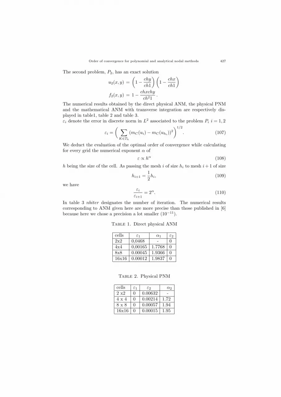
The second problem, P2, has an exact solution

u2(x, y) =(

1 − chy

ch1

) (1 − chx

ch1

)

f2(x, y) = 1 − chxchy

ch21.

The numerical results obtained by the direct physical ANM, the physical PNMand the mathematical ANM with transverse integration are respectively dis-played in table1, table 2 and table 3.εi denote the error in discrete norm in L2 associated to the problem Pi i = 1, 2

εi =( ∑

K∈Th

(mC(ui) − mC(uhi))2

)1/2

. (107)

We deduct the evaluation of the optimal order of convergence while calculatingfor every grid the numerical exponent α of

ε ∝ hα (108)

h being the size of the cell. As passing the mesh i of size hi to mesh i + 1 of size

hi+1 =12hi, (109)

we haveεi

εi+1= 2α. (110)

In table 3 nbiter designates the number of iteration. The numerical resultscorresponding to ANM given here are more precise than those published in [6]because here we chose a precision a lot smaller (10−11).

Table 1. Direct physical ANM

cells ε1 α1 ε2

2x2 0,0468 - 04x4 0,00165 1.7768 08x8 0.00045 1.9366 016x16 0.00012 1.9837 0

Table 2. Physical PNM

cells ε1 ε2 α2

2 x2 0 0.00632 -4 x 4 0 0.00214 1.728 x 8 0 0.00057 1.9416x16 0 0.00015 1.95


Table 3. Mathematical ANM with transverse integration

cells ε1 α1 nbiter ε2 α2 nbiter2x2 0.23288 - 38 0.00494 - 434x4 0.08113 1,6942 163 0.00053 1.5154 1638x8 0.02177 1,9305 628 0.00014 1.9228 62916x16 0.00505 2.0748 2353 0.00003 1.9814 2356

5.4. Result interpretation

(1) - The gotten numerical results are very important: the error is very weak inthe three cases, hopeless in the direct physical case (polynomial and analytical)when the moment of the exact solution is in the space of approximation :

• ε2 = 0 in table 1 (m0y(u2; x) ∈ S0)

• ε1 = 0 in table 2 (m0y(u1; x) ∈ ℘0)

It confirms the theorem (4) even with the physical method that is theoreticallyprecise than the mathematical method mentioned in the theorem.(2) - In table3 (ANM with transverse integration), we note that:

• The number of iteration is too big. It shows that the direct procedureis faster than the transverse integration.

• The error is small but far from being zero ( ε1 6= 0 and ε2 6= 0). itconfirms the remark (3).

• Let’s notice that the error ε1 is very big in relation to the error ε2 thismakes call to the remark (2). This result confirms our remark (3) againsince if the second members didn’t depend on the approached solution,the solution would be calculated precisely.

References

1. Ciarlet P. G., The finite element method for elliptic problems, North-Holland, Amsterdam,1978.

2. Dorning J. J., Modern coarse-mesh methds. A development of the 70’s, Computationalmethds in Nuclear Engineering, vol. 1, pp. 3.1-3.31, American Nuclear Society, Williams-

burg, Virginia (1979).3. Fedon magnand, Hennart J. P. and Lautard J. J., On the relationship between some nodal

schemes and the finite element method in static diffusion calculations, Advances in ReactorComputations, Vol. 2, Salt Lake City, UT, 1983, pp. 987-1000.

4. Finnemann H., Bennewitz F. and Wagner M. R., Interface current techniques for multi-dimensional reactor calculations, Atomkernenergie 30 (1997), 123- 128.

5. Frohlich R., Summary discussion and state of the art review for coarse-mesh computa-tional methods, Atomkernenergie 13n (1983), 117-126.

6. Guessous N. and Hadfat F., Analytical nodal methods for diffusion equations, Equationsand Mechanics. Electron. J. Diff. Eqns., Conference 11 (2004), 143–155.


7. Hennart J. P., On the numerical analysis of analytical nodal methods, Numerical methodsfor partial differential equations 4 (1988), 233-254.

8. Hennart J. P., A general family of Nodal Schemes, SIAM J. Sci. Stat. Comput. 7 (1986),264.

9. Hennart J. P., A Unified view of finite differences, finite elements, and nodal schemes,National University of Mexico, IIMAS, Mexico City, 01000 Mexico 1986.

10. Langenbuch, Maurer W. and Werner W., coarse-mesh flux-expansion method for the analy-sis of space-time effects in large light water reactor cores, Nucl. Sci.Engng. 63 (1977),437-456.

11. Langenbuch S., W. Maurer and Werner W., High order shemes for neutron kinetics calcu-lations, based on local polynomial approximation, Nucl. Sci. Engng. 64 (1977), 508-516.

12. Meade D., Del Valle E. and Hennart J. P., Unconventional finite element methods forneutron group diffusion equations, IIMAS-UNAM (1986).

13. Shober R. A., Simms R. C. and Henry A. F., Tho Nodal Methods for Solving Time De-pendent Group Diffusion Equations, Nucl. Sci. Engng. 64 (1977), 582.

14. Wagner M. R. and Kobke K., Progress in nodal reactor analysis, Atomkernenergie 13(1983), 117-126.

Najib Guessous

Departement de mathematiques et Informatique, Faculte des sciences Dhar-Mehraz, Uni-versite S. M. Ben Abdellah, B. P. 1796 Fes-Atlas, Fes, Moroccoe-mail: [email protected]

Fouzia Hadfat

Departement de mathematiques et Informatique, Faculte des sciences Dhar-Mehraz, Uni-versite S. M. Ben Abdellah, B. P. 1796 Fes-Atlas, Fes, Moroccoe-mail: [email protected]

Order of convergence for polynomial and analytical nodal methods

Documents

Transcript of Order of convergence for polynomial and analytical nodal methods