Solution of dynamic summation-difference equations by adaptive collocation

Chemical Engineering Science, Vol. 44, No. 5, pp. 1161-I 174, 1989. OOD!J 2509/89 $3.00+0.00 Printed in Great Britain. 0 1989 Pergamon Press plc

SOLUTION OF DYNAMIC SUMMATION-DIFFERENCE EQUATIONS BY ADAPTIVE COLLOCATION

JOSE ALVAREZ and JESUS ALVAREZ7 Departamento de Ingenieria de Procesos, Universidad Autonoma Metropolitana-Iztapalapa, Apdo 55534,

09340 MCxico, D.F., Mexico

(Received 12 August 1987, accepted 11 May 1988)

Abstract-A technique to solve dynamic summation-difference equations is presented. It is applicable to systems whose description is given by sequences, either finite or infinite, that evoIve with time. The technique is intended for sequences whose graphs resemble functions that can be approximated by a global scheme. Following the evolution of the sequence, the technique adapts the location of the collocation points, and, as a consequence, enables the cqnstruction of reduced models for dynamic simulation. The methodology is illustrated with examples taken from staged separations and polymerization reactors.

1. INTRODUCTION

Mathematical models for transients in staged separations, polymerization kinetics, etc., lead to equations where the dependent variable is a sequence that evolves with time. When the size of the sequence is large, or infinite, the rigorous solution of the model implies the solution of a large, or infinite, number of ordinary differential equations (ODES). Therefore, there is an incentive to develop model reduction techniques for this class of problems.

Joseph and coworkers (Cho and Joseph, 1983a, b, 1984; Srivastava and Joseph, 1984, 1985) addressed the model reduction problem for steady-state and transient separation units. These authors adapted the Jacobi collocation technique, for function approximation, to approximate sequences with a finite number of entries. Stewart et &. (1984) developed a technique to approximate finite-aimensional sequences. This technique is known as the Hahn collocation, and it constitutes the sequence counterpart of the Jacobi collocation. In the above treatments the dynamic simulations were done with a fixed collocation mesh. The Hahn, or Jacobi, mesh was obtained after a trial- and-error adjustment of two parameters that defined the trial basis. The mesh was kept fixed during the transients. The aforementioned strategies should only be appropriate when: (i) during the transient, the evolutive sequence does not change its plot signifi- cantly; or (ii) a large enough number of collocation points is utilized so that the entire evolution of the sequence is approximated appropriately.

Problems involving infinite sequences, such as the ones that result in poIymerization kinetics, have usually been treated with the continuous variable approximation (CVA) method (Zeman and Amundson, 1966a, b). With the CVA, the summation-difference (SD) equations are approximated with integro-differential (ID) ones. The latter ones

‘To whom correspondence should be addressed.

have heen solved with finite differences (Zeman and Amundson, 1966a, b) and finite element (FE) with fixed (Coyle et al., 1985) and adaptive (Saldivar, 1986; Alvarez and Saldivar, 1987) meshes. Bamford and Tompa (1954) and Hulburt et al. (1964) utilized associated Laguerre polynomials to generate equations for the moments of a continuous distribution. Hulburt et al. (1964) sought a description in terms of a finite number of moments of the distribution. The approach was restricted to integration kernels that could be expressed as a finite power series. The latter situation is hardly found in nonlinear polymerization kinetics. However, this work showed that the trial functions for the approximation to the solution should adapt themselves according to the shape of the approximated

‘profile. Gonzalez and Rodriguez (1986) solved the problem utilizing a collocation technique based on the roots of a scaled Laguerre polynomial. The domain for collocation was found by a trial-and-error procedure, and the collocation mesh was kept fixed through a transient. Taylor et al. (1986) utilized a piece-wise collocation with a fixed mesh to build a model for on- line estimation. This work stemmed from an application and it conveyed the need for the search of reduced models. It must be pointed out that, since the preceding works in polymerization started from a CVA of the original model, the numerical treatments corresponded to approximations of functions on semi- infinite domains. Alvarez and Alvarez (1987) devised a collocation method to approximate sequences that satisfied SD equations. The technique could be directly applied to the original model, and therefore the detour through a CVA was avoided. The approach could handle finite or infinite sequences satisfying static models, and it was able to obtain simultaneously the mesh collocation and the approximation to the sequence.

The election of a numerical method should take mto account the nature of the expected solution sequence, the programming and implementation efforts, the accuracy of the meihod, the size of the reduced model

1161

1162 Jose ALVAREZ and JES& ALVAREZ

and the computer time. Alvarez et al. (1987) showed that the natural treatment for SD equations was sequence approximation. For problems whose sequence plot resembled functions that could be approximated by a global polynomial, a sequence collocation with adjusting weights led to a technique superior (implementation effort, accuracy and size of reduced-order model) to the standard collocation technique (Jacobi and Laguerre) for the function approximation posed by the CVA method.

In the present work the problem of approximating an evolutive sequence with an adaptive collocation (AC) mesh is addressed. The time-varying sequence satisfies a dynamic summation-difference (DSD) equation. The technique is applicable to sequences whose plots, at any time, resemble functions that can be approximated by a global interpolation scheme. The methodology can handle sequences with a finite number of elements such as in staged separations or sequences with an infinite number of elements such as polymerization kinetics.

A mathematical framework to treat the problem is established. First, a subjacent weighted least squares (WLS) problem for the error of the sequence is formu- lated. This WLS problem has an inner product defined with a time-varying weight. The idea is to assess an evolutive weighting strategy according to the changes in the spread and form of the sequence. This leads to the idea of approximating the sequence in terms of an adaptive set of trial sequences. The trial sequences are orthogonal, and the definition of orthogonality changes with time.

The case of interest arises when the sequence to be approximated is not given explicitly. Instead, the sequence satisfies a given SDE. The transient for the sequence is induced by a nonstationary initial condition, an exogenous input, or by both of them. In this situation, the mathematical treatment is done by establishing a relationship between a subjacent WLS problem for the error of the approximation, and the implementable WLS problem for the residual. The latter one is generated after the substitution of the approximating sequence in the DSD equation.

For the implementation of the AC technique a relationship is devised between certain features of the time-varying sequence and a time-varying parameter that characterizes an evolutive weight sequence. The collocation mesh is allowed to change at discrete times. The resulting scheme that updates the mesh possesses a predictor-corrector structure. The technique is illustrated and tested with examples that include a variety of situations which correspond to transients encountered in staged separations and polymerization reactors. One of the application examples is used to favorably compare the AC technique for sequences with the adaptive FE-CVA technique.

2. STATEMENT OF THE PROBLEM

Suppose that a process is modelled by the following equation:

ti(t)=Lu(t)+f(t), u(O)=u, (1) where J(t) is a given, exogenous, time-varying sequence with M entries:

f(t)={fr(t), . . -AfIt)) (tEC0, Tl). u(t) is also a sequence with M entries:

u(t)={%(t), . . . 3 %fM(t)l

and it stands for the dynamic response of the process to either a forcing sequence f(t), a nonstationary initial sequence u,,, or to both of them. M can be finite, as in the case of staged separators, or infinite, as in the case of polymerization kinetics. L is an SD operator. Boundary conditions, possibly with exogenous inputs, are accounted for in the definition of L. Particular forms of eq. (l), corresponding to various applications, can be seen in the examples considered in Section 5 [eqs (20H22)].

The aim is, given U, andf( t), to solve u(t) in eq. (1) for t E [0, T]. A direct treatment of eq. (1) implies the solution of M ODES coupled to N, algebraic or differential equations. N, stands for the number of boundary conditions. When M is large, or infinite, the objective is to construct a reduced mode1 (N CM) such that its solution approximates, in some sense, the solution of the original model.

Although the ultimate goal is to obtain a reduced number of equations, it is desirable to develop a treatment that shows clearly the nature of the methodology as well as its applicability and limitations.

3. APPROXIMATION OF AN EVOLUTIVE SEQUENCE

Some of the concepts required to deal with a time- varying situation have been introduced by Alvarez et al. (1987), for the time-invariant case. It will therefore not be necessary to develop them at length as the dynamic framework is built.

The conceptualization is facilitated and the manipulations are simplified if one treats the problem with abstract vector spaces. Let H be an M-dimensional (possibly infinite) Hilbert space that consists of squared-summable sequences whose entries are real- valued functions of time:

n(r)= {u,(r). . 1 . > %.fct,> @El)

vt E I

where I denotes the time Interval [0, 7’1. His equipped with the following inner product and its induced norm:

<u(t), v(t)>= 2 wj(t)ui(t)uj(t) VtEI j=l

IlU(t)l <a(t), U(t)>"*.

The time-dependent weight sequence w(t) is also square-summable. It must be pointed out that the notions of size, orientation and distance in W change with time. I is a connected subset of the real line.

Solution of dynamic summation-difference equations by adaptive collocation 1163

Geometrically, at a given time, t,, u( t,) is a point in H, and the trajectory u( r)Vt E I is a connected curve in H.

First, consider the approximation, u”, of a given curve u(t). The weight curve, w(t), is also given. Let S be an N-dimensional (NC M) subspace in n. The approximating subspace S can be spanned by any set of N linearly independent sequences in S. Let u”(t) denote the projection of u(t) in S. The approximation u0 to u is obtained as the solution to the following WLS problem:

s

* Min Ile(r)ll,(,,dr>

UY’)=%.,,, 0

s.t. e(t)=u(t)-uO(t).

Since the integrand in the objective function is a scalar, positive, nondecreasing function of time, the opti- mality principle (Bellman, 1957) allows one to restate the problem as

Min Ile(t)ll w(tJr s.t. e(t)=u(t)-uO(t) VtEt. ~Y~)mu(,)

(2)

The solution to this problem is characterized by the projection theorem (Luenberger, 1969). uO( t) is a solution to eq. (1) if and only if

e(r)E Si;(r) (3)

where Sk is the orthogonal complement of S. The error norm is given by the Pythagorean identity in N:

Alvarez et al. (1987) showed that when the basis sequence was constructed from a polynomial set, and problem (2) was solved exactly, the error norm t14t)llwcr, depended upon the topology of H [as defined by w(t)], and the dimension of the approximating subspace. The orthogonal collocation technique arose as a means to attenuate the propagation of errors due to the use of quadrature formulae for summations. As a result, one ended up with a further approximation, u*(r), to u”(t). The geometric inter- pretation of these concepts is simple: if a vector in R3 is projected on a plane spanned by two closely aligned basis vectors, the representation in the plane (obtained after numerical evaluation of the expansion coef- ficients) will be poor. On the contrary, use of an orthogonal basis to span the plane leads to a better approximation.

Assume that the sequence to be approximated has a graph [u,(t), i]Vt E I that resembles a function that can be approximated by a global polynomial basis. In this case it is possible to construct an evolutive sequence basis in terms of a polynomial set. Here, the polynomial set and hence the basis sequence must be time- varying. The construction of the basis is done with the following formula (Alvarez et al., 1987)

bi(l)=p,- l(j, 2).

bj(t)={b{(t), . . . ,b~(t)}~Swct,,bi(t)~R

where pr(j, t), 1 <j< M ((M if M = CO), is a /&h-degree

polynomial of the form

$K(j, t)= i: a,(t)?. i=O

The w(t) orthogonality of the basis imposes the following restriction on the polynomial set:

5 w,(t)pi_,(k,t)pj-I(k,t)=Ofori#j k=l

(i,j=2 >. -. I N, Vt E I).

Moreover, utilization of w( t)-orthogonal polynomials allows for the use of w(t)-Gaussian quadrature formulae to approximate summations (Szego, 1939). The w( t)-orthogonal collocation technique stems from approximating the inner products in the normal equations with w( t)-Gaussian quadratures. If the sequence is required to satisfy boundary conditions, the essence of the collocation strategy is the same. In this case, the boundaries are incorporated as collocation points. Finally, a Chevysyev point-wise error analysis suggests that criteria to select w(t) should account for the shape of the sequence to be approximated (Alvarez et al., 1987).

To conclude, the approximation of an evolutive sequence should be done in terms of an evolutive set of trial sequences. The trial set should be orthogonal in the sense of a time-varying inner product. The adaptive weight that characterizes the inner product should be obtained from the evolution of the sequence to be approximated. In terms of orthogonal collocation, this means a set of trial sequences generated by a collocation mesh that moves according to the time-varying roots of a w( t)-orthogonal polynomial.

4. EVOLUTIVE CONSTRAINED APPROXIMATION

The results of the previous section could be of value in themselves when approximating given, time- varying, sequences by using AC meshes. However, in the context of the present work, these results are used as a preamble to deal with the problem of interest: the approximation of motions of sequences that are not given explicitly, but instead satisfy a DSD equation. The conceptual framework for the latter situation shall be established by finding out how the error problem, addressed in the last section, manifests itself in a residual problem.

Suppose that the curve u(t) satisfies eq. (1). From a geometric perspective, the RHS of eq. (1) is a time- varying vector field, g= Lu +f( t), on H. Thus, the Solution to eq. (I) is the integral curve of g passing through u,.

Assume, for a moment, that the solution trajectory u(t) is available. It is convenient to think of the weight sequence w(t) as a particular case of a positive-definite, time-varying, self-adjoint operator W(t): H -+ H, that is, W maps sequences to sequences (see Appendix B). As pointed out in the previous section, the weight sequence can be obtained in terms of the sequence u. Represent this trans-

1164

formation as follows

Josh ALVAREZ and JES~JS ALVAREZ

W(t)=GCu(t)] (4)

response, at t,, to an impulse residual input e,(t) ={[l, 1,. . . .]s(t-t,)), at time t,. 6(t-tt,) is a Dirac delta.

where G is a memoriless map that assigns a weight operator to a sequence u(i). The term memoriless means that W(t) depends only upon the current value of u( t). Thus, the adaptive WLS approximation problem, for a fixed number of collocation points, can be posed as follows:

s

, Min <e(z), w(t) e(z)> dz (51

UO(I)ES cl

A residual problem can be generated by substituting eq. (10) in the subjacent WLS problem for the error (6). If so, eq. (6) can be rewritten as

UOTi;,t< @(%+I: Q,(t--+(flJda,

W’(t)[ S(t)e~+~~ Q(t-=)E(=)d*]) (11)

s.t. e(t) =u( t) - zP( t), K’(t)=G[u(t)].

As done in the preceding section, the above minimization problem can be restated as follows:

s.t. E(t)=Lu”+f-tio, W(t)=G[u”(t)].

Min <e(t), W(t)e(t)>VtEZ uO(+=S!v,,,

(6)

s.t. e(t)=u(t)-u”(t), w(t)=G[u”(t)].

As an approximation, the operator W has been posed in terms of the approximated sequence. Except for the fact that a rule has been included to evaluate the weighting operator, the last problem is similar to the one treated in Section 3. Therefore, the solution to problem (6) is characterized by

Equation (11) represents a residual WLS reformu- lation of the WLS problem for the error (6). In order to obtain, from eq. (1 l), a residual problem in the form of eq. (7), the following approximations ought to be introduced (details in Appendix A): (i) only the response to the exogeneous input, E, is kept in eq. (10); and (ii) the objective function to be minimized in problem (11) is replaced by an objective function that is an upper bound for the original one. Consequently, problem (11) becomes

Min <e(t), Q(t)&(t)> Vt s Z (12) Uqt)‘sS(t)

It must be remarked that the use of a time-varying, adaptive, W( t)-orthogonal collocation mesh guaran- tees a least upper bound for the error induced by approximations due the use of quadratures (Alvarez et al., 1987).

s.t. &(t)=LUO+S--o,R(t)=B[u”(t)]

where , *

n(t)= ss

Q(t-a)JJ’(t)Q,(r-~)dadz (13) 0 0

and

Now build an approximation to u(t) in terms of a residual problem. Let u1 (t) be the approximation that is obtained from the solution to the following WLS problem:

Min <&l(t), n(t)&‘(t)> (7) tll(I)E&Xt,

f t B[zf( t)] =

ss cD(t-cr)G[u”(t)]@(t-r)dcrdr. (14)

0 0

@is the operator that appears in eq. (10) when, instead of L, t is utilized in (9), E being the adjoint operator of L.

The inner product for the equivalent, approximated WLS problem for the residual (12) is given in terms of a double summation:

s.t. ri’=Lul+f(t)~&l(t),n(t)=B[U’(t)]

The point is to find a relationship between the subjacent problem (6) and the workable problem (7). To do so, start by expressing problem (6) in terms of a residual, and by assuming that L is linear. Substitution of u,(t) in eq. (1) yields the residual equation:

u”(t)=LuO+-tf(t)--E(t). (8)

Substraction of this equation from eq. (I) produces the residual-error relationship

B=&+&(t). (9)

The solution for e(t) in terms of c(t) can be written as (see Appendix A)

J

t e(t)=@(t-O)e,+ @(t - T)E(~) dr (IO)

0

where the definition of the entries of the double sequence’ associated with the operator Q(t) can be seen in eq. (83). The standard collocatign technique consists of an inner product with a single summation. Hence, only the “diagonal” elements of SZ(t) [in eq. (15)] are taken into account. According to this, eq. (15) becomes

The collocation strategy for the residual would also be posed for an inner product with a single summation. Therefore, the entries associated with the operator W(t) take the following form where O(tZ - tr) is a time-varying operator that maps

sequences to sequences [see eqs (Bl) and (B2) in Appendix B]. Q(t2, tl) can be thought of as the error

<s(t), Q(t) E(t)) = 5 : Wij(t)Ei(t)Ej(t) (15) i=l j=l

M <E(t), fl(t)E(t)>= C -i&?(t). (16)

i=1


where ajj is a Kronecker delta. It must be pointed out that {w,(t), _ . . , wM(t)) is the sequence used in Sec- tion 3 to pose the WLS problem (2) for the error of the approximation of the sequence. In this case eq. (B3) reduces to

oi=wii= z Wk(t) [S I

&(t--r)dz ‘. k=l 0 1

When L is a nonlinear operator, it is still possible to extract some information. To do so, linearize the nonlinear DSD eq. (1) and the residual eq. (9) about the trajectory u”(t). This leads to

L?LU e=L,,,,e+e, L,r,,=7 I .

This linear equation is different from eq. (9) in the following aspect: L, is now a time-varying operator that changes according to the evolution of u(t). Since it is possible to represent L,(*, as an A4 x M time- varying matrix, from well-known results in dynamic matrix systems (Balakrishnan, 1983), it follows that the weight sequence takes the form *

+kt [t - t; u”(r)] dt . (17)

According to this result, in the nonlinear case and at a given time, the weight sequence for the collocation should depend upon the past evolution of rP(t). This inconvenience can be circumvented if it is recalled that uO( t) satisfies an equation which is an initial-value problem in time. Therefore, when w(t) is evaluated in terms of the current value of u’(t), the past history of t&‘(t) has been used implicitly.

4. AC MESH

The adaptation of the mesh requires the com- putation, at a certain time, of the roots of an Nth degree w(f)-orthogonal polynomial. This step can be done with the algorithm developed by Alvarez et al. (1987).

The w( t)-orthogonal collocation equations that solve eq. (15) become

UCri(t)7 tl = LCr(t)lC~trj(t))v t] + FCri(t)* tl

(i’ 1 ,-. . > N)

uCri(oL 01 = u. Cri(O)l f-(t)=RC~(t)l

(18)

where r(t)= (r,(t), . , rN( t)) is the set of collocation abscissae, U and F are continuous functions in L, that approximate the sequences u andJ R is an operator that assigns a set of collocation abscissae to the approximation of the sequence (U( tj). Equation (18) is a set of N nonliriear ODES. If there are N, boundary conditions, there are N + Ns dependent variables and N, additional algebraic or differential equations.

Regarding the relationship between the shape of the approximated sequence and the collocation mesh, Alvarez et al. (1987) showed that a geometric weight

sequence could handle the static solutions of the problems that will be considered here. Hence, in this work, the relationship between the weight sequence and the profile is given by the following formula:

A(t)-1 oi(t)=[A(t)]“~, A=- tl

J(r) (19)

where

l(t)= [ ,“, C @Jr)

and n > 0 is an integer. i, denotes a mean ordinal number for the sequence

and n is an integer that affects the decay ratio of the geometric weight sequence. n is an adjustable parameter that regulates the density of the collocation points over the abscissa domain. For the absorber, where the concentration spreads along the column, n= 1 was used (Alvarez et al., 1987). For polymerization sequences, where the profiles exhibit a larger decay, n = 3 leads to adequate results. The use of the geometric weight (19) allows for a computational simplification. It can be verified that when the argu- ment i in eq. (19) is replaced by a linear transformation i =aj, the new collocation abscissae become scaled values of the original collocation points. Also, the quadrature weights are modified by a linear scaling. As a consequence, the mesh updating scheme reduces to evaluating once the roots of an Nth-degree polynomial and then to resealing its roots according to changes in the parameter 1. The geometric weight (19) should not be taken as a restriction. In fact, more research on this matter should lead to better results.

Within the framework of systems theory, the AC mesh is analogous to the adaptive measurement structure devised by Alvarez et al. (198 1) to estimate states in a system with distributed parameters. Following the latter work, the mesh structural update is allowed to happen at discrete points in time. Similarly to the algorithmic solution of ODES, the time interval between m&h updates is determined by the rate of change, with time, of the graph of the sequence. Before pursuing further, the following notation is introduced:

r(k): (@I( - . . , rN(tk)} is the mesh of interior collocation points at time t,.

uO( k/j): approximation to u( tk) based upon a mesh r(j) updated at time ti < t,.

The AC algorithm for N interior collocation points is sketched in the following sequence:

(1)

(2)

Initialization. The initial condition u, is given. Both the initial approximation [u’(O/O) = u,(O)] and the initial collocation mesh [r(O)] are obtained simultaneously with the strategy for approximating sequences developed by Alvarez et al. (1988). Sequence approximation, one step ahead in time, utilizing a fixed mesh. The collocation ordinates [of u”(k/k)], at the abscissae r(k), are

Jo@ ALVAREZ and JESUSALVAREZ 1166

(3)

fed (as initial values) to the set of N +N, differential-algebraic system of collocation equations built with the mesh r(k). Then the system is integrated up to time tk + 1. The sequence u”(k + 1 /k) follows from an interpolation procedure. Mesh update. A weight sequence w(k + I) based upon u”(k + l/k) is evaluated via eq. (19). If the resulting weight sequence is similar, in some sense, to w(k), the collocation mesh is kept fixed for the next time interval. Otherwise, a new collocation mesh, r(k+ l), is obtained as the roots of an Nth-degree (k + 1) orthogonal polynomial. In this work, the comparison of weight sequences is done in terms of the parameter ;i in eq. (19). Given a tolerance 6 >O, the mesh is updated only when

W+l)--(k)>S,

i(k+ 1)

In other words, the mesh is updated only when the sequence mean, il, has moved beyond the assigned tolerance, 6. As 6 increases, the fre- quency of mesh updating decreases.

The mesh adaptation algorithm has the prediction*orrection structure of a numerical integrator, or that of a nonlinear, extended, Kalman filter (Jazwinski, 1970). In addition to the usual feedback loop of numerical integration, another loop due to mesh adaptation has been introduced. It is a well- known fact in systems theory that feedback loops, properly designed, enhance the robustness of a system. In the present situation robustness means capacity to tolerate errors induced by the reduction of the model. In conclusion, the gain in robustness due to the adaptive mesh leaves room for a larger model reduction (with respect to a fixed mesh), and consequently for a reduction in the computational load.

5. APPLICATION EXAMPLES

In this section the methodology is tested with examples that correspond to staged separations and polymerization kinetics. It was pointed out in Alvarez et al. (1987) that the essence of the approximation problem resided more in the shape of the sequence to be approximated than in the complexity of the equation. Here the examples used to test the methodology were selected to represent, from the point of view of the shape of the graph, a range of situations encountered in staged and polymerization kinetics. The examples cover linear and nonlinear situations, infinite and finite sequences, as well as initial and boundary value problems with respect to the ordinal number of the sequence. Details of the application of the technique and the explicit form of a reduced model can be seen, for one of the application examples, in Appendix C.

5.1. Stripper The model considered corresponds to a gas stripper.

The process takes place in a countercourrent column

with M -2 stages. The dynamic model is given by Amundson (1966)

For 2<i<M-1, t>0:

At i= 1, ra0: u1 =u,(t)

At i=M, t>O: g&)=uJt)

At t=O, 2titM-1: u,(0)=ui,

where u is the concentration sequence, am and u,(t) are the liquid and gas feed concentrations, L and I/ denote liquid and gas molar flow rates, h is the try hold-up and g(u) is the gas-liquid equilibrium relationship. Equation (20) is a two-point boundary value problem for the ordinal number i, and it is an initial- value problem with respect to time. The boundary conditions are specified by algebraic equations.

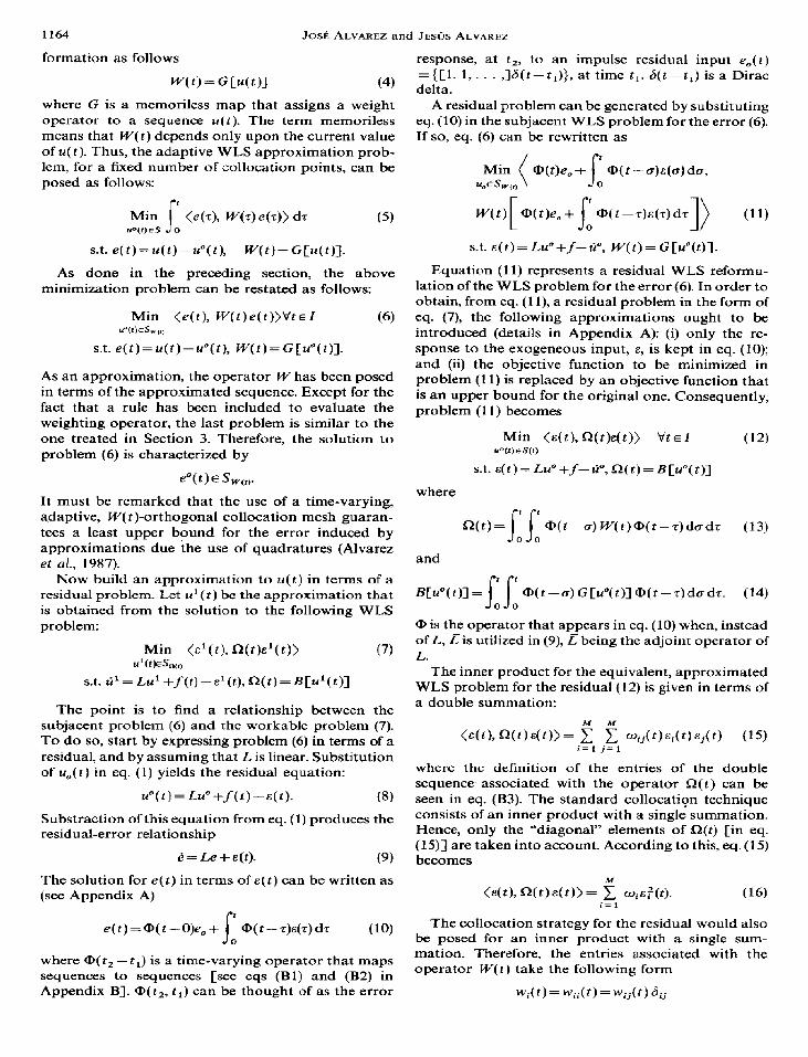
To begin, consider a linear equilibrium relationship. This is, g(u) = Ku. The initial sequence corresponds to a steady state that results from uf = 0.05, uf = 0.0025, L/h= 25, V/h= 10, K = 2, A4 = 32. The interpolation mesh consisted of two boundary abscissae and four adaptive, internal, abscissae. n= 1 was chosen for the weight sequence (19). Figure 1 shows the evolution with time of the concentration uZs(t) obtained from integration of the full model and from integration of the reduced model. Two responses are shown. The transients were induced by a + 15% and a + 10% step change in L/h. As can be observed, the results of the reduced model are very similar to the ones obtained with the full model. The time interval utilized to update the collocation mesh was 0.15 units of time.

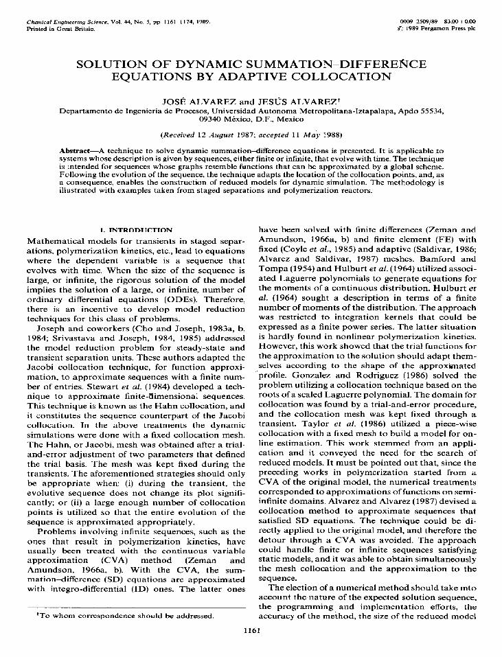
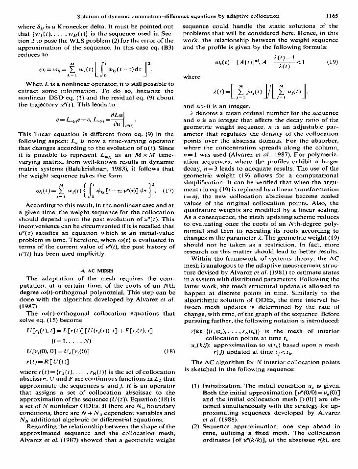
A nonlinear case was generated by setting g(u) = Ku/[ 1+ (l/K)u](K = 2). The simulations done for the linear case were repeated, and the initial conditions were evaluated from a nonlinear steady- state solution using the strategy presented in Alvarez et al. (1987). The results are depicted in Fig. 2. As expected, the evolution and performance of the AC mesh are similar to the ones of the linear case. For about a 5% error, the simulations with reduced models required about one-third of the time needed by the full model.

5.2. CSTR polymerization Consider a free-radical polymerization taking place

in an isothermal CSTR with the following kinetic mechanism (Zeman and Amundson, 1966a, b)

kI d, - Ul (initiation)

kP ui+d, - uii 1 (propagation (1 < i c co)

*r ui+d, - dt+l (termination) (I< i -c co)

where d, is the monomer concentration, di (i> 1) is the i units deactivated polymer concentration, and uj is

0.50

0.35


STRIPPER

g(u )= Ku

(b) ____---- ___---_-----_

COMPLETE MODEL

0.0 ,

0.5 I

1.0

----____ REDUCED MODEL

(0 1 PERTURBATION : IO% (b) 15%

30 STAGES

4 INTERIOR COLLOCATION P‘,,NTS

I I 1.5 2.0

I 2.5

I TIME, t/h

Fig. 1. Dynamic response of a linear stripper with 30 stages. The transients were induced by step changes in L/h. The plots correspond to the evolution of concentration at stage 25.

0. so

STRIPPER lb) _____-- _-___ _-----

---&ii __-_--.

COMPLETE MODEL

----___ REDUCED MODEL

(a) PERTURBATION : IO% (b) 15%

30 STAGES

4 INTERIOR COLLOCATION POINTS

0.0 0.5 1.0 I .!5 2.0 2.5

Fig. 2. Dynamic response of a nonlinear stripper with 30 stages. The transients were induced by a step change in L/h. The plots correspond to the evolution of concentration at stage 2s.

the j units activated polymer concentration. U, is the For 2<i<co,t>0: sequence of concentrations of activated polymer chains at the feed. 8 denotes the ratio of the volumetric Zii= -[CO+(k,+k,)d,]Ui,(k,+k,)d,ui- 1 +OUi,(t)

flow to the reactor volume. The model for isothermic @la)

operation is given by &= -UOd,+k,d,L4_, +Od,,(t) @lb)

1168 Jose ALVAREZ and JES~IS ALVAREZ

At i= 1, t>O: P, =-[e+(Jr,+k,)d,]u,+Ou,.(t) (21~)

8,=- [

O+k,+(k,+k,) f uj 1 dI + edIe(t) (214 j=l

At t = 0, 1 < i < co: d,(O) = di,, u,(O) = uiO. The preceding system is a set of two DSD equations.

The system is an initial-value problem with respect to the ordinal number i, and an initial-value problem with respect to time. At the boundary i= 1, the conditions are specified by two ODES.

The set of eqs (21a), (21~) and (21d) does not require the results from the integration of eq. (2 1 b). Thus, u(t) and d,(t) can be solved separately. The solution for di(t) (i > 2) can be obfained from the integration of eq. (21b) with u(t) and d,(t) entering as exogenous inputs. For illustration purposes, only the concentrations of activated species and monomer, u(t) and d,(t), will be solved for.

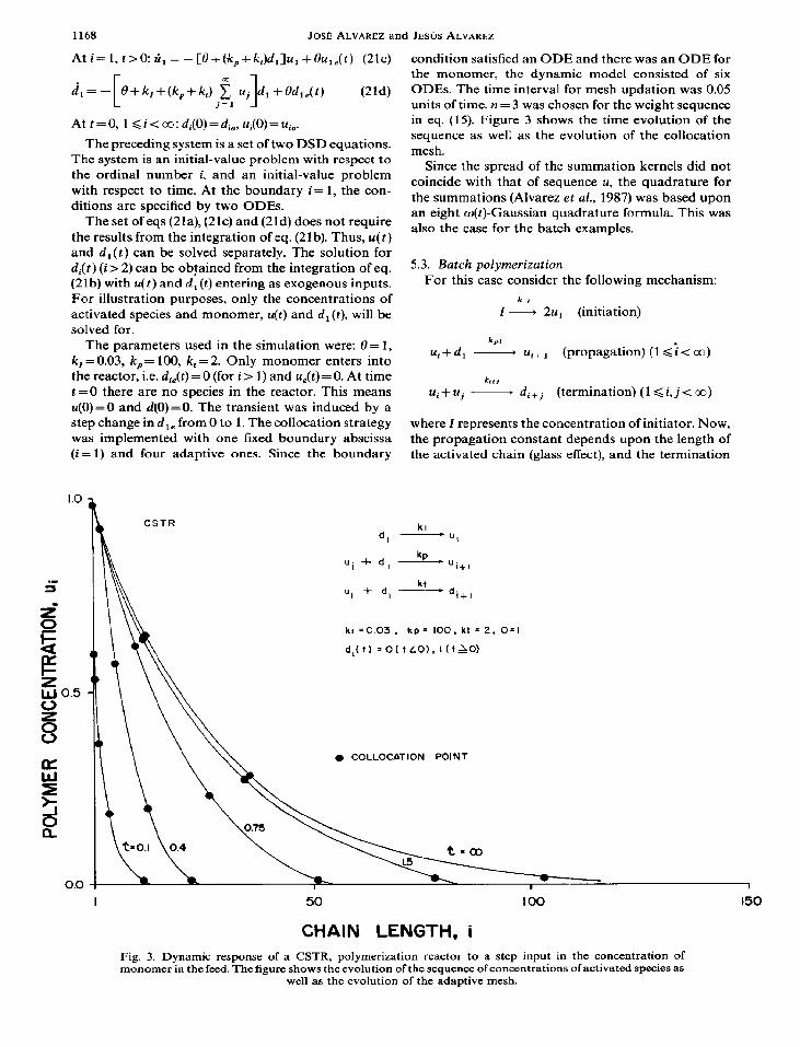
The parameters used in the simulation were: 0= 1, k, = 0.03, k,= 100, k, = 2. Only monomer enters into the reactor, i.e. d,,(t) = 0 (for i > 1) and udt) = 0. At time t = 0 there are no species in the reactor. This means u(O) = 0 and d(O) = 0. The transient was induced by a step change in d,, from 0 to 1. The collocation strategy was implemented with one fixed boundary abscissa (i = 1) and four adaptive ones. Since the boundary

CSTR

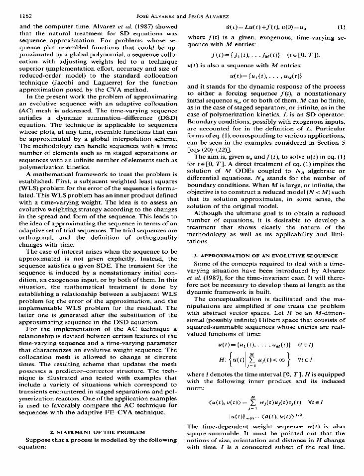
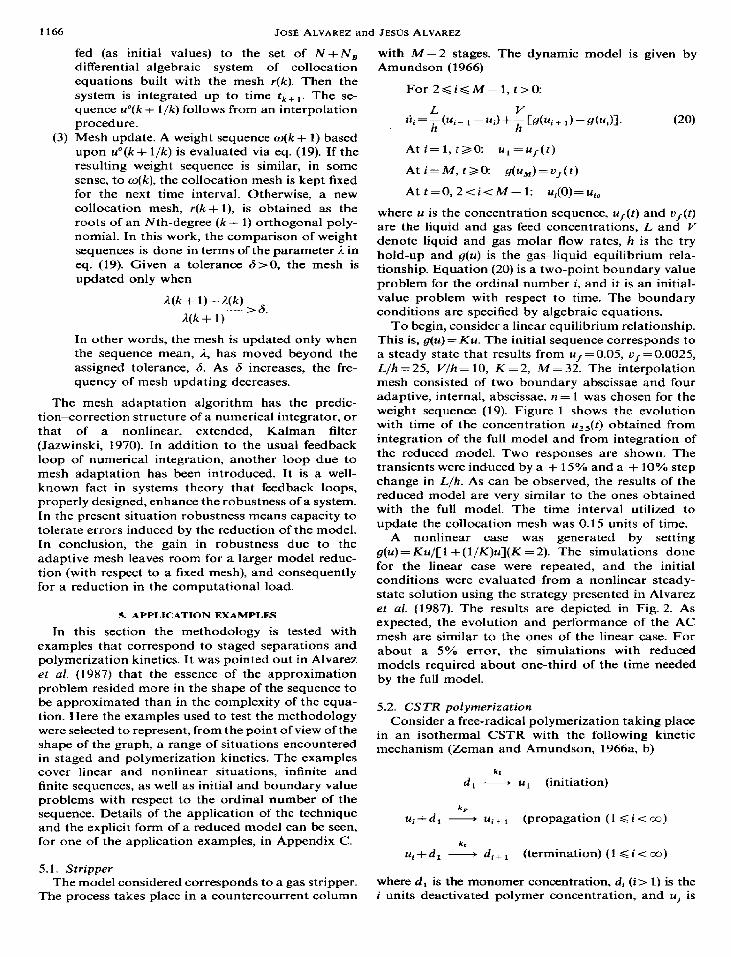
condition satisfied an ODE and there was an ODE for the monomer, the dynamic model consisted of six ODES. The time interval for mesh updation was 0.05 units of time. n = 3 was chosen for the weight sequence in eq. (15). Figure 3 shows the time evolution of the sequence as well as the evolution of the collocation mesh.

Since the spread of the summation kernels did not coincide with that of sequence u, the quadrature for the summations (Alvarez et al., 1987) was based upon an eight w(t)-Gaussian quadrature formula. This was also the case for the batch examples.

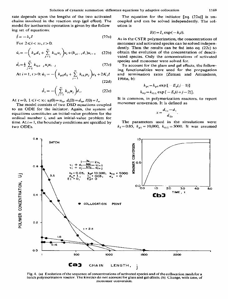
5.3. Batch polymerization For this case consider the following mechanism:

k,

I- 2u, (initiation)

k,i ui+CZ, - ui+1 (propagation) (1 <; < 03)

krij ui + uj - di + j

. . (termination) (1 < r,~ < 00)

where Z represents the concentration of initiator. Now, the propagation constant depends upon the length of the activated chain (glass effect), and the termination

kl d, -u,

ui + d, b _ ‘itI

ui + d, kt

- d. I+1

kj =0.03 , kp= 100, kt = 2, 0.1

d,(t) =O(tLO),I(tAO)

. COLLOCATION POINT

CHAIN LENGTH, i Fig. 3. Dynamic response of a CSTR, polymerization reactor to a step input in the concentration of monomer in the feed. The figure shows the evolution of the sequence ofconcentrations of activated species as

well as the evolution of the adaptive mesh.

Solution of dynamic summationdifference equations by adaptive collocation 1169

rate depends upon the lengths of the two activated chains involved in the reaction step (gel effect). The model for isothermic operation is given by the following set of equations:

i= -k,I (2W

For 2<i< co, t>0:

&= - k,,d, + ‘f ktijui ( >

Ui+(kpi- ,d,)u;- 1 VW i=1

Lii=) 2 k,j,i_jujui-j (22c) j=l

At i= 1, t>O: ti, = - k,,d, + 2 kt,juj u,+2K,f j=1 >

(224

(224

At t = 0, 1 <i < 03: u,(O) = uiO, d,(O) = die, I(0) = I,. The model consists of two DSD equations coupled

to an ODE for the initiator. Again, the system of equations constitutes an initial-value problem for the ordinal number i, and an initial-value problem for time. At i = 1, the boundary conditions are specified by two ODES.

0.8

1 BATCH

I kr zu, Ui+dg kDi k 1;; ui+l Ui + U’ 1 di+j

I.”

1 /--- B 0.5

5 kr = 0.05, 10000,

1,‘003. k,-# kt,, = 5000 P

d,= 1.. =o Et = 0, Ep= 0 “0

The equation for the initiator [eq. (22a)] is un- coupled and can be solved independently. The solution is

Z(t) = I, exp ( - k,t).

As in the CSTR polymerization, the concentrations of monomer and activated species can be solved independently. Then the results can be fed into eq. (22~) to obtain the evolution of the concentration of deactivated species. Only the concentrations of activated species and monomer were solved for.

To account for the glass and gel effects, the following functionalities were used for the propagation and termination rates (Zeman and Amundson, 1966a, b):

kpi=kp~expC-~E,C-ll)l k,ij=k,11exp[-&(i+j-2)].

It is common, in polymerization reactors, to report monomer conversion. It is defined as

d,,--d,

dr,

The parameters used in the simulations were: k,= 0.05, kpl = 10,000, k,* 1 = 5000. It was assumed

0 COLLOCATION POINT

--9: t - 2.5

Ca3 CHAIN LENGTH, j

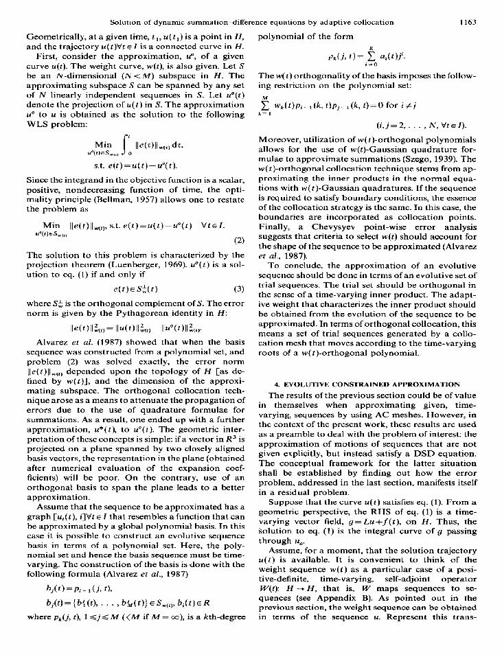
Fig. 4. (a) Evolution of the sequence of concentrations of activated specieS and of the collocation mesh for a batch polymerization reactor. The kinetics do not account for glass and gel effects. (b) Change, with time, of

monomer conversion.

1170 Josh ALVAREZ and JES~~S ALVAREZ

that only monomer and initiator were loaded: d,,=l.O, 1,=0.03 and u,=O.

Figure 4 shows results for E,= E,=O. In other words, the glass and gel effect are not considered. n = 3 was used for the weights (15). The collocation mesh consisted of one fixed boundary abscissa (i= 1) and four adaptive ones. Hence, the reduced model had six ODES. The time step for mesh updation was set to 0.05. Figure 4(a) shows the evolution of the sequence and the mesh, and Fig. 4(b) shows the evolution of the conversion.

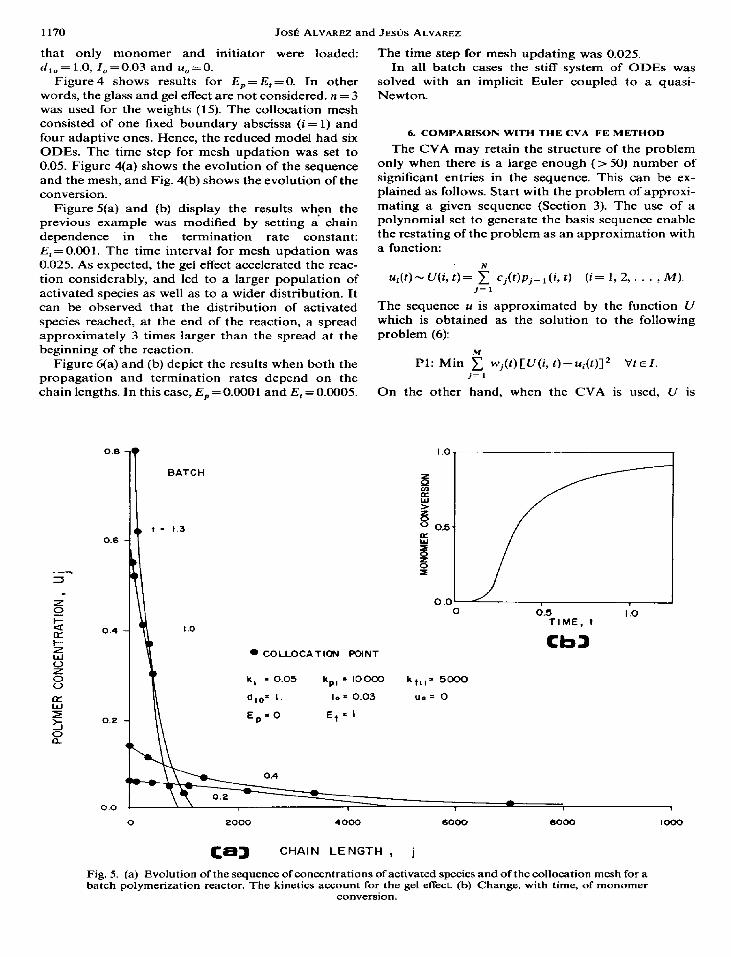
Figure 5(a) and (b) display the results when the previous example was modified by setting a chain dependence in the termination rate constant: E, = 0.001. The time interval for mesh updation was 0.025. As expected, the gel effect accelerated the reaction considerably, and led to a larger population of activated species as well as to a wider distribution. It can be observed that the distribution of activated species reached, at the end of the reaction, a spread approximately 3 times larger than the spread at the beginning of the reaction.

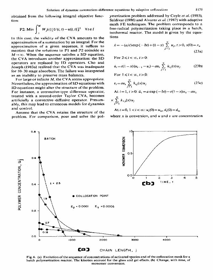
Figure 6(a) and (b) depict the results when both the propagation and termination rates depend on the chain lengths. In this case, E, = 0.0001 and E, = 0.0005.

0.6 I BATCH

l COLLOCATION POINT

The time step for mesh updating was 0.025. In all batch cases the stiff system of ODES was

solved with an implicit Euler coupled to a quasi- Newton.

6. COMPARISON WITH THE CVA FE METHOD

The CVA may retain the structure of the problem only when there is a large enough (z=- 50) number of significant entries in the sequence. This can be ex- plained as follows. Start with the problem of approximating a given sequence (Section 3). The use of a polynomial set to generate the basis sequence enable the restating of the problem as an approximation with a function:

ui(t)mU(i, t)= 2 cj(t)pj_,(i, t) (i= 1, 2,. . . , M). j=l

The sequence u is approximated by the function U which is obtained as the solution to the folIowing problem (6):

Pl: Min 5 Wj(t)[U(i, t)-ui(t)12 vtez. j=i

On the other hand, when the CVA is used, U is

I .a

I

0.5 I .o TIME. t

0 2000 4000 6000 8000

ca3 CHAIN LENGTH , j

(a) Evolution of the sequence of concentrations of activated species and of the collocation mesh for a Fig. 5. batch polymerization reactor. The kinetics account for the gel effect. (b) Change, with time, of monomer

conversion.


obtained from the following integral objective function:

s M

P2: Min W,(t)[U(i, t) -u(i, t)]* VtEl 1

In this case, the validity of the CVA amounts to the approximation of a summation by an integral. For the approximation of a given sequence, it suffices to mention that the solutions to Pl and P2 coincide as M+co. When the sequence satisfies a SD equation, the CVA introduces another approximation: the SD operators are replaced by ID operators. Cho and Joseph (1983a) realized that the CVA was inadequate for IO-30 stage absorbers. The failure was interpreted as an inability to preserve mass balances.

For large or infinite M, the CVA seems appropriate. Nevertheless, the approximation of SD equations with ID equations might alter the structure of the problem. For instance, a convective-type difference operator, treated with a second-order Taylor CVA, becomes artificially a convectivediffusive operator. Presum- ably, this may lead to erroneous models for dynamics and control.

Assume that the CVA retains the structure of the problem. For comparison, pose and solve the pol-

0.6

0.6

\

t * 2.5

2 3 TIME, t

0 COLLOCATION POINT

Ep = 0.0001 Et =0.0005

ca3 CHAIN LENGTH, j

Fig. 6. (a) Evolution of the sequence of concentrations of activated species and of the collocation mesh for a batch polymerization reactor. The kinetics account for the glass and gel effects (b) Change, with time, of I

monomer conversion.

BATCH

ymerization problem addressed by Coyle et al. (1985) Saldivar (1986) and Alvarez et al. (1987) with adaptive mesh FE techniques. The problem corresponds to a free-radical polymerization taking place in a batch, isothermal reactor. The model is given by the equations

Z= -(a/c)exp(-&)+(l -x) 5 uj, t>o, x(0)=x,

j=l

(234

For 2Gi-c 00, t>O:

ti,=c(l -x)(uip* -ui)-aaui 5 kii(X)Uj j=l

G’W

For l<i<co,t>.O:

zIi=aui 5 &j(X) uj j= 1

(23~)

At i=l, t>O: G,=aexp(-_bt)-c(l-x)u,-uau,

x F krj(X)uj j=l

At t = 0, 1~ i-c cm: uJO)= uio, d,(O) = di,

where x is conversion, and u and v are concentration

1172 Josh. ALVAREZ and JESCJS ALVAREZ

sequences of live and dead polymers. u, b and c are applications (like the ones treated here) where the constants. The equations are in the dimensionless solution sequence is not ill-behaved, the global collo- form used by Coyle et al. (1985). The termination cation technique achieves reasonable accuracy re- constant has the form (Coyle et al., 1985)

k jj(x) = km, x <x* K(M,x)-‘-75[l/(n+N,)B+ l/(m+N,)~] +f+“, x>x*.

The implementation procedure as well as the forms of the reduced models, for the adaptive FE and AC techniques, are discussed in Appendix C. The simplicity of the collocation technique yields a procedure that requires considerably less manipulations and programming effort. To compare the computational effort, the following comparison was carried out. The parameters of the model correspond to the batch run at 70°C of Coyle et al. (1985). Alvarez et al’s (1987) CVA-FE technique (with adaptive mesh) was used. Here, the time step was adjusted with a trapezoidal rule based on an implicit Euler method. Eighteen nodes were used before the gel effect (steep increase in the population of live species) and 34 afterwards (Saldivar, 1985). The simulation required 180 time units (HP3000). On the other hand, the AC scheme with the same time step adjustment criteria, achieved a similar accuracy (3%) with eight interior collocation points and one boundary one. The simulation required 83 computer time units.

In principle, a local approximation (as the FE method) leads to more accurate results than a global approximation (de Boor, 1978), and the local-approximation technique demands more implementation effort than the global one. For the numerical solution of a problem, the accuracy, the computer and the implementation efforts must be accounted for in the election of a numerical technique. As computing power and availability proliferate, the time spent by the user in devising and programming acquires more relevance. The purpose of the simulation and the a priori insight about the nature of the solution should also be part of the election procedure of a numerical technique. It must be stressed, that for solutions that are not ill-behaved (abrupt gradients, inflection points), the techniques with global polynomials lead to reasonable approximations. In addition, when the polynomial is based on an interpolation<ollocation scheme, the passage from the original model to the reduced one is a rather simple step which, in comparison with the FE technique, requires less manipulations (see Appendix C). Also, the programming of the reduced model is simpler in a global collocation technique than in an FE technique.

From a conceptual point of view, systems described with sequences in SD equations do not need to be reposed, via the CVA, as problems with functions in ID equations. In other words, collocation, FE or combinations of both should be directly applied to the SD equations. The CVA breaks down for low-dimensional sequences and seems to be adequate for large or infinite-dimensional sequences.

For the accuracy required in many engineering

quirements with a rather simple reduction and implementation scheme.

7. CONCLUSIONS

An AC technique to solve DSD equations has been presented. The technique is applicable for equations involving finite or infinite sequences, and is restricted to time-varying sequences that, at any time, can be approximated by global interpolation. The strategy can deal directly with DSD equations without making use of the continuous variable approximation.

The relation between a subjacent, WLS problem for the error and an equivalent, workable, evolutive, WLS problem for the residual sequence was established. Then, a set of simplifying assumptions to obtain an AC mesh was given. The results were then used to tailor weight sequences, for specific applications, that depended upon the features of the approximated sequence. The mesh updating algorithm paralleled the prediction<orrection scheme utilized in adaptive measurement structures for nonlinear stochastic estimation.

For infinite sequences in polymerization, the AC technique offers advantages over the CVA-FE method in terms of ease of implementation and computational effort while providing the accuracy required in most of the engineering applications.

The examples chosen to test the methodology en- compassed a variety of situations, and were taken from staged separations and polymerization reactors.

REFERENCES

Alvarez, Je. and Alvarez, Jo., 1987, Solution of summation- difference equations by collocation techniques. Chem. Engng Sci. 42, 2883-2898.

Alvarez, J., Romagnoli, J. A. and Stephanopoulos, G., 1982, Variable measurement structure for urocess control. Chem. Engng Sci. 36, 1695-1703.

Alvarez. J. and Saldivar. E.. 1987. Solution for free radical polymerization models b; adaptive finite element. Paper 29i, A.1.Ch.E Annual Meeting, Washington, DC.

Amundson, N. R., 1966, Mathematical Methods in Chemical Engineering. Prentice-Hall, Englewood Cliffs, NJ.

Balakrishnan, 1983, Elements of State Space Theory of Sys- tems. Optimization Software, New York.

Bamford, C. H. and Tompa, H., 1954, Calculation of molecular weight distributions from kinetic schemes. Trans. Faraday Sot. 50, 1097-1108.

Bellman, 1957, Dynamic Progmmming. Princeton University Press, Princeton, NJ.

Cho, Y. S. and Joseph, B., 1983a, Reduced-order steady-state and dynamic models for separation processes, Part I. A.1.Ch.E. J. 29, 261-269.

Cho, Y. S. and Joseph, B., 1983b, Reduced-order steady-state and dynamic models for separation processes, Part II. A.I.Ch.E. J. 29, 27&276.

Solution of dynamic summation+lifference equations by adaptive collocation 1173

Cho, Y. S. and Joseph, B., 1984, Reduced-order models for separation columns, Part III. Application to columns with multiple feeds and sidestreams. Comput. &em. Engng 8, 81-90.

Coyle, D. J., Tulig, T. J. and Tirrel, M., 1985, Finite element analysis of high conversion free-radical polymerization. Ind. Chem. Engng Fundam. 24, 343-351.

de Boor, C., 1978, A Practical Guide to Splines. Springer, New York.

Gonzalez, V. M. and Rodriguez, B. E., 1986, Orthogonal collocation solution for the free radical polymerization with diffusional limitations. A.1.Ch.E. Annual Meeting, Miami.

Jazwinski, A. H., 1970, Stochastic Processes and Filtering Theory. Academic Press, New York.

Luenberger, D., 1969, Optimization by Vector Space Methods. John Wiley, New York.

Saldivar, E., 1986, Modelling of polymerization systems by finite element with adaptive mesh. M.S.c. thesis, IIMAS-UNAM, Mexico. In Spanish.

Srivastava, R. K. and Joseph, B., 1984, Simulation of packed- bed separation processes using orthogonal collocation. Comput. them. Engng 8,43-50.

Srivastava, R. K. and Joseph, B., 1985, Reduced-order models for separation columns. Part V. Comput. them. Engng 9, 601413.

Strang, G. and Fix, G. J., 1973, An Analysis of the Finite Element Method. Prentice-Hall, Englewood Cliffs, NJ.

Stewart, W. E., Levien, K. L. and Morari, M., 1984, Collo- cation methods in distillation, in Proceedings of the 2nd International Conference on Foundations of Computer- aided Process Design (Edited by A. W. Westerberg and H. H. Chien). CACHE, New York.

&ego, G., 1939, Orthogonal Polynomials. American Math- ematical Society, New York.

Taylor, T. W., Gonzalez, V. and Jensen, K. F., 1986, Model- ling and control of the molecular weight distribution in methyl methacrylate polymerization, in Proceedings ofthe International Workshop in Polymer Reaction Engineering, pp. 261-273.

Zeman, R. J. and Amundson, N., 1966a, Continuous polymerization models. Part I. Chem. Engng Sci. 20, 331-361.

Zeman, R. J. and Amundson, N., 1966b, Continuous polymerization models. Part II. Chem. Engng Sri. 20,637-664.

APPENDIX A: THE COLLOCATION TECHNIQUE FOR THE RESIDUAL

Linear case The relationship between residual and error is given by

e= Le+c(r), e(t)=uO(t)-u(t)

e(0) = e,.

Solution for e yields

e(t)=@(-t&,+ ‘@(t--r)E(~)d~. s

(Al) 0

The first term in the RHS is the error response to the initial error. With time this response vanishes. The second term represents the response of the error to the persistent input residual. When only the response to the input residual is kept, and is substituted in eq. (5), one obtains the following inner product:

<e(r), wt1 e(t)>= ’ Sf

’ <4Q), w- 4 w(wo-- r) 0 0

x E(T) > do dr (A21 where @(t, -2.) is the operator that results when eq. (Al) is solved with the adjoint operator, z, of L:

P = Le + E(Z), (Lu, v) = (24. i;v>.

Equation (A2) can be replaced by the following inequality:

<e(r). W(t) e(r)> <<E(r), IYC)E(f)>

where the time-varying operator for the inner product of the residual is given by

L f n(t) =

ss @(t-o) w(t)4(-r)dadr. (A3)

0 0 The relationship B in expression (7) follows from substi-

tution of w(t)= G[u(t)] in eq. (A3): I t

BCu@)l = ss

@((t -a) G[u(t)] Q((t - T) dn dr. CA41 0 0

Concluding, the technique for the residual minimizes <E(t), n(t)r(t)>. The latter inner product is an approximation to an upper bound for the original objective function <tit), w(t) e(t)>.

APPENDIX B: RELATIONSHIP BETWEEN w(r) AND n(r) To obtain an explicit representation of the weight operator

for the collocation on the residual we proceed as follows. The time-varying operators W(t), L?(t) and Q(t) act on sequences and produce sequences. They can be thought off as M x M matrices. For instance

I(([) = w(t) u(t) (Bl) In terms of the entries of the sequences and the entries associated to the operator:

M L+(t)= c Wij(t)Uj P32)

j= I Substitution of the previous definitions (Bl and B2) in eq.

(A3) yields the elements associated with the operator O(t):

wij(t)= : 5 f I

w*,(t) In=, n=1 SI

&(t -a)+&--)dadz. (B3) 0 cl

APPENDlX C: MODEL REDUCTION WITH CVAPFE AND THE AC TECHNXQUES

Cl. CVA-FE technique A second-order CVA of system (23) yields (Coyle et al.,

1985)

dx it = (a/c) exp (- bt) + (1 -x) U(j) dj, t > 0, X(0) = x,

For l-ci-cco, t>0:

au au PU m

-=c(l -x) at -d.+T$- --au > s KG, i, 4 U(j) dj I b

(Cl) For lci<oa, t>O:

av m -=aU dt s

K(i, j, x) U(j) di (C2) 1

At i= 1, t>O: ;(I, t)’ aexp(-bt)-c(t--x)U(l,t)

1

m -aU(l, t) K&j, x1 U(j) dj

1

At i= co, t>O: U(m, t)=O

At t=a,l <i<O: U(i, 0)= U,(i), V(i, 0)= V,(i).

The functions U and V are approximated with piece-wise linear basis functions (Strang and Fix, 1973):

NFE N*e u- c ct(r)&(z)> v- C 4(04,(z)

k=l *=1 where z={z,,(T)=l,. . ,~,._~(t)}. (.z<z~+~) is the set of

1174 Jose ALVAREZ andJ~sljs ALVAREZ

time-varying nodes. The node locations are updated according to Alvarez and Saldivar’s (1987) error equidistribution criterion:

= =ZCc1(t), . . 3 c,,,@)l where Z is an algorithm which requires an iterative scheme. The residuals in eqs (Cl) and (C2) are made orthogonal to the basis functions {#pi, . . _ , 4NFE}. This yields 2N- 2 ODES. The boundary conditions for U at i = 1 yield one ODE. The reduced model takes the following form:

c =f*(x, c, z), z = Z(c)

d =_&(x, c, 2)

At t=O:x(O)=x,,c,(O)=c,,,d,(O)=d,(i=l,. . . ,N)

which is a set of 2N ODES. Details of the reduction process can be seen in Saldivar (1985). Here, it suffices to mention that the obtention of the above reduced model is a laborious task which requires integration by parts, evaluation of single and double integrals with complex integrands and an account of the domain of definition of the local basis functions as well as of the domains where the basis functions overlap.

C2. AC technique The reduced models for system (23) are obtained by forcing

the residual to be zero at the N - I interior collocation points {rl(t). . . , r,(t)} which are w-orthogonal. The summations can be obtained with quadrature formulae (Section 3). If

{s*(t), . . . ,s,(t)} denote the time-varying Gaussian quadrature weights, the reduced model is given by the following set of equations:

N*c %i-= -(a/c)exp(-6bt)f(l-xx) c s,u,, r>o, x(0)=x,

j=*

[

N*c

ri,=c(l-x) 1 Ij(‘;-l)u,-ui i=, 1

NAC

--afJi c sjK(ri, rj, x)Uj(i=2, . _ , ni,,)

j=l

N*c

tii=aUi 1 K(r,,r+x)U,(i=l,. .,NAc)

j=1

0, =nexp(-bbt)-c(1 -x)U, --au, 2 K(1 7 ‘j9 x) uj

j= 1

At t=O: x(0)=x,, U,(O)= U,,, V,(O)= Vi, N*<-

r=R[U,(t), . . . , CJ,,,,@)l, l,(i)= n (i--k)/(~k--j)

k=l jtk

where R is the algorithm described in Section 4. The implementation of R is much simpler than the implementation of Z(FE). It must be emphasized that the simplicity of the above manipulations makes possible to write, in one step, the reduced model. This contrasts with the manipulations required to arrive at the CVA-FE reduced form.

Solution of dynamic summation-difference equations by adaptive collocation

Documents

Transcript of Solution of dynamic summation-difference equations by adaptive collocation