This is an author produced version of a paper published in Nutrient Cycling in Agroecosystems. This paper has been peer-reviewed. It does

not include the final journal pagination.

Citation for the published paper: Andrén, O., Kätterer, T., Karlsson, T. and Eriksson, J. (2008) Soil C balances in Swedish agricultural soils 1990-2004, with preliminary

projections. Nutrient Cycling in Agroecosystems. Volume: 81, Number: 2, pp 129-144.

http://dx.doi.org/10.1007/s10705-008-9177-z

Access to the published version may require journal subscription. Published with permission from: Springer Verlag.

Epsilon Open Archive http://epsilon.slu.se

1

Nutrient Cycling in Agroecosystems 81:129–144

Soil C balances in Swedish agricultural soils 1990-2004, with preliminary projections.

Andrén, O.1,2, Kätterer, T.1, Karlsson, T.3 and Eriksson, J.1

1Department of Soil Sciences, P.O. Box 7014, SLU, S-750 07 Uppsala, Sweden; 2TSBF-CIAT, P.O. Box 30677-00100, Nairobi, Kenya; 3Department of Economics, P.O. Box 7013, SLU, S-750 07 Uppsala, Sweden

Corresponding author: olle.andren@mark.slu.se, Phone +46 18672421 Abstract

Swedish agricultural land comprises about 3 Mha and its topsoil contains about 270 Mt C (0-25 cm depth). Based on daily climate data, annual yield data and a soil database, we calculate the topsoil C dynamics for Swedish agricultural land 1990-2004, using a soil C balance model, ICBM. Losses from high C (organic) soils are calculated from subsidence, which in turn is calculated from soil properties, cropping system and weather conditions. We also present scenarios and projections into the future. Mineral soils are close to balance in all of the eight agricultural regions investigated. Average soil C mass roughly increases from South to North, since the lower yields and thus C inputs in Northern regions are more than balanced by the higher decomposition rates due to warmer climate in the South. The higher proportion of grass leys in the North also contributes to higher C mass. High C soils (>7% C, corresponding to 12% soil organic matter content) lose 2-6 t C ha-1 yr-1, depending on weather and cropping system, and total annual loss from Swedish agricultural high-C soils is about 1 Mt yr-1. This loss is discussed in the context of plant production and remedial actions. Projections into the future, assuming that a temperature increase leading to increased decomposition rates also will lead to higher yields, indicate a potential to at least maintain soil C mass in Swedish agricultural mineral soils. Growing crops with residues more resistant towards decomposition would be an efficient way to increase soil C mass.

See also www-mv.slu.se/vaxtnaring/olle.

Key words: Agriculture, Carbon, Budget, Sequestration, National

2

Introduction Soil carbon dynamics have received much attention in recent years due to the demand for national reporting of changes of soil C stocks in national Greenhouse Gas Inventories according to IPCC guidelines (IPCC, 1997). Further, Article 3.4 of the Kyoto Protocol of the United Nations Framework Convention on Climate Change (UNFCCC) indicates that C sequestration in agricultural soils can be accountable for national budgets, and thus of value for balancing out CO2 emissions. The potential for arable soil C sequestration in EU-15 countries during the first Kyoto commitment period has been estimated to 16 – 19 Mt C yr-1 (Freibauer et al., 2004), but this estimate is dependent on incentives for C sequestration that are not yet in place for most EU countries (Smith et al., 2005b). European projections (Smith et al., 2005a) depend on data sets and calculations at a higher level of resolution, and national budgets and projections based on detailed information have been published for a number of countries. Sweden has about 3 Mha of arable land, and the topsoil has a high C mass, about 94 t ha-1 in the topsoil, 0-25 cm depth. The climate in large parts of Sweden is suitable for agriculture and average yields of winter wheat are 8 t ha-1 in Southern Sweden (about 56° N, annual mean temperature ca. 7.5 °C) and 5 t ha-1 in Central Sweden (about 59° N, annual mean temperature ca. 6 °C). The ICBMregion concept for calculations of annual Swedish arable soil C balances was presented in Andrén et al. (2004). Here it is applied to three data sets: 1. Regional yield data from 9 crop types 1989-2003. 2. Daily data from 22 weather stations 1990-2004 (temperature, precipitation, reference evapotranspiration). 3. A nationwide sampling (Eriksson et al., 1997, 1999) of agricultural soils (Soil type and C concentration). 4. Pedotransfer functions for calculating bulk density developed from a another Swedish data base (Kätterer et al., 2006). A five-parameter soil C balance model is used for the actual calculations (ICBM; Andrén and Kätterer, 1997), and the aim of this paper is to present the trends in arable soil C in Sweden during 1990-2004. Also, future scenarios using a simplified model are presented, e.g., assuming a climate change or changes in crop properties etc.

3

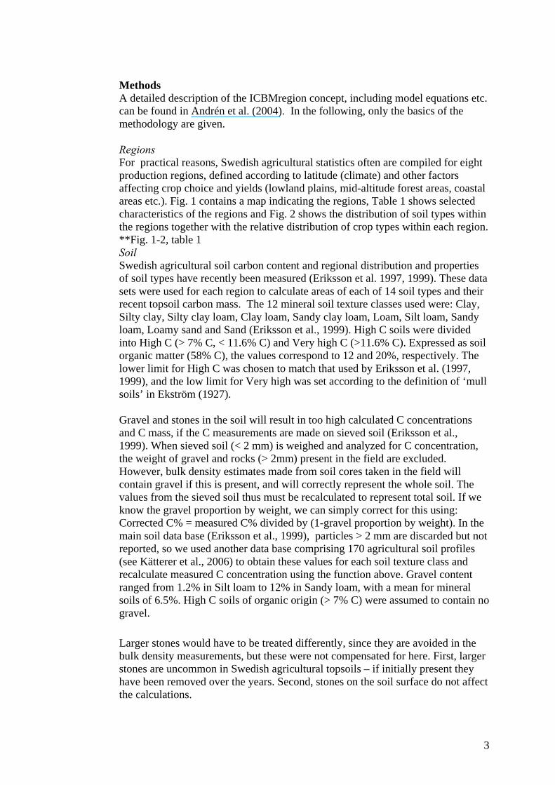
Methods A detailed description of the ICBMregion concept, including model equations etc. can be found in Andrén et al. (2004). In the following, only the basics of the methodology are given. Regions For practical reasons, Swedish agricultural statistics often are compiled for eight production regions, defined according to latitude (climate) and other factors affecting crop choice and yields (lowland plains, mid-altitude forest areas, coastal areas etc.). Fig. 1 contains a map indicating the regions, Table 1 shows selected characteristics of the regions and Fig. 2 shows the distribution of soil types within the regions together with the relative distribution of crop types within each region. **Fig. 1-2, table 1 Soil Swedish agricultural soil carbon content and regional distribution and properties of soil types have recently been measured (Eriksson et al. 1997, 1999). These data sets were used for each region to calculate areas of each of 14 soil types and their recent topsoil carbon mass. The 12 mineral soil texture classes used were: Clay, Silty clay, Silty clay loam, Clay loam, Sandy clay loam, Loam, Silt loam, Sandy loam, Loamy sand and Sand (Eriksson et al., 1999). High C soils were divided into High C (> 7% C, < 11.6% C) and Very high C (>11.6% C). Expressed as soil organic matter (58% C), the values correspond to 12 and 20%, respectively. The lower limit for High C was chosen to match that used by Eriksson et al. (1997, 1999), and the low limit for Very high was set according to the definition of ‘mull soils’ in Ekström (1927). Gravel and stones in the soil will result in too high calculated C concentrations and C mass, if the C measurements are made on sieved soil (Eriksson et al., 1999). When sieved soil (< 2 mm) is weighed and analyzed for C concentration, the weight of gravel and rocks (> 2mm) present in the field are excluded. However, bulk density estimates made from soil cores taken in the field will contain gravel if this is present, and will correctly represent the whole soil. The values from the sieved soil thus must be recalculated to represent total soil. If we know the gravel proportion by weight, we can simply correct for this using: Corrected C% = measured C% divided by (1-gravel proportion by weight). In the main soil data base (Eriksson et al., 1999), particles > 2 mm are discarded but not reported, so we used another data base comprising 170 agricultural soil profiles (see Kätterer et al., 2006) to obtain these values for each soil texture class and recalculate measured C concentration using the function above. Gravel content ranged from 1.2% in Silt loam to 12% in Sandy loam, with a mean for mineral soils of 6.5%. High C soils of organic origin (> 7% C) were assumed to contain no gravel. Larger stones would have to be treated differently, since they are avoided in the bulk density measurements, but these were not compensated for here. First, larger stones are uncommon in Swedish agricultural topsoils – if initially present they have been removed over the years. Second, stones on the soil surface do not affect the calculations.

4

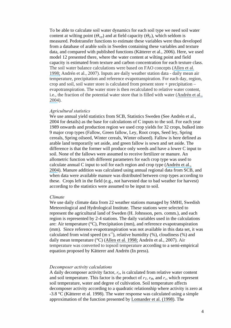
To be able to calculate soil water dynamics for each soil type we need soil water content at wilting point (Θwp) and at field capacity (Θfc), which seldom is measured. Pedotransfer functions to estimate these variables were thus developed from a database of arable soils in Sweden containing these variables and texture data, and compared with published functions (Kätterer et al., 2006). Here, we used model 12 presented there, where the water content at wilting point and field capacity is estimated from texture and carbon concentration for each texture class. The soil water balance calculations were based on FAO concepts (Allen et al. 1998; Andrén et al., 2007). Inputs are daily weather station data - daily mean air temperature, precipitation and reference evapotranspiration. For each day, region, crop and soil, soil water store is calculated from present store + precipitation – evapotranspiration. The water store is then recalculated to relative water content, i.e., the fraction of the potential water store that is filled with water (Andrén et al., 2004). Agricultural statistics We use annual yield statistics from SCB, Statistics Sweden (See Andrén et al., 2004 for details) as the base for calculations of C inputs to the soil. For each year 1989 onwards and production region we used crop yields for 32 crops, bulked into 9 major crop types (Fallow, Green fallow, Ley, Root crops, Seed ley, Spring cereals, Spring oilseed, Winter cereals, Winter oilseed). Fallow is here defined as arable land temporarily set aside, and green fallow is sown and set aside. The difference is that the former will produce only weeds and have a lower C input to soil. None of the fallows were assumed to receive fertilizer or manure. An allometric function with different parameters for each crop type was used to calculate annual C input to soil for each region and crop type (Andrén et al., 2004). Manure addition was calculated using annual regional data from SCB, and when data were available manure was distributed between crop types according to these. Crops left in the field (e.g., not harvested due to bad weather for harvest) according to the statistics were assumed to be input to soil. Climate We use daily climate data from 22 weather stations managed by SMHI, Swedish Meteorological and Hydrological Institute. These stations were selected to represent the agricultural land of Sweden (H. Johnsson, pers. comm.), and each region is represented by 2-4 stations. The daily variables used in the calculations are: Air temperature (°C), Precipitation (mm), and reference evapotranspiration (mm). Since reference evapotranspiration was not available in this data set, it was calculated from wind speed (m s-1), relative humidity (%), cloudiness (%) and daily mean temperature (°C) (Allen et al. 1998; Andrén et al., 2007). Air temperature was converted to topsoil temperature according to a semi-empirical equation proposed by Kätterer and Andrén (In press). Decomposer activity calculations A daily decomposer activity factor, re, is calculated from relative water content and soil temperature. This factor is the product of rΤ, rΘ, and rc, which represent soil temperature, water and degree of cultivation. Soil temperature affects decomposer activity according to a quadratic relationship where activity is zero at -3.8 °C (Kätterer et al. 1998). The water response was calculated using a simple approximation of the function presented by Lomander et al. (1998). The

5

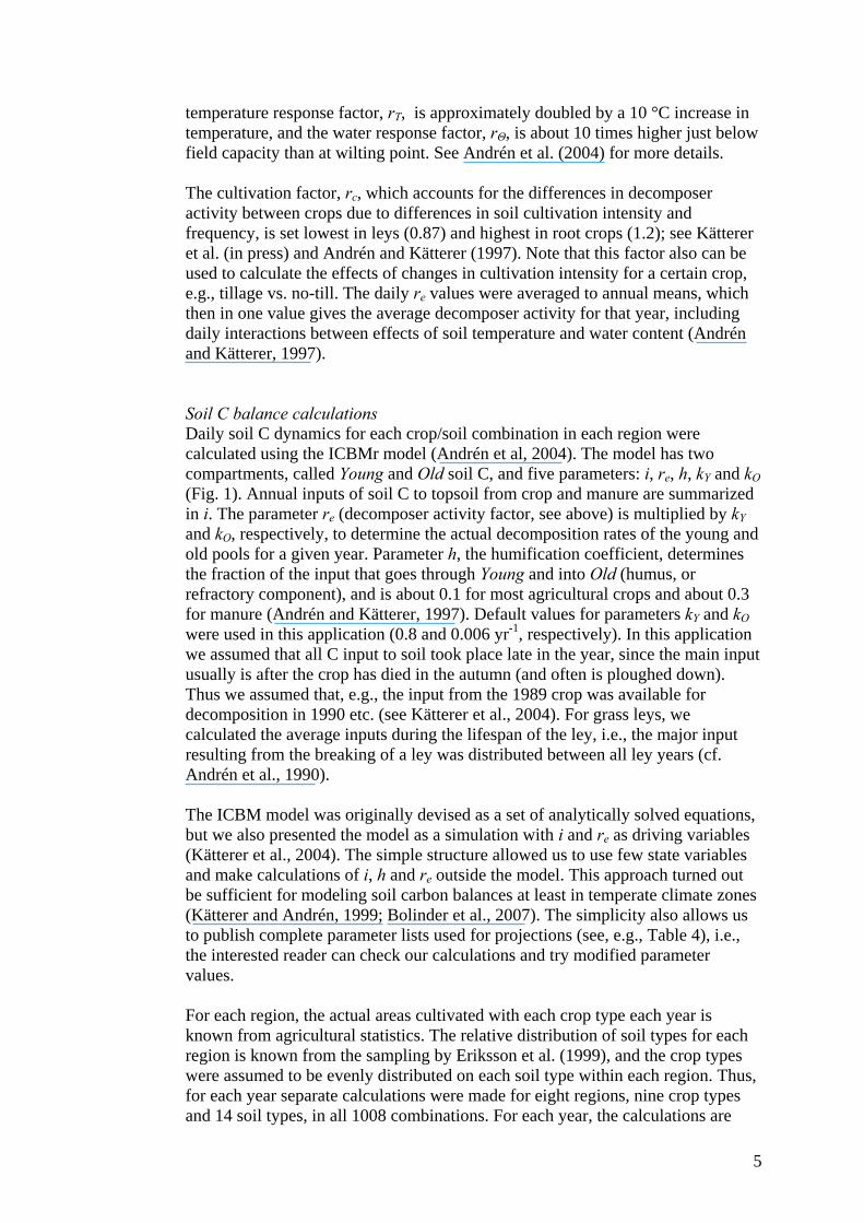
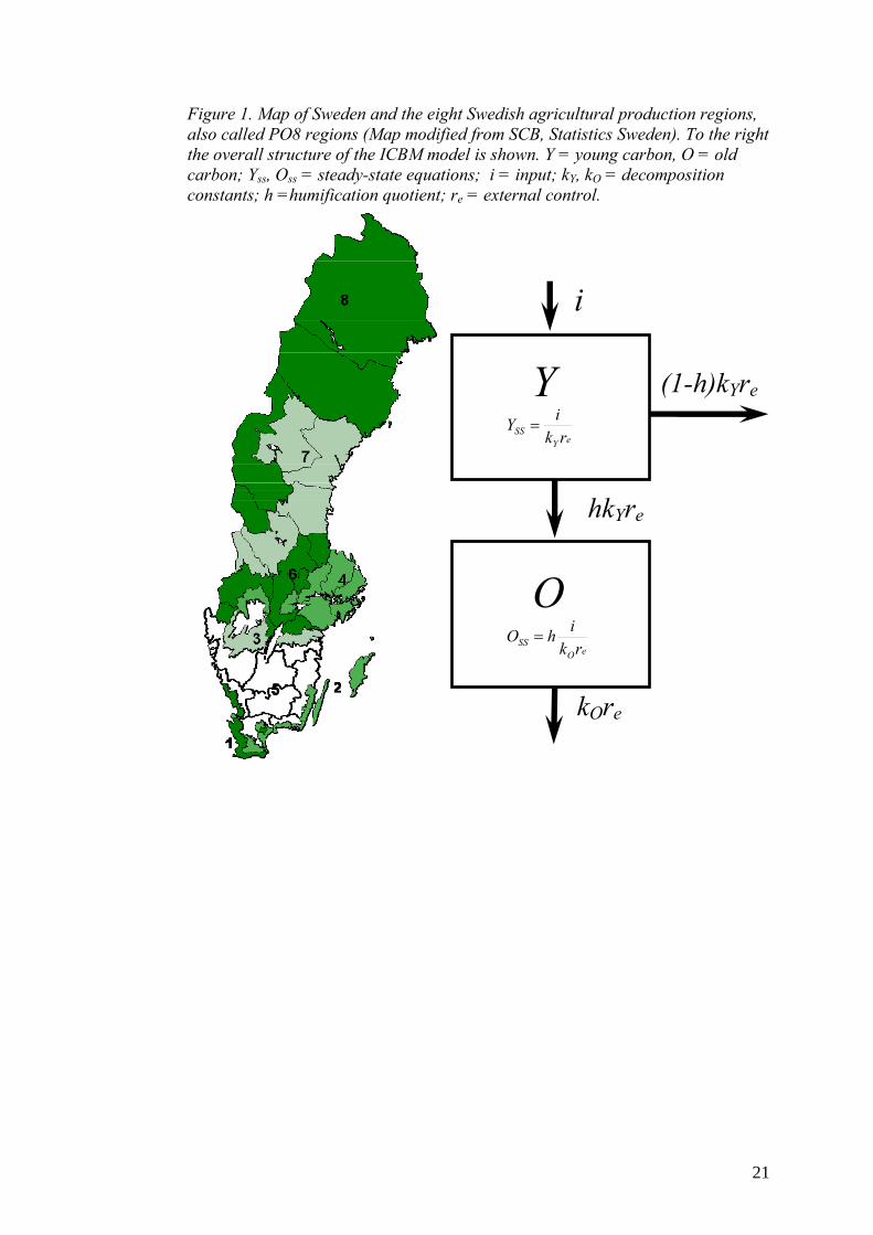
temperature response factor, rΤ, is approximately doubled by a 10 °C increase in temperature, and the water response factor, rΘ, is about 10 times higher just below field capacity than at wilting point. See Andrén et al. (2004) for more details. The cultivation factor, rc, which accounts for the differences in decomposer activity between crops due to differences in soil cultivation intensity and frequency, is set lowest in leys (0.87) and highest in root crops (1.2); see Kätterer et al. (in press) and Andrén and Kätterer (1997). Note that this factor also can be used to calculate the effects of changes in cultivation intensity for a certain crop, e.g., tillage vs. no-till. The daily re values were averaged to annual means, which then in one value gives the average decomposer activity for that year, including daily interactions between effects of soil temperature and water content (Andrén and Kätterer, 1997). Soil C balance calculations Daily soil C dynamics for each crop/soil combination in each region were calculated using the ICBMr model (Andrén et al, 2004). The model has two compartments, called Young and Old soil C, and five parameters: i, re, h, kY and kO (Fig. 1). Annual inputs of soil C to topsoil from crop and manure are summarized in i. The parameter re (decomposer activity factor, see above) is multiplied by kY and kO, respectively, to determine the actual decomposition rates of the young and old pools for a given year. Parameter h, the humification coefficient, determines the fraction of the input that goes through Young and into Old (humus, or refractory component), and is about 0.1 for most agricultural crops and about 0.3 for manure (Andrén and Kätterer, 1997). Default values for parameters kY and kO were used in this application (0.8 and 0.006 yr-1, respectively). In this application we assumed that all C input to soil took place late in the year, since the main input usually is after the crop has died in the autumn (and often is ploughed down). Thus we assumed that, e.g., the input from the 1989 crop was available for decomposition in 1990 etc. (see Kätterer et al., 2004). For grass leys, we calculated the average inputs during the lifespan of the ley, i.e., the major input resulting from the breaking of a ley was distributed between all ley years (cf. Andrén et al., 1990). The ICBM model was originally devised as a set of analytically solved equations, but we also presented the model as a simulation with i and re as driving variables (Kätterer et al., 2004). The simple structure allowed us to use few state variables and make calculations of i, h and re outside the model. This approach turned out be sufficient for modeling soil carbon balances at least in temperate climate zones (Kätterer and Andrén, 1999; Bolinder et al., 2007). The simplicity also allows us to publish complete parameter lists used for projections (see, e.g., Table 4), i.e., the interested reader can check our calculations and try modified parameter values. For each region, the actual areas cultivated with each crop type each year is known from agricultural statistics. The relative distribution of soil types for each region is known from the sampling by Eriksson et al. (1999), and the crop types were assumed to be evenly distributed on each soil type within each region. Thus, for each year separate calculations were made for eight regions, nine crop types and 14 soil types, in all 1008 combinations. For each year, the calculations are

6

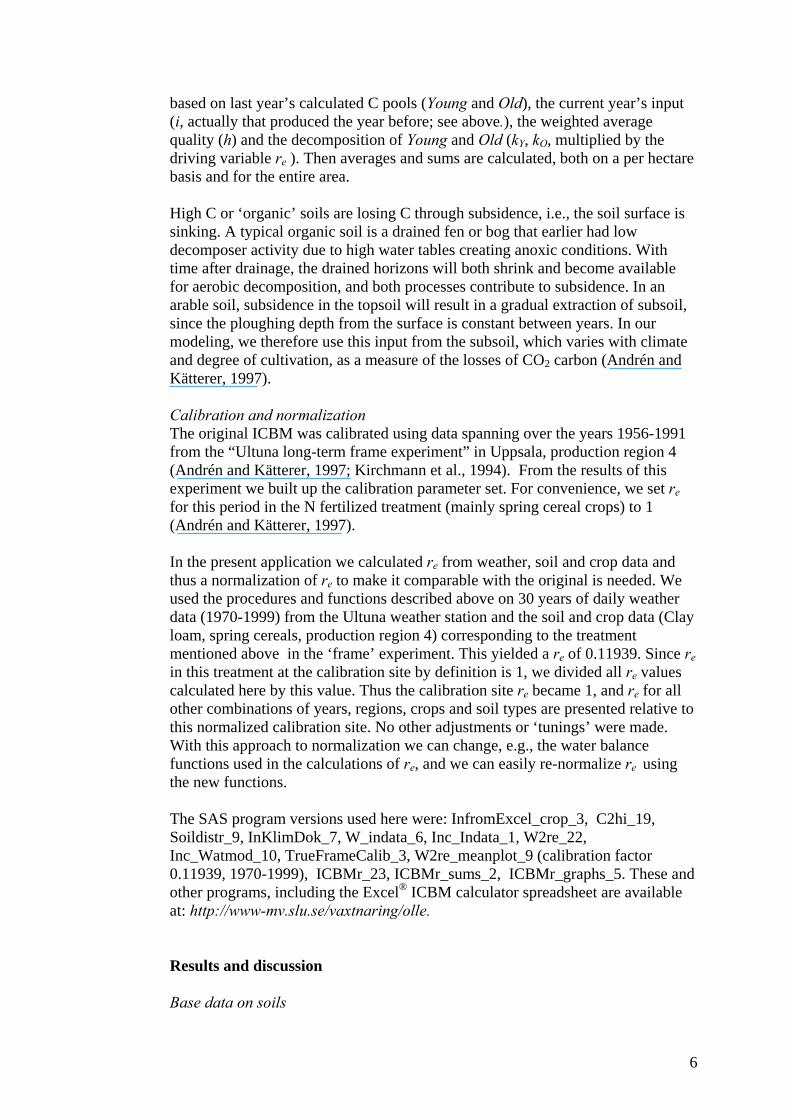
based on last year’s calculated C pools (Young and Old), the current year’s input (i, actually that produced the year before; see above.), the weighted average quality (h) and the decomposition of Young and Old (kY, kO, multiplied by the driving variable re ). Then averages and sums are calculated, both on a per hectare basis and for the entire area. High C or ‘organic’ soils are losing C through subsidence, i.e., the soil surface is sinking. A typical organic soil is a drained fen or bog that earlier had low decomposer activity due to high water tables creating anoxic conditions. With time after drainage, the drained horizons will both shrink and become available for aerobic decomposition, and both processes contribute to subsidence. In an arable soil, subsidence in the topsoil will result in a gradual extraction of subsoil, since the ploughing depth from the surface is constant between years. In our modeling, we therefore use this input from the subsoil, which varies with climate and degree of cultivation, as a measure of the losses of CO2 carbon (Andrén and Kätterer, 1997). Calibration and normalization The original ICBM was calibrated using data spanning over the years 1956-1991 from the “Ultuna long-term frame experiment” in Uppsala, production region 4 (Andrén and Kätterer, 1997; Kirchmann et al., 1994). From the results of this experiment we built up the calibration parameter set. For convenience, we set re for this period in the N fertilized treatment (mainly spring cereal crops) to 1 (Andrén and Kätterer, 1997). In the present application we calculated re from weather, soil and crop data and thus a normalization of re to make it comparable with the original is needed. We used the procedures and functions described above on 30 years of daily weather data (1970-1999) from the Ultuna weather station and the soil and crop data (Clay loam, spring cereals, production region 4) corresponding to the treatment mentioned above in the ‘frame’ experiment. This yielded a re of 0.11939. Since re in this treatment at the calibration site by definition is 1, we divided all re values calculated here by this value. Thus the calibration site re became 1, and re for all other combinations of years, regions, crops and soil types are presented relative to this normalized calibration site. No other adjustments or ‘tunings’ were made. With this approach to normalization we can change, e.g., the water balance functions used in the calculations of re, and we can easily re-normalize re using the new functions. The SAS program versions used here were: InfromExcel_crop_3, C2hi_19, Soildistr_9, InKlimDok_7, W_indata_6, Inc_Indata_1, W2re_22, Inc_Watmod_10, TrueFrameCalib_3, W2re_meanplot_9 (calibration factor 0.11939, 1970-1999), ICBMr_23, ICBMr_sums_2, ICBMr_graphs_5. These and other programs, including the Excel® ICBM calculator spreadsheet are available at: http://www-mv.slu.se/vaxtnaring/olle. Results and discussion Base data on soils

7

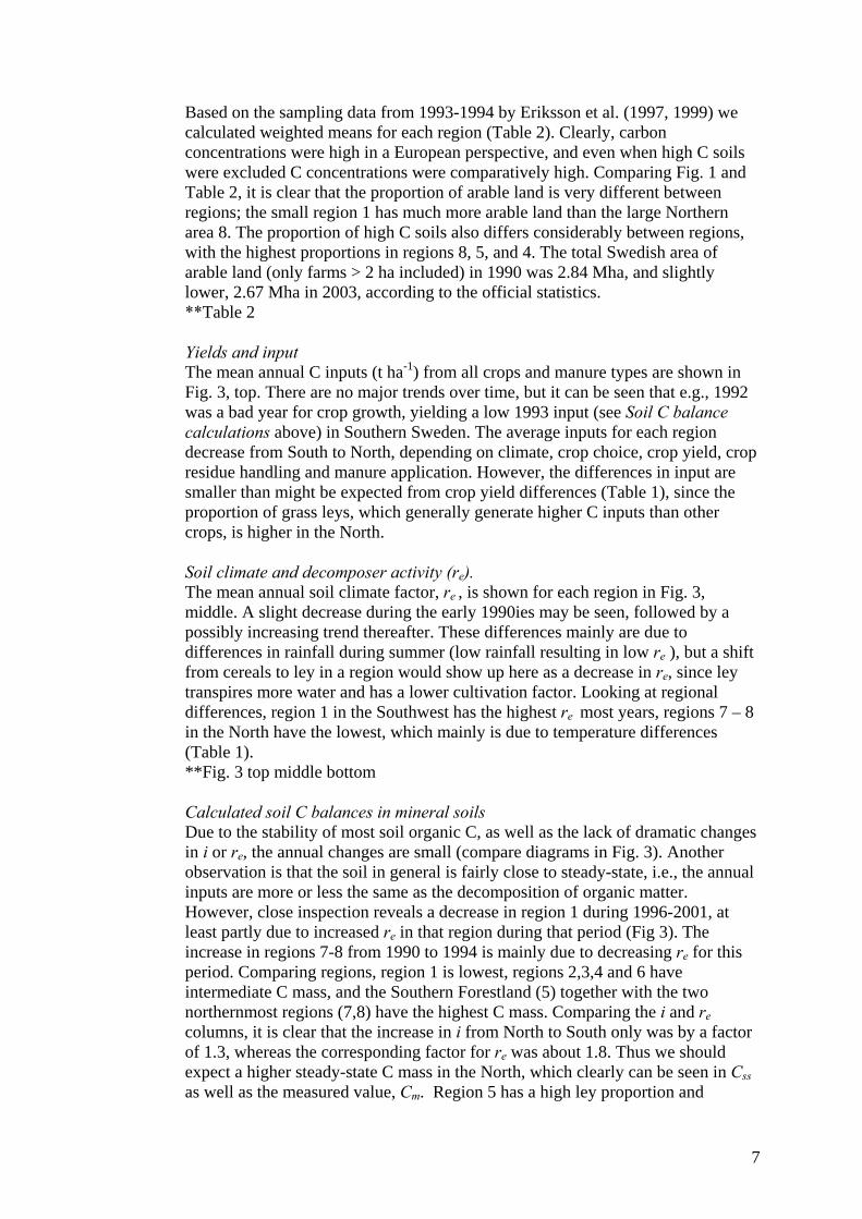
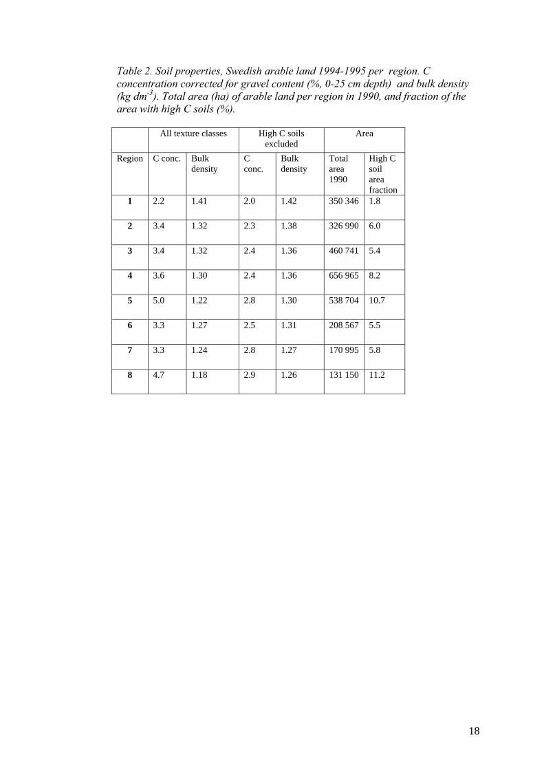
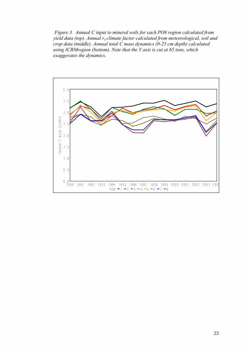
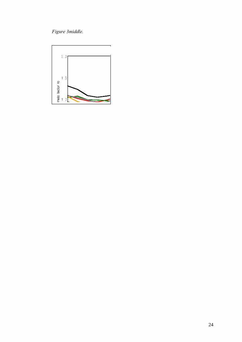
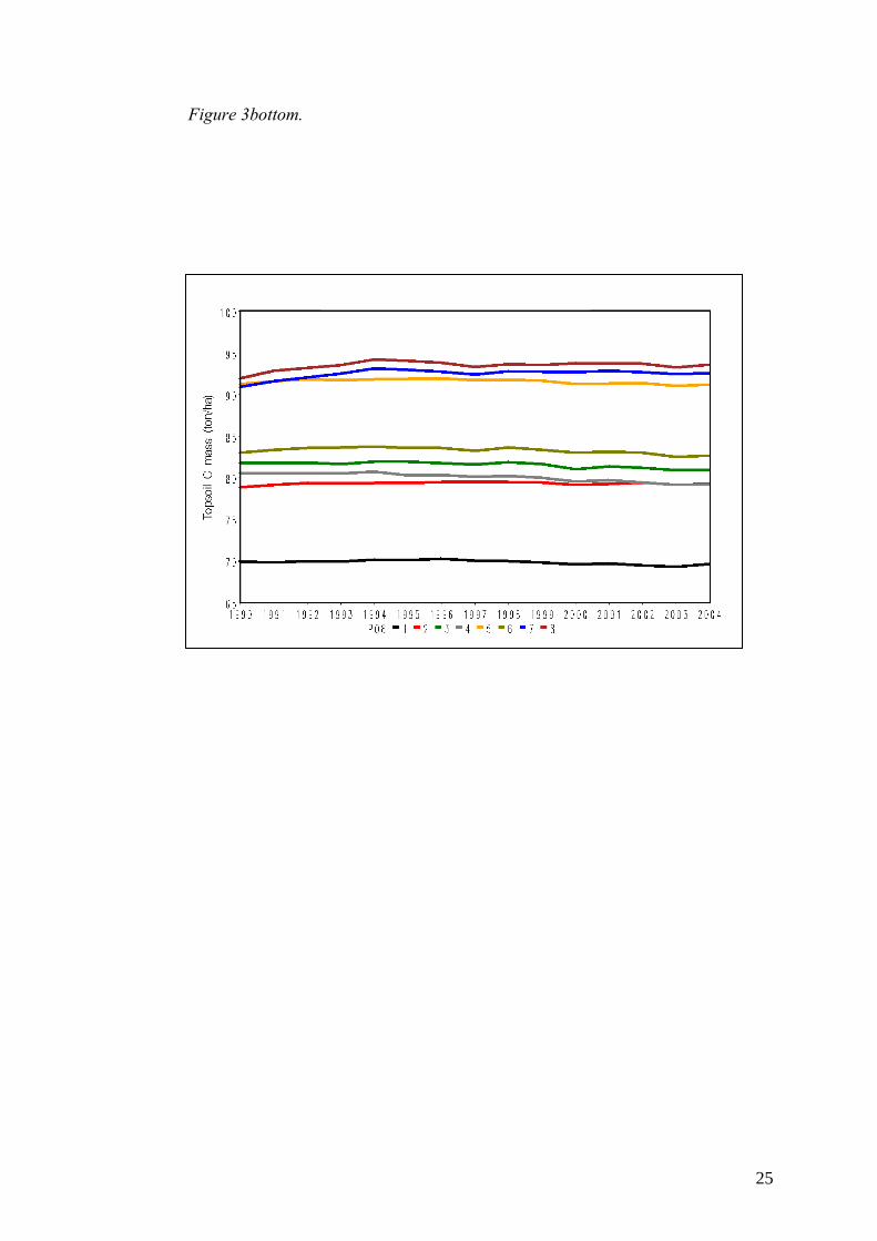
Based on the sampling data from 1993-1994 by Eriksson et al. (1997, 1999) we calculated weighted means for each region (Table 2). Clearly, carbon concentrations were high in a European perspective, and even when high C soils were excluded C concentrations were comparatively high. Comparing Fig. 1 and Table 2, it is clear that the proportion of arable land is very different between regions; the small region 1 has much more arable land than the large Northern area 8. The proportion of high C soils also differs considerably between regions, with the highest proportions in regions 8, 5, and 4. The total Swedish area of arable land (only farms > 2 ha included) in 1990 was 2.84 Mha, and slightly lower, 2.67 Mha in 2003, according to the official statistics. **Table 2 Yields and input The mean annual C inputs (t ha-1) from all crops and manure types are shown in Fig. 3, top. There are no major trends over time, but it can be seen that e.g., 1992 was a bad year for crop growth, yielding a low 1993 input (see Soil C balance calculations above) in Southern Sweden. The average inputs for each region decrease from South to North, depending on climate, crop choice, crop yield, crop residue handling and manure application. However, the differences in input are smaller than might be expected from crop yield differences (Table 1), since the proportion of grass leys, which generally generate higher C inputs than other crops, is higher in the North. Soil climate and decomposer activity (re). The mean annual soil climate factor, re , is shown for each region in Fig. 3, middle. A slight decrease during the early 1990ies may be seen, followed by a possibly increasing trend thereafter. These differences mainly are due to differences in rainfall during summer (low rainfall resulting in low re ), but a shift from cereals to ley in a region would show up here as a decrease in re, since ley transpires more water and has a lower cultivation factor. Looking at regional differences, region 1 in the Southwest has the highest re most years, regions 7 – 8 in the North have the lowest, which mainly is due to temperature differences (Table 1). **Fig. 3 top middle bottom Calculated soil C balances in mineral soils Due to the stability of most soil organic C, as well as the lack of dramatic changes in i or re, the annual changes are small (compare diagrams in Fig. 3). Another observation is that the soil in general is fairly close to steady-state, i.e., the annual inputs are more or less the same as the decomposition of organic matter. However, close inspection reveals a decrease in region 1 during 1996-2001, at least partly due to increased re in that region during that period (Fig 3). The increase in regions 7-8 from 1990 to 1994 is mainly due to decreasing re for this period. Comparing regions, region 1 is lowest, regions 2,3,4 and 6 have intermediate C mass, and the Southern Forestland (5) together with the two northernmost regions (7,8) have the highest C mass. Comparing the i and re columns, it is clear that the increase in i from North to South only was by a factor of 1.3, whereas the corresponding factor for re was about 1.8. Thus we should expect a higher steady-state C mass in the North, which clearly can be seen in Css as well as the measured value, Cm. Region 5 has a high ley proportion and

8

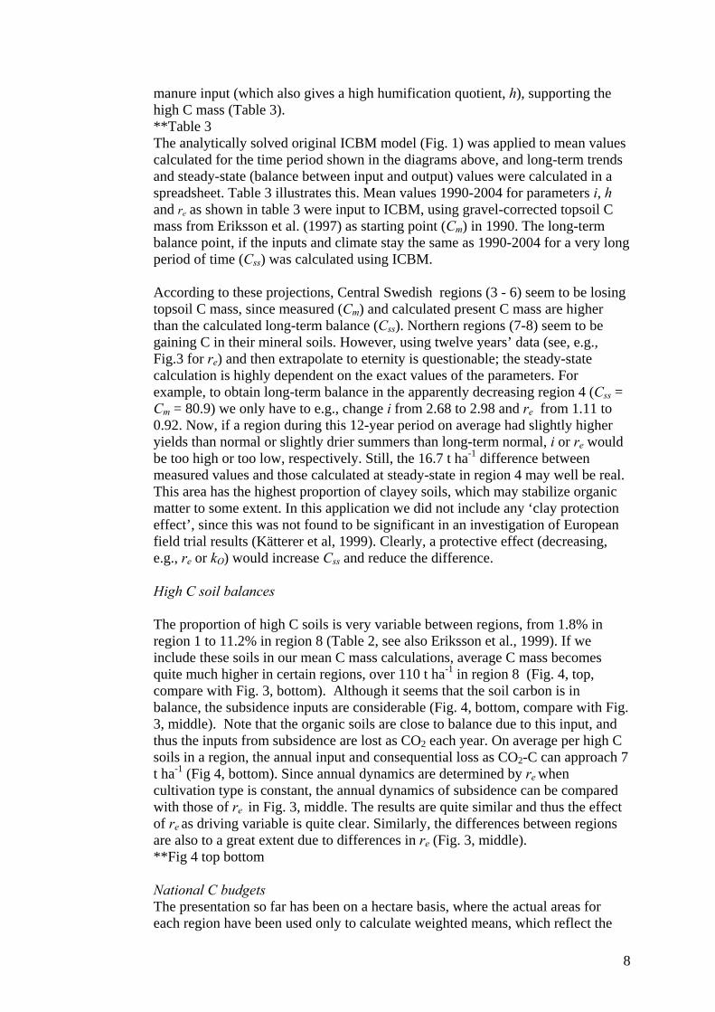
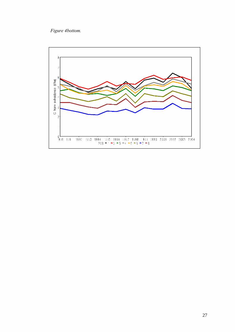
manure input (which also gives a high humification quotient, h), supporting the high C mass (Table 3). **Table 3 The analytically solved original ICBM model (Fig. 1) was applied to mean values calculated for the time period shown in the diagrams above, and long-term trends and steady-state (balance between input and output) values were calculated in a spreadsheet. Table 3 illustrates this. Mean values 1990-2004 for parameters i, h and re as shown in table 3 were input to ICBM, using gravel-corrected topsoil C mass from Eriksson et al. (1997) as starting point (Cm) in 1990. The long-term balance point, if the inputs and climate stay the same as 1990-2004 for a very long period of time (Css) was calculated using ICBM. According to these projections, Central Swedish regions (3 - 6) seem to be losing topsoil C mass, since measured (Cm) and calculated present C mass are higher than the calculated long-term balance (Css). Northern regions (7-8) seem to be gaining C in their mineral soils. However, using twelve years’ data (see, e.g., Fig.3 for re) and then extrapolate to eternity is questionable; the steady-state calculation is highly dependent on the exact values of the parameters. For example, to obtain long-term balance in the apparently decreasing region 4 (Css = Cm = 80.9) we only have to e.g., change i from 2.68 to 2.98 and re from 1.11 to 0.92. Now, if a region during this 12-year period on average had slightly higher yields than normal or slightly drier summers than long-term normal, i or re would be too high or too low, respectively. Still, the 16.7 t ha-1 difference between measured values and those calculated at steady-state in region 4 may well be real. This area has the highest proportion of clayey soils, which may stabilize organic matter to some extent. In this application we did not include any ‘clay protection effect’, since this was not found to be significant in an investigation of European field trial results (Kätterer et al, 1999). Clearly, a protective effect (decreasing, e.g., re or kO) would increase Css and reduce the difference. High C soil balances The proportion of high C soils is very variable between regions, from 1.8% in region 1 to 11.2% in region 8 (Table 2, see also Eriksson et al., 1999). If we include these soils in our mean C mass calculations, average C mass becomes quite much higher in certain regions, over 110 t ha-1 in region 8 (Fig. 4, top, compare with Fig. 3, bottom). Although it seems that the soil carbon is in balance, the subsidence inputs are considerable (Fig. 4, bottom, compare with Fig. 3, middle). Note that the organic soils are close to balance due to this input, and thus the inputs from subsidence are lost as CO2 each year. On average per high C soils in a region, the annual input and consequential loss as CO2-C can approach 7 t ha-1 (Fig 4, bottom). Since annual dynamics are determined by re when cultivation type is constant, the annual dynamics of subsidence can be compared with those of re in Fig. 3, middle. The results are quite similar and thus the effect of re as driving variable is quite clear. Similarly, the differences between regions are also to a great extent due to differences in re (Fig. 3, middle). **Fig 4 top bottom National C budgets The presentation so far has been on a hectare basis, where the actual areas for each region have been used only to calculate weighted means, which reflect the

9

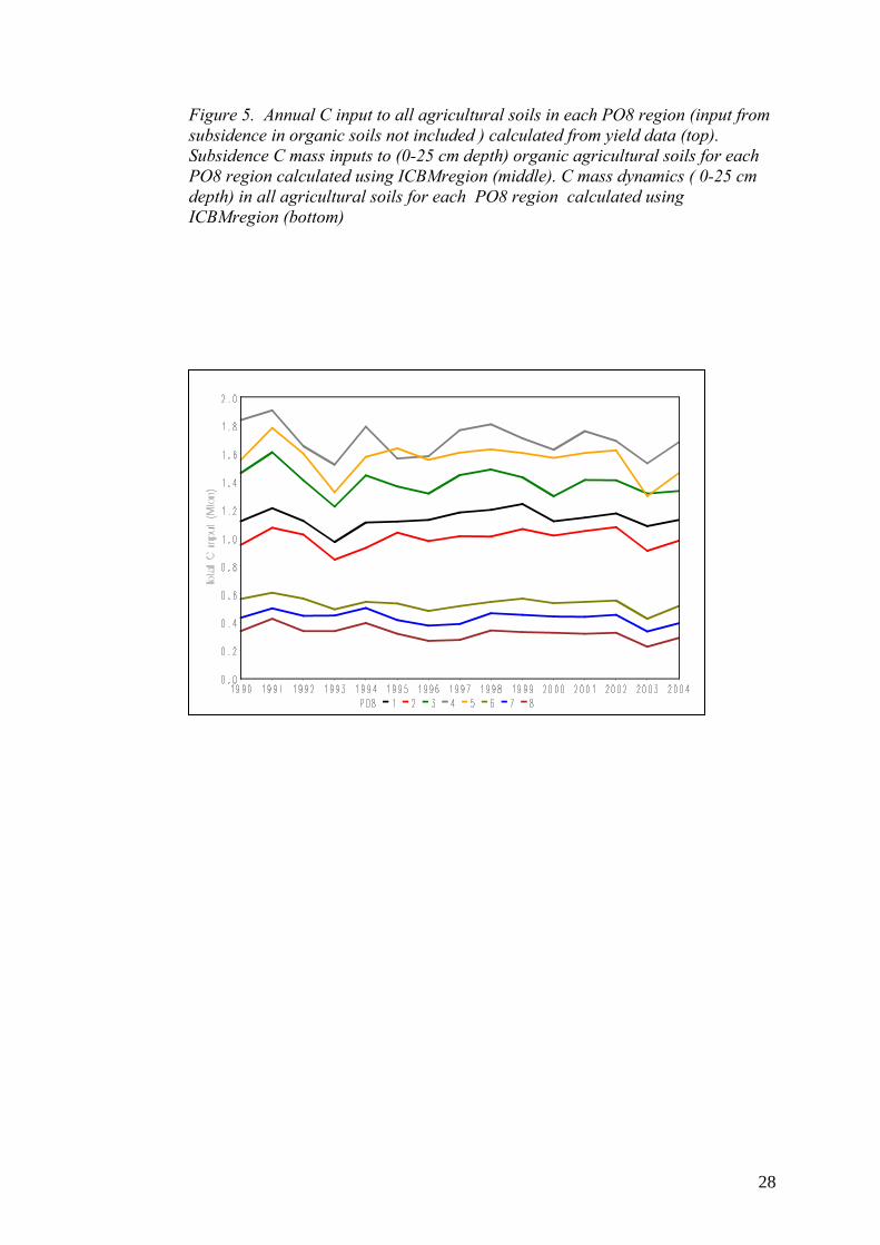
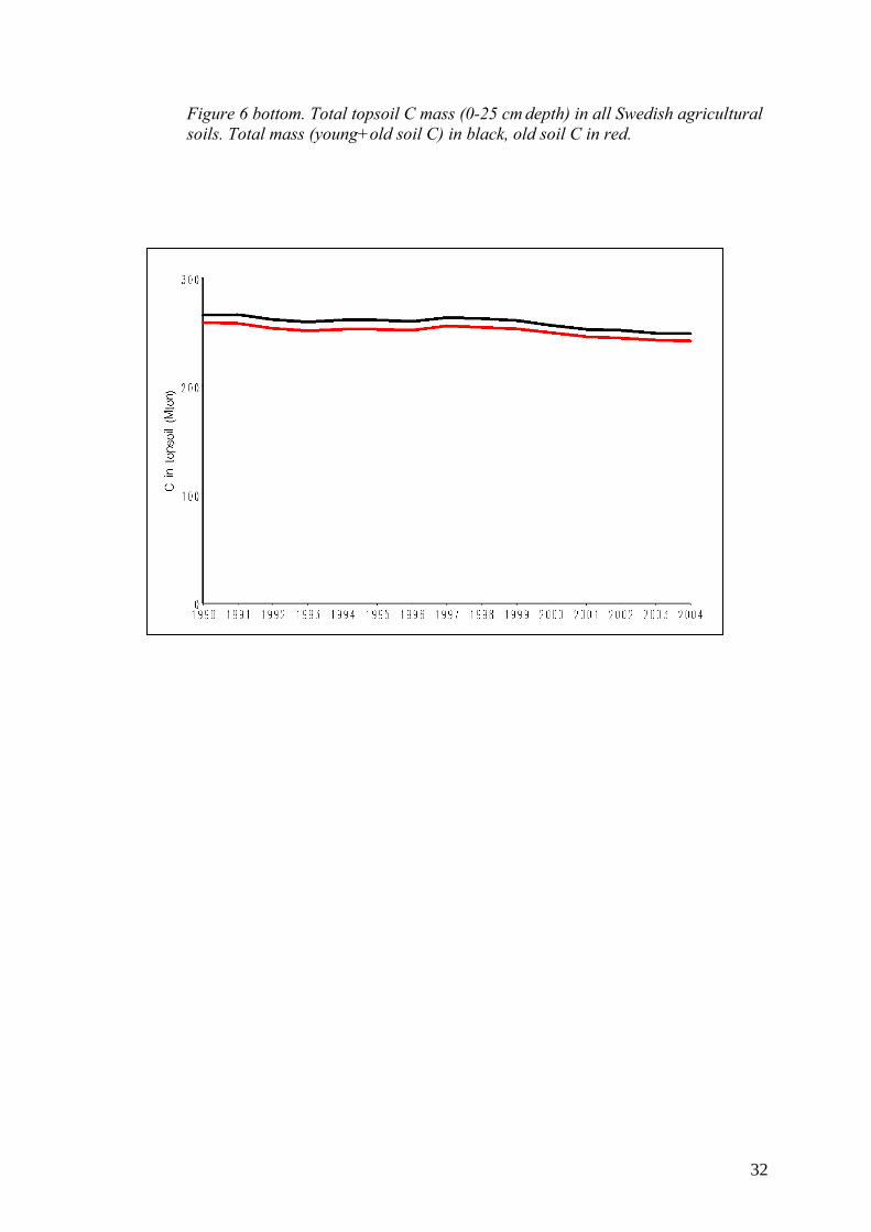
regional conditions, but not a region’s total contribution to national balances. As is clear from Table 1-3, the regions differ considerably in total area of arable land as well as proportion of organic soils etc. For regional and national C budgets summed values for regions and nations are necessary. Relative differences in input between years are fairly similar for the major agricultural regions in Southern and Central Sweden (Fig. 5 top), since the weather patterns in these regions are fairly well correlated. E.g., a growing season with favourable weather for crop yields and C input in Southern Sweden often also is favourable for Central Sweden, which is also reflected in the co-variation of the climate factor re for these regions (Fig. 3, middle). Fig. 5, middle, shows total inputs from subsidence from the different regions. Clearly, regions 5 and 6 in central Sweden each contribute with about 0.3 Mt yr-1. The total annual losses are close to 1 Mt. The regional C mass dynamics are shown in Fig. 5, bottom. Partly due to a slight reduction in the area of arable land between 1990 (2.84 Mha) and 2003 (2.67 Mha), the total C mass in Swedish agricultural top soils has decreased slightly, from 269 Mt in 1990 to 251 Mt in 2003. However, a decrease due to reduced area is different from a decrease per ha, since arable land converted to other uses, e.g., forestry, will still contain the same C mass, at least initially. **Fig 5 top middle bottom The total C inputs for Swedish arable land are shown in Fig. 6, top. About 8 Mt is supplied each year in total from manures, crop residues and root turnover during the growing season, and about 1 Mt yr-1 is supplied from manures only. **Fig 6 top bottom The total topsoil C dynamics for all agricultural land in Sweden (black line) is shown in Fig. 6, bottom. The difference between the black and red lines indicate the amount of “Young” soil C, mainly composed of present and recent years’ input of crop residues. In the ICBM model, the decomposition rate factor of this young material, based on field estimates from litter-bag experiments usually is set to 0.8 yr-1 (Andrén et al, 1990, 1997). This corresponds to an annual mass loss of about 55% in Central Sweden, while the corresponding values for the “Old” fraction are 0.006 and 0.60% yr-1, respectively. In conclusion, the results indicate that the mineral soils are not far from balance and that the simple model approach used here performed satisfactorily. However, to really be able to test and possibly reject the model hypotheses we need more long-term, high-precision and unbiased data sets, which are rare in soil biology (Andrén et al., 2008).

10

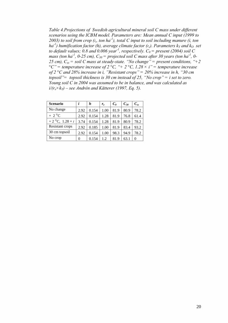
Possible scenarios A simple way to create national scenario projections is to use the analytically solved ICBM model in, e.g., a spreadsheet (http://www-mv.slu.se/vaxtnaring/olle/ICBM_Swed_Afr.xls). Then we can change parameters to reflect overall changes in, e.g. climate, and project the results 30 years into the future (Table 4). **Table 4 For a ‘no-change’ scenario (just an extrapolation from present conditions, assuming no change) we can use the weighted averages of the regional 1990-2004 parameters shown in Table 3. The steady-state topsoil C mass (Css=78.2 t ha-1, reached after a very long time) is lower than present conditions (81.9 t ha-1), but after 30 years only 1 t ha-1 will be lost. A projected C loss of 33 kg yr-1 out of 81.9 t is much smaller than the precision of our measurements and parameter estimates, so we can not say that Swedish mineral agricultural topsoils actually are losing C (see also General discussion). However, with the ‘no-change’ scenario as baseline we can change parameters and project future changes relative to that. There are projections of changing climate, different for different parts of Sweden, made within the global change context (e.g., Jones et al., 2004; Kjellström et al., 2005). Fairly detailed regional projections are available, but here we just assume that every day from now on will be 2 °C warmer, and rainfall, evapotranspiration, crop yield etc. will remain constant. This will affect the climate factor re, since this is partly temperature dependent; an increase with 10 °C would approximately double the re factor if everything else was constant. However, if a winter day is -25 or -23°C affects re less than a summer day increase from +23 to +25 °C, so we had to apply this increase to a real weather data set, and we selected one from our field trials in Uppsala, Central Sweden. The re factor increased by 28%, and the ‘no-change’ re then changed to 1.28. This reduces Css to 61.4 t, and even in the relatively short 30-year perspective 5.1 t ha-1 would be lost. A temperature increase in a cold temperate region would however usually increase crop yields (cf. Table 1), and the ICBM model equations can be used to calculate the increase in crop yield necessary to counteract the increased re (Andrén and Kätterer, 1997). It turns out to be the same as the re increase to obtain the same Css, a 28% increase, and the 30-year projection also becomes the same as for our current climate. However, yield increases of single crops may not be as high as this. According to simulations by Eckersten et al. (2001) conducted for two regions in southern Sweden (two GCM cells; Hadley Centre’s HadCM2) yields for winter wheat were 10-20% (depending on soil type) higher in 2050 than presently. However, not only crop yields but also crop types and management will change in response to changed climate. Comparing the average temperatures and crop yields in Table 1 (e.g. regions 2 and 6) indicates an even greater yield increase due to this temperature increase. Therefore it is quite possible that future agriculture in Sweden may conserve or even increase present soil carbon mass in the soil. Naturally, the temperature distribution over the year as well as changed precipitation amount and pattern may be more crucial for crop yields than a change in mean annual temperature – but future changes in these factors can only be very roughly estimated in current climate models. There is also a possible risk for an increase in ‘catastrophic events’ – e.g., extreme drought in spring, which may result in low crop growth or crop failure.

11

Different crops can have different humification quotients, h, depending on, e.g., lignin content. Let us assume that we breed new crop varieties with 20% higher h and apply this to the business as usual scenario. This will lead to a considerably higher Css, 93.2 t ha-1. Again, after 30 years we will be far from steady-state, and topsoil C will only have increased to 83.4 t ha-1. However, the 1.5 t ha-1 increase, if applied to all Swedish mineral agricultural topsoil (ca 3 Mha), corresponds to 4.5 Mt over the 30-year period. In our calculations, we have assumed a topsoil thickness of 25 cm (cf. Eriksson et al. 1997, 1999). This means that we assume a ploughing depth of 25 cm, and that the crop residues are distributed within this horizon. If we assume the same crop yield and input but use a ploughing depth and topsoil thickness of 30 cm (and ignore the small contribution of roots at 25-30 cm depth), we can calculate the results (Table 4). The present topsoil C would then be 81.9 x 30/25 = 98.3 t ha-1. Clearly, Css will be the same, so the present soil C mass can not be maintained in the long term. However, after 30 years, as much as 94.9 t ha-1 will remain, and the average loss rate during this period, about 110 kg ha-1 yr-1 will be hard to detect on an annual basis. To illustrate the effects of land use change and the resilience of soil C under Swedish conditions, let us assume that the farmers kill all livestock and keep all their land vegetation-free under black fallow. This will reduce the annual C inputs from crop and manure to zero and Css will become zero (cf. Andrén and Kätterer, 2001 but see below). Let us also assume that re increases to 1.2, since without a crop evapotranspiration will be lower and the soils will maintain water longer into drought periods, and soil cultivation will be frequent to keep weeds out. Even under this admittedly extreme and certainly not recommended scenario, 63.1 t ha-1 will remain after 30 years, which still would be high compared with the European average for arable soils, 53 t ha-1 (Mineral soils, < 5% C, 0-30-cm depth, Smith et al., 2001). However, this projection depends heavily on the value of kO, the basic rate of decomposition for old C in the soil and that this value is representative for the whole soil, i.e., there is no large inert fraction such as charcoal. The kO value is mainly based on results from one black fallow long-term experiment (Kirchmann et al., 1997) and the general applicability of this value for all soil types is questionable (Kätterer and Andrén, 1999). General discussion The area of Swedish agricultural land The agricultural yield statistics we have used excludes farms with < 2 ha arable land. There is also semi-natural grazing land, not ploughed, that may be included. The small-farm (typically amateur farmers with horses for recreation; there are over 300 000 horses in Sweden) total area has been estimated to 400 000 ha, and semi-natural grazing land covers a similar area (Andrén and Kätterer, 2001). The area of Swedish agricultural land ca. 1990 can thus be given as 2.8 Mha (Table 2), 3.2 Mha (including small farms), or 3.6 Mha (also including semi-natural grazing lands). The small farm soil C balances will be similar, but not identical to those in official statistics (probably more grass ley etc.), but semi-natural grazing land will be more different, from wet riverbank meadows to thin-soiled hilly landscape with junipers. However, there are national soil samplings that cover both forests and

12

natural grazing land, and these will have to be used for national budgets covering the entire land area. Validity and general precision of estimates The estimates of present (1994-1995) C mass, based on more than 3100 soil samples gives a good baseline estimate of C mass, and every effort was made to give high precision and avoid bias (Eriksson et al. 1997, 1999). This sampling will be repeated (actually one sampling is underway now), and the future results (increase or decrease of soil carbon mass in regions/soil types) will be used for validation of our soil C balance estimates. However, due to the low rate of change expected, only fairly clear trends can be detected, and only after considerable time (10-20 years). With respect to carbon, this type of monitoring is a long-term commitment. Our C balance estimates, based on weather data, yield data and soil property data as well as generally accepted modeling concepts and parameter estimates based on long-term field experiments (Kätterer and Andrén, 1999) should be fairly correct – but until we have a second full sampling we cannot estimate how correct we are. In the meantime, we can focus our attention on comparatively weak areas, where either our general knowledge is poor or the data sets available have weaknesses. One such area is the conversion of crop yield data to annual C input to soil. Actually, we do not only use yield statistics, but also other information, such as amount left in the field (all of this becomes C input) when harvest conditions are bad. Although this correctly accounts for occasions when harvests are low but C inputs are high, the parameter values used to calculate C input from reported yield (see references in Andrén et al., 2004) probably differ not only between crop types, but also between crop species, varieties, climate and e.g., fertilizer dose (Andrén et al., 1990). This is an area that warrants further research, since the magnitude of the C input is one of the crucial factors for the soil C balance (cf. Table 3). Our calculations of the climate factor, re , are based on three components: Effects of soil temperature, soil water content and degree of cultivation (see Methods). The effects of soil temperature and soil water content are fairly general and based on experimental data, but the effects of soil cultivation per se are less investigated and the effects probably are less general. The cultivation factors we have used here, e.g., 1.0 for cereals and 0.87 for grass leys, are based on general experience, but this needs more development. More intense soil cultivation increases decomposer activity through increased aeration and comminution of litter and soil aggregates. However, setting up a general function describing this effect and finding parameter values for different cultivation measures and soils is not an easy task. There are field experiments with different degrees of cultivation, e.g., till/no-till, but the experiments are seldom designed to single out cultivation effects. For example, in till/no-till experiments the no-till plots will have more surface litter and less in the soil, which will affect litter decomposition rates. Comparisons between leys and cereal crops also contain differences in cultivation, but these are mixed with the effects of very different crops. Clearly, this is an area that demands much more attention – theoretical development as well as carefully designed laboratory and field experiments.

13

The current model we use for calculations of daily soil water balances is fairly crude, but perhaps this is sufficient. However, the only effect of soil type on soil C balances we have included so far is that different soil types have different wilting points and field capacities, and the difference between these determines water storage capacity. This capacity defines how long a saturated soil can maintain enough soil water under a drought to maintain decomposer activity, and it differs with a factor of 3 between the lowest (sand) to the highest (silt loam). However, when testing with normal Swedish weather conditions, the differences in mean annual activity between soils due to differences in water storage capacity are small, but for applications in drier and warmer climates this capacity can be crucial (Andrén et al, 2007). It is also possible that the influence of soil type on soil organic matter stability, e.g., clay ‘stabilization’ should be included, as discussed under ‘Calculated soil C balances in mineral soils’. High C ‘organic’ soils The calculations indicate that agricultural high C soils in Sweden lose 3-7 t C ha-1 yr-1 (Fig. 4, bottom) as a regional average over all cropping systems. These losses are lower with reduced soil cultivation, e.g., grass ley cropping, and can be further reduced by hydroamelioration, i.e., raising the water level and thereby moving back towards original bog or fen conditions. This, however, has a number of drawbacks. First, it has dire consequences for the farmer and possibly the region - you cannot grow crops in bogs. Second, putting arable land under water will increase emissions of CH4, and due to the good nitrogen status there is a high risk of N2O emissions, at least initially. Both these gases, and particularly N2O, have a much higher greenhouse warming potential than CO2 so there is a question of how much will be gained. Third and perhaps most important is the choice of system boundaries (cf. Freibauer et al., 2004). It is reasonable to include plant production, or more specifically photosynthesis, in the calculations. For simplicity, let us assume that net C balance the peat bog is zero (the low production of, e.g., Sphagnum sp. balances the low rate of decomposition under water). The drained high C soil under, e.g., grass ley can lose about 2 t C ha-1 yr-1 when normal inputs to soil for leys are included (compare with Fig. 4, bottom, which shows weighted means over different cropping systems). However, the grass harvested from the grass ley can contain 2 t ha-1 C, which has been taken up from the atmosphere (assuming a dry yield of 5 t ha-1, quite normal for Central Sweden, Statistics Sweden, 2006). If this grass is burnt for energy purposes and thus replaces fossil fuels, we can calculate that the annual C balance for a hectare of grass ley (2 t of fuel C produced – 2 t lost through subsidence) can be similar to that of the steady-state peat bog (this is very simplified - transports, fuel efficiency etc. have to included). However, the crucial point is photosynthesis, which is closely correlated with agronomic crop yield – it is sometimes forgotten that this process is where CO2 is taken out from the atmosphere and converted to organic compounds. Equally important is what we do with these compounds – if we put them in soil, most carbon will rapidly be emitted as CO2 with no practical use of the heat generated. If we use their energy through burning we can save fossil fuels and thus reduce global emissions.

14

References Allen R.G., Pereira L.S., Raes D. and Smith M. 1998. Crop evapotranspiration – guidelines for computing crop water requirements. FAO Irrigation and Drainage Paper 56. FAO Rome, 300 pp. Andrén, O., Kätterer, T., 1997. ICBM: The introductory carbon balance model for exploration of soil carbon balances. Ecol. Appl. 7: 1226-1236.

Andrén, O., Kätterer, T., 2001. Basic principles for soil carbon sequestration and calculating dynamic country-level balances including future scenarios. In: Assessment Methods for Soil Carbon. Edited by R. Lal, J.M. Kimble, R.F. Follett, and B. A. Stewart, Lewis Publishers, pp. 495-511. Andrén, O., Kätterer, T. and Karlsson, T., 2004. ICBM regional model for estimations of dynamics of agricultural soil carbon pools. Nutr. Cycl. Agroecosys. 70: 231-239. Andrén, O., Kihara, J., Bationo, A., Vanlauwe, B. and Kätterer, T. 2007. Soil climate and decomposer activity in sub-Saharan Africa estimated from standard weather station data – a simple climate index for soil carbon balance calculations. Ambio 36: 379-386. Andrén, O., Kirchmann, H., Kätterer, T., Magid, J. and Paul, E.A., 2008. Visions of a more precise soil biology. Eur. J. Soil Science 59: 380-390. Andrén, O., Lindberg, T, Paustian, K. and Rosswall, T. (eds). 1990. Ecology of arable land -- organisms, carbon and nitrogen cycling. - Ecol. Bull. (Copenhagen) 40, ca 210 pp. Bolinder, M.A., Andrén, O., Kätterer, T., de Jong, R., VandenBygaart, A.J., Angers, D.A., Parent, L-E and Gregorich, E.G., 2007. Soil carbon dynamics in Canadian agricultural ecoregions : Quantifying climatic influence on soil biological activity. Agric. Ecosys. Environ. 122: 461-470. Eckersten, H., Blombäck K, Kätterer T. and Nyman P. 2001. Modelling C, N, water and heat dynamics in winter wheat under climate change in southern Sweden. Agric. Ecosys. Environ. 86: 221-235. Ekström, G. 1927. Klassifikation av svenska åkerjordar. Sveriges Geologiska Undersökning, Stockholm, Serie C, No 345, Årsbok 20. (In Swedish) Eriksson J., Andersson A. and Andersson R. 1997. Tillståndet i svensk åkermark (Current status of Swedish arable soils). Stockholm, Swedish Environmental Protection Agency, Report 4778. Eriksson J Andersson A and Andersson R. 1999. Åkermarkens matjordstyper (Texture of agricultural topsoils in Sweden). Stockholm, Swedish Environmental Protection Agency, Report 4955. Freibauer A., Rounsevell M.D.A., Smith P. and Verhagen J. 2004. Carbon sequestration in the agricultural soils of Europe. Geoderma 122: 1-23.

15

IPCC 1997. The Revised 1996 IPCC Guidelines for National Greenhouse Gas Inventories. http://www.ipcc-nggip.iges.or.jp/public/gl/invs1.htm. Jones C.G., Ullerstig A., Willén U. and Hansson U. 2004. The Rossby Centre regional atmospheric climate model (RCA). Part I: Model climatology and performance characteristics for present climate over Europe. Ambio 33: 199-210. Kätterer T. and Andrén O. 1999. Long-term agricultural field experiments in Northern Europe: Analysis of the influence of management on soil carbon stocks using the ICBM model. Agric. Ecosys. Environ. 72: 165-179. Erratum: Agric. Ecosys. Environ. 75: 145-146.

Kätterer T., Andrén O. and Persson J. 2004. The impact of altered management on long-term agricultural soil carbon stocks-a Swedish case study. Nutr. Cycl. Agroecosys. 70:179-187. Kätterer T. and Andrén O. In press. Predicting daily soil temperature profiles in arable soils from air temperature and leaf area index. Acta Agric. Scand. Kätterer, T., Andersson, L., Andrén, O. and Persson, J. In press. Long-term impact of chronosequential land use change on soil carbon stocks on a Swedish farm. Nutr. Cycl. Agroecosys. 00:000-000. Kätterer T., Andrén O. and Jansson P.-E. 2005. Pedotransfer functions for estimating plant available water and bulk density in Swedish agricultural soils. Acta Agric. Scand. Sec. B 56: 263-276. Kirchmann, H., Persson, J. and Carlgren, K. 1994. The Ultuna long-term soil organic matter experiment, 1956–1991. Department of Soil Sciences, Reports and Dissertations 17, Swedish University of Agricultural Sciences, Uppsala, Sweden. Kjellström E., Bärring L., Gollvik S., Hansson U., Jones C., Samuelsson P., Rummukainen M., Ullerstig A., Willén U. and Wyser K. 2005. A 140-year simulation of the European climate with the new version of the Rossby Centre regional atmospheric climate model (RCA3). SMHI Reports Meteorology and Climatology No. 108, SMHI, SE-60176 Norrköping, Sweden, 54 pp. Lomander A., Kätterer T. and Andrén O. 1998. Modelling the effects of temperature and moisture on CO2 evolution from top and subsoil using a multi-compartment approach. Soil Biol. Biochem. 30: 2023–2030. Smith P., Smith J.U., Andrén O., Karlsson T., Perälä P., Regina K., Rounsevell M. and Wesemael B. 2005. Carbon sequestration potential in European croplands has been overestimated. Global Change Biol. 11: 2153–2163. Smith P., Smith J.U. and Powlson D.S. 2001. Soil Organic Matter Network (SOMNET): 2001 Model and Experimental Metadata. GCTE Report 7, Second Edition, GCTE Focus 3, Wallingford, Oxon, 223 pp.

16

Smith J.U., Smith P., Wattenbach, M., Zaehle S., Hiederer R., Jones R., Montanarella L., Rounsevell M. Reginster I. and Ewert F. 2005. Projected changes in mineral soil carbon of European croplands and grasslands, 1990–2080. Global Change Biology 11: 2141–2152.

17

Tables and Figures. Table 1. Swedish agricultural production regions, also called PO8 regions (Fig. 1). Region number, Description, Latitude range, mean annual air temperature and mean annual precipitation 1990-2001, Typical crops and soils, spring barley and winter wheat normal grain yield (14% water content, t ha-1) 1989-2003 (Statistics Sweden 2004). NG = crop not grown in this region.

Region Name Latitude °N

Mean temp.

°C

Precip. mm

Typical crops

Typical soils

Barley yield

Wheat yield

1 Southwestern Coastal

55-77 7.8 757 Spring and winter cereals, Sugar beet

Sandy loam, Loam

5.8 7.9

2 Southeastern Coastal

55-58 7.4 612 Grass ley, Spring and winter cereals

Sandy loam, Loam

4.5 6.5

3 South Central Plains

58 6.5 570 Spring and winter cereals, Grass ley

Sandy loam, Loam

4.7 5.9

4 Central Plains 59-60 6.6 601 Spring cereals, Grass ley

Clay, Silty clay

4.1 5.2

5 Southern Forestland

56-58 6.8 769 Grass ley, Spring cereals

Sandy loam, Loamy sand

3.5 5

6 Central Forestland

58-61 5.3 688 Grass ley, Spring Cereals

Silt loam, Silty clay loam

3.3 4.8

7 North 60-65 3.1 600 Grass ley, Spring Cereals

Silt loam, Loam

2.4 NG

8 North and Mountain

63-69 2.2 575 Grass ley, Spring Cereals

Silt loam, Sandy loam

2.2 NG

18

Table 2. Soil properties, Swedish arable land 1994-1995 per region. C concentration corrected for gravel content (%, 0-25 cm depth) and bulk density (kg dm-3). Total area (ha) of arable land per region in 1990, and fraction of the area with high C soils (%).

All texture classes High C soils excluded

Area

Region C conc. Bulk density

C conc.

Bulk density

Total area 1990

High C soil area fraction

1 2.2 1.41 2.0 1.42 350 346 1.8

2 3.4 1.32 2.3 1.38 326 990 6.0

3 3.4 1.32 2.4 1.36 460 741 5.4

4 3.6 1.30 2.4 1.36 656 965 8.2

5 5.0 1.22 2.8 1.30 538 704 10.7

6 3.3 1.27 2.5 1.31 208 567 5.5

7 3.3 1.24 2.8 1.27 170 995 5.8

8 4.7 1.18 2.9 1.26 131 150 11.2

19

Table 3. Averages for 1990 – 2004 for each region, organic soils excluded. Annual C input from crop (ic, t ha-1), including manure (i, t ha-1) humification factor (h), climate factor (re), projected young C (Y), old C (O), total topsoil C (TotC, t ha-1 ). ICBM calculated steady-state total C (Css, t ha-1), measured total C (Cm, t ha-1) (see Methods), and measured total C (Cmu, t ha-1), uncorrected for gravel content (see Methods). Region ic i h re Y O TotC Css Cm Cmu

1 3.00 3.29 0.149 1.30 2.1 67.7 69.8

70.3 70.8 72.1

2 2.58 3.07 0.164 1.05 2.4 76.8 79.3

83.5 79.1 80.6

3 2.81 3.08 0.147 1.04 2.4 79.1 81.5

76.6 81.8 82.9

4 2.52 2.68 0.142 1.04 2.1 77.9 80.0

64.2 80.9 81.6

5 2.44 3.01 0.170 0.99 2.6 88.9 91.5

90.2 91.4 93.7

6 2.37 2.63 0.151 0.88 2.6 80.6 83.2

79.0 82.9 83.6

7 2.17 2.59 0.164 0.69 3.4 89.0 92.4 106.7 90.3 91.7

8 2.17 2.57 0.163 0.67 3.5 89.9 93.4

109.1 91.1 92.0

20

Table 4.Projections of Swedish agricultural mineral soil C mass under different scenarios using the ICBM model. Parameters are: Mean annual C input (1999 to 2003) to soil from crop (ic, ton ha-1), total C input to soil including manure (i, ton ha-1) humification factor (h), average climate factor (re). Parameters kY and kO set to default values; 0.8 and 0.006 year-1, respectively. C0 = present (2004) soil C mass (ton ha-1, 0-25 cm), C30 = projected soil C mass after 30 years (ton ha-1, 0-25 cm), Css = soil C mass at steady-state. “No change” = present conditions, “+2 °C” = temperature increase of 2 °C, “+ 2 °C, 1.28 × i” = temperature increase of 2 °C and 28% increase in i, ”Resistant crops” = 20% increase in h, “30 cm topsoil”= topsoil thickness is 30 cm instead of 25, “No crop” = i set to zero. Young soil C in 2004 was assumed to be in balance, and was calculated as i/(re×kY) – see Andrén and Kätterer (1997, Eq. 5). Scenario i h re C0 C30 Css No change 2.92 0.154 1.00 81.9 80.9 78.2 + 2 °C 2.92 0.154 1.28 81.9 76.8 61.4 + 2 °C, 1.28 × i 3.74 0.154 1.28 81.9 80.9 78.2 Resistant crops 2.92 0.185 1.00 81.9 83.4 93.2 30 cm topsoil 2.92 0.154 1.00 98.3 94.9 78.2 No crop 0 0.154 1.2 81.9 63.1 0

21

Figure 1. Map of Sweden and the eight Swedish agricultural production regions, also called PO8 regions (Map modified from SCB, Statistics Sweden). To the right the overall structure of the ICBM model is shown. Y = young carbon, O = old carbon; Yss, Oss = steady-state equations; i = input; kY, kO = decomposition constants; h =humification quotient; re = external control.

i

Y

O

(1-h)kYre

hkYre

kOre

eYSS rk

iY =

eOSS rk

ihO =

22

Figure 2. Area of Swedish agricultural land (Kha) summed over crop types, per region and soil type. Mean area 1989-2003.(See ‘Methods’ for full names of soil types).

23

Figure 3. Annual C input to mineral soils for each PO8 region calculated from yield data (top). Annual re climate factor calculated from meteorological, soil and crop data (middle). Annual total C mass dynamics (0-25 cm depth) calculated using ICBMregion (bottom). Note that the Y axis is cut at 65 tons, which exaggerates the dynamics.

24

Figure 3middle.

25

Figure 3bottom.

26

Figure 4. Annual total C mass dynamics (0-25 cm depth) in mineral and organic agricultural soils for each PO8 region calculated using ICBMregion. Note that the Y axis is cut at 70 tons, which exaggerates the dynamics (top). Annual subsidence C mass losses to atmosphere from organic agricultural soils in each PO8 region calculated using ICBMregion (bottom).

27

Figure 4bottom.

28

Figure 5. Annual C input to all agricultural soils in each PO8 region (input from subsidence in organic soils not included ) calculated from yield data (top). Subsidence C mass inputs to (0-25 cm depth) organic agricultural soils for each PO8 region calculated using ICBMregion (middle). C mass dynamics ( 0-25 cm depth) in all agricultural soils for each PO8 region calculated using ICBMregion (bottom)

29

Figure 5middle.

30

Figure 5 bottom.

31

Figure 6. Total annual C inputs to all Swedish agricultural soils. Total input from crop residues, root turnover and manures in black, input from manures only in red. Input through subsidence of organic soils not included (top).

32

Figure 6 bottom. Total topsoil C mass (0-25 cm depth) in all Swedish agricultural soils. Total mass (young+old soil C) in black, old soil C in red.