Título: Costos para empresarios - Capítulo 1 Autor - Aula Virtual
Upload
khangminh22Category
view
1download
0
This page intentionally left blank

Software Receiver Design
Build Your Own Digital Communications System in Five Easy Steps
Have you ever wanted to know how modern digital communications systems work?Find out with this step-by-step guide to building a complete digital radio that includesevery element of a typical, real-world communication system. Chapter by chapter, youwill create a MATLAB realization of the various pieces of the system, exploring thekey ideas along the way, as well as analyzing and assessing the performance of eachcomponent. Then, in the final chapters, you will discover how all the parts fit togetherand interact as you build the complete receiver. Can you decode the messages hiddenwithin the received signals?
In addition to coverage of crucial issues, such as timing, carrier recovery, and equaliza-tion, the text contains over 400 practical exercises, providing invaluable preparation forindustry, where wireless communications and software radio are becoming increasinglyimportant. Various extra resources are also provided online, including lecture slides anda solutions manual for instructors.
C. Richard Johnson, Jr. is the Geoffrey S. M. Hedrick Senior Professor of Engineeringat Cornell University, where he has been on the faculty since 1981. He is a Fellow of theIEEE and co-author of Telecommunication Breakdown (2004, with William A. Sethares)and Theory and Design of Adaptive Filters (2001).
William A. Sethares is a Professor in the Department of Electrical and Computer Engi-neering at the University of Wisconsin in Madison. He is the author of Rhythm andTransforms (2007) and Tuning, Timbre, Spectrum, Scale (2005).
Andrew G. Klein is an Assistant Professor at Worcester Polytechnic Institute. In additionto working in academia, he has also held industry positions at several wireless start-upcompanies.


Software Receiver DesignBuild Your Own Digital CommunicationsSystem in Five Easy Steps
C. RICHARD JOHNSON, JR.Cornell University
WILL IAM A. SETHARESUniversity of Wisconsin in Madison
ANDREW G. KLEINWorcester Polytechnic Institute

CAMBRIDGE UNIVERSITY PRESS
Cambridge, New York, Melbourne, Madrid, Cape Town,Singapore, Sao Paulo, Delhi, Tokyo, Mexico City
Cambridge University PressThe Edinburgh Building, Cambridge CB2 8RU, UK
Published in the United States of America by Cambridge University Press, New York
www.cambridge.orgInformation on this title: www.cambridge.org/9781107007529
C© Cambridge University Press 2011
This publication is in copyright. Subject to statutory exceptionand to the provisions of relevant collective licensing agreements,no reproduction of any part may take place without the writtenpermission of Cambridge University Press.
First published 2011
Printed in the United Kingdom at the University Press, Cambridge
A catalogue record for this publication is available from the British Library
Library of Congress Cataloguing in Publication data
ISBN 978-1-107-00752-9 HardbackISBN 978-0-521-18944-6 Paperback
Additional resources for this publication at www.cambridge.org/9781107007529
Cambridge University Press has no responsibility for the persistence oraccuracy of URLs for external or third-party internet websites referred to inthis publication, and does not guarantee that any content on such websites is,or will remain, accurate or appropriate.

To the Instructor . . .
. . . though it’s OK for the student to listen in.
Software Receiver Design helps the reader build a complete digital radio
that includes each part of a typical digital communication system. Chapter by
chapter, the reader creates a MatlabR© realization of the various pieces of the
system, exploring the key ideas along the way. In the final chapters, the reader
“puts it all together” to build fully functional receivers, though as Matlab code
they are not intended to operate in real time. Software Receiver Design
explores telecommunication systems from a very particular point of view: the
construction of a workable receiver. This viewpoint provides a sense of continuity
to the study of communication systems.
The three basic tasks in the creation of a working digital radio are
1. building the pieces,
2. assessing the performance of the pieces,
3. integrating the pieces.
In order to accomplish this in a single semester, we have had to strip away
some topics that are commonly covered in an introductory course and empha-
size some topics that are often covered only superficially. We have chosen not to
present an encyclopedic catalog of every method that can be used to implement
each function of the receiver. For example, we focus on frequency division mul-
tiplexing rather than time or code division methods, and we concentrate only
on pulse amplitude modulation and quadrature amplitude modulation. On the
other hand, some topics (such as synchronization) loom large in digital receivers,
and we have devoted a correspondingly greater amount of space to these. Our
belief is that it is better to learn one complete system from start to finish than
to half-learn the properties of many.
Whole Lotta Radio
Our approach to building the components of the digital radio is consistent
throughout Software Receiver Design. For many of the tasks, we define a
“performance” function and an algorithm that optimizes this function. This

vi To the Instructor . . .
approach provides a unified framework for deriving the AGC, clock recovery, car-
rier recovery, and equalization algorithms. Fortunately, this can be accomplished
using only the mathematical tools that an electrical engineer (at the level of a
college junior) is likely to have, and Software Receiver Design requires no
more than knowledge of calculus, matrix algebra, and Fourier transforms. Any
of the fine texts cited for further reading in Section 3.8 would be fine.
Software Receiver Design emphasizes two ways to assess the behavior of
the components of a communication system: by studying the performance func-
tions and by conducting experiments. The algorithms embodied in the various
components can be derived without making assumptions about details of the
constituent signals (such as Gaussian noise). The use of probability is limited to
naive ideas such as the notion of an average of a collection of numbers, rather
than requiring the machinery of stochastic processes. The absence of an advanced
probability prerequisite for Software Receiver Design makes it possible to
place it earlier in the curriculum.
The integration phase of the receiver design is accomplished in Chapters 9 and
15. Since any real digital radio operates in a highly complex environment, ana-
lytical models cannot hope to approach the “real” situation. Common practice
is to build a simulation and to run a series of experiments. Software Receiver
Design provides a set of guidelines (in Chapter 15) for a series of tests to verify
the operation of the receiver. The final project challenges the digital radio that
the student has built by adding many different kinds of imperfections, includ-
ing additive noise, multipath disturbances, phase jitter, frequency inaccuracies,
and clock errors. A successful design can operate even in the presence of such
distortions.
It should be clear that these choices distinguish Software Receiver Design
from other, more encyclopedic texts. We believe that this “hands-on” method
makes Software Receiver Design ideal for use as a learning tool, though it is
less comprehensive than a reference book. In addition, the instructor may find
that the order of presentation of topics in the five easy steps is different from
that used by other books. Section 1.3 provides an overview of the flow of topics,
and our reasons for structuring the course as we have.
Finally, we believe that Software Receiver Design may be of use to non-
traditional students. Besides the many standard kinds of exercises, there are
many problems in the text that are “self-checking” in the sense that the reader
will know when/whether they have found the correct answer. These may also be
useful to the self-motivated design engineer who is using Software Receiver
Design to learn about digital radio.

To the Instructor . . . vii
How We’ve Used Software Receiver Design
The authors have taught from (various versions of) this text for a number of
years, exploring different ways to fit coverage of digital radio into a “standard”
electrical engineering elective sequence.
Perhaps the simplest way is via a “stand-alone” course, one semester long, in
which the student works through the chapters and ends with the final project
as outlined in Chapter 15. Students who have graduated tell us that when they
get to the workplace, where software-defined digital radio is increasingly impor-
tant, the preparation of this course has been invaluable. After having completed
this course plus a rigorous course in probability, other students have reported
that they are well prepared for the typical introductory graduate-level class in
communications offered at research universities.
At Cornell University, the University of Wisconsin, and Worcester Polytechnic
Institute (the home institutions of the authors), there is a two-semester sequence
in communications available for advanced undergraduates. We have integrated
the text into this curriculum in three ways.
1. Teach from a traditional text for the first semester and use Software
Receiver Design in the second.
2. Teach from Software Receiver Design in the first semester and use a tra-
ditional text in the second.
3. Teach from Software Receiver Design in the first semester and teach a
project-oriented extension in the second.
All three work well. When following the first approach, students often comment
that by reading Software Receiver Design they “finally understand what
they had been doing the previous semester.” Because there is no probability
prerequisite for Software Receiver Design, the second approach can be moved
earlier in the curriculum. Of course, we encourage students to take probability
at the same time. In the third approach, the students were asked to extend the
basic pulse amplitude modulation (PAM) and quadrature amplitude modulation
(QAM) digital radios to incorporate code division multiplexing, to use more
advanced equalization techniques, etc.
We believe that the increasing market penetration of broadband communica-
tions is the driving force behind the continuing (re)design of “radios” (wireless
communications devices). Digital devices continue to penetrate the market for-
merly occupied by analog (for instance, digital television has now supplanted
analog television in the USA) and the area of digital and software-defined radio
is regularly reported in the mass media. Accordingly, it is easy for the instructor
to emphasize the social and economic aspects of the “wireless revolution.” The
impact of digital radio is vast, and it is an exciting time to get involved.

viii To the Instructor . . .
Some Extras
The course website contains extra material of interest, especially to the instruc-
tor. First, we have assembled a complete collection of slides (in .pdf format)
that may help in lesson planning. The final project is available in two complete
forms, one that exploits the block coding of Chapter 14 and one that does not.
In addition, there are several “received signals” on the website, which can be
used for assignments and for the project. Finally, all the Matlab code that is
presented in the text is available on the website. Once these are added to the
Matlab path, they can be used for assignments and for further exploration.1
Mathematical Prerequisites
� G. B. Thomas and R. L. Finney, Calculus and Analytic Geometry, 8th edition,
Addison-Wesley, 1992.� B. Kolman and D. R. Hill, Elementary Linear Algebra, 8th edition, Prentice-
Hall, 2003.� J. H. McClellan, R. W. Schafer, and M. A. Yoder, Signal Processing First,
Prentice-Hall, 2003.
1 The .m scripts will run with either Matlab or GNU Octave, which is freely available athttp://www.gnu.org/software/octave. When using the scripts with Matlab, the Signal Pro-cessing Toolbox is required; all scripts have been tested with Matlab v7.10/R2010a, butare expected to work with older versions of Matlab. For Octave, the scripts were testedwith Octave v3.2.3 and the required Octave-Forge toolboxes signal v1.0.11, specfun v1.0.9,optim v1.0.12, miscellaneous v1.0.9, and audio v1.1.4. When using Octave, the scriptfirpm octave.m can be renamed firpm.m so that identical code will run in the two plat-forms.

Contents
To the Instructor . . . page v
Step 1: The Big Picture 1
1 A Digital Radio 2
1.1 What Is a Digital Radio? 2
1.2 An Illustrative Design 3
1.3 Walk This Way 12
Step 2: The Basic Components 15
2 A Telecommunication System 16
2.1 Electromagnetic Transmission of Analog Waveforms 16
2.2 Bandwidth 18
2.3 Upconversion at the Transmitter 20
2.4 Frequency Division Multiplexing 22
2.5 Filters that Remove Frequencies 23
2.6 Analog Downconversion 24
2.7 Analog Core of a Digital Communication System 26
2.8 Sampling at the Receiver 28
2.9 Digital Communications Around an Analog Core 29
2.10 Pulse Shaping 30
2.11 Synchronization: Good Times Bad Times 33
2.12 Equalization 34
2.13 Decisions and Error Measures 35
2.14 Coding and Decoding 37
2.15 A Telecommunication System 38
2.16 Stairway to Radio 38
3 The Six Elements 40
3.1 Finding the Spectrum of a Signal 41
3.2 The First Element: Oscillators 44
3.3 The Second Element: Linear Filters 46

x Contents
3.4 The Third Element: Samplers 49
3.5 The Fourth Element: Static Nonlinearities 52
3.6 The Fifth Element: Mixers 53
3.7 The Sixth Element: Adaptation 55
3.8 Summary 56
Step 3: The Idealized System 58
4 Modeling Corruption 59
4.1 When Bad Things Happen to Good Signals 59
4.2 Linear Systems: Linear Filters 65
4.3 The Delta “Function” 65
4.4 Convolution in Time: It’s What Linear Systems Do 70
4.5 Convolution ⇔ Multiplication 72
4.6 Improving SNR 76
5 Analog (De)modulation 80
5.1 Amplitude Modulation with Large Carrier 81
5.2 Amplitude Modulation with Suppressed Carrier 84
5.3 Quadrature Modulation 90
5.4 Injection to Intermediate Frequency 93
6 Sampling with Automatic Gain Control 98
6.1 Sampling and Aliasing 99
6.2 Downconversion via Sampling 103
6.3 Exploring Sampling in MATLAB 108
6.4 Interpolation and Reconstruction 110
6.5 Iteration and Optimization 114
6.6 An Example of Optimization: Polynomial Minimization 115
6.7 Automatic Gain Control 120
6.8 Using an AGC to Combat Fading 127
6.9 Summary 129
7 Digital Filtering and the DFT 130
7.1 Discrete Time and Discrete Frequency 130
7.2 Practical Filtering 141
8 Bits to Symbols to Signals 152
8.1 Bits to Symbols 152
8.2 Symbols to Signals 155
8.3 Correlation 157
8.4 Receive Filtering: From Signals to Symbols 160
8.5 Frame Synchronization: From Symbols to Bits 161

Contents xi
9 Stuff Happens 165
9.1 An Ideal Digital Communication System 166
9.2 Simulating the Ideal System 167
9.3 Flat Fading: A Simple Impairment and a Simple Fix 175
9.4 Other Impairments: More “What Ifs” 178
9.5 A B3IG Deal 187
Step 4: The Adaptive Components 191
10 Carrier Recovery 192
10.1 Phase and Frequency Estimation via an FFT 194
10.2 Squared Difference Loop 197
10.3 The Phase-Locked Loop 202
10.4 The Costas Loop 206
10.5 Decision-Directed Phase Tracking 210
10.6 Frequency Tracking 216
11 Pulse Shaping and Receive Filtering 226
11.1 Spectrum of the Pulse: Spectrum of the Signal 227
11.2 Intersymbol Interference 229
11.3 Eye Diagrams 231
11.4 Nyquist Pulses 237
11.5 Matched Filtering 242
11.6 Matched Transmit and Receive Filters 247
12 Timing Recovery 250
12.1 The Problem of Timing Recovery 251
12.2 An Example 252
12.3 Decision-Directed Timing Recovery 256
12.4 Timing Recovery via Output Power Maximization 261
12.5 Two Examples 266
13 Linear Equalization 270
13.1 Multipath Interference 272
13.2 Trained Least-Squares Linear Equalization 273
13.3 An Adaptive Approach to Trained Equalization 284
13.4 Decision-Directed Linear Equalization 288
13.5 Dispersion-Minimizing Linear Equalization 290
13.6 Examples and Observations 294
14 Coding 303
14.1 What Is Information? 304
14.2 Redundancy 308

xii Contents
14.3 Entropy 315
14.4 Channel Capacity 318
14.5 Source Coding 323
14.6 Channel Coding 328
14.7 Encoding a Compact Disc 339
Step 5: Putting It All Together 341
15 Make It So 342
15.1 How the Received Signal Is Constructed 343
15.2 A Design Methodology for the M6 Receiver 345
15.3 No Soap Radio: The M6 Receiver Design Challenge 354
16 A Digital Quadrature Amplitude Modulation Radio 357
16.1 The Song Remains the Same 357
16.2 Quadrature Amplitude Modulation (QAM) 358
16.3 Demodulating QAM 363
16.4 Carrier Recovery for QAM 367
16.5 Designing QAM Constellations 378
16.6 Timing Recovery for QAM 380
16.7 Baseband Derotation 384
16.8 Equalization for QAM 387
16.9 Alternative Receiver Architectures for QAM 391
16.10 The Q3AM Prototype Receiver 397
16.11 Q3AM Prototype Receiver User’s Manual 398
Appendices 404
A Transforms, Identities, and Formulas 404
A.1 Trigonometric Identities 404
A.2 Fourier Transforms and Properties 405
A.3 Energy and Power 409
A.4 Z-Transforms and Properties 409
A.5 Integral and Derivative Formulas 410
A.6 Matrix Algebra 411
B Simulating Noise 412
C Envelope of a Bandpass Signal 416
D Relating the Fourier Transform to the DFT 421
D.1 The Fourier Transform and Its Inverse 421
D.2 The DFT and the Fourier Transform 422

Contents xiii
E Power Spectral Density 425
F The Z-Transform 428
F.1 Z-Transforms 428
F.2 Sketching the Frequency Response from the Z-Transform 432
F.3 Measuring Intersymbol Interference 435
F.4 Analysis of Loop Structures 438
G Averages and Averaging 442
G.1 Averages and Filters 442
G.2 Derivatives and Filters 443
G.3 Differentiation Is a Technique, Approximation Is an Art 446
H The B3IG Transmitter 451
H.1 Constructing the Received Signal 453
H.2 Matlab Code for the Notorious B3IG 455
H.3 Notes on Debugging and Signal Measurement 459
Index 460

xiv Contents
With thanks to ...
Tom Robbins for his foresight, encouragement, and perseverance.
The professors who have taught from earlier versions of this book: Mark Ander-
sland, Marc Buchner, Brian Evans, Edward Doering, Tom Fuja, Brian Sadler,
Michael Thompson, and Mark Yoder.
The classes of students who have learned from earlier versions of this book:
ECE436 and ECE437 at the University of Wisconsin, EE467 and EE468 at
Cornell University, and ECE 3311 at Worcester Polytechnic Institute.
Teaching assistants and graduate students who have helped refine this mate-
rial: Jai Balkrishnan, Rick Brown, Wonzoo Chung, Qingxiong Deng, Matt
Gaubatz, Jarvis Haupt, Sean Leventhal, Yizheng Liao, Katie Orlicki, Jason
Pagnotta, Adam Pierce, Johnson Smith, Charles Tibenderana, and Nick
Xenias.
The companies that have provided data or access to engineers, and joined us
in the field: Applied Signal Technology, Aware, Fox Digital, Iberium, Lucent
Technologies, and NxtWave Communications (now AMD).
The many talented academics and engineers who have helped hone this mate-
rial: Raul Casas, Tom Endres, John Gubner, Rod Kennedy, Mike Larimore,
Rick Martin, Phil Schniter, John Treichler, John Walsh, Evans Wetmore, and
Robert Williamson.
The staff of talented editors at Cambridge University Press: Phil Meyler, Sarah
Finlay, Sarah Matthews, Steven Holt, and Joanna Endell-Cooper. Where
would we have been without LATEX guru Sehar Tahir?
Those with a well-developed sense of humor: Ann Bell and Betty Johnson.
Dread Zeppelin, whose 1999 performance in Palo Alto inspired the title Telecom-
munication Breakdown. In this new, improved, expanded (and more reveal-
ingly titled) version, the legacy continues: how many malapropic Led Zeppelin
song titles are there?
Dedicated to ...
Samantha and Franklin

Step 1: The Big Picture
Software Receiver Design: Build Your Own Digital Communications System
in Five Easy Steps is structured like a staircase with five simple steps. The first
chapter presents a naive digital communications system, a sketch of the digital
radio, as the first step. The second chapter ascends one step to fill in details
and demystify various pieces of the design. Successive chapters then revisit the
same ideas, each step adding depth and precision. The first functional (though
idealized) receiver appears in Chapter 9. Then the idealizing assumptions are
stripped away one by one throughout the remaining chapters, culminating in
sophisticated receiver designs in the final chapters. Section 1.3 on page 12 outlines
the five steps in the construction of the receiver and provides an overview of the
order in which topics are discussed.

1 A Digital Radio
1.1 What Is a Digital Radio?
The fundamental principles of telecommunications have remained much the same
since Shannon’s time. What has changed, and is continuing to change, is how
those principles are deployed in technology. One of the major ongoing changes is
the shift from hardware to software—and Software Receiver Design reflects
this trend by focusing on the design of a digital software-defined radio that you
will implement in Matlab.
“Radio” does not literally mean the AM/FM radio in your car; it represents
any through-the-air transmission such as television, cell phone, or wireless com-
puter data, though many of the same ideas are also relevant to wired systems
such as modems, cable TV, and telephones. “Software-defined” means that key
elements of the radio are implemented in software. Taking a “software-defined”
approach mirrors the trend in modern receiver design in which more and more of
the system is designed and built in reconfigurable software, rather than in fixed
hardware. The fundamental concepts behind the transmission are introduced,
demonstrated, and (we hope) understood through simulation. For example, when
talking about how to translate the frequency of a signal, the procedures are
presented mathematically in equations, pictorially in block diagrams, and then
concretely as short Matlab programs.
Our educational philosophy is that it is better to learn by doing: to motivate
study with experiments, to reinforce mathematics with simulated examples, to
integrate concepts by “playing” with the pieces of the system. Accordingly, each
of the later chapters is devoted to understanding one component of the transmis-
sion system, and each culminates in a series of tasks that ask you to “build” a
particular version of that part of the communication system. In the final chapter,
the parts are combined to form a full receiver.
We try to present the essence of each system component in the simplest possi-
ble form. We do not intend to show all the most recent innovations (though our
A Digital Radio 3
presentation and viewpoint are modern), nor do we intend to provide a complete
analysis of the various methods. Rather, we ask you to investigate the perfor-
mance of the subsystems, partly through analysis and partly using the software
code that you have created and that we have provided. We do offer insight into
all pieces of a complete transmission system. We present the major ideas of com-
munications via a small number of unifying principles such as transforms to teach
modulation, and recursive techniques to teach synchronization and equalization.
We believe that these basic principles have application far beyond receiver design,
and so the time spent mastering them is well worth the effort.
Though far from optimal, the receiver that you will build contains all the
elements of a fully functional receiver. It provides a simple way to ask and answer
what if questions. What if there is noise in the system? What if the modulation
frequencies are not exactly as specified? What if there are errors in the received
digits? What if the data rate is not high enough? What if there are distortion,
reflections, or echoes in the transmission channel? What if the receiver is moving?
The first step begins with a sketch of a digital radio.
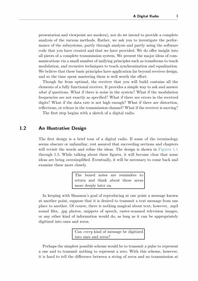
1.2 An Illustrative Design
The first design is a brief tour of a digital radio. If some of the terminology
seems obscure or unfamiliar, rest assured that succeeding sections and chapters
will revisit the words and refine the ideas. The design is shown in Figures 1.1
through 1.5. While talking about these figures, it will become clear that some
ideas are being oversimplified. Eventually, it will be necessary to come back and
examine these more closely.
The boxed notes are reminders to
return and think about these areas
more deeply later on.
In keeping with Shannon’s goal of reproducing at one point a message known
at another point, suppose that it is desired to transmit a text message from one
place to another. Of course, there is nothing magical about text; however, .mp3
sound files, .jpg photos, snippets of speech, raster-scanned television images,
or any other kind of information would do, as long as it can be appropriately
digitized into ones and zeros.
Can every kind of message be digitized
into ones and zeros?
Perhaps the simplest possible scheme would be to transmit a pulse to represent
a one and to transmit nothing to represent a zero. With this scheme, however,
it is hard to tell the difference between a string of zeros and no transmission at

4 Chapter 1. A Digital Radio
Coder
1τ + kT
Text
Symbolss[k]
Scalingfactor
Initiationtrigger
T-wideanalogpulse
shape p(t)generator
Basebandsignal y(t)
Figure 1.1 An idealizedbaseband transmitter.
all. A common remedy is to send a pulse with a positive amplitude to represent
a one and a pulse of the same shape but negative amplitude to represent a zero.
In fact, if the receiver could distinguish pulses of different sizes, then it would
be possible to send two bits with each symbol, for example, by associating the
amplitudes1 of +1, −1, +3, and −3 with the four choices 10, 01, 11, and 00.
The four symbols ±1, ±3 are called the alphabet, and the conversion from the
original message (the text) into the symbol alphabet is accomplished by the
coder in the transmitter diagram Figure 1.1. The first few letters, the standard
ASCII (binary) representation of these letters, and their coding into symbols are
as follows
letter binary ASCII code symbol string
a 01 10 00 01 −1, 1, −3, −1b 01 10 00 10 −1, 1, −3, 1c 01 10 00 11 −1, 1, −3, 3d 01 10 01 00 −1, 1, −1, −3...
......
(1.1)
In this example, the symbols are clustered into groups of four, and each cluster
is called a frame. Coding schemes can be designed to increase the security of a
transmission, to minimize the errors, or to maximize the rate at which data are
sent. This particular scheme is not optimized in any of these senses, but it is
convenient to use in simulation studies.
Some codes are better than others. How
can we tell?
To be concrete, let
� the symbol interval T be the time between successive symbols, and� the pulse shape p(t) be the shape of the pulse that will be transmitted.
1 Many such choices are possible. These particular values were chosen because they are equidis-
tant and so noise would be no more likely to flip a 3 into a 1 than to flip a 1 into a −1.

A Digital Radio 5
For instance, p(t) may be the rectangular pulse
p(t) =
{1 when 0 ≤ t < T,
0 otherwise,(1.2)
which is plotted in Figure 1.2(a). The transmitter of Figure 1.1 is designed so that
every T seconds it produces a copy of p(·) that is scaled by the symbol value s[·].A typical output of the transmitter in Figure 1.1 is illustrated in Figure 1.2(b)
using the rectangular pulse shape. Thus the first pulse begins at some time τ
and it is scaled by s[0], producing s[0]p(t− τ). The second pulse begins at time
τ + T and is scaled by s[1], resulting in s[1]p(t− τ − T ). The third pulse gives
s[2]p(t− τ − 2T ), and so on. The complete output of the transmitter is the sum
of all these scaled pulses:
y(t) =∑i
s[i]p(t− τ − iT ).
Since each pulse ends before the next one begins, successive symbols should
not interfere with each other at the receiver. The general method of sending
information by scaling a pulse shape with the amplitude of the symbols is called
Pulse Amplitude Modulation (PAM). When there are four symbols as in (1.1),
it is called 4-PAM.
For now, assume that the path between the transmitter and receiver, which is
often called the channel, is “ideal.” This implies that the signal at the receiver is
the same as the transmitted signal, though it will inevitably be delayed (slightly)
due to the finite speed of the wave, and attenuated by the distance. When the
ideal channel has a gain g and a delay δ, the received version of the transmitted
signal in Figure 1.2(b) is as shown in Figure 1.2(c).
There are many ways in which a real signal may change as it passes from the
transmitter to the receiver through a real (nonideal) channel. It may be reflected
from mountains or buildings. It may be diffracted as it passes through the atmo-
sphere. The waveform may smear in time so that successive pulses overlap. Other
signals may interfere additively (for instance, a radio station broadcasting at the
same frequency in a different city). Noises may enter and change the shape of
the waveform.
There are two compelling reasons to consider the telecommunication system
in the simplified (idealized) case before worrying about all the things that might
go wrong. First, at the heart of any working receiver is a structure that is able to
function in the ideal case. The classic approach to receiver design (and also the
approach of Software Receiver Design) is to build for the ideal case and later
to refine so that the receiver will still work when bad things happen. Second,
many of the basic ideas are clearer in the ideal case.
The job of the receiver is to take the received signal (such as that in Figure
1.2(c)) and to recover the original text message. This can be accomplished by an
idealized receiver such as that shown in Figure 1.3. The first task this receiver
must accomplish is to sample the signal to turn it into computer-friendly digital

6 Chapter 1. A Digital Radio
r(t)
τ+δ τ+δ+T
3g
g
−g
−3g τ+δ+2T τ+δ+3T
τ+δ+4T
y(t)
τ τ+T
3
1
−1
−3τ+2T τ+3T
τ+4T
p(t) 1
0 T
(a) (b) (c)
Figure 1.2 (a) An isolated rectangular pulse. (b) The transmitted signal consists of asequence of pulses, one corresponding to each symbol. Each pulse has the same shapeas in (a), though offset in time (by τ ) and scaled in magnitude (by the symbols s[k]).(c) In the ideal case, the received signal is the same as the transmitted signal of (b),though attenuated in magnitude (by g) and delayed in time (by δ).
DecoderQuantizer
Reconstructedtext
ReconstructedsymbolsReceived
signal
η + kT
Sampler
Figure 1.3 An idealizedbaseband receiver.
form. But when should the samples be taken? On comparing Figures 1.2(b) and
1.2(c), it is clear that if the received signal were sampled somewhere near the
middle of each rectangular pulse segment, then the quantizer could reproduce
the sequence of source symbols. This quantizer must either
1. know g so the sampled signal can be scaled by 1/g to recover the symbol
values, or
2. separate ±g from ±3g and output symbol values ±1 and ±3.
Once the symbols have been reconstructed, then the original message can be
decoded by reversing the assignment of letters to symbols used at the transmitter
(for example, by reading (1.1) backwards). On the other hand, if the samples
were taken at the moment of transition from one symbol to another, then the
values might become confused.
To investigate the timing question more fully, let T be the sample interval and τ
be the time at which the first pulse begins. Let δ be the time it takes for the signal
to move from the transmitter to the receiver. Thus the (k + 1)st pulse, which
begins at time τ + kT , arrives at the receiver at time τ + kT + δ. The midpoint
of the pulse, which is the best time to sample, occurs at τ + kT + δ + T/2. As
indicated in Figure 1.3, the receiver begins sampling at time η, and then samples
regularly at η + kT for all integers k. If η were chosen so that
η = τ + δ + T/2, (1.3)

A Digital Radio 7
then all would be well. But there are two problems: the receiver does not know
when the transmission began, nor does it know how long it takes for the signal
to reach the receiver. Thus both τ and δ are unknown!
Somehow, the receiver must figure out
when to sample.
Basically, some extra “synchronization” procedure is needed in order to satisfy
(1.3). Fortunately, in the ideal case, it is not really necessary to sample exactly at
the midpoint; it is necessary only to avoid the edges. Even if the samples are not
taken at the center of each rectangular pulse, the transmitted symbol sequence
can still be recovered. But if the pulse shape were not a simple rectangle, then
the selection of η would become more critical.
How does the pulse shape interact with
timing synchronization?
Just as no two clocks ever tell exactly the same time, no two independent
oscillators2 are ever exactly synchronized. Since the symbol period at the trans-
mitter, call it Ttrans, is created by a separate oscillator from that creating the
symbol period at the receiver, call it Trec, they will inevitably differ. Thus another
aspect of timing synchronization that must ultimately be considered is how to
automatically adjust Trec so that it aligns with Ttrans.
Similarly, no clock ticks out each second exactly evenly. Inevitably, there is
some jitter, or wobble in the value of Ttrans and/or Trec. Again, it may be
necessary to adjust η to retain sampling near the center of the pulse shape
as the clock times wiggle about. The timing adjustment mechanisms are not
explicitly indicated in the sampler box in Figure 1.3. For the present idealized
transmission system, the receiver sampler period and the symbol period of the
transmitter are assumed to be identical (both are called T in Figures 1.1 and
1.3) and the clocks are assumed to be free of jitter.
What about clock jitter?
Even under the idealized assumptions above, there is another kind of syn-
chronization that is needed. Imagine joining a broadcast in progress, or one in
which the first K symbols have been lost during acquisition. Even if the symbol
sequence is perfectly recovered after time K, the receiver would not know which
recovered symbol corresponds to the start of each frame. For example, using the
letters-to-symbol code of (1.1), each letter of the alphabet is translated into a
sequence of four symbols. If the start of the frame is off by even a single sym-
2 Oscillators, electronic components that generate repetitive signals, are discussed at length inChapter 3.

8 Chapter 1. A Digital Radio
bol, the translation from symbols back into letters will be scrambled. Does this
sequence represent a or X?
−1,
a︷ ︸︸ ︷−1, 1,−3,−1
−1,−1, 1,−3,︸ ︷︷ ︸X
−1
Thus proper decoding requires locating where the frame starts, a step called
frame synchronization. Frame synchronization is implicit in Figure 1.3 in the
choice of η, which sets the time t (= η with k = 0) of the first symbol of the first
(character) frame of the message of interest.
How to find the start of a frame?
In the ideal situation, there must be no other signals occupying the same fre-
quency range as the transmission. What bandwidth (what range of frequencies)
does the transmitter (1.1) require? Consider transmitting a single T -second-wide
rectangular pulse. Fourier transform theory shows that any such time-limited
pulse cannot be truly bandlimited, that is, cannot have its frequency content
restricted to a finite range. Indeed, the Fourier transform of a rectangular pulse
in time is a sinc function in frequency (see Equation (A.20) in Appendix A). The
magnitude of this sinc is overbounded by a function that decays as the inverse of
frequency (peek ahead to Figure 2.11). Thus, to accommodate this single-pulse
transmission, all other transmitters must have negligible energy below some fac-
tor of B = 1/T . For the sake of argument, suppose that a factor of 5 is safe, that
is, all other transmitters must have no significant energy within 5B Hz. But this
is only for a single pulse. What happens when a sequence of T -spaced, T -wide
rectangular pulses of various amplitudes is transmitted? Fortunately, as will be
established in Section 11.1, the bandwidth requirements remain about the same,
at least for most messages.
What is the relation between the pulse
shape and the bandwidth?
One fundamental limitation to data transmission is the trade-off between the
data rate and the bandwidth. One obvious way to increase the rate at which data
are sent is to use shorter pulses, which pack more symbols into a shorter time.
This essentially reduces T . The cost is that this would require excluding other
transmitters from an even wider range of frequencies since reducing T increases
B.
What is the relation between the data
rate and the bandwidth?

A Digital Radio 9
If the safety factor of 5B is excessive, other pulse shapes that would decay
faster as a function of frequency could be used. For example, rounding the sharp
corners of a rectangular pulse reduces its high-frequency content. Similarly, if
other transmitters operated at high frequencies outside 5B Hz, it would be sen-
sible to add a lowpass filter at the front end of the receiver. Rejecting frequencies
outside the protected 5B baseband turf also removes a bit of the higher-frequency
content of the rectangular pulse. The effect of this in the time domain is that the
received version of the rectangle would be wiggly near the edges. In both cases,
the timing of the samples becomes more critical as the received pulse deviates
further from rectangular.
One shortcoming of the telecommunication system embodied in the transmit-
ter of Figure 1.1 and the receiver of Figure 1.3 is that only one such transmitter
at a time can operate in any particular geographical region, since it hogs all the
frequencies in the baseband, that is, all frequencies below 5B Hz. Fortunately,
there is a way to have multiple transmitters operating in the same region simul-
taneously. The trick is to translate the frequency content so that instead of all
transmitters trying to operate in the 0 and 5B Hz band, one might use the 5B
to 10B band, another the 10B to 15B band, etc. Conceivably, this could be
accomplished by selecting a different pulse shape (other than the rectangle) that
has no low-frequency content, but the most common approach is to “modulate”
(change frequency) by multiplying the pulse-shaped signal by a high-frequency
sinusoid. Such a “radio-frequency” (RF) transmitter is shown in Figure 1.4,
though it should be understood that the actual frequencies used may place it
in the television band or in the range of frequencies reserved for cell phones,
depending on the application.
At the receiver, the signal can be returned to its original frequency (demod-
ulated) by multiplying by another high-frequency sinusoid (and then lowpass
filtering). These frequency translations are described in more detail in Section
2.6, where it is shown that the modulating sinusoid and the demodulating sinu-
soid must have the same frequencies and the same phases in order to return
the signal to its original form. Just as it is impossible to align any two clocks
exactly, it is also impossible to generate two independent sinusoids of exactly the
same frequency and phase. Hence there will ultimately need to be some kind of
“carrier synchronization,” a way of aligning these oscillators.
How can the frequencies and phases of
these two sinusoids be aligned?
Adding frequency translation to the transmitter and receiver of Figures 1.1 and
1.3 produces the transmitter in Figure 1.4 and the associated receiver in Figure
1.5. The new block in the transmitter is an analog component that effectively
adds the same value (in Hz) to the frequencies of all of the components of the
baseband pulse train. As noted, this can be achieved with multiplication by a
“carrier” sinusoid with a frequency equal to the desired translation. The new
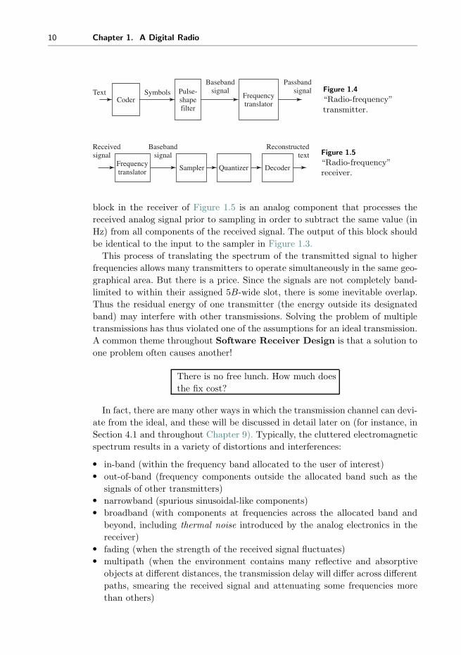
10 Chapter 1. A Digital Radio
Frequencytranslator
Pulse-shapefilter
Coder
Passbandsignal
BasebandsignalSymbolsText Figure 1.4
“Radio-frequency”transmitter.
DecoderQuantizer
Reconstructedtext
Basebandsignal
SamplerFrequencytranslator
Receivedsignal Figure 1.5
“Radio-frequency”receiver.
block in the receiver of Figure 1.5 is an analog component that processes the
received analog signal prior to sampling in order to subtract the same value (in
Hz) from all components of the received signal. The output of this block should
be identical to the input to the sampler in Figure 1.3.
This process of translating the spectrum of the transmitted signal to higher
frequencies allows many transmitters to operate simultaneously in the same geo-
graphical area. But there is a price. Since the signals are not completely band-
limited to within their assigned 5B-wide slot, there is some inevitable overlap.
Thus the residual energy of one transmitter (the energy outside its designated
band) may interfere with other transmissions. Solving the problem of multiple
transmissions has thus violated one of the assumptions for an ideal transmission.
A common theme throughout Software Receiver Design is that a solution to
one problem often causes another!
There is no free lunch. How much does
the fix cost?
In fact, there are many other ways in which the transmission channel can devi-
ate from the ideal, and these will be discussed in detail later on (for instance, in
Section 4.1 and throughout Chapter 9). Typically, the cluttered electromagnetic
spectrum results in a variety of distortions and interferences:
� in-band (within the frequency band allocated to the user of interest)� out-of-band (frequency components outside the allocated band such as the
signals of other transmitters)� narrowband (spurious sinusoidal-like components)� broadband (with components at frequencies across the allocated band and
beyond, including thermal noise introduced by the analog electronics in the
receiver)� fading (when the strength of the received signal fluctuates)� multipath (when the environment contains many reflective and absorptive
objects at different distances, the transmission delay will differ across different
paths, smearing the received signal and attenuating some frequencies more
than others)

A Digital Radio 11
Gainwithdelay
Multipath
+ +
Self-interference
Transmittedsignal
Interferencefrom other
sources
+
Receivedsignal
Broadbandnoises
Figure 1.6 A channel modeladmitting various kinds ofinterferences.
These channel imperfections are all incorporated in the channel model shown in
Figure 1.6, which sits in the communication system between Figures 1.4 and 1.5.
Many of these imperfections in the channel can be mitigated by clever use of
filtering at the receiver. Narrowband interference can be removed with a notch
filter that rejects frequency components in the narrow range of the interferer
without removing too much of the broadband signal. Out-of-band interference
and broadband noise can be reduced using a bandpass filter that suppresses
the signal in the out-of-band frequency range and passes the in-band frequency
components without distortion. With regard to Figure 1.5, it is reasonable to
wonder whether it is better to perform such filtering before or after the sampler
(i.e., by an analog or a digital filter). In modern receivers, the trend is to minimize
the amount of analog processing since digital methods are (often) cheaper and
(usually) more flexible since they can be implemented as reconfigurable software
rather than fixed hardware.
Analog or digital processing?
Conducting more of the processing digitally requires moving the sampler closer
to the antenna. The sampling theorem (discussed in Section 6.1) says that no
information is lost as long as the sampling occurs at a rate faster than twice the
highest frequency of the signal. Thus, if the signal has been modulated to (say)
the band from 20B to 25B Hz, then the sampler must be able to operate at least
as fast as 50B samples per second in order to be able to exactly reconstruct the
value of the signal at any arbitrary time instant. Assuming this is feasible, the
received analog signal can be sampled using a free-running sampler. Interpola-
tion can be used to figure out values of the signal at any desired intermediate
instant, such as at time η + kT (recall (1.3)) for a particular η that is not an
integer multiple of T . Thus, the timing synchronization can be incorporated into
the post-sampler digital signal processing box, which is shown generically in
Figure 1.7. Observe that Figure 1.5 is one particular version of 1.7.
How exactly does interpolation work?

12 Chapter 1. A Digital Radio
Digitalsignal
processing
Analogsignal
processing
Recoveredsource
Receivedsignal
η + kT
Figure 1.7 A generic modernreceiver using both analog signalprocessing (ASP) and digitalsignal processing (DSP).
However, sometimes it is more cost effective to perform certain tasks in analog
circuitry. For example, if the transmitter modulates to a very high frequency, then
it may cost too much to sample fast enough. Currently, it is common practice
to perform some frequency translation and some out-of-band signal reduction in
the analog portion of the receiver. Sometimes the analog portion may translate
the received signal all the way back to baseband. Other times, the analog portion
translates to some intermediate frequency, and then the digital portion finishes
the translation. The advantage of this (seemingly redundant) approach is that
the analog part can be made crudely and, hence, cheaply. The digital processing
finishes the job, and simultaneously compensates for inaccuracies and flaws in
the (inexpensive) analog circuits. Thus, the digital signal processing portion of
the receiver may need to correct for signal impairments arising in the analog
portion of the receiver as well as from impairments caused by the channel.
Use DSP when possible.
The digital signal processing portion of the receiver can perform the following
tasks:
� downconvert the sampled signal to baseband� track any changes in the phase or frequency of the modulating sinusoid� adjust the symbol timing by interpolation� compensate for channel imperfections by filtering� convert modestly inaccurate recovered samples into symbols� perform frame synchronization via correlation� decode groups of symbols into message characters
A central task in Software Receiver Design is to elaborate on the system
structure in Figures 1.4–1.6 to create a working software-defined radio that can
perform these tasks. This concludes the illustrative design at the first, most
superficial step of the radio stairway.
Use DSP to compensate for cheap ASP.
1.3 Walk This Way
This section provides a whirlwind tour of the complete structure of Software
Receiver Design. Each step presents the digital transmission system in greater
depth and detail.

A Digital Radio 13
� Step 1: The Naive Digital Communications System. As we have just seen,
the first step introduced the digital transmission of data, and discussed how
bits of information may be coded into waveforms, sent across space to the
receiver, and then decoded back into bits. Since there is no universal clock,
issues of timing become important, and some of the most complex issues in
digital receiver design involve the synchronization of the received signal. The
system can be viewed as consisting of three parts:
1. a transmitter as in Figure 1.4
2. a transmission channel
3. a receiver as in Figure 1.5
� Step 2: The Basic Components. The next two chapters provide more depth and
detail by outlining a complete telecommunication system. When the trans-
mitted signal is passed through the air using electromagnetic waves, it must
take the form of a continuous (analog) waveform. A good way to understand
such analog signals is via the Fourier transform, and this is reviewed briefly in
Chapter 2. The six basic elements of the receiver will be familiar to many read-
ers, and they are presented in Chapter 3 in a form that will be directly useful
when creating Matlab implementations of the various parts of the commu-
nication system. By the end of the second step, the basic system architecture
is fixed and the ordering of the blocks in the system diagram is stabilized.� Step 3: The Idealized System. The third step encompasses Chapters 4 through
9. Step 3 gives a closer look at the idealized receiver—how things work when
everything is just right: when the timing is known, when the clocks run at
exactly the right speed, when there are no reflections, diffractions, or diffu-
sions of the electromagnetic waves. This step also integrates ideas from pre-
vious systems courses, and introduces a few Matlab tools that are needed
to implement the digital radio. The order in which topics are discussed is
precisely the order in which they appear in the receiver:
channel
Chapter 4
→frequency
translation
Chapter 5
→ sampling
Chapter 6
→
receive
filtering→ equalization︸ ︷︷ ︸
Chapter 7
→decision
device→ decoding︸ ︷︷ ︸
Chapter 8
Channel impairments and linear systems Chapter 4
Frequency translation and modulation Chapter 5
Sampling and gain control Chapter 6
Receive (digital) filtering Chapter 7
Symbols to bits to signals Chapter 8

14 Chapter 1. A Digital Radio
Chapter 9 provides a complete (though idealized) software-defined digital
radio system.� Step 4: The Adaptive Components. The fourth step describes all the practical
fixes that are required in order to create a workable radio. One by one the
various problems are studied and solutions are proposed, implemented, and
tested. These include fixes for additive noise, for timing offset problems, for
clock frequency mismatches and jitter, and for multipath reflections. Again,
the order in which topics are discussed is the order in which they appear in
the receiver:
Carrier recovery Chapter 10
the timing of frequency translation
Receive filtering Chapter 11
the design of pulse shapes
Clock recovery Chapter 12
the timing of sampling
Equalization Chapter 13
filters that adapt to the channel
Coding Chapter 14
making data resilient to noise
� Step 5: Putting It All Together. The final steps are the projects of Chapters
15 and 16 which integrate all the fixes of the fourth step into the receiver
structure of the third step to create a fully functional digital receiver. The well-
fabricated receiver is robust with respect to distortions such as those caused
by noise, multipath interference, timing inaccuracies, and clock mismatches.

Step 2: The Basic Components
The next two chapters provide more depth and detail by outlining a complete
telecommunication system. When the transmitted signal is passed through the
air using electromagnetic waves, it must take the form of a continuous (analog)
waveform. A good way to understand such analog signals is via the Fourier
transform, and this is reviewed briefly in Chapter 2. The six basic elements of
the receiver will be familiar to many readers, and they are presented in Chapter 3
in a form that will be directly useful when creating Matlab implementations of
the various parts of the communications system. By the end of the second step,
the basic system architecture is fixed; the ordering of the blocks in the system
diagram has stabilized.

2 A Telecommunication System
Telecommunications technologies using electromagnetic transmission surround
us: television images flicker, radios chatter, cell phones (and telephones) ring,
allowing us to see and hear each other anywhere on the planet. E-mail and the
Internet link us via our computers, and a large variety of common devices such
as CDs, DVDs, and hard disks augment the traditional pencil and paper storage
and transmittal of information. People have always wished to communicate over
long distances: to speak with someone in another country, to watch a distant
sporting event, to listen to music performed in another place or another time,
to send and receive data remotely using a personal computer. In order to imple-
ment these desires, a signal (a sound wave, a signal from a TV camera, or a
sequence of computer bits) needs to be encoded, stored, transmitted, received,
and decoded. Why? Consider the problem of voice or music transmission. Send-
ing sound directly is futile because sound waves dissipate very quickly in air.
But if the sound is first transformed into electromagnetic waves, then they can
be beamed over great distances very efficiently. Similarly, the TV signal and
computer data can be transformed into electromagnetic waves.
2.1 Electromagnetic Transmission of Analog Waveforms
There are some experimental (physical) facts that cause transmission systems to
be constructed as they are. First, for efficient wireless broadcasting of electro-
magnetic energy, an antenna needs to be longer than about 1/10 of a wavelength
of the frequency being transmitted. The antenna at the receiver should also be
proportionally sized.
The wavelength λ and the frequency f of a sinusoid are inversely propor-
tional. For an electrical signal travelling at the speed of light c (3× 10⁸ m/s),
the relationship between wavelength and frequency is
λ =c
f.

A Telecommunication System 17
For instance, if the frequency of an electromagnetic wave is f = 10 kHz, then
the length of each wave is
λ =3× 10⁸ m/s
104/s= 3× 10⁴ m.
Efficient transmission requires an antenna longer than 0.1λ, which is 3 km! Sinu-
soids in the speech band would require even larger antennas. Fortunately, there is
an alternative to building mammoth antennas. The frequencies in the signal can
be translated (shifted, upconverted, or modulated) to a much higher frequency
called the carrier frequency, at which the antenna requirements are easier to
meet. For instance,
� AM radio: f ≈ 600–1500 kHz ⇒ λ ≈ 500–200 m ⇒ 0.1λ > 20 m� VHF (TV): f ≈ 30–300 MHz ⇒ λ ≈ 10–1 m ⇒ 0.1λ > 0.1 m� UHF (TV): f ≈ 0.3–3 GHz ⇒ λ ≈ 1–0.1 m ⇒ 0.1λ > 0.01 m� Cell phones (USA): f ≈ 824–894 MHz ⇒ λ ≈ 0.36–0.33 m ⇒ 0.1λ > 0.03 m� PCS: f ≈ 1.8–1.9 GHz ⇒ λ ≈ 0.167–0.158 m ⇒ 0.1λ > 0.015 m� GSM (Europe): f ≈ 890–960 MHz ⇒ λ ≈ 0.337–0.313 m ⇒ 0.1λ > 0.03 m� LEO satellites: f ≈ 1.6 GHz ⇒ λ ≈ 0.188 m ⇒ 0.1λ > 0.0188 m
Recall that 1 kHz = 103 Hz; 1 MHz = 106 Hz; 1 GHz = 109 Hz.
A second experimental fact is that electromagnetic waves in the atmosphere
exhibit different behaviors, depending on the frequency of the waves.
� Below 2 MHz, electromagnetic waves follow the contour of the Earth. This
is why shortwave (and other) radios can sometimes be heard hundreds or
thousands of miles from their source.� Between 2 and 30 MHz, sky-wave propagation occurs, with multiple bounces
from refractive atmospheric layers.� Above 30 MHz, line-of-sight propagation occurs, with straight-line travel
between two terrestrial towers or through the atmosphere to satellites.� Above 30 MHz, atmospheric scattering also occurs, which can be exploited
for long-distance terrestrial communication.
Humanmade media in wired systems also exhibit frequency-dependent behav-
ior. In the phone system, due to its original goal of carrying voice signals, severe
attenuation occurs above 4 kHz.
The notion of frequency is central to the process of long-distance communica-
tions. Because of its role as a carrier (the AM/UHF/VHF/PCS bands mentioned
above) and its role in specifying the bandwidth (the range of frequencies occupied
by a given signal), it is important to have tools with which to easily measure the
frequency content in a signal. The tool of choice for this job is the Fourier trans-

18 Chapter 2. A Telecommunication System
form (and its discrete counterparts, the DFT and the FFT).1 Fourier transforms
are useful in assessing energy or power at particular frequencies. The Fourier
transform of a signal w(t) is defined as
W (f) =
∫ ∞
t=−∞w(t)e−j2πftdt = F{w(t)}, (2.1)
where j =√−1 and f is given in Hz (i.e., cycles/s or 1/s).
Speaking mathematically, W (f) is a function of the frequency f . Thus, for
each f , W (f) is a complex number and so can be plotted in several ways. For
instance, it is possible to plot the real part of W (f) as a function of f and to plot
the imaginary part of W (f) as a function of f . Alternatively, it is possible to plot
the real part of W (f) versus the imaginary part of W (f). The most common
plots of the Fourier transform of a signal are done in two parts: the first graph
shows the magnitude |W (f)| versus f (this is called the magnitude spectrum)
and the second graph shows the phase angle of W (f) versus f (this is called the
phase spectrum). Often, just the magnitude is plotted, though this inevitably
leaves out information.
Perhaps the best way to understand the Fourier transform is to look closely
at the inverse function
w(t) =
∫ ∞
f=−∞W (f)ej2πftdf. (2.2)
The complex exponential ej2πft can be interpreted as a (complex-valued) sinu-
soidal wave since it is the sum of a sine term and a cosine term, both of frequency
f (via Euler’s formula). Since W (f) is a complex number at each f , (2.2) can
be interpreted as describing or decomposing w(t) into sinusoidal elements of fre-
quencies f weighted by the W (f). The discrete approximation to the Fourier
transform, called the DFT, is discussed in some detail in Chapter 7, and a table
of useful properties appears in Appendix A.
2.2 Bandwidth
If, at any particular frequency f0, the magnitude spectrum is strictly positive
(|W (f0)| > 0), then the frequency f0 is said to be present in w(t). The set of
all frequencies that are present in the signal is the frequency content, and if the
frequency content consists only of frequencies below some given f †, then the
signal is said to be bandlimited to f †. Some bandlimited signals are
� telephone-quality speech with maximum frequency ∼ 4 kHz and� audible music with maximum frequency ∼ 20 kHz.
1 These are the discrete Fourier transform, which is a computer implementation of the Fouriertransform, and the fast Fourier transform, which is a slick, computationally efficient methodof calculating the DFT.

A Telecommunication System 19
f
|W( f )|
Half-powerBW
Null-to-null BW
Power BW
Absolute BW
1
= 0.70722
Figure 2.1 Various ways todefine bandwidth (BW)for a real-valued signal.
But real-world signals are never completely bandlimited, and there is almost
always some energy at every frequency. Several alternative definitions of band-
width are in common use; these try to capture the idea that “most of” the
energy is contained in a specified frequency region. Usually, these are applied
across positive frequencies, with the presumption that the underlying signals are
real-valued (and hence have symmetric spectra). Here are some of the alternative
definitions.
1. Absolute bandwidth is the smallest interval f2 − f1 for which the spectrum is
zero outside of f1 < f < f2 (only the positive frequencies need be considered).
2. 3-dB (or half-power) bandwidth is f2 − f1, where, for frequencies outside f1 <
f < f2, |H(f)| is never greater than 1/√2 times its maximum value.
3. Null-to-null (or zero-crossing) bandwidth is f2 − f1, where f2 is the first null
in |H(f)| above f0 and, for bandpass systems, f1 is the first null in the enve-
lope below f0, where f0 is the frequency of maximum |H(f)|. For baseband
systems, f1 is usually zero.
4. Power bandwidth is f2 − f1, where f1 < f < f2 defines the frequency band in
which 99% of the total power resides. Occupied bandwidth is such that 0.5%
of power is above f2 and 0.5% below f1.
These definitions are illustrated in Figure 2.1.
The various definitions of bandwidth refer directly to the frequency content
of a signal. Since the frequency response of a linear filter is the transform of its
impulse response, bandwidth is also used to talk about the frequency range over
which a linear system or filter operates.

20 Chapter 2. A Telecommunication System
Exercise 2.1. TRUE or FALSE: Absolute bandwidth is never less than 3-dB
power bandwidth.
Exercise 2.2. Suppose that a signal is complex-valued and hence has a spectrum
that is not symmetric about zero frequency. State versions of the various defini-
tions of bandwidth that make sense in this situation. Illustrate your definitions
as in Figure 2.1.
2.3 Upconversion at the Transmitter
Suppose that the signal w(t) contains important information that must be trans-
mitted. There are many kinds of operations that can be applied to w(t). Linear
time invariant (LTI) operations are those for which superposition applies, but
LTI operations cannot augment the frequency content of a signal—no sine wave
can appear at the output of a linear operation if it was not already present in
the input.
Thus, the process of modulation (or upconversion), which requires a change
of frequencies, must be either nonlinear or time varying (or both). One useful
way to modulate is with multiplication; consider the product of the message
waveform w(t) with a cosine wave
s(t) = w(t) cos(2πf0t), (2.3)
where f0 is called the carrier frequency. The Fourier transform can now be used
to show that this multiplication shifts all frequencies present in the message by
exactly f0 Hz.
Using one of Euler’s identities (A.2),
cos(2πf0t) =1
2
(ej2πf0t + e−j2πf0t
), (2.4)
one can calculate the spectrum (or frequency content) of the signal s(t) from the
definition of the Fourier transform given in (2.1). In complete detail, this is
S(f) = F{s(t)} = F{w(t) cos(2πf0t)}= F
{w(t)
[1
2
(ej2πf0t + e−j2πf0t
)]}
=
∫ ∞
−∞w(t)
[1
2
(ej2πf0t + e−j2πf0t
)]e−j2πftdt
=1
2
∫ ∞
−∞w(t)
(e−j2π(f−f0)t + e−j2π(f+f0)t
)dt
=1
2
∫ ∞
−∞w(t)e−j2π(f−f0)tdt+
1
2
∫ ∞
−∞w(t)e−j2π(f+f0)tdt
=1
2W (f − f0) +
1
2W (f + f0). (2.5)

A Telecommunication System 21
−f † f † f
|W( f )||S( f )|
1
f0 f0 + f †−f0 + f †
0.5
−f0−f0 − f † f0 − f †
(b)(a)
Figure 2.2 Action of a modulator: If the message signal w(t) has the magnitudespectrum shown in part (a), then the modulated signal s(t) has the magnitudespectrum shown in part (b).
Thus, the spectrum of s(t) consists of two copies of the spectrum of w(t),
each shifted in frequency by f0 (one up and one down) and each half as large.
This is sometimes called the frequency-shifting property of the Fourier trans-
form, and sometimes called the modulation property. Figure 2.2 shows how the
spectra relate. If w(t) has the magnitude spectrum shown in part (a) (this is
shown bandlimited to f † and centered at 0 Hz or baseband, though it could be
elsewhere), then the magnitude spectrum of s(t) appears as in part (b). This
kind of modulation (or upconversion, or frequency shift) is ideal for translating
speech, music, or other low-frequency signals into much higher frequencies (for
instance, f0 might be in the AM or UHF bands) so that they can be transmit-
ted efficiently. It can also be used to convert a high-frequency signal back down
to baseband when needed, as will be discussed in Section 2.6 and in detail in
Chapter 5.
Any sine wave is characterized by three parameters: the amplitude, frequency,
and phase. Any of these characteristics can be used as the basis of a modulation
scheme: modulating the frequency is familiar from the FM radio, and phase
modulation is common in computer modems. A major example in this book is
amplitude modulation as in (2.3), where the message w(t) is multiplied by a high-
frequency sinusoid with fixed frequency and phase. Whatever the modulation
scheme used, the idea is the same: a sinusoid is used to translate the message
into a form suitable for transmission.
Exercise 2.3. Referring to Figure 2.2, find which frequencies are present in
W (f) and not in S(f). Which frequencies are present in S(f) but not in W (f)?
Exercise 2.4. Using (2.5), draw analogous pictures for the phase spectrum of
s(t) as it relates to the phase spectrum of w(t).
Exercise 2.5. Suppose that s(t) is modulated again, this time via multiplication
with a cosine of frequency f1. What is the resulting magnitude spectrum? Hint:
let r(t) = s(t) cos(2πf1t), and apply (2.5) to find R(f).

22 Chapter 2. A Telecommunication System
2.4 Frequency Division Multiplexing
When a signal is modulated, the width (in Hz) of the replicas is the same as the
width (in Hz) of the original signal. This is a direct consequence of Equation (2.5).
For instance, if the message is bandlimited to ±f ∗, and the carrier frequency is fc,
then the modulated signal has energy in the range from−f ∗ − fc to +f ∗ − fc and
from −f ∗ + fc to +f ∗ + fc. If f∗ � fc, then several messages can be transmitted
simultaneously by using different carrier frequencies.
This situation is depicted in Figure 2.3, where three different messages are
represented by the triangular, rectangular, and half-oval spectra, each bandlim-
ited to ±f ∗. Each of these is modulated by a different carrier (f1, f2, and f3),
which are chosen so that they are further apart than the width of the messages.
In general, as long as the carrier frequencies are separated by more than 2f ∗,there will be no overlap in the spectrum of the combined signal. This process
of combining many different signals together is called multiplexing, and because
the frequencies are divided up among the users, the approach of Figure 2.3 is
called frequency-division multiplexing (FDM).
Whenever FDM is used, the receiver must separate the signal of interest from
all the other signals present. This can be accomplished with a bandpass filter as
in Figure 2.4, which shows a filter designed to isolate the middle user from the
others.
Exercise 2.6. Suppose that two carrier frequencies are separated by 1 kHz.
Draw the magnitude spectra if (a) the bandwidth of each message is 200 Hz
and (b) the bandwidth of each message is 2 kHz. Comment on the ability of the
bandpass filter at the receiver to separate the two signals.
Another kind of multiplexing is called time-division multiplexing (TDM), in
which two (or more) messages use the same carrier frequency but at alternating
time instants. More complex multiplexing schemes (such as code division mul-
tiplexing) overlap the messages in both time and frequency in such a way that
they can be demultiplexed efficiently by appropriate filtering.
f3f
f2f1−f1−f2−f3
f2 − f * f2 + f *
f3 − f * f3 + f *|W( f )|
Figure 2.3 Three differentupconverted signals areassigned different frequencybands. This is calledfrequency-divisionmultiplexing.

A Telecommunication System 23
f3 ff2f1 f2 − f * f2 + f *
Bandpassfilter
|W( f )|
Figure 2.4 Separationof a single FDMtransmission using abandpass filter.
2.5 Filters that Remove Frequencies
Each time the signal is modulated, an extra copy (or replica) of the spectrum
appears. When multiple modulations are needed (for instance, at the transmitter
to convert up to the carrier frequency, and at the receiver to convert back down to
the original frequency of the message), copies of the spectrum may proliferate.
There must be a way to remove extra copies in order to isolate the original
message. This is one of the things that linear filters do very well.
There are several ways of describing the action of a linear time-invariant filter.
In the time domain (the most common method of implementation), the filter is
characterized by its impulse response (which is defined to be the output of the
filter when the input is an impulse function). Because of the linearity, the output
of the filter in response to any arbitrary input is the superposition of weighted
copies of a time-shifted version of the impulse response, a procedure known as
convolution. Since convolution may be difficult to understand directly in the time
domain, the action of a linear filter is often described in the frequency domain.
Perhaps the most important property of the Fourier transform is the duality
between convolution and multiplication, which says that
� convolution in time ↔ multiplication in frequency, and� multiplication in time ↔ convolution in frequency.
This is discussed in detail in Section 4.5. Thus, the convolution of a linear filter
can readily be viewed in the frequency (Fourier) domain as a point-by-point
multiplication. For instance, an ideal lowpass filter (LPF) passes all frequencies
below fl (which is called the cutoff frequency). This is commonly plotted in a
curve called the frequency response of the filter, which describes the action of the
filter.2 If this filter is applied to a signal w(t), then all energy above fl is removed
from w(t). Figure 2.5 shows this pictorially. If w(t) has the magnitude spectrum
shown in part (a), and the frequency response of the lowpass filter with cutoff
frequency fl is as shown in part (b), then the magnitude spectrum of the output
appears in part (c).
2 Formally, the frequency response can be calculated as the Fourier transform of the impulseresponse of the filter.

24 Chapter 2. A Telecommunication System
−fl fl f(a)
−fl fl f(b)
−fl fl f(c)
|W( f )|
|H( f )|
|Y( f )| = |H( f )| |W( f )|
Figure 2.5 Action of a lowpassfilter: (a) shows the magnitudespectrum of the message whichis input into an ideal lowpassfilter with frequency response(b); (c) shows the point-by-pointmultiplication of (a) and (b),which gives the spectrum of theoutput of the filter.
Exercise 2.7. An ideal highpass filter passes all frequencies above some given
fh and removes all frequencies below. Show the result of applying a highpass
filter to the signal in Figure 2.5 with fh = fl.
Exercise 2.8. An ideal bandpass filter passes all frequencies between an upper
limit f and a lower limit f . Show the result of applying a bandpass filter to the
signal in Figure 2.5 with f = 2fl/3 and f = fl/3.
The problem of how to design and implement such filters is considered in detail
in Chapter 7.
2.6 Analog Downconversion
Because transmitters typically modulate the message signal with a high-
frequency carrier, the receiver must somehow remove the carrier from the mes-
sage that it carries. One way is to multiply the received signal by a cosine wave
of the same frequency (and the same phase) as was used at the transmitter. This
creates a (scaled) copy of the original signal centered at zero frequency, plus some
other high-frequency replicas. A lowpass filter can then remove everything but
the scaled copy of the original message. This is how the box labelled “frequency
translator” in Figure 1.5 is typically implemented.
To see this procedure in detail, suppose that s(t) = w(t) cos(2πf0t) arrives at
the receiver, which multiplies s(t) by another cosine wave of exactly the same

A Telecommunication System 25
frequency and phase to get the demodulated signal
d(t) = s(t) cos(2πf0t) = w(t) cos2(2πf0t).
Using the trigonometric identity (A.4), namely,
cos2(x) =1
2+
1
2cos(2x),
this can be rewritten as
d(t) = w(t)
[1
2+
1
2cos(4πf0t)
]=
1
2w(t) +
1
2w(t) cos(2π(2f0)t).
The spectrum of the demodulated signal can be calculated to be
F{d(t)} = F{1
2w(t) +
1
2w(t) cos(2π(2f0)t)
}=
1
2F{w(t)} + 1
2F{w(t) cos(2π(2f0)t)}
by linearity. Now the frequency-shifting property (2.5) can be applied to show
that
F{d(t)} =1
2W (f) +
1
4W (f − 2f0) +
1
4W (f + 2f0). (2.6)
Thus, the spectrum of this downconverted received signal has the original base-
band component (scaled to 50%) and two matching pieces (each scaled to 25%)
centered around twice the carrier frequency f0 and twice its negative. A lowpass
filter can now be used to extractW (f), and hence to recover the original message
w(t).
This procedure is shown diagrammatically in Figure 2.6. The spectrum of the
original message is shown in (a), and the spectrum of the message modulated by
the carrier appears in (b). When downconversion is done as just described, the
demodulated signal d(t) has the spectrum shown in (c). Filtering by a lowpass
filter (as in part (c)) removes all but a scaled version of the message.
Now consider the FDM transmitted signal spectrum of Figure 2.3. This can be
demodulated/downconverted similarly. The frequency-shifting rule (2.5), with a
shift of f0 = f3, ensures that the downconverted spectrum in Figure 2.7 matches
(2.6), and the lowpass filter removes all but the desired message from the down-
converted signal.
This is the basic principle of a transmitter and receiver pair. But there are
some practical issues that arise. What happens if the oscillator at the receiver
is not completely accurate in either frequency or phase? The downconverted
received signal becomes s(t) cos(2π(f0 + α)t+ β). This can have serious conse-
quences for the demodulated message. What happens if one of the antennas is
moving? The Doppler effect suggests that this corresponds to a small nonzero
value of α. What happens if the transmitter antenna wobbles due to the wind
over a range equivalent to several wavelengths of the transmitted signal? This
can alter β. In effect, the baseband component is perturbed from (1/2)W (f), and
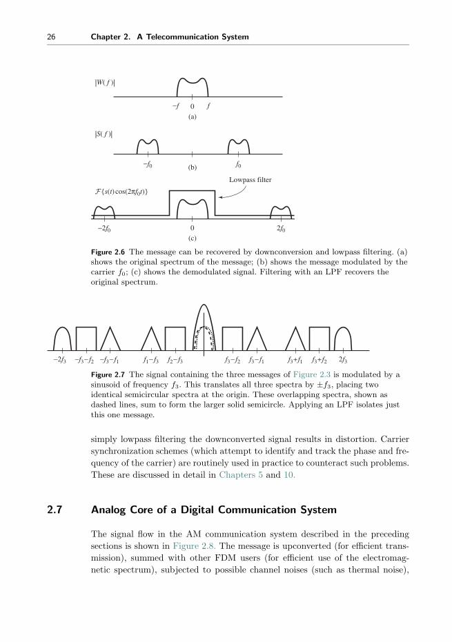
26 Chapter 2. A Telecommunication System
−f 0 f
(a)
0
(b) f0−f0
(c)2f0−2f0
Lowpass filter
{s(t) cos(2πf0t)}
|W( f )|
|S( f )|
Figure 2.6 The message can be recovered by downconversion and lowpass filtering. (a)shows the original spectrum of the message; (b) shows the message modulated by thecarrier f0; (c) shows the demodulated signal. Filtering with an LPF recovers theoriginal spectrum.
f3+f1 f3+f2 2f3f1− f3−f3− f2−2f3 −f3− f1 f2− f3 f3− f1f3− f2
Figure 2.7 The signal containing the three messages of Figure 2.3 is modulated by asinusoid of frequency f3. This translates all three spectra by ±f3, placing twoidentical semicircular spectra at the origin. These overlapping spectra, shown asdashed lines, sum to form the larger solid semicircle. Applying an LPF isolates justthis one message.
simply lowpass filtering the downconverted signal results in distortion. Carrier
synchronization schemes (which attempt to identify and track the phase and fre-
quency of the carrier) are routinely used in practice to counteract such problems.
These are discussed in detail in Chapters 5 and 10.
2.7 Analog Core of a Digital Communication System
The signal flow in the AM communication system described in the preceding
sections is shown in Figure 2.8. The message is upconverted (for efficient trans-
mission), summed with other FDM users (for efficient use of the electromag-
netic spectrum), subjected to possible channel noises (such as thermal noise),

A Telecommunication System 27
OtherFDMusers
Upconversion
Messagewaveform
Bandpassfilter for
FDM userselection
Lowpassfilter
Receivedsignal
Otherinterference
Carrierspecification
Downconversion
Carriersynchronization
+ +
Figure 2.8 Analog AM communication system.
bandpass filtered (to extract the desired user), downconverted (requiring carrier
synchronization), and lowpass filtered (to recover the actual message).
But no transmission system operates perfectly. Each of the blocks in Figure 2.8
may be noisy, may have components which are inaccurate, and may be subject
to fundamental limitations. For instance,
� the bandwidth of a filter may be different from its specification (e.g., the
shoulders might not drop off fast enough to avoid passing some of the adjacent
signal),� the frequency of an oscillator might not be exact, and hence the modulation
and/or demodulation might not be exact,� the phase of the carrier is unknown at the receiver, since it depends on the
time of travel between the transmitter and the receiver,� perfect filters are impossible, even in principle,� no oscillator is perfectly regular, there is always some jitter in frequency.
Even within the frequency range of the message signal, the medium can
affect different frequencies in different ways. (These are called frequency selective
effects.) For example, a signal may arrive at the receiver, and a moment later a
copy of the same signal might arrive after having bounced off a mountain or a
nearby building. This is called multipath interference, and it can be viewed as
a sum of weighted and delayed versions of the transmitted signal. This may be
familiar to the (analog broadcast) TV viewer as “ghosts,” misty copies of the
original signal that are shifted and superimposed over the main image. In the
simple case of a sinusoid, a delay corresponds to a phase shift, making it more
difficult to reassemble the original message. A special filter called the equalizer is
often added to the receiver to help improve the situation. An equalizer is a kind
of “deghosting” circuit,3 and equalization is addressed in detail in Chapter 13.
3 We refrain from calling these ghost busters.

28 Chapter 2. A Telecommunication System
2.8 Sampling at the Receiver
Because of the proliferation of inexpensive and capable digital processors,
receivers often contain chips that are essentially special-purpose comput-
ers. In such receivers, many of the functions that are traditionally han-
dled by discrete components (such as analog oscillators and filters) can
be handled digitally. Of course, this requires that the analog received sig-
nal be turned into digital information (a series of numbers) that a com-
puter can process. This analog-to-digital conversion (A/D) is known as
sampling.
Sampling measures the amplitude of the waveform at regular intervals, and
then stores these measurements in memory. Two of the chief design issues in a
digital receiver are the following.
� Where should the signal be sampled?� How often should the sampling be done?
The answers to these questions are intimately related to each other.
When taking samples of a signal, they must be taken fast enough that impor-
tant information is not lost. Suppose that a signal has no frequency content above
f ∗ Hz. The widely known Nyquist reconstruction principle (see Section 6.1) says
that if sampling occurs at a rate greater than 2f ∗ samples per second, it is pos-
sible to reconstruct the original signal from the samples alone. Thus, as long as
the samples are taken rapidly enough, no information is lost. On the other hand,
when samples are taken too slowly, the signal cannot be reconstructed exactly
from the samples, and the resulting distortion is called aliasing.
Accordingly, in the receiver, it is necessary to sample at least twice as fast as
the highest frequency present in the analog signal being sampled in order to avoid
aliasing. Because the receiver contains modulators that change the frequencies
of the signals, different parts of the system have different highest frequencies.
Hence the answer to the question of how fast to sample is dependent on where
the samples will be taken.
The sampling
1. could be done at the input to the receiver at a rate proportional to the carrier
frequency,
2. could be done after the downconversion, at a rate proportional to the rate of
the symbols, or
3. could be done at some intermediate rate.
Each of these is appropriate in certain situations.
For the first case, consider Figure 2.3, which shows the spectrum of the FDM
signal prior to downconversion. Let f3 + f ∗ be the frequency of the upper edge
of the user spectrum near the carrier at f3. According to the Nyquist principle,
the upconverted received signal must be sampled at a rate of at least 2(f3 + f ∗)to avoid aliasing. For high-frequency carriers, this exceeds the rate of reasonably

A Telecommunication System 29
−f3 − fI −f3 + fI f3 − fI f3 + fI
Figure 2.9 FDM downconversion to an intermediate frequency.
priced A/D samplers. Thus directly sampling the received signal (and performing
all the downconversion digitally) might not be feasible, even though it appears
desirable for a fully software-based receiver.
In the second case, the downconversion (and subsequent lowpass filtering)
are done in analog circuitry, and the samples are taken at the output of the
lowpass filter. Sampling can take place at a rate twice the highest frequency
f∗ in the baseband, which is considerably smaller than twice f3 + f ∗. Since the
downconversion must be done accurately in order to have the shifted spectra
of the desired user line up exactly (and overlap correctly), the analog circuitry
must be quite accurate. This, too, can be expensive.
In the third case, the downconversion is done in two steps: an analog circuit
downconverts to some intermediate frequency, where the signal is sampled. The
resulting signal is then digitally downconverted to baseband. The advantage of
this (seemingly redundant) method is that the analog downconversion can be
performed with minimal precision (and hence inexpensively), while the sampling
can be done at a reasonable rate (and hence inexpensively). In Figure 2.9, the
frequency fI of the intermediate downconversion is chosen to be large enough
so that the whole FDM band is moved below the upshifted portion. Also, fI is
chosen to be small enough so that the downshifted positive frequency portion
lower edge does not reach zero. An analog bandpass filter extracts the whole
FDM band at an intermediate frequency (IF), and then it is only necessary to
sample at a rate greater than 2(f3 + f ∗ − fI).
Downconversion to an intermediate frequency is common since the analog
circuitry can be fixed, and the tuning (when the receiver chooses between users)
can be done digitally. This is advantageous since tunable analog circuitry is
considerably more expensive than tunable digital circuitry.
2.9 Digital Communications Around an Analog Core
The discussion so far in this chapter has concentrated on the classical core of
telecommunication systems: the transmission and reception of analog waveforms.
In digital systems, as considered in the previous chapter, the original signal
consists of a stream of data, and the goal is to send the data from one location
to another. The data may be a computer program, ASCII text, pixels of a picture,
a digitized MP3 file, or sampled speech from a cell phone. “Data” consist of a

30 Chapter 2. A Telecommunication System
sequence of numbers, which can always be converted to a sequence of zeros and
ones, called bits. How can a sequence of bits be transmitted?
The basic idea is that, since transmission media (such as air, phone lines, the
ocean) are analog, the bits are converted into an analog signal. Then this analog
signal can be transmitted exactly as before. Thus at the core of every “digital”
communication system lies an “analog” system. The output of the transmitter,
the transmission medium, and the front end of the receiver are necessarily analog.
Digital methods are not new. Morse-code telegraphy (which consists of a
sequence of dashes and dots coded into long and short tone bursts) became
widespread in the 1850s. The early telephone systems of the 1900s were analog,
with digitization beginning in the 1960s.
Digital (relative to fully analog) communications have the following advan-
tages:
� digital circuits are relatively inexpensive,� data encryption can be used to enhance privacy,� digital realization tends to support greater dynamic range,� signals from voice, video, and data sources can be merged for transmission
over a common system,� digital signals can be easily compressed� noise does not accumulate from repeater to repeater over long distances,� low error rates are possible, even with substantial noise,� errors can be corrected via coding.
In addition, digital receivers can easily be reconfigured or upgraded, because they
are essentially software-driven. For instance, a receiver built for one broadcast
standard (say for the American market) could be transformed into a receiver for
the European market with little additional hardware.
But there are also some disadvantages of digital (relative to fully analog)
communications, including the following:
� more bandwidth is (generally) required than with analog,� synchronization is required.
2.10 Pulse Shaping
In order to transmit a digital data stream, it must be turned into an analog
signal. The first step in this conversion is to clump the bits into symbols that
lend themselves to translation into analog form. For instance, a mapping from
the letters of the English alphabet into bits and then into the 4-PAM symbols
±1, ±3 was given explicitly in (1.1). This was converted into an analog waveform
using the rectangular pulse shape (1.2), which results in signals that look like

A Telecommunication System 31
−T/2 T/2 t
Π(t)1 Figure 2.10 The rectangular pulse
Π(t) of (2.8) is T time units wideand centered at the origin.
Figure 1.2. In general, such signals can be written
y(t) =∑k
s[k]p(t− kT ), (2.7)
where the s[k] are the values of the symbols, and the function p(t) is the pulse
shape. Thus, each member of the 4-PAM data sequence is multiplied by a pulse
that is nonzero over the appropriate time window. Adding all the scaled pulses
results in an analog waveform that can be upconverted and transmitted. If the
channel is perfect (distortionless and noise-free), then the transmitted signal will
arrive unchanged at the receiver. Is the rectangular pulse shape a good idea?
Unfortunately, though rectangular pulse shapes are easy to understand, they
can be a poor choice for a pulse shape because they spread substantial energy
into adjacent frequencies. This spreading complicates the packing of users in
frequency division multiplexing, and makes it more difficult to avoid having
different messages interfere with each other.
To see this, define the rectangular pulse
Π(t) =
{1 −T/2 ≤ t ≤ T/2
0 otherwise(2.8)
as shown in Figure 2.10. The shifted pulses (2.8) are sometimes easier to work
with than (1.2), and their magnitude spectra are the same by virtue of the time-
shifting property (A.37). The Fourier transform can be calculated directly from
the definition (2.1)
W (f) =
∫ ∞
t=−∞Π(t)e−j2πftdt =
∫ T/2
t=−T/2
(1)e−j2πftdt =e−j2πft
−j2πf
∣∣∣∣T/2
t=−T/2
=e−jπfT − ejπfT
−j2πf= T
sin(πfT )
πfT≡ T sinc(fT ). (2.9)
The sinc function is illustrated in Figure 2.11.
Thus, the Fourier transform of a rectangular pulse in the time domain is a
sinc function in the frequency domain. Since the sinc function dies away with
an envelope of 1/(πx), the frequency content of the rectangular pulse shape
is (in principle) infinite. It is not possible to separate messages into different
nonoverlapping frequency regions as is required for an FDM implementation as
in Figure 2.3.
Alternatives to the rectangular pulse are essential. Consider what is really
required of a pulse shape. The pulse is transmitted at time kT and again at time
(k + 1)T (and again at (k + 2)T . . .). The received signal is the sum of all these

32 Chapter 2. A Telecommunication System
−8 −6 −4 −2 0 2 4 6 8
0
0.5
1
sinc(x)
Envelope1/(πx) Figure 2.11 The sinc function
sinc(x) ≡ sin(πx)/(πx) has zeros atevery integer (except zero) and diesaway with an envelope of 1/(πx).
pulses (weighted by the message values). As long as each individual pulse is zero
at all integer multiples of T , then the value sampled at those times is just the
value of the original pulse (plus many additions of zero). The rectangular pulse
of width T seconds satisfies this criterion, as does any other pulse shape that
is exactly zero outside a window of width T . But many other pulse shapes also
satisfy this condition, without being identically zero outside a window of width
T .
In fact, Figure 2.11 shows one such pulse shape—the sinc function itself! It is
zero at all integers4 (except at zero, where it is unity). Hence, the sinc can be
used as a pulse shape. As in (2.7), the shifted pulse shape is multiplied by each
member of the data sequence, and then added together. If the channel is perfect
(distortionless and noise-free), the transmitted signal will arrive unchanged at
the receiver. The original data can be recovered from the received waveform by
sampling at exactly the right times. This is one reason why timing synchroniza-
tion is so important in digital systems. Sampling at the wrong times may garble
the data.
To assess the usefulness of the sinc pulse shape, consider its transform. The
Fourier transform of the rectangular pulse shape in the time domain is the sinc
function in the frequency domain. Analogously, the Fourier transform of the sinc
function in the time domain is a rectangular pulse in the frequency domain (see
(A.22)). Thus, the spectrum of the sinc is bandlimited, and so it is appropriate
for situations requiring bandlimited messages, such as FDM. Unfortunately, the
sinc is not entirely practical because it is doubly infinite in time. In any real
implementation, it will need to be truncated.
The rectangular and the sinc pulse shapes give two extremes. Practical pulse
shapes compromise between a small amount of out-of-band content (in fre-
quency) and an impulse response that falls off rapidly enough to allow reason-
able truncation (in the time domain). Commonly used pulse shapes such as the
square-root raised cosine shape are described in detail in Chapter 11.
4 In other applications, it may be desirable to have the zero crossings occur at places otherthan the integers. This can be done by suitably scaling the x.

A Telecommunication System 33
1
−1
T/2 T
p1(t)
1
−1
T/2 T
p3(t)
1
−1T/2 T
p2(t)
Figure 2.12 Somealternative pulseshapes.
Exercise 2.9. Consider the three pulse shapes sketched in Figure 2.12 for a
T -spaced PAM system.
a. Which of the three pulse shapes in Figure 2.12 has the largest baseband power
bandwidth? Justify your answer.
b. Which of the three pulse shapes in Figure 2.12 has the smallest baseband
power bandwidth? Justify your answer.
Exercise 2.10. TRUE or FALSE: The flatter the top of the pulse shape, the
less sensitive the receiver is to small timing offsets. Explain your reasoning.
2.11 Synchronization: Good Times Bad Times
Synchronization may occur in several places in the digital receiver.
� Symbol phase synchronization—choosing when (within each interval T ) to
sample.� Symbol frequency synchronization—accounting for different clock (oscillator)
rates at the transmitter and receiver.� Carrier phase synchronization—aligning the phase of the carrier at the receiver
with the phase of the carrier at the transmitter.� Carrier frequency synchronization—aligning the frequency of the carrier at
the receiver with the frequency of the carrier at the transmitter.� Frame synchronization—finding the “start” of each message data block.
In digital receivers, it is important to sample the received signal at the appro-
priate time instants. Moreover, these time instants are not known beforehand;
rather, they must be determined from the signal itself. This is the problem of
clock recovery. A typical strategy samples several times per pulse and then uses
some criterion to pick the best one, to estimate the optimal time, or to interpo-
late an appropriate value. There must also be a way to deal with the situation
when the oscillator defining the symbol clock at the transmitter differs from the
oscillator defining the symbol clock at the receiver. Similarly, carrier synchroniza-
tion is the process of recovering the carrier (in both frequency and phase) from
the received signal. This is the same task in a digital receiver as in an analog
34 Chapter 2. A Telecommunication System
design (recall that the cosine wave used to demodulate the received signal in
(2.6) was aligned in both phase and frequency with the modulating sinusoid at
the transmitter), though the details of implementation may differ.
In many applications (such as cell phones), messages come in clusters called
packets, and each packet has a header (that is located in some agreed-upon
place within each data block) that contains important information. The process
of identifying where the header appears in the received signal is called frame
synchronization, and is often implemented using a correlation technique.
The point of view adopted in Software Receiver Design is that many of
these synchronization tasks can be stated quite simply as optimization problems.
Accordingly, many of the standard solutions to synchronization tasks can be
viewed as solutions to these optimization problems.
� The problem of clock (or timing) recovery can be stated as that of finding
a timing offset τ to maximize the energy of the received signal. Solving this
optimization problem via a gradient technique leads to a standard algorithm
for timing recovery.� The problem of carrier phase synchronization can be stated as that of finding
a phase offset θ to minimize a particular function of the modulated received
signal. Solving this optimization problem via a gradient technique leads to
the phase-locked loop, a standard method of carrier recovery.� Carrier phase synchronization can also be stated using an alternative per-
formance function that leads directly to the Costas loop, another standard
method of carrier recovery.
Our presentation focuses on solving problems using simple recursive (gradient)
methods. Once the synchronization problems are correctly stated, techniques
for their solution become obvious. With the exception of frame synchroniza-
tion (which is approached via correlational methods) the problem of designing
synchronizers is unified via one simple concept, that of the minimization (or
maximization) of an appropriate performance function. Chapters 6, 10, and 12
contain details.
2.12 Equalization
When all is well in the digital receiver, there is no interaction between adjacent
data values and all frequencies are treated equally. In most real wireless systems
(and many wired systems as well), however, the transmission channel causes
multiple copies of the transmitted symbols, each scaled differently, to arrive at
the receiver at different times. This intersymbol interference can garble the data.
The channel may also attenuate different frequencies by different amounts. Thus
frequency selectivity can render the data indecipherable.
The solution to both of these problems is to build a filter in the receiver that
attempts to undo the effects of the channel. This filter, called an equalizer, cannot

A Telecommunication System 35
be fixed in advance by the system designer, however, because it must be different
in order to compensate for different channel paths that are encountered when the
system is operating. The problem of equalizer design can be stated as a simple
optimization problem, that of finding a set of filter parameters to minimize an
appropriate function of the error, given only the received data (and perhaps a
training sequence). This problem is investigated in detail in Chapter 13, where
the same kinds of adaptive techniques that are used to solve the synchronization
problems can also be applied to solve the equalization problem.
2.13 Decisions and Error Measures
In analog systems, the transmitted waveform can attain any value, but in a
digital implementation the transmitted message must be one of a small number
of values defined by the symbol alphabet. Consequently, the received waveform
in an analog system can attain any value, but in a digital implementation the
recovered message is meant to be one of a small number of values from the
source alphabet. Thus, when a signal is demodulated to a symbol and it is not
a member of the alphabet, the difference between the demodulated value (called
a soft decision) and the nearest element of the alphabet (the hard decision) can
provide valuable information about the performance of the system.
To be concrete, label the signals at various points as shown in Figure 2.13.
� The binary input message b(·).� The coded signal w(·) is a discrete-time sequence drawn from a finite alphabet.� The signal m(·) at the output of the filter and equalizer is continuous-valued
at discrete times.� Q{m(·)} is a version of m(·) that is quantized to the nearest member of the
alphabet.� The decoded signal b(·) is the final (binary) output of the receiver.
If all goes well and the message is transmitted, received, and decoded success-
fully, then the output should be the same as the input, although there may be
some delay δ between the time of transmission and the time when the output is
available. When the output differs from the message, then errors have occurred
during transmission.
There are several ways to measure the quality of the system. For instance, the
“symbol recovery error”
e(kT ) = w((k − δ)T )−m(kT )
measures the difference between the message and the soft decision. The average
squared error,
1
M
M∑k=1
e2(kT ),

36 Chapter 2. A Telecommunication System
Transmittedsignal
w {−3, −1, 1, 3}
Coding
Pulseshaping
Analogupconversion
Channel
NoiseOther FDM
users
P( f )
Analogconversion
to IF
Digital down-conversionto baseband
EqualizerDownsampling Decision Decoding
TsInput to thesoftware receiver
Timingsynchronization
T
Analogreceivedsignal
Reconstructedmessage
Source anderror coding,with frame
synchronization
Q(m) {−3, −1, 1, 3}
Carriersynchronization
Antenna
Carrierspecification
Binarymessage
sequence b
mb^Pulse-
matchedfilter
+ +
Figure 2.13 PAM system diagram.
gives a measure of the performance of the system. This can be used as in Chapter
13 to adjust the parameters of an equalizer when the source message is known.
Alternatively, the difference between the message w(·) and the quantized output
of the receiver Q{m(·)} can be used to measure the “hard-decision error”
e(kT ) = w((k − δ)T )−Q{m(kT )}.The “decision-directed error” replaces this with
e(kT ) = Q{m(kT )} −m(kT ),
the error between the soft decisions and the associated hard decisions. This error
is used in Section 13.4 as a way to adjust the parameters in an equalizer when
the source message is unknown, as a way of adjusting the phase of the carrier in
Section 10.5, and as a way of adjusting the symbol timing in Section 12.3.
There are other useful indicators of the performance of digital communication
receivers. Let Tb be the bit duration (when there are two bits per symbol, Tb =
T/2). The indicator
c(kTb) =
{1 if b((k − δ)Tb) �= b(kTb)
0 if b((k − δ)Tb) = b(kTb)
counts how many bits have been incorrectly received, and the bit error rate is
BER =1
M
M∑k=1
c(kTb). (2.10)
Similarly, the symbol error rate sums the indicators
c(kT ) =
{1 if w((k − δ)T )) �= Q{m(kT )}0 if w((k − δ)T )) = Q{m(kT )}
counting the number of alphabet symbols that were transmitted incorrectly.
More subjective or context-dependent measures are also possible, such as the

A Telecommunication System 37
percentage of “typical” listeners who can accurately decipher the output of the
receiver.
No matter what the exact form of the error measure, the ultimate goal is the
accurate and efficient transmission of the message.
2.14 Coding and Decoding
What is information? How much can move across a particular channel in a given
amount of time? Claude Shannon proposed a method of measuring information
in terms of bits, and a measure of the capacity of the channel in terms of the bit
rate—the number of bits transmitted per second. This is defined quantitatively
by the channel capacity, which is dependent on the bandwidth of the channel
and on the power of the noise in comparison with the power of the signal. For
most receivers, however, the reality is far from the capacity, and this is caused
by two factors. First, the data to be transmitted are often redundant, and the
redundancy squanders the capacity of the channel. Second, the noise can be
unevenly distributed among the symbols. When large noises disrupt the signal,
then excessive errors occur.
The problem of redundancy is addressed in Chapter 14 by source coding, which
strives to represent the data in the most concise manner possible. After demon-
strating the redundancy and correlation of English text, Chapter 14 introduces
the Huffman code, which is a variable-length code that assigns short bit strings
to frequent symbols and longer bit strings to infrequent symbols. Like Morse
code, this will encode the letter “e” with a short code word, and the letter “z”
with a long code word. When correctly applied, the Huffman procedure can be
applied to any symbol set (not just the letters of the alphabet), and is “nearly”
optimal, that is, it approaches the limits set by Shannon.
The problem of reducing the sensitivity to noise is addressed in Chapter 14
using the idea of linear block codes, which cluster a number of symbols together,
and then add extra bits. A simple example is the (binary) parity check, which
adds an extra bit to each character. If there is an even number of ones then a 1
is added, and if there is an odd number of ones, a 0 is added. The receiver can
always detect that a single error has occurred by counting the number of ones
received. If the sum is even, then an error has occurred, while if the sum is odd
then no single error can have occurred. More sophisticated versions can not only
detect errors, but also correct them.
Like good equalization and proper synchronization, coding is an essential part
of the operation of digital receivers.

38 Chapter 2. A Telecommunication System
2.15 A Telecommunication System
The complete system diagram, including the digital receiver that will be built in
this text, is shown in Figure 2.13. This system includes the following.
� A source coding that reduces the redundancy of the message.� An error coding that allows detection and/or correction of errors that may
occur during the transmission.� A message sequence of T -spaced symbols drawn from a finite alphabet.� Pulse shaping of the message, designed (in part) to conserve bandwidth.� Analog upconversion to the carrier frequency (within a specified tolerance).� Channel distortion of transmitted signal.� Summation with other FDM users, channel noise, and other interferers.� Analog downconversion to intermediate frequency (including bandpass pre-
filtering around the desired segment of the FDM passband).� A/D impulse sampling (preceded by antialiasing filter) at a rate of 1/Ts with
arbitrary start time. The sampling rate is assumed to be at least as fast as
the symbol rate 1/T .� Downconversion to baseband (requiring carrier-phase and frequency synchro-
nization).� Lowpass (or pulse-shape-matched) filtering for the suppression of out-of-band
users and channel noise.� Downsampling with timing adjustment to T -spaced symbol estimates.� Equalization filtering to combat intersymbol interference and narrowband
interferers.� A decision device quantizing soft-decision outputs of the equalizer to the near-
est member of the source alphabet (i.e., the hard decision).� Source and error decoders.
Of course, permutations and variations of this system are possible, but we
believe that Figure 2.13 captures the essence of many modern transmission sys-
tems.
2.16 Stairway to Radio
The path taken by Software Receiver Design is to break down the telecommu-
nication system into its constituent elements: the modulators and demodulators,
the samplers and filters, the coders and decoders. In the various tasks within
each chapter, you are asked to build a simulation of the relevant piece of the sys-
tem. In the early chapters, the parts need to operate only in a pristine, idealized
environment, but as we progress, impairments and noises inevitably intrude. The
design evolves to handle the increasingly realistic scenarios.

A Telecommunication System 39
Throughout this text, we ask you to consider a variety of small questions, some
of which are mathematical in nature, most of which are “what if” questions best
answered by trial and simulation. We hope that this combination of reflection
and activity will be useful in enlarging your understanding and in training your
intuition.
For Further Reading
There are many books about various aspects of communication systems. Here
are some of our favorites. Three basic texts that utilize probability from the
outset, and that also pay substantial attention to pragmatic design issues (such
as synchronization) are the following:
� J. B. Anderson, Digital Transmission Engineering, IEEE Press, 1999;� J. G. Proakis and M. Salehi, Digital Communications, 5th edition, McGraw-
Hill, 2007. [This text also has a Matlab-based companion, J. G. Proakis, M.
Salehi, and G. Bauch, Contemporary Communication Systems Using Matlab,
2nd edition, Cengage Learning, 2004];� S. Haykin, Communication Systems, 4th edition, John Wiley and Sons, 2001.
Three introductory texts that delay the introduction of probability until the
latter chapters are the following:
� L. W. Couch III, Digital and Analog Communication Systems, 6th edition,
Prentice-Hall, 2001;� B. P. Lathi, Modern Digital and Analog Communication Systems, 3rd edition,
Oxford University Press, 1998;� F. G. Stremler, Introduction to Communication Systems, 3rd edition, Addison
Wesley, 1990.
These final three references are probably the most compatible with Software
Receiver Design in terms of the assumed mathematical background.

3 The Six Elements
At first glance, block diagrams such as the communication system shown in Fig-
ure 2.13 probably appear complex and intimidating. There are so many different
blocks and so many unfamiliar names and acronyms! Fortunately, all the blocks
can be built from six simple elements:
� signal generators such as oscillators, which create sine and cosine waves,� linear time-invariant filters, which augment or diminish the amplitude of par-
ticular frequencies or frequency ranges in a signal,� samplers, which change analog (continuous-time) signals into discrete-time
signals,� static nonlinearities such as squarers and quantizers, which can add frequency
content to a signal,� linear time-varying systems such as mixers that shift frequencies around in
useful and understandable ways, and� adaptive elements, which track the desired values of parameters as they slowly
change over time.
This section provides a brief overview of these six elements. In doing so, it also
reviews some of the key ideas from signals and systems. Later chapters explore
how the elements work, how they can be modified to accomplish particular tasks
within the communication system, and how they can be combined to create a
large variety of blocks such as those that appear in Figure 2.13.
The elements of a communication system have inputs and outputs; the element
itself operates on its input signal to create its output signal. The signals that
form the inputs and outputs are functions that represent the dependence of some
variable of interest (such as a voltage, current, power, air pressure, temperature,
etc.) on time.
The action of an element can be described by the manner in which it operates
in the “time domain,” that is, how the element changes the input waveform
moment by moment into the output waveform. Another way of describing the
action of an element is by how it operates in the “frequency domain,” that is,

The Six Elements 41
Time
Am
plitu
de
Time
Am
plitu
de
FrequencyThe magnitude spectrum
shows the frequency context of the input signal
Mag
nitu
de
FrequencyThe magnitude spectrum
shows the frequency content of the output signal
Mag
nitu
de
Input signal as afunction of time
Output signal as afunction of time
Input signal as afunction of frequency
Output signal as afunction of frequency
x(t)X( f )
y(t)Y( f )
Element
Figure 3.1 The elementtransforms the input signal xinto the output signal y. Theaction of an element can bethought of in terms of itseffect on the signals in time,or (via the Fourier transform)in terms of its effect on thespectra of the signals.
by how the frequency content of the input relates to the frequency content of
the output. Figure 3.1 illustrates these two complementary ways of viewing the
elements. Understanding both the time-domain and frequency-domain behavior
is essential. Accordingly, the following sections describe the action of the six
elements in both time and frequency.
Readers who have studied signals and systems (as is often required in elec-
trical engineering degrees) will recognize that the time-domain representation
of a signal and its frequency-domain representation are related by the Fourier
transform, which is briefly reviewed in the next section.
3.1 Finding the Spectrum of a Signal
A signal s(t) can often be expressed in analytical form as a function of time t,
and the Fourier transform is defined as in (2.1) as the integral of s(t)e−2πjft. The
resulting transform S(f) is a function of frequency. S(f) is called the spectrum of
the signal s(t) and describes the frequencies present in the signal. For example,
if the time signal is created as a sum of three sine waves, the spectrum will
have spikes corresponding to each of the constituent sines. If the time signal
contains only frequencies between 100 and 200 Hz, the spectrum will be zero for
all frequencies outside of this range. A brief guide to Fourier transforms appears
in Appendix D, and a summary of all the transforms and properties that are
used throughout Software Receiver Design appears in Appendix A.
Often, however, there is no analytical expression for a signal; that is, there is
no (known) equation that represents the value of the signal over time. Instead,

42 Chapter 3. The Six Elements
the signal is defined by measurements of some physical process. For instance, the
signal might be the waveform at the input to the receiver, the output of a linear
filter, or a sound waveform encoded as an MP3 file. In all these cases, it is not
possible to find the spectrum by calculating a Fourier transform since the signal
is not known in analytical form.
Rather, the discrete Fourier transform (and its cousin, the more rapidly com-
putable fast Fourier transform, or FFT) can be used to find the spectrum or fre-
quency content of a measured signal. The Matlab function plotspec.m, which
plots the spectrum of a signal, is available on the website. Its help file1 notes
% plo t spe c ( x , Ts ) p l o t s the spectrum of x% Ts=time ( in s e c s ) between adjacent samples
The function plotspec.m is easy to use. For instance, the spectrum of a square
wave can be found using the following sequence:
Listing 3.1. specsquare.m plot the spectrum of a square wave
f =10; % ” f r equency” o f square wavetime=2; % length o f timeTs=1/1000; % time i n t e r v a l between samplest=Ts : Ts : time ; % cr ea t e a time vectorx=sign ( cos (2* pi* f * t ) ) ; % square wave = s ign o f cos wavep l o t s p e c (x , Ts ) % c a l l p l o t s p e c to draw spectrum
The output of specsquare.m is shown2 in Figure 3.2. The top plot shows time=2
seconds of a square wave with f=10 cycles per second. The bottom plot shows a
series of spikes that define the frequency content. In this case, the largest spike
occurs at ±10 Hz, followed by smaller spikes at all the odd-integer multiples (i.e.,
at ±30, ±50, ±70, etc.).
Similarly, the spectrum of a noise signal can be calculated as
Listing 3.2. specnoise.m plot the spectrum of a noise signal
time=1; % length o f timeTs=1/10000; % time i n t e r v a l between samplesx=randn (1 , time/Ts ) ; % Ts po ints o f no i s e f o r time secondsp l o t s p e c (x , Ts ) % c a l l p l o t s p e c to draw spectrum
A typical run of specnoise.m is shown in Figure 3.3. The top plot shows
the noisy signal as a function of time, while the bottom shows the magnitude
spectrum. Because successive values of the noise are generated independently, all
frequencies are roughly equal in magnitude. Each run of specnoise.m produces
plots that are qualitatively similar, though the details will differ.
1 You can view the help file for the Matlab function xxx by typing help xxx at the Matlab
prompt. If you get an error such as xxx not found, then this means either that the functiondoes not exist, or that it needs to be moved into the same directory as the Matlab appli-cation. If you don’t know what the proper command to do a job is, then use lookfor. Forinstance, to find the command that inverts a matrix, type lookfor inverse. You will findthe desired command inv.
2 All code listings in Software Receiver Design can be found on the website. We encourageyou to open Matlab and explore the code as you read.
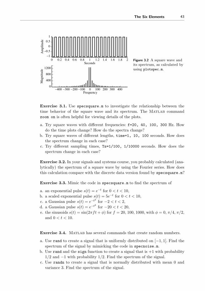
The Six Elements 43
1
0.5
0A
mpl
itude
−0.5
−400 −300 −200 −100 0Frequency
100 200 300 400
−10.2 0.4 0.6 0.8 1
Seconds1.2 1.4 1.6 1.8 20
1200
800
400
0
Mag
nitu
de
Figure 3.2 A square wave andits spectrum, as calculated byusing plotspec.m.
Exercise 3.1. Use specsquare.m to investigate the relationship between the
time behavior of the square wave and its spectrum. The Matlab command
zoom on is often helpful for viewing details of the plots.
a. Try square waves with different frequencies: f=20, 40, 100, 300 Hz. How
do the time plots change? How do the spectra change?
b. Try square waves of different lengths, time=1, 10, 100 seconds. How does
the spectrum change in each case?
c. Try different sampling times, Ts=1/100, 1/10000 seconds. How does the
spectrum change in each case?
Exercise 3.2. In your signals and systems course, you probably calculated (ana-
lytically) the spectrum of a square wave by using the Fourier series. How does
this calculation compare with the discrete data version found by specsquare.m?
Exercise 3.3. Mimic the code in specsquare.m to find the spectrum of
a. an exponential pulse s(t) = e−t for 0 < t < 10,
b. a scaled exponential pulse s(t) = 5e−t for 0 < t < 10,
c. a Gaussian pulse s(t) = e−t2 for −2 < t < 2,
d. a Gaussian pulse s(t) = e−t2 for −20 < t < 20,
e. the sinusoids s(t) = sin(2πft+ φ) for f = 20, 100, 1000, with φ = 0, π/4, π/2,
and 0 < t < 10.
Exercise 3.4. Matlab has several commands that create random numbers.
a. Use rand to create a signal that is uniformly distributed on [−1, 1]. Find the
spectrum of the signal by mimicking the code in specnoise.m.
b. Use rand and the sign function to create a signal that is +1 with probability
1/2 and −1 with probability 1/2. Find the spectrum of the signal.
c. Use randn to create a signal that is normally distributed with mean 0 and
variance 3. Find the spectrum of the signal.
44 Chapter 3. The Six Elements
4
2
0
−4
−2Am
plitu
de
0 0.2 0.4 0.6 0.8 1Seconds
300
200
100
0
Mag
nitu
de
−4000 −2000 0 2000 4000Frequency
Figure 3.3 A noise signal and itsspectrum, as calculated usingplotspec.m.
Exercise 3.5. Modify the code in plotspec.m to also plot the phase spectrum.
a. Plot the phase spectrum of a sine wave and a cosine wave, both of the same
frequency. How do they differ?
b. Plot the phase spectrum of the random signal created in Exercise 3.4(a).
While plotspec.m can be quite useful, ultimately, it will be necessary to have
more flexibility, which, in turn, requires one to understand how the FFT function
inside plotspec.m works. This will be discussed at length in Chapter 7. The
next six sections describe the six elements that are at the heart of communica-
tions systems. The elements are described both in the time domain and in the
frequency domain.
3.2 The First Element: Oscillators
The Latin word oscillare means “to ride in a swing.” It is the origin of oscillate,
which means to move back and forth in steady unvarying rhythm. Thus, a device
that creates a signal that moves back and forth in a steady, unvarying rhythm is
called an oscillator. An electronic oscillator is a device that produces a repetitive
electronic signal, usually a sinusoidal wave.
A basic oscillator is diagrammed in Figure 3.4. Oscillators are typically
designed to operate at a specified frequency f0, and the input specifies the phase
φ(t) of the output
s(t) = cos(2πf0t+ φ(t)).
The input may be a fixed number, but it may also be a signal; that is, it may
change over time. In this case, the output is no longer a pure sinusoid of frequency
f0. For instance, suppose the phase is a “ramp” or line with slope 2πc; that is,
φ(t) = 2πct. Then s(t) = cos(2πf0t+ 2πct) = cos(2π(f0 + c)t), and the “actual”
frequency of oscillation is f0 + c.

The Six Elements 45
cos(2πf0t+φ(t))φ(t)
Figure 3.4 An oscillator creates a sinusoidal oscillationwith a specified frequency f0 and input φ(t).
0.5
0
−0.5
−1
1
0 0.2 0.4 0.6 0.8 1 1.2 1.4 1.6 1.8 2Seconds
Am
plitu
de
80
40
0
120
−50 −40 −30 −20 −10 0 10 20 30 40 50Frequency
Mag
nitu
de
Figure 3.5 A sinusoidal oscillatorcreates a signal that can beviewed in the time domain as inthe top plot, or in the frequencydomain as in the bottom plot.
There are many ways to build oscillators from analog components. Generally,
there is an amplifier and a feedback circuit that returns a portion of the amplified
wave back to the input. When the feedback is aligned properly in phase, sustained
oscillations occur.
Digital oscillators are simpler. Since they can be directly calculated, no ampli-
fier or feedback is needed. For example, a “digital” sine wave of frequency f Hz
and a phase of φ radians can be represented mathematically as
s(kTs) = cos(2πfkTs + φ), (3.1)
where Ts is the time between samples and where k is an integer counter k =
1, 2, 3, . . .. Equation (3.1) can be directly implemented in Matlab:
Listing 3.3. speccos.m plot the spectrum of a cosine wave
f =10; phi=0; % sp e c i f y f r equency and phasetime=2; % length o f timeTs=1/100; % time i n t e r v a l between samplest=Ts : Ts : time ; % cr ea t e a time vectorx=cos (2* pi* f * t+phi ) ; % c r ea t e cos wavep l o t sp e c (x , Ts ) % draw waveform and spectrum
The output of speccos.m is shown in Figure 3.5. As expected, the time plot
shows an undulating sinusoidal signal with f = 10 repetitions in each second.
The spectrum shows two spikes, one at f = 10 Hz and one at f = −10 Hz. Why
are there two spikes? Basic Fourier theory shows that the Fourier transform of
a cosine wave is a pair of delta functions at plus and minus the frequency of the
cosine wave (see Equation (A.18)). The two spikes of Figure 3.5 mirror these
two delta functions. Alternatively, recall that a cosine wave can be written using
Euler’s formula as the sum of two complex exponentials, as in (A.2). The spikes of
Figure 3.5 represent the magnitudes of these two (complex-valued) exponentials.

46 Chapter 3. The Six Elements
Exercise 3.6. Mimic the code in speccos.m to find the spectrum of a cosine
wave
a. for different frequencies f=1, 2, 20, 30 Hz,
b. for different phases φ = 0, 0.1, π/8, π/2 radians,
c. for different sampling rates Ts=1/10, 1/1000, 1/100000.
Exercise 3.7. Let x1(t) be a cosine wave of frequency f = 10, x2(t) be a cosine
wave of frequency f = 18, and x3(t) be a cosine wave of frequency f = 33. Let
x(t) = x1(t) + 0.5 ∗ x2(t) + 2 ∗ x3(t). Find the spectrum of x(t). What property
of the Fourier transform does this illustrate?
Exercise 3.8. Find the spectrum of a cosine wave in the following cases.
a. φ is a function of time. Try φ(t) = 10πt.
b. φ is a function of time. Try φ(t) = πt2.
c. f is a function of time. Try f(t) = sin(2πt).
d. f is a function of time. Try f(t) = t2.
3.3 The Second Element: Linear Filters
Linear time-invariant filters shape the spectrum of a signal. If the signal has
too much energy in the low frequencies, a highpass filter can remove them. If
the signal has too much high-frequency noise, a lowpass filter can reject it. If a
signal of interest resides only between f∗ and f ∗, then a bandpass filter tuned
to pass frequencies between f∗ and f ∗ can remove out-of-band interference and
noise. More generally, suppose that a signal has frequency bands in which the
magnitude of the spectrum is lower than desired and other bands in which the
magnitude is greater than desired. Then a linear filter can compensate by increas-
ing or decreasing the magnitude. This section provides an overview of how to
implement simple filters in Matlab. More thorough treatments of the theory,
design, use, and implementation of filters are given in Chapter 7.
While the calculations of a linear filter are usually carried out in the time
domain, filters are often specified in the frequency domain. Indeed, the words
used to specify filters (such as lowpass, highpass, and bandpass) describe how the
filter acts on the frequency content of its input. Figure 3.6, for instance, shows
a noisy input entering three different filters. The frequency response of the LPF
shows that it allows low frequencies (those below the cutoff frequency f∗) to pass,
while removing all frequencies above the cutoff. Similarly, the HPF passes all the
high frequencies and rejects those below its cutoff f ∗. The frequency response of
the BPF is specified by two frequencies. It will remove all frequencies below f∗and all frequencies above f ∗, leaving only the region between.

The Six Elements 47
Mag.
Freq.White input
−f* f*
−f*
−f*
−f* f* f*
−f* f*LPF
Y1( f )
y1(t)
x(t)Y2( f )
Y3( f )
y2(t)
y3(t)
BPF
HPF
−f*−f* f* f*
f*f*−f*
X( f )
Figure 3.6 A “white”signal containing allfrequencies is passedthrough a lowpass filter(LPF) leaving only thelow frequencies, abandpass filter (BPF)leaving only the middlefrequencies, and ahighpass filter (HPF)leaving only the highfrequencies.
Figure 3.6 shows the action of ideal filters. How close are actual implementa-
tions? The Matlab code in filternoise.m shows that it is possible to create
digital filters that reliably and accurately carry out these tasks.
Listing 3.4. filternoise.m filter a noisy signal three ways
time=3; % length o f timeTs=1/10000; % time i n t e r v a l between samplesx=randn (1 , time /Ts ) ; % generate no i s e s i g n a lf igure ( 1 ) , p l o t s p e c (x , Ts ) % draw spectrum of inputf r e q s =[0 0 . 2 0 . 21 1 ] ;amps=[1 1 0 0 ] ;b=f i rpm (100 , f r eqs , amps ) ; % s p e c i f y the LP f i l t e rylp=f i l t e r (b , 1 , x ) ; % do the f i l t e r i n gf igure ( 2 ) , p l o t s p e c ( ylp , Ts ) % p l o t the output spectrumf r e q s =[0 0 . 24 0 . 26 0 . 5 0 . 51 1 ] ;amps=[0 0 1 1 0 0 ] ;b=f i rpm (100 , f r eqs , amps ) ; % BP f i l t e rybp=f i l t e r (b , 1 , x ) ; % do the f i l t e r i n gf igure ( 3 ) , p l o t s p e c (ybp , Ts) % p l o t the output spectrumf r e q s =[0 0 . 74 0 . 76 1 ] ;amps=[0 0 1 1 ] ;b=f i rpm (100 , f r eqs , amps ) ; % s p e c i f y the HP f i l t e ryhp=f i l t e r (b , 1 , x ) ; % do the f i l t e r i n gf igure ( 4 ) , p l o t s p e c (yhp , Ts) % p l o t the output spectrum
The output of filternoise.m is shown in Figure 3.7. Observe that the spec-
tra at the output of the filters are close approximations to the ideals shown in
Figure 3.6. There are some differences, however. While the idealized spectra are
completely flat in the passband, the actual ones are rippled. While the idealized
spectra completely reject the out-of-band frequencies, the actual ones have small
(but nonzero) energy at all frequencies. Two new Matlab commands are used
in filternoise.m. The firpm command specifies the contour of the filter as a
line graph (Octave and early versions of Matlab call this command remez). For
instance, typing
plot ( [ 0 0 . 24 0 . 26 0 . 5 0 . 51 1 ] , [ 0 0 1 1 0 0 ] )

48 Chapter 3. The Six Elements
Magnitude spectrum at input
Magnitude spectrum at output of lowpass filter
Magnitude spectrum at output of bandpass filter
−4000 −2000 0 2000 4000Magnitude spectrum at output of highpass filter
Figure 3.7 The spectrum of a “white”signal containing all frequencies isshown in the top figure. This ispassed through three filters: alowpass, a bandpass, and a highpass.The spectra at the outputs of thesethree filters are shown in the second,third, and bottom plots. The “actual”filters behave much like theiridealized counterparts in Figure 3.6.
at the Matlab prompt draws a box that represents the action of the BPF
designed in filternoise.m (over the positive frequencies). The frequencies
are specified as percentages of fNYQ = 1/(2Ts), which in this case is equal to
5000 Hz. (fNYQ is discussed further in the next section.) Thus the BPF in
filternoise.m passes frequencies between 0.26×5000 Hz and 0.5×5000 Hz, and
rejects all others. The filter command uses the output of firpm to carry out
the filtering operation on the vector specified in its third argument. More details
about these commands are given in the section on practical filtering in Chapter 7.
Exercise 3.9. Mimic the code in filternoise.m to create a filter that
a. passes all frequencies above 500 Hz,
b. passes all frequencies below 3000 Hz,
c. rejects all frequencies between 1500 and 2500 Hz.
Exercise 3.10. Change the sampling rate to Ts=1/20000. Redesign the three
filters from Exercise 3.9.
Exercise 3.11. Let x1(t) be a cosine wave of frequency f = 800, x2(t) be a cosine
wave of frequency f = 2000, and x3(t) be a cosine wave of frequency f = 4500.
Let x(t) = x1(t) + 0.5 ∗ x2(t) + 2 ∗ x3(t). Use x(t) as input to each of the three
filters in filternoise.m. Plot the spectra, and explain what you see.
Exercise 3.12. TRUE or FALSE: A linear, time-invariant system exists that
has input a cos(bt) and output c sin(dt) with a �= c and |b| �= |d|. Explain.
Exercise 3.13. TRUE or FALSE: Filtering a passband signal with absolute
bandwidth B through certain fixed linear filters can result in an absolute band-
width of the filter output greater than B. Explain.

The Six Elements 49
Exercise 3.14. TRUE or FALSE: A linear, time-invariant, finite-impulse-
response filter with a frequency response having unit magnitude over all fre-
quencies and a straight-line, sloped phase curve has as its transfer function a
pure delay. Explain.
Exercise 3.15. TRUE or FALSE: Processing a bandlimited signal through a
linear, time-invariant filter can increase its half-power bandwidth. Explain.
3.4 The Third Element: Samplers
Since part of any digital transmission system is analog (transmissions through
the air, across a cable, or along a wire are inherently analog), and part of the
system is digital, there must be a way to translate the continuous-time signal
into a discrete-time signal and vice versa. The process of sampling an analog sig-
nal, sometimes called analog-to-digital conversion, is easy to visualize in the time
domain. Figure 3.8 shows how sampling can be viewed as the process of evalu-
ating a continuous-time signal at a sequence of uniformly spaced time intervals,
thus transforming the analog signal x(t) into the discrete-time signal x(kTs).
One of the key ideas in signals and systems is the Fourier series: a signal is
periodic in time (it repeats every P seconds) if and only if the spectrum can
be written as a sum of complex sinusoids with frequencies at integer multiples
of a fundamental frequency f . Moreover, this fundamental frequency can be
written in terms of the period as f = 1/P . Thus, if a signal repeats 100 times
every second (P = 0.01 s), then its spectrum consists of a sum of sinusoids with
frequencies 100, 200, 300, . . . Hz.
Conversely, if a spectrum is built from a sum of sinusoids with frequencies
100, 200, 300, . . . Hz, then it must represent a periodic signal in time that has
period P = 0.01 s. Said another way, the nonzero portions of the spectrum are
uniformly spaced f = 100 Hz apart. This uniform spacing can be interpreted as
a sampling (in frequency) of an underlying continuous-valued spectrum. This is
x(t) x(kTs) = x[k]
Ts
(a)
(b)
x(t)
Ts 2Ts 3Ts 4Ts t
x(Ts)
= x[1]
x(2T s)
= x[2]
x(4T s)
= x[4]
x(3Ts ) = x[3]
Figure 3.8 The sampling process is shown in (b) as an evaluation of the signal x(t) attimes . . . ,−2Ts, Ts, 0, Ts, 2Ts, . . .. This procedure is schematized in (a) as an elementthat has the continuous-time signal x(t) as input and the discrete-time signal x(kTs)as output.

50 Chapter 3. The Six Elements
Pf
fsTs
...
... ...
...
Periodic in time Uniform sampling in frequency
f =1P
fs =1Ts
−3fs2
3fs2
−fs2
0 fs2
f 2f 3f 4f 5f
Fourier Transform
Inverse Fourier Transform
Uniform sampling in time Periodic in frequency
Figure 3.9 Fourier’s result says that any signal that is periodic in time has a spectrumthat consists of a collection of spikes uniformly spaced in frequency. Analogously, anysignal whose spectrum is periodic in frequency can be represented in time as acollection of spikes uniformly spaced in time, and vice versa.
illustrated in the top portion of Figure 3.9, which shows the time-domain repre-
sentation on the left and the corresponding frequency-domain representation on
the right.
The basic insight from Fourier series is that any signal which is periodic in
time can be reexpressed as a collection of uniformly spaced spikes in frequency;
that is,
Periodic in Time ⇔ Uniform Sampling in Frequency.
The same arguments show the basic result of sampling, which is that
Uniform Sampling in Time ⇔ Periodic in Frequency.
Thus, whenever a signal is uniformly sampled in time (say, with sampling interval
Ts seconds), the spectrum will be periodic; that is, it will repeat every fs = 1/Ts
Hz.
Two conventions are often observed when drawing periodic spectra that arise
from sampling. First, the spectrum is usually drawn centered at 0 Hz. Thus, if
the period of repetition is fs, this is drawn from −fs/2 to fs/2, rather than from
0 to fs. This makes sense because the spectra of individual real-valued sinusoidal
components contain two spikes symmetrically located around 0 Hz (as we saw in
Section 3.2). Accordingly, the highest frequency that can be represented unam-
biguously is fs/2, and this frequency is often called the Nyquist frequency fNYQ.
The second convention is to draw only one period of the spectrum. After all,
the others are identical copies that contain no new information. This is evident

The Six Elements 51
y[i]x[k]
m
Figure 3.10 The discrete signal x[k] is downsampled by a factorof m by removing all but one of every m samples. Theresulting signal is y[i], which takes on values y[i] = x[k]whenever k = im+ n.
in the bottom right diagram of Figure 3.9 where the spectrum between −3fs/2
and −fs/2 is the same as the spectrum between fs/2 and 3fs/2. In fact, we
have been observing this convention throughout Sections 3.2 and 3.3, since all
of the figures of spectra (Figures 3.2, 3.3, 3.5, and 3.7) show just one period of
the complete spectrum.
Perhaps you noticed that plotspec.m changes the frequency axis when the
sampling interval Ts is changed. (If not, go back and redo Exercise 3.1(c).) By
the second convention, plotspec.m shows exactly one period of the complete
spectrum. By the first convention, the plots are labeled from −fNYQ to fNYQ.
What happens when the frequency of the signal is too high for the sampling
rate? The representation becomes ambiguous. This is called aliasing, and is inves-
tigated by simulation in the problems below. Aliasing and other sampling-related
issues (such as reconstructing an analog signal from its samples) are covered in
more depth in Chapter 6.
Closely related to the digital sampling of an analog signal is the (digital)
downsampling of a digital signal, which changes the rate at which the signal is
represented. The simplest case downsamples by a factor of m, removing all but
one out of every m samples. This can be written
y[i] = x[im+ n],
where n is an integer between 0 and m− 1. For example, with m = 3 and n = 1,
y[i] is the sequence that consists of every third value of x[k],
y[0] = x[1], y[1] = x[4], y[2] = x[7], y[3] = x[10], etc.
This is commonly drawn in block form as in Figure 3.10. If the spectrum of x[k]
is bandlimited to 1/m of the Nyquist rate, then downsampling by m loses no
information. Otherwise, aliasing occurs. Like analog-to-digital sampling, down-
sampling is a time-varying operation.
Exercise 3.16. Mimicking the code in speccos.m with the sampling interval
Ts=1/100, find the spectrum of a cosine wave cos(2πft) when f=30, 40, 49,
50, 51, 60 Hz. Which of these show aliasing?
Exercise 3.17. Create a cosine wave with frequency 50 Hz. Plot the spec-
trum when this wave is sampled at Ts=1/50, 1/90, 1/100, 1/110, and 1/200.
Which of these show aliasing?
Exercise 3.18. Mimic the code in speccos.m with sampling interval Ts=1/100
to find the spectrum of a square wave with fundamental f=10, 20, 30, 33,

52 Chapter 3. The Six Elements
43 Hz. Can you predict where the spikes will occur in each case? Which of the
square waves show aliasing?
3.5 The Fourth Element: Static Nonlinearities
Linear systems3 such as filters cannot add new frequencies to a signal, though
they can remove unwanted frequencies. Nonlinearities such as squaring and quan-
tizing can and will add new frequencies. These can be useful in the communica-
tion system in a variety of ways.
Perhaps the simplest (memoryless) nonlinearity is the square, which takes
the input at each time instant and multiplies it by itself. Suppose the input
is a sinusoid at frequency f , that is, x(t) = cos(2πft). Then the output is the
sinusoid squared, which can be rewritten using the cosine–cosine product (A.4)
as
y(t) = x2(t) = cos2(2πft) =1
2+
1
2cos(2π(2f)t).
The spectrum of y(t) has a spike at 0 Hz due to the constant, and a spike at
±2f Hz from the double-frequency term. Unfortunately, the action of a squaring
element is not always as simple as this example might suggest. The following
exercises encourage you to explore the kinds of changes that occur in the spectra
when using a variety of simple nonlinear elements.
Exercise 3.19. Mimic the code in speccos.m with Ts=1/1000 to find the
spectrum of the output y(t) of a squaring block when the input is
a. x(t) = cos(2πft) for f = 100 Hz,
b. x(t) = cos(2πf1t) + cos(2πf2t) for f1 = 100 and f2 = 150 Hz,
c. a filtered noise sequence with nonzero spectrum between f1 = 100 and f2 =
300 Hz. Hint: generate the input by modifying filternoise.m.
d. Can you explain the large DC (zero-frequency) component?
Exercise 3.20. TRUE or FALSE: The bandwidth of x4(t) cannot be greater
than that of x(t). Explain.
Exercise 3.21. Try different values of f1 and f2 in Exercise 3.19. Can you
predict what frequencies will occur in the output? When is aliasing an issue?
Exercise 3.22. Repeat Exercise 3.21 when the input is a sum of three sinusoids.
3 To be accurate, these systems must be exponentially stable and time-invariant.

The Six Elements 53
Exercise 3.23. Suppose that the output of a nonlinear block is the rectification
(absolute value) of the input y(t) = |x(t)|. Find the spectrum of the output when
the input is
a. x(t) = cos(2πft) for f = 100 Hz,
b. x(t) = cos(2πf1t) + cos(2πf2t) for f1 = 100 and f2 = 125 Hz.
c. Repeat (b) for f1 = 110 and f2 = 200 Hz. Can you predict what frequencies
will be present for any f1 and f2?
d. What frequencies will be present if x(t) is the sum of three sinusoids f1, f2,
and f3?
Exercise 3.24. Suppose that the output of a nonlinear block is y(t) = g(x(t)),
where
g(t) =
{1 x(t) > 0
−1 x(t) ≤ 0
is a quantizer that outputs plus one when the input is positive and minus one
when the input is negative. Find the spectrum of the output when the input is
a. x(t) = cos(2πft) for f = 100 Hz,
b. x(t) = cos(2πf1t) + cos(2πf2t) for f1 = 100 and f2 = 150 Hz.
Exercise 3.25. Quantization of an input is another kind of common nonlinear-
ity. The Matlab function quantalph.m (available on the website) quantizes a
signal to the nearest element of a desired set. Its help file reads
% y=quantalph (x , a lphabet )%% quant i ze the input s i g n a l x to the alphabet% using nea r e s t neighbor method% input x − vector to be quantized% alphabet − vector o f d i s c r e t e va lues% that y can assume
% sor ted in ascending order% output y − quantized vector
Let x be a random vector x=randn(1,n) of length n. Quantize x to the nearest
[−3,−1, 1, 3].
a. What percentage of the outputs are 1s? 3s?
b. Plot the magnitude spectrum of x and the magnitude spectrum of the output.
c. Now let x=3*randn(1,n) and answer the same questions.
3.6 The Fifth Element: Mixers
One feature of most telecommunications systems is the ability to change the
frequency of the signal without changing its information content. For example,

54 Chapter 3. The Six Elements
speech occurs in the range below about 8 kHz. In order to transmit this, it is
upconverted (as in Section 2.3) to radio frequencies at which the energy can
easily propagate over long distances. At the receiver, it is downconverted (as in
Section 2.6) to the original frequencies. Thus the spectrum is shifted twice.
One way of accomplishing this kind of frequency shifting is to multiply the
signal by a cosine wave, as shown in Figure 3.11. The following Matlab code
implements a simple modulation.
Listing 3.5. modulate.m change the frequency of the input
time =.5; Ts=1/10000; % time and sampling i n t e r v a lt=Ts : Ts : time ; % de f i n e a ’ time ’ vectorf c =1000; cmod=cos (2* pi* f c * t ) ; % c r ea t e cos o f f r eq f cf i =100; x=cos (2* pi* f i * t ) ; % input i s cos o f f r eq f iy=cmod . * x ; % mul t ip ly input by cmodf igure ( 1 ) , p l o t s p e c (cmod , Ts ) % f i nd spec t r a and p l o tf igure ( 2 ) , p l o t s p e c (x , Ts )f igure ( 3 ) , p l o t s p e c (y , Ts )
The first three lines of the code create the modulating sinusoid (i.e., an oscillator).
The next line specifies the input (in this case another cosine wave). The Matlab
syntax .* calculates a point-by-point multiplication of the two vectors cmod and
x.
The output of modulate.m is shown in Figure 3.12. The spectrum of the input
contains spikes representing the input sinusoid at ±100 Hz and the spectrum
of the modulating sinusoid contains spikes at ±1000 Hz. As expected from the
modulation property of the transform, the output contains sinusoids at ±1000±100 Hz, which appear in the spectrum as the two pairs of spikes at ±900 and
±1100 Hz. Of course, this modulation can be applied to any signal, not just to
an input sinusoid. In all cases, the output will contain two copies of the input,
one shifted up in frequency and the other shifted down in frequency.
Exercise 3.26.Mimic the code in modulate.m to find the spectrum of the output
y(t) of a modulator block (with modulation frequency fc = 1000 Hz) when
a. the input is x(t) = cos(2πf1t) + cos(2πf2t) for f1 = 100 and f2 = 150 Hz,
b. the input is a square wave with fundamental f = 150 Hz,
c. the input is a noise signal with all energy below 300 Hz,
d. the input is a noise signal bandlimited to between 2000 and 2300 Hz,
e. the input is a noise signal with all energy below 1500 Hz.
cos(2πf0t+φ) x(t)cos(2πf0t+φ)
x(t)
φ X
Figure 3.11 The mixing operation shifts allfrequencies of a signal x(t) by an amountdefined by the frequency f0 of themodulating sinusoidal wave.

The Six Elements 55
Magnitude spectrum at input
Magnitude spectrum of the oscillator
−3000 −2000 −1000 0 1000 2000 3000Magnitude spectrum at output
Figure 3.12 The spectrum of the input sinusoid is shown in the top figure. The middlefigure shows the spectrum of the modulating wave. The bottom shows the spectrumof the point-by-point multiplication (in time) of the two, which is the same as theirconvolution (in frequency).
3.7 The Sixth Element: Adaptation
Adaptation is a primitive form of learning. Adaptive elements in telecommuni-
cation systems find approximate values for unknown parameters in an attempt
to compensate for changing conditions or to improve performance. A common
strategy in parameter-estimation problems is to guess a value, assess how good
the guess is, and refine the guess over time. With luck, the guesses converge to
a useful estimate of the unknown value.
Figure 3.13 shows an adaptive element containing two parts. The adaptive
subsystem parameterized by a changes the input into the output. The quality-
assessment mechanism monitors the output (and other relevant signals) and tries
to determine whether a should be increased or decreased. The arrow through the
system indicates that the a value is then adjusted accordingly.
Adaptive elements occur in a number of places in the communication system,
including the following.
� In an automatic gain control, the “adaptive subsystem” is multiplication by a
constant a. The quality-assessment mechanism gauges whether the power at
the output of the AGC is too large or too small, and adjusts a accordingly.
aInput Output
QualityAssessment
Figure 3.13 The adaptive element is asubsystem that transforms the inputinto the output (parameterized by a)and a quality-assessment mechanismthat evaluates how to alter a; in thiscase, whether to increase or decreasea.

56 Chapter 3. The Six Elements
� In a phase-locked loop, the “adaptive subsystem” contains a sinusoid with
an unknown phase shift a. The quality-assessment mechanism adjusts a to
maximize a filtered version of the product of the sinusoid and its input.� In a timing recovery setting, the “adaptive subsystem” is a fractional delay
given by a. One mechanism for assessing quality monitors the power of the
output, and adjusts a to maximize this power.� In an equalizer, the “adaptive subsystem” is a linear filter parameterized by
a set of as. The quality-assessment mechanism monitors the deviation of the
output of the system from a target set and adapts the as accordingly.
Chapter 6 provides an introduction to adaptive elements in communication
systems, and a detailed discussion of their implementation is postponed until
then.
3.8 Summary
The bewildering array of blocks and acronyms in a typical communication system
diagram really consists of just a handful4 of simple elements: oscillators, linear
filters, samplers, static nonlinearities, mixers, and adaptive elements. For the
most part, these are ideas that the reader will have encountered to some degree in
previous studies, but they have been summarized here in order to present them in
the same form and using the same notation as in later chapters. In addition, this
chapter has emphasized the “how-to” aspects by providing a series of Matlab
exercises, which will be useful when creating simulations of the various parts of
a receiver.
For Further Reading
The intellectual background of the material presented here is often called signals
and systems. One of the most accessible books is
� J. H. McClellan, R. W. Schafer, and M. A. Yoder, Signal Processing First,
Pearson Prentice-Hall, 2003.
Other books provide greater depth and detail about the theory and uses of
Fourier transforms. We recommend these as both background and supplementary
reading:
� A. V. Oppenheim, A. S. Willsky, and S. H. Nawab, Signals and Systems, 2nd
edition, Prentice-Hall, 1997;� S. Haykin and B. Van Veen, Signals and Systems, Wiley, 2002.
4 Assuming a six-fingered hand.

The Six Elements 57
There are also many wonderful books about digital signal processing, and these
provide both depth and detail about basic issues such as sampling and filter
design. Some of the best are the following:
� A. V. Oppenheim, R. W. Schafer, and J. R. Buck, Discrete-Time Signal Pro-
cessing, Prentice-Hall, 1999;� B. Porat, A Course in Digital Signal Processing, Wiley, 1997;� S. Mitra, Digital Signal Processing: A Computer-Based Approach, McGraw-
Hill, 2005.
Finally, since Matlab is fundamental to our presentation, it is worth mentioning
some books that describe the uses (and abuses) of the Matlab language.
� A. Gilat, MATLAB: An Introduction with Applications, Wiley, 2007;� B. Littlefield and D. Hanselman, Mastering Matlab 7, Prentice-Hall, 2004.

Step 3: The Idealized System
The next step encompasses Chapters 4 through 9. This gives a closer look at
the idealized receiver—how things work when everything is just right: when the
timing is known, when the clocks run at exactly the right speed, when there are
no reflections, diffractions, or diffusions of the electromagnetic waves. This step
also introduces a few Matlab tools that are needed to implement the digital
radio. The order in which topics are discussed is precisely the order in which
they appear in the receiver:
channel
Chapter 4
→frequency
translation
Chapter 5
→ sampling
Chapter 6
→
receive
filtering→ equalization︸ ︷︷ ︸
Chapter 7
→decision
device→ decoding︸ ︷︷ ︸
Chapter 8
Chapter 9 provides a complete (though idealized) software-defined digital radio
system.

4 Modeling Corruption
If every signal that went from here to there arrived at its intended receiver
unchanged, the life of a communications engineer would be easy. Unfortunately,
the path between here and there can be degraded in several ways, including
multipath interference, changing (fading) channel gains, interference from other
users, broadband noise, and narrowband interference.
This chapter begins by describing some of the funny things that can happen
to signals, some of which are diagrammed in Figure 4.1. More important than
locating the sources of the problems is fixing them. The received signal can
be processed using linear filters to help reduce the interferences and to undo,
to some extent, the effects of the degradations. The central question is how to
specify filters that can successfully mitigate these problems, and answering this
requires a fairly detailed understanding of filtering. Thus, a discussion of linear
filters occupies the bulk of this chapter, which also provides a background for
other uses of filters throughout the receiver, such as the lowpass filters used in the
demodulators of Chapter 5, the pulse-shaping and matched filters of Chapter 11,
and the equalizing filters of Chapter 13.
4.1 When Bad Things Happen to Good Signals
The path from the transmitter to the receiver is not simple, as Figure 4.1 sug-
gests. Before the signal reaches the receiver, it may be subject to a series of
strange events that can corrupt the signal and degrade the functioning of the
receiver. This section discusses five kinds of corruption that are used throughout
the chapter to motivate and explain the various purposes that linear filters may
serve in the receiver.

60 Chapter 4. Modeling Corruption
MultipathChanging
gain
Transmittedsignal
Signalsfromotherusers
Broadbandnoise
Narrowbandnoise
Receivedsignal
Types of corruption
+ + +
Figure 4.1 Sources ofcorruption includemultipath interference,changing channel gains,interference from otherusers, broadband noise,and narrowbandinterferences.
4.1.1 Other Users
Many different users must be able to broadcast at the same time. This requires
that there be a way for a receiver to separate the desired transmission from all
the others (for instance, to tune to a particular radio or TV station among a
large number that may be broadcasting simultaneously in the same geographical
region). One standard method is to allocate different frequency bands to each
user. This was called frequency-division multiplexing (FDM) in Chapter 2, and
was shown diagrammatically in Figure 2.3 on page 22. The signals from the
different users can be separated using a bandpass filter, as in Figure 2.4 on page
23. Of course, practical filters do not completely remove out-of-band signals, nor
do they pass in-band signals completely without distortions. Recall the three
filters in Figure 3.7 on page 48.
4.1.2 Broadband Noise
When the signal arrives at the receiver, it is small and must be amplified. While
it is possible to build high-gain amplifiers, the noises and interferences will also
be amplified along with the signal. In particular, any noise in the amplifier itself
will be increased. This is often called “thermal noise” and is usually modeled as
white (independent) broadband noise. Thermal noise is inherent in any electronic
component and is caused by small randommotions of electrons, like the Brownian
motion of small particles suspended in water.
Such broadband noise is another reason why a bandpass filter is applied at
the front end of the receiver. By applying a suitable filter, the total power in
the noise (compared with the total power in the signal) can often be reduced.
Figure 4.2 shows the spectrum of the signal as a pair of triangles centered at the
carrier frequency ±fc with bandwidth 2B. The total power in the signal is the
area under the triangles. The spectrum of the noise is the flat region, and its
power is the shaded area. After applying the bandpass filter, the power in the
signal remains (more or less) unchanged, while the power in the noise is greatly
reduced. Thus, the signal-to-noise ratio (SNR) improves.

Modeling Corruption 61
Powerin signal
Powerin noise
Powerin signalis unchanged
−fc − B −fc + B fc − B fc + B
−fc − B −fc + B fc − B fc + B
(a)
(b)
(c)
Totalpower in noise
is decreased
−fc − B −fc + B fc − B fc + B0
Figure 4.2 The signal-to-noiseratio is depicted graphically asthe ratio of the power of thesignal (the area under thetriangles) to the power in thenoise (the shaded area). Afterthe bandpass filter, the powerin the noise decreases, so theSNR increases.
4.1.3 Narrowband Noise
Noises are not always white; that is, the spectrum need not always be flat. Stray
sine waves (and other signals with narrow spectra) may also impinge on the
receiver. These may be caused by errant transmitters that accidentally broad-
cast in the frequency range of the signal, or they may be harmonics of a lower-
frequency wave as it experiences nonlinear distortion. If these narrowband distur-
bances occur out of band, they will automatically be attenuated by the bandpass
filter just as if they were a component of the wideband noise. However, if they
occur in the frequency region of the signal, they decrease the SNR in proportion
to their power. Judicious use of a “notch” filter (one designed to remove just the
offending frequency) can be an effective tool.
Figure 4.3 shows the spectrum of the signal as the pair of triangles, along with
three narrowband interferers represented by the three pairs of spikes. After the
bandpass filter (BPF), the two pairs of out-of-band spikes are removed, but the
in-band pair remains. Applying a narrow notch filter tuned to the frequency
of the interferer allows its removal, although this cannot be done without also
affecting the signal somewhat.
4.1.4 Multipath Interference
In some situations, an electromagnetic wave can propagate directly from one
place to another. For instance, when a radio signal from a spacecraft is trans-
mitted back to Earth, the vacuum of space guarantees that the wave will arrive
more or less intact (though greatly attenuated by distance). Often, however, the
wave reflects, refracts, or diffracts, and the signal arriving is quite different from
the one that was sent.

62 Chapter 4. Modeling Corruption
Signal plus threenarrowbandinterferers
Removal ofout-of-bandinterferers
Removal ofin-bandinterferers alsomodifier signals
Notchfilter
BPF Figure 4.3 Three narrowbandinterferers are shown in the topfigure (the three pairs of spikes).The BPF cannot remove thein-band interferer, though anarrow notch filter can, at theexpense of changing the signal inthe region where thenarrowband noise occurred.
These distortions can be thought of as a combination of scaled and delayed
reflections of the transmitted signal, which occur when there are different prop-
agation paths from the transmitter to the receiver. Between two transmission
towers, for instance, the paths may include one along the line of sight, reflections
from the atmosphere, reflections from nearby hills, and bounces from a field or
lake between the towers. For indoor digital TV reception, there are many (local)
time-varying reflectors, including people in the receiving room, nearby vehicles,
and the buildings of an urban environment. Figure 4.4, for instance, shows mul-
tiple reflections that arrive after bouncing off a cloud and off a mountain, and
others that are scattered by multiple bounces from nearby buildings.
The strength of the reflections depends on the physical properties of the reflect-
ing surface, while the delay of the reflections is primarily determined by the
length of the transmission path. Let s(t) be the transmitted signal. If N delays
are represented by Δ1, Δ2, . . . , ΔN , and the strengths of the reflections are
h1, h2, . . . , hN , then the received signal r(t) is
r(t) = h1s(t−Δ1) + h2s(t−Δ2) + · · ·+ hNs(t−ΔN ). (4.1)
As will become clear in Section 4.4, this model of the channel has the form of
a linear filter (since the expression on the right-hand side is a convolution of
the transmitted signal and the his). This is shown in part (a) of Figure 4.5.
Since this channel model is a linear filter, it can also be viewed in the frequency
domain, and part (b) shows its frequency response. When this is combined with
the BPF and the spectrum of the signal (shown in (c)), the result is the distorted
spectrum shown in (d).
What can be done?

Modeling Corruption 63
Transmitter
Cloud
Receiver
Buildings
Mountain
Line of sight
Figure 4.4 The receivedsignal may be a combinationof several copies of theoriginal transmitted signal,each with a differentattenuation and delay.
h(t)
Transmittedsignal
Receivedsignal
Fourier Transform
H( f )
Frequency
(a)
(b)
(c)
(d)
Figure 4.5 (a) The channelmodel (4.1) as a filter. (b)The frequency response ofthe filter. (c) An idealizedBPF and the spectrum of thesignal. The product of (b)and (c) gives (d), thedistorted spectrum at thereceiver.
If the kinds of distortions introduced by the channel are known (or can some-
how be determined), then the bandpass filter at the receiver can be modified
in order to undo the effects of the channel. This can be seen most clearly in
the frequency domain, as in Figure 4.6. Observe that the BPF is shaped (part
(d)) to approximately invert the debilitating effects of the channel (part (a)) in
the frequency band of the signal and to remove all the out-of-band frequencies.
The resulting received signal spectrum (part (e)) is again a close copy of the
transmitted signal spectrum, in stark contrast to the received signal spectrum
in Figure 4.5 where no shaping was attempted.

64 Chapter 4. Modeling Corruption
Frequencyresponse ofchannel
Spectrumofsignal
Product of(a) & (b)
Product of(c) & (d)
BPF withshaping
(a)
(b)
(c)
(d)
(e)
Figure 4.6 (a) The frequency response of the channel. (b) The spectrum of the signal.(c) The product of (a) and (b), which is the spectrum of the received signal. (d) ABPF filter that has been shaped to undo the effect of the channel. (e) The product of(c) and (d), which combine to give a clean representation of the original spectrum ofthe signal.
Thus, filtering in the receiver can be used to reshape the received signal within
the frequency band of the transmission as well as to remove unwanted out-of-
band frequencies.
4.1.5 Fading
Another kind of corruption that a signal may encounter on its journey from the
transmitter to the receiver is called “fading,” where the frequency response of the
channel changes slowly over time. This may be caused because the transmission
path changes. For instance, a reflection from a cloud might disappear when the
cloud dissipates, an additional reflection might appear when a truck moves into a
narrow city street, or in a mobile device such as a cell phone the operator might
turn a corner and cause a large change in the local geometry of reflections.
Fading may also occur when the transmitter and/or the receiver are moving.
The Doppler effect shifts the frequencies slightly, causing interferences that may
slowly change.
Such time-varying problems cannot be fixed by a single fixed filter; rather, the
filter must somehow compensate differently at different times. This is an ideal
application for the adaptive elements of Section 3.7, though results from the
study of linear filters will be crucial in understanding how the time variations

Modeling Corruption 65
in the frequency response can be represented as time-varying coefficients in the
filter that represents the channel.
4.2 Linear Systems: Linear Filters
Linear systems appear in many places in communication systems. The trans-
mission channel is often modeled as a linear system as in (4.1). The bandpass
filters used in the front end to remove other users (and to remove noises) are
linear. Lowpass filters are crucial to the operation of the demodulators of Chap-
ter 5. The equalizers of Chapter 13 are linear filters that are designed during the
operation of the receiver on the basis of certain characteristics of the received
signal.
Time-invariant linear systems can be described in any one of three equivalent
ways.
� The impulse response h(t) is a function of time that defines the output of a
linear system when the input is an impulse (or δ) function. When the input
to the linear system is more complicated than a single impulse, the output
can be calculated from the impulse response via the convolution operator.� The frequency response H(f) is a function of frequency that defines how the
spectrum of the input is changed into the spectrum of the output. The fre-
quency response and the impulse response are intimately related: H(f) is the
Fourier transform of h(t).� A linear difference equation with constant coefficients (such as (4.1)) shows
explicitly how the linear system can be implemented and can be useful in
assessing stability and performance.
This chapter describes the three representations of linear systems and shows
how they interrelate. The discussion begins by exploring the δ function, and then
showing how it is used to define the impulse response. The convolution property
of the Fourier transform then shows that the transform of the impulse response
describes how the system behaves in terms of the input and output spectra, and
so it is called the frequency response. The final step is to show how the action
of the linear system can be redescribed in the time domain as a difference (or as
a differential) equation. This is postponed to Chapter 7, and is also discussed in
some detail in Appendix F.
4.3 The Delta “Function”
One way to see how a system behaves is to kick it and see how it responds.
Some systems react sluggishly, barely moving away from their resting state,
while others respond quickly and vigorously. Defining exactly what is meant
mathematically by a “kick” is trickier than it seems because the kick must occur

66 Chapter 4. Modeling Corruption
over a very short amount of time, yet must be energetic in order to have any
effect. This section defines the impulse (or delta) function δ(t), which is a useful
“kick” for the study of linear systems.
The criterion that the impulse be energetic is translated to the mathematical
statement that its integral over all time must be nonzero, and it is typically
scaled to unity, that is, ∫ ∞
−∞δ(t)dt = 1. (4.2)
The criterion that it occur over a very short time span is translated to the
statement that, for every positive ε,
δ(t) =
{0 t < −ε,
0 t > ε.(4.3)
Thus, the impulse δ(t) is explicitly defined to be equal to zero for all t �= 0. On
the other hand, δ(t) is implicitly defined when t = 0 by the requirement that its
integral be unity. Together, these guarantee that δ(t) is no ordinary function.1
The most important consequence of the definitions (4.2) and (4.3) is the sifting
property ∫ ∞
−∞w(t)δ(t − t0)dt = w(t)|t=t0 = w(t0), (4.4)
which says that the delta function picks out the value of the function w(t) from
under the integral at exactly the time when the argument of the δ function is
zero, that is, when t = t0. To see this, observe that δ(t− t0) is zero whenever
t �= t0, and hence w(t)δ(t − t0) is zero whenever t �= t0. Thus,∫ ∞
−∞w(t)δ(t − t0)dt =
∫ ∞
−∞w(t0)δ(t− t0)dt
= w(t0)
∫ ∞
−∞δ(t− t0)dt = w(t0) · 1 = w(t0).
Sometimes it is helpful to think of the impulse as a limit. For instance, define
the rectangular pulse of width 1/n and height n by
δn(t) =
⎧⎨⎩
0 t < −1/(2n),
n −1/(2n) ≤ t ≤ 1/(2n),
0 t > 1/(2n).
Then δ(t) = limn→∞ δn(t) fulfills both criteria (4.2) and (4.3). Informally, it is not
unreasonable to think of δ(t) as being zero everywhere except at t = 0, where it is
infinite. While it is not really possible to “plot” the delta function δ(t− t0), it can
be represented in graphical form as zero everywhere except for an up-pointing
arrow at t0. When the δ function is scaled by a constant, the value of the constant
is often placed in parentheses near the arrowhead. Sometimes, when the constant
1 The impulse is called a distribution and is the subject of considerable mathematical investi-gation.

Modeling Corruption 67
(1)
(3)
−10
(−2)
−5 0 5 10 t
Figure 4.7 The function w(t) = δ(t+ 10)− 2δ(t+ 1) + 3δ(t− 5) consisting of threeweighted δ functions is representedgraphically as three weighted arrows att = −10,−1, 5, weighted by theappropriate constants.
is negative, the arrow is drawn pointing down. For instance, Figure 4.7 shows a
graphical representation of the function w(t) = δ(t+ 10)− 2δ(t+ 1) + 3δ(t− 5).
What is the spectrum (Fourier transform) of δ(t)? This can be calculated
directly from the definition by replacing w(t) in (2.1) with δ(t):
F{δ(t)} =
∫ ∞
−∞δ(t)e−j2πftdt. (4.5)
Apply the sifting property (4.4) with w(t) = e−j2πft and t0 = 0. Thus F{δ(t)} =
e−j2πft|t=0 = 1.
Alternatively, suppose that δ is a function of frequency, that is, a spike at
zero frequency. The corresponding time-domain function can be calculated anal-
ogously using the definition of the inverse Fourier transform, that is, by substi-
tuting δ(f) for W (f) in (A.16) and integrating:
F−1{δ(f)} =
∫ ∞
−∞δ(f)ej2πftdf = ej2πft|f=0 = 1.
Thus a spike at frequency zero is a “DC signal” (a constant) in time.
The discrete time counterpart of δ(t) is the (discrete) delta function
δ[k] =
{1 k = 0,
0 k �= 0.
While there are a few subtle differences between δ(t) and δ[k], for the most part
δ(t) and δ[k] act analogously. For example, the program specdelta.m calculates
the spectrum of the (discrete) delta function.
Listing 4.1. specdelta.m plots the spectrum of a delta function
time=2; % length o f timeTs=1/100; % time i n t e r v a l between samplest=Ts : Ts : time ; % cr ea t e time vectorx=zeros ( size ( t ) ) ; % c r ea t e s i g n a l o f a l l z e r o sx (1)=1; % de l t a f unc t i onp l o t sp e c (x , Ts ) % draw waveform and spectrum
The output of specdelta.m is shown in Figure 4.8. As expected from (4.5),
the magnitude spectrum of the delta function is equal to 1 at all frequencies.
Exercise 4.1. Calculate the Fourier transform of δ(t− t0) from the definition.
Now calculate it using the time-shift property (A.37). Are they the same? Hint:
they had better be.

68 Chapter 4. Modeling Corruption
00
1
0.2 0.4 0.6 0.8 1 1.2 1.4 1.6 1.8Seconds
Am
plitu
de
0
1
2
−40 −30 −20 −10 0 10 20 30 40Frequency
Mag
nitu
de
Figure 4.8 A (discrete) delta functionat time 0 has a magnitude spectrumequal to 1 for all frequencies.
Exercise 4.2. Use the definition of the IFT (A.16) to show that
δ(f − f0) ⇔ ej2πf0t.
Exercise 4.3. Mimic the code in specdelta.m to find the magnitude spectrum
of the discrete delta function in the following cases.
a. The delta does not occur at the start of x. Try x[10]=1, x[100]=1, and
x[110]=1. How do the spectra differ? Can you use the time-shift property
(A.37) to explain what you see?
b. The delta changes magnitude x. Try x[1]=10, x[10]=3, and x[110]=0.1. How
do the spectra differ? Can you use the linearity property (A.31) to explain
what you see?
Exercise 4.4. Modify the code in specdelta.m to find the phase spectrum of a
signal that consists of a delta function when the nonzero term is located at the
start (x(1)=1), in the middle (x(100)=1), and at the end (x(200)=1).
Exercise 4.5. Mimic the code in specdelta.m to find the spectrum of a train of
equally spaced pulses. For instance, x(1:20:end)=1 spaces the pulses 20 samples
apart, and x(1:25:end)=1 places the pulses 25 samples apart.
a. Can you predict how far apart the resulting pulses in the spectrum will be?
b. Show that∞∑
k=−∞δ(t− kTs) ⇔ 1
Ts
∞∑n=−∞
δ(f − nfs), (4.6)
where fs = 1/Ts. Hint: let w(t) = 1 in (A.27) and (A.28).
c. Now can you predict how far apart the pulses in the spectrum are? Your
answer should be in terms of how far apart the pulses are in the time signal.
In Section 3.2, the spectrum of a sinusoid was shown to consist of two sym-
metric spikes in the frequency domain (recall Figure 3.5 on page 45). The next
example shows why this is true by explicitly taking the Fourier transform to find
the spectrum of a sinusoid.

Modeling Corruption 69
f0
|W( f )|
(A/2) (A/2)
f−f0
Figure 4.9 The magnitude spectrum of asinusoid with frequency f0 and amplitude Acontains two δ-function spikes, one at f = f0and the other at f = −f0.
Example 4.1. Let w(t) = A sin(2πf0t), and use Euler’s identity (A.3) to rewrite
w(t) as
w(t) =A
2j
[ej2πf0t − e−j2πf0t
].
Applying the linearity property (A.31) and the result of Exercise 4.2 gives
F{w(t)} =A
2j
[F{ej2πf0t} − F{e−j2πf0t}]= j
A
2[−δ(f − f0) + δ(f + f0)] . (4.7)
Thus, the spectrum of a sine wave is a pair of δ functions with opposite signs,
located symmetrically about zero frequency. The corresponding magnitude spec-
trum, shown in Figure 4.9, is at the heart of one important interpretation of the
Fourier transform: it shows the frequency content of any signal by displaying
which frequencies are present in (and absent from) the waveform. For example,
Figure 4.10(a) shows the magnitude spectrum W (f) of a real-valued signal w(t).
This can be interpreted as saying that w(t) contains (or is made up of) “all the
frequencies” up to B Hz, and that it contains no sinusoids with higher frequency.
Similarly, the modulated signal s(t) in Figure 4.10(b) contains all positive fre-
quencies between fc −B and fc +B, and no others.
Note that the Fourier transform in (4.7) is purely imaginary, as it must be
because w(t) is odd (see (A.37)). The phase spectrum is a flat line at −90◦
because of the factor j.
Exercise 4.6. What is the magnitude spectrum of sin(2πf0t+ θ)? Hint: use the
frequency-shift property (A.34). Show that the spectrum of cos(2πf0t) is12(δ(f −
f0) + δ(f + f0)). Compare this analytical result with the numerical results from
Exercise 3.6.
Exercise 4.7. Let wi(t) = ai sin(2πfit) for i = 1, 2, 3. Without doing any cal-
culations, write down the spectrum of v(t) = w1(t) + w2(t) + w3(t). Hint: use
linearity. Graph the magnitude spectrum of v(t) in the same manner as in Fig-
ure 4.9. Verify your results with a simulation mimicking that in Exercise 3.7.

70 Chapter 4. Modeling Corruption
|S( f )|
f−fc −fc + B(b)
−fc − B fc fc + Bfc − B
1/2
|W( f )|
f−B(a)
+B
1
Figure 4.10 The magnitude spectrum of a message signal w(t) is shown in (a). Whenw(t) is modulated by a cosine at frequency fc, the spectrum of the resulting signals(t) = w(t) cos(2πfct+ φ) is shown in (b).
Exercise 4.8. LetW (f) = sin(2πft0). What is the corresponding time function?
4.4 Convolution in Time: It’s What Linear Systems Do
Suppose that a system has impulse response h(t), and that the input consists of
a sum of three impulses occurring at times t0, t1, and t2, with amplitudes a0,
a1, and a2 (for example, the signal w(t) of Figure 4.7). Because of the linearity
of the Fourier transform, property (A.31), the output is a superposition of the
outputs due to each of the input pulses. The output due to the first impulse is
a0h(t− t0), which is the impulse response scaled by the size of the input and
shifted to begin when the first input pulse arrives. Similarly, the outputs to the
second and third input impulses are a1h(t− t1) and a2h(t− t2), respectively,
and the complete output is the sum a0h(t− t0) + a1h(t− t1) + a2h(t− t2).
Now suppose that the input is a continuous function x(t). At any time instant
λ, the input can be thought of as consisting of an impulse scaled by the amplitude
x(λ), and the corresponding output will be x(λ)h(t − λ), which is the impulse
response scaled by the size of the input and shifted to begin at time λ. The
complete output is then given by integrating over all λ:
y(t) =
∫ ∞
−∞x(λ)h(t − λ)dλ ≡ x(t) ∗ h(t). (4.8)
This integral defines the convolution operator ∗ and provides a way of finding
the output y(t) of any linear system, given its impulse response h(t) and the
input x(t).
Matlab has several functions that simplify the numerical evaluation of con-
volutions. The most obvious of these is conv, which is used in convolex.m to
calculate the convolution of an input x (consisting of two delta functions at times
t = 1 and t = 3) and a system with impulse response h that is an exponential
pulse. The convolution gives the output of the system.
Listing 4.2. convolex.m example of numerical convolution
Ts=1/100; time=10; % sampling i n t e r v a l and t o t a l timet=0:Ts : time ; % cr ea t e time vectorh=exp(− t ) ; % de f i n e impulse r esponsex=zeros ( size ( t ) ) ; % input = sum of two de l t a f unc t i on s
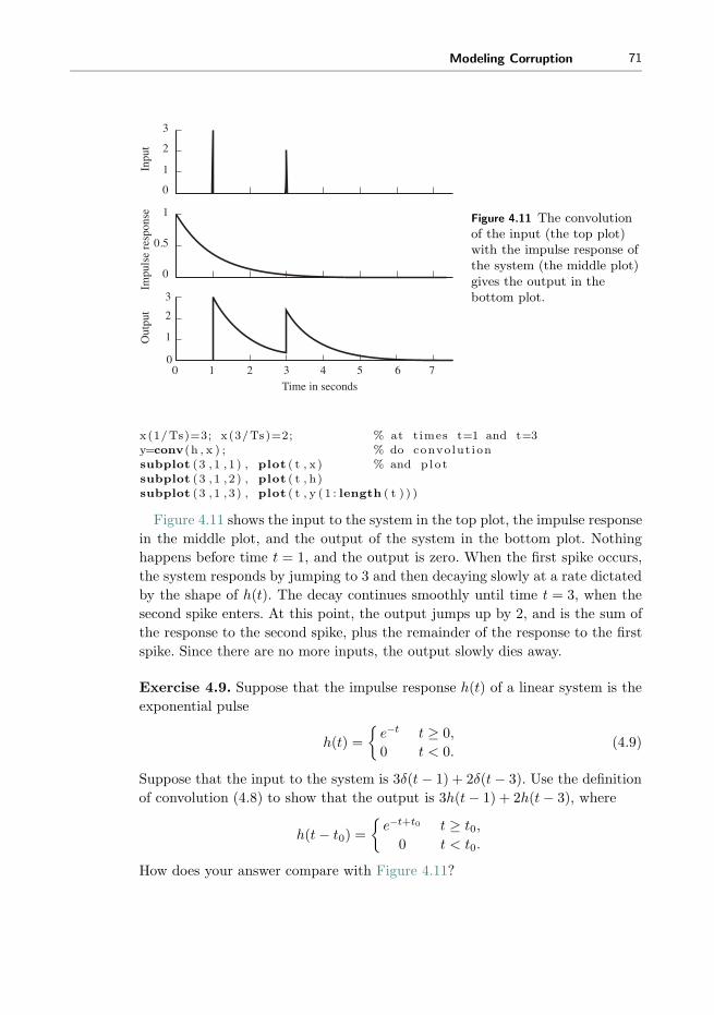
Modeling Corruption 71
0
1
2
3
Inpu
t
0 1 2 3 4 5 6 70
1
2
3
Out
put
Time in seconds
0
0.5
1
Impu
lse
resp
onse Figure 4.11 The convolution
of the input (the top plot)with the impulse response ofthe system (the middle plot)gives the output in thebottom plot.
x (1/Ts)=3; x (3/Ts)=2; % at t imes t=1 and t=3y=conv(h , x ) ; % do convo lut i onsubplot ( 3 , 1 , 1 ) , plot ( t , x ) % and p l o tsubplot ( 3 , 1 , 2 ) , plot ( t , h)subplot ( 3 , 1 , 3 ) , plot ( t , y ( 1 : length ( t ) ) )
Figure 4.11 shows the input to the system in the top plot, the impulse response
in the middle plot, and the output of the system in the bottom plot. Nothing
happens before time t = 1, and the output is zero. When the first spike occurs,
the system responds by jumping to 3 and then decaying slowly at a rate dictated
by the shape of h(t). The decay continues smoothly until time t = 3, when the
second spike enters. At this point, the output jumps up by 2, and is the sum of
the response to the second spike, plus the remainder of the response to the first
spike. Since there are no more inputs, the output slowly dies away.
Exercise 4.9. Suppose that the impulse response h(t) of a linear system is the
exponential pulse
h(t) =
{e−t t ≥ 0,
0 t < 0.(4.9)
Suppose that the input to the system is 3δ(t− 1) + 2δ(t− 3). Use the definition
of convolution (4.8) to show that the output is 3h(t− 1) + 2h(t− 3), where
h(t− t0) =
{e−t+t0 t ≥ t0,
0 t < t0.
How does your answer compare with Figure 4.11?

72 Chapter 4. Modeling Corruption
Exercise 4.10. Suppose that a system has an impulse response that is an expo-
nential pulse. Mimic the code in convolex.m to find its output when the input
is a white noise (recall specnoise.m on page 42).
Exercise 4.11. Mimic the code in convolex.m to find the output of a system
when the input is an exponential pulse and the impulse response is a sum of two
delta functions at times t = 1 and t = 3.
The next two problems show that linear filters commute with differentiation, and
with each other.
Exercise 4.12. Use the definition to show that convolution is commutative (i.e.,
that w1(t) ∗ w2(t) = w2(t) ∗ w1(t)). Hint: apply the change of variables τ = t− λ
in (4.8).
Exercise 4.13. Suppose a filter has impulse response h(t). When the input is
x(t), the output is y(t). If the input is xd(t) = ∂x(t)/∂t, the output is yd(t). Show
that yd(t) is the derivative of y(t). Hint: use (4.8) and the result of Exercise 4.12.
Exercise 4.14. Let w(t) = Π(t) be the rectangular pulse of (2.8). What is
w(t) ∗ w(t)? Hint: a pulse shaped like a triangle.
Exercise 4.15. Redo Exercise 4.14 numerically by suitably modifying
convolex.m. Let T = 1.5 s.
Exercise 4.16. Suppose that a system has an impulse response that is a sinc
function, as shown in Figure 2.11, and that the input to the system is a white
noise (as in specnoise.m on page 42).
a. Mimic convolex.m to numerically find the output.
b. Plot the spectrum of the input and the spectrum of the output (using
plotspec.m). What kind of filter would you call this?
4.5 Convolution ⇔ Multiplication
While the convolution operator (4.8) describes mathematically how a linear sys-
tem acts on a given input, time-domain approaches are often not particularly
revealing about the general behavior of the system.Who would guess, for instance
in Exercises 4.11 and 4.16, that convolution with exponentials and sinc functions
would act like lowpass filters? By working in the frequency domain, however, the
convolution operator is transformed into a simpler point-by-point multiplication,
and the generic behavior of the system becomes clearer.
The first step is to understand the relationship between convolution in time
and multiplication in frequency. Suppose that the two time signals w1(t) and

Modeling Corruption 73
w2(t) have Fourier transforms W1(f) and W2(f). Then,
F{w1(t) ∗ w2(t)} = W1(f)W2(f). (4.10)
To justify this property, begin with the definition of the Fourier transform (2.1)
and apply the definition of convolution (4.8) to obtain
F{w1(t) ∗ w2(t)} =
∫ ∞
t=−∞w1(t) ∗ w2(t)e
−j2πftdt
=
∫ ∞
t=−∞
[∫ ∞
λ=−∞w1(λ)w2(t− λ)dλ
]e−j2πftdt.
Reversing the order of integration and using the time-shift property (A.37) pro-
duces
F{w1(t) ∗ w2(t)} =
∫ ∞
λ=−∞w1(λ)
[∫ ∞
t=−∞w2(t− λ)e−j2πftdt
]dλ
=
∫ ∞
λ=−∞w1(λ)
[W2(f)e
−j2πfλ]dλ
= W2(f)
∫ ∞
λ=−∞w1(λ)e
−j2πfλdλ = W1(f)W2(f).
Thus, convolution in the time domain is the same as multiplication in the fre-
quency domain. See (A.40).
The companion to the convolution property is the multiplication property,
which says that multiplication in the time domain is equivalent to convolution
in the frequency domain (see (A.41)); that is,
F{w1(t)w2(t)} = W1(f) ∗W2(f) =
∫ ∞
−∞W1(λ)W2(f − λ)dλ. (4.11)
The usefulness of these convolution properties is apparent when applying them
to linear systems. Suppose that H(f) is the Fourier transform of the impulse
response h(t). Suppose that X(f) is the Fourier transform of the input x(t) that
is applied to the system. Then (4.8) and (4.10) show that the Fourier transform
of the output is exactly equal to the product of the transforms of the input and
the impulse response, that is,
Y (f) = F{y(t)} = F{x(t) ∗ h(t)} = F{h(t)}F{x(t)} = H(f)X(f).
This can be rearranged to solve for
H(f) =Y (f)
X(f), (4.12)
which is called the frequency response of the system because it shows, for each
frequency f , how the system responds. For instance, suppose that H(f1) = 3 at
some frequency f1. Then, whenever a sinusoid of frequency f1 is input into the
system, it will be amplified by a factor of 3. Alternatively, suppose thatH(f2) = 0
at some frequency f2. Then whenever a sinusoid of frequency f2 is input into

74 Chapter 4. Modeling Corruption
the system, it is removed from the output (because it has been multiplied by a
factor of 0).
The frequency response shows how the system treats inputs containing various
frequencies. In fact, this property was already used repeatedly in Chapter 1 when
drawing curves that describe the behavior of lowpass and bandpass filters. For
example, the filters of Figures 2.4, 2.5, and 2.6 are used to remove unwanted
frequencies from the communications system. In each of these cases, the plot of
the frequency response describes concretely and concisely how the system (or
filter) affects the input, and how the frequency content of the output relates to
that of the input. Sometimes, the frequency response H(f) is called the transfer
function of the system, since it “transfers” the input x(t) (with transform X(f))
into the output y(t) (with transform Y (f)).
Thus, the impulse response describes how a system behaves directly in time,
while the frequency response describes how it behaves in frequency. The two
descriptions are intimately related because the frequency response is the Fourier
transform of the impulse response. This will be used repeatedly in Section 7.2
to design filters for the manipulation (augmentation or removal) of specified
frequencies.
Example 4.2. In Exercise 4.16, a system was defined to have an impulse response
that is a sinc function. The Fourier transform of a sinc function in time is a rect
function in frequency (A.22). Hence, the frequency response of the system is a
rectangle that passes all frequencies below fc = 1/T and removes all frequencies
above (i.e., the system is a lowpass filter).
Matlab can help to visualize the relationship between the impulse response
and the frequency response. For instance, the system in convolex.m is defined
via its impulse response, which is a decaying exponential. Figure 4.11 shows
its output when the input is a simple sum of delta functions, and Exercise 4.10
explores the output when the input is a white noise. In freqresp.m, the behavior
of this system is explained by looking at its frequency response.
Listing 4.3. freqresp.m numerical example of impulse and frequency response
Ts=1/100; time=10; % sampling i n t e r v a l and t o t a l timet=0:Ts : time ; % cr ea t e time vectorh=exp(− t ) ; % de f i n e impulse r esponsep l o t sp e c (h , Ts ) % f i nd and p l o t f r equency r esponse
The output of freqresp.m is shown in Figure 4.12. The frequency response
of the system (which is just the magnitude spectrum of the impulse response)
is found using plotspec.m. In this case, the frequency response amplifies low
frequencies and attenuates other frequencies more as the frequency increases.
This explains, for instance, why the output of the convolution in Exercise 4.10
contained (primarily) lower frequencies, as evidenced by the slower undulations
in time.

Modeling Corruption 75
0
0
0 2 4 6 8 10
1
Am
plitu
de
Seconds
−40 −30 −20 −10 0 10 3020 40
100
Mag
nitu
de
Frequency
Figure 4.12 The action of asystem in time is defined by itsimpulse response (in the topplot). The action of the systemin frequency is defined by itsfrequency response (in thebottom plot), a kind of lowpassfilter.
Exercise 4.17. Suppose a system has an impulse response that is a sinc func-
tion. Using freqresp.m, find the frequency response of the system. What kind
of filter does this represent? Hint: center the sinc in time; for instance, use
h=sinc(10*(t-time/2)).
Exercise 4.18. Suppose a system has an impulse response that is a sin func-
tion. Using freqresp.m, find the frequency response of the system. What kind
of filter does this represent? Can you predict the relationship between the fre-
quency of the sine wave and the location of the peaks in the spectrum? Hint: try
h=sin(25*t).
Exercise 4.19. Create a simulation (analogous to convolex.m) that inputs
white noise into a system with an impulse response that is a sinc function (as in
Exercise 4.17). Calculate the spectra of the input and output using plotspec.m.
Verify that the system behaves as suggested by the frequency response in Exer-
cise 4.17.
Exercise 4.20. Create a simulation (analogous to convolex.m) that inputs
white noise into a system with an impulse response that is a sin function (as in
Exercise 4.18). Calculate the spectra of the input and output using plotspec.m.
Verify that the system behaves as suggested by the frequency response in Exer-
cise 4.18.
So far, Section 4.5 has emphasized the idea of finding the frequency response of
a system as a way to understand its behavior. Reversing things suggests another
use. Suppose it was necessary to build a filter with some special characteristic
in the frequency domain (for instance, in order to accomplish one of the goals
of bandpass filtering in Section 4.1). It is easy to specify the filter in the fre-
quency domain. Its impulse response can then be found by taking the inverse
Fourier transform, and the filter can be implemented using convolution. Thus,

76 Chapter 4. Modeling Corruption
the relationship between impulse response and frequency response can be used
both to study and to design systems.
In general, this method of designing filters is not optimal (in the sense that
other design methods can lead to more efficient designs), but it does show clearly
what the filter is doing, and why. Whatever the design procedure, the represen-
tation of the filter in the time domain and its representation in the frequency
domain are related by nothing more than a Fourier transform.
4.6 Improving SNR
Section 4.1 described several kinds of corruption that a signal may encounter
as it travels from the transmitter to the receiver. This section shows how linear
filters can help. Perhaps the simplest way a linear bandpass filter can be used
is to remove broadband noise from a signal. (Recall Section 4.1.2 and especially
Figure 4.2.)
A common way to quantify noise is the signal-to-noise ratio (SNR), which is
the ratio of the power of the signal to the power of the noise at a given point in
the system. If the SNR at one point is larger than the SNR at another point, the
performance is better at the first point because there is more signal in comparison
with the amount of noise. For example, consider the SNR at the input and output
of a BPF as shown in Figure 4.13. The signal at the input (r(t) in part (a)) is
composed of the message signal x(t) and the noise signal n(t), and the SNR at
the input is therefore
SNRinput =power in x(t)
power in n(t).
Similarly, the output y(t) is composed of a filtered version of the message (yx(t)
in part (b)) and a filtered version of the noise (yn(t) in part (b)). The SNR at
the output can therefore be calculated as
SNRoutput =power in yx(t)
power in yn(t).
Observe that the SNR at the output cannot be calculated directly from y(t) (since
the two components are scrambled together). But, since the filter is linear,
y(t) = BPF{x(t) + n(t)} = BPF{x(t)}+BPF{n(t)} = yx + yn,
which effectively shows the equivalence of parts (a) and (b) of Figure 4.13.
The Matlab program improvesnr.m explores this scenario concretely. The
signal x is a bandlimited signal, containing only frequencies between 3000 and
4000 Hz. This is corrupted by a broadband noise n (perhaps caused by an
internally generated thermal noise) to form the received signal. The SNR of this
input snrinp is calculated as the ratio of the power of the signal x to the power
of the noise n. The output of the BPF at the receiver is y, which is calculated

Modeling Corruption 77
x(t) r(t)
n(t)
BPFy(t)
(a) (b)
yx(t)yn(t)
y(t)
n(t)
x(t)BPF
BPF
+ +
Figure 4.13 Two equivalent ways to draw the same system. In part (a) it is easy tocalculate the SNR at the input, while the alternative form (b) allows easy calculationof the SNR at the output of the BPF.
as a BPF version of x+n. The BPF is created using the firpm command just
like the bandpass filter in filternoise.m on page 47. To calculate the SNR of
y, however, the code also implements the system in the alternative form of part
(b) of Figure 4.13. Thus, yx and yn represent the signal x filtered through the
BPF and the noise n passed through the same BPF. The SNR at the output is
then the ratio of the power in yx to the power in yn, which is calculated using
the function pow.m available on the website.
Listing 4.4. improvesnr.m using a linear filter to improve SNR
time=3; Ts=1/20000; % time and sampling i n t e r v a lf r e q s =[0 0 . 29 0 . 3 0 . 4 0 . 41 1 ] ; % f i l t e r des ign , bandl imitedamps=[0 0 1 1 0 0 ] ; % . . . between 3K and 4Kb=f i rpm (100 , f r eqs , amps ) ; % BP f i l t e rn=0.25*randn (1 , time/Ts ) ; % generate white no i s e s i g n a lx=f i l t e r (b , 1 , 2*randn (1 , time/Ts ) ) ; % do the f i l t e r i n gy=f i l t e r (b , 1 , x+n ) ; % ( a ) f i l t e r the s i g n a l+no i s eyx=f i l t e r (b , 1 , x ) ; % or ( b) f i l t e r s i g n a lyn=f i l t e r (b , 1 , n ) ; % . . . and no i s e s epa r a t e l yz=yx+yn ; % add themd i f f z y=max(abs ( z−y ) ) % and make sur e y = zsnr inp=pow(x )/pow(n) % SNR at inputsnrout=pow( yx )/pow(yn ) % SNR at output
Since the data generated in improvesnr.m are random, the numbers are
slightly different each time the program is run. Using the default values, the
SNR at the input is about 7.8, while the SNR at the output is about 61. This is
certainly a noticeable improvement. The variable diffzy shows the largest dif-
ference between the two ways of calculating the output (that is, between parts
(a) and (b) of Figure 4.13). This is on the order of 10−15, which is effectively
the numerical resolution of Matlab calculations, indicating that the two are
(effectively) the same.
Figure 4.14 plots the spectra of the input and the output of a typical run
of improvesnr.m. Observe the large noise floor in the left plot, and how this is
reduced by passage through the BPF. Observe also that the signal is still changed
by the noise in the passband between 3000 and 4000 Hz, since the BPF has no
effect there.

78 Chapter 4. Modeling Corruption
Magnitude spectrum of signal plus noise Magnitude spectrum after filtering
Figure 4.14 The spectrum of the input to the BPF is shown in the left plot. Thespectrum of the output is shown on the right. The overall improvement in SNR isclear.
The program improvesnr.m can be thought of as a simulation of the effect of
having a BPF at the receiver for the purposes of improving the SNR when the
signal is corrupted by broadband noise, as was described in Section 4.1.2. The
following problems ask you to mimic the code in improvesnr.m to simulate the
benefit of applying filters to the other problems presented in Section 4.1.
Exercise 4.21. Suppose that the noise in improvesnr.m is replaced with nar-
rowband noise (as discussed in Section 4.1.3). Investigate the improvements in
SNR
a. when the narrowband interference occurs outside the 3000 to 4000 Hz pass-
band,
b. when the narrowband interference occurs inside the 3000 to 4000 Hz passband.
Exercise 4.22. Suppose that the noise in improvesnr.m is replaced with “other
users” who occupy different frequency bands (as discussed in Section 4.1.1). Are
there improvements in the SNR?
Exercise 4.23. Consider the interference between two users x1 and x2 occupying
the same frequency band as shown in Figure 4.15. The phases of the two mixers
at the transmitter are unequal with 5π/6 > |φ− θ| > π/3. The lowpass filter
(LPF) has a cutoff frequency of fc, a passband gain of 1.5, a stopband gain of
zero, and zero phase at zero frequency.
LPF
cos(2πfct+θ)
cos(2πfct+α)
cos(2πfct+φ)
x2(t)
x1(t)
y(t)
+
receiver
transmitter
Figure 4.15 Themultiuser transmissionsystem of Exercise4.23.

Modeling Corruption 79
a. For this system Y (f) = c1X1(f) + c2X2(f). Determine c1 and c2 as functions
of fc, φ, θ, and α.
b. With α set to maximize (c1/c2)2, find c1 and c2 as functions of fc, φ, and θ.
c. With α set to minimize (c1/c2)2, find c1 and c2 as functions of fc, φ, and θ.
The other two problems posed in Section 4.1 were multipath interference and
fading. These require more sophisticated processing because the design of the
filters depends on the operating circumstances of the system. These situations
will be discussed in detail in Chapters 6 and 13.
For Further Reading
An early description of the linearity of communication channels can be found in
� P. A. Bello, “Characterization of Randomly Time-Variant Linear Channels,”
IEEE Transactions on Communication Systems, vol. 11, no. 4, pp 360–393,
Dec. 1963.

5 Analog (De)modulation
Several parts of a communication system modulate the signal and change the
underlying frequency band in which the signal lies. These frequency changes
must be reversible; after processing, the receiver must be able to reconstruct (a
close approximation to) the transmitted signal.
The input message w(kT ) in Figure 5.1 is a discrete-time sequence drawn from
a finite alphabet. The ultimate output m(kT ) produced by the decision device
(or quantizer) is also discrete-time and is drawn from the same alphabet. If all
goes well and the message is transmitted, received, and decoded successfully, then
the output should be the same as the input, although there may be some delay
δ between the time of transmission and the time when the output is available.
Though the system is digital in terms of the message communicated and the
performance assessment, the middle of the system is inherently analog from the
(pulse-shaping) filter of the transmitter to the sampler at the receiver.
At the transmitter in Figure 5.1, the digital message has already been turned
into an analog signal by the pulse shaping (which was discussed briefly in Section
2.10 and is considered in detail in Chapter 11). For efficient transmission, the
analog version of the message must be shifted in frequency, and this process
of changing frequencies is called modulation or upconversion. At the receiver,
the frequency must be shifted back down, and this is called demodulation or
downconversion. Sometimes the demodulation is done in one step (all analog) and
sometimes the demodulation proceeds in two steps, an analog downconversion to
the intermediate frequency and then a digital downconversion to the baseband.
This two-step procedure is shown in Figure 5.1.
There are many ways in which signals can be modulated. Perhaps the sim-
plest is amplitude modulation (AM), which is discussed in two forms (large and
small carrier) in the next two sections. This is generalized to the simultane-
ous transmission of two signals using quadrature modulation in Section 5.3, and
it is shown that quadrature modulation uses bandwidth more efficiently than
amplitude modulation. This gain in efficiency can also be obtained using single-
sideband and vestigial-sideband methods, which are discussed in the document

Analog (De)modulation 81
Analogconversion
to IF
Carrier synchronization
Analogupconversion
Interferers Noise
Pulseshaping
Digital down-conversionto baseband
f
Ts
Decision
Reconstructedmessage
m(kT − δ) {−3, −1, 1, 3}
Messagew(kT) {−3, −1, 1, 3}
θ
+ +
Figure 5.1 A complete digital communication system has many parts. This chapterfocuses on the upconversion and the downconversion, which can done in many ways,including large-carrier AM as in Section 5.1, suppressed-carrier AM as in Section 5.2,and quadrature modulation as in Section 5.3.
titled Other Modulations available on the website. Demodulation can also be
accomplished using sampling, as discussed in Section 6.2, and amplitude modu-
lation can also be accomplished with a simple squaring and filtering operation
as in Exercise 5.9.
Throughout, the chapter contains a series of exercises that prepare readers to
create their own modulation and demodulation routines in Matlab. These lie
at the heart of the software receiver that will be assembled in Chapters 9 and
15.
5.1 Amplitude Modulation with Large Carrier
Perhaps the simplest form of (analog) transmission system modulates the mes-
sage signal by a high-frequency carrier in a two-step procedure: multiply the
message by the carrier, then add the product to the carrier. At the receiver, the
message can be demodulated by extracting the envelope of the received signal.
Consider the transmitted/modulated signal
v(t) = Acw(t) cos(2πfct) +Ac cos(2πfct) = Ac(w(t) + 1) cos(2πfct)
diagrammed in Figure 5.2. The process of multiplying the signal in time by a
(co)sinusoid is called mixing. This can be rewritten in the frequency domain by
mimicking the development from (2.3) to (2.5) on page 20. Using the convolution
property of Fourier transforms (4.10), the transform of v(t) is
V (f) = F{Ac(w(t) + 1) cos(2πfct)} = AcF{(w(t) + 1)} ∗ F{cos(2πfct)}. (5.1)
The spectra of F{w(t) + 1} and |V (f)| are sketched in Figure 5.3 (a) and (b). The
vertical arrows in (b) represent the transform of the cosine carrier at frequency
fc (i.e., a pair of delta functions at ±fc) and the scaling by Ac/2 is indicated
next to the arrowheads.
If w(t) ≥ −1, the envelope of v(t) is the same as w(t) and an envelope detector
can be used as a demodulator (envelopes are discussed in detail in Appendix C).
One way to find the envelope of a signal is to lowpass filter the absolute value.

82 Chapter 5. Analog (De)modulation
w(t)
Ac cos(2πfct)
v(t)+
v(t)LPF
m(t)
(a) Transmitter (b) Receiver
envelope detector
| . |
Figure 5.2 A communications system using amplitude modulation with a large carrier.In the transmitter (a), the message signal w(t) is modulated by a carrier wave atfrequency fc and then added to the carrier to give the transmitted signal v(t). In (b),the received signal is passed through an envelope detector consisting of anabsolute-value nonlinearity followed by a lowpass filter. When all goes well, theoutput m(t) of the receiver is approximately equal to the original message.
|V( f )|
f−fc
(b)
fc
(Ac/2) (Ac/2)
|F{w(t)+1}|
f−B
(a)
+B
(Ac)
|F{|cos(2πfct)|}|
f−2fc−4fc
(c)
2fc 4fc
|F{|v(t)|}|
f−2fc−4fc
(d)
2fc 4fc
Figure 5.3 Spectra of the signalsin the large-carrier AM systemof Figure 5.2. Lowpass filtering(d) gives a scaled version of (a).
To see this analytically, observe that
F{|v(t)|} = F{|Ac(w(t) + 1) cos(2πfct)|}= |Ac|F{|w(t) + 1|| cos(2πfct)|} = |Ac|F{w(t) + 1} ∗ F{| cos(2πfct)|},
where the absolute value can be removed from w(t) + 1 because w(t) + 1 > 0 (by
assumption). The spectrum of F{|cos(2πfct)|}, shown in Figure 5.3(c), may be
familiar from Exercise 3.23. Accordingly, F{|v(t)|} is the convolution shown in
Figure 5.3(d). Lowpass filtering this returns w(t) + 1, which is the envelope of
v(t) offset by the constant unity.

Analog (De)modulation 83
An example is given in the following Matlab program. The “message” signal
is a sinusoid with a drift in the DC offset, and the carrier wave is at a much
higher frequency.
Listing 5.1. AMlarge.m large-carrier AM demodulated with “envelope”
time =0.33; Ts=1/10000; % sampling i n t e r v a l & timet=0:Ts : time ; l en t=length ( t ) ; % de f i n e a time vectorfm=20; f c =1000; c=cos (2* pi* f c * t ) ; % de f i n e c a r r i e r at f r eq f c
w=10/ l en t * [ 1 : l en t ]+cos (2* pi*fm* t ) ; % c r ea t e ”message ” > −1v=c . *w+c ; % modulate w/ l a r g e c a r r i e rfbe=[0 0 . 05 0 . 1 1 ] ; % LPF des i gndamps=[1 1 0 0 ] ; f l =100;b=f i rpm ( f l , fbe , damps ) ; % impulse r esponse o f LPFenvv=(pi /2)* f i l t e r (b , 1 , abs (v ) ) ; % f i nd envelope
The output of this program is shown in Figure 5.4. The slowly increasing
sinusoidal “message” w(t) is modulated by the carrier c(t) at fc = 1000 Hz.
The heart of the modulation is the point-by-point multiplication of the message
and the carrier in the fifth line. This product v(t) is shown in Figure 5.4(c). The
enveloping operation is accomplished by applying a lowpass filter to the real part
of 2v(t)ej2πfct (as discussed in Appendix C). This recovers the original message
signal, though it is offset by 1 and delayed by the linear filter.
Exercise 5.1. Using AMlarge.m, plot the spectrum of the message w(t), the
spectrum of the carrier c(t), and the spectrum of the received signal v(t). What
is the spectrum of the envelope? How close are your results to the theoretical
predictions in (5.1)?
Exercise 5.2. One of the advantages of transmissions using AM with a large
carrier is that there is no need to know the (exact) phase or frequency of the
transmitted signal. Verify this using AMlarge.m.
a. Change the phase of the transmitted signal; for instance, let c=cos(2*pi*
fc*t+phase) with phase=0.1, 0.5, pi/3, pi/2, pi, and verify that the
recovered envelope remains unchanged.
b. Change the frequency of the transmitted signal; for instance, let c=cos(2*
pi*(fc+g)*t) with g=10, -10, 100, -100, and verify that the recovered
envelope remains unchanged. Can g be too large?
Exercise 5.3. Create your own message signal w(t), and rerun AMlarge.m.
Repeat Exercise 5.1 with this new message. What differences do you see?
Exercise 5.4. In AMlarge.m, verify that the original message w and the recovered
envelope envv are offset by 1, except at the end points where the filter does not
have enough data. Hint: the delay induced by the linear filter is approximately
fl/2.

84 Chapter 5. Analog (De)modulation
Seconds(d) output of envelope detector
0.070.060.050.040.030.020.010
0
2
4
(b) carrier
−1
01
Am
plitu
de
(c) modulated signal
−2024
(a) message signal
0
2
4
Am
plitu
deA
mpl
itude
Am
plitu
de
Figure 5.4 An undulatingmessage (top) is modulated bya carrier (b). The compositesignal is shown in (c), and theoutput of an envelope detectoris shown in (d).
The principal advantage of transmission systems that use AM with a large
carrier is that exact synchronization is not needed; the phase and frequency of
the transmitter need not be known at the receiver, as was demonstrated in Exer-
cise 5.2. This means that the receiver can be simpler than when synchronization
circuitry is required. The main disadvantage is that adding the carrier into the
signal increases the power needed for transmission but does not increase the
amount of useful information transmitted. Here is a clear engineering trade-off;
the value of the wasted signal strength must be balanced against the cost of the
receiver.
5.2 Amplitude Modulation with Suppressed Carrier
It is also possible to use AM without adding the carrier. Consider the transmit-
ted/modulated signal
v(t) = Acw(t)cos(2πfct)
diagrammed in Figure 5.5(a), in which the message w(t) is mixed with the cosine
carrier. Direct application of the frequency-shift property of Fourier transforms
(A.33) shows that the spectrum of the received signal is
V (f) =1
2AcW (f + fc) +
1
2AcW (f − fc).
As with AM with a large carrier, the upconverted signal v(t) for AM with a
suppressed carrier has twice the bandwidth of the original message signal. If the
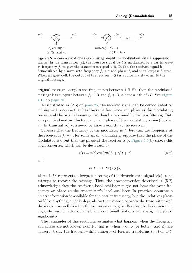
Analog (De)modulation 85
v(t)
cos(2π(fc + γ)t + φ)
(b)(a)
x(t)LPF
m(t)w(t)
Ac cos(2πfct)
v(t)
Transmitter Receiver
Figure 5.5 A communications system using amplitude modulation with a suppressedcarrier. In the transmitter (a), the message signal w(t) is modulated by a carrier waveat frequency fc to give the transmitted signal v(t). In (b), the received signal isdemodulated by a wave with frequency fc + γ and phase φ, and then lowpass filtered.When all goes well, the output of the receiver m(t) is approximately equal to theoriginal message.
original message occupies the frequencies between ±B Hz, then the modulated
message has support between fc −B and fc +B, a bandwidth of 2B. See Figure
4.10 on page 70.
As illustrated in (2.6) on page 25, the received signal can be demodulated by
mixing with a cosine that has the same frequency and phase as the modulating
cosine, and the original message can then be recovered by lowpass filtering. But,
as a practical matter, the frequency and phase of the modulating cosine (located
at the transmitter) can never be known exactly at the receiver.
Suppose that the frequency of the modulator is fc but that the frequency at
the receiver is fc + γ, for some small γ. Similarly, suppose that the phase of the
modulator is 0 but that the phase at the receiver is φ. Figure 5.5(b) shows this
downconverter, which can be described by
x(t) = v(t) cos(2π(fc + γ)t+ φ) (5.2)
and
m(t) = LPF{x(t)},where LPF represents a lowpass filtering of the demodulated signal x(t) in an
attempt to recover the message. Thus, the downconversion described in (5.2)
acknowledges that the receiver’s local oscillator might not have the same fre-
quency or phase as the transmitter’s local oscillator. In practice, accurate a
priori information is available for the carrier frequency, but the (relative) phase
could be anything, since it depends on the distance between the transmitter and
the receiver as well as when the transmission begins. Because the frequencies are
high, the wavelengths are small and even small motions can change the phase
significantly.
The remainder of this section investigates what happens when the frequency
and phase are not known exactly, that is, when γ or φ (or both γ and φ) are
nonzero. Using the frequency-shift property of Fourier transforms (5.3) on x(t)

86 Chapter 5. Analog (De)modulation
in (5.2) produces the Fourier transform X(f)
Ac
4[ejφ{W (f + fc − (fc + γ)) +W (f − fc − (fc + γ))}+ e−jφ{W (f + fc + (fc + γ)) +W (f − fc + (fc + γ))}]
=Ac
4[ejφW (f − γ) + ejφW (f − 2fc − γ)
+ e−jφW (f + 2fc + γ) + e−jφW (f + γ)]. (5.3)
If there is no frequency offset (i.e., if γ = 0), then
X(f) =Ac
4[(ejφ + e−jφ)W (f) + ejφW (f − 2fc) + e−jφW (f + 2fc)].
Because cos(x) = (1/2)(ejx + e−jx) from (A.2), this can be rewritten
X(f) =Ac
2W (f)cos(φ) +
Ac
4
[ejφW (f − 2fc) + e−jφW (f + 2fc)
].
Thus, a perfect lowpass filtering of x(t) with cutoff below 2fc removes the high-
frequency portions of the signal near ±2fc to produce
m(t) =Ac
2w(t) cos(φ). (5.4)
The factor cos(φ) attenuates the received signal (except for the special case when
φ = 0± 2πk for integers k). If φ were sufficiently close to 0± 2πk for some integer
k, then this would be tolerable. But there is no way to know the relative phase,
and hence cos(φ) can assume any possible value within [−1, 1]. The worst case
occurs as φ approaches ±π/2, when the message is attenuated to zero! A scheme
for carrier-phase synchronization, which automatically tries to align the phase
of the cosine at the receiver with the phase at the transmitter, is vital. This is
discussed in detail in Chapter 10.
To continue the investigation, suppose that the carrier-phase offset is zero,
(i.e., φ = 0), but that the frequency offset γ is not. Then the spectrum of x(t)
from (5.3) is
X(f) =Ac
4[W (f − γ) +W (f − 2fc − γ) +W (f + 2fc + γ) +W (f + γ)],
and the lowpass filtering of x(t) produces
M(f) =Ac
4[W (f − γ) +W (f + γ)] .
This is shown in Figure 5.6. Recognizing this spectrum as a frequency-shifted
version of w(t), it can be translated back into the time domain using (A.33) to
give
m(t) =Ac
2w(t) cos(2πγt). (5.5)
Instead of recovering the message w(t), the frequency offset causes the receiver
to recover a low-frequency amplitude-modulated version of it. This is bad with

Analog (De)modulation 87
f
|M( f )| |W( f + γ)|
|W( f − γ)|
0
Ac
4
Figure 5.6 When there is acarrier-frequency offset in the receiveroscillator, the two images of W (·) donot align properly. Their sum is not
equal to (Ac/2)W (f).
even a small carrier-frequency offset. While cos(φ) in (5.4) is a fixed scal-
ing, cos(2πγt) in (5.5) is a time-varying scaling that will alternately recover
m(t) (when cos(2πγt) ≈ 1) and make recovery impossible (when cos(2πγt) ≈ 0).
Transmitters are typically expected to maintain suitable accuracy to a nominal
carrier-frequency setting known to the receiver. Ways of automatically tracking
(inevitable) small frequency deviations are discussed at length in Chapter 10.
The following code AM.m generates a message w(t) and modulates it with a
carrier at frequency fc. The demodulation is done with a cosine of frequency fc +
γ and a phase offset of φ. When γ = 0 and φ = 0, the output (a lowpass version
of the demodulated signal) is nearly identical to the original message, except for
the inevitable delay caused by the linear filter. Figure 5.7 shows four plots: the
message w(t) on top, followed by the upconverted signal v(t) = w(t)cos(2πfct),
followed in turn by the downconverted signal x(t). The lowpass-filtered version
is shown in the bottom plot; observe that it is nearly identical to the original
message, albeit with a slight delay.
Listing 5.2. AM.m suppressed carrier with (possible) freq and phase offset
time =0.3; Ts=1/10000; % sampling i n t e r v a l & timet=Ts : Ts : time ; l en t=length ( t ) ; % de f i n e a time vectorfm=20; f c =1000; c=cos (2* pi* f c * t ) ; % c a r r i e r at f r eq f cw=5/ l en t * (1 : l en t )+cos (2* pi*fm* t ) ; % c r ea t e ”message ”v=c . *w; % modulate with c a r r i e rgam=0; phi=0; % f r eq & phase o f f s e tc2=cos (2* pi *( f c+gam)* t+phi ) ; % c r ea t e co s i n e f o r demodx=v . * c2 ; % demod r e c e i v ed s i g n a lfbe=[0 0 . 1 0 . 2 1 ] ; damps=[1 1 0 0 ] ; % LPF des i gnf l =100; b=f i rpm ( f l , fbe , damps ) ; % impulse r esponse o f LPFm=2* f i l t e r (b , 1 , x ) ; % LPF the demodulated s i g n a l
Exercise 5.5. Using AM.m as a starting point, plot the spectra of w(t), v(t), x(t),
and m(t).
Exercise 5.6. Try different phase offsets φ = [−π, −π/2, −π/3, −π/6, 0, π/6,
π/3, π/2, π]. How well does the recovered messagem(t) match the actual message
w(t)? For each case, what is the spectrum of m(t)?
Exercise 5.7. TRUE or FALSE: A small, fixed phase offset in the receiver
demodulating AM with suppressed carrier produces an undesirable low-frequency
modulated version of the analog message.

88 Chapter 5. Analog (De)modulation
Am
plitu
de
(a) message signal
(b) message after modulation
(d) recovered message is a LPF applied to (c)
−10 0.02 0.04 0.06 0.08
1
3
−1
1
3
−1
1
3
−2
(c) demodulated signal
2
0Figure 5.7 The message signalin the top frame is modulatedto produce the signal in thesecond plot. Demodulationgives the signal in the thirdplot, and the LPF recoversthe original message (withdelay) in the bottom plot.
( )2 Bandpassfilter
Centeredat fc
Addition Square-lawdevice
A0 cos(2πfct)
w(t) 2A0w(t)cos(2πfct)+Figure 5.8 The square-lawmixing transmitter ofExercises 5.9 through5.11.
Exercise 5.8. Try different frequency offsets gam = [0.014, 0.1, 1.0, 10]. How
well does the recovered message m(t) match the actual message w(t)? For each
case, what is the spectrum of m(t)? Hint: look over more than just the first 0.1 s
to see the effect.
Exercise 5.9. Consider the system shown in Figure 5.8. Show that the output
of the system is 2A0w(t) cos(2πfct), as indicated.
Exercise 5.10. Create a Matlab routine to implement the square-law mixing
modulator of Figure 5.8.
a. Create a signal w(t) that has bandwidth 100 Hz.
b. Modulate the signal to 1000 Hz.
c. Demodulate using the AM demodulator from AM.m (to recover the original
w(t)).

Analog (De)modulation 89
w(t)
(a)
(b)
(c)
(d)
cos(2πf1t + φ1)
BPFx(t)
x(t) r(t)
lower cutoff f2upper cutoff f3
r(t)
cos(2πf8t + φ2)
sin(2πf4t) + cos(2πf5t)
lower cutoff f6 cutoff f9upper cutoff f7
BPFy(t)
LPF
BPF +
|W( f )|
f−300−2000 300 2000
2
Figure 5.9 The transmission system for Exercise 5.12: (a) the magnitude spectrum ofthe message, (b) the transmitter, (c) the channel, and (d) the receiver.
Exercise 5.11. Exercise 5.10 essentially creates a transmitter and receiver based
on the square-law modulator (rather than the more standard mixing modulator).
Using this system, do the following.
a. Show how the received signal degrades if the phase of the cosine wave is not
known exactly.
b. Show how the received signal degrades if the frequency of the cosine wave is
not exact.
c. Show how the received signal degrades if the bandpass filter is not centered
at the specified frequency.
Exercise 5.12. Consider the transmission system of Figure 5.9. The message
signal w(t) has the magnitude spectrum shown in part (a). The transmitter in
part (b) produces the transmitted signal x(t), which passes through the chan-
nel in part (c). The channel scales the signal and adds narrowband interferers
to create the received signal r(t). The transmitter and channel parameters are
φ1 = 0.3 radians, f1 = 24.1 kHz, f2 = 23.9 kHz, f3 = 27.5 kHz, f4 = 29.3 kHz,
and f5 = 22.6 kHz. The receiver processing r(t) is shown in Figure 5.9(d). All
bandpass and lowpass filters are considered ideal, with a gain of unity in the
passband and zero in the stopband.
a. Sketch |R(f)| for −30 kHz ≤ f ≤ 30 kHz. Clearly indicate the amplitudes and
frequencies of key points in the sketch.
b. Assume that φ2 is chosen to maximize the magnitude of y(t) and reflects the
value of φ1 and the delays imposed by the two ideal bandpass filters that form
the received signal r(t). Select the receiver parameters f6, f7, f8, and f9, so
the receiver output y(t) is a scaled version of w(t).
Exercise 5.13. An analog baseband message signal w(t) has all energy between
−B and B Hz. It is upconverted to the transmitted passband signal x(t) via AM

90 Chapter 5. Analog (De)modulation
with suppressed carrier
x(t) = w(t) cos(2πfct+ φc),
where the carrier frequency fc > 10B. The channel is a pure delay and the
received signal r is r(t) = x(t− d), where the delay d = nTc + Tc/α is an integer
multiple n ≥ 0 of the carrier period Tc (= 1/fc) plus a fraction of Tc given by
α > 1. The mixer at the receiver is perfectly synchronized to the transmitter so
that the mixer output y(t) is
y(t) = r(t) cos(2πfct+ φr).
The receiver mixer phase need not match the transmitter mixer phase φc. The
receiver lowpass filters y to produce
v(t) = LPF{y(t)},where the lowpass filter is ideal with unity passband gain, linear passband phase
with zero phase at zero frequency, and cutoff frequency 1.2B.
a. Write a formula for the receiver mixer output y(t) as a function of fc, φc, d,
α, φr, and w(t) (without use of x, r, n, or Tc).
b. Determine the amplitude of the minimum and maximum values of y(t) for
α = 4.
c. For α = 6, n = 42, φc = 0.2 radians, and Tc = 20 μs, determine the value of
φr that maximizes the magnitude of the maximum and minimum values of
v(t).
5.3 Quadrature Modulation
In AM transmission, where the baseband signal and its modulated passband ver-
sion are real-valued, the spectrum of the modulated signal has twice the band-
width of the baseband signal. As pictured in Figure 4.10 on page 70, the spectrum
of the baseband signal is nonzero only for frequencies between −B and B. After
modulation, the spectrum is nonzero in the interval [−fc −B,−fc +B] and in
the interval [fc −B, fc +B]. Thus the total width of frequencies occupied by the
modulated signal is twice that occupied by the baseband signal. This represents
a kind of inefficiency or redundancy in the transmission. Quadrature modulation
provides one way of removing this redundancy by sending two messages in the
frequency ranges between [−fc −B,−fc +B] and [fc −B, fc +B], thus utilizing
the spectrum more efficiently.
To see how this can work, suppose that there are two message streams m1(t)
and m2(t). Modulate one message with a cosine to create the in-phase signal,
and the other with (the negative of) a sine to form the quadrature signal. These

Analog (De)modulation 91
+
−
m1(t)
sin(2πfct)
cos(2πfct)cos(2πfct)
Transmitter Receiver
m2(t)
x1(t)
x2(t)
s1(t)
s2(t)LPF
LPF
+
sin(2πfct)
Figure 5.10 In a quadrature modulationsystem, two messages m1(t) and m2(t)are modulated by two sinusoids of thesame frequency, sin(2πfct) andcos(2πfct). The receiver thendemodulates twice and recovers theoriginal messages after lowpass filtering.
are summed1 to form
v(t) = m1(t) cos(2πfct)−m2(t) sin(2πfct), (5.6)
which is then transmitted. A receiver structure that can recover the two messages
is shown in Figure 5.10. The signal s1(t) at the output of the receiver is intended
to recover the first message m1(t). Similarly, the signal s2(t) at the output of the
receiver is intended to recover the (negative of the) second message m2(t).
To examine the recovered signals s1(t) and s2(t) in Figure 5.10, first evaluate
the signals before the lowpass filtering. Using the trigonometric identities (A.4)
and (A.8), x1(t) becomes
x1(t) = v(t) cos(2πfct) = m1(t) cos2(2πfct)−m2(t) sin(2πfct) cos(2πfct)
=m1(t)
2(1 + cos(4πfct))− m2(t)
2sin(4πfct).
Lowpass filtering x1(t) produces
s1(t) =m1(t)
2.
Similarly, x2(t) can be rewritten using (A.5) and (A.8) as
x2(t) = v(t) sin(2πfct) = m1(t) cos(2πfct) sin(2πfct)−m2(t) sin2(2πfct)
=m1(t)
2sin(4πfct)− m2(t)
2(1− cos(4πfct)),
and lowpass filtering x2(t) produces
s2(t) =−m2(t)
2.
Thus, in the ideal situation in which the phases and frequencies of the modu-
lation and the demodulation are identical, both messages can be recovered. But
if the frequencies and/or phases are not exact, then problems analogous to those
1 These are also sometimes modeled as the “real” and the “imaginary” parts of a single“complex-valued” signal. This complex representation is explored more fully in AppendixC.

92 Chapter 5. Analog (De)modulation
x2(t) x3(t) x4(t) x5(t) x6(t)
x1(t)
cos(2πf5t + φ)
cos(2πf1t)
cos(2πf2t)lower cutoff f3 cutoff f6upper cutoff f4
BPF LPF+Figure 5.11 The transmissionsystem of Exercise 5.16.
encountered with AM will occur in the quadrature modulation. For instance,
if the phase of (say) the demodulator x1(t) is not correct, then there will be
some distortion or attenuation in s1(t). However, problems in the demodulation
of s1(t) may also cause problems in the demodulation of s2(t). This is called
cross-interference between the two messages.
Exercise 5.14. Use AM.m as a starting point to create a quadrature modulation
system that implements the block diagram of Figure 5.10.
a. Examine the effect of a phase offset in the demodulating sinusoids of the
receiver, so that x1(t) = v(t) cos(2πfct+ φ) and x2(t) = v(t) sin(2πfct+ φ)
for a variety of φ. Refer to Exercise 5.6.
b. Examine the effect of a frequency offset in the demodulating sinusoids of
the receiver, so that x1(t) = v(t) cos(2π(fc + γ)t) and x2(t) = v(t) sin(2π(fc +
γ)t) for a variety of γ. Refer to Exercise 5.8.
c. Confirm that a ±1◦ phase error in the receiver oscillator corresponds to more
than 1% cross-interference.
Exercise 5.15. TRUE or FALSE: Quadrature amplitude modulation can com-
bine two real, baseband messages of absolute bandwidth B in a radio-frequency
signal of absolute bandwidth B.
Exercise 5.16. Consider the scheme shown in Figure 5.11. The absolute band-
width of the baseband signal x1 is 6 MHz and that of the baseband signal x2(t)
is 4 MHz, f1 = 164 MHz, f2 = 154 MHz, f3 = 148 MHz, f4 = 160 MHz, f5 = 80
MHz, φ = π/2, and f6 = 82 MHz.
a. What is the absolute bandwidth of x3(t)?
b. What is the absolute bandwidth of x5(t)?
c. What is the absolute bandwidth of x6(t)?
d. What is the maximum frequency in x3(t)?
e. What is the maximum frequency in x5(t)?
Thus the inefficiency of real-valued double-sided AM transmission can be
reduced using complex-valued quadrature modulation, which recaptures the lost
bandwidth by sending two messages simultaneously. For simplicity and clarity,

Analog (De)modulation 93
the bulk of Software Receiver Design focuses on the real PAM case and the
complex-valued quadrature case is postponed until Chapter 16. There are also
other ways of recapturing the lost bandwidth: both single-sideband and vestigial-
sideband (discussed in the document Other Modulations on the website) send a
single message, but use only half the bandwidth.
5.4 Injection to Intermediate Frequency
All the modulators and demodulators discussed in the previous sections down-
convert to baseband in a single step, that is, the spectrum of the received signal
is shifted by mixing with a cosine of frequency fc that matches the transmission
frequency fc. As suggested in Section 2.8, it is also possible to downconvert to
some desired intermediate frequency (IF) fI (as depicted in Figure 2.9), and to
then later downconvert to baseband by mixing with a cosine of the intermediate
frequency fI . There are several advantages to such a two-step procedure:
� all frequency bands can be downconverted to the same IF, which allows use
of standardized amplifiers, modulators, and filters on the IF signals; and� sampling can be done at the Nyquist rate of the IF rather than the Nyquist
rate of the transmission.
The downconversion to an intermediate frequency (followed by bandpass filtering
to extract the passband around the IF) can be accomplished in two ways: by a
local oscillator modulating from above the carrier frequency (called high-side
injection) or from below (low-side injection). To see this, consider the double
sideband modulation (from Section 5.2) that creates the transmitted signal
v(t) = 2w(t)cos(2πfct)
from the message signal w(t) and the downconversion to IF via
x(t) = 2[v(t) + n(t)]cos(2πfIt),
where n(t) represents interference such as noise and spurious signals from other
users. By virtue of the frequency-shifting property (A.33),
V (f) = W (f + fc) +W (f − fc), (5.7)
and the spectrum of the IF signal is
X(f) = V (f + fI) + V (f − fI) +N(f + fI) +N(f − fI)
= W (f + fc − fI) +W (f − fc − fI) +W (f + fc + fI)
+W (f − fc + fI) +N(f + fI) +N(f − fI). (5.8)

94 Chapter 5. Analog (De)modulation
−850−1780 −105(a)
105 850 1780
|V( f ) + N( f )|
|X( f )|
f (kHz)
f (kHz)
f (kHz)
−1245−1385 290 1245 1385 2175
(b)
−2175 −455 −290
−500 500
455
455 14101200 2156 3085
(c)−475 475
−2156 −1410 −1200−3085 −455
|X( f )|
Figure 5.12 Example of high-side and low-side injection to an IF at fI = 455 kHz:(a) transmitted spectrum, (b) low-side injected spectrum, and (c) high-side injectedspectrum.
Example 5.1. Consider a message spectrum W (f) that has a bandwidth of
200 kHz, an upconversion carrier frequency fc = 850 kHz, and an objective to
downconvert to an intermediate frequency of fI = 455 kHz. For low-side injec-
tion, where the frequency of the local oscillator is f� < fc, the goal is to cen-
ter W (f − fc + f�) in (5.8) at fI , so that f� = fc − 455 = 395. For high-side
injection (with f� > fc), the goal is to center W (f + fc − f�) at fI , so that
f� = fc + 455 = 1305. For illustrative purposes, Figure 5.12 supposes that the
interference N(f) consists of a pair of delta functions at ±105 and ±1780 kHz.
Figure 5.12 sketches |V (f)| and |X(f)| for both high-side and low-side injection.
In this example, both methods end up with unwanted narrowband interferences
in the passband.
Observe the following.
� Low-side injection results in symmetry in the translated message spectrum
about ±fc on each of the positive and negative half-axes.� High-side injection separates the undesired images further from the lower-
frequency portion (which will ultimately be retained to reconstruct the mes-
sage). This eases the requirements on the bandpass filter.� Both high-side and low-side injection can place frequency interferers in unde-
sirable places. This highlights the need for adequate out-of-band rejection by
a bandpass filter before downconversion to IF.

Analog (De)modulation 95
w(t) r(t) x(t)
cos(2πfct) cos(2πfrt)
+
n(t)
|W( f )|
f (kHz)−22 22
Figure 5.13 Transmission system for Exercise 5.17.
Exercise 5.17. Consider the system described in Figure 5.13. The message w(t)
has a bandwidth of 22 kHz and a magnitude spectrum as shown. The message is
upconverted by a mixer with carrier frequency fc. The channel adds an interferer
n. The received signal r is downconverted to the IF signal x(t) by a mixer with
frequency fr.
a. With n(t) = 0, fr = 36 kHz, and fc = 83 kHz, indicate all frequency ranges
(i)–(x) that include any part of the IF passband signal x(t).
(i) 0–20 kHz, (ii) 20–40 kHz, (iii) 40–60 kHz, (iv) 60–80 kHz, (v) 80–100 kHz,
(vi) 100–120 kHz, (vii) 120–140 kHz, (viii) 140–160 kHz, (ix) 160–180 kHz,
(x) 180–200 kHz.
b. With fr = 36 kHz and fc = 83 kHz, indicate all frequency ranges (i)–(x) that
include any frequency that causes a narrowband interferer n to appear in the
nonzero portions of the magnitude spectrum of the IF passband signal x(t).
c. With fr = 84 kHz and fc = 62 kHz, indicate every range (i)–(x) that includes
any frequency that causes a narrowband interferer n to appear in the nonzero
portions of the magnitude spectrum of the IF passband signal x(t).
Exercise 5.18.A transmitter operates as a standard AM with suppressed carrier
transmitter (as in AM.m). Create a demodulation routine that operates in two
steps, by mixing with a cosine of frequency 3fc/4 and subsequently mixing with
a cosine of frequency fc/4. Where must pass/reject filters be placed in order to
ensure reconstruction of the message? Let fc = 2000.
Exercise 5.19. Consider the scheme shown in Figure 5.14. The absolute band-
width of the baseband signal x1 is 4 kHz, f1 = 28 kHz, f2 = 20 kHz, and f3 = 26
kHz.
a. What is the absolute bandwidth of x2(t)?
b. What is the absolute bandwidth of x3(t)?
c. What is the absolute bandwidth of x4(t)?
d. What is the maximum frequency in x2(t)?
e. What is the maximum frequency in x3(t)?
Exercise 5.20. Using your Matlab code from Exercise 5.18, investigate the
effect of a sinusoidal interference

96 Chapter 5. Analog (De)modulation
X2
Squaringnonlinearity
x4(t)x3(t)x2(t)x1(t)
cos(2πf1t)
BPF
lower cutoff f2upper cutoff f3
Figure 5.14 Transmission systemfor Exercise 5.19.
|X1( f )|
f−f1 f1
1x1(t) x2(t) x3(t) x4(t)
cos(2πf2t)lower cutoff f5upper cutoff f6
BPF+
cos(2πf3t) + cos(2πf4t)
x5(kTs) x6(kTs) x7(kTs) x8(kT)x4(t)
cos(2πf8t)
LPF M
Ts=1/f7cutoff f9
Figure 5.15 Transmission system for Exercise 5.21.
a. at frequency fc/6,
b. at frequency fc/3,
c. at frequency 3fc.
Exercise 5.21. Consider the PAM communication system in Figure 5.15. The
input x1(t) has a triangular baseband magnitude spectrum. The frequency spec-
ifications are f1 = 100 kHz, f2 = 1720 kHz, f3 = 1940 kHz, f4 = 1580 kHz,
f5 = 1720 kHz, f6 = 1880 kHz, and f7 = 1300 kHz.
a. Draw the magnitude spectrum |X5(f)| between ±3000 kHz. Be certain to
give specific values of frequency and magnitude at all breakpoints and local
maxima.
b. Specify values of f8 and f9 for which the system can recover the original
message without corruption with M = 2.
Exercise 5.22. This problem asks you to build a receiver from a limited number
of components. The parts available are
a. two product modulators with input u and output y related by
y(t) = u(t) cos(2πfct)
and carrier frequencies fc of 12 MHz and 50 MHz,
b. two linear bandpass filters with ideal rectangular magnitude spectrum of unity
gain between −fU and −fL and between fL and fU and zero elsewhere with
(fL, fU ) of (12 MHz, 32 MHz) and (35 MHz, 50 MHz),

Analog (De)modulation 97
f (MHz)
|R( f )|
(1) (1)
−46 −40 −36 −30 −10 10 46403630
Figure 5.16 Spectrum ofthe received signal forExercise 5.22.
c. two impulse samplers with input u and output y related by
y(t) =∞∑
k=−∞u(t)δ(t− kTs)
with sample periods of 1/15 and 1/12 μs,
d. one square-law device with input u and output y related by
y(t) = u2(t),
e. three summers with inputs u1 and u2 and output y related by
y(t) = u1(t) + u2(t).
The spectrum of the received signal is illustrated in Figure 5.16. The desired
baseband output of the receiver should be a scaled version of the triangular
portion centered at zero frequency with no other signals in the range between
−8 and 8 MHz. Using no more than four parts from the ten available, build
a receiver that produces the desired baseband signal. Draw its block diagram.
Sketch the magnitude spectrum of the output of each part in the receiver.
For Further Reading
A friendly and readable introduction to analog transmission systems can be found
in
� P. J. Nahin, On the Science of Radio, AIP Press, 1996.

6 Sampling with Automatic GainControl
As foreshadowed in Section 2.8, transmission systems cannot be fully digital
because the medium through which the signal propagates is analog. Hence,
whether the signal begins as analog (such as voice or music) or whether it begins
as digital (such as mpeg, jpeg or wav files), it will be converted into a high-
frequency analog signal when it is transmitted. In a digital receiver, the received
signal must be transformed into a discrete-time signal in order to allow subse-
quent digital processing.
This chapter begins by considering the sampling process both in the time
domain and in the frequency domain. Then Section 6.3 discusses how Matlab
can be used to simulate the sampling process. This is not completely obvious
because analog signals cannot be represented exactly in the computer. Two sim-
ple tricks are suggested. The first expresses the analog signal in functional form
and takes samples at the desired times. The second oversamples the analog signal
so that it is represented at a high data rate; the “sampling” can then be done
on the oversampled signal.
Sampling and quantization are important because they translate the signal
from analog to digital. It is equally important to be able to translate from digital
back into analog, and the celebrated Nyquist sampling theorem shows that this is
possible for any bandlimited signal, assuming the sampling rate is fast enough.
When the goal of this translation is to rebuild a copy of the transmitted signal,
this is called reconstruction. When the goal is to determine the value of the signal
at some particular point, it is called interpolation. Techniques (and Matlab
code) for both reconstruction and interpolation appear in Section 6.4.
Figure 6.1 shows the received signal passing through a BPF (which removes
out-of-band interference and isolates the desired frequency range) followed by a
fixed demodulation to the intermediate frequency (IF) at which sampling takes
place. The automatic gain control (AGC) accounts for changes in the strength
of the received signal. When the received signal is powerful, the gain a is small;
when the signal strength is low, the gain a is high. The goal is to guarantee that
the analog-to-digital converter does not saturate (the signal does not routinely

Sampling with Automatic Gain Control 99
Analogreceivedsignal
Antenna Sampler& Quantizer
r(t) s(kTs) = s[k]
AGC
aAnalog
conversionto IF
BPF
QualityAssessment
Figure 6.1 The front end ofthe receiver. After filteringand demodulation, thesignal is sampled. Anautomatic gain control(AGC) is needed to utilizethe full dynamic range ofthe quantizer.
surpass the highest level that can be represented), and that it does not lose
dynamic range (the digitized signal does not always remain in a small number
of the possible levels). The key in the AGC is that the gain must automatically
adjust to account for the signal strength, which may vary slowly over time.
The AGC provides the simplest example of a system element that must adapt
to changes in its environment (recall the “fifth element” of Chapter 3). How
can such elements be designed? Software Receiver Design suggests a general
method based on gradient-directed optimization. First, a “goal” and an associ-
ated “objective function” are chosen. Since it is desired to maintain the output
of the AGC at a roughly constant power, the associated objective function is
defined to be the average deviation of the power from that constant; the goal is
to minimize the objective function. The gain parameter is then adjusted accord-
ing to a “steepest descent” method that moves the estimate “downhill” towards
the optimal value that minimizes the objective. In this case the adaptive gain
parameter is increased (when the average power is too small) or decreased (when
the average power is too large), thus maintaining a steady power. While it would
undoubtedly be possible to design a successful AGC without recourse to such a
general optimization method, the framework developed in Sections 6.5 through
6.7 will also be useful in designing other adaptive elements such as the phase-
tracking loops of Chapter 10, the clock recovery algorithms of Chapter 12, and
the equalization schemes of Chapter 13.
6.1 Sampling and Aliasing
Sampling can be modeled as a point-by-point multiplication in the time domain
by a pulse train (a sequence of impulses). (Recall Figure 3.8 on page 49.) While
this is intuitively plausible, it is not terribly insightful. The effects of sampling
become apparent when viewed in the frequency domain. When the sampling
is done correctly, no information is lost. However, if the sampling is done too
slowly, aliasing artifacts are inevitable. This section shows the “how” and “why”
of sampling.

100 Chapter 6. Sampling with Automatic Gain Control
Signal w(t)
Pulse trainΣ δ(t − kTs)
Impulse samplingws(t)
Point samplingw[k] = w(kTs) = w(t)|t = kTs
Figure 6.2 An analog signal w(t)is multiplied point-by-point by apulse train. This effectivelysamples the analog signal at arate Ts.
Suppose an analog waveform w(t) is to be sampled every Ts seconds to yield
a discrete-time sequence w[k] = w(kTs) = w(t)|t=kTsfor all integers k.1 This is
called point sampling because it picks off the value of the function w(t) at the
points kTs. One way to model point sampling is to create a continuous-valued
function that consists of a train of pulses that are scaled by the values w(kTs).
The impulse sampling function is
ws(t) = w(t)
∞∑k=−∞
δ(t− kTs) =
∞∑k=−∞
w(t)δ(t − kTs)
=
∞∑k=−∞
w(kTs)δ(t− kTs), (6.1)
and it is illustrated in Figure 6.2. The effect of multiplication by the pulse train
is clear in the time domain. But the relationship between ws(t) and w(t) is
clearer in the frequency domain, which can be understood by writing Ws(f) as
a function of W (f).
The transform Ws(f) is given in (A.27) and (A.28). With fs = 1/Ts, this is
Ws(f) = fs
∞∑n=−∞
W (f − nfs). (6.2)
Thus, the spectrum of the sampled signal ws(t) differs from the spectrum of the
original w(t) in two ways:
� Amplitude scaling—each term in the spectrum Ws(f) is multiplied by the
factor fs.� Replicas—for each n, Ws(f) contains a copy of W (f) shifted to f − nfs.
Sampling creates an infinite sequence of replicas, each separated by fs Hz. Said
another way, the process of sampling in time creates a periodicity in frequency,
1 Observe that the notation w(kTs) means w(t) evaluated at the time t = kTs. This is also
notated w[k] (with the square brackets), where the sampling rate Ts is implicit.

Sampling with Automatic Gain Control 101
−2fs −fs
−B B
−fs+B fs−B−B B fs0
0
0
(b)
(a)
−B B−fs2
fs2
−fs fs
|W( f )|
|Ws( f )|
f
f
0−B B−fs2
fs2
|W( f )|
|Ws( f )|
f
f
… …
……
−fs+B fs−B
Figure 6.3 The spectrumof a sampled signal isperiodic with periodequal to fs. In case (a),the original spectrumW (f) is bandlimited toless than fs/2 and thereis no overlapping of thereplicas. When W (f) isnot bandlimited to lessthan fs/2, as in (b), theoverlap of the replicas iscalled aliasing.
where the period is defined by the sampling rate. Readers familiar with Fourier
series will recognize this as the dual of the property that periodic in time is
the equivalent of sampling in frequency. Indeed, Equation (6.2) shows why the
relationships in Figure 3.9 on page 50 hold.
Figure 6.3 shows these replicas in two possible cases. In (a), fs ≥ 2B, where B
is the bandwidth of w(t), and the replicas do not overlap. Hence, it is possible to
extract the one replica centered at zero by using a lowpass filter. Assuming that
the filtering is without error, W (f) is recovered from the sampled version Ws(f).
Since the transform is invertible, this means that w(t) can be recovered from
ws(t). Therefore, no loss of information occurs in the sampling process.2 This
result is known as the Nyquist sampling theorem, and the minimum allowable
sampling rate is called the Nyquist rate.
2 Be clear about this: the analog signal w(t) is sampled to give ws(t), which is nonzero onlyat the sampling instants kTs. If ws(t) is then input into a perfect analog lowpass filter, itsoutput is the same as the original w(t). Such filtering cannot be done with any digital filteroperating at the sampling rate fs. In terms of Figure 6.3, the digital filter can remove andreshape the frequencies between the bumps, but can never remove the periodic bumps.

102 Chapter 6. Sampling with Automatic Gain Control
Nyquist Sampling Theorem: If the signal w(t) is bandlimited
to B (W (f) = 0 for all |f | > B) and the sampling rate is
faster than fs = 2B, then w(t) can be reconstructed exactly
from its samples w(kTs).
On the other hand, in part (b) of Figure 6.3, the replicas overlap because the
repetitions are narrower than the width of the spectrum W (f). In this case, it is
impossible to recover the original spectrum perfectly from the sampled spectrum,
and hence it is impossible to exactly recover the original waveform from the
sampled version. The overlapping of the replicas and the resulting distortions in
the reconstructed waveform are called aliasing.
Bandwidth can also be thought of as limiting the rate at which data can
flow over a channel. When a channel is constrained to a bandwidth 2B, then the
output of the channel is a signal with bandwidth no greater than 2B. Accordingly,
the output can contain no frequencies above fs, and symbols can be transmitted
no faster than one every Ts seconds, where 1/Ts = fs.
Exercise 6.1. Human hearing extends up to about 20 kHz. What is the min-
imum sampling rate needed to fully capture a musical performance? Compare
this with the CD sampling rate of 44.1 kHz. Some animal sounds, such as the
singing of dolphins and the chirping of bats, occur at frequencies up to about 50
kHz. What does this imply about CD recordings of dolphin or bat sounds?
Exercise 6.2. US high-definition (digital) television (HDTV) is transmitted in
the same frequency bands as conventional television (for instance, Channel 2 is
at 54 MHz), and each channel has a bandwidth of about 6 MHz. What is the
minimum sampling rate needed to fully capture the HDTV signal once it has
been demodulated to baseband?
Exercise 6.3. An analog signal has nonzero values in its magnitude spectrum at
every frequency between −B and B. This signal is sampled with period T where
1/T > B. TRUE or FALSE: The discrete-time signal can have components in its
spectrum at frequencies between B and 1/T .
Exercise 6.4. The triangularly shaped magnitude spectrum of a real message
signal w(t) is shown in Figure 6.4, where B = 0.2 MHz. The received signal
r(t) = 0.15w(t) cos(2πft)
is modulated by an AM with suppressed carrier with f = 1.45 MHz, and atten-
tuated. With 1/f < T1 < 1/(2B), select T1, T2, T3, and β so that the magnitude
spectrum of x3[k] matches the magnitude spectrum of T1-spaced samples of w(t).
Justify your answer by drawing the magnitude spectra of x1, x2, and x3 between
−f and f .

Sampling with Automatic Gain Control 103
|W( f )|
f−B B
4x1[k] x2[k] x3[k]r(t)
β cos(2πkT2)
LPF
kT1cutoff frequency: 1/T3
passband gain: 1stopband gain: 0
Figure 6.4 The triangularly shaped magnitude spectrum of the real message signalw(t) is shown on the left. The receiver structure in Exercise 6.4 is shown on the right.
|X( f )|
f
v2(kTs) v3(kTs) v4(kTs)v1(t)x(t)
cos(400πkTs)
LPFTs = 0.001 s
−450 −400 −350 350 400 450
X2
square law
Figure 6.5 The signal x(t) with spectrum X(f) is input into this communicationsystem. Exercise 6.5 asks for the absolute bandwidth of the signal at each point as itmoves through the system.
Exercise 6.5. The signal x(t) with magnitude spectrum shown in the left part
of Figure 6.5 is input to the transmission system on the right. The lowpass filter
with output v4(kTs) has a cutoff frequency of 200 Hz, a passband gain of 1,
and a stopband gain of zero. Specify all frequencies between zero and 2000 Hz
at which the magnitude spectra of |V1(f)|, |V2(f)|, |V3(f)|, and |V4(f)| havenonzero values.
6.2 Downconversion via Sampling
The processes of modulation and demodulation, which shift the frequencies of
a signal, can be accomplished by mixing with a cosine wave that has a fre-
quency equal to the amount of the desired shift, as was demonstrated repeatedly
throughout Chapter 5. But this is not the only way. Since sampling creates a
collection of replicas of the spectrum of a waveform, it changes the frequencies
of the signal.
When the message signal is analog and bandlimited to ±B, sampling can be
used as a step in the demodulation process. Suppose that the signal is transmitted
with a carrier at frequency fc. Direct sampling of this signal creates a collection
of replicas, one near DC. This procedure is shown in Figure 6.6 for fs = fc/2,
though beware: when fs and fc are not simply related, the replica might not
land exactly at DC.
This demodulation by sampling is diagrammed in Figure 6.7 (with fs = fc/n,
where n is a small positive integer), and can be thought of as an alternative to
mixing with a cosine (that must be synchronized in frequency and phase with
the transmitter oscillator). The magnitude spectrum |W (f)| of a message w(t)

104 Chapter 6. Sampling with Automatic Gain Control
B f−B
1
(a)
f
f
−fc+B−fc−B−fc
fc+Bfc−B
−3fc/2 −fc/2−fc fc /2 3fc /2(= fc+fs)(= fc− fs)
fc0
fc(b)
(c)
1/2
|W( f )|
|S( f )|
|Y( f )|
Figure 6.6 Spectra in asampling downconvertersuch as Figure 6.7. The(bandlimited analog) signalW (f) shown in (a) isupconverted to thetransmitted signal in (b).Directly sampling this (at arate equal to fs = fc/2)results in the spectrumshown in the bottom plot.
is shown in Figure 6.6(a), and the spectrum after upconversion is shown in part
(b); this is the transmitted signal s(t). At the receiver, s(t) is sampled, which
can be modeled as a multiplication with a train of delta functions in time,
y(t) = s(t)∞∑
n=−∞δ(t− nTs),
where Ts is the sample period.
Using (6.2), this can be transformed into the frequency domain as
Y (f) =1
Ts
∞∑n=−∞
S(f − nfs),
where fs = 1/Ts. The magnitude spectrum of Y (f) is illustrated in Figure 6.6(c)
for the particular choice fs = fc/2 (and Ts = 2/fc) with B < fc/4 = fs/2.
There are three ways in which the sampling can proceed:
1. sample faster than the Nyquist rate of the IF frequency,
2. sample slower than the Nyquist rate of the IF frequency, and then downconvert
the replica closest to DC, and
3. sample so that one of the replicas is directly centered at DC.
The first is a direct imitation of the analog situation where no aliasing will occur.
This may be expensive because of the high sample rates required to achieve
Nyquist sampling. The third is the situation depicted in Figures 6.6 and 6.7,
which permit downconversion to baseband without an additional oscillator. This
may be sensitive to small deviations in frequency (for instance, when fs is not

Sampling with Automatic Gain Control 105
LPFw(t) s(t) y(t)
cos(2πfct)
m(t)
Tsfcutoff = B
Figure 6.7 System diagram showing how sampling can be used to downconvert asignal. The spectra corresponding to w(t), s(t), and y(t) are shown in Figure 6.6. Theoutput of the LPF contains only the “M”-shaped portion nearest zero.
exactly fc/2). The middle method downconverts part of the way by sampling
and part of the way by mixing with a cosine. The middle method is used in the
M6 receiver project in Chapter 15.
Exercise 6.6. Create a simulation of a sampling-based modulator that takes a
signal with bandwidth 100 Hz and transforms it into the “same” signal centered
at 5000 Hz. Be careful; there are two “sampling rates” in this problem. One
reflects the assumed sampling rate for the modulation and the other represents
the sampling rate that is used in Matlab to represent a “continuous time”
signal. You may wish to reuse code from sine100hzsamp.m. What choices have
you made for these two sampling rates?
Exercise 6.7. Implement the procedure diagrammed in Figure 6.7. Comment
on the choice of sampling rates. How have you specified the LPF?
Exercise 6.8. Using your code from Exercise 6.7, examine the effect of “incor-
rect” sampling rates by demodulating with fs + γ instead of fs. This is analogous
to the problem that occurs in cosine mixing demodulation when the frequency is
not accurate. Is there an analogy to the phase problem that occurs, for instance,
with nonzero φ in (5.4)?
Exercise 6.9. Consider the part of a communication system shown in Figure
6.8.
a. Sketch the magnitude spectrum |X1(f)| ofx1(t) = w(t)cos(1500πt).
Be certain to give specific values of frequency and magnitude at all significant
points in the sketch.
b. Draw the magnitude spectrum |X2(f)| ofx2(t) = w(t)x1(t).
Be certain to give specific values of frequency and magnitude at all significant
points in the sketch.

106 Chapter 6. Sampling with Automatic Gain Control
|W( f )|
f−220 220
0.2x1(t) x2(t) x3(t)w(t)
cos(1500πt)
Ts
Figure 6.8 Input spectrum and system diagram for Exercise 6.9.
w(t) x1(t)
cos(2πfct) cos(2πfIt)
+ x2[k] x3[k] x4[k]
cos(2πf1kTs)
LPF
kTs cutoff frequency: f2
Figure 6.9 The digitalreceiver used inExercise 6.10.
c. Between −3750 Hz and 3750 Hz, draw the magnitude spectrum |X3(f)| of
x3(t) = x2(t)∞∑
k=−∞δ(t− kTs).
for Ts = 400 μs. Be certain to give specific values of frequency and magnitude
at all significant points in the sketch.
Exercise 6.10. Consider the digital receiver shown in Figure 6.9. The baseband
signal w(t) has absolute bandwidth B and the carrier frequency is fc. The channel
adds a narrowband interferer at frequency fI . The received signal is sampled with
period Ts. As shown, the sampled signal is demodulated by mixing with a cosine
of frequency f1 and the ideal lowpass filter has a cutoff frequency of f2. For the
following designs you are to decide whether they are successful, i.e., whether or
not the magnitude spectrum of the lowpass filter output x4 is the same (up to
a scale factor) as the magnitude spectrum of the sampled w(t) with a sample
period of Ts.
a. Candidate System A: B = 7 kHz, fc = 34 kHz, fI = 49 kHz, Ts = 1/34 ms,
f1 = 0, and f2 = 16 kHz.
b. Candidate System B: B = 11 kHz, fc = 39 kHz, fI = 130 kHz, Ts = 1/52 ms,
f1 = 13 kHz, and f2 = 12 kHz.
Exercise 6.11. Consider the communication system shown in Figure 6.10. In
this problem you are to build a receiver from a limited number of components.
The parts available are
� four mixers with input u and output y related by
y(t) = u(t) cos(2πfot)
and oscillator frequencies fo of 1 MHz, 1.5 MHz, 2 MHz, and 4 MHz,

Sampling with Automatic Gain Control 107
f (MHz)
|R( f )|(1.5) (1.5)
−2 2 4−4 6−6
r(t) y(t)
cos(2πfot)
Ts
BPF
Figure 6.10 The digital receiver used in Exercise 6.11.
� four ideal linear bandpass filters with passband (fL, fU ) of (0.5 MHz, 6 MHz),
(1.2 MHz, 6.2 MHz), (3.4 MHz, 7.2 MHz), and (4.2 MHz, 8.3 MHz),� four impulse samplers with input u and output y related by
y(t) =
∞∑k=−∞
u(t)δ(t− kTs)
with sample periods of 1/7, 1/5, 1/4, and 1/3.5 microseconds.
The magnitude spectrum |R(f)| of the received signal r(t) is shown on the left in
Figure 6.10. The objective is to specify the bandpass filter, sampler, and mixer
so that the “M”-shaped segment of the magnitude spectrum is centered at f = 0
in the output |Y (f)| with no other signals within ±1.5 MHz of the upper and
lower edges.
a. Specify the three parts from the 12 provided:
(i) bandpass filter passband range (fL, fU ) in MHz,
(ii) sampler period Ts in μs,
(iii) mixer oscillator frequency fo in MHz.
b. For the three components selected in part (a), sketch the magnitude spectrum
of the sampler output between −20 and +20 MHz. Be certain to give specific
values of frequency and magnitude at all significant points in the spectra.
c. For the three components selected in part (a), sketch the magnitude spectrum
of y(t) between between the frequencies −12 and +12 MHz for your design.
Be certain to give specific values of frequency and magnitude at all significant
points in the spectra.
d. Is the magnitude spectrum of y(t) identical to the “M”-shaped segment of
|R(f)| first downconverted to baseband and then sampled?
Exercise 6.12. The message signal u(t) and additive interferer w(t) with magni-
tude spectra shown in Figure 6.11(a) are applied to the system in Figure 6.11(b).
The analog mixer frequencies are fc = 1600 kHz and fd = 1240 kHz. The BPF
with output x(t) is assumed ideal, is centered at fc, and has lower cutoff frequency
fL, upper cutoff frequency fU , and zero phase at fc. The period of the sampler
is Ts =171 × 10−4 s . The phase β of the discrete-time mixer is assumed to be
adjusted to the value that maximizes the ratio of signal to interferer noise power
in y(kTs). The LPF with output y(kTs) is assumed ideal with cutoff frequency

108 Chapter 6. Sampling with Automatic Gain Control
|W( f )|
−860 −720 720 860
|U( f )|
f (kHz) f (kHz)−40 40
y(kTs)u(t)
w(t)
x(t)
cos(2παkTs+β)cos(2πfdt)
LPF
cos(2πfct)
BPF
Ts
+
(a) (b)
(c)
Figure 6.11 Magnitude spectra of(a) the message and (b) theinterference signals considered inExercise 6.12. The receiverstructure is shown schematically in(c).
y(kTs)r(t)x(t)
cos(2πfckTs)cos(2πfct)
LPFkTs
Figure 6.12 Digital receiverconsidered in Exercise 6.13.
γ. The design objective is for the spectrum of y(kTs) to estimate the spectrum
of a sampled u(t). You are to select the upper and lower cutoff frequencies of the
BPF, the frequency α of the discrete-time mixer, and the cutoff frequency of the
LPF in order to meet this objective.
a. Design the desired BPF by specifying its upper fU and lower fL cutoff fre-
quencies.
b. Compute the desired discrete-time mixer frequency α.
c. Design the desired LPF by specifying its cutoff frequency γ.
Exercise 6.13. Consider the digital receiver in Figure 6.12 producing y(kTs),
which is intended to match the input x(t) sampled every Ts seconds. The abso-
lute bandwidth of x(t) is B. The carrier frequency fc is 10 times B. The sample
frequency 1/Ts is 2.5 times fc. Note that the sample frequency 1/Ts is above the
Nyquist frequency of the received signal r(t). Determine the maximum cutoff
frequency as a function of the input bandwidth B for the lowpass filter produc-
ing y(kTs) so the design objective of matching samples of x(t) with a sample
frequency of 1/Ts is achieved.
6.3 Exploring Sampling in MATLAB
It is not possible to capture all of the complexities of analog-to-digital conversion
inside a computer program, because all signals within a (digital) computer are
already “sampled.” Nonetheless, most of the key ideas can be illustrated by using
two tricks to simulate the sampling process:

Sampling with Automatic Gain Control 109
� evaluate a function at appropriate values (or times),� represent a data waveform by a large number of samples and then reduce the
number of samples.
The first is useful when the signal can be described by a known function, while
the second is necessary whenever the procedure is data-driven, that is, when no
functional form is available. This section explores both approaches via a series
of Matlab experiments.
Consider representing a sine wave of frequency f = 100 Hz. The sampling
theorem asserts that the sampling rate must be greater than the Nyquist rate
of 200 samples per second. But, in order to visualize the wave clearly, it is
often useful to sample considerably faster. The following Matlab code calculates
and plots the first 1/10 second of a 100 Hz sine wave with a sampling rate of
fs = 1/Ts = 10000 samples per second.
Listing 6.1. sine100hz.m generate 100 Hz sine wave with sampling rate fs=1/Ts
f =100; % f r equency o f wavetime =0.1; % t o t a l time in secondsTs=1/10000; % sampling i n t e r v a lt=Ts : Ts : time ; % de f i n e a ”time ” vectorw=sin (2* pi* f * t ) ; % de f i n e the s i n e waveplot ( t ,w) % p l o t the s i n e vs . timexlabel ( ’seconds ’ )ylabel ( ’amplitude ’ )
Running sine100hz.m plots the first 10 periods of the sine wave. Each period
lasts 0.01 s, and each period contains 100 points, as can be verified by looking
at w(1:100). Changing the variable time or Ts displays different numbers of
cycles of the same sine wave, while changing f plots sine waves with different
underlying frequencies.
Exercise 6.14. What must the sampling rate be so that each period of the wave
is represented by 20 samples? Check your answer using the program above.
Exercise 6.15. Let Ts=1/500. How does the plot of the sine wave appear? Let
Ts=1/100, and answer the same question. How large can Ts be if the plot is to
retain the appearance of a sine wave? Compare your answer with the theoretical
limit. Why are they different?
When the sampling is rapid compared with the underlying frequency of the sig-
nal (for instance, the program sine100hz.m creates 100 samples in each period),
then the plot appears and acts much like an analog signal, even though it is still,
in reality, a discrete-time sequence. Such a sequence is called oversampled relative
to the signal period. The following program simulates the process of sampling
the 100 Hz oversampled sine wave. This is downsampling, as shown in Figure
3.10 on page 51.

110 Chapter 6. Sampling with Automatic Gain Control
Am
plitu
de
Seconds
−1
0
1
0 0.01 0.02 0.03 0.04
Figure 6.13 Removing all but oneof each N points from anoversampled waveform simulatesthe sampling process.
Listing 6.2. sine100hzsamp.m simulated sampling of the 100 Hz sine wave
f =100; time =0.05;Ts=1/10000; t=Ts : Ts : time ; % s e t time vec to r sw=sin (2* pi* f * t ) ; % c r ea t e s i n e wave w( t )s s =10; % take 1 in s s sampleswk=w( 1 : s s : end ) ; % the ” sampled” sequencews=zeros ( size (w) ) ; ws ( 1 : s s : end)=wk ; % sampled waveform ws( t )
plot ( t ,w) % p l o t the waveformhold on , plot ( t , ws , ’r’ ) , hold o f f % p l o t ”sampled” wave
Running sine100hzsamp.m results in the plot shown in Figure 6.13, where the
“continuous” sine wave w is downsampled by a factor of ss=10; that is, all but
one of each ss samples is removed. Thus, the waveform w represents the analog
signal that is to be sampled at the effective sampling interval ss*Ts. The spiky
signal ws corresponds to the sampled signal ws(t), while the sequence wk contains
just the amplitude values at the tips of the spikes.
Exercise 6.16. Modify sine100hzsamp.m to create an oversampled sinc wave,
and then sample this with ss=10. Repeat this exercise with ss=30, ss=100, and
ss=200. Comment on what is happening. Hint: in each case, what is the effective
sampling interval?
Exercise 6.17. Plot the spectrum of the 100 Hz sine wave when it is created
with different downsampling rates ss=10, ss=11, ss=30, and ss=200. Explain
what you see.
6.4 Interpolation and Reconstruction
The previous sections explored how to convert analog signals into digital signals.
The central result is that, if the sampling is done faster than the Nyquist rate,
then no information is lost. In other words, the complete analog signal w(t)
can be recovered from its discrete samples w[k]. When the goal is to find the
complete waveform, this is called reconstruction; when the goal is to find values
of the waveform at particular points between the sampling instants, it is called
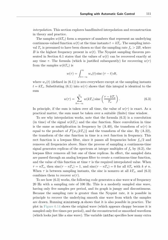
Sampling with Automatic Gain Control 111
interpolation. This section explores bandlimited interpolation and reconstruction
in theory and practice.
The samples w(kTs) form a sequence of numbers that represent an underlying
continuous-valued function w(t) at the time instants t = kTs. The sampling inter-
val Ts is presumed to have been chosen so that the sampling rate fs > 2B, where
B is the highest frequency present in w(t). The Nyquist sampling theorem pre-
sented in Section 6.1 states that the values of w(t) can be recovered exactly at
any time τ . The formula (which is justified subsequently) for recovering w(τ)
from the samples w(kTs) is
w(τ) =
∫ ∞
t=−∞ws(t) sinc (τ − t) dt,
where ws(t) (defined in (6.1)) is zero everywhere except at the sampling instants
t = kTs. Substituting (6.1) into w(τ) shows that this integral is identical to the
sum
w(τ) =
∞∑k=−∞
w(kTs) sinc
(τ − kTs
Ts
). (6.3)
In principle, if the sum is taken over all time, the value of w(τ) is exact. As a
practical matter, the sum must be taken over a suitable (finite) time window.
To see why interpolation works, note that the formula (6.3) is a convolution
(in time) of the signal w(kTs) and the sinc function. Since convolution in time
is the same as multiplication in frequency by (A.40), the transform of w(τ) is
equal to the product of F{ws(kTs)} and the transform of the sinc. By (A.22),
the transform of the sinc function in time is a rect function in frequency. This
rect function is a lowpass filter, since it passes all frequencies below fs/2 and
removes all frequencies above. Since the process of sampling a continuous-time
signal generates replicas of the spectrum at integer multiples of fs by (6.2), the
lowpass filter removes all but one of these replicas. In effect, the sampled data
are passed through an analog lowpass filter to create a continuous-time function,
and the value of this function at time τ is the required interpolated value. When
τ = nTs, then sinc(τ − nTs) = 1, and sinc(τ − nTs) = 0 for all kTs with k �= n.
When τ is between sampling instants, the sinc is nonzero at all kTs, and (6.3)
combines them to recover w(τ).
To see how (6.3) works, the following code generates a sine wave w of frequency
20 Hz with a sampling rate of 100 Hz. This is a modestly sampled sine wave,
having only five samples per period, and its graph is jumpy and discontinuous.
Because the sampling rate is greater than the Nyquist rate, it is possible in
principle to recover the underlying smooth sine wave from which the samples
are drawn. Running sininterp.m shows that it is also possible in practice. The
plot in Figure 6.14 shows the original wave (which appears choppy because it is
sampled only five times per period), and the reconstructed or smoothed waveform
(which looks just like a sine wave). The variable intfac specifies how many extra

112 Chapter 6. Sampling with Automatic Gain Control
−1
0
1
Am
plitu
de
10 10.1 10.2 10.3 10.4Time
Figure 6.14 A convincing sine wavecan be reconstructed from itssamples using sinc interpolation.The choppy wave represents thesamples, and the smooth waveshows the reconstruction.
interpolated points are calculated, and need not be an integer. Larger numbers
result in smoother curves but also require more computation.
Listing 6.3. sininterp.m demonstrate interpolation/reconstruction using sin wave
f =20; Ts=1/100; time=20; % sampling i n t e r v a l and timet=Ts : Ts : time ; % time vectorw=sin (2* pi* f * t ) ; % w( t ) = a s i n e wave o f f Hertzover=100; % # of data po ints in smoothingi n t f a c =10; % how many i n t e r po l a t ed po intstnow=10.0/Ts :1/ i n t f a c : 1 0 . 5 /Ts ; % i n t e r p o l a t e from 10 to 10 . 5
wsmooth=zeros ( size ( tnow ) ) ; % save smoothed data herefor i =1: length ( tnow ) % and loop f o r next point
wsmooth( i )= i n t e r p s i n c (w, tnow ( i ) , over ) ;end
In implementing (6.3), some approximations are used. First, the sum cannot
be calculated over an infinite time horizon, and the variable over replaces the
sum∑∞
k=−∞ with∑over
k=−over . Each pass through the for loop calculates one
point of the smoothed curve wsmooth using the Matlab function interpsinc.m,
which is shown below. The value of the sinc is calculated at each time using the
function srrc.m with the appropriate offset tau, and then the convolution is
performed by the conv command. This code is slow and unoptimized. A clever
programmer will see that there is no need to calculate the sinc for every point, and
efficient implementations use sophisticated look-up tables to avoid the calculation
of transcendental functions completely.
Listing 6.4. interpsinc.m interpolate to find a single point using the direct method
function y=i n t e r p s i n c (x , t , l , beta )% x = sampled data% t = place at which value de s i r ed% l = one−s ided l ength o f data to i n t e r p o l a t e% beta = r o l l o f f f a c t o r f o r s r r c f unc t i on% = 0 i s a s i n ci f nargin==3, beta=0; end ; % i f un spe c i f i ed , beta i s 0tnow=round ( t ) ; % s e t index tnow=i n t e g e r parttau=t−round ( t ) ; % plus tau=f r a c t i o n a l parts tau=s r r c ( l , beta , 1 , tau ) ; % i n t e r p o l a t e s i n c at o f f s e t taux tau=conv(x ( tnow− l : tnow+l ) , s tau ) ; % i n t e r p o l a t e the s i g n a ly=x tau (2* l +1); % to get the new sample
While the indexing needed in interpsinc.m is a bit tricky, the basic idea is
not: the sinc interpolation of (6.3) is just a linear filter with impulse response
h(t) = sinc(t). (Remember, convolutions are the hallmark of linear filters.) Thus,

Sampling with Automatic Gain Control 113
it is a lowpass filter, since the frequency response is a rect function. The delay τ
is proportional to the phase of the frequency response.
Exercise 6.18. In sininterp.m, what happens when the sampling rate is too
low? How large can the sampling interval Ts be? How high can the frequency f
be?
Exercise 6.19. In sininterp.m, what happens when the window is reduced?
Make over smaller and find out. What happens when too few points are inter-
polated? Make intfac smaller and find out.
Exercise 6.20. Create a more interesting (more complex) wave w(t). Answer
the above questions for this w(t).
Exercise 6.21. Let w(t) be a sum of five sinusoids for t between −10 and 10 s.
Let w(kT ) represent samples of w(t) with T = 0.01 s. Use interpsinc.m to inter-
polate the values w(0.011), w(0.013), and w(0.015). Compare the interpolated
values with the actual values. Explain any discrepancies.
Observe that sinc(t) dies away (slowly) in time at a rate proportional to
1/(πt). This is one of the reasons why so many terms are used in the convo-
lution (i.e., why the variable over is large). A simple way to reduce the num-
ber of terms is to use a function that dies away more quickly than the sinc; a
common choice is the square-root raised cosine (SRRC) function, which plays
an important role in pulse shaping in Chapter 11. The functional form of the
SRRC is given in Equation (11.8). The SRRC can easily be incorporated into
the interpolation code by replacing the code interpsinc(w,tnow(i),over)with
interpsinc(w,tnow(i),over,beta).
Exercise 6.22. With beta=0, the SRRC is exactly the sinc. Redo the above
exercises trying various values of beta between 0 and 1.
The function srrc.m is available on the website. Its help file is
% s=s r r c ( syms , beta , P, t o f f ) ;% Generate a Square−Root Raised Cosine Pulse% ’ syms ’ i s 1/2 the l ength o f s r r c pu l s e% in symbol durat i ons% ’ beta ’ i s the r o l l o f f f a c t o r :% beta=0 g i v e s the s i n c f unc t i on% ’P’ i s the oversampl ing f a c t o r% t o f f i s the phase ( or t iming ) o f f s e t
Matlab also has a built-in function called resample, which has the following
help file:
% Change the sampling r a t e o f a s i g n a l% Y = resample (X,P,Q) resamples the sequence% in vector X at P/Q times the o r i g i n a l sample

114 Chapter 6. Sampling with Automatic Gain Control
% rate us ing a polyphase implementation .% Y i s P/Q times the l ength o f X.% P and Q must be p o s i t i v e i n t e g e r s .
This technique is different from that used in (6.3). It is more efficient numer-
ically at reconstructing entire waveforms, but it works only when the desired
resampling rate is rationally related to the original. The method of (6.3) is far
more efficient when isolated (not necessarily evenly spaced) interpolating points
are required, which is crucial for synchronization tasks in Chapter 12.
6.5 Iteration and Optimization
An important practical part of the sampling procedure is that the dynamic range
of the signal at the input to the sampler must remain within bounds. This can be
accomplished using an automatic gain control, which is depicted in Figure 6.1 as
multiplication by a scalar a, along with a “quality assessment” block that adjusts
a in response to the power at the output of the sampler. This section discusses
the background needed to understand how the quality assessment works. The
essential idea is to state the goal of the assessment mechanism as an optimization
problem.
Many problems in communications (and throughout engineering) can be
framed in terms of an optimization problem. Solving such problems requires
three basic steps:
1. setting a goal—choosing a “performance” or “objective” function,
2. choosing a method of achieving the goal—minimizing or maximizing the objec-
tive function, and
3. testing to make sure the method works as anticipated.
“Setting the goal” usually consists of finding a function that can be minimized
(or maximized), and for which locating the minimum (or maximum) value pro-
vides useful information about the problem at hand. Moreover, the function
must be chosen carefully so that it (and its derivative) can be calculated from
quantities that are known, or that can be derived from signals that are easily
obtainable. Sometimes the goal is obvious, and sometimes it is not.
There are many ways of carrying out the minimization or maximization pro-
cedure. Some of these are direct. For instance, if the problem is to find the point
at which a polynomial function achieves its minimum value, this can be solved
directly by finding the derivative and setting it equal to zero. Often, however,
such direct solutions are impossible, and, even when they are possible, recursive
(or adaptive) approaches often have better properties when the signals are noisy.
This chapter focuses on a recursive method called steepest descent, which is the
basis of many adaptive elements used in communications systems (and of all the
elements used in Software Receiver Design).

Sampling with Automatic Gain Control 115
The final step in implementing any solution is to check that the method
behaves as desired, despite any simplifying assumptions that may have been
made in its derivation. This may involve a detailed analysis of the resulting
methodology, or it may involve simulations. Thorough testing would involve both
analysis and simulation in a variety of settings that mimic, as closely as possible,
the situations in which the method will be used.
Imagine being lost on a mountainside on a foggy night. Your goal is to
get to the village which lies at the bottom of a valley below. Though
you cannot see far, you can reach out and feel the nearby ground. If you
repeatedly step in the direction that heads downhill most steeply, you
eventually reach a depression in which all directions lead up. If the con-
tour of the land is smooth, and without any local depressions that can
trap you, then you will eventually arrive at the village. The optimization
procedure called “steepest descent” implements this scenario mathemat-
ically, where the mountainside is defined by the “performance” function
and the optimal answer lies in the valley at the minimum value. Many
standard communications algorithms (adaptive elements) can be viewed
in this way.
6.6 An Example of Optimization: Polynomial Minimization
This first example is too simple to be of practical use, but it does show many
of the ideas starkly. Suppose that the goal is to find the value at which the
polynomial
J(x) = x2 − 4x+ 4 (6.4)
achieves its minimum value. Thus step (1) is set. As any calculus book will
suggest, the direct way to find the minimum is to take the derivative, set it
equal to zero, and solve for x. Thus, dJ(x)/dx = 2x− 4 = 0 is solved when x =
2. This is indeed the value of x for which the parabola J(x) reaches bottom.
Sometimes (one might truthfully say “often”), however, such direct approaches
are impossible. Maybe the derivative is just too complicated to solve (which can
happen when the functions involved in J(x) are extremely nonlinear). Or maybe
the derivative of J(x) cannot be calculated precisely from the available data, and
instead must be estimated from a noisy data stream.
One alternative to the direct solution technique is an adaptive method called
“steepest descent” (when the goal is to minimize) or “hill climbing” (when the
goal is to maximize). Steepest descent begins with an initial guess of the loca-
tion of the minimum, evaluates which direction from this estimate is most steeply
“downhill,” and then makes a new estimate along the downhill direction. Simi-
larly, hill climbing begins with an initial guess of the location of the maximum,
evaluates which direction climbs the most rapidly, and then makes a new esti-
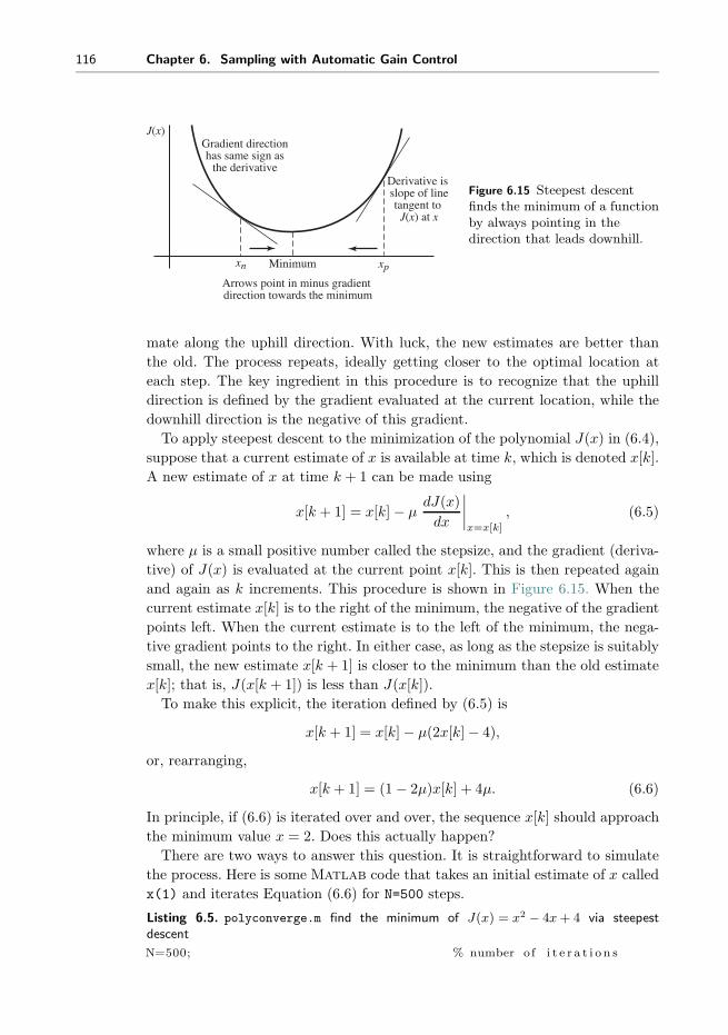
116 Chapter 6. Sampling with Automatic Gain Control
J(x)
Minimum
Derivative is slope of linetangent to
J(x) at x
Gradient directionhas same sign as
the derivative
xn xp
Arrows point in minus gradient direction towards the minimum
Figure 6.15 Steepest descentfinds the minimum of a functionby always pointing in thedirection that leads downhill.
mate along the uphill direction. With luck, the new estimates are better than
the old. The process repeats, ideally getting closer to the optimal location at
each step. The key ingredient in this procedure is to recognize that the uphill
direction is defined by the gradient evaluated at the current location, while the
downhill direction is the negative of this gradient.
To apply steepest descent to the minimization of the polynomial J(x) in (6.4),
suppose that a current estimate of x is available at time k, which is denoted x[k].
A new estimate of x at time k + 1 can be made using
x[k + 1] = x[k]− μdJ(x)
dx
∣∣∣∣x=x[k]
, (6.5)
where μ is a small positive number called the stepsize, and the gradient (deriva-
tive) of J(x) is evaluated at the current point x[k]. This is then repeated again
and again as k increments. This procedure is shown in Figure 6.15. When the
current estimate x[k] is to the right of the minimum, the negative of the gradient
points left. When the current estimate is to the left of the minimum, the nega-
tive gradient points to the right. In either case, as long as the stepsize is suitably
small, the new estimate x[k + 1] is closer to the minimum than the old estimate
x[k]; that is, J(x[k + 1]) is less than J(x[k]).
To make this explicit, the iteration defined by (6.5) is
x[k + 1] = x[k]− μ(2x[k]− 4),
or, rearranging,
x[k + 1] = (1− 2μ)x[k] + 4μ. (6.6)
In principle, if (6.6) is iterated over and over, the sequence x[k] should approach
the minimum value x = 2. Does this actually happen?
There are two ways to answer this question. It is straightforward to simulate
the process. Here is some Matlab code that takes an initial estimate of x called
x(1) and iterates Equation (6.6) for N=500 steps.
Listing 6.5. polyconverge.m find the minimum of J(x) = x2 − 4x+ 4 via steepestdescent
N=500; % number o f i t e r a t i o n s

Sampling with Automatic Gain Control 117
−2
−1
0
1
2
3
4
5
0 50 100 150 200 250 300 350 400
Star
ting
valu
es
Time
Figure 6.16 The programpolyconverge.m attempts tolocate the smallest value ofJ(x) = x2 − 4x+ 4 by descendingthe gradient. Fifty differentstarting values all converge to thesame minimum at x = 2.
mu=.01; % algor i thm s t e p s i z ex=zeros (1 ,N) ; % i n i t i a l i z e x to zerox (1)=3; % s t a r t i n g point x (1)for k=1:N−1
x (k+1)=(1−2*mu)*x ( k)+4*mu; % update equationend
Figure 6.16 shows the output of polyconverge.m for 50 different x(1) starting
values superimposed; all converge smoothly to the minimum at x = 2.
Exercise 6.23. Explore the behavior of steepest descent by running
polyconverge.m with different parameters.
a. Try mu = −0.01, 0, 0.0001, 0.02, 0.03, 0.05, 1.0, 10.0. Can mu be too large or
too small?
b. Try N = 5, 40, 100, 5000. Can N be too large or too small?
c. Try a variety of values of x(1). Can x(1) be too large or too small?
As an alternative to simulation, observe that the process (6.6) is itself a linear
time-invariant system, of the general form
x[k + 1] = ax[k] + b, (6.7)
which is stable as long as |a| < 1. For a constant input, the final-value theorem of
z-transforms (see (A.55)) can be used to show that the asymptotic (convergent)
output value is limk→∞ xk = b/(1− a). To see this without reference to arcane
theory, observe that if xk is to converge, then it must converge to some value,
say x∗. At convergence, x[k + 1] = x[k] = x∗, so (6.7) implies that x∗ = ax∗ +b, which implies that x∗ = b/(1− a). (This holds assuming that |a| < 1.) For
example, for (6.6), x∗ = 4μ/[1− (1− 2μ)] = 2, which is indeed the minimum.
Thus, both simulation and analysis suggest that the iteration (6.6) is a viable
way to find the minimum of the function J(x), as long as μ is suitably small. As
will become clearer in later sections, such solutions to optimization problems are
almost always possible—as long as the function J(x) is differentiable. Similarly, it

118 Chapter 6. Sampling with Automatic Gain Control
is usually quite straightforward to simulate the algorithm to examine its behavior
in specific cases, though it is not always so easy to carry out a theoretical analysis.
By their nature, steepest-descent and hill-climbing methods use only local
information. This is because the update from a point x[k] depends only on the
value of x[k] and on the value of its derivative evaluated at that point. This can
be a problem, since if the objective function has many minima, the steepest-
descent algorithm may become “trapped” at a minimum that is not (globally)
the smallest. These are called local minima. To see how this can happen, consider
the problem of finding the value of x that minimizes the function
J(x) = e−0.1|x| sin(x). (6.8)
Applying the chain rule, the derivative is
e−0.1 |x| cos(x) − 0.1e−0.1 |x| sin(x) sign(x),
where
sign(x) =
{1 x > 0
−1 x < 0(6.9)
is the formal derivative of |x|. Solving directly for the minimum point is nontrivial
(try it!). Yet implementing a steepest-descent search for the minimum can be
done in a straightforward manner using the iteration
x[k + 1] = x[k]− μe−0.1 |x[k]| · (cos(x[k])− 0.1 sin(x[k])sign(x)). (6.10)
To be concrete, replace the update equation in polyconverge.m with
x (k+1) = x(k ) − mu * exp(−0.1 * abs ( x (k ) ) ) * . . .( cos (x ( k ) ) − 0 .1 * sin (x ( k ) ) * sign ( x (k ) ) ) ;
Exercise 6.24. Implement the steepest-descent strategy to find the minimum of
J(x) in (6.8), modeling the program after polyconverge.m. Run the program for
different values of mu, N, and x(1), and answer the same questions as in Exercise
6.23.
One way to understand the behavior of steepest-descent algorithms is to plot
the error surface, which is basically a plot of the objective as a function of the
variable that is being optimized. Figure 6.17(a) displays clearly the single global
minimum of the objective function (6.4) while Figure 6.17(b) shows the many
minima of the objective function defined by (6.8). As will be clear to anyone
who has attempted Exercise 6.24, initializing within any one of the valleys causes
the algorithm to descend to the bottom of that valley. Although true steepest-
descent algorithms can never climb over a peak to enter another valley (even if
the minimum there is lower), it can sometimes happen in practice when there is
a significant amount of noise in the measurement of the downhill direction.
Essentially, the algorithm gradually descends the error surface by moving
in the (locally) downhill direction, and different initial estimates may lead to

Sampling with Automatic Gain Control 119
−20 −15 −10 −5 0 5 10 15 20
−0.5
0.5
0
10
20
30
40
−4 −2 0 2 4 6 8
J(x)
J(x)
xx
Figure 6.17 Error surfaces corresponding to (a) the objective function (6.4) and (b)the objective function (6.8).
different minima. This underscores one of the limitations of steepest-descent
methods—if there are many minima, then it is important to initialize near an
acceptable one. In some problems such prior information may easily be obtained,
while in others it may be truly unknown.
The examples of this section are somewhat simple because they involve static
functions. Most applications in communication systems deal with signals that
evolve over time, and the next section applies the steepest-descent idea in a
dynamic setting to the problem of automatic gain control (AGC). The AGC
provides a simple setting in which all three of the major issues in optimization
must be addressed: setting the goal, choosing a method of solution, and verifying
that the method is successful.
Exercise 6.25. Consider performing an iterative maximization of
J(x) = 8− 6|x|+ 6 cos(6x)
via (6.5) with the sign on the update reversed (so that the algorithm will maxi-
mize rather than minimize). Suppose the initialization is x[0] = 0.7.
a. Assuming the use of a suitably small stepsize μ, determine the convergent
value of x.
b. Is the convergent value of x in part (a) the global maximum of J(x)? Justify
your answer by sketching the error surface.
Exercise 6.26. Suppose that a unimodal single-variable performance function
has only one point with zero derivative and that all points have a positive second
derivative. TRUE or FALSE: A gradient-descent method will converge to the
global minimum from any initialization.
Exercise 6.27. Consider the modulated signal
r(t) = w(t) cos(2πfct+ φ),

120 Chapter 6. Sampling with Automatic Gain Control
where the absolute bandwidth of the baseband message waveform w(t) is less
than fc/2. The signals x and y are generated via
x(t) = LPF{r(t) cos(2πfct+ θ)},y(t) = LPF{r(t) sin(2πfct+ θ)},
where the LPF cutoff frequency is fc/2.
a. Determine x(t) in terms of w(t), fc, φ, and θ.
b. Show that
d
dθ
{1
2x2(t)
}= −x(t)y(t)
using the fact that derivatives and filters commute as in (G.5).
c. Determine the values of θ maximizing x2(t).
Exercise 6.28. Consider the function
J(x) = (1− |x− 2|)2 .a. Sketch J(x) for −5 ≤ x ≤ 5.
b. Analytically determine all local minima and maxima of J(x) for −5 ≤ x ≤ 5.
Hint: d|f(b)|db
= sign(f(b))df(b)db
where sign(a) is defined in (6.9).
c. Is J(x) unimodal as a function of x? Explain your answer.
d. Develop an iterative gradient-descent algorithm for updating x to minimize
J .
e. For an initial estimate of x = 1.2, what is the convergent value of x determined
by an iterative gradient-descent algorithm with a satisfactorily small stepsize?
f. Compute the direction (either increasing x or decreasing x) of the update
from (d) for x = 1.2.
g. Does the direction determined in part (f) point from x = 1.2 toward the con-
vergent value of part (e)? Should it (for a correct answer to (e))? Explain your
answer.
6.7 Automatic Gain Control
Any receiver is designed to handle signals of a certain average magnitude most
effectively. The goal of an AGC is to amplify weak signals and to attenuate strong
signals so that they remain (as much as possible) within the normal operating
range of the receiver. Typically, the rate at which the gain varies is slow compared
with the data rate, though it may be fast by human standards.
The power in a received signal depends on many things: the strength of the
broadcast, the distance from the transmitter to the receiver, the direction in
which the antenna is pointed, and whether there are any geographical features
such as mountains (or tall buildings) that block, reflect, or absorb the signal.

Sampling with Automatic Gain Control 121
(a) (b)
quan
tizat
ion
leve
ls
Figure 6.18 The goal of the AGC is tomaintain the dynamic range of thesignal by attenuating it when it is toolarge (as in (a)) and by increasing itwhen it is too small (as in (b)).
ar(t) s(kT) = s[k]
SamplerInput Output
QualityAssessment
Figure 6.19 An automatic gain control adjusts thegain parameter a so that the average energy atthe output remains (roughly) fixed, despitefluctuations in the average received energy.
While more power is generally better from the point of view of trying to deci-
pher the transmitted message, there are always limits to the power-handling
capabilities of the receiver. Hence, if the received signal is too large (on average),
it must be attenuated. Similarly, if the received signal is weak (on average), then
it must be amplified.
Figure 6.18 shows the two extremes that the AGC is designed to avoid. In part
(a), the signal is much larger than the levels of the sampling device (indicated
by the horizontal lines). The gain must be made smaller. In part (b), the signal
is much too small to be captured effectively, and the gain must be increased.
There are two basic approaches to an AGC. The traditional approach uses ana-
log circuitry to adjust the gain before the sampling. The more modern approach
uses the output of the sampler to adjust the gain. The advantage of the analog
method is that the two blocks (the gain and the sampling) are separate and
do not interact. The advantage of the digital adjustment is that less additional
hardware is required since the DSP is already present for other tasks.
A simple digital system for AGC adjustment is shown in Figure 6.19. The
input r(t) is multiplied by the gain a to give the normalized signal s(t). This is
then sampled to give the output s[k]. The assessment block measures s[k] and
determines whether a must be increased or decreased.
The goal is to choose a so that the power (or average energy) of s(t) is approx-
imately equal to some specified S2. Since
a2 avg{r2(t)}∣∣t=kT
≈ avg{s2(kT )} ≈ avg{s2[k]},

122 Chapter 6. Sampling with Automatic Gain Control
it would be ideal to choose
a2 ≈ S2
avg{r2(kT )} , (6.11)
because this would imply that avg{s2(kT )} ≈ S2. The averaging operation (in
this case a moving average over a block of data of size N) is defined by
avg{x[k]} =1
N
k∑i=k−N+1
x[i]
and is discussed in Appendix G in amazing detail. Unfortunately, neither the
analog input r(t) nor its power is directly available to the assessment block in
the DSP portion of the receiver, so it is not possible to directly implement (6.11).
Is there an adaptive element that can accomplish this task? As suggested at
the beginning of Section 6.5, there are three steps to the creation of a viable
optimization approach: setting a goal, choosing a solution method, and testing.
As in any real-life engineering task, a proper mathematical statement of the
goal can be tricky, and this section proposes two (slightly different) possibilities
for the AGC. By comparing the resulting algorithms (essentially, alternative
forms for the AGC design), it may be possible to trade off among various design
considerations.
One sensible goal is to try to minimize a simple function of the difference
between the power of the sampled signal s[k] and the desired power S2. For
instance, the averaged squared error in the powers of s and S,
JLS(a) = avg
{1
4(s2[k]− S2)2
}=
1
4avg{(a2r2(kT )− S2)2}, (6.12)
penalizes values of a that cause s2[k] to deviate from S2. This formally mimics
the parabolic form of the objective (6.4) in the polynomial minimization example
of the previous section. Applying the steepest-descent strategy yields
a[k + 1] = a[k]− μdJLS(a)
da
∣∣∣∣a=a[k]
, (6.13)
which is the same as (6.5), except that the name of the parameter has changed
from x to a. To find the exact form of (6.13) requires the derivative of JLS(a) with
respect to the unknown parameter a. This can be approximated by swapping the
derivative and the averaging operations, as formalized in (G.12), to give
dJLS(a)
da=
1
4
davg{(a2r2(kT )− S2)2}da
≈ 1
4avg
{d(a2r2(kT )− S2)2
da
}= avg{(a2r2(kT )− S2)ar2(kT )}.
The term a2r2(kT ) inside the parentheses is equal to s2[k]. The term ar2(kT )
outside the parentheses is not directly available to the assessment mechanism,

Sampling with Automatic Gain Control 123
though it can reasonably be approximated by s2[k]/a. Substituting the derivative
into (6.13) and evaluating at a = a[k] gives the algorithm
a[k + 1] = a[k]− μ avg
{(s2[k]− S2)
s2[k]
a[k]
}. (6.14)
Care must be taken when implementing (6.14) that a[k] does not approach zero.
Of course, JLS(a) of (6.12) is not the only possible goal for the AGC problem.
What is important is not the exact form of the performance function, but where
the performance function has its optimal points. Another performance function
that has a similar error surface (peek ahead to Figure 6.21) is
JN (a) = avg
{|a|(s2[k]
3− S2
)}= avg
{|a|(a2r2(kT )
3− S2
)}. (6.15)
Taking the derivative gives
dJN (a)
da=
davg{|a|(a2r2(kT )/3− S2)}da
≈ avg
{d |a|(a2r2(kT )/3− S2)
da
}= avg{sgn(a[k])(s2[k]− S2)},
where the approximation arises from swapping the order of the differentiation
and the averaging (recall (G.12)) and the derivative of | · | is the signum or sign
function, which holds as long as the argument is nonzero. Evaluating this at
a = a[k] and substituting into (6.13) gives another AGC algorithm:
a[k + 1] = a[k]− μ avg{sgn(a[k])(s2[k]− S2)}. (6.16)
Consider the “logic” of this algorithm. Suppose that a is positive. Since S is
fixed,
avg{sgn(a[k])(s2[k]− S2)} = avg{(s2[k]− S2)} = avg{s2[k]} − S2.
Thus, if the average energy in s[k] exceeds S2, a is decreased. If the average energy
in s[k] is less than S2, a is increased. The update ceases when avg{s2[k]} ≈ S2,
that is, where a2 ≈ S2/r2, as desired. (An analogous logic applies when a is
negative.)
The two performance functions (6.12) and (6.15) define the updates for the
two adaptive elements in (6.14) and (6.16). JLS(a) minimizes the square of the
deviation of the power in s[k] from the desired power S2. This is a kind of
“least-square” performance function (hence the subscript LS). Such squared-
error objectives are common, and will reappear in phase-tracking algorithms
in Chapter 10, in clock recovery algorithms in Chapter 12, and in equalization
algorithms in Chapter 13. On the other hand, the algorithm resulting from JN (a)
has a clear logical interpretation (the N stands for “naive”), and the update is
simpler, since (6.16) has fewer terms and no divisions.
To experiment concretely with these algorithms, agcgrad.m provides an imple-
mentation in Matlab. It is easy to control the rate at which a[k] changes by

124 Chapter 6. Sampling with Automatic Gain Control
choice of stepsize: a larger μ allows a[k] to change faster, while a smaller μ allows
greater smoothing. Thus, μ can be chosen by the system designer to trade off
the bandwidth of a[k] (the speed at which a[k] can track variations in the energy
levels of the incoming signal) versus the amount of jitter or noise. Similarly, the
length over which the averaging is done (specified by the parameter lenavg)
will also influence the speed of adaptation; longer averages imply slower-moving,
smoother estimates while shorter averages imply faster-moving, more jittery esti-
mates.
Listing 6.6. agcgrad.m minimize the performance function J(a) = avg{|a|((1/3)a2r2 −ds)} by choice of a
n=10000; % number o f s t ep s in s imulat i onvr =1.0; % power o f the inputr=sqrt ( vr )*randn (n , 1 ) ; % generate random inputsds =0.15; % de s i r ed power o f outputmu=0.001; % algor i thm s t e p s i z elenavg =10; % length over which to averagea=zeros (n , 1 ) ; a (1)=1; % i n i t i a l i z e AGC parameters=zeros (n , 1 ) ; % i n i t i a l i z e outputsavec=zeros (1 , l enavg ) ; % vector to s to r e averag ing termsfor k=1:n−1
s ( k)=a ( k )* r (k ) ; % normal ize by a ( k ) & add to avec
avec=[sign ( a ( k ) )* ( s (k)ˆ2−ds ) , avec ( 1 : lenavg −1 ) ] ;a ( k+1)=a (k)−mu*mean( avec ) ; % average adaptive update o f a ( k )
end
Typical output of agcgrad.m is shown in Figure 6.20. The gain parameter a
adjusts automatically to make the overall power of the output s roughly equal
to the specified parameter ds. Using the default values above, where the average
power of r is approximately 1, we find that a converges to about 0.38 since
0.382 ≈ 0.15 = S2.
The objective JLS(a) can be implemented similarly by replacing the avec
calculation inside the for loop with
avec =[( s ( k)ˆ2−ds )* ( s ( k )ˆ2)/ a (k ) , avec ( 1 :end−1 ) ] ;
In this case, with the default values, a converges to about 0.22, which is the
value that minimizes the least-square objective JLS(a). Thus, the answer which
minimizes JLS(a) is different from the answer which minimizes JN (a)! More on
this later.
As it is easy to see when playing with the parameters in agcgrad.m, the
size of the averaging parameter lenavg is relatively unimportant. Even with
lenavg=1, the algorithms converge and perform approximately the same! This
is because the algorithm updates are themselves in the form of a lowpass filter.
(See Appendix G for a discussion of the similarity between averagers and lowpass
filters.) Removing the averaging from the update gives the simpler form for JN (a)
a (k+1)=a ( k)−mu* sign ( a (k ) )* ( s (k)ˆ2−ds ) ;
or, for JLS(a),
a (k+1)=a ( k)−mu*( s ( k)ˆ2−ds )* ( s ( k )ˆ2)/ a (k ) ;

Sampling with Automatic Gain Control 125
0 2000 4000 6000 8000 10000
Iterations
Am
plitu
de
Output s(k)
Input r(k)
Adaptive gain parameter
−5
0
5
−5
0
5
0
1
2
1.5
0.5
Figure 6.20 An automatic gaincontrol adjusts the parameter a(in the top panel) automaticallyto achieve the desired outputpower.
Try them!
Perhaps the best way to formally describe how the algorithms work is to plot
the performance functions. But it is not possible to directly plot JLS(a) or JN (a),
since they depend on the data sequence s[k]. What is possible (and often leads
to useful insights) is to plot the performance function averaged over a number
of data points (also called the error surface). As long as the stepsize is small
enough and the average is long enough, the mean behavior of the algorithm will
be dictated by the shape of the error surface in the same way that the objective
function of the exact steepest-descent algorithm (for instance, the objectives
(6.4) and (6.8)) dictates the evolution of the algorithms (6.6) and (6.10).
The following code agcerrorsurf.m shows how to calculate the error surface
for JN (a). The variable n specifies the number of terms to average over, and tot
sums up the behavior of the algorithm for all n updates at each possible param-
eter value a. The average of these (tot/n) is a close (numerical) approximation
to JN (a) of (6.15). Plotting over all a gives the error surface.
Listing 6.7. agcerrorsurf.m draw the error surface for the AGC
n=10000; % number o f s t ep s in s imulat i onr=randn (n , 1 ) ; % generate random inputsds =0.15; % de s i r ed power o f outputrange = [ − 0 . 7 : 0 . 0 2 : 0 . 7 ] ; % s p e c i f y range o f va lues o f aJagc=zeros ( size ( range ) ) ; j =0;for a=range % f o r each value a
j=j +1; tot =0; % t o t a l cos tfor i =1:n % over a l l p o s s i b i l i t i e s
tot=tot+abs ( a )* ( (1/3)* aˆ2* r ( i )ˆ2−ds ) ;end
Jagc ( j )=tot /n ; % take average valueend

126 Chapter 6. Sampling with Automatic Gain Control
−0.6 −0.4 −0.2 0 0.2 0.4 0.60
0.005
0.015
0.025
cost
JL
S(a)
−0.04
−0.02
0
0.02
cost
JN
(a)
Adaptive gain a
−0.6 −0.4 −0.2 0 0.2 0.4 0.6
Adaptive gain a
Figure 6.21 The error surface for the AGC objective functions (6.12) and (6.15) eachhave two minima. As long as a can be initialized with the correct (positive) sign,there is little danger of converging to the wrong minimum.
Similarly, the error surface for JLS(a) can be plotted using
tot=tot +0.25*(aˆ2* r ( i )ˆ2−ds )ˆ2 ; % er r o r su r f a c e f o r JLS
The output of agcerrorsurf.m for both objective functions is shown in Figure
6.21. Observe that zero (which is a critical point of the error surface) is a local
maximum in both cases. The final converged answers (a ≈ 0.38 for JN (a) and a ≈0.22 for JLS(a)) occur at minima. Were the algorithm to be initialized improperly
to a negative value, then it would converge to the negative of these values. As
with the algorithms in Figure 6.17, examination of the error surfaces shows why
the algorithms converge as they do. The parameter a descends the error surface
until it can go no further.
But why do the two algorithms converge to different places? The facile answer
is that they are different because they minimize different performance functions.
Indeed, the error surfaces in Figure 6.21 show minima in different locations.
The convergent value of a ≈ 0.38 for JN (a) is explicable because 0.382 ≈ 0.15 =
S2. The convergent value of a = 0.22 for JLS(a) is calculated in closed form in
Exercise 6.30, and this value does a good job minimizing its cost, but it has not
solved the problem of making a2 close to S2. Rather, JLS(a) calculates a smaller
gain that makes avg{s2} ≈ S2. The minima are different. The moral is this: be
wary of your performance functions—they might do what you ask.
Exercise 6.29. Use agcgrad.m to investigate the AGC algorithm.
a. What range of stepsize mu works? Can the stepsize be too small? Can the
stepsize be too large?
b. How does the stepsize mu affect the convergence rate?
c. How does the variance of the input affect the convergent value of a?
d. What range of averages lenavg works? Can lenavg be too small? Can lenavg
be too large?
e. How does lenavg affect the convergence rate?

Sampling with Automatic Gain Control 127
Exercise 6.30. Show that the value of a that achieves the minimum of JLS(a)
can be expressed as
±√
S2∑
k r2k∑
k r4k
.
Is there a way to use this (closed-form) solution to replace the iteration (6.14)?
Exercise 6.31. Consider the alternative objective function J(a) =12a
2(s2[k]/6− S2). Calculate the derivative and implement a variation of
the AGC algorithm that minimizes this objective. How does this version
compare with the algorithms (6.14) and (6.16)? Draw the error surface for this
algorithm. Which version is preferable?
Exercise 6.32. Try initializing the estimate a(1)=-2 in agcgrad.m. Which min-
imum does the algorithm find? What happens to the data record?
Exercise 6.33. Create your own objective function J(a) for the AGC problem.
Calculate the derivative and implement a variation of the AGC algorithm that
minimizes this objective. How does this version compare with the algorithms
(6.14) and (6.16)? Draw the error surface for your algorithm. Which version do
you prefer?
Exercise 6.34. Investigate how the error surface depends on the input signal.
Replace randn with rand in agcerrorsurf.m and draw the error surfaces for
JN (a) and JLS(a).
6.8 Using an AGC to Combat Fading
One of the impairments encountered in transmission systems is the degradation
due to fading, when the strength of the received signal changes in response
to changes in the transmission path. (Recall the discussion in Section 4.1.5 on
page 64.) This section shows how an AGC can be used to counteract the fading,
assuming the rate of the fading is slow, and provided the signal does not disappear
completely.
Suppose that the input consists of a random sequence undulating slowly up
and down in magnitude, as in the top plot of Figure 6.22. The adaptive AGC
compensates for the amplitude variations, growing small when the power of the
input is large, and large when the power of the input is small. This is shown
in the middle graph. The resulting output is of roughly constant amplitude, as
shown in the bottom plot of Figure 6.22.
This figure was generated using the following code:

128 Chapter 6. Sampling with Automatic Gain Control
−5
x104
0
5
0 1 2 3 4 5
−5
0
5
Input r[k]
Adaptive gain parameter
0.5
1
0
1.5
Output s[k]
Iterations
Figure 6.22 When the signal fades(top), the adaptive parametercompensates (middle), allowingthe output to maintain nearlyconstant power (bottom).
Listing 6.8. agcvsfading.m compensating for fading with an AGC
n=50000; % # s tep s in s imulat i onr=randn (n , 1 ) ; % generate random inputsenv=0.75+abs( sin (2* pi * [ 1 : n ] ’ / n ) ) ; % the f ad ing p r o f i l er=r . * env ; % apply to raw input r [ k ]ds =0.5; % de s i r ed power o f outputa=zeros (1 , n ) ; a (1)=1; % i n i t i a l i z e AGC parameters=zeros (1 , n ) ; % i n i t i a l i z e outputsmu=0.01; % algor i thm s t e p s i z efor k=1:n−1
s ( k)=a ( k )* r (k ) ; % normal ize by a to get sa ( k+1)=a (k)−mu*( s (k)ˆ2−ds ) ; % adaptive update o f a ( k )
end
The “fading profile” defined by the vector env is slow compared with the rate
at which the adaptive gain moves, which allows the gain to track the changes.
Also, the power of the input never dies away completely. The problems that
follow ask you to investigate what happens in more extreme situations.
Exercise 6.35. Mimic the code in agcvsfading.m to investigate what happens
when the input signal dies away. (Try removing the abs command from the
fading profile variable.) Can you explain what you see?
Exercise 6.36. Mimic the code in agcvsfading.m to investigate what happens
when the power of the input signal varies rapidly. What happens if the sign of
the gain estimate is incorrect?
Exercise 6.37. Would the answers to the previous two problems change on
using algorithm (6.14) instead of (6.16)?

Sampling with Automatic Gain Control 129
6.9 Summary
Sampling transforms a continuous-time analog signal into a discrete-time digital
signal. In the time domain, this can be viewed as a multiplication by a train of
pulses. In the frequency domain this corresponds to a replication of the spectrum.
As long as the sampling rate is fast enough that the replicated spectra do not
overlap, the sampling process is reversible; that is, the original analog signal can
be reconstructed from the samples.
An AGC can be used to make sure that the power of the analog signal remains
in the region where the sampling device operates effectively. The same AGC,
when adaptive, can also provide a protection against signal fades. The AGC can
be designed using a steepest-descent (optimization) algorithm that updates the
adaptive parameter by moving in the direction of the negative of the derivative.
This steepest-descent approach to the solution of optimization problems will be
used throughout Software Receiver Design.
For Further Reading
Details about resampling procedures are available in the published works of
� Smith, J. O. “Bandlimited interpolation—interpretation and algorithm,”
1993, http://ccrma-www.stanford.edu/∼jos/resample/ .
A general introduction to adaptive algorithms centered around the steepest-
descent approach can be found in
� B. Widrow and S. D. Stearns, Adaptive Signal Processing, Prentice-Hall, 1985.
One of our favorite discussions of adaptive methods is
� C. R. Johnson Jr., Lectures on Adaptive Parameter Estimation, Prentice-Hall,
1988.

7 Digital Filtering and the DFT
Once the received signal is sampled, the real story of the digital receiver begins.
An analog bandpass filter at the front end of the receiver removes extraneous
signals (for instance, it removes television-frequency signals from a radio receiver)
but some portion of the signal from other FDM users may remain. While it would
be conceptually possible to remove all but the desired user at the start, accurate
retunable analog filters are complicated and expensive to implement. Digital
filters, on the other hand, are easy to design, inexpensive (once the appropriate
DSP hardware is present), and easy to retune. The job of cleaning up out-of-
band interferences left over by the analog BPF can be left to the digital portion
of the receiver.
Of course, there are many other uses for digital filters in the receiver, and
this chapter focuses on how to “build” digital filters. The discussion begins by
considering the digital impulse response and the related notion of discrete-time
convolution. Conceptually, this closely parallels the discussion of linear systems in
Chapter 4. The meaning of the DFT (discrete Fourier transform) closely parallels
the meaning of the Fourier transform, and several examples encourage fluency in
the spectral analysis of discrete data signals. The final section on practical filter-
ing shows how to design digital filters with (more or less) any desired frequency
response by using special Matlab commands.
7.1 Discrete Time and Discrete Frequency
The study of discrete-time (digital) signals and systems parallels that of
continuous-time (analog) signals and systems. Many digital processes are fun-
damentally simpler than their analog counterparts, though there are a few sub-
tleties unique to discrete-time implementations. This section begins with a brief
overview and comparison, and then proceeds to discuss the DFT, which is the
discrete counterpart of the Fourier transform.

Digital Filtering and the DFT 131
Just as the impulse function δ(t) plays a key role in defining signals and systems
in continuous time, the discrete pulse
δ[k] =
{1 k = 0
0 k �= 0(7.1)
can be used to decompose discrete signals and to characterize discrete-time
systems.1 Any discrete-time signal can be written as a linear combination
of discrete impulses. For instance, if the signal w[k] is the repeating pattern
{−1, 1, 2, 1,−1, 1, 2, 1, . . .}, it can be written
w[k] =− δ[k] + δ[k − 1] + 2δ[k − 2] + δ[k − 3]− δ[k − 4]
+ δ[k − 5] + 2δ[k − 6] + δ[k − 7] . . .
In general, the discrete-time signal w[k] can be written
w[k] =∞∑
j=−∞w[j]δ[k − j].
This is the discrete analog of the sifting property (4.4); simply replace the integral
with a sum, and replace δ(t) with δ[k].
Like their continuous-time counterparts, discrete-time systems map input sig-
nals into output signals. Discrete-time LTI (linear time-invariant) systems are
characterized by an impulse response h[k], which is the output of the system
when the input is an impulse, though, of course, (7.1) is used instead of (4.2).
When an input x[k] is more complicated than a single pulse, the output y[k] can
be calculated by summing all the responses to all the individual terms, and this
leads directly to the definition of discrete-time convolution:
y[k] =∞∑
j=−∞x[j]h[k − j] ≡ x[k] ∗ h[k]. (7.2)
Observe that the convolution of discrete-time sequences appears in the recon-
struction formula (6.3), and that (7.2) parallels continuous-time convolution in
(4.8) with the integral replaced by a sum and the impulse response h(t) replaced
by h[k].
The discrete-time counterpart of the Fourier transform is the discrete Fourier
transform (DFT). Like the Fourier transform, the DFT decomposes signals into
their constituent sinusoidal components. Like the Fourier transform, the DFT
provides an elegant way to understand the behavior of LTI systems by looking
at the frequency response (which is equal to the DFT of the impulse response).
Like the Fourier transform, the DFT is an invertible, information-preserving
transformation.
1 The pulse in discrete time is considerably more straightforward than the implicit definitionof the continuous-time impulse function in (4.2) and (4.3).

132 Chapter 7. Digital Filtering and the DFT
The DFT differs from the Fourier transform in three useful ways. First, it
applies to discrete-time sequences, which can be stored and manipulated directly
in computers (rather than to analog waveforms, which cannot be directly stored
in digital computers). Second, it is a sum rather than an integral, and so is easy
to implement either in hardware or in software. Third, it operates on a finite
data record, rather than an integration over all time. Given a data record (or
vector) w[k] of length N , the DFT is defined by
W [n] =
N−1∑k=0
w[k]e−j(2π/N)nk (7.3)
for n = 0, 1, 2, . . . , N − 1. For each value n, (7.3) multiplies each term of the
data by a complex exponential, and then sums. Compare this with the Fourier
transform; for each frequency f , (2.1) multiplies each point of the waveform by
a complex exponential, and then integrates. Thus W [n] is a kind of frequency
function in the same way that W (f) is a function of frequency. The next section
will make this relationship explicit by showing how e−j(2π/N)nk can be viewed as
a discrete-time sinusoid with frequency proportional to n. Just as a plot of the
frequency function W (f) is called the spectrum of the signal w(t), plots of the
frequency function W [n] are called the (discrete) spectrum of the signal w[k].
One source of confusion is that the frequency f in the Fourier transform can
take on any value while the frequencies present in (7.3) are all integer multiples
n of a single fundamental with frequency 2π/N . This fundamental is precisely
the sine wave with period equal to the length N of the window over which the
DFT is taken. Thus, the frequencies in (7.3) are constrained to a discrete set;
these are the “discrete frequencies” of the section title.
The most common implementation of the DFT is called the fast Fourier trans-
form (FFT), which is an elegant way to rearrange the calculations in (7.3) so that
it is computationally efficient. For all purposes other than numerical efficiency,
the DFT and the FFT are synonymous.
Like the Fourier transform, the DFT is invertible. Its inverse, the IDFT, is
defined by
w[k] =1
N
N−1∑n=0
W [n]ej(2π/N)nk (7.4)
for k = 0, 1, 2, . . . , N − 1. The IDFT takes each point of the frequency function
W [n], multiplies by a complex exponential, and sums. Compare this with the
IFT; (D.2) takes each point of the frequency function W (f), multiplies by a
complex exponential, and integrates. Thus, the Fourier transform and the DFT
translate from the time domain into the frequency domain, while the inverse
Fourier transform and the IDFT translate from frequency back into time.
Many other aspects of continuous-time signals and systems have analogs in
discrete time. Here are some that will be useful in later chapters.

Digital Filtering and the DFT 133
� Symmetry—if the time signal w[k] is real, then W ∗[n] = W [N − n]. This is
analogous to (A.35).� Parseval’s theorem holds in discrete time—
∑k w
2[k] = 1/N∑
n |W [n]|2. Thisis analogous to (A.43).
� The frequency response H [n] of an LTI system is the DFT of the impulse
response h[k]. This is analogous to the continuous-time result that the fre-
quency response H(f) is the Fourier transform of the impulse response h(t).� Time-delay property in discrete time—w[k − l] ⇔ W [n]e−j(2π/N)l. This is
analogous to (A.37).� Modulation property—this frequency-shifting property is analogous to (A.34).� If w[k] = sin(2πfk/T ) is a periodic sine wave, then the spectrum is a sum of
two delta impulses. This is analogous to the result in Example 4.1.� Convolution2 in (discrete) time is the same as multiplication in (discrete)
frequency. This is analogous to (4.10).� Multiplication in (discrete) time is the same as convolution in (discrete) fre-
quency. This is analogous to (4.11).� The transfer function of a LTI system is the ratio of the DFT of the output
and the DFT of the input. This is analogous to (4.12).
Exercise 7.1. Show why Parseval’s theorem is true in discrete time.
Exercise 7.2. Suppose a filter has impulse response h[k]. When the input is
x[k], the output is y[k]. Show that, if the input is xd[k] = x[k]− x[k − 1], then
the output is yd[k] = y[k]− y[k − 1]. Compare this result with Exercise 4.13.
Exercise 7.3. Let w[k] = sin(2πk/N) for k = 1, 2, . . . ,N − 1. Use the definitions
(7.3) and (7.4) to find the corresponding values of W [n].
7.1.1 Understanding the DFT
Define a vector W containing all N frequency values and a vector w containing
all N time values,
w = (w[0], w[1], w[2], . . . , w[N − 1])T,
W = (W [0],W [1],W [2], . . . ,W [N − 1])T,
2 To be precise, this should be circular convolution. However, for the purposes of designinga workable receiver, this distinction is not essential. The interested reader can explore therelationship of discrete-time convolution in the time and frequency domains in a concreteway using waystofilt.m on page 143.

134 Chapter 7. Digital Filtering and the DFT
and let M−1 be a matrix with columns of complex exponentials⎡⎢⎢⎢⎢⎢⎢⎢⎢⎣
1 1 1 1 · · · 1
1 ej2π/N ej4π/N ej6π/N · · · ej2π(N−1)/N
1 ej4π/N ej8π/N ej12π/N · · · ej4π(N−1)/N
1 ej6π/N ej12π/N ej18π/N · · · ej6π(N−1)/N
......
......
...
1 ej2π(N−1)/N ej4π(N−1)/N ej6π(N−1)/N · · · ej2π(N−1)2/N
⎤⎥⎥⎥⎥⎥⎥⎥⎥⎦.
Then the IDFT equation (7.4) can be rewritten as a matrix multiplication
w =1
NM−1W (7.5)
and the DFT is
W = NMw. (7.6)
Since the inverse of an orthonormal matrix is equal to its own complex conjugate
transpose, M in (7.6) is the same as M−1 in (7.5) with the signs on all the
exponents flipped.
The matrix M−1 is highly structured. Let Cn be the nth column of M−1. On
multiplying both sides by N , (7.5) can be rewritten as
Nw = W [0] C0 +W [1] C1 + · · ·+W [N − 1] CN−1 =N−1∑n=0
W [n]Cn. (7.7)
This form displays the time vectorw as a linear combination3 of the columns Cn.
What are these columns? They are vectors of discrete (complex-valued) sinusoids,
each at a different frequency. Accordingly, the DFT reexpresses the time vector
as a linear combination of these sinusoids. The complex scaling factors W [n]
define how much of each sinusoid is present in the original signal w[k].
To see how this works, consider the first few columns. C0 is a vector of all ones;
it is the zero-frequency sinusoid, or DC. C1 is more interesting. The ith element
of C1 is ej2iπ/N , which means that, as i goes from 0 to N − 1, the exponential
assumes N uniformly spaced points around the unit circle. This is clearer in
polar coordinates, where the magnitude is always unity and the angle is 2iπ/N
radians. Thus, C1 is the lowest-frequency sinusoid that can be represented (other
than DC); it is the sinusoid that fits exactly one period in the time interval NTs,
where Ts is the distance in time between adjacent samples. C2 is similar, except
that the ith element is ej4iπ/N . Again, the magnitude is unity and the phase is
4iπ/N radians. Thus, as i goes from 0 to N − 1, the elements are N uniformly
spaced points which go around the circle twice. Thus, C2 has frequency twice
that of C1, and it represents a complex sinusoid that fits exactly two periods into
3 Those familiar with advanced linear algebra will recognize that M−1 can be thought of as achange of basis that reexpresses w in a basis defined by the columns of M−1.

Digital Filtering and the DFT 135
the time interval NTs. Similarly, Cn represents a complex sinusoid of frequency
n times that of C1; it orbits the circle n times and is the sinusoid that fits exactly
n periods in the time interval NTs.
One subtlety that can cause confusion is that the sinusoids in Ci are complex-
valued, yet most signals of interest are real. Recall from Euler’s identities (2.4)
and (A.3) that the real-valued sine and cosine can each be written as a sum of
two complex-valued exponentials that have exponents with opposite signs. The
DFT handles this elegantly. Consider CN−1. This is[1, ej2(N−1)π/N , ej4(N−1)π/N , ej6(N−1)π/N , . . . , ej2(N−1)2π/N
]T,
which can be rewritten as[1, e−j2π/N , e−j4π/N , e−j6π/N , . . . , e−j2π(N−1)/N
]T,
since e−j2π = 1. Thus, the elements of CN−1 are identical to the elements of C1,
except that the exponents have the opposite sign, implying that the angle of
the ith entry in CN−1 is −2iπ/N radians. Thus, as i goes from 0 to N − 1, the
exponential assumes N uniformly spaced points around the unit circle, in the
opposite direction from C1. This is the meaning of what might be interpreted
as “negative frequencies” that show up when taking the DFT. The complex
exponential proceeds in a (negative) clockwise manner around the unit circle,
rather than in a (positive) counterclockwise direction. But it takes both to make
a real-valued sine or cosine, as Euler’s formula shows. For real-valued sinusoids
of frequency 2πn/N , both W [n] and W [N − n] are nonzero, and they are equal
in magnitude.4
Exercise 7.4. Which column Ci represents the highest possible frequency in the
DFT? What do the elements of this column look like? Hint: look at CN/2 and
think of a square wave. This “square wave” is the highest frequency that can be
represented by the DFT, and occurs at exactly the Nyquist rate.
7.1.2 Using the DFT
Fortunately, Matlab makes it easy to do spectral analysis with the DFT by pro-
viding a number of simple commands that carry out the required calculations
and manipulations. It is not necessary to program the sum (7.3) or the matrix
multiplication (7.5). The single-line commands W = fft(w) and w = ifft(W)
invoke efficient FFT (and IFFT) routines when possible, and relatively ineffi-
cient DFT (and IDFT) calculations otherwise. The numerical idiosyncrasies are
completely transparent, with one annoying exception. In Matlab, all vectors,
including W and w, must be indexed from 1 to N instead of from 0 to N − 1.
4 The discrete version of the symmetry property (A.35) shows that W [n] = W ∗[N − n]. Hencethe magnitudes are equal but the phases have opposite signs.

136 Chapter 7. Digital Filtering and the DFT
0 200 400 600 800 1000 1200
What do these mean?
Mag
nitu
de
N = 210
0 500 1000 1500 2000 2500
Mag
nitu
de
N = 211
Figure 7.1 Naive and deceptiveplots of the spectrum of a sinewave in which the frequency ofthe analyzed wave appears todepend on the size N of theanalysis window. The topfigure has N = 210, while thebottom uses N = 211.
While the FFT/IFFT commands are easy to invoke, their meaning is not
always instantly transparent. The intent of this section is to provide some exam-
ples that show how to interpret (and how not to interpret) the frequency-analysis
commands in Matlab.
Begin with a simple sine wave of frequency f sampled every Ts seconds, as
is familiar from previous programs such as speccos.m. The first step in any
frequency analysis is to define the window over which the analysis will take
place, since the FFT/DFT must operate on a finite data record. The program
specsin0.m defines the length of the analysis with the variable N (powers of
two make for fast calculations), and then analyzes the first N samples of w. It is
tempting to simply invoke the Matlab commands fft and to plot the results.
Typing plot(fft(w(1:N))) gives a meaningless answer (try it!) because the
output of the fft command is a vector of complex numbers. When Matlab
plots complex numbers, it plots the imaginary vs. the real parts. In order to view
the magnitude spectrum, first use the abs command, as shown in specsin0.m.
Listing 7.1. specsin0.m naive and deceptive spectrum of a sine wave via the FFT
f =100; Ts=1/1000; time =5.0; % f r eq , sampling i n t e r va l , timet=Ts : Ts : time ; % de f i n e a time vectorw=sin (2* pi* f * t ) ; % de f i n e the s i nu s o i dN=2ˆ10; % s i z e o f a n a l y s i s windowfw=abs( f f t (w( 1 :N) ) ) ; % f i nd magnitude o f DFT/FFTplot ( fw ) % p l o t the waveform
Running this program results in a plot of the magnitude of the output of the
FFT analysis of the waveform w. The top plot in Figure 7.1 shows two large
spikes, one near “100” and one near “900.” What do these mean? Try a simple
experiment. Change the value of N from 210 to 211. This is shown in the bottom
plot of Figure 7.1, where the two spikes now occur at about “200” and at about
“1850.” But the frequency of the sine wave hasn’t changed! It does not seem
reasonable that the window over which the analysis is done should change the
frequencies in the signal.

Digital Filtering and the DFT 137
0 100 200 300 400 500
Mag
nitu
de
−500 −400 −300 −200 −100 0 100 200 300 400 500
Mag
nitu
de
Frequency
Figure 7.2 Proper use of theFFT command can be done asin specsin1.m (the top graph),which plots only the positivefrequencies, or as inspecsin2.m (the bottomgraph), which shows the fullmagnitude spectrumsymmetric about f = 0.
There are two problems. First, specsin0.m plots the magnitude data against
the index of the vector fw, and this index (by itself) is meaningless. The dis-
cussion surrounding (7.7) shows that each element of W [n] represents a scaling
of the complex sinusoid with frequency ej2πn/N . Hence, these indices must be
scaled by the time over which the analysis is conducted, which involves both
the sampling interval and the number of points in the FFT analysis. The second
problem is the ordering of the frequencies. Like the columns Cn of the DFT
matrix M (7.6), the frequencies represented by the W [N − n] are the negative
of the frequencies represented by W [n].
There are two solutions. The first is appropriate only when the original sig-
nal is real-valued. In this case, the W [n]s are symmetric and there is no extra
information contained in the negative frequencies. This suggests plotting only
the positive frequencies, a strategy that is followed in specsin1.m.
Listing 7.2. specsin1.m spectrum of a sine wave via the FFT/DFT
f =100; Ts=1/1000; time =5.0; % f r eq , sampling i n t e r va l , timet=Ts : Ts : time ; % de f i n e a time vectorw=sin (2* pi* f * t ) ; % de f i n e the s i nu s o i dN=2ˆ10; % s i z e o f a n a l y s i s windows s f =(0:N/2−1)/(Ts*N) ; % f r equency vectorfw=abs ( f f t (w( 1 :N) ) ) ; % f i nd magnitude o f DFT/FFTplot ( s s f , fw ( 1 :N/2)) % p l o t f o r p o s i t i v e f r eq only
The output of specsin1.m is shown in the top plot of Figure 7.2. The magnitude
spectrum shows a single spike at 100 Hz, as is expected. Change f to other values,
and observe that the location of the peak in frequency moves accordingly. Change
the width and location of the analysis window N and verify that the location of
the peak does not change. Change the sampling interval Ts and verify that the
analyzed peak remains at the same frequency.
The second solution requires more bookkeeping of indices, but gives plots
that more closely accord with continuous-time intuition and graphs. specsin2.m
exploits the built-in function fftshift, which shuffles the output of the FFT com-
mand so that the negative frequencies occur on the left, the positive frequencies
on the right, and DC in the middle.

138 Chapter 7. Digital Filtering and the DFT
Listing 7.3. specsin2.m spectrum of a sine wave via the FFT/DFT
f =100; Ts=1/1000; time =10.0 ; % f r eq , sampling i n t e r va l , timet=Ts : Ts : time ; % de f i n e a time vectorw=sin (2* pi* f * t ) ; % de f i n e the s i nu s o i dN=2ˆ10; % s i z e o f a n a l y s i s windows s f=(−N/2:N/2−1)/(Ts*N) ; % f r equency vectorfw=f f t (w( 1 :N) ) ; % do DFT/FFTfws=f f t sh i f t ( fw ) ; % s h i f t i t f o r p l o t t i n gplot ( s s f , abs( fws ) ) % p l o t magnitude spectrum
Running this program results in the bottom plot of Figure 7.2, which shows the
complete magnitude spectrum both for positive and for negative frequencies. It
is also easy to plot the phase spectrum by substituting phase for abs in either
of the preceding two programs.
Exercise 7.5. Explore the limits of the FFT/DFT technique by choosing
extreme values. What happens in the following cases?
a. f becomes too large. Try f = 200, 300, 450, 550, 600, 800, 2200 Hz. Comment
on the relationship between f and Ts.
b. Ts becomes too large. Try Ts = 1/500, 1/250, 1/50. Comment on the rela-
tionship between f and Ts. (You may have to increase time in order to have
enough samples to operate on.)
c. N becomes too large or too small. What happens to the location in the peak
of the magnitude spectrum when N = 211, 214, 28, 24, 22, 220? What happens
to the width of the peak in each of these cases? (You may have to increase
time in order to have enough samples to operate on.)
Exercise 7.6. Replace the sin function with sin2. Use w=sin(2*pi*f*t).ˆ2. What
is the spectrum of sin2? What is the spectrum of sin3? Consider sink. What is the
largest k for which the results make sense? Explain what limitations there are.
Exercise 7.7. Replace the sin function with sinc. What is the spectrum of the
sinc function? What is the spectrum of sinc2?
Exercise 7.8. Plot the spectrum of w(t) = sin(t) + je−t. Should you use the
technique of specsin1.m or of specsin2.m? Hint: think symmetry.
Exercise 7.9. The FFT of a real sequence is typically complex, and sometimes
it is important to look at the phase (as well as the magnitude).
a. Let w=sin(2*pi*f*t+phi). For phi = 0, 0.2, 0.4, 0.8, 1.5, 3.14, find the phase of
the FFT output at the frequencies ±f.
b. Find the phase of the output of the FFT when w=sin(2*pi*f*t+phi).ˆ2.
These are all examples of “simple” functions, which can be investigated (in
principle, anyway) analytically. The greatest strength of the FFT/DFT is that
it can also be used for the analysis of data when no functional form is known.
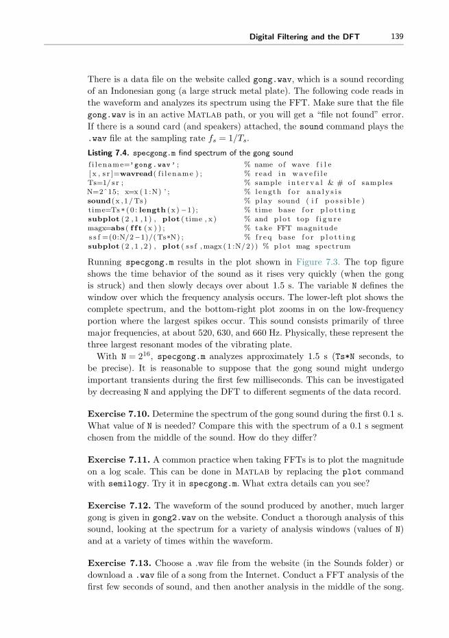
Digital Filtering and the DFT 139
There is a data file on the website called gong.wav, which is a sound recording
of an Indonesian gong (a large struck metal plate). The following code reads in
the waveform and analyzes its spectrum using the FFT. Make sure that the file
gong.wav is in an active Matlab path, or you will get a “file not found” error.
If there is a sound card (and speakers) attached, the sound command plays the
.wav file at the sampling rate fs = 1/Ts.
Listing 7.4. specgong.m find spectrum of the gong sound
f i l ename=’gong.wav ’ ; % name of wave f i l e[ x , s r ]=wavread( f i l ename ) ; % read in wave f i l eTs=1/ s r ; % sample i n t e r v a l & # of samplesN=2ˆ15; x=x ( 1 :N) ’ ; % l ength f o r a n a l y s i ssound(x , 1/Ts) % play sound ( i f p o s s i b l e )time=Ts * (0 : length (x )−1); % time base f o r p l o t t i n gsubplot ( 2 , 1 , 1 ) , plot ( time , x ) % and p l o t top f i g u r emagx=abs ( f f t (x ) ) ; % take FFT magnitudes s f =(0:N/2−1)/(Ts*N) ; % f r eq base f o r p l o t t i n gsubplot ( 2 , 1 , 2 ) , plot ( s s f ,magx ( 1 :N/2)) % p l o t mag spectrum
Running specgong.m results in the plot shown in Figure 7.3. The top figure
shows the time behavior of the sound as it rises very quickly (when the gong
is struck) and then slowly decays over about 1.5 s. The variable N defines the
window over which the frequency analysis occurs. The lower-left plot shows the
complete spectrum, and the bottom-right plot zooms in on the low-frequency
portion where the largest spikes occur. This sound consists primarily of three
major frequencies, at about 520, 630, and 660 Hz. Physically, these represent the
three largest resonant modes of the vibrating plate.
With N = 216, specgong.m analyzes approximately 1.5 s (Ts*N seconds, to
be precise). It is reasonable to suppose that the gong sound might undergo
important transients during the first few milliseconds. This can be investigated
by decreasing N and applying the DFT to different segments of the data record.
Exercise 7.10. Determine the spectrum of the gong sound during the first 0.1 s.
What value of N is needed? Compare this with the spectrum of a 0.1 s segment
chosen from the middle of the sound. How do they differ?
Exercise 7.11. A common practice when taking FFTs is to plot the magnitude
on a log scale. This can be done in Matlab by replacing the plot command
with semilogy. Try it in specgong.m. What extra details can you see?
Exercise 7.12. The waveform of the sound produced by another, much larger
gong is given in gong2.wav on the website. Conduct a thorough analysis of this
sound, looking at the spectrum for a variety of analysis windows (values of N)
and at a variety of times within the waveform.
Exercise 7.13. Choose a .wav file from the website (in the Sounds folder) or
download a .wav file of a song from the Internet. Conduct a FFT analysis of the
first few seconds of sound, and then another analysis in the middle of the song.

140 Chapter 7. Digital Filtering and the DFT
0 0.5 1Time in seconds
Frequency in Hertz
1.5−1
0
1
Am
plitu
de
0 0.5 21.51 2.50
1
2
3
4
Mag
nitu
de
Frequency in Hertz400 450 500 800750600 650 700550
0
1
2
3
4
x104
Figure 7.3 Time and frequency plots of the gong waveform. The top figure shows thedecay of the signal over 1.5 s. The bottom left figure shows the magnitude spectrum,and the right figure zooms in on the low-frequency portion so that the frequencies aremore legible.
How do the two compare? Can you correlate the FFT analysis with the pitch of
the material? With the rhythm? With the sound quality?
The key factors in a DFT- or FFT-based frequency analysis are as follows.
� The sampling interval Ts is the time resolution, the shortest time over which
any event can be observed. The sampling rate fs = 1/Ts is inversely propor-
tional.� The total time is T = NTs, where N is the number of samples in the analysis.� The frequency resolution is 1/T = 1/(NTs) = fs/N . Sinusoids closer together
(in frequency) than this value are indistinguishable.
For instance, in the analysis of the gong conducted in specgong.m, the sampling
interval Ts = 1/44100 is defined by the recording. With N = 216, the total time
is NTs = 1.48 s, and the frequency resolution is 1/(NTs) = 0.67 Hz.
Sometimes the total absolute time T is fixed. Sampling faster decreases Ts and
increases N , but cannot give better resolution in frequency. Sometimes it is pos-
sible to increase the total time. Assuming a fixed Ts, this implies an increase in
N and better frequency resolution. Assuming a fixed N , this implies an increase
in Ts and worse resolution in time. Thus, better resolution in frequency means
worse resolution in time. Conversely, better resolution in time means worse res-
olution in frequency. If this is still confusing, or if you would like to see it from
a different perspective, check out Appendix D.
The DFT is a key tool in analyzing and understanding the behavior of com-
munications systems. Whenever data flow through a system, it is a good idea
to plot the data as a function of time, and also as a function of frequency; that
is, to look at the data in the time domain and in the frequency domain. Often,

Digital Filtering and the DFT 141
aspects of the data that are clearer in time are hard to see in frequency, and
aspects that are obvious in frequency are obscure in time. Using both points of
view is common sense.
7.2 Practical Filtering
Filtering can be viewed as the process of emphasizing or attenuating certain
frequencies within a signal. Linear time-invariant filters are common because they
are easy to understand and straightforward to implement. Whether in discrete
or continuous time, an LTI filter is characterized by its impulse response (i.e.,
its output when the input is an impulse). The process of convolution aggregates
the impulse responses from all the input instants into a formula for the output.
It is hard to visualize the action of convolution directly in the time domain,
making analysis in the frequency domain an important conceptual tool. The
Fourier transform (or the DFT in discrete time) of the impulse response gives
the frequency response, which is easily interpreted as a plot that shows how much
gain or attenuation (or phase shift) each frequency experiences as a result of the
filtering operation. Thus, while implementing the filter in the time domain as a
convolution, it is normal to specify, design, and understand it in the frequency
domain as a point-by-point multiplication of the spectrum of the input and the
frequency response of the filter.
In principle, this provides a method not only of understanding the action
of a filter, but also of designing a filter. Suppose that a particular frequency
response is desired, say one that removes certain frequencies, while leaving others
unchanged. For example, if the noise is known to lie in one frequency band while
the important signal lies in another frequency band, then it is natural to design
a filter that removes the noisy frequencies and passes the signal frequencies.
This intuitive notion translates directly into a mathematical specification for the
frequency response. The impulse response can then be calculated directly by
taking the inverse transform, and this impulse response defines the desired filter.
While this is the basic principle of filter design, a number of subtleties can arise,
and sophisticated routines are available in Matlab that make the filter design
process flexible, even if they are not foolproof.
Filters are classified in several ways.
� Lowpass filters (LPF) try to pass all frequencies below some cutoff frequency
and remove all frequencies above.� Highpass filters try to pass all frequencies above some specified value and
remove all frequencies below.� Notch (or bandstop) filters try to remove particular frequencies (usually in a
narrow band) and to pass all others.� Bandpass filters try to pass all frequencies in a particular range and to reject
all others.

142 Chapter 7. Digital Filtering and the DFT
The region of frequencies allowed to pass through a filter is called the passband,
while the region of frequencies removed is called the stopband. Sometimes there
is a region between where it is relatively less important what happens, and this
is called the transition band.
By linearity, more complex filter specifications can be implemented as sums
and concatenations of the above basic filter types. For instance, if h1[k] is the
impulse response of a bandpass filter that passes only frequencies between 100
and 200 Hz, and h2[k] is the impulse response of a bandpass filter that passes
only frequencies between 500 and 600 Hz, then h[k] = h1[k] + h2[k] passes only
frequencies between 100 and 200 Hz or between 500 and 600 Hz. Similarly, if
hl[k] is the impulse response of a lowpass filter that passes all frequencies below
600 Hz, and hh[k] is the impulse response of a highpass filter that passes all
frequencies above 500 Hz, then h[k] = hl[k] ∗ hh[k] is a bandpass filter that passes
only frequencies between 500 and 600 Hz, where ∗ represents convolution.
Filters are also classified by the length of their impulse response. If the output
of a filter depends only on a specified number of samples, the filter is said to
have a finite impulse response, abbreviated FIR. Otherwise, it is said to have an
infinite impulse response, abbreviated IIR. The bulk of the filters in Software
Receiver Design are FIR filters with a flat passband, because these are the
most common filters in a typical receiver. But other filter profiles are possible,
and the techniques of filter design are not restricted to flat passbands. Section
7.2.1 shows several ways that digital FIR filters can be implemented in Matlab.
IIR filters arise whenever there is a loop (such as in a phase-locked loop), and
one special case (the integrator) is an intrinsic piece of the adaptive elements.
Section 7.2.2 shows how to implement IIR filters. Section 7.2.3 shows how to
design filters with specific properties, and how they behave on a number of test
signals.
7.2.1 Implementing FIR Filters
Suppose that the impulse response of a discrete-time filter is h[i], i =
0, 1, 2, . . . , N − 1. If the input to the filter is the sequence x[i], i = 0, 1, . . . ,M − 1,
then the output is given by the convolution Equation (7.2). There are four ways
to implement this filtering in Matlab.
� conv directly implements the convolution equation and outputs a vector of
length N +M − 1.� filter implements the convolution so as to supply one output value for each
input value; the output is of length M .� In the frequency domain, take the FFT of the input and the FFT of the
output, multiply the two, and take the IFFT to return to the time domain.� In the time domain, pass through the input data, at each time multiplying by
the impulse response and summing the result.
Probably the easiest way to see the differences is to play with the four methods.

Digital Filtering and the DFT 143
Listing 7.5. waystofilt.m “conv” vs. “filter” vs. “freq domain” vs. “time domain”
h=[1 −1 2 −2 3 −3] ; % impulse r esponse h [ k ]x=[1 2 3 4 5 6 −5 −4 −3 −2 −1] ; % input data x [ k ]
yconv=conv(h , x ) % convolve x [ k ] * h [ k ]y f i l t=f i l t e r (h , 1 , x ) % f i l t e r x [ k ] with h [ k ]n=length (h)+length (x)−1; % pad l ength f o r FFTf f t h=f f t ( [ h zeros (1 ,n−length (h ) ) ] ) ; % FFT of h [ k ] i s H[ n ]f f t x=f f t ( [ x , zeros (1 ,n−length ( x ) ) ] ) ; % FFT of input i s X[ n ]f f t y=f f t h . * f f t x ; % product o f H[ n ] and X[ n ]y f r eq=real ( i f f t ( f f t y ) ) % IFFT of product g i v e s y [ k ]z=[zeros (1 , length (h)−1) ,x ] ; % i n i t i a l f i l t e r s t a t e=0for k=1: length (x ) % time−domain method
ytim (k)= f l i p l r (h)* z (k : k+length (h ) −1) ’ ; % do f o r each x [ k ]end % to d i r e c t l y c a l c u l a t e y [ k ]
Observe that the first M terms of yconv, yfilt, yfreq, and ytim are the same,
but that both yconv and yfreq have N-1 extra values at the end. For both the
time-domain method and the filter command, the output values are aligned
in time with the input values, one output for each input. Effectively, the filter
command is a single-line implementation of the time-domain for loop.
For the FFT method, the two vectors (input and convolution) must both have
length N+M-1. The raw output has complex values due to numerical roundoff,
and the command real is used to strip away the imaginary parts. Thus, the
FFT-based method requires more Matlab commands to implement. Observe
also that conv(h,x) and conv(x,h) are the same, whereas filter(h,1,x) is
not the same as filter(x,1,h).
To view the frequency response of the filter h, Matlab provides the command
freqz, which automatically zero pads5 the impulse response and then plots both
the magnitude and the phase. Type
f r eq z (h )
to see that the filter with impulse response h=[1, 1, 1, 1, 1] is a (poor)
lowpass filter with two dips at 0.4 and 0.8 of the Nyquist frequency as shown in
Figure 7.4. The command freqz always normalizes the frequency axis so that
“1.0” corresponds to the Nyquist frequency fs/2. The passband of this filter
(all frequencies less than the point where the magnitude drops 3 dB below the
maximum) ends just below 0.2. The maximum magnitude in the stopband occurs
at about 0.6, where it is about 12 dB down from the peak at zero. Better (i.e.,
closer to the ideal) lowpass filters would attenuate more in the stopband, would
be flatter across the passband, and would have narrower transition bands.
5 By default, the Matlab command freqz creates a vector of length 512 that contains thespecified impulse response followed by zeros. The FFT of this elongated vector is used forthe magnitude and phase plots, giving the plots a smoother appearance than when takingthe FFT of the raw impulse response.

144 Chapter 7. Digital Filtering and the DFT
−40
−20
0
20
Mag
nitu
de (
dB)
0 0.2 0.4 0.6 0.8 1Normalized frequency (Nyquist = 1)
−100
0
100
Phas
e (d
egre
es)
Figure 7.4 The frequencyresponse of the filter withimpulse response h=[1, 1,
1, 1, 1] has a poor lowpasscharacter. It is easier to seethis in the frequency domainthan directly in the timedomain.
7.2.2 Implementing IIR Filters
At first glance it might seem counterintuitive that a useful filter could have an
impulse response that is infinitely long. To see how this infiniteness might arise
in a specific case, suppose that the output y[k] of an LTI system is created from
the input x[k] according to the formula
y[k + 1] = ay[k] + bx[k], (7.8)
where a and b are constants. This is shown in the left-hand portion of Figure
7.5, where the time delay between successive terms (between k and k + 1 for
instance) is represented by z−1. This is an example of the Z-transform, and is
described more fully in Appendix F. If the initial value is y[0] = 0, the response
of the system (7.8) to an impulse x[k] = δ[k] (where δ[k] is the discrete impulse
function (7.1)) is
b, ba, ba2, ba3, ba4, . . . . (7.9)
If |a| > 1, this impulse response increases towards infinity and the system is
said to be unstable. If |a| < 1, the values in the sequence die away towards (but
never quite reaching) zero, and the system is stable. In both cases, the impulse
response is infinitely long and so the system (7.8) is IIR. The special case when
a = 1 is called a summer (or, in analogy with continuous time, an integrator)
because y[k] = y[0] + b∑k−1
i=0 x[i] sums up all the inputs. The summer is often
represented symbolically as in the right-hand part of Figure 7.5.
The general form of an IIR filter is
y[k + 1] = a0y[k] + a1y[k − 1] + · · ·+ any[k − n]
+ b0x[k] + b1x[k − 1] + · · ·+ bmx[k −m],
which can be rewritten more concisely as
y[k + 1] = aTy[k] + bTx[k]

Digital Filtering and the DFT 145
z−1b
a
y[k+1]x[k] x[k]y[k] y[k]
Σb+Delay
Figure 7.5 The LTI system y[k + 1] = ay[k] + bx[k], with input x[k] and output y[k], isrepresented schematically using the delay z−1 in this simple block diagram. Thespecial case when a = 1 is called a summer because it effectively adds up all the inputvalues, and it is often drawn more concisely as on the right side of the figure.
where
a = [a0, a1, . . . , an]T
b = [b0, b1, . . . , bm]T
are column vectors of the parameters of the filter and where
x[k] = [x[k], x[k − 1], . . . , x[k −m]]T
y[k] = [y[k], y[k − 1], . . . , y[k − n]]T
are vectors of past input and output data. The symbol zT indicates the transpose
of the vector z. In Matlab, transpose is represented using the single apostrophe
’, but take care: when using complex numbers, the apostrophe actually imple-
ments a complex conjugate as well as transpose.
Matlab has a number of functions that make it easy to explore IIR filtering.
For example, the function impz plots the impulse response of a discrete IIR (or
FIR) filter. The impulse response of the system (7.8) is found by entering
b=1;a=[1 , −0 .8 ] ;impz (b , a )
The parameters are the vectors b=[b0, b1, . . . , bm] and a=[1,−a0,−a1, . . . ,−an].
Hence the above code gives the response when a of (7.8) is +0.8. Similarly, the
command freqz(b,a) displays the frequency response for the IIR filter, where
b and a are constructed in the same way.
The routine waystofiltIIR.m explores ways of implementing IIR filters. The
simplest method uses the filter command. For instance filter(b,a,d) filters
the data d through the IIR system with parameters b and a defined as above.
This gives the same output as first calculating the impulse response h and then
using filter(h,1,d). The fastest (and most general) way to implement the
filter is in the for loop at the end, which mimics the time-domain method for
FIR filters, but includes the additional parameters a.
Listing 7.6. waystofiltIIR.m ways to implement IIR filters
a=[1 −0 .8 ] ; l ena=length ( a )−1; % au t o r e g r e s s i v e c o e f f i c i e n t sb= [ 1 ] ; l enb=length (b ) ; % moving average c o e f f i c i e n t sd=randn ( 1 , 2 0 ) ; % data to f i l t e r

146 Chapter 7. Digital Filtering and the DFT
i f lena>=lenb , % dimpulse needs lena>=lenbh=impz (b , a ) ; % impulse r esponse o f f i l t e ry f i l t=f i l t e r (h , 1 , d) % f i l t e r x [ k ] with h [ k ]
end
y f i l t 2=f i l t e r (b , a , d) % f i l t e r us ing a and by=zeros ( lena , 1 ) ; x=zeros ( lenb , 1 ) ; % i n i t i a l s t a t e s in f i l t e rfor k=1: length (d)− l enb % time−domain method
x=[d( k ) ; x ( 1 : lenb −1 ) ] ; % past va lues o f i nputsytim (k)=−a ( 2 : l ena+1)*y+b*x ; % d i r e c t l y c a l c u l a t e y [ k ]y=[ytim (k ) ; y ( 1 : lena −1 ) ] ; % past va lues o f outputs
end
Like FIR filters, IIR filters can be lowpass, bandpass, and highpass, or can
have almost any imaginable effect on the spectrum of their input.
Exercise 7.14. Some IIR filters can be used as inverses to some FIR filters.
Show that the FIR filter
x[k] =1
br[k] − a
br[k − 1]
is an inverse of the IIR filter (7.8).
Exercise 7.15. FIR filters can be used to approximate the behavior of IIR filters
by truncating the impulse response. Create a FIR filter with impulse response
given by the first 10 terms of (7.9) for a = 0.9 and b = 2. Simulate the FIR filter
and the IIR filter (7.8) in Matlab, using the same random input to both. Verify
that the outputs are (approximately) the same.
7.2.3 Filter Design
This section gives an extended explanation of how to use Matlab to design a
bandpass filter to fit a specified frequency response with a flat passband. The
same procedure (with suitable modification) also works for the design of other
basic filter types.
A bandpass filter is intended to scale, but not distort, signals with frequen-
cies that fall within the passband, and to reject signals with frequencies in the
stopband. An ideal, distortionless response for the passband would be perfectly
flat in magnitude, and would have linear phase (corresponding to a delay). The
transition band from the passband to the stopband should be as narrow as pos-
sible. In the stopband, the frequency response magnitude should be sufficiently
small and the phase is of no concern. These objectives are captured in Figure
7.6. Recall (from (A.35)) for a real w(t) that |W (f)| is even and � W (f) is odd,
as illustrated in Figure 7.6.
Matlab has several commands that carry out filter design. The firpm com-
mand6 provides a linear phase impulse response (with real, symmetric coefficients
6 Some early versions of Matlab use remez instead of firpm.
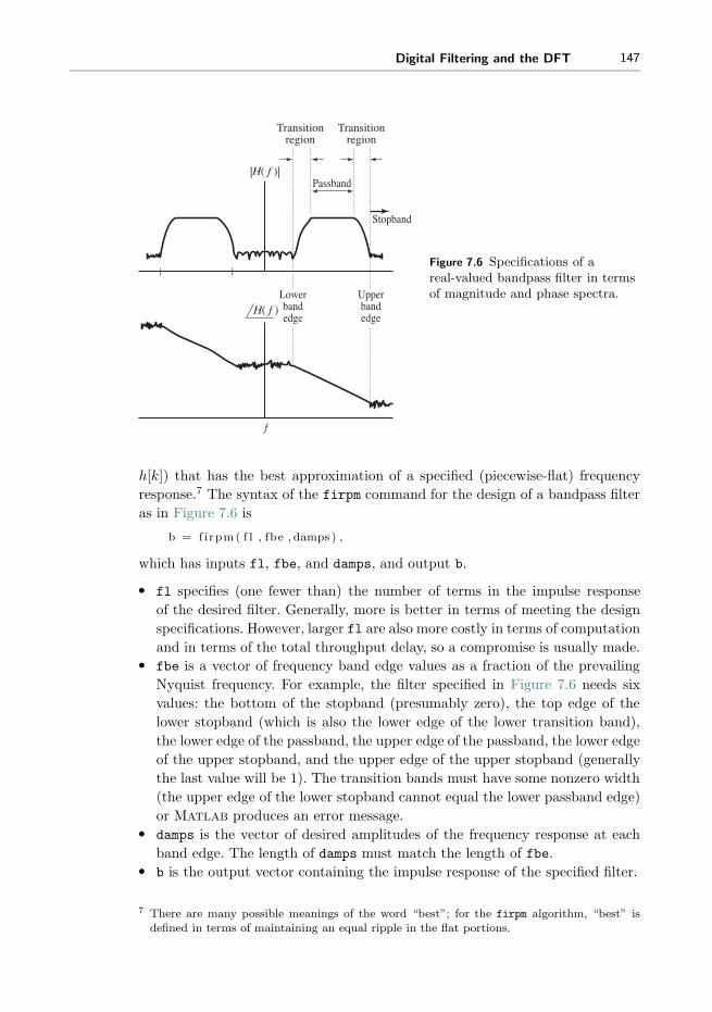
Digital Filtering and the DFT 147
|H( f )|
H( f )
Transitionregion
Transitionregion
Passband
Stopband
f
Lowerbandedge
Upperbandedge
Figure 7.6 Specifications of areal-valued bandpass filter in termsof magnitude and phase spectra.
h[k]) that has the best approximation of a specified (piecewise-flat) frequency
response.7 The syntax of the firpm command for the design of a bandpass filter
as in Figure 7.6 is
b = f i rpm ( f l , fbe , damps ) ,
which has inputs fl, fbe, and damps, and output b.
� fl specifies (one fewer than) the number of terms in the impulse response
of the desired filter. Generally, more is better in terms of meeting the design
specifications. However, larger fl are also more costly in terms of computation
and in terms of the total throughput delay, so a compromise is usually made.� fbe is a vector of frequency band edge values as a fraction of the prevailing
Nyquist frequency. For example, the filter specified in Figure 7.6 needs six
values: the bottom of the stopband (presumably zero), the top edge of the
lower stopband (which is also the lower edge of the lower transition band),
the lower edge of the passband, the upper edge of the passband, the lower edge
of the upper stopband, and the upper edge of the upper stopband (generally
the last value will be 1). The transition bands must have some nonzero width
(the upper edge of the lower stopband cannot equal the lower passband edge)
or Matlab produces an error message.� damps is the vector of desired amplitudes of the frequency response at each
band edge. The length of damps must match the length of fbe.� b is the output vector containing the impulse response of the specified filter.
7 There are many possible meanings of the word “best”; for the firpm algorithm, “best” isdefined in terms of maintaining an equal ripple in the flat portions.

148 Chapter 7. Digital Filtering and the DFT
−80
−60
−40
−20
0
20
Mag
nitu
de R
espo
nse
(dB
)
0 0.1 0.2 0.3 0.4 0.5 0.6 0.7 0.8 0.9 1Normalized frequency (Nyquist = 1)
−1500
−1000
−500
0
500
Phas
e (d
egre
es)
Figure 7.7 Frequency responseof the bandpass filter designedby the firpm command inbandex.m. The variable fbe
specifies a set of frequencies (asa fraction of the Nyquist rate)and damps specifies thecorresponding amplitudes. Thefreqz command plots both themagnitude and phase spectraof the filter.
The following Matlab script designs a filter that mimics Figure 7.6:
Listing 7.7. bandex.m design a bandpass filter and plot frequency response
f be=[0 0 . 24 0 . 26 0 . 74 0 . 76 1 ] ; % f r eq band edges as a f r a c t i o n o f% the Nyquist f r equency
damps=[0 0 1 1 0 0 ] ; % de s i r ed ampl i tudes at band edgesf l =30; % f i l t e r s i z eb=f i rpm ( f l , fbe , damps ) ; % b i s the des igned impulse r esponsef igure (1)f r eq z (b) % p l o t f r eq r esponse to check des i gn
The frequency response of the resulting finite impulse response (FIR) filter is
shown in Figure 7.7. Observe that the stopband is about 14 dB lower than the
passband, a marginal improvement over the naive lowpass filter of Figure 7.4,
but the design is much flatter in the passband. The “equiripple” nature of this
filter is apparent in the slow undulations of the magnitude in the passband.
Designing IIR filters is also straightforward. For example, the code
[ b , a ]=cheby1 ( 1 0 , 5 , 0 . 2 5 ) ;
designs a 10th-order lowpass filter with 5 dB of ripple in the passband, which
extends from DC to 0.25 times the Nyquist rate.
While commands such as firpm and cheby1 make filter design easy, be
warned—strange things can happen, even to nice filters. Whenever using any
of the filter design tools, always check freqz(b,a) to verify that the output of
the design behaves as anticipated. There are many other ways to design LTI
filters, and Matlab includes several commands that design filter coefficients:
cfirpm, firls, fir1, fir2, butter, cheby2, and ellip. The subject of filter
design is vast, and each of these is useful in certain applications. For simplic-
ity, we have chosen to present most examples throughout Software Receiver
Design by using firpm.

Digital Filtering and the DFT 149
Exercise 7.16. Rerun bandex.m with very narrow transition regions, for
instance fbe = [0, 0.24, 0.2401, 0.6, 0.601, 1]. What happens to the ripple in
the passband? Compare the minimum magnitude in the passband with the max-
imum value in the stopband.
Exercise 7.17. Returning to the filter specified in Figure 7.6, try using different
numbers of terms in the impulse response, fl = 5, 10, 100, 500, 1000. Comment
on the resulting designs in terms of flatness of the frequency response in the
passband, attenuation from the passband to the stopband, and the width of the
transition band.
Exercise 7.18. Specify and design a lowpass filter with cutoff at 0.15. What
values of fl, fbe, and damps work best?
Exercise 7.19. Specify and design a filter that has two passbands, one between
[0.2, 0.3] and another between [0.5, 0.6]. What values of fl, fbe, and damps work
best?
Exercise 7.20. Use the filter designed in bandex.m to filter a white-
noise sequence (generated by randn) using the time-domain method from
waystofilt.m. Verify that the output has a bandpass spectrum.
The preceding filter designs do not explicitly require the sampling rate of the
signal. However, since the sampling rate determines the Nyquist rate, it is used
implicitly. The next exercise asks that you familiarize yourself with “real” units
of frequency in the filter design task.
Exercise 7.21. In Exercise 7.10, the program specgong.m was used to ana-
lyze the sound of an Indonesian gong. The three most prominent partials (or
narrowband components) were found to be at about 520, 630, and 660 Hz.
a. Design a filter using firpm that will remove the two highest partials from this
sound without affecting the lowest partial.
b. Use the filter command to process the gong.wav file with your filter.
c. Take the FFT of the resulting signal (the output of your filter) and verify that
the partial at 520 remains while the others are removed.
d. If a sound card is attached to your computer, compare the sound of the raw
and the filtered gong sound by using Matlab’s sound command. Comment
on what you hear.
The next set of problems examines how accurate digital filters really are.
Exercise 7.22. With a sampling rate of 44100 Hz, let x[k] be a sinusoid of
frequency 3000 Hz. Design a lowpass filter with a cutoff frequency fl of 1500
Hz, and let y[k] = LPF{x[k]} be the output of the filter.

150 Chapter 7. Digital Filtering and the DFT
a. How much does the filter attenuate the signal? (Express your answer as the
ratio of the power in the output y[k] to the power in the input x[k].)
b. Now use an LPF with a cutoff of 2500 Hz. How much does the filter attenuate
the signal?
c. Now use an LPF with a cutoff of 2900 Hz. How much does the filter attenuate
the signal?
Exercise 7.23. Repeat Exercise 7.22 without using the filter command
(implement the filtering, using the time-domain method in waystofilt.m).
Exercise 7.24. With the same setup as in Exercise 7.22, generate x[k] as a
bandlimited noise signal containing frequencies between 3000 Hz and the Nyquist
rate.
a. Use an LPF with cutoff frequency fl of 1500 Hz. How much does the filter
attenuate the signal?
b. Now use an LPF with a cutoff of 2500 Hz. How much does the filter attenuate
the signal?
c. Now use an LPF with a cutoff of 3100 Hz. How much does the filter attenuate
the signal?
d. Now use an LPF with a cutoff of 4000 Hz. How much does the filter attenuate
the signal?
Exercise 7.25. Let f1 < f2 < f3. Suppose x[k] has no frequencies above f1 Hz,
while z[k] has no frequencies below f3. If an LPF has cutoff frequency f2, in
principle,
LPF{x[k] + z[k]} = LPF{x[k]}+ LPF{z[k]} = x[k] + 0 = x[k].
Explain how this is (and is not) consistent with the results of Exercises 7.22
and 7.24.
Exercise 7.26. Let the output y[k] of an LTI system be created from the input
x[k] according to the formula
y[k + 1] = y[k] + μx[k],
where μ is a small constant. This is drawn in Figure 7.5.
a. What is the impulse response of this filter?
b. What is the frequency response of this filter?
c. Would you call this filter lowpass, highpass, or bandpass?
Exercise 7.27. Using one of the alternative filter design routines (cfirpm,
firls, fir1, fir2, butter, cheby1, cheby2, or ellip), repeat Exercises 7.16–
7.21. Comment on the subtle (and the not-so-subtle) differences in the resulting
designs.

Digital Filtering and the DFT 151
Exercise 7.28. The effect of bandpass filtering can be accomplished by
a. modulating to DC,
b. lowpass filtering, and
c. modulating back.
Repeat the task given in Exercise 7.21 (the Indonesian gong filter design problem)
by modulating with a 520 Hz cosine, lowpass filtering, and then remodulating.
Compare the final output of this method with the direct bandpass filter design.
For Further Reading
Here are some of our favorite books on signal processing:
� K. Steiglitz, A Digital Signal Processing Primer, Addison-Wesley, 1996;� J. H. McClellan, R. W. Schafer, and M. A. Yoder, DSP First: A Multimedia
Approach, Prentice-Hall, 1998;� C. S. Burrus and T. W. Parks, DFT/FFT and Convolution Algorithms:
Theory and Implementation, Wiley-Interscience, 1985.

8 Bits to Symbols to Signals
Any message, whether analog or digital, can be translated into a string of binary
digits. In order to transmit or store these digits, they are often clustered or
encoded into a more convenient representation whose elements are the symbols
of an alphabet. In order to utilize bandwidth efficiently, these symbols are then
translated (again!) into short analog waveforms called pulse shapes that are com-
bined to form the actual transmitted signal.
The receiver must undo each of these translations. First, it examines the
received analog waveform and decodes the symbols. Then it translates the sym-
bols back into binary digits, from which the original message can, with luck, be
reconstructed.
This chapter briefly examines each of these translations, and the tools needed
to make the receiver work. One of the key ideas is correlation, which can be used
as a kind of pattern-matching tool for discovering key locations within the signal
stream. Section 8.3 shows how correlation can be viewed as a kind of linear filter,
and hence its properties can be readily understood both in the time and in the
frequency domain.
8.1 Bits to Symbols
The information that is to be transmitted by a communication system comes in
many forms: a pressure wave in the air, a flow of electrons in a wire, a digitized
image or sound file, the text in a book. If the information is in analog form, then
it can be sampled (as in Chapter 6). For instance, an analog-to-digital converter
can transform the output of a microphone into a stream of numbers representing
the pressure wave in the air, or it can turn measurements of the current in the wire
into a sequence of numbers that are proportional to the electron flow. The sound
file, which is already digital, contains a long list of numbers that correspond to
the instantaneous amplitude of the sound. Similarly, the picture file contains a
list of numbers that describe the intensity and color of the pixels in the image.

Bits to Symbols to Signals 153
The text can be transformed into a numerical list using the ASCII code. In all
these cases, the raw data represent the information that must be transmitted by
the communication system. The receiver, in turn, must ultimately translate the
received signal back into the data.
Once the information is encoded into a sequence of numbers, it can be re-
expressed as a string of binary digits 0 and 1. This is discussed at length in
Chapter 14. But the binary 0–1 representation is not usually very convenient
from the point of view of efficient and reliable data transmission. For example,
directly modulating a binary string with a cosine wave would result in a small
piece of the cosine wave for each 1 and nothing (the zero waveform) for each 0.
It would be very hard to tell the difference between a message that contained a
string of zeros, and no message at all!
The simplest solution is to recode the binary 0, 1 into binary ±1. This can be
accomplished using either the linear operation 2x− 1 (which maps 0 into −1,
and 1 into 1), or −2x+ 1 (which maps 0 into 1, and 1 into −1). This “binary”
±1 is an example of a two-element symbol set. There are many other common
symbol sets. In multilevel signaling, the binary terms are gathered into groups.
Regrouping in pairs, for instance, recodes the information into a four-level signal.
For example, the binary sequence might be paired thus:
. . . 000010110101 . . .→ . . . 00 00 10 11 01 01 . . . . (8.1)
Then the pairs might be encoded as
11 → +3
10 → +1
01 → −1
00 → −3
(8.2)
to produce the symbol sequence
. . . 00 00 10 11 01 01 . . . → . . .−3, −3, +1, +3 ,−1, −1 . . . .
Of course, there are many ways in which such a mapping between bits and
symbols might be made, and Exercise 8.2 explores one simple alternative called
the Gray code. The binary sequence may be grouped in many ways: into triplets
for an 8-level signal, into quadruplets for a 16-level scheme, into “in-phase” and
“quadrature” parts for transmission through a quadrature system. The values
assigned to the groups (±1,±3 in (8.2)) are called the alphabet of the given
system.
Example 8.1. Text is commonly encoded using ASCII, and Matlab automat-
ically represents any string file as a list of ASCII numbers. For instance, let
str=’I am text’ be a text string. This can be viewed in its internal form by
typing real(str), which returns the vector 73 32 97 109 32 116 101 120 116,
which is the (decimal) ASCII representation of this string. This can be viewed

154 Chapter 8. Bits to Symbols to Signals
in binary using dec2base(str,2,8), which returns the binary (base 2) repre-
sentation of the decimal numbers, each with eight digits.
The Matlab function letters2pam.m, provided on the website, changes a
text string into the four-level alphabet ±1,±3. Each letter is represented by a
sequence of four elements, for instance the letter I is −1,−3, 1,−1. The func-
tion is invoked with the syntax letters2pam(str). The inverse operation is
pam2letters.m. Thus pam2letters(letters2pam(str)) returns the original
string.
One complication in the decoding procedure is that the receiver must figure
out when the groups begin in order to parse the digits properly. For example,
if the first element of the sequence in (8.1) were lost, the message would be
mistranslated as
. . . 00010110101 . . .→ . . .00 01 01 10 10 . . .
→ . . .−3, −1, −1, 1, 1, . . . .
Similar parsing problems occur whenever messages start or stop. For example,
if the message consists of pixel values for a television image, it is important that
the decoder be able to determine precisely when the image scan begins. These
kinds of synchronization issues are typically handled by sending a special “start
of frame” sequence that is known both to the transmitter and to the receiver.
The decoder then searches for the start sequence, usually using some kind of
correlation (pattern-matching) technique. This is discussed in detail in Section
8.3.
Example 8.2. There are many ways to translate data into binary equiva-
lents. Example 8.1 showed one way to convert text into 4-PAM and then into
binary. Another way exploits the Matlab function text2bin.m and its inverse
bin2text.m, which use the 7-bit version of the ASCII code (rather than the
8-bit version). This representation is more efficient, since each pair of text letters
can be represented by 14 bits (or seven 4-PAM symbols) rather than 16 bits (or
eight 4-PAM symbols). On the other hand, the 7-bit version can encode only
half as many characters as the 8-bit version. Again, it is important to be able to
correctly identify the start of each letter when decoding.
Exercise 8.1. The Matlab code in naivecode.m, which is on the website,
implements the translation from binary to 4-PAM (and back again) suggested in
(8.2). Examine the resiliency of this translation to noise by plotting the number
of errors as a function of the noise variance v. What is the largest variance for
which no errors occur? At what variance are the errors near 50%?
Exercise 8.2. A Gray code has the property that the binary representation for
each symbol differs from its neighbors by exactly one bit. A Gray code for the

Bits to Symbols to Signals 155
translation of binary into 4-PAM is
01 → +3
11 → +1
10 → −1
00 → −3
Mimic the code in naivecode.m to implement this alternative and plot the num-
ber of errors as a function of the noise variance v. Compare your answer with
Exercise 8.1. Which code is better?
8.2 Symbols to Signals
Even though the original message is translated into the desired alphabet, it is
not yet ready for transmission: it must be turned into an analog waveform. In the
binary case, a simple method is to use a rectangular pulse of duration T seconds
to represent +1, and the same rectangular pulse inverted (i.e., multiplied by −1)
to represent the element −1. This is called a polar non-return-to-zero line code.
The problem with such simple codes is that they use bandwidth inefficiently.
Recall that the Fourier transform of the rectangular pulse in time is the sinc(f)
function in frequency (A.20), which dies away slowly as f increases. Thus, simple
codes like the non-return-to-zero are compact in time, but wide in frequency,
limiting the number of simultaneous nonoverlapping users in a given spectral
band.
More generally, consider the four-level signal of (8.2). This can be turned into
an analog signal for transmission by choosing a pulse shape p(t) (that is not
necessarily rectangular and not necessarily of duration T ) and then transmitting
p(t− kT ) if the kth symbol is 1
−p(t− kT ) if the kth symbol is −1
3p(t− kT ) if the kth symbol is 3
−3p(t− kT ) if the kth symbol is −3
Thus, the sequence is translated into an analog waveform by initiating a scaled
pulse at the symbol time kT , where the amplitude scaling is proportional to the
associated symbol value. Ideally, the pulse would be chosen so that
� the value of the message at time k does not interfere with the value of the
message at other sample times (the pulse shape causes no intersymbol inter-
ference),� the transmission makes efficient use of bandwidth, and� the system is resilient to noise.
Unfortunately, these three requirements cannot all be optimized simultaneously,
and so the design of the pulse shape must consider carefully the tradeoffs that are
needed. The focus in Chapter 11 is on how to design the pulse shape p(t), and the

156 Chapter 8. Bits to Symbols to Signals
0 0.1 0.2 0.3 0.4 0.5 0.6 0.7 0.8 0.9The pulse shape
0
0.2
0.4
0.6
0.8
1
0 10 20 30 40 50 60 70 80 90 100The waveform representing “Transmit this text”
−3
−2
−1
0
1
2
3
Figure 8.1 The process of pulse shaping replaces each symbol of the alphabet (in thiscase, ±1, ±3) with an analog pulse (in this case, the short blip function shown in thetop panel).
consequences of that choice in terms of possible interference between adjacent
symbols and in terms of the signal-to-noise properties of the transmission.
For now, to see concretely how pulse shaping works, let’s pick a simple non-
rectangular shape and proceed without worrying about optimality. Let p(t) be
the symmetric blip shape shown in the top part of Figure 8.1, and defined in
pulseshape.m by the hamming command. The text string in str is changed into
a four-level signal as in Example 8.1, and then the complete transmitted wave-
form is assembled by assigning an appropriately scaled pulse shape to each data
value. The output appears at the bottom of Figure 8.1. Looking at this closely,
observe that the first letter T is represented by the four values −1, −1, −1, and
−3, which correspond exactly to the first four negative blips, three small and
one large.
The program pulseshape.m represents the “continuous-time” or analog signal
by oversampling both the data sequence and the pulse shape by a factor of
M. This technique was discussed in Section 6.3, where an “analog” sine wave
sine100hzsamp.m was represented digitally at two sampling intervals, a slow
digital interval Ts and a faster rate (shorter interval) Ts/M representing the
underlying analog signal. The pulse shaping itself is carried out by the filter
command which convolves the pulse shape with the data sequence.
Listing 8.1. pulseshape.m applying a pulse shape to a text string
s t r=’Transmit this text string ’ ; % message to be transmi t tedm=let te r s2pam ( s t r ) ; N=length (m) ; % 4− l e v e l s i g n a l o f l ength N

Bits to Symbols to Signals 157
M=10; mup=zeros (1 ,N*M) ; mup( 1 :M:N*M)=m; % oversample by Mps=hamming (M) ; % b l i p pu l s e o f width Mx=f i l t e r ( ps , 1 ,mup ) ; % convolve pu l s e shape & data
Exercise 8.3. Assume the sampling period is T = 0.1, and then plot the spec-
trum of the output x. What is the bandwidth of this signal?
Exercise 8.4. Again with T = 0.1, plot the spectrum of the output x when the
pulse shape is changed to a rectangular pulse. (Change the definition of ps in
the next-to-last line of pulseshape.m.) What is the bandwidth of this signal?
Exercise 8.5. Can you think of a pulse shape that will have a narrower band-
width than either of the above but that will still be time limited by T ? Implement
it by changing the definition of ps, and check to see whether you are correct.
Thus the raw message is prepared for transmission by
� encoding into an alphabet (in this case ±1,±3), and then� pulse shaping the elements of the alphabet using p(t).
The receiver must undo these two operations; it must examine the received signal
and recover the elements of the alphabet, and then decode these to reconstruct
the message. Both of these tasks are made easier using correlation, which is
discussed in the next section. The actual decoding processes used in the receiver
are then discussed in Section 8.4.
8.3 Correlation
Suppose there are two signals or sequences. Are they similar, or are they differ-
ent? If one is just shifted in time relative to the other, how can the time shift
be determined? The approach called correlation shifts one of the sequences in
time, and calculates how well they match (by multiplying point by point and
summing) at each shift. When the sum is small, they are not much alike; when
the sum is large, many terms are similar. Thus, correlation is a simple form of
pattern matching, which is useful in communication systems for aligning signals
in time. This can be applied at the level of symbols when it is necessary to find
appropriate sampling times, and it can be applied at the “frame” level when it
is necessary to find the start of a message (for instance, the beginning of each
frame of a television signal). This section discusses various techniques of cross-
correlation and autocorrelation, which can be viewed in either the time domain
or the frequency domain.

158 Chapter 8. Bits to Symbols to Signals
In discrete time, cross-correlation is a function of the time shift j between two
sequences w[k] and v[k + j]:
Rwv(j) = limT→∞
1
T
T/2∑k=−T/2
w[k]v[k + j]. (8.3)
For finite data records, the sum need only be accumulated over the nonzero
elements, and the normalization by 1/T is often ignored. (This is how
Matlab’s xcorr function works.) While this may look like the convolution
Equation (7.2), it is not identical since the indices are different (in convolu-
tion, the index of v(·) is j − k instead of k + j). The operation and meaning
of the two processes are also not identical: convolution represents the man-
ner in which the impulse response of a linear system acts on its inputs to
give the outputs, while cross-correlation quantifies the similarity of two sig-
nals.
In many communication systems, each message is parcelled into segments or
frames, each having a predefined header. As the receiver decodes the transmitted
message, it must determine where the message segments start. The following
code simulates this in a simple setting in which the header is a predefined binary
string and the data consist of a much longer binary string that contains the
header hidden somewhere inside. After performing the correlation, the index
with the largest value is taken as the most likely location of the header.
Listing 8.2. correx.m correlation can locate the header within the data
header =[1 −1 1 −1 −1 1 1 1 −1 −1] ; % header i s pr ede f i ned s t r i n gl o c =30; r =25; % place header in p o s i t i o n l o cdata=[sign (randn (1 , loc −1)) header sign (randn (1 , r ) ) ] ; % make s i g n a lsd=0.25; data=data+sd*randn ( size ( data ) ) ; % add no i s ey=xcor r ( header , data ) ; % do cros s−c o r r e l a t i o n[m, ind ]=max( y ) ; % f i nd l a r g e s t c o r r e l a t i o nheads tar t=length ( data )− ind+1; % place where header s t a r t s
Running correx.m results in a trio of figures much like those in Figure 8.2.
(Details will differ each time it is run, because the actual “data” are randomly
generated with Matlab’s randn function.) The top plot in Figure 8.2 shows the
10-sample binary header. The data vector is constructed to contain l = 30 data
values followed by the header (with noise added), and then r = 25 more data
points, for a total block of 65 points. It is plotted in the middle of Figure 8.2.
Observe that it is difficult to “see” where the header lies among the noisy data
record. The correlation between the data and the header is calculated and plotted
at the bottom of Figure 8.2 as a function of the lag index. The index for which
the correlation attains its largest value defines where the best match between the
data and the header occurs. Most likely this will be at index ind=35 (as in Figure
8.2). Because of the way Matlab orders its output, the calculations represent
sliding the first vector (the header), term by term, across the second vector (the

Bits to Symbols to Signals 159
1 2 3 4 5 6 7 8 9 10−1
−0.5
0
0.5
1
Header
−2
−1
0
1
2
0 20 40 60 80 100 120 140−10
−5
0
5
10Correlation of header with data
Data with embedded header
0 10 20 30 40 50 60 70
Figure 8.2 The correlation can be used to locate a known header within a long signal.The predefined header is shown in the top graph. The data consist of a randombinary string with the header embedded and noise added. The bottom plot shows thecorrelation. The location of the header is determined by the peak occurring at 35.
data). The long string of zeros at the end1 occurs because the two vectors are of
different lengths. The start of the header is given by length(data)-ind+1.
One way in which the correlation might fail to find the correct location of
the header is if the header string accidently occurred in the data values. If this
happened, then the correlation would be as large at the “accidental” location
as at the intended location. This becomes increasingly unlikely as the header
is made longer, though a longer header also wastes bandwidth. Another way to
decrease the likelihood of false hits is to average over several headers.
Exercise 8.6. Rerun correx.m with different-length data vectors (try loc=100,
r=100 and loc=10, r=10). Observe how the location of the peak changes.
Exercise 8.7. Rerun correx.m with different-length headers. Does the peak in
the correlation become more or less distinct as the number of terms in the header
increases?
1 Some versions of Matlab use a different convention with the xcorr command. If you findthat the string of zeros occurs at the beginning, try reversing the order of the arguments.

160 Chapter 8. Bits to Symbols to Signals
Exercise 8.8. Rerun correx.m with different amounts of noise. Try sd=0, 0.1,
0.3, 0.5, 1, 2. How large can the noise be made if the correlation is still to
find the true location of the header?
Exercise 8.9. The code in corrvsconv.m explores the relationship between
the correlation and convolution. The convolution of two sequences is essentially
the same as the cross-correlation of the time-reversed signal, except that the
correlation is padded with extra zeros. (The Matlab function fliplr carries
out the time reversal.) If h is made longer than x, what needs to be changed so
that yconv and ycorr remain equal?
Listing 8.3. corrvsconv.m comparing correlation and convolution
h=[1 −1 2 −2 3 −3] ; % de f i n e sequence h [ k ]x=[1 2 3 4 5 6 −5 −4 −3 −2 −1] ; % de f i n e sequence x [ k ]yconv=conv(x , h) % convolve x [ k ] * h [ k ]ycor r=xcor r (h , f l i p l r ( x ) ) % c o r r e l a t e f l i p p ed x and h
8.4 Receive Filtering: From Signals to Symbols
Suppose that a message has been coded into its alphabet, pulse-shaped into
an analog signal, and transmitted. The receiver must then “un-pulse-shape” the
analog signal back into the alphabet, which requires finding where in the received
signal the pulse shapes are located. Correlation can be used to accomplish this
task, because it is effectively the task of locating a known sequence (in this case
the sampled pulse shape) within a longer sequence (the sampled received signal).
This is analogous to the problem of finding the header within the received signal,
although some of the details have changed. While optimizing this procedure is
somewhat involved (and is therefore postponed until Chapter 11), the gist of the
method is reasonably straightforward, and is shown by continuing the example
begun in pulseshape.m.
The code in recfilt.m below begins by repeating the pulse-shaping code
from pulseshape.m, using the pulse shape ps defined in the top plot of Figure
8.1. This creates an “analog” signal x that is oversampled by a factor M . The
receiver begins by correlating the pulse shape with the received signal, using the
xcorr function.2 After appropriate scaling, this is downsampled to the symbol
rate by choosing one out of each M (regularly spaced) samples. These values
are then quantized to the nearest element of the alphabet using the function
quantalph (which was introduced in Exercise 3.25). The function quantalph
has two vector arguments; the elements of the first vector are quantized to the
2 Because of the connections between cross-correlation, convolution, and filtering, this processis often called pulse-matched filtering because the impulse response of the filter is matchedto the shape of the pulse.

Bits to Symbols to Signals 161
nearest elements of the second vector (in this case quantizing z to the nearest
elements of [−3,−1, 1, 3]).
If all has gone well, the quantized output mprime should be identical to the
original message string. The function pam2letters.m rebuilds the message from
the received signal. The final line of the program calculates how many symbol
errors have occurred (how many of the ±1,±3 differ between the message m and
the reconstructed message mprime).
Listing 8.4. recfilt.m undo pulse shaping using correlation
% run pulseshape .m & cr ea t e xy=xcor r (x , ps ) ; % co r r e l a t e pu l s e & s i g n a lz=y(N*M:M:N*M)/(pow( ps )*M) ; % downsample to symbol r a t emprime=quantalph ( z , [ −3 , −1 ,1 , 3 ] ) ’ ; % quant i ze to alphabetpam2l et te r s (mprime) % r econ s t r uc t messagesum(abs ( sign (mprime−m) ) ) % ca l c u l a t e number o f e r r o r s
In essence, pulseshape.m from page 156 is a transmitter, and recfilt.m is the
corresponding receiver. Many of the details of this simulation can be changed and
the message will still arrive intact. The following exercises encourage exploration
of some of the options.
Exercise 8.10. Other pulse shapes may be used. Try
a. a sinusoidal shaped pulse ps=sin(0.1*pi*(0:M−1));
b. a sinusoidal shaped pulse ps=cos(0.1*pi*(0:M−1));
c. a rectangular pulse shape ps=ones(1,M);
Exercise 8.11. What happens if the pulse shape used at the transmitter differs
from the pulse shape used at the receiver? Try using the original pulse shape
from pulseshape.m at the transmitter, but using the following.
a. ps=sin(0.1*pi*(0:M−1)); at the receiver. What percentage errors occur?
b. ps=cos(0.1*pi*(0:M−1)); at the receiver. What percentage errors occur?
Exercise 8.12. The received signal might not always arrive at the
receiver unchanged. Simulate a noisy channel by including the command
x=x+1.0*randn(size(x)) before the xcorr command in recfilt.m. What percent-
age errors occur? What happens as you increase or decrease the amount of noise
(by changing the 1.0 to a larger or smaller number)?
8.5 Frame Synchronization: From Symbols to Bits
In many communication systems, the data in the transmitted signal are separated
into chunks called frames. In order to correctly decode the text at the receiver, it
is necessary to locate the boundary (the start) of each chunk. This was done by
fiat in the receiver of recfilt.m by correctly indexing into the received signal

162 Chapter 8. Bits to Symbols to Signals
y. Since this starting point will not generally be known beforehand, it must
somehow be located. This is an ideal job for correlation and a marker sequence.
The marker is a set of predefined symbols embedded at some specified location
within each frame. The receiver can locate the marker by cross-correlating it with
the incoming signal stream. What makes a good marker sequence? This section
shows that not all markers are created equally.
Consider the binary data sequence
. . .+ 1,−1,+1,+1,−1,−1,−1,+1,M,+1,−1,+1, . . . , (8.4)
where the marker M is used to indicate a frame transition. A seven-symbol
marker is to be used. Consider two candidates:
� marker A: 1, 1, 1, 1, 1, 1, 1� marker B: 1, 1, 1, −1, −1, 1, −1
The correlation of the signal with each of the markers can be performed as
indicated in Figure 8.3.
For marker A, correlation corresponds to a simple sum of the last seven values.
Starting at the location of the seventh value available to us in the data sequence
(two data points before the marker), marker A produces the sequence
−1, −1, 1, 1, 1, 3, 5, 7, 7, 7, 5, 5.
For marker B, starting at the same point in the data sequence and performing
the associated moving weighted sum produces
1, 1, 3, −1, −5, −1, −1, 1, 7, −1, 1, −3.
With the two correlator output sequences shown, started two values prior to
the start of the seven-symbol marker, we want the flag indicating a frame start
to occur with point number 9 in the correlator sequences shown. Clearly, the
correlator output for marker B has a much sharper peak at its ninth value than
does the correlator output of marker A. This should enhance the robustness of
the use of marker B relative to that of marker A against the unavoidable presence
of noise.
Marker B is a “maximum-length pseudo-noise (PN)” sequence. One property
of a maximum-length PN sequence {ci} of plus and minus ones is that its auto-
correlation is quite peaked:
Rc(k) =1
N
N−1∑n=0
cncn+k =
{1 k = �N,
−1/N k �= �N.
Another technique that involves the chunking of data and the need to locate
boundaries between chunks is called scrambling. Scrambling is used to “whiten”
a message sequence (to make its spectrum flatter) by decorrelating the message.
The transmitter and receiver agree on a binary scrambling sequence s that is
repeated over and over to form a periodic string S that is the same size as the
message. S is then added (using modulo 2 arithmetic) bit by bit to the message

Bits to Symbols to Signals 163
Sum products of corresponding values
Data sequence with embedded marker
m1 m2 m3 m4 m5 m6 m7
1 −1 1 1 −1 −1 −1 1 m1 m2 m3 m4 m5 m6 m7 1 −1 1
Shift marker to right and repeat
m1 m2 m3 m4 m5 m6 m7
1 −1 1 1 −1 −1 −1 1 m1 m2 m3 m4 m5 m6 m7 1 −1 1
sum = −m1 + m2 + m3 − m4 − m5 − m6 + m7
sum = m1 − m2 + m3 + m4 − m5 − m6 − m7
Shift marker to right and repeat
m1 m2 m3 m4 m5 m6 m7
1 −1 1 1 −1 −1 −1 1 m1 m2 m3 m4 m5 m6 m7 1 −1 1
sum = m1 + m2 − m3 − m4 − m5 + m6 + m1m7
Shift marker to right and repeat
m1 m2 m3 m4 m5 m6 m7
1 −1 1 1 −1 −1 −1 1 m1 m2 m3 m4 m5 m6 m7 1 −1 1
sum = m1 − m2 − m3 − m4 + m5 + m1m6 + m2m7
Shift marker to right and repeat
m1 m2 m3 m4 m5 m6 m7
1 −1 1 1 −1 −1 −1 1 m1 m2 m3 m4 m5 m6 m7 1 −1 1
sum = m1m1+m2m2+m3m3+m4m4+m5m5+m6m6+m7m7
Figure 8.3 The binary signal from (8.4) is shown with a seven-symbol embeddedmarker m1, m2, . . ., m7. The process of correlation multiplies successive elements ofthe signal by the marker, and sums. The marker shifts to the right and the processrepeats. The sum is largest when the marker is aligned with itself because all theterms are positive, as shown in the bottom part of the diagram. Thus the shift withthe largest correlation sum points towards the embedded marker in the datasequence. Correlation can often be useful even when the data are noisy.
m at the transmitter, and then S is added bit by bit again at the receiver. Since
both 1 + 1 = 0 and 0 + 0 = 0,
m+ S + S = m
and the message is recaptured after the two summing operations. The scrambling
sequence must be aligned so that the additions at the receiver correspond to the

164 Chapter 8. Bits to Symbols to Signals
appropriate additions at the transmitter. The alignment can be accomplished
using correlation.
Exercise 8.13. Redo the example of this section, using Matlab.
Exercise 8.14. Add a channel with impulse response 1, 0, 0, a, 0, 0, 0, b to this
example. (Convolve the impulse response of the channel with the data sequence.)
a. For a = 0.1 and b = 0.4, how does the channel change the likelihood that the
correlation correctly locates the marker? Try using both markers A and B.
b. Answer the same question for a = 0.5 and b = 0.9.
c. Answer the same question for a = 1.2 and b = 0.4.
Exercise 8.15.Generate a long sequence of binary random data with the marker
embedded every 25 points. Check that marker A is less robust (on average) than
marker B by counting the number of times marker A misses the frame start
compared with the number of times marker B misses the frame start.
Exercise 8.16. Create your own marker sequence, and repeat the previous prob-
lem. Can you find one that does better than marker B?
Exercise 8.17. Use the 4-PAM alphabet with symbols ±1,±3. Create a marker
sequence, and embed it in a long sequence of random 4-PAM data. Check to
make sure it is possible to correctly locate the markers.
Exercise 8.18. Add a channel with impulse response 1, 0, 0, a, 0, 0, 0, b to this
4-PAM example.
a. For a = 0.1 and b = 0.4, how does the channel change the likelihood that the
correlation correctly locates the marker?
b. Answer the same question for a = 0.5 and b = 0.9.
Exercise 8.19. Choose a binary scrambling sequence s that is 17 bits long.
Create a message that is 170 bits long, and scramble it using bit-by-bit mod 2
addition.
a. Assuming the receiver knows where the scrambling begins, add s to the scram-
bled data and verify that the output is the same as the original message.
b. Embed a marker sequence in your message. Use correlation to find the marker
and to automatically align the start of the scrambling.

9 Stuff Happens
There is nothing new in this chapter. Really. By peeling away the outer, most
accessible layers of the communication system, the previous chapters have pro-
vided all of the pieces needed to build an idealized digital communication system,
and this chapter just shows how to combine the pieces into a functioning system.
Then we get to play with the system a bit, asking a series of “what if” questions.
In outline, the idealized system consists of two parts, rather than three, since
the channel is assumed to be noiseless and disturbance-free.
The Transmitter
� codes a message (in the form of a character string) into a sequence of symbols,� transforms the symbol sequence into an analog signal using a pulse shape, and� modulates the scaled pulses up to the passband.
The Digital Receiver
� samples the received signal,� demodulates to baseband,� filters the signal to remove unwanted portions of the spectrum,� correlates with the pulse shape to help emphasize the “peaks” of the pulse
train,� downsamples to the symbol rate, and� decodes the symbols back into the character string.
Each of these procedures is familiar from earlier chapters, and you may have
already written Matlab code to perform them. It is time to combine the ele-
ments into a full simulation of a transmitter and receiver pair that can function
successfully in an ideal setting.

166 Chapter 9. Stuff Happens
9.1 An Ideal Digital Communication System
The system is illustrated in the block diagram of Figure 9.1. This system is
described in great detail in Section 9.2, which also provides a Matlab version
of the transmitter and receiver. Once everything is pieced together, it is easy to
verify that messages can be sent reliably from transmitter to receiver.
Unfortunately, some of the assumptions made in the ideal setting are unlikely
to hold in practice; for example, the presumption that there is no interference
from other transmitters, that there is no noise, that the gain of the channel is
always unity, that the signal leaving the transmitter is exactly the same as the
signal at the input to the digital receiver. All of these assumptions will almost
certainly be violated in practice. Stuff happens!
Section 9.3 begins to accommodate some of the nonidealities encountered in
real systems by addressing the possibility that the channel gain might vary with
time. For example, a large metal truck might abruptly move between a cell phone
and the antenna at the base station, causing the channel gain to drop precipi-
tously. If the receiver cannot react to such a change, it may suffer debilitating
errors when reconstructing the message. Section 9.3 examines the effectiveness of
incorporating an automatic gain control (AGC) adaptive element (as described
in Section 6.8) at the front end of the receiver. With care, the AGC can accom-
modate the varying gain. The success of the AGC is encouraging. Perhaps there
are simple ways to compensate for other common impairments.
Section 9.4 presents a series of “what if” questions concerning the various
assumptions made in the construction of the ideal system, focusing on perfor-
(a) Transmitter
Pulsefilter
Coder
T-spacedsymbol
sequence
Basebandsignal
Passbandsignal
Messagecharacter
string
Mixer
cos(2πfct)
(b) Receiver
Lowpassfilter
Ts-spacedpassband
signal
Ts-spacedbaseband
signalReceivedsignal
Mixer
Demodulator
Downsampler
kTsk = 0, 1, 2, ...
n(MTs) + lTsn = 0, 1, 2, ...
Sampler
cos(2πfckTs)
Pulsecorrelator
filterDecoderQuantizer
MTs-spacedsoft
decisions
MTs-spacedhard
decisions
Recoveredcharacter
string
Figure 9.1 Block diagram of an ideal communication system.

Stuff Happens 167
mance degradations caused by synchronization loss and various kinds of distor-
tions.
What if there is channel noise? (The ideal system is noise-free.)
What if the channel has multipath interference? (There are no reflections or
echoes in the ideal system.)
What if the phase of the oscillator at the transmitter is unknown (or guessed
incorrectly) at the receiver? (The ideal system knows the phase exactly.)
What if the frequency of the oscillator at the transmitter is off just a bit from
its specification? (In the ideal system, the frequency is known exactly.)
What if the sample instant associated with the arrival of top-dead-center of the
leading pulse is inaccurate so that the receiver samples at the “wrong” times?
(The sampler in the ideal system is never fooled.)
What if the number of samples between symbols assumed by the receiver is
different from that used at the transmitter? (These are the same in the ideal
case.)
These questions are investigated via a series of experiments that require only
modest modification of the ideal system simulation. These simulations will show
(as with the time-varying channel gain) that small violations of the idealized
assumptions can often be tolerated. However, as the operational conditions
become more severe (as more stuff happens), the receiver must be made more
robust.
Of course, it is not possible to fix all these problems in one chapter. That’s
what the rest of the book is for!
Chapter 10 deals with methods to acquire and track changes in the carrier phase
and frequency.
Chapter 11 describes better pulse shapes and corresponding receive filters that
perform well in the presence of channel noise.
Chapter 12 discusses techniques for tracking the symbol clock so that the samples
can be taken at the best possible times.
Chapter 13 designs a symbol-spaced filter that undoes multipath interference
and can reject certain kinds of in-band interference.
Chapter 14 describes simple coding schemes that provide protection against
channel noise.
9.2 Simulating the Ideal System
The simulation of the digital communication system in Figure 9.1 divides into
two parts just as the figure does. The first part creates the analog transmitted
signal, and the second part implements the discrete-time receiver.
The message consists of the character string

168 Chapter 9. Stuff Happens
01234 I wish I were an Oscar Meyer wiener 56789
In order to transmit this important message, it is first translated into the 4-PAM
symbol set ±1,±3 (which is designated m[i] for i = 1, 2, . . . , N) using the sub-
routine letters2pam.m. This can be represented formally as the analog pulse
train∑N−1
i=0 m[i]δ(t− iT ), where T is the time interval between symbols. The
simulation operates with an oversampling factor M , which is the speed at which
the “analog” portion of the system evolves. The pulse train enters a filter with
pulse shape p(t). The sifting property (A.56) shows that the output of the pulse-
shaping filter is the analog signal∑N−1
i=0 m[i]p(t− iT ), which is then modulated
(by multiplication with a cosine at the carrier frequency fc) to form the trans-
mitted signal
N−1∑i=0
m[i]p(t− iT )cos(2πfct).
Since the channel is assumed to be ideal, this is equal to the received signal r(t).
This ideal transmitter is simulated in the first part of idsys.m.
Listing 9.1. idsys.m (part 1) idealized transmission system - the transmitter
% encode text s t r i n g as T−spaced 4−PAM sequences t r=’01234 I wish I were an Oscar Meyer wiener 56789 ’ ;m=let te r s2pam ( s t r ) ; N=length (m) ; % 4− l e v e l s i g n a l o f l ength N% zero pad T−spaced symbol sequence to c r ea t e upsampled
% T/M−spaced sequence o f s ca l ed T−spaced pu l s e s (T=1)M=100; % oversampl ing f a c t o rmup=zeros (1 ,N*M) ; % Hamming pu l s e f i l t e r withmup( 1 :M:N*M)=m; % T/M−spaced impulse r esponsep=hamming (M) ; % b l i p pu l s e o f width Mx=f i l t e r (p , 1 ,mup ) ; % convolve pu l s e shape with dataf igure ( 1 ) , p l o t s p e c (x , 1/M) % baseband AM modulationt=1/M:1/M: length (x )/M; % T/M−spaced time vectorf c =20; % c a r r i e r f r equencyc=cos (2* pi* f c * t ) ; % c a r r i e rr=c . * x ; % modulate message with c a r r i e r
Since Matlab cannot deal directly with analog signals, the “analog” signal
r(t) is sampled at M times the symbol rate, and r(t)|t=kTs(the signal r(t)
sampled at times t = kTs) is the vector r in the Matlab code. The vector r is
also the input to the digital portion of the receiver. Thus, the first sampling block
in the receiver of Figure 9.1 is implicit in the way Matlab emulates the analog
signal. To be specific, k can be represented as the sum of an integer multiple of
M and some positive integer ρ smaller than M such that
kTs = (iM + ρ)Ts.
Since T = MTs,
kTs = iT + ρTs.

Stuff Happens 169
Thus, the received signal sampled at t = kTs is
r(t)|t=kTs=
N−1∑i=0
m[i]p(t− iT )cos(2πfct)|t=kTs=iT+ρTs
=
N−1∑i=0
m[i]p(kTs − iT )cos(2πfckTs).
The receiver performs downconversion in the second part of idsys.m with a
mixer that uses a synchronized cosine wave, followed by a lowpass filter that
removes out-of-band signals. A quantizer makes hard decisions that are then
decoded back from symbols to the characters of the message. When all goes
well, the reconstructed message is the same as the original.
Listing 9.2. idsys.m (part 2) idealized transmission system - the receiver
% AM demodulation o f r e c e i v ed s i g n a l sequence rc2=cos (2* pi* f c * t ) ; % synchronized co s i n e f o r mixingx2=r . * c2 ; % demod r e c e i v ed s i g n a lf l =50; fbe=[0 0 . 1 0 . 2 1 ] ; % LPF parametersdamps=[1 1 0 0 ] ;b=f i rpm ( f l , fbe , damps ) ; % cr ea t e LPF impulse r esponsex3=2* f i l t e r (b , 1 , x2 ) ; % LPF and s c a l e s i g n a l% ex t r a c t upsampled pu l s e s us ing c o r r e l a t i o n implemented% as a convo lv ing f i l t e r ; f i l t e r with pu l s e and normal izey=f i l t e r ( f l i p l r (p )/( pow(p)*M) , 1 , x3 ) ;% s e t delay to f i r s t symbol−sample and increment by Mz=y (0 . 5* f l+M:M:N*M) ; % downsample to symbol r a t ef igure ( 2 ) , plot ( [ 1 : length ( z ) ] , z , ’.’ ) % p l o t s o f t d e c i s i o n s% de c i s i o n dev i ce and symbol matching performance assessmentmprime=quantalph ( z , [ −3 , −1 ,1 , 3 ] ) ’ ; % quant i ze alphabetcvar=(mprime−z )* (mprime−z ) ’ / length (mprime) , % c l u s t e r var i ancelmp=length (mprime ) ;p e r e r r =100*sum(abs ( sign (mprime−m(1 : lmp ) ) ) ) / lmp , % symbol e r r o r% decode d e c i s i o n dev i ce output to text s t r i n gr econs t ructed message=pam2l et te r s (mprime)
This ideal system simulation is composed primarily of code recycled from
previous chapters. The transformation from a character string to a four-level T -
spaced sequence to an upsampled (T/M -spaced) T -wide (Hamming) pulse-shape
filter output sequence mimics pulseshape.m from Section 8.2. This sequence of
T/M -spaced pulse filter outputs and its magnitude spectrum are shown in Figure
9.2 (type plotspec(x,1/M) after running idsys.m).
Each pulse is one time unit long, so successive pulses can be initiated without
any overlap. The unit duration of the pulse could be a millisecond (for a pulse
frequency of 1 kHz) or a microsecond (for a pulse frequency of 1 MHz). The
magnitude spectrum in Figure 9.2 has little apparent energy outside bandwidth
2 (the meaning of 2 in Hz is dependent on the units of time).
This oversampled waveform is upconverted by multiplication with a sinusoid.
This is familiar from AM.m of Section 5.2. The transmitted passband signal and its
spectrum (created using plotspec(v,1/M)) are shown in Figure 9.3. The default
carrier frequency is fc=20. Nyquist sampling of the received signal occurs as long

170 Chapter 9. Stuff Happens
3
1
2
0
−2
−1
−3
Am
plitu
de
0
0
40 80 120 160 200Seconds
8000
6000
4000
2000
Mag
nitu
de
−50 −40 −30 −20 −10 0 10 20 30 40 50Frequency
Figure 9.2 The transmitter ofidsys.m creates the messagesignal x in the top plot byconvolving the 4-PAM data in m
with the pulse shape p. Themagnitude spectrum X(f) isshown at the bottom.
3
1
2
0
−2
−1
−3
Am
plitu
de
0 20 40 60 80 100 120 140 160 180Seconds
4000
3000
2000
1000
0
Mag
nitu
de
−50 −40 −30 −20 −10 0 10 20 30 40 50Frequency
Figure 9.3 The received signal rand its spectrum R(f) afterupconversion.
as the sample frequency 1/(T/M) = M for T = 1 is twice the highest frequency
in the received signal, which will be the carrier frequency plus the baseband
signal bandwidth of approximately 2. Thus, M should be greater than 44 to
prevent aliasing of the received signal. This allows reconstruction of the analog
received signal at any desired point, which could prove valuable if the times at
which the samples were taken were not synchronized with the received pulses.
The transmitted signal reaches the receiver portion of the ideal system in
Figure 9.1. Downconversion is accomplished by multiplying the samples of the
received signal by an oscillator that (miraculously) has the same frequency and
phase as was used in the transmitter. This produces a signal with the spectrum
shown in Figure 9.4 (type plotspec(x2,1/M) after running idsys.m), a spec-
trum that has substantial nonzero components (that must be removed) at about
twice the carrier frequency.
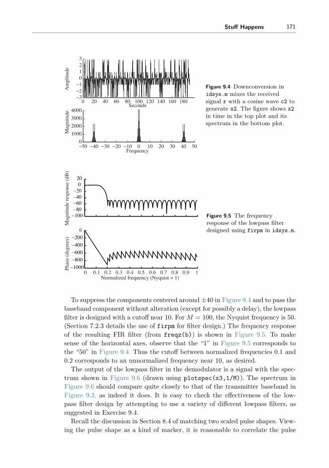
Stuff Happens 171
3
12
0
−2−1
−3
Am
plitu
de
0 20 40 60 80 100 120 140 160 180Seconds
4000
3000
2000
1000
0
Mag
nitu
de
−50 −40 −30 −20 −10 0 10 20 30 40 50Frequency
Figure 9.4 Downconversion inidsys.m mixes the receivedsignal r with a cosine wave c2 togenerate x2. The figure shows x2in time in the top plot and itsspectrum in the bottom plot.
Mag
nitu
de r
espo
nse
(dB
)Ph
ase
(deg
rees
)
0 0.1 0.2 0.3 0.4 0.5 0.6 0.7 0.8 0.9 1Normalized frequency (Nyquist = 1)
−1000
−800−600−400
−2000
−100−80−60−40−20
020
Figure 9.5 The frequencyresponse of the lowpass filterdesigned using firpm in idsys.m.
To suppress the components centered around ±40 in Figure 9.4 and to pass the
baseband component without alteration (except for possibly a delay), the lowpass
filter is designed with a cutoff near 10. For M = 100, the Nyquist frequency is 50.
(Section 7.2.3 details the use of firpm for filter design.) The frequency response
of the resulting FIR filter (from freqz(b)) is shown in Figure 9.5. To make
sense of the horizontal axes, observe that the “1” in Figure 9.5 corresponds to
the “50” in Figure 9.4. Thus the cutoff between normalized frequencies 0.1 and
0.2 corresponds to an unnormalized frequency near 10, as desired.
The output of the lowpass filter in the demodulator is a signal with the spec-
trum shown in Figure 9.6 (drawn using plotspec(x3,1/M)). The spectrum in
Figure 9.6 should compare quite closely to that of the transmitter baseband in
Figure 9.2, as indeed it does. It is easy to check the effectiveness of the low-
pass filter design by attempting to use a variety of different lowpass filters, as
suggested in Exercise 9.4.
Recall the discussion in Section 8.4 of matching two scaled pulse shapes. View-
ing the pulse shape as a kind of marker, it is reasonable to correlate the pulse

172 Chapter 9. Stuff Happens
3
1
2
0
−2
−1
−3
Am
plitu
de
0 20 40 60 80 100 120 140 160 180Seconds
8000
6000
4000
2000
0
Mag
nitu
de
−50 −40 −30 −20 −10 0 10 20 30 40 50Frequency
Figure 9.6 After demodulationand lowpass filtering, the signalx3 in idsys.m is approximatelythe same as the basebandtransmitted signal (andspectrum) in Figure 9.2.
3
2
1
0
−1
−2
−30 50 100 150
Best times to take samples
Ts-spaced samples
T-spaced samples
Am
plitu
de o
f re
ceiv
ed s
igna
l
Delay
200 250 300 350 400
0 T 2T 3T 4T
Figure 9.7 The first four symbolperiods (recall that the oversamplingfactor was M = 100) of the signal atthe receiver (after the demodulation,LPF, and pulse correlator filter). Thefirst three symbol values are −3, +3,−3, which can be deciphered fromthe signal, assuming that the delaycan be selected appropriately.
shape with the received signal in order to locate the pulses. (More justifica-
tion for this procedure is forthcoming in Chapter 11.) This appears in Figure
9.1 as the block labelled “pulse correlation filter.” The code in idsys.m imple-
ments this using the filter command to carry out the correlation (rather than
the xcorr function), though the choice was a matter of convenience. (Refer to
corrvsconv.m in Exercise 8.9 to see how the two functions are related.)
The first 4M samples of the resulting signal y are plotted in Figure 9.7 (via
plot(y(1:4*M))). The first three symbols of the message (i.e., m(1:3)) are −3,
3, and −3, and Figure 9.7 shows why it is best to take the samples at indices
125 + kM . The initial delay of 125 corresponds to half the length of the lowpass
filter (0.5*fl) plus half the length of the correlator filter (0.5*M) plus half a
symbol period (0.5*M), which accounts for the delay from the start of each pulse
to its peak.

Stuff Happens 173
3
2
1
0
−1
−2
−3
0 50 100 150 200 250 300 350 400
Figure 9.8 Repeatedly overlaying atime width of four symbols yieldsan eye diagram.
Selecting this delay and the associated downsampling are accomplished in the
code
z=y (0 . 5* f l+M:M:end ) ; % downsample to symbol r a t e
in idsys.m, which recovers the T -spaced samples z. With reference to Figure
9.1, the parameter l in the downsampling block is 125.
A revealing extension of Figure 9.7 is to plot the oversampled waveform y for
the complete transmission in order to see whether the subsequent peaks of the
pulses occur at regular intervals precisely on source alphabet symbol values, as
we would hope. However, even for small messages (such as the wiener jingle),
squeezing such a figure onto one graph makes a detailed visual examination of the
peaks fruitless. This is precisely why we plotted Figure 9.7—to see the detailed
timing information for the first few symbols.
One idea is to plot the next four symbol periods on top of the first four by
shifting the start of the second block to time zero. Continuing this approach
throughout the data record mimics the behavior of a well-adjusted oscilloscope
that triggers at the same point in each symbol group. This operation can be
implemented in Matlab by first determining the maximum number of groups
of 4*M samples that fit inside the vector y from the lth sample on. Let
ul=f loor ( ( length ( y)− l −1)/(4*M) ) ;
then the reshape command can be used to form a matrix with 4*M rows and ul
columns. This is easily plotted using
plot ( reshape (y ( l : u l *4*M+124) ,4*M, u l ) )
and the result is shown in Figure 9.8. Note that the first element plotted in Figure
9.8 is the lth element of Figure 9.7. This type of figure, called an eye diagram, is
commonly used in practice as an aid in troubleshooting. Eye diagrams will also
be used routinely in succeeding chapters.
Four is an interesting grouping size for this particular problem because four
symbols are used to represent each character in the coding and decoding imple-
mented in letters2pam.m and pam2letters.m. One idiosyncrasy is that each
character starts off with a negative symbol. Another is that the second symbol in

174 Chapter 9. Stuff Happens
−40 20 40 60 80 100 120 140 160 180 200
−3
−2
−1
0
1
3
2
4
Figure 9.9 Values of thereconstructed symbols, called thesoft decisions, are plotted in thisconstellation diagram timehistory.
each character is never −1 in our chosen message. These are not generic effects;
they are a consequence of the particular coding and message used in idsys.m.
Had we chosen to implement a scrambling scheme (recall Exercise 8.19) the
received signal would be whitened and these particular peculiarities would not
occur.
The vector z contains estimates of the decoded symbols, and the command
plot([1:length(z)],z,’.’)produces a time history of the output of the down-
sampler, as shown in Figure 9.9. This is called the time history of a constellation
diagram in which all the dots are meant to lie near the allowable symbol values.
Indeed, the points in Figure 9.9 cluster tightly about the alphabet values ±1 and
±3. How tightly they cluster can be quantified using the cluster variance, which
is the average of the square of the difference between the decoded symbol values
(the soft decisions) in z and the nearest member of the alphabet (the final hard
decisions).
The Matlab function quantalph.m is used in idsys.m to calculate the hard
decisions, which are then converted back into a text character string using
pam2letters.m. If all goes well, this reproduces the original message. The only
flaw is that the last symbol of the message has been lost due to the inherent delay
of the lowpass filtering and the pulse-shape correlation. Because four symbols are
needed to decode a single character, the loss of the last symbol also results in
the loss of the last character. The function pam2letters.m provides a friendly
reminder in the Matlab command window that this has happened.
The problems that follow give a few more ways to explore the behavior of the
ideal system.
Exercise 9.1. Using idsys.m, examine the effect of using different carrier fre-
quencies. Try fc = 50, 30, 3, 1, 0.5. What are the limiting factors that cause
some to work and others to fail?

Stuff Happens 175
Exercise 9.2. Using idsys.m, examine the effect of using different oversampling
frequencies. Try M = 1000, 25, 10. What are the limiting factors that cause some
to work and others to fail?
Exercise 9.3. What happens if the LPF at the beginning of the receiver is
removed? What do you think will happen if there are other users present? Try
adding in “another user” at fc = 30.
Exercise 9.4. What are the limits to the LPF design at the beginning of the
receiver? What is the lowest cutoff frequency that works? The highest?
Exercise 9.5. Using the same specifications (fbe=[0 0.1 0.2 1]; damps= [1
1 0 0 ];), how short can you make the LPF? Explain.
9.3 Flat Fading: A Simple Impairment and a Simple Fix
Unfortunately, a number of the assumptions made in the simulation of the ideal
system idsys.m are routinely violated in practice. The designer of a receiver
must somehow compensate by improving the receiver. This section presents an
impairment (flat fading) for which we have already developed a fix (an AGC).
Later sections describe misbehavior due to a wider variety of common impair-
ments that we will spend the rest of the book combating.
Flat fading occurs when there are obstacles moving in the path between the
transmitter and receiver or when the transmitter and receiver are moving with
respect to each other. It is most commonly modeled as a time-varying channel
gain that attenuates the received signal. The modifier “flat” implies that the
loss in gain is uniform over all frequencies. (In communications jargon, it is
not frequency-selective.) This section begins by studying the loss of performance
caused by a time-varying channel gain (using a modified version of idsys.m) and
then examines the ability of an adaptive element (the automatic gain control,
AGC) to make things right.
In the ideal system of the preceding section, the gain between the transmit-
ter and the receiver was implicitly assumed to be unity. What happens when
this assumption is violated, when flat fading is experienced in midmessage? To
examine this question, suppose that the channel gain is unity for the first 20%
of the transmission, but that for the last 80% it drops by half. This flat fade can
easily be studied by inserting the following code between the transmitter and
the receiver parts of idsys.m.
Listing 9.3. idsysmod1.m modification of idsys.m with time-varying fading channel
l r=length ( r ) ; % l ength o f t r ansmi t ted s i g n a l vectorfp=[ ones (1 , f loor ( 0 . 2* l r ) ) , . . .
. . . 0 . 5 * ones (1 , l r−f loor ( 0 . 2* l r ) ) ] ; % f l a t f ad ing p r o f i l er=r . * fp ; % apply p r o f i l e to t ransmi t ted s i g n a l

176 Chapter 9. Stuff Happens
−40 20 40 60 80 100 120 140 160 180 200
−3
−2
−1
0
1
2
3
Figure 9.10 Soft decisions withuncompensated flat fading.
The resulting plot of the soft decisions in Figure 9.10 (obtained via
plot([1:length(z)], z,’.’)) shows the effect of the fade in the latter 80%
of the response. Shrinking the magnitude of the symbols ±3 by half puts them
in the decision region for ±1, which generates a large number of symbol errors.
Indeed, the recovered message looks nothing like the original.
Section 6.8 has already introduced an adaptive element designed to compen-
sate for flat fading: the automatic gain control, which acts to maintain the
power of a signal at a constant known level. Stripping out the AGC code from
agcvsfading.m on page 128 and combining it with the fading channel just dis-
cussed creates a simulation in which the fade occurs, but in which the AGC can
actively work to restore the power of the received signal to its desired nominal
value ds ≈ 1.
Listing 9.4. idsysmod2.m modification of idsys.m with fading plus automatic gain control
ds=pow( r ) ; % de s i r ed average power o f s i g n a ll r=length ( r ) ; % l ength o f t r ansmi tted s i g n a lfp=[ ones (1 , f loor ( 0 . 2* l r ) ) , . . .
0 . 5* ones (1 , l r−f loor ( 0 . 2* l r ) ) ] ; % f l a t f ad ing p r o f i l er=r . * fp ; % apply to transmi tted s i g n a lg=zeros (1 , l r ) ; g (1)=1; % i n i t i a l i z e gainnr=zeros (1 , l r ) ;mu=0.0003; % s t e p s i z efor i =1: l r −1 % adaptive AGC element
nr ( i )=g ( i )* r ( i ) ; % AGC outputg ( i+1)=g ( i )−mu*( nr ( i )ˆ2−ds ) ; % adapt gain
end
r=nr ; % r ec e i v ed s i g n a l i s s t i l l c a l l e d r
Inserting this segment into idsys.m (immediately after the time-varying fading
channel modification) results in only a small number of errors that occur right at
the time of the fade. Very quickly, the AGC kicks in to restore the received power.
The resulting plot of the soft decisions (via plot([1:length(z)],z,’.’)) in
Figure 9.11 shows how quickly after the abrupt fade the soft decisions return
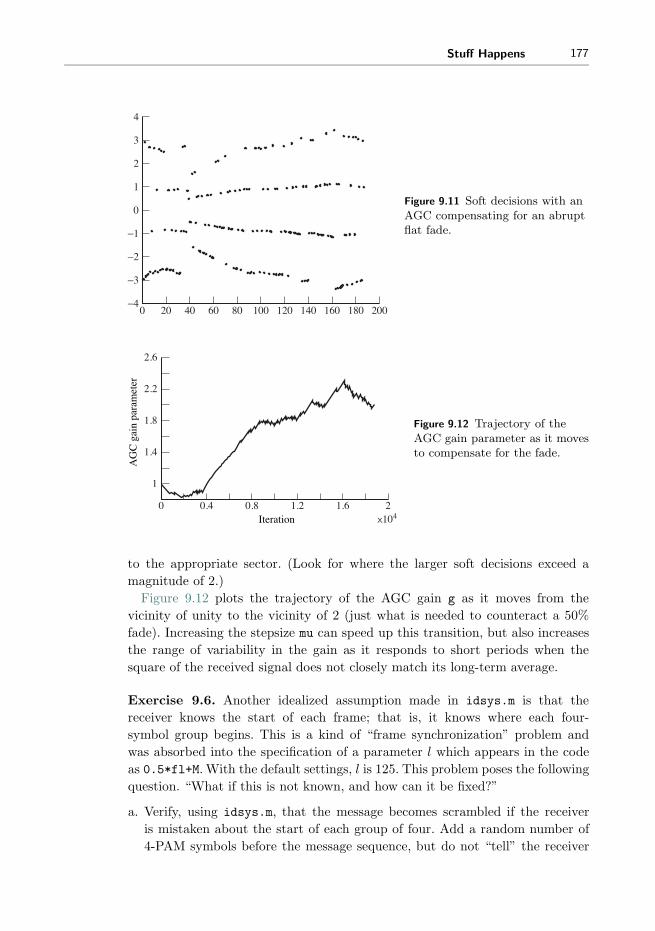
Stuff Happens 177
0 20 40 60 80 100 120 140 160 180 200
4
3
2
1
0
−1
−2
−3
−4
Figure 9.11 Soft decisions with anAGC compensating for an abruptflat fade.
2.6
2.2
1.8
1.4
1
0 0.4 0.8 1.2 1.6 2x10⁴
AG
C g
ain
para
met
er
Iteration
Figure 9.12 Trajectory of theAGC gain parameter as it movesto compensate for the fade.
to the appropriate sector. (Look for where the larger soft decisions exceed a
magnitude of 2.)
Figure 9.12 plots the trajectory of the AGC gain g as it moves from the
vicinity of unity to the vicinity of 2 (just what is needed to counteract a 50%
fade). Increasing the stepsize mu can speed up this transition, but also increases
the range of variability in the gain as it responds to short periods when the
square of the received signal does not closely match its long-term average.
Exercise 9.6. Another idealized assumption made in idsys.m is that the
receiver knows the start of each frame; that is, it knows where each four-
symbol group begins. This is a kind of “frame synchronization” problem and
was absorbed into the specification of a parameter l which appears in the code
as 0.5*fl+M. With the default settings, l is 125. This problem poses the following
question. “What if this is not known, and how can it be fixed?”
a. Verify, using idsys.m, that the message becomes scrambled if the receiver
is mistaken about the start of each group of four. Add a random number of
4-PAM symbols before the message sequence, but do not “tell” the receiver

178 Chapter 9. Stuff Happens
that you have done so (i.e., do not change l). What value of l would fix the
problem? Can l really be known beforehand?
b. Section 8.5 proposed the insertion of a marker sequence as a way to synchro-
nize the frame. Add a seven-symbol marker sequence just prior to the first
character of the text. In the receiver, implement a correlator that searches for
the known marker. Demonstrate the success of this modification by adding
random symbols at the start of the transmission. Where in the receiver have
you chosen to put the correlation procedure? Why?
c. One quirk of the system (observed in the eye diagram in Figure 9.8) is that
each group of four begins with a negative number. Use this feature (rather
than a separate marker sequence) to create a correlator in the receiver that
can be used to find the start of the frames.
d. The previous two exercises showed two possible solutions to the frame-
synchronization problem. Explain the pros and cons of each method, and
argue which is a “better” solution.
9.4 Other Impairments: More “What Ifs”
Of course, a fading channel is not the only thing that can go wrong in a telecom-
munication system. (Think back to the “what if” questions in the first section
of this chapter.) This section considers a range of synchronization and interfer-
ence impairments that violate the assumptions of the idealized system. Though
each impairment is studied separately (i.e., assuming that everything functions
ideally except for the particular impairment of interest), a single program is
written to simulate any of the impairments. The program impsys.m leaves both
the transmitter and the basic operation of the receiver unchanged; the primary
impairments are to the sampled sequence that is delivered to the receiver.
The rest of this chapter conducts a series of experiments dealing with stuff
that can happen to the system. Interference is added to the received signal as
additive Gaussian channel noise and as multipath interference. The oscillator at
the transmitter is no longer presumed to be synchronized with the oscillator at
the receiver. The best sample times are no longer presumed to be known exactly
in either phase or period.
Listing 9.5. impsys.m impairments to the receiver
cng=input ( ’channel noise gain: try 0, 0.6 or 2 :: ’ ) ;cd i=input ( ’channel multipath : 0 for none ,...
1 for mild or 2 for harsh :: ’ ) ;f o=input ( ’tranmsitter mixer freq offset in percent :...
try 0 or 0.01 :: ’ ) ;po=input ( ’tranmsitter mixer phase offset in rad :...
try 0, 0.7 or 0.9 :: ’ ) ;toper=input ( ’baud timing offset as percent of symb period :...
try 0, 20 or 30 :: ’ ) ;so=input ( ’symbol period offset : try 0 or 1 :: ’ ) ;

Stuff Happens 179
% INSERT TRANSMITTER CODE (FROM IDSYS .M) HERE
i f cd i < 0 . 5 , % channel IS Imc=[1 0 0 ] ; % d i s t o r t i on − f r e e channel
e l s e i f cdi <1.5 , % mild mult ipath channelmc=[1 zeros (1 ,M) 0 .28 zeros ( 1 , 2 . 3*M) 0 . 1 1 ] ;
else % harsh mult ipath channelmc=[1 zeros (1 ,M) 0 .28 zeros ( 1 , 1 . 8*M) 0 . 4 4 ] ;
end
mc=mc/( sqrt (mc*mc ’ ) ) ; % normal ize channel powerdv=f i l t e r (mc, 1 , r ) ; % f i l t e r s i g n a l through channelnv=dv+cng *(randn ( size ( dv ) ) ) ; % add Gaussian channel no i s eto=f loor (0 . 01* toper *M) ; % f r a c t i o n a l per i od delayrnv=nv(1+ to :N*M) ; % delay in on−symbol de s i gna t i onr t=(1+to )/M:1/M: length ( nv )/M; % time vector with delayed s t a r trM=M+so ; % r e c e i v e r sampler t iming o f f s e t
% INSERT RECEIVER CODE (FROM IDSYS .M) HERE
The first few lines of impsys.m prompt the user for parameters that define the
impairments. The channel noise gain parameter cng is a gain factor associated
with a Gaussian noise that is added to the received signal. The suggested values
of 0, 0.6, and 2 represent no impairment, mild impairment (that only rarely
causes symbol recovery errors), and a harsh impairment (that causes multiple
symbol errors), respectively.
The second prompt selects the multipath interference: none, mild, or harsh.
In the mild and harsh cases, three copies of the transmitted signal are summed
at the receiver, each with a different delay and amplitude. This is implemented
by passing the transmitted signal through a filter whose impulse response is
specified by the variable mc. As occurs in practice, the transmission delays are
not necessarily integer multiples of the symbol interval. Each of the multipath
models has its largest tap first. If the largest path gain were not first, this could
be interpreted as a delay between the receipt of the first sample of the first pulse
of the message and the optimal sampling instant.
The next pair of prompts concern the transmitter and receiver oscillators.
The receiver assumes that the phase of the oscillator at the transmitter is zero
at the time of arrival of the first sample of the message. In the ideal system,
this assumption was correct. In impsys.m, however, the receiver makes the same
assumption, but it might no longer be correct. Mismatch between the phase of
the oscillator at the transmitter and the phase of the oscillator at the receiver is
an inescapable impairment (unless there is also a separate communication link or
added signal such as an embedded pilot tone that synchronizes the oscillators).
The user is prompted for a carrier phase offset in radians (the variable po) that
is added to the phase of the oscillator at the transmitter, but not at the receiver.
Similarly, the frequencies of the oscillators at the transmitter and receiver may
differ by a small amount. The user specifies the frequency offset in the variable
fo as a percentage of the carrier frequency. This is used to scale the carrier
frequency of the transmitter, but not of the receiver. This represents a difference

180 Chapter 9. Stuff Happens
between the nominal values used by the receiver and the actual values achieved
by the transmitter.
Just as the receiver oscillator need not be fully synchronized with the transmit-
ter oscillator, the symbol clock at the receiver need not be properly synchronized
with the transmitter symbol period clock. Effectively, the receiver must choose
when to sample the received signal on the basis of its best guess as to the phase
and frequency of the symbol clock at the transmitter. In the ideal case, the delay
between the receipt of the start of the signal and the first sample time was read-
ily calculated using the parameter l. But l cannot be known in a real system
because the “first sample” depends, for instance, on when the receiver is turned
on. Thus, the phase of the symbol clock is unknown at the receiver. This impair-
ment is simulated in impsys.m using the timing offset parameter toper, which
is specified as a percentage of the symbol period. Subsequent samples are taken
at positive integer multiples of the presumed sampling interval. If this interval
is incorrect, then the subsequent sample times will also be incorrect. The final
impairment is specified by the “symbol period offset,” which sets the symbol
period at the transmitter to so less than that at the receiver.
Using impsys.m, it is now easy to investigate how each impairment degrades
the performance of the system.
9.4.1 Additive Channel Noise
Whenever the channel noise is greater than half the gap between two adjacent
symbols in the source constellation, a symbol error may occur. For the constel-
lation of ±1s and ±3s, if a noise sample has magnitude larger than 1, then the
output of the quantizer may be erroneous.
Suppose that a white, broadband noise is added to the transmitted sig-
nal. The spectrum of the received signal, which is plotted in Figure 9.13 (via
plotspec(nv,1/rM)), shows a nonzero noise floor compared with the ideal
(noise-free) spectrum in Figure 9.3. A noise gain factor of cng=0.6 leads to a
cluster variance of about 0.02 and no symbol errors. A noise gain of cng=2 leads
to a cluster variance of about 0.2 and results in approximately 2% symbol errors.
When there are 10% symbol errors, the reconstructed text becomes undecipher-
able (for the particular coding used in letters2pam.m and pam2letters.m).
Thus, as should be expected, the performance of the system degrades as the
noise is increased. It is worthwhile taking a closer look to see exactly what goes
wrong.
The eye diagram for the noisy received signal is shown in Figure 9.14, which
should be compared with the noise-free eye diagram in Figure 9.8. This is plotted
using the following Matlab commands:
ul=f loor ( ( length ( x3 )−124)/(4* rM) ) ;plot ( reshape ( x3 (125 : u l *4*rM+124) ,4*rM, u l ) ) .

Stuff Happens 181
5
0
−50 20 40 60 80 100
Seconds120 140 160 180 200
Am
plitu
de
5000
4000
3000
2000
1000
0−50 −40 −30 −20 −10 0
Frequency10 20 30 40 50
Mag
nitu
de
Figure 9.13 When noise isadded, the received signalappears jittery. The spectrumhas a noticeable noise floor.
5
4
3
2
1
0
−1
−2
−3
−4
−50 50 100 150 200 250 300 350 400
Figure 9.14 The eye diagramof the received signal x3repeatedly overlaysfour-symbol-wide segments.The channel noise is notinsignificant.
It should be clear from the noisy eye diagram that it would be very difficult to
correctly decode the symbols directly from this signal. Fortunately, the correla-
tion filter reduces the noise significantly, as shown in the eye diagram in Figure
9.15. (This is plotted as before, substituting y for x3.) Comparing Figures 9.14
and 9.15 closely, observe that the whole of the latter is shifted over in time by
about 50 samples. This is the effect of the time delay of the correlator filter,
which is half the length of the filter. Clearly, it is much easier to correctly decode
using y than using x3, though the pulse shapes of Figure 9.15 are still blurred
when compared with the ideal pulse shapes in Figure 9.8.
Exercise 9.7. The correlation filter in impsys.m is a lowpass filter with impulse
response given by the pulse shape p.
a. Plot the frequency response of this filter. What is the bandwidth of this filter?

182 Chapter 9. Stuff Happens
4
3
2
1
0
−1
−2
−3
−40 50 100 150 200 250 300 350 400
Figure 9.15 The eye diagramof the received signal y afterthe correlation filter. Thenoise is reduced significantly.
b. Design a lowpass filter using firpm that has the same length and the same
bandwidth as the correlation filter.
c. Use your new filter in place of the correlation filter in impsys.m. Has the
performance improved or worsened? Explain in detail what tests you have
used.
No peeking ahead to Chapter 11.
9.4.2 Multipath Interference
The next impairment is interference caused by a multipath channel, which occurs
whenever there is more than one route between the transmitter and the receiver.
Because these paths experience different delays and attenuations, multipath
interference can be modeled as a linear filter. Since filters can have complicated
frequency responses, some frequencies may be attenuated more than others, and
so this is called frequency-selective fading.
The “mild” multipath interference in impsys.m has three (nonzero) paths
between the transmitter and the receiver. Its frequency response has numer-
ous dips and bumps that vary in magnitude from about +2 to −4 dB. (Verify
this using freqz.) A plot of the soft decisions is shown in Figure 9.16 (from
plot([1:length(z)],z,’.’)), which should be compared with the ideal con-
stellation diagram in Figure 9.9. The effect of the mild multipath interference
is to smear the lines into stripes. As long as the stripes remain separated, the
quantizer is able to recover the symbols, and hence the message, without errors.
The “harsh” multipath channel in impsys.m also has three paths between the
transmitter and receiver, but the later reflections are larger than in the mild
case. The frequency response of this channel has peaks up to about +4 dB and
down to about −8 dB, so its effects are considerably more severe. The effect
of this channel can be seen directly by looking at the constellation diagram of
the soft decisions in Figure 9.17. The constellation diagram is smeared, and it is

Stuff Happens 183
4
3
2
1
0
−1
−2
−3
−40 20 40 60 80 100 120 140 200160 180
Figure 9.16 With mild multipathinterference, the soft decisionscan readily be segregated intofour stripes that correspond tothe four symbol values.
4
3
2
1
0
−1
−2
−3
−40 20 40 60 80 100 120 140 200160 180
Figure 9.17 With harshermultipath interference, the softdecisions smear and it is nolonger possible to see whichpoints correspond to which of thefour symbol values.
no longer possible to visually distinguish the four stripes that represent the four
symbol values. It is no surprise that the message becomes garbled. As the output
shows, there are about 10% symbol errors, and most of the recovered characters
are wrong.
9.4.3 Carrier Phase Offset
For the receiver in Figure 9.1, the difference between the phase of the modulating
sinusoid at the transmitter and the phase of the demodulating sinusoid at the
receiver is the carrier phase offset. The effect of a nonzero offset is to scale the
received signal by a factor equal to the cosine of the offset, as was shown in (5.4)
of Section 5.2. Once the phase offset is large enough, the demodulated signal
contracts so that its maximum magnitude is less than 2. When this happens, the
quantizer always produces a ±1. Symbol errors abound.

184 Chapter 9. Stuff Happens
2
1.5
1
0.5
0
−0.5
−1
−1.5
−20 20 40 60 80 100 120 140 200160 180
Figure 9.18 Soft decisions forharsh carrier phase offset arenever greater than 2. Thequantizer finds no ±3s andmany symbol errors occur.
When running impsys.m, there are two suggested nonzero choices for the
phase-offset parameter po. With po=0.9, cos(0.9) = 0.62, and 3 cos(0.9) < 2.
This is shown in the plot of the soft-decision errors in Figure 9.18. For the
milder carrier phase offset (po=0.7), the soft decisions result in no symbol errors,
because the quantizer will still decode values at ±3 cos(0.7) = ±2.3 as ±3.
As long as the constellation diagram retains distinct horizontal stripes, all is
not lost. In Figure 9.18, even though the maximum magnitude is less than 2,
there are still four distinct stripes. If the quantizer could be scaled properly, the
symbols could be decoded successfully. Such a scaling might be accomplished,
for instance, by another AGC, but such scaling would not improve the signal-
to-noise ratio. A better approach is to identify the ‘unknown’ phase offset, as
discussed in Chapter 10.
Exercise 9.8. Using impsys.m as a basis, implement an AGC-style adaptive
element to compensate for a phase offset. Verify that your method works for a
phase offset of 0.9 and for a phase offset of 1.2. Show that the method fails when
the phase offset is π/2.
9.4.4 Carrier Frequency Offset
The receiver in Figure 9.1 has a carrier frequency offset when the frequency of
the carrier at the transmitter differs from the assumed frequency of the carrier
at the receiver. As was shown in (5.5) in Section 5.2, this impairment is like
a modulation by a sinusoid with frequency equal to the offset. This modulat-
ing effect is catastrophic when the low-frequency modulator approaches a zero
crossing, since then the gain of the signal approaches zero. This effect is apparent
for a 0.01% frequency offset in impsys.m in the plot of the soft decisions (via
plot([1:length(z)],z,’.’)) in Figure 9.19. This experiment suggests that the
receiver mixer frequency must be adjusted to track that of the transmitter.

Stuff Happens 185
3
2
1
0
−1
−2
−30 20 40 60 80 100 120 140 200160 180
Figure 9.19 Soft decisions for0.01% carrier frequency offset.
9.4.5 Downsampler Timing Offset
As shown in Figure 9.7, there is a sequence of “best times” at which to down-
sample. When the starting point is correct and no intersymbol interference (ISI)
is present, as in the ideal system, the sample times occur at the top of the pulses.
When the starting point is incorrect, all the sample times are shifted away from
the top of the pulses. This was set in the ideal simulation using the parameter
l, with its default value of 125. The timing-offset parameter toper in impsys.m
is used to offset the received signal. Essentially, this means that the best value
of l has changed, though the receiver does not know it.
This is easiest to see by drawing the eye diagram. Figure 9.20 shows an overlay
of four-symbol wide segments of the received signal (using the reshape command
as in the code on page 173). The receiver still thinks the best times to sample
are at l + nT , but this is clearly no longer true. In fact, whenever the sample
time begins between 100 and 140 (and lies in this or any other shaded region),
there will be errors when quantizing. For example, all samples taken at 125 lie
between ±1, and hence no symbols will ever be decoded at their ±3 value. In
fact, some even have the wrong sign! This is a far worse situation than in the
carrier phase impairment because no simple amplitude scaling will help. Rather,
a solution must correct the problem; it must slide the times so that they fall
in the unshaded regions. Because these unshaded regions are wide open, this is
often called the open-eye region. The goal of an adaptive element designed to fix
the timing-offset problem is to open the eye as wide as possible.
9.4.6 Downsampler Period Offset
When the assumed period of the downsampler is in error, there is no hope. As
mentioned in the previous impairment, the receiver believes that the best times

186 Chapter 9. Stuff Happens
−30
−2
50 100 150 200 250 300 350 400
−1
0
1
2
3
Assumed "best times" to take samples
Figure 9.20 Eye diagram withdownsampler timing offset of50%. Sample times used by theideal system are no longer valid,and lead to numerous symbolerrors.
to sample are at l + nT . When there is a period offset, it means that the value
of T used at the receiver differs from the value actually used at the transmitter.
The prompt in impsys.m for symbol period offset suggests trying 0 or 1. A
response of 1 results in the transmitter creating the signal assuming that there
are M − 1 samples per symbol period, while the receiver retains the setting of
M samples per symbol, which is used to specify the correlator filter and to
pick subsequent downsampling instants once the initial sample time has been
selected. The symptom of a misaligned sample period is a periodic collapse of
the constellation, similar to that observed when there is a carrier frequency offset
(recall Figure 9.19). For an offset of 1, the soft decisions are plotted in Figure
9.21. Can you connect the value of the period of this periodic collapse to the
parameters of the simulated example?
9.4.7 Repairing Impairments
When stuff happens and the receiver continues to operate as if all were well,
the transmitted message can become unintelligible. The various impairments of
the preceding sections point the way to the next step in the design process by
showing the kinds of problems that may arise. Clearly, the receiver must be
improved to counteract these impairments.
Coding (Chapter 14) and matched receive filtering (Chapter 11) are intended
primarily to counter the effects of noise. Equalization (Chapter 13) compensates
for multipath interference, and can reject narrowband interferers. Carrier recov-
ery (Chapter 10) will be used to adjust the phase, and possibly the frequency
as well, of the receiver oscillator. Timing recovery (Chapter 12) aims to reduce
downsampler timing and period offset. All of these fixes can be viewed as digital
signal processing (DSP) solutions to the impairments explored in impsys.m.

Stuff Happens 187
−3−2−1
0
23
1
400350300250200150100500
−3−2−1
0
23
1
2000 20 40 60 80 100 120 140 160 180
Figure 9.21 When there is a1% downsampler periodoffset, all is lost, as shownby the eye diagram in thetop plot and the softdecisions in the bottom.
Each of these fixes will be designed separately, as if the problem it is intended
to counter were the only problem in the world. Fortunately, somehow they can
all work together simultaneously. Examining possible interactions between the
various fixes, which is normally a part of the testing phase of a receiver design,
will be part of the receiver design project of Chapter 15.
9.5 A B3IG Deal
While the idealized communication systems in idsys.m and impsys.m illustrate
the basic operation of a transmitter–receiver pair, practical systems are a bit
more complicated. One of the problems is keeping track of all the problems that
can arise! In order to help organize all the possibilities, this section introduces
the Basic Black Box Impairment Generator, or B3IG, as shown in Figure 9.22.
Signal r as itenters the receiver
Basic Black BoxImpairment Generator
MATLABscript
definingtransmitterparameters
Figure 9.22 The Basic Black Box Impairment Generator, or B3IG, inputs a Matlab
script that specifies the operation of the transmitter along with any desiredimpairments. The output is the (received) signal r that enters the receiver. You canfind out how the system operates by peering ahead to Appendix H, but we reallyshouldn’t mention it at this point.

188 Chapter 9. Stuff Happens
The B3IG transmitter is a souped-up version of the idealized transmitters in
idsys.m and impsys.m. It allows easy incorporation of a number of impairments,
singly or in combination, and is especially useful when examining possible inter-
actions between the various receiver strategies and fixes that are discussed in
forthcoming chapters. Though a complete description of the B3IG transmitter is
presented in Appendix H, it is probably not useful to jump ahead at this point.
Better to think of B3IG as a tool for exploration, for generating noisy received
signals with various user-specified and user-controlled impairments. In keeping
with the theme of this chapter, there is nothing genuinely new in B3IG; the basic
building blocks are the same as those in the previous chapters.
Using the B3IG transmitter is easy: just type the command in Listing 9.6.
Listing 9.6. This code calls the B3IG transmitter. The received signal is in r and thetransmitted (encoded) symbols are in s.
[ r , s ]=BigTransmitter (m, frameParams , . . .rfParams , chanParams ) ;
There are four inputs to the B3IG. The message that is to be transmitted is spec-
ified in the variable m. The frame parameters frameParams include a specification
for how many symbols are included in each block and a string that represents
the preamble (or header). These are familiar from Chapter 8. In order to mimic
the idealized transmission in idsys.m and impsys.m, the length of a block is set
to 1 and there is no preamble. The message includes the Oscar Meyer jingle and
some numbers. The complete list of parameters is given in Listing 9.7.
Listing 9.7. Parameters in the script BigIdeal.m allow the B3IG transmission to mimicthe idealized system idsys.m and impsys.m.
% Message Generationm=’01234 I wish I were an Oscar Meyer ...
wiener 56789 ’ ;
% Frame parametersframeParams . userDataLength=1;frameParams . preamble=’’ ;frameParams . chanCodingFlag =0;frameParams . bi tEncodingFlag=0;
% Channel parameters , Adj Users , Int . ,chanParams . c1=[1 0 0 ] ;chanParams . c2=[1 0 0 ] ;chanParams . randomWalkVariance=0;chanParams .SNR=Inf ;chanParams . adjacentUser1Power=−Inf ;chanParams . a d j a c e n tU s e r 1 f i f =0;chanParams . adjacentUser1Chan=[1 0 0 ] ;chanParams . adjacentUser2Power=−Inf ;chanParams . a d j a c e n tU s e r 2 f i f =0;chanParams . adjacentUser2Chan=[1 0 0 ] ;chanParams . NBIfreq=0;chanParams . NBIPower=−Inf ;
% RF Parameters

Stuff Happens 189
rfParams . f i f e r r =0;rfParams . T t e r r =0;rfParams . phaseNoiseVar iance=0;rfParams . SRRCLength=4;rfParams . SRRCrol lo f f=0.3 ;rfParams . f s =100;rfParams . T t=1;rfParams . f i f =20;
The channel parameters chanParams specify how the message is distorted as
it moves from the transmitter to the receiver. Intersymbol interference, additive
noise, and interference from other users can all be modeled by changing these
values. Finally, the RF parameters rfParams specify the parameters used: the
frequency of the transmitter, the symbol rate, the size of the pulse shape, the
intermediate frequency, etc. All frequency values are specified in Hz, and all time
values are given in seconds. As before, the values in BigIdeal.m of Listing 9.7
mimic the idealized transmission.
Exercise 9.9. One difference between BigIdeal.m and the received signal in
impsys.m is that the pulse shape is a square-root raised cosine pulse instead of
a Hamming pulse. Run the script and plot the spectrum of the received signal
in BigIdeal.m. Compare this with the spectrum of the received signal from
impsys.m. How do the spectra change when the SNR of the additive channel
noise is decreased?
Exercise 9.10. A rudimentary receiver is provided in Listing 9.8. Observe that
the code makes errors when noise is added because the gain (the parameter
receiver gain) has not been chosen appropriately. Find a new choice of gain
that permits the receiver to operate error-free even with the level of noise present.
How did you find this choice of gain?
Listing 9.8. BigIdeal.m (part 2) idealized B3IG receiver
% Adjustable r e c e i v e r parametersr e c e i v e r g a i n =1;da ta s ta r t =5;% Fixed r e c e i v e r parametersM=100; % upsampling r a t i of c =20; % c a r r i e r f r equencys r r c l e n g t h =4; % length o f pu l s e shape% am demodulation o f r e c e i v ed s i g n a l sequence rc2=cos (2* pi* f c * [ 1/M:1/M: length ( r )/M] ’ ) ; % co s i n e f o r mixingx2=r . * c2 ; % demod r e c e i v ed s i g n a l% co r r e l a t e ( f i l t e r ) to ex t r a c t upsampled pu l s e sy=f i l t e r ( s r r c ( s r r c l eng th , 0 . 3 , 1 0 0 ) , 1 , x2 ) ; % f i l t e r with pu l s e% s e t delay to f i r s t symbol−sample and increment by Mz=y( s r r c l e n g t h *M:M: end ) ; % downsample to symbol r a t e% to s s out f i r s t few symbols , s c a l e by gainz=z ( da ta s ta r t : da ta s ta r t+length (m)*4−1) ’* r e c e i v e r g a i n ;plot ( [ 1 : length ( z ) ] , z , ’.’ ) % p l o t s o f t d e c i s i o n s% de c i s i o n dev i ce and symbol matching performance assessment

190 Chapter 9. Stuff Happens
mprime=quantalph ( z , [ −3 , −1 ,1 , 3 ] ) ’ ; % quant i ze to alphabetcvar=(mprime−z )* (mprime−z ) ’ / length (mprime) % c l u s t e r var i ancelmp=length (mprime ) ;p e r e r r =100*sum(abs ( sign (mprime−l e t te r s2pam (m) ) ) ) / lmp % symb er r% decode d e c i s i o n dev i ce output to text s t r i n gr econs t ructed message=pam2l et te r s (mprime)
Exercise 9.11. Use the AGC code from agcgrad.m to find the proper gain for
the receiver in BigIdeal.m. If the AGC converges slowly, you may wish to use a
longer message m.
Exercise 9.12. Observe that when the parameter dstart is specified incorrectly,
the message is not reconstructed correctly, even when there is no additive noise.
Implement a strategy to identify dstart from the received signal. Hint: perhaps
a header or frame would help.
Exercise 9.13. How would you change the frame, channel, or RF parameters
to reproduce Figures 9.16 and 9.17?
Exercise 9.14. How would you change the frame, channel, or RF parameters
to reproduce Figure 9.19?

Step 4: The Adaptive Components
The fourth step describes all the practical fixes that are needed in order to create
a workable radio. One by one the various pragmatic problems are studied and
solutions are proposed, implemented, and tested. These include fixes for additive
noise, for timing offset problems, for clock frequency mismatches and jitter, and
for multipath reflections. The order in which topics are discussed is the order in
which they appear in the receiver.
Carrier recovery Chapter 10
the timing of frequency translation
Receive filtering Chapter 11
the design of pulse shapes
Clock recovery Chapter 12
the timing of sampling
Equalization Chapter 13
filters that adapt to the channel
Coding Chapter 14
making data resilient to noise

10 Carrier Recovery
Figure 10.1 shows a generic transmitter and receiver pair that emphasizes the
modulation and corresponding demodulation. Even assuming that the transmis-
sion path is ideal (as in Figure 10.1), the signal that arrives at the receiver is a
complicated analog waveform that must be downconverted and sampled before
the message can be recovered. For the demodulation to be successful, the receiver
must be able to figure out both the frequency and the phase of the modulating
sinusoid used in the transmitter, as was shown in (5.4) and (5.5) and graphically
illustrated in Figures 9.18 and 9.19. This chapter discusses a variety of strategies
that can be used to estimate the phase and frequency of the carrier and to fix the
gain problem (of (5.4) and Figure 9.18) and the problem of vanishing amplitudes
(in (5.5) and Figure 9.19). This process of estimating the frequency and phase
of the carrier is called carrier recovery.
Figure 10.1 shows two downconversion steps: one analog and one digital. In
a purely analog system, no sampler or digital downconversion would be needed.
The problem is that accurate analog downconversion requires highly precise ana-
log components, which can be expensive. In a purely digital receiver, the sampler
would directly digitize the received signal, and no analog downconversion would
be required. The problem is that sampling this fast can be prohibitively expen-
sive. The happy compromise is to use an inexpensive analog downconverter to
translate to some lower intermediate frequency, at which it is possible to sample
cheaply enough. At the same time, sophisticated digital processing can be used to
compensate for inaccuracies in the cheap analog components. Indeed, the same
adaptive elements that estimate and remove the unknown phase offset between
the transmitter and the receiver automatically compensate for any additional
phase inaccuracies in the analog portion of the receiver.
Normally, the transmitter and receiver agree to use a particular frequency for
the carrier, and in an ideal world, the frequency of the carrier of the transmitted
signal would be known exactly. But even expensive oscillators may drift apart
in frequency over time, and cheap (inaccurate) oscillators may be an economic
necessity. Thus, there needs to be a way to align the frequency of the oscillator at

Carrier Recovery 193
Pulseshaping
Messagem(kT)
Modulation
Receivedsignal
Ts
Analogconversion
to IF
Digital down-conversionto baseband
Resampling Decision
Reconstructedmessagem(kT)
T
Timingsynchronization
τFrequency andphase tracking
f0 θfc φ
Figure 10.1 Diagram of a communications system emphasizing the need forsynchronization with the frequency fc and phase φ of the carrier. Thefrequency-tracking element adjusts the parameter f0 in an attempt to match fc andthe phase-tracking element adjusts the parameter θ in an attempt to match φ.
the transmitter with the frequency of the oscillator at the receiver. Since the goal
is to find the frequency and phase of a signal, why not use a Fourier transform
(or, more properly, an FFT)? Section 10.1 shows how to isolate a sinusoid that is
at twice the frequency of the carrier by squaring and filtering the received signal.
The frequency and phase of this sinusoid can then be found in a straightforward
manner by using the FFT, and the frequency and phase of the carrier can then
be simply deduced. Though feasible, this method is rarely used because of the
computational cost.
The strategy of the following sections is to replace the FFT operation with
an adaptive element that achieves its optimum value when the phase of an esti-
mated carrier equals the phase of the actual carrier. By moving the estimates in
the direction of the gradient of a suitable performance function, the element can
recursively hone in on the correct value. Assuming initially that the frequency
is known, there are various ways to structure adaptive elements that iteratively
estimate the unknown phase of a carrier. One such performance function, dis-
cussed in Section 10.2, is the square of the difference between the received signal
and a locally generated sinusoid. Another performance function leads to the
well-known phase-locked loop, which is discussed in depth in Section 10.3, and
yet another performance function leads to the Costas loop of Section 10.4. An
alternative approach uses the decision-directed method detailed in Section 10.5.
Each of these methods is derived from an appropriate performance function, each
is simulated in Matlab, and each can be understood by looking at the appro-
priate error surface. This approach should be familiar from Chapter 6, where it
was used in the design of the AGC.
Section 10.6 then shows how to modify the adaptive elements to attack the
frequency-estimation problem. Three ways are shown. The first tries (unsuc-
cessfully) to apply a direct adaptive method, and the reasons for the failure
provide a cautionary counterpoint to the indiscriminate application of adaptive
elements. The second, a simple indirect method detailed in Section 10.6.2, uses
two loops. Since the phase of a sinusoid is the derivative of its frequency, the
first loop tracks a “line” (the frequency offset) and the second loop fine-tunes
the estimation of the phase. The third technique, in Section 10.6.3, shows how

194 Chapter 10. Carrier Recovery
the dual-loop method can be simplified and generalized by using an integrator
within a single phase-locked loop. This forms the basis for an effective adaptive
frequency-tracking element.
10.1 Phase and Frequency Estimation via an FFT
As indicated in Figure 10.1, the received signal consists of a message m(kT )
modulated by the carrier. In the simplest case, when the modulation uses AM
with a large carrier as in Section 5.1, it may be quite easy to locate the carrier
and its phase. More generally, however, the carrier will be well hidden within the
received signal and some kind of extra processing will be needed to bring it to
the foreground.
To see the nature of the carrier-recovery problem explicitly, the following code
generates two different “received signals”: the first is AM modulated with large
carrier and the second is AM modulated with suppressed carrier. The phase
and frequencies of both signals can be recovered using an FFT, though the
suppressed-carrier scheme requires additional processing before the FFT can
successfully be applied.
Drawing on the code in pulseshape.m on page 156, and modulating with
the carrier c, pulrecsig.m creates the two different received signals. The pam
command creates a random sequence of symbols drawn from the alphabet ±1,
±3, and then uses hamming to create a pulse shape.1 The oversampling factor M
is used to simulate the “analog” portion of the transmission, and MTs is equal
to the symbol time T .
Listing 10.1. pulrecsig.m make pulse-shaped signal
N=10000; M=20; Ts=.0001; % # symbols , oversampl ing f a c t o rtime=Ts*N*M; t=Ts : Ts : time ; % sampling i n t e r v a l & time vectorm=pam(N, 4 , 5 ) ; % 4− l e v e l s i g n a l o f l ength Nmup=zeros (1 ,N*M) ;mup( 1 :M:N*M)=m; % oversample by i n t e g e r l ength Mps=hamming (M) ; % b l i p pu l s e o f width Ms=f i l t e r ( ps , 1 ,mup ) ; % convolve pu l s e shape with dataf c =1000; pho f f =−1.0; % c a r r i e r f r eq and phasec=cos (2* pi* f c * t+phof f ) ; % cons truct c a r r i e rr s c=s . * c ; % modulated s i g n a l ( smal l c a r r i e r )r l c =(s +1).* c ; % modulated s i g n a l ( l a r g e c a r r i e r )
Figure 10.2 plots the spectra of the large- and suppressed-carrier signals rlc
and rsc. The carrier itself is clearly visible in the top plot, and its frequency and
phase can readily be found by locating the maximum value in the FFT:
f f t r l c=f f t ( r l c ) ; % spectrum of r l c[m, imax]=max(abs ( f f t r l c ( 1 : end / 2 ) ) ) ; % index o f max peaks s f =(0: length ( t )−1)/(Ts* length ( t ) ) ; % f r equency vector
1 This is not a common (or a particularly useful) pulse shape. It is just easy to use. Goodpulse shapes are considered in detail in Chapter 11.

Carrier Recovery 195
0 1000 2000 3000 4000 5000
0 1000 2000 3000 4000 5000
0 1000 2000 3000 4000 5000
Figure 10.2 The magnitude spectrum of the received signal of a system using AM withlarge carrier has a prominent spike at the frequency of the carrier, as shown in the topplot. When using the suppressed-carrier method in the middle plot, the carrier is notclearly visible. After preprocessing of the suppressed-carrier signal using the schemein Figure 10.3, a spike is clearly visible at twice the desired frequency (and with twicethe desired phase). In the time domain, this corresponds to an undulating sine wave.
f r eqL=s s f ( imax ) % f r eq at the peakphaseL=angle ( f f t r l c ( imax ) ) % phase at the peak
Changing the default phase offset phoff changes the phaseL variable accordingly.
Changing the frequency fc of the carrier changes the frequency freqL at which
the maximum occurs. Note that the max function used in this fashion returns
both the maximum value m and the index imax at which the maximum occurs.
On the other hand, applying the same code to the FFT of the suppressed-
carrier signal does not recover the phase offset. In fact, the maximum often
occurs at frequencies other than the carrier, and the phase values reported bear
no resemblance to the desired phase offset phoff. There needs to be a way to
process the received signal to emphasize the carrier.
A common scheme uses a squaring nonlinearity followed by a bandpass filter,
as shown in Figure 10.3. When the received signal r(t) consists of the pulse-
modulated data signal s(t) times the carrier cos(2πfct+ φ), the output of the
squaring block is
r2(t) = s2(t) cos2(2πfct+ φ). (10.1)
This can be rewritten using the identity 2 cos2(x) = 1 + cos(2x) in (A.4) to pro-
duce
r2(t) = (1/2)s2(t)[1 + cos(4πfct+ 2φ)].
Rewriting s2(t) as the sum of its (positive) average value and the variation about
this average yields
s2(t) = s2avg + v(t).

196 Chapter 10. Carrier Recovery
Thus,
r2(t) = (1/2)[s2avg + v(t) + s2avg cos(4πfct+ 2φ) + v(t) cos(4πfct+ 2φ)].
A narrow bandpass filter centered near 2fc passes the pure cosine term in r2 and
suppresses the DC component, the (presumably) lowpass v(t), and the upcon-
verted v(t). The output of the bandpass filter is approximately
rp(t) = BPF{r2(t)} ≈ 1
2s2avg cos(4πfct+ 2φ+ ψ), (10.2)
where ψ is the phase shift added by the BPF at frequency 2fc. Since ψ is known
at the receiver, rp(t) can be used to find the frequency and phase of the carrier. Of
course, the primary component in rp(t) is at twice the frequency of the carrier,
the phase is twice the original unknown phase, and it is necessary to take ψ
into account. Thus some extra bookkeeping is needed. The amplitude of rp(t)
undulates slowly as s2avg changes.
The following Matlab code carries out the preprocessing of Figure 10.3. First,
run pulrecsig.m to generate the suppressed carrier signal rsc.
Listing 10.2. pllpreprocess.m send received signal through square and BPF
r=r s c ; % suppressed c a r r i e r rq=r . ˆ 2 ; % square n on l i n e a r i t yf l =500; f f =[0 . 38 . 39 . 41 . 42 1 ] ; % BPF center f r equency at . 4f a =[0 0 1 1 0 0 ] ; % which i s twice f ch=f i rpm ( f l , f f , f a ) ; % BPF des i gn v ia f i rpmrp=f i l t e r (h , 1 , q ) ; % f i l t e r g i v e s pr eproces s ed r
Then the phase and frequency of rp can be found directly by using the FFT.
% recover unknown f r eq and phase us ing FFTfftrBPF=f f t ( rp ) ; % spectrum of rBPF[m, imax]=max(abs ( f ftrBPF ( 1 : end / 2 ) ) ) ; % f i nd f r eq o f max peaks s f =(0: length ( rp ) )/ ( Ts* length ( rp ) ) ; % f r equency vectorf r eqS=s s f ( imax ) % f r eq at the peakphasep=angle ( f ftrBPF ( imax ) ) ; % phase at the peak[ IR , f ]= f r eq z (h , 1 , length ( rp ) , 1/Ts ) ; % f r eq r esponse o f f i l t e r[ mi , im]=min(abs ( f−f r eqS ) ) ; % f r eq where peak occur sphaseBPF=angle ( IR ( im ) ) ; % < o f BPF at peak f r eqphaseS=mod( phasep−phaseBPF , pi ) % est imated angle
Observe that both freqS and phaseS are twice the nominal values of fc and
phoff, though there may be a π ambiguity (as will occur in any phase estima-
tion).
The intent of this section is to clearly depict the problem of recovering the fre-
quency and phase of the carrier even when it is buried within the data-modulated
signal. The method used to solve the problem (application of the FFT) is not
common, primarily because of the numerical complexity. Most practical receivers
use some kind of adaptive element to iteratively locate and track the frequency
and phase of the carrier. Such elements are explored in the remainder of this
chapter.

Carrier Recovery 197
X2 BPFr(t) r2(t)
Squaringnonlinearity
Center frequency~ 2fc
rp(t) ~ cos(4π fc t + 2φ + ψ)
Figure 10.3 Preprocessing the input to a PLL via a squaring nonlinearity and BPFresults in a sinusoidal signal at twice the frequency with a phase offset equal to twicethe original plus a term introduced by the known bandpass filtering.
Exercise 10.1. The squaring nonlinearity is only one possibility in the
pllpreprocess.m routine.
a. Try replacing the r2(t) with |r(t)|. Does this result in a viable method of
emphasizing the carrier?
b. Try replacing the r2(t) with r3(t). Does this result in a viable method of
emphasizing the carrier?
c. Can you think of other functions that will result in viable methods of empha-
sizing the carrier?
d. Will a linear function work? Why or why not?
Exercise 10.2. Determine the phase shift ψ at the frequency 2fc caused by the
BPF when
a. fl=490, 496, 502,
b. Ts=0.0001, 0.000101,
c. M=19, 20, 21. Explain why ψ should depend on fl, Ts, and M.
10.2 Squared Difference Loop
The problem of phase tracking is to determine the phase φ of the carrier and
to follow any changes in φ using only the received signal. The frequency fc of
the carrier is assumed known, though ultimately it too must be estimated. The
received signal can be preprocessed (as in the previous section) to create a signal
that strips away the data, in essence fabricating a sinusoid which has twice the
frequency at twice the phase of the unmodulated carrier. This can be idealized
to
rp(t) = cos(4πfct+ 2φ), (10.3)
which suppresses2 the dependence on the known phase shift ψ of the BPF and
sets the constant s2avg/2 to unity (compare with (10.2)). The form of rp(t) implies
that there is an essential ambiguity in the phase since φ can be replaced by
φ+ nπ for any integer n without changing the value of (10.3). What can be
done to recover φ (modulo π) from rp(t)?
2 An example that takes ψ into account is given in Exercise 10.8.

198 Chapter 10. Carrier Recovery
Is there some way to use an adaptive element? Section 6.5 suggested that there
are three steps to the creation of a good adaptive element: setting a goal, finding
a method, and then testing. As a first try, consider the goal of minimizing the
average of the squared difference between rp(t) and a sinusoid generated, using
an estimate of the phase; that is, seek to minimize
JSD(θ) = avg{e2(θ, k)} =1
4avg{(rp(kTs)− cos(4πf0kTs + 2θ))2} (10.4)
by choice of θ, where rp(kTs) is the value of rp(t) sampled at time kTs and
where f0 is presumed equal to fc. (The subscript SD stands for squared differ-
ence, and is used to distinguish this performance function from others that will
appear in this and other chapters.) This goal makes sense because, if θ could be
found so that θ = φ+ nπ, then the value of the performance function would be
zero. When θ �= φ+ nπ, then rp(kTs) �= cos(4πf0kTs + 2θ), e(θ, k) �= 0, and so
JSD(θ) > 0. Hence, (10.4) is minimized when θ has correctly identified the phase
offset, modulo the inevitable π ambiguity.
While there are many methods of minimizing (10.4), an adaptive element that
descends the gradient of the performance function JSD(θ) leads to the algorithm3
θ[k + 1] = θ[k]− μdJSD(θ)
dθ
∣∣∣∣θ=θ[k]
, (10.5)
which is the same as (6.5) with the variable changed from x to θ. Using the
approximation detailed in (G.12), which holds for small μ, the derivative and
the average commute. Thus,
dJSD(θ)
dθ=
davg{e2(θ, k)}dθ
≈ avg
{de2(θ, k)
dθ
}
=1
2avg
{e(θ, k)
de(θ, k)
dθ
}(10.6)
= avg{(rp(kTs)− cos(4πf0kTs + 2θ)) sin(4πf0kTs + 2θ)}.Substituting this into (10.5) and evaluating at θ = θ[k] gives4
θ[k + 1] = θ[k]− μavg{(rp(kTs)− cos(4πf0kTs + 2θ[k]))
× sin(4πf0kTs + 2θ[k])}. (10.7)
This is implemented in pllsd.m for a phase offset of phoff=-0.8 (i.e., φ of (10.3)
is −0.8, though this value is unknown to the algorithm). Figure 10.4 plots the
estimates theta for 50 different initial guesses theta(1). Observe that many
converge to the correct value at −0.8. Others converge to −0.8 + π (about 2.3)
and to −0.8− π (about −4).
Listing 10.3. pllsd.m phase tracking minimizing SD
Ts=1/10000; time=1; t=0:Ts : time−Ts ; % time i n t e r v a l & vector
3 Recall the discussion surrounding the AGC elements in Chapter 6.4 Recall the convention that θ[k] = θ(kTs) = θ(t)|t=kTs
.

Carrier Recovery 199
1 2
Phas
e of
fset
3 4 5Time
6 7 8 9 100
−3
−2
−1
0
1
2
3
Figure 10.4 The phase-trackingalgorithm (10.7) converges tothe correct phase offset (in thiscase −0.8 or to some multiple−0.8 + nπ) depending on theinitial estimate.
f c =100; pho f f =−0.8; % c a r r i e r f r eq and phaserp=cos (4* pi* f c * t+2*pho f f ) ; % s imp l i f i e d r ec s i g n a lmu=.001; % algor i thm s t e p s i z e
theta=zeros (1 , length ( t ) ) ; theta (1)=0; % i n i t i a l i z e es t imatesf l =25; h=ones (1 , f l )/ f l ; % averag ing c o e f f i c i e n t sz=zeros (1 , f l ) ; f 0=f c ; % bu f f e r f o r avgfor k=1: length ( t )−1 % run algor i thm
f i l t i n =(rp (k)−cos (4* pi* f0 * t (k)+2* theta (k ) ) ) . . .
* sin (4* pi* f0 * t (k)+2* theta (k ) ) ;z=[ z ( 2 : f l ) , f i l t i n ] ; % z conta ins past inputstheta ( k+1)=theta (k)−mu* f l i p l r (h)* z ’ ; % update = z convolve h
end
Observe that the averaging (a kind of lowpass filter, as discussed in Appendix
G) is not implemented using the filter or conv commands because the complete
input is not available at the start of the simulation. Instead, the “time-domain”
method is used, and the code here may be compared to the fourth method in
waystofilt.m on page 143. At each time k, there is a vector z of past inputs.
These are multiplied, point by point, with the impulse response h, which is flipped
in time so that the sum properly implements a convolution. Because the filter is
just a moving average, the impulse response is constant (1/fl) over the length
of the filtering.
Exercise 10.3. Use the preceding code to “play with” the SD phase-tracking
algorithm.
a. How does the stepsize mu affect the convergence rate?
b. What happens if mu is too large (say mu=10)?
c. Does the convergence speed depend on the value of the phase offset?
d. How does the final converged value depend on the initial estimate theta(1)?
Exercise 10.4. Investigate these questions by making suitable modifications to
pllsd.m.

200 Chapter 10. Carrier Recovery
a. What happens if the phase slowly changes over time? Consider a slow, small-
amplitude undulation in phoff.
b. Consider a slow linear drift in phoff.
c. What happens if the frequency f0 used in the algorithm is (slightly) different
from the frequency fc used to construct the carrier?
d. What happens if the frequency f0 used in the algorithm is greatly different
from the frequency fc used to construct the carrier?
Exercise 10.5. How much averaging is necessary? Reduce the length of the
averaging filter. Is it possible to make the algorithm work with no averaging?
Why does this work? Hint: yes, it is possible. Consider the relationship between
(10.7) and (G.4).
Exercise 10.6. Derive (10.6), following the technique used in Example G.3.
The performance function JSD(θ) of (10.4) provides a mathematical statement
of the goal of an adaptive phase-tracking element. The method is defined by the
algorithm (10.7) and simulations such as pllsd.m suggest that the algorithm
can function as desired. But why does it work?
One way to understand adaptive elements, as discussed in Section 6.6 and
shown in Figure 6.17 on page 119, is to draw the “error surface” for the per-
formance function. But it is not immediately clear what this looks like, since
JSD(θ) depends on the frequency f0, the time kTs, and the unknown φ (through
rp(kTs)), as well as the estimate θ. Recognizing that the averaging operation acts
as a kind of lowpass filter (see Appendix G if this makes you nervous) allows
considerable simplification of JSD(θ). Rewrite (10.4) as
JSD(θ) =1
4LPF{(rp(kTs)− cos(4πf0kTs + 2θ))2}. (10.8)
Substituting rp(kTs) from (10.3) and assuming fc = f0, this can be rewritten
JSD(θ) =1
4LPF{(cos(4πf0kTs + 2φ)− cos(4πf0kTs + 2θ))2}.
Expanding the square gives
JSD(θ) =1
4LPF{cos2(4πf0kTs + 2φ)− 2 cos(4πf0kTs + 2φ)
× cos(4πf0kTs + 2θ) + cos2(4πf0kTs + 2θ)}.Using the trigonometric formula (A.4) for the square of a cosine and the formula
(A.13) for the cosine angle sum (i.e., expand cos(x+ y) with x = 4πf0kTs and
y = 2φ, and then again with y = 2θ) yields
JSD(θ) =1
8LPF{2 + cos(8πf0kTs + 4φ)− 2 cos(2φ− 2θ)
− 2 cos(8πf0kTs + 2φ+ 2θ) + cos(8πf0kTs + 4θ)}.

Carrier Recovery 201
−4
0.4
−0.4
0.4
0
0.8
0−2 0 2
Phase estimates θ
J PL
L
0
0.8
0.4J SD
J C
4 6 8
Figure 10.5 The error surface (10.9)for the SD phase-tracking algorithmis shown in the top plot. Analogouserror surfaces for the phase-lockedloop (10.11) and the Costas loop(10.13) are shown in the middle andbottom plots. All have minima (ormaxima) at the desired locations (inthis case −0.8) plus nπ offsets.
Since the LPF is linear,
=1
4+
1
8LPF{cos(8πf0kTs + 4φ)} − 1
4LPF{cos(2φ− 2θ)}
− 1
4LPF{cos(8πf0kTs + 2φ+ 2θ)}+ 1
8LPF{cos(8πf0kTs + 4θ)}.
Assuming that the cutoff frequency of the lowpass filter is less than 4f0, this
simplifies to
JSD(θ) ≈ 1
4(1 − cos(2φ− 2θ)), (10.9)
which is shown in the top plot of Figure 10.5 for φ = −0.8. The algorithm (10.7)
is initialized with θ[0] at some point on the surface of the undulating sinusoidal
curve. At each iteration of the algorithm, it moves downhill. Eventually, it will
reach one of the nearby minima, which occur at θ = −0.8± nπ for some n.
Thus, Figure 10.5 provides evidence that the algorithm can successfully locate
the unknown phase, assuming that the preprocessed signal rp(t) has the form
of (10.3).
Figure 10.6 shows the algorithm (10.7) with the averaging operation replaced
by the more general LPF. In fact, this provides a concrete answer to Exercise 10.5;
the averaging, the LPF, and the integral block all act as lowpass filters. All that
was required of the filtering in order to arrive at (10.9) from (10.8) was that it
remove frequencies above 4f0. This mild requirement is accomplished even by
the integrator alone.
Exercise 10.7. The code in pllsd.m is simplified in the sense that the received
signal rp contains just the unmodulated carrier. Implement a more realistic
scenario by combining pulrecsig.m to include a binary message sequence,
pllpreprocess.m to create rp, and pllsd.m to recover the unknown phase offset
of the carrier.

202 Chapter 10. Carrier Recovery
LPF
2
−μΣ
sin(4πf0kTs + 2θ[k])cos(4πf0kTs + 2θ[k])
θ[k]+
+
−
rp(kTs)
Figure 10.6 A block diagram of the squared-difference phase-tracking algorithm (10.7).The input rp(kTs) is a preprocessed version of the received signal as shown inFigure 10.3. The integrator block Σ has a lowpass character, and is equivalent to asum and delay as shown in Figure 7.5.
Exercise 10.8. Using the default values in pulrecsig.m and pllpreprocess.m
results in a ψ of zero. Exercise 10.2 provided several situations in which ψ �=0. Modify pllsd.m to allow for nonzero ψ, and verify the code for the cases
suggested in Exercise 10.2.
Exercise 10.9. Investigate how the SD algorithm performs when the received
signal contains pulse-shaped 4-PAM data. Can you choose parameters so that
θ → φ?
Exercise 10.10. Consider the sampled cosine wave
x(kTs) = cos(2πf0kTs + α),
where the frequency f0 is known but the phase α is not. Form
v(kTs) = x(kTs) cos(2πf0kTs + β(k))
using the current (i.e., at the kth sample instant) estimate β(k) of α and define
the candidate performance function
J(β) = LPF{v2(kTs)},where the cutoff frequency of the ideal lowpass filter is 0.8f0.
a. Does minimizing or maximizing J(β) result in β = α? Justify your answer.
b. Develop a small-stepsize gradient-descent algorithm for updating β(k) to esti-
mate α. Be certain that all of the signals needed to implement this algorithm
are measurable quantities. For example, x is directly measurable, but α is not.
c. Determine the range of the initial guesses for β(k) in the algorithm of part (b)
that will lead to the desired convergence to α given a suitably small stepsize.
10.3 The Phase-Locked Loop
Perhaps the best-loved method of phase tracking is known as the phase-locked
loop (PLL). This section shows that the PLL can be derived as an adaptive

Carrier Recovery 203
element ascending the gradient of a simple performance function. The key idea
is to modulate the (processed) received signal rp(t) of Figure 10.3 down to DC,
using a cosine of known frequency 2f0 and phase 2θ + ψ. After filtering to remove
the high-frequency components, the magnitude of the DC term can be adjusted
by changing the phase. The value of θ that maximizes the DC component is the
same as the phase φ of rp(t).
To be specific, let
JPLL(θ) =1
2LPF{rp(kTs) cos(4πf0kTs + 2θ + ψ)}. (10.10)
Using the cosine product relationship (A.9) and the definition of rp(t) from (10.3)
under the assumption that fc = f0,
JPLL(θ) =1
2LPF{cos(4πf0kTs + 2φ+ ψ) cos(4πf0kTs + 2θ + ψ)}
=1
4LPF{cos(2φ− 2θ) + cos(8πf0kTs + 2θ + 2φ+ 2ψ)}
=1
4LPF{cos(2φ− 2θ)} + 1
4LPF{cos(8πf0kTs + 2θ + 2φ+ 2ψ)}
≈ 1
4cos(2φ− 2θ), (10.11)
assuming that the cutoff frequency of the lowpass filter is well below 4f0. This
is shown in the middle plot of Figure 10.5 and is the same as JSD(θ), except
for a constant and a sign. The sign change implies that, while JSD(θ) needs to
be minimized to find the correct answer, JPLL(θ) needs to be maximized. The
substantive difference between the SD and the PLL performance functions lies
in the way that the signals needed in the algorithm are extracted.
Assuming a small stepsize, the derivative of (10.10) with respect to θ at time
k can be approximated (using (G.12)) as
dLPF{rp(kTs) cos(4πf0kTs + 2θ + ψ)}dθ
∣∣∣∣θ=θ[k]
≈ LPF
{drp(kTs) cos(4πf0kTs + 2θ + ψ)
dθ
∣∣∣∣θ=θ[k]
}= LPF{−rp(kTs) sin(4πf0kTs + 2θ[k] + ψ)}.
The corresponding adaptive element,
θ[k + 1] = θ[k]− μLPF{rp(kTs) sin(4πf0kTs + 2θ[k] + ψ)}, (10.12)
is shown in Figure 10.7. Observe that the sign of the derivative is preserved in
the update (rather than its negative), indicating that the algorithm is searching
for a maximum of the error surface rather than a minimum. One difference
between the PLL and SD algorithms is clear from a comparison of Figures 10.6
and 10.7. The PLL requires one fewer oscillator (and one fewer addition block).
Since the performance functions JSD(θ) and JPLL(θ) are effectively the same,
the performance characteristics of the two are roughly equivalent.

204 Chapter 10. Carrier Recovery
sin(4πf0kTs + 2θ[k] + ψ)
LPF F(z)
2
−μΣθ[k]rp(kTs) e[k]
Figure 10.7 A block diagram of the digital phase-locked-loop algorithm (10.12). Theinput signal rp(kTs) has already been preprocessed to emphasize the carrier as inFigure 10.3. The sinusoid mixes with the input and shifts the frequencies; after theLPF only the components near DC remain. The loop adjusts θ to maximize thislow-frequency energy.
Suppose that fc is the frequency of the transmitter and f0 is the assumed
frequency at the receiver (with f0 close to fc). The following program simulates
(10.12) for time seconds. Note that the firpm filter creates an h with a zero
phase at the center frequency and so ψ is set to zero.
Listing 10.4. pllconverge.m simulate Phase-Locked Loop
Ts=1/10000; time=1; t=Ts : Ts : time ; % time vector
f c =1000; pho f f =−0.8; % c a r r i e r f r eq and phaserp=cos (4* pi* f c * t+2*pho f f ) ; % s imp l i f i e d rec ’ d s i g n a lf l =100; f f =[0 . 01 . 02 1 ] ; f a =[1 1 0 0 ] ;h=f i rpm ( f l , f f , f a ) ; % LPF des i gnmu=.003; % algor i thm s t e p s i z ef 0 =1000; % f r eq at r e c e i v e rtheta=zeros (1 , length ( t ) ) ; theta (1)=0; % i n i t i a l i z e es t imatesz=zeros (1 , f l +1); % i n i t i a l i z e LPFfor k=1: length ( t )−1 % z conta ins past inputs
z=[z ( 2 : f l +1) , rp (k )* sin (4* pi* f0 * t ( k)+2* theta ( k ) ) ] ;update=f l i p l r (h)* z ’ ; % new output o f LPFtheta (k+1)=theta (k)−mu*update ; % algor i thm update
end
Figures 10.8(a) and (b) show the output of the program when f0 = fc and
f0 �= fc, respectively. When the frequencies are the same, θ converges to a region
about the correct phase offset φ and wiggles about, with a size proportional
to the size of μ and dependent on details of the LPF. When the frequencies
are not the same, θ has a definite trend (the simulation in Figure 10.8(b) used
f0 = 1000 Hz and fc = 1001 Hz). Can you figure out how the slope of θ relates
to the frequency offset? The caption in Figure 10.8(b) provides a hint. Can you
imagine how the PLL might be used to estimate the frequency as well as to find
the phase offset? These questions, and more, will be answered in Section 10.6.
Exercise 10.11. Use the preceding code to “play with” the phase-locked-loop
algorithm. How does μ affect the convergence rate? How does μ affect the oscil-
lations in θ? What happens if μ is too large (say μ = 1)? Does the convergence
speed depend on the value of the phase offset?

Carrier Recovery 205
−0.8
0 0.2 0.4Time(a) (b)
0.6 0.8 1
−0.6Phas
e of
fset
−0.4
−0.2
0
−80 2 4
Time6 8 10
−6
−4
−2
0
Figure 10.8 Using the PLL, the estimates θ in (a) converge to a region about thephase offset φ, and then oscillate. When the frequency estimate is incorrect as in (b),θ becomes a “line” whose slope is proportional to the frequency difference.
Exercise 10.12. In pllconverge.m, how much filtering is necessary? Reduce
the length of the filter. Does the algorithm still work with no LPF? Why? How
does your filter affect the convergent value of the algorithm? How does your filter
affect the tracking of the estimates when f0 �= fc?
Exercise 10.13. The code in pllconverge.m is simplified in the sense that the
received signal rp contains just the unmodulated carrier. Implement a more real-
istic scenario by combining pulrecsig.m to include a binary message sequence,
pllpreprocess.m to create rp, and pllconverge.m to recover the unknown
phase offset of the carrier.
Exercise 10.14.Using the default values in pulrecsig.m and pllpreprocess.m
results in a ψ of zero. Exercise 10.2 provided several situations in which ψ �= 0.
Modify pllconverge.m to allow for nonzero ψ, and verify the code on the cases
suggested in Exercise 10.2.
Exercise 10.15. TRUE or FALSE: The optimum settings of phase recovery for
a PLL operating on a preprocessed (i.e., squared and narrowly bandpass-filtered
at twice the carrier frequency) received PAM signal are unaffected by the channel
transfer function outside a narrow band around the carrier frequency.
Exercise 10.16. Investigate how the PLL algorithm performs when the received
signal contains pulse-shaped 4-PAM data. Can you choose parameters so that
θ → φ?
Exercise 10.17. Many variations on the basic PLL theme are possible. Let-
ting u(kTs) = rp(kTs) cos(4πf0kTs + θ), the preceding PLL corresponds to a per-
formance function of JPLL(θ) = LPF{u(kTs)}. Consider the alternative J(θ) =

206 Chapter 10. Carrier Recovery
LPF{u2(kTs)}, which leads directly to the algorithm5
θ[k + 1] = θ[k]− μLPF
{u(kTs)
du(kTs)
dθ
∣∣∣∣θ=θ[k]
},
which is
θ[k + 1] = θ[k]− μLPF{r2p(kTs) sin(4πf0kTs + 2θ[k]) cos(4πf0kTs + 2θ[k])}.a. Modify the code in pllconverge.m to “play with” this variation on the PLL.
Try a variety of initial values theta(1). Are the convergent values always the
same as with the PLL?
b. How does μ affect the convergence rate?
c. How does μ affect the oscillations in θ?
d. What happens if μ is too large (say μ = 1)?
e. Does the convergence speed depend on the value of the phase offset?
f. What happens when the LPF is removed (set equal to unity)?
g. Draw the corresponding error surface.
Exercise 10.18. Consider the alternative performance function J(θ) = |u(kTs)|,where u(kTs) is defined in Exercise 10.17. Derive the appropriate adaptive ele-
ment, and implement it by imitating the code in pllconverge.m. In what ways
is this algorithm better than the standard PLL? In what ways is it worse?
The PLL can be used to identify the phase offset of the carrier. It can be
derived as a gradient descent on a particular performance function, and can
be investigated via simulation (with variants of pllconverge.m, for instance).
When the phase offset changes, the PLL can track the changes up to some
maximum rate. Conceptually, tracking a small frequency offset is identical to
tracking a changing phase, and Section 10.6 investigates how to use the PLL as
a building block for the estimation of frequency offsets. Section 10.6.3 also shows
how a linearized analysis of the behavior of the PLL algorithm can be used
to concretely describe the convergence and tracking performance of the loop in
terms of the implementation of the LPF.
10.4 The Costas Loop
The PLL and the SD algorithms are two ways of synchronizing the phase at
the receiver to the phase at the transmitter. Both require that the received
signal be preprocessed (for instance, by a squaring nonlinearity and a BPF as
in Figure 10.3) in order to extract a “clean” version of the carrier, albeit at
twice the frequency and phase. An alternative approach operates directly on the
5 This is sensible because values of θ that minimize u2(kTs) also minimize u(kTs).

Carrier Recovery 207
received signal r(kTs) = s(kTs) cos(2πfckTs + φ) by reversing the order of the
processing: first modulating to DC, then lowpass filtering, and finally squaring.
This reversal of operations leads to the performance function
JC(θ) = avg{(LPF{r(kTs) cos(2πf0kTs + θ)})2}. (10.13)
The resulting algorithm is called the Costas loop after its inventor J. P. Costas.
Because of the way in which the squaring nonlinearity enters JC(θ), it can operate
without preprocessing of the received signal as in Figure 10.3. To see why this
works, suppose that fc = f0, and substitute r(kTs) into (10.13):
JC(θ) = avg{(LPF{s(kTs) cos(2πf0kTs + φ) cos(2πf0kTs + θ)})2}.Assuming that the cutoff of the LPF is larger than the absolute bandwidth of
s(kTs), and following the same logic as in (10.11) but with φ instead of 2φ, θ in
place of 2θ, and 2πf0kTs replacing 4πf0kTs shows that
LPF{s(kTs) cos(2πf0kTs + φ) cos(2πf0kTs + θ)}=
1
2LPF{s(kTs)} cos(φ− θ). (10.14)
Substituting (10.14) into (10.13) yields
JC(θ) = avg
{(1
2s(kTs) cos(φ− θ)
)2}
=1
4avg{s2(kTs) cos
2(φ− θ))}
≈ 1
4s2avg cos
2(φ − θ),
where s2avg is the (fixed) average value of the square of the data sequence s(kTs).
Thus JC(θ) is proportional to cos2(φ− θ). This performance function is plotted
(for an “unknown” phase offset of φ = −0.8) in the bottom part of Figure 10.5.
Like the error surface for the PLL (the middle plot), this achieves a maximum
when the estimate θ is equal to φ. Other maxima occur at φ+ nπ for integer n.
In fact, except for a scaling and a constant, this is the same as JPLL because
cos2(φ− θ) = 12 (1 + cos(2φ− 2θ)), as shown using (A.4).
The Costas loop can be implemented as a standard adaptive element (10.5).
The derivative of JC(θ) is approximated by swapping the order of the differ-
entiation and the averaging (as in (G.12)), applying the chain rule, and then
swapping the derivative with the LPF. Thus dJC(θ)/dθ can be approximated as
≈ avg
{dLPF{r(kTs) cos(2πf0kTs + θ)}2
dθ
}
= 2 avg
{LPF{r(kTs) cos(2πf0kTs + θ)}dLPF{r(kTs) cos(2πf0kTs + θ)}
dθ
}
≈ 2 avg
{LPF{r(kTs) cos(2πf0kTs + θ)}LPF{dr(kTs) cos(2πf0kTs + θ)}
dθ
}= −2 avg{LPF{r(kTs) cos(2πf0kTs + θ)}LPF{r(kTs) sin(2πf0kTs + θ)}}.

208 Chapter 10. Carrier Recovery
LPF
LPF
−μΣ
2sin(2πf0kTs + θ[k])
2cos(2πf0kTs + θ[k])
θ[k]r(kTs)
Figure 10.9 The Costas loop is aphase-tracking algorithm basedon the performance function(10.13). The input need not bepreprocessed (as is required bythe PLL).
Accordingly, an implementable version of the Costas loop can be built as
θ[k + 1] = θ[k] + μdJC(θ)
dθ
∣∣∣∣θ=θ[k]
= θ[k]− μ avg{LPF{r(kTs) cos(2πf0kTs + θ[k])}× LPF{r(kTs) sin(2πf0kTs + θ[k])}}.
This is diagrammed in Figure 10.9, leaving off the first (or outer) averaging
operation (as is often done), since it is redundant given the averaging effect of
the two LPFs and the averaging effect inherent in the small-stepsize update.
With this averaging removed, the algorithm is
θ[k + 1] = θ[k]− μLPF{r(kTs) cos(2πf0kTs + θ[k])}× LPF{r(kTs) sin(2πf0kTs + θ[k])}. (10.15)
Basically, there are two paths. The upper path modulates by a cosine and then
lowpass filters to create (10.14), while the lower path modulates by a sine wave
and then lowpass filters to give −s(kTs) sin(φ− θ). These combine to give the
equation update, which is integrated to form the new estimate of the phase. The
latest phase estimate is then fed back (this is the “loop” in “Costas loop”) into
the oscillators, and the recursion proceeds.
Suppose that a 4-PAM transmitted signal r is created as in pulrecsig.m
(from page 194) with carrier frequency fc=1000. The Costas-loop phase-tracking
method (10.15) can be implemented in much the same way that the PLL is
implemented in pllconverge.m.
Listing 10.5. costasloop.m simulate the Costas loop with input from pulrecsig.m
r=r s c ; % r s c from pu l r e c s i g .mf l =500; f f =[0 . 01 . 02 1 ] ; f a =[1 1 0 0 ] ;h=f i rpm ( f l , f f , f a ) ; % LPF des i gnmu=.003; % algor i thm s t e p s i z ef 0 =1000; % f r eq at r e c e i v e rtheta=zeros (1 , length ( t ) ) ; theta (1)=0; % es t imate vectorzs=zeros (1 , f l +1); zc=zeros (1 , f l +1); % bu f f e r s f o r LPFsfor k=1: length ( t )−1 % z conta ins past inputs

Carrier Recovery 209
0 0.4 0.8 1.2 1.6Time
−4
−3
−2
−1
0
1
2
3
Phas
e of
fset
Figure 10.10 Depending onwhere it is initialized, theestimates made by theCostas-loop algorithmconverge to φ± nπ. For thisplot, the “unknown” φ was−0.8, and there were 50different initializations.
zs=[ zs ( 2 : f l +1) , 2* r (k )* sin (2* pi* f0 * t (k)+theta (k ) ) ] ;zc=[ zc ( 2 : f l +1) , 2* r (k )* cos (2* pi* f0 * t (k)+theta (k ) ) ] ;l p f s=f l i p l r (h)* zs ’ ; l p f c=f l i p l r (h)* zc ’ ; % output o f f i l t e r stheta ( k+1)=theta (k)−mu* l p f s * l p f c ; % algor i thm update
end
Typical output of costasloop.m is shown in Figure 10.10, which shows the
evolution of the phase estimates for 50 different starting values theta(1). Some
of these converge to φ = −0.8, and others converge to nearby π multiples. These
stationary points occur at all the maxima of the error surface (the bottom plot
in Figure 10.5).
When the frequency is not exactly known, the phase estimates of the Costas
algorithm try to follow. For example, in Figure 10.11, the frequency of the carrier
is fc = 1000, while the assumed frequency at the receiver was f0 = 1000.1. Fifty
different starting points are shown, and in all cases the estimates converge to a
line. Section 10.6 shows how this linear phase motion can be used to estimate
the frequency difference.
Exercise 10.19. Use the preceding code to “play with” the Costas-loop algo-
rithm.
a. How does the stepsize mu affect the convergence rate?
b. What happens if mu is too large (say mu=1)?
c. Does the convergence speed depend on the value of the phase offset?
d. When there is a small frequency offset, what is the relationship between the
slope of the phase estimate and the frequency difference?
Exercise 10.20. How does the filter h influence the performance of the Costas
loop?

210 Chapter 10. Carrier Recovery
0 0.4 0.8 1.2 1.6 2Time
Phas
e of
fset
6
4
2
0
−2
−4
Figure 10.11 When thefrequency of the carrier isunknown at the receiver,the phase estimates“converge” to a line.
a. Try fl=1000, 30, 10, 3.
b. Remove the LPFs completely from costasloop.m. How does this affect the
convergent values and the tracking performance?
Exercise 10.21. Oscillators that can adjust their phase in response to an input
signal are more expensive than free-running oscillators. Figure 10.12 shows an
alternative implementation of the Costas loop.
a. Show that this is actually carrying out the same calculations (albeit in a
different order) as the implementation in Figure 10.9.
b. Write a simulation (or modify costasloop.m) to implement this alternative.
Exercise 10.22. Reconsider the modified PLL of Exercise 10.17. This algorithm
also incorporates a squaring operation. Does it require the preprocessing step of
Figure 10.3? Why?
Exercise 10.23. TRUE or FALSE: Implementing a Costas-loop phase-recovery
scheme on the preprocessed version (i.e., squared and narrowly bandpass-filtered
at twice the carrier frequency) of a received PAM signal results in one and only
one local minimum in any 179◦ window of the adjusted phase.
In some applications, the Costas loop is considered a better solution than the
standard PLL because it can be more robust in the presence of noise.
10.5 Decision-Directed Phase Tracking
A method of phase tracking that works only in digital systems exploits the error
between the received value and the nearest symbol. For example, suppose that

Carrier Recovery 211
LPF
LPF
+
+
cos(θ[k])
cos(θ[k])
sin(θ[k])
−μΣ
2cos(2πf0kT)
2sin(2πf0kT)
θ[k]
r(kTs)
−1
Figure 10.12 An alternative implementation of the Costas loop trades off lessexpensive oscillators for a more complex structure, as discussed in Exercise 10.21.
a 0.9 is received in a binary ±1 system, suggesting that a +1 was transmitted.
Then the difference between the 0.9 and the nearest symbol +1 provides infor-
mation that can be used to adjust the phase estimate. This method is called
decision-directed (DD) because the “decisions” (the choice of the nearest allow-
able symbol) “direct” (or drive) the adaptation.
To see how this works, let s(t) be a pulse-shaped signal created from a message
in which the symbols are chosen from some (finite) alphabet. At the transmitter,
s(t) is modulated by a carrier at frequency fc with unknown phase φ, creating
the signal r(t) = s(t) cos(2πfct+ φ). At the receiver, this signal is demodulated
by a sinusoid and then lowpass filtered to create
x(t) = 2LPF{s(t) cos(2πfct+ φ) cos(2πf0t+ θ)}. (10.16)
As shown in Chapter 5, when the frequencies (f0 and fc) and phases (φ and θ)
are equal, then x(t) = s(t). In particular, x(kTs) = s(kTs) at the sample instants
t = kTs, where the s(kTs) are elements of the alphabet. On the other hand, if
φ �= θ, then x(kTs) will not be a member of the alphabet. The difference between
what x(kTs) is and what it should be can be used to form a performance function
and hence a phase-tracking algorithm. A quantization function Q(x) is used to
find the nearest element of the symbol alphabet.
The performance function for the decision-directed method is
JDD(θ) =1
4avg{(Q(x[k])− x[k])2}. (10.17)

212 Chapter 10. Carrier Recovery
LPF
LPFx(kT)
x(kT).
Q( )
−
+
+M
M
−μΣθ[k]
r(kTs)
2sin(2πf0kTs + θ[k])
2cos(2πf0kTs + θ[k]) Figure 10.13 Thedecision-directedphase-trackingalgorithm (10.18)operates on thedifference between thesoft decisions and thehard decisions to drivethe updates of theadaptive element.
This can be used as the basis of an adaptive element by using the approximation
(G.12) to calculate
dJDD(θ)
dθ≈ 1
4avg
{d (Q(x[k])− x[k])2
dθ
}= −1
2avg
{(Q(x[k])− x[k])
dx[k]
dθ
},
which assumes that the derivative of Q with respect to θ is zero. The derivative
of x[k] can similarly be approximated as (recall that x[k] = x(kTs) = x(t)|t=kTs
is defined in (10.16))
dx[k]
dθ≈ −2LPF{r[k] sin(2πfckTs + θ)}.
Thus, the decision-directed algorithm for phase tracking is
θ[k + 1] = θ[k]− μavg{(Q(x[k])− x[k]) LPF{r[k] sin(2πf0kTs + θ[k])}}.Suppressing the (redundant) outer averaging operation gives
θ[k + 1] = θ[k]− μ(Q(x[k])− x[k])LPF{r[k] sin(2πf0kTs + θ[k])}, (10.18)
which is shown in block diagram form in Figure 10.13.
Suppose that a 4-PAM transmitted signal rsc is created as in pulrecsig.m
(from page 194) with oversampling factor M=20 and carrier frequency fc=1000.
Then the DD phase-tracking method (10.18) can be simulated.
Listing 10.6. plldd.m decision-directed phase tracking
f l =100; fbe=[0 . 2 . 3 1 ] ; % LPF parametersdamps=[1 1 0 0 ] ; h=f i rpm ( f l , fbe , damps ) ; % & impulse r esponsef z c=zeros (1 , f l +1); f z s=zeros (1 , f l +1); % i n i t i a l i z e f i l t e r stheta=zeros (1 ,N) ; theta (1)=−0.9; % i n i t i a l phasemu=.03; j =1; f 0=f c ; % algor i thm s t e p s i z efor k=1: length ( r s c )
cc=2*cos (2* pi* f0 * t ( k)+theta ( j ) ) ; % co s i n e f o r demods s=2*sin (2* pi* f0 * t ( k)+theta ( j ) ) ; % s i n e f o r demodrc=r s c ( k )* cc ; r s=r s c (k )* s s ; % do the demodsf z c =[ f z c ( 2 : f l +1) , r c ] ; % s t a t e s f o r LPFsf z s =[ f z s ( 2 : f l +1) , r s ] ;

Carrier Recovery 213
x(k)= f l i p l r (h)* f zc ’ ; % LPF g i v e s xxder=f l i p l r (h)* f z s ’ ; % & i t s d e r i v a t i v ei f mod(0 . 5* f l+M/2−k ,M)==0 % downsample f o r t iming
qx=quantalph ( x (k ) , [ −3 , −1 , 1 , 3 ] ) ; % quant i ze to alphabettheta ( j+1)=theta ( j )−mu*(qx−x(k ))* xder ; % algor i thm updatej=j +1;
end
end
The same lowpass filter is used after demodulation with the cosine (to create
x) and with the sine (to create its derivative xder). The filtering is done using
the time-domain method (the fourth method presented in waystofilt.m on page
143) because the demodulated signals are unavailable until the phase estimates
are made. One subtlety in the decision-directed phase-tracking algorithm is that
there are two time scales involved. The input, oscillators, and LPFs operate at
the faster sampling rate Ts, while the algorithm update (10.18) operates at the
slower symbol rate T . The correct relationship between these is maintained in
the code by the mod function, which picks one out of each M Ts-rate sampled data
points.
The output of plldd.m (for many different starting values) is shown in Figure
10.14. For initializations near the correct answer φ = −1.0, the estimates con-
verge to −1.0. Of course, there is the (by now familiar) π ambiguity. But there
are also other values for which the DD algorithm converges. What are these
values?
As with any adaptive element, it helps to draw the error surface in order
to understand its behavior. In this case, the error surface is JDD(θ) plotted
as a function of the estimates θ. The following code approximates JDD(θ) by
averaging over N=1000 symbols drawn from the 4-PAM alphabet.
Listing 10.7. plldderrsys.m error surface for decision-directed phase tracking
N=1000; % average over N symbols ,m=pam(N, 4 , 5 ) ; % use 4−PAM symbolsphi =−1.0; % unknown phase o f f s e t phitheta = −2: .01:6 ; % gr i d f o r phase es t imatesfor k=1: length ( theta ) % f o r each po s s i b l e theta
x=m*cos ( phi−theta ( k ) ) ; % f i nd x with t h i s thetaqx=quantalph (x , [ −3 , −1 ,1 , 3 ] ) ; % q( x ) f o r t h i s thetaj the ta (k)=(qx ’−x )* ( qx ’−x ) ’ /N; % J f o r t h i s theta
end
plot ( theta , j th e ta )
The output of plldderrsys.m is shown in Figure 10.15. First, the error surface
inherits a basic periodicity6 in θ of period 2π from the cosine function. Within
each 2π repetition, there are six minima, two of which are broad and deep. One of
these corresponds to the correct phase at φ = −1.0± 2nπ and the other (at φ =
−1.0 + π ± 2nπ) corresponds to the situation in which the cosine takes on a value
6 Actually, the error surface is periodic with period π, but the behavior of the algorithm iseasier to understand by considering the fundamental periods in pairs.
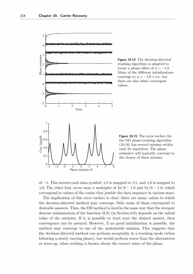
214 Chapter 10. Carrier Recovery
0 1 2 3 4
5
4
3
2
1
0
−1
−2
Time
Pha
se e
stim
ates
5
Figure 10.14 The decision-directedtracking algorithm is adapted tolocate a phase offset of φ = −1.0.Many of the different initializationsconverge to φ = −1.0 ± nπ, butthere are also other convergentvalues.
−2 −1 0 1 2 3 4 5 60
0.2
0.4
0.6
0.8
1
Phase estimates θ
Cos
t J D
D(θ
) Figure 10.15 The error surface forthe DD phase-tracking algorithm(10.18) has several minima withineach 2π repetition. The phaseestimates will typically converge tothe closest of these minima.
of −1. This inverts each data symbol: ±1 is mapped to ∓1, and ±3 is mapped to
∓3. The other four occur near π multiples of 3π/8− 1.0 and 5π/8− 1.0, which
correspond to values of the cosine that jumble the data sequence in various ways.
The implication of this error surface is clear: there are many values to which
the decision-directed method may converge. Only some of these correspond to
desirable answers. Thus, the DD method is local in the same way that the steepest
descent minimization of the function (6.8) (in Section 6.6) depends on the initial
value of the estimate. If it is possible to start near the desired answer, then
convergence can be assured. However, if no good initialization is possible, the
method may converge to one of the undesirable minima. This suggests that
the decision-directed method can perform acceptably in a tracking mode (when
following a slowly varying phase), but would perform worse than the alternatives
at start-up, when nothing is known about the correct value of the phase.

Carrier Recovery 215
Exercise 10.24. Use the code in plldd.m to “play with” the DD algorithm.
a. How large can the stepsize be made?
b. Is the LPF of the derivative really needed?
c. How crucial is it to the algorithm to pick the correct timing? Examine this
question by choosing incorrect j at which to evaluate x.
d. What happens when the assumed frequency f0 is not the same as the fre-
quency fc of the carrier?
Exercise 10.25. The direct calculation of dx(kTs)/dθ as a filtered version of
(10.16) is only one way to calculate the derivative. Replace this using a numerical
approximation (such as the forward or backward Euler, or the trapezoidal rule).
Compare the performance of your algorithm with that of plldd.m.
Exercise 10.26. Consider the DD phase-tracking algorithm when the message
alphabet is binary ±1.
a. Modify plldd.m to simulate this case.
b. Modify plldderrsys.m to draw the error surface. Is the DD algorithm better
(or worse) suited to the binary case than the 4-PAM case?
Exercise 10.27. Consider the DD phase-tracking algorithm when the message
alphabet is 6-PAM.
a. Modify plldd.m to simulate this case.
b. Modify plldderrsys.m to draw the error surface. Is the DD algorithm better
(or worse) suited to 6-PAM than to 4-PAM?
Exercise 10.28. What happens when the number of inputs used to calculate
the error surface is too small? Try N = 100, 10, 1. Can N be too large?
Exercise 10.29. Investigate how the error surface depends on the input signal.
a. Draw the error surface for the DD phase-tracking algorithm when the inputs
are binary ±1.
b. Draw the error surface for the DD phase-tracking algorithm when the inputs
are drawn from the 4-PAM constellation, for the case in which the symbol −3
never occurs.
Exercise 10.30. TRUE or FALSE: Decision-directed phase recovery can exhibit
local minima of different depths.
Exercise 10.31. This problem uses the B3IG to test the carrier-recovery algo-
rithm of your choice.
a. Currently, the receiver portion of the script in BigIdeal.m “knows” the phase
of the carrier. Add a carrier-recovery algorithm of your choice to BigIdeal.m

216 Chapter 10. Carrier Recovery
so that the receiver can accommodate unknown carrier phases. Run the mod-
ified code and use the carrier-recovery algorithm to estimate the phase offset
φ. State the carrier-recovery method used and plot the tracking of φ. If the
receiver employs preprocessing, take care to design the BPF appropriately.
b. Modify the B3IG so that a phase offset is introduced. In BigTransmitter.m,
set the variable phi=-0.5, and add a phase offset
x_rf=x.*cos(2*pi*rfParams.f_if_tx*...
[1:length(x)]’*rfParams.T_t_tx/M+p_noise+phi);
where upconversion is performed. Rerun the code. How does the behavior of
your algorithm differ? Include plots to justify your claim.
c. Repeat part (b) for the case when phi=1.2.
10.6 Frequency Tracking
The problems inherent in even a tiny difference in the frequency of the carrier
at the transmitter and the assumed frequency at the receiver are shown in (5.5)
and illustrated graphically in Figure 9.19 on page 185. Since no two independent
oscillators are ever exactly aligned, it is important to find ways of estimating the
frequency from the received signal. The direct method of Section 10.6.1 derives
an algorithm based on a performance function that uses a square difference in
the time domain. Unfortunately, this does not work well, and its failure can be
traced to the shape of the error surface.
Section 10.6.2 begins with the observation (familiar from Figures 10.8(b) and
10.11) that the estimates of phase made by the phase-tracking algorithms over
time lie on a line whose slope is proportional to the difference in frequency
between the modulating and the demodulating oscillators. This slope contains
valuable information that can be exploited to indirectly estimate the frequency.
The resulting dual-loop element is actually a special case of a more general (and
ultimately simpler) technique that puts an integrator in the forward part of the
loop in the PLL. This is detailed in Section 10.6.3.
10.6.1 Direct Frequency Estimation
Perhaps the simplest setting in which to begin frequency estimation is to assume
that the received signal is r(t) = cos(2πfct), where fc is unknown. By analogy
with the squared-difference method of phase estimation in Section 10.2, a rea-
sonable strategy is to try to choose f0 so as to minimize
J(f0) =1
2LPF{(r(t) − cos(2πf0t))
2}. (10.19)

Carrier Recovery 217
0 4 8 12 16Time
102
100
98
Freq
uenc
y es
timat
es f 0
Figure 10.16 Thefrequency-estimationalgorithm (10.20) appears tofunction well at first. But,over time, the estimatesdiverge from the desiredanswer.
Following a gradient strategy for updating the estimates f0 leads to the algorithm
f0[k + 1] = f0[k]− μdJ(f0)
df0
∣∣∣∣f0=f0[k]
(10.20)
= f0[k]− μLPF{2πkTs(r(kTs)− cos(2πkTsf0[k])) sin(2πkTsf0[k])}.How well does this algorithm work? First, observe that the update is multi-
plied by 2πkTs. (This arises from application of the chain rule when taking the
derivative of sin(2πkTsf0[k]) with respect to f0[k].) This factor increases contin-
uously, and acts like a stepsize that grows over time. Perhaps the easiest way to
make any adaptive element fail is to use a stepsize that is too large; the form of
this update ensures that eventually the “stepsize” will be too large.
Putting on our best engineering hat, let us just remove this offending term,
and go ahead and simulate the method.7 At first glance it might seem that the
method works well. Figure 10.16 shows 20 different starting values. All 20 appear
to converge nicely within one second to the unknown frequency value at fc=100.
But then something strange happens: one by one, the estimates diverge. In the
figure, one peels off at about 6 seconds, and one at about 17 seconds. Simulations
can never prove conclusively that an algorithm is good for a given task, but if
even simplified and idealized simulations function poorly, it is a safe bet that the
algorithm is somehow flawed. What is the flaw in this case?
Recall that error surfaces are often a good way of picturing the behavior
of gradient-descent algorithms. Expanding the square and using the standard
identities (A.4) and (A.9), J(f0) can be rewritten
J(f0) =1
2LPF
{1 +
1
2cos(4πfct)− cos(2π(fc − f0)t)
+1
2cos(4πf0t)− cos(2π(fc + f0)t)
}=
1
2− 1
2LPF{cos(2π(fc − f0)t)}, (10.21)
7 The code is available in the program pllfreqest.m on the website.

218 Chapter 10. Carrier Recovery
0.5
0fc
Frequency estimate f0
J( f 0
) Figure 10.17 The error surfacecorresponding to the frequencyestimation performance function(10.19) is flat everywhere exceptfor a deep crevice at the correctanswer f0 = fc.
assuming that the cutoff frequency of the lowpass filter is less than fc and that
f0 ≈ fc. At the point where f0 = fc, J(f0) = 0. For any other value of f0, how-
ever, as time progresses, the cosine term undulates up and down with an average
value of zero. Hence J(f0) averages to12for any f0 �= fc! This pathological situ-
ation is shown in Figure 10.17.
When f0 is far from fc, this analysis does not hold because the LPF no longer
removes the first two cosine terms in (10.21). Somewhat paradoxically, the algo-
rithm behaves well until the answer is nearly correct. Once f0 ≈ fc, the error
surface flattens, and the estimates wander around. There is a slight possibil-
ity that it might accidently fall into the exact correct answer, but simulations
suggest that such luck is rare. Oh well, never mind.
10.6.2 Indirect Frequency Estimation
Because the direct method of the previous section is unreliable, this section
pursues an alternative strategy based on the observation that the phase estimates
of the PLL “converge” to a line that has a slope proportional to the difference
between the actual frequency of the carrier and the frequency that is assumed at
the receiver. (Recall Figures 10.8(b) and 10.11.) The indirect method cascades
two PLLs: the first finds this line (and hence indirectly specifies the frequency),
the second converges to a constant appropriate for the phase offset.
The scheme is pictured in Figure 10.18. Suppose that the received signal has
been preprocessed to form rp(t) = cos(4πfct+ 2φ). This is applied to the inputs
of two PLLs.8 The top PLL functions exactly as expected from previous sections:
if the frequency of its oscillator is 2f0, then the phase estimates 2θ1 converge to
a ramp with slope 2π(f0 − fc), that is,
θ1(t) → 2π(fc − f0)t+ b,
8 Or two SD phase-tracking algorithms or two Costas loops, though in the latter case thesquaring preprocessing is unnecessary.

Carrier Recovery 219
LPF F1(z)
LPF F2(z)
2
2
X
X +
−μ1Σ
sin(4πf0kTs+2θ1[k] + 2θ2[k])
sin(4πf0kTs+2θ1[k])
θ1[k] + θ2[k]
θ1[k]
−μ2Σθ2[k]
rp(kTs)e1[k]
e2[k]
Figure 10.18 A pair of PLLs can efficiently estimate the frequency offset at thereceiver. The parameter θ1 in the top loop “converges to” a slope that corrects thefrequency offset and the parameter θ2 in the bottom loop corrects the residual phaseoffset. The sum θ1 + θ2 is used to drive the sinusoid in the carrier-recovery scheme.
where b is the y-intercept of the ramp. The θ1 values are then added to θ2, the
phase estimate in the lower PLL. The output of the bottom oscillator is
sin(4πf0t+ 2θ1(t) + 2θ2(t)) = sin(4πf0t+ 4π(fc − f0)t+ 2b+ 2θ2(t))
→ sin(4πfct+ 2b+ 2θ2(t)).
Effectively, the top loop has synthesized a signal that has the “correct” frequency
for the bottom loop. Accordingly, θ2(t) → φ− b. Since a sinusoid with frequency
2πf0t and “phase” θ1(t) + θ2(t) is indistinguishable from a sinusoid with fre-
quency 2πfct and phase θ2(t), these values can be used to generate a sinusoid
that is aligned with rp(t) in both frequency and phase. This signal can then be
used to demodulate the received signal.
Some Matlab code to implement this dual PLL scheme is provided by
dualplls.m.
Listing 10.8. dualplls.m estimation of carrier via dual-loop structure
Ts=1/10000; time=5; t=0:Ts : time−Ts ; % time vectorf c =1000; pho f f=−2; % c a r r i e r f r eq and phaserp=cos (4* pi* f c * t+2*pho f f ) ; % preproces s ed s i g n a l rBPFmu1=.01; mu2=.003; % algor i thm s t e p s i z e sf 0 =1001; % assumed f r eq at r e c e i v e rl en t=length ( t ) ; th1=zeros (1 , l en t ) ; % i n i t i a l i z e es t imatesth2=zeros (1 , l en t ) ; c a r e s t=zeros (1 , l en t ) ;for k=1: l ent −1 % combine top PLL th1
th1 (k+1)=th1 (k)−mu1*rp (k )* sin (4* pi* f0 * t (k)+2* th1 (k ) ) ;th2 (k+1)=th2 (k)−mu2*rp (k )* sin (4* pi* f0 * t (k)+2* th1 (k)+2* th2 (k ) ) ;% with bottom PLL th2 to form es t imate o f pr eproces s ed s i g n a lc a r e s t ( k)=cos (4* pi* f0 * t (k)+2* th1 ( k)+2* th2 ( k ) ) ;
end
The output of this program is shown in Figure 10.19. The upper graph shows
that θ1, the phase estimate of the top PLL, converges to a ramp. The middle plot

220 Chapter 10. Carrier Recovery
−20
0
20
−0.10
0.10.20.3
0 1 2 3 4 5
−101
Time
erro
rθ
1θ
2
Figure 10.19 The output ofMatlab program dualplls.m
shows the output of the first PLLconverging to a line, which allowsthe second PLL to converge to aconstant. The bottom figure showsthat this estimator can be used toconstruct a sinusoid that is veryclose to the (preprocessed) carrier.
shows that θ2, the phase estimate of the bottom PLL, converges to a constant.
Thus the procedure is working. The bottom graph shows the error between the
preprocessed signal rp and a synthesized carrier carest. The parameters f0,
th1, and th2 can then be used to synthesize a cosine wave that has the correct
frequency and phase to demodulate the received signal.
It is clear from the top plot of Figure 10.19 that θ1 converges to a line. What
line does it converge to? Looking carefully at the data generated by dualplls.m,
the line can be calculated explicitly. The two points at (2,−11.36) and (4,−23.93)
fit a line with slope m = −6.28 and an intercept b = 1.21. Thus,
2π(fc − f0) = −6.28,
or fc − f0 = −1. Indeed, this was the value used in the simulation. Reading the
final converged value of θ2 from the simulation shown in the middle plot gives
−0.0627. b− 0.0627 is 1.147, which is almost exactly π away from −2, the value
used in phoff.
Exercise 10.32. Use the preceding code to “play with” the frequency estimator.
a. How far can f0 be from fc before the estimates deteriorate?
b. What is the effect of the two stepsizes mu? Should one be larger than other?
If so, which one?
c. How does the method fare when the input is noisy?
d. What happens when the input is modulated by pulse-shaped data instead of
by a simple sinusoid?
Exercise 10.33. Build a frequency estimator using two SD phase-tracking algo-
rithms, rather than two PLLs. How does the performance change? Which do you
think is preferable?

Carrier Recovery 221
Exercise 10.34. Build a frequency estimator that incorporates the preprocess-
ing of the received signal from Figure 10.3 (as coded in pllpreprocess.m).
Exercise 10.35.Build a frequency estimator using two Costas loops, rather than
two PLLs. How does the performance change? Which do you think is preferable?
Exercise 10.36. Investigate (via simulation) how the PLL functions when there
is white noise (using randn) added to the received signal. Do the phase estimates
become worse as the noise increases? Make a plot of the standard deviation of
the noise versus the average value of the phase estimates (after convergence).
Make a plot of the standard deviation of the noise versus the jitter in the phase
estimates.
Exercise 10.37. Repeat Exercise 10.36 for the dual SD algorithm.
Exercise 10.38. Repeat Exercise 10.36 for the dual Costas-loop algorithm.
Exercise 10.39. Repeat Exercise 10.36 for the dual DD algorithm.
Exercise 10.40. Investigate (via simulation) how the PLL functions when
there is intersymbol interference caused by a nonunity channel. Pick a channel
(for instance chan=[1, .5, .3, .1];) and incorporate this into the simulation
of the received signal. Using this received signal, are the phase estimates worse
when the channel is present? Are they biased? Are they more noisy?
Exercise 10.41. Repeat Exercise 10.40 for the dual Costas loop.
Exercise 10.42. Repeat Exercise 10.40 for the Costas-loop algorithm.
Exercise 10.43. Repeat Exercise 10.40 for the DD algorithm.
10.6.3 Generalized PLL
Section 10.6.2 showed that two loops can be used in concert to accomplish the
carrier-recovery task: the first loop estimates frequency offset and the second
loop estimates the phase offset. This section shows an alternative structure that
folds one of the loops into the lowpass filter in the form of an IIR filter and
accomplishes both estimations at once. This is shown in Figure 10.20, which
looks the same as Figure 10.7 but with the FIR lowpass filter F (z) replaced by
an IIR lowpass filter G(z) = GN (z)/GD(z).
To see the operation of the generalized PLL concretely, pllgeneral.m imple-
ments the system of Figure 10.20 with GN (z) = 2− μ− 2z and GD(z) = z −1. The implementation of the IIR filter follows the time-domain method in
waystofiltIIR.m on page 145. When the frequency offset is zero (when f0=fc),

222 Chapter 10. Carrier Recovery
sin(4πf0kTs + 2θ[k])
G(z)
2
rp(kTs)μ + z−1
θ[k]θ[k+1]
Figure 10.20 The general PLL can track both phase and frequency offsets using an IIRLPF G(z). This figure is identical to Figure 10.7, except that the FIR lowpass filter isreplaced by a suitable IIR lowpass filter. Linearizing this structure gives Figure 10.22.Appendix F presents conditions on G(z) under which the tracking occurs.
theta converges to phoff. When there is a frequency offset (as in the default
values with f0=fc+0.1), theta converges to a line. Essentially, this θ value con-
verges to θ1 + θ2 in the dual-loop structure of Figure 10.19.
Listing 10.9. pllgeneral.m the PLL with an IIR LPF
Ts=1/10000; time=1; t=Ts : Ts : time ; % time vectorf c =1000; pho f f =0.8; % c a r r i e r f r eq and phaserp=cos (4* pi* f c * t+2*pho f f ) ; % s imp l i f i e d rec ’ d s i g n a lmu=.003; % algor i thm s t e p s i z ea=[1 −1] ; l ena=length ( a )−1; % au t o r e g r e s s i v e termsb=[−2 2−mu ] ; l enb=length (b ) ; % moving average termsxvec=zeros ( lena , 1 ) ; % i n i t i a l i z e f i l t e r sevec=zeros ( lenb , 1 ) ;f 0 =1000.0 ; % f r eq at r e c e i v e rtheta=zeros (1 , length ( t ) ) ; theta (1)=0; % i n i t i a l i z e es t imatesfor k=1: length ( t )−1
e=rp ( k )* sin (4* pi* f0 * t ( k)+2* theta (k ) ) ; % input to f i l t e revec=[e ; evec ( 1 : lenb −1 ) ] ; % past va lues o f i nputsx=−a ( 2 : l ena+1)* xvec+b* evec ; % output o f f i l t e rxvec=[x ; xvec ( 1 : lena −1 , 1 ) ] ; % past va lues o f outputstheta (k+1)=theta (k)+mu*x ; % algor i thm update
end
All of the PLL structures are nonlinear, which makes them hard to analyze
exactly. One way to study the behavior of a nonlinear system is to replace non-
linear components with nearby linear elements. A linearization is valid only for
a small range of values. For example, the nonlinear function sin(x) is approxi-
mately x for small values. This can be seen by looking at sin(x) near the origin:
it is approximately a line with slope unity. As x increases or decreases away from
the origin, the approximation worsens.
The nonlinear components in a loop structure such as Figure 10.7 are the
oscillators and the mixers. Consider a nonideal lowpass filter F (z) with impulse
response f [k] that has a cutoff frequency below 2f0. The output of the LPF is
e[k] = f [k] ∗ sin(2θ[k]− 2φ[k]), where ∗ represents convolution. With φ ≡ θ − φ
and φ ≈ θ, sin(2φ[k]) ≈ 2φ[k]. Thus the linearization is
f [k] ∗ sin(2φ[k]) ≈ f [k] ∗ 2φ[k]. (10.22)

Carrier Recovery 223
In words, applying an LPF to sin(x) is approximately the same as applying the
LPF to x, at least for sufficiently small x.
There are two ways to understand why the general PLL structure in Figure
10.20 works, both of which involve linearization arguments. The first method lin-
earizes Figure 10.20 and applies the final-value theorem for Z-transforms. Details
can be found in Section F.4. The second method is to show that a linearization
of the generalized single-loop structure of Figure 10.20 is the same as a lineariza-
tion of the dual-loop method of Figure 10.19, at least for certain values of the
parameters. Exercise 10.50 shows that, for certain special cases, the two strate-
gies (the dual-loop and the generalized single-loop) behave similarly in the sense
that both have the same linearization.
Exercise 10.44. What is the largest frequency offset that pllgeneral.m can
track? How does theta behave when the tracking fails?
Exercise 10.45. Examine the effect of different filters in pllgeneral.m.
a. Show that the filter used in pllgeneral.m has a lowpass character.
b. Let a=[1 0]. What kind of IIR filter does this represent? How does the loop
behave for a frequency offset?
c. Can you choose b so that the loop fails?
d. Design an IIR a and b pair using cheby1 or cheby2. Test whether the loop
functions to track small frequency offsets.
Exercise 10.46. Design the equivalent squared-difference loop, combining the
IIR structure of pllgeneral.m with the squared-difference objective function as
in pllsd.m.
Exercise 10.47. Design the equivalent general Costas-loop structure. Hint:
replace the FIR LPFs in Figure 10.9 with suitable IIR filters. Create a simu-
lation to verify the operation of the method.
Exercise 10.48. The code in pllgeneral.m is simplified in the sense that the
received signal rp contains just the unmodulated carrier. Implement a more real-
istic scenario by combining pulrecsig.m to include a binary message sequence,
pllpreprocess.m to create rp, and pllgeneral.m to recover the unknown phase
offset of the carrier. Demonstrate that the same system can track a frequency
offset.
Exercise 10.49. Investigate how the method performs when the received signal
contains pulse-shaped 4-PAM data. Verify that it can track both phase and
frequency offsets.

224 Chapter 10. Carrier Recovery
μ+ +
+
z−1θ1[k]
2φ[k]θ1[k+1]
2θ1[k] + 2θ2[k]
+
−
μ+ + z−1θ2[k]θ2[k+1]+
−
e1[k]
e2[k]
F1(z)
F2(z)
2
2
Figure 10.21 A linearization of the dual-loop frequency tracker of Figure 10.18. Forsmall offsets, this linear structure closely represents the behavior of the system.
μ+ + z−1θ[k]
2φ[k]θ[k+1]+
−
e[k]__
GD(z)
GN(z)
2
Figure 10.22 This is thelinearization of Figure10.20.
+ +−
A
B
C
A
B
B
C
+−
Figure 10.23 The left-hand block diagram with overlapping loops can be redrawn asthe right-hand split diagram.
Exercise 10.50. This exercise outlines the steps needed to show the conditions
under which the general PLL of Figure 10.20 and the dual-loop structure of
Figure 10.18 are the same (in the sense of having the same linearization).
a. Show that Figure 10.21 is the linearization of Figure 10.18.
b. Show that Figure 10.22 is the linearization of the general PLL of Figure 10.20.
c. Show that the two block diagrams in Figure 10.23 are the same.
d. Suppose that the lowpass filters are ideal: F1(z) = F2(z) = 1 for all frequencies
below the cutoff and F1(z) = F2(z) = 0 at all frequencies above. Make the
following assignments:
A =μ
z − 1 + 2μ, B =
μ
z − 1, and C = 2.

Carrier Recovery 225
Using the block-diagram manipulation of part (c), show that Figures 10.21
and 10.22 are the same when GN (z) = μ(2z − 2 + 2μ) and GD(z) = z − 1.
For Further Reading
� J. P. Costas, “Synchronous Communications,” Proceedings of the IRE, vol.
44, no. 12, pp. 1713–1718, Dec. 1956.� L. E. Franks, “Carrier and Bit Synchronization in Data Communication—
A Tutorial Review,” IEEE Transactions on Communications, vol. 28, no. 8,
pp. 1107–1120, Aug. 1980.

11 Pulse Shaping and Receive Filtering
When the message is digital, it must be converted into an analog signal in order
to be transmitted. This conversion is done by the “transmit” or “pulse-shaping”
filter, which changes each symbol in the digital message into a suitable analog
pulse. After transmission, the “receive” filter assists in recapturing the digital
values from the received pulses. This chapter focuses on the design and specifi-
cation of these filters.
The symbols in the digital input sequence w(kT ) are chosen from a finite set
of values. For instance, they might be binary ±1, or they may take values from
a larger set such as the four-level alphabet ±1, ±3. As suggested in Figure 11.1,
the sequence w(kT ) is indexed by the integer k, and the data rate is one symbol
every T seconds. Similarly, the output m(kT ) assumes values from the same
alphabet as w(kT ) and at the same rate. Thus the message is fully specified at
times kT for all integers k. But what happens between these times, between kT
and (k + 1)T ? The analog modulation of Chapter 5 operates continuously, and
some values must be used to fill in the digital input between the samples. This
is the job of the pulse-shaping filter: to turn a discrete-time sequence into an
analog signal.
Each symbol w(kT ) of the message initiates an analog pulse that is scaled by
the value of the signal. The pulse progresses through the communications system,
and, if all goes well, the output (after the decision) should be the same as the
input, although perhaps with some delay. If the analog pulse is wider than the
time between adjacent symbols, the outputs from adjacent symbols may overlap,
a problem called intersymbol interference, which is abbreviated ISI. A series of
examples in Section 11.2 shows how this happens, and the eye diagram is used
in Section 11.3 to help visualize the impact of ISI.
What kinds of pulses minimize the ISI? One possibility is to choose a shape
that is one at time kT and zero at mT for all m �= k. Then the analog wave-
form at time kT contains only the value from the desired input symbol, and no
interference from other nearby input symbols. These are called Nyquist pulses in
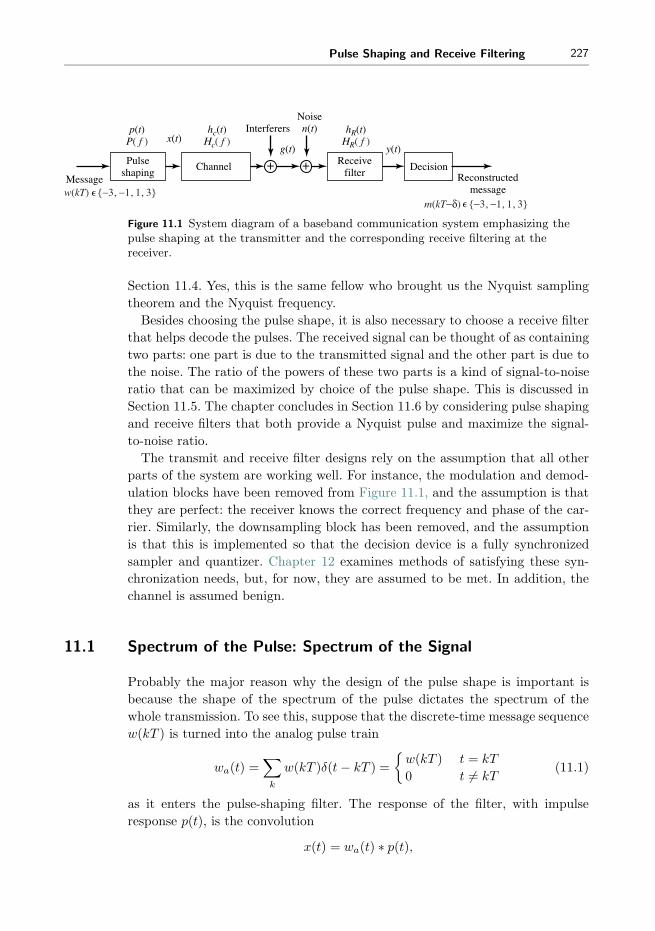
Pulse Shaping and Receive Filtering 227
Pulseshaping
Message Reconstructedmessage
InterferersNoisen(t)
x(t)
Receivefilter
Channel Decision+ +
p(t)P( f )
hc(t)Hc( f )
hR(t)HR( f )
g(t) y(t)
w(kT) {−3, −1, 1, 3}m(kT−δ) {−3, −1, 1, 3}
Figure 11.1 System diagram of a baseband communication system emphasizing thepulse shaping at the transmitter and the corresponding receive filtering at thereceiver.
Section 11.4. Yes, this is the same fellow who brought us the Nyquist sampling
theorem and the Nyquist frequency.
Besides choosing the pulse shape, it is also necessary to choose a receive filter
that helps decode the pulses. The received signal can be thought of as containing
two parts: one part is due to the transmitted signal and the other part is due to
the noise. The ratio of the powers of these two parts is a kind of signal-to-noise
ratio that can be maximized by choice of the pulse shape. This is discussed in
Section 11.5. The chapter concludes in Section 11.6 by considering pulse shaping
and receive filters that both provide a Nyquist pulse and maximize the signal-
to-noise ratio.
The transmit and receive filter designs rely on the assumption that all other
parts of the system are working well. For instance, the modulation and demod-
ulation blocks have been removed from Figure 11.1, and the assumption is that
they are perfect: the receiver knows the correct frequency and phase of the car-
rier. Similarly, the downsampling block has been removed, and the assumption
is that this is implemented so that the decision device is a fully synchronized
sampler and quantizer. Chapter 12 examines methods of satisfying these syn-
chronization needs, but, for now, they are assumed to be met. In addition, the
channel is assumed benign.
11.1 Spectrum of the Pulse: Spectrum of the Signal
Probably the major reason why the design of the pulse shape is important is
because the shape of the spectrum of the pulse dictates the spectrum of the
whole transmission. To see this, suppose that the discrete-time message sequence
w(kT ) is turned into the analog pulse train
wa(t) =∑k
w(kT )δ(t− kT ) =
{w(kT ) t = kT
0 t �= kT(11.1)
as it enters the pulse-shaping filter. The response of the filter, with impulse
response p(t), is the convolution
x(t) = wa(t) ∗ p(t),

228 Chapter 11. Pulse Shaping and Receive Filtering
1
0.8
0.6
0.4
0.2
0
Puls
e sh
ape
0.1 0.2 0.3 0.4 0.5 0.6 0.7 0.8 0.90Sample periods(a)
102
100
10−2
10−4
Spec
trum
of
the
puls
e sh
ape
0.1 0.2 0.3 0.4 0.5 0.6 0.7 0.8 0.9 10Normalized frequency(b)
Figure 11.2 The Hammingpulse shape and itsmagnitude spectrum.
as suggested by Figure 11.1. Since the Fourier transform of a convolution is the
product of the Fourier transforms (from (A.40)), it follows that
X(f) = Wa(f)P (f).
Though Wa(f) is unknown, this shows that X(f) can have no energy at fre-
quencies at which P (f) vanishes. Whatever the spectrum of the message, the
transmission is directly scaled by P (f). In particular, the support of the spec-
trum X(f) is no larger than the support of the spectrum P (f).
As a concrete example, consider the pulse shape used in Chapter 9, which
is the “blip” function shown in the top plot of Figure 11.2. The spectrum of
this pulse shape can readily be calculated using freqz, and this is shown at the
bottom plot of Figure 11.2. It is a kind of mild lowpass filter. The following code
generates a sequence of N 4-PAM symbols, and then carries out the pulse shaping
using the filter command.
Listing 11.1. pulsespec.m spectrum of a pulse shape
N=1000; w=pam(N, 4 , 5 ) ; % 4− l e v e l s i g n a l o f l ength NM=10; wup=zeros (1 ,N*M) ; % oversampl ing f a c t o rwup ( 1 :M:N*M)=w; % oversample by Mps=hamming (M) ; % b l i p pu l s e o f width Mx=f i l t e r ( ps , 1 ,wup ) ; % convolve pu l s e shape with data
The program pulsespec.m represents the “continuous-time” or analog sig-
nal by oversampling both the data sequence and the pulse shape by a fac-
tor of M. This technique was discussed in Section 6.3, where an “analog” sine
wave sine100hzsamp.m was represented digitally at two sampling intervals, a
slow symbol interval T = MTs and a faster rate (shorter interval) Ts represent-
ing the underlying analog signal. The pulse shape ps is a blip created by the
hamming function, and this is also oversampled at the same rate. The convo-
lution of the oversampled pulse shape and the oversampled data sequence is
accomplished by the filter command. Typical output is shown in the top plot

Pulse Shaping and Receive Filtering 229
3
2
1
0
−1
−2
−30 5 10 15 20 25
Symbols
Out
put o
f pu
lse
shap
ing
filte
r
104
102
100
10−2
10−4
0 0.1 0.2 0.3 0.4 0.5 0.6 0.7 0.8 0.9 1Normalized frequency
Spec
trum
of
the
outp
ut
Figure 11.3 The top plot shows a segment of the output x of the pulse-shaping filter.The bottom plot shows the magnitude spectrum of x, which has the same generalcontour as the spectrum of a single copy of the pulse. Compare this with the bottomplot of Figure 11.2.
of Figure 11.3, which shows the “analog” signal over a time interval of about 25
symbols. Observe that the individual pulse shapes are clearly visible, one scaled
blip for each symbol.
The spectrum of the output x is plotted at the bottom of Figure 11.3. As
expected from the previous discussion, the spectrum X(f) has the same contour
as the spectrum of the individual pulse shape in Figure 11.2.
11.2 Intersymbol Interference
There are two situations in which adjacent symbols may interfere with each other:
when the pulse shape is wider than a single symbol interval T , and when there is
a nonunity channel that “smears” nearby pulses, causing them to overlap. Both
of these situations are called intersymbol interference (ISI). Only the first kind of
ISI will be considered in this chapter; the second kind is postponed until Chapter
13. Before tackling the general setup, this section provides an instructive example
where the ISI is caused by an overly wide pulse shape.
Example 11.1. Suppose that the pulse shape in pulsespec.m is stretched so
that its width is 3T . This triple-width Hamming pulse shape is shown in Figure
11.4, along with its spectrum. Observe that the spectrum has (roughly) one-third
the null-to-null bandwidth of the single-symbol-wide Hamming pulse. Since the

230 Chapter 11. Pulse Shaping and Receive Filtering
1
0.8
0.6
0.4
0.2
0
The
pul
se s
hape
0 0.5 1 1.5 2 2.5 3
Sample periods(a)
102
100
10−2
10−4
Spec
trum
of
the
puls
e sh
ape
0 0.1 0.2 0.3 0.4 0.5 0.6 0.7 0.8 0.9 1
Normalized frequency(b)
Figure 11.4 The triple-widthHamming pulse shape and itsmagnitude spectrum, which isdrawn using freqz.
width of the spectrum of the transmitted signal is dictated by the width of the
spectrum of the pulse, this pulse shape is three times as parsimonious in its use
of bandwidth. More FDM users can be active at the same time.
As might be expected, this boon has a price. Figure 11.5 shows the output of
the pulse-shaping filter over a time of about 25 symbols. There is no longer a
clear separation of the pulse corresponding to one data point from the pulses of
its neighbors. The transmission is correspondingly harder to properly decode. If
the ISI caused by the overly wide pulse shape is too severe, symbol errors may
occur.
Thus, there is a trade-off. Wider pulse shapes can occupy less bandwidth,
which is always a good thing. On the other hand, a pulse shape like the Hamming
blip does not need to be very many times wider before it becomes impossible to
decipher the data because the ISI has become too severe. How much wider can it
be without causing symbol errors? The next section provides a way of picturing
ISI that answers this question. Subsequent sections discuss the practical issue of
how such ISI can be prevented by a better choice of pulse shape. Yes, there are
good pulse shapes that are wider than T .
Exercise 11.1. Modify pulsespec.m to reproduce Figures 11.4 and 11.5 for the
double-width pulse shape.
Exercise 11.2. Modify pulsespec.m to examine what happens when Hamming
pulse shapes of width 4T , 6T , and 10T are used. What is the bandwidth of the
resulting transmitted signals? Do you think it is possible to recover the message
from the received signals? Explain.

Pulse Shaping and Receive Filtering 231
0
0 5 10 15 20 25−5
5
Symbols
0.1 0.2 0.3 0.4 0.5 0.6 0.7 0.8 0.9 10Normalized frequency
Out
put o
f pu
lse-
shap
ing
filte
r
102
100
10−2
104
Spec
trum
of
the
outp
ut
Figure 11.5 The top plot shows a segment of the output x of the pulse-shaping filter.With this 3T -wide pulse shape, the pulses from adjacent symbols interfere with eachother. The bottom plot shows the magnitude spectrum of the output, which has thesame general contour as the spectrum of a single copy of the pulse, as in the bottomplot of Figure 11.4.
11.3 Eye Diagrams
While the differences between the pulse-shaped sequences in Figures 11.3 and
11.5 are apparent, it is difficult to see directly whether the distortions are seri-
ous; that is, whether they cause errors in the reconstructed data (i.e., the hard
decisions) at the receiver. After all, if the reconstructed message is the same as
the real message, then no harm has been done, even if the values of the received
analog waveform are not identical. This section uses a visualization tool called
eye diagrams that show how much smearing there is in the system, and whether
symbol errors will occur. Eye diagrams were encountered briefly in Chapter 9
(refer back to Figure 9.8) when visualizing how the performance of the idealized
system degraded when various impairments were added.
Imagine an oscilloscope that traces out the received signal, with the special
feature that it is set to retrigger or restart the trace every nT seconds without
erasing the screen. Thus the horizontal axis of an eye diagram is the time over
which n symbols arrive, and the vertical axis is the value of the received wave-
form. In the ideal case, the trace begins with n pulses, each of which is a scaled
copy of p(t). Then the (n+ 1)st to 2nth pulses arrive, and overlay the first n,
though each is scaled according to its symbol value. When there is noise, channel
distortion, and timing jitter, the overlays will differ.

232 Chapter 11. Pulse Shaping and Receive Filtering
3
2
1
0
−1
−2
−3
Optimum sampling times
Sensitivity totiming error
Distortionat zero
crossings
The "eye"Noisemargin
kT (k + 1)T
Figure 11.6 Interpretingeye diagrams: a T -wideHamming blip is used topulse shape a 4-PAMdata sequence.
As the number of superimposed traces increases, the eye diagram becomes
denser, and gives a picture of how the pulse shape, channel, and other factors
combine to determine the reliability of the recovered message. Consider the n =
2-symbol eye diagram shown in Figure 11.6. In this figure, the message is taken
from the 4-PAM alphabet ±1 ±3, and the Hamming pulse shape is used. The
center of the “eye” gives the best times to sample, since the openings (i.e., the
difference between the received pulse shape when the data value is −1 and the
received pulse shape when the data value is 1, or between the received pulse
shape when the data value is 1 and the received pulse shape when the data value
is 3) are the largest. The width marked “sensitivity to timing error” shows the
range of time over which the samples quantize correctly. The noise margin is the
smallest vertical distance between the bands, and is proportional to the amount
of additive noise that can be resisted by the system without reporting erroneous
values.
Thus, eye diagrams such as Figure 11.6 give a clear picture of how good (or
how bad) a pulse shape may be. Sometimes the smearing in this figure is so great
that the open segment in the center disappears. The eye is said to be closed, and
this indicates that a simple quantizer (slicer) decision device will make mistakes
in recovering the data stream. This is not good!
For example, reconsider the 4-PAM example of the previous section that used
a triple-width Hamming pulse shape. The eye diagram is shown in Figure 11.7.
No noise was added when drawing this picture. In the left two plots there are
clear regions about the symbol locations where the eye is open. Samples taken
in these regions will be quantized correctly, though there are also regions where
mistakes will occur. The other plots show the closed eye diagrams using 3T -

Pulse Shaping and Receive Filtering 233
4
2
0
−2
−4
Eye diagram for the T-wide Hamming pulse shape
4
2
0
−2
−4
Eye diagram for the 2T-wide Hamming pulse shape
4
2
0
−2
−4
Eye diagram for the 3T-wide Hamming pulse shape
5
0
−5
Eye diagram for the 5T-wide Hamming pulse shape
Symbols0 1 2 3 4 5
Symbols0 1 2 3 4 5
Figure 11.7 Eye diagrams for T -, 2T -, 3T -, and 5T -wide Hamming pulse shapes showhow the sensitivity to noises and timing errors increases as the pulse shape widens.The closed eye in the bottom plot on the right means that symbol errors areinevitable.
wide and 5T -wide Hamming pulse shapes. Symbol errors will inevitably occur,
even if all else in the system is ideal. All of the measures (the noise margin, the
sensitivity to timing, and the distortion at zero crossings) become progressively
worse, and ever smaller amounts of noise can cause decision errors.
The following code draws eye diagrams for the pulse shapes defined by the
variable ps. As in the pulse-shaping programs of the previous section, the N
binary data points are oversampled by a factor of M and the convolution of
the pulse shapes with the data uses the filter command. The reshape(x,a,b)
command changes a vector x of size a*b into a matrix with a rows and b columns,
which is used to segment x into b overlays, each a samples long. This works
smoothly with the Matlab plot function.
Listing 11.2. eyediag.m plot eye diagrams for a pulse shape
N=1000; m=pam(N, 2 , 1 ) ; % random s i g n a l o f l ength NM=20; mup=zeros (1 ,N*M) ; % oversampl ing f a c t o r o f Mmup( 1 :M:N*M)=m; % oversample by Mps=hamming (M) ; % hamming pu l s e o f width Mx=f i l t e r ( ps , 1 ,mup ) ; % convolve pu l s e shapeneye=5; % s i z e o f groupsc=f loor ( length (x )/( neye *M) ) ; % number o f eyes to p l o txp=x(N*M−neye*M*c+1:N*M) ; % ignor e t r a n s i e n t s at s t a r tplot ( reshape (xp , neye *M, c ) ) % p l o t in groups
Typical output of eyediag.m is shown in Figure 11.8. The rectangular pulse
shape in the top plot uses ps=ones(1,M), the Hamming pulse shape in the middle
uses ps=hamming(M), and the bottom plot uses a truncated sinc pulse shape
ps=srrc(L,0,M) for L=10 that is normalized so that the largest value is one. The
rectangular pulse is insensitive to timing errors, since sampling almost anywhere
(except right at the transition boundaries) will return the correct values. The
Hamming pulse shape has a wide eye, but may suffer from a loss of SNR if the

234 Chapter 11. Pulse Shaping and Receive Filtering
0
Eye diagram for rectangular pulse shape1
−1
0
Eye diagram for Hamming pulse shape1
−1
2
0
Eye diagram for sinc pulse shape
−2
Optimum sampling times
Figure 11.8 Eye diagramsfor rectangular, Hamming,and sinc pulse shapes withbinary data.
samples are taken far from the center of the eye. Of the three, the sinc pulse is the
most sensitive, since it must be sampled near the correct instants or erroneous
values will result.
Exercise 11.3. Modify eyediag.m so that the data sequence is drawn from the
alphabet ±1, ±3, ±5. Draw the appropriate eye diagram for the rectangular,
Hamming, and sinc pulse shapes.
Exercise 11.4.Modify eyediag.m to add noise to the pulse-shaped signal x. Use
the Matlab command v*randn for different values of v. Draw the appropriate
eye diagrams. For each pulse shape, how large can v be and still have the eye
remain open?
Exercise 11.5. Combine the previous two exercises. Modify eyediag.m as in
Exercise 11.3 so that the data sequence is drawn from the alphabet ±1, ±3, ±5.
Add noise, and answer the same question as in Exercise 11.4. Which alphabet is
more susceptible to noise?
Exercise 11.6. TRUE or FALSE: For two rectangular impulse responses with
the same maximum magnitude but different time widths with T1 > T2, the half-
power bandwidth of the frequency response of the pulse with width T1 exceeds
that of the pulse with width T2.

Pulse Shaping and Receive Filtering 235
u[k] y[k]
kT+equalizerreceive
filterchannel
pulse-shapefilter
m[k] Figure 11.9 The basebandcommunications system ofExercise 11.9.
Exercise 11.7. TRUE or FALSE: For the PAM baseband signals created by
a rectangular pulse and a triangular pulse with the same time width and the
same maximum amplitude, the half-power bandwidth of the sequence using the
triangular pulse exceeds that of the rectangular pulse.
Exercise 11.8. Exercise 2.10 asked the following question: TRUE or FALSE:
The flatter the top of the pulse shape, the less sensitive the receiver is to small
timing offsets. In the absence of noise and without matched filtering, this is
TRUE. Describe a noisy situation and a matched filtering that might cause the
answer to be FALSE.
Exercise 11.9. Consider the baseband communication system in Figure 11.9.
The difference equation relating the symbolsm[k] to the T -spaced equalizer input
u[k] for the chosen baud-timing factor ε is
u[k] = 0.04m[k − ρ] + 1.00m[k − 1− ρ] + 0.60m[k − 2− ρ] + 0.38m[k − 3− ρ],
where ρ is a nonnegative integer. The finite-impulse-response equalizer (filter) is
described by the difference equation
y[k] = u[k] + αu[k − 1].
a. Suppose α = −0.4 and the message source is binary ±1. Is the system from
the source symbols m[k] to the equalizer output y[k] open-eye? Justify your
answer.
b. If the message source is 4-PAM (±1,±3), can the system from m[k] to the
equalizer output y[k] be made open-eye by selection of α? If so, provide a
successful value of α. If not, explain.
It is now easy to experiment with various pulse shapes. pulseshape2.m applies
a sinc-shaped pulse to a random binary sequence. Since the sinc pulse extends
infinitely in time (both backward and forward), it cannot be represented exactly
in the computer (or in a real communication system) and the parameter L spec-
ifies the duration of the sinc, in terms of the number of symbol periods.
Listing 11.3. pulseshape2.m pulse shape a (random) sequence
N=2000; m=pam(N, 2 , 1 ) ; % 2−PAM s i gn a l o f l ength NM=10; mup=zeros (1 ,N*M) ; % oversampl ing f a c t o rmup( 1 :M:N*M)=m; % oversample by ML=10; ps=s r r c (L , 0 ,M) ; % s i n c pu l s e shape 2*L symbols widesc=sum( ps )/M; % normal i z ing constant
x=f i l t e r ( ps / sc , 1 ,mup ) ; % convolve pu l s e shape with data

236 Chapter 11. Pulse Shaping and Receive Filtering
0.4
0.3
0.2
0.1
0
−0.1
Using a sinc pulse shape
−10 −8 −6 −4 −2 0 2 4 6 8 10
3
2
1
0
−1
−2
Pulse-shaped data sequence
Symbol numberSymbol interval0 2 4 6 8 10 12 14 16 18 20
Figure 11.10 A binary ±1 data sequence is pulse shaped using a sinc pulse.
Figure 11.10 plots the output of pulseshape2.m. The left figure shows the
pulse shape while the right plot shows the “analog” pulse-shaped signal x(t)
over a duration of about 25 symbols. The function srrc.m first appeared in the
discussion of interpolation in Section 6.4 (and again in Exercise 6.22), and is used
here to generate the sinc pulse shape. The sinc function that srrc.m produces
is actually scaled, and this effect is removed by normalizing with the variable
sc. Changing the second input argument from beta=0 to other small positive
numbers changes the shape of the curve, each with a “sinc-like” shape called a
square-root raised cosine. This will be discussed in greater detail in Sections 11.4
and 11.6. Typing help srrc in Matlab gives useful information on using the
function.
Observe that, even though the signal oscillates above and below the ±1 lines,
there is no intersymbol interference. When using the Hamming pulse as in Fig-
ure 11.3, each binary value was clearly delineated. With the sinc pulse of Figure
11.10, the analog waveform is more complicated. However, at the correct sam-
pling instances, it always returns to ±1 (the horizontal lines at ±1 are drawn to
help focus the eye on the crossing times). Unlike the T -wide Hamming shape,
the signal need not return to near zero with each symbol.
Exercise 11.10. In pulseshape2.m, examine the effect of using different over-
sampling rates M. Try M = 1, 5, 100.
Exercise 11.11. Change pulseshape2.m so that the data sequence is drawn
from the alphabet ±1,±3,±5. Can you visually identify the correct values in the
pulse-shaped signal?
Exercise 11.12. In pulseshape2.m, examine the effect of using sinc approxi-
mations of different lengths L. Try L = 1, 5, 100, 1000.
Exercise 11.13. In pulseshape2.m, examine the effect of adding noise to the
received signal x. Try Matlab commands randn and rand. How large can the
noise be and still allow the data to be recognizable?

Pulse Shaping and Receive Filtering 237
Exercise 11.14. The goal is to design a frequency-division multiplexed (FDM)
system with a square-root raised cosine as the transmitter pulse shape. The
symbol period is T = 137 ms. The design uses T/4 sampling, pulse lengths of
8T , and a rolloff factor of 0.9, but it does not work, since only three modulated
carrier signals fit into the allotted bandwidth without multiuser interference.
Five are needed. What parameters in the design would you change and why?
Exercise 11.15. Using the code from Exercise 11.11, examine the effects of
adding noise in pulseshape2.m. Does the same amount of noise in the six-level
data have more or less effect than in the two-level data?
Exercise 11.16. Modify pulseshape2.m to include the effect of a nonunity
channel. Try both a highpass channel and a bandpass channel. Which appears
worse? What are reasonable criteria for “better” and “worse” in this context?
Exercise 11.17. A Matlab question: in pulseshape2.m, examine the effect of
using the filtfilt command for the convolution instead of the filter com-
mand. Can you figure out why the results are different?
Exercise 11.18. Another Matlab question: in pulseshape2.m, examine the
effect of using the conv command for the convolution instead of the filter
command. Can you figure out how to make this work?
11.4 Nyquist Pulses
Consider a multilevel signal drawn from a finite alphabet with values w(kT ),
where T is the sampling interval. Let p(t) be the impulse response of the linear
filter representing the pulse shape. The signal just after pulse shaping is
x(t) = wa(t) ∗ p(t),where wa(t) is the pulse-train signal (11.1).
The corresponding output of the received filter is
y(t) = wa(t) ∗ p(t) ∗ hc(t) ∗ hR(t),
as depicted in Figure 11.1, where hc(t) is the impulse response of the channel and
hR(t) is the impulse response of the receive filter. Let hequiv(t) = p(t) ∗ hc(t) ∗hR(t) be the overall equivalent impulse response. Then the equivalent overall
frequency response (i.e., F{hequiv(t)}) isHequiv(f) = P (f)Hc(f)HR(f). (11.2)
One approach would be to attempt to choose HR(f) so that Hequiv(f) attained
a desired value (such as a pure delay) for all f . This would be a specification of

238 Chapter 11. Pulse Shaping and Receive Filtering
the impulse response hequiv(t) at all t, since the Fourier transform is invertible.
But such a distortionless response is unnecessary, since it does not really matter
what happens between samples, but only what happens at the sample instants. In
other words, as long as the eye is open, the transmitted symbols are recoverable
by sampling at the correct times. In general, if the pulse shape is zero at all
integer multiples of kT but one, then it can have any shape in between without
causing intersymbol interference.
The condition that one pulse does not interfere with other pulses at subsequent
T -spaced sample instants is formalized by saying that hNYQ(t) is a Nyquist pulse
if there is a τ such that
hNYQ(kT + τ) =
{c k = 0
0 k �= 0(11.3)
for all integers k, where c is some nonzero constant. The timing offset τ in (11.3)
will need to be found by the receiver.
A rectangular pulse with time-width less than T certainly satisfies (11.3), as
does any pulse shape that is less than T wide. But the bandwidth of the rectan-
gular pulse (and other narrow pulse shapes such as the Hamming pulse shape)
may be too wide. Narrow pulse shapes do not utilize the spectrum efficiently. But
if just any wide shape is used (such as the multiple-T -wide Hamming pulses),
then the eye may close. What is needed is a signal that is wide in time (and
narrow in frequency) that also fulfills the Nyquist condition (11.3).
One possibility is the sinc pulse
hsinc(t) =sin(πf0t)
πf0t,
with f0 = 1/T . This has the narrowest possible spectrum, since it forms a rect-
angle in frequency (i.e., the frequency response of a lowpass filter). Assuming
that the clocks at the transmitter and receiver are synchronized so that τ = 0,
the sinc pulse is Nyquist because hsinc(0) = 1 and
hsinc(kT ) =sin(πk)
πk= 0
for all integers k �= 0. But there are several problems with the sinc pulse.
� It has infinite duration. In any real implementation, the pulse must be trun-
cated.� It is noncausal. In any real implementation, the truncated pulse must be
delayed.� The steep band edges of the rectangular frequency function Hsinc(f) are dif-
ficult to approximate.� The sinc function sin(t)/t decays slowly, at a rate proportional to 1/t.
The slow decay (recall the plot of the sinc function in Figure 2.11 on page 32)
means that samples that are far apart in time can interact with each other when
there are even modest clock-synchronization errors.

Pulse Shaping and Receive Filtering 239
Fortunately, it is not necessary to choose between a pulse shape that is con-
strained to lie within a single symbol period T and the slowly decaying sinc.
While the sinc has the smallest dispersion in frequency, there are other pulse
shapes that are narrower in time and yet are only a little wider in frequency.
Trading off time and frequency behaviors can be tricky. Desirable pulse shapes
1. have appropriate zero crossings (i.e., they are Nyquist pulses),
2. have sloped band edges in the frequency domain, and
3. decay more rapidly in the time domain (compared with the sinc), while main-
taining a narrow profile in the frequency domain.
One popular option is called the raised cosine-rolloff (or raised cosine) filter.
It is defined by its Fourier transform
HRC(f) =
⎧⎨⎩
1 |f | < f112+ 1
2cos (π(|f | − f1)/(2fΔ)) f1 < |f | < B
0 |f | > B
where
� B is the absolute bandwidth,� f0 is the 6 dB bandwidth, equal to 1/(2T ), half the symbol rate,� fΔ = B − f0, and� f1 = f0 − fΔ.
The corresponding time-domain function is
hRC(t) = F−1{HRC(f)} = 2f0
(sin(2πf0t)
2πf0t
)[cos(2πfΔt)
1− (4fΔt)2
]. (11.4)
Define the rolloff factor β = fΔ/f0. Figure 11.11 shows the magnitude spectrum
HRC(f) of the raised cosine filter on the right and the associated time response
hRC(t) on the left, for a variety of rolloff factors. With T = 1/(2f0), hRC(kT ) has
a factor sin(πk)/(πk) that is zero for all integer k �= 0. Hence the raised cosine
is a Nyquist pulse. In fact, as β → 0, hRC(t) becomes a sinc.
The raised cosine pulse hRC(t) with nonzero β has the following characteristics:
� zero crossings at desired times,� band edges of HRC(f) that are less severe than with a sinc pulse,� an envelope that falls off at approximately 1/|t|3 for large t (look at (11.4)).
This is significantly faster than 1/|t|. As the rolloff factor β increases from 0
to 1, the significant part of the impulse response gets shorter.
Thus, we have seen several examples of Nyquist pulses: rectangular, Hamming,
sinc, and raised cosine with a variety of rolloff factors. What is the general
principle that distinguishes Nyquist pulses from all others? A necessary and
sufficient condition for a signal v(t) with Fourier transform V (f) to be a Nyquist
pulse is that the sum (over all n) of V (f − nf0) be constant. To see this, use the

240 Chapter 11. Pulse Shaping and Receive Filtering
1
1
0
0.5
0
−0.5−3T 0 f0/2 3f0/2 2f0f0−2T −T 0 T 2T 3T
β = 1β = 0
β = 0
β = 1
β = 0.5
β = 0.5
FrequencyTime
Figure 11.11 Raised cosine pulse shape in the time and frequency domains.
sifting property of an impulse (A.56) to factor V (f) from the sum:
∞∑n=−∞
V (f − nf0) = V (f) ∗[ ∞∑n=−∞
δ(f − nf0)
].
Given that convolution in the frequency domain is multiplication in the time
domain (A.40), on applying the definition of the Fourier transform, and using
the transform pair (from (A.28) with w(t) = 1 and W (f) = δ(f))
F{∞∑
k=−∞δ(t− kT )} =
1
T
∞∑n=−∞
δ(f − nf0),
where f0 = 1/T , this becomes
∞∑n=−∞
V (f − nf0) =
∫ ∞
t=−∞
[v(t)
(T
∞∑k=−∞
δ(t− kT )
)]e−j2πftdt
=
∞∑k=−∞
Tv(kT )e−j2πfkT . (11.5)
If v(t) is a Nyquist pulse, the only nonzero term in the sum is v(0), and
∞∑n=−∞
V (f − nf0) = Tv(0).
Thus, the sum of the V (f − nf0) is a constant if v(t) is a Nyquist pulse. Con-
versely, if the sum of the V (f − nf0) is a constant, then only the DC term in
(11.5) can be nonzero, and so v(t) is a Nyquist pulse.
Exercise 11.19. Write a Matlab routine that implements the raised cosine
impulse response (11.4) with rolloff parameter β. Hint 1: if you have trouble
with “divide by zero” errors, imitate the code in srrc.m. Plot the output of
your program for a variety of β. Hint 2: there is an easy way to use the function
srrc.m.

Pulse Shaping and Receive Filtering 241
3
−3
1.5
−1.5
p(t)
t (ms)
0.2 0.6 1.0Figure 11.12 Pulse shape for Exercise11.23.
Exercise 11.20. Use your code from the previous exercise, along with
pulseshape2.m to apply raised cosine pulse shaping to a random binary
sequence. Can you spot the appropriate times to sample “by eye?”
Exercise 11.21.Use the code from the previous exercise and eyediag.m to draw
eye diagrams for the raised cosine pulse with rolloff parameters r = 0, 0.5, 0.9,
1.0, 5.0. Compare these with the eye diagrams for rectangular and sinc functions.
Consider
a. sensitivity to timing errors,
b. peak distortion,
c. distortion of zero crossings, and
d. the noise margin.
Exercise 11.22. TRUE or FALSE: The impulse response of a series combination
of any α-second-wide pulse-shape filter and its matched filter form a Nyquist
pulse shape for a T -spaced symbol sequence for any T ≥ α.
Exercise 11.23. Consider the pulse shape p(t) of width 1.2 ms shown in Figure
11.12.
a. Is p(t) a Nyquist pulse for the symbol period T = 0.35 ms? Justify your
answer.
b. Is p(t) a Nyquist pulse for the symbol period T = 0.70 ms? Justify your
answer.
Exercise 11.24. Neither s1(t) nor s2(t) is a Nyquist pulse.
a. Can the product s1(t)s2(t) be a Nyquist pulse? Explain.
b. Can the convolution s1(t) ∗ s2(t) be a Nyquist pulse? Explain.
Intersymbol interference occurs when data values at one sample instant inter-
fere with the data values at another sampling instant. Using Nyquist shapes such
as the rectangle, sinc, and raised cosine pulses removes the interference, at least
at the correct sampling instants, when the channel is ideal. The next sections

242 Chapter 11. Pulse Shaping and Receive Filtering
parlay this discussion of isolated pulse shapes into usable designs for the pulse
shaping and receive filters.
11.5 Matched Filtering
Communication systems must be robust against the presence of noises and other
disturbances that arise in the channel and in the various stages of processing.
Matched filtering is aimed at reducing the sensitivity to noise, which can be
specified in terms of the power spectral density (this is reviewed in some detail
in Appendix E).
Consider the filtering problem in which a message signal is added to a noise
signal and then both are passed through a linear filter. This occurs, for instance,
when the signal g(t) of Figure 11.1 is the output of the pulse-shaping filter
(i.e., no interferers are present), the channel is the identity, and there is noise
n(t) present. Assume that the noise is “white”; that is, assume that its power
spectral density Pn(f) is equal to some constant η for all frequencies.
The output y(t) of the linear filter with impulse response hR(t) can be
described as the superposition of two components, one driven by g(t) and the
other by n(t); that is,
y(t) = v(t) + w(t),
where
v(t) = hR(t) ∗ g(t) and w(t) = hR(t) ∗ n(t).This is shown in block-diagram form in Figure 11.13. In both components, the
processing and the output signal are the same. The bottom diagram separates
out the component due to the signal (v(kT ), which contains the message filtered
through the pulse shape and the receive filter), and the component due to the
noise (w(kT ), which is the noise filtered through the receive filter). The goal of
this section is to find the receive filter that maximizes the ratio of the power in
the signal v(kT ) to the power in the noise w(kT ) at the sample instants.
Consider choosing hR(t) so as to maximize the power of the signal v(t) at
time t = τ compared with the power in w(t) (i.e., to maximize v2(τ) relative
to the total power of the noise component w(t)). This choice of hR(t) tends to
emphasize the signal v(t) and suppress the noise w(t). The argument proceeds
by finding the transfer function HR(f) that corresponds to this hR(t).
From (E.2), the total power in w(t) is
Pw =
∫ ∞
−∞Pw(f)df.
From the inverse Fourier transform,
v(τ) =
∫ ∞
−∞V (f)ej2πfτdf,

Pulse Shaping and Receive Filtering 243
Pulseshaping
Receivefilter
Downsample
m(kT)y(t) y(kT)
y(kT)
n(t)
n(t)
P( f )
P( f )
Pulseshaping
HR( f )
HR( f )
HR( f )
Receivefilter
g(t)
g(t)
v(t)+
+
Receivefilter
Downsample
w(t) w(kT)
v(kT)
Downsample
m(kT)
Figure 11.13 The two block diagrams result in the same output. The top shows thedata flow in a normal implementation of pulse shaping and receive filtering. Thebottom shows an equivalent that allows easy comparison between the parts of theoutput due to the signal (i.e., v(kT )) and the parts due to the noise (i.e., w(kT )).
where V (f) = HR(f)G(f). Thus,
v2(τ) =
∣∣∣∣∫ ∞
−∞HR(f)G(f)ej2πfτdf
∣∣∣∣2 .Recall (E.3), which says that, for Y (f) = HR(f)U(f), Py(f) = |HR(f)|2Pu(f).
Thus,
Pw(f) = |HR(f)|2Pn(f) = η|HR(f)|2.The quantity to be maximized can now be described by
v2(τ)
Pw=
| ∫∞−∞ HR(f)G(f)ej2πfτdf |2∫∞
−∞ η|HR(f)|2df. (11.6)
Schwarz’s inequality (A.57) says that∣∣∣∣∫ ∞
−∞a(x)b(x)dx
∣∣∣∣2 ≤{∫ ∞
−∞|a(x)|2dx
}{∫ ∞
−∞|b(x)|2dx
},
and equality occurs only when a(x) = kb∗(x). This converts (11.6) to
v2(τ)
Pw≤(∫∞
−∞ |HR(f)|2df) (∫∞
−∞ |G(f)ej2πfτ |2df)η∫∞−∞ |HR(f)|2df
, (11.7)
which is maximized with equality when
HR(f) = k(G(f)ej2πfτ )∗.

244 Chapter 11. Pulse Shaping and Receive Filtering
HR(f) must now be transformed to find the corresponding impulse response
hR(t). Since Y (f) = X(−f) when y(t) = x(−t) (use the frequency-scaling prop-
erty of Fourier transforms (A.38) with a scale factor of −1),
F−1{W ∗(−f)} = w∗(t) ⇒ F−1{W ∗(f)} = w∗(−t).
Applying the time-shift property (A.37) yields
F−1{W (f)e−j2πfTd} = w(t− Td).
Combining these two transform pairs yields
F−1{(W (f)ej2πfTd)∗} = w∗(−(t− Td)) = w∗(Td − t).
Thus, when g(t) is real,
F−1{k(G(f)ej2πfτ )∗} = kg∗(τ − t) = kg(τ − t).
Observe that this filter has the following characteristics.
� This filter results in the maximum signal-to-noise ratio of v2(t)/Pw at the
time instant t = τ for a noise signal with a flat power spectral density.� Because the impulse response of this filter is a scaled time reversal of the
pulse shape p(t), it is said to be “matched” to the pulse shape, and is called
a “matched filter.”� The shape of the magnitude spectrum of the matched filter HR(f) is the same
as the magnitude spectrum G(f).� The shape of the magnitude spectrum of G(f) is the same as the shape of
the frequency response of the pulse shape P (f) for a broadband m(kT ), as in
Section 11.1.� The matched filter for any filter with an even symmetric (about some t) time-
limited impulse response is a delayed replica of that filter. The minimum delay
is the upper limit of the time-limited range of the impulse response.
The following code allows hands-on exploration of this theoretical result.
The pulse shape is defined by the variable ps (the default is the sinc function
srrc(L,0,M) for L=10). The receive filter is analogously defined by recfilt. As
usual, the symbol alphabet is easily specified by the pam subroutine, and the
system operates at an oversampling rate M. The noise is specified in n, and the
ratio of the powers is output as powv/poww. Observe that, for any pulse shape,
the ratio of the powers is maximized when the receive filter is the same as the
pulse shape (the fliplr command carries out the time reversal). This holds no
matter what the noise, no matter what the symbol alphabet, and no matter what
the pulse shape.
Listing 11.4. matchfilt.m test of SNR maximization
N=2ˆ15; m=pam(N, 2 , 1 ) ; % 2−PAM s i gn a l o f l ength NM=10; mup=zeros (1 ,N*M) ; % oversampl ing f a c t o rmup( 1 :M:N*M)=m; % oversample by ML=10; ps=s r r c (L , 0 ,M) ; % de f i n e pu l s e shape

Pulse Shaping and Receive Filtering 245
ps=ps/sqrt (sum( ps . ˆ 2 ) ) ; % and normal izen=0.5*randn ( size (mup ) ) ; % no i s eg=f i l t e r ( ps , 1 ,mup ) ; % convolve ps with datar e c f i l t=s r r c (L , 0 ,M) ; % r e c e i v e f i l t e r H sub Rr e c f i l t=r e c f i l t / sqrt (sum( r e c f i l t . ˆ 2 ) ) ; % normal ize pu l s e shapev=f i l t e r ( f l i p l r ( r e c f i l t ) , 1 , g ) ; % matched f i l t e r with dataw=f i l t e r ( f l i p l r ( r e c f i l t ) , 1 , n ) ; % matched f i l t e r with no i s evdownsamp=v ( 1 :M:N*M) ; % downsample to symbol r a t ewdownsamp=w( 1 :M:N*M) ; % downsample to symbol r a t epowv=pow(vdownsamp ) ; % power in downsampled vpoww=pow(wdownsamp ) ; % power in downsampled wpowv/poww % ra t i o
In general, when the noise power spectral density is flat (i.e., Pn(f) = η), the
output of the matched filter may be realized by correlating the input to the
matched filter with the pulse shape p(t). To see this, recall that the output is
described by the convolution
x(α) =
∫ ∞
−∞s(λ)h(α − λ)dλ
of the matched filter with the impulse response h(t). Given the pulse shape p(t)
and the assumption that the noise has flat power spectral density, it follows that
h(t) =
{p(α− t) 0 ≤ t ≤ T,
0 otherwise,
where α is the delay used in the matched filter. Because h(t) is zero when t is
negative and when t > T , h(α− λ) is zero for λ > α and λ < α− T . Accordingly,
the limits on the integration can be converted to
x(α) =
∫ α
λ=−α−T
s(λ)p(α− (α− λ))dλ =
∫ α
λ=−α−T
s(λ)p(λ)dλ.
This is the cross-correlation of p with s as defined in (8.3).
When Pn(f) is not a constant, (11.6) becomes
v2(τ)
Pw=
| ∫∞−∞ H(f)G(f)ej2πfτdf |2∫∞
−∞ Pn(f)|H(f)|2df .
To use the Schwarz inequality (A.57), associate a with H√Pn and b with
Gej2πfτ/√Pn. Then (11.7) can be replaced by
v2(τ)
Pw≤(∫∞
−∞ |H(f)|2Pn(f)df) (∫∞
−∞ |G(f)ej2πfτ |2/Pn(f)df)∫∞
−∞ |H(f)|2Pn(f)df,
and equality occurs when a(·) = kb∗(·); that is,
H(f) =kG∗(f)e−j2πfτ
Pn(f).
When the noise power spectral density Pn(f) is not flat, it shapes the matched
filter. Recall that the power spectral density of the noise can be computed from
its autocorrelation, as is shown in Appendix E.

246 Chapter 11. Pulse Shaping and Receive Filtering
Transmitfilter
Receivefilter
+y[k] s[i]
k = iN + σ
w[k]
m[k]
f [k] g[k]
Figure 11.14 Basebandcommunication systemconsidered in Exercise11.29.
Exercise 11.25. Let the pulse shape be a T -wide Hamming blip. Use the code
in matchfilt.m to find the ratio of the power in the downsampled v to that in
the downsampled w when
a. the receive filter is an SRRC with beta = 0, 0.1, 0.5,
b. the receive filter is a rectangular pulse, and
c. the receive filter is a 3T -wide Hamming pulse.
When is the ratio largest?
Exercise 11.26. Let the pulse shape be an SRRC with beta = 0.25. Use the
code in matchfilt.m to find the ratio of the power in the downsampled v to that
in the downsampled w when
a. the receive filter is an SRRC with beta = 0, 0.1, 0.25, 0.5,
b. the receive filter is a rectangular pulse, and
c. the receive filter is a T -wide Hamming pulse.
When is the ratio largest?
Exercise 11.27. Let the symbol alphabet be 4-PAM.
a. Repeat Exercise 11.25.
b. Repeat Exercise 11.26.
Exercise 11.28. Create a noise sequence that is uniformly distributed (using
rand) with zero mean.
a. Repeat Exercise 11.25.
b. Repeat Exercise 11.26.
Exercise 11.29. Consider the baseband communication system in Figure 11.14.
The symbol period T is an integer multiple of the sample period Ts, i.e., T = NTs.
The message sequence is nonzero only eachNth k, i.e., k = NTs + δTs, where the
integer δ is within the range 0 ≤ δ < N and δTs is the “on-sample” baud-timing
offset at the transmitter.
a. Suppose that f [k] = {0.2, 0, 0, 1.0, 1.0, 0, 0,−0.2} for k = 0, 1, 2, 3, 4, 5, 6, 7 and
zero otherwise. Determine the causal g[k] that is the matched filter to f [k].
Arrange g[k] so that the final nonzero element is as small as possible.

Pulse Shaping and Receive Filtering 247
b. For the g[k] specified in part (a), determine the smallest possibleN so the path
from m[k] to y[k] forms an impulse response that would qualify as a Nyquist
pulse for some well-chosen baud-timing offset σ when y is downsampled by
N .
c. For the g[k] chosen in part (a) and the N chosen in part (b), determine the
downsampler offset σ for s[i] to be the nonzero entries of m[k] when w[k] = 0
for all k.
11.6 Matched Transmit and Receive Filters
While focusing separately on the pulse shaping and the receive filtering makes
sense pedagogically, the two are intimately tied together in the communication
system. This section notes that it is not really the pulse shape that should be
Nyquist, but rather the convolution of the pulse shape with the receive filter.
Recall the overall block diagram of the system in Figure 11.1, where it was
assumed that the portion of the system from upconversion (to passband) to final
downconversion (back to baseband) is done perfectly and that the channel is just
the identity. Thus, the central portion of the system is effectively transparent
(except for the intrusion of noise). This simplifies the system to the baseband
model in Figure 11.15.
The task is to design an appropriate pair of filters: a pulse shape for the
transmitter, and a receive filter that is matched to the pulse shape and the
presumed noise description. It is not crucial that the transmitted signal itself
have no intersymbol interference. Rather, the signal after the receive filter should
have no ISI. Thus, it is not the pulse shape that should satisfy the Nyquist pulse
condition, but the combination of the pulse shape and the receive filter.
The receive filter should simultaneously
1. allow no intersymbol interference at the receiver, and
2. maximize the signal-to-noise ratio.
Hence, it is the convolution of the pulse shape and the receive filter that should be
a Nyquist pulse, and the receive filter should be matched to the pulse shape. Con-
sidering candidate pulse shapes that are both symmetric and even about some
time t, the associated matched filter (modulo the associated delay) is the same as
the candidate pulse shape. What symmetric pulse shapes, when convolved with
themselves, form a Nyquist pulse? Previous sections examined several Nyquist
Pulseshape
Receivefilter
Noise
+Signal
Figure 11.15 Noisy basebandcommunication system.

248 Chapter 11. Pulse Shaping and Receive Filtering
pulse shapes, the rectangle, the sinc, and the raised cosine. When convolved with
themselves, do any of these shapes remain Nyquist?
For a rectangle pulse shape and its rectangular matched filter, the convolution
is a triangle that is twice as wide as the original pulse shape. With precise timing,
(so that the sample occurs at the peak in the middle), this triangular pulse shape
is also a Nyquist pulse. This exact situation will be considered in detail in Section
12.2.
The convolution of a sinc function with itself is more easily viewed in the fre-
quency domain as the point-by-point square of the transform. Since the transform
of the sinc is a rectangle, its square is a rectangle as well. The inverse transform
is consequently still a sinc, and is therefore a Nyquist pulse.
The raised cosine pulse fails. Its square in the frequency domain does not
retain the odd symmetry around the band edges, and the convolution of the
raised cosine with itself does not retain its original zero crossings. But the raised
cosine was the preferred Nyquist pulse because it conserves bandwidth effectively
and because its impulse response dies away quickly. One possibility is to define
a new pulse shape that is the square root of the raised cosine (the square root is
taken in the frequency domain, not the time domain). This is called the square-
root raised cosine filter (SRRC). By definition, the square in frequency of the
SRRC (which is the raised cosine) is a Nyquist pulse.
The time-domain description of the SRRC pulse is found by taking the inverse
Fourier transform of the square root of the spectrum of the raised cosine pulse.
The answer is a bit complicated:
v(t) =
⎧⎪⎪⎪⎪⎨⎪⎪⎪⎪⎩
(1 − β + 4β/π)/√T t = 0
β(π+2)√2Tπ
sin(
π4β
)+ β(π−2)√
2Tπcos
(π4β
)t = ± T
4β
sin(π(1−β)t/T )+(4βt/T ) cos(π(1+β)t/T )√T (πt/T )(1−(4βt/T )2)
otherwise.
(11.8)
Exercise 11.30. Plot the SRRC pulse in the time domain and show that it is
not a Nyquist pulse (because it does not cross zero at the desired times). The
Matlab routine srrc.m will make this easier.
Though the SRRC is not itself a Nyquist pulse, the convolution in time of two
SRRCs is a Nyquist pulse. The square-root raised cosine is the most commonly
used pulse in bandwidth-constrained communication systems.
Exercise 11.31. Consider the baseband communication system with a symbol-
scaled impulse train input
s(t) =
∞∑i=−∞
siδ(t− iT − ε)
where T is the symbol period in seconds and 0 < ε < 0.25 ms. The system con-
tains a pulse-shaping filter P (f), a channel transfer function C(f) with additive

Pulse Shaping and Receive Filtering 249
1
−1
x(t)
t (ms)1 2 3 4 5
y[k]
kT + Δ
P( f ) C( f ) V( f )s(t) y(t)
+
n(t)
Figure 11.16 The system of Exercise 11.31 and the time signal x(t) corresponding tothe inverse Fourier transform of X(f).
noise n(t), and a receive filter V (f), as shown in Figure 11.16. In addition, con-
sider the time signal x(t) shown in the left part of Figure 11.16, where each of
the arcs is a half-circle. Let X(f) be the Fourier transform of x(t).
a. If the inverse of P (f)C(f)V (f) is X(f), what is the highest symbol frequency
with no intersymbol interference supported by this communication system
when Δ = 0?
b. If the inverse of P (f)C(f)V (f) is X(f), select a sampler time offset T/2 >
Δ > −T/2 to achieve the highest symbol frequency with no intersymbol inter-
ference. What is this symbol rate?
c. Consider designing the receive filter under the assumption that a symbol
period T can be (and will be) chosen so that samples yk of the receive filter
output suffer no intersymbol interference. If the inverse of P (f)C(f) is X(f),
and the power spectral density of n(t) is a constant, plot the impulse response
of the causal, minimum-delay, matched receive filter for V (f).

12 Timing Recovery
When the signal arrives at the receiver, it is a complicated analog waveform that
must be sampled in order to eventually recover the transmitted message. The
timing-offset experiments of Section 9.4.5 showed that one kind of “stuff” that
can “happen” to the received signal is that the samples might inadvertently be
taken at inopportune moments. When this happens, the “eye” becomes “closed”
and the symbols are incorrectly decoded. Thus there needs to be a way to deter-
mine when to take the samples at the receiver. In accordance with the basic
system architecture of Chapter 2, this chapter focuses on baseband methods
of timing recovery (also called clock recovery). The problem is approached in
a familiar way: find performance functions that have their maximum (or mini-
mum) at the optimal point (i.e., at the correct sampling instants when the eye
is open widest). These performance functions are then used to define adaptive
elements that iteratively estimate the sampling times. As usual, all other aspects
of the system are presumed to operate flawlessly: the up and down conversions
are ideal, there are no interferers, and the channel is benign.
The discussion of timing recovery begins in Section 12.1 by showing how a
sampled version of the received signal x[k] can be written as a function of the
timing parameter τ , which dictates when to take samples. Section 12.2 gives
several examples that motivate several different possible performance functions,
(functions of x[k]), which lead to “different” methods of timing recovery. The
error between the received data values and the transmitted data (called the
source recovery error) is an obvious candidate, but it can be measured only
when the transmitted data are known or when there is an a priori known or
agreed-upon header (or training sequence). An alternative is to use the cluster
variance, which takes the square of the difference between the received data
values and the nearest element of the source alphabet. This is analogous to
the decision-directed approach to carrier recovery (from Section 10.5), and an
adaptive element based on the cluster variance is derived and studied in Section
12.3. A popular alternative is to measure the power of the T -spaced output of
the matched filter. Maximizing this power (by choice of τ) also leads to a good

Timing Recovery 251
answer, and an adaptive element based on output power maximization is detailed
in Section 12.4.
In order to understand the various performance functions, the error surfaces
are drawn. Interestingly, in many cases, the error surface for the cluster variance
has minima wherever the error surface for the output power has maxima. In these
cases, either method can be used as the basis for timing-recovery methods. On
the other hand, there are also situations when the error surfaces have extremal
points at different locations. In these cases, the error surface provides a simple
way of examining which method is most fitting.
12.1 The Problem of Timing Recovery
The problem of timing recovery is to choose the instants at which to sample the
incoming (analog) signal. This can be translated into the mathematical problem
of finding a single parameter, the timing offset τ , which minimizes (or maximizes)
some function (such as the source recovery error, the cluster variance, or the
output power) of τ given the input. Clearly, the output of the sampler must
also be a function of τ , since τ specifies when the samples are taken. The first
step is to write out exactly how the values of the samples depend on τ . Suppose
that the interval T between adjacent symbols is known exactly. Let gT (t) be
the pulse-shaping filter, gR(t) the receive filter, c(t) the impulse response of the
channel, s[i] the data from the signal alphabet, and w(t) the noise. Then the
baseband waveform at the input to the sampler can be written explicitly as
x(t) =∞∑
i=−∞s[i]δ(t− iT ) ∗ gT (t) ∗ c(t) ∗ gR(t) + w(t) ∗ gR(t).
Combining the three linear filters with
h(t) = gT (t) ∗ c(t) ∗ gR(t), (12.1)
as shown in Figure 12.1, and sampling at interval T/M (M is again the over-
sampling factor) yields the sampled output at time kT/M + τ :
x
(kT
M+ τ
)=
∞∑i=−∞
s[i]h(t− iT ) + w(t) ∗ gR(t)∣∣∣∣∣t=kT/M+τ
.
Assuming that the noise has the same distribution no matter when it is sam-
pled, the noise term v[k] = w(t) ∗ gR(t)|t=kT/M+τ is independent of τ . Thus, the
goal of the optimization is to find τ so as to maximize or minimize some simple
function of the samples, such as
x[k] = x
(kT
M+ τ
)=
∞∑i=−∞
s[i]h
(kT
M+ τ − iT
)+ v[k]. (12.2)

252 Chapter 12. Timing Recovery
Transmitfilter
Receivefilter
Sampler
Channels[i]
w(t)
x(t) x(kT/M + τ)
h(t) = gR(t)*c(t)*gT(t)
gT(t) c(t) gR(t)
+
Figure 12.1 The transferfunction h combines theeffects of the transmitterpulse shaping gT , thechannel c, and the receivefilter gR.
ASP DSP
Sampler
(a)
ASP DSP
DSP
Sampler
(b)
ASP
Sampler
(c)
Figure 12.2 Three generic structures for timing recovery. In (a), an analog processordetermines when the sampling instants will occur. In (b), a digital post-processor isused to determine when to sample. In (c), the sampling instants are chosen by afree-running clock, and digital post-processing is used to recover the values of thereceived signal that would have occurred at the optimal sampling instants.
There are three ways in which timing-recovery algorithms can be implemented,
and these are shown in Figure 12.2. In the first, an analog processor determines
when the sampling instants will occur. In the second, a digital post-processor
is used to determine when to sample. In the third, the sampling instants are
chosen by a free-running clock, and digital post-processing (interpolation) is
used to recover the values of the received signal that would have occurred at the
optimal sampling instants. The adaptive elements of the next sections can be
implemented in any of the three ways, though in digital radio systems the trend
is to remove as much of the calculation from analog circuitry as possible.
12.2 An Example
This section works out in complete and gory detail what may be the simplest
case of timing recovery. More realistic situations will be considered (by numerical
methods) in later sections.

Timing Recovery 253
0 τ0
Time t
h(t)
1.0
T 2TT+τ0
Figure 12.3 For the example of this section,the concatenation of the pulse shape, thechannel, and the receive filtering (h(t) of(12.1)) is assumed to be a symmetric trianglewave with unity amplitude and support 2T .
Consider a noise-free binary ±1 baseband communication system in which the
transmitter and receiver have agreed on the rate of data flow (one symbol every
T seconds, with an oversampling factor of M = 1). The goal is to select the
instants kT + τ at which to sample, that is, to find the offset τ . Suppose that
the pulse-shaping filter is chosen so that h(t) is Nyquist; that is,
h(kT ) =
{1 k = 1,
0 k �= 1.
The sampled output sequence is the amplitude-modulated impulse train s[i] con-
volved with a filter that is the concatenation of the pulse shaping, the channel,
and the receive filtering, and evaluated at the sampler closure times, as in (12.2).
Thus,
x[k] =∑i
s[i]h(t− iT )
∣∣∣∣∣t=kT+τ
.
To keep the computations tractable, suppose that h(t) has the triangular shape
shown in Figure 12.3. This might occur, for instance, if the pulse-shaping filter
and the receive filter are both rectangular pulses of width T and the channel is
the identity.
There are three cases to consider: τ = 0, τ > 0, and τ < 0.
� With τ = 0, which synchronizes the sampler to the transmitter pulse times,
h(t− iT )|t=kT+τ = h(kT + τ − iT )
= h((k − i)T + τ) = h((k − i)T )
=
{1 k − i = 1 ⇒ i = k − 1,
0 otherwise.
In this case, x[k] = s[k − 1] and the system is a pure delay.� With τ = τ0 > 0, the only two nonzero points among the sampled impulse
response are at h(τ0) and h(T + τ0), as illustrated in Figure 12.3. Therefore,
h(t− iT )|t=kT+τ0 = h((k − i)T + τ0) =
⎧⎨⎩
1− τ0/T k − i = 1,
τ0/T k − i = 0,
0 otherwise.

254 Chapter 12. Timing Recovery
To work out a numerical example, let k = 6. Then
x[6] =∑i
s[i]h((6− i)T + τ0)
= s[6]h(τ0) + s[5]h(T + τ0) = s[6]τ0T
+ s[5](1− τ0
T
).
Since the data are binary, there are four possibilities for the pair (s[5], s[6]):
(s[5], s[6]) = (+1,+1) ⇒ x[6] = τ0/T + 1− τ0/T = 1,
(s[5], s[6]) = (+1,−1) ⇒ x[6] = −τ0/T + 1− τ0/T = 1− 2τ0/T,
(s[5], s[6]) = (−1,+1) ⇒ x[6] = τ0/T − 1 + τ0/T = −1 + 2τ0/T,
(s[5], s[6]) = (−1,−1) ⇒ x[6] = −τ0/T − 1 + τ0/T = −1.
(12.3)
Note that two of the possibilities for x[6] give correct values for s[5], while
two are incorrect.� With τ = τ0 < 0, the only two nonzero points among the sampled impulse
response are at h(2T + τ0) and h(T + τ0). In this case,
h(t− iT )|t=kT+τ0 =
⎧⎨⎩
1− |τ0|/T k − i = 1,
|τ0|/T k − i = 2,
0 otherwise.
The next two examples look at two possible measures of the quality of τ : the
cluster variance and the output power.
Example 12.1. The decision device Q(x[k]) quantizes its argument to the nearest
member of the symbol alphabet. For binary data, this is the signum operator that
maps any positive number to +1 and any negative number to −1. If −T/2 < τ0 <
T/2, then Q(x[k]) = s[k − 1] for all k, the eye is open, and the source recovery
error can be written as e[k] = s[k − 1]− x[k] = Q(x[k])− x[k]. Continuing the
example, and assuming that all symbol-pair choices are equally likely, the average
squared error at time k = 6 is
1
4
{(1− 1)2 +
(1−
(1− 2|τ0|
T
))2
+
(−1−
(−1 +
2|τ0|T
))2
+ (−1− (−1))2
},
which simplifies to avg{e2[6]} = 2τ20 /T2. The same result occurs for any other
k.
If τ0 is outside the range of (−T/2, T/2) then Q(x[k]) no longer equals s[k − 1]
(but it does equal s[j] for some j �= k − 1). The cluster variance
CV = avg{e2[k]} = avg{(Q(x[k])− x[k])2} (12.4)
is a useful measure, and this is plotted in Figure 12.4 as a function of τ . The
periodic nature of the function is clear, and the problem of timing recovery can
be viewed as a one-dimensional search for τ that minimizes the CV.

Timing Recovery 255
−3T/2 −T −T/2 T/2 T 3T/2
0.5
Timing offset τ
avg{(Q(x) − x)2}
Figure 12.4 Cluster variance as afunction of offset timing τ .
−3T/2 −T −T/2 T/2 T 3T/2
0.5
1.0
Timing offset τ
avg{x2}
Figure 12.5 Average squaredoutput as a function of timingoffset τ .
Example 12.2. Another measure of the quality of the timing parameter τ is given
by the power (average energy) of the x[k]. Using the four formulas (12.3), and
observing that analogous formulas also apply when τ0 < 0, the average energy
can be calculated for any k by
avg{x2[k]} = (1/4)[(1)2 + (1− (2|τ |/T ))2 + (−1 + (2|τ |/T ))2 + (−1)2]
= (1/4)[2 + 2(1− (2|τ |/T ))2] = 1− (2|τ |/T ) + (2|τ |2/T 2),
assuming that the four symbol pairs are equally likely. The average of x2[k] is
plotted in Figure 12.5 as a function of τ . Over −T/2 < τ < T/2, this average is
maximized with τ = 0. Thus, the problem of timing recovery can also be viewed
as a one-dimensional search for the τ that maximizes avg{x2[k]}.
Thus, at least in the simple case of binary transmission with h(t) a triangular
pulse, the optimal timing offset (for the plots in Figures 12.4 and 12.5, at τ = nT
for integer n) can be obtained either by minimizing the cluster variance or by
maximizing the output power. In more general situations, the two measures
might not be optimized at the same point. Which approach is best when
� there is channel noise,� the source alphabet is multilevel,� more common pulse shapes are used, and� there is intersymbol interference?
The next two sections show how to design adaptive elements that carry out
these minimizations and maximizations. The error surfaces corresponding to

256 Chapter 12. Timing Recovery
the performance functions will be used to gain insight into the behavior of the
methods even in nonideal situations.
12.3 Decision-Directed Timing Recovery
If the combination of the pulse shape, channel, and matched filter has the Nyquist
property, then the value of the waveform is exactly equal to the value of the data
at the correct sampling times. Thus, there is an obvious choice for the per-
formance function: find the sampling instants at which the differences between
the received values and the transmitted values are smallest. This is called the
source recovery error and can be used when the transmitted data are known—for
instance, when there is a training sequence. However, if the data are unavailable
(which is the normal situation), then the source recovery error cannot be mea-
sured and hence cannot form the basis of a timing-recovery algorithm.
The previous section suggested that a possible substitute is to use the cluster
variance avg{(Q(x[k])− x[k])2}. Remember that the samples x[k] = x(kT/M +
τ) are functions of τ because τ specifies when the samples are taken, as is evident
from (12.2). Thus, the goal of the optimization is to find τ so as to minimize
JCV (τ) = avg{(Q(x[k])− x[k])2}. (12.5)
Solving for τ directly is nontrivial, but JCV (τ) can be used as the basis for an
adaptive element
τ [k + 1] = τ [k]− μdJCV (τ)
dτ
∣∣∣∣τ=τ [k]
. (12.6)
Using the approximation (G.12), which swaps the order of the derivative and the
average, yields
dJCV (τ)
dτ≈ avg
{d (Q(x[k])− x[k])2
dτ
}
= −2 avg
{(Q(x[k])− x[k])
dx[k]
dτ
}. (12.7)
The derivative of x[k] can be approximated numerically. One way of doing this
is to use
dx[k]
dτ=
dx(kT/M + τ)
dτ≈ x(kT/M + τ + δ)− x(kT/M + τ − δ)
2δ, (12.8)
which is valid for small δ. Substituting (12.8) and (12.7) into (12.6) and evalu-
ating at τ = τ [k] gives the algorithm
τ [k + 1] = τ [k] + μavg {(Q(x[k])− x[k])
× [x (kT/M + τ [k] + δ)− x (kT/M + τ [k]− δ)]} ,

Timing Recovery 257
μΣ
x(t)
τ[k]
Resample
x(kT/M + τ[k])
x(kT/M + τ[k] + δ)
x(kT/M + τ[k] − δ)
Q( )
Sampler
Resample
Resample
x[k]
+
+
+
+
−
−
Figure 12.6 One implementation of the adaptive element (12.9) uses three digitalinterpolations (resamplers). After the τ [k] converge, the output x[k] is a sampledversion of the input x(t), with the samples taken at times that minimize the clustervariance.
where the stepsize μ = μ/δ. As usual, this algorithm acts as a lowpass filter to
smooth or average the estimates of τ , and it is common to remove the explicit
outer averaging operation from the update, which leads to
τ [k + 1] = τ [k] + μ(Q(x[k])− x[k])
× [x (kT/M + τ [k] + δ)− x (kT/M + τ [k]− δ)] . (12.9)
If the τ [k] are too noisy, the stepsize μ can be decreased (or the length of the
average, if present, can be increased), although these will inevitably slow the
convergence of the algorithm.
The algorithm (12.9) is easy to implement, though it requires samples of the
waveform x(t) at three different points: x(kT/M + τ [k]− δ), x(kT/M + τ [k]),
and x(kT/M + τ [k] + δ). One possibility is to straightforwardly sample three
times. Since sampling is done by hardware, this is a hardware-intensive solu-
tion. Alternatively, the values can be interpolated. Recall from the sampling
theorem that a waveform can be reconstructed exactly at any point, as long as
it is sampled faster than twice the highest frequency. This is useful since the
values at x(kT/M + τ [k]− δ) and at x(kT/M + τ [k] + δ) can be interpolated
from the nearby samples x[k]. Recall that interpolation was discussed in Sec-
tion 6.4, and the Matlab routine interpsinc.m on page 112 makes it easy to
implement bandlimited interpolation and reconstruction. Of course, this requires
extra calculations, so it is a more “software-intensive” solution. This strategy is
diagrammed in Figure 12.6.
The following code prepares the transmitted signal that will be used subse-
quently to simulate the timing-recovery methods. The user specifies the signal
constellation (the default is 4-PAM), the number of data points n, and the over-
sampling factor m. The channel is allowed to be nonunity, and a square-root raised
cosine pulse with width 2*l+1 and rolloff beta is used as the default transmit
(pulse-shaping) filter. An initial timing offset is specified in toffset, and the

258 Chapter 12. Timing Recovery
code implements this delay with an offset in the srrc.m function. The matched
filter is implemented using the same SRRC (but without the time delay). Thus,
the timing offset is not known at the receiver.
Listing 12.1. clockrecDD.m (part 1) prepare transmitted signal
n=10000; % number o f data po intsm=2; % oversampl ing f a c t o rbeta=0.3; % r o l l o f f parameter f o r s r r cl =50; % 1/2 l ength o f pu l s e shapechan = [ 1 ] ; % T/m ’ channel ’t o f f s e t =−0.3; % i n i t i a l t iming o f f s e tpulshap=s r r c ( l , beta ,m, t o f f s e t ) ; % pul s e shape with o f f s e ts=pam(n , 4 , 5 ) ; % random data sequence var=5sup=zeros (1 , n*m) ; % upsample the data , p l a c i ng . . .sup ( 1 :m: n*m)=s ; % m−1 ze r o s between data po intshh=conv( pulshap , chan ) ; % and pu l s e shape
r=conv(hh , sup ) ; % to get r e c e i v ed s i g n a lmatch f i l t=s r r c ( l ,beta ,m, 0 ) ; % matched f i l t e r=s r r cx=conv( r , match f i l t ) ; % convolve with matched f i l t e r
The goal of the timing recovery in clockrecDD.m is to find (the negative of)
the value of toffset using only the received signal—that is, to have tau converge
to -toffset. The adaptive element is implemented in clockrecDD.m using the
iterative cluster variance algorithm (12.9). The algorithm is initialized with an
offset estimate of tau=0 and stepsize mu. The received signal is sampled at m
times the symbol rate, and the while loop runs though the data, incrementing i
once for each symbol (and incrementing tnow by m for each symbol). The offsets
tau and tau+m are indistinguishable from the point of view of the algorithm. The
update term contains the interpolated value xs as well as two other interpolated
values to the left and right that are used to approximate the derivative term.
Listing 12.2. clockrecDD.m (part 2) clock recovery minimizing cluster variance
tnow=l *m+1; tau=0; xs=zeros (1 , n ) ; % i n i t i a l i z e v a r i a b l e stausave=zeros (1 , n ) ; tausave (1)= tau ; i =0;mu=0.01; % algor i thm s t e p s i z ede l t a =0.1; % time f o r d e r i v a t i v ewhile tnow<length ( x)−2* l *m % run i t e r a t i o n
i=i +1;xs ( i )= i n t e r p s i n c (x , tnow+tau , l ) ; % i n t e r p value at tnow+taux de l tap=i n t e r p s i n c (x , tnow+tau+del ta , l ) ; % value to r i gh tx deltam=i n t e r p s i n c (x , tnow+tau−del ta , l ) ; % value to l e f tdx=x del tap −x deltam ; % numer ical d e r i v a t i v eqx=quantalph ( xs ( i ) , [ −3 , −1 , 1 , 3 ] ) ; % quant i ze to alphabettau=tau+mu*dx*(qx−xs ( i ) ) ; % a lg update : DDtnow=tnow+m; tausave ( i )=tau ; % save f o r p l o t t i n g
end
Typical output of the program is plotted in Figure 12.7, which shows the 4-
PAM constellation diagram, along with the trajectory of the offset estimation as
it converges towards the negative of the “unknown” value −0.3. Observe that,
initially, the values are widely dispersed about the required 4-PAM values, but,
as the algorithm nears its convergent point, the estimated values of the symbols
converge nicely.

Timing Recovery 259
Constellation history
0 1000 2000 3000 4000 5000−4
0
4
−2
2
Iterations0 1000 2000 3000 4000 5000
0.1
0.3
0
2
Sym
bol e
stim
ates
Off
set e
stim
ates
Figure 12.7 Output of theprogram clockrecDD.m showsthe symbol estimates in thetop plot and the trajectory ofthe offset estimation in thebottom.
As usual, a good way to conceptualize the action of the adaptive element is
to draw the error surface—in this case, to plot JCV (τ) of (12.5) as a function
of the timing offset τ . In the examples of Section 12.2, the error surface was
drawn by exhaustively writing down all the possible input sequences, and evalu-
ating the performance function explicitly in terms of the offset τ . In the binary
setup with an identity channel, where the pulse shape is only 2T long, and with
M = 1 oversampling, there were only four cases to consider. But when the pulse
shape and channel are long and the constellation has many elements, the num-
ber of cases grows rapidly. Since this can get out of hand, an “experimental”
method can be used to approximate the error surface. For each timing offset,
the code in clockrecDDcost.m chooses n random input sequences, evaluates the
performance function, and averages.
Listing 12.3. clockrecDDcost.m error surfaces for cluster variance performance function
l =10; % 1/2 durat ion o f pu l s e shapebeta=0.5; % r o l l o f f f o r pu l s e shapem=20; % eva luate at m d i f f e r e n t po intsps=s r r c ( l ,beta ,m) ; % make s r r c pu l s e shapeps r c=conv( ps , ps ) ; % convolve 2 s r r c ’ s to get r cps r c=psr c ( l *m+1:3* l *m+1); % truncate to same l ength as pscos t=zeros (1 ,m) ; n=20000; % exper imental performancex=zeros (1 , n ) ;for i =1:m % f o r each o f f s e t
pt=psr c ( i :m: end ) ; % rc i s s h i f t e d i /m of a symbolfor k=1:n % do i t n t imes
rd=pam( length ( pt ) , 4 , 5 ) ; % random 4−PAM vectorx (k)=sum( rd . * pt ) ; % r e c e i v ed data point w/ ISI
end
e r r=quantalph (x , [−3 ,−1 ,1 ,3])−x ’ ; % quant i ze to alphabetcos t ( i )=sum( e r r . ˆ2 )/ length ( e r r ) ; % DD performance f unc t i on
end
The output of clockrecDDcost.m is shown in Figure 12.8. The error surface
is plotted for the SRRC with five different rolloff factors. For all β, the correct

260 Chapter 12. Timing Recovery
0
0.1
0.2
0.3
0.4
0.5V
alue
of
perf
orm
ance
fun
ctio
n
0 T/2 TTiming offset τ
β = 0.4
β = 0.6
β = 0.8
β = 0.2 β = 0
Figure 12.8 The performancefunction (12.5) is plotted as afunction of the timing offset τfor five different pulse shapescharacterized by different rollofffactors β. The correct answer isat the global minimum at τ = 0.
answer at τ = 0 is a minimum. For small values of β, this is the only minimum
and the error surface is unimodal over each period. In these cases, no matter
where τ is initialized, it should converge to the correct answer. As β is increased,
however, the error surface flattens across its top and gains two extra minima.
These represent erroneous values of τ to which the adaptive element may con-
verge. Thus, the error surface can warn the system designer to expect certain
kinds of failure modes in certain situations (such as certain pulse shapes).
Exercise 12.1. Use clockrecDD.m to “play with” the clock-recovery algorithm.
a. How does mu affect the convergence rate? What range of stepsizes works?
b. How does the signal constellation of the input affect the convergent value of
tau? (Try 2-PAM and 6-PAM. Remember to quantize properly in the algo-
rithm update.)
Exercise 12.2. Implement a rectangular pulse shape. Does this work better or
worse than the SRRC?
Exercise 12.3. Add noise to the signal (add a zero-mean noise to the received
signal using the Matlab randn function). How does this affect the convergence
of the timing-offset parameter tau. Does it change the final converged value?
Exercise 12.4. Modify clockrecDD.m by setting toffset=-0.8. This starts the
iteration in a closed-eye situation. How many iterations does it take to open the
eye? What is the convergent value?
Exercise 12.5. Modify clockrecDD.m by changing the channel. How does this
affect the convergence speed of the algorithm? Do different channels change the
convergent value? Can you think of a way to predict (given a channel) what the
convergent value will be?

Timing Recovery 261
Exercise 12.6. Modify the algorithm (12.9) so that it minimizes the source
recovery error (s[k − d]− x[k])2, where d is some (integer) delay. You will need to
assume that the message s[k] is known at the receiver. Implement the algorithm
by modifying the code in clockrecDDcost.m. Compare the new algorithm with
the old in terms of convergence speed and final convergent value.
Exercise 12.7.Using the source recovery error algorithm of Exercise 12.6, exam-
ine the effect of different pulse shapes. Draw the error surfaces (mimic the code in
clockrecDDcost.m). What happens when you have the wrong d? What happens
when you have the right d?
Exercise 12.8. Investigate how the error surface depends on the input signal.
a. Draw the error surface for the DD timing-recovery algorithm when the inputs
are binary ±1.
b. Draw the error surface when the inputs are drawn from the 4-PAM constel-
lation, for the special case in which the symbol −3 never occurs.
12.4 Timing Recovery via Output Power Maximization
Any timing-recovery algorithm must choose the instants at which to sample the
received signal. The previous section showed that this can be translated into the
mathematical problem of finding a single parameter, the timing offset τ , which
minimizes the cluster variance. The extended example of Section 12.2 suggests
that maximizing the average of the received power (i.e., maximizing avg{x2[k]})leads to the same solutions as minimizing the cluster variance. Accordingly, this
section builds an element that adapts τ so as to find the sampling instants at
which the power (in the sampled version of the received signal) is maximized.
To be precise, the goal of the optimization is to find τ so as to maximize
JOP (τ) = avg{x2[k]} = avg
{x2(kT
M+ τ
)}, (12.10)
which can be optimized using an adaptive element
τ [k + 1] = τ [k] + μdJOP (τ)
dτ
∣∣∣∣τ=τ [k]
. (12.11)
The updates proceed in the same direction as the gradient (rather than minus the
gradient) because the goal is to maximize, to find the τ that leads to the largest
value of JOP (τ) (rather than the smallest). The derivative of JOP (τ) can be
approximated using (G.12) to swap the differentiation and averaging operations
dJOP (τ)
dτ≈ avg
{dx2[k]
dτ
}= 2avg
{x[k]
dx[k]
dτ
}. (12.12)

262 Chapter 12. Timing Recovery
Resample
Sampler
Resample
Resample
x(kT/M + τ[k])
x(kT/M + τ[k] + δ)
x(kT/M + τ[k] − δ)
μΣ
x(t)
τ[k]
x[k]
++
−
Figure 12.9 One implementation of the adaptive element (12.13) uses three digitalinterpolations (resamplers). After the τ [k] converge, the output x[k] is a sampledversion of the input x(t), with the samples taken at times that maximize the power ofthe output.
The derivative of x[k] can be approximated numerically. One way of doing this
is to use (12.8), which is valid for small δ. Substituting (12.8) and (12.12) into
(12.11) and evaluating at τ = τ [k] gives the algorithm
τ [k + 1] = τ [k] + μavg
{x[k]
[x
(kT
M+ τ [k] + δ
)− x
(kT
M+ τ [k] − δ
)]},
where the stepsize μ = μ/δ. As usual, the small-stepsize algorithm acts as a
lowpass filter to smooth the estimates of τ , and it is common to remove the
explicit outer averaging operation, leading to
τ [k + 1] = τ [k] + μx[k]
[x
(kT
M+ τ [k] + δ
)− x
(kT
M+ τ [k]− δ
)]. (12.13)
If τ [k] is noisy, then μ can be decreased (or the length of the average, if present,
can be increased), although these will inevitably slow the convergence of the
algorithm.
Using the algorithm (12.13) is similar to implementing the cluster variance
scheme (12.9), and a “software-intensive” solution is diagrammed in Figure
12.9. This uses interpolation (resampling) to reconstruct the values of x(t) at
x(kT/M + τ [k]− δ) and at x(kT/M + τ [k] + δ) from nearby samples x[k]. As
suggested by Figure 12.2, the same idea can be implemented in analog, hybrid,
or digital form.
The following program implements the timing-recovery algorithm using
the recursive output-power-maximization algorithm (12.13). The user speci-
fies the transmitted signal, channel, and pulse shaping exactly as in part 1 of
clockrecDD.m. An initial timing offset toffset is specified, and the algorithm
in clockrecOP.m tries to find (the negative of) this value using only the received
signal.
Listing 12.4. clockrecOP.m clock recovery maximizing output power
tnow=l *m+1; tau=0; xs=zeros (1 , n ) ; % i n i t i a l i z e v a r i a b l e s

Timing Recovery 263
Constellation history
Sym
bol e
stim
ates
Iterations
Off
set e
stim
ates
0 1000 2000 3000 4000 5000
0
1.5
−1
1
0.2
0.4
0
Figure 12.10 Output of theprogram clockrecOP.m showsthe estimates of the symbolsin the top plot and thetrajectory of the offsetestimates in the bottom.
tausave=zeros (1 , n ) ; tausave (1)= tau ; i =0;mu=0.05; % algor i thm s t e p s i z ede l t a =0.1; % time f o r d e r i v a t i v ewhile tnow<length (x)− l *m % run i t e r a t i o n
i=i +1;xs ( i )= i n t e r p s i n c (x , tnow+tau , l ) ; % i n t e r p at tnow+taux de l tap=i n t e r p s i n c (x , tnow+tau+del ta , l ) ; % value to r i gh tx deltam=i n t e r p s i n c (x , tnow+tau−del ta , l ) ; % value to l e f tdx=x del tap−x deltam ; % numer ical d e r i v a t i v etau=tau+mu*dx*xs ( i ) ; % a lg update ( energy )tnow=tnow+m; tausave ( i )=tau ; % save f o r p l o t t i n g
end
Typical output of the program is plotted in Figure 12.10. For this plot, the
message was drawn from a 2-PAM binary signal, which is recovered nicely by
the algorithm, as shown in the top plot. The bottom plot shows the trajectory
of the offset estimation as it converges to the “unknown” value at -toffset.
The error surface for the output-power-maximization algorithm can be drawn
using the same “experimental” method as was used in clockrecDDcost.m.
Replacing the line that calculates the performance function with
cos t ( i )=sum(x . ˆ2 )/ length (x ) ;
calculates the error surface for the output power algorithm (12.13). Figure 12.11
shows this, along with three variants:
1. the average value of the absolute value of the output of the sampler
avg{|x[k]|},2. the average of the fourth power of the output of the sampler avg{x4[k]}, and3. the average of the dispersion avg{(x2[k]− 1)2}.Clearly, some of these require maximization (the output power and the absolute
value), while others require minimization (the fourth power and the dispersion).
While they all behave more or less analogously in this easy setting (the figure

264 Chapter 12. Timing Recovery
0 TT/20
0.2
0.4
0.6
0.8
1
1.2
Timing offset τ
Dispersion
Fourth Power
Output Power
Abs. Value
Val
ue o
f pe
rfor
man
ce f
unct
ions
Figure 12.11 Four performancefunctions that can be used fortiming recovery, plotted as afunction of the timing offset τ . Inthis figure, the optimal answer isat τ = 0. Some of the performancefunctions must be minimized andsome must be maximized.
shows the 2-PAM case with an SRRC pulse shape with beta=0.5), the maxima
(or minima) may occur at different values of τ in more extreme settings.
Exercise 12.9. TRUE or FALSE: The optimum settings of timing recovery via
output power maximization with and without intersymbol interference in the
analog channel are the same.
Exercise 12.10. Use the code in clockrecOP.m to “play with” the output power
clock-recovery algorithm. How does mu affect the convergence rate? What range
of stepsizes works? How does the signal constellation of the input affect the
convergent value of tau (try 4-PAM and 8-PAM)?
Exercise 12.11. Implement a rectangular pulse shape. Does this work better or
worse than the SRRC?
Exercise 12.12. Add noise to the signal (add a zero-mean noise to the received
signal using the Matlab randn function). How does this affect the convergence
of the timing-offset parameter tau? Does it change the final converged value?
Exercise 12.13. Modify clockrecOP.m by setting toffset=-1. This starts the
iteration in a closed-eye situation. How many iterations does it take to open
the eye? What is the convergent value? Try other values of toffset. Can you
predict what the final convergent value will be? Try toffset=-2.3. Now let the
oversampling factor be m = 4 and answer the same questions.
Exercise 12.14. Redo Figure 12.11 using a sinc pulse shape. What happens to
the output power performance function?
Exercise 12.15. Redo Figure 12.11 using a T -wide Hamming pulse shape.
Which of the four performance functions need to be minimized and which need
to be maximized?

Timing Recovery 265
Exercise 12.16. Consider the sampled version x(kT + τ) of the baseband signal
x(t) recovered by the receiver in a 2-PAM communication system with source
alphabet ±1. In ideal circumstances, the baud-timing variable τ could be set
so x(kT + τ) exactly matched the source symbol sequence at the transmitter.
Suppose τ is selected as the value that optimizes
JDM(τ) =1
N
k0+N∑k=k0+1
(1 − x2(kTs + τ))2
for a suitably large N .
a. Should JDM be minimized or maximized?
b. Use the choice in part (a) and the approximation
d(x(kTs + τ))
dτ≈ x(kTs + τ) − x(kTs + τ − ε)
ε
for small ε > 0 to derive a gradient algorithm that optimizes JDM .
Exercise 12.17.Consider a resampler with input x(kTs) and output x(kTs + τ).
Use the approximation in Exercise 12.16(b) to derive an approximate gradient-
descent algorithm that minimizes the fourth-power performance function
JFP (τ) =1
N
k0+N∑k=k0+1
x4(kTs + τ)
for a suitably large N .
Exercise 12.18. Implement the algorithm from Exercise 12.16 using
clockrecOP.m as a basis and compare the behavior with the output power max-
imization. Consider
a. convergence speed,
b. resilience against noise, and
c. misadjustment when ISI is present.
Now answer the same questions for the fourth-power algorithm of Exercise 12.17.
Exercise 12.19. This problem explores a receiver that requires carrier recovery,
timing recovery, and automatic gain correction in order to function properly.
Hint: you may want to peek ahead to Exercise 15.1.
a. Write a carrier-recovery routine for the signal generated by BigEx1.m. You
may want to use the receiver in BigIdeal.m for inspiration. Pay particular
attention to the given parameters (Hint: the sampling rate is below the IF
frequency, so the receiver front end effectively employs subsampling). Describe
the carrier-recovery method used and plot the tracking of φ. If the receiver
employs preprocessing, take care to design the BPF appropriately.

266 Chapter 12. Timing Recovery
b. Add a timing-recovery algorithm to the receiver so that the receiver samples
at the appropriate time. State the timing-recovery method used and plot the
tracking of τ .
c. Add an AGC to the code and decode the message. Does the code recover the
message appropriately? Calculate the error rate of the receiver.
12.5 Two Examples
This section presents two examples in which timing recovery plays a significant
role. The first looks at the behavior of the algorithms in the nonideal setting.
When there is channel ISI, the answer to which the algorithms converge is not
the same as in the ISI-free setting. This happens because the ISI of the channel
causes an effective delay in the energy that the algorithm measures. The sec-
ond example shows how the timing-recovery algorithms can be used to estimate
(slow) changes in the optimal sampling time. When these changes occur linearly,
they are effectively a change in the underlying period, and the timing-recovery
algorithms can be used to estimate the offset of the period in the same way that
the phase estimates of the PLL in Section 10.6 can be used to find a (small)
frequency offset in the carrier.
Example 12.3.Modify the simulation in clockrecDD.m by changing the channel:
chan=[1 0 . 7 0 0 . 5 ] ; % T/m channel
With an oversampling of m=2, 2-PAM constellation, and beta=0.5, the output
of the output-power-maximization algorithm clockrecOP.m is shown in Figure
12.12. With these parameters, the iteration begins in a closed-eye situation.
Because of the channel, no single timing parameter can hope to achieve a perfect
±1 outcome. Nonetheless, by finding a good compromise position (in this case,
converging to an offset of about 0.6), the hard decisions are correct once the eye
has opened (which first occurs around iteration 500).
Example 12.3 shows that the presence of ISI changes the convergent value of
the timing-recovery algorithm. Why is this?
Suppose first that the channel was a pure delay. (For instance, set chan=[0
1] in Example 12.3). Then the timing algorithm will change the estimates tau
(in this case, by one) to maximize the output power to account for the added
delay. When the channel is more complicated, the timing recovery again moves
the estimates to that position which maximizes the output power, but the actual
value attained is a weighted version of all the taps. For example, with chan=[1
1], the energy is maximized halfway between the two taps and the answer is
offset by 0.5. Similarly, with chan=[3 1], the energy is located a quarter of the
way between the taps and the answer is offset by 0.25. In general, the offset is
(roughly) proportional to the size of the taps and their delay.
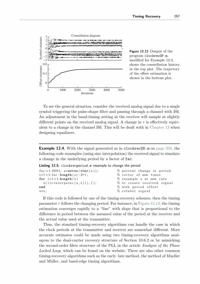
Timing Recovery 267
Constellation diagram
Iterations0 1000 2000 3000 4000 5000
−3
0
3
−2
1
−1
2
0.4
0.8
0
Sym
bol e
stim
ates
Off
set e
stim
ates
Figure 12.12 Output of theprogram clockrecOP.m,modified for Example 12.3,shows the constellation historyin the top plot. The trajectoryof the offset estimation isshown in the bottom plot.
To see the general situation, consider the received analog signal due to a single
symbol triggering the pulse-shape filter and passing through a channel with ISI.
An adjustment in the baud-timing setting at the receiver will sample at slightly
different points on the received analog signal. A change in τ is effectively equiv-
alent to a change in the channel ISI. This will be dealt with in Chapter 13 when
designing equalizers.
Example 12.4. With the signal generated as in clockrecDD.m on page 258, the
following code resamples (using sinc interpolation) the received signal to simulate
a change in the underlying period by a factor of fac.
Listing 12.5. clockrecperiod.m resample to change the period
f a c =1.0001; z=zeros ( size (x ) ) ; % per cent change in per i odt=l +1: f a c : length ( x)−2* l ; % vector o f new timesfor i=l +1: length ( t ) % resample x at new ra t e
z ( i )= i n t e r p s i n c (x , t ( i ) , l ) ; % to c r ea t e r e c e i v ed s i g n a lend % with per i od o f f s e tx=z ; % r e l a b e l s i g n a l
If this code is followed by one of the timing-recovery schemes, then the timing
parameter τ follows the changing period. For instance, in Figure 12.13, the timing
estimation converges rapidly to a “line” with slope that is proportional to the
difference in period between the assumed value of the period at the receiver and
the actual value used at the transmitter.
Thus, the standard timing-recovery algorithms can handle the case in which
the clock periods at the transmitter and receiver are somewhat different. More
accurate estimates could be made using two timing-recovery algorithms anal-
ogous to the dual-carrier recovery structure of Section 10.6.2 or by mimicking
the second-order filter structure of the PLL in the article Analysis of the Phase
Locked Loop, which can be found on the website. There are also other common
timing-recovery algorithms such as the early–late method, the method of Mueller
and Muller, and band-edge timing algorithms.

268 Chapter 12. Timing Recovery
Constellation history
Iterations
0 0.5 1 1.5 2x10⁴
−1.5
0
1.5
−1
0.5
−0.5
1
−4
−101
−3−2
Sym
bol e
stim
ates
Off
set e
stim
ates
Figure 12.13 Output ofclockrecperiod.m as modified forExample 12.4 shows theconstellation history in the topplot and the trajectory of theoffset estimation in the bottom.The slope of the estimates isproportional to the differencebetween the nominal and theactual clock period.
Exercise 12.20. Modify clockrecOP.m to implement one of the alternative
performance functions of Figure 12.11: avg{|x[k]|}, avg{x2[k]}, or avg{(x2[k]−1)2}.
Exercise 12.21. Modify clockrecOP.m by changing the channel as in Exam-
ple 12.3. Use different values of beta in the SRRC pulse-shape routine. How does
this affect the convergence speed of the algorithm? Do different pulse shapes
change the convergent value?
Exercise 12.22. Investigate how the error surface depends on the input signal.
a. Draw the error surface for the output-energy-maximization timing-recovery
algorithm when the inputs are binary ±1.
b. Draw the error surface when the inputs are drawn from the 4-PAM constel-
lation, for the case in which the symbol −3 never occurs.
Exercise 12.23. Imitate Example 12.3 using a channel of your own choosing.
Do you expect that the eye will always be able to open?
Exercise 12.24. Instead of the ISI channel used in Example 12.3, include a
white-noise channel. How does this change the timing estimates?
Exercise 12.25. Explore the limits of the period tracking in Example 12.4.
How large can fac be made and still have the estimates converge to a line?
What happens to the cluster variance when the estimates cannot keep up? Does
it help to increase the size of the stepsize mu?
For Further Reading
A comprehensive collection of timing- and carrier-recovery schemes can be found
in the following two texts:

Timing Recovery 269
� H. Meyr, M. Moeneclaey, and S. A. Fechtel, Digital Communication Receivers,
Wiley, 1998;� J. A. C. Bingham, The Theory and Practice of Modem Design, Wiley Inter-
science, 1988.

13 Linear Equalization
When all is well in the receiver, there is no interaction between successive sym-
bols; each symbol arrives and is decoded independently of all others. But when
symbols interact, when the waveform of one symbol corrupts the value of a nearby
symbol, then the received signal becomes distorted. It is difficult to decipher
the message from such a received signal. This impairment is called “intersym-
bol interference” and was discussed in Chapter 11 in terms of non-Nyquist pulse
shapes overlapping in time. This chapter considers another source of interference
between symbols that is caused by multipath reflections (or frequency-selective
dispersion) in the channel.
When there is no intersymbol interference (from a multipath channel, from
imperfect pulse shaping, or from imperfect timing), the impulse response of the
system from the source to the recovered message has a single nonzero term.
The amplitude of this single “spike” depends on the transmission losses, and the
delay is determined by the transmission time. When there is intersymbol inter-
ference caused by a multipath channel, this single spike is “scattered,” duplicated
once for each path in the channel. The number of nonzero terms in the impulse
response increases. The channel can be modeled as a finite-impulse-response,
linear filter C, and the delay spread is the total time interval during which reflec-
tions with significant energy arrive. The idea of the equalizer is to build (another)
filter in the receiver that counteracts the effect of the channel. In essence, the
equalizer must “unscatter” the impulse response. This can be stated as the goal
of designing the equalizer E so that the impulse response of the combined chan-
nel and equalizer CE has a single spike. This can be cast as an optimization
problem, and can be solved using techniques familiar from Chapters 6, 10, and
12.
The transmission path may also be corrupted by additive interferences such
as those caused by other users. These noise components are usually presumed
to be uncorrelated with the source sequence and they may be broadband or
narrowband, in band or out of band relative to the bandlimited spectrum of the
source signal. Like the multipath channel interference, they cannot be known to

Linear Equalization 271
Pulseshaping
Analogchannel
Decisiondevice
Lineardigital
equalizer
Digitalsource
Receivedanalogsignal
Sampledreceivedsignal
Noise and interferers
Ts
+
Figure 13.1 The baseband linear (digital) equalizer is intended to (automatically)cancel out unwanted effects of the channel and to cancel out certain kinds of additiveinterferences.
the system designer in advance. The second job of the equalizer is to reject such
additive narrowband interferers by designing appropriate linear notch filters “on-
the-fly.” At the same time, it is important that the equalizer does not unduly
enhance the broadband noise.
The signal path of a baseband digital communication system is shown in Fig-
ure 13.1, which emphasizes the role of the equalizer in trying to counteract the
effects of the multipath channel and the additive interference. As in previous
chapters, all of the inner parts of the system are assumed to operate precisely:
thus, the upconversion and downconversion, the timing recovery, and the car-
rier synchronization (all those parts of the receiver that are not shown in Figure
13.1) are assumed to be flawless and unchanging. Modeling the channel as a time-
invariant FIR filter, the next section focuses on the task of selecting the coeffi-
cients in the block labeled “linear digital equalizer,” with the goal of removing the
intersymbol interference and attenuating the additive interferences. These coeffi-
cients are to be chosen using the sampled received signal sequence and (possibly)
knowledge of a prearranged “training sequence.” While the channel may actually
be time-varying, the variations are often much slower than the data rate, and
the channel can be viewed as (effectively) time-invariant over small time scales.
This chapter suggests several different ways in which the coefficients of the
equalizer can be chosen. The first procedure, in Section 13.2.1, minimizes the
square of the symbol-recovery error1 over a block of data, which can be done
using a matrix pseudoinversion. Minimizing the (square of the) error between the
received data values and the transmitted values can also be achieved using an
adaptive element, as detailed in Section 13.3. When there is no training sequence,
other performance functions are appropriate, and these lead to equalizers such as
the decision-directed approach in Section 13.4 and the dispersion-minimization
method in Section 13.5. The adaptive methods considered here are only modestly
complex to implement, and they can potentially track time variations in the
channel model, assuming that the changes are sufficiently slow.
1 This is the error between the equalizer output and the transmitted symbol, and is knownwhenever there is a training sequence.

272 Chapter 13. Linear Equalization
13.1 Multipath Interference
The villains of this chapter are multipath and other additive interferers. Both
should be familiar from Section 4.1.
The distortion caused by an analog wireless channel can be thought of as a
combination of scaled and delayed reflections of the original transmitted signal.
These reflections occur when there are different paths from the transmitting
antenna to the receiving antenna. Between two microwave towers, for instance,
the paths may include one along the line of sight, reflections from nearby hills,
and bounces from a field or lake between the towers. For indoor digital TV
reception, there are many (local) time-varying reflectors, including people in the
receiving room, and nearby vehicles. The strength of the reflections depends on
the physical properties of the reflecting objects, while the delay of the reflections
is primarily determined by the length of the transmission path. Let u(t) be the
transmitted signal. If N delays are represented by Δ1, Δ2, . . . , ΔN , and the
strength of the reflections is α1, α2, . . . , αN , then the received signal is
y(t) = α1u(t−Δ1) + α2u(t−Δ2) + · · ·+ αNu(t−ΔN ) + η(t), (13.1)
where η(t) represents additive interferences. This model of the transmission chan-
nel has the form of a finite-impulse-response filter, and the total length of time
ΔN −Δ1 over which the impulse response is nonzero is called the delay spread
of the physical medium.
This transmission channel is typically modeled digitally assuming a fixed sam-
pling period Ts. Thus, (13.1) is approximated by
y(kTs) = a0u(kTs) + a1u((k − 1)Ts) + · · ·+ anu((k − n)Ts) + η(kTs). (13.2)
In order for the model (13.2) to closely represent the system (13.1), the total time
over which the impulse response is nonzero (the time nTs) must be at least as
large as the maximum delay ΔN . Since the delay is not a function of the symbol
period Ts, smaller values of Ts require more terms in the filter (i.e., larger n).
For example, consider a sampling interval of Ts ≈ 40 ns (i.e., a transmission
rate of 25 MHz). A delay spread of approximately 4 μs would correspond to 100
taps in the model (13.2). Thus, at any time instant, the received signal would
be a combination of (up to) 100 data values. If Ts were increased to 0.4 μs
(i.e., 2.5 MHz), only 10 terms would be needed, and there would be interference
with only the 10 nearest data values. If Ts were larger than 4 μs (i.e., 0.25
MHz), only one term would be needed in the discrete-time impulse response.
In this case, adjacent sampled symbols would not interfere. Such finite-duration
impulse-response models as (13.2) can also be used to represent the frequency-
selective dynamics that occur in the wired local end-loop in telephony, and other
(approximately) linear, finite-delay-spread channels.
The design objective of the equalizer is to undo the effects of the channel and to
remove the interference. Conceptually, the equalizer attempts to build a system
that is a “delayed inverse” of (13.2), removing the intersymbol interference while

Linear Equalization 273
simultaneously rejecting additive interferers uncorrelated with the source. If the
interference η(kTs) is unstructured (for instance white noise) then there is little
that a linear equalizer can do to remove it. But when the interference is highly
structured (such as narrowband interference from another user), then the linear
filter can often notch out the offending frequencies.
As shown in Example 12.3 of Section 12.5, the solution for the optimal sam-
pling times found by the clock-recovery algorithms depends on the ISI in the
channel. Consequently, the digital model (such as (13.2)) formed by sampling an
analog transmission path (such as (13.1)) depends on when the samples are taken
within each period Ts. To see how this can happen in a simple case, consider a
two-path transmission channel
δ(t) + 0.6δ(t−Δ),
where Δ is some fraction of Ts. For each transmitted symbol, the received signal
will contain two copies of the pulse shape p(t), the first undelayed and the second
delayed by Δ and attenuated by a factor of 0.6. Thus, the receiver sees
c(t) = p(t) + 0.6p(t−Δ).
This is shown in Figure 13.2 for Δ = 0.7Ts. The clock-recovery algorithms cannot
separate the individual copies of the pulse shapes. Rather, they react to the
complete received shape, which is their sum. The power maximization will locate
the sampling times at the peak of this curve, and the lattice of sampling times
will be different from what would be expected without ISI. The effective (digital)
channel model is thus a sampled version of c(t). This is depicted in Figure 13.2
by the small circles that occur at Ts-spaced intervals.
In general, an accurate digital model for a channel depends on many things:
the underlying analog channel, the pulse shaping used, and the timing of the
sampling process. At first glance, this seems like it might make designing an
equalizer for such a channel almost impossible. But there is good news. No
matter what timing instants are chosen, no matter what pulse shape is used, and
no matter what the underlying analog channel may be (as long as it is linear),
there is an FIR linear representation of the form (13.2) that closely models its
behavior. The details may change, but it is always a sampling of the smooth curve
(like c(t) in Figure 13.2) that defines the digital model of the channel. As long
as the digital model of this channel does not have deep nulls (i.e., a frequency
response that practically zeroes out some important band of frequencies), there
is a good chance that the equalizer can undo the effects of the channel.
13.2 Trained Least-Squares Linear Equalization
When there is a training sequence available (for instance, in the known frame
information that is used in synchronization), this can also be used to help build
or “train” an equalizer. The basic strategy is to find a suitable function of the

274 Chapter 13. Linear Equalization
0
Lattice of Ts-spaced optimal sampling times
with ISI
p(t)
0.6 p(t − Δ)
c(t) = p(t) + 0.6 p(t − Δ)
Lattice of Ts-spaced optimalsampling times with no ISI
Sum of received pulses
The digital channelmodel is given by
Ts-spaced samples of c(t)
Figure 13.2 The optimum sampling times (as found by the energy-maximizationalgorithm) differ when there is ISI in the transmission path, and change the effectivedigital model of the channel.
Sources[k]
Channel Equalizer
Additiveinterferers
Delay
Impulse response f
Receivedsignal r[k]
Training signalErrore[k]−
Equalizeroutput y[k]
+
+
Figure 13.3 The problem of linear equalization is to find a linear system f that undoesthe effects of the channel while minimizing the effects of the interferences.
unknown equalizer parameters that can be used to define an optimization prob-
lem. Then, applying the techniques of Chapters 6, 10, and 12, the optimization
problem can be solved in a variety of ways.
13.2.1 A Matrix Description
The linear equalization problem is depicted in Figure 13.3. A prearranged train-
ing sequence s[k] is assumed known at the receiver. The goal is to find an FIR
filter (called the equalizer) so that the output of the equalizer is approximately
equal to the known source, though possibly delayed in time. Thus, the goal is to
choose the impulse response fi so that y[k] ≈ s[k − δ] for some specific δ.

Linear Equalization 275
y[k]
r[k]z−1 z−1 z−1
f0 f1 fn
. . .
. . .
+ +
Figure 13.4 The direct-form FIR filter of Equation (13.3) can be pictured as a tappeddelay line where each z−1 block represents a time delay of one symbol period. Theimpulse response of the filter is f0, f1, . . ., fn.
The input–output behavior of the FIR linear equalizer can be described as the
convolution
y[k] =n∑
j=0
fjr[k − j], (13.3)
where the lower index on j can be no lower than zero (or else the equalizer
is noncausal; that is, it can illogically respond to an input before the input is
applied). This convolution is illustrated in Figure 13.4 as a “direct-form FIR” or
“tapped delay line.”
The summation in (13.3) can also be written (e.g., for k = n+ 1) as the inner
product of two vectors
y[n+ 1] = [r[n+ 1], r[n], . . . , r[1]]
⎡⎢⎢⎢⎣f0f1...
fn
⎤⎥⎥⎥⎦ . (13.4)
Note that y[n+ 1] is the earliest output that can be formed given no knowledge
of r[i] for i < 1. Incrementing the time index in (13.4) gives
y[n+ 2] = [r[n+ 2], r[n + 1], . . . , r[2]]
⎡⎢⎢⎢⎣f0f1...
fn
⎤⎥⎥⎥⎦
and
y[n+ 3] = [r[n+ 3], r[n+ 2], . . . , r[3]]
⎡⎢⎢⎢⎣f0f1...
fn
⎤⎥⎥⎥⎦ .
Observe that each of these uses the same equalizer parameter vector. Concate-
nating p− n of these measurements into one matrix equation over the available

276 Chapter 13. Linear Equalization
data set for i = 1 to p gives⎡⎢⎢⎢⎢⎢⎣
y[n+ 1]
y[n+ 2]
y[n+ 3]...
y[p]
⎤⎥⎥⎥⎥⎥⎦ =
⎡⎢⎢⎢⎢⎢⎣
r[n+ 1] r[n] · · · r[1]
r[n+ 2] r[n+ 1] · · · r[2]
r[n+ 3] r[n+ 2] · · · r[3]...
......
r[p] r[p− 1] · · · r[p − n]
⎤⎥⎥⎥⎥⎥⎦
⎡⎢⎢⎢⎣f0f1...
fn
⎤⎥⎥⎥⎦ , (13.5)
or, with the appropriate matrix definitions,
Y = RF. (13.6)
Note that R has a special structure, namely that the entries along each diagonal
are the same. R is known as a Toeplitz matrix and the toeplitz command in
Matlab makes it easy to build matrices with this structure.
13.2.2 Source Recovery Error
The delayed source recovery error is
e[k] = s[k − δ]− y[k] (13.7)
for a particular δ. This section shows how the source recovery error can be used
to define a performance function that depends on the unknown parameters fi.
Calculating the parameters that minimize this performance function provides a
good solution to the equalization problem.
Define
S =
⎡⎢⎢⎢⎢⎢⎣
s[n+ 1− δ]
s[n+ 2− δ]
s[n+ 3− δ]...
s[p− δ]
⎤⎥⎥⎥⎥⎥⎦ and E =
⎡⎢⎢⎢⎢⎢⎣
e[n+ 1]
e[n+ 2]
e[n+ 3]...
e[p]
⎤⎥⎥⎥⎥⎥⎦ . (13.8)
Using (13.6), write
E = S − Y = S −RF. (13.9)
As a measure of the performance of the fi in F , consider
JLS =
p∑i=n+1
e2[i]. (13.10)
JLS is nonnegative since it is a sum of squares. Minimizing such a summed
squared delayed source recovery error is a common objective in equalizer design,
since the fi that minimize JLS cause the output of the equalizer to become close
to the values of the (delayed) source.

Linear Equalization 277
Given (13.8) and (13.9), JLS in (13.10) can be written as
JLS = ETE = (S −RF )T(S −RF )
= STS − (RF )TS − STRF + (RF )TRF. (13.11)
Because JLS is a scalar, (RF )TS and STRF are also scalars. Since the transpose
of a scalar is equal to itself, (RF )TS = STRF , and (13.11) can be rewritten as
JLS = STS − 2STRF + (RF )TRF. (13.12)
The issue is now one of choosing the n+ 1 entries of F to make JLS as small as
possible.
13.2.3 The Least-Squares Solution
Define the matrix
Ψ = [F − (RTR)−1RTS]T(RTR)[F − (RTR)−1RTS]
= FT(RTR)F − STRF − FTRTS + STR(RTR)−1RTS.
The purpose of this definition is to rewrite (13.12) in terms of Ψ:
JLS = Ψ+ STS − STR(RTR)−1RTS
= Ψ+ ST[I −R(RTR)−1RT]S. (13.13)
Since ST[I −R(RTR)−1RT]S is not a function of F , the minimum of JLS
occurs at the F that minimizes Ψ. This occurs when
F † = (RTR)−1RTS, (13.14)
assuming that (RTR)−1 exists.2 The corresponding minimum achievable by JLS
at F = F † is the summed squared delayed source recovery error. This is the
remaining term in (13.13); that is,
JminLS = ST[I −R(RTR)−1RT]S. (13.15)
The formulas for the optimum F in (13.14) and the associated minimum
achievable JLS in (13.15) are for a specific δ. To complete the design task, it
is also necessary to find the optimal delay δ. The most straightforward approach
is to set up a series of S = RF calculations, one for each possible δ, to compute
the associated values of JminLS , and pick the delay associated with the smallest
one.
This procedure is straightforward to implement in Matlab, and the program
LSequalizer.m allows you to play with the various parameters to get a feel for
their effect. Much of this program will be familiar from openclosed.m. The first
2 A matrix is invertible as long as it has no eigenvalues equal to zero. Since RTR is a quadraticform it has no negative eigenvalues. Thus, all eigenvalues must be positive in order for it tobe invertible.

278 Chapter 13. Linear Equalization
three lines define a channel, create a binary source, and then transmit the source
through the channel using the filter command. At the receiver, the data are
put through a quantizer, and then the error is calculated for a range of delays.
The new part is in the middle.
Listing 13.1. LSequalizer.m find a LS equalizer f for the channel b
b=[0.5 1 −0 .6 ] ; % de f i n e channelm=1000; s=sign (randn (1 ,m) ) ; % binary sour ce o f l ength mr=f i l t e r (b , 1 , s ) ; % output o f channeln=3; % length o f e qua l i z e r − 1de l t a =3; % use delay <=n* l ength (b)p=length ( r )−de l t a ;
R=toepl itz ( r (n+1:p ) , r (n+1: −1:1)) ; % bui ld matrix RS=s (n+1−de l t a : p−de l t a ) ’ ; % and vector Sf=inv (R’ *R)*R’ * S % ca l c u l a t e e qua l i z e r fJmin=S ’ *S−S ’ *R* inv (R’ *R)*R’ *S % Jmin f o r t h i s f and de l t ay=f i l t e r ( f , 1 , r ) ; % equa l i z e r i s a f i l t e rdec=sign ( y ) ; % quant i ze and f i nd e r r o r se r r =0.5*sum(abs ( dec ( de l t a +1:m)− s ( 1 :m−de l t a ) ) )
The variable n defines the length of the equalizer, and delta defines the delay
that will be used in constructing the vector S defined in (13.8) (observe that
delta must be positive and less than or equal to n). The Toeplitz matrix R
is defined in (13.5) and (13.6), and the equalizer coefficients f are computed
as in (13.14). The value of minimum achievable performance is Jmin, which is
calculated as in (13.15). To demonstrate the effect of the equalizer, the received
signal r is filtered by the equalizer coefficients, and the output is then quantized.
If the equalizer has done its job (i.e., if the eye is open), then there should be
some shift sh at which no errors occur.
For example, using the default channel b= [0.5, 1,−0.6], and length-4 equalizer
(n=3), four values of the delay delta give
delay delta Jmin equalizer f
0 832 {0.33, 0.027, 0.070, 0.01}1 134 {0.66, 0.36, 0.16, 0.08}2 30 {−0.28, 0.65, 0.30, 0.14}3 45 {0.1, −0.27, 0.64, 0.3}
(13.16)
The best equalizer is the one corresponding to a delay of 2, since this Jmin is the
smallest. In this case, however, any of the last three will open the eye. Observe
that the number of errors (as reported in err) is zero when the eye is open.
Exercise 13.1. Plot the frequency response (using freqz) of the channel b
in LSequalizer.m. Plot the frequency response of each of the four equalizers
found by the program. For each channel/equalizer pair, form the product of the
magnitude of the frequency responses. How close are these products to unity?
Exercise 13.2. Add (uncorrelated, normally distributed) noise into the simula-
tion using the command r=filter(b,1,s)+sd*randn(size(s)).

Linear Equalization 279
a. For the equalizer with delay 2, what is the largest sd you can add and still
have no errors?
b. Make a plot of Jmin as a function of sd.
c. Now try the equalizer with delay 1. What is the largest sd you can add, and
still have no errors?
d. Which is a better equalizer?
Exercise 13.3. Use LSequalizer.m to find an equalizer that can open the eye
for the channel b = [1, 1, −0.8, −0.3, 1, 1].
a. What equalizer length n is needed?
b. What delays delta give zero error at the output of the quantizer?
c. What is the corresponding Jmin?
d. Plot the frequency response of this channel.
e. Plot the frequency response of your equalizer.
f. Calculate and plot the product of the two.
Exercise 13.4. Modify LSequalizer.m to generate a source sequence from the
alphabet ±1,±3. For the default channel [0.5, 1, −0.6], find an equalizer that
opens the eye.
a. What equalizer length n is needed?
b. What delays delta give zero error at the output of the quantizer?
c. What is the corresponding Jmin?
d. Is this a fundamentally easier or more difficult task than when equalizing a
binary source?
e. Plot the frequency response of the channel and of the equalizer.
There is a way to convert the exhaustive search over all the delays δ in the
previous approach into a single matrix operation. Construct the (p− α)× (α+
1) matrix of training data
S =
⎡⎢⎢⎢⎣s[α+ 1] s[α] · · · s[1]
s[α+ 2] s[α+ 1] · · · s[2]...
......
s[p] s[p− 1] · · · s[p− α]
⎤⎥⎥⎥⎦ , (13.17)
where α specifies the number of delays δ that will be searched, from δ = 0 to
δ = α. The (p− α) × (n+ 1) matrix of received data is
R =
⎡⎢⎢⎢⎣r[α + 1] r[α] · · · r[α− n+ 1]
r[α + 2] r[α + 1] · · · r[α − n+ 2]...
......
r[p] r[p− 1] · · · r[p− n]
⎤⎥⎥⎥⎦ , (13.18)
where each column corresponds to one of the possible delays. Note that α > n is
required in order to keep the lowest index of r[·] positive. In the (n+ 1)× (α+ 1)

280 Chapter 13. Linear Equalization
matrix
F =
⎡⎢⎢⎢⎣
f00 f01 · · · f0αf10 f11 · · · f1α...
......
fn0 fn1 · · · fnα
⎤⎥⎥⎥⎦ ,
each column is a set of equalizer parameters, one corresponding to each of the
possible delays. The strategy is to use S and R to find F . The column of F that
results in the smallest value of the performance function JLS is then the optimal
receiver at the optimal delay.
The jth column of F corresponds to the equalizer parameter vector choice
for δ = j − 1. The product of R with this jth column from F is intended to
approximate the jth column of S. The least-squares solution of S ≈ RF is
F † = (RTR)−1RTS, (13.19)
where the number of columns of R (i.e., n+ 1) must be less than or equal to
the number of rows of R (i.e., p− α) for (RTR)−1 to exist. Consequently, p−α ≥ n+ 1 implies that p > n+ α. If so, the minimum value associated with a
particular column of F † (e.g., F †� ) is, from (13.15),
Jmin,�LS = ST
� [I − R(RTR)−1RT]S�, (13.20)
where S� is the �th column of S. Thus, these Jmin,�LS are all along the diagonal of
Φ = ST[I − R(RTR)−1RT]S. (13.21)
Hence, the minimum value on the diagonal of Φ (e.g., at the (j, j)th entry)
corresponds to the optimum δ.
Example 13.1. Consider the low-order example with n = 1 (so F has two param-
eters), α = 2 (so α > n), and p = 5 (so p > n+ α). Thus,
S =
⎡⎣ s[3] s[2] s[1]
s[4] s[3] s[2]
s[5] s[4] s[3]
⎤⎦ , R =
⎡⎣ r[3] r[2]
r[4] r[3]
r[5] r[4]
⎤⎦ , and F =
[f00 f01 f02f10 f11 f12
].
For the example, assume that the true channel is
r[k] = ar[k − 1] + bs[k − 1].
A two-tap equalizer F = [f0, f1]T can provide perfect equalization for δ = 1 with
f0 = 1/b and f1 = −a/b, since
y[k] = f0r[k] + f1r[k − 1] =1
b[r[k]− ar[k − 1]]
=1
b[ar[k − 1] + bs[k − 1]− ar[k − 1]] = s[k − 1].

Linear Equalization 281
Consider
{s[1], s[2], s[3], [s4], s[5]} = {1, −1, −1, 1, −1},which results in
S =
⎡⎣ −1 −1 1
1 −1 −1
−1 1 −1
⎤⎦ .
With a = 0.6, b = 1, and r[1] = 0.8. Similarly,
r[2] = ar[1] + bs[1] = 0.48 + 1 = 1.48,
r[3] = 0.888− 1 = −0.112,
r[4] = −1.0672,
r[5] = 0.3597.
Example 13.2. The effect of channel noise can be simulated by rounding these
values for r in composing
R =
⎡⎣ −0.1 1.5
−1.1 −0.1
0.4 −1.1
⎤⎦ .
Thus, from (13.21),
Φ =
⎡⎣ 1.2848 0.0425 0.4778
0.0425 0.0014 0.0158
0.4778 0.0158 0.1777
⎤⎦ ,
and from (13.19),
F † =[ −1.1184 0.9548 0.7411
−0.2988 −0.5884 0.8806
].
Since the second diagonal term in Φ is the smallest diagonal term, δ = 1 is the
optimum setting (as expected) and the second column of F † is the minimum
summed squared delayed recovery error solution (i.e., f0 = 0.9548 (≈ 1/b = 1)
and f1 = −0.5884 (≈ −a/b = −0.6)).
With a “better” received signal measurement, for instance,
R =
⎡⎣ −0.11 1.48
−1.07 −0.11
0.36 −1.07
⎤⎦ ,
the diagonal of Φ is [1.3572, 0.0000, 0.1657] and the optimum delay is again
δ = 1, and the optimum equalizer settings are 0.9960 and −0.6009, which give a
better fit to the ideal noise-free answer. Infinite precision in R (measured without

282 Chapter 13. Linear Equalization
channel noise or other interferers) produces a perfect fit to the “true” f0 and f1and a zeroed delayed source recovery error.
13.2.4 Summary of Least-Squares Equalizer Design
The steps of the linear FIR equalizer design strategy are as follows.
1. Select the order n for the FIR equalizer in (13.3).
2. Select the maximum of candidate delays α > n used in (13.17) and (13.18).
3. Utilize a set of p training signal samples {s[1], s[2], . . . , s[p]} with p > n+ α.
4. Obtain a corresponding set of p received signal samples {r[1], r[2], . . . , r[p]}.5. Compose S in (13.17).
6. Compose R in (13.18).
7. Check whether RTR has poor conditioning induced by any (near) zero eigen-
values. Matlab will return a warning (or an error) if the matrix is too close
to singular.3
8. Compute F † from (13.19).
9. Compute Φ by substituting F † into (13.21), rewritten as
Φ = ST[S − RF †].
10. Find the minimum value on the diagonal of Φ. This index is δ + 1. The asso-
ciated diagonal element of Φ is the minimum achievable summed squared
delayed source recovery error∑p
i=α+1 e2[i] over the available data record.
11. Extract the (δ + 1)th column of the previously computed F †. This is the
impulse response of the optimum equalizer.
12. Test the design. Test it on synthetic data, and then on measured data (if
available). If it is inadequate, repeat the design stage, perhaps increasing n
or twiddling some other designer-selected quantity.
This procedure, along with three others that will be discussed in the ensuing
sections, is available on the website in the program dae.m. Combining the var-
ious approaches makes it easier to compare their behaviors in the examples of
Section 13.6.
13.2.5 Complex Signals and Parameters
The preceding development assumes that the source signal and channel, and
therefore the received signal, equalizer, and equalizer output, are all real-valued.
However, the source signal and channel may be modeled as complex-valued when
using modulations such as QAM of Section 5.3. This is explored in some detail
3 The condition number (i.e., the maximum eigenvalue divided by the minimum eigenvalue) ofRTR should be checked. If the condition number is extremely large, start again with different{s[·]}. If all choices of {s[·]} result in poorly conditioned RTR, then most likely the channelhas deep nulls that prohibit the successful application of a T -spaced linear equalizer.

Linear Equalization 283
in the document A Digital Quadrature Amplitude Modulation Radio, which can
be found on the website. The same basic strategy for equalizer design can also
be used in the complex case.
Consider a complex delayed source recovery error
e[k] = eR[k] + jeI [k],
where j =√−1. Consider its square,
e2[k] = e2R[k] + 2jeR[k]eI [k]− e2I [k],
which is typically complex-valued, and potentially real-valued and negative when
eR ≈ 0. Thus, a sum of e2 is no longer a suitable measure of performance since
|e| might be nonzero but its squared average might be zero.
Instead, consider the product of a complex e with its complex conjugate e∗ =eR − jeI ; that is,
e[k]e∗[k] = e2R[k]− jeR[k]eI [k] + jeR[k]eI [k]− j2e2I [k] = e2R[k] + e2I [k].
In vector form, the summed squared error of interest is EHE (rather than
the EHE of (13.11)), where the superscript H denotes the operations of both
transposition and complex conjugation. Thus, (13.14) becomes
F † = (RHR)−1RHS.
Note, that in implementing this refinement in the Matlab code, the symbol pair
.’ implements a transpose, while ’ alone implements a conjugate transpose.
13.2.6 Fractionally Spaced Equalization
The preceding development assumes that the sampled input to the equalizer
is symbol spaced with the sampling interval equal to the symbol interval of T
seconds. Thus, the unit delay in realizing the tapped-delay-line equalizer is T
seconds. Sometimes, the input to the equalizer is oversampled such that the
sample interval is shorter than the symbol interval, and the resulting equalizer
is said to be fractionally spaced. The same kinds of algorithms and solutions can
be used to calculate the coefficients in fractionally spaced equalizers as are used
for T -spaced equalizers. Of course, details of the construction of the matrices
corresponding to S and R will necessarily differ due to the structural differences.
The more rapid sampling allows greater latitude in the ordering of the blocks in
the receiver. This is discussed at length in Equalization on the website.
Exercise 13.5. Consider the multiuser system shown in Figure 13.5. Both users
transmit binary ±1 PAM signals that are independent and equally probable sym-
bols. The signal from the first user is distorted by a frequency-selective channel
with impulse response
h1[k] = δ[k] + bδ[k − 1].

284 Chapter 13. Linear Equalization
+x[k]r[k] y[k]Channel 1
h2[k]Equalizer
f [k]Decisiondevice
Channel 2h1[k]
User 1s1[k]
User 2s2[k]
Figure 13.5 Basebandcommunication system withmultiuser interference used inExercise 13.5.
The signal from the second (interfering) user is scaled by h2[k] = cδ[k]. The
difference equation generating the received signal r is
r[k] = s1[k] + bs1[k − 1] + cs2[k].
The difference equation describing the equalizer input–output behavior is
x[k] = r[k] + dr[k − 1].
The decision device is the sign operator.
a. Write out the difference equation relating s1[k] and s2[k] to x[k].
b. Consider the performance function
JMSE =1
N
k0+N∑k=k0+1
(s1[k]− x[k])2.
For uncorrelated source symbol sequences, JMSE is minimized by minimizing∑ρ2i . For b = 0.8 and c = 0.3 compute the equalizer setting d that minimizes
JMSE .
c. For b = 0.8, c = 0.3, and d = 0 (i.e., equalizer-less reception), does the system
exhibit decision errors?
d. For b = 0.8, c = 0.3, and your d from part (b), does the system exhibit decision
errors? Does this system suffer more severe decision errors than the equalizer-
less system of part (c)?
13.3 An Adaptive Approach to Trained Equalization
The block-oriented design of the previous section requires substantial compu-
tation even when the system delay is known since it requires calculating the
inverse of an (n+ 1)× (n+ 1) matrix, where n is the largest delay in the FIR
linear equalizer. This section considers using an adaptive element to minimize
the average of the squared error,
JLMS =1
2avg{e2[k]}. (13.22)

Linear Equalization 285
Observe that JLMS is a function of all the equalizer coefficients fi, since
e[k] = s[k − δ]− y[k] = s[k − δ]−n∑
j=0
fjr[k − j], (13.23)
which combines (13.7) with (13.3), and where r[k] is the received signal at base-
band after sampling. An algorithm for the minimization of JLMS with respect
to the ith equalizer coefficient fi is
fi[k + 1] = fi[k]− μ∂JLMS
∂fi
∣∣∣∣fi=fi[k]
. (13.24)
To create an algorithm that can easily be implemented, it is necessary to evaluate
this derivative with respect to the parameter of interest. This is
∂JLMS
∂fi=
∂ avg{ 12e2[k]}
∂fi≈ avg
{ 12∂e2[k]
∂fi
}= avg
{e[k]
∂e[k]
∂fi
}, (13.25)
where the approximation follows from (G.12) and the final equality from the
chain rule (A.59). Using (13.23), the derivative of the source recovery error e[k]
with respect to the ith equalizer parameter fi is
∂e[k]
∂fi=
∂s[k − δ]
∂fi−
n∑j=0
∂fjr[k − j]
∂fi= −r[k − i], (13.26)
since ∂s[k − δ]/∂fi = 0 and ∂fjr[k − j]/∂fi = 0 for all i �= j. On substituting
(13.26) into (13.25) and then into (13.24), the update for the adaptive element
is
fi[k + 1] = fi[k] + μavg{e[k]r[k − i]}.Typically, the averaging operation is suppressed since the iteration with small
stepsize μ itself has a lowpass (averaging) behavior. The result is commonly
called the least mean squares (LMS) algorithm for direct linear equalizer impulse
response coefficient adaptation:
fi[k + 1] = fi[k] + μe[k]r[k − i]. (13.27)
This adaptive equalization scheme is illustrated in Figure 13.6.
When all goes well, the recursive algorithm (13.27) converges to the vicinity
of the block least-squares answer for the particular δ used in forming the delayed
recovery error. As long as μ is nonzero, if the underlying composition of the
received signal changes so that the error increases and the desired equalizer
changes, then the fi react accordingly. It is this tracking ability that earns it the
label adaptive.4
The following Matlab code implements an adaptive equalizer design. The
beginning and ending of the program are familiar from openclosed.m and
4 To provide tracking capability, the matrix solution of Section 13.2.1 could be recomputed forsuccessive data blocks, but this requires significantly more computation.

286 Chapter 13. Linear Equalization
f [k] Sign[·]
r[k] y[k]
e[k] s[k]trainingsignal
Equalizer
Adaptivealgorithm
Performanceevaluation
Decisiondevice
Sampledreceivedsignal
Figure 13.6 A trained adaptive linear equalizer uses the difference between thereceived signal and a prespecified training sequence to drive the adaptation of thecoefficients of the equalizer.
LSequalizer.m. The heart of the recursion lies in the for loop. For each new
data point, a vector is built containing the new value and the past n values of the
received signal. This is multiplied by f to make a prediction of the next source
symbol, and the error is the difference between the prediction and the reality.
(This is the calculation of e[k] from (13.23).) The equalizer coefficients f are then
updated as in (13.27).
Listing 13.2. LMSequalizer.m find a LMS equalizer f for the channel b
b=[0.5 1 −0 .6 ] ; % de f i n e channelm=1000; s=pam(m, 2 , 1 ) ; % binary sour ce o f l ength mr=f i l t e r (b , 1 , s ) ; % output o f channeln=4; f=zeros (n , 1 ) ; % i n i t i a l i z e e qua l i z e r at 0mu=.01; d e l t a =2; % s t e p s i z e and delay de l t afor i=n+1:m % i t e r a t e
r r=r ( i :−1: i−n+1) ’ ; % vector o f r e c e i v ed s i g n a le=s ( i−de l t a )− rr ’ * f ; % ca l c u l a t e e r r o rf=f+mu*e* r r ; % update e qu a l i z e r c o e f f i c i e n t s
end
As with the matrix approach, the default channel b=[0.5 1 -0.6] can be
equalized easily with a short equalizer (one with a small n). The convergent val-
ues of the f are very close to the final values of the matrix approach; that is, for a
given channel, the value of f given by LMSequalizer.m is very close to the value
found using LSequalizer.m. A design consideration in the adaptive approach to
equalization involves the selection of the stepsize. Smaller stepsizes μ mean that
the trajectory of the estimates is smoother (tends to reject noises better) but
it also results in a slower convergence and slower tracking when the underlying
solution is time-varying. Similarly, if the explicit averaging operation is retained,
longer averages imply smoother estimates but slower convergence. Similar trade-
offs appear in the block approach in the choice of block size: larger blocks average
the noise better, but give no details about changes in the underlying solution
within the time span covered by a block.
The following code EqualizerTest.m shows one way to verify that the equal-
izer has (or has not) done a good job. The code generates a new received signal
and passes it through the same channel and the final converged equalizer from
LMSequalizer.m. The decision sequence dec (the sign of the data for a binary

Linear Equalization 287
transmission) is then compared with the original transmitted data s. Since the
delay of the equalizer cannot be known beforehand, the loop on sh tests all the
possible delays (shifts) that might occur. If one of these is zero (or very small)
then the equalizer is doing a good job.
Listing 13.3. EqualizerTest.m verify the operation of an equalizer f for the channel b
% F i r s t run LMSequal izer .m to s e t channel b and equa l i z e r ff i n a l e q=f ; % t e s t f i n a l f i l t e r f
m=1000; % new data po intss=pam(m, 2 , 1 ) ; % new binary sour ce o f l ength mr=f i l t e r (b , 1 , s ) ; % output o f channelyt=f i l t e r ( f , 1 , r ) ; % use f i n a l f i l t e r f to t e s tdec=sign ( real ( yt ) ) ; % quant i zat i onfor sh=0:n % i f e qua l i z e r i s working , one
e r r ( sh+1)=0.5*sum(abs ( dec ( sh+1:m)− s ( 1 :m−sh ) ) ) ;end % of these de l ays has zero e r r o r
This trained adaptive approach, along with several others, is implemented in
the program dae.m, which is available on the website. Simulated examples of
LMS with training and other adaptive equalization methods are presented in
Section 13.6.
Exercise 13.6. Verify that, by proper choice of n and delta, the convergent
values of f in LMSequalizer.m are close to the values shown in (13.16).
Exercise 13.7. What happens in LMSequalizer.mwhen the stepsize parameter
mu is too large? What happens when it is too small?
Exercise 13.8. Add (uncorrelated, normally distributed) noise into the simula-
tion using the command r=filter(b,1,s)+sd*randn(size(s)).
a. For the equalizer with delay 2, what is the largest sd you can add, and still
have no errors? How does this compare with the result from Exercise 13.2?
Hint: it may be necessary to simulate for more than the default m data points.
b. Now try the equalizer with delay 1. What is the largest sd you can add, and
still have no errors?
c. Which is a better equalizer?
Exercise 13.9. Use LMSequalizer.m to find an equalizer that can open the eye
for the channel b = [1, 1, −0.8, −0.3, 1, 1].
a. What equalizer length n is needed?
b. What delays delta give zero error in the output of the quantizer?
c. How does the answer compare with the design in Exercise 13.3?
Exercise 13.10. Modify LMSequalizer.m and EqualizerTest.m to generate a
source sequence from the alphabet ±1, ±3. For the default channel [0.5, 1, −0.6],
find an equalizer that opens the eye.

288 Chapter 13. Linear Equalization
a. What equalizer length n is needed?
b. What delays delta give zero error in the output of the quantizer?
c. Is this a fundamentally easier or more difficult task than when equalizing a
binary source?
d. How does the answer compare with the design in Exercise 13.4?
Exercise 13.11. The trained adaptive equalizer updates its impulse response
coefficients fi[k] via (13.27) using a gradient descent of the performance function
JLMS (13.22). With channels that have deep nulls in their frequency response
and a high SNR in the received signal, the minimization of (the average of)
JLMS results in a large spike in the equalizer frequency response (in order for
their product to be unity at the frequency of the channel null). Such large spikes
in the equalizer frequency response also amplify channel noise. To inhibit the
resulting large values of fi needed to create a frequency response with segments
of high gain, consider a cost function that also penalizes the sum of the squares
of the fi, e.g.,
1
2
(e2[k] + λ
N−1∑i=0
f2i [k]
)
Derive the associated adaptive-element update law corresponding to this perfor-
mance function.
13.4 Decision-Directed Linear Equalization
During the training period, the communication system does not transmit any
message data. Commonly, a block of training data is followed by a block of
message data. The fraction of time devoted to training should be small, but can
be up to 20% in practice. If it were possible to adapt the equalizer parameters
without using the training data, the message-bearing (and revenue-generating)
capacity of the channel would be enhanced.
Consider the situation in which some procedure has produced an equalizer
setting that opens the eye of the channel. Thus, all decisions are perfect, but
the equalizer parameters might not yet be at their optimal values. In such a
case, the output of the decision device is an exact replica of the delayed source
(i.e., it is as good as a training signal). For a binary ±1 source and decision
device that is a sign operator, the delayed source recovery error can be computed
as sign{y[k]} − y[k], where y[k] is the equalizer output and sign{y[k]} equals
s[k − δ]. Thus, the trained adaptive equalizer of Figure 13.6 can be replaced by
the decision-directed equalizer shown in Figure 13.7. This converts (13.27) into
decision-directed LMS, which has the update
fi[k + 1] = fi[k] + μ(sign(y[k])− y[k])r[k − i]. (13.28)

Linear Equalization 289
Sign[·]
Equalizer
Adaptivealgorithm
Performanceevaluation
Decisiondevice
f [k]
r[k] y[k]
e[k]
Sampledreceivedsignal
Figure 13.7 A decision-directed adaptive linear equalizer uses the difference betweenthe received signal and the output of the decision device to drive the adaptation ofthe coefficients of the equalizer.
When the signal s[k] is multilevel instead of binary, the sign function in (13.28)
can be replaced with a quantizer.
Exercise 13.12. Show that the decision-directed LMS algorithm (13.28)
can be derived as an adaptive element with performance function
(1/2) avg{(sign(y[k])− y[k])2}. Hint: suppose that the derivative of the sign func-
tion dsign(x)/dx is zero everywhere.
Observe that the source signal s[k] does not appear in (13.28). Thus, no train-
ing signal is required for its implementation and the decision-directed LMS equal-
izer adaptation law of (13.28) is called a “blind” equalizer. Given its genesis, one
should expect decision-directed LMS to exhibit poor behavior when the assump-
tion regarding perfect decisions is violated. The basic rule of thumb is that 5%
(or so) decision errors can be tolerated before decision-directed LMS fails to
converge properly.
The Matlab program DDequalizer.m has a familiar structure. The only code
changed from LMSequalizer.m is the calculation of the error term, which imple-
ments e[k] = sign{y[k]} − y[k] rather than the LMS error (13.23), and the ini-
tialization of the equalizer. Because the equalizer must begin with an open eye,
f=0 is a poor choice. The initialization that follows starts all taps at zero except
for one in the middle that begins at unity. This is called the “center-spike” ini-
tialization. If the channel eye is open, then the combination of the channel and
equalizer will also have an open eye when initialized with the center spike. The
exercises ask you to explore the issue of finding good initial values for the equal-
izer parameters. As with the LMS equalizer, the code in EqualizerTest.m can
be used to test the operation of the converged equalizer.
Listing 13.4. DDequalizer.m find a DD equalizer f for the channel b
b=[0.5 1 −0 .6 ] ; % de f i n e channelm=1000; s=sign (randn (1 ,m) ) ; % binary sour ce o f l ength mr=f i l t e r (b , 1 , s ) ; % output o f channeln=4; f =[0 1 0 0 ] ’ ; % i n i t i a l i z e e qu a l i z e rmu=.1; % s t e p s i z efor i=n+1:m % i t e r a t e
r r=r ( i :−1: i−n+1) ’ ; % vector o f r e c e i v ed s i g n a l

290 Chapter 13. Linear Equalization
e=sign ( f ’ * r r )− f ’ * r r ; % ca l c u l a t e e r r o rf=f+mu*e* r r ; % update e qu a l i z e r c o e f f i c i e n t s
end
Exercise 13.13. Try the initialization f=[0 0 0 0]’ in DDequalizer.m. With
this initialization, can the algorithm open the eye? Try increasing m. Try changing
the stepsize mu. What other initializations will work?
Exercise 13.14.What happens in DDequalizer.mwhen the stepsize parameter
mu is too large? What happens when it is too small?
Exercise 13.15. Add (uncorrelated, normally distributed) noise into the simu-
lation using the command r=filter(b,1,s)+sd*randn(size(s)). What is the
largest sd you can add, and still have no errors? Does the initial value for f
influence this number? Try at least three initializations.
Exercise 13.16. Use DDequalizer.m to find an equalizer that can open the eye
for the channel b=[1 1 -0.8 -0.3 1 1].
a. What equalizer length n is needed?
b. What initializations for f did you use?
c. How does the converged answer compare with the design in Exercises 13.3
and 13.9?
Exercise 13.17. Modify DDequalizer.m to generate a source sequence from the
alphabet ±1,±3. For the default channel [0.5 1 -0.6], find an equalizer that
opens the eye.
a. What equalizer length n is needed?
b. What initializations for f did you use?
c. Is this a fundamentally easier or more difficult task than when equalizing a
binary source?
d. How does the answer compare with the design in Exercises 13.4 and 13.10?
Section 13.6 provides the opportunity to view the simulated behavior of the
decision-directed equalizer, and to compare its performance with the other meth-
ods.
13.5 Dispersion-Minimizing Linear Equalization
This section considers an alternative performance function that leads to another
kind of blind equalizer. Observe that, for a binary ±1 source, the square of the
source is known, even when the particular values of the source are not. Thus
s2[k] = 1 for all k. This suggests creating a performance function that penalizes

Linear Equalization 291
Equalizer
Adaptivealgorithm
X2
γ
y2[k]
Performance evaluation
+−r[k] y[k]
e[k]
Sampledreceivedsignal
Figure 13.8 A dispersion-minimizing adaptive linear equalizer for binary data uses thedifference between the square of the received signal and unity to drive the adaptationof the coefficients of the equalizer.
the deviation from this known squared value γ = 1. In particular, consider
JDM =1
4avg{(γ − y2[k])2},
which measures the dispersion of the equalizer output about its desired squared
value γ.
The associated adaptive element for updating the equalizer coefficients is
fi[k + 1] = fi[k]− μ∂JDM
∂fi
∣∣∣∣fi=fi[k]
.
Mimicking the derivation in (13.24) through (13.27) yields the dispersion-
minimizing algorithm5 (DMA) for blindly adapting the coefficients of a linear
equalizer. The algorithm is
fi[k + 1] = fi[k] + μavg{(1− y2[k])y[k]r[k − i]}.Suppressing the averaging operation, this becomes
fi[k + 1] = fi[k] + μ(1 − y2[k])y[k]r[k − i], (13.29)
which is shown in the block diagram of Figure 13.8.
When the source alphabet is ±1, then γ = 1. When the source is multilevel,
it is still useful to minimize the dispersion, but the constant should change to
γ = avg{s4}/avg{s2}.While DMA typically may converge to the desired answer from a worse ini-
tialization than decision-directed LMS, it is not as robust as trained LMS. For a
particular delay δ, the (average) squared recovery error surface being descended
(approximately) along the gradient by trained LMS is unimodal (i.e., it has
only one minimum). Therefore, no matter where the search is initialized, it finds
the desired sole minimum associated with the δ used in computing the source
recovery error. The dispersion performance function is multimodal with separate
minima corresponding to different achieved delays and polarities. To see this in
5 This is also known as the constant-modulus algorithm and as the Godard algorithm.

292 Chapter 13. Linear Equalization
the simplest case, observe that an answer in which all +1s are swapped with
all −1s has the same value at the optimal point. Thus, the convergent delay
and polarity achieved depend on the initialization used. A typical initialization
for DMA is a single nonzero spike located near the center of the equalizer. The
multimodal nature of DMA can be observed in the examples in the next section.
A simple Matlab program that implements the DMA algorithm is given in
DMAequalizer.m. The first few lines define the channel, create the binary source,
and pass the input through the channel. The last few lines implement the equal-
izer and calculate the error between the output of the equalizer and the source as
a way of measuring the performance of the equalizer. These parts of the code are
familiar from LSequalizer.m. The new part of the code is in the center, which
defines the length n of the equalizer, the stepsize mu of the algorithm, and the
initialization of the equalizer (which defaults to a “center-spike” initialization).
The coefficients of the equalizer are updated as in (13.29). As with the other
equalizers, the code in EqualizerTest.m can be used to test the operation of
the converged equalizer.
Listing 13.5. DMAequalizer.m find a DMA equalizer f for the channel b
b=[0.5 1 −0 .6 ] ; % de f i n e channelm=1000; s=sign (randn (1 ,m) ) ; % binary sour ce o f l ength mr=f i l t e r (b , 1 , s ) ; % output o f channeln=4; f =[0 1 0 0 ] ’ ; % center−sp ike i n i t i a l i z a t i o nmu=.01; % algor i thm s t e p s i z efor i=n+1:m % i t e r a t e
r r=r ( i :−1: i−n+1) ’ ; % vector o f r e c e i v ed s i g n a le=(f ’ * r r )*(1−( f ’ * r r ) ˆ 2 ) ; % ca l c u l a t e e r r o rf=f+mu*e* r r ; % update e qu a l i z e r c o e f f i c i e n t s
end
Running DMAequalizer.m results in an equalizer that is numerically similar
to the equalizers of the previous two sections. Initializing with the “spike” at dif-
ferent locations results in equalizers with different effective delays. The following
exercises are intended to encourage you to explore the DMA equalizer method.
Exercise 13.18. Try the initialization f=[0 0 0 0]’ in DMAequalizer.m. With
this initialization, can the algorithm open the eye? Try increasing m. Try changing
the stepsize mu. What other nonzero initializations will work?
Exercise 13.19. What happens in DMAequalizer.m when the stepsize parame-
ter mu is too large? What happens when it is too small?
Exercise 13.20. Add (uncorrelated, normally distributed) noise into the simu-
lation using the command r=filter(b,1,s)+sd*randn(size(s)). What is the
largest sd you can add and still have no errors? Does the initial value for f
influence this number? Try at least three initializations.

Linear Equalization 293
Exercise 13.21. Use DMAequalizer.m to find an equalizer that can open the
eye for the channel b=[1 1 -0.8 -0.3 1 1].
a. What equalizer length n is needed?
b. What initializations for f did you use?
c. How does the converged answer compare with the designs in Exercises 13.3,
13.9, and 13.16?
Exercise 13.22. Modify DMAequalizer.m to generate a source sequence from
the alphabet ±1,±3. For the default channel [0.5 1 -0.6], find an equalizer
that opens the eye.
a. What equalizer length n is needed?
b. What is an appropriate value of γ?
c. What initializations for f did you use?
d. Is this a fundamentally easier or more difficult task than when equalizing a
binary source?
e. How does the answer compare with the designs in Exercises 13.4, 13.10,
and 13.17?
Exercise 13.23. Consider a DMA-like performance function J = 12 avg{|1−
y2[k]|}. Show that the resulting gradient algorithm is
fi[k + 1] = fi[k] + μavg{sign(1− y2[k])y[k]r[k − i]}.Hint: assume that the derivative of the absolute value is the sign function. Imple-
ment the algorithm and compare its performance with the DMA of (13.29) in
terms of
a. speed of convergence,
b. number of errors in a noisy environment (recall Exercise 13.20), and
c. ease of initialization.
Exercise 13.24. Consider a DMA-like performance function J = avg{|1−|y[k]||}. What is the resulting gradient algorithm? Implement your algorithm
and compare its performance with the DMA of (13.29) in terms of
a. speed of convergence of the equalizer coefficients f,
b. number of errors in a noisy environment (recall Exercise 13.20), and
c. ease of initialization.

294 Chapter 13. Linear Equalization
13.6 Examples and Observations
This section uses the Matlab program dae.m which is available on the website.
The program demonstrates some of the properties of the least-squares solution to
the equalization problem and its adaptive cousins LMS, decision-directed LMS,
and DMA.6
The default settings in dae.m are used to implement the equalizer designs for
three channels. The source alphabet is a binary ±1 signal. Each channel has an
FIR impulse response, and its output is summed with a sinusoidal interference
and some uniform white noise before reaching the receiver. The user is prompted
for the
1. choice of channels (0, 1, or 2),
2. maximum delay of the equalizer,
3. number of samples of training data,
4. gain of the sinusoidal interferer,
5. frequency of the sinusoidal interferer (in radians), and
6. magnitude of the white noise.
The program returns plots of the
1. received signal,
2. optimal equalizer output,
3. impulse response of the optimal equalizer and the channel,
4. recovery error at the output of the decision device,
5. zeros of the channel and the combined channel–equalizer pair, and
6. magnitude and phase frequency responses of the channel, of the equalizer, and
of the combined channel–equalizer pair.
For the default channels and values, these plots are shown in Figures 13.9–13.14.
The program also prints the condition number of RTR, the minimum average
squared recovery error (i.e., the minimum value achieved by the performance
function by the optimal equalizer for the optimum delay δopt), the optimal value
of the delay δopt, and the percentage of decision device output errors in matching
the delayed source. These values were as follows:
� Channel 0
– condition number: 130.2631
– minimum value of performance function: 0.0534
– optimum delay: 16
– percentage of errors: 0
6 Throughout these simulations, other aspects of the system are assumed optimal; thus, thedownconversion is numerically perfect and the synchronization algorithms are assumed tohave attained their convergent values.

Linear Equalization 295
0
−0.5
−1
0.5
0 1000 2000 3000 4000
1
0.8
0.4
0
0 10 20 30 40
1.2
0
−1
−2
1
0 1000 2000 3000 4000
2
Decision device recovery error
0
−1
1
−20 1000 2000 3000 4000Combined channel and optimal
equalizer impulse response
Optimal equalizer outputReceived signal
Figure 13.9 Trained least-squares equalizer for channel 0: time responses. The receivedsignal is messy and cannot be used directly to recover the message. After passingthrough the optimal equalizer, there is sufficient separation to open the eye. Thebottom-left figure shows the impulse response of the channel convolved with theimpulse response of the optimal equalizer; it is close to an ideal response (whichwould be unity at one delay and zero everywhere else). The bottom-right plot showsthat the message signal is recovered without error.
� Channel 1
– condition number: 14.795
– minimum value of performance function: 0.0307
– optimum delay: 12
– percentage of errors: 0� Channel 2
– condition number: 164.1081
– minimum value of performance function: 0.0300
– optimum delay: 10
– percentage of errors: 0
To see what these figures mean, consider the eight plots contained in Figures
13.9 and 13.10. The first plot is the received signal, which contains the trans-
mitted signal corrupted by the sinusoidal interferer and the white noise. After
the equalizer design, this received signal is passed through the equalizer, and the
output is shown in the plot entitled “optimal equalizer output.” The equalizer
transforms the data in the received signal into two horizontal stripes. Passing

296 Chapter 13. Linear Equalization
−30
−50−60
−10−20
−40
0
0 1 2 3 4
10
0
0.5
-0.5
−1
1
−1 0 1
0
−10
−20
10
0 1 2 3 4
20
Freq Resp Phase
−0.5
0
0.5
−1−1 0−0.5 0.5 1
1
Zeros of channel/equalizer combination
Freq Resp Magnitude
Normalized frequency
FIR channel zeros
Imag
inar
y pa
rtIm
agin
ary
part
dbra
dian
s
Real part
Normalized frequencyReal part
Figure 13.10 Trained least-squares equalizer for channel 0: singularities and frequencyresponses. The large circles show the locations of the zeros of the channel in theupper-left plot and the locations of the zeros of the combined channel–equalizer pairin the lower-left plot. The dotted line represents the frequency response of thechannel, the dashed line is the frequency response of the equalizer, and the solid lineis the frequency response of the combined channel–equalizer pair.
0 1000 2000 3000 4000−1
−0.5
0
0.5
1Received signal
0 1000 2000 3000 4000
Optimal equalizer output
−1.5
−1
−0.5
0
0.5
1.5
1
0 10 20 30 40
Combined channel and optimalequalizer impulse response
0 1000 2000 3000 4000
Decision device recovery error
−1
−0.5
0
0.5
1
−0.2
0.2
0.6
0
0.4
0.81
1.2
Figure 13.11 Trained least-squares equalizer for channel 1: time responses. As inFigure 13.9, the equalizer is able to effectively undo the effects of the channel.

Linear Equalization 297
−1 0 1
FIR channel zeros
0 1 2 3 4
Freq Resp Magnitude
Zeros of channel/equalizer combination
0 1 2 3 4
Freq Resp Phase
Normalized frequency
radi
ans
db
Normalized frequency
Real part
Real part
Imag
inar
y pa
rtIm
agin
ary
part
−40
−30
−20
−10
0
−1−0.5
0.50
1
−20
−10
0
10
20
−2
−4
0
2
4
−10 −8 −6 −4 −2 0
Figure 13.12 Trained least-squares equalizer for channel 1: singularities and frequencyresponses. The large circles show the locations of the zeros of the channel in theupper-left plot and the locations of the zeros of the combined channel–equalizer pairin the lower-left plot. The dotted line represents the frequency response of thechannel, the dashed line is the frequency response of the equalizer, and the solid lineis the frequency response of the combined channel–equalizer pair.
this through a simple sign device recovers the transmitted signal.7 The width of
these stripes is related to the cluster variance. The difference between the sign of
the output of the equalizer and the transmitted data is shown in the plot labeled
“decision device recovery error.” This is zero, indicating that the equalizer has
done its job. The plot entitled “combined channel and optimal equalizer impulse
response” shows the convolution of the impulse response of the channel with the
impulse response of the equalizer. If the design was perfect and there was no
interference present, one tap of this combination would be unity and all the rest
would be zero. In this case, the actual design is close to this ideal.
The plots in Figure 13.10 show the same situation, but in the frequency
domain. The zeros of the channel are depicted in the upper-left plot. This con-
stellation of zeros corresponds to the darkest of the frequency responses drawn
in the second plot. The primarily lowpass character of the channel can be intu-
ited directly from the zero plot with the technique of Section F.2. The T -spaced
equalizer, accordingly, has a primarily highpass character, as can be seen from
the dashed frequency response in the upper-right plot of Figure 13.10. Combin-
ing these two gives the response in the middle. This middle response (plotted
with the solid line) is mostly flat, except for a large dip at 1.4 radians. This
is exactly the frequency of the sinusoidal interferer, and this demonstrates the
7 Without the equalizer, the sign function would be applied directly to the received signal, andthe result would bear little relationship to the transmitted signal.

298 Chapter 13. Linear Equalization
1.5
1
0.5
0
−0.5
−1
−1.50 1000 2000 3000 4000
Received signal
1.21
0.80.6
0.20.4
0
1
0.5
0
−0.5
−1−0.20 0 1000 2000 3000 400010 20 30 40 50
Combined channel and optimalequalizer impulse response
1.51
0.50
−0.5
−1.5−1
−20 1000 2000 3000 4000
Optimal equalizer output
Decision device recovery error
Figure 13.13 Trained least-squares equalizer for channel 2: time responses. Even forthis fairly severe channel, the equalizer is able to effectively undo the effects of thechannel as in Figures 13.9 and 13.11.
second major use of the equalizer; it is capable of removing uncorrelated interfer-
ences. Observe that the equalizer design is given no knowledge of the frequency
of the interference, nor even that any interference exists. Nonetheless, it auto-
matically compensates for the narrowband interference by building a notch at
the offending frequency. The plot labeled “Zeros of channel/equalizer combina-
tion” shows the zeros of the convolution of the impulse response of the channel
and the impulse response of the optimal equalizer. Were the ring of zeros at
a uniform distance from the unit circle, then the magnitude of the frequency
response would be nearly flat. But observe that one pair of zeros (at ±1.4 radi-
ans) is considerably closer to the circle than all the others. Since the magnitude
of the frequency response is the product of the distances from the zeros to the
unit circle, this distance becomes small where the zero comes close. This causes
the notch.8
The eight plots for each of the other channels are displayed in similar fashion
in Figures 13.11 to 13.14.
Figures 13.15–13.17 demonstrate equalizer design using the various recursive
methods of Sections 13.3 to 13.5 on the same problem. After running the least-
squares design in dae.m, the script asks whether you wish to simulate a recursive
solution. If yes, then you can choose
� which algorithm to run (trained LMS, decision-directed LMS, or blind DMA),� the stepsize, and
8 If this kind of argument relating the zeros of the transfer function to the frequency responseof the system seems unfamiliar, see Appendix F.
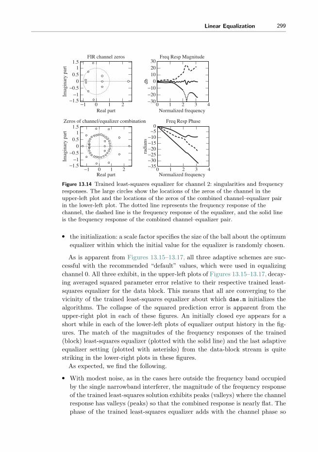
Linear Equalization 299
1.51
0.50
−0.5−1
−1.5−1 0 1 2
FIR channel zeros
Real part
Imag
inar
y pa
rt
db
0
−10−15
−5
−20−25−30−35
0 1 2 3 4
Zeros of channel/equalizer combination
3020100
−10
−30−20
0 1 2 3 4
Freq Resp Magnitude
Normalized frequency
Normalized frequency
Freq Resp Phase1.5
10.5
0−0.5
−1−1.5
−1 0 1 2Real part
Imag
inar
y pa
rt
radi
ans
Figure 13.14 Trained least-squares equalizer for channel 2: singularities and frequencyresponses. The large circles show the locations of the zeros of the channel in theupper-left plot and the locations of the zeros of the combined channel–equalizer pairin the lower-left plot. The dotted line represents the frequency response of thechannel, the dashed line is the frequency response of the equalizer, and the solid lineis the frequency response of the combined channel–equalizer pair.
� the initialization: a scale factor specifies the size of the ball about the optimum
equalizer within which the initial value for the equalizer is randomly chosen.
As is apparent from Figures 13.15–13.17, all three adaptive schemes are suc-
cessful with the recommended “default” values, which were used in equalizing
channel 0. All three exhibit, in the upper-left plots of Figures 13.15–13.17, decay-
ing averaged squared parameter error relative to their respective trained least-
squares equalizer for the data block. This means that all are converging to the
vicinity of the trained least-squares equalizer about which dae.m initializes the
algorithms. The collapse of the squared prediction error is apparent from the
upper-right plot in each of these figures. An initially closed eye appears for a
short while in each of the lower-left plots of equalizer output history in the fig-
ures. The match of the magnitudes of the frequency responses of the trained
(block) least-squares equalizer (plotted with the solid line) and the last adaptive
equalizer setting (plotted with asterisks) from the data-block stream is quite
striking in the lower-right plots in these figures.
As expected, we find the following.
� With modest noise, as in the cases here outside the frequency band occupied
by the single narrowband interferer, the magnitude of the frequency response
of the trained least-squares solution exhibits peaks (valleys) where the channel
response has valleys (peaks) so that the combined response is nearly flat. The
phase of the trained least-squares equalizer adds with the channel phase so

300 Chapter 13. Linear Equalization
−5
−10
−15
0
0 1 2 3 4
5
Normalized frequency
0
−1
−2
−3
1
0 1000 2000 3000 4000
2
Iterations
dB
Ada
ptiv
e eq
ualiz
er o
utpu
t
2
1.5
1
0.5
0
2.5
0 1000 2000 3000 4000
3
Iterations
Combined magnitude response
100
10−10 1000 2000 3000
101
Iterations
Squa
red
pred
ictio
n er
ror
Sum
med
squ
ared
par
amet
er e
rror
Figure 13.15 Trained LMS equalizer for channel 0. The dotted line represents theachieved frequency response of the equalizer while the solid line represents thefrequency response of the desired (optimal) mean-square-error solution.
that their combination approximates a linear phase curve. Refer to plots in
the right columns of Figures 13.10, 13.12, and 13.14.� With modest channel noise and interferers, as the length of the equalizer
increases, the zeros of the combined channel and equalizer form rings. The
rings are denser the nearer the channel zeros are to the unit circle.
There are many ways in which the program dae.m can be used to investigate
and learn about equalization. Try to choose the various parameters to observe
the following
1. Increasing the power of the channel noise suppresses the frequency response of
the least-squares equalizer, with those frequency bands most suppressed being
those in which the channel has a null (and the equalizer—without channel
noise—would have a peak).
2. Increasing the gain of a narrowband interferer results in a deepening of a
notch in the trained least-squares equalizer at the frequency of the interferer.
3. DMA is considered slower than trained LMS. Do you find that DMA takes
longer to converge? Can you think of why it might be slower?
4. DMA typically accommodates larger initialization error than decision-directed
LMS. Can you find cases where, with the same initialization, DMA converges
to an error-free solution but the decision-directed LMS does not? Do you think
there are cases in which the opposite holds?

Linear Equalization 301
−5
−10
−15
0
0 1 2 3 4
5
Normalized frequency
1
0
−1
−2
−3
2
0 1000 2000 3000 4000
3
Iterations
dB
Ada
ptiv
e eq
ualiz
er o
utpu
t
1
0.5
0
1.5
0 1000 2000 3000 4000
2
Iterations
Combined magnitude response
100
10−1
0 1000 2000 3000
101
Iterations
Squa
red
pred
ictio
n er
ror
Sum
med
squ
ared
par
amet
er e
rror
Figure 13.16 Decision-directed LMS equalizer for channel 0. The dotted line representsthe achieved frequency response of the equalizer while the solid line represents thefrequency response of the desired (optimal) mean-square-error solution.
−5
−10
−15
0
0 1 2 3 4
5
Normalized frequency
1
0
−1
−2
−3
2
0 1000 2000 3000 4000
3
Iterations
dB
Ada
ptiv
e eq
ualiz
er o
utpu
t
2
1
0
3
0 1000 2000 3000 4000
4
Iterations
Combined magnitude response
100
10−1
0 1000 2000 3000
101
Iterations
Squa
red
pred
ictio
n er
ror
Sum
med
squ
ared
par
amet
er e
rror
Figure 13.17 Blind DMA equalizer for channel 0. The dotted line represents theachieved frequency response of the equalizer while the solid line represents thefrequency response of the desired (optimal) mean-square-error solution.

302 Chapter 13. Linear Equalization
5. It is necessary to specify the delay δ for the trained LMS, whereas the blind
methods do not require the parameter δ. Rather, the selection of an appro-
priate delay is implicit in the initialization of the equalizer coefficients. Can
you find a case in which, with the delay poorly specified, DMA outperforms
trained LMS from the same initialization?
For Further Reading
A comprehensive survey of trained adaptive equalization can be found in
� S. U. H. Qureshi, “Adaptive Equalization,” Proceedings of the IEEE, vol. 73,
no. 9, pp. 1349–1387, Sept. 1985.
An overview of the analytical tools that can be used to analyze LMS-style adap-
tive algorithms can be found in
� W. A. Sethares, “The LMS Family,” in Efficient System Identification and Sig-
nal Processing Algorithms, Eds. N. Kalouptsidis and S. Theodoridis, Prentice-
Hall, 1993.
A copy of this paper can also be found on the accompanying website.
One of our favorite discussions of adaptive methods is
� C. R. Johnson Jr., Lectures on Adaptive Parameter Estimation, Prentice-Hall,
1988.
This whole book can be found in .pdf form on the website.
An extensive discussion of equalization can also be found in Equalization on
the website.

14 Coding
The underlying purpose of any communication system is to transmit information.
But what exactly is information? How is it measured? Are there limits to the
amount of data that can be sent over a channel, even when all the parts of the
system are operating at their best? This chapter addresses these fundamental
questions using the ideas of Claude Shannon (1916–2001), who defined a measure
of information in terms of bits. The number of bits per second that can be
transmitted over the channel (taking into account its bandwidth, the power of
the signal, and the noise) is called the bit rate, and can be used to define the
capacity of the channel.
Unfortunately, Shannon’s results do not give a recipe for how to construct
a system that achieves the optimal bit rate. Earlier chapters have highlighted
several problems that can arise in communication systems (including synchro-
nization errors such as intersymbol interference). This chapter assumes that all
of these are perfectly mitigated. Thus, in Figure 14.1, the inner parts of the
communication system are assumed to be ideal, except for the presence of chan-
nel noise. Even so, most systems still fall far short of the optimal performance
promised by Shannon.
There are two problems. First, most messages that people want to send are
redundant, and the redundancy squanders the capacity of the channel. A solu-
tion is to preprocess the message so as to remove the redundancies. This is called
source coding, and is discussed in Section 14.5. For instance, as demonstrated in
Section 14.2, any natural language (such as English), whether spoken or written,
is repetitive. Information theory (as Shannon’s approach is called) quantifies the
repetitiveness, and gives a way to judge the efficiency of a source code by com-
paring the information content of the message with the number of bits required
by the code.
The second problem is that messages must be resistant to noise. If a message
arrives at the receiver in garbled form, then the system has failed. A solution is
to preprocess the message by adding extra bits, which can be used to determine
whether an error has occurred, and to correct errors when they do occur. For

304 Chapter 14. Coding
Sourcecoding
Channelcoding
Undochannelcoding
Undosourcecoding
Transmitter Channel Receiver
(Inherently redundant)message to be
transmitted
Compressed(redundancy
removed)
Structured redundancy
removed
Structured redundancy
addedReconstructed
messageNoise
+
Figure 14.1 Source and channel coding techniques manage redundancies in digitalcommunication systems: by first removing inherent redundancies in the message, thenadding structured redundancies (which aid in combatting noise problems) and finallyrestoring the original message.
example, one simple system would transmit each bit three times. Whenever a
single-bit error occurs in transmission, then the decoder at the receiver can figure
out by a simple voting rule that the error has occurred and what the bit should
have been. Schemes for finding and removing errors are called error-correcting
codes or channel codes, and are discussed in Section 14.6.
At first glance, this appears paradoxical; source coding is used to remove
redundancy, while channel coding is used to add redundancy. But it is not really
self-defeating or contradictory because the redundancy that is removed by source
coding does not have a structure or pattern that a computer algorithm at the
receiver can exploit to detect or correct errors. The redundancy that is added in
channel coding is highly structured, and can be exploited by computer programs
implementing the appropriate decoding routines. Thus Figure 14.1 begins with
a message, and uses a source code to remove the redundancy. This is then coded
again by the channel encoder to add structured redundancy, and the resulting
signal provides the input to the transmitter of the previous chapters. One of the
triumphs of modern digital communications systems is that, by clever choice of
source and channel codes, it is possible to get close to the Shannon limits and
to utilize all the capacity of a channel.
14.1 What Is Information?
Like many common English words, information has many meanings. The Amer-
ican Heritage Dictionary catalogs six:
1. Knowledge derived from study, experience, or instruction.
2. Knowledge of a specific event or situation; intelligence.
3. A collection of facts or data.
4. The act of informing or the condition of being informed; communication of
knowledge.
5. Computer Science. A nonaccidental signal or character used as an input to a
computer or communication system.
6. A numerical measure of the uncertainty of an experimental outcome.

Coding 305
It would clearly be impossible to capture all of these senses in a technical defini-
tion that would be useful in transmission systems. The final definition is closest
to our needs, though it does not specify exactly how the numerical measure
should be calculated. Shannon does. Shannon’s insight was that there is a sim-
ple relationship between the amount of information conveyed in a message and
the probability of the message being sent. This does not apply directly to “mes-
sages” such as sentences, images, or .wav files, but to the symbols of the alphabet
that are transmitted.
For instance, suppose that a fair coin has heads H on one side and tails T
on the other. The two outcomes are equally uncertain, and receiving either H
or T removes the same amount of uncertainty (conveys the same amount of
information). But suppose the coin is biased. The extreme case occurs when the
probability of H is 1. Then, when H is received, no information is conveyed,
because H is the only possible choice! Now suppose that the probability of send-
ing H is 0.9 while the probability of sending T is 0.1. Then, if H is received, it
removes a little uncertainty, but not much. H is expected, since it usually occurs.
But if T is received, it is somewhat unusual, and hence conveys a lot of informa-
tion. In general, events that occur with high probability give little information,
while events of low probability give considerable information.
To make this relationship between the probability of events and information
more plain, imagine a game in which you must guess a word chosen at random
from the dictionary. You are given the starting letter as a hint. If the hint is
that the first letter is “t,” then this does not narrow down the possibilities very
much, since so many words start with “t.” But if the hint is that the first letter
is “x,” then there are far fewer choices. The likely letter (the highly probable
“t”) conveys little information, while the unlikely letter (the improbable “x”)
conveys a lot more information by narrowing down the choices.
Here’s another everyday example. Someone living in Ithaca (New York) would
be completely unsurprised that the weather forecast called for rain, and such
a prediction would convey little real information since it rains frequently. On
the other hand, to someone living in Reno (Nevada), a forecast of rain would
be very surprising, and would convey that very unusual meteorological events
were at hand. In short, it would convey considerable information. Again, the
amount of information conveyed is inversely proportional to the probabilities of
the events.
To transform this informal argument into a mathematical statement, consider
a set of N possible events xi, for i = 1, 2, . . . , N . Each event represents one pos-
sible outcome of an experiment, such as the flipping of a coin or the transmission
of a symbol across a communication channel. Let p(xi) be the probability that
the ith event occurs, and suppose that some event must occur.1 This means that
1 When flipping the coin, it cannot roll into the corner and stand on its edge; each flip resultsin either H or T .

306 Chapter 14. Coding
∑Ni=1 p(xi) = 1. The goal is to find a function I(xi) that represents the amount
of information conveyed by each outcome.
The following three qualitative conditions all relate the probabilities of events
with the amount of information they convey:
(i) p(xi) = p(xj) ⇒ I(xi) = I(xj);
(ii) p(xi) < p(xj) ⇒ I(xi) > I(xj);
(iii) p(xi) = 1 ⇒ I(xi) = 0.
(14.1)
Thus, receipt of the symbol xi should
1. give the same amount of information as receipt of xj if they are equally likely,
2. give more information if xi is less likely than xj , and
3. convey no information if it is known a priori that xi is the only alternative.
What kinds of functions I(xi) fulfill these requirements? There are many. For
instance, I(xi) = 1/p(xi)− 1 and I(xi) = (1− p2(xi))/p(xi) both fulfill (i)–(iii).
To narrow down the possibilities, consider what happens when a series of
experiments is conducted, or equivalently, when a series of symbols is transmit-
ted. Intuitively, it seems reasonable that, if xi occurs at one trial and xj occurs
at the next, the total information in the two trials should be the sum of the
information conveyed by receipt of xi and the information conveyed by receipt
of xj ; that is, I(xi) + I(xj). This assumes that the two trials are independent
of each other, namely, that the second trial is not influenced by the outcome of
first (and vice versa).
Formally, two events are defined to be independent if the probability that both
occur is equal to the product of the individual probabilities—that is, if
p(xi and xj) = p(xi)p(xj), (14.2)
where p(xi and xj) means that xi occurred in the first trial and xj occurred
in the second. This additivity requirement for the amount of information con-
veyed by the occurrence of independent events is formally stated in terms of the
information function as
(iv) I(xi and xj) = I(xi) + I(xj)
when the events xi and xj are independent.
On combining the additivity in (iv) with the three conditions (i)–(iii), there is
one (and only one) possibility for I(xi):
I(xi) = log
(1
p(xi)
)= − log(p(xi)). (14.3)

Coding 307
It is easy to see that (i)–(iii) are fulfilled, and (iv) follows from the properties of
the log (recall that log(ab) = log(a) + log(b)). Therefore,
I(xi and xj) = log
(1
p(xi and xj)
)= log
(1
p(xi)p(xj)
)
= log
(1
p(xi)
)+ log
(1
p(xj)
)= I(xi) + I(xj).
The base of the logarithm can be any (positive) number. The most common
choice is base 2, in which case the measurement of information is called bits.
Unless otherwise stated explicitly, all logs in this chapter are assumed to be
base 2.
Example 14.1. Suppose there are N = 3 symbols in the alphabet, which are
transmitted with probabilities p(x1) = 1/2, p(x2) = 1/4, and p(x3) = 1/4. Then
the information conveyed by receiving x1 is 1 bit, since
I(x1) = log
(1
p(x1)
)= log(2) = 1.
Similarly, the information conveyed by receiving either x2 or x3 is I(x2) =
I(x3) = log(4) = 2 bits.
Example 14.2. Suppose that a length m binary sequence is transmitted, with
all symbols equally probable. Thus N = 2m, xi is the binary representation of
the ith symbol for i = 1, 2, . . . , N , and p(xi) = 2−m. The information contained
in the receipt of any given symbol is
I(xi) = log
(1
p(xi)
)= log(2m) = m bits.
Exercise 14.1. Consider a standard six-sided die. Identify N , xi, and p(xi).
How many bits of information are conveyed if a 3 is rolled? Now roll two dice,
and suppose the total is 12. How many bits of information does this represent?
Exercise 14.2. Consider transmitting a signal with values chosen from the six-
level alphabet ±1,±3,±5.
a. Suppose that all six symbols are equally likely. Identify N , xi, and p(xi), and
calculate the information I(xi) associated with each i.
b. Suppose instead that the symbols ±1 occur with probability 1/4 each, ±3
occur with probability 1/8 each, and 5 occurs with probability 1/4. What

308 Chapter 14. Coding
percentage of the time is −5 transmitted? What is the information conveyed
by each of the symbols?
Exercise 14.3. The 8-bit binary ASCII representation of any letter (or
any character of the keyboard) can be found using the Matlab command
dec2bin(text), where text is any string. Using ASCII, how much information
is contained in the letter “a,” assuming that all the letters are equally probable?
Exercise 14.4. Consider a decimal representation of π = 3.1415926 . . . Calcu-
late the information (number of bits) required to transmit successive digits of π,
assuming that the digits are independent. Identify N , xi, and p(xi). How much
information is contained in the first million digits of π?
There is an alternative definition of information (in common usage in the
mathematical-logic and computer-science communities) in which information is
defined in terms of the complexity of representation, rather than in terms of
the reduction in uncertainty. Informally speaking, this alternative defines the
complexity (or information content) of a message by the length of the shortest
computer program that can replicate the message. For many kinds of data, such
as a sequence of random numbers, the two measures agree because the shortest
program that can represent the sequence is just a listing of the sequence. But in
other cases, they can differ dramatically. Consider transmitting the first million
digits of the number π. Shannon’s definition gives a large information content (as
in Exercise 14.4), while the complete sequence can, in principle, be transmitted
with a very short computer program.
14.2 Redundancy
All the examples in the previous section presume that there is no relationship
between successive symbols. (This was the independence assumption in (14.2).)
This section shows by example that real messages often have significant corre-
lation between symbols, which is a kind of redundancy. Consider the following
sentence from Shannon’s paper A Mathematical Theory of Communication:
It is clear, however, that by sending the
information in a redundant form the
probability of errors can be reduced.
This sentence contains 20 words and 115 characters, including the commas,
period, and spaces. It can be “coded” into the 8-bit binary ASCII character
set recognized by computers as the “text” format, which translates the char-
acter string (that is readable by humans) into a binary string containing 920
(= 8× 115) bits.

Coding 309
Suppose that Shannon’s sentence is transmitted, but that errors occur so that
1% of the bits are flipped from one to zero (or from zero to one). Then about
3.5% of the letters have errors:
It is clea2, however, that by sendhng the
information in a redundaNt form the
probabilipy of errors can be reduced.
The message is comprehensible, although it appears to have been typed poorly.
With 2% bit error, about 7% of the letters have errors:
It is clear, howaver, thad by sending the
information in a redundan4 form phe
prkbability of errors cAf be reduced.
Still the underlying meaning is decipherable. A dedicated reader can often deci-
pher text with up to about 3% bit error (10% symbol error). Thus, the message
has been conveyed, despite the presence of the errors. The reader, with an exten-
sive familiarity with English words, sentences, and syntax, is able to recognize
the presence of the errors and to correct them.
As the bit error rate grows to 10%, about one third of the letters have errors,
and many words have become incomprehensible. Because “space” is represented
as an ASCII character just like all the other symbols, errors can transform spaces
into letters or letters into spaces, thus blurring the true boundaries between the
words.
Wt is ahear, h/wav3p, dhat by sending phc
)hformatIon if a rEdundaft fnre thd
prkba@)hity ob erropc can be reduaed.
With 20% bit error, about half of the letters have errors and the message is
completely illegible:
I4 "s C‘d‘rq h+Ae&d"( ‘(At by s‘jdafd th$
hfFoPmati/. )f a p(d5jdan‘ fLbe thd
‘r’‘ab!DITy o& dr‘kp1 aa& bE rd@u!ed.
These examples were all generated using the following Matlab program
redundant.m which takes the text textm, translates it into a binary string, and
then causes per percent of the bits to be flipped. The program then gathers
statistics on the resulting numbers of bit errors and symbol errors (how many
letters were changed).
Listing 14.1. redundant.m redundancy of written english in bits and letters
textm=’It is clear , however , that by sending the ...

310 Chapter 14. Coding
information in a redundant form the ...
probability of errors can be reduced .’
% 8−b i t a s c i i ( b inary ) equ i va l en t o f textascm=dec2bin ( double ( textm ) , 8 ) ;% turn i n to one long binary s t r i n gbinm=reshape ( ascm ’ , 1 , 8* length ( textm ) ) ;per =.01; % p r ob ab i l i t y o f b i t e r r o rfor i =1:8* length ( textm )
r=rand ; % swap 0 and 1 with p r ob ab i l i t y peri f ( r>1−per ) & binm( i )==’0’ , binm( i )=’1’ ; end
i f ( r>1−per ) & binm( i )==’1’ , binm( i )=’0’ ; end
end
ascr=reshape (binm ’ , 8 , length ( textm ) ) ’ ; % to a s c i i b inaryt ex t r=setstr ( bin2dec ( ascr ) ’ ) % to textb i t e r r o r=sum(sum(abs ( ascr−ascm ) ) ) % # of b i t e r r o r ssymerrror=sum( sign (abs ( textm−t ex t r ) ) ) % # of symbol e r r o r snumwords=sum( sign ( find ( textm==32)))+1 % # of words in textml e t t e r r o r=symerrror / length ( textm ) % # of l e t t e r e r r o r s
Exercise 14.5. Read in a large text file using the following Matlab code. (Use
one of your own or use one of the included text files.)2 Make a plot of the symbol
error rate as a function of the bit error rate by running redundant.m for a variety
of values of per. Examine the resulting text. At what value of per does the text
become unreadable? What is the corresponding symbol error rate?
Listing 14.2. readtext.m read in a text document and translate to character string
[ f i d , messagei ] = fopen ( ’OZ.txt ’ , ’r’ ) ; % f i l e must be textfdata=fread ( f i d ) ’ ; % read text as a vectortext=char ( fdata ) ; % to character s t r i n g
Thus, for English text encoded as ASCII characters, a significant number of
errors can occur (about 10% of the letters can be arbitrarily changed) without
altering the meaning of the sentence. While these kinds of errors can be corrected
by a human reader, the redundancy is not in a form that is easily exploited by a
computer. Even imagining that the computer could look up words in a dictionary,
the person knows from context that “It is clear” is a more likely phrase than “It
is clean” when correcting Shannon’s sentence with 1% errors. The person can
figure out from context that “cAf” (from the phrase with 2% bit errors) must
have had two errors by using the long-term correlation of the sentence (i.e., its
meaning). Computers do not deal readily with meaning.3
In the previous section, the information contained in a message was defined to
depend on two factors: the number of symbols and their probability of occurrence.
But this assumes that the symbols do not interact—that the letters are indepen-
2 Through the Looking Glass by Lewis Carroll (carroll.txt) and The Wonderful Wizard of Oz
by Frank Baum (OZ.txt) are available on the website.3 A more optimistic rendering of this sentence: “Computers do not yet deal readily with mean-ing.”

Coding 311
dent. How good an assumption is this for English text? It is a poor assumption.
As the preceding examples suggest, normal English is highly correlated.
It is easy to catalog the frequency of occurrence of the letters. The letter “e”
is the most common. In Frank Baum’s Wizard of Oz, for instance, “e” appears
20,345 times and “t” appears 14,811 times, but the letters “q” and “x” appear
only 131 and 139 times, respectively (“z” might be a bit more common in Baum’s
book than normal because of the title). The percentage occurrence for each letter
in the Wizard of Oz is
a 6.47 h 5.75 o 6.49 v 0.59
b 1.09 i 4.63 p 1.01 w 2.49
c 1.77 j 0.08 q 0.07 x 0.07
d 4.19 k 0.90 r 4.71 y 1.91
e 10.29 l 3.42 s 4.51 z 0.13
f 1.61 m 1.78 t 7.49
g 1.60 n 4.90 u 2.05
(14.4)
“Space” is the most frequent character, occurring 20% of the time. It was easier
to use the following Matlab code, in conjunction with readtext.m, than to
count the letters by hand.
Listing 14.3. freqtext.m frequency of occurrence of letters in text
l i t t l e=length ( find ( t e x t s t r i n g==’t’ ) ) ; % how many times t occur sbig=length ( find ( t e x t s t r i n g==’T’ ) ) ; % how many times T occur sf r eq=( l i t t l e+big )/ length ( t e x t s t r i n g ) % percentage
If English letters were truly independent, then it should be possible to generate
“English-like” text using this table of probabilities. Here is a sample:
Od m shous t ad schthewe be amalllingod
ongoutorend youne he Any bupecape tsooa w
beves p le t ke teml ley une weg rloknd
which does not look anything like English. How can the nonindependence of the
text be modeled? One way is to consider the probabilities of successive pairs of
letters instead of the probabilities of individual letters. For instance, the pair
“th” is quite frequent, occurring 11,014 times in the Wizard of Oz, while “sh”
occurs 861 times. Unlikely pairs such as “wd” occur in only five places4 and “pk”
not at all. For example, suppose that “He” was chosen first. The next pair would
be “e” followed by something, with the probability of the something dictated by
the entries in the table. Following this procedure results in output like this:
Her gethe womfor if you the to had the sed
th and the wention At th youg the yout by
and a pow eve cank i as saing paill
4 In the words “crowd” and “sawdust.”

312 Chapter 14. Coding
Observe that most of the two-letter combinations are actual words, as well as
many three-letter words. Longer sets of symbols tend to wander improbably.
While, in principle, it would be possible to continue gathering probabilities of all
three-letter combinations, then four, etc., the table begins to get rather large (a
matrix with 26n elements would be needed to store all the n-letter probabilities).
Shannon5 suggests another way:
. . . one opens a book at random and selects a letter on the page. This letter is recorded.The book is then opened to another page, and one reads until this letter is encountered.The succeeding letter is then recorded. Turning to another page, this second letter issearched for, and the succeeding letter recorded, etc.
Of course, Shannon did not have access to Matlab when he was writing in
1948. If he had, he might have written a program like textsim.m, which allows
specification of any text (with the default being The Wizard of Oz) and any num-
ber of terms for the probabilities. For instance, with m=1, the letters are chosen
completely independently; with m=2, the letters are chosen from successive pairs;
and with m=3, they are chosen from successive triplets. Thus, the probabilities
of clusters of letters are defined implicitly by the choice of the source text.
Listing 14.4. textsim.m use (large) text to simulate transition probabilities
m=1; % # terms f o r t r a n s i t i o nl i n e l e n g t h =60; % # l e t t e r s in each l i n eload OZ.mat % f i l e f o r inputn=text ( 1 :m) ; n l i n e=n ; n l e t=’x’ ; % i n i t i a l i z e v a r i a b l e sfor i =1:100 % # l i n e s in output
j =1;while j<l i n e l e n g t h | n l e t ˜=’ ’ % scan through f i l e
k=f indstr ( text , n ) ; % a l l occur r ences o f seedind=round ( ( length (k)−1)*rand)+1; % pick onen l e t=text (k ( ind)+m) ;i f abs ( n l e t )==13 % tr ea t c a r r i a g e r e tu r n s
n l e t=’ ’ ; % as spacesend
n l i n e =[ n l i ne , n l e t ] ; % add next l e t t e rn=[n ( 2 :m) , n l e t ] ; % new seedj=j +1;
end
disp ( [ n l i n e setstr ( 1 3 ) ] ) % format output/ add CRsn l i n e=’’ ; % i n i t i a l i z e next l i n e
end
Typical output of textsim.m depends heavily on the number of terms m used for
the transition probabilities. With m=1 or m=2, the results appear much as above.
When m=3,
Be end claime armed yes a bigged wenty for me
fearabbag girl Humagine ther mightmarkling the
5 C. E. Shannon, “A Mathematical Theory of Communication,” The Bell System Technical
Journal, vol. 27, nos. 7 and 10, pp. 379–423 and 623–656, July and October, 1948.

Coding 313
many the scarecrow pass and I havely and lovery
wine end at then only we pure never
many words appear, and many combinations of letters that might be words,
but aren’t quite. “Humagine” is suggestive, though it is not clear exactly what
“mightmarkling” might mean. When m=4,
Water of everythinkies friends of the scarecrow
no head we She time toto be well as some
although to they would her been Them became the
small directions and have a thing woodman
the vast majority of words are actual English, though the occasional conjunction
of words (such as “everythinkies”) is not uncommon. The output also begins to
strongly reflect the text used to derive the probabilities. Since many four-letter
combinations occur only once, there is no choice for the method to continue
spelling a longer word; this is why the “scarecrow” and the “woodman” figure
prominently. For m=5 and above, the “random” output is recognizably English,
and strongly dependent on the text used:
Four trouble and to taken until the bread
hastened from its Back to you over the emerald
city and her in toward the will Trodden and
being she could soon and talk to travely lady
Exercise 14.6. Run the program textsim.m using the input file carroll.mat,
which contains the text to Lewis Carroll’s Through the Looking Glass, with m =
1, 2, . . ., 8. At what point does the output repeat large phrases from the input
text?
Exercise 14.7. Run the program textsim.m using the input file foreign.mat,
which contains a book that is not in English. Looking at the output for various
m, can you tell what language the input is? What is the smallest m (if any) at
which it becomes obvious?
The following two problems might not appeal to everyone.
Exercise 14.8. The program textsim.m operates at the level of letters and the
probabilities of transition between successive sets of m-length letter sequences.
Write an analogous program that operates at the level of words and the prob-
abilities of transition between successive sets of m-length word sequences. Does
your program generate plausible-sounding phrases or sentences?

314 Chapter 14. Coding
Exercise 14.9. There is nothing about the technique of textsim.m that is
inherently limited to dealing with text sequences. Consider a piece of (notated)
music as a sequence of symbols, labeled so that each “C” note is 1, each “C �” note
is 2, each “D” note is 3, etc. Create a table of transition probabilities from a piece
of music, and then generate “new” melodies in the same way that textsim.m
generates “new” sentences. (Observe that this procedure can be automated using
standard MIDI files as input.)
Because this method derives the multiletter probabilities directly from a text,
there is no need to compile transition probabilities for other languages. Using
Vergil’s Aeneid (with m=3) gives
Aenere omnibus praeviscrimus habes ergemio nam
inquae enies Media tibi troius antis igna volae
subilius ipsis dardatuli Cae sanguina fugis
ampora auso magnum patrix quis ait longuin
which is not real Latin. Similarly,
Que todose remosotro enga tendo en guinada y
ase aunque lo Se dicielos escubra la no fuerta
pare la paragales posa derse Y quija con figual
se don que espedios tras tu pales del
is not Spanish (the input file was Cervante’s Don Quijote, also with m=3), and
Seule sontagne trait homarcher de la t au onze
le quance matices Maississait passepart penaient
la ples les au cherche de je Chamain peut accide
bien avaien rie se vent puis il nez pande
is not French (the source was Le Tour du Monde en Quatre Vingts Jours, a
translation of Jules Verne’s Around the World in Eighty Days.)
The input file to the program textsim.m is a Matlab .mat file that has been
preprocessed to remove excessive line breaks, spaces, and capitalization using
textman.m, which is why there is no punctuation in these examples. A large
assortment of text files is available for downloading at the website of Project
Gutenberg (at http://www.gutenberg.org/).
Text, in a variety of languages, retains some of the character of its language
with correlations of 3 to 5 letters (21–35 bits, when coded in ASCII). Thus, mes-
sages written in those languages are not independent, except possibly at lengths
greater than this. A result from probability theory suggests that, if the letters are
clustered into blocks that are longer than the correlation, then the blocks may
be (nearly) independent. This is one strategy to pursue when designing codes

Coding 315
that seek to optimize performance. Section 14.5 will explore some practical ways
to attack this problem, but the next two sections establish a measure of perfor-
mance such that it is possible to know how close to the optimal any given code
lies.
14.3 Entropy
This section extends the concept of information from a single symbol to a
sequence of symbols. As defined by Shannon,6 the information in a symbol is
inversely proportional to its probability of occurring. Since messages are com-
posed of sequences of symbols, it is important to be able to talk concretely about
the average flow of information. This is called the entropy and is formally defined
as
H(x) =
N∑i=1
p(xi)I(xi)
=
N∑i=1
p(xi) log
(1
p(xi)
)
= −N∑i=1
p(xi) log(p(xi)), (14.5)
where the symbols are drawn from an alphabet xi, each with probability p(xi).
H(x) sums the information in each symbol, weighted by the probability of that
symbol. Those familiar with probability and random variables will recognize
this as an expectation. Entropy7 is measured in bits per symbol, and so gives
a measure of the average amount of information transmitted by the symbols of
the source. Sources with different symbol sets and different probabilities have
different entropies. When the probabilities are known, the definition is easy to
apply.
Example 14.3. Consider the N = 3 symbol set defined in Example 14.1. The
entropy is
H(x) =1
2· 1 + 1
4· 2 + 1
4· 2 = 1.5 bits/symbol.
6 Actually, Hartley was the first to use this as a measure of information in his 1928 paper inthe Bell System Technical Journal called “Transmission of Information.”
7 Warning: though the word is the same, this is not the same as the notion of entropy that isfamiliar from physics since the units here are in bits per symbol while the units in physicsare energy per degree Kelvin.

316 Chapter 14. Coding
Exercise 14.10. Reconsider the fair die of Exercise 14.1. What is its entropy?
Example 14.4. Suppose that the message {x1, x3, x2, x1} is received from a
source characterized as follows.
1. N = 4, p(x1) = 0.5, p(x2) = 0.25, p(x3) = p(x4) = 0.125. The total informa-
tion is
4∑i=1
I(xi) =
4∑i=1
log
(1
p(xi)
)= 1 + 2 + 3 + 3 = 9 bits.
The entropy of the source is
H(x) =1
2· 1 + 1
4· 2 + 1
8· 3 + 1
8· 3 = 1.75 bits/symbol.
2. N = 4, p(xi) = 0.25 for all i. The total information is I(xi) = 2 + 2 + 2 + 2 =
8. The entropy of the source is
H(x) =1
4· 2 + 1
4· 2 + 1
4· 2 + 1
4· 2 = 2 bits/symbol.
In Example 14.4, messages of the same length from the first source give less
information than those from the second source. Hence, sources with the same
number of symbols but different probabilities can have different entropies. The
key is to design a system to maximize entropy since this will have the largest
throughput, or largest average flow of information. But how can this be achieved?
First, consider the simple case in which there are two symbols in the alphabet,
x1 with probability p, and x2 with probability 1− p. (Think of a coin that is
weighted so as to give heads with higher probability than tails.) Applying the
definition (14.5) shows that the entropy is
H(p) = −p log(p)− (1− p) log(1− p).
This is plotted as a function of p in Figure 14.2. For all allowable values of
p, H(p) is positive. As p approaches either zero or one, H(p) approaches zero,
which represent the symmetric cases in which either x1 occurs all the time or x2
occurs all the time, and no information is conveyed. H(p) reaches its maximum
in the middle, at p = 0.5. For this example, entropy is maximized when the two
symbols are equally likely.
Exercise 14.11. Show that H(p) is maximized at p = 0.5 by taking the deriva-
tive and setting it equal to zero.
The next result shows that an N -symbol source cannot have entropy larger
than log(N), and that this bound is achieved when all the symbols are equally
likely. Mathematically, H(x) ≤ log(N), which is demonstrated by showing that

Coding 317
1
0.8
0.6
0.4
0.2
0
H(p
)
0 0.1 0.2 0.3 0.4 0.5 0.6 0.7 0.8 0.9 1Probability p
Figure 14.2 Entropy of a binarysignal with probabilities p and1− p.
H(x) − log(N) ≤ 0. First,
H(x)− log(N) =N∑i=1
p(xi) log
(1
p(xi)
)− log(N)
=N∑i=1
p(xi) log
(1
p(xi)
)−
N∑i=1
p(xi) log(N),
since∑N
i=1 p(xi) = 1. Gathering terms, this can be rewritten
H(x)− log(N) =N∑i=1
p(xi)
[log
(1
p(xi)
)− log(N)
]
=
N∑i=1
p(xi) log
(1
Np(xi)
),
and changing the base of the logarithm (using log(z) ≡ log2(z) = log2(e) ln(z),
where ln(z) ≡ loge(z)), gives
H(x)− log(N) = log(e)N∑i=1
p(xi) ln
(1
Np(xi)
).
If all symbols are equally likely, p(xi) = 1/N , then 1/(Np(xi)) = 1 and
ln(
1Np(xi)
)= ln(1) = 0. Hence H(x) = log(N). On the other hand, if the sym-
bols are not equally likely, then the inequality ln(z) ≤ z − 1 (which holds for
z ≥ 0) implies that
H(x)− log(N) ≤ log(e)N∑i=1
p(xi)
[1
Np(xi)− 1
]
= log(e)
[N∑i=1
1
N−
N∑i=1
p(xi)
]
= log(e) [1− 1] = 0. (14.6)
Rearranging (14.6) gives the desired bound on the entropy, namely that H(x) ≤log(N). This says that, all else being equal, it is preferable to choose a code

318 Chapter 14. Coding
in which each symbol occurs with the same probability. Indeed, Example 14.5
provides a concrete source for which the equal-probability case has higher entropy
than the unequal-probability case.
Section 14.2 showed how letters in the text of natural languages do not occur
with equal probability. Thus, naively using the letters will not lead to an effi-
cient transmission. Rather, the letters must be carefully translated into equally
probable symbols in order to increase the entropy. A method for accomplishing
this translation is given in Section 14.5, but Section 14.4 examines the limits of
attainable performance when transmitting symbols across a noisy (but otherwise
perfect) channel.
14.4 Channel Capacity
Section 14.1 showed how much information (measured in bits) is contained in
a given symbol, and Section 14.3 generalized this to the average amount of
information contained in a sequence or set of symbols (measured in bits per
symbol). In order to be useful in a communication system, however, the data must
move from one place to another. What is the maximum amount of information
that can pass through a channel in a given amount of time? The main result of
this section is that the capacity of the channel defines the maximum possible flow
of information through the channel. The capacity is a function of the bandwidth
of the channel and of the amount of noise in the system, and it is measured in
bits per second.
If the data are encoded using N = 2 equally probable bits per symbol, and if
the symbols are independent, the entropy is H2 = 0.5 log(2) + 0.5 log(2) = 1 bit
per symbol. Why not increase the number of bits per symbol? This would allow
representing more information. On doubling to N = 4, the entropy increases to
H4 = 2. In general, when using N bits, the entropy is HN = log(N). By increas-
ing N without bound, the entropy can be increased without bound! But is it
really possible to send an infinite amount of information?
When doubling the size of N , one of two things must happen. Either the dis-
tance between the levels must decrease, or the power must increase. For instance,
it is common to represent the binary signal as ±1 and the four-level signal as
±1,±3. In this representation, the distance between neighboring values is con-
stant, but the power in the signal has increased. Recall that the power in a
discrete signal x[k] is
limT→∞
1
T
T∑k=1
x2[k].
For a binary signal with equal probabilities, this is P2 = 12 (1
2 + (−1)2) = 1. The
four-level signal has power P4 = 14(1
2 + (−1)2 + 32 + (−3)2) = 5. To normalize
the power to unity for the four-level signal, calculate the value x such that

Coding 319
1.5
1
0.5
0
−0.5
−1
−1.5
−2
2A
mpl
itude
2-level signal 4-level signal 8-level signal
N-level signals with equal power
16-level signal
Figure 14.3 When the power isequal, the values of theN-level signal grow closer asN increases.
14 (x
2 + (−x)2 + (3x)2 + (−3x)2) = 1, which is x =√
1/5. Figure 14.3 shows how
the values of the N -level signal become closer together as N increases, when the
power is held constant.
Now it will be clearer why it is not really possible to send an infinite amount
of information in a single symbol. For a given transmitter power, the amplitudes
become closer together for large N , and the sensitivity to noise increases. Thus,
when there is noise (and some is inevitable), the four-level signal is more prone to
errors than the two-level signal. Said another way, a higher signal-to-noise ratio8
(SNR) is needed to maintain the same probability of error in the four-level signal
as in the two-level signal.
Consider the situation in terms of the bandwidth required to transmit a given
set of data containing M bits of information. From the Nyquist sampling the-
orem of Section 6.1, data can be sent through a channel of bandwidth B at a
maximum rate of 2B symbols per second. If these symbols are coded into two
levels, then M symbols must be sent. If the data are transmitted with four levels
(by assigning pairs of binary digits to each four-level symbol), then only M/2
symbols are required. Thus the multilevel signal can operate at half the symbol
rate of the binary signal. Said another way, the four-level signal requires only
half the bandwidth of the two-level signal.
The previous two paragraphs show the trade-off between SNR and bandwidth.
To maintain the same probability of error, larger bandwidth allows smaller SNR;
larger SNR allows the use of a narrower frequency band. Quantifying this trade-
off was one of Shannon’s greatest contributions.
While the details of a formal proof of the channel capacity are complex, the
result is believable when thought of in terms of the relationship between the
8 As the term suggests, SNR is the ratio of the energy (or power) in the signal to the energy(or power) in the noise.

320 Chapter 14. Coding
distance between the levels in a source alphabet and the average amount of
noise that the system can tolerate. A digital signal with N levels has a maximum
information rate C = log(N)/T , where T is the time interval between transmitted
symbols. C is the capacity of the channel, and has units of bits per second.
This can be expressed in terms of the bandwidth B of the channel by recalling
Nyquist’s sampling theorem, which says that a maximum of 2B pulses per second
can pass through the channel. Thus the capacity can be rewritten
C = 2B log(N) bits per second.
To include the effect of noise, observe that the power of the received signal is
S + P (where S is the power of the signal and P is the power of the noise).
Accordingly, the average amplitude of the received signal is√S + P and the
average amplitude of the noise is√P . The average distance d between levels
is twice the average amplitude divided by the number of levels (minus one),
and so d = 2√S + P/(N − 1). Many errors will occur in the transmission unless
the distance between the signal levels is separated by at least twice the average
amplitude of the noise, that is, unless
d =2√S + PN − 1
> 2√P .
Rearranging this implies that N − 1 must be no larger than√S + P/
√P. The
actual bound (as Shannon shows) is that N ≈ √S + P/√P , and using this value
gives
C = 2B log
(√S + P√P
)= B log
(1 +
SP)
(14.7)
bits per second.
Observe that, if either the bandwidth or the SNR is increased, so is the chan-
nel capacity. For white noise, as the bandwidth increases, the power in the noise
increases, the SNR decreases, and so the channel capacity does not become infi-
nite. For a fixed channel capacity, it is easy to trade off bandwidth against SNR.
For example, suppose a capacity of 1000 bits per second is required. Using a
bandwidth of 1 kHz, we find that the signal and the noise can be of equal power.
As the allowed bandwidth is decreased, the ratio S/P increases rapidly:
Bandwidth S/P1000 Hz 1
500 Hz 3
250 Hz 15
125 Hz 255
100 Hz 1023
Shannon’s result can now be stated succinctly. Suppose that there is a source
producing information at a rate of R bits per second and a channel of capacity
C. If R < C (where C is defined as in (14.7)) then there exists a way to represent

Coding 321
(or code) the data so that it can be transmitted with arbitrarily small error.
Otherwise, the probability of error is strictly positive.
This is tantalizing and frustrating at the same time. The channel capacity
defines the ultimate goal beyond which transmission systems cannot go, yet it
provides no recipe for how to achieve the goal. The next sections describe various
methods of representing or coding the data that assist in approaching this limit
in practice.
The following Matlab program explores a noisy system. A sequence of four-
level data is generated by calling the pam.m routine. Noise is then added with
power specified by p, and the number of errors caused by this amount of noise
is calculated in err.
Listing 14.5. noisychan.m generate 4-level data and add noise
m=1000; % length o f data sequencep=1/15; s =1.0; % power o f no i s e and s i g n a lx=pam(m, 4 , s ) ; % 4−PAM input with power 1 . . .L=sqrt ( 1 / 5 ) ; % . . . with amp l e v e l s Ln=sqrt (p)*randn (1 ,m) ; % no i s e with power py=x+n ; % output adds no i s e to dataqy=quantalph (y , [−3*L,−L ,L,3*L ] ) ; % quant i ze to [−3*L,−L ,L ,3*L ]e r r=sum(abs ( sign ( qy’−x ) ) )/m; % percent t ransmi s s i on e r r o r s
Typical outputs of noisychan.m are shown in Figure 14.4. Each plot shows the
input sequence (the four solid horizontal lines), the input plus the noise (the cloud
of small dots), and the error between the input and quantized output (the dark
stars). Thus the dark stars that are not at zero represent errors in transmission.
The noise P† in the right-hand case is the maximum noise allowable in the
plausibility argument used to derive (14.7), which relates the average amplitudes
of the signal plus the noise to the number of levels in the signal. For S = 1 (the
same conditions as in Exercise 14.12(a)), the noise was chosen to be independent
and normally distributed with power P† to ensure that 4 =√1 + P†/
√P†. The
middle plot used a noise with power P†/3 and the left-hand plot had noise
power P†/6. As can be seen from the plots, there were essentially no errors when
using the smallest noise, a handful of errors in the middle, and about 6% errors
when the power of the noise matched the Shannon capacity. Thus, this naive
transmission of four-level data (i.e., with no coding) has many more errors than
the Shannon limit suggests.
Exercise 14.12. Find the amplitudes of the N -level (equally spaced) signal with
unity power when
a. N = 4,
b. N = 6,
c. N = 8.
Exercise 14.13. Use noisychan.m to compare the noise performance of two-
level, four-level, and six-level transmissions.

322 Chapter 14. Coding
2
1
−1
−22000 4000
0
1/6 max noise200000 4000
1/3 max noise20000 4000
max noise
Am
plitu
de
Figure 14.4 Each plot shows a four-level PAM signal (the four solid lines), the signalplus noise (the scattered dots), and the error between the data and the quantizedoutput (the dark stars). The noise in the right-hand plot was at the Shannon limitN ≈ √S + P†/
√P†, the noise in the middle plot was at one-third the power, and the
noise in the left-hand plot was at one-sixth the power.
a. Modify the program to generate two- and six-level signals.
b. Make a plot of the noise power versus the percentage of errors for two, four,
and six levels.
Exercise 14.14. Use noisychan.m to compare the power requirements for two-
level, four-level, and six-level transmissions. Fix the noise power at p=0.01, and
find the error probability for four-level transmission. Experimentally find the
power S that is required to make the two-level and six-level transmissions have
the same probability of error. Can you think of a way to calculate this?
Exercise 14.15. Consider the (asymmetric, nonuniformly spaced) alphabet con-
sisting of the symbols −1, 1, 3, 4.
a. Find the amplitudes of this four-level signal with unity power.
b. Use noisychan.m to examine the noise performance of this transmission by
making a plot of the noise power versus the percentage of errors.
c. Compare this alphabet with 4-PAM using the standard alphabet ±1,±3.
Which would you prefer?
There are two different problems that can keep a transmission system from
reaching the Shannon limit. The first is that the source might not be coded with
maximum entropy, and this will be discussed next in Section 14.5. The second
is when different symbols experience different amounts of noise. Recall that the
plausibility argument for the channel capacity rested on the idea of the average

Coding 323
noise. When symbols encounter anything less than the average noise, then all is
well, since the average distance between levels is greater than the average noise.
But errors occur when symbols encounter more than the average amount of noise.
(This is why there are so many errors in the right-hand plot of Figure 14.4.) Good
coding schemes try to ensure that all symbols experience (roughly) the average
noise. This can be accomplished by grouping the symbols into clusters or blocks
that distribute the noise evenly among all the symbols in the block. Such error
coding is discussed in Section 14.6.
14.5 Source Coding
The results from Section 14.3 suggest that, all else being equal, it is preferable to
choose a code in which each symbol occurs with the same probability. But what if
the symbols occur with widely varying frequencies? Recall that this was shown
in Section 14.2 for English and other natural languages. There are two basic
approaches. The first aggregates the letters into clusters, and provides a new
(longer) code word for each cluster. If properly chosen, the new code words can
occur with roughly the same probability. The second approach uses variable-
length code words, assigning short codes to common letters like “e” and long
codes to infrequent letters like “x.” Perhaps the most common variable-length
code was that devised by Morse for telegraph operators, which used a sequence
of “dots” and “dashes” (along with silences of various lengths) to represent the
letters of the alphabet.
Before discussing how source codes can be constructed, consider an example
using the N = 4 code from Example 14.4(a) in which p(x1) = 0.5, p(x2) = 0.25,
and p(x3) = p(x4) = 0.125. As shown earlier, the entropy of this source is 1.75
bits/symbol, which means that there must be some way of coding the source so
that, on average, 1.75 bits are used for each symbol. The naive approach to this
source would use 2 bits for each symbol, perhaps assigning
x1 ↔ 11, x2 ↔ 10, x3 ↔ 01, and x4 ↔ 00. (14.8)
An alternative representation is
x1 ↔ 1, x2 ↔ 01, x3 ↔ 001, and x4 ↔ 000, (14.9)
where more-probable symbols use fewer bits, and less-probable symbols require
more. For instance, the string
x1, x2, x1, x4, x3, x1, x1, x2
(in which each element appears with the expected frequency) is coded as
10110000011101.
This requires 14 bits to represent the eight symbols. The average is 14/8 = 1.75
bits per symbol, so this coding is as good as possible, since it equals the entropy.
324 Chapter 14. Coding
In contrast, the naive code of (14.8) requires 16 bits to represent the eight sym-
bols for an average of 2 bits per symbol. One feature of the variable-length
code in (14.9) is that there is never any ambiguity about where it starts,
since any occurrence of a 1 corresponds to the end of a symbol. The naive
code requires knowledge of where the first symbol begins. For example, the
string 01− 10− 11− 00− 1 is very different from 0− 11− 01− 10− 01 even
though they contain the same bits in the same order. Codes for which the
start and end are immediately recognizable are called instantaneous or prefix
codes.
Since the entropy defines the smallest number of bits that can be used to
encode a source, it can be used to define the efficiency of a code
efficiency =entropy
average # of bits per symbol. (14.10)
Thus the efficiency of the naive code (14.8) is 1.75/2 = 0.875 while the effi-
ciency of the variable-rate code (14.9) is 1. Shannon’s source coding theorem
says that, if an independent source has entropy H , then there exists a pre-
fix code in which the average number of bits per symbol is between H and
H + 1. Moreover, there is no uniquely decodable code that has smaller aver-
age length. Thus, if N symbols (each with entropy H) are compressed into
fewer than NH bits, information is lost, while information need not be lost
if N(H + 1) bits are used. Shannon has defined the goal towards which all
codes aspire, but provides no way of finding good codes for any particular
case.
Fortunately, D. A. Huffman proposed an organized procedure to build variable-
length codes that are as efficient as possible. Given a set of symbols and their
probabilities, the procedure is as follows.
1. List the symbols in order of decreasing probability. These are the original
“nodes.”
2. Find the two nodes with the smallest probabilities, and combine them into
one new node, with probability equal to the sum of the two. Connect the new
nodes to the old ones with “branches” (lines).
3. Continue combining the pairs of nodes with the smallest probabilities. (If
there are ties, pick any of the tied symbols.)
4. Place a 0 or a 1 along each branch. The path from the rightmost node to the
original symbol defines a binary list, which is the code word for that symbol.
This procedure is probably easiest to understand by working through an example.
Consider again the firstN = 4 code from Example 14.4 in which the symbols have
probabilities p(x1) = 0.5, p(x2) = 0.25, and p(x3) = p(x4) = 0.125. Following the
foregoing procedure leads to the chart shown in Figure 14.5. In the first step, x3
and x4 are combined to form a new node with probability equal to 0.25 (the sum
p(x3) + p(x4)). Then this new node is combined with x2 to form a new node with
probability 0.5. Finally, this is combined with x1 to form the rightmost node.

Coding 325
1
1
0
1
0
0
0.25
0.5
Symbol Probability
x1 0.5
x3 0.125
x2 0.25
x4 0.125
Figure 14.5 The Huffman code for thesource defined in the first part ofExample 14.4 can be read directly fromthis chart, which is constructed usingthe procedure (1) to (4) in the text.
Each branch is now labeled. The convention used in Figure 14.5 is to place a 1
on the top and a 0 on the bottom (assigning the binary digits in another order
just relabels the code). The Huffman code for this source can be read from the
chart. Reading from the right-hand side, x1 corresponds to 1, x2 to 01, x3 to
001, and x4 to 000. This is the same code as in (14.9).
The Huffman procedure with a consistent branch-labeling convention always
leads to a prefix code because all the symbols end the same (except for the
maximal-length symbol x4). More importantly, it always leads to a code that
has average length very near the optimal.
Exercise 14.16. Consider the source with N = 5 symbols with probabilities
p(x1) = 1/16, p(x2) = 1/8, p(x3) = 1/4, p(x4) = 1/16, and p(x5) = 1/2.
a. What is the entropy of this source?
b. Build the Huffman chart.
c. Show that the Huffman code is
x1 ↔ 0001, x2 ↔ 001, x3 ↔ 01, x4 ↔ 0000, and x5 ↔ 1.
d. What is the efficiency of this code?
e. If this source were encoded naively, how many bits per symbol would be
needed? What is the efficiency?
Exercise 14.17. Consider the source with N = 4 symbols with probabilities
p(x1) = 0.3, p(x2) = 0.3, p(x3) = 0.2, and p(x4) = 0.2.
a. What is the entropy of this source?
b. Build the Huffman code.
c. What is the efficiency of this code?
d. If this source were encoded naively, how many bits per symbol would be
needed? What is the efficiency?
Exercise 14.18. Build the Huffman chart for the source defined by the 26
English letters (plus “space”) and their frequency in the Wizard of Oz as given
in (14.4).

326 Chapter 14. Coding
The Matlab program codex.m demonstrates how a variable-length code can
be encoded and decoded. The first step generates a 4-PAM sequence with the
probabilities used in the first part of Example 14.4. In the code, the symbols
are assigned numerical values {±1,±3}. The symbols, their probabilities, the
numerical values, and the variable-length Huffman code are as follows.
symbol probability value Huffman code
x1 0.5 +1 1
x2 0.25 −1 01
x3 0.125 +3 001
x4 0.125 −3 000
This Huffman code was derived in Figure 14.5. For a length-m input sequence, the
second step replaces each symbol value with the appropriate binary sequence,
and places the output in the vector cx.
Listing 14.6. codex.m step 2: encode the sequence using Huffman code
j =1;cx = [ ] ;for i =1:m
i f x ( i )==+1, cx ( j )= [ 1 ] ; j=j +1;e l s e i f x ( i )==−1, cx ( j : j +1)=[0 ,1 ] ; j=j +2;e l s e i f x ( i )==+3, cx ( j : j +2)=[0 , 0 , 1 ] ; j=j +3;e l s e i f x ( i )==−3, cx ( j : j +2)=[0 , 0 , 0 ] ; j=j +3;end
end
The third step carries out the decoding. Assuming the encoding and decoding
have been done properly, cx is transformed into the output y, which should be
the same as the original sequence x.
Listing 14.7. codex.m step 3: decode the variable-length sequence
j =1; i =1;y= [ ] ;while i<=length ( cx )
i f cx ( i : i )== [ 1 ] , . . .y ( j )=+1; i=i +1; j=j +1;
e l s e i f cx ( i : i +1)==[0 , 1 ] , . . .y ( j )=−1; i=i +2; j=j +1;
e l s e i f cx ( i : i +2)==[0 , 0 , 1 ] , . . .y ( j )=+3; i=i +3; j=j +1;
e l s e i f cx ( i : i +2)==[0 , 0 , 0 ] , . . .y ( j )=−3; i=i +3; j=j +1; end
end
Indeed, running the program codex.m (which contains all three steps) gives a
perfect decoding.
Exercise 14.19. Mimicking the code in codex.m, create a Huffman encoder and
decoder for the source defined in Example 14.16.
Exercise 14.20. Use codex.m to investigate what happens when the probabili-
ties of the source alphabet change.

Coding 327
a. Modify step 1 of the program so that the elements of the input sequence have
probabilities
x1 ↔ 0.1, x2 ↔ 0.1, x3 ↔ 0.1, and x4 ↔ 0.7. (14.11)
b. Without changing the Huffman encoding to account for these changed prob-
abilities, compare the average length of the coded data vector cx with the
average length of the naive encoder (14.8). Which does a better job compress-
ing the data?
c. Modify the program so that the elements of the input sequence all have the
same probability, and answer the same question.
d. Build the Huffman chart for the probabilities defined in (14.11).
e. Implement this new Huffman code and compare the average length of the
coded data cx with the previous results. Which does a better job compressing
the data?
Exercise 14.21. Using codex.m, implement the Huffman code from Exer-
cise 14.18. What is the length of the resulting data when applied to the text
of the Wizard of Oz? What rate of data compression has been achieved?
Source coding is used to reduce the redundancy in the original data. If the
letters in the Wizard of Oz were independent, then the Huffman coding in Exer-
cise 14.21 would be optimal: no other coding method could achieve a better com-
pression ratio. But the letters are not independent. More sophisticated schemes
would consider not just the raw probabilities of the letters, but the probabilities
of pairs of letters, or of triplets, or more. As suggested by the redundancy stud-
ies in Section 14.2, there is a lot that can be gained by exploiting higher-order
relationships between the symbols.
Exercise 14.22. “Zipped” files (usually with a .zip extension) are a popular
form of data compression for text (and other data) on the web. Download a
handful of .zip files. Note the file size when the file is in its compressed form and
the file size after decompressing (“unzipping”) the file. How does this compare
with the compression ratio achieved in Exercise 14.21?
Exercise 14.23. Using the routine writetext.m (this file, which can be found
on the website, uses the Matlab command fwrite), write the Wizard of Oz
text to a file OZ.doc. Use a compression routine (uuencode on a Unix or Linux
machine, zip on a Windows machine, or stuffit on a Mac) to compress OZ.doc.
Note the file size when the file is in its compressed form, and the file size after
decompressing. How does this compare with the compression ratio achieved in
Exercise 14.21?

328 Chapter 14. Coding
14.6 Channel Coding
The job of channel or error-correcting codes is to add some redundancy to a
signal before it is transmitted so that it becomes possible to detect when errors
have occurred and to correct them, when possible.
Perhaps the simplest technique is to send each bit three times. Thus, in order
to transmit a 0, the sequence 000 is sent. In order to transmit a 1, 111 is sent.
This is the encoder. At the receiver, there must be a decoder. There are eight
possible sequences that can be received, and a “majority-rules” decoder assigns
000 ↔ 0 001 ↔ 0 010 ↔ 0 100 ↔ 0
101 ↔ 1 110 ↔ 1 011 ↔ 1 111 ↔ 1.(14.12)
This encoder/decoder can identify and correct any isolated single error and so
the transmission has smaller probability of error. For instance, assuming no more
than one error per block, if 101 was received, then the error must have occurred
in the middle bit, whereas if 110 was received, then the error must have been
in the third bit. But the majority-rules coding scheme is costly: three times the
number of symbols must be transmitted, which reduces the bit rate by a factor of
three. Over the years, many alternative schemes have been designed to reduce the
probability of error in the transmission without incurring such a heavy penalty.
Linear block codes are popular because they are easy to design, easy to imple-
ment, and have a number of useful properties. With n > k, an (n, k) linear
code operates on sets of k symbols, and transmits a length-n code word for each
set. Each code is defined by two matrices: the k by n generator matrix G, and
the n− k by n parity-check matrix H . In outline, the operation of the code is
as follows.
1. Collect k symbols into a vector x = {x1, x2, . . . , xk}.2. Transmit the length-n code word c = xG.
3. At the receiver, the vector y is received. Calculate yHT.
4. If yHT = 0, then no errors have occurred.
5. When yHT �= 0, errors have occurred. Look up yHT in a table of “syn-
dromes,” which contains a list of all possible received values and the most
likely code word to have been transmitted, given the error that occurred.
6. Translate the corrected code word back into the vector x.
The simplest way to understand this is to work through an example in detail.
14.6.1 A (5, 2) Binary Linear Block Code
To be explicit, consider the case of a (5, 2) binary code with generator matrix
G =
[1 0 1 0 1
0 1 0 1 1
](14.13)

Coding 329
Table 14.1. Modulo 2 arithmetic
+ 0 1
0 0 1
1 1 0
· 0 1
0 0 0
1 0 1
and parity-check matrix
HT =
⎡⎢⎢⎢⎢⎣1 0 1
0 1 1
1 0 0
0 1 0
0 0 1
⎤⎥⎥⎥⎥⎦ . (14.14)
This code bundles the bits into pairs, and the four corresponding code words are
x1 = 00 ↔ c1 = x1G = 00000,
x2 = 01 ↔ c2 = x2G = 01011,
x3 = 10 ↔ c3 = x3G = 10101,
and
x4 = 11 ↔ c4 = x4G = 11110.
There is one subtlety. The arithmetic used in the calculation of the code words
(and indeed throughout the linear-block-code method) is not standard. Because
the input source is binary, the arithmetic is also binary. Binary addition and
multiplication are shown in Table 14.1. The operations of binary arithmetic may
be more familiar as exclusive OR (binary addition) and logical AND (binary
multiplication).
In effect, at the end of every calculation, the answer is taken modulo 2. For
instance, in standard arithmetic, x4G = 11112. The correct code word c4 is
found by reducing each calculation modulo 2. In Matlab, this is done with
mod(x4*g,2), where x4=[1,1] and g is defined as in (14.13). In modulo 2 arith-
metic, 1 represents any odd number and 0 represents any even number. This is
also true for negative numbers so that, for instance, −1 = +1 and −4 = 0.
After transmission, the received signal y is multiplied by HT. If there were no
errors in transmission, then y is equal to one of the four code words ci. With H
defined as in (14.14), c1HT = c2H
T = c3HT = c4H
T = 0, where the arithmetic
is binary, and where 0 means the zero vector of size 1 by 3 (in general, 1 by
(n− k)). Thus yHT = 0 and the received signal is one of the code words.
However, when there are errors, yHT �= 0, and the value can be used to deter-
mine the most likely error to have occurred. To see how this works, rewrite
y = c+ (y − c) ≡ c+ e,

330 Chapter 14. Coding
Table 14.2. Syndrome table for the binary (5, 2) code with generator matrix (14.13) andparity-check matrix (14.14)
Syndrome eHT Most likely error e
000 00000
001 00001
010 00010
011 01000
100 00100
101 10000
110 11000
111 10010
where e represents the error(s) that have occurred in the transmission. Note that
yHT = (c+ e)HT = cHT + eHT = eHT,
since cHT = 0. The value of eHT is used by looking in the syndrome table,
Table 14.2. For example, suppose that the symbol x2 = 01 is transmitted using
the code c2 = 01011. But an error occurs in transmission so that y = 11011 is
received. Multiplication by the parity-check matrix gives yHT = eHT = 101.
Looking this up in the syndrome table shows that the most likely error was
10000. Accordingly, the most likely code word to have been transmitted was
y − e = 11011− 10000 = 01011, which is indeed the correct code word c2.
On the other hand, if more than one error occurred in a single symbol, then the
(5, 2) code cannot necessarily find the correct code word. For example, suppose
that the symbol x2 = 01 is transmitted using the code c2 = 01011 but that two
errors occur in transmission so that y = 00111 is received. Multiplication by the
parity-check matrix gives yHT = eHT = 111. Looking this up in the syndrome
table shows that the most likely error was 10010. Accordingly, the most likely
symbol to have been transmitted was y − e = 00111 + 10010 = 10101, which is
the code word c3 corresponding to the symbol x3, and not c2.
The syndrome table can be built as follows. First, take each possible single
error pattern, that is, each of the n = 5 es with exactly one 1, and calculate eHT
for each. As long as the columns ofH are nonzero and distinct, each error pattern
corresponds to a different syndrome. To fill out the remainder of the table, take
each of the possible double errors (each of the es with exactly two 1s) and
calculate eHT. Pick two that correspond to the remaining unused syndromes.
Since there are many more possible double errors n(n− 1) = 20 than there are
syndromes (2n−k = 8), these are beyond the ability of the code to correct.
The Matlab program blockcode52.m shows details of how this encoding and
decoding proceeds. The first part defines the relevant parameters of the (5, 2)
binary linear block code: the generator g, the parity-check matrix h, and the

Coding 331
syndrome table syn. The rows of syn are ordered so that the binary digits of
eHT can be used to directly index into the table.
Listing 14.8. blockcode52.m part 1: definition of (5, 2) binary linear block code, thegenerator and parity-check matrices
g=[1 0 1 0 1 ;0 1 0 1 1 ] ;
h=[1 0 1 0 0 ;0 1 0 1 0 ;1 1 0 0 1 ] ;
% the f our code words cw=x*g (mod 2)x (1 , : )= [ 0 0 ] ; cw (1 , : )=mod(x ( 1 , : ) * g , 2 ) ;x (2 , : )= [ 0 1 ] ; cw (2 , : )=mod(x ( 2 , : ) * g , 2 ) ;x (3 , : )= [ 1 0 ] ; cw (3 , : )=mod(x ( 3 , : ) * g , 2 ) ;x (4 , : )= [ 1 1 ] ; cw (4 , : )=mod(x ( 4 , : ) * g , 2 ) ;% the syndrome tab l esyn=[0 0 0 0 0 ;
0 0 0 0 1 ;0 0 0 1 0 ;0 1 0 0 0 ;0 0 1 0 0 ;1 0 0 0 0 ;1 1 0 0 0 ;1 0 0 1 0 ] ;
The second part carries out the encoding and decoding. The variable p specifies
the chance that bit errors will occur in the transmission. The code words c are
constructed using the generator matrix. The received signal is multiplied by the
parity-check matrix h to give the syndrome, which is then used as an index into
the syndrome table (matrix) syn. The resulting “most likely error” is subtracted
from the received signal, and this is the “corrected” code word that is translated
back into the message. Because the code is linear, code words can be translated
back into the message using an “inverse” matrix9 and there is no need to store
all the code words. This becomes important when there are millions of possible
code words, but when there are only four it is not crucial. The translation is
done in blockcode52.m in the for j loop by searching.
Listing 14.9. blockcode52.m part 2: encoding and decoding data
p=.1; % p r ob ab i l i t y o f b i t f l i pm=10000; % l ength o f messagedat =0.5*( sign (rand (1 ,m) −0.5)+1); % m random 0s and 1 sfor i =1:2 :m
c=mod ( [ dat ( i ) dat ( i +1)]*g , 2 ) ; % bui ld codewordfor j =1: length ( c )
i f rand<p , c ( j )=−c ( j )+1; end % f l i p b i t s with prob pend
y=c ; % r ec e i v ed s i g n a leh=mod(y*h ’ , 2 ) ; % mul t ip ly by pa r i t y check h ’ehind=eh(1)*4+eh(2)*2+eh (3)+1; % turn syndrome i n to indexe=syn ( ehind , : ) ; % e r r o r from syndrome tab l ey=mod(y−e , 2 ) ; % add e to c o r r e c t e r r o r s
9 This is explored in the context of blockcode52.m in Exercise 14.26.

332 Chapter 14. Coding
for j =1:max( size (x ) ) % get message from codewordsi f y==cw( j , : ) , z ( i : i +1)=x( j , : ) ; end
end
end
e r r=sum(abs ( z−dat ) ) % how many e r r o r s occurred
Running blockcode52.m with the default parameters of 10% bit errors and
length m=10000 will give about 400 errors, a rate of about 4%. Actually, as
will be shown in the next section, the performance of this code is slightly better
than these numbers suggest, because it is also capable of detecting certain errors
that it cannot correct, and this feature is not implemented in blockcode52.m.
Exercise 14.24. Use blockcode52.m to investigate the performance of the
binary (5, 2) code. Let p take on a variety of values p = 0.001, 0.01, 0.02, 0.05,
0.1, 0.2, and 0.5 and plot the percentage of errors as a function of the percentage
of bits flipped.
Exercise 14.25. This exercise compares the performance of the (5, 2) block
code in a more “realistic” setting and provides a good warm-up exercise for the
receiver to be built in Chapter 15. The program nocode52.m (all Matlab files are
available on the website) provides a template with which you can add the block
coding into a “real” transmitter and receiver pair. Observe, in particular, that
the block coding is placed after the translation of the text into binary but before
the translation into 4-PAM (for transmission). For efficiency, the text is encoded
using text2bin.m (recall Example 8.2). At the receiver, the process is reversed:
the raw 4-PAM data are translated into binary, then decoded using the (5, 2)
block decoder, and finally translated back into text (using bin2text.m) where
you can read it. Your task in this problem is to experimentally verify the gains
possible when using the (5, 2) code. First, merge the programs blockcode52.m
and nocode52.m. Measure the number of errors that occur as noise is increased
(the variable varnoise scales the noise). Make a plot of the number of errors
as the variance increases. Compare this with the number of errors that occur as
the variance increases when no coding is used (i.e., running nocode52.m without
modification).
Exercise 14.26. Use the matrix ginv=[1 1;1 0 ;0 0;1 0;0 1]; to replace
the for j loop in blockcode52.m. Observe that this reverses the effect of con-
structing the code words from the x since cw*ginv=x (mod 2).
Exercise 14.27. Implement the simple majority-rules code described in (14.12).
a. Plot the percentage of errors after coding as a function of the number of
symbol errors.
b. Compare the performance of the majority-rules code to the (5, 2) block code.
c. Compare the data rate required by the majority-rules code with that required
by the (5, 2) code and with the naive (no coding) case.

Coding 333
14.6.2 Minimum Distance of a Linear Code
In general, linear codes work much like the example in the previous section,
although the generator matrix, parity-check matrix, and syndrome table are
unique to each code. The details of the arithmetic may also be different when
the code is not binary. Two examples will be given later. This section discusses
the general performance of linear block codes in terms of the minimum distance
of a code, which specifies how many errors the code can detect and how many
errors it can correct.
A code C is a collection of code words ci, which are n-vectors with elements
drawn from the same alphabet as the source. An encoder is a rule that assigns
a k-length message to each codeword.
Example 14.5. The code words of the (5, 2) binary code are 00000, 01011, 10101,
and 11110, which are assigned to the four input pairs 00, 01, 10, and 11, respec-
tively. The Hamming distance10 between any two elements in C is equal to the
number of places in which they disagree. For instance, the distance between 00000
and 01011 is 3, which is written d(00000, 01011) = 3. The distance between 1001
and 1011 is d(1001, 1011) = 1. The minimum distance of a code C is the smallest
distance between any two code words. In symbols,
dmin = mini�=j
d(ci, cj),
where ci ∈ C.
Exercise 14.28. Show that the minimum distance of the (5, 2) binary linear
block code is dmin = 3.
Exercise 14.29. Write down all code words for the majority-rules code (14.12).
What is the minimum distance of this code?
Exercise 14.30. A code C has four elements {0000, 0101, 1010, 1111}. What
is the minimum distance of this code?
Let Di(t) be the “decoding sets” of all possible received signals that are less
than t away from ci. For instance, the majority-rules code has two code words,
and hence two decoding sets. With t = 1, these are
D1(1) = {000, 001, 100, 010},D2(1) = {111, 110, 011, 101}. (14.15)
10 Named after R. Hamming, who also created the Hamming blip as a windowing function.Software Receiver Design adopted the blip in previous chapters as a convenient pulseshape.

334 Chapter 14. Coding
When any of the elements in D1(1) are received, the code word c1 = 0 is used;
when any of the elements in D2(1) are received, the code word c2 = 1 is used.
For t = 0, the decoding sets are
D1(0) = {000} and D2(0) = {111}. (14.16)
In this case, when 000 is received, c1 is used; when 111 is received, c2 is used.
When the received bits are in neither of the Di, an error is detected, though it
cannot be corrected. When t > 1, the Di(t) are not disjoint and hence cannot be
used for decoding.
Exercise 14.31. What are the t = 0 decoding sets for the four-element code in
Exercise 14.30? Are the t = 1 decoding sets disjoint?
Exercise 14.32. Write down all possible disjoint decoding sets for the (5, 2)
linear binary block code.
One use of decoding sets lies in their relationship with dmin. If 2t < dmin, then
the decoding sets are disjoint. Suppose that the code word ci is transmitted over
a channel, but that c (which is obtained by changing at most t components of ci)
is received. Then c still belongs to the correct decoding set Di, and is correctly
decoded. This is an error-correction code that handles up to t errors.
Now suppose that the decoding sets are disjoint with 2t+ s < dmin, but that
t < d(c, ci) ≤ t+ s. Then c is not a member of any decoding set. Such an error
cannot be corrected by the code, though it is detected. The following example
shows how the ability to detect errors and the ability to correct them can be
traded off.
Example 14.6. Consider again the majority-rules code C with two elements
{000, 111}. This code has dmin = 3 and can be used as follows.
1. t = 1, s = 0. In this mode, using decoding sets (14.15), code words could suffer
any single error and still be correctly decoded. But, if two errors occurred,
the message would be incorrect.
2. t = 0, s = 2. In this mode, using decoding sets (14.16), the code word could
suffer up to two errors and the error would be detected, but there would be
no way to correct it with certainty.
Example 14.7. Consider the code C with two elements {0000000, 1111111}.Then, dmin = 7. This code can be used in the following ways.
1. t = 3, s = 0. In this mode, the code word could suffer up to three errors and
still be correctly decoded. But, if four errors occurred, the message would be
incorrect.

Coding 335
Table 14.3. Syndrome table for the binary (7, 3) code
Syndrome Most likely
eHT error e
0000 0000000
0001 0000001
0010 0000010
0100 0000100
1000 0001000
1101 0010000
1011 0100000
0111 1000000
0011 0000011
0110 0000110
1100 0001100
0101 0011000
1010 0001010
1001 0010100
1110 0111000
1111 0010010
2. t = 2, s = 2. In this mode, if the codeword suffered up to two errors, then it
would be correctly decoded. If there were three or four errors, then the errors
would be detected, but, because they cannot be corrected with certainty, no
(incorrect) message is generated.
Thus, the minimum distance of a code is a resource that can be allocated
between error detection and error correction. How to trade these off is a system
design issue. In some cases, the receiver can ask for a symbol to be retransmitted
when an error occurs (for instance, in a computer modem or when reading a file
from disk), and it may be sensible to allocate dmin to detecting errors. In other
cases (such as broadcasting), it is more common to focus on error correction.
The discussion in this section so far is completely general; that is, the definition
and results on minimum distance apply to any code of any size, whether linear
or nonlinear. There are two problems with large nonlinear codes.
� It is hard to specify codes with large dmin.� Implementing coding and decoding can be expensive in terms of memory and
computational power.
To emphasize this, consider a code that combines binary digits into clusters of
56 and codes these clusters using 64 bits. Such a code requires about 10101 code
words. Considering that the estimated number of elementary particles in the
universe is about 1080, this is a problem. When the code is linear, however, it is
not necessary to store all the code words; they can be generated as needed. This

336 Chapter 14. Coding
was noted in the discussion of the (5, 2) code of the previous section. Moreover,
finding the minimum distance of a linear code is also easy, since dmin is equal
to the smallest number of nonzero coordinates in any code word (not counting
the zero code word). Thus dmin can be calculated directly from the definition
by finding the distances between all the code words, or by finding the code word
that has the smallest number of 1s. For instance, in the (5, 2) code, the two
elements 01011 and 10101 each have exactly three nonzero terms.
14.6.3 Some More Codes
This section gives two examples of (n, k) linear codes. If the generator matrix G
has the form
G = [Ik|P ], (14.17)
where Ik is the k by k identity matrix and P is some k by n− k matrix, then
[Ik |P ]
⎡⎣ −P
−−−In−k
⎤⎦ = 0, (14.18)
where the 0 is the k by n− k matrix of all zeros. Hence, define H = [−P |In−k].
Observe that the (5, 2) code is of this form, since in binary arithmetic −1 = +1
and so −P = P .
Example 14.8. A (7, 3) binary code has generator matrix
G =
⎡⎣1 0 0 0 1 1 1
0 1 0 1 0 1 1
0 0 1 1 1 0 1
⎤⎦
and parity-check matrix
HT =
⎡⎢⎢⎢⎢⎢⎢⎢⎢⎢⎢⎢⎣
0 1 1 1
1 0 1 1
1 1 0 1
− − − −1 0 0 0
0 1 0 0
0 0 1 0
0 0 0 1
⎤⎥⎥⎥⎥⎥⎥⎥⎥⎥⎥⎥⎦.
The syndrome Table 14.3 is built by calculating which error pattern is most likely
(i.e., has the fewest bits flipped) for each given syndrome eHT. This code has
dmin = 4, and hence the code can correct any 1-bit errors, 7 (out of 21) possible
2-bit errors, and 1 of the many 3-bit errors.

Coding 337
Table 14.4. Modulo 5 arithmetic
+ 0 1 2 3 4
0 0 1 2 3 4
1 1 2 3 4 0
2 2 3 4 0 1
3 3 4 0 1 2
4 4 0 1 2 3
· 0 1 2 3 4
0 0 0 0 0 0
1 0 1 2 3 4
2 0 2 4 1 3
3 0 3 1 4 2
4 0 4 3 2 1
Exercise 14.33. Using the code from blockcode52.m, implement the binary
(7, 3) linear block code. Compare its performance and efficiency with the (5, 2)
code and the majority-rules code.
a. For each code, plot the percentage p of bit flips in the channel versus the
percentage of bit flips in the decoded output.
b. For each code, what is the average number of bits transmitted for each bit in
the message?
Sometimes, when the source alphabet is not binary, the elements of the code
words are also not binary. In this case, using the binary arithmetic of Table 14.1 is
inappropriate. For example, consider a source alphabet with five symbols labeled
0, 1, 2, 3, 4. Arithmetic operations for these elements are addition and multipli-
cation modulo 5, which are defined in Table 14.4. These can be implemented
in Matlab using the mod function. For some source alphabets, the appropriate
arithmetic operations are not modulo operations, and in these cases, it is normal
to simply define the desired operations via tables like Tables 14.1 and 14.4.
Example 14.9. A (6, 4) code using a q = 5-element source alphabet has generator
matrix
G =
⎡⎢⎢⎣1 0 0 0 4 4
0 1 0 0 4 3
0 0 1 0 4 2
0 0 0 1 4 1
⎤⎥⎥⎦
and parity-check matrix
HT =
⎡⎢⎢⎢⎢⎢⎢⎢⎣
−4 −4
−4 −3
−4 −2
−4 −1
1 0
0 1
⎤⎥⎥⎥⎥⎥⎥⎥⎦=
⎡⎢⎢⎢⎢⎢⎢⎢⎣
1 1
1 2
1 3
1 4
1 0
0 1
⎤⎥⎥⎥⎥⎥⎥⎥⎦,
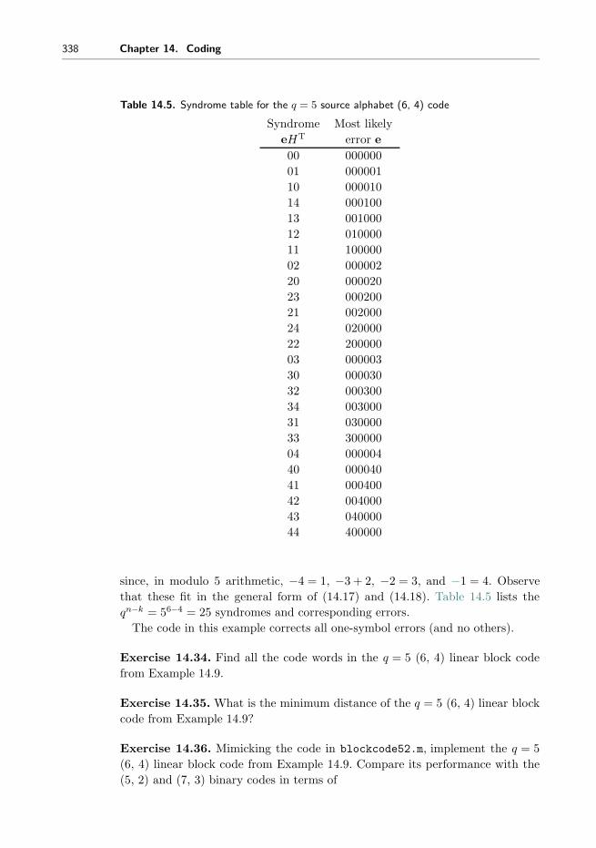
338 Chapter 14. Coding
Table 14.5. Syndrome table for the q = 5 source alphabet (6, 4) code
Syndrome Most likely
eHT error e
00 000000
01 000001
10 000010
14 000100
13 001000
12 010000
11 100000
02 000002
20 000020
23 000200
21 002000
24 020000
22 200000
03 000003
30 000030
32 000300
34 003000
31 030000
33 300000
04 000004
40 000040
41 000400
42 004000
43 040000
44 400000
since, in modulo 5 arithmetic, −4 = 1, −3 + 2, −2 = 3, and −1 = 4. Observe
that these fit in the general form of (14.17) and (14.18). Table 14.5 lists the
qn−k = 56−4 = 25 syndromes and corresponding errors.
The code in this example corrects all one-symbol errors (and no others).
Exercise 14.34. Find all the code words in the q = 5 (6, 4) linear block code
from Example 14.9.
Exercise 14.35. What is the minimum distance of the q = 5 (6, 4) linear block
code from Example 14.9?
Exercise 14.36. Mimicking the code in blockcode52.m, implement the q = 5
(6, 4) linear block code from Example 14.9. Compare its performance with the
(5, 2) and (7, 3) binary codes in terms of

Coding 339
a. performance in correcting errors,
b. data rate.
Be careful: how can a q = 5 source alphabet be compared fairly with a binary
alphabet? Should the comparison be in terms of percentage of bit errors or
percentage of symbol errors?
14.7 Encoding a Compact Disc
The process of writing to and reading from a compact disc is involved. The
essential idea in optical media is that a laser beam bounces off the surface of
the disc. If there is a pit, then the light travels a bit further than if there is no
pit. The distances are controlled so that the extra time required by the round
trip corresponds to a phase shift of 180◦. Thus, the light traveling back interferes
destructively if there is a pit, whereas it reinforces constructively if there is no
pit. The strength of the beam is monitored to detect a 0 (a pit) or a 1 (no pit).
While the complete system can be made remarkably accurate, the reading and
writing procedures are prone to errors. This is a perfect application for error-
correcting codes! The encoding procedure is outlined in Figure 14.6. The original
signal is digitized at 44,100 samples per second in each of two stereo channels.
Each sample is 16 bits, and the effective data rate is 1.41 Mbps (megabits per
second). The Cross Interleave Reed–Solomon Code (CIRC) encoder (described
shortly) has an effective rate of about 3/4, and its output is at 1.88 Mbps. Then
control and timing information is added, which contains the track and subtrack
numbers that allow CD tracks to be accessed rapidly. The “EFM” (Eight-to-
Fourteen Module) is an encoder that spreads the audio information in time by
changing each possible 8-bit sequence into a predefined 14-bit sequence so that
each one is separated by at least two (and at most ten) zeros. This is used to
help the tracking mechanism. Reading errors on a CD often occur in clusters (a
small scratch may be many hundreds of bits wide) and interleaving distributes
the errors so that they can be corrected more effectively. Finally, a large number
of synchronization bits is added. These are used by the control mechanism of
the laser to tell it where to shine the beam in order to find the next bits. The
final encoded data rate is 4.32 Mbps. Thus, about 1/3 of the bits on the CD are
actual data, and about 2/3 of the bits are present to help the system function
and to detect (and/or correct) errors when they occur.
The CIRC encoder consists of two special linear block codes called Reed–
Solomon codes (which are named after their inventors). Both use q = 256 (8-
bit) symbols, and each 16-bit audio sample is split into two code words. The
first code is a (32,28) linear code with dmin = 5, and the second code is a linear
(28,24) code, also with dmin = 5. These are nonbinary and use special arithmetic
operations defined by the “Galois field” with 256 symbols. The encoding is split

340 Chapter 14. Coding
Music
A/D
MUX
EFM
MUX
Optical media
CIRCEncoder
1.41 Mbps
1.88 Mbps
1.92 Mbps
4.32 Mbps
44.1 kHz per channelat 16 bits/sample
Reed−SolomonLinear Block Codes
"Control and timing track/subtracks"
"Eight-to-Fourteen Module"
"Synchronization"
Figure 14.6 CDs can be usedfor audio or for data. Theencoding procedure is thesame, though decoding maybe done differently fordifferent applications.
into two separate codes so that an interleaver can be used between them. This
spreads out the information over a larger range and helps to spread out the errors
(making them easier to detect and/or correct).
The encoding process on the CD is completely specified, but each manufacturer
can implement the decoding as they wish. Accordingly, there are many choices.
For instance, the Reed–Solomon codes can be used to correct two errors each,
or to detect up to five errors. When errors are detected, a common strategy is
to interpolate the audio, which may be transparent to the listener as long as the
error rate is not too high. Manufacturers may also choose to mute the audio when
the error rate is too high. For data purposes, the controller can also ask that the
data be reread. This may allow correction of the error when it was caused by
mistracking or some other transitory phenomenon, but will not be effective if the
cause is a defect in the medium.
For Further Reading
The paper that started information theory is still a good read half a century
after its initial publication:
� C. E. Shannon, “A Mathematical Theory of Communication,” The Bell Sys-
tem Technical Journal, vol. 27, pp. 379–423 and 623–656, July and October,
1948.

Step 5: Putting It All Together
The projects of Chapters 15 and 16 integrate all the fixes of the fourth step
into the receiver structure of the third step to create fully functional digital
receivers. The well-fabricated receiver is robust with respect to distortions such
as those caused by noise, multipath interference, timing inaccuracies, and clock
mismatches.
After building the components, testing them, assembling them into a receiver,
and testing the full design, your receiver is ready. Congratulations. You have
earned the degree of Master of Digital Radio. You are now ready to conquer the
world!
Master
of
Digital
Radio
______________
your name here

15 Make It So
This chapter describes a software-defined-radio design project calledM6, theMix
‘n’ Match Mostly Marvelous Message Machine. The M6 transmission standard
is specified so that the receiver can be designed using the building blocks of the
preceding chapters. The DSP portion of the M6 can be simulated in Matlab
by combining the functions and subroutines from the examples and exercises of
the previous chapters.
The input to the digital portion of the M6 receiver is a sampled signal at
intermediate frequency (IF) that contains several simultaneous messages, each
transmitted in its own frequency band. The original message is text that has
been converted into symbols drawn from a 4-PAM constellation, and the pulse
shape is a square-root raised cosine. The sample frequency can be less than twice
the highest frequency in the analog IF signal, but it must be sufficiently greater
than the inverse of the transmitted symbol period to be twice the bandwidth of
the baseband signal. The successful M6 Matlab program will demodulate, syn-
chronize, equalize, and decode the signal, so it is a “fully operational” software-
defined receiver (although it is not intended to work in “real time”). The receiver
must overcome multiple impairments. There may be phase noise in the trans-
mitter oscillator. There may be an offset between the frequency of the oscillator
in the transmitter and the frequency of the oscillator in the receiver. The pulse
clocks in the transmitter and receiver may differ. The transmission channel may
be noisy. Other users in spectrally adjacent bands may be actively transmitting
at the same time. There may be intersymbol interference caused by multipath
channels.
The next section describes the transmitter, the channel, and the analog front
end of the receiver. Then Section 15.2 makes several generic observations about
receiver design, and proposes a methodology for the digital receiver design. The
final section describes the receiver design challenge that serves as the culminating
design experience of this book. Actually building the M6 receiver, however, is
left to you. You will know that your receiver works when you can recover the
mystery message hidden inside the received signal.

Make It So 343
15.1 How the Received Signal Is Constructed
Receivers cannot be designed in a vacuum; they must work in tandem with a par-
ticular transmitter. Sometimes, a communication system designer gets to design
both ends of the system. More often, however, the designer works on one end or
the other, with the goal of making the signal in the middle meet some standard
specifications. The standard for the M6 is established on the transmitted signal,
and consists, in part, of specifications on the allowable bandwidth and on the
precision of its carrier frequency. The standard also specifies the source constel-
lation, the modulation, and the coding schemes to be used. The front end of the
receiver provides some bandpass filtering, downconversion to IF, and automatic
gain control prior to the sampler.
This section describes the construction of the sampled IF signal that must
be processed by the M6 receiver. The system that generates the analog received
signal is shown in block-diagram form in Figure 15.1. The front end of the receiver
that turns this into a sampled IF signal is shown in Figure 15.2.
The original message in Figure 15.1 is a character string of English text. Each
character is converted into a 7-bit binary string according to the ASCII conver-
sion format (e.g., the letter “a” is 1100001 and the letter “M” is 1001101), as in
Example 8.2. The bit string is coded using the (5, 2) linear block code specified in
blockcode52.m which associates a 5-bit code with each pair of bits. The output
of the block code is then partitioned into pairs that are associated with the four
CodingCharacterto binaryconversion
Pulseshape
Textmessage
Basebandsignal
Transmittedpassband
signal Analogreceived
signal
Adjacentusers
Broadbandnoise
Modulation
includes phase noise
ChannelBits
Symbolssi
Scaling
1Trigger
i Tt + εt
+ +
includes periodicmarker and training
sequence
Figure 15.1 Construction of the received signal.
Bandpassfilter
Downconversionto IF
Automaticgain
control kTs
Analogreceivedsignal
Sampledreceivedsignal Figure 15.2 Front end of
the receiver.

344 Chapter 15. Make It So
integers of a 4-PAM alphabet ±1 and ±3 via the mapping
11 → +3
10 → +1
01 → −1
00 → −3
(15.1)
as in Example 8.1. Thus, if there are n letters, there are 7n (uncoded) bits, 7n(52 )
coded bits, and 7n(52 )(12 ) 4-PAM symbols. These mappings are familiar from Sec-
tion 8.1, and are easy to use with the help of the Matlab functions bin2text.m
and text2bin.m. Exercise 14.25 provides several hints to help implement the M6
encoding, and the Matlab function nocode52.m outlines the necessary trans-
formations from the original text into a sequence of 4-PAM symbols s[i].
In order to decode the message at the receiver, the recovered symbols must
be properly grouped and the start of each group must be located. To aid this
frame synchronization, a marker sequence is inserted into the symbol stream at
the start of every block of 100 letters (at the start of every 875 symbols). The
header/training sequence that starts each frame is given by the phrase
A0Oh well whatever Nevermind (15.2)
which codes into 245 4-PAM symbols and is assumed to be known at the receiver.
This marker text string can be used as a training sequence by the adaptive
equalizer. The unknown message begins immediately after each training segment.
Thus, the M6 symbol stream is a coded message periodically interrupted by the
same marker/training clump.
As indicated in Figure 15.1, pulses are initiated at intervals of Tt seconds,
and each is scaled by the 4-PAM symbol value. This translates the discrete-
time symbol sequence s[i] (composed of the coded message interleaved with the
marker/training segments) into a continuous-time signal
s(t) =∑i
s[i]δ(t− iTt − εt).
The actual transmitter symbol period Tt is required to be within 0.01% of a
nominal M6 symbol period T = 6.4 μs. The transmitter symbol period clock
is assumed to be steady enough that the timing offset εt and its period Tt are
effectively time-invariant over the duration of a single frame.
Details of the M6 transmission specifications are given in Table 15.1. The
pulse-shaping filter P (f) is a square-root raised cosine filter symmetrically trun-
cated to eight symbol periods. The rolloff factor β of the pulse-shaping filter is
fixed within some range and is known at the receiver, though it could take on
different values with different transmissions. The (half-power) bandwidth of the
square-root raised cosine pulse could be as large as ≈102 kHz for the nominal T .
With double-sideband modulation, the pulse-shape bandwidth doubles so that
each passband FDM signal will need a bandwidth at least 204 kHz wide.

Make It So 345
Table 15.1. M6 Transmitter specifications
Symbol source alphabet ±1, ±3
Assigned intermediate frequency 2 MHz
Nominal symbol period 6.4 μs
SRRC pulse-shape rolloff factor β ∈ [0.1, 0.3]
FDM user slot allotment 204 kHz
Width of SRRC pulse shape 8 clock periods
Frame marker/training sequence See (15.2)
Frame marker sequence period 1120 symbols
Time-varying IF carrier phase Filtered white noise
IF offset Fixed, < 0.01%
Timing offset Fixed
Symbol period offset Fixed, < 0.01%
Intersymbol interference Max. delay spread = 7 symbols
Sampler frequency 850 kHz
The channel may be near ideal (i.e., a unit gain multisymbol delay) or it may
have significant intersymbol interference. In either case, the impulse response of
the channel is unknown at the receiver, though an upper bound on its delay
spread may be available. There are also disturbances that may occur during the
transmission. These may be wideband noise with flat power spectral density or
they may be narrowband interferers, or both. They are unknown at the receiver.
The achieved intermediate frequency is required to be within 0.01% of its
assigned value. The carrier phase θ(t) is unknown to the receiver and may vary
over time, albeit slowly. This means that the phase of the intermediate-frequency
signal presented to the receiver sampler may also vary.
The bandpass filter before the downconverter in the front end of the receiver
in Figure 15.2 partially attenuates adjacent 204-kHz-wide FDM user bands. The
automatic gain control is presumed locked and fixed over each transmission.
The free-running sampler frequency of 850 kHz is well above twice the 102 kHz
baseband bandwidth of the user of interest. This is necessary for the baseband
analog signal interpolator used in the timer in the DSP portion of the receiver
in Figure 15.3. However, the sampler frequency is not above twice the highest
frequency of the IF signal. This means that the sampled received signal has
replicated the spectrum at the output of the front end analog downconverter
lowpass filter to frequencies between zero and IF.
15.2 A Design Methodology for the M6 Receiver
Before describing the specific design requirements that must be met by a suc-
cessful M6 receiver, this section makes some generic remarks about a systematic
approach to receiver design. There are four generic stages.

346 Chapter 15. Make It So
DownconversionMatched
filter
Carrierrecovery
Timingrecovery
Interpolatordownsampler
Adaptive layer
Sampledreceivedsignal
EqualizerDecisiondevice
Equalizeradaptation
Trainingsegmentlocator
Framesynchronization
Decoder
Recoveredsource
Figure 15.3 DSP portion of software-defined receiver.
1. Choose the order in which the basic operations of the receiver occur.
2. Select components and methods that can perform the basic operations in an
ideal setting.
3. Select adaptive elements that allow the receiver to continue functioning when
there are impairments.
4. Verify that the performance requirements are met.
While it may seem as though each stage requires that choices made in the preced-
ing stages be fixed, in reality, difficulties encountered at one stage in the design
process may require a return to (and different choices to be made in) earlier
stages. As will soon become clear, the M6 problem specification has basically
(pre)resolved the design issues of the first two stages.
15.2.1 Stage One: Ordering the Pieces
The first stage is to select the basic components and the order in which they
occur. The design layout first established in Figure 2.13 (and reappearing in the
DSP portion of the receiver in Figure 15.3) suggests one feasible structure. As the
signal enters the receiver it is downconverted (with carrier recovery), matched
filtered, interpolated (with timing recovery), equalized (adaptively), quantized,
and decoded (with frame synchronization). This classical ordering, while popular,
is not the only (nor necessarily the best) way to recover the message from the
noisy, ISI-distorted, FDM–PAM–IF received signal. However, it offers a useful
foundation for assessing the relative benefits and costs of alternative receiver
configurations. Also, we know for sure that the M6 receiver can be built this
way. Other configurations may work, but we have not tested them.1
How was this ordering of components chosen? The authors have consulted
with, worked for, talked about (and argued with) engineers working on a num-
ber of receiver systems, including HDTV (high-definition television), DSL, and
1 If this sounds like a challenge, rest assured it is. Research continues worldwide, makingcompilation of a complete handbook of receiver designs and algorithms a Sisyphean task.The creation of “new” algorithms with minor variations that exploit a particular application-specific circumstance is a popular pastime of communication engineers. Perhaps you too willcome up with a unique approach!

Make It So 347
AlohaNet. The ordering of components in Figures 2.13 and 15.3 represents an
amalgamation of ideas from these (and other) systems. Sometimes it is easy to
argue why a particular order is good, sometimes it is a matter of preference or
personal experience, and sometimes the choice is based on factors outside the
engineer’s control.2
For example, the carrier-recovery algorithms of Chapter 10 are not greatly
affected by noise or intersymbol interference (as was shown in Exercises 10.36
and 10.40). Thus carrier recovery can be done before equalization, and this is the
path we have followed. But it need not be done in this order.3 Another example
is the placement of the timing-recovery element. The algorithms of Chapter 12
operate at baseband, and hence the timing recovery in Figure 15.3 is placed after
the demodulation. But there are passband timing-recovery algorithms that could
have been used to reverse the order of these two operations.
15.2.2 Stage Two: Selecting Components
Choices for the second design stage are relatively set as well. Since the sampling
is done at a sub-Nyquist rate fs (relative to the IF frequency fI), the spec-
trum of the analog received signal is replicated every fs. The integer n for which
f † = |fI − nfs| is smallest defines the nominal frequency f † from which further
downconversion is needed. Recall that such downconversion by sampling was dis-
cussed in Section 6.2. Using different specifications, the M6 sampling frequency
fs may be above the Nyquist frequency associated with the IF frequency fI .4
The most common method of downconversion is to use mixing followed by
an FIR lowpass filter. This will be followed by an FIR matched filter, an
interpolator–decimator for downsampling, and a symbol-spaced FIR equalizer
that adapts its coefficients in response to the training data contained in the trans-
mission. The output of the equalizer is quantized to the nearest 4-PAM symbol
value, translated back into binary, decoded (using the (5, 2) block decoder), and
finally turned back into readable text.
Given adequate knowledge of the operating environment (the SNR in the
received signal, the carrier frequency and phase, the clock period and symbol
timing, and the marker location), the designer-selected parameters within these
components can be set to recover the message. This was, in fact, the strategy
followed in the idealized receiver of Chapter 9. Said another way, the choices
in stages one and two are presumed to admit an acceptable answer if prop-
erly tuned. Component selections at this point (including specification of the
2 For instance, the company might have a patent on a particular method of timing recoveryand using any other method might require royalty payments.
3 For instance, in the QAM radio of A Digital Quadrature Amplitude Modulation Radio, avail-able in the website, the blocks appear in a different order.
4 Indeed, changing parameters such as this allows an instructor to create new transmission“standards” for each class!

348 Chapter 15. Make It So
fixed lowpass filter in the downconverter and the fixed matched filter preceding
the interpolator/downsampler) can be confirmed by simulations of the ISI-free
ideal/full-knowledge setting. Thus, the upper half of Figure 15.3 is specified by
stage-two activities.
15.2.3 Stage Three: Anticipating Impairments
In the third design stage, the choices are less constrained. Elements of the third
stage are shown in the lower half of the receiver (the “adaptive layer” of Fig-
ure 15.3) and include the selection of algorithms for carrier, timing, frame syn-
chronization, and equalizer adaptation. There are several issues to consider.
One of the primary stage-three activities is algorithm selection—which per-
formance function to use in each block. For example, should the M6 receiver
use a phase-locked loop, a Costas loop, or a decision-directed method for carrier
recovery? Is a dual loop needed to provide adequate carrier tracking, or will a
single loop suffice? What performance function should be used for the equalizer?
Which algorithm is best for the timing recovery? Is simple correlation suitable
to locate the training and marker segment?
Once the specific methods have been chosen, it is necessary to select specific
variables and parameters within the algorithms. This is a traditional aspect
of engineering design that is increasingly dominated by computer-aided design,
simulation, and visualization tools. For example, error surfaces and eye diagrams
can be used to compare the performance of the various algorithms in particular
settings. They can be used to help determine which technique is more effective
for the application at hand.
As software-aided design packages proliferate, the need to understand the com-
putational mechanics underlying a particular design becomes less of a barrier.
For instance, Software Receiver Design has relied exclusively on the filter-
design algorithms built into Matlab. But the specification of the filter (its shape,
cutoff frequencies, computational complexity, and filter length) cannot be left to
Matlab. The more esoteric the algorithm, the less transparent is the process
of selecting design parameters. Thus, Software Receiver Design has devoted
considerable space to the design and operation of adaptive elements.
But, even assuming that the trade-offs associated with each of the individual
components are clear, how can everything be integrated together to succeed at
a multifaceted design objective such as the M6 receiver?
15.2.4 Sources of Error and Trade-offs
Even when a receiver is fully operational, it might not decode every symbol
precisely. There is always a chance of error. Perhaps part of the error is due to a
frequency mismatch, part of the error is due to noise in the channel, part of the
error is due to a nonoptimal timing offset, etc. This section (and the next) suggest
a general strategy for allocating “part of” the error to each component. Then, as

Make It So 349
long as the sum of all the partial errors does not exceed the maximum allowable
error, there is a good chance that the complete receiver will work according to
its specifications.
The approach is to choose a method of measuring the amount of error, for
instance, the average of the squared recovery error. Each individual component
can be assigned a threshold, and its parameters can be adjusted so that it does
not contribute more than its share to the total error. Assuming that the accu-
mulation of the errors from various sources is additive, the complete receiver
will have no larger error than the concatenation of all its parts. This additivity
assumption is effectively an assumption that the individual pieces of the system
do not interact with each other. If they do (or when they do), then the threshold
allotments may need to be adjusted.
There are many factors that contribute to the recovery error, including the
following.
� Residual interference from adjacent FDMbands (caused by imperfect bandpass
filtering before downconversion and imperfect lowpass filtering after downcon-
version).� AGC jitter (caused by the deviation in the instantaneous signal from its
desired average and scaled by the stepsize in the AGC element).� Quantization noise in the sampler (caused by coarseness in the magnitudes of
the quantizer).� Round-off noise in filters (caused by wordlength limitations in filter parame-
ters and filter algebra).� Residual interference from the doubly upconverted spectrum (caused by
imperfect lowpass filtering after downconversion).� Carrier phase jitter (occurs physically as a system impairment and is caused
by the stepsize in the carrier-recovery element).� Timing jitter (occurs physically as a system impairment and is caused by the
stepsize in the timing-recovery element).� Residual mean-squared error left by the equalizer (even an infinitely long lin-
ear equalizer cannot remove all recovery error in the presence of simultaneous
channel noise and ISI).� Equalizer parameter jitter (caused by the nonvanishing stepsize in the adap-
tive equalizer).� Noise enhancement by the equalizer (caused by ISI that requires large equal-
izer gains, such as a deep channel null at frequencies that also include noise).
Because Matlab implements all calculations in floating-point arithmetic, the
quantization and round-off noise in the simulations is imperceptible. The project
setup presumes that the AGC has no jitter. A well-designed and sufficiently long
lowpass filter in the downconverter can effectively remove the interference from
outside the user band of interest. The in-band interference from sloppy adjacent
FDM signals should be considered part of the in-band channel noise. This leaves

350 Chapter 15. Make It So
carrier phase, timing jitter, imperfections in the equalizer, tap jitter, and noise
gain. All of these are potentially present in the M6 software-defined digital radio.
In all of the cases in which error is due to the jiggling of the parameters in
adaptive elements (in the estimation of the sampling instants, the phase errors,
the equalizer taps), the errors are proportional to the stepsize used in the algo-
rithm. Thus, the (asymptotic) recovery error can be made arbitrarily small by
reducing the appropriate stepsize. The problem is that, if the stepsize is too
small, the element takes longer to converge. If the time to convergence of the ele-
ment is too long (for instance, longer than the complete message), then the error
is increased. Accordingly, there is some optimal stepsize that is large enough to
allow rapid convergence yet small enough to allow acceptable error. An analo-
gous trade-off arises with the choice of the length of the equalizer. Increasing its
length reduces the size of the residual error. But as the length grows, so does the
amount of tap jitter.
Such trade-offs are common in any engineering design task. The next section
suggests a method of quantifying the trade-offs to help make concrete decisions.
15.2.5 Tuning and Testing
The testing and verification stage of receiver design is not a simple matter
because there are so many things that can go wrong. (There is so much stuff
that can happen!) Of course, it is always possible to simply build a proto-
type and then test to see whether the specifications are met. Such a haphazard
approach may result in a working receiver, but then again, it might not. Surely
there is a better way! This section suggests a commonsense approach that is not
uncommon among practicing engineers. It represents a “practical” compromise
between excessive analysis (such as one might find in some advanced commu-
nication texts) and excessive trial and error (such as “try something and cross
your fingers”).
The idea is to construct a simulator that can create a variety of test signals that
fall within the M6 specification. The parameters within the simulator can then
be changed one at a time, and their effect on various candidate receivers noted.
By systematically varying the test signals, the worst components of the receiver
can be identified and then replaced. As the tests proceed, the receiver gradually
improves. As long as the complete set of test signals accurately represents the
range of situations that will be encountered in operation, the testing will lead to
a successful design.
Given the particular stage-one and -two design choices for the M6 receiver,
the previous section outlined the factors that may degrade the performance of
the receiver. The following steps suggest some detailed tests that may facilitate
the design process.

Make It So 351
� Step 1: Tuning the Carrier Recovery As shown in Chapter 10, any of the
carrier-recovery algorithms will be capable of locating a fixed phase offset in
a receiver in which everything else is operating optimally. Even when there is
noise or ISI, the best settings for the frequency and phase of the demodulation
sinusoid are those that match the frequency and phase of the carrier of the
IF signal. For the M6 receiver, there are two issues that must be considered.
First, the M6 specification allows the frequency to be (somewhat) different
from its nominal value. Is a dual-loop structure needed? Or can a single loop
adequately track the expected variations? Second, the transmitter phase may
be jittering.
The user-choosable features of the carrier-recovery algorithms are the LPF
and the algorithm stepsize, both of which influence the speed at which the
estimates can change. Since the carrier-recovery scheme needs to track a time-
varying phase, the stepsize cannot be chosen too small. Since a large stepsize
increases the error due to phase jitter, it cannot be chosen too large. Thus,
an acceptable stepsize will represent a compromise.
To conduct a test to determine the stepsize (and LPF) requires creating test
signals that have a variety of off-nominal frequency offsets and phase jitters.
A simple way to model phase jitter is to add a lowpass-filtered version of
zero-mean white noise to a nominal value. The quality of a particular set
of parameters can then be measured by averaging (over all the test signals)
the mean squared recovery error. Choosing the LPF and stepsize parameters
to make this error as small as possible gives the “best” values. This average
error provides a measure of the portion of the total error that is due to the
carrier-recovery component in the receiver.� Step 2: Tuning the Timing Recovery As shown in Chapter 12, there are several
algorithms that can be used to find the best timing instants in the ideal setting.
When the channel impairment consists purely of additive noise, the optimal
sampling times remain unchanged, though the estimates will likely be more
noisy. As shown by Example 12.3, and in Figure 12.12, however, when the
channel contains ISI, the answer returned by the algorithms differs from what
might be naively expected.
There are two parts to the experiments at this step. The first is to locate the
best timing-recovery parameter for each test signal. (This value will be needed
in the next step to assess the performance of the equalizer.) The second part
is to find the mean squared recovery error due to jitter of the timing-recovery
algorithm.
The first part is easy. For each test signal, run the chosen timing-recovery
algorithm until it converges. The convergent value gives the timing offset
(and indirectly specifies the ISI) to which the equalizer will need to respond.
(If it jiggles excessively, then decrease the stepsize.)
Assessing the mean squared recovery error due to timing jitter can be done
much like the measurement of jitter for the carrier recovery: measure the
average error that occurs over each test signal when the algorithm is initialized

352 Chapter 15. Make It So
at its optimum answer; then average over all the test signals. The answer may
be affected by the various parameters of the algorithm: the δ that determines
the approximation to the derivative, the l parameter that specifies the time
support of the interpolation, and the stepsize (these variable names are from
the first part of the timing-recovery algorithm clockrecDD.m on page 258.)
In operation, there may also be slight inaccuracies in the specification of the
clock period. When the clock period at the transmitter and that at the receiver
differ, the stepsize must be large enough that the timing estimates can follow
the changing period. (Recall the discussion surrounding Example 12.4.) Thus,
again, there is a tension between a large stepsize needed to track rapid changes
and a small stepsize to minimize the effect of the jitter on the mean squared
recovery error. In a more complex environment, in which clock phases might be
varying, it might be necessary to follow a procedure more like that considered
in step 1.� Step 3: Tuning the Equalizer After choosing the equalizer method (as specified
by the performance function), there are parameters that must be chosen and
decisions that must be made in order to implement the linear equalizer. These
are
– the order of the equalizer (number of taps),
– the initial values of the equalizer,
– the training signal delay (if using the training signal), and
– the stepsize.
As in the previous steps, it is a good idea to create a collection of test signals
using a simulation of the transmitter. To test the performance of the equal-
izer, the test signals should contain a variety of ISI channels and/or additive
interferences.
As suggested in Chapter 13, in a high-SNR scenario the T -spaced equalizer
tries to implement an approximation of the inverse of the ISI channel. If the
channel is mild, with all its roots well away from the unit circle, then its
inverse may be fairly short. But if the channel has zeros that are near the unit
circle, then its FIR inverse may need to be quite long. While much can be
said about this, a conservative guideline is that the equalizer should be from
two to five times longer than the maximum anticipated channel delay spread.
One subtlety that arises in making this decision and in consequent testing is
that any channel ISI that is added into a simulation may appear differently
at the receiver because of the sampling. This effect was discussed at length in
Section 13.1, where it was shown how the effective digital model of the channel
includes the timing offset. Thus (as mentioned in the previous step) assess-
ing the “actual” channel to which the equalizer will adapt requires knowing
the timing offset that will be found by the timing recovery. Fortunately, in
the M6 receiver structure of Figure 15.3, the timing-recovery algorithm oper-
ates independently of the equalizer, and so the optimal value can be assessed
beforehand.

Make It So 353
For most of the adaptive equalizers in Chapter 13, the center-spike initial-
ization is used. This was justified in Section 13.4 (see page 289) as a useful
method of initialization. Only if there is some concrete a priori knowledge of
the channel characteristics would other initializations be used.
The problem of finding an appropriate delay was discussed in Section 13.2.3,
where the least-squares solution was recomputed for each possible delay. The
delay with the smallest error was the best. In a real receiver, it will not be
possible to do an extensive search, and so it is necessary to pick some delay.
TheM6 receiver uses correlation to locate the marker sequence and this can be
used to locate the time index corresponding to the first training symbol. This
location plus half the length of the equalizer should correspond closely to the
desired delay. Of course, this value may change depending on the particular
ISI (and channel lengths) used in a given test signal. Choose a value that,
over the complete set of test signals, provides a reasonable answer.
The remaining designer-selected variable is stepsize. As with all adaptive
methods, there is a trade-off inherent in stepsize selection: making it too large
can result in excessive jitter or algorithm instability, while making it too small
can lead to an unacceptably long convergence time. A common technique is
to select the largest stepsize consistent with achievement of the component’s
assigned asymptotic performance threshold.� Step 4: Frame Synchronization Any error in locating the first symbol of each
four-symbol block can completely garble the reconstructed text. The frame
synchronizer operates on the output of the quantizer, which should contain few
errors once the equalizer, timing recovery, and phase recovery have converged.
The success of frame synchronization relies on the peakiness of the correlation
of the marker/training sequence. The chosen marker/training sequence “A0Oh
well whatever Nevermind” should be long enough that there are few false
spikes when correlating to find the start of the message within each block.
To test software written to locate the marker, feed it a sample symbol string
assembled according to the specifications described in the previous section as
if the downconverter, clock timing, equalizer, and quantizer had recovered the
transmitted symbol sequence perfectly.
Finally, after tuning each component separately, it is necessary to confirm
that, when all the pieces of the system are operating simultaneously, there are
no excessive negative interactions. With luck, little further tuning will prove
necessary to complete a successful design. The next section has more specifics
about the M6 receiver design.
Exercise 15.1. From the parameters in Table 15.1, do the following.
a. Determine the oversampling (or upsampling) factor.
b. Determine what frequency the sampled received signal will be centered
around. Recall that the receiver front end samples at a rate lower than the IF
frequency, and your answer should be something between 0 and fs/2.

354 Chapter 15. Make It So
Exercise 15.2. The B3IG transmitter can be used to implement the M6 trans-
mission specifications, as provided in m6params.m. Plot the received signal and
its spectrum. Use these plots to explain why your answers to Exercise 15.1 are
correct.
15.3 No Soap Radio: The M6 Receiver Design Challenge
The analog front end of the receiver in Figure 15.2 takes the signal from an
antenna, amplifies it, and crudely bandpass filters it to (partially) suppress fre-
quencies outside the desired user’s frequency band. An analog downconverter
modulates the received signal (approximately) down to the nominal IF fI at
2 MHz. The output of the analog downconverter is set by an automatic gain
controller to fit the range of the sampler. The output of the AGC is sampled at
intervals of Ts = 850 kHz to give r[k], which provides a “Nyquist” bandwidth
of 425 kHz that is ample for a 102 kHz baseband user bandwidth. The sampled
received signal r[k] from Figure 15.2 is the input to the DSP portion of the
receiver in Figure 15.3.
The following comments on the components of the digital receiver in Fig-
ure 15.3 help characterize the design task.
� The downconversion to baseband uses the sampler frequency fs, the known
intermediate frequency fI , and the current phase estimates to determine the
mixer frequency needed to demodulate the signal. The M6 receiver may use
any of the phase-tracking algorithms of Chapter 10. A second loop may also
help with frequency offset.� The lowpass filtering in the demodulator should have a bandwidth of roughly
102 kHz, which will cover the selected source spectrum but reject components
outside the frequency band of the desired user.� The interpolator/downsampler implements the reduction in sample rate to
T -spaced values. This block must also implement the timing synchronization,
so that the time between samples after timing recovery is representative of
the true spacing of the samples at the transmitter. You are free to implement
this in any of the ways discussed in Chapter 12.� Since there could be a significant amount of intersymbol interference due
to channel dynamics, an equalizer is essential. Any one will do. A trained
equalizer requires finding the start of the marker/training segment while a
blind equalizer may converge more slowly.� The decision device is a quantizer defined to reproduce the known alphabet
of the s[i] by a memoryless nearest-element decision.� At the final step, the decoding from blockcode52.m in conjunction with
bin2text.m can be used to reconstruct the original text. This also requires
a frame synchronization that finds and removes the start block consisting of
Make It So 355
marker plus training, which is most likely implemented using a correlation
technique.
The software-defined radio should have the following user-selectable variables
that can readily be set at the start of processing of the received block of data:
� rolloff factor β for the square-root raised cosine pulse shape,� initial phase offset,� initial timing offset, and� initial equalizer parameterization.
The following are some suggestions.
� Use the B3IG transmitter with m6params.m to implement the M6 transmis-
sion specification along with various impairments. This will enable you to test
your receiver (as described in the preceding section) over a wider range of
conditions than just the test signals available on the website.� Try to break your receiver. See how much noise can be present in the received
signal before accurate (e.g., less than 1% symbol errors) demodulation seems
impossible. Find the fastest change in the carrier phase that your receiver can
track, even with a bad initial guess.� In order to facilitate more effective debugging while building the project,
implementation of a debug mode in the receiver is recommended. The infor-
mation of interest will be plots of the time histories of pertinent signals as well
as timing information (e.g., a graph of matched filter average output power
versus receiver symbol timing offset). One convenient way to add this feature
to your Matlab receiver would be to include a debug flag as an argument
that produces these plots when the flag is activated.� When debugging adaptive components, use a test with initialization at the
right answer and zero stepsize to determine whether the problem is in the
adaptation or in the fixed component structure. An initialization very near
the desired answer with a small stepsize will reveal that the adaptive portion
is working properly if the adaptive parameter trajectory remains in the close
vicinity of the desired answer. A rapid divergence may indicate that the update
has the wrong sign or that the stepsize is way too large. An aimless wandering
that drifts away from the vicinity of the desired answer represents a more
subtle problem that requires reconsideration of the algorithm code and/or its
suitability for the circumstance at hand.
Several test files that contain a “mystery signal” with a quote from a
well-known book are available on the website. They are labeled easy.mat,
medium.mat, and hard.mat.5 These have been created with a variety of different
5 One student remarked that these should have been called hard.mat, harder.mat, andcompletelyridiculous.mat. Nonetheless, a well-crafted M6 receiver can recover the hiddenmessages.

356 Chapter 15. Make It So
rolloff factors, carrier frequencies, phase noises, ISI, interferers, and symbol tim-
ing offsets. We encourage the adventurous reader to try to “receive” these secret
signals. Solve the mystery. Break it down.
For Further Reading
An overview of a practical application of software-defined radio emphasizing the
redefinability of the DSP portion of the receiver can be found in
� B. Bing and N. Jayant, “A Cellphone for All Standards,” IEEE Spectrum, pp.
34–39, May 2002.
The field of “software radio” erupted with a special issue of the IEEE Commu-
nications Magazine in May 1995. This was called a “landmark special issue” in
an editorial in the more recent
� J. Mitola, III, V. Bose, B. M. Leiner, T. Turletti, and D. Tennenhouse, Eds.,
IEEE Journal on Selected Areas in Communications (Special Issue on Soft-
ware Radios), vol. 17, April 1999.
For more information on the technological context and the relevance of software
implementations of communications systems, see
� E. Buracchini, “The Software Radio Concept,” IEEE Communications Mag-
azine, vol. 38, pp. 138–143, September 2000
and papers from the (occasional) special section in the IEEE Communications
Magazine on topics in software and DSP in radio. For much more, see
� J. H. Reed, Software Radio: A Modern Approach to Radio Engineering,
Prentice-Hall, 2002,
which overlaps in content (if not style) with the first half of Software Receiver
Design.
Two recommended monographs that devote more attention than most to the
methodology of the same slice of digital receiver design as we consider here are
� J. A. C. Bingham, The Theory and Practice of Modem Design, Wiley Inter-
science, 1988 (especially Chapter 5);� H. Meyr, M. Moeneclaey, and S. A. Fechtel, Digital Communication Receivers:
Synchronization, Channel Estimation, and Signal Processing, Wiley Inter-
science, 1998 (especially Section 4.1).

16 A Digital Quadrature AmplitudeModulation Radio
The preceding chapters of Software Receiver Design focus on a real-valued
PAM transmission protocol. Though this is one of the simplest digital trans-
mission systems, a working radio for PAM needs to include a variety of tech-
niques that address the nonideal behaviors encountered in reality. Fixes such
as the PLL, the Costas loop, timing recovery, and equalization are necessary
parts of the system. This chapter describes a complex-valued generalization of
PAM called quadrature amplitude modulation (QAM), which forms the basis
of a “better radio.” While the change from real-valued PAM to complex-valued
QAM signals is straightforward, the bulk of this chapter fleshes out the details
of operation of the resulting system. The various parts of the digital radio need
to be rethought (carrier recovery, timing recovery, and equalization). The theme
of this chapter is that such rethinking can follow the same path as the original
designs. The basic techniques for the PAM radio of earlier chapters generalize
smoothly to more sophisticated designs.
This chapter begins with the observation (already noted in Section 5.3) that
PAM modulations waste bandwidth. QAM, a more clever modulation strategy,
is able to halve the bandwidth requirements, which represents a significant step
towards practicality. This is accomplished by sending, and then unravelling, two
real PAM signals simultaneously on orthogonal carriers (sine and cosine) that
occupy the same frequency band. A straightforward way to describe QAM is to
model the two signals as the real and imaginary portions of a single complex-
valued signal.
16.1 The Song Remains the Same
Sections 16.2 and 16.3 show explicitly how QAM can be viewed as PAM that uses
complex-valued modulation and demodulation. In an ideal world, this would be
the end of the story. But reality intrudes in several ways. Just as a PAM radio
needs to align the phase at the transmitter with the phase at the receiver, so

358 Chapter 16. A Digital Quadrature Amplitude Modulation Radio
will a QAM radio. While the basic ideas of carrier recovery remain the same,
the details of the QAM protocol require changes in the operation of the adaptive
elements used to estimate the parameters. Similarly, the frequency of the carrier
at the transmitter and the frequency of the demodulating signal at the receiver
must be aligned. For example, Section 16.4.1 extends the Costas-loop idea to
4-QAM while Section 16.4.3 extends the PLL for 4-QAM.
Just as a PAM radio needs to align the sampling times and rates at the receiver
with the symbol times and rates, so will a QAM radio. While the basic ideas
of timing recovery remain the same, the details of the QAM protocol require
changes in the detailed operation of the adaptive elements. Section 16.6 extends
the timing-recovery methods of PAM in Chapter 12 to QAM.
Just as a PAM radio needs to build an equalizer to combat intersymbol inter-
ference, so will a QAM radio. While the basic ideas of equalization remain the
same as in Chapter 13, equalization of the two real signal streams of QAM is most
easily described in terms of a complex-valued adaptive equalizer as in Section
16.8.
An interesting feature of QAM is that the carrier recovery can be carried
out before the equalizer (as in Section 16.4) or after the equalizer. Such post-
equalization carrier recovery can be accomplished as in Section 16.7 by derotating
the complex-valued constellation at the output of the equalizer. This is just one
example of the remarkable variety of ways in which a QAM receiver can be
structured. Several different possible QAM constellations are discussed in Section
16.5 and several possible ways of ordering the receiver elements are drawn from
the technical literature in Section 16.9.
As is done throughout Software Receiver Design, exercises are structured
as mini-design exercises for individual pieces of the system. These pieces come
together at the end, with a description of (and Matlab code for) the Q3AM
prototype receiver, which parallels the M6 receiver of Chapter 15, but for QAM.
A series of experiments with the Q3AM receiver is intended to encourage explo-
ration of a variety of alternative architectures for the radio. Exercises ask for
assessments of the practicality of the various extensions, and allow for experi-
mentation, discovery, and perhaps even a small dose of frustration, as the impor-
tance of real-world impairments stresses the radio designs. The objective of this
chapter is to show the design process in action and to give the reader a feel for
how to generalize the original PAM system for new applications.
16.2 Quadrature Amplitude Modulation (QAM)
Sections 5.1 and 5.2 demonstrate the use of amplitude modulation with and
without a (large) carrier. An unfortunate feature of these modulation techniques
(and of the resulting real-valued AM systems) is that the range of frequencies
used by the modulated signal is twice as wide as the range of frequencies in the
baseband. For example, Figures 4.10 and 5.3 (on pages 70 and 82) show baseband

A Digital Quadrature Amplitude Modulation Radio 359
signals that are nonzero for frequencies between −B and B while the spectrum
of the modulated signals is nonzero in the interval [−fc −B,−fc +B] and in
the interval [fc −B, fc + B]. Since bandwidth is a scarce resource, it would be
preferable to use a scheme such as quadrature modulation (QM, introduced in
Section 5.3), which provides a way to remove this redundancy. Since the spectrum
of the resulting signal is asymmetric in QM, such a system can be modeled using
complex-valued signals, though these can always be rewritten and realized as (a
pair of) real-valued signals.
As described in Equation (5.6) on page 91, QM sends two message signals
m1(t) and m2(t) simultaneously in the same 2B passband bandwidth using two
orthogonal carriers (cosine and sine) at the same frequency fc,
v(t) = m1(t) cos(2πfct+ φ)−m2(t) sin(2πfct+ φ). (16.1)
φ is the fixed offset of the carrier phase. Define the complex-valued message
m(t) = m1(t) + jm2(t)
and the complex sinusoid ej(2πfct+φ). Observe that the real part of the product
m(t)ej(2πfct+φ) = m1(t) cos(2πfct+ φ)−m2(t) sin(2πfct+ φ)
+ j[m2(t) cos(2πfct+ φ) +m1(t) sin(2πfct+ φ)]
is precisely v(t) from (16.1), that is,
v(t) = Re{m(t)ej(2πfct+φ)}, (16.2)
where Re{a+ jb} = a takes the real part of its argument.
The two message signals may be built (as in previous chapters) by pulse-
shaping a digital symbol sequence using a time-limited pulse shape p(t). Thus
the messages are represented by the signal
mi(t) =∑k
si[k]p(t− kT ), (16.3)
where T is the interval between adjacent symbols and si[k], drawn from a finite
alphabet, is the ith message symbol at time k. The corresponding transmitted
signal is
v(t) =∑k
p(t− kT )[s1[k] cos(2πfct+ φ)− s2[k] sin(2πfct+ φ)]
= Re
{∑k
p(t− kT )s[k]ej(2πfct+φ)
}, (16.4)
where
s[k] = s1[k] + js2[k]
is a complex-valued symbol obtained by combining the two real-valued messages.
The two data streams could arise from separate messages. For instance, one
user might send a binary ±1 sequence s1[k] while another user transmits a binary

360 Chapter 16. A Digital Quadrature Amplitude Modulation Radio
0111
10 00
(a)
s1
s2
1
1
−1
−1
0001
11 10
(b)
s1
s2
1
1
−1
−1
Figure 16.1 Two choices for associatingsymbol pairs (s1, s2) with bit pairs. In(a), (1,−1) is associated with 00, (1, 1)with 01, (−1, 1) with 11, and (−1,−1)with 10. In (b), (1,−1) is associatedwith 10, (1, 1) with 00, (−1, 1) with 01,and (−1,−1) with 11.
±1 sequence s2[k]. Taken together, these can be thought of as the 4-QAM constel-
lation±1± j. There are many ways in which two binary signals can be combined;
two are shown in Figure 16.1, which plots (s1, s2) pairs in a two-dimensional plane
with s1 values on one axis and s2 values on the other.
Alternatively, the two messages could be a joint encoding of a single mes-
sage. For example, a ±1,±3 4-PAM coding could be recast as 4-QAM using an
assignment like
−3 ↔ −1− j
−1 ↔ −1 + j
+1 ↔ +1− j
+3 ↔ +1+ j
In either case, s1[k] and s2[k] are assumed to have zero average and to be uncor-
related so that their average product is zero.
The process of generating QAM signals such as (16.4) is demonstrated in
qamcompare.m, which draws on the PAM pulse-shaping routine pulrecsig.m
from page 194. qamcompare.m uses a simple Hamming pulse shape p(t) and ran-
dom binary values for the messages s1[k] and s2[k]. The modulation is carried out
in two ways, with real sines and cosines (corresponding to the first part of (16.4))
and with complex modulation (corresponding to the second part of (16.4)). The
two outputs can be compared by calculating max(abs(vcomp-vreal)), which
verifies that the two are identical.
Listing 16.1. qamcompare.m compare real and complex QAM implementations
N=1000; M=20; Ts=.0001; % # symbols , oversampl ing f a c t o rtime=Ts*(N*M−1); t=0:Ts : time ; % sampling i n t e r v a l and times1=pam(N, 2 , 1 ) ; s2=pam(N, 2 , 1 ) ; % l ength N r e a l 2− l e v e l s i g n a l sps=hamming (M) ; % pul s e shape o f width Mf c =1000; th=−1.0; j=sqrt (−1); % c a r r i e r f r eq and phases1up=zeros (1 ,N*M) ; s2up=zeros (1 ,N*M) ;s1up ( 1 :M: end)=s1 ; % oversample by Ms2up ( 1 :M: end)=s2 ; % oversample by Msp1=f i l t e r ( ps , 1 , s1up ) ; % convolve pu l s e shape with s1sp2=f i l t e r ( ps , 1 , s2up ) ; % convolve pu l s e shape with s2% make r e a l and complex−valued ve r s i on s and comparev r ea l=sp1 . * cos (2* pi* f c * t+th)−sp2 . * sin (2* pi* f c * t+th ) ;vcomp = real ( ( sp1+j * sp2 ) . * exp ( j *(2* pi* f c * t+th ) ) ) ;max(abs (vcomp−v r ea l ) ) % v e r i f y that they ’ r e the same
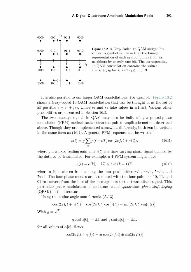
A Digital Quadrature Amplitude Modulation Radio 361
0000 0001 0011 0010
0100 0101 0111 0110
1100 1101 1111 1110
1000 1001 1011 1010
s1
s2
1
1
−1−1
3
3
−3
−3
Figure 16.2 A Gray-coded 16-QAM assigns bitvalues to symbol values so that the binaryrepresentation of each symbol differs from itsneighbors by exactly one bit. The corresponding16-QAM constellation contains the valuess = s1 + js2 for s1 and s2 ∈ ±1,±3.
It is also possible to use larger QAM constellations. For example, Figure 16.2
shows a Gray-coded 16-QAM constellation that can be thought of as the set of
all possible s = s1 + js2, where s1 and s2 take values in ±1,±3. Various other
possibilities are discussed in Section 16.5.
The two message signals in QAM may also be built using a pulsed-phase
modulation (PPM) method rather than the pulsed-amplitude method described
above. Though they are implemented somewhat differently, both can be written
in the same form as (16.4). A general PPM sequence can be written
v(t) = g∑k
p(t− kT ) cos(2πfct+ γ(t)), (16.5)
where g is a fixed scaling gain and γ(t) is a time-varying phase signal defined by
the data to be transmitted. For example, a 4-PPM system might have
γ(t) = α[k], kT ≤ t < (k + 1)T, (16.6)
where α[k] is chosen from among the four possibilities π/4, 3π/4, 5π/4, and
7π/4. The four phase choices are associated with the four pairs 00, 10, 11, and
01 to convert from the bits of the message bits to the transmitted signal. This
particular phase modulation is sometimes called quadrature phase-shift keying
(QPSK) in the literature.
Using the cosine angle-sum formula (A.13),
cos(2πfct+ γ(t)) = cos(2πfct) cos(γ(t)) − sin(2πfct) sin(γ(t)).
With g =√2,
g cos(α[k]) = ±1 and g sin(α[k]) = ±1,
for all values of α[k]. Hence
cos(2πfct+ γ(t)) = ± cos(2πfct)± sin(2πfct))

362 Chapter 16. A Digital Quadrature Amplitude Modulation Radio
and the resulting QPSK signal can be written
v(t) =∑k
p(t− kT )[s1[k] cos(2πfct)− s2[k] sin(2πfct)],
which is the same as (16.4) with si = ±1 and with zero phase φ = 0. Thus, QPSK
and QAM are just different realizations of the same underlying process.
Exercise 16.1.Use qamcompare.m as a basis to implement a 4-PPMmodulation.
Identify the values of si that correspond to the values of α[k]. Demonstrate that
the two modulated signals are the same.
Exercise 16.2. Use qamcompare.m as a basis to implement a 16-QAM mod-
ulation as shown in Figure 16.2. Compare this system with 4-QAM in terms
of
a. amount of spectrum used, and
b. required power in the transmitted signal.
What other trade-offs are made when moving from a 4-QAM to a 16-QAM
modulation scheme?
Exercise 16.3. Consider a complex-valued modulation system defined by
v(t) = Im{m(t)ej(2πfct+φ)},where Im{a+ jb} = b takes the imaginary part of its argument.
a. Find a modulation formula analogous to the left-hand side of (16.4) to show
that v(t) be implemented using only real-valued signals.
b. Demonstrate the operation of this “imaginary” modulation scheme in a sim-
ulation modeled on qamcompare.m.
Exercise 16.4. Consider the pulsed-phase modulation scheme in (16.5)–
(16.6) with 16 elements, where the angle α can take values α = 2nπ/16 for
n = 0, 1, . . . , 15. How does this scheme differ from, and how is it similar to, the
16-QAM of Figure 16.2?
Exercise 16.5. In PAM, the data are modulated by a single sinusoid. In QAM,
two sets of data are modulated by a pair of sinusoids of the same frequency but
90◦ out of phase. Is it possible to build a communications protocol in which four
sets of data are modulated by four sinusoids 45◦ out of phase? If so, describe the
modulation procedure. If not, explain why not.

A Digital Quadrature Amplitude Modulation Radio 363
m(t)
e j(2πfct+θ) e−j(2πf0t+φ)
Transmitter Receiver
x(t)v(t) s(t)LPFRe{ }
Figure 16.3 Quadrature-modulation transmitter and receiver (complex-valuedversion). When f0 = fc and φ = θ, the output s(t) is equal to the message m(t). Thisis mathematically the same as the real-valued system shown in Figure 16.5.
16.3 Demodulating QAM
Figure 5.10 on page 91 shows how a quadrature-modulated signal like (16.1) can
be demodulated using two mixers, one with a sin(·) and one with a cos(·). Theunderlying trigonometry (under the assumptions that the carrier frequency fcis known exactly and that the phase term φ is zero) is written out in complete
detail in Section 5.3, and is also shown (in the context of finding the envelope
of a complex signal) in Appendix C. This section focuses on the more practical
case where there may be phase and frequency offsets. The math is simplified by
using the complex-valued form where the received signal v(t) of (16.2) is mixed
with the complex sinusoid e−j(2πf0t+θ) as in Figure 16.3.
Algebraically, this can be written
x(t) = e−j(2πf0t+θ)v(t) = e−j(2πf0t+θ)Re{m(t)ej(2πfct+φ)}= e−j(2πf0t+θ)(m1(t) cos(2πfct+ φ)−m2(t) sin(2πfct+ φ))
=ej(φ−θ)
2(m1(t)e
−j2π(f0+fc)t +m1(t)e−j2π(f0−fc)t)
+ jej(φ−θ)
2(m2(t)e
−j2π(f0+fc)t +m2(t)e−j2π(f0−fc)t).
Assuming fc ≈ f0 and that the cutoff frequency of the LPF is less than 2fc (and
greater than fc), the two high-frequency terms are removed by the LPF so that
s(t) = LPF{x(t)} =ej(φ−θ)
2(m1(t)e
−j2π(f0−fc)t + jm2(t)e−j2π(f0−fc)t)
=1
2e−j2π(f0−fc)t+j(φ−θ)m(t), (16.7)
where m(t) = m1(t) + jm2(t). When the demodulating frequency f0 is identical
to the modulating frequency fc and when the modulating phase φ is identical to
the demodulating phase θ, the output of the receiver s(t) is an attenuated copy
of the message m(t). The spectra of the various signals in the demodulation
process are shown in Figure 16.4. The transmitted signal v(t) is real-valued and
hence has a symmetric spectrum. This is shifted by the mixer so that one of the
(asymmetric) pieces of |X(f)| is near the origin and the other lies near −2fc.
The lowpass filter removes the high-frequency portion, leaving only the copy of

364 Chapter 16. A Digital Quadrature Amplitude Modulation Radio
−fc fc
|V( f )|
−fc−2fc fc
|X( f )|
−fc fc
|S( f )|
Figure 16.4 Spectra of the various signals in the complex-valued demodulator ofFigure 16.3. Observe the asymmetry of the spectra |X(f)| and |S(f)|.
+
−
m1(t)
sin(2πf0t+θ)
cos(2πf0t+θ)cos(2πfct+φ)
Transmitter Receiver
m2(t)
x1(t)
v(t)
x2(t)
s1(t)
s2(t)LPF
LPF
+
sin(2πfct+φ)
−1
Figure 16.5 Quadrature modulation transmitter and receiver (real-valued version).This is mathematically identical to the system shown in Figure 16.3.
m(t) near the origin. Though the calculations use complex-valued signals, the
same procedure can be implemented purely with real signals as shown in Figure
16.5.
When f0 = fc but θ �= φ, s(t) of (16.7) simplifies to ej(φ−θ)m(t)/2. This can be
interpreted geometrically by observing that multiplication by a complex expo-
nential ejα is a rotation (in the complex plane) through an angle α. In terms of
the pulsed data sequences s1 and s2 shown in Figures 16.1 and 16.2, the constel-
lations become rotated about the origin through an angle given by φ− θ. This
is the difference between the actual and the estimated phase. In order to recover
the transmitted data properly (to deduce the correct sequence of symbols), it is
necessary to derotate s(t). This can be accomplished by estimating the unknown
values using techniques that are analogous to the phase-locked loop, the Costas
loop, and decision-directed methods, as will be discussed in Section 16.4. The
details will change in order to account for the differences in the problem setting,
but the general techniques for carrier recovery will be familiar from the PAM
setting in Chapter 10.
When f0 �= fc and φ = θ, the output of the demodulator in (16.7) is s(t) =12m(t)e−j2π(f0−fc)t. This is a time-varying rotation of the constellation: the points
s1 and s2 spin as a function of time at a rate proportional to the frequency
difference between the carrier frequency fc and the estimate f0. Again, it is
necessary to estimate this difference using carrier-recovery techniques.
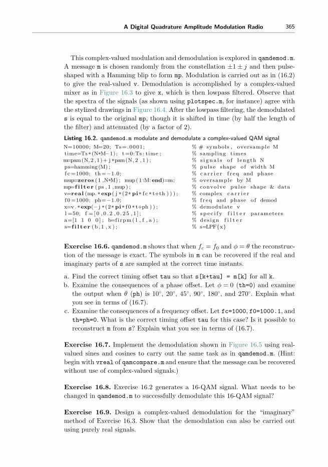
A Digital Quadrature Amplitude Modulation Radio 365
This complex-valued modulation and demodulation is explored in qamdemod.m.
A message m is chosen randomly from the constellation ±1± j and then pulse-
shaped with a Hamming blip to form mp. Modulation is carried out as in (16.2)
to give the real-valued v. Demodulation is accomplished by a complex-valued
mixer as in Figure 16.3 to give x, which is then lowpass filtered. Observe that
the spectra of the signals (as shown using plotspec.m, for instance) agree with
the stylized drawings in Figure 16.4. After the lowpass filtering, the demodulated
s is equal to the original mp, though it is shifted in time (by half the length of
the filter) and attenuated (by a factor of 2).
Listing 16.2. qamdemod.m modulate and demodulate a complex-valued QAM signal
N=10000; M=20; Ts=.0001; % # symbols , oversample Mtime=Ts*(N*M−1); t=0:Ts : time ; % sampling t imesm=pam(N,2 ,1)+ j *pam(N, 2 , 1 ) ; % s i g n a l s o f l ength Nps=hamming (M) ; % pul s e shape o f width M
f c =1000; th=−1.0; % c a r r i e r f r eq and phasemup=zeros (1 ,N*M) ; mup( 1 :M: end)=m; % oversample by Mmp=f i l t e r ( ps , 1 ,mup ) ; % convolve pu l s e shape & datav=real (mp. *exp ( j *(2* pi* f c * t+th ) ) ) ; % complex c a r r i e rf 0 =1000; ph=−1.0; % f r eq and phase o f demodx=v . *exp(− j *(2* pi* f0 * t+ph ) ) ; % demodulate vl =50; f = [ 0 , 0 . 2 , 0 . 2 5 , 1 ] ; % s p e c i f y f i l t e r parametersa=[1 1 0 0 ] ; b=f i rpm ( l , f , a ) ; % des i gn f i l t e rs=f i l t e r (b , 1 , x ) ; % s=LPF{x}
Exercise 16.6. qamdemod.m shows that when fc = f0 and φ = θ the reconstruc-
tion of the message is exact. The symbols in m can be recovered if the real and
imaginary parts of s are sampled at the correct time instants.
a. Find the correct timing offset tau so that s[k+tau] = m[k] for all k.
b. Examine the consequences of a phase offset. Let φ = 0 (th=0) and examine
the output when θ (ph) is 10◦, 20◦, 45◦, 90◦, 180◦, and 270◦. Explain what
you see in terms of (16.7).
c. Examine the consequences of a frequency offset. Let fc=1000, f0=1000.1, and
th=ph=0. What is the correct timing offset tau for this case? Is it possible to
reconstruct m from s? Explain what you see in terms of (16.7).
Exercise 16.7. Implement the demodulation shown in Figure 16.5 using real-
valued sines and cosines to carry out the same task as in qamdemod.m. (Hint:
begin with vreal of qamcompare.m and ensure that the message can be recovered
without use of complex-valued signals.)
Exercise 16.8. Exercise 16.2 generates a 16-QAM signal. What needs to be
changed in qamdemod.m to successfully demodulate this 16-QAM signal?
Exercise 16.9. Design a complex-valued demodulation for the “imaginary”
method of Exercise 16.3. Show that the demodulation can also be carried out
using purely real signals.

366 Chapter 16. A Digital Quadrature Amplitude Modulation Radio
e−j(2πf0t+θ)
x(t)v(t) s(t)phasesplitter
Figure 16.6 An alternative demodulation schemefor QAM uses a phase splitter followed by amixing with a complex exponential.
Exercise 16.10. Multiply the complex number a+ jb by ejα. Show that the
answer can be interpreted as a rotation through an angle α. Verify that the
matrix
R(α) =
(cos(α) − sin(α)
sin(α) cos(α)
)
carries out the same rotation when multiplied by the vector
(a
b
).
Exercise 16.11. Let s1(t), s2(t), m1(t), and m2(t) be defined as the inputs and
outputs of Figure 16.5. Show that(s1(t)
s2(t)
)=
1
2R(α)
(m1(t)
m2(t)
)for α = 2π(fc − f0)t+ φ− θ, where the rotation matrix R(α) is defined in Exer-
cise 16.10.
Exercise 16.12. Is it possible to build a demodulator for the 16-PPM protocol
of Exercise 16.4? Draw a block diagram or explain why it cannot be done.
Exercise 16.13. Is it possible to build a demodulator for the four-cosine mod-
ulation scheme of Exercise 16.5? Draw a block diagram or explain why it cannot
be done.
Exercise 16.14. An alternative method of demodulating a QAM signal uses a
“phase splitter,” which is a filter with Fourier transform
θ(f) =
{1 f ≥ 0,
0 f < 0.(16.8)
The phase splitter is followed by exponential multiplication as in Figure 16.6.
a. Implement a phase-splitter demodulation directly in the frequency domain
using (16.8).
b. Sketch the spectra of the signals v(t), x(t), and s(t) in Figure 16.6. The answer
should look something like the spectra in Figure 16.4.
c. Show that when fc = f0 and φ = θ the reconstruction of the message is exact.
d. Examine (by simulation) the consequences of a phase offset.
e. Examine (by simulation) the consequences of a frequency offset.

A Digital Quadrature Amplitude Modulation Radio 367
16.4 Carrier Recovery for QAM
It should be no surprise that the ability to reconstruct the message symbols from
a demodulated QAM signal depends on identifying the phase and frequency of
the carrier, because these are also required in the simpler PAM case of Chapter
10. Equation (16.7) illustrates explicitly what is required in order to recover
m(t) from s(t). To see how the recovery might begin, observe that the receiver
can adjust the phase θ and demodulating frequency f0 to any desired values. If
necessary, the receiver could vary the parameters over time. This section discusses
two methods of building an adaptive element to iteratively estimate a time-
varying θ, including the Costas loop for 4-QAM (which parallels the discussion
in Section 10.4 of the Costas loop for PAM) and a phase-locked loop for 4-QAM
(which parallels the discussion in Section 10.3 of a PLL for PAM). The variations
in phase can then be parlayed into improved frequency estimates following the
same kinds of strategies as in Section 10.6.
16.4.1 Costas Loop for 4-QAM
If it were possible to choose a time-varying θ(t) in (16.7) so that
θ(t) = 2π(fc − f0)t+ φ (16.9)
then s(t) would be directly proportional to m(t) because e−j2π(f0−fc)t+j(φ−θ(t)) =
1. The simplest place to begin is to assume that the frequencies are correct (i.e.,
that fc = f0) and that φ is fixed but unknown.
As in previous chapters, the approach is to design an adaptive element by
specifying a performance (or objective) function. Equation (16.9) suggests that
the goal in carrier recovery of QAM should involve an adaptive parameter θ that
is a function of the (unknown) parameter φ. Once this objective has been chosen,
an iterative algorithm can be implemented to achieve convergence.
Sampling perfectly downconverted 4-QAM signals s1(t) and s2(t) at the proper
times should produce one of the four pairs (1, 1), (1,−1), (−1, 1), and (−1,−1)
from the symbol constellation diagram in Figure 16.1. A rotation through 90◦ρ(for any integer ρ) will also produce samples with the same values, though they
may be a mixture of the symbol values from the two original messages. (Recall
that Exercise 16.6(b) asked for an explicit formula relating the various rotations
to the sampled (s1, s2) pairs.)
For the PAM system of Chapter 10, the phase θ is designed to converge to an
offset of an integer multiple of 180◦. The corresponding objective function JC for
the Costas loop from (10.15) is proportional to cos2(φ− θ), which has maxima
at θ = φ+ ρπ for integers ρ. This observation can be exploited by seeking an
objective function for QAM that causes the carrier-recovery phase to converge
to an integer multiple of 90◦. It will later be necessary to resolve the ambiguity
among the four choices. This is postponed until Section 16.4.2.
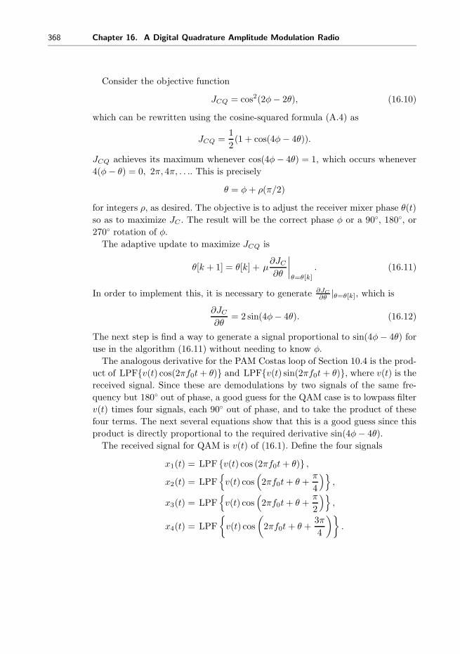
368 Chapter 16. A Digital Quadrature Amplitude Modulation Radio
Consider the objective function
JCQ = cos2(2φ− 2θ), (16.10)
which can be rewritten using the cosine-squared formula (A.4) as
JCQ =1
2(1 + cos(4φ− 4θ)).
JCQ achieves its maximum whenever cos(4φ− 4θ) = 1, which occurs whenever
4(φ− θ) = 0, 2π, 4π, . . .. This is precisely
θ = φ+ ρ(π/2)
for integers ρ, as desired. The objective is to adjust the receiver mixer phase θ(t)
so as to maximize JC . The result will be the correct phase φ or a 90◦, 180◦, or270◦ rotation of φ.
The adaptive update to maximize JCQ is
θ[k + 1] = θ[k] + μ∂JC∂θ
∣∣∣∣θ=θ[k]
. (16.11)
In order to implement this, it is necessary to generate ∂JC
∂θ |θ=θ[k], which is
∂JC∂θ
= 2 sin(4φ− 4θ). (16.12)
The next step is find a way to generate a signal proportional to sin(4φ− 4θ) for
use in the algorithm (16.11) without needing to know φ.
The analogous derivative for the PAM Costas loop of Section 10.4 is the prod-
uct of LPF{v(t) cos(2πf0t+ θ)} and LPF{v(t) sin(2πf0t+ θ)}, where v(t) is thereceived signal. Since these are demodulations by two signals of the same fre-
quency but 180◦ out of phase, a good guess for the QAM case is to lowpass filter
v(t) times four signals, each 90◦ out of phase, and to take the product of these
four terms. The next several equations show that this is a good guess since this
product is directly proportional to the required derivative sin(4φ− 4θ).
The received signal for QAM is v(t) of (16.1). Define the four signals
x1(t) = LPF {v(t) cos (2πf0t+ θ)} ,x2(t) = LPF
{v(t) cos
(2πf0t+ θ +
π
4
)},
x3(t) = LPF{v(t) cos
(2πf0t+ θ +
π
2
)},
x4(t) = LPF
{v(t) cos
(2πf0t+ θ +
3π
4
)}.

A Digital Quadrature Amplitude Modulation Radio 369
Using (A.8) and (A.9), and assuming f0 = fc,
x1(t) = LPF
{1
2m1(t)[cos(φ− θ) + cos(4πfct+ φ+ θ)]
−m2(t)[sin(φ − θ) + sin(4πfct+ φ+ θ)]
}=
1
2[m1(t) cos(φ− θ)−m2(t) sin(φ− θ)].
Similarly,
x2(t) =1
2[m1(t) cos(φ− θ − π/4)−m2(t) sin(φ − θ − π/4)] ,
x3(t) =1
2[m1(t) sin(φ− θ) +m2(t) cos(φ− θ)] ,
x4(t) =1
2[m1(t) cos(φ− θ − 3π/4)−m2(t) sin(φ− θ − 3π/4)] .
Now form the product of the four xi(t)s and simplify to obtain
x1(t)x2(t)x3(t)x4(t) =1
128[4m1(t)m2(t)(m
22(t)−m2
1(t)) cos(4φ− 4θ) (16.13)
− (m41(t)− 6m2
1(t)m22(t) +m4
2(t)) sin(4φ− 4θ)].
For a pulse shape p(t) such as a rectangle or the Hamming blip that is time-
limited to within one T -second symbol interval, p(t) = 0 for t < 0 or t > T .
Squaring both sides of the QAM pulse train (16.3) gives
m2i (t) =
∑k
s2i [k]p2(t− kT )
=∑k
p2(t− kT ) ≡ η(t)
for 4-QAM, where si[k] = ±1 and η(t) is some periodic function with period T .
Thus,
m21(t)−m2
2(t) = 0,
m41(t) = m4
2(t) = m21(t)m
22(t) = η2(t).
Accordingly, the four-term product simplifies to
x1(t)x2(t)x3(t)x4(t) = 4η2(t) sin(4φ− 4θ),
which is directly proportional to the desired derivative (16.12).
In this special case (where the pulse shape is time-limited to a single symbol
interval), θ of (16.11) becomes
θ[k + 1] = θ[k] + μx1(t)x2(t)x3(t)x4(t)∣∣t=kTs,θ=θ[k] , (16.14)
where Ts defines the time between successive updates (which is typically less
than the symbol period T ).

370 Chapter 16. A Digital Quadrature Amplitude Modulation Radio
LPF
LPF
−μΣ
cos(2πf0kTs+θ[k]+π/2)
cos(2πf0kTs+θ[k]+π/4)
θ[k]
LPF
cos(2πf0kTs+θ[k])
v(kTs)
LPF
cos(2πf0kTs+θ[k]+3π/4)
x1[k]
x2[k]
x3[k]
x4[k]
Figure 16.7 This “quadriphase”Costas-loop adaptive elementcan be used to identify anunknown phase offset in a4-QAM transmission. Thefigure is a block diagram ofEquation (16.14).
This adaptive element is shown schematically in Figure 16.7, where the
received signal v(t) is sampled to give v[k] and then mixed with four out-of-
phase cosines. Each path is lowpass filtered (with a cutoff frequency above 2fc)
and then multiplied to give the update term. The integrator μΣ is the standard
structure of an adaptive element, indicating that the new value is updated at
each iteration with a step size of μ.
The QAM Costas loop of (16.14) and Figure 16.7 is implemented in
qamcostasloop.m. The received signal is from the routine qamcompare.m on page
360, where the variable vreal is created by modulating a pair of binary message
signals. The four filters are implemented using the “time-domain method” of
Section 7.2.1 and the entire procedure mimics the Costas loop for PAM, which
is implemented in costasloop.m on page 208.
Listing 16.3. qamcostasloop.m simulate Costas loop for QAM
r=vr ea l ; % vr ea l from qamcompare .mf l =100; f =[0 . 2 . 3 1 ] ; a=[1 1 0 0 ] ; % f i l t e r s p e c i f i c a t i o nh=f i rpm ( f l , f , a ) ; % LPF des i gnmu=.003; % algor i thm s t ep s i z ef 0 =1000; q=f l +1; % f r eq at r e c e i v e rth=zeros (1 , length ( t ) ) ; th (1)=randn ; % i n i t i a l i z e es t imatez1=zeros (1 , q ) ; z2=zeros (1 , q ) ; % i n i t i a l i z e LPFsz4=zeros (1 , q ) ; z3=zeros (1 , q ) ; % z ’ s conta in past inputsfor k=1: length ( t )−1
s=2*r (k ) ;z1=[z1 ( 2 : q ) , s *cos (2* pi* f0 * t ( k)+th ( k ) ) ] ;z2=[z2 ( 2 : q ) , s *cos (2* pi* f0 * t ( k)+pi/4+th ( k ) ) ] ;z3=[z3 ( 2 : q ) , s *cos (2* pi* f0 * t ( k)+pi/2+th ( k ) ) ] ;z4=[z4 ( 2 : q ) , s *cos (2* pi* f0 * t ( k)+3*pi/4+th (k ) ) ] ;

A Digital Quadrature Amplitude Modulation Radio 371
0 0.2 0.4 0.6
−4
−2
0
2
Time
Phas
e of
fset Figure 16.8 Depending on where it is
initialized, the estimates made by theQAM Costas-loop element converge toθ ± ρπ/2. For this plot, the“unknown” θ was −1.0, and therewere 50 different initializations.
l p f 1=f l i p l r (h)* z1 ’ ; % output o f f i l t e r 1l p f 2=f l i p l r (h)* z2 ’ ; % output o f f i l t e r 2l p f 3=f l i p l r (h)* z3 ’ ; % output o f f i l t e r 3l p f 4=f l i p l r (h)* z4 ’ ; % output o f f i l t e r 4th ( k+1)=th (k)+mu* l p f 1 * l p f 2 * l p f 3 * l p f 4 ; % algor i thm update
end
Typical output of qamcostasloop.m appears in Figure 16.8, which shows the
evolution of the phase estimates for 50 different starting values of θ, th(1). Some
of these converge to the correct phase offset θ = −1.0, and others converge to
nearby values −1 + ρπ/2 for integers ρ. As expected, these stationary points
occur at all the 90◦ offsets of the desired value of θ.
When the frequency is not exactly known, the phase estimates of the Costas
algorithm try to follow. For example, in Figure 16.9, the frequency of the carrier
is f0 = 1000, while the assumed frequency at the receiver was fc = 1000.1. Fifty
different starting points were used, and in all cases the estimates converge to
lines with the same slope. The slope of these lines is directly proportional to
the difference in frequency between fc and f0, and this slope can be used as in
Section 10.6 to estimate the frequency difference.
Exercise 16.15. Use the preceding code to “play with” the Costas loop for
QAM.
a. How does the stepsize mu affect the convergence rate?
b. What happens if mu is too large (say mu=1)?
c. Does the convergence speed depend on the value of the phase offset?
d. When there is a small frequency offset, what is the relationship between the
slope of the phase estimate and the frequency difference?
Exercise 16.16. How does the filter h influence the performance of the Costas
loop?

372 Chapter 16. A Digital Quadrature Amplitude Modulation Radio
0 0.2 0.4 0.6
−4
−6
−2
0
2
Time
Phas
e of
fset
Figure 16.9 When the frequency of thecarrier is unknown at the receiver, thephase estimates “converge” to lines.The slope of these lines isproportional to the frequency offset,and can be used to correct theestimate of the carrier frequency.
a. Try fl = 1000, 30, 10, 3. In each case, use freqz to verify that the filter has
been properly designed.
b. Remove the LPFs completely from costasloop.m. How does this affect the
convergent values? The tracking performance?
Exercise 16.17. What changes are needed to qamcostasloop.m to enable it to
function with 16-QAM? (Recall Exercises 16.2 and 16.8.)
Exercise 16.18. Exercise 10.21 shows an alternative implementation of the PAM
Costas loop that uses cheaper fixed-phase oscillators rather than adjustable-
phase oscillators. Refer to Figure 10.12 on page 211. Design an analogous QAM
implementation and write a simulation (or modify qamcostasloop.m) to demon-
strate its operation.
Exercise 16.19. Figure 16.10 shows a high-level block diagram of a “dual-loop”
system for tracking a frequency offset in a QAM system.
a. Draw a detailed block diagram labeling all signals and blocks. For comparison,
the PAM equivalent (using PLLs) is shown in Figure 10.18.
b. Implement the dual-loop frequency tracker and verify that small frequency
offsets can be tracked. For comparison, the PAM equivalent is implemented
in dualplls.m on page 219.
c. How large can the frequency offset be before the tracking fails?
The previous discussion focused on the special case where the pulse shape is
limited to a single symbol interval. In fact, the same algorithm functions for more

A Digital Quadrature Amplitude Modulation Radio 373
θ1[k]v[k]
θ2[k] θ[k]+
CarrierRecovery
CarrierRecovery
Figure 16.10 Dual-carrier-recovery-loopConfiguration.
general pulse shapes. The key is to find conditions under which the update term
(16.13) remains proportional to the derivative of the objective function (16.12).
The generic effect of any small-stepsize adaptive element like (16.14) is to
average the update term over time. Observe that the four-term product (16.13)
has two parts: one is proportional to cos(4φ− 4θ) and the other is proportional
to sin(4φ− 4θ). Two things must happen for the algorithm to work: the average
of the cos term must be zero and the average of the sin term must always have
the same sign. The average of the first term is
avg{4m1(t)m32(t)− 4m2(t)m
31(t)}
while the average of the second is
avg{m41(t)− 6m2
1(t)m22(t) +m4
2(t)}.In QAM, the messages mi(t) are built as the product of the data si[k] and a
pulse shape as in (16.3). Even assuming that the average of the data values
is zero (which implies that the average of the messages is also zero), finding
these by hand for various pulse shapes is not easy. But they are straightforward
to find numerically. The following program calculates the desired quantities by
averaging over N symbols. The default pulse shape is the Hamming blip, but
others can be tested by redefining the variable unp=srrc(10,0.3,M,0) for a
square-root raised cosine pulse or unp=ones(1,M) for a rectangular pulse shape.
In all cases, the cosine term cterm is near zero while the sine term sterm is a
negative constant. Since the term appears in (16.13) with a negative sign, the
sine term is proportional to the derivative sin(4φ− 4θ). Thus it is possible to
approximate all the terms that enter into the algorithm (16.14).
Listing 16.4. qamconstants.m calculate constants for avg{x1 x2 x3 x4}N=2000; M=50; % # of symbols , oversample Ms1=pam(N, 2 , 1 ) ; s2=pam(N, 2 , 1 ) ; % r e a l 2− l e v e l s i g n a l smup1=zeros (1 ,N*M) ; mup2=zeros (1 ,N*M) ;mup1 ( 1 :M: end)=s1 ; % zero pad T−spaced sequencemup2 ( 1 :M: end)=s2 ; % oversample by Munp=hamming (M) ; % unnormalized pu l s e shapep=sqrt (M)*unp/ sqrt (sum( unp . ˆ 2 ) ) ; % normal ized pu l s e shapem1=f i l t e r (p , 1 ,mup1 ) ; % convolve pu l s e shape & datam2=f i l t e r (p , 1 ,mup2 ) ; % convolve pu l s e shape & datasterm=sum( (m1.ˆ4)−6*(m1. ˆ 2 ) . * (m2.ˆ2)+(m2. ˆ 4 ) ) / (N*M)cterm=sum(4*m1. *m2.ˆ3−4*m1. ˆ 3 . *m2)/(N*M)

374 Chapter 16. A Digital Quadrature Amplitude Modulation Radio
Exercise 16.20. Find a pulse shape p(t) and a set of symbol values s1 and s2that will cause the QAM Costas loop to fail. Hint: find values so that the average
of the sinusoidal term is near zero. Redo the simulation qamcostasloop.m with
these values and verify that the system does not achieve convergence.
Exercise 16.21. Suppose that si[k] are binary ±1 and that avg{s1[k]} =
avg{s2[k]} = 0. The message sequences mi(t) are generated as in (16.3). Show
that avg{m1(t)} = avg{m2(t)} = 0 for any pulse shape p(t).
Exercise 16.22. Suppose that avg{m1(t)} = avg{m2(t)} = 0. Which of the
following are true?
a. avg{m1(t)}+ avg{m2(t)} = avg{m1(t) +m2(t)}b. avg{4m1(t)} + 2avg{m2(t)} = avg{4m1(t) + 2m2(t)}c. avg{m1(t)m2(t)} = avg{m1(t)}avg{m2(t)}d. avg{m2
1(t)} = avg{m1(t)}2e. avg{m2
1(t)m22(t)} = avg{m2
1(t)}avg{m22(t)}
f. Show that, even if (c) holds, (e) need not.
Other variations of this “quadriphase” Costas loop can be found in Sections
6.3.1 and 6.3.2 of Bingham (1988) and in Section 4.2.3 of Anderson (1999).
16.4.2 Resolution of the Phase Ambiguity
The carrier-recovery element for QAM does not have a unique convergent
point because the objective function JCQ of (16.10) has maxima whenever
θ = φ+ ρπ/2. This is shown clearly in the multiple convergence points of Figure
16.8. The four possibilities are also evident from the rotational symmetry of the
constellation diagrams (such as Figures 16.1 and 16.2). There are several ways
in which the phase ambiguity can be resolved, including
1. the output of the downsampler can be correlated with a known training signal,
2. the message source can be differentially encoded so that the information is
carried in the successive changes in the symbol values (rather than in the
symbol values themselves)
One way to implement the first method is to correlate the real part of the
training signal t with both the real s1 and the imaginary s2 portions of the
output of the downsampler. Whichever correlation has the larger magnitude is
selected and its polarity examined. To write this concisely, let 〈t, si〉 represent

A Digital Quadrature Amplitude Modulation Radio 375
the correlation of t with si. The four possibilities are as follows:
if |〈t, s1〉| > |〈t, s2〉|〈t, s1〉 > 0 → no change,
〈t, s1〉 < 0 → add 180◦;
if |〈t, s1〉| < |〈t, s2〉|〈t, s2〉 > 0 → add 90◦,
〈t, s2〉 < 0 → add − 90◦.
Using differential encoding of the data bypasses the need for resolving the
ambiguous angle. To see how this might work, consider the 2-PAM alphabet ±1
and re-encode the data so that a +1 is transmitted when the current symbol is
the same as the previous symbol and a −1 is transmitted whenever it changes.
Thus the sequence
1,−1,−1, 1,−1,−1, 1, 1, 1, . . .
is differentially encoded (starting from the second element) as
−1, 1,−1,−1, 1,−1, 1, 1, . . .
The process can be reversed as long as the value of the first bit (in this case a 1)
is known. This strategy can be extended to complex-valued 4-QAM by encoding
the differences s[k]− s[k − 1]. This is described in Figure 16-4 of Barry, Lee, and
Messerschmitt (2004). An advantage of differential encoding is that no training
sequence is required. A disadvantage is that a single error in the transmission
can cause two symbol errors in the recovered sequence.
Exercise 16.23. Implement the correlation method to remove the phase ambi-
guity.
a. Generate a complex 4-QAM signal with a phase rotation φ by use of
qamcompare.m. Specify a fixed training sequence.
b. Use the QAM Costas loop qamcostasloop.m to estimate φ.
c. Implement the correlation method in order to disambiguate the received sig-
nal. Verify that the disambiguation works with φ = 60◦, 85◦, and 190◦.
Exercise 16.24. Design a differential encoding scheme for 4-QAM using suc-
cessive differences in the data. Verify that the scheme is insensitive to a 90◦
rotation.
16.4.3 Phase-Locked Loop for 4-QAM
Section 10.1 shows how the carrier signal in a PAM transmission is concealed
within the received signal. Using a squaring operation followed by a bandpass

376 Chapter 16. A Digital Quadrature Amplitude Modulation Radio
filter (as in Figure 10.3 on page 197) passes a strong sinusoid at twice the fre-
quency and twice the phase of the carrier. This double-frequency surrogate can
then be used as an input to a phase-locked loop for carrier recovery as in Section
10.3.
In QAM, the carrier is better hidden because it is generated as in (16.1) by
combining two different signals modulated by both sin(·) and cos(·) or, equiv-
alently, by the real and imaginary parts of a complex modulating wave as in
(16.2). What kind of preprocessing can bring the carrier into the foreground?
An analogy with the processing in the Costas loop suggests using the fourth
power of the received signal. This will quadruple (rather than double) the fre-
quency of the underlying carrier, and so the fourth power needs to be followed
by a narrow-bandpass filter centered at (about) four times the carrier frequency.
This quadruple-frequency surrogate can then be used as an input to a standard
phase-locked loop for carrier recovery.
The first step is to verify that using the square really is futile. With v(t) defined
in (16.1), it is straightforward (though tedious) to show that
v2(t) =1
2[m2
1(t) +m22(t) + (m2
1(t)−m22(t)) cos(4πfct+ 2φ)
− 2m1(t)m2(t) sin(4πfct+ 2φ)].
A bandpass filter with center frequency at 2fc removes the constant DC term,
and this cannot be used (as in PAM) to extract the carrier since avg{m21(t)−
m22(t)} = avg{m1(t)m2(t)} = 0. Nothing is left after passing v2(t) through a
narrow-bandpass filter.
The fourth power of v(t) has three kinds of terms: DC terms, terms near
2fc, and terms near 4fc. All but the latter are removed by a BPF with center
frequency near 4fc. The remaining terms are
BPF{v4(t)} =1
8[4m1(t)m2(t)(m
22(t)−m2
1(t)) sin(8πfct+ 4φ)
− (m41(t)− 6m2
1(t)m22(t) +m4
2(t)) cos(8πfct+ 4φ)].
What is amazing about this equation is that the two terms 4m1m2(m22 −m2
1)
and m41 − 6m2
1m22 +m4
2 are identical to the two terms in (16.13). Accordingly,
the former averages to zero while the latter has a nonzero average. Thus
BPF{v4(t)} ∝ cos(8πfct+ 4φ)
and this signal can be used to identify (four times) the frequency and (four times)
the phase of the carrier.
In typical application, the carrier frequency is known only approximately, that
is, the BPF must use the center frequency f0 rather than fc itself. In order to
make sure that the filter passes the needed sinusoid, it is wise to make sure that
the bandwidth is not too narrrow. On the other hand, if the bandwidth of the
BPF is too wide, unwanted extraneous noises will also be passed. This tension

A Digital Quadrature Amplitude Modulation Radio 377
−μΣθ[k]v(kTs)
sin(8πf0kTs+4θ[k])
LPFBPFX4
centeredat ~4fc
Figure 16.11 The sampled QAM input v(kTs) is raised to the fourth power and passedthrough a BPF. This extracts a sinusoid with frequency 4fc and phase 4φ. Astandard PLL extracts 2φ for use in carrier recovery.
suggests a design trade-off between the uncertainty in fc and the desire for a
narrow BPF.
Exercise 16.25. Generate a complex 4-QAM signal v(t) with phase shift φ as in
qamcompare.m. Imitate the code in pllpreprocess.m on page 196, but raise the
signal to the fourth power and choose the center frequency of the BPF to be 4fc.
Verify that the output is (approximately) a cos wave of the desired frequency
4fc and phase 4φ. This may be more obvious in the frequency domain.
Exercise 16.26. What happens on raising v(t) to the eighth power? Can this
be used to recover (eight times) the carrier frequency at (eight times) the phase?
Explain why or why not.
The output BPF{v4(t)} of the preprocessor is presumed to be a sinusoid that
can be applied to a phase-tracking element such as the digital phase-locked loop
(PLL) from Section 10.3. The preprocessor plus PLL are shown in Figure 16.11,
which is the same as the PLL derived for PAM in Figure 10.7, except that it
must operate at 4fc (instead of 2fc) and extract a phase equal to 4φ (instead
of 2φ). Observe that this requires that the digital signal be sampled at a rate
sufficient to operate at 4fc in order to avoid aliasing. In practice, such a rapid
sampling rate can be a tall order.
Though this section has focused on a fourth-power method of carrier recovery
for 4-QAM, the methods are also applicable to larger constellations such as 16-
QAM. The literature offers some encouraging comments. For instance, Anderson
(1999) on page 149 states:
When the . . . modulation is, for instance 16-QAM instead of QPSK, the PLL refer-ence signal is not a steady cos(4ω0t+ 4ψ0) and the phase difference signal has othercomponents besides sin(4ψ0 − 4φ0). Nonetheless, the synchronizer still works passablywell.
Bingham (1988) on page 173 says:
This simple method [PLL tracking of quadrupled frequency] can be used for constel-lations with 16 points . . . but it has been generally assumed that the pattern jitterwould be intolerable. However, it can be shown that, at least for 16-QAM, the outerpoints dominate, and the fourth-power signal has a component at 4fc that is usableif a very narrow band PLL is used to refine it. Whether the independence from data

378 Chapter 16. A Digital Quadrature Amplitude Modulation Radio
decisions and equalizer convergence that this forward-acting method offers outweighsthe problems of such a narrow-band PLL remains to be seen.
Exercise 16.27. Implement the 4-QAM PLL system shown in Figure 16.11.
Begin with the preprocessor from Exercise 16.25 and combine this with a modi-
fied version of pllconverge.m from page 204.
Exercise 16.28. What changes need to be made to the 4-QAM preprocessor of
Exercise 16.25 and the corresponding PLL of Exercise 16.27 in order to operate
with a 16-QAM constellation?
16.5 Designing QAM Constellations
This chapter has focused on 4-QAM, and occasionally considered other QAM
constellations such as the 16-QAM configuration in Figure 16.2. This section
shows a few common variations and suggests some of the trade-offs that occur
with different spacing of the points in the constellation.
As with PAM, the clearest indicator of the resilience of a constellation with
respect to noise is the distance between points. The transmission is less likely to
have bits (and hence symbols) changed when the points are far apart and more
likely to encounter errors when the points are close together. This means that,
when greater power is used in the transmission, more noise can be tolerated.
Accordingly, it is common to normalize the power and to consider the symbol
error rate (SER) as a function of the signal-to-noise ratio (SNR). Effectively,
this means that the points in a constellation such as 16-QAM of Figure 16.2 are
closer together than in a simpler constellation such as 4-QAM.
It is straightforward to calculate the SER as a function of the SNR via simula-
tion. The routine qamser.m specifies a M-QAM constellation and then generates
N symbols. Noise with variance N0 is added and then a comparison is made. If
the noise causes the symbol to change then an error has occurred. This can be
plotted for a number of different noise variances. The most complicated lines
in the routine are those comparing the real and imaginary portions of the data
s and the noisy version r to determine whether the noise has caused a symbol
error.
Listing 16.5. qamser.m symbol error rate for QAM in additive noise
N0=10.ˆ(0: − . 2 : −3) ; % no i s e va r i anc e sN=10000; % # symbols to s imulateM=4; % # symbols in c o n s t e l l a t i o ns=pam(N, sqrt (M) ,1)+ j *pam(N, sqrt (M) , 1 ) ; % QAM symbolss=s/ sqrt ( 2 ) ; % normal ize powerconst=unique ( real ( s ) ) ; % normal ized symbol va luesa l l s e r s = zeros ( size (N0 ) ) ;for i =1: length (N0) % loop over SNR
n=sqrt (N0( i )/2)* (randn (1 ,N)+ j *randn (1 ,N) ) ;r=s+n ; % r ec e i v ed s i g n a l+no i s e

A Digital Quadrature Amplitude Modulation Radio 379
0 5 10 15 20 25 30
10−4
10−3
10−2
10−1
100
Sym
bol E
rror
Rat
e
SNR in dB
4-QAM
16-QAM64-QAM
256-QAM
Figure 16.12 SER versus SNR forvarious M -QAM constellations.For a given SNR, simplerconstellations provide a morerobust transmission. For a givenconstellation, larger SNRs givefewer errors. The black dots areplotted by the simulation inqamser.m. The lines are a plot ofthe theoretical formula (16.15).
r e a l e r r=quantalph ( real ( r ) , const )==quantalph ( real ( s ) , const ) ;imagerr=quantalph ( imag( r ) , const )==quantalph ( imag( s ) , const ) ;SER=1−mean( r e a l e r r . * imagerr ) ; % determine SER by countinga l l s e r s ( i )=SER; % # symbols w/ RE+IM co r r e c t
end
When the percentage of errors is plotted against the SNR, the result is a
“waterfall” plot such as Figure 16.12. Large noises (small SNR) imply large
error rates while small noises cause few errors. Thus each constellation shows a
characteristic drop-off as the SNR increases. On the other hand, for a given SNR,
the constellations with the most widely distributed points have fewer errors.
For Gaussian noises (as generated by randn), soft errors in recovering the mes-
sage pairs are circularly distributed about each constellation point. Accordingly,
it is wise to try to keep the points as far apart as possible, under the constraint
of equal power. Thus any four-point constellation should be a square in order to
avoid one pair of symbol errors becoming more likely.
The simulation qamser.m can be run with any noise distribution and with
any conceivable constellation. For regular QAM constellations and independent
Gaussian noise, there is a formula that predicts the theoretical shape of the
waterfall curve. Let σ2a be the variance of the Gaussian noise and σ2
s the variance
of the symbol sequence. Proakis and Salehi (2002), on page 422, show that the
probability of an incorrect decision for an M -QAM system is
1−[1−
(1− 1√
M
)erfc
(√3σ2
s
2(M − 1)σ2a
)]2, (16.15)
where the erfc is the complementary error function (see help erfc in Matlab).
This formula is superimposed on the simulations for 4-, 16-, 64-, and 256-QAM
in Figure 16.12 and obviously agrees closely with the simulated results. This plot
was generated by the routine sersnr.m which is available on the website.
Of course, there is no need to restrict a constellation to a regular grid of points,
though rectangular grids will tend to have better noise rejection. For example,

380 Chapter 16. A Digital Quadrature Amplitude Modulation Radio
Figure 16.13 The V.29 constellation has 16 symbolsand four different energy levels.
a system designer could choose to omit the four corner points in a square QAM
constellation. This would reduce the signal power range over which analog elec-
tronics of the system must retain linearity. Nonsquare QAM constellations can
also be easier to synchronize, though they will tend to have higher SER (for
the same SNR) than square constellations because there is a smaller minimum
distance between points in constellations of the same total power. For exam-
ple, Figure 16.13 shows an irregular constellation called the V.29 constellation.
Anderson (1999) comments on page 97 that the V.29 modem standard
has worse error performance in AWGN than does . . . [square] 16-QAM, but it is easierto synchronize.
Another consideration in constellation design is the assignment of bit values
to the points of the constellation. One common goal is to reduce the number of
bit changes between adjacent symbols. For 4-QAM, this might map 45◦ → 00,
135◦ → 01, −135◦ → 11, and −45◦ → 10. Mappings from constellation points to
symbols that minimize adjacent symbol errors are called Gray codes.
Exercise 16.29. Adapt qamser.m to draw the waterfall plot for the V.29 con-
stellation of Figure 16.13.
Exercise 16.30. If different noises are used, the waterfall plot may look signif-
icantly different than Figure 16.12. Redraw the SER vs SNR curves for 4-, 16-,
64-, and 256-QAM when the noise is uniform.
16.6 Timing Recovery for QAM
When a QAM signal arrives at the receiver it is a complicated analog waveform
that must be demodulated and sampled in order to eventually recover the two
messages hidden within. The timing-recovery element specifies the exact times
at which to sample the demodulated signals. One approach would be to use
two timing parameters τ1 and τ2 operating independently on the two message
signals s1 and s2 using any of the methods described in Chapter 12. But the two

A Digital Quadrature Amplitude Modulation Radio 381
sampled signals are not unrelated to each other. Though the messages themselves
are typically considered to be uncorrelated, the two signals have been modulated
and demodulated simultaneously, and so they are tightly synchronized with each
other. A better approach is to adapt a single parameter τ that specifies when to
sample both signals.
The problem is approached by finding performance or objective functions that
have maxima (or minima) at the optimal point (i.e., at the correct sampling
instants). The performance functions are then used to define adaptive elements
that iteratively estimate the correct sampling times. As usual in Software
Receiver Design, all other aspects of the system are presumed to operate
flawlessly: the upconversions and downconversions are ideal, the pulse-matched
filters are well designed, there is no interference, and the channel is benign. More-
over, both baseband signals are assumed to occupy the same bandwidth and the
sampling is fast enough to avoid problems with aliasing.
The oversampled sequences are filtered by matched filters that correspond to
the pulse shape at the transmitter. The output of the matched filters is sent into
interpolators that extract the two baud-spaced sequences. When all goes well,
these can be decoded into the original messages s1 and s2. For PAM signals as in
Chapter 12, the baud-timing rate can be found by optimizing the average of the
first, second, or fourth power of the absolute values of the baud-spaced sequence
values. For some pulse shapes and powers, it is necessary to minimize, whereas
others require maximization.
The demodulated QAM signal contains two independent signals s1 and s2 with
the same timing offset, or, equivalently, it is a single complex-valued signal s. By
analogy with PAM, it is reasonable to consider optimizing the average of powers
of s, that is, to maximize or minimize
JQ(τ) = avg{(|s1|p + |s2|p)q} (16.16)
for p = 1, 2, or 4 and q = 12 , 1, or 2. Of course, other values for p and q might
also be reasonable.
While the error surfaces for these objective functions are difficult to draw
exactly, they are easy to calculate numerically, as is familiar for PAM from
clockrecDDcost.m on page 259 (also see Figures 12.8 and 12.11). The routine
qamtimobj.m calculates the value of the objective function over a range of dif-
ferent τs for a given pulse shape unp. In this simulation, an offset of τ = 12is the
desired answer.
Listing 16.6. qamtimobj.m draw error surfaces for baseband signal objective functions
m=20; n=1000; % n data points , m+1 tausunp=hamming (m) ; % pul s e shapecp=conv(unp , unp ) ; % matched f i l t e rps=sqrt (m)* cp/ sqrt (sum( cp . ˆ 2 ) ) ; % normal izecos t=zeros (m+1 ,1) ;for i =1:m+1 % f o r each o f f s e t
s1=pam(n/m, 2 , 1 ) ; s2=pam(n/m, 2 , 1 ) ; % c r ea t e 4−QAM sequencemup1=zeros (1 , n ) ;mup1 ( 1 :m:end)=s1 ; % zero pad and upsample

382 Chapter 16. A Digital Quadrature Amplitude Modulation Radio
0 0.2 0.4 0.6 0.8 1Timing offset τ
Val
ue o
f ob
ject
ive
func
tions
(b)(d)
(c)
(e)
(a)
Figure 16.14 Five objective functionsJQ(τ ) of (16.16) for the timing-recoveryproblem are plotted versus the timingoffset τ . For the computation, τ = 1
2is
the desired answer. This figure assumesthe Hamming pulse shape. (a) p = 2,q = 1
2, (b) p = 2, q = 1, (c) p = 2, q = 2,
(d) p = 1, q = 1, (e) p = 4, q = 1.
mup2=zeros (1 , n ) ;mup2 ( 1 :m: end)=s2 ;m1=f i l t e r ( ps , 1 ,mup1 ) ; % convolve pu l s e shape & datam2=f i l t e r ( ps , 1 ,mup2 ) ; % convolve pu l s e shape & datasm1=m1( ( length ( ps )−1)/2+ i :m: end ) ; % sampled baseband datasm2=m2( ( length ( ps )−1)/2+ i :m: end ) ; % with timing o f f s e t iT/mcos t ( i )=sum( sqrt ( sm1.ˆ2+sm2 . ˆ 2 ) ) / length ( sm1 ) ; % obj . f unc t i on
end
The output of qamtimobj.m is shown in Figure 16.14 for several objective
functions using the Hamming pulse shape:
a)( p = 2, q = 12: avg{
√s21 + s22}
b)( p = 2, q = 1: avg{s21 + s22}c)( p = 2, q = 2: avg{(s21 + s22)
2}d)( p = 1, q = 1: avg{|s1|+ |s2|}e)( p = 4, q = 1: avg{s41 + s42}
Observe that the solid curve (c), called the fourth-power objective function
because it can also be written avg{||s||4}, has the steepest slope about the desiredanswer. This should exhibit the fastest convergence, though it will also react most
quickly to noises. This is an example of the classic trade-off in adaptive systems
between speed of convergence and robustness to disturbances. Similar curves can
be drawn for other pulse shapes such as the square-root raised cosine. As occurs
for the PAM case in Figure 12.11, some of these may require maximization, while
others require minimization.
Using the fourth-power objective function (e) (i.e., p = 4, q = 1 in (16.16)), an
adaptive element can be built by descending the gradient. This is
τ [k + 1] = τ [k] − ¯μ∂(m4
1(kT + τ) +m42(kT + τ))
∂τ
∣∣∣∣τ=τ [k]
= τ [k]− μ
[(m3
1(kT + τ) +m32(kT + τ))
× ∂(m1(kT + τ) +m2(kT + τ))
∂τ
]∣∣∣∣τ=τ [k]
.

A Digital Quadrature Amplitude Modulation Radio 383
As in Sections 12.3 and 12.4, the derivative can be approximated numerically
τ [k + 1] = τ [k]− μ(m31(kT + τ [k]) +m3
2(kT + τ [k]))
× [m1(kT + τ + δ)−m1(kT + τ − δ)
+m2(kT + τ + δ)−m2(kT + τ − δ)],
where μ = μ/δ and δ is small and positive. All of the values for the mi(t) for
the offsets τ [k], τ [k]− δ, and τ [k] + δ can be interpolated from the oversampled
mi. Clearly, a similar derivation can be made for any of the objective functions
(a)–(e).
Which criterion is “best”? Barry, Lee, and Messerschmitt (2004) on page 747
say that:
For some signals, particularly when the excess bandwidth is low, a fourth power nonlin-earity . . . is better than the magnitude squared. In fact, fourth-power timing recoverycan even extract timing tones from signals with zero excess bandwidth. . . . Simulationsfor QPSK . . . suggest that fourth-power circuits out-perform absolute-value circuits forsignals with less than about 20% excess bandwidth.
What about aliasing? Barry, Lee, and Messerschmitt continue:
If timing recovery is done in discrete-time, aliasing must be considered . . . Any non-linearity will increase the bandwidth of the . . . signal . . . In the presence of sampling,however, the high frequency components due to the nonlinearity can alias back into thebandwidth of the bandpass filter, resulting in additional timing jitter. . . . Therefore, ina discrete-time realization, a magnitude-squared nonlinearity usually has a considerableadvantage over either absolute-value or fourth-power nonlinearity.
What about attempting baud-timing recovery on a passband signal prior to full
downconversion to baseband? Barry, Lee, and Messerschmitt (2004) consider this
on page 750:
The same relative merits of squaring, absolute-value, and fourth-power techniques applyto passband timing recovery as to baseband. In particular, absolute-value and fourth-power are usually better than squaring, except when aliasing is a problem in discrete-time implementations. As with baseband signals, it is sometimes advantageous to pre-filter the signal before squaring.
Exercise 16.31. Use qamtimobj.m as a basis to calculate the five objective
functions for 4-QAM using the SRRC pulse shape with rolloff factors 0.1, 0.5,
and 0.7.
a. For each case, state whether the objective must be maximized or minimized.
b. Do any of the objective functions have local stationary points that are not
globally optimal? (Recall Figure 12.8, which shows local minima for PAM.)
c. Derive the corresponding adaptive element (i.e., the update equation for τ [k])
for one of the objective functions when using the SRRC. Which rolloff factor
is best? Why?

384 Chapter 16. A Digital Quadrature Amplitude Modulation Radio
Exercise 16.32. Mimic clockrecOP.m on page 262 to implement the timing-
recovery algorithm for τ [k] using objective function (e).
a. Derive the adaptive-element update for objective function (a).
b. Implement the adaptive element for objective (a).
c. Choose stepsizes μ so that the two methods converge in approximately the
same number of iterations.
d. Add noise to the two methods. Which of the methods is more resilient to the
added noise?
Exercise 16.33. State a dispersion-based objective function for timing recovery
of QAM analogous to that in Figure 12.11.
a. Plot the value of the objective function against the timing offset τ .
b. Derive the corresponding adaptive element, i.e., the update equation for τ [k].
c. Implement the adaptive element (mimicking clockrecOP.m on page 262).
16.7 Baseband Derotation
Carrier recovery identifies the phase and frequency differences between the mod-
ulating sinusoids at the transmitter and the demodulating sinusoids at the
receiver. Standard approaches such as the PLL or Costas loop of Section 16.4
operate at “passband,” that is, the iteration that identifies the phases and fre-
quencies operates at the sampling rate of the receiver, which is typically higher
than the symbol rate.
As observed in Section 16.3, a phase offset can be pictured as a rotation of
the constellation and a frequency offset can be interpreted as a spinning of the
constellation diagram. Of course these are “baseband” diagrams, which show
the symbol values after the timing recovery has downsampled the signal to the
symbol rate. This suggests that it is also possible to approach carrier recovery
at baseband, by constructing an adaptive element that can derotate a skewed
constellation diagram. This section shows how carefully designed adaptive ele-
ments can derotate a QAM constellation. These are essentially single-parameter
equalizers that operate on the two real data streams by treating the signal and
equalizer as complex-valued quantities.
Bingham (1988), on page 231, motivates the post-equalization carrier-recovery
process for QAM:
A complex equalizer . . . can compensate for any demodulating carrier phase, but itis easier to deal with frequency offset by using a separate circuit or algorithm that,because it deals with only one variable, carrier phase, can move faster without causingjitter.

A Digital Quadrature Amplitude Modulation Radio 385
r(t)s(t) x(t)e−jφ ejθ
Figure 16.15 The complex-valued signal r(t) hasbeen rotated through an (unknown) angle −φ. Ifthis is passed through a complex factor ejθ withθ ≈ φ, the complex-valued x(t) approaches theunrotated message s(t).
The situation is this: some kind of (passband) carrier recovery has been done,
but it is imperfect and a slow residual rotation of the constellation remains.
Bingham’s first sentence observes that a complex-valued equalizer (such as those
detailed in Section 16.8) can accomplish the derotation at the same time that it
equalizes, by multiplying all of the (complex) equalizer coefficients by the same
complex factor ejθ. But equalizers have many parameters: real-valued equalizers
such as those in Chapter 13 can have dozens (and some real-world equalizers
have hundreds) of parameters. It takes longer to adjust a dozen parameters than
to adjust one. A dozen parameters introduce more jitter than a single parameter.
Even worse, consider a situation where a multitap equalizer has adapted to
perfectly equalize a complex channel. If the carrier now begins to develop a
rotational offset, all of the coefficients of the equalizer will move (multiplied by
the factor ejθ). Thus all of the otherwise well-set equalizer gains move in order
to accomplish a task that could be dealt with by a single parameter (the value
of the rotation θ). Never send a dozen parameters to do a job when one will do!
To see how this works, model the (downsampled) received signal as r(t) =
e−jφs(t), where −φ represents the carrier phase offset. A “one-tap equalizer”
is the system ejθ as shown in Figure 16.15. Clearly, if the parameter θ can
be adjusted to be equal to the unknown φ, the carrier offset is corrected and
x(t) = s(t).
As in the design of any adaptive element, it is necessary to choose an objective
function. There are several possibilities, and the remainder of this section details
two: a decision-directed strategy and a dispersion-minimization strategy. At the
end of the day, the derotated signals x1 and x2 will be sampled and quantized
to give the hard decisions s1 = sign(x1) and s2 = sign(x2), which can be written
more compactly as s = sign(x) with s = s1 + js2.
Consider as objective function the average of
JBD(θ) = (1/2)(s− x)(s− x)∗,
where the superscript ∗ indicates complex conjugation. An element that adapts
θ so as to minimize this objective is
θ[k + 1] = θ[k]− μ
2
∂(s− x)(s − x)∗
∂θ
∣∣∣∣θ=θ[k]
.
The objective can be rewritten
(s− x)(s − x)∗ = (s1 − x1)2 + (s2 − x2)
2
since the imaginary parts cancel out. Hence
∂JBD(θ)
∂θ= −(s1 − x1)
∂x1
∂θ− (s2 − x2)
∂x2∂θ
.

386 Chapter 16. A Digital Quadrature Amplitude Modulation Radio
The x can be rewritten explicitly as a function of θ since x = ejθr, which is
x1 = r1 cos(θ)− r2 sin(θ),
x2 = r2 cos(θ) + r1 sin(θ)
when expressed in real and imaginary form (observe the similarity to Exercise
16.10). Accordingly,
∂x1
∂θ= −r1 sin(θ)− r2 cos(θ) = −x2,
∂x2
∂θ= −r2 sin(θ) + r1 cos(θ) = x1.
Thus
∂JBD(θ)
∂θ= (s1 − x1)x2 − (s2 − x2)x1 = s1x2 − s2x1
leads to the adaptive update for 4-QAM
θ[k + 1] = θ[k]− μ(s1[k]x2[k]− s2[k]x1[k]), (16.17)
which can be compared directly to Figure 16-6 in Barry, Lee, and Messerschmitt.
Implementation of (16.17) requires access to the signals s1[k] and s2[k]. This
can be accomplished using a training sequence, or more commonly by using a
decision-directed variation that replaces s1[k] with s1[k] and s2[k] with s2[k].
The adaptive derotator element can be examined in operation in
qamderotate.m, where the 4-QAM message is rotated by an angle -phi. After
the derotator, the x (and the hard decisions shat1 and shat2) restore the con-
stellation to its proper orientation.
Listing 16.7. qamderotate.m derotate a complex-valued QAM signal
N=1000; j=sqrt (−1); % # symbols , time bases=pam(N,2 ,1)+ j *pam(N, 2 , 1 ) ; % s i g n a l s o f l ength Nphi =−0.1; % angle to r o ta t er=s . *exp(− j * phi ) ; % r o ta t i onmu=0.01; theta =0; theta=zeros (1 ,N) ; % i n i t i a l i z e v a r i a b l e sfor i =1:N−1 % adapt through a l l data
x=exp ( j * theta ( i ) )* r ( i ) ; % x=rotated ( r )x1=real ( x ) ; x2=imag(x ) ; % r e a l and imaginary par tsshat1=sign ( x1 ) ; shat2=sign ( x2 ) ; % hard d e c i s i o n stheta ( i+1)=theta ( i )−mu*( shat1 *x2−shat2 *x1 ) ; % i t e r a t i o n
end
An alternative objective function based on dispersion minimization considers
the average of
JDM (θ) = (Re{rejθ}2 − γ)2, (16.18)
where γ is a real constant. This objective function can be viewed as the projection
onto the real axis of a rotated, but otherwise perfect, symbol constellation. Since
the real parts of the 4-QAM symbols cluster around ±1, choosing γ = 1 allows
JDM (θ) to be zero when θ = φ. For other constellations, JDM (θ)|θ=φ will, on

A Digital Quadrature Amplitude Modulation Radio 387
average, be smaller than nearby values. The associated dispersion-minimizing
adaptive element is
θ[k + 1] = θ[k]− μ(Re{rejθ}2 − γ)Re{rejθ[k]}Im{rejθ[k]}. (16.19)
Exercise 16.34. Rewrite the system in Figure 16.15 in its real (implementable)
form by letting s(t) = s1(t) + js2(t) and ejz = cos(z) + j sin(z). Express x(t)
directly as a function of the real-valued signals s1(t) and s2(t). Show that θ = φ
implies x(t) = s(t).
Exercise 16.35. Reimplement the qamderotate.m routine without using any
complex numbers.
Exercise 16.36. Calculate the derivative of JDM (θ) of (16.18) with respect to
θ, which is used to implement the algorithm (16.19).
Exercise 16.37. Implement the dispersion-minimization derotator by mimick-
ing qamderotate.m.
Exercise 16.38. Formulate a DD derotator for use with 16-QAM. Implement
it in imitation of qamderotate.m. Is the convergence faster or slower than with
4-QAM?
Exercise 16.39. Formulate a dispersion-minimization derotator for use with
16-QAM.
Exercise 16.40. Formulate a derotator for use with 16-QAM that uses only the
four corner points of the constellation, those with the highest SNR.
16.8 Equalization for QAM
Intersymbol interference (ISI) occurs when symbols interact, when the waveform
of one symbol overlaps and corrupts the waveform of other symbols nearby in
time. ISI may be caused by overlapping pulse shapes (as discussed in Chapter
11) or it may be caused by a nonunity transmission channel, physically a result of
multipath reflections or frequency-selective dispersion. Chapter 13 showed that
for PAM, the (real-valued) received symbols can often be passed through a (real-
valued) equalizer in order to undo the effects of the channel. It is possible to pass
both the real and the imaginary parts of a QAM signal through separate (real-
valued) equalizers, but it is far more convenient to model the equalization portion
of a QAM receiver as complex-valued symbols passing through a complex-valued
equalizer.
This section shows that complex-valued equalizers are no more difficult to
design and implement than their real-valued counterparts. As in Chapter 13, the

388 Chapter 16. A Digital Quadrature Amplitude Modulation Radio
operation of the equalizer can be pictured in the frequency domain. For example,
Figures 13.10, 13.12, and 13.14 (on pages 296–299) show frequency responses of
a channel and its converged equalizer. The product of the two is near unity:
that is, the product has magnitude response (approximately) equal to unity at
all frequencies. This is the sense in which the equalizer undoes the effect of the
channel. With complex-valued QAM, the signal has a frequency response that
is not necessarily symmetric about zero. The equalizer can thus be pictured
in exactly the same way (with the goal of attaining a unity product) but the
frequency response of the equalizer may also need to be asymmetric in order to
achieve this goal. Thus the equalizer must be complex-valued in order to achieve
an asymmetric frequency response.
The first step in the design of any adaptive element is to choose an objective
function. One approach, analogous to the LMS equalizer of Section 13.3, is to
presume that a (complex-valued) training sequence d[k] is available. The output
of the equalizer can be written as an inner product of a set of n+ 1 (complex-
valued) filter coefficients fi with a vector of (complex-valued) received signals
r[k − i] as
y[k] =
n∑i=1
fir[k − i] = (r[k], r[k − 1], . . . , r[k − n])T
⎛⎜⎜⎜⎝
f1f2...
fn
⎞⎟⎟⎟⎠ = XT[k]f. (16.20)
Let e[k] be the difference between the training signal d and the output of the
equalizer
e[k] = d[k]−XT[k]f, (16.21)
and define the objective function
JLMS(f) =1
2avg{e[k]e∗[k]}.
From now on, everything in this section is complex-valued, and any term can be
broken into its real and imaginary parts with the appropriate subscripts. Hence
e[k] = eR[k] + jeI [k],
d[k] = dR[k] + jdI [k],
X [k] = XR[k] + jXI [k],
f [k] = fR[k] + jfI [k].
The filter coefficients f can be updated by minimizing JLMS(f) using
f [k + 1] = f [k]− μ
{∂
∂fR[e[k]e∗[k]]
∣∣∣∣fR=fR[k]
+ j∂
∂fI[e[k]e∗[k]]
∣∣∣∣fI=fI [k]
},

A Digital Quadrature Amplitude Modulation Radio 389
where ∗ indicates complex conjugation. The output of the equalizer y[k] =
XT[k]f can be expanded as
XT[k]f = (XTR [k] + jXT
I [k])(fR + jfI)
= (XTR [k]fR −XT
I [k]fI) + j(XTI [k]fR +XT
R [k]fI),
which has complex conjugate
(XT[k]f)∗ = (XTR [k]fR −XT
I [k]fI)− j(XTI [k]fR +XT
R [k]fI).
Note that
e[k]e∗[k] = e2R[k] + e2I [k],
which can be expanded using (16.21) as
eR[k] = Re{e[k]} = Re{d[k]} − Re{XT[k]f} = dR[k]−XTR [k]fR +XT
I [k]fI ,
eI [k] = Im{e[k]} = Im{d[k]} − Im{XT[k]f} = dI [k]−XTI [k]fR −XT
R [k]fI .
Since the training sequence d is independent of the filter f , the derivative
∂d/∂f = 0, and
∂e[k]e∗[k]∂fR
=∂e2R[k] + e2I [k]
∂fR
=∂e2R[k]
∂eR[k]
∂eR[k]
∂fR+
∂e2I [k]
∂eI [k]
∂eI [k]
∂fR
= −2eR[k]XR[k]− 2eI [k]XI [k].
Similarly,
∂e[k]e∗[k]∂fI
= 2eR[k]XI [k]− 2eI [k]XR[k].
Therefore the update is
f [k + 1] = f [k] + μ(eR[k]XR[k] + eI [k]XI [k] + j(−eR[k]XI [k] + eI [k]XR[k])),
which simplifies to
f [k + 1] = f [k] + μe[k]X∗[k]. (16.22)
Compare this with the real version of trained LMS for PAM in (13.27). Except
for the notation (the present version is written with vectors), the only difference
is the complex conjugation.
The complex-valued 4-QAM equalizer LMSequalizerQAM.m passes a 4-QAM
signal through an arbitrary (complex) channel to simulate the occurrence of ISI.
The equalizer f adapts, and, with luck, converges to a filter that is roughly
the inverse of the channel. The equalizer can be tested by generating a new
set of data filtered through the same channel and then filtered through the
equalizer. If it is working, the doubly filtered signal should be almost equal to
the original, though it will likely be shifted in time as it passes through the two

390 Chapter 16. A Digital Quadrature Amplitude Modulation Radio
filters. Observe that, in Matlab, when the transpose operator ’ is applied to
a complex-valued vector, the result is the complex-conjugated transpose. Hence
the final line directly implements (16.22).
Listing 16.8. LMSequalizerQAM.m 4-QAM LMS equalizer
b=[0.5+0.2* j 1 −0.6−0.2* j ] ; % de f i n e complex channelm=1000; % how many data po intss=pam(m,2 ,1)+ j *pam(m, 2 , 1 ) ; % 4−QAM source o f l ength m
r=f i l t e r (b , 1 , s ) ; % output o f channeln=4; f=zeros (n , 1 ) ; % i n i t i a l i z e e qua l i z e r at 0mu=.01; d e l t a =2; % s t e p s i z e and delay de l t ay=zeros (n , 1 ) ; % place to s to r e outputfor i=n+1:m % i t e r a t e
y ( i )=r ( i :−1: i−n+1)* f ; % output o f e qu a l i z e re=s ( i−de l t a )−y ( i ) ; % ca l c u l a t e e r r o r termf=f+mu*e* r ( i :−1: i−n+1) ’ ; % update e qu a l i z e r c o e f f i c i e n t s
end
There are several ways to test how well the equalizer is working. One simple
way is to look at the convolution of the channel with the final converged equalizer;
if this is close to a pure (possibly multisample) delay (i.e., an impulse response
with a 1 in the ith location and zeros elsewhere), all is well. For example, with
the default channel b above, the converged equalizer f is approximately
−0.31− 0.019j, 0.66− 0.15j, 0.34 + 0.01j, 0.14+ 0.03j.
and the convolution of b and f is
−0.15− 0.07j, 0.05+ 0.04j, 1.01− 0.01j,
−0.02 + 0.01j,−0.06− 0.04j,−0.08− 0.05j,
which is reasonably close to 0, 0, 1, 0, 0, 0.
The test routine LMSequalizerQAMTest.m uses the final converged value f of
the equalizer and the definition of the channel b from LMSequalizerQAM.m. A
new set of data is generated, passed through the equalizer, and then quantized
to form the hard decisions dec. The vector err counts up the number of errors
that have occurred for each delay. If one of the entries is zero then the equalizer
has done its job perfectly for that delay. The loop in Listing 16.9 searches over
a number of different time shifts (the terms sh) because the output will be a
delayed version of the input and the best delay might not be known beforehand.
In practice, a typical equalizer uses only one delay.
Listing 16.9. LMSequalizerQAMTest.m tests final equalizer filter
f i n a l e q=f ; % t e s t f i n a l f i l t e r fm=1000; % new data po intss=pam(m,2 ,1)+ j *pam(m, 2 , 1 ) ; % new 4−QAM source o f l ength mr=f i l t e r (b , 1 , s ) ; % output o f channelyt=f i l t e r ( f , 1 , r ) ; % use f i n a l f i l t e r f to t e s tdec=sign ( real ( yt ))+ j * sign ( imag( yt ) ) ; % quant i zat i onfor sh=0:n % i f e qua l i z e r working , one
e r r ( sh+1)=0.5*sum(abs ( dec ( sh+1:end)− s ( 1 :end−sh ) ) ) ;end % of these de l ays = zero e r r o r

A Digital Quadrature Amplitude Modulation Radio 391
Exercise 16.41. Derive a decision-directed equalizer for 4-QAM analogous to
the DD equalizer for PAM in Section 13.4. Implement the DD equalizer starting
with LMSequalizerQAM.m. Find a channel b for which the LMS equalizer provides
a correct equalizer while the DD equalizer does not.
Exercise 16.42. Another way of investigating the quality of an equalizer is to
plot the frequency responses. Use freqz to plot the frequency response of the
default channel and of the resulting equalizer. How close is their product to a
transfer function that has magnitude unity at all frequencies? Because the signals
are complex, it is necessary to plot both positive and negative frequencies. The
phase spectrum should be approximately a straight line. Can you relate the slope
of this line to the total delay in the filter?
Exercise 16.43. Show that a complex dispersion-minimization equalizer for 4-
QAM (analogous to the dispersion-minimization equalizer for PAM in Section
13.5) is given by the update
f [k + 1] = f [k] + μX [k]y∗[k](γ − |y[k]|2),where y[k] is defined in (16.20) and where γ = 1. Implement the equalizer start-
ing with LMSequalizerQAM.m. Discuss the advantages and disadvantages of this
equalizer in comparison with LMS.
Exercise 16.44. Modify LMSequalizerQAM.m to generate a source sequence
from the 16-QAM alphabet ±a± jb, where a and b can be be 1 or 3. For the
default channel [0.5+0.2*j 1 -0.6-0.2*j], find an equalizer that opens the
eye.
a. What equalizer length n is needed?
b. What delays delta give zero error in the output of the quantizer?
c. Is this a fundamentally easier or more difficult task than equalizing a 4-QAM
signal?
Exercise 16.45. Derive and implement a dispersion-minimization equalizer for
16-QAM using the update in Exercise 16.43. Hint: the 4-QAM algorithm is still
OK but γ = 1 might scale the constellation improperly.
16.9 Alternative Receiver Architectures for QAM
There are many ways to organize a digital receiver. This section takes a glance
at the QAM literature and shows how the components of the receiver can be
shuffled and rearranged in a surprising number of ways. Bingham (1988) calls the
receiver in Figure 16.16 the analog receiver because the filtering, downconversion,

392 Chapter 16. A Digital Quadrature Amplitude Modulation Radio
and timing recovery are done before the sampling into digital form. The decision
blocks quantize to the points of the QAM constellation.
The most interesting feature of Bingham’s second receiver, shown in Figure
16.17, is the decision-directed carrier recovery. The outputs of the quantizer are
assumed to be correct and are fed back to adjust the phase of the sinusoids in
the mixers, as discussed in Section 16.4.2.
The third of Bingham’s receiver structures is the “nearly-all-digital” receiver
of Figure 16.18. This uses a free-running sampler and digital interpolation to esti-
mate the value of the signals at the desired sampling times, as is familiar from
Chapter 12. There is a free-running downconversion before the equalizer and
post-equalization carrier recovery (as described in Section 16.4.2) that operates
on the hard decisions. The equalization element is also decision-directed. Inter-
estingly, the AGC also incorporates feedback from the same signals entering the
carrier recovery.
The final architecture from Bingham is the “all-digital” receiver of Figure
16.19. The initial sampling is accomplished by a free-running sampler that oper-
ates at a sub-Nyquist rate (compared with the RF of the carrier). Again, the
AGC incorporates feedback on the magnitude of the error between the output of
the equalizer and the hard decisions. The control of the timing recovery is purely
digital and requires an interpolator. The downconversion is accomplished in two
stages: a fixed free-running oscillator followed by a decision-directed derotation.
The decision-feedback equalizer is a finite-impulse-response filter that operates
in the feedback loop. It is adapted using a decision-directed objective function.
LPF
TimingRecovery
Dec
odercos(2πf0t)
sin(2πf0t)
CarrierRecovery
LPF
BPF
Figure 16.16 Bingham’s analog receiver for QAM carries out the bulk of the processingin analog circuitry before sampling. This is a redrawing of Figure 5.1 in Bingham(1988). The figure is c©1988 John Wiley & Sons, Inc., and is reprinted withpermission.
TimingRecovery
Dec
odercos(2πf0t)
sin(2πf0t)
DD CarrierRecovery
AGCBPF
LPF
LPF
Figure 16.17 The secondof Bingham’s QAMradio designs uses adecision-directed carrierrecovery. This is aredrawing of Figure 5.2in Bingham (1988). Thefigure is c©1988 JohnWiley & Sons, Inc., andis reprinted withpermission.

A Digital Quadrature Amplitude Modulation Radio 393
AGC ADCBPF LPF
TimingRecovery
CarrierRecovery
PhaseSplitter
MagnitudeError
Equalizer +
interpolationfilter Rotator
Derotator
e jθ
e−j2πfckTs
e−jθ
+
−
Figure 16.18 Bingham’s third receiver digitizes near the start of the signal chain andadapts many of its elements using feedback from the hard decisions. Redrawn fromFigure 5.3 of Bingham (1988). The figure is c©1988 John Wiley & Sons, Inc., and isreprinted with permission.
AGCADC BPF
TimingRecovery Carrier
Recovery
PhaseSplitter
MagnitudeError
AllpassFilter +Interpolator
e jθ
e −j2πfckTs
e−jθ
+
+
−
Equalizer
+
−
Figure 16.19 Bingham’s all-digital receiver structure is a redrawing of Figure 5.4 ofBingham (1988). The receiver samples at the start of the signal chain and carries outall processes in the digital domain. The figure is c©1988 John Wiley & Sons, Inc., andis reprinted with permission.
The receiver structures in Figures 16.16 to 16.19 follow the development of the
generic receivers in Figure 12.2 on page 252 which progress from mostly analog
to completely digital. Many of the details in the structures can be rearranged
without undue concern: for instance, a decision-feedback equalizer could replace
a feedforward equalizer, the adaptive elements could operate by optimizing a dis-
persion objective rather than a decision-directed objective, etc. The possibilities
are staggering!
A “typical digital QAM receiver” is presented in Figure 4-2 of Meyr,
Moeneclaey, and Fechtel (1998), and is shown here in Figure 16.20. The front
end uses an analog mixer for coarse downconversion and a digital derotation (in
the block labeled “phase estimator”) fed back from after the downsampler. The
free-running sampling is done at a rate Ts faster than the symbol rate T , and
uses digital interpolation from the timing recovery. Observe that the matched
filter occurs after the interpolation but before the timing element. This helps to

394 Chapter 16. A Digital Quadrature Amplitude Modulation Radio
TimingRecovery
PhaseEstimator
an
mn
FrequencyIntegrator
FrequencyIntegrator
FrequencyError
Detection
FrequencySynthesizer
CoarseFrequencyCorrection
AnalogPrefilter
InterpolatorFilter
MatchedPrefilter
SymbolDetection
mnTs
unTs
z(nT+εT)rf (kTs)rf (t)r(t)
f=1/Ts
ej(ω0+Δω)t e −jθ(mnTs)
Figure 16.20 This “typical digital QAM receiver” is adopted from Figure 4-2 in Meyr,Moeneclaey, and Fechtel (1998). Two sampling rates are shown, the bulk of theprocessing uses a sampling period Ts that is faster than the symbol rate T . The figureis c©1998 John Wiley & Sons, Inc., and is reprinted with permission.
smooth the signal for the timing recovery, which also feeds forward to control
the downsampling to the symbol rate.
Figure 16.21 shows a “generic equalized data demodulator” from Treichler,
Larimore, and Harp (1998). The most prominent feature of this design is the
control-loop architecture, which emphasizes how tightly coupled the various com-
ponents are. As in previous structures, the mixing is accomplished by a local
oscillator that has feedback from the output of the decision device. A second
local oscillator down-modulates again after the equalizer, which is working faster
than the symbol rate. Two equalizers are shown, a feedforward equalizer and a
decision-feedback equalizer.
The “generic blind demodulator” for QAM shown in Figure 16.22 is also taken
from Treichler, Larimore, and Harp (1998). The “control sequencer” amalga-
mates signals from various places in the receiver and uses them to create a more
centralized control structure, embedding various elements within the loops of oth-
ers. As before, the analog AGC uses feedback correction from the free-running
sampler output. The quadrature free-running downconversion is trimmed by the
hard decisions and the resampler uses a timing-recovery method that adapts
using only the largest values in the constellation. The objective function of the
equalizer is selected dynamically from either LMS (with a training sequence) or
CMA, which uses the dispersion minimization for blind adaptation.
The “multipoint network modem” of Jablon (1992) is shown in Figure 16.23.
The design uses a sampler with an adjustable clock rate, a passband equalizer
with de-spun error, and a post-equalization carrier recovery.
The final architecture of this section is Lee and Messerschmitt’s “typical pass-
band QAM receiver” that begins with an analog bandpass filter and uses a

A Digital Quadrature Amplitude Modulation Radio 395
Control-Loop Bus
CarrierRecovery
ForwardError
Correction
TimingRecovery
Soft Decisions
Hard Decisions(w/ FEC)
Hard Decisions(no FEC)
PowerEstimation
BPF AGC Equalizer +
EqualizerAdjustment
DFE
Δθ
Figure 16.21 This “generic equalized data demodulator,” redrawn from Figure 4 inTreichler, Larimore, and Harp (1998), emphasizes the degree of coordination in theprocessing of the receiver. Signals are fed back from the output of the hard decisionsand from the decision-directed carrier recovery. Many of the loops include significant(and complicated) portions of the receiver such as the feedforward equalizer and thedecision-feedback equalizer. Such nesting of adaptive elements is a tricky businesssince they must must not interfere with each other. The figure is c©1998 IEEE and isused with permission.
Control Sequencer
CarrierRecovery
TimingRecovery
Soft Decisions
CMA
LMS
Hard Decisions
PowerEstimation
BPF AGC QDCA/D Equalizer
EqualizerAdjustment
Δθ
Figure 16.22 This receiver can switch between two equalizers: LMS for fasterconvergence when there is a training sequence available and CMA (dispersionminimization) when there is no training. Redrawn from Figure 11 in Treichler,Larimore, and Harp (1998). The figure is c©1998 IEEE and is used with permission.
sampler adjusted by a decision-directed method as shown in Figure 16.24. The
phase splitter is followed by a preliminary free-running downconversion and then
downsampled to T/2 sampling, again with a decision-directed adjustment. The
fractionally spaced equalizer has a “de-spun” decision-directed adjustment and
the digital downconversion uses a decision-directed carrier recovery. The decision-
feedback equalizer at the end is also decision-directed.

396 Chapter 16. A Digital Quadrature Amplitude Modulation Radio
TimingRecovery
ErrorComputation
Sampling Clock
PLL
AGCA/D Equalizer Decoding
ejθ[k]e−jθ[k]
Figure 16.23 This QAM receiver, simplified from the original Figure 2 in Jablon(1992), uses a passband equalizer before the demodulation and trimming by the PLL.The figure is c©1992 IEEE and is used with permission.
CarrierRecovery
Timing Recovery
BPF +Fractionally
SpacedPrecursorEqualizer
+
PostcursorEqualizer
e −j2πfckTs
PhaseSplitter
Twicesymbol-rate
sampling
Symbol-ratesampling
Preliminarydemodulation
Nyquist-ratesampling
+
+
−
−
Hard Decisions
Figure 16.24 This “typical passband QAM receiver” is redrawn from Figure 5-21 ofBarry, Lee, and Messerschmitt (2004). The figure is c©2004 Kluwer Academic, and isused with the kind permission of Springer Science and Business Media.
Why are there so many receiver architectures? Why not figure out once and
for all which is the best, and stick with it? One reason is that some structures are
more suited to particular operating circumstances than others: some components,
some objective functions, and some ordering of the elements may be better in
certain situations. For example, Barry, Lee, and Messerschmitt (2004) state the
following on page 733:
One practical difficulty arises when an adaptive equalizer is used in conjunction with adecision-directed carrier recovery loop. Baseband adaptive equalizers assume that theinput has been demodulated. The solution to this difficulty . . . is to use a passbandequalizer. . . . By placing the forward equalizer before the carrier recovery demodulation,we avoid having the equalizer inside the carrier recovery loop. By contrast, a basebandequalizer would follow the demodulator and precede the slicer. This means that it isinside the carrier recovery loop. Consequently, the loop transfer function of the carrierrecovery includes the time-varying equalizer, causing considerable complication. Atthe very least, the long delay (several symbol intervals) associated with the basebandequalizer would force the loop gain of the carrier recovery to be reduced to ensurestability, impairing its ability to track rapidly varying carrier phase. The passbandequalizer . . . mitigates this problem by equalizing prior to demodulation.

A Digital Quadrature Amplitude Modulation Radio 397
From page 429 of Gitlin, Hayes, and Weinstein (1992):
At low SNR, the designer can of course use the nonlinear/PLL carrier recovery scheme. . . but at moderate-to-high SNR levels, when data decisions reliably replicate thetransmitted data, the data-directed loop has become the preferred carrier recoverysystem.
These represent only a handful of the many possible architectures for a QAM
radio. The next section asks you to explore some alternatives.
16.10 The Q3AM Prototype Receiver
Chapter 15 asked you to code the complete M6 receiver using only the tiny
building blocks from the homework and book chapters. The task with the Quasi-
Quixotic QAM receiver (Q3AM for short) is somewhat different. A complete
(working) prototype was coded by a crack team of students at Cornell University
in winter of 2002.1 The routine qpskRx.m can be found on the website, and the
transmission protocol and receiver architecture are described in the next two
sections. Your job, should you choose to accept it, is to make changes to this
receiver: to improve the radio by using better “parts” (such as a PLL in place of
a Costas loop), to explore alternative structures (such as those of the previous
section), and to adapt it to work with bigger constellations (such as 16-QAM).
As Section 16.9 showed, there are many ways to structure a QAM receiver.
Exploring various rearrangements of the modules and submodules should provide
insight into the inner working of the radio at a slightly higher level than when
designing the M6 radio. There are a variety of disturbances and impairments
that the Q3AM receiver will be asked to handle, including
� a carrier frequency that may differ from its nominal value� a clock frequency that may differ from its nominal value� phase noise that may vary over time� a timing offset that may vary over time� multipath interference� time-varying multipath gains� wideband additive channel noise� interference from other narrowband signals nearby in frequency
These impairments also bedeviled the M6 design challenge.
The receiver will include many fixes for these impairments:
1. a free-running four times oversampled (relative to baud interval) received
passband signal
2. a mixer with phase adaptation via dual quadriphase Costas loop
1 Many thanks to J. M. Walsh, C. E. Orlicki, A. G. Pierce, J. W. Smith, and S. R. Leventhal.

398 Chapter 16. A Digital Quadrature Amplitude Modulation Radio
3. lowpass filtering for downconversion, matched filter, and interpolation all pro-
vided by a matched filter with adjusted timing offset adapted with maximiza-
tion of the fourth power of downsampled signals in dual-loop configuration
4. correlation used to resolve phase ambiguity and to locate the start of the
training sequence in the equalizer input
5. linear equalizer adaptation via LMS; switched to decision-directed LMS adap-
tation during the data (i.e. non-training) portion
6. frame-synchronized descrambler and (5, 2) linear block-code decoder
16.11 Q3AM Prototype Receiver User’s Manual
This section outlines the operation and usage of the Q3AM software radio,
including the specifications for the transmitter and the receiver. The full struc-
ture is diagrammed in Figure 16.25 and the .m software routines may be found
on the website.
16.11.1 Transmitter and Impairments Generated in the Received Signal
The transmitter and channel portions of the software use a number of parameters
as shown in Tables 16.1 and 16.2 in order to generate a sampled received signal
with the following impairments.
Descramblingand Decoding
Comparisonand BER calculation
Carrier Recovery Timing Recovery
Trained LMSEqualization
Decision-DirectedEqualization
Correlation
Oversampled
Carrier Synchronized
Signal
Baud-SpacedClock-Synchronized
Signal
Equalized and Quantized Message
Message
Recovered
OversampledOutput from
Analog Front End
MessageOriginal
Receiver InputsBit Error Rate Receiver Output
initialequalizer
training data
Figure 16.25 An overview of the receiver simulator and tester.

A Digital Quadrature Amplitude Modulation Radio 399
Phase Noise: The carrier phase noise is modeled as a random walk, such that
θk+1 = θk + δk, (16.23)
where δk is a white noise whose variance is dictated when running the software.
(See Section 16.11.3.)
Timing Offset Noise: The timing offset noise is modeled in the same manner
as the phase noise, only with a white noise δ of a different variance, which is
specified when running the software.
Carrier Oscillator Frequency and Phase Offset: The frequency offset between
the transmitter and receiver carrier oscillators is specified as a ratio, γoff ,
such that fact = (1− γoff )fc. The phase offset can be specified in any region
from 0 to 2π.
Baud Oscillator Frequency and Phase Offset: The frequency offset between the
transmitter and receiver baud oscillators (aka clocks) is also specified as a
ratio, σoff , such that Tsact = Tsσoff/(1− σoff ). The baud oscillator phase
offset, which is also known as the fixed timing offset, may also be specified.
Multipath Channels: The software has the ability to simulate transmission
through a fixed multipath channel specified at run time.
Time-Varying Multipath: It is possible to study the receiver’s ability to track
timing-varying multipath by turning on a flag in the software and specifying
the speed of time variation for a particular built-in time-varying multipath
channel. (See Section 16.11.3.)
Wideband Additive Channel Noise The received signal includes additive noise,
which is modeled as a white Gaussian random process. This noise is added in
the channel, and its variance can be specified by specifying the channel SNR
when running the software.
16.11.2 The Receiver
Carrier Recovery and DownconversionThe input to the receiver from the channel and transmitter is an upconverted
signal centered in frequency at fc, and oversampled by a factor of four. The
first block this data enters is the carrier-recovery unit, which uses a quadriphase
Costas loop. The estimates, φest[k], from the adaptive Costas loop are then used
to demodulate the signal by multiplication by exp(−j(2πfcTsk + φest[k]). The
lowpass filtering done in the timing-recovery unit by the matched filter completes
the demodulation.
Timing RecoveryThe oversampled signal is then sent to the baud-timing-recovery unit, which
interpolates the signal using a pulse shape with nonzero timing offset (with the
timing offset estimated adaptively) matched to the transmitter pulse shape. This
is slightly different from sinc-interpolation, because it uses the time-shifted pulse

400 Chapter 16. A Digital Quadrature Amplitude Modulation Radio
Table 16.1. The parameters which must be set in the first structure, b, passed into thetransmitter portion of the software suite. See the example in Section 16.11.3 for moredetails.
Name Description
debugFlag Flag to indicate whether or not to generate plots
ph off Phase offset between the transmitter and receiver carrier
f off Frequency offset between the transmitter and receiver carrier
t off Timing offset between the transmitter and receiver baud
SNR Signal-to-noise ratio in the channel
channel Fixed channel impulse response (ignored if TVChan = 1)
tNoiseVar Variance of noise in the receiver baud timing
bfo Frequency offset between the transmitter and receiver baud
pNoiseVar Variance of phase noise in receiver and transmitter carrier
TVChan = 0, use static channel defined by channel parameter
= 1, use [1, 0, 0, 0, c+ g cos(2πfcαkTs)]
alpha Controls parameter α variation in time-varying channel
c Mean value c of the time-varying channel tap
g Variation g about mean value of time-varying channel tap
Table 16.2. The parameters which must be specified in the second structure, specs, whenrunning the transmitter portion of the the software suite. See the example in Section 16.11.3for more details.
Name Description
v Square QAM constellation has 22v points (v = 1 for QPSK)
codingF Whether or not to use coding (same as for transmitter)
scrambleF1 Whether or not to generate diagnostic plots when scrambling
beta The rolloff factor used in the SRRC matched filter
scrambleF2 Whether or not to scramble (same as for transmitter)
OverSamp Oversampling factor, usually set to 4
shape to interpolate instead. The timing offset is estimated using an adaptive
fourth-power maximization scheme. The signal is then downsampled to symbol-
spaced samples.
CorrelationCorrelation must be performed to find the segment used to train the equalizer,
thus this block correlates the signal with the pre-arranged training data. Once
the training segment is found, the correlation block passes the starting location
on to the equalizer along with the training data.
EqualizationEqualization is performed first using an adaptive trained LMS algorithm, and
then, when the training runs out, using the adaptive decision-directed LMS

A Digital Quadrature Amplitude Modulation Radio 401
algorithm. Step sizes for this algorithm (along with those mentioned above) may
be specified as inputs to the software.
Descrambling and DecodingIn order to lower the probability of symbol error, the data are mapped to binary
and coded at the transmitter using a (5, 2) linear block code. Because coding cor-
relates the data, scrambling with a length-21 random sequence is then performed
to restore signal whiteness. Scrambling is done by “exclusive-or”ing the data
with a length-21 sequence. Descrambling is then performed at the receiver by
“exclusive-or”ing with the same sequence. The synchronization for the descram-
bling is aided by the equalizer training data. Just as soon as the equalizer training
data end, the descrambling begins.
Performance EvaluationAfter the receiver has finished processing the received signal, its soft decisions
(data at the equalizer output) are compared with the original sent symbols
in order to determine the mean-squared error at the equalizer output. It is
then assumed that the dispersion around the decisions is due to additive cir-
cularly Gaussian noise, and a probability of symbol error is determined using
this assumption and the average of the squared error over all data after the
training phase. Also, the hard decisions on the equalized, pre-decoding data
are compared with the original coded message symbols to give an empirical
SER. Furthermore, the hard decisions are descrambled and decoded, and the bit
error rate is measured by comparing the transmitted (uncoded) data. Thus, an
uncoded SER based on the mean-squared error, a measured pre-decoder SER,
and an empirical coded BER are determined. If the coded BER is sufficiently low
and the errors are sparsely distributed so that there is no more than one error
per symbol, the coded SER can be approximated by multiplying the BER (units:
errors/bit) by the number of bits/symbol (i.e., 2 for 4-QAM). When there is only
a small amount of data running through the system, the first method with its
MSE-based approximation will be capable of more accurately estimating smaller
probabilities of error, because the MSE becomes substantial before the SER does.
16.11.3 Using the Software
The parameters that must be specified when running the software are all listed
and explained in Table 16.3. These parameters must be within a structure that
is passed to the software suite as an argument. An example run can be found
in sampleTest.m. In this example, m and specs were the structures that were
used to pass the arguments into the transmitter software, b was the structure
used to pass parameters into the receiver software, t was the SER derived from a
Gaussian approximation of the “noise,” z was the measured pre-decoding SER,
and c was the measured BER after decoding.

402 Chapter 16. A Digital Quadrature Amplitude Modulation Radio
Table 16.3. The parameters to specify when running the receiver portion of the softwaresuite. These parameters are all within a structure that is passed to the receiver port of thesoftware when running a simulation. See the example of Section 16.11.3.
Name Description
Costas Mu1 First step size to use in the type-II Costas loop
Costas Mu2 Second step size to use in the type-II Costas loop
Time mu1 First step size to use in the dual timing recovery
Time mu2 Second step size to use in the dual timing recovery
EqMu Step size to use with the trained LMS equalizer
ddEqMu Step size to use with the decision-directed equalizer
debugFlag Flag that indicates whether or not to generate plots
(If debugFlag = 1, the plots are drawn)
scrambleF Flag that turns on and off the scrambling of the signal
codingFlag Flag that turns on and off the coding of the signal
OverSamp Oversampling factor, usually set to 4
The code to run a performance study that shows how the symbol error rate of
the scheme varies with the SNR in the channel, as plotted in Figure 16.26, can
be found in snrTest.m.
5 10 15 20
10−3
10−2
10−1
100
SER as the SNR increases
SNR
SER
ApproximateMeasured
Figure 16.26 The plot generatedby the example performancestudy code. snrTest
References
The following papers and books were utilized in preparing this chapter and are
recommended as more comprehensive sources on QAM radio.
J. B. Anderson, Digital Transmission Engineering, Prentice-Hall, 1999.
J. R. Barry, E. A. Lee, and D. G. Messerschmitt, Digital Communication, 3rd
edition, Kluwer Academic, 2004.
J. A. C. Bingham, The Theory and Practice of Modem Design, Wiley, 1988.

A Digital Quadrature Amplitude Modulation Radio 403
R. D. Gitlin, J. F. Hayes, and S. B. Weinstein, Data Communication Principles,
Plenum Press, 1992.
N. K. Jablon, “Joint Blind Equalization, Carrier Recovery, and Timing Recovery
for High-Order QAM Signal Constellations,” IEEE Transactions on Signal
Processing, vol. 40, no. 6, pp. 1383–1398, June 1992.
H. Meyr, M. Moeneclaey, and S. A. Fechtel, Digital Communication Receivers:
Synchronization, Channel Estimation, and Signal Processing, Wiley, 1998.
J. G. Proakis and M. Salehi, Communication Systems Engineering, 2nd edition,
Prentice-Hall, 2002.
J. R. Treichler, M. R. Larimore, and J. C. Harp, “Practical Blind Demodulators
for High-Order QAM Signals,” Proceedings of the IEEE, vol. 86, no. 10, pp.
1907–1926, October 1998.

A Transforms, Identities, andFormulas
This appendix gathers together all of the math facts used in the text. They are
divided into six categories:
� Trigonometric identities� Fourier transforms and properties� Energy and power� Z-transforms and properties� Integral and derivative formulas� Matrix algebra
So, with no motivation or interpretation, just labels, here they are.
A.1 Trigonometric Identities
� Euler’s relation
e±jx = cos(x)± j sin(x) (A.1)
� Exponential definition of a cosine
cos(x) =1
2
(ejx + e−jx
)(A.2)
� Exponential definition of a sine
sin(x) =1
2j
(ejx − e−jx
)(A.3)
� Cosine squared
cos2(x) =1
2(1 + cos(2x)) (A.4)
� Sine squared
sin2(x) =1
2(1− cos(2x)) (A.5)

Transforms, Identities, and Formulas 405
� Sine and cosine as phase shifts of each other
sin(x) = cos(π2− x
)= cos
(x− π
2
)(A.6)
cos(x) = sin(π2− x
)= − sin
(x− π
2
)(A.7)
� Sine–cosine product
sin(x) cos(y) =1
2[sin(x− y) + sin(x + y)] (A.8)
� Cosine–cosine product
cos(x) cos(y) =1
2[cos(x − y) + cos(x+ y)] (A.9)
� Sine–sine product
sin(x) sin(y) =1
2[cos(x− y)− cos(x+ y)] (A.10)
� Odd symmetry of the sine
sin(−x) = − sin(x) (A.11)
� Even symmetry of the cosine
cos(−x) = cos(x) (A.12)
� Cosine angle sum
cos(x± y) = cos(x) cos(y)∓ sin(x) sin(y) (A.13)
� Sine angle sum
sin(x± y) = sin(x) cos(y)± cos(x) sin(y) (A.14)
A.2 Fourier Transforms and Properties
� Definition of Fourier transform
W (f) =
∫ ∞
−∞w(t)e−j2πftdt (A.15)
� Definition of inverse Fourier transform
w(t) =
∫ ∞
−∞W (f)ej2πftdf (A.16)
� Fourier transform of a sine
F{A sin(2πf0t+ φ)} = jA
2
[−ejφδ(f − f0) + e−jφδ(f + f0)]
(A.17)
� Fourier transform of a cosine
F{A cos(2πf0t+ φ)} =A
2
[ejφδ(f − f0) + e−jφδ(f + f0)
](A.18)

406 Appendix A. Transforms, Identities, and Formulas
� Fourier transform of impulse
F{δ(t)} = 1 (A.19)
� Fourier transform of rectangular pulse
With
Π(t) =
{1 −T/2 ≤ t ≤ T/2
0 otherwise,(A.20)
F{Π(t)} = Tsin(πfT )
πfT≡ T sinc(fT ). (A.21)
� Fourier transform of sinc function
F{sinc(2Wt)} =1
2WΠ
(f
2W
)(A.22)
� Fourier transform of raised cosine
With
w(t) = 2f0
(sin(2πf0t)
2πf0t
)[cos(2πfΔt)
1− (4fΔt)2
], (A.23)
F{w(t)} =
⎧⎪⎪⎪⎨⎪⎪⎪⎩
1 |f | < f1
1
2
(1 + cos
[π(|f | − f1)
2fΔ
])f1 < |f | < B
0 |f | > B,
(A.24)
where the rolloff factor is β = fΔ/f0.� Fourier transform of square-root raised cosine (SRRC)
With w(t) given by
1√T
sin(π(1 − β)t/T ) + (4βt/T ) cos(π(1 + β)t/T )
(πt/T )(1− (4βt/T )2)t �= 0,±(T/4β)
1√T(1 − β + (4β/π)) t = 0 (A.25)
β√2T
[(π + 2
π
)sin
(π
4β
)+
(π − 2
π
)cos
(π
4β
)]t = ±T/(4β),
F{w(t)} =
⎧⎪⎪⎨⎪⎪⎩
1 |f | < f1[1
2
(1 + cos
[π(|f | − f1)
2fΔ
])]1/2f1 < |f | < B
0 |f | > B.
(A.26)
� Fourier transform of periodic impulse sampled signal
With
F{w(t)} = W (f)

Transforms, Identities, and Formulas 407
and
ws(t) = w(t)∞∑
k=−∞δ(t− kTs), (A.27)
F{ws(t)} =1
Ts
∞∑n=−∞
W (f − (n/Ts)). (A.28)
� Fourier transform of a step
With
w(t) =
{A t > 0
0 t < 0,
F{w(t)} = A
[δ(f)
2+
1
j2πf
]. (A.29)
� Fourier transform of ideal π/2 phase shifter (Hilbert transformer)
filter impulse response
With
w(t) =
{1/(πt) t > 0
0 t < 0,
F{w(t)} =
{−j f > 0,
j f < 0.(A.30)
� Linearity property
With F{wi(t)} = Wi(f),
F{aw1(t) + bw2(t)} = aW1(f) + bW2(f). (A.31)
� Duality property
With F{w(t)} = W (f),
F{W (t)} = w(−f). (A.32)
� Cosine modulation frequency-shift property
With F{w(t)} = W (f),
F{w(t) cos(2πfct+ θ)} =1
2
[ejθW (f − fc) + e−jθW (f + fc)
]. (A.33)
� Exponential modulation frequency-shift property
With F{w(t)} = W (f),
F{w(t)ej2πf0t} = W (f − f0). (A.34)
� Complex conjugation (symmetry) property
If w(t) is real-valued,
W ∗(f) = W (−f), (A.35)
where the superscript ∗ denotes complex conjugation (i.e., (a+ jb)∗ = a− jb).
In particular, |W (f)| is even and � W (f) is odd.

408 Appendix A. Transforms, Identities, and Formulas
� Symmetry property for real signals
Suppose w(t) is real.
If w(t) = w(−t),W (f) is real. (A.36)
If w(t) = −w(−t),W (f) is purely imaginary.
� Time-shift property
With F{w(t)} = W (f),
F{w(t− t0)} = W (f)e−j2πft0 . (A.37)
� Frequency scale property
With F{w(t)} = W (f),
F{w(at)} =1
aW
(f
a
). (A.38)
� Differentiation property
With F{w(t)} = W (f),
dw(t)
dt= j2πfW (f). (A.39)
� Convolution ↔ multiplication property
With F{wi(t)} = Wi(f),
F{w1(t) ∗ w2(t)} = W1(f)W2(f) (A.40)
and
F{w1(t)w2(t)} = W1(f) ∗W2(f), (A.41)
where the convolution operator “∗” is defined via
x(α) ∗ y(α) ≡∫ ∞
−∞x(λ)y(α − λ)dλ. (A.42)
� Parseval’s theorem
With F{wi(t)} = Wi(f),∫ ∞
−∞w1(t)w
∗2(t)dt =
∫ ∞
−∞W1(f)W
∗2 (f)df. (A.43)
� Final-value theorem
With limt→−∞ w(t) = 0 and w(t) bounded,
limt→∞
w(t) = limf→0
j2πfW (f), (A.44)
where F{w(t)} = W (f).

Transforms, Identities, and Formulas 409
A.3 Energy and Power
� Energy of a continuous-time signal s(t) is
E(s) =
∫ ∞
−∞s2(t)dt (A.45)
if the integral is finite.� Power of a continuous-time signal s(t) is
P (s) = limT→∞
1
T
∫ T/2
−T/2
s2(t)dt (A.46)
if the limit exists.� Energy of a discrete-time signal s[k] is
E(s) =∞∑−∞
s2[k] (A.47)
if the sum is finite.� Power of a discrete-time signal s[k] is
P (s) = limN→∞
1
2N
N∑k=−N
s2[k] (A.48)
if the limit exists.� Power spectral density
With input and output transforms X(f) and Y (f) of a linear filter with
impulse response transform H(f) (such that Y (f) = H(f)X(f)),
Py(f) = Px(f)|H(f)|2, (A.49)
where the power spectral density (PSD) is defined as
Px(f) = limT→∞
|XT (f)|2T
(Watts/Hz), (A.50)
where F{xT (t)} = XT (f) and
xT (t) = x(t)Π
(t
T
), (A.51)
where Π(·) is the rectangular pulse (A.20).
A.4 Z-Transforms and Properties
� Definition of the Z-transform
X(z) = Z{x[k]} =
∞∑k=−∞
x[k]z−k (A.52)

410 Appendix A. Transforms, Identities, and Formulas
� Time-shift property
With Z{x[k]} = X(z),
Z{x[k −Δ]} = z−ΔX(z). (A.53)
� Linearity property
With Z{xi[k]} = Xi(z),
Z{ax1[k] + bx2[k]} = aX1(z) + bX2(z). (A.54)
� Final-value theorem for z-transforms
If X(z) converges for |z| > 1 and all poles of (z − 1)X(z) are inside the unit
circle, then
limk→∞
x[k] = limz→1
(z − 1)X(z). (A.55)
A.5 Integral and Derivative Formulas
� Sifting property of impulse∫ ∞
−∞w(t)δ(t − t0)dt = w(t0) (A.56)
� Schwarz’s inequality∣∣∣∣∫ ∞
−∞a(x)b(x)dx
∣∣∣∣2 ≤{∫ ∞
−∞|a(x)|2dx
}{∫ ∞
−∞|b(x)|2dx
}(A.57)
and equality occurs only when a(x) = kb∗(x), where superscript ∗ indicates
complex conjugation (i.e., (a+ jb)∗ = a− jb).� Leibniz’s rule
d
[∫ b(x)
a(x)
f(λ, x)dλ
]dx
= f(b(x), x)db(x)
dx− f(a(x), x)
da(x)
dx
+
∫ b(x)
a(x)
∂f(λ, x)
∂xdλ (A.58)
� Chain rule of differentiation
dw
dx=
dw
dy
dy
dx(A.59)
� Derivative of a product
d
dx(wy) = w
dy
dx+ y
dw
dx(A.60)

Transforms, Identities, and Formulas 411
� Derivative of signal raised to a power
d
dx(yn) = nyn−1 dy
dx(A.61)
� Derivative of cosine
d
dx(cos(y)) = −(sin(y))
dy
dx(A.62)
� Derivative of sine
d
dx(sin(y)) = (cos(y))
dy
dx(A.63)
A.6 Matrix Algebra
� Transpose transposed
(AT)T = A (A.64)
� Transpose of a product
(AB)T = BTAT (A.65)
� Transpose and inverse commutativity
If A−1 exists, (AT
)−1=(A−1
)T. (A.66)
� Inverse identity
If A−1 exists,
A−1A = AA−1 = I. (A.67)
B Simulating Noise
Noise generally refers to unwanted or undesirable signals that disturb or interfere
with the operation of a system. There are many sources of noise. In electrical
systems, there may be coupling with the power lines, lightning, bursts of solar
radiation, or thermal noise. Noise in a transmission system may arise from atmo-
spheric disturbances, from other broadcasts that are not well shielded, and from
unreliable clock pulses or inexact frequencies used to modulate signals.
Whatever the physical source, there are two very different kinds of noise: nar-
rowband and broadband. Narrowband noise consists of a thin slice of frequencies.
With luck, these frequencies will not overlap the frequencies that are crucial to
the communication system. When they do not overlap, it is possible to build fil-
ters that reject the noise and pass only the signal, analogous to the filter designed
in Section 7.2.3 to remove certain frequencies from the gong waveform. When
running simulations or examining the behavior of a system in the presence of
narrowband noise, it is common to model the narrowband noise as a sum of
sinusoids.
Broadband noise contains significant amounts of energy over a large range of
frequencies. This is problematic because there is no obvious way to separate the
parts of the noise that lie in the same frequency regions as the signals from the
signals themselves. Often, stochastic or probabilistic models are used to charac-
terize the behavior of systems under uncertainty. The simpler approach employed
here is to model the noise in terms of its spectral content. Typically, the noise v
will also be assumed to be uncorrelated with the signal w, in the sense that Rwv
of (8.3) is zero. The remainder of this section explores mathematical models of
(and computer implementations for simulations of) several kinds of noise that
are common in communications systems.
The simplest type of broadband noise contains “all” frequencies in equal
amounts. By analogy with white light, which contains all frequencies of visi-
ble light, this is called white noise. Most random-number generators, by default,
give (approximately) white noise. For example, the following Matlab code uses

Simulating Noise 413
0 10 20 30 40 50 60(a) Time in seconds
−5
0
5
Am
plitu
de
−400 −200 0 200 400(b) Frequency in Hz
0
600
800
400200
1000
Mag
nitu
de
Figure B.1 (a) The samples of arandom signal and (b) its (white)spectrum.
the function randn to create a vector with N normally distributed (or Gaussian)
random numbers.
Listing B.1. randspec.m spectrum of random numbers
N=2ˆ16; % how many random numbersTs=0.001; t=Ts * (1 :N) ; % de f i n e a time vectorx=randn (1 ,N) ; % N random numbersp l o t s p e c (x , Ts ) ; % p l o t no i s e and i t s spectrum
Running randspec.m gives a plot much like that shown in Figure B.1, though
details may change because the random numbers are different each time the
program is run.
The random numbers themselves fall mainly between ±4, though most are less
than ±2. The average (or mean) value is
m =1
N
N∑k=1
x[k] (B.1)
and is very close to zero, as can be verified by calculating
m=sum(x )/ length ( x ) .
The variance (the width, or spread of the random numbers) is defined by
v =1
N
N∑k=1
(x[k]−m)2 (B.2)
and can easily be calculated with the Matlab code
v=sum( ( x−m) . * ( x−m))/ length ( x ) .
For randn, this is very close to 1.0. When the mean is zero, this variance is the
same as the power. Hence, if m=0, v=pow(x) also gives the variance.
The spectrum of a numerically generated white-noise sequence typically
appears as in the bottom plot of Figure B.1. Observe the symmetry in the spec-
trum (which occurs because the random numbers are real-valued). In principle,
the spectrum is flat (all frequencies are represented equally), but in reality, any

414 Appendix B. Simulating Noise
given time the program is run, some frequencies appear slightly larger than oth-
ers. In Figure B.1, there is such a spurious peak near 275 Hz, and a couple more
near 440 Hz. Verify that these spurious peaks occur at different frequencies each
time the program is run.
Exercise B.1. Use randspec.m to investigate the spectrum when different num-
bers of random values are chosen. Try N = 10, 100, 210, 218. For each of the values
N, locate any spurious peaks. When the same program is run again, do they occur
at the same frequencies?1
Exercise B.2. Matlab’s randn function is designed so that the mean is always
(approximately) zero and the variance is (approximately) unity. Consider a signal
defined by w = a randn + b; that is, the output of randn is scaled and offset.
What are the mean and variance of w? Hint: use (B.1) and (B.2). What values
must a and b have to create a signal that has mean 1.0 and variance 5.0?
Exercise B.3. Another Matlab function to generate random numbers is rand,
which creates numbers between 0 and 1. Try the code x=rand(1,N)-0.5 in
randspec.m, where the 0.5 causes x to have zero mean. What are the mean
and the variance of x? What does the spectrum of rand look like? Is it also
“white”? What happens if the 0.5 is removed? Explain what you see.
Exercise B.4. Create two different white signals w[k] and v[k] that are at least
N = 216 elements long.
a. For each j between −100 and +100, find the cross-correlation Rwv[j] between
w[k] and v[k].
b. Find the autocorrelations Rw[j] and Rv[j]. What value(s) of j give the largest
autocorrelation?
Though many types of noise may have a wide bandwidth, few are truly white.
A common way to generate random sequences with (more or less) any desired
spectrum is to pass white noise through a linear filter with a specified passband.
The output then has a spectrum that coincides with the passband of the filter.
For example, the following program creates such “colored” noise by passing white
noise through a bandpass filter that attenuates all frequencies but those between
100 and 200 Hz:
Listing B.2. randcolor.m generating a colored noise spectrum
N=2ˆ16; % how many random numbersTs=0.001; nyq=0.5/Ts ; % sampling and nyqu i s t r a t e ss s f=(−N/2:N/2−1)/(Ts*N) ; % f r equency vector
1 Matlab allows control over whether the “random” numbers are the same each time usingthe “seed” option in the calls to the random-number generator. Details can be found in thehelp files for rand and randn.

Simulating Noise 415
(a) Spectrum of input random numbers
−400 −200 0 200 400(b) Spectrum of output random numbers (Frequency in Hz)
0
600
400
200
0
800
600
400
200
Mag
nitu
deM
agni
tude
Figure B.2 A white input signal(top) is passed through abandpass filter, creating anoisy signal with bandwidthbetween 100 and 200 Hz.
x=randn (1 ,N) ; % N random numbersfbe=[0 100 110 190 200 nyq ] / nyq ; % de f i n e de s i r ed f i l t e rdamps=[0 0 1 1 0 0 ] ; % de s i r ed ampl i tudesf l =70; % f i l t e r s i z eb=f i rpm ( f l , fbe , damps ) ; % des i gn impulse r esponsey=f i l t e r (b , 1 , x ) ; % f i l t e r x with b
Plots from a typical run of randcolor.m are shown in Figure B.2, which illus-
trates the spectrum of the white input and the spectrum of the colored output.
Clearly, the bandwidth of the output noise is (roughly) between 100 and 200 Hz.
Exercise B.5. Create a noisy signal that has no energy below 100 Hz. It should
then have (linearly) increasing energy from 100 Hz to the Nyquist rate at 500 Hz.
a. Design an appropriate filter using firpm. Verify its frequency response by
using freqz.
b. Generate a white noise and pass it through the filter. Plot the spectrum of
the input and the spectrum of the output.
Exercise B.6. Create two noisy signals w[k] and v[k] that are N = 216 elements
long. The bandwidths of both w[k] and v[k] should lie between 100 and 200 Hz
as in randcolor.m.
a. For each j between −100 and +100, find the cross-correlation Rwv[j] between
w[k] and v[k].
b. Find the autocorrelations Rw[j] and Rv[j]. What value(s) of j give the largest
autocorrelation?
c. Are there any similarities between the two autocorrelations?
d. Are there any similarities between these autocorrelations and the impulse
response b of the bandpass filter?

C Envelope of a Bandpass Signal
The envelope of a signal is a curve that smoothly encloses the signal, as shown in
Figure C.1. An envelope detector is a circuit (or computer program) that outputs
the envelope when the signal is applied at its input.
In early analog radios, envelope detectors were used to help recover the mes-
sage from the modulated carrier, as discussed in Section 5.1. One simple design
includes a diode, capacitor, and resistor arranged as in Figure C.2. The oscillat-
ing signal arrives from an antenna. When the voltage is positive, current passes
through the diode, and charges the capacitor. When the voltage is negative,
the diode blocks the current, and the capacitor discharges through the resistor.
The time constants are chosen so that the charging of the capacitor is quick (so
that the output follows the upward motion of the signal), but the discharging is
relatively slow (so that the output decays slowly from its peak value). Typical
output of such a circuit is shown by the jagged line in Figure C.1, a reasonable
approximation to the actual envelope.
It is easy to approximate the action of an envelope detector. The essence
of the method is to apply a static nonlinearity (analogous to the diode in the
circuit) followed by a lowpass filter (the capacitor and resistor). For example, the
Matlab code in AMlarge.m on page 83 extracted the envelope using an absolute-
value nonlinearity and an LPF, and this method is also used in envsig.m.
Listing C.1. envsig.m envelope of a bandpass signal
time =.33; Ts=1/10000; % sample i n t e r v a l & timet=0:Ts : time ; l en t=length ( t ) ; % de f i n e time vectorf c =1000; c=cos (2* pi* f c * t ) ; % s i g n a l i s f a s t wavefm=10; % f r eq f o r slow wavew=cos (2* pi*fm* t ) . * exp(−5* t )+0.5 ; % times slow decayx=c . *w; % with o f f s e tfbe=[0 0 . 05 0 . 1 1 ] ; damps=[1 1 0 0 ] ; % lowpass f i l t e r des i gnf l =100; b=f i rpm ( f l , fbe , damps ) ; % impulse r esponse o f LPFenvx=(pi /2)* f i l t e r (b , 1 , abs ( x ) ) ; % r e c t i f y f o r envelope
Suppose that a pure sine wave is input into this envelope detector. Then the
output of the LPF would be the average of the absolute value of the sine wave
(the integral of the absolute value of a sine wave over a period is π/2). The factor

Envelope of a Bandpass Signal 417
Signal
Lowerenvelope
Upperenvelope
Approximation ofenvelope usinganalog circuit
Figure C.1 The envelopeof a signal outlines theextremes in a smoothmanner.
SignalEnvelope
Figure C.2 A circuit thatextracts the envelope froma signal.
π/2 in the definition of envx accounts for this factor so that the output rides
on crests of the wave. The output of envsig.m is shown in Figure C.3(a), where
the envelope signal envx follows the outline of the narrow-bandwidth passband
signal x, though with a slight delay. This delay is caused by the linear filter, and
can be removed by shifting the envelope curve by the group delay of the filter.
This is fl/2, half the length of the lowpass filter when designed using the firpm
command.
A more formal definition of envelope uses the notion of in-phase and quadra-
ture components of signals to reexpress the original bandpass signal x(t) as the
product of a complex sinusoid and a slowly varying envelope function,
x(t) = Re{g(t)ej2πfct}. (C.1)
The function g(t) is called the complex envelope of x(t), and fc is the carrier
frequency in Hz.
To see that this is always possible, consider Figure C.4. The input x(t) is
assumed to be a narrowband signal centered near fc (with support between
fc −B and fc +B for some small B). Multiplication by the two sine waves
modulates this to a pair of signals centered at baseband and at 2fc. The LPF
removes all but the baseband, and so the spectra of both xc(t) and xs(t) are
contained between −B to B. Modulation by the final two sinusoids returns the
baseband signals to a region around fc, and adding them together gives exactly
the signal x(t). Thus, Figure C.4 represents an identity. It is useful because it
allows any passband signal to be expressed in terms of two baseband signals,
which are called the in-phase and quadrature components of the signal.

418 Appendix C. Envelope of a Bandpass Signal
0 0.05 0.1 0.15 0.2 0.25 0.3Time(a)
−1.5
1.51
0.50
−0.5−1
Am
plitu
de
0 0.05 0.1 0.15 0.2 0.25 0.3Time(b)
−1.5
1.51
0.50
−0.5−1
Am
plitu
de
Figure C.3 The envelopesmoothly outlines thecontour of the signal:(a) shows the output ofenvsig.m, while (b) shiftsthe output to account forthe delay caused by thelinear filter.
x(t) x(t)
LPF
LPF
xc(t)
xs(t)−
+
+
sin(2πf0kT)
cos(2πf0kT)
2 sin(2πf0kT)
2 cos(2πf0kT)Figure C.4 The envelope canbe written in terms of thetwo baseband signals xc(t)(the in-phase component)and xs(t) (the quadraturecomponent). Assuming thatthe lowpass filters areperfect, this represents anidentity; x(t) at the inputequals x(t) at the output.
Symbolically, the signal x(t) can be written
x(t) = xc(t) cos(2πfct)− xs(t) sin(2πfct),
where
xc(t) = LPF{2x(t) cos(2πfct)}, (C.2)
xs(t) = −LPF{2x(t) sin(2πfct)}. (C.3)
Applying Euler’s identity (A.1) then shows that the envelope g(t) can be
expressed in terms of the in-phase and quadrature components as
g(t) =√x2c(t) + x2s(t).
Any physical (real-valued) bandlimited waveform can be represented as in
(C.1) and so it is possible to represent many of the standard modulation schemes
in a unified notation.

Envelope of a Bandpass Signal 419
For example, consider the case in which the complex envelope is a scaled
version of the message waveform (i.e., g(t) = Acw(t)). Then
x(t) = Re{Acw(t)ej2πfct}.
Using e±jx = cos(x) ± j sin(x),
x(t) = Re{w(t)[Ac cos(2πfct) + jAc sin(2πfct)]}= w(t)Ac cos(2πfct),
which is the same as AM with a suppressed carrier from Section 5.2.
AM with a large carrier can also be written in the form of (C.1) with g(t) =
Ac[1 + w(t)]. Then
x(t) = Re{Ac[1 + w(t)]ej2πfct}= Re{Ace
j2πfct +Acw(t)ej2πfct}
= Ac cos(2πfct) + w(t)Ac cos(2πfct).
The envelope g(t) is real in both of these cases when w(t) is real.
When the envelope g(t) = x(t) + jy(t) is complex-valued, x(t) in (C.1)
becomes
x(t) = Re{(x(t) + jy(t))ej2πfct}.With ejx = cos(x) + j sin(x),
x(t) = Re{x(t) cos(2πfct) + jx(t) sin(2πfct) + jy(t) cos(2πfct) + j2y(t) sin(2πfct)}= x(t) cos(2πfct)− y(t) sin(2πfct).
This is the same as the quadrature modulation of Section 5.3.
Exercise C.1. Replace the filter command with the filtfilt command and
rerun envsig.m. Observe the effect of the delay. Read the Matlab help file for
filtfilt, and try to adjust the programs so that the outputs coincide. Hint:
you will need to change the filter parameters as well as the decay of the output.
Exercise C.2. Replace the absolute-value nonlinearity with a rectifying nonlin-
earity
x(t) =
{x(t) t ≥ 0
0 t < 0,
which more closely simulates the action of a diode. Mimic the code in envsig.m
to create an envelope detector. What is the appropriate constant that must be
used to make the output smoothly touch the peaks of the signal?
Exercise C.3. Use envsig.m and the following code to find the envelope of a
signal. Can you see how to write these three lines of code in one (complex-valued)
line?

420 Appendix C. Envelope of a Bandpass Signal
xc=f i l t e r (b , 1 , 2* x . * cos (2* pi* f c * t ) ) ; % in−phase componentxs=f i l t e r (b , 1 , 2* x . * sin (2* pi* f c * t ) ) ; % quadrature componentenvx=abs ( xc+sqrt (−1)* xs ) ; % envelope o f s i g n a l
Exercise C.4. For those who have access to the Matlab signal-processing tool-
box, an even simpler syntax for the complex envelope is
envx=abs(hilbert(x));
Can you figure out why the “Hilbert transform” is useful for calculating the
envelope?
Exercise C.5. Find a signal x(t) for which all the methods of envelope detection
fail to provide a convincing “envelope.” Hint: try signals that are not narrowband.
D Relating the Fourier Transform tothe DFT
Most people are quite familiar with “time-domain” thinking: a plot of voltage
versus time, how stock prices vary as the days pass, a function that grows (or
shrinks) over time. One of the most useful tools in the arsenal of an electrical
engineer is the idea of transforming a problem into the frequency domain. Some-
times this transformation works wonders; what at first seemed intractable is now
obvious at a glance. Much of this appendix is about the process of making the
transformation from time into frequency, and back again from frequency into
time. The primary mathematical tool is the Fourier transform (and its discrete-
time counterparts).
D.1 The Fourier Transform and Its Inverse
By definition, the Fourier transform of a time function w(t) is
W (f) =
∫ ∞
−∞w(t)e−j2πftdt, (D.1)
which appeared earlier in Equation (2.1). The inverse Fourier transform is
w(t) =
∫ ∞
−∞W (f)ej2πftdf. (D.2)
Observe that the transform is an integral over all time, while the inverse trans-
form is an integral over all frequency; the transform converts a signal from time
into frequency, while the inverse converts from frequency into time. Because the
transform is invertible, it does not create or destroy information. Everything
about the time signal w(t) is contained in the frequency signal W (f) and vice
versa.
The integrals (D.1) and (D.2) do not always exist; they may fail to converge
or they may become infinite if the signal is bizarre enough. Mathematicians
have catalogued exact conditions under which the transforms exist, and it is a

422 Appendix D. Relating the Fourier Transform to the DFT
reasonable engineering assumption that any signal encountered in practice fulfills
these conditions.
Perhaps the most useful property of the Fourier transform (and its inverse) is
its linearity. Suppose that w(t) and v(t) have Fourier transformsW (f) and V (f),
respectively. Then superposition suggests that the function s(t) = aw(t) + bv(t)
should have transform S(f) = aW (f) + bV (f), where a and b are any complex
numbers. To see that this is indeed the case, observe that
S(f) =
∫ ∞
−∞s(t)e−j2πftdt =
∫ ∞
−∞(aw(t) + bv(t))e−j2πftdt
= a
∫ ∞
−∞w(t)e−j2πftdt+ b
∫ ∞
−∞v(t)e−j2πftdt
= aW (f) + bV (f).
What does the transform mean? Unfortunately, this is not immediately appar-
ent from the definition. One common interpretation is to think of W (f) as
describing how to build the time signal w(t) out of sine waves (more accurately,
out of complex exponentials). Conversely, w(t) can be thought of as the unique
time waveform that has the frequency content specified by W (f).
Even though the time signal is usually a real-valued function, the transform
W (f) is, in general, complex-valued due to the complex exponential e−j2πft
appearing in the definition. Thus W (f) is a complex number for each frequency
f . The magnitude spectrum is a plot of the magnitude of the complex numbers
W (f) as a function of f , and the phase spectrum is a plot of the angle of the
complex numbers W (f) as a function of f .
D.2 The DFT and the Fourier Transform
This section derives the DFT as a limiting approximation of the Fourier trans-
form, showing the relationship between the continuous-time and discrete-time
transforms.
The Fourier transform cannot be applied directly to a waveform that is defined
only on a finite interval [0, T ]. But any finite-length signal can be extended to
infinite length by assuming it is zero outside of [0, T ]. Accordingly, consider the
windowed waveform
ww(t) =
{w(t) 0 ≤ t ≤ T
0 t otherwise
}= w(t)Π
(t− (T/2)
T
),
where Π is the rectangular pulse (2.8). The Fourier transform of this windowed
(finite-support) waveform is
Ww(f) =
∫ ∞
t=−∞ww(t)e
−j2πftdt =
∫ T
t=0
w(t)e−j2πftdt.

Relating the Fourier Transform to the DFT 423
Approximating the integral at f = n/T and replacing the differential dt with Δt
(= T/N) allows it to be approximated by the sum∫ T
0
w(t)e−2jπftdt
∣∣∣∣f=n/T
≈N−1∑k=0
w(kΔt)e−j2π(n/T )k(T/N)Δt
= Δt
N−1∑k=0
w(kΔt)e−j(2π/N)nk ,
where the substitution t ≈ kΔt is used. Identifying w(kΔt) with w[k] gives
Ww(f)|f=n/T ≈ Δt W [n].
As before, T is the time window of the data record, and N is the number of
data points. Δt (= T/N) is the time between samples (or the time resolution),
which is chosen to satisfy the Nyquist rate so that no aliasing will occur. T is
selected for a desired frequency resolution Δf = 1/T ; that is, T must be chosen
large enough so that Δf is small enough. For a frequency resolution of 1 Hz, a
second of data is needed. For a frequency resolution of 1 kHz, 1 ms of data is
needed.
Suppose N is to be selected so as to achieve a time resolution Δt = 1/(αf †),where α > 2 causes no aliasing (i.e., the signal is bandlimited to f †). SupposeT is specified to achieve a frequency resolution 1/T that is β times the signal’s
highest frequency, so T = 1/(βf †). Then the (required) number of data points
N , which equals the ratio of the time window T to the time resolution Δt, is
α/β.
For example, consider a waveform that is zero for all time before −Td/2, when
it becomes a sine wave lasting until time Td/2. This “switched sinusoid” can be
modeled as
w(t) = Π
(t
Td
)A sin(2πf0t) = Π
(t
Td
)A cos(2πfot− π/2).
From (2.9), the transform of the pulse is
F{Π
(t
Td
)}= Td
sin(πfTd)
πfTd.
Using the frequency-translation property, the transform of the switched sinusoid
is
W (f) = A
(1
2
)[e−jπ/2Td
sin(π(f − f0)Td)
π(f − f0)Td+ ejπ/2Td
sin(π(f + f0)Td)
π(f + f0)Td
],
which can be simplified (using e−jπ/2 = −j and ejπ/2 = j) to
W (f) =jATd
2
[sin(π(f + f0)Td)
π(f + f0)Td− sin(π(f − f0)Td)
π(f − f0)Td
]. (D.3)
This transform can be approximated numerically, as in the following program
switchsin.m. Assume the total time window of the data record of N = 1024

424 Appendix D. Relating the Fourier Transform to the DFT
1
0.5
0
−0.5
−1−4 −2 0 2 4
(a) Switched sinusoid (b) Raw DFT magnitude
(c) Magnitude spectrum (d) Zoom into magnitude spectrum
Time/seconds
0.5
0.4
0.3
0.1
0.2
0−100 −50 0 50 100
Frequency/Hz
0.5
0.4
0.3
0.1
0.2
0−40 −20 0 20 40
Frequency/Hz
60
40
20
00 500 1000 1500
Bin number
Figure D.1 Spectrum of theswitched sinusoidcalculated using the DFT:(a) the time waveform,(b) the raw magnitudedata, (c) the magnitudespectrum, and (d) zoomedinto the magnitudespectrum.
samples is T = 8 s and that the underlying sinusoid of frequency f0 = 10 Hz is
switched on for only the first Td = 1 s.
Listing D.1. switchsin.m spectrum of a switched sine
Td=1; % pul s e width [−Td/2 ,Td/2 ]N=1024; % number o f data po intsf =10; % f r equency o f s i n eT=8; % t o t a l time windowt r e z=T/N; f r e z=1/T; % time and f r eq r e s o l u t i o nw=zeros (1 ,N) ; % vector f o r f u l l data r ecordw(N/2−Td/( t r e z *2)+1:N/2+Td/(2* t r e z ))= sin ( t r e z * (1 :Td/ t r e z )*2* pi* f ) ;dftmag=abs ( f f t (w) ) ; % magnitude o f spectrum of wspec=t r e z * [ dftmag ( (N/2)+1:N) , dftmag ( 1 :N/ 2 ) ] ;s s f=f r e z *[−(N/2)+1:1 : (N/ 2 ) ] ; % f r equency vector
plot ( t r e z *[− length (w)/2+1: length (w) / 2 ] ,w, ’-’ ) ; % p l o t ( a )plot ( dftmag , ’-’ ) ; % p l o t ( b)plot ( s s f , spec , ’-’ ) ; % p l o t ( c )
Plots of the key variables are shown in Figure D.1. The switched sinusoid w
is shown plotted against time, and the “raw” spectrum dftmag is plotted as
a function of its index. The proper magnitude spectrum spec is plotted as a
function of frequency, and the final plot shows a zoom into the low-frequency
region. In this case, the time resolution is Δt = T/N = 0.0078 s and the frequency
resolution is Δf = 1/T = 0.125 Hz. The largest allowable f0 without aliasing is
N/(2T ) = 64 Hz.
Exercise D.1. Rerun the preceding program with T=16, Td=2, and f=5. Com-
ment on the location and the width of the two spectral lines. Can you find
particular values so that the peaks are extremely narrow? Can you relate the
locations of these narrow peaks to (D.3)?

E Power Spectral Density
One way of classifying and measuring signals and systems is by their power (or
energy), and the amount of power (or energy) in various frequency regions. This
section defines the power spectral density, and shows how it can be used to
measure the power in signals, to measure the correlation within a signal, and to
talk about the gain of a linear system. In Software Receiver Design, power
spectral density is used mainly in Chapter 11 in the discussion of the design of
matched filtering.
The (time) energy of a signal was defined in (A.45) as the integral of the signal
squared, and Parseval’s theorem (A.43) guarantees that this is the same as the
total energy measured in frequency
E =
∫ ∞
−∞|W (f)|2df,
where W (f) = F{w(t)} is the Fourier transform of w(t).
When E is finite, w(t) is called an energy waveform. But E is infinite for many
common signals in communications such as the sine wave and the sinc functions.
In this case, the power, as defined in (A.46), is
P = limT→∞
1
T
∫ T/2
t=−T/2
|w(t)|2dt, (E.1)
which is the average of the energy, and which can be used to measure the signal.
Signals for which P is nonzero and finite are called power waveforms.
Define the truncated waveform
wT (t) = w(t) Π
(t
T
),
where Π(·) is the rectangular pulse (2.8) that is 1 between −T/2 and T/2, and
is zero elsewhere. When w(t) is real-valued, (E.1) can be rewritten
P = limT→∞
1
T
∫ ∞
t=−∞w2
T (t)dt.

426 Appendix E. Power Spectral Density
Parseval’s theorem (A.43) shows that this is the same as
P = limT→∞
1
T
∫ ∞
f=−∞|WT (f)|2df =
∫ ∞
f=−∞
(limT→∞
|WT (f)|2T
)df,
where WT (f) = F{wT (t)}. The power spectral density (PSD) is then defined as
Pw(f) = limT→∞
|WT (f)|2T
(Watts/Hz),
which allows the total power to be written
P =
∫ ∞
f=−∞Pw(f)df. (E.2)
Observe that the PSD is always real and nonnegative. When w(t) is real-valued,
then the PSD is symmetric, Pw(f) = Pw(−f).
The PSD can be used to reexpress the autocorrelation function (the correlation
of w(t) with itself),
Rw(τ) = limT→∞
1
T
∫ T/2
−T/2
w(t)w(t + τ)dt,
in the frequency domain. This is the continuous-time counterpart of the cross-
correlation (8.3) with w = v. First, replace τ with −τ . Now the integrand is a
convolution, and so the Fourier transform is the product of the spectra. Hence,
F{Rw(τ)} = F{Rw(−τ)} = F{
limT→∞
1
Tw(t) ∗ w(t)
}= lim
T→∞1
TF{w(t) ∗w(t)} = lim
T→∞1
T|W (f)|2 = Pw(f).
Thus, the Fourier transform of the autocorrelation function of w(t) is equal to
the power spectral density of w(t),1 and it follows that
P =
∫ ∞
−∞Pw(f)df = Rw(0),
which says that the total power is equal to the autocorrelation at τ = 0.
The PSD can also be used to quantify the power gain of a linear system.
Recall that the output y(t) of a linear system is given by the convolution of the
impulse response h(t) with the input x(t). Since convolution in time is the same
as multiplication in frequency, Y (f) = X(f)H(f). Assuming thatH(f) has finite
energy, the PSD of y is
Py(f) = limT→∞
1
T|YT (f)|2 = lim
T→∞1
T|XT (f)|2 |H(f)|2 = Px(f)|H(f)|2, (E.3)
1 This is known as the Wiener–Khintchine theorem, and it formally requires that∫ ∞−∞ τRw(τ)dτ be finite; that is, the correlation between w(t) and w(t+ τ) must die away
as τ gets large.

Power Spectral Density 427
where yT (t) = y(t)Π(t/T ) and xT (t) = x(t)Π(t/T ) are truncated versions of y(t)
and x(t). Thus, the PSD of the output is precisely the PSD of the input times
the magnitude of the frequency response (squared), and the power gain of the
linear system is exactly |H(f)|2 for each frequency f .

F The Z-Transform
This appendix presents background material that is useful when designing equal-
izers and when analyzing feedback systems such as the loop structures that occur
in many adaptive elements. The Z and the s play more than an orthographic
role since the Z-transform (the discrete-time counterpart of the s-domain Laplace
transform) can be used to represent a linear system such as a channel model or
a filter in a concise way. The frequency response of these models can easily be
derived using a simple graphical technique that also provides insight into the
inverse model. This can be useful in visualizing equalizer design as in Chapter
13, and the same techniques are useful in the analysis of systems such as the
PLLs of Chapter 10. The “open-eye” criterion provides a way of determining
how good the design is.
F.1 Z-Transforms
Fundamental to any digital signal is the idea of the unit delay, a time delay T of
exactly one sample interval. There are several ways to represent this mathemati-
cally, and this section uses the Z-transform, which is closely related to a discrete
version of the Fourier transform. Define the variable z to represent a (forward)
time shift of one sample interval. Thus, zu(kT ) ≡ u((k + 1)T ). The inverse is the
backward time shift z−1u(kT ) ≡ u((k − 1)T ). These are most commonly written
without explicit reference to the sampling rate as
zu[k] = u[k + 1] and z−1u[k] = u[k − 1].
For example, the FIR filter with input u[k] and output
y[k] = u[k] + 0.6u[k − 1]− 0.91u[k − 2]
can be rewritten in terms of the time-delay operator z as
y[k] = (1 + 0.6z−1 − 0.91z−2)u[k].

The Z-Transform 429
Similarly, the IIR filter
y[k] = a1y[k − 1] + a2y[k − 2] + b0u[k] + b1u[k − 1]
can be rewritten
(1− a1z−1 − a2z
−2)y[k] = (b0 + b1z−1)u[k].
As will become clear, it is often quite straightforward to implement and analyze
a system described using polynomials in z.
Formally, the Z-transform is defined much like the transforms of Chapter 5.
The Z-transform of a sequence y[k] is
Y (z) = Z{y[k]} =
∞∑k=−∞
y[k]z−k. (F.1)
Though it might not at first be apparent, this definition corresponds to the
intuitive idea of a unit delay. The Z-transform of a delayed sequence is
Z{y[k −Δ]} =∞∑
k=−∞y[k −Δ]z−k.
Applying the change of variable k −Δ = j (so that k = j +Δ), this can be
rewritten
Z{y[k −Δ]} =
∞∑j+Δ=−∞
y[j]z−(j+Δ) = z−Δ∞∑
j+Δ=−∞y[j]z−j = z−ΔY (z). (F.2)
In words, the Z-transform of the time-shifted sequence y[k −Δ] is z−Δ times the
Z-transform of the original sequence y[k]. Observe the similarity between this
property and the time-delay property of Fourier transforms, Equation (A.37).
This similarity is no coincidence; formally substituting z ↔ ej2πf and Δ ↔ t0turns (F.2) into (A.37).
In fact, most of the properties of the Fourier transform and the DFT have a
counterpart in Z-transforms. For instance, it is easy to show from the definition
(F.1) that the Z-transform is linear; that is,
Z{ay[k] + bu[k]} = aY (z) + bU(z).
Similarly, the product of two Z-transforms is given by the convolution of the
time sequences (analogous to (7.2)), and the ratio of the Z-transform of the
output to the Z-transform of the input is a (discrete-time) transfer function.
For instance, the simple two-tap finite-impulse-response difference equation,
y[k] = u[k]− bu[k − 1], (F.3)

430 Appendix F: The Z-Transform
can be represented in transfer-function form by taking the Z-transform of both
sides of the equation, applying (F.2), and using linearity. Thus,
Y (z) ≡ Z{y[k]} = Z{u[k]− bu[k − 1]} = Z{u[k]} − Z{bu[k − 1]}= U(z)− bz−1U(z) = (1− bz−1)U(z),
which can be solved algebraically for
H(z) =Y (z)
U(z)= 1− bz−1 =
z − b
z. (F.4)
H(z) is called the transfer function of the filter (F.3).
There are two types of singularities that a z-domain transfer function may
have. Poles are those values of z that make the magnitude of the transfer function
infinite. The transfer function in (F.4) has a pole at z = 0. Zeros are those values
of z that make the magnitude of the frequency response equal to zero. The
transfer function in (F.4) has one zero at z = b. There are always exactly as
many poles as there are zeros in a transfer function, though some may occur at
infinite values of z. For example, the transfer function (z − a)/1 has one finite-
valued zero at z = a and a pole at z = ∞.
A z-domain discrete-time system transfer function is called minimum phase
(maximum phase) if it is causal and all of its singularities are located inside
(outside) the unit circle. If some singularities are inside and others outside the
unit circle, the transfer function is mixed phase. If it is causal and all of the poles
of the transfer function are strictly inside the unit circle (i.e., if all the poles have
magnitudes less than unity), then the system is stable, and a bounded input
always leads to a bounded output. For example, the FIR difference equation
y[k] = u[k] + 0.6u[k − 1]− 0.91u[k − 2]
has the transfer function
H(z) =Y (z)
U(z)= 1 + 0.6z−1 − 0.91z−2
= (1− 0.7z−1)(1 + 1.3z−1) =(z − 0.7)(z + 1.3)
z2.
This is mixed phase and stable, with zeros at z = 0.7 and −1.3 and two poles at
z = 0.
It can also be useful to represent IIR filters analogously. For example, Section
7.2.2 shows that the general form of an IIR filter is
y[k] = a0y[k − 1] + a1y[k − 2] + · · ·+ any[k − n− 1]
+ b0x[k] + b1x[k − 1] + · · ·+ bmx[k −m].
This can be rewritten more concisely as
(1− a0z−1 − a1z
−2 − · · · − anz−n)Y (z) = (1 + b0z
−1 + b1z−2 + · · ·+ bmz−m)U(z)

The Z-Transform 431
and rearranged to give the transfer function
H(z) =Y (z)
U(z)=
1 + b0z−1 + b1z
−2 + · · ·+ bmz−m
1 − a0z−1 − a1z−2 − · · · − anz−n
=zm + b0z
m−1 + b1zm−2 + · · ·+ bm
zn − a0zn−1 − a1zn−2 − · · · − an. (F.5)
An interesting (and sometimes useful) feature of the Z-transform is the relation-
ship between the asymptotic value of the sequence in time and a limit of the
transfer function.
Final-Value Theorem for Z-transforms: If X(z) converges for |z| > 1 and
all poles of (z − 1)X(z) are inside the unit circle, then
limk→∞
x[k] = limz→1
(z − 1)X(z). (F.6)
Exercise F.1. Use the definition of the Z-transform to show that the transform
is linear; that is, show that Z{ax[k] + bu[k]} = aX(z) + bU(z).
Exercise F.2. Find the z-domain transfer function of the system defined by
y[k] = b1u[k] + b2u[k − 1].
a. What are the poles of the transfer function?
b. What are the zeros?
c. Find limk→∞ y[k].
d. For what values of b1 and b2 is the system stable?
e. For what values of b1 and b2 is the system minimum phase?
f. For what values of b1 and b2 is the system maximum phase?
Exercise F.3. Find the z-domain transfer function of the system defined by
y[k] = ay[k − 1] + bu[k − 1].
a. What are the poles of the transfer function?
b. What are the zeros?
c. Find limk→∞ y[k].
d. For what values of a and b is the system stable?
e. For what values of a and b is the system minimum phase?
f. For what values of a and b is the system maximum phase?
Exercise F.4. Find the z-domain transfer function of the filter defined by y[k] =
y[k − 1]− 2u[k] + (2− μ)u[k − 1].
a. What are the poles of the transfer function?
b. What are the zeros?
c. Find limk→∞ y[k].
d. Is this system stable?

432 Appendix F: The Z-Transform
F.2 Sketching the Frequency Response from the Z-Transform
A complex number α = a+ jb can be drawn in the complex plane as a vector
from the origin to the point (a, b). Figure F.1 is a graphical illustration of the
difference between two complex numbers β − α, which is equal to the vector
drawn from α to β. The magnitude is the length of this vector, and the angle
is measured counterclockwise from the horizontal drawn to the right of α to the
direction of β − α, as shown.
As with Fourier transforms, the discrete-time transfer function in the z-domain
can be used to describe the gain and phase that a sinusoidal input of frequency
ω (in radians/second) will experience when passing through the system. With
transfer function H(z), the frequency response can be calculated by evaluating
the magnitude of the complex number H(z) at all points on the unit circle, that
is, at all z = ejωT . (T has units of seconds/sample.)
For example, consider the transfer function H(z) = z − a. At z = ej0T = 1
(zero frequency), H(z) = 1− a. As the frequency increases (as ω increases), the
“test point” z = ejωT moves along the unit circle (think of this as the β in
Figure F.1). The value of the frequency response at the test point H(ejωT ) is
the difference between this β and the zero of H(z) at z = a (which corresponds
to α in Figure F.1).
Suppose that 0 < a < 1. Then the distance from the test point to the zero is
smallest when z = 1, and increases continuously as the test point moves around
the circle, reaching a maximum at ωT = π radians. Thus, the frequency response
is highpass. The phase goes from 0◦ to 180◦ as ωT goes from 0 to π. On the other
hand, if −1 < a < 0, then the system is lowpass.
More generally, consider any polynomial transfer function
aNzN + aN−1zN−1 + · · ·+ a2z
2 + a1z + a0.
Im
Im(β)−Im(α)
Re
β
α
−α
β − α
|β + α|
−
Re(β)−Re(α)
Figure F.1 Graphical calculation ofthe difference between two complexnumbers.

The Z-Transform 433
DC or zerofrequency
Frequency oftest points given in radians
z2
z1
180o = π radians Nyquist samplingrate
a3
b3
b1
a2
b2
a1
Zeros
Figure F.2 Suppose a transferfunction has three zeros. At anyfrequency “test point” (specifiedin radians around the unitcircle), the magnitude of thetransfer function is the productof the distances from the testpoint to the zeros.
This can be factored into a product of N (possibly complex) roots:
H(z) = gΠNi=1(z − γi). (F.7)
Accordingly, the magnitude of this FIR transfer function at any value z is the
product of the magnitudes of the distances from z to the zeros. For any test
point on the unit circle, the magnitude is equal to the product of all the distances
from the test point to the zeros. An example is shown in Figure F.2, where a
transfer function has three zeros. Two “test points” are shown at frequencies
corresponding to (approximately) 15◦ and 80◦. The magnitude at the first test
point is equal to the product of the lengths a1, a2, and a3, while the magnitude at
the second is b1b2b3. Qualitatively, the frequency response begins at some value
and slowly decreases in magnitude until it nears the second test point. After this,
it rises. Accordingly, this transfer function is a “notch” filter.
Exercise F.5. Consider the transfer function (z − a)(z − b) with 1 > a > 0 and
0 > b > −1. Sketch the magnitude of the frequency response, and show that it
has a bandpass shape over the range of frequencies between 0 and π radians.
As another example, consider a ring of equally spaced zeros in the complex-z
plane. The resulting frequency-response magnitude will be relatively flat because,
no matter where the test point is taken on the unit circle, the distance to the
zeros in the ring of zeros is roughly the same. As the number of zeros in the ring
decreases (increases), scallops in the frequency-response magnitude will become
more (less) pronounced. This is true irrespective of whether the ring of transfer-
function zeros is inside or outside the unit circle. Of course, the phase curves will
be different in the two cases.
Exercise F.6. Sketch the frequency response of H(z) = z − a when a = 2.
Sketch the frequency response of H(z) = z − a when a = −2.
Exercise F.7. Sketch the frequency responses of

434 Appendix F: The Z-Transform
a. H(z) = (z − 1)(z − 0.5)
b. H(z) = z2 − 2z + 1
c. H(z) = (z2 − 2z + 1)(z + 1)
d. H(z) = g(zn − 1) for g = 0.1, 1.0, 10 and n = 2, 5, 25, 100.
Exercise F.8. A second-order FIR filter has two zeros, both with positive real
parts. TRUE or FALSE: The filter is a highpass filter.
Exercise F.9. TRUE or FALSE: The linear, time-invariant filter with impulse
response
f [k] =
∞∑j=−∞
βδ[k − j]
is a highpass filter.
Of course, these frequency responses can also be evaluated numerically. For
instance, the impulse response of the system described by H(z) = 1 + 0.6z−1 −0.91z−2 is the vector h=[1 0.6 -0.91]. Using the command freqz(h) draws
the frequency response.
Exercise F.10. Draw the frequency response for each of the systems H(z) in
Problem F.7 using Matlab.
Exercise F.11. Develop a formula analogous to (F.7) that holds when H(z)
contains both poles and zeroes as in (F.5).
a. Sketch the frequency response for the system of Exercise F.3 when a = 0.5
and b = 1.
b. Sketch the frequency response for the system of Exercise F.3 when a = 0.98
and b = 1.
c. Sketch the frequency response for the system of Exercise F.3 when a = 1 and
b = 1.
If the transfer function includes finite-valued poles, the gain of the transfer
function is divided by the product of the distances from a test point on the unit
circle to the poles. The counterclockwise angle from the positive horizontal at
each pole location to the vector pointing from there to the test point on the unit
circle is subtracted in the overall phase formula. The point of this technique is
not to carry out complex calculations better left to computers, but to learn to
reason qualitatively using plots of the singularities of transfer functions.

The Z-Transform 435
F.3 Measuring Intersymbol Interference
The ideas of frequency response and difference equations can be used to inter-
pret and analyze properties of the transmission system. When all aspects of the
system operate well, quantizing the received signal to the nearest element of the
symbol alphabet recovers the transmitted symbol. This requires (among other
things) that there is no significant multipath interference. This section uses the
graphical tool of the eye diagram to give a measure of the severity of the inter-
symbol interference. In Section 11.3, the eye diagram was introduced as a way
to visualize the intersymbol interference caused by various pulse shapes. Here,
the eye diagram is used to help visualize the effects of intersymbol interference
caused by multipath channels such as (13.2).
For example, consider a binary ±1 source s[k] and a three-tap FIR channel
model that produces the received signal
r[k] = b0s[k] + b1s[k − 1] + b2s[k − 2].
This is shown in Figure F.3, where the received signal is quantized using the
sign operator in order to produce the binary sequence y[k], which provides an
estimate of the source. Depending on the values of the bi, this estimate may, but
might not, accurately reflect the source.
Suppose b1 = 1 and b0 = b2 = 0. Then r[k] = s[k − 1] and the output of the
decision device is, as desired, a replica of a delayed version of the source
(i.e., y[k] = sign{s[k − 1]} = s[k − 1]). Like the eye diagrams of Chapter 9, which
are “open” whenever the intersymbol interference admits perfect reconstruction
of the source message, the eye is said to be open.
If b0 = 0.5, b1 = 1, and b2 = 0, the system is r[k] = 0.5s[k] + s[k − 1] and there
are four possibilities: (s[k], s[k − 1]) = (1, 1), (1,−1), (−1, 1), or (−1,−1), for
which r[k] is 1.5, −0.5, 0.5, and −1.5, respectively. In each case, sign{r[k]} =
s[k − 1]. The eye is still open.
Now consider b0 = 0.4, b1 = 1, and b2 = −0.2. The eight possibilities for
(s[k], s[k − 1], s[k − 2]) in
r[k] = 0.4s[k] + s[k − 1]− 0.2s[k − 2]
are (1, 1, 1), (1, 1,−1), (1,−1, 1), (1,−1,−1), (−1, 1, 1), (−1, 1,−1), (−1,−1, 1),
and (−1,−1,−1). The resulting choices for r[k] are 1.2, 1.6, −0.8, −0.4, 0.4,
0.8, −1.6, and −1.2, respectively, with the corresponding s[k − 1] of 1, 1, −1,
−1, 1, 1, −1, and −1. For all of the possibilities, y[k] = sign{r[k]} = s[k − 1].
b0 + b1z−1 + b2z−2 sign(.)
Decisiondevice
Reconstructedsource
estimate
ChannelReceived
signalSource
yrs
Figure F.3 Channel andbinary decision device.

436 Appendix F: The Z-Transform
Furthermore, y[k] �= s[k] and y[k] �= s[k − 2] across the same set of choices. The
eye is still open.
Now consider b0 = 0.5, b1 = 1, and b2 = −0.6. The resulting r[k] are 0.9, 2.1,
−1.1, 0.1, −0.1, 1.1, −2.1, and −0.9, with s[k − 1] = 1, 1, −1, −1, 1, 1, −1, and
−1. Out of these eight possibilities, two cause sign{r[k]} �= s[k − 1]. (Neither s[k]
nor s[k − 2] does better.) The eye is closed.
This can be explored in Matlab using the program openclosed.m, which
defines the channel in b and implements it using the filter command. After
passing through the channel, the binary source becomes multivalued, taking on
values ±b1 ± b2 ± b3. Typical outputs of openclosed.m are shown in Figure F.4
for channels b=[0.4 1 -0.2] and [0.5 1 -0.6]. In the first case, four of the
possible values are above zero (when b2 is positive) and four are below (when
b2 is negative). In the second case, there is no universal correspondence between
the sign of the input data and the sign of the received data y. This is the purpose
of the final for statement, which counts the number of errors that occur at each
delay. In the first case, there is a delay that causes no errors at all. In the second
case, there are always errors.
Listing F.1. openclosed.m draw eye diagrams
b=[0.4 1 −0 .2 ] ; % de f i n e channelm=1000; s=sign (randn (1 ,m) ) ; % binary input o f l ength mr=f i l t e r (b , 1 , s ) ; % output o f channely=sign ( r ) ; % quant i zat i onfor sh=0:5 % er r o r at d i f f e r e n t de l ays
e r r ( sh+1)=0.5*sum(abs ( y ( sh+1:m)− s ( 1 :m−sh ) ) ) ;end
In general for the binary case, if for some i
|bi| >∑j �=i
|bj|,
then such incorrect decisions cannot occur. The greatest distortion occurs at the
boundary between the open and closed eyes. Let α be the index at which the
impulse response has its largest coefficient (in magnitude), so |bα| ≥ |bi| for all
i. Define the open-eye measure for a binary ±1 input
OEM = 1−∑
i�=α |bi||bα| .
For b0 = 0.4, b1 = 1, and b2 = −0.2, OEM = 1− (0.6/1) = 0.4. This value is
how far from zero (i.e., crossing over to the other source-alphabet value) the
equalizer output is in the worst case (as can be seen in Figure F.4). Thus, error-
free behavior could be assured as long as all other sources of error are smaller
than this OEM. For the channel [0.5, 1, −0.6], the OEM is negative, and the
eye is closed.

The Z-Transform 437
100
Am
plitu
de
0
−2−3
−10123
200 300 400 500Symbol number
600 700 800 900 1000
100
Am
plitu
de
0−2
−1
0
1
2
200 300 400 500
Eye is closed for the channel [0.5, 1, −0.6]
Eye is open for the channel [0.4, 1, −0.2]
600 700 800 900 1000
Figure F.4 Eye diagramsfor two channels.
If the source is not binary, but instead takes on maximum (smax) and minimum
(smin) magnitudes, then, as a worst-case measure,
OEM = 1− (∑
i�=α |bi|)smax
|bα|smin.
As defined, OEM is always less than unity, with this value achieved only in the
trivial case that all |bi| are zero for i �= α and |bα| > 0. Thus,
� OEM > 0 is good (i.e., open eye)� OEM < 0 is bad (i.e., closed eye)
The OEM provides a way of measuring the interference from a multipath
channel. It does not measure the severity of other kinds of interference such as
noise or in-band interferences caused by (say) other users.
Exercise F.12. Use openclosed.m to investigate the channels
a. b = [0.3, −0.3, 0.3, 1, 0.1]
b. b = [0.1, 0.1, 0.1, −0.1, −0.1, −0.1, −0.1]
c. b = [1, 2, 3, −10, 3, 2, 1]
For each channel, is the eye open? If so, what is the delay associated with the
open eye? What is the OEM measure in each case?
Exercise F.13. Modify openclosed.m so that the received signal is corrupted
by a (bounded uniform) additive noise with maximum amplitude s. How does
the equivalent of Figure F.4 change? For what values of s do the channels in
Problem F.12 have an open eye? For what values of s does the channel b = [0.1,

438 Appendix F: The Z-Transform
−0.1, 10, −0.1] have an open eye? Hint: use 2*s*(rand-0.5) to generate the
noise.
Exercise F.14.Modify openclosed.m so that the input uses the source alphabet
±1,±3. Are any of the channels in Problem F.12 open eye? Is the channel b=
[0.1, −0.1, 10, −0.1] open eye? What is the OEM measure in each case?
When a channel has an open eye, all the intersymbol interference can be
removed by the quantizer. But when the eye is closed, something more must
be done. Opening a closed eye is the job of an equalizer, and is discussed at
length in Chapter 13.
Exercise F.15. The sampled impulse response from symbol values to the out-
put of the downsampler in the receiver depends on the baud timing of the
downsampler. For example, let h(t) be the impulse response from symbol values
m(kT ) to downsampler output y(kT ). The sampled impulse response sequence
is h(t)|t=kT+δ for integers k and symbol period T , where δ is the selected baud-
timing offset. Consider the nonzero impulse response values for two different
choices for δ,
h(t)|t=kT+δ1 = {−0.04, 1.00, 0.52, 0.32, 0.18},h(t)|t=kT+δ2 = {0.01, 0.94, 0.50, 0.26, 0.06}
for k = 0, 1, 2, 3, 4.
a. With δ = δ1 and a binary source alphabet ±1, is the system from the source
symbols to the downsampler output open-eye? Clearly justify your answer.
b. With δ = δ2 and a binary source alphabet ±1, is the system from the source
symbols to the downsampler output open-eye? Clearly justify your answer.
c. Consider filtering the downsampler output with an equalizer with transfer
function F (z) = (z − γ)/z to produce soft decisions y[k]. Thus, the discrete-
time impulse response from the symbols m[k] to the soft decisions y[k] is the
convolution of the sampled impulse response from the symbol values to the
downsampler output with the equalizer impulse response. With δ = δ1 and a
four-element source alphabet {±1,±3} can the system from the source sym-
bols to the equalizer output be made open-eye by selecting γ = 0.6? Explain.
F.4 Analysis of Loop Structures
The Z-transform can also be used to understand the behavior of linearized loop
structures such as the PLL and the dual-loop variations. This section begins by
studying the stability and tracking properties of the system in Figure 10.22 on
page 224, which is the linearization of the general structure in Figure 10.20. The
final-value theorem (F.6) shows that, for certain choices of the transfer function

The Z-Transform 439
G(z) = B(z)/A(z), the loop can track both step inputs (which correspond to
phase offsets in the carrier) and ramp inputs (which correspond to frequency
offsets in the carrier). This provides analytical justification of the assertions in
Chapter 10 on the tracking capabilities of the loops.
As discussed in Section 10.6.3, Figure 10.22 is the linearization of Figure 10.20.
The input to the linearized system is 2φ and the goal is to choose the LPFG(z) so
that 2θ converges to 2φ. This can be rewritten as the desire to drive e = 2φ− 2θ
to zero. Observe that a phase offset in the carrier corresponds to a nonzero φ and
a step input applied to the linearized system. A frequency offset in the carrier
corresponds to a ramp input (i.e., a line with slope proportional to the frequency
offset) applied to the linearized system.
Accordingly, the behavior of the system can be studied by finding the transfer
function E(z)/Φ(z) from φ to e. The asymptotic value of E(z)/Φ(z) can be
found using the final-value theorem with Φ(z) equal to a step and with Φ(z)
equal to a ramp. If these are zero, the linearized system converges to the input,
i.e., e converges to zero and so θ converges to φ. This demonstrates the desired
tracking behavior.
The transfer function from the output of the block G(z) to θ[k] is μ/(z − 1) and
so the transfer function from e to θ[k] is μG(z)/(z − 1). With G(z) = B(z)/A(z)
expressed as a ratio of two polynomials in z, the transfer function from φ to e is
E(z)
Φ(z)=
(z − 1)A(z)
(z − 1)A(z) + 2μB(z). (F.8)
To apply the final-value theorem, let φ[k] be a step with height α,
φ[k] =
{0 k < 0
α k ≥ 0.
Then the Z-transform of φ is Φ(z) = αz/(z − 1) and
E(z) =(z − 1)A(z)
(z − 1)A(z) + 2μB(z)Φ(z) =
αzA(z)
(z − 1)A(z) + 2μB(z).
Applying the final-value theorem shows that
limk→∞
e[k] = limz→1
z − 1
z
αzA(z)
(z − 1)A(z) + 2μB(z)= lim
z→1
α(z − 1)A(z)
(z − 1)A(z) + 2μB(z)
as long as B(1) �= 0 and the roots of
Δ(z) = (z − 1)A(z) + 2μB(z) (F.9)
are strictly inside the unit circle. Since the numerator is zero, limk→∞ e[k] = 0.
In other words, as time k increases, the estimated phase converges to φ[k]. Thus
the system can track a phase offset in the carrier.
When φ[k] is a ramp with slope α,
φ[k] =
{0 k < 0
αk k ≥ 0,

440 Appendix F: The Z-Transform
and so Φ(z) = αz/(z − 1)2. In this case,
E(z) =αzA(z)
(z − 1)((z − 1)A(z) + 2μB(z))
and the final-value theorem shows that
limk→∞
e[k] = limz→1
z − 1
zE(z) = lim
z→1
αA(z)
(z − 1)A(z) + 2μB(z)=
αA(1)
2μB(1)
as long as B(1) �= 0 and the roots of (F.9) are strictly inside the unit circle.
If A(1) �= 0, limk→∞ e[k] is nonzero and decreases with larger μ. If A(1) = 0,
limk→∞ e[k] is zero and θ[k] converges to the ramp φ[k]. This means that the
loop can also asymptotically track frequency offsets in the carrier.
Changing μ shifts the closed-loop poles in (F.9). This impacts both the stabil-
ity of the roots of Δ(z) and the decay rate of the transient response as θ[k] locks
onto and tracks φ[k]. Poles closer to the origin of the z-plane correspond to faster
decay of the transient repsonse. Poles closer to the origin of the z-plane than to
z = 1 tend to de-emphasize the lowpass nature of the G(z), thereby weaken-
ing the suppression of any high-frequency disturbances from the input. Thus,
the location of the closed-loop poles compromises between improved removal of
broadband noises and a faster decay of the transient error.
The choice of G(z) which includes a pole at z = 1 (i.e., an integrator) results
in a PLL with “type-II” tracking capability, a designation commonly used in
feedback control systems where polynomial tracking is a frequent task. The name
arises from the ability to track a type-I polynomial (i = 1 in input αki with k
the time index) with zero error asymptotically and a type-II polynomial (αk2)
with asymptotically constant (and finite) offset.
Exercise F.16. Suppose that a loop such as Figure 10.20 has G(z) = b/(z − a).
a. What is the corresponding Δ(z) of (F.9)?
b. Does this loop track phase offsets? Does it track frequency offsets?
c. For what value of μ does Δ(z) become unstable?
d. Find a value of μ for which the roots of Δ(z) are complex-valued. What does
this imply about the convergence of the loop?
e. Describe the behavior of the loop when a = 1.
Exercise F.17. Suppose that a loop such as Figure 10.20 has G(z) = b(z −c)/(z − 1).
a. What is the corresponding Δ(z) of (F.9)?
b. Does this loop track phase offsets? Does it track frequency offsets?
c. For what value of μ does Δ(z) become unstable?
d. Find a value of μ for which the roots of Δ(z) are complex-valued. What does
this imply about the convergence of the loop?

The Z-Transform 441
Exercise F.18. Suppose that a loop such as Figure 10.20 has G(z) = b(z −1)2/(z − 1− μ).
a. What is the corresponding Δ(z) of (F.9)?
b. Does this loop track phase offsets? Does it track frequency offsets?
c. For what value of μ does Δ(z) become unstable?
Exercise F.19. The general loop in Figure 10.20 is simulated in pllgeneral.m.
a. Implement the filter G(z) from Exercise F.16 and verify that it behaves as
predicted.
b. Implement the filter G(z) from Exercise F.17 and verify that it behaves as
predicted.
c. Implement the filter G(z) from Exercise F.19 and verify that it behaves as
predicted.

G Averages and Averaging
There are two results in this appendix. The first section argues that averages
(whether implemented as a simple sum, as a moving average, or in recursive form)
have an essentially “lowpass” character. This is used repeatedly in Chapters
6, 10, 12, and 13 to study the behavior of adaptive elements by simplifying
the objective function to remove extraneous high-frequency signals. The second
result is that the derivative of an average (or an LPF) is almost the same as
the average (or LPF) of the derivative. This approximation is formalized in
(G.12) and is used throughout Software Receiver Design to calculate the
derivatives that occur in adaptive elements such as the phase-locked loop, the
automatic gain control, output energy maximization for timing recovery, and
various equalization algorithms.
G.1 Averages and Filters
There are several kinds of averages. The simple average α[N ] of a sequence of N
numbers σ[i] is
α[N ] = avg{σ[i]} =1
N
N∑i=1
σ[i]. (G.1)
For instance, the average temperature last year can be calculated by adding up
the temperature on each day, and then dividing by the number of days.
When talking about averages over time, it is common to emphasize recent
data and to de-emphasize data from the distant past. This can be done using a
moving average of length P , which has a value at time k of
α[k] = avg{σ[i]} =1
P
k∑i=k−P+1
σ[i]. (G.2)

Averages and Averaging 443
This can also be implemented as a finite-impulse-response filter
α[k] =1
Pσ[k] +
1
Pσ[k − 1] + · · ·+ 1
Pσ[k − P + 1]. (G.3)
Instead of averaging the temperature over the whole year all at once, a moving
average over a month (P = 30) finds the average over each consecutive 30-day
period. This would show, for instance, that it is very cold in Wisconsin in the
winter and hot in the summer. The simple annual average, on the other hand,
would be more useful to the Wisconsin tourist bureau, since it would show a
moderate yearly average of about 50 degrees.
Closely related to these averages is the recursive summer,
α[i] = α[i − 1] + μσ[i] for i = 1, 2, 3, . . . , (G.4)
which adds up each new element of the input sequence σ[i], scaled by μ. Indeed,
if the recursive filter (G.4) has μ = 1/N and is initialized with α[0] = 0, then
α[N ] is identical to the simple average in (G.1).
Writing these averages in the form of the filters (G.4) and (G.3) suggests the
following question: what kind of filters are these? The impulse response h[k] of
the moving average filter is
h[k] =
⎧⎪⎨⎪⎩
0 k < 01
P0 ≤ k < P
0 k ≥ P,
which is essentially a “rectangle” shape in time. Accordingly, the frequency
response is sinc-shaped, from (A.20). Thus, the averaging “filter” passes very
low frequencies and attenuates high frequencies. It thus has a lowpass character,
though it is far from an ideal LPF.
The impulse response for the simple recursive filter (G.4) is
h[k] =
[0 k < 0
μ k ≥ 0.
This is also a “rectangle” that widens as k increases, which again represents a
filter with a lowpass character. This can be seen using the techniques of Appendix
F by observing that the transfer function of (G.4) has a single pole at 1 which
causes the magnitude of the frequency response to decrease as the frequency
increases. Thus, averages such as (G.1), moving-average filters such as (G.3),
and recursive filters such as (G.4) all have a “lowpass” character.
G.2 Derivatives and Filters
Averages and lowpass filters occur within the definitions of the performance func-
tions associated with many adaptive elements. For instance, the AGC of Chapter
6, the phase-tracking algorithms of Chapter 10, the timing-recovery methods of

444 Appendix G. Averages and Averaging
Chapter 12, and the equalizers of Chapter 13 all involve LPFs, averages, or both.
Finding the correct form for the adaptive updates requires taking the derivative
of filtered and averaged signals. This section shows when it is possible to com-
mute the two operations, that is, when the derivative of the filtered (averaged)
signal is the same as a filtering (averaging) of the derivative. The derivative is
taken with respect to some variable β, and the key to the commutativity is how
β enters the filtering operation. Sometimes the derivative is taken with respect
to time, sometimes it is taken with respect to a coefficient of the filter, and
sometimes it appears as a parameter within the signal.
When the derivative is taken with respect to time, the LPF and/or average
commute with the derivative; that is,
LPF
{dα
dβ
}=
d
dβLPF{α} (G.5)
and
avg
{dα
dβ
}=
d
dβavg{α}, (G.6)
where α is the signal and β represents time. This is a direct consequence of lin-
earity; the LPF and the derivative are both linear operations. Since linear oper-
ations commute, so do the filters (averages) and the derivatives. This is demon-
strated using the code in dlpf.m in which a random signal s is passed through
an arbitrary linear system defined by the impulse response h. The derivative is
approximated in dlpf.m using the diff function, and the calculation is done two
ways: first by taking the derivative of the filtered signal, and then by filtering the
derivative. Observe that the two methods give the same output after the filters
have settled.
Listing G.1. dlpf.m differentiation and filtering commute
s=randn ( 1 , 100 ) ; % generate random ’ data ’h=randn ( 1 , 1 0 ) ; % an a rb i t r a r y impulse r esponsed l p f s=di f f ( f i l t e r (h , 1 , s ) ) ; % take der i v o f f i l t e r e d inputl p f d s=f i l t e r (h , 1 , di f f ( s ) ) ; % f i l t e r the der i v o f inputd lp f s− l p f d s % compare the two
When the derivative is taken with respect to a coefficient (tap weight) of the
filter, then (G.5) does not hold. For example, consider the time-invariant linear
filter
α[k] =
P−1∑i=0
biσ[k − i],
which has impulse response [bP−1, . . . , b1, b0]. If the bi are chosen so that α[k]
represents a lowpass filtering of the σ[k], then the notation
α[k] = LPF{σ[k]}

Averages and Averaging 445
is appropriate, while if bi = 1/P , then α[k] = avg{σ[k]} might be more apropos.
In either case, consider the derivative of α[k] with respect to a parameter bj:
dα[k]
dbj=
d
dbj(b0σ[k] + b1σ[k − 1] + · · ·+ bP−1σ[k − P + 1])
=db1σ[k]
dbj+
db2σ[k − 1]
dbj+ · · ·+ dbP−1σ[k − P + 1]
dbj. (G.7)
Since all the terms biσ[k − i] are independent of bj for i �= j, all of the derivatives
dbiσ[k − i]/dbj are zero. For i = j,
dbjσ[k − j]
dbj= σ[k − j]
dbjdbj
= σ[k − j],
so
dα[k]
dbj=
dLPF{σ[k]}dbj
= σ[k − j]. (G.8)
On the other hand, LPF {dσ[k]/dbj} = 0 because σ[k] is not a function of bj.
The derivative and the filter do not commute and (G.5) (with β = bj) does not
hold.
An interesting and useful case is when the signal that is to be filtered is a
function of β. Let σ[β, k] be the input to the filter that is explicitly parameterized
by both β and by time k. Then
α[k] = LPF{σ(β, k)} =P−1∑i=0
biσ(β, k − i).
The derivative of α[k] with respect to β is
dLPF{σ(β, k)}dβ
=d
dβ
P−1∑i=0
biσ(β, k − i) =P−1∑i=0
bidσ(β, k − i)
dβ= LPF
{dσ(β, k)
dβ
}.
Thus, (G.5) holds in this case.
Example G.1. This example is reminiscent of the phase-tracking algorithms in
Chapter 10. Let β = θ and σ(β, k) = σ(θ, k) = sin(2πfkT + θ). Then
dLPF{σ(θ, k)}dθ
=d
dθ
P−1∑i=0
bi sin(2π(k − i)T + θ) =P−1∑i=0
bid
dθsin(2π(k − i)T + θ)
= −P−1∑i=0
bi cos(2π(k − i)T + θ) = LPF
{dσ(θ, k)
dθ
}. (G.9)
Example G.2. This example is reminiscent of the equalization algorithms that
appear in Chapter 13 in which the signal σ(β, k) is formed by filtering a signal

446 Appendix G. Averages and Averaging
u[k] that is independent of β. To be precise, let β = a1 and σ(β, k) = σ(a1, k) =
a0u[k] + a1u[k − 1] + a2u[k − 2]. Then dLPF{σ(a1, k)}/da1 is given by
=d
da1
P−1∑i=0
bi(a0u[k − i] + a1u[k − i− 1] + a2u[k − i− 2])
=P−1∑i=0
bid
da1(a0u[k − i] + a1u[k − i− 1] + a2u[k − i− 2])
=
P−1∑i=0
biu[k − i− 1] = LPF
{dσ(a1, k)
da1
}.
The transition between the second and third equality mimics the transition from
(G.7) to (G.8), with u playing the role of σ and a1 playing the role of bj.
G.3 Differentiation Is a Technique, Approximation Is an Art
When β (the variable with respect to which the derivative is taken) is not a
function of time, then the derivatives can be calculated without ambiguity or
approximation, as was done in the previous section. In most of the applications in
Software Receiver Design, however, the derivative is being calculated for the
express purpose of adapting the parameter; that is, with the intent of changing
β so as to maximize or minimize some performance function. In this case, the
derivative is not straightforward to calculate, and it is often simpler to use an
approximation.
To see the complication, suppose that the signal σ is a function of time k and
the parameter β and that β is itself time-dependent. Then it is more proper to
use the notation σ(β[k], k), and to take the derivative with respect to β[k]. If it
were simply a matter of taking the derivative of σ(β[k], k) with respect to β[k],
then there would be no problem, since
dσ(β[k], k)
dβ[k]=
dσ(β, k)
dβ
∣∣∣∣β=β[k]
. (G.10)
When taking the derivative of a filtered version of the signal σ(β[k], k), how-
ever, all the terms are not exactly of this form. Suppose, for example, that
α[k] = LPF{σ(β[k], k)} =
P−1∑i=0
biσ(β[k − i], k − i)
is a filtering of σ and the derivative is to be taken with respect to β[k]:
dα[k]
dβ[k]=
P−1∑i=0
bidσ(β[k − i], k − i)
dβ[k].

Averages and Averaging 447
Only the first term in the sum has the form of (G.10). All others are of the form
dσ(β[k − i], k − i)
dβ[k],
with i �= 0. If there were no functional relationship between β[k] and β[k − i],
this derivative would be zero, and
dα[k]
dβ[k]= b0
dσ(β, k)
dβ
∣∣∣∣β=β[k]
.
But, of course, there generally is a functional relationship between β at different
times, and proper evaluation of the derivative requires that this relationship be
taken into account.
The situation that is encountered repeatedly throughout Software Receiver
Design occurs when β[k] is defined by a small-stepsize iteration; that is,
β[k] = β[k − 1] + μγ(β[k − 1], k − 1), (G.11)
where γ(β[k − 1], k − 1) is some bounded signal (with bounded derivative) which
may itself be a function of time k − 1 and the state β[k − 1]. A key feature of
(G.11) is that μ is a user-choosable stepsize parameter. As will be shown, when
a sufficiently small μ is chosen, the derivative dα[k]/dβ[k] can be approximated
efficiently as
dLPF{σ(β[k], k)}dβ[k]
=
P−1∑i=0
bidσ(β[k − i], k − i)
dβ[k]≈
P−1∑i=0
bidσ(β[k − i], k − i)
dβ[k − i]
= LPF
{dσ(β, k)
dβ
∣∣∣∣β=β[k]
}, (G.12)
which nicely recaptures the commutativity of the LPF and the derivative as in
(G.5). A special case of (G.12) is to replace “LPF” with “avg.”
The remainder of this section provides a detailed justification for this approx-
imation and provides two detailed examples. Other examples appear throughout
Software Receiver Design.
As a first step, consider the derivative which appears in the second term of
the sum in (G.12). This can be rewritten using the chain rule (A.59) as
dσ(β[k − 1], k − 1)
dβ[k]=
dσ(β[k − 1], k − 1)
dβ[k − 1]
dβ[k − 1]
dβ[k].
Rewriting (G.11) as β[k − 1] = β[k]− μγ(β[k − 1], k − 1) yields
=dσ(β[k − 1], k − 1)
dβ[k − 1]
d(β[k]− μγ(β[k − 1], k − 1))
dβ[k]
=dσ(β, k − 1)
dβ
∣∣∣∣β=β[k−1]
(1− μ
dγ(β[k − 1], k − 1)
dβ[k]
). (G.13)

448 Appendix G. Averages and Averaging
Applying similar logic to the derivative of γ shows that
dγ(β[k − 1], k − 1)
dβ[k]=
dγ(β[k − 1], k − 1)
dβ[k − 1]
dβ[k − 1]
dβ[k]
=dγ(β[k − 1], k − 1)
dβ[k − 1]
d(β[k]− μγ(β[k − 1], k − 1))
dβ[k]
=dγ(β, k − 1)
dβ
∣∣∣∣β=β[k−1]
(1− μ
dγ(β[k − 1], k − 1)
dβ[k]
).
While this may appear at first glance to be a circular argument (since
dγ(β[k − 1], k − 1)
dβ[k]
appears on both sides), it can be solved algebraically as
dγ(β[k − 1], k − 1)
dβ[k]=
dγ(β, k − 1)
dβ
∣∣∣∣β=β[k−1]
1 + μdγ(β, k − 1)
dβ
∣∣∣∣β=β[k−1]
≡ γ01 + μγ0
, (G.14)
where
γ0 =dγ(β, k − 1)
dβ
∣∣∣∣β=β[k−1]
. (G.15)
Substituting (G.14) back into (G.13) and simplifying yields
dσ(β[k − 1], k − 1)
dβ[k]=
dσ(β, k − 1)
dβ
∣∣∣∣β=β[k−1]
1
1 + μγ0.
The point of this calculation is that, since the value of μ is chosen by the user,
it can be made as small as needed to ensure that
dσ(β[k − 1], k − 1)
dβ[k]≈ dσ(β, k − 1)
dβ
∣∣∣∣β=β[k−1]
.
Following the same basic steps for the general delay term in (G.12) shows that
dσ(β[k − n], k − n)
dβ[k]=
dσ(β, k − n)
dβ
∣∣∣∣β=β[k−n]
(1− μγn),
where
γn =γ0
1 + μγ0
⎛⎝1− μ
n−1∑j=1
γj
⎞⎠
is defined recursively with γ0 given in (G.15) and γ1 = γ0/(1 + μγ0). For small
μ, this implies that
dσ(β[k − n], k − n)
dβ[k]≈ dσ(β, k − n)
dβ
∣∣∣∣β=β[k−n]
(G.16)

Averages and Averaging 449
for each n. Combining these yields the approximation (G.12).
Example G.3. Example G.1 assumes that the phase angle θ is fixed, even though
the purpose of the adaptation in a phase-tracking algorithm is to allow θ to follow
a changing phase. To investigate the time-varying situation, let β[k] = θ[k] and
σ(β[k], k) = σ(θ[k], k) = sin(2πfkT + θ[k]). Suppose also that the dynamics of θ
are given by
θ[k] = θ[k − 1] + μγ(θ[k − 1], k − 1).
Using the approximation (G.16) yields
dLPF{σ(θ[k], k)}dθ[k]
=d
dθ[k]
P−1∑i=0
biσ(θ[k − i], k − i)
=d
dθ[k]
P−1∑i=0
bi sin(2π(k − i)T + θ[k − i])
=P−1∑i=0
bid
dθ[k]sin(2π(k − i)T + θ[k − i])
≈P−1∑i=0
bid
dθ[k − i]sin(2π(k − i)T + θ[k − i])
= −P−1∑i=0
bi cos(2π(k − i)T + θ[k − i])
= LPF
{dσ(θ, k)
dθ
∣∣∣∣θ=θ[k]
}. (G.17)
Example G.4. Example G.2 assumes that the parameter a1 of the linear filter
is fixed, even though the purpose of the adaptation is to allow a1 to change
in response to the behavior of the signal. Let σ(β[k], k) be formed by filtering
a signal u[k] that is independent of β[k]. To be precise, let β[k] = a1[k] and
σ(β[k], k) = σ(a1[k], k) = a0[k]u[k] + a1[k]u[k − 1] + a2[k]u[k − 2]. Suppose also
that the dynamics of a1[k] are given by
a1[k] = a1[k − 1] + μγ(a1[k − 1], k − 1).

450 Appendix G. Averages and Averaging
Then the approximation (G.16) yields
dLPF{σ(a1[k], k)}da1[k]
=d
da1[k]
P−1∑i=0
biσ(a1[k − i], k − i)
=d
da1[k]
P−1∑i=0
bi(a0[k − i]u[k − i] + · · ·+ a2[k − i]u[k − i− 2])
=
P−1∑i=0
bid
da1[k](a0[k − i]u[k − i] + · · ·+ a2[k − i]u[k − i− 2])
=P−1∑i=0
bida1[k − i]u[k − i− 1]
da1[k]≈
P−1∑i=0
bida1[k − i]u[k − i− 1]
da1[k − i]
=P−1∑i=0
biu[k − i− 1] = LPF
{dσ(a1, k)
da1
∣∣∣∣a1=a1[k]
}.

H The B3IG Transmitter
In Chapter 9, the Basic Black Box Impairment Generator of Figure 9.22 (on page
187) was described as a routine that transforms a Matlab script specifying the
operation of the transmitter into the (received) signal that appears at the input of
the receiver. This appendix opens up the black box, shining light on the internal
operation of the B3IG.
The B3IG is implemented in Matlab as the routine BigTransmitter.m, and
it allows straightforward modeling of any (or all) of the possible impairments
discussed throughout Software Receiver Design, including carrier-frequency
offset, baud-timing offsets, and frequency-selective and time-varying channels,
as well as channel noise. Since many of the impairments and nonidealities that
arise in a communication system occur in the channel and RF front end, B3IG
is more than a transmitter: it includes the communication channel and receiver
RF front end as well. An overview of the B3IG is shown in Figure H.1.
The B3IG architecture expands on the simplified communication system of
Chapter 9 and has more options than the M6 transmitter of Chapter 15. Some
of the additional features are as follows.
Support for multiple users. The transmitter generates a signal that may contain
information intended for more than one receiver.
TransmitterChannel Between
Base Stationand User n
Sampled IFReceiver for User n
Received DigitalSignal
Message forUser 1
Message for User 2
Message for User K
...
Figure H.1 The B3IG picture: an overview of the transmission system which can beused with multiple users, and has numerous ways to model impairments of thereceived signal.

452 Appendix H. The B3IG Transmitter
Figure H.2 A base station transmitting to severalmobile users within a single cell. Users withinthe cell may use a time-delay protocol wherebyeach user is assigned a sequential time slot, whileadjacent cells operate using nearby frequencies.
Assumption that the receiver employs a sampled intermediate-frequency archi-
tecture. Section 6.2 presented several choices for performing downsampling in
a receiver. In modern communication systems, where carrier frequencies can
be on the order of several gigahertz, it is rarely feasible to build a receiver
front end that samples at the Nyquist rate. The B3IG transmitter generates a
received signal that has been brought down to a lower, intermediate frequency
(IF) and then sampled at some specified rate assumed to be lower than the
Nyquist rate of the IF.
Insertion of periodic preamble data. In practice, transmission of some known
preamble data is required so that the receiver can learn how to combat the
various impairments and nonidealities. In addition, the preamble permits the
receiver to identify the start of a frame or transmission.
The B3IG is intended to mimic the base station in a cellular system in which
the geographical coverage area is split into hexagonally shaped cells as in Fig-
ure H.2. Thus there are many users in the same geographical region all wishing
to transmit and receive simultaneously. How is a given receiver able to sepa-
rate its message from the composite received signal? The key is to separate the
transmission either in time or in frequency (or using a mixture of time and
frequency called the code space). These separation techniques are called time-
division multiple access (TDMA), frequency-division multiple access (FDMA),
and code-division multiple access (CDMA).
Within a single cell, the transmitter implements multiple users that send mes-
sages by sequencing them in time. In TDMA, where the signal intended for each
user is transmitted during a designated time slot, all users employ the same band
of frequencies. The frame structure for the B3IG TDMA is shown in Figure H.3.
This may be contrasted with the FDMA situation where users each employ their
own frequency range, as was discussed in Figure 2.3 on page 22.
Typically, adjacent cells transmit on different frequencies, though frequencies
may be reused in cells that are sufficiently far away. Adjacent cells may use
frequencies that are close to each other—and may even overlap slightly due to
relaxed spectral masks. Consequently, it is not unreasonable to expect some

The B3IG Transmitter 453
{ {
{User K User KUser 2User 1 User 1Preamble
Np Charactersin Preamble
Ns Charactersper User Slot
4(Ns + KNp) Symbols per Frame
Preamble...... ...
Figure H.3 Thetime-division multipleaccess (TDMA) framestructure used in the B3IG.The indicated sizes arevalid for the 8-bit ASCIIencoding.
interference from adjacent cells. The B3IG makes it easy to study the effects of
this kind of interference.
In code-division multiple access (CDMA), each user is assigned a code that is
mutually orthogonal to all of the other users. All users transmit at the same time
and in the same frequency range, and the decoding relies on the orthogonality of
the codes. The B3IG does not currently implement a CDMA protocol. Adding a
CDMA component to the receiver would make a great course project!
H.1 Constructing the Received Signal
The B3IG transmitter (i.e., the base station) simulates K simultaneous users
using TDMA. Each receiver (i.e., each mobile device in Figure H.2) retains and
decodes only its intended portion of the signal. For single-user operation, K = 1.
Each of the three blocks in Figure H.1 is itself built from several components
that are familiar from previous chapters. The system that generates the ana-
log received signal (i.e., the actual transmitter and channel) is shown in block
diagram form in Figure H.4. This is, of course, the marginally magical M6 trans-
mitter from Chapter 15. When the signal arrives at the front end of the receiver,
it is transformed into a sampled IF signal as in Figure H.5.
The original message in Figure H.4 is a character string of English text. Each
character is mapped into a sequence of 4-PAM symbols. The mappings may be
made using the Matlab function letters2pam.m, which converts each letter
into an 8-bit binary string, and hence to four 4-PAM symbols as in Example
8.1. Alternatively, the mappings may be made with the more terse text2bin.m,
TDMA usermultiplexing
Character-to-binaryconversion
Pulseshape P( f )
Textmessage
Basebandsignal
s(t)
Transmittedpassband
signal Analogreceived
signal
Adjacentusers
Broadbandnoise
Modulationincludingphase noise
Channel
Bits Symbolss[i] Scaling
1Trigger
iTt + εt
+ +
Figure H.4 The signal-flow diagram of the B3IG transmitter closely follows that of theM6 transmitter of Figure 15.1 on page 343.

454 Appendix H. The B3IG Transmitter
IF Filter
mixer
AGC
oscillator
Preselect Filter kTs
r[k]
Figure H.5 The front endof the B3IG transmissionsystem filters for thedesired frequency range,adjusts the gain, andmodulates to theintermediate frequency.After a final filtering, thesamples give the receivedsignal r.
which converts each letter into a 7-bit binary string, thus assigning seven 4-PAM
symbols to every pair of letters. This mapping is familiar from Example 8.2.
In order to decode the message at the receiver, the recovered symbols must be
properly grouped, the start of each group must be located, and the desired user
data must be extracted. To aid this TDMA frame synchronization, a preamble
is inserted in the symbol stream at the start of every frame. The preamble is
a short text message that starts each frame and it is assumed to be known at
the receiver. Like the message, it is encoded in 4-PAM symbols. The unknown
messages for each user are placed in sequence after the preamble, as in Figure
H.3.
As indicated in Figure H.4, pulses are initiated at intervals of Tt seconds,
and each is scaled by the 4-PAM symbol value. This translates the discrete-time
symbol sequence s[i] (composed of the messages interleaved with the preamble)
into a continuous time signal
s(t) =∑i
s[i]δ(t− iTt − εt).
The actual transmitter symbol period Tt is required to be within some tolerance
of the nominal symbol period T , but the B3IG transmitter allows the introduc-
tion of a nonideal clock that is slightly different from the specified (true) clock
at the receiver. The transmitter-symbol-period clock is assumed to be steady
enough that the timing offset εt and its period Tt are effectively time-invariant
over the duration of a single frame.
The pulse-shaping filter P (f) is a square-root raised cosine filter symmetrically
truncated to a specified number of symbol periods. The rolloff factor β of the
pulse-shaping filter is fixed within some range and is known at the receiver,
though it could take on different values with different transmissions. The pulse-
shaped signal is then converted to the radio frequency and passed through the
channel. Since the receiver is assumed to employ a sampled IF architecture, the
IF completely specifies the behavior of the signal in the frequency domain. While
it might seem preferable to generate simulated signals at the radio frequency (to
more accurately model the physical system), the number of samples needed is so
large that computer memory would be quickly exhausted.

The B3IG Transmitter 455
The channel may be near ideal, i.e., a unit gain multi-symbol delay, or it may
have significant intersymbol interference. In addition it can be time-varying, and
the B3IG code allows two ways to introduce time variation. The first permits
specification of the channel impulse response �c1 at the start of the transmission
and the channel impulse response �c2 at the end of the transmission. At any
time in between, the actual impulse response moves linearly from �c1 to �c2. The
second method of introducing time variation is to model the channel variation
as a random walk. The variance of the random-walk process can be specified.
In either case, the impulse response of the channel is unknown at the receiver,
though an upper bound on its delay spread may be available in practice. There
are also other disturbances that may be present, including interference from
adjacent channels and narrowband interferers. These disturbances can also be
controlled using the B3IG transmitter, and they are assumed to be unknown at
the receiver.
The achieved intermediate frequency is required to be within some user-
specified tolerance of its assigned value. The carrier phase θ(t) is unknown to the
receiver and may vary over time, albeit slowly, due to phase noise. This means
that the phase of the intermediate-frequency signal presented to the receiver
sampler may also vary.
The front end of the sampled IF receiver, as shown in Figure H.5, consists
of a low-noise amplifier, a preselect filter, an AGC, a mixer for downconversion
to IF, and the sampler. The preselect filter partially attenuates adjacent FDM
user bands. The automatic gain control is presumed locked and fixed over each
transmission, and outputs a signal whose average power is unity. The free-running
sampler frequency fs needs to be well above twice the baseband bandwidth of
the user of interest to allow proper functioning of the baseband analog signal
interpolator in the DSP timer in the receiver. However, fs need not be twice
the highest frequency of the IF signal. This implies that the sampled received
signal has replicated the spectrum of the user transmission at the output of the
front-end analog downconverter lowpass filter to frequencies between zero and
IF.
H.2 Matlab Code for the Notorious B3IG
H.2.1 Function Call
To generate the received signal, the B3IG transmitter is called by
[r, s]=BigTransmitter(m, frameParams, rfParams, chanParams);
where m is the message (or messages, in the case of multiple users) to be
transmitted, frameParams is a structure containing the parameters relating to
the frame structure, rfParams contains the analog/RF-related parameters, and

456 Appendix H. The B3IG Transmitter
chanParams contains the channel parameters. There are two output arguments:
r is the received sampled signal and s is the 4-PAM symbols which were trans-
mitted. Thus, the length of s is approximately equal to the length of r times the
effective oversampling factor.
H.2.2 The Input Parameters
In order to control all these features of the B3IG, various parameters are needed.
An overview of these parameters is given in Figure H.6, and more details are as
follows.
m: A character-string matrix, with dimensions equal to the number of users by
the message length, containing the ASCII messages to be transmitted. If there
is only a single user, this is a single string (row vector).
Description Symbol Matlab variable
message m
number of characters per user per frame Ns frameParams.userDataLength
character string of preamble text frameParams.preamble
channel coefficients at start of transmission cc
1 chanParams.c1
channel coefficients at end of transmission 2 chanParams.c2
variance of time-varying channel
enable or disable channel coding frameParams.chanCodingFlag
7-bit or 8-bit ASCII representation frameParams.bitEncodingFlag
chanParams.randomWalkVariance
SNR SNR chanParams.SNR
power of adjacent interferer 1 chanParams.adjacentUser1Power
carrier frequency of adjacent interferer 1 chanParams.adjacentUser1f if
channel of adjacent interferer 1 chanParams.adjacentUser1Chan
power of adjacent interferer 2 chanParams.adjacentUser2Power
carrier frequency of adjacent interferer 2 chanParams.adjacentUser2f if
channel of adjacent interferer 2 chanParams.adjacentUser2Chan
frequency of narrowband interferer chanParams.NBIfreq
power of narrowband interferer chanParams.NBIPower
sampler frequency fs rfParams.f s
nominal symbol period Tt rfParams.T t
% error of transmitter symbol period rfParams.T t err
assigned intermediate frequency f IF rfParams.f if
% error transmitter intermediate frequency rfParams.f if err
variance of phase noise rfParams.phaseNoiseVariance
SRRC filter length rfParams.SRRCLength
SRRC pulse-shape rolloff factor β rfParams.SRRCrolloff
Figure H.6 B3IG parameters passed via the stuctures frameParams, rfParams, andchanParams.

The B3IG Transmitter 457
frameParams.userDataLength: The number of text characters per user per
frame which (together with frameParams.preamble) effectively determines
the length of a frame. See Figure H.3.
frameParams.preamble: A character string (i.e., a row vector) containing the
preamble text which is presumed known at all receivers.
frameParams.chanCodingFlag: This parameter can be set to either 0 or 1. If set
to 0, the transmitter sends uncoded bits. If set to 1, the transmitter encodes
the data using the binary block (5,2) channel code described in Section 14.6.1.
frameParams.bitEncodingFlag: This parameter can be set to either 0 or 1,
and controls how the transmitter translates text into bits. If set to 0, the
transmitter uses an 8-bit representation of the ASCII code, and employs
letters2pam.m. If set to 1, the transmitter uses the 7-bit representation of the
ASCII code, and employs text2bin.m. See Examples 8.1 and 8.2 for details.
chanParams.c1: The impulse response of the time-varying channel at the start
of the transmission is specified as a row vector.
chanParams.c2: The impulse response of the time-varying channel at the end of
the transmission is also a row vector. The actual channel varies linearly over
the course of the transmission from the impulse response in chanParams.c1
to that in chanParams.c2. Hence, if chanParams.c1 = chanParams.c2 and
chanParams.randomWalkVariance = 0, the channel will be time invariant.
chanParams.randomWalkVariance: In addition to being able to control the evo-
lution of the channel using chanParams.c1 and chanParams.c2, this param-
eter specifies a random variation in the channel taps using a random walk.
The parameter controls the variance of the random-walk process.
chanParams.SNR: The signal-to-noise ratio of the signal. Note that it controls
only the amount of AWGN present in the band of the transmitted signal.
chanParams.adjacentUser1Power: The relative power of the interference caused
by the first adjacent user, specified in dB. Thus, when set to 0 dB the interferer
will have the same power as the transmitter. When set to -Inf, the interferer
is effectively disabled.
chanParams.adjacentUser1f if: The carrier frequency of the first interfering
user after conversion to IF.
chanParams.adjacentUser1Chan: The time-invariant channel impulse response
of the first interfering user.
chanParams.adjacentUser2Power: The relative power of the second interfering
user, specified in dB.
chanParams.adjacentUser2f if: The carrier frequency of the second interfering
user after conversion to IF.
chanParams.adjacentUser2Chan: The time-invariant channel impulse response
of the second interfering user.
chanParams.NBIfreq: The frequency of a narrowband interferer, after conversion
to IF.
chanParams.NBIPower: The relative power of the narrowband interferer, speci-
fied in dB.

458 Appendix H. The B3IG Transmitter
rfParams.f s: The sampler frequency.
rfParams.T t: The nominal (i.e., expected) symbol period.
rfParams.T t err: The percentage error in the transmitter’s symbol period,
which is presumed unknown at the receiver.
rfParams.f if: The assigned intermediate carrier frequency (or frequencies).
rfParams.f if err: The percentage error in the transmitter’s local oscillator,
which is presumed unknown at the receiver.
rfParams.phaseNoiseVariance: The variance of the additive noise used to
model phase noise in the transmitter.
rfParams.SRRCLength: The length of the square-root raised cosine filter.
rfParams.SRRCrolloff: The rolloff factor of the square-root raised cosine filter.
H.2.3 Overview of the BigTransmitter.m Code
While the B3IG transmitter is a bit more sophisticated than the simple commu-
nications systems of Chapter 9, it still consists of the same basic operations. This
section provides a high-level outline of the code in BigTransmitter.m, which can
be compared with idsys.m of Chapter 9. Peeking inside the B3IG transmitter
code, you will find many familiar operations. In addition, acquainting yourself
with the inner workings of code will help prepare you for the receiver design
challenges that await. The commented sections in BigTransmitter.m point to
the code that implements the following operations:
Parse message, convert to bits, perform coding if requested, insert preamble, and
generate 4-PAM sequence
Create adjacent user signals
Add in main transmission, narrowband interference, adjacent users, and AWGN
Calculate the transmitter’s slightly inaccurate sample rate and IF
Upsample signal, perform pulse-shaping
Generate phase noise process
Mix signal to IF, while incorporating phase noise
Pass signal through channel (time-invariant case)
Pass signal through channel (time-varying case)
Perform downsampling and normalization (i.e., AGC)
Exercise H.1. Figure H.7 shows a typical received signal and its spectrum as
generated by B3IG. The desired message is centered at 10 MHz and has an
absolute bandwidth of 1 MHz. As seen in the figure, there is an interfering
adjacent user centered at baseband with a 1 MHz absolute bandwidth. Assume
that the desired user’s signal was transmitted at a frequency of fRF = 300 MHz
and that the local oscillator shown in Figure H.5 operates at fLO = 90 MHz.
Assume that the preselect and IF filters are ideal bandpass filters from 250 to
350 MHz and 200 to 260 MHz, respectively. Complete the transmitter script
in BigEx2.m to generate a received signal identical to Figure H.7. Note that

The B3IG Transmitter 459
0 0.004 0.008 0.012−5
0
5
(a) Seconds
Am
plitu
de
−2 −1 0 1 20
2
4
6
8
(b) Frequency (x107)
Mag
nitu
de (x10
4 )
Figure H.7 (a) received signal r[l]and (b) its magnitude spectrumR(f).
three parameters have been left incomplete, as indicated by the question marks
in BigEx2.m. Determine the intermediate frequencies of the desired user and
adjacent interfering user, and the sampling frequency fs in order to generate the
signal in Figure H.7. Plot the spectrum of the signal you generate.
Exercise H.2. The script in BigEx3.m generates an ideal received signal much
like idsys.m from Chapter 9. This time, however, the transmitter sends signals
for two users using TDMA, where frameParams.userDataLength = 5. Mimic
the receiver code in BigIdeal.m to accurately decode the signal for each user.
Write your receiver code so that it stores the message for the first user in a
variable called decoded1, and the message for the second user in a variable
called decoded2.
H.3 Notes on Debugging and Signal Measurement
In experimenting with the B3IG transmitter, you may find that it will be very
useful to look closely at intermediate signals the are inside the transmitter func-
tion. This can be accomplished in a variety of ways. Some possibilities are listed
here.
� Add more output arguments to BigTransmitter.m so that the variables are
available in the Matlab workspace.� Use the debugging capabilities of Matlab, including breakpoints, step exe-
cution, etc.� Add plotting commands within the transmitter code.

Index
(5, 2) block code, 330, 333, 334
(6, 4) block code, 337(7, 3) block code, 33616-QAM, 3614-PAM, 5, 30, 153, 202, 205, 208, 212, 223,
232, 258, 293, 326, 3424-QAM, 3606-PAM, 307
adaptive components, 191adaptive derotation, 386adaptive element, 55–56, 65, 114
Costas phase tracking, 208CV clock recovery, 256DD equalization, 288DD for phase tracking, 212DMA equalization, 291LMS equalization, 285LMS for AGC, 123output power, 261PLL for phase tracking, 203SD for phase tracking, 198simple AGC, 123testing, 355
Aeneid, 314AGC, 55, 120–128, 166, 175aliasing, 28, 51, 52, 99, 102alphabet, 4, 35, 152, 211, 291, 323AM
large carrier, 81, 419suppressed carrier, 84, 419
analog vs digital, 11, 28, 30, 121Anderson, J. B., 39, 377, 380, 402angle formulas, 405automatic gain control, see AGCaveraging, 122–124, 199, 256, 261, 285,
442–450averaging and LPF, 442
bandlimited, 18, 101, 418bandpass filter, see BPFbandwidth, 8, 18, 85, 101, 102, 155, 230, 414bandwidth vs data rate, 319
bandwidth vs SNR, 320
Barry, J. R., 383, 396, 402baseband, 9, 247, 251, 271, 285Baum, Frank, 310Bello, P. A., 79B3IG transmitter, 187–190, 215, 265, 354,
451–459binary arithmetic, 329binary to text, 154Bing, B., 356Bingham, J. A. C., 356, 377, 392–393, 402bit error rate, 36bit error vs symbol error, 310bits definition, 307bits to letters, 4, 153bits to text, 4, 153blind equalization, 289, 290block codes, 314BPF, 22, 24, 46, 60, 63, 76, 141, 151, 377
phase shift, 196, 197, 203Buracchini, E., 356Burrus, C. S., 151
capacity, see channel capacitycarrier
frequency, 17, 20, 22recovery, 9, 33, 192–221, 367recovery, tuning, 351
Carroll, Lewis, 310CD encoding, 339CDMA, 22cell phones, 17center spike initialization, 292Cervantes, M., 314chain rule, 410channel, 5, 11, 62, 164, 179, 221, 237, 260,
266, 270, 272channel capacity, 37, 318–323CIRC encoder, 339clock recovery, 33, 251–269
decision-directed, 256output power, 261tuning, 351
460

Index 461
cluster variance, 174, 251, 254, 256code division multiplexing, see CDMAcodeword, 333coding, 4, 37, 303–340
block, 314, 328channel, 328efficiency, 324instantaneous, 324majority rules, 328prefix, 324source, 323–327, 339variable length, 325
colored noise, 414complex equalization, 282complex-valued modulation, see modulationcomponent architecture, 15compression
mp3, 327uuencode, 327zip, 327
computers and meaning, 310constellation diagram, 174, 379convolution, 23, 70, 72, 131, 142, 156, 158,
275, 408correlation, 152, 157–160, 172, 178, 245, 374,
426correlation vs convolution, 160Costas loop
PAM, 206QAM, 367–374
Costas, J. P, 225Couch, L. W. III, 39
data rate, 8, 102data rate vs bandwidth, 319DD, see decision-directeddecision, 35, 174
directed equalization, 288directed phase tracking, 211hard, 35soft, 36, 176
decoder, 328delay spread, 270, 272δ function, 65
discrete, 67
sifting property, 66, 131spectrum, 67
demodulation, see modulationdemodulation via sampling, 103dependence of English text, 311derotation, 385design methodology, 345destructive interference, 339dice, 307difference equation, 65, 430differential encoding, 375
digital radio, 1, 14, 342discrete frequencies, 132dispersion minimization, 290, 386distortionless, 238DMA, see dispersion minimizationDon Quixote, 314Doppler effect, 25, 64downconversion, 25
via sampling, 103downsampling, 51, 109, 161, 173, 185dual PLLs, 218duality, 23, 407dynamic range, 121
efficiency, 324electromagnetic transmission, 16encoder, 328, 333encoding a CD, 339energy, 18, 409, 425English
dependency, 311frequency of letters, 311random, 312
entropy, 315–318, 324envelope, 81, 416–420envelope detector, 416equalization, 27, 34, 56, 270–302, 387–391
blind, 289, 290complex, 282dispersion minimization, 290fractionally spaced, 283initialization, 289, 292, 353tuning, 352
error measures, 35error surface, 118, 125, 200, 207, 213, 259,
261, 263errors in transmission, 308Euler’s formulas, 404exclusive OR, 329eye diagram, 173, 181, 185, 231–237, 241,
250, 435
fading, 10, 64, 127, 175FDM, 22, 25, 29, 60FFT, 18, 42, 131, 133–141, 422–424
frequency estimation, 194of a sinusoid, 136phase estimation, 195vs DFT, 424
filter design, 76, 77, 130, 141, 146filters, 23, 46, 62, 141, 275final value theorem, 117, 408, 410, 431firpm, see Matlab firpmfixes, overview, 191flat fading, 175Fourier transform, 18, 41, 131, 405–408

462 Index
meaning of, 422vs DFT, 421
fractionally spaced equalization, 283frame, 4Franks, L. E., 225frequency, 16
carrier, 20content, 19, 20, 40discrete, 132division multiplexing, see FDMdomain, 23, 40, 72, 132, 140, 421intermediate, 29, 93, 130, 192measuring, 18of letters in English, 311offset, 85, 88, 179, 184, 266radio, 9resolution, 140response, 23, 65, 74, 133, 432scale, 408selectivity, 27shift, 407synchronization, 85tracking, 216, 218translation, 9, 17, 20, 21, 24, 54, 80–97,
103, 192freqz, see Matlab freqz
gain of a linear system, 426Galois fields, 339generator matrix, 328Gitlin, R. D., 397, 403gong analysis, 139, 149gradient, 34gradient descent, 114Gray code, 154, 361
Hammingblip, 156, 169, 194, 228, 233distance, 333wide blip, 230
hard decision, 174Haykin, S., 39, 56HDTV, 102header, 158, 344, 454high-side injection, 93
highpass filter, see HPFHilbert transform, 407, 420hill climbing, 115HPF, 24, 46, 141Huffman code, 37, 324human hearing, 102
idealchannel, 5receiver, 4, 5, 13, 58, 165transmitter, 165
important message, 167impulse response, 23, 65, 70, 74, 131, 141,
142, 270impulse sampling, 100independence
of English text, 311independent events, 306information, 37, 303
and complexity, 308and uncertainty, 305axioms, 306definitions, 304in a letter, 308in digits of π, 308vs meaning, 310
initialization, center spike, 292instantaneous code, 324, 325instructor, to the, viiintegration layer, 341interference, 10, 59intermediate frequency, 29, 93, 192, 342interpolation, 11, 110, 257, 262intersymbol interference, see ISIISI, 34, 229–230, 241, 247, 266, 270, 273,
387, 435iteration, 447
Jablon, N. K., 394, 403Jayant, N., 356jitter, visualizing, 231Johnson, C. R. Jr., 129, 302
Lathi, B. P., 39least mean square algorithm, 285, 388least squares, 277Lee, E. A., 375, 386, 395, 402Leibniz rule, 410letters to bits, 4, 153linear, 20, 23, 407, 422linear block codes, 37linear filters, 59, 65, 70, 130–151linear vs nonlinear codes, 335LMS, see least mean squareslocal minima, 118logical AND, 329
lookfor, see Matlab lookforlow-side injection, 93lowpass filter, see LPFLPF, 23, 141, 171LPF and averaging, 442
M6 receiver, 342–356majority rules, 328, 332marker, 162, 172, 178, 344, 454matched filter, 242–249mathematical prerequisites, v

Index 463
Matlab
AGC, 124averaging, 124block code, 331clock recovery, 258, 262convolution, 70, 237correlation, 158DMA equalizer, 292envelope, 416equalizer
DD, 289LMS, 286LS, 278
error surface, 125, 213, 259eye diagrams, 233FFT, 135filter, 47, 48, 70, 142, 237firpm, vii, 47, 77, 146, 415frequency response, 74frequency tracking, 219freqz, 143help, 42ideal receiver, 169ideal transmitter, 168interpolation, 112lookfor, 42matched filter, 244mod, 329noise, 413phase tracking, 198, 204, 208, 212plotspec, 42, 51quantalph, 53, 161rand vs randn, 414random, 43random sentences, 312remez, 47resample, 113reshape, 233sampling, 98, 108source code, 326spectrum of a pulse sequence, 228timing recovery, 258, 262toeplitz, 276
maximum phase, 430maximum-length pseudo-noise sequence, 162
McClellan, J. H., 56, 151mean, 413Meyr, H., 268, 356, 394, 403minimum distance, 333, 338minimum phase, 430Mitola, J. et al., 356Mitra, S., 57mixers, 53–54mixing, 81mod, see Matlab modmodular arithmetic, 329, 337
modulation, 9, 17, 20complex-valued, 359large carrier, 81quadrature, 90–93, 283, 417quadrature amplitude, 357–403single sideband, 81small carrier, 84–90vestigal sideband, 81
Morse code, 323moving average, 442mp3 compression, 327multipath, 10, 27, 34, 61, 179, 182, 270,
272–273, 435mystery signal, 355
Nahin, P. J., 97naive receiver, 12Nevermind, 344noise, 42, 77, 179
broadband, 60, 76, 180, 242, 412colored, 414in-band, 10, 60narrowband, 61, 270, 412out-of-band, 10, 60simulating, 412–415spectrum of, 413thermal, 60, 76white, 245, 412
nonlinear, 20nonlinear vs linear codes, 335nonlinearities, 52–53, 196, 197, 376, 416nonreturn to zero, 236number of particles in the Universe, 336numerical approximation to derivative, 256,
262Nyquist
frequency, 50pulse, 237–242, 247rate, 101sampling theorem, 28, 101
open eye, 185, 232, 266, 278, 287, 290, 435open-eye measure, 436Oppenheim, A. V., 56optimization, 34, 114
oscillators, 44–46, 192, 210other users, 60, 270output power, 251, 254oversampling, 109, 156, 168, 194, 228, 236
PAM, 5parity check, 328, 330Parseval’s theorem, 133, 408, 425passband, 141pedagogical method, ivperformance function, 114, 263, 293, 381

464 Index
Costas loop, 207CV timing recovery, 256DD carrier recovery, 211DD equalization, 289DMA equalization, 291for QAM, 381–383LMS equalization, 284LMS for AGC, 122LS equalization, 276output power, 261PLL carrier recovery, 203SD carrier recovery, 198simple AGC, 123
period offset, 185periodicity, 49, 101, 406phase
ambiguity, 374maximum, 430minimum, 430offset, 86, 87, 179, 183, 192shift, 404splitter, 366synchronization, 86
phase trackinganalysis, 206Costas loop, 206, 367, 376decision-directed, 210dual algorithm, 218phase-locked loop, 55, 202, 375squared difference, 197
PLL, see phase trackingPorat, B., 57power, 18, 76, 84, 120, 242, 409, 413, 425
and correlation, 426power spectral density, 242, 245, 409,
425–427PPM, 362prefix code, 324, 325Proakis, J. G., 39, 379, 403probability, use of, vproperties of discrete-time signals, 132pulse amplitude modulation, see PAMpulse shaping, 30–32, 155, 160, 161, 172, 194,
226–249, 251, 273pulse train, 68, 99
pulse-matched filtering, 160, 172pulse-phase modulation, see PPM
QAM, 357–403Q3AM receiver, 397, 398QPSK, 361, 377, 383quadrature phase shift keying, see QPSKquantization, 36, 161, 211Qureshi, S. U. H., 302
radio
AM, 17, 21, 80digital, 14, 342FM, 17, 21
raised cosine pulse, 239, 240, 248, 406rand, see Matlab randomrandom
numbers, 413seed, 414
receive filtering, 160, 226–249, 251receiver
M6, 342Q3AM , 397, 398design, 345ideal, 165smart, 16testing, 350, 355
reconstruction, 110rectangular pulse, 8, 31, 72, 111, 238, 248,
406redundancy, 37, 304, 308–315Reed, J. H., 356Reed–Solomon codes, 339replicas, 23, 24, 100, 103resample, see Matlab resamplereshape, see Matlab reshaperesolution in time vs frequency, 140, 423Robbins, T., xiii
sampling, 11, 28, 33, 49, 98–129, 251for downconversion, 103
sampling theorem, 28Schafer, R. W., 57Schwarz’s inequality, 243, 245, 410scrambling, 162seed for random numbers, 414Sethares, W. A., 302Shannon, C., 3, 37, 305, 308, 312, 340sifting property of impulse, 410signal, 40, 41, 131Signal Processing First, vsignal-to-noise ratio, see SNRsimple average, 442simulating noise, 412–415sinc function, 8, 31, 72, 111, 138, 236, 238,
248, 406
sine wave, 21spectrum, 69
single-sideband modulation, 81sketching frequency response, 432SNR, 60, 76, 244SNR vs bandwidth, 320soft decision, 174software-defined radio, 2, 14, 342, 356source coding, 37source recovery error, 251, 256, 261, 276, 285source vs channel coding, 304

Index 465
sources of error, 348spectrum, 41, 132, 135
δ function, 67magnitude, 18, 23of a pulse sequence, 227phase, 18sine wave, 69
square-law mixing, 88square-root raised cosine, see SRRCsquared error, 35squaring, 52, 195, 207SRRC, 113, 236, 240, 248, 344, 406steepest descent, 114Steiglitz, K., 151step
1 to build a radio, 12 basic components, 153 idealized receiver, 584 adaptive components, 1915 putting it all together, 341
step function, 407stepsize, 116, 123, 126, 199, 204, 209, 220,
257, 262, 287, 290, 292, 350, 353, 371,447
Stonick, V., 57stopband, 141Stremler, F. G., 39symbol error vs bit error, 310symbol recovery error, 35, 271symmetry, 132, 405, 407synchronization, 7, 33–34
carrier, 9, 192frame, 7, 34, 154, 161, 177, 344, 353, 454frequency, 85phase, 86unnecessary, 84
syndrome table, 330, 336, 338system, 40, 131
tapped-delay line, 275Taylor, F. J., 56TDM, 22temperature in Wisconsin, average, 443testing the receiver, 350text to binary, 154
text to bits, 4, 153Through the Looking Glass, 310time, 250
delay operator, 428division multiplexing, see TDMdomain, 23, 40, 132, 140, 421resolution, 140shift, 408, 410, 428
timing, 33jitter, 7offset, 6, 179, 185
recovery, 251–269, 380–384Toeplitz matrix, 276, 278tracking, 124trade-offs, 350training sequence, 273, 284, 344, 454transfer function, 74, 133, 430transition
band, 142probabilities, 313
transmitterB3IG, 187, 451design, 343ideal, 165
transpose, 411Treichler, J. R., 394, 403trial and error, 350trigonometric identities, 404tuning the receiver, 350TV, 17
uniform sampling, 50unit circle, 430unit delay, 429
variable length code, 323variance, 413Vergil, 314Verne, Jules, 314vestigal sideband modulation, 81
wavelength, 16what if?, 3, 167, 178whatever, 344Widrow, B., 129wiener, 168Wizard of Oz, 310, 325, 327
zip compression, 327Z-transforms, 409, 428–434
Copyright © 2022 FDOKUMEN