Soft Inflatable Robots forSafe Physical Human Interaction

Siddharth Sanan

CMU-RI-TR-13-23

Submitted in partial fulfillment of therequirements for the degree of

Doctor of Philosophy in Robotics

THE ROBOTICS INSTITUTE

CARNEGIE MELLON UNIVERSITY

PITTSBURGH, PENNSYLVANIA 15213

August, 2013

Thesis Committee:Christopher G. Atkeson (Chair)

Howie ChosetSteven H. Collins

J. Edward Colgate, Northwestern University

Copyright c©2013 by Siddharth Sanan. All rights reserved.

To my parents,

Neeta and Sammi Sushil Sanan

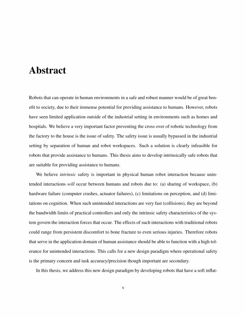
Abstract

Robots that can operate in human environments in a safe and robust manner would be of great ben-

efit to society, due to their immense potential for providing assistance to humans. However, robots

have seen limited application outside of the industrial setting in environments such as homes and

hospitals. We believe a very important factor preventing the cross over of robotic technology from

the factory to the house is the issue of safety. The safety issue is usually bypassed in the industrial

setting by separation of human and robot workspaces. Such a solution is clearly infeasible for

robots that provide assistance to humans. This thesis aims to develop intrinsically safe robots that

are suitable for providing assistance to humans.

We believe intrinsic safety is important in physical human robot interaction because unin-

tended interactions will occur between humans and robots due to: (a) sharing of workspace, (b)

hardware failure (computer crashes, actuator failures), (c) limitations on perception, and (d) limi-

tations on cognition. When such unintended interactions are very fast (collisions), they are beyond

the bandwidth limits of practical controllers and only the intrinsic safety characteristics of the sys-

tem govern the interaction forces that occur. The effects of such interactions with traditional robots

could range from persistent discomfort to bone fracture to even serious injuries. Therefore robots

that serve in the application domain of human assistance should be able to function with a high tol-

erance for unintended interactions. This calls for a new design paradigm where operational safety

is the primary concern and task accuracy/precision though important are secondary.

In this thesis, we address this new design paradigm by developing robots that have a soft inflat-

v

able structure, i.e, inflatable robots. Inflatable robots can improve intrinsic safety characteristics

by being extremely lightweight and by including surface compliance (due to the compressibility

of air) as well as distributed structural compliance (due to the lower Young’s modulus of the mate-

rials used) in the structure. This results in a lower effective inertia during collisions which implies

a lower impact force between the inflatable robot and human. Inflatable robots can essentially be

manufactured like clothes and can therefore also potentially lower the cost of robots to an extent

where personal robots can be an affordable reality.

In this thesis, we present a number of inflatable robot prototypes to address challenges in the

area of design and control of such systems. Specific areas addressed are: structural and joint design,

payload capacity, pneumatic actuation, state estimation and control. The CMU inflatable arm is

used in tasks like wiping and feeding a human to successfully demonstrate the use of inflatable

robots for tasks involving close physical human interaction.

vi

Acknowledgements

I would like to thank my advisor, Chris Atkeson, for all the support and guidance he has provided

during my thesis work. He has been a constant source of inspiration throughout the work presented

in this thesis and to me as a roboticist. I would also like to thank my thesis committee members,

Howie Choset, Steve Collins and Ed Colgate (Northwestern) for their insightful questions and

advice during my thesis research.

I would like to thank everyone at the Quality of Life Technology Center (QoLT) for supporting

the work in this thesis from its very beginnings and for all the other enriching experiences I have

had because of QoLT. I would also like to thank my external collaborators, Pete Lynn and Saul

Griffith at Otherlab, and Annan Mozeika at iRobot for specific work in this thesis that was carried

out with their help.

Thank you to Mike Ornstein, Alex Kan May and Justin Moidel for spending their summers in

the lab and helping with so much of the intricate work that has gone into making inflatable robots

a reality. I would also like to thank all my friends at CMU and lab-mates at the CGA lab. Its been

fun learning so much from all of you.

I would also like to thank my advisors prior to joining CMU, G.K. Ananthasuresh (IISc),

Madhava Krishna (IIIT) and Sartaj Singh (CAIR) for guiding me when I was a budding researcher.

Thank you to my friends at Manipal for being the team that we were.

Thank you to my fiancee, Gracee Agrawal, for her love and support through the years. I could

not have made it without you. Thank you to my parents, Neeta and Sammi Sanan, for always

supporting me and encouraging me to follow my dreams and passions. Thank you for everything.

vii

Contents

Abstract v

Acknowledgements vii

1 Introduction 1

1.1 Motivation . . . . . . . . . . . . . . . . . . . . . . . . . . . . . . . . . . . . . . . 1

1.2 Challenges . . . . . . . . . . . . . . . . . . . . . . . . . . . . . . . . . . . . . . . 3

1.3 Thesis Outline . . . . . . . . . . . . . . . . . . . . . . . . . . . . . . . . . . . . . 4

2 Background 5

2.1 Injury Modes . . . . . . . . . . . . . . . . . . . . . . . . . . . . . . . . . . . . . 5

2.1.1 Quasi-Static Loading . . . . . . . . . . . . . . . . . . . . . . . . . . . . . 6

2.1.2 Dynamic Loading . . . . . . . . . . . . . . . . . . . . . . . . . . . . . . . 6

2.1.3 Other Injury Mechanisms . . . . . . . . . . . . . . . . . . . . . . . . . . 7

2.2 Safety Indices . . . . . . . . . . . . . . . . . . . . . . . . . . . . . . . . . . . . . 8

2.2.1 The Head Injury Criterion (HIC) . . . . . . . . . . . . . . . . . . . . . . . 8

2.2.2 Contact Force . . . . . . . . . . . . . . . . . . . . . . . . . . . . . . . . . 9

2.3 Compliant Control . . . . . . . . . . . . . . . . . . . . . . . . . . . . . . . . . . 11

2.4 Flexible Robots . . . . . . . . . . . . . . . . . . . . . . . . . . . . . . . . . . . . 12

2.4.1 Soft Coverings . . . . . . . . . . . . . . . . . . . . . . . . . . . . . . . . 12

ix

2.4.2 Flexible Joints . . . . . . . . . . . . . . . . . . . . . . . . . . . . . . . . 13

2.4.3 Flexible Links . . . . . . . . . . . . . . . . . . . . . . . . . . . . . . . . 14

2.4.4 Continuum Robots . . . . . . . . . . . . . . . . . . . . . . . . . . . . . . 15

2.4.5 Inflatable Robots . . . . . . . . . . . . . . . . . . . . . . . . . . . . . . . 17

2.5 The Continuum Arm . . . . . . . . . . . . . . . . . . . . . . . . . . . . . . . . . 18

2.5.1 System Description . . . . . . . . . . . . . . . . . . . . . . . . . . . . . . 18

2.5.2 Analytical Kinematics . . . . . . . . . . . . . . . . . . . . . . . . . . . . 20

2.5.3 Experimental Kinematics . . . . . . . . . . . . . . . . . . . . . . . . . . . 22

2.5.4 Application to Human Interaction Tasks . . . . . . . . . . . . . . . . . . . 25

2.5.5 Discussion . . . . . . . . . . . . . . . . . . . . . . . . . . . . . . . . . . 27

2.6 Single Link Inflatable Robot . . . . . . . . . . . . . . . . . . . . . . . . . . . . . 27

2.6.1 System Description . . . . . . . . . . . . . . . . . . . . . . . . . . . . . . 28

2.6.2 Large Deflection Beam Analysis . . . . . . . . . . . . . . . . . . . . . . . 29

2.6.3 Pseudo Rigid Body Model . . . . . . . . . . . . . . . . . . . . . . . . . . 30

2.6.4 Experimental Deflection Testing . . . . . . . . . . . . . . . . . . . . . . . 32

2.6.5 System Model and Behavior . . . . . . . . . . . . . . . . . . . . . . . . . 34

2.6.6 Force Control . . . . . . . . . . . . . . . . . . . . . . . . . . . . . . . . . 36

2.6.7 Experimental Results . . . . . . . . . . . . . . . . . . . . . . . . . . . . . 39

2.6.8 Discussion . . . . . . . . . . . . . . . . . . . . . . . . . . . . . . . . . . 40

2.7 Variable Morphology Robots . . . . . . . . . . . . . . . . . . . . . . . . . . . . . 41

2.7.1 The Variable Buckling Hinge Mechanism . . . . . . . . . . . . . . . . . . 42

2.8 Summary . . . . . . . . . . . . . . . . . . . . . . . . . . . . . . . . . . . . . . . 44

3 Design for Safe Physical Human Interaction 45

3.1 Design Paradigms For Safe Robots . . . . . . . . . . . . . . . . . . . . . . . . . . 45

3.2 Synthesis of Safe Systems . . . . . . . . . . . . . . . . . . . . . . . . . . . . . . 47

x

3.2.1 Characterization of Soft Robots . . . . . . . . . . . . . . . . . . . . . . . 47

3.2.2 Compliance Distribution . . . . . . . . . . . . . . . . . . . . . . . . . . . 51

3.2.3 Problem Formulation . . . . . . . . . . . . . . . . . . . . . . . . . . . . . 55

3.2.4 Number Synthesis . . . . . . . . . . . . . . . . . . . . . . . . . . . . . . 56

3.2.5 Flexible Links . . . . . . . . . . . . . . . . . . . . . . . . . . . . . . . . 60

3.2.6 Performance comparison in the presence of safety constraints . . . . . . . 61

3.3 Summary . . . . . . . . . . . . . . . . . . . . . . . . . . . . . . . . . . . . . . . 65

4 Hardware 66

4.1 The CMU Inflatable Arm . . . . . . . . . . . . . . . . . . . . . . . . . . . . . . . 66

4.1.1 The Arm . . . . . . . . . . . . . . . . . . . . . . . . . . . . . . . . . . . 67

4.1.2 Actuation . . . . . . . . . . . . . . . . . . . . . . . . . . . . . . . . . . . 71

4.1.3 The End Effector . . . . . . . . . . . . . . . . . . . . . . . . . . . . . . . 75

4.1.4 Kinematics . . . . . . . . . . . . . . . . . . . . . . . . . . . . . . . . . . 80

4.1.5 Joint Stiffness . . . . . . . . . . . . . . . . . . . . . . . . . . . . . . . . . 81

4.1.6 Design Procedure for Inflatable Links . . . . . . . . . . . . . . . . . . . . 82

4.1.7 Payload Capacity and Safety . . . . . . . . . . . . . . . . . . . . . . . . . 86

4.2 The PneuArm . . . . . . . . . . . . . . . . . . . . . . . . . . . . . . . . . . . . . 88

4.3 The AIRarm . . . . . . . . . . . . . . . . . . . . . . . . . . . . . . . . . . . . . . 91

4.4 Summary . . . . . . . . . . . . . . . . . . . . . . . . . . . . . . . . . . . . . . . 93

5 Fabrication 94

5.1 Thermal Welding . . . . . . . . . . . . . . . . . . . . . . . . . . . . . . . . . . . 94

5.2 Sewing . . . . . . . . . . . . . . . . . . . . . . . . . . . . . . . . . . . . . . . . 95

5.3 Other Methods . . . . . . . . . . . . . . . . . . . . . . . . . . . . . . . . . . . . 97

5.4 Summary . . . . . . . . . . . . . . . . . . . . . . . . . . . . . . . . . . . . . . . 98

xi

6 Strength and Range of Motion 99

6.1 Introduction . . . . . . . . . . . . . . . . . . . . . . . . . . . . . . . . . . . . . . 99

6.2 Description of the PneuArm . . . . . . . . . . . . . . . . . . . . . . . . . . . . . 100

6.2.1 General Design . . . . . . . . . . . . . . . . . . . . . . . . . . . . . . . . 101

6.2.2 PneuArm Payload Capacity . . . . . . . . . . . . . . . . . . . . . . . . . 102

6.2.3 Joints . . . . . . . . . . . . . . . . . . . . . . . . . . . . . . . . . . . . . 103

6.2.4 Actuators . . . . . . . . . . . . . . . . . . . . . . . . . . . . . . . . . . . 105

6.2.5 Hand . . . . . . . . . . . . . . . . . . . . . . . . . . . . . . . . . . . . . 107

6.3 Actuator Modeling and Control . . . . . . . . . . . . . . . . . . . . . . . . . . . . 109

6.4 Characterization . . . . . . . . . . . . . . . . . . . . . . . . . . . . . . . . . . . . 111

6.5 Discussion . . . . . . . . . . . . . . . . . . . . . . . . . . . . . . . . . . . . . . . 114

6.6 Summary . . . . . . . . . . . . . . . . . . . . . . . . . . . . . . . . . . . . . . . 115

7 Pneumatic Actuators for Inflatable Robots 117

7.1 Introduction . . . . . . . . . . . . . . . . . . . . . . . . . . . . . . . . . . . . . . 117

7.2 Antagonistic Torsion Shape Actuators . . . . . . . . . . . . . . . . . . . . . . . . 119

7.2.1 Principle . . . . . . . . . . . . . . . . . . . . . . . . . . . . . . . . . . . 119

7.2.2 Torque-Displacement Characteristics . . . . . . . . . . . . . . . . . . . . 120

7.3 Rotary Peano Actuators . . . . . . . . . . . . . . . . . . . . . . . . . . . . . . . . 123

7.3.1 Peano Actuators Review . . . . . . . . . . . . . . . . . . . . . . . . . . . 123

7.3.2 Design . . . . . . . . . . . . . . . . . . . . . . . . . . . . . . . . . . . . 124

7.3.3 Actuator Motion . . . . . . . . . . . . . . . . . . . . . . . . . . . . . . . 124

7.3.4 Torque-Displacement Characteristics . . . . . . . . . . . . . . . . . . . . 128

7.4 Torsion Weave Actuator . . . . . . . . . . . . . . . . . . . . . . . . . . . . . . . . 130

7.4.1 Kinematics . . . . . . . . . . . . . . . . . . . . . . . . . . . . . . . . . . 130

7.4.2 Static Torque-Displacement Characteristics . . . . . . . . . . . . . . . . . 131

xii

7.5 Discussion . . . . . . . . . . . . . . . . . . . . . . . . . . . . . . . . . . . . . . . 132

7.6 Summary . . . . . . . . . . . . . . . . . . . . . . . . . . . . . . . . . . . . . . . 133

8 Accuracy 135

8.1 Design and Modeling of Inflatable Structures . . . . . . . . . . . . . . . . . . . . 135

8.1.1 Structural Model for Strength and Stiffness . . . . . . . . . . . . . . . . . 137

8.2 Inflatable Manipulator Control . . . . . . . . . . . . . . . . . . . . . . . . . . . . 142

8.2.1 Soft Inverse Kinematics using assumed kinematics . . . . . . . . . . . . . 142

8.2.2 Soft Inverse Kinematics for Jointless Soft Robots . . . . . . . . . . . . . . 145

8.3 Inflatable Joint Angle Estimation . . . . . . . . . . . . . . . . . . . . . . . . . . . 147

8.3.1 Joint Angle Estimation using Pressure Sensors at the Joints . . . . . . . . . 148

8.3.2 Joint Angle Estimation using Inertial Measurement Units (IMUs) . . . . . 149

8.3.3 Discussion on Alternate Sensors for Joint Angle estimation . . . . . . . . . 153

8.4 Vibrations and Bandwidth . . . . . . . . . . . . . . . . . . . . . . . . . . . . . . 155

8.4.1 Reducing Vibrations . . . . . . . . . . . . . . . . . . . . . . . . . . . . . 157

8.5 Discussion . . . . . . . . . . . . . . . . . . . . . . . . . . . . . . . . . . . . . . . 161

8.6 Summary . . . . . . . . . . . . . . . . . . . . . . . . . . . . . . . . . . . . . . . 162

9 Physical Human Interaction 163

9.1 Inflatable Joint Angle Estimation using Pressure Sensors . . . . . . . . . . . . . . 163

9.1.1 Contact Detection . . . . . . . . . . . . . . . . . . . . . . . . . . . . . . . 164

9.2 Reaction Schemes . . . . . . . . . . . . . . . . . . . . . . . . . . . . . . . . . . . 166

9.2.1 Unintended Interaction . . . . . . . . . . . . . . . . . . . . . . . . . . . . 166

9.2.2 Intended Interaction - Sponging . . . . . . . . . . . . . . . . . . . . . . . 166

9.2.3 Nudging . . . . . . . . . . . . . . . . . . . . . . . . . . . . . . . . . . . 168

9.3 Feeding . . . . . . . . . . . . . . . . . . . . . . . . . . . . . . . . . . . . . . . . 171

9.3.1 User Studies . . . . . . . . . . . . . . . . . . . . . . . . . . . . . . . . . 173

xiii

9.4 Summary . . . . . . . . . . . . . . . . . . . . . . . . . . . . . . . . . . . . . . . 174

10 Conclusion 176

10.1 Contributions . . . . . . . . . . . . . . . . . . . . . . . . . . . . . . . . . . . . . 176

10.2 Future Work . . . . . . . . . . . . . . . . . . . . . . . . . . . . . . . . . . . . . . 179

A Synthesis of Safe Systems 181

A.1 Closed Loop Performance Based Synthesis . . . . . . . . . . . . . . . . . . . . . 181

A.1.1 System Model and Problem Formulation . . . . . . . . . . . . . . . . . . 182

A.1.2 A Simplified Problem: Stand-alone Control Synthesis . . . . . . . . . . . 185

A.1.3 Control-Structure Synthesis . . . . . . . . . . . . . . . . . . . . . . . . . 186

A.1.4 An Alternate Approach . . . . . . . . . . . . . . . . . . . . . . . . . . . . 187

B User Study Protocol 189

Bibliography 210

xiv

Chapter 1

Introduction

The use of robots in assistive roles will be an increasingly significant application for robotics. The

application of robots in these roles has unique demands from a mechanical and control design

perspective, which have not been thoroughly addressed in the past. Safety, as stated by [3], is

of prime importance when humans are involved. The paradigm shift thus needed in the way we

design robots is a unique departure from the way humans have thought about machines in the past.

The robot must minimize the risk of injury to others during its operation. This thesis deals with

the development of soft inflatable robots that for providing assistance to humans.

1.1 Motivation

Robots designed and controlled with a traditional approach that stems from industrial automation

may not be the best answer to robots in human environments. These robots are often designed with

the objective of improving accuracy of the system. This demand for functional performance has

lead most robots to have rigid links and high stiffness, in part due to the availability of accurate

modeling techniques, advanced control methods and simple mechanical design techniques for rigid

body systems. Due to this, the approach towards human safety in the presence of robots has largely

1

involved the use of segregation methods to keep human and robots in non-intersecting workspaces.

However, this approach fails when humans and robots need to work in physically close spaces,

such as in tasks involving robots assisting humans. New approaches in the design and control of

robots need to be developed which incorporate the shift from performance oriented systems to safe

systems, needed for robots in human environments.

A large proportion of prior research related to improving characteristics of human robot inter-

action has been devoted to compliant control of robots. Compliant control of robot manipulators

[46, 89] aims to reduce the impedance of the robot as seen from the contact end. However, limita-

tions due to the bandwidth of the controller prohibit impedance control at high frequencies. This

limitation is a crucial drawback from the standpoint of safety in physical human robot interaction

(pHRI). Impacts are a primary risk in pHRI , and the interaction during impacts is at high frequen-

cies. Without impedance control at high frequencies, the interaction between human and robot

cannot be controlled during impacts. This leads to a very high risk situation. The interaction at

higher frequencies is therefore mostly dependent on the open loop (uncontrolled) characteristics of

any practical robot manipulator. Safety that is independent of the control scheme, is referred to as

intrinsic or inherent safety. Besides the finite control bandwidth issue, inherent safety is also nec-

essary in the event of control failure, hardware failure and other such malfunction that can easily

occur in a complex system.

As described in [137, 8], compliance in a system improves the open loop characteristics needed

for safety by reducing the reflected inertia on the contact side of the impact.The reflected inertia at

the contact end can be modified in a number of ways, albeit with different performance characteris-

tics: (a) the mass of the entire system can be reduced, (b) the overall stiffness of the system can be

reduced, i.e., some form of additional compliance, e.g., a soft covering can be introduced, (c) the

mass distribution within the system can be modified, and (d) the stiffness distribution within the

system can be modified. Robots that utilize soft and inflatable structures can embody these princi-

ples well and can lead to systems that are extremely safe.

2

1.2 Challenges

While the safety of inflatable robots is intuitive, inflatable robots present a number of other chal-

lenges in their development and use. This thesis addresses a number of these challenges that exist

towards realizing inflatable robots for safe physical human interaction.

Design for safety and performance

Clearly, soft robots can satisfy safety requirements that are needed for working in close proximity

to humans. The question that needs to be answered then is: how do we design a soft robot that is

also functional? Are traditional static design requirements such as payload capacity, manipulability

etc. enough? Often soft systems can be engineered practically never fail, e.g., a soft jelly fish like

robot can be repeatedly smashed without incurring any damage at all. What should guide the

design in such a case? In Chapter 3, we discuss various design paradigms for soft and safe robots.

We also seek to develop a framework that can be used to synthesize the design of soft robots.

Strength

One of the main challenges has been to show that inflatable robot which are safe and light can

actually have a usable payload capacity while still having a large range-of-motion. This problem

is different from static inflatable structures that maintain their shape once inflated, which are of-

ten employed in architectural and space applications. Chapter 6 addresses issues in developing

high strength inflatable robots and successfully demonstrates these capabilities using a prototype

inflatable robot that has a payload to weight ratio of 2.5 and an absolute payload of 2.25 kg.

Motion

Inflatable robots, unlike static inflatable structures, require motion across the inflatable structure.

This presents a challenge because mechanisms or joints need to be developed and realized that

3

can allow motion across the structure. Additionally, actuation techniques that can provide motive

force across the joints are needed. Various types of joints and actuation techniques have been

explored and developed in this thesis that address these need. As a result, inflatable structures with

large range of motion (> 300◦) have been successfully realized. Chapter 6, 4 and 7 discuss the

developments made with regards to actuators and joints.

Accuracy

A number of challenges exist with regards to developing inflatable robots that are also accurate in

a position control sense. Because inflatable robots by definition have no rigid joints, accurate joint

angle measurement is a challenge. Another challenge is the dependence of the motion of inflatable

robots on the structural deformation models. In chapter 8, we address issues in sensing, estimation

and model dependent kinematics for inflatable robots.

1.3 Thesis Outline

The outline of this document is as follows. Chapter 2 describes related work: safety metrics,

impact modeling, compliant control, robust control and reaction strategies and flexible robots.

Chapter 3 describes design issues for developing safe and robots. Chapter 4 describes the inflatable

manipulator prototypes that were realized and utilized as part of this thesis. Chapter 6 describes

advancements made to develop high strength inflatable robots. Chapter 7 describes developments

made in the area of pneumatic actuators for inflatable robots. Chapter 8 describes models, model

based algorithms and sensing and estimation work to improve the accuracy of motion of inflatable

robots. Chapter 9 describes experiments and examples of the inflatable robots carrying out task

involving human interaction.

4

Chapter 2

Background

The problem of designing and controlling a robotic system for safe operation in human environ-

ments requires knowledge from many areas including biomechanics, impact mechanics, compliant

control, robust control, smart materials and flexible robots. These are briefly described in this

chapter. Additionally some foundational work carried out towards developing soft robots for hu-

man interaction is described. The continuum arm, which belongs to a different class of soft robots

than inflatable robots is described. Force control experiments with a single link inflatable robot are

also presented.

2.1 Injury Modes

During physical human robot interaction injury can occur via a variety of mechanisms. They

include quasi-static loading, dynamic loading and other mechanisms such as shearing and punc-

turing.

5

2.1.1 Quasi-Static Loading

When the interaction forces between the robot and human change slowly such loading is referred

to as quasi-static loading. The injuries possible due to quasi-static interactions include fractures

and soft tissue injuries [40]. This loading situation is relatively simple in terms of its description

and effect on the two interacting bodies.

Compliant control, which is discussed in sec. 2.3, is useful in limiting contact forces and

preventing injuries due to quasi-static loading. However, as tactile sensing has not completely ma-

tured as a technology, quasi-static loading still poses a some level of risk in pHRI. Measures to

improve safety against quasi-static loading, besides compliant control, include limiting the actua-

tion force/torque at the joints and limiting the workspace of the manipulator based on its contact

Jacobian.

2.1.2 Dynamic Loading

Dynamic loading refers to the condition where the interaction forces between the robot and the

human vary over a short time scale. Collisions or impacts are the most common form of dynamic

loading. Injuries possible due to such loading have been detailed by Haddadin et al. [40]. In-

juries include fractures, internal injuries and soft tissue injuries. It is reasonable to assume that

the human is fixed (constrained) at all times during the interaction, as this is the situation which

poses the maximum risk of injury [40] and hence any injury analysis based on this assumption is

conservative.

Impacts between two bodies can be analyzed in a number of ways, depending on the charac-

teristics of the two bodies. Stronge [112] provides basic classifications based on the nature of the

two bodies involved in the impact. It must be noted that we will be dealing with impacts that are

considered relatively low speed (≈ 1 m/s). This implies that in most cases plastic flow in the two

interacting bodies does not occur. In situations such as a bullet penetrating a human body, plastic

6

flow does occur and an impact theory for high speed collisions is needed. Gilardi and Sharf [32]

provide a recent review of impact modeling of impacts. Essentially, two kinds of models exist for

impact: 1) Discrete models and 2) Continuous models. The discrete models such as the Newton’s

model [81] utilize an instantaneous change in velocities of the impacting bodies, while continuous

models such as the spring-dashpot model [35] utilize interaction force models during the contact

period to propagate the dynamics of the system through the impact phase. For the most part, we

shall utilize continuous models in this thesis.

We often use flexible structures like flexible links. Modeling and analysis of impacts with

flexible bodies is therefore important. Khulief and Shabana [60] compare the accuracy of lumped

mass versus consistent mass modeling techniques for flexible bodies undergoing impact. Other

researches have studied the dynamics of flexible links with impact [134, 135, 128].

2.1.3 Other Injury Mechanisms

Shearing

Shearing refers to the case where in the human comes in contact with a sharp edge of the robot.

Such a scenario is possible when the robot is utilizing a sharp tool as an end effector. This injury

mechanism can cause lacerations, and penetration of the human skin and soft tissue. Data regarding

forces and parameters of the tool needed to causes such injuries is available in literature [42, 71, 72,

84, 34, 33]. Preventing injuries in such scenarios is a major challenge since the robot is inherently

unsafe when equipped with a sharp tool.

Puncturing

Puncturing occurs when the human comes into point contact with an external object. Such an

interaction is possible if there are sharp corners on the robot or the robot is carrying a pointed object

such as a nail. Wounds caused by puncturing are very similar to those caused due to shearing.

7

Abrasion

Relative motion of a rough surface with human skin can lead to injury due to abrasion. Abrasion

causes superficial damage to the skin.

2.2 Safety Indices

A safety index is used to quantify the severity of an interaction (impact, quasi-static) between a

human and any external agent. In our case, the robot is the external agent. The safety index can

then be mapped to the level of injury caused in the human subject. We shall limit our discussion of

safety indices to impacts only as we hope to address impact safety. When the interaction is quasi-

static, the interaction force between the human subject and robot can be used directly to evaluate

safety of interaction. Research in finding an appropriate safety index in pHRI is still an ongoing

area of research, with only a few published results [40, 83].

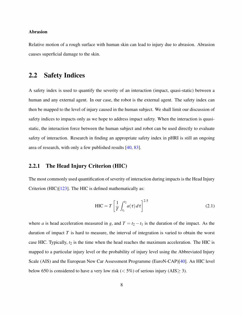
2.2.1 The Head Injury Criterion (HIC)

The most commonly used quantification of severity of interaction during impacts is the Head Injury

Criterion (HIC)[123]. The HIC is defined mathematically as:

HIC = T[

1T

∫ t2

t1a(τ)dτ

]2.5

(2.1)

where a is head acceleration measured in g, and T = t2− t1 is the duration of the impact. As the

duration of impact T is hard to measure, the interval of integration is varied to obtain the worst

case HIC. Typically, t2 is the time when the head reaches the maximum acceleration. The HIC is

mapped to a particular injury level or the probability of injury level using the Abbreviated Injury

Scale (AIS) and the European New Car Assessment Programme (EuroN-CAP)[40]. An HIC level

below 650 is considered to have a very low risk (< 5%) of serious injury (AIS≥ 3).

8

The HIC was formulated to measure impact severity in the case of indirect interaction, such

as that in an automobile crash. The impact scenario in an automobile crash is very different from

an impact scenario with a robot manipulator. In an automobile crash an external agent impacts

the automobile, in which the subject is placed, which causes large accelerations of the head. The

duration and magnitude of the these accelerations are measured by the HIC. Therefore, the HIC

is a good indicator for internal injuries, such as brain hemorrhage. However, effects such as those

caused by direct interaction between the agent and the subject in an impact situation are ignored by

the HIC. Such interactions are likely in a human-robot impact situation. These direct interactions

can cause injuries such as fracturing of bones and soft tissue injuries. The HIC has been used in

the past [8, 137] to speak about injury potential in pHRI, but its use has been largely limited in lieu

of results demonstrating its inappropriateness for pHRI [40].

2.2.2 Contact Force

Measurements such as the contact force Fext are deemed more suitable to types of injuries possible

in human robot interaction. The time history of contact force between a subject and an external

agent yields important information regarding the possibility of injuries like bone fractures. Bone

fractures are an instance of mechanical failure of the bone leading to the formation of a crack

in the bone or complete separation of the bone into two or more pieces. When the contact force

exerted on a particular bone exceeds its sustainable limit, the bone fractures due to the development

of stresses in the material beyond the safe value. It must be noted that along with magnitude of

the maximum contact force Fmax, the time period of loading tmax, shown in Fig 2.1, is also an

important feature of the interaction. If tmax is large the loading can be considered quasi-static, if

tmax is small the loading can be treated as an impact. High rates of loading, which usually occur

in impacts between two hard objects, cause brittle behavior in the materials. This causes failure of

the object via brittle fracture at stresses below quasi-static limits. At short time scales materials are

more brittle than on long time scales. Therefore to reduce the risk of bone fracture it is useful to

9

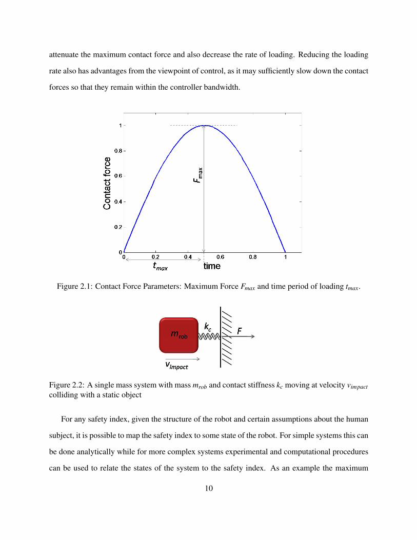
attenuate the maximum contact force and also decrease the rate of loading. Reducing the loading

rate also has advantages from the viewpoint of control, as it may sufficiently slow down the contact

forces so that they remain within the controller bandwidth.

Figure 2.1: Contact Force Parameters: Maximum Force Fmax and time period of loading tmax.

Figure 2.2: A single mass system with mass mrob and contact stiffness kc moving at velocity vimpactcolliding with a static object

For any safety index, given the structure of the robot and certain assumptions about the human

subject, it is possible to map the safety index to some state of the robot. For simple systems this can

be done analytically while for more complex systems experimental and computational procedures

can be used to relate the states of the system to the safety index. As an example the maximum

10

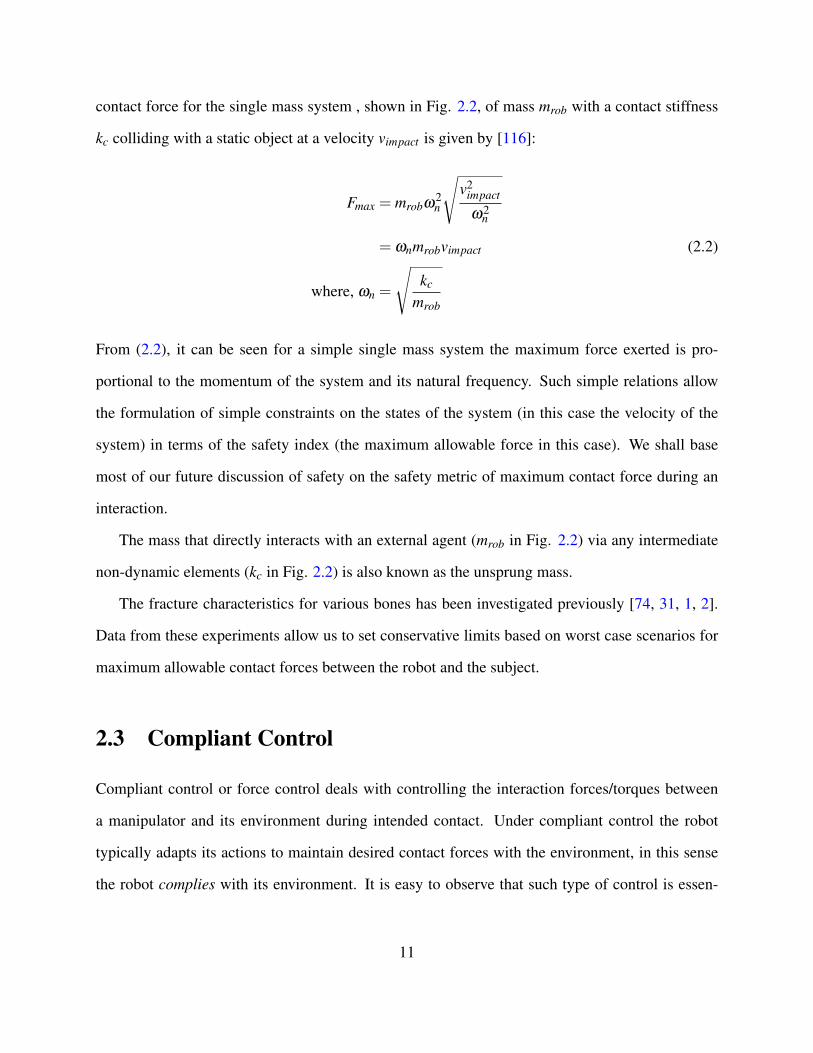
contact force for the single mass system , shown in Fig. 2.2, of mass mrob with a contact stiffness

kc colliding with a static object at a velocity vimpact is given by [116]:

Fmax = mrobω2n

√v2

impact

ω2n

= ωnmrobvimpact (2.2)

where, ωn =

√kc

mrob

From (2.2), it can be seen for a simple single mass system the maximum force exerted is pro-

portional to the momentum of the system and its natural frequency. Such simple relations allow

the formulation of simple constraints on the states of the system (in this case the velocity of the

system) in terms of the safety index (the maximum allowable force in this case). We shall base

most of our future discussion of safety on the safety metric of maximum contact force during an

interaction.

The mass that directly interacts with an external agent (mrob in Fig. 2.2) via any intermediate

non-dynamic elements (kc in Fig. 2.2) is also known as the unsprung mass.

The fracture characteristics for various bones has been investigated previously [74, 31, 1, 2].

Data from these experiments allow us to set conservative limits based on worst case scenarios for

maximum allowable contact forces between the robot and the subject.

2.3 Compliant Control

Compliant control or force control deals with controlling the interaction forces/torques between

a manipulator and its environment during intended contact. Under compliant control the robot

typically adapts its actions to maintain desired contact forces with the environment, in this sense

the robot complies with its environment. It is easy to observe that such type of control is essen-

11

tial for tasks involving physical human robot interaction. In the context of pHRI, tasks such as

hand shakes, haptic teleoperation, payload assistance, or any task involving physical co-operation

between human and robot must utilize some form of compliant control for safe and effective exe-

cution.

There are a number of techniques for force control which involve controlling the compliance,

impedance or admittance of the robot to achieve desired force interaction characteristics. While

other force control techniques explicitly involve a force feedback loop to control the interaction

forces. Thorough reviews of these techniques are available [124, 49, 129].

The techniques for force control can be used to realize compliant behaviors to limit injury

risks due to quasi-static loading discussed in Sec. 2.1.1. However the limited control bandwidth

decreases its usefulness towards reducing risks due to dynamic loading discussed in 2.1.2

2.4 Flexible Robots

Considering limitations in the bandwidth of active force control [26], it is necessary to improve the

open loop characteristics of the systems. One of the methods of doing this, is by the introduction

of flexible elements in the robot. A brief survey of various cases of robot flexibility follows.

2.4.1 Soft Coverings

Soft coverings constitute the most basic type of compliance that can be introduced to a robot

structure. The robot is simply padded with soft material such as silicone, rubber etc. to introduce

compliance into the system. Robots like the RI-MAN [78] utilize such soft coverings to improve

interaction characteristics.

Various contact models have been derived that relate the material properties of the covering and

the geometry of the contacting object to a stiffness value for the covering [58, 56]. These models

can be used to select materials and material thicknesses based on desired contact stiffness.

12

2.4.2 Flexible Joints

Joints with flexibility or compliance geometrically collocated with the joint axis are known as flex-

ible joints. Robots with such flexible joints have compliance concentrated at isolated locations on

its structure. This is the most common type of flexibility encountered in robots, due to transmis-

sion elements such as harmonic drives, cables, gears etc. Flexible joints have also been received

considerable attention recently for the development of inherently safe robots.

The Series Elastic Actuator (SEA) [90] was developed to reduce the impedance of stiff actua-

tors by introducing compliance between the link and the actuator. The SEA can be considered to

be a case of designed joint flexibility. Improving on the performance limitations posed by SEA,

recently [137, 98] introduced flexibility in the joints to improve safety characteristics of robots

involved in pHRI. The joint flexibility allows inertial decoupling between the actuator and the link

during impacts [41].

Flexible joints with constant joint compliance, while reducing output impedance at high fre-

quencies, do result in performance deterioration in tasks such as high speed trajectory following.

The high frequency torque from the actuator to the link falls off with increasing frequency [137].

Citing this and other performance limitation using constant joint compliance, many researchers

have proposed the use of variable impedance actuators (VIA) [119, 98, 131, 53, 121]. These ac-

tuators allow the mechanical compliance of the actuator to be varied in accordance with the need

of the task. In the context of pHRI, Bicchi and Tonietti [8] proposed an optimization scheme to

compute the optimal desired stiffness trajectory for a minimum time maneuver of a linear system

with safety constraints.

The dynamic model for robots with flexible joints is twice the order of an identical system with

ideal joints. For example, assuming a planar serial manipulator with all flexible revolute joints, if

N is the number of links and there are N joints, then the total mechanical degrees of freedom of

the system is 2N while the number of actuators are N. As a result such systems are underactuated.

13

2.4.3 Flexible Links

Besides flexibility at the joints, a robot manipulator may also have flexibility distributed throughout

the length of its links. Link flexibility can be thought of as a more general case of flexible joints. In

the past, flexible links have been studied in cases where it is impossible to eliminate link flexibility

due to specific requirements of the task. Space applications and confined operational environments

often present design constraints which make link flexibility unavoidable. In this thesis, the useful-

ness of link flexibility in the context of pHRI will be demonstrated. We look at link flexibility as a

blessing rather than a curse.

Dynamic models for flexible manipulators have been researched in the past. Shabana [101],

Dwivedy and Eberhard [25], Robinett et al. [92] and Tokhi and Azad [118] provide thorough

overviews of the techniques developed to model systems with flexible components. The most

popular techniques used to model system including link flexibility are the finite segment approach

[54, 99], assumed modes method (AMM) [11, 127, 45] and the finite element method (FEM)[117,

75, 9, 79].

The finite segment or lumped parameter approach treats the flexible links as a collection of

the rigid bodies connected by elastic elements and/or dampers. In the assumed modes method

(AMM) displacements along the length of a flexible link are represented as a truncated series of

the spatial modal functions and time varying modal amplitude. In most cases, the mode shapes

are computed from the partial differential equations (PDE) for the unforced vibrations of the link.

When this is not possible (due to complicated link geometry), approximate mode shapes computed

using static deflections may be used. The finite element method models each link as an assembly of

elements whose displacements are compatible at the boundaries. The elastic displacements of the

link are represented by the nodal displacement values of the elements. The nodal displacements

are interpolated within an element by the use of predefined shape functions. The shape functions

are usually chosen to be polynomial in the nodal displacements for ease of integration.

The AMM is well suited to manipulators involving only a single flexible link and simple link

14

geometries. For the case of multi-linked flexible manipulator the finite element approach may

be better suited. An extensive comparison of the two approaches is available([115]). From the

purpose of simplicity the lumped parameter approach is the easiest to analyze, as it permits the use

of the vast number of tools developed for rigid multi-body systems. It may therefore be the most

suited for controller synthesis. It should be noted that in the context of flexible multi-body systems

FEM and AMM have been applied mostly in the linear deflection regime only, the finite segment

approach allows the inclusion of geometric nonlinear deflections.

The use of flexible links introduces a variety of challenging control problems. The reasons

for this is the non-minimum phase behavior of such systems and difficulty in obtaining full state

feedback. A major cause of concern is the issue of vibrations when flexible links are utilized.

One strategy is to modify the input command to the system based on knowledge of the certain

parameters of the system to minimize vibrations in the system. The Input Shaping technique

[106, 108] utilizes this idea. Feedback methods based on estimating link deflections using sensory

data from strain gauges placed along the length of the arm may also be used ([44, 136]). These

sensors can be placed such that they are nearly collocated with the actuator. Tip position data

may also be obtained using optical sensing/vision and utilized in the feedback control scheme .

Such sensing is non-collocated and therefore stability issues may arise [11]. A variety of other

specialized techniques to control flexible manipulators exists, Robinett et al. [92] and Tokhi and

Azad [118] provide a detailed account of these.

2.4.4 Continuum Robots

Continuum robots are robots that consist of a continuous backbone and move via deformation of

this backbone. No kinematic joints are present on the structure. This class of robots utilizes hyper-

elastic structures that can tolerate large deformations. Other terminologies often used to describe

such robots are: snake robots, elephant trunk robot, tentacle robots etc. Like robots with flexible

links these systems possess distributed compliance all throughout their structure, however unlike

15

flexible link robots they utilize compliance to achieve motion as well. The distributed nature of

the motion and compliance in the system can offer distinct advantages for safe physical human

interaction.

A number of continuum robots have been designed in the past [114, 36, 73, 48, 105]. [93]

provides a review of some of the efforts in realizing continuum robots. Most continuum systems

are actuated either by the use of remotely actuated tendons [36, 105] or by the use of pneumatic

actuators [114, 73, 48]. These actuators modify the shape of the robot by application of geomet-

ric constraints on the structure. Inspiration from biological systems such as elephant trunks and

octopus tentacles have driven the design of these systems. The primary motivation is applications

involving convoluted spaces, whole arm manipulation and locomotion.

Theoretically continuum robots posses infinite degrees of freedom. However, only a few of the

DoF’s are usually actively controlled. Therefore continuum robots may be underactuated. There

are also example systems which approximate continuum systems by using a large number of rigid

links thus making them very large but finite DoF systems [130, 17, 43, 86]. The infinite degrees of

freedom in continuum robots pose interesting challenges in their modeling. A significant portion

of research has focussed on modeling continuum robots from the kinematics and dynamics per-

spective. Chirikjian and Burdick [15] provide a modal approach to formulate the kinematics for

hyper-redundant robots. Some of the results from this work are directly applicable to continuum

robots. Gravagne and Walker [38, 37] address the kinematics of multi-section remotely actuated

continuum robots. Simaan et al. [105] provide a kinematic formulation, based on the reasonable

assumptions noted by Gravagne and Walker [38], for a snake like arm with secondary backbones

functioning as push-pull tendons. Dynamic models for continuum robots using a continuum me-

chanics formulation were explored by Chirikjian [14]. [126] provides a general overview of design

and motion planning issues for continuum robots and their discrete approximations.

16

2.4.5 Inflatable Robots

An inflatable structure refers to a structure that is made using membrane material (can only hold

tensile stress) and maintains structural integrity by virtue of internal pressure. Such structures

are a special case of a class of structures known as membrane structures. Based on the method

of pressurization, inflatable structures using air can be classified as either (a) air supported or

(b) air inflated. Air supported structures commonly utilize a small pressure differential between

internal and external pressure and are continuously replenished with air as they are usually open

structures. Examples include inflatable roofs and other inflatable structures used in entertainment.

Air inflated structures consist of pneumatically closed structures that are inflated to any desired

pressure above the external pressure. Unlike air supported structure continuous replenishment of

air is not needed and therefore higher pressure differentials can be generated between the internal

and external pressures. Examples include inflatable space structures, inflatable wings, inflatable

tents, inflatable toys, etc.

Use of inflatable links instead of traditional rigid metallic links can help incorporate the de-

sign paradigms listed Sec. 3.1. They can be potentially extremely lightweight, have low contact

stiffness (due to the compressibility of air) and also possess distributed compliance due to the rela-

tively higher elasticity of the materials used to make these links as compared to aluminium or other

conventional metals. In addition, there are also numerous other possibilities using inflatable struc-

tures such as good post-buckling characteristics which is not available from conventional robot

materials. Other advantages of inflatable structures include collapsibility (deployable) and low

cost. Multiple links offer a feasible way to generate multi-DoF systems using inflatable structures.

In such a configuration, interesting opportunities and challenges present themselves regarding the

joints that connect the multiple links. Traditional bearing based joint designs are often heavy and

can therefore adversely affect payload capacities of the structure. Fortunately, it is possible to uti-

lize inflatable structures that allow relative motion between different section of the structure. In

Chapter 4 we describe a number of realizations of such inflatable structures.

17

Besides this thesis, other prior attempts to utilize inflatable structures in robot manipulators

have been made. Most notably in the early 1980s, [5] built a manipulator consisting of a single

inflatable link with pneumatic actuators along its length that caused bending of the link in multiple

directions. [94] appended a traditional rigid robot manipulator (PUMA) with an inflatable link at

the distal end and presented an analysis of this system. More recent attempts have been also been

made to build inflatable manipulators using pneumatic actuation [69]. [125] developed a novel

constant volume joint for inflatable robots. These efforts suggest the applicability of inflatable

structures for robot manipulators, however, they represent only a preliminary exploration of the

design space of such robots.

2.5 The Continuum Arm

The continuum arm is a continuum robot and belongs to the category of C1 manipulators described

in 3.2.1. This section details our work with such a system.

2.5.1 System Description

Fig. 2.3 shows an image of the continuum arm prototyped in our lab. We will refer to the moving

section of the robot as the robot arm and the stationary base as the robot base. The robot does not

contain any rigid joints and rigid links. As can be seen in the image, the robot consists of three

linear actuators which actuate three tendons. The main structural element of the robot consists

of a hollow latex tube which is appended with a number of guide collars, shown in Fig. 2.4b,

made using polyurethane sheets. These guide collars are used to guide the three tendons which are

made using Kevlar R© thread of 1mm diameter. The latex tube and tendons are attached to an end

flange, shown in Fig. 2.4a, which is made from polyethylene. This is the only other element which

moves along with the robot arm. An inherent safety feature in the design of the system is the near

monolithic structure of the arm leading to fewer edges and a lighter design. Notably there are also

18

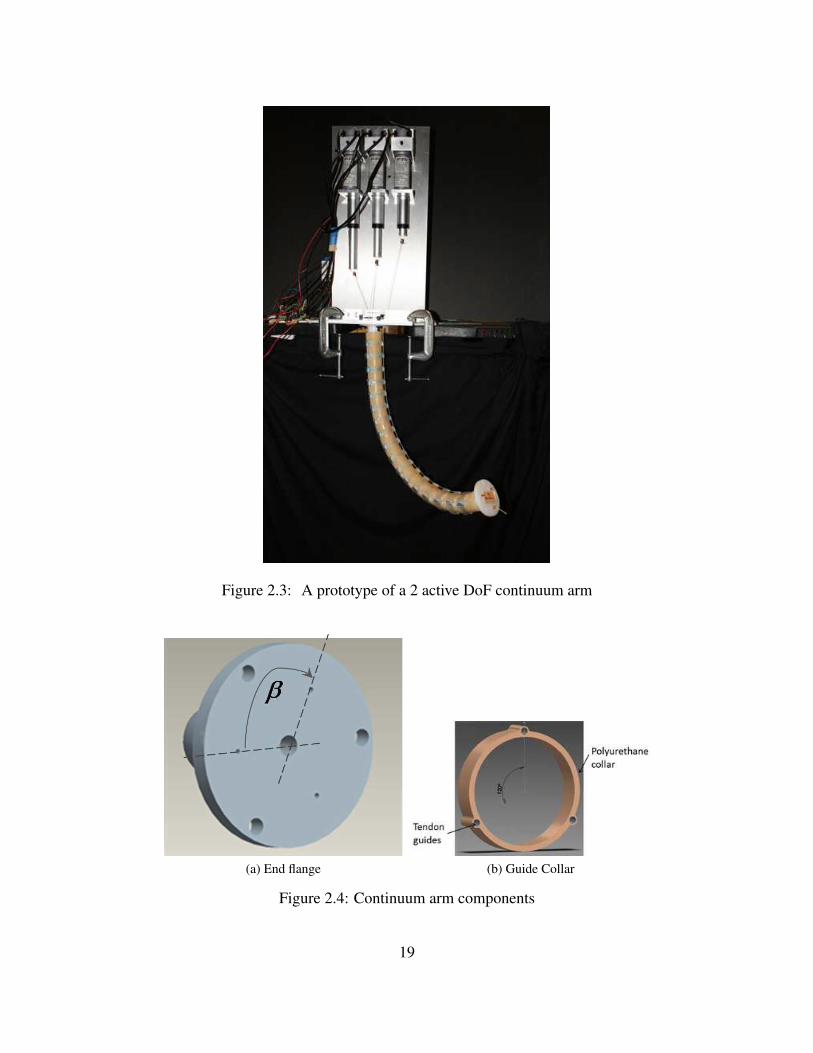
Figure 2.3: A prototype of a 2 active DoF continuum arm

(a) End flange (b) Guide Collar

Figure 2.4: Continuum arm components

19

no hard metallic surfaces in the robot arm.

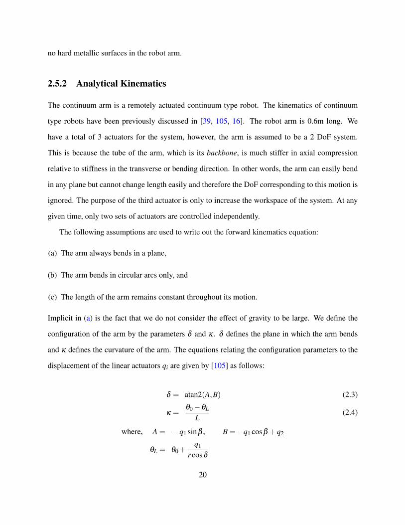
2.5.2 Analytical Kinematics

The continuum arm is a remotely actuated continuum type robot. The kinematics of continuum

type robots have been previously discussed in [39, 105, 16]. The robot arm is 0.6m long. We

have a total of 3 actuators for the system, however, the arm is assumed to be a 2 DoF system.

This is because the tube of the arm, which is its backbone, is much stiffer in axial compression

relative to stiffness in the transverse or bending direction. In other words, the arm can easily bend

in any plane but cannot change length easily and therefore the DoF corresponding to this motion is

ignored. The purpose of the third actuator is only to increase the workspace of the system. At any

given time, only two sets of actuators are controlled independently.

The following assumptions are used to write out the forward kinematics equation:

(a) The arm always bends in a plane,

(b) The arm bends in circular arcs only, and

(c) The length of the arm remains constant throughout its motion.

Implicit in (a) is the fact that we do not consider the effect of gravity to be large. We define the

configuration of the arm by the parameters δ and κ . δ defines the plane in which the arm bends

and κ defines the curvature of the arm. The equations relating the configuration parameters to the

displacement of the linear actuators qi are given by [105] as follows:

δ = atan2(A,B) (2.3)

κ =θ0−θL

L(2.4)

where, A = −q1 sinβ , B =−q1 cosβ +q2

θL = θ0 +q1

r cosδ

20

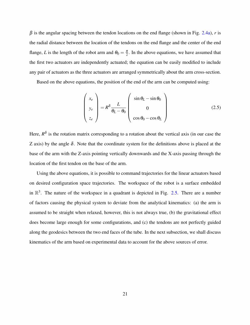
β is the angular spacing between the tendon locations on the end flange (shown in Fig. 2.4a), r is

the radial distance between the location of the tendons on the end flange and the center of the end

flange, L is the length of the robot arm and θ0 =π

2 . In the above equations, we have assumed that

the first two actuators are independently actuated; the equation can be easily modified to include

any pair of actuators as the three actuators are arranged symmetrically about the arm cross-section.

Based on the above equations, the position of the end of the arm can be computed using:

xe

ye

ze

= Rδ LθL−θ0

sinθL− sinθ0

0

cosθ0− cosθL

(2.5)

Here, Rδ is the rotation matrix corresponding to a rotation about the vertical axis (in our case the

Z axis) by the angle δ . Note that the coordinate system for the definitions above is placed at the

base of the arm with the Z-axis pointing vertically downwards and the X-axis passing through the

location of the first tendon on the base of the arm.

Using the above equations, it is possible to command trajectories for the linear actuators based

on desired configuration space trajectories. The workspace of the robot is a surface embedded

in R3. The nature of the workspace in a quadrant is depicted in Fig. 2.5. There are a number

of factors causing the physical system to deviate from the analytical kinematics: (a) the arm is

assumed to be straight when relaxed, however, this is not always true, (b) the gravitational effect

does become large enough for some configurations, and (c) the tendons are not perfectly guided

along the geodesics between the two end faces of the tube. In the next subsection, we shall discuss

kinematics of the arm based on experimental data to account for the above sources of error.

21

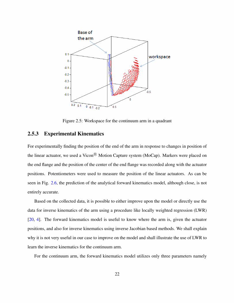
Figure 2.5: Workspace for the continuum arm in a quadrant

2.5.3 Experimental Kinematics

For experimentally finding the position of the end of the arm in response to changes in position of

the linear actuator, we used a Vicon R© Motion Capture system (MoCap). Markers were placed on

the end flange and the position of the center of the end flange was recorded along with the actuator

positions. Potentiometers were used to measure the position of the linear actuators. As can be

seen in Fig. 2.6, the prediction of the analytical forward kinematics model, although close, is not

entirely accurate.

Based on the collected data, it is possible to either improve upon the model or directly use the

data for inverse kinematics of the arm using a procedure like locally weighted regression (LWR)

[20, 4]. The forward kinematics model is useful to know where the arm is, given the actuator

positions, and also for inverse kinematics using inverse Jacobian based methods. We shall explain

why it is not very useful in our case to improve on the model and shall illustrate the use of LWR to

learn the inverse kinematics for the continuum arm.

For the continuum arm, the forward kinematics model utilizes only three parameters namely

22

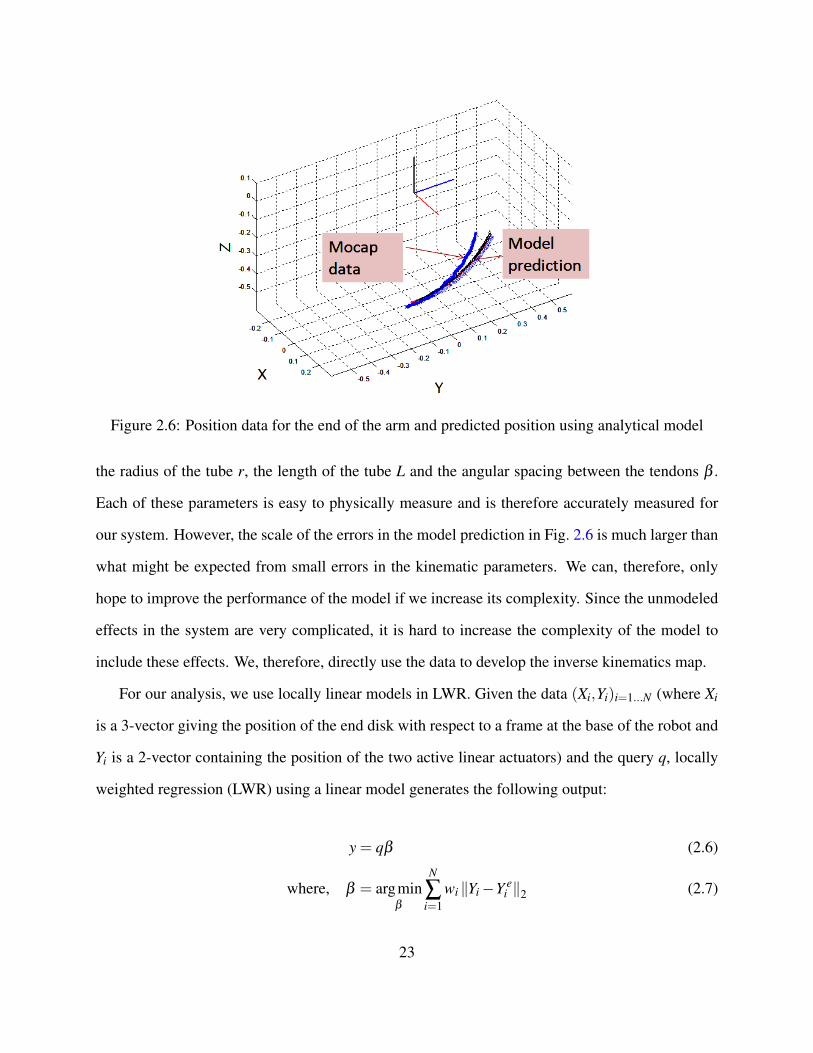
Figure 2.6: Position data for the end of the arm and predicted position using analytical model

the radius of the tube r, the length of the tube L and the angular spacing between the tendons β .

Each of these parameters is easy to physically measure and is therefore accurately measured for

our system. However, the scale of the errors in the model prediction in Fig. 2.6 is much larger than

what might be expected from small errors in the kinematic parameters. We can, therefore, only

hope to improve the performance of the model if we increase its complexity. Since the unmodeled

effects in the system are very complicated, it is hard to increase the complexity of the model to

include these effects. We, therefore, directly use the data to develop the inverse kinematics map.

For our analysis, we use locally linear models in LWR. Given the data (Xi,Yi)i=1...N (where Xi

is a 3-vector giving the position of the end disk with respect to a frame at the base of the robot and

Yi is a 2-vector containing the position of the two active linear actuators) and the query q, locally

weighted regression (LWR) using a linear model generates the following output:

y = qβ (2.6)

where, β = argminβ

N

∑i=1

wi ‖Yi−Y ei ‖2 (2.7)

23

−0.1 0 0.1 0.2 0.3 0.40.0127

0.0254

0.0381

0.0508

0.0635

0.0762

0.0889

0.1016

Y (m)

q 2 (m

)MoCap data

Predicted (LWR)

(a) Predicted and actual position values of the secondactuator q2 plotted with Y coordinate of the arm end

−0.7 −0.6 −0.5 −0.4 −0.30.0127

0.0254

0.0381

0.0508

0.0635

0.0762

0.0889

0.1016

Z (m)

q 2 (m

)

MoCap Data

Predicted (LWR)

(b) Predicted and actual position values of the secondactuator q2 plotted with Z coordinate of the arm end

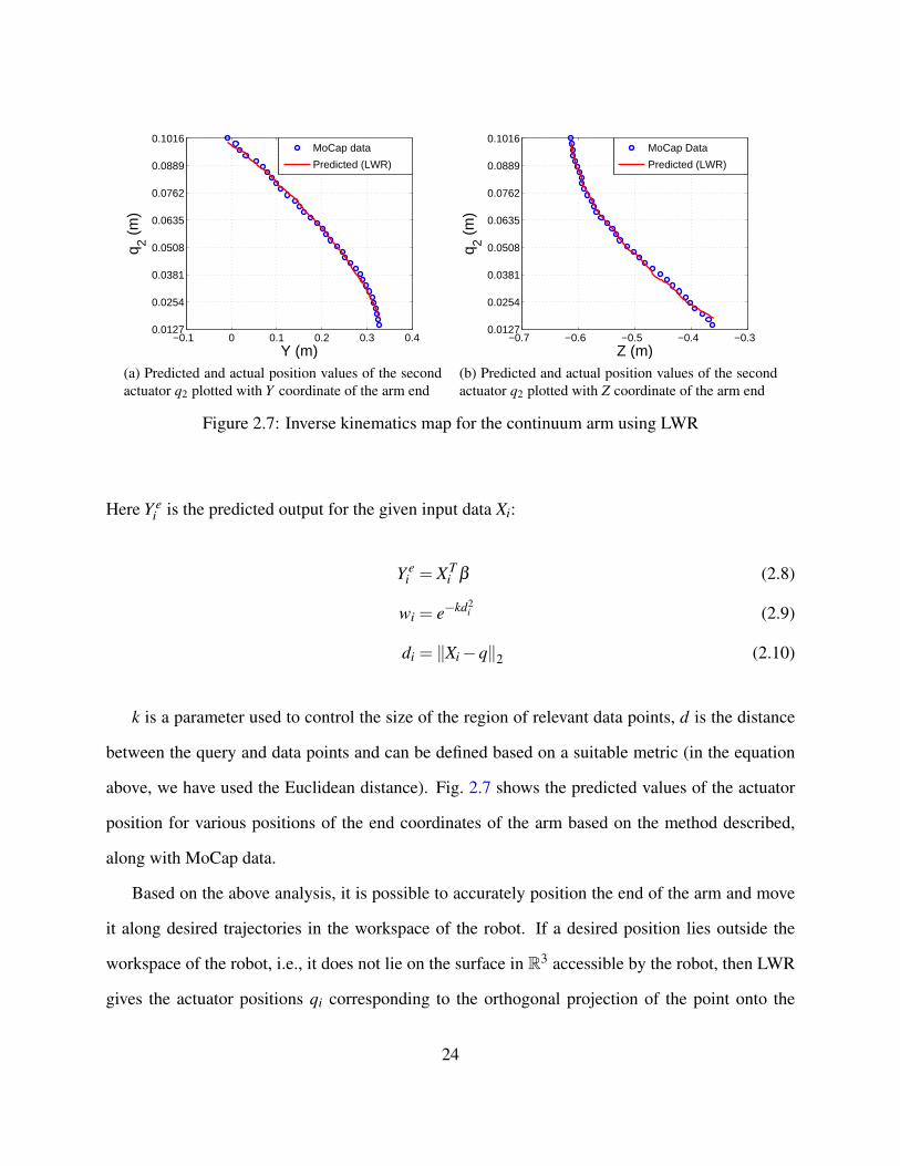
Figure 2.7: Inverse kinematics map for the continuum arm using LWR

Here Y ei is the predicted output for the given input data Xi:

Y ei = XT

i β (2.8)

wi = e−kd2i (2.9)

di = ‖Xi−q‖2 (2.10)

k is a parameter used to control the size of the region of relevant data points, d is the distance

between the query and data points and can be defined based on a suitable metric (in the equation

above, we have used the Euclidean distance). Fig. 2.7 shows the predicted values of the actuator

position for various positions of the end coordinates of the arm based on the method described,

along with MoCap data.

Based on the above analysis, it is possible to accurately position the end of the arm and move

it along desired trajectories in the workspace of the robot. If a desired position lies outside the

workspace of the robot, i.e., it does not lie on the surface in R3 accessible by the robot, then LWR

gives the actuator positions qi corresponding to the orthogonal projection of the point onto the

24

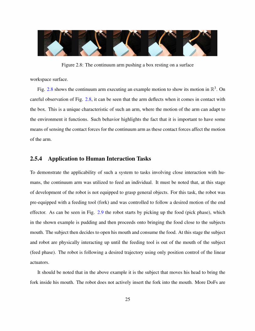
Figure 2.8: The continuum arm pushing a box resting on a surface

workspace surface.

Fig. 2.8 shows the continuum arm executing an example motion to show its motion in R3. On

careful observation of Fig. 2.8, it can be seen that the arm deflects when it comes in contact with

the box. This is a unique characteristic of such an arm, where the motion of the arm can adapt to

the environment it functions. Such behavior highlights the fact that it is important to have some

means of sensing the contact forces for the continuum arm as these contact forces affect the motion

of the arm.

2.5.4 Application to Human Interaction Tasks

To demonstrate the applicability of such a system to tasks involving close interaction with hu-

mans, the continuum arm was utilized to feed an individual. It must be noted that, at this stage

of development of the robot is not equipped to grasp general objects. For this task, the robot was

pre-equipped with a feeding tool (fork) and was controlled to follow a desired motion of the end

effector. As can be seen in Fig. 2.9 the robot starts by picking up the food (pick phase), which

in the shown example is pudding and then proceeds onto bringing the food close to the subjects

mouth. The subject then decides to open his mouth and consume the food. At this stage the subject

and robot are physically interacting up until the feeding tool is out of the mouth of the subject

(feed phase). The robot is following a desired trajectory using only position control of the linear

actuators.

It should be noted that in the above example it is the subject that moves his head to bring the

fork inside his mouth. The robot does not actively insert the fork into the mouth. More DoFs are

25

Figure 2.9: The continuum arm feeding a subject

Figure 2.10: Passive compliance allowing subject neck motion

needed to allow the bowl and subject position to be varied arbitrarily in the robots workspace. The

passive rather than active approach of food insertion demonstrated here would be suitable only

to people with disabilities that do not affect head motion capabilities. For individuals with more

severe disabilities that does not allow head motion an active feeding approach must be taken.

The active approach of for food insertion bears resemblance to the peg in hole problem studied

extensively in force control literature [91, 70]. In this case the location of the hole in not fixed

during the insertion phase. Since the subject is free to move his/her head the interaction during this

phase must be compliant. In the continuum arm compliant interaction is achieved by the passive

compliance in the system. The passive compliance allows for small neck motion that occur during

the feeding phase as shown in Fig. 2.10.

26

2.5.5 Discussion

The continuum arm moves using only continuous deformation along its structure. This allows

using an extremely flexible robot structure for safety while using the same flexibility to move the

system. Our approach towards developing the continuum arm has been to use minimal rigid parts

in the structure which potentially negate the safety benefits of the system. This has lead to a design

consisting of a single rubber tuber with tendon guides. The kinematics for the resulting system

are complex enough to warrant to use the of a data driven approach to develop the kinematic map

between actuator positions and the end effector pose. One of the key drawbacks of the system is

the lack of structural damping leading to uncontrolled undulatory motion in the arm even at low

speeds. Further work is necessary to analyze the arm motion in the presence of external forces, as

the arm motion is highly dependent on these unlike rigid systems.

2.6 Single Link Inflatable Robot

The next few subsections will provide details regarding some of our initial development work on

inflatable link robots. We shall first study the modeling and control of a single inflatable link. This

section of work is largely based on [97]. The system shown in Fig. 2.11, although very simple

is important in understanding and addressing certain key challenges in developing an actuated

inflatable link. The development lead to ideas regarding the type of material to be used and some

unique ideas regarding how to couple the links to actuators. We shall describe these developments

in subsequent subsections.

Besides the challenge of designing a practical inflatable link robot, we also need to establish

the ability to do useful tasks using robots with inflatable links. One such ability is force control.

We attempt to develop such capability for a single link inflatable robot. The purpose of doing so

will be two fold: a) develop a modeling technique for inflatable link systems b) utilize the model to

design controllers for the system. We shall describe both of these aspects along with experimental

27

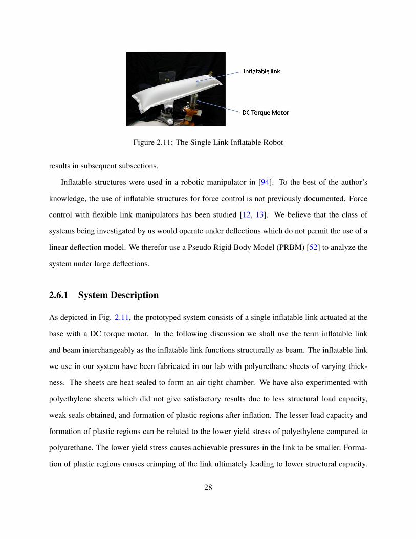
Figure 2.11: The Single Link Inflatable Robot

results in subsequent subsections.

Inflatable structures were used in a robotic manipulator in [94]. To the best of the author’s

knowledge, the use of inflatable structures for force control is not previously documented. Force

control with flexible link manipulators has been studied [12, 13]. We believe that the class of

systems being investigated by us would operate under deflections which do not permit the use of a

linear deflection model. We therefor use a Pseudo Rigid Body Model (PRBM) [52] to analyze the

system under large deflections.

2.6.1 System Description

As depicted in Fig. 2.11, the prototyped system consists of a single inflatable link actuated at the

base with a DC torque motor. In the following discussion we shall use the term inflatable link

and beam interchangeably as the inflatable link functions structurally as beam. The inflatable link

we use in our system have been fabricated in our lab with polyurethane sheets of varying thick-

ness. The sheets are heat sealed to form an air tight chamber. We have also experimented with

polyethylene sheets which did not give satisfactory results due to less structural load capacity,

weak seals obtained, and formation of plastic regions after inflation. The lesser load capacity and

formation of plastic regions can be related to the lower yield stress of polyethylene compared to

polyurethane. The lower yield stress causes achievable pressures in the link to be smaller. Forma-

tion of plastic regions causes crimping of the link ultimately leading to lower structural capacity.

28

For a polyurethane inflatable beam of length 50 cm, we were able to successfully carry a force of

8 N at its end. The limitation in load capacity is largely due to certain prototyping issues. With

this load capacity, the system can be used for applications such as manipulation of lightweight

objects and grooming which have small force requirements and are relevant to assistance in activ-

ities of daily living (ADLs). Higher load capacities on the order of a few hundred Newtons can be

achieved as is shown in [122, 64].

Inflatable beams are different from traditional beams as the material used to make them can

only hold tensile stress. An inflatable tube can be modeled in a number of ways as suggested in

[52, 113, 122]. The simplest approach is to consider the effect of pressure in the tube as a pre-stress

in the tube. Then the Euler-Bernoulli beam theory for large deflections can be applied to obtain

deflections and stresses in the beam. The beam fails when the stress at any point on the surface of

the beam is less than zero. In the following subsections, we discuss a system model and system

behavior.

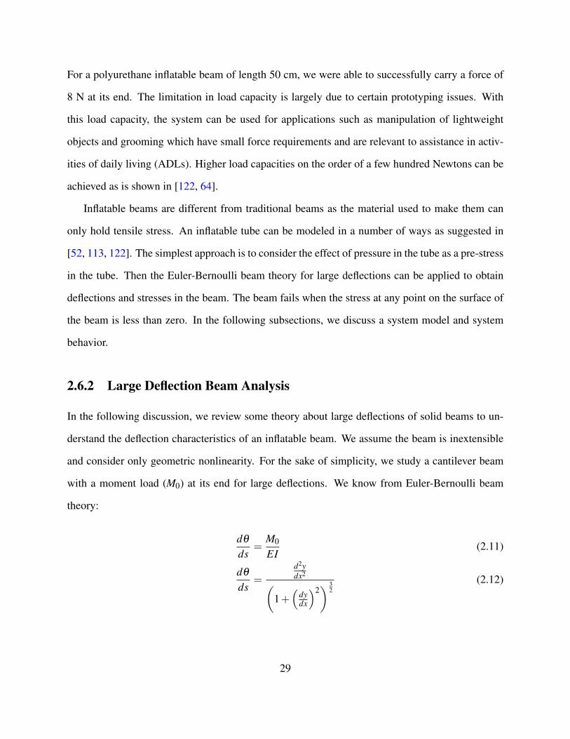
2.6.2 Large Deflection Beam Analysis

In the following discussion, we review some theory about large deflections of solid beams to un-

derstand the deflection characteristics of an inflatable beam. We assume the beam is inextensible

and consider only geometric nonlinearity. For the sake of simplicity, we study a cantilever beam

with a moment load (M0) at its end for large deflections. We know from Euler-Bernoulli beam

theory:

dθ

ds=

M0

EI(2.11)

dθ

ds=

d2ydx2(

1+(

dydx

)2) 3

2(2.12)

29

where, E is the Young’s Modulus of the beam material, I is the area moment of the cross section

of the beam, s is the arc length along the beam, θ is the angle of the tangent to the beam from the

horizontal, y is the transverse deflection of the beam which is a function of the position x along

axial direction. In linear analysis, we say the slopes in 2.12 are small and neglect its powers and get

the standard equation. For the large deflection case, the powers of the slope cannot be neglected.

Therefore we start with 2.11 and integrate along the arc length s, for the length L of the beam.

∫θ0

0dθ =

∫ L

0

M0

EIds

⇒ θ0 =M0LEI

(2.13)

Hence the angular deflection at the end of the beam, with no small deflection assumptions, is

given by 2.13. From 2.13, the relationship between angular deflection and moment at the end of the

beam is linear. Such a relation allows for a simple representation of a flexible link with sufficient

accuracy using only a few parameters as discussed in the next subsection. Such simplifications are

also possible for beams with other loading conditions. For a detailed analysis of beams with end

loads and large deflection, see [50].

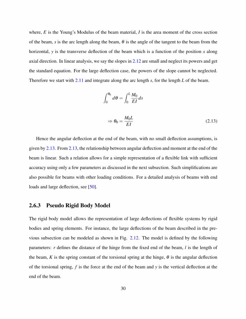
2.6.3 Pseudo Rigid Body Model

The rigid body model allows the representation of large deflections of flexible systems by rigid

bodies and spring elements. For instance, the large deflections of the beam described in the pre-

vious subsection can be modeled as shown in Fig. 2.12. The model is defined by the following

parameters: r defines the distance of the hinge from the fixed end of the beam, l is the length of

the beam, K is the spring constant of the torsional spring at the hinge, θ is the angular deflection

of the torsional spring, f is the force at the end of the beam and y is the vertical deflection at the

end of the beam.

30

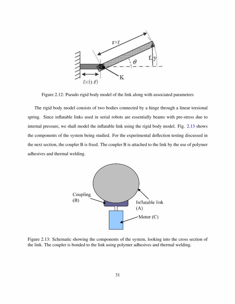
Figure 2.12: Pseudo rigid body model of the link along with associated parameters

The rigid body model consists of two bodies connected by a hinge through a linear torsional

spring. Since inflatable links used in serial robots are essentially beams with pre-stress due to

internal pressure, we shall model the inflatable link using the rigid body model. Fig. 2.13 shows

the components of the system being studied. For the experimental deflection testing discussed in

the next section, the coupler B is fixed. The coupler B is attached to the link by the use of polymer

adhesives and thermal welding.

Figure 2.13: Schematic showing the components of the system, looking into the cross section ofthe link. The coupler is bonded to the link using polymer adhesives and thermal welding.

31

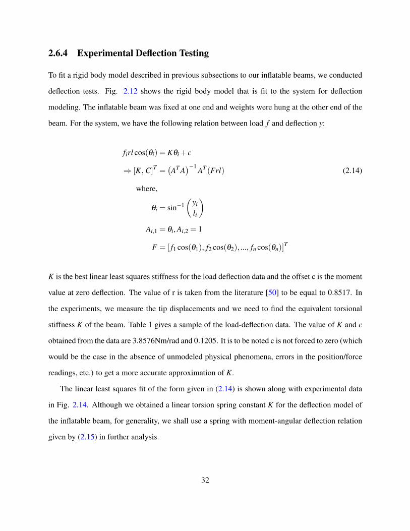
2.6.4 Experimental Deflection Testing

To fit a rigid body model described in previous subsections to our inflatable beams, we conducted

deflection tests. Fig. 2.12 shows the rigid body model that is fit to the system for deflection

modeling. The inflatable beam was fixed at one end and weights were hung at the other end of the

beam. For the system, we have the following relation between load f and deflection y:

firl cos(θi) = Kθi + c

⇒ [K, C]T =(AT A

)−1AT (Frl) (2.14)

where,

θi = sin−1(

yi

li

)Ai,1 = θi, Ai,2 = 1

F = [ f1 cos(θ1), f2 cos(θ2), ..., fn cos(θn)]T

K is the best linear least squares stiffness for the load deflection data and the offset c is the moment

value at zero deflection. The value of r is taken from the literature [50] to be equal to 0.8517. In

the experiments, we measure the tip displacements and we need to find the equivalent torsional

stiffness K of the beam. Table 1 gives a sample of the load-deflection data. The value of K and c

obtained from the data are 3.8576Nm/rad and 0.1205. It is to be noted c is not forced to zero (which

would be the case in the absence of unmodeled physical phenomena, errors in the position/force

readings, etc.) to get a more accurate approximation of K.

The linear least squares fit of the form given in (2.14) is shown along with experimental data

in Fig. 2.14. Although we obtained a linear torsion spring constant K for the deflection model of

the inflatable beam, for generality, we shall use a spring with moment-angular deflection relation

given by (2.15) in further analysis.

32

Table 2.1: Load deflection data for inflatable beamsLoad (N) y (mm)

0.6 61.1 122.6 323.7 544.3 625.0 725.6 84

Figure 2.14: Linear spring fit to the load deflection data.

τ = k1θ + k2θ3 (2.15)

Equation (2.15) is useful if in addition to geometric nonlinearities, other nonlinearities due to

material properties, motor-link coupling and other un-modeled effects in the system exist. In fact

for all the analysis presented in subsequent sections, (2.15) can be replaced by any higher order

function of the angular deflection as well, without affecting the validity of the analysis.

33

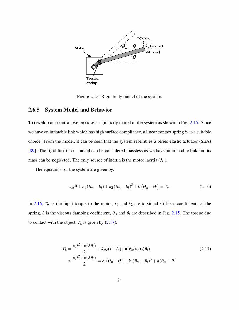
Figure 2.15: Rigid body model of the system.

2.6.5 System Model and Behavior

To develop our control, we propose a rigid body model of the system as shown in Fig. 2.15. Since

we have an inflatable link which has high surface compliance, a linear contact spring ks is a suitable

choice. From the model, it can be seen that the system resembles a series elastic actuator (SEA)

[89]. The rigid link in our model can be considered massless as we have an inflatable link and its

mass can be neglected. The only source of inertia is the motor inertia (Jm).

The equations for the system are given by:

Jmθ + k1 (θm−θl)+ k2 (θm−θl)3 +b

(θm− θl

)= Tm (2.16)

In 2.16, Tm is the input torque to the motor, k1 and k2 are torsional stiffness coefficients of the

spring, b is the viscous damping coefficient, θm and θl are described in Fig. 2.15. The torque due

to contact with the object, TL is given by (2.17).

TL =ksl2

c sin(2θl)

2+ kslc(l− lc)sin(θm)cos(θl) (2.17)

≈ ksl2c sin(2θl)

2= k1(θm−θl)+ k2(θm−θl)

3 +b(θm− θl)

34

assuming ksl2c sin(2θl)

2 � kslc(l− lc)sin(θm)cos(θl).

where lc = rl and r ' 1. Note that from (2.17) TL is a function of θl , further we define the

stiffness fN at any deflection as

TN(θm−θl) = k1(θm−θl)+ k2(θm−θl)3 (2.18)

Using (2.16) and (2.17) we can obtain the state space form of the dynamic equations:

x1 = x2

x2 =1

Jm

(Tm−

ksl2c sin(2x3)

2

)(2.19)

x3 =1b

(k1(x1− x3)+ k2(x1− x3)

3 +bx2−ksl2

c sin(2x3)

2

)

where x1 = θm, x2 = θm and x3 = θl .

Figure 2.16: Step response of the system.

System Behavior The system described by (2.19) was simulated with an input u = Tm = 1. Fig.

2.16 describes the response with time. For the step input T m = 1 applied at t = 0, the system

35

exhibits stable characteristics as can be seen from the response.

Lyapunov Stability Analysis We use the Lyapunov method for studying the stability of the

system [109]. For understanding the stability properties of the system, we take the candidate

Lyapunov function V as:

V =12

x22 +

∫ x1−x2

0Tn(σ)dσ +

∫ x3

0TL(σ)dσ (2.20)

V is a positive definite function as each of the terms involving the spring stiffness integrates to

positive values. Here TL, fN were defined in (2.17) and (2.18) respectively.

Differentiating (2.20) we get,

V = x2x2 +TN(x1− x3)+TL(x3)x3 (2.21)

Using (2.17) and (2.18) in (2.21

V =−bx22 +2bx2x3−bx2

3 + x2u

=−b(x2− x3)2 + x2u (2.22)

As can be seen from (2.22), for the open loop response i.e. when u = 0, V ≤ 0 . Therefore as

can be seen from Fig. 2.16, the system is stable. Further, asymptotic stability can be proved by

invoking LaSalle’s theorem. For the closed loop system, the control law u needs to be chosen to

ensure stability in the Lyapunov sense.

2.6.6 Force Control

Considering the system behavior, there are a number of options regarding what states we need

to measure and the states we want to control. We shall explore two sensing options: a) place an

36

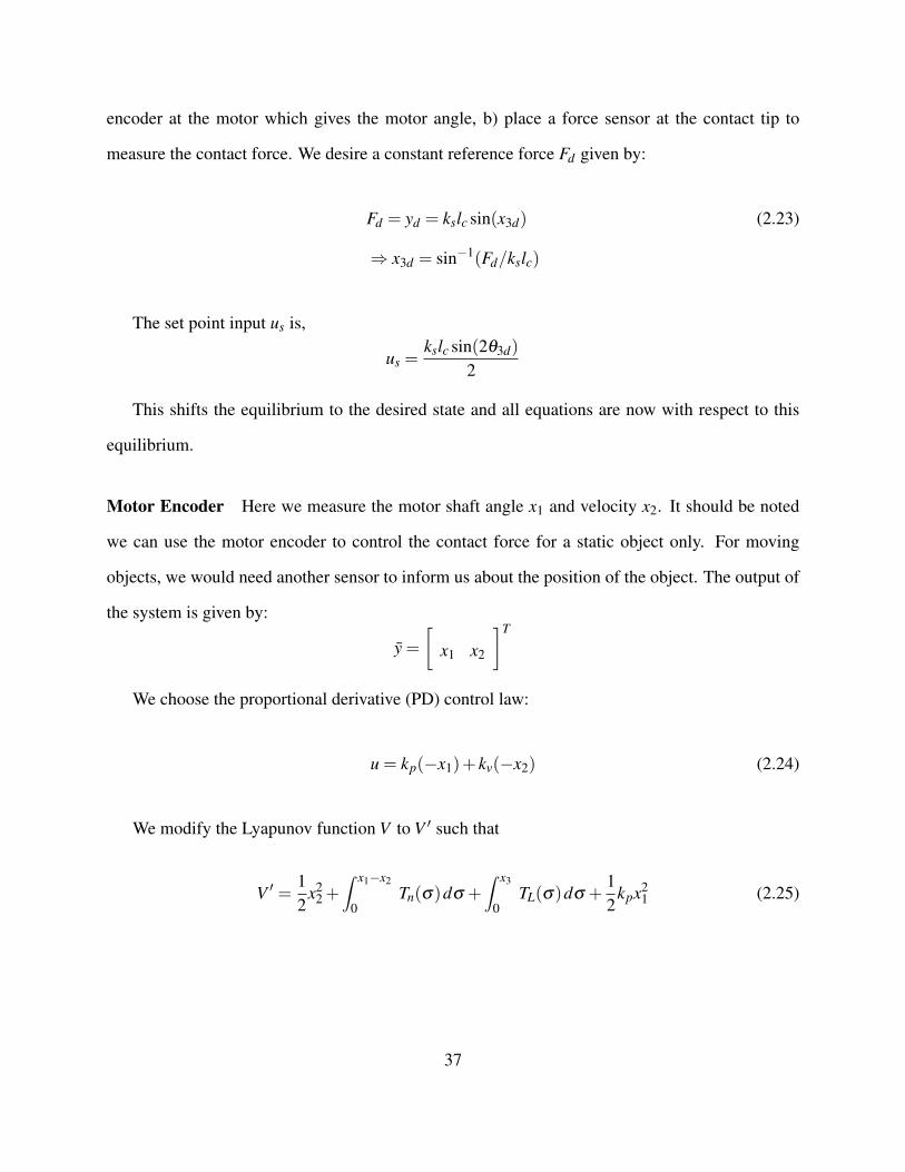
encoder at the motor which gives the motor angle, b) place a force sensor at the contact tip to

measure the contact force. We desire a constant reference force Fd given by:

Fd = yd = kslc sin(x3d) (2.23)

⇒ x3d = sin−1(Fd/kslc)

The set point input us is,

us =kslc sin(2θ3d)

2

This shifts the equilibrium to the desired state and all equations are now with respect to this

equilibrium.

Motor Encoder Here we measure the motor shaft angle x1 and velocity x2. It should be noted

we can use the motor encoder to control the contact force for a static object only. For moving

objects, we would need another sensor to inform us about the position of the object. The output of

the system is given by:

y =[

x1 x2

]T

We choose the proportional derivative (PD) control law:

u = kp(−x1)+ kv(−x2) (2.24)

We modify the Lyapunov function V to V ′ such that

V ′ =12

x22 +

∫ x1−x2

0Tn(σ)dσ +

∫ x3

0TL(σ)dσ +

12

kpx21 (2.25)

37

Again differentiating (2.25) with time:

V ′ =−bx22 +2bx2x3−bx2

3 + kpx1x2

=−b(x2− x3)2− kvx2

2 (2.26)

Clearly, V ′ ≤ 0. Hence the system is stable in the sense of Lyapunov. Fig. 2.17 and Fig. 2.18

show the simulation of the above system.

Figure 2.17: Model states in simulation with PD control on motor angle.

Contact Force Sensor Here we place a force sensor at the contact point and measure the contact

force. We assume that the contact force lies in the plane of the actuation torque from the motor.

The output is given by:

y = kslc sin(x3)

The proposed control law u is:

u = kp(−y) (2.27)

38

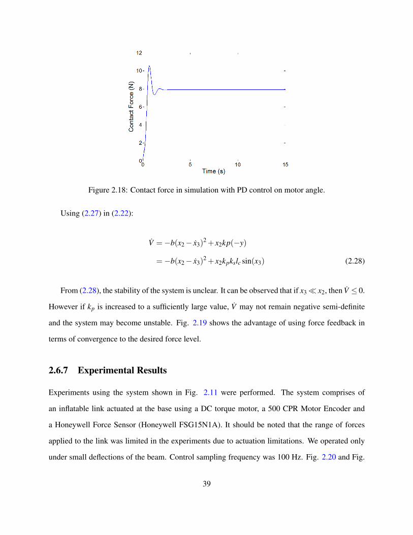
Figure 2.18: Contact force in simulation with PD control on motor angle.

Using (2.27) in (2.22):

V =−b(x2− x3)2 + x2kp(−y)

=−b(x2− x3)2 + x2kpkslc sin(x3) (2.28)

From (2.28), the stability of the system is unclear. It can be observed that if x3� x2, then V ≤ 0.

However if kp is increased to a sufficiently large value, V may not remain negative semi-definite

and the system may become unstable. Fig. 2.19 shows the advantage of using force feedback in

terms of convergence to the desired force level.

2.6.7 Experimental Results

Experiments using the system shown in Fig. 2.11 were performed. The system comprises of

an inflatable link actuated at the base using a DC torque motor, a 500 CPR Motor Encoder and

a Honeywell Force Sensor (Honeywell FSG15N1A). It should be noted that the range of forces

applied to the link was limited in the experiments due to actuation limitations. We operated only

under small deflections of the beam. Control sampling frequency was 100 Hz. Fig. 2.20 and Fig.

39

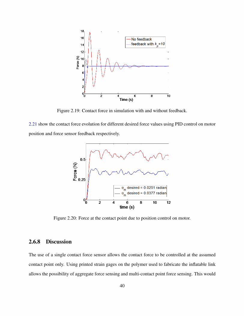
Figure 2.19: Contact force in simulation with and without feedback.

2.21 show the contact force evolution for different desired force values using PID control on motor

position and force sensor feedback respectively.

Figure 2.20: Force at the contact point due to position control on motor.

2.6.8 Discussion

The use of a single contact force sensor allows the contact force to be controlled at the assumed

contact point only. Using printed strain gages on the polymer used to fabricate the inflatable link

allows the possibility of aggregate force sensing and multi-contact point force sensing. This would

40

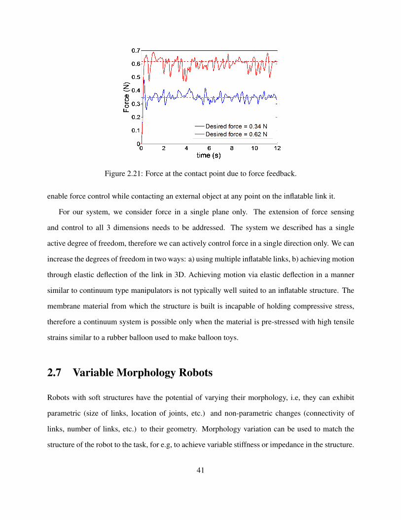
Figure 2.21: Force at the contact point due to force feedback.

enable force control while contacting an external object at any point on the inflatable link it.

For our system, we consider force in a single plane only. The extension of force sensing

and control to all 3 dimensions needs to be addressed. The system we described has a single

active degree of freedom, therefore we can actively control force in a single direction only. We can

increase the degrees of freedom in two ways: a) using multiple inflatable links, b) achieving motion

through elastic deflection of the link in 3D. Achieving motion via elastic deflection in a manner

similar to continuum type manipulators is not typically well suited to an inflatable structure. The

membrane material from which the structure is built is incapable of holding compressive stress,

therefore a continuum system is possible only when the material is pre-stressed with high tensile

strains similar to a rubber balloon used to make balloon toys.

2.7 Variable Morphology Robots

Robots with soft structures have the potential of varying their morphology, i.e, they can exhibit

parametric (size of links, location of joints, etc.) and non-parametric changes (connectivity of

links, number of links, etc.) to their geometry. Morphology variation can be used to match the

structure of the robot to the task, for e.g, to achieve variable stiffness or impedance in the structure.

41

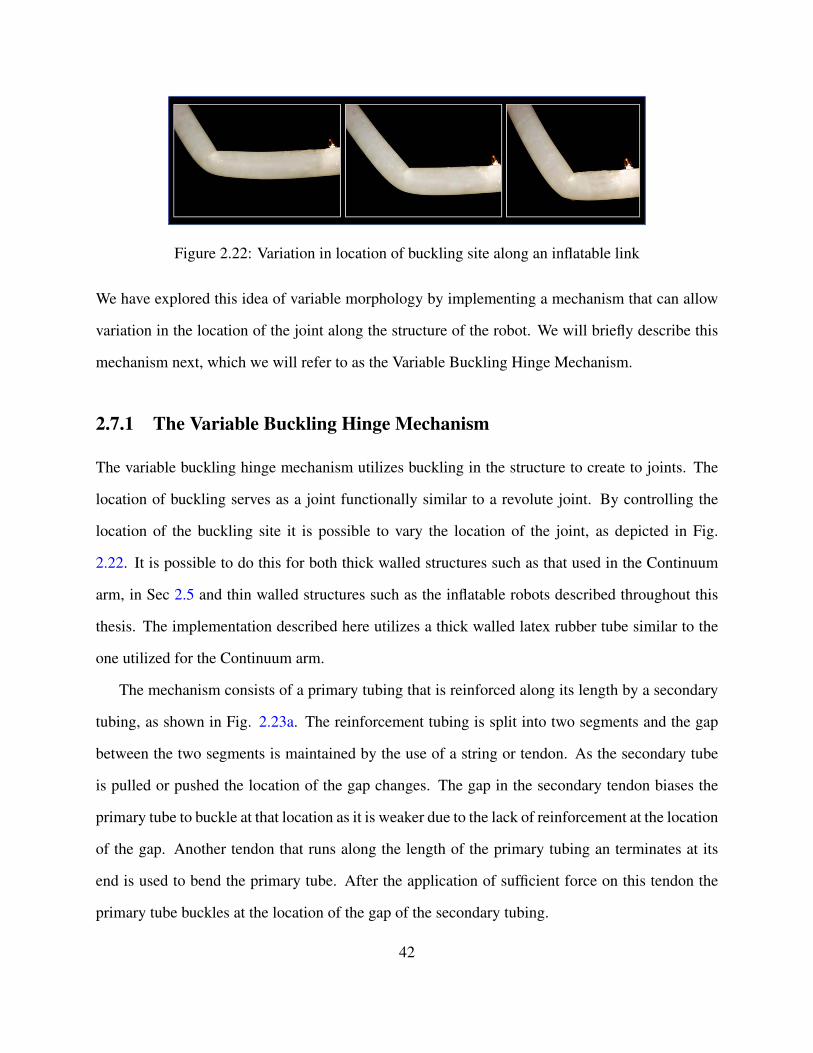
Figure 2.22: Variation in location of buckling site along an inflatable link

We have explored this idea of variable morphology by implementing a mechanism that can allow

variation in the location of the joint along the structure of the robot. We will briefly describe this

mechanism next, which we will refer to as the Variable Buckling Hinge Mechanism.

2.7.1 The Variable Buckling Hinge Mechanism

The variable buckling hinge mechanism utilizes buckling in the structure to create to joints. The

location of buckling serves as a joint functionally similar to a revolute joint. By controlling the

location of the buckling site it is possible to vary the location of the joint, as depicted in Fig.

2.22. It is possible to do this for both thick walled structures such as that used in the Continuum

arm, in Sec 2.5 and thin walled structures such as the inflatable robots described throughout this

thesis. The implementation described here utilizes a thick walled latex rubber tube similar to the

one utilized for the Continuum arm.

The mechanism consists of a primary tubing that is reinforced along its length by a secondary

tubing, as shown in Fig. 2.23a. The reinforcement tubing is split into two segments and the gap

between the two segments is maintained by the use of a string or tendon. As the secondary tube

is pulled or pushed the location of the gap changes. The gap in the secondary tendon biases the

primary tube to buckle at that location as it is weaker due to the lack of reinforcement at the location

of the gap. Another tendon that runs along the length of the primary tubing an terminates at its

end is used to bend the primary tube. After the application of sufficient force on this tendon the

primary tube buckles at the location of the gap of the secondary tubing.

42

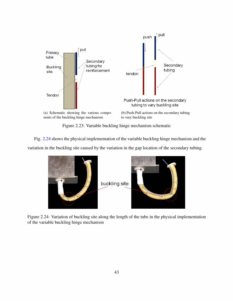
(a) Schematic showing the various compo-nents of the buckling hinge mechanism

(b) Push-Pull actions on the secondary tubingto vary buckling site

Figure 2.23: Variable buckling hinge mechanism schematic

Fig. 2.24 shows the physical implementation of the variable buckling hinge mechanism and the

variation in the buckling site caused by the variation in the gap location of the secondary tubing.

Figure 2.24: Variation of buckling site along the length of the tube in the physical implementationof the variable buckling hinge mechanism

43

2.8 Summary

In this chapter, we reviewed various injury modes that can occur during physical human robot in-

teraction and safety indices to measure the severity of injury during collisions between a human

and a robot. We also reviewed some of the existing techniques used to mitigate the risk of injury

such as compliant control, joint compliance and other existing relevant robot designs such as that

flexible link robots, soft coverings, continuum robots and inflatable robots. Some of our prelim-

inary work carried out in developing two types of soft robots: continuum robots and inflatable

robots was also described.

44

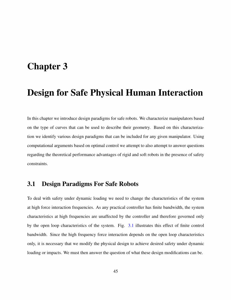
Chapter 3

Design for Safe Physical Human Interaction

In this chapter we introduce design paradigms for safe robots. We characterize manipulators based

on the type of curves that can be used to describe their geometry. Based on this characteriza-

tion we identify various design paradigms that can be included for any given manipulator. Using

computational arguments based on optimal control we attempt to also attempt to answer questions

regarding the theoretical performance advantages of rigid and soft robots in the presence of safety

constraints.

3.1 Design Paradigms For Safe Robots

To deal with safety under dynamic loading we need to change the characteristics of the system

at high force interaction frequencies. As any practical controller has finite bandwidth, the system

characteristics at high frequencies are unaffected by the controller and therefore governed only

by the open loop characteristics of the system. Fig. 3.1 illustrates this effect of finite control

bandwidth. Since the high frequency force interaction depends on the open loop characteristics

only, it is necessary that we modify the physical design to achieve desired safety under dynamic

loading or impacts. We must then answer the question of what these design modifications can be.

45

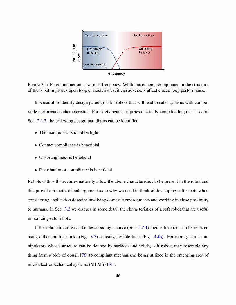
Figure 3.1: Force interaction at various frequency. While introducing compliance in the structureof the robot improves open loop characteristics, it can adversely affect closed loop performance.

It is useful to identify design paradigms for robots that will lead to safer systems with compa-

rable performance characteristics. For safety against injuries due to dynamic loading discussed in

Sec. 2.1.2, the following design paradigms can be identified:

• The manipulator should be light

• Contact compliance is beneficial

• Unsprung mass is beneficial

• Distribution of compliance is beneficial

Robots with soft structures naturally allow the above characteristics to be present in the robot and

this provides a motivational argument as to why we need to think of developing soft robots when

considering application domains involving domestic environments and working in close proximity

to humans. In Sec. 3.2 we discuss in some detail the characteristics of a soft robot that are useful

in realizing safe robots.

If the robot structure can be described by a curve (Sec. 3.2.1) then soft robots can be realized

using either multiple links (Fig. 3.5) or using flexible links (Fig. 3.4b). For more general ma-

nipulators whose structure can be defined by surfaces and solids, soft robots may resemble any

thing from a blob of dough [76] to compliant mechanisms being utilized in the emerging area of

microelectromechanical systems (MEMS) [61].

46

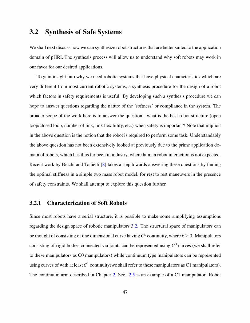
3.2 Synthesis of Safe Systems

We shall next discuss how we can synthesize robot structures that are better suited to the application

domain of pHRI. The synthesis process will allow us to understand why soft robots may work in

our favor for our desired applications.

To gain insight into why we need robotic systems that have physical characteristics which are

very different from most current robotic systems, a synthesis procedure for the design of a robot

which factors in safety requirements is useful. By developing such a synthesis procedure we can

hope to answer questions regarding the nature of the ’softness’ or compliance in the system. The

broader scope of the work here is to answer the question - what is the best robot structure (open

loop/closed loop, number of link, link flexibility, etc.) when safety is important? Note that implicit

in the above question is the notion that the robot is required to perform some task. Understandably

the above question has not been extensively looked at previously due to the prime application do-

main of robots, which has thus far been in industry, where human robot interaction is not expected.

Recent work by Bicchi and Tonietti [8] takes a step towards answering these questions by finding

the optimal stiffness in a simple two mass robot model, for rest to rest maneuvers in the presence

of safety constraints. We shall attempt to explore this question further.

3.2.1 Characterization of Soft Robots

Since most robots have a serial structure, it is possible to make some simplifying assumptions

regarding the design space of robotic manipulators 3.2. The structural space of manipulators can

be thought of consisting of one dimensional curve having Ck continuity, where k≥ 0. Manipulators

consisting of rigid bodies connected via joints can be represented using C0 curves (we shall refer

to these manipulators as C0 manipulators) while continuum type manipulators can be represented

using curves of with at least C1 continuity(we shall refer to these manipulators as C1 manipulators).

The continuum arm described in Chapter 2, Sec. 2.5 is an example of a C1 manipulator. Robot

47

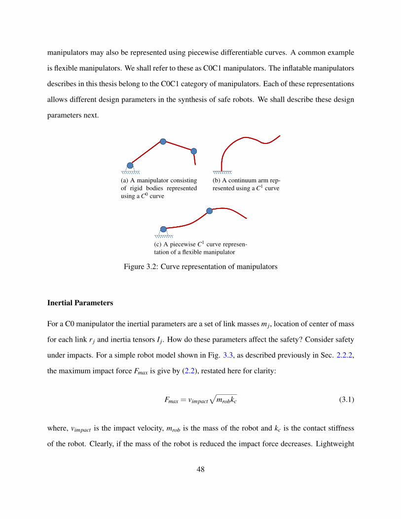
manipulators may also be represented using piecewise differentiable curves. A common example

is flexible manipulators. We shall refer to these as C0C1 manipulators. The inflatable manipulators

describes in this thesis belong to the C0C1 category of manipulators. Each of these representations

allows different design parameters in the synthesis of safe robots. We shall describe these design

parameters next.

(a) A manipulator consistingof rigid bodies representedusing a C0 curve

(b) A continuum arm rep-resented using a C1 curve

(c) A piecewise C1 curve represen-tation of a flexible manipulator

Figure 3.2: Curve representation of manipulators

Inertial Parameters

For a C0 manipulator the inertial parameters are a set of link masses m j, location of center of mass

for each link r j and inertia tensors I j. How do these parameters affect the safety? Consider safety

under impacts. For a simple robot model shown in Fig. 3.3, as described previously in Sec. 2.2.2,

the maximum impact force Fmax is give by (2.2), restated here for clarity:

Fmax = vimpact√

mrobkc (3.1)

where, vimpact is the impact velocity, mrob is the mass of the robot and kc is the contact stiffness

of the robot. Clearly, if the mass of the robot is reduced the impact force decreases. Lightweight

48

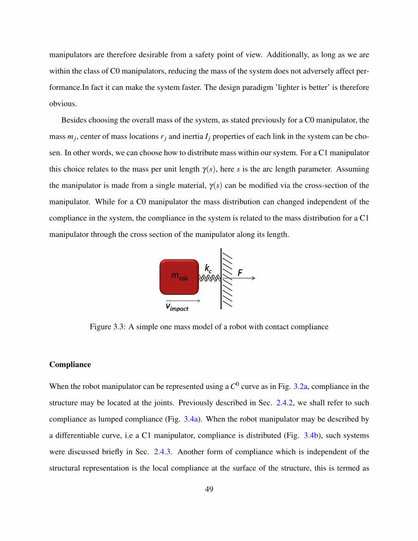
manipulators are therefore desirable from a safety point of view. Additionally, as long as we are

within the class of C0 manipulators, reducing the mass of the system does not adversely affect per-

formance.In fact it can make the system faster. The design paradigm ’lighter is better’ is therefore

obvious.

Besides choosing the overall mass of the system, as stated previously for a C0 manipulator, the

mass m j, center of mass locations r j and inertia I j properties of each link in the system can be cho-

sen. In other words, we can choose how to distribute mass within our system. For a C1 manipulator

this choice relates to the mass per unit length γ(s), here s is the arc length parameter. Assuming

the manipulator is made from a single material, γ(s) can be modified via the cross-section of the

manipulator. While for a C0 manipulator the mass distribution can changed independent of the

compliance in the system, the compliance in the system is related to the mass distribution for a C1

manipulator through the cross section of the manipulator along its length.

Figure 3.3: A simple one mass model of a robot with contact compliance

Compliance

When the robot manipulator can be represented using a C0 curve as in Fig. 3.2a, compliance in the

structure may be located at the joints. Previously described in Sec. 2.4.2, we shall refer to such

compliance as lumped compliance (Fig. 3.4a). When the robot manipulator may be described by

a differentiable curve, i.e a C1 manipulator, compliance is distributed (Fig. 3.4b), such systems

were discussed briefly in Sec. 2.4.3. Another form of compliance which is independent of the

structural representation is the local compliance at the surface of the structure, this is termed as

49

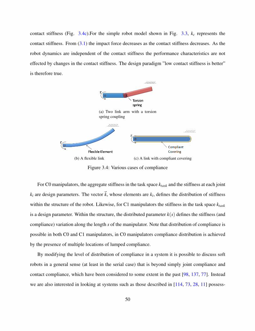
contact stiffness (Fig. 3.4c).For the simple robot model shown in Fig. 3.3, kc represents the

contact stiffness. From (3.1) the impact force decreases as the contact stiffness decreases. As the

robot dynamics are independent of the contact stiffness the performance characteristics are not

effected by changes in the contact stiffness. The design paradigm ”low contact stiffness is better”

is therefore true.

(a) Two link arm with a torsionspring coupling

(b) A flexible link (c) A link with compliant covering

Figure 3.4: Various cases of compliance

For C0 manipulators, the aggregate stiffness in the task space ktask and the stiffness at each joint

ki are design parameters. The vector~k, whose elements are ki, defines the distribution of stiffness

within the structure of the robot. Likewise, for C1 manipulators the stiffness in the task space ktask

is a design parameter. Within the structure, the distributed parameter k(s) defines the stiffness (and

compliance) variation along the length s of the manipulator. Note that distribution of compliance is

possible in both C0 and C1 manipulators, in C0 manipulators compliance distribution is achieved

by the presence of multiple locations of lumped compliance.

By modifying the level of distribution of compliance in a system it is possible to discuss soft

robots in a general sense (at least in the serial case) that is beyond simply joint compliance and

contact compliance, which have been considered to some extent in the past [98, 137, 77]. Instead

we are also interested in looking at systems such as those described in [114, 73, 28, 11] possess-

50

ing some form of distributed compliance. When compliance distribution is allowed in a system

the design space of the manipulator vastly increases. We shall discuss this issue of compliance

distribution for synthesis of safe systems in greater detail next.

3.2.2 Compliance Distribution

When compliance is continuously associated with several regions of the structure of the robot, we

will refer to such compliance as distributed compliance. Compliance distribution has two important

effects:

1. It decreases the unsprung mass during an impact, thus decreasing the maximum impact force.

2. By definition it introduces compliance at multiple location. The unsprung mass during an

impact is therefore reduced even as the impact location changes on the structure.

In Fig. 3.5 the unsprung mass is simply the last link that interacts with the external object. We shall

see the effect of unsprung mass reduction via compliance distribution on impact contact forces, for

a system with rigid bodies using simulations later in this section.

While the above effects are beneficial for safety, The dynamics of the robot are affected by

changing the distribution of compliance. It is therefore not clear whether distributed compliance

has a degrading or positive effect on performance of the system. We shall attempt to answer this

question using optimization.

Given the large number of design parameters available for a system with distributed compli-

ance, we shall focus on the problem of optimizing these parameters from the standpoint of safety

and performance. In the case of rigid bodies (Fig. 3.5), the parameters may include the number,

mass and length of the intermediate links, the stiffness of the torsion springs connecting the inter-

mediate links, etc. The design parameters for a flexible link may include: the shape of the link, the

material’s Young’s modulus, the cross section, the mass density.

51

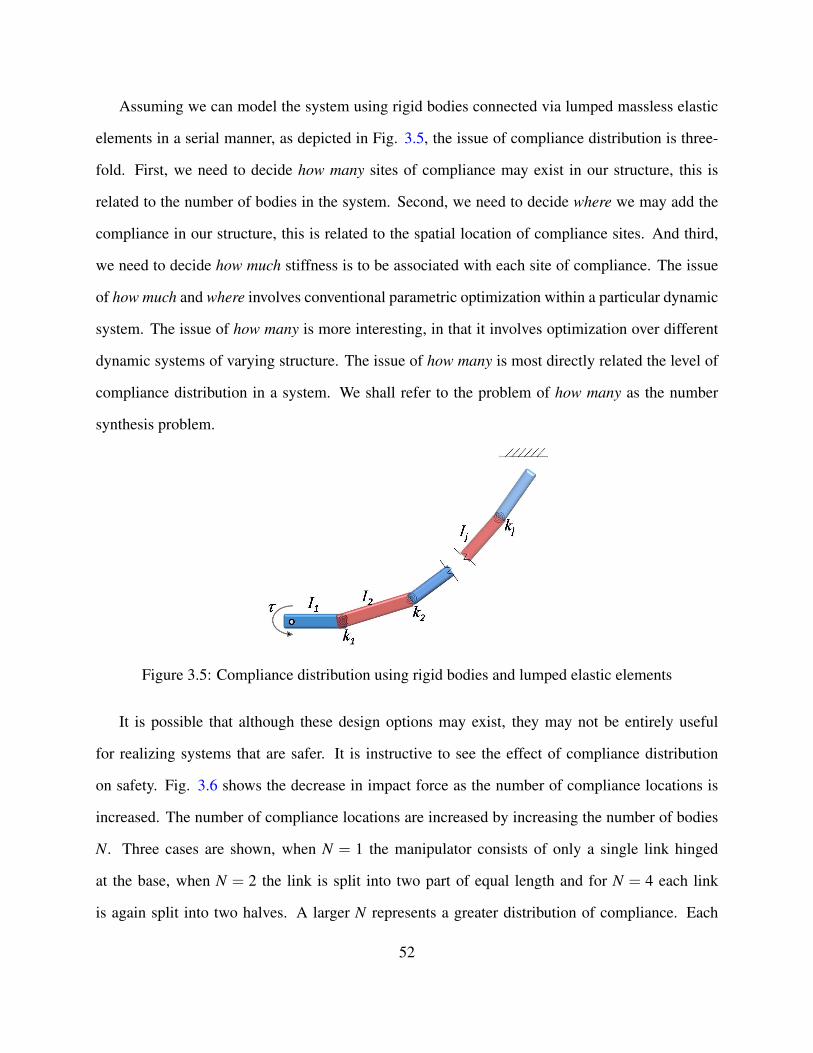
Assuming we can model the system using rigid bodies connected via lumped massless elastic

elements in a serial manner, as depicted in Fig. 3.5, the issue of compliance distribution is three-

fold. First, we need to decide how many sites of compliance may exist in our structure, this is

related to the number of bodies in the system. Second, we need to decide where we may add the

compliance in our structure, this is related to the spatial location of compliance sites. And third,

we need to decide how much stiffness is to be associated with each site of compliance. The issue

of how much and where involves conventional parametric optimization within a particular dynamic

system. The issue of how many is more interesting, in that it involves optimization over different

dynamic systems of varying structure. The issue of how many is most directly related the level of

compliance distribution in a system. We shall refer to the problem of how many as the number

synthesis problem.

Figure 3.5: Compliance distribution using rigid bodies and lumped elastic elements

It is possible that although these design options may exist, they may not be entirely useful

for realizing systems that are safer. It is instructive to see the effect of compliance distribution

on safety. Fig. 3.6 shows the decrease in impact force as the number of compliance locations is

increased. The number of compliance locations are increased by increasing the number of bodies

N. Three cases are shown, when N = 1 the manipulator consists of only a single link hinged

at the base, when N = 2 the link is split into two part of equal length and for N = 4 each link

is again split into two halves. A larger N represents a greater distribution of compliance. Each

52

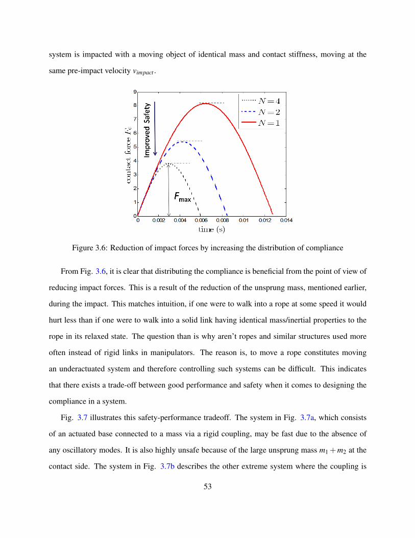
system is impacted with a moving object of identical mass and contact stiffness, moving at the

same pre-impact velocity vimpact .

Figure 3.6: Reduction of impact forces by increasing the distribution of compliance

From Fig. 3.6, it is clear that distributing the compliance is beneficial from the point of view of

reducing impact forces. This is a result of the reduction of the unsprung mass, mentioned earlier,

during the impact. This matches intuition, if one were to walk into a rope at some speed it would

hurt less than if one were to walk into a solid link having identical mass/inertial properties to the

rope in its relaxed state. The question than is why aren’t ropes and similar structures used more

often instead of rigid links in manipulators. The reason is, to move a rope constitutes moving

an underactuated system and therefore controlling such systems can be difficult. This indicates

that there exists a trade-off between good performance and safety when it comes to designing the

compliance in a system.

Fig. 3.7 illustrates this safety-performance tradeoff. The system in Fig. 3.7a, which consists

of an actuated base connected to a mass via a rigid coupling, may be fast due to the absence of

any oscillatory modes. It is also highly unsafe because of the large unsprung mass m1 +m2 at the

contact side. The system in Fig. 3.7b describes the other extreme system where the coupling is

53

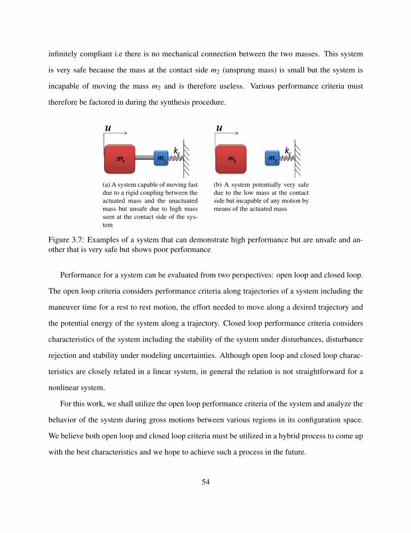
infinitely compliant i.e there is no mechanical connection between the two masses. This system

is very safe because the mass at the contact side m2 (unsprung mass) is small but the system is

incapable of moving the mass m2 and is therefore useless. Various performance criteria must

therefore be factored in during the synthesis procedure.

(a) A system capable of moving fastdue to a rigid coupling between theactuated mass and the unactuatedmass but unsafe due to high massseen at the contact side of the sys-tem

(b) A system potentially very safedue to the low mass at the contactside but incapable of any motion bymeans of the actuated mass

Figure 3.7: Examples of a system that can demonstrate high performance but are unsafe and an-other that is very safe but shows poor performance

Performance for a system can be evaluated from two perspectives: open loop and closed loop.

The open loop criteria considers performance criteria along trajectories of a system including the

maneuver time for a rest to rest motion, the effort needed to move along a desired trajectory and

the potential energy of the system along a trajectory. Closed loop performance criteria considers

characteristics of the system including the stability of the system under disturbances, disturbance

rejection and stability under modeling uncertainties. Although open loop and closed loop charac-

teristics are closely related in a linear system, in general the relation is not straightforward for a

nonlinear system.

For this work, we shall utilize the open loop performance criteria of the system and analyze the

behavior of the system during gross motions between various regions in its configuration space.

We believe both open loop and closed loop criteria must be utilized in a hybrid process to come up

with the best characteristics and we hope to achieve such a process in the future.

54

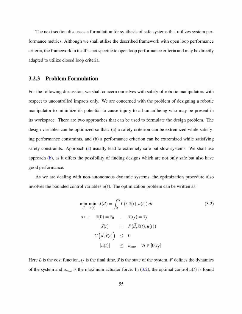
The next section discusses a formulation for synthesis of safe systems that utilizes system per-

formance metrics. Although we shall utilize the described framework with open loop performance

criteria, the framework in itself is not specific to open loop performance criteria and may be directly

adapted to utilize closed loop criteria.

3.2.3 Problem Formulation

For the following discussion, we shall concern ourselves with safety of robotic manipulators with

respect to uncontrolled impacts only. We are concerned with the problem of designing a robotic

manipulator to minimize its potential to cause injury to a human being who may be present in

its workspace. There are two approaches that can be used to formulate the design problem. The

design variables can be optimized so that: (a) a safety criterion can be extremized while satisfy-

ing performance constraints, and (b) a performance criterion can be extremized while satisfying

safety constraints. Approach (a) usually lead to extremely safe but slow systems. We shall use

approach (b), as it offers the possibility of finding designs which are not only safe but also have

good performance.

As we are dealing with non-autonomous dynamic systems, the optimization procedure also

involves the bounded control variables u(t). The optimization problem can be written as:

min~d

minu(t)

J(~d) =∫ t f

0L(t,~x(t),u(t)) dt (3.2)

s.t. : ~x(0) =~x0 , ~x(t f ) =~x f

~x(t) = F(~d,~x(t),u(t))

C(~d,~x(t)

)≤ 0

|u(t)| ≤ umax ∀t ∈ [0, t f ]

Here L is the cost function, t f is the final time,~x is the state of the system, F defines the dynamics

of the system and umax is the maximum actuator force. In (3.2), the optimal control u(t) is found

55

such that it minimizes the cost functional J(~d) for a particular set of design variables ~d; J(~d) is

then minimized over the set of design variables ~d. The approach described above is similar to [8]

where optimal control is used to generate the functional for the optimal design problem, however

they use this method to optimize for the mechanism stiffness only. We are concerned with a

more general design problem. Based on the above formulation, it is possible to answer important

questions regarding the design of a manipulator such as what is the best topology of the actuator

link transmission and what is the best stiffness and mass distribution within this topology, etc.

The idea of modifying the actuator-link topology to improve interaction characteristics of the

system has been used before. Designs such as the Series Elastic Actuators (SEA) [89] split the

actuator and link and couple them with an elastic element. [137] uses series elastic actuators and

also modifies the mass distribution within the system to improve performance.

Having presented a general synthesis framework, in the subsequent section, we shall utilize the

above framework to gain insight into the nature of compliance distribution needed for safety and

performance of linear systems of the type shown in Fig. 3.8. As mentioned previously the number

of the bodies in the system affect the distribution of compliance in the system and so we shall focus

on the number synthesis problem for this system.

3.2.4 Number Synthesis

Figure 3.8: The number synthesis problem

A schematic of the number synthesis problem introduced in Sec. 3.2.2 is shown in Fig. 3.8.

To simplify our discussion and to neglect geometric effects, we shall only consider linear time-

56

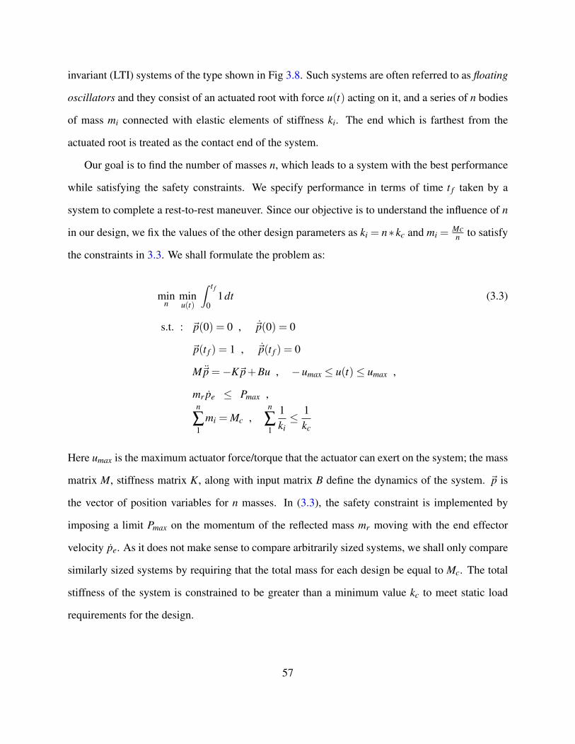
invariant (LTI) systems of the type shown in Fig 3.8. Such systems are often referred to as floating

oscillators and they consist of an actuated root with force u(t) acting on it, and a series of n bodies

of mass mi connected with elastic elements of stiffness ki. The end which is farthest from the

actuated root is treated as the contact end of the system.

Our goal is to find the number of masses n, which leads to a system with the best performance

while satisfying the safety constraints. We specify performance in terms of time t f taken by a

system to complete a rest-to-rest maneuver. Since our objective is to understand the influence of n

in our design, we fix the values of the other design parameters as ki = n∗kc and mi =Mcn to satisfy

the constraints in 3.3. We shall formulate the problem as:

minn

minu(t)

∫ t f

01dt (3.3)

s.t. : ~p(0) = 0 , ~p(0) = 0

~p(t f ) = 1 , ~p(t f ) = 0

M~p =−K~p+Bu , −umax ≤ u(t)≤ umax ,

mr pe ≤ Pmax ,n

∑1

mi = Mc ,n

∑1

1ki≤ 1

kc

Here umax is the maximum actuator force/torque that the actuator can exert on the system; the mass

matrix M, stiffness matrix K, along with input matrix B define the dynamics of the system. ~p is

the vector of position variables for n masses. In (3.3), the safety constraint is implemented by

imposing a limit Pmax on the momentum of the reflected mass mr moving with the end effector

velocity pe. As it does not make sense to compare arbitrarily sized systems, we shall only compare

similarly sized systems by requiring that the total mass for each design be equal to Mc. The total

stiffness of the system is constrained to be greater than a minimum value kc to meet static load

requirements for the design.

57

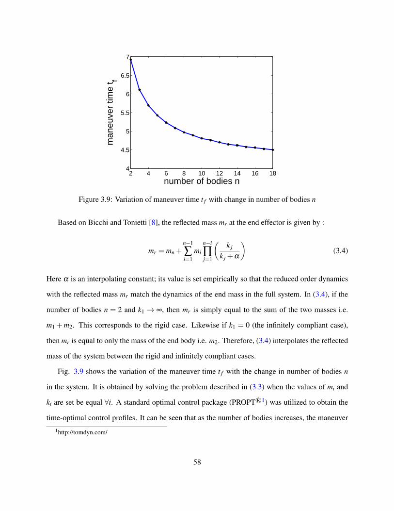
2 4 6 8 10 12 14 16 184

4.5

5

5.5

6

6.5

7

number of bodies n

man

euve

r tim

e t f

Figure 3.9: Variation of maneuver time t f with change in number of bodies n

Based on Bicchi and Tonietti [8], the reflected mass mr at the end effector is given by :

mr = mn +n−1

∑i=1

mi

n−i

∏j=1

(k j

k j +α

)(3.4)

Here α is an interpolating constant; its value is set empirically so that the reduced order dynamics

with the reflected mass mr match the dynamics of the end mass in the full system. In (3.4), if the

number of bodies n = 2 and k1 → ∞, then mr is simply equal to the sum of the two masses i.e.

m1 +m2. This corresponds to the rigid case. Likewise if k1 = 0 (the infinitely compliant case),

then mr is equal to only the mass of the end body i.e. m2. Therefore, (3.4) interpolates the reflected

mass of the system between the rigid and infinitely compliant cases.

Fig. 3.9 shows the variation of the maneuver time t f with the change in number of bodies n

in the system. It is obtained by solving the problem described in (3.3) when the values of mi and

ki are set be equal ∀i. A standard optimal control package (PROPT R©1) was utilized to obtain the

time-optimal control profiles. It can be seen that as the number of bodies increases, the maneuver

1http://tomdyn.com/

58

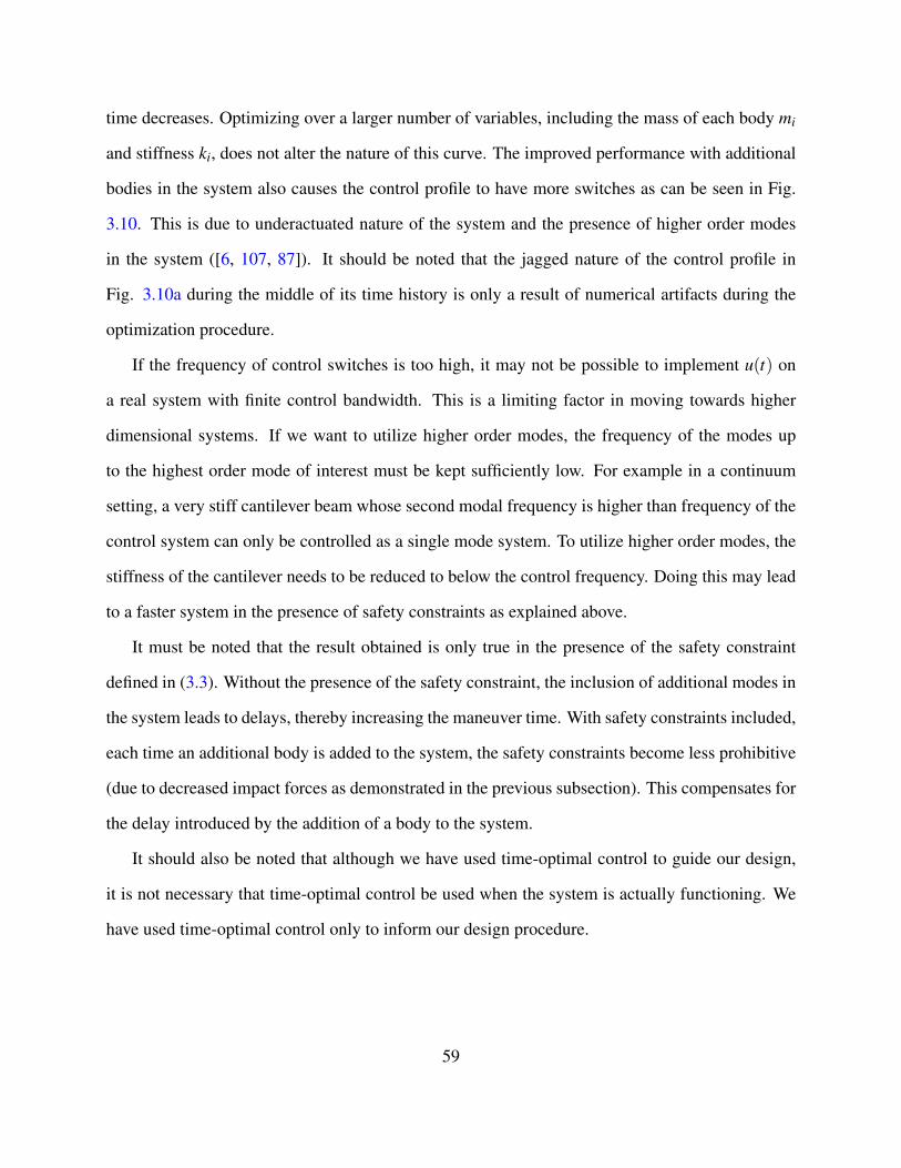
time decreases. Optimizing over a larger number of variables, including the mass of each body mi

and stiffness ki, does not alter the nature of this curve. The improved performance with additional

bodies in the system also causes the control profile to have more switches as can be seen in Fig.

3.10. This is due to underactuated nature of the system and the presence of higher order modes

in the system ([6, 107, 87]). It should be noted that the jagged nature of the control profile in

Fig. 3.10a during the middle of its time history is only a result of numerical artifacts during the

optimization procedure.

If the frequency of control switches is too high, it may not be possible to implement u(t) on

a real system with finite control bandwidth. This is a limiting factor in moving towards higher

dimensional systems. If we want to utilize higher order modes, the frequency of the modes up

to the highest order mode of interest must be kept sufficiently low. For example in a continuum

setting, a very stiff cantilever beam whose second modal frequency is higher than frequency of the

control system can only be controlled as a single mode system. To utilize higher order modes, the

stiffness of the cantilever needs to be reduced to below the control frequency. Doing this may lead

to a faster system in the presence of safety constraints as explained above.

It must be noted that the result obtained is only true in the presence of the safety constraint

defined in (3.3). Without the presence of the safety constraint, the inclusion of additional modes in

the system leads to delays, thereby increasing the maneuver time. With safety constraints included,

each time an additional body is added to the system, the safety constraints become less prohibitive

(due to decreased impact forces as demonstrated in the previous subsection). This compensates for

the delay introduced by the addition of a body to the system.

It should also be noted that although we have used time-optimal control to guide our design,

it is not necessary that time-optimal control be used when the system is actually functioning. We

have used time-optimal control only to inform our design procedure.

59

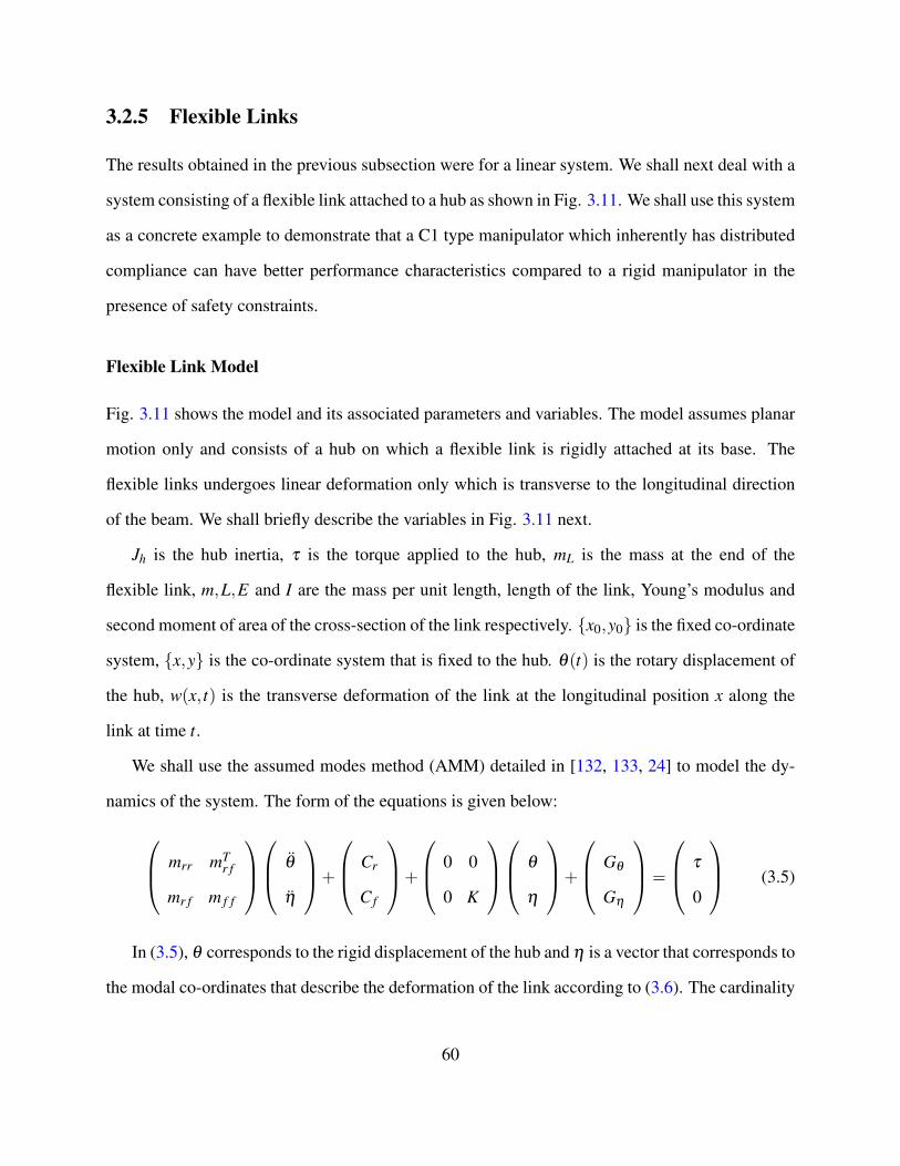
3.2.5 Flexible Links

The results obtained in the previous subsection were for a linear system. We shall next deal with a

system consisting of a flexible link attached to a hub as shown in Fig. 3.11. We shall use this system

as a concrete example to demonstrate that a C1 type manipulator which inherently has distributed

compliance can have better performance characteristics compared to a rigid manipulator in the

presence of safety constraints.

Flexible Link Model

Fig. 3.11 shows the model and its associated parameters and variables. The model assumes planar

motion only and consists of a hub on which a flexible link is rigidly attached at its base. The

flexible links undergoes linear deformation only which is transverse to the longitudinal direction

of the beam. We shall briefly describe the variables in Fig. 3.11 next.

Jh is the hub inertia, τ is the torque applied to the hub, mL is the mass at the end of the

flexible link, m,L,E and I are the mass per unit length, length of the link, Young’s modulus and

second moment of area of the cross-section of the link respectively. {x0,y0} is the fixed co-ordinate

system, {x,y} is the co-ordinate system that is fixed to the hub. θ(t) is the rotary displacement of

the hub, w(x, t) is the transverse deformation of the link at the longitudinal position x along the

link at time t.

We shall use the assumed modes method (AMM) detailed in [132, 133, 24] to model the dy-

namics of the system. The form of the equations is given below:

mrr mTr f

mr f m f f

θ

η

+

Cr

C f

+

0 0

0 K

θ

η

+

Gθ

Gη

=

τ

0

(3.5)

In (3.5), θ corresponds to the rigid displacement of the hub and η is a vector that corresponds to

the modal co-ordinates that describe the deformation of the link according to (3.6). The cardinality

60

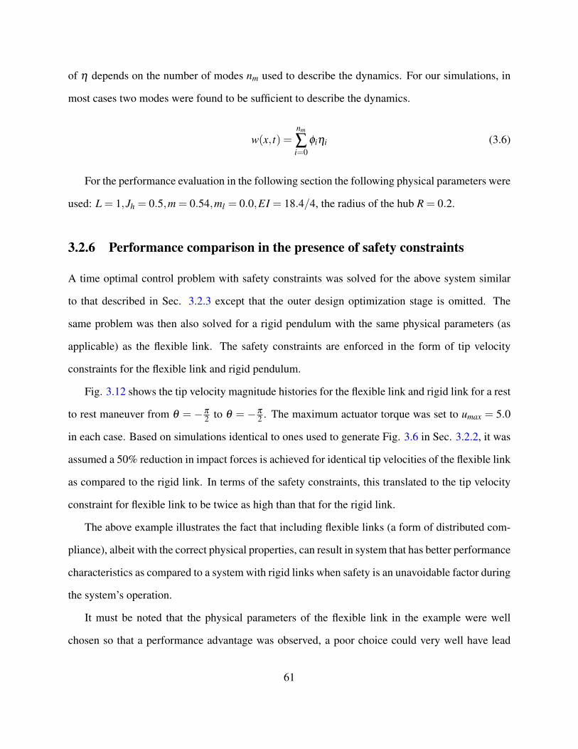
of η depends on the number of modes nm used to describe the dynamics. For our simulations, in

most cases two modes were found to be sufficient to describe the dynamics.

w(x, t) =nm

∑i=0

φiηi (3.6)

For the performance evaluation in the following section the following physical parameters were

used: L = 1,Jh = 0.5,m = 0.54,ml = 0.0,EI = 18.4/4, the radius of the hub R = 0.2.

3.2.6 Performance comparison in the presence of safety constraints

A time optimal control problem with safety constraints was solved for the above system similar

to that described in Sec. 3.2.3 except that the outer design optimization stage is omitted. The

same problem was then also solved for a rigid pendulum with the same physical parameters (as

applicable) as the flexible link. The safety constraints are enforced in the form of tip velocity

constraints for the flexible link and rigid pendulum.

Fig. 3.12 shows the tip velocity magnitude histories for the flexible link and rigid link for a rest

to rest maneuver from θ = −π

2 to θ = −π

2 . The maximum actuator torque was set to umax = 5.0

in each case. Based on simulations identical to ones used to generate Fig. 3.6 in Sec. 3.2.2, it was

assumed a 50% reduction in impact forces is achieved for identical tip velocities of the flexible link

as compared to the rigid link. In terms of the safety constraints, this translated to the tip velocity

constraint for flexible link to be twice as high than that for the rigid link.

The above example illustrates the fact that including flexible links (a form of distributed com-

pliance), albeit with the correct physical properties, can result in system that has better performance

characteristics as compared to a system with rigid links when safety is an unavoidable factor during

the system’s operation.

It must be noted that the physical parameters of the flexible link in the example were well

chosen so that a performance advantage was observed, a poor choice could very well have lead

61

to a performance disadvantage. The correct physical parameters can of course be arrived at by an

optimization procedure such as that described in Sec. 3.2.3 and we hope to do such a problem

in the future. In the above example we are answering the question of existence of such a set of

physical parameters.

62

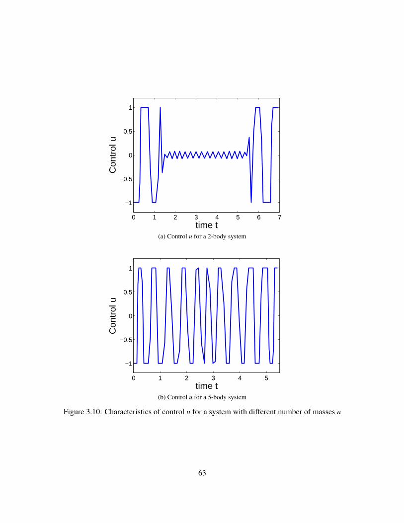
0 1 2 3 4 5 6 7

−1

−0.5

0

0.5

1

time t

Con

trol

u

(a) Control u for a 2-body system

0 1 2 3 4 5

−1

−0.5

0

0.5

1

time t

Con

trol

u

(b) Control u for a 5-body system

Figure 3.10: Characteristics of control u for a system with different number of masses n

63

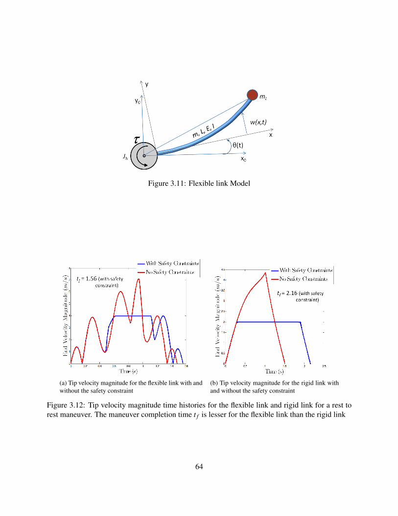
Figure 3.11: Flexible link Model

(a) Tip velocity magnitude for the flexible link with andwithout the safety constraint

(b) Tip velocity magnitude for the rigid link withand without the safety constraint

Figure 3.12: Tip velocity magnitude time histories for the flexible link and rigid link for a rest torest maneuver. The maneuver completion time t f is lesser for the flexible link than the rigid link

64

3.3 Summary

In this chapter, various design paradigms that are useful for improving safety of robotic system are

discussed. Specifically, the role of inertial and stiffness parameters is discussed. A differentiating

feature of soft robots from rigid robots with soft coverings is the presence of distributed compliance

along the structure of the system. Results from a control-design optimization technique developed

indicate that compliance distribution which is a useful property for safety and can also lead to

systems with good performance characteristics. The performance criteria considered in this chapter

are open-loop, however closed-loop criteria may also be used as in Sec. A.1.

65

Chapter 4

Hardware

In this chapter, we will provide a brief overview of the inflatable prototypes developed and utilized

for this thesis. Three inflatable manipulator prototypes, shown in Fig. 4.1, will be discussed: (1)

the CMU inflatable arm, (2) the PneuArm, (3) the AIRarm 1. We will discuss the CMU inflatable

arm in greater detail and will defer some details of the other prototypes to later chapters.

4.1 The CMU Inflatable Arm

The inflatable manipulator (Fig. 4.2) is built using membrane material (polyurethane film: Cat-

alogue #3460, McMaster-Carr) which is maintained under tension by the use of pressurized air.

This leads to an extremely lightweight structure which has a weight of the order of a few grams

(≈ 5 gm). Besides being extremely lightweight, it allows for a low contact stiffness providing

a soft contact interface throughout the structure. In addition, the inflatable structure allows for

structural compliance in the form of link flexibility due to the relatively low Young’s modulus of

polyurethane (≈ 0.025 GPa) used in its construction when compared to traditional materials such

as aluminum (≈ 69 GPa) and steel (≈ 200 GPa). The above features are all highly desirable in a

1The AIRarm hardware was developed at iRobot as part of a collaborative project with CMU

66

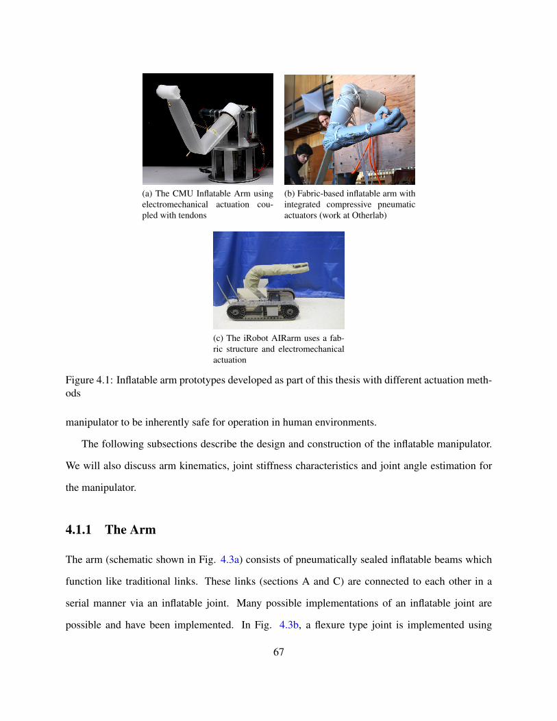
(a) The CMU Inflatable Arm usingelectromechanical actuation cou-pled with tendons

(b) Fabric-based inflatable arm withintegrated compressive pneumaticactuators (work at Otherlab)

(c) The iRobot AIRarm uses a fab-ric structure and electromechanicalactuation

Figure 4.1: Inflatable arm prototypes developed as part of this thesis with different actuation meth-ods

manipulator to be inherently safe for operation in human environments.

The following subsections describe the design and construction of the inflatable manipulator.

We will also discuss arm kinematics, joint stiffness characteristics and joint angle estimation for

the manipulator.

4.1.1 The Arm

The arm (schematic shown in Fig. 4.3a) consists of pneumatically sealed inflatable beams which

function like traditional links. These links (sections A and C) are connected to each other in a

serial manner via an inflatable joint. Many possible implementations of an inflatable joint are

possible and have been implemented. In Fig. 4.3b, a flexure type joint is implemented using

67

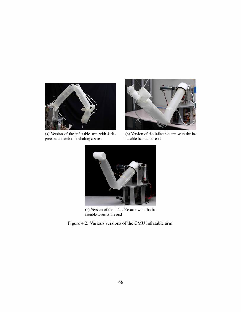
(a) Version of the inflatable arm with 4 de-grees of a freedom including a wrist

(b) Version of the inflatable arm with the in-flatable hand at its end

(c) Version of the inflatable arm with the in-flatable torus at the end

Figure 4.2: Various versions of the CMU inflatable arm

68

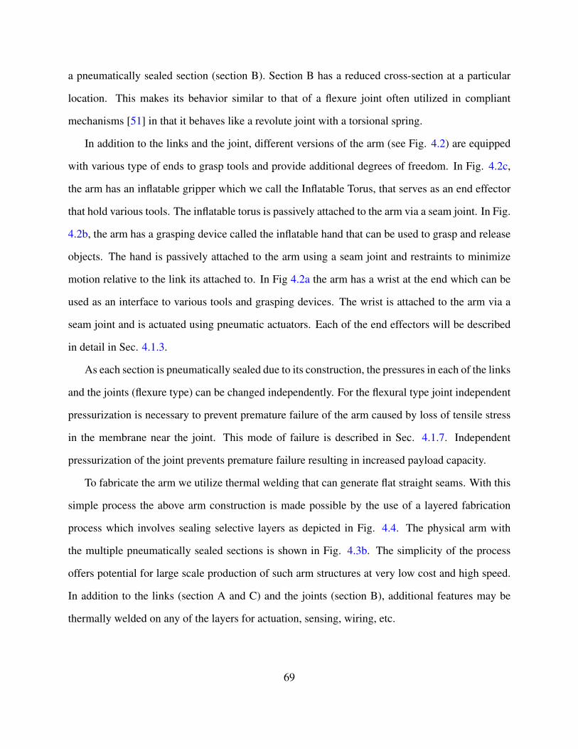
a pneumatically sealed section (section B). Section B has a reduced cross-section at a particular

location. This makes its behavior similar to that of a flexure joint often utilized in compliant

mechanisms [51] in that it behaves like a revolute joint with a torsional spring.

In addition to the links and the joint, different versions of the arm (see Fig. 4.2) are equipped

with various type of ends to grasp tools and provide additional degrees of freedom. In Fig. 4.2c,

the arm has an inflatable gripper which we call the Inflatable Torus, that serves as an end effector

that hold various tools. The inflatable torus is passively attached to the arm via a seam joint. In Fig.

4.2b, the arm has a grasping device called the inflatable hand that can be used to grasp and release

objects. The hand is passively attached to the arm using a seam joint and restraints to minimize

motion relative to the link its attached to. In Fig 4.2a the arm has a wrist at the end which can be

used as an interface to various tools and grasping devices. The wrist is attached to the arm via a

seam joint and is actuated using pneumatic actuators. Each of the end effectors will be described

in detail in Sec. 4.1.3.

As each section is pneumatically sealed due to its construction, the pressures in each of the links

and the joints (flexure type) can be changed independently. For the flexural type joint independent

pressurization is necessary to prevent premature failure of the arm caused by loss of tensile stress

in the membrane near the joint. This mode of failure is described in Sec. 4.1.7. Independent

pressurization of the joint prevents premature failure resulting in increased payload capacity.

To fabricate the arm we utilize thermal welding that can generate flat straight seams. With this

simple process the above arm construction is made possible by the use of a layered fabrication

process which involves sealing selective layers as depicted in Fig. 4.4. The physical arm with

the multiple pneumatically sealed sections is shown in Fig. 4.3b. The simplicity of the process

offers potential for large scale production of such arm structures at very low cost and high speed.

In addition to the links (section A and C) and the joints (section B), additional features may be

thermally welded on any of the layers for actuation, sensing, wiring, etc.

69

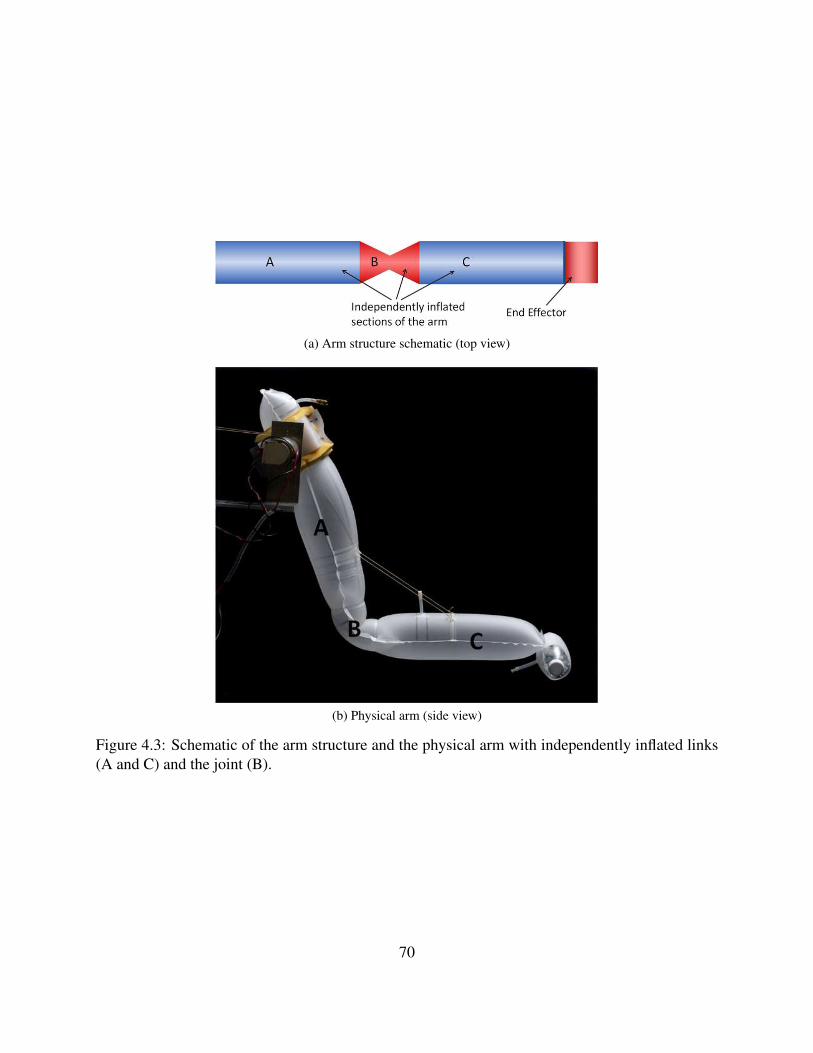
(a) Arm structure schematic (top view)

(b) Physical arm (side view)

Figure 4.3: Schematic of the arm structure and the physical arm with independently inflated links(A and C) and the joint (B).

70

(a) Cross-section in the side view plane revealing layered design toachieve independently inflated sections. Black lines labeled S1-S8 rep-resent seams joining the two layers which are intersected by the lines.

(b) Top view revealing additional seams S9-S14 and shape of the flatstructure.

Figure 4.4: Schematic showing layered design of inflatable arm to achieve independently inflatedsections in the arm structure using flat straight seams.

4.1.2 Actuation

In its current form (Fig. 4.2a, the inflatable manipulator has four active degrees of freedom. The

first link (section A in Fig. 4.3a) is actuated in the plane by directly coupling it to a DC servo

motor. The second link (section C in Fig. 4.3a) is actuated using tendons which are driven by DC

servo motors as shown in the schematic in Fig. 4.5. The arm can also move out of the plane using

the degree of freedom at the base that is actuated by another DC motor. In addition to these three

degrees of freedom the arm has an in plane degree of motion at the wrist that is pneumatically

actuated. We have also explored other actuation schemes using McKibben pneumatics where the

tendons are connected to the McKibben actuators rather than motors (see Fig. 4.6).

The actuation of the second link can be described as an open-ended tendon drive as the tendon

terminates at link 2. As the joint between link 1 and link 2 (section B in Fig. 4.3a) has finite

stiffness, the tendon works against this stiffness at the joint and allows the joint to be position

controlled to any desired angle (θ2 > 0). The tendon passes through the axis of rotation of joint

1 to avoid kinematic coupling between the two joint angles. As the tendon drives the joint in

71

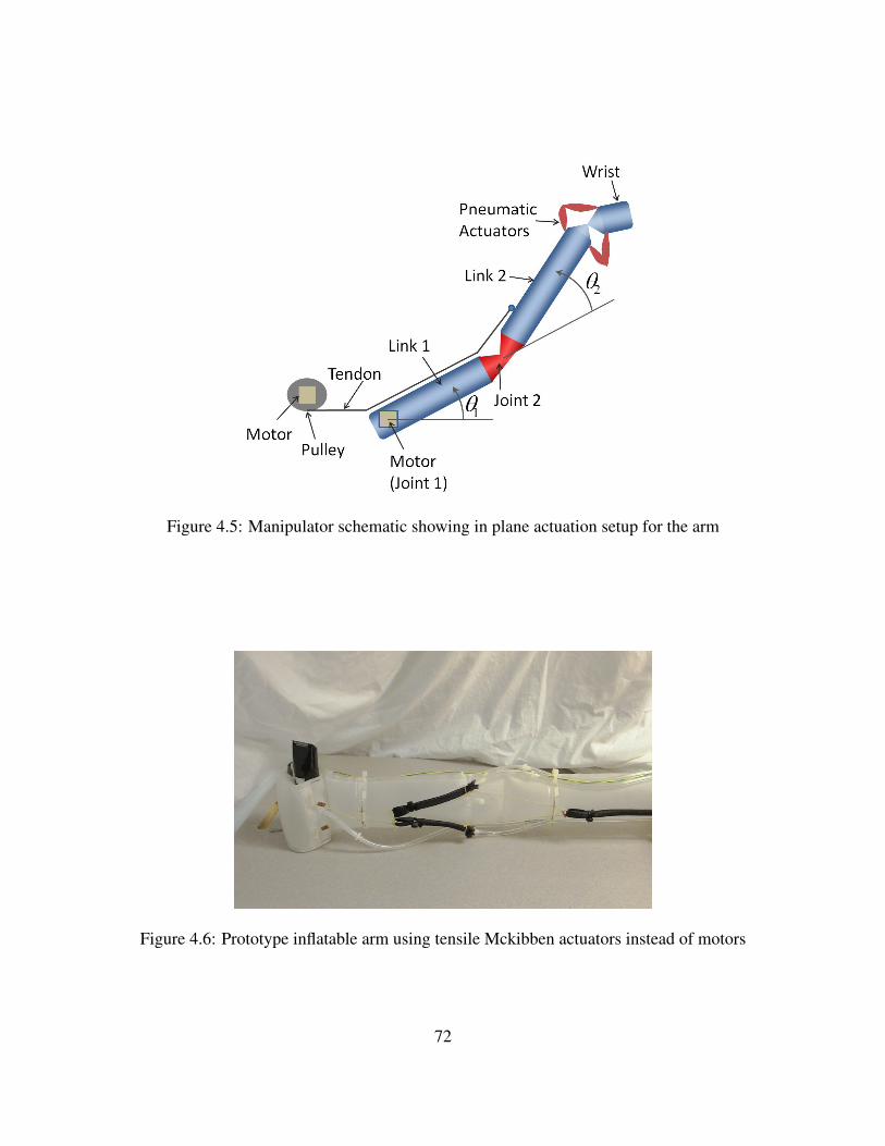
Figure 4.5: Manipulator schematic showing in plane actuation setup for the arm

Figure 4.6: Prototype inflatable arm using tensile Mckibben actuators instead of motors

72

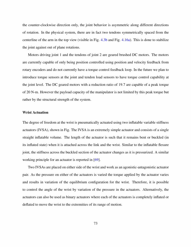
the counter-clockwise direction only, the joint behavior is asymmetric along different directions

of rotation. In the physical system, there are in fact two tendons symmetrically spaced from the

centerline of the arm in the top view (visible in Fig. 4.3b and Fig. 4.16a). This is done to stabilize

the joint against out of plane rotations.

Motors driving joint 1 and the tendons of joint 2 are geared brushed DC motors. The motors

are currently capable of only being position controlled using position and velocity feedback from

rotary encoders and do not currently have a torque control feedback loop. In the future we plan to

introduce torque sensors at the joint and tendon load sensors to have torque control capability at

the joint level. The DC geared motors with a reduction ratio of 19.7 are capable of a peak torque

of 20 N-m. However the payload capacity of the manipulator is not limited by this peak torque but

rather by the structural strength of the system.

Wrist Actuation

The degree of freedom at the wrist is pneumatically actuated using two inflatable variable stiffness

actuators (IVSA), shown in Fig. The IVSA is an extremely simple actuator and consists of a single

straight inflatable volume. The length of the actuator is such that it remains bent or buckled (in

its inflated state) when it is attached across the link and the wrist. Similar to the inflatable flexure

joint, the stiffness across the buckled section of the actuator changes as it is pressurized. A similar

working principle for an actuator is reported in [69].

Two IVSAs are placed on either side of the wrist and work as an agonistic-antagonistic actuator

pair. As the pressure on either of the actuators is varied the torque applied by the actuator varies

and results in variation of the equilibrium configuration for the wrist. Therefore, it is possible

to control the angle of the wrist by variation of the pressure in the actuators. Alternatively, the

actuators can also be used as binary actuators where each of the actuators is completely inflated or

deflated to move the wrist to the extremities of its range of motion.

73

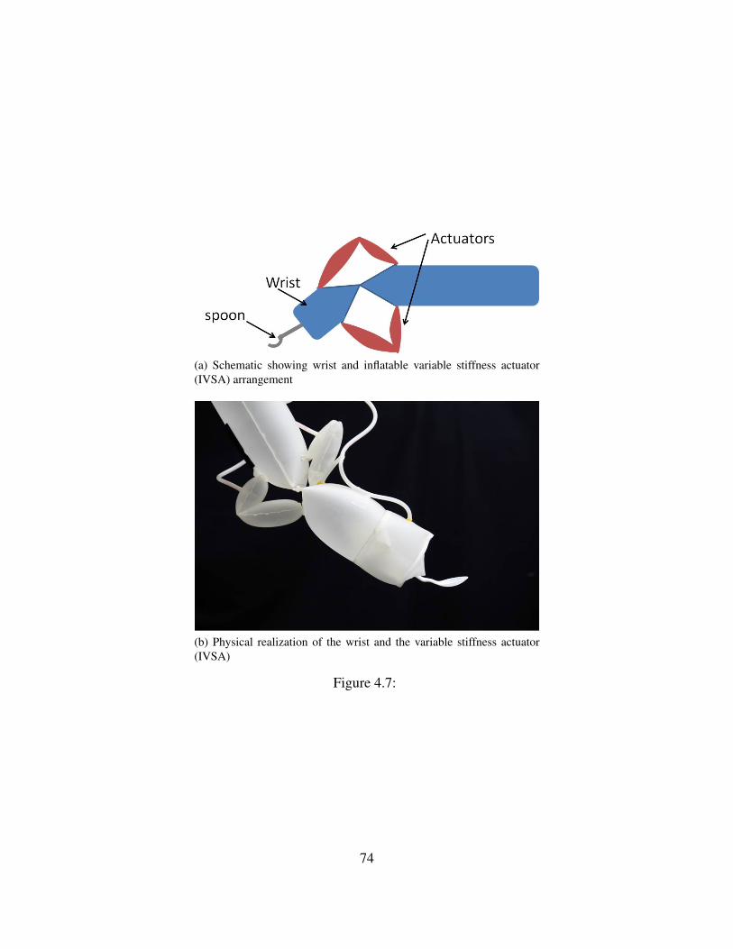
(a) Schematic showing wrist and inflatable variable stiffness actuator(IVSA) arrangement

(b) Physical realization of the wrist and the variable stiffness actuator(IVSA)

Figure 4.7:

74

(a) The Inflatable Torus in its deflated state with objectto be grasped.

(b) The Inflatable Torus inflated with air to grasp ob-ject.

Figure 4.8: Schematic showing the Inflatable Torus in its deflated and inflated state. The torusutilizes a force sensor embedded in its surface to sense contact forces between the external objectand the gripper.

4.1.3 The End Effector

For the inflatable manipulator to manipulate real world objects, it needs to be equipped with an

end effector that can grasp objects. A rigid end effector would add additional weight and decrease

payload capabilities for the manipulator besides reducing some of the safety advantages gained

from using an inflatable structure. An end effector that is inflatable gripper does not suffer from

these disadvantages and is also easy to integrate with the inflatable structure of the arm during

fabrication. A number of inflatable end effectors have been developed for the inflatable arm, we

will describe three of them next: (1) the Inflatable Torus (2) the Inflatable Hand, and (3) the

Inflatable Wrist.

The Inflatable Torus

The Inflatable Torus, seen in Fig. 4.2c, is an end effector that allows the arm to be equipped with

various tools like a spoon, trimmer, etc. As shown in Fig. 4.8, it grasps objects by trapping the

75

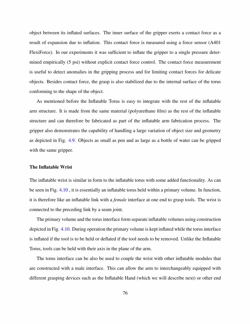
object between its inflated surfaces. The inner surface of the gripper exerts a contact force as a

result of expansion due to inflation. This contact force is measured using a force sensor (A401

FlexiForce). In our experiments it was sufficient to inflate the gripper to a single pressure deter-

mined empirically (5 psi) without explicit contact force control. The contact force measurement

is useful to detect anomalies in the gripping process and for limiting contact forces for delicate

objects. Besides contact force, the grasp is also stabilized due to the internal surface of the torus

conforming to the shape of the object.

As mentioned before the Inflatable Torus is easy to integrate with the rest of the inflatable

arm structure. It is made from the same material (polyurethane film) as the rest of the inflatable

structure and can therefore be fabricated as part of the inflatable arm fabrication process. The

gripper also demonstrates the capability of handling a large variation of object size and geometry

as depicted in Fig. 4.9. Objects as small as pen and as large as a bottle of water can be gripped

with the same gripper.

The Inflatable Wrist

The inflatable wrist is similar in form to the inflatable torus with some added functionality. As can

be seen in Fig. 4.10 , it is essentially an inflatable torus held within a primary volume. In function,

it is therefore like an inflatable link with a female interface at one end to grasp tools. The wrist is

connected to the preceding link by a seam joint.

The primary volume and the torus interface form separate inflatable volumes using construction

depicted in Fig. 4.10. During operation the primary volume is kept inflated while the torus interface

is inflated if the tool is to be held or deflated if the tool needs to be removed. Unlike the Inflatable

Torus, tools can be held with their axis in the plane of the arm.

The torus interface can be also be used to couple the wrist with other inflatable modules that

are constructed with a male interface. This can allow the arm to interchangeably equipped with

different grasping devices such as the Inflatable Hand (which we will describe next) or other end

76

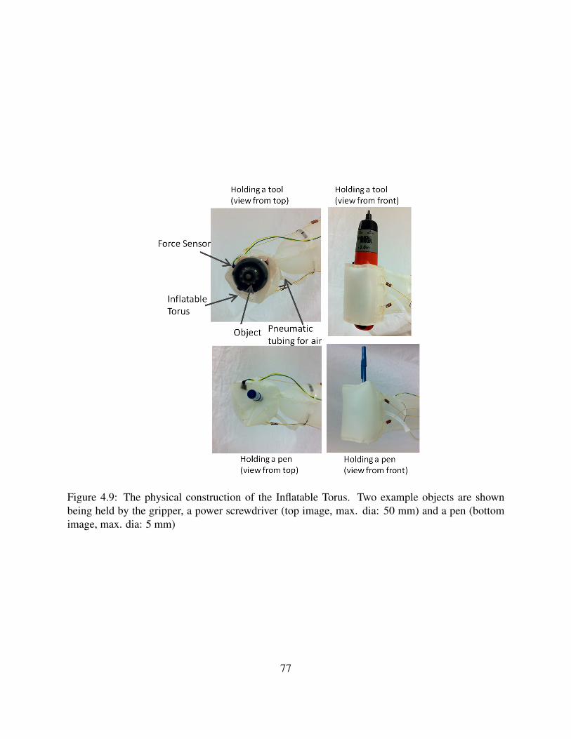
Figure 4.9: The physical construction of the Inflatable Torus. Two example objects are shownbeing held by the gripper, a power screwdriver (top image, max. dia: 50 mm) and a pen (bottomimage, max. dia: 5 mm)

77

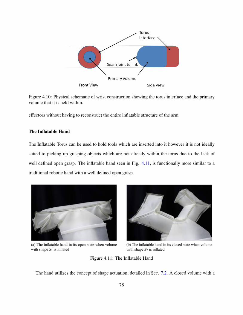
Figure 4.10: Physical schematic of wrist construction showing the torus interface and the primaryvolume that it is held within.

effectors without having to reconstruct the entire inflatable structure of the arm.

The Inflatable Hand

The Inflatable Torus can be used to hold tools which are inserted into it however it is not ideally

suited to picking up grasping objects which are not already within the torus due to the lack of

well defined open grasp. The inflatable hand seen in Fig. 4.11, is functionally more similar to a

traditional robotic hand with a well defined open grasp.

(a) The inflatable hand in its open state when volumewith shape S1 is inflated

(b) The inflatable hand in its closed state when volumewith shape S2 is inflated

Figure 4.11: The Inflatable Hand

The hand utilizes the concept of shape actuation, detailed in Sec. 7.2. A closed volume with a

78

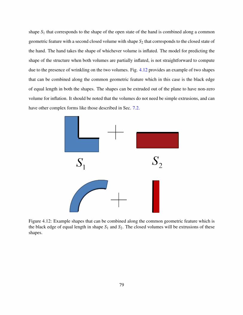
shape S1 that corresponds to the shape of the open state of the hand is combined along a common

geometric feature with a second closed volume with shape S2 that corresponds to the closed state of

the hand. The hand takes the shape of whichever volume is inflated. The model for predicting the

shape of the structure when both volumes are partially inflated, is not straightforward to compute

due to the presence of wrinkling on the two volumes. Fig. 4.12 provides an example of two shapes

that can be combined along the common geometric feature which in this case is the black edge

of equal length in both the shapes. The shapes can be extruded out of the plane to have non-zero

volume for inflation. It should be noted that the volumes do not need be simple extrusions, and can

have other complex forms like those described in Sec. 7.2.

Figure 4.12: Example shapes that can be combined along the common geometric feature which isthe black edge of equal length in shape S1 and S2. The closed volumes will be extrusions of theseshapes.

79

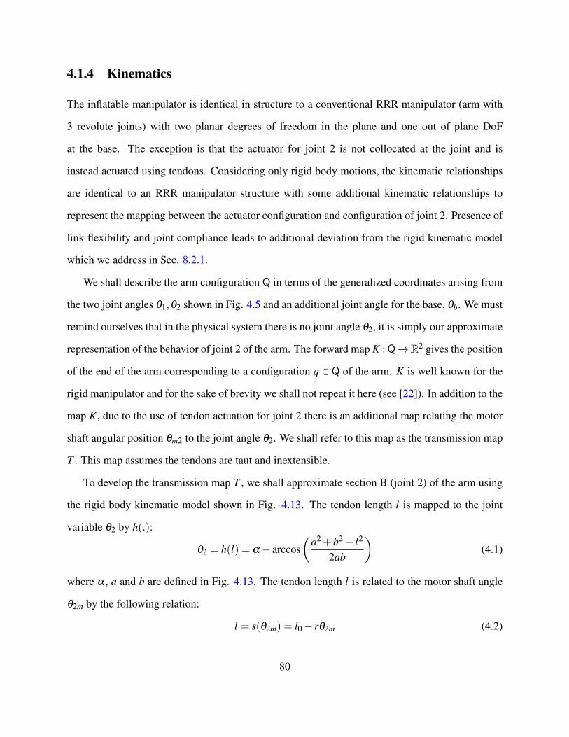
4.1.4 Kinematics

The inflatable manipulator is identical in structure to a conventional RRR manipulator (arm with

3 revolute joints) with two planar degrees of freedom in the plane and one out of plane DoF

at the base. The exception is that the actuator for joint 2 is not collocated at the joint and is

instead actuated using tendons. Considering only rigid body motions, the kinematic relationships

are identical to an RRR manipulator structure with some additional kinematic relationships to

represent the mapping between the actuator configuration and configuration of joint 2. Presence of

link flexibility and joint compliance leads to additional deviation from the rigid kinematic model

which we address in Sec. 8.2.1.

We shall describe the arm configuration Q in terms of the generalized coordinates arising from

the two joint angles θ1,θ2 shown in Fig. 4.5 and an additional joint angle for the base, θb. We must

remind ourselves that in the physical system there is no joint angle θ2, it is simply our approximate

representation of the behavior of joint 2 of the arm. The forward map K :Q→R2 gives the position

of the end of the arm corresponding to a configuration q ∈ Q of the arm. K is well known for the

rigid manipulator and for the sake of brevity we shall not repeat it here (see [22]). In addition to the

map K, due to the use of tendon actuation for joint 2 there is an additional map relating the motor

shaft angular position θm2 to the joint angle θ2. We shall refer to this map as the transmission map

T . This map assumes the tendons are taut and inextensible.

To develop the transmission map T , we shall approximate section B (joint 2) of the arm using

the rigid body kinematic model shown in Fig. 4.13. The tendon length l is mapped to the joint

variable θ2 by h(.):

θ2 = h(l) = α− arccos(

a2 +b2− l2

2ab

)(4.1)

where α , a and b are defined in Fig. 4.13. The tendon length l is related to the motor shaft angle

θ2m by the following relation:

l = s(θ2m) = l0− rθ2m (4.2)

80

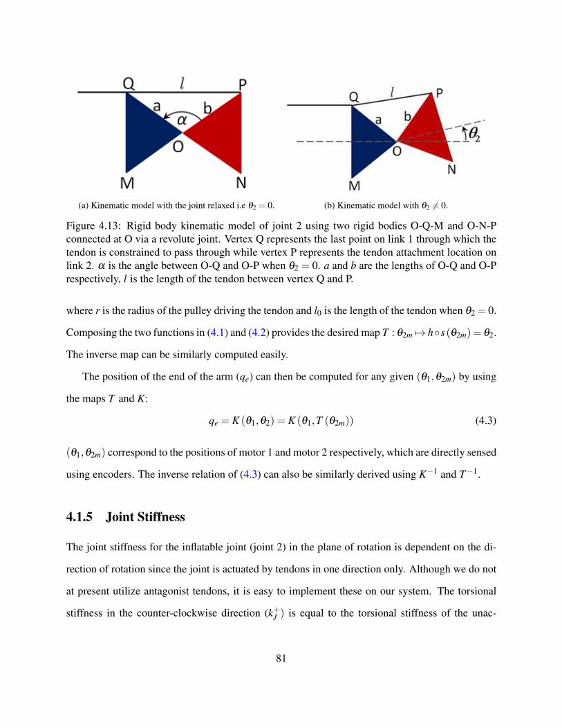
(a) Kinematic model with the joint relaxed i.e θ2 = 0. (b) Kinematic model with θ2 6= 0.

Figure 4.13: Rigid body kinematic model of joint 2 using two rigid bodies O-Q-M and O-N-Pconnected at O via a revolute joint. Vertex Q represents the last point on link 1 through which thetendon is constrained to pass through while vertex P represents the tendon attachment location onlink 2. α is the angle between O-Q and O-P when θ2 = 0. a and b are the lengths of O-Q and O-Prespectively, l is the length of the tendon between vertex Q and P.

where r is the radius of the pulley driving the tendon and l0 is the length of the tendon when θ2 = 0.

Composing the two functions in (4.1) and (4.2) provides the desired map T : θ2m 7→ h◦s(θ2m)= θ2.

The inverse map can be similarly computed easily.

The position of the end of the arm (qe) can then be computed for any given (θ1,θ2m) by using

the maps T and K:

qe = K (θ1,θ2) = K (θ1,T (θ2m)) (4.3)

(θ1,θ2m) correspond to the positions of motor 1 and motor 2 respectively, which are directly sensed

using encoders. The inverse relation of (4.3) can also be similarly derived using K−1 and T−1.

4.1.5 Joint Stiffness

The joint stiffness for the inflatable joint (joint 2) in the plane of rotation is dependent on the di-

rection of rotation since the joint is actuated by tendons in one direction only. Although we do not

at present utilize antagonist tendons, it is easy to implement these on our system. The torsional

stiffness in the counter-clockwise direction (k+J ) is equal to the torsional stiffness of the unac-

81

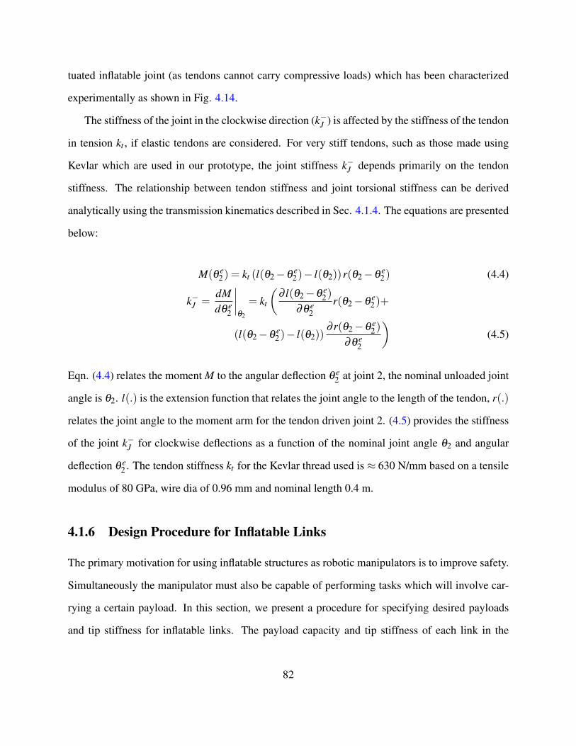
tuated inflatable joint (as tendons cannot carry compressive loads) which has been characterized

experimentally as shown in Fig. 4.14.

The stiffness of the joint in the clockwise direction (k−J ) is affected by the stiffness of the tendon

in tension kt , if elastic tendons are considered. For very stiff tendons, such as those made using

Kevlar which are used in our prototype, the joint stiffness k−J depends primarily on the tendon

stiffness. The relationship between tendon stiffness and joint torsional stiffness can be derived

analytically using the transmission kinematics described in Sec. 4.1.4. The equations are presented

below:

M(θ e2) = kt (l(θ2−θ

e2)− l(θ2))r(θ2−θ

e2) (4.4)

k−J =dMdθ e

2

∣∣∣∣θ2

= kt

(∂ l(θ2−θ e

2)

∂θ e2

r(θ2−θe2)+

(l(θ2−θe2)− l(θ2))

∂ r(θ2−θ e2)

∂θ e2

)(4.5)

Eqn. (4.4) relates the moment M to the angular deflection θ e2 at joint 2, the nominal unloaded joint

angle is θ2. l(.) is the extension function that relates the joint angle to the length of the tendon, r(.)

relates the joint angle to the moment arm for the tendon driven joint 2. (4.5) provides the stiffness

of the joint k−J for clockwise deflections as a function of the nominal joint angle θ2 and angular

deflection θ e2 . The tendon stiffness kt for the Kevlar thread used is ≈ 630 N/mm based on a tensile

modulus of 80 GPa, wire dia of 0.96 mm and nominal length 0.4 m.

4.1.6 Design Procedure for Inflatable Links

The primary motivation for using inflatable structures as robotic manipulators is to improve safety.

Simultaneously the manipulator must also be capable of performing tasks which will involve car-

rying a certain payload. In this section, we present a procedure for specifying desired payloads

and tip stiffness for inflatable links. The payload capacity and tip stiffness of each link in the

82

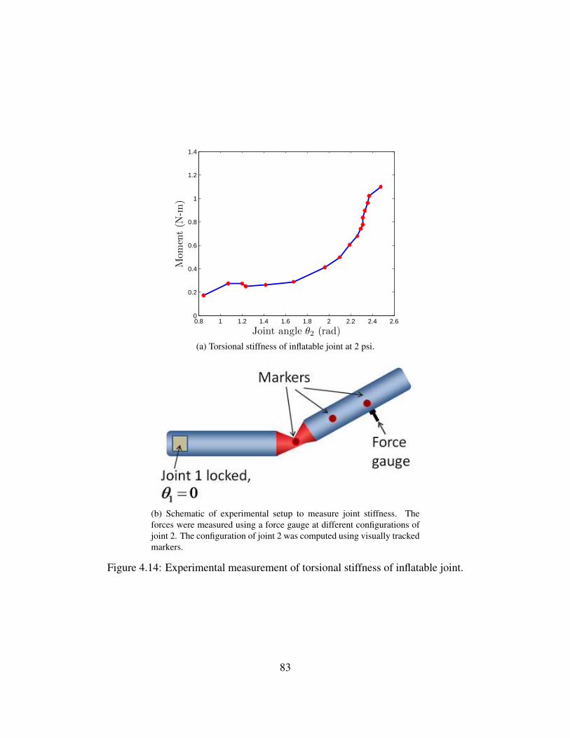
0.8 1 1.2 1.4 1.6 1.8 2 2.2 2.4 2.60

0.2

0.4

0.6

0.8

1

1.2

1.4

Joint angle θ2 (rad)

Moment(N

-m)

(a) Torsional stiffness of inflatable joint at 2 psi.

(b) Schematic of experimental setup to measure joint stiffness. Theforces were measured using a force gauge at different configurations ofjoint 2. The configuration of joint 2 was computed using visually trackedmarkers.

Figure 4.14: Experimental measurement of torsional stiffness of inflatable joint.

83

Figure 4.15: Schematic of the procedure for designing an inflatable link. The desired tip stiffnessk is used in a link stiffness model f (k) to arrive at the radius of the cross-section r. The desiredpayload along with r is used in a link failure model g(r,F) to arrive at a desired membrane pre-stress σpre for the inflatable arm. r and σpre are then used to compute the desired internal pressureP using the link pressure model h(σpre,r).

manipulator affects the overall payload and safety characteristics of the manipulator.

Inflatable links can be operated at a range of internal pressures. This allows for independent

specification of payload capacity and tip stiffness for an inflatable link. These specifications can be

utilized to arrive at the appropriate cross-section (size) and internal pressure at which the inflatable

link must be operated. Fig. 4.15 details the procedure of arriving at the size and pressure param-

eters for an individual link. It is assumed that the inflatable link has a circular cross-section. The

cross-section can be therefore represented by a single parameter r, the radius of the cross-section.

Example Inflatable Link Design

We shall use an example design problem for the inflatable link to explain the procedure illustrated

in Fig. 4.15. The specifications for the design problem are the following: Payload (F): 10 N,

Stiffness of the link (k): 50 N/m. Following the procedure in Fig. 4.15 we can arrive at the desired

84

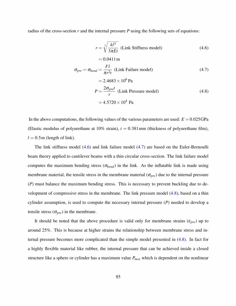
radius of the cross-section r and the internal pressure P using the following sets of equations:

r = 3

√kl3

3πEt(Link Stiffness model) (4.6)

= 0.0411m

σpre = σbend =Fl

πr2t(Link Failure model) (4.7)

= 2.4683×106 Pa

P =2σpret

r(Link Pressure model) (4.8)

= 4.5720×104 Pa

In the above computations, the following values of the various parameters are used: E = 0.025GPa

(Elastic modulus of polyurethane at 10% strain), t = 0.381mm (thickness of polyurethane film),

l = 0.5m (length of link).

The link stiffness model (4.6) and link failure model (4.7) are based on the Euler-Bernoulli

beam theory applied to cantilever beams with a thin circular cross-section. The link failure model

computes the maximum bending stress (σbend) in the link. As the inflatable link is made using

membrane material, the tensile stress in the membrane material (σpre) due to the internal pressure

(P) must balance the maximum bending stress. This is necessary to prevent buckling due to de-

velopment of compressive stress in the membrane. The link pressure model (4.8), based on a thin

cylinder assumption, is used to compute the necessary internal pressure (P) needed to develop a

tensile stress (σpre) in the membrane.

It should be noted that the above procedure is valid only for membrane strains (εpre) up to

around 25%. This is because at higher strains the relationship between membrane stress and in-

ternal pressure becomes more complicated than the simple model presented in (4.8). In fact for

a highly flexible material like rubber, the internal pressure that can be achieved inside a closed

structure like a sphere or cylinder has a maximum value Pmax which is dependent on the nonlinear

85

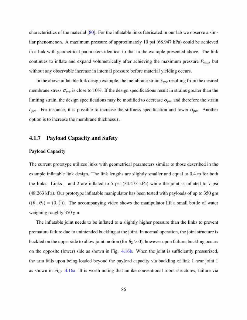
characteristics of the material [80]. For the inflatable links fabricated in our lab we observe a sim-

ilar phenomenon. A maximum pressure of approximately 10 psi (68.947 kPa) could be achieved

in a link with geometrical parameters identical to that in the example presented above. The link

continues to inflate and expand volumetrically after achieving the maximum pressure Pmax, but

without any observable increase in internal pressure before material yielding occurs.

In the above inflatable link design example, the membrane strain εpre resulting from the desired

membrane stress σpre is close to 10%. If the design specifications result in strains greater than the

limiting strain, the design specifications may be modified to decrease σpre and therefore the strain

εpre. For instance, it is possible to increase the stiffness specification and lower σpre. Another

option is to increase the membrane thickness t.

4.1.7 Payload Capacity and Safety

Payload Capacity

The current prototype utilizes links with geometrical parameters similar to those described in the

example inflatable link design. The link lengths are slightly smaller and equal to 0.4 m for both

the links. Links 1 and 2 are inflated to 5 psi (34.473 kPa) while the joint is inflated to 7 psi

(48.263 kPa). Our prototype inflatable manipulator has been tested with payloads of up to 350 gm

((θ1,θ2) = (0, π

3 )). The accompanying video shows the manipulator lift a small bottle of water

weighing roughly 350 gm.

The inflatable joint needs to be inflated to a slightly higher pressure than the links to prevent

premature failure due to unintended buckling at the joint. In normal operation, the joint structure is

buckled on the upper side to allow joint motion (for θ2 > 0), however upon failure, buckling occurs

on the opposite (lower) side as shown in Fig. 4.16b. When the joint is sufficiently pressurized,

the arm fails upon being loaded beyond the payload capacity via buckling of link 1 near joint 1

as shown in Fig. 4.16a. It is worth noting that unlike conventional robot structures, failure via

86

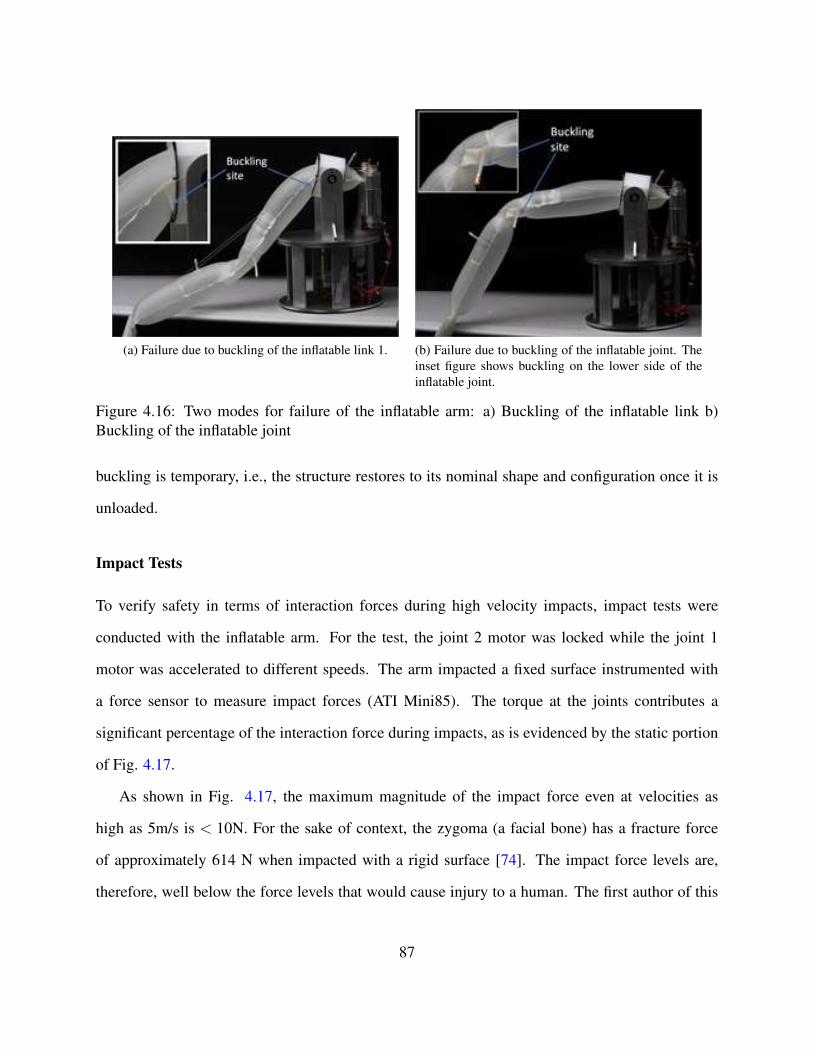
(a) Failure due to buckling of the inflatable link 1. (b) Failure due to buckling of the inflatable joint. Theinset figure shows buckling on the lower side of theinflatable joint.

Figure 4.16: Two modes for failure of the inflatable arm: a) Buckling of the inflatable link b)Buckling of the inflatable joint

buckling is temporary, i.e., the structure restores to its nominal shape and configuration once it is

unloaded.

Impact Tests

To verify safety in terms of interaction forces during high velocity impacts, impact tests were

conducted with the inflatable arm. For the test, the joint 2 motor was locked while the joint 1

motor was accelerated to different speeds. The arm impacted a fixed surface instrumented with

a force sensor to measure impact forces (ATI Mini85). The torque at the joints contributes a

significant percentage of the interaction force during impacts, as is evidenced by the static portion

of Fig. 4.17.

As shown in Fig. 4.17, the maximum magnitude of the impact force even at velocities as

high as 5m/s is < 10N. For the sake of context, the zygoma (a facial bone) has a fracture force

of approximately 614 N when impacted with a rigid surface [74]. The impact force levels are,

therefore, well below the force levels that would cause injury to a human. The first author of this

87

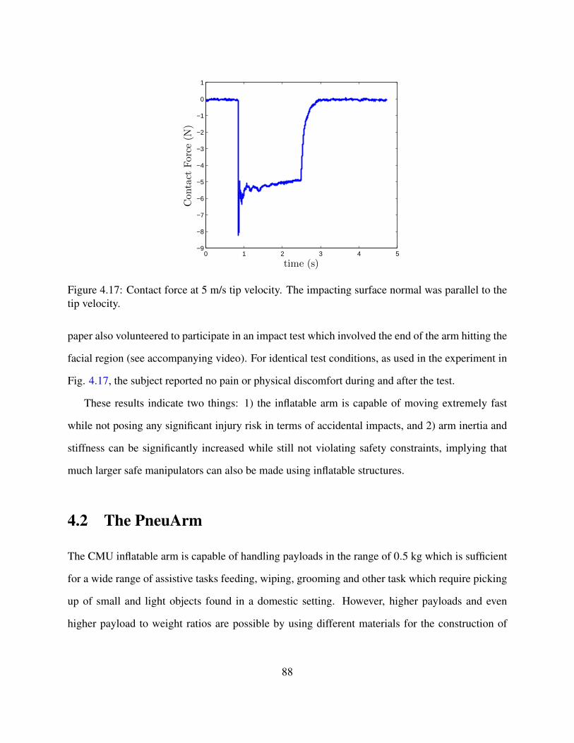
0 1 2 3 4 5−9

−8

−7

−6

−5

−4

−3

−2

−1

0

1

time (s)

Contact

Force(N

)

Figure 4.17: Contact force at 5 m/s tip velocity. The impacting surface normal was parallel to thetip velocity.

paper also volunteered to participate in an impact test which involved the end of the arm hitting the

facial region (see accompanying video). For identical test conditions, as used in the experiment in

Fig. 4.17, the subject reported no pain or physical discomfort during and after the test.

These results indicate two things: 1) the inflatable arm is capable of moving extremely fast

while not posing any significant injury risk in terms of accidental impacts, and 2) arm inertia and

stiffness can be significantly increased while still not violating safety constraints, implying that

much larger safe manipulators can also be made using inflatable structures.

4.2 The PneuArm

The CMU inflatable arm is capable of handling payloads in the range of 0.5 kg which is sufficient

for a wide range of assistive tasks feeding, wiping, grooming and other task which require picking

up of small and light objects found in a domestic setting. However, higher payloads and even

higher payload to weight ratios are possible by using different materials for the construction of

88

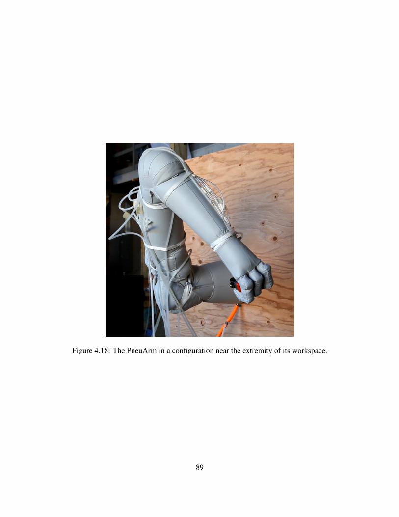
Figure 4.18: The PneuArm in a configuration near the extremity of its workspace.

89

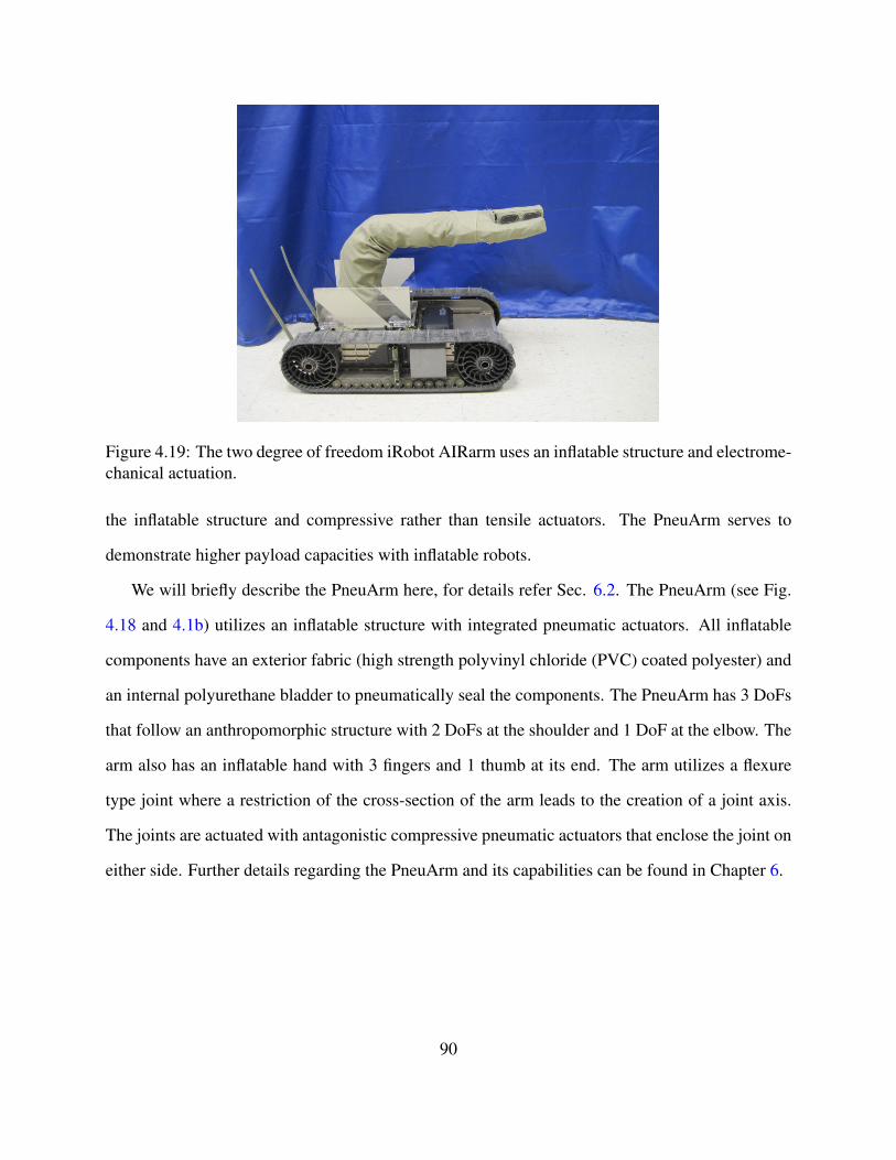
Figure 4.19: The two degree of freedom iRobot AIRarm uses an inflatable structure and electrome-chanical actuation.

the inflatable structure and compressive rather than tensile actuators. The PneuArm serves to

demonstrate higher payload capacities with inflatable robots.

We will briefly describe the PneuArm here, for details refer Sec. 6.2. The PneuArm (see Fig.

4.18 and 4.1b) utilizes an inflatable structure with integrated pneumatic actuators. All inflatable

components have an exterior fabric (high strength polyvinyl chloride (PVC) coated polyester) and

an internal polyurethane bladder to pneumatically seal the components. The PneuArm has 3 DoFs

that follow an anthropomorphic structure with 2 DoFs at the shoulder and 1 DoF at the elbow. The

arm also has an inflatable hand with 3 fingers and 1 thumb at its end. The arm utilizes a flexure

type joint where a restriction of the cross-section of the arm leads to the creation of a joint axis.

The joints are actuated with antagonistic compressive pneumatic actuators that enclose the joint on

either side. Further details regarding the PneuArm and its capabilities can be found in Chapter 6.

90

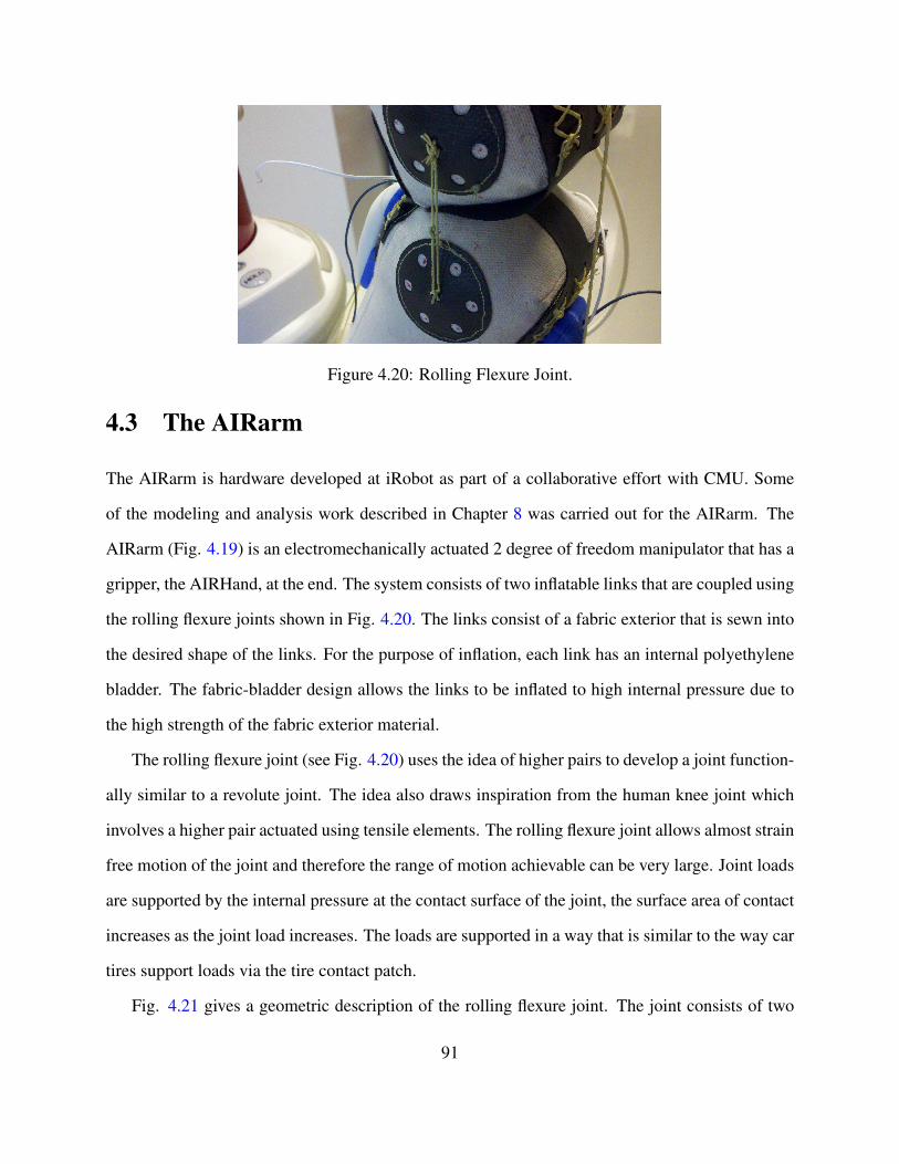
Figure 4.20: Rolling Flexure Joint.

4.3 The AIRarm

The AIRarm is hardware developed at iRobot as part of a collaborative effort with CMU. Some

of the modeling and analysis work described in Chapter 8 was carried out for the AIRarm. The

AIRarm (Fig. 4.19) is an electromechanically actuated 2 degree of freedom manipulator that has a

gripper, the AIRHand, at the end. The system consists of two inflatable links that are coupled using

the rolling flexure joints shown in Fig. 4.20. The links consist of a fabric exterior that is sewn into

the desired shape of the links. For the purpose of inflation, each link has an internal polyethylene

bladder. The fabric-bladder design allows the links to be inflated to high internal pressure due to

the high strength of the fabric exterior material.

The rolling flexure joint (see Fig. 4.20) uses the idea of higher pairs to develop a joint function-

ally similar to a revolute joint. The idea also draws inspiration from the human knee joint which

involves a higher pair actuated using tensile elements. The rolling flexure joint allows almost strain

free motion of the joint and therefore the range of motion achievable can be very large. Joint loads

are supported by the internal pressure at the contact surface of the joint, the surface area of contact

increases as the joint load increases. The loads are supported in a way that is similar to the way car

tires support loads via the tire contact patch.

Fig. 4.21 gives a geometric description of the rolling flexure joint. The joint consists of two

91

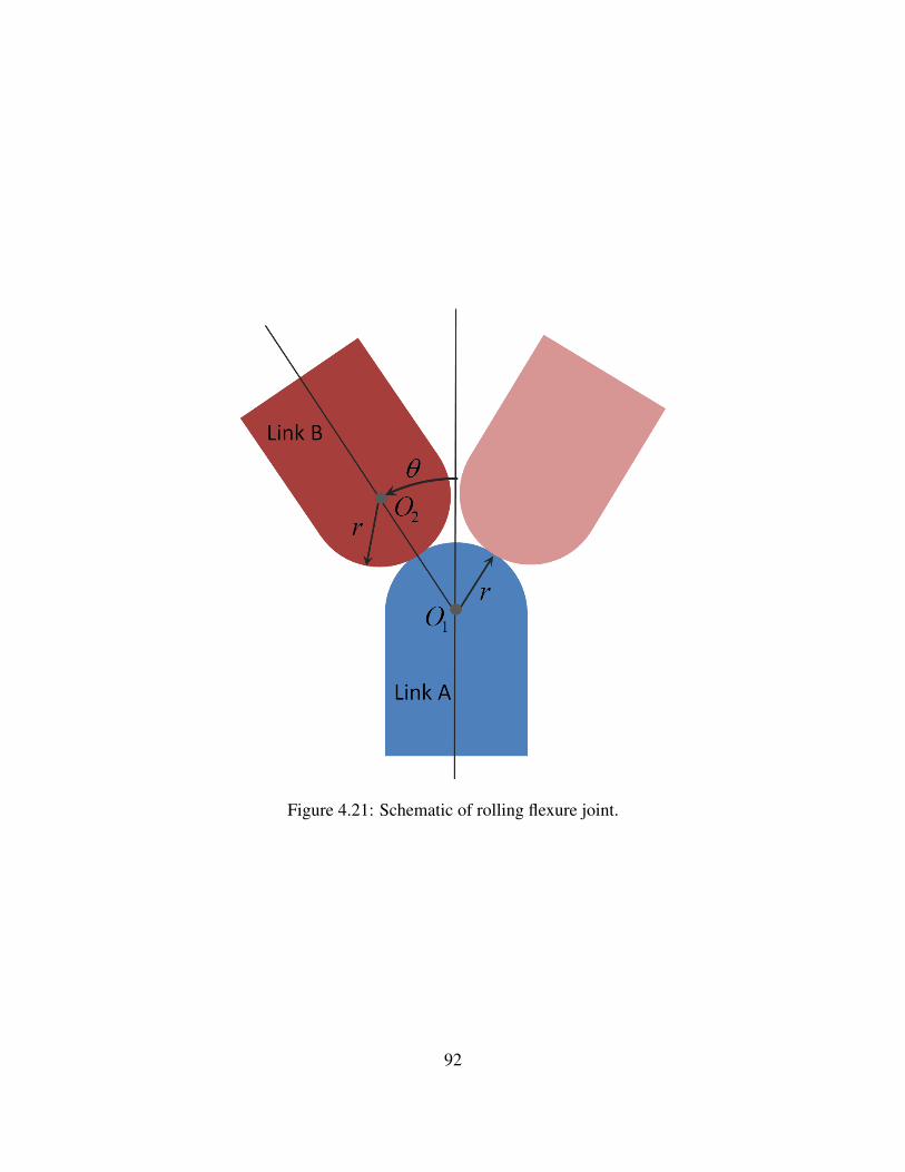
Figure 4.21: Schematic of rolling flexure joint.

92

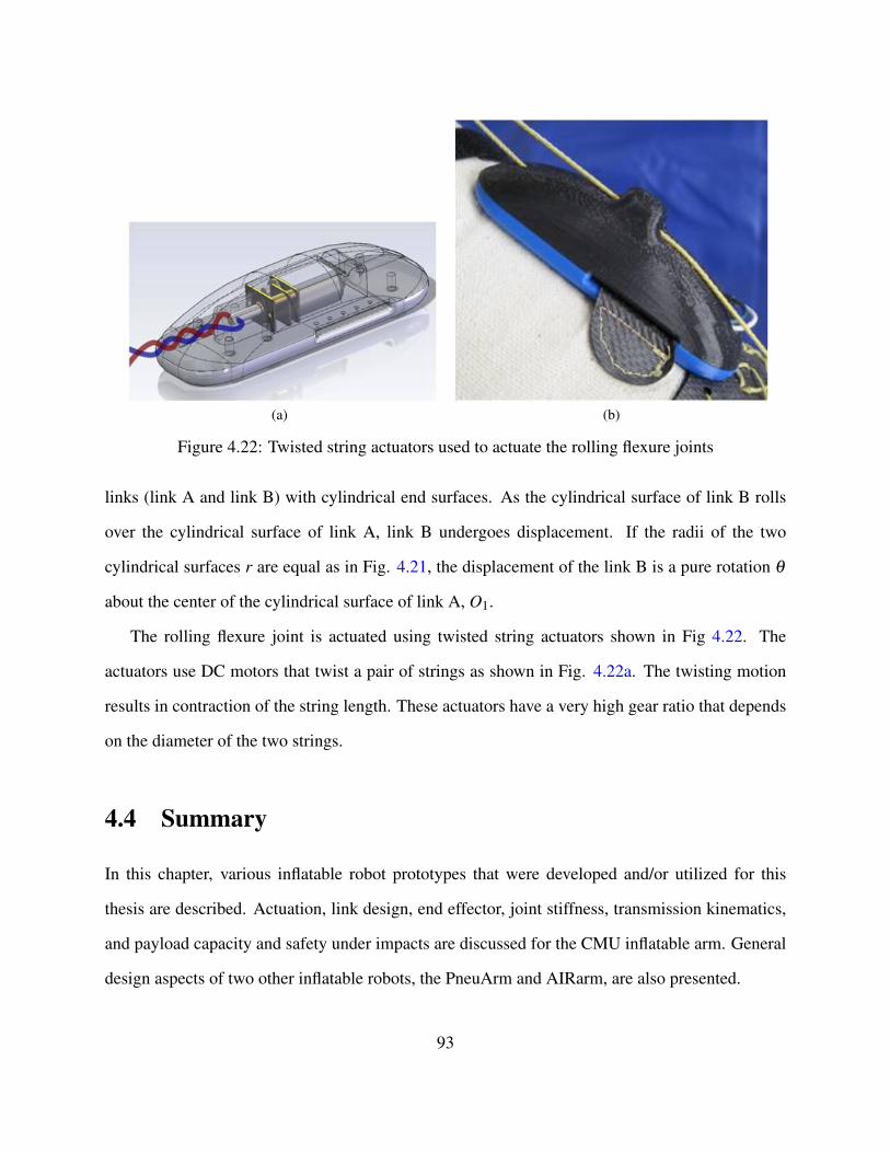
(a) (b)

Figure 4.22: Twisted string actuators used to actuate the rolling flexure joints

links (link A and link B) with cylindrical end surfaces. As the cylindrical surface of link B rolls

over the cylindrical surface of link A, link B undergoes displacement. If the radii of the two

cylindrical surfaces r are equal as in Fig. 4.21, the displacement of the link B is a pure rotation θ

about the center of the cylindrical surface of link A, O1.

The rolling flexure joint is actuated using twisted string actuators shown in Fig 4.22. The

actuators use DC motors that twist a pair of strings as shown in Fig. 4.22a. The twisting motion

results in contraction of the string length. These actuators have a very high gear ratio that depends

on the diameter of the two strings.

4.4 Summary

In this chapter, various inflatable robot prototypes that were developed and/or utilized for this

thesis are described. Actuation, link design, end effector, joint stiffness, transmission kinematics,

and payload capacity and safety under impacts are discussed for the CMU inflatable arm. General

design aspects of two other inflatable robots, the PneuArm and AIRarm, are also presented.

93

Chapter 5

Fabrication

In this chapter, we will briefly describe some of the fabrication techniques used to manufacture the

inflatable robots described in this thesis. The fabrication methods are unconventional but not new

and used regularly in other application areas besides robotics.

5.1 Thermal Welding

Figure 5.1: An impulse sealer used for generating straight seams between layers of plastic film

The primary inflatable structure of the CMU inflatable arm, the bladders of the PneuArm and

AIRarm are fabricated by thermal welding of multiple layers of plastic film. The impulse sealer

94

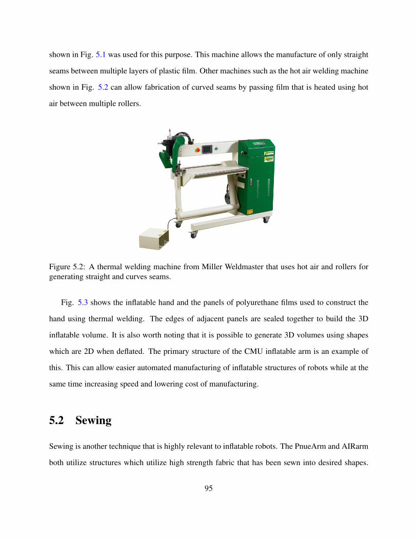
shown in Fig. 5.1 was used for this purpose. This machine allows the manufacture of only straight

seams between multiple layers of plastic film. Other machines such as the hot air welding machine

shown in Fig. 5.2 can allow fabrication of curved seams by passing film that is heated using hot

air between multiple rollers.

Figure 5.2: A thermal welding machine from Miller Weldmaster that uses hot air and rollers forgenerating straight and curves seams.

Fig. 5.3 shows the inflatable hand and the panels of polyurethane films used to construct the

hand using thermal welding. The edges of adjacent panels are sealed together to build the 3D

inflatable volume. It is also worth noting that it is possible to generate 3D volumes using shapes

which are 2D when deflated. The primary structure of the CMU inflatable arm is an example of

this. This can allow easier automated manufacturing of inflatable structures of robots while at the

same time increasing speed and lowering cost of manufacturing.

5.2 Sewing

Sewing is another technique that is highly relevant to inflatable robots. The PnueArm and AIRarm

both utilize structures which utilize high strength fabric that has been sewn into desired shapes.

95

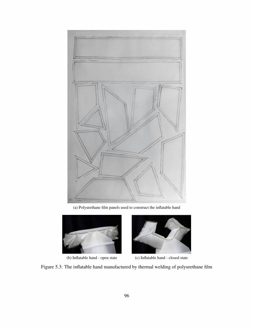
(a) Polyurethane film panels used to construct the inflatable hand

(b) Inflatable hand - open state (c) Inflatable hand - closed state

Figure 5.3: The inflatable hand manufactured by thermal welding of polyurethane film

96

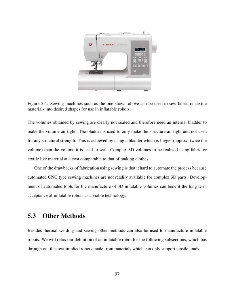
Figure 5.4: Sewing machines such as the one shown above can be used to sew fabric or textilematerials into desired shapes for use in inflatable robots.

The volumes obtained by sewing are clearly not sealed and therefore need an internal bladder to

make the volume air tight. The bladder is used to only make the structure air tight and not used

for any structural strength. This is achieved by using a bladder which is bigger (approx. twice the

volume) than the volume it is used to seal. Complex 3D volumes to be realized using fabric or

textile like material at a cost comparable to that of making clothes.

One of the drawbacks of fabrication using sewing is that it hard to automate the process because

automated CNC type sewing machines are not readily available for complex 3D parts. Develop-

ment of automated tools for the manufacture of 3D inflatable volumes can benefit the long term

acceptance of inflatable robots as a viable technology.

5.3 Other Methods

Besides thermal welding and sewing other methods can also be used to manufacture inflatable

robots. We will relax our definition of an inflatable robot for the following subsections, which has

through out this text implied robots made from materials which can only support tensile loads.

97

Seamless Knitting

Seamless knitting is another technique that can be used to manufacture inflatables with an outer

fabric shell and bladder lining. This technique allows fabrication of 3D shapes and volumes with-

out the use of cutting and sewing. The lack of seams in the structure implies an overall stronger

structure, as failure in inflatable structures often occurs across the seams. The other advantage of

seamless knitting is that process can be automated. Machines that can output seamless volumes

are commercially available, see [18] for details.

5.4 Summary

This chapter discusses the various techniques that were used to fabricate the prototypes described

in this thesis. Thermal welding and sewing are the two main techniques used. The fabrication

techniques used are identical to that used to make clothes and inflatable pool toys. These fabri-

cation techniques allow extremely low cost manufacturing of inflatable robots and can serve as

an enabling factor to make personal robots accessible to large segments of the general popula-

tion and researchers. Automation of the manufacturing process using 2D printing and lamination

techniques and 3D printing and knitting techniques might be beneficial for future applications.

98

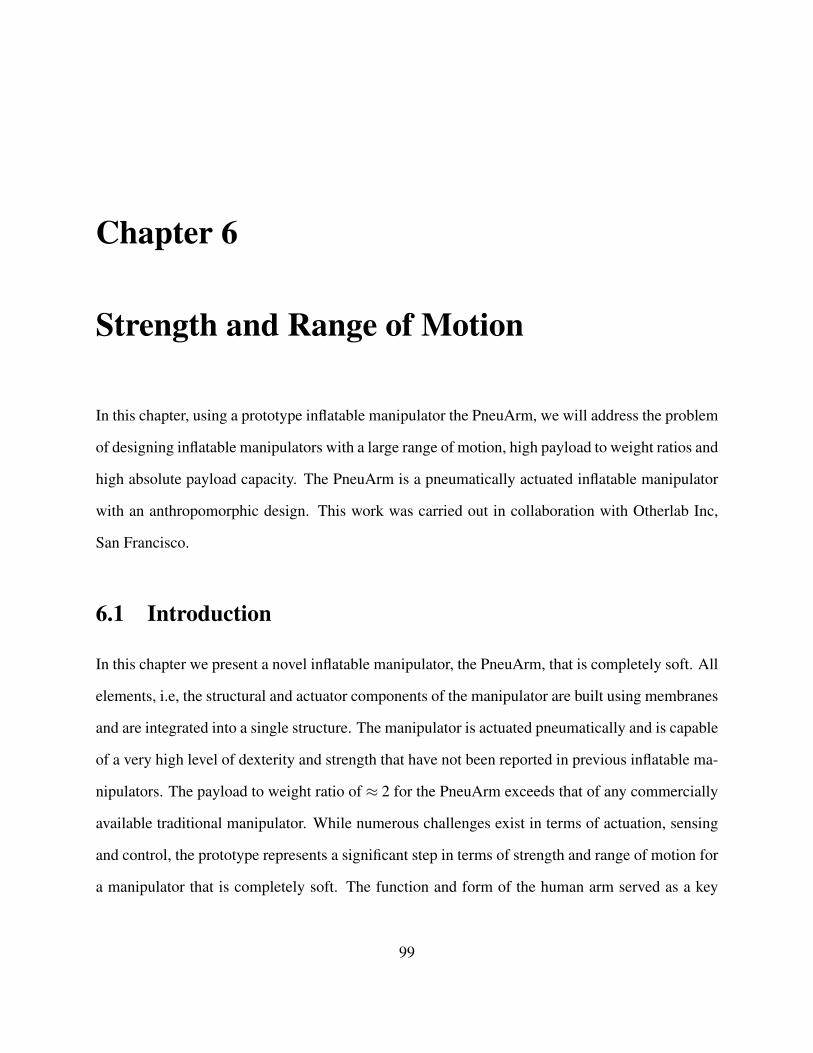
Chapter 6

Strength and Range of Motion

In this chapter, using a prototype inflatable manipulator the PneuArm, we will address the problem

of designing inflatable manipulators with a large range of motion, high payload to weight ratios and

high absolute payload capacity. The PneuArm is a pneumatically actuated inflatable manipulator

with an anthropomorphic design. This work was carried out in collaboration with Otherlab Inc,

San Francisco.

6.1 Introduction

In this chapter we present a novel inflatable manipulator, the PneuArm, that is completely soft. All

elements, i.e, the structural and actuator components of the manipulator are built using membranes

and are integrated into a single structure. The manipulator is actuated pneumatically and is capable

of a very high level of dexterity and strength that have not been reported in previous inflatable ma-

nipulators. The payload to weight ratio of ≈ 2 for the PneuArm exceeds that of any commercially

available traditional manipulator. While numerous challenges exist in terms of actuation, sensing

and control, the prototype represents a significant step in terms of strength and range of motion for

a manipulator that is completely soft. The function and form of the human arm served as a key

99

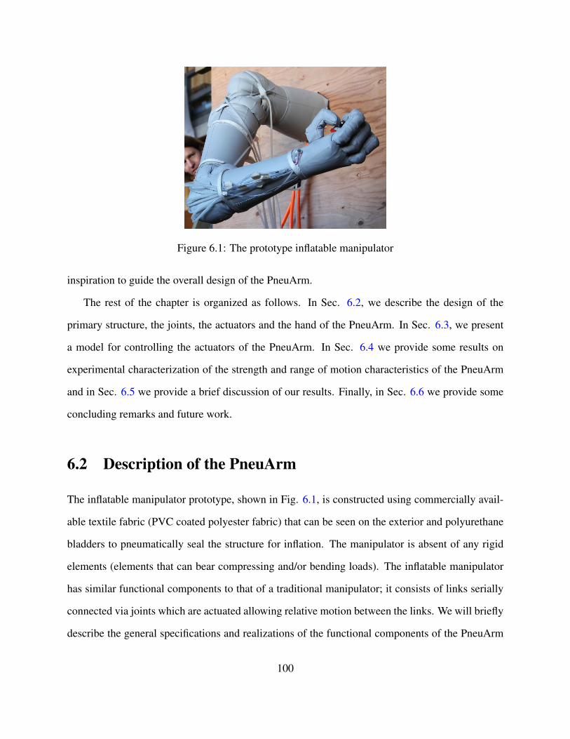
Figure 6.1: The prototype inflatable manipulator

inspiration to guide the overall design of the PneuArm.

The rest of the chapter is organized as follows. In Sec. 6.2, we describe the design of the

primary structure, the joints, the actuators and the hand of the PneuArm. In Sec. 6.3, we present

a model for controlling the actuators of the PneuArm. In Sec. 6.4 we provide some results on

experimental characterization of the strength and range of motion characteristics of the PneuArm

and in Sec. 6.5 we provide a brief discussion of our results. Finally, in Sec. 6.6 we provide some

concluding remarks and future work.

6.2 Description of the PneuArm

The inflatable manipulator prototype, shown in Fig. 6.1, is constructed using commercially avail-

able textile fabric (PVC coated polyester fabric) that can be seen on the exterior and polyurethane

bladders to pneumatically seal the structure for inflation. The manipulator is absent of any rigid

elements (elements that can bear compressing and/or bending loads). The inflatable manipulator

has similar functional components to that of a traditional manipulator; it consists of links serially

connected via joints which are actuated allowing relative motion between the links. We will briefly

describe the general specifications and realizations of the functional components of the PneuArm

100

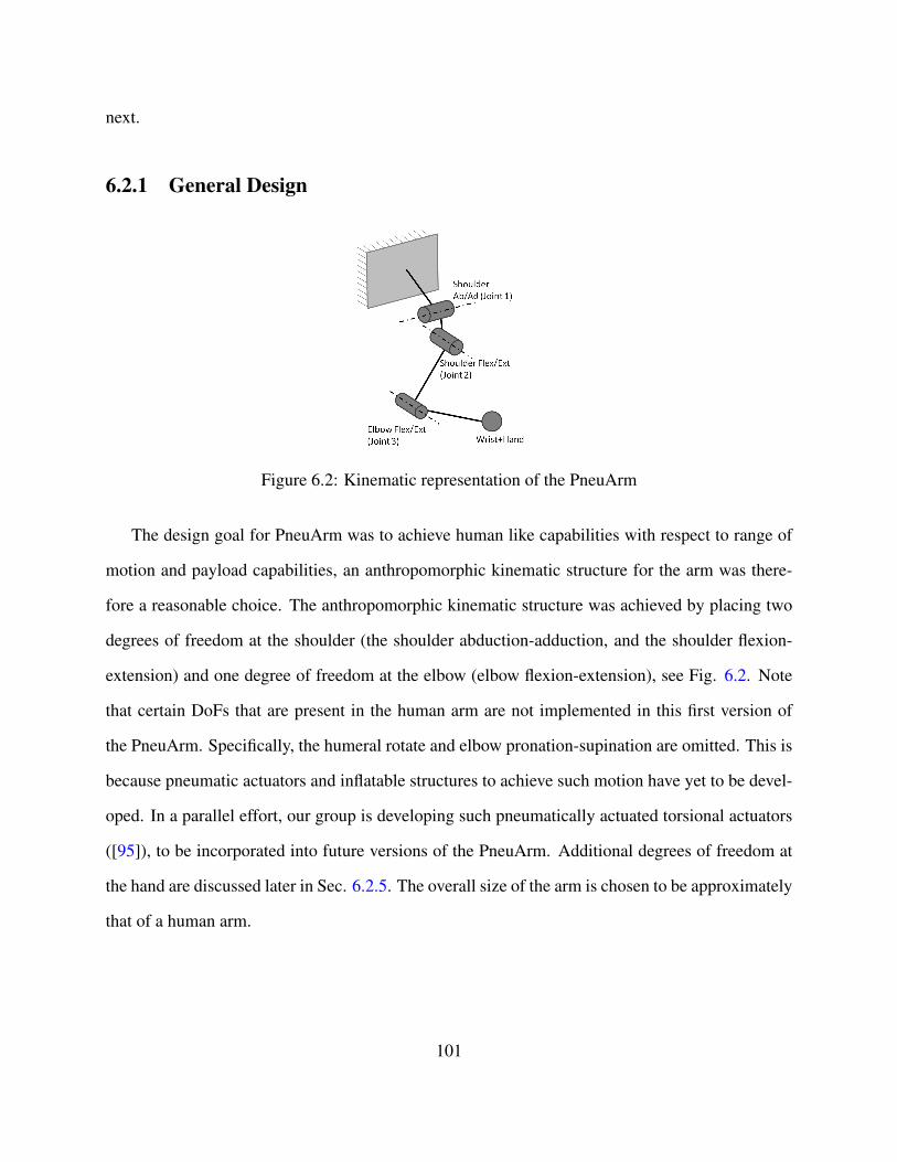
next.

6.2.1 General Design

Figure 6.2: Kinematic representation of the PneuArm

The design goal for PneuArm was to achieve human like capabilities with respect to range of

motion and payload capabilities, an anthropomorphic kinematic structure for the arm was there-

fore a reasonable choice. The anthropomorphic kinematic structure was achieved by placing two

degrees of freedom at the shoulder (the shoulder abduction-adduction, and the shoulder flexion-

extension) and one degree of freedom at the elbow (elbow flexion-extension), see Fig. 6.2. Note

that certain DoFs that are present in the human arm are not implemented in this first version of

the PneuArm. Specifically, the humeral rotate and elbow pronation-supination are omitted. This is

because pneumatic actuators and inflatable structures to achieve such motion have yet to be devel-

oped. In a parallel effort, our group is developing such pneumatically actuated torsional actuators

([95]), to be incorporated into future versions of the PneuArm. Additional degrees of freedom at

the hand are discussed later in Sec. 6.2.5. The overall size of the arm is chosen to be approximately

that of a human arm.

101

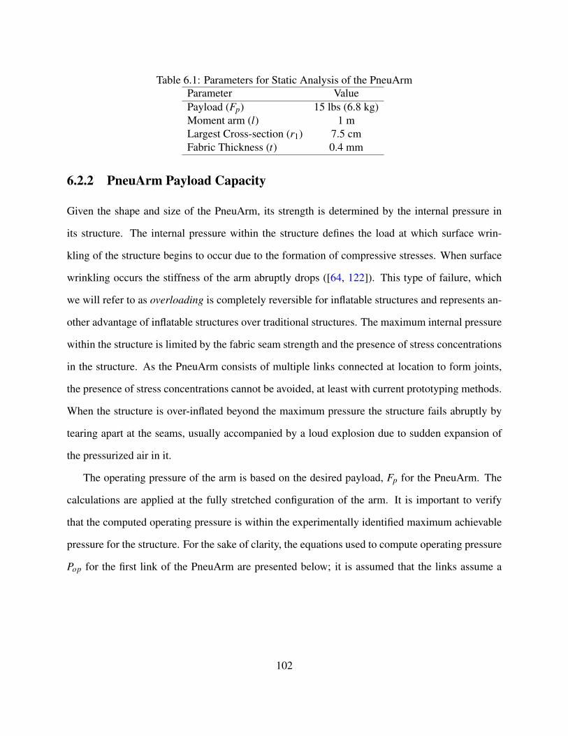
Table 6.1: Parameters for Static Analysis of the PneuArmParameter ValuePayload (Fp) 15 lbs (6.8 kg)Moment arm (l) 1 mLargest Cross-section (r1) 7.5 cmFabric Thickness (t) 0.4 mm

6.2.2 PneuArm Payload Capacity

Given the shape and size of the PneuArm, its strength is determined by the internal pressure in

its structure. The internal pressure within the structure defines the load at which surface wrin-

kling of the structure begins to occur due to the formation of compressive stresses. When surface

wrinkling occurs the stiffness of the arm abruptly drops ([64, 122]). This type of failure, which

we will refer to as overloading is completely reversible for inflatable structures and represents an-

other advantage of inflatable structures over traditional structures. The maximum internal pressure

within the structure is limited by the fabric seam strength and the presence of stress concentrations

in the structure. As the PneuArm consists of multiple links connected at location to form joints,

the presence of stress concentrations cannot be avoided, at least with current prototyping methods.

When the structure is over-inflated beyond the maximum pressure the structure fails abruptly by

tearing apart at the seams, usually accompanied by a loud explosion due to sudden expansion of

the pressurized air in it.

The operating pressure of the arm is based on the desired payload, Fp for the PneuArm. The

calculations are applied at the fully stretched configuration of the arm. It is important to verify

that the computed operating pressure is within the experimentally identified maximum achievable

pressure for the structure. For the sake of clarity, the equations used to compute operating pressure

Pop for the first link of the PneuArm are presented below; it is assumed that the links assume a

102

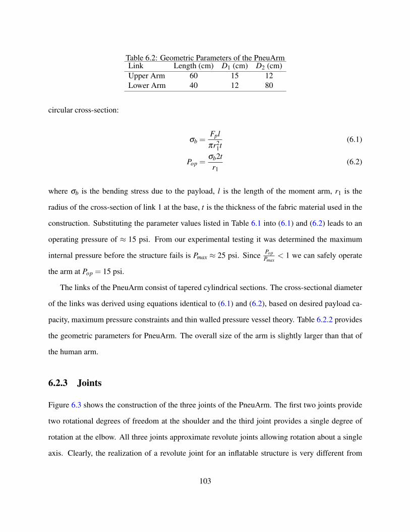
Table 6.2: Geometric Parameters of the PneuArmLink Length (cm) D1 (cm) D2 (cm)Upper Arm 60 15 12Lower Arm 40 12 80

circular cross-section:

σb =Fplπr2

1t(6.1)

Pop =σb2t

r1(6.2)

where σb is the bending stress due to the payload, l is the length of the moment arm, r1 is the

radius of the cross-section of link 1 at the base, t is the thickness of the fabric material used in the

construction. Substituting the parameter values listed in Table 6.1 into (6.1) and (6.2) leads to an

operating pressure of ≈ 15 psi. From our experimental testing it was determined the maximum

internal pressure before the structure fails is Pmax ≈ 25 psi. Since PopPmax

< 1 we can safely operate

the arm at Pop = 15 psi.

The links of the PneuArm consist of tapered cylindrical sections. The cross-sectional diameter

of the links was derived using equations identical to (6.1) and (6.2), based on desired payload ca-

pacity, maximum pressure constraints and thin walled pressure vessel theory. Table 6.2.2 provides

the geometric parameters for PneuArm. The overall size of the arm is slightly larger than that of

the human arm.

6.2.3 Joints

Figure 6.3 shows the construction of the three joints of the PneuArm. The first two joints provide

two rotational degrees of freedom at the shoulder and the third joint provides a single degree of

rotation at the elbow. All three joints approximate revolute joints allowing rotation about a single

axis. Clearly, the realization of a revolute joint for an inflatable structure is very different from

103

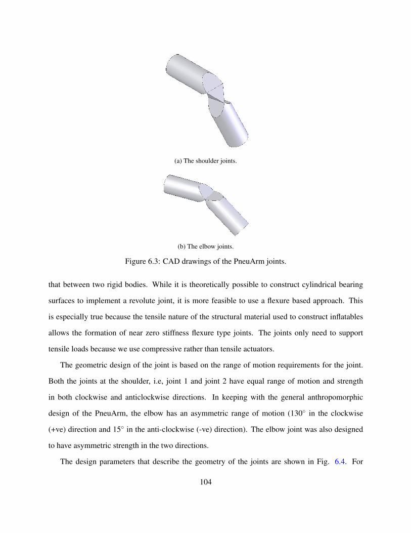
(a) The shoulder joints.

(b) The elbow joints.

Figure 6.3: CAD drawings of the PneuArm joints.

that between two rigid bodies. While it is theoretically possible to construct cylindrical bearing

surfaces to implement a revolute joint, it is more feasible to use a flexure based approach. This

is especially true because the tensile nature of the structural material used to construct inflatables

allows the formation of near zero stiffness flexure type joints. The joints only need to support

tensile loads because we use compressive rather than tensile actuators.

The geometric design of the joint is based on the range of motion requirements for the joint.

Both the joints at the shoulder, i.e, joint 1 and joint 2 have equal range of motion and strength

in both clockwise and anticlockwise directions. In keeping with the general anthropomorphic

design of the PneuArm, the elbow has an asymmetric range of motion (130◦ in the clockwise

(+ve) direction and 15◦ in the anti-clockwise (-ve) direction). The elbow joint was also designed

to have asymmetric strength in the two directions.

The design parameters that describe the geometry of the joints are shown in Fig. 6.4. For

104

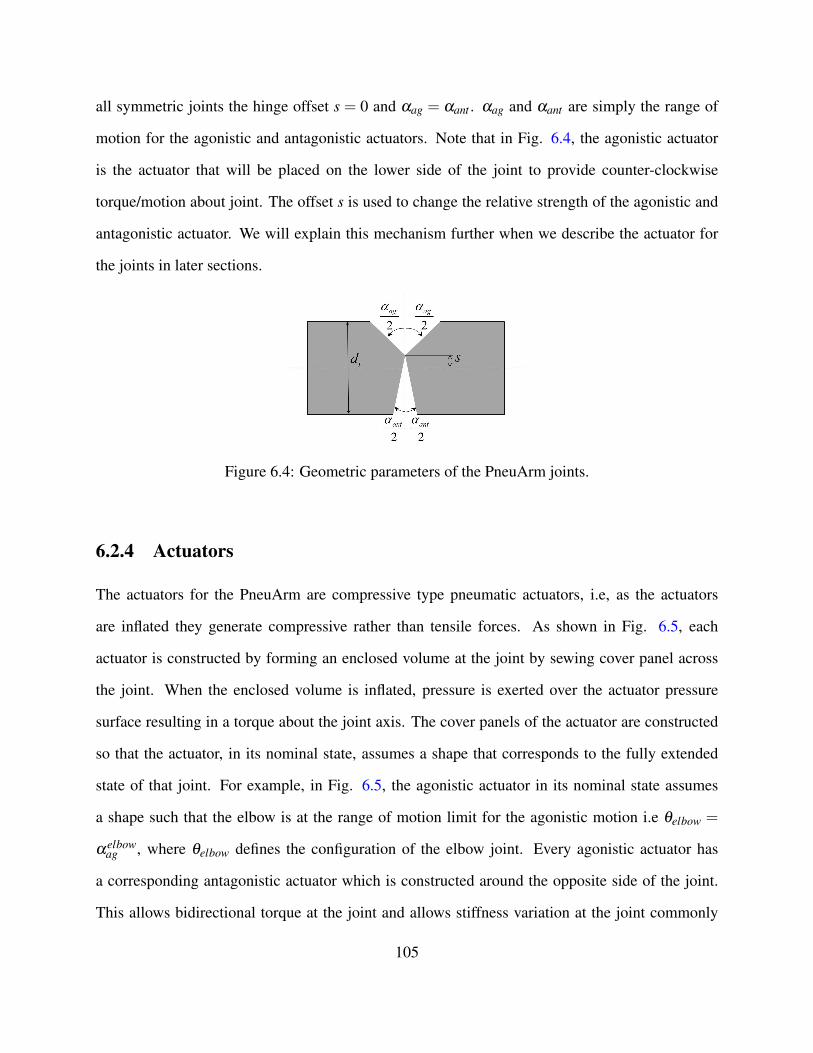
all symmetric joints the hinge offset s = 0 and αag = αant . αag and αant are simply the range of

motion for the agonistic and antagonistic actuators. Note that in Fig. 6.4, the agonistic actuator

is the actuator that will be placed on the lower side of the joint to provide counter-clockwise

torque/motion about joint. The offset s is used to change the relative strength of the agonistic and

antagonistic actuator. We will explain this mechanism further when we describe the actuator for

the joints in later sections.

Figure 6.4: Geometric parameters of the PneuArm joints.

6.2.4 Actuators

The actuators for the PneuArm are compressive type pneumatic actuators, i.e, as the actuators

are inflated they generate compressive rather than tensile forces. As shown in Fig. 6.5, each

actuator is constructed by forming an enclosed volume at the joint by sewing cover panel across

the joint. When the enclosed volume is inflated, pressure is exerted over the actuator pressure

surface resulting in a torque about the joint axis. The cover panels of the actuator are constructed

so that the actuator, in its nominal state, assumes a shape that corresponds to the fully extended

state of that joint. For example, in Fig. 6.5, the agonistic actuator in its nominal state assumes

a shape such that the elbow is at the range of motion limit for the agonistic motion i.e θelbow =

αelbowag , where θelbow defines the configuration of the elbow joint. Every agonistic actuator has

a corresponding antagonistic actuator which is constructed around the opposite side of the joint.

This allows bidirectional torque at the joint and allows stiffness variation at the joint commonly

105

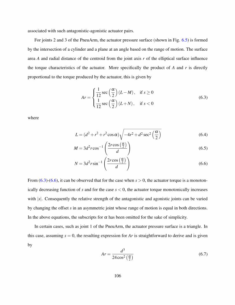
associated with such antagonistic-agonistic actuator pairs.

For joints 2 and 3 of the PneuArm, the actuator pressure surface (shown in Fig. 6.5) is formed

by the intersection of a cylinder and a plane at an angle based on the range of motion. The surface

area A and radial distance of the centroid from the joint axis r of the elliptical surface influence

the torque characteristics of the actuator. More specifically the product of A and r is directly

proportional to the torque produced by the actuator, this is given by

Ar =

1

12sec(

α

2

)(L−M) , if s≥ 0

112

sec(

α

2

)(L+N) , if s < 0

(6.3)

where

L = (d2 + r2 + r2 cosα)

√−4r2 +d2 sec2

(α

2

)(6.4)

M = 3d2r cos−1

(2r cos

(α

2

)d

)(6.5)

N = 3d2r sin−1

(2r cos

(α

2

)d

)(6.6)

From (6.3)-(6.6), it can be observed that for the case when s > 0, the actuator torque is a monoton-

ically decreasing function of s and for the case s < 0, the actuator torque monotonically increases

with |s|. Consequently the relative strength of the antagonistic and agonistic joints can be varied

by changing the offset s in an asymmetric joint whose range of motion is equal in both directions.

In the above equations, the subscripts for α has been omitted for the sake of simplicity.

In certain cases, such as joint 1 of the PneuArm, the actuator pressure surface is a triangle. In

this case, assuming s = 0, the resulting expression for Ar is straightforward to derive and is given

by

Ar =d3

24cos2(

α

2

) (6.7)

106

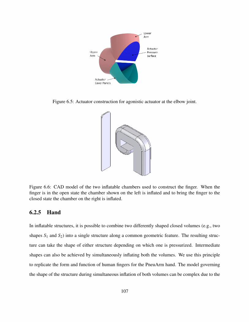
Figure 6.5: Actuator construction for agonistic actuator at the elbow joint.

Figure 6.6: CAD model of the two inflatable chambers used to construct the finger. When thefinger is in the open state the chamber shown on the left is inflated and to bring the finger to theclosed state the chamber on the right is inflated.

6.2.5 Hand

In inflatable structures, it is possible to combine two differently shaped closed volumes (e.g., two

shapes S1 and S2) into a single structure along a common geometric feature. The resulting struc-

ture can take the shape of either structure depending on which one is pressurized. Intermediate

shapes can also be achieved by simultaneously inflating both the volumes. We use this principle

to replicate the form and function of human fingers for the PneuArm hand. The model governing

the shape of the structure during simultaneous inflation of both volumes can be complex due to the

107

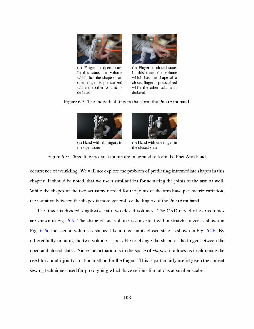
(a) Finger in open state.In this state, the volumewhich has the shape of anopen finger is pressurizedwhile the other volume isdeflated.

(b) Finger in closed state.In this state, the volumewhich has the shape of aclosed finger is pressurizedwhile the other volume isdeflated.

Figure 6.7: The individual fingers that form the PneuArm hand.

(a) Hand with all fingers inthe open state

(b) Hand with one finger inthe closed state

Figure 6.8: Three fingers and a thumb are integrated to form the PneuArm hand.

occurrence of wrinkling. We will not explore the problem of predicting intermediate shapes in this

chapter. It should be noted, that we use a similar idea for actuating the joints of the arm as well.

While the shapes of the two actuators needed for the joints of the arm have parametric variation,

the variation between the shapes is more general for the fingers of the PneuArm hand.

The finger is divided lengthwise into two closed volumes. The CAD model of two volumes

are shown in Fig. 6.6. The shape of one volume is consistent with a straight finger as shown in

Fig. 6.7a; the second volume is shaped like a finger in its closed state as shown in Fig. 6.7b. By

differentially inflating the two volumes it possible to change the shape of the finger between the

open and closed states. Since the actuation is in the space of shapes, it allows us to eliminate the

need for a multi-joint actuation method for the fingers. This is particularly useful given the current

sewing techniques used for prototyping which have serious limitations at smaller scales.

108

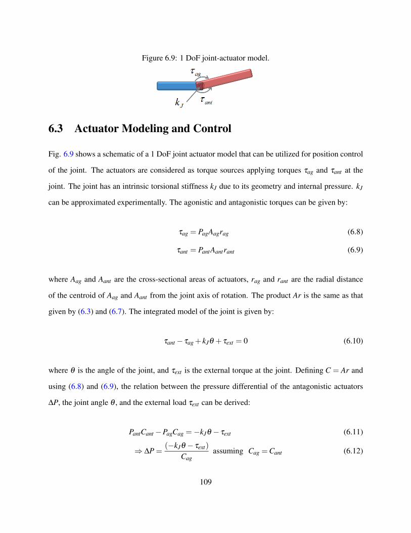
Figure 6.9: 1 DoF joint-actuator model.

6.3 Actuator Modeling and Control

Fig. 6.9 shows a schematic of a 1 DoF joint actuator model that can be utilized for position control

of the joint. The actuators are considered as torque sources applying torques τag and τant at the

joint. The joint has an intrinsic torsional stiffness kJ due to its geometry and internal pressure. kJ

can be approximated experimentally. The agonistic and antagonistic torques can be given by:

τag = PagAagrag (6.8)

τant = PantAantrant (6.9)

where Aag and Aant are the cross-sectional areas of actuators, rag and rant are the radial distance

of the centroid of Aag and Aant from the joint axis of rotation. The product Ar is the same as that

given by (6.3) and (6.7). The integrated model of the joint is given by:

τant− τag + kJθ + τext = 0 (6.10)

where θ is the angle of the joint, and τext is the external torque at the joint. Defining C = Ar and

using (6.8) and (6.9), the relation between the pressure differential of the antagonistic actuators

∆P, the joint angle θ , and the external load τext can be derived:

PantCant−PagCag =−kJθ − τext (6.11)

⇒ ∆P =(−kJθ − τext)

Cagassuming Cag =Cant (6.12)

109

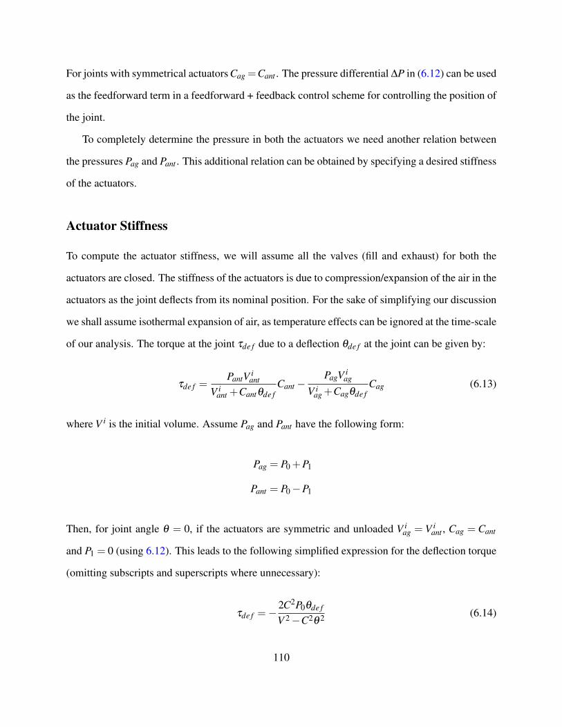
For joints with symmetrical actuators Cag =Cant . The pressure differential ∆P in (6.12) can be used

as the feedforward term in a feedforward + feedback control scheme for controlling the position of

the joint.

To completely determine the pressure in both the actuators we need another relation between

the pressures Pag and Pant . This additional relation can be obtained by specifying a desired stiffness

of the actuators.

Actuator Stiffness

To compute the actuator stiffness, we will assume all the valves (fill and exhaust) for both the

actuators are closed. The stiffness of the actuators is due to compression/expansion of the air in the

actuators as the joint deflects from its nominal position. For the sake of simplifying our discussion

we shall assume isothermal expansion of air, as temperature effects can be ignored at the time-scale

of our analysis. The torque at the joint τde f due to a deflection θde f at the joint can be given by:

τde f =PantV i

ant

V iant +Cantθde f

Cant−PagV i

ag

V iag +Cagθde f

Cag (6.13)

where V i is the initial volume. Assume Pag and Pant have the following form:

Pag = P0 +P1

Pant = P0−P1

Then, for joint angle θ = 0, if the actuators are symmetric and unloaded V iag = V i

ant , Cag = Cant

and P1 = 0 (using 6.12). This leads to the following simplified expression for the deflection torque

(omitting subscripts and superscripts where unnecessary):

τde f =−2C2P0θde f

V 2−C2θ 2 (6.14)

110

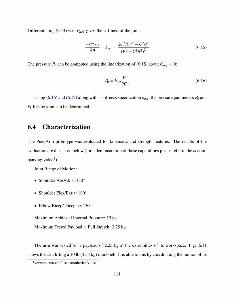
Differentiating (6.14) w.r.t θde f gives the stiffness of the joint:

−∂τde f

∂θ= kact =

2C2P0V 2 +C2θ 2

(V 2−C2θ 2)2 (6.15)

The pressure P0 can be computed using the linearization of (6.15) about θde f = 0:

P0 = kactV 2

2C2 (6.16)

Using (6.16) and (6.12) along with a stiffness specification kact , the pressure parameters P0 and

P1 for the joint can be determined.

6.4 Characterization

The PneuArm prototype was evaluated for kinematic and strength features. The results of the

evaluation are discussed below (for a demonstration of these capabilities please refer to the accom-

panying video1).

Joint Range of Motion:

• Shoulder Ab/Ad: ≈ 180◦

• Shoulder Flex/Ext:≈ 180◦

• Elbow Bicep/Tricep: ≈ 150◦

Maximum Achieved Internal Pressure: 15 psi

Maximum Tested Payload at Full Stretch: 2.25 kg

The arm was tested for a payload of 2.25 kg at the extremities of its workspace. Fig. 6.11

shows the arm lifting a 10 lb (4.54 kg) dumbbell. It is able to this by coordinating the motion of its1www.cs.cmu.edu/˜ssanan/otherlab/video

111

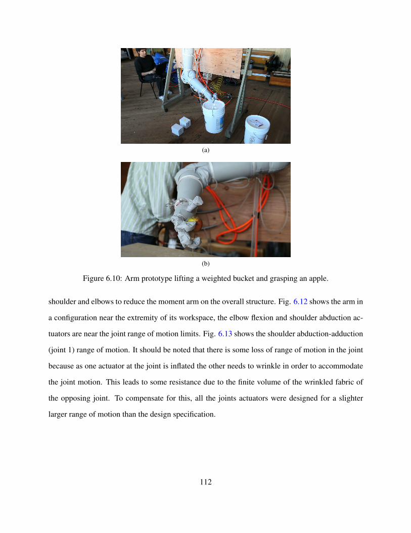
(a)

(b)

Figure 6.10: Arm prototype lifting a weighted bucket and grasping an apple.

shoulder and elbows to reduce the moment arm on the overall structure. Fig. 6.12 shows the arm in

a configuration near the extremity of its workspace, the elbow flexion and shoulder abduction ac-

tuators are near the joint range of motion limits. Fig. 6.13 shows the shoulder abduction-adduction

(joint 1) range of motion. It should be noted that there is some loss of range of motion in the joint

because as one actuator at the joint is inflated the other needs to wrinkle in order to accommodate

the joint motion. This leads to some resistance due to the finite volume of the wrinkled fabric of

the opposing joint. To compensate for this, all the joints actuators were designed for a slighter

larger range of motion than the design specification.

112

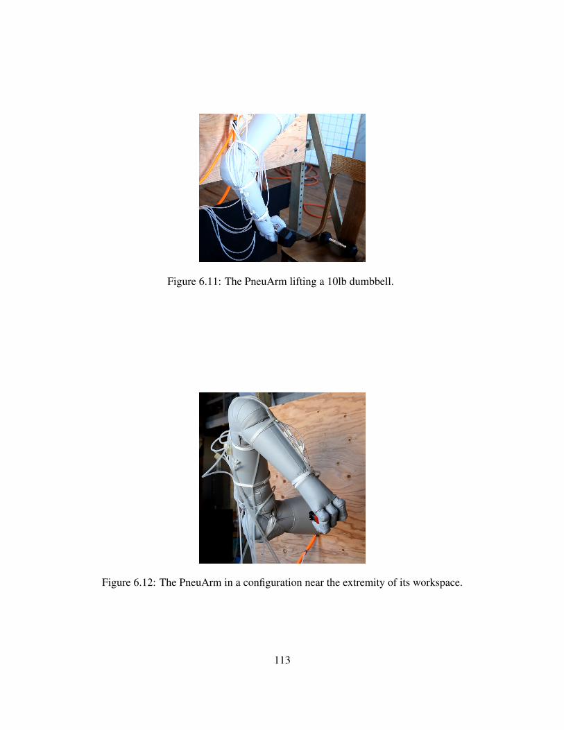
Figure 6.11: The PneuArm lifting a 10lb dumbbell.

Figure 6.12: The PneuArm in a configuration near the extremity of its workspace.

113

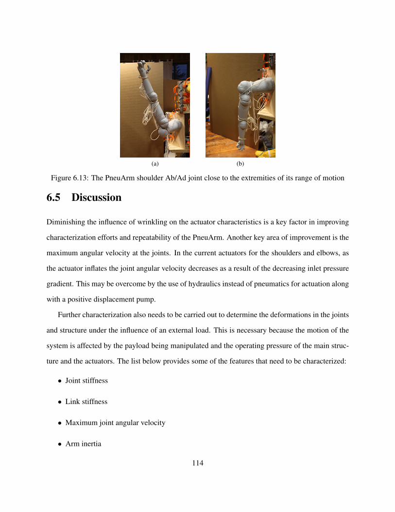
(a) (b)

Figure 6.13: The PneuArm shoulder Ab/Ad joint close to the extremities of its range of motion

6.5 Discussion

Diminishing the influence of wrinkling on the actuator characteristics is a key factor in improving

characterization efforts and repeatability of the PneuArm. Another key area of improvement is the

maximum angular velocity at the joints. In the current actuators for the shoulders and elbows, as

the actuator inflates the joint angular velocity decreases as a result of the decreasing inlet pressure

gradient. This may be overcome by the use of hydraulics instead of pneumatics for actuation along

with a positive displacement pump.

Further characterization also needs to be carried out to determine the deformations in the joints

and structure under the influence of an external load. This is necessary because the motion of the

system is affected by the payload being manipulated and the operating pressure of the main struc-

ture and the actuators. The list below provides some of the features that need to be characterized:

• Joint stiffness

• Link stiffness

• Maximum joint angular velocity

• Arm inertia

114

The above characterizations will help build a more complete model of the arm suitable for de-

veloping control schemes for the whole arm. Besides characterization for modeling, performance

metrics to evaluate the developed controlled schemes are needed, some of these are listed below:

• Joint position accuracy

• Tip position accuracy

• Joint trajectory tracking performance

• Tip trajectory tracking performance

• Joint torque control performance

• Tip impedance control performance

6.6 Summary

In this chapter, we have presented a dextrous, high payload, and high payload-to-weight ratio

inflatable manipulator, the PneuArm. The inflatable manipulator represents a significant step in

our understanding of designing and manufacturing inflatable robotic systems with high strength.

With a manufacturing process as simple as sewing we succeeded in developing a manipulator that

is complex enough to be ‘human-like’. The arm has a payload-to-weight ratio of ≈ 2 and an

absolute mass of ≈ 1 kg. Actuator and joint models for joint based position control of the arm

were also developed. A novel hand that resembles the human hand in form and function is also

shown and initial experiments have shown it to be capable of grasping a variety of objects.

One of the limiting factors that affects the overall payload capacity of the system is the max-

imum pressure that the system can be inflated to. Though this is currently limited by our manu-

facturing process, the ultimate reason to limit the maximum pressure within the structure is due to

safety concerns. If the energy stored in the inflatable chambers in the form of compressed air is too

115

high, this could lead to potentially dangerous high energy loud explosions. One way to minimize

such safety hazards is to divide the inflatable structures into multiple chambers that have signif-

icantly smaller volumes. This is a possible future direction for inflatable robots to achieve even

greater strength and reliability. Another important direction for future research is the development

of valve technology for actuating these systems. The valves are currently placed away from the

arm and are the only rigid components needed to run the PneuArm. Lightweight and soft valve

technology that integrates in a more seamless manner with pneumatically actuated inflatable robots

would be highly beneficial to inflatable robotics.

116

Chapter 7

Pneumatic Actuators for Inflatable Robots

This chapter discusses a variety of novel fluidic or pneumatic actuators to generate rotary motion

for inflatable robots. These actuators differ from linear actuators such as the McKibben actua-

tors utilized for the prototype in Chapter 4, Fig. 4.6 and from the compressive actuators used to

drive the Pneuarm in the previous chapter, as they provide rotary motion along the axial direction

of the actuator. While pneumatic artificial muscles (PAMs) that can generate linear motion have

been researched and developed fairly extensively, little effort has been devoted to develop simple

actuators that can provide rotary motion. A variety of possible designs and principles are dis-

cussed to achieve such rotary motion, along with accompanying analysis to understand motion and

torque characteristics of each actuator. Experiments with prototype actuators validate performance

expectations of each design.

7.1 Introduction

The dominant actuation method for most robots in the past has been electro-magnetic rotary actua-

tors or motors. These actuators tend to be heavy, adding mass and inertia to the system. For robots

that need to function in human environments and physically interact with humans the actuator

117

weight and inertia present a challenge from the safety perspective. Although various techniques,

like Series Elastic Actuation and similar approaches [89, 137] have been proposed to hide the high

inertia of the actuators, these actuators still present a fundamental limitation in terms of the weight

of the robots. Besides lightweight actuation, there has also been a demonstrated need for Variable

Impedance Actuators (VIAs) to satisfy safety and performance requirements of robots [8]. Pneu-

matic Artificial Muscles (PAMs) are a promising solution for providing lightweight actuation with

variable impedance.

Numerous examples of PAMs exist today, mostly for providing linear actuation. The McK-

ibben actuator [100, 19] is probably the most extensively used and studied PAM and can be setup

in antagonistic actuation scheme to allow position and stiffness control of the actuator. [23] pro-

vides an extensive review of the numerous other type of PAMs that exist. While a number of

these actuators were developed in the past for actuating rigid robots, the application of pneumatic

actuation principles to develop soft robots has seen an increasing interest recently [55, 102].

We are interested in developing simple pneumatic actuators that can provide direct rotary mo-

tion, like that needed to generate a twisting motion at the wrist of the PneuArm inflatable ma-

nipulator [96] shown in Fig. 7.1 that is being developed by our group. Pneumatic actuators can

integrate seamlessly with an inflatable manipulator such and this was our primary consideration

for choosing pneumatic ‘skin-based’ actuators. Very little effort has been devoted in the past to

develop actuators that can provide such direct rotary motion and we hope to advance the design

space of such actuators. Recently, a carbon nanotube actuator that provides such motion for micro-

scale applications was reported in [30]. We will refer to actuators providing direct rotary motion

as torsional actuators because these actuators deform torsionally along their length. It should also

be noted that because our application domain is inflatable robots, our goal is to develop torsional

actuators without the use of any rigid components.

In the following sections we will describe the design and analysis of three novel pneumatic tor-

sional actuators along with accompanying prototypes. The first actuator design uses the concept of

118

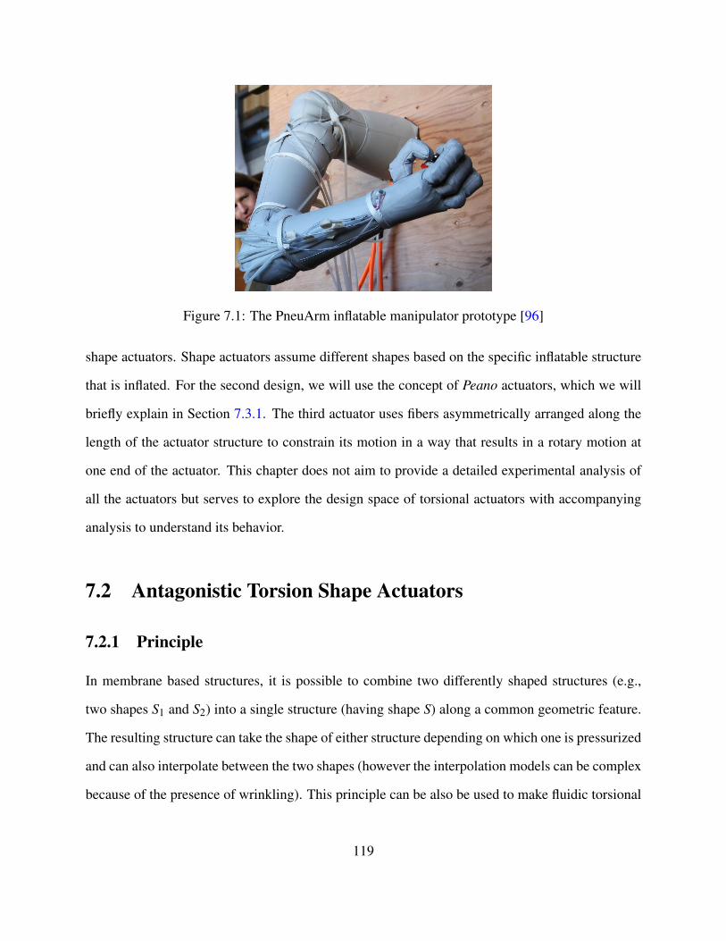
Figure 7.1: The PneuArm inflatable manipulator prototype [96]

shape actuators. Shape actuators assume different shapes based on the specific inflatable structure

that is inflated. For the second design, we will use the concept of Peano actuators, which we will

briefly explain in Section 7.3.1. The third actuator uses fibers asymmetrically arranged along the

length of the actuator structure to constrain its motion in a way that results in a rotary motion at

one end of the actuator. This chapter does not aim to provide a detailed experimental analysis of

all the actuators but serves to explore the design space of torsional actuators with accompanying

analysis to understand its behavior.

7.2 Antagonistic Torsion Shape Actuators

7.2.1 Principle

In membrane based structures, it is possible to combine two differently shaped structures (e.g.,

two shapes S1 and S2) into a single structure (having shape S) along a common geometric feature.

The resulting structure can take the shape of either structure depending on which one is pressurized

and can also interpolate between the two shapes (however the interpolation models can be complex

because of the presence of wrinkling). This principle can be also be used to make fluidic torsional

119

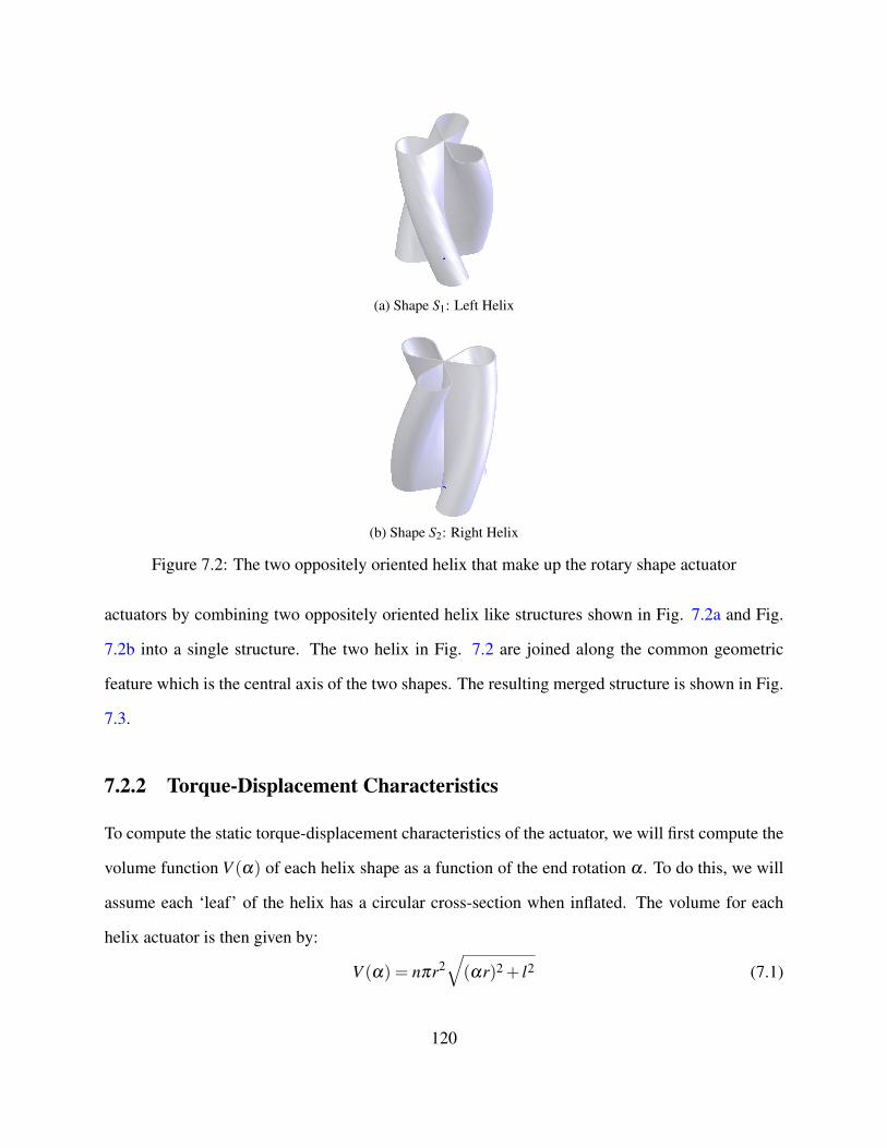
(a) Shape S1: Left Helix

(b) Shape S2: Right Helix

Figure 7.2: The two oppositely oriented helix that make up the rotary shape actuator

actuators by combining two oppositely oriented helix like structures shown in Fig. 7.2a and Fig.

7.2b into a single structure. The two helix in Fig. 7.2 are joined along the common geometric

feature which is the central axis of the two shapes. The resulting merged structure is shown in Fig.

7.3.

7.2.2 Torque-Displacement Characteristics

To compute the static torque-displacement characteristics of the actuator, we will first compute the

volume function V (α) of each helix shape as a function of the end rotation α . To do this, we will

assume each ‘leaf’ of the helix has a circular cross-section when inflated. The volume for each

helix actuator is then given by:

V (α) = nπr2√

(αr)2 + l2 (7.1)

120

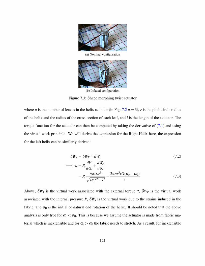
(a) Nominal configuration

(b) Inflated configuration

Figure 7.3: Shape morphing twist actuator

where n is the number of leaves in the helix actuator (in Fig. 7.2 n = 3), r is the pitch circle radius

of the helix and the radius of the cross-section of each leaf, and l is the length of the actuator. The

torque function for the actuator can then be computed by taking the derivative of (7.1) and using

the virtual work principle. We will derive the expression for the Right Helix here, the expression

for the left helix can be similarly derived:

δWτ = δWP +δWs (7.2)

=⇒ τr = PrdVdαr

+dWs

dαr

= Prnπαrr3√α2

r r2 + l2− 2πnr3tG(αr−α0)

l(7.3)

Above, δWτ is the virtual work associated with the external torque τ , δWP is the virtual work

associated with the internal pressure P, δWs is the virtual work due to the strains induced in the

fabric, and α0 is the initial or natural end rotation of the helix. It should be noted that the above

analysis is only true for αr < α0. This is because we assume the actuator is made from fabric ma-

terial which is inextensible and for αr > α0 the fabric needs to stretch. As a result, for inextensible

121

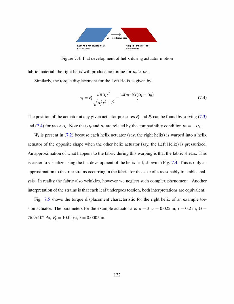
Figure 7.4: Flat development of helix during actuator motion

fabric material, the right helix will produce no torque for αr > α0.

Similarly, the torque displacement for the Left Helix is given by:

τl = Plnπαlr3√α2

l r2 + l2− 2πnr3tG(αl +α0)

l(7.4)

The position of the actuator at any given actuator pressures Pl and Pr can be found by solving (7.3)

and (7.4) for αr or αl . Note that αr and αl are related by the compatibility condition αl =−αr.

Ws is present in (7.2) because each helix actuator (say, the right helix) is warped into a helix

actuator of the opposite shape when the other helix actuator (say, the Left Helix) is pressurized.

An approximation of what happens to the fabric during this warping is that the fabric shears. This

is easier to visualize using the flat development of the helix leaf, shown in Fig. 7.4. This is only an

approximation to the true strains occurring in the fabric for the sake of a reasonably tractable anal-

ysis. In reality the fabric also wrinkles, however we neglect such complex phenomena. Another

interpretation of the strains is that each leaf undergoes torsion, both interpretations are equivalent.

Fig. 7.5 shows the torque displacement characteristic for the right helix of an example tor-

sion actuator. The parameters for the example actuator are: n = 3, r = 0.025 m, l = 0.2 m, G =

76.9x106 Pa, Pr = 10.0 psi, t = 0.0005 m.

122

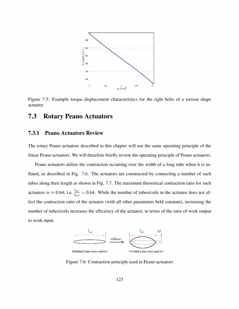
Figure 7.5: Example torque displacement characteristics for the right helix of a torsion shapeactuator

7.3 Rotary Peano Actuators

7.3.1 Peano Actuators Review

The rotary Peano actuators described in this chapter will use the same operating principle of the

linear Peano actuators. We will therefore briefly review the operating principle of Peano actuators.

Peano actuators utilize the contraction occurring over the width of a long tube when it is in-

flated, as described in Fig. 7.6. The actuators are constructed by connecting a number of such

tubes along their length as shown in Fig. 7.7. The maximum theoretical contraction ratio for such

actuators is ≈ 0.64, i.e, lin flde f

= 0.64. While the number of tubes/coils in the actuator does not af-

fect the contraction ratio of the actuator (with all other parameters held constant), increasing the

number of tubes/coils increases the efficiency of the actuator, in terms of the ratio of work output

to work input.

Figure 7.6: Contraction principle used in Peano actuators

123

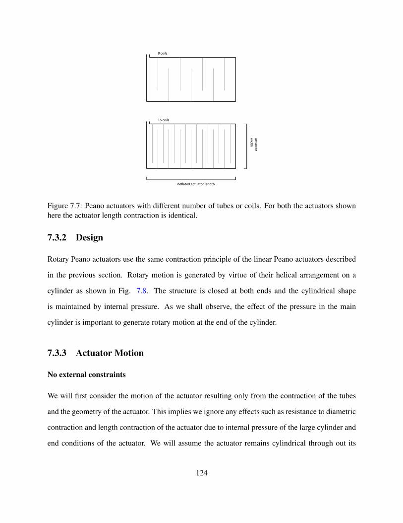
de�ated actuator length

actuatorw

idth

8 coils

16 coils

Figure 7.7: Peano actuators with different number of tubes or coils. For both the actuators shownhere the actuator length contraction is identical.

7.3.2 Design

Rotary Peano actuators use the same contraction principle of the linear Peano actuators described

in the previous section. Rotary motion is generated by virtue of their helical arrangement on a

cylinder as shown in Fig. 7.8. The structure is closed at both ends and the cylindrical shape

is maintained by internal pressure. As we shall observe, the effect of the pressure in the main

cylinder is important to generate rotary motion at the end of the cylinder.

7.3.3 Actuator Motion

No external constraints

We will first consider the motion of the actuator resulting only from the contraction of the tubes

and the geometry of the actuator. This implies we ignore any effects such as resistance to diametric

contraction and length contraction of the actuator due to internal pressure of the large cylinder and

end conditions of the actuator. We will assume the actuator remains cylindrical through out its

124

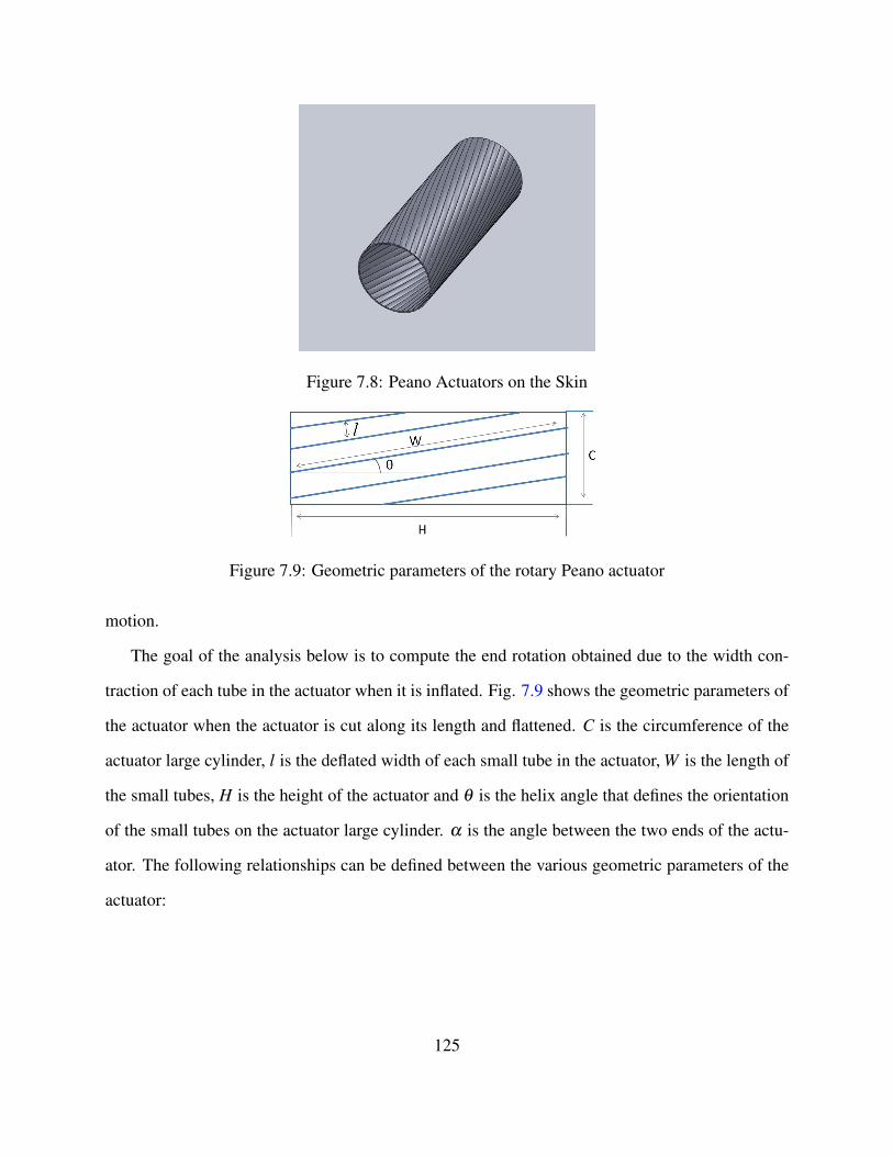
Figure 7.8: Peano Actuators on the Skin

Figure 7.9: Geometric parameters of the rotary Peano actuator

motion.

The goal of the analysis below is to compute the end rotation obtained due to the width con-

traction of each tube in the actuator when it is inflated. Fig. 7.9 shows the geometric parameters of

the actuator when the actuator is cut along its length and flattened. C is the circumference of the

actuator large cylinder, l is the deflated width of each small tube in the actuator, W is the length of

the small tubes, H is the height of the actuator and θ is the helix angle that defines the orientation

of the small tubes on the actuator large cylinder. α is the angle between the two ends of the actu-

ator. The following relationships can be defined between the various geometric parameters of the

actuator:

125

C =nvl

cosθ(7.5)

H =nhl

sinθ(7.6)

α =2πW cosθ sinθ

nvl(7.7)

θ = cos−1 HW

(7.8)

where,

nv =Cde f cosθde f

lde f

nh =Hde f sinθde f

lde f

Assuming the contraction ratio lin flde f

= 0.64, the following relations follow for the inflated actuator:

θin f = cos−1 Hin f

W

= cos−1 0.64cosθde f sinθde f

sinθin f

=⇒ cosθin f sinθin f = 0.64cosθde f sinθde f (7.9)

Using (7.7) and (7.9):

αin f =2πW cosθin f sinθin f

0.64nvlde f(7.10)

126

⇒ αin f −αde f =2πWnvl

(cosθin f sinθin f

0.64− cosθde f sinθde f

)(7.11)

= 0

It is clear that if there is no work associated with the change of length and diameter of the

actuator, the actuator will not undergo any twist as derived in (7.11). To cause a twisting action

an additional constraint on the motion is needed. This additional constraint can be introduced by

including the work effects of the internal pressure in the main cylinder and the end constraints on

the motion of the actuator.

Constant Main Cylinder Diameter

To simplify our analysis, we will consider the case where the cylinder is closed at both ends with

a circular end made from a high tensile strength fabric. For a short actuator, the effect of the end

constraint can be approximated by keeping the diameter D of actuator constant. To compute the

rotary motion achieved at one end of the actuator, we will modify the analysis of the previous

subsection by including this assumption.

If the diameter D is held constant, the circumference C = πD is constant. Therefore, the helix

angle of the small tubes θ can be directly computed from (7.5):

θ = cos−1 nvlC

(7.12)

Using (7.12), (7.7) can be modified to:

α =2WD

√1−(

nvlC

)2

(7.13)

Using the above analysis, for a prototype with the following geometric parameters: D = 50 mm,

θde f = π/4, lde f = 5 mm, Hde f = 100 mm, the net rotation (αin f −αde f ) obtained is 57.46◦ as-

127

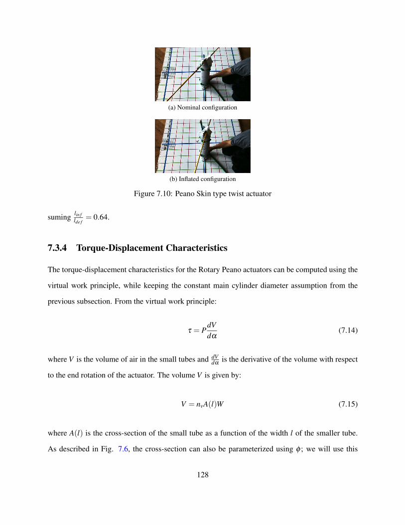
(a) Nominal configuration

(b) Inflated configuration

Figure 7.10: Peano Skin type twist actuator

suming lin flde f

= 0.64.

7.3.4 Torque-Displacement Characteristics

The torque-displacement characteristics for the Rotary Peano actuators can be computed using the

virtual work principle, while keeping the constant main cylinder diameter assumption from the

previous subsection. From the virtual work principle:

τ = PdVdα

(7.14)

where V is the volume of air in the small tubes and dVdα

is the derivative of the volume with respect

to the end rotation of the actuator. The volume V is given by:

V = nvA(l)W (7.15)

where A(l) is the cross-section of the small tube as a function of the width l of the smaller tube.

As described in Fig. 7.6, the cross-section can also be parameterized using φ ; we will use this

128

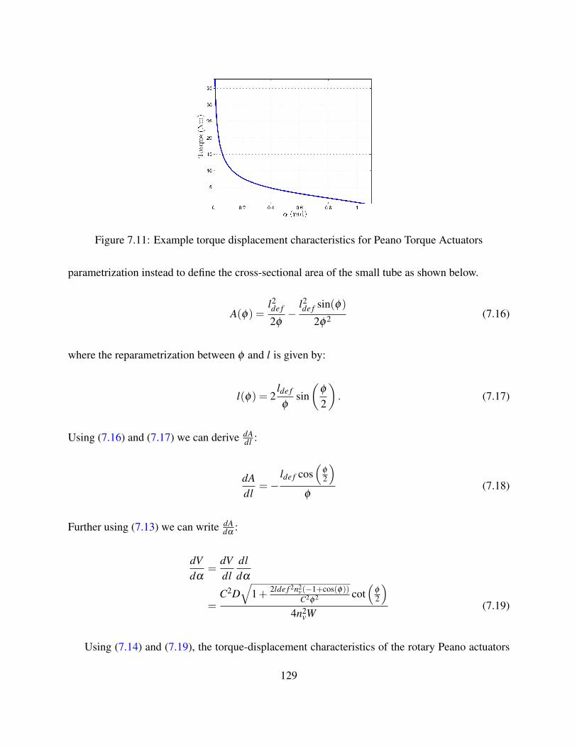
Figure 7.11: Example torque displacement characteristics for Peano Torque Actuators

parametrization instead to define the cross-sectional area of the small tube as shown below.

A(φ) =l2de f

2φ−

l2de f sin(φ)

2φ 2 (7.16)

where the reparametrization between φ and l is given by:

l(φ) = 2lde f

φsin(

φ

2

). (7.17)

Using (7.16) and (7.17) we can derive dAdl :

dAdl

=−lde f cos

(φ

2

)φ

(7.18)

Further using (7.13) we can write dAdα

:

dVdα

=dVdl

dldα

=C2D

√1+ 2lde f 2n2

v(−1+cos(φ))C2φ 2 cot

(φ

2

)4n2

vW(7.19)

Using (7.14) and (7.19), the torque-displacement characteristics of the rotary Peano actuators

129

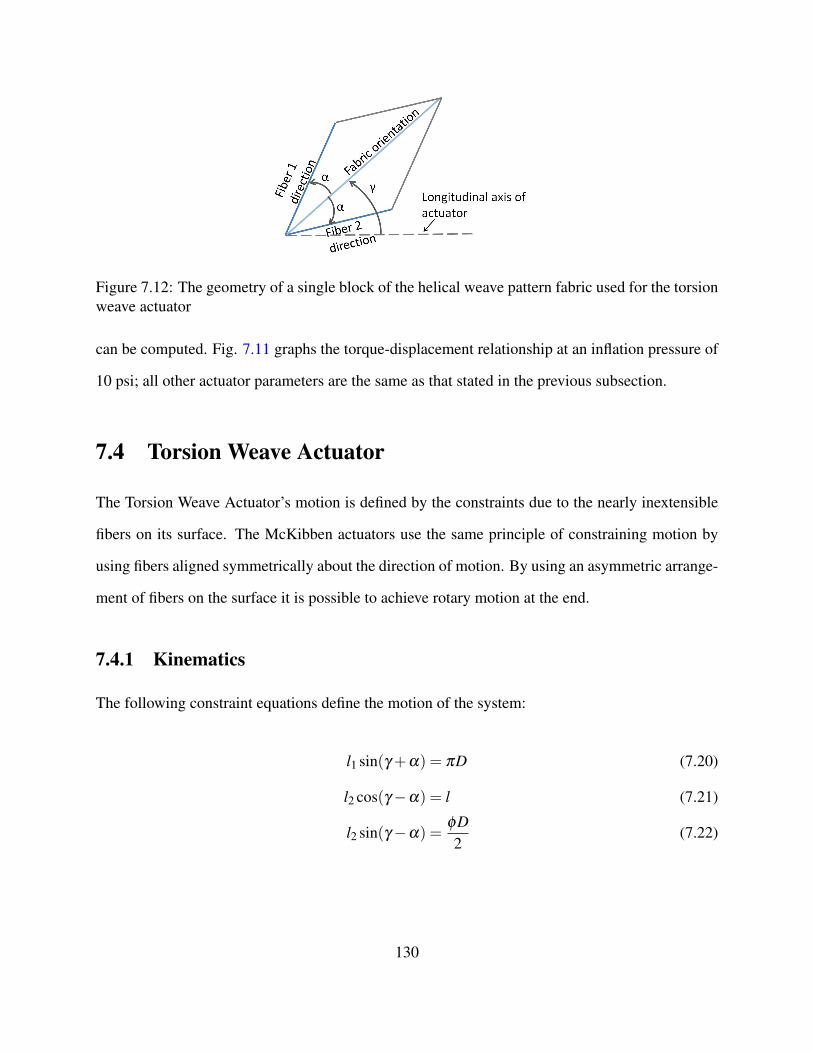
Figure 7.12: The geometry of a single block of the helical weave pattern fabric used for the torsionweave actuator

can be computed. Fig. 7.11 graphs the torque-displacement relationship at an inflation pressure of

10 psi; all other actuator parameters are the same as that stated in the previous subsection.

7.4 Torsion Weave Actuator

The Torsion Weave Actuator’s motion is defined by the constraints due to the nearly inextensible

fibers on its surface. The McKibben actuators use the same principle of constraining motion by

using fibers aligned symmetrically about the direction of motion. By using an asymmetric arrange-

ment of fibers on the surface it is possible to achieve rotary motion at the end.

7.4.1 Kinematics

The following constraint equations define the motion of the system:

l1 sin(γ +α) = πD (7.20)

l2 cos(γ−α) = l (7.21)

l2 sin(γ−α) =φD2

(7.22)

130

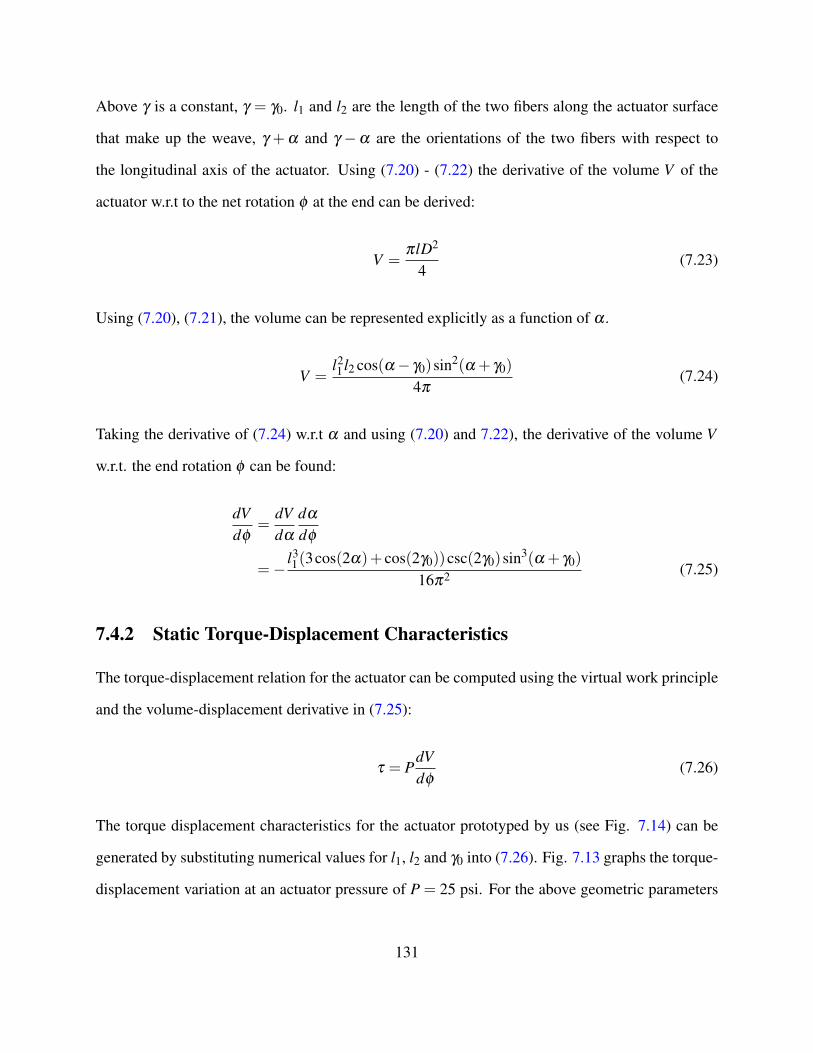
Above γ is a constant, γ = γ0. l1 and l2 are the length of the two fibers along the actuator surface

that make up the weave, γ +α and γ −α are the orientations of the two fibers with respect to

the longitudinal axis of the actuator. Using (7.20) - (7.22) the derivative of the volume V of the

actuator w.r.t to the net rotation φ at the end can be derived:

V =πlD2

4(7.23)

Using (7.20), (7.21), the volume can be represented explicitly as a function of α .

V =l21 l2 cos(α− γ0)sin2(α + γ0)

4π(7.24)

Taking the derivative of (7.24) w.r.t α and using (7.20) and 7.22), the derivative of the volume V

w.r.t. the end rotation φ can be found:

dVdφ

=dVdα

dα

dφ

=− l31(3cos(2α)+ cos(2γ0))csc(2γ0)sin3(α + γ0)

16π2 (7.25)

7.4.2 Static Torque-Displacement Characteristics

The torque-displacement relation for the actuator can be computed using the virtual work principle

and the volume-displacement derivative in (7.25):

τ = PdVdφ

(7.26)

The torque displacement characteristics for the actuator prototyped by us (see Fig. 7.14) can be

generated by substituting numerical values for l1, l2 and γ0 into (7.26). Fig. 7.13 graphs the torque-

displacement variation at an actuator pressure of P = 25 psi. For the above geometric parameters

131

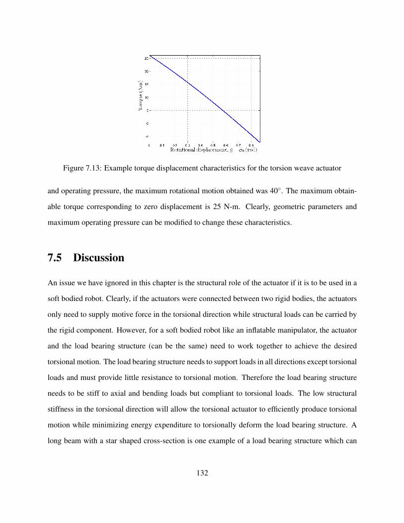
Figure 7.13: Example torque displacement characteristics for the torsion weave actuator

and operating pressure, the maximum rotational motion obtained was 40◦. The maximum obtain-

able torque corresponding to zero displacement is 25 N-m. Clearly, geometric parameters and

maximum operating pressure can be modified to change these characteristics.

7.5 Discussion

An issue we have ignored in this chapter is the structural role of the actuator if it is to be used in a

soft bodied robot. Clearly, if the actuators were connected between two rigid bodies, the actuators

only need to supply motive force in the torsional direction while structural loads can be carried by

the rigid component. However, for a soft bodied robot like an inflatable manipulator, the actuator

and the load bearing structure (can be the same) need to work together to achieve the desired

torsional motion. The load bearing structure needs to support loads in all directions except torsional

loads and must provide little resistance to torsional motion. Therefore the load bearing structure

needs to be stiff to axial and bending loads but compliant to torsional loads. The low structural

stiffness in the torsional direction will allow the torsional actuator to efficiently produce torsional

motion while minimizing energy expenditure to torsionally deform the load bearing structure. A

long beam with a star shaped cross-section is one example of a load bearing structure which can

132

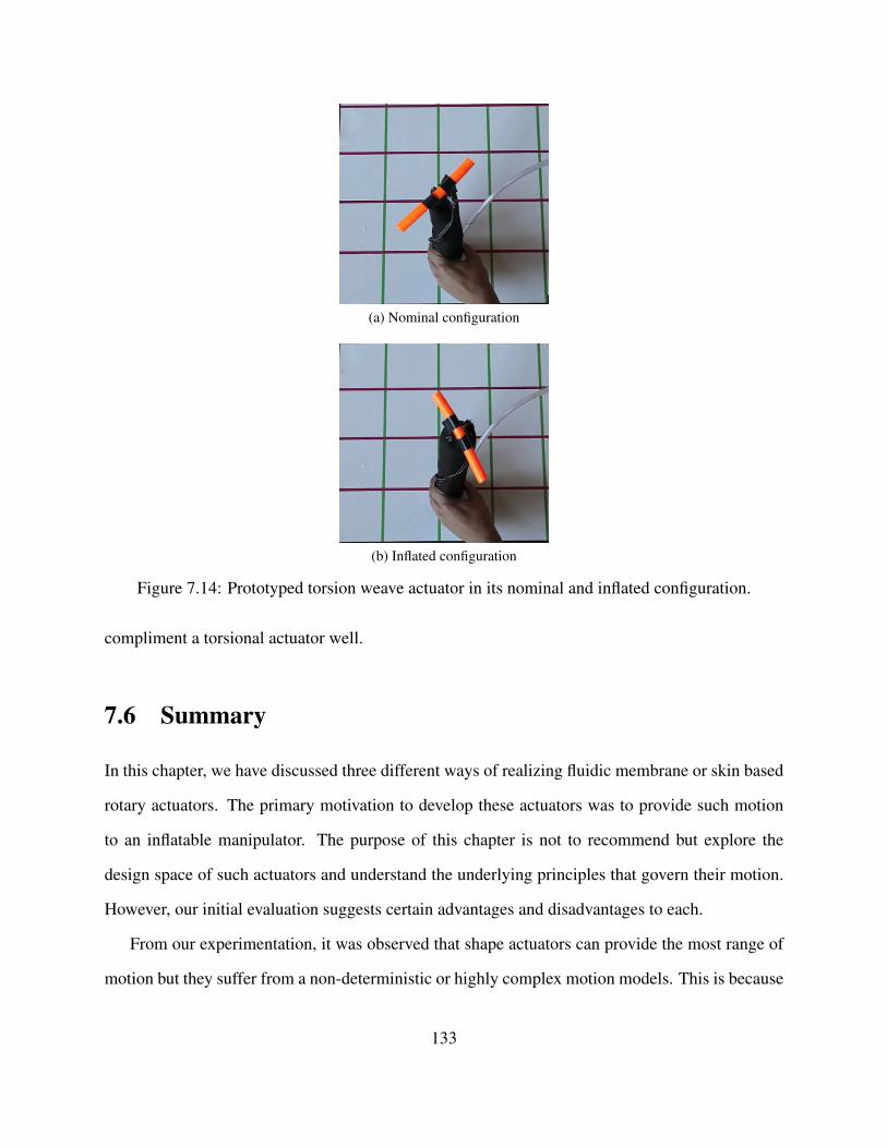
(a) Nominal configuration

(b) Inflated configuration

Figure 7.14: Prototyped torsion weave actuator in its nominal and inflated configuration.

compliment a torsional actuator well.

7.6 Summary

In this chapter, we have discussed three different ways of realizing fluidic membrane or skin based

rotary actuators. The primary motivation to develop these actuators was to provide such motion

to an inflatable manipulator. The purpose of this chapter is not to recommend but explore the

design space of such actuators and understand the underlying principles that govern their motion.

However, our initial evaluation suggests certain advantages and disadvantages to each.

From our experimentation, it was observed that shape actuators can provide the most range of

motion but they suffer from a non-deterministic or highly complex motion models. This is because

133

of the presence of wrinkling on the actuator structure in intermediate states. The shape actuators

are the easiest to implement in order to obtain bi-directional torque using a single actuator struc-

ture. However, in their current development stage, these actuators are best suited to applications

requiring binary actuation, i.e, motion between two states only. From our experiments and theo-

retical models, the Peano rotary actuators provide relatively less range of motion compared to the

other two actuator types. These actuators can provide higher speeds because of the low volume of

air needed to generate motion. The Peano actuators also have a deterministic model of operation

for all states that span its range of motion. The McKibben actuators have a highly deterministic

model for their motion because of the relatively simple length constraints that cause its motion;

no fabric shear is involved unlike the other two actuator types. Bi-directional torque is somewhat

complicated to achieve with a single McKibben type actuator, however this can be done with two

actuators in an antagonistic configuration connected end to end.

134

Chapter 8

Accuracy

This chapter discusses modeling, control and sensing for inflatable robots. The goal is to develop

models that help in the design of inflatable structures for robots and to utilize models for improving

accuracy in position control tasks. Models that allow prediction of strength and deformations of

inflatable manipulators are identified and experimentally verified. An inverse kinematics scheme

is developed that utilizes the deformation model. Simulations showing the effectiveness of the

scheme are presented. We also address the problem of joint angle estimation for inflatable manip-

ulators which is necessary for accurate positioning of the manipulator.

8.1 Design and Modeling of Inflatable Structures

Fig. 8.1 provides one framework within which we can think of modeling inflatable robots. For

the purpose of designing inflatable robot structures for desired payload and strength properties a

strength model is needed. The strength model can be used to predict strength properties of the

structure given the 3D inflated geometrical model of the structure and vice versa. There has been

some prior work in developing models to predict the strength of inflatable volumes [21, 68], we

will build on these existing models and explain them in Sec. 8.1.1.

135

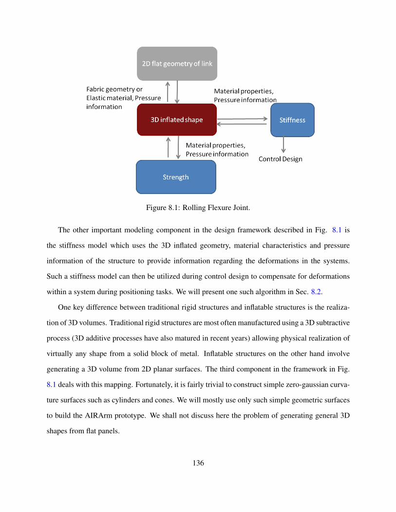
Figure 8.1: Rolling Flexure Joint.

The other important modeling component in the design framework described in Fig. 8.1 is

the stiffness model which uses the 3D inflated geometry, material characteristics and pressure

information of the structure to provide information regarding the deformations in the systems.

Such a stiffness model can then be utilized during control design to compensate for deformations

within a system during positioning tasks. We will present one such algorithm in Sec. 8.2.

One key difference between traditional rigid structures and inflatable structures is the realiza-

tion of 3D volumes. Traditional rigid structures are most often manufactured using a 3D subtractive

process (3D additive processes have also matured in recent years) allowing physical realization of

virtually any shape from a solid block of metal. Inflatable structures on the other hand involve

generating a 3D volume from 2D planar surfaces. The third component in the framework in Fig.

8.1 deals with this mapping. Fortunately, it is fairly trivial to construct simple zero-gaussian curva-

ture surfaces such as cylinders and cones. We will mostly use only such simple geometric surfaces

to build the AIRArm prototype. We shall not discuss here the problem of generating general 3D

shapes from flat panels.

136

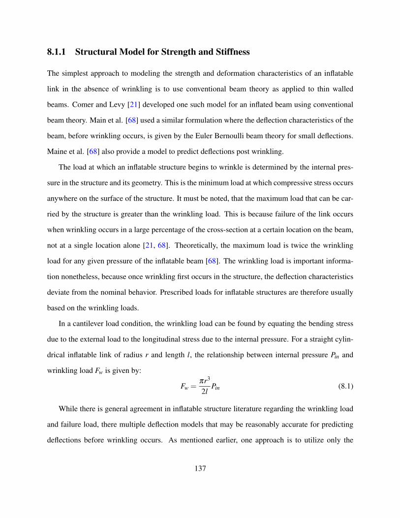
8.1.1 Structural Model for Strength and Stiffness

The simplest approach to modeling the strength and deformation characteristics of an inflatable

link in the absence of wrinkling is to use conventional beam theory as applied to thin walled

beams. Comer and Levy [21] developed one such model for an inflated beam using conventional

beam theory. Main et al. [68] used a similar formulation where the deflection characteristics of the

beam, before wrinkling occurs, is given by the Euler Bernoulli beam theory for small deflections.

Maine et al. [68] also provide a model to predict deflections post wrinkling.

The load at which an inflatable structure begins to wrinkle is determined by the internal pres-

sure in the structure and its geometry. This is the minimum load at which compressive stress occurs

anywhere on the surface of the structure. It must be noted, that the maximum load that can be car-

ried by the structure is greater than the wrinkling load. This is because failure of the link occurs

when wrinkling occurs in a large percentage of the cross-section at a certain location on the beam,

not at a single location alone [21, 68]. Theoretically, the maximum load is twice the wrinkling

load for any given pressure of the inflatable beam [68]. The wrinkling load is important informa-

tion nonetheless, because once wrinkling first occurs in the structure, the deflection characteristics

deviate from the nominal behavior. Prescribed loads for inflatable structures are therefore usually

based on the wrinkling loads.

In a cantilever load condition, the wrinkling load can be found by equating the bending stress

due to the external load to the longitudinal stress due to the internal pressure. For a straight cylin-

drical inflatable link of radius r and length l, the relationship between internal pressure Pin and

wrinkling load Fw is given by:

Fw =πr3

2lPin (8.1)

While there is general agreement in inflatable structure literature regarding the wrinkling load

and failure load, there multiple deflection models that may be reasonably accurate for predicting

deflections before wrinkling occurs. As mentioned earlier, one approach is to utilize only the

137

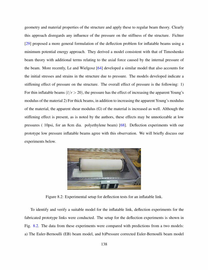
geometry and material properties of the structure and apply these to regular beam theory. Clearly

this approach disregards any influence of the pressure on the stiffness of the structure. Fichter

[29] proposed a more general formulation of the deflection problem for inflatable beams using a

minimum potential energy approach. They derived a model consistent with that of Timoshenko

beam theory with additional terms relating to the axial force caused by the internal pressure of

the beam. More recently, Le and Wielgosz [64] developed a similar model that also accounts for

the initial stresses and strains in the structure due to pressure. The models developed indicate a

stiffening effect of pressure on the structure. The overall effect of pressure is the following: 1)

For thin inflatable beams (l/r > 20), the pressure has the effect of increasing the apparent Young’s

modulus of the material 2) For thick beams, in addition to increasing the apparent Young’s modulus

of the material, the apparent shear modulus (G) of the material is increased as well. Although the

stiffening effect is present, as is noted by the authors, these effects may be unnoticeable at low

pressures ( 10psi, for an 8cm dia. polyethylene beam) [68]. Deflection experiments with our

prototype low pressure inflatable beams agree with this observation. We will briefly discuss our

experiments below.

Figure 8.2: Experimental setup for deflection tests for an inflatable link.

To identify and verify a suitable model for the inflatable link, deflection experiments for the

fabricated prototype links were conducted. The setup for the deflection experiments is shown in

Fig. 8.2. The data from these experiments were compared with predictions from a two models:

a) The Euler-Bernoulli (EB) beam model, and b)Pressure corrected Euler-Bernoulli beam model

138

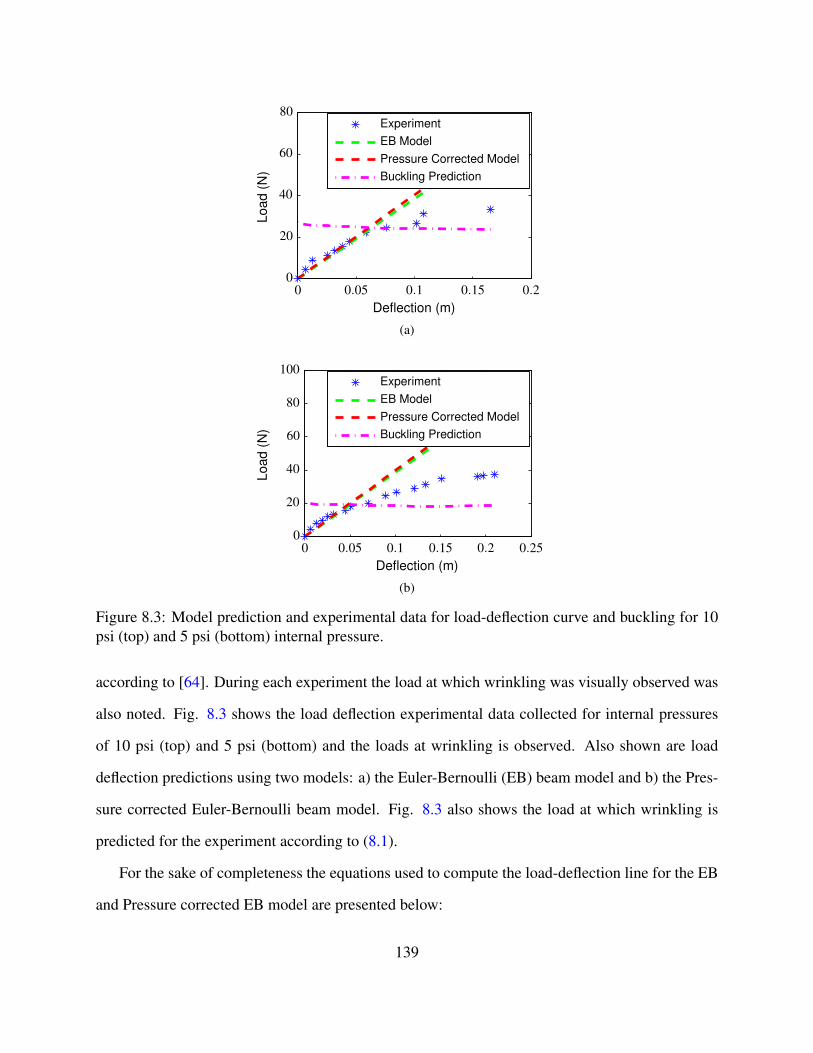
Buckling Prediction

Pressure Corrected Model

EB Model

Experiment

Load

(N)

Deflection (m)

0 0.05 0.1 0.15 0.20

20

40

60

80

(a)

Buckling Prediction

Pressure Corrected Model

EB Model

Experiment

Load

(N)

Deflection (m)

0 0.05 0.1 0.15 0.2 0.25

0

20

40

60

80

100

(b)

Figure 8.3: Model prediction and experimental data for load-deflection curve and buckling for 10psi (top) and 5 psi (bottom) internal pressure.

according to [64]. During each experiment the load at which wrinkling was visually observed was

also noted. Fig. 8.3 shows the load deflection experimental data collected for internal pressures

of 10 psi (top) and 5 psi (bottom) and the loads at wrinkling is observed. Also shown are load

deflection predictions using two models: a) the Euler-Bernoulli (EB) beam model and b) the Pres-

sure corrected Euler-Bernoulli beam model. Fig. 8.3 also shows the load at which wrinkling is

predicted for the experiment according to (8.1).

For the sake of completeness the equations used to compute the load-deflection line for the EB

and Pressure corrected EB model are presented below:

139

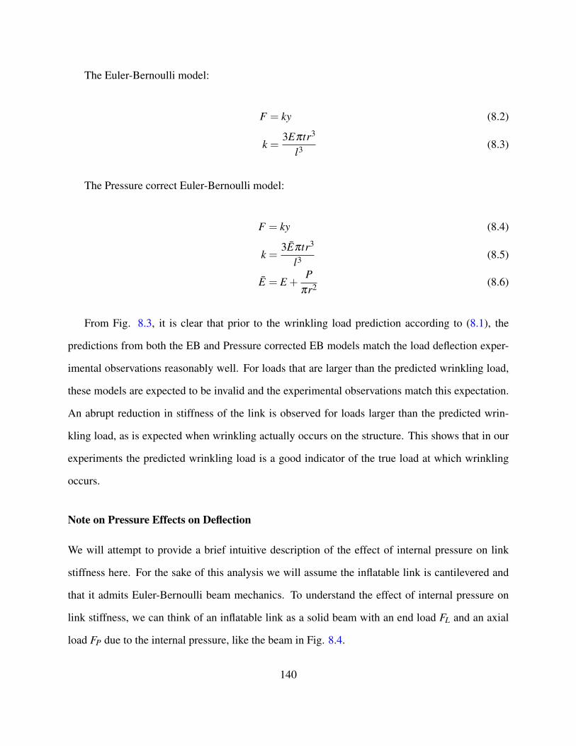
The Euler-Bernoulli model:

F = ky (8.2)

k =3Eπtr3

l3 (8.3)

The Pressure correct Euler-Bernoulli model:

F = ky (8.4)

k =3Eπtr3

l3 (8.5)

E = E +P

πr2 (8.6)

From Fig. 8.3, it is clear that prior to the wrinkling load prediction according to (8.1), the

predictions from both the EB and Pressure corrected EB models match the load deflection exper-

imental observations reasonably well. For loads that are larger than the predicted wrinkling load,

these models are expected to be invalid and the experimental observations match this expectation.

An abrupt reduction in stiffness of the link is observed for loads larger than the predicted wrin-

kling load, as is expected when wrinkling actually occurs on the structure. This shows that in our

experiments the predicted wrinkling load is a good indicator of the true load at which wrinkling

occurs.

Note on Pressure Effects on Deflection

We will attempt to provide a brief intuitive description of the effect of internal pressure on link

stiffness here. For the sake of this analysis we will assume the inflatable link is cantilevered and

that it admits Euler-Bernoulli beam mechanics. To understand the effect of internal pressure on

link stiffness, we can think of an inflatable link as a solid beam with an end load FL and an axial

load FP due to the internal pressure, like the beam in Fig. 8.4.

140

We will first derive the governing differential equation for the angular deflection θ of the beam

cross-section along its length s with respect to the coordinate frame X ,Y at the tip. Using large

deflection Euler-Bernoulli beam mechanics, this can be derived as:

EIdθ

ds=−Fp

∫ s

0sinθ(σ)dσ +FL

∫ s

0cosθ(σ)dσ (8.7)

Differentiating (8.7) w.r.t s again and rearranging, we get:

EIdθ

ds2 +Fp sinθ = FL cosθ (8.8)

If θ is small, (8.8) reduces to:

EIdθ

ds2 +Fpθ = FLθ (8.9)

The integral solution of (8.9) with the appropriate boundary conditions of the problem is:

θ =FL

Fp− FL

Fpcos

(√Fp

EI

)(8.10)

A series expansion of the cosine term in (8.10) reveals the role of Fp in the angular deflection of

the beam:

θ =FL

2EIs2− FL

24E2I2 s4Fp +O(F2p ) (8.11)

From (8.11), it can be seen that the effect of the axial force Fp due to internal pressure is to reduce

the angular deflection at all locations along the length of the beam. In other words the internal

pressure can be seen to have a stiffening effect on the inflatable link. In a first order analysis,

the magnitude of the stiffening effect is directly proportional to the internal pressure P because

Fp = Pπr2 (r is the radius of the link at the end) and is inversely proportional to the square of the

Young’s modulus E and the square of the second moment of area of cross-section of the link I.

141

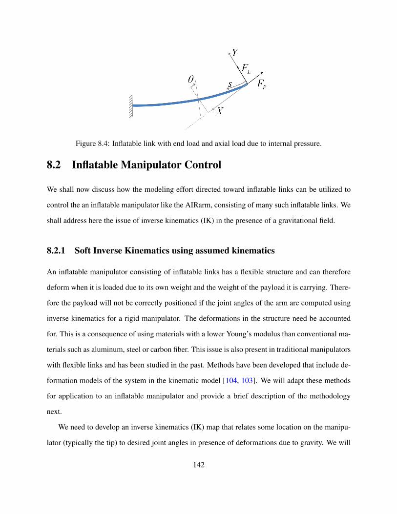
Figure 8.4: Inflatable link with end load and axial load due to internal pressure.

8.2 Inflatable Manipulator Control

We shall now discuss how the modeling effort directed toward inflatable links can be utilized to

control the an inflatable manipulator like the AIRarm, consisting of many such inflatable links. We

shall address here the issue of inverse kinematics (IK) in the presence of a gravitational field.

8.2.1 Soft Inverse Kinematics using assumed kinematics

An inflatable manipulator consisting of inflatable links has a flexible structure and can therefore

deform when it is loaded due to its own weight and the weight of the payload it is carrying. There-

fore the payload will not be correctly positioned if the joint angles of the arm are computed using

inverse kinematics for a rigid manipulator. The deformations in the structure need be accounted

for. This is a consequence of using materials with a lower Young’s modulus than conventional ma-

terials such as aluminum, steel or carbon fiber. This issue is also present in traditional manipulators

with flexible links and has been studied in the past. Methods have been developed that include de-

formation models of the system in the kinematic model [104, 103]. We will adapt these methods

for application to an inflatable manipulator and provide a brief description of the methodology

next.

We need to develop an inverse kinematics (IK) map that relates some location on the manipu-

lator (typically the tip) to desired joint angles in presence of deformations due to gravity. We will

142

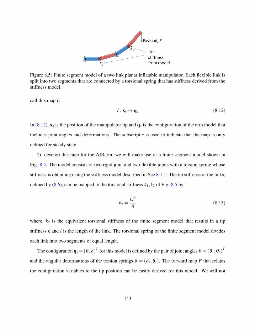
Figure 8.5: Finite segment model of a two link planar inflatable manipulator. Each flexible link issplit into two segments that are connected by a torsional spring that has stiffness derived from thestiffness model.

call this map I:

I : xs 7→ qs (8.12)

In (8.12), xs is the position of the manipulator tip and qs is the configuration of the arm model that

includes joint angles and deformations. The subscript s is used to indicate that the map is only

defined for steady state.

To develop this map for the AIRarm, we will make use of a finite segment model shown in

Fig. 8.5. The model consists of two rigid joint and two flexible joints with a torsion spring whose

stiffness is obtaining using the stiffness model described in Sec 8.1.1. The tip stiffness of the links,

defined by (8.6), can be mapped to the torsional stiffness k1,k2 of Fig. 8.5 by:

kτ =kl2

4(8.13)

where, kτ is the equivalent torsional stiffness of the finite segment model that results in a tip

stiffness k and l is the length of the link. The torsional spring of the finite segment model divides

each link into two segments of equal length.

The configuration qs =(θ ,δ )T for this model is defined by the pair of joint angles θ =(θ1,θ2)T

and the angular deformations of the torsion springs δ = (δ1,δ2). The forward map F that relates

the configuration variables to the tip position can be easily derived for this model. We will not

143

repeat it here for the sake of brevity:

xs = F (qs)

= F (θ ,δ ) (8.14)

Furthermore, a stiffness matrix K = diag(k1,k2) relates the torques and deformations at the torsion

spring. Using this stiffness matrix K, we can rewrite (8.14) as:

xs = F(θ ,K−1Gδ (θ)

)(8.15)

= F (θ) (8.16)

In (8.15), Gδ (θ) is the gravitational load on the torsion springs a given θ . If F−1 can be analyti-

cally derived then the soft inverse kinematics can be explicitly derived as:

θ

δ s

=

F−1 (xs)

K−1 (Gδ

(F−1 (xs)

)) (8.17)

In general, F−1 cannot be analytically derived we can proceed by computing the differential dx

from 8.15:

dx = Jθ dθ + Jδ K−1 ∂Gδ

∂θdθ

=

(Jθ + Jδ K−1 ∂Gδ

∂θ

)dθ (8.18)

In (8.18), J is the partial derivative of F(θ ,δs) with respect to the subscript. The expression within

the parentheses in (8.18) resembles a regular Jacobian found in the differential kinematic equations

for rigid systems with some additional terms that account for variation of tip position due to gravity

loads on the torsion springs.

144

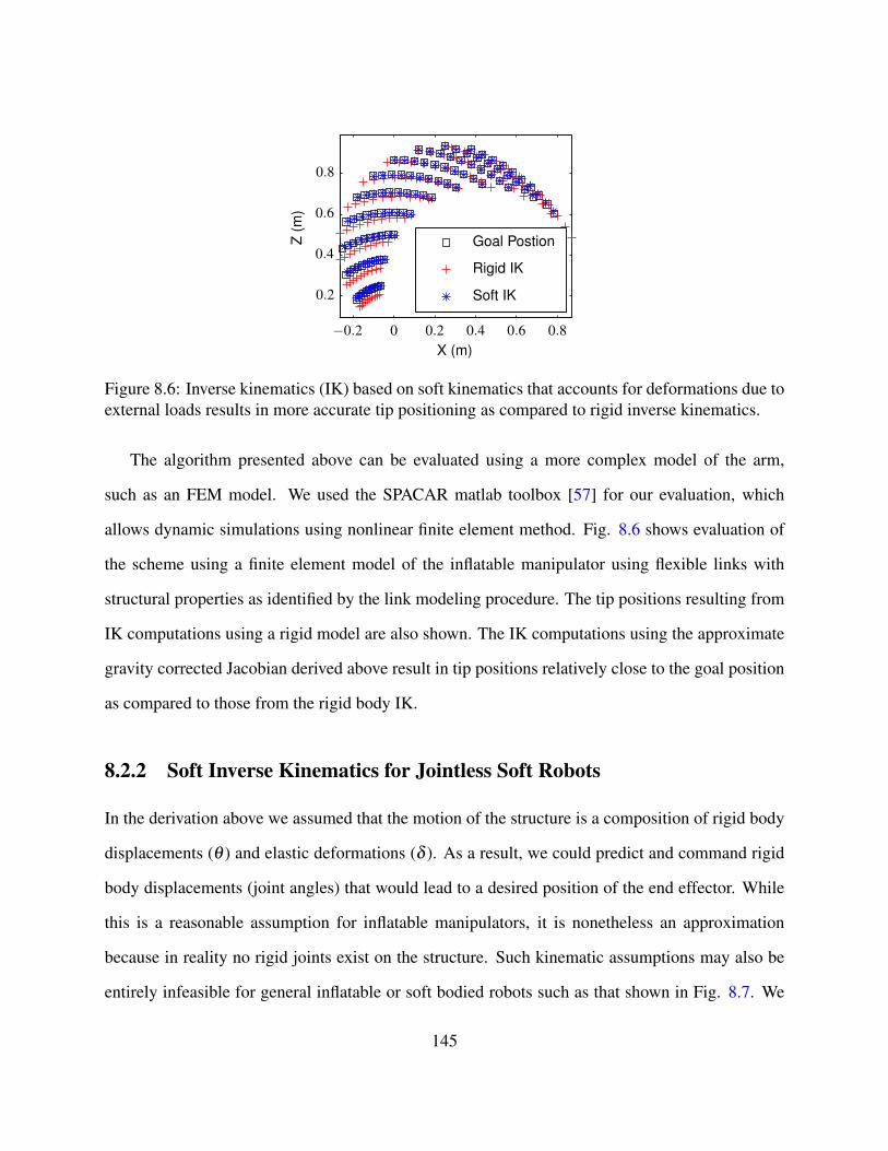
Soft IK

Rigid IK

Goal PostionZ(m

)

X (m)

−0.2 0 0.2 0.4 0.6 0.8

0.2

0.4

0.6

0.8

Figure 8.6: Inverse kinematics (IK) based on soft kinematics that accounts for deformations due toexternal loads results in more accurate tip positioning as compared to rigid inverse kinematics.

The algorithm presented above can be evaluated using a more complex model of the arm,

such as an FEM model. We used the SPACAR matlab toolbox [57] for our evaluation, which

allows dynamic simulations using nonlinear finite element method. Fig. 8.6 shows evaluation of

the scheme using a finite element model of the inflatable manipulator using flexible links with

structural properties as identified by the link modeling procedure. The tip positions resulting from

IK computations using a rigid model are also shown. The IK computations using the approximate

gravity corrected Jacobian derived above result in tip positions relatively close to the goal position

as compared to those from the rigid body IK.

8.2.2 Soft Inverse Kinematics for Jointless Soft Robots

In the derivation above we assumed that the motion of the structure is a composition of rigid body

displacements (θ ) and elastic deformations (δ ). As a result, we could predict and command rigid

body displacements (joint angles) that would lead to a desired position of the end effector. While

this is a reasonable assumption for inflatable manipulators, it is nonetheless an approximation

because in reality no rigid joints exist on the structure. Such kinematic assumptions may also be

entirely infeasible for general inflatable or soft bodied robots such as that shown in Fig. 8.7. We

145

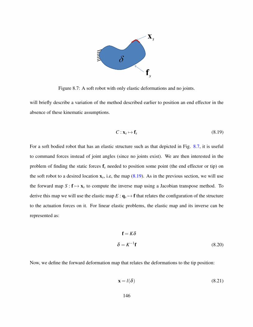
Figure 8.7: A soft robot with only elastic deformations and no joints.

will briefly describe a variation of the method described earlier to position an end effector in the

absence of these kinematic assumptions.

C : xs 7→ fs (8.19)

For a soft bodied robot that has an elastic structure such as that depicted in Fig. 8.7, it is useful

to command forces instead of joint angles (since no joints exist). We are then interested in the

problem of finding the static forces fs needed to position some point (the end effector or tip) on

the soft robot to a desired location xs, i.e, the map (8.19). As in the previous section, we will use

the forward map S : f 7→ xs to compute the inverse map using a Jacobian transpose method. To

derive this map we will use the elastic map E : qs 7→ f that relates the configuration of the structure

to the actuation forces on it. For linear elastic problems, the elastic map and its inverse can be

represented as:

f = Kδ

δ = K−1f (8.20)

Now, we define the forward deformation map that relates the deformations to the tip position:

x = l(δ ) (8.21)

146

Note that we can arrive at the identical derivation as in 8.2.1, by substituting the finite segment

forward kinematic map in (8.21). Composing (8.21) and (8.20) we get the forward map S:

x = l(K−1 f ) (8.22)

Using (8.22), we can compute the differential dx:

dx =∂ l(δ )

δ

∂δ

fdf (8.23)

= Jδ K−1df (8.24)

Using (8.24), we can employ a Jacobian transpose method to compute the inverse map I : xs 7→

f. The usefulness of such a map lies in the fact that we can plan in the space of forces being exerted

on the robot which is a lower dimensional space than the full configuration space is the elastic

body.

8.3 Inflatable Joint Angle Estimation

In the above section on soft kinematics (8.2.1), we were able to achieve accurate positioning of

a soft manipulator by factoring in the load dependent deformations in the system to compute the

desired joint angles of the system. Clearly, it is necessary to be able to accurately control joint an-

gles in the system in order to realize accurate positioning using the soft inverse kinematics scheme.

For inflatable joints this is not a straightforward to achieve due to two reasons: (1) inflatable joint

kinematic models are an approximation and (2) sensors for direct measurement of inflatable joint

angles are not readily available. The issue of kinematic models can be addressed by improving

joint design so that its motion more closely approximates the desired motion between links. In this

section, we will address the issue of sensors for estimating inflatable joint angles.

147

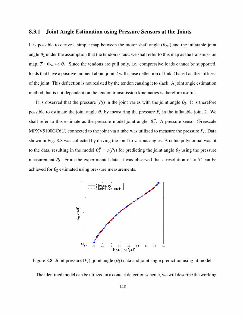
8.3.1 Joint Angle Estimation using Pressure Sensors at the Joints

It is possible to derive a simple map between the motor shaft angle (θ2m) and the inflatable joint

angle θ2 under the assumption that the tendon is taut, we shall refer to this map as the transmission

map, T : θ2m 7→ θ2. Since the tendons are pull only, i.e. compressive loads cannot be supported,

loads that have a positive moment about joint 2 will cause deflection of link 2 based on the stiffness

of the joint. This deflection is not resisted by the tendon causing it to slack. A joint angle estimation

method that is not dependent on the tendon transmission kinematics is therefore useful.

It is observed that the pressure (PJ) in the joint varies with the joint angle θ2. It is therefore

possible to estimate the joint angle θ2 by measuring the pressure PJ in the inflatable joint 2. We

shall refer to this estimate as the pressure model joint angle, θ P2 . A pressure sensor (Freescale

MPXV5100GC6U) connected to the joint via a tube was utilized to measure the pressure PJ . Data

shown in Fig. 8.8 was collected by driving the joint to various angles. A cubic polynomial was fit

to the data, resulting in the model θ P2 = z(PJ) for predicting the joint angle θ2 using the pressure

measurement PJ . From the experimental data, it was observed that a resolution of ≈ 5◦ can be

achieved for θ2 estimated using pressure measurements.

Figure 8.8: Joint pressure (PJ), joint angle (θ2) data and joint angle prediction using fit model.

The identified model can be utilized in a contact detection scheme, we will describe the working

148

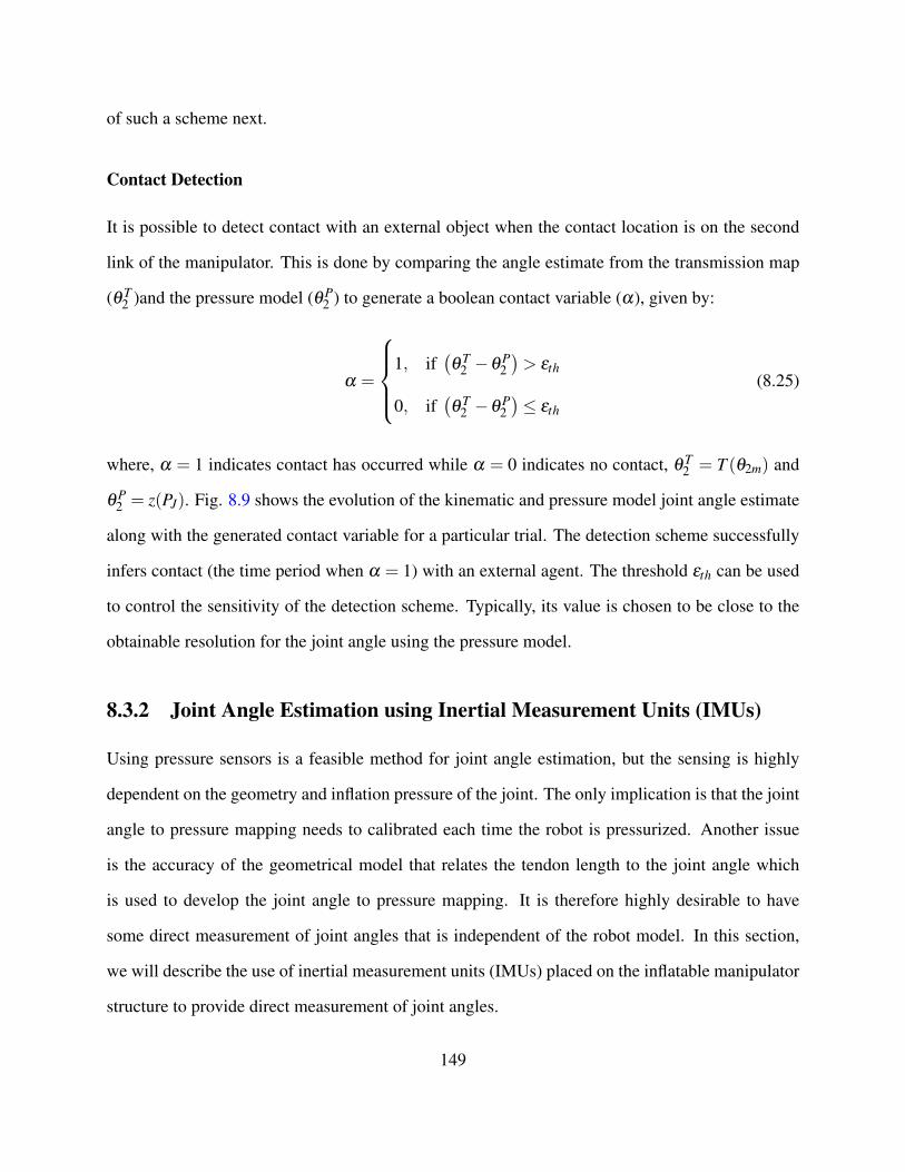
of such a scheme next.

Contact Detection

It is possible to detect contact with an external object when the contact location is on the second

link of the manipulator. This is done by comparing the angle estimate from the transmission map

(θ T2 )and the pressure model (θ P

2 ) to generate a boolean contact variable (α), given by:

α =

1, if

(θ T

2 −θ P2)> εth

0, if(θ T

2 −θ P2)≤ εth

(8.25)

where, α = 1 indicates contact has occurred while α = 0 indicates no contact, θ T2 = T (θ2m) and

θ P2 = z(PJ). Fig. 8.9 shows the evolution of the kinematic and pressure model joint angle estimate

along with the generated contact variable for a particular trial. The detection scheme successfully

infers contact (the time period when α = 1) with an external agent. The threshold εth can be used

to control the sensitivity of the detection scheme. Typically, its value is chosen to be close to the

obtainable resolution for the joint angle using the pressure model.

8.3.2 Joint Angle Estimation using Inertial Measurement Units (IMUs)

Using pressure sensors is a feasible method for joint angle estimation, but the sensing is highly

dependent on the geometry and inflation pressure of the joint. The only implication is that the joint

angle to pressure mapping needs to calibrated each time the robot is pressurized. Another issue

is the accuracy of the geometrical model that relates the tendon length to the joint angle which

is used to develop the joint angle to pressure mapping. It is therefore highly desirable to have

some direct measurement of joint angles that is independent of the robot model. In this section,

we will describe the use of inertial measurement units (IMUs) placed on the inflatable manipulator

structure to provide direct measurement of joint angles.

149

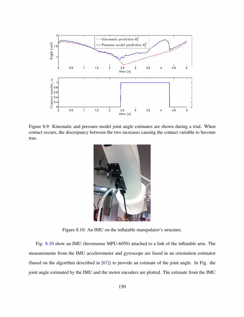
Figure 8.9: Kinematic and pressure model joint angle estimates are shown during a trial. Whencontact occurs, the discrepancy between the two increases causing the contact variable to becometrue.

Figure 8.10: An IMU on the inflatable manipulator’s structure.

Fig. 8.10 show an IMU (Invensense MPU-6050) attached to a link of the inflatable arm. The

measurements from the IMU accelerometer and gyroscope are fused in an orientation estimator

(based on the algorithm described in [67]) to provide an estimate of the joint angle. In Fig. the

joint angle estimated by the IMU and the motor encoders are plotted. The estimate from the IMU

150

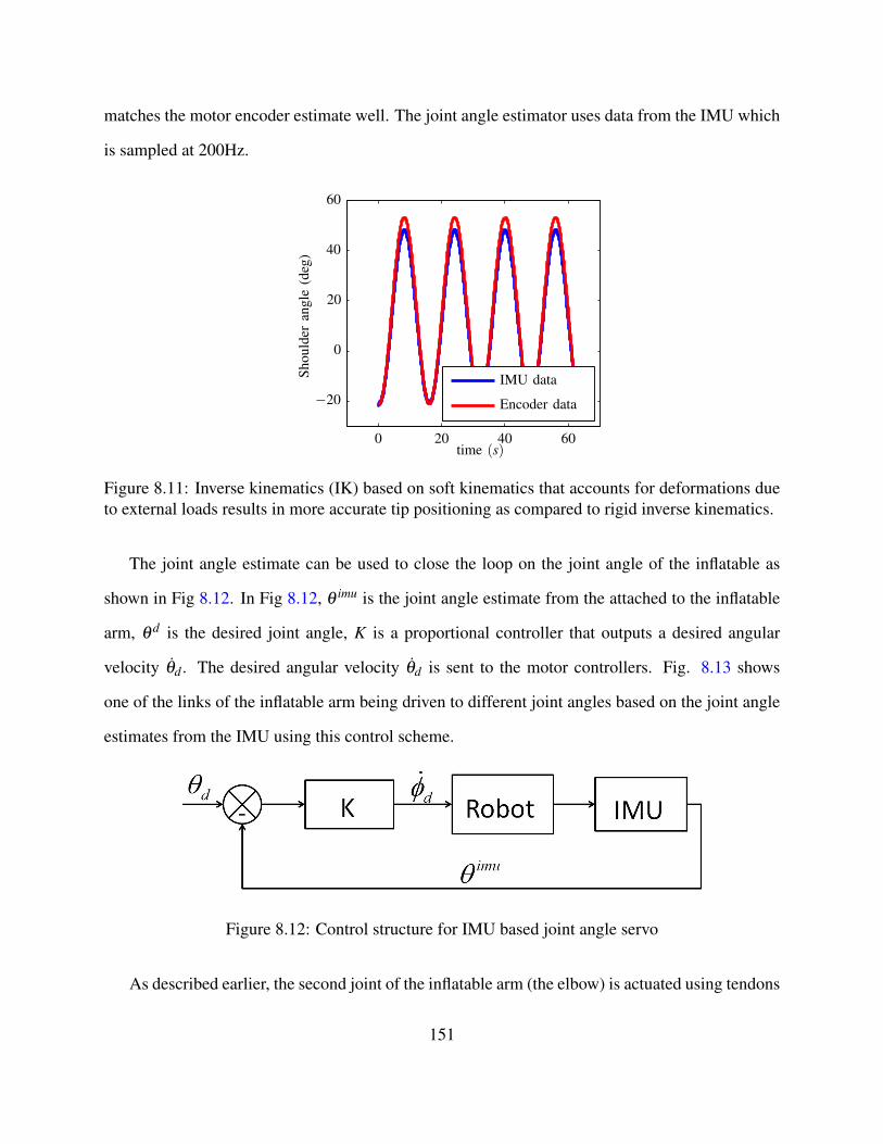
matches the motor encoder estimate well. The joint angle estimator uses data from the IMU which

is sampled at 200Hz.

Encoder data

IMU dataShould

eran

gle

(deg

)

time (s)0 20 40 60

−20

0

20

40

60

Figure 8.11: Inverse kinematics (IK) based on soft kinematics that accounts for deformations dueto external loads results in more accurate tip positioning as compared to rigid inverse kinematics.

The joint angle estimate can be used to close the loop on the joint angle of the inflatable as

shown in Fig 8.12. In Fig 8.12, θ imu is the joint angle estimate from the attached to the inflatable

arm, θ d is the desired joint angle, K is a proportional controller that outputs a desired angular

velocity θd . The desired angular velocity θd is sent to the motor controllers. Fig. 8.13 shows

one of the links of the inflatable arm being driven to different joint angles based on the joint angle

estimates from the IMU using this control scheme.

Figure 8.12: Control structure for IMU based joint angle servo

As described earlier, the second joint of the inflatable arm (the elbow) is actuated using tendons

151

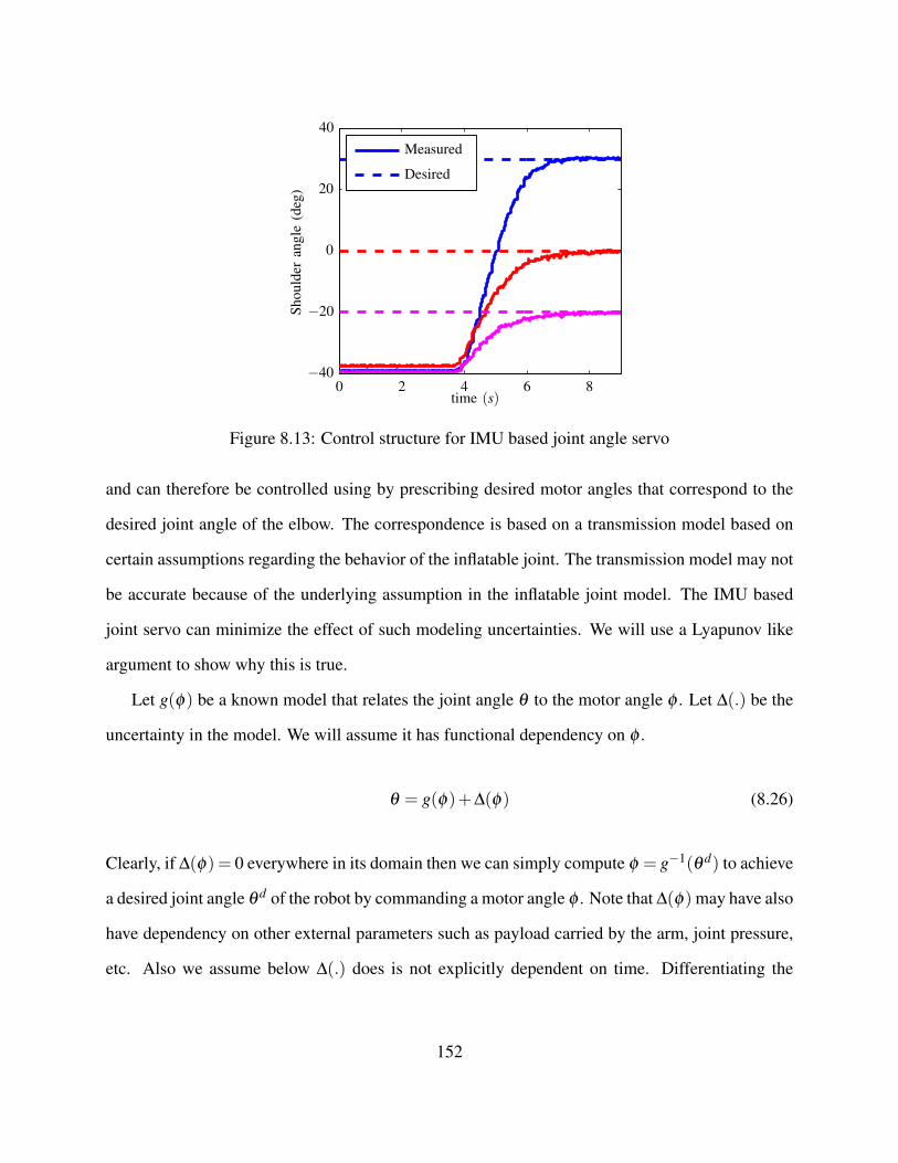
Desired

Measured

Should

eran

gle

(deg

)

time (s)0 2 4 6 8

−40

−20

0

20

40

Figure 8.13: Control structure for IMU based joint angle servo

and can therefore be controlled using by prescribing desired motor angles that correspond to the

desired joint angle of the elbow. The correspondence is based on a transmission model based on

certain assumptions regarding the behavior of the inflatable joint. The transmission model may not

be accurate because of the underlying assumption in the inflatable joint model. The IMU based

joint servo can minimize the effect of such modeling uncertainties. We will use a Lyapunov like

argument to show why this is true.

Let g(φ) be a known model that relates the joint angle θ to the motor angle φ . Let ∆(.) be the

uncertainty in the model. We will assume it has functional dependency on φ .

θ = g(φ)+∆(φ) (8.26)

Clearly, if ∆(φ) = 0 everywhere in its domain then we can simply compute φ = g−1(θ d) to achieve

a desired joint angle θ d of the robot by commanding a motor angle φ . Note that ∆(φ) may have also

have dependency on other external parameters such as payload carried by the arm, joint pressure,

etc. Also we assume below ∆(.) does is not explicitly dependent on time. Differentiating the

152

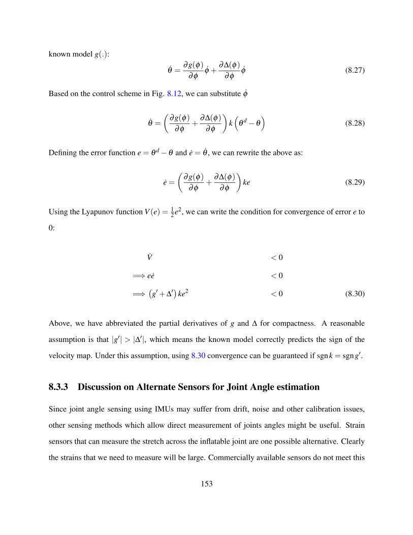
known model g(.):

θ =∂g(φ)

∂φφ +

∂∆(φ)

∂φφ (8.27)

Based on the control scheme in Fig. 8.12, we can substitute φ

θ =

(∂g(φ)

∂φ+

∂∆(φ)

∂φ

)k(

θd−θ

)(8.28)

Defining the error function e = θ d−θ and e = θ , we can rewrite the above as:

e =(

∂g(φ)∂φ

+∂∆(φ)

∂φ

)ke (8.29)

Using the Lyapunov function V (e) = 12e2, we can write the condition for convergence of error e to

0:

V < 0

=⇒ ee < 0

=⇒(g′+∆

′)ke2 < 0 (8.30)

Above, we have abbreviated the partial derivatives of g and ∆ for compactness. A reasonable

assumption is that |g′| > |∆′|, which means the known model correctly predicts the sign of the

velocity map. Under this assumption, using 8.30 convergence can be guaranteed if sgnk = sgng′.

8.3.3 Discussion on Alternate Sensors for Joint Angle estimation

Since joint angle sensing using IMUs may suffer from drift, noise and other calibration issues,

other sensing methods which allow direct measurement of joints angles might be useful. Strain

sensors that can measure the stretch across the inflatable joint are one possible alternative. Clearly

the strains that we need to measure will be large. Commercially available sensors do not meet this

153

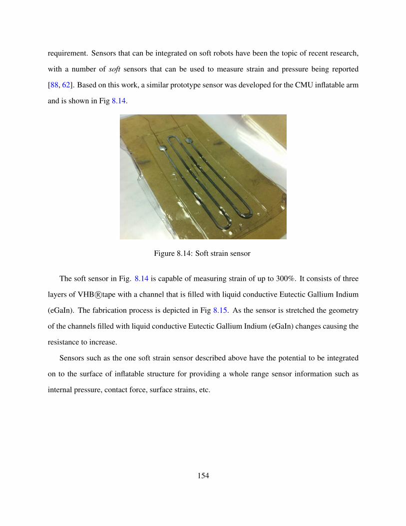
requirement. Sensors that can be integrated on soft robots have been the topic of recent research,

with a number of soft sensors that can be used to measure strain and pressure being reported

[88, 62]. Based on this work, a similar prototype sensor was developed for the CMU inflatable arm

and is shown in Fig 8.14.

Figure 8.14: Soft strain sensor

The soft sensor in Fig. 8.14 is capable of measuring strain of up to 300%. It consists of three

layers of VHB R©tape with a channel that is filled with liquid conductive Eutectic Gallium Indium

(eGaIn). The fabrication process is depicted in Fig 8.15. As the sensor is stretched the geometry

of the channels filled with liquid conductive Eutectic Gallium Indium (eGaIn) changes causing the

resistance to increase.

Sensors such as the one soft strain sensor described above have the potential to be integrated

on to the surface of inflatable structure for providing a whole range sensor information such as

internal pressure, contact force, surface strains, etc.

154

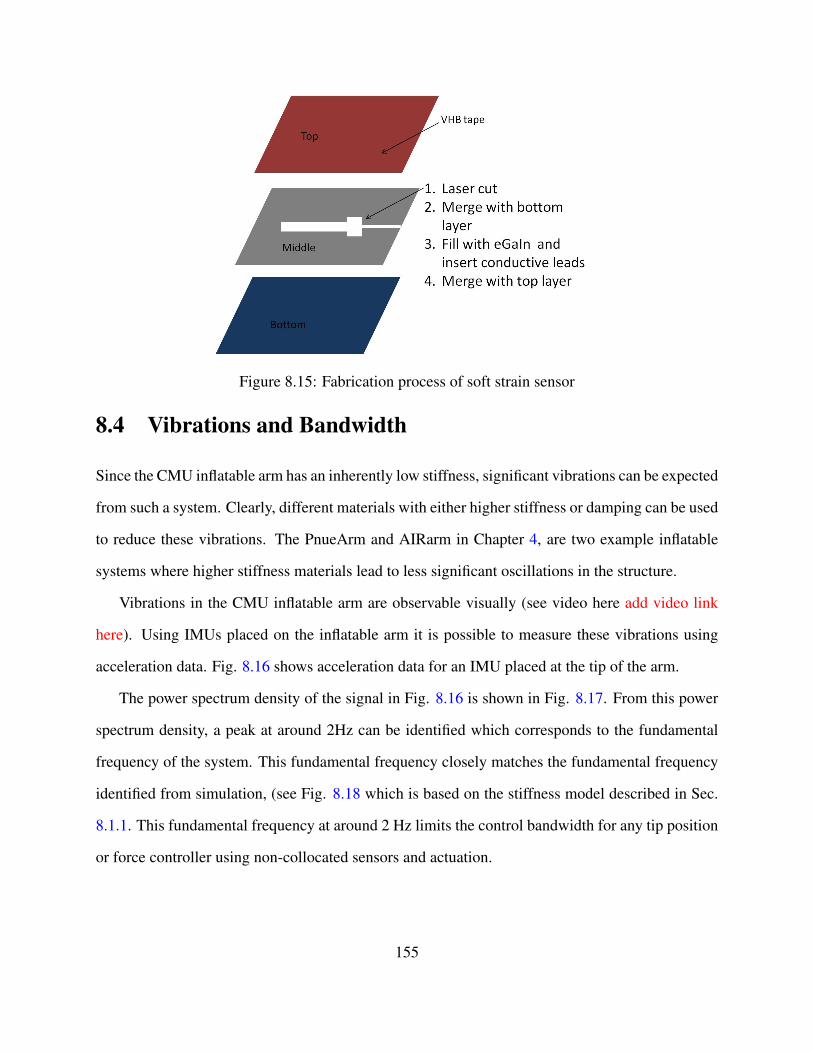
Figure 8.15: Fabrication process of soft strain sensor

8.4 Vibrations and Bandwidth

Since the CMU inflatable arm has an inherently low stiffness, significant vibrations can be expected

from such a system. Clearly, different materials with either higher stiffness or damping can be used

to reduce these vibrations. The PnueArm and AIRarm in Chapter 4, are two example inflatable

systems where higher stiffness materials lead to less significant oscillations in the structure.

Vibrations in the CMU inflatable arm are observable visually (see video here add video link

here). Using IMUs placed on the inflatable arm it is possible to measure these vibrations using

acceleration data. Fig. 8.16 shows acceleration data for an IMU placed at the tip of the arm.

The power spectrum density of the signal in Fig. 8.16 is shown in Fig. 8.17. From this power

spectrum density, a peak at around 2Hz can be identified which corresponds to the fundamental

frequency of the system. This fundamental frequency closely matches the fundamental frequency

identified from simulation, (see Fig. 8.18 which is based on the stiffness model described in Sec.

8.1.1. This fundamental frequency at around 2 Hz limits the control bandwidth for any tip position

or force controller using non-collocated sensors and actuation.

155

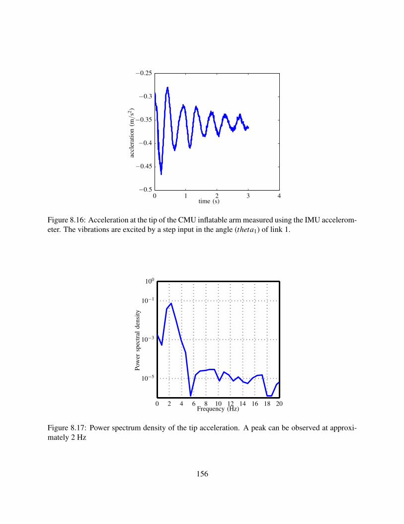
accle

rati

on

(m/s

2)

time (s)0 1 2 3 4

−0.5

−0.45

−0.4

−0.35

−0.3

−0.25

Figure 8.16: Acceleration at the tip of the CMU inflatable arm measured using the IMU accelerom-eter. The vibrations are excited by a step input in the angle (theta1) of link 1.

Pow

ersp

ectr

alden

sity

Frequency (Hz)0 2 4 6 8 10 12 14 16 18 20

10−5

10−3

10−1

100

Figure 8.17: Power spectrum density of the tip acceleration. A peak can be observed at approxi-mately 2 Hz

156

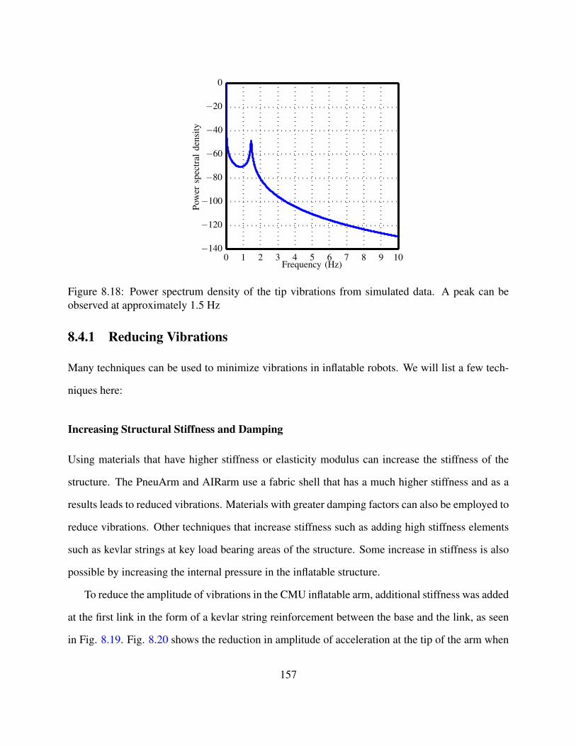
Pow

ersp

ectr

alden

sity

Frequency (Hz)0 1 2 3 4 5 6 7 8 9 10

−140

−120

−100

−80

−60

−40

−20

0

Figure 8.18: Power spectrum density of the tip vibrations from simulated data. A peak can beobserved at approximately 1.5 Hz

8.4.1 Reducing Vibrations

Many techniques can be used to minimize vibrations in inflatable robots. We will list a few tech-

niques here:

Increasing Structural Stiffness and Damping

Using materials that have higher stiffness or elasticity modulus can increase the stiffness of the

structure. The PneuArm and AIRarm use a fabric shell that has a much higher stiffness and as a

results leads to reduced vibrations. Materials with greater damping factors can also be employed to

reduce vibrations. Other techniques that increase stiffness such as adding high stiffness elements

such as kevlar strings at key load bearing areas of the structure. Some increase in stiffness is also

possible by increasing the internal pressure in the inflatable structure.

To reduce the amplitude of vibrations in the CMU inflatable arm, additional stiffness was added

at the first link in the form of a kevlar string reinforcement between the base and the link, as seen

in Fig. 8.19. Fig. 8.20 shows the reduction in amplitude of acceleration at the tip of the arm when

157

the kevlar reinforcement is added in response to a step input in the desired angle at joint 1 (θ1).

Figure 8.19: Kevlar string reinforcement between the base and the top side of link 1. The kevlarreinforcement provides additional support to the link increasing its overall stiffness.

Feedforward Control Techniques

If the structural stiffness is limited by safety or other factors (such as size limitations) a number

of open loop control techniques exist to decrease vibrations. This has been studied in the past for

flexible link robots and other systems that exhibit residual vibrations ([110, 27, 106, 120] and many

others) . A relatively simply idea is to utilize reference trajectories that minimize jerk. Limiting

jerk in trajectories reduces the transient vibrations in flexible systems ([66, 63]).

Fig. 8.21 shows the response of two control schemes used for positioning a simulated CMU

inflatable arm. The first control scheme uses a joint level PD control along with gravity compensa-

tion to drive the joints to desired angles. The second control scheme uses minimum jerk reference

158

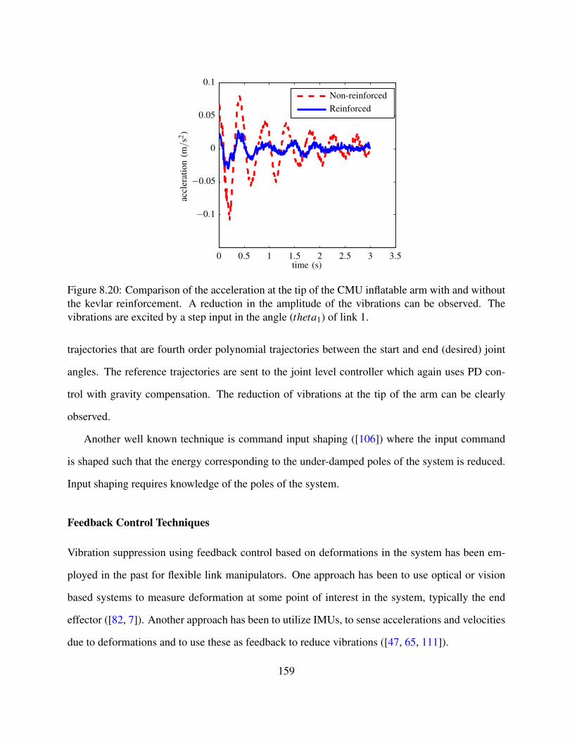
Reinforced

Non-reinforced

accle

rati

on

(m/s

2)

time (s)0 0.5 1 1.5 2 2.5 3 3.5

−0.1

−0.05

0

0.05

0.1

Figure 8.20: Comparison of the acceleration at the tip of the CMU inflatable arm with and withoutthe kevlar reinforcement. A reduction in the amplitude of the vibrations can be observed. Thevibrations are excited by a step input in the angle (theta1) of link 1.

trajectories that are fourth order polynomial trajectories between the start and end (desired) joint

angles. The reference trajectories are sent to the joint level controller which again uses PD con-

trol with gravity compensation. The reduction of vibrations at the tip of the arm can be clearly

observed.

Another well known technique is command input shaping ([106]) where the input command

is shaped such that the energy corresponding to the under-damped poles of the system is reduced.

Input shaping requires knowledge of the poles of the system.

Feedback Control Techniques

Vibration suppression using feedback control based on deformations in the system has been em-

ployed in the past for flexible link manipulators. One approach has been to use optical or vision

based systems to measure deformation at some point of interest in the system, typically the end

effector ([82, 7]). Another approach has been to utilize IMUs, to sense accelerations and velocities

due to deformations and to use these as feedback to reduce vibrations ([47, 65, 111]).

159

(a) Arm tip vertical position (in meters) when only PD control + gravity compensation isused to move between desired joint angles of the simulated inflatable arm

(b) Arm tip vertical position (in meters) when minimum jerk trajectories are used to movebetween desired joint angles of the simulated inflatable arm

Figure 8.21: Time histories of arm tip vertical position in meters, showing reduction in vibrationsat the tip when minimum jerk trajectories are commanded for the joint angles. The time axis is inseconds.

160

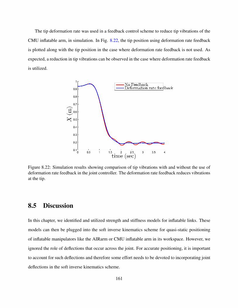
The tip deformation rate was used in a feedback control scheme to reduce tip vibrations of the

CMU inflatable arm, in simulation. In Fig. 8.22, the tip position using deformation rate feedback

is plotted along with the tip position in the case where deformation rate feedback is not used. As

expected, a reduction in tip vibrations can be observed in the case where deformation rate feedback

is utilized.

Figure 8.22: Simulation results showing comparison of tip vibrations with and without the use ofdeformation rate feedback in the joint controller. The deformation rate feedback reduces vibrationsat the tip.

8.5 Discussion

In this chapter, we identified and utilized strength and stiffness models for inflatable links. These

models can then be plugged into the soft inverse kinematics scheme for quasi-static positioning

of inflatable manipulators like the AIRarm or CMU inflatable arm in its workspace. However, we

ignored the role of deflections that occur across the joint. For accurate positioning, it is important

to account for such deflections and therefore some effort needs to be devoted to incorporating joint

deflections in the soft inverse kinematics scheme.

161

8.6 Summary

In this chapter, we developed models and state estimation methods to improve the accuracy of mo-

tion of inflatable manipulators. Models to predict the strength and stiffness of inflatable links were

identified and these models were compared with experimental data. The strength model predicts

the load at which wrinkling begins to occur on the structure. We use this load to specify payload

capacity for the links and the manipulator. The stiffness model is used in to predict deflections

of the links when loaded. While the internal pressure of the links, directly influences the payload

capacity of the links, for the range of pressures used in our experiments, the effect on stiffness was

not significant.

The Soft Inverse Kinematics scheme developed utilizes the stiffness model to allow quasi-

static positioning of the inflatable manipulator in the presence of link deflections. The scheme

was evaluated using a nonlinear finite element simulation an inflatable manipulator. The results

indicate that the soft inverse kinematics scheme allows more accurate positioning of the arm tip

when compared to rigid inverse kinematics. A generalization of the scheme was also developed to

allow positioning of soft robots using actuator forces rather than joint angles. Tracking control for

the arm which is not addressed in this chapter needs to be developed to allow the arm to follow

trajectories that respect the deformations in the system.

Another issue which unique to soft and inflatable robots is that of estimating configuration

variables like joint angles. In this chapter, we address joint angle sensing is addressed by the use

of pressure sensors and inertial measurement units (IMUs). One key assumption is that the joint

kinematics are assumed to be idealized. Further work is needed to either improve joint design to

match the idealized joint kinematics or to use methods that do not rely on these assumptions.

162

Chapter 9

Physical Human Interaction

This chapter describes some of the capabilities developed for the CMU inflatable arm to handle

tasks involving human interaction. We will describe a contact detection scheme based on joint

pressure sensing using which the arm handles unintended contacts. Contact detection is also used

to initiate a task where contact is intended, such as wiping. Experiments verifying the efficacy of

the contact detection scheme are shown using the two interaction scenarios. We will also describe

the inflatable arm carrying a feeding task. Result from a user study to evaluate user safety and

comfort during the task are also presented.

9.1 Inflatable Joint Angle Estimation using Pressure Sensors

For the sake of clarity, we will restate the pressure sensor based joint angle estimation and contact

detection scheme described in Sec. 8.3.1 in this section.

It is possible to derive a simple map between the motor shaft angle (θ2m) and the inflatable joint

angle θ2 under the assumption that the tendon is taut, we shall refer to this map as the transmission

map, T : θ2m 7→ θ2. Since the tendons are pull only, i.e. compressive loads cannot be supported,

loads that have a positive moment about joint 2 will cause deflection of link 2 based on the stiffness

163

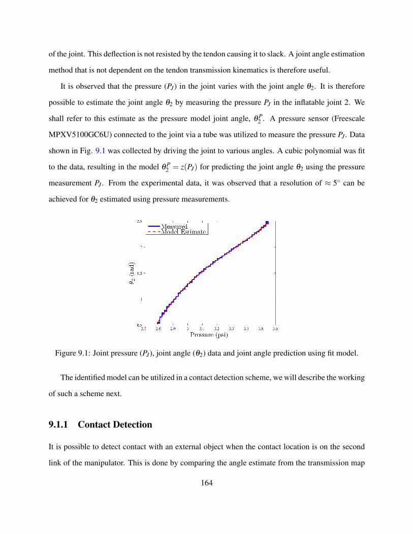
of the joint. This deflection is not resisted by the tendon causing it to slack. A joint angle estimation

method that is not dependent on the tendon transmission kinematics is therefore useful.

It is observed that the pressure (PJ) in the joint varies with the joint angle θ2. It is therefore

possible to estimate the joint angle θ2 by measuring the pressure PJ in the inflatable joint 2. We

shall refer to this estimate as the pressure model joint angle, θ P2 . A pressure sensor (Freescale

MPXV5100GC6U) connected to the joint via a tube was utilized to measure the pressure PJ . Data

shown in Fig. 9.1 was collected by driving the joint to various angles. A cubic polynomial was fit

to the data, resulting in the model θ P2 = z(PJ) for predicting the joint angle θ2 using the pressure

measurement PJ . From the experimental data, it was observed that a resolution of ≈ 5◦ can be

achieved for θ2 estimated using pressure measurements.

Figure 9.1: Joint pressure (PJ), joint angle (θ2) data and joint angle prediction using fit model.

The identified model can be utilized in a contact detection scheme, we will describe the working

of such a scheme next.

9.1.1 Contact Detection

It is possible to detect contact with an external object when the contact location is on the second

link of the manipulator. This is done by comparing the angle estimate from the transmission map

164

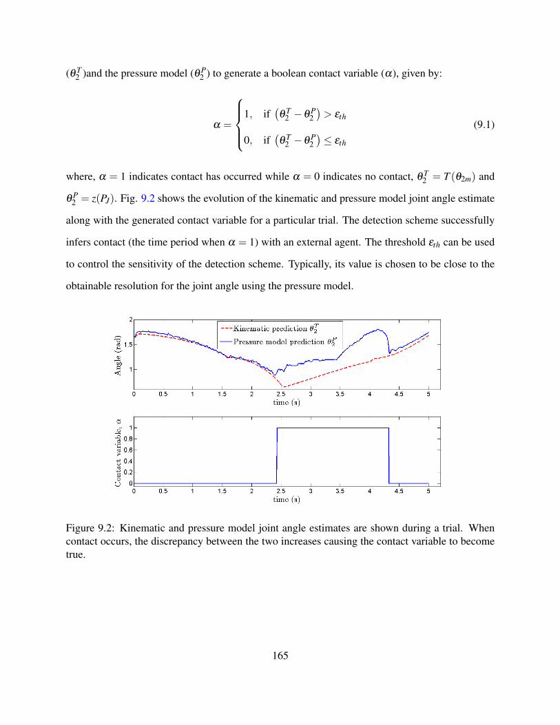
(θ T2 )and the pressure model (θ P

2 ) to generate a boolean contact variable (α), given by:

α =

1, if

(θ T

2 −θ P2)> εth

0, if(θ T

2 −θ P2)≤ εth

(9.1)

where, α = 1 indicates contact has occurred while α = 0 indicates no contact, θ T2 = T (θ2m) and

θ P2 = z(PJ). Fig. 9.2 shows the evolution of the kinematic and pressure model joint angle estimate

along with the generated contact variable for a particular trial. The detection scheme successfully

infers contact (the time period when α = 1) with an external agent. The threshold εth can be used

to control the sensitivity of the detection scheme. Typically, its value is chosen to be close to the

obtainable resolution for the joint angle using the pressure model.

Figure 9.2: Kinematic and pressure model joint angle estimates are shown during a trial. Whencontact occurs, the discrepancy between the two increases causing the contact variable to becometrue.

165

9.2 Reaction Schemes

A reaction scheme coupled with the above contact detection scheme can be used to generate a

variety of behavior for the inflatable manipulator. For instance, the reaction scheme can be used

to minimize unintended interactions between the manipulator and an external agent by causing

the manipulator to move away from the external agent once contact is detected. In other cases

when interaction is intended, such as for sponging, the reaction scheme can also be used to execute

a wiping motion upon detecting contact. We will next describe these two reactions schemes as

implemented on the inflatable manipulator.

9.2.1 Unintended Interaction

As mentioned above, the reaction scheme may be used to minimize unintended interactions. Such

a reaction scheme is useful, for instance, when the manipulator is following a trajectory and an

unobserved external agent enters the path of the manipulator. For this reaction scheme, the contact

detection scheme must initiate motion of the manipulator away from the external agent, when

contact is detected. Fig. 9.3 shows the typical operation of the manipulator using such a reaction

scheme.

Fig. 9.4 shows the contact forces occurring with the above reaction scheme implemented on the

inflatable manipulator. A flat surface instrumented with a force/torque sensor was used to obstruct

the path of the manipulator. Fig. 9.5a shows the motion of the manipulator under this reaction

scheme when contact occurs with a human.

9.2.2 Intended Interaction - Sponging

For the simplified sponging task shown in Fig. 9.5b, the contact detection scheme is used to switch

between two motion primitives: 1) Approach and 2) Wipe. The approach primitive essentially pre-

scribes an end effector motion to seek contact with an external object. The wipe motion assumes

166

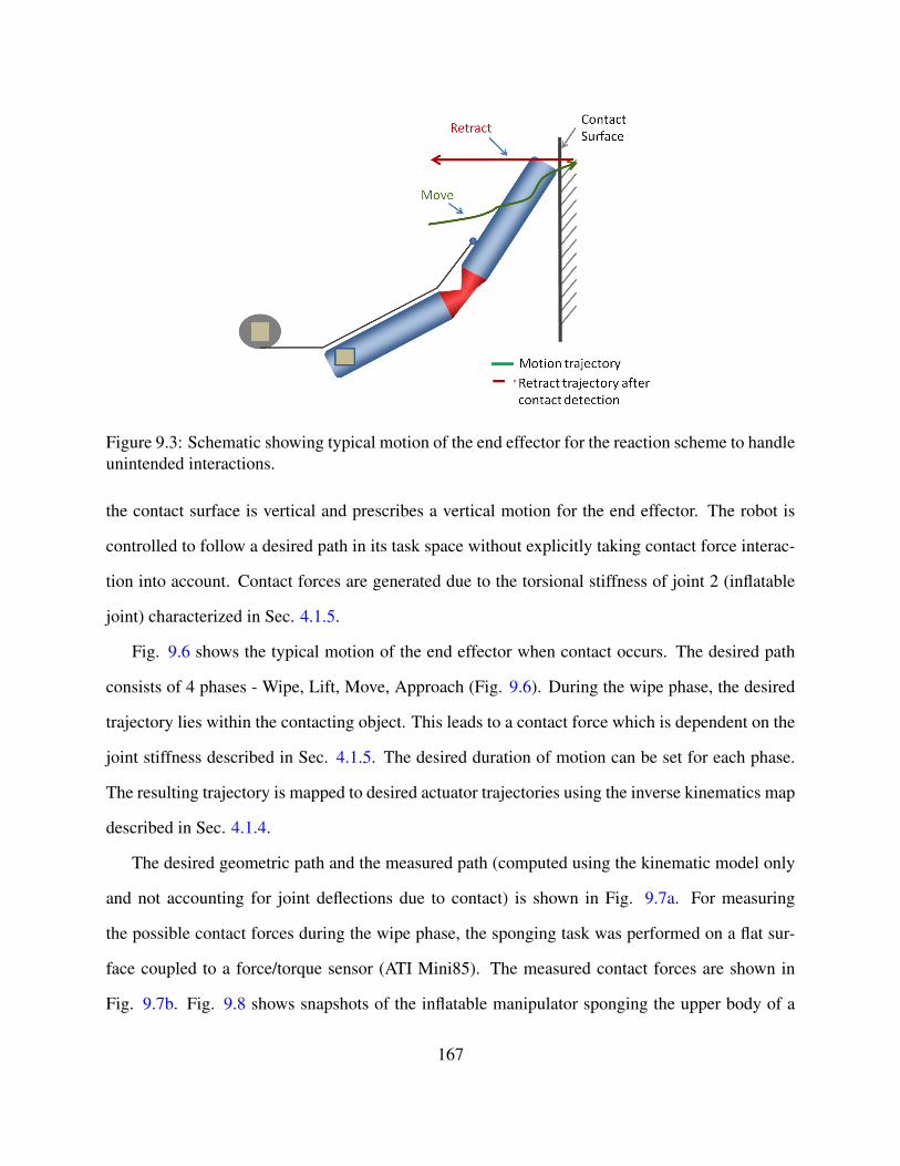
Figure 9.3: Schematic showing typical motion of the end effector for the reaction scheme to handleunintended interactions.

the contact surface is vertical and prescribes a vertical motion for the end effector. The robot is

controlled to follow a desired path in its task space without explicitly taking contact force interac-

tion into account. Contact forces are generated due to the torsional stiffness of joint 2 (inflatable

joint) characterized in Sec. 4.1.5.

Fig. 9.6 shows the typical motion of the end effector when contact occurs. The desired path

consists of 4 phases - Wipe, Lift, Move, Approach (Fig. 9.6). During the wipe phase, the desired

trajectory lies within the contacting object. This leads to a contact force which is dependent on the

joint stiffness described in Sec. 4.1.5. The desired duration of motion can be set for each phase.

The resulting trajectory is mapped to desired actuator trajectories using the inverse kinematics map

described in Sec. 4.1.4.

The desired geometric path and the measured path (computed using the kinematic model only

and not accounting for joint deflections due to contact) is shown in Fig. 9.7a. For measuring

the possible contact forces during the wipe phase, the sponging task was performed on a flat sur-

face coupled to a force/torque sensor (ATI Mini85). The measured contact forces are shown in

Fig. 9.7b. Fig. 9.8 shows snapshots of the inflatable manipulator sponging the upper body of a

167

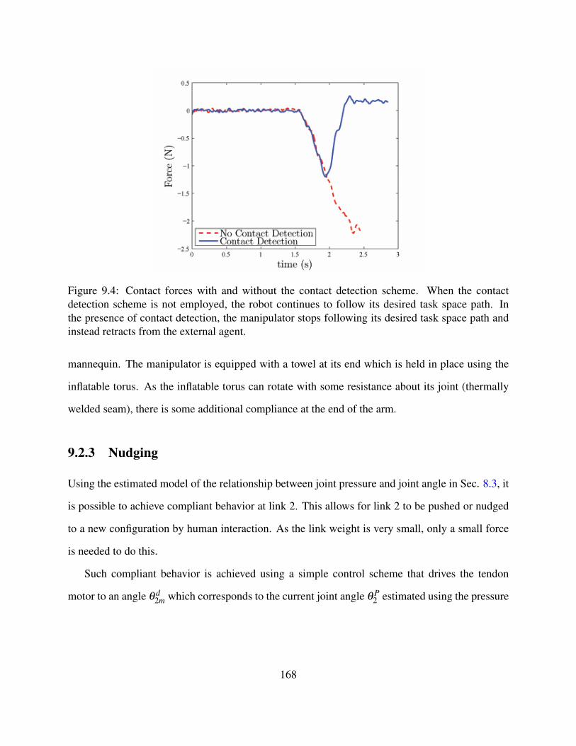
Figure 9.4: Contact forces with and without the contact detection scheme. When the contactdetection scheme is not employed, the robot continues to follow its desired task space path. Inthe presence of contact detection, the manipulator stops following its desired task space path andinstead retracts from the external agent.

mannequin. The manipulator is equipped with a towel at its end which is held in place using the

inflatable torus. As the inflatable torus can rotate with some resistance about its joint (thermally

welded seam), there is some additional compliance at the end of the arm.

9.2.3 Nudging

Using the estimated model of the relationship between joint pressure and joint angle in Sec. 8.3, it

is possible to achieve compliant behavior at link 2. This allows for link 2 to be pushed or nudged

to a new configuration by human interaction. As the link weight is very small, only a small force

is needed to do this.

Such compliant behavior is achieved using a simple control scheme that drives the tendon

motor to an angle θ d2m which corresponds to the current joint angle θ P

2 estimated using the pressure

168

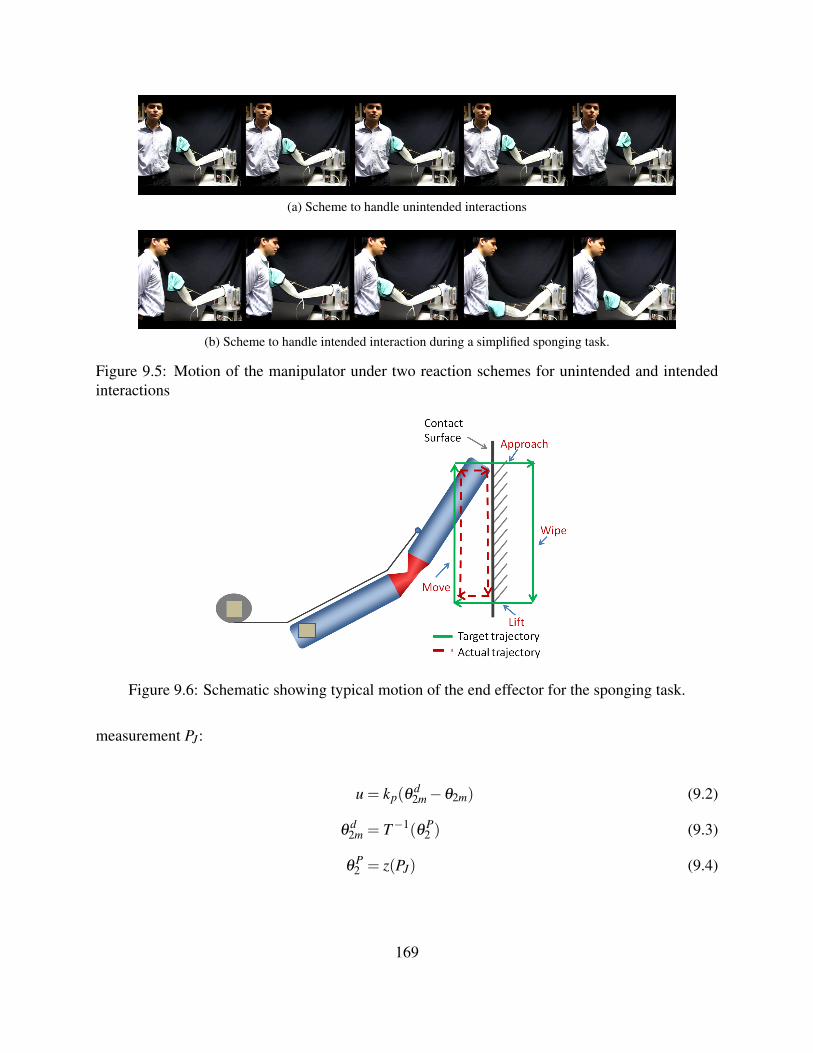
(a) Scheme to handle unintended interactions

(b) Scheme to handle intended interaction during a simplified sponging task.

Figure 9.5: Motion of the manipulator under two reaction schemes for unintended and intendedinteractions

Figure 9.6: Schematic showing typical motion of the end effector for the sponging task.

measurement PJ:

u = kp(θd2m−θ2m) (9.2)

θd2m = T−1(θ P

2 ) (9.3)

θP2 = z(PJ) (9.4)

169

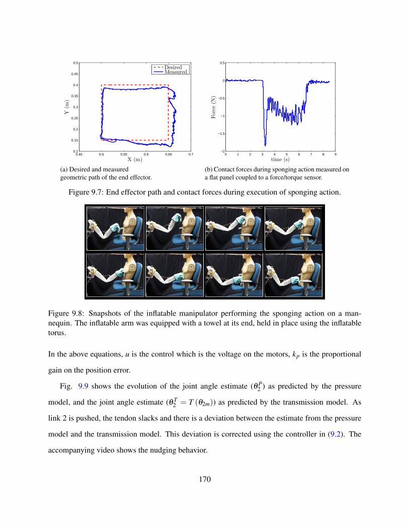
0.45 0.5 0.55 0.6 0.65 0.70.1

0.15

0.2

0.25

0.3

0.35

0.4

0.45

0.5

X (m)

Y(m

)

DesiredMeasured

(a) Desired and measuredgeometric path of the end effector.

0 1 2 3 4 5 6 7 8 9−2

−1.5

−1

−0.5

0

0.5

time (s)

Force(N

)

(b) Contact forces during sponging action measured ona flat panel coupled to a force/torque sensor.

Figure 9.7: End effector path and contact forces during execution of sponging action.

Figure 9.8: Snapshots of the inflatable manipulator performing the sponging action on a man-nequin. The inflatable arm was equipped with a towel at its end, held in place using the inflatabletorus.

In the above equations, u is the control which is the voltage on the motors, kp is the proportional

gain on the position error.

Fig. 9.9 shows the evolution of the joint angle estimate (θ P2 ) as predicted by the pressure

model, and the joint angle estimate (θ T2 = T (θ2m)) as predicted by the transmission model. As

link 2 is pushed, the tendon slacks and there is a deviation between the estimate from the pressure

model and the transmission model. This deviation is corrected using the controller in (9.2). The

accompanying video shows the nudging behavior.

170

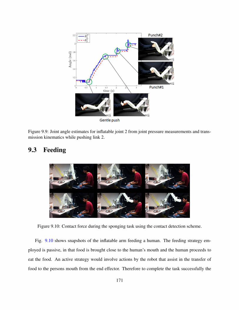
Figure 9.9: Joint angle estimates for inflatable joint 2 from joint pressure measurements and trans-mission kinematics while pushing link 2.

9.3 Feeding

Figure 9.10: Contact force during the sponging task using the contact detection scheme.

Fig. 9.10 shows snapshots of the inflatable arm feeding a human. The feeding strategy em-

ployed is passive, in that food is brought close to the human’s mouth and the human proceeds to

eat the food. An active strategy would involve actions by the robot that assist in the transfer of

food to the persons mouth from the end effector. Therefore to complete the task successfully the

171

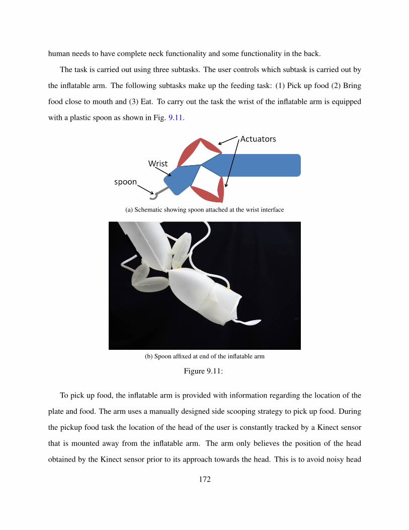
human needs to have complete neck functionality and some functionality in the back.

The task is carried out using three subtasks. The user controls which subtask is carried out by

the inflatable arm. The following subtasks make up the feeding task: (1) Pick up food (2) Bring

food close to mouth and (3) Eat. To carry out the task the wrist of the inflatable arm is equipped

with a plastic spoon as shown in Fig. 9.11.

(a) Schematic showing spoon attached at the wrist interface

(b) Spoon affixed at end of the inflatable arm

Figure 9.11:

To pick up food, the inflatable arm is provided with information regarding the location of the

plate and food. The arm uses a manually designed side scooping strategy to pick up food. During

the pickup food task the location of the head of the user is constantly tracked by a Kinect sensor

that is mounted away from the inflatable arm. The arm only believes the position of the head

obtained by the Kinect sensor prior to its approach towards the head. This is to avoid noisy head

172

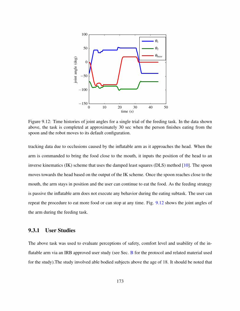
θbase

θ2

θ1

join

tan

gle

(deg

)

time (s)0 10 20 30 40 50

−150

−100

−50

0

50

100

Figure 9.12: Time histories of joint angles for a single trial of the feeding task. In the data shownabove, the task is completed at approximately 30 sec when the person finishes eating from thespoon and the robot moves to its default configuration.

tracking data due to occlusions caused by the inflatable arm as it approaches the head. When the

arm is commanded to bring the food close to the mouth, it inputs the position of the head to an

inverse kinematics (IK) scheme that uses the damped least squares (DLS) method [10]. The spoon

moves towards the head based on the output of the IK scheme. Once the spoon reaches close to the

mouth, the arm stays in position and the user can continue to eat the food. As the feeding strategy

is passive the inflatable arm does not execute any behavior during the eating subtask. The user can

repeat the procedure to eat more food or can stop at any time. Fig. 9.12 shows the joint angles of

the arm during the feeding task.

9.3.1 User Studies

The above task was used to evaluate perceptions of safety, comfort level and usability of the in-

flatable arm via an IRB approved user study (see Sec. B for the protocol and related material used

for the study).The study involved able bodied subjects above the age of 18. It should be noted that

173

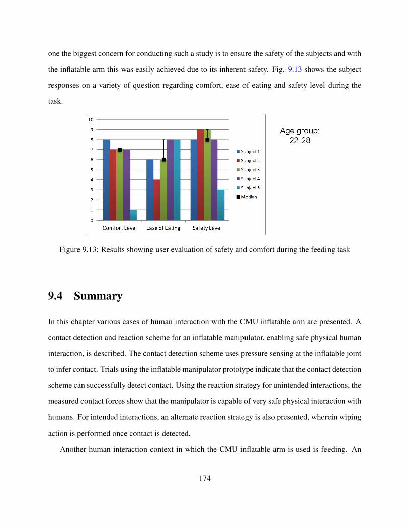
one the biggest concern for conducting such a study is to ensure the safety of the subjects and with

the inflatable arm this was easily achieved due to its inherent safety. Fig. 9.13 shows the subject

responses on a variety of question regarding comfort, ease of eating and safety level during the

task.

Figure 9.13: Results showing user evaluation of safety and comfort during the feeding task

9.4 Summary

In this chapter various cases of human interaction with the CMU inflatable arm are presented. A

contact detection and reaction scheme for an inflatable manipulator, enabling safe physical human

interaction, is described. The contact detection scheme uses pressure sensing at the inflatable joint

to infer contact. Trials using the inflatable manipulator prototype indicate that the contact detection

scheme can successfully detect contact. Using the reaction strategy for unintended interactions, the

measured contact forces show that the manipulator is capable of very safe physical interaction with

humans. For intended interactions, an alternate reaction strategy is also presented, wherein wiping

action is performed once contact is detected.

Another human interaction context in which the CMU inflatable arm is used is feeding. An

174

IRB approved user study to asses various parameters concerning safety and ease of eating with the

CMU inflatable arm was conducted. Only able bodied subjects were included in this study. The

results indicate acceptable levels of comfort and safety as perceived by the users. In the future,

developing active strategies for transferring food from the spoon to the subject mouth might be

beneficial for target populations with severe disabilities. Some level of force/torque sensing will

be needed at the wrist in order to successfully carry out an active feeding strategy.

175

Chapter 10

Conclusion

The thesis demonstrates the use of soft structured inflatable robots for safe physical human robot

interaction. The primary motivation for this work is the need for intrinsically safe robots in assis-

tive roles. Inflatable robots as demonstrated in this thesis satisfy requirements of intrinsic safety.

This thesis addresses a number of key challenges towards developing inflatable robots for tasks

involving close physical interaction with humans. We address questions regarding the design and

manufacture, actuation methods, strength and accuracy of inflatable robots. Some of the contribu-

tions of this thesis are listed below:

10.1 Contributions

Understanding performance advantages of soft robots over rigid robots in human interaction

tasks

Soft robots can have high inherent safety during impacts because of their highly compliant structure

and low-weight. This allows soft robots to have relatively small safety constraints as compared to

their rigid counterparts. At the same time, soft robots can be ’floppy’, i.e, they can have large

time constants leading to slower movements. Therefore, in the absence of safety constraints it

176

is absolutely true that a soft robot will be slower than a rigid robot. However safety constraints

usually take the form of velocity constraints at multiple locations along the robot’s structure where

contact is expected. In theory, because these safety constraints are large for rigid robots they can

make rigid robots slower than soft robots, in spite of the larger time constants in soft systems.

This is demonstrated in Chapter 3. Our specific contribution lies in identifying that distributed

compliance can contribute to performance improvements.

Framework for the design of soft robots

How does one proceed to design a soft robot? Are traditional static design requirements enough?

Often soft systems can be engineered practically never fail for, e.g., a soft jelly fish like robot can

be repeatedly smashed without incurring any damage at all. What should guide the design in such

a case? Since the structural parameters of a soft robot affect the dynamic characteristics of a robot

to a large extent these metric on these characteristic must be included in the design process. In

Chapter 3 we developed a multi stage optimization framework that uses objective function scores

from optimal control to iterate over the design variables.

Inverse kinematics for general elastic soft bodied robots

Kinematics of a soft robot are influenced by external factors such a loads and constraints due to

contact, as well as its own weight. Therefore a purely geometric description of the kinematics for a

soft robot is not possible. In Chapter 8 we developed methods to solve inverse kinematics problems

for soft robots of various types by including a deformation model in the kinematics. One insight

from these methods is that it is useful to prescribe forces to generate motions rather than prescribing

configurations. While the configuration space of general soft robots may be infinite dimensional,

often these robots live in a lower dimensional subspace because of the finite dimensional actuation

and external forces that drive these robots.

177

Direct actuation in shape space using shape based actuators

Inflatable structures when inflated are defined by maximum volume surfaces. However, when

deflated, the structure can take on a variety of shapes. We use this property of inflatable structure

to develop shape based actuators in Chapters 4 and 7. These actuators are formed by combining

differently shaped inflatable volumes along common geometric features. This allows the actuator

to take the shape of whichever actuator is inflated. Therefore, unlike traditional actuators that cause

some scalar parameter to vary when they are actuated shape based actuators allow us to actuate a

structure directly in the shape space.

Expanding the design space for inflatable robots

This thesis contributes towards expanding the relatively unexplored design space for inflatable

robots. In Chapters 4, 6 and 7 we have developed a catalogue of inflatable robot components such

as links, wrists, joints, grasping devices, actuators, etc. that can be utilized for future iteration of

inflatable robots.

Low cost robots that can be made like clothes and inflatable pool toys

Inflatable robots represent a key departure from traditional robots in terms of the manufacturing

techniques that are used to manufacture them. Instead of subtractive or more recent additive 3D

processes, these robots are manufactured using from 2D planar surfaces (fabric/plastic sheets) that

are seamed together. This can be potentially transformative from a cost perspective because these

robots can be manufactured like clothes with embedded sensing and actuation. Alternate seamless

techniques can also be used such as that used in knitting. Further, if all seams in the structure are

flat these robots can be manufactured using batch processing techniques similar to that found in

the semiconductor industry.

178

10.2 Future Work

This section presents some possible directions for future research based on the work presented in

this thesis. We also explore some future application for robotics based on inflatable structures.

Visual Servoing

Some of the drawbacks that exist, in terms of sensor hardware for accurate state estimation and

motion of inflatable robots, can be overcome by the use of task space visual servoing. Visual ser-

voing has been used in the past to improve accuracy for manipulators with flexible links and rigid

manipulators ([85, 59]) and these techniques can be applied to inflatable robots. One distinction

for inflatable robots is the lack of joint angle sensing which was addressed in Chapter 8.

State Estimation

In Chapter 8, we developed a method to estimate joint angles using Inertial Measurement Units

(IMUs). The use of IMUs can be further extended to develop a state observer for the inflatable

robots based on the acceleration and angular rate observations from the IMU. The state observer

can be used be employed in a control scheme for force control, vibration suppression, load esti-

mation etc. New sensor hardware similar to the stretch sensors described in Chapter 8 are also

needed.

Vibration Suppression Techniques

Slow oscillations caused by external forces is often observed with inflatable robots. Methods to

introduce damping into the structure either via design or control are needed. Developments in state

estimation, joint design, actuation techniques and materials can aid progress in the area.

179

Variable Morphology Robots

Variable morphology robots refers to robots that can take on different physical forms based on

the task. For instance, the robot can have different number of links based on the environment

it is operating it to give it greater dexterity. Inflatable robots can be built to have such variable

morphology. The variable buckling mechanism in Chapter 2 explores this idea by introducing

variability in the location of the joint on the robot structure. Much more general variability is

possible and can lead to interesting applications.

180

Appendix A

Synthesis of Safe Systems

A.1 Closed Loop Performance Based Synthesis

In Sec. 3.2, we detailed a synthesis procedure for soft robots to obey safety constraints and max-

imize some performance criteria. The performance criteria mentioned therein optimized some

metric of the trajectory being followed by the system, in other words the metric was based on per-

formance parameters in the time domain. This allowed for optimizing gross motions of the system

for specific properties such as maneuver completion time, actuator effort along the trajectory etc.

It is also possible to consider performance of the system from the perspective of its response to

disturbances i.e its behavior with a feedback controller.

The purpose of the exercise in this chapter is to optimize the structure of the system such that

the behavior of the system is acceptable across the frequency spectrum of disturbances. In some

sense, we are attempting to improve the shape of the frequency response shown in the illustration

in Fig. A.1.

181

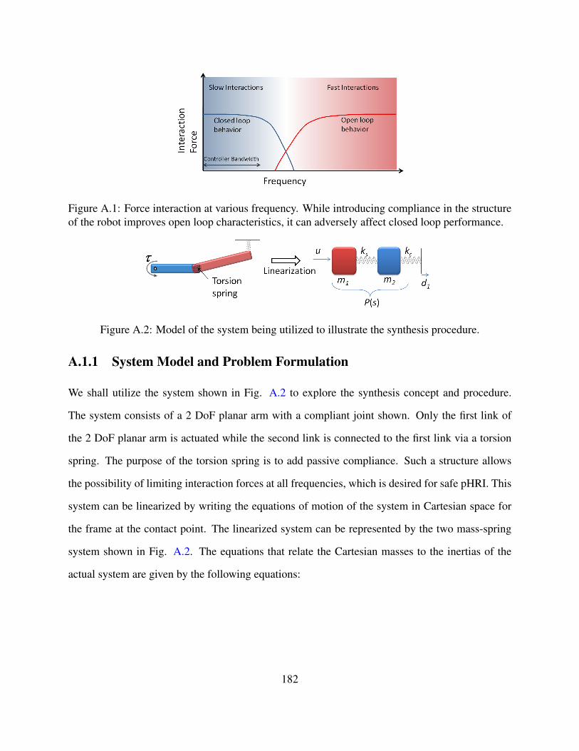
Figure A.1: Force interaction at various frequency. While introducing compliance in the structureof the robot improves open loop characteristics, it can adversely affect closed loop performance.

Figure A.2: Model of the system being utilized to illustrate the synthesis procedure.

A.1.1 System Model and Problem Formulation

We shall utilize the system shown in Fig. A.2 to explore the synthesis concept and procedure.

The system consists of a 2 DoF planar arm with a compliant joint shown. Only the first link of

the 2 DoF planar arm is actuated while the second link is connected to the first link via a torsion

spring. The purpose of the torsion spring is to add passive compliance. Such a structure allows

the possibility of limiting interaction forces at all frequencies, which is desired for safe pHRI. This

system can be linearized by writing the equations of motion of the system in Cartesian space for

the frame at the contact point. The linearized system can be represented by the two mass-spring

system shown in Fig. A.2. The equations that relate the Cartesian masses to the inertias of the

actual system are given by the following equations:

182

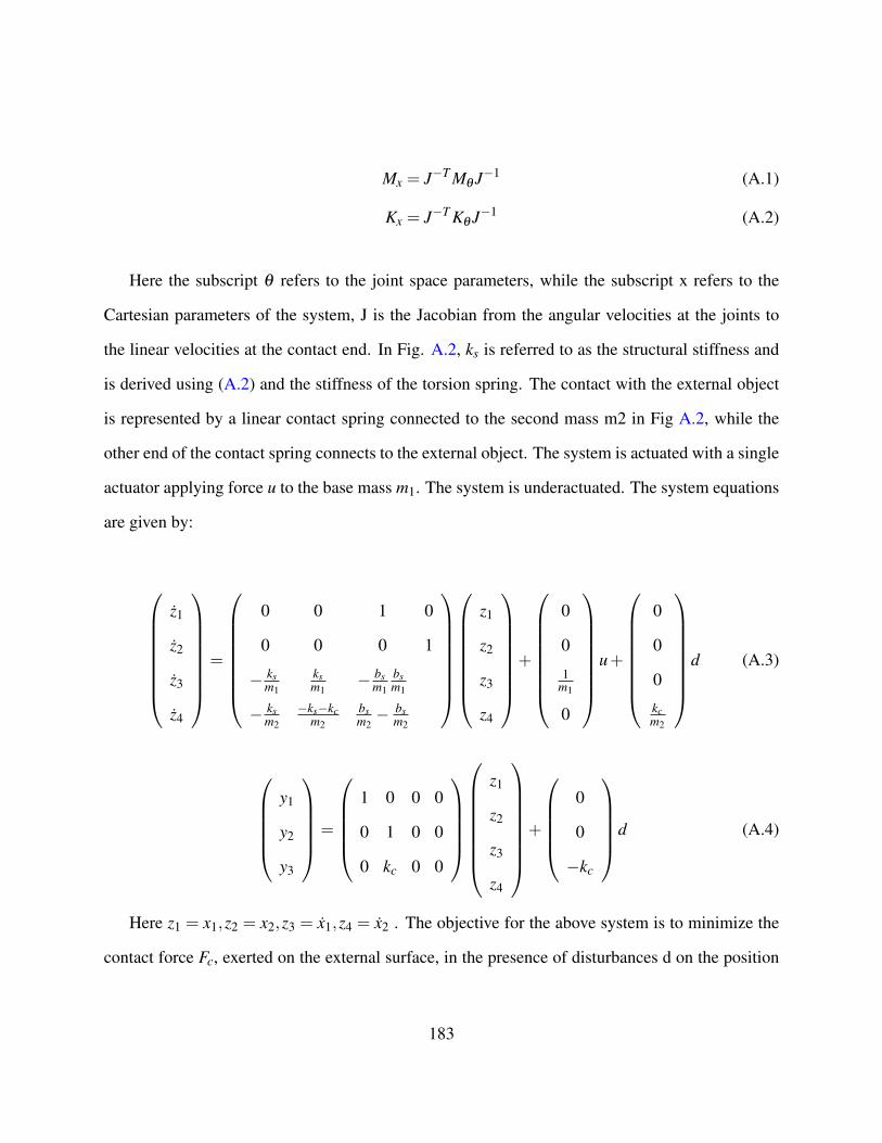
Mx = J−T Mθ J−1 (A.1)

Kx = J−T Kθ J−1 (A.2)

Here the subscript θ refers to the joint space parameters, while the subscript x refers to the

Cartesian parameters of the system, J is the Jacobian from the angular velocities at the joints to

the linear velocities at the contact end. In Fig. A.2, ks is referred to as the structural stiffness and

is derived using (A.2) and the stiffness of the torsion spring. The contact with the external object

is represented by a linear contact spring connected to the second mass m2 in Fig A.2, while the

other end of the contact spring connects to the external object. The system is actuated with a single

actuator applying force u to the base mass m1. The system is underactuated. The system equations

are given by:

z1

z2

z3

z4

=

0 0 1 0

0 0 0 1

− ksm1

ksm1

− bsm1

bsm1

− ksm2

−ks−kcm2

bsm2− bs

m2

z1

z2

z3

z4

+

0

0

1m1

0

u+

0

0

0

kcm2

d (A.3)

y1

y2

y3

=

1 0 0 0

0 1 0 0

0 kc 0 0

z1

z2

z3

z4

+

0

0

−kc

d (A.4)

Here z1 = x1,z2 = x2,z3 = x1,z4 = x2 . The objective for the above system is to minimize the

contact force Fc, exerted on the external surface, in the presence of disturbances d on the position

183

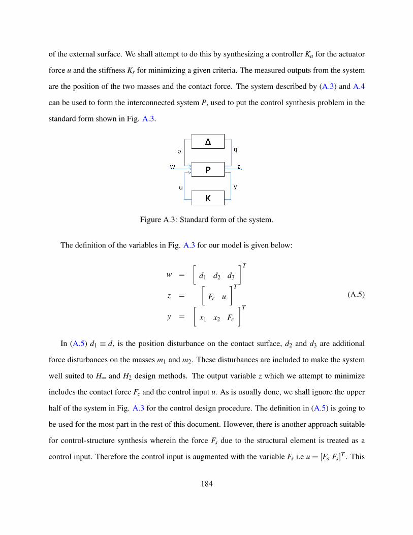
of the external surface. We shall attempt to do this by synthesizing a controller Ku for the actuator

force u and the stiffness Ks for minimizing a given criteria. The measured outputs from the system

are the position of the two masses and the contact force. The system described by (A.3) and A.4

can be used to form the interconnected system P, used to put the control synthesis problem in the

standard form shown in Fig. A.3.

Figure A.3: Standard form of the system.

The definition of the variables in Fig. A.3 for our model is given below:

w =

[d1 d2 d3

]T

z =

[Fc u

]T

y =

[x1 x2 Fc

]T

(A.5)

In (A.5) d1 ≡ d, is the position disturbance on the contact surface, d2 and d3 are additional

force disturbances on the masses m1 and m2. These disturbances are included to make the system

well suited to H∞ and H2 design methods. The output variable z which we attempt to minimize

includes the contact force Fc and the control input u. As is usually done, we shall ignore the upper

half of the system in Fig. A.3 for the control design procedure. The definition in (A.5) is going to

be used for the most part in the rest of this document. However, there is another approach suitable

for control-structure synthesis wherein the force Fs due to the structural element is treated as a

control input. Therefore the control input is augmented with the variable Fs i.e u = [Fa Fs]T . This

184

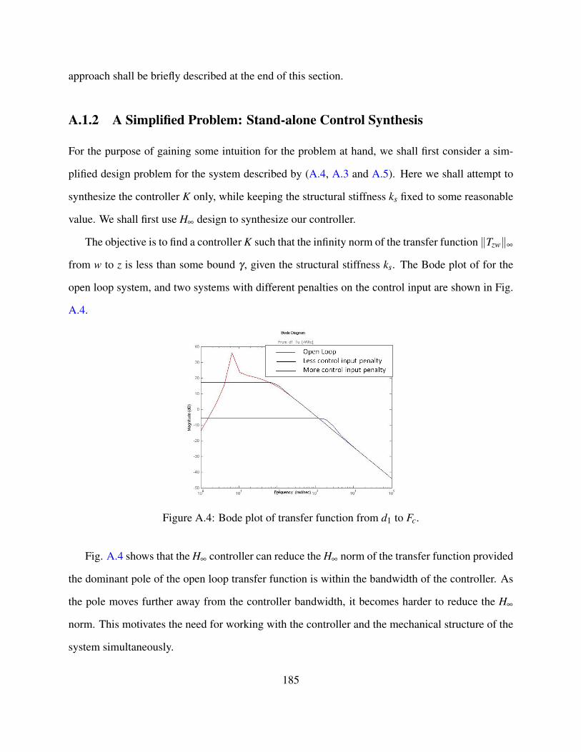
approach shall be briefly described at the end of this section.

A.1.2 A Simplified Problem: Stand-alone Control Synthesis

For the purpose of gaining some intuition for the problem at hand, we shall first consider a sim-

plified design problem for the system described by (A.4, A.3 and A.5). Here we shall attempt to

synthesize the controller K only, while keeping the structural stiffness ks fixed to some reasonable

value. We shall first use H∞ design to synthesize our controller.

The objective is to find a controller K such that the infinity norm of the transfer function ‖Tzw‖∞

from w to z is less than some bound γ , given the structural stiffness ks. The Bode plot of for the

open loop system, and two systems with different penalties on the control input are shown in Fig.

A.4.

Figure A.4: Bode plot of transfer function from d1 to Fc.

Fig. A.4 shows that the H∞ controller can reduce the H∞ norm of the transfer function provided

the dominant pole of the open loop transfer function is within the bandwidth of the controller. As

the pole moves further away from the controller bandwidth, it becomes harder to reduce the H∞

norm. This motivates the need for working with the controller and the mechanical structure of the

system simultaneously.

185

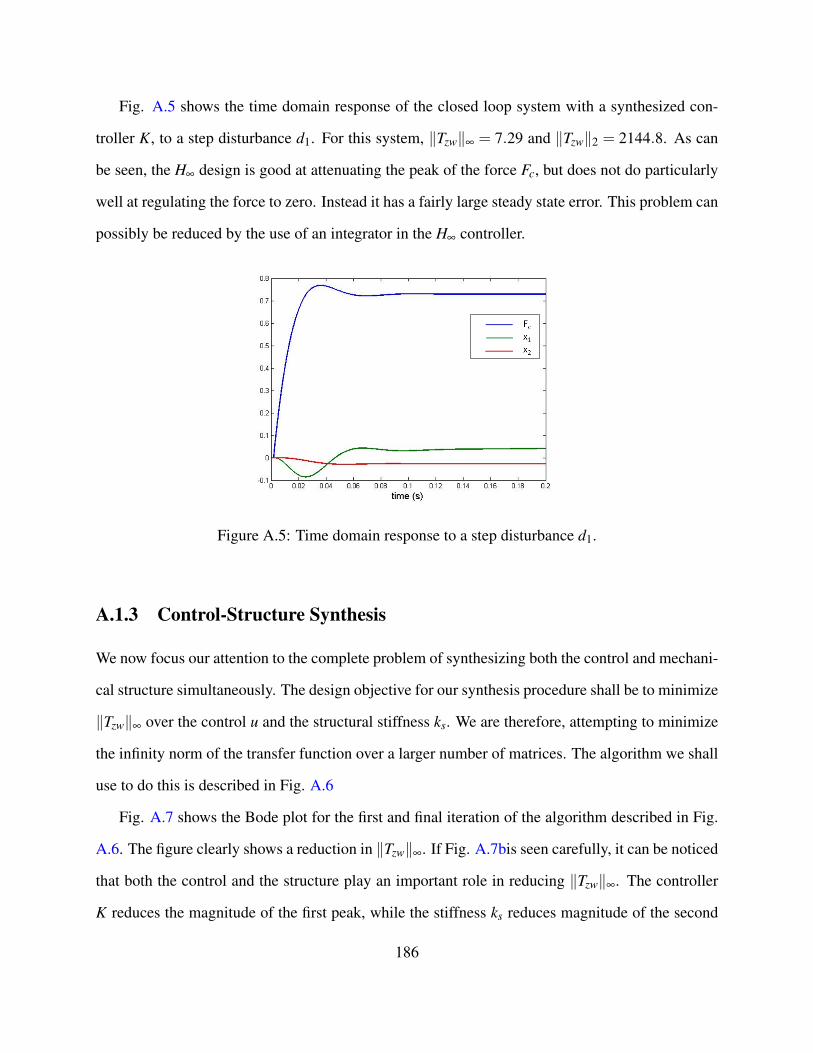
Fig. A.5 shows the time domain response of the closed loop system with a synthesized con-

troller K, to a step disturbance d1. For this system, ‖Tzw‖∞ = 7.29 and ‖Tzw‖2 = 2144.8. As can

be seen, the H∞ design is good at attenuating the peak of the force Fc, but does not do particularly

well at regulating the force to zero. Instead it has a fairly large steady state error. This problem can

possibly be reduced by the use of an integrator in the H∞ controller.

Figure A.5: Time domain response to a step disturbance d1.

A.1.3 Control-Structure Synthesis

We now focus our attention to the complete problem of synthesizing both the control and mechani-

cal structure simultaneously. The design objective for our synthesis procedure shall be to minimize

‖Tzw‖∞ over the control u and the structural stiffness ks. We are therefore, attempting to minimize

the infinity norm of the transfer function over a larger number of matrices. The algorithm we shall

use to do this is described in Fig. A.6

Fig. A.7 shows the Bode plot for the first and final iteration of the algorithm described in Fig.

A.6. The figure clearly shows a reduction in ‖Tzw‖∞. If Fig. A.7bis seen carefully, it can be noticed

that both the control and the structure play an important role in reducing ‖Tzw‖∞. The controller

K reduces the magnitude of the first peak, while the stiffness ks reduces magnitude of the second

186

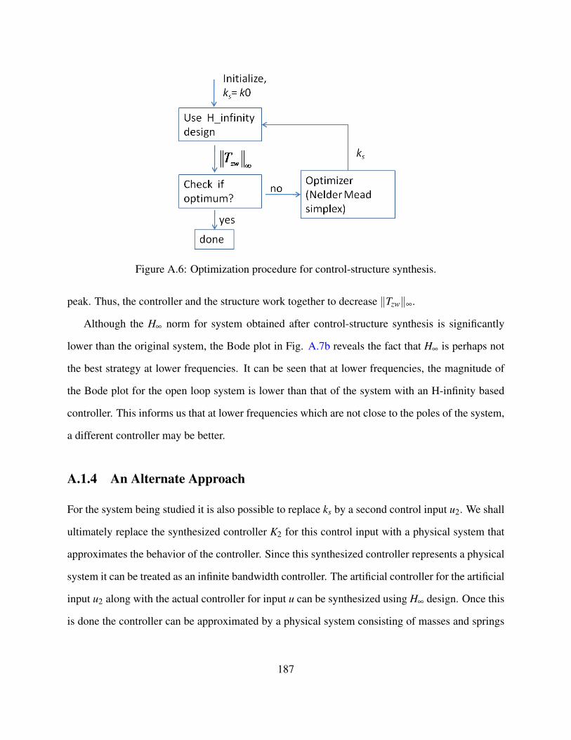
Figure A.6: Optimization procedure for control-structure synthesis.

peak. Thus, the controller and the structure work together to decrease ‖Tzw‖∞.

Although the H∞ norm for system obtained after control-structure synthesis is significantly

lower than the original system, the Bode plot in Fig. A.7b reveals the fact that H∞ is perhaps not

the best strategy at lower frequencies. It can be seen that at lower frequencies, the magnitude of

the Bode plot for the open loop system is lower than that of the system with an H-infinity based

controller. This informs us that at lower frequencies which are not close to the poles of the system,

a different controller may be better.

A.1.4 An Alternate Approach

For the system being studied it is also possible to replace ks by a second control input u2. We shall

ultimately replace the synthesized controller K2 for this control input with a physical system that

approximates the behavior of the controller. Since this synthesized controller represents a physical

system it can be treated as an infinite bandwidth controller. The artificial controller for the artificial

input u2 along with the actual controller for input u can be synthesized using H∞ design. Once this

is done the controller can be approximated by a physical system consisting of masses and springs

187

(a) Bode plot from w to z at the first iteration of the algo-rithm

(b) Bode plot from w to z at the final iteration of the algo-rithm

Figure A.7: Bode plot for first and final iteration of the control-structure synthesis procedure

as shown in Fig. A.8. In the approximation ‖∆‖∞ may be limited based on robust stability margin

obtained for the previously synthesized controller for the input u.

Figure A.8: Optimization procedure for control-structure synthesis.

This approach has not been entirely explored. We mention it here only to bring up the possibil-

ity of generalizing the closed loop synthesis procedure to allow synthesis of structural topologies

in addition to structural parameters such as stiffness.

188

Appendix B

User Study Protocol

In this chapter we will present the CMU IRB approved protocol and associated material that was

utilized to conduct the user study in Sec. 9.3 of Chapter 9. The CMU IRB application which

includes the study protocol, the consent form and questionnaire used in the user study are included

in the following pages.

189

Carnegie Mellon University

1 v7/2011

For IRB Office Use IRB No:_______________ Rec’d:____________________

APPLICATION FOR IRB REVIEW OF RESEARCH INVOLVING HUMAN SUBJECTS (Not for exempt research)

Please complete this application as thoroughly as possible. Your application should include the following:

1. A consent form using the current CMU template that the participants and/or parent/guardian will be required to sign.

2. A copy of any questionnaires, surveys, images, de-briefings that will be used. 3. A copy of any recruitment documents (including advertisements, flyers, letters, invitations, email) to be used; 4. A copy of the training certificates for all individuals working on the research unless they are on file with the CMU

IRB. Training is available at: http://www.citiprogram.org. See the IRB website for details. 5. If the PI is a student, the faculty advisor must submit a Faculty Advisor Assurance Form.

Please email all documents to irb-review@andrew.cmu.edu. For assistance call the CMU Office of Research Integrity and

Compliance @ 412-268-5460 or email irb-review@andrew.cmu.edu. Additional information and templates are available at

http://www.cmu.edu/osp/regulatory-compliance/human-subjects.html

1. Protocol

Title: Robot-Assisted Feeding using the Inflatable Manipulator

This is a previously approved study that has lapsed. Previous IRB No: HS

2. Principal Investigator (PI)

Name: Siddharth Sanan Department: Robotics

Telephone: 412-999-6115 E-mail: sanan@cmu.edu Training Cert. Attached On File

I am a student. If so, please provide information about your faculty advisor below.

Faculty Advisor Name: Christopher G.

Atkeson

E-mail: cga@cmu.edu Training Cert. Attached On File

If a student is the PI, the faculty advisor must complete and submit a Faculty Advisor Assurance Form.

If there is someone other than PI to correspond with regarding this protocol, please list below.

Contact Person Name: Telephone: E-mail:

Business Manager for your department: E-mail:

3. Co-investigators

Name: E-mail: Training Cert. Attached On File

Name: E-mail: Training Cert. Attached On File

Name: E-mail: Training Cert. Attached On File

Name: E-mail: Training Cert. Attached On File

Name: E-mail: Training Cert. Attached On File

Name: E-mail: Training Cert. Attached On File

Name: E-mail: Training Cert. Attached On File

4. Funding

Unfunded research External Funding Internal Funding

Sponsor/Source: NSF NIH Other, please specify:

Grant Title: Quality of Life Technology Engineering Research Center #0540865

If federally funded, is this application consistent with the grant? Yes No

Is CMU the prime recipient of funding? Yes No Is CMU a sub-recipient? Yes No

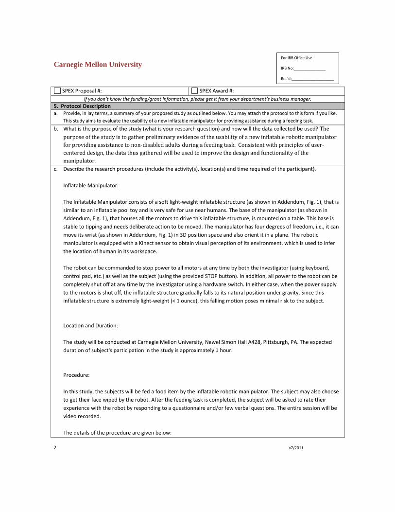
Carnegie Mellon University

2 v7/2011

For IRB Office Use IRB No:_______________ Rec’d:____________________

SPEX Proposal #: SPEX Award #:

If you don’t know the funding/grant information, please get it from your department’s business manager. 5. Protocol Description a. Provide, in lay terms, a summary of your proposed study as outlined below. You may attach the protocol to this form if you like.

This study aims to evaluate the usability of a new inflatable manipulator for providing assistance during a feeding task.

b. What is the purpose of the study (what is your research question) and how will the data collected be used? The

purpose of the study is to gather preliminary evidence of the usability of a new inflatable robotic manipulator

for providing assistance to non-disabled adults during a feeding task. Consistent with principles of user-

centered design, the data thus gathered will be used to improve the design and functionality of the

manipulator.

c. Describe the research procedures (include the activity(s), location(s) and time required of the participant).

Inflatable Manipulator:

The Inflatable Manipulator consists of a soft light-weight inflatable structure (as shown in Addendum, Fig. 1), that is

similar to an inflatable pool toy and is very safe for use near humans. The base of the manipulator (as shown in

Addendum, Fig. 1), that houses all the motors to drive this inflatable structure, is mounted on a table. This base is

stable to tipping and needs deliberate action to be moved. The manipulator has four degrees of freedom, i.e., it can

move its wrist (as shown in Addendum, Fig. 1) in 3D position space and also orient it in a plane. The robotic

manipulator is equipped with a Kinect sensor to obtain visual perception of its environment, which is used to infer

the location of human in its workspace.

The robot can be commanded to stop power to all motors at any time by both the investigator (using keyboard,

control pad, etc.) as well as the subject (using the provided STOP button). In addition, all power to the robot can be

completely shut off at any time by the investigator using a hardware switch. In either case, when the power supply

to the motors is shut off, the inflatable structure gradually falls to its natural position under gravity. Since this

inflatable structure is extremely light-weight (< 1 ounce), this falling motion poses minimal risk to the subject.

Location and Duration:

The study will be conducted at Carnegie Mellon University, Newel Simon Hall A428, Pittsburgh, PA. The expected

duration of subject's participation in the study is approximately 1 hour.

Procedure:

In this study, the subjects will be fed a food item by the inflatable robotic manipulator. The subject may also choose

to get their face wiped by the robot. After the feeding task is completed, the subject will be asked to rate their

experience with the robot by responding to a questionnaire and/or few verbal questions. The entire session will be

video recorded.

The details of the procedure are given below:

Carnegie Mellon University

3 v7/2011

For IRB Office Use IRB No:_______________ Rec’d:____________________

- After providing written informed consent, the subject will be shown a video depicting the inflatable robotic

manipulator feeding the PI while seated in the laboratory in Newell-Simon Hall.

- The subject will be then shown the robot and oriented to its functionalities. The subject will also be shown how to

STOP the robot at any time during the task.

- The subject will be informed of the food item that will be fed to him/her by the inflatable robot. The food items

may include pudding, cereal, yogurt, applesauce, canned fruit, etc.

- The subject will be provided protective eyewear to be worn during the task. The subject will also be offered an

apron or bib to wear, if they prefer.

- When the subject is ready to proceed with the feeding task, the investigator will first issue a "Pick up food"

command to the robot. The robot will then pick up the food item from a dish using a feeding utensil such as a

rubberized spoon attached to the wrist of the manipulator. The investigator will then issue a "Bring food close to

mouth" command, upon which the robot will proceed to bring the food close to the subject's mouth. The subject

will then be asked to eat the food item. At this time, the subject may choose to get his/her mouth wiped by the

robot. If the subject chooses to do so, the investigator will issuing a "Wipe face" command to the robot. This

command causes the robot's tool to change from a spoon to a towel, which is used to wipe the subject's face. This

this procedure will be repeated at least 3 times.

- After completing the above feeding task, the subject will be asked to rate their experience with the robot by

responding to a questionnaire and/or few verbal questions. Specifically, they will be queried about their comfort and

sense of safety while being fed.

d. Who will be asked to participate? Typical adults, without any disability

e. Will questionnaires or surveys be used? Yes No If yes, please attach.

f. Will tasks be done on a computer? Yes No

If yes, how will the tasks be accessed? Remotely via the internet? In the research lab? Other, please

explain:

g. Will deception be used? Yes No

If yes, describe how participants will be debriefed. Please include the de-briefing material and/or script.

h. In what country will the research be conducted (check all that apply)? United States Qatar

Other country, please list:

i. Will the research be conducted on a CMU campus? Pittsburgh Silicon Valley Qatar No

If no, please indicate the location(s).

If applicable, please attach documentation of permission to conduct research in private, non-CMU space.

6. Participants

a. Will any of the following classes of vulnerable subjects be involved in the proposed study? (check all that apply)

Class Comments

Pregnant women, human fetuses Yes No Pregnant women will not be

specifically included or excluded. (See

http://www.hhs.gov/ohrp/humansubjects/guidance/45cfr46.htm, research that is incidental to pregnancy and has

no risk to the fetus can only include pregnant women if ALL aspects of Subpart B are met.)

Neonates Yes No

Prisoners Yes No

Children Yes No

b. Individuals with compromised mental status Yes No

If yes, indicate how this will be determined.

Carnegie Mellon University

4 v7/2011

For IRB Office Use IRB No:_______________ Rec’d:____________________

c. Will the participants be capable of understanding the nature of the study and the consent process? Yes No

If no, explain.

d. What is the age range of participants in the proposed study? 18 years and older

e. How many participants are needed for the study? 10

How was that number determined? Consistent with usability testing, we will be recruiting a small sample and have

not conducted a power analysis to determine sample size. We anticipate that our small number of participants will

be sufficient to achieve our iterative design objective.

f. What do you estimate the ratio of males to females to be? 50:50

Will this be reflective of the local population? Yes No

Will you target a certain population? Yes No Please explain

g. Do you anticipate that your participants will represent a cross-section of the population in the region where the

study is being conducted? Yes No

If yes, please describe and estimate the percentage that will be from minority groups. 20%

If no, please describe your study population and address why minority representation is not considered.

h. Please list inclusion and exclusion criteria.

Inclusion criteria:

- Age 18 and older

- Able to read and understand the consent form

Exclusion criteria:

- Any physical or mental disability

- Known allergy to food items used in the study

7. Participant Recruitment

a. Describe how participant recruitment will be performed. Include how and by whom potential participants are

introduced to the study. Participants will be solicited using emails on mailing lists (misc.cmu) and posters at

CMU (see attached recruitment poster/email template).

Check all boxes below that apply.

Flyers Where will they be posted? CMU campus

Radio, TV

E-mail solicitation Indicate how the email addresses are obtained.public email lists like misc.cmu

Web-based solicitation. Specify sites:

Participant Pool. Specify what pool:

Other, please specify:

b. Will participants undergo screening prior to their participation? If yes, please describe. No

Please attach any recruiting materials you plan to use and the text of e-mail or web-based solicitations you will use.

8. Consent

a. Do you plan to use consent forms? Yes No

If no, you must complete the section 8e below on waiver of informed consent.

If yes, describe how consent will be obtained and by whom. Written informed consent will be obtained by the PI

prior to initiating any study procedures.

Will consent be obtained online? Yes No

If yes, you must request a waiver of written documentation below in section 8h.

Carnegie Mellon University

5 v7/2011

For IRB Office Use IRB No:_______________ Rec’d:____________________

b. If participants are minors will assent forms be used? Yes No If no, please explain. NA no minors

c. Will the consent form be presented on paper or online? Paper Online

d. Are you requesting to use a consent format that is different from the CMU model consent? Yes No

If yes, please explain.

e. Are you requesting a waiver of informed consent? Yes No

If yes, please explain how each of the elements listed apply to your request for a waiver:

The research involves no more than minimal risk to the subjects;

The waiver will not adversely affect the rights and welfare of the subjects;

The research could not practicably be carried out without the waiver and ;

Whenever appropriate, the subjects will be provided with additional pertinent information after participation.

Explain:

f. Is the waiver for all study participants? Yes No

If no, to whom does the waiver apply?

g. Is the waiver for all study procedures? Yes No

If no, to what procedures does the waiver apply?

h. Are you requesting a waiver of written documentation (signed) of informed consent? Yes No

If yes, please indicate which one of the following applies:

The only record linking the participant and the research will be the consent document and the principal risk to

the participant harm would be from breach of confidentiality.

I consider this a minimal risk study that involves no procedures for which written consent is normally required

outside of research.

i. Explain how the study meets the criteria checked above.

9. Risks and Benefits (Note: payments to participants are not considered to be a benefit)

a. Will participants receive intangible benefit from the study? Yes No

b. Discuss the direct and indirect benefits to participants. The participants will gain knowledge of state-of-the-art

robotics research being conducted at CMU, and they may derive satisfaction from helping to improve robotic

manipulation for feeding.

c. Discuss the risks to participants. 1) Injury resulting from contact with the robotic manipulator or feeding utensil; 2)

Anxiety related to the robot's proximity to the participant; 3) Soiling of clothing; 4)Breach of confedentiality

d. Discuss how any risks will be managed and/or minimized.

To minimize risk of injury:

The inflatable manipulator consists of an entirely soft lightweight inflatable moving structure and therefore, is

very safe for use near humans. This inflatable structure can be thought of as an inflatable pool toy, which is

unlikely to cause physical injury. Preliminary investigations by the researchers regarding collisions with

inflatable robots support this intuition, and this has been our experience in the laboratory as the manipulator

has been developed. Therefore, accidental physical contact with the inflatable structure poses minimal risk to

the subject. The only significant non-inflatable appendage on the inflatable structure will be the feeding utensil

(rubberized spoon). All edges on the spoon will be rounded, minimizing the risk of puncture wounds,

lacerations or contusions due to contact with the spoon. The spoon will also be extremely lightweight because

of its plastic construction. To prevent any accidental contact of the manipulator with the subject's eyes,

protective eyegear will be mandatory for all subjects and will be made available by the investigator.

Carnegie Mellon University

6 v7/2011

For IRB Office Use IRB No:_______________ Rec’d:____________________

To minimize risk of anxiety:

Subjects will be oriented to the robot and its functionalities before interacting with it, so that they know its

capabilities and limitations when moving within their personal space. In addition, the robot's design includes

software and hardware stops that completely render the system powerless, when necessary, to minimize

accidental contact. At all times during every experiment, the subject and the investigator will have access to

buttons that can shut-off power supply to the system. When power is shut-off, the inflatable structure does not

maintain its position, but rather falls under gravity to its rest position. Since the inflatable structure is

lightweight (< 1 ounce) and will not be carrying a heavy payload, its free motion under gravity does not pose a

significant risk.

To minimize risk of soiled clothing:

Subjects will be offered to wear an apron or bib during the feeding task.

To minimize risk of breach of confidentiality:

All study data will be coded by assigning a unique case number. The information linking the case number to the

subject's identity will be stored electronically in a secure machine with restricted access. The study data and

consent forms will be stored in separate secure locations at CMU, with access available only to the investigators

involved in the study. All email correspondence with prospective subjects will be carried out via a secure CMU email

account that is accessible by only the PI of the study.

e. If deception is involved, please explain.

f. Indicate the degree of physical or psychological risk you believe the research poses to human subjects (check which

one applies).

Minimal Risk: A risk is minimal where the probability and magnitude of harm or discomfort anticipated in the proposed research are not greater, in and of themselves, than those ordinarily encountered in daily life of during the performance o routine physical or psychological examinations or tests.

Greater than Minimal Risk: A risk is greater than minimal where the probability and magnitude of harm or discomfort anticipated in the proposed research are greater than those ordinarily encountered in daily life or during the performance of routine physical or psychological examinations or tests.

g. Describe how the study fits in this risk level. The magnitude and probablity of harm have been minimized by various hardware design choices and study protocols.

10. Participant Compensation and Costs

a. Are participants to be compensated for the study? Yes No

If yes, what is the amount, type and source of funds?

Amount: $20 Source:Grant Type (gift card, cash):Cash

b. Will participants who are students be offered class credit? Yes No

If yes, please indentify the class and instructor.

c. Are other inducements planned to recruit participants? Yes No

If yes, please describe.

d. Are there any costs to participants? Yes No

If yes, please explain.

e. Will you compensate participants for injury resulting from participation? Yes No NA

If yes, please describe.

11. Confidentiality and Data Security

a. Will personal identifiers be collected? Yes No

Carnegie Mellon University

7 v7/2011

For IRB Office Use IRB No:_______________ Rec’d:____________________

If yes, list the personal identifiers to be collected. Personal identifiers such as name, signature, age and gender will

be collected.

b. Will identifiers be translated to a code? Yes No

If no, indicate why.

c. Will audio recordings be made? Yes No

If yes, please describe.

d. Will video recordings be made? Yes No

If yes, please describe. Video recording of the entire session will be made. Identifiers will be removed from

these recordings.

e. Is the information so sensitive that you will obtain a certificate of confidentiality from NIH? Yes No

f. Who will have access to data (surveys, questionnaires, recordings, interview records, etc.)? Investigators assigned to

this study will have access to data. Research records may be disclosed, if required by federal law.

g. Describe how you will protect participant confidentiality and secure research records (Will they be stored on a

secure computer, locked cabinet, etc?). All study data will be coded by assigning a unique case number. The

information linking the case number to the subject's identity will be stored electronically in a secure machine with

restricted access. The study data and consent forms will be stored in separate secure locations at CMU, with access

available only to the investigators involved in the study. All email correspondence with prospective subjects will be

carried out via a secure CMU email account that is accessible by only the PI of the study.

h. Describe your process for monitoring data to ensure that study goals are met. (Review of lab notebooks, frequency

of meetings to review data, who will be present at the meetings, how recruitment and retention will be monitored,

etc.) Analysis on the data collected will be performed by the investigators involved in the study. Weekly meetings to

review the study progress will be held to ensure study procedures are being followed and to discuss any unforeseen

concerns that might have arisen during the study.

12. Conflict of Interest

Do you or any individual who is associated with or responsible for the design, the conduct of or the reporting of this

research have an economic or financial interest in, or act as an officer or director for any outside entity whose interests

could reasonably appear to be affected by this research project? Yes No

If yes, please provide detailed information to permit the IRB to determine if such involvement should be disclosed to

potential research subjects.

13. Cooperating Institutions

a. Is this research being done in cooperation with any institutions, individuals or organizations not affiliated with CMU?

Yes No

If yes, please list and describe their role in this research.

b. Have you received IRB approval from another IRB for this study? Yes No Pending

If yes, please attach a copy of the IRB approval.

c. If multiple institutions are involved in this study indicate who is responsible for oversight of the entire study. N/A

If applicable, please provide the name(s) and address(es) of all officials authorizing to access human subjects in

cooperating institutions not affiliated with CMU. N/A

Please attach documentation of approval.

Principal Investigator’s Assurance Statement for Using Human Subjects in Research

Carnegie Mellon University

8 v7/2011

For IRB Office Use IRB No:_______________ Rec’d:____________________

I certify that the information provided in this IRB application is complete and accurate.

I understand that as Principal Investigator, I have ultimate responsibility for the conduct of IRB approved studies, the ethical performance of protocols, the protection of the rights and welfare of human participants, and strict adherence to the studies protocol and any stipulations imposed by Carnegie Mellon University Institutional Review Board.

I understand that it is my responsibility to ensure that the human participants’ involvement as described in the funding proposal(s) is consistent in principle, to that contained in the IRB application. I will submit modifications and/or changes to the IRB as necessary.

I agree to comply with all Carnegie Mellon University policies and procedures, as well as with all applicable federal, state, and local laws, regarding the protection of human participants in research, including, but not limited to:

Ensuring all investigators and key study personnel have completed human subjects training program;

Ensuring protocols are conducted by qualified personnel following the approved IRB application;

Implementing no changes in approved IRB applications or informed consent documents without prior IRB approval in accordance with CMU IRB policy (except in an emergency, if necessary to safeguard the well-being of a human participant, and will report to the IRB within 1 day of such change);

Obtaining the legally effective informed consent from human participants or their representative, using only the currently approved date-stamped informed consent documents, and providing a copy to the participant.

Ensuring that only IRB-approved investigators for this study obtain informed consent from potential subjects.

Informing participants of any relevant new information regarding their participation in the research that becomes available.

Promptly reporting to the IRB any new information involving risks to research participants, including reporting to the IRB, Data Safety and Monitoring Boards, sponsors and appropriate federal agencies any adverse experiences and all unanticipated problems involving risks to human subjects or others that occur in the course of the research.

If unavailable to conduct research personally, as when on sabbatical leave or vacation, arrangements for another investigator to assume direct responsibility for studies will be made through modification requests to the IRB;

Promptly providing the IRB with any information requested relative to protocols;

Promptly and completely complying with IRB decisions to suspend or withdraw approval for projects;

Obtaining Continuing Review approval prior to the date the approval for a study expires (approval for the study will automatically expire);

Maintaining accurate and complete research records, including, but not limited to, all informed consent documents for 3 years from the date of study completion;

Informing the CMU IRB of all locations in which human participants will be recruited for protocols and being responsible for obtaining and maintaining current IRB approvals/letters of cooperation when applicable;

Complying with federal, state and local laws and regulations and sponsor terms and conditions; and

Complying with CMU policies on the responsible conduct of research. Siddharth Sanan 12/19/2012 Principal Investigator Name and Signature Date Note: If e-mailed from the PI’s CMU e-mail account a hand written signature is not needed. Please type in name and date. If the PI is a student, the faculty advisor must submit a Faculty Advisor Assurance Form.

Please email all documents to irb-review@andrew.cmu.edu.

Note: Links to the policies and Federal regulations for the protection of human research subjects (including the Code of Federal Regulations [.CF.R.] Title 45 CFR Part 46 and Title 21 C.F.R. parts 50 and 56) are available on the IRB web page

Carnegie Mellon University

9 v7/2011

For IRB Office Use IRB No:_______________ Rec’d:____________________

(http://www.cmu.edu/provost/spon-res/compliance/hs.htm).

Comments:

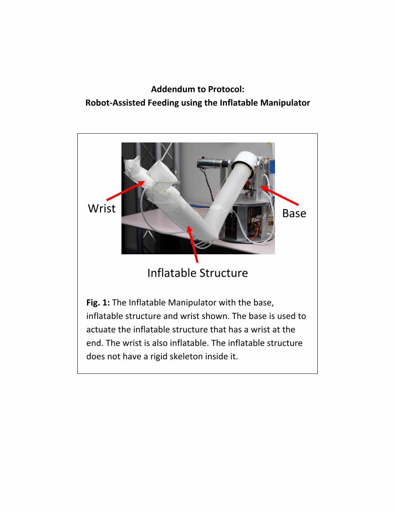
Addendum to Protocol:

Robot-Assisted Feeding using the Inflatable Manipulator

Base

Inflatable Structure

Wrist

Fig. 1: The Inflatable Manipulator with the base,

inflatable structure and wrist shown. The base is used to

actuate the inflatable structure that has a wrist at the

end. The wrist is also inflatable. The inflatable structure

does not have a rigid skeleton inside it.

Carnegie Mellon University

Consent Form for Participation in Research

IRB No: [this section will be completed by the IRB office] page 1 Approved: Expires: Modified: Version 4/2010

Study Title: Robot-Assisted Feeding using the Inflatable Manipulator Principal Investigator: Siddharth Sanan The Robotics Institute NSH A428 Pittsburgh, PA 15213 Email: sanan@cmu.edu 412-999-6115 Faculty Advisor: Christopher G. Atkeson The Robotics Institute NSH A428 Pittsburgh, PA 15213 Email: cga@cmu.edu _______________________________________________________________________________ Purpose of this Study The purpose of this study is to evaluate usability of a new inflatable robotic arm (as shown in Fig. 1) for providing assistance to adults during a feeding task. The data gathered from the study will be used to improve the design and functionality of the inflatable robotic arm.

Fig. 1: Inflatable Robotic Arm

Carnegie Mellon University

Consent Form for Participation in Research

IRB No: [this section will be completed by the IRB office] page 2 Approved: Expires: Modified: Version 4/2010

Procedures This study is estimated to take 1 hour to complete and will be conducted at the following address: Carnegie Mellon University 5000 Forbes Ave Newell Simon Hall A428 Pittsburgh, PA 15213 In this study, you will be fed a food item with the help of an inflatable robotic arm (Fig. 1). The task of feeding will be divided into four smaller tasks: 1) robot picking up food, 2) robot bringing the food item close to your mouth, 3) you eating the food item, and 4) robot wiping your face (optional). This series of tasks will be repeated at least three times. After the feeding task is completed, you will be asked to rate your experience with the robot arm by responding to a questionnaire and/or verbal questions. The entire study will be video recorded. The details of the procedures are given below:

1. You will be shown a video of the inflatable robotic arm feeding a person.

2. You will then be familiarized with the robot arm and oriented to its functionalities. You will be shown how to STOP the robot at any time during the task. There is no harm to the robot if you issue a stop command, so you should not hesitate to issue a stop command at any time.

3. You will be informed of the food item being used in the task. If the food item is not to your preference, you can request the use of a different food item that is available.

4. At this point, you will be provided with protective eyewear that you will be required to wear during the task. Aprons and bibs will also be made available and you can choose to wear these.

5. When you are ready to proceed with the feeding task, the investigator will command the robot to pick up the food item using a spoon from a dish in front of you.

6. After the robot arm finishes picking up the food item, the investigator will ask the robot to bring food close to your mouth.

7. When the robot arm brings the food close to your mouth, the investigator will ask you to eat the food item from the spoon.

8. After eating the food item, if you wish to wipe your face, you may indicate this to the investigator. If you do so, the investigator will command the robot arm to wipe your face with a towel. You can choose to skip this step.

9. The feeding task (steps 5 to 8) will be repeated at least 3 times.

10. After completing the feeding task with the robot arm, you will be asked to rate your experience with the robot arm by responding to a questionnaire and/or verbal questions.

Carnegie Mellon University

Consent Form for Participation in Research

IRB No: [this section will be completed by the IRB office] page 3 Approved: Expires: Modified: Version 4/2010

Participant Requirements You must be above the age of 18 to participate and have no physical or mental disabilities. You must be able to read and understand the contents of this consent form. Risks During the task, the inflatable robotic arm may have accidental contact with you. Since the arm has a soft and lightweight inflatable structure, accidental contact poses minimal risk of physical injury to you. To minimize any risk of injury due to the spoon attached at the end of the inflatable arm, it will be made of plastic and will have rounded edges. You will be provided with protective eyewear during the study to prevent any accidental contact of the arm with your eyes. You may also not be certain of the robot’s intent and actions during the task. To reduce your discomfort regarding the robot’s movements, the investigator will familiarize you with the robot and its functions. The investigator will be present during the entire duration of the task and can stop the robot at any time. You will also have the ability to stop the robot at any time during the task using the provided stop button. You will be shown how to use this stop button before the feeding task begins. Food spillage may also occur during the task. Aprons and bibs will be available for use by you during the study. There is a risk that confidentiality of your personal identifiable information may be compromised. This risk will be minimized by assigning a unique case number to the data collected from this study. The information linking the case number to your identity will be stored electronically in a secure machine with restricted access. The study data and consent forms will be stored in separate secure locations at CMU, with access available only to the investigators involved in the study. Your email address will be kept confidential. All email correspondence with you was carried out via a secure CMU email account that is accessible by only the PI of the study. Benefits There is no personal benefit to you from your participation in the study, but the knowledge received may be of value to robotics research conducted at Carnegie Mellon University and humanity. Compensation & Costs You will be compensated $20 (cash) upon completion of the study. Partial payment will not be given if you choose to withdraw from the study at any time.

Carnegie Mellon University

Consent Form for Participation in Research

IRB No: [this section will be completed by the IRB office] page 4 Approved: Expires: Modified: Version 4/2010

There will be no cost to you if you participate in this study. Confidentiality By participating in the study, you understand and agree that Carnegie Mellon may be required to disclose your consent form, data and other personally identifiable information as required by law, regulation, subpoena or court order. Otherwise, your confidentiality will be maintained in the following manner: Your data and consent form will be kept separate. Your consent form will be stored in a locked location on Carnegie Mellon property and will not be disclosed to third parties. By participating, you understand and agree that the data and information gathered during this study may be used by Carnegie Mellon and published and/or disclosed by Carnegie Mellon to others outside of Carnegie Mellon. However, your name, address, contact information and other direct personal identifiers in your consent form will not be mentioned in any such publication or dissemination of the research data and/or results by Carnegie Mellon. The researchers will take the following steps to protect participants’ identities during this study: (1) Each subject will be assigned a unique number; (2) The researchers will record any data collected during the study by number, not by name; (3) Only members of the research group will view collected data in detail; (4) Any recordings or data files will be stored in a secured location accessed only by authorized researchers. Optional Permission I understand that the researchers may want to use portions of any video or audio recording for illustrative reasons in presentations of this work for scientific or educational purposes, including videos put on the internet (research web pages, youtube.com, etc.). I give my permission to do so provided that my name will not appear.

YES NO (Please initial here ________) Rights Your participation is voluntary. You are free to stop your participation at any point. Refusal to participate or withdrawal of your consent or discontinued participation in the study will not result in any penalty or loss of benefits or rights to which you might otherwise be entitled. The Principal Investigator may at his/her discretion remove you from the study for any of a number of reasons. In such an event, you will not suffer any penalty or loss of benefits or rights which you might otherwise be entitled.

Carnegie Mellon University

Consent Form for Participation in Research

IRB No: [this section will be completed by the IRB office] page 5 Approved: Expires: Modified: Version 4/2010

Right to Ask Questions & Contact Information If you have any questions about this study, you should feel free to ask them now. If you have questions later, desire additional information, or wish to withdraw your participation please contact the Principal Investigator by mail, phone or e-mail in accordance with the contact information listed on the first page of this consent. If you have questions pertaining to your rights as a research participant; or to report objections to this study, you should contact the Research Regulatory Compliance Office at Carnegie Mellon University. Email: irb-review@andrew.cmu.edu . Phone: 412-268-1901 or 412-268-5460. Voluntary Consent By signing below, you agree that the above information has been explained to you and all your current questions have been answered. You understand that you may ask questions about any aspect of this research study during the course of the study and in the future. By signing this form, you agree to participate in this research study. PARTICIPANT SIGNATURE DATE I certify that I have explained the nature and purpose of this research study to the above individual and I have discussed the potential benefits and possible risks of participation in the study. Any questions the individual has about this study have been answered and any future questions will be answered as they arise. SIGNATURE OF PERSON OBTAINING CONSENT DATE

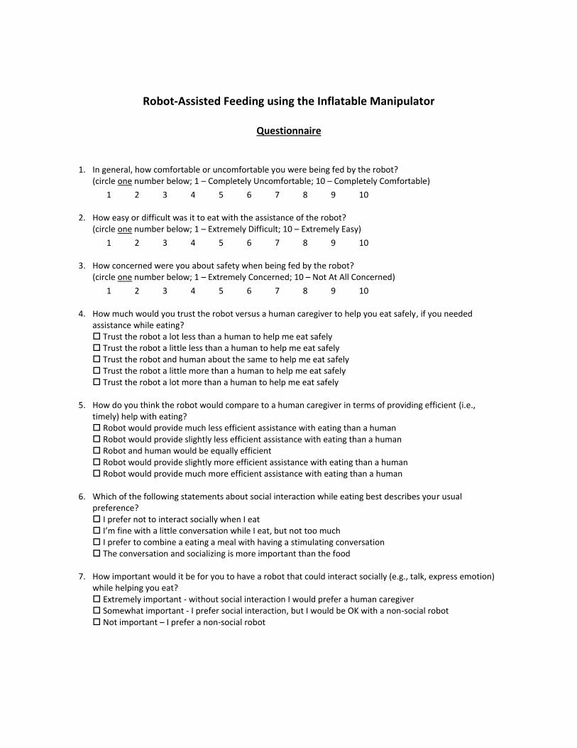
Robot-Assisted Feeding using the Inflatable Manipulator

Questionnaire

1. In general, how comfortable or uncomfortable you were being fed by the robot? (circle one number below; 1 – Completely Uncomfortable; 10 – Completely Comfortable)

1 2 3 4 5 6 7 8 9 10 2. How easy or difficult was it to eat with the assistance of the robot? (circle one number below; 1 – Extremely Difficult; 10 – Extremely Easy)

1 2 3 4 5 6 7 8 9 10 3. How concerned were you about safety when being fed by the robot? (circle one number below; 1 – Extremely Concerned; 10 – Not At All Concerned)

1 2 3 4 5 6 7 8 9 10 4. How much would you trust the robot versus a human caregiver to help you eat safely, if you needed

assistance while eating? Trust the robot a lot less than a human to help me eat safely Trust the robot a little less than a human to help me eat safely Trust the robot and human about the same to help me eat safely Trust the robot a little more than a human to help me eat safely Trust the robot a lot more than a human to help me eat safely

5. How do you think the robot would compare to a human caregiver in terms of providing efficient (i.e.,

timely) help with eating? Robot would provide much less efficient assistance with eating than a human Robot would provide slightly less efficient assistance with eating than a human Robot and human would be equally efficient Robot would provide slightly more efficient assistance with eating than a human Robot would provide much more efficient assistance with eating than a human

6. Which of the following statements about social interaction while eating best describes your usual

preference? I prefer not to interact socially when I eat I’m fine with a little conversation while I eat, but not too much I prefer to combine a eating a meal with having a stimulating conversation The conversation and socializing is more important than the food

7. How important would it be for you to have a robot that could interact socially (e.g., talk, express emotion)

while helping you eat? Extremely important - without social interaction I would prefer a human caregiver Somewhat important - I prefer social interaction, but I would be OK with a non-social robot Not important – I prefer a non-social robot

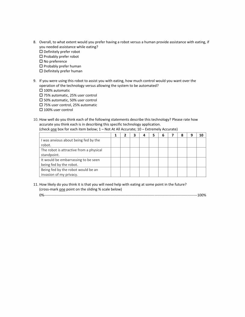
8. Overall, to what extent would you prefer having a robot versus a human provide assistance with eating, if you needed assistance while eating? Definitely prefer robot Probably prefer robot No preference Probably prefer human Definitely prefer human

9. If you were using this robot to assist you with eating, how much control would you want over the

operation of the technology versus allowing the system to be automated? 100% automatic 75% automatic, 25% user control 50% automatic, 50% user control 75% user control, 25% automatic 100% user control

10. How well do you think each of the following statements describe this technology? Please rate how

accurate you think each is in describing this specific technology application. (check one box for each item below; 1 – Not At All Accurate; 10 – Extremely Accurate)

1 2 3 4 5 6 7 8 9 10

I was anxious about being fed by the robot.

The robot is attractive from a physical standpoint.

It would be embarrassing to be seen being fed by the robot.

Being fed by the robot would be an invasion of my privacy.

11. How likely do you think it is that you will need help with eating at some point in the future? (cross-mark one point on the sliding % scale below)

0%------------------------------------------------------------------------------------------------------------------------------100%

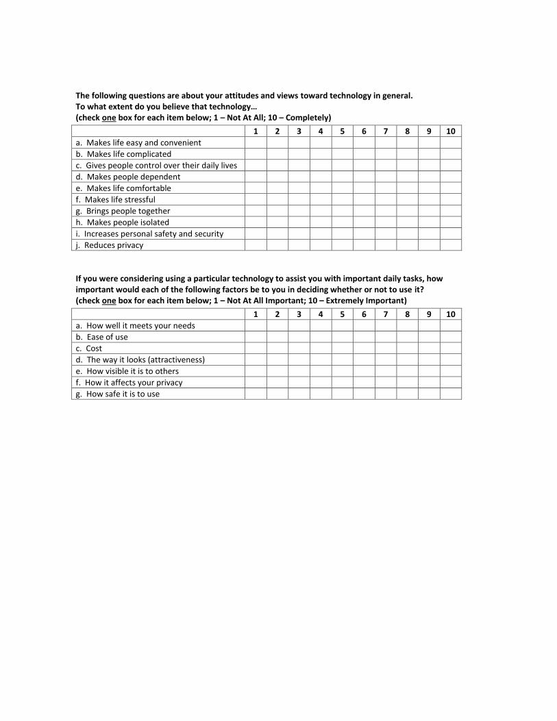
The following questions are about your attitudes and views toward technology in general. To what extent do you believe that technology… (check one box for each item below; 1 – Not At All; 10 – Completely)

1 2 3 4 5 6 7 8 9 10

a. Makes life easy and convenient

b. Makes life complicated

c. Gives people control over their daily lives

d. Makes people dependent

e. Makes life comfortable

f. Makes life stressful

g. Brings people together

h. Makes people isolated

i. Increases personal safety and security

j. Reduces privacy

If you were considering using a particular technology to assist you with important daily tasks, how important would each of the following factors be to you in deciding whether or not to use it? (check one box for each item below; 1 – Not At All Important; 10 – Extremely Important)

1 2 3 4 5 6 7 8 9 10

a. How well it meets your needs

b. Ease of use

c. Cost

d. The way it looks (attractiveness)

e. How visible it is to others

f. How it affects your privacy

g. How safe it is to use

Background Please answer the following questions. All of your answers will be treated confidentially. If there is a question you do not wish to answer, please leave it blank and go on to the next question. Thank you in advance for your help. Gender: □ Male □ Female Age: _____ What is your highest level of education?

□ No formal education □ Less than high school graduate □ High school graduate / GED □ Vocational training □ Some college / Associate’s degree □ Bachelor’s degree (BA, BS) □ Master’s degree (or other post-graduate training) □ Doctoral degree (PhD, MD, EdD, DDS, JD, etc.)

Current marital status

□ Single □ Married □ Separated □ Divorced □ Widowed □ Other (please specify) ______________________________________________

Do you consider yourself Hispanic or Latino?

□ Yes □ No

How would you describe your primary racial group?

□ No primary group □ White Caucasian □ Black / African American □ Asian □ American Indian / Alaska Native □ Native Hawaiian / Pacific Islander □ Multi-racial □ Other (please specify) ______________________________________________

Which category best describes your yearly household income? (Do not give the dollar amount, just check the category.)

□ Less than $5,000 □ $5,000-$9,999 □ $10,000-$14,999 □ $15,000-$19,999 □ $20,000-$29,999

□ $30,000-$39,999 □ $40,000-$49,999 □ $50,000-$59,999 □ $60,000-$69,999 □ $70,000-$99,999 □ $100,000 or more □ Do not know for certain □ Do not wish to answer

What is your primary occupational status?

□ Work full-time □ Work part-time □ Student □ Homemaker □ Retired □ Volunteer worker □ Seeking employment, laid off, etc. □ Other (please specify) ______________________________________________

Have you ever interacted with anyone (e.g., family member, friend, co-worker) who needed assistance with eating? □ Yes □ No Do you know anyone (family, friend, co-worker), who because of a health problem, needs assistance with (Check one or many):

□ Bathing □ Dressing □ Grooming (e.g., shaving, brushing teeth) □ Feeding □ Taking medications □ Completing other treatments (e.g., exercise, speech therapy, special diet) □ Transferring in and out of bed or chair □ Walking □ Preparing meals □ Doing laundry □ Cleaning □ Shopping □ Transportation □ Going to medical appointments □ Other (please specify) ____________________________________________

Have you ever interacted with a robot before? □ Yes □ No (If yes), What kind of robot was it? What was the name and what did you do with the robot?

________________________________________________________________________

Bibliography

[1] D.L. Allsop, T.R. Perl, and C.Y. Warner. Force/Deflection and Fracture Characteristics of

the Temporor-Parietal Region of the Human Head. 1991.

[2] D.L. Allsop, C.Y. Warner, M.G. Wille, D.C. Schneider, and A.M. Nahum. Facial Impact

Response–A Comparison of the Hybrid III Dummy and Human Cadaver. 1988.

[3] I. Asimov. The Caves of Steel. 1954.

[4] C.G. Atkeson, A.W. Moore, and S. Schaal. Locally weighted learning. Artificial Intell. Rev.,

11(1):11–73, 1997.

[5] R. Baldur and W. Blach. Inflatable manipulator. Society of Manufacturing Engineers, 1985.

[6] E. Barbieri and U. Ozguner. A new minimum-time control law for a one-mode model of a

flexible slewing structure. IEEE Transactions on Automatic Control, 38(1):142–146, 1993.

[7] Luca Bascetta and P Rocco. Task space visual servoing of eye-in-hand flexible manipulators.

In Advanced Intelligent Mechatronics, 2003. AIM 2003. Proceedings. 2003 IEEE/ASME

International Conference on, volume 2, pages 1442–1448. IEEE, 2003.

[8] A. Bicchi and G. Tonietti. Fast and soft-arm tactics. IEEE Robot. Autom. Mag., 11(2):22–33,

2004.

210

[9] J.N. Bricout, J.C. Debus, and P. Micheau. A finite element model for the dynamics of

flexible manipulators. Mech. Mach. Theory., 25(1):119–128, 1990.

[10] Samuel R Buss. Introduction to inverse kinematics with jacobian transpose, pseudoinverse

and damped least squares methods. IEEE Journal of Robotics and Automation, 17, 2004.

[11] R.H. Cannon Jr and E. Schmitz. Initial experiments on the end-point control of a flexible

one-link robot. The International Journal of Robotics Research, 3(3):62, 1984.

[12] J.L. Chang and Y.P. Chen. Force control of a single-link flexible arm using sliding-mode

theory. Journal of vibration and control, 4(2):187, 1998.

[13] B.C. Chiou and M. Shahinpoor. Dynamic stability analysis of a one-link force-controlled

flexible manipulator. Journal of robotic systems, 5(5):443–451, 2007.

[14] G.S. Chirikjian. Hyper-redundant manipulator dynamics: A continuum approximation. Ad-

vanced Robotics, 9(3):217–243, 1994.

[15] G.S. Chirikjian and J.W. Burdick. Kinematics of hyper-redundant manipulators. In Proc.

2nd International Workshop on Advances in Robot Kinematics, Linz, page 392, 1990.

[16] G.S. Chirikjian and J.W. Burdick. A modal approach to hyper-redundant manipulator kine-

matics. IEEE Trans. Robot. Autom., 10(3):343–354, Jun 1994.

[17] G.S. Chirikjian and JW Burdick. Design and Experiments with a 30 DOF Robot. In Robotics

and Automation, 1993. Proceedings., 1993 IEEE International Conference on, pages 113–

119. IEEE, 2002.

[18] Wonseok Choi and Nancy B Powell. Three dimensional seamless garment knitting on v-

bed flat knitting machines. Journal of Textile and Apparel, Technology and Management,

4(3):1–33, 2005.

211

[19] C.P. Chou and B. Hannaford. Measurement and modeling of mckibben pneumatic artificial

muscles. Robotics and Automation, IEEE Transactions on, 12(1):90–102, 1996.

[20] W.S. Cleveland and S.J. Devlin. Locally weighted regression: an approach to regression

analysis by local fitting. J. Amer. Stat. Assoc., 83(403):596–610, 1988.

[21] RL Comer and S. Levy. Deflections of an inflated circular-cylindrical cantilever beam. AIAA

journal, 1(7), 2012.

[22] J.J. Craig. Introduction to Robotics. Addison-Wesley Reading, MA, 1989.

[23] F. Daerden and D. Lefeber. Pneumatic artificial muscles: actuators for robotics and au-

tomation. European journal of mechanical and environmental engineering, 47(1):11–21,

2002.

[24] A. De Luca and B. Siciliano. Closed-form dynamic model of planar multilink lightweight

robots. Systems, Man and Cybernetics, IEEE Transactions on, 21(4):826–839, 2002.

[25] S.K. Dwivedy and P. Eberhard. Dynamic analysis of flexible manipulators, a literature

review. Mechanism and Machine Theory, 41(7):749–777, 2006.

[26] S. Eppinger and W. Seering. Understanding bandwidth limitations in robot force control. In

IEEE International Conference on Robotics and Automation, volume 4, pages 904 – 909,

Mar 1987.

[27] RL Farrenkopf. Optimal open-loop maneuver profiles for flexible spacecraft. Journal of

Guidance, Control, and Dynamics, 2(6):491–498, 1979.

[28] Festo AG. Festo Handling Assistant.

[29] WB Fichter. A theory for inflated thin-wall cylindrical beams. National Aeronautics and

Space Administration, 1966.

212

[30] Javad Foroughi, Geoffrey M Spinks, Gordon G Wallace, Jiyoung Oh, Mikhail E Kozlov,

Shaoli Fang, Tissaphern Mirfakhrai, John DW Madden, Min Kyoon Shin, Seon Jeong Kim,

et al. Torsional carbon nanotube artificial muscles. Science, 334(6055):494–497, 2011.

[31] EC Framework. Improved Frontal Impact Protection through a World Frontal Impact

Dummy. Project No. GRD1 1999, 10559, 2003.

[32] G. Gilardi and I. Sharf. Literature survey of contact dynamics modelling. Mechanism and

Machine Theory, 37(10):1213–1239, 2002.

[33] M.D. Gilchrist, S. Keenan, M. Curtis, M. Cassidy, G. Byrne, and M. Destrade. Measuring

knife stab penetration into skin simulant using a novel biaxial tension device. Forensic

science international, 177(1):52–65, 2008.

[34] M.D. Gilchrist, S. Keenan, M. Curtis, M. Cassidy, G. Byrne, and M. Destrade. Mechanics

of Stabbing: Biaxial Measurement of Knife Stab Penetration of Skin Simulant. Imprint,

2008.

[35] W. Goldsmith. Impact: the theory and physical behaviour of colliding solids. Dover Pubns,

2001.

[36] I.A. Gravagne, C.D. Rahn, and I.D. Walker. Large deflection dynamics and control for

planar continuum robots. IEEE/ASME transactions on mechatronics, 8(2):299–307, 2003.

[37] I.A. Gravagne and I.D. Walker. Kinematic transformations for remotely-actuated planar

continuum. In IEEE Conf. on Robotics and Automation, pages 19–26, 2000.

[38] I.A. Gravagne and I.D. Walker. On the kinematics of remotely-actuated continuum

robots. In IEEE International Conference on Robotics and Automation, 2000. Proceedings.

ICRA’00, volume 3, 2000.

213

[39] I.A. Gravagne and I.D. Walker. On the kinematics of remotely-actuated continuum robots.

In Proc. 2000 IEEE Int. Conf. Robot. Autom. (ICRA), volume 3, pages 2544–2550, 2000.

[40] S. Haddadin, A. Albu-Schaffer, and G. Hirzinger. Safe physical human-robot interaction:

measurements, analysis & new insights. In 2007 Int. Symp. Robot. Res. (ISRR), Hiroshima,

Japan, 2007.

[41] Sami Haddadin, Alin Albu-Schaffer, and Gerd Hirzinger. Requirements for Safe Robots:

Measurements, Analysis and New Insights. The International Journal of Robotics Research,

28(11-12):1507–1527, 2009.

[42] S.V. Hainsworth, R.J. Delaney, and G.N. Rutty. How sharp is sharp? Towards quantification

of the sharpness and penetration ability of kitchen knives used in stabbings. International

Journal of Legal Medicine, 122(4):281–291, 2008.

[43] MW Hannan and ID Walker. Analysis and initial experiments for a novel elephant’s trunk

robot. In Intelligent Robots and Systems, 2000.(IROS 2000). Proceedings. 2000 IEEE/RSJ

International Conference on, volume 1, pages 330–337. IEEE, 2002.

[44] G. Hastings and W. Book. Reconstruction and robust reduced-order observation of flexible

variables. In ASME, Winter Annual Meeting, Annaheim, CA, page 1986, 1986.

[45] G. Hastings and W. Book. Verification of a linear dynamic model for flexible robotic manip-

ulators. In 1986 IEEE International Conference on Robotics and Automation. Proceedings,

volume 3, 1986.

[46] Chi haur Wu and Richard P. Paul. Manipulator compliance based on joint torque control.

In Decision and Control including the Symposium on Adaptive Processes, 1980 19th IEEE

Conference on, volume 19, pages 88–94, Dec. 1980.

214

[47] Kenneth L Hillsley and Stephen Yurkovich. Vibration control of a two-link flexible robot

arm. Dynamics and Control, 3(3):261–280, 1993.

[48] H.O.S. Hirose, A. Ochiai, and T. Aoki. Study on Slime Robot. In Proc. IEEE Int. Conf.

Robot. Autom, pages 2808–2813, 2004.

[49] N. Hogan and E. Colgate. Robotics Review. Cambridge, MA (US); MIT Press, 1989.

[50] L.L. Howell. Compliant mechanisms. Wiley-Interscience, 2001.

[51] LL Howell and A. Midha. A method for the design of compliant mechanisms with small-

length flexural pivots. Journal of Mechanical Design, 116:280, 1994.

[52] L.L. Howell, A. Midha, and T.W. Norton. Evaluation of equivalent spring stiffness for

use in a pseudo-rigid-body model of large-deflection compliant mechanisms. Journal of

Mechanical Design, 118:126, 1996.

[53] J. Hurst, J. Chestnutt, and A. Rizzi. An actuator with physically variable stiffness for highly

dynamic legged locomotion. In IEEE International Conference on Robotics and Automa-

tion, volume 5, pages 4662–4667. Citeseer, 2004.

[54] R.L. Huston and Y. Wang. Flexibility effects in multibody systems. Computer-Aided Anal-

ysis of Rigid and Flexible Mechanical Systems, pages 351–376, 1993.

[55] F. Ilievski, A.D. Mazzeo, R.F. Shepherd, X. Chen, and G.M. Whitesides. Soft robotics for

chemists. Angewandte Chemie, 123(8):1930–1935, 2011.

[56] K.L. Johnson. Contact mechanics. Cambridge Univ Pr, 1987.

[57] Ben Jonker. A finite element dynamic analysis of spatial mechanisms with flexible links.

Computer Methods in Applied Mechanics and Engineering, 76(1):17–40, 1989.

215

[58] I. Kao, K. Lynch, and J.W. Burdick. Springer handbook of robotics. Springer-Verlag New

York Inc, 2008.

[59] Rafael Kelly. Robust asymptotically stable visual servoing of planar robots. Robotics and

Automation, IEEE Transactions on, 12(5):759–766, 1996.

[60] Y.A. Khulief and A.A. Shabana. Impact responses of multi-body systems with consistent

and lumped masses. Journal of Sound Vibration, 104:187–207, 1986.

[61] S. Kota, J. Joo, Z. Li, S.M. Rodgers, and J. Sniegowski. Design of compliant mecha-

nisms: applications to MEMS. Analog Integrated Circuits and Signal Processing, 29(1):7–

15, 2001.

[62] Rebecca K Kramer, Carmel Majidi, Ranjana Sahai, and Robert J Wood. Soft curvature

sensors for joint angle proprioception. In Intelligent Robots and Systems (IROS), 2011

IEEE/RSJ International Conference on, pages 1919–1926. IEEE, 2011.

[63] Konstantinos J Kyriakopoulos and George N Saridis. Minimum jerk path generation. In

Robotics and Automation, 1988. Proceedings., 1988 IEEE International Conference on,

pages 364–369. IEEE, 1988.

[64] A. V. Le and C. Wielgosz. Bending and buckling of inflatable beams: Some new theoretical

results. J. Thin-Walled Struct., 43(8):1166–1187, 2005.

[65] YF Li and XB Chen. End-point sensing and state observation of a flexible-link robot.

Mechatronics, IEEE/ASME Transactions on, 6(3):351–356, 2001.

[66] Sonja Macfarlane and Elizabeth A Croft. Jerk-bounded manipulator trajectory planning: de-

sign for real-time applications. Robotics and Automation, IEEE Transactions on, 19(1):42–

52, 2003.

216

[67] Sebastian OH Madgwick, Andrew JL Harrison, and Ravi Vaidyanathan. Estimation of

imu and marg orientation using a gradient descent algorithm. In Rehabilitation Robotics

(ICORR), 2011 IEEE International Conference on, pages 1–7. IEEE, 2011.

[68] JA Main, SW Peterson, and AM Strauss. Load-deflection behavior of space-based inflatable

fabric beams. Journal of Aerospace Engineering, 7(2):225–238, 1994.

[69] D. Maruyama, H. Kimura, M. Koseki, and N. Inou. Driving force and structural strength

evaluation of a flexible mechanical system with a hydrostatic skeleton. Journal of Zhejiang

University-Science A, 11(4):255–262, 2010.

[70] M.T. Mason. Compliance and Force Control. IEEE Trans. Sys. Man Cyb, 6:418–432, 1981.

[71] C.T. McCarthy, A.N. Annaidh, and M.D. Gilchrist. On the sharpness of straight edge blades

in cutting soft solids: Part II-Analysis of blade geometry. Engineering Fracture Mechanics,

2009.

[72] C.T. McCarthy, M. Hussey, and M.D. Gilchrist. On the sharpness of straight edge blades

in cutting soft solids: Part I–indentation experiments. Engineering Fracture Mechanics,

74(14):2205–2224, 2007.

[73] W. McMahan, B.A. Jones, and I.D. Walker. Design and implementation of a multi-section

continuum robot: Air-Octor. In 2005 IEEE/RSJ International Conference on Intelligent

Robots and Systems, 2005.(IROS 2005), pages 2578–2585, 2005.

[74] J. Melvin. Human tolerance to impact conditions as related to motor vehicle design. SAE

J885 APR80, 1980.

[75] H. Moulin and E. Bayo. On the accuracy of end-point trajectory tracking for flexible arms

by noncausal inverse dynamic solutions. Journal of Dynamic Systems, Measurement, and

Control, 113:320, 1991.

217

[76] A. Mozeika, E. Steltz, and H.M. Jaeger. The first steps of a robot based on jamming skin

enabled locomotion. In Proceedings of the 2009 IEEE/RSJ international conference on

Intelligent robots and systems, pages 408–409. IEEE Press, 2009.

[77] T. Mukai, M. Onishi, T. Odashima, S. Hirano, and Z. Luo. Development of the Tactile

Sensor System of a Human-Interactive Robot” RI-MAN”. IEEE Transactions on Robotics,

24(2):505, 2008.

[78] T. Mukai, M. Onishi, T. Odashima, S. Hirano, and Zhiwei Luo. Development of the tactile

sensor system of a human-interactive robot ri-man. IEEE. Trans. Robot., 24(2):505–512,

April 2008.

[79] S. Nagarajan and D.A. Turcic. Lagrangian Formulation of the Equations of Motion for Elas-

tic Mechanisms With Mutual Dependence Between Rigid Body and Elastic Motions: Part

II-System Equations. Journal of Dynamic Systems, Measurement, and Control, 112:215,

1990.

[80] A. Needleman. Inflation of spherical rubber balloons. International Journal of Solids and

Structures, 13(5):409–421, 1977.

[81] I. Newton, T. Leseur, and F. Jacquier. Philosophiae naturalis principia mathematica. 1833.

[82] Celia M Oakley and Robert H Cannon. End-point control of a two-link manipulator with

a very flexible forearm: Issues and experiments. In American Control Conference, 1989,

pages 1381–1389. IEEE, 1989.

[83] S. Oberer and R.D. Schraft. Robot-dummy crash tests for robot safety assessment. In

Robotics and Automation, 2007 IEEE International Conference on, pages 2934–2939, April

2007.

218

[84] P.T. O’Callaghan, M.D. Jones, D.S. James, S. Leadbeatter, C.A. Holt, and L.D.M. Nokes.

Dynamics of stab wounds: force required for penetration of various cadaveric human tissues.

Forensic science international, 104(2-3):173–178, 1999.

[85] L Ott, Ph Zanne, Fl Nageotte, M de Mathelin, and J Gangloff. Physiological motion rejec-

tion in flexible endoscopy using visual servoing. In Robotics and Automation, 2008. ICRA

2008. IEEE International Conference on, pages 2928–2933. IEEE, 2008.

[86] E. Paljug, T. Ohm, and S. Hayati. The JPL Serpentine Robot: a 12-DOF system for inspec-

tion. In Robotics and Automation, 1995. Proceedings., 1995 IEEE International Conference

on, volume 3, pages 3143–3148. IEEE, 2002.

[87] L.Y. Pao. Characteristics of the time-optimal control of flexible structures with damping. In

IEEE Conference on Control Applications, pages 1299–1304. Citeseer, 1994.

[88] Yong-Lae Park, Carmel Majidi, Rebecca Kramer, Phillipe Berard, and Robert J Wood. Hy-

perelastic pressure sensing with a liquid-embedded elastomer. Journal of Micromechanics

and Microengineering, 20(12):125029, 2010.

[89] G.A. Pratt and M.M. Williamson. Series elastic actuators. In Proc. 1995 IEEE/RSJ Int. Conf.

Intell. Robots Syst. (IROS) - ’Human Robot Interaction and Cooperative Robots’, volume 1,

pages 399–406, Aug 1995.

[90] G.A. Pratt and M.M. Williamson. Series elastic actuators. In Proceedings of the IEEE/RSJ

International Conference on Intelligent Robots and Systems (IROS-95), volume 1, pages

399–406, 1995.

[91] M.H. Raibert and J.J. Craig. Hybrid position/force control of manipulators. Journal of

Dynamic Systems, Measurement, and Control, 102(127):126–133, 1981.

219

[92] R.D. Robinett, C. Dohrmann, G.R. Eisler, J. Feddema, G.G. Parker, D.G. Wilson, and

D. Stokes. Flexible robot dynamics and controls. Kluwer Academic Pub, 2002.

[93] G. Robinson and JBC Davies. Continuum robots-a state of the art. In Robotics and Au-

tomation, 1999. Proceedings. 1999 IEEE International Conference on, volume 4, pages

2849–2854. IEEE, 2002.

[94] N. Salomonski, M. Shoham, and G. Grossman. Light robot arm based on inflatable structure.

CIRP Annals-Manufacturing Technology, 44(1):87–90, 1995.

[95] S. Sanan, P. Lynn, and S. T. Griffith. Pneumatic torsional actuators for inflatable robots. In

submitted, 2012.

[96] S. Sanan, P. Lynn, and S. T. Griffith. Pneuarm: An anthropomorphic pneumatically actuated

inflatable manipulator. submitted to the IEEE Transactions on Robotics, 2013.

[97] S. Sanan, J.B. Moidel, and C.G. Atkeson. Robots with Inflatable Links. In IEEE/RSJ

International Conference on Intelligent Robots and Systems, IROS 2009, pages 4331–4336,

2009.

[98] R. Schiavi, G. Grioli, S. Sen, and A. Bicchi. Vsa-ii: a novel prototype of variable stiffness

actuator for safe and performing robots interacting with humans. In IEEE International

Conference on Robotics and Automation, pages 2171 –2176, May 2008.

[99] W.O Schiehlen and J. Rauh. Modeling of flexible multibeam systems by rigid-elastic su-

perelements. Revista Brasiliera de Ciencias Mecanicas, 8(2), 1986.

[100] HF Schulte. The characteristics of the mckibben artificial muscle. The application of exter-

nal power in prosthetics and orthotics, pages 94–115, 1961.

[101] A.A. Shabana. Flexible multibody dynamics: review of past and recent developments.

Multibody system dynamics, 1(2):189–222, 1997.

220

[102] Robert F Shepherd, Filip Ilievski, Wonjae Choi, Stephen A Morin, Adam A Stokes, Aaron D

Mazzeo, Xin Chen, Michael Wang, and George M Whitesides. Multigait soft robot. Pro-

ceedings of the National Academy of Sciences, 108(51):20400–20403, 2011.

[103] Bruno Siciliano. An inverse kinematics scheme for a flexible arm in contact with a compliant

surface. In Decision and Control, 1998. Proceedings of the 37th IEEE Conference on,

volume 4, pages 3617–3622. IEEE, 1998.

[104] Bruno Siciliano. Closed-loop inverse kinematics algorithm for constrained flexible manip-

ulators under gravity. Journal of Robotic Systems, 16(6):353–362, 1999.

[105] N. Simaan, R. Taylor, and P. Flint. A dexterous system for laryngeal surgery. In Proc. 2004

IEEE Int. Conf. Robot. Autom. (ICRA), volume 1, pages 351–357, April-1 May 2004.

[106] N.C. Singer and W.P. Seering. Preshaping command inputs to reduce system vibration.

ASME, Transactions, Journal of Dynamic Systems, Measurement, and Control, 112:76–82,

1990.

[107] G. Singh, P. Kabamba, and N. McClamroch. Planar, time-optimal, rest-to-rest slewing ma-

neuvers of flexible spacecraft. Journal of Guidance, Control, and Dynamics, 12:71–81,

1989.

[108] W. Singhose, W. Seering, and N. Singer. Residual vibration reduction using vector diagrams

to generate shaped inputs. Journal of Mechanical Design, 116:654, 1994.

[109] J.J.E. Slotine, W. Li, et al. Applied nonlinear control, volume 461. Prentice hall Englewood

Cliffs, NJ, 1991.

[110] Otto JM Smith. Posicast control of damped oscillatory systems. Proceedings of the IRE,

45(9):1249–1255, 1957.

221

[111] Peter Staufer and Hubert Gattringer. Passivity-based tracking control of a flexible link robot.

In Multibody System Dynamics, Robotics and Control, pages 95–112. Springer, 2013.

[112] W.J. Stronge. Impact mechanics. Cambridge Univ. Pr., 2000.

[113] J.D. Suhey, N.H. Kim, and C. Niezrecki. Numerical modeling and design of inflat-

able structures–application to open-ocean-aquaculture cages. Aquacultural Engineering,

33(4):285–303, 2005.

[114] K. Suzumori, S. Iikura, and H. Tanaka. Development of flexible microactuator and its

applications torobotic mechanisms. In Proc. 1991 IEEE Int. Conf. Robot. Autom. (ICRA),

pages 1622–1627, 1991.

[115] R.J. Theodore and A. Ghosal. Comparison of the assumed modes and finite element mod-

els for flexible multilink manipulators. The International Journal of Robotics Research,

14(2):91, 1995.

[116] William T. Thomson. Theory of Vibration with Applications. Prentice Hall, 1988.

[117] M.O. Tokhi, Z. Mohamed, and A.K.M. Azad. Finite difference and finite element ap-

proaches to dynamic modelling of a flexible manipulator. Proceedings of the Institution

of Mechanical Engineers, Part I: Journal of Systems and Control Engineering, 211(2):145–

156, 1997.

[118] Azad A. K. M. Tokhi M. O. Flexible robot manipulators: modelling, simulation and control.

IET, 2008, 2008.

[119] G. Tonietti, R. Schiavi, and A. Bicchi. Design and control of a variable stiffness actuator

for safe and fast physical human/robot interaction. In IEEE International Conference on

Robotics and Automation, volume 1, page 526. IEEE; 1999, 2005.

222

[120] Anthony P Tzes and Stephen Yurkovich. Adaptive precompensators for flexible-link manip-

ulator control. In Decision and Control, 1989., Proceedings of the 28th IEEE Conference

on, pages 2083–2088. IEEE, 1989.

[121] R. Van Ham, B. Vanderborght, M. Van Damme, B. Verrelst, and D. Lefeber. MACCEPA, the

mechanically adjustable compliance and controllable equilibrium position actuator: Design

and implementation in a biped robot. Robotics and Autonomous Systems, 55(10):761–768,

2007.

[122] S.L. Veldman. Design and analysis methodologies for inflated beams. 2005.

[123] J. Versace. A review of the severity index. 1971.

[124] L. Villani and J. D. Schutter. Springer handbook of robotics. Springer-Verlag New York

Inc, 2008.

[125] S Voisembert, A Riwan, N Mechbal, and A Barraco. A novel inflatable robot with constant

and continuous volume. In Robotics and Automation (ICRA), 2011 IEEE International

Conference on, pages 5843–5848. IEEE, 2011.

[126] ID Walker. Some issues in creating invertebraterobots. In Proceedings of the International

Symposium on Adaptive Motion of Animals and Machines. Citeseer, 2000.

[127] P.K.C. Wang and J.D. Wei. Vibrations in a moving flexible robot arm. Journal of sound and

vibration, 116(1):149–160, 1987.

[128] Q.F. Wei, P.S. Krishnaprasad, and W.P. Dayawansa. Modeling of impact on a flexible beam.

1993.

[129] D.E. Whitney. Historical perspective and state of the art in robot force control. The Inter-

national Journal of Robotics Research, 6(1):3, 1987.

223

[130] A. Wolf, HB Brown, R. Casciola, A. Costa, M. Schwerin, E. Shamas, and H. Choset. A

mobile hyper redundant mechanism for search and rescue tasks. In Intelligent Robots and

Systems, 2003.(IROS 2003). Proceedings. 2003 IEEE/RSJ International Conference on, vol-

ume 3, pages 2889–2895. IEEE, 2004.

[131] S. Wolf and G. Hirzinger. A new variable stiffness design: matching requirements of the

next robot generation. In IEEE International Conference on Robotics and Automation, pages

19–23, 2008.

[132] KS Yeung and YP Chen. Regulation of a one-link flexible robot arm using sliding-mode

technique. International Journal of Control, 49(6):1965–1978, 1989.

[133] K.S. Yeung and Y.P. Chen. Sliding-mode controller design of a single-link flexible manipu-

lator under gravity. International Journal of Control, 52(1):101–117, 1990.

[134] A.S. Yigit, A.G. Ulsoy, and R.A. Scott. Dynamics of a radially rotating beam with impact,

Part 1: theoretical and computational model. Journal of Vibration and Acoustics, 112:65,

1990.

[135] A.S. Yigit, A.G. Ulsoy, and R.A. Scott. Dynamics of a radially rotating beam with impact,

part 2: experimental and simulation results. Journal of Vibration and Acoustics, 112:71,

1990.

[136] B.S. Yuan, J.D. Huggins, and W.J. Book. Small motion experiments on a large flexible arm

with strain feedback. In 1989 American Control Conference, 8 th, Pittsburgh, PA, pages

2091–2095, 1989.

[137] M. Zinn, O. Khatib, and B. Roth. A new actuation approach for human friendly robot

design. In Proc. 2004 IEEE Int. Conf. Robot. Autom. (ICRA), volume 1, pages 249–254,

April-1 May 2004.

224