
Socio-environmental modelling for sustainable development ... - UFZ
225
-
Upload
khangminh22 -
Category
Documents
-
view
5 -
download
0
Transcript of Socio-environmental modelling for sustainable development ... - UFZ


Socio-environmental modelling forsustainable development:
Exploring the interplay of formal insuranceand risk-sharing networks
Dissertation
zur Erlangung des akademischen GradesDoktor der Naturwissenschaften
(Dr. rer. nat.)
Universität OsnabrückFachbereich Mathematik/Informatik
vorgelegt von
Meike Willgeboren in Aschaffenburg
Oktober 2021


Abstract
As envisaged in the Sustainable Development Goals, eradicating poverty by 2030 is amongthe most important steps to achieve a better and more sustainable future. A key contributionto reach this target is to ensure that vulnerable households are effectively protected againstweather-related extreme events and other economic, social and ecological shocks and dis-asters. Insurance products specifically designed for the needs of low-income households indeveloping countries are seen as an effective instrument to encompass also the poor with anaffordable risk-coping mechanism and are thus highly promoted and supported by govern-ments in recent years. However, apart from direct positive effects, the introduction of formalinsurance may have unintended side effects. In particular, it might affect traditional risk-sharing arrangements where income losses are covered by an exchange of money, labour andin-kind goods between neighbours, relatives or friends. A weakening of informal safety netsmay increase social inequality if poor households cannot afford formal insurance. In order todesign insurance products in a sustainable way, sound understanding of their interplay withrisk-sharing networks is urgently needed.
Socio-environmental modelling is a suitable approach to address the complexity of this chal-lenge. In the first part of this thesis, an agent-based model is developed to investigate theeffects of formal insurance and informal risk-sharing on the resilience of smallholders. To laythe conceptual foundation for this approach, a literature review is presented which providesan overview of how to couple agent-based modelling with social network analysis. In twosubsequent modelling studies, it is analysed (i) how the introduction of insurance influencesthe overall welfare in a population and (ii) what determines the resilience of the poorest toshocks when income is heterogeneously distributed and not all households can afford formalinsurance. The simulation results underline the importance of designing insurance policiesin close alignment with established risk-coping arrangements to ensure sustainability whilestriving to eradicate poverty. It is shown that introducing formal insurance can have nega-tive side effects when insured households have fewer resources to share with their uninsuredpeers after paying the insurance premium or when they reduce their solidarity. However,especially when many households are simultaneously affected by a shock, e.g. by droughtsor floods, formal insurance is a valuable addition to informal risk-sharing. By applying aregression analysis to simulation results for an empirical network from the Philippines, it isfurthermore inferred that network characteristics must be considered in addition to individ-ual household properties to identify the most vulnerable households that neither have accessto formal insurance nor are adequately protected through informal risk-sharing.
In the second part of this thesis, a broader perspective is taken on the use of models in socio-environmental systems. First, it is envisioned how models in combination with empiricalstudies could improve insurance design under climate change. Second, requirements formaking socio-environmental modelling more useful to support policy and management andscientific results more influential on policy-making are synthesised.
Overall, this thesis offers new insights into the interplay of formal and informal risk-copinginstruments that complement existing empirical research and underlines the potential ofsocio-environmental modelling to address sustainability and development challenges.
iii


Contents
List of Figures ix
List of Tables xiii
1 Introduction 11.1 Background: Risk management with formal and informal instruments . . . . . 11.2 Methodological background: Socio-environmental modelling . . . . . . . . . . 3
1.2.1 Using models to address sustainability and development challenges . . 31.2.2 Using models to support policy and management . . . . . . . . . . . . . 4
1.3 Objectives and structure of this thesis . . . . . . . . . . . . . . . . . . . . . . . . 51.3.1 Overall structure . . . . . . . . . . . . . . . . . . . . . . . . . . . . . . . 51.3.2 Chapter overview . . . . . . . . . . . . . . . . . . . . . . . . . . . . . . . 6
I Modelling the interplay of formal insurance and risk-sharing networks 9
2 Combining social network analysis and agent-based modelling to explore dy-namics of human interaction: A review 112.1 Introduction . . . . . . . . . . . . . . . . . . . . . . . . . . . . . . . . . . . . . . 112.2 Methods . . . . . . . . . . . . . . . . . . . . . . . . . . . . . . . . . . . . . . . . 132.3 Potential of linking ABM with social networks . . . . . . . . . . . . . . . . . . . 13
2.3.1 Purpose . . . . . . . . . . . . . . . . . . . . . . . . . . . . . . . . . . . . . 152.3.1.1 Diffusion . . . . . . . . . . . . . . . . . . . . . . . . . . . . . . 152.3.1.2 Social integration . . . . . . . . . . . . . . . . . . . . . . . . . . 152.3.1.3 Recommendations . . . . . . . . . . . . . . . . . . . . . . . . . 16
2.3.2 Network integration . . . . . . . . . . . . . . . . . . . . . . . . . . . . . 162.3.2.1 Exogenously imposed and endogenously emerging networks . 162.3.2.2 Co-evolutionary networks . . . . . . . . . . . . . . . . . . . . . 162.3.2.3 Recommendations . . . . . . . . . . . . . . . . . . . . . . . . . 17
2.3.3 Types of analysis . . . . . . . . . . . . . . . . . . . . . . . . . . . . . . . 182.3.3.1 Agent-centric analysis . . . . . . . . . . . . . . . . . . . . . . . 192.3.3.2 Network-centric analysis . . . . . . . . . . . . . . . . . . . . . 202.3.3.3 Structurally explicit analysis . . . . . . . . . . . . . . . . . . . 202.3.3.4 Recommendations . . . . . . . . . . . . . . . . . . . . . . . . . 21
2.3.4 Condensed classification of models included in the review . . . . . . . 212.4 Conceptualization and documentation of social networks in agent-basedmodels 24
2.4.1 Incorporating theoretical and empirical insights . . . . . . . . . . . . . 242.4.2 Guidelines for model set-up and evaluation . . . . . . . . . . . . . . . . 24
2.5 Conclusion . . . . . . . . . . . . . . . . . . . . . . . . . . . . . . . . . . . . . . . 27
3 Informal risk-sharing between smallholders may be threatened by formal in-surance: Lessons from a stylized agent-based model 293.1 Introduction . . . . . . . . . . . . . . . . . . . . . . . . . . . . . . . . . . . . . . 29
v

Contents
3.2 Methods . . . . . . . . . . . . . . . . . . . . . . . . . . . . . . . . . . . . . . . . 313.2.1 Model description . . . . . . . . . . . . . . . . . . . . . . . . . . . . . . . 313.2.2 Parameter selection . . . . . . . . . . . . . . . . . . . . . . . . . . . . . . 33
3.3 Results . . . . . . . . . . . . . . . . . . . . . . . . . . . . . . . . . . . . . . . . . 343.3.1 Effectiveness of risk-coping instruments over time . . . . . . . . . . . . 343.3.2 Effectiveness of risk-coping instruments for different external conditions 373.3.3 Effectiveness of risk-coping instruments for covariate shocks . . . . . . 38
3.4 Discussion . . . . . . . . . . . . . . . . . . . . . . . . . . . . . . . . . . . . . . . 393.5 Conclusion . . . . . . . . . . . . . . . . . . . . . . . . . . . . . . . . . . . . . . . 42
4 Determinants of household resilience in networks with formal insurance andinformal risk-sharing 454.1 Introduction . . . . . . . . . . . . . . . . . . . . . . . . . . . . . . . . . . . . . . 454.2 Methods . . . . . . . . . . . . . . . . . . . . . . . . . . . . . . . . . . . . . . . . 47
4.2.1 Model description and parametrization . . . . . . . . . . . . . . . . . . 474.2.2 Case study . . . . . . . . . . . . . . . . . . . . . . . . . . . . . . . . . . . 49
4.3 Results . . . . . . . . . . . . . . . . . . . . . . . . . . . . . . . . . . . . . . . . . 504.3.1 Effectiveness of informal risk-sharing . . . . . . . . . . . . . . . . . . . . 504.3.2 Determinants for the survival of the poorest . . . . . . . . . . . . . . . . 524.3.3 Transferability to the empirical network . . . . . . . . . . . . . . . . . . 534.3.4 Transferability to different external conditions . . . . . . . . . . . . . . 564.3.5 Transferability to covariate shocks . . . . . . . . . . . . . . . . . . . . . 57
4.4 Discussion . . . . . . . . . . . . . . . . . . . . . . . . . . . . . . . . . . . . . . . 584.5 Conclusion . . . . . . . . . . . . . . . . . . . . . . . . . . . . . . . . . . . . . . . 61
II Using models to address socio-environmental challenges 63
5 Improving insurance design under climate change: Combining empirical ap-proaches and modelling 655.1 Introduction . . . . . . . . . . . . . . . . . . . . . . . . . . . . . . . . . . . . . . 655.2 Strengths and limitations of current methods to evaluate insurance design . . 67
5.2.1 Experimental games . . . . . . . . . . . . . . . . . . . . . . . . . . . . . 675.2.2 Econometric analysis of household surveys . . . . . . . . . . . . . . . . 685.2.3 Process-based crop models . . . . . . . . . . . . . . . . . . . . . . . . . . 695.2.4 Agent-based models . . . . . . . . . . . . . . . . . . . . . . . . . . . . . . 69
5.3 Synergies between different approaches to improve insurance design . . . . . . 705.3.1 Interplay between empirical data and ABMs . . . . . . . . . . . . . . . . 705.3.2 Interplay between ABMs and process-based crop models . . . . . . . . 72
5.4 Conclusions . . . . . . . . . . . . . . . . . . . . . . . . . . . . . . . . . . . . . . 73
6 How to make socio-environmental modelling more useful to support policy andmanagement? 756.1 Introduction . . . . . . . . . . . . . . . . . . . . . . . . . . . . . . . . . . . . . . 756.2 Methods . . . . . . . . . . . . . . . . . . . . . . . . . . . . . . . . . . . . . . . . 77
6.2.1 Interview framework . . . . . . . . . . . . . . . . . . . . . . . . . . . . . 776.2.2 Interviews . . . . . . . . . . . . . . . . . . . . . . . . . . . . . . . . . . . 776.2.3 Gradients to describe good practice examples . . . . . . . . . . . . . . . 78
6.2.3.1 Purpose . . . . . . . . . . . . . . . . . . . . . . . . . . . . . . . 786.2.3.2 Processes . . . . . . . . . . . . . . . . . . . . . . . . . . . . . . 78
vi
Contents
6.2.3.3 Partnerships . . . . . . . . . . . . . . . . . . . . . . . . . . . . . 786.2.3.4 Products . . . . . . . . . . . . . . . . . . . . . . . . . . . . . . . 80
6.3 Good practice examples . . . . . . . . . . . . . . . . . . . . . . . . . . . . . . . . 806.4 Results: Observed patterns in good practice examples . . . . . . . . . . . . . . 846.5 Discussion: Specific recommendations for SES Modelling . . . . . . . . . . . . 86
6.5.1 Purpose: Human dimension . . . . . . . . . . . . . . . . . . . . . . . . . 866.5.2 Processes: Data availability and accessibility . . . . . . . . . . . . . . . 876.5.3 Partnerships: Collaboration, trust and acceptance . . . . . . . . . . . . 876.5.4 Products: Decision process . . . . . . . . . . . . . . . . . . . . . . . . . . 89
6.6 Conclusion . . . . . . . . . . . . . . . . . . . . . . . . . . . . . . . . . . . . . . . 90
7 Synthesis, discussion and outlook 937.1 Summary of main results: Effects of formal and informal risk management on
the resilience of low-income households . . . . . . . . . . . . . . . . . . . . . . 937.2 Methodological reflections . . . . . . . . . . . . . . . . . . . . . . . . . . . . . . 95
7.2.1 Value of an agent-based modelling framework with integrated socialnetwork . . . . . . . . . . . . . . . . . . . . . . . . . . . . . . . . . . . . 95
7.2.2 Using models to address socio-environmental challenges . . . . . . . . 977.3 Final conclusion and outlook . . . . . . . . . . . . . . . . . . . . . . . . . . . . . 99
Appendices 101
A Appendix of Chapter 2 103A.1 Selection criteria for review articles . . . . . . . . . . . . . . . . . . . . . . . . . 103A.2 Classification of the reviewed models . . . . . . . . . . . . . . . . . . . . . . . . 103
B Appendix of Chapter 3 135B.1 Model documentation . . . . . . . . . . . . . . . . . . . . . . . . . . . . . . . . . 135B.2 Parameter selection . . . . . . . . . . . . . . . . . . . . . . . . . . . . . . . . . . 147B.3 Additional results for idiosyncratic shocks (selected parameter combination) . 148
B.3.1 Fraction of surviving households . . . . . . . . . . . . . . . . . . . . . . 149B.3.2 Fraction of surviving uninsured households . . . . . . . . . . . . . . . . 149B.3.3 Total transfer . . . . . . . . . . . . . . . . . . . . . . . . . . . . . . . . . 151B.3.4 Budget per surviving household . . . . . . . . . . . . . . . . . . . . . . . 151
B.4 Additional results for idiosyncratic shocks (all parameter combinations) . . . . 153B.5 Additional results for covariate shocks . . . . . . . . . . . . . . . . . . . . . . . 153
C Appendix of Chapter 4 161C.1 Model documentation . . . . . . . . . . . . . . . . . . . . . . . . . . . . . . . . . 161C.2 Parameter selection . . . . . . . . . . . . . . . . . . . . . . . . . . . . . . . . . . 162C.3 Characteristics of the empirical support network . . . . . . . . . . . . . . . . . 164C.4 Additional results for selected parameter combination . . . . . . . . . . . . . . 167C.5 Additional results for idiosyncratic shocks . . . . . . . . . . . . . . . . . . . . . 171C.6 Additional results for covariate shocks . . . . . . . . . . . . . . . . . . . . . . . 177
D Appendix of Chapter 6 183D.1 Questionnaire for the semi-structured interviews . . . . . . . . . . . . . . . . . 183
Bibliography 185
vii

Contents
Danksagung 207
Erklärung über die Eigenständigkeit 209
viii

List of Figures
1.1 Schematic overview of the chapters in Part I and Part II and their relationswithin the two overarching research objectives of this thesis . . . . . . . . . . . 6
2.1 Exogenous, endogenous and co-evolutionary networks in agent-based modelswith social networks . . . . . . . . . . . . . . . . . . . . . . . . . . . . . . . . . 17
2.2 Time scales of variation of network structure and agent states and adequateways of integrating social networks in ABM . . . . . . . . . . . . . . . . . . . . 18
2.3 Agent-centric analysis, network-centric analysis, and structurally explicit ana-lysis of social networks in agent-based models . . . . . . . . . . . . . . . . . . . 19
3.1 Fraction of surviving households for different risk-coping instruments and in-surance rates . . . . . . . . . . . . . . . . . . . . . . . . . . . . . . . . . . . . . . 35
3.2 Fraction of surviving uninsured households among the 20 households that areuninsured in every scenario for different risk-coping instruments with insur-ance rates . . . . . . . . . . . . . . . . . . . . . . . . . . . . . . . . . . . . . . . . 36
3.3 Total transfer (A) received and (B) given by all 20 households that are unin-sured in every scenario per time step . . . . . . . . . . . . . . . . . . . . . . . . 36
3.4 Budget per surviving household calculated based on (A) the 20 households thatare uninsured in every scenario and (B) the 15 households that are insured inevery scenario . . . . . . . . . . . . . . . . . . . . . . . . . . . . . . . . . . . . . 37
3.5 Fraction of surviving uninsured households among the 20 households that areuninsured in every scenario depending on insurance rates, shock probabilityand shock intensity for idiosyncratic shocks with fixed income and level ofliving costs . . . . . . . . . . . . . . . . . . . . . . . . . . . . . . . . . . . . . . . 38
3.6 Fraction of surviving uninsured households among the 20 households that areuninsured in every scenario depending on insurance rates, shock probabilityand shock intensity for covariate shocks with fixed income and level of livingcosts . . . . . . . . . . . . . . . . . . . . . . . . . . . . . . . . . . . . . . . . . . . 39
4.1 (A) Fraction of surviving uninsured households without enough financial re-sources to insure for three different insurance propensities. (B) Mean transferthat households without enough financial resources to insure receive per timestep . . . . . . . . . . . . . . . . . . . . . . . . . . . . . . . . . . . . . . . . . . . 51
4.2 Fraction of runs out of 1000 repetitions in which a household with a given in-come survives in random networks that are newly created in every simulationrun and the empirical network where a household with a certain income hasalways the same position in the network . . . . . . . . . . . . . . . . . . . . . . 52
4.3 Fraction of surviving uninsured households without enough financial re-sources to insure for different shock probabilities and income thresholds forinsurance . . . . . . . . . . . . . . . . . . . . . . . . . . . . . . . . . . . . . . . . 56
4.4 Fraction of surviving uninsured households without enough financial re-sources to insure for different shock probabilities and income thresholds forinsurance for covariate shocks . . . . . . . . . . . . . . . . . . . . . . . . . . . . 58
ix

List of Figures
5.1 Schematic representation of the interplay between empirical data and ABMsto determine the effectiveness of formal and informal risk-coping instrumentsunder climate change . . . . . . . . . . . . . . . . . . . . . . . . . . . . . . . . . 71
5.2 Schematic representation of the interplay between empirical data and ABMsto quantify the side effects of insurance coverage on rural communities . . . . 72
5.3 Schematic representation of the interplay between ABMs and process-basedcrop models to improve index design . . . . . . . . . . . . . . . . . . . . . . . . 73
6.1 Classification of the good practice examples along the 14 gradients . . . . . . . 85
B.1 Conceptual diagram of the model . . . . . . . . . . . . . . . . . . . . . . . . . . 136B.2 Representation of the parameter space that results from assumptions for rea-
sonable budget changes of a household per time step . . . . . . . . . . . . . . . 148B.3 Fraction of surviving households for different risk-coping instruments and in-
surance rates with (A) high rewiring probability, (B) small average degree and(C) large average degree . . . . . . . . . . . . . . . . . . . . . . . . . . . . . . . 150
B.4 Fraction of surviving uninsured households among the 20 households that areuninsured in every scenario for different risk-coping instruments with insur-ance rates and (A) high rewiring probability, (B) small average degree and (C)large average degree . . . . . . . . . . . . . . . . . . . . . . . . . . . . . . . . . . 151
B.5 Total transfer received and given by all 20 households that are uninsured inevery scenario per time step for (A) high rewiring probability, (B) small averagedegree and (C) large average degree . . . . . . . . . . . . . . . . . . . . . . . . . 152
B.6 Budget per surviving household calculated based on the 20 households that areuninsured in every scenario and the 15 households that are insured in everyscenario for (A) high rewiring probability, (B) small average degree and (C)large average degree . . . . . . . . . . . . . . . . . . . . . . . . . . . . . . . . . . 154
B.7 Fraction of surviving uninsured households among the 20 households that areuninsured in every scenario for idiosyncratic shocks and low level of livingcosts for (A) average degree and rewiring probability as in main text, (B) highrewiring probability, (C) small average degree and (D) large average degree . . 155
B.8 Fraction of surviving uninsured households among the 20 households that areuninsured in every scenario for idiosyncratic shocks and medium level of liv-ing costs for (A) high rewiring probability, (B) small average degree and (C)large average degree . . . . . . . . . . . . . . . . . . . . . . . . . . . . . . . . . . 156
B.9 Fraction of surviving uninsured households among the 20 households that areuninsured in every scenario for idiosyncratic shocks and high level of livingcosts for (A) average degree and rewiring probability as in main text, (B) highrewiring probability, (C) small average degree and (D) large average degree . . 157
B.10 Fraction of surviving uninsured households among the 20 households that areuninsured in every scenario for covariate shocks and low level of living costs . 159
B.11 Fraction of surviving uninsured households among the 20 households that areuninsured in every scenario for covariate shocks and medium level of livingcosts . . . . . . . . . . . . . . . . . . . . . . . . . . . . . . . . . . . . . . . . . . . 159
B.12 Fraction of surviving uninsured households among the 20 households that areuninsured in every scenario for covariate shocks and high level of living costs 160
C.1 Network of the reported support links within the village Maramig . . . . . . . 165C.2 Distribution of the indegree (A) and outdegree (B) in the empirically observed
network. . . . . . . . . . . . . . . . . . . . . . . . . . . . . . . . . . . . . . . . . 166
x

List of Figures
C.3 Asset distribution in the village Maramig that is used in the simulations andin a larger sample that was obtained in the same survey campaign . . . . . . . 166
C.4 Fraction of surviving uninsured households with enough financial resourcesto insure for three different insurance propensities . . . . . . . . . . . . . . . . 167
C.5 Fraction of runs out of 1000 repetitions in which a household with a given in-come survives in random networks that are newly created in every simulationrun and a selected random network that is kept fixed for the 1000 repetitionswhere a household with a certain income has always the same position in thenetwork . . . . . . . . . . . . . . . . . . . . . . . . . . . . . . . . . . . . . . . . . 168
C.6 Graphical representation of the goodness-of-fit between simulated and pre-dicted survival probabilities obtained in the empirical network . . . . . . . . . 168
xi


List of Tables
2.1 Summary of classification aspects for social networks in ABM used in this re-view . . . . . . . . . . . . . . . . . . . . . . . . . . . . . . . . . . . . . . . . . . . 14
2.2 Overview of common network measures for the selection of seeding scenarioswith application examples among the articles in the literature review . . . . . 22
2.3 Classification of models included in the review . . . . . . . . . . . . . . . . . . 23
4.1 Standardised regression coefficients for the selected parameter combination ofshock probability and shock intensity for the data obtained from the simula-tion on random networks that are newly generated for each simulation run . . 54
4.2 Goodness-of-fit statistics (R2, RMSE and bias) for the estimation of the survivalprobabilities of households without enough financial resources to insure fordifferent insurance propensities and predictors in the regression model . . . . 55
5.1 Challenges for insurance design under climate change . . . . . . . . . . . . . . 67
6.1 The 14 gradients used to classify the good practice examples . . . . . . . . . . 796.2 Overview of the seven good practice examples that were evaluated . . . . . . . 82
7.1 Differences of the two agent-based modelling studies in this thesis . . . . . . . 947.2 Classification of how the aspects for social networks in agent-based models
defined in Chapter 2 were used in the two modelling studies of this thesis . . . 96
B.1 Budget change of a household per time step depending on its insurance stateand the occurrence of a shock . . . . . . . . . . . . . . . . . . . . . . . . . . . . 147
C.1 Selected parameter combinations of shock intensity and shock probability withresulting insurance threshold . . . . . . . . . . . . . . . . . . . . . . . . . . . . 163
C.2 Household characteristics of the village Maramig . . . . . . . . . . . . . . . . . 164C.3 Unstandardised regression coefficients for the selected parameter combination
of shock probability and shock intensity as in the main text . . . . . . . . . . . 169C.4 Regression coefficients (unstandardised and standardised) for the selected pa-
rameter combination of shock probability and shock intensity as in the maintext with the disposable income of insured neighbours and uninsured neigh-bours considered separately for insurance propensity δ = 0.5 . . . . . . . . . . 170
C.5 Z-scores from a two-sample z-test for the change in mean fraction of survivinguninsured households without enough financial resources to insure at the lastsimulated time step between different combinations of shock probability andshock intensity in case of idiosyncratic shocks . . . . . . . . . . . . . . . . . . . 171
C.6 Z-scores from a two-sample z-test for the change in mean fraction of surviv-ing uninsured households without enough financial resources to insure at thelast simulated time step between different insurance propensities in case ofidiosyncratic shocks . . . . . . . . . . . . . . . . . . . . . . . . . . . . . . . . . . 171
C.7 Unstandardised regression coefficients for the model described in the maintext for different scenarios of external conditions for idiosyncratic shocks . . . 172
xiii

List of Tables
C.8 Standardised regression coefficients for the model described in the main textfor different scenarios of external conditions for idiosyncratic shocks . . . . . . 173
C.9 Unstandardised regression coefficients for the model described in the maintext with the disposable income of insured neighbours and uninsured neigh-bours considered separately for insurance propensity δ = 0.5 for different sce-narios of external conditions for idiosyncratic shocks . . . . . . . . . . . . . . . 174
C.10 Standardised regression coefficients for the model described in the main textwith the disposable income of insured neighbours and uninsured neighboursconsidered separately for insurance propensity δ = 0.5 with different scenariosof external conditions for idiosyncratic shocks . . . . . . . . . . . . . . . . . . . 175
C.11 Goodness-of-fit statistics (R2, RMSE and bias) for the estimation of the sur-vival probabilities of households without enough financial resources to insurefor different insurance propensities and predictors in the regression model fordifferent external conditions for idiosyncratic shocks . . . . . . . . . . . . . . . 176
C.12 Z-scores from a two-sample z-test for the change in mean fraction of survivinguninsured households without enough financial resources to insure betweenidiosyncratic and covariate shocks for the three insurance propensities at thelast simulated time step . . . . . . . . . . . . . . . . . . . . . . . . . . . . . . . . 177
C.13 Z-scores from a two-sample z-test for the change in mean fraction of survivinguninsured households without enough financial resources to insure at the lastsimulated time step between different combinations of shock probability andshock intensity in case of covariate shocks . . . . . . . . . . . . . . . . . . . . . 177
C.14 Z-scores from a two-sample z-test for the change in mean fraction of surviv-ing uninsured households without enough financial resources to insure at thelast simulated time step between different insurance propensities in case ofcovariate shocks . . . . . . . . . . . . . . . . . . . . . . . . . . . . . . . . . . . . 177
C.15 Unstandardised regression coefficients for the model described in the maintext for different scenarios of external conditions for covariate shocks . . . . . 178
C.16 Standardised regression coefficients for the model described in the main textfor different scenarios of external conditions for covariate shocks . . . . . . . . 179
C.17 Unstandardised regression coefficients for the model described in the maintext with the disposable income of insured neighbours and uninsured neigh-bours considered separately for insurance propensity δ = 0.5 for different sce-narios of external conditions for covariate shocks . . . . . . . . . . . . . . . . . 180
C.18 Standardised regression coefficients for the model described in the main textwith the disposable income of insured neighbours and uninsured neighboursconsidered separately for insurance propensity δ = 0.5 with different scenariosof external conditions for covariate shocks . . . . . . . . . . . . . . . . . . . . . 181
C.19 Goodness-of-fit statistics (R2, RMSE and bias) for the estimation of the sur-vival probabilities of households without enough financial resources to insurefor different insurance propensities and predictors in the regression model fordifferent external conditions for covariate shocks . . . . . . . . . . . . . . . . . 182
xiv

1 Introduction
1.1 Background: Risk management with formal and informalinstruments
Floods, droughts, storms and other extreme weather events pose significant financial risks, inparticular to agricultural households in developing countries. Especially when people havelimited resources at hand, unexpected incidents resulting in crop failures or livestock losscan have serious implications for the standard of living. Climate change, which leads to in-creased frequency and severity of weather-related shocks (Sheffield &Wood, 2008; Dai, 2013;Thornton et al., 2014; Tabari, 2020) and disproportionately affects people living in poverty(Linnerooth-Bayer & Hochrainer-Stigler, 2015; Hallegatte & Rozenberg, 2017; Charles et al.,2019), could therefore threaten sustainable development. Global change processes such asdemographic growth leading to a rising competition for land, water and energy (Godfrayet al., 2010) or increased health threats from the spread of new diseases (Bong et al., 2020;Josephson et al., 2021) or air pollution (Kurmi et al., 2012; Gordon et al., 2014) may furtherincrease individual risks.
To defeat poverty, as envisaged in the Sustainable Development Goals by the United Nations(UN, 2015), encompassing also the poor with appropriate and affordable risk-coping instru-ments is consequently a key component (GIZ, 2015). Microinsurance or inclusive insurance,i.e. insurance products specifically designed for the needs of low-income households, are seenas a promising tool to protect the most vulnerable from climate-related extreme events andother economic, social and ecological shocks and disasters, and strengthen their resilience tounforeseen losses (Schaefer &Waters, 2016; Wanczeck et al., 2017). These insurance schemesare characterized by modest premium levels that are intended to be affordable for the low-income population (Churchill, 2006). Current programs include life, accident, and funeralinsurance, as well as low-cost health insurance, which mainly covers hospitalization. In addi-tion, agricultural insurance against crop failures and livestock loss is offered (Merry, 2020).While personal insurance products are mostly indemnity-based, i.e. they cover the actuallosses occurred, insurance against the impacts of natural hazards is increasingly linked to anindex. In this case, payouts are triggered when an index that maps a weather-related vari-able exceeds a predefined threshold. The level of a drought can, for example, be inferredusing the normalized difference vegetation index (NDVI) as a proxy for vegetation condition,water level indices denote the severity of flood events, and wind indices can provide an esti-mate of the intensity of storms (Brown et al., 2011; Benami et al., 2021). This concept bearsthe advantage of low operation costs compared to traditional insurance product since actuallosses do not need to be controlled by the insurance company or proven by the policy holder(Alderman & Haque, 2007; Barnett & Mahul, 2007; Hazell et al., 2010). In recent years,microinsurance products have been highly promoted and supported by governments. The‘InsuResilience’ initiative launched by the G7 countries in 2015, for example, promotes thedevelopment of innovative and sustainable climate risk insurance in developing and emerg-ing countries (GIZ, 2015). The Global Index Insurance Facility managed by the World BankGroup (GIIF, 2019) and the Access to Insurance Initiative (A2ii, 2020) have similar aims.
1

1 Introduction
In the absence of formal protection mechanisms, in many developing countries, social net-works are an important element of risk-coping (Platteau, 1991; Dercon, 2002; Cronk et al.,2019a). To deal with the consequences of unexpected income losses, households in needborrow from neighbours, relatives or friends (Fafchamps & Lund, 2003; De Weerdt & Der-con, 2006; Kinnan & Townsend, 2012). In addition to monetary support, exchanges alsoinclude in-kind transfers, such as when households share food (Nolin, 2010; Nolin, 2012)or borrow material goods like kerosene from their neighbours (Banerjee et al., 2013). Infor-mal support in social networks is often established on the basis of agreements among severalhouseholds in a village (De Weerdt & Dercon, 2006; Caudell et al., 2015). In addition, thereare also community-based arrangements with often hundreds of members. In Ethiopia, forexample, such groups offer financial assistance to compensate costs for funerals, medical ex-penses or food shortage against the payment of a premium (Dercon et al., 2006; Aredo, 2010;Abay et al., 2018). Some of these semi-formal risk-sharing arrangements include external en-forcement through courts and other adjudication processes (Barr et al., 2012). Most supportnetworks are, however, based on unwritten rules with punishment being only implicitly in-cluded through reductions in support (Coate & Ravallion, 1993; Kranton, 1996; Fafchamps,2011). Twomain motives are assumed for people to engage in informal risk-sharing: altruismand reciprocity. In the case of altruism, contributions are driven solely by a preference forsocial welfare, i.e. people help either because they are concerned about the well-being of aparticular person or out of a general sense of goodwill or duty (Foster & Rosenzweig, 2001;Leider et al., 2009; Ligon & Schechter, 2012). Altruism might also be driven by the existenceof social norms with people contributing to transfers to avoid social sanctions (De Weerdt &Fafchamps, 2011; Fafchamps, 2011; Ligon & Schechter, 2012). On the other hand, transfersmight be granted on the basis of self-interest if households assume reciprocity and expecttheir generosity to be returned when they are in need themselves (Coate & Ravallion, 1993;Leider et al., 2009; Fafchamps, 2011).
In general, social support arrangements have the potential to contribute to risk management.However, among the poorest, most households are exposed to strong income fluctuations andhave few financial resources at their disposal (Banerjee & Duflo, 2007). In addition, certaintypes of risks are better insured by informal risk-coping arrangements than others. Whileidiosyncratic shocks that affect only particular individuals or households can be covered byprivate transfers, risk-sharing networks may not work for covariate shocks that hit manyhouseholds simultaneously (Gautam et al., 1994; Dercon, 2002; Devereux, 2007). Becausenetworks are often not diversified and risks are therefore spread across households that livegeographically close or have similar occupations, connected households are more likely tobe affected by similar shock events and often not able to support each other when in need(Banerjee & Duflo, 2007). Especially as the threat of weather-related losses due to climatechange will continue to increase, the fact that informal risk-sharing arrangements do notprovide adequate support for these types of losses becomes particularly concerning.
While formal insurance products are undoubtedly an important contribution to addressingthe shortcomings of informal risk-sharing arrangements, assessment studies of these poli-cies show that, apart from direct positive effects, the introduction of formal insurance mayhave unintended side effects (see review in Müller et al., 2017). Two potential consequencesdeserve particular attention: First, the availability of insurance might result in a change ofland-use strategies leading to a degradation of natural resources. Insurance coverage provid-ing financial means for supplementary fodder may, for example, prevent the need to reducelivestock following a drought (Schulze et al., 2016; Gebrekidan et al., 2019). While havinga positive impact on households’ livelihood in the short-term, this may result in overgrazingand pasture degradation, which increases the vulnerability to future extreme events. Sim-
2

1.2 Methodological background: Socio-environmental modelling
ilarly, the availability of insurance may create incentives to intensify production and, forinstance, turn to cash crops or mono-cropping, which yield higher returns but are riskierand potentially less environmentally sustainable (Mobarak & Rosenzweig, 2012; Mobarak &Rosenzweig, 2013; Cai, 2016; Cole & Xiong, 2017; Jensen et al., 2017). Reduced diversity inagricultural production systems may also ultimately have a crucial impact on household foodand nutrition security (Habtemariam et al., 2021). Second, lab-in-the-field experiments andhousehold surveys covering different cultural contexts and insurance products have providedevidence that households covered by formal insurance may be more reluctant to help unin-sured neighbours (Landmann et al., 2012; Lin et al., 2014; Geng et al., 2018; Strupat & Klohn,2018; Anderberg & Morsink, 2020; Lenel & Steiner, 2020). This would not only have con-sequences for households that cannot afford formal insurance and thus may no longer haveaccess to support, but could also have far-reaching consequences in other areas of life. Infor-mal social networks provide social capital that goes beyond mere financial support includinginformation sharing, access to resources or equipment, or conflict intervention (Fletcher etal., 2020). These features may get lost if social networks become less important when formalinsurance is available.
When introducing insurance products, potential side effects must be taken into account.However, only few studies analyse possible long-term implications on the welfare of a popu-lation and consequences on the environment following the introduction of insurance. In par-ticular, little is known about lasting impacts that potential behavioural changes in informalsupport from households with access to insurance may have on the effectiveness of formaland informal risk-coping instruments and whether this may result in unintended social sideeffects. In addition, insurance policies must be able to deal with changing circumstances thatpose new challenges for developing the measures. In particular, increasing shock frequencyand intensity due to climate change must be explicitly taken into account in the design ofinsurance products in order to continue to provide adequate protection against unexpectedincome losses. Therefore, to help policymakers shape insurance products for sustainable andeffective risk management, a better understanding of these interrelated aspects is urgentlyneeded.
1.2 Methodological background: Socio-environmental modelling
1.2.1 Using models to address sustainability and development challenges
Unintended side effects of policies can occur if a system is not considered as a whole but onlyparticular components are taken into account. Especially in socio-environmental systems, itis important to take an integrated view on coupled natural and human components and theirfeedbacks to derive sustainable solutions (Reid et al., 2010; Liu et al., 2015). To deal with thecomplexity of sustainability and development challenges in such interlinked systems, simu-lation models are a suitable approach. They allow to explore dependencies between social,environmental and economic influences that need to be understood to effectively managerisks (Barbero Vignola et al., 2020). By including quantitative descriptions of the main com-ponents of a system and their relationships, models can help to disentangle cause and effectof human behaviour, environmental dynamics, and policy implications, and identify wheresolutions are needed and how they can be reached (Levin et al., 2013; Barbero Vignola et al.,2020). Since models of socio-environmental systems can cover different temporal and spatialscales, an additional advantage is that they can represent short- or long-term effects as well as
3

1 Introduction
regional or global developments, depending on the focus of the research question (Elsawahet al., 2020).
When a system of interest is composed of autonomous decision-making entities like humans,households, firms or institutions, agent-based modelling is a particularly well suited analysistool (Parker et al., 2003; Squazzoni et al., 2014; Schulze et al., 2017). It allows includingthe complexity of a system as well as the diversity of its individual actors (Bonabeau, 2002;Railsback & Grimm, 2012). By accounting for agents’ micro-level behaviour, capturing feed-back between their current state and interactions with other agents and the environment,they enable the exploration of emergent patterns at the macro-level. Policies can only lead toa change towards sustainable management if human behaviour is appropriately consideredand the instruments are aligned accordingly. When models are used to depict the effects ofpolicy measures in socio-environmental systems, an adequate representation of human be-haviour is therefore as important as a sound account of environmental components (Milner-Gulland, 2012; World Bank, 2014). A particular strength of agent-basedmodels in this regardis that different aspects of human behaviour, such as learning, adaptation or uncertainty, canbe included (Bonabeau, 2002; An, 2012). However, despite the importance of integratinghuman decision-making explicitly, the theoretical basis of the behavioural frameworks usedin agent-based models is often still quite simplified (Groeneveld et al., 2017; Schlüter et al.,2017). Furthermore, analyses of human behaviour in socio-environmental models are de-manding and often not systematic enough (Schlüter et al., 2012; Schulze et al., 2017; Schwarzet al., 2020).
Human decisions are rarely made independently of others but are often affected by personalrelationships or communities. To understand complex socio-environmental processes, it istherefore essential to consider the structure and dynamics of social networks that influenceindividual decisions. A promising approach to address these aspects is to combine agent-based models with social network analysis, which can help to understand social phenomenaby quantifying patterns of relationships among social entities using formally defined graph-theoretic methods (Emirbayer & Goodwin, 1994; Wasserman & Faust, 1994; Scott, 2011).Since the interaction of agents with one another can be mapped to the concept of nodes andlinks established in the field of network science, a combination of both approaches can be eas-ily achieved. This helps to fill gaps that both methods have and opens many possibilities tostudy human behaviour that neither the evaluation of social networks nor agent-based mod-els alone can provide. However, despite a wide range of applications in various disciplinesof current research, the potential for combining both approaches is far from being exhaustedand needs to be further pursued to adequately represent and evaluate the dynamics of humaninteractions in agent-based models.
1.2.2 Using models to support policy and management
Models are a critical tool to inform decision-making, as they allow to evaluate consequencesof specific policies prior to their implementation (Baumgärtner et al., 2008; Holtz et al., 2015;Grimm et al., 2020). With the help of models, it can be assessed which of the intendedgoals can be achieved with an intervention and which undesirable side effects may occur. Bymeans of a multi-criteria analysis that takes into account effects on different aspects of a sys-tem, models can provide concrete contributions to disentangle interdependencies betweendifferent objectives (IPBES, 2016; Barbero Vignola et al., 2020). This can help to harmonizesocioeconomic and environmental goals (Allen et al., 2016). In other words, models can beused as a “virtual lab” to test the impact of different policy options and evaluate multiple
4

1.3 Objectives and structure of this thesis
scenarios (Carley et al., 2009; Seppelt et al., 2009). Scenarios are considered as possible fu-tures of individual components of the combined human and environmental system (Swartet al., 2004; Baumgärtner et al., 2008). This includes direct and indirect drivers and theiranticipated change, as well as alternative policy and management options that target thesedrivers (IPBES, 2016). Models can help to translate these different future scenarios into so-cioeconomic and environmental consequences (Holtz et al., 2015; Allen et al., 2016; IPBES,2016).
Despite the fact that modelling can provide effective support to decision-making, dynamicprocess-based modelling, and agent-based modelling in particular, has so far mainly madecontributions in the scientific field, but few socio-environmental models have had impacton decision support and policy-making (Schulze et al., 2017; Polhill et al., 2019; Elsawahet al., 2020). To make progress in this regard, it is important to understand the underlyingreasons of the low application to date, so that socio-environmental modelling can be furtheradvanced and eventually realize its full potential.
1.3 Objectives and structure of this thesis
The preceding sections provided the motivation for the two overarching research objectives(R1 and R2) of this thesis, each of which is composed of two subthemes (i and ii):
R1: Assessing risk management with formal and informal instruments: (i) Explore the in-terplay of formal insurance and risk-sharing networks and (ii) advance insurance designunder climate change
R2: Advancing socio-environmental modelling: (i) Investigate the potential of social net-work analysis and agent-based modelling to explore dynamics of human interaction and(ii) make socio-environmental modellingmore useful to support policy andmanagement
In this thesis, these objectives are approached in several interlinked steps (Figure 1.1) whichare structured in two main parts. Part I focusses on modelling the interplay of formal insur-ance and risk-sharing networks and comprises the core of this thesis. Part II is in close relationto Part I and takes a broader perspective on the use of models to address socio-environmentalchallenges in the context of risk management and beyond. In the following, the overall struc-ture of the two parts is presented, after which a brief summary of each chapter of this thesisis given.
1.3.1 Overall structure
In Part I, the focus is on modelling the effects of the interplay of formal and informal riskmanagement instruments (insurance and risk-sharing networks) on the resilience of small-holders (R1.i). This topic is presented in two studies with different problem settings andmethodological emphases. To lay the conceptual foundation for these studies, an introduc-tory literature review provides an overview on coupling agent-based models with social net-works and on evaluating the integrated approach (R2.i, Chapter 2). The first modelling studyanalyses the social side effect on the overall welfare in a population when insured house-holds no longer show solidarity with their uninsured peers after the introduction of formalinsurance (Chapter 3). In the second modelling study, it is examined what determines theresilience of the poorest to shocks when income is heterogeneously distributed (Chapter 4).
5

1 Introduction
Behavioural change:Solidarity
and no solidarity(Chapter 3)
Income inequality:Determinants for
resilience to shocks(Chapter 4)
Effects of formal insurance and
risk-sharing networks on
the resilience of smallholders
Improving insurancedesign under
climate change:
Combining empiri-
cal approaches
and modelling
(Chapter 5)
Making socio-environmental
modelling more use-
ful to support policy
and management
(Chapter 6)
Combining social network analysisand agent-based modelling to
explore dynamics of human interaction
(Chapter 2)
R1: Assessing risk management with formal and informal instruments
R2: Advancing socio-environmental modelling
Figure 1.1: Schematic overview of the chapters in Part I (red) and Part II (blue) and their relationswithin the two overarching research objectives (R1 and R2) of this thesis (grey)
In this case, it is assumed that all households show solidarity, but not everyone can affordformal insurance.
Part II focuses on the importance of models to address pressing socio-environmental chal-lenges in the context of risk management and beyond. First, it is outlined how empiricaland model-based approaches should be combined to advance insurance design under cli-mate change (R1.ii, Chapter 5). Second, the topic is addressed from a broader perspectiveby giving an overview on what has to be done to make socio-environmental modelling moreuseful to support policy and management, i.e. how scientific results such as those derived inthis thesis can have an impact on actual policy-making (R2.ii, Chapter 6).
1.3.2 Chapter overview
Chapter 2: An introductory literature review provides an overview on the coupling of agent-based models with social networks and the evaluation of the integrated approach. Selectedstudies from three main areas of application (epidemiology, marketing and social dynam-ics) are classified based on three aspects covering the purpose of networks in agent-basedmodels, the way of integrating networks in models and the type of their analysis. All ofthese approaches are illustrated with key examples from the reviewed literature. Current
6
1.3 Objectives and structure of this thesis
implementations are critically evaluated and recommendations on how to overcome com-mon shortcomings are provided. The findings are synthesized in guidelines that contain themain aspects to consider when integrating social networks into agent-based models. Thischapter has been published in Socio-Environmental Systems Modelling (Will et al., 2020).
Chapter 3: The first modelling study presents a stylized agent-basedmodel to explore indirecteffect of the introduction of formal insurance products on the resilience of those smallholdersin a social network who cannot afford this financial instrument. Specifically, it is analysedwhether and how economic needs of households (i.e. level of living costs) and characteristicsof extreme events (i.e. frequency, intensity and type of shock) influence the ability of for-mal insurance and informal risk-sharing to buffer income losses. In the model, householdscan request money from their neighbours in a stylized small-world network when their fi-nancial resources are not sufficient to sustain themselves. To investigate which unintendedside effects might arise when insured households lower their contribution to traditional in-formal arrangements, two types of behaviour with regard to monetary transfers are explicitlyconsidered. First, all households are assumed to provide financial assistance whenever theyare asked for support and can afford to contribute. In a second scenario, only uninsuredhouseholds show solidarity and insured households do not transfer. All households have ac-cess to the same financial resources and insurance uptake is randomly distributed across thepopulation neglecting explicit reasons behind the decision to insure. This chapter has beenpublished in PLOS ONE (Will et al., 2021a).
Chapter 4: In a second study using the same modelling approach as in the previous chapter,the focus is not on transfer decisions but on the effectiveness of formal and informal riskmanagement in communities with heterogeneous wealth. While many aspects of the modelare still stylized, income distribution and network characteristics are based on a householdsurvey that was conducted in 2012 on the Philippines (Lenel, 2017). In this study, insuranceuptake is linked to the financial resources of a household. Only households that are wealthyenough to cover the costs of insurance can decide to insure. All households are assumed toshow solidarity with uninsured peers. Themodel is used to assess the impact of heterogeneityin income and network characteristics on the effectiveness of informal risk-sharing for thepoorest that cannot afford formal insurance. With the help of a logistic regression analysis ofsimulation outcomes, a variety of factors going beyond the individual financial resources areidentified that determine the households’ resilience to shocks.
Chapter 5: A broad range of methods including experimental games, household surveys,process-based crop models and agent-based models is currently used to assess the demandfor and the effectiveness of insurance products. However, climate change raises specific so-cioeconomic as well as environmental challenges that need to be considered when designinginsurance schemes. In the light of these challenges, some of the currently used methodolog-ical approaches might reach their limits when applied independently. In this chapter, it isenvisioned how methodological synergies, particularly when linking empirical analyses andmodelling, can make insurance products more effective in supporting the most vulnerable,especially under changing climatic conditions. This chapter is currently under review inClimate and Development.
Chapter 6: In this chapter, a broader view is taken on dynamic process-based modelling thatis often proposed as a powerful tool to understand complex socio-environmental problemsbut has so far only limited impact to support policy-making. By investigating a number ofgood practice examples from fields where models have influenced policy and management,themain aspects that promote or impede the application of thesemodels are identified. These
7

1 Introduction
insights are used to synthesise four key factors for successful modelling for policy and man-agement support in socio-environmental systems and to give recommendations specificallyto modellers, decision-makers or both to make the use of models for practice more effective.This chapter has been published in People and Nature (Will et al., 2021b).
Chapter 7: The last chapter of this thesis summarizes the main finding on the interplay offormal insurance and risk-sharing networks and provides methodological reflections on thevalue of an agent-based modelling framework with integrated social network and the generalmerit of models to address socio-environmental challenges. The thesis concludes with a finalsummary and an outlook on future studies and potential areas of application.
8

Part I
Modelling the interplay of formal insuranceand risk-sharing networks


2 Combining social network analysis and agent-based
modelling to explore dynamics of human
interaction: A review
This chapter has been published as Will, M., Groeneveld, J., Frank, K., & Müller, B. (2020). Com-bining social network analysis and agent-based modelling to explore dynamics of human inter-action: A review. Socio-Environmental Systems Modelling 2, 16325. DOI: 10.18174/sesmo.2020a16325
Abstract
Agent-based modelling (ABM) and social network analysis (SNA) are both valuable tools forexploring the impact of human interactions on a broad range of social and ecological pat-terns. Integrating these approaches offers unique opportunities to gain insights into humanbehaviour that neither the evaluation of social networks nor agent-based models alone canprovide. There are many intriguing examples that demonstrate this potential, for instance inepidemiology, marketing or social dynamics. Based on an extensive literature review, we pro-vide an overview on coupling ABMwith SNA and evaluating the integrated approach. Build-ing on this, we identify current shortcomings in the combination of the two methods. Thegreatest room for improvement is found with regard to (i) the consideration of the concept ofsocial integration through networks, (ii) an increased use of the co-evolutionary character ofsocial networks and embedded agents, and (iii) a systematic and quantitative model analysisfocusing on the causal relationship between the agents and the network. Furthermore, wehighlight the importance of a comprehensive and clearly structured model conceptualizationand documentation. We synthesize our findings in guidelines that contain the main aspectsto consider when integrating social networks into agent-based models.
2.1 Introduction
Many of the challenges society is facing today are not determined by individualistic action,but by behaviour embedded in complex networks of personal relationships, communitiesand markets. Climate change, for example, can only be tackled if people change their every-day behaviour, which strongly depends on actions of their surroundings (Senbel et al., 2014;Kjeldahl & Hendricks, 2018). Connections in a digitalized world allow communication in-dependent of physical distances, but also bear specific risks (Pastor-Satorras & Vespignani,2001; Kaplan & Haenlein, 2010). Epidemics such as measles and Ebola spread more easilythe more people resist proper prevention (Andre et al., 2008; Chowell & Nishiura, 2014), andglobal markets are largely dominated by the interaction of customers, suppliers and busi-nesses (Gereffi, 1999; Garlaschelli & Loffredo, 2005). To understand these complex socialprocesses of our time, it is essential that research draws attention both to human behaviour
11

2 Social network analysis and agent-based modelling
and to the structure of social networks and their dynamics. A promising approach to ad-dress these two aspects is the combination of social network analysis (SNA) and agent-basedmodelling (ABM).
Analysing social structure in a formalized way has attracted interest from a wide range ofsocial and behavioural disciplines (Borgatti et al., 2009; Butts, 2009). As an approach torigorously quantifying patterns of relations between social entities by means of formally de-fined graph-theoretic methods, SNA can contribute to the understanding of various socialphenomena (Emirbayer & Goodwin, 1994; Wasserman & Faust, 1994; Scott, 2011). On theother hand, ABM, too, has proven to be a valuable approach to address the complex taskof analysing the interplay between individuals or groups (Gilbert, 2008; Squazzoni, 2010).Agent-based models are process-based simulation tools that can capture feedbacks betweenthe behaviour of heterogeneous agents and their surroundings. In this context, agents can beentities such as humans, households, firms or institutions (Railsback & Grimm, 2012). Ona micro-level, agents act interdependently according to prescribed rules and adjust their be-haviour to the current state of themselves, of other agents and of the environment (Bonabeau,2002; Railsback & Grimm, 2012). On the macro-level, emergent patterns and dynamics arisefrom the aggregated individual behaviours and the interactions between the agents (Kieslinget al., 2012).
As the interaction of agents with one another can be mapped to the concept of nodes andlinks established in the field of network science, a combination of both approaches can beeasily achieved. Embedding networks in ABM makes it possible to define the set of agentswith which a focal agent interacts not exclusively via spatial relationships, as in virtually allspatial agent-based models, but via the agent’s social network, i.e. a (dynamic) set of otheragents (Railsback & Grimm, 2012). Since individual behaviour and network structure arelargely intertwined, social systems often show nonlinear and unpredictable behaviour. In-tegrating social networks in computer simulations such as ABM helps to understand theseprocesses (Bonabeau, 2002; Squazzoni et al., 2014). Furthermore, ABM can complement thesampling bias that is common in network structures mapped by empirical approaches of thesocial sciences (Costenbader & Valente, 2003; Stumpf et al., 2005). As complete network datais rare, a comprehensive picture of the whole node-ties landscape is often missing. Compu-tational modelling can be used as a “virtual lab” to explore systems in space and time and totest hypotheses about causal relationships (Carley, 2009). A systematic combination of thesetheory-driven approaches with the empirically-driven aspects of network science thus helpsto fill gaps that both approaches have and opens many possibilities to investigate humanbehaviour that neither the evaluation of social networks nor agent-based models alone canprovide.
The potential to explore the dynamics of social networks with agent-based models has beenrecognized in various disciplines of contemporary research. Examples can be found, amongothers, in the context of epidemiology (Eubank et al., 2004; Verelst et al., 2016), marketing(Rand & Rust, 2011; Kiesling et al., 2012; Rai & Henry, 2016) or social dynamics (Macy &Willer, 2002; Castellano et al., 2009; Squazzoni et al., 2014). Despite this broad range ofapplication, the potential to combine both approaches is far from being exhausted, as will beshown in this review.
The aim of this paper is threefold: (i) bring together different research streams, in which ABMis coupled with social networks, to enable an increased methodological cross-fertilization be-tween disciplines, which has so far been hardly realized, (ii) detect current limitations inthe combination of the two methods, and (iii) propose guidelines that provide a basis fora comprehensive and clearly structured model set-up which supports the application of a
12

2.2 Methods
systematic and quantitative analysis of social networks in agent-based models. The guide-lines take full advantage of combining both approaches to explore human interaction andare meant to serve modellers in future projects.
2.2 Methods
To reveal the diverse range of applications and identify key challenges when combiningagent-based models and social networks, we provide a review of a selection of exemplarystudies. We evaluated 54 publications from different fields to gain an overview of the currentusage of social networks in agent-based models and to find possible gaps in their implemen-tation and analysis. Our search was limited to agent-based and multi-agent models, a termoften used as a synonym for agent-based models, where it is explicitly stated that social net-works are integrated (see Appendix A.1 for details). We are aware that especially in the areaof network research there are other terminologies (e.g. network model or game-theoreticmodel) that refer to similar concepts and do not fall under our search restrictions. However,we believe that ABM is a reasonable umbrella term for all these approaches and that mostresults are transferable. Furthermore, we did not aim to conduct a systematic review of allsampled models, but tried to cover the most recent and, according to the number of cita-tions, the most established results (see Appendix A.1 for the selection criteria and AppendixA.2 for a detailed classification of the reviewed models). As an outcome of this investiga-tion, we elaborate in the remainder of the review on the potential of linking ABM with socialnetworks. We highlight three areas of common shortcomings and offer opportunities for im-provement. First, we focus on the role of social networks in agent-based models in terms oftheir purposes. Second, we distinguish ways of integrating networks in agent-based models;and third, we emphasize currently used as well as potentially more beneficial approaches formodel analysis. Table 2.1 summarizes all aspects on the classification for social networks inABM that will be revealed in the course of the review. To address the observed deficiencies interms of comprehensive and clearly structured model conceptualization and evaluation, weconclude with proposing guidelines covering all aspects that need to be considered for soundmodelling and systematic analysis of social networks.
2.3 Potential of linking ABM with social networks
The unmatched potential to address the dynamics of social interaction through a coupled so-cial network and ABM approach has been recognized in various disciplines of contemporaryresearch. By reviewing the selected publications, we identified three main areas of appli-cation, which are not without overlaps: epidemiology, marketing and social dynamics. Toreveal the full spectrum of social networks in these contexts, we illustrate different (i) pur-poses, (ii) ways of network integration, and (iii) types of analysis of social networks in ABMand give recommendations on how to overcome common shortcomings. For all approachesin the following sections, we include key examples from the reviewed literature to illustratedifferent possible realizations and their suitability.
13

2 Social network analysis and agent-based modelling
Table 2.1: Summary of classification aspects for social networks in ABM used in this review withreference to the respective sections that address these aspects
Levels
Purpose(section2.3.1)
Diffusion: Links between agentsin a network serve as channelsfor transfer of material ornon-material resources.
Social integration: Social tiesrepresent integration of actors ina group; agent’s network positionprovides social capital whichleads to achievements, success orpower.
Networkintegration(section2.3.2)
Endogenous:Network topologyevolves during thesimulation based onindividual decisionsof agents and furtherimpacts through theenvironment.
Exogenous: Networktopology is imposedand fixed during thesimulation; focus onhow social networkstructure affectsstate of the agentsand systemdynamics.
Co-evolutionary:Feedback loopbetween changingthe states of agentsthrough theirinteraction andadapting thetopology of thenetwork leads todynamicallyevolving network.
Types ofanalysis(section2.3.3)
Agent-centric: Effectof parameters notrelated to thenetwork.
Network-centric:Effect of linkproperties or globalnetwork measures.
Structurallyexplicit: Causalrelation betweenagents and networkstructure, effect oflocal networkmeasures.
14

2.3 Potential of linking ABM with social networks
2.3.1 Purpose
Social networks in ABM have two main purposes: diffusion and social integration (Macy& Willer, 2002; Borgatti & Foster, 2003; Goldstone & Janssen, 2005; Granovetter, 2005;Klabunde &Willekens, 2016). The relevance of both is addressed separately in the followingtwo sections.
2.3.1.1 Diffusion
If diffusion is the model purpose, the linkages between agents in a network serve as channelsfor transfer of material (e.g. goods) or non-material resources (e.g. information). Implement-ing connections between agents allows to model how new ideas, practices or diseases spreadwithin and between communities through interpersonal contacts (Wasserman & Faust, 1994;Valente, 2005).
In epidemiology, ABMwith integrated social networks is widely used to overcome the unreal-istic assumptions of homogeneous mixing used in traditional models of disease spread basedon differential equations (Eubank et al., 2004; Rahmandad & Sterman, 2008). As the trans-mission of a disease is directly influenced by the behaviour of individuals, social networksare not only included in the models to serve as a channel for the diffusion of epidemics butthey allow the direct incorporation of social factors such as the propensity to vaccinate (Fu etal., 2011) or hygiene compliance (Hornbeck et al., 2012) that can influence health outcomes(El-Sayed et al., 2012; Verelst et al., 2016).
Marketing research addresses the spread of non-material processes when dealing with thediffusion of innovations (Peres et al., 2010; Kiesling et al., 2012). Agents exchange informa-tion with their peers which influences their decision towards a new product (Janssen & Jager,2001; Janssen & Jager, 2003; Goldenberg et al., 2007; Bohlmann et al., 2010; Amini et al.,2012; Haenlein & Libai, 2013; Libai et al., 2013; Hu et al., 2018; Negahban & Smith, 2018)or technology such as sustainable mobility (Huétink et al., 2010), solar photovoltaics (Pearce& Slade, 2018; Wang et al., 2018), water conservation (Rasoulkhani et al., 2018), smart me-tering (Zhang & Nuttall, 2011), flood prevention measures (Erdlenbruch & Bonte, 2018) orinnovations like autonomous vehicles (Talebian & Mishra, 2018).
Similar research questions are addressed with respect to social dynamics (Macy & Willer,2002; Bianchi & Squazzoni, 2015). In this field, the main focus is on social influence onthe dissemination of attitudes (e.g. regarding sustainable energy use (Moglia et al., 2018;Niamir et al., 2018) or organic farming (Kaufmann et al., 2009)), culture (Flache & Macy,2011; Keijzer et al., 2018), language (Ke et al., 2008; Lou-Magnuson & Onnis, 2018), opinions(Lu et al., 2009; Biondo et al., 2018; Piedrahita et al., 2018), trends (Weng et al., 2012; Schlaileet al., 2018) or information (Chareunsy, 2018; Frank et al., 2018).
2.3.1.2 Social integration
Interaction between agents, however, does not necessarily involve a direct exchange. Apartfrom being channels for transfer, social ties also represent the social integration of actors in agroup. These connections to others provide possibilities and constraints for action (Granovet-ter, 1985; Macy & Willer, 2002; Borgatti & Foster, 2003; Smith & Christakis, 2008; Bianchi &Squazzoni, 2015). The network structure can be seen as a form of coordination which enablescollective action, self-organization and cross-scale support (Cumming, 2016; Rockenbauch &
15

2 Social network analysis and agent-based modelling
Sakdapolrak, 2017). An agent’s network position provides social capital which leads to cer-tain achievements, success or power. Examples include the evolution of cooperation basedon familiarity (Son & Rojas, 2011), similarities (Hadzibeganovic et al., 2018) or trust (Bravoet al., 2012; Growiec et al., 2018; Laifa et al., 2018). Additionally, a social environment canprovide existential security (Gore et al., 2018) or can support people to promote an activity(Garcia et al., 2018).
2.3.1.3 Recommendations
We observe that ABM most often addresses the concept of networks as channels for transfersand considers social integration only rarely. We want to underline that the two differentpurposes of networks, however, both have their justification and want to encouragemodellersto apply the concept of social integration which is one of the main thrusts of SNA in agent-based simulations.
2.3.2 Network integration
2.3.2.1 Exogenously imposed and endogenously emerging networks
The critical specification for networks in agent-based models is whether their structure isexogenously imposed or endogenously emerging (Macy &Willer, 2002; Jackson, 2010; Bruch& Atwell, 2015; Namatame & Chen, 2016). In the first case the network structure is fixedand the focus is on how social network structures affect the state of the agents and systemdynamics (Figure 2.1a). The vast majority of the models assessed in this review focuses onthis approach.
On the other hand, networks can also emerge based on predefined rules in the model. In thiscase, agents are aware of the impacts of each connection and decide whether they establishrelations with other agents, depending on the gains these links provide (Figure 2.1b). In es-tablished network formation models such as random networks (Erdős & Rényi, 1959), small-world networks (Watts & Strogatz, 1998) or scale-free networks (Albert & Barabási, 2002),the formation rules are not necessarily appropriate to describe sociological questions (Flache& Snijders, 2008). Endogenously evolving networks in agent-based models of social networksenable the integration of individual decisions of agents and further impacts through the en-vironment in the formation process and can therefore be used to investigate which structuresare likely to emerge in certain contexts. Furthermore, ABM allows to analyse the effect ofagents’ knowledge of the network on the choice of connections. Partial or imperfect informa-tion on existing and possible connections induces agents to create, maintain or strategicallyinvest in their ties. Examples of network formation can be found mostly in context of socialdynamics and include friendship selection in secondary schools (Fetta et al., 2018), relation-ships based on similar attitudes (Neal & Neal, 2014) or creation of urban networks due tospatial closeness of agents’ residential locations and workplaces (Zhuge et al., 2018).
2.3.2.2 Co-evolutionary networks
Models considering both endogenous network formation and a dynamic update of the stateof the agents depending on the network and vice versa are often called co-evolutionary net-work models (Gross & Blasius, 2008) (Figure 2.1c). The incorporation of the feedback loop
16

2.3 Potential of linking ABM with social networks
c. Co-evolutionary network:
dynamics on network
affect network formation
and vice versa
b. Endogenous network formation
a. Dynamics on exogenously imposed network
Figure 2.1: Exogenous, endogenous and co-evolutionary networks in agent-based models with socialnetworks. a. Exogenous network: Social networks enable an appropriate representation of the socialinteraction between agents. The model dynamics are determined by the interaction of agents linked inan exogenously imposed network which is fixed during the simulation. Here, the focal agent (markedwith a bulb) decides to change its state (black to grey) based on the current status of the agents it islinked to. b. Endogenous network: Agent-basedmodels allow the integration of individual behaviourand environmental influences in models of network formation. Links between agents emerge anddisappear, but the states of the agents do not necessarily change. Here, the focal agent decides toestablish a new link to another agent. c. Co-evolutionary network: The combined approach of bothaspects takes into account the feedback loop between state of agents and topology. Agents changetheir state according to their network connections and their network connections according to theirstate. Figure adapted from Gross & Blasius (2008).
between changing the states of agents through their interaction and adapting the topology ofthe network (i.e. the arrangement of nodes representing agents and links connecting them)through link formation and dissolution combines the advantages of pure networkmodels andthe modelling of human behaviour in agent-based models. We observed, however, that thishas rarely been used in ABM so far. Examples for co-evolutionary networks comprise agentsthat add or remove links to maximize the information they can gain from their acquaintances(Frank et al., 2018; Lozano et al., 2018; Moradianzadeh et al., 2018; Phan & Godes, 2018), toestablish monogamous mating relationships (Simão & Todd, 2002), to express their dissatis-faction within a cooperation (Bravo et al., 2012) or if the trust between agents has vanisheddue to offenses between neighbours (Laifa et al., 2018). Additionally, modified spatial con-figurations that emerge from the behaviour of the agents (e.g. migration decisions (Fu &Hao, 2018)) or the appearance and disappearance of additional agents due to birth and death(Hadzibeganovic et al., 2018) can lead to changes in the network structure.
2.3.2.3 Recommendations
The choice of a suitable approach for network integration depends, apart from the researchquestion at hand and the availability of data, largely on the time scale on which the relevantprocesses take place (Figure 2.2). Both the network structure and the interaction of the agents
17

2 Social network analysis and agent-based modelling
fast
slow
slow fast
variation of
network
structure
variation of
agent states
endogenously
emerging
networks
exogenously
imposed
networks
co-evolutionary
networks
Figure 2.2: Time scales of variation of network structure and agent states and adequate ways of inte-grating social networks in ABM. Fixed exogenously imposed networks are suitable if the states of theagents adapt rapidly but changes on the network structure are slow. Endogenously emerging networkscapture situations with fast network changes and slowly adjusting agent states. In co-evolutionarynetworks both processes, variation of network structure and agent states, run fast.
can change slowly or quickly (for an overview on the concept of slow and fast variables seee.g. Walker et al., 2012). A network that slowly adapts to the actions of the agents can beconsidered constant, i.e. it can be determined by fixed exogenously imposed structures. Incases where connections between agents change rapidly but their states adjust slowly, net-works form endogenously without affecting the internal characteristics of the agents. If bothprocesses run fast, co-evolutionary networks are the appropriate method of choice. As manysocial connections change over time, this allows adopting concepts of dynamic social net-works observed in reality for connections in agent-based models. We strongly recommendthat modellers carefully determine the relevant time scales of network and agent dynamicsin the specific cases to capture cross-fertilization between network topology and agent be-haviour if needed. In situations in which either only the causes or only the consequences ofnetworks are to be investigated, however, the use of endogenously emerging or exogenouslyimposed structures, respectively, is equally appropriate.
2.3.3 Types of analysis
Understanding overarching patterns that emerge from assumptions and model rules at theindividual level is the key challenge in interpreting the outcomes of agent-based models.We distinguish three approaches to assessing social networks in agent-based models with
18

2.3 Potential of linking ABM with social networks
a. agent-centric
1. Reference state
2. Varying agent state
3. Varying external
influences
b. network-centric
1. Reference state
2. Varying network density
3. Varying network size
c. structurally explicit
1. Highly connected agent
as innovator
2. Loosely connected agent
as innovator
Figure 2.3: Agent-centric analysis, network-centric analysis, and structurally explicit analysis of socialnetworks in agent-based models. a. Agent-centric analysis: The network plays an important role inthe interaction between agents, but different model outcomes are obtained by varying input param-eters that are not related to the network itself, such as agent states (1,2), which here are representedby the agent colours, or external influences such as policies (3). b. Network-centric analysis: Agentstates are kept constant and the focus is on the impact of modifications at the network level such asvarying initial network density (1, 2) or size (3). c. Structurally explicit analysis: Model outcomes areassessed not only based on agent or network properties but depend on the location of specific agentsin the network. The example shows the initial condition for an innovation to spread (grey colour)for two different scenarios: highly connected agent as innovator (1) and loosely connected agent asinnovator (2).
increasing emphasis on structural characteristics: (i) agent-centric, (ii) network-centric, and(iii) structurally explicit analysis. Figure 2.3 illustrates all three types of analysis exemplar-ily. These distinctions mainly apply to exogenously imposed and co-evolutionary networks,since the analysis of models dealing with endogenous network formation is always network-centric. However, driving mechanisms behind endogenous network formation can be classi-fied similarly.
2.3.3.1 Agent-centric analysis
Topics that require agent-centric analysis cover cases where the network plays an importantrole in the interaction between agents, but the effect of its structure on model results doesnot need to be explicitly addressed. Figure 2.3a shows a stylized representation of the initialstate of a diffusive system. Input parameters that are not related to the network itself, suchas agent states, e.g. the number of black and grey agents, or external influences, e.g. policies,can have effects on the outcome, i.e. howmany agents are of grey state at the end of the simu-lation. Examples from the literature include the comparison of agent properties like variable
19

2 Social network analysis and agent-based modelling
adoption thresholds (Bohlmann et al., 2010) or group identification of agents (Frank et al.,2018), or the inclusion of external influences such as policies accompanying the introductionof new products (Amini et al., 2012; Negahban & Smith, 2018), influencing risk preventionof individuals (Erdlenbruch & Bonte, 2018), mitigating influenza pandemics (Davey et al.,2008; Perlroth et al., 2010) or encouraging the transformation towards sustainable behaviour(Kaufmann et al., 2009; Zhang & Nuttall, 2011; Rasoulkhani et al., 2018; Wang et al., 2018).
2.3.3.2 Network-centric analysis
Network-centric analysis, on the other hand, is applicable for questions where agent proper-ties can be kept constant and the focus is on the impact of modifications on the network level.This can be induced by varying link properties or global networkmeasures (such as density orsize, see stylized example in Figure 2.3b) or by a comparison of different network topologies.In contrast to modifications at the agent level, these changes affect the network as a whole.Global network measures map network properties to a single value (Araújo & Banisch, 2016),thus modifying them also changes the entire network. SNA provides several metrics at thislevel such as network density (Kaufmann et al., 2009; Chica et al., 2018; Growiec et al., 2018;Phan & Godes, 2018) and size (Janssen & Jager, 2001; Ke et al., 2008; Chen et al., 2012;Laifa et al., 2018) or the rewiring probability in small-world networks (Janssen & Jager, 2001;Janssen & Jager, 2003; Bohlmann et al., 2010; Baggio & Hillis, 2018). In addition, the globalclustering coefficient, network diameter and average path length fall under this category. Forthe comparison of network topologies, model outcomes emerge based on different networkstructures such as scale-free, small-world or regular networks (Janssen & Jager, 2003; Ke etal., 2008; Lu et al., 2009; Bohlmann et al., 2010; Huétink et al., 2010; Fu et al., 2011; Bravoet al., 2012; Chen et al., 2012; Chica et al., 2018; Erdlenbruch & Bonte, 2018; Hadzibeganovicet al., 2018; Heinrich, 2018; Keijzer et al., 2018; Moglia et al., 2018; Negahban & Smith, 2018;Rasoulkhani et al., 2018; Schlaile et al., 2018). Changes in link properties include strength(Goldenberg et al., 2007) and direction of social interaction (Flache & Macy, 2011).
2.3.3.3 Structurally explicit analysis
Both agent- and network-centric analysis methods capture the network as a way to connectagents, but do not address its internal characteristics. The third approach, a structurally ex-plicit analysis, allows a shift to a more causal relation between agents and network structure(Bodin et al., 2011). Here, SNA is applied at the local level to determine the association be-tween the state of the agents and their location in the network. This approach goes beyondthe mere combination of agent- and network-centric analysis. The network is not evaluatedseparately, but directly associated with the properties of agents. Network metrics that canbe considered from this perspective are for example degree distribution, local clustering andcentrality measures. These local network measures provide information about the relativeposition to other agents, the importance of specific agents or the existence of subgroups.The stylized example in Figure 2.3c shows the initial condition for an innovation to spreadfor two different scenarios with either a highly or a loosely connected agent as innovator.With insights into the correlation between network and agents, implications of the networkstructure on human behaviour and vice versa can be sensibly addressed. In comparison tonetwork-centric analysis, this allows a targetedmodification of both network andmodel rulesto compare the results of different scenarios. Agents can be selected and manipulated notonly according to their properties, but also depending on their position in the network.
20

2.3 Potential of linking ABM with social networks
An example that underlines this advantage is given in the context of models dealing with dif-fusion in networks. The position of the seed, i.e. depending on the context the first infectedor convinced agents, strongly influences model outcomes, as the number and type of contactsof the selected agents can increase or decrease the dissemination. Although there exists anextensive theoretical background on this aspect in social network sciences (Freeman, 1979;Friedkin, 1991; Borgatti, 2006), we observed that in ABM the choice of specific key play-ers based on network properties is often undervalued. In most models the set of actors fromwhich a diffusion starts to propagate is selected randomly or according to agent-centric prop-erties such as personality. Table 2.2 is based on the few examples among the articles in theliterature review where common network measures have been used to determine individualsselected as first adopters of an innovation or technology (Haenlein & Libai, 2013; Libai et al.,2013; Beretta et al., 2018; Hu et al., 2018; Negahban & Smith, 2018).
2.3.3.4 Recommendations
In our evaluation, we observed that the use of agent- and network-centric analysis methodsis widespread. However, the application of SNA at the local level to gain insights into the re-lation between network structure and agent properties is the exception. Examples for specif-ically targeted selection of first adopters were found only in models in the context of productor technology diffusion (Table 2.2), although this issue is also relevant for the disseminationof knowledge or information in social systems or with respect to epidemic diffusion. Themost common approach to assessing model outcomes is to implement various network struc-tures and compare the results under these different assumptions. However, restricting theanalysis to a limited set of network metrics that only monitor global properties of networksand omit the full range of SNA at the local level ignores a valuable aspect of the integrationof social networks in agent-based models. Depending on the research problem and ques-tions at hand, a structural analysis of the network is not a prerequisite to gain new insights.However, we would like to emphasize the additional benefits of the causal relation betweennetwork connections and agent properties and therefore encourage modellers to devote moreattention to approach (iii), the structurally explicit analysis.
2.3.4 Condensed classification of models included in the review
Table 2.3 classifies all models evaluated in the review according to the types of analysis andthe context of application (see Appendix A.2 for the corresponding references). It is clearlyvisible that most of the reviewed models focus on agent- or network centric analysis or acombination of both methods. Within the subset of studies we analysed for the review, struc-turally explicit analysis was found only in models in the context of marketing. Only oneof the selected publications managed to combine all three methods: to evaluate the optimalcombination of seeding and inventory build-up policies for new products, Negahban & Smith(2018) compared the effect of different strategies of initial dissemination, build-up periodsbefore a product is launched and stylized network structures on adoption rates. In general,this overview provides a good starting point for a transfer of concepts between disciplines, asit facilitates seeing what has been successfully applied in one discipline and what is missingin others. We would like to stress that none of the categories is superior to the others. It isessential to consider the degree of feedback between network structure and agent states andthe research questions that the model should address in order to make an informed decisionabout the appropriate levels of network integration and analysis.
21

2 Social network analysis and agent-based modelling
Table 2.2: Overview of common network measures for the selection of seeding scenarios, i.e. depend-ing on the context first infected or convinced agents, with application examples among the articles inthe literature review where innovation diffusion is studied with ABM
Networkmeasure
Description References
Degree Select agents based on their number ofneighbours. Select agents with high degreefirst.
Haenlein & Libai(2013), Libai et al.(2013), Hu et al.(2018), and Negahban& Smith (2018)
Localclusteringcoefficient
Select agents based on the number of edgesbetween neighbouring nodes divided by thetotal number of possible edges betweenneighbouring nodes. Select agents with lowclustering as there is less overlap betweenthe neighbours.
Negahban & Smith(2018)
Closenesscentrality(average pathlength)
Select agents based on the average numberof steps to reach any other node in thenetwork. Select agents with the shortestaverage path length first.
Beretta et al. (2018)and Negahban &Smith (2018)
Betweennesscentrality
Select agents based on the number of timesthey act as a bridge along the shortest pathbetween two other nodes. Select agents withthe highest betweenness centrality first.
Beretta et al. (2018)
Eigenvectorcentrality
Select agents based on the centrality of theirneighbours. The eigenvector centrality ishigher the more central the neighbouringagents are. Select agents with the highesteigenvector centrality first.
Beretta et al. (2018)
22

2.3
Potentia
loflin
kingABM
with
socialnetw
orks
Table 2.3: Classification of models included in the review. The studies are distinguished according to the types of analysis (agent-centric, network-centric and structurally explicit), the network integration (endogenous, exogenous and co-evolutionary), and the context in which the model is applied(epidemiology/public health, marketing and social dynamics). Models in the context of social integration are written in italics; all other models deal withdiffusion processes.
Analysis Network integration Context
Agent-centric
Network-centric
Structurallyexplicit
Endo-genous
Exo-genous
Co-evolutionary
Epidemiology/Public Health Marketing Social dynamics
X XDavey et al. (2008), Perlroth et al.(2010), and Hornbeck et al. (2012)
Zhang & Nuttall (2011), Amini et al.(2012), Chareunsy (2018), Niamiret al. (2018), Talebian & Mishra(2018), and Wang et al. (2018)
Biondo et al. (2018), Garcia et al.(2018), Gore et al. (2018), Piedrahita
et al. (2018)
X X Moradianzadeh et al. (2018)Simão & Todd (2002), Frank et al.
(2018), and Lozano et al. (2018), Son& Rojas (2011)
X X
Goldenberg et al. (2007), Huétinket al. (2010), Chen et al. (2012),
Heinrich (2018), and Pearce & Slade(2018)
Bravo et al. (2012), Flache & Macy(2011), Growiec et al. (2018), Weng
et al. (2012), Keijzer et al. (2018), andLou-Magnuson & Onnis (2018)
X X Bravo et al. (2012), Fu & Hao (2018)
X X Libai et al. (2013)
X X X Fu et al. (2011)
Janssen & Jager (2001), Janssen &Jager (2003), Kaufmann et al. (2009),Bohlmann et al. (2010), Baggio &Hillis (2018), Erdlenbruch & Bonte(2018), Moglia et al. (2018), and
Rasoulkhani et al. (2018)
Ke et al. (2008), Lu et al. (2009), Chicaet al. (2018), and Schlaile et al. (2018)
X X X Phan & Godes (2018)Hadzibeganovic et al. (2018), Laifa
et al. (2018)
X X X Hu et al. (2018)
X X XHaenlein & Libai (2013) and Beretta
et al. (2018)
X X X X Negahban & Smith (2018)
X Fetta et al. (2018)Neal & Neal (2014) and Zhuge et al.
(2018)
23

2 Social network analysis and agent-based modelling
2.4 Conceptualization and documentation of social networks inagent-based models
When implementing social networks in agent-based models, several decisions have to bemade about the structure and character of the network and the interaction of agents on it.As these choices decisively influence the model outcome, model conceptualization and doc-umentation are crucial to make the modelling process transparent and reproducible. How-ever, on the basis of our literature review, we observed, on the one hand, that the reasoningbehind the choice of certain network topologies and network properties is often based on adhoc assumptions, not on insights from the broad field of social network research. On theother hand, the model and in particular the network and the interactions on it are often notsufficiently documented. Similar aspects have been criticized in reviews with regard to theoperationalization of decision making in agent-based models (Crooks et al., 2008; Kieslinget al., 2012; Müller et al., 2013; Flache et al., 2017; Groeneveld et al., 2017; Janssen, 2017).We build on the solutions to overcome the problems proposed in these studies and focus on(i) incorporating theoretical and empirical insights in the process of model conceptualiza-tion and (ii) guidelines as a basis for comprehensive and clearly structured model set-up andevaluation.
2.4.1 Incorporating theoretical and empirical insights
Modelling precisely how agents are linked is an essential task when integrating social net-works in ABM (Amblard et al., 2015; Klabunde & Willekens, 2016). Inspired by empiricalstudies, a multitude of theoretical network topologies have been developed that allow an in-formed decision on the choice of suitable networks and their characteristics (Newman, 2003).Because of the variety of options available, the reasoning behind each choice of topology isparticularly important (Cointet & Roth, 2007; Zacharias et al., 2008; Amblard et al., 2015). Athorough analysis of the impact of the underlying topology on the model outcome, which canthen be tested with ABM, is required. Only when these considerations are made in advance,a meaningful conclusion can be drawn from the results. Additionally, hypotheses about thebehaviour of humans in networks such as homophily (i.e. the tendency to form links withsimilar others), reciprocity (i.e. the number of reciprocated ties of an actor) or transitivity (i.e.friends of friends become friends), which can be drawn from empirical studies, should be in-tegrated in the process of model design (Snijders et al., 2010). The inclusion of knowledgefrom empirical network research in the decisionmaking of agents on the network is necessaryto enable an adequate representation of the co-evolution of networks and behaviour.
2.4.2 Guidelines for model set-up and evaluation
Hand in hand with a sound justification of decisions made for the model conceptualizationgoes a precise documentation of the model (Grimm et al., 2006; Schmolke et al., 2010; Rand& Rust, 2011). The choice of a particular network model and the corresponding propertiesfor the interaction of agents need to be substantiated in the model documentation to ensurecomprehensibility, comparability and replicability of models which highly strengthens theadvancement of the method and its use. We summarize the main aspects that need to beconsidered for agent-based models combined with social networks in guidelines which caneasily be integrated in existing standards for the description of agent-based models, such as
24

2.4 Conceptualization and documentation of social networks in agent-based models
the ODD protocol (Grimm et al., 2006; Grimm et al., 2010) or its extension concerning theintegration of decision making, the ODD+D protocol (Müller et al., 2013). Following the cat-egories of these formats, networks can, for example, be listed as state variables and referred towhen specifying the design concepts “Interactions” and “Collectives”. Our proposed guide-lines are divided into three main categories: network definition, dynamics of the network,and dynamics on the network. The first section covers different aspects of complexity con-cerning the set-up of nodes and links and network initialization. The two remaining sectionsfocus on the co-evolution of networks and agents and comprise dynamics of and on the net-work (Gross & Blasius, 2008). Dynamics of the network cover the network itself as a dynamicsystem that changes according to specific rules. This section introduces the rules to be de-scribed when modifying the topology. Dynamics on the network deal with the dynamicallychanging state of each node, and comprise the conditions for interactions between agents, theinteraction direction and the choice of interaction partners as well as the state transition ofthe agents and are thus only relevant for exogenously imposed and co-evolutionary networks.
The guidelines with the main principles that need to be considered for model set-up anddocumentation are presented in Box 2.1. Modellers intending to design a model with en-dogenously emerging networks need to focus specifically on the section on the dynamics ofthe network. For models with exogenously imposed networks, the section on the dynamics onthe networks is most applicable. In models with co-evolutionary networks, all sections mustbe considered. Careful reflection and justification of all relevant aspects of the guidelinesduring the model building process provides a solid foundation for analysis. The guidelinesensure that all variables that can be investigated with an agent- or network-centric sensitivityanalysis are properly introduced. In addition, it is particularly useful when local networkmetrics are evaluated in a structurally explicit analysis.
Box 2.1: Guidelines for improved model set-up and documentation
i. Network definition
a. Nodes
Level of aggregation: What is represented by an agent (c.f. “Collectives” in ODDdesign concepts)?The chosen subdivision that represents interacting partners has crucial influ-ence on the network (Levin, 1992). Subdivisions depend on the level of de-cision making or action and the required level of accuracy but are limited bycomputational power (number of interacting agents grows fast if low level ofaggregation is chosen). Possible subdivisions are:
• Individual agents: used in situations where the personal context is rele-vant (e.g. epidemics, opinion formation)
• Households: aggregated behaviour of family members or relevant deci-sions made by household head (e.g. land-use context: farmers, energyconsumption: data availability on household level)
• Firms: similar to households but no relation to family (e.g. marketing:product diffusion can be either on individual or on firm level)
• Higher level of aggregation possible (e.g. regions, countries)
Typology of agents: Which entities are grouped together and treated in a similarmanner?
25

2 Social network analysis and agent-based modelling
Within the levels of aggregation, agents are grouped according to their at-tributes to allow generalizations of individual actors (Arneth et al., 2014). Thisincludes classification on the same organisational level with same (e.g. greenvs. conventional farmers, early vs. late adopters) and different functions (e.g.buyers vs. sellers) or across hierarchical organisational scales (e.g. land usersvs. government).
b. Links
Reciprocity: Are the links directed or undirected?Some problems need reciprocal links, some can deal with both but are prob-ably more realistic with either directed or undirected links (opinion diffusionsometimes modelled in directed networks, sometimes in undirected), someneed directed links (e.g. material transfer often only in one direction).
Weight: Do the links include weighted relationships and preferences?Link strength allows including weighted relationships and preferences amongneighbours. Link strength can be discrete (e.g. strong/weak) or continuous(assigning relative or absolute weights to links) and can be determined by thenumber of common contacts or emotional intensity such as trust or similarityof opinions.
c. Initialization
Initial condition: Which links are present as initial conditions?The network formation can start from scratch with no links between thenodes established at the beginning of the simulation or with links set up ac-cording to a specified topology.
Network topology: How are initial links motivated?If links are set up according to a specified topology, initial network topolo-gies can be calibrated with empirical data or with idealized topologies (e.g.random, small-world or scale-free).
ii. Dynamics of the network
Link formation: Why are links formed between agents?The formation of links between agents can be based on agent properties (e.g. spa-tial proximity or similarity), probability, utility maximization, etc.
Network size: Does the number of nodes in the network vary during the simulation?Network size can be static if the network consists of the same nodes over the wholesimulation or dynamic if the nodes vanish or appear during the simulation (e.g.due to extinction and reproduction processes or migration).
iii. Dynamics on the network
Condition for interaction: When do agents interact?In some contexts, interaction takes place independent of the network. Thus, nocondition on the interaction is needed (e.g. if influence of social norms is alwayspresent). Alternatively, a threshold (e.g. number of neighbours, fraction of neigh-bours, distance (spatially or between opinions), properties of neighbours etc.) hasto be reached before the agents interact (Granovetter, 1978).
26

2.5 Conclusion
Interaction direction and partners: Who do agents interact with?The interaction direction has a large effect on the dynamics on the network as itinfluences the direction of causality and therefore the relevance of the positionsof the agents. The acting agent can either be influenced by the agents in its net-work (“in”, unidirectional) or influence other agents it has links to (“out”, unidirec-tional). Additionally, both agents can change their status based on the interaction(“both”, bidirectional). The acting agent can either pick one (“pairwise”), several(“selected”) or all other agents of its network as interaction partners.
direction
in out bothpairwise
partner selected
all
Agent state transition: How do agents change their status?Change of agent state is influenced by processes like e.g. imitation or averagingor based on probability, distance, utility, etc. The representation of agent state(i.e. behaviour, opinion, health condition etc.) is possible either as continuoustraits (e.g. opinions) or distinct nominal categories (e.g. product adoption levels,epidemics). Change of agent state is possible either in one way only (e.g. adoptionof an innovation: once somebody has adopted a product he will never come back tothe non-adopted state; opinion dynamics: models of assimilative social influence(Flache et al., 2017)) or in two or more ways (e.g. opinion dynamics: models withrepulsive influence, opinions can be influenced positively or negatively (Jager &Amblard, 2005; Flache et al., 2017); epidemiology: agents can get infected but alsorecover from a disease).
2.5 Conclusion
In this review, we analysed studies in the field of ABM and social networks with a focus on theconditions for sound implementation and evaluation. We stressed that ABM in combinationwith social networks is a promising approach to address the behaviour of interacting indi-viduals. However, we also indicated that there is room for improvement and offered waysto overcome the deficits. Explicitly, we encourage modellers to improve the integration ofthe two methods with respect to three main aspects: (1) to not only focus on the networkas channels for transfer of material or non-material resources, but also design models wherethe network provides social integration, such that an agent’s network position allows for cer-tain achievements, success or power; (2) to carefully determine the appropriate approach forthe integration of social networks in ABM, being it endogenously emerging, exogenously im-posed or co-evolutionary, according to the research question at hand, the availability of databut also the relevant time scales of network and agent dynamics; and (3) to devote attention
27

2 Social network analysis and agent-based modelling
to structurally explicit analysis of the model, i.e. to use local network metrics to gain insightsinto causal relations between network connections and agent properties.
In addition to these recommendations, we would like to point out that the integration ofsocial networks in agent-based models highly benefits from interdisciplinary exchange. Thecore themes for the use of networks are similar in different contexts, regardless of the concreteproblem they are applied to. Our cross-disciplinary review provides a starting point for thisexchange, but is not intended to give a comprehensive overview of all possible realizations.Further efforts are needed to bring together the achievements in different areas and to lowerdisciplinary barriers that currently hinder a broader transfer of concepts. A systematic doc-umentation of the model conceptualization, as supported by the guidelines, would facilitatethis goal by allowing an efficient way of comparing models and their analyses. Additionally,as in many areas of ABM, also with regard to social networks in agent-based models the in-clusion of empirical data is a crucial issue (Grimm et al., 2005; Laatabi et al., 2018). For thispurpose, the approach of stochastic actor-oriented models is worth to consider. This statis-tical method is similar to agent-based models in the property to include local rules for actorbehaviour and is an established tool for the analysis of longitudinal network data (Snijders etal., 2010; Snijders & Steglich, 2015). ABM has, however, more opportunities to include envi-ronmental constraints and heterogeneity among agents (Bruch & Atwell, 2015). Calibrationof network initialization and validation of model outcomes with empirical data are thereforecrucial next steps to fully exploit the potential of ABM.
Acknowledgements
We thank Sven Banisch, Thomas Banitz, Volker Grimm, David Kreuer and Till Rockenbauchand two anonymous reviewers for helpful comments on a previous version of this paper. MWwas supported by the Deutsche Forschungsgemeinschaft (DFG, German Research Founda-tion) in the project SEEMI (Social-Ecological Effects of Microinsurance) – 321077328. BMacknowledges funding by the German Federal Ministry of Education and Research (BMBF-01LN1315A) within the Junior Research Group POLISES.
28

3 Informal risk-sharing between smallholders may be
threatened by formal insurance: Lessons from a
stylized agent-based model
This chapter has been published as Will, M., Groeneveld, J., Frank, K., & Müller, B. (2021). Infor-mal risk-sharing between smallholders may be threatened by formal insurance: Lessons from a styl-ized agent-based model. PLOS ONE 16(3), e0248757. DOI: 10.1371/journal.pone.0248757
Abstract
Microinsurance is promoted as a valuable instrument for low-income households to bufferfinancial losses due to health or climate-related risks. However, apart from direct positiveeffects, such formal insurance schemes can have unintended side effects when insured house-holds lower their contribution to traditional informal arrangements where risk is sharedthrough private monetary support. Using a stylized agent-based model, we assess impactsof microinsurance on the resilience of those smallholders in a social network who cannotafford this financial instrument. We explicitly include the decision behavior regarding in-formal transfers. We find that the introduction of formal insurance can have negative sideeffects even if insured households are willing to contribute to informal risk arrangements.However, when many households are simultaneously affected by a shock, e.g. by droughts orfloods, formal insurance is a valuable addition to informal risk-sharing. By explicitly takinginto account long-term effects of short-term transfer decisions, our study allows to comple-ment existing empirical research. The model results underline that new insurance programshave to be developed in close alignment with established risk-coping instruments. Only thencan they be effective without weakening functioning aspects of informal risk management,which could lead to increased poverty.
3.1 Introduction
Within its Sustainable Development Goals, the United Nations has identified the eradicationof poverty as one of the most important goals that humanity should meet by 2030 (UN, 2015).An essential contribution to achieving this target is to ensure that vulnerable households areeffectively protected against extreme climate-related events and other economic, social andecological shocks and disasters (Wanczeck et al., 2017). Traditionally, households in ruralcommunities across the world manage to cope with such threats through informal arrange-ments (Platteau et al., 2017; Cronk et al., 2019a). These risk-sharing networks buffer incomeshocks by an exchange of money, labor or in-kind goods between households in need andthose with the capacity to help. Various forms of such informal networks exist. In Ethiopia,for example, group-based support arrangements with often hundreds of members, so-callediddirs, offer informal insurance to compensate costs for funerals, medical expenses or food
29

3 Informal risk-sharing threatened by formal insurance
shortage against the payment of a premium (Aredo, 2010; Dercon et al., 2014; Abay et al.,2018). Similarly, in Burkina Faso, individuals linked by neighborship, religious confessionor shared ethnic affiliation arrange in tontines and make monetary contributions to a com-mon fund from which risk-sharing is financed (Sommerfeld et al., 2002). Among the Maasai,the bilateral gift-giving concept osotua is established where, based on reciprocity, householdsexchange livestock or other goods when in need (Cronk, 2007). However, when the wholerisk-sharing network is affected by a large-scale extreme event such that many householdssuffer substantial losses simultaneously, private transfers can no longer provide buffering(Barrett, 2011; Wossen et al., 2016). Droughts or floods, which both are expected to increaseunder climate change (Sheffield & Wood, 2008; Dai, 2013; Thornton et al., 2014; Tabari,2020), are an example of such shocks. Insurance products specifically designed for the needsof low-income households in developing countries, known as microinsurance or inclusiveinsurance, are seen as an effective tool to address these challenges and are therefore highlypromoted and supported by governments in recent years. Current programs to help vul-nerable countries, particularly in the southern hemisphere, include the G7 ‘InsuResilience’initiative launched in 2015 (GIZ, 2015) or the Global Index Insurance Facility managed bythe World Bank Group (GIIF, 2019).
However, apart from direct positive effects, the introduction of formal insurance in commu-nities where informal risk-coping instruments exist may have unintended side effects (Mülleret al., 2017). In lab-in-the-field experiments and household surveys covering different cul-tural contexts and insurance products, evidence has been found that formal insurance cancrowd-out informal risk-sharing arrangements (Landmann et al., 2012; Lin et al., 2014; Genget al., 2018; Strupat & Klohn, 2018; Anderberg & Morsink, 2020; Lenel & Steiner, 2020).
It was shown that households reduce their willingness to provide informal support if theythemselves do not need any other risk coverage apart from insurance. In the case of index in-surance in Ethiopia, the results of household surveys suggest, conversely, that the availabilityof insurance could encourage informal transfers, as insured households are better able to help(Takahashi et al., 2018; Matsuda et al., 2019). Theoretical models show, on the one hand, thatthe introduction of insurance can lead to a decline in welfare due to reduced private transfers(Attanasio & Ríos-Rull, 2000; Boucher & Delpierre, 2014), but also that informal safety netsand microinsurance can complement each other in the presence of basis risk – the potentialmismatch between actual losses and received insurance payouts (Mobarak & Rosenzweig,2012; Dercon et al., 2014).
This broad range of studies underlines the different implications that the introduction of for-mal insurance can have on people’s behavior towards informal transfers. However, long-termeffects of these changes on the resilience of low-income households, particularly through adirect comparison of the various potential behavioral responses to private monetary support,have not yet been investigated. To address this gap, we develop an agent-based model thatconsiders smallholders in a social network and captures dynamics between income losses,insurance payments and informal risk-sharing. We focus our analysis on smallholder farm-ing, a predominant form of rural agriculture in developing countries that is driven by sub-sistence production. Households practicing this type of agriculture have limited financialmeans to deal with the multiple risks that affect them individually or hit an entire commu-nity. Therefore, they rely on effective mechanisms to cope with risk (Morton, 2007). By usingan agent-based modelling approach, we exploit several advantages compared to empiricaland theoretical methods already applied in studies on formal and informal insurance. First,insights can be gained independently of the specific local context and where empirical datais lacking (Squazzoni et al., 2014; Bruch & Atwell, 2015). In contrast to household surveys
30

3.2 Methods
or behavioral games that cover only short time spans limited to specific regions, a modelcan represent conditions from several regions with different risk contexts independent of aparticular case study. Second, agent-based models allow us to include complex strategies ofhuman decision making (An, 2012; Schulze et al., 2017) that go beyond economic rationalesimplemented in existing theoretical models on formal and informal insurance. In particular,it is possible to integrate that households differ in their behavior as they adapt their decisionsto individual characteristics and influences from their environment (Bonabeau, 2002). Third,with our model we can analyze the implications of transfer behavior of households linkedto several others in a network. In most theoretical models, it is assumed that households in-teract only bilaterally or that all households in a community are connected. However, whenhouseholds have a limited number of neighbors that they can request for help, this can givecrucial information on how effective monetary transfers can be. In the context of informalrisk-sharing, agent-based modelling has already helped to assess whether traditional gift-giving relationships increase the viability of pastoralists’ herds (Aktipis et al., 2011; Aktipiset al., 2016) and how spatial and temporal correlations of shock events impact the resilienceof households (Hao et al., 2015). Furthermore, agent-based models have been used to analyzethe ecological effects of formal insurance on rangeland management and pasture conditions(Müller et al., 2011; John et al., 2019).
With our study, we contribute to that research strain by evaluating impacts of the combina-tion of formal and informal risk-sharing mechanisms. The main objective of our model is toreveal unintended social consequences of insurance programs when households additionallyhelp each other informally when in need. Specifically, we analyze whether and how economicneeds of households (i.e. level of living costs) and characteristics of extreme events (i.e. fre-quency, intensity and type of shock) influence the ability of formal insurance and informalrisk-sharing to buffer income losses. We assume that households are connected in a socialnetwork and can request money from their neighbors when their financial resources are notsufficient to sustain themselves. We explicitly distinguish two types of behavior with regardto monetary transfers that are based on observations from empirical studies. First, we assumethat all households provide financial resources whenever they are requested and can afford to(solidarity). Second, we simulate scenarios where only uninsured households show solidarityand insured households do not transfer (no solidarity). With its stylized characterization oftransfer behavior and budget dynamics, our modelling approach provides a qualitative un-derstanding of when formal insurance complements existing risk mitigation tools and whenpotentially reduced support from insured households has harmful consequences for the re-silience of smallholders. On the basis of a systematic analysis of external conditions andhuman behavior, we highlight aspects that are necessary for effective insurance design toprevent a degradation of functioning aspects of informal risk management and thus avoid anincrease in poverty.
3.2 Methods
3.2.1 Model description
The model is not used to analyze a particular case study, but represents conditions fromseveral regions with different risk contexts where informal support networks between small-holder farmers are prevalent. We simulate NH = 50 households which roughly correspondswith empirical observations of traditional support arrangements (Sommerfeld et al., 2002;Aredo, 2010; Dercon et al., 2014). Each agent Hi , i = 1, ...,NH, represents a smallholder
31

3 Informal risk-sharing threatened by formal insurance
household and is characterized by its budget Yi . Households are endowed with an initialbudget Y 0. They generate a regular yearly income I and have to spend an amount C to coverannual living costs. The population is homogeneous with all households having the sameinitial budget, income level and annual living costs. Income shocks reduce the budget of ahousehold by an amount S if the household is affected. We distinguish unexpected eventswhich are either idiosyncratic, hitting the households independently (such as illness), or co-variate, affecting many households at the same time (such as droughts or floods). Only oneshock type is considered per simulation run. Idiosyncratic shocks occur with a probability psfor each household. For covariate shocks, the chance of a shock at village level is pV. If sucha shock occurs, households are hit with probability pH. Households that are not affected inthis case might, for example, have a more favorable geographical location in case of floods oran agricultural management strategy more adapted to drought risks. Overall, this results ina shock probability ps = pV × pH for an individual household.
To smooth income shocks households can engage in informal safety nets. Households are con-nected in an undirected network on which they can request money from and donate moneyto other households. The network is imposed during the initialization of the model and iskept constant (i.e. static) for a simulation run. We have implemented small-world networksusing the Watts-Strogatz model (Watts & Strogatz, 1998). This algorithm creates a regularring network with each household connected to NN/2 neighbors on either side and each linkrewired with probability pr.
Some households have access to formal insurance schemes. Why households decide to insureis currently a highly explored topic. Next to purely economic aspects, social and cultural in-fluences such as risk aversion and influence from peers or personal and demographic factorssuch as age and gender are also considered being important (Eling et al., 2014; Platteau et al.,2017). Explicitly including reasons behind the decision to insure is therefore out of the scopeof this paper. Hence, we assume that a fixed proportion γ of households is informed aboutinsurance and choose to buy it. Insurance status is then randomly assigned to households atthe beginning of the simulation and is kept throughout the simulated period. Insured house-holds insure their complete income. We model indemnity insurance that covers the actuallosses a household suffers from. The payout α in case of a shock is α = S . The yearly premiumβ, which insured households have to pay, is actuarially fair and thus equals the expected lossgiven the shock probability ps and the shock intensity S and reads β = ps × S .
Each household’s objective is to maintain prosperity with a budget above or equal to zero.Households whose budget is below this threshold may receive transfers from householdswith whom they share a link in the network that are rich enough to help others, i.e. that havea budget above zero. The household randomly picks one of its neighbors and requests trans-fers. If the request cannot be fulfilled by one single agent, households continue requestingthe missing amount from other agents in their network. We explicitly distinguish two typesof transfer behavior: solidarity and no solidarity. For simplicity, in one simulation run allhouseholds decide on their transfers according to the same strategy. When households showsolidarity, they transfer whenever they can afford it. This implies that households may as-sume that the requesting household will return the transfer in the future if they need supportthemselves. Since, in the simulated scenarios, insurance covers all losses, this will only occurfor uninsured households. It is incorporated that donors do not put themselves at financialrisk through transfers. Therefore, it is ensured that the minimum budget of a donor after atransfer is zero. On the other hand, the household in need should not get too rich through thehelp of others. The maximum achievable budget through support of other households is thusalso zero. For the second type of transfers (no solidarity), only uninsured households show
32

3.2 Methods
solidarity and contribute to informal risk-sharing whenever they can afford it; insured house-holds do not transfer at all. Here, we assume that insured households refuse contribution asthey are not dependent on reciprocal behavior of others.
We assume that if households do not manage to reach the poverty threshold either on theirown or with the support of their neighbors, they must leave the system. This implicitlyincludes that households that cannot cover their living costs may migrate to other regionswhere they expect to strengthen their resilience to shocks through improved economic, envi-ronmental or social conditions(Black et al., 2011; Neumann & Hermans, 2017) but neglectsthat households may have other sources of support from outside the village that they coulduse to cover their losses (Adams & Page, 2005; Giuliano & Ruiz-Arranz, 2009). We condensethe capacity of households to cope with income shocks in a ‘survival rate’ that indicates thefraction of households that manages to maintain a budget above zero over the simulated timespan.
In order to make our observations comparable between scenarios with varying number of in-sured households, we present the results always for the same subgroup of households. Whenreferring to uninsured households, we determined the reference group by all households thatare uninsured in the case with the highest insurance rate (NH = 20, γ = 60%). We ensuredthat these households are uninsured in every other scenario. The shock exposure, networkrelationships and transfer requests of this reference group is the same for each repetition ofthe simulation run regardless of the specific scenario. When presenting results for insuredhouseholds, we refer to those households that are insured in the scenario with lowest in-surance rate (NH = 15, γ = 30%). These households are insured in every scenario (exceptγ = 0%).
The model uses discrete annual time steps and a long-term perspective of T = 50 years isassumed. For each setting, we have carried out 100 repetitions. A detailed model descriptionin a structured form based on the ODD+D protocol (Müller et al., 2013) can be found inAppendix B.1. The model is implemented in NetLogo and available to download at CoMSESNet (Will et al., 2021c).
3.2.2 Parameter selection
We calculate the expected value of budget change per time step to select parameter combi-nations for living costs C, shock probability ps and shock intensity S in a range where formaland informal insurance can both be used effectively. This implies (1) that the shock intensityshould be high enough to make financial protection necessary and (2) that formal insuranceshould be affordable. Additionally to the mathematical restrictions, we constrain the param-eters with respect to ecological and economic observations. We divide all parameter ranges inequidistant steps of 0.1, which results in 52 reasonable parameter combinations that meet theconstraints. Amore detailed description of the selection procedure can be found in AppendixB.2.
33
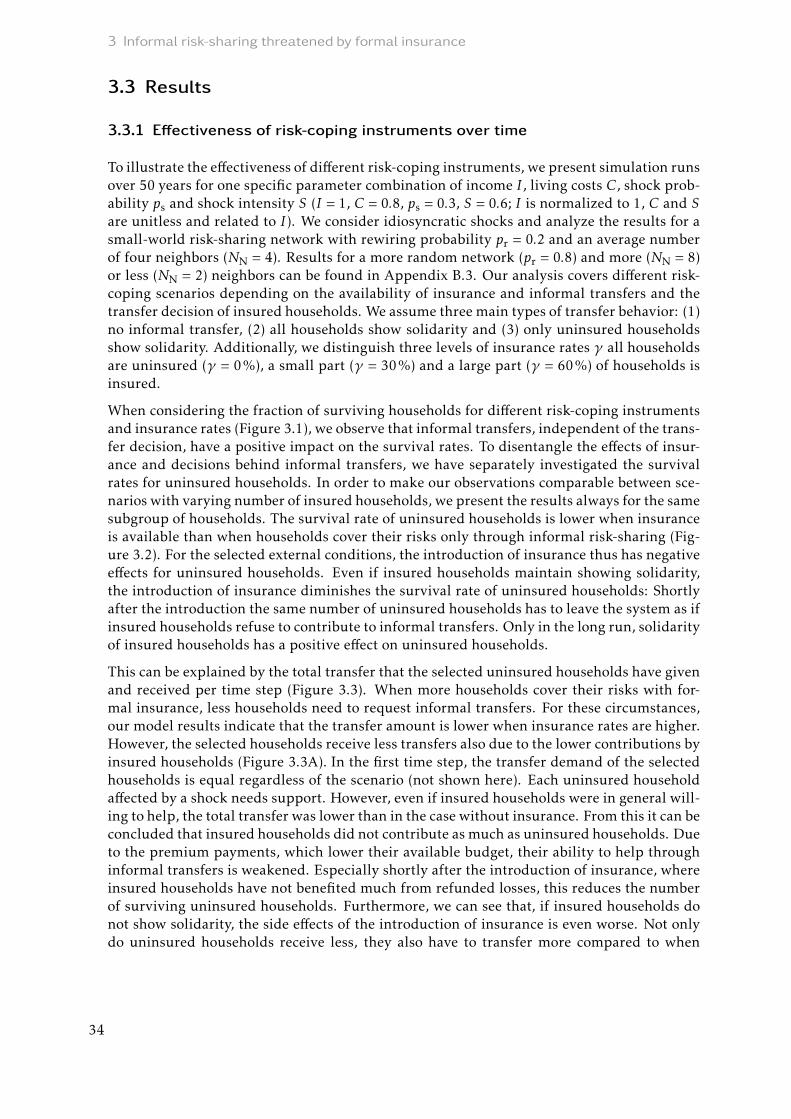
3 Informal risk-sharing threatened by formal insurance
3.3 Results
3.3.1 Effectiveness of risk-coping instruments over time
To illustrate the effectiveness of different risk-coping instruments, we present simulation runsover 50 years for one specific parameter combination of income I , living costs C, shock prob-ability ps and shock intensity S (I = 1, C = 0.8, ps = 0.3, S = 0.6; I is normalized to 1, C and S
are unitless and related to I ). We consider idiosyncratic shocks and analyze the results for asmall-world risk-sharing network with rewiring probability pr = 0.2 and an average numberof four neighbors (NN = 4). Results for a more random network (pr = 0.8) and more (NN = 8)or less (NN = 2) neighbors can be found in Appendix B.3. Our analysis covers different risk-coping scenarios depending on the availability of insurance and informal transfers and thetransfer decision of insured households. We assume three main types of transfer behavior: (1)no informal transfer, (2) all households show solidarity and (3) only uninsured householdsshow solidarity. Additionally, we distinguish three levels of insurance rates γ all householdsare uninsured (γ = 0%), a small part (γ = 30%) and a large part (γ = 60%) of households isinsured.
When considering the fraction of surviving households for different risk-coping instrumentsand insurance rates (Figure 3.1), we observe that informal transfers, independent of the trans-fer decision, have a positive impact on the survival rates. To disentangle the effects of insur-ance and decisions behind informal transfers, we have separately investigated the survivalrates for uninsured households. In order to make our observations comparable between sce-narios with varying number of insured households, we present the results always for the samesubgroup of households. The survival rate of uninsured households is lower when insuranceis available than when households cover their risks only through informal risk-sharing (Fig-ure 3.2). For the selected external conditions, the introduction of insurance thus has negativeeffects for uninsured households. Even if insured households maintain showing solidarity,the introduction of insurance diminishes the survival rate of uninsured households: Shortlyafter the introduction the same number of uninsured households has to leave the system as ifinsured households refuse to contribute to informal transfers. Only in the long run, solidarityof insured households has a positive effect on uninsured households.
This can be explained by the total transfer that the selected uninsured households have givenand received per time step (Figure 3.3). When more households cover their risks with for-mal insurance, less households need to request informal transfers. For these circumstances,our model results indicate that the transfer amount is lower when insurance rates are higher.However, the selected households receive less transfers also due to the lower contributions byinsured households (Figure 3.3A). In the first time step, the transfer demand of the selectedhouseholds is equal regardless of the scenario (not shown here). Each uninsured householdaffected by a shock needs support. However, even if insured households were in general will-ing to help, the total transfer was lower than in the case without insurance. From this it can beconcluded that insured households did not contribute as much as uninsured households. Dueto the premium payments, which lower their available budget, their ability to help throughinformal transfers is weakened. Especially shortly after the introduction of insurance, whereinsured households have not benefited much from refunded losses, this reduces the numberof surviving uninsured households. Furthermore, we can see that, if insured households donot show solidarity, the side effects of the introduction of insurance is even worse. Not onlydo uninsured households receive less, they also have to transfer more compared to when
34

3.3 Results
AAAAAAAAAAAAAAAAAAAAAAAAAAAAAAAAAAAAAAAAAAAAAAAAAAAAAAAAAAAAAAAAAAAAAAAAAAAAAAAAAAAAAAAAAAAAAAAAAAAAAA BBBBBBBBBBBBBBBBBBBBBBBBBBBBBBBBBBBBBBBBBBBBBBBBBBBBBBBBBBBBBBBBBBBBBBBBBBBBBBBBBBBBBBBBBBBBBBBBBBBBBBBBBBBBBBBBBBBBBBBBBBBBBBBBBBBBBBBBBBBBBBBBBBBBBBBBB CCCCCCCCCCCCCCCCCCCCCCCCCCCCCCCCCCCCCCCCCCCCCCCCCCCCCCCCCCCCCCCCCCCCCCCCCCCCCCCCCCCCCCCCCCCCCCCCCCCCCCCCCCCCCCCCCCCCCCCCCCCCCCCCCCCCCCCCCCCCCCCCCCCCCCCCC
Insurance rate γ = 0% Insurance rate γ = 30% Insurance rate γ = 60%
0 10 20 30 40 50 0 10 20 30 40 50 0 10 20 30 40 50
0.00
0.25
0.50
0.75
1.00
Time step
Fra
ctio
n o
fsu
rviv
ing
ho
use
ho
lds
No informal transfer Solidarity No solidarity
Figure 3.1: Fraction of surviving households for different risk-coping instruments and insurance ratesγ (A – 0%, B – 30%, C – 60%). Results show the mean over 100 repetitions for a selected parametercombination of income I , living costs C, shock probability ps and shock intensity S (I = 1, C = 0.8,ps = 0.3, S = 0.6).
insured households contribute as well (Figure 3.3B). This is particularly evident for high in-surance rates. If transfers are only provided by households that are themselves vulnerable totransfers, this in the end lowers their own ability to cope with future losses and leads to evenlower survival rates.
Resilience to shocks, i.e. the ability to recover from losses, is manifested not only in whetherhouseholds survive at all but also in the amount of their financial resources. By comparingthe budgets of the surviving insured and uninsured households separately (Figure 3.4), wecan observe financial consequences of insurance and informal transfers. This may help tounderstand reasons for the empirically observed transfer decisions of insured households.Comparing the budgets of the surviving households underlines that individual uninsuredhouseholds manage to obtain substantially higher budgets than insured households (Figure3.4A). However, especially in the scenario without informal transfers, this applies only to asmall fraction of households and can therefore not be seen as a sustainable strategy to ensurethat budgets are resilient to shocks. Additionally, since the transfers are not repaid, thesegains are at the expense of the insured households that show solidarity, which end up with abudget that is lower than what they could have received without helping households in need(Figure 3.4B).
For all outcome measures, we observe differences between the scenarios with and withoutsolidarity of insured households. As showing no solidarity de facto reduces the links of thenetwork that embeds the uninsured households, this indicates the importance of the num-ber of neighbors. To investigate the relevance of the network structure more systematically,we present the same outcome measures for a small-world network with more (NN = 8) or less(NN = 2) neighbors in Appendix B.3. Overall, these results confirm our hypothesis and under-line that a network withmore interactions leads to higher resilience of uninsured households.
35

3 Informal risk-sharing threatened by formal insurance
0.00
0.25
0.50
0.75
1.00
0 10 20 30 40 50
Time step
Fra
ctio
n o
f su
rviv
ing
un
insu
red
ho
use
ho
lds
No informal transfer
Solidarity, γ = 0%
Solidarity, γ = 30%
Solidarity, γ = 60%
No solidarity, γ = 30%
No solidarity, γ = 60%
Figure 3.2: Fraction of surviving uninsured households among the 20 households that are uninsuredin every scenario for different risk-coping instruments with insurance rates γ . Results show the meanover 100 repetitions for a selected parameter combination of income I , living costs C, shock prob-ability ps and shock intensity S (I = 1, C = 0.8, ps = 0.3, S = 0.6). Without informal transfers thesurvival rates are independent of the insurance rates and the resulting curves for different insurancerates would overlap. They are therefore not represented separately.
AAAAAAAAAAAAAAAAAAAAAAAAAAAAAAAAAAAAAAAAAAAAAAAAAAAAAAAAAAAAAAAAAAAAAAAAAAAAAAAAAAAAAAAAAAAAAAAAAAAAAAAAAAAAAAAAAAAAAAAAAAAAAAAAAAAAAAAAAAAAAAAAAAAAAAAAAAAAAAAAAAAAAAAAAAAAAAAAAAAAAAAAAAAAAAAAAAAAAAAAAAAAAAAAAAAAAAAAAAAAAAAAAAAAAAAAAAAAAAAAAAAAAAAAAAAAAAAAAAAAAAAAAAAAAAAAAAAAAAAAAAAAAAAAAAAAAAAAAAAAAAAAAA BBBBBBBBBBBBBBBBBBBBBBBBBBBBBBBBBBBBBBBBBBBBBBBBBBBBBBBBBBBBBBBBBBBBBBBBBBBBBBBBBBBBBBBBBBBBBBBBBBBBBBBBBBBBBBBBBBBBBBBBBBBBBBBBBBBBBBBBBBBBBBBBBBBBBBBBBBBBBBBBBBBBBBBBBBBBBBBBBBBBBBBBBBBBBBBBBBBBBBBBBBBBBBBBBBBBBBBBBBBBBBBBBBBBBBBBBBBBBBBBBBBBBBBBBBBBBBBBBBBBBBBBBBBBBBBBBBBBBBBBBBBBBBBBBBBBBBBBBBBBBBBBBB
Received by uninsured Given by uninsured
0 10 20 30 40 50 0 10 20 30 40 50
0.0
0.5
1.0
1.5
Time step
To
tal tr
an
sfe
r p
er
tim
e s
tep
No informal transfer
Solidarity, γ = 0%
Solidarity, γ = 30%
Solidarity, γ = 60%
No solidarity, γ = 30%
No solidarity, γ = 60%
Figure 3.3: Total transfer (A) received and (B) given by all 20 households that are uninsured in everyscenario per time step. Results show the mean over 100 repetitions for a selected parameter combi-nation of income I , living costs C, shock probability ps and shock intensity S (I = 1, C = 0.8, ps = 0.3,S = 0.6).
36
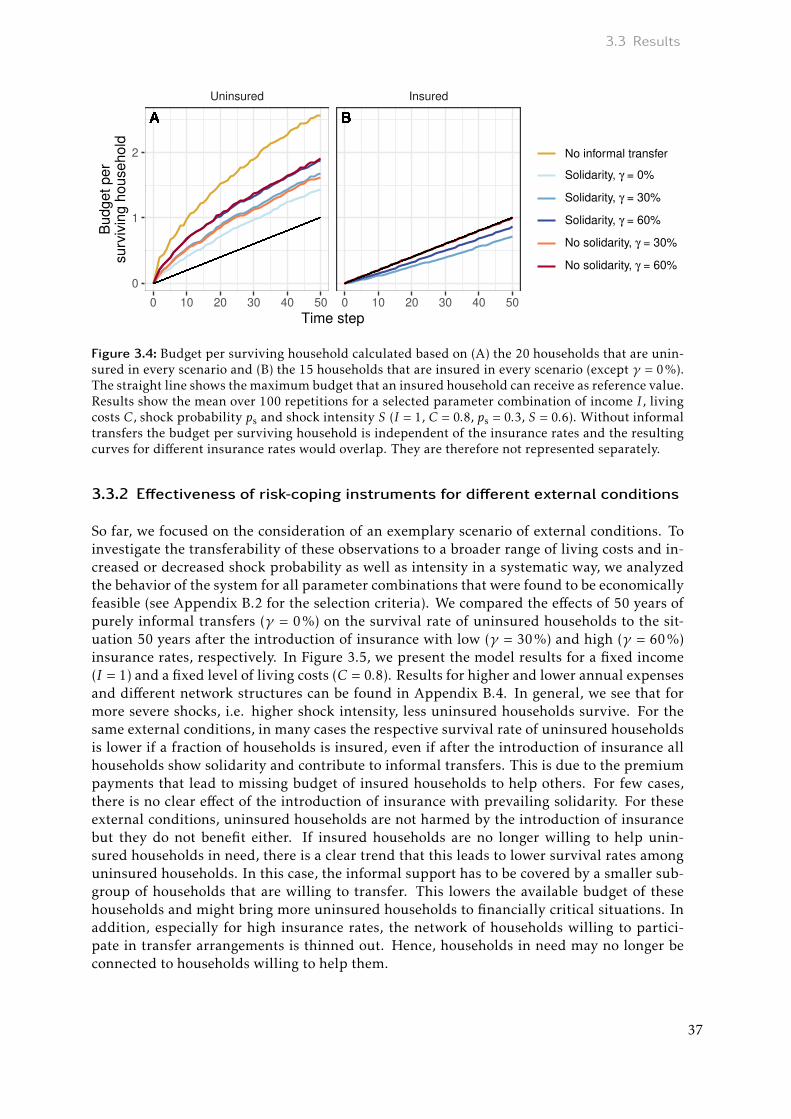
3.3 Results
AAAAAAAAAAAAAAAAAAAAAAAAAAAAAAAAAAAAAAAAAAAAAAAAAAAAAAAAAAAAAAAAAAAAAAAAAAAAAAAAAAAAAAAAAAAAAAAAAAAAAAAAAAAAAAAAAAAAAAAAAAAAAAAAAAAAAAAAAAAAAAAAAAAAAAAAAAAAAAAAAAAAAAAAAAAAAAAAAAAAAAAAAAAAAAAAAAAAAAAAAAAAAAAAAAAAAAAAAAAAAAAAAAAAAAAAAAAAAAAAAAAAAAAAAAAAAAAAAAAAAAAAAAAAAAAAAAAAAAAAAAAAAAAAAAAAAAAAAAAAAAAAAA BBBBBBBBBBBBBBBBBBBBBBBBBBBBBBBBBBBBBBBBBBBBBBBBBBBBBBBBBBBBBBBBBBBBBBBBBBBBBBBBBBBBBBBBBBBBBBBBBBBBBBBBBBBBBBBBBBBBBBBBBBBBBBBBBBBBBBBBBBBBBBBBBBBBBBBBBBBBBBBBBBBBBBBBBBBBBBBBBBBBBBBBBBBBBBBBBBBBBBBBBBBBBBBBBBBBBBBBBBBBBBBBBBBBBBBBBBBBBBBBBBBBBBBBBBBBBBB
Uninsured Insured
0 10 20 30 40 50 0 10 20 30 40 50
0
1
2
Time step
Bu
dg
et
pe
rsu
rviv
ing
ho
use
ho
ld
No informal transfer
Solidarity, γ = 0%
Solidarity, γ = 30%
Solidarity, γ = 60%
No solidarity, γ = 30%
No solidarity, γ = 60%
Figure 3.4: Budget per surviving household calculated based on (A) the 20 households that are unin-sured in every scenario and (B) the 15 households that are insured in every scenario (except γ = 0%).The straight line shows themaximum budget that an insured household can receive as reference value.Results show the mean over 100 repetitions for a selected parameter combination of income I , livingcosts C, shock probability ps and shock intensity S (I = 1, C = 0.8, ps = 0.3, S = 0.6). Without informaltransfers the budget per surviving household is independent of the insurance rates and the resultingcurves for different insurance rates would overlap. They are therefore not represented separately.
3.3.2 Effectiveness of risk-coping instruments for different external conditions
So far, we focused on the consideration of an exemplary scenario of external conditions. Toinvestigate the transferability of these observations to a broader range of living costs and in-creased or decreased shock probability as well as intensity in a systematic way, we analyzedthe behavior of the system for all parameter combinations that were found to be economicallyfeasible (see Appendix B.2 for the selection criteria). We compared the effects of 50 years ofpurely informal transfers (γ = 0%) on the survival rate of uninsured households to the sit-uation 50 years after the introduction of insurance with low (γ = 30%) and high (γ = 60%)insurance rates, respectively. In Figure 3.5, we present the model results for a fixed income(I = 1) and a fixed level of living costs (C = 0.8). Results for higher and lower annual expensesand different network structures can be found in Appendix B.4. In general, we see that formore severe shocks, i.e. higher shock intensity, less uninsured households survive. For thesame external conditions, in many cases the respective survival rate of uninsured householdsis lower if a fraction of households is insured, even if after the introduction of insurance allhouseholds show solidarity and contribute to informal transfers. This is due to the premiumpayments that lead to missing budget of insured households to help others. For few cases,there is no clear effect of the introduction of insurance with prevailing solidarity. For theseexternal conditions, uninsured households are not harmed by the introduction of insurancebut they do not benefit either. If insured households are no longer willing to help unin-sured households in need, there is a clear trend that this leads to lower survival rates amonguninsured households. In this case, the informal support has to be covered by a smaller sub-group of households that are willing to transfer. This lowers the available budget of thesehouseholds and might bring more uninsured households to financially critical situations. Inaddition, especially for high insurance rates, the network of households willing to partici-pate in transfer arrangements is thinned out. Hence, households in need may no longer beconnected to households willing to help them.
37

3 Informal risk-sharing threatened by formal insurance
1
1
1
1
1
1
1
1
1
0.99
0.99
0.99
0.98
0.98
0.97
0.97
0.95
0.95
0.93
0.92
0.91
0.92
0.89
0.89
1
0.99
1
0.98
0.98
0.93
0.97
0.93
0.92
0.85
0.92
0.84
0.86
0.77
0.84
0.75
1 1 1 0.99 0.98 0.97 0.93 0.92
1
1
1
1
0.99
1
0.96
0.97
0.98
0.94
0.91
0.9
0.82
0.8
0.78
0.7
0.65
0.64
0.43
0.41
0.43
0.99
0.96
0.98
0.94
0.9
0.79
0.86
0.73
0.68
0.55
0.58
0.46
0.34
0.29
1 1 0.96 0.94 0.82 0.7 0.43
0.99
1
1
0.97
0.95
0.95
0.8
0.79
0.81
0.55
0.47
0.45
0.97
0.9
0.92
0.82
0.67
0.52
0.42
0.33
0.99 0.97 0.8 0.55
Shock probability ps = 0.1 Shock probability ps = 0.2 Shock probability ps = 0.3S
olid
arity
No
so
lidarity
0.3 0.4 0.5 0.6 0.7 0.8 0.9 1.0 0.3 0.4 0.5 0.6 0.7 0.8 0.9 1.0 0.3 0.4 0.5 0.6 0.7 0.8 0.9 1.0
0
30
60
0
30
60
Shock intensity
Insu
ran
ce
ra
te (
%)
0.00 0.25 0.50 0.75 1.00
Fraction of surviving uninsured households:
Figure 3.5: Fraction of surviving uninsured households among the 20 households that are uninsuredin every scenario depending on insurance rates γ , shock probability ps and shock intensity S foridiosyncratic shocks with fixed income (I = 1) and level of living costs (C = 0.8). Upper rows showthe results for solidarity between all households, lower rows show the results for solidarity betweenuninsured households only. The darker the color the less households survive, numbers in each paneldenote the exact fraction. If a panel is left blank, the parameter combination is economically notfeasible (see Appendix B.2) and therefore not selected for the analysis. Results show the mean over100 repetitions of the number of surviving uninsured households at the last simulation step (t = 50).
The overall conclusions drawn from the selected parameter combination are therefore foundto be robust and valid for a broad range of external conditions with different levels of livingcosts, probabilities for shock occurrence and shock intensity. Households that cannot affordformal insurance do not benefit from its introduction even if their insured peers are willingto help them. In many situations, insured households might simply be not able to coverrequests from the informal network in addition to their regular premium payments.
3.3.3 Effectiveness of risk-coping instruments for covariate shocks
To investigate how shocks which affect many households simultaneously stress the perfor-mance of informal risk-coping instruments, we conduct the same model analysis for covari-ate shocks. We again present an overview of the behavior of the system for all economicallyfeasible parameter combinations and conduct the analysis for the subset of those householdsthat are uninsured in every scenario to allow for best comparison. In Figure 3.6, we show theresulting survival rates of uninsured households when 80% of the households are affected ifa shock hits the village (pH = 0.8). The model results for the more extreme case in which allhouseholds are affected by the shock (pH = 1) can be found in Appendix B.5. Although, intotal, each household suffers equally often from a shock in the idiosyncratic and the covariatecases, the survival rate of uninsured households is lower when they are exposed to covariateshocks in all external conditions which were considered. This implies that protection againstthis type of shock is more difficult without formal insurance. In contrast to what we observedfor idiosyncratic shocks, the introduction of insurance leads to slightly higher survival ratesof uninsured households if insured households are willing to contribute informal transfers.This is because, in case of idiosyncratic shocks, uninsured households were in general able
38

3.4 Discussion
0.94
0.98
1
0.92
0.94
0.97
0.86
0.91
0.96
0.85
0.88
0.92
0.79
0.84
0.89
0.76
0.82
0.87
0.7
0.78
0.84
0.65
0.74
0.82
0.94
0.93
0.92
0.92
0.86
0.84
0.84
0.83
0.78
0.76
0.75
0.74
0.68
0.65
0.63
0.6
0.94 0.92 0.86 0.85 0.79 0.76 0.7 0.65
0.88
0.94
0.99
0.82
0.86
0.94
0.7
0.77
0.86
0.61
0.67
0.75
0.46
0.55
0.66
0.36
0.42
0.51
0.22
0.26
0.33
0.87
0.86
0.81
0.8
0.68
0.65
0.6
0.58
0.45
0.44
0.35
0.34
0.21
0.19
0.88 0.82 0.7 0.61 0.46 0.36 0.22
0.78
0.9
0.98
0.64
0.69
0.79
0.38
0.47
0.59
0.24
0.26
0.3
0.76
0.73
0.63
0.6
0.36
0.33
0.24
0.22
0.78 0.64 0.38 0.24
Shock probability ps = 0.1 Shock probability ps = 0.2 Shock probability ps = 0.3
Solid
arity
No
so
lidarity
0.3 0.4 0.5 0.6 0.7 0.8 0.9 1.0 0.3 0.4 0.5 0.6 0.7 0.8 0.9 1.0 0.3 0.4 0.5 0.6 0.7 0.8 0.9 1.0
0
30
60
0
30
60
Shock intensity
Insu
ran
ce
ra
te (
%)
0.00 0.25 0.50 0.75 1.00
Fraction of surviving uninsured households:
Figure 3.6: Fraction of surviving uninsured households among the 20 households that are uninsuredin every scenario depending on insurance rates γ , shock probability ps and shock intensity S for co-variate shocks with fixed income (I = 1) and level of living costs (C = 0.8). In case of a shock at villagelevel, 80% of the households are affected (pH = 0.8). Upper rows show the results for solidarity be-tween all households, lower rows show the results for solidarity between uninsured households only.The darker the color the less households survive, numbers in each panel denote the exact fraction. Ifa panel is left blank, the parameter combination is economically not feasible (see Appendix B.2) andtherefore not selected for the analysis. Results show the mean over 100 repetitions of the number ofsurviving uninsured households at the last simulation step (t = 50).
to make larger contributions to the transfers than insured households if not in need them-selves. For covariate shocks, however, it is unlikely that an uninsured neighbor is able tomake a contribution at all, as many households are in need at the same time. In this case,even the sometimes small contribution of insured households can help to ensure the survivalof some uninsured households. On the other hand, if insured households are not willing togive transfer payments, this leads, as in the case of idiosyncratic shocks, to lower survivalrate of uninsured households. Then, a link to an uninsured household is more valuable thanthat to an insured households. Uninsured households can at least provide informal transfersin the few situations where they are not affected by a shock but their neighbors are.
3.4 Discussion
To fight poverty, the poorest and most vulnerable households need opportunities to recoverfrom financial losses that result from climate-related extreme events or other unexpectedshocks. Microinsurance products are promoted as effective tools to address this challenge.With this study, we aimed to assess potential long-term consequences of introducing suchformal insurance schemes to communities in which informal risk-sharing arrangements be-tween smallholder farmers are prevalent. Since empirical studies have shown how diversethe transfer behavior of households can be after they have purchased insurance (Landmannet al., 2012; Lin et al., 2014; Strupat & Klohn, 2018; Takahashi et al., 2018; Matsuda etal., 2019; Anderberg & Morsink, 2020; Lenel & Steiner, 2020), it is important to explic-itly take transfer decisions into account when assessing the effectiveness of the combination
39

3 Informal risk-sharing threatened by formal insurance
of these risk-coping instruments. To systematically distinguish situations where formal in-surance complements existing risk-sharing arrangements from situations in which harmfulconsequences on the resilience of smallholders emerge, we developed an agent-based modelwith formal and informal insurance options and combined this with social network analyses.We explicitly included two behavioral implications of the availability of insurance on infor-mal transfers: We assumed that insured households in the social network either continueto engage in informal risk-sharing arrangements or refuse transfers after taking up formalinsurance.
Our model results showed that the introduction of formal insurance can have serious conse-quences, even if insured households maintain private transfers. Informal risk-sharing is onlyeffective with a sufficient number of strong actors. Insured households that do not contributeat all or are, due to premium payments, only able to contribute a small amount, reduce thestrength of informal transfers. Similarly, in the case of covariate shocks where many house-holds are affected simultaneously, purely informal risk-coping cannot be considered effective.In this case, the solidarity of insured households contributes to saving some uninsured house-holds, which makes formal insurance a valuable complement to informal private transfers.As extreme weather events like droughts or floods which cause such types of shocks are ex-pected to occur more frequently under climate change (Sheffield & Wood, 2008; Dai, 2013;Thornton et al., 2014; Tabari, 2020), formal insurance will become increasingly important inthe future. In any case, the resilience of the financial resources to shocks is the highest forinsured households. In general, households can financially benefit from not investing in anyform of risk protection, but this is at the expense of a small number of uninsured householdswhich can survive and is therefore the riskiest option. Taking part in informal risk-copingwithin social networks lowers this risk and, at the same time, still leads to individual budgetswhich are on average higher than those of insured households. From this perspective, it isunderstandable that insured households might stop their contribution to uninsured house-holds.
The use of an agent-based model in this theoretical study enabled a systematic analysis of ex-ternal conditions as well as human behavior in a social network, and allowed to disentangleeffects of formal and informal insurance on the resilience of smallholders to shocks. With theparticular focus on the role of monetary transfers as a risk-coping mechanism emerging fromthe social network and insurance as an external factor, we provided a differentiated viewon drivers contributing to vulnerability and resilience in coupled human-environmental sys-tems (Turner et al., 2003). Here, the combination of agent-based modelling with social net-works was crucial (Will et al., 2020). It allowed, on the one hand, to integrate individualbehavior explicitly and distinguish responses to the introduction of formal insurance de-pending on the insurance status of the households. On the other hand, it was possible toassess how these specific decisions affect other households given the limited the range of in-teraction with few neighboring households defined by the imposed network structure. Bothaspects, household behavior and network characteristics, could be modified and tested sep-arately which contributed to an improved mechanistic understanding that would not havebeen possible without the use of these two methods.
Still, the model results should be seen in light of our rather stylized conceptualization thatentails some limitations which narrow the external validity of our conclusions to some de-gree. Specifically, the assumption that all households have the same initial budget, incomelevel and annual living costs, the actuarially fair insurance design with losses being coveredcompletely and the stylized network offer plenty of potential for further studies.
40

3.4 Discussion
In particular, if households had different financial resources, the decision to insure and po-tential changes in transfer behavior could be included into the model in more detail. Whenlimited economic means alone inhibit some households from purchasing insurance (Elinget al., 2014; Platteau et al., 2017), uninsured households would on average have lower as-sets at their disposal which might increase their dependence on informal support. Giventhe different characteristics of the shock events this could have various consequences. Onthe one hand, the capacity of insured households to support their peers might be substan-tially lowered through premium payments even though they have more financial resourcesavailable than their uninsured peers. As a result, the negative effects of introducing formalinsurance might potentially be even greater than that revealed in our analyses, as poor unin-sured households could be less often able to sustain themselves. On the other hand, wealthyhouseholds with insurance might still be able to make effective contributions to informalrisk-sharing when the premium payments only cover a small share of their available budget.In this case, informal risk-sharing could probably increase the overall welfare and formalinsurance might pay-off not only for the insured households themselves but also for theiruninsured peers.
Furthermore, when it is assumed that not all households with the possibility to insure arewilling to do so, a heterogeneous income distribution would allow to include changes intransfer behavior more specifically. In addition to the two extreme cases of full support, onthe one hand, and complete decline of solidarity by insured households, on the other hand,as shown in our analyses, a more nuanced sharing scenario could be taken into account. Onecould, for example, assume that insured households help only those who cannot afford insur-ance but do not support households with sufficient financial resources who have deliberatelychosen not to purchase insurance (Lenel & Steiner, 2020). In this case, the poorest mightbenefit from their insured peers being protected against income shocks and richer house-holds that do not get any help from others might be able to cover losses from shocks throughtheir own budget, making the lack of informal support potentially less severe.
Additional dynamics could also be observed when taking into account a discrepancy betweenactual losses and insurance payouts. This could be due to basis risk, i.e. when index insur-ance measurements do not match the suffered damages, or due to a contract with reducedinsurance coverage that requires insured households to pay for parts of their losses. Sim-ilarly, when insurance is actuarially unfair, i.e. when it comprises an insurance load thatcovers administrative costs, moral hazard and adverse selection or allows the insurance com-pany to make profit, households get on average less return in case of a loss compared to whatthey have paid as premium (Gollier, 2003; Landes, 2015). In these cases, informal supportmight get more important also for insured households that could profit from neighbors tak-ing over losses not covered by insurance (Mobarak & Rosenzweig, 2012; Dercon et al., 2014;Takahashi et al., 2018; Matsuda et al., 2019).
Another step towards increased realism would be the use of empirical social networks inwhich households differ in their number of neighbors. Heterogeneity with respect to the net-work position could affect the resilience to shocks of uninsured households. If a household inneed has few neighbors and is not connected to those having enough resources to share, theinformal support might not be able to effectively cover its losses. Next to further alignmentwith context-specific details, the model could also be used to test other behavioral theoriesand try to replicate empirically observed practices (Schlüter et al., 2017). This could includeexplicit assumptions on risk-sharing motives such as tit-for tat (Axelrod & Hamilton, 1981)or indirect reciprocity (Nowak & Sigmund, 2005; Clark et al., 2020) combined with punish-ment to those who free-ride on the cooperation of others (Fehr & Gächter, 2002). On the
41
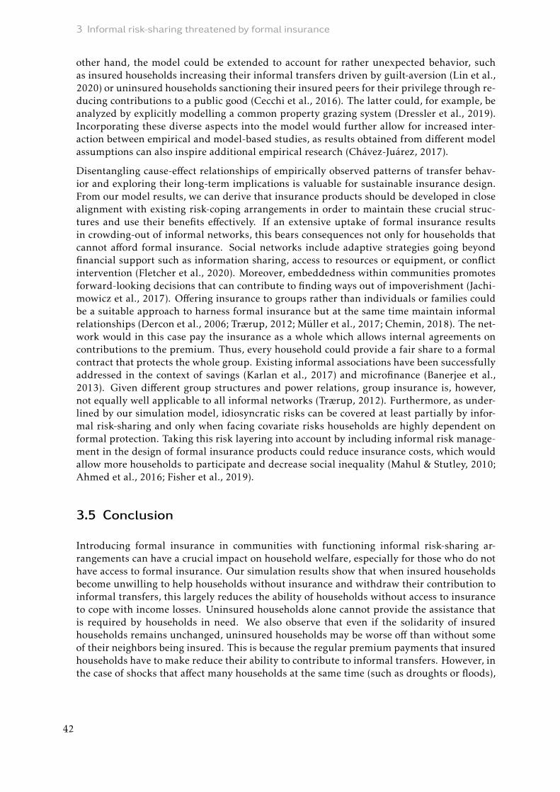
3 Informal risk-sharing threatened by formal insurance
other hand, the model could be extended to account for rather unexpected behavior, suchas insured households increasing their informal transfers driven by guilt-aversion (Lin et al.,2020) or uninsured households sanctioning their insured peers for their privilege through re-ducing contributions to a public good (Cecchi et al., 2016). The latter could, for example, beanalyzed by explicitly modelling a common property grazing system (Dressler et al., 2019).Incorporating these diverse aspects into the model would further allow for increased inter-action between empirical and model-based studies, as results obtained from different modelassumptions can also inspire additional empirical research (Chávez-Juárez, 2017).
Disentangling cause-effect relationships of empirically observed patterns of transfer behav-ior and exploring their long-term implications is valuable for sustainable insurance design.From our model results, we can derive that insurance products should be developed in closealignment with existing risk-coping arrangements in order to maintain these crucial struc-tures and use their benefits effectively. If an extensive uptake of formal insurance resultsin crowding-out of informal networks, this bears consequences not only for households thatcannot afford formal insurance. Social networks include adaptive strategies going beyondfinancial support such as information sharing, access to resources or equipment, or conflictintervention (Fletcher et al., 2020). Moreover, embeddedness within communities promotesforward-looking decisions that can contribute to finding ways out of impoverishment (Jachi-mowicz et al., 2017). Offering insurance to groups rather than individuals or families couldbe a suitable approach to harness formal insurance but at the same time maintain informalrelationships (Dercon et al., 2006; Trærup, 2012; Müller et al., 2017; Chemin, 2018). The net-work would in this case pay the insurance as a whole which allows internal agreements oncontributions to the premium. Thus, every household could provide a fair share to a formalcontract that protects the whole group. Existing informal associations have been successfullyaddressed in the context of savings (Karlan et al., 2017) and microfinance (Banerjee et al.,2013). Given different group structures and power relations, group insurance is, however,not equally well applicable to all informal networks (Trærup, 2012). Furthermore, as under-lined by our simulation model, idiosyncratic risks can be covered at least partially by infor-mal risk-sharing and only when facing covariate risks households are highly dependent onformal protection. Taking this risk layering into account by including informal risk manage-ment in the design of formal insurance products could reduce insurance costs, which wouldallow more households to participate and decrease social inequality (Mahul & Stutley, 2010;Ahmed et al., 2016; Fisher et al., 2019).
3.5 Conclusion
Introducing formal insurance in communities with functioning informal risk-sharing ar-rangements can have a crucial impact on household welfare, especially for those who do nothave access to formal insurance. Our simulation results show that when insured householdsbecome unwilling to help households without insurance and withdraw their contribution toinformal transfers, this largely reduces the ability of households without access to insuranceto cope with income losses. Uninsured households alone cannot provide the assistance thatis required by households in need. We also observe that even if the solidarity of insuredhouseholds remains unchanged, uninsured households may be worse off than without someof their neighbors being insured. This is because the regular premium payments that insuredhouseholds have to make reduce their ability to contribute to informal transfers. However, inthe case of shocks that affect many households at the same time (such as droughts or floods),
42

3.5 Conclusion
formal insurance complements informal risk-sharing, since in this case uninsured householdscannot do much to help their peers.
Overall, our study offers new perspectives on the interplay of formal and informal risk-copinginstruments that complement existing empirical research. The combination of agent-basedmodelling and social networks made it possible to systematically analyze the effects of ex-ternal conditions as well as human interaction on the resilience of smallholders to shocks.By embedding a broad range of theoretical and experimental findings, our results allow con-clusions on potential unintended consequences that the introduction of formal insurancemay have on the functioning of informal transfers in a long-term perspective. These poten-tial feedbacks have to be kept in mind for an effective design of insurance policies as onlyif formal insurance and existing risk-sharing mechanisms are well aligned, they provide agood basis for achieving the goal of eradicating poverty worldwide in a sustainable manner.However, since our results are based on a theoretical simulation model, which by its natureinvolves a number of simplifying assumptions, the specific empirical circumstances must betaken into account in any case when evaluating an appropriate insurance design. To this end,our analyses provide an orientation on which potential side effects should be borne in mind.
Acknowledgments
We thank Niklas Hase for helpful comments on a previous version of the model, FriederikeLenel for insightful discussions and David Kreuer for helpful comments on a previous ver-sion of the paper.
Funding
MWwas supported by the Deutsche Forschungsgemeinschaft (DFG, German Research Foun-dation) in the project SEEMI (Social-Ecological Effects of Microinsurance) – 321077328. BMacknowledges funding by the German Federal Ministry of Education and Research (BMBF-01LN1315A) within the Junior Research Group POLISES. The funders had no role in studydesign, data collection and analysis, decision to publish, or preparation of the manuscript.
Author contributions
Conceptualization: Meike Will, Jürgen Groeneveld, Karin Frank, Birgit Müller; Data cura-tion: Meike Will; Formal analysis: Meike Will; Funding acquisition: Birgit Müller; Inves-tigation: Meike Will; Methodology: Meike Will; Software: Meike Will; Supervision: Jür-gen Groeneveld, Karin Frank, Birgit Müller; Visualization: Meike Will; Writing – originaldraft: Meike Will, Jürgen Groeneveld, Karin Frank, Birgit Müller; Writing – review & edit-ing: Meike Will, Jürgen Groeneveld, Karin Frank, Birgit Müller.
43


4 Determinants of household resilience in networks
with formal insurance and informal risk-sharing
This chapter is based on a manuscript in preparation for submission: Will, M., Groeneveld, J.,Lenel, F., Frank, K., & Müller, B. Determinants of household resilience in networks with formalinsurance and informal risk-sharing
Abstract
Insurance products specifically designed for the needs of low-income households in devel-oping countries can effectively buffer financial losses from personal or weather-related risks.However, even though this type of insurance specifically addresses the poor, not all house-holds can afford to pay the regular premiums. The resilience of these households to shocks,i.e. their ability to cope with income losses, often highly depends on traditional informalarrangements where risk is shared through private monetary support in social networks. Ifincome is heterogeneously distributed in a network and poor households are not connectedto those with enough resources and willing to share, this support might, however, not reachthe households in need. With this study, we assess the impact of heterogeneity in incomeand network characteristics on the effectiveness of informal risk-coping for the poorest whensome of their neighbours have access to formal insurance. In addition, we derive a functionalrelationship between the resilience of the poorest and key household and network charac-teristics to obtain a measure for actual vulnerability. Using a stylized agent-based model,we show that formal insurance pays off not only for the insured households themselves, butalso for poor households that benefit from their neighbours being insured, especially whenshocks affect many households simultaneously. By applying logistic regression to the simu-lated data for random networks, we infer that, in addition to one’s own financial situation,the financial situation of neighbouring households and the position in the network, which isdetermined by a household’s indegree and outdegree, are crucial for coping with income loss.We show the transferability of our findings by testing the accuracy of the regressionmodel foran empirical risk-sharing network of a village on the Philippines. Our study highlights thepotential of using model-based approaches to identify vulnerable households by assessingtheir financial as well as network characteristics. This can help to effectively target subsidieswhen informal risk-sharing is insufficient and households cannot afford formal insurance.
4.1 Introduction
Unexpected losses due to personal or weather-related shocks pose significant financial risksto the poor in developing countries (Dercon, 2002; Xu et al., 2003; Strömberg, 2007). Illness,for example, can force people to use a large share of their income to cover costs of medicalcare and is simultaneously often associated with reduced labour supply and a loss of income
45

4 Determinants of household resilience
(Gertler & Gruber, 2002). Additionally, many households in low-income countries are par-ticularly susceptible to damages by natural disasters such as droughts or floods resulting inharvest failure or livestock loss (Barrett & Santos, 2014; Thornton et al., 2014). Due to cli-mate change it is expected that such weather-related shock events become evenmore frequentand severe in the future (Sheffield & Wood, 2008; Dai, 2013; Thornton et al., 2014; Tabari,2020). Building resilience of the most vulnerable against income loss is thus key to endingpoverty as aspired by the Sustainable Development Goals (UN, 2015). Microinsurance or in-clusive insurance, i.e. insurance products specifically designed for the needs of low-incomehouseholds, are seen as a promising tool to encompass also the poor with an appropriateand affordable risk-coping instrument and strengthen their resilience to unforeseen losses(Wanczeck et al., 2017). Current programs include funeral insurance, health insurance aswell as crop and livestock insurance (Merry, 2020).
However, even though these schemes are intentionally designed for the most vulnerable, theymight not reach the poorest as for this part of the population unsubsidised premiums are of-ten still too expensive (Biener & Eling, 2012; Eling et al., 2014; Marr et al., 2016; Platteauet al., 2017). The ability of these households to cope with income losses therefore highlydepends on traditional informal arrangements where households help each other in times ofneed with money, labour, or in-kind goods (Platteau, 1997; Cronk et al., 2019a). Such risk-sharing networks exist in various forms and cover extended families, villages, ethnic groups,or professional relations (Dercon, 2002). It is assumed that engaging in these arrangementsis driven by altruism and reciprocity, i.e. by contributions solely due to a preference for so-cial welfare and those where later reward is expected (Leider et al., 2009; Ligon & Schechter,2012). However, when households rely on informal support, their ability to maintain re-silience to shocks depends largely on their position in these networks. If income is heteroge-neously distributed and poor households are not connected to those with enough resourcesand willing to share, the informal support might not reach the households in need. Similarly,if many households seek financial help from the same households that are expected to bewealthy these may not be able to fulfil all requests. Yet, while several studies consider theeffect of wealth differences on the formation of risk-sharing networks (Fafchamps & Gubert,2007; Schechter & Yuskavage, 2011; Caudell et al., 2015; Lenel, 2017), little is known abouthow well households are protected in these arrangements, especially if some households canafford formal insurance in addition to informal risk-sharing and others cannot.
We address this gap by analysing the impact of heterogeneity in income and network char-acteristics on the effectiveness of informal risk-sharing for the poorest when some of theirneighbours have access to formal insurance. Specifically, we assess under which conditionsformal insurance complements informal risk-sharing and whether the availability of insur-ance can have an indirect benefit for poor, uninsured households. In addition, we derive afunctional relationship between the resilience of the poorest and key household and networkcharacteristics to obtain a measure for actual vulnerability. Using a stylized agent-basedmodel, we simulate the resilience of individual households to income losses. By applyinglogistic regression to the simulated data, we reveal which household and network character-istics can strengthen a household’s ability to cope with extreme events.
Agent-based modelling is a valuable approach to disentangle the complex interplay of formaland informal insurance, network characteristics, and external conditions as it allows to sys-tematically analyse interlinked causal relationships of human and environmental processes(Schulze et al., 2017). The method already helped to understand how different degrees ofinequality between nodes evolve in stylized risk-sharing networks (Chiang, 2015). In a more
46

4.2 Methods
applied setting, agent-based models provided useful insights into how risk-sharing can sta-bilize herd sizes when households exchange livestock (Aktipis et al., 2011; Aktipis et al.,2016). The approach was also used to determine how the resilience of pastoralists dependson whether households in need prefer to ask the wealthiest of their partners for help (Haoet al., 2015) and whether households with the capacity to help decide to provide transfersbased on the social status or the financial situation (Kayser & Armbruster, 2019).
We contribute to the literature by evaluating the interplay of formal and informal risk-copinginstruments in the presence of wealth inequality. We analyse a broad range of conditions inorder to provide insights on how these mechanisms might be affected by climate change re-sulting in more frequent extreme weather events like droughts or floods (Dai, 2013; Tabari,2020) or by demographic changes such as urbanization that impose greater health threats es-pecially with respect to chronic diseases (Allender et al., 2008; Vearey et al., 2019). We buildon an existing model (Will et al., 2021a) and extend this model by incorporating incomeand network characteristics based on empirical observations of a village on the Philippines(Lenel, 2017). Through the development of a functional relationship between the resilienceof the poorest and key household and network properties, our study helps to reveal whichcharacteristics are crucial to identify those households that neither have access to formal in-surance nor are adequately protected through informal risk-sharing. In cases where informalrisk-sharing is insufficient and not all households have enough financial resources to coverformal insurance premiums, additional support, for example through subsidised insurancecontracts, is needed to make more households resilient to shocks. Assessing financial as wellas network characteristics of households allows a systematic understanding of their vulnera-bility that can be used to effectively target such external assistance. In combination with animproved insurance design that is attractive to a large share of the population, this can havea major impact on reducing poverty.
4.2 Methods
4.2.1 Model description and parametrization
We describe the key processes of the model with a focus on budget dynamics of individualhouseholds and their formal and informal risk-coping instruments. The main processes ofthe simulation model, presented in a structured form based on the ODD+D protocol (Mülleret al., 2013), can be found in Appendix B.1. Details on the differences to the model versionused in Chapter 3 are outlined in Appendix C.1. The model is implemented in NetLogo andthe source code of the model is available at CoMSES Net (Will et al., 2021d).
To model the effectiveness of formal and informal risk-coping instruments, we simulateNH = 65 households and the dynamics of their budgets Y over a long-term perspective of50 years with annual time steps. We consider households connected in a social network asindividual agents. All households gain a regular income I and have to spend a fraction c
of their income to cover living costs. Additionally, they are exposed to unexpected eventsthat lower their budget by an amount S . These income shocks either occur independentlyfor each household with probability ps (idiosyncratic shocks) or affect several households inthe village simultaneously, e.g. through extreme weather events. In case of such covariateshocks, the village is hit with probability pV. The individual households are then affectedwith probability pH which reflects that some households are resistant to income losses, e.g.due to a more favourable geographical location or better adapted agricultural strategy. To
47

4 Determinants of household resilience
make individual shock frequencies ps comparable to that of the idiosyncratic shocks, we as-sume that the probability for a specific household to be hit by a shock is ps = pV ×pH. In eachsimulation run, only one shock type is considered.
When their financial resources are not sufficient to sustain their livelihood, i.e. when theirbudget is below zero, households can request money from other households to which they areconnected in a social network. A household requests as much money as is needed to reach thepoverty threshold of zero from a household randomly chosen among its links. If the selectedhousehold cannot provide the full amount, the household in need asks further neighboursfor support until it obtains the desired amount or until no more households are left to ask.To investigate to which extent our results can be generalized or are conditional on specificnetwork properties, we simulate two different types of networks in which the households areconnected: Households are either linked based on an empirical network (see section 4.2.2) orin random networks with the same number of nodes and links as in the empirical case.
We assume that income is distributed heterogeneously among the households and householdsgain an individual income Ii . In the empirical network, the income distribution is derivedfrom the survey data (see section 4.2.2). In the artificially created networks, the same distri-bution of income as in the empirical case is assumed. Here, the position of households in thenetwork is randomly assigned and varies for each newly created network topology. House-holds are endowed with an initial budget Y 0 which is set to zero to facilitate comparisonacross different external conditions. Relations between income and consumption are not un-ambiguously confirmed in the literature (Howe et al., 2009). As a first approach to accountfor heterogeneous consumption, we assume a simplistic linear relation where householdsspend a fixed proportion c of their income to cover their living costs. We model a subsistenceeconomy with low saving rates and set c = 0.8. The increase in consumption with income canbe justified by the fact that income is not adjusted for household size and that there is po-tentially higher consumption of goods exceeding basic needs when more income is availablethan needed.
In addition to informal risk-sharing, some households have access to formal insuranceschemes. Formal insurance is offered with a yearly premium that is actuarially fair, i.e. thepremium β equals the expected payout determined by the shock probability ps and shockintensity S (β = ps ×S). Only households that have enough budget available to cover the pre-mium after paying the living costs can decide to insure. This is in accordance with empiricalstudies showing a positive relationship between wealth and insurance purchase (Eling et al.,2014). We assume that not all households with enough financial resources to insure are will-ing to do so and distinguish three levels of insurance propensity δ, where either none (δ = 0),half (δ = 0.5), or all (δ = 1) of the households wealthy enough to afford the premium choose toinsure. This allows us to implicitly account for other non-financial factors, such as social orcultural influences, that affect the decision to insure but are not included in the model (Elinget al., 2014; Platteau et al., 2017; Panda et al., 2020). For each simulated scenario, we assumea constant insurance propensity for all households that can afford insurance.
Households that do not manage to reach the poverty threshold either on their own or withthe help of others are excluded in further time steps of the model, i.e. it is assumed that thesehouseholds are no longer part of the system. This assumption implicitly includes migration,as households that are not able to cover their living costs might leave the region and search forimproved economic, ecological, or social conditions elsewhere (Black et al., 2011; Neumann& Hermans, 2017). However, this does not take into account that households might obtainfurther support from outside the village which is not included in the model (Adams & Page,2005; Giuliano & Ruiz-Arranz, 2009). We summarize the resilience of households to shocks,
48

4.2 Methods
i.e. their capacity to cope with income losses, in a ‘survival rate’ which indicates the fractionof households that manage to maintain a budget above zero over a specific time span.
For further analyses, we examine selected parameter conditions for shock intensity ps andshock probability S for which, due to the resulting premium levels, a different proportionof the population can afford insurance. On the one hand, as microinsurance products arespecifically designed for low-income households, we consider scenarios where at least 50%of all households can afford to insure. On the other hand, as we are particularly interestedin how households that do not have enough financial resources to insure cope with incomelosses, we focus on external conditions of shock frequency and severity where at least 25% ofthe population are too poor to afford the regular premium payments. We assume a shock fre-quency between 10 and 30% which is in the range of empirically observed values (see section4.2.2 for the reported shock frequency in the case study on the Philippines). Dividing all pa-rameters in equidistant steps of 0.1, this results in five possible parameter combinations withbetween 54% and 75% of the population having enough financial resources to insure. If notall households that can in principle afford the insurance are inclined to pay the annual pre-miums, the effective insurance rate in the population is reduced accordingly (see AppendixC.2 for details on the parameter selection and the resulting number of insured householdsfor different external conditions).
4.2.2 Case study
Empirical network and income data are based on a household survey that was conductedin 2012 in small fishing villages in the provinces Antique and Iloilo in the region WesternVisayas on the Philippines (Lenel, 2017). The focus of the survey was the use of financial ser-vices and the structure of support networks. One village with 65 households was surveyedcompletely. The survey covered socioeconomic characteristics of all household members,including access and use of formal financial services, housing characteristics, as well as de-tailed questions on the informal support networks within and outside the community (seeTable C.2 for a summary of the household characteristics). In particular, the respondentswere asked to provide a list of households that they consider as close to their household.There were no limitations on the number of names that respondents could list. For each ofthe mentioned households, the respondent was asked (1) “Would these people help you ifyou/the main income provider would turn very ill and would not be able anymore to earnincome and in addition you would need to cover the medical expenses?” and (2) “Would youask these people for help?”. For these questions, respondents could respond “Immediately”,“After some hesitation”, “Only in extreme emergency situations”, or “Never”. A support linkwas defined as existing if a respondent answered “Immediately” for both questions. In total,236 links were reported with on average 3.63 support links per household (see Figure C.1for the resulting network and Figure C.2 for the degree distribution). 55 of the 65 house-holds named at least one other household from the village as a potential source of supportand 62 households were named by at least one household. One household is isolated, i.e.this household was neither naming other households nor was this household named by anyother household. The resulting network characteristics resemble those of rural social net-works in villages in Malawi, Uganda and India, where similar data have been collected (foran overview see Chandrasekhar, 2016).
As most of the declared income is highly irregular and income reports are not always reli-able, an asset index normalized to a value between 0 and 1 was derived as a measure forwealth (Moser & Felton, 2007). The asset index includes variables that describe ownership
49

4 Determinants of household resilience
of technical devices, agricultural tools, or livestock and housing characteristics such as roofmaterials, source of lighting, and general housing conditions. The asset distribution of theselected village fits well with that of a larger sample obtained in the same survey campaignwith only slightly less poor households and slightly more rich households (Figure C.3) andcan therefore be seen as a good proxy for the wealth distribution in the region. Althoughan asset index differs from income as a wealth measure (Poirier et al., 2020), it is seen as avaluable proxy to differentiate the economic status of households (Ucar, 2015). We thereforebase the income distribution in the model on the empirically derived asset values and assumethat households gain a regular income according to their asset index.
Among all households in the sample, 24.6% reported a severe health shock in the year previ-ous to the survey. This is in accordance with a study from Kenya, where households denotedto experience losses due to illness in 26.6% of the weeks in one year (Geng et al., 2018).
4.3 Results
4.3.1 Effectiveness of informal risk-sharing
We focus our analysis of the effectiveness of informal risk-sharing on the poorest of the pop-ulation, i.e. households that cannot afford formal insurance. To determine their long-termprotection against income losses and their dependency on transfers from other households,we present simulation runs over 50 years with varying degrees of propensity to insure δ
among those households with sufficient income to consider insurance. We show results forcases with half (δ = 0.5) or all (δ = 1) of these households being insured and, as reference,scenarios without formal insurance (δ = 0). In a first step, we analyse one specific parametercombination of shock probability ps = 0.1 and shock intensity S = 0.6. For this scenario, thethreshold below which households cannot afford insurance is at It = 0.3 which leads to aneffective insurance rate of 31% (δ = 0.5) and 62% (δ = 1) in the whole population. We firstfocus on the outcome for random networks that are newly generated in every repetition ofthe simulation. In a second step, we compare the results with those for the empirical networkthat does not change between simulation runs.
To analyse to which extent households that cannot afford formal insurance rely on the sup-port of others, we present how many of them manage to cover their living expenses overthe simulated time span (Figure 4.1A) and the transfer amount that these households receiveduring this period (Figure 4.1B). Whereas without the help of their neighbours only 8% ofthese households manage to survive the entire simulated period, the fraction increases toup to 47% when other households provided informal transfers to those in need. The mostimportant contribution to the survival of uninsured households comes from wealthy house-holds with enough financial resources to insure (Figure 4.1B). The positive effect of informalrisk-sharing on the survival of the poorest slightly varies for different insurance levels. Inthe long-term, poor households benefit from many of their neighbours being insured (δ = 1).Only shortly after the introduction of insurance, rich households cannot cover the requeststo the same extent as they could when they were not insured (δ = 0). This is due to the lowerbudget that insured households have available after paying the insurance premium which isespecially pronounced in the early years of the contract, when insured households have notyet benefited from reduced losses due to insurance payouts (Will et al., 2021a). In the longrun, however, formal insurance pays off not only for the insured households themselves butalso for their uninsured peers. For households that can afford insurance but choose not to, we
50

4.3 Results
AAAAAAAAAAAAAAAAAAAAAAAAAAAAAAAAAAAAAAAAAAAAAAAAAAAAAAAAAAAAAAAAAAAAAAAAAAAAAAAAAAAAAAAAAAAAAAAAAAAAAAAAAAAAAAAAAAAAAAAAAAAAAAAAAAAAAAAAAAAAAAAAAAAAAAAAAAAAAAAAAAAAAAAAAAAAAAAAAAAAAAAAAAAAAAAAAAAAAAAAAAAA
0.00
0.25
0.50
0.75
1.00F
ractio
n o
f su
rviv
ing
un
insu
red
ho
use
ho
lds
0 10 20 30 40 50
Time step
δ 0 0.5 1 No transfer
BBBBBBBBBBBBBBBBBBBBBBBBBBBBBBBBBBBBBBBBBBBBBBBBBBBBBBBBBBBBBBBBBBBBBBBBBBBBBBBBBBBBBBBBBBBBBBBBBBBBBBBBBBBBBBBBBBBBBBBBBBBBBBBBBBBBBBBBBBBBBBBBBBBBBBBBBBBBBBBBBBBBBBBBBBBBBBBBBBBBBBBBBBBBBBBBBBBBBBBBBBBBBBBBBBBBBBBBBBBBBBBBBBBBBBBBBBBBBBBBBBBBBBBBBBBBBBBBBBBBBBBBBBBBBBBBBBBBBBBBBBBBBBBBBBBBBBBBBBBBBBBBBBBBBBBBBBBBBBBBBBBBBBBBBBBBBBBBBBBBBBBBBBBBBBBBBBBBBBBBBBBBBBBBBBBBBBBBBBBBBBBBBBBBBBBBBBBBBBBBBBBBBBBBBBBBBBBBBBBBBBBBBBBBBBBBBBBBBBBBBBBBBBBBBBBBBBBBBBB
0.0
0.2
0.4
0.6
Tra
nsfe
r p
er
tim
e s
tep
0 10 20 30 40 50
Time step
Total From wealthy From poor
Figure 4.1: (A) Fraction of surviving uninsured households without enough financial resources toinsure for three different insurance propensities δ. The scenario without informal transfer is addedas reference (yellow line). As in this case the survival rates are independent of the insurance rates,results for different insurance rates overlap and are not represented separately. The shaded areasrepresent the 95% confidence interval. (B) Mean transfer that households without enough financialresources to insure receive per time step. Line types distinguish the source of the transfer. For bothpanels, results show the mean over 1000 repetitions for a selected parameter combination of shockprobability ps = 0.1 and shock intensity S = 0.6 and households connected in a random network thatis newly created in every repetition.
observe in general similar trends (Figure C.4). However, their higher income makes it easierfor them to buffer income shocks which reduces their dependence on informal transfers.
Based on this analysis, it is, however, still unclear why some households survive and others donot. One reason could be the heterogeneous income distribution, which allows some to savemore than others when not affected by a shock. To examine the importance of households’own financial situation, we determine the survival probability of a household with certainincome for 1000 replications of the simulation (Figure 4.2). We observe that in random net-works, households tend to survive more often the higher their income. Because insurancecovers complete losses, survival is certain for insured households. This is reflected in theincrease in survival probability for income greater than 0.3, which denotes the threshold be-low which households cannot afford insurance. In the empirical network described in section4.2.2, i.e. a specific network configuration that is fixed for every repetition of the simulation,a household with the lowest income is, however, far more likely to survive than one withnearly enough financial resources to insure (similar observations can be made for a selectedrandom network kept fixed for 1000 repetitions, see Figure C.5). Thus, income does not seemto be the only determinant for survival. In addition, network characteristics, which vary be-tween simulation runs in the case of the random networks but remain fixed for the empiricalnetwork, might influence the survival rate.
51

4 Determinants of household resilience
●●
●
●
●
●●●
●● ●
●●●●
●●●
●
●
●●●
●●
●●
●
●●
●●●●
●●●
● ●
●
●
●
●
● ●
●
●
●
●
●
●
●
●
●
●
●
●
●
●
●
●
●
●
●
●
●
●
●
●
●
●
●
●
●
●
●
●
●
●
●AAAAAAAAAAAAAAAAAAAAAAAAAAAAAAAAAAAAAAAAAAAAAAAAAAAAAAAAAAAAAAAAAAAAAAAAAAAAAAAA
● ●
●
●
●
●●
●●●
●
●●●
●●●●●
●
●●●●
●●
●
●●●
●●●
●●●● ●
●
●
●
●
●
●
●
●
●
●
●
●
●
●
●
●
●
●
●
●●
●
●
●
●
●
●
●
●
●
●
●
●
●
●
●
●
●
●
●
●
●BBBBBBBBBBBBBBBBBBBBBBBBBBBBBBBBBBBBBBBBBBBBBBBBBBBBBBBBBBBBBBBBBBBBBBBBBBBBBBBB
●
●
●
●
●
●● ●
●● ●
●●●
●●●●●●●●●●●●● ●●●●●●● ●●● ● ● ●
●
●
●
●
●
●
●
●
●
●
●
●
●
●
● ●●●●● ● ●● ● ●● ● ● ●● ●● ● ● ●●● ● ● ●CCCCCCCCCCCCCCCCCCCCCCCCCCCCCCCCCCCCCCCCCCCCCCCCCCCCCCCCCCCCCCCCCCCCCCCCCCCCCCCC
Insurance propensity δ = 0 Insurance propensity δ = 0.5 Insurance propensity δ = 1
0.00 0.25 0.50 0.75 1.00 0.00 0.25 0.50 0.75 1.00 0.00 0.25 0.50 0.75 1.00
0.00
0.25
0.50
0.75
1.00
Income
Su
rviv
alp
rob
ab
ility
● ●Random networks Empirical network
Figure 4.2: Fraction of runs out of 1000 repetitions in which a household with a given income Ii sur-vives in random networks that are newly created in every simulation run (black) and the empiricalnetwork where a household with a certain income has always the same position in the network (or-ange). For each simulation run, shocks occur in random order for individual households. As somehouseholds have the same income, not all dots represent exactly one household. Results are shown fora selected parameter combination of shock probability ps = 0.1 and shock intensity S = 0.6 (with re-sulting threshold below which households cannot afford insurance at It = 0.3) and different insurancepropensities δ.
4.3.2 Determinants for the survival of the poorest
To reveal the functional influence of various factors on the survival probability of thosehouseholds that do not have enough financial resources to pay for formal insurance, we per-form a logistic regression on the simulated data of households’ survival after a time span of 50years. Specifically, we include as dependent variable the survival of the poorest householdsthat cannot afford formal insurance (25 households). We consider three different insurancepropensities δ and 1000 repetitions of the simulation which overall leads to 75000 observa-tions that are used in the regression. The regression model contains independent variables onthe financial situation of a household and its neighbours as well as information on its networkposition. For the financial situation, we include in particular the household’s income and thedisposable income of its neighbours. The latter includes the budget that all households ahousehold is connected to can on average share, i.e. the amount that they have available afterpaying their living costs and the insurance premium. For uninsured households, the averageexpected loss from shock events is deducted instead of the premium. Households that havea negative budget after subtracting these costs do not contribute the disposable income ofa household’s neighbours. With respect to network characteristics, we include the numberof households that can be asked for support (outdegree) and the number of households thatpotentially need support (indegree). Here, we only consider links from households that arenot insured as insured households do not need informal support. We test the influence of in-surance propensity δ by including interactions between all four predictors and the insurancelevels δ = 0.5 and δ = 1. In particular, we estimate with a logistic regression the following
52

4.3 Results
specification
P(activei = 1) = β0 + β1 Ii + β2Di + β3degout,i + β4deguninsin,i + β5 δ0.5 + β6 δ1
+ β7 Ii × δ0.5 + β8Di × δ0.5 + β9degout,i × δ0.5 + β10deguninsin,i × δ0.5 (4.1)
+ β11 Ii × δ1 + β12Di × δ1 + β13degout,i × δ1 + β14deguninsin,i × δ1 + εi
i.e. the probability P(activei = 1) that household i survives the simulated time span of50 years is explained by i’s income Ii , the disposable income of i’s neighbours Di , whereDi =
∑Jj=1max{Ij (1 − c) − ps × S,0} with j = 1, ..., J being those households household i can
ask for support, i’s outdegree degout,i , and i’s indegree from uninsured households deguninsin,i .Furthermore, we include the prevalent insurance propensity, where the dummy variables δ0.5and δ1 denote whether the insurance propensity equals 0.5 or 1, respectively. Standard errorsεi are clustered on household level.
Results using standardised coefficients for better interpretability are reported in Table 4.1.Unstandardised coefficients can be found in Table C.3. As already assumed, a household’ssurvival depends less on its own financial situation than on how much potential donors canshare. The number of neighbours that can be asked for support (outdegree) is also crucialwhereas the number of households that might approach a household for support (indegree)plays a smaller role. Requests from other households lead to a slight decrease in a house-hold’s survival probability, since the money given to others in one year might be missing insubsequent years. With increasing insurance propensity, the importance of the donors’ dis-posable income further increases while the number of potential donors (outdegree) becomesless important. It should be kept in mind that the higher the propensity to insure, the lowerthe number of households a donor’s disposable income must be shared with. In addition, foruninsured households the disposable income is only an average value that results from theshock probability and shock intensity. When these households are affected by shocks, theyhave a smaller budget to share and may not be able to fulfil requests. Only for insured house-holds does disposable income represent the amount actually available for transfers. Thisfurther explains why this factor becomes more important as insurance propensity increases.
When not all households with enough financial resources decide for or against insurance(δ = 0.5), we can furthermore disentangle whether insured or uninsured neighbours are moreimportant for the survival of the poorest. We therefore run an additional regression withthe donors’ disposable income split into two parts (Table C.4). Both predictors are of highimportance with the disposable income of insured neighbours having slightly higher impacton the survival of poor uninsured households.
4.3.3 Transferability to the empirical network
To assess whether the regression results obtained for the random networks are a suit-able proxy to derive survival rates of the poorest households, we test the accuracy of theregression-based predictions compared to the simulation results for the empirical supportnetwork from the Philippines. Here, we exploit the fact that for this network the replicationsof the simulation differ only in the occurrence of shocks but not in the household characteris-tics considered in the regression. We can therefore directly compare the survival probabilitiesfor each individual household obtained through regression with the fraction of runs amongthe 1000 simulations where this household manages to cover the living costs over the wholesimulated period. To assess how well the survival rates of these two approaches match, we
53
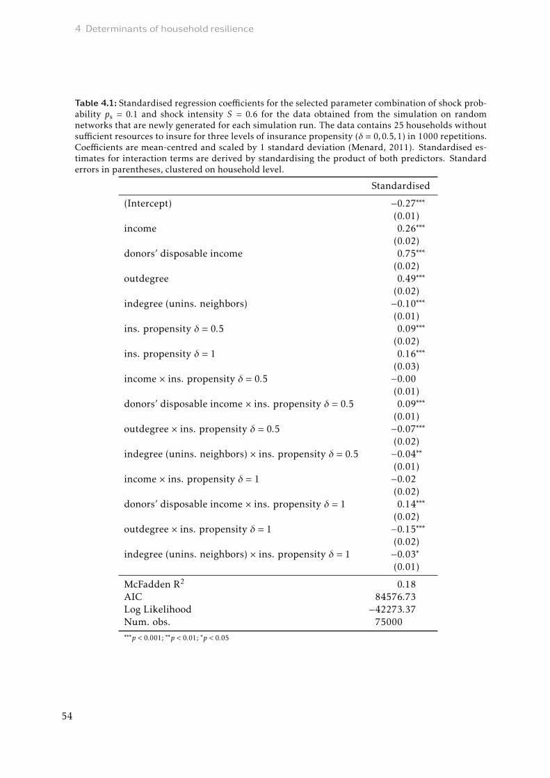
4 Determinants of household resilience
Table 4.1: Standardised regression coefficients for the selected parameter combination of shock prob-ability ps = 0.1 and shock intensity S = 0.6 for the data obtained from the simulation on randomnetworks that are newly generated for each simulation run. The data contains 25 households withoutsufficient resources to insure for three levels of insurance propensity (δ = 0,0.5,1) in 1000 repetitions.Coefficients are mean-centred and scaled by 1 standard deviation (Menard, 2011). Standardised es-timates for interaction terms are derived by standardising the product of both predictors. Standarderrors in parentheses, clustered on household level.
Standardised
(Intercept) −0.27∗∗∗
(0.01)income 0.26∗∗∗
(0.02)donors’ disposable income 0.75∗∗∗
(0.02)outdegree 0.49∗∗∗
(0.02)indegree (unins. neighbors) −0.10∗∗∗
(0.01)ins. propensity δ = 0.5 0.09∗∗∗
(0.02)ins. propensity δ = 1 0.16∗∗∗
(0.03)income × ins. propensity δ = 0.5 −0.00
(0.01)donors’ disposable income × ins. propensity δ = 0.5 0.09∗∗∗
(0.01)outdegree × ins. propensity δ = 0.5 −0.07∗∗∗
(0.02)indegree (unins. neighbors) × ins. propensity δ = 0.5 −0.04∗∗
(0.01)income × ins. propensity δ = 1 −0.02
(0.02)donors’ disposable income × ins. propensity δ = 1 0.14∗∗∗
(0.02)outdegree × ins. propensity δ = 1 −0.15∗∗∗
(0.02)indegree (unins. neighbors) × ins. propensity δ = 1 −0.03∗
(0.01)
McFadden R2 0.18AIC 84576.73Log Likelihood −42273.37Num. obs. 75000∗∗∗p < 0.001; ∗∗p < 0.01; ∗p < 0.05
54

4.3 Results
Table 4.2: Goodness-of-fit statistics (R2, RMSE and bias) for the estimation of the survival probabil-ities of households without enough financial resources to insure for different insurance propensitiesδ and predictors in the regression model. In addition to the dummy variables for insurance propen-sity, the following predictors are included: (#4) donors’ disposable income, own income, outdegree,indegree from uninsured neighbours; (#2a) own income, outdegree; (#2b) own income, outdegree towealthy households; (#1) own income.
δ = 0 δ = 0.5 δ = 1
# R2 RMSE Bias R2 RMSE Bias R2 RMSE Bias
4 0.806 0.150 0.098 0.878 0.113 0.070 0.906 0.089 0.0452a 0.515 0.191 0.068 0.514 0.180 0.048 0.465 0.175 0.0322b 0.673 0.149 0.021 0.643 0.150 −0.001 0.561 0.159 −0.0151 0.018 0.259 −0.050 0.016 0.257 −0.070 0.010 0.247 −0.081
provide goodness-of-fit statistics including R2, root mean square error (RMSE), and bias, i.e.the mean difference between the values predicted by the regression model and those derivedby the simulation. This allows us to analyse whether the variability in the survival rates iscaptured accordingly (R2), how accurate the fit is (RMSE) and whether the prediction showssome general trends (bias).
Survival rates of the poorest households in the empirical network can be adequately pre-dicted, even without explicitly mapping the temporal dynamics of the budget but by aggre-gating the most important influence factors and assessing the survival rate only at the end ofthe simulated period (Table 4.2, see Figure C.6 for a graphical representation). However, onaverage, the regression model tends to slightly overestimate the survival rate of the poorest(positive bias). The better prediction quality for higher insurance propensities is due to thefact that the disposable income of the neighbours becomes more reliable as δ increases. Thedrawback of such an accurate regression model is the amount of information needed aboutthe income distribution of all households as well as the network structure. Since this mightnot be available for all empirically observed networks, we also test the performance of mod-els with fewer predictors. Specifically, we consider models in which, in addition to one’s ownfinancial situation, only the number of neighbours one would approach if in need (outdegree)is included, but no information about their income. In addition, we assume that householdsare able to estimate whether their neighbours are wealthy enough to insure.
Missing information about the financial resources available for transfers crucially lower theprediction accuracy of the regression model. Nevertheless, when the network structure, i.e.the number of households that could be asked for support, is included in the regression, theprediction is much more reliable than when only the household’s own income is considered.Including information on whether a neighbour is wealthy enough to afford insurance furtherimproves prediction accuracy. The analysis underlines the importance of network character-istics for revealing the actual vulnerability of households in situations where informal trans-fers are an important risk-sharing mechanism and income is not homogeneously distributed.In contrast to networks where all households have on average the same budget, including thedisposable income of potential donors is essential to precisely predict the surviving chancesof households that are unable to formally insure.
55

4 Determinants of household resilience
0.54 0.41 0.27
0.41
0.45
S = 0.5 S = 0.6 S = 0.7
S = 0.3
S = 0.2
AAAAA
0.56 0.44 0.31
0.45
0.48
S = 0.5 S = 0.6 S = 0.7
S = 0.3
S = 0.2
BBBBB
0.58 0.47 0.34
0.47
0.5
S = 0.5 S = 0.6 S = 0.7
S = 0.3
S = 0.2
CCCCC
Insurance propensity δ = 0 Insurance propensity δ = 0.5 Insurance propensity δ = 1
0.25 0.30 0.35 0.25 0.30 0.35 0.25 0.30 0.35
0.1
0.2
0.3
Income threshold for insurance
Sh
ock
pro
ba
bili
ty
0.3 0.4 0.5
Fraction of surviving uninsured households:
Figure 4.3: Fraction of surviving uninsured households without enough financial resources to insurefor different shock probabilities ps and income thresholds for insurance It (due to different shockintensities S , It = ps × S/(1 − c)). The darker the colour, the less households survive, numbers in eachpanel denote the exact fraction. If a panel is left blank, the parameter combination was not selectedfor the analysis (see Appendix C.2 for details on the selection criteria). Results show the mean over1000 repetitions for different insurance propensities δ at the last simulation step (t = 50). Tables C.5and C.6 report Z-scores to assess whether the differences between the survival rates are statisticallysignificant.
4.3.4 Transferability to different external conditions
So far, the results were obtained for one selected parameter combination of shock probabil-ity and intensity. To investigate the effect of other external conditions that might arise, forexample, from changing climatic or demographic circumstances, we perform the same ana-lyses on the survival rate of the poorest, the logistic regression, and the prediction accuracyin empirical networks for the remaining four of the selected parameter combinations. First,we compare scenarios with the same shock probability (ps = 0.1) but lower (S = 0.5) or higher(S = 0.7) shock intensity than in the previous case. Here, 75% and 54% of all householdshave enough financial resources to insure. In addition, we analyse cases in which shocks oc-cur more frequently but less severe (ps = 0.2, S = 0.3 and ps = 0.3, S = 0.2), and where thenumber of households with access to insurance remains the same (62% of all households).
For all parameter combinations, the same trend as described in section 4.3.1 is prevalent: Themore households decide to insure the more households without enough financial resourcesto formally insure survive (Figure 4.3). This overall picture underlines the importance of thecontributions of insured households to informal risk-sharing for the poorest. When compar-ing the outcome for different external conditions, we observe a large effect of shock intensitywhen shocks occur equally often (ps = 0.1) but with different intensities. Since less severeshocks result in lower premiums, more households can afford insurance and at the sametime more budget is available for informal transfers, leading to more effective informal risk-sharing. When the same number of households are insured (It = 0.3) and the scenarios differin the combination of shock probability ps and intensity S , the variation in the survival rate isless pronounced. There is no significant difference between seldom shocks where householdslose a large share of their income (ps = 0.1, S = 0.6) and shocks that occur more frequently
56
4.3 Results
but impose lower losses (ps = 0.2, S = 0.3). Only for shocks that hit households even more fre-quently and cause even smaller losses (ps = 0.3, S = 0.2), a slight increase in survival rates canbe observed. Here, low support request make it easier to help others, even when householdshave to cover own losses.
By applying the regression analysis to the different scenarios, the trends observed for the se-lected parameter combination can be confirmed for all combinations of shock probability andintensity (Tables C.7 and C.8). For each scenario, the disposable income of the neighboursis most important followed by the outdegree and the own income. The slightly negativeinfluence of links from uninsured households is also present independent of the shock char-acteristics. For all scenarios, the disposable income of insured neighbours has a larger impacton the survival of the poorest than that of uninsured neighbours when these are treated sep-arately for δ = 0.5 (Tables C.9 and C.10). Overall, the main conclusions on the determinantsfor household survival are independent of the frequency and intensity of extreme events.
Across all scenarios, the simulated data of the empirical network can be reproduced with sim-ilar prediction accuracy with the regression model. Again, information about the financialsituation of all households in combination with details on network characteristics reveals thebest prediction on the survival rate of the poorest (Table C.11). For shocks that occur rarelyand with low intensity (ps = 0.1, S = 0.5), we observe that restricting the predictor that coversthe outdegree of a household only to the wealthy neighbours does not lead to an increasedprediction accuracy compared to considering all links. This can be explained by the factthat for low losses not only the rich but all households can contribute effectively to informalrisk-sharing.
4.3.5 Transferability to covariate shocks
For some types of shocks, households are not affected independently but several householdshave to deal with financial losses simultaneously, e.g. if households derive their income fromagriculture and extreme weather events reduce the yields. To investigate the effect of suchcovariate shocks, we perform the same analyses on the survival rate of the poorest, logisticregression and prediction accuracy for the empirical network when in case of a shock event80% of all households face losses at the same time.
Although on average each household is affected equally often by shock events for idiosyn-cratic and covariate shocks, we observe that less of the poorest households can cover theirliving costs when many households suffer from shocks simultaneously for all of the con-sidered external conditions (Figure 4.4). However, the relative difference between survivingrates for idiosyncratic (Figure 4.3) and covariate shocks (Figure 4.4) decreases with increas-ing insurance rate. This indicates that insured households can cover most of the requestseven if many of their peers need help simultaneously. For covariate shocks, the increase insurvival with insurance level is much more pronounced than for idiosyncratic shocks, whichhighlights the importance of insurance in these cases. When comparing the different externalconditions for shock events, we observe similar trends as for idiosyncratic shocks. Householdsurvival is strongly affected by the intensity of the shocks with more severe shocks leading tofewer households that can cope with the losses. Again, the survival rate of the poorest doesnot vary significantly between frequent shocks with low intensity and seldom shocks whichimpose high losses.
Looking at the regression model, also for covariate shocks the disposable income of the po-tential donors has the largest influence on the survival of the poorest (Tables C.15 and C.16).
57

4 Determinants of household resilience
0.36 0.29 0.22
0.25
0.25
S = 0.5 S = 0.6 S = 0.7
S = 0.3
S = 0.2
AAAAA
0.44 0.34 0.25
0.31
0.33
S = 0.5 S = 0.6 S = 0.7
S = 0.3
S = 0.2
BBBBB
0.53 0.4 0.29
0.39
0.42
S = 0.5 S = 0.6 S = 0.7
S = 0.3
S = 0.2
CCCCC
Insurance propensity δ = 0 Insurance propensity δ = 0.5 Insurance propensity δ = 1
0.25 0.30 0.35 0.25 0.30 0.35 0.25 0.30 0.35
0.1
0.2
0.3
Income threshold for insurance
Sh
ock
pro
ba
bili
ty
0.3 0.4 0.5
Fraction of surviving uninsured households:
Figure 4.4: Fraction of surviving uninsured households without enough financial resources to insurefor different shock probabilities ps and income thresholds for insurance It (due to different shockintensities S , It = ps × S/(1 − c)) for covariate shocks. In case of a shock at village level, 80% of thehouseholds are affected (pH = 0.8). The darker the colour, the less households survive, numbers ineach panel denote the exact fraction. If a panel is left blank, the parameter combination was notselected for the analysis (see Appendix C.2 for details on the selection criteria). Results show themean over 1000 repetitions for different insurance propensities δ at the last simulation step (t = 50).Tables C.12, C.13 and C.14 report Z-scores to assess whether the differences between the survival ratesare statistically significant.
In contrast to idiosyncratic shocks, the number of neighbours that can be asked for trans-fer is, however, less important than the own income. This could be because having a largenumber of neighbours is of little use if many of them are affected by shocks at the same timeas oneself. The number of uninsured households requesting informal transfers is insignifi-cant for the survival of the poorest. This is plausible as only few of the poor households cancontribute to informal transfers when most of them deal with the same shocks. The impor-tance of insured neighbours becomes even more apparent when the influence of insured anduninsured donors is considered separately (Tables C.17 and C.18).
The simulated survival probabilities of the poorest households in the empirical network canbe predicted with slightly lower accuracy than for idiosyncratic shocks (Table C.19). Whenrestricting the regression to predictors that can more easily be obtained from interview data,the prediction accuracy for covariate shocks is far lower than that for idiosyncratic shocks.This indicates that for covariate shocks exact information about the financial situation ofall households is even more important to effectively estimate the vulnerability of specifichouseholds.
4.4 Discussion
With this study, we gained insights into how effectively households without formal insur-ance can cope with income shocks by interacting in a social network. We specifically anal-ysed whether the availability of insurance can have an indirect benefit for poor, uninsured
58

4.4 Discussion
households. To identify which households are most vulnerable, we uncovered the functionalrelationship between the survival probability and key household and network characteristicsby combining agent-based modelling with regression analysis.
Our model results show that formal insurance does not only pay off for the insured house-holds themselves, but also for poor households that benefit from their peers being insured.The actual effectiveness of the interplay between formal insurance and informal risk-sharingis dependent on the characteristics of the shock events: Mild losses can be well covered withprivate transfers and without formal insurance. For more severe shocks, such support is lim-ited as households have fewer resources to share due to higher losses. Especially in this case,insurance significantly increases the chances of survival also of the weakest. Furthermore,the indirect positive effect of insurance is particularly strong in the case of covariate shocksthat affect many households simultaneously. Since few of the uninsured households can helptheir peers as they also face losses, insurance plays an even more important role: When manyhouseholds are insured, private transfers can be provided almost as effectively as in the caseof idiosyncratic shocks.
By applying a logistic regression analysis to the outcomes of the agent-based model, we wereable to show that a household’s financial situation alone says little about its ability to copewith income losses. Rather, in addition to the individual budget, the disposable income of po-tential donors and the network position must be taken into account. We tested the predictionaccuracy of the regression model on empirical network data from the Philippines. When in-corporating detailed information about household and network characteristics, we were ableto precisely reproduce the simulated results. Furthermore, we showed that even a simplifiedmodel can give important insights into the resilience of individual households. The regres-sion model can therefore be considered a valuable proxy for the outcome of the structuredagent-based model and a predictor of the survival probability of the poorest households.In this sense, the regression analysis can serve as an ‘early-warning system’ to test whetherformal and informal risk-coping instruments are effectively interplaying for the benefit of aparticular household or whether additional support is needed.
Given the stylized character of our model, we, however, neglected a number of factors, whichneeds to be taken into account when interpreting the results. First, we assumed that allhouseholds are unconditionally willing to provide informal transfers. Yet, households mightdecide how much to transfer and to whom, depending on their wealth differences, possibleother sources of support that a household might have or the neediness of a household rela-tive to others (Chiang, 2015). Second, the insurance status was not explicitly considered inthe transfer decision. This neglects empirical observations which show that the availabilityof formal insurance can alter transfer behaviour (Strupat & Klohn, 2018; Takahashi et al.,2018). Insured households might, for example, no longer be willing to transfer to uninsuredhouseholds, at least not to those that could have afforded to insure (Anderberg & Morsink,2020; Lenel & Steiner, 2020). In a previous modelling study, this was shown to greatly reducethe ability of uninsured households to cope with income losses when the income distributionis homogeneous (Will et al., 2021a). If households differ in income and the poorest rely solelyon informal transfers in times of need, a decline in solidarity could have an even greater im-pact on their resilience. Third, the network was assumed to be fixed, but connections mightchange over time and in response to external circumstances. To improve the external validityof the result, these aspects could be incorporated into later model versions.
Potential for further studies also exists with regard to the regression model. For simpli-city, we focussed on a small subset of potential explanatory variables, namely the financial
59

4 Determinants of household resilience
resources of a household and its neighbours as well as its network position. However, espe-cially with regard to the disposable income of the neighbours, there are a number of furtherscaling options that could increase the explanatory power of the regression and the respec-tive influence factors. We could imagine weighting the disposable income with the numberof households that are requesting support from the same household and their probability ofbeing affected by income losses. Effects of an even higher order can be considered if we wouldincorporate information on how many further possibilities of informal support are availableto the requesting households and how effective this help is likely to be, i.e. how wealthy theother neighbours are. Moreover, in most analyses, we only considered the survival of thepoorest after a given period of time but did not include the complete temporal dynamics.Especially for the regression analysis, we did not predict every single time step of the simu-lation but used the aggregated outcome of the complete simulated time span. However, thismight overlook certain situations, such as when insured neighbours have few resources forprivate support immediately after the introduction of insurance because they have not yetbenefited from reimbursed losses but must cover premium payments. By taking into accountthe temporal dynamics more explicitly, it would be possible to examine even more specifi-cally which households can cope with shocks and for how long, and when households needexternal support in the form of subsidies.
In our study, the regression approach allowed us to aggregate the results of the agent-basedmodel and to make general statements about the resilience of an uninsured household to in-come losses. However, all results are based on the same income distribution derived fromempirical observations on the Philippines. A systematic comparison of different networkstructures and income distributions is needed to test which further insights emerge fromspecific household and network characteristics. For example, in networks where segregationbetween wealthier and less wealthy households is prevalent and households in need are notsupported by wealthier peers, informal risk-sharing might not be effective. Similarly, it couldhave an effect whether income differences in the population are extreme, i.e. there are manyrich and many poor households, or whether all households have roughly the same level ofincome. The structure of the network might also have an influence. For example, the effec-tiveness of informal transfers might be different with a homogeneous distribution of linksthan when there are pronounced hubs where many households ask the same few for help.To obtain a comprehensive picture and develop a reliable tool to derive implications on theresilience of the poorest, it would therefore be necessary to systematically analyse differentnetwork configurations and compare the regression results in these scenarios. The basis forthe regression analysis yielding valuable results lies in the fact that household and networkcharacteristics were explicitly considered and disentangled in the agent-based model. Such astructurally explicit approach is essential for understanding systems where humans interactwith each other as well as with the environment (Will et al., 2020). Despite the simplifiedsetting, our study already shows the potential of systematically analysing the sensitivity ofresilience to structural household and network characteristics and provides far-reaching in-sights into the effectiveness of formal and informal risk-coping mechanisms under differentexternal conditions. Exploiting this strategy even further by analysing the interplay of house-hold and network characteristics more systematically will further improve the understandingof the effects of formal insurance and informal risk-sharing on the ability of the poorest todeal with extreme events. If this model-based approach was applied to other network typolo-gies and overarching conclusions could be found, this would allow transferability to any em-pirical network to make predictions about the actual vulnerability of individual householdswithout having complete information about all network characteristics, but by aggregatingthe relevant metrics.
60

4.5 Conclusion
While this study showed that formal insurance is a valuable complement to informal risk-sharing for households that are too poor to pay insurance premiums, a large fraction of thesehouseholds still cannot cover their living costs over a long period of time when regularlyaffected by income shocks. This underlines how important it is that also the poorest haveaccess to formal protection instruments in order to reduce their dependence on other house-holds and strengthen the resilience of the entire population. One way to achieve this goalwould be to make insurance more widely accessible. There are various options for doingthis: First, transaction costs related to distribution and administration must be reduced inorder to lower insurance premiums (Eling et al., 2014; Platteau et al., 2017). With respectto weather-related risks, index-based insurance where payouts are linked to environmentalproxies rather than individual losses, is a promising approach for decreasing costs (Barnett &Mahul, 2007). Similarly, for other types of insurance, using local infrastructure to distributethe products, collect premiums and process claims might lower transaction costs (Biener &Eling, 2012). Second, insurance schemes that incorporate price differentiation, with premi-ums specifically tailored to the available financial resources of potential policyholders, couldhelp make insurance accessible to a larger part of the population. By making richer house-holds pay a higher share than poorer ones, coverage for the entire population can improve.When combined with collective insurance programs where insurance is offered to groupsrather than individuals (Trærup, 2012; Santos et al., 2021), internal agreements within a so-cial network on contributions to the premium would be possible. Third, especially for cropfarmers where income is only realized at the end of the harvesting season, delaying premiumpayments until the end of the insured period is another option to improve accessibility toinsurance (Liu & Myers, 2016). Finally, offering direct subsidies is also an effective tool toachieve affordability and promote insurance, at least for a finite period after the introductionof a new scheme (Mahul & Stutley, 2010; Biener & Eling, 2012; Hazell & Varangis, 2020).Here, the insights obtained in our studies can help to target them effectively to support themost vulnerable. In addition to insurance products, other government and non-governmentsocial assistance programs that provide asset and cash transfers can contribute to promotingresilience among the very poor (Johnson et al., 2013).
4.5 Conclusion
Even though insurance products specifically designed for the needs of low-income house-holds are a valuable tool to buffer financial losses from personal or weather-related risks,they might not be able to strengthen the resilience of all parts of the population as premiumpayments can be too expensive for the poorest. Our simulation results show, however, thatthese households can also indirectly benefit from formal insurance when requesting informalsupport through their social network. Especially for covariate shocks where many householdare affected by income losses simultaneously, access to insurance increases the resilience ofthe whole population including those that cannot afford the premiums. By aggregating ourresults from a structurally realistic agent-based model in a regression model, we derived thata household’s own income is not the main determinant of its financial survival. Rather, itis important that its neighbours have enough disposable income and an atmosphere of soli-darity is preserved. By testing the predictive accuracy of the regression model for simulateddata of an empirically observed support network on the Philippines, we conclude that thisaggregated model is a valuable tool for identifying those households among the poorest ina population that benefit from informal protection, but also those households that are notprotected from income loss and are thus particularly vulnerable. This information can be
61

4 Determinants of household resilience
used to effectively target subsidies to households that cannot afford formal insurance and forwhom also informal support is insufficient.
The combination of agent-based modelling and social networks on the one hand and an ag-gregated regression analysis on the other hand made it possible to systematically test theeffects of varying external conditions. While the implications for the resilience of the poorestare based on a theoretical simulation model with a range of simplifying assumptions, the pre-sented analyses nevertheless provide helpful insights into how effective the combination offormal and informal risk-coping instruments can be and which factors have to be consideredwhen estimating the vulnerability of specific households.
62

Part II
Using models to addresssocio-environmental challenges


5 Improving insurance design under climate change:
Combining empirical approaches and modelling
This chapter is currently under review in Climate and Development as Will, M., Backes, A., Camp-enni, M., Cronk, L., Dressler, G., Gornott, C., Groeneveld, J., Habtemariam, L. T., Kraehnert, K.,Kraus, M., Lenel, F., Osgood, D., Taye, M., & Müller, B. Improving insurance design under climatechange: Combining empirical approaches and modelling.
Abstract
Extreme weather conditions in the face of climate change often disproportionately affect theweakest members of society. Agricultural insurance programs that are specifically designedfor smallholders in low-income countries are seen as valuable tools that can help farmersto cope with the resulting risks. At the moment, a broad range of methods including ex-perimental games, household surveys, process-based crop models and agent-based models isused to assess the demand for and the effectiveness of such insurance products. However,climate change raises specific socioeconomic as well as environmental challenges that needto be considered when designing insurance schemes. We argue that in light of these pressingchallenges, some of the currently used methodological approaches reach their limits whenapplied independently. We therefore advocate for a sound combination of different methodsespecially by linking empirical analyses and modelling and underline the resulting poten-tial with the help of stylized examples that address the main challenges for insurance designunder extreme weather conditions. Our study highlights how methodological synergies canmake insurance products more effective in supporting the most vulnerable, especially underchanging climatic conditions.
5.1 Introduction
Extreme weather events resulting from climate change, such as droughts or floods, posea particular threat to low-income households in developing countries that are engaged inagricultural activities (World Bank, 2009; Hallegatte & Rozenberg, 2017). Agricultural in-surance products specifically designed for the needs of smallholder farmers, known as mi-croinsurance or inclusive insurance, are seen as a promising tool for managing disaster risks.The International Panel on Climate Change (IPCC), for example, has stressed the need forrisk-sharing and transfer mechanisms such as insurance as a climate adaptation mechanism(IPCC, 2012). Similarly, the UNFCCC has pointed out the importance of insurance for ad-dressing effects of climate change in their Warsaw International Mechanism for Loss andDamage (UNFCCC, 2013). However, climate change poses specific socioeconomic as well asenvironmental challenges to effective insurance design (Table 5.1). First, to allow for an ade-quate combination of insurance with other risk management options such as credits, savings,
65
5 Improving insurance design under climate change
and traditional informal risk-sharing arrangements, it has to be considered that an increas-ing number of extreme events can alter the effectiveness or increase the costs of these existingstrategies (Peterson, 2012; Trærup, 2012; Linnerooth-Bayer & Hochrainer-Stigler, 2015). Sec-ond, the introduction of insurance might have environmental side effects such as degradationof natural resources (Bhattacharya & Osgood, 2014; Müller et al., 2017) as smallholders withaccess to insurance might, for example, be able to quickly restock their livestock herd size af-ter an extreme event (Bertram-Huemmer & Kraehnert, 2018), giving the pasture hardly anytime to regenerate. Changing climatic conditions that lead to an increased risk of droughtsand other extreme weather events further weaken the state of the natural resource. Third, aparticular challenge for agricultural index insurance, where payouts depend on exceeding orfalling short of a threshold derived from rainfall or vegetation data (Brown et al., 2011; Be-nami et al., 2021), is the accurate assessment of crop yields especially when extreme eventsoccur on a local scale. A mismatch between actual losses from a weather shock and receivedinsurance payouts, commonly defined as spatial basis risk, could lead to low acceptance ratesof the insurance (Clement et al., 2018).
With experimental games, household surveys, process-based crop models or agent-basedmodels, a wide range of methods is currently used to assess the demand for and impactof agricultural insurance and to identify its shortcomings and unintended side effects. How-ever, with respect to the pressing questions arising due to climate change, some of the meth-ods reach their limits. Experimental games, for example, are a valuable tool to assess specificbehaviour, but they usually include only a small number of individuals and, unless the sameexperimental design is replicated in different contexts, the results are difficult to general-ize. The econometric analysis of household surveys allows researchers to draw inferencesfrom large samples representative of the population. However, such surveys, and householdpanel surveys in particular, from which conclusions can be drawn about the impacts of po-tentially changing external conditions, are time and cost intensive. Modelling approachesallow researchers to overcome these time and space constraints: Process-based crop modelsthat cover biophysical aspects of crop yield dynamics and agronomic management informa-tion, however, do not include human behaviour explicitly. Agent-based models, on the otherhand, where human decision-making can be implemented in detail, depend heavily on theavailability of data to validate model assumptions.
From our point of view, the potential of each of these methods to contribute to a better un-derstanding of insurance could be considerably enhanced by combining them. We believethat this could lead to a more appropriate and sustainable insurance design given the currentchallenges of climate change. Mixed-method approaches that link quantitative and qualita-tive techniques have already been advocated in the context of microinsurance (White, 2014).We reinforce this demand by proposing a combination of modelling and empirical analyses.We address this aim by (a) exploring strengths and limitations of current approaches to as-sess and improve the impact of insurance; (b) illustrating how a more holistic approach canbe beneficial to advance an appropriate and sustainable insurance design; and (c) underlin-ing the potential of combining different methods with three stylized examples that addresschallenges for insurance design under climate change.
66

5.2 Strengths and limitations of current methods to evaluate insurance design
Table 5.1: Challenges for insurance design under climate change
Research theme Challenges
Risk managementoptions
How can insurance products be adequately combined with otherrisk mitigation strategies especially when an increasing numberof shocks occurs? How can insurance be used to overcomeshortcomings of other risk mitigation strategies?
Environmentaleffects
Which (indirect) effects does insurance have on natural resourceuse? How can insurance design mitigate unintendedconsequences?
Index design How to accurately assess crop yields and yield losses remotely tominimize basis risk? How to distinguish betweenclimate-related and non-climate-related yield loss?
5.2 Strengths and limitations of current methods to evaluateinsurance design
Below, we provide brief descriptions of several methods that illustrate the range of ap-proaches currently used to assess insurance demand and the impact of insurance payouts,identify unintended social and environmental side effects, and develop appropriate insur-ance indices. We focus on experimental games, the econometric analysis of household sur-veys, process-based crop models and agent-based models, as these are the methods we pro-pose to combine to tackle current challenges. For each of these approaches, we describe thetechnique in general, highlight their strengths and limitations, and present problems thathave been addressed in the context of insurance. Importantly, the methods discussed are notexclusive; analytical models, Bayesian Belief Networks, or qualitative research, for example,may be similarly useful in examining the impact of microinsurance and improving its design.
5.2.1 Experimental games
Experimental games are used to learn what choices people make in specific, well-definedsituations and which factors drive these choices. Games can contribute to understandingindividuals and groups by mimicking the actual environments where policy interventionswill take place (Hernandez-Aguilera et al., 2020a). In most experimental games, the exper-imenter first endows participants with a fixed amount of money or another easily sharedresource such as small packages of food and then gives them one or more decisions to makeabout what to do with the resource. Because experimental games can be conducted in labo-ratory and field settings located in any society in the world, they can yield useful insights notonly into behaviour but also into local cultural models (Henrich et al., 2004). One weaknessof the game method is that a researcher’s choice of a game and its usefulness for addressingthe research question at hand depends on the researcher’s understanding of the local culturalcontext; in turn, researchers’ design choices can interact with the cultural contexts that sub-jects bring to an experimental game. Indeed, small variations in the game design have beenshown to affect results considerably (DellaVigna & Pope, 2019; Landy et al., 2020). Another
67

5 Improving insurance design under climate change
drawback is that it can be difficult at many field sites to obtain large sample sizes, particu-larly if the game takes a long time to play or requires participants to play simultaneously.Furthermore, although games aim to map realistic situations, participants might not behaveas they do in their everyday life, but rather as they think they should (Zizzo, 2010; de Quidtet al., 2018). In the context of insurance, experimental games have been used primarily tostudy whether formal insurance crowds out grassroots risk pooling. Such experiments havebeen conducted in laboratory settings (Lin et al., 2014), and at field sites in the Philippines(Landmann et al., 2012), Ethiopia (Anderberg & Morsink, 2020), and Cambodia (Lenel &Steiner, 2020). Similarly, Cecchi et al. (2016) studied at a field site in Uganda whether formalinsurance crowds out social capital, operationalized as donations to a public goods game.Norton et al. (2014) assessed demand for index insurance among farmers in Ethiopia by us-ing a game in which people could allocate money across different risk management options.Agricultural insurance is furthermore beginning to adopt game approaches known as “gam-ification” (Hernandez-Aguilera et al., 2020b), which is the use of game design elements innon-game contexts (Seaborn & Fels, 2015).
5.2.2 Econometric analysis of household surveys
Household surveys are an essential source of information on the well-being and behaviour ofindividuals. The sample of households surveyed is ideally representative of subgroups andgeographical areas of the population of interest, and is usually based on census or administra-tive data. Household surveysmay address different objectives, ranging from documenting theliving conditions of a target population to estimating the impact of development programsand policies on households’ well-being (Grosh & Glewwe, 2000). Cross-sectional surveys thatare implemented with similar questionnaire design in several years, allow monitoring howliving standards change over time. A special case particularly informative to policy designare household panel surveys, in which the same households are traced over time. When anal-ysed with econometric methods, household surveys are a key source to establish a cause andeffect relationship between policy-relevant variables and household-level outcomes.
Despite these major advantages, household surveys are also subject to limitations. Depend-ing on the level of representativeness and, in turn, the sample size, implementing householdsurveys – and especially panel surveys – can be expensive. Furthermore, the amount of in-formation that can be recorded in household surveys is constrained by the time respondentsreadily devote to a survey interview. Also, there is a limit to the level of detail that respon-dents can be asked to recall. While major events in life are usually remembered well, indi-viduals typically face more difficulties to recall income streams retrospectively (Wooldridge,2012). Moreover, some information can hardly be recorded at all, such as inherent ability,skills, or work attitude. Finally, specific mechanisms that drive behavioural changes are diffi-cult to detect with pure survey data. In the context of agricultural insurance, the econometricanalysis of household surveys was used to study drivers of the demand for insurance amongfarmers in India (Mobarak & Rosenzweig, 2012; Cole et al., 2013; Mobarak & Rosenzweig,2013), Ethiopia (Dercon et al., 2014), and Ghana (Karlan et al., 2014). In addition, the im-pacts of agricultural insurance ex ante, i.e. before an extreme weather event occurred, on theinvestment decisions of farm households were quantified using household survey data (Hill& Viceisza, 2012; Cai, 2016; Cole et al., 2017; Hill et al., 2019). A related field of researchassesses whether indemnity payments from index insurance help farmers to recover fromlosses. Studies quantifying these ex post effects of agricultural insurance based on survey
68

5.2 Strengths and limitations of current methods to evaluate insurance design
data have focused on Kenya (Jensen et al., 2017; Janzen & Carter, 2019), Mongolia (Bertram-Huemmer & Kraehnert, 2018), and Bangladesh (Hill et al., 2019).
5.2.3 Process-based crop models
Process-based crop models include biophysical plant and soil processes such as the growthof above- and below-ground biomass as well as water and nutrient flows in the plant andthe soil to calculate interactions between environment and crop development (White et al.,2011; Boote et al., 2013). Due to their plant physiological algorithm, the models can cap-ture effects like extreme temperatures, dry spells or shifts in the growing season which havenot been observed in the past. Hence, these models can be used for quantifying yield andenvironmental effects of adaptation measures and for projections of future periods or otherenvironments which is particularly interesting in the face of changing climatic conditions(Wallach et al., 2016; Lobell & Asseng, 2017; Rötter et al., 2018). Since process-based cropmodels can provide information on yield losses immediately after the harvest, they can beused for risk assessments and adaptation planning (Challinor et al., 2018; Webber et al.,2020). This is highly relevant for insurance indices, in particular in developing countries,where crop yield information is not available and/or too expensive to collect because of re-motely located fields. Furthermore, the process-based organization of the model allows todistinguish between weather and management attributable influences on crop yield which iscrucial for the design of insurance indices, as only weather-induced losses should be coveredby the insurance product (Arumugam et al., 2020).
To feed process-based models, weather, soil and management information are needed.Weather information is available on a global scale informed by weather stations, satelliteobservations and weather models. Soil data are also widely accessible from global or regionalsoil maps. However, there is often little information about management practices and under-lying drivers of management decisions (Asseng et al., 2013; Folberth et al., 2019; Wang et al.,2019). In particular, responses of farmers to changing environmental and economic condi-tions are not reflected. This lowers the ability of process-based cropmodels to capture and re-produce accurate crop yields, especially in developing countries where the range of manage-ment practices differs highly across space, time, and farmer groups. So far, mainly weatherindexes (Dalhaus & Finger, 2016), remote sensing satellite vegetation indexes (Enenkel et al.,2019), and statistical models (Conradt et al., 2015) have been used to quantify crop yieldlosses. However, there is a growing interest among governments and insurance companies inprocess-based model assessments, for instance in India (Arumugam et al., 2020).
5.2.4 Agent-based models
Agent-based models (ABMs) are simulation tools that focus on individual actors such as hu-mans, households, firms or institutions. The interaction of these agents with each other andthe environment is explicitly considered in behavioural rules (Bonabeau, 2002; Railsback &Grimm, 2012). Agents can differ in their characteristics, i.e. they can be heterogeneous intheir attributes and decision rules. Based on the prescribed rules and micro-level properties,emergent temporal dynamics such as the spread of an innovation or collective behaviour canbe observed on a macro-level. ABMs can be used to systematically disentangle several influ-ence factors by including and excluding environmental features or aspects that impact theindividual decision-making. Furthermore, they have few time and space constraints: Results
69

5 Improving insurance design under climate change
can be obtained for large regions, which would require high financial resources if empiri-cal methods were used. In addition, ABMs can simulate long-term effects of new policiesor altered climatic conditions on a time scale beyond what can be detected with empiricalobservations. Apart from such explorative analyses, ABMs can also take a backward perspec-tive and help to uncover relations that cannot be fully explained empirically. This so-calledpattern-oriented modelling can be used to test assumptions about human behaviour, whichcan then be compared to observed results (Grimm et al., 2005).
As every other modelling approach, ABMs are only a simplified version of reality which hasto be taken into account when drawing general conclusions. Furthermore, ABMs can easilybecome complex when many influencing factors are included, which can make it impossibleto derive cause and effect relations of certain aspects. Besides this, model outcomes cruciallydepend on assumptions that require careful calibration with data that is often not available.Moreover, although the explicit integration of human behaviour is one of the strengths ofABMs, the theoretical basis of the decision-making frameworks used in such models is oftenquite simplified (Groeneveld et al., 2017; Schlüter et al., 2017).
ABMs have been used to analyse potential long-term effects of index insurance on sustain-ability of rangeland management (Müller et al., 2011) and resulting pasture conditions (Johnet al., 2019). In other studies, the effectiveness of insurance through informal risk-sharing(Aktipis et al., 2011; Hao et al., 2015; Aktipis et al., 2016) and impacts of combining formaland informal insurance (Will et al., 2021a) were investigated.
5.3 Synergies between different approaches to improveinsurance design
To overcome some of the individual limitations of the different methods, a holistic approachthat couples several approaches could be beneficial. We use three examples that focus on(1) combining different risk management options, (2) evaluating environmental effects of in-surance uptake, and (3) appropriately designing insurance indices to show how this can beused to address pressing challenges of insurance design under climate change. We suggestapproaching these challenges by linking empirical analyses that provide grounding in real-ity and models that reduce this complex reality to a limited number of key variables andprocesses. We use the first two examples to elaborate on combining household surveys, ex-perimental games and ABMs, mediated by the use of econometric methods; with the thirdexample, we show the potential of integrating empirically parameterized ABMs into process-based crop models.
5.3.1 Interplay between empirical data and ABMs
The general insights from household surveys and specific hypotheses tested using experi-mental games provide an excellent basis for specifying ABMs. While econometric analyses ofhousehold surveys can be used to parameterize individual household characteristics such asincome, social relationships, insurance status, and environmental conditions (Smajgl et al.,2011), decision-making in ABMs can be based on inferences drawn from small-scale exper-imental games with the same decision space (Smith & Rand, 2018). The outcome of ABMscan, in return, help to refine experimental research. If this results in new observations, thesecan again be implemented in ABMs (Chávez-Juárez, 2017). There exist successful examples
70

5.3 Synergies between different approaches to improve insurance design
Agent-based modelsWhat are long-term consequences ofthe introduction of formal insurance onthe welfare in a community? What consequences does increasedfrequency or intensity of shockshave on the effectiveness of formal andinformal risk-coping?
selectrepresentative
sample
definetransfer
behaviour
test behaviourof specificsubgroups
refinesurveyitems
parameterize household andnetwork variables
refine surveyitems
Experimental gamesDo households alter theirtransfer behaviour wheninsured? How much do householdstransfer to their neighbors?
Household surveys Which householdcharacteristics influence whethera household buys insurance? Between which households doesinformal transfer take place?
Figure 5.1: Schematic representation of the interplay between empirical data and ABMs to determinethe effectiveness of formal and informal risk-coping instruments under climate change
of such back-and-forth approaches. Cronk et al. (2019b), for instance, designed a two-playergame to study risk pooling in a laboratory based on earlier ABMs of risk pooling in dyads(Aktipis et al., 2011; Aktipis et al., 2016). The results from the game and ABMs were thenused to inform the design of additional experimental games (Claessens et al., 2021).
In the context of insurance, we suggest that a combination of methods could help to deter-mine the effectiveness of formal and informal risk-coping instruments under climate change(Figure 5.1). An increasing number of covariate shocks may threaten existing risk-sharinginstruments, such as when an entire community is affected by an extreme event and informalsafety nets can no longer absorb the losses (Wossen et al., 2016). At the same time, the in-troduction of insurance may lead to rising social inequality if insured households no longercontribute to traditional risk-sharing arrangements (Anderberg & Morsink, 2020; Lenel &Steiner, 2020). The behaviour of insured households can be tested in experimental gameswhere participants are randomly matched. In reality, however, the structure of risk-sharingnetworks determines their effectiveness. Informal protection varies depending on whether,for example, particularly poor households are linked to rich households or whether there isincome segregation. Network structures can be revealed with the help of survey campaigns.Integrating information on household behaviour observed during the games as well as net-work structures of specific villages in ABMs allows researchers to draw precise conclusionson the long-term welfare effects of potentially altered solidarity norms in a society.
A combination of methods is also promising for investigating the potentially negative sideeffects of insurance uptake on the environment (Figure 5.2). In pastoralist communities, in-surance coverage may prevent the need to reduce livestock following a drought (Gebrekidanet al., 2019). While having a positive impact on households’ livelihood in the short-term,this may result in overgrazing and pasture degradation, which increases the vulnerability tofuture extreme events. In agricultural communities, insurance coverage may create incen-tives to intensify production and, for instance, turn to cash crops or mono-cropping, whichyield higher returns but are riskier (Mobarak & Rosenzweig, 2012; Mobarak & Rosenzweig,2013; Cai, 2016; Cole et al., 2017; Jensen et al., 2017). To grasp the long-term effects of insur-
71

5 Improving insurance design under climate change
Agent-based modelsWhat are long-termconsequences fromchanges in agriculturalpractices and attitudeson the environment?
selectrepresentative
sample
parameterize household attributes
identify scenariosto be used in
further games
refinesurveyitems
parameterize household variables
Experimental gamesHow do householdschange their attitudestowards managing theglobal commons wheninsured?
Household surveys How do householdschange their agriculturalpractices when insured(ex ante and ex post anextreme event)?
Figure 5.2: Schematic representation of the interplay between empirical data and ABMs to quantifythe side effects of insurance coverage on rural communities
ance uptake on the environment, econometric methods may be used to infer from surveys,how households adapt their agricultural practices in response to purchasing insurance. Here,behavioural changes before a payment-inducing extreme event (ex ante) as well as once pay-ments from insurance are made (ex post) are of interest. Complementary experimental games,conducted in the same empirical context, may reveal more explicitly how the introduction ofagricultural insurance changes households’ attitudes towards managing the global commons,e.g. to what extent households shift priorities betweenmaximizing their own utility and com-munal welfare. Agent-based models may be used to extrapolate from the behaviour observedat the micro-level and derive macro-level trends in natural resource use under different sce-narios of insurance design and uptake.
5.3.2 Interplay between ABMs and process-based crop models
In order for insurance products to be effective not only under the given conditions but also inthe long term, their design must take into account changes in climate but also adjustments inagricultural practices (Siebert, 2016; Surminski et al., 2016). Whereas several long-term cli-mate projections exist and can be used in agricultural modelling (Asseng et al., 2013; Jones &Thornton, 2013; Folberth et al., 2019), future management decisions are much more difficultto predict. Agricultural practices are highly dependent on a farmer’s individual psychologi-cal and socioeconomic characteristics such as risk aversion, habits or openness to innovations.Furthermore, there is a feedback between farming strategies and global change processes.Farmers might adjust their crop portfolios or invest in irrigation to avoid losses due to alteredclimatic conditions (Collier et al., 2009). In addition, there might be indirect adaptations offarming decisions when insurance uptake incentivizes different management strategies (cf.section 5.3.1) and insurance uptake is largely determined by farmers’ satisfaction with theproduct (Shirsath et al., 2019).
The exchange of in- and output between process-based crop models and ABMs can helpto disentangle the complex interplay between human and environmental processes. ABMsare suggested to be a powerful tool to investigate land use decisions (Parker et al., 2003;
72
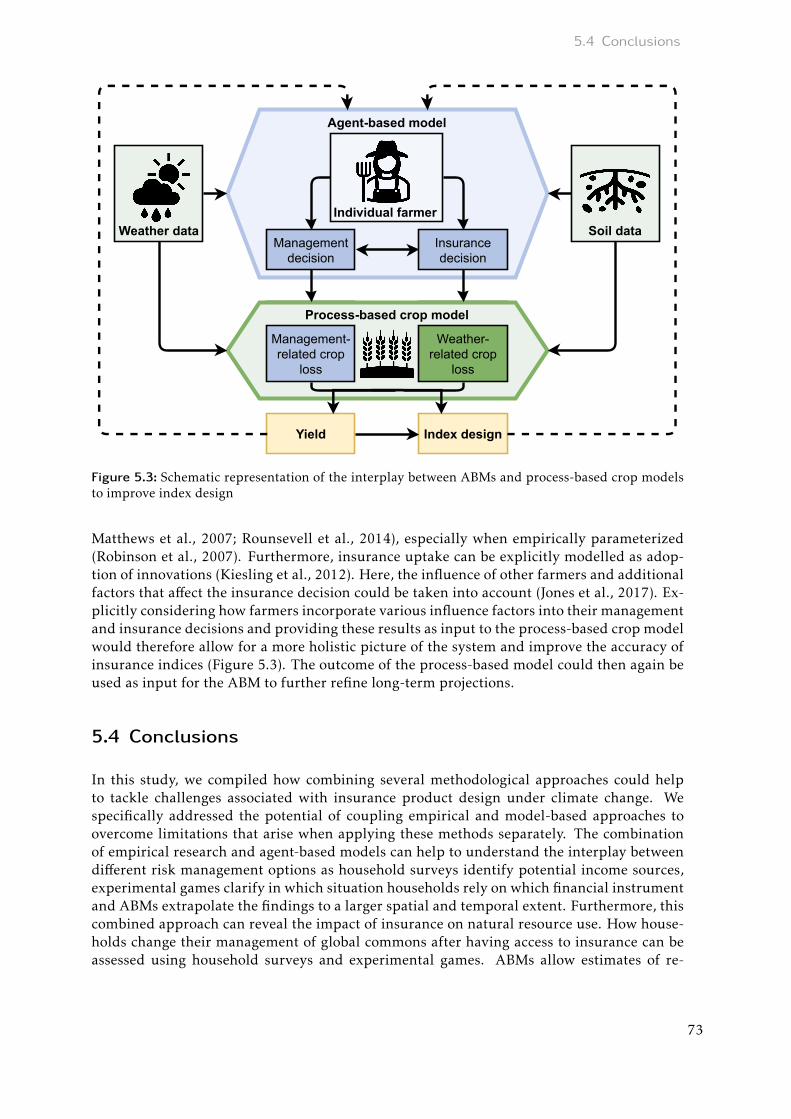
5.4 Conclusions
Management-related crop
loss
Management-related crop
loss
Process-based crop model
Agent-based model
Managementdecision
Insurancedecision
Management-related crop
loss
Weather-related crop
loss
Yield Index design
Weather data Soil dataIndividual farmer
Figure 5.3: Schematic representation of the interplay between ABMs and process-based crop modelsto improve index design
Matthews et al., 2007; Rounsevell et al., 2014), especially when empirically parameterized(Robinson et al., 2007). Furthermore, insurance uptake can be explicitly modelled as adop-tion of innovations (Kiesling et al., 2012). Here, the influence of other farmers and additionalfactors that affect the insurance decision could be taken into account (Jones et al., 2017). Ex-plicitly considering how farmers incorporate various influence factors into their managementand insurance decisions and providing these results as input to the process-based crop modelwould therefore allow for a more holistic picture of the system and improve the accuracy ofinsurance indices (Figure 5.3). The outcome of the process-based model could then again beused as input for the ABM to further refine long-term projections.
5.4 Conclusions
In this study, we compiled how combining several methodological approaches could helpto tackle challenges associated with insurance product design under climate change. Wespecifically addressed the potential of coupling empirical and model-based approaches toovercome limitations that arise when applying these methods separately. The combinationof empirical research and agent-based models can help to understand the interplay betweendifferent risk management options as household surveys identify potential income sources,experimental games clarify in which situation households rely on which financial instrumentand ABMs extrapolate the findings to a larger spatial and temporal extent. Furthermore, thiscombined approach can reveal the impact of insurance on natural resource use. How house-holds change their management of global commons after having access to insurance can beassessed using household surveys and experimental games. ABMs allow estimates of re-
73

5 Improving insurance design under climate change
sulting long-term consequences on the environment. The challenge of adequately defininginsurance indices can be mitigated by established process-based crop models. Combiningthis approach with ABMs helps to further improve the insurance design as it allows incor-porating feedback loops between humans and the environment by explicitly including localenvironmental constraints and potential effects on farmers’ behaviour.
To successfully combine different methods, it is important to clearly indicate which contri-bution can be achieved with which methods while keeping the limits of each approach inmind (White, 2014; Jones et al., 2017; Kline et al., 2017). An issue that needs to be addressedin the context of microinsurance is, for example, choosing the most representative time toobtain information on insurance uptake or land use. While this is also crucial for stand-aloneempirical studies, it is especially important in combination with models, since model rulesbased on these observations are used to make statements about broad temporal and spatialscales. Furthermore, it must be clearly communicated how much data is needed for the sim-ulations and uncertainties in the empirical observations must be accounted for in the model(Cheong et al., 2012). Additional challenges that arise for interdisciplinary research, such asestablishing a common language for exchange and allowing sufficient time for iterative cyclesof reflection across all phases of the research process, should also be considered (Kelly et al.,2019).
In this study, we did not focus on the integration of qualitative research which can add fur-ther relevant perspectives (Paluck, 2010; White, 2014; Millington &Wainwright, 2017). Sinceunderstanding the local cultural process is crucial to framing specific research questions,the use of quantitative methods should ideally be combined with qualitative ethnographicapproaches obtained through interviews and participant observation. For example, Cronk(2007) used trust games to study a Maasai risk pooling system. He selected the game basedon what he learned during a first round of interviews and conducted a second round of inter-views in light of the results of the game. In the context of microinsurance, qualitative meth-ods could be used to assess risk exposure, risk perceptions, and risk management strategiesto gain an overall understanding of vulnerability particularly under climate change (Turneret al., 2003).
Overall, we believe that the use of complementary methods to evaluate the effectiveness ofinsurance and to elucidate potential (unintended) side effects as presented in our study mayimprove insurance design and make this instrument more powerful in supporting the mostvulnerable in a sustainable manner. Future research projects should strive for such method-ological synergies to tackle the pressing issue of effectively protecting the poorest againstextreme events that will be even more pronounced under climate change.
Acknowledgements
The paper results from a workshop on “Exploring effects of microinsurance: Synergies ofdifferent methodological approaches” that was funded by the Deutsche Forschungsgemein-schaft (DFG, German Research Foundation) in the project SEEMI (Social-Ecological Effectsof Microinsurance) – 321077328.
74

6 How to make socio-environmental modelling more
useful to support policy and management?
This chapter has been published as Will, M., Dressler, G., Kreuer, D., Thulke, H.-H., Grêt-Regamey,A., &Müller, B. (2021). How to make socio-environmental modelling more useful to support policyand management? People and Nature. DOI: 10.1002/pan3.10207
Abstract
Dynamic process-based modelling is often proposed as a powerful tool to understand com-plex socio-environmental problems and to provide sustainable solutions as it allows disen-tangling cause and effect of human behaviour and environmental dynamics. However, theimpact of such models in decision-making and to support policy-making has so far been verylimited. In this paper, we want to take a critical look at the reasons behind this situation andpropose steps that need to be taken to change it. We investigate a number of good practiceexamples from fields where models have influenced policy-making and management to iden-tify the main aspects that promote or impede the application of these models. Specifically,we compare examples that differ in their extent to how explicitly they represent human be-haviour as part of the model, ranging from purely environmental systems (including modelsfor river management, honeybee colonies and animal diseases), where modelling techniqueshave long been established, to coupled socio-environmental systems (including models forland use, fishery management and sustainable water use). We use these examples to synthe-sise four key factors for successful modelling for policy and management support in socio-environmental systems. They cover (a) the specific requirements caused by modelling thehuman dimension, (b) the importance of data availability and accessibility, (c) essential ele-ments of the partnership between modellers and decision-makers and (d) insights related tocharacteristics of the decision process. For each of these aspects, we give recommendationsspecifically to modellers, decision-makers or both to make the use of models for practicemore effective. We argue that if all parties involved in the modelling and decision-makingprocess take into account these suggestions during their collaboration, the full potential thatsocio-environmental modelling bears can increasingly unfold.
6.1 Introduction
Socio-environmental systems (SES) are characterised by a tight coupling of human and en-vironmental dynamics (Berkes & Folke, 1998; Folke et al., 2010; Schulze et al., 2017). Bothaspects need to be understood to support sustainable management of these systems (Carpen-ter et al., 2009; Ostrom, 2009; Chapin et al., 2010). Dynamic process-based modelling, andin particular agent-based or individual-based modelling, is often proposed as an effective ap-proach to address such interlinked dynamics and provide solutions to pressing challenges, as
75

6 Modelling for policy and management
it allows disentangling cause and effect of human and environmental processes (Levin et al.,2013).
Socio-environmental modelling has made many contributions in the scientific realm answer-ing environmental issues on the sustainable management of natural resources focusing onland use/land cover change (Parker et al., 2003), agriculture (Huber et al., 2018), fisherymanagement (Lindkvist et al., 2020) or biodiversity conservation (Drechsler, 2020). How-ever, few SES models have had impact on decision support and policy-making (Schulze etal., 2017; Polhill et al., 2019; Elsawah et al., 2020). In contrast, models from other areassuch as transportation planning, epidemiology or pesticide risk assessment have been rou-tinely integrated into policy-making processes. Literature reviews evaluate the usefulness ofmodels for specific fields such as conservation management (Addison et al., 2013), marinesystems (Gregr & Chan, 2015), agriculture (Primdahl et al., 2010; Reidsma et al., 2018) orenvironmental health (Currie et al., 2018), but this work does not address how to foster theintegration of socio-environmental modelling into practice.
With this paper, we aim to explore models across disciplines and topics that have already in-fluenced policy-making and management. We look at seven good practice examples rangingfrom those tackling purely environmental problems that do not explicitly represent a humancomponent as part of the model, such as the management of rivers for both fish and am-phibian populations or control of animal diseases, to coupled SES models such as sustainablefisheries in Australia andwater management in Jordan. Based on the evaluation of thesemod-els, we explore factors that enabled or impeded the transfer of management-oriented modelresults into practice. The examples have in common that they did deliver scientifically in-novative insights and had an impact on policy or management decisions. Impact can rangefrom stimulating a discussion process (e.g. raising awareness for so far neglected issues), in-fluencing debates around a decision (e.g. laying out certain options or scenarios), to policy ormanagement decisions being directly based on model results (see van Daalen et al. (2002) fordifferent roles of computer models in the environmental policy cycle). Impact does not statewhether the outcome of the decision was positive or negative from a given perspective. Inthe context of modelling for decision support and policy-making, participatory approachesfor involving non-scientists in the modelling process have been suggested as an effective toolto incorporate expert knowledge not only to validate model assumptions but also to tailorpolicies to relevant local practices (Castella et al., 2014). Stakeholders’ expertise is requiredin different stages of the project, ranging from defining a problem to solving conflict situa-tions after the implementation of a measure (Pahl-Wostl, 2002). Several methods of citizenengagement have proven to be effective including interviews, focus groups, scenario work-shops, citizen science and digital participation (Šucha & Sienkiewicz, 2020). In the contextof modelling, various studies show the demand for stakeholder participation with a focus onparticipatory modelling (Voinov & Bousquet, 2010; Voinov et al., 2016) where different ap-proaches have been reviewed (Voinov et al., 2018; Sterling et al., 2019), classified (Barreteauet al., 2017) and standardised (Seidl, 2015; Gray et al., 2018).
While we acknowledge both the benefits and the challenges of such transdisciplinary stake-holder engagement, this is not the focus of this paper. Instead, we concentrate specificallyon the potential science–policy interface between (academic) modellers and (administrative)decision-makers. When referring to stakeholders, we therefore primarily address decision-makers who work in policy and management. Better integration of models in policy-makinghas been suggested with a focus on modelling for public policy (Gilbert et al., 2018), modelacceptance in policy-making (Kolkman et al., 2016) and models used as decision support
76

6.2 Methods
tools (McIntosh et al., 2007; van Delden et al., 2011; Zasada et al., 2017). Our paper con-tributes to this strand of literature targeting the special requirements that SES modellingbears.
The paper is structured as follows: in the next section, we present how the good practice ex-amples were evaluated, and list the criteria used to classify them. We introduce backgroundinformation about the seven models in section 6.3. In section 6.4, we present key princi-ples of success or failure that we derive from the evaluation. We conclude our paper withrecommendations to make modelling more relevant in policy-making and management.
6.2 Methods
6.2.1 Interview framework
Based on an initial literature review and the authors’ experience, we drafted a list of ana-lytical categories which we suspected to be relevant to our problem regarding the practicalimpact of SES models. We arranged them according to the ‘Four Ps’ framework developed byGray et al. (2018) which focuses on the purpose of the modelling endeavour, the processes ofexchange between modellers and managers, details on these partnerships, and the productsthat emerge from this exchange, that is, the range and type of application of the model out-come in practice. This results in the following grouping of the categories:
1. Purpose: background information, relevance of outcome, driving motivation
2. Processes: group size, actors involved, data availability and accessibility
3. Partnerships: previous relationship and experience, organisation of modelling process
4. Products: building confidence and transparency, learning processes, difficulties in theproject, usability of the model.
We formulated these categories as questions to compose a questionnaire for semi-structuredinterviews (see Appendix D).
6.2.2 Interviews
Based on the questionnaire, we conducted semi-structured interviews with seven researcherswho were currently or had previously been part of modelling projects in a policy or manage-ment context. The selection was by referral through colleagues and collaboration partnersand reflects a wide spectrum of models with impact in policy or management, ranging frompurely environmental models that do not explicitly involve a human component to socio-environmental models coupling human and environmental processes. All interviews weredigitally recorded. Prior to the interviews, informed verbal consent to be included in this re-search was obtained from the participants. As the study only includes expert interviews andthe participants were informed about the research objectives, it does not require ethical ap-proval according to the criteria of the German Research Foundation (Deutsche Forschungs-gemeinschaft, DFG). We assessed the respondents’ narratives against our categories. Thisprocess helped us identify missing aspects as well as emerging common themes, which weadded and condensed in subsequent iterations, loosely inspired by ‘grounded theory’ ap-proaches (Strauss & Corbin, 1997). This led, in the end, to a set of 14 gradients that include
77

6 Modelling for policy and management
most of our questionnaire items but also go beyond them and thus reflect a conceptual learn-ing process by which we amended our initial assumptions.
6.2.3 Gradients to describe good practice examples
The 14 gradients are again grouped according to the ‘Four Ps’ framework (Purpose, Processes,Partnerships, Products; Gray et al., 2018) and listed with their definitions in Table 6.1. Foreach gradient, the seven case studies are categorised as ‘low’, ‘medium’ or ‘high’. The inter-viewees reviewed our evaluation afterwards (and sometimes suggested modifications). In thefollowing, we present details on the classification according to the gradients.
6.2.3.1 Purpose
The first three gradients (system complexity, model complexity and demand-drivenness) ad-dress the background of the modelling example and ask by whom the modelling process wasinitiated. System complexity, on the one hand, refers to the real-world system under study interms of the number of actors involved or the diversity of processes and interactions that areimportant in that system. Depending on the research question, the identification of a ‘system’already involves some degree of abstraction, as in most SES it is difficult to clearly delineatewhat elements and links to include and which ones to leave out. On the other hand, modelcomplexity indicates to what level of detail elements and mechanisms of the real-world sys-tem are represented in the model, that is, whether they are included in detail, appear instrongly simplified form or are ignored altogether. Demand-drivenness reflects how far theinitiation of the modelling process was driven by demand from the decision-makers’ side.
6.2.3.2 Processes
The five gradients in this section (persons involved, decision-maker involvement, academicfields, data availability and data accessibility) relate to the organisation of the modelling pro-cess. This includes the number of persons involved (ranging from a single-person projectto a high number of participants involved), the number of academic fields or backgroundsinvolved (from a single discipline to a highly interdisciplinary project) or the involvement ofdecision-makers in the conceptualisation and development of the model. The latter relatesboth to the number of decision-makers involved and to the extent of their participation inthe process. Availability of data refers to the general abundance of qualitative and quanti-tative data needed to build the model. Here, the situation can be mixed, with, for example,biological data readily available and socio-economic data hard to come by. Data accessibilityreflects that even when sufficient data bases exist, for example, within a public institution,accessibility may be low if it is difficult for modellers to obtain access to them.
6.2.3.3 Partnerships
Gradients of partnerships (familiarity, modelling experience, exchange frequency and con-tinued support) address the relations and interactions between the different project partners,especially between modellers and decision-makers. Familiarity indicates how well projectpartners already knew each other at the beginning of the modelling process. Modellingexperience summarises how experienced decision-makers were with modelling approaches
78
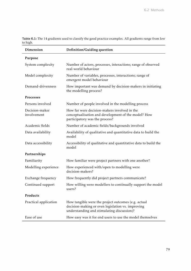
6.2 Methods
Table 6.1: The 14 gradients used to classify the good practice examples. All gradients range from lowto high.
Dimension Definition/Guiding question
Purpose
System complexity Number of actors, processes, interactions; range of observedreal-world behaviour
Model complexity Number of variables, processes, interactions; range ofemergent model behaviour
Demand-drivenness How important was demand by decision-makers in initiatingthe modelling process?
Processes
Persons involved Number of people involved in the modelling process
Decision-makerinvolvement
How far were decision-makers involved in theconceptualisation and development of the model? Howparticipatory was the process?
Academic fields Number of academic fields/backgrounds involved
Data availability Availability of qualitative and quantitative data to build themodel
Data accessibility Accessibility of qualitative and quantitative data to build themodel
Partnerships
Familiarity How familiar were project partners with one another?
Modelling experience How experienced with/open to modelling weredecision-makers?
Exchange frequency How frequently did project partners communicate?
Continued support How willing were modellers to continually support the modelusers?
Products
Practical application How tangible were the project outcomes (e.g. actualdecision-making or even legislation vs. improvingunderstanding and stimulating discussion)?
Ease of use How easy was it for end users to use the model themselves
79

6 Modelling for policy and management
before the project. Exchange frequency indicates how often the project partners met or com-municated during the project. This may in practice be restricted by project funding timelines,staff turnover or changing situations on the ground that make models obsolete. Continuedsupport reflects the modellers’ willingness and ability to provide ongoing support for modelusers, including beyond the official project duration.
6.2.3.4 Products
The last two gradients (practical application and ease of use) relate to the end product ofthe modelling project: practical application reflects whether outcomes of the model havebeen relevant for decision-making or to initiate legislative changes (‘high’ practical applica-tion), versus stimulating discussion and generating understanding (‘low’ practical applica-tion). Ease of use reflects the complexity of the final model and how intuitive it is for the endusers to utilise the model by themselves. This depends, for example, on the availability of agraphical user interface, compared to just a command line tool.
6.3 Good practice examples
The seven case studies we selected represent a wide range of influential modelling projects.They span different regional scales: some deal with concrete environmental questions whileothers attempt to understand complex socio-environmental or hydro-economic systems intheir entirety. In the following paragraphs, we briefly introduce the seven projects. Addi-tional background information is presented in Table 6.2.
• FYFAM: The Foothill Yellow-legged Frog Assessment Model (FYFAM) shows how rivermanagement affects frog breeding. It was designed to address the potential for conflictsbetween river management for salmon and frogs: if we provide certain conditions forthe benefit of salmon, what are the impacts to frogs? Certain parts of the model (theriver habitat) were borrowed from a fish model. The FYFAM model has been used tosupport the decision-making for river management at several sites.
• BEEHAVE simulates the development of a honeybee colony and its nectar and pollenforaging behaviour in different landscapes. The goal is to understand how honeybeecolonies respond to multiple stressors (disease, extreme weather, beekeeping practice,insufficient forage supply and pesticides), to identify stress levels and stressor combi-nations that put honeybees at risk, to support risk assessment and devise mitigationmeasures. The model has been used by different authorities and industries to explorethe effects of multiple stressors and suitable management options.
• FarmNet-BVD is an epidemic model. It evaluates the effectiveness of two differentstrategies to identify virus infections among cattle. The policy question was whethera switch to a new testing strategy would be beneficial to farmers in terms of the costsinvolved. This was linked to the goal of completely eradicating a cattle-related virusfrom the Irish cattle population. The model provided a quantitative basis for strategycomparison and influenced the decision taken by managers on a new legislation forspecific testing strategies in Ireland.
80

6.3 Good practice examples
• Ecopay: This ecological-economic model is able to simulate 15 endangered bird species,15 endangered butterfly species and 7 rare grassland habitat types in combination withseveral hundred grassland conservation measures (such as different mowing and graz-ing regimes) in different regions in Germany and Belgium. Its objective was to identifyboth ecologically effective and cost-efficient payment schemes for land use measuresthat contribute to the conservation of endangered species and habitats in agriculturallandscapes. The model systematically presents the range of alternatives, but no con-crete measures were taken based on the outcomes of the model.
• Atlantis-SE is a fishery model representing Australia’s southeast regional marineecosystem. It covers 3 million km2 of Australia’s fisheries. The model evaluates dif-ferent alternative management strategies for a complex multispecies fishery. Outcomesfrom the model provided information that supported change in a fishery law.
• ALUAM-AB is a land use model. It studies agro-pastoral systems and ecosystem ser-vices in the Swiss Alps under socio-economic and climate change. The research interestwas how to make payments for ecosystem services more effective, based on biophysicalfactors and taking into account cooperation between land users rather than a uniformdistribution scheme. Moreover, ALUAM-AB was applied to better understand whichactor types and which type of collaboration are necessary to foster resilience to climateand socio-economic changes. These results were incorporated in a new agrarian policyfor Switzerland.
• JWP: The Jordan Water Project is a coupled hydro-economic multi-agent model of theentire Jordanian water sector, allowing for an integrated analysis of short- and long-term sustainability challenges in this sector. More generally, the aim was to develop anintegrated framework for the evaluation of water policy interventions in water-stressedcountries, using Jordan as an example. The systematic representation of important in-fluence factors regarding the water sector improved the awareness for socially acceptedand sustainable use of water among relevant authorities in Jordan.
81

6Modellin
gforpolic
yandmanagement
Table 6.2: Overview of the seven good practice examples that were evaluated. The models are arranged by how explicitly they represent human behaviouras part of the model, ranging from purely environmental to socio-environmental models.
FYFAM BEEHAVE FarmNet-BVD Ecopay Atlantis-SE ALUAM-AB JWP
Degree ofexplicitlyrepresent-
inghuman
behaviour
EnvironmentalSocio-
environmental
Casestudysetting
Rivermanagementmodel for onefrog species
Development ofhoneybeecolonies,foragingbehaviour
Identification ofvirus infectionsamong animals
Grasslandspecies andconservationmeasures
Marineecosystems and
fishing
Mountainagro-pastoralsystems andecosystemservices
Hydro-economicmodel of the
Jordanian watersector
Locationand
spatialscale
Managed riversof northern
California; themodel typically
represents≈1 km length of
river
England,Hertfordshire,5 km × 5 km
(can be appliedto any region ofsame scale)
Ireland,resolution
depending ongeographical
coordinates andcadastral maps
Saxony andLower Saxony(Germany) and
Flanders(Belgium),
resolution 250m× 250m
SE Australia (3million km2)
Swiss Alps,smallest
landscape unit100m × 100m
Representationof whole
country (Jordan)
Researchquestion
How does frogbreeding successdepend on river
flows,temperatures,and channel
characteristics?
How dohoneybee
colonies respondto multiple
stressors? Whatmitigation
measures willreduce risk?
Will theintroduction of a
new virusmonitoring
approach payoff?
What land usemeasures areeffective toconserve
endangeredspecies andgrasslandhabitats?
Whichmanagementstrategies best
achieveecosystem-based
fisheriesmanagement
goals?
How to manageland to fosterecosystem
services supplyand increaseresilience toclimate and
socio-economicchanges?
How will waterpolicy
interventionsaffect
water-stressedcountries?
82

6.3
Goodpractic
eexa
mples
Projectduration
2014–2018Since 2008,ongoing
2015–20172008–2018 (inseveral projects)
2003–2007(ongoing, use fornew questions)
2008–2020Since 2014,ongoing
Modeltype
ABM
ABM +simulated
age-structuredmodel
Spatiallyexplicit,
stochastic,pseudo
individual-based
Ecological-economicmodelling,optimisation
ODE (ordinarydifferentialequation)
model; complexhybrid
approach: 58ecological
componentsmodelled; 26
fisheriesrepresented
ABM ABM
Peopleinvolved
Modeller, riverengineer (formodelling
hydraulics) andbiologists
Modellers, beeecologists,industry
Authorities(ministry);official
veterinarians;private
veterinarians;subject matterscientists;
modelling team;farmers’
organisations
Scientists(mostly
modellers),nature
conservationfoundation,ministry ofagriculture(Saxony)
Scientists,industry
representatives,managers,
policymakersand economists
Empiricalscientists,modellers,(local)
authorities,engineers,
experts fromdifferent field(land use,hydrology,
natural hazards,forest, ruraldevelopment)
Scientists,Jordan Ministry
of Water
Keyreference
Railsback et al.(2016)
Becher et al.(2014)
Thulke et al.(2018)
Mewes et al.(2017)
Fulton et al.(2014)
Grêt-Regameyet al. (2019)
Klassert et al.(2015)
83

6 Modelling for policy and management
6.4 Results: Observed patterns in good practice examples
Reviewing the interviews, we evaluated the good practice modelling studies along the gradi-ents explained in section 6.2. The results are graphically represented in Figure 6.1. As thepositions on these gradients are not necessarily stable over the course of a project, we markedthe dominant position.
By definition, all of the selected examples had some kind of impact with policy-makingor management. However, the type of practical application differs, ranging from modelsas tools for discussion (JWP) or a systematic representation of alternatives (Ecopay) to di-rect influence on the decision-making of legislative or management authorities (ALUAM-AB,Atlantis-SE).
According to the answers obtained from our interviews, few factors are truly indispensablefor models that have successfully been used for policy-making or management. Exchangefrequency, continued support and data availability stand out as the factors with consis-tently high or high and medium ratings for all models. The majority of the aspects werementioned as being important only in some cases and not in others. In the following, we dis-cuss the observed patterns of all dimensions of the modelling endeavour separately to extractimportant factors and correlations.
In our sample, systems with a focus on environmental processes are in general less complexthan systems explicitly involving a social component. These systems are also characterised bylowermodel complexity. In our good practices examples, model complexity always matchessystem complexity. We decided to keep both gradients in our framework because complexitymismatch may easily occur in other case studies. Similarly, the complexity of models with asocial and an environmental component tends to require higher numbers of persons involvedin the process. Due to the diverse aspects addressed, those people also have a broader rangeof academic backgrounds.
Many models were used for policy-making after modellers themselves had advocated them.Some processes were initiated on a joint proposal by decision-makers and modellers, but thecase that the demand came solely from decision-makers was rare. In our case, only the de-velopment of FarmNet-BVD was initiated by policymakers. However, the source of originalinterest in the collaboration does not influence the effectiveness of the process: models ini-tiated by modellers can also be successful in policy-making. Independently of who initiatedthe process, decision-makers were involved in model conceptualisation and development tovarying degrees. Some of the projects under consideration were developed in a participatoryway with considerable influence of decision-makers on the model implementation (FYFAM,Atlantis-SE and FarmNet-BVD), others were developed from an academic perspective andlater applied to concrete policy-making settings (BEEHAVE, JWP). Project partners were notnecessarily familiar with one another beforehand. Similarly, not all decision-makers wereexperienced with modelling in advance.
Our interviews suggest the exchange frequency as the most critical aspect during the wholeprocess. Meeting on a regular basis to discuss model results and project development ensuresa stable ground for project impact. For all our examples, it was furthermore guaranteed thatthe model developers continued the support at the end of the project duration such thatsome of the models could be adapted to new situations with similar research questions (Eco-pay, FarmNet-BVD). Besides reusing the same model in follow-up projects, continuing theapplication of models in policy-making can also be facilitated when decision-makers can
84

6.4 Results: Observed patterns in good practice examples
Purpose
Pro
cess
es
Pa
rtne
rship
s
Products
low
medium
high
Sy
ste
m c
om
ple
xit
y
Mo
de
l co
mp
lex
ity
Demand-d
rivenness
Persons involved
Decision-maker involv.Academic fields
Da
ta a
vaila
bility
Da
ta a
cc
es
sib
ility
Fa
mil
iari
ty
Modelli
ng experie
nceExchange frequency
Continued support
Practical application
Ea
se o
f use
SC
MC
DD
PI
DI
AF
DA
v
DA
c
F
ME
EF
CS
PA
Eo
U
FYFAM
SC
MC
DD
PI
DI
AF
DA
v
DA
c
F
ME
EF
CS
PA
Eo
U
BEEHAVE
SC
MC
DD
PI
DI
AF
DA
v
DA
c
F
ME
EF
CS
PA
Eo
U
FarmNet-BVD
SC
MC
DD
PI
DI
AF
DA
v
DA
c
F
ME
EF
CS
PA
Eo
U
Ecopay
SC
MC
DD
PI
DI
AF
DA
v
DA
c
F
ME
EF
CS
PA
Eo
U
Atlantis-SE
SC
MC
DD
PI
DI
AF
DA
v
DA
c
F
ME
EF
CS
PA
Eo
U
ALUAM-AB
S
C
MC
DD
PI
DI
AF
DA
v
DA
c
F
ME
EF
CS
PA
Eo
U
JWP
Degree of representing human behaviour low medium high
Figure 6.1: Classification of the good practice examples along the 14 gradients. The large panel showsthe number of studies classified as low, medium or high for each gradient. The outer radar charts showthe classification of the individual models. Abbreviations correspond to the gradient named at therespective circular position on the large panel. The outer charts are arranged according to their degreeof explicitly representing human behaviour as part of the model, ranging from purely environmentalto socio-environmental models. For better visualisation in the larger panel, we divided this continuousgradient in three distinct groups with similar degree of human behaviour and use different colours inthe large panel to represent the classification of the models with low (white), medium (grey) and high(black) level of human behaviour.
85

6 Modelling for policy and management
apply the models to specific questions, potentially also different to the original one, indepen-dent of the modellers. Only two models in our sample (FYFAM, BEEHAVE) are designed in away that policymakers can use them completely on their own. In other models, policymakersdesign new scenarios or evaluation options in direct collaboration with modellers (Ecopay,ALUAM-AB, JWP). One factor that simplifies the ease of use of models by non-modellers isthe creation of an intuitively designed graphical interface. Furthermore, training providedby modellers can encourage decision-makers to work with the models on their own. Here,the application of a programming language with low complexity (e.g. NetLogo) might bebeneficial.
Another key aspect across all selected studies which allowed them to be good practice ex-amples is the availability and accessibility of data. Calibrating and validating models toexisting data at the required resolution is essential to make policy or management decisionsdrawn from the models as precise and reliable as possible. Although all interview partnersconfirmed that their models had excellent or appropriate data available, two also mentionedthat data accessibility can be an issue, for example, due to European data sharing regulations(FarmNet-BVD, ALUAM-AB).
6.5 Discussion: Specific recommendations for SES Modelling
From the seven interviews and our general experience in the field, which also includes mod-elling endeavours that were not seen as having achieved an impact in the sense used here, weconclude that there are four key factors for ‘successful’ models. These factors refer to whatwas mentioned as important by all our interviewees (data availability, exchange frequencyand continued support) but also go beyond that. Once more structured around the ‘Four Ps’framework, we discuss the importance of modelling the human dimension (purpose); dataavailability and accessibility (processes); collaboration, trust and acceptance (partnerships);and decision processes (products). We give recommendations for each of these factors onhow to overcome difficulties that arise when modelling for policy and management support.Some parts of the discussion are transferable to other domains, but as most of the aspectsare more difficult to address for socio-environmental models compared to models with a fo-cus on environmental processes, the four key factors may explain why models have foundcomparatively little use in policy or management advice in this field in particular.
6.5.1 Purpose: Human dimension
The human dimension, the ‘socio-’ in socio-environmental systems, adds levels of complex-ity as humans, more vehemently than other species, continually innovate and adapt theirpractices while negotiating their interests. This sometimes leads to what has been called‘wicked problems’ (Churchman, 1967; Davis et al., 2018)—problems that involve a host ofstakeholders with conflicting interests, and for which no simple or optimal solutions exist.Such a situation occurred, for example, when discussing effects of strategies to prevent newinfections during the coronavirus pandemic (Squazzoni et al., 2020). Here, models can beparticularly useful in providing a forum for discussion by revealing the interests and as-sumptions of the different parties involved, creating a space to take new perspectives and,thus, have the potential to stimulate a change in lines of thinking. With respect to our goodpractice examples, such an approach was employed in the JWP example that aimed at along-term sustainability perspective—a view the involved ministry had not taken before.
86

6.5 Discussion: Specific recommendations for SES Modelling
However, as structures and dynamics that involve humans are difficult to formalise in modelterms (Schlüter et al., 2017), their inclusion in a model may drastically increase the com-plexity of model dynamics as well as the uncertainty around model results (Squazzoni et al.,2014).
Recommendations: We encourage the use of models as discussion tools to bring different per-spectives of stakeholders together—a process that is also referred to as social learning (Ed-monds et al., 2019; Schlüter et al., 2019). Furthermore, we recommend that modellers anddecision-makers acknowledge that the understanding of complex socio-environmental sys-tems depends to a large extent on a sound representation of human decision-making. Theneed for rapid answers must therefore not lead to models being overly simplified (Squazzoniet al., 2020). The trade-off between the expectation of quick responses and precise projectionsof the future, which can only be achieved by a detailed implementation of human behaviour,should rather be resolved by clearly communicating the purpose of a model (Grimm et al.,2020).
6.5.2 Processes: Data availability and accessibility
The seemingly obvious assumption that it is generally more difficult to obtain reliable dataon socio-environmental problems compared to purely environmental ones, once again dueto the complexity added by the human factor, was not fully confirmed by our good practiceexamples. In the cases of JWP and Atlantis-SE, socio-environmental data were relativelyabundant and accessible. In contrast, accessing existing databases was an issue in two of ourexamples, as mentioned above. Since these difficulties arose in both the socio-economic andthe ecological context, this factor appears to be context-specific rather than systematic. Inthe case of the BEEHAVE model, the interview partner indicated that industry partners hadeasier access to data; however, most of these data were subject to company confidentialityregulations and would therefore not be available for other projects to use.
Recommendations: As we have observed for our good practice examples that data availabilitywas a key aspect for impactful models, we highly encourage coordinated and harmoniseddata collection not only of ecological but also of socio-economic data. Examples for this areendeavours such as Long-Term Socio-Ecological Research (LTSER) platforms, where socio-ecological data collection is organised across the world (Dick et al., 2018). These systematicefforts come along with transparent rules for data accessibility which are crucial for impactfulmodelling projects.
6.5.3 Partnerships: Collaboration, trust and acceptance
With exchange frequency and continued support, two aspects of the partnership betweenmodellers and decision-makers stood out as being important in all our case studies. This sug-gests that the collaborative process is critical to an impactful modelling endeavour. Strongexchange can help to prevent false expectations of decision-makers concerning the powerof models (Kolkman et al., 2016). In the Ecopay project, there were diverging expectationsbetween scientists on the one hand (long-term project, transferable models) and decision-makers on the other (concrete measures). Providing enough time to understand the per-spectives of other disciplines and to find a common language was seen as crucial. In theJWP project, for example, a series of four 2-week workshops was organised to foster un-derstanding of the model. However, a large heterogeneity in the group of stakeholders and
87

6 Modelling for policy and management
disciplines involved made it difficult to find the appropriate speed for workshop discussions.Continuous communication ensures the understanding of decision-makers concerning limi-tations and uncertainty of models and prevents turning models into black boxes (Gilbert etal., 2018). Due to a broader range of backgrounds of people involved in the process, all thesefactors seem to be more pronounced in socio-environmental than in purely environmentalcontexts (see Kline et al. (2017) for their experience in a project investigating forest wildfires,Squazzoni et al. (2020) for the importance of interdisciplinary research on the coronaviruspandemic).
When the involved parties are not familiar with one another in advance, project partners needto be aware that creating trust between collaborators needs time, which has to be includedin planning the process (see also Briggs (2006) for the difficulties of integrating science andpolicy on natural resources in general). The establishment of mutual reliance in the projectteam was often, but not always, related to a specific ‘eye-opener’ or breakthrough momentwhich advanced the shared understanding of different stakeholder groups, led to bondingbetween them, and created strong confidence in the project’s usefulness. In our case studies,methods that induced breakthrough moments included the use of graphical representations,games and simulation runs based on past conditions showing that the model was able to rep-resent the recent past correctly (Atlantis-SE). During workshops in the FarmNet-BVD project,it proved helpful to explore contradictions in the assumptions of decision-makers to open upthe debate about alternatives. Conventional methods of trust-building are equally importantin successful projects; these can consist in benchmarking with existing models, or having anindependent peer review of project-related documents and models (Atlantis-SE, BEEHAVE).In the case of BEEHAVE, such a peer review of the formerly used model of the EFSA (Euro-pean Food Safety Authority) and the BEEHAVE model assured the quality of the model andfinally led to the replacement of the original model with BEEHAVE. The establishment ofsuch instances of quality control may also foster the acceptance of models in policy-makingand management support. These can range from simple model code review (e.g. as offeredby CoMSES Net) to the examination of complete modelling assessments (e.g. as done by theRegulatory Scrutiny Board of the European Commission).
It is not essential that decision-makers are experienced with modelling in advance. How-ever, openness for such an approach and knowledge of similar methods such as statisticalmodels simplifies communication and collaboration. In general, standard economic modelsappear to be more broadly accepted in policy and management support than SES models,which is partly a matter of traditions that have been established for longer, but also of manypolicymakers having a background in economics rather than the interdisciplinary trainingthat is often helpful for SES analysis. We generally observe that the acceptance and use ofSES modelling has actually been steadily spreading, from research to industry and on to pub-lic authorities—but it takes time. Mixed institutions that involve industry, researchers andpolicymakers might facilitate this process.
Recommendations: First, with respect to collaboration, we highly encourage all parties in-volved to make their expectations explicit at the beginning, especially concerning the out-comes of the policy-making process. To achieve successful exchange, we furthermore under-line that finding a common language is crucial to combine expertise from a wide range ofdisciplines.
Second, to foster the understanding of models and facilitate trust in them, we encouragemodellers to promote the emergence of ‘eye-opener’ moments using various tools of visuali-sation. Additionally, modellers can contribute to confidence in model results through bench-marking, independent peer review or by including quality control in the project structure
88

6.5 Discussion: Specific recommendations for SES Modelling
(Houweling et al., 2015). Transparent handling of model code through open-source devel-opment and sharing of models on public repositories (GitHub, CoMSES Net, etc.) helps tofoster this.
Third, as in the quote famously attributed to Henry Ford that states that if one had askedpeople what they wanted, they would have said faster horses but not cars, decision-makersmay simply not be aware of the benefits and feasibility of state-of-the-art modelling ap-proaches. To reach acceptance of models, modellers should therefore disseminate informa-tion to decision-makers, promote exchange betweenmodellers and decision-makers, be readyto teach modelling skills, and engage in the organisation of workshops that attract both sides.Large institutions and authorities can contribute to this exchange by employing modellingexperts for consulting, evaluation and assistance.
6.5.4 Products: Decision process
Research objects in SES models tend to be more contested than those mapped by purelyenvironmental models since they touch the interests of a broader set of stakeholders whomayhave diverging opinions. In contrast, resource management decisions such as in the FYFAMmodel—frogs versus salmon—are often less politically debated. Favouring one species overthe other cannot easily be characterised as ‘progressive’ or ‘conservative’ political positions,for instance. Gotts et al. (2019) accordingly speak of SES as ‘contested systems’. Furthermore,a chain of institutions with diverging time horizons are involved in the policy cycle. Toensure that an SES model can have true impact, it is hence important (and at the same timechallenging) to include those decision-makers who actually have the power and legitimacyto implement model findings. In the FarmNet-BVD model, for example, having both theministry and farmers on board facilitated the uptake of model outcomes in new legislationin Ireland as the two implementing forces were able to discuss details during the modeldevelopment phase. In ALUAM-AB, one of the key researchers later on became an influentialperson in the policy sector. On the other hand, for Atlantis-SE, it was reported that theabsence of a competent ‘policy champion’ that modellers could turn to slowed down thepolicy-making process.
In general, only if model assumptions and rules are well-grounded and fitting to purposeand context, their outcomes will be able to support wise policy-making and managementand should be included in the decision-making process. This can be especially harmful whenmodels are not properly adapted to a context different to the one they were originally devel-oped for (Squazzoni et al., 2020) or when they are still widely used in consultancy but not up-dated to standard practices (Railsback, 2016). One of the rare documented examples of neg-ative impact of models can be found in the context of the 2001 outbreak of foot-and-mouthdisease in the United Kingdom where misguided interpretation of mathematical model re-sults led to the slaughtering of a large number of animals, which was later considered to havebeen unnecessary (Kitching et al., 2006). The modelling endeavour may, moreover, be cap-tured by decision-makers to one-sidedly support their previously held convictions and shutdown rather than open up discussions of policy or management alternatives (Squazzoni etal., 2020). Modellers thereby inevitably have to take on the role of translators for the modelresults, as only this allows a sound understanding by decision-makers which needs to be thebasis to use the model in any decision process (Gilbert et al., 2018). Explicitly communicatingassumptions in the model conceptualisation and uncertainties in the model output is partic-ularly important for an effective incorporation of the results in the decision-making process
89

6 Modelling for policy and management
(Brugnach et al., 2007; Gregr & Chan, 2015; Davis et al., 2018). But even if the coopera-tion process is carefully framed, modellers need to be aware that policy advice is simply notalways desired (Squazzoni et al., 2020) as for some problems there is only a small ‘windowof opportunity’ (Kingdon, 1984) where policymakers are open to tackle a problem and needadvice that could then be provided by models.
Recommendations: We underline that model users (including from the decision-makers’ side)should have a profound understanding of the model and only apply it in cases where modelassumptions are suitable. In the end, the consequences of decisions may reach well beyondthe original scope of any single research question and model. In this regard, due to highercomplexity, modellers are even more obliged to apply good modelling practices (Schmolke etal., 2010; Schulze et al., 2017) to SES models. Furthermore, policymakers are highly encour-aged to provide a ‘policy champion’ or ‘knowledge broker’ as interface person to modellers.Ideally, this should be someone open to modelling approaches and at an influential positionin the decision-making process who is able to mediate between both parties.
6.6 Conclusion
By evaluating seven good practice examples, we show that leverage points for increasing theimpact of socio-environmental models in policy-making or management are manifold. Whileour paper focuses on the transfer of knowledge generated by models to the actual decision-making process and therefore mainly refers to the community of modellers and to decision-makers, many of the aspects we highlight, especially those referring to model development,will also apply to situations where a broader range of stakeholders is involved, such as duringparticipatory modelling (Castella et al., 2014; Reid et al., 2016).
We conclude that the main reason currently inhibiting a wider use of socio-environmentalmodels in policy-making or management is their higher complexity compared to purely en-vironmental models that arises from explicitly incorporating the human dimension. Addinglevels of behaviour results in more difficult models. These additional aspects also impedesimple solutions for policy-making and management. This is reinforced by the fact that ad-dressing both the social and the environmental dimension adequately in models requires in-volvement of people from different backgrounds. Their potentially contested positions makeconsensus building and thus decision-making for policies more challenging. In contrast toother problems, where decision-makers rely on the judgement of experts to assess the impor-tance of influencing factors that should be integrated into models, human behaviour is moretangible for many of the actors involved so that more concrete expectations are placed onthe representation of processes in models. This can easily threaten the acceptance of modelswhen not all of the desired factors can be addressed. Furthermore, data accessibility, a crucialaspect of impactful modelling projects, is more difficult due to privacy issues.
All these factors pinpoint the importance of using models for SES problems on the one handto provide a common ground for exchange and on the other hand to allow disentangling causeand effect of human and environmental processes. The same factors, however, urge to respectfundamental aspects of science–practice interactions, such as clear communication of expec-tations and results or building trust. Even though any model can depict only a part of reality,this issue is, more than in other disciplines, pertinent to the inclusion of human behaviour,as some patterns will never be reproducible in model rules due to the inherent complexity ofdecision-making. Nevertheless, modellers and decision-makers should continue to embark
90

6.6 Conclusion
on common projects and learn from successful examples to increasingly unfold the full po-tential that socio-environmental modelling bears. We have synthesised recommendations fordealing with common difficulties that may arise during the process of modelling for policyor management support, which are addressed to modellers, decision-makers or both. If allparties involved in the modelling and decision-making process take into account our sug-gestions during their collaboration, socio-environmental modelling will hopefully no longerbe largely limited to contributions to the scientific debate, but will be able to be effectivelyintegrated into supporting decisions for policy-making and management.
Acknowledgements
We thank Martin Drechsler, Beth Fulton, Christian Klassert, Steve Railsback and PernilleThorbek for their availability for interviews and for their willingness to provide us with in-formation about the projects they were involved in. Furthermore, we thank Volker Grimm,Martin Kraus and Christian Kuhlicke for helpful comments on the conceptualisation of thispaper. M.W. and B.M. were supported by the Deutsche Forschungsgemeinschaft (DFG, Ger-man Research Foundation) in the project SEEMI (Social-Ecological Effects of Microinsur-ance)—321077328 and by the European Union’s Horizon 2020 research and innovation pro-gramme under grant agreement No. 817501 (BESTMAP). G.D., D.K. and B.M. acknowledgefunding by the German Federal Ministry of Education and Research (BMBF-01LN1315A)within the Junior Research Group POLISES. A.G.-R. was supported by the project ‘Mnt-Paths—Pathways for global change adaptation of mountain socio-ecological systems’, grantno. 20521L_169916, funded by the Swiss National Science Foundation. Open Access fundingenabled and organized by Projekt DEAL.
Authors’ contributions
M.W., G.D., D.K. and B.M. conceived the ideas and designed the interview questionnaire;M.W., G.D. and B.M. conducted the interviews; H.-H.T. and A.G.-R. were part of the inter-viewed group of experts; M.W., G.D., D.K. and B.M. analysed the interviews; G.D. createdthe figure; M.W. led the writing of the manuscript. All authors contributed critically to thedrafts and gave final approval for publication.
91


7 Synthesis, discussion and outlook
7.1 Summary of main results: Effects of formal and informal riskmanagement on the resilience of low-income households
The aim of the first part of this thesis was to contribute to the understanding of the im-pact of risk management with formal and informal instruments on the resilience of low-income households in developing countries (research objective R1.i). A main focus was onpotential unintended social side effects of microinsurance as novel policy instruments whenhouseholds additionally help each other in informal risk-sharing networks in times of need.These objectives were addressed using socio-environmental modelling in two studies thatwere based on the same agent-based modelling framework, but differed in certain aspects(see Table 7.1 for a summary of the differences between the studies). As the degree of realismwas gradually increased between the studies, it was possible to gain a generic understandingof the system behaviour before explaining outcomes from more complex interactions of thecomponents (Schlüter et al., 2019). Deliberately omitting income and network heterogeneityin the first study (Chapter 3) provided the opportunity to uncover and understand possibleside effects of the introduction of formal insurance in general. The specific effects on par-ticularly poor households could then be examined separately in the second study (Chapter4).
In Chapter 3, it was shown that the introduction of formal insurance in communities withexisting informal risk-sharing arrangements can have crucial impacts on household welfare.On the one hand, insurance in the model provided full protection against income losses forhouseholds that signed an insurance contract and thus made an important contribution to theresilience of these households. On the other hand, when insured households in the modelbecame unwilling to help households without insurance and withdrew their contributionto informal transfers, this largely reduced the ability of uninsured households to cope withincome losses. In the model, uninsured households alone could not provide the assistancewhich households in need required from their network. Even more critical, however, was thefinding that even if insured households remained willing to help their uninsured neighbours,these were less effectively protected against income losses with some of their potential donorsbeing insured. This was largely driven by the fact that insured households had less moneyavailable to support others after paying the regular insurance premium. Especially in theyears following the introduction of formal insurance instruments, this had a large impact onthe volume of informal transfers in traditional risk-sharing networks. However, when shockevents such as droughts or floods affected many households simultaneously, formal insurancecomplemented informal risk-sharing in our model setting to a large extent. These modeloutcomes underline the increasing importance of formal insurance instruments, especiallysince weather-related extreme events are expected to occur more frequently under climatechange (Sheffield & Wood, 2008; Dai, 2013; Thornton et al., 2014; Tabari, 2020).
In the case of heterogeneity in income and network links investigated in Chapter 4, it wasshown that formal insurance can pay off not only for the insured households themselves,
93

7 Synthesis, discussion and outlook
Table 7.1: Differences of the two agent-based modelling studies in this thesis regarding the networkimplementation, household characteristics including income distribution and insurance uptake, andtransfer behaviour
Behavioural change (Chapter 3) Income inequality (Chapter 4)
Network Stylized small-world network(undirected links)
Empirical network of a village onthe Philippines and stylizedrandom networks based oncharacteristics of the Philippinenetwork (directed links)
Incomedistribution
Homogeneous Heterogeneous, based onempirical data
Insuranceuptake
Random Based on available financialresources
Transferbehaviour
“Solidarity” shown by allhouseholds vs. “Solidarity”shown by uninsured householdsand “No solidarity” shown byinsured households
“Solidarity” shown by allhouseholds
but also for poor households that may benefit from many of their peers being insured. Inthe model, this effect was found to be particularly strong for severe shocks where uninsuredhouseholds had fewer resources to share. Similar to what was observed in Chapter 3, the pos-itive impact of insurance for uninsured households turned out to be especially pronouncedfor shocks that affected many households simultaneously. However, it must be taken intoaccount that these results only cover cases with insured households showing solidarity withtheir uninsured peers. Since, in the case of a heterogeneous income distribution, a large shareof informal transfers was contributed by wealthy households who could afford insurance, thewithdrawal of solidarity from insured households would likely have a particularly strong im-pact on the resilience of uninsured households (Anderberg &Morsink, 2020; Lenel & Steiner,2020). It was also shown that in addition to the individual budget, the disposable income ofpotential donors and the number of neighbours that can be asked for help must be takeninto account to derive insights into how well a household can cope with income losses. Howmany households might ask the household for help also played a role, as household may needthe money they distribute to others in years without shocks in subsequent years themselves.These results highlight the importance of considering both individual household character-istics and network position to identify vulnerable households that can neither afford formalinsurance nor are effectively protected in informal risk-sharing networks. The resulting re-gression model can be seen as a decision support tool, as it aggregates all effects relevantto the resilience of households and allows the same conclusions to be drawn based on thespecified attributes as with the full simulation model.
The results obtained in the two modelling studies offer new perspectives on the interplay offormal and informal risk-coping instruments that complement existing empirical research.They uncover potential long-term implications and feedbacks that need to be considered todesign insurance products in an effective way such that they provide a good basis for achiev-ing the goal of eradicating poverty worldwide in a sustainable manner (UN, 2015). While it
94

7.2 Methodological reflections
was shown that formal insurance is often a valuable complement to informal risk-sharing, itwas also revealed that, under certain conditions, insurance can have negative consequencesfor households that do not have sufficient financial resources to insure (Chapter 4) or choosenot to purchase insurance due to other reasons (Chapter 3). To strengthen the resilience ofthe entire population, it is therefore necessary to develop insurance products in close align-ment with existing risk-coping arrangements. This might help to maintain these importantstructures and use their benefits effectively.
Several aspects that have been found to positively affect insurance uptake can be addressedby actively involving the existing social network. Among others, economic factors regardingthe affordability of insurance and social factors including trust in the product have a crucialinfluence on the decision to insure (Patt et al., 2009; Eling et al., 2014; Dror et al., 2016; Plat-teau et al., 2017). When insurance is offered to groups rather than to individuals, the networkcould pay the premium as a whole which would allow internal agreements on financial con-tributions making insurance affordable also to the poorest of the population (Dercon et al.,2006; Trærup, 2012; Sibiko et al., 2018). Similar approaches have been taken with respect tosavings (Karlan et al., 2017) and microfinance (Banerjee et al., 2013). However, if householdsare facing different risks (Barrett et al., 2001), group-level insurance might in turn triggerinequalities, when some in the group benefit more from payouts than others. Here, pricedifferentiations with every household providing a fair share to a formal contract accordingto its available resources and risk exposure could help to insure a larger part of the popula-tion while at the same time avoiding conflicts. Additionally, losses from idiosyncratic shocksthat can be well covered by the informal network could be excluded from formal insurance.Explicitly involving the informal network as part of the risk management could reduce insur-ance costs, which would allow more households to participate and decrease social inequality(Mahul & Stutley, 2010; Ahmed et al., 2016; Fisher et al., 2019). Furthermore, the networkcould also play a significant role in increasing trust in insurance products and the institutionthat sells and manages them (Trærup, 2012; Sibiko et al., 2018). It was shown that people aremore likely to purchase insurance when advised by a trusted farmer or village leader (Ginéet al., 2008). Involving the social network in the insurance decision could therefore help toestablish confidence in the product.
7.2 Methodological reflections
7.2.1 Value of an agent-based modelling framework with integrated socialnetwork
The literature review on agent-based modelling and social network analysis presented inChapter 2 highlighted how essential the explicit inclusion of network structures and house-hold properties is for understanding coupled human–natural systems (R2.i). This potentialwas addressed in the two agent-based modelling studies of this thesis to understand the im-pact of formal insurance and informal risk-sharing on the resilience of smallholders. In thisregard, the concepts identified through the literature review provided a basis for addressingvarious content-related research questions. At the same time, the wide range of possibilitiesfor integrating social networks in agent-based models and analysing the combined approachidentified in the review also shows where there is room for further model-based studies thataddress formal and informal risk-coping instruments. In order to highlight how the conceptsfrom the review have been implemented in the modelling studies and what advantage each
95

7 Synthesis, discussion and outlook
Table 7.2: Classification of how the aspects for social networks in agent-based models defined inChapter 2 were used in the two modelling studies (Chapters 3 and 4) of this thesis
Levels
Purpose Diffusion: Links as channels formonetary transfers betweenhouseholds
Social integration: Networkproviding social capital throughrisk-sharing
Networkintegration
Endogenous: Notconsidered within thisthesis
Exogenous:Small-world network(Chapter 3),empirical networkand empirical-basedrandom network(Chapter 4)
Co-evolutionary:Not considered withinthis thesis
Types ofanalysis
Agent-centric:Variation ofeconomic needs ofhouseholds andexternal influencesthrough differentcharacteristics ofextreme events(Chapter 3)
Network-centric:Variation of rewiringprobability andnumber ofneighbours insmall-world network(Chapter 3)
Structurallyexplicit: Functionalrelationship betweenresilience andincome situation aswell as networkposition (Chapter 4)
approach has brought for the understanding of the effectiveness of different insurance in-struments, the classification of the two studies according to three main aspects covered inthe review (purpose, network integration, type of analysis) is discussed hereafter (see Table7.2 for a summary of this overview).
The primary purpose of the network in both studies was ‘diffusion’ as the links in the networkserved as channels for monetary transfers between households with the capacity to help andthose in need. ‘Social integration’ with the network position providing social capital wasimplicitly also considered as the main focus of both studies was to assess consequence ofsolidarity for risk management.
With respect to the network integration, the focus of both studies was on an exogenous net-work, i.e. the network topology was defined at the beginning of the simulation and keptfixed during the model run. The network topologies differed between the two studies witha stylized approach in Chapter 3 (small-world network) and an empirically-based approachin Chapter 4 where a network of a village on the Philippines built the basis for the analysis.Networks that evolve during the simulation based on individual decisions of agents and fur-ther impacts through the environment (endogenous networks) or feedback loops betweenthe states of agents and the topology of the network (co-evolutionary networks) were notconsidered within this thesis.
From a methodological point of view, the main difference between the two modelling studieswas with respect to their type of analysis, i.e. the way in which the social network in theagent-based model was evaluated. In the first model study (Chapter 3), agent-centric aspects
96

7.2 Methodological reflections
were addressed by considering the effect of the economic needs of households (i.e. their levelof living costs) and external influences through different characteristics of extreme events (i.e.frequency, intensity and type of shock). A network-centric analysis was included in Chap-ter 3 by varying the properties of the stylized small-world network in which the householdswere connected. Specifically, the effect of different numbers of neighbours and the rewiringprobability indicating the randomness of the network were systematically analysed. A struc-turally explicit analysis was applied in the second model study (Chapter 4) with the aim touncover the functional dependence of the simulated resilience of households without accessto formal insurance on both network characteristics such as the number of potential donors(outdegree) and the number of households that might ask for support (indegree), as well ashousehold attributes such as the income of each household and the disposable income of itsneighbours.
The two modelling studies underlined how important the integration of social networks inagent-based models is when addressing effects of formal and informal insurance. First, it al-lowed to explicitly consider the transfer behaviour between the individual households. Theunderlying network provided a way to map potential unintended side effects of introduc-ing formal insurance on uninsured households. Without the explicit consideration of net-work links, it would still be possible to test the interplay of formal and informal insuranceassuming a common risk-sharing pool (see e.g. Santos et al., 2021), however, the limitedrange of interaction with particular other households as described in several empirical stud-ies (Fafchamps & Lund, 2003; De Weerdt & Dercon, 2006; Kinnan & Townsend, 2012) is onlypossible when considering an underlying network structure. Second, by explicitly represent-ing the network structure, it was possible to address and systematically test the effects ofdifferent household and network characteristics separately. Analysing system responses tothe resilience of households revealed detailed insights into the effectiveness of formal andinformal risk-coping mechanisms under different external conditions (e.g. shock frequencyand intensity) and support characteristics (e.g. the number of neighbours). Third, the com-bination of the two methods provided the basis to test, especially in Chapter 4, the relativeimportance of household attributes and network characteristics for the effectiveness of differ-ent risk-coping instruments. If these two main sources of influence had not been explicitlyconsidered in the agent-basedmodel, a generalization of these factors whichmakes it possibleto detect vulnerable households could not have been realized.
Further insights into the effectiveness of formal and informal risk-coping instruments couldbe gained if the entire range of the review framework outlined in Chapter 2 was exhausted.This is particularly applicable to the network integration, which was assumed to be static(exogenous) in both modelling studies. However, connections might change over time andin response to external circumstances, so it would be worth considering a co-evolutionaryapproach (for an example in this direction, see Bramoullé & Kranton, 2007). This could in-clude, for example, agents abandoning connections to households when they realize that anexchange is not reciprocal as the other household is not willing or wealthy enough to makea transfer. In addition, when shock frequency increases or more covariate shocks occur, con-nections to insured households are particularly helpful. This might be reflected in networkdynamics through newly emerging links.
7.2.2 Using models to address socio-environmental challenges
For the research questions addressed in this thesis, the use of an agent-based model had sev-eral advantages which can also be beneficially to solve other socio-environmental challenges.
97

7 Synthesis, discussion and outlook
First, the modelling approach provided a detailed system understanding which helped todisentangle how the effectiveness of different risk-coping instruments depends on householdcharacteristics and the surrounding network structure. Second, the approach was not limitedto time and space constraints that many empirical approaches face. For the specific case ad-dressed in this thesis, this advantage was exploited to combine empirical knowledge obtainedin laboratory settings (Lin et al., 2014) and at field sites in Cambodia (Lenel & Steiner, 2020),the Philippines (Landmann et al., 2012), and Ethiopia (Anderberg & Morsink, 2020). Usingthe stylized modelling approach, it was possible to draw overarching conclusions on the ef-fectiveness of formal insurance and informal risk-sharing when insured households changetheir transfer behaviour (Chapter 3) or some households do not have enough financial re-sources to insure (Chapter 4). In addition, agent-based models can simulate long-term effectsof new policies or altered climatic conditions on a time scale beyond what can be detectedwith empirical observations. In this thesis, the modelling approach allowed to identify riskareas that might potentially emerge in the future due to rising living costs or climate changeresulting in an increased frequency or intensity of extreme weather events.
To exploit the full potential of socio-environmental modelling, it should be used in combi-nation with several other methodological approaches. While this is true for several contexts(Janssen et al., 2006; Robinson et al., 2007; Bruch & Atwell, 2015), in this thesis, the partic-ular advantage of a synthesis of several methods was highlighted with respect to insurancedesign under climate change (R1.ii). In Chapter 5, it was envisioned that experimental games,household surveys, process-based crop models, and agent-based models could be effectivelycombined to contribute to better insights into insurance. Such an improved understandingis needed to effectively address the challenge of strengthening the resilience of the most vul-nerable, especially under climate change.
As every theoretical simulation model, also the model framework used in this thesis involvesa number of simplifying assumptions that need to be taken into account when interpretingthe results and evaluating an appropriate insurance design. While the stylized modellingapproach of the two studies has the potential to reveal qualitative trends, it cannot providequantitative predictions. By clearly communicating the model purpose (in this case ‘theoret-ical exposition’ following the classification in Edmonds et al. (2019) or ‘demonstration’ fol-lowing the classification in Grimm et al. (2020)), such models can nevertheless be helpful fordecision support (Schlüter et al., 2019; Grimm et al., 2020). In Chapter 6, it was outlined howsocio-environmental modelling can be effectively integrated into policy-making and man-agement (R2.ii). It was argued that models are a powerful tool to address the complexityadded to a system by the human dimension when used as a discussion tool to bring differentperspectives of stakeholders together. Furthermore, the importance of data availability andaccessibility for a successful use of models for policy-making was highlighted. With respectto the partnership between modellers and decision-makers, three elements were found tobe essential for an impactful modelling endeavour: (i) the collaborative process includingfrequent exchange, (ii) building trust in model outcomes by including quality control in theproject structure, and (iii) increasing the acceptance of models by promoting the exchangebetween modellers and decision-makers. While the modelling framework used in this studywas not created with the intention of directly guiding policy and therefore does not meetsome of the key aspects raised in Chapter 6, it has in general the potential to be used forexchange with policymakers. The model allows clearly structured conclusions that highlightfundamental problem areas, point to possible side effects and call for caution. The broadrange of different scenarios, for example with regard to shock frequency and intensity, butalso to household and network characteristics, allows policymakers to understand the impactof policy measures under different assumptions. While the model remained stylized within
98

7.3 Final conclusion and outlook
the scope of this thesis, it could be extended to incorporate empirical data in a more con-crete way. For example, specific shock events or economic conditions could be included suchthat the results could be targeted to local insurance products which could then be directlyimproved.
7.3 Final conclusion and outlook
In order to achieve the target to eradicate poverty by 2030 set by the United Nations withinthe Sustainable Development Goals (UN, 2015), protection of the most vulnerable against ex-treme climate-related events and other economic, social and ecological shocks and disastersis a key component (GIZ, 2015). This work contributes to addressing these sustainability anddevelopment challenges in two ways. First, insurance products that are seen as an effectivetool to strengthen the resilience of low-income households to unforeseen losses are investi-gated in three studies (Chapters 3, 4 and 5) to improve the effectiveness of these risk-copinginstruments (R1). Second, the advancement of socio-environmental modelling (R2) – an ap-proach that is particularly helpful to tackle coupled human–natural challenges – is addressedin two studies with a focus on adequately representing the dynamics of human interaction inagent-based models (Chapter 2) and successful modelling for policy and management sup-port (Chapter 6).
Beyond the results shown in this thesis, socio-environmental models have further potential toprovide insights into the effectiveness of insurance products and reveal potential side effects.The focus of the two modelling studies in this thesis was strongly on social aspects. How-ever, it has been shown that a potentially harmful impact of insurance on the environmentshould also be considered, for example, when insurance uptake leads to a change in land usestrategies (Bhattacharya & Osgood, 2014; Bulte & Haagsma, 2021). Models have already beenused to study the long-term effects of these change processes (Müller et al., 2011; John et al.,2019). By combining the model developed in this thesis with these models, a comprehensivepicture of potential side effects of insurance and a holistic view on the human–environmentsystem could be obtained. This could provide further helpful knowledge for the design ofeffective and sustainable insurance products. In addition, to increase the impact of the find-ings of this thesis, a more intensive exchange with policymakers is desirable. Discussingpotential implications of the introduction of insurance observed in the model could broadenpolicymakers’ awareness of potential side effects that need to be considered when designinginsurance products. On the other hand, researchers would also benefit from increased col-laboration with decision-makers to gain a deeper understanding of current challenges withrespect to insurance products. When these further insights are incorporated into the mod-elling framework, it would provide a more holistic view on the system. Overall, this mutualexchange would help to ensure that insurance products serve their purpose and contributeto strengthening the resilience of the poorest.
99


Appendices


A Appendix of Chapter 2
A.1 Selection criteria for review articles
We conducted a Web of Science Topic Search (TS) using the search term TS = (“agent basedmodel*” OR “agent based simulation” OR “multi-agent model*” OR “multi-agent simula-tion”) AND “social network*”. We restricted our search to publications published until theend of 2018 in English which yielded 518 results. We are aware that especially in the areaof network research there are other terminologies (e.g. network model or game-theoreticmodel) that refer to similar concepts and do not fall under our search restrictions. However,we believe that agent-based modelling is a reasonable umbrella term for all these approachesand that most results are transferable.
Due to the broad range of agent-based models coupled with social networks we did not aim toprovide a systematic comparison of all publications in the field. We narrowed the focus to twomain aspects: awareness and recentness. We thus pre-selected the most-cited publications(publications with 30 or more citations (66), 4 January 2019) and the newest articles (thosepublished in 2018 (70)). Of course, this selection is not intended to be exhaustive but itprovides an overview of the diverse ways of integrating and evaluating social networks inagent-based models.
From this redefined data set, we selected 54 publications to be included in the review (23 with30 or more citations and 31 published in 2018) in the following way: We excluded articles ifthe methods used did not fit with the focus of our examination. This was the case if no agent-based model was presented in the paper, or if no social network was explicitly integrated inthe model, or if the agent-based model has not been used to study social networks or the net-work did not play a significant role in the model description or evaluation. Additionally, weexcluded models without an explicit connection between the agents (covering e.g. locationbased networks where the agents move around and visit the same spaces but do not directlylink to each other) and models relying only on lattice networks or fully connected graphs asthese structures limit the range of methods for evaluation that we suggest as being advanta-geous for agent-based models with integrated social networks. We furthermore focused onsocial networks where the connections are set up between human beings and thus removedarticles targeting at ecology and animal related questions. As we concentrate on applicationsof agent-based models, we also did not include reviews.
A.2 Classification of the reviewed models
The following table provides the classification of the reviewed agent-based models. It isstructured according to the three main areas of application: Epidemiology/public health (6publications), marketing (25 publications) and social dynamics (23 publications). The de-scription of the studies includes a summary of the research interest and key findings as wellas a characterization of the main aspects concerning agent behaviour and network properties.
103

A Appendix of Chapter 2
In particular, this covers information on the decision making of the agents, the interactiontopology (exogenously imposed, endogenously emerging or co-evolutionary), the relevance ofthe network to the model (network effect) and aspects considered in the analysis of the model(agent-centric, network-centric or structurally explicit for exogenous or co-evolutionary net-works and evaluation quantity for endogenous network formation). Furthermore, modelswhere the purpose of the network is social integration are marked (in section research focus);all other models deal with diffusion processes. We do not provide information on networkproperties such as link reciprocity and link weight as this information is not clearly stated inall reviewed studies.
104

A.2
Classifi
catio
noftherevie
wedmodels
Epidemiology/Public Health
Reference Research focus Agent decision-making Interaction topology Network effect Model analysis Key findings
Davey et al.(2008)
Examine interventionsand strategy combinationsfor pandemic influenzamitigation.
The spread of influenza ina person-to-persontransmission event shouldbe reduced by network-and case-basedinterventions. Agentscannot actively makedecisions.
Exogenous network:Groups of given sizeswithin which individualsof specified ages (kids,teens, adults, seniors)interact and averagenumber of individualswith which a person hascontact within the groupis specified; basis for fullyconnected, random or ringnetworks for each group;contact network exhibits“small-world” characterand multiply-overlappingquality of structuredcommunity; demographicsof the population withinthis model conform to the2000 U.S. Census Detail
Person-to-persontransmission event withincontact network;simulation instigated with10 adults chosen atrandom
Agent-centric: Effect ofnetwork-based (schoolclosure, child and teensocial distancing, adultand senior socialdistancing) and case-based(quarantine, antiviraltreatment, householdantiviral prophylaxis,extended contactprophylaxis) interventionson percentage ofpopulation infected,average adult days athome and populationantiviral coverage
Best strategy combinesnetwork-based andcase-based interventionsand is robust to a widerange of uncertainty.
Fetta et al.(2018)
Explore the effect ofindividual friendshipselection decisions and theimpact they may have onthe overall evolution of asocial network. Comparethe resulting network withexisting data from asmoking cessationprogram in secondaryschools.
Agents decide whether toform links based on sixdifferent approaches:random, Adamic/Adar,Katz, Stochastic ActorBased, PageRank and anewly developedalgorithm PageRank-Max(based on the optimisationof an individuals’eigencentrality).
Endogenous networkformation
Agents iterate through thelinks changes offered bythe selected linkprediction method findingtheir maximum personalobjective function.
Evaluation quantity:Precision of networkformation algorithms toreplicate existing schoolnetwork data
The proposedPageRank-Max methods isthe most successful inpredicting the evolution ofadolescent friendships, interms of both precisionand network structure.
105

AAppendixofChapter2
Reference Research focus Agent decision-making Interaction topology Network effect Model analysis Key findings
Fu et al. (2011) Explore the roles ofindividual imitationbehaviour and populationstructure in vaccination.
Agents decide whether tochange their vaccinationuptake strategy dependingon their own currentpayoff and that of onerandomly chosen otheragent.
Exogenous networks:Lattice (von Neumann),random, scale-free
Spread of disease (SIRModel) and vaccinationbehaviour (probability foradoption given by Fermifunction)
Agent-centric/Network-centric: Effect ofpopulation structure(structured vs. well-mixedcase) on vaccination leveland final epidemic sizeParameter variation: Costof vaccination, sensitivityto observed payoffs
Vaccination uptakedepends on agent’ssensitivity to observedpayoffs and costs. Asagents become more adeptat imitating successfulstrategies, the equilibriumlevel of vaccination fallsbelow the rationalindividual optimum. Instructured populations,vaccination is widespreadover a range of lowvaccination costs, butcoverage plummets aftercost exceeds a criticalthreshold.
Hornbeck et al.(2012)
Determine the impact ofhand hygienenoncompliance amongperipatetic healthcareworks compared withless-connected workers.
Agents are assigned a levelof hand hygienenoncompliance whichinfluences the spread ofpathogens.
Exogenous network:Empirical data recordingcontacts among healthcareworkers and patients
Infection is passed withfixed probability in case ofcontact between infectedand uninfected individual,additional infection byenvironment possible.
Agent-centric: Parametervariation: Probability oftransmission, handhygiene baselinecompliance, hand hygieneefficacy, environmentalcontaminationtransmission rateScenarios: Impact of handhygiene compliance basedon connectedness ofhealthcare workers
The average number ofinfected patients is higherwhen the most connectedhealthcare worker notpractice hand hygiene andlower when the leastconnected healthcareworkers are noncompliant.
Moradianzadehet al. (2018)
Optimize the palliativecare system where agentssearch the networks tofind a proper team of careprovider agents to fulfiltheir missing capabilitieswith the lowest overallcost.
Patients need help to fulfiltheir goal and sendrequests to care providerswhich can also spread thisrequest to other careproviders in their ownnetwork. Patients choosethe team with minimaloperational andgeographical distancecosts.
Co-evolutionary network:Initial network structuregenerated by an algorithmthat is following thepower-law distribution;links are added betweencare provider and patientif care provider forwardsrequest to its network andpatient makes use of theoffer it is not linked to sofar
Care provider linked topatients in the networkoffer their help to supportthem in achieving theirgoals.
Agent-centric: Comparisonof synthetic networks withvarious distributions ofpatients and careproviders againstsimulations with BruteForce model (patients cansearch among all careproviders) and randomselection model (patientrequest is sent to a set ofcare provider agentswhich are chosenrandomly)
The proposed approach iscapable of finding theproper team of careproviders with the highestsatisfaction rates in ashorter time (compared toother models taken intoaccount).
106

A.2
Classifi
catio
noftherevie
wedmodels
Reference Research focus Agent decision-making Interaction topology Network effect Model analysis Key findings
Perlroth et al.(2010)
Evaluate health outcomes,costs andcost-effectiveness ofantiviral and socialdistancing strategies(combinations of adultsocial distancing, childsocial distancing, schoolclosure, householdquarantine, antiviraltreatment and antiviralhousehold prophylaxis)during an influenzapandemic.
The spread of influenza ina person-to-persontransmission event shouldbe reduced by network-and case-basedinterventions. Agentscannot actively makedecisions.
Exogenous network: Samenetwork structure as inDavey et al. (2008)
Same transmission as inDavey et al. (2008)
Agent-centric: Effect ofmitigation strategies onhealth outcomes and costsand cost-effectivenessParameter variation:Infectivity, case fatalityrate, level of populationcompliance and antiviraleffectiveness
Preferred mitigationresponse to a pandemicdepends on its severity.Influenza pandemic withmoderate severity, themost cost-effectivestrategy involves acombination of adult andchild social distancing,school closure andantiviral treatment andprophylaxis, if available.For mild pandemics, amulti-layered strategy ofadult and child socialdistancing and antiviraltreatment and prophylaxisis effective andcost-effective but that theaddition of school closureis relatively expensive.
107

AAppendixofChapter2
Marketing
Reference Research focus Agent decision-making Interaction topology Network effect Model analysis Key findings
Amini et al.(2012)
Compare the impact ofthree supply chainproduction-sales policiesand negativeword-of-mouth on thesupply restricted diffusionprocess of a new genericproduct and the netproduct value of profitgenerated by this product.
The probability thatagents adopt a newproduct depends onpositive word-of-mouth,advertising, and/ornegative word-of-mouth.
Exogenous network:Random
Adoption of new productwith probabilities basedon number ofsatisfied/dissatisfiedadopters, rejecters and lostconsumers
Agent-centric: Performancecharacteristics of threeproduction-sales policiesbased on the net presentvalue of profit generatedover the diffusion process
Build-up policy withdelayed marketing is thepreferred policy. It iscritical to consider theimpact of negativeword-of-mouth inchoosing production-salespolicies.
Baggio & Hillis(2018)
Examine the simultaneousdiffusion of ecologicaldisturbances andmanagement strategiesacross a multiplex,social-ecological network.Address the relationshipbetween learning,social-ecologicalstructural properties andthe adoption of treatmentstrategies that counterecological disturbances.
Each social agent is able toexclusively manage onepatch. Agents are able toadopt a treatment at aspecific cost. Agents maketheir adoption based ontheir payoff, the type oflearning they employ(individual or social), thefeedback from theecological path they aremanaging, and theinformation they acquirefrom their social network.Feedbacks between thesocial and ecologicalsystems occur in form ofgeneral utility that a socialagent receives from theecological path they aremanaging.
Exogenous networks:Ecological: Spatial; Social:Spatial (matchingecological network),random, small-world withrewiring probability 0.2and 0.3, scale-free withlow or high preferentialattachment
When agents employsocial learning, they areeither conformists (adoptstrategy adopted by themajority of their socialneighbours) orsuccess-biased imitators(adopt strategy of theindividual neighbour thatis doing best).
Agent-centric/Network-centric: Effect of learningtypes and networkstructural properties onthe expected disturbance
Managers who imitateother successful managersand have access toaccurate information aremost effective atcontrolling disturbances.The structural propertiesof the social-ecologicalnetwork also play animportant role: Anincrease in inter-layerassortativity and averagemultiplex degree reducethe expected disturbanceprevalence, while anincrease in local clusteringincreases it.
108
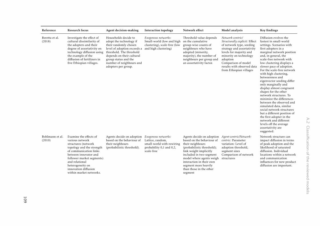
A.2
Classifi
catio
noftherevie
wedmodels
Reference Research focus Agent decision-making Interaction topology Network effect Model analysis Key findings
Beretta et al.(2018)
Investigate the effect ofcultural dissimilarity ofthe adopters and theirdegree of assortativity ontechnology diffusion usingthe example of thediffusion of fertilizers infive Ethiopian villages.
Households decide toadopt the technology iftheir randomly chosenlevel of adoption exceeds athreshold. The thresholddepends on their culturalgroup status and thenumber of neighbours andadopters per group.
Exogenous networks:Small-world (low and highclustering), scale-free (lowand high clustering)
Threshold value dependson the cumulativegroup-wise counts ofneighbours who haveadopted (minority,majority), the number ofneighbours per group andan assortativity factor.
Network-centric/Structurally explicit: Effectof network type, seedingstrategy and assortativitylevels for majority andminority on technologyadoptionComparison of modelresults with observed datafrom Ethiopian villages
Diffusion evolves thefastest in small-worldsettings. Scenarios withfirst adopters in amarginal network positionand, in general, thescale-free network withlow clustering displays aslower pace of adoption.For the scale-free networkwith high clustering,betweenness andeigenvector seeding differonly marginally anddisplay almost congruentshapes for the othernetwork structures. Tominimize the differencesbetween the observed andsimulated data, similarsocial network structuresbut a different position ofthe first adopter in thenetwork and differentlevels off the averageassortativity aresuggested.
Bohlmann et al.(2010)
Examine the effects ofvarious networkstructures (networktopology and the strengthof communication linksbetween innovator andfollower market segments)and relationalheterogeneity oninnovation diffusionwithin market networks.
Agents decide on adoptionbased on the behaviour oftheir neighbours(probabilistic threshold).
Exogenous networks:Lattice, random,small-world with rewiringprobability 0,1 and 0,2,scale-free
Agents decide on adoptionbased on the behaviour oftheir neighbours(probabilistic threshold);link weight implicitlyincluded in two-segmentmodel where agents weighinteraction in their ownsegment more heavilythan those in the othersegment
Agent-centric/Network-centric: Parametervariation: Level ofadoption threshold,segment sizesComparison of networkstructures
Network structure canimpact diffusion in termsof peak adoption and thelikelihood of saturateddiffusion. Individuallocations within a networkand communicationinfluences for new productdiffusion are important.
109

AAppendixofChapter2
Reference Research focus Agent decision-making Interaction topology Network effect Model analysis Key findings
Chareunsy(2018)
Simulate the diffusion ofthree developmentinitiatives (encourageschool attendance,introduce safe waterhandling practices, feederroad to facilitateengagement with markets)that differ in theirapproaches to reachingtargeted groups in asouthern Lao community.
The decision to adopt achange in behaviour isbased on the relativeinfluence of adopters andnon-adopters within ahousehold’s network.Agent will choose to adopta practice if the window ofinfluence of adoption(determined by theweighted sum of agentsacross common networkactivities) is greater thatthe window of influencefor non-adoption. At thebeginning, an outsiderrecruits selected agents tochange their behaviour.
Exogenous network:Connection to all agentswith common activities
Agents’ decision to adoptis based on relativeinfluence of adoptees vs.non-adoptees in thenetwork.
Agent-centric: Comparisonof the dynamics of thethree developmentinitiatives for a syntheticpopulation of 58 agentsequipped with propertiesfrom household surveydata
The Water initiative is themost successful both forthe community as a wholeand in reaching the lowesttier of society. TheEducation initiative failsto transmit a behaviourchange, such thatultimately even theeducators (the chosenagents) give up. TheMarket initiative succeedsin reaching all communitymembers but the gainsaccrue disproportionatelyto the well-off who arebest positioned to absorbthe initial impetus.
Chen et al.(2012)
Examine the influencebetween networkstructure (size, degree,weight) and energy-savingbehaviour.
Agents decide whether toincrease or decrease theirenergy consumption basedon the norm imposed bythe energy use of theirpeers.
Exogenous networks:Random (varying numberof nodes, degree and linkweight)
Agents change theirenergy consumptionbehaviour based on thebehaviour of theirnetwork neighbours.
Network-centric:Comparison of networkstructure
Network energyconsumption does notdecrease or increase withthe expansion of therandom network, if newlyadded vertices have asimilar level of energyconsumption. Connectiondegree and strength of therelationship betweenresidents each has apositive impact onresidents’ energy saving.
110

A.2
Classifi
catio
noftherevie
wedmodels
Reference Research focus Agent decision-making Interaction topology Network effect Model analysis Key findings
Erdlenbruch &Bonte (2018)
Simulate the adoption ofindividual adaptationmeasures to floods andevaluate the efficiency ofdifferent communicationpolicies in a modelparameterized with datafrom a survey conductedin France.
The decision model of theagents is based on thepsychological protectionmotivation theory (PMT)that decomposes theindividual adaptationmotivation into variablesrelating to threat appraisaland coping appraisal. Alogistic regression of anindividual’s intention toimplementnon-permanentadaptation measures onthe household’s attributesis run.
Exogenous networks:Spatial, small-world(spatially explicit),random (varying degree)
The higher the proportionof neighbours in thehousehold’s network whohave adapted, the higherits attribute level for thesocial network variable.
Agent-centric/Network-centric: Comparison ofadaptation levels with andwithout network influenceComparison of networkstructures
Policies which containinformation on both therisk of flooding and howto cope with it performbetter than policies whichonly deal with risk. Peoplecentred policies on riskand coping perform thebest in all scenarios. Theabsence of the small-worldnetwork decreases theabsolute value ofadaptation levels. Thenetwork types and degreeshave no impact on thesimulation results.
Goldenberg et al.(2007)
Understand how theinterplay between positiveand negative information,as well as weak and strongties, affects the growth ofnew products and theconsequent economicresults.
The probability thatagents adopt a newproduct depends onpositive word-of-mouth,advertising, and/ornegative word-of-mouth.
Exogenous network withdynamic properties:“dynamic small-world”with strong-tie structureinside each social systembeing fixed and weak-tiestructure randomlyreassigned in each period
Spread of information onnew product withprobabilities based onnumber ofsatisfied/dissatisfiedadopters and rejecters
Network-centric: Linearregression with dependentvariable of Net PresentValue to analyse the effectsof dissatisfaction, strengthof the weak ties,advertising andinteraction effects (level ofweak and strong ties)
The effect of negativeword-of-mouth on the NetPresent Value of the firmis substantial. Weak tieshelp to spread harmfulinformation throughnetworks and can becomea negative force for theproduct’s spread.
Haenlein & Libai(2013)
Compare the effectivenessof revenue leader seedingwith opinion leaderseeding and randomseeding on the spread of anew product.
The probability thatagents adopt a newproduct depends onpositive word-of-mouth,advertising, and/ornegative word-of-mouth.
Exogenous network:Algorithm reproducinglink formation in actualsocial networks (relativelysmall average distancebetween pairs of nodes,clustering coefficientlarger than in randomnetworks, approximatelyscale-free degreedistribution)
Adoption of new productwith probabilities basedon number ofsatisfied/dissatisfiedadopters, rejecters and lostconsumers
Network-centric/Structurally explicit:Parameter variation:Network clusteringcoefficient, standarddeviation of the customerlifetime value, customerlifetime value assortativityand seed size
Both revenue leaderseeding and opinionleader seeding can creategreater value comparedwith random customerseeding. The distributionof customer lifetime valuein the population and theseed size play a major rolein determining whichseeding approach ispreferable.
111
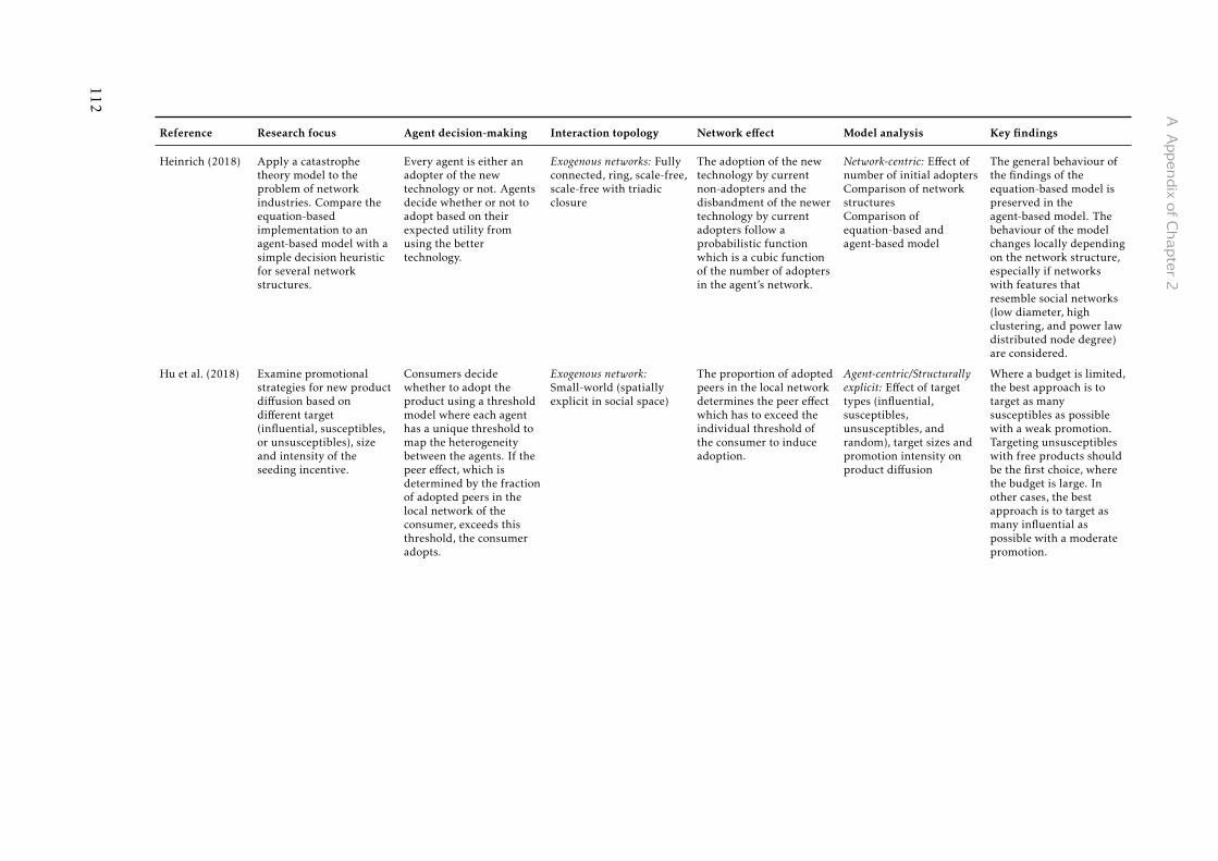
AAppendixofChapter2
Reference Research focus Agent decision-making Interaction topology Network effect Model analysis Key findings
Heinrich (2018) Apply a catastrophetheory model to theproblem of networkindustries. Compare theequation-basedimplementation to anagent-based model with asimple decision heuristicfor several networkstructures.
Every agent is either anadopter of the newtechnology or not. Agentsdecide whether or not toadopt based on theirexpected utility fromusing the bettertechnology.
Exogenous networks: Fullyconnected, ring, scale-free,scale-free with triadicclosure
The adoption of the newtechnology by currentnon-adopters and thedisbandment of the newertechnology by currentadopters follow aprobabilistic functionwhich is a cubic functionof the number of adoptersin the agent’s network.
Network-centric: Effect ofnumber of initial adoptersComparison of networkstructuresComparison ofequation-based andagent-based model
The general behaviour ofthe findings of theequation-based model ispreserved in theagent-based model. Thebehaviour of the modelchanges locally dependingon the network structure,especially if networkswith features thatresemble social networks(low diameter, highclustering, and power lawdistributed node degree)are considered.
Hu et al. (2018) Examine promotionalstrategies for new productdiffusion based ondifferent target(influential, susceptibles,or unsusceptibles), sizeand intensity of theseeding incentive.
Consumers decidewhether to adopt theproduct using a thresholdmodel where each agenthas a unique threshold tomap the heterogeneitybetween the agents. If thepeer effect, which isdetermined by the fractionof adopted peers in thelocal network of theconsumer, exceeds thisthreshold, the consumeradopts.
Exogenous network:Small-world (spatiallyexplicit in social space)
The proportion of adoptedpeers in the local networkdetermines the peer effectwhich has to exceed theindividual threshold ofthe consumer to induceadoption.
Agent-centric/Structurallyexplicit: Effect of targettypes (influential,susceptibles,unsusceptibles, andrandom), target sizes andpromotion intensity onproduct diffusion
Where a budget is limited,the best approach is totarget as manysusceptibles as possiblewith a weak promotion.Targeting unsusceptibleswith free products shouldbe the first choice, wherethe budget is large. Inother cases, the bestapproach is to target asmany influential aspossible with a moderatepromotion.
112

A.2
Classifi
catio
noftherevie
wedmodels
Reference Research focus Agent decision-making Interaction topology Network effect Model analysis Key findings
Huétink et al.(2010)
Study the development ofthe market for hydrogenvehicles taking intoaccount differentstrategies for hydrogeninfrastructuredevelopment and userbehaviour.
Consumers: The decisionof the consumers to adopta hydrogen vehicledepends on their level ofinnovativeness, theirreservation price and onthe perceived attributes ofhydrogen vehicletechnology determined bytechnological learning,social learning processesand fuel availability.Refuelling station: Therefuelling stationconsiders the percentageof consumers within itscustomer base that haveadopted a hydrogenvehicle. When thispercentage of adoptersexceeds a threshold value,the station adds hydrogento its product range.
Exogenous networks: Fullyconnected, lattice (Moore),small-world
Consumers evaluate thefraction of adopters intheir network and adoptthe innovation if theadoption rate exceedstheir personal thresholddetermined by the adoptergroup they are assigned to.
Network-centric: Effect ofinfrastructure strategies(station placement, size ofinitial fuel infrastructure)on number of adoptersParameter variation:Number of initial adoptersComparison of networkstructures
Maximum geographicalcoverage with initialstations is more effectiveas a deployment strategythan focusing on denselypopulated areas. Thestructure of the socialnetwork amongconsumers does influencethe resulting diffusionpatterns; a small worldsocial network is mostfavourable to fastdiffusion.
Janssen & Jager(2001)
Explore the dynamics ofmarkets where artificialconsumers have to chooseeach period betweensimilar products from apsychological perspective.Explore the consequencesof changing preferencesand the size of socialnetworks.
Depending on uncertaintyand satisfaction of socialneeds, agents applydifferent mechanisms tochoose a product:Repetition, deliberation,imitation or socialcomparison (“consumat”approach).
Exogenous networks:Small-world with rewiringprobability 0, 0.01 and 0.1
For imitation and socialcomparison, agentsevaluate the productwhich is consumed themost in its social network.
Agent-centric/Network-centric: Effect of minimumlevel of need satisfactionand uncertainty toleranceon market share ofproductsComparison of networktopology and size
Behavioural rules thatdominate the artificialconsumer’s decisionmaking determine theresulting marketdynamics. Psychologicalvariables like socialnetworks, preferences andthe need for identity areimportant to explain thedynamics of markets. Ifsocial processes dominatea market, an increase inthe size of the networkcauses the market to bedominated by a fewproducts.
113

AAppendixofChapter2
Reference Research focus Agent decision-making Interaction topology Network effect Model analysis Key findings
Janssen & Jager(2003)
Investigate the effects ofdifferent networkstructures on marketdynamics.
Depending on uncertaintyand satisfaction of socialneeds, agents applydifferent mechanisms tochoose a product:Repetition, deliberation,imitation or socialcomparison (“consumat”approach).
Exogenous networks:Small-world with rewiringprobability 0, 0.1 and 1,scale-free, scale-free with1% inactive links
For imitation and socialcomparison, agentsevaluate the productwhich is consumed themost in its social network.
Agent-centric/Network-centric: Extension ofJanssen & Jager (2001)Comparison of networktopology and networkparameters
Market dynamics is aself-organized propertydepending on theinteraction between theagents’ decision-makingprocess, the productcharacteristics, and thestructure of interactionsbetween agents (size ofnetwork and hubs in asocial network).
Kaufmann et al.(2009)
Study the diffusion oforganic practices throughfarming populations inLatvia and Estonia andevaluate the effectivenessof policies (effect of socialinfluence, introduction ofa higher subsidy,increased support byorganic farm advisors) topromote them.
Based on Theory ofPlanned Behaviour, farmagents exchange opinions,update subjective normestimates, and adoptorganic farming practicesif intention exceeds anempirically derivedthreshold.
Exogenous network:Small-world andscale-free properties(network parameterderived from survey)
Subjective norm as onefactor characterizingintention towardsadoption is influenced byone selected neighbourusing the relativeagreement model.
Agent-centric/Network-centric: Effects of socialinfluence, introduction ofa higher subsidy and ofincreased support byorganic farm advisors onthe diffusion of organicfarming practicesParameter variation:Network density,preferential attachmentand small-world property,type of agents on the hubs(not shown)
Social influence alonemakes little difference;introduction of a subsidyis more influential. Thecombined adoption ratefrom social and economicinfluences is higher thanthe sum of the proportionof adopters resulting fromjust social influence andfrom just subsidies.
114

A.2
Classifi
catio
noftherevie
wedmodels
Reference Research focus Agent decision-making Interaction topology Network effect Model analysis Key findings
Libai et al.(2013)
Explore how accelerationand market expansioncombine to generate valuein a word-of-mouthseeding program for twocompeting products.
The probability thatagents adopt one of thecompeting productsdepends on external andinternal factors.
Exogenous networks: 12empirical networks
Adoption of new productwith probabilities basedon number of consumersin network who havealready adopted
Structurally explicit:Comparison of socialvalue of word-of-mouthprograms for differentseeding strategies affectedby competition, programtargeting, profit decline,and retention
Market expansiondominates the social valueof word-of-mouthprograms. Relative torandom programs,acceleration drives agreater proportion ofinfluential programs’social value. The strongera brand is relative to itscompetitor, the moreacceleration drives itsseeding program’s socialvalue, and the lower theprogram’s social value isoverall. The lower thefuture value of customers,the higher the accelerationratio and the higher therelative social value of aprogram. A shorterhorizon of analysis on theprogram’s effect leads to ahigher overestimation biasof the seeding program’ssocial value. The higherthe disadoption rate, thelower the accelerationratio.
Moglia et al.(2018)
Describe the uptake of lowcarbon and energyefficient technologies andpractices by householdsand under differentinterventions(non-financial and socialnetwork).
Households decidewhether to buy a newproduct if the old producthas reached the end of itslife or the agent has beenapproached by a salesagent. The decision whichproduct to buy dependson the level of needssatisfaction anduncertainty and results inrepetition, imitation oroptimisation or inquiry(based on the “consumat”approach).
Exogenous networks:Small-world, scale-free,spatial, random
For imitation, agents copythe behaviour of asatisfied household intheir social network.
Agent-centric/Network-centric: Comparison ofinterventions on adoptionratesComparison of networkstructures
Focus of the model onquestions whether it ismore effective toincentivise sales agents topromote energy efficienttechnologies, whether it ismore effective to provide asubsidy directly tohouseholds, or whether itis better to work withplumbers so that they canpromote these systems.Effect of social networkson adoption is onlymarginally discussed.115

AAppendixofChapter2
Reference Research focus Agent decision-making Interaction topology Network effect Model analysis Key findings
Negahban &Smith (2018)
Evaluate the optimalcombination of seedingand inventory build-uppolicies for new products.
Consumers adopt or rejectwith probabilitiesdepending on number ofsatisfied consumers ordissatisfied adopters,rejecters and lostcustomers that did notreceive the product due tosupply shortages,respectively.
Exogenous networks:Lattice (26 neighbours),random, small-world(based on lattice network),scale-free
Adoption of new productwith probabilities basedon number of satisfied anddissatisfied adopters,rejecters and lostcustomers (customers thatdid not receive theproduct due to supplyshortages)
Agent-centric/Network-centric/Structurally explicit:Effect of seeding strategy(number of neighbours,number of nodesreachable within twosteps, shortest averagepath length, lowestclustering coefficient,random), seeding fractionand build-up period (timebefore product islaunched) on productadoptionComparison of networkstructures
The seeding strategy thatmaximizes the adoptionrate is not necessarilyoptimal in the presence ofsupply constraints.Random seeding canmaximize the expected netproduct value of profit fora scale-free network.However, random seedingincreases the uncertaintyin the diffusion dynamics.
116

A.2
Classifi
catio
noftherevie
wedmodels
Reference Research focus Agent decision-making Interaction topology Network effect Model analysis Key findings
Niamir et al.(2018)
Track impacts ofbehavioural changes inindividual energy usebehaviour concerning (1)investments to save orproduce energy, (2)conservation of energy bychanging consumptionpatterns and habits, and(3) switching to anotherenergy source.
Based on Norm ActivationTheory, households assessa four step procedure topursue an economicdecision: (1) If householdsfeel guilty as theirawareness (based onsurvey data) exceeds athreshold they (2) checktheir personal andsubjective norms tocalculate their motivationfor each of the threeactions. For those actionsfor which the motivationexceeds a threshold, thehouseholds feelresponsible and go into (3)the consideration stepwhere their perceivedbehavioural control isassessed to measure theirintention. If a householdhas high intentions toundertake any of the threeactions for making anenergy decision, itsexpected utility based onits current energy sourcesand its budget constraintsis calculated. To maximizetheir utility and maketheir energy decisions,households analyse theirutility expectations andcompare it with theircurrent utility.
Exogenous network: Spatial Households comparevalues of their ownbehavioural factors(awareness andmotivation) with those oftheir 8 closest neighboursand adjust their value tobecome the mean of the 9compared values.
Agent-centric: Effect ofsocial learning inknowledge activation or inknowledge activation andmotivation on thebehavioural changes inindividual energy use
Exchange in knowledgeabout energy and climateleads to a significantlyhigher total count of thethree types of householdactions, while there ismore intentions forinvestments that for thetwo other actions.Introducing additionallyopinion dynamicsregarding householdmotivation to act leads toa further increase in thediffusion of all threeactions.
117

AAppendixofChapter2
Reference Research focus Agent decision-making Interaction topology Network effect Model analysis Key findings
Pearce & Slade(2018)
Simulate the adoption ofsmall-scale solarphotovoltaic systems (PV)in Great Britain byconsideringdecision-making ofindividual householdsbased on householdincome, social network,total capital cost of the PVsystem, and the paybackperiod of the investment.
Agents calculate the totalutility of adoption andadapt if the utility exceedsa threshold. The totalutility is made up of aweighted sum of partialutilities depending onhousehold income, thesocial environment of theagent, economicattractiveness of theinvestment, and thecapital cost of theinvestment.
Exogenous network:Random
Social utility of an agentdepends on the number ofadopters and agent isconnected to and increasesif an agent they areconnected to adopts.
Network-centric: Effect ofnumber of links toadopters on social utility(Social influence is notanalysed in more detail)
Focus of the model is onthe effect of feed-in tariffs.Effect of social networkson adoption is onlymarginally discussed.
Phan & Godes(2018)
Analyse the dynamics ofthe diffusion of severalideas for two types ofindividuals (independentswith exogenousinformation and imitators)with endogenous linkformation.
Independents areinfluenced with a fixedprobability. Imitatorsadopt if the proportion ofneighbours who haveadopted exceeds athreshold. Between thediffusion of two ideas,agents may drop and addlinks while maintainingthe same in-degree.Communication can beinfluenced by noise andtime discounting.
Co-evolutionary network:Initially random; linksdeleted based on adoptionstatus, new links formedrandomly
Agents adopt if theproportion of neighbourswho have adopted exceedsa threshold.
Agent-centric/Network-centric: Effect ofpenetration rate forvariation in networkdensity, probability thatindependents receiveinformation, probabilitythat independents listento others in a period andprobability thatindependent listen toother independents in aperiod for fixed networkdensity on diffusion ofideasScenarios with andwithout noise and withand without timediscounting
In the baseline study (nonoise, no timediscounting) penetrationis increasing with networkdensity. Independentswith good exogenousinformation have fewerfollowers than the averageimitator. Whenindependents listen toother agents, they gainmore influence byproducing access to betterinformation. Less noiseallows agents to be furtheraway from the originalsource.
118

A.2
Classifi
catio
noftherevie
wedmodels
Reference Research focus Agent decision-making Interaction topology Network effect Model analysis Key findings
Rasoulkhaniet al. (2018)
Identify the effects ofdemographic andhousehold characteristics,social network influence,and external factors suchas water price and rebatepolicy on residential waterconservation technologyadoption.
Households are in one ofthe three states:non-adopter, potentialadopter or adopter of thetechnology. The transitionbetween non-adopter andpotential adopter andbetween potential adopterand adopter is reached ifthe adoption utility andthe affordability indexexceed a utility andaffordability threshold,respectively. If the utilitythreshold for thetransition betweennon-adopter and potentialadopter status is notreached, an agent canadditionally be positivelyinfluenced by the networkwhich also induces atransition.
Exogenous networks:Random, ring,small-world, scale-free
Given a user-definedlikelihood of influence, ifthe non-adopter agent isconnected to an adopteragent, there is a chancethat the non-adopter willtransition into thepotential adopter state.
Agent-centric/Network-centric: Effect of waterprice and rebate scenarioson technology adoptionComparison of networkstructures
The adoption percentagefluctuates across all fivesocial networking schemesunder each scenario ofwater price and rebatestatus. The distance basednetwork reachedequilibrium in a shorterperiod. The peer effectthrough neighbouringsocial connections canspeed up technologyadoption potential morethan other socialnetworks.
Talebian &Mishra (2018)
Forecast long-termadoption of connectedautonomous vehicles(CAVs) and show theapplicability of theapproach is using surveydata.
Individuals decide toadopt when (1) there is aneed for a new vehicle, (2)their willingness-to-pay(WTP) is greater than theCAV price, and (3) theiroverall impression aboutCAVs reaches a cut-offvalue. Agents update theirperception about CAVsbased on advertisementand peer-to-peercommunication.
Exogenous network:8-dimensional distanceminimization in socialspace
The influence depends onthe number of binaryinteraction between thetwo agents and the weightof the social tie.Depending of theopponent being satisfiedor dissatisfied theinfluence is positive ornegative. Similarly, theWTP is updated.
Agent-centric: Effect ofannual rate of CAV pricereduction,(pre-introduction)advertisement,peer-to-peercommunication on WTPand probability ofbecoming a dissatisfiedadopter on CAV adoption
The automobile fleet willbe near homogeneous inabout 2050 only if CAVprices decrease at anannual rate of 15% or20%. A 6-monthpre-introductionmarketing campaign mayhave no significant impacton adoption trend.Marketing will ignite CAVdiffusion but its effect iscapped. CAV market sharegrows with the effect ofpeer-to-peercommunication of WTP.
119

AAppendixofChapter2
Reference Research focus Agent decision-making Interaction topology Network effect Model analysis Key findings
Wang et al.(2018)
Assess households’decision-making processtowards the adoption ofresidential photovoltaic(PV) under differentscenarios about policiesthat concern both theeconomic benefits and theinformation diffusion onsocial networks.
Agents are either adoptersor non-adopters ofresidential photovoltaicand have a positive ornegative attitude towardsthe technology. Thedecision to adoptresidential PV is made ateach time-step if theutility to the householdoutweighs the adoptionbarriers. The utility is acombination of economicfactors, social effect andpersonal preference.Before thedecision-making processagents assess the revenueand quality information ofPV and can change theirattitude accordingly.
Exogenous network:Scale-free
The social effect is theaverage of the attitude ofthe adjacent nodes.Revenue informationincludes the expectedrevenue according to theexperience of theirfriends. Qualityinformation includes therisk probability accordingto the performance offriends’ residential PV.
Agent-centric: Effect ofpolicy scenarios (withparameter variation) onadoption of residential PV
Providing free insurancefor damage of residentialPV to adopters canimprove the adoption rate.The intervention ofinformation campaigns iseffective and necessary topromote the diffusion ofresidential PV.Information screeningintervention which blocksrumours and deliberatelydiscrediting for residentialPV can only work whenthe policy strength is highenough. The enhancementin communications(increase of socialnetworks’ mean degree)can become new barriersto the residential PVadoption.
Zhang & Nuttall(2011)
Study the impact of policyoptions on the dynamicsof smart meteringdiffusion in retailelectricity markets andsuggest policyimplications.
Based on Theory ofPlanned Behaviour,consumer agents exchangeopinions with otherconsumers and electricsupplier agent and adoptthe energy suppliertowards which theirintention is maximal.
Exogenous network:Small-world (based onlattice network (parameterdefining radius ofinteraction))
Subjective norm towardschoosing an option iscalculated as the sum ofweighted influences fromresidential electricityconsumer agents in theneighbourhood.
Agent-centric: Effect ofdifferent policy options onthe patterns of diffusion
“S-curve” pattern oftechnology adoption isreproduced for all policyscenarios. The mostsuccessful scenario is thegovernment financedcompetitive roll-out. Astable market share ofelectricity supplier agentsappears. Residentialelectricity consumeragents switch electricitysupplier agentsdynamically.
120

A.2
Classifi
catio
noftherevie
wedmodels
Social dynamics
Reference Research focus Agent decision-making Interaction topology Network effect Model analysis Key findings
Biondo et al.(2018)
Study the impact of newsmedia and public surveyson the electoral campaignsfor political competitions.
Agents favour one of twopolitical parties (or areundecided). Theirpreference is influencedby a randomly chosenopinion of one of theirneighbours. Additionally,their opinion is influencedby survey results.
Exogenous network:Small-world (based onlattice network (vonNeumann))
Agent’s opinion isinfluenced by onerandomly chosen agent intheir network. The value,corresponding to the partythe chosen neighbourfavours, is changed by agiven amount.
Agent-centric: Effects ofsurvey on electoralcampaigns
Surveys accentuate thespontaneous clustering ofvoting intentionsemerging among peopledue to the opinionsdynamics. Surveys canchange the final electoralresult and let the party,that otherwise would lose,to win the electoralcompetition.
Bravo et al.(2012)
Investigate the importanceof the endogenousselection of partners fortrust and cooperation inmarket exchangesituations, where there isinformation asymmetrybetween investors andtrustees.(social integration)
Agents decide on theamount to invest andreturn based on theamounts invested andreceived in the previousperiod and coefficientsestimated fromexperimental data.
Exogenous andco-evolutionary networksExogenous networks:Experimental data asinput with variation ofcharacteristics: Randomcoupling with one and twoway interaction, fixedcouples (maintaininginitial couples), fullyconnected, small-world,scale-freeCo-evolutionary networks:Initially random coupling,fully connected networkor regular network;unsatisfied agents canbreak the link, new linksare included either forboth of the formerlylinked agents or only forisolated agents
Agents exchange moneybeing either in the role ofthe investor or the role ofthe trustee.
Network-centric:Comparison of networkstructures (especiallydistinguishing exogenousand co-evolutionarynetworks)
Dynamic networks lead tomore cooperation whenagents can create morelinks and reduceexploitation opportunitiesby free riders. Theendogenous networkformation is moreimportant for cooperationthan the type of network.
121

AAppendixofChapter2
Reference Research focus Agent decision-making Interaction topology Network effect Model analysis Key findings
Chica et al.(2018)
Investigate the dynamicsof the N-playerevolutionary trust gameconsisting of three typesof players: (1) an investor,(2) a trustee who istrustworthy, and (3) atrustee who isuntrustworthy.
Each player makes thedecision (1) whether or notto be trustworthy and (2)whether to be an investoror a trustee. An investorpays to the trustee.Trustworthy trusteesreturn the received fundmultiplied by a factor.Untrustworthy trusteesreturn nothing but keepfor themselves thereceived funds multipliedby a factor. Agents decideon which strategies tochoose based on thewealth of a randomlychosen neighbour.
Exogenous networks:Scale-free (varyingdensity), lattice (vonNeumann), random
An agent decides whetherto imitate or not arandomly chosen directneighbour’s strategy basedon the payoff of itsstrategy. If the wealth ofthe opponent in theprevious time step ishigher than that of theagent if will adopt thestrategy of its opponentwith a probability thatdepends on the differencebetween their payoffs.
Agent-centric/Network-centric: Parametervariation: Temptationdefect ratio,trustworthinessComparison of networkstructures
Trust can be promotedwith the model for lowand medium temptationto defect, for high level oftemptation to defect trustis only promoted when nountrustworthy players arepresent in the initialpopulation. Without anetwork structure, evenone untrustworthy playercan fully eliminateinvestors and lead to zeroglobal net wealth.Network densities havehigh importance forpromoting trust andglobal net wealth.
122

A.2
Classifi
catio
noftherevie
wedmodels
Reference Research focus Agent decision-making Interaction topology Network effect Model analysis Key findings
Flache & Macy(2011)
Show the effects ofpositive and negativevalences of interactionand short- and long-rangeties on polarization orconsensus in disconnectedand connected networks.
All agents executeinfluence based on theweighted differencebetween positions.
Exogenous networks:Disconnected/connectedcaveman graph with short-and long-range ties addedat different time points ofthe simulation
Agents are influenced byaggregated opinions of allneighbours in network.
Network-centric: Effect ofcave size, number ofcultural issues, negativevalence of interaction andadditional short- andlong-range ties onpolarization
With only positiveinfluence and selection,long-range ties promotegreater culturalintegration andassimilation. When bothpositive and negativevalences of interaction areassumed, long range tiesbecome conduits for thespread of locallydeveloped polarizationand the effect is reversed.In connected networks,when only positiveinfluence and selection areassumed, consensus is theinevitable outcome.Neither long-range norshort-range ties have aneffect on the level ofconsensus. When bothpositive and negativeinfluence and selection areallowed, long-range tiesincrease polarizationsharply, but short-rangeties do not.
123

AAppendixofChapter2
Reference Research focus Agent decision-making Interaction topology Network effect Model analysis Key findings
Frank et al.(2018)
Attend how an externalagent’s message(policy-aligned orbalanced) interacts withintra-organizationalnetwork dynamics toaffect the distribution ofpractices and networkstructure within anorganization.
If actors receive newinformation from theirnetwork connections,actors adjust theirbehaviours based oninformation and norm.Actors decide whether tomaintain current networkconnections and if actorsdecide to dissolve acurrent connection, theyfrom new connections.
Co-evolutionary network:Initially random networkwith higher connectionprobability within the twosubgroups than between;links deleted based onhow many consecutivetimes an actor is exposedto redundant informationfrom the networkconnection, links formedbased on utility to connectwith every other actor inthe organization whilekeeping the out-degreeconstant
Each member of an actor’snetwork randomlyprovides one piece ofinformation in theirpossession to the actor. Ifthe information is new tothe actor, the actor willadd this piece ofinformation to its owninformation list. Actorschoose their behaviouraccording to theirprevious behaviour, newinformation they receiveand the mean behaviour oftheir network members.Depending on thestrength of organizationalidentification, more or lessweight is given to theinfluence of the networkor on own information.Another parameterdetermines the strength ofnormative influencerelative to that ofselection.
Agent-centric: Parametervariation: Organizationalidentification for twolevels of influenceComparison ofpolicy-aligned andbalanced messages withbaseline case (no externalmessage)
When organizationalidentification is high,those predisposed to apolicy-aligned messagewill engage the messageand one another,becoming more extreme intheir behaviours. Othersnot predisposed to themessage will divert awayfrom the message. Thisproduces a divergence ofbehaviour based onpredisposition and littleoverall change.Divergence does not occureven when organizationalidentification is high for abalanced message, whichprovides opportunities foractors to integrate. Thetrade-off is that thebalanced message does notgenerate as large changesin average behaviour asdoes the policy-alignedmessage whenorganizationalidentification is low. Thus,when organizationalidentification is low, abalanced message may bea missed opportunity toshape behaviour.
124
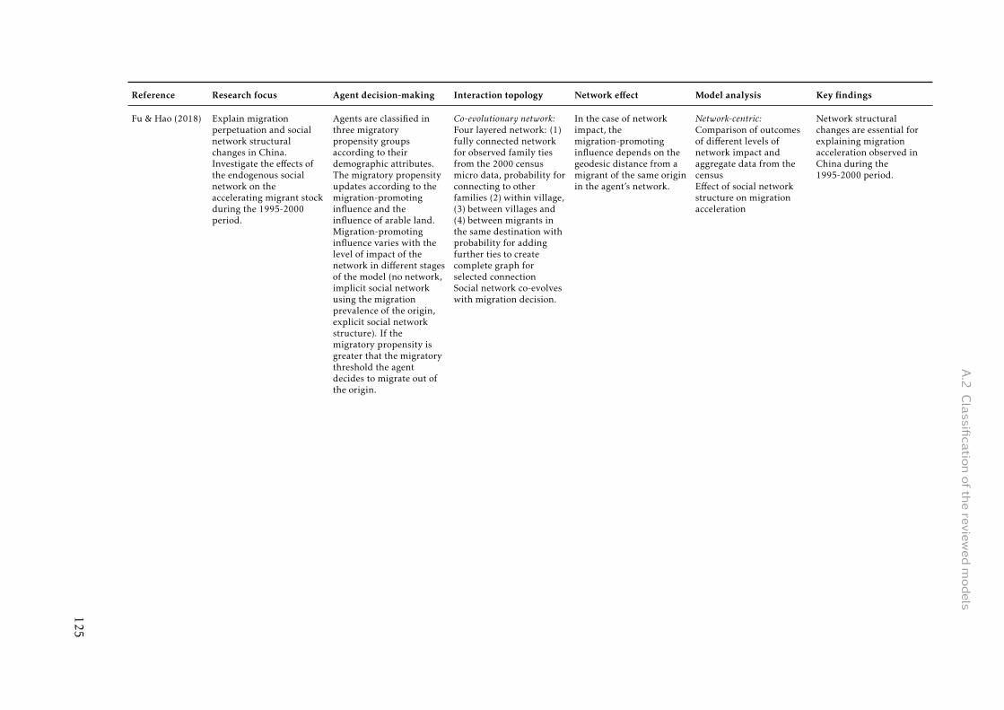
A.2
Classifi
catio
noftherevie
wedmodels
Reference Research focus Agent decision-making Interaction topology Network effect Model analysis Key findings
Fu & Hao (2018) Explain migrationperpetuation and socialnetwork structuralchanges in China.Investigate the effects ofthe endogenous socialnetwork on theaccelerating migrant stockduring the 1995-2000period.
Agents are classified inthree migratorypropensity groupsaccording to theirdemographic attributes.The migratory propensityupdates according to themigration-promotinginfluence and theinfluence of arable land.Migration-promotinginfluence varies with thelevel of impact of thenetwork in different stagesof the model (no network,implicit social networkusing the migrationprevalence of the origin,explicit social networkstructure). If themigratory propensity isgreater that the migratorythreshold the agentdecides to migrate out ofthe origin.
Co-evolutionary network:Four layered network: (1)fully connected networkfor observed family tiesfrom the 2000 censusmicro data, probability forconnecting to otherfamilies (2) within village,(3) between villages and(4) between migrants inthe same destination withprobability for addingfurther ties to createcomplete graph forselected connectionSocial network co-evolveswith migration decision.
In the case of networkimpact, themigration-promotinginfluence depends on thegeodesic distance from amigrant of the same originin the agent’s network.
Network-centric:Comparison of outcomesof different levels ofnetwork impact andaggregate data from thecensusEffect of social networkstructure on migrationacceleration
Network structuralchanges are essential forexplaining migrationacceleration observed inChina during the1995-2000 period.
125

AAppendixofChapter2
Reference Research focus Agent decision-making Interaction topology Network effect Model analysis Key findings
Garcia et al.(2018)
Explore how theinteractions betweenpsychological attributesand built and socialenvironments may lead tothe emergence andevolution of leisure-timephysical activity (LTPA)patterns among adults.(social integration)
Agents decide whetherthey will practice LTPAduring the current week,based on the level ofintention and conditionalto the perceived builtenvironment. Persons andLTPA-places are placedrandomly over patches ofa grid. Person’s intentionto practice LTPA dependson the behaviour of thosein the proximal networkand perceived community,the person’s behaviour inthe previous week, currentlevel of intention and thehighest perceived utilityamongst the LTPA sites inthe person’s perceptionradius.
Exogenous networks:Proximal network:Spatial, each link can berandomly exchanged for alink with any other personoutside the initialproximal networkPerceived community:Spatial (perception radius)
Person’s intention isincreased or reduced dueto the average behaviourof all agents in theproximalnetwork/perceivedcommunity times afunction of the conditionallikelihood that people inthe proximalnetwork/perceivedcommunity will practiceLTPA if it is the bestoption.
Agent-centric: Parametervariation: Level ofintentionIndividual and globalsensitivity analysis
Time trends of LTPApractice and populationdistribution of levels ofintention are similar thosereported in literature.Influence of the person’sbehaviour in the previousweek over his currentintention, the size of theperson’s perceptionradius, and the proportionof patches in the grid thatare LTPA sitessignificantly influence thetemporal trends in themodel.
Gore et al. (2018) Forecast changes inreligiosity and existentialsecurity among acollective of individualsover time.(social integration)
Agents update theirreligiosity based on socialnetwork interactions.Additionally, agentsinteract with theenvironment by checkingif their value forexistential insecurity isbelow the existentialsecurity value of theenvironment.
Exogenous network:Algorithm reproducingsocial networks observedin the wild
The extent to which thevariable is influenced isdetermined by atime-dependent weighedaverage.
Agent-centric: Comparisonof the accuracy ofpredictions fromcompeting approaches(baseline based entirely onhistorical data, LinearRegression, ABM) forcountries on which modelswhere trained/not trained
For a given country and agiven time period, theABM provides a moreaccurate forecast ofchanges in the existentialsecurity and the religiositythan the two alternativeapproaches for a specifictime period for specificcountry.
126

A.2
Classifi
catio
noftherevie
wedmodels
Reference Research focus Agent decision-making Interaction topology Network effect Model analysis Key findings
Growiec et al.(2018)
Identify the keymechanism allowing thesocial network structure toaffect individuals’ socialtrust, willingness tocooperate, economicperformance and socialutility, and trace howthese individual-leveloutcomes aggregate up tothe society level.(social integration)
Agents are matched inpairs and engage ineconomic interaction. Thematching is random butthe probability of a matchdepends on the degree ofmutual trust between thetwo agents, implying thatagents who are generallymore trustful are alsorelatively more likely toengage in economicinteraction.
Exogenous network:Small-world (varyingdensity)
Probability that agent willchoose to cooperate isnegatively related to thedistance to the opposingagent in the social networkand positively related tothe decision maker’sbridging social capital.
Network-centric: Effect ofnetwork density, invertedprobability of localcliques, and the invertedshare of local cliques thatare family-based onaverage economicperformance in the society
Societies that are betterconnected, exhibit a lowerfrequency of local cliques,or have a smaller share offamily-based cliques,record relatively betteraggregate economicperformance. As long asfamily ties are sufficientlyvaluable, there is atrade-off betweenaggregate social utilityand economicperformance, and smallworld networks are thensocially optimal. In densenetworks and trustfulsocieties, there is atrade-off betweenindividual social utilityand economicperformance; otherwiseboth outcomes arepositively correlated in thecross section.
127

AAppendixofChapter2
Reference Research focus Agent decision-making Interaction topology Network effect Model analysis Key findings
Hadzibeganovicet al. (2018)
Study the effects ofphenotypic diversity,network structure, andrewards on cooperativebehaviour in a populationof reproducing artificialdecision makers playingtag-mediated evolutionarygames.(social integration)
Depending upon the tagcolour of the neighbouringopponents, agents decidewhether to cooperate ordefect in Prisoner’sDilemma-like pairwiseinteractions. Ethnocentricagents will cooperate onlywith neighbours whoshare the same tag colour,cosmopolitans willprovide help only toothers displaying adifferent tag colour,altruists will alwayscooperate, and egoists willalways defect. Eachcooperation act is relatedto a reduction of thereproductive potential ofthe donator and anincrease of thereproductive potential ofthe receiver.
Co-evolutionary networks:Lattice (von Neumann),small-world (based onlattice network)Networks change due toreproduction and death
Agents chose one of theirneighbours to playpairwise Prisoner’sDilemma and decidewhether to cooperate anddefect based on theirattitude which influencesthe reproduction rate ofthe receiver andthemselves.
Agent-centric/Network-centric: Parametervariation: Number of tagcolours, length of rewardframeComparison ofbehavioural strategiesComparison of networkstructures
Small reward framespromote unconditionalcooperation inpopulations with both lowand high diversity. Whenthe reward frame is large,there is a strong differencebetween the frequencies ofconditional co-operatorspopulating rewired versusnon-rewired networks. Ina less diverse population,the total number ofdefections is comparableacross different networktopologies; in morediverse environmentsdefections become morefrequent in a regularlystructured than in arewired, small-worldnetwork of contacts.
Ke et al. (2008) Simulate language changeas a process of innovationdiffusion. Examine theeffect of four differentnetwork types, differenttypes of learners and thenetwork size on thediffusion.
Agents decide whichlanguage (unchanged orinnovative) to use basedon the frequencies of usersof the two variants in theirnetwork and thefunctional values of thelanguages.
Exogenous networks: Ring,random, small-world,scale-free
Agents evaluate thefrequencies of users of thetwo variants of thelanguage in theirnetworks.
Agent-centric/Network-centric: Effect of differenttypes of learners andnetwork size on thediffusionComparison of networkstructures
Innovations always diffuseto the whole population aslong as the advantage ofthe innovation over theunchanged form is highenough. The success ratesand the speed of thediffusion vary across thedifferent networkstructures. The presenceof statistical learners whocan learn and use bothlinguistic variantsincreases the probabilityfor linguistic innovations.Population size has aninfluence on the diffusiononly in regular networks.
128

A.2
Classifi
catio
noftherevie
wedmodels
Reference Research focus Agent decision-making Interaction topology Network effect Model analysis Key findings
Keijzer et al.(2018)
Analyse the implicationsof one-to-manycommunication (aspresent e.g. in onlinesocial networks) on thepopulation usingAxelrod’s model ofcultural dissemination asan example.
The social influencecomponent of Axelrod’smodel of culturaldissemination is adaptedto a one-to-manycommunication:Randomly selected agentsfrom the populationcommunicate one of theirfeatures on which theydiffer with at least oneneighbour.
Exogenous networks:Lattice (Moore), spatial,ring (rewired following analgorithm which decreasesnetwork transitivity whilepreserving the degreedistribution)
Neighbours adopt thefeature with a probabilityequal to the proportion oftraits that they share withthe communicating agent.
Network-centric:Comparison of theone-to-one and theone-to-manycommunication regime fordifferent scenarios indifferent networkstructures
One-to-manycommunication fosters theisolation in biggerpopulations. Networktransitivity fosters theemergence of isolatedindividuals and culturalclusters. These findingshold for networktopologies that mimic thestructure of real socialnetworks.
Laifa et al.(2018)
Study the consequences ofdifferent trust dynamicswith forgiving andunforgiving strategiesafter an offence.(social integration)
Offences occur betweentwo connected agents.Agents can react on theseoffences with two differentstrategies: Either thenetwork is updated bydeleting the affectedrelationships consideringneither relationshipscharacteristics norforgiveness or the trustvalue is reduced.
Co-evolutionary network:
Initially random (size 102
and 103 and connectionprobability 0.05 and 0.1);links are weighted by trustwhich is influenced byoffences that occur in thenetwork, links are deletedif trust value falls below athreshold
Between connected agentsa specific number ofrandomly assignedoffences occur. Agentsreact on these defencesand thereby modify thenetwork structure.
Agent-centric/Network-centric: Effects of networkstructure on averagedegree, averagebetweenness centralityand density of thenetworks after revaluatingtrust with both forgivingand unforgiving strategies
The average degreedecreases for all thenetworks and with bothstrategies. When thenumber of links in anetwork decreases, thedensity of the networkdeclines as well. Thenetwork density lessensmore for the first strategy,where networks becamevery sparse, compared tothe resulting networksfrom the second strategyin which they wererelatively dense. Forbetweenness centrality,oscillating curves can beobserved for all thenetworks and with bothstrategies.
129

AAppendixofChapter2
Reference Research focus Agent decision-making Interaction topology Network effect Model analysis Key findings
Lou-Magnuson& Onnis (2018)
Simulate how humanlanguages may changeover time across a socialnetwork of speakers.
Speakers select a signalfrom their activerepertoire and present itto their partner (hearer).The Partners use theirpassive repertoire to see ifthey know that signal orsearch the passiverepertoire for asignificantly close signalof the same meaning. If asignal in an agent’s passiverepertoire can be foundsuch that the signal beingshared with it isintelligible, the agent addsit to the passive repertoireif not already present. If asignal cannot be found inthe passive repertoire, thespeaker will try and repairthe communication byusing any other activesignals it possesses withthe same meaning. After aset number ofcommunication events,each agent undergoes areplacement process thatsimulatesintergenerational transfer.
Exogenous networks: Fullyconnected, random(different connectionprobabilities),hierarchical, scale-free
Agents exchange linguisticsignals in agent-agentcommunication.
Network-centric: Effect oftransitivity (differentconnection probabilities inrandom networks) andnetwork topology(complete, hierarchical,scale-free, randomnetwork) and network sizeon linguistic reanalysis
Transitivity is critical forthe evolution ofcompositional structure.The hierarchicalpatterning of scale-freedistributions is inhibitory.
130

A.2
Classifi
catio
noftherevie
wedmodels
Reference Research focus Agent decision-making Interaction topology Network effect Model analysis Key findings
Lozano et al.(2018)
Simulate Prisoner’sDilemma (PD) gameswhere reputation can befaked and compare theresults to experimentalwork. Simulate muchlarger population sizesover longer times and testother model parameters tosee whether the observedbehaviour generalizes inthose conditions thatcannot easily beconducted in experiments.
Agents receive a randomsequence of past actions todetermine their initialcooperation index. Agentsreceive information on thecooperation index of theircurrent neighbours andselect cooperation ordefection as action for allPD games with theirneighbours withprobability proportionalto the average cooperationindex of their neighbours.In selected simulationruns, cheater areintroduced that defectwith fixed probability.
Co-evolutionary network:Random regular graph;links deleted based onhow many times the agentcooperated, new linkcreated randomly
Agents play PD gameswith all their neighboursand select cooperation ordefection based on theaverage cooperation indexof their neighbours.
Agent-centric: Comparisonof simulated andempirical results for realand faked reputationParameter variation:Number of participants,time frame
Comparison betweennumerical simulationresults and laboratoryexperiment leads to goodqualitative fit. Largerpopulations essentiallybehave in the samequalitative manner as thesmall one, except that allresults have smallerfluctuations.
Lu et al. (2009) Study how the communitystructure of theunderlying graphs affectsthe emergence ofmeta-stable or long-livingopinion clusters.Investigate how choosingcommitting agents andexternal influencefacilitate convergence toglobal consensus.
Speakers transmit a wordfrom their lists to listenerswho add it to their list ifthey do not know thetransmitted word or bothplayers delete all otherwords and agree ontransmitted word iflisteners know it.
Exogenous networks:Empirical data(high-school friendshipnetwork), small-worldwith same number ofnodes, average degree andclustering coefficient
Speaker transmit words torandomly chosen listenersfrom network.
Agent-centric/Network-centric: Effect of differentselection methods forcommitted agents andstrength of externalinfluence on communitystructureComparison of networkstructures
Networks with strongcommunity structurehinder the system fromreaching globalagreement; the evolutionof the Naming Game inthese networks maintainsclusters of coexistingopinions indefinitely.Small number ofcommitting agents issufficient to facilitate anexponential decay towardglobal consensus of theselected opinion. Globalexternal influence leads toan increasing rate ofconvergence.
131

AAppendixofChapter2
Reference Research focus Agent decision-making Interaction topology Network effect Model analysis Key findings
Neal & Neal(2014)
Explore whether innetwork formation respectfor diversity and sense ofcommunity can both beachieved following theprinciples of homophilyand proximity.
Agents form links witheach other based on alogistic selection functiondepending on theirsimilarity and physicaldistance weighted by thedirection and strength ofthe tendency towardshomophily and proximity.
Endogenous networkformation
Agents establish linksbased on their similarityand physical distance andtheir tendency towardshomophily and proximity.
Evaluation quantity:Relationship betweendiversity and sense ofcommunity depending onthe weight given to thedirection and strength ofthe tendency towardshomophily and proximity
It is not possible tosimultaneously promoterespect for diversity andsense of community in aworld where relationshipformation is driven byhomophily and proximity.
Piedrahita et al.(2018)
Analyse the contagiondynamics that emerge innetworks when repeatedaction is allowed, that is,when actors can engagerecurrently in a collectiveeffort. Investigate how thestructure ofinterdependence, thevariance in individualpropensities to activateand the strength of socialinfluence affect contagionand the emergence oflarge-scale coordination.
Agents’ propensity toparticipate in collectiveevents depends on theirintrinsic motivation (howquickly they reach theactivation limit (and ontheir social influence(strength of signalsreceived from otheragents). When nodesactivate, they shift thestate of their neighboursand reset their own stateback to the beginningphase. If an actor isactivated, connectedactors’ activation increasesby a fixed amount.
Exogenous networks:Random, ring,small-world, scale-free
Agents influence theirneighbours whenactivated towards a higherlevel of activation.
Agent-centric: Effect ofintrinsic motivation andsocial influence forhomogeneous andheterogeneousdistribution of theintrinsic motivation ontime to coordinate
Homogeneous networks(degree distribution notsignificantly skewed) aremore conducive tocoordination. There is acritical value for socialinfluence for all topologiesand levels of intrinsicmotivation below whichactors do not achievecoordination.
132

A.2
Classifi
catio
noftherevie
wedmodels
Reference Research focus Agent decision-making Interaction topology Network effect Model analysis Key findings
Schlaile et al.(2018)
Illuminate the influence ofparticular social networkcharacteristics on the ALSIce Bucket Challenge’s(IBC) diffusion.
The simulation is initiallyseeded by five randomlychosen initiators whoalready performed theIBC. Each agent whoaccepted the challengenominates three of itsneighbours who have notpreviously accepted theIBC. Agents are resistantagainst the challenge witha factor drawn from arandom distribution in afixed interval. Each timean agent is nominated, itsresistance value is reducedby another value,determined as the effect ofnomination. If an agent’sresistance is reduced tozero or lower, the agentwill accept the challenge.
Exogenous networks:Scale-free, small-world,random
Agents nominate threeneighbours from theirnetwork to participate atthe challenge. Thenomination reduces theirresistance against thechallenge.
Agent-centric/Network-centric: Parametervariation: Mean resistanceagainst the challengeComparison of networkstructuresEffect of average degreeand celebrities
The model canqualitatively reproducecentral elements of theempirically observed IBC’sdiffusion pattern. The IBChas to reach a critical massof carriers in order to stallprematurely. Networkswith a high averageclustering coefficient aswell as a moderate averagedegree are beneficial forthe IBC meme’s diffusionperformance. Theassumption that hubshave a higher influence onothers leads to a faster andmore wide-rangingdiffusion of the IBC innetworks exhibiting ahighly skewed degreedistribution.
Simão & Todd(2002)
Study mate choice inmonogamous matingsystems and evaluateperformance androbustness of differentagent strategies.
Agents decide on whetherto initiate relationship orswitch partner based on(1) the age and quality ofthe potential and currentpartner and the focalagent and (2) theiraspiration level.
Co-evolutionary network:Pairs of male and femalemeet at certain stochasticrate, agents switchbetween single andcourting state based onthe quality of the partnerand their aspiration level
Agents try to find optimalpartner based on theproperties of the otheragents and their aspirationlevel.
Agent-centric: Comparisonof the efficiency of thedifferent mating strategiesComparison of thepredictions of the modelwith theories from socialsciences
Being able to switchpartners during acourtship period issuperior to courtshipwithout partner switching.
133

AAppendixofChapter2
Reference Research focus Agent decision-making Interaction topology Network effect Model analysis Key findings
Son & Rojas(2011)
Understand how teamnetworks evolve over timeand affect performance.(social integration)
Agents participate insocial interactions with aprobability determined bytheir familiarity towardsthe other agent. Agentschoose whether tocooperate or to defectfrom a newly met agentbased on comparison ofthe current payoff thatthey are attaining from acombination of existingpartners and the potentialpayoff that they couldachieve by forming a newrelationship with thecandidate partners andsevering the least efficientrelationships.
Co-evolutionary network:Social interactions withprobability depending onfamiliarity, links createdand deleted based onexpected payoff,maximum number ofconnections limited
Agents get payoff fromrelationships with otheragents which they try tomaximize. Agents’behavioural dynamics andoverall network dynamicsco-evolve duringinteraction. When twoagents meet, theirfamiliarity with oneanother increases.
Agent-centric: Effects ofcosts for relationshipswith other agents fromsame or different groupand for familiarity
The fewer individuals arefamiliar with others in thenetwork, the more time ittakes for networks toreach stable states. Thetendency of cohesionincreased as the effort toform relationships withoutside partners rose. Themore effort needed to fromrelationships with thosefrom other organizations,the less efficient thenetworks were.
Weng et al.(2012)
Study whethercompetition among ideasmay affect the popularityof different memes, thediversity of informationwe are exposed to, and thefading of our collectiveinterests for specifictopics.
Agents spread informationwith fixed probability. Theinformation is eitherchosen from the memoryof the agents (recordsposted memes) or fromthe screen (recordsreceived memes).
Exogenous networks:Random, sampled graphfrom Twitter followernetwork, empirical datawith only retweets
Spread of informationbetween connected agentswith probabilitiesdepending on the sourceof the information
Network-centric: Effect ofnetwork structures andmeme competition (lengthof time window untilmeme is removed) onmeme lifetime, memepopularity, user activityand breadth of userattention
The massive heterogeneityin the popularity andpersistence of memes canbe explained as derivingfrom a combination of thecompetition for ourlimited attention and thestructure of the socialnetwork, without the needto assume differentintrinsic values amongideas.
Zhuge et al.(2018)
Generate both close andsomewhat close socialnetworks separately for asynthetic populationcontaining individualsand their attributes andlocations and compare thenetworks to survey datafrom Beijing, China.
Agents built and resolvefriendships based on autility function whichincorporates the similaritybetween a pairs of agentsand the spatial closenessof their residentiallocations and workplaces.
Endogenous networkformation
A social network isgenerated by fitting thedegree distribution andthe transitivitydistribution considering autility function of thesimilarity between theagents.
Evaluation quantity:Generation of close andsomewhat close socialnetworks
Close and somewhat closesocial networks generatedfor Beijing exhibit a goodability to match target andgenerated distributions ofnetwork degree andtransitivity.
134

B Appendix of Chapter 3
B.1 Model documentation
In the following, we describe the main processes of the simulation model in a structuredform based on the ODD+D protocol (Müller et al., 2013). A conceptual diagram of the modelentities and their relationships is shown in Figure B.1.
I OverviewI.i PurposeI.i.a What is the purpose of the study?
The purpose of the study is to assess the impact of microinsurance and informal safetynets on the resilience of smallholders. We systematically compare the effectiveness offormal insurance and informal risk-sharing to buffer income shocks given different eco-nomic needs and characteristics of extreme events. We explicitly distinguish two typesof behavior of insured households with regard to private monetary transfers.
I.i.b For whom is the model designed?
Due to the stylized character of the model, it is primarily designed for the scientificcommunity to understand impacts of the combination of formal and informal insur-ance. However, with adaptation to specific regions, it could be also valuable to increaseunderstanding of political decision-makers and insurance providers.
I.ii Entities, state variables, and scalesI.ii.a What kinds of entities are in the model?
There is a single type of agents representing smallholder households. Each householdis linked to other households in an undirected small-world network (Watts & Strogatz,1998) with given number of neighbors and rewiring probability.
I.ii.b By what attributes (i.e. state variables and parameters) are these entities character-ized?
• Budget: Current budget of a household determined by its initial budget, regular earn-ings, regular expenses, budget loss due to shocks, insurance premium payment, insur-ance payout in case of a shock and private monetary transfers to or from other house-holds
• Insurance: Status of a household whether insured or not
• Shock affection: Status of a household whether affected income shocks or not
• Donation willingness: Status of household whether willing to transfer or not (seeIII.iv.a for details)
• Transfer-behavior: Type of behavior that the household follows when asked for trans-fers (see III.iv.a for details)
135

B Appendix of Chapter 3
Informal safety nets
Private monetary transfer
Regular earnings and expenditures
request
decision
transfer
decision
+
-
-
-
triggers
+ -
Insurance
Income
Payout Premium
Household
budget
+
Living costs
Shock event
Figure B.1: Conceptual diagram of the model showing the household budget, its main drivers andtheir relationships. Long-dashed relations are only important for insured households, short-dashedrelations only for uninsured households.
• Links: Households are connected to other households via undirected links
I.ii.c What are the exogenous factors/drivers of the model?
Households are exposed to income shocks whose occurrence is determined stochasti-cally.
I.ii.d If applicable, how is space included in the model?
Space is not explicitly included in the model. However, the small-world network al-gorithm allows to create networks with varying levels of heterogeneity which can beseen as roughly representing different spatial clustering in villages. Low rewiring prob-abilities lead to highly clustered regular networks whereas high rewiring probabilitiescreate poorly clustered random networks.
I.ii.e What are the temporal and spatial resolutions and extents of the model?
The model uses discrete time steps. One time step (tick) represents one year. The timehorizon of the model is 50 years. Space is not explicitly included.
I.iii Process overview and schedulingI.iii.a What entity does what, and in what order?
1. Initialization: Set up of households (initial budget, insurance status, donation willing-ness) and small-world network
2. In every tick:
• All households (synchronous):
– Budget increases by income and decreases by annual living costs
– Insured households: Pay insurance premium
– Shock affected households: Budget decreases by shock intensity
– Insured households affected by shock: Receive payout
• All households (random order):
136

B.1 Model documentation
– Households in need request transfers from randomly chosen households theyare connected to in the network
– Requested households transfer money to requesting households according totransfer behavior
• Check for surviving households: If household’s budget is below zero, householdhas to leave the system.
II Design ConceptsII.i Theoretical and Empirical BackgroundII.i.a Which general concepts, theories or hypotheses are underlying the model’s designat the system level or at the level(s) of the submodel(s) (apart from the decision model)?What is the link to complexity and the purpose of the model?
• We assume that households have access to formal insurance and traditional informalsafety nets to secure themselves against income shocks. These shocks can be idiosyn-cratic shocks, hitting the households independently (such as health shocks), or covariateshocks, affecting many households at the same time (such as drought shocks).
• Complexity results from the feedback between the dynamics of the budget of individualhouseholds and monetary transfers between households in networks.
• By explicitly including two types of behavior of insured households with regard to pri-vate monetary transfers, the model contributes to the debate of unintended side effectsof formal insurance schemes and helps to identify long-term effects and structural pe-culiarities that influence the outcome.
II.i.b On what assumptions is/are the agents’ decision model(s) based?
The decision models for transfer provision are based on observations from case studiesand reflect behavior with and without solidarity of insured households.
II.i.c Why is a/are certain decision model(s) chosen?
Empirical observations show mixed results with respect to the transfer behavior of in-sured households. Therefore, we have chosen two strategies of transfer decisions whichreflect behavior with and without solidarity towards uninsured households. In one sim-ulation run, all households decide on their transfers according to the same strategy. Forthe first strategy, all households show solidarity, i.e. they transfer whenever they can af-ford it. In a second strategy, we assume that only uninsured households show solidarityand contribute to informal risk-sharing whenever they can afford it; insured householdsdo not transfer at all. We have implemented the two decision rules to compare the ef-fects of both behaviors on the resilience of smallholders.
II.i.d If the model/a submodel (e.g. the decision model) is based on empirical data, wheredoes the data come from?
Most parts of the model are not directly based on empirical data. The values of house-hold characteristics are chosen in a range derived from literature on microinsuranceand informal transfer networks in different countries (for specific references see III.iv.b).Furthermore, the combined parameter space for income, living costs, shock probabilityand shock intensity is reduced based on economic constraints (for details see III.iv.c).
II.i.e At which level of aggregation were the data available?
Not applicable.
137

B Appendix of Chapter 3
II.ii Individual Decision-MakingII.ii.a What are the subjects and objects of decision-making? On which level of aggrega-tion is decision-making modeled? Are multiple levels of decision-making included?
There is one level of decision-making, the household level. Households are the sub-ject of decision-making. The monetary transfer provision from wealthy households tohouseholds in need in the network is the object.
II.ii.b What is the basic rationality behind agents’ decision-making in the model? Doagents pursue an explicit objective or have other success criteria?
• Transfer request: Each household’s objective is to maintain prosperity with a budgetabove or equal to zero. Households with a budget below zero request help from otheragents with a budget above zero in their network.
• Transfer provision:
– Solidarity: Households transfer whenever they can afford it (i.e. have a budgetabove zero). This implies that households may assume that the requesting house-hold will return the transfer in the future if they need support themselves. Since,in the simulated scenarios, insurance covers all losses, this will only occur for unin-sured households.
– No solidarity: Only uninsured households show solidarity and contribute to in-formal risk-sharing whenever they can afford it (i.e. have a budget above zero);insured households do not transfer at all. This implicitly includes that they are(1) not dependent on reciprocal behavior of other households because shocks arefully covered by the insurance and (2) not willing to transfer as they have morecosts due to the insurance that uninsured households avoided.
II.ii.c How do agents make their decisions?
Agents’ decision rules are implemented as if-then rules.
• Transfer request: Households in need randomly pick one of the households intheir network with budget above zero. If the request cannot be fulfilled by one sin-gle agent, households continue requesting the missing amount from other agentsin their network.
• Transfer provision: Households that have been requested for a transfer decidehow much to transfer based on one of two decision rules:
– Solidarity: The transfer amount is determined by the request and their ownbudget. The minimum budget of a donating household after the transfer iszero.
– No solidarity: Insured households do not transfer at all; uninsured house-holds show solidarity. In this case, the transfer amount is determined accord-ing to the same rules as for solidarity.
II.ii.d Do the agents adapt their behavior to changing endogenous and exogenous statevariables? And if yes, how?
138

B.1 Model documentation
Yes. Households adapt the transfer amount to the requested amount and their ownbudget. It is incorporated that donors do not put themselves at financial risk throughtransfers. Therefore, the minimum budget of a donor after a transfer is zero. On theother hand, the household in need should not get too rich through the help of others.The maximum budget that can be achieved through transfers is thus also zero.
II.ii.e Do social norms or cultural values play a role in the decision-making process?
Transfer behavior with solidarity is implicitly based on expected reciprocity.
II.ii.f Do spatial aspects play a role in the decision process?
No, space is not explicitly included in the model.
II.ii.g Do temporal aspects play a role in the decision process?
Households make decisions based only on the current state of the system.
II.ii.h To which extent and how is uncertainty included in the agents’ decision rules?
Uncertainty is not included in the decision-making.
II.iii LearningII.iii.a Is individual learning included in the decision process? Howdo individuals changetheir decision rules over time as consequence of their experience?
No, learning is not included.
II.iii.b Is collective learning implemented in the model?
No.
II.iv Individual SensingII.iv.a What endogenous and exogenous state variables are individuals assumed to senseand consider in their decisions? Is the sensing process erroneous?
Households adapt their decision-making to variables of households they are linked toin the network (see II.iv.b).
II.iv.b What state variables of which other individuals can an individual perceive? Is thesensing process erroneous?
Requested households sense the amount asked for by the household in need. The sens-ing is not erroneous, i.e. the households always perceive the true requested amount.Households in need do not know the insurance status of their neighbors.
II.iv.c What is the spatial scale of sensing?
Not applicable directly as space is not explicitly included in the model. Concerningsensing in the network, households include their direct neighbors in the network only.
II.iv.d Are the mechanisms by which agents obtain information modeled explicitly, or areindividuals simply assumed to know these variables?
Agents are assumed to know the values of the sensed variables.
II.iv.e Are costs for cognition and costs for gathering information included in the model?
No.
139

B Appendix of Chapter 3
II.v Individual PredictionII.v.a Which data uses the agent to predict future conditions?
Households do not predict future conditions.
II.v.b What internal models are agents assumed to use to estimate future conditions orconsequences of their decisions?
Not applicable.
II.v.c Might agents be erroneous in the prediction process, and how is it implemented?
Not applicable.
II.vi InteractionII.vi.a Are interactions among agents and entities assumed as direct or indirect?
Interactions between households are direct. Households in need request money fromhouseholds they are linked to in the network which then decide how much to transfer.
II.vi.b On what do the interactions depend?
Interactions depend on the budget of the household in need and the requested house-hold as well as the transfer decision and insurance status of the requested household.
II.vi.c If the interactions involve communication, how are such communications repre-sented?
Communication is represented by transfer request and provision. The transferredamount is reduced from the budget of the giving household and added to the budget ofthe household in need.
II.vi.d If a coordination network exists, how does it affect the agent behavior? Is the struc-ture of the network imposed or emergent?
The network does not directly influence the behavior, but requests for transfers are onlypossible between directly linked households. The network structure is imposed duringthe initialization of the model and is kept constant (i.e. static) for a simulation run.
II.vii CollectivesII.vii.a Do the individuals form or belong to aggregations that affect, and are affected by,the individuals? Are these aggregations imposed by themodeler or do they emerge duringthe simulation?
Households are connected in a network that influences their interaction range for mon-etary transfers. The network is imposed during the initialization of the model and iskept constant (i.e. static) during the simulation run. The network is based on a stylizedsmall-world network.
II.vii.b How are collectives represented?
Collectives are represented as a network.
II.viii HeterogeneityII.viii.a Are the agents heterogeneous? If yes, which state variables and/or processes differbetween the agents?
140

B.1 Model documentation
All agents have the same set of state variables and processes. A fixed proportion of thehouseholds is insured, the rest is uninsured. The population is homogeneous with allhouseholds having the same initial budget, income level and annual living costs.
II.viii.b Are the agents heterogeneous in their decision-making? If yes, which decisionmodels or decision objects differ between the agents?
Households take the same decisions on whom to ask for transfers and how much totransfer. However, based on their insurance status, households’ choices on transfer pro-vision can be heterogeneous (see II.ii.b or III.iv.a).
II.ix StochasticityII.ix.a What processes (including initialization) are modeled by assuming they are ran-dom or partly random?
• Insurance status is assigned randomly.
• Income shocks occur randomly (different for idiosyncratic and covariate shocks, seeIII.iv.a).
• Households in need request transfers from households randomly chosen among thehouseholds they are linked to in the network.
II.x ObservationII.x.a What data are collected from the ABM for testing, understanding, and analyzing it,and how and when are they collected?
For parameter variations conducted with the R-package nlrx (Salecker et al., 2019), wecollect for every time step the states of (NetLogo variable names are given in brackets):
• Resilience: Fraction of surviving households (fraction–active) and surviving unin-sured households (fraction–active–uninsured)
• Budget: Total budget of all (total–budget), insured (total–budget–insured) anduninsured households (total–budget–uninsured) and mean budget of all (mean–budget), insured (mean–budget–insured) and uninsured households (mean–budget–uninsured)
• Transfer requests: Number of households that need help per time step (requesting–households), the amount of money they need per time step (total–money–needed)and the total amount of money needed up to that time step (cum–money–needed)
• Transfer provision: Total transfer given up to that time step by all (total–trans-fer), active (total–transfer–active), insured (total–transfer–given–insured), uninsured(total–transfer–given–uninsured) and uninsured active households (total–transfer–given–uninsured–active) and transfer received by uninsured active households (to-tal–transfer–received–uninsured–active)
• Inequality: GINI coefficient of all (get–gini), insured (get–gini–insured) and unin-sured households (get–gini–uninsured)
For each household, we collect for every time step:
• Budget: The total budget of a household (budget) and if a households’ budget isabove or equal to zero (active)
141

B Appendix of Chapter 3
• Transfer: If a household is willing to provide transfers (donation–willingness),the total amount of money received by (received) and transferred to (given) otherhouseholds, the total number of transfers (total–donates) and transfers per timestep (current–donates) and the total number of requests (total–requests) and requestsper time step (current–requests)
• Shock: Whether a household is affected by a shock in that time step (shock–affected)and how often a household was affected by a shock (shock–affected–sum)
For each link, we collect for every time step:
• Transfer: The total amount of money (total–flow) and the amount per time step(current–flow) transferred between the two households in the direction of the linkand the number of transfers on that link (number–flows)
• Resilience: If a link is active, i.e. if both connected households have a budgetabove zero (active–link)
In the graphical user interface, we plot the values of the following variables for eachtime step:
• Resilience: Fraction of surviving households (fraction–active) and surviving unin-sured households (fraction–active–uninsured)
• Budget: Mean budget of all (mean–budget), insured (mean–budget–insured) anduninsured households (mean–budget–uninsured)
• Transfer provision: Current transfer per time step given by all, insured and unin-sured households
• Inequality: GINI coefficient of all (get–gini), insured (get–gini–insured) and unin-sured households (get–gini–uninsured)
II.x.b What key results, outputs or characteristics of the model are emerging from theindividuals? (Emergence)
We can observe the effectiveness of formal and informal insurance given different eco-nomic needs (income, living costs), characteristics of extreme events (shock probability,shock intensity, type of shock), transfer behavior (solidarity, no solidarity) and networkproperties (average degree, rewiring probability) on the resilience of the households,i.e. the fraction of surviving households, and their budget.
III DetailsIII.i Implementation DetailsIII.i.a How has the model been implemented?
The model has been implemented in NetLogo 6.1.1.
III.i.b Is the model accessible and if so where?
The model is available at CoMSES Net (Will et al., 2021c).
III.ii InitializationIII.ii.a What is the initial state of the model world, i.e. at time t = 0 of a simulation run?
At the beginning of each simulation, households are initialized with initial budget andinsurance status. Shock type and households’ transfer behavior is defined according tothe chosen scenarios (see III.iv).
142

B.1 Model documentation
III.ii.b Is initialization always the same, or is it allowed to vary among simulations?
Initialization varies between different scenarios (for details of the implementation ofthe scenarios see III.iv.a).
III.ii.c Are the initial values chosen arbitrarily or based on data?
Initial values are arbitrarily chosen.
III.iii Input DataIII.iii.a Does the model use input from external sources such as data files or other modelsto represent processes that change over time?
The model does not use input data to represent time-varying processes.
III.iv SubmodelsIII.iv.a What, in detail, are the submodels that represent the processes listed in ‘Processoverview and scheduling’?
1. Setup processesFunction name: setup
a) Household setupFunction name: setup–householdsNH households are created and initialized with an initial budget Y 0. Initial budgetand income level is the same for all households. A shock series is determinedfor the simulated time span T . The calculation of the shock series is different foridiosyncratic shocks hitting the households independently and covariate shocksaffecting many households at the same time:
• Idiosyncratic shocks: For each household, the shock series is determined in-dividually. Shocks occur with probability ps.
• Covariate shocks: A shock series is determined for the whole village. Shocksoccur with probability pV = ps/pH. In time steps where the village is affectedby a shock, individual households are affected with probability pH. This re-sults in an overall shock probability ps = pV × pH for an individual house-hold. We distinguish between cases in which all households without excep-tion are affected by the shock (pH = 1) and cases in which some householdsare exempted (pH = 0.8), for example by a more favorable geographical loca-tion in case of floods or an agricultural management strategy more adapted todrought risks.
To make the strategies comparable, in one repetition the shock series of one spe-cific household is the same for every risk-coping instrument.
b) Network setupFunction name: create–small–world–networkA small-world network is generated using the generate–watts–strogatz primitivein the NetLogo Nw Extension which is based on theWatts-Strogatz model (Watts &Strogatz, 1998). Essentially, the algorithm creates a ring of households with eachnode connected to NN nodes on either side. Each link is rewired with rewiringprobability pr. To allow for the control of the transfers in both directions of alink separately, the algorithm is slightly modified so that directed links to NN/2households are created on one side of the agent. After rewiring, a link in theopposite direction is established for each existing link. This leads to an undirected
143
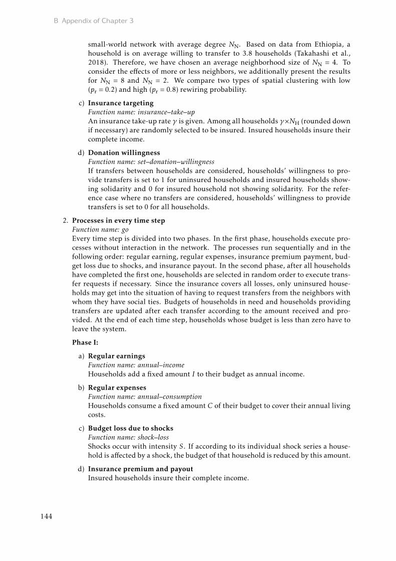
B Appendix of Chapter 3
small-world network with average degree NN. Based on data from Ethiopia, ahousehold is on average willing to transfer to 3.8 households (Takahashi et al.,2018). Therefore, we have chosen an average neighborhood size of NN = 4. Toconsider the effects of more or less neighbors, we additionally present the resultsfor NN = 8 and NN = 2. We compare two types of spatial clustering with low(pr = 0.2) and high (pr = 0.8) rewiring probability.
c) Insurance targetingFunction name: insurance–take–upAn insurance take-up rate γ is given. Among all households γ×NH (rounded downif necessary) are randomly selected to be insured. Insured households insure theircomplete income.
d) Donation willingnessFunction name: set–donation–willingnessIf transfers between households are considered, households’ willingness to pro-vide transfers is set to 1 for uninsured households and insured households show-ing solidarity and 0 for insured household not showing solidarity. For the refer-ence case where no transfers are considered, households’ willingness to providetransfers is set to 0 for all households.
2. Processes in every time stepFunction name: goEvery time step is divided into two phases. In the first phase, households execute pro-cesses without interaction in the network. The processes run sequentially and in thefollowing order: regular earning, regular expenses, insurance premium payment, bud-get loss due to shocks, and insurance payout. In the second phase, after all householdshave completed the first one, households are selected in random order to execute trans-fer requests if necessary. Since the insurance covers all losses, only uninsured house-holds may get into the situation of having to request transfers from the neighbors withwhom they have social ties. Budgets of households in need and households providingtransfers are updated after each transfer according to the amount received and pro-vided. At the end of each time step, households whose budget is less than zero have toleave the system.
Phase I:
a) Regular earningsFunction name: annual–incomeHouseholds add a fixed amount I to their budget as annual income.
b) Regular expensesFunction name: annual–consumptionHouseholds consume a fixed amount C of their budget to cover their annual livingcosts.
c) Budget loss due to shocksFunction name: shock–lossShocks occur with intensity S . If according to its individual shock series a house-hold is affected by a shock, the budget of that household is reduced by this amount.
d) Insurance premium and payoutInsured households insure their complete income.
144

B.1 Model documentation
• PayoutFunction name: insurance–payoutThe insurance covers the actual losses a household suffers from. The payout αin case of a shock is α = S .
• PremiumFunction name: insurance–premiumThe insurance is actuarially fair. Insured households have to pay a yearly pre-mium β equal to the expected payout: β = ps × S .
Phase II: Informal monetary transfersFunction name: informal–transfers
a) Transfer requestFunction name: transfer–requestHouseholds request monetary transfers from households they are linked to in thenetwork if their budget is below zero. A requesting household i requests a transferamount Ti,req that covers its debts Yi : Ti,req = |Yi |. A household in need can askhouseholds in its network for help which have a budget above zero. The householdrandomly picks one of the possible households. The budgets are updated afterevery transfer. Households continue to ask until they obtain the requested amountor until no more households are able to support them.
b) Transfer provisionFunction name: transfer–money, transfer–amountHouseholds are potential donors if their budget Yj is above zero. Depending onthe scenario, all households show solidarity or only uninsured households showsolidarity and insured households do not transfer. Households in need do notknow the insurance status of their neighbors.
• Solidarity: All potential donors are willing to transfer if requested. If therequested amount is smaller than their own budget, the amount transferredTi,j equals the requested amount Ti,req, otherwise they transfer their completebudget Yj : Ti,j =min{Yj ;Ti,req}
• No solidarity: Potential donors that are uninsured behave as in the solidaritycase. Insured households do not transfer.
c) Household budget equationAll processes sum up to the following equation for the budget Yi(t) of household i
at time step t:
Yi(t) =
Yi(t − 1) + I −C − β − Si +αi +∑
j∈Ni
Tij (t) for insured HH
Yi(t − 1) + I −C − Si +∑
j∈Ni
Tij (t) for uninsured HH
with income I , annual living costs C and premium β. The shock intensity Si equalsS if a household is affected by a shock and is zero otherwise. The same holds truefor the insurance payout αi . For t = 1 the budget of the previous time step t − 1 isgiven by the initial budget Y 0.Ni denotes all households that share a link with household i and Ti,j (t) is the trans-fer between households i and j at time step t. Transfers can be positive, negativeor zero for uninsured households (receiving and providing transfers) and negativeor zero for insured households (only providing transfers).
145

B Appendix of Chapter 3
d) Check for surviving householdsIf a household’s budget is below zero at the end of a time step, the household hasto leave the system.
III.iv.b What are the model parameters, their dimensions and reference values?
Parameter Description NetLogoname
Unit Standardvalue/range
Reference
T Number of ticks thatthe model runs
timesteps Years 50 –
NH Number of householdsin the system
number–households
Unitless 50 –
NN Neighborhood size(small-world network)
neighbor-hood–size
Unitless 2, 4, 8 Takahashiet al. (2018)
pr Rewiring probability(small-world network)
rewire–prob Unitless(rate)
0.2, 0.8 –
I Annual householdincome
income–lvl Norma-lized to1
1 –
Y 0 Initial budget budget–init Unitless,relatedto I
0 –
γ Insurance take-up rate insurance–take–up–rate
Unitless(rate)
0, 0.3, 0.6 Takahashiet al. (2018)
C Annual living costs consump-tion–lvl
Unitless,relatedto I
0.7 – 0.9 Takahashiet al. (2016)andMatsudaet al. (2019)
ps Probability for shockoccurrence
shock–prob Unitless(rate)
0.1 – 0.3 Geng et al.(2018) andAnderberg& Morsink(2020)
pV Probability for shockoccurrence at villagelevel (covariate shock)
covariate–shock–prob–vlg
Unitless(rate)
pV = ps/pH –
pH Probability thatindividual householdsare affected by a shockif the village is affected(covariate shock)
covariate–shock–prob–hh
Unitless(rate)
0.8, 1 –
S Shock intensity, i.e.budget loss due toshock
shock–intensity
Unitless,relatedto I
0.2 – 1 –
146

B.2 Parameter selection
III.iv.c How were submodels designed or chosen, and how were they parameterized andthen tested?
The different decision submodels were chosen to build a “virtual lab” to test how trans-fer decisions influence overall welfare of the population and if different behavioral mod-els lead to different outcomes. The parameter range for the network model has beenadapted to literature values (see III.iv.b). The combined parameter ranges for income I ,living costs C, shock probability ps and shock intensity S need to meet two constraints:(1) Shock intensity must be high enough to make financial protection necessary and (2)formal insurance must be affordable. The resulting reduced parameter space has beenadapted to economic constraints from literature values (for resulting parameter rangessee III.iv.b).
B.2 Parameter selection
To assess the impact of formal and informal insurance on the resilience of smallholders, themodel should depict conditions in which both instruments are important and can be usedeffectively. This implies (1) that the shock intensity should be high enough to make financialprotection necessary and (2) that formal insurance should be affordable. To select parametercombinations for living costs C, shock probability ps and shock intensity S that fulfill theseconstraints, we calculate the budget change of a household per time step depending on itsinsurance state and the occurrence of a shock (see Table B.1). Based on the probability pswith which each of these cases occur, the expected value of budget change without informaltransfers equals E[∆Y ] = I − C − β for an insured household and E[∆Y ] = I − C − ps × S foran uninsured households. As the insurance is assumed to be fair (β = ps × S), the expectedvalue E[∆Y ] is the same for insured and uninsured households. Based on the expected valuewe can select cases that are suitable for the analysis. We exclude parameter combinationswith E[∆Y ] < 0, as in this situations insured households lose money in every time step whichwould contradict the intention of insurance to protect household from monetary losses. Wefurthermore exclude combinations for which uninsured households do not have a negativebudget change in case of a loss, i.e. we exclude cases with E[∆Y ] > 0 and I − C − S > 0.In these cases, risk-coping instruments are not needed. Figure B.2 graphically shows theresulting parameter space. For the simulation, we use values with spacing of 0.1 for the threedimensions living costs C, shock probability ps and shock intensity S .
Table B.1: Budget change of a household per time step depending on its insurance state and theoccurrence of a shock. Budget change is calculated based on the annual income I , living costs C,shock intensity S , premium β and payout α.
Shock No shock
Insured I −C − S +α − β I −C − β
Not insured I −C − S I −C
Additionally to the mathematical restrictions, we constrain the parameters with respect toecological and economic observations. We assume subsistence farmers that need consumea large proportion of their income to cover their living costs. Studies for livestock farmersin Ethiopia show, for example, that households consume between 69% (322 Ethiopian Birr
147

B Appendix of Chapter 3
Shock probability ps = 0.1 Shock probability ps = 0.2 Shock probability ps = 0.3
0.0 0.2 0.4 0.6 0.8 1.0 0.0 0.2 0.4 0.6 0.8 1.0 0.0 0.2 0.4 0.6 0.8 1.00.0
0.2
0.4
0.6
0.8
1.0
Shock intensity
Liv
ing
co
sts
−0.25 0 0.25 0.5 0.75 1
Expected value of budget change: Parameter combinationsselected for simulation
Figure B.2: Representation of the parameter space that results from assumptions for reasonable bud-get changes of a household per time step. White lines connect parameter combinations with equalexpected value of budget change E[∆Y ]. The parameter space is divided in three main zones: Forparameter combinations below the dotted line E[∆Y ] > 0 and I − C − S > 0 applies; for parametercombinations above the dashed line E[∆Y ] < 0 applies. Parameter combinations in between those twozones are suitable for the analysis. Dots represent parameter combinations that fulfill the additionalecological and economic constraints (0.1 ≤ ps ≤ 0.3,0.7 ≤ C < 1). These parameter combinations areselected for the simulation.
mean monthly per capita consumption with 467 Ethiopian Birr mean monthly per capitaincome (Takahashi et al., 2016)) and 81% (mean annual household consumption 21,482Ethiopian Birr with annual household income 26,631 Ethiopian Birr (Matsuda et al., 2019))of their income. We therefore restrict the parameter for living costs to 0.7 ≤ C < 1. We fur-thermore assume shock probabilities in a range of 0.1 ≤ ps ≤ 0.3 which relate to empiricallyobserved income losses. According to a study in Ethiopia, for example, the probability tolose 25-50% of the crop yield was on average 21% (Anderberg & Morsink, 2020). The rateof health shocks is similarly high. In a survey conducted in Kenya, households denoted toexperience a health shock in 26.6% of the weeks in one year (Geng et al., 2018). We donot include any further restrictions for shock intensity S to cover a broad range of possibleoutcomes. Based on suitable expected values, values for shock probabilities ps and levels ofannual living costs C, shock intensity S is within 0.2 ≤ S ≤ 1. We divide all parameter rangesin equidistant steps of 0.1, which results in 52 reasonable parameter combinations that meetthe constraints.
B.3 Additional results for idiosyncratic shocks (selectedparameter combination)
We present additional results for idiosyncratic shocks, i.e. shocks that occur for all house-holds independently with shock probability ps. Tomake the different risk-coping instrumentscomparable, for each household the order of shocks is determined at the beginning of eachsimulation run. This individual shock series is equal for the same parameter combination
148

B.3 Additional results for idiosyncratic shocks (selected parameter combination)
and random seed independent of the network characteristics and risk-coping instrumentsthat are analyzed. We present simulation runs over 50 years for one specific parameter com-bination of income I , living costs C, shock probability ps and shock intensity S (I = 1, C = 0.8,ps = 0.3, S = 0.6). All results show the mean over 100 repetitions. The outcomes can be com-pared to the observations shown in the main text where results for a small-world networkwith rewiring probability pr = 0.2 and an average number of four neighbors (NN = 4) areshown. Here, we analyze the fraction of surviving households (Figure B.3), the fraction ofsurviving uninsured households (Figure B.4), the total transfer (Figure B.5) and the budgetper surviving household (Figure B.6) for (a) higher rewiring probability, (b) smaller and (c)larger average degrees.
B.3.1 Fraction of surviving households
We observe that rewiring probability (Figure B.3A) has almost no effect on the survival ratesn. Only when all households show solidarity and 60% of the households are insured slightlymore households survive than for a low rewiring probability. In the 60% insurance scenario,the survival rate is slightly lower when only uninsured households show solidarity. As evenwith higher rewiring probability, the average number of neighbors remains at NN = 4, thesimilar survival rates show that, in most cases, households can rely on the same number ofhelping households. Only if a large number of households is insured, some households ben-efit from a higher number of neighbors, which can result from a high rewiring probability.With a higher number of neighbors, the small contributions of insured households can moreeasily sum up to effective contributions. This suggests that the average number of neigh-bors could play an important role. We have therefore investigated which effects a smaller(Figure B.3B) and larger (Figure B.3C) average degree than that presented in the main text(NN = 4) has on the survival rate. As expected, a low number of neighbors (NN = 2) clearlylowers the number of households that manage to stay in the system whereas a larger numberof neighbors (NN = 8) helps more households to survive. This is reasonable, since when ahousehold in need is connected to more households, the chance that enough neighbors canand are willing to help is higher. Furthermore, the chance that even small contributions sumup to helpful transfers increases with more neighbors.
B.3.2 Fraction of surviving uninsured households
When focusing the analysis on the fraction of surviving uninsured households among the20 households that are uninsured in every scenario, we again observe that a higher rewiringprobability (Figure B.4A) has only small effects. When changing the average degree (FigureB.4B, Figure B.4C), we observe that this influences, on the one hand, the fraction of survivinguninsured households as already observable for the fraction of surviving households and,on the other hand, the effect of solidarity from insured households. The higher the averagenumber of neighbors, the larger is the difference between uninsured households survivingwith solidarity of insured households and without. This is due to the fact that when a house-hold in need is connected to more other households, contributions of insured households thatare potentially smaller than those of uninsured households more easily sum up to effectivecontributions.
149

B Appendix of Chapter 3
Insurance rate γ = 0% Insurance rate γ = 30% Insurance rate γ = 60%
A
B
C
0 10 20 30 40 50 0 10 20 30 40 50 0 10 20 30 40 50
0.00
0.25
0.50
0.75
1.00
0.00
0.25
0.50
0.75
1.00
0.00
0.25
0.50
0.75
1.00
Time step
Fra
ctio
n o
f su
rviv
ing
ho
use
ho
lds
No informal transfer Solidarity No solidarity
Figure B.3: Fraction of surviving households for different risk-coping instruments and insurance rates(γ = 0%, γ = 30%, γ = 60%) with (A) high rewiring probability (NN = 4, pr = 0.8), (B) small averagedegree (NN = 2, pr = 0.2) and (C) large average degree (NN = 8, pr = 0.2).
150

B.3 Additional results for idiosyncratic shocks (selected parameter combination)
AAAAAAAAAAAAAAAAAAAAAAAAAAAAAAAAAAAAAAAAAAAAAAAAAAAAAAAAAAAAAAAAAAAAAAAAAAAAAAAAAAAAAAAAAAAAAAAAAAAAAAAAAAAAAAAAAAAAAAAAAAAAAAAAAAAAAAAAAAAAAAAAAAAAAAAAAAAAAAAAAAAAAAAAAAAAAAAAAAAAAAAAAAAAAAAAAAAAAAAAAAAAAAAAAAAAAAAAAAAAAAAAAAAAAAAAAAAAAAAAAAAAAAAAAAAAAAAAAAAAAAAAAAAAAAAAAAAAAAAAAAAAAAAAAAAAAAAAAAAAAAAAAA BBBBBBBBBBBBBBBBBBBBBBBBBBBBBBBBBBBBBBBBBBBBBBBBBBBBBBBBBBBBBBBBBBBBBBBBBBBBBBBBBBBBBBBBBBBBBBBBBBBBBBBBBBBBBBBBBBBBBBBBBBBBBBBBBBBBBBBBBBBBBBBBBBBBBBBBBBBBBBBBBBBBBBBBBBBBBBBBBBBBBBBBBBBBBBBBBBBBBBBBBBBBBBBBBBBBBBBBBBBBBBBBBBBBBBBBBBBBBBBBBBBBBBBBBBBBBBBBBBBBBBBBBBBBBBBBBBBBBBBBBBBBBBBBBBBBBBBBBBBBBBBBBB CCCCCCCCCCCCCCCCCCCCCCCCCCCCCCCCCCCCCCCCCCCCCCCCCCCCCCCCCCCCCCCCCCCCCCCCCCCCCCCCCCCCCCCCCCCCCCCCCCCCCCCCCCCCCCCCCCCCCCCCCCCCCCCCCCCCCCCCCCCCCCCCCCCCCCCCCCCCCCCCCCCCCCCCCCCCCCCCCCCCCCCCCCCCCCCCCCCCCCCCCCCCCCCCCCCCCCCCCCCCCCCCCCCCCCCCCCCCCCCCCCCCCCCCCCCCCCCCCCCCCCCCCCCCCCCCCCCCCCCCCCCCCCCCCCCCCCCCCCCCCCCCCC
0 10 20 30 40 50 0 10 20 30 40 50 0 10 20 30 40 50
0.00
0.25
0.50
0.75
1.00
Time step
Fra
ctio
n o
f su
rviv
ing
un
insu
red
ho
use
ho
lds
No informal transfer No solidarity, γ = 30% No solidarity, γ = 60%
Solidarity, γ = 0% Solidarity, γ = 30% Solidarity, γ = 60%
Figure B.4: Fraction of surviving uninsured households among the 20 households that are uninsuredin every scenario for different risk-coping instruments with insurance rates γ and (A) high rewiringprobability (NN = 4, pr = 0.8), (B) small average degree (NN = 2, pr = 0.2) and (C) large average degree(NN = 8, pr = 0.2).
B.3.3 Total transfer
The total transfer received and given by the 20 households that are uninsured in every sce-nario per time step underlines the observations for the survival rates of uninsured householdsfor different network conditions. The transfers in a network with high rewiring probability(Figure B.5A) are, as expected from the similar survival rates, in the same range than thoseprovided in a network with small rewiring probability. For a smaller average degree (FigureB.5B) than that presented in the main text, we observe less transfers given and received byuninsured households, for a larger average degree (Figure B.5C) correspondingly more. Thetrends that were observed for the baseline case presented in the main text hold, however, truefor all additional network scenarios. The fact that households have to provide lower transferswhen insured households show solidarity is even more pronounced with many neighbors.This is due to the fact that in this case the transfers tend to be spread over several shouldersand even small contributions can be effective.
B.3.4 Budget per surviving household
The observations for the total transfer that uninsured households receive and give for the dif-ferent scenarios are directly related to the budget per surviving household. We compare thebudget based on the 20 households that are uninsured in every scenario and the 15 house-holds that are insured in every scenarios (except γ = 0%). The straight line shows the max-imum budget that an insured household can receive as reference value. As the case with noinformal transfers is independent of the network characteristics, the budget per survivinghousehold is in this case not affected by changes of rewiring probability or neighborhoodsize. As in all other output measures, budget as well is not affected by a larger rewiring prob-ability (Figure B.6A). However, smaller (Figure B.6B) and larger (Figure B.6C) neighborhoodsizes have effects on the budgets of uninsured and insured households. We observe that the
151

B Appendix of Chapter 3
Received by uninsured Given by uninsured
A
B
C
0 10 20 30 40 50 0 10 20 30 40 50
0.0
0.5
1.0
1.5
0.0
0.5
1.0
0.0
0.5
1.0
1.5
2.0
Time step
To
tal tr
an
sfe
r p
er
tim
e s
tep
No informal transfer No solidarity, γ = 30% No solidarity, γ = 60%
Solidarity, γ = 0% Solidarity, γ = 30% Solidarity, γ = 60%
Figure B.5: Total transfer received and given by all 20 households that are uninsured in every scenarioper time step. Results show (A) high rewiring probability (NN = 4, pr = 0.8), (B) small average degree(NN = 2, pr = 0.2) and (C) large average degree (NN = 8, pr = 0.2).
152
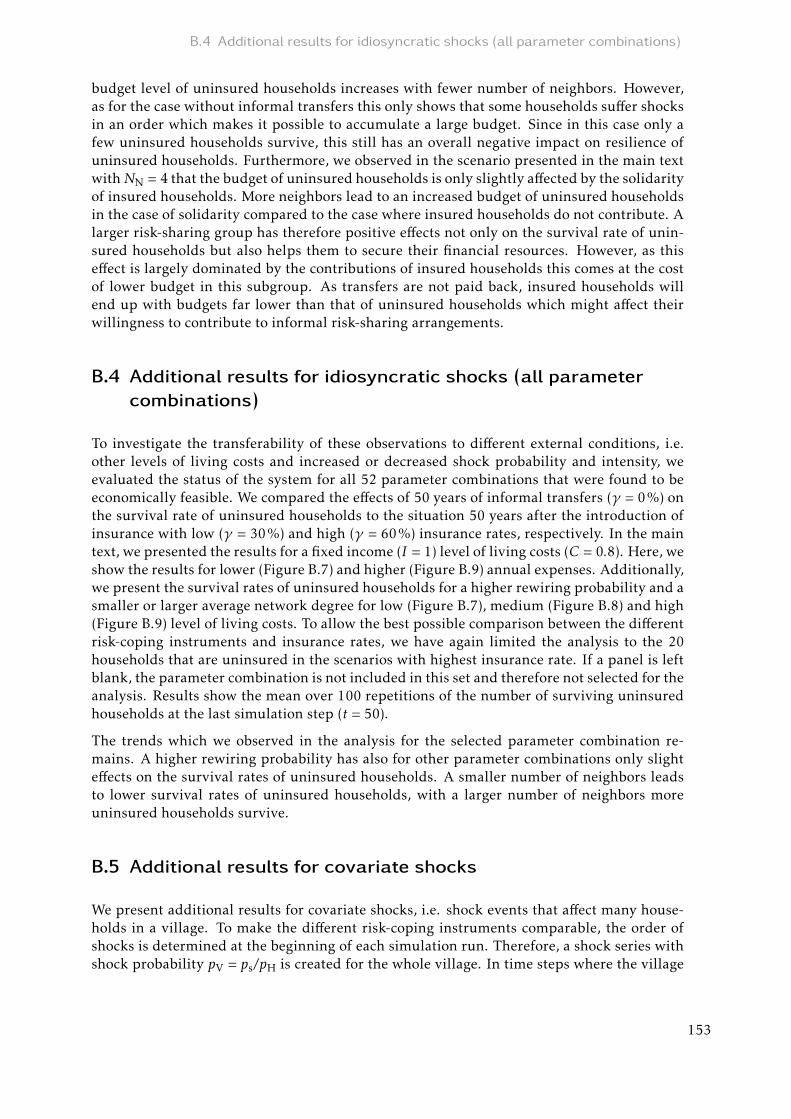
B.4 Additional results for idiosyncratic shocks (all parameter combinations)
budget level of uninsured households increases with fewer number of neighbors. However,as for the case without informal transfers this only shows that some households suffer shocksin an order which makes it possible to accumulate a large budget. Since in this case only afew uninsured households survive, this still has an overall negative impact on resilience ofuninsured households. Furthermore, we observed in the scenario presented in the main textwithNN = 4 that the budget of uninsured households is only slightly affected by the solidarityof insured households. More neighbors lead to an increased budget of uninsured householdsin the case of solidarity compared to the case where insured households do not contribute. Alarger risk-sharing group has therefore positive effects not only on the survival rate of unin-sured households but also helps them to secure their financial resources. However, as thiseffect is largely dominated by the contributions of insured households this comes at the costof lower budget in this subgroup. As transfers are not paid back, insured households willend up with budgets far lower than that of uninsured households which might affect theirwillingness to contribute to informal risk-sharing arrangements.
B.4 Additional results for idiosyncratic shocks (all parametercombinations)
To investigate the transferability of these observations to different external conditions, i.e.other levels of living costs and increased or decreased shock probability and intensity, weevaluated the status of the system for all 52 parameter combinations that were found to beeconomically feasible. We compared the effects of 50 years of informal transfers (γ = 0%) onthe survival rate of uninsured households to the situation 50 years after the introduction ofinsurance with low (γ = 30%) and high (γ = 60%) insurance rates, respectively. In the maintext, we presented the results for a fixed income (I = 1) level of living costs (C = 0.8). Here, weshow the results for lower (Figure B.7) and higher (Figure B.9) annual expenses. Additionally,we present the survival rates of uninsured households for a higher rewiring probability and asmaller or larger average network degree for low (Figure B.7), medium (Figure B.8) and high(Figure B.9) level of living costs. To allow the best possible comparison between the differentrisk-coping instruments and insurance rates, we have again limited the analysis to the 20households that are uninsured in the scenarios with highest insurance rate. If a panel is leftblank, the parameter combination is not included in this set and therefore not selected for theanalysis. Results show the mean over 100 repetitions of the number of surviving uninsuredhouseholds at the last simulation step (t = 50).
The trends which we observed in the analysis for the selected parameter combination re-mains. A higher rewiring probability has also for other parameter combinations only slighteffects on the survival rates of uninsured households. A smaller number of neighbors leadsto lower survival rates of uninsured households, with a larger number of neighbors moreuninsured households survive.
B.5 Additional results for covariate shocks
We present additional results for covariate shocks, i.e. shock events that affect many house-holds in a village. To make the different risk-coping instruments comparable, the order ofshocks is determined at the beginning of each simulation run. Therefore, a shock series withshock probability pV = ps/pH is created for the whole village. In time steps where the village
153

B Appendix of Chapter 3
Uninsured Insured
A
B
C
0 10 20 30 40 50 0 10 20 30 40 50
0
1
2
0
1
2
0
1
2
Time step
Bu
dg
et
pe
r su
rviv
ing
ho
use
ho
ld
No informal transfer No solidarity, γ = 30% No solidarity, γ = 60%
Solidarity, γ = 0% Solidarity, γ = 30% Solidarity, γ = 60%
Figure B.6: Budget per surviving household calculated based on the 20 households that are uninsuredin every scenario and the 15 households that are insured in every investigated scenario (except γ =0%). The straight line shows the maximum budget that an insured household can receive as referencevalue. Results show (A) high rewiring probability (NN = 4, pr = 0.8), (B) small average degree (NN = 2,pr = 0.2) and (C) large average degree (NN = 8, pr = 0.2).
154

B.5 Additional results for covariate shocks
1
1
1
1
1
1
1
1
1
1
1
1
0.99
1
1
0.99
0.99
0.99
0.98
0.99
0.98
AAAAAAAAAAAAAAAAAAAAA
1
0.99
1
0.98
1
0.98
0.98
0.93
0.97
0.93
0.97
0.93
0.93
0.85
1 1 1 1 0.99 0.99 0.98
1
1
1
1
1
1
1
1
1
0.99
1
1
0.99
0.99
0.99
0.99
0.98
0.98
0.97
0.98
0.98
BBBBBBBBBBBBBBBBBBBBB
1
0.98
1
0.98
1
0.98
0.97
0.93
0.97
0.92
0.96
0.92
0.92
0.86
1 1 1 0.99 0.99 0.99 0.97
1
1
1
1
1
1
1
0.99
0.99
0.97
0.98
0.98
0.96
0.96
0.95
0.96
0.94
0.92
0.88
0.89
0.9
CCCCCCCCCCCCCCCCCCCCC
0.99
0.96
0.98
0.95
0.98
0.95
0.92
0.87
0.92
0.86
0.91
0.86
0.85
0.8
1 1 1 0.97 0.96 0.96 0.88
1
1
1
1
1
1
1
1
1
1
1
1
1
1
1
1
1
1
1
1
1
DDDDDDDDDDDDDDDDDDDDD
1
1
1
1
1
1
1
0.98
1
0.97
1
0.97
0.99
0.94
1 1 1 1 1 1 1
1
1
1
1
1
1
1
0.99
1
0.97
0.98
0.98
0.95
0.95
0.94
0.94
0.91
0.9
0.84
0.85
0.82
0.99
0.97
0.98
0.95
0.98
0.94
0.91
0.8
0.88
0.76
0.86
0.73
0.71
0.58
1 1 1 0.97 0.95 0.94 0.84
1
1
1
1
1
1
1
0.99
0.99
0.96
0.97
0.97
0.94
0.94
0.93
0.93
0.89
0.88
0.84
0.84
0.84
0.99
0.95
0.98
0.94
0.98
0.93
0.9
0.8
0.87
0.76
0.85
0.73
0.72
0.58
1 1 1 0.96 0.94 0.93 0.84
0.99
1
1
0.98
0.99
0.99
0.98
0.97
0.95
0.86
0.87
0.87
0.84
0.8
0.79
0.81
0.77
0.74
0.63
0.66
0.67
0.96
0.91
0.95
0.88
0.94
0.87
0.78
0.7
0.75
0.66
0.72
0.63
0.57
0.51
0.99 0.98 0.98 0.86 0.84 0.81 0.63
1
1
1
1
1
1
1
1
1
1
1
1
0.99
0.99
1
0.98
0.98
0.98
0.96
0.97
0.96
1
0.99
1
0.98
1
0.98
0.99
0.91
0.98
0.88
0.96
0.86
0.9
0.75
1 1 1 1 0.99 0.98 0.96
0.99
1
1
0.98
0.99
0.99
0.97
0.95
0.95
0.85
0.83
0.84
0.71
0.68
0.66
0.55
0.47
0.45
0.98
0.92
0.94
0.86
0.92
0.82
0.72
0.56
0.58
0.44
0.42
0.33
0.99 0.98 0.97 0.85 0.71 0.55
0.99
0.99
1
0.98
0.97
0.98
0.97
0.94
0.93
0.84
0.82
0.82
0.71
0.68
0.68
0.55
0.5
0.46
0.96
0.89
0.93
0.85
0.91
0.82
0.73
0.58
0.59
0.44
0.43
0.32
0.99 0.98 0.97 0.84 0.71 0.55
0.96
0.98
0.99
0.94
0.92
0.9
0.91
0.87
0.81
0.65
0.63
0.63
0.51
0.49
0.5
0.36
0.33
0.33
0.91
0.82
0.86
0.76
0.84
0.73
0.55
0.46
0.42
0.36
0.3
0.27
0.96 0.94 0.91 0.65 0.51 0.36
1
1
1
1
1
1
1
0.99
1
0.96
0.96
0.96
0.9
0.89
0.87
0.77
0.73
0.66
1
0.98
0.99
0.93
0.98
0.9
0.91
0.74
0.82
0.6
0.65
0.46
1 1 1 0.96 0.9 0.77
Shock probability ps = 0.1 Shock probability ps = 0.2 Shock probability ps = 0.3S
olid
arity
No s
olid
arity
Solid
arity
No s
olid
arity
Solid
arity
No s
olid
arity
Solid
arity
No s
olid
arity
0.4 0.5 0.6 0.7 0.8 0.9 1.0 0.4 0.5 0.6 0.7 0.8 0.9 1.0 0.4 0.5 0.6 0.7 0.8 0.9 1.0
0
30
60
0
30
60
0
30
60
0
30
60
0
30
60
0
30
60
0
30
60
0
30
60
Shock intensity
Insu
ran
ce
ra
te (
%)
0.00 0.25 0.50 0.75 1.00
Fraction of surviving uninsured households:
Figure B.7: Fraction of surviving uninsured households among the 20 households that are uninsuredin every scenario for idiosyncratic shocks and low level of living costs (C = 0.7) for (A) average degreeand rewiring probability as in main text (NN = 4, pr = 0.2), (B) high rewiring probability (NN = 4,pr = 0.8), (C) small average degree (NN = 2, pr = 0.2) and (D) large average degree (NN = 8, pr = 0.2).
155

B Appendix of Chapter 3
1
1
1
1
1
1
0.99
1
1
0.99
0.98
0.98
0.97
0.97
0.96
0.96
0.95
0.94
0.92
0.92
0.91
0.9
0.89
0.89
AAAAAAAAAAAAAAAAAAAAAAAA
1
0.98
1
0.98
0.97
0.93
0.96
0.92
0.92
0.85
0.91
0.84
0.85
0.76
0.83
0.74
1 1 0.99 0.99 0.97 0.96 0.92 0.9
1
1
1
1
0.99
0.99
0.97
0.98
0.98
0.96
0.94
0.92
0.88
0.88
0.88
0.87
0.87
0.86
0.81
0.83
0.83
0.78
0.8
0.81
BBBBBBBBBBBBBBBBBBBBBBBB
0.99
0.96
0.98
0.95
0.92
0.86
0.91
0.86
0.84
0.8
0.84
0.78
0.77
0.7
0.74
0.67
1 1 0.97 0.96 0.88 0.87 0.81 0.78
1
1
1
1
1
1
1
1
1
1
1
1
1
1
1
1
1
1
0.99
0.99
0.99
0.99
0.98
0.98
CCCCCCCCCCCCCCCCCCCCCCCC
1
1
1
1
1
0.98
1
0.97
0.99
0.94
0.99
0.93
0.97
0.88
0.96
0.86
1 1 1 1 1 1 0.99 0.99
1
1
1
1
0.99
0.99
0.96
0.96
0.97
0.93
0.89
0.88
0.81
0.79
0.79
0.71
0.65
0.64
0.45
0.41
0.4
0.99
0.95
0.98
0.93
0.89
0.79
0.85
0.73
0.68
0.55
0.57
0.45
0.34
0.27
1 1 0.96 0.93 0.81 0.71 0.45
0.99
0.99
1
0.98
0.97
0.95
0.86
0.87
0.87
0.81
0.77
0.74
0.6
0.62
0.63
0.49
0.49
0.52
0.29
0.3
0.31
0.96
0.9
0.94
0.87
0.77
0.69
0.72
0.63
0.54
0.48
0.44
0.4
0.27
0.24
0.99 0.98 0.86 0.81 0.6 0.49 0.29
1
1
1
1
1
1
1
1
1
0.98
0.98
0.98
0.96
0.95
0.94
0.9
0.86
0.84
0.69
0.63
0.61
1
0.99
1
0.98
0.98
0.9
0.96
0.86
0.88
0.72
0.79
0.61
0.53
0.38
1 1 1 0.98 0.96 0.9 0.69
0.99
0.99
1
0.97
0.94
0.93
0.8
0.78
0.78
0.55
0.5
0.46
0.96
0.88
0.91
0.82
0.67
0.53
0.43
0.32
0.99 0.97 0.8 0.55
0.96
0.97
0.99
0.91
0.87
0.81
0.59
0.58
0.6
0.36
0.33
0.33
0.9
0.8
0.84
0.73
0.5
0.42
0.3
0.27
0.96 0.91 0.59 0.36
1
1
1
1
0.99
1
0.95
0.94
0.93
0.77
0.73
0.66
1
0.97
0.98
0.9
0.88
0.7
0.65
0.46
1 1 0.95 0.77
Shock probability ps = 0.1 Shock probability ps = 0.2 Shock probability ps = 0.3
Solid
arity
No s
olid
arity
Solid
arity
No s
olid
arity
Solid
arity
No s
olid
arity
0.3 0.4 0.5 0.6 0.7 0.8 0.9 1.0 0.3 0.4 0.5 0.6 0.7 0.8 0.9 1.0 0.3 0.4 0.5 0.6 0.7 0.8 0.9 1.0
0
30
60
0
30
60
0
30
60
0
30
60
0
30
60
0
30
60
Shock intensity
Insu
ran
ce
ra
te (
%)
0.00 0.25 0.50 0.75 1.00
Fraction of surviving uninsured households:
Figure B.8: Fraction of surviving uninsured households among the 20 households that are uninsuredin every scenario for idiosyncratic shocks and medium level of living costs (C = 0.8) for (A) highrewiring probability (NN = 4, pr = 0.8), (B) small average degree (NN = 2, pr = 0.2) and (C) largeaverage degree (NN = 8, pr = 0.2).
156

B.5 Additional results for covariate shocks
1
1
1
0.99
0.99
0.99
0.97
0.95
0.95
0.92
0.89
0.89
0.82
0.81
0.82
0.73
0.72
0.73
0.59
0.58
0.58
0.42
0.41
0.41
AAAAAAAAAAAAAAAAAAAAAAAA
1
0.98
0.97
0.93
0.92
0.84
0.84
0.75
0.75
0.65
0.63
0.51
0.5
0.42
0.37
0.32
1 0.99 0.97 0.92 0.82 0.73 0.59 0.42
1
1
1
0.99
0.98
0.98
0.96
0.95
0.94
0.9
0.89
0.89
0.83
0.81
0.82
0.73
0.72
0.72
0.59
0.58
0.59
0.43
0.41
0.41
BBBBBBBBBBBBBBBBBBBBBBBB
1
0.98
0.96
0.92
0.91
0.84
0.83
0.74
0.74
0.64
0.64
0.53
0.5
0.41
0.38
0.32
1 0.99 0.96 0.9 0.83 0.73 0.59 0.43
1
0.99
0.99
0.96
0.94
0.92
0.87
0.87
0.86
0.78
0.8
0.81
0.7
0.71
0.72
0.57
0.57
0.58
0.45
0.46
0.46
0.33
0.32
0.32
CCCCCCCCCCCCCCCCCCCCCCCC
0.98
0.95
0.91
0.86
0.84
0.78
0.74
0.67
0.64
0.57
0.52
0.45
0.4
0.36
0.3
0.28
1 0.96 0.87 0.78 0.7 0.57 0.45 0.33
1
1
1
1
1
1
1
1
1
0.99
0.98
0.98
0.96
0.95
0.93
0.91
0.87
0.85
0.81
0.76
0.76
0.61
0.57
0.55
DDDDDDDDDDDDDDDDDDDDDDDD
1
1
1
0.97
0.99
0.93
0.96
0.86
0.9
0.77
0.82
0.65
0.68
0.53
0.51
0.38
1 1 1 0.99 0.96 0.91 0.81 0.61
1
0.99
1
0.94
0.91
0.9
0.7
0.65
0.64
0.98
0.94
0.86
0.73
0.58
0.46
1 0.94 0.7
1
0.99
0.99
0.93
0.89
0.88
0.71
0.65
0.64
0.98
0.93
0.85
0.73
0.57
0.45
1 0.93 0.71
0.98
0.97
0.95
0.81
0.77
0.74
0.49
0.49
0.52
0.94
0.87
0.72
0.63
0.44
0.4
0.98 0.81 0.49
1
1
1
0.98
0.98
0.98
0.9
0.86
0.84
1
0.98
0.96
0.86
0.79
0.61
1 0.98 0.9
0.97
0.95
0.95
0.55
0.47
0.45
0.92
0.82
0.42
0.33
0.97 0.55
0.97
0.94
0.93
0.55
0.5
0.46
0.91
0.82
0.43
0.32
0.97 0.55
0.91
0.87
0.81
0.36
0.33
0.33
0.84
0.73
0.3
0.27
0.91 0.36
1
0.99
1
0.77
0.73
0.66
0.98
0.9
0.65
0.46
1 0.77
Shock probability ps = 0.1 Shock probability ps = 0.2 Shock probability ps = 0.3S
olid
arity
No s
olid
arity
Solid
arity
No s
olid
arity
Solid
arity
No s
olid
arity
Solid
arity
No s
olid
arity
0.2 0.3 0.4 0.5 0.6 0.7 0.8 0.9 0.2 0.3 0.4 0.5 0.6 0.7 0.8 0.9 0.2 0.3 0.4 0.5 0.6 0.7 0.8 0.9
0
30
60
0
30
60
0
30
60
0
30
60
0
30
60
0
30
60
0
30
60
0
30
60
Shock intensity
Insu
ran
ce
ra
te (
%)
0.00 0.25 0.50 0.75 1.00
Fraction of surviving uninsured households:
Figure B.9: Fraction of surviving uninsured households among the 20 households that are uninsuredin every scenario for idiosyncratic shocks and high level of living costs (C = 0.9) for (A) average degreeand rewiring probability as in main text (NN = 4, pr = 0.2), (B) high rewiring probability (NN = 4,pr = 0.8), (C) small average degree (NN = 2, pr = 0.2) and (D) large average degree (NN = 8, pr = 0.2).
157

B Appendix of Chapter 3
is affected by a shock, individual households are affected with probability pH. This individualshock series is equal for the same parameter combination and random seed independent ofthe network characteristics and risk-coping instruments that are analyzed.
In the main text, we have shown the survival rate of uninsured households for networkswith average number of neighbors NN = 4 and rewiring probability pr = 0.2. Among the 52parameter combinations that were found to be economically feasible we selected the resultsfor a medium level of living costs (C = 0.8). We have presented the results for within-villageshock probability pH = 0.8. In this case an individual household is affected by a shock with80% probability if a shock event occurs at village level. Here, we additionally include theresult for the more extreme case of pH = 1 where all households are affected simultaneouslyif a shock occurs.
We present the full parameter set divided according to the level of living costs C with C = 0.7(Figure B.10), C = 0.8 (Figure B.11) and C = 0.9 (Figure B.12). If a panel is left blank, theparameter combination is not selected for the analysis. Results show the mean over 100repetitions of the number of surviving uninsured households at the last simulation step (t =50).
We observe that, as expected, a higher within-village shock probability leads to lower survivalrates of uninsured household. In this case, informal risk-coping is only possible by transfersfrom insured households which is not as effective as if at least some uninsured householdscan contribute, too. When all households are affected by shocks simultaneously and insuredhouseholds do not show solidarity, the fraction of insured households has obviously no in-fluence on the survival rate of uninsured households (lower rows in panels for pH = 1).
158

B.5 Additional results for covariate shocks
0.95
0.99
1
0.92
0.97
0.99
0.92
0.94
0.97
0.87
0.91
0.96
0.86
0.9
0.94
0.85
0.88
0.92
0.79
0.86
0.91
AAAAAAAAAAAAAAAAAAAAA
0.95
0.93
0.92
0.92
0.92
0.92
0.86
0.85
0.85
0.83
0.84
0.83
0.79
0.77
0.95 0.92 0.92 0.87 0.86 0.85 0.79
0.91
0.97
1
0.91
0.95
0.99
0.91
0.92
0.96
0.81
0.89
0.95
0.78
0.87
0.92
0.78
0.84
0.91
0.72
0.82
0.9
BBBBBBBBBBBBBBBBBBBBB
0.91
0.91
0.91
0.91
0.91
0.91
0.81
0.81
0.78
0.78
0.78
0.78
0.72
0.72
0.91 0.91 0.91 0.81 0.78 0.78 0.72
0.9
0.97
1
0.84
0.93
0.99
0.82
0.86
0.94
0.72
0.79
0.87
0.66
0.74
0.82
0.61
0.67
0.75
0.51
0.6
0.7
0.89
0.87
0.84
0.82
0.81
0.8
0.7
0.67
0.65
0.62
0.6
0.58
0.49
0.47
0.9 0.84 0.82 0.72 0.66 0.61 0.51
0.82
0.94
0.99
0.78
0.88
0.97
0.76
0.81
0.9
0.63
0.74
0.83
0.54
0.66
0.78
0.53
0.6
0.72
0.43
0.54
0.66
0.82
0.82
0.78
0.78
0.76
0.76
0.63
0.63
0.54
0.54
0.53
0.53
0.43
0.43
0.82 0.78 0.76 0.63 0.54 0.53 0.43
0.83
0.93
0.99
0.7
0.8
0.91
0.64
0.69
0.79
0.41
0.52
0.64
0.32
0.38
0.48
0.24
0.26
0.3
0.8
0.76
0.69
0.67
0.63
0.6
0.4
0.38
0.31
0.29
0.24
0.22
0.83 0.7 0.64 0.41 0.32 0.24
0.7
0.85
0.98
0.64
0.72
0.86
0.58
0.64
0.74
0.33
0.47
0.62
0.22
0.3
0.45
0.17
0.19
0.24
0.7
0.7
0.64
0.64
0.58
0.58
0.33
0.33
0.22
0.22
0.17
0.17
0.7 0.64 0.58 0.33 0.22 0.17
Shock probability ps = 0.1 Shock probability ps = 0.2 Shock probability ps = 0.3
Solid
arity
No s
olid
arity
Solid
arity
No s
olid
arity
0.4 0.5 0.6 0.7 0.8 0.9 1.0 0.4 0.5 0.6 0.7 0.8 0.9 1.0 0.4 0.5 0.6 0.7 0.8 0.9 1.0
0
30
60
0
30
60
0
30
60
0
30
60
Shock intensity
Insu
ran
ce
ra
te (
%)
0.00 0.25 0.50 0.75 1.00
Fraction of surviving uninsured households:
Figure B.10: Fraction of surviving uninsured households among the 20 households that are uninsuredin every scenario for covariate shocks (NN = 4, pr = 0.2) and low level of living costs (C = 0.7). Upperrows show the results for solidarity between all households, lower rows show the results for solidaritybetween uninsured households only when (A) 80% of the households (pH = 0.8) and (B) all householdsare affected by a shock at village level (pH = 1).
0.91
0.95
0.99
0.91
0.92
0.96
0.8
0.88
0.95
0.78
0.84
0.91
0.72
0.78
0.87
0.66
0.75
0.84
0.57
0.7
0.8
0.56
0.66
0.77
0.91
0.91
0.91
0.91
0.8
0.8
0.78
0.78
0.72
0.72
0.66
0.66
0.57
0.57
0.56
0.56
0.91 0.91 0.8 0.78 0.72 0.66 0.57 0.56
0.82
0.9
0.98
0.76
0.81
0.9
0.6
0.71
0.82
0.53
0.6
0.72
0.37
0.48
0.6
0.29
0.36
0.47
0.13
0.18
0.28
0.82
0.82
0.76
0.76
0.6
0.6
0.53
0.53
0.37
0.37
0.29
0.29
0.13
0.13
0.82 0.76 0.6 0.53 0.37 0.29 0.13
0.68
0.82
0.96
0.58
0.64
0.74
0.26
0.42
0.58
0.17
0.19
0.24
0.68
0.68
0.58
0.58
0.26
0.26
0.17
0.17
0.68 0.58 0.26 0.17
Shock probability ps = 0.1 Shock probability ps = 0.2 Shock probability ps = 0.3
Solid
arity
No s
olid
arity
0.3 0.4 0.5 0.6 0.7 0.8 0.9 1.0 0.3 0.4 0.5 0.6 0.7 0.8 0.9 1.0 0.3 0.4 0.5 0.6 0.7 0.8 0.9 1.0
0
30
60
0
30
60
Shock intensity
Insu
ran
ce
ra
te (
%)
0.00 0.25 0.50 0.75 1.00
Fraction of surviving uninsured households:
Figure B.11: Fraction of surviving uninsured households among the 20 households that are uninsuredin every scenario for covariate shocks (NN = 4, pr = 0.2) and medium level of living costs (C = 0.8)when all households are affected by a shock at village level (pH = 1).
159

B Appendix of Chapter 3
0.92
0.94
0.97
0.85
0.88
0.92
0.76
0.82
0.87
0.65
0.74
0.82
0.56
0.62
0.72
0.43
0.5
0.6
0.31
0.38
0.46
0.19
0.21
0.28
AAAAAAAAAAAAAAAAAAAAAAAA
0.92
0.92
0.84
0.83
0.75
0.74
0.63
0.6
0.55
0.53
0.41
0.39
0.29
0.27
0.18
0.17
0.92 0.85 0.76 0.65 0.56 0.43 0.31 0.19
0.91
0.92
0.96
0.78
0.84
0.91
0.66
0.75
0.84
0.56
0.66
0.77
0.48
0.55
0.66
0.33
0.43
0.54
0.22
0.3
0.42
0.18
0.2
0.24
BBBBBBBBBBBBBBBBBBBBBBBB
0.91
0.91
0.78
0.78
0.66
0.66
0.56
0.56
0.48
0.48
0.33
0.33
0.22
0.22
0.18
0.18
0.91 0.78 0.66 0.56 0.48 0.33 0.22 0.18
0.82
0.86
0.94
0.61
0.67
0.75
0.36
0.42
0.51
0.81
0.8
0.6
0.58
0.35
0.34
0.82 0.61 0.36
0.76
0.81
0.9
0.53
0.6
0.72
0.29
0.36
0.47
0.76
0.76
0.53
0.53
0.29
0.29
0.76 0.53 0.29
0.64
0.69
0.79
0.24
0.26
0.3
0.63
0.6
0.24
0.22
0.64 0.24
0.58
0.64
0.74
0.17
0.19
0.24
0.58
0.58
0.17
0.17
0.58 0.17
Shock probability ps = 0.1 Shock probability ps = 0.2 Shock probability ps = 0.3
Solid
arity
No s
olid
arity
Solid
arity
No s
olid
arity
0.2 0.3 0.4 0.5 0.6 0.7 0.8 0.9 0.2 0.3 0.4 0.5 0.6 0.7 0.8 0.9 0.2 0.3 0.4 0.5 0.6 0.7 0.8 0.9
0
30
60
0
30
60
0
30
60
0
30
60
Shock intensity
Insu
ran
ce
ra
te (
%)
0.00 0.25 0.50 0.75 1.00
Fraction of surviving uninsured households:
Figure B.12: Fraction of surviving uninsured households among the 20 households that are uninsuredin every scenario for covariate shocks (NN = 4, pr = 0.2) and high level of living costs (C = 0.9) when(A) 80% of the households (pH = 0.8) and (B) all households are affected by a shock at village level(pH = 1).
160

C Appendix of Chapter 4
C.1 Model documentation
The main processes of the simulation model described in a structured form based on theODD+D protocol (Müller et al., 2013) can be found in Appendix B.1. Here, we present thedifferences to the model version used in Chapter 3 and outline additional processes.
The focus of this study is not on transfer decisions but on the effectiveness of formal andinformal risk-coping in communities with heterogeneous income distribution. Therefore, themodel only covers some aspects of empirically observed transfer behaviour (altruism andexpected reciprocity) but does not include that households might withdraw their solidaritywith uninsured households when being insured. While many aspects of the model are stillstylized, income distribution and network characteristics are based on a household surveythat was conducted in 2012 in small fishing villages in the provinces Antique and Iloilo inthe region Western Visayas on the Philippines (Lenel, 2017).
For the social network in which the households are connected, we distinguish two scenarios:Either it is based on empirical data from the Philippines (Lenel, 2017) or on random networkswith the same number of nodes and links as in the empirical case. In both cases, directedlinks (instead of undirected links in the previous model version) between the households arecreated.
In the previous model, all households were endowed with the same income I per time step.Here, we assume an income distribution based on empirically derived asset values from thePhilippines. The asset index includes variables that describe ownership of technical devices,agricultural tools or livestock and housing characteristics such as roof materials, source oflighting and general housing conditions. We assume that households gain a regular incomeIi equal to their asset index which is normalized to a value between 0 and 1. In the artifi-cially created random networks, the same distribution of income as in the empirical case isassumed. Heterogeneity between households is also reflected in the consumption. Insteadof spending a fixed amount C per time step, household use a proportion c of their incometo cover their living costs. For a fixed income as in the previous model version, both imple-mentations lead to the same outcome. However, to avoid confusion, we state this differenceexplicitly. All households have the same initial budget Y 0. All processes sum up to the fol-lowing equation for the budget Yi(t) of household i at time step t:
Yi(t) =
Yi(t − 1) + Ii(1− c)− β − Si +αi +∑
j∈Ni
Tij (t) for insured HH
Yi(t − 1) + Ii(1− c)− Si +∑
j∈Ni
Tij (t) for uninsured HH
with individual income Ii of household i, the fraction c of their income that households haveto spend to cover their annual living costs and the premium β that insured households haveto pay. The shock intensity Si equals S if a household is affected by a shock and is zerootherwise. The same holds true for the insurance payout αi . For t = 1 the budget of theprevious time step t − 1 is given by the initial budget Y 0.
161

C Appendix of Chapter 4
Insurance uptake was randomly distributed across the population in the previous modelversion. Here, it is linked to the financial resources of a household. Only households thathave enough budget left to cover the premium after paying their living costs can decide toinsure. An insurance threshold It is calculated based on the shock characteristics (frequencyps and intensity S) and the consumption level c, It = ps×S/(1−c). Households with an incomebelow this threshold cannot insure as the premium payments would on average exceed theiravailable budget. Among all households with I ≥ It , a fraction δ (rounded up if necessary)of households is randomly selected to be insured. Insured households insure their completeincome.
The model is implemented in NetLogo and the source code of the model is available at CoM-SES Net (Will et al., 2021d).
C.2 Parameter selection
To assess the impact of formal and informal insurance on the resilience of the households,the model should depict conditions in which a reasonable fraction of the population hasaccess to both instruments. Households can only afford the insurance when they can coverthe premium β = ps×S as well as their regular expenses which are given as fraction c of theirincome Ii , i.e. households can insure when Ii(1−c)−ps×S ≥ 0 holds. As described in the maintext, we assume a subsistence economy where households spend 80% of their endowments tocover living costs (c = 0.8). The income distribution is empirically observed and not affectedby the parameter selection. The remaining parameters that have to be explicitly defined areshock probability ps and shock intensity S .
We assume shock probabilities in a range of 0.1 ≤ ps ≤ 0.3 which corresponds with empiri-cally observed values. For the empirical data from the Philippines, for example, 16 out of 65households (24.6%) reported a serious illness/accident of a household member in the yearbefore the survey (Lenel, 2017). Similar frequencies were observed in other studies. In asurvey conducted in Kenya, for example, households reported experiencing a health shockin 26.6% of the weeks in one year (Geng et al., 2018). Values for shock intensity S are notfurther restricted to cover a broad range of possible outcomes.
We divide all parameter ranges in equidistant steps of 0.1 and, based on these assump-tions, derive for all combinations of shock intensity and probability the threshold valuefor It that denotes the minimum income that is needed to be able to afford insurance, i.e.It(1− c)− ps × S = 0. As the income I is bound to 0 and 1, we exclude cases with It > 1 whichwould result in no households being insured in our sample. We restrict the analysis to caseswhere at least 50% of all households can afford insurance which is a reasonable fraction giventhat microinsurance products are specifically designed for low-income people. To ensure thiscondition, we exclude all parameter combinations that result in an income threshold It largerthan the average income I (I = 0.39 for the empirical income distribution used in the sim-ulations, see asset wealth in Table C.2). Furthermore, as we are in particular interested inhow the availability of formal insurance affects the resilience of households that do not haveenough financial resources to insure, we assume a minimum income Imin that householdsneed to have to be able to insure which intentionally excludes the poorest households frominsurance. We set Imin = 0.25, which results in approximately one quartile of the households(16 households) never having enough financial resources to insure, regardless of externalconditions.
162

C.2 Parameter selection
Table C.1: Selected parameter combinations of shock intensity S and shock probability ps with re-sulting insurance threshold It. Effective insurance rates γ and the resulting number of insured house-holds are calculated for the empirically observed asset distribution for insurance propensities δ = 1and δ = 0.5.
δ = 1 δ = 0.5
ps S It γ# insuredhouseholds
γ# insuredhouseholds
0.1 0.5 0.25 75% 49 38% 250.1 0.6 0.3 62% 40 31% 200.2 0.3 0.3 62% 40 31% 200.3 0.2 0.3 62% 40 31% 200.1 0.7 0.35 54% 35 28% 18
The five resulting parameter combinations of shock intensity S and shock probability ps withthe respective insurance threshold It are shown in Table C.1. Additionally, the resultingnumber of insured households and the effective insurance rate γ (rounded to whole numbers)are given for the empirically observed asset distribution assuming insurance propensitiesδ = 1 and δ = 0.5.
163

C Appendix of Chapter 4
C.3 Characteristics of the empirical support network
Table C.2: Household characteristics of the village Maramig. Surveyed 65 households, covering 225household members; hh - households; PHP - Philippine Pesos. Income from last month includessalary, proceeds from self-employment, remittances, loans, public assistance, pensions, payouts fromsavings and other income (such as gambling).
mean sd min max median count
Household size 3.46 1.71 1 8 3 65
Female head 0.35 0.48 0 1 0 65
Head has no basic education 0.28 0.45 0 1 0 65
Head completed high school 0.40 0.49 0 1 0 65
No. of family hh within village 9.46 6.51 0 25 10 65
No. of family hh outside village 3.17 2.83 0 15 3 65
% of adults working 0.57 0.35 0 1 .5 65
% of adults working outside village 0.10 0.24 0 1 0 65
Covered by social security 0.20 0.40 0 1 0 65
Fishing as main income source 0.22 0.42 0 1 0 54
Farming as main income source 0.41 0.50 0 1 0 54
Household income last month (PHP) 14,919 43,671 160 330,975 4,000 65
Asset Wealth 0.39 0.20 .0041 1 .36 65
OFW exists 0.12 0.33 0 1 0 65
Remittances recipient 0.57 0.50 0 1 1 65
Amount remittances last year (PHP) 34,388 60,007 2,000 312,000 18,000 37
Coop member 0.34 0.48 0 1 0 65
Bank account 0.05 0.21 0 1 0 65
MFI Member 0.03 0.17 0 1 0 65
Health insurance 0.62 0.49 0 1 1 65
Informal borrowing and lending 0.66 0.48 0 1 1 65
Observations 65
164
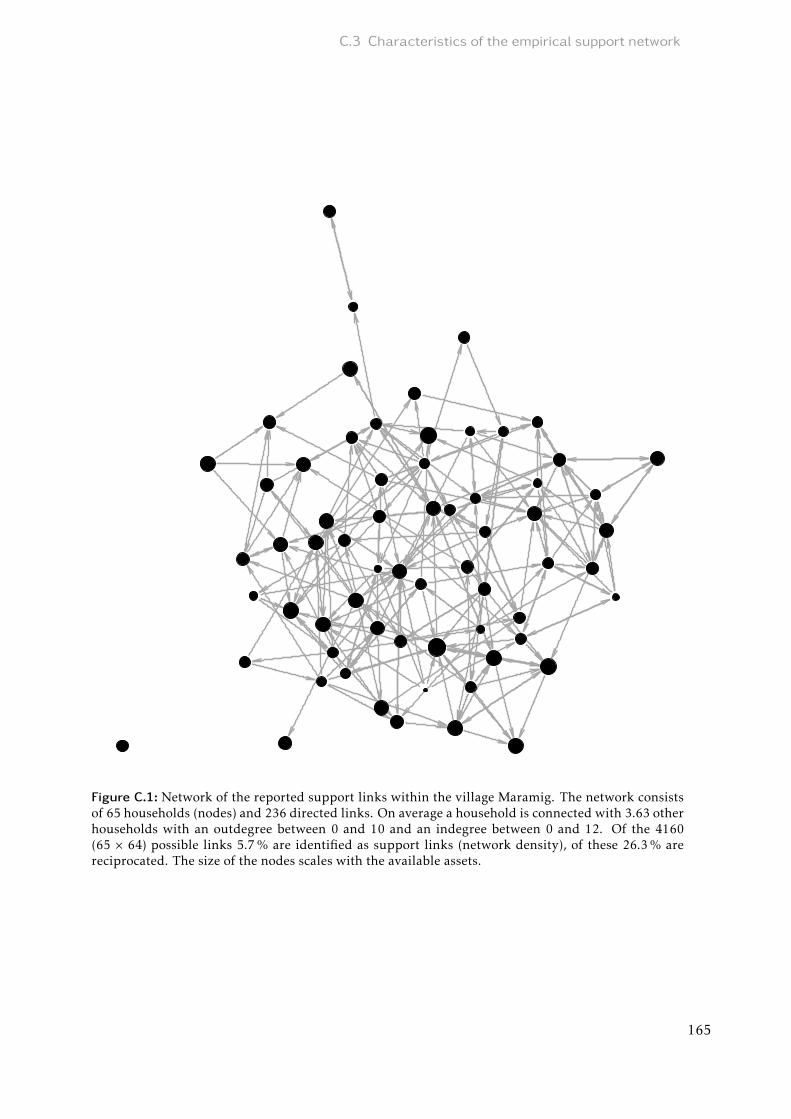
C.3 Characteristics of the empirical support network
Figure C.1: Network of the reported support links within the village Maramig. The network consistsof 65 households (nodes) and 236 directed links. On average a household is connected with 3.63 otherhouseholds with an outdegree between 0 and 10 and an indegree between 0 and 12. Of the 4160(65 × 64) possible links 5.7% are identified as support links (network density), of these 26.3% arereciprocated. The size of the nodes scales with the available assets.
165

C Appendix of Chapter 4
AAAAAAAAAAAAAAAAAAAAAAAAAAAAAAAAAAAAAAAAAAAAAAAAAAAAAAAAAAAAAAAAA BBBBBBBBBBBBBBBBBBBBBBBBBBBBBBBBBBBBBBBBBBBBBBBBBBBBBBBBBBBBBBBBB
Indegree Outdegree
0 1 2 3 4 5 6 7 8 9 10 11 12 0 1 2 3 4 5 6 7 8 9 10 11 12
0
5
10
15
Nu
mb
er
of
ho
use
ho
lds
Figure C.2: Distribution of the indegree (A) and outdegree (B) in the empirically observed network.
0.00
0.25
0.50
0.75
1.00
0.00 0.25 0.50 0.75 1.00
Asset index
Cu
mu
lative
pro
ba
bili
ty
Large sample Village Maramig
Figure C.3: Asset distribution in the village Maramig (grey) that is used in the simulations and in alarger sample (black) that was obtained in the same survey campaign. The larger sample comprisesa subset of 14 households in 22 villages covering around 15% of each village’s population (including14 randomly selected households of the village which was completely surveyed).
166

C.4 Additional results for selected parameter combination
C.4 Additional results for selected parameter combination
0.00
0.25
0.50
0.75
1.00
0 10 20 30 40 50
Time step
Fra
ctio
n o
f su
rviv
ing
un
insu
red
ho
use
ho
lds
Insurance propensity δ 0 0.5 No informal transfer
Figure C.4: Fraction of surviving uninsured households with enough financial resources to insure forthree different insurance propensities δ. The scenario without informal transfer is added as reference(yellow line). The shaded areas represent the 95% confidence interval. Results show the mean over1000 repetitions for a selected parameter combination of shock probability ps = 0.1 and shock inten-sity S = 0.6 and households connected on a random network that is newly created in every repetition.
167

C Appendix of Chapter 4
●●
●
●
●
●●●
●● ●
●●●●
●●●
●
●
●●●
●●
●●
●
●●
●●●●
●●●
● ●
●
●
●
●
●●
●
●
●
●
●
●
●
●
●
●
●
●
●
●
●
●
●
●
●
●
●
●
●
●
●
●
●
●
●
●
●
●
●
●
●
AAAAAAAAAAAAAAAAAAAAAAAAAAAAAAAAAAAAAAAAAAAAAAAAAAAAAAAAAAAAAAAAAAAAAAAAAAAAAAAA
● ●
●
●
●
●●
●●●
●
●●●
●●●●●
●
●●●●
●●
●
●●●
●●●
●●●● ●
●
●
●
●
●
●
●
●
●
●
●
●
●
●
●
●
●
●
●
●
●
●
●
●
●
●
●
●
●
●
●
●
●
●
●
● ●
●
●
●
●
●
BBBBBBBBBBBBBBBBBBBBBBBBBBBBBBBBBBBBBBBBBBBBBBBBBBBBBBBBBBBBBBBBBBBBBBBBBBBBBBBB
●
●
●
●
●
●● ●
●● ●
●●●
●●●●●●●●●●●●● ●●●●●●● ●●● ● ● ●
●
●
●●
●
●
●
●
●
●
●
●
●
●
● ●●●●● ● ●● ● ●● ● ● ●● ●● ● ● ●●● ● ● ●CCCCCCCCCCCCCCCCCCCCCCCCCCCCCCCCCCCCCCCCCCCCCCCCCCCCCCCCCCCCCCCCCCCCCCCCCCCCCCCC
Insurance propensity δ = 0 Insurance propensity δ = 0.5 Insurance propensity δ = 1
0.00 0.25 0.50 0.75 1.00 0.00 0.25 0.50 0.75 1.00 0.00 0.25 0.50 0.75 1.00
0.00
0.25
0.50
0.75
1.00
Income
Su
rviv
alp
rob
ab
ility
● ●Random networks Fixed random network
Figure C.5: Fraction of runs out of 1000 repetitions in which a household with a given income Ii sur-vives in random networks that are newly created in every simulation run (black) and a selected ran-dom network that is kept fixed for the 1000 repetitions where a household with a certain income hasalways the same position in the network (orange). For each simulation run, shocks occur in randomorder for individual households. As some households have the same income, not all dots representexactly one household. Results are shown for a selected parameter combination of shock probabilityps = 0.1 and shock intensity S = 0.6 (with resulting threshold below which households cannot affordinsurance at It = 0.3) and different insurance propensities δ.
●
●
●
●
●
●
●
●
●
●
●
●
●
●
●
●
●
●
●
●
●
●
●
●●
●
●
●
●
●
●●
●
●
●
●
●●
●
●
●
●
●
●
●
●
●
●
●●
●
●
●
●
●
● ●
●
●
●
●
● ●
●
●
●
●
●
●
●
●
●
●
●●
0.00
0.25
0.50
0.75
1.00
0.00 0.25 0.50 0.75 1.00
Simulated
Pre
dic
ted
Insurance propensity δ ● ● ●0 0.5 1
Figure C.6: Graphical representation of the goodness-of-fit between simulated and predicted survivalprobabilities obtained in the empirical network for the selected parameter combination of shock prob-ability ps = 0.1 and shock intensity S = 0.6.
168

C.4 Additional results for selected parameter combination
Table C.3: Unstandardised regression coefficients for the selected parameter combination of shockprobability ps = 0.1 and shock intensity S = 0.6 as in the main text. Standard errors in parentheses,clustered on household level.
Unstandardised
(Intercept) −2.78∗∗∗
(0.06)income 3.34∗∗∗
(0.20)donors’ disposable income 9.94∗∗∗
(0.23)outdegree 0.26∗∗∗
(0.01)indegree (unins. neighbors) −0.05∗∗∗
(0.01)ins. propensity δ = 0.5 0.18∗∗∗
(0.05)ins. propensity δ = 1 0.35∗∗∗
(0.06)income × ins. propensity δ = 0.5 −0.01
(0.15)donors’ disposable income × ins. propensity δ = 0.5 1.47∗∗∗
(0.23)outdegree × ins. propensity δ = 0.5 −0.04∗∗∗
(0.01)indegree (unins. neighbors) × ins. propensity δ = 0.5 −0.03∗∗
(0.01)income × ins. propensity δ = 1 −0.16
(0.18)donors’ disposable income × ins. propensity δ = 1 2.22∗∗∗
(0.28)outdegree × ins. propensity δ = 1 −0.08∗∗∗
(0.01)indegree (unins. neighbors) × ins. propensity δ = 1 −0.03∗
(0.01)
McFadden R2 0.18AIC 84576.73Log Likelihood −42273.37Num. obs. 75000∗∗∗p < 0.001; ∗∗p < 0.01; ∗p < 0.05
169

C Appendix of Chapter 4
Table C.4: Regression coefficients (unstandardised and standardised) for the selected parameter com-bination of shock probability ps = 0.1 and shock intensity S = 0.6 as in the main text with the dis-posable income of insured neighbours and uninsured neighbours considered separately for insurancepropensity δ = 0.5. Standardised coefficients are mean-centred and scaled by 1 standard deviation(Menard, 2011). Standardised estimates for interaction terms are derived by standardising the productof the predictors. Standard errors in parentheses, clustered on household level.
Unstandardised Standardised
(Intercept) −2.60∗∗∗ −0.26∗∗∗
(0.05) (0.01)income 3.33∗∗∗ 0.25∗∗∗
(0.19) (0.01)unins. donors’ disposable income 10.76∗∗∗ 0.58∗∗∗
(0.29) (0.02)ins. donors’ disposable income 12.07∗∗∗ 0.65∗∗∗
(0.32) (0.02)outdegree 0.23∗∗∗ 0.42∗∗∗
(0.01) (0.02)indegree (unins. neighbors) −0.08∗∗∗ −0.12∗∗∗
(0.01) (0.02)
McFadden R2 0.18 0.18AIC 28110.39 28110.39Log Likelihood −14049.20 −14049.20Num. obs. 25000 25000∗∗∗p < 0.001; ∗∗p < 0.01; ∗p < 0.05
170

C.5 Additional results for idiosyncratic shocks
C.5 Additional results for idiosyncratic shocks
Table C.5: Z-scores from a two-sample z-test for the change in mean fraction of surviving uninsuredhouseholds without enough financial resources to insure at the last simulated time step (t = 50) be-tween different combinations of shock probability and shock intensity (ps1, S1 and ps2, S2) in case ofidiosyncratic shocks.
ps1 S1 ps2 S2 zδ=0 zδ=0.5 zδ=1
0.1 0.5 0.1 0.6 23.03∗∗∗ 21.80∗∗∗ 21.13∗∗∗
0.1 0.5 0.1 0.7 48.51∗∗∗ 46.90∗∗∗ 47.32∗∗∗
0.1 0.6 0.2 0.3 1.55 1.09 0.310.1 0.6 0.3 0.2 7.72∗∗∗ 7.79∗∗∗ 7.65∗∗∗
0.2 0.3 0.3 0.2 6.36∗∗∗ 6.87∗∗∗ 7.54∗∗∗
∗∗∗p < 0.01; ∗∗p < 0.05; ∗p < 0.1
Table C.6: Z-scores from a two-sample z-test for the change in mean fraction of surviving uninsuredhouseholds without enough financial resources to insure at the last simulated time step (t = 50) be-tween different insurance propensities δ in case of idiosyncratic shocks.
ps S zδ=0→δ=0.5 zδ=0.5→δ=1 zδ=0→δ=1
0.1 0.5 3.07∗∗∗ 3.89∗∗∗ 6.88∗∗∗
0.1 0.6 6.53∗∗∗ 5.89∗∗∗ 12.24∗∗∗
0.2 0.3 6.33∗∗∗ 5.39∗∗∗ 11.60∗∗∗
0.3 0.2 6.54∗∗∗ 5.82∗∗∗ 12.32∗∗∗
0.1 0.7 7.88∗∗∗ 6.49∗∗∗ 14.59∗∗∗
∗∗∗p < 0.01; ∗∗p < 0.05; ∗p < 0.1
171

CAppendixofChapter4
Table C.7: Unstandardised regression coefficients for the model described in the main text for different scenarios of external conditions for idiosyncraticshocks denoted by the shock probability ps and shock intensity S (Scenario 1: ps = 0.1, S = 0.5; Scenario 2: ps = 0.1, S = 0.6; Scenario 3: ps = 0.2, S = 0.3;Scenario 4: ps = 0.3, S = 0.2; Scenario 5: ps = 0.1, S = 0.7). Standard errors in parentheses, clustered on household level.
Scenario 1 Scenario 2 Scenario 3 Scenario 4 Scenario 5
(Intercept) −2.34∗∗∗ −2.78∗∗∗ −3.43∗∗∗ −3.81∗∗∗ −3.29∗∗∗
(0.08) (0.06) (0.07) (0.07) (0.05)income 3.35∗∗∗ 3.34∗∗∗ 4.32∗∗∗ 5.06∗∗∗ 3.40∗∗∗
(0.27) (0.20) (0.19) (0.21) (0.15)donors’ disposable income 10.05∗∗∗ 9.94∗∗∗ 14.57∗∗∗ 17.43∗∗∗ 9.37∗∗∗
(0.38) (0.23) (0.28) (0.38) (0.24)outdegree 0.29∗∗∗ 0.26∗∗∗ 0.27∗∗∗ 0.30∗∗∗ 0.27∗∗∗
(0.02) (0.01) (0.01) (0.01) (0.01)indegree (unins. neighbors) −0.04∗∗∗ −0.05∗∗∗ −0.05∗∗∗ −0.04∗∗∗ −0.07∗∗∗
(0.01) (0.01) (0.01) (0.01) (0.01)ins. propensity δ = 0.5 0.22∗∗∗ 0.18∗∗∗ 0.06 0.03 0.16∗∗∗
(0.07) (0.05) (0.05) (0.06) (0.04)ins. propensity δ = 1 0.35∗∗∗ 0.35∗∗∗ 0.34∗∗∗ −0.04 0.27∗∗∗
(0.08) (0.06) (0.07) (0.07) (0.05)income × ins. propensity δ = 0.5 −0.29 −0.01 0.16 0.04 0.13
(0.22) (0.15) (0.18) (0.18) (0.14)donors’ disposable income × ins. propensity δ = 0.5 1.61∗∗∗ 1.47∗∗∗ 1.51∗∗∗ 2.36∗∗∗ 1.94∗∗∗
(0.29) (0.23) (0.24) (0.35) (0.22)outdegree × ins. propensity δ = 0.5 −0.09∗∗∗ −0.04∗∗∗ −0.02 −0.02 −0.05∗∗∗
(0.01) (0.01) (0.01) (0.01) (0.01)indegree (unins. neighbors) × ins. propensity δ = 0.5 −0.01 −0.03∗∗ −0.02 −0.01 −0.00
(0.01) (0.01) (0.01) (0.01) (0.01)income × ins. propensity δ = 1 −0.11 −0.16 −0.08 0.57∗ 0.16
(0.28) (0.18) (0.24) (0.25) (0.14)donors’ disposable income × ins. propensity δ = 1 2.66∗∗∗ 2.22∗∗∗ 2.05∗∗∗ 4.83∗∗∗ 3.74∗∗∗
(0.37) (0.28) (0.36) (0.43) (0.29)outdegree × ins. propensity δ = 1 −0.14∗∗∗ −0.08∗∗∗ −0.06∗∗∗ −0.03∗∗ −0.08∗∗∗
(0.01) (0.01) (0.01) (0.01) (0.01)indegree (unins. neighbors) × ins. propensity δ = 1 −0.02 −0.03∗ −0.05∗∗ −0.05∗∗ −0.03∗∗
(0.02) (0.01) (0.02) (0.02) (0.01)
McFadden R2 0.20 0.18 0.16 0.25 0.32AIC 53011.19 84576.73 76969.34 70927.46 93399.71Log Likelihood −26490.59 −42273.37 −38469.67 −35448.73 −46684.85Num. obs. 48000 75000 75000 75000 90000∗∗∗p < 0.001; ∗∗p < 0.01; ∗p < 0.05
172

C.5
Additio
nalresu
ltsforidiosyncratic
shocks
Table C.8: Standardised regression coefficients for the model described in the main text for different scenarios of external conditions for idiosyncraticshocks denoted by the shock probability ps and shock intensity S (Scenario 1: ps = 0.1, S = 0.5; Scenario 2: ps = 0.1, S = 0.6; Scenario 3: ps = 0.2, S = 0.3;Scenario 4: ps = 0.3, S = 0.2; Scenario 5: ps = 0.1, S = 0.7). Coefficients are mean-centred and scaled by 1 standard deviation (Menard, 2011). Standardisedestimates for interaction terms are derived by standardising the product of the predictors. Standard errors in parentheses, clustered on household level.
Scenario 1 Scenario 2 Scenario 3 Scenario 4 Scenario 5
(Intercept) 0.38∗∗∗ −0.27∗∗∗ −0.23∗∗∗ −0.00 −0.96∗∗∗
(0.02) (0.01) (0.01) (0.01) (0.01)income 0.23∗∗∗ 0.26∗∗∗ 0.33∗∗∗ 0.39∗∗∗ 0.29∗∗∗
(0.02) (0.02) (0.01) (0.02) (0.01)donors’ disposable income 0.88∗∗∗ 0.75∗∗∗ 1.10∗∗∗ 1.32∗∗∗ 0.60∗∗∗
(0.03) (0.02) (0.02) (0.03) (0.02)outdegree 0.54∗∗∗ 0.49∗∗∗ 0.50∗∗∗ 0.56∗∗∗ 0.50∗∗∗
(0.03) (0.02) (0.02) (0.02) (0.02)indegree (unins. neighbors) −0.08∗∗∗ −0.10∗∗∗ −0.08∗∗∗ −0.06∗∗∗ −0.12∗∗∗
(0.02) (0.01) (0.02) (0.02) (0.01)ins. propensity δ = 0.5 0.10∗∗∗ 0.09∗∗∗ 0.03 0.01 0.07∗∗∗
(0.03) (0.02) (0.02) (0.03) (0.02)ins. propensity δ = 1 0.16∗∗∗ 0.16∗∗∗ 0.16∗∗∗ −0.02 0.13∗∗∗
(0.04) (0.03) (0.04) (0.03) (0.02)income × ins. propensity δ = 0.5 −0.02 −0.00 0.02 0.00 0.01
(0.02) (0.01) (0.02) (0.02) (0.02)donors’ disposable income × ins. propensity δ = 0.5 0.12∗∗∗ 0.09∗∗∗ 0.09∗∗∗ 0.15∗∗∗ 0.10∗∗∗
(0.02) (0.01) (0.01) (0.02) (0.01)outdegree × ins. propensity δ = 0.5 −0.17∗∗∗ −0.07∗∗∗ −0.03 −0.04 −0.10∗∗∗
(0.02) (0.02) (0.02) (0.03) (0.02)indegree (unins. neighbors) × ins. propensity δ = 0.5 −0.01 −0.04∗∗ −0.02 −0.01 −0.01
(0.02) (0.01) (0.01) (0.02) (0.01)income × ins. propensity δ = 1 −0.01 −0.02 −0.01 0.06∗ 0.02
(0.02) (0.02) (0.02) (0.02) (0.02)donors’ disposable income × ins. propensity δ = 1 0.20∗∗∗ 0.14∗∗∗ 0.13∗∗∗ 0.30∗∗∗ 0.19∗∗∗
(0.03) (0.02) (0.02) (0.03) (0.01)outdegree × ins. propensity δ = 1 −0.29∗∗∗ −0.15∗∗∗ −0.12∗∗∗ −0.07∗∗ −0.17∗∗∗
(0.03) (0.02) (0.03) (0.02) (0.02)indegree (unins. neighbors) × ins. propensity δ = 1 −0.01 −0.03∗ −0.04∗∗ −0.05∗∗ −0.03∗∗
(0.01) (0.01) (0.01) (0.01) (0.01)
McFadden R2 0.20 0.18 0.16 0.25 0.32AIC 53011.19 84576.73 76969.34 70927.46 93399.71Log Likelihood −26490.59 −42273.37 −38469.67 −35448.73 −46684.85Num. obs. 48000 75000 75000 75000 90000∗∗∗p < 0.001; ∗∗p < 0.01; ∗p < 0.05173

CAppendixofChapter4
Table C.9: Unstandardised regression coefficients for the model described in the main text with the disposable income of insured neighbours and unin-sured neighbours considered separately for insurance propensity δ = 0.5 for different scenarios of external conditions for idiosyncratic shocks denoted bythe shock probability ps and shock intensity S (Scenario 1: ps = 0.1, S = 0.5; Scenario 2: ps = 0.1, S = 0.6; Scenario 3: ps = 0.2, S = 0.3; Scenario 4: ps = 0.3,S = 0.2; Scenario 5: ps = 0.1, S = 0.7). Standard errors in parentheses, clustered on household level.
Scenario 1 Scenario 2 Scenario 3 Scenario 4 Scenario 5
(Intercept) −2.11∗∗∗ −2.60∗∗∗ −3.36∗∗∗ −3.78∗∗∗ −3.13∗∗∗
(0.07) (0.05) (0.07) (0.07) (0.05)income 3.06∗∗∗ 3.33∗∗∗ 4.48∗∗∗ 5.10∗∗∗ 3.54∗∗∗
(0.27) (0.19) (0.18) (0.23) (0.19)unins. donors’ disposable income 10.96∗∗∗ 10.76∗∗∗ 15.43∗∗∗ 19.01∗∗∗ 10.36∗∗∗
(0.48) (0.29) (0.41) (0.48) (0.31)ins. donors’ disposable income 12.36∗∗∗ 12.07∗∗∗ 16.75∗∗∗ 20.60∗∗∗ 12.21∗∗∗
(0.43) (0.32) (0.34) (0.42) (0.31)outdegree 0.21∗∗∗ 0.23∗∗∗ 0.25∗∗∗ 0.28∗∗∗ 0.22∗∗∗
(0.02) (0.01) (0.01) (0.01) (0.01)indegree (unins. neighbors) −0.05∗∗∗ −0.08∗∗∗ −0.06∗∗∗ −0.04∗∗∗ −0.07∗∗∗
(0.01) (0.01) (0.01) (0.01) (0.01)
McFadden R2 0.20 0.18 0.16 0.26 0.31AIC 17690.50 28110.39 25452.82 23720.96 31358.59Log Likelihood −8839.25 −14049.20 −12720.41 −11854.48 −15673.30Num. obs. 16000 25000 25000 25000 30000∗∗∗p < 0.001; ∗∗p < 0.01; ∗p < 0.05
174
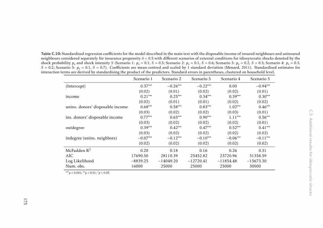
C.5
Additio
nalresu
ltsforidiosyncratic
shocks
Table C.10: Standardised regression coefficients for the model described in the main text with the disposable income of insured neighbours and uninsuredneighbours considered separately for insurance propensity δ = 0.5 with different scenarios of external conditions for idiosyncratic shocks denoted by theshock probability ps and shock intensity S (Scenario 1: ps = 0.1, S = 0.5; Scenario 2: ps = 0.1, S = 0.6; Scenario 3: ps = 0.2, S = 0.3; Scenario 4: ps = 0.3,S = 0.2; Scenario 5: ps = 0.1, S = 0.7). Coefficients are mean-centred and scaled by 1 standard deviation (Menard, 2011). Standardised estimates forinteraction terms are derived by standardising the product of the predictors. Standard errors in parentheses, clustered on household level.
Scenario 1 Scenario 2 Scenario 3 Scenario 4 Scenario 5
(Intercept) 0.37∗∗∗ −0.26∗∗∗ −0.22∗∗∗ 0.00 −0.94∗∗∗
(0.02) (0.01) (0.02) (0.02) (0.01)income 0.21∗∗∗ 0.25∗∗∗ 0.34∗∗∗ 0.39∗∗∗ 0.30∗∗∗
(0.02) (0.01) (0.01) (0.02) (0.02)unins. donors’ disposable income 0.68∗∗∗ 0.58∗∗∗ 0.83∗∗∗ 1.02∗∗∗ 0.46∗∗∗
(0.03) (0.02) (0.02) (0.03) (0.01)ins. donors’ disposable income 0.77∗∗∗ 0.65∗∗∗ 0.90∗∗∗ 1.11∗∗∗ 0.56∗∗∗
(0.03) (0.02) (0.02) (0.02) (0.01)outdegree 0.39∗∗∗ 0.42∗∗∗ 0.47∗∗∗ 0.52∗∗∗ 0.41∗∗∗
(0.03) (0.02) (0.02) (0.02) (0.02)indegree (unins. neighbors) −0.07∗∗∗ −0.12∗∗∗ −0.10∗∗∗ −0.06∗∗∗ −0.11∗∗∗
(0.02) (0.02) (0.02) (0.02) (0.02)
McFadden R2 0.20 0.18 0.16 0.26 0.31AIC 17690.50 28110.39 25452.82 23720.96 31358.59Log Likelihood −8839.25 −14049.20 −12720.41 −11854.48 −15673.30Num. obs. 16000 25000 25000 25000 30000∗∗∗p < 0.001; ∗∗p < 0.01; ∗p < 0.05
175

CAppendixofChapter4
Table C.11: Goodness-of-fit statistics (R2, RMSE and bias) for the estimation of the survival probabilities of households without enough financial resourcesto insure for different insurance propensities δ and predictors in the regression model. In addition to the dummy variables for insurance propensity, thefollowing predictors are included: (#4) donors’ disposable income, own income, outdegree, indegree from uninsured neighbours; (#2a) own income,outdegree; (#2b) own income, outdegree to wealthy households; (#1) own income. Subsections show different external conditions for idiosyncratic shocksdenoted by the shock probability ps and shock intensity S (Scenario 1: ps = 0.1, S = 0.5; Scenario 2: ps = 0.1, S = 0.6; Scenario 3: ps = 0.2, S = 0.3; Scenario4: ps = 0.3, S = 0.2; Scenario 5: ps = 0.1, S = 0.7).
δ = 0 δ = 0.5 δ = 1
# R2 RMSE Bias R2 RMSE Bias R2 RMSE Bias
Scenario 1
4 0.743 0.134 0.072 0.827 0.098 0.042 0.891 0.078 0.0292a 0.635 0.140 0.047 0.625 0.120 0.020 0.486 0.132 0.0132b 0.598 0.142 0.025 0.593 0.124 −0.001 0.451 0.138 −0.0081 0.075 0.238 −0.109 0.058 0.225 −0.126 0.024 0.216 −0.123
Scenario 2
4 0.806 0.150 0.098 0.878 0.113 0.070 0.906 0.089 0.0452a 0.515 0.191 0.068 0.514 0.180 0.048 0.465 0.175 0.0322b 0.673 0.149 0.021 0.643 0.150 −0.001 0.561 0.159 −0.0151 0.018 0.259 −0.050 0.016 0.257 −0.070 0.010 0.247 −0.081
Scenario 3
4 0.767 0.196 0.129 0.841 0.145 0.085 0.900 0.099 0.0442a 0.441 0.248 0.102 0.443 0.228 0.065 0.417 0.215 0.0352b 0.624 0.192 0.046 0.609 0.185 0.005 0.564 0.185 −0.0231 0.020 0.301 −0.032 0.017 0.299 −0.071 0.010 0.291 −0.095
Scenario 4
4 0.718 0.233 0.156 0.801 0.172 0.100 0.872 0.121 0.0512a 0.369 0.291 0.133 0.400 0.257 0.083 0.398 0.241 0.0442b 0.563 0.227 0.067 0.579 0.204 0.014 0.549 0.207 −0.0261 0.016 0.323 −0.013 0.013 0.317 −0.065 0.014 0.319 −0.104
Scenario 5
4 0.848 0.128 0.086 0.923 0.104 0.076 0.936 0.092 0.0622a 0.510 0.164 0.041 0.511 0.169 0.031 0.458 0.185 0.0272b 0.701 0.130 0.037 0.660 0.141 0.026 0.578 0.163 0.0201 0.007 0.229 −0.019 0.014 0.238 −0.030 0.017 0.250 −0.035
176

C.6 Additional results for covariate shocks
C.6 Additional results for covariate shocks
Table C.12: Z-scores from a two-sample z-test for the change in mean fraction of surviving uninsuredhouseholds without enough financial resources to insure between idiosyncratic and covariate shocksfor the three insurance propensities δ at the last simulated time step (t = 50).
ps S zδ=0 zδ=0.5 zδ=1
0.1 0.5 14.55∗∗∗ 10.57∗∗∗ 5.03∗∗∗
0.1 0.6 10.33∗∗∗ 9.50∗∗∗ 6.67∗∗∗
0.2 0.3 16.21∗∗∗ 13.51∗∗∗ 8.84∗∗∗
0.3 0.2 19.72∗∗∗ 16.33∗∗∗ 10.48∗∗∗
0.1 0.7 5.11∗∗∗ 6.01∗∗∗ 5.55∗∗∗
∗∗∗p < 0.01; ∗∗p < 0.05; ∗p < 0.1
Table C.13: Z-scores from a two-sample z-test for the change in mean fraction of surviving uninsuredhouseholds without enough financial resources to insure at the last simulated time step (t = 50) be-tween different combinations of shock probability and shock intensity (ps1, S1 and ps2, S2) in case ofcovariate shocks.
ps1 S1 ps2 S2 zδ=0 zδ=0.5 zδ=1
0.1 0.5 0.1 0.6 4.60∗∗∗ 6.65∗∗∗ 9.17∗∗∗
0.1 0.5 0.1 0.7 8.99∗∗∗ 12.78∗∗∗ 17.91∗∗∗
0.1 0.6 0.2 0.3 2.69∗∗∗ 1.62 0.790.1 0.6 0.3 0.2 2.24∗∗ 0.45 1.500.2 0.3 0.3 0.2 0.55 1.31 2.52∗∗
∗∗∗p < 0.01; ∗∗p < 0.05; ∗p < 0.1
Table C.14: Z-scores from a two-sample z-test for the change in mean fraction of surviving unin-sured households without enough financial resources to insure at the last simulated time step (t = 50)between different insurance propensities δ in case of covariate shocks.
ps S zδ=0→δ=0.5 zδ=0.5→δ=1 zδ=0→δ=1
0.1 0.5 4.81∗∗∗ 6.25∗∗∗ 11.02∗∗∗
0.1 0.6 3.32∗∗∗ 4.56∗∗∗ 7.87∗∗∗
0.2 0.3 5.04∗∗∗ 6.17∗∗∗ 11.21∗∗∗
0.3 0.2 6.12∗∗∗ 7.89∗∗∗ 13.98∗∗∗
0.1 0.7 2.16∗∗ 2.81∗∗∗ 4.97∗∗∗
∗∗∗p < 0.01; ∗∗p < 0.05; ∗p < 0.1
177

CAppendixofChapter4
Table C.15: Unstandardised regression coefficients for the model described in the main text for different scenarios of external conditions for covariateshocks denoted by the shock probability ps and shock intensity S (Scenario 1: ps = 0.1, S = 0.5; Scenario 2: ps = 0.1, S = 0.6; Scenario 3: ps = 0.2, S = 0.3;Scenario 4: ps = 0.3, S = 0.2; Scenario 5: ps = 0.1, S = 0.7). Standard errors in parentheses, clustered on household level.
Scenario 1 Scenario 2 Scenario 3 Scenario 4 Scenario 5
(Intercept) −1.66∗∗∗ −1.97∗∗∗ −2.47∗∗∗ −2.69∗∗∗ −2.31∗∗∗
(0.06) (0.06) (0.06) (0.06) (0.05)income 1.99∗∗∗ 1.94∗∗∗ 2.47∗∗∗ 2.62∗∗∗ 2.08∗∗∗
(0.26) (0.20) (0.20) (0.21) (0.18)donors’ disposable income 5.17∗∗∗ 5.01∗∗∗ 7.15∗∗∗ 8.70∗∗∗ 5.50∗∗∗
(0.27) (0.23) (0.19) (0.27) (0.25)outdegree 0.04∗∗∗ 0.05∗∗∗ 0.03∗∗∗ 0.04∗∗∗ 0.05∗∗∗
(0.01) (0.01) (0.01) (0.01) (0.01)indegree (unins. neighbors) −0.00 −0.00 −0.00 0.01 −0.01
(0.01) (0.01) (0.01) (0.01) (0.01)ins. propensity δ = 0.5 −0.03 −0.08∗ −0.08 −0.10∗ −0.13∗∗∗
(0.04) (0.04) (0.05) (0.05) (0.03)ins. propensity δ = 1 −0.17∗∗ −0.25∗∗∗ −0.17∗∗ −0.35∗∗∗ −0.29∗∗∗
(0.06) (0.05) (0.06) (0.07) (0.04)income × ins. propensity δ = 0.5 0.38∗ 0.25∗ 0.33∗ 0.58∗∗∗ 0.40∗∗∗
(0.16) (0.12) (0.14) (0.16) (0.09)donors’ disposable income × ins. propensity δ = 0.5 2.10∗∗∗ 2.33∗∗∗ 2.70∗∗∗ 3.05∗∗∗ 2.36∗∗∗
(0.20) (0.15) (0.18) (0.20) (0.16)outdegree × ins. propensity δ = 0.5 0.02∗ 0.01 0.02∗∗ 0.02∗∗ −0.00
(0.01) (0.01) (0.01) (0.01) (0.01)indegree (unins. neighbors) × ins. propensity δ = 0.5 −0.00 0.00 −0.00 −0.00 0.01
(0.01) (0.01) (0.01) (0.01) (0.01)income × ins. propensity δ = 1 1.07∗∗∗ 0.81∗∗∗ 0.71∗∗∗ 1.42∗∗∗ 0.90∗∗∗
(0.22) (0.14) (0.19) (0.20) (0.14)donors’ disposable income × ins. propensity δ = 1 5.99∗∗∗ 5.34∗∗∗ 6.64∗∗∗ 8.35∗∗∗ 5.41∗∗∗
(0.31) (0.21) (0.25) (0.29) (0.19)outdegree × ins. propensity δ = 1 0.02 0.02∗∗ 0.03∗∗∗ 0.04∗∗∗ −0.00
(0.01) (0.01) (0.01) (0.01) (0.01)indegree (unins. neighbors) × ins. propensity δ = 1 −0.01 0.01 −0.01 −0.02 0.00
(0.02) (0.01) (0.01) (0.01) (0.01)
McFadden R2 0.10 0.08 0.07 0.13 0.17AIC 58982.64 88246.51 81579.75 79350.32 94863.56Log Likelihood −29476.32 −44108.26 −40774.87 −39660.16 −47416.78Num. obs. 48000 75000 75000 75000 90000∗∗∗p < 0.001; ∗∗p < 0.01; ∗p < 0.05
178

C.6
Additio
nalresu
ltsforcova
riate
shocks
Table C.16: Standardised regression coefficients for the model described in the main text for different scenarios of external conditions for covariate shocksdenoted by the shock probability ps and shock intensity S (Scenario 1: ps = 0.1, S = 0.5; Scenario 2: ps = 0.1, S = 0.6; Scenario 3: ps = 0.2, S = 0.3; Scenario4: ps = 0.3, S = 0.2; Scenario 5: ps = 0.1, S = 0.7). Coefficients are mean-centred and scaled by 1 standard deviation (Menard, 2011). Standardised estimatesfor interaction terms are derived by standardising the product of the predictors. Standard errors in parentheses, clustered on household level.
Scenario 1 Scenario 2 Scenario 3 Scenario 4 Scenario 5
(Intercept) −0.23∗∗∗ −0.71∗∗∗ −0.86∗∗∗ −0.79∗∗∗ −1.16∗∗∗
(0.01) (0.01) (0.01) (0.01) (0.01)income 0.14∗∗∗ 0.15∗∗∗ 0.19∗∗∗ 0.20∗∗∗ 0.18∗∗∗
(0.02) (0.02) (0.02) (0.02) (0.02)donors’ disposable income 0.45∗∗∗ 0.38∗∗∗ 0.54∗∗∗ 0.66∗∗∗ 0.35∗∗∗
(0.02) (0.02) (0.01) (0.02) (0.02)outdegree 0.08∗∗∗ 0.09∗∗∗ 0.06∗∗∗ 0.07∗∗∗ 0.09∗∗∗
(0.02) (0.02) (0.02) (0.02) (0.02)indegree (unins. neighbors) −0.01 −0.01 −0.01 0.02 −0.02
(0.02) (0.01) (0.02) (0.02) (0.01)ins. propensity δ = 0.5 −0.01 −0.04∗ −0.04 −0.05∗ −0.06∗∗∗
(0.02) (0.02) (0.02) (0.02) (0.02)ins. propensity δ = 1 −0.08∗∗ −0.12∗∗∗ −0.08∗∗ −0.16∗∗∗ −0.14∗∗∗
(0.03) (0.02) (0.03) (0.03) (0.02)income × ins. propensity δ = 0.5 0.03∗ 0.03∗ 0.03∗ 0.06∗∗∗ 0.04∗∗∗
(0.01) (0.01) (0.01) (0.02) (0.01)donors’ disposable income × ins. propensity δ = 0.5 0.16∗∗∗ 0.15∗∗∗ 0.17∗∗∗ 0.19∗∗∗ 0.12∗∗∗
(0.01) (0.01) (0.01) (0.01) (0.01)outdegree × ins. propensity δ = 0.5 0.04∗ 0.01 0.05∗∗ 0.04∗∗ −0.00
(0.02) (0.01) (0.02) (0.01) (0.01)indegree (unins. neighbors) × ins. propensity δ = 0.5 −0.01 0.00 −0.00 −0.00 0.01
(0.01) (0.01) (0.01) (0.01) (0.01)income × ins. propensity δ = 1 0.09∗∗∗ 0.08∗∗∗ 0.07∗∗∗ 0.14∗∗∗ 0.10∗∗∗
(0.02) (0.01) (0.02) (0.02) (0.02)donors’ disposable income × ins. propensity δ = 1 0.45∗∗∗ 0.33∗∗∗ 0.42∗∗∗ 0.52∗∗∗ 0.27∗∗∗
(0.02) (0.01) (0.02) (0.02) (0.01)outdegree × ins. propensity δ = 1 0.05 0.04∗∗ 0.06∗∗∗ 0.09∗∗∗ −0.01
(0.02) (0.02) (0.02) (0.02) (0.01)indegree (unins. neighbors) × ins. propensity δ = 1 −0.01 0.01 −0.01 −0.01 0.00
(0.01) (0.01) (0.01) (0.01) (0.01)
McFadden R2 0.10 0.08 0.07 0.13 0.17AIC 58982.64 88246.51 81579.75 79350.32 94863.56Log Likelihood −29476.32 −44108.26 −40774.87 −39660.16 −47416.78Num. obs. 48000 75000 75000 75000 90000∗∗∗p < 0.001; ∗∗p < 0.01; ∗p < 0.05179

CAppendixofChapter4
Table C.17: Unstandardised regression coefficients for the model described in the main text with the disposable income of insured neighbours anduninsured neighbours considered separately for insurance propensity δ = 0.5 for different scenarios of external conditions for covariate shocks denoted bythe shock probability ps and shock intensity S (Scenario 1: ps = 0.1, S = 0.5; Scenario 2: ps = 0.1, S = 0.6; Scenario 3: ps = 0.2, S = 0.3; Scenario 4: ps = 0.3,S = 0.2; Scenario 5: ps = 0.1, S = 0.7). Standard errors in parentheses, clustered on household level.
Scenario 1 Scenario 2 Scenario 3 Scenario 4 Scenario 5
(Intercept) −1.70∗∗∗ −2.06∗∗∗ −2.56∗∗∗ −2.80∗∗∗ −2.46∗∗∗
(0.06) (0.05) (0.06) (0.05) (0.05)income 2.40∗∗∗ 2.21∗∗∗ 2.84∗∗∗ 3.23∗∗∗ 2.51∗∗∗
(0.27) (0.20) (0.20) (0.23) (0.17)unins. donors’ disposable income 5.03∗∗∗ 5.18∗∗∗ 7.32∗∗∗ 9.31∗∗∗ 5.86∗∗∗
(0.29) (0.30) (0.28) (0.36) (0.34)ins. donors’ disposable income 9.69∗∗∗ 9.53∗∗∗ 12.50∗∗∗ 14.36∗∗∗ 9.91∗∗∗
(0.38) (0.28) (0.34) (0.33) (0.30)outdegree 0.06∗∗∗ 0.06∗∗∗ 0.06∗∗∗ 0.06∗∗∗ 0.05∗∗∗
(0.01) (0.01) (0.01) (0.01) (0.01)indegree (unins. neighbors) −0.01 −0.00 −0.01 0.01 −0.00
(0.01) (0.01) (0.01) (0.01) (0.01)
McFadden R2 0.09 0.07 0.06 0.12 0.15AIC 19978.99 29568.24 27486.47 27025.10 31682.68Log Likelihood −9983.50 −14778.12 −13737.24 −13506.55 −15835.34Num. obs. 16000 25000 25000 25000 30000∗∗∗p < 0.001; ∗∗p < 0.01; ∗p < 0.05
180

C.6
Additio
nalresu
ltsforcova
riate
shocks
Table C.18: Standardised regression coefficients for the model described in the main text with the disposable income of insured neighbours and uninsuredneighbours considered separately for insurance propensity δ = 0.5 with different scenarios of external conditions for covariate shocks denoted by the shockprobability ps and shock intensity S (Scenario 1: ps = 0.1, S = 0.5; Scenario 2: ps = 0.1, S = 0.6; Scenario 3: ps = 0.2, S = 0.3; Scenario 4: ps = 0.3, S = 0.2;Scenario 5: ps = 0.1, S = 0.7). Coefficients are mean-centred and scaled by 1 standard deviation (Menard, 2011). Standardised estimates for interactionterms are derived by standardising the product of the predictors. Standard errors in parentheses, clustered on household level.
Scenario 1 Scenario 2 Scenario 3 Scenario 4 Scenario 5
(Intercept) −0.27∗∗∗ −0.74∗∗∗ −0.88∗∗∗ −0.82∗∗∗ −1.17∗∗∗
(0.01) (0.01) (0.01) (0.01) (0.01)income 0.17∗∗∗ 0.17∗∗∗ 0.22∗∗∗ 0.25∗∗∗ 0.21∗∗∗
(0.02) (0.01) (0.02) (0.02) (0.01)unins. donors’ disposable income 0.31∗∗∗ 0.28∗∗∗ 0.39∗∗∗ 0.50∗∗∗ 0.27∗∗∗
(0.02) (0.02) (0.01) (0.02) (0.02)ins. donors’ disposable income 0.61∗∗∗ 0.51∗∗∗ 0.68∗∗∗ 0.78∗∗∗ 0.45∗∗∗
(0.02) (0.02) (0.02) (0.02) (0.01)outdegree 0.11∗∗∗ 0.10∗∗∗ 0.11∗∗∗ 0.11∗∗∗ 0.09∗∗∗
(0.02) (0.02) (0.02) (0.02) (0.01)indegree (unins. neighbors) −0.01 −0.00 −0.01 0.01 −0.01
(0.02) (0.01) (0.02) (0.02) (0.02)
McFadden R2 0.09 0.07 0.06 0.12 0.15AIC 19978.99 29568.24 27486.47 27025.10 31682.68Log Likelihood −9983.50 −14778.12 −13737.24 −13506.55 −15835.34Num. obs. 16000 25000 25000 25000 30000∗∗∗p < 0.001; ∗∗p < 0.01; ∗p < 0.05
181

CAppendixofChapter4
Table C.19: Goodness-of-fit statistics (R2, RMSE and bias) for the estimation of the survival probabilities of households without enough financial resourcesto insure for different insurance propensities δ and predictors in the regression model. In addition to the dummy variables for insurance propensity, thefollowing predictors are included: (#4) donors’ disposable income, own income, outdegree, indegree from uninsured neighbours; (#2a) own income,outdegree; (#2b) own income, outdegree to wealthy households; (#1) own income. Subsections show different external conditions for covariate shocksdenoted by the shock probability ps and shock intensity S (Scenario 1: ps = 0.1, S = 0.5; Scenario 2: ps = 0.1, S = 0.6; Scenario 3: ps = 0.2, S = 0.3; Scenario4: ps = 0.3, S = 0.2; Scenario 5: ps = 0.1, S = 0.7).
δ = 0 δ = 0.5 δ = 1
# R2 RMSE Bias R2 RMSE Bias R2 RMSE Bias
Scenario 1
4 0.785 0.087 0.050 0.837 0.097 0.058 0.877 0.102 0.0652a 0.234 0.107 0.030 0.313 0.131 0.035 0.327 0.155 0.0432b 0.311 0.110 0.029 0.430 0.124 0.031 0.449 0.141 0.0351 0.097 0.105 −0.035 0.098 0.147 −0.054 0.078 0.182 −0.071
Scenario 2
4 0.820 0.085 0.051 0.848 0.102 0.064 0.859 0.115 0.0762a 0.332 0.091 0.025 0.314 0.131 0.034 0.328 0.174 0.0462b 0.540 0.078 0.016 0.536 0.109 0.019 0.529 0.145 0.0221 0.028 0.105 −0.017 0.029 0.149 −0.027 0.030 0.203 −0.036
Scenario 3
4 0.789 0.101 0.049 0.838 0.116 0.066 0.857 0.124 0.0742a 0.258 0.121 0.016 0.304 0.163 0.033 0.309 0.212 0.0462b 0.470 0.105 0.007 0.527 0.137 0.016 0.524 0.175 0.0181 0.023 0.139 −0.032 0.026 0.191 −0.039 0.023 0.249 −0.049
Scenario 4
4 0.802 0.112 0.060 0.844 0.128 0.081 0.847 0.145 0.0912a 0.227 0.155 0.025 0.292 0.194 0.047 0.289 0.250 0.0672b 0.446 0.132 0.014 0.509 0.162 0.027 0.498 0.206 0.0291 0.019 0.173 −0.032 0.028 0.220 −0.035 0.026 0.283 −0.043
Scenario 5
4 0.802 0.076 0.039 0.870 0.089 0.052 0.886 0.105 0.0672a 0.330 0.073 0.011 0.301 0.110 0.016 0.289 0.153 0.0242b 0.599 0.060 0.015 0.630 0.083 0.022 0.599 0.117 0.0301 0.014 0.088 −0.008 0.017 0.130 −0.011 0.022 0.177 −0.013
182
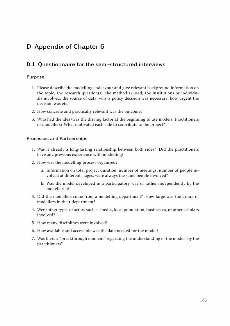
D Appendix of Chapter 6
D.1 Questionnaire for the semi-structured interviews
Purpose
1. Please describe the modelling endeavour and give relevant background information onthe topic, the research question(s), the method(s) used, the institutions or individu-als involved, the source of data, why a policy decision was necessary, how urgent thedecision was etc.
2. How concrete and practically relevant was the outcome?
3. Who had the idea/was the driving factor at the beginning to use models: Practitionersor modellers? What motivated each side to contribute to the project?
Processes and Partnerships
1. Was it already a long-lasting relationship between both sides? Did the practitionershave any previous experience with modelling?
2. How was the modelling process organised?
a. Information on total project duration, number of meetings, number of people in-volved at different stages, were always the same people involved?
b. Was the model developed in a participatory way or rather independently by themodeller(s)?
3. Did the modellers come from a modelling department? How large was the group ofmodellers in their department?
4. Were other types of actors such as media, local population, businesses, or other scholarsinvolved?
5. How many disciplines were involved?
6. How available and accessible was the data needed for the model?
7. Was there a “breakthrough moment” regarding the understanding of the models by thepractitioners?
183

D Appendix of Chapter 6
Products
1. What was your “recipe” that the practitioners got confidence in the model/the mod-ellers? Did they understand the (main) functioning of the model or did they blindlytrust the modellers, since the model was too complex and it was okay for them to havea black box?
2. Did you have the impression that the model was used to support the pre-set opinion/target of the practitioners involved? Or in contrary: Was the opinion of the practitionerschanged?
3. Where did you encounter difficulties during the course of the project?
4. (How) was the model usable for practitioners?
General final questions
1. What were the reasons that other modelling endeavours have failed to have an impact?
2. What were the most important factors for success in your endeavour?
3. Open question at the end: Is there anything you would like to add?
184

Bibliography
A2ii (2020). A2ii Factsheet. Access to Insurance Initiative.Abay, K. A., Kahsay, G. A., & Berhane, G. (2018). Social Networks and Factor Markets: PanelData Evidence from Ethiopia. The Journal of Development Studies 54(1), 174–190.
Adams, R. H. & Page, J. (2005). Do international migration and remittances reduce povertyin developing countries? World Development 33(10), 1645–1669.
Addison, P. F. E., Rumpff, L., Bau, S. S., Carey, J. M., Chee, Y. E., Jarrad, F. C., McBride, M. F.,& Burgman, M. A. (2013). Practical solutions for making models indispensable in conser-vation decision-making. Diversity and Distributions 19(5-6), 490–502.
Ahmed, S., Hoque, M. E., Sarker, A. R., Sultana, M., Islam, Z., Gazi, R., & Khan, J. A. M. (2016).Willingness-to-Pay for Community-Based Health Insurance among Informal Workers inUrban Bangladesh. PLOS ONE 11(2), e0148211.
Aktipis, A., Cronk, L., & de Aguiar, R. (2011). Risk-Pooling and Herd Survival: An Agent-Based Model of a Maasai Gift-Giving System. Human Ecology 39(2), 131–140.
Aktipis, A., de Aguiar, R., Flaherty, A., Iyer, P., Sonkoi, D., & Cronk, L. (2016). Cooperationin an Uncertain World: For the Maasai of East Africa, Need-Based Transfers OutperformAccount-Keeping in Volatile Environments. Human Ecology 44(3), 353–364.
Albert, R. & Barabási, A.-L. (2002). Statistical mechanics of complex networks. Reviews ofModern Physics 74(1), 47–97.
Alderman, H. & Haque, T. (2007). Insurance Against Covariate Shocks. Washington, DC.Allen, C., Metternicht, G., & Wiedmann, T. (2016). National pathways to the Sustainable De-velopment Goals (SDGs): A comparative review of scenario modelling tools. EnvironmentalScience & Policy 66, 199–207.
Allender, S., Foster, C., Hutchinson, L., & Arambepola, C. (2008). Quantification of Urbaniza-tion in Relation to Chronic Diseases in Developing Countries: A Systematic Review. Journalof Urban Health 85(6), 938–951.
Amblard, F., Bouadjio-Boulic, A., Sureda Gutiérrez, C., & Gaudou, B. (2015). Which modelsare used in social simulation to generate social networks? A review of 17 years of publica-tions in JASSS. Winter Simulation Conference Proceedings, pp. 4021–4032.
Amini, M., Wakolbinger, T., Racer, M., & Nejad, M. G. (2012). Alternative supply chainproduction–sales policies for new product diffusion: An agent-based modeling and sim-ulation approach. European Journal of Operational Research 216(2), 301–311.
An, L. (2012). Modeling human decisions in coupled human and natural systems: Review ofagent-based models. Ecological Modelling 229, 25–36.
Anderberg, D. & Morsink, K. (2020). The introduction of formal insurance and its effect onredistribution. Journal of Economic Behavior & Organization 179, 22–45.
Andre, F. E., Booy, R., Bock, H. L., Clemens, J., Datta, S. K., John, T. J., Lee, B. W., Lolekha, S.,Peltola, H., Ruff, T. A., Santosham, M., & Schmitt, H. J. (2008). Vaccination greatly reducesdisease, disability, death and inequity worldwide. Bulletin of the World Health Organization86(2), 140–146.
Araújo, T. & Banisch, S. (2016). Multidimensional Analysis of Linguistic Networks. In A.Mehler, A. Lücking, S. Banisch, P. Blanchard, & B. Job (Eds.), Towards a Theoretical Frame-work for Analyzing Complex Linguistic Networks. Berlin, Heidelberg: Springer Berlin Heidel-berg, pp. 107–131.
185

Bibliography
Aredo, D. (2010). The IDDIR: An Informal Insurance Arrangement in Ethiopia. Savings andDevelopment 34(1), 53–72.
Arneth, A., Brown, C., & Rounsevell, M. D. A. (2014). Global models of human decision-making for land-based mitigation and adaptation assessment. Nature Climate Change 4(7),550–557.
Arumugam, P., Chemura, A., Schauberger, B., & Gornott, C. (2020). Near Real-Time Biophys-ical Rice (Oryza sativa L.) Yield Estimation to Support Crop Insurance Implementation inIndia. Agronomy 10(11), 1674.
Asseng, S., Ewert, F., Rosenzweig, C., Jones, J. W., Hatfield, J. L., Ruane, A. C., Boote, K. J.,Thorburn, P. J., Rötter, R. P., Cammarano, D., Brisson, N., Basso, B., Martre, P., Aggarwal,P. K., Angulo, C., Bertuzzi, P., Biernath, C., Challinor, A. J., Doltra, J., Gayler, S., Goldberg,R., Grant, R., Heng, L., Hooker, J., Hunt, L. A., Ingwersen, J., Izaurralde, R. C., Kersebaum,K. C., Müller, C., Naresh Kumar, S., Nendel, C., O’Leary, G., Olesen, J. E., Osborne, T. M.,Palosuo, T., Priesack, E., Ripoche, D., Semenov, M. A., Shcherbak, I., Steduto, P., Stöckle, C.,Stratonovitch, P., Streck, T., Supit, I., Tao, F., Travasso, M., Waha, K., Wallach, D., White,J. W., Williams, J. R., & Wolf, J. (2013). Uncertainty in simulating wheat yields under cli-mate change. Nature Climate Change 3(9), 827–832.
Attanasio, O. & Ríos-Rull, J.-V. (2000). Consumption smoothing in island economies: Canpublic insurance reduce welfare? European Economic Review 44(7), 1225–1258.
Axelrod, R. & Hamilton, W. D. (1981). The evolution of cooperation. Science 211(4489), 1390–1396.
Baggio, J. A. &Hillis, V. (2018). Managing ecological disturbances: Learning and the structureof social-ecological networks. Environmental Modelling & Software 109, 32–40.
Banerjee, A., Chandrasekhar, A. G., Duflo, E., & Jackson, M. O. (2013). The Diffusion of Mi-crofinance. Science 341(6144).
Banerjee, A. V. & Duflo, E. (2007). The Economic Lives of the Poor. Journal of Economic Per-spectives 21(1), 141–168.
Barbero Vignola, G., Acs, S., Borchardt, S., Sala, S., Giuntoli, J., Smits, P., & Marelli, L. (2020).Modelling for Sustainable Development Goals (SDGs): Overview of JRC models. Publica-tion Office of the European Union EU Science Hub - European Commission. Luxembourg.
Barnett, B. J. & Mahul, O. (2007). Weather Index Insurance for Agriculture and Rural Areasin Lower-Income Countries. American Journal of Agricultural Economics 89(5), 1241–1247.
Barr, A., Dekker, M., & Fafchamps, M. (2012). Who Shares Risk with Whom under DifferentEnforcement Mechanisms? Economic Development and Cultural Change 60(4), 677–706.
Barreteau, O., Bots, P., Daniell, K., Etienne, M., Perez, P., Barnaud, C., Bazile, D., Becu, N.,Castella, J.-C., Daré, W., & Trebuil, G. (2017). Participatory Approaches. In B. Edmonds &R. Meyer (Eds.), Simulating Social Complexity: A Handbook. Cham: Springer InternationalPublishing, pp. 253–292.
Barrett, C. B. (2011). Covariate Catastrophic Risk Management in the Developing World:Discussion. American Journal of Agricultural Economics 93(2), 512–513.
Barrett, C. B. & Santos, P. (2014). The impact of changing rainfall variability on resource-dependent wealth dynamics. Ecological Economics 105, 48–54.
Barrett, C. B., Smith, K., & Box, P. W. (2001). Not Necessarily In The Same Boat: Heteroge-neous Risk Assessment Among East African Pastoralists. The Journal of Development Studies37(5), 1–30.
Baumgärtner, S., Becker, C., Frank, K., Müller, B., & Quaas, M. (2008). Relating the philoso-phy and practice of ecological economics: The role of concepts, models, and case studies ininter- and transdisciplinary sustainability research. Ecological Economics 67(3), 384–393.
186

Bibliography
Becher, M. A., Grimm, V., Thorbek, P., Horn, J., Kennedy, P. J., & Osborne, J. L. (2014). BEE-HAVE: a systems model of honeybee colony dynamics and foraging to explore multifacto-rial causes of colony failure. Journal of Applied Ecology 51(2), 470–482.
Benami, E., Jin, Z., Carter, M. R., Ghosh, A., Hijmans, R. J., Hobbs, A., Kenduiywo, B., & Lo-bell, D. B. (2021). Uniting remote sensing, crop modelling and economics for agriculturalrisk management. Nature Reviews Earth & Environment.
Beretta, E., Fontana, M., Guerzoni, M., & Jordan, A. (2018). Cultural dissimilarity: Boon orbane for technology diffusion? Technological Forecasting and Social Change 133, 95–103.
Berkes, F. & Folke, C. (Eds.) (1998). Linking Social and Ecological Systems: Management Prac-tices and Social Mechanisms for Building Resilience. Cambridge, UK: Cambridge Univer-sity Press.
Bertram-Huemmer, V. & Kraehnert, K. (2018). Does Index Insurance Help Households Re-cover from Disaster? Evidence from IBLI Mongolia. American Journal of Agricultural Eco-nomics 100(1), 145–171.
Bhattacharya, H. & Osgood, D. E. (2014). Weather Index Insurance and Common PropertyResources. Agricultural and Resource Economics Review 43(3), 438–450.
Bianchi, F. & Squazzoni, F. (2015). Agent-based models in sociology. Wiley InterdisciplinaryReviews: Computational Statistics 7(4), 284–306.
Biener, C. & Eling, M. (2012). Insurability in Microinsurance Markets: An Analysis of Prob-lems and Potential Solutions. The Geneva Papers on Risk and Insurance - Issues and Practice37(1), 77–107.
Biondo, A. E., Pluchino, A., & Rapisarda, A. (2018). Modeling surveys effects in politicalcompetitions. Physica A: Statistical Mechanics and its Applications 503, 714–726.
Black, R., Adger, W. N., Arnell, N. W., Dercon, S., Geddes, A., & Thomas, D. (2011). The effectof environmental change on human migration. Global Environmental Change 21, S3–S11.
Bodin, Ö., Ramirez-Sanchez, S., Ernstson, H., & Prell, C. (2011). A social relational approachto natural resource governance. In C. Prell & Ö. Bodin (Eds.), Social Networks and NaturalResource Management: Uncovering the Social Fabric of Environmental Governance. Cambridge,UK: Cambridge University Press, pp. 3–28.
Bohlmann, J. D., Calantone, R. J., & Zhao, M. (2010). The Effects of Market Network Hetero-geneity on Innovation Diffusion: An Agent-Based Modeling Approach. Journal of ProductInnovation Management 27(5), 741–760.
Bonabeau, E. (2002). Agent-based modeling: Methods and techniques for simulating hu-man systems. Proceedings of the National Academy of Sciences of the United States of America99(suppl 3), 7280–7287.
Bong, C.-L., Brasher, C., Chikumba, E., McDougall, R., Mellin-Olsen, J., & Enright, A. (2020).The COVID-19 Pandemic: Effects on Low- and Middle-Income Countries. Anesthesia &Analgesia 131(1), 86–92.
Boote, K. J., Jones, J. W., White, J. W., Asseng, S., & Lizaso, J. I. (2013). Putting mechanismsinto crop production models. Plant, Cell & Environment 36(9), 1658–1672.
Borgatti, S. P. (2006). Identifying sets of key players in a social network. Computational &Mathematical Organization Theory 12(1), 21–34.
Borgatti, S. P. & Foster, P. C. (2003). The Network Paradigm in Organizational Research: AReview and Typology. Journal of Management 29(6), 991–1013.
Borgatti, S. P., Mehra, A., Brass, D. J., & Labianca, G. (2009). Network Analysis in the SocialSciences. Science 323(5916), 892–895.
Boucher, S. & Delpierre, M. (2014). The impact of index-based insurance on informal risk-sharing arrangement. LISER Working Paper Series.
Bramoullé, Y. & Kranton, R. (2007). Risk-sharing networks. Journal of Economic Behavior &Organization 64(3–4), 275–294.
187

Bibliography
Bravo, G., Squazzoni, F., & Boero, R. (2012). Trust and partner selection in social networks:An experimentally grounded model. Social Networks 34(4), 481–492.
Briggs, S. V. (2006). Integrating policy and science in natural resources: Why so difficult?Ecological Management and Restoration 7(1), 37–39.
Brown, M. E., Osgood, D. E., & Carriquiry, M. A. (2011). Science-based insurance. NatureGeoscience 4(4), 213–214.
Bruch, E. & Atwell, J. (2015). Agent-Based Models in Empirical Social Research. SociologicalMethods & Research 44(2), 186–221.
Brugnach, M., Tagg, A., Keil, F., & de Lange, W. J. (2007). Uncertainty Matters: ComputerModels at the Science-Policy Interface. Water Resources Management 21(7), 1075–1090.
Bulte, E. & Haagsma, R. (2021). TheWelfare Effects of Index-Based Livestock Insurance: Live-stock Herding on Communal Lands. Environmental and Resource Economics 78(4), 587–613.
Butts, C. T. (2009). Revisiting the Foundations of Network Analysis. Science 325(5939), 414–416.
Cai, J. (2016). The Impact of Insurance Provision on Household Production and FinancialDecisions. American Economic Journal: Economic Policy 8(2), 44–88.
Carley, K. M. (2009). Computational modeling for reasoning about the social behavior ofhumans. Computational & Mathematical Organization Theory 15(1), 47–59.
Carley, K. M., Martin, M. K., & Hirshman, B. R. (2009). The etiology of social change. Topicsin Cognitive Science 1(4), 621–650.
Carpenter, S. R., Mooney, H. A., Agard, J., Capistrano, D., DeFries, R. S., Díaz, S., Dietz, T.,Duraiappah, A. K., Oteng-Yeboah, A., Pereira, H. M., Perrings, C., Reid, W. V., Sarukhan,J., Scholes, R. J., & Whyte, A. (2009). Science for managing ecosystem services: Beyond theMillennium Ecosystem Assessment. Proceedings of the National Academy of Sciences 106(5),1305–1312.
Castella, J.-C., Bourgoin, J., Lestrelin, G., & Bouahom, B. (2014). A model of the science-practice-policy interface in participatory land-use planning: lessons from Laos. LandscapeEcology 29(6), 1095–1107.
Castellano, C., Fortunato, S., & Loreto, V. (2009). Statistical physics of social dynamics. Re-views of Modern Physics 81(2), 591–646.
Caudell, M., Rotolo, T., & Grima, M. (2015). Informal lending networks in rural Ethiopia.Social Networks 40, 34–42.
Cecchi, F., Duchoslav, J., & Bulte, E. (2016). Formal Insurance and the Dynamics of SocialCapital: Experimental Evidence from Uganda. Journal of African Economies 25(3), 418–438.
Challinor, A. J., Müller, C., Asseng, S., Deva, C., Nicklin, K. J., Wallach, D., Vanuytrecht,E., Whitfield, S., Ramirez-Villegas, J., & Koehler, A.-K. (2018). Improving the use of cropmodels for risk assessment and climate change adaptation. Agricultural Systems 159, 296–306.
Chandrasekhar, A. G. (2016). Econometrics of Network Formation. In Y. Bramoullé, A. Ga-leotti, & B. W. Rogers (Eds.), The Oxford Handbook of the Economics of Networks. OxfordUniversity Press, pp. 303–357.
Chapin, F. S., Carpenter, S. R., Kofinas, G. P., Folke, C., Abel, N., Clark, W. C., Olsson, P.,Smith, D. M. S., Walker, B., Young, O. R., Berkes, F., Biggs, R., Grove, J. M., Naylor, R. L.,Pinkerton, E., Steffen, W., & Swanson, F. J. (2010). Ecosystem stewardship: sustainabilitystrategies for a rapidly changing planet. Trends in Ecology & Evolution 25(4), 241–249.
Chareunsy, A. K. (2018). Diffusion of development initiatives in a southern Lao community:An agent based evaluation. Journal of Asian Economics 54, 53–68.
Charles, A., Kalikoski, D., & Macnaughton, A. (2019). Addressing the climate change andpoverty nexus: a coordinated approach in the context of the 2030 agenda and the Parisagreement. FAO. Rome.
188
Bibliography
Chávez-Juárez, F. (2017). On the Role of Agent-basedModeling in the Theory of DevelopmentEconomics. Review of Development Economics 21(3), 713–730.
Chemin, M. (2018). Informal Groups and Health Insurance Take-up Evidence from a FieldExperiment. World Development 101, 54–72.
Chen, J., Taylor, J. E., & Wei, H. H. (2012). Modeling building occupant network energy con-sumption decision-making: The interplay between network structure and conservation.Energy and Buildings 47, 515–524.
Cheong, S.-M., Brown, D. G., Kok, K., & Lopez-Carr, D. (2012). Mixedmethods in land changeresearch: towards integration. Transactions of the Institute of British Geographers 37(1), 8–12.
Chiang, Y. S. (2015). Good samaritans in networks: An experiment on how networks influenceegalitarian sharing and the evolution of inequality. PLoS ONE 10(6).
Chica, M., Chiong, R., Kirley, M., & Ishibuchi, H. (2018). A Networked N-Player Trust Gameand Its Evolutionary Dynamics. IEEE Transactions on Evolutionary Computation 22(6), 866–878.
Chowell, G. & Nishiura, H. (2014). Transmission dynamics and control of Ebola virus disease(EVD): a review. BMC Medicine 12(196).
Churchill, C. (2006). What is insurance for the poor? In C. Churchill (Ed.), Protecting the poor:A microinsurance compendium. International Labour Organization and Munich Re Founda-tion.
Churchman, C. W. (1967). Guest Editorial: Wicked Problems. Management Science 14(4),B141–B142.
Claessens, S., Ayers, J. D., Cronk, L., & Aktipis, A. (2021). Need-based transfer systems aremore vulnerable to cheating when resources are hidden. Evolution and Human Behavior42(2), 104–112.
Clark, D., Fudenberg, D., & Wolitzky, A. (2020). Indirect reciprocity with simple records.Proceedings of the National Academy of Sciences 117(21), 11344–11349.
Clement, K. Y., Botzen, W. J. W., Brouwer, R., & Aerts, J. C. J. H. (2018). A global review of theimpact of basis risk on the functioning of and demand for index insurance. InternationalJournal of Disaster Risk Reduction 28, 845–853.
Coate, S. & Ravallion, M. (1993). Reciprocity without commitment. Journal of DevelopmentEconomics 40(1), 1–24.
Cointet, J. P. & Roth, C. (2007). HowRealistic Should Knowledge DiffusionModels Be? Journalof Artificial Societies and Social Simulation 10(3), 5.
Cole, S., Giné, X., Tobacman, J., Topalova, P., Townsend, R., & Vickery, J. (2013). Barriersto Household Risk Management: Evidence from India. American Economic Journal: AppliedEconomics 5(1), 104–35.
Cole, S., Giné, X., & Vickery, J. (2017). How Does Risk Management Influence ProductionDecisions? Evidence from a Field Experiment. The Review of Financial Studies 30(6), 1935–1970.
Cole, S. & Xiong, W. (2017). Agricultural Insurance and Economic Development. Annual Re-view of Economics 9(1), 235–262.
Collier, B., Skees, J., & Barnett, B. (2009). Weather Index Insurance and Climate Change:Opportunities and Challenges in Lower Income Countries. The Geneva Papers on Risk andInsurance - Issues and Practice 34(3), 401–424.
Conradt, S., Finger, R., & Spörri, M. (2015). Flexible weather index-based insurance design.Climate Risk Management 10, 106–117.
Costenbader, E. & Valente, T. W. (2003). The stability of centrality measures when networksare sampled. Social Networks 25(4), 283–307.
Cronk, L. (2007). The influence of cultural framing on play in the trust game: a Maasai ex-ample. Evolution and Human Behavior 28(5), 352–358.
189

Bibliography
Cronk, L., Berbesque, C., Conte, T., Gervais, M., Iyer, P., McCarthy, B., Sonkoi, D., Townsend,C., & Aktipis, A. (2019a). Managing Risk Through Cooperation: Need-Based Transfers andRisk Pooling Among the Societies of the Human Generosity Project. In L. R. Lozny & T. H.McGovern (Eds.), Global Perspectives on Long Term Community Resource Management. Stud-ies in Human Ecology and Adaptation. Springer International Publishing, pp. 41–75.
Cronk, L., Aktipis, A., Gazzillo, S., White, D., Wutich, A., & Sopher, B. (2019b). Commonknowledge promotes risk pooling in an experimental economic game. PLOS ONE 14(8),e0220682.
Crooks, A., Castle, C., & Batty, M. (2008). Key challenges in agent-based modelling for geo-spatial simulation. Computers, Environment and Urban Systems 32(6), 417–430.
Cumming, G. S. (2016). Heterarchies: Reconciling Networks and Hierarchies. Trends in Ecol-ogy & Evolution 31(8), 622–632.
Currie, D. J., Smith, C., & Jagals, P. (2018). The application of system dynamics modelling toenvironmental health decision-making and policy - a scoping review. BMC Public Health18, 402.
Dai, A. (2013). Increasing drought under global warming in observations and models. NatureClimate Change 3(1), 52–58.
Dalhaus, T. & Finger, R. (2016). Can Gridded Precipitation Data and Phenological Observa-tions Reduce Basis Risk of Weather Index–Based Insurance? Weather, Climate, and Society8(4), 409–419.
Davey, V. J., Glass, R. J., Min, J. H., Beyeler, W. E., & Glass, L. M. (2008). Effective, RobustDesign of Community Mitigation for Pandemic Influenza: A Systematic Examination ofProposed US Guidance. PLoS ONE 3(7).
Davis, P. K., O’Mahony, A., Gulden, T. R., Osoba, O. A., & Sieck, K. (2018). Priority Challengesfor Social and Behavioral Research and Its Modeling. RAND Corporation. Santa Monica,CA.
De Weerdt, J. & Dercon, S. (2006). Risk-sharing networks and insurance against illness. Jour-nal of Development Economics 81(2), 337–356.
De Weerdt, J. & Fafchamps, M. (2011). Social Identity and the Formation of Health InsuranceNetworks. Journal of Development Studies 47(8), 1152–1177.
DellaVigna, S. & Pope, D. G. (2019). Stability of Experimental Results: Forecasts and Evi-dence. NBER Working Paper No. w25858.
de Quidt, J., Haushofer, J., & Roth, C. (2018). Measuring and Bounding Experimenter De-mand. American Economic Review 108(11), 3266–3302.
Dercon, S. (2002). Income Risk, Coping Strategies, and Safety Nets. The World Bank ResearchObserver 17(2), 141–166.
Dercon, S., De Weerdt, J., Bold, T., & Pankhurst, A. (2006). Group-based funeral insurance inEthiopia and Tanzania. World Development 34(4), 685–703.
Dercon, S., Hill, R. V., Clarke, D., Outes-Leon, I., & Seyoum Taffesse, A. (2014). Offering rain-fall insurance to informal insurance groups: Evidence from a field experiment in Ethiopia.Journal of Development Economics 106, 132–143.
Devereux, S. (2007). The impact of droughts and floods on food security and policy optionsto alleviate negative effects. Agricultural Economics 37(s1), 47–58.
Dick, J., Orenstein, D. E., Holzer, J. M., Wohner, C., Achard, A.-L., Andrews, C., Avriel-Avni,N., Beja, P., Blond, N., Cabello, J., Chen, C., Díaz-Delgado, R., Giannakis, G. V., Gingrich, S.,Izakovicova, Z., Krauze, K., Lamouroux, N., Leca, S., Melecis, V., Miklós, K., Mimikou, M.,Niedrist, G., Piscart, C., Postolache, C., Psomas, A., Santos-Reis, M., Tappeiner, U., Vander-bilt, K., & Ryckegem, G. V. (2018). What is socio-ecological research delivering? A literaturesurvey across 25 international LTSER platforms. Science of The Total Environment 622-623,1225–1240.
190

Bibliography
Drechsler, M. (2020). Model-based integration of ecology and socio-economics for the man-agement of biodiversity and ecosystem services: State of the art, diversity and currenttrends. Environmental Modelling & Software 134, 104892.
Dressler, G., Groeneveld, J., Buchmann, C. M., Guo, C., Hase, N., Thober, J., Frank, K., &Müller, B. (2019). Implications of behavioral change for the resilience of pastoral systems– Lessons from an agent-based model. Ecological Complexity 40.
Dror, D. M., Hossain, S. A. S., Majumdar, A., Koehlmoos, T. L. P., John, D., & Panda, P. K.(2016). What Factors Affect Voluntary Uptake of Community-Based Health InsuranceSchemes in Low- and Middle-Income Countries? A Systematic Review and Meta-Analysis.PLOS ONE 11(8), e0160479.
Edmonds, B., Page, C. L., Bithell, M., Chattoe-Brown, E., Grimm, V., Meyer, R., Montañola-Sales, C., Ormerod, P., Root, H., & Squazzoni, F. (2019). Different Modelling Purposes. Jour-nal of Artificial Societies and Social Simulation 22(3), 6.
Eling, M., Pradhan, S., & Schmit, J. T. (2014). The Determinants of Microinsurance Demand.The Geneva Papers on Risk and Insurance - Issues and Practice 39(2), 224–263.
Elsawah, S., Filatova, T., Jakeman, A. J., Kettner, A. J., Zellner, M. L., Athanasiadis, I. N.,Hamilton, S. H., Axtell, R. L., Brown, D. G., Gilligan, J. M., Janssen, M. A., Robinson,D. T., Rozenberg, J., Ullah, I. I. T., & Lade, S. J. (2020). Eight grand challenges in socio-environmental systems modeling. Socio-Environmental Systems Modelling 2, 16226.
Emirbayer, M. & Goodwin, J. (1994). Network Analysis, Culture, and the Problem of Agency.American Journal of Sociology 99(6), 1411–1454.
Enenkel, M., Osgood, D., Anderson, M., Powell, B., McCarty, J., Neigh, C., Carroll, M.,Wooten, M., Husak, G., Hain, C., & Brown, M. (2019). Exploiting the Convergence of Ev-idence in Satellite Data for Advanced Weather Index Insurance Design. Weather, Climate,and Society 11(1), 65–93.
Erdlenbruch, K. & Bonte, B. (2018). Simulating the dynamics of individual adaptation tofloods. Environmental Science & Policy 84, 134–148.
Erdős, P. & Rényi, A. (1959). On random graphs I. Publicationes Mathematicae Debrecen 6,290–297.
Eubank, S., Guclu, H., Anil Kumar, V. S., Marathe, M. V., Srinivasan, A., Toroczkai, Z., &Wang, N. (2004). Modelling disease outbreaks in realistic urban social networks. Nature429(6988), 180–184.
Fafchamps, M. (2011). Chapter 24 - Risk Sharing Between Households. In J. Benhabib, A.Bisin, &M. O. Jackson (Eds.),Handbook of Social Economics. North-Holland, pp. 1255–1279.
Fafchamps, M. & Gubert, F. (2007). The formation of risk sharing networks. Journal of Devel-opment Economics 83(2), 326–350.
Fafchamps, M. & Lund, S. (2003). Risk-sharing networks in rural Philippines. Journal of De-velopment Economics 71(2), 261–287.
Fehr, E. & Gächter, S. (2002). Altruistic punishment in humans. Nature 415(6868), 137–140.Fetta, A., Harper, P., Knight, V., & Williams, J. (2018). Predicting adolescent social networksto stop smoking in secondary schools. European Journal of Operational Research 265(1), 263–276.
Fisher, E., Hellin, J., Greatrex, H., & Jensen, N. (2019). Index insurance and climate risk man-agement: Addressing social equity. Development Policy Review 37(5), 1–22.
Flache, A. & Macy, M. W. (2011). Small Worlds and Cultural Polarization. Journal of Mathe-matical Sociology 35(1-3), 146–176.
Flache, A., Mäs, M., Feliciani, T., Chattoe-Brown, E., Deffuant, G., Huet, S., & Lorenz, J. (2017).Models of Social Influence: Towards the Next Frontiers. Journal of Artificial Societies andSocial Simulation 20(4), 2.
191

Bibliography
Flache, A. & Snijders, T. A. B. (2008). Die Modellierung komplexer Netzwerke: zum Nutzenagentenbasierter Modelle in der neuen Netzwerkforschung. Die Natur der Gesellschaft: Ver-handlungen des 33. Kongresses der Deutschen Gesellschaft für Soziologie in Kassel 2006. Teilbd.1 u. 2. Ed. by K.-S. Rehberg. Frankfurt: Campus Verlag, pp. 781–797.
Fletcher, A. J., Akwen, N. S., Hurlbert, M., & Diaz, H. P. (2020). “You relied on God andyour neighbour to get through it”: social capital and climate change adaptation in the ruralCanadian Prairies. Regional Environmental Change 20(2), 61.
Folberth, C., Elliott, J., Müller, C., Balkovic, J., Chryssanthacopoulos, J., Izaurralde, R. C.,Jones, C. D., Khabarov, N., Liu, W., Reddy, A., Schmid, E., Skalský, R., Yang, H., Arneth,A., Ciais, P., Deryng, D., Lawrence, P. J., Olin, S., Pugh, T. A. M., Ruane, A. C., & Wang, X.(2019). Parameterization-induced uncertainties and impacts of crop management harmo-nization in a global gridded crop model ensemble. PLOS ONE 14(9), e0221862.
Folke, C., Carpenter, S. R., Walker, B., Scheffer, M., Chapin, T., & Rockström, J. (2010). Re-silience Thinking: Integrating Resilience, Adaptability and Transformability. Ecology andSociety 15(4), 20.
Foster, A. D. & Rosenzweig, M. R. (2001). Imperfect Commitment, Altruism, and the Family:Evidence from Transfer Behavior in Low-Income Rural Areas. The Review of Economics andStatistics 83(3), 389–407.
Frank, K. A., Xu, R., & Penuel, W. R. (2018). Implementation of Evidence-Based Practice inHuman Service Organizations: Implications from Agent-Based Models. Journal of PolicyAnalysis and Management 37(4), 867–895.
Freeman, L. C. (1979). Centrality in Social Networks Conceptual Clarification. Social Net-works 1(3), 215–239.
Friedkin, N. E. (1991). Theoretical Foundations for Centrality Measures. American Journal ofSociology 96(6), 1478–1504.
Fu, F., Rosenbloom, D. I., Wang, L., & Nowak, M. A. (2011). Imitation dynamics of vacci-nation behaviour on social networks. Proceedings of the Royal Society B: Biological Sciences278(1702), 42–49.
Fu, Z. & Hao, L. (2018). Agent-based modeling of China’s rural–urban migration and socialnetwork structure. Physica A: Statistical Mechanics and its Applications 490, 1061–1075.
Fulton, E. A., Smith, A. D. M., Smith, D. C., & Johnson, P. (2014). An Integrated Approach IsNeeded for Ecosystem Based Fisheries Management: Insights from Ecosystem-Level Man-agement Strategy Evaluation. PLOS ONE 9(1), e84242.
Garcia, L. M. T., Roux, A. V. D., Martins, A. C. R., Yang, Y., & Florindo, A. A. (2018). Explor-ing the emergence and evolution of population patterns of leisure-time physical activitythrough agent-based modelling. International Journal of Behavioral Nutrition and PhysicalActivity 15(1), 112.
Garlaschelli, D. & Loffredo, M. I. (2005). Structure and evolution of the world trade network.Physica A: Statistical Mechanics and its Applications 355(1), 138–144.
Gautam, M., Hazell, P., & Alderman, H. (1994). Rural demand for drought insurance. PolicyResearch Working Paper Series 1383.
Gebrekidan, T., Guo, Y., Bi, S., Wang, J., Zhang, C., Wang, J., & Lyu, K. (2019). Effect of index-based livestock insurance on herd offtake: Evidence from the Borena zone of southernEthiopia. Climate Risk Management 23, 67–77.
Geng, X., Janssens, W., Kramer, B., & van der List, M. (2018). Health insurance, a friend inneed? Impacts of formal insurance and crowding out of informal insurance. World Devel-opment 111, 196–210.
Gereffi, G. (1999). International trade and industrial upgrading in the apparel commoditychain. Journal of International Economics 48(1), 37–70.
192

Bibliography
Gertler, P. & Gruber, J. (2002). Insuring Consumption Against Illness. American EconomicReview 92(1), 51–70.
GIIF (2019). GIIF ProgramOne-pager 2019: Providing Access to Finance to Help SmallholderFarmers, Micro-entrepreneurs and Micro-finance Institutions. Global Index Insurance Fa-cility.
Gilbert, N. (2008). Agent-Based Models. Thousand Oaks, CA: SAGE Publications.Gilbert, N., Ahrweiler, P., Barbrook-Johnson, P., Narasimhan, K. P., & Wilkinson, H. (2018).Computational Modelling of Public Policy: Reflections on Practice. Journal of Artificial So-cieties and Social Simulation 21(1), 14.
Giné, X., Townsend, R., & Vickery, J. (2008). Patterns of Rainfall Insurance Participation inRural India. The World Bank Economic Review 22(3), 539–566.
Giuliano, P. & Ruiz-Arranz, M. (2009). Remittances, financial development, and growth. Jour-nal of Development Economics 90(1), 144–152.
GIZ (2015). Climate Risk Insurance for Strengthening Climate Resilience of Poor PeopleinVulnerable Countries: A Background Paper on Challenges, Ambitions and Perspectives.Deutsche Gesellschaft für Internationale Zusammenarbeit (GIZ), commissioned by BMZ.
Godfray, H. C. J., Beddington, J. R., Crute, I. R., Haddad, L., Lawrence, D., Muir, J. F., Pretty,J., Robinson, S., Thomas, S. M., & Toulmin, C. (2010). Food Security: The Challenge ofFeeding 9 Billion People. Science 327(5967), 812–818.
Goldenberg, J., Libai, B., Moldovan, S., & Muller, E. (2007). The NPV of bad news. Interna-tional Journal of Research in Marketing 24(3), 186–200.
Goldstone, R. L. & Janssen, M. A. (2005). Computational models of collective behavior. Trendsin Cognitive Sciences 9(9), 424–430.
Gollier, C. (2003). To Insure or Not to Insure?: An Insurance Puzzle. The Geneva Papers onRisk and Insurance Theory 28(1), 5–24.
Gordon, S. B., Bruce, N. G., Grigg, J., Hibberd, P. L., Kurmi, O. P., Lam, K.-b. H., Mortimer, K.,Asante, K. P., Balakrishnan, K., Balmes, J., Bar-Zeev, N., Bates, M. N., Breysse, P. N., Buist,S., Chen, Z., Havens, D., Jack, D., Jindal, S., Kan, H., Mehta, S., Moschovis, P., Naeher,L., Patel, A., Perez-Padilla, R., Pope, D., Rylance, J., Semple, S., & Martin, W. J. (2014).Respiratory risks from household air pollution in low and middle income countries. TheLancet Respiratory Medicine 2(10), 823–860.
Gore, R. J., Lemos, C., Shults, F. L., &Wildman, W. (2018). Forecasting Changes in Religiosityand Existential Security with an Agent-Based Model. Journal of Artificial Societies and SocialSimulation 21(1), 4.
Gotts, N. M., van Voorn, G. A. K., Polhill, J. G., de Jong, E., Edmonds, B., Hofstede, G. J., &Meyer, R. (2019). Agent-based modelling of socio-ecological systems: Models, projects andontologies. Ecological Complexity 40(Part B), 100728.
Granovetter, M. (1978). Threshold Models of Collective Behavior. American Journal of Sociol-ogy 83(6), 1420–1443.
Granovetter, M. (1985). Economic Action and Social Structure: The Problem of Embedded-ness. American Journal of Sociology 91(3), 481–510.
Granovetter, M. (2005). The Impact of Social Structure on Economic Outcomes. Journal ofEconomic Perspectives 19(1), 33–50.
Gray, S., Voinov, A., Paolisso, M., Jordan, R., BenDor, T., Bommel, P., Glynn, P., Hedelin, B.,Hubacek, K., Introne, J., Kolagani, N., Laursen, B., Prell, C., Schmitt Olabisi, L., Singer, A.,Sterling, E., & Zellner, M. (2018). Purpose, processes, partnerships, and products: four Psto advance participatory socio-environmental modeling. Ecological Applications 28(1), 46–61.
Gregr, E. J. & Chan, K. M. A. (2015). Leaps of Faith: How Implicit Assumptions Compromisethe Utility of Ecosystem Models for Decision-making. BioScience 65(1), 43–54.
193

Bibliography
Grêt-Regamey, A., Huber, S. H., & Huber, R. (2019). Actors’ diversity and the resilience ofsocial-ecological systems to global change. Nature Sustainability 2(4), 290–297.
Grimm, V., Berger, U., Bastiansen, F., Eliassen, S., Ginot, V., Giske, J., Goss-Custard, J., Grand,T., Heinz, S. K., Huse, G., Huth, A., Jepsen, J. U., Jørgensen, C., Mooij, W. M., Müller, B.,Pe’er, G., Piou, C., Railsback, S. F., Robbins, A. M., Robbins, M. M., Rossmanith, E., Rüger,N., Strand, E., Souissi, S., Stillman, R. A., Vabø, R., Visser, U., & DeAngelis, D. L. (2006).A standard protocol for describing individual-based and agent-based models. EcologicalModelling 198(1–2), 115–126.
Grimm, V., Berger, U., DeAngelis, D. L., Polhill, J. G., Giske, J., & Railsback, S. F. (2010). TheODD protocol: A review and first update. Ecological Modelling 221(23), 2760–2768.
Grimm, V., Johnston, A. S. A., Thulke, H.-H., Forbes, V. E., & Thorbek, P. (2020). Three ques-tions to ask before using model outputs for decision support.Nature Communications 11(1),4959.
Grimm, V., Revilla, E., Berger, U., Jeltsch, F., Mooij, W. M., Railsback, S. F., Thulke, H.-H.,Weiner, J., Wiegand, T., & DeAngelis, D. L. (2005). Pattern-Oriented Modeling of Agent-Based Complex Systems: Lessons from Ecology. Science 310(5750), 987.
Groeneveld, J., Müller, B., Buchmann, C. M., Dressler, G., Guo, C., Hase, N., Hoffmann, F.,John, F., Klassert, C., Lauf, T., Liebelt, V., Nolzen, H., Pannicke, N., Schulze, J., Weise, H.,& Schwarz, N. (2017). Theoretical foundations of human decision-making in agent-basedland use models – A review. Environmental Modelling & Software 87, 39–48.
Grosh, M. E. & Glewwe, P. (Eds.) (2000). Designing Household Survey Questionnaires forDeveloping Countries: Lessons from 15 Years of the Living Standards Measurement Study.Washington, DC: The World Bank.
Gross, T. & Blasius, B. (2008). Adaptive coevolutionary networks: a review. Journal of the RoyalSociety Interface 5(20), 259–271.
Growiec, K., Growiec, J., & Kaminski, B. (2018). Social network structure and the trade-offbetween social utility and economic performance. Social Networks 55, 31–46.
Habtemariam, L. T., Will, M., & Müller, B. (2021). Agricultural insurance through the lens ofrural household dietary diversity. Global Food Security 28, 100485.
Hadzibeganovic, T., Stauffer, D., & Han, X. P. (2018). Interplay between cooperation-enhancing mechanisms in evolutionary games with tag-mediated interactions. Physica A:Statistical Mechanics and its Applications 496, 676–690.
Haenlein, M. & Libai, B. (2013). Targeting Revenue Leaders for a New Product. Journal ofMarketing 77(3), 65–80.
Hallegatte, S. & Rozenberg, J. (2017). Climate change through a poverty lens. Nature ClimateChange 7(4), 250–256.
Hao, Y., Armbruster, D., Cronk, L., & Aktipis, C. A. (2015). Need-based transfers on a net-work: a model of risk-pooling in ecologically volatile environments. Evolution and HumanBehavior 36(4), 265–273.
Hazell, P., Anderson, J., Balzer, N., Clemmensen, A. H., Hess, U., & Rispoli, F. (2010). Potentialfor scale and sustainability in weather index insurance for agriculture and rural livelihood.International Fund for Agricultural Development and World Food Programme. Rome.
Hazell, P. & Varangis, P. (2020). Best practices for subsidizing agricultural insurance. GlobalFood Security, 100326.
Heinrich, T. (2018). A Discontinuity Model of Technological Change: Catastrophe Theory andNetwork Structure. Computational Economics 51(3), 407–425.
Henrich, J., Boyd, R., Bowles, S., Camerer, C., Fehr, E., & Gintis, H. (Eds.) (2004). Foundationsof Human Sociality. Oxford University Press.
Hernandez-Aguilera, J. N., Mauerman, M., Herrera, A., Vasilaky, K., Baethgen, W., Loboguer-rero, A. M., Diro, R., Tesfamariam Tekeste, Y., & Osgood, D. (2020a). Games and Fieldwork
194
Bibliography
in Agriculture: A Systematic Review of the 21st Century in Economics and Social Science.Games 11(4), 47.
Hernandez-Aguilera, J. N., Mauerman, M., & Osgood, D. (2020b). Playing to Adapt: Crowd-sourcing Historical Climate Data with Gamification to Improve Farmer’s RiskManagementInstruments.
Hill, R. V., Kumar, N., Magnan, N., Makhija, S., de Nicola, F., Spielman, D. J., & Ward, P. S.(2019). Ex ante and ex post effects of hybrid index insurance in Bangladesh. Journal ofDevelopment Economics 136, 1–17.
Hill, R. V. & Viceisza, A. (2012). A field experiment on the impact of weather shocks andinsurance on risky investment. Experimental Economics 15(2), 341–371.
Holtz, G., Alkemade, F., de Haan, F., Köhler, J., Trutnevyte, E., Luthe, T., Halbe, J., Papachris-tos, G., Chappin, E., Kwakkel, J., & Ruutu, S. (2015). Prospects of modelling societal tran-sitions: Position paper of an emerging community. Environmental Innovation and SocietalTransitions 17, 41–58.
Hornbeck, T., Naylor, D., Segre, A. M., Thomas, G., Herman, T., & Polgreen, P. M. (2012).Using Sensor Networks to Study the Effect of Peripatetic Healthcare Workers on the Spreadof Hospital-Associated Infections. Journal of Infectious Diseases 206(10), 1549–1557.
Houweling, H., van Voorn, G. A. K., van der Giessen, A., &Wiertz, J. (2015). Quality of modelsfor policy support. Statutory Research Tasks Unit for Nature & the Environment (WOTNatuur & Milieu). WOt-paper 38.
Howe, L. D., Hargreaves, J. R., Gabrysch, S., & Huttly, S. R. A. (2009). Is the wealth index aproxy for consumption expenditure? A systematic review. Journal of Epidemiology & Com-munity Health 63(11), 871–877.
Hu, H. H., Lin, J., Qian, Y. J., & Sun, J. (2018). Strategies for new product diffusion: Whomand how to target? Journal of Business Research 83, 111–119.
Huber, R., Bakker, M., Balmann, A., Berger, T., Bithell, M., Brown, C., Gret-Regamey, A.,Xiong, H., Le, Q. B., Mack, G., Meyfroidt, P., Millington, J., Müller, B., Polhill, J. G., Sun, Z.,Seidl, R., Troost, C., & Finger, R. (2018). Representation of decision-making in Europeanagricultural agent-based models. Agricultural Systems 167, 143–160.
Huétink, F. J., der Vooren, A. V., & Alkemade, F. (2010). Initial infrastructure developmentstrategies for the transition to sustainable mobility. Technological Forecasting and SocialChange 77(8), 1270–1281.
IPBES (2016). The methodological assessment report on scenarios and models of biodiversityandecosystem services. Secretariat of the Intergovernmental Science-Policy Platform onBiodiversity and Ecosystem Services. Bonn, Germany.
IPCC (2012). Summary for Policymakers. In C. B. Field, V. Barros, T. F. Stocker, D. Qin, D. J.Dokken, K. L. Ebi, M. D. Mastrandrea, K. J. Mach, G.-K. Plattner, S. K. Allen, M. Tignor, &P. M. Midgley (Eds.), Managing the Risks of Extreme Events and Disasters to Advance ClimateChange Adaptation. A Special Report of Working Groups I and II of the Intergovernmental Panelon Climate Change. Cambridge, UK, and New York, NY: Cambridge University Press, pp. 1–19.
Jachimowicz, J. M., Chafik, S., Munrat, S., Prabhu, J. C., & Weber, E. U. (2017). Commu-nity trust reduces myopic decisions of low-income individuals. Proceedings of the NationalAcademy of Sciences 114(21), 5401–5406.
Jackson, M. O. (2010). Social and Economic Networks. Princeton, NJ: Princeton UniversityPress.
Jager, W. & Amblard, F. (2005). Uniformity, Bipolarization and Pluriformity Captured asGeneric Stylized Behavior with an Agent-Based Simulation Model of Attitude Change.Computational & Mathematical Organization Theory 10(4), 295–303.
195

Bibliography
Janssen, M. A. (2017). The Practice of Archiving Model Code of Agent-Based Models. Journalof Artificial Societies and Social Simulation 20(1), 2.
Janssen, M. A., Bodin, Ö., Anderies, J. M., Elmqvist, T., Ernstson, H., McAllister, R. R. J.,Olsson, P., & Ryan, P. (2006). Toward a Network Perspective of the Study of Resilience inSocial-Ecological Systems. Ecology and Society 11(1), 15.
Janssen, M. A. & Jager, W. (2001). Fashions, habits and changing preferences: Simulation ofpsychological factors affecting market dynamics. Journal of Economic Psychology 22(6), 745–772.
Janssen, M. A. & Jager, W. (2003). Simulating Market Dynamics: Interactions between Con-sumer Psychology and Social Networks. Artificial Life 9(4), 343–356.
Janzen, S. A. & Carter, M. R. (2019). After the Drought: The Impact of Microinsurance onConsumption Smoothing and Asset Protection. American Journal of Agricultural Economics101(3), 651–671.
Jensen, N. D., Barrett, C. B., & Mude, A. G. (2017). Cash transfers and index insurance: Acomparative impact analysis from northern Kenya. Journal of Development Economics 129,14–28.
John, F., Toth, R., Frank, K., Groeneveld, J., & Müller, B. (2019). Ecological VulnerabilityThrough Insurance? Potential Unintended Consequences of Livestock Drought Insurance.Ecological Economics 157, 357–368.
Johnson, C., Dulal, H. B., Prowse, M., Krishnamurthy, K., & Mitchell, T. (2013). Social Protec-tion and Climate Change: Emerging Issues for Research, Policy and Practice. DevelopmentPolicy Review 31(s2), o2–o18.
Jones, J. W., Antle, J. M., Basso, B., Boote, K. J., Conant, R. T., Foster, I., Godfray, H. C. J.,Herrero, M., Howitt, R. E., Janssen, S., Keating, B. A., Munoz-Carpena, R., Porter, C. H.,Rosenzweig, C., & Wheeler, T. R. (2017). Toward a new generation of agricultural systemdata, models, and knowledge products: State of agricultural systems science. AgriculturalSystems 155, 269–288.
Jones, P. G. & Thornton, P. K. (2013). Generating downscaled weather data from a suite ofclimate models for agricultural modelling applications. Agricultural Systems 114, 1–5.
Josephson, A., Kilic, T., & Michler, J. D. (2021). Socioeconomic impacts of COVID-19 in low-income countries. Nature Human Behaviour, 1–9.
Kaplan, A. M. & Haenlein, M. (2010). Users of the world, unite! The challenges and opportu-nities of Social Media. Business Horizons 53(1), 59–68.
Karlan, D., Osei, R., Osei-Akoto, I., & Udry, C. (2014). Agricultural Decisions after RelaxingCredit and Risk Constraints. The Quarterly Journal of Economics 129(2), 597–652.
Karlan, D., Savonitto, B., Thuysbaert, B., & Udry, C. (2017). Impact of savings groups on thelives of the poor. Proceedings of the National Academy of Sciences 114(12), 3079–3084.
Kaufmann, P., Stagl, S., & Franks, D. W. (2009). Simulating the diffusion of organic farmingpractices in two New EU Member States. Ecological Economics 68(10), 2580–2593.
Kayser, K. & Armbruster, D. (2019). Social optima of need-based transfers. Physica A: Statis-tical Mechanics and its Applications, 121011.
Ke, J., Gong, T., & Wang, W. S. Y. (2008). Language change and social networks. Communica-tions in Computational Physics 3(4), 935–949.
Keijzer, M. A., Mas, M., & Flache, A. (2018). Communication in Online Social Networks Fos-ters Cultural Isolation. Complexity.
Kelly, R., Mackay, M., Nash, K. L., Cvitanovic, C., Allison, E. H., Armitage, D., Bonn, A.,Cooke, S. J., Frusher, S., Fulton, E. A., Halpern, B. S., Lopes, P. F. M., Milner-Gulland, E. J.,Peck, M. A., Pecl, G. T., Stephenson, R. L., & Werner, F. (2019). Ten tips for developinginterdisciplinary socio-ecological researchers. Socio-Ecological Practice Research 1(2), 149–161.
196

Bibliography
Kiesling, E., Günther, M., Stummer, C., & Wakolbinger, L. M. (2012). Agent-based simulationof innovation diffusion: a review. Central European Journal of Operations Research 20(2),183–230.
Kingdon, J. W. (1984). Agendas, alternatives, and public policies. Little, Brown.Kinnan, C. & Townsend, R. (2012). Kinship and Financial Networks, Formal Financial Access,and Risk Reduction. American Economic Review 102(3), 289–293.
Kitching, R. P., Thrusfield, M. V., & Taylor, N. M. (2006). Use and abuse of mathematicalmodels : an illustration from the 2001 foot and mouth disease epidemic in the UnitedKingdom. Revue Scientifique et Technique (International Office of Epizootics) 25(1), 293–311.
Kjeldahl, E. M. & Hendricks, V. F. (2018). The sense of social influence: pluralistic ignorancein climate change. EMBO reports 19(11).
Klabunde, A. & Willekens, F. (2016). Decision-Making in Agent-Based Models of Migration:State of the Art and Challenges. European Journal of Population 32(1), 73–97.
Klassert, C., Sigel, K., Gawel, E., & Klauer, B. (2015). Modeling Residential Water Consump-tion in Amman: The Role of Intermittency, Storage, and Pricing for Piped and Tanker Wa-ter. Water 7(7), 3643–3670.
Kline, J. D., White, E. M., Fischer, A. P., Steen-Adams, M. M., Charnley, S., Olsen, C. S., Spies,T. A., & Bailey, J. D. (2017). Integrating social science into empirical models of coupledhuman and natural systems. Ecology and Society 22(3), 25.
Kolkman, D. A., Campo, P., Balke-Visser, T., & Gilbert, N. (2016). How to build models forgovernment: criteria driving model acceptance in policymaking. Policy Sciences 49(4), 489–504.
Kranton, R. E. (1996). Reciprocal Exchange: A Self-Sustaining System. The American EconomicReview 86(4), 830–851.
Kurmi, O. P., Lam, K. B. H., & Ayres, J. G. (2012). Indoor air pollution and the lung in low-and medium-income countries. European Respiratory Journal 40(1), 239–254.
Laatabi, A., Marilleau, N., Nguyen-Huu, T., Hbid, H., & Ait Babram, M. (2018). ODD+2D:An ODD Based Protocol for Mapping Data to Empirical ABMs. Journal of Artificial Societiesand Social Simulation 21(2), 9.
Laifa, M., Akrouf, S., & Mammeri, R. (2018). Forgiveness and trust dynamics on social net-works. Adaptive Behavior 26(2), 65–83.
Landes, X. (2015). How Fair Is Actuarial Fairness? Journal of Business Ethics 128(3), 519–533.Landmann, A., Vollan, B., & Frölich, M. (2012). Insurance Versus Savings for the Poor: WhyOne Should Offer Either Both or None.
Landy, J. F., Jia, M., Ding, I. L., Viganola, D., Tierney, W., Dreber, A., Johannesson, M., Pfeiffer,T., Ebersole, C. R., Gronau, Q. F., Ly, A., van den Bergh, D., Marsman, M., Derks, K., Wagen-makers, E.-J., Proctor, A., Bartels, D. M., Bauman, C. W., Brady, W. J., Cheung, F., Cimpian,A., Dohle, S., Donnellan, M. B., Hahn, A., Hall, M. P., Jiménez-Leal, W., Johnson, D. J., Lu-cas, R. E., Monin, B., Montealegre, A., Mullen, E., Pang, J., Ray, J., Reinero, D. A., Reynolds,J., Sowden, W., Storage, D., Su, R., Tworek, C. M., Bavel, J. J. V., Walco, D., Wills, J., Xu,X., Yam, K. C., Yang, X., Cunningham, W. A., Schweinsberg, M., Urwitz, M., Collaboration,T. C. H. T., & Uhlmann, E. L. (2020). Crowdsourcing hypothesis tests: Making transparenthow design choices shape research results. Psychological Bulletin 146(5), 451–479.
Leider, S., Möbius, M. M., Rosenblat, T., & Do, Q.-A. (2009). Directed Altruism and EnforcedReciprocity in Social Networks. Quarterly Journal of Economics 124(4), 1815–1851.
Lenel, F. (2017). Informal Support and Insurance. PhD thesis. Humboldt-Universität zuBerlin, Wirtschaftswissenschaftliche Fakultät.
Lenel, F. & Steiner, S. (2020). Formal insurance and solidarity. Experimental evidence fromCambodia. Journal of Economic Behavior and Organization 174, 212–234.
197

Bibliography
Levin, S., Xepapadeas, T., Crépin, A.-S., Norberg, J., de Zeeuw, A., Folke, C., Hughes, T., Ar-row, K., Barrett, S., Daily, G., Ehrlich, P., Kautsky, N., Mäler, K.-G., Polasky, S., Troell, M.,Vincent, J. R., & Walker, B. (2013). Social-ecological systems as complex adaptive systems:modeling and policy implications. Environment and Development Economics 18(2), 111–132.
Levin, S. A. (1992). The Problem of Pattern and Scale in Ecology: The Robert H. MacArthurAward Lecture. Ecology 73(6), 1943–1967.
Libai, B., Muller, E., & Peres, R. (2013). Decomposing the Value of Word-of-Mouth SeedingPrograms: Acceleration versus Expansion. Journal of Marketing Research 50(2), 161–176.
Ligon, E. & Schechter, L. (2012). Motives for sharing in social networks. Journal of DevelopmentEconomics 99(1), 13–26.
Lin, W., Liu, Y., & Meng, J. (2014). The crowding-out effect of formal insurance on informalrisk sharing: An experimental study. Games and Economic Behavior 86, 184–211.
Lin, W., Meng, J., & Weng, X. (2020). Formal insurance and informal risk sharing dynamics.Journal of Economic Behavior & Organization 180, 837–863.
Lindkvist, E., Wijermans, N., Daw, T. M., Gonzalez-Mon, B., Giron-Nava, A., Johnson, A. F.,van Putten, I., Basurto, X., & Schlüter, M. (2020). Navigating Complexities: Agent-BasedModeling to Support Research, Governance, and Management in Small-Scale Fisheries.Frontiers in Marine Science 6, 733.
Linnerooth-Bayer, J. & Hochrainer-Stigler, S. (2015). Financial instruments for disaster riskmanagement and climate change adaptation. Climatic Change 133(1), 85–100.
Liu, J., Mooney, H., Hull, V., Davis, S. J., Gaskell, J., Hertel, T., Lubchenco, J., Seto, K. C.,Gleick, P., Kremen, C., & Li, S. (2015). Systems integration for global sustainability. Science347(6225).
Liu, Y. & Myers, R. J. (2016). The Dynamics of Microinsurance Demand in Developing Coun-tries Under Liquidity Constraints and Insurer Default Risk. Journal of Risk and Insurance83(1), 121–138.
Lobell, D. B. & Asseng, S. (2017). Comparing estimates of climate change impacts fromprocess-based and statistical crop models. Environmental Research Letters 12(1), 015001.
Lou-Magnuson, M. & Onnis, L. (2018). Social Network Limits Language Complexity. Cogni-tive Science 42(8), 2790–2817.
Lozano, P., Antonioni, A., Tomassini, M., & Sánchez, A. (2018). Cooperation on dynamic net-works within an uncertain reputation environment. Scientific Reports 8, 9093.
Lu, Q., Korniss, G., & Szymanski, B. K. (2009). The Naming Game in social networks: commu-nity formation and consensus engineering. Journal of Economic Interaction and Coordination4(2), 221–235.
Macy, M.W. &Willer, R. (2002). From Factors to Actors: Computational Sociology and Agent-Based Modeling. Annual Review of Sociology 28(1), 143–166.
Mahul, O. & Stutley, C. J. (2010). Government support to agricultural insurance : challengesand options for developing countries. World Bank Group. Washington, D.C.
Marr, A., Winkel, A., van Asseldonk, M., Lensink, R., & Bulte, E. (2016). Adoption and impactof index-insurance and credit for smallholder farmers in developing countries: A system-atic review. Agricultural Finance Review 76(1), 94–118.
Matsuda, A., Takahashi, K., & Ikegami, M. (2019). Direct and indirect impact of index-basedlivestock insurance in Southern Ethiopia. The Geneva Papers on Risk and Insurance - Issuesand Practice 44(3), 481–502.
Matthews, R. B., Gilbert, N. G., Roach, A., Polhill, J. G., & Gotts, N. M. (2007). Agent-basedland-use models: a review of applications. Landscape Ecology 22(10), 1447–1459.
McIntosh, B. S., Seaton, R. A. F., & Jeffrey, P. (2007). Tools to think with? Towards under-standing the use of computer-based support tools in policy relevant research. Environmen-tal Modelling & Software 22(5), 640–648.
198

Bibliography
Menard, S. (2011). Standards for Standardized Logistic Regression Coefficients. Social Forces89(4), 1409–1428.
Merry, A. (2020). The Landscape of Microinsurance 2020. Microinsurance Network.Mewes, M., Drechsler, M., Johst, K., Sturm, A., &Wätzold, F. (2017). Für besseren Artenschutzin Agrarlandschaften –Entscheidungshilfe-Software DSS-Ecopay®. Natur und Landschaft92, 504–510.
Millington, J. D. A. & Wainwright, J. (2017). Mixed qualitative-simulation methods: Under-standing geography through thick and thin. Progress in Human Geography 41(1), 68–88.
Milner-Gulland, E. J. (2012). Interactions between human behaviour and ecological systems.Philosophical Transactions of the Royal Society B: Biological Sciences 367(1586), 270–278.
Mobarak, A. M. & Rosenzweig, M. R. (2012). Selling Formal Insurance to the Informally In-sured.
Mobarak, A. M. & Rosenzweig, M. R. (2013). Informal Risk Sharing, Index Insurance, andRisk Taking in Developing Countries. American Economic Review 103(3), 375–380.
Moglia, M., Podkalicka, A., & McGregor, J. (2018). An Agent-Based Model of Residential En-ergy Efficiency Adoption. Journal of Artificial Societies and Social Simulation 21(3), 3.
Moradianzadeh, N., Zadeh, P. M., Kobti, Z., Hansen, S., & Pfaff, K. (2018). Using social net-work analysis to model palliative care. Journal of Network and Computer Applications 120,30–41.
Morton, J. F. (2007). The impact of climate change on smallholder and subsistence agricul-ture. Proceedings of the National Academy of Sciences 104(50), 19680–19685.
Moser, C. & Felton, A. (2007). The Construction of an Asset Index Measuring Asset Accumu-lation in Ecuador. Working Paper 87 Chronic Poverty Research Center.
Müller, B., Bohn, F., Dreßler, G., Groeneveld, J., Klassert, C., Martin, R., Schlüter, M., Schulze,J., Weise, H., & Schwarz, N. (2013). Describing human decisions in agent-based models–ODD + D, an extension of the ODD protocol. Environmental Modelling & Software 48, 37–48.
Müller, B., Johnson, L., & Kreuer, D. (2017). Maladaptive outcomes of climate insurance inagriculture. Global Environmental Change 46, 23–33.
Müller, B., Quaas, M. F., Frank, K., & Baumgärtner, S. (2011). Pitfalls and potential of insti-tutional change: Rain-index insurance and the sustainability of rangeland management.Ecological Economics 70(11), 2137–2144.
Namatame, A. & Chen, S. H. (2016). Agent-Based Modeling and Network Dynamics. Oxford,UK: Oxford University Press.
Neal, Z. P. & Neal, J. W. (2014). The (In)compatibility of Diversity and Sense of Community.American Journal of Community Psychology 53(1-2), 1–12.
Negahban, A. & Smith, J. S. (2018). A joint analysis of production and seeding strategies fornew products: an agent-based simulation approach. Annals of Operations Research 268(1-2),41–62.
Neumann, K. & Hermans, F. (2017). What Drives Human Migration in Sahelian Countries? AMeta-analysis. Population, Space and Place 23(1), e1962.
Newman, M. E. J. (2003). The Structure and Function of Complex Networks. SIAM Review45(2), 167–256.
Niamir, L., Filatova, T., Voinov, A., & Bressers, H. (2018). Transition to low-carbon economy:Assessing cumulative impacts of individual behavioral changes. Energy Policy 118, 325–345.
Nolin, D. A. (2010). Food-Sharing Networks in Lamalera, Indonesia. Human Nature 21(3),243–268.
Nolin, D. A. (2012). Food-sharing networks in Lamalera, Indonesia: status, sharing, and sig-naling. Evolution and Human Behavior 33(4), 334–345.
199

Bibliography
Norton, M., Osgood, D., Madajewicz, M., Holthaus, E., Peterson, N., Diro, R., Mullally, C., Teh,T.-L., & Gebremichael, M. (2014). Evidence of Demand for Index Insurance: ExperimentalGames and Commercial Transactions in Ethiopia. Journal of Development Studies 50(5), 630–648.
Nowak, M. A. & Sigmund, K. (2005). Evolution of indirect reciprocity. Nature 437(7063),1291–1298.
Ostrom, E. (2009). A General Framework for Analyzing Sustainability of Social-EcologicalSystems. Science 325(5939), 419–422.
Pahl-Wostl, C. (2002). Participative and Stakeholder-Based Policy Design,Evaluation andModeling Processes. Integrated Assessment 3(1), 3–14.
Paluck, E. L. (2010). The Promising Integration of Qualitative Methods and Field Experi-ments. The ANNALS of the American Academy of Political and Social Science 628(1), 59–71.
Panda, A., Lambert, P., & Surminski, S. (2020). Insurance and financial services across devel-oping countries: an empirical study of coverage and demand. Centre for Climate ChangeEconomics and PolicyWorking Paper 367/GranthamResearch Institute on Climate Changeand the Environment Working Paper 336. London.
Parker, D. C., Manson, S. M., Janssen, M. A., Hoffmann, M. J., & Deadman, P. (2003). Multi-Agent Systems for the Simulation of Land-Use and Land-Cover Change: A Review. Annalsof The Association of American Geographers 93(2), 314–337.
Pastor-Satorras, R. & Vespignani, A. (2001). Epidemic Spreading in Scale-Free Networks.Physical Review Letters 86(14), 3200–3203.
Patt, A., Peterson, N., Carter, M., Velez, M., Hess, U., & Suarez, P. (2009). Making index in-surance attractive to farmers. Mitigation and Adaptation Strategies for Global Change 14(8),737–753.
Pearce, P. & Slade, R. (2018). Feed-in tariffs for solar microgeneration: Policy evaluation andcapacity projections using a realistic agent-based model. Energy Policy 116, 95–111.
Peres, R., Muller, E., & Mahajan, V. (2010). Innovation diffusion and new product growthmodels: A critical review and research directions. International Journal of Research in Mar-keting 27(2), 91–106.
Perlroth, D. J., Glass, R. J., Davey, V. J., Cannon, D., Garber, A. M., & Owens, D. K. (2010).Health Outcomes and Costs of CommunityMitigation Strategies for an Influenza Pandemicin the United States. Clinical Infectious Diseases 50(2), 165–174.
Peterson, N. D. (2012). Developing Climate Adaptation: The Intersection of Climate Researchand Development Programmes in Index Insurance. Development and Change 43(2), 557–584.
Phan, T. Q. & Godes, D. (2018). The Evolution of Influence Through Endogenous Link For-mation. Marketing Science 37(2), 259–278.
Piedrahita, P., Borge-Holthoefer, J., Moreno, Y., & Gonzalez-Bailon, S. (2018). The contagioneffects of repeated activation in social networks. Social Networks 54, 326–335.
Platteau, J.-P. (1991). Traditional Systems of Social Security and Hunger Insurance: PastAchievements and Modern Challenges. In E. Ahmad, J. Drèze, J. Hills, & A. Sen (Eds.),Social Security in Developing Countries. Oxford University Press, pp. 112–170.
Platteau, J.-P. (1997). Mutual insurance as an elusive concept in traditional rural communi-ties. The Journal of Development Studies 33(6), 764–796.
Platteau, J.-P., De Bock, O., & Gelade, W. (2017). The Demand for Microinsurance: A Litera-ture Review. World Development 94, 139–156.
Poirier, M. J. P., Grépin, K. A., & Grignon, M. (2020). Approaches and Alternatives to theWealth Index to Measure Socioeconomic Status Using Survey Data: A Critical InterpretiveSynthesis. Social Indicators Research 148(1), 1–46.
200
Bibliography
Polhill, J. G., Ge, J., Hare, M. P., Matthews, K. B., Gimona, A., Salt, D., & Yeluripati, J. (2019).Crossing the chasm: a ‘tube-map’ for agent-based social simulation of policy scenarios inspatially-distributed systems. GeoInformatica 23(2), 169–199.
Primdahl, J., Vesterager, J. P., Finn, J. A., Vlahos, G., Kristensen, L., & Vejre, H. (2010). Currentuse of impact models for agri-environment schemes and potential for improvements ofpolicy design and assessment. Journal of Environmental Management 91(6), 1245–1254.
Rahmandad, H. & Sterman, J. (2008). Heterogeneity and Network Structure in the Dynam-ics of Diffusion: Comparing Agent-Based and Differential Equation Models. ManagementScience 54(5), 998–1014.
Rai, V. & Henry, A. D. (2016). Agent-based modelling of consumer energy choices. NatureClimate Change 6(6), 556–562.
Railsback, S. F. (2016). Why It Is Time to Put PHABSIM Out to Pasture. Fisheries 41(12), 720–725.
Railsback, S. F. & Grimm, V. (2012). Agent-Based and Individual-BasedModeling: A PracticalIntroduction. Princeton, NJ: Princeton University Press.
Railsback, S. F., Harvey, B. C., Kupferberg, S. J., Lang, M. M., McBain, S., & Welsh, H. H.(2016). Modeling potential river management conflicts between frogs and salmonids.Cana-dian Journal of Fisheries and Aquatic Sciences 73(5), 773–784.
Rand, W. & Rust, R. T. (2011). Agent-based modeling in marketing: Guidelines for rigor.International Journal of Research in Marketing 28(3), 181–193.
Rasoulkhani, K., Logasa, B., Reyes, M. P., & Mostafavi, A. (2018). Understanding Fundamen-tal Phenomena Affecting theWater Conservation Technology Adoption of Residential Con-sumers Using Agent-Based Modeling. Water 10(8).
Reid, R. S., Nkedianye, D., Said, M. Y., Kaelo, D., Neselle, M., Makui, O., Onetu, L., Kiruswa,S., Kamuaro, N. O., Kristjanson, P., Ogutu, J., BurnSilver, S. B., Goldman, M. J., Boone,R. B., Galvin, K. A., Dickson, N. M., & Clark, W. C. (2016). Evolution of models to supportcommunity and policy action with science: Balancing pastoral livelihoods and wildlife con-servation in savannas of East Africa. Proceedings of the National Academy of Sciences 113(17),4579–4584.
Reid, W. V., Chen, D., Goldfarb, L., Hackmann, H., Lee, Y. T., Mokhele, K., Ostrom, E., Raivio,K., Rockstrom, J., Schellnhuber, H. J., & Whyte, A. (2010). Earth System Science for GlobalSustainability: Grand Challenges. Science 330(6006), 916–917.
Reidsma, P., Janssen, S., Jansen, J., & van Ittersum, M. K. (2018). On the development and useof farm models for policy impact assessment in the European Union – A review. Agricul-tural Systems 159, 111–125.
Robinson, D. T., Brown, D. G., Parker, D. C., Schreinemachers, P., Janssen, M. A., Huigen,M., Wittmer, H., Gotts, N., Promburom, P., Irwin, E., Berger, T., Gatzweiler, F., & Barnaud,C. (2007). Comparison of empirical methods for building agent-based models in land usescience. Journal of Land Use Science 2(1), 31–55.
Rockenbauch, T. & Sakdapolrak, P. (2017). Social networks and the resilience of rural commu-nities in the Global South: a critical review and conceptual reflections. Ecology and Society22(1), 10.
Rötter, R. P., Hoffmann, M. P., Koch, M., & Müller, C. (2018). Progress in modelling agricul-tural impacts of and adaptations to climate change. Current Opinion in Plant Biology 45,255–261.
Rounsevell, M. D. A., Arneth, A., Alexander, P., Brown, D. G., de Noblet-Ducoudré, N., Ellis,E., Finnigan, J., Galvin, K., Grigg, N., Harman, I., Lennox, J., Magliocca, N., Parker, D.,O’Neill, B. C., Verburg, P. H., & Young, O. (2014). Towards decision-based global land usemodels for improved understanding of the Earth system. Earth System Dynamics 5(1), 117–137.
201

Bibliography
Salecker, J., Sciaini, M., Meyer, K. M., & Wiegand, K. (2019). The NLRX R package: A next-generation framework for reproducible NetLogo model analyses. Methods in Ecology andEvolution 10(11), 1854–1863.
Santos, F. P., Pacheco, J. M., Santos, F. C., & Levin, S. A. (2021). Dynamics of informal risksharing in collective index insurance. Nature Sustainability.
El-Sayed, A. M., Scarborough, P., Seemann, L., & Galea, S. (2012). Social network analysis andagent-based modeling in social epidemiology. Epidemiologic Perspectives & Innovations 9.
Schaefer, L. & Waters, E. (2016). Climate Risk Insurance for The Poor & Vulnerable: Howto Effectivelly Implement the Pro-Poor Focus of Insuresilience. MunichClimate InsuranceInitiative.
Schechter, L. & Yuskavage, A. (2011). Inequality, Reciprocity, and Credit in Social Networks.American Journal of Agricultural Economics 94(2), 402–410.
Schlaile, M. P., Knausberg, T., Mueller, M., & Zeman, J. (2018). Viral ice buckets: A memeticperspective on the ALS Ice Bucket Challenge’s diffusion. Cognitive Systems Research 52,947–969.
Schlüter, M., Baeza, A., Dressler, G., Frank, K., Groeneveld, J., Jager, W., Janssen, M. A., McAl-lister, R. R. J., Müller, B., Orach, K., Schwarz, N., & Wijermans, N. (2017). A framework formapping and comparing behavioural theories in models of social-ecological systems. Eco-logical Economics 131, 21–35.
Schlüter, M., McAllister, R. R. J., Arlinghaus, R., Bunnefeld, N., Eisenack, K., Hölker, F.,Milner-Gulland, E. J., Müller, B., Nicholson, E., Quaas, M., & Stöven, M. (2012). New Hori-zons for Managing the Environment: A Review of Coupled Social-Ecological Systems Mod-eling. Natural Resource Modeling 25(1), 219–272.
Schlüter, M., Müller, B., & Frank, K. (2019). The potential of models and modeling for social-ecological systems research: the reference frame ModSES. Ecology and Society 24(1), 31.
Schmolke, A., Thorbek, P., DeAngelis, D. L., & Grimm, V. (2010). Ecological models support-ing environmental decision making: a strategy for the future. Trends in Ecology & Evolution25(8), 479–486.
Schulze, J., Frank, K., & Müller, B. (2016). Governmental response to climate risk: Model-based assessment of livestock supplementation in drylands. Land Use Policy 54, 47–57.
Schulze, J., Müller, B., Groeneveld, J., & Grimm, V. (2017). Agent-Based Modelling of Social-Ecological Systems: Achievements, Challenges, and a Way Forward. Journal of Artificial So-cieties and Social Simulation 20(2), 8.
Schwarz, N., Dressler, G., Frank, K., Jager, W., Janssen, M., Müller, B., Schlüter, M., Wijer-mans, N., & Groeneveld, J. (2020). Formalising theories of human decision-making foragent-based modelling of social-ecological systems: practical lessons learned and ways for-ward. Socio-Environmental Systems Modelling 2, 16340–16340.
Scott, J. (2011). Social network analysis: developments, advances, and prospects. Social Net-work Analysis and Mining 1(1), 21–26.
Seaborn, K. & Fels, D. I. (2015). Gamification in theory and action: A survey. InternationalJournal of Human-Computer Studies 74, 14–31.
Seidl, R. (2015). A functional-dynamic reflection on participatory processes in modelingprojects. Ambio 44(8), 750–765.
Senbel, M., Ngo, V. D., & Blair, E. (2014). Social mobilization of climate change: Universitystudents conserving energy through multiple pathways for peer engagement. Journal ofEnvironmental Psychology 38, 84–93.
Seppelt, R., Müller, F., Schröder, B., & Volk, M. (2009). Challenges of simulating complexenvironmental systems at the landscape scale: A controversial dialogue between two cupsof espresso. Ecological Modelling 220(24), 3481–3489.
202

Bibliography
Sheffield, J. & Wood, E. F. (2008). Projected changes in drought occurrence under futureglobal warming frommulti-model, multi-scenario, IPCC AR4 simulations. Climate Dynam-ics 31(1), 79–105.
Shirsath, P., Vyas, S., Aggarwal, P., & Rao, K. N. (2019). Designing weather index insurance ofcrops for the increased satisfaction of farmers, industry and the government. Climate RiskManagement 25, 100189.
Sibiko, K. W., Veettil, P. C., & Qaim, M. (2018). Small farmers’ preferences for weather indexinsurance: insights from Kenya. Agriculture & Food Security 7(1), 53.
Siebert, A. (2016). Analysis of the future potential of index insurance in the West AfricanSahel using CMIP5 GCM results. Climatic Change 134(1), 15–28.
Simão, J. & Todd, P. M. (2002). Modeling Mate Choice in Monogamous Mating Systems withCourtship. Adaptive Behavior 10(2), 113–136.
Smajgl, A., Brown, D. G., Valbuena, D., & Huigen, M. G. A. (2011). Empirical characterisationof agent behaviours in socio-ecological systems. Environmental Modelling & Software 26(7),837–844.
Smith, E. B. & Rand, W. (2018). Simulating Macro-Level Effects from Micro-Level Observa-tions. Management Science 64(11), 5405–5421.
Smith, K. P. & Christakis, N. A. (2008). Social Networks and Health. Annual Review of Sociol-ogy 34(1), 405–429.
Snijders, T. A. B. & Steglich, C. E. G. (2015). Representing Micro-Macro Linkages by Actor-based Dynamic Network Models. Sociological Methods & Research 44(2), 222–271.
Snijders, T. A. B., van de Bunt, G. G., & Steglich, C. E. G. (2010). Introduction to stochasticactor-based models for network dynamics. Social Networks 32(1), 44–60.
Sommerfeld, J., Sanon, M., Kouyate, B. A., & Sauerborn, R. (2002). Informal risk-sharingarrangements (IRSAs) in rural Burkina Faso: lessons for the development of community-based insurance (CBI). The International Journal of Health Planning and Management 17(2),147–163.
Son, J. & Rojas, E. M. (2011). Evolution of Collaboration in Temporary Project Teams: AnAgent-Based Modeling and Simulation Approach. Journal of Construction Engineering andManagement 137(8), 619–628.
Squazzoni, F. (2010). The Impact of Agent-Based Models in the Social Sciences after 15 Yearsof Incursions. History of Economic Ideas 18(2), 197–233.
Squazzoni, F., Jager, W., & Edmonds, B. (2014). Social Simulation in the Social Sciences: ABrief Overview. Social Science Computer Review 32(3), 279–294.
Squazzoni, F., Polhill, J. G., Edmonds, B., Ahrweiler, P., Antosz, P., Scholz, G., Chappin, É.,Borit, M., Verhagen, H., Giardini, F., & Gilbert, N. (2020). Computational Models That Mat-ter During a Global Pandemic Outbreak: A Call to Action. Journal of Artificial Societies andSocial Simulation 23(2), 10.
Sterling, E. J., Zellner, M., Jenni, K. E., Leong, K., Glynn, P. D., BenDor, T. K., Bommel, P.,Hubacek, K., Jetter, A. J., Jordan, R., Olabisi, L. S., Paolisso, M., & Gray, S. (2019). Try,try again: Lessons learned from success and failure in participatory modeling. Elementa:Science of the Anthropocene 7(1), 9.
Strauss, A. & Corbin, J. M. (1997). Grounded Theory in Practice. Thousand Oaks, CA: SAGEPublications.
Strömberg, D. (2007). Natural Disasters, Economic Development, and Humanitarian Aid.Journal of Economic Perspectives 21(3), 199–222.
Strupat, C. & Klohn, F. (2018). Crowding out of solidarity? Public health insurance versusinformal transfer networks in Ghana. World Development 104, 212–221.
203
Bibliography
Stumpf, M. P. H., Wiuf, C., & May, R. M. (2005). Subnets of scale-free networks are not scale-free: Sampling properties of networks. Proceedings of the National Academy of Sciences of theUnited States of America 102(12), 4221–4224.
Šucha, V. & Sienkiewicz, M. (Eds.) (2020). Science for Policy Handbook. Elsevier.Surminski, S., Bouwer, L. M., & Linnerooth-Bayer, J. (2016). How insurance can support cli-mate resilience. Nature Climate Change 6(4), 333–334.
Swart, R. J., Raskin, P., & Robinson, J. (2004). The problem of the future: sustainability scienceand scenario analysis. Global Environmental Change 14(2), 137–146.
Tabari, H. (2020). Climate change impact on flood and extreme precipitation increases withwater availability. Scientific Reports 10(1), 13768.
Takahashi, K., Barrett, C. B., & Ikegami, M. (2018). Does Index Insurance Crowd In or CrowdOut Informal Risk Sharing? Evidence from Rural Ethiopia. American Journal of AgriculturalEconomics 101(3).
Takahashi, K., Ikegami, M., Sheahan, M., & Barrett, C. B. (2016). Experimental Evidence onthe Drivers of Index-Based Livestock Insurance Demand in Southern Ethiopia. World De-velopment 78, 324–340.
Talebian, A. & Mishra, S. (2018). Predicting the adoption of connected autonomous vehicles:A new approach based on the theory of diffusion of innovations. Transportation ResearchPart C: Emerging Technologies 95, 363–380.
Thornton, P. K., Ericksen, P. J., Herrero, M., & Challinor, A. J. (2014). Climate variability andvulnerability to climate change: a review. Global Change Biology 20(11), 3313–3328.
Thulke, H.-H., Lange, M., Tratalos, J. A., Clegg, T. A., McGrath, G., O’Grady, L., O’Sullivan,P., Doherty, M. L., Graham, D. A., & More, S. J. (2018). Eradicating BVD, reviewing Irishprogramme data andmodel predictions to support prospective decisionmaking. PreventiveVeterinary Medicine 150, 151–161.
Trærup, S. L. M. (2012). Informal networks and resilience to climate change impacts: A col-lective approach to index insurance. Global Environmental Change 22(1), 255–267.
Turner, B. L., Kasperson, R. E., Matson, P. A., McCarthy, J. J., Corell, R. W., Christensen, L.,Eckley, N., Kasperson, J. X., Luers, A., Martello, M. L., Polsky, C., Pulsipher, A., & Schiller,A. (2003). A framework for vulnerability analysis in sustainability science. Proceedings ofthe National Academy of Sciences 100(14), 8074–8079.
Ucar, B. (2015). The Usability of Asset Index as an Indicator of Household Economic Status inTurkey: Comparison with Expenditure and Income Data. Social Indicators Research 121(3),745–760.
UN (2015). Transforming our world : the 2030 Agenda for Sustainable Development. UNGeneral Assembly.
UNFCCC (2013). Approaches to address loss and damage associated with climate changeimpacts in developing countries that are particularly vulnerable to the adverse effects ofclimate change. United Nations Framework Convention on Climate Change.
Valente, T. W. (2005). Network Models and Methods for Studying the Diffusion of Innova-tions. In P. J. Carrington, J. Scott, & S. Wasserman (Eds.), Models and Methods in SocialNetwork Analysis. Structural Analysis in the Social Sciences. Cambridge, UK: CambridgeUniversity Press, pp. 98–116.
van Daalen, C. E., Dresen, L., & Janssen, M. A. (2002). The roles of computer models in theenvironmental policy life cycle. Environmental Science & Policy 5(3), 221–231.
van Delden, H., Seppelt, R., White, R., & Jakeman, A. J. (2011). A methodology for the de-sign and development of integrated models for policy support. Environmental Modelling &Software 26(3), 266–279.
Vearey, J., Luginaah, I., Magitta, N. F., Shilla, D. J., & Oni, T. (2019). Urban health in Africa: acritical global public health priority. BMC Public Health 19(1), 340.
204

Bibliography
Verelst, F., Willem, L., & Beutels, P. (2016). Behavioural change models for infectious diseasetransmission: a systematic review (2010-2015). Journal of the Royal Society Interface 13(125).
Voinov, A. & Bousquet, F. (2010). Modelling with stakeholders. Environmental Modelling &Software 25(11), 1268–1281.
Voinov, A., Jenni, K., Gray, S., Kolagani, N., Glynn, P. D., Bommel, P., Prell, C., Zellner, M.,Paolisso, M., Jordan, R., Sterling, E., Olabisi, L. S., Giabbanelli, P. J., Sun, Z., Page, C. L.,Elsawah, S., BenDor, T. K., Hubacek, K., Laursen, B. K., Jetter, A., Basco-Carrera, L., Singer,A., Young, L., Brunacini, J., & Smajgl, A. (2018). Tools and methods in participatory mod-eling: Selecting the right tool for the job. Environmental Modelling & Software 109, 232–255.
Voinov, A., Kolagani, N., McCall, M. K., Glynn, P. D., Kragt, M. E., Ostermann, F. O., Pierce,S. A., & Ramu, P. (2016). Modelling with stakeholders – Next generation. EnvironmentalModelling & Software 77, 196–220.
Walker, B. H., Carpenter, S. R., Rockstrom, J., Crépin, A.-S., & Peterson, G. D. (2012). Drivers,“Slow” Variables, “Fast” Variables, Shocks, and Resilience. Ecology and Society 17(3), 30.
Wallach, D., Mearns, L. O., Ruane, A. C., Rötter, R. P., & Asseng, S. (2016). Lessons fromclimate modeling on the design and use of ensembles for crop modeling. Climatic Change139(3), 551–564.
Wanczeck, S., McCord, M., Wiedmaier-Pfister, M., & Biese, K. (2017). Inclusive Insurance andthe Sustainable Development Goals. GIZ on behalf of BMZ.
Wang, E., Brown, H. E., Rebetzke, G. J., Zhao, Z., Zheng, B., & Chapman, S. C. (2019). Improv-ing process-based crop models to better capture genotype × environment × managementinteractions. Journal of Experimental Botany 70(9), 2389–2401.
Wang, G., Zhang, Q., Li, Y., & Li, H. L. (2018). Policy simulation for promoting residential PVconsidering anecdotal information exchanges based on social network modelling. AppliedEnergy 223, 1–10.
Wasserman, S. & Faust, K. (1994). Social Network Analysis: Methods and Applications. Cam-bridge, UK: Cambridge University Press.
Watts, D. J. & Strogatz, S. H. (1998). Collective dynamics of ‘small-world’ networks. Nature393(6684), 440–442.
Webber, H., Lischeid, G., Sommer, M., Finger, R., Nendel, C., Gaiser, T., & Ewert, F. (2020).No perfect storm for crop yield failure in Germany. Environmental Research Letters 15(10),104012.
Weng, L., Flammini, A., Vespignani, A., & Menczer, F. (2012). Competition among memes ina world with limited attention. Scientific Reports 2, 335.
White, H. (2014). The case of mixed methods for impact evaluation in microinsurance. In R.Radermacher & K. Roth (Eds.), A Practical Guide to Impact Assessments in Microinsurance.Microinsurance Network and Micro Insurance Academy.
White, J. W., Hoogenboom, G., Kimball, B. A., & Wall, G. W. (2011). Methodologies for sim-ulating impacts of climate change on crop production. Field Crops Research 124(3), 357–368.
Will, M., Groeneveld, J., Frank, K., & Müller, B. (2020). Combining social network analysisand agent-based modelling to explore dynamics of human interaction: A review. Socio-Environmental Systems Modelling 2, 16325.
Will, M., Groeneveld, J., Frank, K., &Müller, B. (2021a). Informal risk-sharing between small-holdersmay be threatened by formal insurance: Lessons from a stylized agent-basedmodel.PLOS ONE 16(3), e0248757.
Will, M., Dressler, G., Kreuer, D., Thulke, H.-H., Grêt-Regamey, A., &Müller, B. (2021b). Howto make socio-environmental modelling more useful to support policy and management?People and Nature.
205
Bibliography
Will, M., Groeneveld, J., Frank, K., & Müller, B. (2021c). RiskNetABM (Version 1.0.1). CoM-SES Computational Model Library. url: https://www.comses.net/codebases/0f779ef3-5c89-4fe0-be7f-2757f9789028/releases/1.0.1/.
Will, M., Groeneveld, J., Lenel, F., Frank, K., & Müller, B. (2021d). RiskNetABM (Ver-sion 1.1.0). CoMSES Computational Model Library. url: https : / / www . comses . net /codebases/0f779ef3-5c89-4fe0-be7f-2757f9789028/releases/1.1.0/.
Wooldridge, J. M. (2012). Introductory Econometrics: A Modern Approach. Cengage Learn-ing.
World Bank (2009). World Development Report 2010: Development and Climate Change.World Development Report.
World Bank (2014). World Development Report 2015: Mind, Society, and Behavior. WorldDevelopment Report.
Wossen, T., Di Falco, S., Berger, T., & McClain, W. (2016). You are not alone: social capital andrisk exposure in rural Ethiopia. Food Security 8(4), 799–813.
Xu, K., Evans, D. B., Kawabata, K., Zeramdini, R., Klavus, J., & Murray, C. J. L. (2003). House-hold catastrophic health expenditure: a multicountry analysis. The Lancet 362(9378), 111–117.
Zacharias, G. L., MacMillan, J., & Van Hemel, S. B. (2008). Behavioral Modeling and Simula-tion: From Individuals to Societies. Ed. by G. L. Zacharias, J. MacMillan, & S. B. Van Hemel.Washington, D.C.: The National Academies Press.
Zasada, I., Piorr, A., Novo, P., Villanueva, A. J., & Valánszki, I. (2017). What do we knowabout decision support systems for landscape and environmental management? A reviewand expert survey within EU research projects. Environmental Modelling & Software 98, 63–74.
Zhang, T. & Nuttall, W. J. (2011). Evaluating Government’s Policies on Promoting Smart Me-tering Diffusion in Retail ElectricityMarkets via Agent-Based Simulation. Journal of ProductInnovation Management 28(2), 169–186.
Zhuge, C. X., Shao, C. F., & Wei, B. R. (2018). An Agent-based Spatial Urban Social NetworkGenerator: A Case Study of Beijing, China. Journal of Computational Science 29, 46–58.
Zizzo, D. J. (2010). Experimenter demand effects in economic experiments. Experimental Eco-nomics 13(1), 75–98.
206

Danksagung
Auch beim Verfassen dieser Arbeit war die Unterstützung durch ein soziales Netzwerk vonentscheidender Bedeutung. Im Folgenden möchte ich mich bei all denen bedanken, die michauf dem Weg der Doktorarbeit begleitet und bestärkt haben.
Mein besonderer Dank gilt Birgit Müller, Jürgen Groeneveld und Karin Frank, die mir dieMöglichkeit gaben, diese Arbeit anzufertigen und wesentlichen Anteil an ihrem Gelingenhatten. Ihre unterschiedlichen Perspektiven haben zahlreiche Diskussionen und meine per-sönliche Entwicklung sehr bereichert. Birgit Müller danke ich für die Zeit und Energie, mitder sie mich bei allen Herausforderungen unterstützt hat. Sie hat mir viel Freiraum gelassen,meine eigenen Ideen zu verwirklichen, gleichzeitig aber auch das große Ganze im Blick behal-ten und mir an den entscheidenden Stellen die richtigen Hinweise gegeben. Von ihr habe ichsowohl in fachlicher als auch in persönlicher Hinsicht viel gelernt. Jürgen Groeneveld dankeich für seine schnelle Auffassungsgabe, mit der er Dinge einordnet. Er hat mich sowohl er-mutigt, neue Wege zu gehen, als auch vor allzu großen Umwegen bewahrt. Seine ehrlicheMeinung habe ich immer sehr geschätzt. Karin Frank danke ich für ihren Enthusiasmus,mit dem sie diese Arbeit und meine eigene Entwicklung begleitet und gefördert hat, und fürihren unermüdlichen Einsatz für alles, was ihr am Herzen liegt.
Ich danke allen anderen Co-Autoren der Manuskripte, die in diese Arbeit eingeflossen sind,für spannende Diskussionen und Einblicke in neue Methoden und Themenfelder. Beson-derer Dank gilt dabei Friederike Lenel, die in den letzten Monaten viel dafür getan hat, mirdie Welt der Regressionsanalyse näherzubringen.
Für finanzielle Unterstützung bedanke ich mich bei der Deutsche Forschungsgemeinschaft(DFG), die diese Arbeit im Rahmen des Projekts SEEMI (Social-Ecological Effects of Microin-surance) gefördert hat, und bei der Graduiertenschule HIGRADE.
Die großartige Arbeitsatmosphäre und der freundschaftliche Zusammenhalt amDepartmentÖkologische Systemanalyse hatten ebenfalls einen großen Anteil am Gelingen dieser Arbeit.Besonderer Dank gebührt den OESA Juniors für ihre stetige Ermutigung, die gegenseitigeUnterstützung und die schöne gemeinsame Zeit. Meinen aktuellen und ehemaligen Kol-leginnen und Kollegen der Arbeitsgruppe POLISES danke ich für den vielfältigen Austauschund intensive Diskussionen. David danke ich dabei besonders für seine ausführlichen Kom-mentare zu meinen Manuskripten. Gunnar danke ich dafür, dass er mir Fragen jeglicher Artbeantwortet hat. Bei David, Felix, Martin, Annika und Jessica möchte ich mich bedankenfür die angenehme Atmosphäre in unserem Büro und die vielen wissenschaftlichen undnicht-wissenschaftlichen Gespräche, die meinen Arbeitsalltag sehr bereichert haben. Thomasdanke ich für viele hilfreiche Ratschläge von der Entscheidung für diese Dissertation bis zuihrem Abschluss. Edna, Niko und Sara danke ich dafür, wie sie mich auf meinemWeg durchdie Dissertationszeit geleitet haben.
Meinen Eltern, meinen Geschwistern und Johannes danke ich für ihren uneingeschränktenRückhalt. Ohne diese Unterstützung wäre das alles nicht möglich gewesen.
207


Erklärung über die Eigenständigkeit der erbrachten
wissenschaftlichen Leistung
Ich erkläre hiermit, dass ich die vorliegende Arbeit ohne unzulässige Hilfe Dritter undohne Benutzung anderer als der angegebenen Hilfsmittel angefertigt habe. Die aus anderenQuellen direkt oder indirekt übernommenen Daten und Konzepte sind unter Angabe derQuelle gekennzeichnet.
Bei der Auswahl und Auswertung folgenden Materials haben mir die nachstehend aufge-führten Personen in der jeweils beschriebenen Weise unentgeltlich geholfen.
Kapitel 1: Kommentare und sprachliche Korrekturen: Birgit Müller, Jürgen Groeneveld, KarinFrank
Kapitel 2: Co-Autoren des veröffentlichten Artikels: Jürgen Groeneveld, Karin Frank, BirgitMüller
Kapitel 3: Co-Autoren des veröffentlichten Artikels: Jürgen Groeneveld, Karin Frank, BirgitMüller
Kapitel 4: Co-Autoren des Manuskripts: Jürgen Groeneveld, Friederike Lenel, Karin Frank,Birgit Müller
Kapitel 5: Co-Autoren des eingereichten Manuskripts: Annika Backes, Marco Campenni, LeeCronk, Gunnar Dressler, Christoph Gornott, Jürgen Groeneveld, Lemlem Tekle-giorgis Habtemariam, Kati Kraehnert, Martin Kraus, Friederike Lenel, Daniel Os-good, Masresha Taye, Birgit Müller
Kapitel 6: Co-Autoren des veröffentlichten Artikels: Gunnar Dressler, David Kreuer, Hans-Hermann Thulke, Adrienne Grêt-Regamey, Birgit Müller
Kapitel 7: Kommentare und sprachliche Korrekturen: Birgit Müller, Jürgen Groeneveld, KarinFrank
Weitere Personen waren an der inhaltlichen materiellen Erstellung der vorliegenden Arbeitnicht beteiligt. Insbesondere habe ich hierfür nicht die entgeltliche Hilfe von Vermittlungs-bzw. Beratungsdiensten (Promotionsberater oder andere Personen) in Anspruch genommen.Niemand hat vonmir unmittelbar odermittelbar geldwerte Leistungen für Arbeiten erhalten,die im Zusammenhang mit dem Inhalt der vorgelegten Dissertation stehen.
Die Arbeit wurde bisher weder im In- noch im Ausland in gleicher oder ähnlicher Form eineranderen Prüfungsbehörde vorgelegt.
. . . . . . . . . . . . . . . . . . . . . . . . . . . . . . . . . . .(Ort, Datum)
. . . . . . . . . . . . . . . . . . . . . . . . . . . . . . . . . . .(Unterschrift)
209


![Complexitat i fenomen (socio)lingüístic [Complexity and (socio)linguistic phenomenon]](https://static.fdokumen.com/doc/165x107/63130623c32ab5e46f0c3b37/complexitat-i-fenomen-sociolingueistic-complexity-and-sociolinguistic-phenomenon.jpg)