1

SOCIO-ECONOMIC AND ENVIRONMENTAL IMPACTS OF TECHNOLOGICAL

CHANGE IN BANGLADESH AGRICULTURE

by

Sanzidur Rahman

A dissertation submitted in partial fulfillment of the requirements for the degree of Doctor of

Philosophy

Examination Committee Dr. Jayant K. Routray (Chairman)

Professor A.T.M. Nurul Amin (Member)

Dr. Gopal B. Thapa (Member)

Dr. Gunner K. Hansen (Member)

External Examiner Professor PingSun Leung

Department of Agricultural and Resource Economics

University of Hawaii at Manoa

3050 Maile Way, Gilmore 115, Honolulu

Hawaii 96822, USA

Nationality Bangladeshi

Previous Degree(s) M.S. Agriculture (Agricultural Systems)

Chiang Mai University, Chiang Mai, Thailand

B.Sc.Ag.Econ. (Hons.)

Bangladesh Agricultural University, Mymensingh, Bangladesh

Scholarship Donor Government of Japan

Research Grant HSD, AIT and AITAA, Bangkok, Thailand

BRAC, Dhaka, Bangladesh

Asian Institute of Technology

School of Environment, Resources and Development

Bangkok, Thailand

August 1998

2

ACKNOWLEDGEMENT

This dissertation would not have been completed without the contribution of many

faculty members, staff and friends of School of Environment, Resources and Development,

Asian Institute of Technology, to all of whom I am sincerely indebted.

I express my deepest gratitude and respect to Dr. Jayant K. Routray, chairman of my

dissertation committee, whose generous support, advises, recommendations and criticisms

have guided me throughout the doctoral program to the final completion of this research. I am

particularly grateful to him for introducing me to the area of regional planning techniques for

applied research by imparting his expertise and insights in this field.

I am also sincerely indebted to Professor ATM Nurul Amin and Dr. Gopal B. Thapa,

members of my dissertation committee, whose advises, recommendations and critical

evaluations at various stages of this research kept me focussed on the problem area. Comments

and criticisms from Dr. Gunner K. Hansen, member of my dissertation committee are also

gratefully acknowledged.

My special gratitude is due to Professor PingSun Leung, University of Hawaii at

Manoa, external examiner of my dissertation, for providing a thorough evaluation and

approval of this research.

I am especially thankful to the farmers whose patience and sincerity in answering the

lengthy survey questionnaire and other form of interviews made this study possible.

Congeniality, friendship, and warm relation provided by friends and their families

during this three-year of doctoral study had been stimulating and cheerful, particularly, Khan

Kamaluddin Ahmed, MA Kabir Chowdhury, Kamaluddin, and Mustafa Kamal.

Special thanks are due to Government of Japan for providing the generous scholarship

support through AIT and HSD/AIT, AITAA, and BRAC (Bangladesh) for providing required

research funds. Encouragement from Dr. AMR Chowdhury and MG Sattar of RED, BRAC

have been stimulating.

Above all, I am blessed with the love, patience and encouragement from my father,

source of my inspiration and dedication. Also, my brothers, sisters and friends (Zahurul Haque

and Nasima Akhter) for their understanding and encouragement throughout my stay in

Thailand.

Sanzidur Rahman

3

DEDICATION

This dissertation is dedicated to my demised mother, Begum Shahan-Ara-Shafi, who could not

see the success of her son.

Sanzidur Rahman

4

ABSTRACT

Widespread controversies exist on the delayed consequences of technological change or ‘Green

Revolution’ technology in agriculture largely due to the approach utilized in the evaluation

process and the extent of issues covered. Early evaluations, focussing on issues of production,

employment, and income only, failed to account for the delayed consequences of

technological change on regional variations, gender equity, poverty and the environment. The

present study employed a holistic approach to evaluate the impacts of technological change in

agriculture, specifically, on productivity, employment, gender equity, income distribution,

poverty and the environment at the local level and on regional development, aggregate crop

production and foodgrain sustainability at the national level. The overall hypothesis is that though

modern agricultural technology increased production, employment and income, it has

exacerbated income inequality, poverty, gender gap in employment, regional disparity and

environmental degradation and is threatening food production sustainability. In this context, the

research is designed with a blend of economic (crop input-output), biophysical (soil fertility) and

behavioral (farmers’ perception) analyses to capture the diverse issues (employment, income,

income distribution, poverty and environment). Database of the study consists of time-series data

for 47 years (1948 – 1994) and farm-level cross-section data of cropyear 1996 collected from

three agro-ecological regions including soil samples from representative locations and

information on infrastructural facilities. Economic principles and concepts are used as the basic

tools of analysis and hypotheses are empirically tested using quantitative as well as qualitative

techniques.

The results of the analyses validated the concerns raised at the outset of the study. At

the national level, though technological change played a significant role in raising regional

agricultural development level, it has also contributed significantly to regional disparity with

most regions being stagnant and underdeveloped over the past 20 years. Technological change

also significantly contributed to aggregate crop productivity over the past 30 years. Returns to

scale estimation using conventional factors revealed that ‘constant return to scale’ prevails in

Bangladesh agriculture. Incorporation of technological and infrastructural factors in the

estimation revealed ‘increasing returns to scale’. But, declining productivity of modern rice,

the major vehicle of technological change, is raising doubts on sustaining food production.

The current increase in food production is largely due to switching from local to modern rice

varieties and may not be sustainable in the long run. Trend analyses of 47 years of foodgrain

(rice and wheat) production revealed that productivity is reaching a saturation value of 2,200

kg/ha, raising doubts on food production sustainability to meet the growing demand for food.

Farm-level analysis of farmers’ response to price changes revealed that probability of

adopting modern technology increases with output price rise and decreases with input price

rise. Intensity of modern technology adoption is higher in underdeveloped regions. Farmers

have moderately inelastic response to price changes for foodgrain crops and highly elastic

response for non-cereal crops. Consideration of the possibility of switching between local and

modern foodgrain varieties, that is, allowing movement along a ‘meta-production function’

improved the elasticity estimates for foodgrain crops. Highly elastic response is observed for

soil fertility improvement in foodgrain production and inelastic response for non-cereal crops.

The response to infrastructural development and education work in opposite direction for these

crop groups. While infrastructure development and farmers’ education level increase input

5

demand and output supply of non-cereal crops, these decreases input demand and output

supply of foodgrain.

At the local level, although modern agricultural technology significantly increased

employment, input demand, prices and crop incomes, the gain from employment remained

skewed in favor of men and income in favor of large/medium farmers. Also, significantly

lower wage is paid to female labor, if hired, indicating further discrimination against women.

Land and other resource owners are the highest beneficiaries of technological change.

Production of modern varieties alone contributes 35% to total income inequality, thereby,

indicating unexpected adversity of modern technology on income distribution. Poverty is

estimated to be highest in ‘high adopter villages’ with 63% of population below poverty line,

thus, reinforcing the unexpected adversity associated with technological change. ‘Declining

soil fertility’, ‘effect on human health’, ‘reduction of fish catch’, and ‘increase in insect, pest

and disease attacks’ are the major environmental impacts of technological change identified in

the study regions as perceived by farmers. Soil fertility positively influences prices, modern

technology adoption, crop and agricultural income and negatively influences demand for

labor, animal power and pesticides, and non-agricultural income. Infrastructure development

also positively influences prices and non-agricultural income and negatively influences

technology adoption and input demand (except animal power and agricultural credit).

The ‘medium adopter’ villages characterized by diversified cropping system, larger

with land endowment (0.96 ha/farm), better soil fertility and developed rural infrastructure

revealed least income inequality and incidence of poverty. The gini-ratio of per capita income

is estimated at 0.34 for the ‘medium adopter’ villages as compared to 0.44 and 0.45 for the

‘high adopter’ and ‘low adopter’ villages, respectively. Findings of this study, therefore,

establish the superiority of ‘medium adopter’ villages with respect to distributional

implications and challenge the conventional notion that high level of modern technology

diffusion is the key to agricultural development and economic growth. Rather, a diversified

cropping system including medium level of modern variety adoption yields higher income and

causes least inequality and poverty.

Therefore, based on the study results, an integrated agricultural development planning

model comprising of six components: (1) limited modern technology diffusion, (2) crop

diversification, (3) soil fertility management, (4) rural infrastructure development, (5) price

policy and (6) economic diversification to non-agricultural activities, is proposed. The first

three components are interlinked and needs to be implemented simultaneously. The remaining

three components will smoothen the process by: (a) enhancing effective input delivery and

output marketing systems through developed infrastructure, (b) responding to price signals

through appropriate pricing policies, and (c) engaging in other income generating activities

through economic diversification. A policy of animal power and output price subsidy is

suggested to curb price risk and promote crop diversification. Also, crop insurance policies,

marketing, transportation and infrastructure development are suggested to reduce yield and

marketing risks. Human resources development, intensification of bottom-up planning and

collaboration with non-governmental organizations (NGOs) are suggested as strategies to

improve farmers’ technical skills. Integration and close coordination among facilitators:

relevant government agencies, NGOs, financial institutes and the farmers are identified as the

key to achieving the goal of sustainable agricultural development.

6

Table of Contents

Chapter Title Page

Title Page i

Acknowledgement ii

Dedication iii

Abstract iv

Table of Contents vi

List of Figures xii

List of Tables xiii

1. Introduction 1

1.1 Technological Change: Related Developmental Issues 1

1.1.1 Technological Change in Agriculture 2

1.1.2 Technological Change and Agricultural Productivity 3

1.2 The ‘Green Revolution’ 3

1.2.1 ‘Green Revolution’ Controversies 4

1.3 The Research Problem 5

1.4 Bangladesh: General Characteristics and Overview of the Agricultural

Sector

7

1.4.1 Overview of Agriculture 8

1.5 Rationale of the Study 9

1.6 Research Framework 10

1.7 Objectives of the Study 12

1.8 Hypotheses of the Study 13

1.9 Scope and Limitation of the Study 15

1.10 Scope of the Study within the Context of Rural-Regional Development

Planning

15

1.11 Usefulness of the Study 16

1.12 Structure and Outline of the Dissertation 17

2. Multifaceted Impacts of Technological Change in Agriculture: A Review 20

2.1 Concepts, Definitions and Measurement of Technological Change 20

2.2 Factors Influencing Productivity Growth 22

2.2.1 Role of Infrastructure, Research and Extension on Productivity

Growth

24

2.3 Multifaceted Impacts of Technological Change in Agriculture 26

2.3.1 Technological Change and its Impact on Income Distribution 27

2.3.2 Technological Change and Employment Effects 29

2.3.3 Technological Change and Regional Disparities 31

2.3.4 Technological Change and Demographic Effects 32

2.3.5 Technological Change and Consumption Effects 33

2.3.6Environmental Impacts of Technological Change and Sustainable

7

Development 33

2.4 Concluding Remarks 35

3. Research Design and Methodology 36

3.1 Data Sources 36

3.1.1 Secondary Data Source 36

3.1.2 Primary Data Source 36

3.2 Study Area 37

3.3 Sampling Design 38

3.3.1 A Test of Representativeness of the Sample 38

3.4 Location of the Study Areas 40

3.4.1 Agro-ecological Characteristics of the Study Areas 40

3.5 Questionnaire Design 47

3.6 Methodologies for National Level Analyses 48

3.6.1 Methodology for Analyzing Regional Disparity 48

3.6.2 Methodology for Aggregate Production Function Estimation 50

3.6.3 Methodology for Analyzing Food Production Sustainability 50

3.7 Methodologies for Local Level Analyses 51

3.7.1 Methodology for Farm-Level Decision Analysis of Alternative

Technologies

51

3.7.1.1 Estimation 53

3.7.1.2 Input Demand Elasticities 55

3.7.1.3 Output Supply Elasticities 56

3.7.1.4 Input Demand Elasticities Allowing for Seed

Switching

57

3.7.1.5 Methodology for Constructing Composite Index of

Infrastructure

58

3.7.2 Methodology for Analyzing Determinants of Adoption of Modern

Technology

58

3.7.3 Methodology for Analyzing Impact of Modern Technology on

Employment, Labor Market and other Factor Markets

59

3.7.4 Methodology for Analyzing Distributional Impact of Modern

Technology

59

3.7.5 Methodology for Analyzing Environmental Impacts of Modern

Technology

60

3.7.5.1 Methodology for Soil Fertility and Water Quality

Evaluation

60

3.7.5.2 Soil and Water Sampling 61

3.7.5.3 Composite Index of Soil Fertility 62

4. Techonological Change and Its Impacts on Regional Variation, Aggregate Crop

Production and Sustainability

63

4.1 Technological Change and Regional Disparity 64

4.1.1 Specification of the Model 64

4.1.2 The Data 65

4.1.3 Determinants of Regional Variation: A Multivariate Analysis 67

4.1.4 Construction of the Weighted Standard Score 69

8

4.1.5 Results 69

4.2 Technological Change and Aggregate Crop Production 74

4.2.1 The Data 74

4.2.2 Estimation of the Aggregate Production Function 75

4.3 Technological Change and Sustainability of Food Production 77

4.4 Inferences 80

5. Farm-Level Decision Analysis Of Alternative Agricultural Technologies: A

‘Meta-Production Function’ Approach

82

5.1 Analytical Framework: The ‘Meta-Production Function’ Hypothesis 82

5.2 Nature of Alternative Crop Production Technologies and Resource Use 84

5.2.1 Land Use and Cropping Intensity 84

5.2.2 Yield Rates of Crops 85

5.2.3 Fertilizer Use Rates for Crops 86

5.2.4 Irrigation and Pesticide Use Rates for Crops 87

5.2.5 Human Labor and Animal Power in Crop Production 88

5.2.6 Cost amd Return Analyses of Crop Production 89

5.3 Infrastructure Level in the Study Area and Construction of

Infrastructure Index

93

5.4 Soil Fertility Status of the Study Area and Construction of Soil Fertility

Index

95

5.5 Farm-Level Input Demand Estimation Using ‘Meta-Production Function’

Approach

97

5.5.1 Specification of the Model 98

5.5.2 The First Stage Estimation: Probit Maximum Likelihood Model 99

5.5.3 The Second Stage Estimation: Maximization of the Profit Function 101

5.5.4 Input Demand and Output Supply Elasticities 103

5.5.5 Maximization of the Profit Function for Non-cereals: One Stage

Estimation

104

5.5.6 Input Demand and Output Supply Elasticities for Non-cereal Crops

105

5.5.7 Indirect Estimation of Production Elasticities 106

5.6 Inferences 108

6. Adoption of Modern Agricultural Technology 110

6.1 Issues Related to Modern Agricultural Technology Adoption 110

6.2 Farmers’ Motivation and Modern Agricultural Technology Adoption 111

6.2.1 Farmers’ Motives behind Growing Modern Varieties of Rice and

Wheat

111

6.2.2 Farmers’ Motives behind Growing Local Varieties of Rice and

Wheat

113

6.2.3 Farmers’ Motives behind Not Growing Local Varieties of Rice and

Wheat

114

6.3 Patterns of Modern Agricultural Technology Adoption 115

6.4 Determinants of Modern Technology Adoption: A Multivariate Analysis 117

6.5 Support Services for Modern Agricultural Technology Diffusion 120

6.6 Inferences 123

9

7. Technological Change and Its Impact on Employment, Rural Labor Market and

Factor Markets

124

7.1 Employment Effects of Technological Change: Analytical Framework 124

7.2 Issues Related to Impact of Modern Agricultural Technology on

Employment

125

7.3 Technological Change and Employment Opportunities for Women 126

7.4 Participation of Sample Households in Economic Activities 127

7.5 Gender Distribution of Labor Input in Crop Production 128

7.6 Technological Change and Operation of the Labor Market 129

7.6.1 Demand for Hired Agricultural Labor 129

7.6.2 Wage Rate Distribution by Gender 131

7.6.3 Determinants of Labor Demand: A Multivariate Regression

Analysis

132

7.6.4 Impact of Modern Agricultural Technology on Labor Wage 133

7.7 Issues Related to Impacts of Modern Agricultural Technology on Factor

Markets

135

7.8 Technological Change and Fertilizer Market Operations 136

7.8.1 Impact of Modern Agricultural Technology on Fertilizer Prices 137

7.9 Technological Change and Pesticide Market Operations 139

7.9.1 Determinants of Pesticide Use: A Multivariate Analysis 140

7.10 Technological Change and Land Market Operations 142

7.10.1 Land Transactions 143

7.10.2 Tenancy Market Operations 144

7.10.3 Impact of Technological Change on Land Rent 145

7.11 Technological Change and Credit Market Operations 147

7.11.1 Impact of Technological Change on Agricultural Credit Market 148

7.12 Technological Change and Output Market Operations 150

7.12.1 Impact of Technological Change on Output Market 150

7.12.2 Storage Facilities 152

7.13 Technological Change and Demand for Modern Inputs: A Simultaneous

Equation Analysis

153

7.14 Inferences 155

8. Technological Change and Its Impact on Income Distribution and Poverty 157

8.1 Definition of Household Income 157

8.1.1 Derivation of Various Sources of Household Incomes 157

8.2 Description of Household Income from Various Sources 158

8.2.1 Income from Agriculture 158

8.2.2 Income from Non-agriculture 160

8.2.3 Total Family Income 160

8.3 Income Distribution by Land Ownership and Tenurial Categories 161

8.4 Determinants of Household Income: A Mutivariate Regression Analysis 164

8.5 Distributional Impact of Technological Change on Farm Households 166

8.5.1 Impact on Factor Shares 166

8.5.2 Impact on Income Distribution 167

8.5.3 Analysis of Income Concentration 170

10

8.5.4 Measuring Degree of Income Inequality: A Gini-coefficient

Analysis

171

8.5.5 Contribution of Technological Change to Inequality: Gini-

Decomposition Analysis

173

8.6 Impact of Technological Change on Poverty 174

8.6.1 Estimation of Poverty Indices 176

8.7 Inferences 178

9. Technological Change and Its Impact on the Environment 179

9.1 Direct and Indirect Impacts of Modern Agricultural Technology: An

Overview

179

9.2 Farmer’s Perception on Environmental Impacts of Modern Agricultural

Technology

181

9.3 Soil Fertility Analysis of the Study Areas 183

9.3.1 Soil Fertility Parameters and Nutrient Availability 183

9.3.2 Overall Soil Fertility Evaluation 186

9.3.3 Relationship between Soil Fertility and Crop Production: A

Regression Analysis

187

9.4 Analysis of Decline in Soil Fertility 188

9.5 Analysis of Health Effects 191

9.6 Analysis of Decline in Fish Catch 194

9.7 Analysis of Insect, Pest and Disease Infestations in Crop Production 195

9.8 Analysis of Water Quality 196

9.9 Arsenic Pollution is Water and Soil 197

9.9.1 Water Use Pattern in the Study Areas 199

9.10 Inferences 200

10. Summary of Findings, Synthesis of Impacts of Technological Change and

Policy Options

202

10.1 Summary of Findings of the Study and Results of the Hypothesis Tests 203

10.1.1 Impacts of Technological Change at the National Level on

Regional Variation, Aggregate Crop Production and

Sustainability

203

10.1.2 Farmers’ Decision Making Process under Changing Production

Environment

205

10.1.3 Factors Affecting Adoption of Modern Agricultural Technology 212

10.1.4 Multifaceted Impacts of Technological Change on Employment,

Income Distribution, Poverty and the Environment

212

10.2 Synthesis of the Approaches Used and Their Implication on the Study

Results

216

10.3 Synthesis of Impacts of Technological Change 219

10.3.1 ‘Balanced Adoption is Equitable’: Salient Features of ‘Medium

Adopter’ Villages

224

10.4 Strategies for Agricultural Development Planning and Policy Options 226

Policy #1: Balancing Modern Technology Diffusion 226

Policy #2: Crop Diversification 228

Policy #3: Strengthening Bottom-up Planning and Agril. Extension 230

11

Services

Policy #4: Soil Fertility Management 231

Policy #5: Price Policy Prescription 232

Policy #6: Rural Infrastructure Development 234

10.5 Potential for Economic Diversification in the Study Regions 234

10.6 Conclusions 235

10.7 Direction for Further Research 237

References 238

Appendices 255

Appendix A: Supplementary Tables 256

Appendix B: Coordination Schema 311

Appendix C: Questionnaires 319

Appendix D: Price Policy Analysis 339

12

List of Figures

Figure Title Page

1.1 Conceptual framework of the study 11

1.2 Conceptual framework for decentralized planning 16

1.3 Structure of the dissertation 19

3.1 Map of Bangladesh showing the study regions 41

3.2 Base Map of Jamalpur Sadar Thana showing the study villages 42

3.3 Base Map of Manirampur Thana showing the study villages 43

3.4 Base Map of Matlab Thana showing the study villages 44

4.1 Regional variation in agricultural development levels in Bangladesh, 1973 – 93 70

4.2 Trends in foodgrain yields per hectare of net cropped area in Bangladesh,

1947/48 – 1993/94

79

5.1 Fertilizer response pattern within a on a ‘Meta-Production Function’

framework

83

7.1 Technological change and factor proportion 125

7.2 Technological change and labor use 125

8.1 Lorenz curve showing income inequality across study regions based on per

capita income scale, 1996

172

10.1 Synthesis of socio-economic and environmental impacts of technological

change in agriculture in Bangladesh, 1996

221

10.2 Synthesis of multifaceted impacts of rural infrastructural development in

Bangladesh, 1996

222

10.3 Synthesis of multifaceted impacts of soil fertility in Bangladesh, 1996 223

List of Tables

Table Title Page

1.1 Global food outlook for the period, 1984-94. 7

3.1 Sample size of the study, 1996 39

3.2 Agro-ecological characteristics of the study regions 46

4.1 List of indicators used for identifying regional disparities in agricultural

development in Bangladesh, 1973 – 93

66

4.2 Determinants of regional variation: A multivariate analysis 68

4.3 Grouping of regions into descending order of agricultural development. 71

4.4 Differences in agricultural development levels among regions 73

4.5 Estimates of aggregate crop output of Bangladesh, 1960/61 – 1991/92 75

4.6 Output elasticities and returns to scale in crop production in Bangladesh,

1960/61 – 1991/92

76

4.7 Average annual compound growth rate in yield per gross hectare (mton/ha) of

major food crops in the study regions for the period, 1947/48 – 1993/94.

78

4.8 Farm-level estimates of rice yield rates (mton/ha) in selective large-scale

surveys conducted covering the period, 1980 – 96

80

13

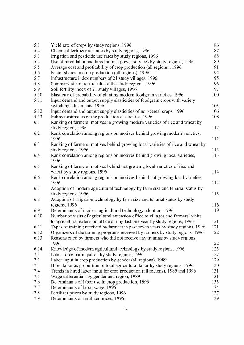
5.1 Yield rate of crops by study regions, 1996 86

5.2 Chemical fertilizer use rates by study regions, 1996 87

5.3 Irrigation and pesticide use rates by study regions, 1996 88

5.4 Use of hired labor and hired animal power services by study regions, 1996 89

5.5 Average cost and profitability of crop production (all regions), 1996 91

5.6 Factor shares in crop production (all regions), 1996 92

5.7 Infrastructure index numbers of 21 study villages, 1996 95

5.8 Summary of soil test results of the study regions, 1996 96

5.9 Soil fertility index of 21 study villages, 1996 97

5.10 Elasticity of probability of planting modern foodgrain varieties, 1996 100

5.11 Input demand and output supply elasticities of foodgrain crops with variety

switching adustments, 1996

103

5.12 Input demand and output supply elasticities of non-cereal crops, 1996 106

5.13 Indirect estimates of the production elasticities, 1996 108

6.1 Ranking of farmers’ motives in growing modern varieties of rice and wheat by

study region, 1996

112

6.2 Rank correlation among regions on motives behind growing modern varieties,

1996

112

6.3 Ranking of farmers’ motives behind growing local varieties of rice and wheat by

study regions, 1996

113

6.4 Rank correlation among regions on motives behind growing local varieties,

1996

113

6.5 Ranking of farmers’ motives behind not growing local varieties of rice and

wheat by study regions, 1996

114

6.6 Rank correlation among regions on motives behind not growing local varieties,

1996

114

6.7 Adoption of modern agricultural technology by farm size and tenurial status by

study regions, 1996

115

6.8 Adoption of irrigation technology by farm size and tenurial status by study

regions, 1996

116

6.9 Determinants of modern agricultural technology adoption, 1996 119

6.10 Number of visits of agricultural extension office to villages and farmers’ visits

to agricultural extension office during last one year by study regions, 1996

121

6.11 Types of training received by farmers in past seven years by study regions, 1996 121

6.12 Organizers of the training programs received by farmers by study regions, 1996 122

6.13 Reasons cited by farmers who did not receive any training by study regions,

1996

122

6.14 Knowledge of modern agricultural technology by study regions, 1996 123

7.1 Labor force participation by study regions, 1996 127

7.2 Labor input in crop production by gender (all regions), 1989 129

7.3 Hired labor as proportion of total agricultural labor by study regions, 1996 130

7.4 Trends in hired labor input for crop production (all regions), 1989 and 1996 131

7.5 Wage differentials by gender and region, 1989 131

7.6 Determinants of labor use in crop production, 1996 133

7.7 Determinants of labor wage, 1996 134

7.8 Fertilizer prices by study regions, 1996 137

7.9 Determinants of fertilizer prices, 1996 139

14

7.10 Type of pesticides used by farmers by study regions, 1996 139

7.11 Determinants of pesticide use, 1996 141

7.12 Land ownership structure of the study regions, 1996 142

7.13 Tenurial arrangement by farm size and tenurial status by study regions, 1996 145

7.14 Determinants of land rent, 1996 146

7.15 Determinants of agricultural credit, 1996 149

7.16 Determinants of crop prices, 1996 151

7.17 Storage facilities by study regions, 1996 152

7.18 Joint determination of input demand functions, 1996 154

8.1 Average annual crop income (Tk.) per household by study regions,1996 158

8.2 Average annual agricultural income (Tk.) by study regions, 1996 159

8.3 Average annual non-agricultural income (Tk.) by study regions, 1996 160

8.4 Structure of annual family income (Tk.) per household by study regions, 1996 161

8.5 Average annual crop income (Tk.) per capita by land ownership categories by

study regions, 1996

161

8.6 Average annual agricultural income (Tk.) per capita by tenurial categories by

study regions, 1996

162

8.7 Average per capita income (Tk.) from agricultural and non-agricultural sources

by land ownership categories by study regions, 1996

163

8.8 Structure of annual household income (Tk.) by land ownership and tenurial

categories (all regions), 1996

164

8.9 Determinants of rural household income , 1996 165

8.10 Factor shares of local and modern varieties of rice (all regions), 1996 167

8.11 Level of modern agricultural technology adoption in the study villages, 1996 168

8.12 Structure of annual household income (Tk.) by status of modern agricultural

technology adoption (all regions), 1996

168

8.13 Structure of annual household income (Tk.) of landless and marginal farmers by

status of modern agricultural technology adoption (all regions), 1996

169

8.14 Pattern of income distribution by status of modern agricultural technology

adoption based on per capita income scale (all regions), 1996

170

8.15 Inequality in income distribution by status of modern agricultural technology

adoption, 1996

172

8.16 Income shares, Gini-coefficients, rank correlation ratios, and contribution of

income components to the overall Gini-ceofficient in the study regions, 1996

174

8.17 Minimum nutritional requirement for a person per day 175

8.18 Poverty line income (Tk.) required to fulfill the nutritional and other

requirements by study regions, 1996

176

8.19 Estimation of poverty in the study regions, 1996 177

9.1 Selected indicators of technological change in Bangladesh agriculture, 1949/50

– 1993/94

180

9.2 Farmers’ perception of 12 specific environmental impacts of modern

agricultural technology by study regions, 1996

181

9.3 Ranking of farmers’ perception on 12 specific environmental impacts of modern

agricultural technology by study regions, 1996

182

9.4 Rank correlation of environmental impact ranking among regions, 1996 183

9.5 Overall soil fertility evaluation of the study regions, 1997 186

9.6 Soil fertility and crop productivity relations in the study regions, 1996 188

15

9.7 Average levels of available soil nutrients, fertilizer and pesticide use levels in

the study regions, 1996

189

9.8 Correlation between available soil nutrients and levels of fertilizer and pesticide

use in the study regions, 1996

189

9.9 Growth trends in fertilizer use and fertilizer productivity in the study regions,

1960/61 – 1991/92.

191

9.10 Number of applications of pesticides by study regions, 1996 192

9.11 Farmers’ perception on beneficial and harmfull effects of pesticide use by study

regions, 1996

193

9.12 Type of pesticides used by farmers by study regions, 1996 193

9.13 Average annual compound growth rates of fish-catch in study regions for the

period 1983/84 – 1993/94

195

9.14 Average annual compound growth rates of pesticides in study regions for the

period 1983/84 – 1993/94

196

9.15 Summary of water quality test results (6 surface water and 7 ground water

samples) by study regions, 1997

197

9.16 Arsenic pollution in groundwater in the study regions, 1997 198

9.17 Drainage and flooding problem by study regions, 1996 200

10.1 Hypothesis test results at a glance 206

10.2 Synthesis of approaches used and their implication on the results of the study 216

10.3 Selected socio-economic characteristics of the villages by status of modern

technology adoption, 1996

225

10.4 SWOT analysis of the integrated agricultural development planning components 227

Appendix Tables 258-306

16

CHAPTER I

INTRODUCTION

Technological change is an important factor in economic growth and development. Historical

experience suggests that technology, by raising productivity of factors (e.g. labor, capital, land

and other natural resources), played an important role in economic growth. Though developed

countries, being the forerunner in technological innovations, benefited most from technical

change, particularly industrial technology, the developing countries also benefited from the

technological innovations, particularly in agriculture (Hayami and Ruttan, 1985).

Agriculture constitutes the major source of livelihood in Bangladesh. The agricultural

sector accounts for more than 50 percent of national income and employs two-third of the labor

force. Being one of the most densely populated country of the world, the land-man ratio is

extremely low and majority of the population lack food security. Therefore, continued

agricultural growth is deemed pivotal in alleviating poverty and raising the levels of living for

the whole population. As such, over the past four decades, the major thrust of national policies

were directed towards transforming the agricultural sector via the route of rapid technological

progress. The purpose of the present study is to examine the distributional consequences and

sustainability of this rapid technological progress in Bangladesh agriculture within the context of

the nation’s economic development. Specifically, the distributional consequences of modern

agricultural technology were evaluated in terms of its impact on productivity, employment,

income, income distribution and poverty. Sustainability is evaluated in terms of its impact on

selected components of environment and trend in long-term productivity growth.

In this section, the importance of technological change in augmenting agricultural

productivity is highlighted with particular emphasis on the role of ‘Green Revolution’

technology and its related controversies in order to focus on the research problem for the study.

Furthermore, rationale of the study in the context of Bangladesh is provided. Finally, the

research framework, specific research objectives, relevant hypotheses, scope of the study in

general as well as within the context of rural-regional development planning, and structure of the

dissertation are outlined.

1.1 Technological Change: Related Developmental Issues

It has now been widely recognized (Tisdell, 1988; Clapham, 1980) that a high level of

interconnection exists among technological change, economic development, environmental

quality, population growth and social change. Tisdell (1988) noted that, new technology (its

availability and application) is vital not only as factor of economic growth and development, but

also as a determinant of the nature and structure of society and as a contributor to changes in

environmental quality. Dean (1955) suggested that the major reason for sustained economic

growth commenced in the eighteenth century in Great Britain was the new inventions and their

application rather than the high level of savings and capital accumulation (in Tisdell, 1988).

Some researchers (Blum et al., 1967 and Denison, 1962) claimed that for most of the developed

countries, qualitative factors (such as improved technologies and their adoption) served as a

major source of economic growth than the quantitative factors (such as increase in savings and

capital accumulation). Such line of reasoning goes against the views of Rostow (1952) who

17

prescribed that necessary condition for an economy to reach the take-off stage in economic

growth is to achieve a high level of savings and capital accumulation. Though economists and

social scientists now recognize the critical role of technological change in these respects, its

importance has not been fully appreciated.

1.1.1 Technological Change in Agriculture

Technological change in agriculture has been one of the most rapidly growing area of

study within the field of agricultural economics right after the World War II (Hayami and

Ruttan, 1985). Two main reasons can be forwarded for its growing importance. First, prior to

1960s, particularly the first two decades after World War II, the agricultural productivity gap

between the developed and developing countries widened. There has been an increase in the

supply of agricultural products relative to its demand in the developed world, thereby leading to

a decline in farm prices and incomes. The second reason for rapid growth in the study of

technological change is due to the difficulty faced by the developing countries to increase their

agricultural output to feed the growing population. Though the technical breakthrough in grain

production during the 1960s opened up new opportunities for the developing countries to rapidly

raise their output, a major issue faced by their policymakers and planners remain to determine,

whether the potential agricultural surpluses that are produced can be sustained to continuously

feed the engine of economic growth, without jeopardizing the environment (Hayami and Ruttan,

1985; Alauddin and Tisdell, 1991; and Murshid, 1986).

It should be recognized that there are multiple paths of technological development.

Hayami and Ruttan (1985) noted that technology could be developed to facilitate the substitution

of relatively abundant factors for relatively scarce factors. In terms of cost, it implies that the

relatively cheap factors can be substituted for the relatively expensive factors. For example, the

high-yielding crop varieties are one such categories of inputs that are developed to facilitate the

substitution of fertilizer (or other inputs) for land, thereby releasing the constraints imposed by

inelastic supply of land and can be termed as ‘land-saving’ technology. Similarly, in economies

characterized by relatively scarce supply of labor, land and capital can be substituted for labor by

developing improved agricultural machineries and equipments (e.g. tractors, irrigation

equipments, combine harvesters, etc), which can be termed as ‘labor-saving’ technologies.

Hayami and Ruttan (1985) named the land-saving technology as ‘biological’ and ‘chemical’

technology, and ‘labor-saving’ technology as ‘mechanical’ technology. However, it should be

noted that in both cases the new technology, embodied in new crop varieties or new equipments,

might not always substitute by itself for land and labor inputs. Sometimes, it may rather serve as

a catalyst only to facilitate the substitution of the relatively abundant factors (such as fertilizers)

for the relatively scarce factors (the land).

In agriculture, biological and chemical technologies are more basic than mechanization

or mechanical technology. This is mainly due to the spatial nature of agricultural production that

imposes constraints on efficiency of large-scale production using mechanized processes. The

main thrust in the development of biological and chemical technology is to release the

constraints imposed by the inelastic supply of land and therefore targeted to increase crop output

per unit of land (land productivity) and/or increase the intensity of cropping by inducing

multiple cropping technology. Hayami and Ruttan (1985) noted that technological change in

crop production typically involves any of the three elements. One, land and water resource

18

development to provide a more congenial environment for plant growth. Two, modification of

the environment by adding organic and inorganic sources of plant nutrients to the soil, and

biological and chemical compounds for protection of plants from insect-pest attacks and

diseases. And three, selection and breeding of new biologically efficient crop varieties

specifically adapted to respond to the controlled environment.

1.1.2 Technological Change and Agricultural Productivity

It has now been widely recognized that rapid growth in agricultural output and

productivity is essential as effective development strategy particularly in the early stages of

economic growth (Hayami and Ruttan, 1979, 1985; and Dayal, 1989). Historical experience

from developed countries suggests that the key factor in accelerating the growth of agricultural

output has been in the productivity of inputs (Hayami and Ruttan, 1979) and technological

change is an important factor in influencing agricultural productivity growth (Tisdell, 1988; and

Hossain, 1989). A widely accepted argument is that the basic source of technological change is

in the improvement of the quality of factor inputs. Yudelman et al., (1971) defined technological

change in this context as “the introduction of new or non-conventional resources into

agricultural production as substitutes for the conventional resources. The effect of technological

change must be evident as a change in the yield per acre, as a change in the cultivated acreage

available or both” (p.38-9).

Hayami and Ruttan (1985) identified that the capacity to develop technology that

conforms to the existing resource endowments of respective economy is the single most

important factor explaining differences in agricultural productivity among countries. Using a

cross-country analysis of 43 countries: 21 developed countries (DCs) and 22 less developed

countries (LDCs), Hayami and Ruttan (1985) concluded that high potential exists among the

LDCs to increase their output by appropriate investments in education, research, and the supply

of modern technical inputs.

Therefore, for the developing nations, an all out effort is required to accelerate the rate of

agricultural productivity in order satisfy the increasing food demand owing to booming

population pressure.

1.2 The ‘Green Revolution’

Over the past centuries, the path of technological change in agriculture had passed

through a smooth transition from a resource-based system to a science-based system. The

twentieth century experienced a major technological breakthrough in agricultural history. The

success was largely in the development of high-yielding modern grain varieties of wheat (from

CIMMYT - International Maize and Wheat Improvement Centre, Mexico) and rice (from IRRI -

International Rice Research Institute, Philippines) which are highly responsive to inorganic

fertilizers, insecticides, effective soil management and water control. The high returns

(reportedly) associated with the adoption of these new varieties of wheat and rice led to their

rapid diffusion in countries of Asia and Latin America consequently leading to a dramatic

increase in food production. The increase in food production was dramatic enough to be

heralded as the ‘Green Revolution’ (Hayami and Ruttan, 1985) and the technology facilitating

its widespread adoption is coined as the ‘Green Revolution Technologies’. Wolf (1986) noted

19

that, this strategy of developing new seed varieties, which has transformed the lives of millions

of people, is considered to be the most successful achievement in international development

efforts. The short-maturity and photo-period insensitivity of these high yielding modern varieties

of wheat and rice enabled the farmers to dramatically increase their cropping intensity by

harvesting two-three crops from a same piece of land in one year. In other words, by raising crop

output per unit of land (hence land productivity) and increasing cropping intensity, ‘Green

Revolution’ technically released the constraints imposed by the inelastic supply of land by

substituting fertilizers (with associated crop management and water control practices) for scarce

land.

1.2.1 ‘Green Revolution’ Controversies

The impact of ‘Green Revolution’ has been mixed. Though the spread of this technology

has been fastest of all in the history of technological innovations in agriculture, the post-adoption

stage of ‘Green Revolution’ provide mixed consequences. Wolf (1986) noted that these modern

grain varieties spread rapidly only in Asia (including China) and Latin America. Africa

benefited least from the ‘Green Revolution’, as none of these grain varieties were staples for the

life of rural Africans.

The critics of ‘Green Revolution’ (Wharton, 1969; Falcon, 1970; and Griffin, 1974),

argued that the new technology is not scale neutral, that is, as farm size increases it becomes

profitable to employ machineries. Also, the high-yielding variety technology tended to be

monopolized by large farmers equipped with better information and financial capability. And the

technology is capital intensive and, as such, small and poor farmers cannot adopt them.

However, contrasting views to the above are also being appreciated by many. It is

suggested (Hossain et al., 1990; Mellor, 1978; and Dantwala, 1985), that the new technology

may benefit the poor in the long run in two ways. One, by reducing the cost of production and

thereby lowering the prices of foodgrain on which the poor spent most of their money, and two,

by generating more non-farm employment opportunities by suppressing real wages down and

stimulating demand for non-farm goods and services. In this view, the cause of poverty is seen

as the delayed adoption of technological change such that the beneficial effects tend to be offset

by high population growth. Therefore, slow rate of technological progress will accentuate

poverty.

Ruttan (1977) forwarded seven generalizations of ‘Green Revolution’ based on a

comprehensive survey of early literature. First, modern varieties (MVs) of wheat and rice are

adapted fast where they are technically and economically superior to local varieties. Second,

farm-size and tenure do not pose serious constraints to the adoption of MVs. Third, farm-size

and tenure has not been an important source of differential growth in productivity. Fourth, the

introduction of MVs resulted in increased demand for labor. Fifth, landowners gained relative to

tenants and laborers from the adoption of MVs. Sixth, the introduction of MVs contributed to

widening the wage and income differentials across regions. And seventh, the introduction of

MVs dampened the rate of increase in food grain prices at the consumer level. Lipton and

Longhurst (1989), drawing on various literatures, also derived similar conclusions that although

small farmers and tenants initially lag behind large farmers in the process, they catch up quickly

thereby making farm size and tenurial status invariant to technological adoption.

20

Major criticism on ‘Green Revolution’ relates to equity concerns. It is suggested (Lipton

and Longhurst, 1989; Hossain, et al., 1990; and Singh, 1994) that the technology may accentuate

regional inequality in the distribution of income. Therefore, technological change need support

through investment on development of irrigation facilities, flood control and drainage for

increased water control in order to bring in additional land that were previously unsuited for MV

cultivation. Having done this, the increased diffusion of new technology will further widen the

gap across region. Also, since the new technology reduces unit cost of production and output

prices and raise real wages, farmers not adopting modern technology will lose due to the onset of

external diseconomies of scale.

Freebairn (1995), analyzing the results of 307 studies undertaken during the period 1970-

89, observed that about 80% of these studies had conclusions that the new technology widened

both inter-farm and inter-regional income inequality. The interesting point in this study is that

the nature of conclusion drawn from these evaluation studies were found to be influenced by

regional origin of the authors, location of the study area, methodology followed, and the

geographic extension of the study area. For instance, Freebairn (1995) summarized that, ‘studies

done by Western developed-country authors, those employing an essay approach, and those

looking at multicountry region are most likely to conclude that income inequalities increased. By

contrast, work done by Asia-origin authors, with study areas located in India or the Philippines,

and using the case study method are more likely to conclude that increasing inequality is not

associated with the new technology’ (pp.265).

As a whole, one can see that there is considerable controversy relating to the

distributional impact of ‘Green Revolution’ and/or the modern agricultural technology. In case

of Bangladesh, which experienced the onset of ‘Green Revolution’ technology since the mid-

sixties, similar controversies exists related to its distributional consequences.

1.3 The Research Problem

An interesting point to note that the early evaluations of modern technology and/or

‘Green Revolution’ (Sidhu, 1974; Cleaver, 1972; Gotsch, 1972; Griffin, 1974; Jose, 1974; Lal,

1976; Parthasarathy, 1974; Rao, 1976; Sen, 1974, Harris, 1977; and Bisaliah, 1982) centered

mostly on the concerns of growth, productivity, efficiency and equity. The anticipation that the

modern technology can affect other spheres of life remains ignored. Evaluation of the effect of

modern technology, particularly ‘Green Revolution’, within the context of a broader perspective

encompassing ecological and environmental compatibility was nascent. The delayed

consequences of ‘Green Revolution’ on environment and sustainable development came up on

the agenda for research only recently, for instance, Shiva (1991), Kang (1982), Brown (1988),

Wolf (1986), Clapham (1980), Redclift (1989), and Bowonder (1979 and 1981).

Also, in identifying factors influencing the diffusion of technology, past studies (e.g.,

Sidhu, 1974; Hossain and Quasem, 1986; Boyce, 1986; Hossain, 1977; 1978; and 1986; Abedin,

1985) concentrated mainly on conventional factors such as irrigation, fertilizers, tenancy and

farm sizes while paying no or little attention to other infrastructural factors, for example, roads

and transportation networks, markets, storage facilities, service centers, extension networks,

21

credit institutions, government agencies, etc. Therefore, policy recommendations emerging from

these studies remained quite ineffective due to their partial nature.

Clapham (1980) noted that though evaluation of agricultural policy and farmers behavior

are abundant, the environmental dimensions of agriculture remains unclear. Shiva (1991)

claimed that though ‘Green Revolution’ is based on the assumption that technology is a superior

substitute of nature and is a source of abundance (by releasing constraints imposed by nature),

but at an ecological level, it produced scarcity and not abundance (by reducing the availability of

fertile land and genetic diversity of crops). Brown (1988) noted that the foodgrain production

has been dramatically falling, both nationally and globally, largely due to ecological instabilities

including drought, climatic change, greenhouse effect and desertification. Hazell (1984)

indicated that production and yield of foodgrain might have become more instable in the period

following the introduction of modern technology in India. Bowonder (1979) identified a number

of direct and indirect consequences of ‘Green Revolution’ (both positive and negative) on

various sectors of the economy.

In addition to productivity, efficiency and equity concerns of technological change, the

question of sustainability in food production is gaining momentum (Alauddin and Tisdell, 1991;

Marten, 1988; and Redclift, 1989). Trends in global food outlook for the period 1984-94

presented in Table 1.1 are no doubt alarming. During the decade of 1984-94, the global cereal

production increased only marginally, at an average annual growth rate of 0.9 percent. On the

contrary, the world population grew at an average annual rate of 1.8 percent showing clearly that

food production failed to keep up with the population growth. Simultaneously, on account of

inputs, the net irrigated land increased in all regions and fertilizer use significantly increased in

the developing countries of Asia-Pacific region, implying that despite increased input intensity,

response of output is slowing down.

The fact that global food production is either stagnated or declining despite

corresponding increases in inputs raised concerns over the future prospects of food security for

the growing world population. There has been a growing interest in evaluating the merits of

traditional agriculture and it was increasingly realized that modern technology, particularly the

‘Green Revolution’, though dramatically increased food production in its initial years of

inception, its production potential is tapering off in later years.

Conway (1986) suggested that alternative agricultural technologies need to be judged

against the criterion of stability (of yields and incomes) and sustainability (of production and

yield). In recent years, focus of evaluation has shifted on considering the sustainability of the

ecosystems and environmental factors on which agriculture depend (Alauddin and Tisdell, 1991;

and Redclift, 1989).

Table 1.1 Global food outlook for the period, 1984-94.

Country Average annual growth rate (%)

Population

(1984-94)

Cereals1

(1984-94)

Roots and tubers2

(1984-94)

Irrigation3

(1983-93)

Fertilizer4

(1983-93)

Asia-Pacific 1.9 1.9 0.8 1.6 -0.1

22

Developing5

Developed6

Rest of the world

World

2.0

0.5

1.7

1.8

2.1

-2.2

0.2

0.9

0.9

-1.0

0.2

0.4

1.6

0.7

1.1

1.4

5.5

-0.3

-2.9

-0.1

Notes: 1 cereals include rice-paddy, wheat, maize and millet;

2 include cassava, potatoes, sweet

potatoes, and taro; 3 refer to net irrigated land;

4 refers to fertilizer in plant nutrient units;

5 include 27 countries;

6 include 3 countries, namely, Australia, Japan and New Zealand.

Source:Based on FAO (1995, p. 5, 9, 11, 33, 51).

Thus far, most of the evaluation studies of modern technology remained partial in the

sense that these studies focused either on issues of productivity, efficiency or equity, while

paying little or no attention for other direct or indirect effects of technological change. Also, in

identifying factors influencing diffusion of technology, the crucial role of infrastructure is

ignored and less studied. Sustainability of a system requires that, the approach need to be

holistic, meaning that one should focus on detailed assessment of a technology within the

context of broadest possible perspective. In other words, it requires that the impact of technology

need to be assessed by identifying its multifarious linkages with other sectors of the economy.

Such an all encompassing impact analysis of modern agricultural technology will enable to

identify the existing gaps and potentials and assist in devising policies for effective resource

development planning. The present study is an attempt in this line and is conducted for one of

the most vulnerable country of Asia in terms of food security, namely, Bangladesh.

1.4 Bangladesh: General Characteristics and Overview of the Agricultural Sector

Bangladesh, a predominantly agrarian economy, characterized by small-scale,

fragmented farming, and employing primitive technology, is one of the poorest and most

populous nations of the world. The country has to support an estimated 124 million people with

a density of 860 persons per sq km (BBS, 1997). The majority of the population lack food

security as reflected in extreme poverty and widespread hunger. Though agriculture serves as the

mainstay of the population contributing about half of the Gross Domestic Product (GDP) and

employing two-third of the total labor force, the high population growth rate offsets the

increased agricultural production thereby exacerbating the food deficit and poverty. The land-

man ratio is one of the lowest in the world. Hossain (1989) rightly remarked that, ‘there are few

countries in the Third World where technological progress is of higher importance in

maintaining the food-population balance than in Bangladesh ... if the country is to maintain a

modest per capita income growth of about 2 percent a year ... food production has to grow over

3.4 percent a year to avoid a further increase in cereal imports, which are currently about 10

percent of domestic demand’ (pp.14). Further, Hossain (1989) stressed that the agriculture does

not have the resources to meet such a challenge as all the cultivable land is in use. In addition,

the increasing population pressure dramatically reduced the average farm size holdings to less

than a hectare. Therefore, he opted for rapid technological progress as the key to maintain the

food-population balance in the country.

1.4.1 Overview of Agriculture

23

Agricultural sector dominates Bangladesh economy in terms of contribution to national

income as well as employment. Bangladesh's export mainly consists of jute, jute goods, and tea.

Crop production dominates Bangladesh agriculture accounting for more than 60 percent of

agricultural value added (BBS, 1996). Alauddin and Tisdell (1991) noted that if supporting

activities like transport and marketing of agricultural products are taken into account, the share

of agricultural sector GDP is likely to be over 60 percent of total. Within the crop sub-sector,

foodgrain production is central to the economy dominated by rice monoculture. About 80

percent of the gross cropped area is planted with rice that accounts for about 93 percent of total

cereal production (BBS, 1996). In recent times, wheat is also gaining importance though its

coverage remains extremely low.

Over the past forty years, the major development influence in Bangladesh agriculture has

been the introduction of ‘Green Revolution’ technologies. This bio-chemical ‘land-saving’

technology which transformed much of the Asian region were introduced at a relatively later

stage (during the late 1960s) and at a much slower pace (Alauddin and Tisdell, 1991).

Though the basic aim of agricultural development policies over the last four decades

remained at increased food production, the program components underwent vast changes

shifting from one category to the other. In the early 1960s, flooding during the monsoon and

lack of irrigation facilities during the dry periods were identified as the major constraints

hindering use of modern agricultural inputs. As such, the government aimed at building large-

scale irrigation and drainage facilities (Alauddin and Tisdell, 1991; Hossain, 1989). From the

late 1960s, the program strategies shifted from building large scale irrigation installations to

more divisible and modern techniques of irrigation (e.g., shallow tube well, deep tube wells and

low-lift pumps) coupled with increased distribution of highly subsidized chemical fertilizer and

modern varieties of rice. In the early 1970s, modern varieties of wheat were introduced. As

noted by Alauddin and Tisdell (1991), during the initial years until the early 1970s, modern

varieties of rice (e.g., IR-8, IR-5, and IR-20) used to be imported directly. However,

subsequently the Bangladesh agricultural research system adapted and indigenously developed

different varieties of rice and wheat, which were then multiplied and released for farm

production.

1.5 Rationale of the Study

Given the dependence of a vast majority of total population on agriculture for their

livelihood, and relative contribution of this sector to national income, it is evident that, the key to

economic development of Bangladesh lies in the growth of the agricultural sector even in much

of the foreseeable future. As mentioned earlier, since the sector does not have the adequate

resources to meet the growing challenge, the key to maintain food-population balance was

sought in accelerating the rate of technological progress. Accordingly, development programs

were diverted in spreading the modern varieties of rice and wheat with corresponding support in

the provision of modern inputs, e.g., irrigation installations, chemical fertilizers, pesticides,

institutional credit, product procurement, storage and marketing facilities. However, after the

lapse of first two decades of ‘Green Revolution’, i.e., by early 1980s, it was felt by many (e.g.,

24

Ahmed and Hossain, 1990; Khan, 1985) that modern technology has contributed in worsening

income inequality and exacerbating absolute poverty. Other studies mainly dealing with

movement of real wages and nutritional issues revealed downward trends in real wages in

agriculture as well as decline in calorie intake of the rural poor (Hasan and Ahmad, 1984).

On the other hand, contradictions to above are evident as well. Hossain (1989), Alauddin

and Tisdell (1991), Hossain et al., (1990), Ahmed and Sampath (1992), claimed that modern

technology as a whole increased productivity, increased real wages (marginally) and contributed

positively towards distribution of income. However, on the question of improving nutrition the

result was not decisive. Alauddin and Tisdell (1991) claimed that food consumption per capita

failed to increase (though not declined) on one hand, and become less varied on the other, since

the average Bangladeshi seemed to increase his/her dietary dependence on cereals alone and less

on other protein rich food.

A major disturbing conclusion is arrived by Bera and Kelly (1990) who claimed that the

ceiling adoption level for modern varieties of rice in Bangladesh has nearly been reached.

Whereas in reality, only 41 percent of all rice area is planted by modern varieties until 1989

(Hossain, et al., 1990) which is even less than half of total rice area. Furthermore, Bangladesh

Agricultural Sector Review (BASR, 1989) observed that there is a widespread slow-down in

cereal production during the 1980s, particularly in previous high-growth regions and continued

sluggish-growth in the low-growth regions. More specifically, in terms of varieties, negative

growth rates are observed for all three major MV rice crops: MV Aus, MV Aman and MV Boro.

On the other hand, Alauddin and Tisdell (1991) concluded that foodgrain production recorded a

higher growth rate during the post-Green Revolution period, particularly, due to change in

cropping intensity (owing to the introduction of MV rice), and boost in productivity of MV

wheat. Their analysis of regional (inter-district) variation in growth revealed that though there

remain differences in inter-district growth of production and yield, the extent of divergence has

been moderated in the post-Green Revolution period. The proportion of area under MVs has

been identified as an important determinant for output increase per unit of land area.

Given such controversial results it is worthwhile to investigate the nature and extent of

technological progress in agriculture and its impact on production growth, income, employment,

income distribution, poverty, regional disparity, and other spheres of human welfare at this later

stage of diffusion. Thus far, the issue of technological change in agriculture has been less studied

in the Bangladesh context (Alauddin and Tisdell, 1991; Hossain, 1989; and Hossain et al.,

1990). As mentioned earlier, most of the studies dealing with the issues of technological change

were partial in nature. Also, past studies on agriculture dealing with issue of regional variation in

growth performance (BASR 1989; Hossain, 1984; Boyce, 1986; Alauddin and Tisdell, 1991)

based their analyses on arbitrary regional units (the administrative districts) which has no

bearing in depicting the agro-ecological, socio-economic and infrastructural characteristics in

influencing growth patterns. Also, the issue of sustainability as well as environmental

consequences of modern agricultural technology, though gained momentum only recently, has

not been explicitly dealt in case of Bangladesh. Moreover, in identifying factors influencing

agricultural growth, much emphasis has been laid only on irrigation, tenurial status, and inputs.

The crucial role of technological, biophysical as well as rural infrastructure in influencing

25

growth has been less studied. Only a few studies (Ahmed and Hossain1, 1990 and Hossain et al.,

1990) explicitly dealt with the role of rural infrastructure in agricultural and economic

development. Evenson (1986) and Easter et al., (1977) noted that investments in rural

infrastructures are designed to change the behavior of farmers and identification of their

contribution are important in providing insights for the direction of agricultural development

efforts.

The proposed study is aimed at explicitly incorporating the deficiencies mentioned

above. That is to say, analyze the impact of technological change in influencing regional

variation of agricultural development levels and aggregate crop production and examine the

sustainability of food production at the national level. At the local level, examine the influence

of technological, soil fertility and rural infrastructural factors on crop production decision and

examine the factors affecting modern technology diffusion as well as assess the impact of

technological change on employment, income, distribution of income, poverty and the

environment. The study is expected to enhance existing knowledge on the differential impact of

modern agricultural technology and will assist in formulating policy guidelines and strategic

recommendations for an integrated rural-regional development planning. In this study, two terms

‘technological change’ and ‘modern agricultural technology’ is used interchangeably. Both these

terms refer to the ‘Green Revolution’ technology or the ‘modern varieties-fertilizers-pesticides-

irrigation’ technology.

1.6 Research Framework

Given the importance of technological innovation in agriculture and associated

controversies discussed so far, a conceptual framework of the study is developed and is

presented in Figure 1.1.

1 Though this study is considered as a seminal work conducted by IFPRI (International Food Policy Research

Institute), the survey period dates back to crop-year 1982, a period when the MVs of rice started to depict a

declining trend and MV wheat is at its initial stage. Also, the level of rural infrastructural development during

that period has been rudimentary.

26

If unconstrained (+)

(+) (+)

(+)

(+)

If adequate (+)

If no inequality/ If no adversity/

discrimination deterioration

(+) (+)

Figure 1.1 Conceptual framework of the study.

POPULATION

GROWTH Drain foreign

currency

(not promoted)

FOOD

DEFICIT

FOOD

IMPORT

Mechanizatio

n

(not

promoted)

SOLUTION

LAND SAVING

TECHNOLOGY

LABOR SAVING

TECHNOLOGY

‘GREEN REVOLUTION’

TECHNOLOGY

PRODUCTION INCOME EMPLOYMENT

MULTIFACETED IMPACTS

SOCIO-ECONOMIC IMPACTS

Employment and gender equity

Factor markets

Income and income distribution

Poverty

ENVIRONMENTAL I MPACTS

Soil fertility

Water quality

Human health

Environment and fisheries

SUSTAINABLE AGRICULTURAL

DEVELOPMENT

FACTOR INPUTS

Land, labor, animal

power, fertilizer,

irrigation, farmasset

HIGH SOIL

FERTILITY

INFRASTRUCTURE

Markets, storage, roads,

banks, extension office,

local office, college, etc.

27

The framework is developed hypothesizing that undertaking the route of technological

progress as a solution to chronic food deficit provided mixed results. The exclusive promotion of

‘Green Revolution’ technology though apparently succeeded in providing increased production

and income, its distributional consequences have been mixed. In addition to its influence on

distributive justice and poverty, ‘Green Revolution’ technology is believed to have widespread

direct and indirect impact on the environment and other sectors of the economy.

Further, serious constraints exist among various factors, particularly rural infrastructure

and soil fertility, which contributes positively to production growth, income and employment.

Removal of these bottlenecks is a priority concern. Thus, the present study will adopt an

evaluative approach to provide a detailed understanding of the aforementioned issues in order to

formulate viable policy prescriptions.

1.7 Objectives of the Study

The main objectives of the study are to conduct a detailed evaluation of the delayed

consequences of technological change in agriculture and to examine the prospect of sustaining

food production in Bangladesh. The focus is on evaluating the multifaceted socio-economic and

environmental impacts of modern agricultural technology within a broadest possible perspective.

As such, the present study employed a holistic approach consisting of a blend of aggregate

analysis at the national level as well as in-depth farm survey analysis at the local level.

Specifically, the study is aimed at evaluating the impacts of modern agricultural technology on

productivity, employment, gender equity in employment, operation of factor markets, income,

distribution of income, poverty and the environment at the local level and on regional

disparity, aggregate crop production and food production sustainability at the national level.

The research is designed with a blend of economic (crop input-output), biophysical (soil

fertility) and behavioral (farmers’ perception) analyses to cover the diverse range of issues.

The national level analysis deals with time-series analysis of the impacts of technological

change on regional variation in agricultural development levels for the period 1972/73 - 1992/93

and on aggregate crop production using regionwise data for the period 1960/61 - 1991/92,

respectively. It also deals with the examination of food production sustainability by analyzing

the long-run trend in crop productivity growth for the period 1947/48 - 1993/94. Therefore, the

specific objectives dealing with impacts of technological change at the national level are:

(1) to examine the impact of technological change on regional variation in agricultural

development levels and to identify relatively homogenous agricultural regions with

respect to a set of technological, demographic, infrastructural, and crop production

efficiency parameters,

(2) to examine the impact of technological change on long-run aggregate crop production,

(3) to estimate the output elasticities and returns to scale from the aggregate crop production

function in order to determine the prospect of sustaining food production in future,

(4) to examine the long-run growth path of crop productivity using logistic and linear

functions in order to determine the prospect of food production sustainability,

28

The local level analysis deals with identification of the influence of technological, soil

fertility, and infrastructural factors in crop production and technology adoption decisions, and a

detailed impact analysis of technological change on crop production, employment, income,

distribution of income, poverty, and the environment. Therefore, the specific objectives dealing

with identification of factors influencing crop production and modern technology adoption

decisions at the local level are:

(5) to assess the soil fertility status of the farmers’ field in terms of availability of major

plant nutrients influencing crop productivity,

(6) to analyze the farmers’ decision making process in foodgrain production with respect to

changes in variable input prices at the same time allowing for making a choice between

local and modern varieties of rice and wheat using ‘meta-production function’ approach,

(7) to identify determinants of modern agricultural technology adoption at the farm-level,

(8) to identify the role of technological, infrastructural and soil fertility factors in influencing

crop production decisions,

And the specific objectives dealing with multifaceted impacts of technological change at

the local level are:

(9) to examine the impact of modern agricultural technology on employment and gender

equity in employment in the rural labor market as well as on factor markets, such as,

fertilizers, pesticides, crop output, agricultural credit, and tenancy markets,

(10) to examine the impact of modern agricultural technology on income, distribution of

income and poverty,

(11) to examine the impact of modern agricultural technology on selected aspects of

environment, such as, soil fertility, water quality, human health and fisheries resources.

The final task is to synthesize the multifaceted impacts of technological change in

agriculture based on the outcomes of national level and local level analyses and then to

integrate the results to formulate strategies for an integrated agricultural development plan.

1.8 Hypotheses of the Study

The overall premise of the study is that though the diffusion of modern agricultural

technology contributed to increased production, income and employment, its distributional

consequences have been mixed. Also, it has exerted adverse impacts on the environment.

Moreover, diffusion of modern agricultural technology has not been uniform across region and,

therefore, contributed to regional disparities. Finally, the long-run crop productivity is reaching a

saturation value thereby posing a threat to keep up with rapid population growth.

Therefore, hypotheses to fulfill the specified objectives of this study are grouped under

following basic categories outlined below. For the purpose of deducing concrete and specific

29

results, the hypotheses are postulated in null form with open alternative hypotheses since

relationship of factors, particularly the non-conventional factors with crop production cannot be

determined a priori. Therefore, the null-hypotheses to be tested are:

Hypotheses Related to Impacts of Modern Agricultural Technology at the National Level

(H1) There is no influence of technological, demographic, infrastructural, and crop production

efficiency factors on regional variation in agricultural development levels. There are no

regional differences in levels of agricultural development.

(H2) Technological, human capital and infrastructural factors do not influence aggregate

crop production growth.

(H3) Aggregate crop production in Bangladesh exhibits constant returns to scale.

(H4) The long-run growth rate of crop productivity is zero.

Hypothesis Related to Farmers’ Decision Making Process in Changing Production

Environment

(H5) Farmers in Bangladesh are not profit-maximizers. Farmers do not respond to variation in

input prices and changing production environment by reallocating resources and

switching between local and modern agricultural technologies.

Hypotheses Related to Factors Influencing Adoption of Modern Agricultural Technology

(H6) Socio-economic factors, such as, land ownership, farm size and tenurial status does not

influence modern technology adoption decisions.

(H7) Non-conventional factors, such as, technological, soil fertility and rural infrastructural

factors does not influence modern technology adoption decisions.

Hypotheses Related to Impacts of Modern Agricultural Technology at the Local Level

(H8) Modern agricultural technology does not influence employment, operation of the labor

market as well as operation of other factor markets.

(H9) Modern agricultural technology does not influence income from agricultural production.

(H10) Modern agricultural technology does not contribute to income inequality and influence

poverty.

(H11) Modern agricultural technology does not have adverse effects on selective environmental

factors, such as, soil fertility, water quality, human and animal health, and fisheries.

1.9 Scope and Limitation of the Study

30

Detailed impact analysis of a technological innovation on each and every sector of the

economy is a formidable task. The present study, therefore, utilizes the economic principles and

concepts in analyzing the issues. It also contains a blend of biophysical as well as behavioral

analyses in order to capture the diverse range of issues. As the study is mainly targeted to

evaluate the delayed consequences of three decades of modern agricultural technology diffusion

in Bangladesh, it is based on a blend of aggregate time-series analysis at the national level as

well as cross-section farm-survey analysis at the local level. Though time-series data in

Bangladesh is far from being comprehensive (Pray, 1980), as elsewhere in most of the

developing countries, it is nevertheless essential to make use of the existing information and

construct required indices from these existing sets of statistical series on the basis of certain

assumptions. For the local level analysis, it would have been highly desirable to possess detailed

information at the village levels for all the regions of Bangladesh. However, such a desire need

to be restricted based on time, budget and analytical tractability. As such, only three agro-

ecological regions were selected for local level analysis.

As mentioned earlier that the scope of analysis is limited to economic and selective

biophysical and behavioral analysis to capture the dynamics of technological change. Therefore,

details of technical issues (such as, agronomic features of crop production, nutrient uptake

mechanisms of plants) and social issues (such as, change in the composition of inter and intra-

household division of labor, kinship and community structures, nutritional intake at household

level) related to modern agricultural technology are not covered.

1.10 Scope of the Study within the Context of Rural-Regional Development Planning

Within a decentralized planning framework, forwarded by Thapliyal (1990), the four

principle components of planning are: (i) development of production sectors, (ii) development of

basic infrastructure, (iii) development of social amenities, and (iv) poverty alleviation. The

former two falls under the purview of resource development planning conducted at the area

level, and the later two fall under the purview of rural development planning conducted at

household/village level. The integration of both types of planning leads to an integrated rural-

regional development planning for a specific region (Fig.1.2).

In order to operationalize a decentralized planning process there are four basic steps

(Thapliyal, 1990). First, decide on a basic planning unit for resource development planning

through an ‘spatial analysis’ as it requires a larger unit consisting of a cluster of villages with

greater degree of homogeneity in terms of geography, resource distribution pattern and socio-

economic status. Second, planning for production sectors which includes analysis of past

performance and present status of the sectors, identification of alternative strategies and thrust

areas, and then formulation of projects and phasing them over a time period. Third, planning for

infrastructural facilities involving identification of existing gaps in the requirement and

availability of infrastructural facilities, estimate the future demand taking into account the

population increase and determine additional capacities to fill the gaps with locational

specifications. And fourth, planning for rural development through poverty alleviation and

minimum needs programs which involves village-level analysis of extent of poverty, existing

occupation pattern, assessment of resource and infrastructural requirements, identification of

target beneficiaries for projects.

31

Figure 1.2 Conceptual Framework for Decentralized Planning

Objectives Growth oriented Quality of life

oriented

Equity oriented

Components Development of

production sectors

Development of

basic infrastructure

Development of social

amenities

Poverty alleviation

Elements Agriculture

Irrigation

Livestock

Fisheries Forestry

Mining

Industries

Road/Transport

Market

Credit

Storage

Institutions

Power/Energy

Communication

Safe water/sanitation

Primary health care

Education for all

Housing/slum dev.

Family welfare

Environment Public distribution

Income

Employment

Skills training

Nutrition

Approach Area level Community level Household level

Concept Resource development planning Rural development planning

Integrated rural-regional development planning

Note: The present study covers the issues written in bold letters.

Source:Modified from Thapliyal (1990).

The present study, in this context, is designed to serve as information base to provide

basic analytical information required for aforementioned four steps of planning that are

necessary to successfully accomplish an integrated rural-regional plan for a specific region.

1.11 Usefulness of the Study

The study makes following contributions to empirical knowledge, particularly for

agricultural development in Bangladesh. The study highlighted the significant role of

technological and infrastructural factors in determining regional variation and identified regions

that are relatively homogenous with respect to agricultural development levels and corresponds

to existing administrative regions for which time-series data were published, thereby, will

facilitate in decentralized planning. Second, the study offered policy-relevant estimates of the

economic parameters of foodgrain and non-cereal crop production, their factor demand and

output supply responses in Bangladesh. Third, the study highlighted the significant role of

technological, infrastructural as well as soil fertility factors in influencing crop production

decisions. Fourth, the study provided a detailed analysis on the gender inequality in gains from

employment owing to technological change. Fifth, the study confirmed the claim of worsening

income distribution owing to technological change and exacerbation of rural poverty in

technologically developed villages. Sixth, the study provided information on specific

environmental impacts of modern agricultural technology. Seventh, the study provided an

evaluation of long term productivity of foodgrain crops and the prospect of sustaining food

production in Bangladesh. Finally, the study also indicated on the correspondence between

short-run factor utilization pattern with the long-run pattern through the comparison of returns to

scale estimates directly from time-series aggregate production function and indirectly from

cross-section farm-level profit function.

32

The study, by providing in-depth analytical information on the multifaceted impacts of

modern technology diffusion in the agricultural sector, will therefore, strengthen the existing

information base essential for undertaking planning decisions, particularly decentralized

planning decisions. The study will be particularly useful in facilitating implementation of

integrated rural-regional plans that are more realistic and wellsuited within the socio-economic

and environmental constraint imposed by each specific region of Bangladesh.

1.12 Structure and Outline of the Dissertation

The dissertation is organized into ten chapters (Figure 1.3). The review of relevant

literatures on evaluation of modern agricultural technology is presented in Chapter II. The

research design, description of the study area, and principal methodologies utilized for

quantitative and qualitative evaluation of technological change in agriculture at the national and

local level is presented in Chapter III.

The impacts of technological change on regional variation in agricultural development

levels and aggregate crop production are presented in Chapter IV. Also, an examination of food

production sustainability is presented in this chapter. Stepwise forward regression procedure is

used to select significant indicators (including technological factors) in explaining regional

variation and then composite indices of weighted standard scores are constructed to rank the

regions. Finally, the regions are delineated in descending orders of development by weighting

their relative standings in three periods, namely, Period 1 (1973 – 1975), Period 2 (1980 – 1983),

and Period 3 (1990 – 1993). Aggregate crop production function of the Cobb-Douglas form is

estimated to determine the impact of technological change on long run aggregate crop

production and estimate output elasticities and returns to scale using regionwise time-series

data covering 29 years (1960/61 – 1991/92). Logistic and linear regression analyses were

utilized to determine the productivity path of foodgrain and its sustainability using the longest

time-series data of Bangladesh covering 47 years (1947/48 – 1993/94). This chapter, therefore,

accomplishes all the national level objectives, Objective #1, Objective #2, Objective #3, and

Objective #4, respectively, as well as finalizes the selection of the study area for farm survey at

the local level.

The farm-level decision analysis of alternative technologies is presented in Chapter V.

The analysis is conducted for local and modern varieties of rice and wheat utilizing the ‘meta-

production function’ approach that allows for switching between varieties while responding to

changing input prices and production environment by profit maximizing farmers. The dual

measure of technological change, that is, the profit function analysis is used for the purpose

using normalized restricted translog profit functions for local rice as well as modern rice and

wheat varieties, respectively. The chapter also contains a composite profit function analysis of

other non-cereal crops in order to provide the complete scenario if an agricultural diversification

policy is sought. This chapter, therefore, accomplishes Objective #6 of the study.

Analysis of factors affecting adoption of modern agricultural technology is presented in

Chapter VI utilizing multivariate regression procedures. In addition to conventional variables,

the effect of soil fertility and infrastructure on adoption decision is analyzed. This chapter,

therefore, accomplishes Objective #7 and Objective #8 of the study.

33

The analyses of socio-economic and environmental impacts of technological change

are provided sequentially in Chapters VII, VIII and IX. The socio-economic component is

composed of impacts on employment and gender equity in employment in the rural labor

market, and on other factor markets, income, income distribution and poverty. The

environment component is composed of impacts on soil fertility, water quality, human health,

and fisheries resources.

Impact analyses of technological change on employment, gender equity in

employment, demand for hired and total labor, wages, animal power prices, land rent,

agricultural credit, fertilizer, pesticide, irrigation and output markets is presented in Chapter

VII. Multivariate analysis as well as simultaneous equation estimation procedures were

utilized for the purpose. This chapter, therefore, accomplishes Objective #9 of the study.

Analyses of determinants of rural household income, distributional consequences of

modern technology adoption and its impact on poverty are presented in Chapter VIII utilizing

multivariate analysis as well as various income distribution and poverty measures, thereby,

accomplishing Objective #10 of the study.

Environmental impacts of technological change are analyzed using a combination of

qualitative as well as quantitative methods. Firstly, the farmers’ perceptions on specific

environmental impacts and their relative ranking are computed. Then, available material

evidences, such as results of soil fertility analysis, nutrient pathway analysis, time-trend

analysis of relevant variables, were used to support or refute these perceptions. This chapter,

therefore, accomplishes Objective #5 and Objective #11, respectively.

Summary of the findings of the study, results of hypothesis tests, synthesis of the

multifaceted impacts of technological change, policy options and conclusions drawn from this

dissertation research are presented in Chapter X.

34

Figure 1.3 Structure of the dissertation.

CHAPTER II

Multifaceted Impacts of Technological Change

in Agriculture: A Review

CHAPTER III

Research design

and methodology

CHAPTER IV

Technological change and its

impact on regional variation,

aggregate crop production

and sustainability

CHAPTER V

Decision analysis of

alternative technologies:

A ‘Meta-production

Function’ approach

CHAPTER VI

Adoption of modern

agricultural technology

CHAPTER VII

Technological change and

its impact on employment

and factor markets

CHAPTER VIII

Technological change

and its impact on income

distribution and poverty

CHAPTER IX

Technological change

and its impact on the

environment

CHAPTER X

Summary of findings, synthesis

of impacts of technological

change and policy options

Conclusions

35

CHAPTER II

MULTIFACETED IMPACTS OF TECHNOLOGICAL CHANGE IN

AGRICULTURE: A REVIEW

The literature on agricultural development is replete with studies on technological

change and its impact on production growth and income distribution. The reason that this issue

has received such a prominent place in the development literature is due to its far-reaching

impact on economic growth and development. In this chapter, a brief review on the relevant

literature is presented. For simplicity, the review is broadly categorized into three sections. The

first section deals with the concepts, definitions and measurements of technological change and

the approach adopted in this study. The second section highlights the role of research,

infrastructure, and institution alongwith the influence of factor inputs in augmenting agricultural

productivity through technological innovation. The third section concentrates on selected impact

evaluation studies of modern agricultural technology. The intent is to highlight the advances

made in: (a) conceptualizing technological change in agriculture, (b) identification of factors

influencing agricultural productivity, and (c) understanding the nature and dimension of

multifaceted impacts that the modern agricultural technology has on the economy. Also, gaps in

knowledge regarding the multifaceted impacts of technological change in agriculture are

identified that forms the premise of the present study.

2.1 Concepts, Definitions and Measurement of Technological Change

There are two broad views of defining technology and technological change: the general

view and the economic and/or neoclassical view. Generally, technology is defined as the

operative knowledge of means of production of a particular group of goods or services

(Yudelman et al., 1971). Technological change, in this respect, refers to the changes in a

production process that comes from the application of scientific knowledge. Morroni (1992)

defined technological change as a variation in the method of production and/or quality of goods

produced. He emphasizes that, though the distinction between changes in processes and changes

in products are very important, they are intricately linked with each other in the sense that a

change in the product leads to a change in the process and vice versa. Cyert and Mowry (1987)

noted that technological change has two major effects: (1) it transforms the processes by which

inputs (including labor, capital and other forms of materials) are transformed into outputs; and (2)

it enables the production of entirely new outputs. They distinguished between process innovation

and product innovation. Process innovation is referred to as the technological change that

improves efficiency, with which inputs are transformed into outputs, whereas product innovation

leads to the production on new products.

The neoclassical definition of technology is based on the production function. The latter

defines the maximum output obtainable from a specified set of inputs. In other words, the

production function defines the upper bound or the frontier of the production possibility set in an

input-output plane. In economics, there are two ways to define technological change. One in

terms of productivity index and the other in terms of production function. The former is defined

as the production of a greater output with a given amount of resources. According to this

definition, technological change, therefore, leads to an increase in output per unit of input.

Peterson and Hayami (1977) indicated that the method of production function views

36

technological change in a production context and defines it as a change in the parameters of the

production function or a creation of a new production function. More specifically, technological

change is defined as a shift of the production function (Nelson, 1981 and Fan, 1991). However,

both ways of defining technological change is complementary to each other, because construction

of a productivity index implies the existence of a production function and vice versa.

Thorbecke (1973) classified technologies into three categories: (a) traditional technology

(involving no increase in the use of intermediate (biological-chemical) or capital (monetized)

inputs); (b) intermediate technology (characterized with increased use of intermediate inputs but

no further mechanization); and (c) modern technology (characterized with increased use of

intermediate inputs and mechanization). Bartch (1977) noted that any change brought in

traditional, intermediate and modern categories of technologies would have differential

implications on the labor use patterns which is a major source of concern in the agricultural

sector.

Technological changes in the production process at the farm level can be realized in

various ways. For instance, if the change is realized through improved methods of utilizing

available resources so that a higher level of output per unit of input is obtained, then this change

is termed as disembodied technological change. Disembodied technological change can be

modeled in terms of the shift in the production function and is relatively simpler to measure. If

the technological change occurs through changes in the quality of inputs utilized, then it is

referred to as embodied technological change. Embodied technological change, a measure of

input quality change, introduces measurement problems, and in economic literature, this problem

is often dealt in terms of measurement of the physical capital. Antle and Capalbo (1988) noted

that technological change might occur also through introduction of new processes and new

inputs. And in such cases the technology becomes both multiproduct and multifactor technology

and introduces measurement problems. In order to tackle the problems, it is sometimes easier to

utilize the duality theory, and estimate either the profit function or the cost function to measure

the technological change, instead of estimating the production function. Here, the effects of

technological change are expressed in terms of either a reduction in the cost of production (given

input prices) or an increase in profits (given output prices).

Technological change can either be neutral or biased in favor of specific factor inputs.

Hicks (1963) defined the concepts of neutral and biased technological change in terms of the

marginal rate of technical substitution (MRTS) in the production process. He mentioned that if

we consider only two groups of factors, labor and capital, then we can classify different

technology according to their initial effect on the marginal product ratio of capital to that of labor.

Hicks identified three possibilities. One, if the technology increases the marginal product ratio of

capital to labor, then the technology is termed ‘labor-saving’ (i.e., the technology is biased

toward saving labor). Two, if the technology leaves the marginal product ratio of capital to labor

unchanged, then the technology is termed ‘neutral’. And three, if the technology decreases the

marginal product ratio of capital to labor, then the technology is termed as ‘capital-saving’ (i.e.,

the technology is biased toward saving capital). The ‘Green Revolution’ technology is viewed to

be biased towards use of labor and is termed as labor-using (capital–saving) technology.

When technological change is measured directly by estimating the production function

then the measure is termed as the primal rate of technological change. When dual measure

37

(profit function or cost function) is used the resulting measure is termed as dual rate of

technological change. Antle and Capalbo (1988) noted that dual measures of technological

change also contain difficulties. For instance, when the technological change involves use of new

inputs or production of new outputs, it might happen that some input are not used or some outputs

are not produced, resulting in corner solutions for the firm in question. This violates the

assumption of duality theory which is based on interior solutions only meaning no inputs can be

used or outputs can be produced at zero level. However, with certain modifications in

assumptions, such obstacles can be tackled. The primal rate of technological change and dual rate

of technological change will differ if the scale of the firm changes. That is, when firms adjust its

production optimally in response to technological change. Such scale effects are required to take

into consideration while comparing the primal and dual rate of technological change. It can be

asserted that the primal and dual rate of technological change must be equal to each other, if and

only if, the technology exhibits a constant return to scale.

In the present study, the production function based definition of technological change is

adopted. The ‘Green Revolution’ and/or ‘modern agricultural technology’, which is under

scrutiny in this study, is an amalgamation of embodied as well as disembodied technological

change. The modern varieties of rice and wheat seeds are basically change in input quality, and

hence reflect embodied technological change. On the other hand, the use of chemical fertilizers,

pesticides, irrigation and water control and transplanting technique are new inputs and new ways

of producing rice or wheat crops, and hence reflect disembodied technological change. Two

separate profit functions (dual measure of production functions), one for local varieties of rice and

wheat and the other for modern varieties of rice and wheat, are estimated within a meta-

production function framework in order to determine the nature of farmers’ decision making

process in a changing production environment. It should be noted that no attempt has been made

to measure the specific rate of technological change since the focus in this study is on evaluating

the multifaceted impacts of three decades of modern agricultural technology diffusion in the

economy. However, the nature of bias in technological change (as noted by Hicks, 1963) with its

impact on the gender distribution of labor is explicitly examined in this study.

2.2 Factors Influencing Productivity Growth

Historically, it was assumed that conventional inputs are the major determinants for

raising agricultural productivity. However, in recent years, it was increasingly recognized that,

apart from conventional inputs, such as, labor, fertilizers, pesticides, irrigation and water

control, non-conventional inputs, such as, rural infrastructure and institutions, play a vital role

in the diffusion of modern agricultural technology.

Technological change is an important factor influencing agricultural productivity

growth. In a land scarce country, increase in land productivity is viewed the key to output

growth. The ‘Green Revolution’ technology, which incorporates the biological technology

(BTC), can raise land productivity by substituting, e.g., fertilizers, for scarce land. Diwan and

Kallianpur (1985) in an attempt to quantify the contribution of BTC (proxied by fertilizers) to

agricultural production over time observed that contribution of BTC to foodgrain production is

quite low. This raises the important policy questions related to finding alternatives on how to

increase food production and alleviate world hunger. Alauddin and Tisdell (1991) applying the

method of Diwan and Kallianpur (1985) on foodgrain production in Bangladesh using

38

historical data (1949-84) observed relatively higher contribution of BTC to agricultural

production. Hossain (1984) in analyzing the long-term (1949-84) growth performance of

Bangladesh noted that the decline in per capita agricultural production is mainly due to

stagnation during the late fifties and the early seventies caused by natural factors and

disruptions of the liberation war. The ‘Green Revolution’ contributed only one-fourth of the

growth during the decade of sixties. However, during the post-1975 period the new technology

accounted for more than two-third of the growth. Hossain (1984) argued that there is little

scope for promoting future growth by providing price incentives as it might even put negative

pressure on agricultural growth. Therefore, he recommended for public policy aiming at

accelerating the diffusion of new technology. However, the decline in the productivity of

modern varieties of rice noted by BASR (1989) for all crop seasons raises doubt on the merit

of new technology in sustaining food production. The observed increase in productivity

growth in late 1980s is perhaps due to shift from local to modern varieties of rice whose yield

levels are still substantially higher resulting in increased productivity. Also, there are

concomitant increase in inputs, particularly, fertilizers and pesticides coupled with irrigation

and water control. For example, a re-survey of the same two villages during crop 1977/78 and

1983/84 revealed that fertilizer consumption has increased by 68 percent (Hossain and

Quasem, 1986).

Apart from BTC (fertilizers), irrigation and/or water control has been a major driving

force in boosting agricultural production through the adoption of modern agricultural

technology. Irrigation served as the leading input in Asian rice agriculture (Ishikawa, 1967).

Hayami and Ruttan (1979) noted that at the beginning of the modernization in Japan, Taiwan,

Korea and the Philippines, land-man ratios were less disparate and when adjustment is made for

the differences in irrigation development, the land productivity become comparable to each

other. Boyce (1986) examining the role of water control in agriculture for the period 1949-81

identified strong complementarity among water control2, fertilizer use and adoption of MVs and

suggested that water control may pose the key to technological constraint to agricultural growth

in Bangladesh. Hossain (1986) utilizing the cross-section districtwise data of 1983/84 observed

stronger relationship between irrigation and crop productivity growth, thereby, reinforcing

Boyce’s (1986) conclusion. Rahman (1983) also noted that irrigation is the most important

supply side constraint to modern technology expansion in Bangladesh.

Thus far, the expansion of modern irrigation facilities has been highly skewed across

regions. The irrigated area as percent of gross cropped area varies from 2 – 45 percent across

regions with mean level at 21 percent in 1993. It should be noted that, in Bangladesh, modern

varieties of rice is also grown under rainfed conditions in the monsoon (Aman) season though

the productivity level might not be as high as those grown under irrigated condition.

Credit (both formal and informal) is also considered as an important factor influencing

agricultural growth, particularly in developing countries. As such, governments in these

countries lay significant emphasis on providing institutional credit to farming population and

Bangladesh being no exception in the process. Elahi (1995), using farm level data of Boro rice

2 It should be noted that water control differs from other inputs in that it requires prior investment and institutional

arrangements for co-ordinated action among farmers.

39

for the crop year 1991/92, noted that credit has significant impact on production of crops

where purchased inputs are used in greater amount, i.e., Boro rice crop. The weighted average

production elasticity of all paddy was 0.13 while for Boro it was 0.20. Therefore, provision of

credit is also vital for agricultural growth in Bangladesh.

2.2.1 Role of Infrastructure, Research and Extension on Productivity Growth

The key to transform traditional agriculture into a productive source of economic growth

is to invest in making modern inputs available to the farmers (Schultz, 1964). This implies three

types of investments for agricultural development. These are, to increase the capacity of: (a) the

agricultural experiment stations to produce new knowledge, (b) industries to develop, produce

and market modern inputs, and (c) the farmers to utilize modern inputs and technologies

effectively (Hayami and Ruttan, 1985).

Starting from the late fifties till the end of seventies, a considerable number of studies

undertaken worldwide, demonstrated the high private and social returns to investment in

education (both formal and informal), research, and extension3 (Hayami and Ruttan, 1985).

However, the crucial role of infrastructure and institutions in augmenting agricultural

productivity has been felt only recently, in the mid-eighties, spurred by the observation of

widespread stagnancy and sluggish growth in agricultural productivity. Evenson (1986) noted

that investments in rural infrastructures, such as roads, rural electrification, etc., is designed to

change behavior of farmers, and so is the land reform. The main intent is to make the farmers

respond to changes: changing in quantities they produce and quantities they utilize in

production. Also, it is expected to increase productivity. Mann (1992) drawing on experience

from Pakistan suggested that a realistic strategy to promote agricultural growth through national

policies would be to repair the massive infrastructure of the agricultural system since the root

causes of low farm productivity lies into biological, institutional and social constraints.

Empirical studies on the contribution of infrastructure, human capital, research and

extension in Asian region are limited. Evenson (1986), using time series data (1948 – 84) of

Philippine agriculture, suggested that technological variables (modern varieties, research and

extension programs) showed strong factor bias in favor of fertilizer and tractor use. Research

expenditure showed a bias against labor use while extension and modern varieties use labor.

Regional and national research showed the highest impact and provided highest rate of return

to investment. Roads (infrastructure variable) had a substantial impact on use of input and

output. Land reform also had positive impact on productivity. Easter et al., (1977), using

pooled data for 1959-62 and 1967-69 in rice and wheat regions of India, suggested that in the

wheat region, quality and quantity of irrigation and improved crop varieties are important

sources of growth. In the rice region, development of rural roads and markets, quality of

irrigation and improved rice varieties are important. Quasem (1992), using farm level data for

1989/90, suggested that ecologically unfavorable areas are not financially worse than the

favorable areas in terms of both household as well as per capita income despite lower income

from crops. He attributed this to significant higher earning from non-farm sources (more

prominent in salinity affected areas), remittances from abroad and larger farm sizes, and

3 For details, please see Table 3.A1, 3.A2, and 3.A3 in Hayami and Ruttan (1985).

40

therefore, recommended for enhancing non-farm activities in rural areas through roads, markets

and skills development. Feder and Slade (1986), analyzing the impact of Training and Visit

System (T&V) in India suggested that extension agents’ interaction with farmers is a significant

source of information in areas covered by T&V system than in areas with different extension

system. Yield levels of farmers whose main source of information is the T&V extension agent

are found to be higher and the incremental investment in T&V extension seem to generate at

least 15-20 percent rate of return. Khan and Akbari (1986), using Pakistan data for 1955 – 81,

suggested that the internal rate of return for research and extension is around 36 percent (a high

return) and as such recommended for higher allocation of resources for research. However,

Zahid and Mukhtar (1989) challenged the findings of Khan and Akbari (1986) on

methodological grounds and claimed that the conclusions reached by them is incorrect and

misleading.

Rajeswari (1995) emphasized on getting a clear conceptual clarity while modeling

agricultural research efforts as it will help reduce the misinterpretation of historical and

institutional contexts underlying research efforts. She argued that each of the geographical,

institutional and organizational, disciplinary, resource, entrepreneurial, social and cultural,

contexts would have a particular impact on the measure of research effort and therefore on the

econometric model used for estimating returns to research effort. Therefore, she concluded that

conceptual clarity regarding the measure is essential in the understanding of the research

process, the social, economic and organizational constraints and conflicts that engender research.

Eicher (1995) asserted that the biggest challenge for Zimbabwe's maize-based ‘Green

Revolution’ is to develop cost-effective marketing policies and institutions. He also suggested

that countries trying to replicate the model of Zimbabwe should focus on fulfilling four

interrelated preconditions: political, technological, economic and institutional. Smale (1995) also

maintained that the pattern of maize seed development in Malawi demonstrated the importance

of the farmers' capacity to articulate their interests through collective action and institutions. In

the past, limited research in maize seed development resulted in technological stagnation.

Azhar (1991) examined the effect of education on technical efficiency in Pakistan

hypothesizing that education affects productivity in two ways: (a) via a choice of better inputs

and outputs, implying improvement in allocative efficiency, and (b) through better utilization of

existing inputs, implying technical efficiency improvement. Utilizing farm level data for the

crop year 1976/77, he concluded that education has a more pronounced effect on technical

efficiency in case of modern crop varieties. However, the elementary education, i.e. four years of

schooling, is not sufficient to ensure a positive impact on productivity. Deb (1995), using time

series data for 1961-92 of Bangladesh, also observed negative influence of education in

agricultural growth in Bangladesh

Momin (1991) examining the impact of agrarian structure on agricultural growth

performance in Bangladesh concluded that the country is in a low level productivity trap. The

tenurial structure plays a negative role in augmenting agricultural investment. Also, the present

land distribution pattern and physical characteristics of landholding are not conducive to

adoption of capital-intensive modern technologies required to enhance production growth.

Renkow (1993), in his examination of intertemporal behavior of land prices and land rents in

two production environments (irrigated and rainfed) in Pakistan, indicated that agricultural

41

technology adoption had a strong impact on real land rents over the past 30 years in both

irrigated and rainfed areas.

From the aforementioned studies it is clear that non-conventional factors, such as,

infrastructure, human capital, research and extension play a significant role in agricultural

growth. However, the effects are not uniform depending on the technological, institutional,

political, and economic situation of individual countries. Also, results on the same set of

parameters differ when one uses cross-section farm level data against the time series data. While

time series analysis tend to provide consistent results across nations, the farm level analyses fail

to validate and/or verify the national level notions of the problem under investigation. This calls

for an examination of the correspondence between the results from national level analysis as

well as local level analyses which is however seems to be absent in most of the aforementioned

studies. The present study attempted to overcome such shortcomings by setting the research

design covering both national and local context of the impacts of technological change in

agriculture. For example, the correspondence between the impacts of technological change and

infrastructures on the same set of key economic variables at the national and local level are

examined to allow valid inferences and conclusions.

2.3 Multifaceted Impacts of Technological Change in Agriculture

A comprehensive assessment of the multifaceted impacts of technological change is a

huge task. Bowonder (1979) presented a multi-criteria analysis approach to analyze the impact

of ‘Green Revolution’ by deriving its effect on different sectors of the economy, e.g.,

industrial, economic, social, agricultural, demographic, political, and ecological impacts,

respectively. However, the study was based on broad perspectives and is indicative in nature.

The present study, in fact, attempted to provide an in-depth analysis of impacts of

technological change on most of the mentioned sectors (except political) with a national-local

coverage. The present section provides a review of selected literatures that examined some of

the multifaceted impacts of technological change in agriculture in developing economies and

inferences drawn from them.

Since the widespread diffusion of ‘Green Revolution’ technology throughout Asia, Latin

America and Africa in the early 1960s, hundreds of studies are conducted on analyzing the

welfare impact of modern technology, particularly on income distribution. The major criticism

of these studies is that new technology is not scale neutral, the modern technology is capital

intensive and it tend to be monopolized by large farmers equipped with better information and

financial capability (Wharton, 1969; Falcon, 1970; Griffin, 1974; etc.). Lipton (1978) claimed

that the new technology on average benefits the small farmers as well. But it is the public policy

on prices, credit, irrigation, fertilizers, mechanization, research and extension, which is highly

skewed towards favoring the large farmers. In fact, the landless are supposed to gain relatively

more as compared to the landowners from modern varieties through rise in wages and

employment and lowering of food prices. Distortions in urban price policies resulted in gain of

less-poor urban consumers at the expense of the rural poor. The later argument, were also

supported by Ruttan (1977), Mellor (1978), Dantwala (1985), Hossain (1989), Lipton and

Longhurst (1989), and Hossain et al. (1990).

42

Freebairn (1995) analyzing the results of 307 studies undertaken during the period 1970-

89, observed that about 80 percent of these studies had conclusions that the new technology had

widen income inequality both inter-farm and inter-regional. The interesting point in this study is

that the nature of conclusion drawn from these evaluation studies were found to be influenced by

regional origin of the authors, location of the study area, methodology followed, and the

geographic extension of the study area. For instance, Freebairn (1995) summarized that, “studies

done by Western developed-country authors, those employing an essay approach, and those

looking at multicountry region are most likely to conclude that income inequalities increased. By

contrast, work done by Asia-origin authors, with study areas located in India or the Philippines,

and using the case study method are more likely to conclude that increasing inequality is not

associated with the new technology” (p.265).

2.3.1 Technological Change and Its Impact on Income Distribution

The distributional impact of technological change is usually analyzed mainly at two

levels, national level and local level. At national level, the analyses base on either partial

equilibrium models or the general equilibrium models. For the local level, the approach varies

widely, ranging from comprehensive farm surveys to in-depth participatory observations to

case study analyses.

Hayami and Herdt (1977), using Philippines data for the period 1968-73 developed a

market model (later widely known as H-H model) and suggested that modern technology

benefited both consumers and producers. Within agriculture, modern technology promoted

income distribution by depressing prices and hence incomes of large farmers with a large

proportion of marketable surplus. The ‘Green Revolution’ technology tended to transfer

income from large commercial farmers to urban poor and landless and they suggested policies

to intensify the efforts for developing improved technology for the subsistence crop sector.

However, in order to avoid the adverse effects of modern technology, efforts should be

focussed on to facilitate the adoption of technological innovations by small farmers through

improving public services for extension, credit, marketing as well as irrigation.

Singh (1994) examined the long-term impact of new technology on employment and

income distribution in rural areas of India's semi-arid tropics. The farm-level data was collected

for consecutive 9 cropping years (1981-90) to enable detailed analysis on the issues of income

distribution. Results suggested that mean income is substantially higher in areas where rainfall is

assured and where the adoption of modern technology is also high. The differential effect of new

technology is partly due to physical conditions and level of infrastructural development. Further,

he observed that though income of all households increased over time through increased

adoption of new technology, the inequality has not widened than the previous level, implying

new technology did not increase inequality. At the farm level, the largest contributor to income

variability were the farmer's resource base, labor participation and managerial practices, and at

the regional level, agro-climatic factors were also important. Shrestha (1982) analyzing the

impact of irrigation technology on the rural poorest in Nepal concluded that productivity and

income of small farmers were higher than big farmers due to labor intensive farming by the

former. Therefore, breaking of larger landholdings may promote employment as well as

production. He prescribed for designing taxation and credit policies in such a way so as to push

43

the big landowners to reduce their holdings while enabling the very small farmers to increase

their holding to a more economic size.

Otsuka et al. (1992) examined the impact of differential adoption of modern varieties

and land reform on functional and household income distribution using farm level data for the

crop year 1985 in five villages of Philippines. Their results suggested that income distribution

has not been very adverse because the inequitable effect of modern variety adoption on

regional income distribution in favorable areas is mitigated by the implementation of land

reform and reallocation of resources to non-rice production in unfavorable areas. They indicate

that since the poor are geographically mobile, their relative incomes are not significantly

affected by differential modern variety adoption in the long run. They recommended for

further research on other crops suitable to these environments, such as corn, root crops, and

trees. Behrman and Murty (1985) evaluated the market impacts of technological change for a

near-subsistence crop, sorghum, in semi-arid tropical India utilizing a dynamic multi-

commodity market model on panel data for the period 1957-74 for 73 districts. They suggested

that increased sorghum productivity would have spillover effects on other markets and

increase the welfare of the sorghum consumers.

The available literature on the distributional consequences of modern agricultural

technology in Bangladesh, however, provides controversial results depending on the levels at

which the analyses are done as well as the time when the studies were conducted. The

aggregate level as well as selective nationwide farm-survey analyses suggested that the

modern technology improved welfare of the poor (Alauddin and Tisdell, 1991; Ahmed and

Sampath, 1992; Hossain, 1989; and Ahmed and Hossain, 1990). On the other hand, with few

exceptions, the intensive local level studies suggested adverse distributional consequences of

‘Green Revolution’ in Bangladesh (Hamid, 1982; Abedin and Bose, 1988; Hossain et al.,

1990).

Alauddin and Tisdell (1991) applying the H-H model on Bangladesh rice economy

suggested that the gains of consumers were higher after the introduction of modern varieties.

Ahmed and Sampath (1992) using an improved version of the H-H model suggested that, with

the irrigation induced technological change (ITC), the annual growth rate of rice production

would surpass the population growth resulting in an increase in per capita rice consumption.

Rice production has a substantial impact on GDP growth through its significant linkage effects

in the economy. Their analysis projected a 16 percent increase in average per capita income

from 1987 level to 1995 and concluded that ITC would significantly reduce poverty on one

hand and promote distributive justice on the other. Therefore, they recommended that ITC

should be the basic rice production strategy requiring large investments from government,

donor agencies and the private sector. Hossain (1989), using farm level data of crop year

1981/82, concluded that there is high potential for increasing rural incomes through diffusion

of modern technology. The proportion of people below poverty line, the poverty gap ratio and

the concentration ratio of income of the poor are lower in technologically developed villages.

In fact, the income is about 40 percent higher in villages having more than 65 percent of area

under modern varieties.

However, contrasting evidence to above for the Bangladesh case is also available.

Hamid (1982) analyzing the impacts of ITC on agricultural productivity, employment and

44

income concluded that ITC actually widened the existing income gap between the ‘haves’ and

‘have-nots’. In his words, “because of the prevailing socio-politico-economic circumstances

superimposed by the organizational and institutional factors, the diffusion of this technology

seems to have stagnated around 11.5 percent of the total cropped area”. He recommended for

an effective rural institution containing a built-in mechanism for the poorest to participate in

the process of development as none of the existing rural institution fulfill this condition and

hinted that the government and donors should act as a catalytic rather than directing agents.

Hossain et al. (1990), using nationwide farm level data collected for the crop year 1987,

observed that Gini-ratio for both agricultural and total household income is higher for high-

adopter villages compared to low-adopter ones suggesting that income inequality increases

with the diffusion of modern varieties. However, they also observed that diffusion of modern

technology had a positive effect on the alleviation of poverty measured in terms of proportion

of poor. However, this difference is only marginal, 55 percent in non-adopting villages and 51

percent in adopting villages, and may be not significant at all. Abedin and Bose (1988) noted

that there is a positive relationship between farm size and productivity in Bangladesh, so far as

modern rice production technology is concerned, implying ‘Green Revolution’ widens income

gap between small and large farms. However, they cautioned on generalizing their result

because the analysis is based on farm level data for the crop year 1983/84 collected in only

one area and for a single crop, modern transplanted Aman rice.

From the aforementioned selective studies, it can be safely concluded that when national

level analysis is employed, the general tendency is to conclude in favor of modern technology,

while in-depth local level studies provide mixed results. The implication is that modern

technology, as a whole promote, equity through the operation of market forces, which is best

analyzed at an aggregate level. In farm level surveys, information pertains to certain socio-

economic environment within which a given market operates and, therefore, provides mixed

results, as evidenced from six studies on Bangladesh. In the present study, the distributional

consequence of modern agricultural technology is analyzed at farm-level.

2.3.2 Technological Change and Employment Effects

In general, technological change is aimed at augmenting land and labor productivity, and

as such has profound implication for labor absorption and/or employment in agriculture.

Jayasuriya and Shand (1986) claimed that though the new seed-fertilizer technology increased

labor absorption at its initial stage, but the rapid adoption of the new labor-saving chemical and

mechanical innovations4 in developing countries is resulting in net reductions of agricultural

labor use. They recommended that the solution to underemployment need to be sought in

developing the off-farm sector for increased absorption. Balisacan (1993) analyzing patterns of

employment, income and poverty in Philippines for the period 1961-88 noted that though rapid

agricultural growth has contributed to the reduction of rural poverty, its effect has been minimal

as compared to other Asian regions. The root causes, he claimed, are low productivity,

landlessness, high underemployment and high incidence of rural poverty, and solution of those

would go beyond agricultural development policies. Therefore, he recommended for a

4 These new mechanical and biological technologies generally originate from the developed world. These

technologies are adopted increasingly by farmers in developing countries due to their cost saving characteristics.

45

nationwide policy reform aimed at correcting the disincentives against the production of labor

intensive goods, particularly, exports and at promoting backward regions.

Ahmed (1976) in evaluating the employment potential of ‘Green Revolution’ at its early

stage (1969/70) concluded that: if the objective of introducing ‘Green Revolution’ is to

maximize employment the agricultural innovation would have to be aimed at attaining the

combination of modern technology in association with traditional power technology. This

implies that promotion of labor saving mechanization that generally accompanies the modern

technologies should be avoided. Laxminarayan (1982) from his experience on Punjab for the

period 1961-77 predicted that as agricultural development continues labor demand will increase.

This increase demand will be felt strongly in regions where industrialization is also in progress

and will consequently raise the wages leading farmers to seek for mechanization. He prescribed

for promoting selective mechanization and facilitating labor mobility from depressed regions to

booming regions and emphasized the need for a national policy rather than a regional outlook.

Ahmed (1982) analyzing the impact of modern post-harvest technology suggested that

rice mills displaced 29 percent of the total husking labor. Almost all hired labor displaced were

women who have limited alternative employment opportunity. His crude nationwide estimate

revealed that, if rice mills are made adequately available throughout the country, a total of 45

million person-days of hired labor would be displaced leading to a reduction of rural poor's

income of about Tk.450 million. Khan (1985), examining the pattern of labor absorption in

Bangladesh for the period 1953-83, suggested that demand for labor in agriculture increased

mainly due to: (a) increase in cropping intensity (explaining more than 50 percent of total), and

(b) adoption of modern varieties (relatively less important in explaining labor absorption). He

recommended for policies to increase cropping intensity in order to improve labor absorption in

agriculture.

In contrast, Alauddin and Tisdell (1995), observing historical data for Bangladesh,

claimed that significant employment gains has resulted from the ‘Green Revolution’

technologies in Bangladesh. The employment in the dry season increased four times from 1960s

to 1980s while the wet season employment remained stagnant. However, they concluded that the

employment generating effect of the ‘Green Revolution’, in recent years, is slowing down

showing little prospect for increased absorption. Also, there is little prospect of having a major

turning point in labor absorption in non-farm sector to lead a successful industrialization as

observed in East Asian regions, thereby providing a gloomy future for Bangladesh. Similar

conclusion has also been arrived by Osmani (1990). He noted that the drastic fall in total labor

force in agriculture is not an indication of a turning point5 but rather the consequence of

increasing work-sharing arrangement and consequent decline in average productivity per

worker. He claimed that the true nature of shift gets revealed in areas where technological

change has opened up new opportunities for gainful employment in agriculture. In these areas, a

reverse flow of surplus labor from non-farm sectors to farm activities, are observed.

5 The notion is that the slow growth rate of agricultural labor force implies a movement towards a priori

expectation of reaching a turning point in the growth of agricultural labor force. Such an occupational shift from

agriculture to non-agriculture and/or modern sector implies the onset of a Lewisian transition of labor surplus

economy.

46

Analysis on the impact of technological change on gender distribution of labor is limited.

A large number of studies are mainly confined to time-use studies of men and women. Sharma

(1995), using time-use of men and women in intra-household activities in two villages of Nepal,

concluded that there was variation in the division of labor across the types of crops cultivated.

Labor allocated for rice cultivation is strictly based on exclusive role as compared to wheat and

maize crops. Both men and women spent a longer average time each day in the irrigated area as

compared to rainfed area. Her policy interventions and mechanisms to improve gender balances

included introduction of labor saving productive and reproductive technologies to reduce

existing workloads of women, thereby, encouraging men's sharing in the reproductive spheres.

Zaman (1995) also observed increased workload for women engaged in agriculture in rural

Bangladesh.

It is clear from the aforementioned studies that controversies also exist on the issue of

employment effect of technological change in agriculture. It seems that the modern technology

has a depressing effect on labor absorption and employment at the later stage where the level of

technological diffusion is tapering off towards a saturation point. Also, it is the increase in

cropping intensity, which can be accomplished with crop diversification as well, accounts more

for increased demand for labor rather than the diffusion of modern agricultural technology.

Particularly lacking, in case of Bangladesh, is the knowledge on the impact of technological

change on gender equity. If Hamid’s (1982) estimate is taken seriously, then the picture is quite

disturbing. Since, women constitute half of the total population, their equity in terms of

employment must be ensured in setting any policy for pursuing the goal of sustainable

development. The present study, therefore, attempts to contribute to the existing literature on the

effect of modern agricultural technology by explicitly analyzing its effect on gender equity with

respect to employment and participation in the rural labor market.

2.3.3 Technological Change and Regional Disparities

It has been widely argued that technological change though significantly enhances

agricultural productivity, the level and distribution of this productivity vary across regions

(Easter et al., 1977; Lipton and Longhurst, 1989; Hossain et al., 1990; Singh, 1994 and

Freebairn, 1995). Therefore, technological change need to be supported through investment in

the development of irrigation facilities, flood control and drainage for increased water control

in order to bring in additional land that were previously unsuited for modern variety

cultivation. As a result, with the diffusion of new technology the gap across region will widen.

Considerable amount of work has been done on the issue of regional differences in

agricultural productivity in India (Easter et al. 1977; Routray and Patnayek, 1981;

Prahladachar, 1989; and Goel and Haque, 1990). Easter et al. (1977) in their analysis of the

sources of regional differences concluded that infrastructural and environmental factors are

important in explaining productivity differences across rice and wheat regions of India.

Routray and Patnayek (1981) emphasized on a detailed study of soil fertility status by

watersheds as essential to implement new cropping pattern induced by technological change.

Goel and Haque (1990) conducted a zoning exercise for India and suggested that there is a

need for reclassification of Indian States due to the prevalence of wide variations in the

availability of resources and their use patterns to assist in devising specific programs.

Goldman and Smith (1995) in their analyses of agricultural transformation in India and

47

Nigeria suggested that introduction of new varieties resulted in bringing a broad set of

mutually reinforcing changes, such as alteration in cropping patterns, changes in labor

economy, changes in the utilization of power sources, etc. These has resulted in substantial

increase in regional income and output owing to intensification and extensification of

agriculture. They further noted that the market force rather than the population pressure have

been the result of such transformation. The diffusion of modern technology and consequent

changes has been geographically uneven and there is need to mitigate the regional inequities

by suppressing the factors that are responsible.

Prahladachar (1989), summarizing studies of regional disparities in India, outlined

three salient features. First, the pace of diffusion of modern varieties of specific crops among

farms and across regions overtime revealed a linkage with the nature and level of regional

development in terms of physical and institutional infrastructure. Second, the ‘Green

Revolution’ positively impacted on the absolute income status of the landless laborers through

increased demand for labor, though the producers gained more from the technological change

than the laborers. And third, the regional income differences widened through modern variety

adoption mainly due to differentials in levels of physical and infrastructural development of

regions and product-location-specificity characteristics of the modern varieties.

There is a dearth of knowledge on the effect of technological change on regional

disparity in Bangladesh, though such analyses are abundant in India. To note among the few

existing ones, Alauddin and Tisdell (1991) and the BASR (1989) both concluded that

widespread regional disparity exists in productivity growth in Bangladesh. However, there are

controversies related to the identification of sources of these differences. The BASR (1989)

attributed the differential expansion of irrigation facilities while Alauddin and Tisdell (1991)

hinted on differential rate of adoption of modern varieties. The present study, therefore, attempts

to contribute to the literature by determining the sources responsible for the observed regional

disparities and regroup regions according to similarities in agricultural development levels using

historical cross-section data.

2.3.4 Technological Change and Demographic Effects

Robinson and Schutjer (1984) argued that the link between agricultural development and

demographic change has not been studied well. Though there are abundant literature in each of

the three areas: agricultural development, general economic development, and population

change in relation to economic development, they represent totally different perspectives on the

same process. Robinson and Schutjer (1984) noted that it is important for the agricultural sector

to assist in creating and supporting a dynamic domestic urban industrial sector, because the long-

term perspective suggests that the future of the rural sector will depend on inputs, which it can

obtain only from such a sector. This requires spread of market based commercial activities and

public services, such as health and education, in the countryside since these are most closely

related with decline of fertility level, particularly in developing nations.

There is also a dearth of knowledge on the demographic effect of technological change.

Only one study, Chaudhury (1981), analyzed explicitly the dynamics of relationship between

population pressure and agricultural productivity in Bangladesh using data for the period 1961-

64 and 1974 -77. His hypothesis was that land-man ratio will be inversely related to agricultural

48

yield and results validated the notion. He observed that the relationship becomes weak when

districts are classified according to their productivity levels and there is a dynamic relationship

between yield and population pressure with the causation from higher productivity leading to

higher density by attracting migrants from other non-developing areas. This movement of

population from poor agricultural districts to districts of better agricultural performance has

resulted in higher population density in high growth rate districts and lower density in low and

negative growth rate districts. In the present study, the effect of population density in influencing

agricultural production and in explaining regional disparity is examined at the national level.

2.3.5 Technological Change and Consumption Effects

Major thrust of technological change in agriculture of developing countries is in the

foodgrain sector. Though a positive impact on calorie intake is expected from this technological

change, the composition of food consumed may become less varied with high proportion of

starch in diet. Alauddin and Tisdell (1991) noted that the food consumption in Bangladesh not

only declined but also became less varied. They claimed that now, the average Bangladeshi diet

depends solely on cereals and is forced to reduce consumption of pulses, fruits, vegetables and

other protein-rich foods due to considerable price hike. Braun (1988) using Gambian data from

West Africa noted that technological change lead to increased food consumption (calories) at the

household level, thereby, significantly improving children's nutritional status, especially in the

‘rainy’ season. Such increase in food consumption occurred through the increased income

effected through technological change. Chaudhri and Dasgupta (1985) indicated that a change in

the food consumption is observed in rural Indian Punjab in the ‘post-Green Revolution’ period

(1979/80). The striking increase has been in the share of milk and milk products. Also, the

average calorie intake in rural Punjab is 3,000 calories, which is quite high with respect to

developing country standard.

The number of studies dealing directly with consumption effects of technological change

in the developing countries are limited and results from those studies are not uniform, as

indicated above. For example, the per capita food intake in Bangladesh declined and became less

varied while in Gambia and Indian Punjab, the nutrition level increased substantially. Though,

examination of consumption effects of technological change is important, it cannot be included

in the present study mainly due to the requirement of multi-period farm level consumption

expenditure data which is beyond the scope, given time and budget constraints.

2.3.6 Environmental Impacts of Technological Change and Sustainable Development

The question of sustainability of agricultural growth is gaining momentum in recent

times (Marten, 1988; Redclift, 1989; and Alauddin and Tisdell, 1991). Though there are early

indications of the need to incorporate environmental issues in evaluating technological change

(Clapham, 1980 and Bowonder, 1979 and 1981), the delayed consequences of ‘Green

Revolution’ technology on environment received priority only recently (Wossink et al., 1992;

Shiva, 1991; Redclift, 1989; Brown, 1988; and Wolf, 1986). Also, during the early eighties,

studies dealing with variability in crop production following the introduction of ‘Green

Revolution’ technology were undertaken (Hazell, 1984 and Murshid, 1986 and 1987). For

example, Hazell (1984) indicated that production and yield of foodgrain might have become

more instable in the period following the introduction of modern technology in India. Murshid

49

(1986 and 1987) noted that the impact of the diffusion of the ‘Green Revolution’ on instability

of foodgrain production in Bangladesh has not been great so far. However, he cautioned that a

higher rate of adoption is likely to generate further instability and, therefore, it is important to

recognize the potential hazard and undertake preparatory measures. He recommended for the

development of institutional and organizational structure to ensure smooth irrigation systems

and timely delivery of critical inputs and promotion of crops that are less critically dependent on

favorable weather or man-made factors. Brown (1988) noted that the foodgrain production has

been dramatically falling, both nationally and globally, largely due to ecological instabilities

including drought, climatic change, greenhouse effect and desertification.

Clapham (1980) noted that though evaluation of agricultural policy and farmers’

behavior are abundant, the environmental dimensions of agriculture remains unclear and

therefore should be studied in greater details. Bowonder (1979 and 1981) identified a number of

direct and indirect consequences of ‘Green Revolution’ (both positive and negative) on various

sectors of the economy and forwarded an early apprehension on the ills of technological

breakthrough in agriculture.

It was the study of Shiva (1991) that spurred widespread concern over the environmental

impacts of technological change in agriculture. Shiva (1991) in her analyses of agricultural

transformation in Indian Punjab concluded that ‘Green Revolution’ produced scarcity and not

abundance (by reducing the availability of fertile land and genetic diversity of crops), though it

was believed to be the superior substitute of nature and a source of abundance. Redclift (1989)

examining the issues of environmental degradation in rural areas of Latin America noted that it

is closely linked to agricultural modernization, which is relatively more advanced in Latin

America as compared to other developing countries. He noted that the environmental problems

of rural areas will not be addressed until and unless policies are undertaken to improve food

security, secure the livelihoods of the rural poor and conserve rural resources. Alauddin and

Tisdell (1991) examining historical data, suggested that Bangladesh is failing to produce

sufficient food to sustain its growing population and becoming increasingly dependent on food

import. However, they were unclear about the ecological sustainability of food production as a

consequence of modern technology and recommended further intensification of food production

in order to restore supply-demand balance. Wossink et al. (1992) urged that measures to control

increasing environmental problems in agriculture should be effective both from the ecological

point of view (a public goal) and farmers’ point of view (a private goal) and necessitates

information on complex interaction of production intensity, environmental aspects and farm

income. Chapman and Barker (1991) argued that the threat to sustained agricultural growth

comes mainly from energy consumption in the non-agricultural sector. Also, the present policy

and short-run price incentives are unlikely to encourage investment in environmental protection

and research in alternative energy sources, particularly by the developing countries. They noted

that, among the alternative technologies, biotechnology possesses the potential for reducing

threat to sustainability for both the developed and developing nations. However, if the issue

were to be addressed from a global perspective, both the developed and developing countries

would benefit from biotechnology research.

Though widespread concern over the environmental impacts of technological change is

observed these days, the explicit incorporation of this issue in evaluation studies has been

nascent, particularly, in case of Bangladesh. Studies on ‘Green Revolution’ in Bangladesh

50

dealing with production variability (Murshid, 1986 and 1987) dealt with impact of environment

on agriculture and therefore should not be taken as studies on environmental impacts of

technological change. Given the deficiency in knowledge on the environmental impacts of

modern agricultural technology, the present study attempted to contribute to the existing

literature by explicitly analyzing the issue with a broadest possible perspective. The major focus

is on understanding the level of farmers’ awareness on the issue of environmental impacts of

technological change in agriculture on other spheres of life, the nature of impacts, and if

possible, the extent of these impacts. Further, the issue of sustainability has also been explicitly

analyzed using the longest possible constructed historical data covering 47 years (1947/48 –

1993/94).

2.4 Concluding Remarks

Significant advances have been made in the analysis of technological change and

associated impacts. In this chapter, selective empirical studies are reviewed which show the

various ways the impacts of technological change are analyzed and relevant policy implications

drawn from them. The chapter demonstrated the contrasting conclusions that one arrives based

on one's individual circumstances. Further, the chapter also highlighted the deficiency in areas of

knowledge regarding the understanding of multifaceted impacts of technological change in

agriculture on other spheres of the economy, which formed the basis of the present study.

It can be concluded that the findings from the review are indicative of the forces at work

in the process of agricultural development in developing countries following the widespread

diffusion of modern agricultural technology, the ‘Green Revolution’, and the resulting

consequences arising thereof. Also, the mutually reinforcing effect of infrastructure and

technological change in augmenting productivity growth and in increasing income and

employment opportunities has been a major driving force in economic development. The

burning question remains that how far can we sustain the food production by undertaking the

route of technological change alone and what are the socio-economic and environmental

consequences of this pursuit for food production sustainability. A question the present study

attempts to answer or at least provide a reflection to some extent.

51

CHAPTER III

RESEARCH DESIGN AND METHODOLOGY

The primary goal of this research is to evaluate the socio-economic and environmental impacts

of technological change in Bangladesh agriculture. The research is geared towards formulating

policy guidelines and strategies for effective agricultural and rural-regional development

planning by explicitly taking into account the scope and limitations posed by regional

characteristics of the country.

Given the objectives and specific hypotheses, analyses was set out to test the hypotheses

through testing of models and/or theories by application of quantitative and qualitative

techniques relevant to objectives of the study. The following sections provide details of the

research design and methodologies of the study.

3.1 Data Source

The research is based on primary data as well as secondary data and extensive literature

review. As most of the aggregate data for this study is not readily available in the form required,

extensive field works, for collection, coordination and screening of data from secondary sources

were done. For primary data collection, field observation, participatory rural appraisal (PRA)

technique, and structured questionnaire survey was conducted. A detailed coordination schema

is prepared (Appendix B) which is designed to identify sources of data from the structured

questionnaire (Appendix C) against each parameters of the study.

3.1.1 Secondary Data Source

The first level of analysis in this study is based on the analysis of aggregate time-series

data constructed from secondary sources. The principle sources are: Various issues of Yearbook

of Agricultural Statistics in Bangladesh, Statistical Yearbook of Bangladesh, Bangladesh

Economic Survey, Bangladesh Census of Agriculture and Livestock, Bangladesh Population

Census, Bangladesh Labor Force Survey, Five Year Plan Documents, Agricultural Databeses of

Bangladesh, and Baseline Studies of Farm-level Fertilizer Use Surveys.

In addition, studies conducted by Bangladesh Institute of Development Studies (BIDS),

International Food Policy Research Institute (IFPRI), Bangladesh Agricultural Research Institute

(BARI), Bangladesh Rice Research Institute (BRRI), Bangladesh Agricultural Research Council

(BARC), Bangladesh Agricultural University Research System (BAURES), and other Ph.D.

dissertations served as useful secondary sources for this study. Among the unpublished sources,

farm-level survey data of BRAC, a national private development organization, served as an

important source for selected sections of the study.

3.1.2 Primary Data Source

Primary data for this study is required to analyze the dynamics of technological progress

at the farm level and its associated multifaceted impacts. Primary data, therefore, was generated

from an extensive farm-survey at three distinct agro-ecological regions of Bangladesh. In order

52

to select the regions for farm-level survey, a major exercise at the national level was performed

as outlined in the following section (detail analysis of this exercise is presented in Chapter IV).

3.2 Study Area

For the national level analysis, the proposed study area comprises of all the agricultural

regions of the country. For in-depth local level analysis the following method was adopted. First,

relatively homogenous agricultural regions with respect to a set of technological, demographic,

infrastructural, and crop production efficiency parameters were identified at the national level

which were then classified into five levels of development6. Then, one region each from ‘high’,

‘medium’, and ‘low’ level is selected7. The specific selected regions are Comilla, Jamalpur, and

Jessore region, respectively. Once the regions are selected, multi-stage random sampling

technique was employed. As each of these selected regions comprises of a number of districts,

one district from each of the three regions is selected at random in the first stage. The selected

districts are Chandpur, Jamalpur, and Jessore, respectively. In the second stage, one thana (sub-

district) from each of the selected three districts is selected at random. The selected thanas are

Matlab thana of Chandpur district in Comilla region, Jamalpur Sadar thana (central

administrative sub-district) of Jamaplur district in Jamalpur region, and Manirampur thana of

Jessore district in Jessore region, respectively.

The third stage is the random selection of specific villages in each of the selected thanas.

As a first step, 8 villages from each of the three thanas were randomly selected which resulted in

a large sample size. However, in order to decide concretely on the number of villages and

corresponding households to be covered in order to make the study finding as true representive

of the regions, advantages of having any additional unpublished information with respect to in-

depth farm-level data were taken into account. A carefull scrutiny revealed that, BRAC (one of

the largest non-governmental organization in the Asia and Pacific region) which operates in over

50 districts covering about 35,000 villages of rural Bangladesh collects large-scale baseline

information on rural livelihood in a number of its operational areas for its program purposes.

From the scrutiny, it was observed that BRAC has extensive unpublished raw data on

agricultural production and technology in all of the selected 8 villages of Jamalpur Sadar thana

and 6 out of 8 selected villages of Manirampur thana8. The information pertains to crop year

1989. Also, limited relevant household information on 7 out of 8 selected villages of Matlab

6 Essentially, this is an outcome obtained by accomplishing specific study objective (1) conducted at national-

level. The five levels are: ‘very high’, ‘high’, ‘medium’, ‘low’, and ‘very low’ level, respectively. For details,

please see Chapter IV.

7 Regions from the two extremes, ‘very high’ and ‘very low’ level are avoided. The justification is that Chittagong

region falling under ‘very high’ level is already transforming into an urban indiustrial region and the regions under

‘very low’ level, namely, Khulna, and Faridpur regions, suffers from agro-ecological and other biophysical

constraints.

8 BRAC collected these data mainly to serve as base-line information for a ten-year longitudinal study project, the

Village Study Project (VSP). As such, a census of all the 14 villages were conducted on virtually all types of

information prevailing in a rural setting, for the cropyear 1989. The base-line data collection took about 6 months

engaging 16 field researchers who were stationed in the core village of each thana. The author of this dissertation

was then entrusted as the coordinator of the baseline data collection team.

53

thana for the cropyear 19929 were available. Therefore, in order to make use of such valuable

farm-level information, number of sample villages were restricted to those 8 villages of

Jamalpur Sadar thana, 6 villages of Manirampur thana and 7 villages of Matlab thana. Then, at

the final stage, sample households were selected at random using standardized sampling

technique discussed in the following section.

3.3 Sampling Design

Having arrived at the sampling of villages, the sample households were selected as

follows. The total households in each village with land-ownership category were obtained from

BRAC, which served as the population for the present study. Then the sample size (n) of

household units in the study area is determined by applying the following formula (Arkin and

Colton, 1963):

Where: n = sample size

N = total number of households (2,717)

z = confidence level (at 95% level z = 1.96)

p = estimated population proportion (0.5, this maximizes the sample size)

d = error limit of 5% (0.05)

Application of the above sampling formula with the values specified, which in fact

maximizes the sample size, yielded a total required sample of 337. Including a reserve of 20

percent, the total sample requirement stands at 404. The present study collected 406 samples

(Table 3.1). Having determined the sample size (n) using the aforementioned method, the

households are then classified into five groups on the basis of size of landholding. Then

proportionate random sampling was applied in order to ensure representation of all land-

ownership categories in the sample.

3.3.1 A Test of Representativeness of the Sample

In order to test the strength of the sampling procedure for the present study, a test of

representativeness of the current sample is conducted by comparing mean owned land per

household of respective land ownership categories for the two time periods. The assumption is

that mean owned land per household is a fairly stable criteria and does not vary quickly over

time and represents the household’s wealth status. F-test is used for the purpose. The basic

hypothesis is that the sampled households of the two time periods belong to the same population.

Therefore, non-significance of the F-test will validate that the samples drawn for both time

periods belong to the same population, thereby, establishing the representativeness of the current

samples to those of samples collected in 1989. It should be mentioned that such exercise is done

9 BRAC collected these data mainly to serve as base-line information for a five-year joint study project with

ICDDR,B (International Centre for Diarrhoeal Disease and Research, Bangladesh) and BRAC, the BRAC-

ICDDR,B Joint Research Project. The base-line data cover 12,500 households of the thana with general

information.

)1.3.3.......()1(

)1(22

2

ppzNd

ppNzn

−+−

=

54

for Jamalpur Sadar thana and Manirampur thana only, as no prior detailed information from

Matlab thana exists to permit such comparison. The result of this exercise revealed that except

the landless category, all other categories including the overall category are representative of

each other (Appendix Table A3.1). The deviation of the landless category is largely due to

exclusion of landless households who do not cultivate any crop in the current sample, as the

focus of the study is in identifying socio-economic and environmental impacts of technological

change, the actual crop producers are more relevant respondents.

Table 3.1 Sample size of the study, 1996.

Name of the region Village Households in

1989a and 1992b Required

sample size

Households

sampled in 1996

Jamalpur region

(Jamalpur Sadar thana

of Jamalpur district)

Rupshi

Karanipara

Munshipara

Sonakata

Jaliarpar

Sapleja

Deuliabari

Manikbari

110

106

161

289

69

64

79

56

14

13

20

36

9

8

9

7

26

19

30

60

9

9

13

9

Sub-total 934 116 175

Jessore region

(Manirampur thana of

Jessore district)

Mohanpur

Taherpur

Juranpur

Monaharpur

Chandipur

Subalkati

164

146

138

163

83

127

20

18

17

20

10

17

20

20

17

20

10

18

Sub-total 821 102 105

Comilla region

(Matlab thana of

Chandpur district)

Dhakirgaon

Shilmondi

Fatehpur

Sonaterkandi

Uddamdi

Khas Uddamdi

Begumpur

81

75

169

152

202

120

163

10

9

20

19

26

15

20

11

9

20

20

28

18

20

Sub-total 962 119 126

All region Grand-total 2,717 337 406

Note: a = The base-line information of villages of Jamalpur Sadar thana and Manirampur thana

is for the cropyear 1989. b = The base-line information of villages of Matlab thana is for the cropyear 1992.

Source: Field survey, 1997; BRAC-VSP Survey, 1990; and BRAC-ICDDR,B Joint Research

Project, 1992.

3.4 Location of the Study Areas

55

The location of the study areas is provided in Figures 3.1, 3.2, 3.3 and 3.4. Figure 3.1

provides the location of study areas at the national level. Figures 3.2, 3.3, and 3.4 provide a

detailed location of specific study villages within their respective thanas. The shaded areas in the

maps represent the study locations.

The study area of Jamalpur region is located within Jamalpur Sadar thana which in turn

is located at southeastern part of the Jamalpur district. The distance of the study area is about

11 km by road from district headquarter and 182 km northwest from the capital Dhaka. The

total area of the Thana is 489 sq km of which water bodies including river occupy 23.7 sq km

and occupy 13 sq km forest area (SRDI, 1991; and BBS, 1996a).

The study area of Jessore region is located at Manirampur Thana in southern part of the

Jessore district. The distance of the study area is about 20 km by road from district headquarter

and 294 km southwest from the capital Dhaka. The total area of the thana is 445 sq km of

which river and water bodies occupy 7 sq km (SRDI, 1990; and BBS 1996b).

The study area of Comilla region is located at Matlab Thana in southeastern part of the

Chandpur district. The distance of this study area is about 18 km by road from Chandpur

district headquarter and 120 km southeast from the capital Dhaka. The Chandpur district as

well as Matlab Thana is also easily accessible by river transport. The distance is about 55

nautical miles from Dhaka. The total area of the Matlab Thana is 409 sq km of which river and

water bodies occupy 61 sq km. (BBS, 1996c).

3.4.1 Agro-ecological Characteristics of the Study Areas

The Land Resources Appraisal (1988) classified Bangladesh into 30 distinct agro-

ecological regions (88 including sub-regions) based on information relevant for land use and

assessment of agricultural potential. These units combine four levels of environmental

information. These are: (a) physiography (providing information on landforms and soil parent

material); (b) soils; (c) land levels in relation to seasonal flooding; and (d) agro-climatology

(which includes four individual elements: (i) length of rainfed kharif (summer) and rabi

(winter) growing seasons; (ii) length of the pre-kharif period of unreliable rainfall; (iii) length

of the cool winter period; and (iv) frequency of occurrence of extremely high (>400) summer

temperatures (UNDP/FAO, 1988). Table 3.2 provides brief characteristics of the agro-

ecological characteristics of the study locations.

The Jamalpur study region falls under Agro-ecological Region 9 defined as Old

Brahmaputra Floodplain.This region occupies a large area of Brahmaputra sediments, which

were deposited since the river shifted to present Jamuna channel about 200 years ago. This

region encompasses large areas of Sherpur, Jamalpur, Tangail, Mymensingh, Netrakona,

Kishoreganj, Narshingdi, and Narayanganj districts. Small areas of east of Dhaka and Gazipur

districts are also included. The region covers a total area of 7,230 sq km. The entire region has

broad ridges and basins with irregular relief. The elevation between ridge tops and basin

centres range between 2-3 m. There are five sub-regions in this region with transitional

delineations across sub-regions. The study area specifically falls under sub-region 9b

characterized as medium high land and is mainly shallowly flooded during peak monsoon.

56

Flooding is entirely by rainwater and/or raised groundwater table. Table 3.2 provides the land

type distribution based on flood depth. Noncalcareous Dark Grey Floodplain Soils10

are

predominant (63% of total area) in this sub-region 9b. The silt loam and silty clay loams are

prominent. A total of 17 soil series are identified in Jamalpur Sadar Thana. However, for the

specific study area, the dominant soil series are, Sonatala, and Silmandi (details of soil fertility

evaluation of the study villages are analyzed in Chapter IX). The agricultural system is mainly

rainfed. However, a large land area of Jamalpur Sadar Thana is irrigated with Shallow Tube

Wells and Deep Tube Wells. Two rice crops Aman and Boro dominate the cropping pattern.

The Jessore study region falls under Agro-ecological Region 11 defined as High

Ganges River Floodplain.This region includes the western part of the Ganges River

Floodplain, which is predominantly composed of highland and medium highland. This region

encompasses Chapai Nawabganj, Rajshahi, southern Pabna, Kushtia, Meherpur, Chuadanga,

Jhenaidah, Magura, Jessore, and northern parts of Satkhira and Khulna districts. The region

covers a total area 13,205 sq km. Most areas have complex relief of broad and narrow ridges

and inter-ridge depressions. There are three sub-regions in this region. The study area

specifically falls under sub-region 11a with smooth ridge and basin relief crossed by broad and

narrow belts of irregular relief adjoining old river channels. Lower ridges and basins are

shallowly flooded by either rainwater or by raised groundwater table during heavy rainfall.

Table 3.2 provided information on land types. The overall soils are olive-brown silt loams and

silty clay loams on the upper part of floodplain ridges and dark gray clay soils on lower ridges

and in basins. Calcareous Dark Grey Floodplain Soils11

(54% of total area) and Calcareous

Brown Floodplain Soils12

(24% of total area) are predominant in this sub-region 11a. A total

of 7 soil series are identified in Manirampur thana. However, for the specific study area, the

dominant soil series are, Gopalpur, Ishwardi, and Gheor (details of soil fertility evaluation of

the study villages are analyzed in Chapter IX). The agricultural system is mainly rainfed.

However, a large land area of Manirampur thana is irrigated with Shallow Tube Wells and

Deep Tube Wells. Two rice crops Aman and Boro dominate the cropping pattern.

Table 3.2 Agro-ecological characteristics of the study regions.

Characteristics Jamalpur region Jessore region Comilla region

10

Floodplain soils refer to soils that have formed in river and piedmont alluvium ranging from very recent to

several thousand years old. All except highest soils are subject to seasonal flooding either by accumulated

rainwater or by raised groundwater table. Noncalcareous Dark Grey Floodplain Soils are seasonally flooded soils,

which is dominantly dark grey and/or dark grey gleyans; not calcareous within 125 cm from surface. Topsoil

generally is slightly to very strongly acid; lower layers are less acidic to moderately alkaline (UNDP/FAO, 1988).

11

Calcareous Dark Grey Floodplain Soils are seasonally flooded soils whcih either is dominantly dark grey or has

prominent dark grey gleyans or pressure faces; calcareous within 125 cm from surface. Many basin soils have a

nuetral to acid topsoil and a near neutral subsoil over a calcareous substratum at 40-60 cm (UNDP/FAO, 1988).

12

Calcareous Brown Floodplain Soils are moderately well to imperfectly drained floodplain reidge soils;

calcareous throughout or within 125 cm from surface (UNDP/FAO, 1988).

57

Geographic

location

North latitude

East longitude

24042’ – 24

058’

89052’ – 90

012’

22055’ - 23

006’

89009’ - 89

022’

23015’ – 23

030’

90033’ – 90

049’

Area

(sq km) Total

Water body

489

24

445

7

409

61

Distance

(km)

District HQ

Capital Dhaka

11

182

20

294

8

120

Direction from Capital Dhaka Northwest Southwest Southeast

Agro-ecological region Old Brahmaputra

Floodplain (9b)

High Ganges

River FP (11a)

Middle Meghna

River FP (16)

Land types 13

(%)

High (F0)

Medium high (F1)

Medium low (F2)

Low (F3)

Very low (F4)

Homestead, Rivers

28

43

16

3

-

10

43

33

10

2

-

12

<1

8

29

25

11

27

Annual

rainfall (mm)

Mean of 1992

Monthly average

of 1962 – 77

2000 +

2160

1300 - 1600

1625

2200 - 2300

1708

Annual

Temperature

(0C)

Min-Max (1992)

Average min-max

of 1971 – 81

17 – 34

10 – 35

21 – 32

10 – 35

19 – 33

11 – 34

Soil types

(%)

NC D G FS

NC G FS

C D G FS

C B FS

NC Alluvium

63

23

-

-

-

6

-

54

24

-

4

56

-

-

13

Soil texture

(%)

Sandy

Loamy

Clayey

1

52

47

<1

51

49

14

59

27

Major irrigation source Ground water Ground water Surface

Note: FP = Floodplain, NC = Noncalcareous, C = Calcareous, D = Dark, G = Grey, B =

Brown, FS = Floodplain soils.

Source: Adapted from UNDP/FAO (1988), SRDI (1990, 1991), BBS (1994), and Rashid (1991).

The Comilla study region falls under Agro-ecological Region 16 defined as Middle

Meghna River Floodplain.This region occupies the abandoned channel of river Brahmaputra

on the border of the Dhaka and Comilla regions. This region occurs between the southern part

of the Sylhet basin and the confluence of river Meghna with Dhaleshwari and Ganges rivers.

The region encompasses parts of Kishoreganj, Brahmanbaria, Comilla, Chandpur, Narsingdi,

and Narayanganj. This region covers a total area of 1,555 sq km. No sub-region is recognized.

13

The land types are classified according to flooding depth during the flooding season: (1) Highland (F0): land

that is above normal flood level; (2) Medium Highland (F1): flooded up to about 90 cm deep; (3) Medium

Lowland (F2): flooded up to 90 – 180 cm deep; (4) Lowland (F3): flooded up to 180 – 300 cm deep; and (5) Very

Lowland (F4): flooded deeper than 300 cm (UNDP/FAO, 1988).

58

Most soils are deeply flooded, except on high floodplain ridges. Basins and inter-ridge

depressions flood early and drain late. River levels starts to rise in March, following early

rains in the upper catchment area of the Meghna. The rivers are tidal in the dry season but are

not saline. Table 3.2 provides the distribution of the land types. Three main kinds of soils

occur in this region. The grey loams and clay in areas of Meghna alluvium occupies greater

part of the region. Noncalcareous Grey Floodplain Soils14

(56% of total area) and

Noncalcareous Alluvium15

(13% of total area) are predominant in this region. Ample surface

water resource exists in the Meghna channels to irrigate the agricultural crops throughout the

area. A Flood Control, Drainage and Irrigation (FCD/I) project is constructed with

embankment on only one side of the Matlab Thana in 1987. This lead to increase in cropping

intensity inside the embankment, with two or three rice crops grown in a year.

3.5 Questionnaire Design

Two sets of structured questionnaires (Appendix C) were administered to collect

information on following broad categories:

1. Detailed statistics on household characteristics, household assets and liabilities; Costs

and returns of farm production activities covering all three seasons: Aus - the summer

season, Aman - the autumn, and Boro - the winter season16

. Weekly expenditures: on

food and non-food necessities, non-farm income, employment, and wage earnings17

.

Monthly/annual expenditure: on durables, such as clothing, household durables,

education, health, housing, acquisition of physical assets, and credit.

2. A village level questionnaire to provide information on infrastructure: access of study

areas to transport, communication, electricity, markets, cooperatives, banks, extension

services, supply points of modern inputs, storage, educational institutes, hospitals, and

health service centres.

A pre-testing of the questionnaire was conducted in Kotchandpur thana of Jessore

district. The questionnaire is then revised. The revision was mainly in organizing the sequence

of questions that are aimed at extracting information on impacts. The questionnaires were

administered during the months of mid-February to mid-April, 1997 covering the information

for the cropyear 1996.

14

Noncalcareous Grey Floodplain Soils are similar to Noncalcareous Dark Grey Floodplain Soils except the color

is greyish rather than dark grey (UNDP/FAO, 1988).

15

Noncalcareous Alluvium are raw or stratified alluvium; not calcareous or sulphidic within 125 cm from surface

(but generally neutral to moderately alkaline) (UNDP/FAO, 1988).

16

Ideally, questionnaire should be administered at the end of each season. However, since this is not feasible,

information on production activities of all three seasons was collected once solely based on recall basis of the

respondent.

17 Ideally, data should be collected at least eight times in a year to capture the seasonality in expenditure patterns.

However, since this is infeasible at the present context, only expenditures records for the week preceding the date of

interview was collected

59

3.6 Methodology for National Level Analyses

For national level analysis, the basic unit is the region (former greater districts). Also,

analysis on country level is used.

3.6.1 Methodology for Analyzing Regional Disparity

Numerical taxonomy technique was utilized to identify differences among districts (or)

to regroup districts according to their similarities with respect to selected technological,

infrastructural, crop production efficiency, and demographic parameters. First of all, from a

given set of indicators, the significant indicators influencing agricultural growth is identified

by applying Stepwise Forward Regression procedure. Then, these numerical indexes for each

administrative region were standardised by using the regression coefficients of the significant

indicators selected from the regression. Finally, the regions were delineated using mean and

standard deviation criteria and are displayed in maps.

The basic assumption of the model is that there exists a linear relationship among the

explained indicator and the set of explanatory indicators (Pokhriyal and Naithani, 1996).

Consider that an explained indicator Y has a linear relation with K number of explanatory

indicators, X1, X2... Xk, Then the model can be expressed as (Gujarati, 1978):

Y = Xββββ + εεεε, (3.6.1.1)

Where, Y = N x 1 column vector of observations on the explanatory indicators, Y.

X = N x (K + 1) matrix of N observations on K explanatory indicators with all

elements in the first column being set to 1.

ββββ = (K + 1) x 1 column vector of unknown parameters

εεεε = N x 1 column vector of the error term.

The model is true under the following assumptions:

1. E (εεεε) = 0

2. E (εεεεεεεε’) = σ2I

3. Matrix X is non-stochastic

4. Rank of X is (K + 1) and N > (K + 1).

Applying the Stepwise Forward Regression estimation procedure, we can identify the

significant indicators on the basis of partial F-test to examine the significance of the marginal

contribution of an explanatory indicator on the value of adjusted coefficient of multiple

determination, R2. Let the number of selected significant indicators be P < K, then based on

these P indicators, weighted standard score for each region can be computed using the

following method by Bhagat (1982) (cited in Pokhriyal and Naithani, 1996).

Zwj = Σ ri * zij /Σri; j = 1, 2,....., N; and i = 1, 2, ......., P; (3.6.1.2)

60

Where, Zwj = weighted standard score of jth region.

zij = (Xij - Xi)/si is the standard score of the ith indicator in the jth region, andXi and si

is the mean and standard deviation of ith indicator.

ri = correlation coefficient between the explained and ith explanatory indicator.

Pokhriyal and Naithani (1996) claimed that theoretically Bhagat’s weighting criterion

fails when the sum of ri’s is zero and provided following alternatives:

Zwj = Σ βi x zij /Σβi; (3.6.1.3)

Zwj = Σ ri x zij /Σri; (3.6.1.4)

Zwj = Σ βi x zij /Σβi; (3.6.1.5)

where, βi = is the regression coefficient of the ith explanatory indicator. Eq. (3.6.1.4) and

(3.6.1.5) differs from eq. (3.6.1.2) and (3.6.1.3) in that they use the absolute values of the

coefficients to prevent the denominator being zero. The preference lies in the choice of eq.

(3.6.1.2) and (3.6.1.3) provided the denominators are non-zero. In this study, eq. (3.6.1.3) is

preferred and used in all the subsequent analyses. The reason is that eq. (3.6.1.3) utilizes the

regression results as compared to eq. (3.6.1.2) which uses the correlation results. The

advantage of using regression result is that it provides information on the strength of the

concerned indicator in influencing the dependent variable. Also, the overall explanatory power

of the model can also be determined from the coefficient of determination (R2/Adjusted R

2)

provided by the regression function.

Based on the weighted-standard score, the regions can be arranged in descending

order. The categorization of regions into various levels of development can be done, by using

the following method:

Lk = Zwj ± mσj , (3.6.1.6)

Where, Lk = the kth level of development,

m = is the level of deviation from the mean standard score.

However, prior to the computation of Lk’s, an adjustment in Zwj is necessary to express

the scores in positive integers which is done using the following method (Pokhriyal and

Naithani, 1996):

Zwj (adj.) = Zwj + A; (3.6.1.7)

where A = is an arbitrary positive integer just greater than the absolute value of the most

negative Zwj .

In the present study, the model is used including indicators representing crop

production efficiency, technological, agro-ecological, demographic, human capital, as well as

infrastructural factors. The specific variables used for the analysis are detailed in Chapter IV.

3.6.2 Methodology for Aggregate Production Function Estimation

An aggregate production function of the Cobb-Douglas form is given by:

61

ln Yij = ln αij + βij ln Xij + εij (3.6.2.1)

where Yij = is the crop output of the ith region in the jth year,

i = 1, 2, .... 19, (1 = region 1, 2 = region 2, ... 19 = for region 19),

and j = 1, 2, ...., 29 (1 = 1960/61, 2 =1962, ... 29 = 1991/92).

Xij = is the matrix of factor inputs for ith region in the jth year,

α and β = parameter to be estimated.

ε = error term.

Since the Cobb-Douglas specification is in double-log form, vector β becomes the

estimate of output elasticities.

For the Cobb-Douglas case, returns to scale of crop production can be directly

estimated by summing up the output elasticities with following conditions:

[β’s > 1], then there is increasing returns to scale in factor utilization,

If the sum of [β’s = 1], then there is constant returns to scale in factor utilization,

[β’s < 1], then there is decreasing returns to scale in factor utilization.

The indication on the sustainability in food production is, therefore, can be obtained by

analyzing aforementioned estimation results. As the issue of sustainability is complex and

multifaceted, a further analysis that would serve as a complement to the results of the

aggregate production function analysis is provided below. The additional advantage of using

the following methodology is that it utilizes a longer time-series data (47 years) on foodgrain

crops.

3.6.3 Methodology for Analyzing Food Production Sustainability

The long-term trend in productivity of foodgrain (rice and wheat) for 47 years

(1947/48 – 1993/94) is estimated by applying linear semi-log trend function. Sustainability of

food production is analyzed by superimposing the logistic function on the linear trend function

as well as the observed values.

The models are as follows:

Linear semi-log trend function:

ln Y = α + βt + ε (3.6.3.1)

where Y = yield rate of foodgrain output (rice and wheat of all varieties)

t = time

α and β = parameters to be estimated.

ε = error term.

62

ln = natural logarithm.

The parameter β is the average annual exponential compound growth rate.

Logistic trend function:

P = 1/(1 + e-Xβ) (3.6.3.2)

ln [P/(1-P)] = Xβ + ε = α + βt + ε (3.6.3.3)

where P is the yield rate of foodgrain output in proportion form.

The concluding remark on the sustainability of food production is, therefore, can be

arrived by considering the outcome of all the analyses presented in sections 3.6.2 and 3.6.3,

respectively.

3.7 Methodologies for Local Level Analyses

For the local level analysis the basic unit of analysis is household unit as well as the crop

production unit, that is the individual farm plots allocated for specific crops by same farm

households. The basic method used is the comparison of relevant constructed variables across

regions to identify inter- and intra-regional differences and/or similarities.

3.7.1 Methodology for Farm-level Decision Analysis of Alternative Technologies

The analytical framework utilizes the ‘meta-production function’ hypothesis and is

detailed in Chapter V. The empirical estimation procedure essentially incorporates the joint

determination of demand for input and output supply at the same time allowing for farmers to

switch between local and modern varieties of seed. In this study the two distinct technologies

under scrutiny are the local varieties of rice and wheat versus the modern varieties of rice and

wheat. In order to determine jointly the farm-level input demand and output supply of foodgrain

(rice and wheat) crops while allowing for chosing between modern and local varieties, the

following model is postulated.

Farmers are assumed to choose between modern varieties and local varieties of rice and

wheat, respectively, so as to maximize profits. With every combination of fixed factors and

variable factor prices, there is an associated variable profit for the two sets of seed varieties.

Farmers will choose to plant modern seeds if the variable profit obtained by doing so exceeds that

obtained by planting local seeds.

The general model consists of two regimes described by the simultaneous equations,

63

where Pi is a vector of variable factors and output prices; Zi is a vector of fixed factors; πhi and πli

represent variable profits under the modern and local variety regime, respectively; i = 1, 2, .. N;

βh, βl, γh, γl, and λ are vector of parameters; and

Equations (3.7.1.1) and (3.7.1.2) are variable profit functions. Equation (3.7.1.3) is the selection

criterion function, and I' is an unobservable variable. A dummy variable, Ii is observed. It takes

the value of 1 if a plot is planted with modern varieties, 0 otherwise: i.e.,

Ii = 1, if I’i ≥ 0

= 0, otherwise (3.7.1.4)

Since modern and local varieties are mutually exclusive, planting of both varieties cannot be

observed simultaneously on any one plot. Thus, observed variable profit πi take the values

Heckman (1976) indicated that, all of the models in the literature developed for limited

dependent variables and sample selection bias may be interpreted within a missing data

framework. Suppose that we seek to estimate equation (1), but that for some observations from a

larger random sample data are missing on πq. But, there is a sample of N1 complete observations.

The population regression function for equation (3.7.1.1) may be written as

This function could be estimated without bias from a random sample of the population of rice and

wheat cultivators. The regression function for the incomplete sample (modern variety cultivators

only) may be written as

where without loss of generality the first N1 observations are assumed to contain data on πh. If

the conditional expectation of εhi is zero, regression on the incomplete sample will provide

unbiased estimates of βhi and γhi. Regression estimates of (3.7.1.1) fitted directly on a selected

sample omit the final term, i.e., the conditional mean of εhi, shown on the right hand side of

),0(~),,0(~),,0(~222

εσεσεσε NNN illhh

)5.1.7.3(0,

1,

====

ilii

ihii

Iiff

Iiff

ππππ

)6.1.7.3(,.....1,),|( NiZPZPE hiihiiiihi =+= γβπ

)7.1.7.3(,,.....1),|(

),,|(

NiruleselectionsampleEZP

ruleselectionsampleZPE

hihiihii

iihi

=++= εγβπ

)3.1.7.3()('

)2.1.7.3(

)1.1.7.3(

ilihi

lililili

hihihihi

I

ZP

ZP

ελππεγβπεγβπ

−−=

++=++=

64

equation (3.7.1.7). Thus the bias that arises from using least squares to fit models for limited

dependent variables or models with truncation solely because the conditional mean of εhi is not included as a regressor. Therefore, the bias that arises from selection may be interpreted as

arising from an ordinary specification error with the conditional mean deleted as an explanatory

variable (Heckman, 1976).

However, it is not likely that both

This would occur only in very special situations (Lee, 1978). In the model, suppose that λ > 0,

then it is likely that an observation of Ii = 1 will be associated with a positive value of εhi or

negative value of εli. That is, random factors associated with high modern variety profit are likely

to be associated with observed adoption.

3.7.1.1 Estimation

The variable profit functions of (3.7.1.1) and (3.7.1.2) are represented by Transcendental

Logarithmic (translog) functions. The translog form is much less restrictive than the

Cobb-Douglas form. It does not maintain additivity or unitary Hicks-Allen elasticities of

substitution (Pitt, 1983). A general normalized restricted translog profit function for a single

output is written as (Sidhu and Baanante, 1981):

where γid = γdi for all d, i, and the function is homogenous of degree one in prices of all variable

inputs and output. P’ is the restricted profit (total revenue less total costs of variable inputs)

normalized by output price, Pi’ is the price of variable input Xi, normalized by the output price,

Zk is the kth fixed inputs; i = d = 1,2,3,...,n+k = j = 1,2,3,....,m; ln is the natural logarithm; the

parameters α0, αi, γij, βk, δik and ψkj are to be estimated.

From the profit function (3.7.1.9), the following equation can be derived for a variable

input (Diewert, 1974 and Sidhu and Baanante, 1981)

where Si is the ratio of variable expenditures for the ith input to variable profit. Profits and

variable input demands are determined simultaneously. Under price-taking behavior of the

)8.1.7.3(0)0|(,1)1|( ==== iliihi IEIE εε

)9.1.7.3(lnln

lnln'ln'ln'ln'ln'ln

1 121

1 1 1 1 1121

0

∑∑

∑ ∑∑ ∑ ∑∑

= =

= = = = ==

+

++++=

k

i

m

j

jkkj

n

i

n

i

n

d

n

i

k

i

kk

k

i

kiikdiidii

ZZ

ZZPPPP

ψ

βδγααπ

∑ ∑= =

++=∂∂

=−=n

d

k

i

kikdidi

i

ii

i ZPP

XPS

1 1

)10.1.7.3(ln'ln'ln

'ln

'

'δγαπ

π

65

farms, the normalized input prices and quantities of fixed factors are considered to be the

exogenous variables.

Estimation of the variable profit functions (3.7.1.9) with selected samples can be done

with the Two-stage Switching Regression method described by Lee (1978) and Heckman (1976).

The objective is to find an expression that adjusts the profit function error terms so that they have

zero means. A reduced-form seed selection equation is obtained by substituting the profit

functions (3.7.1.1) and (3.7.1.2) into the seed selection equation (3.7.1.3).

I’i = θ0 + Piθ1 + Ziθ2 - ε’i (3.7.1.11)

By estimating (3.7.1.11) as a typical probit equation, it is possible to compute the probability that

any plot has missing data on πhi or πli. The probit reduced form itself shows how prices and fixed

factors affect the probability of adopting modern varieties. If the joint density of εhi, εli and εi is

multivariate normal, then the conditional expectation on right-hand side of (3.7.1.11) is

where F is the cumulative normal distribution and ƒ is its density function, both evaluated at φi.

F(φi) is the probability that πhi is observed.

The two-stage procedure uses -ƒ(φi)/F(φi) and ƒ(φi)/[1 - F(φi)] as regressors in the modern

and local variety profit function, respectively, to purge them of bias. Estimates of φi are just θ^0 +

Piθ^1 + Ziθ^2, obtained from the estimated probit reduced-form equation (3.7.1.11).

We get estimates θ^0, θ^1, and θ^2 using the probit Maximum Likelihood Estimation

(MLE) method. Then, conditional on selection status, the variable profit equation for modern

varieties is

where ƒ is the density function and F the distribution function of the standard normal, φi = θ0

+ Piβh + Ziγh , and σ1ε' = Cov(εh,ε'). Similarly, conditional on selection status, the variable profit

equation for local varieties is,

where σ2ε' = Cov(εl,ε'). After getting φ^ from the probit estimates of θ0, θ1 and θ2 and substituting

it for φi in equations (3.7.1.13) and (3.7.1.14), these equations can be estimated by Ordinary Least

Squares (OLS). However, a more efficient estimate would be obtained by estimating jointly the

profit function and the share equations using Zellner's Seemingly Unrelated Regressions

)12.1.7.3())(

)(()1|( '1

i

i

ihiF

fIE

φφ

σεε

−==

)13.1.7.3())(

)(('1 h

i

i

hihihiF

fZP ξ

φφ

σγβπε

+−

++=

)14.1.7.3())(1

)(('2 l

i

i

lililiF

fZP ξ

φφ

σγβπε

+−

++=

66

Estimator (SURE) (Heckman, 1976). The coefficient estimates of the profit functions obtained

from this two-stage procedure are consistent (Lee, 1978).

3.7.1.2 Input Demand Elasticities

After obtaining the parameter estimates of equations (3.7.1.9) and (3.7.1.10), one can

compute the elasticities of variable input demand and output supply with respect to all exogenous

variables evaluated at averages of the Si and given levels of variable input prices and fixed

factors. However, in order to allow for the seed switching options a further treatment would be

necessary on these estimates discussed later in this chapter.

From (3.7.1.10) the demand equation for the ith variable input can be written as (Sidhu

and Baanante, 1981)

The own-price elasticity of demand (ηii) for Xi then becomes

where Si' is the simple average of Si.

Similarly, from (3.7.1.16) the cross-price elasticity of demand (ηid) for input i with respect

to the price of the dth input can be obtained

where i ≠ d.

The elasticity of demand for input i (ηiy) with respect to output price, Py, can also be

obtained from (3.7.1.16),

where i = 1, .... n, h = 1, ....., n.

Finally the elasticity of demand (ηik) for input i with respect to kth fixed factor Zk is

obtained from (3.7.1.16)

)16.1.7.3()ln

lnln(lnlnln

)15.1.7.3()ln

ln(

i

ii

ii

i

PPX

PPX

∂∂

−+−=

∂∂

−=

ππ

ππ

)17.1.7.3('

1'i

ii

iiiS

Sγ

η −−−=

)18.1.7.3('

'i

id

didS

Sγ

η −−=

∑ ∑= =

++=n

i

n

i i

id

iiyS

S1 1

)19.1.7.3('

1'γ

η

67

3.7.1.3 Output Supply Elasticities

Output supply elasticities with respect to output prices and variable inputs of production

and quantities of fixed factors evaluated at averages of the Si and at given levels of exogenous

variables, can also be expressed as linear functions of parameters of the restricted profit function.

From the duality theory (Lau and Yotopoulus, 1972) the equation for output supply V can be

written as (Sidhu and Baanante, 1981)

The various supply elasticity estimates can be derived from this equation. Rewriting (3.7.1.21)

with the help of (3.7.1.15) as follows

Then the elasticity of supply (εvi) with respect to the price of the ith variable input is given by

where i=h=1,.....,n.

The own-price elasticity of supply (εvv) is given by

Finally, the elasticity of output supply (εvk) with respect to fixed inputs Zk is given by

∑=

−+=n

i i

ik

kiikikS

P1

)20.1.7.3('

lnδ

βδη

∑=

+=n

i

ii XPV1

)21.1.7.3(π

∑= ∂∂

−+=n

i iPV

1

)22.1.7.3()ln

ln1ln(lnln

ππ

)23.1.7.3(

'1

'

1

1

∑

∑

=

=

+−−=

n

d

d

n

d

di

ivi

S

S

γε

)24.1.7.3(

'1

'

1

1 1

1 ∑

∑∑∑

=

= =

= ++=

n

d

d

n

i

n

d

idn

i

ivv

S

S

γε

68

3.7.1.4 Input Demand Elasticities Allowing for Seed Switching

The price elasticity of demand for inputs allowing for seed switching can be readily

calculated from the parameters of the probit seed selection equation and the corresponding three

sets of input demand equations or share equations.

The expected demand for variable input i by a representative cultivator having mean

levels of fixed factors and facing mean prices is (Pitt, 1983):

E(Xi) = E(Xi|I = 1) Prob (I=1) + E(Xi|I = 0) Prob (I=0), (3.7.1.26)

where E(XiI = 1) and E(XiI = 0) are the demand for input i under a modern and a local variety

regime, respectively; and Prob (I = 1) and Prob (I = 0) are probabilities of observing a modern

and a local variety regime, respectively. The log derivative of this expectation with respect to the

price of ith input is the total price elasticity of demand (η), which can be reduced to:

where ζh is the elasticity of the probability of choosing modern variety with respect to the price of

the ith input, and for estimating the total own price-elasticity of demand, ηh and ηl are given by

Similarly, the total cross-price elasticity of demand with respect to input prices and cross-

price elasticities with respect to fixed factors can be obtained from the above expression

(3.7.1.27) by replacing (3.7.1.28) with (3.7.1.18), (3.7.1.19) and (3.7.1.20) as required.

The vectors of explanatory variables used are the variable input prices, fertilizer, labor

and animal power, and the levels of fixed factors, land area, value of non-land fixed farm capital

assets, index of underdevelopment of infrastructure, soil fertility index, and education level of the

farmer.

3.7.1.5 Methodology for Constructing Composite Index of Infrastructure

∑∑

∑=

=

=

+−+=

n

in

d

d

n

i

ik

kiikvk

S

P1

1

1 )25.1.7.3(

'1

ln

δβδε

)27.1.7.3()(

)1(Pr)]0|()1|([

)(

)0(Pr)0|(

)(

)1(Pr)1|(

i

iih

i

il

i

ih

XE

IobIXEIXE

XE

IobIXE

XE

IobIXE

==−=+

==+

===

ζ

ηηη

)28.1.7.3(,var,'

1',

ietylocalModernpS

Si

pii

ip =−−−=γ

η

69

In this study, the following elements of infrastructure were identified to construct a

composite index of development infrastructure. These are: primary markets, secondary markets

and/or growth centres, primary school, secondary school, college, post ofice, thana headquarter,

bus stop, paved road, river jetty, rail station, bank, storage facilities and/or food godowns, rural

electrification, agricultural extension office, and union council office.

First, distance from the study villages to these elements of infrastructure, were

empirically measured using the Thana Base Maps18

(1:50,000 scale). Also, the village-level

questionnaire (Appendix C) contained questions relating to distance, travel time and travel costs

for each of these elements of infrastructure, thereby, providing an opportunity for double-check.

Second, total cost (TC) of access was computed by summing up individual costs (ICi) of access.

Then, following the method proposed by Ahmed and Hossain (1990), the TC was correlated

with costs for each element (ICi) which provided correlation coefficients (Wi). The formulation

is:

ICi = distance x cost per km to element i

TC = ∑i ICi

Wi = correlation of ICi with TC, and

INF = ∑i(Wi x ICi)/ ∑iWi

Here the set of infrastructural variable is expressed as a single index, which is later

incorporated explicitly for analytical purposes.

3.7.2 Methodology for Analyzing Determinants of Adoption of Modern Technology

In analyzing the determinants of modern agricultural technology adoption multivariate

regression analyses is performed.

The explanatory variables are: prevailing wage rate; number of members participating in

income earning activity; proportion of female workers; land ownership; farm size; amount of

land rented-in; family size; dependency ratio; value of non-land capital assets; education; index

of underdevelopment of infrastructure index, and soil fertility index.

3.7.3 Methodology for Analyzing Impact of Modern Technology on Employment, Labor

Market and other Factor Markets

In determining the impact of modern agricultural technology on employment, labor

market, and various factor markets multivariate analyses is utilized by postulating relevant

regression models, such as, labor demand function, wage function, fertilizer price function,

pesticide demand function, land rent function, agricultural credit function, and output price

function, respectively. Ordinary Least Squares (OLS) regression as well as Tobit (Two-limit

Probability) or Truncated regression procedures were applied as required.

18

The Local Government and Engineering Department (LGED) published Thana Base Maps for each of the 490

thanas of Bangladesh in 1994. These Base Maps contain explicit information of various physical, agricultural,

and socio-economic infrastructures, most of which is utilized in this study.

70

Also, to determine the relationship between technological change and joint demand for

inputs, a simultaneous equation model incorporating fertilizer demand function, labor demand

function, animal power demand function, modern technology adoption function, and irrigation

demand function is estimated using Three-Stage Least Squares (3SLS) procedure.

The set of explanatory variables incorporated in individual model varies from function to

function. However, the following variables comprise the total set of explanatory variables. These

are, family labor, hired labor, wage rate, animal power services and price, fertilizer quantity and

price, pesticide cost, number of working members in the family, area under modern varieties,

irrigated area, male and female workers, land ownership, farm size, amount of land rented-in,

family size, dependency ratio, value of non-land capital assets, farmers’ education level, non-

agricultural income, agricultural credit, soil fertility index, and index of underdevelopment of

infrastructure.

3.7.4 Methodology for Analyzing Distributional Impact of Modern Technology

The income effect of modern agricultural technology was estimated by using multiple

regression technique. Crop production income, agricultural income, non-agricultural income as

well as overall household income (farm family income) are regressed separately by the

following explanatory variables. These are, land ownership, amount of land rented-in, value of

non-farm capital assets, farmers’ education level, number of working members in the family,

technology index, index of underdevelopment of infrastructure and soil fertility index.

To examine distribution of income, Lorenz curve and Gini-coefficient of income and

land is computed. To analyze the contribution of technological change on income inequality,

gini-decomposition analysis is applied. Further, to analyze the impact of technological change

on poverty, poverty line expenditure, head count index, poverty-gap ratio, Sen’s poverty index,

Kakwani’s poverty index, and FGT (Foster-Greer-Thorbecke) distributionally sensitive index of

poverty are estimated.

3.7.5 Methodology for Analyzing Environmental Impacts of Modern Technology

For analyzing the environmental impact of modern technology, two approaches were

utilized. In the first approach, the farmers’ responses on impact of modern agricultural

technology on various components as well as their corresponding ranks in terms of intensity of

impacts were identified. These informations were then standardized by the use of Likert Type

Scale with ranks as weights.

Where: IEE = environmental impact index

I1 to In = individual impacts

)1.5.7.3,......(...2211

N

rIrIrIIEE nn++

=

71

r1 to rn = ranks of individual impacts used as weights

N = total number of cases

This analysis provided the level of awareness of the farmers about the impact of modern

agricultural technology.

The second approach is the validation of the farmers’ perception rankings on the basis of

analyzing relevant material evidences that either support or refute these perceptions. The major

thrust is in evaluating the soil fertility status of the study areas since there is a widespread belief

that the diffusion of modern agricultural technology resulted in rapid depletion of soil fertility.

Also, water quality is evaluated since chemical pollution, particularly arsenic pollution in the

northern regions of the country raised worldwide concerns. Further, time trend analyses of the

relevant indicators of various sectors at the regional-level is also conducted that are supposed to

be affected with the diffusion of modern agricultural technology. The methodology utilized for

soil and water quality evaluation is provided in the following section.

3.7.5.1 Methodology for Soil Fertility and Water Quality Evaluation

In order to identify a comprehensive information on the socio-economic and

environmental impacts of modern agricultural technology, it would be inadequate if some

important agronomic aspects were overlooked. Therefore, physical and chemical analyses of soil

and irrigation water was conducted to evaluate the general fertility status of the soil and the

inter-regional differences (if any) of the study areas.

The following soil parameters were specifically analysed:

1. Soil reaction (pH)

2. Available Nitrogen (N)

3. Available Phosphorus (P)

4. Available Potassium (K)

5. Available Sulphur (S)

6. Available Zinc (Zn)

7. Organic Matter Content (OM)

8. Cation Exchange Capacity (CEC)

9. Electric Conductivity (µS)

10. Textural Analysis (proportion of clay, sand, and silt)

For water quality analyses, samples of groundwater as well as surface water used for

irrigation were collected. The specific analyses accomplished for the groundwater properties are:

1. Water reaction (pH)

2. Electric conductivity (µS)

3. Available Chlorine (Cl)

4. Available Iron (Fe).

5. Level of Arsenic concentration (As).

The specific analyses accomplished for the surface water properties are:

72

1. Water reaction (pH)

2. Electric conductivity (µS)

3. Available Nitrogen (N)

4. Available Phosphorus (P).

It should be mentioned that the soil test results are a measure of accessible nutrient

contents in the soils and they do not provide indication on the quantity of nutrients required for a

given level of output. As such, the soil test provides only an index of soil fertility status. Similar

is the case with water quality status that is used to irrigate these agricultural lands.

3.7.5.2 Soil and Water Sampling

A total of 15 composite soil samples (5 composite samples from each region) of rice

fields were randomly selected from within the total sampled households. In order to ensure the

representativeness of the soil, sub-samples were collected from interior of the large patches of

irrigated rice fields (about 100 to 250 ha) and three such sub-samples together form each

composite sample. The soil samples were taken from recently transplanted rice fields of Boro

season. Soil samples were taken at a vertical depth of plow layer (15-20 cm) by spade. Each

plastic bag contained about 1 kg of soil. The crop/fertilizer use history for one year was labeled

to the respective sample bags and send to the Soil Test Laboratory of Department of Soil

Science, University of Dhaka, Bangladesh.

A total of 6 surface water samples (2 samples from each region) and 7 groundwater

samples (2-3 samples from each region) from source were collected. Each water sample

contained about 1 litre kept in plastic bottles. The choice of water samples was made in such a

way that it directly corresponds with the soil samples collected for the study. In other words,

water samples were taken from the source of irrigation for the lands from which soil samples

were also collected.

In order to identify relationship among soil fertility and productivity of various crops,

multivariate regression analyses was conducted.

3.7.5.3 Composite Index of Soil Fertility

To analyze soil fertility information, a series of weighted-index was constructed to

summarize each of the soil test results. Finally, a composite weighted-index was constructed

utilizing information from the individual indices. The basic format is as follows:

where :SFERT = overall soil fertility

SP1 to SPn = response to each of soil quality parameters, i = 1, ...... n

)3.2.7.3,......(....2211

N

wSPwSPwSPSFERT nn+++

=

73

w1 to wn = weights, i = 1, .....n

N = total number of samples.

This composite index of soil fertility is incorporated as an independent explanatroy

variable in all the relevant economic decision making analyses in this study.

74

CHAPTER IV

TECHNOLOGICAL CHANGE AND ITS IMPACTS ON REGIONAL VARIATION,

AGGREGATE CROP PRODUCTION AND SUSTAINABILITY

Analysis of regional variation in agricultural development process is important for spatial as

well as development policy perspective. Regional variations arise largely due to diverse agro-

ecological factors as well as disparate access to technological innovation and infrastructural

facilities among regions. As a result, the capacity for utilization of these inputs varies across

regions. Moreover, study on regional variation help to identify policy biases (if any) and its

consequences.

The major thrust of the agricultural development policies for the past four decades was

in achieving self sufficiency in food production, particularly, foodgrain (rice and wheat)

production. A number of factors influence decision to adopt modern agricultural technology.

Spurred by the introduction and diffusion of ‘Green Revolution’ technology, it was hoped that

such dream would come true. The foodgrain production grew at an estimated annual rate of

about 3.25 percent during the period 1947/48 – 1993/94 while the population growth rate kept

increasing at an estimated annual rate of 2.45 percent during the period 1949/50 – 1993/94.

However, it is increasingly felt that in the later years the productivity from new technology is

tapering off towards a saturation value which is a threat to sustainability of economic

development in Bangladesh (Alauddin and Tisdell, 1991). Adoption of modern technology is

dependent upon availability of land, irrigation facilities, fertilizers, infrastructure, human

capital, etc. Also, it was widely accepted that there is a greater degree of complementarity in

these sets of technologies: water control, biological (new seed varieties) and chemical

(fertilizers) technologies. Moreover, since the ‘Green Revolution’ technology is modern input

intensive, it subsequently increased dependency on imported inputs.

Therefore, in this chapter, the impact of technological change on regional variation is

analyzed using cross-section regionwise data for three periods covering a span of 20 years

(1972/73 – 1992/93). In addition, impacts of infrastructural, demographic and crop production

efficiency factors on regional variation are also examined. Then weighted standard scores are

constructed and used to delineate the regions in descending orders of development levels in

order to identify homogenous agricultural regions that will facilitate in identifying sampling

locations for the local level component of this study.

The impact of technological change on crop production is analyzed by estimating an

aggregate crop production function with regionwise disaggregated data for 29 years (1960/61

– 1991/92). In addition, an estimate of long run output elasticities of conventional and non-

conventional factor inputs as well as the returns to scale in crop production is presented.

Finally, an attempt has been made to see to what extent growth rates in food production is

likely to be sustained by applying logistic function and comparing it with the linear trend

function on the data of foodgrain yield per net hectare for 47 years (1947/48 - 1993/94). Also,

long term compound annual growth rates of food crops were estimated for the entire period by

breaking the time into two segments, the pre-technological change period (1947/48 - 1967/68)

and post-technological change period (1969/70 - 1993/94).

75

4.1 Technological Change and Regional Disparity

Over the past two decades, large number of studies were undertaken to analyze

regional variation in development efforts in the Indian context using a variety of approaches

(Pokhriyal and Naithani, 1996; Routray, 1993 and 1984; Sidhu, 1992; Goel and Haque, 1990;

Shastri, 1988; Yadav and Minocha, 1987; Tewari and Singh, 1985; Suar, 1984; and Routray

and Patnaik, 1981). Review of these studies reveals that the major trend in these analyses is in

the use of principal component and/or factor analysis (Routray, 1993 and 1984; Sidhu, 1992;

Shastri, 1988; Suar, 1984; and Routray and Patnaik, 1981). However, multiple regression

techniques were also applied in some of these studies (Yadav and Minocha, 1987; Tewari and

Singh, 1985; and Easter et al., 1977).

Another feature that emerges from the review is that there exists a strong tendency to

add a large number of variables in these studies to explain regional variations. For instance,

Shastri (1988) used 32 indicators to identify regional disparities in economic development of

Rajasthan on a cross-section data of two periods, 1961 and 1984 respectively. Goel and Haque

(1990), applying cluster analysis, used a total of 39 indicators to identify regional variations of

Indian States. Routray (1984) utilized 21 indicators to identify levels of development vis-a-vis

development potential for Boudh-Khandmals district of Orissa, India.

Pokhriyal and Naithani (1996) claimed that factor analysis assumes equal weights for

each of the indicators used and as such significant role of individual indicators in explaining

the regional variations can not be obtained from such analysis. Also, most of the countries do

not systematically report a wide range of indicators at much disaggregated level suitable for

such analysis. Therefore, in the present study, an attempt is made to identify the significance

of technological change as well as other explanatory indicators and eliminate the less

important ones in explaining regional variation in agricultural development levels in

Bangladesh. As such, multiple regression technique using Stepwise Forward Regression

procedure is applied, which selects significant variables and discards the insignificant ones

from a complete model. Also, by using this approach, the problem of assuming equal weights

for each of the indicators, as done in the case of factor analyses is eliminated. Next, using the

information from the regression results, a composite index of agricultural development is

constructed which is then used to delineate the regions into five categories of development

levels. The theoretical basis of the methodology including the assumptions for the model is

discussed below.

4.1.1 Specification of the Model

The theoretical framework and the methodology are detailed in Section 3.3 of Chapter

III. The basic assumption of the model is that there exists a linear relationship among the

explained indicator and the set of explanatory indicators (Pokhriyal and Naithani, 1996). In the

present study the model is specified including indicators representing technological,

infrastructural, agro-ecological, crop production efficiency, demographic, and human capital

factors. The complete specification is given by:

76

GVFOOD = β0 + β1MVYLD + β2LVYLD + β3WHTYLD + β4FERT + β5PEST + β6PMVAR

+ β7PIRRIG + β8CI + β9SEED + β10RAIN + β11DENS + β12HCAP + β13CREDIT +

β14ROAD + β15RDQLTY + ε (4.1.1)

where, GVFOOD = vector of explained indicator.

MVYLD... RDQLTY = vectors of explanatory indicators

β0 .... β15 = parameters to be estimated.

ε = vector of error term.

The explanatory notes for variables are presented in Table 4.1.

4.1.2 The Data

In the present study, regional variation in gross value of foodgrain production per ha of

gross cropped area (GVFOOD)19 is analyzed for three specific time periods in order to identify

the inter-regional disparities within each time periods as well as inter-period disparity for each

regions of Bangladesh.

Period 1 (1973-75) refers to the period just following the independence of Bangladesh

which is also considered as the beginning of the take-off stage for technological breakthrough

in agricultural development through the diffusion of modern varieties of rice and wheat.

Period 2 (1981-83) is the stage at which the first phase of the thrust in modern technology

diffusion in agriculture started to pay off. Period 3 (1991-93) is considered as one of the most

normal years in terms of agricultural production and achievement towards self-sufficiency,

since the devastating floods of 1987 and 1988. Also, all these periods incorporate exact count

of population coming from three population censuses, Population Census of 1974 (BBS,

1974), Population Census of 1981 (BBS, 1981a) and Population Census of 1991 (BBS,

1991a).

The triennium average of years 1972/73, 1973/74, and 1974/75 centered at the year

ending 1973/74 is designated as Period 1 (1973-75). Similarly, triennium average of years

1980/81, 1981/82 and 1982/83 centered at the year ending 1981/82 is designated as Period 2

(1981-83), and triennium averages of years 1990/91, 1991/92, and 1992/93 centered at the year

ending 1991/92 is designated as Period 3 (1991-93). This is done mainly to tackle the year to

year variability in the selected indicators. However, it should be noted that, a single year is used

for cases where triennium averages for certain indicators could not be computed or such

computation would reduce the validity of the data, for instance, use of population census data for

computing population density and literacy.

Table 4.1. List of indicators used for identifying regional disparities in agricultural development

of Bangladesh, 1973 – 93.

Indicators Variable Data period

19

The study concentrates only on foodgrain production which is used as a proxy for agricultural development

because rice and wheat alone accounts for about 80 percent of the gross cropped area. Moreover, the major

technological breakthrough and policy thrusts for the past four decades focussed on diffusion of modern varieties

of rice and wheat only.

77

Name Period 1 Period 2 Period 3

1 Weighted average yield per ha of all

modern varieties of rice (ton/ha)

MVYLD 1973-75

average

1981-83

average

1991-93

average

2 Weighted average yield per ha of all local

varieties of rice (ton/ha)

LVYLD 1973-75

average

1981-83

average

1991-93

average

3 Weighted average yield per ha of all

varieties of wheat (ton/ha)

WHTYLD 1973-75

average

1981-83

average

1991-93

average

4 Fertilizer used per ha of gross cropped area

(kg/ha)

FERT 1973-75

average

1981-83

average

1989/9020

single

5 Pesticide used per ha of gross cropped area

(Tk/ha)

PEST not

available

1981-83

average

1987-89

average

6 Area of all modern rice variety and wheat

as percent of gross cropped area (%)

PMVAR 1973-75

average

1981-83

average

1991-93

average

7 Irrigated area (all types) as percent of

gross cropped area (%)

PIRRIG 1973-75

average

1981-83

average

1991-93

average

8 Cropping Intensity (%) CI 1973-75

average

1981-83

average

1991-93

average

9 Improved seed of rice and wheat distribu-

ted per ha of gross cropped area (kg/ha)

SEED 1973-75

average

1981-83

average

1991-93

average

10 Actual total annual rainfall (mm) RAIN 1973-75

average

1981-83

average

1990-92

average

11 Population density per ha of gross cropped

area (persons/ha)

DENS 1974

census

1981

census

1991

census

12 Percent of literate population (%)

HCAP 1974

census

1981

census

1991

census

13 Agricultural credit disbursed per ha of

gross cropped area (‘000 Tk/ha)

CREDIT 1973-75

average

1981-83

average

1991-93

average

14 Road density per sq km of land area

(km/km2)

ROAD 196521

single

1984

single

1992

single

15 Ratio of unpaved road to paved road (unit

less)

RDQLTY Not

available

1984

single

1992

single

16 Gross value of all varieties of rice and

wheat per ha of gross cropped area (‘000

Tk/ha)

GVFOOD 1973-75

average

1981-83

average

1991-93

average

Source: BBS (Various issues), Khalil (1991), Verma (1974) and Hamid (1991).

The set of explanatory indicators representing crop production efficiency (1 through 5),

technological (6 through 9), agro-ecological (10), demographic (11), human capital (12), and

infrastructural (13 through 15) factors is presented in Table 4.1. Gross value of foodgrain

produced per ha of gross cropped area (GVFOOD) is used as the explained indicator. The

basic data for the study is mainly collected from various issues of the Statistical Yearbook of

Bangladesh (BBS, 1979; 1980; 1981; 1992; and 1994), Yearbook of Agricultural Statistics of

Bangladesh (BBS, 1978; 1986; and 1992a), and Hamid (1991). Appendix Table A4.1 presents

20

Data is computed from Khalil (1991). 21

Data is adapted from Verma (1974).

78

the regions and the composition of the individual districts in each of these regions22

. Period 1

includes a total of 19 regions, as Jamalpur was included in Mymensingh district. Period 2 and

3, however, includes a total of 20 regions following the separation of Jamalpur in 1978.

The mean values and standard deviation of the selected indicators for the three time

periods are presented in Appendix Table A4.2. At current prices, though it seems that the

gross value per ha of foodgrain production increased by a remarkable 720%, but at real prices

(i.e., at 1972/73 constant prices) the actual increase is only a meagre 18% in about two

decades revealing the stagnancy in the agricultural sector. Further, it is clear from Appendix

Table A4.2 that despite increase in the use of fertilizers, area under modern varieties,

irrigation, and pesticides, the yield level of modern varieties of rice showed a decline, a

finding consistent with the report of Bangladesh Agricultural Sector Review (BASR, 1989).

However, it is encouraging to note the increase in yield levels of local varieties of rice, which

could be due to use of modern inputs, such as fertilizers and irrigation that resulted in

increased production. The yield levels of wheat though increased during Period 2, but recorded

a decline in Period 3. There has been a marked increase in road communication, an indicator

apparently reflecting major infrastructural improvement and increased access to secondary and

tertiary markets for agricultural produces.

4.1.3 Determinants of Regional Variation: A Multivariate Analysis

Applying the Stepwise Forward Regression estimation procedure to Eq (4.1.1), we can

identify the significant indicators on the basis of partial F-test to examine the significance of

the marginal contribution of an explanatory indicator on the value of adjusted coefficient of

multiple determination, R2.

Table 4.2 presents the result of the regression analysis wherein the set of explanatory

indicators listed in Table 4.1 was regressed against the single explained indicator GVFOOD

using the Stepwise Forward Regression procedure23

. The complete model for Period 1 consists

of 13 explanatory indicators as information on the remaining three indicators are not available.

Period 2 and 3 utilizes all of the 15 explanatory indicators.

22

It should be noted that major changes occurred in classifying total number of adiministrative regions since the

early 1970s. Prior to the independence of Bangladesh in 1971, the total number of administrative regions/

districts was 17. After 1972, the total number of regions/districts was increased to 19. Currently, the number of

districts stands at 64 while, until today, major time-series data are usually published for only 20 regions or

former/greater districts.

23

SPSS for Windows Version 7.0 software was used for the analysis.

79

Table 4.2 Determinants of regional variation: A multivariate analysis.

Explanatory indicators Period 1 (1973 – 75) Period 2 (1981 – 83) Period 3 (1991 – 93)

Intercept -0.012 0.515 -4.627a

PMVAR 1.882a 3.496

a 6.762

a

LVYLD 0.829b 1.921

a 5.042

a

RAIN - 0.003b -

RDQLTY - - 0.360a

PIRRIG - - 5.849a

ROAD - - 26.279a

DENS - - -0.109b

Adjusted R2

0.76 0.80 0.92

F – ratio 29.28a

25.90a 37.66

a

Degree of freedom 2, 16 3, 16 6, 13

Note: a = significant at 1 percent level (p<0.01); b = significant at 5 percent level (p<0.05).

- = not selected in the regression.

Source: Computed.

The technology indicator (PMVAR) is the single most important variable that enters

first in the models for all three periods emphasizing its crucial role in explaining regional

variation in foodgrain production (Table 4.2). The coefficient is significantly (p<0.01)

postitively related to foodgrain output. The second most important variable is the yield levels

of local varieties of rice (LVYLD), which enters second in all three regressions. The yield

levels of modern varieties does not enter the regression probably because the yield levels are

more or less similar across regions and its effect is realized by the technology indicator

(PMVAR). However, since local rice variety yield vary largely across regions, it exerts

profound influence on regional variation in foodgrain production.

Apart from technological and crop productivity factors, demographic as well as

infrastructural factors (DENS, ROAD, RDQLTY) also influence foodgrain production. The

irrigation factor was also found to be an important in explaining regional variation. For Period

2, the naturally occurring annual rainfall (RAIN) and for Period 3 the percentage of area under

irrigation (PIRRIG) was identified as important factors. BASR (1989) as well as Alauddin and

Tisdell (1991) attributed varied access to irrigation as the major reason for regional variation

in crop production growth.

The infrastructural variables were also found to be significant in explaining regional

variation, as indicated by the road density (ROAD) as well as the ratio of unpaved to paved

road (RDQLTY) reflecting quality of the road for Period 3 (Table 4.2). It was increasingly

recognized that infrastructure play a dominant role in agricultural growth (Mann, 1992;

Quasem, 1992; Ahmed and Donovan, 1992; Ahmed and Hossain, 1990; Evenson, 1986; and

Easter et al., 1977). All these findings are consistent with a priori expectation.

Increased population pressure (DENS) negatively influence the foodgrain production, a

finding consistent with a priori expectation (Table 4.2). It should be noted that indicator

80

representing popoulation pressure (DENS) is selected only at Period 3 when the population

density is highest. One can take this finding as an indication of surpassing the threshold level

of carrying capacity of the agricultural land, thereby, exerting a negative influence on

foodgrain production.

As a whole, the explanatory power of the selected indicators are very high, as

indicated by the values of Adjusted R2: 0.76, 0.80 and 0.92 for Period 1, Period 2, and Period

3, respectively. The sequence with which indicators enter in subsequent iterations of the

regression function is presented in Appendix Table A4.3.

The correlation between the explained indicator and the indicators selected from the

regression for each period is presented in Appendix Table A4.4. For all three periods, the

technology indicators (PMVAR and PIRRIG) and crop productivity indicator (LVYLD), were

found to be significantly (p<0.01 and p<0.05) positively correlated to foodgrain output

(GVFOOD) thereby reinforcing the confidence in the analysis.

4.1.4 Construction of the Weighted Standard Score

The next step is to utilize the information of the regression results and construct a

composite index of weighted standard scores. These scores are then used to delineate the

regions in descending orders of agricultural development levels. Composite weighted standard

scores reflecting agricultural development levels for each of the periods were constructed

applying Equation (3.6.1.3) on information provided by Table 4.2. The regions were then

ranked in descending orders of development for each period. Threshold for the delineation of

the regions falling into five levels of agricultural development, namely ‘very high’, ‘high’,

‘medium’, ‘low’, and ‘very low’ level is done using Equation (3.6.1.6) and varying the value

of m24 = 1 and 2.

The overall level of agricultural development index is then constructed by using the

averages of the weighted standard scores of the three periods for each individual region and then

finally ranked in descending order of development. The result of this exercise is presented in

Table 4.3 and Figure 4.1, respectively.

4.1.5 Results

The last two columns of Table 4.3 provide the final outcome of this exercise. It

provides the ranking of regions according to descending levels of development, which is based

on the analysis of their relative standing in three selected periods, Period 1 (1973-75), Period 2

(1981-83) and Period 3 (1991-93), respectively. The result is further summarized in Figure

4.1. Table 4.3 reveals that Chittagong was ranked top for Period 1 and 2 and ranked third in

Period 3. Therefore, as a whole it was ranked top with highest mean weighted standard score.

In fact, the gross value of foodgrain production, the yield levels of local rice varieties, area

24

Prior to using Equation (3.6.1.6), the weighted standard scores are adjusted using Equation (3.6.1.7). Regions

with the value of adjusted standard score lying beyond two standard deviations above mean score is classified as

‘very high’, between one and two standard deviation above mean as ‘high’, within one standard deviation above

mean as ‘medium’, within one standard deviation below mean as ‘low’, and beyond one standard deviation below

mean as ‘very low’, respectively.

81

under modern varieties and area under irrigation for Chittagong region was highest in all three

periods. All these factors together placed Chittagong at the ‘very high’ level of agricultural

development. Dey and Evenson (1991), Hossain (1989), Ahmed and Hossain (1990), and

Hossain et al. (1990) also identified Chittagong as the region with highest levels of modern

variety diffusion and designated as the leading region.

Table 4.3 Grouping of regions into descending order of agricultural development.

Region Weighted standard score Final index

(average scores of

three periods) Period 1

(1973-75)

Period 2

(1981-83)

Period 3

(1991-93)

Z-score Rank/

Level

Z-score Rank/

Level

Z-score Rank/

Level

Z-score Rank/

Level

Chittagong 4.40 1 VH 3.80 1 VH 1.98 3 H 3.39 1 VH

Comilla 2.06 2 M 2.11 2 H 2.24 2 H 2.14 2 H

Bogra 1.91 4 M 1.65 5 M 1.91 4 M 1.82 3 M

Dhaka 1.16 11 L 1.41 8 M 2.73 1 VH 1.77 4 M

Mymensingh 1.71 5 M 1.77 4 M 1.27 8 M 1.58 5 M

Noakhali 1.57 8 M 1.37 9 M 1.62 6 M 1.52 6 M

Sylhet 1.93 3 M 1.20 10 L 1.17 12 L 1.43 7 M

Dinajpur 1.61 7 M 1.42 7 M 1.09 14 L 1.37 8 M

Jamalpur 1.71 5 M 1.12 12 L 1.14 13 L 1.32 9 M

Barisal 1.21 10 L 1.14 11 L 1.21 10 L 1.19 10 L

Ch. Hill Tract 1.67 6 M 1.80 3 M 0.09 19 VL 1.18 11 L

Rangpur 1.38 9 M 1.44 6 M 0.68 17 L 1.17 12 L

Kushtia 0.78 15 L 0.96 15 L 1.66 5 M 1.13 13 L

Tangail 0.86 12 L 1.04 13 L 1.24 9 L 1.05 14 L

Rajshahi 0.85 13 L 1.03 14 L 1.20 11 L 1.03 15 L

Pabna 0.35 18 VL 0.82 16 L 1.38 7 M 0.85 16 L

Jessore 0.61 17 L 0.65 18 L 0.95 15 L 0.74 17 L

Patuakhali 0.76 16 L 0.76 17 L 0.61 18 L 0.70 18 L

Khulna 0.78 14 L 0.48 19 VL 0.04 20 VL 0.43 19 VL

Faridpur 0.05 19 VL 0.03 20 VL 0.81 16 L 0.30 20 VL

Mean score 1.37 1.30 1.25 1.31

Standard dev. (0.91) (0.76) (0.66) (0.67)

Adjustment

factor

1.35 1.30 1.25

Note: VH = very high, H = high, M = medium, L = low, and VL = very low.

Source: Computed.

It is worth noting from this analysis that only high gross value of foodgrain production

is not necessarily the prime determinant for particular region to be classified as having ‘very

high’ or ‘high’ level of agricultural development. For example, Dhaka in Period 3 is ranked

top though its gross value of foodgrain production is not the highest. However, the modern

variety rice yield of Dhaka is highest and percentage of area under modern varieties is also

82

high coupled with highest road density. Characteristics of all these indicators together placed

Dhaka at the top rank in Period 3.

Comilla region consistently held the second rank in all the three periods and therefore

was placed in rank 2 with second highest mean weighted standard score. The region is

characterized by high values for foodgrain output, local rice yield, area under modern varieties

and area under irrigation. These factors together placed Comilla at the ‘high’ level of

agricultural development. It should be noted that Comilla is commonly considered as the

birthplace of modern technology diffusion as well as other well-known agricultural

development initiatives. However, it could not reach the peak level due to high population

density and relatively lower farm size. The average literacy in this region is also high leading

to higher level of economic diversification since deriving total household income from

agriculture is very competitive and often inadequate. This might be one important reason for

Comilla region to consistently hold the second position over the 20-year period under

consideration.

Seven regions, Bogra through Jamalpur with ranks 3 through 9, were categorized into

‘medium’ level of agricultural development. The inter-period standing of each of these regions

has been variable. However, as a whole, these seven regions are grouped in a single category

with Bogra reaching the upper limit and Jamalpur the lower limit. For each individual period,

these regions have moderately varying values for foodgrain output, local rice variety yield,

area under modern varieties and area under irrigation. Three regions, Bogra, Mymensingh and

Noakhali, consistently maintained the ‘medium’ level throughout while others experienced a

decline in relative ranks, except Jamalpur. This is consistent with the findings of Bangladesh

Agricultural Sector Review (BASR, 1989) which identified Mymensingh, Bogra and Noakhali

among the high crop growth regions (above 2.86 percent growth rate) during 1981-87 period

and are not slowing down lately in terms of foodgrain production. BASR (1989), however,

stressed mainly on differential irrigation coverage as the prime reason for having regional

variation as it leads to rapid shifts in varieties from local to modern, increase in fertilizer use

as well as change in crop composition, since irrigation induces an extra rice crop under Boro

season.

Next nine regions, Barisal through Patuakhali with ranks from 10 to 18, were grouped

into ‘low’ level of agricultural development. These regions are characterzed by low values for

foodgrain output, local rice yield, area under modern varieties and area under irrigation. Most

of the regions under this category remained stagnant in all the three consecutive periods.

Regions such as Barisal, Tangail, Rajshahi, Jessore, and Patuakhali maintained the ‘low’ level

throughout. However, the drastic decline in relative rank in this category was for Chittagong

Hill Tracts region which ranked 19th

in Period 3, declining from from rank 6 in Period 1 and

rank 3 in Period 2. Rangpur region also revealed similar decline.

The remaining two regions, Khulna and Faridpur, were grouped into ‘very low’ levels

of agricultural development. These two regions are characterized by lowest values for

foodgrain output, local rice yield, area under modern varieties and area under irrigation. The

decline is relatively sharp for Khulna region, declining from 14th in Period 1 to 19th in Period 2

and last (20th

) in Period 3.

83

The phenomenon behind this stagnation for regions that are classified into ‘low’ or

‘very low’ levels for all three periods becomes clear once the agro-ecological and physical

constraints of these regions are highlighted. For instance, Rajshahi region is the hardest hit

region following the drying of the main river Padma (Ganges) and onset of the dessertification

process largely owing to the building of Farakka barrage at the upstream of Padma river.

Patuakhali is a low-lying riverine region with numerous char (delta) lands, which yields one

rice crop only. Faridpur lies at the confluence of Jamuna and Meghna rivers and often faces

severe river erosion and flooding. Khulna is a saline area wherein most of the prime

agricultural lands are converted into shrimp culture area, thereby, destroying the productive

capacity of the lands.

In order to verify whether regions grouped into various development levels differs

from each other, variance analysis (ANOVA) across regions was conducted. Results confirm

that significant (p<0.05) differences exist among regions grouped into five different levels of

development (Table 4.4). This finding, therefore, nullify the first hypothesis (# H1) that

agricultural development levels across regions are uniform in Bangladesh. Rather, it indicates

that significant differences exist in development levels that are explained to a large extent by

technological change (diffusion of modern rice and wheat varieties and level of irrigation

development), crop productivity (yield levels of local rice varieties), rainfall, level of

infrastructural development, and population density.

Table 4.4 Differences in agricultural development levels among regions.

Development

levels

Number of regions corresponding to each level

Period 1 Period 2 Period 3 All period

Very high 1A

1A 1

A 1

A

High - 1B 2

B 1

B

Medium 9B 7

C 5

C 7

C

Low 8C 9

D 10

D 9

D

Very low 2D 2

E 2

E 2

E

F-ratio for differ-

ence across levels

25.783a 25.224

a 3.643

b 57.297

a

Note: F-test shows the difference across levels based on weighted standard scores of

individual region.

Same uppercase letters in the superscript represents similarity in weighted standard

scores of individual region based on LSD at 5 percent level of significance (p<0.05).

a = significant at 1 percent level (p<0.01);

b = significant at 5 percent level (p<0.05).

Source: Computed.

4.2 Technological Change and Aggregate Crop Production

A number of factors influence decision to adopt modern agricultural technology. In

order to identify the influence of various factors in crop production, an aggregate production

function of the Cobb-Douglas form is estimated using regionwise time series data for 29 years

(1960/61 - 1991/92). A total of 19 regions excluding only the Chittagong Hill Tracts are

84

covered in this regionwise analysis (for details please see Table A4.1 in the appendix). The

following aggregate production function model is used for the estimation:

ln CROP = β0 + β1lnLAND + β2lnLABOR + β3lnANIMAL + β4lnFERT + γ1HCAP

+ γ2ROAD +γ3PMVAR +γ4PIRRIG + ε (4.2.1)

where

CROP = value of rice (all varieties), wheat, jute, sugarcane, potato, pulses, oilseeds at

1984/85 prices of each region (‘000 taka)

LAND = area under all crops included in output (CROP) is considered as the land area

under cultivation (ha)

LABOR = agricultural labor force of the region (persons)

ANIMAL = total draft animals of the region (number)

FERT = total fertilizer (urea, phosphate, potash, and gypsum) use in the region weighted

at 1984/85 prices (taka)

PMVAR = area of all modern rice variety and wheat as percent of gross cropped area (%)

PIRRIG = irrigated area (all types) as percent of gross cropped area (%)

ROAD = road density per sq km of land area (km/km2), a proxy measure of infrastructure

HCAP = percent of literate population above 10 years (%), a proxy measure for human

capital

βi and γi’ = parameters to be estimated

ε = the error term

4.2.1 The Data

The data used for this analysis is adapted from Deb (1995). The aggregate crop output

includes all varieties of rice (Aus, Aman, and Boro), wheat, jute, sugarcane, potato, pulses,

and oilseeds for each region. The output (CROP) is measured in values estimated at constant

1984/85 prices. The unskilled labor variable (LABOR) is constructed from census data using

linear trend extrapolation model. The total area (LAND) in hectares under all crops included in

output is considered as the land area under cultivation. The number of livestock (ANIMAL) is

also estimated using linear trend extrapolation from livestock census data. The fertilizer data

(FERT) is the total amount of fertilizers (urea, phosphate, potash, and gypsum) weighted by

constant 1984/85 prices to convert it into value form. The average years of schooling of the

rural male population above 10 years of age is used as a proxy for human capital (HCAP). The

technological index (PMVAR) is measured as the proportion of total cultivable area under

modern varieties of all rice and wheat crops. The irrigated area as a proportion of total cropped

area is used as irrigation index (PIRRIG). The infrastructure variable is proxied by a measure

of kilometers of paved road per unit cropped area (For details see Deb, 1995).

4.2.2 Estimation of theAggregate Production Function

Three alternative models were tried by varying the variable representing technology.

Model 1 uses the irrigation index as the proxy for technology variable. Model 2 uses the

proportion of area under modern varieties of rice and wheat as the technology variable. Since

both the irrigation index and area under modern varieties are complements, the multiplication

85

of irrigation index and area under modern varieties (PIRRIG*PMVAR) is used in Model 3.

This would break the multicollinearity between these two variables to a large extent.

Table 4.5 presents the results of the estimation. The fit is remarkable for all the three

specifications as indicated by the value of adjusted R2 (0.91 in all three models) and significance

of the variables (for details see Appendix Table A4.5). The coefficients are corrected for

autocorrelated disturbances, which were found to be significant (p<0.01) in all three models. All

the conventional inputs, land, labor, fertilizers, and animal power services, are significantly

(p<0.01 and p<0.05) positively related to output as expected. The influence of land is highest in

increasing crop production as indicated by the large coefficient in all the models. Animal power

services also contribute largely to crop production followed by labor and fertilizers, respectively.

Table 4.5 Estimates of Aggregate Crop Output of Bangladesh, 1960/61 – 1991/92.

Variables Model 1 Model 2 Model 3

Estimated coefficient Estimated coefficient Estimated coefficient

Constant 7.565a

7.835a 7.615

a

lnLAND 0.827a 0.744

a 0.785

a

lnLABOR 0.085b 0.113

a 0.099

a

lnANIMAL 0.132a 0.160

a 0.134

a

lnFERT 0.037a 0.051a 0.061a

HCAP 0.034b -0.021 0.002

ROAD 0.738a 0.417a 0.471a

PIRRIG 0.748a - -

PMVAR - 0.469a -

PIRRIG*PMVAR - - 1.169a

Adjusted R2

0.91 0.91 0.91

F(7, 456) 665.978a 654.402

a 664.505

a

D.W. Statistic 2.05 2.06 2.05

Note: The estimates are corrected for first degree autocorrelated disturbances using Prais-

Winsten method. D.W. Statistics is of the transformed residuals.

a = significant at 1 percent level (p<0.01);

b = significant at 5 percent level (p<0.05).

Source: Computed from data of Deb (1995).

The technology variable is significant (p<0.01) in all the models irrespective of

specification and the large coefficient indicates that technological change is a major factor in

increasing aggregate crop production. The infrastructure variable is significantly (p<0.01)

positively related to aggregate crop output in all the models indicating its importance in crop

production. The human capital variable has mixed signs. It is significantly (p<0.05) positively

related to aggregate crop output in Model 1 while it is negative in Model 2 and weakly positive in

Model 3. However, precise inference can be drawn from the elasticities derived from the

aggregate production function.

As the specification of the model is of Cobb-Douglas form, the coefficients of the

conventional factor inputs are the output elasticities and can be read directly. However, since the

86

non-conventional factor inputs, HCAP, ROAD, PIRRIG, and PMVAR are expressed in

proportions the coefficients cannot directly reveal the elasticities. Therefore, the output elasticities

of these inputs are computed at the mean levels of these variables. The output elasticities and the

measure of returns to scale of crop production are provided in Table 4.6.

Table 4.6 Ouput elasticities and returns to scale in crop production in Bangladesh, 1960/61 –

1991/92.

Variable Output elasticities

Model 1 Model 2 Model 3

Land 0.827 0.744 0.785

Labor 0.085 0.113 0.099

Animal power 0.132 0.160 0.134

Fertilizers 0.037 0.051 0.061

Human capital 0.069 -0.042 0.005

Road infrastructure 0.096 0.054 0.061

Irrigation index 0.087 - -

Technology index - 0.089 -

Irrigation * Technology - - 0.046

Returns to scale

(conventional inputs)

1.081 1.068 1.079

Returns to scale

(all inputs)

1.333 1.169 1.191

Source: Computed from data of Deb (1995).

The elasticity values reveal that land is the major factor in crop production followed by

animal power services, labor, and fertilizers, respectively. Technological change as well as

infrastructure development also has important impact on aggregate crop production. This finding

is consistent with the results from the analyses of regional variation in Section 4.1.

The estimate of returns to scale using conventional inputs reveals that ‘constant returns to

scale (1.08 ≈ 1.00)’ prevails in crop sector in Bangladesh. When non-conventional factors are

incorporated in the estimation, it can be decisively stated that ‘increasing returns to scale (1.17 >

1.00)’ prevails in crop production. Deb (1995) also provided similar conclusion. This finding,

therefore, provides the hope that crop production can be sustained in future by increasing input

use intensity as the output response would increase by a constant or increased proportion.

However, it should be borne in mind that such analyses do not incorporate the issue of

environmental compatibility of this technological breakthrough in agriculture and nor does it

indicate its impact on the environment which is a major concern of this study.

4.3 Technological Change and Sustainability of Food Production

It was already mentioned earlier that the major thrust of the agricultural

development policies for the past four decades has been in achieving self sufficiency in food

production, particularly, foodgrain production. The target has been mainly to keep up food

87

production at par with population growth. However, the widespread observation on slowing

down of modern variety yield levels (BASR, 1989; and Yano, 1986) raised concern over the

sustainability of food production through technological progress. The estimated annual

compound growth rates of yield levels of local and modern varieties of rice, wheat and potato for

the study regions as well as Bangladesh for the 47-year period (1947/48 - 1993/94) is presented in

Table 4.7. Three sets of average annual compound growth rate are estimated: the pre-

technological change period (1947/48 – 1967/68), the post-technological change period (1969/70

– 1993/94), and the total period (1947/48 – 1993/94). It is alarming to note that though the

productivity growth rate of all rice varieties is higher in the post-technological change period, the

productivity growth rates of modern rice varieties is negative. The modern rice productivity

declined from 3.6 mt/ha in 1968/69 to 2.4 mt/ha in 1993/94. This raises serious doubt on

sustaining the foodgrain production in future. The reason for increase in the productivity growth

of all rice varieties is due to shift in varieties from local to modern rice. Until today, the absolute

yield level of modern rice variety is about twice the yield level of local rice, which offset the

depressing effect of decline in modern rice productivity. The productivity of local rice variety

increased slightly from 0.9 mt/ha in 1947/48 to 1.2 mt/ha in 1993/94. This phenomenon though

results in overall gains in foodgrain productivity it casts illusion on the sustainability of food

production in the future.

The productivity of modern varieties is declining continuously despite dramatic increases

in input usage, such as, fertilizers, pesticides and irrigation which further reinforces the notion

that soil fertility is on the decline (this issue dealt in detail in Chapter IX). It is encouraging to

note the high productivity growth of wheat in the post-technological change period which further

assisted in keeping the food production increasing. The productivity of wheat increased sharply

due to total shift from local to modern varieties. The yield level of wheat increased three-folds

from 0.6 mt/ha in 1947/48 to 1.8 mt/ha in 1993/94.

The productivity of potato also increased about two-folds from 5.1 mt/ha in 1955/56 to

11.0 mt/ha in 1993/94. However, the decline in the productivty growth rates of potatoes during

the post-technological change period reveals that the ceiling productivity level for this crop have

been achieved and it became stagnant indicating probable limitation in seeking crop

diversification as a solution to food deficit. The scenario mentioned above shows similar trends

for all the study regions as well as the country as a whole (Table 4.7). Dey and Evenson (1991)

also noted that Bangladesh enjoyed major gains in yield performance in wheat and potato over

the past four decades.

Table 4.7 Average annual compound growth rate in yield per gross hectare (mton/ha) of major

food crops in the study regions for the period, 1947/48 – 1993/94.

88

Crops Pre-technological change

period (1947/48 – 1967/68)

Post-technological change

period (1968/69 – 1993/94)

Total period

(1947/48 – 1993/94)

Growth rate (%) Adj. R2

Growth rate (%) Adj. R2

Growth rate (%) Adj.R2

Jamalpur region

All rice 1.08b 0.26 1.60a 0.41 1.54a 0.73

Local rice 1.08b 0.26 0.04 0.01 0.71a 0.31

Modern rice - - -1.06a 0.34 -1.06a 0.34

Wheat 0.27 0.01 3.56a 0.33 3.52 a 0.68

Potato 1.84 0.12 3.06a 0.81 1.99

a 0.66

Jessore region

All rice 1.07a

0.39 3.22a 0.84 1.38

a 0.61

Local rice 1.07a 0.39 0.68

a 0.51 0.72

b 0.11

Modern rice - - -1.17a 0.36 -1.17

a 0.36

Wheat 1.28a 0.35 3.90

a 0.57 3.59

a 0.82

Potato 5.06a 0.56 2.43

a 0.56 2.24

a 0.67

Comilla region

All rice 2.21a 0.56 1.18a 0.71 1.75a 0.81

Local rice 2.21a 0.56 0.67c 0.14 0.61a 0.26

Modern rice - - -0.67c 0.13 -0.67c 0.31

Wheat 2.47a 0.38 3.46

a 0.36 3.09

a 0.83

Potato 4.49a 0.64 2.61

a 0.75 3.39

a 0.89

Bangladesh

All rice 1.36a 0.56 2.05

a 0.92 1.45

a 0.89

Local rice 1.36a 0.56 0.71

a 0.41 0.82

a 0.44

Modern rice - - -1.16a 0.40 -1.16

a 0.40

Wheat 1.67a 0.31 3.63

a 0.57 3.58

a 0.84

Potato 3.87a 0.77 0.61

a 0.38 1.26

a 068

Note: Growth rates are estimated using semi-log trend function lnY = αααα + ββββt where t is

time.

Data for local rice varieties and wheat is from 1947/48, for modern rice varieties from

1968/69, and for potato is from 1955/56, respectively.

a = significant at 1 percent level (p<0.01);

b = significant at 5 percent level (p<0.05);

c = significant at 10 percent level (p<0.10).

Source: Computed from Hamid (1991, 1993) and BBS (various issues).

Though it is clear from the aforementioned analyses that there is a potential threat to

sustain future food production by diffusing modern rice technology alone, a further analysis on

the issue of sustainability is presented in Figure 4.2.

89

The fitted equations are as follows:

Linear function: FOODYLD = 785.520 + 43.057 T

(4.3.1)

(R2 = 0.846, t-ratio = 15.703

a)

Logistic function: FOODYLD =1004.6 + (1185.96) / (1 + e-(-4.0500 + 0.1557T)

)

(4.3.2)

(R2 = 0.970, t-ratio = 37.987

a)

The logistic function analysis reveals that foodgrain productivity is reaching a ceiling

level of about 2,200 kg per net hectare of land area. This estimate is quite close to 2,300 kg

per net hectare reported by Alauddin and Tisdell (1991) using a 37-year period data (1947/48 -

1983/84). An addition of another 10 years on the time-series resulted in a decline in

productivity of 100 kg per net hectare of land, which further enforces the fact that soil fertility

is sharply deteroriating in recent years, particularly, during the late 1980s and the 1990s.

The foregoing analysis suggests that the belief of food production growth to be

tapering off in later years is valid to a large extent. On the other hand, overall growth rate in

foodgrain productivity was observed to be higher during the post-technological change period

Fig.4.2 Trends in foodgrain yield per hectare of net

cropped area in Bangladesh, 1947/48 - 1993/94.

Year

1993

1990

1987

1984

1981

1978

1975

1972

1969

1966

1963

1960

1957

1954

1951

1948

Foodg

rain

yie

ld p

er n

et h

ecta

re (

kg)

3500

3000

2500

2000

1500

1000

500

Observed yield

Logistic yield curve

Linear yield trend

90

largely due to widespread adoption of the modern technology. Also, the overall crop

production growth is depicting ‘constant return to scale’. Therefore, it may be unwise and

overly pessimistic if one tends to conclude that sustainability in food production in Bangladesh

may not be achieved at all. Selective farm-level large-sample surveys covering the period

1979/80 - 1995/96 reveals an upward trend in yield estimates for both local and modern

varieties of rice (Table 4.8) indicating food production can be increased.

Table 4.8 Farm-level estimates of rice yield rates (mton/ha) in selective large-scale

surveys conducted covering the period, 1980 – 1996.

Rice varieties IFDC

survey

(1980-82)

IFPRI/BIDS

survey

(1981/82)

GOB

Survey

(1982-85)

BIDS/BRRI

survey

(1987)

BIDS/IFPRI

survey

(1991)

Present

study

(1996)

Local Aus 1.31 1.19 1.24 1.69 1.55 2.06

Modern Aus 3.16 3.24 3.26 4.23 3.63 3.56

Local Aman 1.90 1.73 1.85 2.63 2.10 2.85

Modern Aman 2.74 2.87 2.89 3.50 3.50 3.44

Local Boro 1.95 2.50 2.30 2.66 2.19 2.30

Modern Boro 3.73 3.73 4.10 5.07 4.34 4.67

Source: Field survey (1997); Mahmud et al., (1994); Hossain et al., (1990); Sanyal

(1993); and Hossain (1989).

Also, the total factor productivity (TFP) growth for rice in Bangladesh is estimated at

only 0.98 percent for the period (1952 – 1971) and 1.15 percent for the period (1973 – 1989),

respectively. When all crops are included the TFP growth rate further declines to 0.72 percent

and 0.96 percent for the aformentioned period (Dey and Evenson, 1991). However, the

encouraging feature to note in these TFP estimates is that the growth rate of TFP is higher during

the post-technological change period though the overall rate of increase is very low in absolute

terms. Further, it should be mentioned that the TFP index estimate also fails to incorporate the

environmental impacts associated with technological change in agriculture.

4.4 Inferences

Technological change has a profound influence on regional variation in agricultural

development. The coefficient is significantly positively related to foodgrain output in all the

three periods, implying that technological change significantly contribute to variation in

foodgrain output. The second most important determinant of regional variation is the yield

level of local rice varieties. In addition to these two factors, infrastructural, irrigation and

demographic factors also influence regional variation. However, most of the regions in

Bangladesh are underdeveloped in terms of agricultural development levels. Out of a total of

20 regions, 9 regions are classified under ‘low’ and two at ‘very low’ levels as compared to

only one region each under ‘very high’ and ‘high’ level, respectively. Remaining seven

regions are classified under ‘medium’ level. The agro-ecological and biophysical constraints

are largely responsible for the stagnancy of ‘very low’ and ‘low’ regions.

91

Analysis of long-run trend in crop production using aggregate production function

estimation with regionwise time-series data revealed that in addition to conventional factor

inputs, technological and infrastructural factors significantly increases crop production. The

role of human capital in increasing crop production is indecisive (significantly positive in only

one model).

Computation of returns to scale revealed that ‘constant returns to scale (1.08 ≈ 1.00)’ prevails in the long-run crop production when conventional inputs are considered. Inclusion of

non-conventional inputs in returns to scale computation decisively revealed that ‘increasing

returns to scale (1.17 > 1.00)’ prevails in crop production. This finding indicates that crop

production can be sustained in the future by manipulating the non-conventional inputs,

particularly modern agricultural technology, irrigation and infrastructures in addition to the

conventional inputs of land and labor.

Sustainability analysis of foodgrain production revealed that though the productivity of

food crops is increasing the productivity of modern varieties of rice is decreasing thereby

casting doubt on sustaining foodgrain production in future through technological change

alone. Further, result from the logistic function analysis suggested that the yield level of

foodgrain seems to be tapering off towards a saturation value of 2,200 kg/ha which poses a

threat to sustaining foodgrain production over a long time horizon.

92

CHAPTER V

FARM-LEVEL DECISION ANALYSIS OF ALTERNATIVE AGRICULTURAL

TECHNOLOGIES: A ‘META-PRODUCTION FUNCTION’ APPROACH

Several studies on farm-level input demand estimations were made in the past two decades in

Bangladesh. Demand relationships in these studies were typically estimated from a sample of

farms in which a common variety of rice or wheat was planted. Such studies ignored the

possibility that cultivators can respond to price changes not only by adjusting their use of

variable inputs but also by switching to different rice and wheat seed varieties. Also, ignoring

this choice factor results in bias in the estimated results (Pitt, 1983).

In a situation of rising costs of production and high competition in the market,

Bangladeshi farmers would require to switch between seed varieties in order to bring higher

profit and insure against crop losses. It was observed that for the past two decades, farmers

were increasingly switching varieties of rice as well as wheat from local to modern one

released by the Bangladesh Rice Research Institute (BRRI) and Wheat Research Centre of

Bangladesh Agricultural Research Institute (BARI). Therefore, in this study, input demand at

farm-level is jointly determined while allowing for the possibility of seed variety switching

following a ‘meta-production function’ framework as discussed below.

The chapter is organized into following major sections. The first section provides the

analytical framework. Second section provides concise analyses of nature of alternative crop

production technologies and resource use patterns covering the overall cropping system practiced

by the Bangladeshi farmers. The analyses of factor shares in crop production provide the relative

profitability of major and minor crops. The final section provides the estimated parameters of the

input demand and output supply elasticities of local and modern varieties of rice and wheat as

well as non-cereal crops. These estimated parameters form the basis of policy analyses conducted

in the final chapter of this dissertation.

5.1 Analytical Framework: The ‘Meta-Production Function’ Hypothesis

Hayami and Ruttan (1985) asserted that a requisite for agricultural productivity growth

is the capacity of the agricultural sector to adapt to a new set of factor and product prices. And

this adaptation involves not only the movement along a fixed production surface but also the

build up of a new production surface that is optimal for the new set of prices. For instance,

take the example of fertilizer use. Hayami and Ruttan (1985) noted that ‘even if fertilizer

prices decline relative to the prices of land and farm products, increases in the use of fertilizer

may be limited unless new crop varieties are developed which are more responsive to high

levels of biological and chemical inputs than are traditional varieties’.

Stated in simpler terms, it implies that ‘changes in the relative price of fertilizer will

induce cultivators to switch to seed varieties of differing fertilizer intensiveness so as to maximize

profits with respect to a ‘meta-production function’. ‘The meta-production’ function is the

envelope containing the production surfaces of all potential seed varieties, irrigation system and

cultivation techniques’ (Pitt, 1983). The concept can be best illustrated as follows.

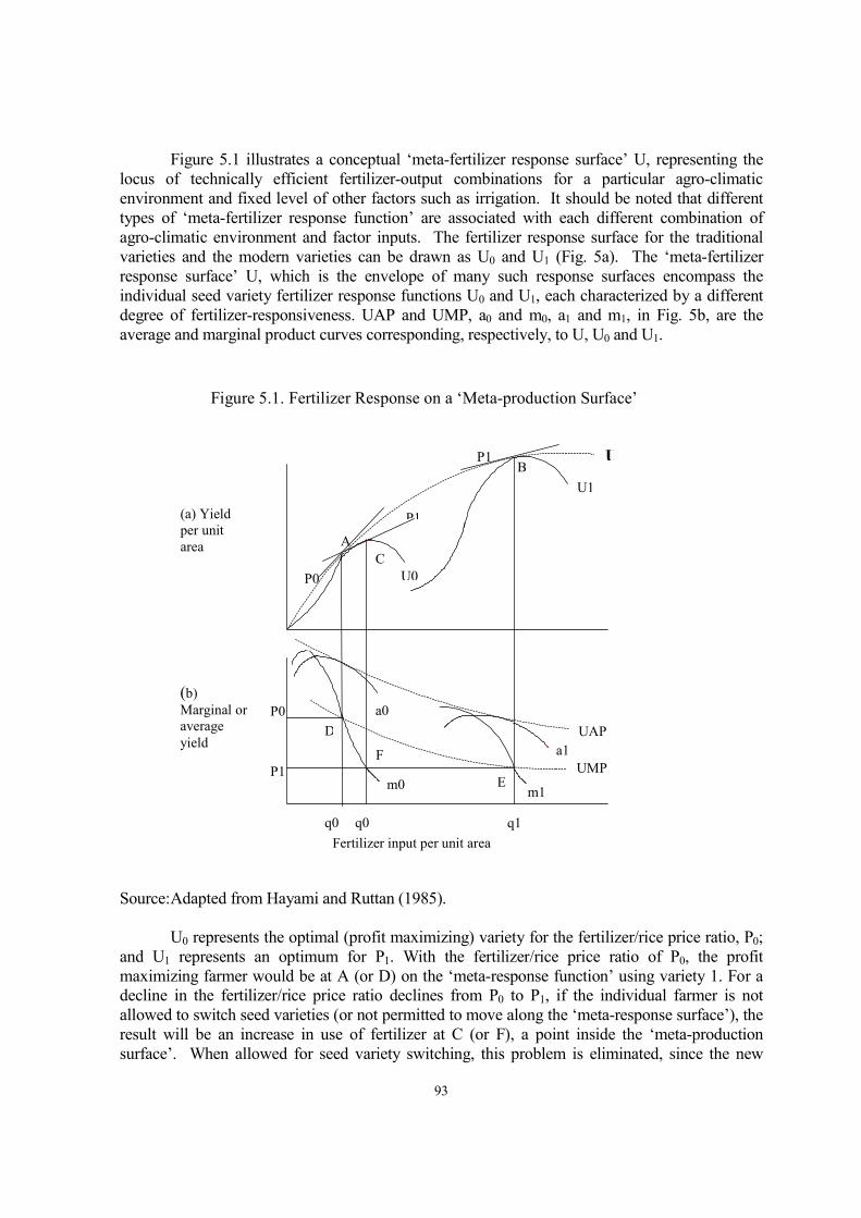
93

Figure 5.1 illustrates a conceptual ‘meta-fertilizer response surface’ U, representing the

locus of technically efficient fertilizer-output combinations for a particular agro-climatic

environment and fixed level of other factors such as irrigation. It should be noted that different

types of ‘meta-fertilizer response function’ are associated with each different combination of

agro-climatic environment and factor inputs. The fertilizer response surface for the traditional

varieties and the modern varieties can be drawn as U0 and U1 (Fig. 5a). The ‘meta-fertilizer

response surface’ U, which is the envelope of many such response surfaces encompass the

individual seed variety fertilizer response functions U0 and U1, each characterized by a different

degree of fertilizer-responsiveness. UAP and UMP, a0 and m0, a1 and m1, in Fig. 5b, are the

average and marginal product curves corresponding, respectively, to U, U0 and U1.

Source: Adapted from Hayami and Ruttan (1985).

U0 represents the optimal (profit maximizing) variety for the fertilizer/rice price ratio, P0;

and U1 represents an optimum for P1. With the fertilizer/rice price ratio of P0, the profit

maximizing farmer would be at A (or D) on the ‘meta-response function’ using variety 1. For a

decline in the fertilizer/rice price ratio declines from P0 to P1, if the individual farmer is not

allowed to switch seed varieties (or not permitted to move along the ‘meta-response surface’), the

result will be an increase in use of fertilizer at C (or F), a point inside the ‘meta-production

surface’. When allowed for seed variety switching, this problem is eliminated, since the new

A

P1

P0

P1 UB

U1

D

F a1

E m1

q1

m0

a0

U0

C

(a) Yield

per unit

area

(b)

Marginal or

average

yield

P1

P0

Fertilizer input per unit area

Figure 5.1. Fertilizer Response on a ‘Meta-production Surface’

q0 q0

UAP

UMP

94

fertilizer-output combination will be at B (or E) with variety type 2 on the ‘meta-response

surface’. Point C represents equilibrium for response surface U0 if undertaken by farmers, but a

disequilibrium in terms of potential alternatives described by the ‘meta-production function’ U. It

is worthy to note that fertilizer response to price is larger for movements along the

‘meta-response surface’ than along the seed variety specific surface (Hayami and Ruttan, 1985

and Pitt, 1983).

5.2 Nature of Alternative Crop Production Technologies and Resource Use

The term ‘technology’ generally refers to the application of knowledge to produce

output by utilizing factor inputs. Technological change in this context refers to change in the

process and combination of inputs to produce output. In this section, details of production

technologies of foodgrains (local and modern varieties of rice and wheat of all three seasons),

jute, potato, oilseeds, pulses, vegetables and cotton is outlined including their implications for

cost of production, capital requirements, profitability of cultivation, and returns to factor

shares. Thus far, most of the studies on nature and impact of ‘Green Revolution’ technologies

concentrated in the analyses of rice only, such as Hossain (1989), Ahmed and Hossain (1990),

Hossain et al. (1990), and Alauddin and Tisdell (1991). However, this study extends the scope

by including similar details for modern wheat varieties as well as other non-cereal crops in

order to cross-examine the viability of switching not only to modern varieties (MVs) of rice

and wheat, but also to other crops. Moreover, data for the aforementioned studies dates back to

1982 and 1987 at the latest. Therefore, even a reassessment of similar issues seems justified. It

should be noted that the main thrust of technological change in Bangladesh agriculture is

confined to rice and wheat and negligible in potato, jute and oilseeds. This is possibly another

reason for confinement of all major studies in rice alone.

5.2.1 Landuse and Cropping Intensity

Prior to the analyses of economics of various crops it would be worthwhile to highlight

the cropping seasons and major crops grown therein. Rice occupies about 70 percent of the

cultivated land and grown in all three seasons, Aus, Aman, and Boro, respectively (Appendix

Table A5.1). Aman is the monsoon season while Boro and Aus fall in the dry season and

overlap each other. Moreover, the modern Boro rice competes with modern Aus rice and has

similar characteristics. And these modern varieties are grown by substituting land from local

Aus rice, jute, broadcast Aman rice and minor dry season crops such as pulses and oilseeds

(Hossain et al., 1990). This is also evident in data of the present study where modern Boro rice

areas are very high covering about 35 percent of gross cropped area.

The cropping intensity of the surveyed region is estimated at 172.8 and closely

matches with the comparison study25

of 174.5, thereby, rendering confidence in the

25

In this chapter, three extensive survey based studies were used as comparison. These are: (a) Differential

Impact Study (DIS) of Modern Rice Technology conducted jointly by Bangladesh Institute of Development

Studies (BIDS) and BRRI covering 62 villages of 62 new districts. The data pertains to crop year 1987; (b) Farm

Level Fertilizer Use Study (FLFUS) conducted by International Fertilizer Development Centre (IFDC) covering

56 locations in 30 new districts. Data pertains to crop years, 1990, 1991, and 1992, respectively; and (c)

Agricultural Diversification Study conducted jointly by International Food Policy Research Institute (IFPRI) and

BIDS. Data pertains to crop year 1990/91.

95

representativeness of the data (Appendix Table A5.1). Among the three regions, however,

sharp differences exist in cropping intensity. The intensity of cropping is highest in Jamalpur

(183.3) followed by Jessore (178.2). Comilla region has the lowest cropping intensity (148.2)

largely due to the extensive rice monoculture in two seasons, Aman and Boro facilitated by the

large scale Meghna-Dhonagoda Flood Control Drainage and Irrigation (FCD/I) project, which

become operational in 1987.

The interesting point to note between the present study and comparison study is the

changes in the proportion of local Aus rice area and modern Boro rice area while the total

proportion of all rice area remains strikingly close (Appendix Table A5.1). The jute area

remained the same while pulse area dropped sharply. As for the other crops, they remain

comparable revealing little change has occurred in an attempt to diversify to non-cereal crops.

5.2.2 Yield Rates of Crops

Bangladesh agriculture is already operating at its land frontier and has very little or no

scope to increase the supply of land to meet the growing demand for food required for the

ever-increasing population. Moreover, owing to stagnation in industrial and services sector,

rural people tend to cling to the agricultural land making the land market very thin. Therefore,

only solution to increase food production lies in raising the productivity of land, either by

increasing the yield levels of crops or by increasing cropping intensity. Table 5.1 provides the

information on normal yield levels of all crops. The overall yield levels of crops are strikingly

close to the estimates of comparison studies thereby rendering confidence in these estimates

(Appendix Table A5.2).

It is clear from Table 5.1 that the yield levels of modern rice varieties are significantly

(p<0.01) higher than the local varieties in all regions. This explains the phenomena of drastically

declining local rice area in Bangladesh. Among the modern rice varieties of all three seasons, the

modern Boro rice yield levels are highest (Appendix Table A5.2). This is because modern Boro

rice requires complete mechanical irrigation while modern Aman rice and modern Aus rice is

grown mainly under rainfed conditions. It is interesting to note that though there are significant

differences in the yield levels of local varieties of rice across regions, the yield levels of modern

rice varieties as well as modern wheat is similar. This finding is consistent with the analyses of

regional variation in agricultural development levels done in Chapter IV which revealed that the

difference in the yield levels of local rice varieties is an important factor in explaining regional

differences.

Sharp inter-regional differences in yield levels are also observed for non-cereal crops

(Table 5.1). Comilla region has intensive production practices for potato, which resulted in

significantly (p<0.05) higher yield as compared to Jamalpur and Jessore regions. The reason is

mainly due to differential access to infrastructures. Only, Comilla region has a large cold storage

facility within 3-5 km from the study villages. Existence of cold storage is vital for storing

potato in order to fetch higher prices during off-season since the potato price hits record low

levels during harvest season. In case of spice production, Jamalpur region has significantly

(p<0.05) higher yield levels as compared to Comilla region. This is largely due to the individual

micro-climatic requirements for specific crops. This complex variability of agro-ecological

features for non-cereal/commercial crops limits the scope for a general policy of crop

96

diversification for the country as a whole. Rather, it demands careful analyses of soil as well as

micro-climatic suitability for individual crops, particularly, non-cereals.

Table 5.1 Yield rate of crops by study regions, 1996.

Crops Yield rates (mt/ha) in present study F-ratio for

regional

difference Jamalpur

region

Jessore

Region

Comilla

region

All region

Foodgrain crops

Modern wheat 2.14A 2.27

A 2.12

A 2.18 0.60

Local rice 2.59A 1.98

B 2.10

BC 2.32 5.29

a

Modern rice 4.17A 4.16

A 4.20

A 4.18 0.03

t-ratio for rice

variety difference

-8.72a -4.49

a -11.12

a -14.98

a

Non-cereal crops

Jute 1.63A 2.33

B 1.74

A 1.99 11.95

a

Potato

Pulses

Oilseeds

Spices

Vegetables

Cotton

11.56A

ng

1.18A

3.32A

8.84A

ng

8.80A

0.72A

1.02A

2.85AB

7.72A

1.30

16.04B

0.92B

1.29A

1.55B

ng

ng

13.93

0.76

1.17

2.75

8.00

1.30

9.75a

5.59b

1.15

3.76b

0.52

-

Note: Same block letters in superscript represents similarity in yield levels across regions for

individual crop based on LSD at 5 percent level of significance (p<0.05).

ng = not grown.

a = significant at 1 percent level (p<0.01);

b = significant at 5 percent level (p<0.05);

c = significant at 10 percent level (p<0.10).

Source: Field Survey, (1997).

5.2.3 Fertilizer Use Rates for Crops

Fertilizer use has been widespread in Bangladesh since the diffusion of modern

varieties of rice and wheat. Almost all of the farmers apply chemical fertilizers in modern rice,

wheat, potato and vegetables. However, the intensity of fertilizer use varies sharply with

higher levels of application on modern varieties grown during the dry season.

The fertilizer use rates for various crops are presented in Table 5.2. The intensity of

fertilizer use for crops is quite comparable with the comparison studies, particularly for rice

and wheat (Appendix Table A5.3). Fertilizer use rates are significantly (p<0.01) higher for all

modern rice varieties across regions. This is expected as the new technology require intensive

use of inputs, particularly, fertilizer, labor and irrigation, in order to realize the potential yield

levels. Moreover, there is significant (p<0.01, p<0.05, and p<0.10) inter-regional variation in

fertilizer use rates. Comilla region has the highest intensity of fertilizer use for most of the

crops followed by Jamalpur region. This is consistent since the soil fertility status of Comilla

97

and Jamalpur regions is tested to be poor as compared to Jessore region (see Chapter IX for

detail analysis).

In case of non-cereal crops, significant (p<0.05) regional differences in fertilizer use

rates are observed. The rate is highest for potato (348 kg/ha). The major reason is the use of

modern varieties of potato, which requires high doses of fertilizers, particularly, in Comilla

region. Cotton, a specialized crop, grown only in Jessore also consumes high doses of

fertilizers (326 kg/ha). The use rates are high and similar for spices and vegetables with high

inter-regional difference. Such sharp variation in use rates of fertilizers can also be attributed

to differences in soil fertility status of the study villages (analyzed in detail in Chapter IX).

Table 5.2 Chemical fertilizer use rates by study regions, 1996.

Crops Fertilizer use rates (kg/ha) in present study F-ratio for

regional

difference Jamalpur

region

Jessore

Region

Comilla

region

All region

Foodgrain crops

Modern wheat 218A 225

A 239

A 230 0.38

Local rice 126A 112

B 61

B 94 6.81

a

Modern rice 231A 244

A 279

B 246 17.71

a

t-ratio for rice

variety difference

-7.62a -3.44a -17.45a -16.11a

Non-cereal crops

Jute 132A 178

B 78

C 140 9.67

a

Potato

Pulses

Oilseeds

Spices

Vegetables

Cotton

286A

ng

175A

301A

175A

ng

392B

26A

117A

223A

286B

326

387B

95B

122A

230A

ng

ng

348

37

125

271

258

326

5.11a

10.32a

0.73

1.16

3.92b

-

Note: Same block letters in superscript represents similarity in yield levels across regions for

individual crop based on LSD at 5 percent level of significance (p<0.05).

ng = not grown.

a = significant at 1 percent level (p<0.01);

b = significant at 5 percent level (p<0.05);

Source: Field Survey, (1997).

5.2.4 Irrigation and Pesticide Use Rates for Crops

The market of irrigation in rural Bangladesh is imperfect and varies widely (Hossain,

1989). Until recently, irrigation was used only for growing modern varieties of rice. However,

due to erratic rainfall and to increase responsiveness of fertilizers, mechanical irrigation is

provided for most of the crops. Table 5.3 reveals that the cost for irrigation is highest for

modern rice varieties as expected. However, use of irrigation for other crops, including local

varieties, is a new phenomenon. Irrigation cost for Comilla region is significantly lower as

compared to other regions due to Meghna-Dhonagoda FCD/I Project, which supplies irrigation

98

through canals free of cost for sample households within its command area. For the non-cereal

crops, irrigation cost is also quite high, particularly, for vegetables, spices and potato with

sharp inter-regional differences. Irrigation cost for potato is high in Jessore region because this

is a dry region with less rainfall, thereby, requiring frequent irrigation.

Table 5.3 Irrigation and pesticide use rates by study regions, 1996.

Crops Irrigation cost (Taka/ha) Pesticides use rates (Taka/ha)

Jamalpur

region

Jessore

region

Comilla

region

All region Jamalpur

region

Jessore

region

Comilla

region

All

region

Foodgrain

Mod. wheat 1,161 1,612 113 835 86 13 78 56

Local rice 724 504 0 365 45 121 171 110

Modern rice 2,257 2,047 1,118 1,929 182 397 1,022 439

Non-cereals

Jute 494 1,011 0 612 71 123 0 78

Potato

Pulses

Oilseed

Spices

Vegetables

Cotton

1,319

ng

158

2,080

1,675

ng

3,118

232

768

1,265

1,635

682

518

0

0

706

ng

ng

962

196

316

1,584

1,645

682

1,029

ng

0

1,046

498

ng

94

23

10

0

1,687

1,926

1,347

0

130

0

ng

ng

1,159

20

72

623

1,390

1,926

Note: ng means not grown.

Source: Field Survey, 1997.

Use of pesticides in crops is dependent upon the disease and pest infestations and also

the type of crops grown. Though, in the past, pesticides are rarely applied in local rice crops, its

use rates substantially increased since the introduction of the modern varieties of rice and wheat.

Also, for the non-cereal crops, pesticide usage became a must. The large expenses incurred for

pesticides in modern rice, vegetables, and cotton is the evidence (Table 5.3). There are sharp

inter-regional differences in pesticide usage for crops. Comilla region with its poor soil quality

and intensive rice monoculture, use pesticides intensively as compared to other regions (Table

5.3). Except for vegetables and cotton production, pesticide use in Jessore region is generally

lower. Few studies report explicitly the usage of pesticides. As such, comparison for the change

in rate of pesticide use remains limited. However, it can be confidently stated that the current

level of pesticide use is much higher than the previous levels (detail time-trend analysis is

attempted in Chapter IX).

5.2.5 Human Labor and Animal Power in Crop Production

Traditionally, family-labor were the major sources of labor input in agricultural

production. Since the diffusion of modern agricultural technology, the demand for hired labor

increased substantially (Hossain, 1989; Ahmed and Hossain, 1990; and Hossain et al. 1990).

Table 5.4 reinforces the fact that demand for hired labor increased from previous 1987 cropyear

levels of 44 and 52 percent for local and modern rice varieties (Hossain et al., 1990) to 56 and 61

percent, respectively, and spread evenly across all crops. This has profound implication for

99

distribution of gains from modern agricultural technology as rural labor market is largely

composed of landless and marginal farmers. There are sharp differences in proportion of hired

labor use across regions for specific crops though a definite pattern cannot be ascertained. Since

labor requirement for each crop is different, the proportion of hired labor varies sharply across

regions as well as crops (for details of labor use see Chapter VII).

Table 5.4 Use of hired labor and hired animal power services by study regions, 1996.

Crops Hired labor as percent of total (%) Hired animal power as percent of total (%)

Jamalpur

region

Jessore

region

Comilla

region

All

region

Jamalpur

region

Jessore

region

Comilla

region

All

region

Foodgrain

Mod. wheat 64.2 50.6 57.8 56.3 34.5 52.0 85.3 66.7

Local rice 56.3 70.8 52.9 55.5 38.9 57.1 89.3 64.1

Modern rice 59.6 60.5 62.8 60.6 45.2 58.4 75.5 55.9

Non-cereals

Jute 60.0 60.0 72.1 63.1 26.9 47.8 79.3 52.0

Potato

Pulses

Oilseed

Spices

Vegetables

Cotton

51.2

ng

52.5

54.5

81.3

ng

78.6

50.0

63.3

41.4

42.6

72.7

46.2

39.5

52.9

51.4

ng

ng

49.4

47.6

55.8

51.1

52.4

72.7

58.1

ng

82.8

40.7

42.9

ng

30.8

50.0

60.9

61.5

33.3

45.8

94.3

92.7

83.8

72.9

ng

ng

59.3

74.2

78.8

56.3

36.0

45.8

Note: ng means not grown.

Source: Field Survey, 1997.

Until present time, use of mechanical power for agricultural operation,

particularly for land preparation, land leveling and transportation of harvests from fields to home

and market has been nascent. These activities are mainly performed by bullocks and cows, which

are used in pairs. Since the diffusion of the modern varieties of rice and wheat, demand for hired

animal power increased considerably (Table 5.4). Table 5.4 reveals that demand for hired animal

power increased sharply from previous 1987 cropyear levels of 10 – 13 percent (Hossain et al.,

1990) to 56 – 64 percent for rice crops. Also the rate of increase in hired animal power services is

much higher than the rise in hired labor indicating shortage of draft power resulting in a rapidly

growing market for hired animal power services. However, the implication for gains from

modern technology diffusion in this case is not the same as that of hired labor. Generally, the rich

and medium farmers own one or more pairs of bullock and/or cows. Therefore, sharp increase in

market for hired animal services implies that they gain from the modern technology diffusion on

two counts, first by cultivating modern varieties and second by hiring out animal services in

response to increased demand owing to technological change. It should be worth noting that each

bullock pair includes a hired labor and as such, it will have a complementary effect on the market

for hired labor demand but the extent of gain is much less.

5.2.6 Cost and Return Analyses of Crop Production

100

The estimates of costs and returns from crop production are computed at actual

prices paid and received by the farmers. Prior to the analysis of costs, the cost components are

discussed in details along with their justification.

Land is an important fixed asset and a source of wealth in rural setting. Therefore,

the opportunity cost of land for the owner operator is imputed at the net rental cost of land

incurred by the tenant farmer. The family supplied inputs of human labor and animal power

services, seeds, and manures are imputed at their market rates. One cost element that has not been

included is the opportunity cost of capital invested in crop production. Generally, farmers borrow

from non-institutional sources, such as moneylender, friends and relatives. Interest rates for these

sources are substantially higher than the bank rates for rural credit. Since these loans are mostly

taken for a number of purposes, such as, consumption, crop production, education, health care

and other services, and their duration being very short and diversified, apportioning the actual

cost for individual crop production seems intractable.

The items included in the estimation of cost and return variables are:

Cost components

Current inputs = seeds, manures, fertilizers, pesticides, and irrigation charges.

Purchased inputs = current inputs plus hired labor and hired animal power services.

Total cost of production = purchased inputs plus imputed value of family labor and animal

power services supplied from the household.

Land rent (opportunity

cost of land)

= gross value of output share received by landowner minus value of

input cost share paid by landowner.

Return components

Gross return

(gross value of output)

= value of total production plus value of by-product.

Farm family income = gross value of output minus purchased input.

Value added = gross value of output minus current inputs.

Profits (gross margin) = gross value of output minus total cost.

Farm operator surplus

(net of land rental cost)

= gross value of output minus total cost minus value of rent paid to

landowner.

Farm operator surplus

(Owner operator)

= gross value of output minus total cost.

Farm operator surplus

(Part tenant farmer)

= gross value of output minus total cost minus rent paid to landowner

for the portion of land rented-in.

Farm operator surplus

(Tenant farmer)

= gross value of output minus total cost minus rent paid to landowner

for the land rented-in.

The average profitability of producing various crops per unit of land area is presented

in Table 5.5. The relative weights of land area devoted to individual crop groups indicate the

dominance of the modern varieties of rice in the cropping system. Profits from modern

varieties of rice is significantly (p<0.01) higher for all crop seasons and highest in Boro season

(Tk.14,157/ha) followed by Aus (Tk.12,273/ha) and Aman (Tk.11,310/ha) seasons,

respectively (Appendix Table A5.4). Among the non-cereals, vegetables, spices, and potato

yields very high return per unit of land and the amount is at least twice the returns from

modern rice varieties and about four times of returns from local rice varieties. Despite such

101

high rates of return, these crops are grown selectively in specific regions largely due to high

price and yield risk associated with these crops and also marketing bottlenecks. Return from

jute is strikingly close to return from modern rice varieties while modern wheat yields much

less (Tk.7,790/ha). Even then, the area under jute has been declining sharply all over

Bangladesh mainly due to difficulty of jute retting in open water bodies, storing and marketing

bottlenecks and availability of cheap substitutes, the plastics.

Table 5.5 Average cost and profitability of crop production (all regions), 1996.

Crops Weights1 Yield

(ton/ha)

Price

(Tk/ton)

Gross value

(Tk/ha)

Variable cost

(Tk/ha)

Profits

(Tk/ha)

Foodgrain crops

Modern wheat 0.046 2.18 7,984 18,082 10,292 7,790

Local rice 0.092 2.32 5,452 13,952 7,347 6,515

Modern rice 0.700 4.18 5,637 24,809 11,983 12,826

t-ratio for rice

variety difference

- -14.98a

-3.72a -13.50

a -12.16

a -8.70

a

Non-cereal crops

Jute 0.047 1.99 9,395 20,539 9,089 11,450

Potato

Pulses

Oilseeds

Spices

Vegetables

Cotton

0.017

0.038

0.031

0.008

0.013

0.008

13.93

0.76

1.17

2.75

8.00

1.30

3,790

19,559

13,058

25,202

6,120

23,546

51,708

14,650

14,535

46,620

42,970

30,139

24,718

6,138

7,431

17,400

13,203

11,720

26,990

8,512

7,104

29,220

29,767

18,419

Note: a = significant at 1 percent level (p<0.01)

1 Weights as percent of gross cropped area.

Source: Field Survey, 1997.

Factor shares in crop production are estimated to analyze the distribution of gains from

crop production. Comparison of factor shares of crops provides a first hand knowledge on the

relative differences among crops with respect to the contribution of individual inputs to gross

value of production and, therefore, possess distributional implications. The actual contribution

of various factors in absolute terms may be largely different among crops depending on the

gross value of output realized from specific crops and thus, limits the scope for comparison.

The major argument in favor of modern agricultural technology is that it is labor intensive and

as such utilizes more hired labor. Therefore, gains from modern technology diffusion

indirectly reach to landless and marginal farmers who sell their labor in the rural labor market.

The factor shares in crop production at the mean level of all three regions are presented in

Table 5.6.

Factor shares of current input is higher for modern rice and wheat varieties as

compared to local rice varieties thereby confirming the capital intensity argument of the

modern agricultural technology (Table 5.6). The proportion of hired labor is similar between

local and modern varieties, about 11 – 13 percent of gross value of production distributed in

the form of wages for hired labor services, which presumably goes to landless and marginal

102

farmers. The rate is similar for some non-cereal crops, such as, jute, oilseeds, spices and

cotton.

The opportunity cost of land, the land rent ranges between 36 – 44 percent of gross

value of output. This indicates the scarcity and importance of land, as the prime source of

wealth in the rural region since for the owner operator, this cost component would be added as

return. Also, this explains the extent of vulnerability of tenant farmers most of whom become

bankrupt in case of crop failures and lose their meager landholdings to landlords and/or

moneylenders, thereby, exacerbating the pauperization process. The estimates of land rent

reported by Hossain et al. (1990) ranges between 43 – 45 percent of gross value of rice

production which is very close to the current estimates thereby rendering confidence in results.

Table 5.6 Factor shares in crop production (all regions), 1996.

Factors Factor shares as percent of gross value of production (%)

Local

rice

Moder

n rice

Mod.

wheat

Jute

Oil-

seeds

Potato Pulses Spices Vege-

tables

Cotton

Current input 13.7 21.2 23.2 11.4 14.9 31.0 13.9 12.6 13.7 17.0

Family 4.0 4.0 3.7 1.7 2.0 11.9 3.3 1.6 1.1 0.8

Purchased 9.7 17.2 19.5 9.7 12.9 19.1 10.6 11.0 12.6 16.2

Animal labor 14.1 8.7 12.6 10.2 15.7 4.5 15.5 5.1 5.4 7.6

Family 5.5 4.2 4.6 5.3 4.4 1.1 6.3 2.4 3.5 4.3

Hired 8.6 4.5 8.0 4.9 11.3 3.4 9.2 2.7 1.9 3.3

Human labor 24.9 18.4 21.1 22.6 20.5 12.3 12.5 19.6 11.8 14.2

Family 11.7 7.3 9.3 8.5 8.9 6.2 6.5 9.2 5.9 3.9

Hired 13.2 11.1 11.8 14.1 11.6 6.1 6.0 10.4 5.9 10.3

Land rent 39.4 37.5 38.7 35.7 41.5 42.8 39.3 43.5 40.1 36.4

Gross value

of output

13,952 24,809 18,082 20,538 14,535 51,708 14,650 46,620 42,970 30,139

Value added 86.3 78.8 76.8 88.6 85.1 69.0 86.1 87.4 86.8 82.9

Farm family

income

64.5 63.2 56.9 69.6 62.2 59.5 71.0 74.3 78.9 69.3

Farm Opera-

tor surplus

8.0 14.2 4.4 20.0 7.3 9.4 18.8 19.2 29.5 24.7

Observations 117 829 103 92 71 59 70 47 44 16

Note: Figures in parentheses are percentages of gross value of output (return).

Source: Field Survey, 1997.

The value added from crop production is around 77 – 89 percent of gross value of

output for all crops except for potato (69 percent only). The value added for modern rice

varieties is estimated at 79 percent and is lower by 7 percent when compared to local rice

varieties. This is largely due to high cost incurred for irrigation and/or water charge for

modern rice varieties. The irrigation cost include two cost components: fuel cost which is an

intermediate consumption, and depreciation cost of using the irrigation equipment which is a

return to capital and should be included in value added. However, difficulty in disaggregation

103

of the two cost components led to treat the entire water charge as the irrigation cost which is

underestimation of value added. Since modern varieties use higher level of irrigation, the

underestimation is higher thereby leading to lower value added.

Since land is scarce, farmers would tend to maximize the return from land. The return

over family resources, the farm family income, in absolute term is 74 and 14 percent higher

for modern rice and wheat varieties when compared to local rice varieties (Table 5.6). Hossain

et al. (1990) estimated that the farm family income is 72 percent higher for modern varieties

than for local varieties, which is strikingly close with the current estimate. The farm family

incomes for potato, spices, vegetables and cottons are similar for oilseeds and pulses when

compared to local rice varieties. This also explains the sharply declining trend of area under

oilseeds and pulses in Bangladesh as it yields as low as the local rice varieties.

The net return from per unit of land (farm operator surplus) is 3.2 times higher for

modern rice varieties as compared to local rice varieties when cost of land is included. The gap

in net return per unit of land among the non-cereals and foodgrain is much narrower as

compared to gap in farm family income for the same set of crops. The difference is largely due

to the high land rent. The net return from jute and potato becomes closely comparable to

modern rice varieties while spices, vegetables and cotton are significantly higher.

The labor productivity, estimated as value added per day of labor, was Tk. 190 for

modern varieties, which is 36 percent higher than Tk. 140 estimated for local varieties. The

labor productivity for modern wheat is Tk. 145. All these compare very favorably to the

prevailing wage rate of Tk. 46 per day. Hossain et al. (1990) also reported 31 percent higher

labor productivity for modern rice (Tk. 133) as compared to local rice varieties (Tk. 86) for the

crop year 1987.

5.3 Infrastructure Level in the Study Area and Construction of Infrastructure Index

Infrastructure, in development literature, generally refers to services and facilities that

are an integral part of human life. Infrastructure includes facilities for transportation,

communications, power, water supplies, education, health care, irrigation, drainage, and all

types of public utilities. The role of infrastructure in economic development is complex and its

effects are indirect. Ahmed and Hossain (1990) noted that infrastructure drastically reduce the

cost of marketing of agricultural products thereby exerting far reaching consequences for

comparative advantage of a country to compete in the world market. They also indicated that

the existence of interlocked labor market with land and credit markets is largely due to lack of

opportunity of alternative jobs in non-farm sectors that are constrained due to poor access and

infrastructural facilities. Also, infrastructure is critical in diffusion of modern agricultural

technology as easy access to transportation and communication system could promote

extension activities, marketing of products, and purchase of modern inputs. However, the

crucial role of infrastructure and institutions in augmenting agricultural productivity has been

felt only recently, in the mid-1980s, spurred by the observation of widespread stagnancy and

sluggish growth in agricultural productivity. Evenson (1986) noted that investments in rural

infrastructures, such as roads and rural electrification, is designed to change behavior of

farmers. Mann (1992), drawing on experience from Pakistan, suggested that a realistic strategy

to promote agricultural growth through national policies would be to repair the massive

104

infrastructure of the agricultural system as the root cause of low farm productivity lies into

biological, institutional, and social constraints.

In this study, one of the focuses is to measure the effects of rural infrastructure on

agricultural production and household economy in rural areas. As such, the urban and first-

order infrastructures such as national highway, ports, airports, etc. were excluded. Ahmed and

Donovan (1989) demonstrated that there is a gap in the methods of empirically measuring

effects of infrastructure. Ahmed and Hossain (1990) developed a composite measure of

infrastructure development using a cost-of-access approach, which is then successfully

employed as an explanatory indicator in subsequent quantitative analyses. In this study, the

composite index of infrastructure development is constructed using the same cost-of-access

approach while including a wider range of elements as compared to Ahmed and Hossain’s

(1990) index.

The infrastructure index for this study is constructed from village level information. A

total of 14 elements of infrastructure are selected. These are: primary markets (haat), growth

centers or secondary markets, high school (secondary school), college, post office, thana

headquarter, bus stop, paved road, bank, storage facilities, agricultural extension office, rice mill,

union council office, and health center. The railway and water transportation stations were

excluded because, only Comilla region use the Meghna river in addition to road, the Jamalpur

region use only the railway in addition to road, and Jessore region does not use any of these

two. The data includes distances in km, common mode of transport used and total cost of

travel in taka. The index formulation is shown in Section 3.7.1.5 of Chapter III.

In order to assess the representativeness of the infrastructure index so constructed using

the aforementioned procedure, rotated factor analysis is applied to the infrastructure variables.

The first three factors, agricultural extension office, bank, and bus stop explained about 83

percent of total variation (Appendix Table A5.5). The rank correlation among the two sets of

weights, the communality and correlation coefficients (of ICi with TC) is 0.43 and is significant

at 5 percent level (p<0.05). This indicates that the index constructed using cost-of-access

approach represents satisfactorily the index constructed using factor analytic approach.

However, for the present purpose, the infrastructure index constructed by using cost-of-access is

utilized throughout as an independent explanatory variable in subsequent analyses. However, it

should be noted that this is a village level index and, as such, households from a single village

will have the same index value.

Information on mean distances and inter- and intra-regional differences in distances of

14 elements of infrastructure from the study villages is provided in Appendix Tables A5.6 and

A5.7, respectively. Except paved road, union office and highschool, significant (p<0.01 and

p<0.05) regional differences exists in distances of these infrastructures from the study villages.

Observations of homogeneity among regions revealed that Comilla and Jessore are similar

while Jamalpur region is different (Appendix Table A5.7). The constructed infrastructure

index confirmed this intuition (Table 5.7). The distinction between developed and

underdeveloped villages is based on the value of index number below and above the mean

score of infrastructure index. The mean score of the index is estimated at 31.2. It is clear from

Table 5.7 that all six villages of Jessore region, five out of seven villages of Comilla region is

classified under developed infrastructure category as compared to only one village out of eight

105

of Jamalpur region, thereby, confirming the intuition reflected from Appendix Table A5.7.

The intra-regional classification also revealed that about half of Jamalpur villages are in the

underdeveloped category. The lower index value implies cheaper cost-of-access to the

infrastructural facilities indicating develop infrastructure. Therefore, the higher the index the

less developed the infrastructure. In other words, the index can be termed as ‘the index of

underdevelopment of infrastructure’ (Ahmed and Hossain, 1990).

Table 5.7 Infrastructure index numbers of 21 study villages, 1996.

Developed villages Underdeveloped villages

Region Name of village Index number Region Name of village Index number

Jessore

Comilla

Jessore

Jessore

Comilla

Jessore

Comilla

Comilla

Jamalpur

Jessore

Jessore

Comilla

Taherpur

Dhakirgaon

Mohanpur

Subalkati

Uddamdi

Juranpur

Silmondi

KhasUddam

Manikbari

Chandipur

Monaharpur

Fatehpur

14.87

16.32

16.37

17.18

18.81

19.28

21.22

21.96

24.71

24.83

26.14

30.05

Jamalpur

Jamalpur

Jamalpur

Jamalpur

Comilla

Jamalpur

Jamalpur

Jamalpur

Comilla

Karanipara

Rupshi

Sapleja

Deuliabari

Sonaterkandi

Sonakata

Munshipara

Jaliarpar

Begumpur

31.98

35.74

36.63

39.37

41.89

47.01

47.78

49.32

73.55

Note: The higher the infrastructure index the less developed the infrastructure.

Source: Computed from Field Survey, 1997.

5.4 Soil Fertility Status of the Study Area and Construction of Soil Fertility Index

Soil fertility refers to the inherent capacity of soil to supply plant nutrients in proper

amount, forms, and proportions required for the maximum plant growth (Uexkull, 1988). The

inherent capacity of supplying nutrients itself is a function of the type and nature of the

minerals present and the organic matter content in soils. And both the minerals and organic

components determine the amount of nutrients reserved in the soil and the rate at which these

nutrients are released to plants in available form (Dahal, 1996). However, it should be

mentioned that though fertility can be measured in terms of compounds or ions it does not

reflect the nature of crop productivity. This is because fertile soil may not necessarily be a

productive soil as all productive soils are not fertile (Dahal, 1996). This call for the concept of

nutrient availability closely associated with the concept of soil fertility. The nutrients, either in

soluble or exchangeable ions, become available to the plant root system once is in direct

contact. However, it is the capacity of the soil to release the unavailable minerals to the plant

in the required form that determines the crop productivity.

In this study, an attempt has been made to evaluate the existing soil fertility status of

the study villages. A total of ten soil fertility parameters, namely, soil reaction (pH), available

nitrogen (N), available phosphorus (P), available potassium (P), available sulfur (S), and

106

available zinc (Zn), organic matter content (OM), cation exchange capacity (CEC), electrical

conductivity (EC), and textural class are analyzed. Table 5.8 provides the summary results.

It is evident from Table 5.8 that the soil nutrient content largely varies across regions.

A test of homogeneity is performed in order to get a detailed grasp of the regional differences

in soil fertility status which revealed that Jamalpur and Comilla region have more or less

similar soil fertility levels while Jessore is largely different. The sharp difference is in organic

matter content of soils (Table A5.8 in the appendix).

Table 5.8 Summary of soil test results of the study regions, 1996.

Soil variable Jamalpur region Jessore region Comilla region All region Difference

(F-value) Mean CV Mean CV Mean CV Mean CV

pH 6.0 9 7.8 3 7.2 7 7.0 13 20.11a

OM (%) 2.0 39 6.5 44 1.5 24 3.3 85 12.96a

N (µg/g) 16.0 42 19.1 43 25.5 29 20.2 40 2.11

P (µg/g) 26.7 24 22.3 71 20.4 10 23.1 41 0.53

K (µg/g) 32.2 52 52.4 26 20.2 30 34.9 52 7.89a

S (µg/g) 7.8 20 10.2 36 5.5 13 7.8 37 5.08b

Zn (µg/g) 5.0 74 7.6 42 4.1 73 5.5 62 1.51

Sand (%) 19.9 28 8.7 64 3.5 49 10.7 78 16.19a

Silt (%) 57.7 14 52.2 17 74.9 6 61.6 20 12.70a

Clay (%) 22.4 30 39.1 36 21.7 24 27.7 44 5.43b

EC (µS/cm) 75.0 40 176.2 19 112.5 28 121.2 43 12.81a

CEC

(meq/100g)

10.9 32 26.2 33 15.8 29 17.6 49 8.52a

Note: CV = coefficient of variation expressed as (σ /x) * 100.

a = significant at 0.01 level (p<0.01); b = significant at 0.05 level (p<0.05).

Source: Field survey, 1997.

In addition to the analysis of infrastructural factors, another focus of this study is to

evaluate and measure the effects of soil fertility factor in agricultural production and

household economy. For this purpose, a composite index of overall soil fertility status of the

study villages is constructed. In deriving the mean index, nine soil test parameters are

considered. The soil texture parameter is excluded since it is quite similar across villages. The

index is constructed following the procedure adopted by Motsara (1994) and Dahal (1996).

First, the number of samples falling in each soil nutrient class (high, medium, and low) is

identified. The range of soil nutrient values used for classifying the samples in each class is

adopted from the ‘Soil Guides for Crop Production’ (in Bangla) published by Soil Resource

Development Institute (SRDI, 1990 and 1991) of Bangladesh. The detail of soil fertility index

of individual soil parameter is presented in Appendix Tables A9.1 – A9.9. Table 5.9 presents

the composite index value of soil fertility for the study villages.

It is clear from Table 5.9 that the soil fertility level is consistently low in Jamalpur and

Comilla region and medium in Jessore region. It should be noted that this index is also a

village level index and, therefore, households from a single village will have the same index

107

number representing overall soil fertility. This evaluation is particularly useful in the context

of the study because the inferences drawn from the analyses of productivity performance and

resource use efficiency of farmers of the study regions will incorporate this knowledge of bio-

physical limitation faced by them.

Table 5.9 Soil fertility index of 21 study villages, 1996.

Medium quality soil (index value 1.67 – 2.33) Low quality soil (index value < 1.67)

Region Name of village Index number Region Name of village Index number

Jessore

Jessore

Jessore

Jessore

Jessore

Jessore

Jamalpur

Subalkati

Mohanpur

Taherpur

Juranpur

Monaharpur

Chandipur

Sonakata

2.00

1.88

1.88

1.88

1.88

1.88

1.88

Jamalpur

Jamalpur

Jamalpur

Jamalpur

Jamalpur

Jamalpur

Jamalpur

Comilla

Comilla

Comilla

Comilla

Comilla

Comilla

Comilla

Rupshi

Karanipara

Munshipara

Jaliarpar

Sapleja

Deuliabari

Manikbari

Dhakirgaon

Shilmondi

Fatehpur

Sonaterkandi

Begumpur

Uddamdi

Khas uddamdi

1.38

1.50

1.50

1.50

1.50

1.63

1.63

1.38

1.50

1.63

1.63

1.63

1.50

1.63

Note: Index = {(n1 * 1) + (n2 * 2) + (n3 * 3)}/ n

where n1 ... n3 are respective number of sample in each class, and 1, 2, 3 are the

weights for low, medium, and high class and n is the sample size. The range of

available nutrient contents for each soil parameter for each class is taken from ‘Soil

Guide for Crop Production’ (in Bangla) of the Soil Resource Development Institute,

Bangladesh. The index value rated as < 1.67 = low, 1.67 – 2.33 = medium, and > 2.33

= high following Motsara (1994) and Dahal (1996)

Source: Field survey, 1997.

5.5 Farm-Level Input Demand Estimation Using ‘Meta-Production Function’ Approach

Section 5.2 elaborated on the nature of alternative production technologies, level of input

use, and relative profitability of major and minor crops comprising of the entire cropping system

of Bangladesh. Also Sections 5.3 and 5.4 elaborated on the construction of two special indices,

index of underdevelopment of infrastructure and index of soil fertility level of the study villages

that are to be incorporated as independent arguments in decision-making models.

The present section is set to empirically estimate the input demand and output supply

elasticities within a ‘meta-production function’ framework (elaborated in Section 5.1) which

allows for technology choices reflected in switching between modern and local varieties of seed.

108

Such analysis required to be conducted in two stages utilizing the Two-stage Switching

Regression procedure. The first stage is the estimation of reduced-form seed selection equation

which will enable us to compute the probability that any farm has information on modern variety

profit function (regime 1) or the local variety profit function (regime 2) using Probit Maximum

Likelihood Estimation procedure. It also shows how prices and fixed factors affect the probability

of choosing modern seed varieties. The second stage is the joint estimation of the normalized

restricted translog profit function and the variable factor share equations for the two separate

regimes using the Zellner's Seemingly Unrelated Regression Estimator26

(SURE).

5.5.1 Specification of the Model

The generalized translog profit function model and the ith share equation was developed

in Chapter III. From the general function (3.7.1.1), the normalized restricted translog profit

function for the farms can be specified in actual variables as:

where π' is the restricted profit from foodgrain (rice and wheat) production per farm: total

revenue less total costs of labor, chemical fertilizer, manures, irrigation, pesticides, and animal

power services normalized by the price of foodgrain; PW' is the money wage rate of labor per day

normalized by the price of foodgrain; PF' is the money price per kg of fertilizer materials

normalized by the price of foodgrain; and PM' is the money price of animal power per hectare

normalized by the price of foodgrain.

Five fixed inputs are included in the specification of the profit function. ZL is the land

input per farm measured as hectare of foodgrain (all rice and wheat varieties) grown in one year;

ZA is the value of the non-farm fixed capital assets used for foodgrain production per farm

measured as taka of total stock value; ZI is the index of underdevelopment of infrastructure

measured at the village level; ZS is the soil fertility index measured at the village level; and ZE is

the level of education of the farmer measured as years of schooling completed. The variable MR

represents the Mill’s Ratio to be obtained from the first stage probit estimate of the reduced-form

seed selection equation. The parameters α0, α, β, γ, δ, ψ, ω and σ are to be estimated and

subscripts W, F, and M stands for the variable inputs of production, viz., labor, chemical

fertilizer, and animal power, respectively.

26

LIMDEP Version 6 (1992) is used for the purpose.

)1.5.5(lnlnlnln

lnlnlnlnlnlnlnlnlnln

lnlnlnlnlnlnlnlnlnln

lnlnlnlnlnlnln'lnln'ln

ln'lnln'lnln'lnln'lnln'ln

ln'lnln'lnln'lnln'lnln'ln

ln'lnln'lnlnlnlnlnln

'ln'ln'ln'ln'ln'ln'ln'ln

'ln'ln'ln'ln'ln'ln'ln'ln

21

21

21

21

21

21

21

21

0

υσωωωωωωωωωωψψ

ψψψδδδδδδδδδδδδδδβββββ

γγγγγγααααπ

+++++++++

+++++

+++++

++++++++++

+++++++

++++

+++++=

MRZZZZ

ZZZZZZZZZZ

ZZZZZZZZZZ

ZZZZZZZPZP

ZPZPZPZPZP

ZPZPZPZPZP

ZPZPZZZZZ

PPPPPPPP

PPPPPPP

iuESSEEIIE

SIISEAAESAASIAAIELLE

SLLSILLIALLAEEEESSSS

IIIIAAAALLLLEEMESMMS

IMMIAMMALMMLSFFSIFFI

AFFALFFLEWWESWWSIWWI

AWWALWWLEESSIIAALL

MFFMMWWMFWWFMMMM

FFFFWWWWMMFFWW

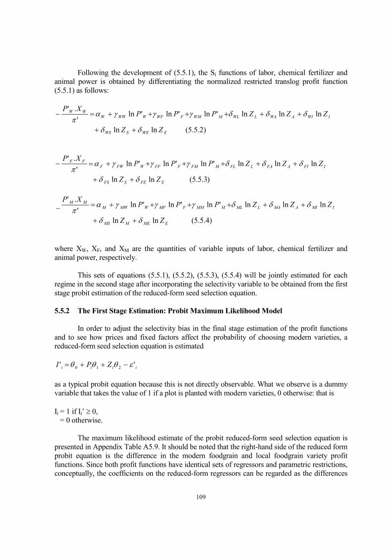
109

Following the development of (5.5.1), the Si functions of labor, chemical fertilizer and

animal power is obtained by differentiating the normalized restricted translog profit function

(5.5.1) as follows:

where XW, XF, and XM are the quantities of variable inputs of labor, chemical fertilizer and

animal power, respectively.

This sets of equations (5.5.1), (5.5.2), (5.5.3), (5.5.4) will be jointly estimated for each

regime in the second stage after incorporating the selectivity variable to be obtained from the first

stage probit estimation of the reduced-form seed selection equation.

5.5.2 The First Stage Estimation: Probit Maximum Likelihood Model

In order to adjust the selectivity bias in the final stage estimation of the profit functions

and to see how prices and fixed factors affect the probability of choosing modern varieties, a

reduced-form seed selection equation is estimated

as a typical probit equation because this is not directly observable. What we observe is a dummy

variable that takes the value of 1 if a plot is planted with modern varieties, 0 otherwise: that is

Ii = 1 if Ii’ ≥ 0,

= 0 otherwise.

The maximum likelihood estimate of the probit reduced-form seed selection equation is

presented in Appendix Table A5.9. It should be noted that the right-hand side of the reduced form

probit equation is the difference in the modern foodgrain and local foodgrain variety profit

functions. Since both profit functions have identical sets of regressors and parametric restrictions,

conceptually, the coefficients on the reduced-form regressors can be regarded as the differences

)2.5.5(lnln

lnlnln'ln'ln'ln'

.'

EWESWS

IWIAWALWLMWMFWFWWWW

WW

ZZ

ZZZPPPXP

δδ

δδδγγγαπ

++

++++++=−

)3.5.5(lnln

lnlnln'ln'ln'ln'

.'

EFESFS

IFIAFALFLMFMFFFWFWF

FF

ZZ

ZZZPPPXP

δδ

δδδγγγαπ

++

++++++=−

)4.5.5(lnln

lnlnln'ln'ln'ln'

.'_

EMEMMS

IMIAMALMLMMMFMFWMWM

MM

ZZ

ZZZPPPXP

δδ

δδδγγγαπ

++

++++++=

iiii ZPI '' 210 εθθθ −++=

110

between the modern foodgrain and local foodgrain variety profit function coefficients for the

same regressors (Pitt, 1983).

Thirteen of the total forty-five estimated coefficients are statistically significant at 10

percent level at the least (Appendix Table A5.9). About 89 percent of the observations are

accurately predicted and the McFadden's R-squared27

was 0.23. The coefficients of probit

reduced form seed selection function cannot directly reveal the sign or magnitude of the change

in the probability of cultivating modern foodgrain varieties in response to change in the

exogenous variables. The probit estimation is used mainly to obtain the selectivity variable (or

Mill's ratio) to be incorporated in the second stage of estimation and to check the accuracy of

prediction. Information on the magnitude and direction of factors affecting seed selection is

provided as elasticities in Table 5.10.

The following procedures were used to obtain the probit elasticities: the derivative of the

probabilities with respect to a particular exogenous variable for the probit model is given by:

where F is the distribution function and f is the density of the standard normal; βk is the

coefficient attached to the exogenous variable Xik (Maddala, 1987). Therefore, the elasticity of

the probability of ith exogenous variable is:

where p is the probability.

Seven of the nine elasticities (at the sample means) are significantly different from zero at

1 percent level (p<0.01) suggesting that seed selection is highly responsive to changes in prices

and fixed factors (Table 5.10). The highly elastic response to foodgrain price change reflects the

responsiveness of the farmers to increase their stagnant income through operating in the output

market. The elasticity of probability with respect to land area is positive, though small, suggesting

that farm size, is positively related with modern foodgrain production.

Table 5.10 Elasticity of probability of planting modern foodgrain varieties, 1996.

Exogenous variables Estimated coefficients t-ratio

Rice price

Labor price

Fertilizer price

Animal power price

Land area

2.425

-0.366

-0.045

-0.486

0.005

65.899a

- 5.097a

- 1.405

-18.489a

0.838

27

McFadden's R² is not comparable to the R² in the OLS regression. McFadden's R² lies in the range of 0.20 to

0.40 in this type of model (Sonka et al., 1989).

)5.5.5()()(

ki

ik

i fX

Fβφ

φ=

∂∂

)6.5.5(.)(.)(

i

ik

ki

i

ik

ik

i

hp

Xf

p

X

X

Fβφ

φς =

∂∂

=

111

Farm capital

Underdevelopment of infrastructure

Soil fertility

Education of farmer

0.354

0.086

0.635

-0.152

44.279a

4.072a

20.238a

-23.498a

Note: a = significant at 1 percent level (p<0.01).

Source: Computed.

The significant (p<0.01) influence of non-conventional factors in increasing probability of

planting modern varieties is an indication of the bottlenecks existing in the present foodgrain

production system. The positive coefficient of index of underdevelopment of infrastructure

indicates that modern technology adoption is higher in the underdeveloped regions. This finding

is apparently in contrast with the expectation, which however, becomes clear when all other

factors are considered in details. In an underdeveloped region, the choices open to farmers are

highly limited. Also, access to non-farm activities is limited. It was also shown in Section 5.2 that

though the profitability of modern rice and wheat is significantly higher than the local rice

varieties but it is not higher than most of the non-cereal crops, particularly, potato, vegetables,

spices and cotton. Therefore, in a rural region with underdeveloped infrastructure, limits to

produce commercial crops and poor access to non-farm activities would induce farmers to adopt

modern foodgrain technology because it would ensure significantly higher income than growing

traditional foodgrain at the minimum. The argument will be clearer in the subsequent analyses.

The soil fertility index has a large positive value indicating that diffusion of modern

agricultural technology will increase significantly with improvement in soil fertility status as

expected. However, the education level of farmer has a negative influence in increasing modern

technology diffusion. Deb (1995) also reported negative influence of education level in modern

technology adoption citing that the education system in Bangladesh is not agriculture oriented

and therefore pulls people out of agriculture and induce them to engage in non-farm activities that

are more rewarding in general.

5.5.3 The Second Stage Estimation: Maximization of the Profit Function

From the first stage probit estimation, we defined the Mill's ratio or selectivity variable

which are used as identifiability restriction to adjust the selectivity bias and force the separation

of the translog profit function of the two regimes (1) and (2). One of the interesting properties of

the Mill's ratio is that, the higher the value of the ratio, the lower is the probability that an

observation is having data on Ii = 1 (Heckman, 1976).

The final specification of the reduced-form of the translog profit function with the

inclusion of the selectivity variable are restated as:

112

These translog profit functions and the corresponding three share equations for each

regimes were jointly estimated by using Zellner's Seemingly Unrelated Regressions Estimator

(SURE).

The joint restricted parameter estimates of the normalized restricted translog profit

function and labor, fertilizer, and animal power share equations adjusted for selectivity bias for

modern foodgrain and local foodgrain varieties are presented in Appendix Table A5.10. The

Wald Test satisfies the validity of the estimation of two functions and are highly significant (see

bottom of Appendix Table A5.10). This proves, among other things, that the sample farms, on an

average, maximize profits with respect to normalized prices of the variable inputs, thus

supporting empirically the assumption of profit maximization. Evidence of profit maximizing

behavior of the Bangladeshi farmers were also noted by Hossain (1989), Hossain et al., (1990)

and Ahmed and Hossain (1990).

Fifty-four and thirty-five coefficients of the total 73 coefficients in each set of functions

are statistically significant at 10 percent level at the least (Appendix Table A5.10). The adjusted

R-squared is 0.64 and 0.43 in modern foodgrain and local foodgrain functions, respectively. This

is quite satisfactory as it maintains the validity of including large number of fixed factors along

with interaction terms in each of the functions.

At the bottom of the profit function in Appendix Table A5.10, the coefficients of the

selectivity variables appear, -ƒ(φi)/F(φi) for the modern foodgrain variety function and ƒ(φi)/[1

- F(φi)] for the local foodgrain variety function. The selection variable is significantly different

from zero at 1 percent level of significance (p<0.01) in the modern foodgrain profit function.

This is the evidence of pronounced selection bias in estimating equations from a subsample of

cultivators (Pitt, 1983). On the other hand, there appears to be no significant selection bias in

the estimation of the local foodgrain variety function. Therefore, single stage estimation of this

function from a subsample of local variety cultivators should be unbiased28.

Most of γij coefficients are of negative signs in both the regimes as expected. The

negative cross-price coefficients imply a complementarity in inputs. Land coefficient (βL) is small

but positive in modern variety regime implying profitability would increase with increase in land

while it is negative for local variety regime implying that planting more land with local varieties

will incur loss. This is consistent with the analysis of factor shares in rice and wheat production

which, revealed that the net income from growing local varieties of rice is negative for Aus and

Boro season for many farmers. The positive farm capital coefficients (βA) in both function

implies that increase in capital endowment would increase profitability. The large positive soil

fertility coefficient implies that profitability will increase with improvement in soil quality, which

28

In general, the selectivity variable may be significant in any or both of the equations (Lee, 1978 and Pitt, 1983).

ietiesfoodgrainlocalforf

fZP

ietiesfoodgrainernforF

fZP

li

i

i

lilili

hi

i

i

hihihi

var))(1

)((

varmod)(

)((

'2

'1

ξφ

φσγβπ

ξφφ

σγβπ

ε

ε

+−

++=

+−

++=

113

is consistent with our a priori expectation. The infrastructure coefficient is positive implying that

profitability will be higher in underdeveloped regions. This is due to increase in return from

foodgrain production in case of shortage in supply and with little scope for bringing in foodgrain

from other areas owing to underdeveloped infrastructure. The education coefficients are small,

non-significant and have mixed signs, positive for modern variety regime and negative for local

variety regime.

The coefficients are generally found to be larger in magnitude for local foodgrain

function. This is because the profitability in local foodgrain variety production is significantly

lower as compared to modern foodgrain. As such, variations in input prices and exogenous

factors would lead to larger decreases in profitability in absolute terms. On the other hand,

smaller coefficient in modern foodgrain function implies that the extent on reduction would be

lower for an equivalent change in input prices and exogenous factors. However, firm conclusions

can be drawn only from the elasticities to be computed using these profit function coefficients,

factor demand functions and input prices.

5.5.4 Input Demand and Output Supply Elasticities

The estimates presented in Appendix Table A5.10 form the basis for deriving elasticity

estimates for foodgrain supply and demand for the variable inputs of labor, fertilizer, and animal

power services. These elasticity estimates for individual varieties were first obtained by using

equation (3.7.1.18), (3.7.1.19), (3.7.1.20), (3.7.1.23), (3.7.1.24), and (3.7.1.25) of Chapter III. As

noted earlier, the elasticities are functions of variable input ratios, variable input prices, level of

fixed inputs, and the parameter estimates of the translog profit function presented in Appendix

Table A5.10. These elasticities are evaluated at simple averages of the Si variable input prices and

fixed inputs. This provides the basis of using equation (3.7.1.27), which uses these estimates from

each regime plus the elasticities of the probabilities presented in Table 5.10. The total elasticity of

demand after allowing for seed switching adjustments (or permitting movements along the ‘meta-

response surfaces’) are presented in Table 5.11.

Table 5.11 Input demand and output supply elasticities of foodgrain crops with variety switching

adjustments, 1996.

Output

price

Labor

price

Fertilizer

price

Animal

price

Land Farm

capital

Infra-

structure

Soil

quality

Educa-

tion

Output

supply

0.6470

(30.0)

-0.2357

-0.0759 -0.1384 0.5997 0.5746 4.8706 7.7288 -0.3175

Labor

demand

0.4229 -0.5322

(18.9)

0.0399 0.1186 0.4495 0.4631 5.1172 6.7776 -0.2500

Fertilizer

demand

0.7832 -0.1396 -0.5951

(6.2)

-0.1845 0.7164 0.6902 5.1812 7.9856 -0.3228

Animal

demand

1.0626 0.2154 -0.1063 -0.9770

(0.7)

0.5966 0.4275 4.7235 7.1266 -0.2097

Note: Figures in parentheses represents percent of improvement due to variety switching

adjustments.

Source: Computed.

114

In the translog function, unlike Cobb-Douglas, the impact across variable input

demand functions for labor, fertilizer, and animal power of a given change in any of the

exogenous variables is not symmetric. It varies across demand equations, which is consistent

with a priori theoretical expectations (Sidhu and Baanante, 1981). All the own-price

elasticities of demand are less than one except for labor in local variety regime indicating an

inelastic response of factor utilization (Appendix Table A5.11). The total own price elasticity

for labor was estimated at -0.45 and the seed switching adjustments increases the elasticity by

about 18 percent to -0.53. The improvement in own price elasticity of fertilizer is about 6

percent, from -0.56 to –0.60. The highest level of increase is in the output supply elasticity.

The total own price elasticity of supply changes from 0.50 to 0.65, a 30 percent increase.

Rahman and Sriboonchitta (1995) reported that allowance for seed switching between high

quality aromatic rice and low quality glutinous rice in Chiang Mai valley of Thailand

improved the elasticity estimates by 16, 49, 42, and 58 percent for fertilizer, labor, tractor

power and rice output, respectively. Pitt (1983) reported that allowance for seed switching

between modern and local varieties of rice in Java, Indonesia improve the elasticity of

fertilizer demand by 11 percent.

The fixed inputs appear to be important in influencing foodgrain supply. Their influence,

however, is not uniform on labor, fertilizer and animal power demand functions. The exogenous

increases in land quantities and expansion in farm capital increases output supply and demand for

all variable inputs of production. The elasticities of output supply with respect to land size and

value of fixed farm assets are estimated at 0.60 and 0.57, respectively. This indicates that a one

percent increase in land size would increase output supply by 0.60 percent while a one percent

increase in the value of fixed farm assets would increase output supply by 0.57 percent.

The influence of soil fertility status is very high. The elasticity value indicates that 1

unit increase in the index of overall soil fertility (which is almost a movement from one class

to another class in such a composite index) would increase output supply by 7.7 units and

increase input demand by 6.7 to 7.9 units. The influence of infrastructure is also very high.

Both output supply as well as input demand will increase in underdeveloped region, as

increasing demand for input may not be adequately supplied owing to underdeveloped

infrastructure. On the other hand, the supply of output will be higher due to marketing

bottlenecks in underdeveloped region. All price effects are quite reasonable, and

nonsymmetrical nature of their impact, contrary to the Cobb-Douglas case, is as expected and

more natural.

At an individual variety level, the own-price elasticity of fertilizer input is relatively

higher (-0.52) for modern varieties and is consistent with the expectation (Appendix Table

A5.11). Few farmers expressed interest to expand local foodgrain area, as the existing level of

production is enough for consumption and market opportunities for local foodgrain is uncertain.

Price elasticity of labor is higher in local foodgrain function. In Section 5.2, it was revealed that

relatively less hired labor was used in local foodgrain production implying farmers’ responses

would be higher to changes in labor price. Also, since the profit margin in local rice is

significantly lower as compared to modern foodgrain, farmers tend to response actively to price

increases because it would result in larger cuts in absolute profits than modern foodgrain for an

equivalent rise in prices. On the other hand, changes in output price have higher response in local

115

foodgrain function as compared to modern foodgrain because of its preference for consumption

and could be inherent attachment to tradition and culture as well.

The cross-price effects for both regimes are not different from each other, due to the

inelastic nature of overall response to price changes. Output supply and input demand elasticities

with respect to fixed farm assets were, however, largely different between two functions. The

influence of soil fertility in local variety function is more than double to that of modern variety

function implying that farmers would like to grow local varieties if soil fertility status increases.

This is because producing local varieties will exert less pressure on capital requirements and

increase in soil fertility would raise productivity to a desired level. Also, the education variable

has a larger negative effect indicating that farmers with higher level of education discards

growing local varieties to a larger extent.

5.5.5 Maximization of Profit Function for Non-cereals: One Stage Estimation

Since most of the farmers interviewed in this survey also produced a wide variety of non-

cereals, an attempt has been made to evaluate their response to prices and fixed factors with

respect to non-cereal production by utilizing a farm-level aggregate profit function framework.

The reason for aggregation is largely due to the limitation posed by few observations on

individual non-cereal crops, such as oilseeds, pulses, vegetables, potatoes and cotton. An

aggregate profit function for non-cereals with the same set of variables used for foodgrain

function is estimated. Appendix Table A5.12 provides the joint restricted parameter estimates of

the normalized restricted translog profit function and labor, fertilizer, and animal power share

equations. The Wald Test satisfy the validity of the estimation of function and is highly

significant (see bottom of Appendix Table A5.12). This proves, among other things, that the

sample farms, on an average, maximize profits with respect to normalized prices of the variable

inputs, thus supporting empirically the assumption of profit maximization for the non-cereal

crops as well.

Twenty-six coefficients of the total 73 coefficients of the functions are statistically

significant at 10 percent level at the least (Appendix Table A5.12). The adjusted R-squared is

0.38 which can be considered as satisfactory since the function includes a diverse range of crops

while still maintains the validity of a large number of fixed factors along with interaction terms.

Most of γij coefficients are of negative signs as expected. The negative cross-price

coefficients imply a complementarity in inputs. Land coefficient (βL) is large and positive

implying that profitability would increase with increase in land. This is consistent with the

analysis of factor shares in non-cereal crop production, which reveal that the net income from

growing non-cereal crops is very high. The small but positive soil fertility coefficient implies that

profitability will increase with improvement in soil quality consistent with a priori expectation.

The infrastructure coefficient is negative indicating that profitability from commercial

crop production is higher in developed region, a finding exactly opposite to that of foodgrain

production. However, this is expected since development of infrastructure is intricately linked

with the marketing and storage facilities which is vital for realizing profits from these crops. Also,

as explained earlier that developed infrastructure offers more choices to farmers. The education

coefficient is also positive indicating that educated farmers chose to grow non-cereal crops which

116

provides higher profitability as shown in Section 5.2. However, firm conclusions can be drawn

only from the elasticities to be computed using these profit function coefficients, factor demand

functions and input prices.

5.5.6 Input Demand and Output Supply Elasticities of Non-cereal Crops

The price elasticities for non-cereal crops are presented in Table 5.12. All the own-price

elasticities of demand are greater than one except for fertilizer indicating highly elastic response

of factor utilization. A finding opposite to foodgrain production where farmers are more or less

showed inelastic response to factor utilization. The output supply elasticity is also highly elastic

(1.33) indicating that farmers respond sharply to output price changes. The own price elasticities

for labor, fertilizer and animal power services are estimated at -1.55, -0.72 and -1.22,

respectively.

The fixed inputs also seem to be important in influencing output supply as well as

input demand. The elasticities of output supply with respect to land size is 0.23 indicating that

a one percent increase in land size would increase output supply by 0.23 percent. The

influence of soil fertility status is quite high and positive indicating that improvement in soil

quality will increase non-cereal output supply and input demand.

Table 5.12 Input demand and output supply elasticities of non-cereal crops, 1996.

Output

price

Labor

price

Fertilizer

price

Animal

price

Land Farm

capital

Infra-

structure

Soil

quality

Educa-

tion

Output

supply

1.3370 -0.6928 -0.1761 -0.4072 0.2349 -0.0715 -1.3889 0.6067 0.3295

Labor

demand

2.6050 -1.5524 -0.4286 -0.6240 0.2026 -0.0654 -1.2787 0.2787 0.3121

Fertilizer

demand

2.4649 -1.7981 -0.7221 0.0554 0.3784 -0.1079 -1.0989 0.4634 0.4221

Animal

demand

2.4063 -1.2106 0.0256 -1.2213 0.3217 -0.0985 -1.3480 1.0708 0.3248

Note: Non-cereal crops include jute, potato, pulses, oilseeds, spices, vegetables, and cotton.

Source: Computed.

The influence of infrastructure is also very high. The negative elasticity values of this

variable indicates that both non-cereal output supply as well as input demand is higher in

developed region, a finding opposite to that of foodgrain production and is expected. Also, the

education variable has a positive coefficient indicating that farmers with higher level of

education chose to grow non-cereal crops, which yields higher profitability. All price effects

are quite reasonable, and nonsymmetrical nature of their impact, contrary to the Cobb-Douglas

case, is as expected and more natural.

5.5.7 Indirect Estimates of Production Elasticities

117

The usual approach for estimating production elasticities or the output elasticities is by

estimating the production function directly. However, farm-level estimation of production

function suffers from a number of limitations, particularly the multicolliniarity problem. A

profit function approach is considered a superior technique and avoids the multicollinearity

problem and thus, utilized in this study. However, if one wishes, the production elasticities can

be indirectly derived from the information of price elasticities.

The indirect estimate of output elasticities of input i can be obtained by utilizing the

following identities (Puapanichya and Panayotou, 1985):

γi* = -γi (1 - µ)-1

, i = W, F, M. (5.5.7)

βi* = -βi (1 - µ)-1

, i = L, A, E, I, S. (5.5.8)

where,

γi = production elasticities of variable input i

βi = production elasticities of fixed input i

Summing up (5.5.7) we obtain:

And by substituting eq. (5.5.10) into eq. (5.5.9), we obtain

µ* = -µ(1-µ)-1

Therefore

(1-µ) = (1-µ*)-1

(5.5.11)

Finally substituting eq. (5.5.11) in eq. (5.5.7) and (5.5.8), we obtain

γi = -γi* (1 - µ*)-1

, i = W, F, M. (5.5.12)

βi = -βi*(1 - µ*)-1 , i = L, A, E, I, S. (5.5.13)

∑=

=3

1i

iγµ

∑=

−−−=3

1

1 )9.5.5()1(*i

i µµγ

∑=3

)10.5.5(**i

iγµ

118

Now, the computation of production elasticities of inputs is straightforward as eq.

(5.5.12) and eq. (5.5.13) are expressed in terms of price elasticities of inputs that are available

from Tables 5.11 and 5.12 for foodgrain crops and non-cereal crops, respectively. Table 5.13

presents the indirect estimates of production elasticities.

The role of fertilizer in modern varieties of rice and wheat is distinct from Table 5.13.

The output elasticity is almost double to that of elasticity of local rice varieties. The elasticity

of fertilizer for non-cereal crop is also very high. It is interesting to note that the production

elasticities of variable inputs are much higher than the fixed inputs, land and farm capital. The

effect of education level of farmers has a negative impact on foodgrain production indicated

by the negative coefficient of education variable while it is positive for non-cereal crop

production. Soil fertility has a very high elastic response to crop production which, is

expected. The elasticity of underdeveloped infrastructure indicates that foodgrain production is

higher in underdeveloped regions while for non-cereal crop it is higher in developed regions.

The estimate of the returns to scale of conventional inputs, that is, labor, animal power,

fertilizers, land and farm capital reveals that ‘increasing returns to scale (1.13 > 1)’ prevails in

local rice production while modern rice and wheat production is characterized with ‘constant

returns to scale (0.98 ≈ 1)’ (Table 5.21). The overall foodgrain production is very likely to be

characterized by ‘constant returns to scale (1.04 ≥ 1)’. The non-cereal crop production,

however, depicts ‘decreasing returns to scale (0.82 < 1)’ which is quite disturbing as this might

limit any scope for crop diversification. It should be noted that this aggregate non-cereal crop

model incorporates a diverse set of crops in which returns to scale for individual crops may be

variable. Therefore, it would be desirable to empirically estimate individual non-cereal crop

elasticities which, is beyond the scope of this study due to the focus of the study in one hand,

and the small sample size of individual non-cereal crops grown by these predominantly rice

farmers on the other.

Table 5.13 Indirect estimates of the production elasticities, 1996.

Factors/inputs Name of the crops for which the elasticities are estimated

Local varieties

of rice

Modern varieties

of rice and

wheat

All foodgrain

crops

Non-cereal crops

Conventional inputs

Labor 0.3431 0.1472 0.1741 0.3453

Animal power 0.2634 0.3294 0.3147 0.2717

Fertilizer 0.0950 0.1795 0.1917 0.1606

Land 0.1874 0.1944 0.1902 0.0633

Farm capital 0.2428 0.1314 0.1736 -0.0191

Non-conventional inputs

Education -0.2542 -0.0688 -0.0886 0.0772

Infrastructure 0.5240 1.6321 1.6021 -0.2844

Soil fertility 4.3282 2.3416 2.3853 0.1345

Returns to scale

(Conventional inputs)

1.13 0.98 1.04 0.82

119

Note: The infrastructure variable is defined as underdevelopment of infrastructure, therefore,

positive elasticity means negative response on output.

Source: Computed.

5.6 Inferences

Input-output analysis of crop production revealed that yield per unit of land area for

modern rice varieties is significantly higher than the local varieties in all crop seasons. The

yield levels for modern and local rice varieties are estimated at 4.18 ton/ha and 2.32 ton/ha,

respectively. The estimates for crops seasons for modern rice variety yields are 3.6 ton/ha, 3.5

ton/ha, and 4.8 ton/ha for Aus, Aman and Boro season while local rice varieties are 1.99

ton/ha, 2.38 ton/ha, and 2.60 ton/ha, respectively. No significant regional differences in yield

levels of modern rice varieties are observed contrary to local rice varieties. The fertilizer use

rates per unit of land (kg/ha) is significantly higher for modern rice varieties (246 kg/ha) than

local rice varieties (94 kg/ha).

The profit (gross margin) per ha for modern rice varieties are estimated to be

significantly higher than the local rice varieties. The profit per ha of land area is estimated at

Tk. 12,822, Tk. 7,790, and Tk. 6,515 for modern rice, modern wheat and local rice,

respectively. Highest modern rice variety profit per ha of land area is estimated at Tk.14,157

during Boro season followed by Tk.12,273 for Aus and Tk. 11,310 for Aman season,

respectively. Among the non-cereal crops, highest gross profit per ha is estimated at Tk.

29,767 for vegetables followed by spices (Tk. 29,220) and potato (Tk. 26, 990).

The net return (farm operator surplus) for modern rice varieties is estimated at 14

percent of gross value of output (Tk. 3, 529) while it is 8 percent (Tk. 1,111) for local rice

varieties. The highest net return is estimated at Tk. 12,608 (29 percent of gross value of

output) for vegetables followed by Tk. 8, 938 (19 percent of gross value of output) for spices,

respectively.

With respect to infrastructural development, all villages of Jessore region and five out

of seven villages of Comilla region was classified as developed villages while all but one

villages of Jamalpur region was classified as underdeveloped villages. With respect to soil

fertility status, villages of Jessore region was classified under ‘medium’ level while villages of

Jamalpur and Comilla are classified under ‘low’ level.

Farm-level decision analysis of alternative technologies revealed that farmers are profit

maximizers and their response to variation in input prices and changing environment is high.

Probit analysis revealed that farmer’s probability of switching from local to modern foodgrain

varieties will increase with an increase in output price and decrease in input prices. Among the

fixed inputs, availability of land and farm capital, and improved soil fertility will increase

probability of planting modern varieties while infrastructural development and education will

decrease the probability.

Estimation of price elasticities for foodgrain crops revealed inelastic response to price

changes. Allowance for seed switching improved the input and output price elasticity

120

estimates. On the contrary, highly elastic response to changes in soil fertility status and

infrastructural development for foodgrain crop is observed. The sign of elasticity estimates

reveal that input demand and output supply will increase with improvement in soil fertility

status and decrease with infrastructural development.

For the non-cereal crops, elastic response to factor utilization was observed, except for

fertilizers, which is at the upper end of the inelastic range. Also, response to infrastructure and

farmer’s education level is in contrast. The sign of elasticity estimate reveal that input demand

and output supply will increase with infrastructural development and higher education level of

farmers. Improvement in soil fertility status will also increase input demand and output supply.

Indirect estimation of production elasticities from price elasticity information revealed

the dominant role of variable inputs as compared to the fixed inputs of land and farm capital

for all crops. Constant returns to scale prevails in foodgrain production while decreasing

returns to scale is observed in the non-cereal crop production.

121

CHAPTER VI

ADOPTION OF MODERN AGRICULTURAL TECHNOLOGY

Major criticism of the modern agricultural technology relates to its equity implications and a

crucial factor determining this is the extent and intensity of modern technology adoption by all

groups of farmers (Hossain, 1989). Moreover, relationship between specific individual factors

and adoption decision cannot be determined a priori. Adoption decision may be influenced by

a number of factors, such as, technical, infrastructural, soil quality, and socio-economic

factors. In general, qualitative techniques, such as preference rankings, farmers’ own perceptions,

motives and attitudes facilitate our understanding of the decision making process. However,

qualitative analysis alone cannot be considered as complete. Quantitative techniques, on the other

hand, reconfirms conclusions and enable us to predict on farmers’ responses, hence, their decision

making process with respect to economic variables, through testing various hypotheses developed

from a priori knowledge of the situation. Therefore, one strategy to analyze the issues is to use a

combination of methods. The present chapter attempts to provide a detailed understanding of

the diverse factors influencing adoption of modern agricultural technology utilizing both

qualitative and quantitative analytical techniques.

6.1 Issues Related to Modern Agricultural Technology Adoption

Decision making process is a complicated issue dealing with which calls for substantial

evidences to support the notions. A number of socio-economic issues relating to land ownership,

farm size, and tenurial structure may influence adoption decision and their relationship varies

widely depending on specific circumstances. For instance, relationship between farm size and

modern technology adoption cannot be determined a priori. This is because, farm size is

surrogate for a number of factors that may have an important bearing in adoption decision

(Hossain, 1989). Impact of tenurial structure on adoption decision is another major issue with

substantial controversy. Bhaduri (1973), using Indian experience, revealed that it is the interest

of the landlords, who derive income from land rent and money lending, not to allow tenants to

adopt new technology, as it would reduce their indebtedness and dependence. Bardhan (1971)

argued that the new agricultural technology would induce higher incidence of tenancy. On the

other hand, risk aversion theory implies that share tenancy may be a preferred arrangement for

modern technology adoption as the risk can be shared by both, the tenants and the landlords

(Hossain, 1989).

Availability of working capital and farm assets may be an important determinant in

adoption decision. As shown in Chapter V that modern rice varieties requires substantially

higher capital investments. Therefore, access to capital source, that is the financial institutions

(formal or informal) may influence adoption decision. Access to information and sources of

inputs and knowledge of new technology relating to its optimal and efficient use is another

important factor. Farmers’ education can be taken as a proxy measure for this variable. As

modern agricultural technology involves higher labor input, availability of family labor may

also be a crucial factor in adoption decision. Also, the consumption unit of the family in

relation to the production unit (land and working member) may be another factor.

122

At the technical level, availability of inputs, such as fertilizers, pesticides and irrigation

facilities, are vital factors in influencing adoption decision. Agro-ecological suitability, for

instance, soil fertility status, may also be an important determinant. The infrastructural

facilities that facilitate the availability of inputs and marketability of outputs, may also be an

important element in adoption decision.

6.2 Farmers’ Motivation and Modern Agricultural Technology Adoption

As mentioned earlier, decision making is a complicated process and is influenced by a

number of factors. In this section, the qualitative features particularly, the farmers’ motivation

behind cultivating/not cultivating modern/local varieties of rice and wheat is presented. For

this purpose, a set of motives, determined during pre-testing of questionnaire, was read to the

farmers who ranked them on a five-point scale.

Modern agricultural technology has been diffused in the study region more than a

decade ago (Appendix Table A6.1). Majority of Comilla farmers (57 percent) reported that

modern rice varieties were introduced more than 10 years ago followed by Jamalpur (55

percent) and Jessore (47 percent), respectively. Modern wheat was also introduced earlier in

Comilla. This result is expected since Comilla region is considered as the birthplace of most of

the agricultural innovations since 1960s. Therefore, it is clear that modern agricultural

technology was introduced in the study regions at an early stage, prior to the 1980s. As such, a

clear understanding of the long-term or delayed consequences of modern technology adoption

can be expected from the study regions.

It is interesting to note that, though farmers are growing modern varieties for more than

10 years, their perception with respect to trends in productivity varies widely across regions.

While about 60 percent of sample farmers in Jamalpur and Jessore consider that the

productivity level is somewhat increasing, 57 percent of farmers in Comilla considers that it

remained unchanged and 31 percent considers that productivity is rather declining (Appendix

Table A6.2). This finding indirectly supports the hypothesis of declining soil fertility, one of

the major delayed consequences of modern agricultural technology adoption. Since majority

of farmers in Comilla region adopted modern rice technology more than a decade ago, the

effect is more profound in the region as compared to Jessore where intensity of modern variety

cultivation increased only in recent years. It is worthy to mention that mean fertilizer use rate

per ha for modern rice varieties is significantly higher in Comilla region (279 kg/ha) as

compared to Jamalpur (231 kg/ha) and Jessore (244 kg/ha) while mean yield rates are same

(4.2 ton/ha) in all these regions. Also, soil fertility analysis revealed that Comilla has the

poorest soil fertility status followed by Jamalpur. Soil fertility status of Jessore, however, is

relatively better.

6.2.1 Farmers’ Motives behind Growing Modern Varieties of Rice and Wheat

Information on farmers’ motive behind growing modern varieties of rice and wheat is

presented in Table 6.1. A total of six motives were elicited, out of which ‘high yield’ of modern

varieties of rice and wheat came as the prime motivation followed by ‘ready marketability’ of

the product. It is interesting to note that comparatively lower proportion of farmers cited ‘higher

profit’ as their motive to grow modern varieties of rice and wheat. The implication is further

123

strengthened when the relative ranking among motives to grow modern varieties of rice and

wheat are considered. As a whole, ‘high yield’ was ranked one followed by ‘ready

marketability’ while ‘high profit’ is ranked lowest (Table 6.1). For individual regions, the

relative strength of motives drops sharply after the first rank, except in Jessore region, where the

level of decline is lower. As indicated by the index value, the motive is strongest in Jessore

region followed by Jamalpur and Comilla, respectively. Though there are differences in relative

ranks against each motive across regions, the pattern of motive behind growing modern varieties

of rice and wheat is quite clear. The strength of such ranking is validated by estimation of rank

correlation coefficients among regions. Table 6.2 reveals that relative ranking of Jessore and

Comilla region is significantly (p<0.01 and p<0.05) correlated with ranking of all the regions.

For Jamalpur region, though the correlation is not significant, the value is quite high. The inter-

regional rank correlation coefficients are, however, weak implying diversity in secondary

motives while the primary motive (high yield levels) is uniform across all regions (Table 6.2).

Table 6.1 Ranking of farmers’ motives in growing modern varieties of rice and wheat by study

regions, 1996.

Motives for growing

modern varieties

Jamalpur region Jessore region Comilla region All region

%a

Indexb

Rc

%a

Indexb

Rc

%a

Indexb

Rc

%a

Indexb

Rc

High yield 99 0.97 1 97 0.96 1 94 0.82 1 97 0.93 1

Ready market 70 0.47 2 91 0.73 2 54 0.32 3 70 0.49 2

Short maturity period 46 0.37 4 58 0.52 3 72 0.31 4 57 0.39 3

High quality of grain 52 0.31 6 66 0.42 5 42 0.45 2 53 0.38 4

High price 50 0.35 5 56 0.43 4 43 0.28 5 50 0.35 5

Higher profit 58 0.39 3 40 0.35 6 34 0.16 6 46 0.31 6

All motivesd

63 0.48 2 68 0.57 1 57 0.39 3 62 0.48

Note: a

Multiple responses. Indicates the percent of farmers responding in the affirmative. b

Index = {RVH (1.0) + RH (0.8) + RM (0.6) + RL (0.4) + RVL (0.2) + R0 (0.0)} / N

where RVH = farmers giving very high rank, RH = high rank, RM = medium rank, RL =

low rank, RVL = very low rank, and R0 = farmers responding in the negative, respectively;

and N = sample size.

The higher the index the stronger is the motive. c R = Rank. d Overall rank computed across three regions.

Source: Field Survey, 1997.

Table 6.2 Rank correlation among regions on motives behind growing modern varieties, 1996.

Jamalpur region Jessore region Comilla region All region

Jamalpur region 1.00

Jessore region 0.66 1.00

Comilla region 0.26 0.66 1.00

All region 0.60 0.94a 0.83b 1.00

Note: a = significant at 1 percent level (p<0.01);

b = significant at 5 percent level (p<0.05).

124

Source: Field Survey, 1997.

6.2.2 Farmers’ Motives behind Growing Local Varieties of Rice and Wheat

Since, farmers still grow local varieties of rice, if not wheat, similar questions

relevant for choosing local varieties were asked to the respondents. Out of nine motives,

‘reliability of yield’ and ‘low labor intensity’ were reported as the main reason behind growing

local varieties of rice (particularly in Aman season when irrigation is not generally used) followed

by ‘high fodder output’ and ‘ready marketability’ (Table 6.3). The ‘yield reliability’ of local rice

varieties stands out as the prime motive behind farmers when relative ranking of each motive is

considered. The second most important reason is the ‘low labor intensity’. As shown in Chapter

V that local variety cultivation requires less labor. The value of each index is very low because

few farmers actually grow local varieties of rice. Relative strength of these inter-regional ranking

is comparatively weaker than ranking done for modern varieties. However, the rank correlation is

significant (p<0.01 and p<0.05) for Jamalpur and Jessore region with the overall ranking of

regions (Table 6.4).

Table 6.3 Ranking farmers’ motives behind growing local varieties of rice and wheat by study

regions, 1996.

Motives for growing

local varieties

Jamalpur region Jessore region Comilla region All region

%a

Indexb

Rc

%a

Indexb

Rc

%a

Indexb

Rc

%a

Indexb

Rc

Reliable yield 26 0.20 2 48 0.46 1 6 0.06 3 25 0.22 1

Low labor intensity 31 0.26 1 20 0.25 5 14 0.11 1 25 0.21 2

High fodder output 21 0.18 3 39 0.30 2 7 0.02 7 21 0.16 3

Higher profit 21 0.15 6 34 0.27 3 6 0.04 5 20 0.15 4

Ready market 26 0.16 5 38 0.26 4 - - 9 21 0.14 5

Don’t need irrigation 23 0.17 4 18 0.16 9 14 0.08 2 19 0.13 6

High price 19 0.13 7 25 0.19 7 2 0.05 4 15 0.11 7

Disease resistant 14 0.12 8 18 0.17 8 7 0.03 6 13 0.10 8

High quality 17 0.11 9 26 0.20 6 1 0.01 8 14 0.09 9

All motivesd

22 0.17 2 31 0.25 1 6 0.05 3 19 0.15

Note: a Multiple responses. Indicates the percent of farmers responding in the affirmative. b See explanation in Table 6.1. c

R = Rank. d Overall rank computed across three regions.

Source: Field Survey, 1997.

Table 6.4 Rank correlation among regions on motives behind growing local varieties, 1996.

Jamalpur region Jessore region Comilla region All region

Jamalpur region 1.00

Jessore region 0.46 1.00

Comilla region 0.67b -0.07 1.00

All region 0.89a 0.79b 0.50 1.00

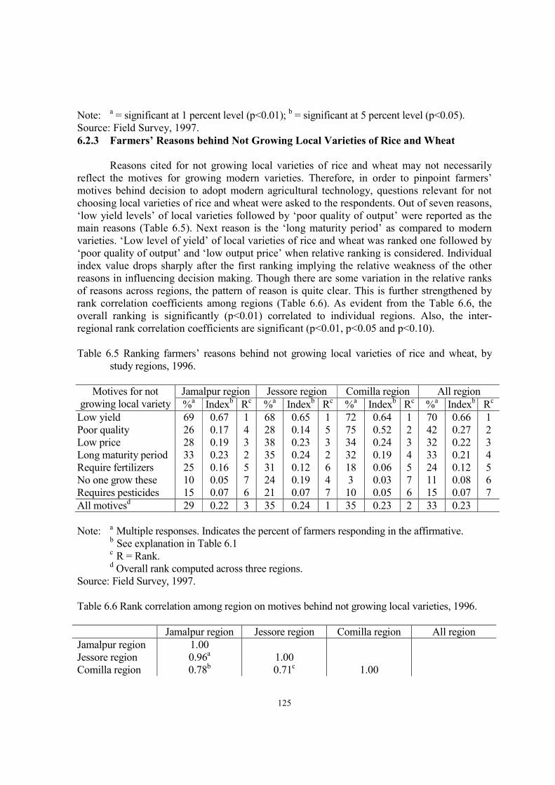
125

Note: a = significant at 1 percent level (p<0.01);

b = significant at 5 percent level (p<0.05).

Source: Field Survey, 1997.

6.2.3 Farmers’ Reasons behind Not Growing Local Varieties of Rice and Wheat

Reasons cited for not growing local varieties of rice and wheat may not necessarily

reflect the motives for growing modern varieties. Therefore, in order to pinpoint farmers’

motives behind decision to adopt modern agricultural technology, questions relevant for not

choosing local varieties of rice and wheat were asked to the respondents. Out of seven reasons,

‘low yield levels’ of local varieties followed by ‘poor quality of output’ were reported as the

main reasons (Table 6.5). Next reason is the ‘long maturity period’ as compared to modern

varieties. ‘Low level of yield’ of local varieties of rice and wheat was ranked one followed by

‘poor quality of output’ and ‘low output price’ when relative ranking is considered. Individual

index value drops sharply after the first ranking implying the relative weakness of the other

reasons in influencing decision making. Though there are some variation in the relative ranks

of reasons across regions, the pattern of reason is quite clear. This is further strengthened by

rank correlation coefficients among regions (Table 6.6). As evident from the Table 6.6, the

overall ranking is significantly (p<0.01) correlated to individual regions. Also, the inter-

regional rank correlation coefficients are significant (p<0.01, p<0.05 and p<0.10).

Table 6.5 Ranking farmers’ reasons behind not growing local varieties of rice and wheat, by

study regions, 1996.

Motives for not

growing local variety

Jamalpur region Jessore region Comilla region All region

%a Indexb Rc %a Indexb Rc %a Indexb Rc %a Indexb Rc

Low yield 69 0.67 1 68 0.65 1 72 0.64 1 70 0.66 1

Poor quality 26 0.17 4 28 0.14 5 75 0.52 2 42 0.27 2

Low price 28 0.19 3 38 0.23 3 34 0.24 3 32 0.22 3

Long maturity period 33 0.23 2 35 0.24 2 32 0.19 4 33 0.21 4

Require fertilizers 25 0.16 5 31 0.12 6 18 0.06 5 24 0.12 5

No one grow these 10 0.05 7 24 0.19 4 3 0.03 7 11 0.08 6

Requires pesticides 15 0.07 6 21 0.07 7 10 0.05 6 15 0.07 7

All motivesd

29 0.22 3 35 0.24 1 35 0.23 2 33 0.23

Note: a Multiple responses. Indicates the percent of farmers responding in the affirmative. b

See explanation in Table 6.1 c

R = Rank. d Overall rank computed across three regions.

Source: Field Survey, 1997.

Table 6.6 Rank correlation among region on motives behind not growing local varieties, 1996.

Jamalpur region Jessore region Comilla region All region

Jamalpur region 1.00

Jessore region 0.96a 1.00

Comilla region 0.78b 0.71c 1.00

126

All region 0.97a 0.94

a 0.90

a 1.00

Note: a = significant at 1 percent level (p<0.01);

b = significant at 5 percent level (p<0.05).

c = significant at 10 percent level (p<0.10).

Source: Field Survey, 1997.

Therefore, a cross-examination of motives behind growing modern varieties and

reasons behind not growing local varieties clearly reveal that it is the ‘yield advantage’ of

modern varieties which is the prime determinant of adoption of modern agricultural

technology. The ‘ready marketability’ and ‘short maturity period’ of modern varieties of rice

and wheat is also important in adoption decision. However, though modern varieties yield

higher returns per unit of land, ‘higher profitability’ do not seem to be the prime determinant

implying that other crops, particularly the non-cereal cash/commercial crops, yield higher

profit as compared to modern varieties of rice and wheat (for details see Chapter V).

6.3 Patterns of Modern Agricultural Technology Adoption

It was mentioned earlier that socio-economic and technical factors may influence

adoption decision and their relationships cannot be determined a priori. In this section,

influence of major socio-economic factors such as farm size classes and tenurial status, and

technical factors such irrigation technology in decision to adopt modern varieties is analyzed.

The proportion of farmers using modern varieties of rice or wheat in at least one season

appears to be highest in Jessore region followed closely by Jamalpur region and substantially

lower in Comilla region, irrespective of size classes and tenurial status (Table 6.7).

Table 6.7 Adoption of modern agricultural technology by farm size and tenurial status by

study regions, 1996.

Farmers Percent of farmers using modern varieties Percent of area under modern varieties1

Jamalpur Jessore Comilla All region Jamalpur Jessore Comilla All region

Land ownership categories2

Landless

Marginal

Small

Medium

Large

83.7

86.1

86.0

89.7

83.3

94.4

95.5

93.7

100.0

93.3

69.8

71.9

62.2

42.9

na

82.1

83.3

78.1

81.3

88.9

87.3

85.9

89.1

84.4

78.8

69.9

72.2

52.8

62.5

61.2

69.0

77.3

67.8

62.6

na

77.3

80.0

75.7

74.1

69.3

Tenurial status3

Own-oper.

Part tenant

Tenant

87.0

85.7

80.8

95.4

91.3

100.0

64.8

67.5

60.0

82.6

80.4

81.0

83.7

88.2

83.7

61.5

65.7

70.1

68.6

74.0

57.7

73.3

79.4

72.2

All 85.7 95.2 65.1 81.8 84.8 62.8 69.0 74.7

Note: na means not applicable. 1

As percent of gross cropped area. 2 Landless = less than 0.20 ha of owned land, marginal = owned land 0.21 – 0.40 ha,

small = owned land 0.41 – 1.00 ha, medium = owned land 1.01 – 2.00 ha, and large =

owned land above 2 ha.

127

3 Owner operator = operates owned land; part tenant = operates own land and rent-in

additional land, tenant = do not operate owned land but rent-in land for crop

production.

Source: Field Survey, 1997.

There is a moderate declining trend in proportion of farmers adopting modern varieties

with increasing farm size for Comilla region. However, when the proportion of gross cropped

area devoted to modern varieties of rice and wheat is considered, Jamalpur region stands out

highest while Jessore and Comilla regions become closely comparable, irrespective of size

classes and tenurial status. This is due to the fact that Jessore region has diverse cropping

system as compared to Comilla region. Therefore, even though very high proportion of

farmers in Jessore region grow modern varieties of rice and wheat, the land they allocate for

this purpose competes with non-cereal crops, particularly, pulses, oilseeds, jute and cotton.

Table 6.7 further reveals that though there are some variations in absolute proportions, no

definite pattern between decision to adopt and size classes or tenurial status can be observed.

This indicates that size classes and tenurial status do not adversely impact on adoption

decisions, and therefore, not a constraint in modern agricultural technology diffusion in

Bangladesh. It is evident from Table 6.7 that landless and marginal farmers are higher

adopters who in turn operate mostly on rented-in lands, a notion also supported by Hossain et

al. (1990). This finding, therefore, supports the argument of Bardhan (1971) who noted that

modern technology would increase tenancy, which is implied from the observation of higher

adoption intensity by landless and marginal farmers operating mostly as tenants.

Water control is one of the major pre-requisites for modern rice cultivation. Without

assured supply of water, the yield levels of modern varieties could be even lower than the local

varieties. Table 6.8 reveals that 60 percent of farmers in Comilla region is using irrigation in at

least one season followed by Jessore and Comilla region. Substantially high proportion of

farmers using irrigation in Comilla region is due to their location within Meghna-Dhonagoda

FCD/I project command area. However, there is no major difference in area under irrigation

between Jessore and Jamalpur regions while Comilla has comparatively lower proportion of

land under irrigation (Table 6.8).

Table 6.8 Adoption of irrigation technology by farm size and tenurial status by study regions,

1996.

Farmers Percent of farmers using irrigation Percent of area under irrigation1

Jamalpur Jessore Comilla All region Jamalpur Jessore Comilla All region

Land ownership categories2

Landless

Marginal

Small

Medium

Large

43.6

22.2

20.9

51.7

50.0

50.0

36.4

56.3

43.8

53.3

65.1

62.5

51.4

64.3

nil

52.2

40.0

38.5

52.5

51.8

63.7

56.6

62.1

67.9

73.3

60.7

62.6

53.1

64.1

64.3

56.6

61.9

48.5

52.7

nil

60.8

59.7

55.7

64.1

68.5

Tenurial status3

Own-oper.

Part tenant

35.0

30.6

44.6

52.2

56.3

67.5

44.1

48.2

67.4

60.1

61.6

65.6

54.2

58.2

62.9

61.1

128

Tenant 46.2 52.9 60.0 51.7 67.3 63.6 41.4 57.4

All 35.4 47.6 60.3 46.3 65.8 62.4 53.9 62.1

Note: na means not applicable. 1

As percent of gross cropped area. 2

Landless = less than 0.20 ha of owned land, marginal = owned land 0.21 – 0.40 ha,

small = owned land 0.41 – 1.00 ha, medium = owned land 1.01 – 2.00 ha, and large =

owned land above 2 ha. 3 Owner operator = operates owned land; part tenant = operates own land and rent-in

additional land, tenant = do not operate owned land but rent-in land for crop

production.

Source: Field Survey, 1997.

The reason for such contrasting observation could be due to the degree of scatteredness

of plots under individual ownership. Land owned by an individual farmer in Jamalpur and

Jessore tend to be in close proximity as compared to Comilla region where the scatter is wider.

Therefore, for an individual farmer, a certain portion of the land is within command area of the

surface irrigation system. Also, due to the existence of a large-scale irrigation system, the

minor irrigation installations, such as shallow tube wells are not developed for drier pockets

within the command area of the irrigation project, thereby reducing the overall proportion

under irrigation. Also, there is sharp variability in proportion of farmers using irrigation and

area under irrigation across regions with respect to size classes and tenurial status. Therefore,

no definite pattern of adverse effect of size classes and tenurial structure in accessing modern

irrigation can be observed from Table 6.8.

6.4 Determinants of Modern Technology Adoption: A Multivariate Analysis

The aforementioned sections attempted to provide a sketch of the motives for adopting

modern agricultural technology as well as patterns of adoption across farm size classes and

tenurial categories. Though considerable amount of information is provided in these analyses,

a complete picture of factors determining adoption behavior cannot be ascertained from them.

Therefore, in order to explain the extent of modern agricultural technology adoption and

factors determining decision to adopt, the following equation is fitted at the household level:

PMVAR = f (OWNLND, PIRRIG, PTNC, AMLND, FPR, WAGER, ANIMPR, LBR, CAPL,

AGCR, NAGI, EDUCH, FAMILY, WORK, WORKW, INFRA, SOIL)

PMVAR = proportion of cultivated land under modern varieties of rice and wheat (%)

OWNLND = amount of land owned by the household (ha)

PIRRIG = proportion of cultivated land under irrigation (%)

PTNC = proportion of cultivated land rented-in (%)

AMLND = amount of land cultivated by the household (ha)

FPR = fertilizer price relative to price of rice and wheat at farm-level

WAGER = labor wage relative to price of rice and wheat at farm-level

ANIMPR = animal power price relative to price of rice and wheat at the farm-level

LBR = amount of land cultivated per agricultural worker (ha)

CAPL = value of farm capital excluding land asset (‘000 taka)

129

AGCR = amount of agricultural credit borrowed by the household (‘000 taka)

NAGI = income from non-agricultural sources of the household (‘000 taka)

EDUCH = completed years of formal schooling of the head of household (years)

FAMILY = number of family members in the household (persons)

WORK = number of working members in the household (persons)

WORKW = number of female working members in the household (persons)

INFRA = index of underdevelopment of infrastructure

SOIL = index of soil fertility

Justification for incorporating the variables is as follows. As mentioned earlier,

land ownership and farm size are surrogates for a large number of factors. Also, there are

considerable debate relating to tenurial status and adoption of modern technology. Availability of

irrigation is a major complementary factor in adoption decision. Therefore, all these variables are

incorporated to test their influence in adoption decision.

As the modern agricultural technology is input intensive the relative profitability of

growing modern varieties of rice and wheat may depend on the prices of these inputs. The labor

variable defined as amount of land cultivated per unit of labor is a measure of labor scarcity and

is assumed to influence adoption decision. Farm capital may also influence adoption decision as

higher availability of farm capital lowers borrowing cost. Capital constraint is also an important

factor that may influence adoption decision adversely. As such, availability of agricultural credit

serves as a major means to liquidate this constraint. Also, availability of non-agricultural income

may influence farmers to switch away from labor intensive agricultural production to non-farm

activities. Therefore, the non-agricultural income variable is incorporated to test this influence.

Access to information and ability to utilize inputs optimally and/or opportunity to switch away

from agriculture to higher income earning non-agricultural activity may also influence adoption

decision. Farmers’ education is incorporated to capture this effect.

According to Chayanovian theory of peasant economy, the consumption unit of the

family in relation to the production unit may be an important determinant of modern technology

adoption (Hossain, 1989). Family size is incorporated to capture the effect of subsistence

pressure. The number of working members in the family might ease the labor constraint and

reduce hired labor requirement. As such this variable is added to capture its influence. There has

been considerable debate relating to gender equity and technological change. It was increasingly

observed that modern agricultural technology largely displaced women from the rural labor

market, particularly, in post-harvest operations. Number of working female members is

incorporated in the function to observe whether women have any influence in adoption decision.

One of the major objective of this study is to highlight the role of non-conventional factors:

infrastructural and soil fertility factors in influencing decision-making. The two variables, the

index of underdevelopment of infrastructure and index of soil fertility are incorporated to test

their influence in adoption decision.

Estimation:

As data of the dependent variable is observed in the range between 0 and 100, the

values are censored at both tails. The most appropriate estimation technique for such case is the

Tobit (two limit probit) procedure (Hossain, 1989; Ahmed and Hossain, 1990; and Hossain et al.

130

1990). For the present study, both OLS (Ordinary Least Squares) and Tobit estimation procedures

were applied to the data29

. The estimated parameters of the model are presented in Table 6.9 with

asymptotic t-ratios. Table 6.9 reveals that both OLS and Tobit model provide similar results. The

most significant (p<0.01) factor that influences modern technology adoption is the irrigation

variable reflected by highest t-value. This is expected, as irrigation is a major complementary

input in growing modern varieties. Tenurial status measured by amount of land rented-in is

positively related with adoption. The value is close to be significant at 10 percent level.

Therefore, the argument that modern technology increases intensity of tenancy (Bardhan, 1971) is

validated. The signs of land ownership and farm size variables are negative, the later being

significant (p<0.01). The negative coefficient for farm size indicates that modern technology is

adopted more in areas with poor land endowments. That is the smaller the farm size the higher

the intensity to adopt modern technology in order to earn more income from limited resource

base. This further implies that, contrary to the expected a priori hypothesis, economically

unfavorable areas may have benefited more from the adoption of modern technology (see

Chapter V). This finding was first supported by Hossain et al. (1990) in contrast to the earlier

conclusion by Hossain (1989). The present study seems to reinforce this argument, however, the

equity implication can be judged only by analyzing the issue of income distribution and poverty

(dealt in detail in Chapter VIII).

Input prices seem to have positive relation with adoption rate. This can be explained in

the context of relative profitability between modern and local varieties. As shown in Chapter V,

profitability from local variety is significantly lower than modern varieties. Therefore, in a

situation of increasing input prices, particularly, price of animal power services, which is

invariant to growing either local or modern varieties, it would be better to chose a high income

yielding crop to cover the increasing costs, leading to the adoption of modern varieties.

Table 6.9 Determinants of modern agricultural technology adoption, 1996.

Variables OLS estimate Tobit estimate

Coefficients t-ratio Coefficients t-ratio

Intercept 0.115 0.89 -0.090 -0.40

OWNLND -0.001 -0.04 0.031 0.66

PIRRIG 0.372 9.90a 0.542 8.23

a

PTNC 0.044 0.98 0.129 1.62

AMLND -0.037 -1.86c -0.088 -2.64

a

FPR -0.040 -0.90 0.005 0.07

WAGER 0.009 0.89 0.004 0.22

ANIMPR 0.008 1.65c 0.017 2.11b

LBR -2.686 -1.22 -1.844 -0.47

CAPL 0.002 1.81c 0.002 1.28

AGCR -0.001 -0.99 -0.001 -0.37

NAGI -0.001 -2.45b -0.001 -1.73

c

EDUCH -0.004 -1.36 -0.008 -1.38

FAMILY -0.003 -0.59 -0.005 -0.57

WORK 0.004 0.29 0.005 0.22

29

LIMDEP Software Version 6 (1992) is used for the analysis.

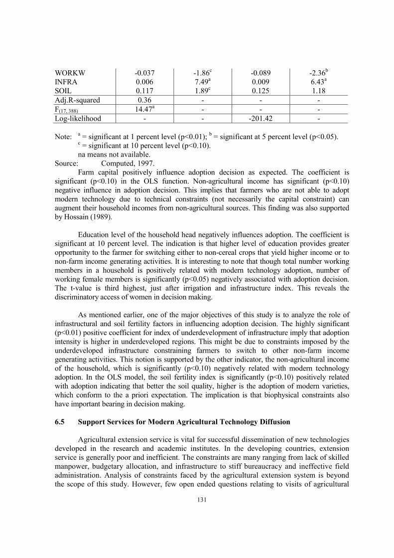
131

WORKW -0.037 -1.86c -0.089 -2.36

b

INFRA 0.006 7.49a 0.009 6.43

a

SOIL 0.117 1.89c 0.125 1.18

Adj.R-squared 0.36 - - -

F(17, 388) 14.47a - - -

Log-likelihood - - -201.42 -

Note: a = significant at 1 percent level (p<0.01);

b = significant at 5 percent level (p<0.05).

c = significant at 10 percent level (p<0.10).

na means not available.

Source: Computed, 1997.

Farm capital positively influence adoption decision as expected. The coefficient is

significant (p<0.10) in the OLS function. Non-agricultural income has significant (p<0.10)

negative influence in adoption decision. This implies that farmers who are not able to adopt

modern technology due to technical constraints (not necessarily the capital constraint) can

augment their household incomes from non-agricultural sources. This finding was also supported

by Hossain (1989).

Education level of the household head negatively influences adoption. The coefficient is

significant at 10 percent level. The indication is that higher level of education provides greater

opportunity to the farmer for switching either to non-cereal crops that yield higher income or to

non-farm income generating activities. It is interesting to note that though total number working

members in a household is positively related with modern technology adoption, number of

working female members is significantly (p<0.05) negatively associated with adoption decision.

The t-value is third highest, just after irrigation and infrastructure index. This reveals the

discriminatory access of women in decision making.

As mentioned earlier, one of the major objectives of this study is to analyze the role of

infrastructural and soil fertility factors in influencing adoption decision. The highly significant

(p<0.01) positive coefficient for index of underdevelopment of infrastructure imply that adoption

intensity is higher in underdeveloped regions. This might be due to constraints imposed by the

underdeveloped infrastructure constraining farmers to switch to other non-farm income

generating activities. This notion is supported by the other indicator, the non-agricultural income

of the household, which is significantly (p<0.10) negatively related with modern technology

adoption. In the OLS model, the soil fertility index is significantly (p<0.10) positively related

with adoption indicating that better the soil quality, higher is the adoption of modern varieties,

which conform to the a priori expectation. The implication is that biophysical constraints also

have important bearing in decision making.

6.5 Support Services for Modern Agricultural Technology Diffusion

Agricultural extension service is vital for successful dissemination of new technologies

developed in the research and academic institutes. In the developing countries, extension

service is generally poor and inefficient. The constraints are many ranging from lack of skilled

manpower, budgetary allocation, and infrastructure to stiff bureaucracy and ineffective field

administration. Analysis of constraints faced by the agricultural extension system is beyond

the scope of this study. However, few open ended questions relating to visits of agricultural

132

extension officials and training received by farmers were asked to the respondents in order to

assess the current level of inter-relationship among farmers and field level agricultural

extension officials in the study regions.

The distance of nearest agricultural extension office from the study villages across

regions is highly variable (Appendix Table A6.3). About 77 percent of the respondents

reported that the nearest agricultural extension office is within three kms from their

households in Comilla region, an infrastructurally developed area. The distance of the office is

above five kms for 42 percent and 79 percent of respondents in Jessore and Jamalpur region,

respectively. It should be noted that almost all villages in the Jamalpur region were

categorized as underdeveloped villages in terms of infrastructure (see Chapter V).

Table 6.10 clearly reveals that the exchange of ideas and knowledge between farmers

and agricultural extension officials are almost negligible. The number of visits made by the

agricultural extension officials to the village is less than 10 percent in each region. Similarly,

the visits made by farmers to the nearest agricultural extension office are less than 10 percent.

This is an indication of the level of extension support provided for technology transfer in

Bangladesh. It should be noted that agricultural extension official here refers to Thana

Agricultural Extension Officer and higher, not the Block Supervisor who usually stays in any

of the village within his/her command area.

Table 6.10 Number of visits of agricultural extension office to villages and farmers’ visits to

agricultural extension office during last one year by study regions, 1996.

Number of visits made in the

last one year

Number and percent of households (%)

Jamalpur region Jessore region Comilla region All region

Agricultural extension officer making visits to the village

Once 10 (5.7) 3 (2.9) 2 (1.6) 15 (3.7)

Between two to three times 2 (1.2) 6 (5.8) 2 (1.6) 10 (2.4)

Between four to ten times 1 (0.6) 3 (2.9) - 4 (0.9)

No visits by AEO to village 162 (92.5) 93 (88.4) 122 (96.8) 377 (92.1)

Farmers making visits to agricultural extension office

Once 5 (2.9) 5 (4.8) 2 (1.6) 12 (3.0)

Between two to three times 2 (1.1) 5 (4.8) - 7 (1.7)

Between four to twenty times 3 (1.7) 2 (1.9) - 5 (1.2)

No visits by farmers to office 165 (94.3) 93 (88.6) 124 (98.4) 382 (94.1)

Total households 175 (100.0) 105 (100.0) 126 (100.0) 406 (100.0)

Note: Figures in parentheses are percentages of total households.

Source: Field Survey, 1997.

An inquiry on whether the farmers had received any training related to agricultural

production in past seven years revealed that except Jessore region, negligible number of farmers

received any formal training (Table 6.11). This is another indication of persistent lack of support

for modern technology transfer to and from the research centers.

Table 6.11. Types of training received by farmers in past seven years by study regions, 1996.

133

Type of training received by

farmers in past seven years

Number and percent of households

Jamalpur region Jessore region Comilla region All region

Farmers received training 7 (4.0) 16 (15.2) 3 (2.4) 26 (6.4)

Seed bed preparation 1 (0.6) 1 (0.9) 1 (0.8) 3 (0.8)

Crop production 6 (3.4) 8 (7.7) 2 (1.6) 16 (3.9)

Fertilizers/pesticides application - 7 (6.9) - 7 (1.3)

Farmers not received training 168 (96.0) 89 (84.8) 123 (97.6) 380 (93.6)

Total households 175 (100.0) 105 (100.0) 126 (100.0) 406 (100.0)

Note: Figures in parentheses are percentages of total households.

Source: Field Survey, 1997.

Further, a breakdown of sources of training revealed that the government agencies,

particularly, the agricultural extension office network provided training in Jessore and Comilla

region, while the non-governmental organizations (NGOs) provided training in Jamalpur region

(Table 6.12). This reflects the differential focus of government agencies and NGOs in their

approach to rural development in Bangladesh. While the government with its minimal support

tends to stick to agricultural development per se, the NGOs focuses on building up capacities

and skills in small-scale cottage industries and trading activities. Also, spread of NGOs across

all regions of the country is highly variable. The concentration of NGOs working at the

grassroots is highly concentrated in the upper northern Bangladesh and selective central regions

located in closer proximity from the capital Dhaka. Among the study regions, the extent of

NGOs are relatively abundant in Jamalpur region followed by Jessore and Comilla. This might

be another reason for dominance of NGOs training farmers in Jamalpur.

Table 6.12 Organizers of the training programs received by farmers by study regions, 1996.

Organizers of the training

programs

Number and percent of households (%)

Jamalpur region Jessore region Comilla region All region

Government agencies 1 (0.6) 16 (15.2) 3 (2.4) 20 (4.9)

Non-governmental organizations 6 (3.4) - - 6 (1.5)

Total households 175 (100.0) 105 (100.0) 126 (100.0) 406 (100.0)

Note: Figures in parentheses are percentages of total households.

Source: Field Survey, 1997.

An inquiry into the reasons for not receiving training in past seven years revealed that

majority of the farmers did not deem it necessary (Table 6.13). Only few reported that they did

not get the opportunity to receive training. However, 33 percent farmers in Comilla and 11

percent farmers in Jamalpur region reported that no one ever came to offer training, indicating

their desire to receive training if offered (Table 6.13).

Table 6.13 Reasons cited by farmers who did not receive any training by study regions, 1996.

Reasons cited by farmers who

did not receive any training

Number and percent of households (%)

Jamalpur region Jessore region Comilla region All region

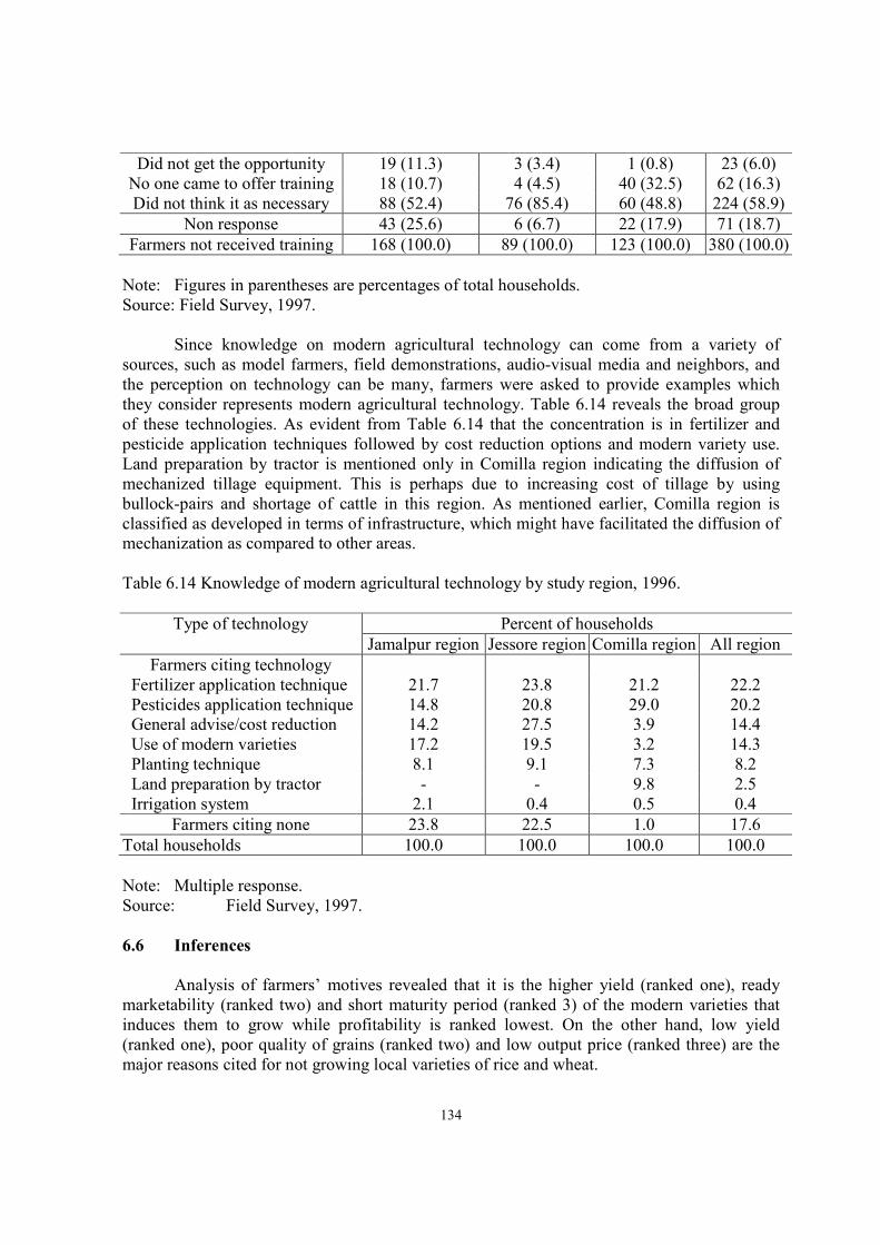
134

Did not get the opportunity 19 (11.3) 3 (3.4) 1 (0.8) 23 (6.0)

No one came to offer training 18 (10.7) 4 (4.5) 40 (32.5) 62 (16.3)

Did not think it as necessary 88 (52.4) 76 (85.4) 60 (48.8) 224 (58.9)

Non response 43 (25.6) 6 (6.7) 22 (17.9) 71 (18.7)

Farmers not received training 168 (100.0) 89 (100.0) 123 (100.0) 380 (100.0)

Note: Figures in parentheses are percentages of total households.

Source: Field Survey, 1997.

Since knowledge on modern agricultural technology can come from a variety of

sources, such as model farmers, field demonstrations, audio-visual media and neighbors, and

the perception on technology can be many, farmers were asked to provide examples which

they consider represents modern agricultural technology. Table 6.14 reveals the broad group

of these technologies. As evident from Table 6.14 that the concentration is in fertilizer and

pesticide application techniques followed by cost reduction options and modern variety use.

Land preparation by tractor is mentioned only in Comilla region indicating the diffusion of

mechanized tillage equipment. This is perhaps due to increasing cost of tillage by using

bullock-pairs and shortage of cattle in this region. As mentioned earlier, Comilla region is

classified as developed in terms of infrastructure, which might have facilitated the diffusion of

mechanization as compared to other areas.

Table 6.14 Knowledge of modern agricultural technology by study region, 1996.

Type of technology Percent of households

Jamalpur region Jessore region Comilla region All region

Farmers citing technology

Fertilizer application technique 21.7 23.8 21.2 22.2

Pesticides application technique 14.8 20.8 29.0 20.2

General advise/cost reduction 14.2 27.5 3.9 14.4

Use of modern varieties 17.2 19.5 3.2 14.3

Planting technique 8.1 9.1 7.3 8.2

Land preparation by tractor - - 9.8 2.5

Irrigation system 2.1 0.4 0.5 0.4

Farmers citing none 23.8 22.5 1.0 17.6

Total households 100.0 100.0 100.0 100.0

Note: Multiple response.

Source: Field Survey, 1997.

6.6 Inferences

Analysis of farmers’ motives revealed that it is the higher yield (ranked one), ready

marketability (ranked two) and short maturity period (ranked 3) of the modern varieties that

induces them to grow while profitability is ranked lowest. On the other hand, low yield

(ranked one), poor quality of grains (ranked two) and low output price (ranked three) are the

major reasons cited for not growing local varieties of rice and wheat.

135

Farm size and tenurial status do not seem to affect adversely to modern technology

adoption decisions. The landless and marginal farmers are observed to be higher adopters who

in turn mainly operate as tenants. Irrigation was found to be the major determining factor in

influencing adoption decisions. Farm size, number of female family labor, non-agricultural

income, and infrastructure development negatively influence adoption decisions. Soil fertility

has positive influence in adoption decisions.

The support services for agricultural extension is very weak. There is a serious lack of

interaction among agricultural extension officials and farmers. Knowledge of modern

agricultural technology is mainly confined to application techniques of fertilizers and

pesticides only while dissemination of relevant information for crop diversification, variety

screening, health hazards of pesticide uses, and adverse impacts of modern agricultural

technology is non-existent.

136

CHAPTER VII

TECHNOLOGICAL CHANGE AND ITS IMPACT ON EMPLOYMENT,

RURAL LABOR MARKET AND FACTOR MARKETS

The literatures analyzing impacts of modern agricultural technology mostly emphasized on

the direct effects on income distribution and geographical regions with a basic argument that

the technology is not scale neutral and benefited most in areas endowed with favorable agro-

ecological conditions (Lipton and Longhurst, 1989). However, Hossain et al. (1990) argued

that modern agricultural technology may also have indirect effect that operates through factor

markets and enables transfer of income across socio-economic groups as well as regions. This

could occur from a change in the nature of operation of the land, labor and other input markets

thereby indirectly smoothing income disparity across socio-economic groups through an

adjustment process.

The present chapter analyzes the direct and/or indirect effects of modern technology

diffusion on employment, rural labor market and other factor markets. The employment effect

of the modern agricultural technology is analyzed with particular reference to its effect on

gender distribution of labor, which is a major source of controversy. It also provides a

systematic estimation of the women’s participation in agricultural operations. The other factor

markets on which the impact of technological change is analyzed include fertilizer, pesticide,

land, agricultural credit, and output markets.

7.1 Employment Effects of Technological Change: Analytical Framework

Prior to the analysis of the employment effects, a brief on the theoretical framework of

the labor use effect of technological change would be worthwhile. Figure 7.1 shows the impact

of three basic types of technological change and their impact on labor use. In Figure 7.1 point

A is the combination of factor used with the old technology. The three new isoquants D, B,

and C represent labor-saving, neutral and labor-using technologies that are capable of

producing the same level of output utilizing cost minimization principles. Though, labor

productivity increases in all these three cases, due to the variation of factor proportions, the

demand for labor also varies (Unnevehr and Stanford, 1985).

In a situation of growing supply of labor, they will only benefit from productivity

increases if it is accompanied by increased demand for their labor. Figure 7.2 shows impact of

labor demand from three types of technological change at an individual household level.

Under a given set of prices of inputs and output, LO amount of labor is used for the traditional

(old) technology. With either a neutral or labor-using shift in the production function, it will be

profitable for the household to employ additional labor to produce more output. If this

additional demand for labor were to be absorbed by women then only the women will benefit

from this technological change.

137

Land Output Labor-saving

Labor-using

Neutral

D

KA A Old

B

C

0 LA Labor 0 LS LO LN LU Labor

Figure 7.1 Technological change and factor Figure 7.2. Technological change and

proportion labor use.

Source: Adapted from Unnevehr and Stanford (1985).

7.2 Issues Related to Impact of Modern Agricultural Technology on Employment

Nearly one third of rural households in Bangladesh do not own any cultivable land and

about half of them own less than 0.2 ha of land making farming as only a marginal source of

income (Hossain, 1989). Due to such low access to land, the main source of livelihood of these

households depend on the condition of the rural labor market, that is, the extent and duration of

employment and the wage rate. Technological change in agriculture is expected to change the

condition of rural labor market by increasing the labor use intensity through increased cropping

intensity and productivity of labor thereby influencing the wage rate. Since the supply of labor is

likely to be fixed in the short-run, increased demand will result in rise in wages, provided that

shortage is not met by in-migration of labor from other regions. Also, as the rural labor market is

largely composed of landless and marginal farmers, the upward pressure in wages would entail

redistribution of gains from modern agricultural technology through a process of income transfer

from producer farmers to hired laborers. Hossain et al. (1990) argued that, even if increased

demand for labor were met by rural-rural in-migration, then the shortage of labor in non-

adopting villages would cause an upward pressure in wages. Eventually the wage differential

between adopter and non-adopter villages will narrow down at a higher wage level.

Technological change may also indirectly affect the non-agricultural labor market as the

expenditure of increased agricultural income would generate additional demand for non-

agricultural goods and services (Hossain, 1989).

Alauddin and Tisdell (1995), observing historical data for Bangladesh, claimed that

though significant employment gains has resulted from the ‘Green Revolution’ technologies in

Bangladesh, however, the employment generating effect of the ‘Green Revolution’, in recent

years, is slowing down showing little prospect for increased absorption. Also, there is little

prospect of having a major turning point in labor absorption in non-farm sector to lead a

successful industrialization as observed in East Asian regions, thereby providing a gloomy

138

future for Bangladesh. Similar conclusion has also been arrived by Osmani (1990). He noted that

the drastic fall in total labor force in agriculture is not an indication of a turning point30

but rather

the consequence of increasing work-sharing arrangement and consequent decline in average

productivity per worker. He claimed that the true nature of shift gets revealed in areas where

technological change has opened up new opportunities for gainful employment in agriculture. In

these areas, a reverse flow of surplus labor from non-farm sectors to farm activities, are

observed.

7.3 Technological Change and Employment Opportunities for Women

Rural women in Asia play a major role in agricultural sector particularly in the post

harvest processing. With the advent of ‘Green Revolution’ there was an increased demand for

labor owing to increased cropping and labor intensity of modern varieties. The scope of

mechanization in the production arena remained only within provision of water for irrigation

and to some extent for land preparation. However, a major shift in technology occurred in the

post harvesting processing sector, the introduction of rice mills, which dramatically displaced

employment opportunities of rural women involved in manual husking operation of rice

grains. Ahmed (1982) estimated that rice mills displaced 29% of the total husking labor and

almost all hired labor displaced were women who have limited alternative employment

opportunity. His crude nationwide estimate reveals that, if rice mills are made adequately

available throughout the country, a total of 45 million person-days of hired labor would be

displaced leading to a reduction of rural poor’s income of about Tk.450 million at its 1982 level

estimates.

As the employment opportunities of rural women are closing in the post harvesting

processing sector and non-farm sector is being highly stagnant, the alternative lies in actively

involving them directly in crop production activities. In this respect, it is worth mentioning that

gender division of labor in Bangladesh agriculture is strictly demarcated with women being

responsible for most of agricultural work within the household and are not generally allowed to

undertake field or market work (Begum, 1985; and Abdullah, 1985). However, contrasting

version is also evident. Zaman (1995) observed that village women are working in fields with

men as agricultural wage laborers. Women not only participate in rice crop production and

processing but also involved in the production and processing of other major crops such as

sugarcane, jute, wheat, and other winter crops.

Large number of studies were undertaken in evaluating impact of ‘Green Revolution’

in Bangladesh agriculture (e.g., Hossain, 1989; Ahmed and Hossain, 1990; Hossain et al.

1990; and Alauddin and Tisdell, 1991). Though these studies explicitly examined the

employment effects of modern agricultural technology, however, they did not incorporate any

gender dimension in their analyses. Furthermore, there is a dearth of knowledge about

employment effect of modern agricultural technology for rural women and studies dealing

with the issue remained confined in the post harvesting processing activities only (e.g.,

30

The notion is that the slow growth rate of agricultural labor force implies a movement towards a priori expectation

of reaching a turning point in the growth of agricultural labor force. Such an occupational shift from agriculture to

non-agriculture and/or modern sector implies the onset of a Lewisian transition of labor surplus economy.

139

Begum, 1985; and Abdullah, 1985). As such, no systematic estimate of gender division of

labor use for agricultural crops is available for Bangladesh. Also, the time-use approach used

by almost all the studies dealing with gender roles examined daily workloads by activities, but

did not provide the total labor input used for specific crops by gender.

A Note on Data Sources for Analyzing Gender Dimension of Employment Effects

In addition to the Field Survey 1997, the primary data for this section of the study comes

from another intensive farm-survey conducted in crop year 1989 covering the same villages of

Jamalpur and Jessore regions31

. Therefore, total sampled households for the crop year 1989

stands at 1,755 in two regions (BRAC-VSP Survey, 1990). Though details of crop input-output

data were collected in both surveys, only the BRAC-VSP Survey (1990), i.e., the survey of crop

year 1989, contains labor input data for each agricultural operation and for specific crop

production activities classified by men and women. Therefore, the analytical results for this

section relates to the results of both surveys.

7.4 Participation of Sample Households in Economic Activities

In this study a worker is defined as a person who is available for work in income

earning activities or expenditure saving activities during the week of the survey period and

also identified as working member by the respondent. The activities include both agricultural

and non-agricultural activities. Table 7.1 presents the labor force participation rate.

Table 7.1 Labor force participation by study regions, 1996.

Region Average

family

member

Average

working

members

Participation

rate in economic

activity

Male worker

as proportion

of family size

Female worker

as proportion

of family size

(persons) (persons) (percent) (percent) (percent)

Jamalpur region 5.27 1.88 38.49 25.81 12.68

Jessore region 6.24 2.47 40.78 29.44 11.34

Comilla region 6.90 1.88 29.31 27.88 1.43

All region 6.02 2.03 36.23 27.39 8.84

Note: na means not applicable.

Source: Field Survey, 1997.

The average family size is highest in Comilla (6.9 persons) followed by Jessore (6.2

persons) and Jamalpur regions (5.3 persons), respectively (Table 7.1). The average number of

workers per household is estimated at 1.9 persons for both Comilla and Jamalpur and 2.5 for

Jessore region, respectively. The number of workers in Comilla is less despite highest family

31

These data were collected by BRAC (one of the largest national non-governmental organization) to serve as

base-line information for a ten-year longitudinal study project, called as Village Study Project (VSP). As such, a

census of all the 14 villages were conducted on virtually all types of information prevailing in a rural setting, for

the cropyear 1989. The base-line data collection took about 6 months engaging 16 field researchers who were

stationed in the core village of each thana. The first author of this study was responsible for coordinating the data

collection.

140

size is due to non-participation of female as working members. There is an increasing trend in

family size with land size categories for all regions (Appendix Table A7.1). Similar trend is

observed for the average number of working members in the family as well as the labor force

participation rate. Though the relative proportion of male working members is around 25 – 30

percent the proportion of female working members is much lower in all regions. In

Bangladesh there is a social stigma against women working in the field or work as wage

laborer (Hossain, 1989). The strikingly lower proportion of female workers in Comilla region

reflects that the social stigma in labor use pattern is strongest in that region. However, women

members from very poor family supply labor in all regions in order to raise subsistence.

7.5 Gender Distribution of Labor Input in Crop Production

Gender based human labor input for crop production by sources of supply is presented

in Table 7.2. It is clear from Table 7.2 that women’s labor input varies substantially across

crop groups. Women’s involvement in rice production is less than 13 percent, while for wheat

and other non-cereal crops, such as pulses, oilseeds, spices, cotton and vegetables the range is

above 13 percent. Their highest involvement is in vegetable production (about 48 percent of

total labor requirement). This finding, therefore, proves that the claim that women labor is

actively utilized only at post harvest processing stage in Bangladesh is an underestimation. A

comparison of labor input data of present study with other evaluation studies of ‘Green

Revolution’ reveals that inclusion of women labor separately in labor accounting does not

distort the total labor requirements of crop production (Table 7.2). Rather, the estimates are

strikingly close. However, leaving women labor in labor accounting seriously under-mine their

important role in agricultural production.

Limiting the analyses of labor use only at this point can lead to serious misleading

conclusion if one wish to predict the market for hired women labor requirements. A close look

at the columns of hired labor input in Table 7.2 will clarify the matter by revealing the dismal

scenario of hired women labor. The figures for hired women are practically zero for rice and

less than 3 percent for wheat and non-cereal crop production except cotton. Only cotton

production, a specialized crop grown in Jessore region, involves large amount of hired women

labor. This proves that the theoretical framework within which this analyses is performed

remains true only for men labor since the proportion of hired labor is substantially higher for

modern varieties of rice and wheat. In other words, the increased demand for labor owing to

the rapid technological progress in the foodgrain production was totally absorbed by hired men

labor alone.

Breakdown of women labor input by agricultural operations reveals that though a

major portion of women labor input goes into threshing operation for foodgrain crops, about 5

- 10 percent is involved in harvesting operations, weeding, and fertilizing, respectively

(Appendix Table A7.2). For the non-cereal crops, the extent of involvement is wider,

practically, in all types of agricultural operations, such as, in potato, spices, and vegetables

production which again challenges the claim that women are involved only in post harvest

processing of agricultural crops.

141

Table 7.2 Labor input in crop production by gender (all regions), 1989.

Crops/

seasons

Proportion of labor use per hectare of land Comparison

study Family labor Hired labor Total labor

Men Women Men Women Men Women Total labor Total labor

Aus season (early monsoon)

L Aus rice 43.1 11.1 45.1 0.7 88.2 11.8 100 (153) 152a

M Aus rice 35.0 11.5 52.9 0.6 87.9 12.1 100 (174) 185a

Jute 38.3 5.3 55.5 0.9 93.8 6.2 100 (227) 245b

Aman Season (monsoon)

L Aman rice 40.0 11.0 48.4 0.6 88.4 11.6 100 (155) 160b

M Aman rice 35.6 9.2 54.6 0.6 90.2 9.8 100 (174) 189b

Boro Season (dry winter)

L Boro rice 39.9 12.4 47.2 0.5 87.1 12.9 100 (178) 152a

M Boro rice 39.6 10.8 48.6 1.0 88.2 11.8 100 (212) 203a

L wheat 46.2 16.1 35.6 2.1 81.8 18.2 100 (143) 146b

M wheat 44.1 13.2 41.2 1.5 85.3 14.7 100 (136) 159b

Potato 52.4 12.5 33.8 1.3 86.2 13.8 100 (311) 295b

Pulses 41.3 25.7 31.2 1.8 72.5 27.5 100 (109) 82b

Oilseeds 38.5 18.3 40.4 2.8 78.9 21.1 100 (109) 118b

Spices 50.4 18.8 27.8 1.0 78.2 21.8 100 (276) 321b

Vegetables 34.9 46.5 17.4 1.2 52.3 47.7 100 (186) 217c

Cotton 50.1 15.3 23.1 11.5 73.2 26.8 100 (295) 211b

Note: Figures in parentheses are total number of labor used per hectare of land. a Selected from Hossain et al. (1990).

b Selected from Mahmud et al. (1994).

c Selected from Sanyal (1993).

Source: BRAC-VSP Survey, 1990.

7.6 Technological change and Operation of the Labor Market

Though it is widely recognized that modern technology adoption directly influences

the distribution of income across all classes of farmers and geographical regions, the scale

neutrality of modern technology has been seriously criticized resulting in diversified

evaluations. This is evident in the conclusion drawn by Freebairn (1995) from his analyses of

307 evaluation studies. However, researchers (e.g., Hossain, 1989; Hossain et al., 1990; and

Ahmed and Hossain, 1990) argue that modern technology adoption may also have indirect

effect through operation of factor markets, particularly, the hired labor market. There those

discriminated by the advent of modern technology would benefit from a redistribution of

income through increased wages owing to increased labor demand.

7.6.1 Demand for Hired Agricultural Labor

Demand for hired labor is significantly (p<0.01) positively related with amount of land

owned by households (Table 7.3). The correlation coefficients are estimated at 0.75, 0.87, and

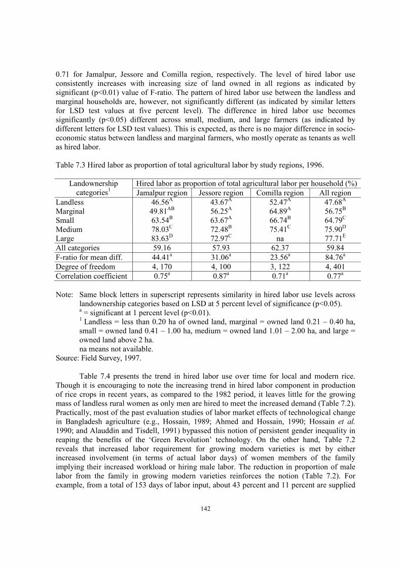
142

0.71 for Jamalpur, Jessore and Comilla region, respectively. The level of hired labor use

consistently increases with increasing size of land owned in all regions as indicated by

significant (p<0.01) value of F-ratio. The pattern of hired labor use between the landless and

marginal households are, however, not significantly different (as indicated by similar letters

for LSD test values at five percent level). The difference in hired labor use becomes

significantly (p<0.05) different across small, medium, and large farmers (as indicated by

different letters for LSD test values). This is expected, as there is no major difference in socio-

economic status between landless and marginal farmers, who mostly operate as tenants as well

as hired labor.

Table 7.3 Hired labor as proportion of total agricultural labor by study regions, 1996.

Landownership

categories1

Hired labor as proportion of total agricultural labor per household (%)

Jamalpur region Jessore region Comilla region All region

Landless 46.56A

43.67A 52.47

A 47.68

A

Marginal 49.81AB

56.25A 64.89

A 56.75

B

Small 63.54B 63.67

A 66.74

B 64.79

C

Medium 78.03C 72.48

B 75.41

C 75.90

D

Large 83.63D 72.97

C na 77.71

E

All categories 59.16 57.93 62.37 59.84

F-ratio for mean diff. 44.41a

31.06a 23.56

a 84.76

a

Degree of freedom 4, 170 4, 100 3, 122 4, 401

Correlation coefficient 0.75a 0.87

a 0.71

a 0.77

a

Note: Same block letters in superscript represents similarity in hired labor use levels across

landownership categories based on LSD at 5 percent level of significance (p<0.05). a = significant at 1 percent level (p<0.01).

1 Landless = less than 0.20 ha of owned land, marginal = owned land 0.21 – 0.40 ha,

small = owned land 0.41 – 1.00 ha, medium = owned land 1.01 – 2.00 ha, and large =

owned land above 2 ha.

na means not available.

Source: Field Survey, 1997.

Table 7.4 presents the trend in hired labor use over time for local and modern rice.

Though it is encouraging to note the increasing trend in hired labor component in production

of rice crops in recent years, as compared to the 1982 period, it leaves little for the growing

mass of landless rural women as only men are hired to meet the increased demand (Table 7.2).

Practically, most of the past evaluation studies of labor market effects of technological change

in Bangladesh agriculture (e.g., Hossain, 1989; Ahmed and Hossain, 1990; Hossain et al.

1990; and Alauddin and Tisdell, 1991) bypassed this notion of persistent gender inequality in

reaping the benefits of the ‘Green Revolution’ technology. On the other hand, Table 7.2

reveals that increased labor requirement for growing modern varieties is met by either

increased involvement (in terms of actual labor days) of women members of the family

implying their increased workload or hiring male labor. The reduction in proportion of male

labor from the family in growing modern varieties reinforces the notion (Table 7.2). For

example, from a total of 153 days of labor input, about 43 percent and 11 percent are supplied

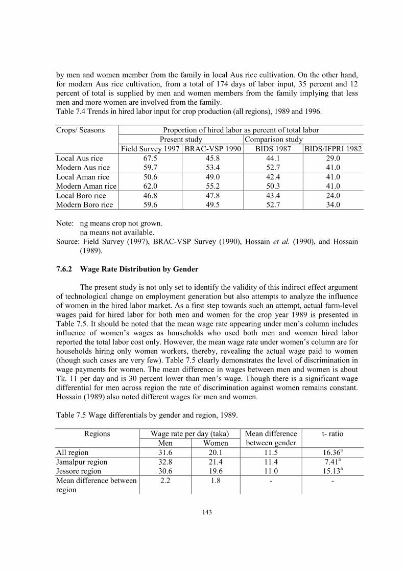
143

by men and women member from the family in local Aus rice cultivation. On the other hand,

for modern Aus rice cultivation, from a total of 174 days of labor input, 35 percent and 12

percent of total is supplied by men and women members from the family implying that less

men and more women are involved from the family.

Table 7.4 Trends in hired labor input for crop production (all regions), 1989 and 1996.

Crops/ Seasons Proportion of hired labor as percent of total labor

Present study Comparison study

Field Survey 1997 BRAC-VSP 1990 BIDS 1987 BIDS/IFPRI 1982

Local Aus rice

Modern Aus rice

67.5

59.7

45.8

53.4

44.1

52.7

29.0

41.0

Local Aman rice

Modern Aman rice

50.6

62.0

49.0

55.2

42.4

50.3

41.0

41.0

Local Boro rice

Modern Boro rice

46.8

59.6

47.8

49.5

43.4

52.7

24.0

34.0

Note: ng means crop not grown.

na means not available.

Source: Field Survey (1997), BRAC-VSP Survey (1990), Hossain et al. (1990), and Hossain

(1989).

7.6.2 Wage Rate Distribution by Gender

The present study is not only set to identify the validity of this indirect effect argument

of technological change on employment generation but also attempts to analyze the influence

of women in the hired labor market. As a first step towards such an attempt, actual farm-level

wages paid for hired labor for both men and women for the crop year 1989 is presented in

Table 7.5. It should be noted that the mean wage rate appearing under men’s column includes

influence of women’s wages as households who used both men and women hired labor

reported the total labor cost only. However, the mean wage rate under women’s column are for

households hiring only women workers, thereby, revealing the actual wage paid to women

(though such cases are very few). Table 7.5 clearly demonstrates the level of discrimination in

wage payments for women. The mean difference in wages between men and women is about

Tk. 11 per day and is 30 percent lower than men’s wage. Though there is a significant wage

differential for men across region the rate of discrimination against women remains constant.

Hossain (1989) also noted different wages for men and women.

Table 7.5 Wage differentials by gender and region, 1989.

Regions Wage rate per day (taka) Mean difference

between gender

t- ratio

Men Women

All region 31.6 20.1 11.5 16.36a

Jamalpur region 32.8 21.4 11.4 7.41a

Jessore region 30.6 19.6 11.0 15.13a

Mean difference between

region

2.2 1.8 - -

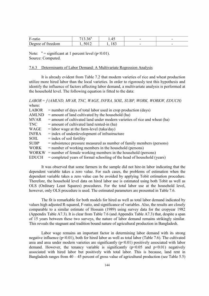
144

F-ratio 713.36a 1.45 - -

Degree of freedom 1, 5012 1, 183 - -

Note: a = significant at 1 percent level (p<0.01).

Source: Computed.

7.6.3 Determinants of Labor Demand: A Multivariate Regression Analysis

It is already evident from Table 7.2 that modern varieties of rice and wheat production

utilize more hired labor than the local varieties. In order to rigorously test this hypothesis and

identify the influence of factors affecting labor demand, a multivariate analysis is performed at

the household level. The following equation is fitted to the data:

LABOR = f (AMLND, MVAR, TNC, WAGE, INFRA, SOIL, SUBP, WORK, WORKW, EDUCH)

where:

LABOR = number of days of total labor used in crop production (days)

AMLND = amount of land cultivated by the household (ha)

MVAR = amount of cultivated land under modern varieties of rice and wheat (ha)

TNC = amount of cultivated land rented-in (ha)

WAGE = labor wage at the farm-level (taka/day)

INFRA = index of underdevelopment of infrastructure

SOIL = index of soil fertility

SUBP = subsistence pressure measured as number of family members (persons)

WORK = number of working members in the household (persons)

WORKW = number of female working members in the household (persons)

EDUCH = completed years of formal schooling of the head of household (years)

It was observed that some farmers in the sample did not hire-in labor indicating that the

dependent variable takes a zero value. For such cases, the problems of estimation when the

dependent variable takes a zero value can be avoided by applying Tobit estimation procedure.

Therefore, the household level data on hired labor use is estimated using both Tobit as well as

OLS (Ordinary Least Squares) procedures. For the total labor use at the household level,

however, only OLS procedure is used. The estimated parameters are presented in Table 7.6.

The fit is remarkable for both models for hired as well as total labor demand indicated by

values high adjusted R-squared, F-ratio, and significance of variables. Also, the results are closely

comparable to a similar estimate of Hossain (1989) using survey data for the cropyear 1982

(Appendix Table A7.3). It is clear from Table 7.6 (and Appendix Table A7.3) that, despite a span

of 15 years between these two surveys, the nature of labor demand remains strikingly similar.

This reveals the stagnant and tradition bound nature of agricultural production in Bangladesh.

Labor wage remains an important factor in determining labor demand with its strong

negative influence (p<0.01), both for hired labor as well as total labor (Table 7.6). The cultivated

area and area under modern varieties are significantly (p<0.01) positively associated with labor

demand. However, the tenancy variable is significantly (p<0.05 and p<0.01) negatively

associated with hired labor but positively with total labor. This is because, land rent in

Bangladesh ranges from 40 – 45 percent of gross value of agricultural production (see Table 5.5)

145

therefore, hiring more wage labor would seriously depress any profit from crop production. The

situation is same 15 years ago as evident from the comparison study.

The index of under development of infrastructure also operates in similar way. The higher

the level of infrastructural development the higher will be the demand for hired labor as the

members of the households are expected to engage more in non-farm activities leading to

shortage of family labor available for crop production. Education level of the household head is

positively associated with hired as well as total labor demand. The comparison study also

revealed the same results (Appendix Table A7.3).

Table 7.6 Determinants of labor use in crop production, 1996.

Variables Demand for hired labor Demand for total labor

OLS estimate Tobit estimate OLS estimate

Intercept 162.780a 170.900

a 155.420

a

AMLND 35.253a 35.981

a 57.668

a

MVAR 29.231a 29.694

a 16.000

a

TNC -15.560b -14.502

c 29.185

a

WAGE -1.007a -1.065

a -1.502

a

INFRA -0.197 -0.238c 0.267

b

SOIL -54.030a -57.608

a -41.744

a

SUBP -2.646b -3.027

a -2.794

b

WORK -5.780a -6.083

a -0.248

WORKW 1.218 1.575 -3.717

EDUCH 0.942b 1.096

a 0.541

Adjusted R-squared 0.73 - 0.80

F-value (10, 395) 111.43a - 163.36

a

Log likelihood - -1886.42 -

Note: a = significant at 1 percent level (p<0.01);

b = significant at 5 percent level (p<0.05);

c = significant at 10 percent level (p<0.10).

Source: Computed.

Soil fertility appears to influence labor demand significantly (p<0.01). The higher the soil

quality, the lower will be the demand for hired as well as total labor. This is expected, as high soil

quality would require less labor input for all operations. The subsistence pressure and total

number of working members is negatively associated with hired and total labor demand

consistent with the a priori expectation.

Total number of working female in the family negatively influences the total demand for

labor. A finding also observed in Hossain (1989). This reveals the consistency of important role

that women play by substituting for hired labor from the family in agricultural production in

Bangladesh.

7.6.4 Impact of Modern Agricultural Technology on Labor Wage

146

In order to determine the optimum wage rate, both demand and supply factors are to be

determined. This would require information on in-migration of labor as well. Also, seasonality of

labor supply and demand factors require that the data collection period should be spread over a

calendar year which is beyond the scope of this study both in terms of time and fund. Therefore,

the supply aspect of labor is avoided in this study. However, past studies (Hossain 1989; and

Hossain et al. 1990) revealed that technological progress is an important variable affecting wage

rate. In the present study, the following wage equation is fitted to the plot level data:

WAGE = f (LABOR, OWNLND, MVAR, INFRA, SOIL)

where:

WAGE = labor wage at the farm-level (taka/day)

LABOR = number of days of total labor used in crop production (days)

OWNLND = amount of land owned by the household (ha)

MVAR = amount of cultivated land under modern varieties of rice and wheat (ha)

INFRA = index of underdevelopment of infrastructure

SOIL = index of soil fertility

OLS model was fitted separately for rice crops (all varieties of rice) foodgrain crops

(all varieties of rice and wheat) and all crops (foodgrain plus non-cereal crops). Regression

results show that the price quantity relationship has the expected signs and is highly significant

(p<0.01) in all equations (Table 7.7). Also see Appendix Table A7.4 for details.

Table 7.7 Determinants of labor wage, 1996.

Variables Rice crops Foodgrain crops All crops

OLS estimate OLS estimate OLS estimate

Constant 36.297a 25.147a 18.822a

LABOR -0.046a -0.030a -0.023a

OWNLND 0.978 0.153 0.613b

MVAR 9.770a 8.749

a 6.465

a

INFRA 0.062b 0.086

a 0.083

a

SOIL 3.737a 9.293

a 13.125

a

Adj. R2

0.09 0.10 0.14

F-ratio 9.19a 13.10

a 28.02

a

Degrees of freedom 5, 391 5, 491 5, 843

Note: a = significant at 1 percent level (p<0.01); b = significant at 5 percent level (p<0.05);

c = significant at 10 percent level (p<0.10).

Source: Computed.

Land ownership status is positively related to wage rates and is significant (p<0.05)

when all crops are considered indicating that wage rates are higher in areas with large

landowners. The technology variable, the area under modern varieties, is one of the most

important variable which is significantly (p<0.01) positively related with wage rates indicating

that labor wages are higher in areas with high level of diffusion of modern agricultural

technology.

147

The effect of the state of infrastructure as well as soil fertility status on labor wages is

also very pronounced. The positive significant (p<0.05 and p<0.01) coefficient for

underdevelopment of infrastructure indicates that labor wages are higher in underdeveloped

areas. This is expected given the structure of production in the underdeveloped areas explained

in earlier chapters. It was observed that intensity of modern technology adoption is higher in

underdeveloped regions and also labor requirement is higher for modern rice cultivation. The

joint operation of these factors will lead to increase in demand for labor that will eventually

push up wages given limited supply of labor within the village and lower level of labor in-

migration owing to underdeveloped infrastructure. The positive significant (p<0.10 and

p<0.01) coefficient of soil fertility variable indicates that wages are higher in areas with higher

soil fertility status largely due to increased cropping intensity and land use. All the three

regression estimates show similar results, thereby, reinforcing confidence in the estimated

functions.

7.7 Issues Related to Impacts of Modern Agricultural Technology on Factor Markets

As the increased diffusion of modern agricultural technology will increase the supply

of foodgrains, the price of foodgrain is likely to remain low relative to other crops. This will

lead to rise in real wages for agricultural laborers for both adopting as well as non-adopting

regions. This notion of relatively lower and/or stagnant price of foodgrain, particularly rice,

was already observed in the study region. However, this phenomenon will adversely affect the

farmers not adopting modern agricultural technology who will lose out in the pursuit of

subsistence. One of the many responses to combat the situation would be to switch from local

varieties of rice and wheat to high income generating non-cereal crops, which would largely

compensate income loss from non-adoption of modern technology or even raise income than

the adopter farmers. However, it should be noted that foodgrain crop still covers more than 80

percent of gross cropped area in Bangladesh.

Historically, agriculture in Bangladesh has been dominated by rice monoculture. With

the increased diffusion of modern varieties of rice and wheat, there will be a concentration of

foodgrain crop production in regions with favorable irrigation as well as agro-ecological

features. This will lead to specialization in foodgrain crop production and increase in

marketable surplus thereby transforming consumption oriented subsistence farmers into

market oriented foodgrain farmers. In the long run, this will spur growth of non-agricultural

activities in the region with consequent increase in employment in the non-agricultural sector.

Apart from the indirect favorable impact of modern agricultural technology on the

labor and output market, similar adjustment of income transfer can occur through the

operation of the land market, particularly through change in tenurial arrangements, rental

income from land and increased transactions in buying and selling operations. The prime

effect of modern agricultural technology is increase in land productivity. Also, the short

maturity of modern varieties of rice lead to an increase in cropping intensity, which

complements to increased land productivity. As supply of land is relatively inelastic as

compared to any other rural asset and wealth, the increased productivity per unit of land will

raise its prices in the land market. Also, the rental income from a given piece of land will

increase. As seen in Table 5.5, the factor share for land is within 40-45 percent of gross value

148

of production while for hired labor the share is less than 20 percent. This implies that the gain

derived from modern agricultural technology is much higher for landowners than for the

laborers. However, increased land productivity would induce farmers from low productive

regions to in-migrate through purchase of land. In the long run the effect would be the

reduction of farm size in high adopter regions and an increase in farm size for low adopter

regions. This notion is already observed in the study regions, since there are no farmers in the

large farmer category (land owned > 2.00 ha) in Comilla region. While in Jessore region 16

percent of sample farmers fall in this category with average holding of 3.0 ha followed by 7

percent in Jamalpur region with average holding of 2.75 ha. It is needless to mention that

Comilla region is categorized as representative of highly developed agricultural region,

followed by Jamalpur region at the lower margin of medium developed region and Jessore at

the lower end of low developed region (see Table 4.3).

Since the cultivation of modern varieties of rice and wheat is input intensive, the

historically existing tenurial arrangement is likely to be changed. For example, in the past the

most common form of sharecropping system was 50-50 crop sharing arrangement with no

input costs shared by the landowner. Though a number of legislations were passed to change

the land rental arrangement to 33-67 crop sharing arrangement between landowner and

sharecropper, the implementation has been ineffective. However, with the increased diffusion

of modern agricultural technology, a change was observed in the land rental arrangement,

particularly, the input sharing arrangement between the landowner and the tenant farmer,

which are detailed in subsequent analyses.

7.8 Technological Change and Fertilizer Market Operations

Fertilizer is a major input required for the cultivation of modern varieties of rice and

wheat. Fertilizer subsidies have been a major component of government policy with a

guaranteed distribution system since the early stages of modern agricultural technology

diffusion, the late 1960s. However, with an increase in the use of fertilizers, the cost of

subsidy became very high and made it difficult to be afforded by the government. Moreover,

the primary policy of fertilizer subsidy was to promote use of fertilizers and diffusion of

modern varieties of rice which were largely successful as the yield rates doubled in a span of

30 years. It should be noted that the rate of subsidy used in fertilizer distribution underwent

major changes within this period. In later years, during the 1980s, the level of subsidy was

gradually reduced and finally the subsidy was formally removed on December 1992 (Baanante

et al., 1993). The removal of subsidy incorporated the privatization of the delivery and

marketing system as well. An evaluation study on the impact of removal of fertilizer subsidy

conducted by International Fertilizer Development Centre (IFDC) showed that the increase in

fertilizer prices as the consequence of removal of subsidy have a very small negative impact

on rice yield. For instance, the 30 percent increase in fertilizer/rice price ratio is estimated to

cause a decrease of only 1 percent in the increment of rice yield associated with the use of

nitrogen and phosphate fertilizers in Aman season. The impact is even lower for Boro and Aus

seasons. However, the effect of the subsidy removal on farmer’s income and profitability is

much higher. The authors argued that this will be offset by developing an efficient marketing

system since the reduction of rice price has a much higher impact than increase in fertilizer

prices, and therefore, opted for removal of fertilizer subsidy (Baanante et al., 1993).

149

It was shown in Table 5.2 that fertilizer use rates are significantly higher for modern

varieties as compared to local varieties. The fertilizer use rates are also very high for non-

cereal crops, such as potato, vegetables and cotton (Table 5.2). Table 7.8 shows that there is

significant (p<0.01) differences in farm specific prices of all types of fertilizers across regions.

The sharp variation is in the price of phosphate fertilizers (TSP) followed by potash fertilizers.

This shows the effect of subsidy removal and liberalization of delivery system of fertilizers.

The rise in prices during peak season is much higher than anticipated due to ineffective

marketing system and hoarding by limited number of fertilizer dealers. The sharp price

difference of TSP fertilizers across regions is the example of imperfect market liberalization.

Therefore, the results of the impact study on fertilizer removal, which was conducted only a

year after the subsidy removed formally (1992), remains quite questionable.

Table 7.8 Fertilizer prices by study regions, 1996.

Type of

fertilizers

Farm specific mean prices of fertilizers (Tk/kg) F-ratio for mean

regional difference Jamalpur region Jessore region Comilla region All region

Urea

TSP

MP

Gypsum

5.77

7.44

6.87

3.26

5.61

12.32

7.20

3.16

6.61

8.00

8.00

4.71

5.96

9.22

7.29

3.51

34.66a

402.86a

28.29a

40.16a

All types 6.08 7.32 7.26 6.80 81.99a

Note: Urea = 46 percent nitrogen (N); TSP (Triple Super Phosphate) = 46 percent potash

(P2O5); MP (Muriate of Potash) = 60 percent of potassium (P2O); and Gypsum = zinc

(BBS, 1994).

a = significant at 1 percent level (p<0.01)

Source: Field Survey, 1997.

The primary markets, in other words the village markets, serves as the major source

for fertilizer supply with the exception of Comilla region where the secondary market is very

close to the sample villages (Appendix Table A7.5). A negligible portion of farmers in the

Jamalpur region reported city market as the primary source. An inquiry on the distance of

buying places of fertilizers revealed that majority of farmers can buy their fertilizers within

three kms from the village (Appendix Table A7.6). About 40 percent of them reported that the

distance of fertilizer buying place is within one km, implying negligible transport costs

incurred for fertilizer purchases.

In an attempt to identify problems related to purchase of fertilizers after the removal of

subsidy and liberalization of the delivery and marketing system, it was revealed that the

problems and/or effects are not uniform across regions. For example, about 57 percent of

farmers in Jamalpur region reported problems as compared to only 36 percent in Comilla and

11 percent in Jessore. The major problems cited are high price of fertilizers and shortage in

supply. Cheating in weight also came up as third major reason in Jamalpur region (Appendix

Table A7.7). It is already known from Chapter V that Jamalpur region is characterized with

underdeveloped infrastructure relative to Comilla and Jessore, respectively.

150

7.8.1 Impact of Modern Agricultural Technology on Fertilizer Prices

As mentioned earlier that fertilizer is an integral component of the modern agricultural

technology. Hence, a positive association between fertilizer demand and area cultivated under

modern variety of rice and wheat is expected. The increased demand for fertilizer might put an

upward pressure to fertilizer prices. Also, since each single region is very small compared to

the overall fertilizer demand of the country, the fertilizer prices is most likely to be determined

exogenously with no influence of technological change in affecting its prices. In order to

identify factors affecting fertilizer prices, the following fertilizer price equation is fitted to the

plot level data.

FP = f (FERT, OWNLND, MVAR, INFRA, SOIL)

where:

FP = price of fertilizer at the farm-level (taka/kg)

FERT = amount of fertilizer used by the household (kg)

OWNLND = amount of land owned by the household (ha)

MVAR = amount of cultivated land under modern varieties of rice and wheat (ha)

INFRA = index of underdevelopment of infrastructure

SOIL = index of soil fertility

Reason for using land endowment, as one of the arguments is obvious. Availability of

land is intricately linked with crop production. As such, the area under modern variety is used

to capture the impact of technological change on fertilizer prices. Higher soil fertility status

implies favorable physical condition for agricultural production thereby increases cropping as

well as landuse intensity. This in turn would increase the demand for inputs as well as supply

of outputs. As soil fertility varies from region to region, farmer’s response pattern relating to

use of land will vary. As such the soil fertility factor is incorporated in the model to capture

this effect of soil quality on fertilizer prices.

Under the assumption of competitive market, prices of inputs and outputs are expected

to be exogenous. Infrastructural factors, in terms of better transportation and marketing

facilities would affect prices through transport costs and profit margin of traders. The prices

farmers pay for inputs and receive for outputs includes this transportation cost as well as

traders margin which is likely to vary across farms and regions, depending on the state of

development of infrastructure. This effect will be captured by the index of underdevelopment

of infrastructure variable.

Ordinary Least Square (OLS) model was fitted separately for rice (all varieties of rice)

foodgrain crops (all varieties of rice and wheat) and all crops (foodgrain plus non-cereal

crops). Regression results show that the price quantity relationship has the expected signs

though the coefficient is not significant (Table 7.9, also see Appendix Table A7.8 for details).

The low adjusted R2 indicates the exogenous nature of prices (Ahmed and Hossain, 1990).

This finding conforms to our expectation.

Land ownership status and area under modern varieties also have positive relationship

with fertilizer price indicating prices are higher in areas with large landowners and high level

151

of diffusion of modern agricultural technology. However, the effect is not significant resulting

in weak conformity to our a priori expectation. The effect of the state of infrastructure as well

as soil fertility status on fertilizer prices is very pronounced. The negative significant (p<0.01)

coefficient for underdevelopment of infrastructure indicates that fertilizer prices are higher in

developed areas. This is expected due to the fact that in developed regions, there are more

choices open to the farmers, particularly, in growing non-cereal crops that uses higher doses of

fertilizers (see Table 5.2). The positive significant (p<0.01) coefficient of soil fertility variable

indicates that fertilizer price is higher in areas with higher soil fertility status largely due to

increased cropping intensity and land use. All the three regression estimates show similar

results, thereby, reinforcing confidence in the estimated functions.

Table 7.9 Determinants of fertilizer prices, 1996.

Variables Rice crops Foodgrain crops All crops

OLS estimate OLS estimate OLS estimate

Intercept 5.100a 5.936

a 6.321

FERT -0.001 -0.001 -0.001

OWNLND 0.092 0.031 0.002

MVAR 0.015 0.119 Na

INFRA -0.013a -0.017

a -0.023

a

SOIL 1.341a 0.901a 0.805a

Adj. R2 0.07 0.06 0.09

F-ratio 7.08a 7.33

a 18.56

a

Degrees of freedom 5, 391 5, 491 5, 843

Note: a = significant at 1 percent level (p<0.01).

na means not applicable.

Source: Computed.

7.9. Technological Change and Pesticide Market Operations

Though pesticide has not been considered as a complementary input to be used in

conjunction with new seeds, fertilizers, and irrigation while promoting diffusion of modern

agricultural technology, it nevertheless, became a major input in present day agriculture.

Pesticide use has a number of adverse effects, ranging from toxification of soil and water

bodies to human health effects. The pesticides used for agriculture may be broadly classified

in four categories: (a) organophosphate, (b) organochlorine, (c) carbamate, and (d) pyrithroid.

According to World Health Organization (WHO), pesticides of organophosphate and

organochlorine group are highly hazardous for human health (WHO, 1984). Table 7.10

presents the type of pesticides used in the study regions.

Table 7.10 Type of pesticides used by farmers by study regions, 1996.

Types Percent of total households (%)

Jamalpur region Jessore region Comilla region All region

Organophosphate 86.1 76.5 53.3 69.4

152

Carbamate 1.8 10.5 36.7 19.2

Organochlorine 5.5 9.1 6.2 6.8

Pyrithroid 6.6 3.9 3.8 4.6

Total number of

households

100.0

(175)

100.0

(105)

100.0

(126)

100.0

(406)

Note: Figures in parentheses are percentage of total households.

Source: Field Survey, 1997.

It is clear from Table 7.10 that the chemical composition of pesticide used differs very

sharply across regions. Though no information on human health component is collected in this

study, one can get an indication of the potential human health hazard by observing the type

and level of pesticide use (for details see Chapter IX). The concentration of pesticides of

organophosphate group is highest in Jamalpur region followed by Jessore region while it is

substantially less in Comilla region. However, the organophosphate pesticides, ranging from

extremely to highly hazardous category, dominates pesticide use in the study regions followed

by carbamates which is less hazardous to human health. The lower use of organophosphate

chemicals in Comilla may be linked to the early adoption of modern agricultural technology in

this region as compared to Jamalpur and Jessore. As such the hazards of pesticide use might

have been realized early leading the farmers to switch to less hazardous chemicals, such as,

carbamates.

While primary markets (village markets) serves as the major source for fertilizers, the

supply source of pesticides are mainly the secondary markets (growth centers) in

the rural region (Appendix Table A7.9). Few farmers in Jamalpur reported city

market as the primary source. However, an inquiry on the distance of buying

places of pesticides revealed that majority of farmers can buy their pesticides

within three kms from the villages (Appendix Table A7.10). About 41 percent of

them reported that the distance of pesticide buying place is within one km,

implying negligible transport costs incurred for pesticide purchases as well.

However, it is a relief (satisfaction) to find that a large majority (66 – 95 percent) of

farmers considers that they use sufficient amount of pesticides for their crops

(Appendix Table A7.11). The current mean level of pesticide use per ha for all

crops is Tk. 240, Tk. 404, and Tk. 633 for Jamalpur, Jessore, and Comilla region,

respectively. Once again, the high cost incurred in pesticides as well as fertilizers

in Comilla region can be linked to its early adoption and delayed consequences of

modern agricultural technology. Few farmers reported any problems regarding

the purchase of pesticides and the vast majority (92 – 99 percent) cited no

problem, which is very surprising. Among those who cited problems in buying

pesticides, reported high price of pesticides as the main problem (Appendix Table

A7.12).

7.9.1 Determinants of Pesticide Use: A Multivariate Analysis

It is already evident from Table 5.3 that pesticide use is very high for production of

modern varieties of rice and potato irrespective of regions. In order to test

153

whether there is a significant association between modern variety cultivation and

subsequent pesticide use, a multivariate analysis is performed at the crop level.

The following equation is fitted to the data:

PEST = f (AMLND, PMVAR, PIRRIG, AGCR, INFRA, SOIL)

where:

PEST = amount of pesticide used by the household (taka)

AMLND = amount of land cultivated by the household (ha)

PMVAR = proportion of cultivated land under modern varieties of rice and wheat (%)

PIRRIG = proportion of cultivated land under irrigation (%)

AGCR = amount of agricultural credit borrowed by the household (‘000 taka)

INFRA = index of underdevelopment of infrastructure

SOIL = index of soil fertility

Since pesticide comes in various forms, granular and/or liquid, and their usage is

diversified, a close approximation for pesticide use is to enumerate the cost incurred for its

use. Also, price determination is ambiguous. Depending on the rate of concentration of active

ingredients and the form of the product, prices vary widely. Moreover, farmer can report only

the name and cost of pesticide, not the quantity or the price per unit. Therefore, no attempt is

made to determine the unit price of pesticides.

The amount of land cultivated is incorporated in the model to see whether area under

crop is associated with increased pest infestation. The modern variety proportion is included to

capture the effect of modern agricultural technology. The availability of cash may be a

determining factor enabling the farmer to purchase pesticide as required. The agricultural

credit variable is incorporated to capture this effect. The argument in favor of infrastructure

and soil fertility variable is similar with that cited in examining fertilizer market operations.

The Tobit model is used, as many observations include zero values implying that many

farmers did not use pesticides. The analysis is done for rice (all varieties of all seasons),

foodgrain (rice and wheat), non-cereal crops, and all crops (rice, wheat, and non-cereal crops).

The result of the exercise is presented in Table 7.11 (also see Appendix Table A7.13 for

details).

All the regression provides similar results (Table 7.11). Amount of land cultivated is

significantly positively (p<0.01 and p<0.05) related to pesticide use. Irrigation is also a major

determinant of pesticide use. The proportion of irrigated area is significantly positively

(p<0.01) related to pesticide use levels.

Table 7.11 Determinants of pesticide use, 1996.

Variables Rice crops Foodgrain crops Non-cereal crops All crops

Tobit estimate Tobit estimate Tobit estimate Tobit estimate

Intercept -187.680 -292.340 175.860 -126.800

AMLND 134.440a 178.69

a 224.21 237.24

b

PMVAR 0.074 0.214 na 0.163

154

PIRRIG 297.52a 82.128 199.81

a 145.77

a

AGCR 8.9246a 7.911

a 2.636

c 3.601

a

INFRA 1.882 3.717 a 0.106 2.987

a

SOIL 28.520 31.046 -306.48b -116.87

Log-likelihood -2176.48 -2297.146 -983.805 -3294.367

Observations 397 497 352 849

Note: a = significant at 1 percent level (p<0.01); b = significant at 5 percent level (p<0.05) c = significant at 10 percent level (p<0.10).

na means not applicable.

Source: Computed.

Though the technology variable is positively related with pesticide use the coefficient

is very small and not significant. Therefore, based on this analysis, one cannot conclude that

increase in pesticide use is a direct consequence of modern variety diffusion. The availability

of cash approximated by the agricultural credit variable is significantly positively (p<0.01 and

p<0.10) related with pesticide use indicating that greater liquidity increase use rates. The index

of underdevelopment of infrastructure is significantly positively (p<0.01) related to pesticide

use in foodgrain as well as all-crop equations indicating that the pesticide use and/or cost is

higher in underdeveloped region. The reason may be the higher prices for the pesticides in

underdeveloped regions, which is expected. The soil fertility variable is significantly

negatively (p<0.05) related to pesticide use in non-cereal crop model and also all crop model

(though not significant). The implication is that the lower the soil fertility status the higher is

the use of pesticides, which is expected. The positive relationship of this variable in rice and

foodgrain crop has very small t-ratio, which might not be the true relation.

7.10 Technological Change and Land Market Operations

As mentioned earlier, land is a primary source of wealth and status in rural regions.

The land ownership structure of the study regions is highly skewed in favor of the landed

elites as elsewhere across the country (Table 7.12). On an average, while the bottom 50

percent of farmers (landless plus marginal farmers) commands only less than 15 percent of

land, the top 7 percent farmers (large landowners) commands about 30 percent of total land. In

order to identify the implication of this land ownership structure, Gini-coefficient is computed

for each region. The Gini-coefficient is computed by using the following formula

(Puapanichya and Panayotou, 1985):

G = 1 + 1/n – 2/(n2µ) [L1 + 2L2 + 3L3+.......nLn] for L1 > L2 > L3 > .... > Ln (7.10.1)

where, G = gini-coefficient

n = number of cases (farm households)

µ = mean amount of land owned per household

L = amount of land owned by each household

The Gini-concentration ratio (Gini coefficient) is estimated at 0.47, 0.53, and 0.60 for

Comilla, Jamalpur, and Jessore region, respectively. This indicates that land ownership

155

structure is highly skewed in Jessore region followed by Jamalpur region and finally by

Comilla region. This conforms to the spatio-economic classification of regions computed at

the national level where Comilla was designated in ‘high level’, Jamalpur in ‘medium level’,

and Jessore in ‘low level’ category of agricultural development (see Table 4.3). The

implication of this concentration of land is that if land serves as the main source of income

than the income distribution is likely to be skewed in favor of landowners/large farmers. Since

the nature of technological change introduced in Bangladesh seeks to raise the income through

raising the productivity of land, therefore, the incremental income is distributed unevenly

across the land size classes. However, conclusive decision regarding the distributional impact

of modern agricultural technology needs further analyses dealt explicitly in Chapter VIII.

Table 7.12 Land ownership structure of the study regions, 1996.

Land Ownership category1

Percent of households (%)

Jamalpur region Jessore region Comilla region All region

Landless 28.6 (3.8) 32.4 (4.2) 33.3 (7.3) 31.0 (4.7)

Marginal 22.3 (9.7) 21.9 (7.7) 22.2 (14.4) 22.2 (10.1)

Small 25.7 (23.7) 16.2 (12.3) 33.3 (45.3) 25.6 (24.8)

Medium 16.6 (34.9) 15.2 (23.6) 11.1 (33.0) 14.5 (30.7)

Large 6.9 (27.9) 14.3 (52.2) nil 6.7 (29.7)

All land categories (%) 100.0 100.0 100.0 100.0

Total land (ha) 116.8 88.3 59.4 264.5

Gini-coefficient 0.532 0.596 0.468 0.555

Note: Figures in parentheses are proportion of total land owned by respective size classes. 1

Landless = less than 0.20 ha of owned land, marginal = owned land 0.21 – 0.40 ha,

small = owned land 0.41 – 1.00 ha, medium = owned land 1.01 – 2.00 ha, and large =

owned land above 2 ha.

Source: Field Survey, 1997.

7.10.1 Land Transactions

Land market in Bangladesh is very thin. In order to observe the dynamics of land

exchange, specific questions were asked on the incidence of land purchased and sold during

the past five-year period. Questions were also asked on purpose of purchase, sources of

finance and reasons for sale.

About 16 percent of the total households purchased land over the last five years

(Appendix Table A7.14). The incidence of purchase is highest in Jamalpur (23 percent)

followed by Jessore (19 percent) and Comilla region (11 percent), respectively The

concentration of purchase is on the agricultural land. About 77 percent of purchasing

households bought for agricultural use as compared to only 23 percent for homestead use. It is

also interesting to note the similarity of average investment in land purchase per household on

agricultural land across region (Tk. 27,477 per household) though per unit cost of land vary

156

across region. On the other hand, the average spending on purchase of homestead land per

household is sharply different across regions. The cost is highest in Comilla (Tk. 29,875)

followed by Jamalpur (Tk. 27,880) and substantially lower in Jessore region (Tk. 15,367).

Farmers’ estimate on the present value of their land purchased over the last five years revealed

that appreciation in value of the purchased amount of land is higher for agricultural land (42

percent) as compared to homestead land (28 percent) except for Jessore region (Appendix

Table A7.14).

About 72 percent of those who purchased land over the last five years reported that the

main purpose for land purchase is for cultivation purpose followed by 16 percent reporting

home construction as the main purpose (Appendix Table A7.15). The major source of finance

is their own source (31 percent of total purchasing households) followed by income generated

from agricultural production (30 percent). Income through mortgaged land is the fourth

principal source (11 percent) indicating the process of pauperization in the rural region of

Bangladesh. The contribution of income from business and services are not high in relation to

agriculture. The reason can be explained within the context of net income generated from

agriculture and business. Households engaged in business tend to invest in capital building and

find it unattractive to invest in agricultural land, which nowadays yield less income. While

households engaged in farming still value agricultural land as the prime source of wealth and

tend to acquire more agricultural land which is revealed in the source of income for purchase.

A striking similarity in characteristics of purchase and sale was observed in the study

region (Appendix Table A7.16). The proportion of farmers who sold their lands in

the past five years closely matches with the proportion of farmers who purchased

land (16 percent of total households). Also, the concentration of land sale is

confined within agricultural land (77 percent of purchasing households). Further,

the amount received per household through land sale was found to be similar to

the average amount spent on land purchase (Tk. 28,118 per household). However,

when question was asked to estimate the level of appreciation in value, striking

difference in response pattern was observed. The appreciation in value of

agricultural land sold is estimated at only 7 percent of initial value as compared to

43 percent appreciation in value of land purchased (Appendix Table A7.16). This

is a reflection of cultural attachment to land in the rural regions where those who

sells land find it always cheaper and feel cheated than those who purchase them

and feel that they are highly benefited from the transaction. Among the reasons,

dowry requirements for marriage, release of land from mortgage and cash

investment required to send member of the family for working abroad,

particularly, in Mid-east countries, are reported as the main reasons for selling

land (Appendix Table A7.17).

7.10.2 Tenancy Market Operations

A major form of transaction of land is through the operation of tenancy market. The

most common form of tenurial arrangement in Bangladesh was share tenancy with 50-50

percent crop sharing arrangement with no input cost sharing by landowner. However, with the

increased diffusion of modern agricultural technology, the tenurial arrangement underwent

changes in terms of shares of input and/or output between the tenants and the landowners. A

157

market for fixed rent tenurial system is also dominant in certain areas of the country. Under

the fixed rent tenancy, the tenant pays the owner a fixed amount of money in advance and

contract is done usually on a yearly basis. On the other hand, the crop share tenancy is season

specific. In the present study, we observed only crop share tenancy with highly varying crop

and input sharing system.

There is no sharp difference in the proportion of land cultivated under tenancy of

landless and marginal farmers across region (Table 7.13). Also, no substantial difference is

observed in share of land under tenancy. However, when tenurial status is considered, the

proportion of part-tenant is found to be highest in Comilla region followed by Jamalpur and

Jessore region, respectively. The village specific tenurial arrangement in each region is

presented in Appendix Table A7.18. From Table A7.18, it is clear that where the landowner

shares the input costs, the output sharing is on the 50-50 basis. On the other hand, where no

input cost is shared by the landowner, the output sharing is one third for landowner and two-

third for the tenant. However, substantial difference exists in type of input cost shared by the

landowner in each village. Also, there is a clear regional difference in input cost sharing. This

is mainly due to relative scarcity and/or cost of the relevant input that determines the tenurial

arrangement. The dominant cost-sharing inputs are irrigation, fertilizers and seedlings.

However, for selected villages of Comilla region, ploughing cost is borne paid by the

landowner. This is because these villages are within the command area of the Meghna-

Dhonagoda Irrigation project where the water is supplied free of cost. Also, the cost of animal

power service is estimated to be highest in Comilla as compared to other regions. The scarcity

of livestock in Comilla may be due to high population density and relatively smaller

homestead land and lack of grazing fields making it difficult to raise livestock.

Table 7.13 Tenurial arrangement by farm size and tenurial status by study regions, 1996.

Farmers Percent of cultivated land under tenancy Percent of area under tenancy1

Jamalpur

region

Jessore

region

Comilla

region

All region Jamalpur

region

Jessore

region

Comilla

region

All region

Land ownership categories

Landless

Marginal

Small

Medium

Large

57.3

24.0

17.3

1.3

nil

65.0

20.0

5.0

7.5

2.5

58.2

30.9

10.9

nil

nil

59.4

25.6

12.9

1.8

0.6

80.3

48.4

23.5

4.0

nil

77.4

46.2

22.8

6.3

1.1

78.2

52.8

18.6

nil

nil

78.9

49.7

21.3

4.0

1.1

Tenurial status

Own-oper.

Part tenant

Tenant

nil

65.3

34.7

nil

57.5

42.5

nil

72.7

27.3

nil

65.9

34.1

nil

56.0

100.0

nil

45.9

100.0

nil

63.2

100.0

nil

55.2

100.0

All 100.0 100.0 100.0 100.0 19.4 13.1 30.6 19.4

Note: 1

Area as percent of gross cropped area. 2

Landless = less than 0.20 ha of owned land, marginal = owned land 0.21 – 0.40 ha,

small = owned land 0.41 – 1.00 ha, medium = owned land 1.01 – 2.00 ha, and large =

owned land above 2 ha.

158

3 Owner operator = operates owned land; part tenant = operates own land and rent-in

additional land, tenant = do not operate owned land but rent-in land for crop

production.

Source: Field Survey, 1997.

The estimated land rent for different crops in the study regions is presented in Appendix

Table A7.19. There are sharp inter-regional as well as inter-crop variations in

land rents. Highest land rents are for potato, spices, vegetables, and modern Boro

rice. Among the foodgrain crops, rent is substantially higher for modern rice of

all three seasons and is similar across region. This reflects the gain from modern

agricultural technology by landowners.

7.10.3 Impact of Technological Change on Land Rent

It is mentioned above that a major form of land transaction is through tenancy. In order

to test whether there is a significant association between modern variety

cultivation and land rental price, a multivariate analysis is performed at the crop

level. The following equation is fitted to the data:

LANDRENT = f (LANDPC, MVAR, IRRIG, TNC, CAPL, INFRA, SOIL)

where:

LANDRENT = amount of land rent per ha of cultivated land (‘000 taka)

LANDPC = amount of land owned per capita (ha)

MVAR = amount of cultivated land under modern varieties of rice and wheat (ha)

IRRIG = amount of cultivated land under irrigation (ha)

TNC = amount of cultivated land rented-in (ha)

CAPL = value of farm capital excluding land asset (‘000 taka)

INFRA = index of underdevelopment of infrastructure

SOIL = index of soil fertility

The supply of land to be rented will depend on the amount of land available in relation

to population (Hossain et al., 1990). It was already seen that the large landowners control

substantial amount of land in the study regions. The larger the proportion held by large

landowners the more land will be supplied for sharecropping. The land per capita variable is

therefore represents the supply variable. The area under modern variety and the area under

irrigation are included to capture the effect of modern agricultural technology on land rent.

Area under share rent reflects the demand for land. Availability of farm capital may induce the

farmer to rent-in land and engage in crop production, which would then exert demand for land.

The farm capital variable is incorporated to capture its effect on land rent. The argument in

favor of infrastructure and soil fertility variable is similar with that cited in examining

fertilizer and pesticide market operations. The OLS model is used for the analyses. The

analysis is done for rice (all varieties of all seasons), foodgrain (rice and wheat), non-cereal

crops, and all crops (rice, wheat, and non-cereal crops). The regression results were corrected

for first degree autocorrelated disturbances using the Prais-Winsten method. The result of the

exercise is presented in Table 7.14 (also see Appendix Table A7.20 for details).

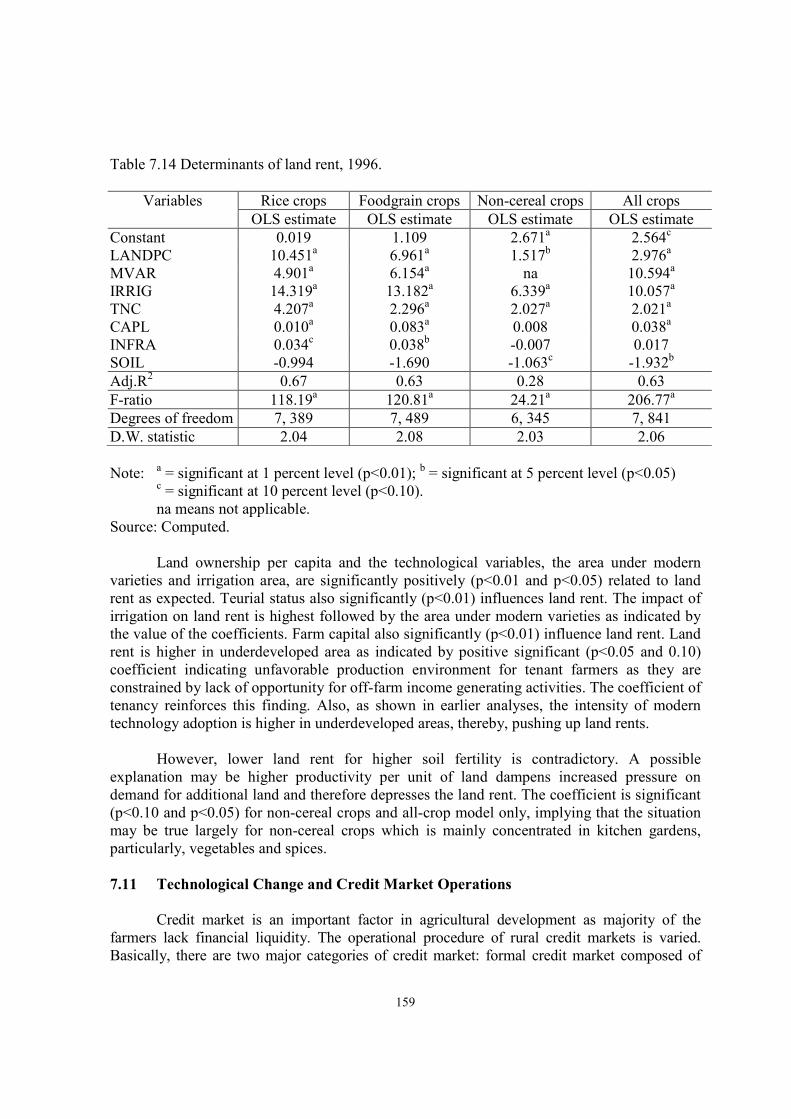
159

Table 7.14 Determinants of land rent, 1996.

Variables Rice crops Foodgrain crops Non-cereal crops All crops

OLS estimate OLS estimate OLS estimate OLS estimate

Constant 0.019 1.109 2.671a 2.564c

LANDPC 10.451a 6.961a 1.517b 2.976a

MVAR 4.901a 6.154a na 10.594a

IRRIG 14.319a 13.182a 6.339a 10.057a

TNC 4.207a 2.296

a 2.027

a 2.021

a

CAPL 0.010a 0.083

a 0.008 0.038

a

INFRA 0.034c 0.038

b -0.007 0.017

SOIL -0.994 -1.690 -1.063c -1.932

b

Adj.R2

0.67 0.63 0.28 0.63

F-ratio 118.19a 120.81

a 24.21

a 206.77

a

Degrees of freedom 7, 389 7, 489 6, 345 7, 841

D.W. statistic 2.04 2.08 2.03 2.06

Note: a = significant at 1 percent level (p<0.01);

b = significant at 5 percent level (p<0.05)

c = significant at 10 percent level (p<0.10).

na means not applicable.

Source: Computed.

Land ownership per capita and the technological variables, the area under modern

varieties and irrigation area, are significantly positively (p<0.01 and p<0.05) related to land

rent as expected. Teurial status also significantly (p<0.01) influences land rent. The impact of

irrigation on land rent is highest followed by the area under modern varieties as indicated by

the value of the coefficients. Farm capital also significantly (p<0.01) influence land rent. Land

rent is higher in underdeveloped area as indicated by positive significant (p<0.05 and 0.10)

coefficient indicating unfavorable production environment for tenant farmers as they are

constrained by lack of opportunity for off-farm income generating activities. The coefficient of

tenancy reinforces this finding. Also, as shown in earlier analyses, the intensity of modern

technology adoption is higher in underdeveloped areas, thereby, pushing up land rents.

However, lower land rent for higher soil fertility is contradictory. A possible

explanation may be higher productivity per unit of land dampens increased pressure on

demand for additional land and therefore depresses the land rent. The coefficient is significant

(p<0.10 and p<0.05) for non-cereal crops and all-crop model only, implying that the situation

may be true largely for non-cereal crops which is mainly concentrated in kitchen gardens,

particularly, vegetables and spices.

7.11 Technological Change and Credit Market Operations

Credit market is an important factor in agricultural development as majority of the

farmers lack financial liquidity. The operational procedure of rural credit markets is varied.

Basically, there are two major categories of credit market: formal credit market composed of

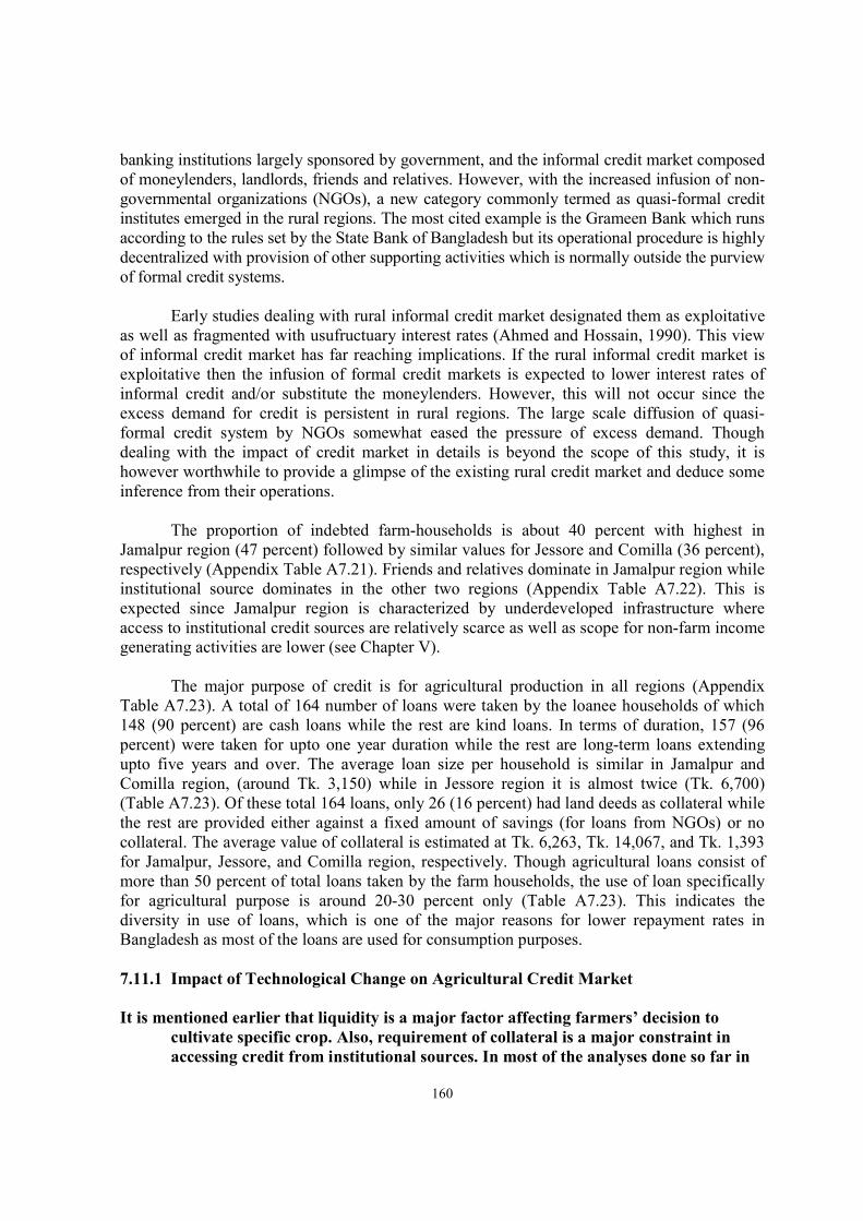
160

banking institutions largely sponsored by government, and the informal credit market composed

of moneylenders, landlords, friends and relatives. However, with the increased infusion of non-

governmental organizations (NGOs), a new category commonly termed as quasi-formal credit

institutes emerged in the rural regions. The most cited example is the Grameen Bank which runs

according to the rules set by the State Bank of Bangladesh but its operational procedure is highly

decentralized with provision of other supporting activities which is normally outside the purview

of formal credit systems.

Early studies dealing with rural informal credit market designated them as exploitative

as well as fragmented with usufructuary interest rates (Ahmed and Hossain, 1990). This view

of informal credit market has far reaching implications. If the rural informal credit market is

exploitative then the infusion of formal credit markets is expected to lower interest rates of

informal credit and/or substitute the moneylenders. However, this will not occur since the

excess demand for credit is persistent in rural regions. The large scale diffusion of quasi-

formal credit system by NGOs somewhat eased the pressure of excess demand. Though

dealing with the impact of credit market in details is beyond the scope of this study, it is

however worthwhile to provide a glimpse of the existing rural credit market and deduce some

inference from their operations.

The proportion of indebted farm-households is about 40 percent with highest in

Jamalpur region (47 percent) followed by similar values for Jessore and Comilla (36 percent),

respectively (Appendix Table A7.21). Friends and relatives dominate in Jamalpur region while

institutional source dominates in the other two regions (Appendix Table A7.22). This is

expected since Jamalpur region is characterized by underdeveloped infrastructure where

access to institutional credit sources are relatively scarce as well as scope for non-farm income

generating activities are lower (see Chapter V).

The major purpose of credit is for agricultural production in all regions (Appendix

Table A7.23). A total of 164 number of loans were taken by the loanee households of which

148 (90 percent) are cash loans while the rest are kind loans. In terms of duration, 157 (96

percent) were taken for upto one year duration while the rest are long-term loans extending

upto five years and over. The average loan size per household is similar in Jamalpur and

Comilla region, (around Tk. 3,150) while in Jessore region it is almost twice (Tk. 6,700)

(Table A7.23). Of these total 164 loans, only 26 (16 percent) had land deeds as collateral while

the rest are provided either against a fixed amount of savings (for loans from NGOs) or no

collateral. The average value of collateral is estimated at Tk. 6,263, Tk. 14,067, and Tk. 1,393

for Jamalpur, Jessore, and Comilla region, respectively. Though agricultural loans consist of

more than 50 percent of total loans taken by the farm households, the use of loan specifically

for agricultural purpose is around 20-30 percent only (Table A7.23). This indicates the

diversity in use of loans, which is one of the major reasons for lower repayment rates in

Bangladesh as most of the loans are used for consumption purposes.

7.11.1 Impact of Technological Change on Agricultural Credit Market

It is mentioned earlier that liquidity is a major factor affecting farmers’ decision to

cultivate specific crop. Also, requirement of collateral is a major constraint in

accessing credit from institutional sources. In most of the analyses done so far in

161

this study, agricultural credit variable is used as an independent variable. In this

section, we are interested in identifying factors determining the availability of

agricultural credit that can serve as a vital instrument in solving liquidity crisis of

farmers. Therefore, in order to test whether there is a significant association

between modern variety cultivation and agricultural credit, a multivariate

analysis is performed at the crop level. The following equation is fitted to the

data:

AGCR= f (OWNLND, MVAR, IRRIG, TNC, CAPL, WORK, FAMILY, EXPCE, INFRA, SOIL)

where:

AGCR = amount of agricultural credit borrowed by the household (‘000 taka)

OWNLND = amount of land owned by the household (ha)

MVAR = amount of cultivated land under modern varieties of rice and wheat (ha)

IRRIG = amount of cultivated land under irrigation (ha)

TNC = amount of cultivated land rented-in (ha)

CAPL = value of farm capital excluding land asset (‘000 taka)

WORK = number of working members in the household (persons)

FAMILY = number of family members in the household (persons)

EXPCE = years of experience of farmer in crop cultivation (years)

INFRA = index of underdevelopment of infrastructure

SOIL = index of soil fertility

The supply of credit will depend on the amount of land owned by the household as it

serves as a major form of collateral. It was already seen that about 40 percent of the sample

households are indebted. The area under modern variety and the area under irrigation are

included to capture the effect of modern agricultural technology on credit demand. Area under

share rent reflects the solvency of the farmer in relation to their demand for land. Availability

of farm capital (particularly livestock) may enable the farmer to access credit. Farm capital

variable is incorporated to capture its effect on credit demand. The argument in favor of

infrastructure and soil fertility variable is similar with that cited in examining other factor

market operations.

The OLS model including only the indebted farmers is used for the analyses. The

analysis is done for rice (all varieties of all seasons), foodgrain (rice and wheat), non-cereal

crops, and all crops (rice, wheat, and non-cereal crops). The result of the exercise is presented

in Table 7.15 (also see Appendix Table A7.24 for details).

Table 7.15 Determinants of agricultural credit, 1996.

Variables Rice crops Foodgrain crops Non-cereal crops All crops

OLS estimate OLS estimate OLS estimate OLS estimate

Constant -3.452 -5.798 -35.585 -14.919

OWNLND -3.333 -2.491 7.565b 3.832

b

MVAR 12.27 12.840c na 2.096

IRRIG -13.210 -14.190c -3.220 -5.468

TNC -3.768 -4.297 -8.592 -5.213

162

CAPL 0.628a 0.603

a 0.518

a 0.523

a

WORK -0.428 -0.593 -8.055a -3.842

a

FAMILY 0.394 0.190 0.788 0.332

EXPCE -0.154b -0.136

b -0.163 -0.161

b

INFRA -0.035 -0.046 -0.212 -0.150c

SOIL 4.998 7.396c 35.047

a 18.417

a

Adj.R2

0.66 0.62 0.31 0.36

F-ratio 22.19a 23.56a 6.60a 15.14a

Degrees of freedom 10, 101 10, 126 9, 106 10, 242

D.W. Statistic 1.96 2.01 2.06 2.07

Note: a = significant at 1 percent level (p<0.01);

b = significant at 5 percent level (p<0.05)

c = significant at 10 percent level (p<0.10).

na means not applicable.

Source: Computed.

Land ownership is significantly (p<0.05) positively related with credit demand as

evident in non-cereal and all-crop models. The insignificant negative sign of the land

coefficient for rice and foodgrain model may not be the true relation. The positive sign is

expected because in order to cultivate additional land more capital is required for which credit

serves as the proxy (Table 7.15). The area under modern varieties is positively related with

credit demand and is significant (p<0.10) in foodgrain model. However, access to modern

irrigation has negative influence on credit demand, which is not very convincing. Farm capital

is significantly positively (p<0.01) related to agricultural credit, implying that credit

requirement is higher for farmers with more farm capital as it complements to undertake

intensive farming at the margin.

The significantly negative (p<0.01) coefficient of working members in the family

indicates that capital requirement is offset by income from working members or in other words

capital constraint is less in farm families with large number of earners which is expected.

Longer farming experience also depresses demand for credit indicating that management

capacity of experienced farmers help mitigate the capital constraint. The coefficient is

significantly negatively (p<0.05) related to credit demand. Demand for agricultural credit is

higher in developed regions as indicated by the significant negative (p<0.10) coefficient of

infrastructure variable. The higher demand for credit in developed region could be attributed to

production of capital intensive non-cereal crops, which was shown to be higher in these

regions. Higher level of soil fertility significantly (p<0.01) increase demand for credit largely

due to opening up opportunity for intensive cropping, thereby, requiring more capital for

farming activities.

7.12 Technological Change and Output Market Operations

Marketing of output is an important factor determining the relative profitability of crop

production. In competitive markets, prices are expected to be exogenous. In the rural markets,

the price that farmers receive includes the transport cost and traders’ margin. State of

infrastructural development plays an important role in this respect, by lowering the transport

163

cost for the produce. Also, access to and availability of storage facilities may influence

cropping pattern in the region. For example, harvest price of potato is very low in peak season.

However, if potato can be stored for a considerable period in cold-storage facilities, it can

fetch substantially higher profit for the farmer. Therefore, options for crop diversification as a

development strategy need to be considered by keeping all these factors in mind. The farm

level prices received by the farmer for specific crop in the study regions is presented in

Appendix Table A7.25. Though there are no sharp regional variation in prices of foodgrain

crops, the prices for spices and pulses are sharply different. This is mainly due to production

of different types of spice and pulse crops in different regions (Appendix Table A7.25).

Primary markets located within 3 kms are the main marketing outlet for the crops

produced in the study region (Tables A7.26 and A7.27). About 78 percent of the farmers sell

their products at the primary market while 7 percent sell at the farmgate level and remaining

sell at secondary markets and/or growth centers also located within 3 kms. Few farmers

actually responded on problems with marketing of outputs. Among those who reported of

facing problems cited poor communication, low output price and illegal brokerage fees as the

major ones (Table A7.28). No single respondent in Jessore region cited problems with

marketing. In fact, all the villages in Jessore study area are very well communicated with the

thana headquarter (sub-district Centre) where all infrastructural facilities are available.

7.12.1 Impact of Technological Change on Output Market

As mentioned earlier, in the competitive market, prices of inputs and outputs are

expected to be exogenous. Also, the prices that farmers pay receive for outputs include

transportation cost and traders’ margin which is likely to vary across farms and regions,

depending on the state of infrastructure development. Higher soil fertility status implies

favorable physical condition for agricultural production thereby increases cropping and land

use intensity leading to increase in supply of outputs. As soil fertility varies from region to

region, farmer’s response pattern relating to use of land will vary. In order to analyze the

impact of technological change on crop prices, the following price equation is fitted to the plot

level data.

OUTP = f (QTY, OWNLND, PMVAR, INFRA, SOIL)

where:

OUTP = price of crop output at the farm-level (taka/kg)

QTY = amount of crop produced by the household (kg)

OWNLND = amount of land owned by the household (ha)

PMVAR = proportion of cultivated land under modern varieties of rice and wheat (%)

INFRA = index of underdevelopment of infrastructure

SOIL = index of soil fertility

OLS model was fitted separately for rice crops (all varieties of rice) foodgrain crops

(all varieties of rice and wheat), non-cereal crops, and all crops (foodgrain plus cash/non-

cereal crops). The results are corrected for first order autocorrelated disturbances. The result of

the exercise is presented in Table 7.16 (also see Appendix Table A7.29 for details).

164

The price quantity relationship has the expected signs and is significant (p<0.01 and

p<0.10) in three regressions (Table 7.16). The low adjusted R2 indicates the exogenous nature

of prices (Ahmed and Hossain, 1990). ). Land ownership status has positive relationship with

crop output price indicating that output price is higher in areas with large landowners. The

coefficient is significantly (p<0.01) positive for foodgrain crops. The negative coefficient in

rice crop is insignificant and therefore may not be the true relationship.

Table 7.16 Determinants of crop prices, 1996.

Variables Rice crops Foodgrain crops Non-cereal crops All crops

OLS estimate OLS estimate OLS estimate OLS estimate

Constant 5.177a 6.144

a 19.739

a 13.967

a

QTY -0.168 -0.051a -1.071

a -0.103

c

OWNLND -0.003 0.194a 0.055 0.112

PMVAR -0.001 -0.001 na 0.006a

INFRA -0.004b -0.016

a -0.054 -0.041

c

SOIL 0.346a 0.269 -2.737 -2.138

Adj. R2

0.05 0.16 0.15 0.12

F-ratio 5.02a 20.01a 16.46a 24.63a

Degrees of freedom 5, 391 5, 491 4, 347 5, 843

D.W. Statistic 2.10 2.51 2.44 2.50

Note: a = significant at 1 percent level (p<0.01);

b = significant at 5 percent level (p<0.05);

c = significant at 10 percent level (p<0.10).

na means not applicable.

Source: Computed.

The impact of technological change is significantly positive (p<0.01) in the all crop

equation implying that prices are higher in areas with high level of modern technology diffusion.

However, this effect is not clear in rice and foodgrain models. The effect of the state of

infrastructure on crop output prices is very pronounced. The negative significant (p<0.01,

p<0.05, and p<0.10) coefficient for underdevelopment of infrastructure indicates that crop prices

are higher in developed areas. The effect of soil fertility status is pronounced in the rice model.

The positive significant (p<0.01) coefficient of soil fertility variable for rice crop indicates that

crop price is higher in areas with higher soil fertility status largely due to better quality of output.

The negative sign of soil fertility coefficient in all crop equation is not significant. The

regression estimate improves as more crops are added.

7.12.2 Storage Facilities

The seasonal nature of agricultural production exerts sharp downward movement of

output prices during peak harvest season. Given the increasing cost of agricultural production,

such fall in prices of crop output spell disaster for farm households. Storage is an important

infrastructural facility that neutralizes this downward movement of prices. Though substantial

amount of cost is involved in storing crop output, particularly perishable products, the gain in

prices in lean season offsets the additional costs involved in the process. There are government

programs on procuring foodgrain crops in the rural regions. However, the storage capacity is

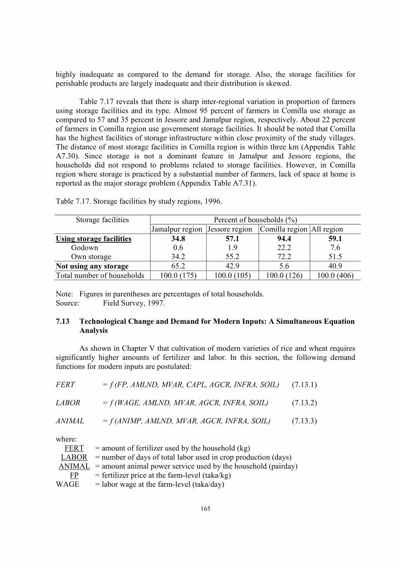
165

highly inadequate as compared to the demand for storage. Also, the storage facilities for

perishable products are largely inadequate and their distribution is skewed.

Table 7.17 reveals that there is sharp inter-regional variation in proportion of farmers

using storage facilities and its type. Almost 95 percent of farmers in Comilla use storage as

compared to 57 and 35 percent in Jessore and Jamalpur region, respectively. About 22 percent

of farmers in Comilla region use government storage facilities. It should be noted that Comilla

has the highest facilities of storage infrastructure within close proximity of the study villages.

The distance of most storage facilities in Comilla region is within three km (Appendix Table

A7.30). Since storage is not a dominant feature in Jamalpur and Jessore regions, the

households did not respond to problems related to storage facilities. However, in Comilla

region where storage is practiced by a substantial number of farmers, lack of space at home is

reported as the major storage problem (Appendix Table A7.31).

Table 7.17. Storage facilities by study regions, 1996.

Storage facilities Percent of households (%)

Jamalpur region Jessore region Comilla region All region

Using storage facilities 34.8 57.1 94.4 59.1

Godown 0.6 1.9 22.2 7.6

Own storage 34.2 55.2 72.2 51.5

Not using any storage 65.2 42.9 5.6 40.9

Total number of households 100.0 (175) 100.0 (105) 100.0 (126) 100.0 (406)

Note: Figures in parentheses are percentages of total households.

Source: Field Survey, 1997.

7.13 Technological Change and Demand for Modern Inputs: A Simultaneous Equation

Analysis

As shown in Chapter V that cultivation of modern varieties of rice and wheat requires

significantly higher amounts of fertilizer and labor. In this section, the following demand

functions for modern inputs are postulated:

FERT = f (FP, AMLND, MVAR, CAPL, AGCR, INFRA, SOIL) (7.13.1)

LABOR = f (WAGE, AMLND, MVAR, AGCR, INFRA, SOIL) (7.13.2)

ANIMAL = f (ANIMP, AMLND, MVAR, AGCR, INFRA, SOIL) (7.13.3)

where:

FERT = amount of fertilizer used by the household (kg)

LABOR = number of days of total labor used in crop production (days)

ANIMAL = amount animal power service used by the household (pairday)

FP = fertilizer price at the farm-level (taka/kg)

WAGE = labor wage at the farm-level (taka/day)

166

ANIMP = animal power price at the farm-level (taka/pairday)

AMLND = amount of land cultivated by the household (ha)

MVAR = amount of cultivated land under modern varieties of rice and wheat (ha)

CAPL = value of farm capital excluding land asset (‘000 taka)

AGCR = amount of agricultural credit borrowed by the household (‘000 taka)

INFRA = index of underdevelopment of infrastructure

SOIL = index of soil fertility

The amount of input used by the household is assumed to be a function of the price of

input, the amount of land under cultivation, and the amount of area devoted to cultivation of

modern varieties of rice and wheat. Also, the amount of non-land farm asset owned by the

households and the amount of agricultural credit received from both institutional and non-

institutional sources may improve the liquidity constraint of the farmers, thereby allowing use

of inputs optimally. Further, the adoption of modern agricultural technology may depend on

the level of infrastructural development and soil fertility status. It was shown above that

infrastructure and soil fertility status influence input and output prices (Tables 7.2 and 7.18).

In addition to these factors, the development of irrigation facilities is also a major factor

determining modern technology adoption rate (Table 6.12). Therefore, the following equations

are presented to explain the variation in the adoption of modern agricultural technology within

the sampled farm households:

MVAR = f (IRRIG, AMLND, CAPL, AGCR, INFRA, SOIL) (7.13.4)

IRRIG = f (AMLND, CAPL, AGCR, INFRA, SOIL) (7.13.5)

where IRRIG is the amount of cultivated land under irrigation (ha).

Given the demand structure of modern inputs, it is clear that the IRRIG and MVAR are

endogenous variables since MVAR appear on the right hand side of eqs. (7.13.1), (7.13.2),

(7.13.3) and IRRIG appear on the right hand side of eq. (7.13.4). This is therefore a case of

simultaneous equation model with recursive structure, where irrigation determines modern

technology adoption, and modern technology adoption determines the demand for fertilizer,

labor and animal power services. Therefore, simultaneous estimation of five equations,

(7.13.1), (7.13.2), (7.13.3) and (7.13.4) or (7.13.5) is conducted using Three-Stage Least

Squares (3SLS) technique that allows correlation among disturbances in individual equations.

The results are presented in Table 7.18 (also see Appendix Table A7.32 for details).

The overall explanatory power of all the five equations are substantially high as

indicated by the values of adjusted R-squared and F-ratio. Also, no

autocorrelated disturbance is observed as indicated by the Durbin-Watson (D.W.)

statistic.

The values of price coefficients have correct signs and are highly significant (p<0.01) for

labor and animal power demand except for fertilizers. The cultivated area is

significantly (p<0.01) positively related to demand for inputs as well as irrigation.

However the significant (p<0.05) negative coefficient for cultivated area in

modern variety adoption function indicates that farmers tend to maximize return

167

from land through cultivation of modern varieties of rice and wheat and is

consistent with a priori expectation and in most of the earlier analyses.

Table 7.18 Joint determination of input demand functions, 1996.

Variables Joint estimates of input demand functions using Three Stage Least Squares

Fertilizer

demand

Labor demand Animal power

demand

Modern techno-

logy adoption

Irrigation

demand

Intercept -82.714c 118.030a 32.463a 0.147 -0.359c

FP -4.578 - - - -

WAGE - -1.110a - - -

ANIMP - - -0.328a - -

AMLND 158.350a 84.485

a 13.601

a -0.478

b 1.056

a

MVAR 119.290a 27.436

b 24.144

a - -

CAPL 1.294b - - 0.002 0.005

a

AGCR -0.659 -0.012 0.056 0.004c -0.005

b

INFRA 0.957 0.316 -0.115a 0.004

b 0.005

a

SOIL 23.219 -34.733a -0.229 -0.097 0.101

IRRIG - - - 1.404a -

Adjusted R2 0.80 0.74 0.86 0.53 0.67

F – ratio 225.56a 195.40

a 427.91

a 77.81

a 167.25

a

Degree of fdm 7, 398 6, 399 6, 399 6, 399 5, 400

D.W. Statistic 1.90 1.95 1.85 1.90 1.79

Note: a = significant at 1 percent level (p<0.01);

b = significant at 5 percent level (p<0.05);

c = significant at 10 percent level (p<0.10).

Source: Computed.

The area devoted to modern varieties of rice and wheat is also significantly (p<0.01

and p<0.05) positively related to input demand, namely, fertilizer, labor as well as animal

power demand. Farm capital also significantly (p<0.05) positively related with fertilizer and

irrigation demand. The coefficient of agricultural credit is weak and provided mixed results.

The significant (p<0.10) positive relation with modern variety adoption is expected and

consistent. However, the significant (p<0.05) negative coefficient of this variable in irrigation

demand function is disturbing. One reason might be that agricultural credit provided by

institutional sources are small and is not sufficient for installing irrigation equipments.

The state of infrastructural development has mixed influence. The positive coefficient

of the state of underdevelopment of infrastructure in fertilizer and labor demand functions

indicate that demands for these inputs are higher in underdeveloped regions. Also the

significant (p<0.05 and p<0.01) positive coefficient of infrastructure index in modern

technology and irrigation demand equation indicates the same. This is expected as in the

underdeveloped areas the scope to switch to other non-farm income generating activities are

lower and therefore the concentration is on agricultural production particularly modern

varieties of rice and wheat which provide significantly higher income. The same results were

168

obtained in a series of analyses explained earlier in this study, thereby, once again validating

the findings. The negative significant (p<0.05) coefficient of the infrastructure variable in

animal power demand function indicates that the demand for animal power services is higher

in developed region. This may be due to substitution of demand for animal power services by

human labor in the underdeveloped areas, which also resulted in higher demand for human

labor. It may also be due to lower incidence of raising livestock in developed regions owing to

high population density and relatively smaller size of homestead areas. The influence of soil

fertility variable is relatively weak and mixed. The significant (p<0.01) negative relation of

soil fertility with labor demand indicates that regions with poor soil fertility will have higher

demand for labor. For other functions the soil variable is not significant.

7.14 Inferences

Substantially higher amount of total labor as well as hired labor per unit of land is

utilized in growing modern rice varieties as compared to local rice varieties. However, the

labor employment pattern is not gender-neutral and is skewed in favor of men. Though female

labor input ranges between 11 – 18 percent and 6 – 48 percent (highest for vegetables) in

foodgrain and non-cereal crop production, respectively, the increased demand for hired labor

is met by hiring male labor only or by substituting female family labor. Also, significantly

lower wage is paid to female labor, if hired, indicating discrimination against women.

Analysis of determinants of labor demand revealed that modern technology, farm size,

and education level of farmers significantly increase demand for hired labor while labor wage,

tenurial status, developed infrastructure, soil fertility, subsistence pressure, and working

members in the family significantly decrease demand for hired labor. However, demand for

total labor is significantly higher in underdeveloped areas.

Analysis of impact on prices revealed that modern technology, soil fertility, land

ownership, and underdeveloped infrastructure significantly increase labor wages while soil

fertility and developed infrastructure significantly increase fertilizer prices. Demand for

pesticide use increase significantly with farm size, irrigation, agricultural credit and

underdeveloped infrastructure. Improved soil fertility significantly reduces demand for

pesticide use, mainly in case of non-cereal crops. In the output market, modern technology,

soil fertility and developed infrastructure significantly increase output prices.

The tenurial arrangements changed substantially from the 50 - 50 output share with no

input sharing system to variable output share and input sharing systems unique to each village.

The input that is relatively scarce is shared between the landowner and the tenant.

Determinants of land rent revealed that per capita land owned, modern technology, irrigation,

tenurial status, farm capital and underdeveloped infrastructure significantly increase rent while

improved soil fertility significantly decreases land rent.

An analysis of demand for agricultural credit revealed that land ownership, farm

capital, soil fertility and developed infrastructure significantly increase credit demand while

number of working members in the family and farming experience significantly reduces

demand for credit.

169

A simultaneous analysis of input demand functions revealed that modern technology

and farm size significantly increases input demand. Irrigation strongly influences modern

technology adoption decisions in addition to agricultural credit and underdeveloped

infrastructure while farm size has significant negative influence on adoption. On the other

hand, farm size, farm capital, agricultural credit, and underdeveloped infrastructure

significantly increases irrigation demand.

170

CHAPTER VIII

TECNOLOGICAL CHANGE AND ITS IMPACT ON INCOME DISTRIBUTION

AND POVERTY

The differential rate of modern variety adoption among farmers, variation in prices, and the

impacts of modern technology on production, employment, and expansion of markets for non-

farm goods and services will ultimately affect the level and pattern of income distribution in

the rural areas (Hossain, 1989). Though it is highly difficult to estimate the exact income of a

rural household from a cross-section sample survey, an attempt has been made to estimate

total income of households from agricultural activities as well as non-agricultural activities in

this study. Based on these estimates of income, the present chapter analyzes the impacts of

technological change on income, income distribution and poverty following certain standard

assumptions. Details are provided in relevant sections.

8.1 Definition of Household Income

Household or family income is defined as the return to family labor and the assets owned

after the current cost of production (excluding family labor and rent for land and

assets) is deducted from the gross value of production (Ahmed and Hossain,

1990). Current cost is the cost incurred by individual households in purchasing

inputs, hiring labor, hiring animal power services, and renting services. The

disaggregation of total family income into a number of following components

provides a firsthand picture of sources of income:

1. Income from crop production (CROPI)

2. Income from livestock (LIVEI)

3. Income from fisheries (FISHI)

4. Income from land leased-out/rented-out (LEASEI)

5. Income from wage (WAGEI)

6. Income from business and miscellaneous sources (BUSI)

7. Total agricultural income (AGI) = CROPI + LIVEI + FISHI + LEASEI

8. Total non-agricultural income (NAGI) = WAGEI + NAGI.

9. Total household income (INC) = AGI + NAGI.

8.1.1 Derivation of Various Sources of Household Incomes

Income derived from crop production (CROPI) is straightforward. As the present study

covers information on all types of crops produced by the households in one year, so the total

income from producing various crops are computed directly from the information detailed in

Chapter V.

Income from livestock sources are estimated from direct question to the respondents on

various products and by-products produced from livestock resources, such as from milk, meat,

egg, sale, value of consumed product, etc. Also, information on weekly expenditure on

livestock raising is collected which is then multiplied by 52 to arrive at an annual expenditure

and deducted from total gross income to yield net income from livestock.

171

Incomes from fisheries resources are estimated from direct question on costs and

returns of fish production in one year. Costs include excavation, liming, fertilizing, feeding,

renting (if multiple owned) and harvesting costs. Incomes include revenue from sale of

harvest, imputed value of fish consumed by the family and value of stock in the pond. The

total cost is then deducted from gross income to yield net income from fisheries.

Income from all other categories are estimated from direct question on type of

activities, in which individual working members of the household is involved for one week

preceding the day of survey, number of days worked and income earned from these activities.

These weekly income derived from various sources is then multiplied by 52 to arrive at the

annual income.

8.2 Description of Household Income from Various Sources

In this section, annual per household income derived from various components for the

study regions is described and then final structure is summarized.

8.2.1 Income from Agriculture

Income from agriculture comprises of income from various crops, fisheries, livestock

and leased-out land. Crop income is derived from the aggregate of local and modern varieties

of rice (all season), wheat, jute, potato, pulses, spices, oilseeds, vegetables and cotton. Table

8.1 presents the disaggregated household level annual income from crops.

Table 8.1 Average annual crop income (Tk.) per household by study regions, 1996.

Source of crop

income

Average annual income per household (Tk.) F-ratio for regional

difference in

income Jamalpur

region

Jessore

region

Comilla

region

All region

Local rice 1,224A 129

B 816

A 814 3.58

b

Modern rice 14,060A 10,387

B 5,725

C 10,524 16.90

a

Modern wheat 194A 738

B 716

B 496 5.70

a

Jute 241A 1,891

B 346

A 700 22.20

a

Potato 288A 131

A 729

B 384 6.12

a

Pulses ng 1,531A 50B 412 34.14a

Oilseeds 37A 578B 242C 240 11.03a

Spices 687A 56B 142B 355 4.00 b

Vegetables 108A 1,395B ng 407 19.39a

Cotton ng 627 ng 162 na

Total crop income 16,839A

17,461A 8,765

B 14,494 11.87

a

Note: Same block letters in superscript represents similarity in income across region based on

LSD at 5 percent level of significance (p<0.05). a = significant at 1 percent level (p<0.01);

b = significant at 5 percent level (p<0.05)..

ng means not grown; na means not applicable.

172

Source: Field Survey, 1997.

It is clear from Table 8.1 that the dominant source of crop income is the modern rice

varieties that accounts for more than 60 percent of total income from crop production. Other

crops including local varieties of rice contribute very little to the total annual income derived

from crop production. There are significant (p<0.01 and p<0.05) inter-regional variations with

respect to income per household derived from individual crops (Table 8.1). Income from non-

cereal crops such as jute, pulses and vegetables are significantly (p<0.05) different between

Jessore and other regions. It is worth noting that the more diversified the cropping system the

higher is the total crop income per household as evidenced in Jessore region. On the other

hand, low crop diversity resulted in low income as evidenced in Comilla region. Also, the

concentration of modern variety cultivation does not necessarily translate into higher income

from crop production (Table 8.1).

The average annual income derived from agricultural sources is presented in Table 8.2.

It is obvious from Table 8.2 that annual income generated from crop production (foodgrain as

well as non-cereal crops) is highest of all sources. Livestock and land leasing also serve as

major sources of household income. There is significant (p<0.01) inter-regional differences in

average agricultural income per household as well as per capita (Table 8.2). The average

annual household agricultural income is similar in Jessore and Jamalpur region and is

significantly (p<0.05) lower in Comilla region. The trend is similar for the per capita

agricultural income as well. The significantly (p<0.05) lower income from all sources in

Comilla region is due to lower level of crop diversification, higher input costs, and higher

involvement in non-agricultural income earning activities as evident in subsequent analyses. It

is clear from Table 8.2 that, the more diversified the cropping system, higher is the income, for

example, for both Jamalpur and Jessore as compared to Comilla region.

Table 8.2 Average annual agricultural income (Tk.) by study regions, 1996.

Source of income Jamalpur

region

Jessore

region

Comilla

region

All region F-ratio for regional

income difference

Income per household

Crops 16,839A

17,461A 8,765

B 14,494 11.87

a

Livestock 4,717A 6,764

B 3,400

C 4,838 11.21

a

Fisheries 1,746A 1,990

A 270

B 1,351 5.73

a

Land leasing 3,334A 2,423

A 265

B 2,146 5.74

a

Total agriculture 26,637A 28,639A 12,700B 22,829 18.41a

Income per capita

Crops 3,254A 2,712

A 1,417

B 2,542 18.76

a

Livestock 1,010A 1,158

A 572

B 912 7.61

a

Fisheries 317A 289

A 37

B 229 5.91

a

Land leasing 646A 389

AB 49

B 393 5.18

a

Total agriculture 5,228A 4,548

A 2,075

B 4,071 24.83

a

Note: Same block letters in superscript represents similarity in income across region based on

LSD at 5 percent level of significance (p<0.05). a = significant at 1 percent level (p<0.01).

173

Source: Field Survey, 1997.

8.2.2 Income from Non-agriculture

The average annual income earned from non-agricultural activities is broadly divided

into two categories: (a) income from wage earning (where income as agricultural

wage labor is also included); and (b) income from business, small trade, cottage

industries, rural transport, carpentry, and other miscellaneous sources. Table 8.3

reveals that though there is no significant difference in wage income across

region, income from business and other activities are significantly (p<0.01)

different. The difference is largely due to significantly (p<0.05) lower income in

this category for Jamalpur region as compared to Jessore and Comilla region

having similar income levels. This is expected as Jamalpur region is characterized

by underdeveloped infrastructure and located at a remote distance from district

headquarter. On the other hand, business income is highest in Comilla, a

developed region, followed by Jessore, also a developed region.

Table 8.3 Average annual non-agricultural income (Tk.) by study regions, 1996.

Source of non-

agricultural income

Jamalpur

region

Jessore

region

Comilla

region

All region F-ratio for regional

income difference

Income per household

Wage income 1,444A 1,446A 2,192A 1,677 0.572

Business and others 3,499A 8,979B 10,422B 7,065 8.581a

Total non-agriculture 4,944A 10,425

B 12,614

B 8,742 9.358

a

Income per capita

Wage income 316A 291

A 378

A 329 0.867

Business and others 656A 1,546

B 1,751

B 1219 7.397

a

Total non-agriculture 952A 1,751

B 2,129

B 1,548 7.050

a

Note: Same block letters in superscript represents similarity in income across region based on

LSD at 5 percent level of significance (p<0.05). a = significant at 1 percent level (p<0.01).

Source: Field Survey, 1997.

8.2.3 Total Family Income

The total family income per household is composed of total agricultural and non-

agricultural income. Table 8.4 presents the composition of average family income

of the study households. Though there is a sharp difference in income derived

from agricultural sources, the inter-regional gap in total family income is

narrower. Particularly, the gap in agricultural income of households in Comilla

narrowed down substantially when total family income is compared across

regions. There are sharp inter-regional differences in share of income derived

from various sources. Nevertheless, it appears that agricultural source,

particularly, the field crops dominate the rural income scenario. The level of

174

infrastructural development has high influence on the amount of income derived

from non-agricultural sources. For example, non-agricultural source contributed

about 50 percent to total family income in Comilla region, which is a developed

region in terms of infrastructure. This is followed by Jessore region where non-

agricultural source contributed about 27 percent to family income, also a

developed region (Table 8.4).

Table 8.4 Structure of annual family income (Tk.) per household by study regions, 1996.

Source of income Share of component incomes to total family income (%)

Jamalpur region Jessore region Comilla region All region

Total agricultural income 84.3 73.3 50.2 72.3

Crops 53.3

44.7 34.6 45.9

Livestock 14.9 17.3 13.4 15.3

Fisheries 5.5 5.1 1.1 4.3

Lease 10.6 6.2 1.1 6.8

Total non-agricultural income 15.7 26.7 49.8 27.7

Wage 4.6

3.7 8.6 5.3

Business and other 11.1 23.0 41.2 22.4

Total family income 100.0

(31,581)

100.0

(39,064)

100.0

(25,314)

100.0

(31,571)

Note: Figures in parentheses represents total family income per household.

Source: Field Survey, 1997.

8.3 Income Distribution by Land Ownership and Tenurial Categories

The striking difference in average household income from crops for Comilla region as

compared to other regions as shown in Table 8.4 becomes smaller when the same income is

computed per capita and distributed by land categories (Table 8.5).

Table 8.5 Average annual crop income (Tk.) per capita by land ownership categories by study

regions, 1996.

Landownership

categories1

Average annual crop income (Tk/capita)

Jamalpur region Jessore region Comilla region All region

Landless 1,536A

1,363A 961

A 1,305

A

Marginal 2,412A 2,088

A 1,369

B 1,957

B

Small 3,185B 1,932

A 1,543

B 2,792

C

Medium 4,293C

4,164B 2,598

C 3,856

D

Large 7,740D 6,152

C na 6,8590

E

All categories 3,254 2,712 1,417 2,542

F-ratio for income

difference by landsize

18.60a 13.10a 6.91a 40.49a

Degree of freedom 4, 170 4, 100 3, 122 4, 401

Correlation coefficient 0.55a 0.64

a 0.39

a 0.56

a

175

Note: Same block letters in superscript represents similarity in income levels across

landownership categories based on LSD at 5 percent level of significance (p<0.05). a = significant at 1 percent level (p<0.01); na means not available.

1 Landless = less than 0.20 ha of owned land, marginal = owned land 0.21 – 0.40 ha,

small = owned land 0.41 – 1.00 ha, medium = owned land 1.01 – 2.00 ha, and large =

owned land above 2 ha.

Correlation coefficient shows relationship between per capita crop income and per

capita land owned by the household.

Source: Field Survey, 1997.

It is clear from Table 8.5 that, for landless and marginal farmers, the average crop

income per capita is similar across regions. The difference becomes strikingly large for small

and medium owner category. No household in Comilla region falls in large category.

Therefore, comparison of this category with other regions cannot be made. However, one can

notice the very high level of crop income earned by large farmers which pushed up the average

income for all categories of households and making the difference between Comilla and other

region strikingly large. The sharply rising average household income from crop with increase

in the amount of land owned reveals the importance of land as a prime source of wealth in the

rural region and the reason for farmers to cling to land for income (Table 8.5). The correlation

between crop income and land ownership is significantly (p<0.01) positively related and the

values are estimated at 0.55, 0.64, and 0.39 for Jamalpur, Jessore, and Comilla region,

respectively (Table 8.5).

Striking difference also exists between Comilla and other regions in terms of per capita

crop income across tenurial categories (Table 8.6). While there are significant (p<0.05)

difference between tenants and owner-operators as well as part-tenants in Jamalpur and

Jessore region, the difference is insignificant in Comilla region. This is largely due to the fact

that, as per capita land size is small in Comilla, most of the farmers rent-in part of the land to

increase the farm size to an economic size. Overall, there is significant (p<0.05) difference in

total crop income across tenurial category (Table 8.6).

Table 8.6 Average annual agricultural income (Tk.) per capita by tenurial categories by study

regions, 1996

Tenurial categories Average annual crop income (Tk/capita)

Jamalpur region Jessore region Comilla region All region

Owner-operator 3,803A 3,038A 1,497A 2,899A

Part-tenant 3,261A 2,804B 1,319A 2,464A

Tenant 1,130B 1,343B 1,312A 1,241B

All 3,254 2,712 1,417 2,542

F-ratio for income

difference by tenancy

8.52a 2.43

c 0.32 9.26

a

Degree of freedom 2, 172 2, 102 2, 123 2, 403

Note: Same block letters in superscript represents similarity in income levels across tenurial

categories based on LSD at 5 percent level of significance (p<0.05). a = significant at 1 percent level (p<0.01); c = significant at 10 percent level (p<0.10).

176

Source: Field Survey, 1997.

The breakdown of per capita income from agricultural and non-agricultural sources by

land ownership categories is presented in Table 8.7. Such breakdown in per capita income by

sources depicts certain interesting features. It is interesting to note that while per capita income

from agricultural source is significantly (p<0.01) positively related with amount of land owned

by the households, the per capita non-agricultural income moves in the opposite direction and

is significant (p<0.10) for Jamalpur region. This finding conforms to a priori expectation that

land serves the major source of wealth and income in rural setting. The per capita income from

non-agricultural sources is negatively correlated with amount of land owned by the household,

a finding reinforcing the a priori expectation. The inter-regional differences in per capita

income from agriculture increased sharply at the upper scale of land ownership category while

for landless, marginal and small farmers the values are relatively close.

Another interesting feature is that the non-agricultural income per capita is highest in

landless categories and has declining trend though not very prominent. This is

consistent with the fact that the landless and marginal farmers usually supply

their labor in the labor market and thus receives the benefit of increased income

from technological change in agriculture through the labor market operations.

Table 8.7 Average per capita income (Tk.) from agricultural and non-agricultural sources by land

ownership categories by study regions, 1996.

Land

ownership

categories

Per capita agricultural income (Tk.) Per capita non-agricultural income (Tk.)

Jamalpur

region

Jessore

region

Comilla

region

All region Jamalpur

region

Jessore

region

Comilla

region

All region

Landless 2,254A

2,179A 1,441

A 1,973

A 1,432 2,000 2,414 1,900

Marginal 3,432A 3,978

B 2,093

B 3,086

B 758 2,127 2,832 1,842

Small 6,830B 4,046

B 2,110

B 4,547

C 859 2,179 1,513 1,331

Medium 7,708B 6,352

C 3,891

C 6,434

D 711 717 1,276 847

Large 12,361C 9,683

D na 10,873

E 238 1,850 na 1,134

All sizes 5,228 4,548 2,075 4,071 952 1,857 2,129 1,548

F-ratio for

catg. diff.

24.69a 16.07a 7.96a 49.27a 1.53 1.02 0.92 1.91

Df 4, 170 4, 100 3, 122 4, 401 4, 170 4, 100 3, 122 4, 401

Correlation 0.55a 0.64

a 0.39

a 0.56

a -0.13

c -0.04 -0.13 -0.09

c

Note: Same block letters in superscript represents similarity in income levels across

landownership categories based on LSD at 5 percent level of significance (p<0.05).

For per capita income from non-agricultural sources LSD values are not computed as

the difference is not significant indicated by F-ratio.

Correlation coefficient shows relationship between per capita income and land owned

by the household. a = significant at 1 percent level (p<0.01); c = significant at 10 percent level (p<0.10).

na means not available.

Source: Field Survey, 1997.

177

The structure of income from various sources by land ownership categories as well

as by tenurial categories are presented in Table 8.8. There is a clear increasing trend in

income from all sources in ascending levels of land ownership except for the wage income

where the trend is reversed. This resulted in similar amount of income from non-

agricultural sources for all land categories (Tk.8,600 – 8,900 per household approx.).

Similarly, the tenants earn higher income per household from non-agricultural sources,

particularly wage income (Table 8.8). This finding further reinforces the expectation

explained above. The tendency to move towards non-agricultural income sources increases

due to lack of access to land which serves as the primary source of production.

Table 8.8 Structure of annual household income (Tk) by land ownership and tenurial

categories (all regions), 1996.

Income categories Land ownership categories Tenurial categories All

household Landless

farmer

Marginal

farmers

Farm

household

Owner

operator

Part

tenant

Tenant

Foodgrain income 27.9 35.4 40.9 37.3 43.9 23.8 37.5

Non-cereal income 6.3 4.7 10.1 9.2 6.7 6.8 8.4

Total crop income 34.2 40.1 51.0 46.5 50.6 30.6 45.9

Wage income 16.2 4.3 2.3 1.8 8.2 23.3 5.3

Miscellaneous inc. 31.3 32.3 17.0 22.6 18.9 28.7 22.4

Agricultural income 52.5 63.4 80.7 75.6 72.9 48.0 72.3

Non-agril. income 47.5 36.6 19.3 24.4 27.1 52.0 27.7

Total household

income

100.0

(18,553)

100.0

(24,283)

100.0

(44,773)

100.0

(36,946)

100.0

(25,596)

100.0

(21,235)

100.0

(31,571)

Per capita income 3,873 5,091 7,242 6,363 4,910 4,201 5,236

Family size 5.49 5.39 6.74 6.26 5.88 5.38 6.03

Observations 134 90 182 236 112 58 406

Note: Figures in parentheses are percentages of total income.

Landless = less than 0.20 ha of owned land, marginal = owned land 0.21 – 0.40 ha,

small = owned land 0.41 – 1.00 ha, medium = owned land 1.01 – 2.00 ha, and large =

owned land above 2 ha.

Farm household refers to the combination of small, medium and large farmers (0.41 –

2.00 + ha).

Source: Field Survey, 1997.

8.4 Determinants of Household Income: A Multivariate Regression Analysis

The previous sections provided an assessment on the structure of household income

derived from various sources. The effect of land ownership on the structure of

income as well as regional variation in level and structure of income was

analyzed. However, income of a household depends on a host of factors, which are

not captured in the aforementioned analyses. Therefore, in order to assess the

178

impact of modern agricultural technology on annual household income, the

following equation is fitted to the household level data.

INCM = f (AMLND, WORK, CAPL, AGE, TNC, PMVAR, PIRRIG, EDUCH, INFRA,

SOIL)

where,

INCM = total family income of the household (‘000 taka)

AMLND = amount of land cultivated by the household (ha)

WORK = number of working members in the household (persons)

CAPL = value of farm capital excluding land asset (‘000 taka)

AGE = age of the farmer (years)

PTNC = proportion of cultivated land rented-in (%)

PMVAR = proportion of cultivated land under modern varieties of rice and wheat (%)

PIRRIG = proportion of cultivated land under irrigation (%)

EDUCH = completed years of formal schooling of the head of household (years)

INFRA = index of underdevelopment of infrastructure

SOIL = index of soil fertility

The effect of technological change on household income is captured with the

multiplicative term PMVAR*PIRRIG. This is done as these two variables tend to be highly

correlated. The regression estimate is specified in log-linear form. Natural logarithm of

amount of land cultivated (AMLND), value of non-land fixed assets (CAPL), number of

working members (WORK) in the family, and age of the farmer (AGE). The education

variable is measured in linear form since many farmers have zero values. The remaining

variables are measured in proportions and indices as the case may be. The OLS method is used

for estimating the parameters. Various components of household income are regressed

independently on the aforementioned set of explanatory variables. The estimated parameters of

the income equations for crop income, agricultural income, non-agricultural income and total

family income per household are presented in Table 8.9. The explanatory variables explained

about 82 percent of the variation in crop income model and 75 percent in agricultural income

model respectively (for details see Appendix Table 8A.1). The very low value of adjusted R-

squared in the non-agricultural income model reflects the exogeniety of income from non-

agricultural sources. The model explains about 46 percent of overall income within the sample

households.

Table 8.9. Determinants of rural household income, 1996.

Variables Crop income

(CROPI)

Agricultural

income (AGI)

Non-agricultural

income (NAGI)

Total family

income (INC)

Constant 9.128a 9.267a 7.260b 10.265a

lnAMLND 0.962a 0.676a -0.741b 0.446a

lnWORK -0.001 0.114b 0.818

c 0.110

c

lnCAPL 0.043a 0.142

a -0.087 0.113

a

lnAGE -0.039 -0.023 -0.206 0.049

PTNC -0.111 -0.264a 0.395 -0.171

PMVAR*PIRRIG 0.238a 0.165

b -2.471

a -0.180

EDUCH -0.020a -0.005 0.004 0.004

INFRA -0.001 -0.002 -0.055a -0.007

a

179

SOIL 0.287b 0.298

b -0.193 -0.090

Adj. R-squared 0.83 0.75 0.07 0.46

F(9, 396) 213.97a 133.81

a 4.23

a 38.63

a

D.W. Statistics 1.74 1.75 1.80 2.02

Note: a = significant at 1 percent level (p<0.01); b = significant at 5 percent level (p<0.05)

c = significant at 10 percent level (p<0.10)

Source: Computed.

Land, value of nonland fixed assets, modern agricultural technology and soil fertility are

the major determinants of income from crop and agricultural sources. The

coefficient of land is positive and highly significant (p<0.01) in crop, agricultural

and family income model. The value of land coefficient in crop model indicates

that one percent increase in land area will raise income by about one percent. The

negative coefficient of tenancy variable indicates that the sharecropping depresses

family income and is consistent with a priori expectation.

The major determinants of non-agricultural income are number of working members in

the family. Land, access to modern agricultural technology, and high value of

non-land fixed capital negatively influence non-agricultural income indicating

that lack of access to modern agricultural technology forces the households to

seek income from non-farm sources.

The technology variable is positive and highly significant (p<0.01) in crop and

agricultural income model as expected. The education level of the household head has a

negative relationship with income from crop and agriculture but positive with non-agricultural

income indicating that higher level of education pulls farmers away from agricultural

activities. Deb (1995) also reported negative influence of education on agricultural growth.

The number of working members in the family significantly (p<0.05) negatively

influence income from agriculture while it is significantly (p<0.10) positively related with

non-agricultural income as well as total family income. The implication is that large number of

working members in the family lead to high involvement in non-farm activities, as expected.

The influence of the state of infrastructural development is very pronounced in non-

agricultural and total family income model and the expected sign is consistent throughout. The

significant (p<0.01) negative coefficient of this variable indicates that household income from

non-agricultural activities as well as overall income is higher in developed region which

reinforces the findings of all the preceding chapters. The significant (p<0.05) positive

coefficient of soil fertility variable indicates that the better the soil quality the higher will be

the agricultural income also reinforcing the findings of previous analyses.

8.5 Distributional Impact of Technological Change on Farm Households

A major focus of this study is to examine the distributive justice of the highly desired

technological change in crop agriculture. The aforementioned analyses already hinted on the

fact that though technological change raised income significantly, yet it failed to bring in

180

distributive justice to the rural household economy. In this section, a rigorous analysis of

impact of technological change on income distribution is attempted in order to confirm the

intuition developed in the foregoing sections.

8.5.1 Impact on Factor Shares

An analysis of the changes in factor shares of crop production will provide a first hand

implication on the distributional impact of modern agricultural technology. In

absolute value terms, significant (p<0.01) differences exists between modern and

local rice varieties in all components of the factor shares (Table 8.10). However,

the column of differences in factor shares (modern over local varieties) provides

some interesting features. Production of modern varieties is heavier on current

inputs with a large purchased component but cheaper on animal power services

as well as human labor input per unit of land area though it employs significantly

(p<0.01) higher amount of hired labor. Though there is no difference in

proportion of family income between alternative rice production technologies, the

proportion of net income (farm operator surplus) is almost double for modern

variety cultivators. Therefore, those farmers who cannot afford to adopt modern

technology lose in terms of net income per unit of land.

Table 8.10 Factor shares of local and modern varieties of rice (all region), 1996.

Factors Local rice varieties Modern rice varieties Share diff.

(modern

over local)

t-ratio for

mean value

difference Tk/ha Share of

gross value

Tk/ha Share of

gross value

Current input 1,906 13.66 5,260 21.04 7.38 12.22a

Family 567 4.06 994 4.01 -0.05 6.17a

Purchased 1,339 9.60 4,266 17.03 7.43 11.37a

Animal labor 1,962 14.06 2,170 8.75 -5.31 5.06a

Family 769 5.51 1,045 4.21 -1.30 2.54a

Hired 1,193 8.55 1,125 4.54 -4.01 -0.61

Human labor 3,479 24.94 4,553 18.35 -6.59 5.66a

Family 1,628 11.67 1,806 7.28 -4.39 1.02

Hired 1,351 13.27 2,747 11.07 -2.20 4.92a

Land rent 5,494 39.38 9,297 37.47 -2.11 10.15a

Operator surplus 1,111 7.96 3,529 14.22 6.26 5.25a

Gross output value 13,952 100.00 24,809 100.00 - 13.50a

Value added 12,045 86.33 19,549 78.80 -7.53 10.37a

Farm-family income 9,002 64.52 15,677 63.19 -1.33 9.04a

Observations 117 829

Note: a = significant at 1 percent level (p<0.01).

Source: Field Survey, 1997.

8.5.2 Impact on Income Distribution

181

To begin with the analysis of distributional impacts of modern agricultural technology,

the structure of income of the rural households is analyzed by categorizing the villages

according to status of modern technology (variety) adoption as well as status of modern

irrigation facilities. Villages with more than 60 percent of land area under modern varieties of

rice and wheat are designated as the ‘high adopter’ villages, between 40 – 60 percent of land

area under modern varieties as ‘medium adopter’ villages, and less than 40 percent land under

modern varieties as ‘low adopter’ villages. The other classification of villages is according to

level of modern irrigation facilities. Villages with more than 50 percent of land area under

modern irrigation facilities are designated as ‘highly irrigated’ villages while the remaining are

designated as ‘poorly irrigated’ villages.

Table 8.11 summarizes the intensity of modern technology adoption in the villages

thus classified. Though the average size of land owned and area cultivated are lowest with

highest incidence of tenancy in ‘low adopter’ villages, the differences are not as sharp between

‘high adopter’ villages as compared to ‘medium adopter’ villages. Similar trend is observed

for the villages classified according to level of irrigation facilities. This reinforces the finding

that intensity of modern agricultural technology is higher in regions with poor land

endowments. But various other factors also determine adoption, which leads to the

differentiation between the two extremes, the ‘high adopter’ and ‘low adopter’ villages. Two

of those factors may be the incidence of tenancy and the level of irrigation facilities.

Table 8.11 Level of modern technology adoption in study villages, 1996.

Variables Adopter categories Irrigation level All

High Medium Low High Low

Average size of land owned (ha) 0.63 0.90 0.51 0.68 0.50 0.65

Average size of land cultivated (ha) 0.95 1.28 0.82 1.01 0.82 0.98

Area under tenancy (%) 19.13 22.74 23.49 20.56 18.30 20.06

Area under modern rice (%) 86.44 57.03 37.26 81.27 55.94 77.59

Area under irrigation (%) 67.02 62.35 17.93 67.42 27.70 61.65

Households in the group (%) 76.35 14.04 9.61 85.47 14.53 100.00

Source: Field Survey, 1997

An analysis of the structure of farmers’ income by status of modern technology adoption

reveals some interesting features. Though foodgrain income is highest in ‘high

adopter’ villages, the overall crop income is highest in ‘medium adopter’ villages

as presented in Table 8.12. This reinforces the finding in previous sections that the

more diversified the agricultural production system, the more is the income.

However, a sufficient condition seems that diversification has to be undertaken

with medium level of modern technology adoption, implying that one season of

modern rice coupled with non-cereal crops in other seasons would bring in

highest income per household.

Table 8.12 Structure of annual household income (Tk.) by status of modern agricultural

technology adoption (all regions), 1996.

182

Income categories Adopter categories of villages Irrigation level of villages All

household High

adopter

Medium

adopter

Low

adopter

High

irrigated

Low

irrigated

Foodgrain income 44.7 24.7 13.5 40.5 18.5 37.5

Non-cereal income 4.5 21.9 10.3 8.3 9.0 8.4

Total crop income 49.2 46.6 23.8 48.8 27.5 45.9

Wage income 4.6 3.3 13.4 4.4 11.2 5.3

Miscellaneous income 16.8 26.8 50.4 18.4 48.0 22.4

Agricultural income 78.6 69.9 36.2 77.2 40.8 72.3

Non-agril. income 21.4 30.1 63.8 22.8 59.2 27.7

Total household

income

100.0

(28,982)

100.0

(42,534)

100.0

(36,124)

100.0

(31,935)

100.0

(29,427)

100.0

(31,571)

Per capita income 5,352 6,902 6,220 5,763 5,009 5,236

Family size 5.87 6.07 7.21 5.85 7.07 6.03

Observations 310 57 39 347 59 406

Note: Figures in parentheses are total family income per household.

Source: Field Survey, 1997.

Wage income, on the other hand, is highest in ‘low adopter’ villages, implying that lower

income from crop agriculture must be supplemented with either wage income or

non-farm income. Interplay of all these diversified factors resulted in lowest

household income for ‘highest adopter’ villages. Consequently, the per capita

income is also estimated to be lowest for farmers of ‘high adopter’ villages. Since,

it was already established that modern variety cultivation fetches significantly

higher income per unit of land, the associated lowest per capita income is solely to

be attributed to high unequal distribution of income across households in these

‘high adopter’ villages. However, firm conclusion on this finding will be drawn

after analyzing the degree of income concentration.

Further, analysis of income structure between villages endowed with ‘high’ and ‘low’

level of modern irrigation facilities reveals that crop income as well as total agricultural

income is higher in ‘highly irrigated’ villages while wage and non-farm income is high in ‘low

irrigated’ villages (Table 8.12). However, it is interesting to observe that income per

household is not sharply different between these two categories of villages. The difference in

per capita income is also not largely different as with the case of villages classified according

modern technology adopter categories. The family size dynamics suppressed the household

income for villages lying at the bottom of both classes. The family size is more than 7 persons

per household in this category as compared to only 6 persons for other categories (Table 8.12).

Conclusion on the existence of income inequality in ‘high adopter’ villages is

reinforced when income structure of only landless and marginal farmers classified by adopter

category and irrigation level is analyzed separately (Table 8.13).

183

Table 8.13 Structure of household income (Tk.) of landless and marginal farmers by status

of modern agricultural technology adoption (all regions), 1996.

Income categories Adopter categories of villages Irrigation level of villages All

household High

adopter

Medium

adopter

Low

adopter

High

irrigated

Low

irrigated

Foodgrain income 39.6 21.7 8.8 36.0 12.2 31.4

Non-cereal income 2.8 14.9 7.4 5.3 6.8 5.6

Total crop income 42.4 36.5 16.2 41.2 19.0 37.0

Wage income 9.9 6.7 17.0 9.5 15.3 10.6

Miscellaneous income 24.3 35.3 57.6 26.2 55.4 31.8

Agricultural income 65.8 58.1 25.5 64.3 29.3 57.6

Non-agril. income 34.2 41.9 74.5 35.7 70.7 42.4

Total household

income

100.0

(18,031)

100.0

(25,811)

100.0

(36,411)

100.0

(19,670)

100.0

(27,883)

100.0

(20,844)

Per capita income 3,847 5,229 7,271 4,178 5,467 4,362

Family size 5.38 5.24 6.32 5.28 6.50 5.45

Observations 173 22 29 192 32 224

Note: Figures in parentheses are total family income per household.

Source: Field Survey, 1997.

The per capita income in ‘high adopter’ village is almost half as compared to ‘low

adopter’ villages. The picture is similar, but less sharp, when per capita income between

‘highly’ and ‘poorly’ irrigated villages are considered. Therefore, one can intuitively state that

expansion of modern irrigation facilities only causes lesser degree of inequality as compared

to intensive diffusion of modern varieties of rice and wheat. This is because availability of

modern irrigation facilities does not exclusively imply high intensity of modern variety

cultivation though it significantly contributes to its diffusion. With access to irrigation and

water control, one can increase the cropping intensity and produce a diverse range of non-

cereal crops that can fetch higher incomes.

8.5.3 Analysis of Income Concentration

In order to identify the level of income concentration, the proportion of income held by

the top 10 percent and bottom 50 percent of households, classified on the basis of per capita

income, are analyzed. The result is presented in Table 8.14.

Table 8.14 Pattern of income distribution by status of modern agricultural technology adoption

based on per capita income scale (all regions), 1996.

Village category Proportion of income held by top 10 % and bottom 50 % households

Foodgrain

income

Agril.

income

Non-agril.

income

Total family

income

Per capita

income

Per capita

land own

High adopter villages (> 60 percent of land under modern varieties)

Top 10 % household 22.4 26.4 27.3 26.6 30.0 33.9

184

Bottom 50 % household 27.6 24.5 13.7 22.1 19.3 28.0

Medium adopter villages (between 40 – 60 percent of land under modern varieties)

Top 10 % household 31.7 26.5 28.7 27.0 25.1 27.7

Bottom 50 % household 25.9 28.3 21.4 26.2 27.2 31.7

Low adopter villages (upto 40 percent of land under modern varieties)

Top 10 % household 2.9 5.1 27.6 19.5 23.3 7.3

Bottom 50 % household 48.7 46.5 19.3 29.2 20.2 41.3

Highly irrigated villages (> 50 percent of land under modern irrigation facilities)

Top 10 % household 22.8 26.2 28.2 26.6 28.7 26.9

Bottom 50 % household 29.0 24.8 16.6 22.9 20.6 27.4

Low irrigated villages (< 50 percent of land under modern irrigation facilities)

Top 10 % household 4.1 8.1 38.6 26.2 35.6 7.0

Bottom 50 % household 40.5 35.4 10.7 20.8 17.3 38.3

All villages

Top 10 % household 22.8 25.3 29.5 26.5 29.7 25.1

Bottom 50 % household 29.4 25.4 15.4 22.7 19.9 28.9

Source: Computed.

It is evident from Table 8.14 that the concentration of income into the hands of top 10

percent of the household is low in ‘low adopter’ villages while it is highest in ‘high adopter’

villages. About 23 percent of per capita income is held by the top 10 percent households in ‘low

adopter’ villages while for the ‘high adopter’ villages the proportion is 30 percent. The structure

of land ownership also reveals similar pattern across village adopter categories. In ‘low adopter’

villages the top 10 percent household control only 7 percent of per capita land while in ‘high

adopter’ villages the proportion is 34 percent. The structure of income concentration changes

when comparison is made between ‘highly’ and ‘poorly’ irrigated villages. The concentration is

high in ‘poorly irrigated’ villages while it is low in ‘highly irrigated’ villages. In the ‘poorly

irrigated’ villages, the top 10 percent households hold 36 percent of per capita income while for

the ‘highly irrigated’ village the proportion is 29 percent (Table 8.14).

It should be noted that, irrespective of any categorical classification, the concentration of

income is high for the top 10 percent of the rural population, which is a general feature of the

persistent inequality in the rural economy of Bangladesh. The concern lies in reducing such

distributive injustice for which technological change in agriculture was deemed as the solution.

However, the present study shows that when the evaluation of the distributional impact of modern

agricultural technology is conducted at a matured stage the picture does not seem to be so rosy as

expected. The modern technology diffusion though significantly increases income derived from

crop production it adds to income inequality as well. The following section reinforces this

argument. In other words, the study supports, without controversy, the statement made by

Freebairn (1995) that 80 percent of the 307 studies on modern agricultural technologies that he

reviewed revealed worsening income distribution.

8.5.4 Measuring Degree of Income Inequality: A Gini-coefficient Analysis

One of the most common measure of inequality in income distribution is the Gini-

coefficient, which is based on the Lorenz curve. A number of definition of gini-coefficient is

185

available, such as Rao’s (1969), Kendall and Stuart’s (1963), Sen’s (1973), and Fei and Ranis

(1974) and geometric definitions (in Anand, 1983). Anand (1983) proved the equivalence of

all these definitions. In this study, the definition of Fei and Ranis (1974) is utilized for the

purpose of measuring degree of inequality. The gini-coefficient defined by Fei and Ranis

(1974) is as follows (in Anand 1983):

G = 2/(n2µ) [1y1 + 2y2 + 3y3 + .......+ nyn], for y1 ≤ y2 ≤ y3 ≤ ..... ≤ yn (8.5.4.1)

where:

G = gini coefficient

µ = mean of per capita income

y1 .... yn = individual per capita income.

The degree of inequality measured by Gini-coefficient for the study regions is

presented in Table 8.15. Two measures were utilized, one based on ‘per capita income scale’

and the other based on ‘per capita land ownership scale’. The later is used to check the

concentration of land ownership status that significantly influence income derived from

modern technologies.

Analysis of Gini-coefficient computed on per capita income scale reveals that degree

of income inequality is less is ‘medium adopter’ villages (0.34) and high but similar in ‘high

adopter’ (0.44) as well as ‘low adopter’ villages (0.45), respectively (Table 8.15). When

villages are classified according to the level of modern irrigation facilities, the degree of

inequality in per capita income is found to be lower in ‘highly irrigated’ villages (0.42) than

the ‘poorly irrigated’ villages (0.48). Regional analysis of income inequality reveals that

Comilla region has highest degree of inequality (0.47) while the other two regions have similar

values (0.40 and 0.41). Figure 8.1 presents the Lorenz curve for each of the regions, which

provides a visual effect of this statement.

Table 8.15 Inequality of income distribution by status of modern agricultural technology

adoption, 1996.

Village category Gini-coefficient computed on per

capita income scale

Gini-coefficient computed on per

capita land ownership scale

Total income

per HH

Per capita

income

Per capita

landown

Total income

per HH

Per capita

income

Per capita

landown

Villages classified by status of modern technology adoption

High adopter village 0.40 0.44 0.34 0.39 0.38 0.59

Med. adopter village 0.36 0.34 0.29 0.29 0.25 0.56

Low adopter village 0.32 0.45 0.14 0.02 0.05 0.53

Villages classified by level of modern irrigation facilities

High irrigated village 0.39 0.42 0.34 0.40 0.38 0.60

Low irrigated village 0.38 0.48 0.17 0.04 0.08 0.51

Villages classified by regions

Comilla region 0.39 0.47 0.16 0.17 0.18 0.53

186

Jamalpur region 0.37 0.41 0.37 0.35 0.35 0.56

Jessore region 0.39 0.40 0.33 0.37 0.32 0.59

All category 0.39 0.43 0.32 0.38 0.37 0.60

Source: Computed.

Analysis of inequality based on per capita land ownership scale provides a different

picture (Table 8.15). The level of inequality in terms of land ownership is

considerably higher than level of inequality measured in terms of per capita

income for all cases (compare the last column with the third column from left).

The level of inequality in per capita land owned is lowest for ‘low adopter’

villages (0.53) and highest in ‘high adopter’ villages (0.59). Same is the case when

comparisons are made between villages based on level of modern irrigation

facilities. The inequality in per capita land ownership is lower in ‘low irrigated’

villages (0.51) and higher in ‘high irrigated’ villages (0.60). However, when

measuring inequality across regions, Comilla reveals the lowest level of inequality

(0.53) followed by Jamalpur (0.56) and Jessore (0.59) regions, respectively.

8.5.5 Contribution of Technological Change to Inequality: Gini-decomposition Analysis

Various studies used Gini-coefficient analysis in comparing income inequality with

and without technological change as done in the previous section. Thapa et al. (1992) noted

that such analysis does not capture the impact of modern technology on various income

components nor do they control the effects of factors other than modern technology in them.

Recognizing this deficiency, a gini-decomposition analysis is attempted in this study. The

Fig. 8.1 Lorenz curve showing income inequality across study regions

based on per capita income scale, 1996.

Cumulative proportion of population

1.00.90.80.70.60.50.40.30.20.10.00

Cum

ulat

ive

pro

port

ion o

f in

com

e

1.00

.80

.60

.40

.20

0.00

All region

Comilla

Jamalpur

Jessore

187

exact decomposition of Gini-coefficient for total income is given by (Thapa et al., 1992 who

in turn adopted from Pyatt, Chen and Fei, 1980):

G (Y) = Σ Sk R (y, xk) G (xk) (8.5.5.1)

where:

Sk is the share of the kth income source in total income,

R (y, xk) is the rank correlation ratio,

G (xk) is the Gini-coefficient for the distribution of individual income source, xk.

Rank correlation is defined as:

R (y, xk) = [Cov (xk, r (y))]/ [Cov (xk, r (xk))] (8.5.5.2)

where:

Cov (xk, r (y)) is the covariance between income from individual sourc and the rank of

household with respect to total income, and

Cov (xk, r (xk)) is the covariance between income from kth source and the rank of household

with respect to total income.

In this formulation, the contribution of each income component to total income

inequality depends on the Gini-coefficient as well as the share of component income in total

income and the rank correlation ratio (Thapa et al., 1992). The Gini-coefficients, income

shares, rank correlation ratios, and contribution of various income components to the overall

Gini-coefficient classified by regions is presented in Table 8.16.

It is evident from Table 8.16 that the contribution of modern agricultural technology to

income inequality is substantial and is estimated at about one-third (35 percent) of total

inequality. Contribution to inequality is lowest in Comilla (27 percent), followed by Jessore

(31 percent) and highest in Jamalpur region (45 percent), respectively. This finding makes it

clear that higher intensity of modern technology adoption increases inequality (the case of

Jamalpur) while medium intensity of technology adoption contributes relatively less to income

inequality (the case of Jessore). On the other hand, higher level of non-agricultural income

also contributes sharply to income inequality (the case of Comilla).

Table 8.16 Income shares, Gini-coefficients, rank correlation ratios, and contribution of income

components to the overall Gini coefficient in study regions, 1996.

Income source Gini

coefficient

Share in

total

income

Rank

correlation

ratio

Contribution

to overall Gini

coefficient

Percentage

contribution to

overall Gini

Jamalpur Region

Total household income 0.427 1.00 1.00 0.427 100.0

Modern rice/wheat income 0.492 0.49 0.79 0.190 44.5

Other agricultural income 0.573 0.38 0.82 0.177 41.4

Non-agricultural income 0.828 0.14 0.53 0.060 14.1

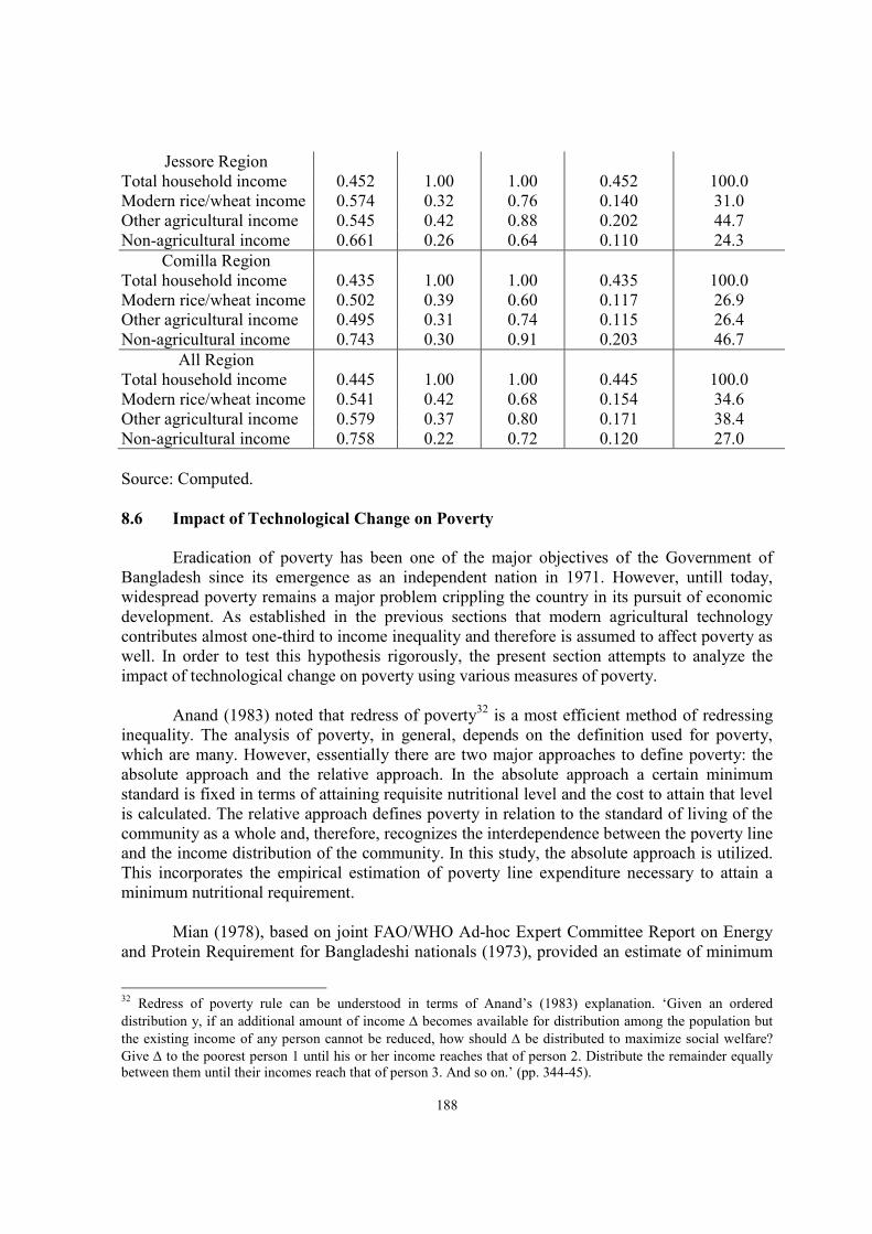
188

Jessore Region

Total household income 0.452 1.00 1.00 0.452 100.0

Modern rice/wheat income 0.574 0.32 0.76 0.140 31.0

Other agricultural income 0.545 0.42 0.88 0.202 44.7

Non-agricultural income 0.661 0.26 0.64 0.110 24.3

Comilla Region

Total household income 0.435 1.00 1.00 0.435 100.0

Modern rice/wheat income 0.502 0.39 0.60 0.117 26.9

Other agricultural income 0.495 0.31 0.74 0.115 26.4

Non-agricultural income 0.743 0.30 0.91 0.203 46.7

All Region

Total household income 0.445 1.00 1.00 0.445 100.0

Modern rice/wheat income 0.541 0.42 0.68 0.154 34.6

Other agricultural income 0.579 0.37 0.80 0.171 38.4

Non-agricultural income 0.758 0.22 0.72 0.120 27.0

Source: Computed.

8.6 Impact of Technological Change on Poverty

Eradication of poverty has been one of the major objectives of the Government of

Bangladesh since its emergence as an independent nation in 1971. However, untill today,

widespread poverty remains a major problem crippling the country in its pursuit of economic

development. As established in the previous sections that modern agricultural technology

contributes almost one-third to income inequality and therefore is assumed to affect poverty as

well. In order to test this hypothesis rigorously, the present section attempts to analyze the

impact of technological change on poverty using various measures of poverty.

Anand (1983) noted that redress of poverty32

is a most efficient method of redressing

inequality. The analysis of poverty, in general, depends on the definition used for poverty,

which are many. However, essentially there are two major approaches to define poverty: the

absolute approach and the relative approach. In the absolute approach a certain minimum

standard is fixed in terms of attaining requisite nutritional level and the cost to attain that level

is calculated. The relative approach defines poverty in relation to the standard of living of the

community as a whole and, therefore, recognizes the interdependence between the poverty line

and the income distribution of the community. In this study, the absolute approach is utilized.

This incorporates the empirical estimation of poverty line expenditure necessary to attain a

minimum nutritional requirement.

Mian (1978), based on joint FAO/WHO Ad-hoc Expert Committee Report on Energy

and Protein Requirement for Bangladeshi nationals (1973), provided an estimate of minimum

32

Redress of poverty rule can be understood in terms of Anand’s (1983) explanation. ‘Given an ordered

distribution y, if an additional amount of income ∆ becomes available for distribution among the population but

the existing income of any person cannot be reduced, how should ∆ be distributed to maximize social welfare?

Give ∆ to the poorest person 1 until his or her income reaches that of person 2. Distribute the remainder equally

between them until their incomes reach that of person 3. And so on.’ (pp. 344-45).

189

average requirement of energy and proteins adjusted for various losses. His estimate is

presented in Table 8.17. He also determined least-cost long-term diet sets with available food

items that attain the level of nutrition set out in Table 8.17.

Table 8.17. Minimum nutritional requirement for a person per day.

Minimum

average daily

requirement

Food

energy

Fats Thia-

mine

Ribo-

flavin

Niacine Vitamin

A

Ascorbic

acid

Iron Cal-

cium

(Kcal) (gm) (mg) (mg) (mg) (I.U.) (mg) (mg) (mg)

Per capita/day 2112.00 17.30 0.84 0.92 13.80 2003 24.90 13.90 450.00

Source: Mian (1978), Table 18.

In this study, one of Mian’s (1978) long-term diet, named Diet A, is adopted with a

minor upward adjustment of food energy from 2,080 to 2,112 kcal and the current cost

required to attain the diet is estimated separately for each region using region-specific retail

prices of the food products. Expenditure on non-durable goods is estimated at 30 percent of

food cost following Hossain et al. (1990). The result of the calculation is provided in Table

8.18. The adjustment for additional calorie is to be obtained from increased allocation of

wheat from an initial 38.3 to 58.3 gms per capita per day. The calculation of poverty line

expenditure provides an estimate of Tk. 5,409 per capita per year (Tk. 5,424, Tk. 5,357, and

Tk.5,329 for Jamalpur, Jessore and Comilla, respectively) as shown in Table 8.19. For the

purpose of computing poverty indices, the overall expenditure of Tk. 5,409 per capita per year

is utilized, as it does not change the composition of poor in each region when computed on the

basis of region-specific poverty line expenditures.

190

Table 8.18. Poverty line income required to fullfil the nutritional and other requirements by study

regions, 1996.

Food item Qty. (gm) of

food included

in optimal diet

Cost (Tk.) of attaining the optimal diet evaluated at region-

specific retail market prices

Jamalpur region Jessore region Comilla region All region

Rice 432.6 4.90 4.36 4.46 4.62

Wheat 58.3 0.64 0.58 0.64 0.62

Potato 36.7 0.15 0.14 0.15 0.14

Lentil 25.0 0.53 0.54 0.53 0.53

Fish 38.3 2.11 2.43 2.24 2.24

Meat 1.7 0.11 0.13 0.11 0.12

Milk 31.1 0.48 0.43 0.53 0.50

Dry milk 2.5 0.55 0.55 0.55 0.55

Sugar 27.2 0.70 0.70 0.70 0.70

Oil 12.2 0.70 0.69 0.63 0.68

Onion 8.5 0.09 0.07 0.07 0.08

Non-leafy vege. 86.8 0.38 0.58 0.52 0.53

Leafy vegetable 20.0 0.09 0.09 0.10 0.09

Cost of food per capita per day 11.43 11.29 11.23 11.40

Annual cost of food 4,172.0 4,120.9 4,099.0 4,161.0

Annual cost of non-food items 1,251.6 1,236.3 1,229.7 1,298.3

Poverty line expenditure per

year per capita

5,423.6 5,357.2 5,328.7 5,409.3

Source: Computed.

8.6.1 Estimation of Poverty Indices

A number of poverty measures are developed during the 1980s of which the popular

indices are Sen’s poverty index (1976), Kakwani’s poverty index (1980) and FGT’s (Foster,

Greer, and Thorbecke) poverty measure (1984). In this study, all of these indices are computed

to examine the degree of poverty, consistency and stability of results when diverse

measurement techniques are utilized. Table 8.19 presents the result of the various poverty

indices.

It is clear from Table 8.19 that poverty is highest in areas with high intensity of modern

technology diffusion followed by low intensity areas. The lowest incidence of poverty is in the

villages with ‘medium intensity’ of modern technology diffusion. The level of income

inequality among the poor is lowest (0.24) in ‘medium adopter’ villages. The per capita

income of the poor is highest in these ‘medium adopter’ villages (Tk. 3,433) as compared to

‘high adopter’ and ‘low adopter’ villages (Tk. 2,570 each). Also, the income gap ratio, poverty

gap ratio, and the number of poor people below poverty line (head count ratio) is lowest in

‘medium adopter’ villages. All measures of poverty, Sen index, Kakwani index and FGT (P2)

index consistently indicate poverty is lowest in ‘medium adopter’ villages. The distributionally

sensitive measure of poverty, FGT (P2), reveals that poverty is strikingly low in ‘medium

191

adopter’ villages with least inequality among the poor, while it is similar and high in ‘high

adopter’ as well as ‘low adopter’ villages. ‘This finding explains to some extent the slow pace

of modern agricultural technology diffusion in Bangladesh. The exclusive diffusion of modern

varieties sharply increases inequality by inducing sharp income difference between adopters

and non-adopters as indicated by head count ratio. On the other hand, total non-adoption of

modern variety technology leads to lower income, consequently leading to poverty again as

indicated by same value of income gap ratio between ‘low adopter’ and ‘high adopter’

villages. The ‘medium level of adoption’ of modern technology opens up the opportunity to

derive higher income from cultivating modern varieties in one season as well as diversifying

agriculture in other seasons. The increase in income is accrued through increase in cropping

intensity as well as diversified agriculture. The modern irrigation facilities also have a

favorable impact on poverty. As explained earlier, modern irrigation opens up opportunities

for diversifying the cropping system in addition to facilitate the diffusion of modern variety

technology. When regional distribution is considered, Jamalpur and Jessore regions faired

similarly with respect to all indices while Comilla region differs distinctly with high level of

inequality among the poor as well as higher incidence of poverty.

Table 8.19 Estimation of poverty in the study regions, 1996.

Villages Inequa-

lity

among

poor

Per

capita

income

of poor

Head

count

ratio

Income

gap

ratio

Sen

index

Kak-

wani

index

FGT

Poverty

gap

ratio

FGT

Distribut

ionally

sensitive

(G*) (M*) (H) (I) (PSen) (P1K) (P1) (P2)

Villages classified by status of modern technology adoption

High adopter village 0.301 2,569.4 0.63 0.53 0.42 0.43 0.33 0.21

Medium adopter village 0.243 3,433.4 0.46 0.37 0.24 0.19 0.17 0.09

Low adopter village 0.304 2,569.8 0.54 0.52 0.36 0.31 0.28 0.18

Villages classified by level of modern irrigation facilities

High irrigated village 0.293 2,731.9 0.58 0.50 0.38 0.35 0.29 0.18

Low irrigated village 0.320 2,304.0 0.66 0.57 0.47 0.51 0.37 0.26

Villages classified by regions

Comilla region 0.319 2,303.6 0.74 0.57 0.52 0.68 0.42 0.28

Jamalpur region 0.268 2,785.7 0.51 0.49 0.32 0.27 0.25 0.15

Jessore region 0.291 3,047.5 0.55 0.44 0.33 0.28 0.24 0.15

All category 0.300 2,662.7 0.59 0.51 0.39 0.37 0.30 0.19

Note: Head count ratio (H) = q/N where q is the number of poor households having income

no greater than poverty line expenditure X (Tk. 5,409) and N is the total number of

households.

Income gap ratio (I) = [X-M*]/M*.

Sen index (PSen) = H [I + (1-I) G*]

Kakwani index (taking into account inequality among poor) (P1K) = (H/M) [X-M*(1-

G*)], where M is the per capita income of all households.

FGT Poverty gap ratio (P1) = H * I.

FGT Distributionally sensitive measure (P2) = P2 (M*; X) = 1/N Σiq [(X – M*/M*]

2.

192

Source: Computed.

8.7 Inferences

There are significant regional differences in income derived from agricultural as well

as non-agricultural sources. Income from crop production is significantly different across land

ownership and tenurial classes.

Farm size, working members, farm capital, modern technology, and soil fertility

significantly increase crop as well as agricultural income while farmers’ education level

significantly decreases crop income. Developed infrastructure significantly increases non-

agricultural income while farm size and modern technology significantly decreases non-

agricultural income. The analysis is similar for landless and marginal farmers.

Analysis of impact of modern technology on factor shares revealed that significant

differences exist in absolute values of factor shares between modern and local varieties of rice.

Labor wages of about Tk.2,747 (11 percent of gross value of production) per ha of modern

rice cultivation goes to landless and marginal farmers through the hired labor market which is

double the size of wages estimated at Tk 1,351 (13 percent of gross value of production) for

local rice production.

An analysis of distributional impact of modern agricultural technology revealed that

income inequality is higher in ‘high adopter’ villages as well as ‘low adopter’ villages. Gini-

coefficient computed on per capital income scale is estimated at 0.44 and 0.45 for ‘high

adopter’ and ‘low adopter’ villages while it is 0.34 in ‘medium adopter’ villages characterized

with greater crop diversity. Similarly, with respect to irrigation status, income inequality is

higher in low irrigated villages. Gini-coefficient is estimated at 0.42 and 0.48 in ‘high’ and

‘low’ irrigated villages. On a regional basis, inequality is higher (0.47) in Comilla region while

it is lower and similar 0.41 and 0.40 in Jamalpur and Jessore region, respectively. The

differences across categories become less prominent when Gini-coefficient is computed on per

capita land ownership scale. The inequality in per capita land ownership remains within 0.50

to 0.60 with minor variations.

Modern technology alone contributes to about 35 percent (minimum 27 percent in

Comilla and maximum 45 percent in Jamalpur) to total income inequality. The contribution of

non-agricultural income is about 27 percent while other agricultural income contributes the

remaining 38 percent to total income inequality.

Analysis of technological change on poverty using a number of measures revealed that

poverty is lowest in ‘medium adopter’ villages. The number of population below poverty line

is lowest (46 percent) in ‘medium adopter’ villages as compared to 63 percent and 54 percent

in ‘high adopter’ and low adopter’ villages, respectively. On a regional basis, poverty is

similar in Jamalpur and Jessore region while it is sharply higher in Comilla. All measures

including the distributionally sensitive measure of poverty confirmed that incidence of poverty

is highest in ‘high adopter’ and lowest in ‘medium adopter’ villages.

193

194

CHAPTER IX

TECHNOLOGICAL CHANGE AND ITS IMPACTS ON

THE ENVIRONMENT

Agriculture is characterized by its environmental, behavioral and policy aspects (Clapham,

1980). Though the farmers’ behavioral and government’s policy dimensions of agriculture has

been rigorously analyzed in the past, the environmental dimension is largely neglected and

remains unclear despite the fact that ecological integrity of agricultural production system is a

pre-requisite for sustainability. The concern of environmental impacts of technological change

and sustainability in agriculture has been a recent phenomenon spurred by studies such as

Shiva (1991), Wossink et al., (1992), Brown (1988), Wolf (1986), Clapham (1980), and

Bowonder (1979 and 1981). The present chapter attempts to provide an insight to this less

studied dimension in agriculture. It provides a systematic picture of environmental impacts of

modern agricultural technology as perceived by farmers and their relative adverse strengths as

ranked by the respondent farmers. Further, material evidence in terms of bio-physico-chemical

tests of soil fertility and water quality parameters, and long term trend analysis of indicators

believed to be impacted due to this technological change in agriculture is provided in order to

substantiate, validate, and authenticate the conclusions drawn from farmers’ perceptions and

rankings. It should be reiterated that a soil fertility index based on the test results for the study

area is already quantified and incorporated as an independent variable extensively in the

foregoing analyses (Chapter V through Chapter VIII). Therefore, it is expected that

conclusions drawn from the foregoing analyses of socio-economic impacts and the current

analyses of environmental impacts of technological change would enable to provide a vivid

picture of the present day status and delayed consequences of technological breakthrough in

Bangladesh agriculture.

9.1 Direct and Indirect Impacts of Modern Agricultural Technology: An Overview

Bowonder (1979), in the heyday of technological change in agriculture, provided a

vivid analysis of present and potential multifaceted impacts of ‘Green Revolution’ technology

in India. Using a multi-criteria network analysis, he outlined impacts of ‘Green Revolution’

technology on industry, agriculture, economy, society, demography, ecology as well as

politics. Clapham (1980) viewed that environmental and social factors comprising agriculture

are closely tied together and the environmental problem of agriculture largely stems from the

phenomena associated with agricultural development. He finds it pointless to discuss

sustainability unless linkages among the three domains, environment, farmers decision making

behavior and government policy perspective, are identified, understood and dealt with. He

stresses that any practical analysis of agricultural environment must recognize the cultural,

economic, policy as well as ecological bases of the problems. The present chapter though

cannot deal in its entirety of the domains mentioned above, however, it attempts to provide

possible linkages as evidenced from the available information on farm level production

systems in the study villages.

The technological breakthrough in Bangladesh agriculture has been primarily in the

foodgrain sector, that is the introduction of rice-based ‘Green Revolution’ technology package

followed by a gradual introduction of wheat-based technology package. The overall policy

195

thrust for the past four decades (1960 – till date) has been in provision of technical inputs

complementing the expansion and diffusion of these ‘Green Revolution’ technologies. This is

the prime reason for all of the past studies on technological change in Bangladesh including

the present study to concentrate on evaluating the diffusion of ‘Green Revolution’ technology.

The selected indicators of technological change over the past 45 years (1949/50 – 1993/94) are

presented in Table 9.1 using triennium averages of four periods.

Table 9.1 Selected indicators of technological change in Bangladesh agriculture, 1949/50 –

1993/94.

Indicators Period a

1950-52

Period a

1968-70

Period a

1980-82

Period a

1992-94

1 Total cropped area (TCA) (‘000 ha) 10,614 12,871 13,103 13,753

2 Net cropped area (‘000 ha) 8,274 8,787 8,531 7,812

3 Cropping intensity (%) 128.3 146.5 153.6 176.0

4 Total rice area (‘000 ha) 8,071 10,049 10,310 10,135

5 Rice as percent of total cropped area (%) 76.0 78.1 78.7 73.7

6 Modern rice as percent of total rice area (%) nil 1.5 20.3 49.0

7 Total wheat area (‘000 ha) 39 105 520 609

8 Modern wheat as percent of total wheat (%) nil 6.1 96.2 98.0

9 Total irrigated area (IA) (‘000 ha) < 1 1,057b 1,865 3,257

10 Irrigated area as percent of TCA (%) na 8.2 b 14.2 23.7

11 Foodgrain irrigated area as percent of IA (%) na 85.8 b

78.4 91.2

12 Irrigation by methods Modern (%)

Traditional (%)

na

na

31.5 b

68.5 b

67.2

32.8

70.9

29.1

13 Total fertilizer used (‘000 mt of nutrients) < 1 113.1 380.8 664.8

14 Fertilizer use rate per TCA (kg of nutrients/ha) na 8.8 29.1 48.3

15 Pesticide use (‘000 mt) na na 2.2 6.5

16 Rice production (‘000 mt) 7,367 11,504 13,417 18,211

17 Rice yield (kg/gross ha) Modern variety

Local variety

nil

913

3,809

1,103

2,297

1,048

2,409

1,208

18 Wheat production (‘000 mt) 22 86 932 1,124

19 Wheat yield (kg/gross ha) 564 819 1,792 1,846

Note: a Period 1950-52 refers to average of 1949/50, 1950/51 and 1951/52. Period 1968-70

refers to average of 1967/68, 1968/69, and 1969/70. Period 1980-82 refers to average

of 1979/80, 1980/81 and 1981/82. Period 1992-94 refers to average of 1991/92,

1992/93 and 1993/94. b 1968/69 and 1969/70 only.

Source: BBS (Various issues), Alauddin and Tisdell (1991), Hossain (1989), and Hamid (1991).

It is clear from Table 9.1 that agricultural production in Bangladesh is operating at its

frontier since the 1980s with declining net-cropped area owing to transfer of land for other

uses. The total rice area also reached its frontier and making way for wheat area expansion. It

is also interesting to note that though area under modern rice varieties reached only 50 percent

of total despite its diffusion as early as 1963, the wheat acreage is totally absorbed by modern

196

varieties which picked up in early 1980s. The stagnancy in the diffusion of modern rice

varieties is probably due to slower expansion of modern irrigation facilities, susceptibility to

pest and disease attack, and capital intensity. The fertilizer use rates per hectare of gross

cropped area, though still low, increased about six folds. Pesticide use, negligible until the

1970s, recorded dramatic increase in recent years. The yield rates of modern rice varieties fell

sharply from the 1970 levels while the yield rates of local rice varieties is on the rise probably

owing to the use of modern inputs and variety screening. However, it is encouraging to note

the rising trend in the yield rates of wheat that is exclusively composed of modern varieties

(Table 9.1).

9.2 Farmers’ Perception of Environmental Impacts of Modern Agricultural Technology

Farmers’ perception on environmental impacts is elicited in two steps. First, a set

of 12 specific environmental impacts33

is read to the respondents and was asked to reveal their

opinion on these impacts. Next, they are asked to provide scores on a five-point scale if they

agree. And for disagreement of these impacts the score is zero. It is believed that undergoing

these two step procedures helped in avoiding leading statements and loaded responses. The

results of farmers’ opinion on the environmental impacts are presented in Table 9.2.

Table 9.2 Farmers’ perception on 12 specific environmental impacts of modern agricultural

technology by study regions, 1996.

Sl.

No.

Environmental impacts of modern

agricultural technology

Farmers responding in the affirmative

Jamalpur

region

Jessore

region

Comilla

region

All region

1 Reduce soil fertility 149 (85) 103 (98) 96 (76) 348 (86)

2 Affects human health 129 (74) 92 (87) 88 (70) 309 (76)

3 Reduce fish catch 114 (65) 68 (65) 114 (91) 296 (73)

4 Increase disease in crops 116 (66) 78 (74) 83 (66) 277 (68)

5 Compact/ harden soil 90 (51) 74 (71) 62 (49) 226 (56)

6 Increase insect/ pest attack 93 (53) 71 (68) 26 (21) 190 (47)

7 Increase soil erosion 93 (53) 70 (67) 22 (18) 185 (46)

8 Increase soil salinity 71 (41) 59 (56) 45 (36) 175 (43)

9 Contaminate water source 62 (35) 36 (34) 20 (16) 118 (29)

10 Increase toxicity in soil 39 (22) 21 (20) 27 (21) 87 (21)

11 Creates water logging 38 (22) 23 (22) 7 (6) 68 (17)

12 Increase toxicity in water 30 (17) 11 (10) 25 (20) 66 (16)

All impacts a 1,024 (49) 706 (56) 615 (41) 2,345 (48)

Note: a Multiple responses. The total number of responses equal 2,100 (12 impacts x 175

farmers) for Jamalpur, 1,260 (12 impacts x 105 farmers) for Jessore, and 1,512 (12

impacts x 126 farmers) for Comilla regions. Therefore, for all regions, the number of

responses equal 4,872 (12 impacts x 406 farmers).

Source: Field Survey, 1997.

33

This set of 12 specific environmental impacts were identified in a focus group discussion (FGD) with the

farmers conducted during the pre-testing of structured questionnaire in another sub-district of Jessore region.

197

Among the 12 specific environmental impacts of modern agricultural technology,

majority of the farmers cited ‘decline in soil fertility’, ‘effect on human health’, ‘reduction of fish

catch’, ‘compaction of soil’, and ‘increased incidence of crop disease’ and ‘insect/pest attacks’ as

the major impacts (Table 9.2). The proportion of affirmative responses declines sharply when one

moves down to more intangible and indirect impacts, such as ‘contamination of water bodies and

soils’.

Since there are multiple responses on these impacts which is consistent with the diversity

of impacts of technological change, an attempt has been made to identify the relative strength of

these environmental impacts in terms of farmers’ own perception. To accomplish this, farmers

were asked to rank specific environmental impacts on a five-point scale. The result of this ranking

exercise is presented in Table 9.3.

Table 9.3 Ranking of farmers’ perception on 12 specific environmental impacts of modern

agricultural technology by study regions, 1996.

Sl.

no.

Environmental impacts of

modern agricultural

technology

Index weighted by rank of responses a

Jamalpur region Jessore region Comilla region All region

Index Rank Index Rank Index Rank Index Rank

1 Reduce soil fertility 0.82 1 0.94 1 0.63 1 0.79 1

2 Affects human health 0.60 2 0.79 2 0.45 4 0.60 2

3 Reduce fish catch 0.55 3 0.59 4 0.57 2 0.56 3

4 Increase disease in crops 0.51 4 0.61 3 0.45 3 0.52 4

5 Compact/ harden soil 0.36 7 0.57 6 0.37 5 0.42 5

6 Increase insect/ pest attack 0.43 5 0.58 5 0.12 9 0.37 6

7 Increase soil erosion 0.39 6 0.49 7 0.11 10 0.33 7

8 Increase soil salinity 0.28 8 0.43 8 0.24 6 0.30 8

9 Contaminate water source 0.26 9 0.24 9 0.08 11 0.20 9

10 Increase toxicity in soil 0.14 11 0.16 11 0.13 7 0.15 10

11 Creates water logging 0.14 10 0.18 10 0.05 12 0.13 11

12 Increase toxicity in water 0.12 12 0.07 12 0.13 8 0.11 12

All impacts 0.38b 2 0.47b 1 0.28b 3 0.37

Note: The higher the index the stronger the perception. a Ranking done by weighting individual responses by their ranks.

Index = {RVH (1.0) + RH (0.8) + RM (0.6) + RL (0.4) + RVL (0.2) + R0 (0.0)} / N

where RVH = very high rank, RH = high rank, RM = medium rank, RL = low rank, RVL =

very low rank, and R0 = farmers responding in the negative, respectively. N = sample size. b = Ranking done across 3 regions.

Source: Field Survey, 1997.

‘Decline in soil fertility’ features top of the list of adverse environmental impacts of

technological change followed by ‘health effects’, ‘decline in fish catch’, ‘increase in crop

disease’, ‘soil compaction’, ‘increase in insect/pest attack’ and ‘soil erosion and soil salinity’. It is

interesting to note that the perception on adverse impact of modern technology on water

198

resources is very weak as evident from sharp decline in index values. This leads to the conclusion

that, though farmers’ are aware of the adverse environmental impacts of modern agricultural

technology, their awareness level remains confined to the visible impacts most closely related to

their farm field and sources of livelihood (crops and fish). The awareness on indirect and wider

impacts such as ‘contamination of water bodies’ is not very strong. The consistency of these

response patterns across region is evidenced from the analyses of rank correlation. All relative

rankings of impacts are significantly (p<0.01) positively related across regions thereby providing

confidence in the results (Table 9.4).

Table 9.4 Rank correlation of environmental impact ranking among regions, 1996.

Jamalpur region Jessore region Comilla region All region

Jamalpur region 1.00

Jessore region 0.99a

1.00

Comilla region 0.70a 0.73

a 1.00

All region 0.97a 0.98

a 0.80

a 1.00

Note: a = significant at 1 percent level (p<0.01).

Source: Field Survey, 1997.

9.3 Soil Fertility Evaluation of the Study Areas

Land is the single most important natural resource that provides livelihood for the vast

majority of rural poor in an agrarian economy like Bangladesh. The productivity of land

depends largely on biophysical factors such as soil fertility and water quality. It was largely

perceived that soil fertility status of Bangladesh is on the decline resulting in declining

productivity, particularly for the modern varieties of rice (BASR, 1989). Evidence from the

present study also suggests that the soil fertility status is rather poor and is declining. As

evident from the farmers’ ranking of major environmental impacts, ‘declining soil fertility’

was identified as the major adverse environmental impact that the modern agricultural

technology exerted in the study areas. To further authenticate this version of farmers, a

detailed bio-physico-chemical analysis of soil fertility status of the study area, which was

already an integral part of the research design of this study, is provided below. The present

section provides a brief on the importance of soil properties that are tested and their

comparative fertility status. Later, the general relation between the soil fertility status and crop

productivity is analyzed with the application of multivariate analyses.

A total of 10 properties – soil reaction (pH); available nitrogen (N), phosphorus (P),

potassium (K), sulfur (S), and zinc (Zn); organic matter content (OM), cation exchange

capacity (CEC); electrical conductivity (EC); and textural class were analyzed to evaluate the

general fertility levels of the soil in the study areas.

9.3.1 Soil Fertility Parameters and Nutrient Availability

(a) Soil pH: Soil reaction, a measure of the degree of acidity or alkalinity of a soil usually

expressed on a pH scale, is one of the most important indicator of crop response to soil

nutrients. Generally, the pH range of 6.5 to 7.3 is suitable for most of the nutrient becoming

199

available for plants (Thompson and Troeh, 1973). It is evident from Appendix Table A9.1 that

Jamalpur soils are slightly acidic as compared to Jessore which is slightly alkaline, and

Comilla soils are neutral in reaction. As a whole, the soil reaction of the study area is in the

neutral range (6.6 – 7.3 pH) and are relatively favorable to standard requirements provided that

there are sufficient nutrients in the soil to be supplied to plants, which are investigated

subsequently.

(b) Organic Matter Content: Though organic matter constitutes only a small fraction (3-5 % in

weight) of soils, it has a profound influence in fertility management particularly by influencing

the physical, chemical and biological properties of the soil. The organic matter is mainly

composed of decomposed plant and animal residues. The average organic matter content of

Jamalpur and Comilla region is low while Jessore is very high (Appendix Table A9.2). Low

organic matter in general can be attributed to massive removal of crop straws, plant residues,

and grasses from the soils, lack of litters from shrubs and bushes and increased use of

farmyard manure as fuel instead of applying as source of nutrients and organic matter to the

soil.

(c) Nitrogen Levels: Nitrogen is one of the most important nutrient elements required for plant

growth. In fact, nitrogen is the dominant external fertilizer applied for cereal production by

farmer, as nitrogen deficiency in soils is a common phenomenon in Bangladesh. Since most

nitrogen is associated with organic matter, the rate at which this element is liberated from the

soil organic matter varies with temperature, moisture, and microbial decomposition. Nitrogen

serves as the regulator that governs to a considerable degree the utilization of potassium,

phosphorus, and other nutrients. With cereals, nitrogen increases the plumpness of the grain

and their protein percentage. Plants with deficient nitrogen are stunted in growth and possess

limited root system. On the other hand, oversupply may delay crop maturation by encouraging

excessive vegetative growth as well as reduce resistance to certain crop diseases (Brady,

1974). Appendix Table A9.3 clearly establishes the fact that there is widespread deficiency in

available nitrogen in the soils in the study regions. The reason for low levels of available

nitrogen in soils is obvious. As all these areas grow at least two rice crops a year and burning

of organic matter as fuel is widespread in these regions, the nutrient uptake is greater than the

intake and the consequence is nitrogen deficient soils. This interpretation is further

authenticated by nutrient (N, P) pathway analysis conducted later in this chapter.

(d) Phosphorus Levels: The second major nutrient element critical for plant growth is the

quantity of phosphorous. The major source of phosphorus is mineral appetite, which is also a

principle source of non-cereal fertilizers. Native phosphorus is usually fixed in highly acidic

soils and in soils rich in oxides of iron and aluminum. Though organic matter contains

phosphorus but the amount is very low. Lack of phosphorus prevents acquiring of other

nutrients by the plants. Adequate phosphorus levels promote seed formation, crop maturation,

root development, and resistance to certain diseases (Brady, 1974). Appendix Table A9.4

reveals that the available phosphorus is not as deficient as the case of available nitrogen.

Jamalpur soils have high levels of available phosphorus and Comilla and Jessore have medium

levels of available phosphorus. The reason for high phosphorus content may be due to external

application of phosphate fertilizers rather than the native fertility of the soils.

200

(e) Potassium Levels: The third most important nutrient element in soil is the potassium

content. Under natural condition, it is the most abundant of all soil nutrients. However,

since minerals such as feldspars or mica are very resistant to weathering, about 90

percent of the potassium are termed as unavailable potassium. In fact readily available

potassium which is only 1-2 percent of all potassium element is the major available

source for plant growth (Dahal, 1996). Potassium is essential for photosynthesis and for

starch formation (Brady, 1974). It is clear from Appendix Table A9.5 that, as with the

case of available nitrogen, the available potassium content is low in all study areas. The

availability is far from the upper bound of the ‘low’ range in all the regions. However, in

relative terms, Jessore is in a better position. In general, potassium deficiency occurs in

heavily leached soils, particularly on the light and sandy soils, and leaching loss may be

intensified if the soils become acidic. Moreover, potassium is a mobile element and its

losses are common under poor farm management practices. As such, frequent low doses

of potassium fertilizers is preferable than occasional heavy dose which are consequently

absorbed by the plants but not transferred into increased yield (Dahal, 1996).

(f) Sulfur Levels: Sulfur is another important nutrient required for plant growth. Sulfur

deficiency in soil retards plant growth as well as yield. Plants that are sulfur deficient are

characteristically small and spindly. The maturity of seeds and fruits is delayed in the absence

of adequate sulfur (Brady, 1974). Appendix Table A9.6 reveals that, as with case of nitrogen

and potassium, sulfur availability is also low. Only in relative terms, Jessore seems to be in

better position. Major reason for sulfur deficiency in soils is due to greater removal of this

element in harvested crops through increased yields (Brady, 1974).

(g) Zinc Levels: A total of 17 nutrient elements are essential for plant growth. Of these, eight

are required in such small quantities that they are termed as micronutrients or trace elements.

Zinc is one such important micronutrient. Zinc is essential for formulation of growth

hormones, promotion of protein synthesis, seed and grain maturation and production (Brady,

1974). In recent times, zinc deficiency became a major concern in some regions of

Bangladesh. Appendix Table A9.7 reveals that available zinc in soil is high in Jamalpur and

Jessore region and medium in Comilla region. It should be noted that, since the early 1990s,

widespread publicity of zinc deficiency in many areas aroused interest in the farmers to add

gypsum fertilizers in their farming lands. This might have been one reason for higher

availability of zinc in the study areas. However, it should be noted that excess availability of

this micronutrient element is also harmful (Brady, 1974).

(h) Cation Exchange Capacity: Cation exchange capacity (CEC) is an important soil property.

It affects the capacity of soil to hold nutrients such as ions of calcium (Ca), magnesium (Mg),

potassium (K) and ammonium (NH4). It also affects the quantity of nutrient required to change

its relative level in soils. For example, high CEC soils require more potassium ions to raise

soil potassium from a low to high level than do low CEC soils (Jones, 1982). The amount of

CEC of soils is determined by the amount of clay, the kind of clay, and the amount of

humified organic matter. The amount of CEC possessed by a soil is partly pH dependent. The

CEC is lower under acid conditions and rises as the pH rises (Thompson and Troeh, 1973). In

fact, CEC is a very important indicator of soil fertility, or at least of potential soil fertility.

Appendix Table A9.8 reveals that the CEC levels are low in Jamalpur and Comilla regions

201

where soils are relatively acidic, as compared to Jessore region which is relatively alkaline.

This indicates that the soil fertility status in the study region is poor.

(i) Electrical Conductivity: Electrical conductivity (EC) or the specific conductance is defined

as the inverse of resistivity and is often used for comparing resistance of any materials. The

reciprocal of resistance is known as the mho or Siemen (S) (Gupta, 1992). The conductivity of

any matter is a measure of its ability to convey an electrical current. Different ions vary in

their ability to conduct electricity, but in general, the greater the concentration of ions in soil,

the larger the conductivity (Boyd, 1990). The optimal conductivity for agricultural soils is 200

µS/cm (CCME, 1991). Appendix Table A9.9 reveals that EC is highly variable across regions.

Jessore soils have relatively high EC compared to other areas. However, as a whole the EC of

soils in the study regions are below the optimal conductivity.

(j) Soil Texture: Soil fertility management is not only dependent on bio-chemical properties of

soil, but also on physical properties of the soil. Each type of particle present in the soil makes

its contribution to the nature of the soil as a whole. Physical properties determine nutrient,

water holding and supplying capacity of soils, drainage, extent of water run-off and erosion,

soil aeration, temperature and other processes of the soil ecosystem vital for plant growth.

Loamy soils are highly desirable for most uses. A loamy soil is formed with a combination of

10-25 percent clay, approximately equal amount of silt and sand combined with several

percentage of organic matter (Thompson and Troeh, 1973). The textural analysis results reveal

that most of the soils are silt loam and some are silty clay (Appendix Table A9.10). This

implies that soil texture is fine and the soil in the study regions is moderate with respect to

physical characteristics.

9.3.2 Overall Soil Fertility Evaluation

The previous sections evaluated each of the soil fertility parameters individually. This

section provides an estimate of the overall soil fertility status of the study areas by comparing

all indices together as one. In deriving the mean index, eight soil test variables are considered

for which same procedure for index construction were applied. It is obvious from the Table 9.5

that the overall soil fertility status of Jamalpur and Comilla is ‘low’ and Jessore is ‘medium’.

As a whole, all three regions combined, the overall soil fertility status is in the ‘low’ range.

Table 9.5 Overall soil fertility evaluation of the study regions, 1997.

Region Soil fertility index interpretation Mean

index

Soil

pH

Tex-

ture OM N P K S Zn CEC EC

Jamalpur

region

1.55

1.00 2.60 1.00 1.00 2.40 1.00 1.00 1.44

(low)

6.0 Silt

loam

Jessore

region

2.60 1.00 2.20 1.00 1.40 2.80 1.80 1.2 1.75

(med)

7.9 Silty

clay

Comilla

region

1.20 1.00 2.00 1.00 1.00 2.20 1.20 1.00 1.33

(low)

7.1 Silt

loam

All

region

1.73 1.00 2.27 1.00 1.13 2.47 1.33 1.07 1.50

(low)

6.7 Silty

clay

202

loam

Note: The index value rated as < 1.67 = low, 1.67 – 2.33 = medium, and > 2.33 = high.

Source: Field survey, 1997.

9.3.3 Relationship between Soil Fertility and Crop Productivity: A Regression Analysis

Broadly speaking, biological production is the product of crop genotype and physical

environment. In this study, an attempt has been made to examine the relationship among soil

parameters and crop productivity with mean farm-level yield34

of various crop groups35

as the

dependent variable and the soil variables as the explanatory variables. Stepwise forward

regression procedure, which selects the significant explanatory variables from among the

given set of independent variables, is employed. The full model is provided below:

Model: lnYi = β0 + β1 ln K + β2 ln N + β3 ln P + β4 ln S + β5 ln Zn + β6 ln CEC + β7 OM

+ β8 EC + β9 pH .....(6.1)

where: ln Yi = natural log of crop output i measured in kg/ha.

ln K, ln N, ln P, ln S, ln Zn, and ln CEC = are natural log of available potassium,

nitrogen, phosphorus, sulfur, zinc, and cation exchange capacity measured in kg/ha.

OM = organic matter content measured as % of total.

EC = electrical conductivity measured in µS/cm.

pH = soil reaction which is measured in log scale

β0 ... β9 = are parameters to be estimated.

Table 9.6 presents the results of the selected regression estimates (for details, also see

Appendix Table A9.10). A total of 17 regressions representing each of the 14 crop types and 3

for all local rice varieties, all modern rice varieties, and foodgrain (all varieties of rice and

wheat), were tried. However, results of the 8 regressions, namely, local Aman rice, modern

Aman rice, modern wheat, all foodgrain, jute, pulses, spices, and vegetables, were reported as

the remaining regressions provided weak results. As the variables are measured in natural

logarithms the coefficients can be interpreted as the output elasticities with respect to relevant

soil variables except OM (organic matter) and EC (electrical conductivity). The order in which

coefficients are written (except constant) corresponds to the order in which the relevant variables

34

The yield levels are the averages for observations on crop production in each of the 21 villages. The soil

variables are collected from 15 locations (i.e., 15 villages). Therefore, for the remaining 6 villages the soil

variables are replicated by careful judgement. In fact, adjacent villages having the same soil series is replicated.

35

A total of six crop groups are formed. These are: (a) Foodgrain = includes local and HYV rice of three seasons

(Aus, Aman, and Boro), and local and HYV wheat (n = 1,049); (b) Oilseeds = include rapeseed, mustard and

groundnut (n = 71); (c) Pulses = include lentil, chola, and kalai (n = 70); (d) Spices = include onion, garlic,

turmeric, and chilly (n = 47); (e) Vegetables = include potato, sweet potato, brinjal, cauliflower, seem, radish,

yam, and leafy vegetables (n = 103).

203

enter in subsequent iterations in the stepwise forward regression procedure (Appendix Table

A9.10).

As a whole, all the regression results have consistent signs. The explanatory power,

reflected by the adjusted R2 is highly satisfactory for vegetables, spices, pulses, and jute crops,

moderately satisfactory for local Aman rice and all foodgrain crops, and comparatively weaker

for modern Aman rice and modern wheat crops. It should be noted that the dependent variable

used in this regression is the weighted averages of all individual sample observations from each

of the 21 villages under study. Therefore, the relationship can be interpreted with confidence on

its representativeness though the overall degree of freedom of the regression is rather small.

Table 9.6 Soil fertility and crop productivity relations in the study regions, 1996.

Soil

variable

Stepwise forward regression of soil fertility and crop production relations

Local

Aman rice

Modern

Aman rice

Modern

wheat

All

foodgrain

Jute Pulses Spices Vege-

tables

Intercept 5.968a

7.523a 7.154

a 7.749

a 16.716

a 22.517

a 9.380

a 5.754

a

ln K 0.323 - - 0.144a 0.349

a 0.457

a 1.200

a -1.246

a

ln N - 0.169b - - - - - -0.547

a

ln S - - - - - - - 1.829a

ln Zn - - 0.217b - - - - -

ln CEC 0.557c - - - - - - -

pH -0.401a - - -0.048c - -2.352a -0.935a 1.004a

EC - - - - - - - -0.011a

Adj. R2

0.42 0.20 0.24 0.31 0.56 0.79 0.78 0.95

F-ratio 5.52a 5.36

b 4.78

b 5.57

b 17.25

a 13.88

a 20.59

a 51.58

a

Df 3, 16 1, 17 1, 11 2, 18 1, 12 2, 5 2, 9 5, 8

Note: a = significant at 0.01 level (p<0.01); b = significant at 0.05 level (p<0.05).

c = significant at 0.10 level (p<0.10).

Source: Field survey, 1997.

From Table 9.6, one can readily observe the significance (p<0.01) of available

potassium in the soil for increased crop production, except vegetables. This is consistent with

observed very low levels of available potassium in all regions (Table A9.5 in the appendix).

Available nitrogen in the soil is significant (p<0.05 and p<0.10) for modern Aman rice. This is

consistent with the observation of very low levels of available nitrogen in all the study areas

(Appendix Table A9.2). For MV wheat yield, available zinc in the soil is the significant

(p<0.05) one. Another general observation is the significant (p<0.01 and 0.10) negative

influence of soil pH to crop production, except vegetables, which is also consistent.

9.4 Analysis of Decline in Soil Fertility

Analysis of soil fertility status revealed that soil in the study regions is of poor quality

(Table 9.5). A number of factors may be responsible for soil fertility decline. In general, lack

of knowledge on appropriate dosage of fertilizers to supplement the nutrient uptake by the

204

crop may be one of the crucial factors in soil fertility decline. Farmers using high doses of

fertilizers tend to avoid application of organic manure. Deficiency of organic matter content in

soil cannot be supplemented by application of chemical fertilizers.

Analysis of nutrient uptake revealed that modern varieties of rice alone contributes to

71 percent (highest is Jamalpur 84 percent) of total nutrient (N, P) uptake. The contribution is

lower in areas with diversified cropping system, i.e., Jessore (60 percent of total uptake).

Baanante et al. (1993) noted that the current production of food crops take up an estimated

0.92 million tons of nutrients (NPK and S) from the soil.

In order to validate the claim of ‘declining soil fertility’ and to check whether the

farmers’ perception is reflected in their practice of fertilizer application, the village level data

were analyzed. The a priori expectation is that there will be a negative association between soil

nutrient availability and fertilizer application rate. Also, a negative association between

fertilizer use and organic manure application is expected. The result of the exercise is

presented in Tables 9.7 and 9.8, respectively.

Table 9.7 Average levels of available soil nutrients, fertilizer and pesticide use levels in the study

regions, 1996.

Adopter catogory/region Available NPK

in soil (kg/ha)

Fertilizer use

(kg/ha)

Manure use

(ton/ha)

Pesticide use

(Tk/ha)

Villages classified by adopter categories

High adopter 168.5A 223.6A 1.13A 399.2A

Medium adopter 212.3B 206.4AB 1.47A 476.3A

Low Adopter 137.5A 164.0

B 0.18

B 341.8

A

F-ratio for adopter difference 3.23c

3.24c 1.13 2.00

Villages classified by regions

Comilla region 146.0A

227.3A 0.13

A 663.8

B

Jamalpur region 169.3A 213.4

A 1.71

B 214.2

A

Jessore region 205.4B 204.5

A 1.46

B 356.6

A

F-ratio for regional difference 6.21a

0.68 49.7a 7.36

a

All category/region 171.8 215.5 1.09 404.7

Note: Same block letters in superscript represent similarity in yield levels across regions for

individual crop based on LSD at 5 percent level of significance (p<0.05). a = significant at 1 percent level (p<0.01);

c = significant at 10 percent level (p<0.10)

Source: Field Survey, 1997.

Table 9.8 Correlation between available soil nutrients and levels of fertilizer and pesticide use in

the study regions, 1996.

Available NPK

in soil (kg/ha)

Fertilizer use

(kg/ha)

Manure use

(ton/ha)

Pesticide use

(Tk/ha)

Available NPK in soil (kg/ha) 1.00

Fertilizer use (kg/ha) -0.22 1.00

205

Manure use (ton/ha) 0.40c

-0.23 1.00

Pesticide use (Tk/ha) -0.23 0.52b

-0.59a

1.00

Note: a = significant at 1 percent level (p<0.01);

b = significant at 5 percent level (p<0.05);

c = significant at 10 percent level (p<0.10)

Source: Field Survey, 1997.

It is clear from Table 9.7 that available major soil nutrient (NPK) is significantly

(p<0.05) higher in ‘medium adopter’ villages and the fertilizer application rate is relatively

lower while the manure use rate is highest. There is no significant difference in pesticide use

rate across modern technology adopter categories of villages. It is observed that though higher

doses of fertilizer is applied in areas with low soil nutrient status, the application rate is not

significantly different across villages, while the soil nutrient availability is significantly

(p<0.05) different (Table 9.7). This implies that, though farmers are aware of declining soil

fertility, their knowledge on optimum dose required to make up the deficiency is not clear

resulting in depletion of soil fertility over time.

Table 9.8 clearly reveals that negative association (r = –0.22) exists between available

major soil nutrients and fertilizer application rate per ha of cropped land consistent with the a

priori expectation. Negative association (r = –0.23) between available major soil nutrients and

pesticide use rate per ha of cropped land is also observed. The negative association (r = –0.23)

between fertilizer application rate and organic manure use rate is observed consistent with the

priori expectation. This finding reveals that farmers’ knowledge on soil fertility management

is limited which may have led to soil mining through intensive cropping without proper

replenishment. Also, a contrasting relationship between pesticide use with fertilizer and

organic manure use is observed. While significant (p<0.05) positive relation (r = 0.52) exists

between pesticide and fertilizer use, the association is significantly (p<0.01) negative between

pesticide and organic manure use (r = –0.59). This implies that pesticide usage increases with

fertilizers while it declines with organic manure.

The phenomenon of ‘declining soil fertility’ is no doubt a direct threat to sustainability

unless it can be restored through proper management. Also, conclusion on declining soil fertility

must be made with caution, as it would affect strongly on policy formulation. Therefore, time

trend analyses of fertilizer use rates as well as overall fertilizer productivity for the study regions

for a period of 29 years is attempted to confirm the notion of ‘declining soil fertility’. The result

is presented in Table 9.9.

The annual increase in fertilizer use rate per ha of gross cropped area for the period

1961 – 1992 is estimated at above 10 percent for all regions and is highly significant (p<0.01).

However, it is interesting to note that the fertilizer productivity (output per kg of fertilizer

application) is significantly (p<0.01) declining at an annual rate of about 10 percent. The rate

of decline in fertilizer productivity is almost equivalent to the growth rate of fertilizer use rate

per ha of land. This finding clearly demonstrates the decline in soil fertility which is confirmed

by soil test results as well as from farmers’ perception ranking. It was also shown in Table 4.8

that the productivity of modern varieties of rice per ha of gross cropped area is declining

significantly (p<0.05) at an annual rate of 1.2 percent over the period 1968 – 1994.

206

Therefore, considering the various analyses of the issue of soil fertility, it can now be

safely concluded that one of the major adverse environmental impacts of modern agricultural

technology is the ‘declining soil fertility’ in the rural regions. It should be noted that the reason

for ‘soil fertility decline’ is not due to fertilizer application, rather it is the lack of proper

replenishment of the nutrient uptaken by crops, particularly modern varieties of foodgrain, by

soil fertility management practices, such as, application of organic manure.

Table 9.9 Growth trends in fertilizer use and fertilizer productivity in the study regions, 1960/61 –

1991/92.

Region Growth rate

(%)

t – ratio Adjusted R-

squared

F – ratio Degree of

freedom

Fertilizer use per ha

Comilla region 10.28 12.17a 0.84 148.10

a 1, 27

Jamalpur region1

12.48 22.14a 0.95 489.99

a 1, 27

Jessore region 13.07 20.67a 0.94 427.23

a 1, 27

Bangladesh 11.60 22.27a 0.95 496.06

a 1, 27

Output per unit of Fertilizer

Comilla region -9.50 -11.73a 0.83 137.69

a 1, 27

Jamalpur region1 -11.01 -17.40a 0.92 302.88a 1, 27

Jessore region -11.17 -14.30a 0.88 204.39a 1, 27

Bangladesh -10.40 -19.23a 0.93 369.60

a 1, 27

Note: Growth rates are estimate using semi-log trend function lnY = α + βt where t is time. a = significant at 1 percent level (p<0.01).

The figures are actually for Mymensingh region as a whole, which includes Jamalpur

region.

Source: Computed on data of Deb (1995).

9.5 Analysis of Health Effects

Though ‘adverse effect on human health’ has been reported as the second most

important environmental impact of technological change, the validation of this statement with

material support is beyond the scope of this study. However, an inference is attempted by

analyzing categories of pesticides used by the farmers of the study regions and their perception

on this input. It is needless to mention that health effect of modern agricultural technology

directly stems from the use, inhalation, and handling of the hazardous pesticides/insecticides,

which became a vital input in crop production in recent times. Pingali (1995) noted that

indiscriminate use of pesticide use can result in one or more of the following: (1) health

impairment due to exposure to hazardous chemicals; (2) contamination of ground and surface

waters through pesticide runoff and seepage; (3) the transmittance of pesticide residues in the

food chain ultimately reaching human consumers; (4) an increase in the resistance of pest

populations to pesticides thereby causing outbreaks and poor control; (5) the reduction of

beneficial insects and predators; and (6) the reduction in the populations of micro-organisms in

the soil and water that assists in sustaining soil fertility.

207

An investigation on pesticide uses in the study area revealed that about 77 percent of

farmers (highest 94 percent in Comilla) apply pesticides at least once (Table 9.10). Though

about half of the farmers in Jamalpur and Jessore applies pesticides only once in a crop season,

63 percent of Comilla farmers applies twice in a season. Further, 22 percent of farmers in

Comilla region applies as much as 3 - 5 times in a crop season indicating relatively higher

incidence of pest and insect attack as compared to Jamalpur and Jessore region. About 23

percent of farmers in Jamalpur and Jessore regions are considering to either reduce or stop the

use of pesticides while 81 percent of Comilla farmers considers their present use rate as

appropriate (Appendix Table A9.11).

Table 9.10 Number of applications of pesticides by study regions, 1996.

Number of applications of

pesticides

Number and percent of households (%)

Jamalpur region Jessore region Comilla region All region

Farmers applying pesticides 118 (67.4) 77 (73.3) 119 (94.4) 314 (77.3)

One time 81 (46.3) 57 (54.3) 13 (10.3) 151 (37.2)

Two times 31 (17.7) 17 (16.2) 79 (62.7) 127 (31.3)

Three times 5 (2.8) 3 (2.8) 18 (14.3) 26 (6.4)

Four times 1 (0.6) - 5 (4.0) 6 (1.5)

Five times - - 4 (3.1) 4 (0.9)

Farmers not applying

pesticides

57 (32.6) 28 (26.7) 7 (5.6) 92 (22.7)

Total households 175 (100.0) 105 (100.0) 126 (100.0) 406 (100.0)

Note: Figures in parentheses are percentages of total households.

Source: Field Survey, 1997.

The major beneficial effect of pesticide/insecticide use as perceived by farmers is

destruction of insects and consequent increase in production (Table 9.11). Few (4 percent) link

it to requiring less fertilizer. A large majority in Jessore (63 percent), who uses less pesticides,

considers that harmful effects of pesticides is not critical as compared to only 19 percent of

Comilla farmers who uses high levels of pesticides. About 7 percent of farmers in Jamalpur

link the use of pesticides to result in bitter test for rice. The awareness on health effect of

pesticide use is profound in Comilla (17 percent) while it is negligible and nil in Jamalpur and

Jessore, respectively. Similar is the case with awareness on causes of fish death. The

awareness on the effect on animal health is evident in Comilla and Jamalpur regions. It is

evident from Table 9.11 that the perception on harmful impacts of pesticides use is stronger

and widespread in Comilla region who happen to use more of these pesticides.

An analysis of the types of pesticides used by these farmers raise alarming concern. Table

9.12 reveals that a large majority of farmers in Jamalpur (86 percent) and Jessore (77 percent)

followed by Comilla (53 percent) use organophosphate pesticides which is rated as extremely to

highly hazardous according to World Health Organization (WHO) standard. Few of the selected

pesticides in this group is milder, i.e., between moderately and slightly hazardous for human

health. It is encouraging to note that the Comilla farmers, whose perception on adverse effects of

pesticides is relatively stronger, uses carbamates (37 percent) which is classified between highly

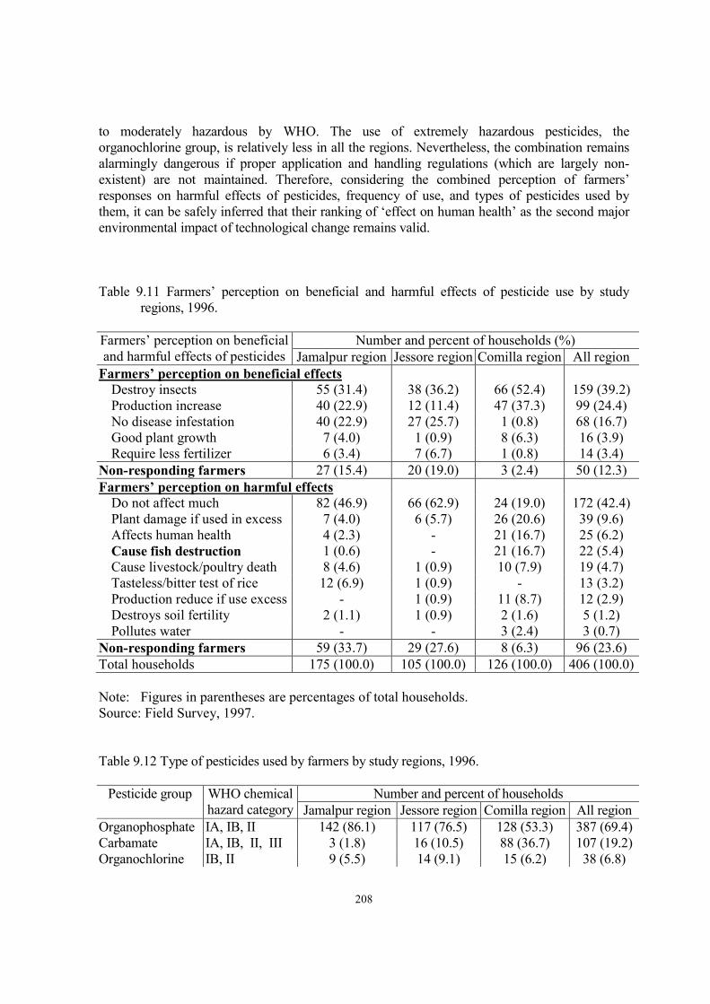
208

to moderately hazardous by WHO. The use of extremely hazardous pesticides, the

organochlorine group, is relatively less in all the regions. Nevertheless, the combination remains

alarmingly dangerous if proper application and handling regulations (which are largely non-

existent) are not maintained. Therefore, considering the combined perception of farmers’

responses on harmful effects of pesticides, frequency of use, and types of pesticides used by

them, it can be safely inferred that their ranking of ‘effect on human health’ as the second major

environmental impact of technological change remains valid.

Table 9.11 Farmers’ perception on beneficial and harmful effects of pesticide use by study

regions, 1996.

Farmers’ perception on beneficial

and harmful effects of pesticides

Number and percent of households (%)

Jamalpur region Jessore region Comilla region All region

Farmers’ perception on beneficial effects

Destroy insects 55 (31.4) 38 (36.2) 66 (52.4) 159 (39.2)

Production increase 40 (22.9) 12 (11.4) 47 (37.3) 99 (24.4)

No disease infestation 40 (22.9) 27 (25.7) 1 (0.8) 68 (16.7)

Good plant growth 7 (4.0) 1 (0.9) 8 (6.3) 16 (3.9)

Require less fertilizer 6 (3.4) 7 (6.7) 1 (0.8) 14 (3.4)

Non-responding farmers 27 (15.4) 20 (19.0) 3 (2.4) 50 (12.3)

Farmers’ perception on harmful effects

Do not affect much 82 (46.9) 66 (62.9) 24 (19.0) 172 (42.4)

Plant damage if used in excess 7 (4.0) 6 (5.7) 26 (20.6) 39 (9.6)

Affects human health 4 (2.3) - 21 (16.7) 25 (6.2)

Cause fish destruction 1 (0.6) - 21 (16.7) 22 (5.4)

Cause livestock/poultry death 8 (4.6) 1 (0.9) 10 (7.9) 19 (4.7)

Tasteless/bitter test of rice 12 (6.9) 1 (0.9) - 13 (3.2)

Production reduce if use excess - 1 (0.9) 11 (8.7) 12 (2.9)

Destroys soil fertility 2 (1.1) 1 (0.9) 2 (1.6) 5 (1.2)

Pollutes water - - 3 (2.4) 3 (0.7)

Non-responding farmers 59 (33.7) 29 (27.6) 8 (6.3) 96 (23.6)

Total households 175 (100.0) 105 (100.0) 126 (100.0) 406 (100.0)

Note: Figures in parentheses are percentages of total households.

Source: Field Survey, 1997.

Table 9.12 Type of pesticides used by farmers by study regions, 1996.

Pesticide group WHO chemical

hazard category

Number and percent of households

Jamalpur region Jessore region Comilla region All region

Organophosphate IA, IB, II 142 (86.1) 117 (76.5) 128 (53.3) 387 (69.4)

Carbamate IA, IB, II, III 3 (1.8) 16 (10.5) 88 (36.7) 107 (19.2)

Organochlorine IB, II 9 (5.5) 14 (9.1) 15 (6.2) 38 (6.8)

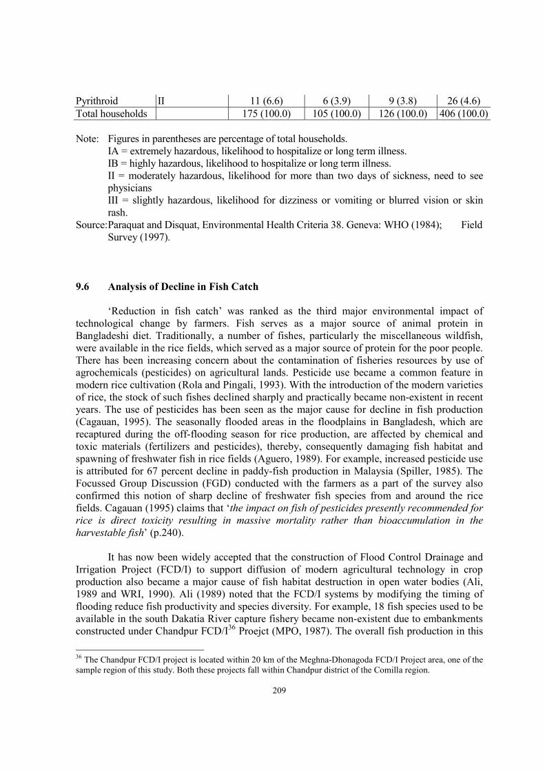
209

Pyrithroid II 11 (6.6) 6 (3.9) 9 (3.8) 26 (4.6)

Total households 175 (100.0) 105 (100.0) 126 (100.0) 406 (100.0)

Note: Figures in parentheses are percentage of total households.

IA = extremely hazardous, likelihood to hospitalize or long term illness.

IB = highly hazardous, likelihood to hospitalize or long term illness.

II = moderately hazardous, likelihood for more than two days of sickness, need to see

physicians

III = slightly hazardous, likelihood for dizziness or vomiting or blurred vision or skin

rash.

Source: Paraquat and Disquat, Environmental Health Criteria 38. Geneva: WHO (1984); Field

Survey (1997).

9.6 Analysis of Decline in Fish Catch

‘Reduction in fish catch’ was ranked as the third major environmental impact of

technological change by farmers. Fish serves as a major source of animal protein in

Bangladeshi diet. Traditionally, a number of fishes, particularly the miscellaneous wildfish,

were available in the rice fields, which served as a major source of protein for the poor people.

There has been increasing concern about the contamination of fisheries resources by use of

agrochemicals (pesticides) on agricultural lands. Pesticide use became a common feature in

modern rice cultivation (Rola and Pingali, 1993). With the introduction of the modern varieties

of rice, the stock of such fishes declined sharply and practically became non-existent in recent

years. The use of pesticides has been seen as the major cause for decline in fish production

(Cagauan, 1995). The seasonally flooded areas in the floodplains in Bangladesh, which are

recaptured during the off-flooding season for rice production, are affected by chemical and

toxic materials (fertilizers and pesticides), thereby, consequently damaging fish habitat and

spawning of freshwater fish in rice fields (Aguero, 1989). For example, increased pesticide use

is attributed for 67 percent decline in paddy-fish production in Malaysia (Spiller, 1985). The

Focussed Group Discussion (FGD) conducted with the farmers as a part of the survey also

confirmed this notion of sharp decline of freshwater fish species from and around the rice

fields. Cagauan (1995) claims that ‘the impact on fish of pesticides presently recommended for

rice is direct toxicity resulting in massive mortality rather than bioaccumulation in the

harvestable fish’ (p.240).

It has now been widely accepted that the construction of Flood Control Drainage and

Irrigation Project (FCD/I) to support diffusion of modern agricultural technology in crop

production also became a major cause of fish habitat destruction in open water bodies (Ali,

1989 and WRI, 1990). Ali (1989) noted that the FCD/I systems by modifying the timing of

flooding reduce fish productivity and species diversity. For example, 18 fish species used to be

available in the south Dakatia River capture fishery became non-existent due to embankments

constructed under Chandpur FCD/I36

Proejct (MPO, 1987). The overall fish production in this

36

The Chandpur FCD/I project is located within 20 km of the Meghna-Dhonagoda FCD/I Project area, one of the

sample region of this study. Both these projects fall within Chandpur district of the Comilla region.

210

project area declined by 35 percent over the first two years of implementation and the major

Indian carp fishery (Labeo ruhita, Catla catla, Cirrhina mrigala, and Labeo Calbasu)

disappeared in open waters inside the embankment (Ali, 1990). Vaughan (1996), in his study

located within the Meghna-Dhonagoda FCD/I Project area (one of the sample region of this

study), noted that there had been a major change in the fisheries as a result of the embankment

and this had affected profoundly on the livelihood of the rural households. ‘Poor people had

been particularly adversely affected as they now had little opportunity of catching or

cultivating fish. The respondents attributed this directly to the reduction of wild fish stocks due

to the lack of annual flooding’ (Vaughan, 1996:p.39) due to the construction of the

embankment.

Trend analyses of fish catch in rivers and open water bodies (beels) in regions

encompassing the study areas for the period 1984 – 1994 confirmed the widespread claim of

fish reduction in open water bodies (Table 9.13). The average annual compound rate of decline

is about 6 percent for Bangladesh and as high as 14 percent for Jamalpur region which is very

alarming. The catch rate is also negative for the beels (all weather depressed water bodies) of

Jessore region (4 percent). It should be noted that, since the early 1990s, a program of fish-

stocking in floodland was undertaken by the government. This stocking might have reduced

the rate of decline in fish catch to some extend. Otherwise, the declining trend would have

been observed in the floodlands as well. Therefore, considering all the evidences, it can be

concluded that the farmers’ claim of ‘reduction in fish catch’ in open water bodies within the

study regions remains valid.

Table 9.13 Average annual compound growth rate of fish-catch in the study regions for the

period, 1983/84 - 1993/94.

Source of catch Annual growth rate (%) t-ratio Adjusted R2

Jamalpur region

Catch from rivers/estuaries -14.42 -2.65b

0.47

Catch from beels (depressions) 1.80 3.25b 0.57

Jessore region

Catch from rivers/estuaries -6.71 -6.48a 0.09

Catch from beels (depressions) -4.15 -1.64 0.25

Comilla region

Catch from rivers/estuaries -0.24 -0.10 0.01

Catch from beels (depressions) 4.23 1.91c 0.31

Bangladesh

Catch from rivers/estuaries -5.87 -6.85a 0.85

Catch from beels (depressions) 0.84 1.18 0.15

Note: Growth rates are estimate using semi-log trend function lnY = α + βt where t is time.

a = significant at 1 percent level (p<0.01);

b = significant at 5 percent level (p<0.05);

c = significant at 10 percent level (p<0.10).

Source: Computed from Hamid (1993) and DoF (1993, 1992, 1991, 1990, 1989, 1988,

and 1986).

211

9.7 Analysis of Insect, Pest and Disease Infestations in Crop Production

There is widespread acceptance that the modern agricultural technologies are

much more prone to insect, pest and disease infestations. Therefore, with the increased diffusion

of modern varieties of rice and wheat, pesticides became and will continue to be a major

component of modern technology. The ‘increase in crop disease’ and ‘insect and pest attack’ has

been ranked 4th and 6

th by farmers of the study areas. Though direct analysis of increase in insect,

pest and disease infestations in crop production requires time-series information and is beyond

the scope of the present study, an indirect analysis of these statements is attempted using time-

trend analysis37

of pesticides use in the study regions. Table 9.15 provides the estimated annual

compound growth rate of pesticides for the period 1976/77 to 1992/93. Annual growth rate of

pesticide use is highest in Jessore (10 percent) closely followed by Jamalpur region (9 percent).

The use rate of pesticides in Comilla region is highly fluctuating and therefore recorded very low

growth rate. The annual growth rate of pesticide use for the country is also very high (8.6

percent). Therefore, it can be safely stated that the farmers’ claim of ‘increased infestation of

pests, insects and diseases’ as a result of the introduction of modern agricultural technology

remains valid.

Table 9.14. Average annual compound growth rates of pesticides in the study regions for the

period, 1976/77 - 1993/94.

Region Period Average annual compound growth rate of pesticides

Growth rate (%) t-ratio Adjusted R2

Jamalpur region 1976/77 – 1988/89 9.30 4.01a 0.60

Jessore region 1976/77 – 1988/89 10.40 3.88a 0.58

Comilla region 1976/77 – 1988/89 4.60 1.51a 0.17

Bangladesh 1976/77 – 1992/93 8.60 7.26a 0.78

Note: Growth rates are estimate using semi-log trend function lnY = α + βt where t is time.

From crop year 1989/90, pesticide market was liberated and therefore regionwise data

became unavailable. Also, pesticide use data for Jamalpur is not available separately.

Therefore, pesticide use data of Mymensingh region is computed and presented which

includes Jamalpur region. a = significant at 1 percent level (p<0.01).

Source: Computed from Hamid (1991) and BBS (various issues).

9.8 Analysis of Water Quality

Water also plays an important role in crop production. The ‘Green Revolution’

technology popularly known as ‘seed-fertilizer-water’ technology relies on water control. In

Bangladesh, both surface water and ground water are used for irrigation depending on the ease

of utilization. Much emphasis is on ground water exploitation for both drinking as well as

irrigation. Previously, there was no concern to test ground water quality to judge its suitability

37

It should be noted that regionwise pesticide use data is not reported systematically. For example, data for

1980/81 and 1981/82 was missing which were interpolated with preceding three-year average use rates. Also, the

data for 1985/86 was missing and was interpolated with preceding three-year average use rate.

212

for drinking as well as for irrigation. Only recently, during the 1990s, when arsenic was found

in groundwater extracted by Deep Tube Wells (DTWs) that lifts water from a depth of more

than 100 meters in many areas, the concern over water quality, particularly for drinking

purpose, became a major issue. Further, ‘contamination of water source’ was ranked 9th

by the

responding farmers. In this study, 6 surface water samples (2 from each region) and 7

groundwater samples (2-3 from each region) were taken from sources that are used to irrigate

the land from where the soil samples were also collected. This was done mainly to check

whether the irrigation sources add nutrients to the soil or not. For the surface water sample,

mainly the river and beels, water pH, electrical conductivity, available nitrogen (µl/l), and

available phosphorus (µl/l) were tested. For the groundwater samples, water pH, electrical

conductivity (µS/cm), available chlorine (µl/l), and available iron (µl/l) were tested.

Table 9.15 presents the summary of water quality test results. Within the region, with

respect to surface water quality, significant difference exists in water pH and electrical

conductivity (ECw) while no significant difference were observed for available nitrogen (Nw)

and available phosphorus (Pw). In case of groundwater, significant difference exists in water

pH only. However, it is worth mentioning that Comilla region do not show traces of iron in the

groundwater samples. A test of differences between the water sources, the groundwater and

the surface water, reveals that both water pH and electrical conductivity are significantly

different (last column of Table 9.15).

Table 9.15 Summary of water quality test results (6 surface water and 7 groundwater

samples) by study regions, 1997.

Water variables Jamalpur

region

Jessore

region

Comilla

region

All region F – ratio for

regional

difference

F- ratio for

water source

difference

Surface water

pH 6.8 7.8 7.3 7.3 54.20a 47.77a

ECw (µS/cm) 96 342 229 222 19.88a 3.37c

Available Nw (µg/l) 3.31 2.94 2.02 2.75 1.87

Available Pw (µg/l) 0.13 0.14 0.15 0.14 0.06

Groundwater

pH 7.0 7.6 7.4 7.4 55.31a

ECw (µS/cm) 188 472 471 390 2.16

Available Cl (µg/l) 3.90 19.50 22.20 15.80 0.41

Available Fe (µg/l) Trace Trace nil Trace

Note: a = significant at 0.01 level (p<0.01);

b = significant at 0.05 level (p<0.05).

c = significant at 0.10 level (p<0.10).

Source: Field survey, 1997.

As a whole, it seems that water quality parameters are somewhat insignificant in their

role in adding nutrients to the soil. The conductivity of surface water is much lower than the

conductivity of groundwater. Water pH is around neutral levels and very little nitrogen,

phosphorus and chlorine is available for supporting the nutrient deficiency in the soils.

213

However, it should be noted that, the number of samples drawn were rather small and few

parameters (though important) were tested to derive any rigorous conclusion with regard to

water quality status of the study areas.

9.9 Arsenic Pollution in Water and Soil

Presence of arsenic in groundwater in most part of the Bangladesh is believed to be due to

geological reason, particularly, in the region of alluvial land (Siddique et al., 1998). These

alluvial lands contain high amount of pyrites rich in arsenic. Sample drilling showed that arsenic

rich layers are in the strata closer to the surface down to about 40 m (Siddique et al., 1998). An

estimated 40 million people are believed to be affected by arsenic contamination in groundwater

in all over Bangladesh (Bhattacharya, et al., 1998). The problem is more acute in the rural areas

where groundwater is used for drinking as well as irrigation purposes.

BRAC, one of the largest non-governmental organizations (NGOs) in the Asia-Pacific

region, carried out a program of testing arsenic contamination in groundwater at its 802 field

offices spread in 61 districts out of a total of 64 districts of Bangladesh during November, 1997.

The program also undertook a complete coverage of all 11,954 tubewells of Hajiganj Thana,

situated within 30 km of the study area of Comilla region of this study. Test result shows that, out

of 802 tubewells of field offices, 94 (12 percent) are contaminated with arsenic. For the Hajiganj

area, only 859 tubewells out of 11,954 tubewells were found to be within the limit set by World

Health Organization (WHO) while 11,093 (93 percent of the total) is contaminated with arsenic

concentration greater than the acceptable limit (Chowdhury, et al., 1998).

Test result of arsenic pollution in groundwater falling within the study regions conducted

by BRAC is provided in Table 9.16. It is evident from Table 9.16 that level of arsenic

concentration in water is very high in study villages of Comilla and Jessore region. It is also

evident that arsenic concentration tends to be high in tubewells that are recently installed, during

the 1990s. Chowdhury et al. (1998) noted that there is strong relationship between the depth of

the tubewell and the arsenic contamination. Very deep tubewells (> 40 m) and shallow tubewells

(< 25 m) are less likely to be contaminated. This finding matches with the claim of Siddique et

al., (1998) that arsenic rich layers are closer at a level of 40 m depth.

Table 9.16 Arsenic pollution in groundwater in study regions, 1997.

Test locations Depth of

Tube Well

Date of

installation

Level of arsenic concentration in water (mg/litre)

Nil 0.01 – 0.05 0.06 – 0.10 0.11 +

Jamalpur region

Rupshi 80 – 85 ft. 1986 – 1990 2 - - -

Other areas 50 – 85 ft. 1986 – 1996 19 3 2 -

Jessore region

Chandipur 90 ft. 1990 1 1 - -

Taherpur 90 – 110 ft. 1988 - 1 - 1

Other areas 105 – 150 ft. 1988 – 1995 6 - - 4

Comilla region

Dhakirgaon 90 – 100 ft. 1990 – 1994 - - - 3

214

Uddamdi 80 ft. 1974 - - - 1

Other areas 75 – 200 ft. 1990 – 1997 2 - - 4

All region

Study villages 80 – 100 ft. 1974 – 1994 3 2 - 5

Other areas 50 – 200 ft. 1986 – 1997 27 3 2 8

Arsenic level < 0.05 Arsenic level > 0.05

All Bangladesh (748 locations in 24 districts) 657 91

Note: Test date is November, 1997.

Named villages are the study villages. Other areas refer to villages within the study

regions but not the study villages.

Source: Adapted from BRAC-RED/HPP/RDP Joint Study Project, 1997 (unpublished).

According to Comittee of CCME (Canadian Council of Ministers of the Environment) on

Environmental Quality Criteria for Contaminated Sites (1991), the safe level of arsenic

concentration is 25 µg/litre (0.025 mg/litre) for drinking purpose and 100 µg/litre (0.100 mg/litre)

for irrigation purpose. Taking safe level set by CCME (1991), it is clear that rural Bangladeshis

are at high risk of arsenic pollution, particularly, in the southwest region, such as, Jessore.

In addition to the widespread contamination of arsenic in groundwater, surface soil

irrigated with these waters is also found contaminated. An estimated 42 districts covering an

area of 87,400 sq km contains arsenic in toxic levels (Ullah, 1998). Irrigation with

groundwater contaminated with arsenic levels above 10 mg As/litre resulted in increasing the

levels of arsenic concentration in soils upto 83 mg As/kg soil in Comilla while the allowable

limit is 20 mg As/kg soil (Ullah, 1998). Though arsenic contamination in groundwater is

geogenic, the agricultural soil contamination is anthropogenic. The diffusion of modern

varieties of rice increased the demand for irrigation (as shown explicitly in Chapters VI and

VII). The major source of irrigation water in Bangladesh is groundwater lifted through either

Shallow Tubewell (for lifting water from a depth of < 40 m) or the Deep Tubewell (for lifting

water from a depth of > 40 m). As a result, excessive groundwater is used, with millions of

tubewells installed for both agricultural as well as safe (?) drinking water purposes leading to

fluctuation of water table from pre-monsoon to post-monsoon season and aeration of

groundwater aquifers. The result is the decomposition of pyrites and acids containing arsenic

from the sediments, which is later uptaken through lifting groundwater (Siddique et al., 1998).

The concentration of arsenic in soil is high at the surface level (0 – 15 cm) and decreases with

depth (Ullah, 1998). Another, anthropogenic source of arsenic in surface soils is the chemical

quoted wooden electric poles installed nationwide under the rural electrification program. It

was found that normal irrigated soils of Bangladesh contain 4 – 8 mg As/kg soil, while areas

with installed wooden electric poles contained upto 87 mg As/kg soil (Ullah, 1998).

Arsenic from these contaminated soils enters the foodchain through crop uptake.

Analyses on the effect of arsenic in plant growth revealed that arsenic antagonized the uptake

of most of the plant nutrients. The antagonization is strongest in uptake of micronutrients

(Ullah, 1998).

215

It should be noted that role of technological change in arsenic pollution is indirect. The

widespread diffusion of modern varieties of rice resulted in an increased demand for irrigation.

This caused the excessive withdrawal of groundwater for irrigation, thereby, bringing the

arsenic from minerals to surface. However, the excessive use of pesticides in causing arsenic

pollution is not tested and established for Bangladesh case, though pesticide is generally cited

as a potential source of arsenic contamination.

9.9.1 Water Use Pattern in the Study Areas

Since high level of arsenic is detected in the groundwater in the study regions as well

as nationwide, an attempt is made to provide some detail on the pattern of water use in the

study regions that will be indicative of the degree of risk for human health hazard. It was

already established that though arsenic contamination in groundwater is geogenic, the

contamination in surface soil is anthropogenic spurred by excessive withdrawals for irrigation

and drinking purposes as well as expansion of rural electrification with wooden electric poles.

All of the sample households reported tubewell as their main source of drinking water

while for washing and cleaning purposes pond and tubewells are equally important (Appendix

Table A9.12). Therefore, presence of arsenic in ground water and the exclusive use of this

source for drinking purpose indicate the magnitude of the potential human health hazard.

Chowdhury et al., (1998) noted that 53 percent of villages of Hajiganj Thana have all their

tubewells contaminated with arsenic. About 40 percent of all households consider water from

hand-pumps is of poor quality while 98 percent perceives that rain water is good (Appendix

Table A9.13). However, about 38 percent of households believe that the ground water drawn

through shallow and/or deep tube well is clean and contains less iron (Appendix Table A9.14).

Also, 15 percent of the households consider pond water clean and good for cooking and

bathing purposes while 7 percent linked it to the cause of diarrhea and rheumatic pain

(Appendix Table A9.14).

About 14 percent of the farmers, who reported insufficiency of water supply for

irrigation, cited lack of electricity supply and coverage of irrigation scheme as the major

reasons (Table A9.15). Finally on the question of water logging, drainage and flooding

problem, about 48 percent of farmers reported to have drainage and flooding problems

sometimes and 20 percent reported that these problems occur every season (Table 9.17).

‘Water logging’ and ‘increased toxicity’ in water has been ranked 11th

and 12th

, respectively

by the farmers in their response of environmental impacts of modern agricultural technology

which seems to be consistent.

Table 9.17 Drainage and flooding problem by study regions, 1996.

Drainage or flooding problem Number and percent of households (%)

Jamalpur

region

Jessore

region

Comilla

region

All region

No drainage or flooding problem 68 (38.9) 82 (78.1) 63 (50.0) 213 (52.5)

Have drainage and flooding problem

Sometimes 107 (61.1) 23 (21.9) 63 (50.0) 193 (47.5)

Every season 53 (30.3) 19 (18.1) 9 (7.1) 81 (20.0)

216

Total households 175 (100.0) 105 (100.0) 126 (100.0) 406 (100.0)

Note: Figures in parentheses are percentages of total households.

Multiple responses.

Source: Field Survey, 1997.

9.10 Inferences

‘Decline in soil fertility’ is identified as the top major adverse environmental impacts

of modern agricultural technology according to farmers’ perception rankings. Results on the

soil fertility analyses and time trend analyses of fertilizer use rate and fertilizer productivity

validated the claim of ‘declining soil fertility’. The second most important impact is the ‘effect

on human health’ which was inferred through the analyses of types of pesticides used,

frequency of use as well as farmers’ perception on the harmful impacts of pesticide use. The

third major impact is the ‘reduction in fish catch in open water bodies’. Results from Focussed

Group Discussion, other sources as well as time trend analyses of fish catch in open water

bodies revealed declining trend in fish catch, thereby, validating the claim.

Apart from these three major impacts, ‘increase disease in crops’, ‘compaction of soil’,

‘increased insect/pest attack’, ‘contamination of water bodies’, etc. are also reported by the

farmers with subsequently lower ranks. The strength of ranking sharply declines as one moves

from visible and direct impacts to intangible and indirect impacts of technological change in

agriculture implying that farmers’ perception is stronger only in case of visible impacts and

that directly effects their livelihood (soil fertility and fish catch).

Widespread arsenic contamination in groundwater and surface soil was found

including groundwater samples of the study villages. Though arsenic contamination in

groundwater is geogenic, the contamination of arsenic in surface soil is largely anthropogenic.

The role of technological change in arsenic contamination is indirect. It is the increased

demand for irrigation resulting in bringing the arsenic from minerals to surface through lifting

groundwater. However, the excessive use of pesticides in causing arsenic pollution is not

tested and established for Bangladesh case, though pesticide is also cited as a potential source

of pollution.

217

CHAPTER X

SUMMARY OF FINDINGS, SYNTHESIS OF IMPACTS OF TECHNOLOGICAL

CHANGE AND POLICY OPTIONS

Technological change is an important factor in economic growth and development.

Technology, by raising productivity of factors, plays an important role in development.

Though the developed countries benefited most from technological progress, particularly in

the industrial sector, the developing countries also benefited from technological innovations in

the agricultural sector.

Agriculture constitutes the major source of livelihood in Bangladesh accounting for

more than 50 percent of national income and employs two-third of the labor force. If

supporting activities, such as, transport, storage and marketing of agricultural products are

taken into account, then the share of agricultural sector GDP is likely to be over 60 percent of

total. Being one of the most densely populated nations of the world, the land-man ratio is

highly unfavorable resulting in lack of food security and widespread hunger. As such,

continued agricultural growth is deemed pivotal in alleviating poverty and raising standard of

living of the population. Consequently, over the past four decades, the major thrust of national

policies were directed towards transforming agriculture through rapid technological progress

to keep up with the increasing population. Accordingly, development programs were

undertaken to diffuse modern varieties of rice and wheat with corresponding support in the

provision of modern inputs, e.g., chemical fertilizers, pesticides, irrigation equipments,

institutional credit, product procurement, storage and marketing facilities.

The overwhelming belief in the pursuit of this ‘high-input payoff’ model of

agricultural development is due to its potential in increasing foodgrain productivity,

employment as well as income (seen in many countries during 1960 – 1970s), thereby,

alleviating poverty and hunger. However, impacts of this ‘Green Revolution’ technology

among the adopting nations have been mixed and are filled with controversies largely due to

the approach utilized in the evaluation process and the extent of issues covered in the analyses.

Particularly, knowledge on the delayed consequences of this technological change on other

spheres of the economy is nascent and has not been felt until recently. Given this backdrop,

the present study employed a holistic approach to evaluate the impacts of technological change

in agriculture in Bangladesh. Specifically, the study is set to evaluate the impacts of

technological change on productivity, employment, gender equity, income distribution,

poverty and the environment at the local level and on regional development, aggregate crop

production and foodgrain sustainability at the national level. The study is accomplished by

specifying eleven objectives: four at the national level and seven at the local level, respectively.

The overall hypothesis of the study is that though the diffusion of modern agricultural

technology has contributed to increased production, employment and income, its distributional

consequences have been mixed. Also, this technological change in agriculture has exerted

adverse impacts on the environment and its diffusion has not been uniform across regions

resulting in regional disparities. Moreover, the long run crop production scenario is believed to

reach a saturation level thereby posing threat to sustainability of food production vis-a-vis

218

agricultural and economic development. As such, the research is designed with a blend of

economic (crop input-output), biophysical (soil fertility) and behavioral (farmers’ perception)

analyses to capture the diverse issues. The study is based on time-series data for 47 years

(1948 – 1994) and farm-level cross-section data of cropyear 1996 collected from three agro-

ecological regions including soil samples from representative locations and information on

infrastructural facilities. Economic principles and concepts are used as the basic tools of

analysis. A total of eleven composite hypotheses were postulated to fulfill the eleven objectives

and are tested using a combination of quantitative and qualitative techniques.

The present chapter provides the major findings of the study drawn from Chapters IV –

IX blended with results of hypothesis tests. Also, a synthesis of the multifaceted impacts of

technological change in agriculture is presented. Finally, an integrated agricultural

development model is proposed that will complement towards achieving sustainable

agricultural vis-a-vis economic development.

10.1 Summary of Findings and Results of the Hypothesis Tests

The major findings together with results of the hypothesis tests are presented under four

broad categories: (a) impacts of technological change at the national level; (b) farmers’ decision

making process under changing production environment; (c) factors influencing adoption of

modern agricultural technology; and (d) impacts of technological change at the local level.

10.1.1 Impacts of Technological Change at the National Level on Regional Variation,

Aggregate Crop Production and Foodgrain Sustainability

Analysis of regional variation in agricultural development process is important for

spatial as well as development policy perspectives. Regional variations arise largely due to

diverse agro-ecological factors as well as disparate access to technological and infrastructural

facilities among various regions. As a result, the capacity for utilization of these factors varies

across regions. The present study attempted to analyze the impact of technological change on

regional agricultural development as well as regional equity in Bangladesh for the 1972 –

1993 period that covers the take-off stage of modern agricultural technology diffusion in the

country.

Results revealed the significant role of technological factors in explaining regional

variations in agricultural development levels. Also, foodgrain productivity, infrastructural

and population factors play important role in explaining inter-regional variations as well as in

bridging the gap among regions over time. From a total of 20 regions, Chittagong region was

ranked top followed by Comilla. Indicators such as the gross output value, local rice variety

yield, area under modern varieties of rice and wheat, fertilizer use and area under irrigation of

Chittagong region was highest in these three periods which altogether placed Chittagong at the

‘very high’ level of agricultural development. The reasons for Chittagong to top the list are

largely due to low population density, high land fertility, and relatively better socio-economic

condition of the rural population. Comilla region consistently held the second rank in all the

three periods and was placed in ‘high’ level. Comilla also possesses similar characteristics as

of Chittagong. It should be mentioned that, though Comilla has high population density, it is

considered as the birthplace of all technological innovations in agriculture since the early

219

1960s. The Comilla model of Integrated Rural Development Program earned widespread

recognition during the 1970s and 1980s. Further, the literacy level is relatively high in this

region for many years. All these factors contributed this region to hold the ‘high’ level for the

two decades under consideration.

Seven regions, Bogra through Jamalpur with ranks 3 through 9, were categorized into

‘medium’ level. The inter-period standing of each of these regions has been variable.

However, as a whole, these seven regions are grouped in a single category with Bogra

reaching the upper limit and Jamalpur the lower limit. Next nine regions, Barisal through

Patuakhali with ranks 10 to 18, were grouped into ‘low’ level of agricultural development. The

least developed regions were Khulna and Faridpur. The phenomenon behind the stagnation of

regions classified under ‘low’ or ‘very low’ levels are due to their agro-ecological and physical

constraints. For instance, Rajshahi is the hardest hit region following the drying of main river

Padma (Ganges) and onset of the desertification process largely owing to building of Farakka

barrage at the upstream of Padma river. Patuakhali is a low-lying riverine region with

numerous char (delta) lands and produces one rice crop only. Faridpur lies at the confluence

of Jamuna and Meghna rivers and often faces severe river erosion and flooding. Khulna is a

saline area wherein most of the prime agricultural lands are converted into shrimp culture area

thereby destroying the productive capacity of the lands for crops.

The analysis of impact of technological change on regional variation highlighted the

significance of non-conventional factors in influencing regional agricultural growth patterns.

Results of the Analysis of Variance (ANOVA) confirmed that significant differences exist

among regions grouped into five different levels of development which therefore nullify the

first hypothesis (# H1) that agricultural development levels across regions are uniform in

Bangladesh (Table 10.1). Rather, it indicated that significant differences exist in development

levels that are explained to a large extent by the level of technology diffusion, irrigation

development, rainfall, local rice variety yield, level of infrastructure and population density.

The major thrust of the agricultural development policies for the past four decades was in

achieving self sufficiency in food production, particularly, foodgrain (rice and wheat) production,

which grew at an estimated annual rate of about 3.25 percent during the 47-year period (1947/48

– 1993/94). Further, it is increasingly felt that, in the later years, the productivity from new

technology is tapering off towards a saturation value which is a threat to sustainability of

economic development in Bangladesh (Alauddin and Tisdell, 1991). The present study attempted

to examine the impact of technological change on total crop production by estimating an

aggregate production function with regionwise disaggregated data for 29 years (1961/62 –

1991/92). Also, it attempted to provide an indication whether the food production is likely to be

sustained by applying logistic function and comparing it with the linear trend function of

foodgrain yield per net hectare for 47 years (1947/48 – 1993/94). Also, long term compound

annual growth rates of major food crops were estimated for the entire period as well as by

breaking the data into two segments, the pre-technological change period (1947/48 – 1967/68)

and post-technological change period (1969/70 – 1993/94).

Results from the aggregate production function estimation revealed that in addition to

conventional factor inputs, technological and infrastructural factors significantly influences

crop production. The role of human capital is mixed (significantly positive in only one

220

model). This finding therefore nullifies the second hypothesis (# H2) and establishes the

significant role of technological as well as infrastructural factors in influencing aggregate

crop production in addition to the conventional factor inputs (Table 10.1).

Computation of returns to scale in crop production revealed that ‘constant returns to

scale (1.08 ≈ 1.00)’ prevails in long-run crop production when only conventional inputs are considered. This estimate match with the ‘constant returns to scale (1.04 ≈ 1.00)’ computed indirectly from the farm-level profit function estimation (Section 10.1.2). This finding, therefore,

maintains the third null hypothesis (# H3) that crop production in Bangladesh exhibits ‘constant

returns to scale’. Inclusion of technological, infrastructural and human capital factors in returns

to scale computation decisively revealed that ‘increasing returns to scale (1.17 > 1.00)’ prevails

in crop production, thus, reinforcing the notion that crop production can be sustained in the

future by manipulating the non-conventional inputs in addition to the conventional inputs.

However, it should be noted that the environmental impact of the modern agricultural

technology is not taken into account in this computation.

Results of the sustainability analysis of foodgrain production suggest that, though

productivity of food crop is increasing at an annual rate of 2.3 percent, the productivity of

modern rice varieties is declining at the rate of 1.25 percent, thereby, casting doubt on

sustaining food production through technological change alone. Moreover, logistic function

analysis suggests that the yield level of foodgrain seems to be tapering off towards a saturation

value of 2,200 kg/ha. This finding therefore nullifies the fourth hypothesis (# H4) and

establishes that, although crop productivity growth is increasing, but it is likely to reach an

upper limit in future (Table 10.1). The implication is that, once foodgrain productivity reaches

the upper limit, capacity of the production level will be unable to support the growing food

demand by the increasing population.

10.1.2 Farmers’ Decision Making Process under Changing Production Environment

Several studies on farm-level input demand estimations were conducted in the past two

decades in Bangladesh. Demand relationships in these studies were typically estimated from a

sample of farms in which a common variety of seed was planted. Such studies ignored the

possibility that cultivators can respond to price changes not only by adjusting their use of

variable inputs but also by switching to different seed varieties. In this study, details of

production technologies of foodgrain, jute, potato, oilseeds, pulses, vegetables and cotton is

analyzed including their implications for cost of production, capital requirements, profitability

of cultivation, and returns to factor shares. The input demand and output supply elasticities for

foodgrain is estimated utilizing the ‘meta-production function’ framework that allows for

switching between seed varieties while responding to price changes. For the non-cereal crops,

input demand and output supply elasticities are estimated using an aggregate production

function.

Results from the input-output analysis of crop production revealed that yields, profit

(gross margin) and net return per unit of land area for modern rice varieties is significantly

higher than the local rice varieties in all crop seasons. The yield level for modern rice

varieties is estimated at 4.2 ton/ha while the yield level of local rice varieties is 2.3 ton/ha,

respectively. No significant regional differences in yield levels of modern rice varieties are

221

observed while significant differences are observed for local rice yield across regions. The

fertilizer use rates per ha of land is also significantly higher for modern rice varieties (246

kg/ha) as compared to local rice varieties (94 kg/ha). Profit per ha of land area is estimated to

be significantly higher for modern rice varieties (Tk. 12, 826) than the local rice varieties (Tk.

6,515). Highest modern rice variety profit per ha is estimated at Tk.14,157 for Boro season

followed by Tk.12,273 and Tk. 11,310 for Aus and Aman season, respectively. Among the

non-cereal crops, highest profit per ha is estimated at Tk. 29,767 for vegetables followed by

spices (Tk. 29,220) and potato (Tk. 26, 990). The net return (farm operator surplus) for

modern rice varieties is estimated at 14 percent of the gross value of output (Tk. 3, 529) while

it is 8 percent (Tk. 1,111) for local rice varieties. The highest net return is estimated at Tk.

12,608 (29 percent of gross output value) for vegetables followed by Tk. 8, 938 (19 percent of

gross output value) for spices, respectively.

Farm-level decision analysis of alternative technologies utilizing the ‘meta-production

function’ framework revealed that farmers are profit maximizers and their response to

variation in input prices and to changing environment is high. Probit analysis of the seed

selection function revealed that farmers’ probability of switching from local to modern

foodgrain varieties increases with increase in output price and/or decrease in input prices.

Among the fixed inputs, availability of land and farm capital, and improved soil fertility

increases the probability of planting modern varieties while infrastructural development and

education decreases the probability. This finding therefore nullifies the fifth hypotheses (# H5)

and establishes the profit maximizing behavior of Bangladeshi farmers (Table 10.1).

Estimation of price elasticities for foodgrain crops revealed inelastic response to price

changes. Allowance for seed switching improved the input and output price elasticity estimates

to a large extent. The price elasticities of demand for foodgrain crops after allowing for seed

switching are estimated at –0.53, -0.60, and –0.98 for labor, fertilizer, and animal power,

respectively. The foodgrain output supply elasticity is estimated at 0.65. On the contrary,

highly elastic response to changes in soil fertility status and infrastructural development and

inelastic response to education level of farmers for foodgrain crop is observed. The sign of

these elasticity estimates revealed that input demand and output supply increases with

improvement in soil fertility status and decreases with infrastructural development and

education level.

In contrast to the estimates for foodgrain crops, the elasticity estimates for non-cereal

crops revealed elastic response to factor utilization, except for fertilizers. The price elasticities

of demand for non-cereal crops are estimated at –1.55, -0.72, and –1.22 for labor, fertilizer,

and animal power, respectively. The non-cereal output supply elasticity is estimated at 1.34.

Also, response to infrastructure and farmer’s education level is in contrast. The sign of these

elasticity estimates revealed that input demand and output supply increases with

infrastructural development and education level of farmers. Soil fertility also increases input

demand and output supply.

Indirect estimation of production elasticities from price elasticity information revealed

the dominant role of variable inputs to crop production growth as compared to the fixed inputs

of land and farm capital for all crops. Computation of returns to scale revealed that ‘constant

returns to scale (1.04 ≈ 1.00)’ prevails in foodgrain production while ‘decreasing returns to

222

scale (0.82<1.00)’ is observed in non-cereal crop production. This finding though provides

hope for sustaining foodgrain production in future but limits the scope to expand non-cereal

crops without proper planning and management to increase its scale efficiency.

10.1.3 Factors Affecting Adoption of Modern Agricultural Technology

Major criticism of the modern agricultural technology relates to its equity implications

and one of the crucial factors determining this equity implication is the extent and intensity of

modern technology adoption by all groups of farmers (Hossain, 1989). Adoption decision may

be influenced by a number of factors, such as, irrigation, infrastructural, soil fertility, and

socio-economic factors. The present study attempted to provide a detailed understanding of the

diverse factors influencing adoption of modern agricultural technology utilizing both

qualitative and quantitative analytical techniques.

Analysis of farmers’ motives revealed that it is the higher yield (ranked one), ready

marketability (ranked two) and short maturity period (ranked three) of the

modern varieties of rice and wheat that induces them to grow the crop while its

profitability is ranked lowest (rank six). On the other hand, low yield (ranked

one), poor quality of grains (ranked two) and low output price (ranked three) are

the major reasons cited for not growing local varieties of rice and wheat. Land

ownership and tenurial status do not seem to adversely affect modern technology

adoption decisions. The landless and marginal farmers are observed to be the

higher adopters who in turn mainly operate as sharecroppers or tenants.

Analysis of determinants of modern technology adoption revealed that irrigation is the

major determining factor in influencing adoption decisions. Farm size, number of female

family labor, non-agricultural income, and infrastructural development significantly negatively

influence adoption decisions. Soil fertility has significant positive influence in adoption

decisions. This finding therefore nullifies the sixth and seventh hypotheses (# H6 and # H7) of

the study and establishes the crucial role of socio-economic as well as irrigation,

infrastructural and soil fertility factors in influencing modern technology adoption decisions.

An investigation into the support services for agricultural extension revealed lack of

interaction among agricultural extension officials and farmers. Lack of training in

agricultural production technologies is also observed. Farmers’ knowledge of modern

agricultural technology are mainly confined to fertilizer and pesticide application techniques

only while knowledge on crop diversification, variety screening, health hazards of pesticide

uses, and adverse impacts of technological change is relatively weak.

10.1.4 Multifaceted Impacts of Technological Change on Employment, Income

Distribution, Poverty and the Environment

Past evaluations of modern agricultural technology mostly emphasized on the direct

effects on income distribution and on geographical regions based on the argument that the

technology is not scale neutral and benefited most in areas endowed with favorable agro-

ecological conditions (Lipton and Longhurst, 1989). However, Hossain et al. (1990) argue

that modern agricultural technology may also have indirect effect, which operates through the

factor markets and enable transfer of income across socio-economic groups as well as regions.

223

The present study analyzed the direct and/or indirect effects of modern technology diffusion

on employment, rural labor market and other factor markets. The employment effect of the

modern agricultural technology is analyzed with particular reference to its effect on gender

distribution of labor, which is a major source of controversy. The other factor markets on

which the impact of technological change is analyzed include fertilizer, pesticide, land, credit,

and output markets.

Analysis of labor utilization in crop production revealed that substantially higher

amount of total labor as well as hired labor per unit of land area is utilized in growing

modern rice varieties as compared to local rice varieties. However, the labor employment

pattern is not gender-neutral and is highly skewed in favor of men. The female labor input

ranges between 11 – 18 percent in foodgrain production and 6 – 48 percent (highest for

vegetables) in non-cereal crop production. The increased demand for labor owing to rapid

technological progress in foodgrain production was absorbed in two ways, first by an

increased supply of women members from farm families, and second by hiring-in male labor

alone. Therefore, women are affected in two ways from this technological change in

agriculture. First, by an increased workload of intensive agriculture if they belong to a farm

family, and second by being displaced from the hired labor market on two counts, from the

post-harvest sector as well as the crop production sector. Also, significantly lower wage is

paid to female labor, if hired, indicating discrimination against women. Analysis of the

employment effect of technological change revealed that modern technology, farm size, and

the education level of farmers significantly increase demand for hired labor while labor wage,

tenurial status, developed infrastructure, soil fertility, subsistence pressure, and working

members in the family significantly decrease demand for hired labor. However, demand for

total labor is significantly higher in underdeveloped areas due to high intensity of modern

technology adoption.

Analysis of the impact of technological change on prices revealed that modern technology,

soil fertility, land ownership, and underdeveloped infrastructure significantly

increase labor wages while soil fertility and developed infrastructure significantly

increase fertilizer prices. Demand for pesticide use increase significantly with farm

size, irrigation, agricultural credit and underdeveloped infrastructure. Improved

soil fertility significantly reduces demand for pesticide use, mainly in case of non-

cereal crops. In the output market, modern technology, soil fertility and rural

infrastructure significantly increase output prices.

Analysis of the impact of technological change on land market operations revealed that

the tenurial arrangements changed substantially from the traditional 50 - 50 output share with

no input sharing system to a variable output share and input sharing system unique to each

village. It is found that relatively scarce input is usually shared between the landowner and

the tenant. Analysis of determinants of land rent revealed that per capita owned land, modern

technology, irrigation, tenurial status, farm capital and underdeveloped infrastructure

significantly increase rent while improved soil fertility significantly decreases rent. Analysis

of the impact of technological change on agricultural credit market operation revealed that

modern technology, land ownership, farm capital, soil fertility and developed infrastructure

significantly increase credit demand while number of working members in the family and

farming experience significantly decreases demand for credit.

224

A simultaneous estimation of input demand functions revealed that modern technology

and farm size significantly increases input demand. Irrigation strongly influences modern

technology adoption decisions in addition to agricultural credit and underdeveloped

infrastructure while farm size has significant negative influence on adoption. On the other

hand, farm size, farm capital, agricultural credit, and underdeveloped infrastructure

significantly increases irrigation demand.

All these aforementioned results individually, and in combination, nullifies the eighth

composite hypothesis (# H8) and establishes the notion of significant influence of modern

agricultural technology on employment, operation of the rural labor market and various

factor markets (Table 10.1).

The most widely debated criticism of the modern agricultural technology relates to its

distributional implications. The impact of differential adoption rate of modern varieties by

farmers, variation in input and output prices, and the impact of technology on production,

employment, and expansion of markets for non-farm goods and services will eventually affect

the level and pattern of income distribution in the rural areas (Hossain, 1989). The present

study analyzed the impact of technological change on income, distribution of income and

poverty using a wide variety of measures.

Results revealed that there are significant regional differences in income derived from

agricultural as well as non-agricultural sources. Income from crop production is significantly

different across land ownership and tenurial classes. Analysis of the determinants of various

income sources revealed that farm size, working members, farm capital, modern technology,

and soil fertility significantly increase crop as well as agricultural income while farmers’

education level significantly decreases crop income. Developed infrastructure significantly

increases non-agricultural income while farm size and modern technology significantly

decreases non-agricultural income. This finding therefore nullify the ninth hypothesis (# H9)

of the study and establishes the crucial role of modern technology in influencing crop as well

as agricultural income (Table 10.1).

Analysis of the impact of modern agricultural technology on factor shares revealed that

significant differences exist in absolute values of factor shares between modern and local

varieties of rice. About 11 percent of the gross value of output (Tk.2,747) per ha of modern

rice cultivation goes to landless and marginal farmers as labor wages through the hired labor

market which is double the size of wages for local rice production and is estimated at Tk 1,351

(13 percent of gross value of production).

Analysis of the distributional impact of technological change revealed that income

inequality is higher in high adopter villages as well as low adopter villages. Gini-coefficient

computed on per capita income scale is estimated at 0.44 and 0.45 for high adopter and low

adopter villages while it is 0.34 in medium adopter villages. With respect to irrigation status,

income inequality is higher in low irrigated villages. Gini-coefficient is estimated at 0.42 and

0.48 in high and low irrigated villages. When analyzed across regions, inequality is found to

be higher (0.47) in Comilla region while it is lower and similar in Jamalpur (0.41) and Jessore

(0.40) region. The differences across adopter categories and/or regional categories become less

225

prominent when Gini-coefficient is computed on per capita land ownership scale. The

inequality in per capita land ownership remains within 0.50 to 0.60 with minor variations

among categories. Modern variety cultivation alone contributes to about 35 percent (minimum

27 percent in Comilla and maximum 45 percent in Jamalpur) to total income inequality. The

contribution of non-agricultural income is about 27 percent while other agricultural income

contributes the remaining 38 percent to total income inequality.

Analysis of the impact of technological change on poverty using a number of measures

revealed that poverty is lowest in medium adopter villages showing consistency with results

from income distribution analysis. When analyzed across regions, poverty is observed to be

similar and low in Jamalpur and Jessore region while it is sharply higher in Comilla. The

distributionally sensitive measure of poverty indicates that ‘high adopter’ villages contribute to

84 percent to total poverty. Villages with ‘high level of irrigation’ also contribute to about 80

percent to total poverty. Among the regions, Comilla region contributes to 46 percent of total

poverty followed by Jamalpur (34 percent) and Jessore (20 percent), respectively.

All these aforementioned results, therefore, nullifies the tenth hypothesis (# H10) of

the study and establishes the fact that technological change in agriculture significantly

contribute to income inequality and poverty (Table 10.1).

Agriculture is characterized by its environmental, behavioral and policy aspects

(Clapham, 1980). Though the farmers’ behavioral and government’s policy dimensions of

agriculture has been rigorously analyzed in the past, the environmental dimension is largely

neglected and remains unclear despite the fact that ecological integrity of agricultural

production system is a pre-requisite for sustainability. The concern of environmental impacts

of technological change and sustainability in agriculture has been a recent phenomenon. The

present study attempted to provide an insight to this less studied dimension in agriculture by

providing a systematic picture of environmental impacts of modern agricultural technology as

perceived by farmers and the relative strengths of adverse impacts as ranked by them. Further,

material evidence in terms of bio-physico-chemical tests of soil fertility and water quality

parameters, and long term trend analysis of indicators believed to be impacted due to this

technological change in agriculture is provided in order to substantiate, validate, and

authenticate the conclusions drawn from farmers’ perceptions and rankings.

‘Decline in soil fertility’ is identified as the first major adverse environmental impact

of modern agricultural technology according to farmers’ perception ranking. The second

important impact is the ‘effect on human health’ followed by ‘reduction in fish catch’,

‘increased disease in crops’, ‘compaction of soil’, ‘increased insect/pest attack’, etc. The

strength of ranking sharply declines as one moves from visible and direct impacts to intangible

and indirect impacts of technological change in agriculture. Results from the soil tests

indicated the poor quality of soil in the study regions. Modern rice varieties alone contribute

to an estimated 71 percent of total nutrient uptake from the annual cropping system. The

inverse relation between fertilizer use and available nutrient in the soil, inverse relation

between fertilizer and organic manure use, as well as time-trend analyses of increasing

fertilizer use rates and declining fertilizer productivity validated the claim of ‘declining soil

fertility’ impact. Time-trend analysis of relevant variables also validated the perception

rankings of other adverse environmental impacts of modern agricultural technology. For

226

example, the negative growth rates of open water fish catch in the respective regions validated

the ‘reduction in fish production’ impact. The positive growth rate of pesticide use in the

respective regions validated the notion of ‘increase disease, insect and pest attack’. In addition,

arsenic pollution in water is identified in Jessore and Comilla region. In fact, arsenic pollution

is estimated to affect 40 million people in about 42 districts of the country. Though arsenic

contamination in groundwater is geogenic, the surface soil contamination is anthropogenic

spurred by the demand for irrigation using groundwater and installation of chemical quoted

wooden electric poles for rural electrification nationwide. The excessive withdrawal of

groundwater for irrigation and drinking purpose resulted in fluctuation of water table causing

aeration of groundwater aeration resulting in decomposition of pyrite and other arsenic

compounds, which reaches the human and animal body. These findings therefore nullifies the

eleventh hypothesis (# H11) and provide evidence that technological change in agriculture

has exerted adverse impacts on selective environmental components, such as soil fertility,

human health, fish production, disease, pest and insect attacks in crops, and contamination of

water.

10.2 Synthesis of the Approaches Used and Their Implication on the Study Results

Since the nature and direction of the impacts of technological change in agriculture is

multifaceted, the present study utilized a blend of economic, biophysical and behavioral

analyses to capture the diverse issues. Particularly, in economic analyses, the modeling

structure included a combination of single equation as well as simultaneous equation

framework. The choice of the modeling structure, single equation and/or simultaneous

equation, is mainly guided by the objectives to be fulfilled as well as a priori knowledge on

the nature and dimension of the relationships among variables. The synthesis of the

quantitative approaches used and their implication on the results of the study is presented in

Table 10.2.

Table 10.2. Synthesis of approaches used and their implication on the results of the study.

Obj.1 To examine the impact of technological change on regional variation in agricultural

development levels and to identify relatively homogenous agricultural regions with

respect to a set of technological, demographic, infrastructural, and crop production

efficiency parameters.

Model Single equation model for analyzing determinants of regional variation

with regionwise disaggregated data for three time periods.

Technique Stepwise Forward Regression procedure.

Output Parameter estimates of significant factor influencing regional foodgrain

production that is then used for constructing index of agricultural

development levels.

Implicatio

n on result

No simultaneity is expected to occurr in this single equation modeling

structure. Therefore, the estimates obtained are unbiased and consistent.

Obj.2

and 3.

To examine the impact of technological change on long-run aggregate crop production,

and to estimate the output elasticities and returns to scale from the aggregate crop

production function in order to determine the prospect of sustaining food production in

future.

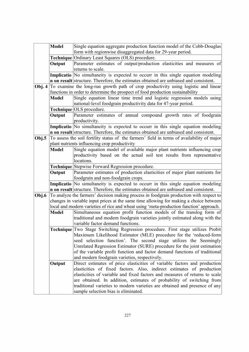
227

Model Single equation aggregate production function model of the Cobb-Douglas

form with regionwise disaggregated data for 29-year period.

Technique Ordinary Least Squares (OLS) procedure.

Output Parameter estimates of output/production elasticities and measures of

returns to scale.

Implicatio

n on result

No simultaneity is expected to occurr in this single equation modeling

structure. Therefore, the estimates obtained are unbiased and consistent.

Obj. 4 To examine the long-run growth path of crop productivity using logistic and linear

functions in order to determine the prospect of food production sustainability

Model Single equation linear time trend and logistic regression models using

national-level foodgrain productivity data for 47-year period.

Technique OLS procedure.

Output Parameter estimates of annual compound growth rates of foodgrain

productivity.

Implicatio

n on result

No simultaneity is expected to occurr in this single equation modeling

structure. Therefore, the estimates obtained are unbiased and consistent.

Obj.5 To assess the soil fertility status of the farmers’ field in terms of availability of major

plant nutrients influencing crop productivity

Model Single equation model of available major plant nutrients influencing crop

productivity based on the actual soil test results from representative

locations.

Technique Stepwise Forward Regression procedure.

Output Parameter estimates of production elasticities of major plant nutrients for

foodgrain and non-foodgrain crops.

Implicatio

n on result

No simultaneity is expected to occurr in this single equation modeling

structure. Therefore, the estimates obtained are unbiased and consistent.

Obj.6 To analyze the farmers’ decision making process in foodgrain production with respect to

changes in variable input prices at the same time allowing for making a choice between

local and modern varieties of rice and wheat using ‘meta-production function’ approach.

Model Simultaneous equation profit function models of the translog form of

traditional and modern foodgrain varieties jointly estimated along with the

variable factor demand functions.

Technique Two Stage Switching Regression procedure. First stage utilizes Probit

Maximum Likelihood Estimator (MLE) procedure for the ‘reduced-form

seed selection function’. The second stage utilizes the Seemingly

Unrelated Regression Estimator (SURE) procedure for the joint estimation

of the variable profit function and factor demand functions of traditional

and modern foodgrain varieties, respectively.

Output Direct estimates of price elasticities of variable factors and production

elasticities of fixed factors. Also, indirect estimates of production

elasticities of variable and fixed factors and measures of returns to scale

are obtained. In addition, estimates of probability of switching from

traditional varieties to modern varieties are obtained and presence of any

sample selection bias is eliminated.

228

Implicatio

n on result

This estimation procedure is considered superior to single equation model

for analyzing farm-level decision making process. Hence, parameter

estimates obtained from this modeling structure is exclusively used for

‘price policy analyses’ focussing on producers’ welfare.

Obj.7

and 8

To identify determinants of modern agricultural technology adoption at the farm-level,

and to identify the role of technological, infrastructural and soil fertility factors in

influencing crop production decisions.

Model Single equation model for analyzing determinants of modern technology

adoption.

Technique OLS and Tobit (Two-limit Probabilistic) procedures.

Output Parameter estimates of factors influencing modern technology adoption.

Implicatio

n on result

Simultaneity bias is expected to occurr in this specification. As such,

adoption behavior is again analyzed within a simultaneous equation

framework discussed below. Decision on the impact is made based only on

the nature and direction of the parameter estimates. The actual value of the

estimated coefficient is not used.

Obj. 9 To examine the impact of modern agricultural technology on employment and gender

equity in employment in the rural labor market as well as on factor markets, such as,

fertilizers, pesticides, crop output, agricultural credit, and tenancy markets.

Model A combination of single equation models of price functions and input

demand functions and a simultaneous equation model of input demand

functions along with modern technology adoption and irrigation demand

function.

Technique OLS procedure for all single equation price functions (fertilizer prices,

labor wages, output prices, and land rents). OLS and Tobit procedures for

single equation model of hired labor demand function, Tobit procedure for

single equation model of pesticide demand function, and only OLS

procedures for single equation models of total labor demand and

agricultural credit demand functions. Three Stage Least Squares (3SLS)

Regression procedures for simultaneous equation model for total labor,

fertilizer, animal power, modern variety adoption and irrigation demand

functions.

Output Parameter estimates of factors influencing prices and input demand

functions as well as modern technology adoption decision.

229

Implicatio

n on result

Since, the prime objective of this study is to analyze the impact of modern

agricultural technology on various components of the factors market, it

must appear as explanatory variable in all functions in one hand, and also

as a dependent variable in the analysis of adoption behavior on the other.

Therefore, simultaneity bias is expected. However, extent of simultaneity

bias is checked by analyzing estimates of same input demand functions

estimated within a single equation framework as well as simultaneous

equation framework. Price functions are, however, tested for their

exogeneity from the farm-level influence and hence not incorporated in

simultaneous equation model. Also, it should be noted that decision on the

impact of technological change is based only on the nature and direction of

the parameter estimates. The actual value of the coefficient is not used

and, therefore, the existence of simultaneity in equations does not pose any

major problem. However, if exact measure of influence is a primary

concern, then the estimates obtained from the simultaneous equation

model should be preferred.

Obj.1

0

To examine the impact of modern agricultural technology on income, distribution of

income and poverty.

Model Single equation model of determinants of income components.

Technique OLS procedure.

Output Parameter estimates of factors infuencing incomes.

Implicatio

n on result

No simultaneity is expected to occurr in this single equation modeling

structure. Therefore, the estimates obtained are unbiased and consistent.

Obj.1

1

To examine the impact of modern agricultural technology on selected aspects of

environment, such as, soil fertility, water quality, human health and fisheries resources.

Model Combination of behavioral model and linear single-equation time-trend

models.

Technique Perception ranking, soil and water quality parameter analyses, and OLS

procedure for time-trend analyses.

Output Rank of adverse environmental impacts of technological change in

agriculture, and trends (annual compound growth rate) of relevant

variables over time.

Implicatio

n on result

No simultaneity is expected to occurr in this single equation modeling

structure. Therefore, the estimates obtained are unbiased and consistent.

10.3 Synthesis of Impacts of Technological Change

The aforementioned summary of major findings provided a comprehensive picture on

the multifaceted impacts of technological change in agriculture. However, synthesizing the

nature of these multifaceted impacts of technological change on key economic variables and the

environment would provide the basis for strategic agricultural development planning for the

future. Also, the crucial role of two factors, infrastructure and soil fertility, are of special concern

since the scope for managing the agricultural production environment depends largely on the

nature of their impacts on the same set of key areas. The key impact areas at the national level

230

are regional equity, aggregate crop production and foodgrain sustainability, and at the local

level, these are input and output prices, input demand, employment, income, distribution of

income and the environment. A synthesis of the multifaceted impacts of modern agricultural

technology as well as infrastructure and soil fertility factors on these areas are presented in

Figures 10.1, 10.2, and 10.3, respectively (the details are provided in Appendix Tables A10.1,

A10.2, A10.3, A10.4 and A10.5, respectively).

At the national level, the nature of impact of technological change is complex and

multidimensional (Figure 10.1). Though modern agricultural technology increases regional crop

production, it also exacerbates regional disparity. On one hand, increase in aggregate crop

production confirms the positive impact of technological change in raising productivity,

implying that food production can be sustained in future. On the other hand, the declining yield

rate of modern rice varieties over time is raising doubt on sustaining food production trhough

technological change alone. However, the observed increase in modern wheat yield over time

will somewhat offset the depressing effect of modern rice yield, thereby, providing hope for

food production sustainability in future. Current increase in foodgrain production is largely due

to switching from local to modern varieties of rice and wheat, which still provides higher yields.

At the local level, it is clear that the modern technology diffusion in agricultural sector

exerted a distinct upward pressure on input and output prices as well as input demands (Figure

10.1). The upward pressure on output price will raise income of the farm producers and the

increase on labor wages will smooth income inequality through an indirect transfer of income

from rich farmers to the poor landless laborers. However, the increase on land rent raises equity

concern since landownership in rural Bangladesh is highly skewed with more than 50 percent of

farming population being landless and tenants. Higher land rent implies that the technological

change opened up opportunities for the landed elites to raise their income through the tenancy

market.

Though technological change significantly raised employment, it remained highly

skewed in favor of men since only male labor are hired to meet the increased demand. Women

constituting half of total population failed to get benefit from this technological progress.

However, it should be noted that failure to generate women’s employment opportunities is not

solely due to the nature of the technology, rather it is the social and cultural barriers that restricts

them to participate and accrue the benefit from this technological change in agriculture. The

simultaneous operation of higher labor wages and demand for hired labor owing to technological

progress may further redistribute income but the level of redistribution will not be substantial to

bridge the gap between the rich and the poor farmers.

Technological change significantly contributed to increase in income from crop as well

as agricultural production. However, it also contributed to worsening income inequality. The

concentration of income was estimated to be highest in ‘high adopter’ villages. Modern

technology diffusion has also exacerbated poverty. All the measures of poverty indices revealed

that poverty is high in ‘high adopter’ as well as ‘low adopter’ villages. It is the ‘medium

adopter’ villages characterized by diversified cropping system that the incidence of poverty and

income inequality is estimated to be lowest.

231

On account of environmental impacts of modern agricultural technology, the picture is

gloomy. The detrimental effect on soil fertility is more than obvious in the present study.

Associated with this are the adverse effects on human health as well as decline in open water

fisheries that served as a major source of animal protein for the rural poor in Bangladesh.

Decline in fisheries resources may also be attributed in part to over-fishing, increased

popoulation pressure and poor management. Increase in crop disease, pest and insect attack is

also clear from the results of this study. In addition to this, contamination of water bodies

through chemical run-off and eutrophication, though cannot be distinctly proved, remains a

major environmental concern in future. Arsenic pollution in groundwater though caused by

geogenic processes, it was brought to surface through anthropogenic processes spurred by

increased demand for irrigation for the modern variety cultivation in one hand and demand for

safe drinking water on the other. The surface soils in intensively irrigated region now contain

high level of arsenic. Therefore, a complex mix of strengths and weaknesses are intertwined

with this highly proclaimed technological breakthrough in agriculture that need to be carefully

screened in order to pave the way for future agricultural development plans.

The influence of soil fertility factor on prices is positive (Figure 10.2). Higher soil

fertility depresses demand for labor, animal power and pesticides. However, the decrease in

demand for labor can be offset by an increase in cropping intensity through crop diversification

in fertile soils. The reduction in pesticide use with improvement in soil fertility strengthens the

case for soil fertility management. The positive impact of soil fertility on crop as well as

agricultural income reinforces the argument.

The influence of infrastructural factor on prices, employment, input demands,

technology adoption and income are mixed (Figure 10.3). Output and fertilizer prices are higher

in infrastructurally developed region implying increase in farm income as well as promoting

optimal use of inputs. Demand for irrigation and modern technology adoption declines with

infrastructure development that would consequently promote crop as well as economic

diversification, thereby, exerting less detrimental effect to the environment. In addition,

influence of infrastructure in increasing income, particularly non-agricultural income, make a

strong case for investment in rural infrastructure. At the national- level, the positive impact of

infrastructure in raising crop production further reinforces the need to invest in infrastructure,

particularly, road, transportation, storage and marketing facilities.

10.3.1 ‘Balanced Adoption is Equitable’: Salient Features of ‘Medium Adopter’ Villages

As mentioned earlier that a complex mix of strengths and weaknesses are intertwined

with this highly proclaimed technological change in crop production in Bangladesh agriculture.

Analyses of the distributive justice of modern technology diffusion clearly revealed that it is the

‘medium adopter’ villages that consistently revealed least income inequality and incidence of

poverty. This finding, therefore, challenges the conventional notion that high level of modern

technology diffusion is the key to agricultural development and economic growth. In order to

232

identify the conditions determining the superiority of this category of villages, selected socio-

economic characteristics of villages by adopter categories is examined (Table 10.3).

It is clear from Table 10.3 that a number of features distinguishes ‘medium adopter’

villages from the other two categories. The striking difference is in the proportion of large

farmers (16 percent) in the ‘medium adopter’ villages as compared to only 6 percent in ‘high

adopter’ and none in ‘low adopter’ villages. Also, the proportion of medium farmers are highest

(18 percent) in these villages. The higher proportion of large farmers resulted in large farm size

(0.96 ha/farm) in ‘medium adopter’ villages, which is more or less an economic size of farm

within the context of Bangladesh. The level of irrigation development is strikingly similar

between the ‘high adopter’ and ‘medium adopter’ villages, 62 percent and 60 percent, while the

difference in the level of modern variety adoption is very large, 75 percent and 47 percent,

respectively. This implies that the medium level of adoption of modern variety is not due to

limitation posed by the lack of irrigation, which is a feature for the ‘low adopter’ villages.

The cropping intensity is very high in ‘medium adopter’ villages (190 percent) and

cropping system is highly diversified. Despite highest level of cropping intensity, the level of

fertilizer use per ha of cropped land is much lower in ‘medium adopter’ villages (209 kg/ha) as

compared to ‘high adopter’ villages (225 kg/ha), while level of organic manure application rate

is highest (1.5 ton/ha). Also, the soil fertility level is relatively better in ‘medium adopter’

villages as compared to other two categories of villages. Further, these villages are located in

areas with most developed rural infrastructure. This has opened up the opportunity to produce

high-valued non-cereal crops in addition to modern varieties of rice and wheat since marketing

risk associated with cash crop production is reduced to a large extent due to developed rural

infrastructure.

All these features combined together resulted in better performance of these ‘medium

adopter’ villages in terms of income inequality and poverty. The per capita income is highest

(Tk. 6,902/person) in the ‘medium adopter’ villages with least income inequality (Gini = 0.34).

The number of population below poverty line is also lowest (46 percent) and all types of poverty

measures consistently revealed lowest incidence of poverty.

Therefore, one of the strategies for sustainable agricultural development planning will be

to internalize the salient features of the ‘medium adopter’ villages and to replicate and/or create

such conditions in ‘high adopter’ as well as ‘low adopter’ villages. In short, following Schultz’s

(1964) terminology of ‘small is beautiful’ (used for small farmers), it can be said in the context

of sustainable agricultural development that, ‘balanced adoption is equitable’.

10.4 Strategies for Agricultural Development Planning and Policy Options

The previous two sections provide a comprehensive summary of the major findings

together with the results of hypothesis tests and a synthesis of multifaceted impacts of

technological change on key economic variables and the environment, respectively. In this

section, an integrated agricultural development plan is outlined. The choice of the program

components is made by applying the SWOT (Strength-Weakness-Opportunity-Threat) analysis

based on the results of multifaceted impacts of technological change discussed so far. The

233

proposed strategic development planning is viewed as an integrated model involving (1) balanced

modern technology diffusion, (2) crop diversification, (3) soil fertility management, (4) rural

infrastructure development, (5) pricing policy and (6) economic diversification. The first three

components are interlinked with each other and need to be implemented simultaneously. The

remaining three components will smoothen the process by: (a) enhancing effective input delivery

and output marketing systems through developed infrastructure, (b) responding to price signals

through appropriate pricing policies, and (c) engaging in non-agricultural income generating

activities through economic diversification. The result of SWOT analysis of the aforementioned

program components is presented in Table 10.4, which formed the basis of devising various

policies for sustainable agricultural development in Bangladesh.

Policy #1: Balancing Modern Technology Diffusion

Results of the SWOT analysis (Table 10.4) clearly revealed that though a number of

strengths and opportunities are associated with this highly proclaimed modern

agricultural technology, the corressponding weaknesses and threats reduce its merit to a

large extent. Particular concern is the adverse effect of modern agricultural technology on

income distribution and poverty and its threat to environmental health. On the other

hand, findings from this study clearly reveals that a balanced level of modern technology

adoption along with crop diversification provides highest per capita income and is

associated with least income inequality and poverty (Table 10.3). Therefore, keeping the

level of modern technology adoption at an optimum level with a right mix of improved

varieties and crop diversification, as opposed to exclusive diffusion suggested in earlier

evaluations of ‘Green Revolution’, seems to be the best option in improving income

distribution and bridging the poverty gap between rich and poor.

It should be noted that, limited adoption of modern technology might not be able to

meet the income needed for year round expenses on family maintenance even in the rural

regions. Therefore, two alternative options are forwarded, crop diversification (an option

allowing the farming households to remain within agriculture) or economic diversification

(an option paving the way for the farming households to move out of agriculture). As there

are two major cropping seasons, rabi (dry winter) and kharif (monsoon), with an

overlapping season for modern Boro rice, one principal strategy would be to allocate land

for modern varieties of rice during the kharif season and diversify the cropping system

during rabi season. Modern transplanted Aman rice played a dominant role in meeting the

foodgrain demand in Bangladesh. The advantage with modern Aman rice is that it is

grown in the monsoon season and, therefore, requires less irrigation as early rain can

supplement the water requirment. Therefore, research must be geared to introduce Aman

varieties that are flood and disease resistant and provides higher yields.

234

Table 10.4 SWOT analysis of the integrated agricultural development planning components.

Component Strength Weakness Opportunity Threat

1.Modern

technolog

y

diffusion

• Increase employment

• Increase

crop income

• Increase

price

• Increase labor wage

• Increase

land rent

• Increase income inequality

• Increase regional

disparity

• Increase gender

inequality

• Increase pesticides and

fertilizer use

• Ignore indigenous

technical

knowledge

• Increase food self-sufficiency

• Reduce food import

• Save foreign

exchange

• Increase poverty

• Decline soil fertility

• Affect human health

• Reduce fish

production

• Increase disease, pest

and insect attack in

crops

• Contaminate water

body

• Reduce biodiversity

• Degrade

environment

2.Crop

diver-

sification

• Increase

crop income

• Increase

employment

• Increase

price

• Increase

labor wage

• Increase

land rent

• Increase fertilizer

use

• Require skilled

labor

• Poor

infrastructure

• Capital intensive

• Improve soil fertility

• Improve income

equality

• Improve regional

equality

• Improve gender

equity

• Promote export

earning

• Substitute import

• Reduce pest attack

• Preserve biodiversity

• Reduce production

risk

• Maximum

production may not

be achieved

• Increase

commerciali-zation

• Increase dependency

on external markets

3.Soil

fertility

manageme

nt

• Increase

crop

productivity

• Increase

crop income

• Increase

management cost

• Require skilled

personnel

• Improve soil

properties

• Preserve soil fertility

• Stabilize crop

productivity

• Sustain food

production

• Intensive agricultural

practice may lead to

environmental

degrada-tion in the

long run

• Risk of pollution

4.Infrastruc-

tural deve-

lopment

• Promote

diversificati

on

• Increase non-

agricultural

income

• Increase

• Require high

implementation

cost

• Require skilled personnel

• Increase

maintenance cost

• Promote access to

inputs and delivery of

outputs

• Promote extension network and facilities

• Increase access to

information

• Facilitate export

• Irreversible

development

threatening

environment in the

long run

• Increase capital out-

flow from rural to

urban areas

235

Component Strength Weakness Opportunity Threat

non-farm

employ-

ment

• Increase

price

• Promote economic

growth

• Raise standard of

living

• Increase

commerciali-zation

5.Price

policy

manageme

nt

• Promote

crop

diversificati

on

• Increase crop income

• Require subsidies

• Poor information

• Poor

infrastructure

• Promote optimum

input utilization

• Promote long run

crop production

stability

• Increase farm

investment

• Promote economic

growth

• Increase risk due to

price fluctuation

• Increase dependency

on external markets

• Increase inequality if

implemented poorly

6.Economic

diversi-

fication

• Increase non-

agricultural

income

• Increase

non-farm

employment

• Investment intensive

• Require skilled

personnel

• Poor

infrastructure

• Develop agro-industries

• Develop enterprise

• Mobilize investment

• Promote economic

growth

• Raise standard of

living

• Increase commerciali-zation

• Increase congestion

• Increase in-migration

• Risk of Pollution

• Environmental

degrada-tion in the

long run

Source: Based on multifaceted impact analysis of technological change in agriculture in

previous chapters, namely, Chapters IV, V, VI, VII, VIII and IX.

236

Policy #2: Crop Diversification

Crop diversification possesses similar strength as that of modern rice and wheat

technology. In addition, it possesses considerable opportunities for environmental

improvement and is accompanied with least threat if managed properly (Table 10.4). The

present study clearly demonstrates that vegetable, spices (chilly, onion, garlic and

turmeric), potato and cotton provide higher return than the modern varieties of rice and

wheat. Mahmud et al. (1994) also reported the superiority of these crops in terms of

returns over modern varieties of foodgrains. Promotion of these crops with appropriate

management and pricing policies would exert favorable impact on income distribution as

well as balance in nutritional intake. Alauddin and Tisdell (1991) noted that Bangladeshi

diet has become highly skewed in favor of starch intake only, which is detrimental to

health in the long run. It should be noted that a general model of crop diversification could

not be implemented in every region due to different micro-climatic requirements for

specific non-cereal crops.

A burning question remains that if non-cereal crops perform so well in terms of returns,

then why their acreage are declining over time? One of the most convincing

answers for this question is the price and yield risks associated with growing these

crops. Thus far, little or no research has been done in the area of risk analyses of

non-cereal crops in Bangladesh. Shahabuddin (1991) using a farm level analysis

of farmer behavior under uncertainty indicates that areas where farm households

are unable to meet consumption needs reveal risk-taking behavior in making crop

choices while those who can meet consumption needs tend to be risk-averter38.

Therefore, one of the principal strategies to promote crop diversification should

be through controlling the price risks (details of price policy analyses is presented

in the subsequent section). Strengthening of crop insurance policies through

public and private insurance agencies could be an additional support to promote

crop diversification. In Bangladesh, the concept of crop insurance to hedge

against risk is non-existent. In an uncertain production environment

characterized by frequent occurrence of natural hazards and calamities, crop

insurance policies can play a major role in hedging yield risks.

In addition to price and yield risk, marketing risk for perishables, such as vegetables, is

another major factor hindering crop diversification. Development of market

facilities coupled with improved transport facilities would be an effective strategy.

Such development would also reduce the price risk to a large extent. The positive

influence of infrastructural development on prices, input demand and non-

agricultural income has been established in this study (Figure 10.2).

Lack of technical skills in growing these crops optimally may be another factor,

hindering the expansion of non-cereal crops. The ‘decreasing returns to scale (0.82 < 1.00)’

computed for non-cereal crops in Chapter V hints on either overutilization or inefficient

38

However, it should be mentioned that data for his study dates back to crop year 1979/80 when the diffusion of

modern agricultural technology was in its mid-stage and the extent of income inequality and poverty were not as

adverse as of now. As such, studies in analyzing risk behavior of farmers need to be emphasized.

237

utilization of resources in non-cereal crop production. It is also shown that the existing

interaction among the agricultural extension system and farmers are weak (Chapter VI).

Therefore, the existing agricultural extension needs to be strengthened (detail is discussed in

subsequent section).

Suggested Crops for Jamalpur Region

Based on the existing land use, yield rates, and profitability (output-input ratio)

criterion, it is suggested that crop diversification policy in Jamalpur region should

focus on oilseeds (mainly mustard), spices (mainly chilly, onion and garlic),

vegetables, modern Aman rice, and potato cultivation. The profitability for these

crops are estimated at 1.27, 1.25, 1.23, 1.19 and 1.15, respectively with

corressponding rank order from 1 to 5 (Appendix Table A10.6). Cultivation of

modern Boro rice provides a profitability of 1.13 and is lower than modern Aman

rice crop while the investment is substantially higher. Since rice is still the major

staple food in Bangladeshi diet, cultivation of at least one crop of rice is a pre-

requisite. Moreover, modern Aman rice is grown in monsoon season, therefore,

require fewer cost for irrigation. The dry winter season can be devoted to growing

oilseeds, spices, vegetables, as well as potato that would bring higher annual farm

family income.

Suggested Crops for Jessore Region

Using the same set of criterion as of Jamalpur region, the crop diversification policy in

Jessore region should focus on vegetables, jute, modern Aman rice, cotton, pulses

and oilseeds. The profitability for these crops are estimated at 1.47, 1.38, 1.36,

1.33, 1.27, and 1.22 respectively with corressponding rank order from 1 to 6

(Appendix Table A10.6). Cultivation of modern Boro rice provides a profitability

of 1.19 and is lower than modern Aman rice crop while the investment is

substantially higher. Similar argument in favor of modern Aman rice also holds

for Jessore region. The yield rate of jute is highest in Jessore, thereby, providing

substantially high net return. Cotton is a specialized crop grown in Jessore region

only largely due to the micro-climatic requirement for this crop. The relatively

better soil fertility status of this region provides high potential for promoting

vegetables, jute, cotton and pulses.

Suggested Crops for Comilla Region

For the Comilla region, the crop diversification policy should focus on spices (mainly

chilly, onion, and garlic), jute, modern Boro rice, potato, and pulse crops. The

profitability for these crops are estimated at 1.25, 1.18, 1.13, 1.10 and 1.08,

respectively with corressponding rank order from 1 to 5 (Appendix Table A10.6).

The profitability of modern Boro rice is higher in Comilla region due to the

existence of Meghna-Dohanagoda Flood Control, Drainage and Irrigation Project

(M-D FCD/I) resulting in substantially lower cost for irrigation. The profitability

of modern Aman rice is lower due to higher cost of other inputs, particularly

animal power price and wage of labor in this region. The profitability of potato is

238

also high in Comilla region due to exclusive use of modern varieties and high

doses of fertilizers. Rate of return from spices is highest. The potential for

diversification is relatively higher in areas outside the embankments of M-D

FCD/I, since a tendency to move out of rice is observed among many farmers

owing to high cost of irrigation as well as land preparation.

Production of modern varieties of wheat is not suggested for any of these

three regions largely due to its low and similar profitability (1.04) across regions

(Appendix Table A10.6). This may be a major reason for slow growth of wheat

acreage in the country. From the aforementioned analysis, it is clear that the

choice of crops in promoting the policy of crop diversification should be region

specific. Though the entire country is characterized with a rice-based cropping

system, dominated by Aman rice crop, the annual crop cycle underwent vast

changes by developing pockets suitable for particular crops, e.g., cotton and

pulses, that has to be taken into account while planning for sustainable

agricultural development.

Policy #3: Strengthening Bottom-up Planning and Agricultural Extension Services

It was observed that lack of technical skills is one of the factors hindering expansion of

non-cereal crop production in Bangladesh. The strategy to improve technical know-how of the

farmers can be undertaken in two ways with effective inter-links: (a) by intensifying the

existing agricultural extension network utilizing a bottom-up planning approach, and (b) by

collaborating with the national and regional level NGOs working at grassroots.

High potential lies with the existing agricultural extension network spread all over the

country. The major need is to transform the existing top-down approach to rural

development to a bottom-up approach where the basic need specific to individual

areas is assessed at the grassroots. Then these needs are converted into action

plans and later delegated up in the hierarchy ultimately reaching the center for

approval and fund allocation. Starting from 1995, the DoAE initiated bottom-up

planning approach to agricultural extension at a pilot scale that require sub-

district and district level extension officials to prepare ‘bottom-up extension

plans’. The department also organized training programs on planning skills for

staff at all levels and published ‘modified agricultural extension manual’ that

emphasizes ‘little or no cost extension system’ (DoAE, 1995 and 1996). Though

the success of this modified extension system is yet to be evaluated, this change of

attitude from the conventional top-down planning approach to bottom-up

planning approach already paved the way to successfully implement the strategies

suggested in this study. The NGOs can be involved to impart training on planning

skills and preparation of individual bottom-up extension plans by working closely

with the sub-district level agricultural extension officials. Involvement of NGOs

from the beginning of the process will enable the government to undertake joint

implementation programs for the proposed individual plans. Also, this will bring

in consistency of development programs undertaken separately by the NGOs and

the governments thereby avoiding duplications of programs. Moreover, it could

239

overcome the constraints faced by government related to budget deficiency as well

as the lack of trained officials and the stiff bureaucratic time killing.

Presently, NGOs in Bangladesh operate in more than 50 percent of the total villages of

the country involving over 3.5 million families as beneficiaries mainly composing

of the most disadvantaged section of the society (Rahman, 1994). Over the past

two decades, NGOs had significant contributions in the areas of health, family

planning and sanitation, education (adult and non-formal primary education),

social forestry, livestock and sericulture. Therefore, the expertise of NGOs in

providing extension services at the grassroots can be tapped through devising

appropriate collaborative mechanisms with the government agencies. Leading

national NGOs, such as BRAC, Proshika, and ASA, initiated programs in

collaboration with the government since the early 1980s in other areas of

development. Starting from the 1990s, BRAC expanded its ‘vegetables production

program’ involving the landless rural women. These women lease-in land or use

their homesteads for growing vegetables. BRAC provides them with training,

technical services, inputs and credits required for the operation. Currently, an

estimated 51,565 women are involved in ‘vegetables programs’ (BRAC, 1996).

Therefore, a formal collaborative arrangement between the Department of

Agricultural Extension (DoAE) and NGOs, such as BRAC, Proshika and ASA,

could promote the scope of crop diversification to a large extent.

Policy #4: Soil Fertility Management

In this study, ‘declining soil fertility’ has been identified as the major adverse

environmental impact of modern agricultural technology diffusion (Chapter IX).

The decline in productivity trend of modern rice in most of the regions has been

detected as early as 1987 (BASR, 1989). Therefore, improving soil fertility is a

major concern in the pursuit for sustainable development in Bangladesh. The

direct approach to improve the soil fertility status would be to test the physico-

chemical parameters of the soil and recommend suitable crop rotation and soil

conservation measures suited to individual soil series. Also, promotion of

biotechnology and use of biofertilizers would restore soil fertility status.

Promotion of crop diversification policy will in turn contribute positively to soil

fertility restoration measures.

In this context, it should be mentioned that the Soil Resources Development Institute

(SRDI) in collaboration with five other institutes39 initiated a project to prepare

‘Land and Soil Resource Use Guide’ (in Bangla) for each of the 460 sub-districts

of the country in the early 1980s. The manual consists of physical and chemical

test results of soil for each of the soil series found in specific sub-district and a soil

map drawn on 1:50,000 scale for each sub-district indicating the soil collection

locations. It also contains fertilizer recommendation guide for optimum

39

The collaborating institutes are Bangladesh Agricultural Research Institute (BARI), Bangladesh Rice Research

Institute (BRRI), Bangladesh Institute of Nuclear Agriculture (BINA), Bangladesh Agricultural Research Council

(BARC) and DoAE, respectively.

240

production for all major and minor crops. Thus far, manual for about two-thirds

of the sub-districts are published and are distributed to the Block Supervisors, the

lowest unit of agricultural extension officials, residing in the rural areas. The

considerable delay (about 15 years since the project started to collect soil samples)

in publishing the manual reduced its effectiveness for planning. For example, the

soil test results collected under this project somewhere between 1980 – 1985 for

two of the regions, Manirampur sub-district of Jessore region and Jamalpur

Sadar sub-district of Jamalpur region is published in 1990 and 1991, respectively.

But manual for the Matlab sub-district of Comilla region is yet to be published. A

comparison of the presently collected soil test results with those reported in the

manual for the same soil series revealed sharply different results. Nevertheless,

these manuals will serve the basic purpose for identification of suitable crops

suited to each individual soil series along with recommended fertilizer doses for

individual crops.

Therefore, an inter-agency coordination is needed to ensure that these soil resource use

manuals as well as training on bottom-up planning skills are provided together to

the root level agricultural extension officials. The joint implementation of both

these programs will lead to the preparation of effective agricultural development

plans at the sub-district level that are conducive to the suggested policies of crop

diversification as well as soil fertility management. Involvement of NGOs will

speed up the process of imparting knowledge on environmental awareness as well

as training on soil conservation measures.

Uncertainty in land tenurial arrangement depresses incentives of farmers to undertake

soil conservation measures. Since, no long-term security is ensured in existing

tenurial arrangements in Bangladesh, tenants find it un-economic to invest in soil

conservation measures. Though no specific analysis on this aspect is conducted in

this study, it is widely accepted that secure tenure indirectly promotes soil

conservation. Therefore, effective implementation of the already existing policies

on security to tenure (currently only on paper) will indirectly influence soil

conservation measures.

Policy #5: Price Policy Prescription

One of the most effective ways to influence individual decision making process is by

exerting an effect on the prices of inputs as well as outputs. Effective price policies have the

unique advantage of minimum control and monitoring requirements and can be implemented

at a national level. But it carries a disadvantage of market distortion and huge investment in

subsidies. However, if the target is to improve the lives of the disadvantaged farming

population, then such investment seems worthwhile if properly implemented. In order to

specify the price policy instruments to be implemented, a rigorous analyses on several policy

alternatives and their welfare implications based on the response of farmers’ to changing

production environment (Chapter V) is presented in the following section. The impact of any

policy instrument would have to work through the actions of the farmers and the agronomic

characteristics of the crops. Therefore, in order to predict the impact of alternative policy

instruments, knowledge of farmers’ quantitative response to economic incentives introduced

241

by these instruments as well as the response of the crops to changes in input use as

consequence of their response to policy instruments is required. Information required for such

analyses is detailed in Chapter V.

Fifteen policy alternatives are considered: four single instrument policies (fertilizer price,

labor price, animal power price and output price); six two-instrument combinations; four three-

instrument combinations; and, one four-instrument combination. For analysis, we consider the

effect of a 10 percent reduction in input prices (i.e., fertilizer, labor and animal power subsidies)

and a 10 percent increase in output prices (output subsidy) both individually and in combination.

The computations were done separately for foodgrain crops and non-cereal crops since the

response pattern is different for these two broad crop groups (see Chapter V). The procedure

used to calculate the cost-effectiveness of the policy alternatives is detailed in Appendix D.

It should be noted that, in this study, the measure of overall welfare conducted through

the price policy analyses focussed only on estimating the operators’ or producers’ surplus. The

detail treatment of consumers’ surplus in this overall welfare analysis has not been attempted,

since the focus is on analyzing the distribution of gains of technological change on farmers’

income.

When only cost-effectiveness rather than distributional implication is concerned, Table

10.6 reveals that the most cost-effective policy for increasing foodgrain production is a reduction

in labor wages (ranked 1) and for non-cereal production a subsidy on fertilizer prices (ranked 1).

The rate of return is 95 percent return on the labor wage subsidy for foodgrain production and the

rate of return is 254 percent on fertilizer price subsidy for non-cereal crop production (Appendix

Tables D3, D4 and D5).

However, it is not desirable to choose policies based on only a single criterion of cost-

effectiveness but also must satisfy distribution considerations. The latter criterion often

complicates the policy prescriptions. If the government’s distributional objective is targeted to

raise the income of farmers, then the most-effective policy appears to be output price subsidy that

would yield substantially higher income to farmers as well as the society, though they rank very

low in terms of cost-effectiveness.

The option for labor wage subsidy is ruled out on the ground that it will adversely affect

the landless and marginal farmers whose major source of income is wage labor. Also, rise in real

wage of labor is desired as a policy in order to bridge the gap between rich and poor. The

fertilizer subsidy policy, though ranks very high in terms of cost-effectiveness, it is ruled out due

to serious controversies in the past as well as its adverse effect on the environment. Fertilizers

were heavily subsidized since the introduction of modern agricultural technology in the early

1960s. The average rate of subsidy was about 58 – 67 percent in 1968/69 and was lowered to

about 25 percent in 1983/84 (Hossain, 1989). Subsidy on fertilizer was finally removed on

December 1992 (Baanante et al., 1993). The International Fertilizer Development Center (IFDC)

study on the impact of fertilizer subsidy removal in Bangladesh showed that the rise in

fertilizer/paddy price ratio due to the removal of subsidy would exert negligible impact on crop

yield and farmers’ income. Moreover, it will save cost of the government and allow efficient

resource allocation (Baanante et al., 1993). Though large fluctuation in fertilizer prices is

242

observed in the present study, an effective marketing policy and retail price control would

optimise the use of fertilizers for agricultural production.

Since both labor wage and fertilizer price subsidies are ruled out, the focal point of the

policy lies in subsidizing animal power services that would be cost-effective, relatively less

expensive to the government, and provide reasonable benefit to the farmers as well as the

society (Appendix Table D5). The subsidy on animal power services can be operated using

two approaches: (a) developing the much desired livestock sector, and/or (b) developing farm

mechanization, particularly, tillage equipments. Farm mechanization in Bangladesh has not

been successful largely due to the biophysical constraints imposed by the maze of canals and

waterbodies separating the scattered fragmented farm plots of individual farmers in almost

every region of the country coupled with poor and inadequate service delivery systems. Also,

the labor displacing potential of farm mechanization is another concern. Studies carried out

during the early 1980s showed that power tillers do not have significant positive effect on land

productivity; cause net labor displacement and benefit the better-off who can afford to buy it

(Jabbar and Green, 1983). Therefore, the best option lies in developing the livestock sector

that would serve the dual purpose of draft power requirements as well as nutritional

requirements of the malnourished population. The current policy thrust in the livestock

development is far from adequate. The plan allocation for livestock sector remained within 2.7

– 6.8 percent of total budget in successive Five-Year Plans covering the 1973 – 1995 period

while its contribution to national GDP ranges between 7.8 – 13.9 percent, respectively

(Rahman and Bhuiyan, 1991). The sector is consistently under-funded with poor research,

training and extension facilities given the magnitude of the problem. For example, budget

allocation for veterinery services and genetic improvements declined steadily since 1980 –

1995 despite the policy thrust on improving the livestock sector (Rahman and Bhuiyan, 1991).

Therefore, existing financial, technological and institutional constraints of the livestock sector

need to be removed as it serves as one of the most important supporting activity in the crop

production sector of Bangladesh providing 98 percent of the draft power requirement.

As providing a complete set of policies is beyond the scope of this study, it seems that

price policies for raising farm incomes in three regions of Bangladesh should focus on animal

power and output price subsidies.

Policy #6: Rural Infrastructure Development

The need to develop rural infrastructure has been indicated a number of times in the

aforementioned strategies. Infrastructural development is emphasized mainly to

pave the way for both crop diversification as well as economic diversification

policies. The present study clearly demonstrates the favorable impact of

infrastructural development on prices, input demand and income (Figure 10.2).

Also, infrastructural development open up opportunities for increased interaction

between urban and rural regions. The major types of infrastructures need to be

developed are: agricultural extension network, markets and marketing facilities,

storage facilities, milling and processing facilities, road and transportation

facilities, financial institutions, educational institutions, and information and

communication networking. The rotated factor matrix analysis of infrastructural

facilities in the study regions revealed that the first five elements of infrastructure,

243

the agricultural extension office, bank, bus stop, storage and growth centers alone

explain more than 85 percent of the variations in the infrastructure index

(Appendix Table A5.1).

The major role has to be taken up by the government to build these facilities, as there

are little scope to engage NGOs in these public sector investments. Though road

communication is quite satisfactory in the study regions, the concomitant development of

market, storage and other infrastructural facilities are far from adequate, particularly, in the

Jamalpur region. Therefore, a balanced development of rural infrastructure is needed to

promote sustainable agricultural development.

10.5 Potential for Economic Diversification in the Study Regions

A major advantage of economic diversification is that it enables to earn income from

non-agricultural sources (Table 10.4), thereby, exerting less pressure on land that

are already intensively utilized with improper soil conservation measures. It was

shown in Figure 10.2 that non-agricultural income is higher in developed

infrastructure regions. Therefore, planning for economic activity for the study

regions should not be confined to crop diversification alone. In general, economic

diversification strategy should focus on developing rural enterprises and cottage

industries that are small and labor intensive and possess a strong marketing

potential.

Based on the observation during the farm-survey and results of the Focussed Grouped

Discussion (FGD) conducted as a part of the survey, considerable potential for diversification to

non-agricultural as well as non-crop agricultural activities are identified. For example, Comilla

study region possesses vast potential to develop fishing industry, as it is located at the

confluence of the Meghna and Dhonagoda rivers. Since there exists a good river as well as road

communication between the Comilla study region and the capital Dhaka, tapping the huge

potential for developing fishing industry through commercial fishing and establishing fish

processing facilities will raise income in the locality. Jessore study region, on the other hand,

possesses huge potential for agro- processing and tile-processing industries. The region is

famous for gur (raw sugar) made from datepalm and the clay available in the region form good

roofing material. An advantage of both these processing industries is that they are labor intensive

and would generate non-farm employment. Therefore, economic diversification strategy for this

region should focus on promoting these industries. For Jamalpur region, enterprise development,

particularly, small-scale cottage industries and handicrafts, may be a desirable strategy for

economic diversification in this region.

Apart from the development of infrastructural facilities to spur economic diversification,

a major strategy would be to implement joint programs promoting rural small-scale labor-

intensive industries by actively involving NGOs in the process. The active involvement of

NGOs in economic diversification programs will release the burden of providing skills training,

supervision and monitoring requirements on the part of the government agencies thereby leaving

only the task of effective promotion of marketing and input delivery systems for the

government. The success in the development of silk production with joint collaboration between

244

Bangladesh Sericulture Board and BRAC is a case in point (Rahman, 1996).

10.6 Conclusions

Widespread controversies exist on the delayed consequences of technological change

or ‘Green Revolution’ technology in agriculture. The reasons can be largely attributed to the

approach utilized in analyzing the impact of technological change as well as the extent of

issues covered in the evaluation processes. The present study employed a holistic approach to

evaluate the multifaceted impacts of the modern agricultural technology diffusion in

Bangladesh from the national as well as local perspective by addressing diverse range of

issues: regional development, foodgrain sustainability, employment, gender gap, income

distribution, poverty, and the environment.

Results revealed that a complex mix of strengths and weaknesses are intertwined with

this highly proclaimed technological breakthrough in agriculture that need to be carefully

screened in order to pave the way for future agricultural development plans. Despite a number

of positive impacts of this technological change in increasing food production, income,

employment and factor prices, it has also increased regional disparity, gender gap, income

inequality, and poverty and is a threat to the environment, particularly, soil fertility, human

health, fisheries resources, and water quality. Also, the declining productivity of the modern

rice varieties, a major vehicle of this technological breakthrough, is raising doubts on

sustaining foodgrain production in the future. However, an interesting feature emerged

from the synthesis of the multifaceted impacts. It is observed that the ‘medium adopter’

villages, characterized by balanced aoption of modern varieties, diversified cropping system,

with larger land endowment, better soil fertility and developed rural infrastructure performed

better and is associated with highest per capita income and least income inequality and

poverty. This finding, therefore, challenges the conventional notion of intensifying modern

technology adoption as the key to agricultural development and economic growth. Rather, it

establishes the fact that ‘balanced adoption is equitable’.

As such, an integrated model of agricultural development plan is outlined using the

SWOT analysis based on the multifaceted impacts of technological change. The proposed

strategic development planning is viewed as an integrated model involving (1) balanced

modern technology diffusion, (2) crop diversification, (3) soil fertility management, (4) rural

infrastructure development, (5) pricing policy and (6) economic diversification.

Balanced adoption of modern agricultural technology along with crop diversification is

suggested as one of the major policy based on the experience of ‘medium adopter’ villages

who revealed a balance between modern varieties of rice and wheat as well as non-cereal

crops. This suggestion contrasts with almost all of the earlier evaluation of ‘Green Revolution’

that recommends spreading of modern technology to its fullest extent. Based on the existing

land use, yield rates, total costs of production and net profit criterion, specific crop

combinations for individual regions are suggested.

In setting the strategies for agricultural development planning, an effective pricing

policy is deemed pivotal in enhancing crop diversification by reducing the price risks

245

associated with non-cereal crop production. Based on distributional considerations, subsidies

on animal power services and output prices are suggested that can be implemented across the

board: from local level to national level. Also, crop insurance policies through public and

private insurance agencies and development of marketing, transportation and infrastructural

facilities is suggested to reduce the yield risks and marketing risks to promote crop

diversification both at the local level as well as the national level.

Human resource development, in terms of providing technical skills in growing non-

cereal crops, raising awareness on adverse environmental impacts of

technological change, and enterprise development skills are suggested to promote

crop diversification as well as economic diversification policies. The strategy to

improve technical know-how of the farmers can be undertaken by: (a)

intensifying the existing agricultural extension network utilizing a bottom-up

planning approach, and (b) collaborating with the national and regional level

NGOs working at grassroots.

The key to success in realizing this planning strategy is integration and coordination

among facilitators: relevant government agencies, NGOs, financial institutes and

the farming communities. The development programs of individual agencies must

be integrated in order to enable the farming and rural communities to reap the

full benefit of interventions. An uncoordinated implementation of the same tasks

will result in failure and which is usually the case. Therefore, at the outset,

substantial changes in the attitudes of the government agencies towards

development programs along with a major restructuring of individual program

scheduling, budgeting, and implementation strategy is a pre-requisite to initiate

the tasks.

Finally, it can be concluded that Bangladesh need agricultural technologies that are labor-

intensive, provide equal opportunities for men and women, smoothen income inequality, reduces

poverty and exerts least effect on the environment. Therefore, a properly designed crop

diversification policy and its implementation would be a first step toward the goal of achieving

sustainable development. Also, implementation of economic diversification policy and

development of rural infrastructure will further complement the pursuit for sustainable

agricultural development in Bangladesh.

10.7 Direction for Further Research

Despite the fact that a large number of issues are covered in this study, some other

issues of importance could not be analyzed mainly due to limitation posed by the nature of

data (multi-period data), time, funding, and scope required for such study. In order to

complement the findings of the present study, the following research is suggested:

1. The analysis of impacts on technological change on consumption, nutrition, savings and

investment is important. It should be mentioned that research on the impacts of modern

agricultural technology on consumption, saving and investment in Bangladesh is

conducted at its early stage of diffusion, the 1980s. However, the current scenario, which

is expected to be largely different, requires fresh examination. Also, the effect on

246

nutritional intake is important to develop a nation with healthy population that has direct

relevance to working ability, work efficiency, and intellectual development.

2. Analyses of intangible environmental impacts of technological change, such as, soil

salinity, compaction of soil, and contamination of water bodies need to be conducted to

authenticate the farmers’ perception and claims.

3. Empirical estimation of the rates and factor biases of technological change with respect to

specific environment, for example, irrigated as well as unirrigated environment, will be

valuable for devising national level agricultural development policies.

4. Studies on farmers’ behavior under risk and uncertainty is nascent in Bangladesh. Details

of farmers’ risk taking behavior under changing production environment will assist greatly

in devising alternative policies for agricultural development.

247

REFERENCES

Abdullah, T., 1985. “Women in Rice Farming in Bangladesh and How Technology Programs

Can Reach Them”. In Women in Rice Farming. Proceedings of a Conference on Women

in Rice Farming Systems. 26-30 September, 1983, International Rice Research Institute

(IRRI), The Philippines. Aldershot: Gower Publishing Co. Ltd.

Abedin, J., 1985. “Input Demand and Output Supply Elasticities for Rice in Bangladesh – A

Study Based on Thakurgaon Farmers”. Bangladesh Development Studies 13, 3 and 4:

111-125.

Abedin, J., and Bose, G.K., 1988. "Farm Size and Productivity Difference: A Decomposition

Analysis". Bangladesh Development Studies 16, 3: 72-79.

Aguero, M., 1989. “Inland Water Fisheries in Bangladesh: Management Options and Natural

Interventions”. In M. Aguero, S. Huq, A.K.A. Rahman and M. Ahmed (eds.) Inland

Fisheries Management in Bangladesh. Manila: International Center for Living Aquatic

Resources Management, The Philippines.

Ahmed, A.U., and Sampath, R.K., 1992. "Effects of Irrigation-Induced Technological Change in

Bangladesh Rice Production". American Journal of Agricultural Economics 74, 1: 144-

157.

Ahmed, I., 1976. "Employment Effects of the Green Revolution". Bangladesh Development

Studies 4, 1: 115-128.

Ahmed, J.U., 1982. "The Impact of New Paddy Post-Harvest Technology on the Rural Poor in

Bangladesh". In M. Greeley and M. Howes (eds) Rural Technology, Rural Institutions

and The Rural Poorest. Comilla: Bangladesh Academy for Rural Development.

Ahmed, R. and Donovan, C., 1992. Issues of Infrastructural Development: A Synthesis of the

Literatures. Washington, D.C.: International Food Policy Research Institute.

Ahmed, R., and Hossain, M., 1990. Development Impact of Rural Infrastructure in Bangladesh.

Research Report. No.83. Washington, D.C: International Food Policy Research Institute.

Alauddin, M., and Tisdell, C., 1991. The Green Revolution and Economic Development: The

Process and its Impact in Bangladesh. London: Macmillan.

Alauddin, M., and Tisdell, C., 1995. "Labor Absorption and Agricultural Development:

Bangladesh's Experience and Predicament". World Development 23, 2: 281-297.

Ali, M.Y., 1990. “Towards Sustainable Development: Fisheries Resource of Bangladesh”. A

Background Paper prepared for National Conservation Strategy of Bangladesh. Dhaka:

Bangladesh Agricultural Research Council, Bangladesh.

Ali, M.Y., 1989. “Environment, Conservation and Fishery Resources in Bangladesh”. In M.

Aguero, S. Huq, A.K.A. Rahman and M. Ahmed (eds.) Inland Fisheries Management in

248

Bangladesh. Manila: International Center for Living Aquatic Resources Management,

The Philippines.

Anand, S., 1983. Inequality and Poverty in Malaysia: Measurement and Decomposition. World

Bank Research Publication. New York: Oxford University Press.

Antle, J.M., and Capalbo, S.M., 1988. "An Introduction to Recent Developments in Production

Theory and Productivity Measurement". In S.M. Capalbo and J.M. Antle (eds)

Agricultural Productivity Measurement and Explanation. Washington, D.C: Resources

for the Future.

Arkin, H., and Colton, R.R., 1963. Tables for Statisticians. 2nd Ed. New York: Harper and Row

Publishers.

Azhar, R.A., 1991. "Education and Technical Efficiency During the Green Revolution in

Pakistan". Economic Development and Cultural Change 39, 3: 651-666.

Baanante, C.A., Henao, J., and Wan, X., 1993. Fertilizer Subsidy Removal in Bangladesh: An

Assessment of the Impact of Fertilizer Use, Crop Yields, and Profits of Farmers. Muscle

Shoals, Alabama: International Fertilizer Development Center.

Balisacan, A.M., 1993. "Agricultural Growth, Landlessness, Off-farm Employment, and Rural

Poverty in the Philippines". Economic Development and Cultural Change 41, 3: 533-

552.

Bardhan, P.K., 1979. “Agricultural Development and Land Tenancy in a Peasant Economy: A

Theoretical and Empirical Analysis”. American Journal of Agricultural Economics 61,

1: 48-56.

Bartch, W.H., 1977. Employment and Technology Choice in Asian Agriculture. London:

Praeger.

BASR, 1989. “Growth Performance of Cereal Production Since the Middle 1970s and

Regional Variations”. Bangladesh Agricultural Sector Review. Dhaka: United Nations

Development Programme (UNDP)/Bangladesh Agricultural Research Council

(BARC).

BBS, 1974. Population Census of Bangladesh, 1974. National Volume. Dhaka: Bangladesh

Bureau of Statistics.

BBS, 1981a. Bangladesh Population Census, 1981. Dhaka: Bangladesh Bureau of Statistics.

BBS, 1991a. Bangladesh Population Census, 1991. National Series. Dhaka: Bangladesh

Bureau of Statistics.

BBS, 1996a. Bangladesh Population Census, 1991. Community Series. Zila Chandpur. Dhaka:

Bangladesh Bureau of Statistics.

249

BBS, 1996b. Bangladesh Population Census, 1991. Community Series. Zila Jessore. Dhaka:

Bangladesh Bureau of Statistics.

BBS, 1996c. Bangladesh Population Census, 1991. Community Series. Zila Chandpur. Dhaka:

Bangladesh Bureau of Statistics.

BBS, 1979. Statistical Yearbook of Bangladesh, 1979. Dhaka: Bangladesh Bureau of Statistics.

BBS, 1980. Statistical Yearbook of Bangladesh, 1980. Dhaka: Bangladesh Bureau of Statistics.

BBS, 1981. Statistical Yearbook of Bangladesh, 1981. Dhaka: Bangladesh Bureau of Statistics.

BBS, 1989. Statistical Yearbook of Bangladesh, 1989. Dhaka: Bangladesh Bureau of Statistics.

BBS, 1991. Statistical Yearbook of Bangladesh, 1991. Dhaka: Bangladesh Bureau of Statistics.

BBS, 1992. Statistical Yearbook of Bangladesh, 1992. Dhaka: Bangladesh Bureau of Statistics.

BBS, 1994. Statistical Yearbook of Bangladesh, 1994. Dhaka: Bangladesh Bureau of Statistics.

BBS, 1996. Statistical Yearbook of Bangladesh, 1995. Dhaka: Bangladesh Bureau of Statistics.

BBS, 1997. Statistical Yearbook of Bangladesh, 1996. Dhaka: Bangladesh Bureau of Statistics.

BBS, 1978. Yearbook of Agricultural Statistics of Bangladesh, 1978. Dhaka: Bangladesh

Bureau of Statistics.

BBS, 1986. Yearbook of Agricultural Statistics of Bangladesh, 1986. Dhaka: Bangladesh

Bureau of Statistics.

BBS, 1992a. Yearbook of Agricultural Statistics of Bangladesh, 1992. Dhaka: Bangladesh

Bureau of Statistics.

Begum, S., 1985. “Women and Technology: Rice Processing in Bangladesh”. In Women in Rice

Farming. Proceedings of a Conference on Women in Rice Farming Systems. 26-30

September, 1983, International Rice Research Institute (IRRI), The Philippines.

Aldershot: Gower Publishing Co. Ltd.

Behrman, J.R., and Murty, K.N., 1985. "Market Impacts of Technological Change for Sorghum

in Indian Near-Subsistence Agriculture". American Journal of Agricultural Economics

67, 3: 539-549.

Bera, A.K., and Kelly, T.G., 1990. "Adoption of High Yielding Rice Varieties in Bangladesh:

An Econometric Analysis". Journal of Development Economics 33, 2: 263-285.

Bhaduri, A., 1973. “ A Study in Agricultural Backwardness under Semi-Feudalism”. Economic

Journal 83, 2: 120-137.

250

Bhattacharya, P., Larsson, M., Leiss, A., Jacks, G., Sracek, A., and Chatterjee, D. 1998.

“Genesis of Arseniferous Groundwater in the Alluvial Aquifers of Bengal Dellta

Plains and Strategies for Low-cost Remediation” In Proceedings of the International

Conference on Arsenic Pollution of Ground Water in Bangladesh: Causes, Effects and

Remedies held on 8 – 12 February 1998. Dhaka: Dhaka Community Hospital Trust,

Bangladesh and School of Environmental Studies, Jadavpur University, Calcutta,

India.

Bisaliah, S., 1982. "Technological Change and Functional Income Distribution Effects in Indian

Agriculture: An Econometric Analysis. Artha Vijnana 24, 1: 1-14.

Blum, J., Cameron, R., and Barnes, T.G., 1967. The Emergence of the European World.

London: Routledge and Kegan Paul.

Bowonder, B., 1979. "Impact Analysis of the Green Revolution in India". Technological

Forecasting and Social Change 15, 3: 297-313.

Bowonder, B., 1981. "The Myth and Reality of HYVs in Indian Agriculture". Development and

Change 12, 2: 293-313.

Boyce, J.K., 1986. "Water Control and Agricultural Performance in Bangladesh". Bangladesh

Development Studies 14, 4: 1-35.

Boyd, C.E., 1990. Water Quality in Ponds for Aquaculture. Birmingham: Birmingham

Publishing Co., USA.

BRAC, 1996. Annual Report, 1996. Dhaka: BRAC.

BRAC-ICDDR,B Joint Research Project, 1992. Unpublished Data. Dhaka: Research and

Evaluation Division, BRAC.

BRAC-RED/HPP/RDP Joint Study Project, 1997. Unpublished Data. Dhaka: Research and

Evaluation Division, BRAC.

BRAC-VSP Survey, 1990. Unpublished Data. Dhaka: Research and Evaluation Division, BRAC.

Brady, N.C., 1974. The Nature and Properties of Soils (8th

edition). New York: Macmillan

Publishing Co., Inc. USA.

Braun, J. V., 1988. "Effects of Technological Change in Agriculture on Food Consumption and

Nutrition: Rice in a West African Setting". World Development 16, 9: 1083-1098.

Brown, L.R., 1988. The Changing World Food Prospect: The Nineties and Beyond. Worldwatch

Paper No. 85. Washington, D.C.: Worldwatch institute

251

Cagauan, A.C., 1995. “The Impact of Pesticides on Ricefield Vertebrates with Emphasis on

Fish” In Pingali, P.L. and P. Roger (eds) Impact of Pesticides on Farmer Health and the

Rice Environment. Boston: Kluwer Academic Publishers.

CCME, 1991. “Interim Canadian Environmental Quality Criteria for Contaminated

Sites”. Canadian Council of Ministers of the Environment (CCME, EPC-CS34). Winnipeg:

CCME, Manitoba, Canada.

Chapman, D., and Barker, R., 1991. "Environmental Protection, Resource Depletion, and the

Sustainability of Developing Country Agriculture". Economic Development and Cultural

Change 39, 4: 723-738.

Chaudhri, D.P., and Dasgupta, A.K., 1985. Agriculture and the Development Process: A Study

of Punjab. London: Croom Helm.

Chaudhury, R.H., 1981. "Population Pressure and Agricultural Productivity". Bangladesh

Development Studies 9, 3: 67-88.

Chowdhury, M., Jakariya, M., Tareq, M.A.H., and Ahmed, J., 1998. “Village Health Workers

Can Test Tubewell for Arsenic”. Focus, Daily Star. March 30, 1998. Dhaka: Daily Star

Newspaper, Bangladesh.

Clapham, W.B., 1980. "Environmental Problems, Development, and Agricultural Production

Systems. Environmental Conservation 7, 2: 145-153.

Cleaver, H.M., 1972. "The Contradictions of the Green Revolution". American Economic

Review 72, 2: 177-188.

Conway, G., 1986. Agroecosystem Analysis for Research and Development. Bangkok: Winrock

International.

Cyert, R.M. and Mowry, D.C., 1987. Technology and Employment: Innovation and Growth in

the U.S. Economy. Washington, D.C.: National Academy Press.

Dahal, H., 1996. “Ecological Approach to Sustainable Agriculture Through Integrated

Nutrient Resource Management: A Micro-Level Study in the Eastern Tarai Farming System,

Nepal”. Unpublished Ph.D. Dissertation No. HS 96-1. Bangkok: Asian Institute of Technology

(AIT). Thailand.

Dantwala, M.L., 1985. "Technology, Growth and Equity in Agriculture". In J.W. Mellor and G.

Desai (eds) Agricultural Change and Rural Poverty. Baltimore: Johns Hopkins

University Press.

Dayal, E., 1989. "Land and Labor Productivity in Bangladesh Agriculture". Asian Profile 17, 4:

337-350.

252

Dean, P., 1955. "The Implications of Early National Income Estimates for the Assessment, of

Long-Term Economic Growth in the United Kingdom". Economic Development and

Cultural Change 4, 1: 3-38.

Deb, U.K., 1995. “Human Capital and Agricultural Growth in Bangladesh”. Ph.D. Dissertation.

Los Banos: University of the Philippines Los Banos.

Denison, E.F., 1962. Survey of Economic and Alternatives before Us. Commitee for

Development. New York.

Dey, M.M., and Evenson, R.E., 1991. “The Economic Impact of Rice Research in Bangladesh”.

Dhaka: BRRI/IRRI/BARC, Bangladesh.

Diewert, W.E., 1974. “Applications of Duality Theory”. In M.D. Intrilligator and D. Kendrick

(eds.) Frontiers of Quantitative Economics. Volume 2. Amsterdam: North Holland

Publishing Co.

Diwan, R.K., and Kallianpur, R., 1985. "Biological Technology and Land Productivity:

Fertilizers and Food Production in India". World Development 13, 5: 627-638.

DoAE, 1995. “Thana and District Agricultural Extension Planning Guidebook” (in Bangla).

Dhaka: Department of Agricultural Extension.

DoAE, 1996. “Low or No Cost Extension Process” (in Bangla). Dhaka: Department of

Agricultural Extension.

DoF, 1986. Fish Catch Statistics of Bangladesh, 1985/86. Dhaka: Department of Fisheries,

Government of Bangladesh.

DoF, 1988. Fish Catch Statistics of Bangladesh, 1987/88. Dhaka: Department of Fisheries,

Government of Bangladesh.

DoF, 1989. Fish Catch Statistics of Bangladesh, 1988/89. Dhaka: Department of Fisheries,

Government of Bangladesh.

DoF, 1990. Fish Catch Statistics of Bangladesh, 1989/90. Dhaka: Department of Fisheries,

Government of Bangladesh.

DoF, 1991. Fish Catch Statistics of Bangladesh, 1990/91. Dhaka: Department of Fisheries,

Government of Bangladesh.

DoF, 1992. Fish Catch Statistics of Bangladesh, 1991/92. Dhaka: Department of Fisheries,

Government of Bangladesh.

DoF, 1993. Fish Catch Statistics of Bangladesh, 1992/93. Dhaka: Department of Fisheries,

Government of Bangladesh.

253

Easter, K.W., Abel, M.E., and Norton. G., 1977. "Regional Differences in Agricultural

Productivity in Selected Areas of India". American Journal of Agricultural Economics

59, 2: 257-265.

Eicher, C.K., 1995. "Zimbabwe's Maize-Based Green Revolution: Preconditions for

Replications". World Development 23, 5: 805-818.

Elahi, K.Q., 1995. "Impact of Institutional Credit on Paddy Production in Bangladesh". Journal

of Rural Development 14, 3: 241-260.

Evenson, R.E., 1986. "Infrastructure, Output Supply and Input Demand in Philippine

Agriculture: Provisional Estimates". Journal of Philippine Development 13, 2 and 3: 62-

76.

Falcon, W.P., 1970. "The Green Revolution: Generations of Problems". American Journal of

Agricultural Economics 52, 5: 698-710.

Fan, S., 1991. "The Effects of Technological Change and Institutional Reform on Agricultural

Production Growth in Chinese Agriculture". American Journal of Agricultural

Economics 71, 2: 266-275.

FAO, 1995. Selected Indicators of Food and Agriculture Development in Asia-Pacific Region,

1984-94. Bangkok: Regional Office for Asia and the Pacific, Food and Agricultural

Organization of the United Nations.

Feder, G., and Slade, R., 1986. "The Impact of Agricultural Extension: The Training and Visit

System in India". World Bank Research Observer 1, 2: 139-162.

Foster, J., Greer, J., and Thorbecke, E. 1984. “A Class of Decomposable Poverty Measures”.

Econometrica 52, 3: 761-766.

Freebairn, D.K., 1995. "Did the Green Revolution Concentrate Incomes? A Quantitative Study

of Research Reports". World Development 23, 2: 265-279.

Goel, S.K., and Haque, T., 1990. “Regional Variations With Respect to Infrastructural and

Crop Production Efficiency Factor in India - A Cluster Analysis of Indian States”.

Journal of Rural Development 9, 4: 485-498.

Goldman, A., and Smith, J., 1995. "Agricultural Transformation in India and Northern Nigeria:

Exploring the Nature of Green Revolution". World Development 23, 2: 243-263.

Gotsch, C.H., 1972. "Technical Change and the Distribution of Income in Rural Areas".

American Journal of Agricultural Economics 54, 3: 326-340.

Griffin, K., 1974. The Political Economy of Agrarian Change: An Essay on the Green

Revolution. Cambridge, Mass.: Harvard University Press.

Gujarati, D., 1978. Basic Econometrics. Tokyo: McGraw Hills Inc. Kogakusha, Japan.

254

Gupta, V., 1992. “Experimental Determination of Electrical Conductivity of Selected

Fruit Juices.” Unpublished M.Sc Thesis (AE: 92-10). Bangkok: Asian Institute of Technology

(AIT).

Hamid, M.A, 1982. "Irrigation Technology, Rural Institutions and the Rural Poor in

Bangladesh". In M. Greeley and M. Howes (eds) Rural Technology, Rural Institutions

and The Rural Poorest. Comilla: Bangladesh Academy for Rural Development.

Hamid, M.A., 1991. A Database on Agriculture and Foodgrains in Bangladesh (1947/48 –

1989/90). Dhaka: Bangladesh Agricultural Research Council/ Winrock International.

Hamid, M.A., 1993. A Database on Minor Crops, Cash Crops, Livestock and Fisheries in

Bangladesh (1947/48 – 1991/92). Dhaka: Bangladesh Agricultural Research Council/

Winrock International.

Harris, J, 1977. "Bias in Perception of Agrarian Change in India". In B.H. Farmer (ed) Green

Revolution: Technology and Change in Rice Growing Areas of Tamil Nadu and Sri

Lanka. London: Macmillan.

Hasan, N. and Ahmad, K. 1984. “Studies on Food and Nutrient Intake by Rural Population of

Bangladesh”. Ecology of Food and Nutrition 15, 12: 143-158.

Hayami, Y., and Herdt, R.W., 1977. "Market Price Effects of Technological Change on Income

Distribution in Semi-subsistence Agriculture". American Journal of Agricultural

Economics 59, 2: 245-256.

Hayami, Y., and Ruttan, V.W., 1985. Agricultural Development: An International Perspective.

Baltimore: Johns Hopkins University Press.

Hayami, Y., and Ruttan, V.W., 1979. "Agricultural Growth in Four Countries". In Y. Hayami,

V.W. Ruttan and H.M. Southworth (eds) Agricultural Growth in Japan, Taiwan, Korea,

and the Philippines. Honolulu: The University Press of Hawaii.

Hazell, P.B.R., 1984. "Sources of Increased Instability in Indian and US Cereal Production".

American Journal of Agricultural Economics 66, 3: 302-311.

Heckman, J., 1976. “The Common Structure of Statistical Models of Truncation, Sample

Selection and Limited Dependent Variables and a Simple Estimator for Such Models”. Annals

of Economic and Social Measurement 5, 3: 475-492.

Hicks, J.R., 1963. The Theory of Wages. New York: St. Martins.

Hossain, M., 1977. “Farm Size, Tenancy, and Land Productivity: An Analysis of Farm Level

Data in Bangladesh Agriculture”. Bangladesh Development Studies 5, 3: 285-348.

Hossain, M., 1978. “Factors Affecting Tenancy: The Case of Bangladesh Agriculture”.

Bangladesh Development Studies 6, 2: 139-162.

255

Hossain, M., 1984. "Agricultural Development in Bangladesh: A Historical Perspective".

Bangladesh Development Studies 12, 4: 29-57.

Hossain, M., 1986. "Irrigation and Agricultural Performance in Bangladesh: Some Further

Results". Bangladesh Development Studies 14, 4: 37-56.

Hossain, M., 1989. Green Revolution in Bangladesh: Impact on Growth and Distribution of

Income. Dhaka: University Press Limited.

Hossain, M., and Quasem, M.A., 1986. "Growth of Fertilizer Consumption in Two Villages of

Bangladesh, 1977-84". Bangladesh Development Studies 14, 1: 59-74.

Hossain, M., Quasem, M.A., Akash, M.M., and Jabber, M.A., 1990. Differential Impact of

Modern Rice Technology: The Bangladesh Case. Dhaka: Bangladesh Institute of

Development Studies.

Ishikawa, S., 1967. Economic Development in Asian Perspective. Tokyo: Kinokuniya

Bookstore.

Jabbar, M.A., and Green, D.J., 1983. The Status and Potential of Livesotck Within the

Agricultural Development Policy in Bangladesh. Aberystwyth: Department of

Agricultural Economics. University College of Wales, UK.

Jayasuriya, S.K., and Shand, R.T. 1986. "Technical Change and Labor Absorption in Asian

Agriculture: Some Emerging Trends". World Development 14, 3: 415-428.

Jones, U.S., 1982. Fertilizers and Soil fertility (2nd edition). Virginia: Reston Publishing Co.

Prentice-Hall Company, USA.

Jose. A.V., 1974. "Trends in Real Wages of Agricultural Laborers". Economic and Political

Weekly 9, March 30: A25-A30

Kakwani, N.C., 1980. Income Inequality and Poverty: Methods of Estimation and Policy

Implications. New York: Oxford University Press.

Kang, D.S., 1982. "Environmental Problems of the Green Revolution with a Focus on Punjab,

India". In R. Barrett (ed) International Dimensions of the Environmental Crisis. Boulder:

Westview Press.

Khalil, I., 1991. The Agricultural Sector in Bangladesh: A Database. Dhaka: U.S. Agency for

International Development (USAID), Bangladesh.

Khan, M.H., and Akbari, A.H., 1986. "Impact of Agricultural Research and Extension on Crop

Productivity in Pakistan: A Production Function Approach". World Development 14, 6:

757-762.

256

Khan, M.M., 1985. "Labor Absorption and Unemployment in Rural Bangladesh". Bangladesh

Development Studies 13, 3 and 4: 67-88.

Lal, D., 1976. "Agricultural Growth, Real Wages, and the Rural Poor in India". Economic and

Political Weekly 11, June 28: A47-A61.

Lau, L.J., and Yotopoulos, P.A., 1972. Profit, Supply, and Factor Demand Functions”. American

Journal of Agricultural Economics 54, 1: 11–18.

Laxminarayan, H., 1982. "The Impact of Agricultural Development on Employment: A Case

Study of Punjab". The Developing Economies 20, 1: 40-51.

Lee, L-F., 1978. “Unionism and Wage Rates: A Simultaneous Equations Model with Qualitative

and Limited Dependent Variables.” International Economic Review 19, 3: 415-433.

Lipton, M., 1978. "Inter-farm, Inter-regional and Farm-Non-farm Income Distribution: The

Impact of the New Cereal Varieties". World Development 6, 3: 319-337.

Lipton, M. and Longhurst, R., 1989. New Seeds and Poor People. London: Unwin Hyman.

Maddala, G.S., 1987. Limited Dependent and Qualitative Variables in Econometrics.Sydney:

Cambridge University Press. (Reprint).

Mahmud, W., Rahman, S.H., Johir, S., 1994. Agricultural Growth Through Crop Diversification

in Bangladesh. Working Papers on Food Policy in Bangladesh, No. 7. Washigton, D.C.:

International Food Policy Research Institute.

Mann, R.A., 1992. "New Dimensions of Crop Productivity Systems in the Developing

Countries: Pakistan's Pursuit". Agricultural Systems 28, 3: 213-235.

Marten, G.G., 1988. "Productivity, Stability, Sustainability, Equitability and Autonomy as

Properties for Agroecosystem Assessment". Agricultural Systems 26, 4: 291-316.

Mellor, J.W., 1978. "Food Price Policy and Income Distribution in Low-Income Countries".

Economic Development and Cultural Change 27, 1: 1-26.

Mian, A.J., 1978. “A Least Cost Nutritional Diet for Bangladesh: An Alternative Approach to

Food Supply”. Ph.D. Dissertation. Ohio: The Ohio State University.

Momin, M.A., 1991. "Impact of Agrarian Structure on Agricultural Growth of Bangladesh". J.

of Rural Development 10, 3: 253-263.

Morroni, M., 1992. Production Process and Technical Change. London: Cambridge University

Press.

Motsara, M.R., 1994. “Soil Testing Services for Ensuring Balanced Fertilization and

Profitable Crop Production”. In Proceedings of the FADINAP Regional Workshop on

Cooperation in Soil Testing for Asia and the Pacific. Bangkok, 16-18 August. 1993/UN.

257

MPO, 1987. Fisheries and Flood Control, Drainage and Irrigation Development. Dhaka:

Master Plan Organization Technical Report # 17, Bangladesh.

Murshid, K.A.S., 1986. "Instability in Food Production in Bangladesh: Nature, Levels, Trends".

Bangladesh Development Studies 14, 2: 33-73.

Murshid, K.A.S., 1987. "Weather, New Technology and Instability in Food Production in

Bangladesh". Bangladesh Development Studies 15, 1: 31-56.

Nelson, R.R., 1981. "Research on Productivity Growth and Productivity Differences: Dead Ends

and New Departures". Journal of Economic Literature 29, 4: 1029-1064.

Osmani, S.R., 1990. "Structural Change and Poverty in Bangladesh: The Case of a False

Turning Point". Bangladesh Development Studies 18, 3: 55-74.

Otsuka, K., Cordova, V. and David, C.C., 1992. "Green Revolution, Land Reform, and

Household Income Distribution in the Philippines. Economic Development and Cultural

Change 40, 4: 719-742.

Parthasarathy, G., 1974. "Wages and Income of the Weaker Sectors in Rural India". Indian

Journal of Agricultural Economics 29, 3: 78-91.

Peterson, W., and Hayami, Y., 1977. "Technical Change in Agriculture". In L.R. Martin (ed) A

Survey of Agricultural Economics Literature,1: Traditional Fields of Agricultural

Economics, 1940s to 1970s. Minneapolis: The University of Minnesota Press.

Pingali, P.L., 1995. “Impact of Pesticides on Farmer Health and the Rice Environment: An

Overview of Results from a Multidisciplinary Study in The Philippines”. In Pingali, P.L.

and P. Roger (eds) Impact of Pesticides on Farmer Health and the Rice Environment.

Boston: Kluwer Academic Publishers.

Pitt, M.M., 1983. “Farm-Level Fertilizer Demand in Java: A Meta-Production Function

Approach”. American Journal of Agricultural Economics 65, 2: 502-508.

Pokhriyal, H.C., and Naithani, P., 1996. “Identification of Levels of Agricultural

Development: A Methodical Inter-District Analysis”. Journal of Rural Development

15, 1: 13-30.

Prahladachar, M., 1983. "Income Distribution Effects of Green Revolution in India: A Review

of Empirical Evidence". World Development 11, 11: 927-944.

Pray, C.E., 1980. "An Assessment of the Accuracy of the Official Agricultural Statistics of

Bangladesh". Bangladesh Development Studies 8, 1 and 2: 1-38.

258

Puapanichya, K. and Panayotou, T., 1985. “Output Supply and Input Demand in Rice in Upland

Crop Production: The Quest for Higher Yields in Thailand”. In T. Panayotou (ed) Food

Policy Analysis in Thailand. Bangkok: Agricultural Development Council.

Quasem, M.A., 1992. "Economic Situation in Ecologically Favorable and Unfavorable Areas in

Rural Bangladesh". Bangladesh Development Studies 20, 4: 103-113.

Rahman, R.I., 1983. "Adoption of HYV: Role of Availability of Inputs and the Supply Side

Problems". Bangladesh Development Studies 11, 4: 61-75.

Rahman, S., 1994. “Environment, People and Sustainable Development: The Role of NGOs”.

Grassroots (An Alternative Development Journal) 4, 13 and 14: 94-100.

Rahman, S., 1996. “The Fine Art of Silk Production -- Spin-offs for Rural Women”. Agroforestry

Today 8, 3: 9-11.

Rahman, S. and Sriboonchitta, S., 1995. “Joint Determination of Demand for Inputs and Choice

of Rice Varieties in Northern Thailand”. The Bangladesh Journal of Agricultural

Economics 18, 1: 1-20.

Rahman, S. and Bhuiyan, S.R., 1991. “Planning Experience and Fourth Five-Year Plan for

Livestock Development”. Farm Economy 8, Conference Issue: 97-108.

Rajeswari, S., 1995. "Agricultural Research Effort: Conceptual Clarity and Measurement".

World Development 23, 4: 617-635.

Rao, C.H.H., 1976. "Factor Endowments, Technology and Farm Employment: Comparison of

East Uttar Pradesh with West Uttar Pradesh and Punjab". Economic and Political Weekly

11, Sept. 25: A117-A123.

Rashid, H-E., 1991. Geography of Bangladesh. Dhaka: University Press Limited.

Redclift, M., 1989. "The Environmental Consequences of Latin America's Agricultural

Development: Some Thoughts on the Brundtland Commission Report". World

Development 17, 3: 365-377.

Renkow, M., 1993. "Differential Technology Adoption and Income Distribution in Pakistan:

Implications for Research Resource Allocation". American Journal of Agricultural

Economics 75, 1: 33-43.

Robinson, W., and Schutjer, W., 1984. "Agricultural Development and Demographic Change: A

Generalization of the Boserup Model". Economic Development and Cultural Change 32,

2: 355-366.

Rola, A.C., and Pingali, P.L., 1993. Pesticides, Rice Productivity, and Farmers’ Health: An

Economic Assessment. Washington, D.C.: World Resources Institute, USA.

259

Rostow, W.W., 1952. Process of Economic Growth. New York: Norton Publications.

Routray, J.K., 1984. “Approaches to Backward District Planning: Case Study of Boudh-

Khandmals District in Orissa”. Indian Journal of Regional Science 16, 1: 91-100.

Routray, J.K., 1993. Geography of Regional Disparity in Orissa. Studies in Rural-Regional

Development Planning in Asia. HSD Research Monograph 30. Bangkok: Asian

Institute of Technology (AIT), Thailand.

Routray, J.K. and Patnaik, M. 1981. “A Spatio-Temporal Variation Analysis in the Levels of

Agricultural Development in Orissa”. Indian Journal of Agricultural Economics 36, 3:

51-55.

Ruttan, V.W., 1977. "The Green Revolution: Seven Generalizations". International

Development Review 19, 1: 16-23.

Sanyal, K.K., 1993. Farm-Level Fertilizer Use Survey: Report on the 1991/92 Aman Season.

Dhaka: International Fertilizer Development Center.

Schultz, T.W., 1964. Transforming Traditional Agriculture. New Haven: Yale University Press.

Sen, A., 1976. “Poverty: An Ordinal Approach to Measurement”. Econometrica 44, 2: 219-231.

Sen, B., 1974. The Green Revolution in India: A Perspective. New Delhi: Wiley Eastern.

Shahabuddin, Q., 1991. Peasant Behaviour Under Uncertainty: Decision Making Among Low-

income Farmers in Bangladesh. Dhaka: Binimoy Printers.

Sharma, M., 1995. "Gender Implications of Changes in Technology and Cropping Patterns on

Labor Use in Rice Based Farming System in Nepal". Unpublished Ph.D. Dissertation.

Bangkok: Asian Institute of Technology.

Shastri, S., 1988. “Regional Disparities in Economic Development of Rajasthan (1961-84).

Indian Journal of Regional Science 20, 1: 11-28.

Shiva, V., 1991. The Violence of the Green Revolution: Third World Agriculture, Ecology and

Politics. London: Zed Books.

Shrestha, M.M., 1982. "Irrigation Technology in Nepal and Its Impact on the Rural Poorest". In

M. Greeley and M. Howes (eds) Rural Technology, Rural Institutions and The Rural

Poorest. Comilla: Bangladesh Academy for Rural Development.

Siddique, A.T., Chatterjee, A., Zheng, J., and Kosmus, W., 1998. “Studies of Drinking Water

Quality and Arsenic Calamity in Ground Water of Bangladesh”. In Proceedings of the

International Conference on Arsenic Pollution of Ground Water in Bangladesh:

Causes, Effects and Remedies held on 8-12 February 1998. Dhaka: Dhaka Community

260

Hospital Trust, Bangladesh and School of Environmental Studies, Jadavpur

University, Calcutta, India.

Sidhu, H.S., 1992. “Regionalization in Haryana in the Context of New Agricultural

Technology”. Indian Journal of Regional Science 24, 1: 85-97.

Sidhu, S.S., 1974. "Economics of Technical Change in Wheat Production in the Indian Punjab".

American Journal of Agricultural Economics 56, 3: 2-21.

Sidhu, S.S. and Ahsan, M.E., 1991. Farm-Level Fertilizer Use Survey: Report on the 1990 Aus

Season. Dhaka: International Fertilizer Development Center.

Sidhu, S.S., and Baanante, C.A., 1981. “Estimating Farm-Level Input Demand and Wheat

Supply in the Indian Punjab Using a Translog Profit Function”. American Journal of

Agricultural Economics 63, 2: 237-246.

Singh, R.P., 1994. "Differential Impact of New Technology on Rural Income and Employment

in Dryland Regions of India". Journal of Rural Development 13, 4: 489-513.

Smale, M., 1995. "`Maize is Life': Malawi's Delayed Green Revolution". World Development

23, 5: 819-831.

Sonka, S.T., Hornbaker, R.H., and Hudson, M.A., 1989. “Managerial Performance and Income

Variability for a Sample of Illinois Cash Grain Producers”. North Central Journal of

Agricultural Economics 11, 3: 101-118.

Spiller G., 1985. Rice-cum-fish Production in Asia: Aspects of Rice and Fish Production

in Asia. Bangkok: FAO/RAPA, Thailand.

SRDI, 1990. Soil Guides for Crop Production (in Bangla). Jamalpur Sadar Thana.

Dhaka: Soil Resource Development Institute.

SRDI, 1991. Soil Guides for Crop Production (in Bangla). Monirampur Thana. Dhaka:

Soil Resource Development Institute.

Suar, D. 1984. “Development Indicator Identification and Regional Disparity in Orissa: A

Factor Analytic Study”. Indian Journal of Regional Science 16, 2: 108-120.

Tewari, R.T., and Singh, N., 1985. “Development and Productivity in Indian Agriculture: A

Cross-section Temporal Analysis”. Indian Journal of Regional Science 17, 1: 65-75.

Thana Base Map, 1994a. Base Map, Thana Jamalpur Sadar, Zila Jamalpur. Dhaka: Local

Government Engineering Department, Bangladesh.

Thana Base Map, 1994b. Base Map, Thana Manirampur, Zila Jessore. Dhaka: Local

Government Engineering Department, Bangladesh.

261

Thana Base Map, 1994c. Base Map, Thana Matlab, Zila Chandpur. Dhaka: Local Government

Engineering Department, Bangladesh.

Thapa, G., Otsuka, K., and Barker, R., 1992. “Effect of Modern Rice Varieties and Irrigation on

Household Income Distribution in Nepalese Villages”. Agricultural Economics 7, 3:

245-265.

Thapliyal, B.K., 1990. "Decentralized Planning: Concept, Scope and Methodology". Journal of

Rural Development 9, 6: 995-1011.

Thompson, L.M. and Troeh, F.R. 1973. Soils and Soil fertility. New York: McGraw-Hill Book

Company. USA.

Thorbecke, E., 1973. “Sector Analysis and Models of Agriculture in Developing Countries”.

Food Research Institute Studies 12, 1: 80-90.

Tisdell, C., 1988. "Technology: A Factor in Development and Socio-economic and

Environmental Change". In C. Tisdell and P. Maitra (eds) Technological Change,

Development and the Environment: Socio-Economic Perspectives. London: Routledge.

1988.

Uexkull, H.R.V., 1988. “Nutrient Cycling in Soil Management and Small Holder

Development in the Pacific Islands”. Proceedings No.8. Hyderabad: IBSRAM, India.

Ullah, S. M., 1998. “Arsenic Contamination of Ground Water and Irrigated Soils of

Bangladesh”. In Proceedings of the International Conference on Arsenic Pollution of

Ground Water in Bangladesh: Causes, Effects and Remedies held on 8-12 February

1998. Dhaka: Dhaka Community Hospital Trust, Bangladesh and School of

Environmental Studies, Jadavpur University, Calcutta, India.

UNDP/FAO, 1988. Land Resources Appraisal of Bangladesh for Agricultural Development.

Report #2: Agroecological Regions of Bangladesh. Rome: United Nations Development

Programme/ Food and Agricultural Organization of the United Nations.

Unnevehr, L.J., and Stanford, M.L., 1985. “Technology and the Demand for Women’s Labor in

Asian Rice Farming”. In Women in Rice Farming. Proceedings of a Conference on

Women in Rice Farming Systems. 26-30 September, 1983, International Rice Research

Institute (IRRI), The Philippines. Aldershot: Gower Publishing Co. Ltd.

Vaughan, C.S., 1996. “Flood Control and Agricultural Development in Bangladesh: The

Impact of Environmental Changes and Peoples Perception of the Meghna-Dhonagoda

Flood Control, Drainage and Irrigation Project”. Unpublished M.Sc. Thesis. Norwich:

University of East Anglia, UK.

Verma, P.C., 1974. “Measurement of Regional Development Levels in Bangladesh”. Indian

Journal of Regional Science 6, 1: 1-12.

262

Wharton, C.R., 1969. "The Green Revolution: Cornucopia or Pandora's Box?" Foreign Affairs

47, April 1969: 464-76.

WHO, 1984. Paraquat and Disquat: Environmental Health Criteria 38. Geneva: World Health

Organization.

Wolf, E.C., 1986. "Beyond the Green Revolution: New Approaches for Third World

Agriculture". Worldwatch Papaer No. 73. Washington, D.C.: Worldwatch institute.

Wossink, G.A.A., Koeijiv, T.J. de, and Renkenc, J.A., 1992. “Environmental-Economic Policy

Assessment: A Farm Economic Approach”. Agricultural Systems 39, 4: 421-438.

WRI, 1990. Bangladesh: Environment and Natural Resource Management. Washington, D.C.:

World Resources Institute, USA.

Yadav, H.S., and Minocha, A.C. 1987. “Spatial Diffusion of Modern Agricultural Technology

in Madhya Pradesh”. Indian Journal of Regional Science 19, 2: 65-80.

Yano, T., 1986. Identification of Problem Areas Based on Yield Trend Analysis: Investigation

of Lands with Declining and Stagnating Productivity Project: Bangladesh, Burma,

Laos, Thailand, and Vietnam. FAO Working Paper 2. AG: GCP/RAS/107/JPN.

Bangkok: RAPA/FAO, Thailand.

Yudelman, M., Butler, G., and Banerji, R., 1971. Technological Change in Agriculture and

Employment (In Developing Countries). Paris: Development Centre of OECD.

Zahid, S.N., and Mukhtar, E.M., 1989. "Comment on Impact of Agricultural Research and

Extension on Crop Productivity in Pakistan: A Production Function Approach". World

Development 17, 4: 589-590.

Zaman, H., 1995. ‘Patterns of Activity and Use of Time in Rural Bangladesh: Class, Gender,

and Seasonal Variations’. Journal of Developing Areas 29, 3: 371-388.

263

APPENDICES

Appendix Title Page

Appendix A Supplementary Tables 256

Appendix B Coordination Schema 311

Appendix C Questionnaires 319

Appendix D Price Policy Analysis 339

264

APPENDIX A

SUPPLEMENTARY TABLES

Table A3.1 Test of representativeness of the sampled households.

Land

ownership

categories

Mean differences in land ownership (ha) of households

between two periods, 1989 and 1996

Remark on

representa-

tiveness Jamalpur region Jessore region All region

Landless

(<0.20 ha) 0.0636

t-ratio = 3.09***

F value = 7.64***

0.0546

t-ratio = 3.09***

F value = 7.64***

0.0685

t-ratio = 3.09***

F value = 7.64***

Not repre-

sentative

Marginal

(0.21 –

0.40 ha)

0.0186

t-ratio = 0.73

F value = 0.04

-0.0079

t-ratio = -0.24

F value = 1.38

0.0163

t-ratio = 0.94

F value = 0.20

Repre-

sentative

Small

(0.41 –

1.00 ha)

-0.1347

t-ratio = -1.77

F value = 6.79

-0.0532

t-ratio = -0.50

F value = 0.11

-0.0795

t-ratio = -1.65

F value = 1.90

Repre-

sentative

Medium

(1.01 –

2.00 ha)

-0.1169

t-ratio = -0.76

F value = 0.41

-0.2246

t-ratio = -1.25

F value = 0.31

-0.0761

t-ratio = -0.75

F value = 0.03

Repre-

sentative

Large

(2.01 > ha) -0.4807

t-ratio = -0.61

F value = 0.34

-0.5523

t-ratio = -0.63

F value = 2.64

-0.6328

t-ratio = -1.02

F value = 2.66

Repre-

sentative

All land

categories 0.5309

t-ratio = 3.46***

F value = 2.22

0.1082

t-ratio = 0.42

F value = 1.59

0.1199

t-ratio = 1.01

F value = 2.26

Repre-

sentative

Note: t-ratio tests the significance of the mean difference in land owned per household. The

non-significance proves that the samples of two periods are not different.

The F value tests the homogeneity of variance between the two populations, here

stands for same population for two periods. The non-significance proves that the

samples are representative of the population.

*** = significant at 1 percent level (p<0.01).

Source: Field survey, 1997 and BRAC-VSP Survey, 1990.

265

Table A4.1 List of regions used for analyzing regional disparity.

Present Administrative Structure of Bangladesh:

Division 5

Regions/ Former districts 20

District (Zila) 64

Police Station (Thana) 490

Union (rural and urban) 4451

Mouza 59990

Municipalities 117

Regions Districts

1. Chittagong Chittagong, Cox’s Bazaar

2. Comilla Comilla, Brahmanbaria, Chandpur

3. Chittagong Hill Tracts Chittagong Hill Tracts, Khagrachari, Rangamati, and

Bandarban

4. Noakhali Noakhali, Feni, and Lakshmipur

5. Sylhet Sylhet, Habiganj, Sunamganj, and Moulavibazaar

6. Dhaka Dhaka, Gazipur, Narshingdi, Narayanganj, Manikganj, and

Munshiganj

7. Faridpur Faridpur, Madaripur, Gopalganj, Rajbari, and Shariatpur

8. Jamalpur Jamalpur and Sherpur

9. Mymensingh Mymensingh, Kishoreganj, and Netrokona

10. Tangail Tangail

11. Barisal Barisal, Pirojpur, Bhola, and Jhalkati

12. Patuakhali Patuakhali and Barguna

13. Jessore Jessore, Magura, Jhenaidah, and Narail

14. Khulna Khulna, Bagerhat, and Satkhira

15. Kushtia Kushtia, Meherpur, and Chuadanga

16. Bogra Bogra and Joypurhat

17. Dinajpur Dinajpur, Thakurgaon, and Panchagarh

18. Pabna Pabna and Sirajganj

19. Rajshahi Rajshahi, Natore, Naogaon, and Nawabganj

20. Rangpur Rangpur, Gaibandha, Kurigram, Lalmonirhat, and

Nilphamari

Source: BBS (Various Issues).

266

Table A4.2 Mean values and standard deviation of the explained and explanatory indicators of

three periods: Period 1 (1973-75), Period 2 (1981-83) and Period 3 (1991-93).

Indicators

Period 1

(1973-75)

Period 2

(1981-83)

Period 3

(1991-93)

Gross output value per ha of gross

cropped area (000 tk/ha)

0.95

(0.25)

3.87

(0.74)

7.79

(1.84)

Cropping intensity (%) 144

(15)

154

(20)

179

(28)

Credit distributed per ha of gross

cropped area (tk/ha)

3.05

(7.09)

240.5

(319.0)

418.83

(517.91)

Density per ha of gross cropped area

(person/ha)

6.34

(1.85)

6.75

(2.34)

8.20

(3.67)

Fertilizer use per ha of gross cropped

area (kg/ha)

30.16

(23.75)

73.55

(32.85)

72.05

(19.43)

Yield of modern variety rice per ha

(mt/ha)

2.48

(0.29)

2.33

(0.26)

2.30

(0.26)

Literacy rate (%) 22

(5)

24

(5)

31

(6)

Yield of local variety rice per ha

(mt/ha)

0.90

(0.12)

1.00

(0.15)

1.25

(0.23)

Pesticide use per ha of gross cropped

area (kg/ha)

-

-

0.19

(0.11)

0.40

(0.21)

Percent of modern rice and wheat

varieties of gross cropped area (%)

11

(7)

23

(14)

39

(17)

Percent of irrigated area of gross

cropped area (%)

10

(6)

12

(6)

22

(10)

Annual rainfall (mm) 2138

(944)

1987

(623)

2277

(632)

Road density per km of land area

(km/sqkm)

0.03

(0.02)

0.07

(0.02)

0.10

(0.02)

Ratio of unpave road to paved road

(unitless)

-

-

1.25

(1.39)

1.17

(1.53)

Improved seed distributed per ha of

gross cropped area (kg/ha)

0.99

(0.45)

0.88

(0.57)

1.28

(0.76)

Wheat yield per ha (kg/ha) 0.78

(0.20)

1.81

(0.35)

1.64

(0.31)

Note: Figures in parentheses are standard deviations.

Source: BBS (Various Issues), Hamid (1991), Verma (1974), and Khalil (1991).

267

Table A4.3 Determinants of Regional Variation: A Stepwise Forward Regression Analyses.

Depen-

dent

variable

Explanatory indicator Adj.

R2

Standard

error of

regression

F-statistic

Indicator Coeff-

icient

t-ratio F-value df

Period 1 (1973-75)

GV

FOOD

Intercept

PMVAR

LVYLD

-0.012

1.882

0.829

-0.046

3.478***

2.585**

0.759

0.1208

29.279***

2, 16

Period 2 (1981-83)

GV

FOOD

Intercept

PMVAR

LVYLD

RAIN

0.515

3.496

1.921

0.003

0.946

5.838***

3.794***

2.456**

0.797

0.3353

25.897***

3, 16

Period 3 (1991-93)

GV

FOOD

Intercept

PMVAR

LVYLD

RDQLTY

PIRRIG

ROAD

DENS

-4.627

6.762

5.042

0.360

5.849

26.279

-0.109

-3.469***

5.681***

6.994***

3.395***

2.873***

3.166***

-2.151**

0.920

0.5135

37.661***

6, 13

Note: *** = significant at 0.01 level (p<0.01); ** = significant at 0.05 level (p<0.05).

Source: Computed.

Table A4.4 Correlation between the explained indicator (GVFOOD) and the explanatory

indicators selected from the regression analyses.

GVFOOD PMVAR LVYLD RAIN PIRRIG ROAD RDQLTY DENS

Period 1 (1973-75)

GVFOOD 1.00

PMVAR 0.83*** 1.00

LVYLD 0.89*** 0.69*** 1.00

Period 2 (1981-83)

GVFOOD 1.00

PMVAR 0.77*** 1.00

LVYLD 0.48** 0.09 1.00

RAIN 0.53** 0.34 0.10 1.00

Period 3 (1991-93)

GVFOOD 1.00

PMVAR 0.82*** 1.00

LVYLD 0.53** 0.26 1.00

PIRRIG 0.67*** 0.74*** 0.04 - 1.00

ROAD 0.11 0.15 -0.51** - 0.23 1.00

RDQLTY -0.35 -0.59*** -0.27 - -0.59*** 0.09 1.00

DENS 0.32 0.39* 0.18 - 0.19 0.50** -0.23 1.00

Note: *** = significant at 1 percent level (p<0.01); ** = significant at 5 percent level

(p<0.05).

268

* = significant at 10 level (p<0.10).

Source: Computed.

Table A4.5 Estimates of Aggregate Crop Output of Bangladesh, 1960/61 – 1991/92.

Variables Model 1 Model 2 Model 3

Coefficient t-ratio Coefficient t-ratio Coefficient t-ratio

Constant 7.5651 33.045*** 7.8353 32.305*** 7.6146 32.703***

lnLAND 0.8270 18.733*** 0.7440 16.364*** 0.7845 17.391***

lnLABOR 0.0853 2.467** 0.1127 3.229*** 0.0993 2.878***

lnANIMAL 0.1321 3.687*** 0.1599 4.406*** 0.1344 3.744***

lnFERT 0.0370 3.269*** 0.0506 4.653*** 0.0606 5.812***

HCAP 0.0340 2.031** -0.0208 -1.150 0.0023 0.891

ROAD 0.7376 5.625*** 0.4172 2.844*** 0.4707 3.315***

PIRRIG 0.7484 7.995*** - - - -

PMVAR - - 0.4689 7.251*** - -

PIRRIG*PMVAR - - - - 1.1692 7.542***

Adj. R-squared 0.911 0.909 0.911

F(7, 456) 665.978*** 654.402*** 664.505***

D.W. Statistic 2.05 2.06 2.05

Note: The estimates are corrected for first degree autocorrelated disturbances using Prais-

Winsten method. D.W. Statistics is of the transformed residuals.

*** = significant at 1 percent level (p<0.01); ** = significant at 5 percent level (p<0.05).

Source: Computed from data of Deb (1995).

269

Table A5.1 Land use and cropping intensity by study regions, 1996.

Crops/ Seasons Estimated area (ha) in present study Comparison

with other

study5

Jamalpur

region

Jessore

region

Comilla

region

All region

Aus Season (early monsoon)

Local Aus rice

Modern Aus rice

Jute

3.45

2.99

3.87

ng

7.95

11.48

1.85

0.69

3.50

5.30 (1.3)

11.63 (2.9)

18.85 (4.7)

179.45 (15.8)

41.88 (3.7)

45.98 (4.0)

Aman Season (monsoon)

Local Aman rice

Modern Aman rice

14.84

74.59

2.19

32.58

12.80

19.87

29.83 (7.5)

127.03 (31.8)

375.76 (33.0)

103.60 (9.1)

Boro Season (dry winter)

Local Boro rice

Modern Boro rice

Wheat

Potato

Pulses1

Oilseeds2

Spices3

Vegetables4

Cotton

0.19

80.24

3.71

2.10

ng

1.00

2.55

1.01

ng

0.25

28.04

6.77

1.42

14.67

7.24

0.30

4.05

3.11

1.08

32.76

8.08

3.08

0.60

4.14

0.47

ng

ng

1.51 (0.4)

141.05 (35.3)

18.55 (4.6)

6.60 (1.7)

15.27 (3.8)

12.38 (3.1)

3.32 (0.8)

5.06 (1.3)

3.11 (0.8)

17.22 (1.5)

98.69 (8.7)

37.79 (3.3)

na

81.92 (7.2)

27.08 (2.4)

16.02 (1.4)

28.47 (2.5)

na

Total cropped area (ha) 190.53 120.06 88.92 399.51 (100) 1137.8 (100)6

Net sown area (ha) 103.93 67.37 59.99 231.28 652.00

Cropping intensity (%) 183.33 178.21 148.22 172.84 174.51

Note: 1 Pulses include lentil, gram, and chola. 2 Oilseeds include sesame, mustard, and groundnut.

3 Spices include onion, garlic, and chilly. 4

Vegetables include brinjal, cauliflower, cabbage, arum, beans, gourds, radish, and

leafy vegetables. 5 Selected from DIS Survey by BIDS/BRRI, crop year 1987.

6 The total area include area under sugarcane, fruits and miscellaneous crops.

Figures in parentheses are percentages of total cropped area.

ng means crop not grown.

na means information not available.

Source: Field Survey 1997, and Hossain et al. (1990).

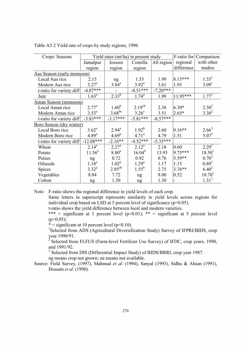
270

Table A5.2 Yield rate of crops by study regions, 1996.

Crops/ Seasons Yield rates (mt/ha) in present study F-ratio for

regional

difference

Comparison

with other

studies Jamalpur

region

Jessore

region

Comilla

region

All region

Aus Season (early monsoon)

Local Aus rice 2.15 ng 1.53 1.99 8.13*** 1.551

Modern Aus rice 3.27a 3.84a 3.92a 3.61 1.93 3.091

t-ratio for variety diff -4.87*** - -8.51*** -7.20***

Jute 1.63a 2.33

b 1.74

a 1.99 11.95*** 1.77

1

Aman Season (monsoon)

Local Aman rice

Modern Aman rice

2.77a

3.53a

1.60b

3.68bc

2.19cb

3.26c

2.38

3.51

6.30*

2.65*

2.302

3.302

t-ratio for variety diff -3.83*** -3.17*** -5.81*** -8.57***

Boro Season (dry winter)

Local Boro rice

Modern Boro rice

3.62a

4.89a

2.94a

4.69a

1.92b

4.71a

2.60

4.79

9.16**

1.51

2.663

5.073

t-ratio for variety diff -12.08*** -2.16** -4.52*** -5.35***

Wheat

Potato

Pulses

Oilseeds

Spices

Vegetables

Cotton

2.14a

11.56a

ng

1.18a

3.32a

8.84

ng

2.27a

8.80a

0.72

1.02a

2.85ab

7.72

1.30

2.12a

16.04b

0.92

1.29a

1.55b

ng

ng

2.18

13.93

0.76

1.17

2.75

8.00

1.30

0.60

9.75***

5.59**

1.15

3.76**

0.52

-

2.291

18.501

0.702

0.891

6.402

10.701

1.311

Note: F-ratio shows the regional difference in yield levels of each crop.

Same letters in superscript represents similarity in yield levels across regions for

individual crop based on LSD at 5 percent level of significance (p<0.05).

t-ratio shows the yield difference between local and modern varieties.

*** = significant at 1 percent level (p<0.01); ** = significant at 5 percent level

(p<0.05);

* = significant at 10 percent level (p<0.10). 1Selected from ADS (Agricultural Diversification Study) Survey of IFPRI/BIDS, crop

year 1990/91. 2

Selected from FLFUS (Farm-level Fertilizer Use Survey) of IFDC, crop years, 1990,

and 1991/92. 3 Selected from DIS (Differential Impact Study) of BIDS/BRRI, crop year 1987.

ng means crop not grown; na means not available.

Source: Field Survey, (1997), Mahmud et al. (1994), Sanyal (1993), Sidhu & Ahsan (1991),

Hossain et al. (1990).

271

Table A5.3 Chemical fertilizer use rates by study regions, 1996.

Crops/ Seasons Fertilizer use rates (kg/ha) in present study F-ratio for

regional

difference

Comparison

with other

studies Jamalpur

region

Jessore

region

Comilla

region

All region

Aus Season (early monsoon)

Local Aus rice 79 ng 91 82 0.09 851

Modern Aus rice 182a 252b 247ab 223 2.98* 2421

t-ratio for variety diff -3.61*** - -2.85*** -5.84***

Jute 132a 178

b 78

c 140 9.67*** 136

1

Aman Season (monsoon)

Local Aman rice

Modern Aman rice

145a

186a

62b

195a

59b

267b

94

204

9.30***

25.20***

762

1922

t-ratio for variety diff -2.78*** -3.41*** -11.92*** -10.14***

Boro Season (dry winter)

Local Boro rice

Modern Boro rice

230a

280a

239a

286a

39b

286a

137

283

7.75**

0.25

573

3203

t-ratio for variety diff -0.80 -0.74 -6.64*** -4.86***

Wheat

Potato

Pulses

Oilseeds

Spices

Vegetables

Cotton

218a

286a

ng

175a

301a

175

ng

225a

392ba

26

117a

223a

286

326

239a

387b

95

122a

230a

ng

ng

230

348

37

125

271

258

326

0.38

5.11***

10.32***

0.73

1.16

3.92**

-

2721

3271

551

2071

2231

1892

2351

Note: F-ratio shows the regional difference in fertilizer use levels of each crop.

Same letters in superscript represents similarity in fertilizer use levels across regions

for individual crop based on LSD at 5 percent level of significance (p<0.05).

t-ratio shows the difference in fertilizer use between local and modern varieties.

*** = significant at 1 percent level (p<0.01); ** = significant at 5 percent level

(p<0.05);

* = significant at 10 percent level (p<0.10). 1Selected from ADS (Agricultural Diversification Study) Survey of IFPRI/BIDS, crop

year 1990/91. 2

Selected from FLFUS (Farm-level Fertilizer Use Survey) of IFDC, crop years, 1990,

and 1991/92. 3 Selected from DIS (Differential Impact Study) of BIDS/BRRI, crop year 1987.

ng means crop not grown; na means not available.

Source: Field Survey, (1997), Mahmud et al. (1994), Sanyal (1993), Sidhu & Ahsan

(1991), Hossain et al. (1990).

272

Table A5.4 Average cost and profitability of crop production (all regions), 1996.

Crops/season Weights1

Yield

(ton/ha)

Price

(Tk/ton)

Gross value

(Tk/ha)

Variable

cost

(Tk/ha)

Profits

(Tk/ha)

Aus Season (early monsoon)

Local Aus rice 0.013 1.99 5,225 11,360 7,435 3,925

Modern Aus rice 0.029 3.61 5,637 21,443 9,170 12,273

t-ratio for variety diff -7.20*** -4.18*** -7.17*** -2.79*** -6.26***

Jute 0.047 1.99 9,395 20,539 9,089 11,450

Aman Season (monsoon)

Local Aman rice

Modern Aman rice

0.075

0.318

2.38

3.51

5,605

5,603

14,785

20,679

7,118

9,369

7,667

11,310

t-ratio for variety diff -8.57*** 0.02 -7.20*** -6.31*** -4.54***

Boro Season (dry winter)

Local Boro rice

Modern Boro rice

0.004

0.353

2.60

4.79

4,500

5,665

12,872

28,647

9,505

14,490

3,367

14,157

t-ratio for variety diff -5.35*** -7.05*** -5.57*** -4.44*** -3.87***

Wheat

Potato

Pulses

Oilseeds

Spices

Vegetables

Cotton

0.046

0.017

0.038

0.031

0.008

0.013

0.008

2.18

13.93

0.76

1.17

2.75

8.00

1.30

7,984

3,790

19,559

13,058

25,202

6,120

23,546

18,082

51,708

14,650

14,535

46,620

42,970

30,139

10,292

24,718

6,138

7,431

17,400

13,203

11,720

7,790

26,990

8,512

7,104

29,220

29,767

18,419

Note: t-ratio shows the difference in fertilizer use between local and modern varieties.

*** = significant at 1 percent level (p<0.01) 1

Weights as percent of gross cropped area.

Source: Field Survey, 1997.

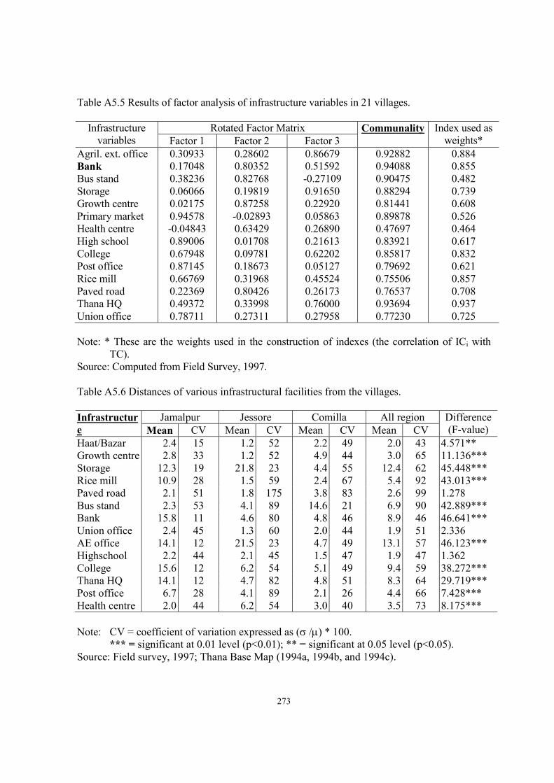
273

Table A5.5 Results of factor analysis of infrastructure variables in 21 villages.

Infrastructure

variables

Rotated Factor Matrix Communality Index used as

weights* Factor 1 Factor 2 Factor 3

Agril. ext. office

Bank

Bus stand

Storage

Growth centre

Primary market

Health centre

High school

College

Post office

Rice mill

Paved road

Thana HQ

Union office

0.30933

0.17048

0.38236

0.06066

0.02175

0.94578

-0.04843

0.89006

0.67948

0.87145

0.66769

0.22369

0.49372

0.78711

0.28602

0.80352

0.82768

0.19819

0.87258

-0.02893

0.63429

0.01708

0.09781

0.18673

0.31968

0.80426

0.33998

0.27311

0.86679

0.51592

-0.27109

0.91650

0.22920

0.05863

0.26890

0.21613

0.62202

0.05127

0.45524

0.26173

0.76000

0.27958

0.92882

0.94088

0.90475

0.88294

0.81441

0.89878

0.47697

0.83921

0.85817

0.79692

0.75506

0.76537

0.93694

0.77230

0.884

0.855

0.482

0.739

0.608

0.526

0.464

0.617

0.832

0.621

0.857

0.708

0.937

0.725

Note: * These are the weights used in the construction of indexes (the correlation of ICi with

TC).

Source: Computed from Field Survey, 1997.

Table A5.6 Distances of various infrastructural facilities from the villages.

Infrastructur

e

Jamalpur Jessore Comilla All region Difference

(F-value) Mean CV Mean CV Mean CV Mean CV

Haat/Bazar 2.4 15 1.2 52 2.2 49 2.0 43 4.571**

Growth centre 2.8 33 1.2 52 4.9 44 3.0 65 11.136***

Storage 12.3 19 21.8 23 4.4 55 12.4 62 45.448***

Rice mill 10.9 28 1.5 59 2.4 67 5.4 92 43.013***

Paved road 2.1 51 1.8 175 3.8 83 2.6 99 1.278

Bus stand 2.3 53 4.1 89 14.6 21 6.9 90 42.889***

Bank 15.8 11 4.6 80 4.8 46 8.9 46 46.641***

Union office 2.4 45 1.3 60 2.0 44 1.9 51 2.336

AE office 14.1 12 21.5 23 4.7 49 13.1 57 46.123***

Highschool 2.2 44 2.1 45 1.5 47 1.9 47 1.362

College 15.6 12 6.2 54 5.1 49 9.4 59 38.272***

Thana HQ 14.1 12 4.7 82 4.8 51 8.3 64 29.719***

Post office 6.7 28 4.1 89 2.1 26 4.4 66 7.428***

Health centre 2.0 44 6.2 54 3.0 40 3.5 73 8.175***

Note: CV = coefficient of variation expressed as (σ /µ) * 100.

*** = significant at 0.01 level (p<0.01); ** = significant at 0.05 level (p<0.05).

Source: Field survey, 1997; Thana Base Map (1994a, 1994b, and 1994c).

274

Table A5.7 Multiple comparison of infrastructural status among regions.

Infrastructural

variable Mean difference of distance among regions Homogenous regions

Jamalpur vs.

Jesssore

Jamalpur vs.

Comilla

Jessore vs.

Comilla

Haat/Bazar 1.13*** 0.14 0.99** Jamalpur, Comilla

Growth centre 1.61** 2.03*** 3.64*** None

Storage 9.55*** 7.93*** 17.48*** None

Rice mill 9.47*** 8.58*** 0.89 Jessore, Comilla

Paved road 0.36 1.69 2.05 Jessore, Jamalpur, Comilla

Bus stand 1.80 12.28*** 10.49*** Jamalpur, Jessore

Bank 11.20*** 11.00*** 0.20 Jessore, Comilla

Union HQ 1.09** 0.40 0.69 Jessore, Comilla, Jamalpur

Ag. Ext. office 7.38*** 9.41*** 16.79*** None

Highschool 0.13 0.73 0.60 Comilla, Jessore, Jamalpur

College 9.43*** 10.53*** 1.10 Jessore, Comilla

Thana HQ 9.41*** 9.34*** 0.07 Jessore, Comilla

Post office 2.58** 4.52*** 1.94 Comilla, Jessore

Health centre 4.19*** 1.07 3.12*** Jamalpur, Comilla

Note: *** = significant at 0.01 level (p<0.01); ** = significant at 0.05 level (p<0.05).

Source: Field survey, 1997.

Table A5.8 Multiple comparison of soil fertility status among regions (n = 15).

Soil variable Absolute mean difference among regions LSD

limits

Homogenous

regions Jamalpur

vs. Jessore

Jamalpur vs.

Comilla

Jessore vs.

Comilla

pH 1.80*** 1.20*** 0.60 0.63 Com, Jes

OM (%) 4.97*** 0.57 5.04*** 2.36 Com, Jam

N (µg/g) 3.06 9.52 6.47 10.33 Jam, Jes, Com

P (µg/g) 4.35 6.31 1.95 13.65 Jam, Jes, Com

K (µg/g) 20.20 11.95 32.15*** 17.83 Jam, Com

S (µg/g) 2.42 2.27 4.69*** 3.21 Com, Jam, Jes

Zn (µg/g) 2.54 0.97 3.51 4.55 Jam, Jes, Com

Sand (%) 11.21*** 16.49*** 5.28 6.45 Com, Jes

Silt (%) 5.52 17.22*** 22.74*** 2.57 Jes, Jam

Clay (%) 16.73*** 0.71 17.44** 13.05 Com, Jam

CEC (meq/100g) 15.32*** 4.94 10.38** 8.26 Jam, Com

EC (µS/cm) 101.20*** 37.50 63.70** 44.06 Jam, Com

Note: LSD = least significant difference beyond which the difference becomes significant.

*** = significant at 0.01 level (p<0.01); ** = significant at 0.05 level (p<0.05).

Source: Field survey, 1997.

275

276

Table A5.9 Probit reduced-form seed selection equation, 1996.

Exogenous

variables

Estimated

coefficients

t-ratio Exogenous

variables

Estimated

coefficients

t-ratio

Intercept

LnPW’

LnPF’

LnPM’

½( lnPW’)2

½( lnPF’)2

½( lnPM’)2

lnPW’ lnPF’

lnPW’ lnPM’

lnPF’ lnPM’

-17.7050

-8.5263

-4.4114

3.5154

6.2869

6.8804

-1.2978

-2.5905

-0.4248

1.4068

-1.422

-1.293

-0.820

0.608

1.759*

2.962***

-0.672

-1.318

-0.212

0.895

lnPM’ lnZL

lnPM’ lnZA

lnPM’ lnZI

lnPM’ lnZS

lnPM’ lnZE

½( lnZL)2

½( lnZA)2

½( lnZI)2

½( lnZS)2

½( lnZE)2

0.0267

-0.1716

0.1140

3.3306

-0.2586

-0.1408

-0.0067

-1.1513

44.0430

-0.6606

0.072

-0.911

0.121

0.879

-0.793

-1.123

-0.170

-1.170

2.662***

-2.521***

lnZL

lnZA

lnZI

lnZS

lnZE

-4.0914

0.6740

7.5144

13.5530

1.0407

-3.204***

1.128

1.495

0.856

1.020

lnZL lnZA

lnZL lnZI

lnZL lnZS

lnZL lnZE

lnZA lnZI

0.0565

0.4047

-0.7964

0.0587

-0.1794

1.209

2.008**

-1.017

0.789

-1.758*

lnPW’ lnZL

lnPW’ lnZA

lnPW’ lnZI

lnPW’ lnZS

lnPW’ lnZE

1.1127

0.1529

0.6633

-11.4820

0.3981

2.316**

0.621

0.541

-2.362**

1.036

lnZA lnZS

lnZA lnZE

lnZI lnZS

lnZI lnZE

lnZS lnZE

0.3047

0.0182

1.3684

-0.0034

-0.1750

0.746

0.455

-2.754***

0.434

-2.449***

lnPF’ lnZL

lnPF’ lnZA

lnPF’ lnZI

lnPF’ lnZS

lnPF’ lnZE

0.4712

-0.3063

0.7510

12.8230

-0.1446

1.440

-1.794*

0.897

3.232***

-0.517

Accuracy of prediction = 88.85 percent

McFadden R2(1-log Lmax/logL0) = 0.233

Chi-squared (χ244 degrees of freedom) = 171.088***

Note: W = labor price, F = fertilizer price, M = animal power price, L = land area, A = farm

capital, I = infrastructure, S = soil quality, E = education of farmer.

*** = significant at 1 percent level (p<0.01); ** = significant at 5 percent level

(p<0.05);

* = significant at 10 percent level (p<0.10).

Source: Computed.

277

Table A5.10 Joint estimation of the normalized profit function and factor share equations for

variable input demands for producing local and modern foodgrain varieties, adjusted

for selectivity bias, 1996.

Exogenous

variables

Para-

meters

Modern foodgrain varieties Local foodgrain varieties

Estimated coefficients t-ratio Estimated coefficients t-ratio

Profit function

Intercept α0 -6.3292 -2.678*** -7.3747 -1.645*

lnPW’ αW 1.9807 5.307*** 2.8191 3.022***

lnPF’ αF 0.2791 1.794* 0.9273 2.716***

lnPM’ αM 0.5181 3.025*** 1.9758 3.564***

½( lnPW’)2 γWW -0.7930 -10.236*** -0.8095 -2.832***

½( lnPF’)2 γFF -0.1653 -6.488*** -0.2083 -1.936**

½( lnPM’)2 γMM -0.1103 -4.889*** -0.3836 -3.501***

lnPW’ lnPF’ γWF -0.1834 -5.677*** -0.0775 -0.697

lnPW’ lnPM’ γWM -0.2852 -8.210*** -0.6456 -4.675***

lnPF’ lnPM’ γFM -0.0408 -2.162** -0.1422 -1.818*

lnZL βL 0.0378 0.132 -0.4385 -0.997

lnZA βA 0.1137 0.829 0.9776 4.531***

lnZI βI 5.6247 5.905*** 1.8110 0.751

lnZS βS 3.1164 1.181 10.047 1.849*

lnZE βE 0.1252 0.553 -0.3058 -0.888

lnPW’ lnZL δWL 0.1387 4.062*** 0.3059 3.738***

lnPW’ lnZA δWA 0.0506 3.299*** -0.0087 -0.193

lnPW’ lnZI δWI -0.2047 -3.008*** 0.0525 0.285

lnPW’ lnZS δWS 0.8259 3.098*** 0.2850 0.342

lnPW’ lnZE δWE -0.0568 -2.068** -0.1178 -1.841*

lnPF’ lnZL δFL -0.0025 -0.178 0.0263 0.965

lnPF’ lnZA δFA 0.0161 2.531*** 0.0158 1.039

lnPF’ lnZI δFI -0.0540 -1.936** -0.1487 -2.269**

lnPF’ lnZS δFS 0.1699 1.568 -0.2097 -0.781

lnPF’ lnZE δFE -0.0238 -2.092** -0.0241 -1.066

lnPM’ lnZL δML 0.0210 1.347 0.0116 0.250

lnPM’ lnZA δMA 0.0251 3.555*** -0.0351 -1.336

lnPM’ lnZI δMI -0.0493 -1.578 -0.0648 -0.607

lnPM’ lnZS δMS 0.2504 2.058** 0.8684 1.828*

lnPM’ lnZE δME -0.0356 -2.823*** -0.0406 -1.093

½( lnZL)2 ψLL -0.1143 -3.293*** 0.0450 0.908

½( lnZA)2 ψAA 0.0077 0.759 -0.0851 -4.754***

½( lnZI)2 ψII -1.0934 -5.480*** 0.4010 0.754

½( lnZS)2 ψSS 4.6332 1.327 -4.6120 -0.572

½( lnZE)2 ψEE -0.0325 -0.501 -0.2431 -1.867*

(continued)

278

Exogenous

variables

Para-

meters

Modern foodgrain varieties Local foodgrain varieties

Estimated coefficients t-ratio Estimated coefficients t-ratio

Profit function

lnZL lnZA ωLA 0.0021 0.185 0.0057 0.256

lnZL lnZI ωLI 0.0928 1.862* 0.4382 4.047***

lnZL lnZS ωLS 0.3202 1.808* -1.2915 -3.080***

lnZL lnZE ωLE 0.0429 2.227** 0.0095 0.283

lnZA lnZI ωAI -0.0582 -2.764*** -0.0845 -1.318

lnZA lnZS ωAS -0.2008 -2.340** -0.0317 -0.119

lnZA lnZE ωAE -0.1211 -1.288 0.0664 3.451***

lnZI lnZS ωIS -1.4070 -2.707*** -3.2802 -2.892***

lnZI lnZE ωIE 0.0618 1.524 0.1303 1.707*

lnZS lnZE ωSE 0.0477 0.315 -0.4397 -1.313

Selectivity

variable σ1u, σ2u 0.4873 3.858*** 0.0105 0.075

Labor share equation

Intercept αW 1.9807 5.307*** 2.8191 3.022***

lnPW’ γWW -0.7930 -10.236*** -0.8095 -2.832***

lnPF’ γWF -0.1834 -5.677*** -0.0775 -0.697

lnPM’ γWM -0.2852 -8.210*** -0.6546 -4.675***

lnZL δWL 0.1387 4.062*** 0.3059 3.738***

lnZA δWA 0.0506 3.299*** -0.0087 -0.193

lnZI δWI -0.2047 -3.008*** 0.0525 0.285

lnZS δWS 0.8259 3.098*** 0.2850 0.342

lnZE δWE -0.0568 -2.068** -0.1178 -1.841*

Fertilizer share equation

Intercept αF 0.2791 1.794* 0.9273 2.716***

lnPW’ γFW -0.1834 -5.677*** -0.0775 -0.697

lnPF’ γFF -0.1653 -6.488*** -0.2083 -1.936**

lnPM’ γFM -0.0408 -2.162** -0.1422 -1.818*

lnZL δFL -0.0025 -0.178 0.0262 0.965

lnZA δFA 0.0161 2.531*** 0.0158 1.039

lnZI δFI -0.0540 -1.936** -0.1487 -2.269**

lnZS δFS 0.1699 1.568 -0.2097 -0.781

lnZE δFE -0.0238 -2.092** -0.0241 -1.066

Animal power share equation

Intercept αM 0.5181 3.025*** 1.9758 3.564***

lnPW’ γMW -0.2852 -8.210*** -0.6456 -4.675***

lnPF’ γMF -0.0408 -2.162** -0.1422 -1.818*

lnPM’ γMM -0.1103 -4.889*** -0.3836 -3.501***

lnZL δML 0.0210 1.347 0.0116 0.250

lnZA δMA 0.0251 3.555*** -0.0351 -1.336

(continued)

279

Exogenous

variables

Para-

meters

Modern foodgrain varieties Local foodgrain varieties

Estimated coefficients t-ratio Estimated coefficients t-ratio

lnZI δMI -0.0493 -1.578 -0.0648 -0.607

lnZS δMS 0.2504 2.058** 0.8684 1.828*

lnZE δME -0.0356 -2.823*** -0.0406 -1.093

Adjusted R-squared = 0.638 0.426

Wald test: χ2(27 degrees of freedom) = 161.559*** 79.451***

Number of observations (n) = 932 117

Selectivity variable = -ƒ(φi)/F(φi) ƒ(φi)/[1-F(φi)]

Note: W = labor price, F = fertilizer price, M = animal power price, L = land area, A = farm

capital, I = infrastructure, S = soil quality, E = education of farmer.

*** = significant at 1 percent level (p<0.01); ** = significant at 5 percent level

(p<0.05);

* = significant at 10 percent level (p<0.10).

Source: Computed.

280

Table A5.11 Input demand and output supply elasticities of foodgrain crops, 1996.

Output

price

Labor

price

Fertilizer

price

Animal

price

Land Farm

capital

Infra-

structure

Soil

quality

Educa-

tion

Local rice varieties (all seasons)

Output

supply

0.8388 -0.3014 -0.0169 -0.1269 0.6611 0.8311 1.5243 14.8540 -0.8919

Labor

demand

2.1157 -1.1494 -0.0633 0.0970 0.4763 0.8295 1.4106 14.2107 -0.8394

Fertilizer

demand

0.6821 -0.4341 -0.3181 0.4339 0.6052 0.7099 2.5073 15.9724 -0.7908

Animal

demand

1.6044 0.1683 0.1098 -0.8825 0.7686 0.8829 1.5793 12.9609 -0.8841

Modern rice and wheat varieties (all seasons)

Output

supply

0.4745 -0.0743 -0.0551 -0.1129 0.5734 0.4028 4.6760 7.0859 -0.2363

Labor

demand

0.2510 -0.4282 0.0498 0.1274 0.4391 0.3668 4.8509 6.3821 -0.2018

Fertilizer

demand

0.5196 0.1389 -0.5222 -0.1389 0.6634 0.3831 4.7678 6.9235 -0.1871

Animal

demand

0.7944 0.2654 -0.1018 -0.9581 0.5852 0.3643 4.6936 6.8509 -0.1750

Total elasticity of demand and supply of foodgrain without variety switching adjustments

Output

supply

0.4977 -0.0797 -0.0569 -0.1177 0.5978 0.4238 4.8342 7.4580 -0.2529

Labor

demand

0.2819 -0.4475 0.0493 0.1298 0.4494 0.3812 4.9122 6.6305 -.02149

Fertilizer

demand

0.5594 0.1465 -0.5603 -0.1465 0.7129 0.4135 5.1144 7.4889 -0.2042

Animal

demand

0.8174 0.2676 -0.1002 -0.9700 0.5960 0.3770 4.7113 7.0361 -0.1880

Note: Figures in parentheses represents percent of improvement due to variety switching

adjustments.

Source: Computed.

281

Table A5.12 Estimation of the normalized profit function and factor share equations for

variable input for non-cereal crops, 1996.

Exogenous

variables

Para-

meter

Estimated

coefficients

t-ratio Exogenous

variables

Para-

meters

Estimated

coefficients

t-ratio

Profit function lnZL lnZS ωLS 0.0832 0.206

Intercept α0 6.1547 1.874* lnZL lnZE ωLE 0.0603 1.495

lnPW’ αW 1.0965 3.176*** lnZA lnZI ωAI 0.0286 0.653

lnPF’ αF 0.1175 0.887 lnZA lnZS ωAS -0.2931 -1.508

lnPM’ αM -0.1355 -0.687 lnZA lnZE ωAE -0.0189 -0.857

½( lnPW’)2 γWW -0.1715 -1.761* lnZI lnZS ωIS -1.0156 -1.276

½( lnPF’)2 γFF -0.0853 -2.208** lnZI lnZE ωIE 0.0743 0.960

½( lnPM’)2 γMM -0.0709 -1.265 lnZS lnZE ωSE -0.3161 -1.026

lnPW’ lnPF’ γWF 0.1889 4.007*** Labor share equation

lnPW’ lnPM’ γWM 0.1742 2.745*** Intercept αW 1.0965 3.176***

lnPF’ lnPM’ γFM -0.0838 -2.415** lnPW’ γWW -0.1715 -1.761*

lnZL βL 0.4858 1.208 lnPF’ γWF 0.1889 4.007***

lnZA βA -0.1638 -0.784 lnPM’ γWM 0.1742 2.745***

lnZI βI -0.2778 -0.170 lnZL δWL -0.0030 -0.072

lnZS βS 0.0364 0.007 lnZA δWA 0.0050 0.242

lnZE βE 0.3087 0.862 lnZI δWI -0.2052 -2.493**

lnPW’ lnZL δWL -0.0030 -0.072 lnZS δWS 0.3276 0.997

lnPW’ lnZA δWA 0.0050 0.242 lnZE δWE 0.0120 0.339

lnPW’ lnZI δWI -0.2052 -2.493*** Fertilizer share equation

lnPW’ lnZS δWS 0.3276 0.997 Intercept αF 0.1175 0.887

lnPW’ lnZE δWE 0.0120 0.339 lnPW’ γFW 0.1889 4.007***

lnPF’ lnZL δFL -0.0331 -2.356** lnPF’ γFF -0.0853 -2.208**

lnPF’ lnZA δFA 0.0090 1.269 lnPM’ γFM -0.0838 -2.415**

lnPF’ lnZI δFI -0.0821 -2.791*** lnZL δFL -0.0331 -2.356**

lnPF’ lnZS δFS 0.0440 0.386 lnZA δFA 0.0090 1.269

lnPF’ lnZE δFE -0.0174 -1.424 lnZI δFI -0.0821 -2.791***

lnPM’ lnZL δML -0.0490 -2.393** lnZS δFS 0.0440 0.386

lnPM’ lnZA δMA 0.0158 1.520 lnZE δFE -0.0174 -1.424

lnPM’ lnZI δMI -0.0782 -1.813* Animal power share equation

lnPM’ lnZS δMS -0.1472 -0.889 Intercept αM -0.1355 -0.687

lnPM’ lnZE δME 0.0011 0.063 lnPW’ γMW 0.1742 2.745***

½( lnZL)2 ψLL 0.0907 1.542 lnPF’ γMF -0.0838 -2.415**

½( lnZA)2 ψAA 0.0331 1.604 lnPM’ γMM -0.0709 -1.265

½( lnZI)2 ψII 0.3582 0.790 lnZL δML -0.0490 -2.393**

½( lnZS)2 ψSS 10.4240 0.956 lnZA δMA 0.0158 1.520

½( lnZE)2 ψEE -0.1054 -0.926 lnZI δMI -0.0782 -1.813*

lnZL lnZA ωLA 0.0007 0.028 lnZS δMS -0.1472 -0.889

lnZL lnZI ωLI 0.1431 1.470 lnZE δME 0.0011 0.063

(continued)

282

Exogenous

variables

Para-

meter

Estimated

coefficients

t-ratio Exogenous

variables

Para-

meters

Estimated

coefficients

t-ratio

Adjusted R-squared = 0.378

Wald test: χ2(27 degrees of freedom) = 211.204***

Number of observations (n) = 399

Note: W = labor price, F = fertilizer price, M = animal power price, L = land area, A = farm

capital, I = infrastructure, S = soil quality, E = education of farmer.

*** = significant at 1 percent level (p<0.01); ** = significant at 5 percent level

(p<0.05);

* = significant at 10 percent level (p<0.10).

Source: Computed.

283

Table A6.1 Years of growing modern varieties of rice and wheat in the study regions, 1996.

Period of growing

modern varieties

Number and percent of farmers responding in the affirmative

Jamalpur region Jessore region Comilla region All region

Modern rice

Within five years

Between five to ten years

More than ten years

19 (10.9)

59 (33.7)

97 (55.4)

23 (21.9)

32 (30.5)

50 (47.6)

14 (11.1)

40 (31.7)

72 (57.2)

56 (13.8)

131 (32.3)

219 (53.9)

Modern wheat

Within five years

Between five to ten years

More than ten years

6 (3.4)

9 (5.1)

8 (4.6)

6 (5.7)

11 (10.5)

11 (10.5)

4 (3.2)

9 (7.1)

26 (20.6)

16 (3.9)

29 (7.1)

45 (11.1)

Total households 175 (100.0) 105 (100.0) 126 (100.0) 406 (100.0)

Note: Figures in parentheses are percentage of total households.

Source: Field Survey, 1997.

Table A6.2 Trend in productivity of modern varieties of rice and wheat, 1996.

Productivity level Number and percent of farmers responding in the affirmative

Jamalpur region Jessore region Comilla region All region

Increasing

Unchanged

Decreasing

104 (59.4)

57 (32.6)

14 (8.0)

64 (61.0)

31 (29.5)

10 (9.5)

15 (11.9)

72 (57.1)

39 (31.0)

183 (45.1)

160 (39.4)

63 (15.5)

Total households 175 (100.0) 105 (100.0) 126 (100.0) 406 (100.0)

Note: Figures in parentheses are percentages of total households.

Source: Field Survey, 1997.

Table A6.3. Distance of nearest agricultural extension office by study regions, 1996.

Distance of agricultural

extension office

Number and percent of households (%)

Jamalpur region Jessore region Comilla region All region

Less than one km 23 (13.1) 25 (23.8) 9 (7.1) 57 (14.0)

Between one to three km 8 (4.6) 28 (26.7) 97 (77.0) 133 (32.8)

Between three to five km 6 (3.4) 8 (7.6) 20 (15.9) 34 (8.4)

More than five km 138 (78.9) 44 (41.9) - 182 (44.8)

Total households 175 (100.0) 105 (100.0) 126 (100.0) 406 (100.0)

Note: Figures in parentheses are percentages of total households.

Source: Field Survey, 1997.

284

Table A7.1 Labor force participation by study region, 1996.

Landownership

categories /

region

Average

family

member

Average

working

members

Participation

rate in economic

activity

Male worker

as proportion

of family size

Female worker

as proportion

of family size

(persons) (persons) (percent) (percent) (percent)

Jamalpur region 5.27 1.88 38.49 25.81 12.68

Landless 4.60 1.56 36.44 24.54 11.90

Marginal 5.00 1.94 40.63 27.15 13.48

Small 4.78 1.74 40.76 27.73 13.03

Medium 6.86 2.24 34.99 24.08 10.90

Large 7.33 2.75 42.02 24.97 17.05

Jessore region 6.24 2.47 40.78 29.44 11.34

Landless 5.63 2.17 38.10 28.67 9.43

Marginal 4.86 1.86 42.25 33.07 9.18

Small 6.00 2.00 37.24 26.69 10.56

Medium 7.25 2.94 43.05 29.25 13.80

Large 8.87 4.07 46.44 29.09 17.35

Comilla region 6.90 1.88 29.31 27.88 1.43

Landless 6.51 1.60 27.05 24.59 2.46

Marginal 6.13 1.75 32.00 29.91 2.08

Small 7.73 2.14 28.78 28.78 1.00

Medium 7.64 2.36 31.51 30.96 0.50

Large na na na na na

All region 6.02 2.03 36.23 27.39 8.84

Landless 5.49 1.74 33.87 25.67 8.20

Marginal 5.37 1.86 37.92 29.61 8.32

Small 6.08 1.94 35.56 27.96 7.59

Medium 7.15 2.46 36.35 27.12 9.23

Large 8.19 3.48 41.48 27.26 17.21

Note: na means not applicable.

Source: Field Survey, 1997.

285

Table A7.2 Women labor input by agricultural operations, crop year 1989 (all regions).

Crops/Seasons Agricultural operations (% of total women’s labor input)

Land

prepara

tion

Sowing/

transp

Lanting

Weed-

ing

Irriga-

tion

Fertili-

zing

Harvest-

ing

Thresh-

ing

All

opera-

tions

Aus season (early monsoon)

Local Aus rice - - 5.6 - - 5.6 88.8 100

Modern Aus rice - - - - 5.0 5.0 90.0 100

Jute 7.2 - 7.2 - - 7.1 78.5 100

Aman Season (monsoon)

Local Aman rice - - - - - 5.6 94.4 100

Modern Aman rice - - - - - 5.9 94.1 100

Boro Season (dry winter)

Local Boro rice - 4.4 - 4.4 - 4.3 86.9 100

Modern Boro rice - 4.0 4.0 4.0 - 4.0 84.0 100

Local wheat - - - 3.8 - 7.7 88.5 100

Modern wheat - - - - - 5.0 95.0 100

Potato 7.0 7.0 2.3 23.3 - 34.9 25.5 100

Pulses - - - - - 10.0 90.0 100

Oilseeds - - - - - 17.4 82.6 100

Spices 8.3 8.3 6.7 3.3 - 26.7 46.7 100

Vegetables 9.8 7.2 2.4 39.1 2.4 34.1 4.9 100

Cotton 7.6 - - - - 70.9 21.5 100

Note: Figures in parentheses are percentages

Source: BRAC-VSP Survey, 1990.

286

Table A7.3 Determinants of labor use in crop production, 1996.

Variables Present study

(Crop year 1996)

Comparison

(BIDS, Crop year 1982)

Demand for hired labor Demand for

total labor

Hired labor Total labor

OLS estimate Tobit estimate OLS estimate Tobit

Estimate

OLS

Estimate

Intercept 162.780

(7.537)***

170.900

(7.453)***

155.420

(6.941)***

56.2

(2.16)**

214.7

(8.70)***

AMLND 35.253

(8.409)***

35.981

(8.153)***

57.668

(13.267)***

9.4

(36.2)***

11.1

(10.88)***

MVAR 29.231

(5.415)***

29.694

(5.226)***

16.000

(2.859)***

29.5

(17.40)***

46.9

(17.68)***

TNC -15.560

(-2.206)**

-14.502

(-1.790)*

29.185

(3.666)***

-2.9

(-1.21)

14.6

(4.19)***

WAGE -1.007

(-4.037)***

-1.065

(-4.035)***

-1.502

(-5.809)***

-2.81

(-2.62)***

-9.20

(-9.63)***

INFRA -0.197

(-1.594)

-0.238

(-1.818)*

0.267

(2.088)**

-0.96

(-0.66)

-1.56

(1.22)

SOIL -54.030

(-5.852)***

-57.608

(-5.860)***

-41.744

(-4.361)***

na na

SUBP -2.646

(-2.313)**

-3.027

(-2.481)***

-2.794

(-2.356)**

na na

WORK -5.780

(-2.553)***

-6.083

(-2.541)***

-0.248

(-0.106)

-3.10

(0.84)

17.78

(4.08)***

WORKW 1.218

(0.357)

1.575

(0.436)

-3.717

(-1.050)

-8.14

(0.60)

-24.77

(-2.26)***

EDUCH 0.942

(2.173)**

1.096

(2.388)***

0.541

(1.204)

5.37

(4.64)***

3.30

(2.97)***

Adjusted R-

squared

0.73 - 0.80 na 0.65

F-value

(10, 395)

111.43*** - 163.36*** na 107.4***

Log

likelihood

- -1886.42 - na -

Note: *** = significant at 1 percent level (p<0.01); ** = significant at 5 percent level

(p<0.05);

* = significant at 10 percent level (p<0.10).

na means not available.

Comparison data is selected from Ahmed and Hossain (1990).

Source: Computed.

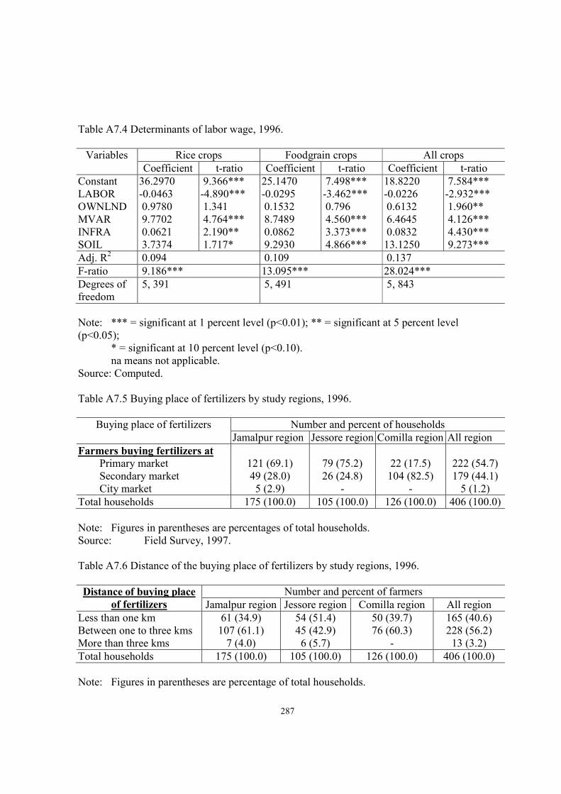
287

Table A7.4 Determinants of labor wage, 1996.

Variables Rice crops Foodgrain crops All crops

Coefficient t-ratio Coefficient t-ratio Coefficient t-ratio

Constant 36.2970 9.366*** 25.1470 7.498*** 18.8220 7.584***

LABOR -0.0463 -4.890*** -0.0295 -3.462*** -0.0226 -2.932***

OWNLND 0.9780 1.341 0.1532 0.796 0.6132 1.960**

MVAR 9.7702 4.764*** 8.7489 4.560*** 6.4645 4.126***

INFRA 0.0621 2.190** 0.0862 3.373*** 0.0832 4.430***

SOIL 3.7374 1.717* 9.2930 4.866*** 13.1250 9.273***

Adj. R2

0.094 0.109 0.137

F-ratio 9.186*** 13.095*** 28.024***

Degrees of

freedom

5, 391 5, 491 5, 843

Note: *** = significant at 1 percent level (p<0.01); ** = significant at 5 percent level

(p<0.05);

* = significant at 10 percent level (p<0.10).

na means not applicable.

Source: Computed.

Table A7.5 Buying place of fertilizers by study regions, 1996.

Buying place of fertilizers Number and percent of households

Jamalpur region Jessore region Comilla region All region

Farmers buying fertilizers at

Primary market 121 (69.1) 79 (75.2) 22 (17.5) 222 (54.7)

Secondary market 49 (28.0) 26 (24.8) 104 (82.5) 179 (44.1)

City market 5 (2.9) - - 5 (1.2)

Total households 175 (100.0) 105 (100.0) 126 (100.0) 406 (100.0)

Note: Figures in parentheses are percentages of total households.

Source: Field Survey, 1997.

Table A7.6 Distance of the buying place of fertilizers by study regions, 1996.

Distance of buying place

of fertilizers

Number and percent of farmers

Jamalpur region Jessore region Comilla region All region

Less than one km

Between one to three kms

More than three kms

61 (34.9)

107 (61.1)

7 (4.0)

54 (51.4)

45 (42.9)

6 (5.7)

50 (39.7)

76 (60.3)

-

165 (40.6)

228 (56.2)

13 (3.2)

Total households 175 (100.0) 105 (100.0) 126 (100.0) 406 (100.0)

Note: Figures in parentheses are percentage of total households.

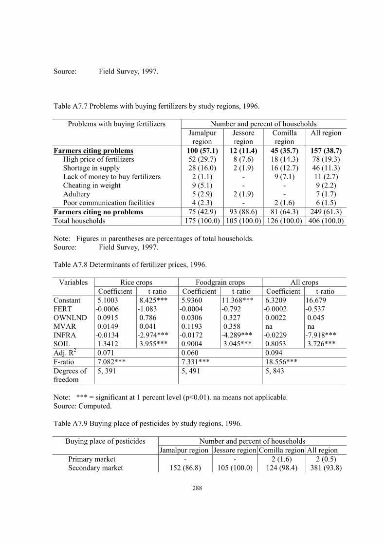
288

Source: Field Survey, 1997.

Table A7.7 Problems with buying fertilizers by study regions, 1996.

Problems with buying fertilizers Number and percent of households

Jamalpur

region

Jessore

region

Comilla

region

All region

Farmers citing problems 100 (57.1) 12 (11.4) 45 (35.7) 157 (38.7)

High price of fertilizers 52 (29.7) 8 (7.6) 18 (14.3) 78 (19.3)

Shortage in supply 28 (16.0) 2 (1.9) 16 (12.7) 46 (11.3)

Lack of money to buy fertilizers 2 (1.1) - 9 (7.1) 11 (2.7)

Cheating in weight 9 (5.1) - - 9 (2.2)

Adultery 5 (2.9) 2 (1.9) - 7 (1.7)

Poor communication facilities 4 (2.3) - 2 (1.6) 6 (1.5)

Farmers citing no problems 75 (42.9) 93 (88.6) 81 (64.3) 249 (61.3)

Total households 175 (100.0) 105 (100.0) 126 (100.0) 406 (100.0)

Note: Figures in parentheses are percentages of total households.

Source: Field Survey, 1997.

Table A7.8 Determinants of fertilizer prices, 1996.

Variables Rice crops Foodgrain crops All crops

Coefficient t-ratio Coefficient t-ratio Coefficient t-ratio

Constant 5.1003 8.425*** 5.9360 11.368*** 6.3209 16.679

FERT -0.0006 -1.083 -0.0004 -0.792 -0.0002 -0.537

OWNLND 0.0915 0.786 0.0306 0.327 0.0022 0.045

MVAR 0.0149 0.041 0.1193 0.358 na na

INFRA -0.0134 -2.974*** -0.0172 -4.289*** -0.0229 -7.918***

SOIL 1.3412 3.955*** 0.9004 3.045*** 0.8053 3.726***

Adj. R2

0.071 0.060 0.094

F-ratio 7.082*** 7.331*** 18.556***

Degrees of

freedom

5, 391 5, 491 5, 843

Note: *** = significant at 1 percent level (p<0.01). na means not applicable.

Source: Computed.

Table A7.9 Buying place of pesticides by study regions, 1996.

Buying place of pesticides Number and percent of households

Jamalpur region Jessore region Comilla region All region

Primary market - - 2 (1.6) 2 (0.5)

Secondary market 152 (86.8) 105 (100.0) 124 (98.4) 381 (93.8)

289

City market 23 (13.1) - - 23 (5.7)

Total households 175 (100.0) 105 (100.0) 126 (100.0) 406 (100.0)

Note: Figures in parentheses are percentages of total households.

Source: Field Survey, 1997.

Table A7.10 Distance of the buying place of pesticides by study regions, 1996.

Distance of buying place

of pesticides

Number and percent of farmers (%)

Jamalpur region Jessore region Comilla region All region

Less than one km 66 (37.7) 32 (30.5) 70 (55.6) 168 (41.4)

Between one to three kms 81 (46.3) 69 (65.7) 56 (44.4) 206 (50.7)

More than three kms 28 (16.0) 4 (3.8) - 32 (7.9)

Total households 175 (100.0) 105 (100.0) 126 (100.0) 406 (100.0)

Note: Figures in parentheses are percentage of total households.

Source: Field Survey, 1997.

Table A7.11 Sufficiency of pesticide use by study regions.

Sufficiency of pesticide use Number and percent of households

Jamalpur

region

Jessore

region

Comilla

region

All region

Farmers considering that they use

enough

115 (65.7) 76 (72.4) 119 (94.4) 310 (76.4)

Farmers seeking to use more 60 (34.3) 29 (27.6) 7 (5.6) 96 (23.6)

Total households 175 (100.0) 105 (100.0) 126 (100.0) 406 (100.0)

Current mean level of pesticide use (Tk/ha) 240 404 633 405

Note: Figures in parentheses are percentages of total households.

Source: Field Survey, 1997.

Table A7.12 Problems with buying pesticides by study regions.

Problems with buying pesticides Number and percent of households (%)

Jamalpur

region

Jessore

region

Comilla

region

All region

Farmers citing problems 14 (8.0) 1 (1.0) 7 (5.6) 22 (5.4)

High price of pesticides 5 (2.9) 1 (1.0) 3 (2.4) 9 (2.2)

Shortage in supply 1 (0.6) - 1 (0.8) 2 (0.5)

Lack of money to buy pesticides 3 (1.6) - 3 (2.4) 6 (1.5)

Adultery 5 (2.9) - - 1 (0.2)

Farmers citing no problems 161 (92.0) 104 (99.0) 119 (94.4) 384 (94.6)

Total households 175 (100.0) 105 (100.0) 126 (100.0) 406 (100.0)

Note: Figures in parentheses are percentages of total households.

Source: Field Survey, 1997.

290

291

Table A7.13 Determinants of pesticide use, 1996.

Variables Rice crops Foodgrain crops Non-cereal crops All crops

Coeffi-

cient

Asymp.

t-ratio

Coeffi-

cient

Asymp.

t-ratio

Coeffi-

cient

Asympt.

t-ratio

Coeffi-

cient

Asympt.

t-ratio

Constant -187.68 -0.908 -292.34 -1.477 175.86 0.685 -126.80 -0.804

AMLND 134.440 5.223*** 178.69 6.736*** 224.21 1.447 237.24 9.910**

PMVAR 0.0744 0.189 0.2144 0.639 na na 0.1632 0.703

PIRRIG 297.52 3.998*** 82.128 1.311 199.81 3.309*** 145.77 3.422***

AGCR 8.9246 4.164*** 7.9109 3.583*** 2.6355 1.782* 3.6009 3.000***

INFRA 1.8824 1.338 3.7172 2.668*** 0.1059 0.051 2.9868 2.617***

SOIL 28.5200 0.252 31.046 0.278 -306.48 -2.032** -116.87 -1.315

Log-L -2176.482 -2297.146 -983.805 -3294.367

N 397 497 352 849

Note: *** = significant at 1 percent level (p<0.01); ** = significant at 5 percent level

(p<0.05)

* = significant at 10 percent level (p<0.10).

na means not applicable.

Source: Computed.

Table A7.14 Land purchase by types in the past five years by study region, 1996.

Land type, purchase value and present

value of land

Value (Tk) of land purchased

Jamalpur

region

Jessore

region

Comilla

region

All region

Land purchase by type (No. of

farmers)

40 (22.8) 20 (19.1) 14 (11.1) 74 (16.0)

Agricultural land 30 (17.1) 17 (16.2) 10 (7.9) 57 (14.0)

Homestead land 10 (5.7) 3 (2.9) 4 (3.2) 17 (4.2)

Purchase value of land (Tk/household)

Agricultural land 28,173 27,676 25,050 27,477

Homestead land 27,880 15,367 29,875 26,141

Present value of land purchased

(Tk/hh)

Agricultural land 37,580 43,588 36,050 39,104

Homestead land 34,750 26,733 35,000 33,394

Appreciation in land value (%)

Agricultural land 33.4 57.5 43.9 42.3

Homestead land 24.6 74.0 17.2 27.7

Total households 175 (100.0) 105 (100.0) 126 (100.0) 406 (100.0)

Note: Figures in parentheses are percentages of total households.

Source: Field Survey, 1997.

292

Table A7.15 Purpose of land purchase and source of finance by study region, 1996.

Purpose of land purchase and source of

finance

Number and percent of households (%)

Jamalpur

region

Jessore

region

Comilla

region

All region

Purpose of land purchase

For cultivation 27 (67.5) 16 (80.0) 10 (71.4) 53 (71.6)

For home construction 8 (20.0) 1 (5.0) 3 (21.4) 12 (16.2)

For family consumption 5 (12.5) - 1 (7.2) 6 (8.1)

For orchard - 3 (15.0) - 3 (4.1)

Source of finance

Own income (unspecified source) 13 (32.5) 10 (50.0) - 23 (31.1)

Agricultural income 14 (35.0) 5 (25.0) 3 (21.4) 22 (29.7)

Service income 3 (7.5) 1 (5.0) 7 (50.0) 11 (14.9)

Mortgaged land income 6 (15.0) 1 (5.0) 1 (7.2) 8 (10.8)

Business income 1 (2.5) 3 (15.0) 2 (14.2) 6 (8.1)

Loan from relatives 3 (7.5) - 1 (7.2) 4 (5.4)

Total land purchasing households 40 (100.0) 20 (100.0) 14 (100.0) 74 (100.0)

Note: Figures in parentheses are percentages of total households.

Source: Field Survey, 1997.

Table A7.16 Land sale by type, actual sale value and present value of land sold in the past five

years by study region, 1996.

Type, actual sale value and present

value of land sold

Value (Tk) of land sold

Jamalpur

region

Jessore

region

Comilla

region

All region

Land sale by type (No. of farmers) 33 (18.9) 17 (16.2) 13 (9.9) 63 (15.5)

Agricultural land 28 (16.0) 16 (15.2) 13 (9.9) 57 (14.0)

Homestead land 5 (2.9) 1 (1.0) - 6 (1.5)

Sale value of land sold (Tk/household)

Agricultural land 26,857 28,750 30,053 28,118

Homestead land 26,200 4,800 - 22,633

Present value of land sold (Tk/hh)

Agricultural land 29,886 30,687 34,285 29,991

Homestead land 44,640 9,000 - 38,700

Appreciation in land value (%)

Agricultural land 11.3 6.7 14.1 6.7

Homestead land 70.4 87.5 - 70.1

Total households 175 (100.0) 105 (100.0) 126 (100.0) 406 (100.0)

293

Note: Figures in parentheses are percentages of total households.

Source: Field Survey, 1997.

Table A7.17 Reason for land sale by study region, 1996.

Reason for land sale and purpose of use

of the sale proceeds

Number and percent of households (%)

Jamalpur

region

Jessore

region

Comilla

region

All region

For daughter’s marriage 3 (9.1) 3 (17.6) 4 (30.8) 10 (15.9)

For debt service/release mortgage land 4 (12.1) 4 (23.5) 1 (7.7) 9 (14.3)

To go abroad for job 2 (6.1) 1 (5.9) 6 (46.1) 9 (14.3)

For family consumption 6 (18.2) 1 (5.9) 1 (7.7) 8 (12.7)

To buy better land 3 (9.1) - 1 (7.7) 4 (6.3)

For treatment 3 (9.1) - - 3 (4.8)

For education 1 (3.0) - - 1 (1.6)

No reason/ non-response 11 (33.3) 8 (47.1) - 19 (30.1)

Total land selling households 33 (100.0) 17 (100.0) 13 (100.0) 63 (100.0)

Note: Figures in parentheses are percentages of total households.

Source: Field Survey, 1997.

Table A7.18 Common land rental arrangements in the study villages, 1996.

Region Villages Input sharing arrangements (%) Output

sharing (%) Animal cost

share

Fertilizer

cost share

Irrigation

cost share

Seed cost

share

Jamalpur Karanipara

Rupshi

Munshipara

Deuliabari

Jaliarpar

Sapleja

Manikbari

Sonakata

50

nil

50

nil

50

nil

nil

50

50

nil

50

50

50

50

nil

50

50

nil

50

50

50

50

nil

50

50

100

50

50

50

50

nil

50

50

33

50

50

50

50

33

50

Jessore Mohanpur

Juranpur

Taherpur

Chandipur

Monaharpur

Subalkati

nil

nil

nil

nil

nil

nil

nil

nil

nil

nil

nil

nil

nil

nil

nil

nil

nil

nil

nil

nil

nil

nil

nil

nil

33

33

33

33

33

33

294

Comilla Dhakirgaon

Shilmondi

Fatehpur

Begumpur

Sonaterkandi

Uddamdi

Khas Uddamdi

nil

nil

100

100

100

nil

nil

nil

nil

50

nil

nil

nil

nil

nil

nil

nil

100

nil

100

nil

nil

nil

100

nil

nil

nil

nil

33

33

50

50

50

50

50

Note: nil means no sharing.

Source: Field Survey, 1997.

Table A7.19 Estimated land rent for different crops by study regions, 1996.

Crops/ Seasons Estimated land rent (Tk/ha)

Jamalpur region Jessore region Comilla region All region

Aus Season (early monsoon)

Local Aus rice

Modern Aus rice

Jute

4,492

7,997

6,613

ng

8,511

8,109

3,774

8,475

6,721

4,312

8,298

7,340

Aman Season (monsoon)

Local Aman rice

Modern Aman rice

7,138

8,692

3,440

7,410

5,378

6,473

5,968

7,947

Boro Season (dry winter)

Local Boro rice

Modern Boro rice

Wheat

Potato

Pulses

Oilseeds

Spices

Vegetables

Cotton

4,567

10,709

6,428

15,136

ng

5,536

21,535

14,100

ng

4,065

9,569

5,795

12,045

5,525

4,856

7,618

18,179

10,983

3,694

11,017

8,145

27,911

7,038

7,010

22,299

ng

ng

4,005

10,541

7,000

22,124

5,763

6,036

20,282

17,160

10,983

All crops (mean land rent) 9,900 8,377 10,143 9,508

Note: ng means crop not grown. na means information not available.

Source: Field Survey 1997.

Table A7.20 Determinants of land rent, 1996.

Variables Rice crops Foodgrain crops Non-cereal crops All crops

Coeffi-

cient

t-ratio Coeffi-

cient

t-ratio Coeffi-

cient

t-ratio Coeffi-

cient

t-ratio

Constant 0.0190 0.007 1.1093 0.436 2.6713 2.695*** 2.5644 1.684*

LANDPC 10.4510 4.448*** 6.9611 3.495*** 1.5166 2.325** 2.9760 2.844***

MVAR 4.9001 3.473*** 6.1544 4.809*** na na 10.5940 13.004***

IRRIG 14.3190 9.823*** 13.1820 9.860*** 6.3386 9.353*** 10.0570 11.405***

TNC 4.2068 3.976*** 2.2964 2.581*** 2.0265 4.945*** 2.0213 3.557***

295

CAPL 0.0102 6.507*** 0.0831 6.046*** 0.0082 1.567 0.0376 4.762***

INFRA 0.0342 1.773* 0.0379 2.032** -0.0069 -0.900 0.0173 1.518

SOIL -0.9941 -0.659 -1.6897 -1.181 -1.0631 -1.875* -1.9322 -2.242**

Adj.R2

0.674 0.628 0.284 0.629

F-ratio 118.188*** 120.810*** 24.212*** 206.770

Df 7, 389 7, 489 6, 345 7, 841

D.W. 2.04 2.08 2.03 2.06

Note: *** = significant at 1 percent level (p<0.01); ** = significant at 5 percent level

(p<0.05)

* = significant at 10 percent level (p<0.10). na means not applicable.

Source: Computed.

Table A7.21 Sources of credit by study region, 1996.

Sources Number and percentage of households (%)

Jamalpur region Jessore region Comilla region All region

Indebted households 82 (46.9) 38 (36.2) 44 (35.0) 164 (40.4)

Institutions/NGOs 24 (13.7) 25 (23.8) 25 (19.8) 74 (18.2)

Money lender 4 (2.3) 3 (2.9) 2 (1.6) 9 (2.2)

Friends/relatives 54 (30.9) 10 (9.5) 17 (13.6) 81 (20.0)

Non-indebted households 93 (53.1) 67 (63.8) 82 (65.0) 242 (59.6)

Total households 175 (100.0) 105 (100.0) 126 (100.0) 406 (100.0)

Note: Figures in parentheses are percentages of total.

Source: Field Survey, 1997.

Table A7.22 Type and amount of loan by study region, 1996.

Uses Average loan amount per household (Tk)

Jamalpur region Jessore region Comilla region All region

Agricultural loan 1,599 (50.8) 5,259 (78.6) 1,702 (53.7) 2,578 (63.3)

Insitutional 658 (20.9) 4,819 (72.0) 1,377 (43.5) 1,957 (48.1)

Non-institutional 941 (29.9) 440 (6.5) 325 (10.3) 621 (15.3)

Non-agricultural loan 1,550 (49.2) 1,436 (21.4) 1,464 (46.3) 1,494 (36.7)

Institutional 385 (12.2) 341 (5.1) 385 (12.1) 374 (9.1)

Non-institutional 1,165 (36.9) 1,095 (16.4) 1,079 (34.1) 1,120 (27.5)

Total loan 3,149 (100.0) 6,695 (100.0) 3,167 (100.0) 4,072 (100.0)

Institutional 1,044 (33.1) 5,160 (77.1) 1,762 (55.6) 2,331 (57.2)

Non-institutional 2,105 (66.8) 1,535 (22.9) 1,405 (44.4) 1,741 (42.8)

Note: Figures in parentheses are percentages of total loan.

Source: Field Survey, 1997.

Table A7.23 Uses of loan by study region, 1996.

Uses Number and percentage of households (%)

296

Jamalpur region Jessore region Comilla region All region

Agriculture 50 (28.6) 27 (25.7) 28 (22.2) 105 (25.9)

Business 2 (1.1) 3 (2.9) 4 (3.2) 9 (2.2)

Consumption/Other 30 (17.2) 8 (7.6) 12 (9.6) 50 (12.3)

Indebted households 82 (46.9) 38 (36.2) 44 (35.0) 164 (40.4)

Non-indebted households 93 (53.1) 67 (63.8) 82 (65.0) 242 (59.6)

Total households 175 (100.0) 105 (100.0) 126 (100.0) 406 (100.0)

Note: Figures in parentheses are percentages of total.

Source: Field Survey, 1997.

Table A7.24 Determinants of agricultural credit, 1996.

Variables Rice crops Foodgrain crops Non-cereal crops All crops

Estimate t-ratio Estimate t-ratio Estimate t-ratio Estimate t-ratio

Constant -3.4516 -0.368 -5.7977 -0.735 -35.585 -1.531 -14.919 -1.334

OWLND -3.3328 -1.596 -2.4910 -1.507 7.5648 2.387** 3.8321 2.114**

MVAR 12.265 1.277 12.837 1.738* na na 2.0955 0.245

IRRIG -13.210 -1.366 -14.187 -1.859* -3.2198 -0.167 -5.4675 -0.557

TNC -3.7680 -1.127 -4.2969 -1.531 -8.5920 -1.110 -5.2128 -1.349

CAPL 0.6277 10.995*** 0.6031 11.472*** 0.5177 4.146*** 0.5229 7.776***

WORK -0.4275 -0.529 -0.5933 -0.802 -8.0553 -3.719*** -3.8422 -3.711***

FAMILY 0.3939 0.903 0.1904 0.488 0.7879 0.694 0.3322 0.604

EXPCE -0.1542 -2.264** -0.1359 -2.261** -0.1628 -1.054 -0.1609 -1.996**

INFRA -0.0347 -0.499 -0.0462 -0.765 -0.2122 -1.251 -0.1495 -1.786*

SOIL 4.9982 0.341 7.3962 1.645* 35.047 2.726*** 18.417 2.915***

Adj.R2

0.656 0.624 0.305 0.359

F-ratio 22.185*** 23.558*** 6.604*** 15.144***

Df 10, 101 10, 126 9, 106 10, 242

D.W. 1.96 2.01 2.06 2.07

Note: *** = significant at 1 percent level (p<0.01); ** = significant at 5 percent level

(p<0.05)

* = significant at 10 percent level (p<0.10). na means not applicable.

Source: Computed.

Table A7.25 Farm level prices of different crops by study regions, 1996.

Crops/ Seasons Farm level crop output prices (Tk/ton)

Jamalpur region Jessore region Comilla region All region

Aus Season (early monsoon)

Local Aus rice

Modern Aus rice

Jute

5,128

5,722

9,493

ng

5,630

9,739

5,516

5,250

8,641

5,225

5,637

9,395

297

Aman Season (monsoon)

Local Aman rice

Modern Aman rice

5,848

5,737

5,722

5,723

5,413

5,069

5,605

5,603

Boro Season (dry winter)

Local Boro rice

Modern Boro rice

Wheat

Potato

Pulses

Oilseeds

Spices

Vegetables

Cotton

4,750

5,670

7,700

3,928

ng

12,275

22,107

4,409

ng

4,250

5,670

7,364

3,833

20,106

14,093

9,500

6,691

23,546

4,500

5,632

8,570

3,689

16,590

12,400

37,000

ng

ng

4,500

5,665

7,984

3,790

19,559

13,058

25,202

6,120

23,546

Note: ng means crop not grown.

Source: Field Survey 1997.

Table A7.26 Selling point of farm products by study regions, 1996.

Selling point of farm products Number and percent of households

Jamalpur region Jessore region Comilla region All region

Farmers selling farm products

at

Farmgate 6 (3.4) 8 (7.6) 15 (11.9) 29 (7.1)

Primary market 165 (94.3) 96 (91.4) 57 (45.2) 318 (78.3)

Secondary market 4 (2.3) 1 (1.0) 54 (42.9) 59 (14.5)

Total households 175 (100.0) 105 (100.0) 126 (100.0) 406 (100.0)

Note: Figures in parentheses are percentages of total households.

Source: Field Survey, 1997.

Table A7.27 Distance of the markets by study regions.

Distance of markets1 Number and percent of households

Jamalpur region Jessore region Comilla region All region

Less than one km

Between one to three kms

More than three kms

63 (36.0)

92 (52.6)

14 (8.0)

36 (34.3)

56 (53.3)

5 (4.8)

28 (22.2)

79 (62.7)

4 (3.2)

127 (31.3)

227 (55.9)

23 (5.7)

Total households 175 (100.0) 105 (100.0) 126 (100.0) 406 (100.0)

Note: Figures in parentheses are percentage of total households.

1

Do not include selling at farmgate.

Source: Field Survey, 1997.

Table A7.28 Problems with marketing by study regions, 1996.

Problems with marketing Number and percent of households

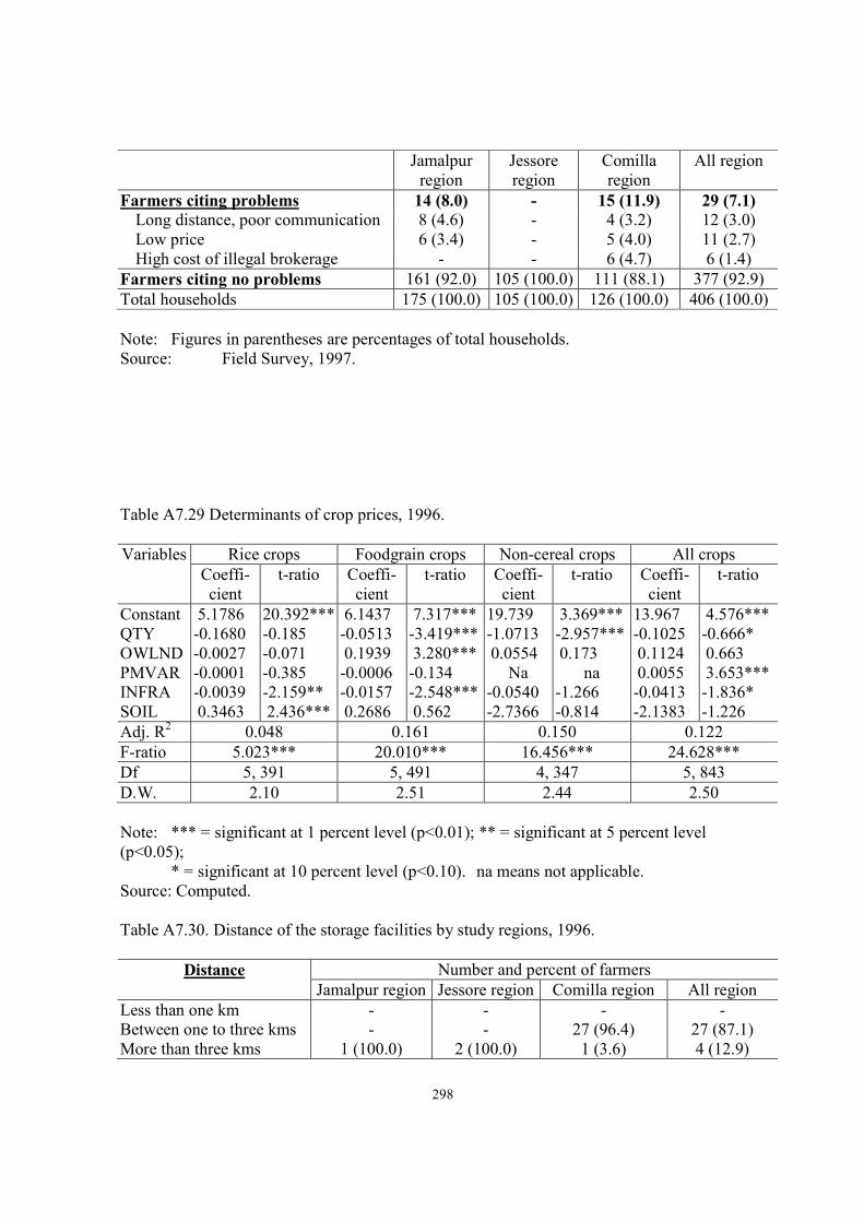
298

Jamalpur

region

Jessore

region

Comilla

region

All region

Farmers citing problems 14 (8.0) - 15 (11.9) 29 (7.1)

Long distance, poor communication 8 (4.6) - 4 (3.2) 12 (3.0)

Low price 6 (3.4) - 5 (4.0) 11 (2.7)

High cost of illegal brokerage - - 6 (4.7) 6 (1.4)

Farmers citing no problems 161 (92.0) 105 (100.0) 111 (88.1) 377 (92.9)

Total households 175 (100.0) 105 (100.0) 126 (100.0) 406 (100.0)

Note: Figures in parentheses are percentages of total households.

Source: Field Survey, 1997.

Table A7.29 Determinants of crop prices, 1996.

Variables Rice crops Foodgrain crops Non-cereal crops All crops

Coeffi-

cient

t-ratio Coeffi-

cient

t-ratio Coeffi-

cient

t-ratio Coeffi-

cient

t-ratio

Constant 5.1786 20.392*** 6.1437 7.317*** 19.739 3.369*** 13.967 4.576***

QTY -0.1680 -0.185 -0.0513 -3.419*** -1.0713 -2.957*** -0.1025 -0.666*

OWLND -0.0027 -0.071 0.1939 3.280*** 0.0554 0.173 0.1124 0.663

PMVAR -0.0001 -0.385 -0.0006 -0.134 Na na 0.0055 3.653***

INFRA -0.0039 -2.159** -0.0157 -2.548*** -0.0540 -1.266 -0.0413 -1.836*

SOIL 0.3463 2.436*** 0.2686 0.562 -2.7366 -0.814 -2.1383 -1.226

Adj. R2

0.048 0.161 0.150 0.122

F-ratio 5.023*** 20.010*** 16.456*** 24.628***

Df 5, 391 5, 491 4, 347 5, 843

D.W. 2.10 2.51 2.44 2.50

Note: *** = significant at 1 percent level (p<0.01); ** = significant at 5 percent level

(p<0.05);

* = significant at 10 percent level (p<0.10). na means not applicable.

Source: Computed.

Table A7.30. Distance of the storage facilities by study regions, 1996.

Distance Number and percent of farmers

Jamalpur region Jessore region Comilla region All region

Less than one km

Between one to three kms

More than three kms

-

-

1 (100.0)

-

-

2 (100.0)

-

27 (96.4)

1 (3.6)

-

27 (87.1)

4 (12.9)

299

Total number of godowns 1 (100.0) 2 (100.0) 28 (100.0) 31 (100.0)

Note: Figures in parentheses are percentage of total households.

Source: Field Survey, 1997.

Table 7.31 Problems with storage facilities by study regions, 1996.

Problems with storage facilities Number and percent of households (%)

Jamalpur

region

Jessore

region

Comilla

region

All region

Farmers citing problems 4 (2.6) - 28 (22.2) 32 (7.9)

Lack of space at home - - 26 (20.6) 26 (6.4)

Insect damage crops 2 (1.1) - 2 (1.6) 4 (0.9)

Leakage of roof requiring maintenance 1 (0.8) - - 1 (0.3)

Threat of burglary 1 (0.7) - - 1 (0.3)

Farmers citing no problems 171 (97.4) 105 (100.0) 98 (77.8) 374 (92.1)

Total households 175 (100.0) 105 (100.0) 126 (100.0) 406 (100.0)

Note: Figures in parentheses are percentages of total households.

Source: Field Survey, 1997.

Table A7.32 Joint determination of input demand functions, 1996.

Variables Joint estimates of input demand functions using Three Stage Least Squares

Fertilizer

demand

Labor demand Animal power

demand

Modern techno-

logy adoption

Irrigation

demand

Intercept -82.714

(-1.662)*

118.030

(4.543)***

32.463

5.651)***

0.147

(0.692)

-0.359

(-1.701)*

FP -4.578

(-1.348)

- - - -

WAGE - -1.110

(-3.228)***

- - -

ANIMP - - -0.328

(-10.890)***

- -

AMLND 158.350

(3.240)***

84.485

(3.609)***

13.601

(3.016)***

-0.478

(-2.339)**

1.056

(22.069)***

MVAR 119.290

(2.497)***

27.436

(2.329)**

24.144

(6.130)***

- -

CAPL 1.294

(2.337)**

- - 0.002

(0.844)

0.005

(2.633)***

AGCR -0.659

(-1.394)

-0.012

(-0.060)

0.056

(0.368)

0.004

(1.801)*

-0.005

(-2.458)**

INFRA 0.957

(1.617)

0.316

(1.289)

-0.115

(-2.001)**

0.004

(2.441)**

0.005

(3.156)***

SOIL 23.219

(0.914)

-34.733

(-3.241)***

-0.229

(-0.086)

-0.097

(-0.853)

0.101

(0.853)

IRRIG - - - 1.404 -

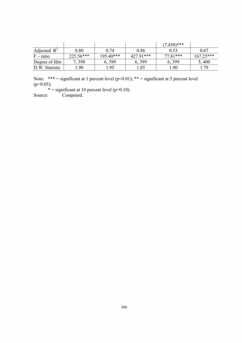
300

(7.450)***

Adjusted R2

0.80 0.74 0.86 0.53 0.67

F – ratio 225.56*** 195.40*** 427.91*** 77.81*** 167.25***

Degree of fdm 7, 398 6, 399 6, 399 6, 399 5, 400

D.W. Statistic 1.90 1.95 1.85 1.90 1.79

Note: *** = significant at 1 percent level (p<0.01); ** = significant at 5 percent level

(p<0.05);

* = significant at 10 percent level (p<0.10).

Source: Computed.

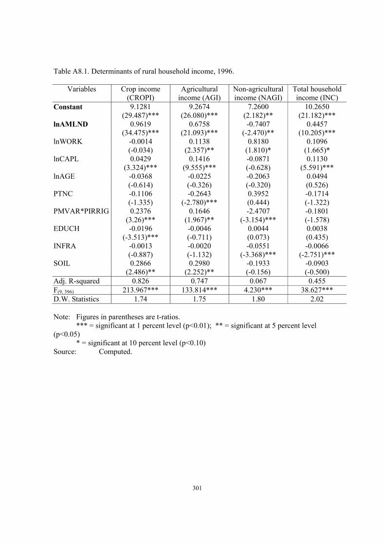
301

Table A8.1. Determinants of rural household income, 1996.

Variables Crop income

(CROPI)

Agricultural

income (AGI)

Non-agricultural

income (NAGI)

Total household

income (INC)

Constant 9.1281

(29.487)***

9.2674

(26.080)***

7.2600

(2.182)**

10.2650

(21.182)***

lnAMLND 0.9619

(34.475)***

0.6758

(21.093)***

-0.7407

(-2.470)**

0.4457

(10.205)***

lnWORK -0.0014

(-0.034)

0.1138

(2.357)**

0.8180

(1.810)*

0.1096

(1.665)*

lnCAPL 0.0429

(3.324)***

0.1416

(9.555)***

-0.0871

(-0.628)

0.1130

(5.591)***

lnAGE -0.0368

(-0.614)

-0.0225

(-0.326)

-0.2063

(-0.320)

0.0494

(0.526)

PTNC -0.1106

(-1.335)

-0.2643

(-2.780)***

0.3952

(0.444)

-0.1714

(-1.322)

PMVAR*PIRRIG 0.2376

(3.26)***

0.1646

(1.967)**

-2.4707

(-3.154)***

-0.1801

(-1.578)

EDUCH -0.0196

(-3.513)***

-0.0046

(-0.711)

0.0044

(0.073)

0.0038

(0.435)

INFRA -0.0013

(-0.887)

-0.0020

(-1.132)

-0.0551

(-3.368)***

-0.0066

(-2.751)***

SOIL 0.2866

(2.486)**

0.2980

(2.252)**

-0.1933

(-0.156)

-0.0903

(-0.500)

Adj. R-squared 0.826 0.747 0.067 0.455

F(9, 396) 213.967*** 133.814*** 4.230*** 38.627***

D.W. Statistics 1.74 1.75 1.80 2.02

Note: Figures in parentheses are t-ratios.

*** = significant at 1 percent level (p<0.01); ** = significant at 5 percent level

(p<0.05)

* = significant at 10 percent level (p<0.10)

Source: Computed.

302

Table A9.1 Soil reaction.

pH range1

Interpretation2

Jamalpur Jessore Comilla All region

4.5 – 5.5 Highly acidic 1 (20) - - 1 (7)

5.6 – 6.5 Slightly acidic 3 (60) - 1 (100) 4 (27)

6.6 – 7.3 Neutral 2 (40) - 2 (100) 3 (20)

7.4 – 8.4 Slightly alkaline 5 (100) 2 (100) 7 (46)

Total 5 (100) 5 (100) 5 (100) 15 (100)

Mean and standard deviation 6.0 [0.5] 7.8 [0.2] 7.2 [0.5] 6.9 [0.9]

pH index 6.0 7.9 7.1 6.7

Index Interpretation Slightly

acidic

Slightly

alkaline

Neutral Neutral

Note: Figures in parentheses are percentage. Figures in square brackets are standard

deviation. 1In case of Bangladesh, the Soil Resource Development Institute (SRDI) provided a

four group classification based on a given range of soil pH which is different from

standard classification (SRDI, 1991). 2

The interpretation is based on classification provided by SRDI (1991). The SRDI also

provided three group classification based on a given range of levels of nutrients for all

macro and micro-nutrients which were utilized in analyzing available N, P, K, Zn, and

S, respectively (Tables 6.4 – 6.9).

pH index = {(m1 * n1) + (m2 * n2) + (m3 * n3) + (m4 * n4)}/ n

where m1 .... m4 are the mid points of pH ranges and n1 ... n4 are respective number of

sample in each class. n = sample size.

Source: Field survey, 1997.

Table A9.2 Organic matter content (%) in the soil.

OM (%) range Interpretation Jamalpur Jessore Comilla All region

< 1.72 Low 3 (60) 1 (20) 4 (80) 8 (53)

1.72 – 3.44 Medium 2 (40) - 1 (20) 3 (20)

3.44 > High - 4 (80) - 4 (27)

Total 5 (100) 5 (100) 5 (100) 15 (100)

Mean and Standard deviation 2.01 [0.79] 6.47 [2.84] 1.45 [0.35] 3.32 [2.82]

OM index 1.55 2.60 1.20 1.73

Index Interpretation1 Low High Low Medium

Note: Figures in parentheses are percentage. Figures in square brackets are standard

deviation. 1The index value is rated as < 1.67 = low, 1.67 – 2.33 = medium, and > 2.33 = high

following Motsara (1994) and Dahal (1996). This index value rating is utilized in

analyzing all other soil fertility parameters (Tables 6.5 – 6.12).

OM index = {(n1 * 1) + (n2 * 2) + (n3 * 3)}/ n

where n1 ... n3 are respective number of sample in each class, and 1, 2, 3 are the

weights for low, medium, and high class.n = sample size.

303

This procedure of index construction is followed in analyzing the remaining soil

fertility parameters (Tables 6.5 – 6.12).

Source: Field survey, 1997.

Table A9.3 Available Nitrogen in the soil.

N (µµµµg/g) range Interpretation Jamalpur Jessore Comilla All region

< 76 Low 5 (100) 5 (100) 5 (100) 15 (100)

76 – 150 Medium - - - -

151 – 300 High/Best - - - -

Total 5 (100) 5 (100) 5 (100) 15 (100)

Mean and standard deviation 16.0 [6.7] 19.1 [8.2] 25.5 [7.5] 20.2 [8.1]

Nitogen index 1.00 1.00 1.00 1.00

Index Interpretation Low Low Low Low

Note: Figures in parentheses are percentage.

Figures in square brackets are standard deviation.

Source: Field survey, 1997.

Table A9.4 Available Phosphorus in the soil.

P (µg/g) range Interpretation Jamalpur Jessore Comilla All region

< 13 Low - - - -

13 – 25 Medium 2 (40) 4 (80) 5 (100) 11 (73)

26 – 75 High/Best 3 (60) 1 (20) - 4 (27)

Total 5 (100) 5 (100) 5 (100) 15 (100)

Mean and standard deviation 26.7 [6.4] 22.3 [15.8] 20.4 [2.0] 23.1 [9.6]

Phosphorus index 2.60 2.20 2.00 2.27

Index Interpretation High Medium Medium Medium

Note: Figures in parentheses are percentage.

Figures in square brackets are standard deviation.

Source: Field survey, 1997.

Table A9.5 Available Potassium in the soil.

K (µg/g) range Interpretation Jamalpur Jessore Comilla All region

< 79 Low 5 (100) 5 (100) 5 (100) 15 (100)

79 – 156 Medium - - - -

157 – 585 High/Best - - - -

Total 5 (100) 5 (100) 5 (100) 15 (100)

Mean and standard deviation 32.2 [16.6] 52.4 [13.8] 20.3 [6.0] 34.9 [18.2]

304

Potassium index 1.00 1.00 1.00 1.00

Index Interpretation Low Low Low Low

Note: Figures in parentheses are percentage.

Figures in square brackets are standard deviation.

Source: Field survey, 1997.

Table A9.5 Available Sulfur in the soil.

S (µg/g) range Interpretation Jamalpur Jessore Comilla All region

< 13 Low 5 (100) 3 (60) 5 (100) 13 (87)

13 – 25 Medium - 2 (40) - 2 (13)

26 – 75 High/Best - - - -

Total 5 (100) 5 (100) 5 (100) 15 (100)

Mean and standard deviation 7.8 [2.9] 10.2 [3.7] 5.5 [0.7] 7.8 [2.9]

Sulfur index 1 1.40 1.00 1.53

Index Interpretation Low Low Low Low

Note: Figures in parentheses are percentage. Figures in square brackets are standard

deviation.

Source: Field survey, 1997.

Table A9.6 Available Zinc in the soil.

Zn (µg/g) range Interpretation Jamalpur Jessore Comilla All region

< 2.1 Low 1 (20) - 2 (40) 3 (20)

2.1 – 4.0 Medium 1 (20) 1 (20) - 2 (13)

4.1 – 18.0 High/Best 3 (60) 4 (80) 3 (60) 10 (67)

Total 5 (100) 5 (100) 5 (100) 15 (100)

Mean and standard deviation 5.0 [3.7] 7.6 [3.2] 4.1 [2.9] 5.5 [3.4]

Zinc index 2.40 2.80 2.20 2.47

Index Interpretation High High Medium High

Note: Figures in parentheses are percentage. Figures in square brackets are standard

deviation.

Source: Field survey, 1997.

Table A9.7 Cation exchange capacity of the soil

CEC range1 (meq/100g) Interpretation Jamalpur Jessore Comilla All region

0 – 20 Low 5 (100) 1 (20) 4 (80) 10 (67)

21 – 40 Medium - 4 (80) 1 (20) 5 (33)

41 > High - - - -

305

Total 5 (100) 5 (100) 5 (100) 15 (100)

Mean and standard deviation 10.9 [3.5] 26.2 [8.7] 15.8 [4.5] 17.6 [8.6]

CEC index 1.00 1.80 1.20 1.33

Index Interpretation Low Medium Low Low

Note: Figures in parentheses are percentage. Figures in square brackets are standard

deviation.

This classification is based on Thompson and Troeh (1973) and Brady (1974).

Thompson and Troeh (1973) revealed that CEC of 10 – 20 meq/100g is observed for

clays found in highly weathered soil in tropical and subtropical areas, 40 – 80

meq/100g for clays in temperate climates and 100 – 200 meq/100g for organic matters.

Brady (1974) revealed that representative CEC of silicate clay (0.5 meq for each 1

percent) and for well-humified organic matter (2.0 meq for each 1 percent) can be

ascertained. For example, silt loam soils in US vary from 9.4 – 26.3 meq/100g.

Source: Field survey, 1997.

Table A9.8 Electrical conductivity of the soil

EC range (µS/cm) Interpretation Jamalpur Jessore Comilla All region

< 200 Low 5 (100) 4 (80) 5 (100) 14 (93)

200 + Optimum - 1 (20) - 1 (7)

Total 5 (100) 5 (100) 5 (100) 15 (100)

Mean and standard deviation 75 [30] 176 [34] 113 [32] 121 [52]

EC index 1.00 1.2 1.00 1.07

Index Interpretation Low Low Low Low

Note: Figures in parentheses are percentage.

Figures in square brackets are standard deviation.

Source: Field survey, 1997.

Table A9.9 Soil texture

Soil texture class Jamalpur Jessore Comilla All region

Silt loam 4 (80) 1 (20) 4 (80) 9 (60)

Silty clay loam - - 1 (20) 1 (7)

Silty clay - 3 (60) - 3 (20)

Clay loam/Clay 1 (20) 1 (20) - 2 (13)

Total 5 (100) 5 (100) 5 (100) 15 (100)

Textural Interpretation Silt loam Silty clay Silt loam Silty clay loam

Note: Figures in parentheses are percentage.

Source: Field survey, 1997.

306

Table A9.10 Regression results of soil fertility and crop productivity relations, 1996.

Dependent

variable

Independent variables

Adj. R2

S.E. of

regression

F – value

Variable

name

Coeff-

icient t - ratio Value df

ln local Aman Constant

ln K

pH

ln CEC

5.958

0.323

-0.401

0.557

5.523***

1.669

-3.193***

1.853*

0.417 0.3386 5.524*** 3,16

ln MV Aman Constant

ln N

7.523

0.169

27.976***

2.316**

0.195 0.1211 5.364** 1,17

ln MV wheat Constant

ln Zn

7.154

0.217

28.620***

2.185**

0.239 0.2584 4.775** 1,11

ln MV rice Constant

ln N

7.750

0.137

27.366***

1.806*

0.102 0.1314 3.263* 1,19

ln foodgrain (all

varieties of rice

and wheat

Constant

ln K

pH

7.749

0.144

-0.048

33.135***

3.044***

-2.011*

0.314 0.098 5.570** 2,18

ln jute Constant

ln K

5.973

0.349

16.716***

4.153***

0.556 0.1499 17.249*** 1,12

ln pulses Constant

pH

ln K

22.517

-2.352

0.457

7.404***

-5.031***

2.767***

0.786 0.1597 13.880*** 2,5

ln spices Constant

pH

ln K

9.380

-0.935

1.200

6.914***

-6.471***

3.287***

0.781 0.3697 20.593*** 2,9

ln vegetables Constant

ln K

pH

ln S

EC

ln N

5.754

-1.246

1.004

1.829

-0.011

-0.547

5.450***

-14.894***

10.128***

8.605***

-6.316***

-4.009***

0.951 0.1143 51.582*** 5,8

Note: *** = significant at 0.01 level (p<0.01); ** = significant at 0.05 level (p<0.05).

* = significant at 0.10 level (p<0.10).

Source: Field survey, 1997.

307

Table A9.11 Farmers’ opinion on present level of pesticide use by study regions, 1996.

Opinion on present level of pesticide use Number and percent of households (%)

Jamalpur

region

Jessore

region

Comilla

region

All region

Farmers thinking present use as appropriate 41 (23.4) 13 (12.4) 103 (81.7) 157 (38.7)

Farmers considering need to use more 24 (13.8) 29 (27.6) 4 (3.2) 57 (14.0)

Farmers considering need to reduce use 27 (15.4) 8 (7.6) 4 (3.2) 39 (9.6)

Farmers not thinking about pesticide use 13 (7.4) 17 (16.2) 4 (3.2) 34 (8.4)

Non-responding farmers 70 (40.0) 38 (36.2) 11 (8.7) 119 (29.3)

Total households 175 (100.0) 105 (100.0) 126 (100.0) 406 (100.0)

Note: Figures in parentheses are percentages of total households.

Source: Field Survey, 1997.

Table A9.12. Source of water for drinking and washing purpose by study regions, 1996.

Sources of water Number and percent of households (%)

Jamalpur

region

Jessore

region

Comilla

region

All region

Source of water for drinking

Tube well 126 (100.0) 175 (100.0) 105 (100.0) 406 (100.0)

Source of water for washing/cleansing

Pond 85 (48.6) 44 (41.9) 101 (80.2) 230 (56.7)

Tube well 126 (72.0) 81 (77.1) 7 (5.6) 214 (52.7)

Canal 3 (1.7) - 13 (12.4) 16 (3.9)

River 1 (0.6) - 11 (8.7) 12 (3.0)

Total households 175 (100.0) 105 (100.0) 126 (100.0) 406 (100.0)

Note: Figures in parentheses are percentages of total households.

Multiple responses.

Source: Field Survey, 1997.

308

Table A9.13 Quality of water by sources by study regions, 1996.

Quality of water of

various sources

Number and percent of households (%)

Jamalpur region Jessore region Comilla region All region

Good quality

Rain water 172 (98.2) 105 (100.0) 123 (97.6) 400 (98.5)

Hand pump 5 (2.9) 32 (30.5) 23 (18.3) 60 (14.8)

Shallow tube well - - 7 (5.6) 7 (1.7)

Deep tube well 2 (1.1) - 3 (2.4) 5 (1.2)

Low lift pump 2 (1.1) - 2 (1.6) 4 (1.0)

Poor quality

Rain water 3 (1.7) - 3 (2.4) 6 (1.5)

Hand pump 63 (36.0) 19 (18.1) 79 (63.0) 162 (39.9)

Shallow tube well 8 (4.6) - 11 (8.7) 19 (4.7)

Deep tube well 7 (4.0) - 3 (2.4) 10 (2.5)

Low lift pump 7 (4.) - 15 (11.9) 22 (5.4)

Total households 175 (100.0) 105 (100.0) 126 (100.0) 406 (100.0)

Note: Figures in parentheses are percentages of total households. Multiple responses.

Source: Field Survey, 1997.

Table A9.14 Remarks about water quality by sources by study regions, 1996.

Quality of water of various

sources

Number and percent of households (%)

Jamalpur region Jessore region Comilla region All region

Ground water (tube well)

Clean/not polluted/good 69 (39.4) 20 (19.0) 68 (54.0) 157 (38.7)

Good for bath/cooking 26 (14.9) 11 (10.1) 55 (43.7) 92 (22.7)

Low iron content 73 (41.7) 59 (56.2) 3 (2.4) 135 (33.2)

Heavy iron content 7 (4.0) 15 (14.3) - 22 (5.4)

Surface water (river/canal)

Clean/not polluted/good 2 (1.1) - 8 (6.3) 10 (2.5)

Polluted/dirty 5 (2.9) - 19 (15.1) 24 (5.9)

Causes diarrhoea/rheumatism 2 (1.1) - 3 (2.4) 5 (1.2)

No response on surface water qlty 166 (94.9) 105 (100.0) 96 (76.2) 367 (90.4)

Surface water (pond)

Clean/not polluted/good 49 (28.0) 8 (7.6) 6 (4.8) 63 (15.5)

Good for bath/cooking - - 15 (11.9) 15 (3.7)

Low iron content 3 (1.7) 3 (2.9) - 6 (1.5)

Polluted/dirty 21 (12.0) 24 (22.9) 77 (61.1) 122 (30.0)

Causes diarrhoea/rheumatism 12 (6.9) 12 (11.4) 6 (4.8) 30 (7.4)

Non-response on pond water qlty 90 (51.4) 58 (55.2) 22 (17.5) 170 (41.9)

Total households 175 (100.0) 105 (100.0) 126 (100.0) 406 (100.0)

Note: Figures in parentheses are percentages of total households. Multiple responses.

Source: Field Survey, 1997.

309

TableA9.15 Sufficiency of water supply for irrigation by study regions, 1996

Sufficiency of water supply for

irrigation

Number and percent of households (%)

Jamalpur

region

Jessore

region

Comilla

region

All region

Sufficient 153 (87.4) 95 (90.5) 100 (79.4) 348 (85.7)

Not sufficient 22 (12.6) 10 (9.5) 26 (20.6) 58 (14.3)

Load shedding/ no electricity supply 13 (7.4) 5 (4.8) 4 (3.2) 22 (5.4)

River/canal/pond dry 1 (0.6) - 14 (11.1) 15 (3.7)

Not under/ far from irrigation scheme 1 (0.6) 3 (2.9) 8 (6.3) 12 (3.0)

High prices for irrigation water 3 (1.7) 2 (1.8) - 5 (1.2)

Mechanical problem of machines 4 (2.3) - - 4 (1.0)

Total households 175 (100.0) 105 (100.0) 126 (100.0) 406 (100.0)

Note: Figures in parentheses are percentages of total households.

Source: Field Survey, 1997.

310

APPENDIX B

COORDINATION SCHEMA FOR THE FARM-SURVEY COMPONENT OF THE STUDY

PARAMETER COMPLEX

VARIABLE

SIMPLE VARIABLE VALUE

Ideographic

Features

Respondent's

Profile

Age Year

Gender Male/Female

Socioeconomic

profile

Education level Degree obtained

Years of schooling completed

Major occupation Fact (Occupation code list)

(e.g., farmer, trader, student, etc)

Minor occupation Fact (occupation code list)

Other skills/training Description

Household

composition

Size Number

Status of other

household

members

Gender Male/female

Age Year

Educational level Years of schooling completed

Major occupation Fact (occupation code list)

Minor occupation Fact (occupation code list)

Other skills Description

Major sources

of income

Employment in

activities

Agriculture Fact

Non-agriculture Fact

Wage Fact

Salaried Fact

Remittance from abroad Fact

Resources

owned by the

household

Fixed assets Homestead

(in numbers and estimated

value at present)

House

Storage

Shed

Land assets Types of land owned Homestead

Cultivated

Rented-out

Mortgaged-out

Amount of land owned by

(also estimated value at

present)

Husband

Wife

Other members

311

PARAMETER COMPLEX

VARIABLE

SIMPLE VARIABLE VALUE

Changes in land

assets during last

5 years

Consolidation Consolidated

Fragmented

Resources

owned by the

household

(continued)

Total land Increased

Decreased

Purchase (amount and

value)

Fact

Sale (amount and value) Fact

Perceived quality at present Declining/Getting better

Other Assets (in

no.and estimated

present value)

Equipments Fact (Assets code list)

Transport Fact

Household durables/

furnitures

Fact

Ornaments Fact

Artisans/Carpenters kits Fact

Shops/godowns Fact

Rice/oil mills Fact

Production

Structure

Tenurial status Type of land under

cultivation (in decimals)

Owned land

Rented-in land

Mortgaged-in land

Leased-in land

Liabilities of

the household

Credit Sources of credit (amount

and time when taken)

Institution

Money lender

Friends/Relatives

Types (amount and value

for kind)

Cash

Kind

Credit conditions Interest rate

Period

Collateral deposited

Uses of credit Land purchase

Equipment purchase

Agril. production

Business

Consumption

Ceremony

Others (specify)

Agricultural

production

Production

practice

Crops grown (area and

production under each crop)

Crop code list

(e.g., MV rice, wheat, etc.)

312

PARAMETER COMPLEX

VARIABLE

SIMPLE VARIABLE VALUE

Utilization of

agricultural

produce

Mode of utilization

(amount and value for each

crop types)

Consumption

Debt service

Sale

Preserved as seed

Present stock

Payment for landlord

Selling station (amount,

distance and transportation

cost)

Farmgate

Local market

Secondary market

Agricultural

production

(continued)

Mode of selling Household member

Broker

Food self sufficiency Proportion of a year

Input Use Material inputs (amount and

value)

Seed, Fertilizer, Manure

Chemicals

Equipments (own and hired

with rental value)

Tractor/power tiller, Thresher,

Plough, Draught animal

Irrigation (area irrigated and

cost)

Modern (DTW, STW,LLP)

Traditional (dhone)

Labor Use Operations (working days of

family and hired labor in

each crops by gender)

Land preparation, Sowing

Weeding, Irrigation

Fertilizing, Harvesting

Threshing

Wages Cash, Food + cash

Use of modern

technology

Irrigation Land categories (amount of

land irrigated)

Owned

Rented-in

Mortgaged-in

Leased-in

Mode of irrigation Deep Tube Well

Shallow Tube Well

Low lift pump (LLP)

Hand pump (HP)

Others (specify)

Land preparation Land categories (amount of

land prepared)

Owned, Rented-in

Mortgaged-in, Leased-in

Mode of land preparation Tractors Power tillers

Draft animals

Farm

machineries

Modern

equipments

Irrigation equipment

(number and present value)

DTW, STW, LLP, HP

Other (specify)

313

PARAMETER COMPLEX

VARIABLE

SIMPLE VARIABLE VALUE

owned by the

household Agricultural implements

(number and present value)

Spade/Sickle, Plow, Ladder

Tractor, Power tiller

Payments for

renting land

(Land rent)

Payments for

rented-in, mort-

gaged-in and

leased-in land

Terms of payment

(proportion, quantity,value)

Crop share

Cash

Terms of sharing (quantity

and value)

Input cost sharing

No input cost sharing

Income from

land renting by

the household

Leased-out/

mortgaged-out/

rented-out land

Relation with the landlord Within the village

Out of the village

Amount of land Within the village Out of the village

Period of lease Start/End

Income from

land renting by

the household

(continued)

Payment received Proportion of harvest

Cash

Cost sharing Irrigation cost

Seed/fertilizer cost

Land preparation cost

Proportion of total cost

Livestock

raising

Raising pattern Type of livestock Cattle, Buffalo,

Goat/sheep,

Chicken/Duck

Others (specify)

Head Figure

Present value Amount

Purchase cost Amount

Purpose of raising Milk, meat, draft power, eggs

Labor used Family labor Days

Hired labor Days

Wage Taka

Feed cost

(purchased)

Forage Amount

Fodder Amount

Income from last

one year

Head Sale Amount

Slaughtered Amount

Lost/dead Amount

Production and

selling

Yield Calves/chicks

Milk/meat/egg

Manure

Draft power

Load hauling

314

PARAMETER COMPLEX

VARIABLE

SIMPLE VARIABLE VALUE

Selling place Farmgate

Local market

Outside market

Mode of selling Household member

Broker

315

PARAMETER COMPLEX

VARIABLE

SIMPLE VARIABLE VALUE

Wage Earning Wage laborer Type Daily

Contract/Annual

Occasional

Type of work Farm work

Household work

Nonfarm work

Earth digging

Construction

Porter

Others (specify)

Working days Dry season

Wet season

Wage rate Cash

Food + cash

Service Service Type Personal

Public

Private

NGO

Others (specify)

Nature Temporary

Permanent

Daily

Period of service Year

Annual earning Amount

Remittance Amount

Business Operation Types of business Business code list (e.g. grocery)

Period of operation Years

Family labor Days

Hired labor Days

Wage Taka

Purchase cost of goods Taka

Rent and storage cost Taka

Transportation cost Taka

Sale price of good Taka

Annual sales Taka

316

PARAMETER COMPLEX

VARIABLE

SIMPLE VARIABLE VALUE

Cottage

industries and

agro-process-ing

industries

Operation Types Cottage industries code list

(e.g., husking, net making, etc.)

Period of operation Years

Nature Permanent/Temporary/Contract

Name of item produced Fact

Quantity produced Number

Amount of investment Taka

Sale price Taka

Family labor cost Taka

Hired labor cost Taka

Other costs Taka

Household

expenditure

Categories of

expenses

Clothes Amount

Education Amount

Ceremonies Amount

Health care Amount

Groceries Amount

Basic food items Amount

Miscellaneous Amount

Sources of money

for expenditure

Household income Proportion of total expense

Other sources (proportion

of total expense from each

source)

Borrowing

Bank loan

Money lender

Gift

Sale of land

Sale of valuables

Others (specify)

Utilization of

borrowed money

Specification Ceremonies

Health care

Education

Others (specify)

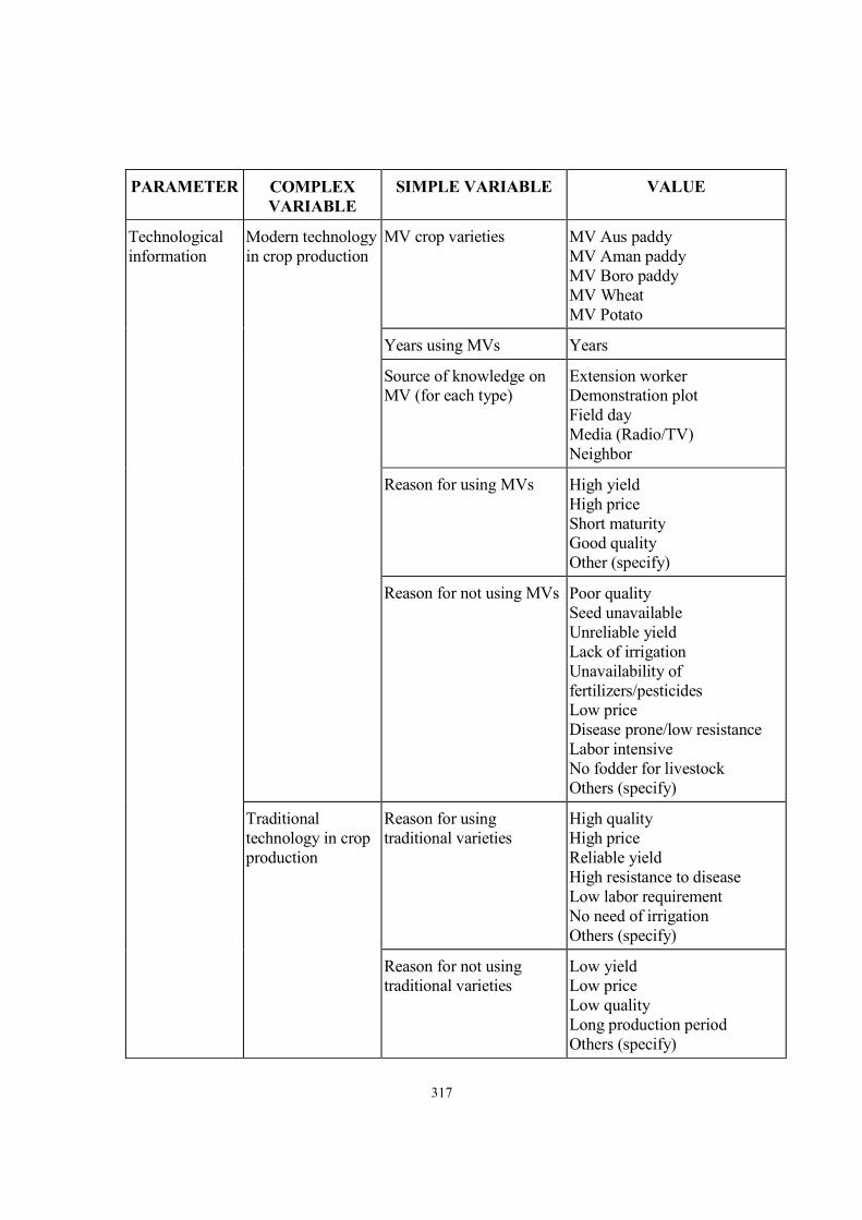
317

PARAMETER COMPLEX

VARIABLE

SIMPLE VARIABLE VALUE

Technological

information

Modern technology

in crop production

MV crop varieties MV Aus paddy

MV Aman paddy

MV Boro paddy

MV Wheat

MV Potato

Years using MVs Years

Source of knowledge on

MV (for each type)

Extension worker

Demonstration plot

Field day

Media (Radio/TV)

Neighbor

Reason for using MVs High yield

High price

Short maturity

Good quality

Other (specify)

Reason for not using MVs Poor quality

Seed unavailable

Unreliable yield

Lack of irrigation

Unavailability of

fertilizers/pesticides

Low price

Disease prone/low resistance

Labor intensive

No fodder for livestock

Others (specify)

Traditional

technology in crop

production

Reason for using

traditional varieties

High quality

High price

Reliable yield

High resistance to disease

Low labor requirement

No need of irrigation

Others (specify)

Reason for not using

traditional varieties

Low yield

Low price

Low quality

Long production period

Others (specify)

318

PARAMETER COMPLEX

VARIABLE

SIMPLE VARIABLE VALUE

Access to

Infrastructure

Physical

infrastructure

Types of infrastructure

Wholesale market

Primary market/Haat/Bazaar

Storage

Fertilizer sales centre

Automatic rice mill

Upazila headquarter

Union office

Extension office

Bank

Post office

Paved road

Bus stop

River transport

Railway station

Electricity

Health care centre

Primary school

Secondary school (boys/girls)

Distance Within village

Miles from village

Cost of travel Taka

Time takes Hours

Environmental

impact of

modern

agricultural

technology

Impact integral to

the production

process

Type of impact

(farmers’ perception and

their relative rankings)

Reduce soil fertility

Increase soil erosion

Increase salinity

Compact soil

Chemical residues in soil

Water logging

Pest and disease attack

Pesticide resistance

Human disease

Eutrophication of water/pond

Chemical runoff in water

Note: The present co-ordination schema is a summarized version of the detailed schema.

Source: Prepared from the Household Level and Village Level Survey Questionnaires

utilized for the local-level component of the present study.

319

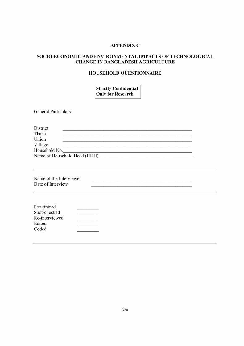
320

APPENDIX C

SOCIO-ECONOMIC AND ENVIRONMENTAL IMPACTS OF TECHNOLOGICAL

CHANGE IN BANGLADESH AGRICULTURE

HOUSEHOLD QUESTIONNAIRE

General Particulars:

District ______________________________________________________

Thana ______________________________________________________

Union ______________________________________________________

Village ______________________________________________________

Household No.______________________________________________________

Name of Household Head (HHH) _______________________________________

Name of the Interviewer __________________________________________

Date of Interview __________________________________________

Scrutinized _________

Spot-checked _________

Re-interviewed _________

Edited _________

Coded _________

Strictly Confidential

Only for Research

321

A1 HOUSEHOLD INFORMATION

1. Relationship with household head (HHH): ______.

2. Age of household head: ____ yrs. Education: _____ completed years of schooling.

Primary occupation: _________. Secondary occupation: _______________.

Farming experience:_________ yrs. Marital status: ___________.

3. Total household members: ______ persons. Total working men: _____ persons.

Total working women: _____ persons.

4. Educated members of household: ______ persons (minimum above Class V).

Educated men: _____ persons. Educated women: ______ persons.

5. Highest level of any household members:

Men: _____ (Yrs. of schooling). Women: ______ (Yrs. of schooling).

6. Membership in any organization: Yes No .

(If yes) Total members: Men: _____ persons. Women: _____ persons.

Name of organization of the men members: ________________________________.

Name of organization of the women members: _____________________________.

Length of membership: Men: _______ yrs. Women: ________ yrs.

A2 LAND OWNERSHIP AND TENURIAL STRUCTURE

1. How much is your total owned land? _______ decimals. (Spell out following categories).

(Units in decimals)

Homestead Cultivated Rented out Leased out Mortgaged out

2. How much is your farm size last year? ________ decimals

3. About your farm size last year. How much is your own and how much is rented-in/leased-

in/mortgaged-in in last year? (Spell out the following categories).

(Units in decimals)

Owned land Rented-in land Leased-in land Mortgaged-in land

4. What Rental Arrangements you had for the rented-in land of yours last year?

Arrangement Irrigated land Rainfed land

Fixed rent Cash

System Kind (Specify)

Crop sharing Output share

System Fertilizer share

(Specify both Irrigation share

In % and Labor share

Value) Draft power share

Others Specify

1

A3 CROP PRODUCTION 1. What types of crops did you grow in the last year? (First record types of crops grown by the farmer and then ask details).

________________________________________________________________________________.

Name Variety Area Land Total Use of total production (kg.)

Of crop cultivated

(dec.)

owning

category

production

(kg)

Consump

tion

Kept as

seed

Sold Price

(Tk/kg)

Value of

sale

Stored Debt

service

1 2 3 4 5 6 7 8 9 10 11 12

A4 CROP DAMAGE

Aus local Aus HYV Aman local Aman HYV Aman

pajam

Boro

local

Boro

HYV

Wheat

local

Wheat

HYV

Percent damaged

Area cultivated year before

Production obtained then

2

A5 COSTS OF CROP PRODUCTION

Name of Land Area Seed cost Ploughing cost Fertilizer cost

crop owning

category

cultivated

(dec.)

Own

(kg)

Buy

(kg)

Price

(Tk/kg)

Own

(A. day)

Buy

(A. day)

Price

(Tk/AD)

Qty

(Kg)

Price

(Tk/kg)

1 2 3 4 5 6 7 8 9 10 11

Name of Manure cost Labor cost Irrigation Pesticide Other equipment

crop Own

qty. (kg)

Purchased

qty. (kg.)

Price

(Tk/kg)

Own

(Mandays)

Hired

(Mandays)

Wage

(Tk/manday)

cost

(Tk)

cost

(Tk)

hiring cost

(Tk)

1 12 13 14 15 16 17 18 19 20

1

A6 FERTILIZER USE INFORMATION

What types of fertilizers did you use in your crop land?

Name of

crop

Types of fertilizers

Urea Triple Super

Phosphate (TSP)

Muriate of Potash

(MP)

Gypsum

Quanity Value Quantity Value Quantity Value Quantity Value

HYV paddy

Local paddy

Wheat

Potato

Vegetables

Others

(Specify)

1. Do you think you are applying enough fertilizers and pesticides for your farm?

Fertilizers: Yes . No. .

2. (If “No”) How much more you need? (Specify the fertilizer and chemical types):

Fertilizers: __________ kg.

3. Where do you buy your fertilizers?

Place: _________________. Distance from village: ______________ km

4. Do you have any problems in buying fertilizers?

Fertilizers: Yes . No .

(If “Yes”) What are those problems? Please provide details.

____________________________________________________________________

____________________________________________________________________.

A7 PESTICIDE USE INFORMATION

Which type of pesticide do you use? (Specify each types used for different crops)

Crop Name Names and prices of pesticides

Paddy

Wheat

Potato

Vegetables

Others (Specify)

1. Do you think that you use appropriate amount of pesticides for your crops?

Yes . No .

2

2 (If “No”) How much more you would like to use?

Pesticide: _______ kg. or litre.

3. Where do you buy your pesticides?

Place: _________________. Distance from village: ______________ km

4. Do you have any problems in buying pesticides?

Pesticides: Yes . No .

(If “Yes”) What are those problems? Please provide details.

____________________________________________________________________

____________________________________________________________________.

5. How many times you generally use pesticides: ________ times.

6. What are the good and harmful effects of using pesticides? (Please write in details).

Good effects

Harmful effects

7. What do you think about the current use-level of pesticides for your farm operation?

___________________________________________________________________________

___________________________________________________________________________

___________________________________________________________________________

A8 DETERMINANTS OF MODERN VARIETY SELECTION

1. How long have you been growing MV/HYVs ?

HYV paddy: ______ yrs. HYV Wheat: _______ yrs.

2. What are the sources for your HYV paddy and wheat seeds?

Source Aus HYV Aman HYV Boro HYV Wheat HYV Potato HYV

Own

Purchase

3. Please provide your opinion on the following questions. Why do you grow HYV?

What is the most important factor regarding these HYV? If you do not grow HYV,

please provide your reasoning for that too. (Spell out all the “reasons for growing

HYV” first and ask to rank these reasons over a five- point scale. Then repeat the

procedure with “reasons for not growing HYV”).

3

Reasons for Growing

HYV

1 = Yes

2 = No

If “Yes”

Then

Rank

Reasons for not

growing HYV

1 = Yes

2 = No

If “Yes”

then

Rank

High yield Seed unavailability

High price Unreliable yield

Ready market Lack of irrigation

Short maturity period Fertilizer shortage

High quality Pesticide shortage

Higher profit Low price

Poor quality

Disease/Pest prone

Labor intensive

No fodder output

High production cost

Others (Specify)

4. Please provide your opinion on the following questions. Why do you grow local variety?

What is the most important factor regarding these local varieties? If you do not grow local

variety, please provide your reasoning for that too. (Spell out all the “reasons for growing

local variety” first and ask to rank these reasons over a five-point scale. Then repeat the

procedure with “reasons for not growing local variety”).

Reasons for Growing

Local Variety

1 = Yes

2 = No

If “Yes”

then Rank

Reasons for not

growing Local Variety

1 = Yes

2 = No

If “Yes”

then Rank

Reliable yield Low yield

High price Low price

Ready market Poor quality

High quality Also need fertilizer

Higher profit Also need pesticide

Low labor requirement Long maturity

Disease resistance Nobody do it

No need irrigation Others (Specify)

Low production cost

High fodder output

Others (Specify)

A9 PRODUCTION TRENDS 1. Do you think that the over the past five year, the per bigha production of HYV is:

Increasing Decreasing or At the same level ?

2. (If “decreasing”) Please explain why? _____________________________________

____________________________________________________________________.

4

A10 MODERN TECHNOLOGY USE

Land Area tilled Area under irrigation Area under land type

Owner

Category

by Power

Tiller/Tractor

DTW STW Others Tradi

tional

Single

cropped

Double

cropped

Tripple

cropped

1 2 3 4 5 6 7 8 9

Owned

Rented-in

Leased-in

Mortgaged-in

A11 ENVIRONMENTAL IMPACT OF MODERN TECHNOLOGY

1. Are you aware that there are environmental impacts associated with the adoption of

modern agricultural technology? Yes . No

(If “Yes”), provide examples: ____________________________________________

(If “No”), explain reason: ____________________________________________

2. Do you agree that the following environmental effects occur as a result of the use of

modern agricultural technology?

Effects 1 = Yes

2 = No

If yes then rank the inidividual effects

on a five-point scale

Reduces soil fertility

Increase soil erosion

Increase soil salinity

Compact the soil

Leaves chemical residues in soil

Creates water logging

Increase pest attack

Increase disease

Effects human health

Deteroriates nearby water body

Causes chemical runoff in water

Reduces fish catch

Others (Specify)

A12 INCOME FROM RENTED-OUT/LEASED-OUT/MORTGAGED-OUT LAND

1. Now I would like to ask you about the income from your rented-out land?

Leased-out Any written Share of output received Share of input cost

area (dec.) condition Type Qty (kg) Value (Tk) Share type Value (Tk)

1 2 3 4 5 6 7

2

A13 LIVESTOCK INCOME

1. Now I would like to ask you about the livestock you own. How many of the following livestock do you own?

Types Number Estimated Weekly caring expenditure Use of this livestock asset in last one year

present

value

(Tk)

Own

labor

(Days)

Hired

labor

(Days)

Wage

(Tk/

day)

Food

cost

(Tk)

Sold

(Tk)

Con-

sumed

(Tk)

Lost

(Tk)

Milk/

Eggs

(Tk)

Manure

(Ton)

Draft

power

(Days)

1 2 3 4 5 6 7 8 9 10 11 12 13

Cattle/Bull

Cow

Buffalo

Goat/Sheep

Poultry

Others

A14 FISHERIES INCOME

1. Now I would like to ask you about Pond Fisheries.

Serial Area Owner Use Fish Expenditure incurred last year (in Tk) Returns in last year (Tk)

Number ship last types Pond Fry Ferti- Fish Pond From Con- Pond Present

Of pond year prepare release lizer harvest rent sale sumed owner Stock

1 2 3 4 5 6 7 8 9 10 11 12 13 14

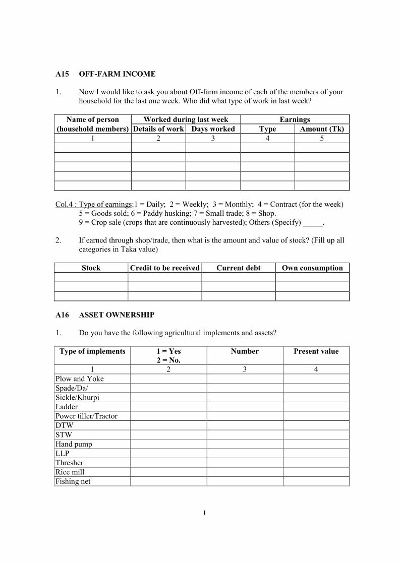
1

A15 OFF-FARM INCOME

1. Now I would like to ask you about Off-farm income of each of the members of your

household for the last one week. Who did what type of work in last week?

Name of person Worked during last week Earnings

(household members) Details of work Days worked Type Amount (Tk)

1 2 3 4 5

Col.4 : Type of earnings:1 = Daily; 2 = Weekly; 3 = Monthly; 4 = Contract (for the week)

5 = Goods sold; 6 = Paddy husking; 7 = Small trade; 8 = Shop.

9 = Crop sale (crops that are continuously harvested); Others (Specify) _____.

2. If earned through shop/trade, then what is the amount and value of stock? (Fill up all

categories in Taka value)

Stock Credit to be received Current debt Own consumption

A16 ASSET OWNERSHIP

1. Do you have the following agricultural implements and assets?

Type of implements 1 = Yes

2 = No.

Number Present value

1 2 3 4

Plow and Yoke

Spade/Da/

Sickle/Khurpi

Ladder

Power tiller/Tractor

DTW

STW

Hand pump

LLP

Thresher

Rice mill

Fishing net

2

A17 MARKETING OF AGRICULTURAL PRODUCTS

1. Where do you sell your crops?

Place Distance from

village (km)

Carrying cost (include

labor cost) (Tk/ton)

Transportation cost

(Tk/ton)

At the farmgate

Nearest market (Haat)

Central market

Others (Specify)

2. Do you have problems with marketing? Yes . No

(If “Yes”, provide details): _______________________________________________

_____________________________________________________________________

_____________________________________________________________________

A18 FOOD STOCK AND STORAGE

1. Do you have sufficient food stock at present? Yes . No

2. Where do you usually store your paddy/wheat and other crops?

Place Distance from

village (km)

Carrying cost

(Tk/ton)

Transportation

cost (Tk/ton)

Storage charge

(Tk./ton)

Own storehouse

Private arat

Public godowns

Others (Specify)

3. Do you have problems with storage facilities? Yes . No

(If “Yes”, provide details): ______________________________________________

____________________________________________________________________

A19 ROLE OF WATER

1. What source of water do you use?

Purpose Tubewell Dug well River Canal Pond Others

Drinking

Cleaning

3

2. What is your opinion about the quality of water that you use from the following sources?

Source Good Bad Open remarks about quality

Tubewell

Dugwell

River

Canal

Pond

Others

3. Which of the listed water sources do you usually use for irrigation?

Sources Kharif season (Monsoon season) Rabi season (Winter season)

Rain-fed

DTW

STW

LLP

Hand pump

Traditional

Others (Specify)

4. Do you think the water supplied by irrigation system is sufficient and timely?

Yes . No

Explain reason in case of “No”: ________________________________________________

____________________________________________________________________

5. Do you have any drainage or flooding problems? Yes . No .

6 Do you face the drainage or flooding problems every season? Yes . No .

7. (If “Yes”) What do you do to solve the problem? (Write in details also note the costs

involved): _____________________________________________________________

______________________________________________________________________

A20 KNOWLEDGE OF MODERN TECHNOLOGY

1. From where are you getting information on modern technology for your crop (Please

rank them)

Type of technology received

Co-farmers __________________________________

Block Supervisor __________________________________

Thana Extension Officer __________________________________

District Extension Officer __________________________________

Demonstration Plot __________________________________

4

Media/TV/Radio __________________________________

Field Day __________________________________

Others (Specify) __________________________________

2. Did you have any training in rice and wheat production in last 7 years?

Yes . No

(If “No”) Why? ______________________________________________________

(If “Yes”, provide details).

Training types Duration Organizers

3. How far is the nearest Agricultural Extension Office from your village? _____ km.

4. How many times the Agricultural Extension Officer visited you in the past one year?

_______ times. Why? _________________________________________________

5. How many times did you visit the nearest Agricultural Extension Office in the past one

year? _______ times. Why? _____________________________________________

A21 LAND ACQUISITION AND CONSOLIDATION

1. Did you purchase any land in the last 5 years? Yes No

(If “Yes” provide details)

Land type Purpose/Use Purchase value Present value Source of finance

Homestead land

Cultivated land

Others (Specify)

2. Did you sell any land in the last 5 years? Yes . No

(If “Yes” provide details)

Land type Sale value Present value Reason for sale

Homestead land

Cultivated land

Others (Specify)

5

A22 DEBT SITUATION

1. Is anyone of your household members has taken loan and still under debt?

Yes . No .

(If “Yes”) Please provide details.

Person Source

of loan

Type of

loan

Duration

of loan

Amount

of loan

Use of

loan

Rate of

interest

Collateral given

Type Value

1 2 3 4 5 6 7 8 9

A23 ECONOMIC CONDITION

The economic condition for the household for the last year.

Condition Jan. Feb. Mar. Apr. May June July Aug. Sept. Oct. Nov. Dec.

Surplus

Level

Deficit

A24 HOUSEHOLD EXPENDITURE

Now I would like to ask you about the household expenditure incurred last week? (Spell out

each items and fill up accordingly).

Item Purchased Own source

Quantity Total expense

(Taka)

Quantity Market value

(Taka) Unit Total Unit Total

1 2 3 4 5 6 7

Weekly expenditure on following items

Rice

Paddy

Wheat flour

Fish

Meat

Egg

Milk

Potato

Vegetables

Oil

Spices

Sugar

Beetle nut/cigar.

6

Item Purchased Own source

Quantity Total expense

(Taka)

Quantity Market value

(Taka) Unit Total Unit Total

1 2 3 4 5 6 7

Monthly/Annual expenditure on following items

Dress/clothing

Fuelwood

Education

Savings

Running capital

Debt service

(non-formal)

Bank debt

service (formal)

Investment

Interest

payment

Maintenance

Social Work

Religious Work

Transport cost

Others (specify)

THANK YOU VERY MUCH FOR YOUR TIME

7

APPENDIX C

SOCIO-ECONOMIC AND ENVIRONMENTAL IMPACTS OF TECHNOLOGICAL

CHANGE IN BANGLADESH AGRICULTURE

VILLAGE LEVEL QUESTIONNAIRE

General Particulars:

District ______________________________________________________

Thana ______________________________________________________

Union ______________________________________________________

Village ______________________________________________________

Household No.______________________________________________________

Name of Household Head (HHH) _______________________________________

Name of the Interviewer __________________________________________

Date of Interview __________________________________________

Scrutinized _________

Spot Checked _________

Re-interviewed _________

Edited _________

Coded _________

Strictly Confidential

Only for Research

8

1. What is the total area of this village? ___________ bigha

2. What is the total agricultural area? ___________ bigha

3. What is the total number of households? ___________ HHs.

4. What is the estimated number of population? ___________ persons

5. What are the major soil types?

Soil type Percent of land area

Loam

Sandy loam

Clay loam

Clay

Silt

Silt loam

Silt sand

Others (Specify)

6. What are the composition of low, medium, and high land?

Elevation Percent of land area

Highland

Medium highland

Medium land

Low land

Very low land

7. What are general cropping pattern of this village?

Pattern Crop sequences

1

2

3

4

5

6

9

8. What are the approximate area of rice and wheat crops in this village?

Crop Types Area under cultivation Year first started

Aus Local

Aus HYV

Aman Local

Aman HYV

Boro Local

Boro HYV

Wheat HYV

9. What types of irrigation facilities are available in this village?

Irrigation type Number Land area under irrigation Year first installed

Deep tube well

Shallow tube well

Hand pump

Low lift pump

Irrigation canal

Traditional

Others (Specify)

10. What is the composition of land ownership categories?

Ownership category Total land area under these Number of households

Landless

0.01 - 0.50 dec

0.51 - 1.00 dec.

1.01 - 2.50 dec

2.50 - 5.00 dec

5.01 - above

11. What is the tenurial structure of this village?

Tenurial Category Number of households

Owner operated

Tenant operated/ Sharecropper

Part tenant operated

12. What are the general terms of tenancy?

____________________________________________________________________________

____________________________________________________________________________

10

13. What is the wage structure for agricultural and non-agricultural activities in this village?

Employment category Only cash (no food) Cash and food

Peak season

Slack season

Contractual agreement

14. What is the wage of hired labor for specific agricultural operations?

Operation Wage (Tk./man-day) Contractual

Cash only (no food) Cash and Food Arrangement (Tk)

Land preparation

Sowing

Weeding

Irrigation

Fertilizing

Harvesting

Threshing and Winnowing

Others (Specify)

15. Does labor shortage occur during peak season?

Yes No

16. (If “Yes”) How the problem is solved? _________________________________________

___________________________________________________________________________

___________________________________________________________________________

17. What are the hiring charges for draft power, power tiller and irrigation fee? (Specify unit)

Implements Peak season Slack season

Tractor/Power tiller

Draft animal pair

Deep tube well

Shallow tube well

Low lift pump

Others

11

18. Please provide details of the following infrastructural facilities?

Type of infrastructure Number Distance

from village

Approximate

commuting time

Approximate

transport cost

Haat/Bazaar

Wholesale market

Local storage depot

Central storage depot

Fertilizer sale centre

Public procurement centre

Automatic rice mill

Thana headquarter

Union office

Agril. Extension office

Bank

Post office

Paved road

Bus stop

River transport

Railway station

Petrol sale point

Health care centre

Secondary school

Primary school

Others (Specify)

19. Does the village have electricity?

Yes No

(If “Yes”) When installed? _______________________.

20. Does the village have supply?

Yes No

(If “Yes”) When installed? _______________________.

THANK YOU VERY MUCH FOR YOUR TIME

12