Social Security and Fertility Policies

Fertility Policies and Social Security Reforms in China

Nicolas Coeurdacier

SciencesPo and CEPR

Stephane Guibaud

SciencesPo

Keyu Jin

London School of Economics

October 11, 2013∗

[PRELIMINARY: PLEASE DO NOT CITE]

Abstract

This paper analyses the consequences of China’s fertility policies and social security reforms

on savings, interest rates and the required social security adjustments. A key innovation is to

allow for endogenous fertility responses and its aggregate feedback effect. We develop an over-

lapping generations model, in which fertility decisions, capital accumulation, and the evolution

of social security are endogenously determined. In our framework, the endogenous response of

fertility and interest rates is crucial to understand the necessary fiscal adjustments of the social

security system. A key result is that the sequence and the combination of fertility, social security

or capital account reforms may be important in determining the fiscal pressure placed on the

social security system. China may need to juggle with policy reforms that have conflicting or

offsetting effects on the financing of its social security.

Key Words: one-child policy, social security, household savings, demographics.

∗We thank Donghyun Park, Pierre-Olivier Gourinchas, Fabrizio Perri, Kjetil Storesletten and seminar partici-pants at the Bank of Korea–IMF Economic Review meeting. Nicolas Coeurdacier thanks the ANR and the Eu-ropean Research Council for financial support. Nicolas Coeurdacier and Stephane Guibaud thanks the Banquede France-SciencesPo partnership for financial assistance. Contact details: [email protected];[email protected]; [email protected].

1 Introduction

Challenges to the financial sustainability of social security programs in many parts of the world is

a shared global concern. The demographic inevitability of aging in industrialized economies—in

the company of large government deficits of many— has put substantial pressure on the pension

program—-the design and reforms of which are at the forefront of a policy debate. The same

challenge is facing China, which, apart from the accelerated demographic transition resulting from

its recent fertility policies, is facing a set of potential policy reforms that will likely further strain

the social security system. We argue in this paper that policy choices—-such fertility restrictions

and its relaxation, social security, and capital account liberalization, interact in such a way that

their sequence and combination are particularly important in exacerbating or reducing the extent

of fiscal pressure placed on the pension program.

A unique and unprecedented program introduced in the early 1980’s targeted to stifle China’s

population growth is the ‘one-child policy’.1 The drastic fall in fertility that ensued is largely the

cause of an accelerated ageing process in China (Table 1)—-a predicted doubling of the share of

the elderly between now and 2050, and a contemporaneous rise in median age from 34.5 to 48.7.

At the same time, the demographic transition hastened by the ‘one-child policy’ first jumpstarts

a sharp fall in the share of young individuals (relative to middle-aged adults), and then followed

by a sharp increase in the share of the elderly one generation later. Concerns over pressure on the

social security program are echoed in works such as Feldstein (1999), Barr and Diamond (2010)

and Song et al. (2013), among others.

The one-child policy has been found to be an important factor behind the sharp rise in China’s

household saving (Curtis, Lugauer and Mark (2011), Ge, Yang, and Zhang (2012), Choukhmane,

Coeurdacier and Jin (2013), Banerjee et al. (2013)).2 By analogy, the gradual unwinding of these

fertility restrictions, starting from the recent move towards a ‘two-children policy’,3 may reverse

these effects on saving and potentially put upward pressure on global interest rates. Beyond their

effects on saving and interest rates, these fertility policies have direct implications on the social

security system by altering the ratio of workers to retirees. The massive demographic shift following

the one-child policy may mean that the government will have to adjust contribution rates and/or

to reduce the generosity of the existing system.4

1Household-level data (Urban Household Survey) indicates a strict enforcement of the policy in urban areas inChina: over the period 2000-2009, 96% of urban households that had children had only one child. The policy howeverwas significantly less strict in rural areas.

2Choukhmane et al. (2013) shows that based on empirical observations comparing twins and only child-households,the one child policy can explain about 35-45% of the rise in household saving between 1980-2010. Though the onechild policy was only strictly enforced in urban areas in China, urban household saving contributed to about 82%of the increase in total household saving between 1982-2012. See also evidence in Wei and Zhang (2011) for ruralhouseholds through a different mechanism based on gender imbalances and competition in the marriage market.

3This new policy, introduced around 2010, stipulates that parents who are both only-children themselves areallowed at most two children together. The policy is subject to further relaxation—as many current young peoplefrom rural areas of child-bearing age have siblings due to less strict fertility controls, are now in consideration for atwo-children-limit.

4Some of these reforms have already started. China’s social security has been reformed in 1997 to deal with someof the legacy costs of the older system. The remaining difficulties to balance the budget has put new reforms at the

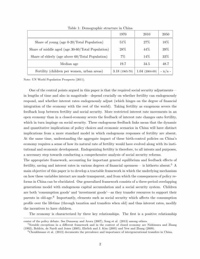
Table 1: Demographic structure in China

1970 2010 2050

Share of young (age 0-20/Total Population) 51% 27% 18%

Share of middle aged (age 30-60/Total Population) 28% 44% 39%

Share of elderly (age above 60/Total Population) 7% 14% 33%

Median age 19.7 34.5 48.7

Fertility (children per women, urban areas) 3.18 (1965-70) 1.04 (2004-09) - n/a -

Note: UN World Population Prospects (2011).

One of the central points argued in this paper is that the required social security adjustments—

in lengths of time and also in magnitude—depend crucially on whether fertility can endogenously

respond, and whether interest rates endogenously adjust (which hinges on the degree of financial

integration of the economy with the rest of the world). Taking fertility as exogenous severs the

feedback loop between fertility and social security. More restricted interest rate movements in an

open economy than in a closed-economy severs the feedback of interest rate changes onto fertility,

which in turn impinge on social security. These endogenous feedback links mean that the dynamic

and quantitative implications of policy choices and economic scenarios in China will have distinct

implications from a more standard model in which endogenous responses of fertility are absent.

At the same time, understanding the aggregate impact of these birth-control policies on China’s

economy requires a sense of how its natural rate of fertility would have evolved along with its insti-

tutional and economic development. Endogenizing fertility is therefore, to all intents and purposes,

a necessary step towards conducting a comprehensive analysis of social security reforms.

The appropriate framework, accounting for important general equilibrium and feedback effects of

fertility, saving and interest rates in various degrees of financial openness— is hitherto absent.5 A

main objective of this paper is to develop a tractable framework in which the underlying mechanism

on how these variables interact are made transparent, and from which the consequences of policy re-

forms in China can be elucidated. Our generalized framework consists of a three-period overlapping

generations model with endogenous capital accumulation and a social security system. Children

are both ‘consumption goods’ and ‘investment goods’—as they transfer resources to support their

parents in old-age.6 Importantly, elements such as social security which affects the consumption

profile over the lifetime (through taxation and transfers when old) and thus interest rates, modify

the incentives to have children.

The economy is characterized by three key relationships. The first is a positive relationship

center of the policy debate. See Dunaway and Arora (2007), Song et al. (2013) among others.5Notable exceptions in a different framework and in the context of closed economy are Nishimura and Zhang

(1992), Boldrin, de Nardi and Jones (2005), Ehrlich and J. Kim (2005) and Yew and Zhang (2009).6Choukhmane et al. (2013) documents the prevalence and importance of intergenerational transfers in China.

2

between fertility and interest rates based on optimal saving and investment decisions. A greater

number of children increases the marginal productivity of capital and thus investment. Moreover,

it is associated with higher expenditures and larger transfers in old-age, both of which lead to

lower saving. Higher fertility thus leads to higher interest rates. The second condition is a negative

relationship based on optimal fertility choices: higher interest rate-to-wage-ratio lowers the financial

benefits of children and hence discourages fertility. The third key relationship is determined by a

sustainable social security system, which embeds endogenous changes in social security variables

when fertility adjusts. We first show analytically how the interactions of these relationships conjoin

to determine interest rates, fertility and social security contribution rates in the long run. We also

investigate how these variables react in the long-run to social security reforms, fertility policies and

growth evolutions–both under autarky and under financial integration.

The framework can be used to analyze the social security implications of various important

policy reforms that policymakers in China are facing, and expose their potentially conflicting or

offsetting nature. The policy choices that are imminent and likely to interact include 1) fertility

controls and their relaxation; 2) social security reforms, in particular increasing the coverage and

generosity of the existing system; and 3) capital account liberalization. On its own, these policies

may impinge on the social security system to various degrees, but our analysis suggests that the

combination and sequence of these reforms may be more or less costly in terms of the amount of

fiscal pressure it exerts on the pension system.

In particular, we show that the population aging subsequent to the one child policy puts less

strain on the generosity of the pension system in a closed economy than in an open economy.

In other words, postponing capital market integration may ease social security pressure and the

amount of tax hikes required to maintain social security benefits. The reason is that although lower

fertility requires an increase in taxes, the endogenous fall in interest rates due to higher saving can

limit the fiscal pressure by indirectly stimulating fertility. Thus, the adverse effects of the one child

policy on the pension system are more severe in an open economy than in a closed economy—and

are also predicted to be more severe in a framework that takes into account the endogenous response

of fertility. The feedback of an increase of social security taxes onto a reduction in fertility— which

then feeds back again onto contribution rates— can imply a much longer adjustment in taxes–thus

making the persistence of the one child policy shock much larger than under a model that treats

fertility as exogenous.

Increasing the coverage and the generosity of the social security system is high on the government

agenda, but is obviously somewhat in conflict with recent policies that aimed at reducing fertility

when it comes to concerns about the financing of the pension system. Jointly undertaken, social

security taxes would need to rise substantially. Postponing this reform after the relaxation of

fertility constraints may ease social security pressure; but also, increasing benefits in conjunction

to (or after) liberalizing the capital account may be more cost-effective. Adverse interest rate

movements following the reform, would thus be mitigated. This, in turn, would limit the endogenous

fall in fertility and thus the necessary tax increase to finance the generosity of the new pension

3

system.

Finally, we investigate how a permanently slower growth path in China would affect the path of

reforms and the sustainability of the pension system. We find that the fiscal pressure on the existing

system could be potentially very large if the growth slowdown occurs in the coming years when the

generation of only-child become the main contributors, and even more so if China liberalize further

its capital account. We find that the required tax rises accompanying the growth slowdown is

actually larger than what standard models with exogenous fertility would predict. As the benefits

of children in terms of future transfers fall—in the face of slower growth—the optimal fertility also

falls, putting further strain on the social security system. In an open economy, the fall in fertility is

even larger since interest rates do not fall (or less so) as growth falls. Thus, under this slow growth

scenario, in order to avoid an immediate and massive tax hike, China would potentially have to

choose between reducing the generosity of the existing system or postponing its capital account

liberalization.

Section 2 describes the basic elements of the framework and the relationships governing the

key endogenous variables in the economy. An analytically tractable case of a paygo system in the

long run is analyzed in Section 3. Section 4 shows the result of various policy experiments under a

closed-economy and open economy setting. Section 5 concludes.

2 Model

The structure of the economy is close to Coeurdacier, Guibaud and Jin (2013), and is characterized

by an overlapping generations structure in which agents live for three periods: youth (y), middle-age

(m), and old-age (o). The measure of total population Lt at date t comprises the three co-existing

generations. We denote Lγ,t the population of each generation γ = {y,m, o} such that the overall

population Lt satisfies: Lt = Ly,t + Lm,t + Lo,t. At the end of their youth period (y), individuals

start working, supplying one unit of labor inelastically but also decide their number of children.

Denote nt the number of children (per head) that young individuals decide to have at the end of

the period t. Then, demographics evolves according to: Ly,t+1 = ntLy,t. Individuals also work in

middle-age (m), and retire when old (o).

2.1 Production

Let Kt−1 denote the aggregate capital stock at the beginning of period t and etLy,t+Lm,t the total

labor input employed in period t, where et is the relative efficiency of young workers (et < 1). The

gross output in country i is:

Yt = (Kt−1)α [At (etLy,t + Lm,t)]1−α ,

where 0 < α < 1, and At is country-specific productivity. We let gA,t denote the exogenous (gross)

rate of growth of productivity, so that At = gA,tAt−1. The capital stock depreciates at a rate δ and

4

evolves according the standard law of motion:

Kt = (1− δ)Kt−1 + It.

where It denotes investment at date t.

Factor markets are competitive so that each factor, capital and labor, earns its marginal product.

Thus, the wage rates per unit of labor in youth and middle age for country i are

wiy,t = et(1− α)At (kt−1)α , wim,t = (1− α)At (kt−1)α , (1)

where kt−1 ≡ Kt−1/[At(etLy,t + Lm,t)] denotes the capital-effective-labor ratio. The rental rate

earned by capital in production equals the marginal product of capital, riK,t = α (kt−1)α−1. The

gross rate of return earned between period t−1 and t in country i is thereforeRt = 1−δ+α (kt−1)α−1.

In what follows, we will make the following assumption throughout, for analytical convenience:

Assumption 1 Full depreciation: δ = 1

This implies that the rate of return to capital equalizes the marginal productivity of capital:

Rt = α (kt−1)α−1 . (2)

This assumption is reasonably innocuous and quantitatively unimportant given that a period cor-

responds to one generation in the current model.

2.2 The Social Security System

The social security system encapsulates a pay-as-you-go system (PAYGO), a fully-funded system,

or more generally, some combination of the two. Each young and middle-aged agent in period t+ 1

pays, respectively, a Social Security tax in the amount of τt+1wy,t+1 and τt+1wm,t+1. An old retiree

in period t + 1 receives social security benefits in the amount of σt+1wm,t, where σt+1 represents

the replacement ratio at date t+ 1.

The government can run budget surpluses and deficits to finance the social security system. Let

Bt denote government assets accumulated at the end of period t. The sources and uses of the funds

for the social security system in period t+ 1 are thus given by

τt+1wy,t+1Ly,t+1 + τt+1wm,t+1Lm,t+1 +Rt+1Bt = σt+1wm,tLo,t+1 +Bt+1. (3)

The left hand side of the equation represents the sources of funds for the Social security system in

period t, which consist of Social Security taxes plus gross returns on assets. The right hand side

represents the uses of funds by the Social Security system in the same period, including retirement

benefits paid to old consumers and the purchase of capital to hold in the trust fund (or issuance of

5

government debt for Bt+1 < 0). Using Eqs. 1 and 2, Eq. 3 can be rewritten as:

(1− α)τt+1nt−1gA,t+1 (1 + ntet+1)

(ktkt−1

)α+ αkα−1

t bt (1 + nt−1et) (4)

= (1− α)σt+1 + bt+1nt−1gA,t+1 (1 + ntet+1)

(ktkt−1

)α,

where bt denotes government assets as a share of GDP: bt ≡ BtYt

. Eq. 4 captures the dynamics of the

social security system, defined by the set of variables {bt; τt;σt}, as a function of the endogenous

state variables {kt;nt−1}. This equation makes clear the impact of growth and the interest rate

on the financing of a social security system. Higher growth driven by productivity, demographics,

or capital accumulation tends to relax the budget constraint through its impact on tax revenues,

relative to spending (first term on the left-hand side), but also implies higher investment into capital

for a given bt+1 > 0. If the government has positive assets (bt > 0), a higher rate of return on

capital (αkα−1t ) increases revenues.

2.3 Households decisions

Consider an individual who is young in period t. The agent supplies inelastically one unit of

labor in youth and in middle-age, and earns a wage rate wy,t and wm,t+1, which is used, in each

period, for consumption and asset accumulation ay,t and am,t+1. At the end of period t, the young

agent then makes the decision on the number of children nt to bear. In middle-age, in t + 1, the

agent transfers a combined amount of Tm,t+1 to his nt children and parents. In old-age, the agent

consumes all available resources, which is financed by gross return on accumulated assets, Ram,t+1,

transfers from children To,t+2 and social security transfers σt+2wm,t+1. A consumer thus maximizes

the life-time utility including benefits from having nt children:

Ut = log(cy,t) + v log(nt) + β log(cm,t+1) + β2 log(co,t+2)

where v > 0 reflects the preference for children, and 0 < β < 1. The sequence of budget constraints

obeys:

cy,t + ayt = (1− τt)wy,tcm,t+1 + am,t+1 = (1− τt+1)wm,t+1 +Rt+1ay,t + Tm,t+1 (5)

co,t+2 = Rt+2am,t+1 + σt+2wm,t+1 + To,t+2.

Without loss of generality, the cost of raising kids is assumed to be paid by parents in middle-

age, in period t + 1, for a child born at the end of period t. The total cost of raising nt children

falls in the mold of a time-cost that is proportional to current wages, φntwm,t+1, where φ > 0.

These costs can be interpreted as “mouth-to-feed-costs” and education costs, which are substantial

6

for Chinese households.7 Transfers made to the middle-aged agent’s parents amount to a fraction

ψn$−1t−1 /$ of current labor income wm,t+1, with ψ > 0 and $ > 0. ψ denotes the degree of altruism

towards parents and is an important feature of Chinese society, where old-age support is mainly

provided by the children (see Choukhmane et al. (2013)). As in Choukhmane et al. (2013), we

assume that the fraction of wages transferred to parents is decreasing in the number of siblings—to

capture the possibility of free-riding among siblings sharing the burden of transfers. The intensity

of free-riding is captured by (1−$).8

The combined amount of transfers made by the middle-aged agent in period t+1 to his children

and parents thus satisfy

Tm,t+1 = −

(φnt + ψ

n$−1t−1

$

)wm,t+1.

In old-age, agents become receivers of transfers from a total of nt number of children:

To,t+2 = ψn$t$wm,t+2.

Assumption 2 The young are subject to a credit constraint which is binding in all periods:

ay,t+1 = −θwm,t+1

Rt+1, (6)

which permits the young to borrow up to a constant fraction θ of the present value of future wage

income. This assumption is realistic in the case of China, where borrowing by young generations is

very small. The parameter θ allows us to generate realistic age-saving profiles and captures the lack

of financial development of the Chinese credit market (see Coeurdacier, Guibaud and Jin (2013)).9

Saving decisions. The assumption of log utility implies that the optimal consumption of the

middle-age is a constant fraction of the present value of lifetime resources, which consist of dis-

posable income—of what remains after the repayment of debt from the previous period—and the

present value of transfers to be received in old-age, less current transfers to children and parents:

cm,t+1 =1

1 + β

[(1− τt+1 − θ − φnt −

ψn$−1t−1

$

)wm,t+1 +

ψn$t$

wm,t+2

Rt+2+σt+2wm,t+1

Rt+2

]7Transfers from middle-aged to their children are not assumed to enter the consumption of the young. Implicitly,

we assume that this is consumed in an interim period when children, before entering the labor markets (or equivalently,costs of children are a pure resource cost). Note that, with credit constraints on young individuals, this is howeverirrelevant as long as those are binding (Assumption 2).

8See Boldrin and Jones (2002) for a model where transfers towards parents are decreasing in the number of siblingsas the outcome of a strategic game between siblings.

9We assume that the income profile is steep enough (e small enough and/or gA high enough relative to θ). Wecheck in our simulations that the constraint is indeed binding.

7

It follows from Eq. 5 that the optimal asset holding of a middle-aged individual is

am,t+1 =β

1 + β

[(1− τt+1 − θ − φnt −

ψn$−1t−1

$

)wm,t+1 −

ψn$tβ$

wm,t+2

Rt+2− σt+2

β

wm,t+1

Rt+2

](7)

Eq. 7 is important in that it shows the partial equilibrium effects of fertility, the interest rate

and the social security system on saving. Higher fertility (nt) tends to lower saving because of

higher spending on children (‘expenditure channel’), and because of higher expected future transfers

received from children (‘transfer channel’). Similarly, higher social security contributions τt+1 and

a higher expected replacement rate σt+2 reduces the incentives to save by respectively lowering

disposable income and increasing future wealth. Finally, a lower interest rate raises the present

value of wealth and thus lowers saving—-with the income and substitution effects associated with

interest rate changes canceling out under the assumption of log-utility.

Fertility decisions. Fertility decisions hinge on equating the marginal utility of bearing an

additional child compared to the net marginal cost of raising the child:

v

nt=

β

cm,t+1

(φwm,t+1 −

ψn$−1t wm,t+2

Rt+2

). (8)

The right hand side is the net cost, in terms of the consumption good, of having an additional child.

The net cost is the current marginal cost of rearing a child, ∂Tm,t+1/∂nt less the present value of

the benefit from receiving transfers next period from an additional child, ∂To,t+2/∂nt. Children

are, at the same time, ‘consumption goods’ (through the parameter v), and ‘investment goods’.

Lower wage growth relative to interest rates lowers the returns to investing in children (relative to

investing in capital), and thus discourages having children. Eq. 8 can be rewritten as

v

nt=

β (1 + β) (φkαt −ψαn

$−1t gA,t+2kt+1)[(

1− τt+1 − θ − φnt − ψ$n

$−1t−1

)kαt + ψ

α$n$t gA,t+2kt+1 + σt+2

α k1−αt+1 k

αt

] , (9)

and is the first equation describing the dynamics of the two endogenous state variables {kt;nt−1},for a given path of social security system {bt; τt;σt}t≥0.

2.4 Capital markets clearing

The market clearing condition for capital markets equalizes the supply of wealth by households and

the government to the aggregate capital stock:

Lm,t+1am,t+1 + Ly,t+1ay,t+1 +Bt+1 = Kt+1,

Using the equations describing the wealth accumulation by households (Eqs. 6 and 7) and the

equilibrium wages and interest rate (Eqs. 1 and 2), the capital market clearing equation can be

8

written as

ntgA,t+2kt+1

[(1 + et+2nt+1)− θ(1− α

α) +

1

1 + β

ψ

$n$−1t (

1− αα

)

](10)

=βkαt

(1 + β)

[(1− τt+1 − θ − φnt −

ψ

$n$−1t−1

)(1− α)− σt+2

β(1− αα

)k1−αt+1 + bt+1 (1 + et+1nt)

]Eq. 10 is our second equation describing the dynamics of our two endogenous state variables

{kt;nt−1} for a given path of social security system {bt; τt;σt}t≥0. This equation equalizes the

demand for capital to its supply by middle-aged consumers and the government. Importantly, the

demand for capital (left hand-side) increases with demographic and productivity growth through

their positive impact on the marginal productivity of capital.

The dynamics of the state variables {kt;nt−1} is thus defined by the equations corresponding the

fertility choice (Eq. 9) and the equilibrium in the capital market (Eq. 10), where the social security

system defined by the path of {bt; τt;σt}t≥0 satisfies the budget constraint of the government (Eq.

4) at all dates. We now turn to the analysis of the model at its steady-state.

2.5 Steady-state analysis: three fundamental equations

To obtain analytical solutions for the long run, we make the following additional assumptions,

Assumption 3 Transfers are not subject to decreasing returns in children: $ = 1

Assumption 4 e = 0

Assumption 5 τ < 1− θ − ψ

Apart from analytical convenience in making the first two assumptions, the third one limits

the scope of taxation for social security to make sure that individuals will want a strictly positive

number of children. With these assumptions we arrive at the three key relationships linking social

security variables, the interest rate and fertility that characterize the economy in the steady-state,

when kt = k; nt = n; gA,t = gA; σt = σ; τt = τ ; bt = b at all dates.

KK curve. The first relationship derives from the capital markets condition, Eq. 10, and captures

saving dynamics:

(KK) : RKK(n+

) =ngAΦ + σ

β (1− τ − θ − φn− ψ) + (1 + β) b1−α

, (11)

where Φ ≡ (1 + β)(

α1−α + θ + ψ

1+β

).

This KK curve is upward sloping with respect to n, based on four different channels. First is the

standard effect that higher population growth (higher fertility) increases the marginal productivity

of capital. Second, a greater number of children raises total expenditures which tends to reduce

9

saving and drives up the rate of return (‘expenditure channel’). This channel disappears whenever

the cost of children φ goes to zero. The third channel relates to the transfers children confer

to parents. With higher fertility, middle-age savers expect to receive larger transfers when old,

which lowers saving and increases the rate of interest (‘transfer channel’). This channel disappears

whenever ψ goes to zero.10 Fourth and last, higher fertility increases the proportion of young

borrowers, increasing the interest rate. This effect is dampened when θ is small. Hence, the

steepness of the interest curve with respect to n is larger whenever the cost of children (φ) are large,

altruism towards parents (ψ) is large and whenever θ is large (i.e more relaxed credit constraints).

The partial equilibrium comparative statics on RKK—-holding social security variables (τ, σ)

and fertility n constant— yield

∂RKK∂θ

> 0;∂RKK∂b

< 0;∂RKK∂gA

> 0.

Less borrowing from households (lower θ), or from the government (higher b), lowers the interest

rate. Higher productivity growth gA increases the interest rate by raising the marginal productivity

of capital, an effect that tends to be magnified whenever altruism towards parents (ψ) is larger—-as

higher growth also increases expected transfers received from children when old and thus lowers

incentives to save.

NN curve. The second important relationship derives from Eq. 9 and captures optimal fertility

decisions:

(NN) : RNN (n−

) =ngAψ + λ0σ

nφ− λ0 (1− τ − θ − ψ), (12)

where we denote λ0 ≡(

vv+β(1+β)

). The NN curve is downward sloping with respect to n,

∂RNN∂n

= −λ0ψgA (1− τ − θ − ψ) + σφ

[nφ− λ0 (1− τ − θ − ψ)]2< 0,

for two main reasons. First, in light of children being ‘investment goods’, higher interest rates

tend to lower the returns from children (relative to capital) and thus discourage fertility (term

proportional to ψgA). This effect disappears when ψ goes to zero. Second, with respect to children

being ‘consumption goods’, higher interest rates which lower intertemporal wealth from social

security transfers (term proportional to σφ) lower consumption—-and hence fertility.

The partial equilibrium comparative statics on n abstracting from social security variables (τ, σ),

and holding R constant are:

10The simplifying assumption of $ = 1 also matters for the response of interest rate to changes in fertility. With$ < 1, on one hand, higher fertility lowers ascendant transfers from middle-aged to older parents, increasing theirdisposable income and saving, thus lowering the real interest rate. On the other hand, when expected receivedtransfers in old-age increase less than proportionally with fertility, the ‘transfer effect’ through which higher fertilityincreases interest rates is dampened.

10

∂n

∂φ< 0;

∂n

∂v> 0;

∂n

∂θ< 0;

∂n

∂gA> 0

For a given R, higher costs of children (resp. lower preference for children) reduce fertility. Tighter

credit constraints (lower θ) increases disposable income for consumption when middle-aged and

thus the demand for children. Most relevant to our analysis is the effect of growth: a growth

slowdown (a fall in gA), holding R constant, is associated with lower returns on children and thus

fertility. This effect is absent when ψ = 0.

Equilibrium for a given social security scheme. A steady-state equilibrium of fertility n

and interest rate R (or equivalently capital per efficiency unit k) for a given social security scheme

(b, τ, σ) is such that RKK(n) = RNN (n) = R. The limiting values of RKK and RNN as n → n =

λ0

(1−τ−θ−ψ

φ

)+and n→ n =

(1−τ−θ−ψ

φ + (1+β)bβ(1−α)

)−satisfy

limn→n

RKK < limn→n

RNN = +∞,

limn→n

RKK = +∞ > limn→n

RNN .

The slopes of these two curves are respectively positive and negative throughout, thus guaranteeing

that their intersection is unique. The equilibrium fertility rate lies in the space λ0

(1−τ−θ−ψ

φ

)<

n <(

1−τ−θ−ψφ + (1+β)b

β(1−α)

). In Figure 1, the equilibrium for a given set of parameter values under

laissez-faire (σ = τ = b = 0), is illustrated graphically.

SS curve. The third equation derives from Eq. 9

(SS) :

(R

ngA− 1

)b =

σ

ngA− τ, (13)

and underpins the sustainability of the government budget in the long-run. The right hand-side

is the (primary) government deficit in a given period, where expenditures are captured by the

replacement rate σ divided by the rate of demographic growth (i.e ratio of contributing workers to

retirees) multiplied by the rate of productivity growth. Higher economic growth (either through

population or productivity growth) relaxes the government’s budget constraint. The left hand side

determines the amount of government assets necessary to stabilize the budget deficit. A higher

interest rate compared to economic growth (ngA) requires a positive government asset over GDP

(b) to finance its primary deficit. On the contrary, the case in which R < ngA allows the government

to stabilize its debt while running primary deficits.

Equations 11, 12 and 13 together determine the long-run equilibrium fertility and interest rate

in the economy. The social security policies are assumed to be exogenous in the present study, and

the government can let either σ, τ , or b to adjust, ensuring 13 holds. Letting b adjust can lead

to multiple equilibria in the steady state (see Appendix 6), and for this reason we choose first to

11

Figure 1: Equilibrium interest rate and fertility

4%

6%

8%

10%

12%

1 1,5 2 2,5 3 3,5 4 4,5

Fertility

Real interest rate (annual basis)

(NN)

(KK)

nmaxnLF

Rnmax

RLF

Notes: Parameters values: Fertility is 2n. β = 0.99 (annual basis), gA − 1 = 4.5% (annual basis), v = 0.12, θ = 1%,α = 30%, φ =8%,ψ = 10%, σ = τ = b = 0 (Laissez Faire). nmax = 1 (’two-children policy’)

ignore this case and consider the alternative cases in which the government targets a given level of

asset over GDP (b) and let the tax rate (τ) and/or the replacement rate (σ) adjust.

2.6 Laissez Faire

We now examine fertility, interest rate and saving dynamics in autarky under laissez-faire—an

absence of a social security system (τt = σt = bt = 0 for all t). This benchmark case helps build

intuition on the workings of the baseline model.

Endogenous Fertility. Let st+1 ≡ Kt+1/Yt+1. In this closed economy with full depreciation, st

is both the national saving rate and investment rate. Using Eqs. 9 and 10, we have the following

expressions for national saving and fertility:

st+1 =αβ(1− θ − φnt − ψ)

Φ(14)

nt =λ0

φ(1− θ − ψ) +

ψ

αφst+1, (15)

which leads to the following proposition:

Proposition 1 Under laissez-faire and endogenous fertility, the saving rate and the fertility rate

12

are constant at all dates t > 0, with

st = sLF =αβ(1− θ − ψ)(1− λ0)

Φ + βψ(16)

nt = nLF =

(1− θ − ψ

φ

)(λ0Φ + βψ

Φ + βψ

). (17)

Comparative Statics. We proceed to investigate the effects of changes in various parameters on

the equilibrium fertility rate and national saving rate in a closed economy—under unconstrained

fertility and binding fertility constraints.

Productivity growth. A fall in productivity growth gA lowers the interest rate as the marginal

productivity of capital falls. However, under laissez faire, growth does not affect fertility and

saving. These decisions are indeed driven by the growth to interest rate ratio, gA/R, which is

independent of gA.11

Credit Constraints. A loosening of credit constraints (higher θ) leads to lower equilibrium fertility

rate and a lower equilibrium saving rate though higher borrowing of the young and lower disposable

income of the middle-aged-savers: dnLF

dθ < 0, dsLF

dθ < 0. This implies that a country with tighter

credit constraints have a higher desired fertility rate than countries with looser credit constraints.

Increased borrowing of the young reduces disposable income in middle age, thus lowering the

number of desired children. A reduced number of children tends to raise the saving rate—partially

offsetting the negative impact of looser credit constraints on saving.

Preference for Children and Costs of Children. Since ∂nLF /∂v > 0, an increase in v raises the

desired number of children nt, given any st+1. The KK curve is unaffected, thus resulting in a

higher fertility rate and a lower equilibrium national saving rate. Changes to v thus exogenously

alter the optimal rate of fertility, and affects the saving rate only through its impact on fertility.

The optimal laissez-faire fertility rate nLF also shows that ∂nLF /∂φ < 0. Higher costs to children

leads to fewer desired children, given any st+1, and higher costs to children lowers saving rate, given

any fertility rate nt. This amounts to a leftward shift of the NN curve and a downward shift of

the KK curve. The net effect is a lower fertility rate, and an unaltered national saving rate: while

higher costs to children leads to a lower saving rate, fewer equilibrium number of children raises

the saving rate; the two effects exactly cancel out in determining national saving rate.

Constrained Fertility. Suppose that the economy starts from the steady state prior to period t,

and fertility becomes binding from t onwards. The NN curve is no longer relevant and is replaced

by a vertical line nt = nmax for all t (shown as a two-children policy in Figure 1). When fertility

constraints are binding (nmax < nLF ), then the national saving rate is higher under constrained

fertility than under unconstrained fertility: snmax > sLF and the interest rate lower Rnmax <

11According to the KK and NN schedules, a constant gA/R ratio is the outcome of two-counteracting forces thatexactly offset each other: lower productivity growth reduces incentives to have children (NN curve shifts to the left);it also lowers the equilibrium interest rate, which tends to increase fertility (KK curve shifts to the right). In otherwords, incentives to have children depends on the ratio gA/R, and optimal saving/borrowing decisions also dependon this ratio, which is independent on productivity growth under laissez-faire.

13

RLF (see Figure 1 for a two-children policy). An exogenous reduction in fertility thus raises the

national saving rate as a consequence of a reduction in total expenditures on children. There is

an additional channel through which fertility could affect saving: lower fertility reduces expected

transfers, stimulating saving (‘transfer channel’). This channel turns out to cancel out in the

autarky general equilibrium due to the adjustment of the interest rate.12 It is however important

to keep in mind that in an open economy setting, this channel will be in operation.

3 Social Security and Fertility Policies: PAYGO in the Long Run

When social security variables can interact with saving and fertility, implications of policy reforms

and growth shocks can be quite different from those under laissez-faire. We proceed to analyze

these issues in an analytically tractable case—where the social security system is characterized by

a paygo scheme, and where social security variables are constant in the long run. We show that the

impact of fertility policies and growth shocks crucially hinge on whether a social security system is

in place, and in particular—under what particular scheme it operates.

3.1 PAYGO in the Closed-Economy

In a PAYGO system (closed economy), b = 0, and the three fundamental steady-state equations

(Eq. 11, 12 and 13) become, in the steady state:

RKK(n) =ngAΦ + σ

β (1− τ − θ − φn− ψ)(KK)

RNN (n) =ngAψ + λ0σ

nφ− λ0 (1− τ − θ − ψ)(NN)

τ =σ

ngA(SS).

Social security policies. Two types of social security schemes are considered, and the combi-

nation thereof is ignored albeit in principle possible. Given a set of parameters, the government

can either target a certain replacement rate σ and let taxes τ adjust, or vice-versa. A σ–scheme

refers to the case where the government sets the replacement ratio σ = σ and lets τ adjust; and a

τ–scheme where the government sets τ = τ and lets σ adjust. Solving for equilibrium fertility rate

n (τ) and interest rate R (τ) after substituting in Eq. (SS) gives:

n (τ) =(1− τ − θ − ψ)

φ

(ψβ + λ0Φ + λ0(1 + β)τ

ψβ + Φ + (1 + βλ0)τ

); R (τ) =

(gAβφ

)(ψβ + λ0Φ + λ0(1 + β)τ

1− λ0

).

Thus, equilibrium fertility rate ns and interest rate Rs under a paygo system of scheme s = {τ ; σ}12The expected total amount of transfers received by parents from children in period t+ 1 is ψn

wt+2

Rt+2, an increase

in n would tend to raise expected transfers and lower saving. The general equilibrium effect of changes in thewage-interest ratio offset the rise in n (wt+2/Rt+2 falls)–and in this case—perfectly.

14

satisfy the following equations:13

nτ = n(τ) ; Rτ = R(τ)

nσ = n(τσ) ; Rσ = R(τσ) where τσ =σ

nσgA.

Compared to laissez-faire (τ = σ = 0), the interest rate is higher in the presence of social security

(τ > 0; σ > 0): a reduced need to save in middle-age together with lower disposable income lower

saving rates and raises the interest rate. The associated fertility rate is also lower with social

security than without—the reasons for which are two-fold: taxes to finance social security lowers

disposable income for consumption in middle-age and thus the demand for children (children as

consumption goods); moreover, by increasing the rate of interest, social security reduces fertility

(children as investment goods). Roughly speaking, children and social security are substitutes.

This is illustrated on Figure 2 where the steady-state equilibrium moves from the laissez-faire to

a paygo system under scheme σ with a replacement rate σ = 30%. Similar results hold under a τ

scheme.

Figure 2: Equilibrium interest rate and fertility: from Laissez Faire to Paygo

4%

6%

8%

10%

12%

1 1,5 2 2,5 3 3,5 4 4,5

Fertility

Real interest rate (annual basis)

(NN)

(KK)Rσ

nσ

Notes: Parameters values: Fertility is 2n. β = 0.99 (annual basis), gA − 1 = 4.5% (annual basis), v = 0.12, θ = 1%,α = 30%, φ =8%,ψ = 10%; σ = τ = 0 under Laissez Faire and moves to a Paygo with σ = 30%.

Importantly, a feedback loop between endogenous taxes τσ and fertility nσ emerges under a

13Equilibrium fertility and interest rate are provided implicitly under a σ–scheme (i.e as a function of endogenoustax policy τσ). We do so to keep expressions compact. Proof of existence (and uniqueness) of the equilibrium for nσand Rσ is relegated into Appendix 6, together with the space of σ for which a solution exists (σ bounded above).

15

σ–scheme: higher replacement rate σ leads to higher taxes, which lowers fertility by reducing

consumption, and lower fertility in turn feeds back onto raising taxes further (viability of the

pension program)— and so on and so forth.

Productivity growth and social security. Any effect of growth on interest rates and fertility

must come through necessary adjustments in social security, as we have shown that in the laissez-

faire case fertility is independent of gA. It turns out that the particular type of scheme under

a paygo system bears very different consequences. Under a τ–scheme, gA/R being independent

of gA means that the demand for children as investment goods is unchanged as before. And as

disposable income in middle-aged also remains constant with a fixed τ , consumption is unaffected,14

and optimal fertility is again independent of growth. Under a σ–scheme however, taxes must rise to

balance the budget—-lowering disposable income, consumption and thus the demand for children.

This fall in fertility forces the government to raise taxes even more to keep replacement rates

constant— inducing a further fall in fertility. The long-run equilibrium is the outcome of this

feedback loop between fertility and taxes. Under any of the two schemes, the interest rate will

be lower under slower productivity growth, due to the fall in the marginal product of capital, but

more so under a σ–scheme than under a τ–scheme. The reason is that the reduction in fertility

under a σ–scheme exerts upward pressure on saving (net of investment) and thereby push down

the interest rate further. These results are given by the following proposition:

Proposition 2 Under endogenous fertility, a fall in productivity growth gA lowers fertility under a

paygo scheme where taxes endogenously adjust (σ–scheme) but leave fertility unchanged if replace-

ment rate endogenously adjust (τ–scheme). Interest rates fall in both cases but by more under a

σ–scheme. That is,

∂n

∂gA|σ

>∂n

∂gA|τ

= 0

∂R

∂gA|σ

>∂R

∂gA|τ> 0.

Constrained fertility and social security. Fertility constraints–such as the one-child policy–

that lowers fertility makes it is necessary for the replacement ratio or taxes to adjust to keep the

PAYGO system viable (Equation (SS)). It is important to note that the impact on the interest

rate of such a policy is different under laissez-faire and under a paygo system, but also different

under the our two alternatives schemes of the paygo system (σ and τ), as demonstrated in the

following proposition:

Proposition 3 Implementing a binding fertility constraint n = nmax raises saving by more under a

paygo scheme where replacement ratios endogenously adjust (τ–scheme) than under a paygo scheme

where taxes endogenously adjust (σ–scheme). That is,

14This includes the fact that discounted social security benefits, which also depends on g/R, does not affect thepropensity to consume.

16

∂R

∂nmax|σ>

∂R

∂nmax|τ.

These results emanate directly from comparative statics conducted on R as determined by the

KK-curve.15 When replacement ratios endogenously adjust, it falls one for one with the fall in n,

causing saving to rise and the interest rate to fall. On the other hand, when σ is constant, taxes

have to rise in order to guarantee the same replacement ratio—inducing saving to fall and the

interest rate to rise. The direct effect of a fall in n is to raise saving in both cases, but some of that

is offset under a tax increase (σ–scheme), whereas it is magnified under a τ–scheme.

We now examine the case in which the country is a small open economy and takes the world

interest as given. While this assumption is arguable for the case of China, the example is never-

theless helpful to build intuition regarding the difference between autarky and the open economy.

One can interpret our results under a small open economy as a limiting case where interest rate do

not adjust at all.

3.2 PAYGO in a Small Open Economy

The dynamics under a small open economy (SOE) are characterized by Eqs.4 and 9, but where kt,

in any period t, is determined by an efficiency condition that equalizes the marginal productivity

of capital to the world interest rate. Consequently, the KK curve is a horizontal line. The other

two equations are, in the steady-state,

R∗ =ngAψ + λ0σ

nφ− λ0 (1− τ − θ − ψ), (NN)(

R∗

ngA− 1

)b =

σ

ngA− τ (SS),

where R∗

denotes the steady-state world interest rate. Under a paygo system (b = 0) following a

σ–scheme, fertility and taxes satisfy

nσ = λ0(1− τσ − θ − ψ) + σ/R∗

φ− ψ (gA/R∗); τσ =

σ

nσgA.

Comparative statics. Fertility reacts less to an increase in σ in the closed-economy scenario

than in the SOE scenario. The prevention of any rise in the interest rate shuts off the feedback

effect onto lower fertility, and consequently, reduces the amount of rise in τσ necessary to balance

the budget. Increasing the replacement rate is thus less costly under an open economy. On the

contrary, fertility reacts more to a fall in productivity growth rate gA in an open economy. The

15Under binding fertility constraints, n = nmax replaces the NN curve and the KK-curve determines the equilib-rium interest rate that correspond to nmax.

17

reason is that in a closed-economy setting, the fall in fertility due to lower growth is dampened by

a fall in the interest rate. When this dampening effect is shut off in the SOE case, the fertility falls

by more and is thus matched by a greater increase in taxes to balance the budget.

4 Policy and Growth Experiments

The transitory and long-run consequences of relevant policy reforms are analyzed under a more

general setting. The three experiments surround (1) a one child policy and its relaxation; (2)

increases in social security benefits; and (3) a permanent growth slowdown in China, as well as

a selected combination thereof. Results predicted by a model with exogenous and endogenous

fertility, under a closed and a small open economy are compared.

4.1 Steady-state and Calibration

In the policy experiments that follow, the economy always starts from a well-defined initial steady-

state under endogenous fertility. The calibration of the initial steady state under autarky is given

in Table 2, along with values for the structural parameters. While our exercise is not meant to be

quantitative, structural parameters are calibrated using reasonable values based on household micro

data (Urban Household Survey for individual income and consumption data and China Health and

Retirement Longitudinal Study (CHARLS) for transfer data; see Choukhmane et al. (2013) for a

detailed description of the data). One period corresponds to a generation, approximately 23 years.

Financial integration of a small open economy. In all our experiments described below, the

economy starts of at t = 1 from its autarkic steady-state. We assume that when liberalizing its

capital account at t = 2 in the SOE case, China opens up to a world with a higher interest rate—an

assumption that is based on the observed direction of capital flows from China to the rest of the

world. Here, the world interest rate is set to R∗ = 9.2% on an annual basis, slightly above the high

growth/high fertility autarky steady-state in China (see Table 2).16 Other parameters values for

China will be kept identical.

The effect of integration is present in all of the policy reforms analyzed under the SOE case–in

addition to the possible effect on fertility brought about by the policy reforms–and therefore merits

mention. The rise in interest rates following integration triggers a fall in the natural rate of fertility

(and higher taxes) from its autarkic level as illustrated by the SOE steady-state in Table 2.17 The

direct impact of integration, however, will be quite restricted in our experiments, as the difference

between the autarkic and world interest rate is rather small.

In the policy experiments that follow, we perform numerical simulations of social security and

fertility policies as well as growth experiments under a σ–scheme. We focus on a σ–scheme since

we aim at assessing how the economy would adjust to shocks while maintaining the generosity of

16Note that such a value for R∗ is in the ballpark of a calibrated US-style economy.17The response of fertility to financial integration depends on the slope of the NN curve. A high level of intra-family

intergenerational transfers in China (ψ relative to v) strengthens the response.

18

Table 2: Benchmark Calibration: steady-state and structural parameters

Autarky Steady-state

nσ 1.43 Fertility of 2.86Rσ − 1 9.04% Annual basisτσ 7.6% /

SOE Steady-state

nσ 1.39 Fertility of 2.78R∗ − 1 9.20% Annual basis. Based on a reasonable calibration for the U.S.τσ 7.8% /

Parameter Calibrated value Target/Description (Data source)

β 0.99 Annual basisgA − 1 4.5% Annual basis. Total Factor Productivity growth rate (1980-2010)v 0.12 Targeted to match the fertility in 1970-1972 of 2.8-3 (Census)θ 1% Saving rate of the 20-25 (UHS)α 30% Capital Shareω 0.7 Elasticity of transfers to elderly w.r.t the nb. of siblings (CHARLS)φ 8% Average education expenditures over income (UHS)ψ 10% Choukhmane et al. (2013), Curtis et al. (2011)σ 30% Aggregate replacement ratios adjusted for coverage (UHS)b 0 Paygo simulation

the existing system. The model dynamics are governed by Eqs. 4, 9, 10 and under a PAYGO

system (b = 0). In the exogenous fertility model, fertility stays at its steady-state value except

when fertility constraints are binding. In the SOE case, interest rate is kept constant to its world

level R∗ after integration (t = 2). Robustness checks with respect to parameters and social security

schemes are relegated to Section 4.4.

4.2 Policy experiments (σ–scheme)

The one child policy. Under this policy, fertility is constrained to one child per household for

one generation (during t = 2), and then fully relaxed at t = 3. The real interest rate, fertility and

taxes under a closed-economy model with exogenous fertility and one under endogenous fertility

are shown in Fig. 3. Juxtaposed is also the small-open economy endogenous fertility case.18

The one-child policy leads to a large rise in saving (net of investment) and a required tax hike

when the one-child generation becomes the main contributors to social security (t = 4)—under

all scenarios. In the closed-economy cases, the large rise in saving occasions a large fall in the

interest rate on impact, followed by a gradual rise as the fertility constraint is relaxed. Taxes rise

the most in the small open economy case, by 14.2% (from 7.8% to 22%) on impact, compared to

18We omit the small open economy exogenous fertility model for convenience, as the dynamics of taxes is similarin the autarky and small open economy case under exogenous fertility.

19

Figure 3: The one child policy.

1 2 3 4 5 65

6

7

8

9

10Net interest rate (annualized, in percentage points)

Autarky & endogenous fertilityAutarky & exogenous fertilitySOE & endogenous fertility

1 2 3 4 5 61

1.5

2

2.5

3Fertility (number of children per family)


1 2 3 4 5 65

10

15

20

25Contribution rate (in percentage points)


Notes: Parameters values are shown in Table 2. The one-child policy is implemented at t=2 and relaxed at t=3.

8.5% on impact in the autarky cases. Comparing with a closed-economy model where fertility is

exogenous, taxes remain persistently higher in the endogenous fertility model (both under autarky

and SOE). This is due to two important feedback loops. The first one is the feedback of higher tax

rates onto lower fertility and back onto higher taxes. This is the feedback effect that is absent in

the exogenous autarky case. Hence, tax rates are higher for longer and interest rates revert more

slowly in the endogenous fertility case (lower fertility limits the fall in saving and thus contains

the subsequent rise in interest rate). The second one is the feedback loop from lower interest rates

to higher fertility–which tends to ease pressure on social security and mitigate the fall in fertility

triggered by the policy. This is the feedback loop that is absent in the small open economy, which

thus features a lower fertility rate. Required tax rates are therefore substantially larger in the open

economy.

In sum, the one child policy shock is more persistent in the endogenous fertility case compared to

the exogenous fertility case under autarky, and is more costly in the open economy than in autarky.

A rise in the replacement ratio σ. As China is currently expanding the coverage of its social

20

Figure 4: A rise in the replacement ratio σ.

1 2 3 4 5 69

9.2

9.4

9.6

9.8



1 2 3 4 5 62.6

2.7

2.8

2.9



1 2 3 4 5 66

8

10

12



Notes: Parameters values are shown in Table 2. The replacement ratio is increased permanently at t=3 from σ = 30%to σ = 50%.

security system, this reform is tantamount to a rise in the replacement ratio in our model.19 The

experiment we analyze consists of a rise in σ from its initial value of 30% to 50%. Results are

shown in Fig. 4. Taxes must rise to stabilize government budget. Under autarky, the immediate

fall in saving resulting from higher social security benefits and subsequently from the required tax

hike exert continued upward pressure on interest rates. Under endogenous fertility however, the

drop in fertility due to higher taxes limits the impact of the drop in saving and thus the rise in

interest rates. The reduction in fertility entails a larger rise in taxes—from 7.6% to 13.9%, under

endogenous fertility compared to only 12.7% under exogenous fertility. Restraints on the interest

rate in the open economy however limits the extent of the fall in fertility compared to autarky and

thus the required rise in tax rates is smaller. In sum, increasing the generosity of social security

benefits requires higher tax rates with longer adjustment under endogenous fertility compared to

exogenous fertility, and is also less costly in an open economy than in a closed-economy.

In an another experiment (not shown), we combine the two experiments described above. We

19Note that the replacement ratio has recently fallen in China but the increase in coverage has been quite largesuch that overall Chinese households are better insured for their old age (see ISSA Report (2013)).

21

analyze the necessary tax adjustment if the Chinese government were to increase the generosity of

the existing system (rising the replacement ratio σ from 30% to 50%) exactly when the generation

of only-child is contributing to the pension system (t = 4). As expected, the tax hike at t = 4 is

very large (taxes increase by 28% in the SOE case and by 18% under autarky). In the short-term,

taxes increase more in the open economy. To the opposite, in the long-term, as the generation

of only child goes into retirement, taxes fall in both cases but remain persistently higher under

autarky.

4.3 Growth experiments (σ–scheme)

Growth has been remarkably high in China over the last thirty years. The recent expansion of

social security coverage in China has been facilitated by this growth success but questions emerge

regarding the growth performance of China in the next decades. We investigate the implications

of a growth slowdown in the next experiments.

A Permanent Slowdown in Growth. In this experiment, China experiences a permanent

growth slowdown from an annual rate of productivity growth of 4.5% to 1.5% (occurring at t = 3).

Results are displayed in Fig. 5.

The permanent fall in the growth rate leads to an immediate and permanent decline in the

autarky interest rates. Higher taxes are required to balance the budget in the face of lower growth,

and the resulting lower saving subsequently dampens the fall in the interest rate. Taxes rise

progressively from 7.6% to 14.9% under exogenous fertility, to 17% under endogenous fertility in

autarky, and to 28% in an open economy. A notable difference between the autarkic cases, is

the larger and more persistent fall in interest rates with endogenous fertility—where the drop in

optimal fertility (due to lower growth) stimulates saving and further lowers the interest rate. The

main difference that marks the closed and open economy endogenous fertility models is the much

larger drop in fertility in the latter. Both low growth and the required tax hike lead to a fall in

the natural fertility rate, but the lower interest rate acts as a counteracting force to the decline in

fertility—an effect that is absent in the SOE scenario. The key parameter determining the response

of fertility to a change in growth over the interest rate (gA/R) is ψ relative to v. With a high value

of ψ (e.g. China), it is expected that a growth slowdown without the counteracting fall in interest

rates (SOE) may trigger a very large fall in fertility. The natural rate of fertility thus declines from

2.86 children to 2.5 children per couple in the closed economy case and to 1.6 in the open economy

case. The fall of fertility to around 1.6 can be treated as an upper bound of the impact —as interest

rates, in reality, do adjust somewhat.

In summary, without the feedback loop of lower fertility and higher tax rates, the exogenous

fertility model predicts the lowest increase in taxes, and without the feedback of lower interest rates

onto higher fertility that tends ease social security pressure, the SOE case thus features the highest

required tax rate. The impact of a permanently growth slowdown is more costly for the stability

of the social security system in an open economy. This means that, facing a growth slowdown,

22

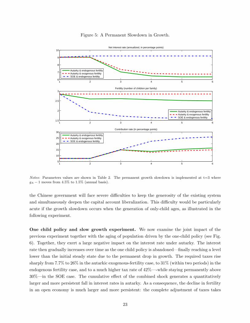
Figure 5: A Permanent Slowdown in Growth.

1 2 3 4 5 66

7

8

9



1 2 3 4 5 61.5

2

2.5



1 2 3 4 5 65

10

15

20

25



Notes: Parameters values are shown in Table 2. The permanent growth slowdown is implemented at t=3 wheregA − 1 moves from 4.5% to 1.5% (annual basis).

the Chinese government will face severe difficulties to keep the generosity of the existing system

and simultaneously deepen the capital account liberalization. This difficulty would be particularly

acute if the growth slowdown occurs when the generation of only-child ages, as illustrated in the

following experiment.

One child policy and slow growth experiment. We now examine the joint impact of the

previous experiment together with the aging of population driven by the one-child policy (see Fig.

6). Together, they exert a large negative impact on the interest rate under autarky. The interest

rate then gradually increases over time as the one child policy is abandoned—finally reaching a level

lower than the initial steady state due to the permanent drop in growth. The required taxes rise

sharply from 7.7% to 26% in the autarkic exogenous-fertility case, to 31% (within two periods) in the

endogenous fertility case, and to a much higher tax rate of 42%—-while staying permanently above

30%—in the SOE case. The cumulative effect of the combined shock generates a quantitatively

larger and more persistent fall in interest rates in autarky. As a consequence, the decline in fertility

in an open economy is much larger and more persistent: the complete adjustment of taxes takes

23

Figure 6: One child policy and slow growth experiment.

1 2 3 4 5 64

6

8



1 2 3 4 5 61

1.5

2

2.5



1 2 3 4 5 60

10

20

30

40



Notes: Parameters values are shown in Table 2. The one-child policy is implemented at t=2 and relaxed at t=3. Thepermanent growth slowdown is implemented at t=3 where gA − 1 moves from 4.5% to 1.5% (annual basis).

four generations. In this experiment, fertility is permanently depressed, and a two-children policy

would no longer be binding in the open economy case. Note that extending the analysis to a large

open economy model, the international consequences would be considerable: the world interest rate

could be persistently depressed under this scenario, due to low growth, high taxes and low fertility

in China.

4.4 Sensitivity analysis

Alternative social security schemes. We investigate how our results depend on the social

security scheme under consideration. An alternative scenario moving away from a paygo system is

the existence of a trust fund, whereby the government holding positive assets (b > 0) can smooth

negative productivity or demographic shocks over time by partly selling its stock of assets. We

assume that the government in China starts out with b = 0.02 before the implementation of the

one child policy.20 If the government maintains it at the same level, any increase in the interest

20In our model, this is equivalent to roughly 30% of the steady-state autarky capital stock that is owned by thegovernment. This is a small share of GDP due to a low capital output ratio in a model with full depreciation and

24

Figure 7: The one child policy: running down the trust fund.

1 2 3 4 5 65

6

7

8

9



1 2 3 4 5 61

1.5

2

2.5

3

3.5Fertility (number of children per family)


1 2 3 4 5 64

6

8

10



Notes: Structural parameters are shown in Table 2 but China starts with b = 0.02 > 0. The one-child policy isimplemented at t=2 and relaxed at t=3. China reduces b to 0.0175 at t=3 and 0 at t=4.

rate will tend to relax its budget constraint. This makes financial integration under a higher world

interest rate than the autarkic level beneficial for the government. In a simulation with b = 0.02

(keeping other parameters constant), for instance, taxes actually fall following integration: the fall

in revenues due to the integration-induced fertility drop is more than compensated by an increase

due to the higher return on government assets. The feedback loop from higher taxes to lower

fertility does not take effect and fertility therefore falls by less.

It is also important to understand the impact of the trust fund on the autarky steady-state: with

a higher b, interest rate is lower (KK shifts upwards) and fertility higher. Conversely, a permanent

fall in the trust fund will increase the interest rate and lower fertility— in the autarkic steady-state.

This means that when the trust fund is used to smooth a negative shock, the government is faced

with a trade-off in the autarky case: limiting the rise in taxes in the short-run, at the expense of

permanently higher taxes in the future.

This is illustrated in Fig. 7 in our one-child policy experiment. The government is assumed

to exhaust its trust fund in two generations after the policy implementation (t = 3, 4), and tax

three periods only.

25

contributions increases significantly less between t = 2 and t = 4 (by 6.5% compared to 9% when

b is kept constant). However, under endogenous fertility, such a policy incurs permanent long-run

costs —in the form of higher taxes and lower fertility in the long-run. Similar findings hold under

the experiment of a permanent growth slowdown.

In the open economy, this trade-off between short-run gains (smoothing) and long-run costs

largely disappears when adverse interest rate movements responding to the fall in the trust fund

are absent. Consequently, only the direct impact of taxes is in operation—smaller revenues due to

the exhaustion of the trust fund and correspondingly higher taxes. The required rise in taxes is

thus significantly less in the SOE case compared to the autarky case. This is also true all along

the transition where the government does not face adverse interest rates movements when selling

assets. The example illustrates clearly how running down the trust fund is more effective to smooth

negative shocks in an open economy as taxes (resp. fertility) are lower (resp. higher) in the former.

Sensitivity to structural parameters.

Intergenerational transfers. We examine the role of intergenerational transfers in generating these

results by adopting an alternative calibration where the steady-state fertility is everywhere identical

except for ψ = 0 presently considered.21 This economy behaves very closely to all experiments

conducted under exogenous fertility— in the sense that fertility reacts less to shocks to growth or

to σ, and adjusts faster to a one-child policy shock. The reason is that when children are no longer

‘investment goods’, fertility reacts much less to changes in the interest rate (NN is steeper) and to

expected changes in growth.

An alternative but equally interesting question is how the Chinese economy would adjust if

altruism towards the parents were to decrease. We investigate the steady-state properties of our

benchmark economy allowing for the parameter ψ to fall from 10% to 5%. Consider the long-run

equilibrium under a σ scheme: both a reduced desire to have children (NN curve shifts left), and a

substitution towards higher saving (KK curve shifts down) would ensue. The equilibrium interest

rate and fertility rate will both fall: under current parameters values, n would fall from 2.85 to 2.5,

and R from 9.04% to 7.7%, while taxes would increase from 7.6% to 8.8%. The fall in fertility and

the rise in taxes would be much higher in an open economy—in the absence of the counteracting

interest rate movements that tend to stimulate fertility. The consequence of a disintegration of the

traditional mode of saving is thus to put more strain on the social security system (unless binding

fertility constraints are kept in place), and exert even larger pressure if capital accounts were open.

Financial development. We also examine the importance of credit constraints, considering that

financial development in China may harbinger a permanent loosening of credit constraints for

households. The model predicts that easing credit constraints would put pressure on a PAYGO

social security system by reducing the equilibrium natural rate of fertility—the extent of which

depends on how strongly fertility reacts to changes in the interest rate (stronger under high ψ).

In the experiment considered, θ rises from 0.01 to 0.1, keeping other parameters constant. Looser

21The preference parameter for children, v, is adjusted to 0.19 to keep fertility constant in the steady-state.

26

credit constraints occasions less saving, for any given fertility rate, and a higher interest rate

under autarky (KK curve shifts up), which further reduces optimal fertility. Tax rates rise to

keep replacement ratios constant. In the autarkic steady state, the interest rate rises to 9.6%

(annualized), fertility falls by 0.3 children (per family) and social security contributions increase

from 7.6% to 9.4%. The transitory dynamics are also affected by financial development of this kind:

with higher θ, aggregate savings respond more to changes in growth. Consequently, interest rates

are also more sensitive to changes in growth—and thus also fertility and taxes. Relaxing credit

constraints, however, is less costly in an open economy, as the additional feedback link between

higher interest rates and lower fertility is absent and the drop in fertility is more limited.

5 Conclusion

Domestic policy reforms along with potential growth shocks in China interact in a way that makes

the timing of the various reforms particularly important to limit the fiscal pressure exerted on the

pension program. In some instances, certain policy reforms jointly undertaken can imply massive

and sudden adjustments in tax contributions that could have otherwise been smaller and better

smoothed over time. Capital account liberalization can either aid or exacerbate the strain on social

security that fertility policies or social security reforms may bring. These interactions are absent

when fertility decisions are taken to be exogenous, and hence our framework–in which interlinkages

between interest rates, fertility and social security are key—yield very different predictions on

the magnitude and dynamics of the necessary fiscal adjustments to maintain (or extend) existing

pension system.

China’s various reforms can also have international ramifications in an increasingly globalised

economy, and the extent of these effects depends on the basic asymmetries that characterise coun-

tries like China and the U.S. Differences in fertility, financial development, and pension systems all

play an important role, and any such policy changes can spillover onto the social security system

abroad. Some policies can potentially relieve pressure on the sustainability of the social security

system in the U.S. For example, policies aimed at reducing fertility in China can inadvertently

stimulate fertility abroad, as can a growth slowdown in China. All in all, policies that lead to

low fertility and consequently high contributions to social security in China might leave the world

interest rates depressed for a long time to come.

27

References

[1] Abel, Andrew B., N. Gregory Mankiw, Lawrence H. Summers, and Richard J. Zeckhauser.

1989. ‘Assessing Dynamic Efficiency: Theory and Evidence. Review of Economic Studies,

56(1): 119.

[2] Abel. A., 2001. The Social Security Trust Fund, the Riskless Interest Rate, and Capital Ac-

cumulation, in John Campbell and Martin Feldstein (eds.) Risk Aspects of Investment-Based

Social Security Reform, Chicago: The University of Chicago Press, Chapter 5, pp. 153 - 193.

[3] Attanasio, O. and Kitao, S., and Violante, G., 2007. Global demographic trends and social

security reform. Journal of Monetary Economics, Elsevier, vol. 54(1), pages 144-198, January.

[4] Auerbach, A., and L. Kotlikoff. 1987. Dynamic Fiscal Policy. Cambridge: Cambridge Univer-

sity Press.

[5] Banerjee, A., Meng, X., Qian, N. and T. Porzion, 2013, Fertility and Household saving: Ev-

idence from a General Equilibrium Model and Micro Data from Urban China. Mimeo Yale

University.

[6] Boldrin, M. and L. Jones, 2002. Mortality, Fertility and Saving in a Malthusian Economy.

Review of Economic Dynamics 5, 775-814.

[7] Boldrin, M., De Nardi, M., and L. Jones, 2005. Fertility and Social Security. Research Depart-

ment Staff Report 359, Federal Reserve Bank of Minneapolis.

[8] Choukhmane, Coeurdacier, and Jin, 2013. The One-Child Policy and Household Saving,

mimeo, London School of Economics.

[9] Coeurdacier, Nicolas, Stephane Guibaud, and Keyu Jin, 2013. Credit Constraints and Growth

in a Global Economy. mimeo.

[10] Curtis, C., Lugauer, S. and N.C. Mark, 2011. Demographic Patterns and Household Saving in

China. Mimeo.

[11] Dunaway, S.V., and V. Arora. 2007. Pension Reform in China: The Need for a New Approach.

IMF Working Paper WP/07/109.

[12] Ehrlich, I. and J. Kim, 2005. Social security and demographic trends: Theory and evidence

from the international experience, Review of Economic Dynamics, 10, 55-77.

[13] Feldstein, Martin. 1999. Social Security Pension Reform in China. China Economic Review,

10(2): 99-107.

[14] Fehr, H., Jokisch, S. and L.J. Kotlikoff, 2007. Will China Eat Our Lunch or Take Us to Dinner?

Simulating the Transition Paths of the United States, the European Union, Japan, and China,

28

in Fiscal Policy and Management in East Asia, NBER-EASE, Volume 16, University of Chicago

Press.

[15] Ge, S., D.T. Yang, and J. Zhang, 2012. Population Policies, Demographic Structural Changes,

and the Chinese Household Saving Puzzle., IZA Discussion paper 7026.

[16] International Social Security Association, 2013. Towards universal social security coverage in

China. ISSA report, Social security coverage extension in the BRICs, Chapter 4.

[17] Nishimura, K and Zhang, J., 1992. Pay-as-you-go Public Pensions with Endogenous Fertility.

Journal of Public Economics, 239-58.

[18] Song, Storesletten, Wang, and Zilibotti, 2013. Sharing high growth across generations: pen-

sions and demographic Transition in China, mimeo.

[19] Wei, S.J. and W. Zhang, 2011. The Competitive Saving Motive: Evidence from Rising Sex

Ratios and saving Rates in China. Journal of Political Economy, vol. 119(3), 511-564.

[20] Yew, S. L. and Zhang, J., 2009. Optimal social security in a dynastic model with human capital

externalities, fertility and endogenous growth. Journal of Public Economics, 93, 605-619.

29

6 Appendix: Proofs

Multiple equilibria and government asset policy

State variables are (kt, bt, nt) whose dynamics is described by Eqs. 4, 9 and 10. We focus on the

dynamic adjustment of b for a given for a given fiscal policy (τ, σ).

Steady-state analysis (three fundamental equations):

(SS) : τ +

(R

ngA− 1

)b

1− α=

σ

ngA(18)

(KK) : R =ngAΦ + σ

β (1− τ − θ − φn− ψ) + (1 + β) b1−α

(19)

(NN) : R =ψngA + λ0σ

nφ− λ0 (1− τ − θ − ψ)(20)

with Φ = (1 + β)(

α1−α + θ + ψ

1+β

)and λ0 = v

[β(1+β)+v] .

We have three equations and three unknown (k, b, n) or equivalently (R, b, n) with R = αkα−1.

First solve for b(n) using Eqs. 18 and 19:

τ +

Φ + σngA− β (1− τ − θ − φn− ψ)− (1 + β) b

1−α(β (1− τ − θ − φn− ψ) + (1 + β) b

1−α

) b

1− α=

σ

ngA

Or equivalently:

A

(b

1− α

)2

−B(n)

(b

1− α

)+ C(n) = 0

with: A = (1 + β); B(n) =[(1 + β)

(τ − σ

ngA

)+ Φ + σ

ngA− β (1− τ − θ − φn− ψ)

];

C(n) =(

σngA− τ)β (1− τ − θ − φn− ψ).

The discriminant of this second-order polynomial is:

∆(n) = B(n)2 + 4 (1 + β)

(τ − σ

ngA

)β (1− τ − θ − φn− ψ)

If ∆(n) > 0 (note that this is always the case if τ > σngA

), two solutions for b(n) denoted b1(n) and

b2(n) with b1(n) < b2(n) for all n:

b1(n) = (1− α)B(n)−

√∆(n)

2 (1 + β); b2(n) = (1− α)

B(n) +√

∆(n)

2 (1 + β)> 0

Then, using Eqs. 19 and 20 gives:

(1 + β)b(n)

1− α=

(Φ + σ

ngA

)(nφ− λ0 (1− τ − θ − ψ))

ψ + λ0σngA

− β (1− τ − θ − φn− ψ)

30

The intersection between b(n) and b1(n) (resp. b(n) and b2(n)), when it exists, gives n1 and n2

(equilibrium fertility associated to b1 and b2). It also gives conditions on the space (τ, σ) for which

the two equilibria exist as function of the parameters. R1 and R2 are immediately deduced using

Eq. 19. This also means that letting b adjust can lead to multiple equilibria (or none if τ is too

small). Note that we also have R1 > R2 and n2 > n1. One can show that the stable equilibrium is

(R2, b2, n2).

Endogenous steady-state fertility and interest rate under a σ–scheme

We use the equilibrium conditions implied by the (KK) and (NN) curves under a paygo:

n (τ) =(1− τ − θ − ψ)

φ

(ψβ + λ0Φ + λ0(1 + β)τ

ψβ + Φ + (1 + βλ0)τ

); R (τ) =

(gAβφ

)(ψβ + λ0Φ + λ0(1 + β)τ

1− λ0

)Equilibrium fertility rate nσ and interest rate Rσ under a σ–scheme satisfy:

nσ = n(τσ) ; Rσ = R(τσ) where τσ =σ

nσgA

Introducing F (n) = φn1− σ

ngA−θ−ψ and G(n) = (ψβ+λ0Φ)ngA+λ0(1+β)σ

(ψβ+Φ)ngA+(1+βλ0)σ .

Using nσ = n( σnσgA

), the equilibrium fertility nσ must satisfy:

F (nσ) = G(nσ).

Assumption 6 σ < (1−θ−ψ)2gAλ0(1+β)4φ(1+βλ0) ; τ < (1−θ−ψ)

2

Assumption 6 provides an upper bound for σ (and restricts the state space for taxation) such

that an equilibrium is unique and well defined as stated in the following proposition:

Lemma 1 Under Assumption 6, there is a unique equilibrium fertility nσ which satisfies F (nσ) =

G(nσ).

Proof. Let us study the variations of F (n) and G(n):

∂F

∂n=φ(

1− θ − ψ − 2 σngA

)(1− σ

ngA − θ − ψ)2

F is increasing for n > 2 σ(1−θ−ψ)gA

; limn→∞ F = +∞ and minF = F (2 σ(1−θ−ψ)gA

) = 4φ σ(1−θ−ψ)2gA

.

∂G

∂n= gAσ

β(1− λ0) [ψ − λ0Φ]

((ψβ + Φ)nσgA + (1 + βλ0)σ)2

– if ψ > λ0Φ:

G is increasing; limn→∞G = ψβ+λ0Φψβ+Φ < limn→∞ F ; limn→0G = λ0(1+β)

1+βλ0> 4φ σ

(1−θ−ψ)2gA= minF

(Assumption 6).

31

The equation F (nσ) = G(nσ) has thus two solutions, one between [ σ(1−θ−ψ)gA

; 2 σ(1−θ−ψ)gA

] and one

above 2 σ(1−θ−ψ)gA

.

If n < 2 σ(1−θ−ψ)gA

, then σngA

= τ > (1−θ−ψ)2 . This equilibrium is ruled out by Assumption 6 (as it

is unstable and features very high taxes and fertility close to zero).

Finally, note that for n < σ(1−θ−ψ)gA

, F (n) < 0 < G(n) (F and G do not cross for n < σ(1−θ−ψ)gA

).

Thus the equilibrium exists and is unique with nσ > 2 σ(1−θ−ψ)gA

.

– if ψ < λ0Φ:

G is decreasing; limn→∞G = ψβ+λ0Φψβ+Φ < limn→∞ F ; limn→0G = λ0(1+β)

1+βλ0> 4φ σ

(1−θ−ψ)2gA= minF

(Assumption 6).

Same reasoning as previously applies.

Rσ is immediately deduced using Rσ = R(τσ) and τσ = σnσgA

.

32

Social Security and Fertility Policies

Documents

Transcript of Social Security and Fertility Policies