Social Learning and Consumer Demand∗

Markus M. MobiusHarvard University and NBER

Paul NiehausHarvard University

Tanya S. RosenblatWesleyan University and IAS

December 17, 2005

Abstract

We conduct a field experiment with the student population at a large privateuniversity to measure the channels through which social learning affects consumerdemand, and to compare them to traditional advertising channels. We find strongsocial learning effects which are at least as big as effects of advertising. Moreover,even though social network effect decline with social distance they decline less fastthan the number of acquaintances increases - therefore, distant acquaintances mighthave the largest effects on social learning. In the baseline stage of the experiment wemeasure (a) social networks of more than 2,300 undergraduates and (b) individualpreference vectors for the product features of six broad product classes (such as cellphones) using a conjoint analysis with monetary incentives. This allows us to predictsubjects’ valuations for a specific product sample (such as a specific cell phone). Inthe treatment stage we conduct various treatments with random sub-samples ofsubjects. (1) We distribute about 50-100 actual product samples for each of thesix product categories to some subjects. When these subjects pick up a product weprime them to focus attention to a random subset of up to 6 product features. (2)All other subjects are treated with up to two specific ads emphasizing one particularfeature of a product through a popular online webpage which is used daily by moststudents and through print ads in the main student newspaper. In the followup stagewe conduct a survey and auction with all subjects to measure (i) their informationabout the features of each of our specific products and (ii) their valuations for eachproduct.

JEL Classification: C91, C92, C93, D44, M37, Z13Keywords: social networks, economic experiments, experimental auctions, conjoint analysissocial learning, peer effects, advertising

∗Very preliminary and incomplete - please do not cite. We would like to thank Rachel Croson, MurielNiederle and Al Roth for very helpful comments. We benefited from discussions with participants at 2005International ESA Meetings and 2005 SITE Conference. We are particularly grateful to facebook.comfor working together with us and letting us use their website and to T-mobile, Phillips, Qdoba, StudentAdvantage and Baptiste Power Yoga for product samples.

1

1 Introduction

We conduct a field experiment at a large private university to measure the channels

through which social learning affects consumer demand and to compare them to tradi-

tional advertising channels. A number of recent papers using both observational and

experimental data have highlighted the importance of networks in technological progress

and knowledge diffusion (Conley and Udry 2002, Foster and Rosenzweig 1995, Kremer

and Miguel 2003) which can translate into significant welfare gains for better connected

agents who have lower unemployment rates, higher incomes (Topa 2001, Granovetter

1974, Jackson and Calvo-Armengol 2004, Munshi 2003) and higher savings rates (Duflo

and Saez 2003).

In our work we build on the existing literature and estimate structural models of

social learning in the context of demand for standard consumer products such as cell

phones and MP3 players. There is ample anecdotal evidence which suggests that fads

and fashions are particularly strong in these industries. Moreover, we can compare the

strength of social learning to the impact of traditional advertising which provides a nat-

ural benchmark to gauge the importance of peer effects. Finally, the distinction between

informative and persuasive advertising is nicely mirrored by the distinction between ac-

tual social learning channels which affect agent’s information about an unknown product

and ‘social persuasion’ channels which change their utility function.

To motivate our experimental design we introduce a simple theoretical framework

where we distinguish between two social learning and one social persuasion channel.

Strong social learning functions through agents sharing actual information about a prod-

uct, while weak social learning operates by drawing inferences from friends’ consumption

choices and valuations for new products. For example, a consumer might learn factual

information about a new cell phone from friends who have either purchased the phone

already or have read about it in magazines and ads. Alternatively, the consumer might

just observe that his better informed friends purchase and/or enjoy using a certain cell

phone and infer that the cell phone has high value to him as well.

One goal of our design is to create a sufficient number of instruments to disentangle

weak social learning from social persuasion where a consumer’s valuation is directly

2

affected by the valuation of his friends’ for a product. We think that social persuasion

comes closest to what is colloquially called a ‘fashion’.

Our design consists of the three main stages. In the baseline stage we measure the

social networks of more than 2,300 undergraduates that constitute about 40 percent of

the student population. We use a novel methodology to measure the structure of the

social network by using a game with financial incentives to encourage truthful revelation

of links. We also measure students’ preferences for six different product classes such as

cell phones or MP3 players by using online ‘configurators’.1 Our approach to conjoint

analysis is novel because we make truthful revelation of preferences incentive compatible.

Our configurators allow students to specify a baseline valuation for a generic member of

the class or products (such as a generic cell phone) and to specify specific valuations for

features (such as camera phone, email, messaging etc.). We ensure incentive compatibil-

ity by informing subjects that their answers will be used to construct a composite ‘bid’

for one specific new product which might or might not have certain features listed in

the configurator. A major advantage of configurators is that we can predict a subjects’

valuation for a new product without telling him or her about the exact features of this

product (which would mitigate social learning).

In the treatment stage we select a random sub-sample of students and distribute

between 50 and 80 samples of new products (431 in total) to this group which they

can use for a period of about 4 weeks. When a subject picks up his or her product we

conduct various randomized treatments with them which are designed to affect both their

information about the product and their valuation of the product. In an information

treatment we draw the attention of a subject to certain features of the product while

a ‘buzz’ treatment is designed to increase a subjects’ excitement and enthusiasm about

a product without affecting her information about a product (such as adding extra

money to a cell phone account). Subject who do not receive products are exposed to

randomized online and print ads. Online ads are individually administered through a

popular webpage which is used daily by the majority of students and which requires a

login while print ads are randomized by student dorm. Each subjects is exposed to up1Configurators have also been used for conjoint analysis in marketing science. This field has generated

an enormous literature on how to measure and decompose individual consumers’ preferences (Green andSrinivasan 1978, Luce and Tukey 1964, Hauser and Rao 2002, Ely Dahan and Toubia 2002).

3

to two different online/print ads for two distinct products and each ad emphasizes one

randomly selected feature of the product (such as the email capability in a cell phone).

In the final followup stage we ask all subjects to submit a bid for each of the six specific

products as well as answer a short quiz on how much they know about the products’

features. We find out about participants’ confidence in answering these questions by

using a novel framing of the incentive compatible BDM procedure. We then analyze

how information disseminated during the treatment stage through the social network

and how strongly it shifted subjects’ valuations.

In section 2 we introduce social learning and persuasion channels using a simple

model. Section 3 explains our experimental design. Results are presented in section 4.

In section 5 we outline how we want to expand our research agenda in future work.

2 Theoretical Framework

We develop a simple theoretical model to formally define the social learning channels

and motivate our experimental design.

2.1 Social Network

There are n agents who live on a connected social network N . We denote the distance

between two agents i and j on the network with dij which takes the value 1 if i is a

direct friend of j, the value 2 if i is the friend of friend of j etc.

2.2 Product Features

A product has K possible features which are described by a vector

m = (m1, .., mk, ..mK). (1)

Each feature k is either implemented (mk = 0) or not implemented (mk = 1). Examples

of features are quality and functionality of the product (such as weight and capacity of

an MP3 player).

4

2.3 Preferences

An agent i forms a (monetary) valuation vi of the product which depends on how much

she appreciates its features. The agent attaches value bi,k to feature mk where each bi,k

is distributed with mean 0 and precision hb. The total value the agent can extract from

those features is the vector product:

b′i ·m (2)

This is the ‘rational’ value of the product based on agent i’s individual preferences and

the features of the product.

Moreover, we also allow the agent’s utility to depend on another’s agent j’s valuation

who owns the product already:

vi = b′i ·m + β(dij)vj (3)

This equation captures the social influence channel which is stronger the longer both

agents interact with each other and which in return depends on social distance dij .2

2.4 Communication

Every agent knows her own preferences but only users of the product know the feature

set m. The expected value of the product in the absence of any information on features

is 0 (save for social influence effects).

However, agent i can learn about the value of the feature set m in two ways. First,

j might directly tell her about the product’s features features (strong learning). Second,

j might tell i his valuation vj = b′j ·m. Depending on the correlation between i’s and

j’s preferences agent i can improve her estimate of how much she values the features of

the product herself.

Strong Social Learning

Agent j and i communicate with each other with probability c(dij) which is decreasing

in social distance. Conditional on communicating with j agent i learns the full set of2We ignore the reflection effect according to which j’s valuation is in return affected by i’s value. This

is possible as long as social influence flows from owners/users of the good to non-owners but not viceversa.

5

features m with probability p(b′i ·m, vj). We allow this probability to depend on both

i’s and j’s preferences because communication is endogenous: an agent is more likely to

tell somebody else about the product either if she values it more highly or if she knows

that the other agent does so.

Weak Social Learning

Sometimes agents i and j communicate (with probability c(dij) but i does not learn

the feature set of the product but instead only learns j’s value vj = b′j ·m for the product.

This occurs with probability q(b′i ·m, vj) which like p(·) is endogenous and depends on

both agent’s preferences.

We assume that agent i knows with probability h(dij) the degree to which her pref-

erences are correlated with the preferences of agent j. Otherwise she assumes that there

is zero correlation between preferences (and hence nothing to learn). The actual degree

of correlation is ρij . Hence we obtain:

E(b′i ·m|vj) = h(dij)ρijvj (4)

A special case is where preferences are perfectly correlated and ρij = 1: if agent i knows

this to be true then she can perfectly infer her valuation of the product’s set of features

from observing vj .

3 Experimental Design

We obtain samples of 6 different products - three electronics durables which we refer to

in shorthand as ‘gadgets’ from now on and three non-durables which we will refer to

as ‘services’. We looked for gadgets and services which are (a) affordable for at least

a large number of students costing between US$70 and US$200 and (b) new products

which only had been just or relatively recently released. We focused on new products so

that subjects could actually learn something through social and advertising channels.

The gadgets included a cellphone with PDA functions, a digital camcorder in the

size of a USB stick and a portable sound system.3 The services included a bundle of five3The products were provided to us at a discount by US mobile phone company T-Mobile and the

consumer electronics division of Philips respectively. The cellphone/PDA and camcorder had been

6

restaurant vouchers to a new Mexican restaurant, a student discount card and a bundle

of five Yoga classes to a local Yoga studio.4

3.1 Baseline Stage

3.1.1 Network Elicitation

We worked with facebook.com to measure the social networks of undergraduates at a

large private university. This social networking website was founded in January 2004

and is by now available to about 500,000 students at more than 200 campuses across

the U.S. All students on campus with valid university email address are eligible to sign

up. Like any old-style facebook it gives access to students’ profiles, their interests and

hobbies. A unique feature of the electronic facebook is the ability to specify friends and

to see the friends of friends. This allows subjects to explore their social network and

has proved to be a highly popular (and addictive) activity for many students. On our

campus about 90 percent of students have signed up to the facebook.com. Of those,

almost 70 percent login daily and 90 percent at least once a week.

The only problem with facebook.com from our perspective is that students discrimi-

nate too little when signing up their friends: the mean number of friends is approximately

30-40 and it is not uncommon to have more than 100 ‘friends’. We therefore use an aux-

iliary game to elicit ‘true’ friends.

This ‘trivia game’ became a full feature of facebook.com for all students on our

campus. First, students were invited to select 10 friends amongst their facebook friends.

To illustrate the game design, assume student A lists student B. At some point B receives

an email asking one multiple-choice question such as: “What time do you get up in the

morning?”. As soon as B answered the question about himself A receives an email asking

the same question about B. Student A has at most 20 seconds to answer the questions

(to prevent gaming). In the case of a correct answer both could earn prizes with some

probability.5

released a few months before our study while the sound system was released during the course of thestudy.

4All vouchers were non-transferable and had student ID numbers printed on the voucher. The discountcard also showed a student’s name and stores routinely made random checks of students’ identity.

5We used an alternative elicitation game in November/December 2003 in two Harvard houses. Stu-dents were invited to visit a webpage where they could select 10 friends for each house and received a

7

We expected that the more time two students spent interacting the more likely they

would be to name each other in this game. We recruited 2939 undergraduates (which

constitutes 46% of the undergraduate population) to participate in the trivia game with

participation rates higher among seniors, juniors and sophomores (45%, 52%, and 53%,

respectively) and 34% by freshmen. The average acquisition cost per subject was $2.50.

The resulting social network data consists of 23,600 links from participants, 12,782

links between participants with 6,880 of these symmetric (resulting in 3,440 coordinated

friendships). Similar to 2003 results, we construct the network using “or” link definition.

Therefore, 5576 out of 6389 undergraduates (87%) participated or were named. The net-

work data constitutes one giant cluster with an average path length between participants

of 4.2. The average cluster coefficient captures the probability that a friend’s friend is

my friend and was 17% for our social network.6

3.1.2 Measuring Preference Vectors

We identified the salient features m of a product using promotional materials from the

manufacturers. Participants in the trivia game received an email invitation in April 2005

to complete a brief online experiment designed to measure a subject’s preference vector

b over the attributes of each of the products.

Importantly, we did not tell subjects the name or the features of each product but

instead only described the general product class and the potential features of the product.

For example, our camcorder product was described generically to subjects as a device

which could record 10 minutes of video and the following add-on features were presented:

(1) produced by a major brand, (2) inbuilt MP3 player, (3) 25 min. video capacity instead

of 10 min. (4) compatibility with Mac OS. The features of this camcorder product lived

in the following four-dimensional space:

{generic, major brand} × {no MP3, MP3} × {10min, 20min} × {no Mac Photo,Mac}small probabilistic prize whenever they named each other. In that study we found that agent have onaverage 3-5 good friends with whom they spend 80-90 percent of their time with.

6Formally, the cluster coefficient for an agent-node is defined as the ratio of all links between theagent and his direct friends and any link between these friends and the number of links in the completegraph involving the agent and his direct friends. The average cluster coefficient simply is the mean ofcluster coefficients averaged across all agents in the network.

8

To elicit the preference vector b over these attributes we use a simple online configurator

as shown in figure 1.7 These online tools are commonly used by online retailers with

just-in-time production. We randomized on which arm of the configurator a feature

slider appeared to avoid order effects.

Subjects were told that a composite bid B0 = b′ ·m would be constructed from their

responses by using the actual attributes of the product. This bid would be entered in a

uniform price multi-unit auction at the end of the spring 2005 semester. Subjects were

also told that they could revise their bid at that time and enter a second bid B1 and that

one of the two bids would actually enter in the auction with 50 percent probability.8

The two main advantages of using this conjoint analysis are (a) that we can measure

individual preferences along several dimension and (b) that we do not have to reveal the

exact product which we plan to introduce later in the study.

The preference vector allows us to compare how similar the tastes of two subjects i

and j were. We added the baseline value to their preference vector b̃ and normalized it

so that its components summed up to 1 to obtain the normalized vector b̃N . We then

constructed the following preference measure TASTESIMij ∈ [0, 1]:

TASTESIMij = 1−∑

f |bBi − bN

j |2

(5)

We later use this measure to capture the correlation between two agents’ tastes and which

can be used by an agent to draw inferences from observing other agents’ valuations. The

distribution of TASTESIM for the six product classes is shown in figure 2.7The configurator was programmed in Macromedia Flash and embedded in the HTML survey.8Subjects were told that they could withdraw from the auction even if they won. However, in that

case five Dollars would be subtracted from their total accumulated earnings in the experiment which werealso paid out at the end. This modified auction mechanism provides subjects with correct incentives toreveal true their preference vector b̃. If subjects can withdraw from the auction it would be riskless forthem to submit a high bid. A risk averse agent whose preference vector b is stochastic and who onlyknows her mean preference for each product feature would therefore always prefer to submit the highestpossible bid unless it is costly for her to withdraw.

9

3.2 Treatment Stage

3.2.1 Product Treatments

We invited a random subsample of participants who completed the baseline survey to

try out samples of our products during a 4-5 week period until the end of the semester.

The product handout lasted about 10 days and a subject was equally likely to be

invited to any of the pickup sessions (see figure 3). The invitation times therefore provides

us with an instrument to measure the intensity of social learning assuming that longer

ownership of a product provides a subject with more opportunities to tell his friends

about it.

For each of the five to six features of a product a treated subject received with 50

percent probability an ‘information treatment’ where the feature was pointed out to him

or her. These sub-treatments provided us with instruments to track the percolation of

information through the social network. The total number of information treatments

received by subjects was random which generated a Bernoulli distribution as shown in

figure 4.

With 50 percent probability a subject would also receive a ‘buzz’ treatment which was

designed to increase the subject’s valuation for the product without providing additional

information to her. For example, for the cellphone/pda product we would add extra

money to the prepaid account balance.

3.2.2 Online and Print Advertising Treatments

Online advertising was administered through facebook.com to all students who had not

received products from us. Since students have to login individually to use this site

we could specify both the type of advertising and the intensity with which an online

ad was shown for each individual subject. Furthermore, since the majority of subjects

login daily the treatment was sufficiently intense to simulate a more broadly targeted

commercial advertising campaign.9

We worked with the manufacturers of our products to modify existing advertising9Advertising companies typically purchase banner ads on many sites simultaneously to ensure that

consumers see an ad with relatively high frequency.

10

material and produce several similarly looking ads for each product which each focused

on one of the 5 to 6 features of our products. Each treated subject received precisely

two such ads for two different products at either high or low intensity.10

Similarly we produced print ads which were added as inlets to the largest student

newspaper on campus. We were able to randomize ads by residency dorm and again we

ensured that a subject would see ads for only 2 products.

We ‘orthogonalized’ the online and print advertising by ensuring that for a given

dorm the online advertised features never included the dorm-wide advertised feature for

that product. We did this to be able to more cleanly separate our information effects

from online advertising and print advertising.

3.3 Followup Stage

In the final stage of our field experiment we conducted a follow-up survey with all subjects

which was designed to measure their final valuations for each of the six products as well

as measure how much they knew about each of the 5 to 6 features of each product.

Final valuations were elicited by asking subjects to directly bid for each product.11

With equal probability the constructed bid B0 from the baseline stage or this new bid

B1 was entered into a uniform price auction.12 We also asked subjects to provide us

with a guess of the bid of other subjects which we could use to ‘detrend’ their bids.

Using an incentive compatible mechanism we then elicit subjects’ estimated proba-

bility that they can answer an arbitrary question about the features of the product. This

measure captures the confidence a subject has in answering a question and provides a

continuous measure of their knowledge.13 Subjects are asked whether each of our 5 to 6

features of the product class is present in our product. Correct answers were rewarded

while incorrect answers are punished. We also asked subjects in an incentive compatible

way to provide us with the probability that each of these answers is correct. This pro-10High intensity meant that a subject would see an ad with 50 percent probability when loading a

page from facebook.com hile low intensity meant 25 probability.11A second conjoint would be interesting but subjects know already which features are present which

makes it difficult to incentivize them correctly for their responses.12Each subject could win at most one product.13To correct for heterogeneity in overconfidence we also construct a ‘detrended’ confidence measure as

the difference between their stated confidence and their estimates of the confidence of others in answeringquestions (also see Mobius and Rosenblat (2006)).

11

vided us with a continuous measure of an agent’s information which we will use as the

main unit of analysis.

4 Analysis

4.1 Treatment Effects

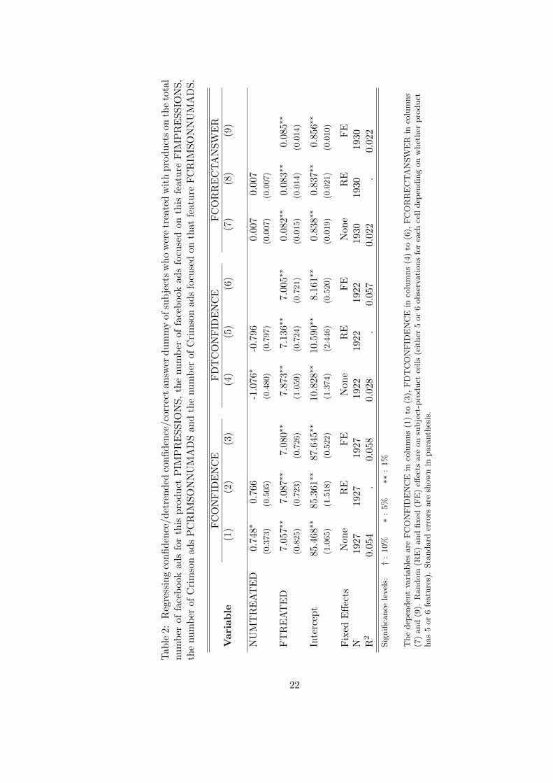
We start with two simple regressions which verify that our information treatments for

subjects who received products as well as the ad treatments have worked.

For subjects in the product group we run the following regression:

Iipf = α0 + α1FTipf + ηip + ε1,ipf (6)

where

Iipf =information (measured either through confidence orthrough correctness of answer to quizz question) aboutfeature f in product p for subject i

FTipf = dummy variable which is 1 if subject i was informed about f

ηip = fixed effect for subject i and product p

Results are shown in table 2 using OLS and random and fixed effects estimation. The

estimates are similar across all specifications.

For subjects in the non-product group we run the following regression:

Iipf = β0 + β1FIMPRESSIONSipf + β2FCRIMSONNUMADSipf + ηip + ε2,ipf(7)

where

FIMPRESSIONSipf =number of online ads (in 100s) received by sub-ject i for product p and feature f

FCRIMSONNUMADSipf =number of paper ads which a subject saw forfeature f

We only include subjects who did not receive print or online ads themselves. We also

include the total number of print and online impressions a subject saw.

12

Regression results are shown in table 3 using OLS and random and fixed effects

estimation. Both web and print ads increase a subject’s information about a product.

Importantly, print and online ads per se do not improve a subject’s knowledge - her

confidence and probability of giving a correct answer to a feature question only increases

if the ad emphasizes the particular feature.

100 online impressions increase a subject’s knowledge by about 12 percent while a

print ad leads to an increase in knowledge by 5 per cent.

4.2 Strong Social Learning

We can now run social learning regression where we regress subjects’ information on the

information of their neighbors. We distinguish between the set NProdi of neighbors of

agent i who did receive a product and the set Nnon−Prodi who did not receive a product.

We only analyze social learning for subjects who received no products themselves nor

saw any online or print ads for the product.

The regression for the learning from neighbors who did receive products is:

Iipf = γ0 +∑

j∈NProdi

γ1(dij) ∗ Ijpf + ε3,ipf (8)

where

dij = distance between agent i and j

Since the information of neighbors is endogenous we instrument for it using our info

treatments. We know from the first stage regressions in the previous section that these

are valid instruments. The results are presented in tables 5 and 6 for confidence and

correctness of answers to quizz questions.

We find strong social learning effects which decrease with social distance: a room

mate matters about three times as much as a direct friend. However, we have to take

into account that the number of friends of a certain distance increases very quickly with

path length as table 1 shows: there about 60 times as many indirect friends (path length

2) than room mates. If products are randomly owned by subjects then the effect of

distant friends will tend to outweigh the effects of close friends.

13

The regression for the learning from neighbors who did not receive products is similar:

Iipf = γ0 +∑

j∈Nnon−Prodi

γ1(dij) ∗ Ijpf + ε3,ipf (9)

where

dij = distance between agent i and j

We now use online and print advertising as instruments. However, print ads will be

particularly weak instruments because we only include subjects on the left-hand side

who did not receive print ads themselves. This in particular excludes all friends within

the same house. The results are presented in tables 7 and 8 for confidence and correctness

of answers to quizz questions.

We do find significant effects of both room mates’ information and indirect friends.

Moreover, the social network coefficients are decreasing with social distance.

5 Conclusion

We constructed a novel field experiment which provides unique data on social learning

in the relatively self-contained social network of university students at one large pri-

vate university. These questions are hard to explore by using only observational micro

data. Even identifying the aggregate social interaction effect is difficult due to the re-

flection problem (Manski 1993) and selection effects, since friends tend to have similar

preferences and therefore make similar consumption decisions. Differentiating between

social learning channels is even more difficult because in typical data we only observe

the outcome of the decision by consumers to purchase a product.

We hope to answer more questions with this unique dataset. In particular we are

interested in the question which agents are influential. This question can be approached

from two directions. First of all, we can look at the position of an agent inside the social

network to identify popular and well-connected individuals and to estimate a ‘multiplier’

for each type of agent identified this way.

A second way to approach this question is to look at individual characteristics such

as gender and physical attractiveness. In Mobius and Rosenblat (2006), for example, we

14

find that physical attractiveness can have substantial effects during wage negotiations

between employers and workers.

In addition to the study of social learning, our paper introduces several methodolog-

ical innovations. First, we develop cheap and effective tools to measure social network

structure. Second, we design incentive compatible configurators to measure preferences

for products. Third, we provide an exciting alternative to an often tedious to explain and

commonly misunderstood BDM procedure. Finally, we specifically design an experiment

to create instruments that are necessary for identification.

15

References

Conley, T. G., and C. R. Udry (2002): “Learning About a New Technology: Pineap-ple in Ghana,” Working paper, University of Chicago.

Duflo, E., and E. Saez (2003): “The Role of Information and Social Interactionsin Retirement Plan Decisions: Evidence from a Randomized Experiment,” QuarterlyJournal of Economics, 118.

Ely Dahan, John R. Hauser, D. I. S., and O. Toubia (2002): “Application andTest of Web-based Adaptive Polyhedral Conjoint Analysis,” Discussion paper, mimeo.

Foster, A., and M. Rosenzweig (1995): “Learning by Doing and Learning fromOthers: Human Capital and Technical Change in Agriculture,” Journal of PoliticalEconomy.

Granovetter, M. (1974): Getting a Job. Harvard University Press, Cambridge.

Green, P., and V. Srinivasan (1978): “Conjoint Analysis in Consumer Research:Issues and Outlook,” Journal of Consumer Research, 5, 103–123.

Hauser, J. R., and V. R. Rao (2002): “Conjoint Analysis, Related Modeling, andApplications,” in Advances in Marketing Research: Progress and Prospects [A tributeto Paul Greens Contributions to Marketing Research Methodology].

Jackson, M., and T. Calvo-Armengol (2004): “The Effects of Social Networks onEmployment and Inequality,” American Economic Review, 94.

Kremer, M., and E. Miguel (2003): “Networks, Social Learning, and TechnologyAdoption: The Case of Deworming Drugs in Kenya,” Discussion paper, Harvard Uni-versity Working Paper.

Luce, R., and J. Tukey (1964): “Simultaneous Conjoint Measurement: A New Typeof Fundamental Measurement,” Journal of Mathematical Psychology, 1, 1–27.

Manski, C. (1993): “Identification of Endogenous Social Effects: The Reflection Prob-lem,” Review of Economic Studies, 60, 531–542.

Mobius, M., and T. Rosenblat (2006): “Why Beauty Matters,” forthcoming in Amer-ican Economic Review.

Munshi, K. (2003): “Networks in the Modern Economy: Mexican Migrants in the USLabor Market,” Quarterly Journal of Economics, 118, 549–599.

Topa, G. (2001): “Social Interactions, Local Spillovers and Unemployment,” Review ofEconomic Studies, 68, 261–295.

16

Table 1: Number of room mate links, friend (N1), indirect friends (N2) and friends ofdistance 3 (N3) for average subject

Type of link Number of links Ratio

Room mate 0.96 1

N1 7.68 8

N2 57.91 60.32

N3 347.14 361.60

17

Figure 1: Online configurator for camcorder product

1 o

f 2

Face

book

Exp

erim

ent

FO

UR

TH

Pro

du

ct

- C

am

co

rd

er

This product is a digital camcorder that is

about half the size

of a mobile phone. It records up

to 10 minutes of continuous

video using the

MPEG-4 standard. It can also snap up to 200

2-megapixel still

photos. A USB connection lets you

upload data to your computer an

d

recharge the camcorder.

18

Figure 2: Distribution of pairwise taste similarity measure TASTESIMij for six productclasses

0 20 40 60 80 1000

2

4

6

8x 10

4

Card0 20 40 60 80 100

0

0.5

1

1.5

2x 10

5

Camcorder

0 20 40 60 80 1000

2

4

6x 10

4

Yoga0 20 40 60 80 100

0

5

10

15x 10

4

Sound

0 20 40 60 80 1000

2

4

6

8x 10

4

Food0 20 40 60 80 100

0

5

10

15x 10

4

PDA

19

Figure 3: Distribution of pickup times

−2 0 2 4 6 8 10 12 14 16 180

20

40

60

80

100

120

140

Pickup day of product (day 0 = start of study)

Num

ber

of s

tude

nts

20

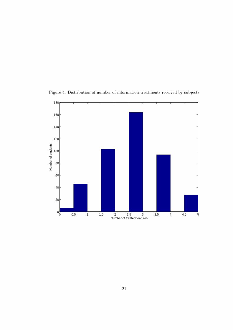
Figure 4: Distribution of number of information treatments received by subjects

0 0.5 1 1.5 2 2.5 3 3.5 4 4.5 50

20

40

60

80

100

120

140

160

180

Number of treated features

Num

ber

of s

tude

nts

21

Tab

le2:

Reg

ress

ing

confi

denc

e/de

tren

ded

confi

denc

e/co

rrec

tan

swer

dum

my

ofsu

bje

ctsw

how

ere

trea

ted

wit

hpr

oduc

tson

the

tota

lnu

mbe

rof

face

book

ads

for

this

prod

uct

PIM

PR

ESS

ION

S,th

enu

mbe

rof

face

book

ads

focu

sed

onth

isfe

atur

eFIM

PR

ESS

ION

S,th

enu

mbe

rof

Cri

mso

nad

sP

CR

IMSO

NN

UM

AD

San

dth

enu

mbe

rof

Cri

mso

nad

sfo

cuse

don

that

feat

ure

FC

RIM

SON

NU

MA

DS.

FC

ON

FID

EN

CE

FD

TC

ON

FID

EN

CE

FC

OR

RE

CTA

NSW

ER

Var

iable

(1)

(2)

(3)

(4)

(5)

(6)

(7)

(8)

(9)

NU

MT

RE

AT

ED

0.74

8∗0.

766

-1.0

76∗

-0.7

960.

007

0.00

7(0

.373)

(0.5

05)

(0.4

80)

(0.7

97)

(0.0

07)

(0.0

07)

FT

RE

AT

ED

7.05

7∗∗

7.08

7∗∗

7.08

0∗∗

7.87

3∗∗

7.13

6∗∗

7.00

5∗∗

0.08

2∗∗

0.08

3∗∗

0.08

5∗∗

(0.8

25)

(0.7

23)

(0.7

26)

(1.0

59)

(0.7

24)

(0.7

21)

(0.0

15)

(0.0

14)

(0.0

14)

Inte

rcep

t85

.468∗∗

85.3

61∗∗

87.6

45∗∗

10.8

28∗∗

10.5

90∗∗

8.16

1∗∗

0.83

8∗∗

0.83

7∗∗

0.85

6∗∗

(1.0

65)

(1.5

18)

(0.5

22)

(1.3

74)

(2.4

46)

(0.5

20)

(0.0

19)

(0.0

21)

(0.0

10)

Fix

edE

ffect

sN

one

RE

FE

Non

eR

EFE

Non

eR

EFE

N19

2719

2719

2719

2219

2219

2219

3019

3019

30R

20.

054

.0.

058

0.02

8.

0.05

70.

022

.0.

022

Sig

nifi

cance

level

s:†:

10%

∗:

5%

∗∗:

1%

The

dep

enden

tva

riable

sare

FC

ON

FID

EN

CE

inco

lum

ns

(1)

to(3

),FD

TC

ON

FID

EN

CE

inco

lum

ns

(4)

to(6

),FC

OR

RE

CTA

NSW

ER

inco

lum

ns

(7)

and

(9).

Random

(RE

)and

fixed

(FE

)eff

ects

are

on

subje

ct-p

roduct

cells

(eit

her

5or

6obse

rvati

ons

for

each

cell

dep

endin

gon

whet

her

pro

duct

has

5or

6fe

atu

res)

.Sta

ndard

erro

rsare

show

nin

para

nth

esis

.

22

Tab

le3:

Reg

ress

ing

confi

denc

e/de

tren

ded

confi

denc

e/co

rrec

tan

swer

dum

my

ofsu

bje

cts

who

wer

eno

ttr

eate

dw

ith

prod

ucts

onth

eto

taln

umbe

rof

face

book

adsfo

rth

ispr

oduc

tP

IMP

RE

SSIO

NS,

the

num

berof

face

book

adsfo

cuse

don

this

feat

ure

FIM

PR

ESS

ION

S,th

enu

mbe

rof

Cri

mso

nad

sP

CR

IMSO

NN

UM

AD

San

dth

enu

mbe

rof

Cri

mso

nad

sfo

cuse

don

that

feat

ure

FC

RIM

SON

NU

MA

DS.

FC

ON

FID

EN

CE

FD

TC

ON

FID

EN

CE

FC

OR

RE

CTA

NSW

ER

Var

iable

(1)

(2)

(3)

(4)

(5)

(6)

(7)

(8)

(9)

PIM

PR

ESS

ION

S1.

108

1.14

2-0

.220

-0.1

67-0

.022†

-0.0

22(0

.698)

(1.1

33)

(0.6

83)

(1.0

95)

(0.0

12)

(0.0

14)

FIM

PR

ESS

ION

S2.

278

2.19

8∗2.

182∗

2.37

02.

245∗

2.22

0∗0.

121∗∗

0.12

1∗∗

0.12

0∗∗

(1.5

25)

(1.0

75)

(1.0

75)

(1.4

92)

(1.0

76)

(1.0

76)

(0.0

26)

(0.0

25)

(0.0

25)

PC

RIM

SON

NU

MA

DS

-0.5

20∗∗

-0.4

96∗

-0.4

15∗∗

-0.3

82-0

.008∗∗

-0.0

08∗∗

(0.1

46)

(0.2

43)

(0.1

43)

(0.2

35)

(0.0

03)

(0.0

03)

FC

RIM

SON

NU

MA

DS

1.88

3∗∗

1.65

9∗∗

1.61

4∗∗

1.78

9∗∗

1.64

2∗∗

1.61

0∗∗

0.05

2∗∗

0.05

1∗∗

0.04

8∗∗

(0.2

64)

(0.1

87)

(0.1

87)

(0.2

58)

(0.1

87)

(0.1

87)

(0.0

05)

(0.0

04)

(0.0

04)

Inte

rcep

t63

.496∗∗

63.5

09∗∗

63.1

44∗∗

11.4

60∗∗

11.4

80∗∗

11.0

28∗∗

0.65

0∗∗

0.65

0∗∗

0.64

0∗∗

(0.2

49)

(0.4

39)

(0.1

38)

(0.2

44)

(0.4

24)

(0.1

38)

(0.0

04)

(0.0

05)

(0.0

03)

Fix

edE

ffect

sN

one

RE

FE

Non

eR

EFE

Non

eR

EFE

N22

959

2295

922

959

2292

122

921

2292

122

995

2299

522

995

R2

0.00

3.

0.00

40.

002

.0.

004

0.00

6.

0.00

8Sig

nifi

cance

level

s:†:

10%

∗:

5%

∗∗:

1%

The

dep

enden

tva

riable

sare

FC

ON

FID

EN

CE

inco

lum

ns

(1)

to(3

),FD

TC

ON

FID

EN

CE

inco

lum

ns

(4)

to(6

),FC

OR

RE

CTA

NSW

ER

inco

lum

ns

(7)

and

(9).

Random

(RE

)and

fixed

(FE

)eff

ects

are

on

subje

ct-p

roduct

cells

(eit

her

5or

6obse

rvati

ons

for

each

cell

dep

endin

gon

whet

her

pro

duct

has

5or

6fe

atu

res)

.Sta

ndard

erro

rsare

show

nin

para

nth

esis

.

23

Table 4: Regressing final bids of subjects who were treated with products on BUZZtreatment dummy and NUMTREATED (number of info treatments received)

All products Services GadgetsVariable (1) (2) (3)

BUZZ 8.504∗ 1.516 23.706∗

(4.206) (1.561) (9.176)

NUMTREATED 3.780∗ 0.822 5.837(1.886) (0.669) (4.526)

N 373 227 146R2 0.019 0.01 0.048Significance levels: † : 10% ∗ : 5% ∗∗ : 1%

The dependent variable is BID in columns (1) to (3); standard errors are shown in paranthesis.

24

Table 5: IV regression of confidence of subjects who were neither treated with theproduct or any type of ad for the product on the confidence of social neighbors atdistance R,NW1,NW2,NW3. Instruments are info treatments.

FCONFIDENCEVariable (1) (2)

PGFCONFIDENCE R 0.064∗ 0.057†

(0.029) (0.031)

PGFCONFIDENCE NW1 0.040∗∗ 0.034∗

(0.013) (0.014)

PGFCONFIDENCE NW2 0.005 0.008†

(0.005) (0.005)

PGFCONFIDENCE NW3 0.003∗∗ 0.009∗∗

(0.001) (0.001)

ELIGIBLE R -0.112(0.986)

ELIGIBLE NW1 -0.131(0.469)

ELIGIBLE NW2 -0.260(0.165)

ELIGIBLE NW3 -0.161∗∗

(0.033)

Intercept 59.628∗∗ 67.870∗∗

(0.826) (1.197)

N 8982 8982R2 0.018 0.045Significance levels: † : 10% ∗ : 5% ∗∗ : 1%

The dependent variable is FCONFIDENCE. Standard errors areshown in paranthesis. Instruments are TREATDONE NNN andFUFTREATED NNN. We include ELIGIBILITY NNN to control forthe number of potential info treatments.

25

Table 6: IV regression of correct answer of subjects who were neither treated with theproduct or any type of ad for the product on the correct answers of social neighbors atdistance R,NW1,NW2,NW3. Instruments are info treatments.

FCORRECTANSWERVariable (1) (2)

PGFCORRECTANSWER R 0.108∗∗ 0.070∗

(0.026) (0.030)

PGFCORRECTANSWER NW1 0.041∗∗ 0.018(0.013) (0.014)

PGFCORRECTANSWER NW2 0.019∗∗ 0.020∗∗

(0.005) (0.005)

PGFCORRECTANSWER NW3 0.007∗∗ 0.018∗∗

(0.001) (0.002)

ELIGIBLE R 0.017(0.011)

ELIGIBLE NW1 0.006(0.005)

ELIGIBLE NW2 0.000(0.002)

ELIGIBLE NW3 -0.003∗∗

(0.000)

Intercept 0.567∗∗ 0.696∗∗

(0.010) (0.014)

N 9006 9006R2 0.033 0.064Significance levels: † : 10% ∗ : 5% ∗∗ : 1%

The dependent variable is FCORRECTANSWER. Standard errorsare shown in paranthesis. Instruments are TREATDONE NNN andFUFTREATED NNN. We include ELIGIBILITY NNN to control forthe number of potential info treatments.

26

Table 7: IV regression of confidence of subjects who were neither treated with theproduct or any type of ad for the product on the confidence of social neighbors atdistance R,NW1,NW2,NW3. Instruments are crimson and facebook ads.

FCONFIDENCEVariable (1) (2) (3)

NPGFCONFIDENCE R -0.032 0.143∗

(0.060) (0.066)

NPGFCONFIDENCE NW1 -0.011 0.039∗ 0.017(0.020) (0.019) (0.014)

NPGFCONFIDENCE NW2 0.008 0.013∗∗ 0.012∗∗

(0.007) (0.005) (0.004)

NPGFCONFIDENCE NW3 -0.001 0.003∗∗ 0.000(0.001) (0.001) (0.001)

R 2.501 1.744∗∗ -3.335(2.082) (0.593) (2.285)

NW1 0.199 -1.266∗ -0.601(0.597) (0.585) (0.459)

NW2 -0.205 -0.264† -0.330∗

(0.204) (0.159) (0.141)

NW3 0.012 -0.076∗∗ 0.007(0.033) (0.027) (0.025)

Intercept 63.995∗∗ 60.988∗∗ 63.406∗∗

(1.360) (1.439) (1.391)

Instruments FB Crimson BothN 8982 8982 8982R2 . . .Significance levels: † : 10% ∗ : 5% ∗∗ : 1%

The dependent variable is FCONFIDENCE. Standard errors are shown inparanthesis. Instruments are PCRIMSONNUMADS NNN and FCRIMSON-NUMADS NNN amd/or PIMPRESSIONS NNN and FIMPRESSIONS NNN.We include numbers of neighbors at distance R, NW1, NW2, NW3 to controlfor the position in the social network.

27

Table 8: IV regression of correct answer of subjects who were neither treated with theproduct or any type of ad for the product on the correct answers of social neighbors atdistance R,NW1,NW2,NW3. Instruments are crimson and facebook ads.

FCORRECTANSWERVariable (1) (2) (3)

NPGFCORRECTANSWER R 0.302∗∗ 0.278∗∗

(0.073) (0.058)

NPGFCORRECTANSWER NW1 0.030 0.009 0.025(0.027) (0.023) (0.017)

NPGFCORRECTANSWER NW2 0.024∗ 0.012∗ 0.018∗∗

(0.010) (0.005) (0.005)

NPGFCORRECTANSWER NW3 -0.001 0.003∗∗ 0.001(0.001) (0.001) (0.001)

R -0.082∗∗ 0.030∗∗ -0.073∗∗

(0.027) (0.006) (0.022)

NW1 -0.009 -0.002 -0.007(0.008) (0.007) (0.006)

NW2 -0.006∗ -0.002 -0.004∗

(0.003) (0.002) (0.002)

NW3 0.000 -0.001∗∗ 0.000(0.000) (0.000) (0.000)

Intercept 0.615∗∗ 0.602∗∗ 0.611∗∗

(0.016) (0.015) (0.016)

Instruments FB Crimson BothN 9006 9006 9006R2 0.055 0.133 0.085Significance levels: † : 10% ∗ : 5% ∗∗ : 1%

The dependent variable is FCORRECTANSWER. Standard errors areshown in paranthesis. Instruments are PCRIMSONNUMADS NNN andFCRIMSONNUMADS NNN amd/or PIMPRESSIONS NNN and FIMPRES-SIONS NNN. We include numbers of neighbors at distance R, NW1, NW2,NW3 to control for the position in the social network.

28