Brigham Young University Brigham Young University

BYU ScholarsArchive BYU ScholarsArchive

Theses and Dissertations

2018-07-01

Smart Technologies for Oil Production with Rod Pumping Smart Technologies for Oil Production with Rod Pumping

Brigham Wheeler Hansen Brigham Young University

Follow this and additional works at: https://scholarsarchive.byu.edu/etd

Part of the Chemical Engineering Commons

BYU ScholarsArchive Citation BYU ScholarsArchive Citation Hansen, Brigham Wheeler, "Smart Technologies for Oil Production with Rod Pumping" (2018). Theses and Dissertations. 6936. https://scholarsarchive.byu.edu/etd/6936

This Thesis is brought to you for free and open access by BYU ScholarsArchive. It has been accepted for inclusion in Theses and Dissertations by an authorized administrator of BYU ScholarsArchive. For more information, please contact scholarsarchive@byu.edu, ellen_amatangelo@byu.edu.

Smart Technologies for Oil Production with Rod Pumping

Brigham Wheeler Hansen

A thesis submitted to the faculty ofBrigham Young University

in partial fulfillment of the requirements for the degree of

Master of Science

John D. Hedengren, ChairAndrew Fry

Morris Argyle

Department of Chemical Engineering

Brigham Young University

Copyright © 2018 Brigham Wheeler Hansen

All Rights Reserved

ABSTRACT

Smart Technologies for Oil Production with Rod Pumping

Brigham Wheeler HansenDepartment of Chemical Engineering, BYU

Master of Science

This work enables accelerated fluid recovery in oil and gas reservoirs by automaticallycontrolling fluid height and bottomhole pressure in wells. Several literature studies show signif-icant increase in recovered oil by determining a target bottomhole pressure but rarely considerhow to control to that value. This work enables those benefits by maintaining bottomhole pressureor fluid height. Moving Horizon Estimation (MHE) determines uncertain well parameters usingonly common surface measurements. A Model Predictive Controller (MPC) adjusts the strokingspeed of a sucker rod pump to maintain fluid height. Pump boundary conditions are simulatedwith Mathematical Programs with Complementarity Constraints (MPCCs) and a nonlinear pro-gramming solver finds a solution in near real-time. A combined rod string, well, and reservoirmodel simulate dynamic well conditions, and are formulated for simultaneous optimization bylarge-scale solvers. MPC increases cumulative oil production vs. conventional pump off controlby maintaining an optimal fluid level height.

Keywords: model predictive control, modeling, sucker rod pumping, gas and oil, MPC, MHE

ACKNOWLEDGMENTS

I acknowledge the financial assistance of Utah Science Technology and Research (USTAR)

through a University Technology Acceleration Grant (UTAG). USTAR is a technology-based eco-

nomic development initiative funded by the state of Utah. Thanks to both Andrew Sweeney and Ivy

Estabrooke who administered and facilitated the UTAG project. Also, thanks to Brigham Young

University for providing a faith-based environment of learning and personal growth

I would like to gratefully thank all those have assisted and mentored me throughout this

work. I am very grateful to Dr. John Hedengren for his selfless mentoring. His coaching and ideas

have been invaluable in the development of this research and in my development as an individual.

Dr. Andrew Fry and Dr. Morris Argyle have also been important mentors. Thanks to Dave Krug,

Jens Griffin, Insu Kim, Craig Schoenberger, and Cory Vernon. Each has taught and assisted me

throughout the project. I owe a special thanks to Brandon Tolbert for his expertise and help in

research, development, and writing.

Finally, I am forever grateful to my spouse, Kyla. She selflessly assists and encourages me.

I love and appreciate her, I would not be where I am today without her.

TABLE OF CONTENTS

LIST OF TABLES . . . . . . . . . . . . . . . . . . . . . . . . . . . . . . . . . . . . . . . vi

LIST OF FIGURES . . . . . . . . . . . . . . . . . . . . . . . . . . . . . . . . . . . . . . vii

NOMENCLATURE . . . . . . . . . . . . . . . . . . . . . . . . . . . . . . . . . . . . . . viii

Chapter 1 Introduction . . . . . . . . . . . . . . . . . . . . . . . . . . . . . . . . . . . 11.1 Reservoir Modeling for Well Control . . . . . . . . . . . . . . . . . . . . . . . . . 21.2 Sucker Rod Pump Artificial Lift . . . . . . . . . . . . . . . . . . . . . . . . . . . 51.3 Automatic Controllers for Rod Pumping Units . . . . . . . . . . . . . . . . . . . . 71.4 Sucker Rod Pump and Well Modeling . . . . . . . . . . . . . . . . . . . . . . . . 81.5 Hardware Interfacing for Advanced Control . . . . . . . . . . . . . . . . . . . . . 91.6 Contributions . . . . . . . . . . . . . . . . . . . . . . . . . . . . . . . . . . . . . 91.7 Publication . . . . . . . . . . . . . . . . . . . . . . . . . . . . . . . . . . . . . . 11

Chapter 2 Model Predictive Control for Sucker Rod Pump Systems . . . . . . . . . . 132.1 Methods . . . . . . . . . . . . . . . . . . . . . . . . . . . . . . . . . . . . . . . . 132.2 Well and Rod String System . . . . . . . . . . . . . . . . . . . . . . . . . . . . . 132.3 Surface Unit Equations of Motion . . . . . . . . . . . . . . . . . . . . . . . . . . 132.4 Rod String and Well Modeling . . . . . . . . . . . . . . . . . . . . . . . . . . . . 172.5 Reservoir Modeling . . . . . . . . . . . . . . . . . . . . . . . . . . . . . . . . . . 182.6 Well Vertical Lift Performance . . . . . . . . . . . . . . . . . . . . . . . . . . . . 202.7 Economics . . . . . . . . . . . . . . . . . . . . . . . . . . . . . . . . . . . . . . . 202.8 Moving Horizon Estimation and Model Predictive Control . . . . . . . . . . . . . 222.9 Solution Methods . . . . . . . . . . . . . . . . . . . . . . . . . . . . . . . . . . . 242.10 Numerical Methods . . . . . . . . . . . . . . . . . . . . . . . . . . . . . . . . . . 242.11 Simulating Pump Boundary Conditions for Optimization . . . . . . . . . . . . . . 252.12 Comparison to Analytical Solution . . . . . . . . . . . . . . . . . . . . . . . . . . 262.13 Grid Independence Study . . . . . . . . . . . . . . . . . . . . . . . . . . . . . . . 292.14 Modeling Results . . . . . . . . . . . . . . . . . . . . . . . . . . . . . . . . . . . 312.15 Reservoir Pressure and Production Dynamics . . . . . . . . . . . . . . . . . . . . 312.16 Rod String Dynamics . . . . . . . . . . . . . . . . . . . . . . . . . . . . . . . . . 362.17 Moving Horizon Estimation Results . . . . . . . . . . . . . . . . . . . . . . . . . 382.18 Annular Fluid Height Estimation . . . . . . . . . . . . . . . . . . . . . . . . . . . 392.19 Reservoir Parameter Estimation . . . . . . . . . . . . . . . . . . . . . . . . . . . . 422.20 Dynamic Optimization & Model Predictive Control . . . . . . . . . . . . . . . . . 462.21 Case 1 - Pump-Off Control With Timer . . . . . . . . . . . . . . . . . . . . . . . . 472.22 Case 2 - Fluid Height Control With PI . . . . . . . . . . . . . . . . . . . . . . . . 482.23 Case 3 - Fluid Height Control With MPC . . . . . . . . . . . . . . . . . . . . . . . 522.24 Comparison of Cases . . . . . . . . . . . . . . . . . . . . . . . . . . . . . . . . . 54

Chapter 3 Conclusions and Future Work . . . . . . . . . . . . . . . . . . . . . . . . . 57

iv

3.1 Future Work . . . . . . . . . . . . . . . . . . . . . . . . . . . . . . . . . . . . . . 58

Appendix A Source Code . . . . . . . . . . . . . . . . . . . . . . . . . . . . . . . . . . . 67

A.

1 Analytical vs. Numerical Comparison . . . . . . . . . . . . . . . . . . . . . . . . 67A.

2 Simulation, MHE, and MPC Model Script . . . . . . . . . . . . . . . . . . . . . 73

v

References . . . . . . . . . . . . . . . . . . . . . . . . . . . . . . . . . . . . . . . . . . . . . . . . . 60

LIST OF TABLES

1.1 Summary of studies in literature controlling BHP or production rate of producing wellsto perform system identification, model training, and production optimization . . . . . 5

2.1 Objective function terms . . . . . . . . . . . . . . . . . . . . . . . . . . . . . . . . . 232.2 Estimation Case Studies . . . . . . . . . . . . . . . . . . . . . . . . . . . . . . . . . . 392.3 Simulated Control Cases . . . . . . . . . . . . . . . . . . . . . . . . . . . . . . . . . 46

vi

LIST OF FIGURES

1.1 Illustration of measured surface dynagraph and corresponding calculated downholedynagraph . . . . . . . . . . . . . . . . . . . . . . . . . . . . . . . . . . . . . . . . . 6

1.2 Demonstration sized hydraulic actuated sucker rod pump . . . . . . . . . . . . . . . . 101.3 Summary of the rod string, well, reservoir dynamics . . . . . . . . . . . . . . . . . . . 12

2.1 Pump and well diagrams . . . . . . . . . . . . . . . . . . . . . . . . . . . . . . . . . 142.2 Shows the free body diagram of the crank arm including an effective force diagram

and applied torque diagram . . . . . . . . . . . . . . . . . . . . . . . . . . . . . . . . 152.3 Comparison of analytical and GEKKO solutions . . . . . . . . . . . . . . . . . . . . . 282.4 Error of proposed solution method vs. analytical solution . . . . . . . . . . . . . . . . 282.5 Fixed rod length discretization of 10 sections . . . . . . . . . . . . . . . . . . . . . . 302.6 Fixed number of time points at 20 . . . . . . . . . . . . . . . . . . . . . . . . . . . . 302.7 Doublet test performed at different net torque values . . . . . . . . . . . . . . . . . . . 322.8 Change in reservoir pressure with cumulative volume produced from the rod pump . . 332.9 The system is a dynamic blend of inflow and outflow of fluids . . . . . . . . . . . . . 332.10 Power consumption of the rod pump motor as FBHP declines and SPM varies . . . . . 342.11 Shows how NPV varies over an 8 year simulation period . . . . . . . . . . . . . . . . 352.12 Dynamic rod string position in space and time (10 seconds) . . . . . . . . . . . . . . 362.13 Pump position, velocity, and velocity sign (20-40 seconds) . . . . . . . . . . . . . . . 372.14 Rod load vs. position . . . . . . . . . . . . . . . . . . . . . . . . . . . . . . . . . . . 382.15 Rod load vs. time . . . . . . . . . . . . . . . . . . . . . . . . . . . . . . . . . . . . . 382.16 Height is estimated with varying inputs of Tnet (which adjusts based off the load) . . . 402.17 Height is estimated with varied Tnet , noise, and an offset initial condition . . . . . . . . 412.18 MHE estimate of porosity from surface loading measurements . . . . . . . . . . . . . 432.19 MHE estimate of skin from surface loading measurements . . . . . . . . . . . . . . . 442.20 MHE estimate of skin and porosity. Figure demonstrates potential collinearity between

skin and porosity . . . . . . . . . . . . . . . . . . . . . . . . . . . . . . . . . . . . . 452.21 Pump-off controller performance . . . . . . . . . . . . . . . . . . . . . . . . . . . . . 482.22 Block diagram of PI and MPC controllers . . . . . . . . . . . . . . . . . . . . . . . . 492.23 Aggressive PI controller performance Kc = 1 f t·lb

f t and τI = 1s . . . . . . . . . . . . . . 502.24 Solve time for combined MHE and PI controller . . . . . . . . . . . . . . . . . . . . . 512.25 Runs MHE and MPC synchronously. . . . . . . . . . . . . . . . . . . . . . . . . . . . 522.26 Runs MHE and MPC synchronously. . . . . . . . . . . . . . . . . . . . . . . . . . . . 532.27 Solve time for combined MPC and MHE . . . . . . . . . . . . . . . . . . . . . . . . . 542.28 Increased cumulative oil production relative to Case 1 ( Pump-off) . . . . . . . . . . . 55

vii

NOMENCLATURE

A drainage area (2 acres)A f cross sectional area of annular fluid ( f t2)Ac cross sectional rod area ( 0.785 in2)At cross sectional area of tubing (in2)API oil API (45 API)B combined viscous friction coefficient ( lb · f t · s)BHP bottom hole pressure or pump intake pressure (psi)Bo formation volume factor ( 1.2 bbl

ST B )c total compressibility factor (0.000013 psi−1)CA drainage area shape factor (31.6)Cinitial initial cost of rod pump ($1,000,000)Dc diameter of well casing (8 in)Dr diameter of sucker rod ( 1 in)Dt diameter of production tubing (2.5 in )E rod string modulus of elasticity (3.2 ·106 psi)emech,loss power to overcome frictional losses (Kw)Ecost cost of electricity ( $

Kwh )f rod load lb f state variableg gravity acceleration (32 f t

s2 )h reservoir thickness (8 f t)h f height of fluid in well annulus ( f t)J0 combined inertia of motor, load, and gear train (lb · f t · s2)k permeability 15 md constantNPV net present value ($)P average reservoir pressure (psi)P(t) pump boundary condition parameterPi initial reservoir pressure (2078.4psi)Po price of oil (60 $

bbl )ppi pump intake pressure (psi)Pw f bottomhole flowing pressure (psi)Pwh well head pressure (psi)pr reservoir pressure (psi)PI well productivity index ( bbl

day·psi )r annual interest rate (12%)R revenue $ state variablerw wellbore radius (0.328 f t) constantS skin 0 constantsa slack variablesb slack variableSPM surface unit strokes per minute ( strokes

min )Tnet net torque ( lb

f t )TV D true vertical depth ( 4800 f t)

viii

u(x, t) relative position of rod segment x at time t ( f t)Vi original oil in place (ST B)Vp cumulative volume produced (ST B)Wmotor rate of work produced by motor (Kw)Wf weight of fluid in production tubing (lb f )Wr weight of rod string (lbm)X expenses ($)αp pump boundary condition coefficient (0.0)α angular acceleration ( radians

s2 )β pump boundary condition coefficient (1.0)γE Euler constant (1.78)γ oil specific gravity (0.8)µ viscosity (1.5cp)ω angular velocity ( radians

s )ρw density of water at standard conditions ( lbm

f t3 )θ rotational angle (radians)

ix

CHAPTER 1. INTRODUCTION

Smart technologies increase data collection, enable real-time data analysis, and improve

equipment controllability. In the upstream oil and gas industry, the application of new smart au-

tomation technologies can increase reservoir recovery and reduce operating expenses. Oil and

gas resources supply a large portion of the world energy resource, and more effective extraction

processes result in lower costs for consumers and greater profitability for producers. Realizing

the maximum benefit of these devices requires the development of system models, automatic con-

trollers, and computer aided optimization routines. There is significant interest in automation in

general because it is disrupting and revolutionizing many industries. Some examples of automation

revolutions are self-driving cars, Unmanned Aerial Vehicle (UAV) delivery services, and advanced

manufacturing technologies. Automation is at the core of each of these innovations. Automation at

a basic level requires three components: 1) a sensor, 2) a controller, and 3) an actuator. In automatic

control, first the sensor measures a process variable. Second, based on the measurement and con-

troller configuration, the controller sends an output to the actuator. Finally, the actuator affects the

process, resulting in closed loop automation. As global Internet connectivity increases the ability

to collect measurements from sensors and send control signals to actuators increases. Meanwhile

the cost of computing devices decreases and computational performance increases. These factors

drive an automation revolution in many industries. To maintain a competitive edge, the oil and gas

companies are beginning to adopt automation technologies.

An important area of smart technology development is sucker-rod artificial lift systems.

Sucker-rod pumping is a widely used artificial lift method for extraction of oil and gas resources.

It is a $3.6B industry in North America and a $5.5B industry worldwide. Current rod pumping

technology was developed in 1926 and has remained largely unchanged since then. In sucker-rod

pumping, a pump at the bottom of the well is actuated by the linear up and down stroking of a

surface unit via a rod string. As fluids are produced from the reservoir, the bottomhole pressure

1

(BHP) of the well decreases, and the reservoir-well pressure differential causes reservoir fluid to

flow into the well bore. Several literature studies show significant increases in ultimate oil recovery

and project Net Present Value (NPV) as a result of optimally controlling BHP of wells in reservoir

systems [13, 3, 30]. However, these researchers rarely consider how the well BHP is maintained at

optimal values. In rod-pumped wells, the BHP is largely dictated by the height of the fluid column

in the well annulus [57]. The well annulus is the space between the well casing, which seals the

well from the rock formation, and the production tubing where the produced fluid flows to the

surface. This research demonstrates a Moving Horizon Estimation (MHE) to determine fluid level

from common measurements, and presents several controllers for controlling annular fluid height.

This research enables the benefits shown by others in the literature by demonstrating automatic

control of BHP.

1.1 Reservoir Modeling for Well Control

This section reviews reservoir modeling with emphasis on well control. Well control tech-

nologies are currently generating significant interest in the oil and gas industry primarily because

producers can increase estimated ultimate recovery by 10-15% [34]. Further, as the speed of com-

puters and data acquisition systems continues to improve, the industry is anticipating that control

technologies will become a more integral part of the life cycle optimization process of a well, as

explained in Jansen et al. [36]. To adopt an optimum production strategy, it is necessary to consider

a closed loop control process, where a controller uses process data to update production system

settings automatically. Most conventional reservoir simulators use a history-matching process to

align model values with production data from a real system [34]. The history matching process

typically involves manual adjustment of model parameters over a period of years. History match-

ing is often considered closed loop since it uses historical data to estimate model parameters, and

parameter estimates update periodically. However, traditionally these models are not used to auto-

matically control production systems. Instead reservoir engineers strive to find optimal production

strategies via the reservoir model and then implement those strategies manually. Some drawbacks

of history matching include (1) manual adjustment of model parameters, (2) violation of system

constraints, and (3) overfitting of real-time data [11]. To help optimize reservoir performance un-

der geologic uncertainties and incorporate real-time updates of changing reservoir parameters, the

2

oil and gas industry has placed an emphasis on exploring smart reservoir modeling. Like history

matching, smart reservoir modeling is a closed loop process. However, it has the added benefits

of (1) systematic updating using real-time data, (2) minimizing the effect of bad data, and (3) re-

ducing uncertainty [34]. Smart well models may also automatically control production systems in

a closed loop control process. Udy et al. [62] reviewed prior applications of reservoir modeling

for well control. They highlight the benefits of combining separate optimizations. Brouwer and

Jansen [12] applied optimal well control using a reservoir model to adjust downhole valve set-

tings of horizontal injector wells to optimize production. The results from his simulations suggest

the cumulative recovery are improved by 20% by implementing optimal control schemes. Sarma

and Chen [59] implemented optimization control strategies to control BHP of reservoir models

depicting offshore wells. The optimal control algorithm increased NPV by 17% over an 8 year

simulation period. Simulations confirm that smart reservoir modeling is superior to traditional

methods. The development of smart rod pumping equipment allows well control optimization to

be applied in practice in two ways. First, it allows for easy implementation of optimal settings by

automatic control. Second, it allows for system identification to characterize the relationship be-

tween controllable variables (e.g. producing well BHP) and system behavior (e.g. fluid production

rate)[62].

System identification determines the relationship between controllable input variables (ma-

nipulated variables) and output variables of the reservoir system. These relationships are typically

determined by perturbing the input variable and then fitting the resulting response of the output

variables to an appropriate model to represent the system. Typical perturbations to manipulated

variables are step tests, doublet tests, and pseudo random binary sequences. For example, pertur-

bations in well BHPs can be implemented and production rates measured to determine the rela-

tionship between them.

System models are used to simulate the reservoir system. Manipulated variables are varied

in the reservoir simulator to maximize objectives such as cumulative oil production or NPV. Many

techniques have been developed to optimally determine controllable well parameters and are thor-

oughly reviewed by Udy et al. [62]. The optimum profiles, or values, of input variables found in

the simulation are then implemented in the field to achieve production objectives. This problem

has elements of control and scheduling optimization [8].

3

Table 1.1 summarizes several studies from literature that vary the BHP or production rate of

producing wells (in simulation) to perform system identification and/or production optimization.

Notably, Cardoso and Durlofsky [15] show a simulated increase of $81M by optimally controlling

the BHP of producing wells in a synthetic heterogeneous reservoir. Alghareeb [3] determines

optimum water injection and producer production rates. In a case study, Alghareeb [3] optimally

sets well control variables and shows an increase in NPV from $3.5M to $11M. He et al. [30]

control the BHP of both the producers and the injectors. In their study, the NPV experiences a

drastic increase from $50M to $170M. These results imply that technologies that facilitate optimal

control of production can significantly increase the profitability of a reservoir system.

These studies, however, focus little on how the well BHP is to be set or maintained at the

optimal pressure. This is an important omission since the ability to control to these set points is

required to realize the simulated benefits in real systems. For a water injection well, operators

adjust the flow rate into the well to maintain the desired pressure. For a production well with

a sucker rod artificial lift system maintaining the optimal BHP requires the operator to adjust

the stroking speed such that desired BHP is maintained. Typically operators are simply trying to

achieve maximum fluid production without causing equipment damage. However, literature studies

illustrate that optimally setting the BHP of producing wells can lead to increased oil recovery from

reservoirs.

In rod pumped wells, the BHP is largely dictated by the height of the fluid column in the

well annulus. The fluid column creates hydrostatic pressure. Rowlan et al. [57] explains three

ways that the bottom hole pressure in rod pumped wells is commonly determined: acoustic fluid-

level survey [67, 68, 35, 51], dynamometer valve checks [21], and dynamometer pump graphs

[27]. Fluid flows from the reservoir into the well annulus through well casing perforations. When

the well is pumped effectively, the column of fluid in the annulus is drawn down, lowering the

BHP. This research enables the benefits shown by others in simulation by demonstrating automatic

control of BHP. In this study we consider optimal control schemes to control the fluid level in the

annulus of a rod pumped well while obeying system constraints.

4

Table 1.1: Summary of studies in literature controlling BHP or production rate ofproducing wells to perform system identification, model training, and produc-

tion optimization

Study Optimized Control Variables Results ShownCardoso [14] Modifies BHP of the producers

in the range of 1000-4000 psiaNPV increased from$725M to $806M

He et al. [30] Modifies BHP of the produc-ers in the range of 600-900 psiaand BHP of CO2 injectors in therange of 1600-1900 psia

Demonstrates systemidentification by varyingBHP of producing wells

Alghareeb [3] Modifies injection rate and pro-duction rate with a range of 0-217 STB/day

NPV increased from$3.5M to $11M

He et al. [30] Modifies BHP of the producersin the range of 1000-4000 psiaand the BHP of the injectors inthe range of 1500-6000 psia

NPV increased from$50M to $170M

1.2 Sucker Rod Pump Artificial Lift

Sucker-rod pumping is a widely used artificial lift method for extraction of oil and gas re-

sources. In sucker-rod pumping, a positive displacement pump at the bottom of the well is actuated

by the linear up and down stroking of a surface unit via a rod string. One challenge frequently en-

countered in rod-pumping applications occurs when the stroking speed of the pump exceeds the

rate at which fluid influx from the reservoir can fill the pump. This leads to a mechanical stress

known as fluid pound. In this condition, the pump barrel partially fills with fluid during the up-

stroke, then the pump plunger abruptly contacts fluid in the pump barrel during the down stroke.

Diagnosing pumping conditions, such as fluid pound, is challenging because measurements are

rarely taken at the pump due to harsh conditions and the inconvenience/expense of installing and

maintaining downhole sensors.

To prevent both inefficient fluid production and equipment damage many methods have

been developed to detect pump-off and control the surface unit. With few exceptions these meth-

ods use reactive controllers that either control motor speed or simply shutdown the unit for some

predetermined time interval. One common method for diagnosing pumping conditions is to mea-

sure the lifting force and the position of the surface unit as it reciprocates the rod string and then

5

calculate corresponding force and position for the pump based on a model of the rod string sys-

tem. The measurements taken at the surface are often called the polished rod load and position.

When the polished rod or pump load is plotted as a function of position for a cyclic stroke it

is called a dynomometer card. The shape of the pump dynomometer card allows the diagnoses

of pumping conditions. Figure 1.1 shows a typical measured surface card and the correspond-

ing calculated pump card where the rectangular shape of the downhole (pump) card indicates that

the pump is liquid full. Methods that automatically diagnose pumping conditions by interpreting

pump dynomometer card shape require training with data sets and are suitable only for feedback

control. To improve the ability to determine BHP and control sucker rod pump systems, this work

proposes an advanced control system that utilizes a novel combination of sucker rod pump, well,

and reservoir models. Pump boundary conditions are formulated as Mathematical Programs with

Complementarity Constraints (MPCCs) to allow for simulation and optimization using simulta-

neous methods with large scale solvers. MHE estimates uncertain parameters for control. An

advanced controller reduces equipment damage and maximizes fluid production.

Figure 1.1: Illustration of measured surface dynagraph and corresponding calculated downholedynagraph

6

1.3 Automatic Controllers for Rod Pumping Units

Westerman [70] summarizes many traditional methods for detecting pump-off using a va-

riety of sensors to measure fluid level, flow, vibration, motor current, and rod loading. Gibbs et al.

[26] present several methods for detecting pump-off conditions using pump dynamometer cards. It

is recommended that several methods be used simultaneously to assure proper controller response.

Pattern recognition is also used to diagnose pumping conditions for control [60, 43, 56, 72]. Pattern

recognition schemes require training with data sets.

In addition to traditional pump-off controllers, recent work uses a variety of other methods

to control/diagnose pumping performance with many reported benefits. Ghareeb et al. [24] show

significant production increases by using an automatic pump controller that utilizes a downhole

pressure sensing device and automatic control algorithm. Ahmed and Nabil [1] show that smart

rod-pump controllers can be used to accurately infer production rates and calculate BHP in close

agreement with traditional measurement techniques. Ehimeakhe [20] develops an algorithm com-

prised of four methods for accurately determining pump fillage from pump dynamometer cards

to allow for control of pumping units. A case study shows a proprietary algorithm that controls

stroking speed to minimize equipment damage and maximize production in horizontal well appli-

cations where slugging is common [22]. Other methods optimize the production from unconven-

tional oil and gas wells using sucker-rod lift [49, 46]. Sanchez et al. [58] show significant benefits

of automatically controlling rod-pump systems. These benefits include energy savings, optimized

production, expense reduction, and better manpower utilization.

Often, producing oil fields are equipped with supervisory control and data acquisition sys-

tems (SCADA) that collect data from individual wells to a central database. These systems are

often referred to as expert systems because the computer program diagnoses, recommends, and in

some cases, automatically implements the course of action that an expert in the field of artificial lift

would recommend [16, 43, 64, 63, 28, 45]. The goal of these systems is often to do some or all of

the following: recommend optimal system design (such as equipment selection and sizing), imple-

ment pump-off controls, and finally, predict equipment failure and maintenance resource alloca-

tion. Expert systems are frequently a rule-based chain of logic leading to a recommended course of

action [16]. Artificial neural networks (ANN) and genetic algorithms (GA) are also used in expert

systems to diagnose pumping conditions and determine pump configurations, respectively [43].

7

SCADA systems include closed loop adjustments of manipulated variables, such as strokes per

minute (SPM) and injection rates. They also compute downhole dynamometer cards to diagnose

pumping conditions and recommend system design [64]. Vazquez and Fernandes [63] perform

computer optimization of a system model using the wave equation to determine optimal SPM. Op-

timization of motor rotations per minute throughout a single pump stroke is also performed with

the objective to maximize production subject to equipment maximum loading constraints [50].

Application of automatic stroking speed controllers is shown to maximize production [54].

The literature demonstrates that implementing automatic control systems for sucker rod

pumps is beneficial to production. Despite the development of many first principles models for

sucker rod pumping systems, they are rarely used directly in rod pump controllers. The two ap-

plications the author is aware of are the following: 1) Vazquez and Fernandes [63] use a wave

equation simulation to optimally set surface unit SPM , and 2) Pałka and Czyz [50] use a similar

wave equation simulation to optimally determine motor rotations per minute (RPM) throughout a

single stroke to maximize SPM subject to maximum loading constraints. Both of these works use

shooting methods with sequential simulation. This work will expand the application of first prin-

ciples modeling in rod pumping controllers by combining rod string, well, and reservoir models,

and by posing them in a form suitable for simultaneous simulation and optimization by large scale

solvers.

1.4 Sucker Rod Pump and Well Modeling

To enable predictive analysis of rod pumping systems, Gibbs [25] simulates the behavior of

the rod string systems using a 1-D wave equation with viscous damping. Surface unit kinematics

and proposed pump boundary conditions allow the simulation of various pumping conditions. The

model is solved using a finite difference solution method. Doty and Schmidt [18] improve the

simulation of sucker rod systems by including the effects of liquid inertia and viscosity which they

show to have a significant effect on pump performance. Wang and Liu [69] show improved well

modeling by including viscous friction, tubing friction, liquid inertia, and plunger barrel friction.

This study will build on the model proposed by Gibbs [25]. Influx of reservoir fluids and height

of fluid in the well annulus will be dynamically considered to simulate the changing production

conditions over time. A summary of the dynamics considered in this study is shown in Figure

8

1.3. Kinematic equations describe the motion of the sucker rod pump at the surface as a function

of motor torque input. A wave equation describes the force and position propagation through the

sucker rod string. A material balance on the annular fluid determines the annular fluid height.

Finally, a material balance reservoir model describes the influx of fluids into the well from the

reservoir.

1.5 Hardware Interfacing for Advanced Control

Part of this work is showing that the types of advanced control systems in development

can be applied on physical systems. One smart oil field device is a hydraulic actuated sucker

rod pumping system. A demonstration sized modular hydraulic rod pumping unit pictured in

Figure 1.2 includes dynamic measurement of polished rod position and force, electric motor energy

consumption or generation [39]. The principal advantage of the hydraulic lift mechanism is that

the stroke can be adjusted automatically to improve the energy efficiency and increase equipment

life. Opto22, an industrial control hardware, interfaces with the demonstration unit to transfer

measured data to and control signals from an advanced controller. The hardware interfacing with

the demonstration unit indicates that the advanced control systems shown in this work can be

applied on existing oil field equipment. The remainder of this work focuses on the results shown

in simulation.

1.6 Contributions

The novel contributions of this work are:

1. An MHE application estimates uncertain well and reservoir parameters or state variables us-

ing only commonly measured data from sucker rod pump systems. These estimates are made

in near real-time, enabling automatic control of well annular fluid height. This development

also lessens the need to stop production to perform a pressure build up test or to characterize

well parameters. These tests are time consuming and costly.

2. A combined sucker rod pump, well, and reservoir model. Model Predictive Control (MPC)

uses the combined model to optimally determine well settings and directly consider physical

system constraints.

9

Figure 1.2: Demonstration sized hydraulic actuated sucker rod pump

3. Downhole pump boundary conditions are formulated with MPCCs to allow the use of simul-

taneous solutions methods with large scale solvers. Prior work models the pump boundary

conditions with a series of conditional statements to simulate pump valve dynamics. These

models are only suitable for sequential shooting methods, that are not fast enough for real-

time control. This work shows nearly real-time estimation and control utilizing simultaneous

methods.

4. Analytical solution that verifies the numerical approximation of a simplified wave equation

to verify the validity of the proposed solution method. Sucker rods are frequently modeled by

a second order hyperbolic Partial Differential Equation (PDE), known as the wave equation,

with a viscous damping term. Hyperbolic PDEs are unstable when approximated with some

10

numerical methods, so it is important to demonstrate the validity of the proposed solution

method. When the viscous damping is neglected and initial conditions are known there are

analytical solutions to the wave equation. The solution method using collocation on a finite

element and automatic differentiation is verified by comparison in the simplified case.

5. Conventional pump off control is compared to advanced control for sucker rod pumps with

a simulation case study. The pros and cons of conventional vs. advanced control are high-

lighted showing that advanced control methods accelerate oil recovery while conventional

control systems have the benefit of simplicity and are well suited for producing fields that do

not have electrical supply.

This work provides a framework to model and optimize production from reservoir systems

with sucker rod pumps with an emphasis on automatically controlling annular fluid height with

surface measurements. The work pertains to researchers and practitioners interested in oil and

gas well control, automation, and production optimization. The following sections of the paper

describe the modeling and solution methods. Next modeling results and control simulations are

compared. Then, conclusions and recommendations for future work are made. Finally Appendix

A gives the python scripts for the analytical vs. numerical comparison and the combined rod pump,

well, and reservoir model control simulation.

1.7 Publication

The major contributions of this work are published in the following article:

Brigham Hansen, Brandon Tolbert, Cory Vernon, John D. Hedengren. Model Predictive Auto-

matic Control of Sucker Rod Pump System with Simulated Case Study. Computers and Chemical

Engineering (Submitted).

11

Figure 1.3: Summary of the rod string, well, reservoir dynamics

12

CHAPTER 2. MODEL PREDICTIVE CONTROL FOR SUCKER ROD PUMP SYS-TEMS

2.1 Methods

This chapter describes the sucker rod, well, and reservoir models. It also describes eco-

nomic considerations, and poses general formulations of MHE and MPC problems. Finally, sub-

sequent sections detail modeling and controller results.

2.2 Well and Rod String System

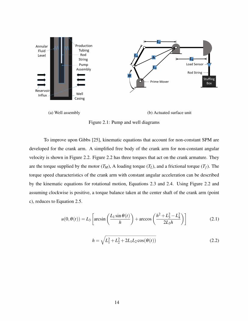
Figure 2.1a is a diagram of the well bottomhole assembly. Reservoir fluid flows into the

well bore through perforations in the well casing. Fluid accumulates in the annular space between

the well casing and the production tubing. Figure 2.1b shows a sucker rod pump surface unit

adapted from Gibbs [25]. A prime mover reciprocates the rod string via a four bar linkage. The

rod string is connected to a positive displacement pump at the bottom of the well. The pump lifts

reservoir fluid to the well surface. When the surface unit lifts the pump, reduced pressure causes

fluid to flow into the bottom of the pump assembly through a stationary one way valve (standing

valve), filling the pump barrel. When the surface unit lowers the pump, the fluid trapped in the

pump barrel is forced past another one way valve (traveling valve) into the production tubing. The

surface unit reciprocates the rod string and the pump produces fluid each upstroke.

2.3 Surface Unit Equations of Motion

Equations 2.1 and 2.2 describe the vertical position of a conventional four bar linkage

sucker rod pump as a function of the prime mover angle, θ . L1 through L5 are unit dimensions

indicated in Figure 2.1b from Gibbs [25]. The same study simulates the polished rod motion

assuming constant stroking speed (SPM).

13

(a) Well assembly

Prime MoverStuffing

Box

Load Sensor

Rod String

(b) Actuated surface unit

Figure 2.1: Pump and well diagrams

To improve upon Gibbs [25], kinematic equations that account for non-constant SPM are

developed for the crank arm. A simplified free body of the crank arm for non-constant angular

velocity is shown in Figure 2.2. Figure 2.2 has three torques that act on the crank armature. They

are the torque supplied by the motor (TM), A loading torque (TL), and a frictional torque (Tf ). The

torque speed characteristics of the crank arm with constant angular acceleration can be described

by the kinematic equations for rotational motion, Equations 2.3 and 2.4. Using Figure 2.2 and

assuming clockwise is positive, a torque balance taken at the center shaft of the crank arm (point

c), reduces to Equation 2.5.

u(0,θ(t)) = L3

[arcsin

(L1 sinθ(t)

h

)+ arccos

(h2 +L2

3−L24

2L3h

)](2.1)

h =√

L21 +L2

2 +2L1L2 cos(θ(t)) (2.2)

14

Figure 2.2: Shows the free body diagram of the crank arm including an effective force diagramand applied torque diagram

dθ

dt= ω (2.3)

dω

dt= α (2.4)

∑Mc = J0α =−Tf −TL +TM (2.5)

The frictional torque within a motor system can be modeled with Equation 2.6 referenced in Virgal

and Kelemen [65] :

Tf = Bω (2.6)

Equation 2.6 is the viscous friction torque model that is commonly used as a damping

term in the modeling of electric motors [71]. To simplify the analysis, the loading torque and

motor torque in Equation 2.5 are lumped into a parameter we will define as net torque (Tnet) where

Tnet = TM−TL. Further, the rotational inertia is assumed to be the combined inertia of the motor,

15

load, and gear train of the rod pump system. Combining Equations 2.3, 2.5, and 2.6 the torque

balance equation reduces to Equation 2.7:

J0dω

dt=−Bω +Tnet (2.7)

Rearranging the equation so that it is in standard form, the equation becomes:

J0

Bdω

dt=−ω +

1B

Tnet (2.8)

which reduces to a standard form for a first order system that is commonly encountered in process

control as shown in Equation 2.9:

τdω

dt=−ω + kTnet (2.9)

where τ = J0B is the time constant and k = 1

B is the gain of the system. For our analysis, it is

convenient to express the dynamic equations in terms of SPM. The angular velocity relates to SPM

by a simple relation given in Equation 2.10:

ω =2π

60SPM (2.10)

Combining Equations 2.9 and 2.10 and solving explicitly for the time derivative results in the

following relation:

dSPMdt

=−1τ

SPM+602π

kτ

Tnet (2.11)

Equation 2.11 expands to a second order system by adding an additional equation that

relates SPM to dθ

dt . This can be achieved by combining Equations 2.3 and 2.10. The result is

Equation 2.12:

dθ

dt=

2π

60SPM (2.12)

Equations 2.11 and 2.12 describe the equations of motion for the crank arm in terms of

SPM. They can be synced with Equations 2.1 and 2.2 to simulate the surface position of the rod

16

string at non-constant SPM values. The surface position is then translated to the dynamics of lower

segments of the rod string through the wave equation given in Equation 2.13.

2.4 Rod String and Well Modeling

The one-dimensional wave equation with viscous damping models the rod string dynamics,

shown in Equation 2.13 [25, 38, 23], with buoyant gravitational effects included, and describes the

propagation of forces and motion in the rod string.

∂ 2u(x, t)∂ t2 = a2 ∂ 2u(x, t)

∂x2 − πaν

2L∂u(x, t)

∂ t−(

1− ρwγ

ρr

)g (2.13)

Simulating the rod string requires two boundary conditions. First, the position of the polished rod

load is specified, as shown generally in Equation 2.14, where F(t) represents an arbitrary motion

profile determined by the surface unit. This work uses kinematic equations for a conventional rod

pump, given in Section 2.3. Second, the behavior of the downhole pump is modeled by Equation

2.15 where α , β , and Pbd(t) depend on the pumping conditions [25]. This study assumes the

produced fluid to be liquid and incompressible. In this case α is equal to 0, β is equal to 1, and

Pbd(t) is given by Equation 2.16. Equation 2.16 implies that the load at the pump is zero when the

pump is descending (the fluid column is held up by production tubing) and equal to the buoyant

weight of the fluid in the production tubing when the pump is ascending.

u(0, t) = F(t) (2.14)

Pbd(t) = αp +β∂u(x f , t)

∂x(2.15)

Pbd(t) =

W f−(At−Ac)Pw f

EAcif: ∂u(x f ,t)

∂ t > 0.0

0.0 if: ∂u(x f ,t)∂ t ≤ 0.0

(2.16)

A differential form of Hook’s Law determines the load at each rod segment as shown in Equation

2.17.

f (x, t) = EAc∂u(x, t)

∂x(2.17)

17

This work also includes the dynamic effects of annulus fluid level and reservoir influx. A

mass material balance on the downhole well assembly shown in Figure 2.1a yields Equation 2.18.

dmdt

= ρwγ(qin−qprod) (2.18)

Where dmdt is the change of mass in the well annulus, and qin and qprod are the influx of

fluids from the reservoir and the fluid produced by the pump. qin and qprod are shown in Equations

2.19 and 2.23, for incompressible fluids. Equation 2.19 is piecewise because fluid is only removed

from the control volume during the pump upstroke.

qprod =

Acpump∂u(x f ,t)

∂ t if: ∂u(x f ,t)∂ t > 0.0

0.0 if: ∂u(x f ,t)∂ t ≤ 0.0

(2.19)

Assuming the fluid is incompressible, Equation 2.18 expands to Equation 2.20. Simplifying

leads to the final equation describing the change in height of fluid in the well annulus, Equation

2.21. Reformulating Equation 2.21 into oilfield units gives Equation 2.22. The simulation solves

Equations 2.13, 2.14, 2.19, 2.21, and 2.23 simultaneously, to dynamically simulate the well.

ρ f γ(Accasing−Actubing)dhdt

= ρwγ(qin−qprod) (2.20)

dhdt

=(qin−qprod)

(Accasing−Actubing)(2.21)

dhdt

=1617

2(qin−qprod)

(Accasing−Actubing)(2.22)

2.5 Reservoir Modeling

The simplified well model considers a solution gas drive reservoir in pseudo-steady state

flow. To simplify the analysis further, we assume gas is held in the solution over the life of the well,

i.e. the oil pressure never falls below bubble point pressure. Thus we do not have to consider more

complicated dynamics such as two phase flow and relative permeability in the reservoir. Using

the assumptions defined above the inflow performance relationship for the reservoir is defined by

18

Equation 2.23 [19].

qin =kh(P−Pw f )

141.2B0µ

(12 ln 4A

γCAr2w+S) (2.23)

At pressures above the bubble point, the fluid recovery from an oil reservoir depends entirely on the

fluid expansion as the reservoir pressure declines. This behavior can be described by the isothermal

compressibility defined by Equation 2.24 [44].

c =− 1V

∂V∂P

(2.24)

Integrating Equation 2.24 by the method of separation of variables from initial reservoir pressure

to the current average reservoir pressure, the solution to the partial differential equation becomes

the following:

VVi

= ec(Pi−P) (2.25)

It should be noted that c is assumed constant over the producing life of the well. The volume at the

lower average reservoir pressure P includes the volume left in the reservoir, Vi, and the volume of

the fluid that has been produced, Vp, i.e.

V =Vi +VP (2.26)

Combining Equations 2.25 and 2.26 an explicit solution for average reservoir pressure can be

derived as a function of the cumulative volume extracted from the reservoir as shown in Equation

2.27:

P = Pi−1c

ln(

Vp

Vi+1)

(2.27)

The cumulative volume produced is given by Equation 2.28:

Vp =∫

qout dt (2.28)

19

Using Equations 2.23, 2.27, and 2.28 an inflow performance relationship (IPR) model of a reservoir

can be developed. The values of the constants given in the equations are shown in the nomenclature

section.

2.6 Well Vertical Lift Performance

The Vertical Lift Performance (VLP) of a rod pumped well is defined by Equation 2.29:

Pw f = 0.433γh f (2.29)

To obtain Equation 2.29 we assumed that the pressure at the liquid surface in the annulus is at

atmospheric pressure, i.e., the casing surface pressure is atmospheric and the hydrostatic pressure

of the gas column above the fluid in the annulus is negligible. Combining Equation 2.23 from IPR

and Equation 2.29 from VLP, nodal analysis can be performed to acquire the flow rate supplied by

the reservoir as the fluid level changes in the annulus.

2.7 Economics

In the oil and gas industry, NPV is a common metric used to measure the economic viability

of a project. NPV considers the time value of money and helps distinguish between multiple

investment options. The continuous form of NPV is given by Equation 2.30:

NPV =∫

S(t)e−rtdt−Cinitial (2.30)

The profit rate, S(t), is given by the difference between the revenue and expense rates as

shown in Equation 2.31:

S(t) =dR(t)

dt− dX(t)

dt(2.31)

For the rod pump system, the revenue rate depends on the production rate and the price of

oil as shown in Equation 2.32:dR(t)

dt= Poqout(t) (2.32)

20

The expenses depend on the initial cost of the rod pump and the cost to operate the motor

to pump the fluid. Applying an energy balance and mass balance between the bottom of the tubing

string to the well head, the work required to produce the fluid with an electric motor can be derived.

The initial energy balance is given by Equation 2.33. The mass balance is given by Equation 2.34:

Wmotor + m(

Pw f

p+

v2in2

+gzin

)= m

(Pwh

p+

v2out2

+gzout

)+ emech,loss (2.33)

ρVinAt = ρVoutAt = ρQ (2.34)

Combining Equations 2.33 and 2.34, and assuming the fluid is incompressible, an explicit

expression for the rate of work of the rod pump motor can be formulated in terms of the pumping

rate, Q. The expression is given by Equation 2.35:

Wmotor = Q(Pwh−Pw f +ρgzout)+ emech,loss (2.35)

The horsepower to overcome frictional losses for a rod pump can be empirically estimated

by Equation 2.36 [19]:

emech,loss = 6.31x10−7WrSlength(SPM) (2.36)

Combining Equations 2.35 and 2.36 and reformulating the equation so that it is compatible

with oilfield units gives Equation 2.37. The rate of work of the rod pump motor has units of

kilowatts.

Wmotor = 1.2687x10−5qout(Pwh−Pw f +0.433γTV D)+4.7053x10−7WrSlengthSPM (2.37)

The expense rate of operating the motor can then be determined. The result is given by Equation

2.38:

dX(t)dt

= 24WmotorEcost (2.38)

21

where Ecost is the cost of electricity per kWh. Substituting Equations 2.32 and 2.38 into

Equation 2.30 gives the final expression to calculate the NPV of operating the rod pump over the

life of the well:

NPV =∫(Poqout(t)−24WmotorEcost)e−rtdt−Cinitial (2.39)

It is important to note that 100% motor efficiency and no mechanical downtime is assumed when

deriving Equation 2.39.

2.8 Moving Horizon Estimation and Model Predictive Control

MHE is a dynamic optimization technique that looks back at a time horizon and fits model

parameters to historical data. MHE approximates uncertain parameters or variables, and performs

well on systems that include large amounts of noise in the data set [42]. MHE also allows process

information to be directly considered during optimization [61]. The main disadvantage of MHE is

computational time, but real time solutions are possible, even for large systems [73]. In this work,

an optimizer uses a squared error objective, as described in Hedengren et al. [32], to minimize

the error in the model fit by varying uncertain model parameters or states. 2.40 Equation 2.40

shows the general MHE squared error. The model equations (Equations 2.1 - 2.39 and 2.55 - 2.59)

are included as Equations 2.41 - 2.43 in nonlinear open-equation form with differential, algebraic,

and inequality constraints, respectively. The objective function minimizes the sum of square error

between measured data and model predictions. Terms used in Equations 2.40 - 2.43 are shown in

Table 2.1.

minx,y,p

Φ = (yx− y)TWm(yx− y) (2.40)

s.t. 0 = f(

dxdt

,x,y, p,u)

(2.41)

0 = g(x,y, p,u) (2.42)

0≤ h(x,y, p,u) (2.43)

22

Estimation of uncertain parameters (p) in wells and reservoirs is an important area of re-

search [47, 62]. The process of estimating reservoir parameters from historical data (yx) is often

called history matching. Prior work illustrates estimation of reservoir properties using simulta-

neous techniques [37, 74]. The ability and importance of estimating parameters in real-time is

also shown [2, 29]. This work expands prior work by utilizing a combined rod string, well, and

reservoir model to estimate parameters in real-time and utilize those parameters in automatic well

control.

Table 2.1: Objective Function Terms from Hedengren et al. [32] for MHE andMPC

Symbol DescriptionΦ objective functionyx measurements (yx,0, ...,yz,n)

T

y model values(y0, ...,yn)T

Wm measurement deviation penaltyx,u, p states (x), inputs (u), and parameters (p)∆p change in parametersf ,g,h equation residuals, output fraction, and inequality constraintsyt ,yt,hi,yt,lo desired trajectory target or dead-bandWhi,Wlo penalty outside trajectory dead-bandcy,cu,c∆u cost of y, u and ∆u, respectivelyτc time constant of desired controlled variable responseelo,ehi slack variable below or above the trajectory dead-bandsplo,sphi lower and upper bounds to final set point dead-band

MPC determines future manipulated variables at control intervals. Industrial MPC began in

the energy industry and has been applied to many systems [53]. The MPC application minimizes

the l1-norm error between the desired controlled variable trajectory and the model prediction by

varying the variables that can be manipulated (u). At each time step the next optimal control move

(u0) is implemented, then the process repeats. A general formulation of the MPC problem is given

in Equations 2.44 - 2.51 Hedengren et al. [32]. The objective function (Equation 2.44) is com-

posed of four terms that minimize an upper trajectory error, a lower trajectory error, the cost of

the controlled variable (y), and the cost of manipulated variable movement (∆u). Equations 2.45

- 2.47 are the nonlinear model equations after spatial discretization of the PDE with differential,

23

algebraic, and inequality constraints, respectively. Equations 2.48 - 2.49 are first-order upper and

lower reference trajectories that guide the speed of the controlled variable response with the pa-

rameter τc. Equations 2.50 - 2.52 are error variables that are used in the objective function to

penalize deviations outside the reference trajectory dead-band. The dead-band is set to ±0.1 ft to

account for the natural variation in fluid height with the discrete stroke cycles. This dead-band can

be further increased to reduce the variation of the stroking speed manipulated variable adjustments

due to process disturbances. Terms used in Equations 2.44 - 2.52 are shown in Table 2.1.

minx,y,u

Φ =W Thi ehi +W T

loelo + yT cy +∆uT c∆u (2.44)

s.t. 0 = f(

dxdt

,x,y, p,d,u)

(2.45)

0 = g(x,y, p,u) (2.46)

0≤ h(x,y, p,u) (2.47)

sphi = τcdyt,hi

dt+ yt,hi (2.48)

splo = τcdyt,lo

dt+ yt,lo (2.49)

ehi ≥ y− yt,hi (2.50)

elo ≥ yt,lo− y (2.51)

0≥ ehi, elo (2.52)

2.9 Solution Methods

Two solution methods to the wave equation include a numerical approximation and an

exact analytical solution. The following sections discuss a numerical and analytical approach to

a simplified problem with the analytical solution verifying the numerical approximations that are

used in optimization, and in the non-ideal case.

24

2.10 Numerical Methods

Equation 2.13 is a second order hyperbolic partial differential equation (PDE). Numerically

simulating hyperbolic PDEs is difficult since they are unstable, or conditionally stable when solved

with some numerical methods. Also, some numerical simulation methods suffer from numerical

damping.

Gibbs [25] uses finite differencing to convert Equation 2.13 into an algebraic expression.

First order forward differencing approximates ∂u(x,t)∂ t . First order central differencing approximates

∂ 2u(x,t)∂ t2 and ∂ 2u(x,t)

∂x2 . Doty and Schmidt [18] use a similar finite difference method to simulate a

sucker rod system.

For converting differential equations into algebraic equations this work utilizes both finite

differencing and orthogonal collocation on a finite element. Partial derivatives with respect to

space (x) in Equation 2.13 are approximated using first order central differencing. First and second

order derivatives with respect to time (t) are approximated by orthogonal collocation on a finite

element. ∂u(x,t)∂x in Equation 2.17 is approximated with a first order central difference at internal

rod positions and by a second order forward difference at the surface, and a second order back-

ward difference at the pump. The GEKKO optimization suite with the IPOPT solver simulate the

system and solve subsequent MHE and MPC applications [7, 9, 66]. To verify the validity of this

method a special case of the solution method is compared to a Fourier series analytical solution. A

grid independence study determines by observation the stability and discretization requirements to

achieve stable and accurate solutions to the well and reservoir model.

2.11 Simulating Pump Boundary Conditions for Optimization

Simulating the sucker rod system requires time varying boundary conditions at the pump.

For example, in the case that the pump is liquid full and the pump valves are operating correctly,

when the pump is traveling upwards it is loaded with the buoyant weight of the fluid in the produc-

tion tubing, and when the pump is descending it is unloaded (the weight is borne by the production

tubing). Previous work simulates these changing conditions with a series of conditional statements

or tests [25, 18]. However, these conditional statements create discontinuities in the model and

these discontinuities are inappropriate for dynamic optimization using simultaneous solvers [32].

25

This work formulates the pump boundary conditions with MPCCs to solve the well model in both

dynamic simulation and optimization modes with large-scale solvers. MPCCs have been used in

similar problems with discrete decisions or switching points [55, 4, 5, 6, 52]. The approach taken

in this work is to include the bilinear switching terms as objective function terms. Alternative

strategies are to include the bilinear switching terms as equality or inequality constraints. The ad-

ditional constraints add computational expense and are not needed for this application. Simulations

in this study verify that the objective function contribution of the MPCC is zero at the solution. The

additional slack variables and bilinear switching terms enable gradient-based solution methods to

be used with the discontinuous pump boundary conditions. An MPCC formulation of the signum

function, shown in Equation 2.53, determines when the pump is traveling up or down. When the

velocity of the pump is positive it is traveling upward, and y is equal to 1. When the pump is

descending the velocity is negative and y is equal to -1.

y(t) = sgn(

∂u(x f , t)∂ t

)(2.53)

The solver solves Equations 2.54 through 2.58 and determines the sign of the velocity, y.

Equation 2.59 uses y to determine the boundary condition at the pump. Pbd(t) = 0 when y = −1

and Pbd(t) =W f−(At−Ac)Pw f

EAcwhen y = 1.

min sa(1− y)+ sb(y−1) (2.54)

∂u(x f , t)∂ t

= sb− sa (2.55)

−1≤ y≤ 1 (2.56)

sa ≥ 0 (2.57)

sb ≥ 0 (2.58)

Pbd(t) =Wf − (At−Ac)Pw f

EAc· (1+ y)

2(2.59)

26

2.12 Comparison to Analytical Solution

A simplified version of Equation 2.13 is obtained when the viscous damping term is equal

to zero and gravitational effects are neglected. The resulting wave equation is shown in Equation

2.60. When initial position and velocity of the rod string are given by Equations 2.62 and 2.63,

a Fourier series provides an analytical solution. The analytical solution to this case is given in

Equation 2.61. This solution is called the d’Alembert solution to the Cauchy problem for the wave

equation [48]. Where φ and ψ are the initial position and velocity of u.

∂ 2u(x, t)∂ t2 = a2 ∂ 2u(x, t)

∂x2 (2.60)

u(x, t) =12(φ(x+at)+φ(x+at))+

12a

∫ x+at

x−atψ(s)ds (2.61)

u(x,0) = φ(x) (2.62)

∂u(x,0)∂ t

= ψ(x) (2.63)

A simulation of this special case compares the analytical solution to the proposed method.

The initial position and velocity of the rod are given in Equations 2.64 and 2.65. The boundary

condition in space is that the rod is of infinite length. Equation 2.61 finds the analytical solution to

this initial value problem which is given in Equation 2.66.

u(x,0) = cos(x) (2.64)

∂u(x,0)∂ t

= sin(2x) f or −∞ < x < ∞ (2.65)

u(x, t) = cos(x)cos(at)+1

2asin(2x)sin(2at) (2.66)

Figure 2.3 shows the analytical solution method versus the orthogonal collocation (in time)

with the finite difference method (in space) over the time domain 0.0≤ t ≤ 0.0005 and the spatial

domain 0.0 ≤ x ≤ 2π . The solutions are very similar. Figure 2.4 shows the difference in the

proposed solution method versus the analytical solution. The difference is small for most of the

domain. Error increases further out from the initial time, t = 0, indicating that the proposed solution

method, in this case, appears to have numerical damping. Despite moderate numerical damping,

27

the results indicate that the proposed method appropriately simulates the simplified wave equation.

A grid independence study identifies criteria for discretization in time and space that allows for

sufficiently accurate solutions to simulate the rod string behavior in the combined rod string, well,

and reservoir model.

Distance (ft)

0 1 2 3 4 5 6 Time (s

econds

)

0.00000.0001

0.00020.0003

0.00040.0005

Posit

ion (ft)

−1.00−0.75−0.50−0.250.000.250.500.751.00

(a) Analytical solution

Distance (ft)

0 1 2 3 4 5 6 Time (s

econds

)

0.00000.0001

0.00020.0003

0.00040.0005

Posit

ion (ft)

−1.00−0.75−0.50−0.250.000.250.500.751.00

(b) GEKKO solution

Figure 2.3: Comparison of analytical and GEKKO solutions

2.13 Grid Independence Study

A grid independence study evaluates the solution dependence on time and space grid size.

Discretizing in time and space to simulate the system creates a large problem with thousands of

variables and equations. This section determines minimum spatial and time resolution to capture

system dynamics. Simulations for the combined rod string, well, and reservoir model are solved

with increasingly fine discretization in time and space. The solver simulates the horizon iteratively

in one second intervals.

The solver attempts to simulate all combinations with the sucker rod discretized in 3, 4,

and 5 to 30 segments in increments of 5, and time discretized with 5 to 30 intervals in each second,

in increments of 5. Figures 2.5 and 2.6 show representative results of the study. In these figures,

the polished rod (surface) load is shown vs. time. Figure 2.5 shows results for 10 rod segments

and varying time discretization. Figure 2.6 shows results for 20 time segments in each second and

varying rod discretization. All simulations are initialized with u(x, t) = 0 and dudt = 0. Cases that

do not successfully solve for the first second of the horizon are omitted.

28

0 1 2 3 4 5 6Distance (ft)

0.0000

0.0001

0.0002

0.0003

0.0004

0.0005Time (sec

onds

)

−0.0825

−0.0660

−0.0495

−0.0330

−0.0165

0.0000

0.0165

0.0330

0.0495

Diffe

renc

e

Figure 2.4: Error of proposed solution method vs. analytical solution

Figure 2.5 shows that when fewer time steps are used, the solution does not adequately

capture the dynamics of the force and position propagation in the sucker rod. 20 segments in time

appears to adequately captures the system dynamics. Figure 2.6 shows that increasing the number

of rod segments changes the shape of the simulation results very little. However, the results do

show that as the number of rod segments increase the entire curve shifts upward, although the am-

plitude of each case stay very similar. Few rod segments are required to capture system dynamics.

These results indicate that 20 time segments per second and 10 rod segments capture a majority of

the system dynamics, shown on Figures 2.5 and 2.6 in dashed red. This discretization is selected

for simulation, estimation, and control in Section 2.20 as a compromise between computational

speed and accuracy. Results shown in Section 2.14 are for 30 points in time per second and 30 rod

segments.

29

20.0 22.5 25.0 27.5 30.0 32.5 35.0 37.5 40.0Time (seconds)

6000

8000

10000

12000

14000Lo

ad (lbf)

npt = 5npt = 10npt = 15npt = 20npt = 25npt = 30

Figure 2.5: Fixed rod length discretization of 10 sections

20.0 22.5 25.0 27.5 30.0 32.5 35.0 37.5 40.0Time (seconds)

4000

6000

8000

10000

12000

14000

Load

(lbf)

npx = 3npx = 4npx = 5npx = 10npx = 15npx = 25npx = 30

Figure 2.6: Fixed number of time points at 20

30

2.14 Modeling Results

Modeling results are discussed for reservoir and rod string dynamics. A unique contribution

of this work is the combined models that are used in optimizing production and NPV. Both MHE

and MPC require a system model. A more accurate system model leads to more accurate parameter

estimation and improved MPC controller performance. This section verifies that the proposed

model accurately describes the system, and is appropriate for MHE and MPC use.

2.15 Reservoir Pressure and Production Dynamics

The well and reservoir model described in Sections 2.1 and 2.9 simulate the well system

over a 30 minute horizon using 30 rod string discretizations and 30 time points per second. It

took 3.14 hours to run the entire 30 minute simulation. Figures 2.7 through 2.15 illustrate the

results of the simulation. Figure 2.11 gives a modified version of the time horizon to demonstrate

NPV. Figure 2.12 captures the transient dynamics within the first ten seconds after the simulation

is initialized. Figures 2.13 to 2.15 capture the steady state dynamics of the rod string shown in the

time interval 20 to 40 seconds after the simulation is initialized.

Figure 2.7 shows how the annular fluid level changes over the 30 minute simulation period

with adjustments to net torque using a doublet test. Tnet is defined as the manipulated variable. Tnet

is initialized at 10 ft-lbs and is adjusted between 5 and 15 ft-lbs over the 30 minute simulation. The

height of the fluid level in the annulus is defined as the controlled variable. During the simulation,

the fluid level in the annulus changes dependent on the torque input. In cases where the fluid level

in the annulus rises, the inflow rate of the reservoir exceeds the motor pumping rate. In cases where

the fluid level in the annulus declines, the pumping rate exceeds the inflow rate of the reservoir.

Figure 2.8 illustrates the reservoir pressure decline over the 30 minute simulation period for

the solution gas drive reservoir. As fluid is produced and enters the annulus, the reservoir reserves

are depleted. In this case, the cumulative volume produced is dependent on the bottomhole flowing

pressure and pumping rate of the motor. As the cumulative volume produced increases, we observe

a decline in pressure in accordance with Equation 2.27.

Figure 2.9 shows the interacting dynamics between the reservoir and rod pump. Figure

2.9a shows the first ten seconds of the simulation. The rod pump is stroking with a Tnet of 10 ft-lbs

31

0 250 500 750 1000 1250 1500 17503500

3525

3550

3575

3600He

ight (ft)

Height in Annulus

0 250 500 750 1000 1250 1500 1750Time (seconds)

5.0

7.5

10.0

12.5

15.0

T net(ft

−lbs)

Tnet

Figure 2.7: Doublet test performed at different net torque values

and the fluid level is oscillating up and down. The fluid level in the annulus exhibits non-linear

behavior because of the intermittent pumping rate of the rod string. The producing flow rate rises

greatly with the upstroke of the rod string and is zero when the pump is not pulling fluid on the

downstroke. It can also be observed that the fluid rate flowing into the annulus (qin) is fairly con-

stant for the first ten seconds. This is because the bottomhole pressure and reservoir pressure does

not change significantly over the first ten seconds of the simulation. Figure 2.9b shows the inter-

acting dynamics between the reservoir and rod pump over the full 30 minute simulation. Initially,

the fluid level in the annulus rises because the reservoir inflow exceeds the pumping rate of the

rod string. When the Tnet is increased to 15 ft-lbs the pumping rate increases, the fluid level in

the annulus decreases. This is because the pumping rate exceeds the reservoir inflow. The ”tug of

war” between inflow and outflow is constantly observed through the changing liquid level height

in the annulus and is difficult to control manually due to the inherent non-linear nature of the sys-

32

0 250 500 750 1000 1250 1500 1750

1500

1600

Pressure (p

si)Reservoir Pressure

0 250 500 750 1000 1250 1500 1750Time (seconds)

35

40

45

50

55

Volume (STB

) Cumulative Volume Produced

Figure 2.8: Change in reservoir pressure with cumulative volume produced from the rod pump

0 2 4 6 8 103599.25

3599.50

3599.75

3600.00

3600.25

Height (f

t)

Fluid Level (ft)

0 2 4 6 8 10Time (seconds)

0.00

0.02

0.04

0.06

Flow

(STB

/s)

qin

qout

(a) The first 10 seconds of the simulation

0 250 500 750 1000 1250 1500 17503500

3525

3550

3575

3600

Heig

ht (f

t)

Fluid Level (ft)

0 250 500 750 1000 1250 1500 1750Time (seconds)

0.00

0.02

0.04

0.06

0.08

Flow

(STB

/s)

qin

qout

(b) The full 30 minute simulation

Figure 2.9: The system is a dynamic blend of inflow and outflow of fluids

33

tem. Using a control scheme like MPC, the fluid level can be controlled to a desired set point and

maintained over the simulation period that otherwise may be difficult to control manually.

0 2 4 6 8 10

20

40

KiloWatts (k

W)

Lifting Power

0 2 4 6 8 109.5

10.0

10.5

SPM

SPM

0 2 4 6 8 10Time (seconds)

1249.4

1249.6

1249.8

FBHP

(psi) Pwf

(a) The first 10 seconds of the simulation

0 200 400 600 800 1000 1200 1400 1600 18000

20

40

KiloWatts (k

W)

Lifting Power

0 200 400 600 800 1000 1200 1400 1600 18005

10

15

SPM

TnetSPM

0 200 400 600 800 1000 1200 1400 1600 1800Time (seconds)

1220

1240

FBHP

(psi) Pwf

(b) The full 30 minute simulation

Figure 2.10: Power consumption of the rod pump motor as FBHP declines and SPM varies

Figures 2.10 shows the interacting dynamics between power consumption, SPM, Tnet , and

Flowing Bottomhole Pressure (FBHP). When SPM is constant it is equal to Tnet , and in the longer

simulation there is a very short time constant following a first order response. Figure 2.10a shows

the first ten seconds of the simulation. The rod pump is stroking at a rate of 10 SPM (which

corresponds to Tnet = 10) and the bottomhole pressure and power consumption is fluctuating up

and down. The bottomhole pressure and power consumption exhibit non-linear behavior because

of the intermittent pumping rate of the rod string. The power consumption rises with the upstroke of

the well. At the same time, the bottomhole pressure declines because the fluid level in the annulus

drops slightly. On the downstroke, the power consumption is zero and the bottomhole pressure

increases. The bottomhole pressure increases on the downstroke because the liquid level height

in the annulus increases due to reservoir inflow. Figure 2.10b shows the interacting dynamics

between power consumption, SPM, Tnet , and FBHP during the full 30 minute simulation. It is

clear that the power consumption increases with increasing Tnet . This makes sense because at

a higher Tnet setting, more volume of fluid moves in a smaller amount of time. Further, power

consumption increases with time at fixed Tnet inputs. This occurs because as FBHP declines, there

34

is less assistance from the reservoir to help push the column of fluid above the pump to surface.

Hence, power consumption increases with time at a fixed Tnet value.

0 1 2 3 4 5 6 7 8Time (years)

−1

0

1

2

3

4

NPV ($ Million

s)

NPV

Figure 2.11: Shows how NPV varies over an 8 year simulation period

Figure 2.11 illustrates how NPV changes over the life of the well. Because the resolution

of a 30 minute simulation cannot capture the entire dynamics of NPV, the simulation is extended

to 8 years. As is expected, the NPV is negative during the early development of the well due

to the initial cost of the rod pump which is assumed to be $1 million. Initially, the rod pump

produces at the maximum SPM and Tnet setting and NPV increases. As time progresses, the income

is discounted and begins to deviate from a linear profile as shown between year 1 and year 3.

Additional factors that cause the the trajectory to deviate from a linear profile include: (1) the

inflow rate from the well declines, forcing the pump to produce at a lower Tnet value and (2)

the operating costs increase because the bottomhole pressure declines providing less assistance to

raise the fluid to surface. As time progresses, the NPV attains a maximum value around year 3 as

35

shown in Figure 2.11. Beyond this point, the operating costs begin to exceed the income produced

from production for the reasons mentioned above. Therefore, a decline in NPV is apparent. As

illustrated by the figure above, the goal of a producer is to attain the maximum NPV. Using control

methods combined with optimization, higher NPV can be realized that would be difficult to attain

through manual control methods.

2.16 Rod String Dynamics

The rod string and pump dynamics are illustrated in this section. The first ten seconds and

the 20 to 40 second interval of the 30 minute simulation (to avoid the noise from the transient start

up of the system) show the quick dynamics of the rod string and pump system. The simulation

takes into account the changes in the reservoir and the oscillations of the pump as it removes

production fluid.

Distance (ft)

010002000300040005000

Time (seconds)0 2 4 6 8 10

Posit

ion (ft)

02468101214

Figure 2.12: Dynamic rod string position in space and time (10 seconds)

Figure 2.12 displays the sucker rod position in time and space. Distance 0 ft represents

the rod at the surface that is actuated by the surface unit. Distance 4800 ft is the rod position

at the pump. Figure 2.13 gives the position and velocity of the pump. The sign of the velocity

36

is also shown, scaled by 10 to be visible. The solver accurately determines when the velocity is

positive, and when it is negative, which determines the fluid load at the pump, simulating pumping

conditions.

20.0 22.5 25.0 27.5 30.0 32.5 35.0 37.5 40.0Time (seconds)

−10

−5

0

5

10

15

Pump Position (ft)Pump Velocity (ft/s)Sgn(V)

Figure 2.13: Pump position, velocity, and velocity sign (20-40 seconds)

Figures 2.14a, 2.14b, 2.15a and 2.15b refer to the load on the system at the surface, for the

pump, and as the pump load changes with position and time. Offset lines on the surface card and

pump card would be present from startup dynamics of the first 10 seconds so the segment of 20-40

seconds is shown. The rod load varies depending on stroking rate and the fluid load at the pump.

The dynamic load is essentially zero when the pump rod rests buoyantly in the annular fluid. The

polished rod load mimics the motion of the pump at the surface and the rod load versus the position

of the pump draws out a dynamometer card in roughly the shape of a rectangle which corresponds

to actual data and previous research on rod pumps.

37

0 25 50 75 100 125 150 175Position (in)

6000

8000

10000

12000

14000Load

(lbf)

Surface Dynagraph

(a) Surface

0 25 50 75 100 125 150 175Position (in)

0

250

500

750

1000

1250

1500

1750

Load

(lbf)

Pump Dynagraph

(b) Pump (rectangular)

Figure 2.14: Rod load vs. position

20.0 22.5 25.0 27.5 30.0 32.5 35.0 37.5 40.0Time (seconds)

6000

8000

10000

12000

14000

Load

(lbf)

Pump Load (lbf)

(a) Surface

20.0 22.5 25.0 27.5 30.0 32.5 35.0 37.5 40.0Time (seconds)

0

200

400

600

800

1000

1200

1400

1600Lo

ad (lbf)

Pump Load (lbf)

(b) Pump (rectangular)

Figure 2.15: Rod load vs. time

2.17 Moving Horizon Estimation Results

In the oil and gas industry, it is common not to have all the available data to carry out

meaningful reservoir engineering analysis. The cost to acquire new information through well in-

tervention techniques such as well logging, pressure build up tests, core analysis, and well sur-

veys, is expensive. Further, those measurements are typically limited to a snapshot in time and

require the well to be shut-in. Other methods used to acquire continuous reservoir surveillance

data through downhole electronic sensors always suffer in reliability due to the extreme pressures

and temperatures encountered downhole [10]. Thus, there is a high degree of risk involved in

implementing downhole measuring devices. Because operators are trained to minimize expenses,

38

reduce downtime, and limit risks, this information is usually never realized, or acquired indirectly

using stochastic estimates from other wells in the area. With MHE, reservoir properties and flow

variables can be estimated at no cost, without shutting in the well, and at no risk. This section high-

lights the results of two simulation case studies where MHE is implemented to (1) infer the fluid

level in the annulus of a rod pumped well and (2) estimate reservoir parameters. Both case studies

use the simulation model from Section 2.14. Two measured parameters are passed to the MHE:

(1) the surface polished rod load and (2) the net torque produced by the motor. This is convenient

for operators because both measurements can be easily acquired from the surface through surface

dynagraph cards and gauges on the motor. The case studies are shown in Table 2.2. In Case 1 the

MHE estimates the annular fluid height given the rod load at the surface (polished rod load) and

the net torque produced by the motor. The MHE estimate of annular fluid height is compared to

the true value to validate that the fluid level in the annulus can be inferred from the surface load. In

Case 2, MHE is used to estimate reservoir properties such as porosity and flow properties such as

skin using the surface load and net torque produced by the motor. The true values are compared to

the estimated values. All MHE figures use a discretization of 20 points in each one second interval

and 10 rod sections.

Table 2.2: Estimation Case Studies

Estimation Estimated Variable(s) Measured VariableCase

1 Annular fluid height Polished rod load, Tnet2 Well Skin factor and Porosity Polished rod load, Tnet

2.18 Annular Fluid Height Estimation

In rod pumped wells, it is critical to maintain the annular fluid level above the pump to

avoid pump-off and fluid pound conditions [41]. Further, it is desirable to produce at the lowest

level possible to maximize NPV over the lifetime of the well. Traditional methods used to measure

the fluid level height in rod pumped wells include echo-meter surveys and electronic bottomhole

pressure gauges. Although these tools have benefits, there are some drawbacks as described in the

39

previous section. Figure 2.16 highlights the MHE estimate of the annular fluid height from the

surface load values and the net torque produced by the motor excluding measurement noise. At the

initial time, it is assumed that the well is not flowing and the hydrostatic head of the fluid is equal

to the reservoir pressure. Therefore, for this scenario the initial condition assigned to the MHE is

assumed to be equivalent to the true initial condition as demonstrated in Figure 17.

2380

2390

2400

Flui

d He

ight

in A

nnul

us (f

t)

TrueEstimated

0 20 40 60 80 100 120Time (seconds)

68

101214

T net (f

t-lbs

)

Tnet

Figure 2.16: Height is estimated with varying inputs of Tnet (which adjusts based off the load)

From Figure 2.16 it is clear that the MHE estimate of annular fluid level height is identical

to the true value. In practice, there may be measurement noise in the load measurements taken

at the surface. Further, there may be uncertainty in the starting fluid level height of the annulus.

To test the robustness of the MHE estimator, an additional scenario is investigated which includes

added measurement noise and an initial condition different from the actual fluid level height. In

this scenario, the initial condition is set to 100 ft below the actual fluid level height (2400 ft) at the

40

initial time. Normally distributed white noise is added to the measured force from the simulator

with a standard deviation of 50 lbs. The results are shown in Figure 2.17:

2360

2380

2400

Fluid He

ight in Annulus (ft)

TrueEstimated

0 20 40 60 80 100 120Time (seconds)

68

101214

T net (ft-lbs)

Tnet

Figure 2.17: Height is estimated with varied Tnet , noise, and an offset initial condition

Figure 2.17 suggests that the measurement noise adversely effects the estimator perfor-

mance. However, the MHE is adequately successful in tracking the actual fluid level height. The

estimator approaches the actual fluid height after about 60 seconds even when the initial condition

is unknown. It is interesting to note that because the system has intermittent production, i.e. fluid

is produced on the upstroke but not on the downstroke, the MHE estimator is only able to retrieve

useful loading data on the upstroke. This is observed in Figure 2.17 where the estimated height

is constant then steps during periods where the fluid level is decreasing. This is because on the

downstroke, when no fluid is produced, the loading condition is constant and does not provide

useful information for the MHE to react. Despite white measurement noise, the MHE application

41

is able to accurately track the fluid level height over the course of the simulation. The results from

the two scenarios validate that the MHE can use surface loading measurements to infer the annular

fluid level height in the well. Thus downhole pressure gauge measurements and acoustic surveys

are not necessarily required. By estimating annular fluid height the MHE can be integrated with

MPC to lead to automated control as described in Section 2.20.

2.19 Reservoir Parameter Estimation

Parameters of interest to reservoir engineers include drainage area, porosity, pressure, per-

meability, skin factor, etc. This study estimates the porosity and skin using MHE.

In general, parameters such as porosity and skin are considered time-invariant in reservoir

modeling. However, in practice, these parameters change during depletion of a well and are not

necessarily time-invariant. For example, depleting reservoirs generally experience a change in

total stress state in the reservoir rock as pressure reduction occurs over time [33]. Therefore, it is

expected that pore volume reduction occurs as the reservoir is depleted. Changes in temperature

and pressure in the reservoir can also cause formation skin damage to change over time. For

example, as the temperature or pressure declines with time, compounds can precipitate from the

wellbore fluids, this results in permeability impairment in the near wellbore region [19]. The

precipitates can build up over time resulting in a constantly changing skin value. MHE has the

capability to track such changes over the life cycle of a well. Further, MHE is an additional

method to retrieve useful information of reservoir parameters. In practice there are several tools

used to estimate the same reservoir properties (e.g. core analysis, logging, seismic, and stochastic

methods can all be used to estimate porosity). Each method has pros and cons. For example, core

analysis has a high resolution, however it is expensive and limited to a snapshot in time. Stochastic

methods are fast and inexpensive, however the results may not be representative of a particular

well because it is relying on a distribution of a statistical data set from other wells of a given

sample size. Seismic is extremely expensive and is also limited to snapshots in time. What makes

MHE unique over the other methods, is it would be relatively inexpensive, does not require well

intervention, and can dynamically estimate reservoir parameters with varying conditions which

allows the reservoir engineer to monitor the health of a particular well in real time.

42

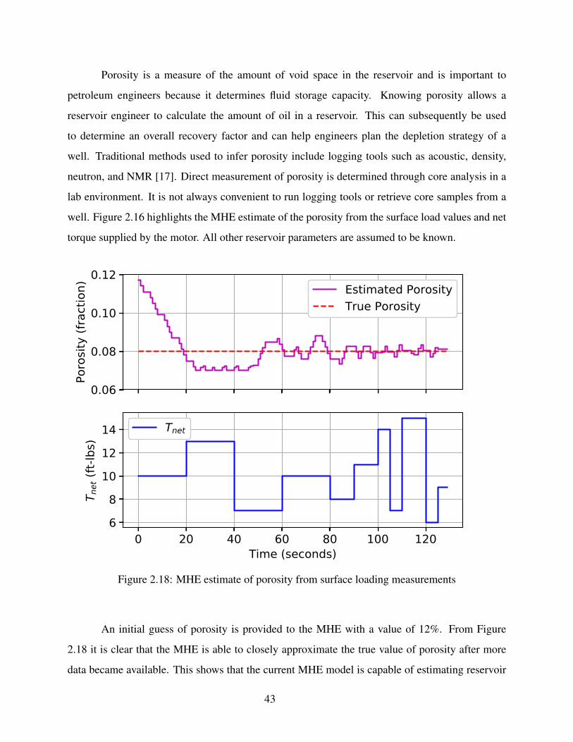
Porosity is a measure of the amount of void space in the reservoir and is important to

petroleum engineers because it determines fluid storage capacity. Knowing porosity allows a

reservoir engineer to calculate the amount of oil in a reservoir. This can subsequently be used

to determine an overall recovery factor and can help engineers plan the depletion strategy of a

well. Traditional methods used to infer porosity include logging tools such as acoustic, density,

neutron, and NMR [17]. Direct measurement of porosity is determined through core analysis in a

lab environment. It is not always convenient to run logging tools or retrieve core samples from a

well. Figure 2.16 highlights the MHE estimate of the porosity from the surface load values and net

torque supplied by the motor. All other reservoir parameters are assumed to be known.

0.06

0.08

0.10

0.12

Porosit

y (fr

actio

n) Estimated PorosityTrue Porosity

0 20 40 60 80 100 120Time (seconds)

68

101214

T net (ft-lbs

)

Tnet

Figure 2.18: MHE estimate of porosity from surface loading measurements

An initial guess of porosity is provided to the MHE with a value of 12%. From Figure

2.18 it is clear that the MHE is able to closely approximate the true value of porosity after more

data became available. This shows that the current MHE model is capable of estimating reservoir

43

parameters from a rod pumped well without well intervention. Thus, well logging and core analysis

are not necessarily required.

2468

10

Skin

Estimated SkinTrue Skin

0 20 40 60 80 100 120Time (seconds)

68

101214

T net (ft-lbs

)

Tnet

Figure 2.19: MHE estimate of skin from surface loading measurements

Skin factor is another parameter of interest to reservoir engineers. Skin is a measure of

formation damage or production enhancement near the wellbore and can change over the produc-

ing life of the well. Examples of formation damage include mud filtrate invasion during drilling,

plugging of pore space by cement solids during completion, and scale buildup during production.

Examples of production enhancement include an acid wash, solvent wash, and various other chem-

ical treatments. Traditional methods used to estimate skin include pressure drawdown or pressure

buildup tests. Each method requires well intervention. With MHE, the skin can be estimated with-

out shutting in the well. Figure 2.19 highlights the MHE estimate of skin from the surface load

values and the net torque supplied by the motor. Note, all other reservoir parameters are assumed

to be known.

44

An initial guess of skin is provided to the MHE with a value of 0. From Figure 2.19 it is

clear that the MHE is able to find the true value of skin after more data became available. This

shows that the current MHE model is capable of estimating reservoir flow parameters from a rod

pumped well without well intervention. Thus pressure drawdown and pressure buildup tests are

not necessarily required. Assuming skin and porosity are unknown, Figure 2.20 shows the case

where both parameters are estimated simultaneously.

2.5

5.0

7.5

10.0

Value

Estimated porosity (%)True porosity (%)

Estimated SkinTrue Skin

0 20 40 60 80 100 120Time (seconds)

68

101214

T net (f

t-lbs

)

Tnet

Figure 2.20: MHE estimate of skin and porosity. Figure demonstrates potential collinearity be-tween skin and porosity

The initial guesses for skin and porosity provided to the MHE are the same values used

previously. From Figure 2.20 it is clear that the MHE estimate of porosity and skin are almost

identical to the true values. It is interesting to note that at different starting initial conditions,

the MHE converged to different values of porosity and skin. Further, from Figure 2.20 it can be

observed that in regions where the solution oscillates, the porosity and skin compensates by an

45

analog negative slope. This behavior suggests that the system of equations and variables may have

multiple solutions for the given simulation conditions when estimating more than one variable.

More information on collinearity of solutions, improving initial conditions, and sensitivity analysis

can be found in Lewis et al. [42]. As demonstrated from the analysis above, MHE is capable of

estimating reservoir and flow parameters from a rod pumped well using information from the

surface. Further, MHE does not require well intervention. For the reasons described above, MHE

has distinct advantages over traditional methods.

2.20 Dynamic Optimization & Model Predictive Control

This section shows how an optimum SPM input to the well is determined to maintain a

constant fluid level in the annulus. The optimized SPM is implemented into the model. Results

are shown and discussed. Three control strategies are demonstrated and compared. Table 2.3

describes each case. All cases utilize the model of a conventional four bar linkage sucker rod

pump described in Section 2.3, with three different control strategies. Case 1 shows control results

for pump-off control. Case 2 combines the MHE estimation of fluid height with a proportional

integral (PI) feedback controller. Case 3 shows control when MHE estimates fluid levels and a

MPC application controls the unit.

Table 2.3: Simulated Control Cases

Case Description Manipulated Control VariableVariable(s) & Objectives

1 Conventional Unit Control - PUMP-OFF/TIMER On/OFF Annular fluid level2 Conventional Unit Control - PI Tnet (SPM) Annular fluid level3 Conventional Unit Control - MPC Tnet (SPM) Annular fluid level

When a producing well is shut down, the fluid influx from the reservoir continues until the

hydrostatic pressure of fluid accumulating in the well annulus equals the reservoir pressure. When

fluid production restarts, the annular fluid level is pumped down and reservoir influx reoccurs. The

well is pumped down until one of two conditions occurs. Either a minimum annular fluid level, or

a predetermined fluid level or FBHP is obtained. The lowest possible FBHP occurs when the fluid

level is drawn down to a minimum, this results in maximum fluid production. This is common in

46

practice. In this case, the main purpose of the controller is to maintain adequate fluid over the pump

to prevent equipment damage. However, this practice does not always result in the largest NPV or

ultimate recovery for a reservoir system. Multiple studies show that determining and maintaining

the optimal FBHPs for a set of wells in a reservoir system increases NPV and ultimate oil recovery

[13, 3, 30]. In either case, the initial pump down period is not interesting for comparing controller

performance since the pump will operate at a maximum rate until the fluid level approaches the set

point. In view of this, the simulation case studies compare the quality of the control when the fluid

level approaches and maintains the set point, which requires a relatively short simulation time.

2.21 Case 1 - Pump-Off Control With Timer

This case simulates a typical pump-off control system that is commonly used in industry.

For these methods, equipment such as a load cell or vibration sensor detect when a pumped off

condition has occurred and/or when the fluid level has fallen below a predetermined threshold. The

controller then turns off the unit for a predetermined time period. The unit restarts after the timer

period ends.

Figure 2.21 shows the results of a 3 minute pump-off control simulation. A major benefit of

pump-off controllers is their simplicity. Additionally, if measurements to detect pump-off are not

available the pumping unit can be run fully on timers where the percent of time the unit operates

in a day is manually tuned to match nominal production rates. These controllers are a great option

when the unit is not electrified since combustion units rarely have automatically adjustable stroking

speed. Further, this type of control may be preferred when the minimum stroking speed of the

unit is faster than the reservoir influx. However, a major downside to these systems is that sub-

optimal production rates are achieved. The time when the unit is down and fluid level is increasing

represents loss in production. In order to maintain maximum production, frequent start stop cycles

are required. These start stop cycles lead to increased equipment degradation. Operators strive to

balance these effects. In some wells where sand is present in the produced fluid, problems occur

when the unit stops and dispersed sand settles.

47

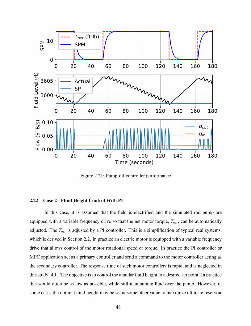
0 20 40 60 80 100 120 140 160 1800

10SP

MTnet (ft-lb)SPM

0 20 40 60 80 100 120 140 160 180

3600

3605

Fluid Level (ft)

ActualSP

0 20 40 60 80 100 120 140 160 180Time (seconds)

0.00

0.05

0.10

Flow

(STB

/s)

qout

qin

Figure 2.21: Pump-off controller performance

2.22 Case 2 - Fluid Height Control With PI

In this case, it is assumed that the field is electrified and the simulated rod pump are

equipped with a variable frequency drive so that the net motor torque, Tnet , can be automatically

adjusted. The Tnet is adjusted by a PI controller. This is a simplification of typical real systems,

which is derived in Section 2.2. In practice an electric motor is equipped with a variable frequency

drive that allows control of the motor rotational speed or torque. In practice the PI controller or

MPC application act as a primary controller and send a command to the motor controller acting as

the secondary controller. The response time of such motor controllers is rapid, and is neglected in

this study [40]. The objective is to control the annular fluid height to a desired set point. In practice

this would often be as low as possible, while still maintaining fluid over the pump. However, in

some cases the optimal fluid height may be set at some other value to maximize ultimate reservoir

48

recovery, or to prevent gas interference at the pump as the pressure falls below the fluid bubble

point. Figure 2.22 shows a diagram of the simulated control system for cases 2 and 3. First the

model simulates a one second horizon. The system then passes the surface load to the MHE ap-

plication. The MHE application estimates the annular fluid height, and passes it to the PI or MHE

controller. The controller then determines the motor torque, Tnet , for the next simulator cycle.

System Model: Surface Unit & Rod String

WellReservoir

Controller:MPC or PI

Set Point Height

Measure: Surface Load

MHE

Figure 2.22: Block diagram of PI and MPC controllers

This application utilizes the MHE described in Section 2.18 because in practice the fluid

level is rarely measured in real-time. The fluid height is usually measured infrequently with an

acoustic device, but the manual measurement and infrequency make it impractical for automatic

control. However, many current pump-off control systems measure the polished rod load and

acceleration. From these, the polished rod load and position are obtained as a function of time.

The MHE application illustrated in 2.18 converts the measured loads into predictions of the fluid

height. The MHE passes the estimated height into the PI controller application as a “measurement”.

The PI controller compares the “measured” height from the MHE application and compares it to

the set point height. The resulting error, e(t), determines the motor torque output via Equation

2.67.

49

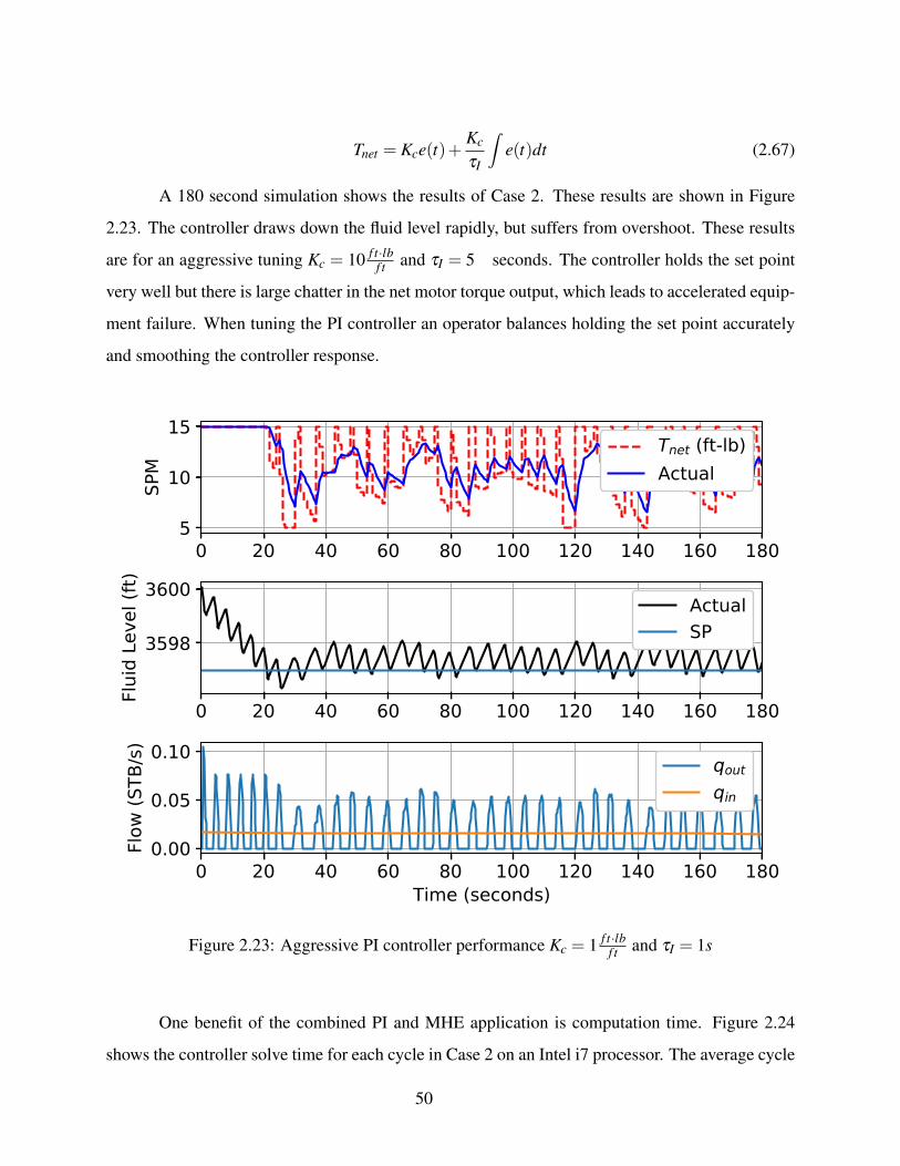
Tnet = Kce(t)+Kc

τI

∫e(t)dt (2.67)

A 180 second simulation shows the results of Case 2. These results are shown in Figure

2.23. The controller draws down the fluid level rapidly, but suffers from overshoot. These results

are for an aggressive tuning Kc = 10 f t·lbf t and τI = 5 seconds. The controller holds the set point

very well but there is large chatter in the net motor torque output, which leads to accelerated equip-

ment failure. When tuning the PI controller an operator balances holding the set point accurately

and smoothing the controller response.

0 20 40 60 80 100 120 140 160 1805

10

15

SPM

Tnet (ft-lb)Actual

0 20 40 60 80 100 120 140 160 180

3598

3600

Fluid Level (ft)

ActualSP

0 20 40 60 80 100 120 140 160 180Time (seconds)

0.00

0.05

0.10

Flow

(STB

/s)

qout

qin

Figure 2.23: Aggressive PI controller performance Kc = 1 f t·lbf t and τI = 1s

One benefit of the combined PI and MHE application is computation time. Figure 2.24

shows the controller solve time for each cycle in Case 2 on an Intel i7 processor. The average cycle

50

time is 1.23 seconds, indicating that, the controller is nearly appropriate for real-time control. To

be appropriate for real-time control a controller cycle time must be faster than real-time. In this

case most of the computation time is solving the MHE application to estimate fluid height, so faster

computation may be achieved with a faster processor or by model simplification, such as, using

fewer rod discretizations.

0 20 40 60 80 100 120 140 160 180Control Cycle

0.0

0.5

1.0

1.5

2.0

2.5

3.0

3.5

4.0

Compu

tatio

n Time (secon

ds)

Solve TimeAverageReal Time

Figure 2.24: Solve time for combined MHE and PI controller

To verify that real time control is possible, Case 2 is re-simulated where the MHE model

utilizes 10 discretizations per second and 5 rod discretizations (npt=10, npx=5). The resulting

average controller solve time is 0.62, indicating that the method is suitable for real time control.

The disadvantage of using a reduced resolution model in the MHE application is that the model-

process mismatch is greater, resulting in less accurate parameter estimates. However, these results

indicate that the proposed controller utilizing MHE and PI control is possible for field-testing with

51

reduced resolution. Future work could explore model linearization around the nominal operating

conditions for both the estimator and controller to further improve computational speed.

2.23 Case 3 - Fluid Height Control With MPC

This case is similar to Case 2, except that instead of PI control a MPC determines the

pumping unit net motor torque. Again, the MHE application described in Section 2.18 estimates

the fluid height, and passes it as a “measurement” to MPC application.

0 20 40 60 80 100 120 140 160 1805

10

15

SPM

Tnet (ft-lb)Actual

0 20 40 60 80 100 120 140 160 1803596

3598

3600

Fluid Level (ft)

ActualSP

0 20 40 60 80 100 120 140 160 180Time (seconds)

0.00

0.05

0.10

Flow

(STB

/s)

qout

qin

Figure 2.25: Runs MHE and MPC synchronously.

Figure 2.26 shows the results of the combined MHE and MPC controller. The MPC appli-

cation determines a 10 second horizon to achieve and hold the set point, varying Tnet . The MPC

then implements the first second of net motor torque as the control move. The MPC controller

achieves the set point with no overshoot and holds the set point adequately. It is interesting to

note that the set point fluid height is constant, but the actual fluid level is inherently cyclical since

52

fluid is only produced from the well during the pump upstroke. This is different from traditional

chemical processes where cyclical changes to a controlled variable are uncommon. However, the

results indicate that MPC is able to track the set point well despite the cycling fluid level, with

a sufficiently long prediction horizon. A measurement dead band is used to allow the height to

oscillate around the set point without penalty. The maximum change in Tnet per controller cycle

is held at 1 f t · lb per second and a minor penalty is allotted to each change in Tnet , to prevent

controller chatter. Overall, the MPC application performs very well.

0 20 40 60 80 100 120 140 160 1805

10

15

SPM

Tnet (ft-lb)Actual

0 20 40 60 80 100 120 140 160 1803596

3598

3600

Fluid Level (ft)

ActualSP

0 20 40 60 80 100 120 140 160 180Time (seconds)

0.00

0.05

0.10

Flow

(STB

/s)

qout

qin

Figure 2.26: Runs MHE and MPC synchronously.

A major downside to the MPC application is long computation time. Figure 2.27 shows

the combined MPC and MHE controller computation time per cycle. The average computation

time for the combined MHE MPC application is 7.4 seconds per one second cycle on an Intel i7

processor. One unsuccessful MPC solve occurred during the horizon at approximately 65 seconds.

A speedup in computation time of 7-8X is required for real-time control with this application. A

53

faster processor or model simplification, such as, using fewer rod discretizations may decrease

computation time. To verify this, Case 3 is resolved using 10 time discretizations per second and 5

rod discretizations (npt = 10, npx = 5). The average controller solve time with this discretization is

1.9 seconds, much closer to real time applicability. As noted in Section 2.22, the main disadvantage

of reduced resolution is increased model-process mismatch, which may lead to suboptimal control.

In addition to reduced model resolution, a shorter MPC prediction horizon can be used, although,

the controller performance degrades. A future area of study is to explore model simplification such

as linear MPC or control parameterization methods such as explicit nonlinear MPC [31].

0 20 40 60 80 100 120 140 160 180Control Cycle

0

10

20

30

40

50

60

Compu

tatio

n Time (secon

ds)

Solve TimeAverageReal Time

Figure 2.27: Solve time for combined MPC and MHE

2.24 Comparison of Cases

The cases each have pros and cons. Case 1 has the benefit of simplicity, and is well suited

for fields where electric power is not available, and functions well when reservoir influx is less

54

than the minimum stroking rate. Case 2 is intermediate in its complexity, and is a common control

algorithm. Combining MHE to determine annular fluid level with PI control enables good fluid

level or bottomhole pressure control with intermediate computational requirements. Finally, Case

3 with MPC provides the best control of annular fluid level, but is the most complex. Case 3 also

has the ability to consider multiple objectives as well as simultaneously consider well and reservoir

interactions. These features enable optimal production and profitability.

0 25 50 75 100 125 150 175Time (seconds)

0.000

0.005

0.010

0.015

0.020

0.025

0.030

Increa

se Cum

ulative Oil P

rodu

ction (%

)

MPC vs. TimerPI vs. Timer

Figure 2.28: Increased cumulative oil production relative to Case 1 ( Pump-off)

Figure 2.28 illustrates the differences in incremental cumulative recovery between MPC,

PI, and pump-off control for a 180 second simulation. In Figure 2.28, pump-off control is the base

case, and increases in production are shown relative to it. From the figure, it is clear that MPC

and PI control outperform pump-off control. MPC produces slightly more oil than PI, but this is

because PI holds the average fluid level slightly above the set point and MPC maintains an average

55

fluid level slightly below the set point. The increase in cumulative recovery is 0.029% over the

simulation period for the MPC case and 0.026% for the PI case. Although these appear to be small

increases in incremental production for a single well, the cumulative effect on a large-scale field

would imply significant gains in field wide production. This needs to be verified in future work

with high fidelity reservoir simulators to quantify production and profitability gains from improved

height control.

56

CHAPTER 3. CONCLUSIONS AND FUTURE WORK

This work illustrates the ability to use MPC and MHE for oil production systems with

sucker rod pumps. The oil production system model includes reservoir well, and pumping unit

dynamics. The models are combined to optimize for closed loop control. MHE estimates either

uncertain well or reservoir parameters or states. Specifically, reservoir skin estimation is illustrated

where the load and position of the rod pumping unit are measured. When fluid height is also

measured, additional reservoir parameters, such as the average reservoir pressure and porosity,

can be estimated. This allows for automatic control of annular fluid level, and decreases the need

for pressure build up tests. This work determines optimal operation by directly considering all

major physical constraints of the system simultaneously. Increased ultimate recovery and NPV are

enabled by automatically controlling annular fluid height and BHP.

Another innovation of this work is the formulation of pump boundary conditions as MPCCs

to allow for simultaneous optimization with large scale solvers. Simultaneous optimization in

many cases is faster than shooting methods when there are many degrees of freedom. Using the

reformulated pump boundary conditions this work shows dynamic optimization in near real time

to estimate annular fluid level for control. MPC is also demonstrated, although, a 7-8X speed up

in computation time is required for real-time control.

An analytical solution verifies the numerical methods used to simulate the sucker rod force

propagation. Collocation on a finite element and automatic differentiation are used with respect to

the time domain and finite differencing is used over the spatial domain. Results of the comparison

show close agreement between the numerical and analytical solutions in a simplified case, although

there appears to be numerical damping at larger times. A grid independence study further verifies

the numerical methods using the full combined sucker rod, well, and reservoir model.

Conventional pump off control is compared to advanced controllers. Predictively setting

strokes per minute for a conventional rod pumping unit is shown where the annular fluid level is

57

inferentially controlled. The fluid height remains controlled within the acceptable region with min-

imal stroking speed adjustments. MPC application results in a slight 0.03% increase in cumulative

oil production vs. conventional pump off control over a period of 3 minutes. Future work will

verify production gains over longer periods with high fidelity reservoir simulations. The models

and methods in this work represent a novel contribution in oil field production well control and

reservoir optimization.

3.1 Future Work

Future work should expand these methods to include: 1) additional artificial lift methods, 2)

more system constraints such as gathering systems, 3) more rigorous well, pump unit, and reservoir

models that include prime mover dynamics, multiple phase flow, and fluid compressibility, and 4)

investigate and improve solve time to determine applicability for real-time control.

This work considers a conventional sucker rod pumping unit and the measured data that

is typically available. Future work should expand the modeling of surface units to include other

types, such as hydraulic actuated, and other types of artificial lift. In addition to including other

types of units, additional system constraints such as gathering systems should be considered. When

more of the system constraints or degrees of freedom are considered more optimal production may

be achieved.

Many literature studies have shown that optimally setting BHP in producing wells can

increase NPV and ultimate recovery from oil and gas reservoirs. These studies are often performed

by fitting low order models to high fidelity reservoir models, and then optimizing the low order

models. Future work should couple these types of low order reservoir models with the sucker rod

and well model in this work to validate the feasibility and benefits of closed loop optimization and

automatic control of BHP.

The pump boundary conditions in this work are only suitable for liquid full pumping con-

ditions. Often oil production involves multiphase flow with compressible fluids. Prior work has

simulated these conditions using sequential methods, and future work should expand the use of

MPCCs to allow simulation of these cases using simultaneous methods. This problem involves

including the pressure volume temperature relationship of the produced fluid and simulating the

standing and traveling valves opening and closing.

58

Finally, for these benefits to be realized in practice they need to be implemented for real-

time control. Future work should explore sucker rod model simplification such as using fewer rod

discretizations or faster processors to improve computation time. A field trial would determine the

required model accuracy for parameter estimation and well control.

59

REFERENCES

[1] M. F. I. Ahmed and S. N. Nabil. Automatic Well Testing and PIP Calculations Using Smart

Rod Pump Controllers. In North Africa Technical Conference and Exhibition, 2012.

[2] M. S. Al-Kadem, F. T. Al-Khelaiwi, and M. A. Al-Amri. Real-time estimation of well

drainage parameters. Journal of Engineering Research, 1(2):93–100, 2013.

[3] Z. M. Alghareeb. Optimal Decision Making in Reservoir Management Using Reduced Or-

der Models. In SPE Annual Technical Conference and Exhibition held in New Orleans,

Louisiana, 2013.

[4] B. Baumrucker, J. Renfro, and L. Biegler. Mpec problem formulations and solution strategies

with chemical engineering applications. Computers & Chemical Engineering, 32(12):2903 –

2913, 2008.

[5] B. T. Baumrucker and L. T. Biegler. MPEC strategies for optimization of a class of hybrid

dynamic systems. Journal of Process Control, 19(8):1248–1256, 2009.

[6] B. T. Baumrucker and L. T. Biegler. MPEC strategies for cost optimization of pipeline oper-

ations. Computers and Chemical Engineering, 34(6):900–913, 2010.

[7] L. D. Beal, D. Petersen, D. Grimsman, S. Warnick, and J. D. Hedengren. Integrated Schedul-

ing and Control in Discrete-time with Dynamic Parameters and Constraints. Computers &

Chemical Engineering, apr 2018.

[8] L. D. R. Beal, J. Park, D. Petersen, S. Warnick, and J. D. Hedengren. Combined model

predictive control and scheduling with dominant time constant compensation. Computers &

Chemical Engineering, 104:271–282, 2017.

[9] L. D. R. Beal, D. Hill, R. A. Martin, and J. D. Hedengren. Gekko optimization suite. Pro-

cesses, 2018.

[10] R. Beckwith. Downhole Electronic Components: Achieving Performance Reliability. JPT,

pages 42–5, 2013.

60

[11] D. Brouwer, G. Naevdal, J. D. Jansen, E. Vefring, and C. Van Kruijsdijk. Improved Reser-

voir Management Through Optimal Control and Continuous Model Updating. SPE Annual

Technical Conference and Exhibition, Houston, Texas, U.S.A., 2004.

[12] R. Brouwer and J. D. Jansen. Dynamic Optimization of Waterflooding With Smart Wells

Using Optimal Control Theory. SPI Journal, 2004.

[13] M. Cardoso and L. Durlofsky. Use of Reduced-Order Modeling Procedures for Production

Optimization. SPE Journal, 15(2):1–10, 2010.

[14] M. A. Cardoso. Development and Application of Reduced-Order Modeling Procedures for

Reservoir Simulation. Ph.d., University of Stanford, 2009.

[15] M. A. Cardoso and L. J. Durlofsky. Use of Reduced-Order Modeling Procedures for Pro-

duction Optimization. In SPE Reservoir Simulation Symposium, volume 15, pages 1–10,

2010.

[16] H. Derek, J. Jennings, and S. Morgan. Sucker Rod Pumping Unit Diagnostics Using an

Expert System. In Permian Basin Oil and Gas Recovery, 1988.

[17] J. Dewan. Essentials of Modern Open-Hole Log Interpretation. PennWell Publishing Com-

pany, Tulsa, Okla, 1983.

[18] D. Doty and Z. Schmidt. An Improved Model for Sucker Rod Pumping. Society of Petroleum

Engineers Journal, 23(February):33–41, 1983.

[19] M. J. Economides, A. D. Hill, C. Ehlig-Conomides, and D. Zhu. Petroleum Production

Systems. Prentice Hall, Upper Saddle River, NJ, 2013.

[20] V. M. Ehimeakhe. Calculating Pump Fillage for Well Control using Transfer Point Location.

In SPE Eastern Regional Meeting. Society of Petroleum Engineers, 2010.

[21] J. R. Eickmeier. PUMPING WELL OPTIMIZATION TECHNIQUES. (1959), 1973.

[22] W. G. Elmer and J. B. Elmer. Pump-Stroke Optimization : Case Study of Twenty-Well Pilot.

In SPE North America Artificial Lift Conference and Exhibition, number July 2016, pages

25–27, 2017.

61

[23] T. A. Everitt and J. W. Jennings. An improved finite-difference calculation of downhole

dynamometer cards for sucker-rod pumps. SPE Production Engineering, 7(01):121–127,

1992.

[24] M. Ghareeb, N. Sadek, A. Sbeih, A. Elfotouh, and A. Nasser. Improved Sucker Rod Pumping

Systems Performance by Fully Automated Closed Loop and Control Solution. In SPE Middle

East Artificial Lift Conference and Exhibition, pages 1–12, 2016.

[25] S. G. Gibbs. Predicting the Behavior of Sucker-Rod Pumping Systems. Journal of Petroleum

Technology, 1963.

[26] S. G. Gibbs, K. Nolen, F. Morrow, and W. Lynch. Monitoring And Controlling Rod Pumped

Wells Using Downhole Pump Cards. Annual Technical Meeting of The Petroleum Society of

CIM, 1995.

[27] W. E. Gilbert. An oil-well pump dynagraph. Drilling and Production Practice, (4), 1936.

[28] D. K. Gold, T. Treiberg, and T. Enterprises. Implementation of Automated Expert Diagnos-

tics to Provide Enhanced Rod Pump Surveillance at S. Belridge Field, CA. In SPE Annual

Technical Conference and Exhibition, number SPE 71527-MS in 10.2118/71527-MS, 2001.

[29] Y. Haitao, M. Lijun, Z. Yaqin, H. Wei, X. Hong, G. Qingming, L. Ming, Z. Lei, and H. Ertao.

Real Time Calculation of Fluid Level Using Dynamometer Card of Sucker Rod Pump Well.

pages 1–7, 2014.

[30] J. He, P. Sarma, and L. J. Durlofsky. 1 . Use of reduced-order models for improved data

assimilation within an EnKF context. In SPE Reservoir Simulation Symposium, page 2014,

2014.

[31] J. D. Hedengren and T. F. Edgar. In situ adaptive tabulation for real-time control. Industrial

& Engineering Chemistry Research, 44(8):2716–2724, 2005.

[32] J. D. Hedengren, R. A. Shishavan, K. M. Powell, and T. F. Edgar. Nonlinear modeling,

estimation and predictive control in {APMonitor}. Computers & Chemical Engineering, 70:

133–148, nov 2014.

62

[33] J. Hook. An introduction to porosity. SPWLA, 44:205–212, 2003.

[34] M. Islam, S. Moussavizadegan, S. Mustafiz, and J. H. Abou-Kassem. Advanced Petroleum

Reservoir Simulation. Scriener Publishing LLC, Hoboken, 2010.

[35] J. Jakosky. Bottom-hole Measurements in Pumping Wells. Transactions of the AIME, pages

62–84, 1939.

[36] J.-D. Jansen, R. Brouwer, and S. G. Douma. Closed Loop Reservoir Management. In SPE

Reservoir Simulation Symposium, 2-4 February, The Woodlands, Texas, 2009. Society of

Petroleum Engineers.

[37] S. Kameswaran, L. T. Biegler, and G. H. Staus. Dynamic optimization for the core-flooding

problem in reservoir engineering. Computers and Chemical Engineering, 29(8):1787–1800,

2005.

[38] R. M. Knapp. A Dynamic Investigation of Sucker-Rod Pumping. MS thesis, University of

Kansas, Topeka, page 46, 1963.

[39] D. A. Krug, S. D. Nelsen, and J. D. Allison. Regenerative hydraulic lift system, oct 2013.

[40] C. Lascu, I. Boldea, and F. Blaabjerg. Variable-Structure Direct Torque Control—A Class of

Fast and Robust Controllers for Induction Machine Drives. IEEE Transactions on Industrial

Electronics, 51(4):785–792, 2004.

[41] J. Lea, J. Cox, H. Nickens, T. Oetama, F. Yavuz, and D. Garg. Wave Equation Simulation of

Fluid Pound and Gas Interference. Proceedings of SPE Production Operations Symposium,

pages 1–12, 2005.

[42] N. Lewis, J. Hedengren, and E. Haseltine. Hybrid Dynamic Optimization Methods for Sys-

tems Biology with Efficient Sensitivities. Processes, 3(3):701–729, 2015.

[43] E. R. Martinez, W. J. Moreno, V. J. Castillo, and J. A. Moreno. Rod Pumping Expert System.

In SPE Petroleum Computer Conference, volume SPE 26246, pages 201–208, 1993.

[44] W. McCain. The Properties of Petroleum Fluids. PennWell Books, Tulsa, Okla, 1990.

63

[45] J. N. McCoy, A. L. Podio, D. J. Becker, and G. Fernandez. Wireless Simultaneous Acquisi-

tion and Analysis of Dynamometer and Fluid Level Data for Real-Time Monitoring of Well

Performance. In SPE Artificial Lift Conference - Americas, 2013.

[46] H. T. Nguyen and F. C. D. Mundo. Improving Artificial Lift Design Through Dynamic

Simulation. In SPE North America Artificial Lift Conference and Exhibition, 2016.

[47] D. S. Oliver and Y. Chen. Recent progress on reservoir history matching: a review. Compu-

tational Geosciences, 15(1):185–221, jan 2011.

[48] P. O’Niel. The Wave Equation, in Beginning Partial Differential Equations, Second Edition.

John Wiley & Sons, Inc, Hobeken, NJ, 2008.

[49] E. Orji, J. Lissanon, and O. Omole. Sucker Rod Lift System Optimization of an Uncon-

ventional Well. In SPE North America Artificial Lift Conference and Exhibition, number

October, pages 25–27, 2016.

[50] K. Pałka and J. Czyz. Optimizing Downhole Fluid Production of Sucker Rod Pumps Using

Variable Motor Speed. In SPE Production and Operations, number 02, 2009.

[51] A. Podio, J. Mccoy, D. Becker, L. Rowlan, and B. Drake. Total Well Management II. In SPE

Production and Operations Symposium, pages 1–14, 2001.

[52] K. M. Powell, A. N. Eaton, J. D. Hedengren, and T. F. Edgar. A continuous formulation for

logical decisions in differential algebraic systems using mathematical programs with com-

plementarity constraints. Processes, 4(1), 2016.

[53] S. Qin and T. A. Badgwell. A survey of industrial model predictive control technology.

Control Engineering Practice, 11(7):733–764, 2003.

[54] T. Radzevicius and F. Clarke. Optimisation of Beam Pump Wells Utilising Variable Speed

Drives and Remote Monitoring Software. In SPE Intelligent Energy Conference and Exhibi-

tion, The Netherlands, 2012.

64

[55] A. U. Raghunathan and L. T. Biegler. Mathematical programs with equilibrium constraints

(MPECs) in process engineering. Computers and Chemical Engineering, 27(10):1381–1392,

2003.

[56] J. Rogers, C. Guffey, and W. Oldham. Artificial neural networks for identification of beam

pump dynamometer load cards. In Annual Technical Conference and Exhibition of the Society

of Petroleum Engineers, New Orleans, LA., 1990.

[57] O. L. Rowlan, J. N. McCoy, and A. L. Podio. Pump intake pressure determined from fluid

levels, dynamometers, and valve-test measurements. In Canadian Petroleum Technology

Conference, volume 50, pages 59–66, 2011.

[58] J. P. Sanchez, D. Festini, and O. Bel. Beam Pumping System Optimization Through Au-

tomation. In Latin American and Caribbean Petroleum Engineering, number SPE 108112,

2007.

[59] P. Sarma and W. H. Chen. Applications of Optimal Control Theory for Efficient Production

Optimisation of Realistic Reservoirs, 2008.

[60] P. Schirmer, J. Gay, and P. Toutain. Use of advancd pattern-recognition and knowledge-based

system in analyzing dynamometer cards. In SPE Petroleum Computer Conference, volume

Spe 22305, pages 21–24, 1991.

[61] B. J. Spivey, J. D. Hedengren, and T. F. Edgar. Constrained Nonlinear Estimation for In-

dustrial Process Fouling. Industrial & Engineering Chemistry Research, 49(17):7824–7831,

2010.

[62] J. Udy, B. Hansen, S. Maddux, D. Petersen, S. Heilner, K. Stevens, D. Lignell, and J. D.

Hedengren. Review of Field Development Optimization of Waterflooding, EOR, and Well

Placement Focusing on History Matching and Optimization Algorithms. Processes, 5(3):34,

jun 2017.

[63] M. Vazquez and J. Fernandes. Rod-pumping optimization through surface and downhole pa-

rameter estimation and simulation. In SPE Mid-Continent Operations Symposium, Oklahoma

City, OK, 1999.

65

[64] M. O. Vazquez. Real Time Expert System (R.T.E.S.) for Rod Pumping Optimization”. In

Petroleum Computer Conference, number SPE 30185, pages 53–60, 1995.

[65] I. Virgal and M. Kelemen. Experimental Friction Identification of DC Motor. International

Journal of Mechanics and Applications, 3:26–30, 2013.

[66] A. Wachter and L. T. Biegler. On the implementation of a primal-dual interior-point filter

line-search algorithm for large-scale nonlinear programming, volume 106. 2006.

[67] C. P. Walker. Determination of Fluid Level in Oil Wells bv the Pressure- wave Echo Method.

Society of Petroleum Engineers, pages 32–43, 1937.

[68] C. P. Walker. Method of determining fluid density, fluid pressure, and the production capacity

of oil wells, 1939.

[69] D. Wang and H. Liu. Dynamic Modeling and Analysis of Sucker Rod Pumping System in a

Dirrectional Well. Mechanism and Machine Science, 408, 2017.

[70] G. W. Westerman. Successful application of pump-off controllers. In SPE Annual Fall Tech-

nical Conference and Exhibition, pages 1–10. Society of Petroleum Engineers, 1977.

[71] P. Wolm, X. Chen, J. Chase, W. Pettigrew, and C. Hann. Analysis of a PM DC Motor

Model for Application in Feedback Design for Electric Powered Mobility. Mechatronics and

Machine Vision in Practice, 2008.

[72] Y. Yu, H. Shi, and L. Mi. Research on feature extraction of indicator card data for

sucker-rod pump working condition diagnosis. Journal of Control Science and Engineer-

ing, 2013(60574:1–6, 2013.

[73] V. M. Zavala, C. D. Laird, and L. T. Biegler. A fast moving horizon estimation algorithm

based on nonlinear programming sensitivity. Journal of Process Control, 18(9):876–884,

2008.

[74] Y. Zhang, H. Li, and D. Yang. Simultaneous Estimation of Relative Permeability and Cap-

illary Pressure Using Ensemble-Based History Matching Techniques. Transport in Porous

Media, 94(1):259–276, 2012.

66

APPENDIX A. SOURCE CODE

A.1 Analytical vs. Numerical Comparison

# compare analytical solution to gekko solution

import numpy as np

import matplotlib.pyplot as plt

from gekko import*

from mpl_toolkits.mplot3d.axes3d import Axes3D

#analytical solution

def phi(x):

phi = np.cos(x)

return phi

def psi(x):

psi = np.sin(2*x)

return psi

def ua(x,t):

#u = np.cos(x)*np.cos(3*t) + 1/6*np.sin(2*x)*np.sin(6*t)

a = 18996.06 # ft/s speed of sound in steel

c = a

#u = 1/2*(np.cos(x-c*t)+np.cos(x+c*t)) - 1/(4*c)*(np.cos(2*(x+c*t)) -np.

cos(2*(x-c*t)))

u = np.cos(x)*np.cos(a*t) + 1/(2*a)*np.sin(2*x)*np.sin(2*a*t)

return u

67

# define time

tf = .0005

npt = 100# number of points in time

xf = 2*np.pi

npx = 100# number of points in space

time = np.linspace(0,tf ,npt) # time array

xpos = np.linspace(0,xf ,npx) # space array

for i in range(npx):

usol = ua(xpos[i],time)

if i == 0:

ustora = usol

else:

ustora = np.vstack([ustora ,usol])

for i in range(npt):

if i ==0:

xstor = xpos

else:

xstor = np.vstack([xstor ,xpos])

for i in range(npx):

if i == 0:

tstor = time

else:

tstor = np.vstack([tstor ,time])

xstor = xstor.T

#%%

# create gekko model

m = GEKKO ()

68

m.time = time

x0 = phi(xpos)

v0 = psi(xpos)

dx = xpos[1]-xpos[0]

a = 18996.06 # ft/s speed of sound in steel

c = m.Const(value = a)

dx = m.Const(value = dx)

u = [m.Var(value = x0[i]) for i in range(npx)]

v = [m.Var(value = v0[i]) for i in range(npx)]

#j = [m.Var() for i in range(npx)]

[m.Equation(u[i].dt()==v[i]) for i in range(npx)]

# top difference eqution (forward) first order

#m.Equation(v[0].dt()==c**2*(1/dx**2)*(u[2]-2*u[1]+u[0]))

# second order

#m.Equation(v[0].dt()==c**2*(1/dx**2)*(-u[3] + 4*u[2])-5*u[1] +2*u[0])

#

m.Equation(v[0].dt()==c **2 * (u[1] - 2.0*u[0] + u[npx-1])/dx **2 )

# central difference (middle)

[m.Equation(v[i+1].dt()== c **2 * (u[i+2] - 2.0*u[i+1] + u[i])/dx **2) for i

in range(npx-2) ]

# bottom (backward) first order

#m.Equation(v[npx -1].dt()==c**2*(1/dx**2)*(u[npx -1] -2*u[npx -2]+u[npx -3]))

# second order

m.Equation(v[npx-1].dt()== c **2 * (u[npx-2] - 2.0*u[npx-1] + u[0])/dx **2 )

# set options

#m.Equaiton(j == v[npx].dt())

m.options.imode = 4

m.options.solver = 1

m.options.nodes = 3

m.solve(remote=False)

69

for i in range(npx):

if i ==0:

ustor = np.array([u[i]])

tstor = np.array([m.time])

else:

ustor = np.vstack([ustor ,u[i]])

tstor = np.vstack([tstor ,m.time])

for i in range(npt):

if i == 0:

xstor = xpos

else:

xstor = np.vstack([xstor ,xpos])

xstor = xstor.T

t = tstor

ustor = np.array(ustor)

#%%

# compute error

error = ustora - ustor

#%%

fig = plt.figure(1)

ax = fig.add_subplot(1,1,1,projection=’3d’)

ax.set_xlabel(’Distance (ft)’, fontsize = 12)

ax.set_ylabel(’Time (seconds)’, fontsize = 12)

ax.set_zlabel(’Position (ft)’, fontsize = 12)

#plt.title(’Analytical Solution ’)

ax.set_zlim ((-1,1))

p = ax.plot_wireframe(xstor ,tstor ,ustora ,rstride=1,cstride=1)

fig.savefig(’analytical_3d.eps’, dpi = 1200 , Transparent = True)

fig.show()

#%%

### WE USE THIS PLOT FOR THE GEKKO SOLUTION

70

# 3d gekko solution plot

fig = plt.figure(2)

ax = fig.add_subplot(1,1,1,projection=’3d’)

ax.set_xlabel(’Distance (ft)’, fontsize = 12)

ax.set_ylabel(’Time (seconds)’, fontsize = 12)

ax.set_zlabel(’Position (ft)’, fontsize = 12)

ax.set_zlim ((-1,1))

#plt.title(’GEKKO Solution ’)

p = ax.plot_wireframe(xstor ,tstor ,ustor ,rstride=1,cstride=1)

fig.savefig(’gekko_3d.eps’, dpi = 1200 , Transparent = True)

fig.show()

#%%

### WE USE THIS PLOT FOR THE ANALYTICAL SOLUTION ###

# PLot analytical solution contour

plt.figure () # start a new figure

plt.contour(xstor , tstor , ustora , 150) # using 50 contour lines.

plt.colorbar () # add a colorbar

plt.xlabel(’X’) # labels for axes

plt.ylabel(’Time’)

plt.title(’Analytical Solution ’)

plt.show() # show plot

#%%

# plot gekko solution contour plot

plt.figure () # start a new figure

plt.contour(xstor , tstor , ustor , 150) # using 50 contour lines.

plt.colorbar () # add a colorbar

plt.xlabel(’X’) # labels for axes

plt.ylabel(’Time’)

plt.title(’GEKKO Solution ’)

plt.show() # show plot

#%%

71

# --- setup grid ---

#nx = 200 # number of points in x-direction

#ny = 150 # number of points in y-direction

#x = np.linspace(-5, 5, nx) # nx points equally spaced between -5...5

#y = np.linspace(-6, 6, ny) # ny points equally spaced between -6...6

#X, Y = np.meshgrid(x, y, indexing=’ij ’) # 2D array (matrix) of points

across x and y

#Z = np.zeros ((nx, ny)) # initialize output of size (nx, ny)

### WE USE THIS PLOT FOR THE DIFFERENCE BETWEEN THE ANALYTICAL AND GEKKO

SOLUTIONS ###

# --- contour plot ---

plt.figure () # start a new figure

plt.contour(xstor , tstor , error , 150) # using 50 contour lines.

cbar = plt.colorbar () # add a colorbar

cbar.ax.tick_params(labelsize=12)

cbar.set_label(’Difference ’, fontsize=12)

plt.xlabel(’Distance (ft)’, fontsize = 12) # labels for axes

plt.ylabel(’Time (seconds)’, fontsize = 12)

#plt.zlabel(’Error ’)

#plt.title(’Error (ft) ’)

plt.savefig(’difference_gekko.eps’, dpi = 1200 , Transparent = True)

plt.show() # show plot

#%%

per_error = error / ustora

per_error = np.abs(per_error)

# --- contour plot ---

plt.figure () # start a new figure

plt.contour(xstor , tstor , per_error , 150) # using 50 contour lines.

plt.colorbar(label = ’Error (%)’) # add a colorbar

plt.xlabel(’X (ft)’) # labels for axes

plt.ylabel(’Time (seconds)’)

#plt.zlabel(’Error (%)’)

#plt.title(’Error (ft) ’)

72

plt.savefig(’error_gekko.eps’)

plt.show() # show plot

A.2 Simulation, MHE, and MPC Model Script

from __future__ import division # compatibility with python 2.7

from gekko import GEKKO

import numpy as np

import matplotlib.pyplot as plt

import time

from mpl_toolkits.mplot3d.axes3d import Axes3D

#%%

#Define Timespace for simulation

tf = 1 # sec , length of simulation

npt = 20 # number of time discretizations

nit = 1 # number of itterations to solve

ti = np.linspace(0,tf ,npt) # times for plotting

# Define time space for MPC

tf_mpc = 5

npt_mpc = npt*tf_mpc

# Define Rod Discretizations

TVD_d = 4800 # ft , lenth of rod

npx = 5 # number of rod discretizations

dx = TVD_d/(npx-1) # #ft lenth of rod discretizations

xi = np.linspace(0,TVD_d ,npx) # possitions allong rod (for plotting)

#Set Points

SPM_in = np.ones(npt)*10

73

#BuildModle ############

mpc = GEKKO()

sim = GEKKO()

mhe = GEKKO()

#Horizon Window

mpc.time = np.linspace(0,tf_mpc ,npt_mpc)

sim.time = np.linspace(0,tf ,npt)

mhe.time = np.linspace(0,tf ,npt)

################################

# Conventional Rod Pump Unit Geometry

# API geometry dimension values

Ag=210.0

Cg=120.3

Ig=120.0

Pg=148.5

Hg=237.88

Gg=86.88

Rg=47.0

#lengths from FIG. 1 - Beam Pumping Unit Shown as a Four -Bar Linkage

L_1 = Rg

L_2 = np.sqrt((Hg-Gg)** 2.0+Ig ** 2.0)

L_3 = Cg

L_4 = Pg

L_5 = Ag

starting_height = 3/4

#Simulation ########################################

for m in [sim ,mpc ,mhe]:

#Constants

m.API = m.Const(value = 45) #API gravity of fluid ,

unitless

74

m.c = m.Const(value = 0.000013) #Compressibility , psi^-1

m.k = m.Const(value = 15) #Permeability , md

m.Bo = m.Const(value = 1.2) #FVF , rb/STB

m.A_d = m.FV(value = 2, ub = 8, lb = 1) #Drainage

Area , Acres

m.sw = m.Const(value = 0.2) #Water Saturation

m.porosity = m.FV(value = 0.08, ub = .12, lb = 0.07) #Porosity ,

unitless

m.gamma_E = m.Const(value = 1.78) #Euler Constant

m.C_a = m.Const(value = 31.6) #Drainage Area Shape

Factor (Circular)

m.rw = m.Const(value = 0.328) #Welbore radius , ft

m.S = m.FV(value = 0, ub = 10, lb = -5) #unitless

m.u_visc = m.Const(value = 1.5) # Viscosity , cp

m.h_pz = m.Const(value = 8) #pay zone thickness , ft

m.D_t = m.Const(value = 2.5) # tubing diameter , in

m.St_length = m.Const(value = 85) # rod pump stroke length , in

m.g = m.Const(value = 32.2) # acceleration due to gravity ,

ft/s^3

m.g_conv= m.Const(value = 32.2) # lbf conversion , lb-ft/s^2-lbf

m.rho_r = m.Const(value = 490) # lbs/ft^3, density of rod

steel

m.rho_w = m.Const(value = 62.3 ) # lbs/ft^3, density of water at

standard conditions

m.a = m.Const(value =18996.06 ) # ft/s speed of sound in

steel

m.D_r = m.Const(value = 1.0) # in, diameter of rod string

m.Ac = m.Const(value= m.D_r.value **2/4.0*np.pi) # in^2, cross sectional

area of rod

m.nu = m.Const(value = 0.01) # unitless , damping

coefficient

m.pi = m.Const(value=np.pi)

m.E = m.Const(value = 32025000.0) # psi sucker rod modulus of

elasticity

m.alpha = m.Const(value = 0.0) # pump parameter , unitless

75

m.beta = m.Const(value = 1.0) # pump parameter , unitless

m.L_1 = m.Const(value =L_1) # unit geometry

m.L_2 = m.Const(value =L_2) # unit geometry

m.L_3 = m.Const(value =L_3) # unit geometry

m.L_4 = m.Const(value =L_4) # unit geometry

m.L_5 = m.Const(value =L_5) # unit geometry

m.dx = m.Const(value = dx) # ft delta x

#Prime Mover Constants (Torque Balance)

m.tau_p = m.Const(value = 3) #tau

m.k_gain = m.Const(value = 1) #one to one ratio between torque and

SPM

##Economic

m.Weight_lb_ft = m.Const(value = m.rho_r.value*m.Ac.value*m.g.value/m.

g_conv/144) #Weight of rod string ,

lbf/ft

m.Capex = m.Const(value = 200000) #Cost of Pumping Rod

Unit ,$?

m.P_o = m.Const(value = 50) #Price of Oil , $/STB

m.r = m.Const(value= .12/365) #Daily Discount Rate ,

%

m.P_th = m.Const(value = 100) #tubing head pressure ,

psi

m.TVD = m.Const(value = 4800) #true vertical depth ,

ft

m.E_cost = m.Const(value = 0.13/3600) #Cost of Electricity ,

cents/Kws

#Calculated Constants #DO NOT MODIFY#

m.Wr = m.Const(value = m.TVD.value*m.Weight_lb_ft.value)

#

Weight of entire rod string , lbm

76

m.D_a = m.Const(value = 2*12*m.rw.value)

#Annulus Diameter , in

m.gamma = m.Const(141.5/(m.API.value+131.5))

#Specific gravity of Fluid

m.P_startpump = m.Const(value = 0.433*m.gamma.value*m.TVD.value)

#Average

Reservoir Pressure at Pump start up

m.Pi = m.Const(value = .433*m.TVD.value)

#Initial Reservoir Pressure , psi

m.A_t = m.Const ((np.pi/4)*m.D_t.value **2) #Cross sectional Area of tubing

, in^2

m.A_a = m.Const ((np.pi/4)*m.D_a.value **2) #Cross Sectional Area of

Annulus , in^2

m.Wf = m.Const(value = m.TVD.value*m.rho_w.value*m.gamma.value*m.g.

value/m.g_conv.value*(m.A_t.value-m.Ac.

value)/144) # lbf , weight of fluid in

tubing

#MV’s

m.SPM_in = m.MV(value = 10, lb = 5, ub = 15) #Rod Pump Pumping

Speed/Torque , spm

#Variables

m.V_i= m.Var(value = 7758*m.A_d.value*m.h_pz.value*m.porosity.value*(1-m

.sw.value)/m.Bo.value) #OOIP , stb

m.Vp = m.Var(value = m.V_i.value*(np.exp(m.c.value*(m.Pi.value-m.

P_startpump.value))-1)) #

initial volume produced prior stb

m.h = m.CV(value = 1.0*m.TVD.value*starting_height)

# Height , ft

77

m.NPV = m.Var(value = -1.0*m.Capex.value)

#Net Present Value , $

m.y = m.Var( lb = -1, ub = 1) # SIGN(x)

m.sa = m.Var(value = 0, lb = 0) # slack variable a

m.sb = m.Var(value = 0, lb = 0) # slack variable b

m.tsi = m.Var(value = 0.0) # mulation time

m.SPM = m.Var(value = 10) #SPM , strokes/min

#omega = m.Var(value = 0)

m.theta = m.Var(value = 0) # rad i.e sec^-1 crank angle of surface unit

m.u = [m.SV(value = 9.22) for i in range(npx)] # relative position of each

rod segment

m.v = [m.Var(value = 0.0) for i in range(npx)] # velocity of reach rod

segment

m.f = [m.SV(value = 0.0) for i in range (npx)] # load at each rod segment

m.P = m.Var(value = 1e-6) # unitless , load at the pump

## State Variables

m.P_res = m.Var(value = m.P_startpump.value*1.0)

#Current Reservoir Pressure , psi

m.P_wf = m.Var(value = 0.433*m.gamma*m.h.value)

#Bottomhole Flowing Pressure , psi

m.q_in = m.Var(value = (1/86400)*m.k.value*m.h_pz.value*(m.P_res.value-m.

P_wf.value)/(141.2*m.Bo.value*m.u_visc.

value*((1/2)*np.log(4*m.A_d.value/(m.

gamma_E.value*m.C_a.value*m.rw.value ** 2)

) + m.S.value))) #IPR -VLP Flow rate , STB

/s

m.q_out = m.Var(value = 0) # Outgoing Flow Rate , STB/s

m.t = m.Var(value = 0)

#Time , days

78

m.W_rod = m.Var(value = (1.0962)*m.q_out.value*(m.P_th.value-m.P_wf.value

+ .433*m.gamma.value*m.TVD.value) + (4.

7053e-7)*m.Wr.value*m.St_length.value*m.

SPM.value) #Work

supplied by electric Motor , KW

#Intermediates

m.hs = m.Intermediate(m.sqrt(L_1 **2 +L_2 **2 + 2 *L_1 *L_2 *m.cos(m.theta))

)

m.V_rp = m.Intermediate ((1/9702)*(np.pi/4)*m.D_t **2*m.St_length) #Volume

Extracted per stroke length , STB

#Equations

##AlgebraicEqns

m.Equation(m.V_i == 7758*m.A_d*m.h_pz*m.porosity*(1-m.sw)/m.Bo)

m.Equation(m.P_wf == 0.433*m.gamma*m.h)

m.Equation(m.P_res == m.Pi-(1/m.c)*m.log((m.Vp/m.V_i)+1))

m.Equation(m.q_in == (1/86400)*m.k*m.h_pz*(m.P_res-m.P_wf)/(141.2*m.Bo*m.

u_visc*((1/2)*m.log(4*m.A_d/(m.gamma_E*m

.C_a*m.rw **2)) + m.S))) #STB/s

m.Equation(m.W_rod == (1.0962)*m.q_out*(m.P_th-m.P_wf + .433*m.gamma*m.TVD

) + (4.7053e-7)*m.Wr*m.St_length*m.SPM)

#Prime Mover Equations - Torque Balance and Kinematic Eqns

m.Equation(m.SPM.dt() == -(1/m.tau_p)*m.SPM + (m.k_gain/m.tau_p)*m.SPM_in)

m.Equation ((2*m.pi/60)*m.SPM == m.theta.dt())

#m.Equation(theta ==2.5118541087922712 +tsi*SPM_in * 2.0 * 3.147 / 60.0) #

convert time to angle in radians

#m.Equation(SPM == omega /(2*pi)/60)

m.Equation(m.u[0] == (1/12)*L_5*(m.asin(L_1*m.sin(m.theta)/m.hs)+m.

acos((m.hs ** 2+L_3 ** 2-L_4 ** 2)/(2*L_3*m.hs

)))) # position of polished rod , inches

[m.Equation(m.v[i+1].dt()== m.a **2 * (m.u[i+2] - 2.0*m.u[i+1] + m.u[i])/m.

dx ** 2 - m.pi*m.a*m.nu/(2.0*m.TVD)*m.v[i+

79

1] - (1-m.rho_w*m.gamma/m.rho_r)*m.g)

for i in range(npx-2) ]# wave equation

m.Equation(m.q_out == m.A_t * m.u[-1].dt()*12/231/42 * (1+m.y)/2) #

rate of fluid production , barrels/

#m.Equation(q_out == (1/60)*V_rp*SPM)

# Equations for calculating rod loading

# Load at surface

m.Equation(m.f[0] == m.E*m.Ac*1/2/m.dx *(-m.u[2] + 4*m.u[1] -3*m.u[0]))

# Load at pump

#m.Equation(f[npx -1] == E*Ac* 1/2.0/dx *(3*u[npx -1] - 4*u[npx -2] + u[npx -3

]))

m.Equation(m.f[npx-1] == m.E*m.Ac* m.P)

# load at intermediate points

[m.Equation(m.f[1+i] == m.E*m.Ac*1/2.0/dx*(m.u[i+2] - m.u[i])) for i in

range(npx-2)]

# pump boundary

m.Equation( m.u[npx-1]*m.alpha + (m.u[npx-1] - m.u[npx-2])/dx == m.P)

#add in signum for lifting and lowering conditions

m.Equation(m.v[-1] == m.sb - m.sa )

m.Equation(m.P == -((m.Wf- (m.A_t - m.Ac)*m.P_wf)/m.E/m.Ac) * (1 + m.y)/2

) # -P_wf*A_t

##DifferentialEans

m.Equation(m.t.dt() == 1)

m.Equation(m.Vp.dt() == m.q_in)

m.Equation(m.NPV.dt() == (m.P_o*m.q_out-m.E_cost*m.W_rod)*m.exp(-m.r*m.t))

m.Equation(m.h.dt() == (1617/2)*(m.q_in - m.q_out)/(m.A_a -m.A_t))

m.Equation(m.tsi.dt()==1.0) # create time variable

[m.Equation(m.u[i].dt()==m.v[i]) for i in range(npx)] # velocity of rod

string

# Set Objectives #######################

m.Obj((m.sa*(1+m.y) + m.sb*(1-m.y))) # objective function to make signum

work.

80

#m.Equation ((m.sa*(1+m.y) + m.sb*(1-m.y)) <= 1e-6)

#SetGlobalOptions(Simulation)##########

sim.options.IMODE = 5 # 4 = Dynamic Simulation (Seqential)

sim.options.NODES = 2 # 3 = 3 Nodes , 2 = No collocation nodes

sim.options.SOLVER = 3 # 1 =APOPT , 3 = IPOPT

sim.options.time_shift = npt-1 # time shift forward for multiple

simulations

sim.options.MAX_ITER = 450

#SetLocalOptions ########################

#N/A

sim.SPM_in.FSTATUS = 1 # accept measurments

sim.SPM_in.STATUS = 0 # don’t let optimizer change (simulation)

#MHE ########################

#Parameters (Holds Measured values from MHE)

hm = mhe.Param(value = 1.0*mhe.TVD.value/2)

#Variables to estimate and initial conditions

##FV

mhe.S.Value = 4 #unitless

#SetGlobalOptions(MHE)####################

mhe.options.IMODE = 5 # 4 = Dynamic Simulation (Seqential)

mhe.options.NODES = 2 # 3 = 3 Nodes , 2 = No collocation nodes

mhe.options.SOLVER = 3 # 1 =APOPT , 3 = IPOPT

mhe.options.time_shift = npt-1 # time shift forward for multiple

simulations

mhe.options.MAX_ITER = 450

mhe.Obj((mhe.h - hm)** 2)

#SetLocalOptions (MHE)#########################

##FV #Variable to estimate

mhe.S.FSTATUS = 0

81

mhe.S.STATUS = 1

mhe.S.DMAX = 1.0

#MV

mhe.SPM_in.FSTATUS = 1

mhe.SPM_in.STATUS = 0

#SetGlobalOptions(MPC)##################

mpc.options.IMODE = 6 # 4 = Dynamic Simulation (Seqential)

mpc.options.NODES = 2 # 3 = 3 Nodes , 2 = No collocation nodes

mpc.options.SOLVER = 3 # 1 =APOPT , 3 = IPOPT

mpc.options.time_shift = npt-1 # time shift forward for multiple

simulations

mpc.options.MAX_ITER = 450

mpc.options.CV_TYPE = 1

#SetLocalOptions ##############

##FV

mpc.SPM_in.STATUS = 1

mpc.SPM_in.FSTATUS = 0 # cound be meausured , but we are setting it

mpc.SPM_in.DMAX = 1 # maximum change in SPM per cycle

mpc.SPM_in.DCOST = 1e-1

#Parameters passed from Estimator

mpc.S.Value = 4

mpc.S.FSTATUS = 1

# CV’s

mpc.h.STATUS = 1 # control h

mpc.h.FSTATUS = 0 # accept measurements

mpc.h.TR_INIT = 2 # create trajectory to setpoint

mpc.h.TAU = .1 # time constant of trajectory to h set point

mpc.u[0].FSTATUS = 1 # position at surface

mpc.f[0].FSTATUS = 1# load at surface

82

#================================

# mhe.A_d.FSTATUS = 0

# mhe.A_d.STATUS = 1

# mhe.A_d.DMAX = 1

#

#=================================

#MV

#CV

#mhe.h.FSTATUS = 1

#mhe.h.STATUS = 1

#mhe.h.MEAS_GAP = 0.001

#Solve ############################

#%%

# Solve the simulation in a loop to simulate a longer horizon

loops = 145 # number of steps forward in time

#Initialize Storage Values

sim_ts = np.ones(npt)*sim.tsi.value # simulation time storage

sim_hstor = np.ones(npt)*sim.h.value # height of fluid in annulus storage

sim_q_ins= np.ones(npt)*sim.q_in.value # reservoir influx storage

sim_q_outs = np.ones(npt)*sim.q_out.value # production rate storage

sim_P_ress = np.ones(npt)*sim.P_res.value # reservoir pressure storage

sim_Vps = np.ones(npt)*sim.Vp.value # cumulative volume produced

storage

sim_NPVs = np.ones(npt)*sim.NPV.value # NPV storage

sim_W_rods = np.ones(npt)*sim.W_rod.value # work of rod (work to lift

fluid) storage

sim_SPMs = np.ones(npt)*sim.SPM_in.value # Strokes per minute/ Torque

storage Set Points

sim_SPMr = np.ones(npt)*sim.SPM.value #SPM storage

sim_thetas = np.ones(npt)*sim.theta.value#Theta storage

sim_P_wfs = np.ones(npt)*sim.P_wf.value # bottom hole pressure storage

sim_ys = np.ones(npt)*sim.y.value # sign of du/dt storage

83

#MHE Storage

mpc_ts = np.empty(0) # simulation time storage

mhe_us = [np.array(mpc.u[i].value) for i in range(npx)] # u relative

position storage

mhe_vs = [np.array(mpc.v[i].value) for i in range(npx)]

mhe_fs = [np.array(mpc.f[i].value) for i in range(npx)] # dynamic load

storage

mpc_hstor = np.empty(0)# height of fluid in annulus storage

mpc_q_ins= np.empty(0) # reservoir influx storage

mpc_q_outs = np.empty(0) # production rate storage

mpc_P_ress = np.empty(0) # reservoir pressure storage

mpc_Vps = np.empty(0) # cumulative volume produced storage

mpc_NPVs = np.empty(0) # NPV storage

mpc_W_rods =np.empty(0) # work of rod (work to lift fluid) storage

mpc_SPMs = np.empty(0) # Strokes per minute/ Torque storage Set Points

mpc_SPMr = np.empty(0) #SPM storage

mpc_thetas = np.empty(0)#Theta storage

mpc_P_wfs = np.empty(0) # bottom hole pressure storage

mpc_ys = np.empty(0) # sign of du/dt storage

mpc_Skins = np.empty(0) #Skin storage

mpc_porosity = np.empty(0)

mpc_A_d = np.empty(0)

mhe_Skins = np.empty(0) #Skin storage

mhe_hstor = np.empty(0)# height of fluid in annulus storage

mpc_Skins = np.empty(0)

mpc_Skinss = np.empty(0)

###########################

for i in range(loops):

# simulate system for 1 second

sim.solve(remote = False)

if i == 0:

# Create and store results

84

sim_ts = np.array(sim.tsi.value) # simulation time storage

sim_us = [np.array(sim.u[i].value) for i in range(npx)] # u relative

position storage

sim_vs = [np.array(sim.v[i].value) for i in range(npx)]

sim_fs = [np.array(sim.f[i].value) for i in range(npx)] # dynamic load

storage

sim_hstor = np.array(sim.h.value) # height of fluid in annulus storage

sim_q_ins= np.array(sim.q_in.value) # reservoir influx storage

sim_q_outs = np.array(sim.q_out.value) # production rate storage

sim_P_ress = np.array(sim.P_res.value) # reservoir pressure storage

sim_Vps = np.array(sim.Vp.value) # cumulative volume produced storage

sim_NPVs = np.array(sim.NPV.value) # NPV storage

sim_W_rods = np.array(sim.W_rod.value) # work of rod (work to lift fluid)

storage

sim_SPMs = np.array(sim.SPM_in.value) # Strokes per minute/ Torque

storage Set Points

sim_SPMr = np.array(sim.SPM.value) #SPM storage

sim_thetas = np.array(sim.theta.value)#Theta storage

sim_P_wfs = np.array(sim.P_wf.value) # bottom hole pressure storage

sim_ys = np.array(sim.y.value) # sign of du/dt storage

elif i>0:

sim_ts = np.append(sim_ts ,sim.tsi.value) # simulation time storage

sim_us = [np.append(sim_us[i],sim.u[i].value) for i in range(npx)] # u

relative position storage

sim_vs = [np.append(sim_vs[i],sim.v[i].value) for i in range(npx)]

sim_fs = [np.append(sim_fs[i],sim.f[i].value) for i in range(npx)] #

dynamic load storage

sim_hstor = np.append(sim_hstor ,sim.h.value) # height of fluid in annulus

storage

sim_q_ins= np.append(sim_q_ins ,sim.q_in.value) # reservoir influx storage

sim_q_outs = np.append(sim_q_outs ,sim.q_out.value) # production rate

storage

sim_P_ress = np.append(sim_P_ress ,sim.P_res.value) # reservoir pressure

storage

85

sim_Vps = np.append(sim_Vps ,sim.Vp.value) # cumulative volume produced

storage

sim_NPVs = np.append(sim_NPVs ,sim.NPV.value) # NPV storage

sim_W_rods = np.append(sim_W_rods ,sim.W_rod.value) # work of rod (work to

lift fluid) storage

sim_SPMs = np.append(sim_SPMs ,sim.SPM_in.value) # Strokes per minute

storage

sim_SPMr = np.append(sim_SPMr ,sim.SPM.value) #Strokes per minute

storage

sim_thetas = np.append(sim_thetas ,sim.theta.value)

sim_P_wfs = np.append(sim_P_wfs ,sim.P_wf.value) # bottom hole pressure

storage

sim_ys = np.append(sim_ys ,sim.y.value) # sign of du/dt storage

##MHE ######################

#Insert Measurements

hm.value = sim.h.value

mhe.SPM_in.value = sim.SPM_in.value

#Solve

mhe.solve(remote = False)

#Pass values to MPC

mpc.S.MEAS = mhe.S.NEWVAL

#Store new values for plotting

mhe_Skins = np.append(mhe_Skins , mhe.S.value)

mhe_hstor = np.append(mhe_hstor ,mhe.h.value)

#mpc

mpc_Skins = np.append(mpc_Skins , mpc.S.value)

mpc_Skinss = np.append(mpc_Skinss ,mpc_Skins[-npt:])

##MPC ##################################

86

#mpc.f[0].value = sim.f[0].value

#mpc.u[0].value = sim.u[0].value

# if i>0:

# mpc.h.value = sim.h.value

# mpc.h.MEAS = sim.h.value[-1] turn on to measure height be sure

to set FSTATUS on for h

mpc.u[0].MEAS = sim.u[0].value[-1]

mpc.f[0].MEAS = sim.f[0].value[-1]

mpc.h.SP = sim.TVD.value * 3 / 4 - 3 # ft

mpc.h.SPHI = sim.TVD.value * 3 / 4 - 3 + .1# + 1

mpc.h.SPLO = sim.TVD.value * 3 / 4 - 3 - .1#-

mpc.h.TAU = .1

mpc.solve(remote = False)

if(mpc.options.APPSTATUS ==1):

# store spm

sim.SPM_in.value = mpc.SPM_in.value[0:20]

else:

#sim.SPM_in.value =

exit

mpc.h.TR_INIT = 1

if i ==0:

mpc_hs = np.array(mpc.h.value[0:npt])

elif i>0:

mpc_hs = np.append(mpc_hs , mpc.h.value[0:npt])

####################

# Plotting

plt.clf()

ax=plt.subplot(411)

ax.grid()

plt.plot(sim_ts[0:i*npt],sim_SPMs[0:i*npt],’ro’,label=’Motor Torque ’)

plt.plot(sim_ts[0:i*npt],sim_SPMr[0:i*npt],’bo’,label=’SPM’)

plt.ylabel(’Strokes per Minute ’)

plt.legend(loc=2)

87

ax=plt.subplot(412)

ax.grid()

plt.plot(sim_ts[0:i*npt],sim_hstor[0:i*npt],’k-’,label= ’height ’)

plt.plot(sim_ts[0:i*npt], np.ones(i*npt)*(sim.TVD.value*3/4 -3), label = ’

height SP’)

#plt.plot(ts[0:i*npt], mpc_hs[0:npt*i], label = ’mpc height ’)

plt.ylabel(’Annular Fluid Height ’)

plt.legend(loc=’best’)

ax = plt.subplot(413)

ax.grid()

plt.plot(sim_ts[0:i*npt], sim_q_outs[0:i*npt], label = ’q_out’)

plt.plot(sim_ts[0:i*npt], sim_q_ins[0:i*npt], label = ’q_in’)

plt.legend ()

plt.ylabel(’Flow Rate , STB/s’)

plt.xlabel(’Time (sec)’)

plt.draw()

ax = plt.subplot(414)

ax.grid()

plt.plot(sim_ts[0:i*npt], mhe_Skins[0:i*npt], label = ’mhe_skin ’)

plt.plot(sim_ts[0:i*npt], mpc_Skinss[0:i*npt], label = ’mpc_skin ’)

plt.legend ()

plt.ylabel(’Skin’)

plt.xlabel(’Time (sec)’)

plt.draw()

plt.pause(0.02)

88