Small-world synchronized computing networks for scalable parallel discrete-event simulations

Small-World Synchronized Computing Networksfor Scalable Parallel Discrete-Event Simulations

Hasan Guclu1, Gyorgy Korniss1, Zoltan Toroczkai2, and Mark A. Novotny3

1 Department of Physics, Applied Physics, and Astronomy, Rensselaer PolytechnicInstitute, 110 8th Street, Troy, NY 12180, USA

2 Theoretical Division and Center for Nonlinear Studies, Los Alamos NationalLaboratory, MS B258 Los Alamos, NM 87545, USA

3 Department of Physics and Astronomy and ERC Center for ComputationalSciences, Mississippi State University, P.O. Box 5167, Mississippi State, MS 39762,USA

Abstract. We study the scalability of parallel discrete-event simulations for arbitraryshort-range interacting systems with asynchronous dynamics. When the synchroniza-tion topology mimics that of the short-range interacting underlying system, the vir-tual time horizon (corresponding to the progress of the processing elements) exhibitsKardar-Parisi-Zhang-like kinetic roughening. Although the virtual times, on average,progress at a nonzero rate, their statistical spread diverges with the number of process-ing elements, hindering efficient data collection. We show that when the synchroniza-tion topology is extended to include quenched random communication links betweenthe processing elements, they make a close-to-uniform progress with a nonzero rate,without global synchronization. We discuss in detail a coarse-grained description forthe small-world synchronized virtual time horizon and compare the findings to thoseobtained by “simulating the simulations” based on the exact algorithmic rules.

1 Introduction

Synchronization is a fundamental problem in natural or artificial coupled multi-component systems [1]. To achieve it in an autonomous fashion can be a particu-larly challenging task from a system design viewpoint. In this chapter we discusssuch a problem in the context of scalable Parallel Discrete-Event Simulations(PDES) [2–4]. Examples of PDES applications include dynamic channel alloca-tion in cell phone communication network [4,5], models of the spread of diseases[6], battle-field simulations [7], and dynamic phenomena in highly anisotropicmagnetic systems [8–10]. In these examples the discrete events are call arrivals,infections, troop movements, and changes of the orientation of the local magneticmoments, respectively. We focus on the basic algorithm suitable for simulatinglarge spatially extended systems with short-range interactions and asynchronousdynamics [11,12].

In discrete-event simulations, the instantaneous local updates (discrete-events) occur in continuous time. The algorithm must faithfully and reproduciblykeep track of the asynchrony of the local updates in the system’s configuration.For example standard random-sequential Monte Carlo simulations naturally pro-duce Poisson asynchrony. In fact, such continuous-time simulations (e.g., sin-

H. Guclu, G. Korniss, Z. Toroczkai, and M.A. Novotny, Small-World Synchronized Computing Net-works for Scalable Parallel Discrete-Event Simulations, Lect. Notes Phys. 650, 255–275 (2004)http://www.springerlink.com/ c© Springer-Verlag Berlin Heidelberg 2004

256 H. Guclu et al.

gle spin-flip Glauber dynamics) were long believed to be inherently serial untilLubachevsky’s illuminating work [11,12] on the parallelization of these simula-tions without altering the underlying dynamics. The essence of the problem is toalgorithmically parallelize “physically” non-parallel dynamics of the underlyingsystem. This requires some kind of synchronization to ensure causality. The twobasic ingredients of PDES are the set of local simulated times (or virtual times[13]) and a synchronization scheme. First, a scalable PDES scheme must ensurethat the average progress rate of the simulation approaches a nonzero constantin the long-time limit as the number of Processing Elements (PEs) N goes toinfinity. Second, the “width” of the simulated time horizon (the spread of theprogress of the individual PEs) should be bounded as N goes to infinity [14].The second requirement is crucial for the measurement phase of the simulationto be scalable: a large width of the virtual time horizon hinders scalable datamanagement. Temporarily storing a large amount of data on each PE (being ac-cumulated for “on-the-fly” measurements) is limited by available memory whilefrequent global synchronizations can get costly for large N . Thus, one aims todevise a scheme where the PEs make a nonzero and close-to-uniform progresswithout global synchronization. In such a scheme, the PEs autonomously learnthe global state of the system (without receiving explicit global messages) andadjust their progress rate accordingly.

As the number of PEs available on parallel architectures increases to hun-dreds of thousands [15], or grid-computing networks proliferate the internet [16,17] fundamental questions of the scalability of the underlying algorithms mustbe addressed. The center of our interest here is to understand the effects ofthe “microscopic dynamics” (corresponding to the algorithmic synchronizationrules) and the effects of the underlying communication network among the PEson the evolution and the morphological properties of the virtual time horizon.We achieve this by looking at the parallel simulation itself as a complex interact-ing system. A similar approach was also successful to establish connection [18]between rollback-based (or optimistic) schemes [13] and self-organized criticality[19]. Our main finding is that extending the basic conservative synchronizationrules [11,12] to a small-world-like [20] communication topology among the PEsresults in both a finite width of the time horizon and a nonzero progress rate ofthe simulation [21]. Performing additional synchronizational steps through therandom links at a very small rate can only reduce the average progress rate in-finitesimally while the width is reduced from infinity (in the limit of an infinitenumber of PEs) to some manageable finite value.

2 The Basic Conservative Scheme

The basic notion of discrete-event simulations is that time is continuous and thediscrete events occur instantaneously. Between events, the state (configuration)of the system remains unchanged. If the events occur at random instants oftime, the dynamics can be referred to as asynchronous. In conservative PDEsschemes [22], only those PEs that are guaranteed not to violate causality are

Small-World Synchronized Scalable Computing Networks 257

allowed to process their events and increment their local time. The rest of thePEs must “idle”. For simplicity we consider an arbitrary but one-dimensionalunderlying system (the “physical” system to be simulated) with nearest-neighborinteractions in which discrete events (update attempts in the local configuration)exhibit Poisson asynchrony. Further, we focus on the one site-per-PE scenariowhere each PE has its own local simulated time hi(t), constituting the virtualtime horizon {hi(t)}Ni=1. Here t is the number of parallel steps executed by allPEs (proportional to the wall-clock time) and N is the number of PEs. Byconstruction, hi(t) is the progress of PE i after parallel step t. In the following, wewill use the terms “height”, “simulated time”, or “virtual time” interchangeably,since we refer to the same observable.

According to the basic conservative synchronization scheme, first introducedby Lubachevsky, [11,12], at each parallel step t, only those PEs for which thelocal simulated time is not greater then the local simulated times of their virtualneighbors, can increment their local time by an exponentially distributed randomamount. (Without loss of generality we assume that the mean of the local timeincrement is one in simulated time units [stu].) Thus, for the one-site-per-PE,one-dimensional regular virtual topology, if hi(t) ≤ min{hi−1(t), hi+1(t)}, PEi can update the configuration of the underlying site it carries and determinethe time of the next event. Otherwise, it idles. Despite its simplicity, this rulepreserves unaltered the asynchronous causal dynamics of the underlying system[11,12]. (More general PDES schemes, where events to be processed by a PE areinitiated (or generated) by the same PE (such as the basic conservative schemeabove), are also referred to as self-initiating discrete-event schemes [23,24].) Inthe original algorithm, the virtual communication topology between PEs mimicsthe interaction topology of the underlying system [11,12,25]. When “simulatingthe simulations” based on the above simple “microscopic” rules for the evolutionof the time horizon, we implemented periodic boundary conditions, i.e., the PEsare placed on a ring. In analyzing the performance of the above scheme, it isenormously helpful that the progress of the simulation itself is decoupled fromthe possibly complex behavior of the underlying system. This is contrary tooptimistic approaches, where the evolution of the underlying system and theprogress of the PDES simulation are strongly entangled [18], making scalabilityanalysis a much more difficult task.

To understand the scalability and performance of the basic conservativescheme we study two basic observables: the average utilization 〈u〉 (the fractionof non-idling PEs), which directly corresponds to the average rate of progress ofthe simulation, and the average width of the virtual time horizon, which probesthe complexity of data management during the simulation. On a regular one-dimensional lattice the utilization is the density of local minima

〈u〉 = 〈Θ(hi−1 − hi)Θ(hi+1 − hi)〉 = 〈Θ(−φi−1)Θ(φi)〉 , (1)

where φi ≡ hi+1 − hi is the local slope, Θ(. . . ) is the Heaviside step function,and 〈. . . 〉 denotes an ensemble average over the stochastic, exponentially dis-tributed local simulated time increments. For a system of identical PEs (imply-ing translational invariance), the above quantity is independent of i. The width,

258 H. Guclu et al.

characterizing the spread of the time horizon, is defined as

〈w2〉 =

⟨1N

N∑

i=1

(hi − h)2⟩

(2)

where h = (1/N)∑Ni=1 hi is the mean-height.

Here we use a coarse-grained description for the virtual time horizon to per-form the scalability analysis [25,26]. It was shown [25] that the virtual time hori-zon exhibits Kardar-Parisi-Zhang (KPZ)-like [27] kinetic roughening [28] and thesteady-state behavior in one dimension is governed by the Edwards-Wilkinson(EW) Hamiltonian [29]. The evolution of the simulated time horizon is effectivelygoverned by the Langevin equation

∂thi(t) = ∇2hi − λ(∇hi)2 + . . .+ ηi(t) , (3)

where ηi(t) is a delta correlated Gaussian noise 〈ηi(t)ηj(t′)〉=2Dδijδ(t− t′), and∇ and ∇2 are the discrete gradient and discrete Laplacian operators on a regularlattice, respectively. The . . . in (3) stands for infinitely many irrelevant termsin the long-time, large-N limit. Being primarily interested in the steady-stateproperties of the algorithm, we consider the equal-time height-height correla-tions, or alternatively, its Fourier transform, the corresponding structure factorS(h)(k, t), defined through

S(h)(k, t)Nδk,−k′ ≡ 〈hk(t)hk′(t)〉 . (4)

Here hk =∑Nj=1 e

−ikjhj is the Fourier transform of the virtual times with thewave number k = (2πn)/N , n = 0, 1, 2, . . . , N−1. In the long time limit in onedimension (EW stationary state), one has [26]

S(h)(k) ≡ limt→∞S

h(k, t) =D

2[1− cos(k)]. (5)

The structure factor essentially contains all the “physics” needed to describe thescaling behavior of the time horizon. Figure 1(a) shows the measured structurefactor, obtained by simulating the PDES simulation itself, based on the exactrules for the evolution of the local times. It confirms the ∼1/k2 coarse-grainedprediction for small k values. Using the steady-state structure factor, one canexpress the width as

〈w2〉 =1N

∑

k =0

S(h)(k) . (6)

The above summation can be carried out for the structure factor given by (5),yielding

〈w2〉N � D

12N ∼ N2α , (7)


10−4

10−3

10−2

10−1

100

k

10−2

100

102

104

106

S(k)

N=1024N=4096N=8192const./k

2

(a)

102

103

104

N

100

101

102

103

104

<w2>N

<∆2

max>N

2α=1

(b)

Fig. 1. (a) Steady-state height-height structure factor for various system sizes for theregular one-dimensional lattice, one-site-per-PE basic conservative PDES time hori-zon. The solid straight line indicates the theoretical ∼1/k2 behavior, (5), for small kvalues. (b) Steady-state width and extreme-height fluctuations for the same scheme asa function of the number of PEs. The dashed straight line corresponds to the exactKPZ (EW in one dimension) roughening (7).

(corresponding to a roughness exponent α=1/2) in the limit of large N . Fig-ure 1(b) shows the measured width, asymptotically approaching the above scal-ing form. For later calculations, we will also need the slope-slope steady-statestructure factor

S(φ)(k) = 2[1− cos(k)]S(h)(k) = D (8)

and the corresponding correlation function

C(φ)(l) = 〈φiφi+l〉 =1N

∑

k =0

eiklS(φ)(k) (9)

to study the density of local minima. From (8) and (9) it trivially follows thatC(φ)(l)=Dδl,0 (i.e., the local slopes become independent) in the infinite system-size limit. Then the probability that two neighboring local slopes form a localminima is 1/4. Hence, the density of local minima and the utilization 〈u〉 [see (1)]approaches 1/4. (The steady state is governed by the EW Hamiltonian wherethe local slopes are independent.)

For more general two-point functions (but still within the coarse-grainedGaussian picture (5), we utilize a simple relationship between the density oflocal minima and the slope-slope correlation function [26]

〈Θ(−φi−1)Θ(φi)〉 =12π

arccos(C(φ)(1)Cφ(0)

). (10)

The above formula can be used, e.g., to extract finite-size corrections to theutilization [26]. From (8) and (9), for a finite system, one finds that C(φ)(l) =

260 H. Guclu et al.

D(δl,0 − 1/N) and from (1) and (10), 〈u〉 � 1/4 + 1/(2πN). Clearly, the specificvalue 1/4 in the thermodynamic limit and the prefactor of the 1/N finite-sizecorrections will differ from those of the actual PDES evolution with its specific“microscopic dynamics”. The density of local minima, however, must remainnonzero and it displays universal finite-size effects [25,26,30–34],

〈u〉N � 〈u〉∞ +O(

1N

), 〈u〉∞ �= 0 , (11)

based on the universality class (EW in one dimension) the virtual time hori-zon belongs to. Thus, the average progress rate of the simulation approaches anonzero constant in the asymptotic long-time, large-N limit. For example, forthe one-site-per PE basic conservative PDES scheme 〈u〉∞�0.2464 [25,26], dueto non-universal short-range correlations between the local slopes [35].

The average width of the virtual time horizon, however, diverges as N→∞[see (7)], making the measurement phase of the PDES scheme (data collection)not scalable [30]. Since the effect of very large fluctuations in the progress of theindividual PEs is also important (after all, delays will be caused by state-savingdifficulties on the individual nodes, where extreme events occur), we investigatedthe properties of the extremal-height fluctuations. We considered the average ofthe largest height fluctuations above the mean ∆max ≡ hmax − h. The averageor typical extreme-height fluctuations in the basic conservative PDES schemeexhibit the same scaling behavior as the width itself, 〈∆2

max〉∼N [Fig. 1(b)]. Thisis not particularly surprising in that the extreme fluctuations emerge throughthe dominating collective long-wavelength modes of the “critical” surface. Thisfinding was also observed [36] for other surface growth models belonging to KPZuniversality class.

Finally, we note that, in an attempt to construct an analytically tractablemodel for PDES, Greenberg et al. [14] introduced the K-random model. Hereat each update attempt, PEs compare their local simulated times to the localsimulated times of K randomly chosen PEs (rechosen at every update attempt).They showed that in the t→∞, N→∞ limit the average rate of progress ofthe simulation converges to a non-zero constant, 1/(K + 1). Further, they alsoshowed that the evolution of the time horizon converges to a traveling wave so-lution described by a finite width of the distribution of the local times. Finally,they suggested that the qualitative properties of the K-random model are uni-versal and hold for regular lattice models as well. As we have shown above, theirlatter conjecture for the width does not hold, thus, the basic conservative PDESscheme for regular lattices cannot be equivalently described by K-random model(at least not below the critical dimension of the KPZ universality class [28,37]).Nevertheless, their “annealed” random connection model is highly inspiring inthat the underlying connection topology can have crucial effects on the univer-sal behavior of the evolution of the virtual time horizon, and in turn, on thesynchronizability of PDES schemes.


3 The Small-World SynchronizedConservative PDES Scheme

3.1 Motivation and Properties for the Synchronization Network

The divergent width and extreme-height fluctuations (with increasing N), dis-cussed in the previous section, are the result of the divergent lateral correlationlength ξ(h) of the virtual time surface, which reaches the system size N in thesteady state [28,30]. To de-correlate the simulated time horizon, first, we modifythe virtual communication topology of the PEs. The resulting communicationnetwork must include the original short-range (nearest-neighbor) connectionsto faithfully simulate the dynamics of the underlying system. In the modifiednetwork, the connectivity of the nodes (the number of neighbors) should remainnon-extensive (i.e., only a finite number of virtual neighbors per node is allowed).This is in accordance with our desire to design a PDES scheme where no global“intervention” or synchronization is employed (PEs can only have O(1) commu-nication exchanges per step). It is clear that the added synchronization links (orat least some of those) have to be long range. (Only short range links would notchange the universality class and the scaling properties of the width of the timehorizon). Also, fluctuations in the individual connectivity should be avoided forload balancing purposes, i.e., requiring the same number of added links (e.g.,one) for each node is a reasonable constraint.

One may wonder how the collective behavior of the PDES scheme wouldchange if each node was connected to the one located at the “maximum” possibledistance away from it (N/2 on a ring) [Fig. 2(a)] [38]. Consider a linear coarse-grained Langevin equation with Gaussian noise where the effective strength ofthe added long-range links is Σ,

∂thi(t) = (hi+1 + hi−1 − 2hi)−Σ(hi − hi+N/2) + ηi(t) , (12)

with periodic boundary conditions. After elementary calculations one obtainsfor the width

〈w2〉 =1N

∑

k =0

S(h)(k) =1N

∑

k =0

D

2[1− cos(k)] + 2Σ[1− cos(kN/2)], (13)

where k = (2πn)/N , n = 0, 1, 2, . . . , N−1 as before (and N is even for simplicity).Separating the terms with even and odd n values above, we find

〈w2〉 =1N

∑

n=odd

D

2[1− cos(2πn/N)] + 4Σ

+1N

∑

n=even

D

2[1− cos(2πn/N)]. (14)

The first sum yields a finite N independent value in the N→∞ limit. The sec-ond sum, on the other hand, is identical to the width of the EW model on

262 H. Guclu et al.

(a) (b)

Fig. 2. Schematic diagrams for the PDES synchronization networks. (a) Maximal-distance connected network as described in the text. (b) Small-world network whereeach PE has exactly one quenched random neighbor.

a regular network of size N/2. Thus, in the large N limit the width for the“maximal-distance” connected network [Fig. 2(a)] diverges as 〈w2〉N�DN/24.Indeed, one can realize, that such regularly patterned long-range links makethe network equivalent to a 2×(N/2) quasi one-dimensional system with onlynearest-neighbor interactions and helical boundary conditions. The above ex-treme case suggests, that the purely maximum-range synchronization cannotwork either.

We then choose the extra synchronization links in such a way that they coverall lengthscales with equal weight [21]. With the one extra link per PE constraint,we employ quenched random bidirectional links, i.e., each PE is connected toexactly one other PE, as illustrated on Fig. 2(b). That is, pairs of sites selectedat random, and once they are linked they cannot be selected again. The resultingnetwork resembles a (constrained) small-world-like network [20]. It differs fromboth the original (“rewiring”) [20,39] and the “soft” version [40,41] of the Small-World (SW) network (where an Erdos-Renyi random graph is thrown on topof a regular lattice). Our construction too, however, exhibits a well balancedcoexistence among short- and long-range links (random links are placed on thetop of a regular substrate), and we will refer to it as a SW network in whatfollows. When explicit distinction is needed among the above versions of theSW networks, we will refer to our construction as the “hard” version of theSW network. This terminology is motivated by the eigenvalue spectrum of theLaplacian on the different variations of the SW networks [42,43], discussed inmore detail in [43,44] and in the chapter by Hastings and Kozma in this book.

As one can expect, the average path length 〈l〉N (the average minimum num-ber of links connecting two randomly chosen nodes) for our synchronization net-work scales logarithmically with the system size N [Fig 3], i.e., like most otherrandom networks [45], it too exhibits the “small-world” character (or low-degreeof separation).

We now describe the modified algorithmic steps for the SW connected PEs[21]. In the modified conservative PDES scheme, at every parallel step eachPE with probability p compares its local simulated time with its full virtual


2 4 6 8 10ln(N)

2

4

6

8

10

12

<l>

N

Fig. 3. Average shortest path as a function of the logarithm of the number of nodes(PEs) for our small-world synchronization network [Fig. 2(b)]. The straight line rep-resents the slope of the asymptotic large N behavior of the average shortest path〈l〉N � 1.42 ln(N).

neighborhood and can only advance if it is a neighborhood minimum, i.e., ifhi(t) ≤ min{hi−1(t), hi+1(t), hr(i)(t)}, where r(i) is the random connection ofPE i. With probability (1 − p) each PE follows the original scheme, i.e., thePE then can advance if hi(t) ≤ min{hi−1(t), hi+1(t)}. Note that the occasionalextra checking of the simulated time of the random neighbor is not needed forthe faithfulness of the simulation. It is merely introduced to control the widthof the time horizon.

3.2 Coarse-Grained Equation of Motionfor the Small-World-Coupled Conservative PDES Scheme

We now obtain a coarse-grained description for the evolution of the virtual timehorizon. The occasional checking of the virtual time (at every 1/p parallel stepson average) through the random links introduces an effective strength p forthese links. Note that this is a dynamic “averaging” process, controlled by theparameter p, the probability of checking the random neighbor as well. The onlyproperties we assume about p(p) is that it is a monotonically increasing functionof p and is only zero when p=0. The effective Langevin equation then becomes

∂thi(t) = (hi+1 + hi−1 − 2hi)−N∑

j=1

Jij(hi − hj) + . . .+ ηi(t) , (15)

where ηi(t) is delta-correlated Gaussian noise as in (3) and Jij is proportional tothe symmetric adjacency matrix of the random part of the network with exactlyone non-zero element (being equal to p) in each row and column. The formerproperty implies that

∑l Jil=p for all i, which is related to our construction that

there are no fluctuations in the individual connectivity. The . . . in (15) stand forall non-linear terms (involving non-linear interactions through the random links

264 H. Guclu et al.

as well). “Phenomenological” results of simulating the simulation (Sect. 3.3)suggest that the dynamic control of the link strength and non-linearities onlygive rise to a renormalized coupling and a corresponding renormalized mass(in a field theory sense). Thus, the dynamics is effectively governed by EWrelaxation in a small world. This motivates the study of the EW model on aSW network, i.e., keeping only the linear terms in (15). That problem is studiedin detail in [43,44] and in the chapter by Hastings and Kozma in this book. Adisorder-averaged systematic perturbation expansion yields an effective “mass”Σ(p) ∼ p + O(p3/2) in the asymptotic small-p limit. In our case, when non-linearities are indeed present and the strength of the random links is controlledby the relative frequency p of the synchronization steps through those links, wewill only assume that Σ(p) is a monotonically increasing function of p and is onlyzero when p=0. In the following, for brevity, 〈. . . 〉 will denote the double average:ensemble average based on the stochastic dynamics [e.g., over the noise in (15)],and disorder average over the random network realizations. The resulting steady-state structure factor (or propagator) for (15) then reads as [44]

S(h)(k) =1N〈hkh−k〉 =

D

2[1− cos(k)] +Σ. (16)

The above structure factor contains the essential properties of the SW synchro-nized PDES scheme at the coarse grained level. In particular, the SW links in-duce a finite correlation length ξ(h) for the surface fluctuations. In the followingwe will only discuss the infinite-system small-Σ behavior, when the finite-sizeeffects vanish and the discrete-lattice effects become negligible. In this limit,ξ(h)�1/

√Σ. Also from (16), for the width of the time horizon one obtains

〈w2〉 =1N

∑

k =0

S(h)(k) � 12√Σ. (17)

i.e., the width remains finite in the N→∞ limit. (Note that Σ(p) is only zerowhen p=0.) The implication of this result for the SW synchronized PDES schemeis that the spread of the virtual time horizon will approach a finite value in thelimit of infinite number of PEs for any nonzero value of p.

We now discuss some general considerations for the the utilization 〈u〉 (theaverage progress rate) for the SW synchronized PDES scheme. From the algo-rithmic rules it follows that

〈u〉 = (1− p)〈Θ(−φi−1)Θ(φi)〉+ p〈Θ(−φi−1)Θ(φi)Θ(hr(i) − hi)〉 , (18)

where p is the probability to include the random neighbor as well in the syn-chronization step. Note that the disorder averaging makes the right hand sideindependent of i. For general p (with the random links present) it is hard to carryout quantitative approximations for the utilization. Since the height fluctuationsbecome short-range correlated (16) and the local slopes remain short-range cor-related [see discussion below, (21)], it is guaranteed that both terms in (18),and subsequently 〈u〉, remain non-zero for any 0≤p≤1 [35,46]. Rearranging theterms in (18) one obtains


〈u〉 = 〈Θ(−φi−1)Θ(φi)〉− p [〈Θ(−φi−1)Θ(φi)〉 − 〈Θ(−φi−1)Θ(φi)Θ(hr(i) − hi)〉

]. (19)

The first term, 〈Θ(−φi−1)Θ(φi)〉=〈Θ(hi−1 − hi)Θ(hi+1 − hi)〉, is an increasingfunction of p, as the heights become less correlated [46]. For example, it wouldbe 1/4 for completely independent slopes, and it would be 1/3 for completelyindependent heights. The actual values differ for the PDES time horizon (theslopes and heights exhibit some short-range correlations), but the above trendremains and 〈Θ(−φi−1)Θ(φi)〉 saturates rapidly as a function of p [46]. Thequantity in [. . . ] in (19) is always positive, bounded from zero, so it will eventuallylead to the decrease in 〈u〉 as O(p), once 〈Θ(−φi−1)Θ(φi)〉 saturates. For verysmall values of p, however, the leading order correction to 〈Θ(−φi−1)Θ(φi)〉 maybecome more dominant than O(p). In this case, as it is clear from (19), the small-p behavior of 〈Θ(−φi−1)Θ(φi)〉 alone yields the asymptotic small-p behavior of〈u〉.

We now continue to discuss the density of local minima and the utilizationfor the coarse-grained linear model with Gaussian noise [(15) and (16)], whichmay capture some of the small-p features of the actual PDES time horizon. Wealso make the mean-field assumption that the structure factor and correlationfunctions are self-averaging in the large system-size limit. First, from (16) wefind for the slope-slope structure factor

S(φ)(k) = 2[1− cos(k)]S(h)(k) = D

{1− Σ

2[1− cos(k)] +Σ

}, (20)

which yields

C(φ)(l) � D{δl,0 −Σe

−l√Σ

2√Σ

}= D

{δl,0 −

√Σ

2e−l

√Σ

}(21)

for the slope correlation function in the infinite system-size, small-Σ limit. Theabove equation shows explicitly, that the local slopes remain short-range corre-lated for the SW-synchronized time horizon. Using (10) and the above form ofthe slope correlations, in the small-Σ limit we obtain

〈Θ(−φi−1)Θ(φi)〉 � 14

+√Σ

4π− Σ

8π+ . . . (22)

This implies that increasing the effective mass increases the density of localminima. This is not surprising, in that increasing Σ reduces the correlationlength ξ(h) for the height fluctuations, as discussed above. Using (19) and (22),we obtain for the utilization

〈u〉 � 14

+

√Σ(p)4π

− Σ(p)8π

+ . . .+O(p) , (23)

where we now explicitly indicated the p-dependence of Σ. If Σ(p) is known,more precisely, if Σ(p)∼ps with s<2 for small p values, the above equation

266 H. Guclu et al.

becomes useful to extract the asymptotic small-p behavior of the utilization. Itis instructive to consider the mean-field case when the effective strength of therandom links [in (15)] scales as p, at least for small p values. Then Σ(p)∼p [44],and to leading order in p, one finds

〈u〉 � 14

+√p

4π+O(p) . (24)

The above counterintuitive behavior of increasing 〈u〉 by actually synchronizing“more” is the result of the gain in 〈Θ(−φi−1)Θ(φi)〉 [O(

√p)] winning over the loss

due to the occasional extra random synchronizations [O(p)], for asymptoticallysmall p values. As p is increased, (24) will not be valid anymore; 〈Θ(−φi−1)Θ(φi)〉starts to saturate, so the change in 〈u〉 will be dominated by the −O(p) factorin (19).

Some analogy between the evolution of the virtual time horizon with quenchedrandom links added and the sliding state of charge-density waves with “no-passing” rule [47] suggests [48] that the above mean-field coarse-graining argu-ment may break down and the average rate of progress of the SW-synchronizedconservative scheme for arbirary small p is bounded by that of the p=0 case.

3.3 Comparison with the Simulated Small-WorldSynchronized PDES Results

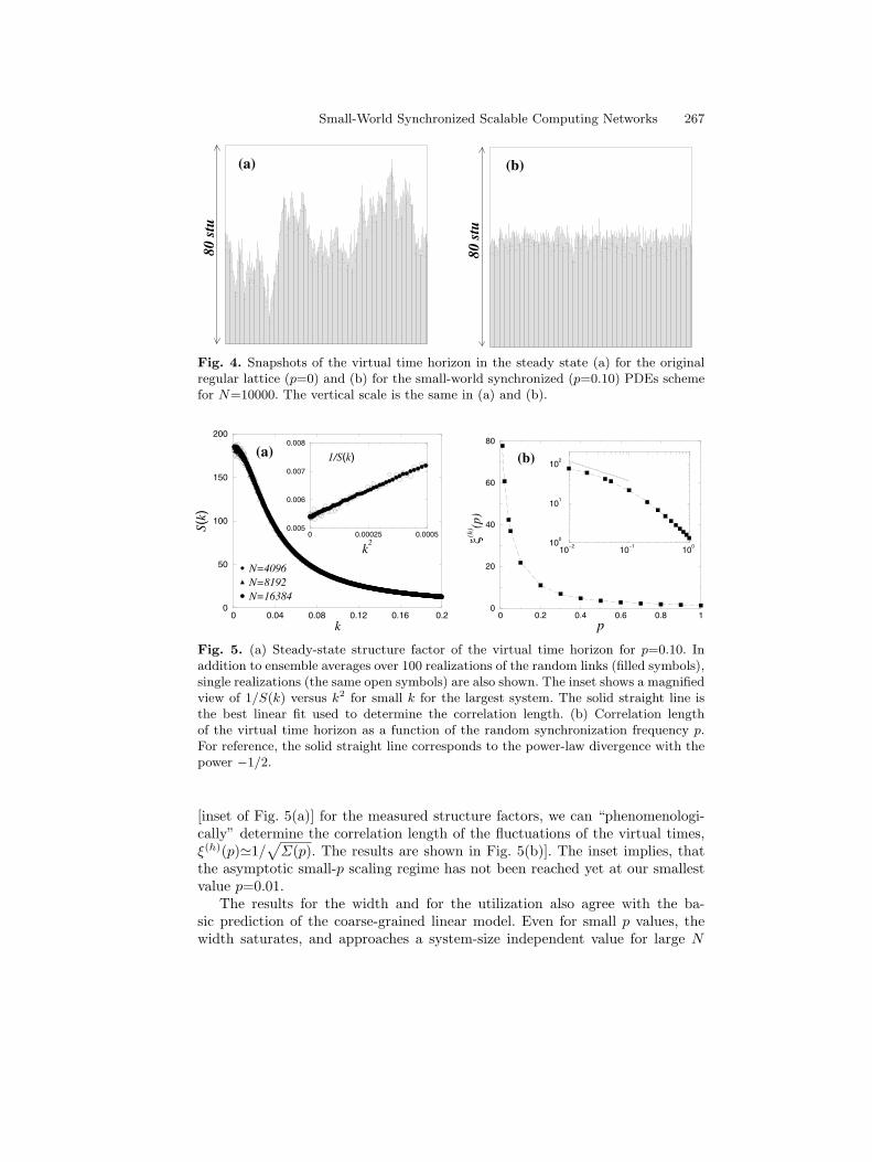
We now turn to discussing the results obtained by simulating the actual PDESscheme, based on the specific update rules for the local simulated times (seethe end of Sect. 3.1). The fundamental difference between the original and theSW-synchronized conservative scheme is illustrated on Fig. 4. The snapshotsof the virtual times indicate that, indeed, the large-amplitude long-wavelengthfluctuations, present in the original time horizon [Fig. 4(a)] are suppressed whenthe extra synchronizations through the quenched random links are implemented[Fig. 4(b)].

Since all steady-state characteristics are “encoded” in the structure factor ofthe virtual times, we measured this quantity, and compared it to

S(h)(k) ∝ 1k2 +Σ(p)

, (25)

the small k limit of (16). Figure 5(a) shows the disorder-averaged structurefactors, as well as individual realizations for various system sizes. As one canobserve, finite-size effects become small and S(h)(k) approaches a finite value ask→0. Thus, there are no large-amplitude, long-wavelength modes in the virtualtime horizon. Further, the inset of Fig. 5(a) confirms the “massive” behavior(25) for small k values. It is important to note that for the actual PDES timehorizon, the effective mass Σ(p) may depend non-trivially on p as a result ofthe dynamic control of the “link strength” and renormalization by nonlinear ef-fects in the specific “microscopic dynamics”. The form of S(k), however, seemsto follow the linear theory, discussed in Sect. 3.2. By plotting 1/S(h)(k) vs. k2


0 2000 4000 6000 8000 100000

20

40

60

80

τi

80 s

tu

(a)

0 2000 4000 6000 8000 100000

20

40

60

80

τi

80 s

tu

(b)

Fig. 4. Snapshots of the virtual time horizon in the steady state (a) for the originalregular lattice (p=0) and (b) for the small-world synchronized (p=0.10) PDEs schemefor N=10000. The vertical scale is the same in (a) and (b).

0 0.04 0.08 0.12 0.16 0.2k

0

50

100

150

200

S(k)

N=4096N=8192N=16384

0 0.00025 0.0005

k2

0.005

0.006

0.007

0.008

1/S(k)(a)

0 0.2 0.4 0.6 0.8 1p

0

20

40

60

80

ξ(h) (p

)

10−2

10−1

10010

0

101

102(b)

Fig. 5. (a) Steady-state structure factor of the virtual time horizon for p=0.10. Inaddition to ensemble averages over 100 realizations of the random links (filled symbols),single realizations (the same open symbols) are also shown. The inset shows a magnifiedview of 1/S(k) versus k2 for small k for the largest system. The solid straight line isthe best linear fit used to determine the correlation length. (b) Correlation lengthof the virtual time horizon as a function of the random synchronization frequency p.For reference, the solid straight line corresponds to the power-law divergence with thepower −1/2.

[inset of Fig. 5(a)] for the measured structure factors, we can “phenomenologi-cally” determine the correlation length of the fluctuations of the virtual times,ξ(h)(p)�1/

√Σ(p). The results are shown in Fig. 5(b)]. The inset implies, that

the asymptotic small-p scaling regime has not been reached yet at our smallestvalue p=0.01.

The results for the width and for the utilization also agree with the ba-sic prediction of the coarse-grained linear model. Even for small p values, thewidth saturates, and approaches a system-size independent value for large N

268 H. Guclu et al.

101

102

103

104

105

N

100

101

102

103

104

<w

2 >N

p=0.00p=0.01p=0.10p=1.00

(a)

0 20000 40000 60000 80000 100000N

0.1

0.15

0.2

0.25

0.3

<u>

N

p=0.00p=0.01p=0.10p=1.00

(b)

Fig. 6. (a) Average steady-state width of the virtual time horizon as function ofthe number of PEs for various values of p. In addition to ensemble averages over 10realizations of the random links (filled symbols), a single realization is also shown (thesame open symbols). The solid straight line represents the asymptotic one-dimensionalKPZ power-law divergence with roughness exponent α=1/2 for the p=0 case. Note thelog-log scales. (b) The steady-state utilization (fraction of non-idling PEs) for the samecases as in (a).

[Fig. 6(a)] while the utilization remains non-zero [Fig. 6(b)]. For example, for ahypothetically infinite system, for p=0.01, 〈w2〉 is reduced from “infinity” (thewidth for the KPZ surface) to about 40, while the utilization drops from 0.2464only to about 0.2460. For p=0.10, the width is further reduced to about 5,while the utilization is down only to 0.242. One can also observe the clear self-averaging property for both global observables (the width and the utilization),i.e., their values become independent of the realization of the SW network forlarge enough N .

To extract the asymptotic small-p behavior of the width and the utilization,one would need larger system sizes, longer steady-state PDES time series, andmore network realizations to obtain reliable statistics, and to compare all as-pects of the linearized coarse-grained model with the actual PDES simulations.In particular, it would be interesting to see, whether the utilization increases ini-tially for sufficiently small p values (the subtle prediction of the coarse-grainedlinear theory). We have not observed this, but the systems we simulated havenot yet reached their asymptotic scaling regime [inset of Fig. 5(b)]. Further,finite-size corrections and error bars may become comparable to this possibleasymptotically small effect in 〈u〉.


3.4 Extremal Fluctuations of the Virtual Time Horizon

In addition to the average value of the fluctuations of the local field variables(such as the height in the context of surface growth models), the typical value ofthe largest fluctuations can also be of great importance [49–51] in a number of ap-plications. For example, in load balancing networks [52] or state-saving schemesfor PDES schemes [30,53], extreme (load or accumulated data) fluctuations onan individual node will cause the delays. Thus, in interacting multi-componentsystems such as the above examples, failures or delays are triggered by extreme-events occurring on the individual components [51].

Relationship between extremum statistics and universal fluctuations in cor-related systems have been discussed intensively in recent years. [36,54–60]. Forthe original PDES scheme (p=0, regular lattice synchronization) exhibiting aKPZ-like rough (or critical) surface, we illustrated (Sect. 2) that the extremalfluctuations of the time horizon diverge in the same fashion as the width itself[Fig. 1(b)]. We now discuss to what extent SW synchronizations lead to thesuppression of the extreme-height fluctuations in the virtual time horizon [53],closely related to the measurement scalability of the conservative PDES scheme.

First, considerN independent identically distributed stochastic variables witha complementer cumulative distribution P>(x) (the probability that the indi-vidual stochastic variable is greater than x). Then the cumulative distributionPmax< (x) for the largest of the N events (the probability that the extremal value

is less than x) can be approximated as [60,61]

Pmax< (x) = [P<(x)]N = [1− P>(x)]N = eN ln[1−P>(x)] � e−NP>(x) , (26)

where one typically assumes that the dominant contribution to the statisticsof the extremes comes from the tail of the individual distribution P>(x). Forexample, for exponentially-tailed individual variables, P>(x)�e−cx, the aboveequation yields

Pmax< (x) � e−e−cx+ln(N)

. (27)

Thus, the sequence of scaled variables x = c(x − ln(N)/c) asymptotically ap-proaches the standard Fisher-Tippett-Gumbel (FTG) distribution [49,50]

Pmax< (x) � e−e−x

(28)

with mean 〈x〉=γ (γ=0.577 . . . being the Euler constant) and variance 〈x2〉 −〈x〉2 = π2/6. It immediately follows that the average value of the largest of theN original random variables then scales as

〈xmax〉 = γ/c+ ln(N)/c � ln(N)/c (29)

for large N values. When comparing with simulation or experimental data, itis often convenient to use the scaled variables x = (x − 〈x〉)/σx which for theabove case yields the FTG limit distribution with zero mean and unit variance

270 H. Guclu et al.

−18 −12 −6 0 6 12 18hi−h

−

10−6

10−4

10−2

100

p(h i−

h−)

N=103

N=104

N=105

Fig. 7. Disorder-averaged probability density (histogram) for the individual simulatedtime fluctuations for various system sizes at p=0.10 (log-normal scales). The solidstraight line indicates a pure exponential tail.

Pmax< (x) � e−e−(ax+γ)

, (30)

where a=π/√

6. Note that with appropriately chosen scaled variables, the conver-gence to the FTG distribution holds not only for exponential variables, but alsofor more general ones with “exponential-like” tails P>(x)�e−cxδ

(i.e., decayingfaster than any power law) [49,50,60,61]. For any δ �=1, however, the convergenceto (28) or (30) is extremely (logarithmically) slow [61].

For the SW synchronized PDES scheme with N PEs we showed that afinite correlation length ξ(h)(p)�1/

√Σ(p) effectively decouples the local sim-

ulated times. Then, the extreme-value limit theorems can be applied [60,61]using the number of independent blocks N/ξ(h) in the system. Further, wefound [62] that the tail of disorder-averaged distribution of the individual rel-ative height fluctuations (independent of the site i) are simple exponentialsP>(hi − h)�exp[−c(hi − h)/w] with w≡√〈w2〉. The histogram for the corre-sponding probability density function, p(hi − h), is shown in Fig. 7.

From the general extreme-value limit theorems, discussed above, it followsthat the scaled extreme-height fluctuations are governed by the FTG distribution(30) (if scaled to zero mean and unit variance). Further, from (29), the averagemaximum relative height, ∆max = hmax − h, will scale as

〈∆max〉 � w

cln(N/ξ(h)) � w

cln(N) , (31)

where we dropped all N -independent terms. Note that both w and ξ(h) approachtheir finite N -independent values for any non-zero p, and the only N dependentfactor is ln(N) for large N values.

Agreement between the simulated PDES extremal fluctuations and the aboveconsiderations are rather convincing. In Fig. 8(a) we show the scaled histograms(to zero mean and unit variance) for the extreme-height fluctuations togetherwith the probability density, corresponding to (30)


−2.0 0.0 2.0 4.0 6.0 8.0 10.0x=(∆max−<∆max>)/σ∆max

10−5

10−4

10−3

10−2

10−1

100

p(x)

N=103

N=104

N=105

Eq. (32)

(a)

4 6 8 10 12ln(N)

0

2

4

6

8

10

12

14

(<w2>)

1/2

<∆max>

(b)

Fig. 8. Extreme fluctuations in the the small-world synchronized PDES time horizonfor p=0.10. (a) Probability density of the scaled extremal fluctuations and comparisonwith the FTG density equation (32). (b) Average of the extremal fluctuations (alsoshown is the width for comparison). The solid straight line indicates the logarithmicdivergence.

p(x) � ae−(ax+γ)−e−(ax+γ), (32)

We note again, that the underlying reason for the fast convergence to the FTGdensity of the simulated time horizon is that the local relative height distri-butions exhibit pure exponential tails. Also, for the more general distributionP>(hi − h)�exp[−c((hi − h)/w)δ], the approach to the FTG limit distributionwould be very slow and the corresponding maximum fluctuations would scale as∼[ln(N)]1/δ [53,61,62], as opposed to (31).

In Fig. 8(b) we show the average of the largest fluctuations above themean, ∆max, for the simulated PDES time horizon. The figure confirms thatfor large enough N (when 〈w2〉 essentially becomes system-size independent)∆max increases logarithmically with the system size, according to (31) [Fig. 8(b].Simulation results for the actual PDES scheme also indicate [62] that the largestdeviations below the mean, ∆min = h − hmin, and the maximum separation,∆ = hmax− hmin, scale the same way as ∆max, i.e., diverge logarithmically withthe system size. Note, that similar to the width and the utilization, the extremalheight fluctuations are also self-averaging [53,62].

The implication of these findings is that while the width becomes finitefor SW-synchronized virtual times, any node can exhibit fluctuations of sizeO(ln(N)) in its local simulated time (related to the local memory need). Werefer to this property as “marginally” scalable for the measurement phase (dueto the weak logarithmic divergence). This property still ensures synchronizationin a practical sense for the SW-synchronized PDES scheme with millions of PEs.Note, that this logarithmic system-size dependence of the extreme fluctuationsis generic to coupled multi-component system, where some local relaxationaldynamics is extended to a SW network [53,62].

272 H. Guclu et al.

4 Summary

Based on a mapping [25] between the evolution of the virtual time horizon for thebasic conservative PDES scheme [11,12] and kinetically grown non-equilibriumsurfaces [28], we constructed a coarse-grained description for the scalability andperformance of such large-scale parallel simulation schemes. These schemes canbe applied to large spatially extended systems with short-range interactions andasynchronous dynamics. The one-site-per PE basic PDES was shown to exhibitKPZ-like kinetic roughening. This scheme is scalable in that the average progressrate of the PEs approaches a non-zero value. The spread of the virtual timehorizon, however, diverges as the square root of the number of PEs, leading to“de-synchronization” and difficulties in data management.

Universality arguments, and actual PDES simulations suggest [31], that theabove characteristics generically hold for any underlying system with short-rangeinteractions for any finite number of sites per PE implementations. Possibleidling due to the conservative synchronization rules and actual communicationtimes can be greatly suppressed by each PE carrying a large block of sites [11,12], yielding encouraging values for the utilization for actual implementations [8].When the PEs carry many sites, however, the saturation value of the width canbecome extremely large. More precisely, there is an additional fast-rougheningphase for early times when the evolution of the time horizon corresponds torandom deposition [31]. Subsequently, it will cross over to the KPZ growth regimeand finally saturate. This further motivates the need for some sort of extrasynchronizations to suppress the roughness of the time horizon.

Our goal here was to achieve synchronization without any global interven-tion. We constructed a specific version of the SW network, where each PE wasconnected to exactly one other randomly chosen PE. The extra synchroniza-tional steps through the random links are merely used to control the width. Thevirtual time horizon for the SW-synchronized PDES scheme becomes “macro-scopically” smooth and essentially exhibits mean-field like characteristics. Therandom links, on top of a regular lattice, generate an effective “mass” for thepropagator of the virtual time horizon, corresponding to a nonzero correlationlength. The width becomes finite, for an arbitrary small rate of synchronizationthrough the random links, while the utilization remains nonzero, yielding a fullyscalable PDES scheme. The former statement is only marginally weakened byobserving that the extreme fluctuations in the time horizon can exhibit loga-rithmically large values as a function of the total number of PEs. The abovepredictions of the coarse-grained PDES model were confirmed by actually “sim-ulating the simulations”.

The generalization when random links are added to a higher-dimensionalunderlying regular lattice is clear: since our construction of the SW network(“hard” version) on a one-dimensional regular substrate is already mean-field,in higher dimensions it will be even more so [44] (i.e., the critical dimension of ourSW network is less than one). Note that synchronizability on scale-free networks[45,63] was also studied recently. The results indicate that a PDES scheme ismarginally scalable if the communication topology between the PEs is a scale-


free network [35]. The implication of this finding is that the internet, which isalready exploited for distributed computing for mostly “embarrassingly parallel”problems through existing GRID-based schemes [16,17], may have the potentialto accommodate efficient complex system simulations (such as asynchronousPDES) where the nodes frequently have to synchronize with each other.

The above construction of a fully scalable algorithm for simulating largesystems with asynchronous dynamics and short-range interactions is an examplefor the enormous “computational power and synchronizability” [20] that can beachieved by SW couplings. The suppression of critical fluctuations of the virtualtime horizon is also closely related to the emergence of mean-field-like phasetransitions and phase ordering in non-frustrated interacting systems [1,64–70].

Recent theoretical work also supports [43,44,71] that systems without inher-ent frustration exhibit strict or anomalous mean-field characteristics when theoriginal short-range interaction topology is modified to a SW network.

Acknowledgements

Discussions with G. Gyorgyi, M.B. Hastings, G. Istrate, B. Kozma, B.D.Lubachevsky, Z. Racz, and P.A. Rikvold, are gratefully acknowledged. G.K. andM.A.N thank CNLS, Los Alamos National Laboratory for their hospitality dur-ing their stays in summer 2002 and 2003 where part of this work was completed.We acknowledge the support of US NSF through Grant No. DMR-0113049 andthe support of the Research Corporation Grant No. RI0761. Z.T. is supportedby the US DOE under contract W-7405-ENG-36. H.G. was also supported inpart by the Los Alamos summer student program in 2002 and 2003, DOE W-7405-ENG-36.

References

1. S.H. Strogatz, Nature 410, 268 (2001).2. R. Fujimoto, Commun. ACM 33, 30 (1990).3. D.M. Nicol, R.M. Fujimoto, Ann. Oper. Res. 53, 249 (1994).4. B.D. Lubachevsky, Bell Labs Tech. J. 5 April-June 2000, 134 (2000).5. A.G. Greenberg et al. in Proc. 8th Workshop on Parallel and Distributed Simulation

(PADS’94), Edinburgh, UK, 1994 (SCS, San Diego, CA, 1994), p. 187.6. E. Deelman, B.K. Szymanski, T. Caraco, in Proc. 28th Winter Simulation Confer-

ence, (ACM, New York, 1996), p. 1191.7. D.M. Nicol, Proc. 1988 SCS Multiconference, Simulation Series, SCS, Vol. 19,

p. 141 (1988).8. G. Korniss, M.A. Novotny, P.A. Rikvold, J. Comput. Phys. 153, 488 (1999).9. G. Korniss, C.J. White, P.A. Rikvold, M.A. Novotny, Phys. Rev. E 63, 016120

(2001).10. G. Korniss, P.A. Rikvold, M.A. Novotny, Phys. Rev. E 66, 056127 (2002).11. B.D. Lubachevsky, Complex Syst. 1, 1099 (1987).12. B.D. Lubachevsky, J. Comput. Phys. 75, 103 (1988).13. D.R. Jefferson, ACM Trans. Prog. Lang. and Syst. 7, 404 (1985).

274 H. Guclu et al.

14. A.G. Greenberg, S. Shenker, and A.L. Stolyar, Performance Eval. Rev. 24, 91(1996).

15. Blue Gene/L project, partnership between IBM and DoE, announced Nov.9, 2001;64K processors, expected scale 200 teraflops, a step towards a petaflop scale; ex-pected completion 2005; IBM Research Report, RC22570 (W0209-033) September10, 2002.

16. See, e.g., www.gridforum.org and setiathome.ssl.berkeley.edu.17. S. Kirkpatrick, Science 299, 668 (2003).18. P.M.A. Sloot, B.J. Overeinder, A. Schoneveld, Comput. Phys. Commun. 142, 76

(2001).19. P. Bak, C. Tang, K. Wiesenfeld, Phys. Rev. Lett. 59, 381 (1987).20. D.J. Watts and S.H. Strogatz, Nature 393, 440 (1998).21. G. Korniss, M.A. Novotny, H. Guclu, Z. Toroczkai, and P.A. Rikvold, Science 299,

677 (2003).22. K.M. Chandy, J. Misra, Commun. ACM 24, 198 (1981).23. R.E. Felderman and L. Kleinrock, ACM Trans. Model. Comput. Simul. 1, 386

(1991).24. D.M. Nicol, ACM Trans. Model. Comput. Simul. 1, 24 (1991).25. G. Korniss, Z. Toroczkai, M.A. Novotny, and P.A. Rikvold, Phys. Rev. Lett. 84,

1351 (2000).26. Z. Toroczkai, G. Korniss, S. Das Sarma, and R.K.P. Zia, Phys. Rev. E 62, 276

(2000).27. M. Kardar, G. Parisi, Y.-C. Zhang, Phys. Rev. Lett. 56, 889 (1986).28. A.-L. Barabasi and H.E. Stanley, Fractal Concepts in Surface Growth (Cambridge

University Press, Cambridge, 1995).29. S.F. Edwards and D.R. Wilkinson, Proc. R. Soc. London, Ser A 381, 17 (1982).30. G. Korniss, M.A. Novotny, A.K. Kolakowska, and H. Guclu, SAC 2002, Proceedings

of the 2002 ACM Symposium on Applied Computing, pp. 132-138, (2002).31. A. Kolakowska, M. A. Novotny, and G. Korniss, Phys. Rev. E 67, 046703 (2003).32. A. Kolakowska, M. A. Novotny, and P.A. Rikvold, Phys. Rev. E 68, 046705 (2003).33. A. Kolakowska and M. A. Novotny, Phys. Rev. B 69, 075407 (2004).34. J. Krug and P. Meakin, J. Phys. A 23, L987 (1990).35. Z. Toroczkai, G. Korniss, M. A. Novotny, and H. Guclu, in Computational Com-

plexity and Statistical Physics, edited by A. Percus, G. Istrate, and C. Moore, SantaFe Institute Studies in the Sciences of Complexity Series (Oxford University Press,2004, in press); arXiv:cond-mat/0304617 (2003).

36. S. Raychaudhuri, M. Cranston, C. Przybyla, and Y. Shapir, Phys. Rev. Lett. 87,136101 (2001).

37. E. Marinari, A. Pagnani, G. Parisi, and Z. Racz, Phys. Rev. E 65, 026136 (2002).38. Z. Racz, private communications.39. D.J. Watts, Small Worlds (Princeton Univ. Press, Princeton, 1999).40. M.E.J. Newman, J. Stat. Phys. 101, 819 (2000).41. M.E.J. Newman and D.J. Watts, Phys. Lett. A 263, 341 (1999).42. R. Monasson, Eur. Phys. J. B 12, 555 (1999).43. B. Kozma and G. Korniss, in Computer Simulation Studies in Condensed Matter

Physics XVI, edited by D.P. Landau, S.P. Lewis, and H.-B. Schuttler, SpringerProceedings in Physics (Springer, Berlin, 2004, in press); arXiv:cond-mat/0305025(2003).

44. B. Kozma, M.B. Hastings, and G. Korniss, arXiv:cond-mat/0309196: Phys. Rev.Lett., in press (2004).


45. Reka Albert and Albert-Laszlo Barabasi, Rev. Mod. Phys. 74, 47 (2002).46. H. Guclu, G. Korniss, M.A. Novotny, and Z. Toroczkai, in preparation.47. A.A. Middleton, Phys. Rev. Lett. 68, 670 (1992).48. M.B. Hastings, private communications (2003).49. R.A. Fisher and L.H.C. Tippett, Proc. Camb. Philos. Soc. 24, 180 (1928)50. E.J. Gumbel, Statistics of Extremes (Columbia University Press, New York, 1958).51. Extreme Value Theory and Applications, edited by J. Galambos, J. Lechner, and

E. Simin (Kluwer, Dordrecht, 1994).52. Y. Rabani, A. Sinclair, and R. Wanka, Proceedings of the 39th Annual Symposium

on Foundations of Computer Science (IEEE Comput. Soc, Los Alamitos, CA, 1998)pp. 694-703.

53. H. Guclu and G. Korniss, arXiv:cond-mat/0311575 (2003).54. S.T. Bramwell, P.C.W. Holdsworth, and J.-F. Plinton, Nature 396 552 (1998).55. S.T. Bramwell et al., Phys. Rev. Lett. 84 3744 (2000).56. S.T. Bramwell et al., Phys. Rev. E 63 041106 (2001).57. T. Antal, M. Droz, G. Gyorgyi, and Z. Racz, Phys. Rev. Lett. 87, 240601 (2001).58. S. C. Chapman, G. Rowlands, and N. W. Watkins, Nonlinear Processes in Geo-

physics 9, 409 (2002); arXiv:cond-mat/0106015.59. V. Aji and N. Goldenfeld, Phys. Rev. Lett. 86, 1007 (2001).60. J.-P. Bouchaud and M. Mezard, J. Phys. A 30, 7997 (1997).61. A. Baldassarri, Statistics of Persistent Extreme Events, Ph.D. Thesis, De

l´Universite Paris XI Orsay (2000).62. H. Guclu and G. Korniss, in preparation.63. A.-L. Barabasi and R. Albert, Science 286 509 (1999).64. A. Barrat, M. Weigt, Eur. Phys. J. B 13, 547 (2000).65. M. Gitterman, J. Phys. A 33, 8373 (2000).66. B.J. Kim et al, Phys. Rev. E 64, 056135 (2001).67. H. Hong, B.J. Kim, M.Y. Choi, Phys. Rev. E 66, 018101 (2002).68. H. Hong, M.Y. Choi, and B.J. Kim, Phys. Rev. E 65, 047104 (2002).69. C.P. Herrero, Phys. Rev. E 65, 066110 (2002).70. M.A. Novotny and Shannon M. Wheeler, Braz. J. Phys., Proceedings for the

III Brazilian Meeting on Simulational Physics (2003); arXiv:cond-mat/0308602(2003).

71. M.B. Hastings, Phys. Rev. Lett. 91, 098701 (2003).

Small-world synchronized computing networks for scalable parallel discrete-event simulations

Documents

Transcript of Small-world synchronized computing networks for scalable parallel discrete-event simulations