Slope Stability in Unsaturated Soils under Static and Rainfall Conditions
110
“OVIDIUS” UNIVERSITY OF CONSTANTZA UNIVERSITATEA „OVIDIUS” CONSTANŢA “OVIDIUS” UNIVERSITY ANNALS - CONSTANTZA Year VII (2005) Series: CIVIL ENGINEERING ANALELE UNIVERSITĂŢII „OVIDIUS”CONSTANŢA ANUL VII (2005) Seria: CONSTRUCŢII Ovidius University Press 2005
Transcript of Slope Stability in Unsaturated Soils under Static and Rainfall Conditions

“OVIDIUS” UNIVERSITY OF CONSTANTZA UNIVERSITATEA „OVIDIUS” CONSTANŢA
“OVIDIUS” UNIVERSITY ANNALS - CONSTANTZA
Year VII (2005)
Series: CIVIL ENGINEERING
ANALELE
UNIVERSITĂŢII „OVIDIUS”CONSTANŢA ANUL VII
(2005)
Seria: CONSTRUCŢII
Ovidius University Press 2005

“OVIDIUS” UNIVERSITY OF CONSTANTZA UNIVERSITATEA „OVIDIUS” CONSTANŢA
“OVIDIUS” UNIVERSITY ANNALS - CONSTANTZA
Year VII (2005)
Series: CIVIL ENGINEERING
ANALELE
UNIVERSITĂŢII „OVIDIUS”CONSTANŢA ANUL VII
(2005)
Seria: CONSTRUCŢII
Ovidius University Press 2005

“OVIDIUS” UNIVERSITY ANNALS - CONSTANTZA YEAR VII
(2005)
SERIES: CIVIL ENGINEERING ANAL ELE
UNIVERSITĂŢII „OVIDIUS”CONSTANŢA ANUL VII
(2005)
SERIA: CONSTRUCŢII
“OVIDIUS” UNIVERSITY OF CONSTANTZA UNIVERSITATEA „OVIDIUS” CONSTANŢA

“OVIDIUS“ UNIVERSITY ANNALS - CONSTANTZA – SERIES: CIVIL ENGINEERING ANALELE UNIVERSITĂŢII „OVIDIUS“ CONSTANŢA – SERIA: CONSTRUCŢII
EDITORS Dumitru Ion ARSENIE, Virgil BREABĂN, Lucica ROŞU “OVIDIUS” University, Faculty of Civil Engineering, 124, Mamaia Blvd., 900527, RO., Constantza, Romania ADVYSORY EDITORIAL BOARD Dumitru Ion ARSENIE, Prof. Ph.D. Eng., “OVIDIUS” University of Constantza, Romania; Roumen ARSOV, Prof. Ph.D. Eng., University of Architecture, Civil Engineering & Geodesy, Sofia, Bulgaria Alex Horia BĂRBAT, Prof. Ph.D. Eng., Technical University of Catalonia, Spain; Virgil BREABĂN, Prof. Ph.D. Eng., “OVIDIUS” University of Constantza, Romania; Pierre CHEVALLIER, Ph.D. Eng., Head of The ILEE – IFR, Montpellier II University, France; Mehmet DURMAN, Prof. Ph.D. Eng., SAKARYA University, Turkey Ion GIURMA, Prof. Ph.D. Eng., “GH. ASACHI”, Technical University, Iassy, Romania; Axinte IONIŢĂ, Ph.D., Eng., Tennessee University, U.S.A. Turan ÖZTURAN, Prof. Ph.D. Eng., BOGAZICI University, Istanbul, Turkey Gheorghe POPA, Prof. Ph.D. Eng., “POLITEHNICA” University of Timişoara, Romania; Mihail POPESCU, Prof. Ph.D. Eng., “OVIDIUS” University of Constantza, Romania; Lucica ROŞU, Prof. Ph.D. Eng., “OVIDIUS” University of Constantza, Romania; Dan STEMATIU, Prof. Ph.D. Eng., Technical University of Civil Engineering of Bucharest, Romania; DESK EDITORS Ichinur OMER, Geanina ADAM, Gabriela BADEA Mail address: “OVIDIUS” University, Faculty of Civil Engineering,
124, Mamaia Blvd., 900527, RO., Constantza, Romania E-mail: [email protected]; [email protected] ORDERING INFORMATION The journal may be obtained by ordering at the “OVIDIUS” University, or on exchange basis with similar romanian or foreign institutions. Revista poate fi procurată prin comandă la Universitatea „OVIDIUS“, sau prin schimb de publicaţii cu instituţii similare din ţară şi străinătate. 124, Mamaia Blvd., 900527, RO., Constantza, Romania © 2000 Ovidius University Press. All rights reserved.
“OVIDIUS” UNIVERSITY OF CONSTANTZA UNIVERSITATEA „OVIDIUS” CONSTANŢA
“OVIDIUS” UNIVERSITY ANNALS - CONSTANTZA
Year VII (2005)
Series: CIVIL ENGINEERING
ANALELE
UNIVERSITĂŢII „OVIDIUS”CONSTANŢA ANUL VII
(2005)
Seria: CONSTRUCŢII
Ovidius University Press 2005

“OVIDIUS” UNIVERSITY ANNALS - CONSTANTZA YEAR VII
(2005)
SERIES: CIVIL ENGINEERING ANAL ELE
UNIVERSITĂŢII „OVIDIUS”CONSTANŢA ANUL VII
(2005)
SERIA: CONSTRUCŢII
“OVIDIUS” UNIVERSITY OF CONSTANTZA UNIVERSITATEA „OVIDIUS” CONSTANŢA

“OVIDIUS“ UNIVERSITY ANNALS - CONSTANTZA – SERIES: CIVIL ENGINEERING ANALELE UNIVERSITĂŢII „OVIDIUS“ CONSTANŢA – SERIA: CONSTRUCŢII
EDITORS Dumitru Ion ARSENIE, Virgil BREABAN, Lucica ROSU “OVIDIUS” University, Faculty of Civil Engineering, 124, Mamaia Blvd., 900527, RO., Constantza, Romania ADVYSORY EDITORIAL BOARD Dumitru Ion ARSENIE, Prof. Ph.D. Eng., “OVIDIUS” University of Constantza, Romania; Roumen ARSOV, Prof. Ph.D. Eng., University of Architecture, Civil Engineering & Geodesy, Sofia, Bulgaria Alex Horia BĂRBAT, Prof. Ph.D. Eng., Technical University of Catalonia, Spain; Virgil BREABĂN, Prof. Ph.D. Eng., “OVIDIUS” University of Constantza, Romania; Pierre CHEVALLIER, Ph.D. Eng., Head of The ILEE – IFR, Montpellier II University, France; Mehmet DURMAN, Prof. Ph.D. Eng., SAKARYA University, Turkey Ion GIURMA, Prof. Ph.D. Eng., “GH. ASACHI”, Technical University, Iassy, Romania; Axinte IONIŢĂ, Ph.D., Eng., Tennessee University, U.S.A. Turan ÖZTURAN, Prof. Ph.D. Eng., BOGAZICI University, Istanbul, Turkey Gheorghe POPA, Prof. Ph.D. Eng., “POLITEHNICA” University of Timişoara, Romania; Mihail POPESCU, Prof. Ph.D. Eng., “OVIDIUS” University of Constantza, Romania; Lucica ROŞU, Prof. Ph.D. Eng., “OVIDIUS” University of Constantza, Romania; Dan STEMATIU, Prof. Ph.D. Eng., Technical University of Civil Engineering of Bucharest, Romania; DESK EDITORS Ichinur OMER, Geanina ADAM, Gabriela BADEA Mail address: “OVIDIUS” University, Faculty of Civil Engineering,
124, Mamaia Blvd., 900527, RO., Constantza, Romania E-mail: [email protected]; [email protected] ORDERING INFORMATION The journal may be obtained by ordering at the “OVIDIUS” University, or on exchange basis with similar romanian or foreign institutions. Revista poate fi procurată prin comandă la Universitatea „OVIDIUS“, sau prin schimb de publicaţii cu instituţii similare din ţară şi străinătate. 124, Mamaia Blvd., 900527, RO., Constantza, Romania © 2000 Ovidius University Press. All rights reserved.

TABLE OF CONTENTS

Ovidius University Annals Series: Civil Engineering Volume 1, Number 7, 2005
ISSN-12223-7221 © 2000 Ovidius University Press
SECTION I
Calculus and Structures Reliability Architecture
Structural analysis problems of lightweight structures, CĂTĂRIG Alexandru KOPENETZ Ludovic ALEXA Pavel
7-10
Dynamic procedure of estimating the hysteretic type equivalent damping, CHIŢAN Violeta-Elena STEFAN Doina
11-14
Study on the use of the torus surface in constructions, DRĂGAN Delia MÂRZA Carmen DARDAI Radu
15-18
Calculations of precast concrete tank foundation on elastic subsoil, GÓRSKI Krzysztof WYJADŁOWSKI Marek
19-24
Determination of mechanical characteristics for composite stone plates, KÜMBETLIAN Garabet GELMAMBET Sunai
25-28
For an unit system of working in strength materials, KÜMBETLIAN Garabet GELMAMBET Sunai
29-34
Considerations regarding residual mechanical characteristics, MIHAI Petru, FLOREA Nicolae BĂRBUŢĂ Marinela
35-38
Evaluation of the safety degree for two old masonry churches, MIHAI Petru FLOREA Nicolae
39-46
Problems and benefits of designing for a composite structures used in construction, NIŢǍ Alexandra
47-50
The architectural diversity management in the academic environment, POPESCU Emil Barbu MOLDOVAN Mircea Sergiu
51-60
Seismic stability of reinforced slopes based on the assessment of permanent displacement, SAKELLARIOU Michael
61-68

Table of Contents / Ovidius University Annals Series: Civil Engineering 7, 113 - 114 (2005)
114
SECTION II Hydraulics and Fluid Mechanics
Determination of the constant c for the Gerstner’s traveller wave potential, CAZACU Mircea Dimitrie MĂCHIŢĂ Dan Aurel
71-74
Flow compensation reservoir at hydro power plants with lengthy pressure pipe, NITESCU Claudiu Stefan
75-78
A kinematic condition concerning the viscous substratum (laminar limited substratum) in the pressure pipes and some consequences for turbulent regime phases, OMER Ichinur ARSENIE Dumitru Ion
79-82
Installation with hydraulic channel for hydro-elasticity tests - velocities distribution, RUSU Ilie BARTHA Iosif CIOBANU Bogdan
83-86
SECTION III
Water Resources Management and Environment Engineering
Engineering of Land Reclamation Systems
Aspects regarding the modelling of environmental impact upon the complex storage lakes, BOLBA Roxana CRĂCIUN Ioan
89-92
The study of potential soil erosivity in area Bozovici-Reşiţa-Ezeriş, CONSTANTINESCU Laura. NEMEŞ N. NEMEŞ I. GROZAV A.
93-96
Phosphorus removal by biological processes, CREŢU Valentin TOBOLCEA Viorel
97-102
Slope stability in unsaturated soils under static and rainfall conditions, MATZIARIS Vasileios SAKELLARIOU Michael
103-110

Ovidius University Annals Series: Civil Engineering Volume 1, Number 7, Nov. 2005
ISSN-12223-7221 © 2000 Ovidius University Press
Structural Analysis Problems of Lightweight Structures
Alexandru CĂTĂRIG a Ludovic KOPENETZ a Pavel ALEXA a
a Technical University Cluj Napoca, Cluj Napoca, 400027, Romania
__________________________________________________________________________________________ Rezumat: Introducerea şi răspândirea în practica construcţiilor a structurilor portante uşoare din ce în ce mai zvelte, având forme şi alcătuiri complexe, a fost posibilă datorită dezvoltării fără precedent a procedeelor de analiză structurală şi a utilizării unor noi materiale cu caracteristici de rezistenţă deosebite. În lucrare sunt prezentate, pe lângă aspecte de analiză structurală, probleme privind alegerea materialelor şi modelarea încărcărilor. Abstract: The development of structural analysis formulations and numerical procedures as well as the unprecedent development of light high - strength materials have pushed the use of lightweight structures to a very large extent. Also, the lightweight structures are becoming more and more slender as the result of the possibility of covering larger areas. The present contribution refers to several aspects brought about by the analysis of these structures. The aspects discussed are associated to analysis formulation, to load modelling and to the selection of materials. Keywords: lightweight structures, dynamic analysis, anizotropic materials, nonlinear analysis, direct integration __________________________________________________________________________________________ 1. Introduction
The lightweight structures due to both, their
structural flexibility and their versatility in forms
became a very economical and rational way of
using the material and human resources in
construction industry. Nevertheless, there are
many situations when the AESTHETICAL aspect
appears to be more important than the
economical aspect. It is the case, for instance, of
the SUNNIBERG (Kloister, Switzerland) bridge.
From a historical point of view, the first
light structures may be considered the suspension
(foot) bridges from South America and China.
Also, the sail ships and the tents are among the
first avant la lettre lightweight structures. The
retractable amphitheatre roofs are – laso-
remarcable examples of lightweight structures.
After a stagnation of almost 15 centuries, the
lightweight structures are, again, in the top of the
construction iundustry. The first mentioned structure
that can be considered a lightweight structure is the
bridge of Verantius (Venice) built in 1617. Beside
its suspension chain, the bridge is provided with
inclined ties for a higher stiffness of the deck.
Sometime later (1784), the ‘’cable stayed’’ bridge
built by C. J. Loscher in Friburg (Switzerland) has
been provided with wood boards (without knags) for
what would become later the cables.
In the field of aerospatial structures, in the
same periode (1785), in France is built, by
Montgolfier brothers, the first balloon filled with
warm aer. In the proper Civil Engineering field, V.
G. Suhov built (1895) the Nijninovgorod exhibition

Structural Analysis Problems … / Ovidius University Annals Series: Civil Engineering Volume 1, Number 7, 7-10 (2005)
8
pavilions as lightweight structures. During the
20th century, the structures design and built by
Otto Frei, Bird, Nowicki, Severnd and others are
considered among the most remarcable
lightweight structures of the contemporary
period.
2. Materials of lightweight structures
Most of the lightweight structures are either
structures in tenssion, or in compression or both,
tenssion and compression. The tenssion state is
undertaken by cables and membranes. During the
history, the materials that were used for cables in
most of the cases of structures in tension have
been: papyrus, camel hair, flax, hemp and, from,
1834, the steel.
The membrane used in lightweight structures
are in the form of foils. Nowadays, two types of
foils are used for membranes: foils made up from
anizotropic materials and foils made up from
izotropic materials.
The most common materials used for
izotropic materials are: steel, aluminium, copper,
polyesters, polyethilene, vynilpolyclorure, etc.
The anizotropic foils are obtained through the
process of reinforcing the izotropic foils with fibres
arranged along one or several directions in one or
several layers. The fibres used as reinforcements
are made up of:
a) organic materials (flax, hemp, cotton),
b) mineral materials (glass fibres, carbon
fibresgraphite fibres),
c) synthetic materials (polyesters, polyamides,
aramides).
3. Structural analysis
The analysis of lightweight structures involves
the solutions for three categories of problems.
a. Setting the initial form or the initial
configuration
Setting the initial form is equivalent to saying
that the form is the structure and the structure means
its form. Finding the equilibrium form associated to the
initial loads (dead weight and prestressing) is, both, the
most difficult and most important step in the structural
analysis.
The weight of the lightweight structures ranges
from 10.0 N/m2 to 50.0 N/m2 and is neglijible to the
snow weight. The dead weight is not taken into
account in the computation of the tension stresses.
Due to the creep phenomenom, two values of the
prestressing force have to be computed: a maximum
and a minimum value. The prestressing via the
maximum value does not necessarily lead to maximum
stress state.
b. Computation of deformation state
This is the step when the deformation from the
initial position to the final (equilibrium) position under
applied loads (snow, wind) is computed. The problem
of assesing the values of acting wind is rather
complicated taking into account that the pressure
A. Cătărig, L. KOPENETZ and P. ALEXA / Ovidius University Annals Series: Civil Engineering 7, 7-10 (2005) 9
coefficients are deeply dependent on the structural
form and no generally valid values are available.
c. Dynamic analysis
Due to their small own weight, the
lightweight structures are very vulnerable to any
load that induces motions into the structure.
The computation has to take into account the
transverse vibrations of the cables since this motion
heavily influences the durability of the structural
make up. In the case of structures with a natural
frequence smaller than 0.6 Hz, the wind may not be
introduced as a dynamic force. In order to avoid the
phenomenom of fluttering, rather impossible to be
predicted from the computations, the curvatures and
the level of prestressing have to be adequately
chosen.
The possible vibrations that yield from the
analysis can be reduced via energy absorbing
devices.
∗ The complexity of the structural analysis is a
direct consequence of the nonlinear behaviour of
these structures. The nonlinear behaviour is, in its
turn, the result of the three classical sources of
nonlinearity:
• Geometrical nonlinearity.
• Material (phisical) nonlinearit.
• Geometrical and material
nonlinearities.
Many times the nonlinearity is the result of
the loading (mainly when the loads depend on the
state parameters). The dynamic analysis, the inertia
and dampiung type phenomena may, also, lead to
nonlinear structural behaviour. The nonlinear dynamic
analysis is and remains complicated even in the
presence of so many computation techniques
(incremental approaches, Newton – Raphson
technique, modified forms of these methods, etc.).
Three methods made their ways through in the
dynamic analysis of lightweight structures:
• Modal superposition method.
• Direct numerical integration method.
• Integration method with transform.
∗∗ The modal superposition method has been rather
little used since this method proves its efficiency
versus the implicit integration techniques only when
the band width of the matrices is large and when there
are a large number of natural modes of vibration.
The techniques of direct integration are a
common place in the linear analysis, but little is known
about their efficiency in the nonlinear dynamic
analysis. The well known β - Newmark and θ - Wilson
direct integration methods loose their unconditional
stable character if an incremental formulation of the
nonlinear oscilations is employed.
Nevertheless, when an iterative equilibrium
check is performed for each incremental step, these
methodes are stable in time.
Concluding, one may say that the dynamic
analysis techniques have – rather – a case study use
and have been reported in isolated (punctual) cases of
structural analysis.
∗∗∗

Structural Analysis Problems … / Ovidius University Annals Series: Civil Engineering Volume 1, Number 7, 7-10 (2005)
10
The authors of the present contribution have
tried to solve the static and dynamic analysis of
lightweight structures in a unitary nonlinear
formulation based on FEM technique and using
Lagrangean coordinates and Piola – Kirchoff
tensor.
The computer programme SUM01 allows the
static and dynamic analyses of lightweight
structures made up of cables, anizotropic
membranes (through a simulation with embeded
fibres) and bars.
The computation technique employed for
nonlinear equilibrium invloves Newton – Raphson
type iterations independent of the type of the finite
elements employed. The integration of equations of
motion is performed using both, the β - Newmark θ
- Wilson direct integration methods.
The structure of the program uses the ideea of
operating using a unique vector and the common
blocks for data delivering. The required memory
depends on the magnitude of these blocks.
4. Concluding remarks
∗ The contribution presents several aspects of
the structural analysis closely related to loading
modelling and the material type.
∗ The revealed problems may be used in the
elaboration of the design provisions for lightweight
structures.
∗ Several classical techniques of approaching
the nonlinear behaviuor of lightweight structures
are reviewed and a unitary procedure developed by the
authors based on Finite Element Method technique and
Langrangean coordinates using Piola – Kirchoff tensor
is described.
5. References
[1] Kopenetz, L., Contributions to Computation of
Cable Structures. 1989, Ph. D. Thesis, Technical
University, Cluj-Napoca.
[2] Cătărig, A., Kopenetz, L., Cable and Membrane
Structures, 1998 , Editura U.T. PRES, Cluj-Napoca.
[3] Kopenetz, L., Ionescu, A., Light weight roof for
dwellings, 1985, Journal for housing and ITS
application, vol..9, no.3, Miami, Florida, USA.
[4] Cătărig, A., Kopenetz, L., Alexa, P., The Use of
Mixt Light Structures for Rezidential and Resort-Type
Buildings,1996, Acta Technica Napocensis, no.39,
Cluj-Napoca.
[5] Cătărig, A., Kopenetz, L., Alexa, P., Light-Weight
Composite Facades, 1997, Proceedings of the IAHS
International Housing Congress, Sinaia.
[6] Cătărig, A., Kopenetz, L., Alexa, P., Problems of
Computation of Structures Made up of Cables and
Membranes, Acta Technica Napocensis, no.40, Cluj-
Napoca, 1997.
Ovidius University Annals Series: Civil Engineering Volume 1, Number 7, Nov. 2005
ISSN-12223-7221 © 2000 Ovidius University Press
Dynamic Procedure of Estimating the Hysteretic Type Equivalent Damping
Violeta-Elena CHIŢAN a Doina STEFANa a “Gh. Asachi” Technical University Iassy, Iassy, 700050, Romania
__________________________________________________________________________________________ Rezumat: Modelarea variaţiei parametrilor dinamici de rigiditate şi amortizare, permite studiul factorilor ce definesc mărimea amortizării în domeniul post-elastic de comportare. Amortizarea vâscoasă histeretică este studiată pe baza unor procedee dinamice ce iau în consideraţie variaţia frecvenţei proprii în funcţie de alura curbei histerezis şi de factorii de ductilitate ce definesc amplitudinea maximă şi cea de la limita de apariţie a deformaţiilor plastice semnificative. Abstract: Modeling the variation of the rigidity and damping dynamic parameters allows the survey of the factors defining the size of the damping in the post-elastic behavior domain. The hysteretic viscous damping is studied based on some dynamic procedures that take into account the natural frequency variation depending on the hysteresis curve rate and on the ductility factors that define the maximum and limit amplitudes of the significant plastic deformation appearance. Keywords: equivalence criteria, hysteretic behavior, dynamic freedom degree, damping factors, bilinear model __________________________________________________________________________________________ 1.Introduction
The use of the equivalence criteria in view of simulating the rigidity and damping parameter variation with a dynamic freedom degree, leads to a series of relations that characterize the viscous type equivalent damping factors [1]. These factors are either the critical damping percentage or the energy dissipation factor that measure the energy loss in an oscillation cycle. The equivalent viscous damping depends on the relation of the rigidity of the bilinear model and by the ductility factor.
In setting the equivalent hysteretic damping expressions it can be used the dynamic processes modeling the frequency variation to the resonance for the hysteretic loop amplitude and the geometrical procedures considering the hysteretic loop configuration in various system degrading stages. 2.Bilinear model associated with constant dynamic properties
The equivalent viscous damping coefficient is obtained by equalizing energy dissipation of the two systems, linear and bilinear equivalent for an oscillation cycle:
)kk)(xx(x4W 21ymy −−⋅=Δ (1)
thus resulting:
⎟⎟⎠
⎞⎜⎜⎝
⎛−⋅
⎟⎠⎞
⎜⎝⎛
−⋅=
1
22 11
2kk
xx
xx
y
m
y
m
eq πη (2)
In this case, the mass is considered constant and
the equivalent height of the reverse pendulum is equal to the height of the oscillator having a constant degree of freedom and rigidity.
The viscous damping variation equivalent is represented to the interval μ = xm/xyЄ1,..,10 and α = K2/K1Є0.1;..;1. It is observed that the damping values show an increase till the maximum for a ductility factor equal to 2, after which, they decrease corresponding to the a rigidity ratio of the two segments of the ascending curve of the hysteresis loop. The above mentioned parameters that characterize the equivalent damping and the energy dissipation coefficient are connected by the expressions:
WW
MCe
eqΔ
=Ψ=Ψ
= ;24 ωπ
η (3)

Dynamic procedure … / Ovidius University Annals Series: Civil Engineering Volume 1, Number 7, 11-14 (2005)
12
3.Bilinear models with variable dynamic characteristics
In order to model the circular frequency in a certain stage of the cyclic process, we shall develop a linear system associated with a frequency to resonance and also with a variable damping coefficient [2]. Because the mono-masses system frequency depends of the mass and the elastic constant, a variable mass or a variable rigidity could be defined. Depending on the selected parameter, can be used various criteria in view of simulating the equivalent system for the nonlinear oscillator.
The dynamic procedures that consider the dynamic parameter variation in order to define a hysteretic damping are: dynamic rigidity variation, dynamic mass variation, keeping constant the critical damping. 4.Equivalence criterion of the dynamic rigidity
The equivalence procedure of the dynamic rigidity allows the simulation of the natural frequency of the oscillator, considering a constant mass, but a variable rigidity of the degrading structure. In this case we shall have:
)x(m)x(K;m)x(m o2
oo ω⋅== where:
⎟⎠⎞
⎜⎝⎛ −= θθ
πωω
2sin211)(
20
02 x , ym xx ≥ (4)
1)(
20
0 =ω
ω x , ym xx < (5)
;21cos. ⎟⎟⎠
⎞⎜⎜⎝
⎛−=
m
y
xx
arcθmk
=20ω (6)
In the case 02 =K expressing the energy
balance so:
)(4)()(2 200 ymym xxxKxxKx −⋅=⋅πζ (7)
we obtain the critical damping factor:
20
020 )(
12
)(
ωω
πζ
xxx
xx
x m
y
m
y⎟⎟⎠
⎞⎜⎜⎝
⎛−⋅⋅
= (8)
For the frequently met case, according to relation
(4), the expression (8) becomes:
⎟⎠⎞
⎜⎝⎛ −
⎟⎟⎠
⎞⎜⎜⎝
⎛−⋅⋅
=θθ
π
πζ
2sin211
12
)( 0m
y
m
y
xx
xx
x (9)
The equivalent viscous damping variation,
depending on the ductility factor, is shown in fig. (1) and (2)
Fig. 1 Type curves
Fig. 2 Equivalent viscous damping variation

V.E. Chiţan and D.Stefan Ovidius University Annals Series: Civil Engineering 7, 11-14 (2005) 13
In the case 02 ≠K , the dissipated equivalence shall be:
eq2meq
2m00 xK2x)x(K)x(2 η⋅⋅⋅π=⋅⋅πζ (10)
where:
20
02
1
2
0 )(
112
)(
ωω
πζ
xKK
xx
xx
x m
y
m
y⎟⎟⎠
⎞⎜⎜⎝
⎛−⎟⎟
⎠
⎞⎜⎜⎝
⎛−⋅⋅
= (11)
5.Mass variation equivalence criterion
In order to simulate the response of the structure beyond the elastic limits, we can maintain the same magnitude of the rigidity but follow the frequency variation to resonance by a fictive variable mass associated to a system with a degree of freedom. Thus, the rigidity becomes a product of two variable quantities that always that always remains constant:
( ) ( )02
0 xxmK ω⋅= (12)
It is considered, for the real and associated systems the same values of the amplitude to resonance and to energy dissipation in the cycle.
For the case 02 =K , the critical damping factor should be:
( ) ⎟⎟⎠
⎞⎜⎜⎝
⎛−⋅=
m
y
m
y
xx
xx
x 120 π
ζ (13)
It is observed that the equivalent viscous
friction expression deduced by D. E. Hudson is met in the relation (13). The maximum value of the function is 15.9% for a ductility factor equal to 2.
The critical damping coefficient is:
θ−θπ
=2sin2
1)x(C ocr (14)
In the case 02 ≠K , the equivalent viscous
damping is:
( ) ⎟⎟⎠
⎞⎜⎜⎝
⎛−⎟⎟
⎠
⎞⎜⎜⎝
⎛−⋅⋅=
1
20 112
KK
xx
xx
xm
y
m
y
πζ (15)
Like in the case 02 =K , the critical damping
factor is independent to frequency variation in the case of phenomenon of fatigue to a reduced number of cycles. The relation that expresses the damping percent (15) is the same with the relation (2), having a
maximum value of 0,159 ⎟⎟⎠
⎞⎜⎜⎝
⎛−
1
21KK .
The critical damping coefficient is:
mKxx
KxC ocr 1
0
0
0
1
)(2
)(2)(
ωω
ω== (16)
The damping coefficient C ( )0x is the same as in
the two previous procedures. Keeping constant in this case the critical
damping, it can be defined and associated linear oscillator in view of modeling frequency variation, respectively the dynamic rigidity in the post-elastic domain.
Because, in this case: .)( 0 constxCcr =
KmxmxK =⋅ )()( 00 (17)
)()()( 02
00 xxmxK ω⋅= (18) where from the dynamic mass results:
)()(
00 x
Kmxmω
= (19)
As we can see, the dynamic mass of the
associated system is also variable, depending on the variation of )( 0xω .

Dynamic procedure … / Ovidius University Annals Series: Civil Engineering Volume 1, Number 7, 11-14 (2005)
14
Fig. 3The equivalence viscous damping on ductility factor for an ideal elastic-plastic behavior.
In the case 0K2 ≠ , the equivalent viscous damping is its maximum value ζ(x0) is 0.272(1-K2/K1). The equivalent viscous damping variation is this case given in fig. 4.
( )⎟⎠⎞
⎜⎝⎛ −
⎟⎟⎠
⎞⎜⎜⎝
⎛−⎟⎟
⎠
⎞⎜⎜⎝
⎛−⋅
=
θθπ
πζ
2sin211
112
1
2
0
KK
xx
xx
x m
y
m
y
(20)
Fig. 4The equivalence viscous damping relation (20)
It is noticed that, in parallel with the increase of α = K2/K1 parameter that take values from 0.1 to 1, the magnitude of the damping substantially decrease, according to relation (20), so that, the elastic-plastic segment functions as a system damper, with beneficial effects in the sense of a significant reduction of the dynamic and seismic response of the structure. 6. Conclusive Remarks
In order to quantify the energy loss and the variation of dynamic parameters beyond the elastic limit , in the, in the nonlinear range of behavior, the analysis of the damping factor of the criticalin different steps of the time history of the structure until failure is very important and is, in fact, a useful tool in predicting the dynamic and seismic structural respons. With thi purpose [3], we have undertaken a presentation of some so-called dynamic procedures which enable the identification of the energy absorbtion at low cycle fatigue considering an equivalent one degree of freedom model with variable parameters matching circular frequency variation for a hysteretic behavior in terms of the shape of the loading and unloading branches and also in terms of the ductility factor. 7.References [1] Strat, L., Budescu, M., Olaru, D., A Simple Bilinear Hysteretic Model Featuring Post–elastic Structural Behavior. Bul. Inst. Pol. Iaşi, XXXIII(XXXVII), 1–4, Constr & Arh., pp. 15–20, 1987. [2] Chitan, Violeta–Elena, Strat, L., Murarasu, V., A Comprehensive Study of Equivalent Hysteretic Viscous Damping in the Post–elastic Range, Bul. Inst. Pol. Iaşi, XLVI(L), (3–4), Constr. & Archit., pp. 7–17, 2000. [3] Violeta Chiţan,. Răspunsul post-elastic, static şi dinamic al unor structuri, Ed. Societăţii Academice "Matei-Teiu Botez", ISBN 973-7962-39-7,Iaşi, 2004, pp.2.
Ovidius University Annals Series: Civil Engineering Volume 1, Number 7, Nov. 2005
ISSN-12223-7221 © 2000 Ovidius University Press
Study on the Use of the Torus Surface in Constructions
Delia DRĂGAN a Carmen MÂRZA a Radu DARDAI a a Technical University Cluj Napoca, Cluj Napoca, 400363, Romania
__________________________________________________________________________________________ Rezumat: În domeniul construcţiilor, alături de suprafeţele riglate (hiperboloid, elicoid, paraboloid hiperbolic) sunt utilizate frecvent suprafeţele de rotaţie: cilindrul, conul, sfera, torul. Lucrarea de faţă reprezintă un studiu asupra suprafeţei torului cu referire la aplicabilitatea acestei suprafeţe în practica construcţiilor şi instalaţiilor. Abstract: In the field of constructions, besides the warped surfaces (hyperboloids, helicoids, hyperbolic paraboloids), the rotation surfaces are frequently used: the cylinder, cone, sphere and torus. This paper studies the torus surface with reference to its applicability in the building and building services practice. Keywords: torus, double torus, triple torus. __________________________________________________________________________________________ 1. Introduction
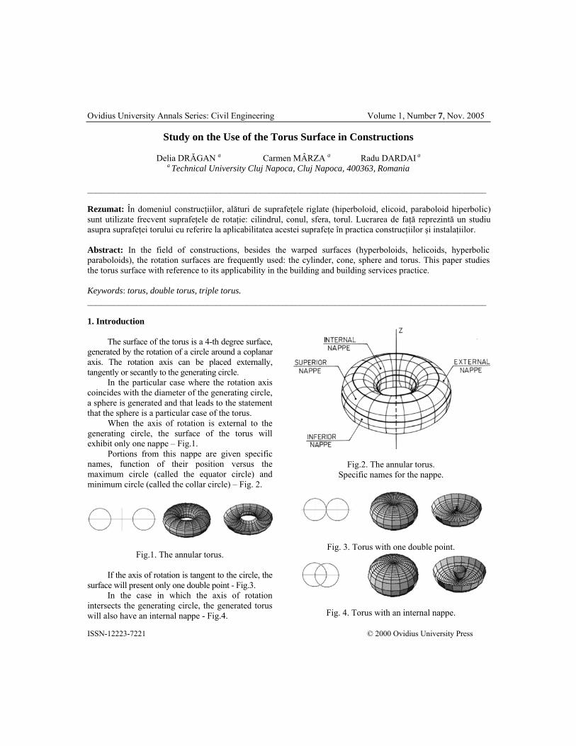
The surface of the torus is a 4-th degree surface, generated by the rotation of a circle around a coplanar axis. The rotation axis can be placed externally, tangently or secantly to the generating circle.
In the particular case where the rotation axis coincides with the diameter of the generating circle, a sphere is generated and that leads to the statement that the sphere is a particular case of the torus.
When the axis of rotation is external to the generating circle, the surface of the torus will exhibit only one nappe – Fig.1.
Portions from this nappe are given specific names, function of their position versus the maximum circle (called the equator circle) and minimum circle (called the collar circle) – Fig. 2.
Fig.1. The annular torus.
If the axis of rotation is tangent to the circle, the surface will present only one double point - Fig.3.
In the case in which the axis of rotation intersects the generating circle, the generated torus will also have an internal nappe - Fig.4.
Fig.2. The annular torus. Specific names for the nappe.
Fig. 3. Torus with one double point.
Fig. 4. Torus with an internal nappe.

Study on the use … / Ovidius University Annals Series: Civil Engineering Volume 1, Number 7, 15-18 (2005)
16
2. Content
In this paper, the author will deal with the case where the axis of rotation is external to the generating circle, when the torus is called annular torus.
We note R – the distance from the axis to the generating circle and r – the radius of the generating circle and hence, we can parametrically define the torus with the equations: x(u,v) = (R+r cos v) cos u (1)
y(u,v) = (R+r cos v) sin u (2)
z(u,v) = r sin v, where u,v∈[0,2л] (3)
The Cartesian coordinate equation for a torus
whose axis of rotation coincides with the Oz is the following:
( ) 222
222 rzyxR =++−
The annular torus surface is equal to A=4л2Rr, and the volume of the solid limited by the torus surface is V=2 л2Rr2 [1].
The most often used surface in the field of constructions and building services is that of one-holed torus, though, when two tori intersect (a particular case) a double torus is obtained – Fig. 5.
Similarly, the intersection of three tori (a particular case) gives a triple torus – Fig. 6.
The geometrical shapes of the double and triple torus could present some interest from the architectural viewpoint.
The classical torus surface, i.e. the one-holed torus that was regarded as the optimal one by the experts was successfully put into practice in building execution.
One of the successful examples, in this respect, is that of Abu-Dhabi Airport project, of the United Arabian Emirates, whose construction was erected in 1976, in the middle of the desert, in very difficult conditions.
Fig.5. Double torus.

D. Drăgan, C. Mârza and R. Dardai / Ovidius University Annals Series: Civil Engineering 7, 15-18 (2005) 17Fig.6. Triple torus.
The project, finished in the year 1980,
belongs to the French Design Office „Aéroports de Paris International” and it was built by the Japanese company Takenaka Corporation.
In Figure 7 it is shown the terminal outside view of the torus-shaped building, while figure 8
presents an inside view of the building, made in the neighbourhood of the minimum circle (collar circle).
The torus surface is used to achieve various joining in the field of services for buildings [2]–Fig. 9.
Fig.7. Abu-Dhabi Airport – exterior view
Fig.8. Abu-Dhabi Airport – interior views

Study on the use … / Ovidius University Annals Series: Civil Engineering Volume 1, Number 7, 15-18 (2005)
18
Fig.9. Intersection between torus and cylinder – Monge projection. 3. Conclusions
Form the architectural point of view, the ideal manner of achieving a building lies in having a form optimally corresponding to the function and chosen constructive system.
The in-depth knowledge of as many as possible surface types leads to a beneficial and harmonious solution for the volumes of the architectural sets.
4. References [1] http://mathworld.wolfram.com, accessed in 2 September 2005. [2] DrăganDelia, Carmen Mârza, Descriptive Geometry, 2005, Edited by U.T.Press Cluj-Napoca, pag. 158.

Ovidius University Annals Series: Civil Engineering Volume 1, Number 7, Nov. 2005
ISSN-12223-7221 © 2000 Ovidius University Press
Calculations of Precast Concrete Tank Foundation on Elastic Subsoil
Krzysztof GÓRSKI a Marek WYJADŁOWSKI b
aTechnical University Opole
bTechnical University Wrocław
__________________________________________________________________________________________ Rezumat: Regularizarea debitelor apelor de ploaie şi apelor uzate prin sistemul de canalizare a fost realizată mult timp prin utilizarea rezervoarelor de înmagazinare periodică a excesului de apă uzată. Această lucrare prezintă caracteristicile şi aplicaţiile rezervoarelor de înmagazinare din beton prefabricat. Acest tip de rezervoare sunt adesea utilizate în domeniul construcţiilor. Pentru proiectarea şi calculul forţelor interne din elementele de beton este utilizat modelul mediului elastic. Abstract: The regulation of rainwater and combined-wastewater flows through sewage systems at the stage of wastewater drainage through sewage networks has been realized for many years with the use of reservoirs for periodic storage of wastewater excess. This paper presents characteristics and application of prefabricated concrete storage reservoirs. Concrete storages are often used in civil engineering. The elastic ground models are used by design of storage and calculation of internal forces in concrete units and theirs locks. Keywords: storage reservoirs, tank foundation, precast concrete tanks, foundations on elastic subsoil. __________________________________________________________________________________________ 1. Introduction
Storage reservoirs serve the periodic gathering of wastewater excess, unload the canalisation network and regulate the efflux to sewage treatment plants. System precast concrete tanks are used as combined-wastewater tanks, rainwater, storage and anti-fire reservoirs, etc. The advantages of the precast concrete tank system result from its fast assembly, simple material quality inspection and the possibility to control the leaktightness right after the tank has been assembled. Time saving in the precast concrete tank construction, in comparison with the monolithic tanks, stems from the short time needed for the assembly, as well as for groundwater drawdown; besides, it allows carrying out of construction works in low-temperature conditions, unfavourable for the cementation process [5].
The rules for the calculation of the tank foundation and the precast concrete tank construction on the elastic subsoil will be presented on the example of a selected system.
2. The characteristics of a selected precast concrete tank system
The precast concrete tank system will be
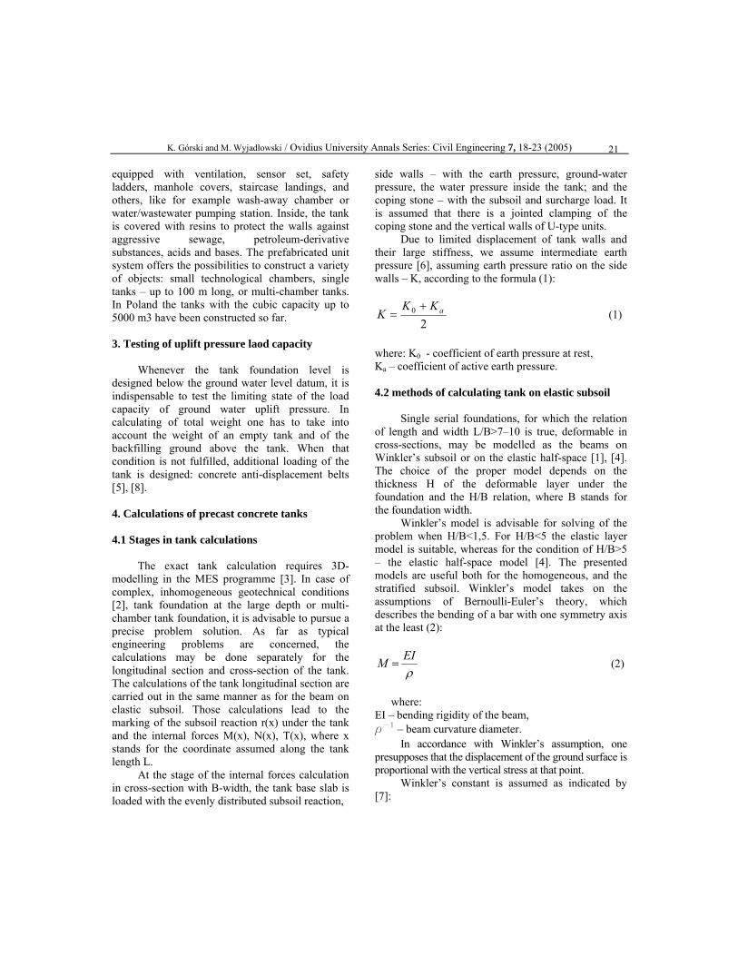
represented here by the system produced by the DYWIDAG AG company. The basic elements of the system are: U-type prefabricated units (see Fig. 1a), end-line tank prefabricated units (U-type, with a lateral wall [see Fig. 1b]) and tank coping stones. Prefabricated units are made of B30– B45 concrete and typically reinforced with the steel of fd = 500 MPa, in accordance with the DIN 1045 norm. The selection of a proper concrete and steel class depends on the individual exploitation parameters, geotechnical conditions, the depth of tank foundation, and others. The manner in which the prefabricated units are connected is a specific, patented technique. Reinforced concrete units are combined with the use of DYWIDAG system fast joints. In the wall chase on the surface combining U-type prefabricated units (see Fig.2.) and the tank coping stone, a rubber gasket is applied. Its diameter is 35 mm and it runs along the joint of prefabricated units. The tank elements are combined by the DYWIDAG system locks (see Fig.2.), bolted with the high-resistance screws.
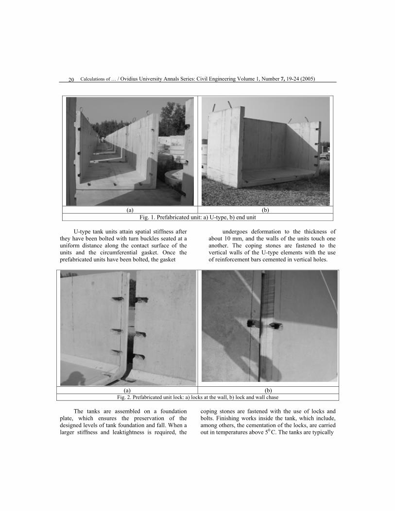
Calculations of … / Ovidius University Annals Series: Civil Engineering Volume 1, Number 7, 19-24 (2005)
20
(a) (b)
Fig. 1. Prefabricated unit: a) U-type, b) end unit
U-type tank units attain spatial stiffness after they have been bolted with turn buckles seated at a uniform distance along the contact surface of the units and the circumferential gasket. Once the prefabricated units have been bolted, the gasket
undergoes deformation to the thickness of about 10 mm, and the walls of the units touch one another. The coping stones are fastened to the vertical walls of the U-type elements with the use of reinforcement bars cemented in vertical holes.
(a) (b) Fig. 2. Prefabricated unit lock: a) locks at the wall, b) lock and wall chase
The tanks are assembled on a foundation
plate, which ensures the preservation of the designed levels of tank foundation and fall. When a larger stiffness and leaktightness is required, the
coping stones are fastened with the use of locks and bolts. Finishing works inside the tank, which include, among others, the cementation of the locks, are carried out in temperatures above 50 C. The tanks are typically
K. Górski and M. Wyjadłowski / Ovidius University Annals Series: Civil Engineering 7, 18-23 (2005) 21
equipped with ventilation, sensor set, safety ladders, manhole covers, staircase landings, and others, like for example wash-away chamber or water/wastewater pumping station. Inside, the tank is covered with resins to protect the walls against aggressive sewage, petroleum-derivative substances, acids and bases. The prefabricated unit system offers the possibilities to construct a variety of objects: small technological chambers, single tanks – up to 100 m long, or multi-chamber tanks. In Poland the tanks with the cubic capacity up to 5000 m3 have been constructed so far. 3. Testing of uplift pressure laod capacity
Whenever the tank foundation level is
designed below the ground water level datum, it is indispensable to test the limiting state of the load capacity of ground water uplift pressure. In calculating of total weight one has to take into account the weight of an empty tank and of the backfilling ground above the tank. When that condition is not fulfilled, additional loading of the tank is designed: concrete anti-displacement belts [5], [8].
4. Calculations of precast concrete tanks 4.1 Stages in tank calculations
The exact tank calculation requires 3D-modelling in the MES programme [3]. In case of complex, inhomogeneous geotechnical conditions [2], tank foundation at the large depth or multi-chamber tank foundation, it is advisable to pursue a precise problem solution. As far as typical engineering problems are concerned, the calculations may be done separately for the longitudinal section and cross-section of the tank. The calculations of the tank longitudinal section are carried out in the same manner as for the beam on elastic subsoil. Those calculations lead to the marking of the subsoil reaction r(x) under the tank and the internal forces M(x), N(x), T(x), where x stands for the coordinate assumed along the tank length L.
At the stage of the internal forces calculation in cross-section with B-width, the tank base slab is loaded with the evenly distributed subsoil reaction,
side walls – with the earth pressure, ground-water pressure, the water pressure inside the tank; and the coping stone – with the subsoil and surcharge load. It is assumed that there is a jointed clamping of the coping stone and the vertical walls of U-type units.
Due to limited displacement of tank walls and their large stiffness, we assume intermediate earth pressure [6], assuming earth pressure ratio on the side walls – K, according to the formula (1):
20 aKK
K+
= (1)
where: K0 - coefficient of earth pressure at rest, Ka – coefficient of active earth pressure. 4.2 methods of calculating tank on elastic subsoil
Single serial foundations, for which the relation of length and width L/B>7–10 is true, deformable in cross-sections, may be modelled as the beams on Winkler’s subsoil or on the elastic half-space [1], [4]. The choice of the proper model depends on the thickness H of the deformable layer under the foundation and the H/B relation, where B stands for the foundation width.
Winkler’s model is advisable for solving of the problem when H/B<1,5. For H/B<5 the elastic layer model is suitable, whereas for the condition of H/B>5 – the elastic half-space model [4]. The presented models are useful both for the homogeneous, and the stratified subsoil. Winkler’s model takes on the assumptions of Bernoulli-Euler’s theory, which describes the bending of a bar with one symmetry axis at the least (2):
ρEIM = (2)
where:
EI – bending rigidity of the beam, r-1 – beam curvature diameter.
In accordance with Winkler’s assumption, one presupposes that the displacement of the ground surface is proportional with the vertical stress at that point.
Winkler’s constant is assumed as indicated by [7]:

Calculations of … / Ovidius University Annals Series: Civil Engineering Volume 1, Number 7, 19-24 (2005)
22
srBEC
ων )1( 20
−= (3)
The factor of proportionality of settlement y(x) to stress at the point q(x) may also be
determined as said by Meyerhof and Baike, Kloppel and Glock, Wlasow [2].
The equation of the axis of the deformed infinite beam on Winkler’s subsoil is formulated in the following way (4):
)sincos()sincos()( 4321 ξξξξξ ξξ CCeCCey +++= − (4)
Integration constants C1, C2, C3, C4, are
obtained from the neutralization conditions of the bending moments and shearing forces at the beam ends. The ultimate solution of forces and displacements in a beam with the finite width and given boundary conditions is attained with the use of Bleich’s method [1]. The calculation of the tank founded on Winkler’s subsoil is correct when the tank possesses a constant stiffness EI along its width. That implies the assumption of fastening of the tank coping stones with locks and bolts.
The solution of beam on the elastic half-space or layer, provided by Gorbunow-Posadow on the basis of Boussinesq solution, is appropriate for the infinite-length beam loaded with a concentrated force. The calculations in accordance with Bleich’s method grant the ultimate results for the finite length beam with given boundary conditions and loading. The above-mentioned solution is suitable for the beam with a constant stiffness EI. It is not indispensable to screw the coping stones with locks and bolts in all the possible cases of loading and all geotechnical condition types. The assumption of the beam constant stiffness leads to multiplying of unjustified costs of the prefabricated unit production and tank assembly.
The economic arguments presented here prove that the designing of a tank should begin with the presupposing of the option of unbolted coping stones. The solution for a beam with variable stiffness on the elastic subsoil may be obtained with the use of combined Zemoczkin-Synicyn’s method [1]. In that method the beam is divided into segments with a constant stiffness EIi. The external load occurs in the form of concentrated forces Qi, which are applied to the centres of beam segments. The contact surface of the beam and the subsoil is smooth, there is no tangential stress, which suitably depicts the prefabricated unit surface – subsoil interaction. The beam is divided into segments with the stiffness that includes the coping stones and the
jointing zones with the stiffness of the U-type element only, which permits to take into consideration the real variables of the tank section strength characteristics.
The internal forces in a one-chamber tank founded on the elastic subsoil may be determined after applying the solution of the beam with stiffness EI, and whose width equals tank width B – in the same manner as for the tank cross-section on Winkler’s elastic subsoil or on the elastic half-space.
The requirements of the DYWIDAG prefabricated unit system restrict the forces that occur in the joints to tensile forces with the value of F=180 kN and allow for the tank settlement by less than s=10 mm. System joints of prefabricated units do not transfer bending moments. The bending moments in element jointing section are transferred by: the concrete in the compression zone, and the bolts fastened in the prefabricated unit locks in the tension zone. On the basis of calculated internal forces the following are possible: the determining of the number of the locks, then joint safety control and the computation of longitudinal reinforcement of tank prefabricated units according to [9].
4.3 Determination of tank stiffness
Preliminary selection of the sections of
prefabricated units takes place basing on the experience of the tanks which have been already carried out. The differentiation in calculating the beam stiffness occurs due to the way in which the tank coping stones are fastened. If the jointing is executed with the use of DYWIDAG system fast joints, in calculations one has to assume the stiffness of the whole tank cross-section. The whole tank cross-section transfers internal forces. When the tank precast coping stones are not clamped together with bolts, the joint does not transfer internal forces, and the computations are carried out as in the case of the beam whose

K. Górski and M. Wyjadłowski / Ovidius University Annals Series: Civil Engineering 7, 18-23 (2005) 23stiffness at the prefabricated unit jointing point is reduced to the stiffness of the U-type unit.
The differentiation of tank stiffness may be essential in its end segments, if system tops are designed, fastened stiffly to the tank, which
increase the end segment stiffness. Schematic division of the tank into segments has been presented in Fig. 3, Fig. 4.
Fig. 3. Tank stiffness and the loading of the beam with concentrated forces on elastic
Fig. 4. Statical scheme
Tank load consists in: tank deadweight, the weight of the liquid inside the tank, ground above the tank and the load on the surcharge.
The loads distributed evenly along the tank length cause neither non-uniform settlement, bending moments, nor shearing forces in sections. The stresses in the soil coming form evenly distributed load are summed up with the stresses from concentrated loads. Vertical loads affecting the tank are modelled as concentrated forces, and applied to the beam on the elastic subsoil. The chambers integrated with tank end units, manhole covers and technological equipment inside the tank contribute to the concentrated loads of the tank.
In calculations the variants of an empty and filled tank are considered.
Figure 3 presents the diagram of tank loading.
5. Conclusions
The calculations of precast concrete tanks in engineering problems are carried out by solving the beam on the elastic subsoil. The subsoil is modelled as a one-parameter Winkler’s elastic continuum, double-parameter elastic subsoil or some other advanced soil model. The selection of the optimal tank solution should be preceded by the analysis of geotechnical and technological conditions, after the execution and exploitation costs of particular tank variants have been estimated. In the method of computation it is vital to take into account the real beam stiffness, which may be invariable along the length of the tank: reduced at the joints of prefabricated units, and increased at the ends of the tank. In case of the variable stiffness of the tank it is obligatory to use an adequate solution method, e.g.

Calculations of … / Ovidius University Annals Series: Civil Engineering Volume 1, Number 7, 19-24 (2005)
24
Żemoczkin-Synicyn’s method. The additional advantage of this method is that it offers the possibility of modelling the subsoil as elastic-plastic.
6. References [1]Brząkała W., Fundamentowanie. Przewodnik do projektowania t. II, Politechnika Wrocławska, Wrocław 1990 /in Polish/ [2]Elachachi S.M., Breysse D., Houy L., Longitudidal variability of soil and structural response of sewer networks, Computers and Geotechnics 31 (2004) 625-641, Elsevier. [3]COSMOS/M Basic FEA System, Structural Research and Analysis Corporation, Santa Monica 1994 [4]Gorbunow-Posadow M.I., Obliczenia konstrukcji na podłożu sprężystym, Budownictwo Architektura, Warszawa 1956. /in Polish/
[5]Kobiak J., Stachurski W., Konstrukcje żelbetowe, t. 2, Arkady, Warszawa, 1989. /in Polish/ [6]Krasiński A., Tejchman A., Obliczenia konstrukcji podziemnej komory rozładowczej w terminalu zbożowym w Porcie Północnym w Gdańsku, XLVI Konferencja naukowa KILiW PAN i Komitetu Nauki PZITB, Krynica 2000 /in Polish/ [7]Wiłun Z., Zarys geotechniki, WKiŁ Warszawa 1993. /in Polish/ Polish Standards [8]PN-81/B-03020, Posadowienie bezpośrednie budowli. Obliczenia statyczne i projektowanie. PKN, Warszawa 1981. [9]PN-B-03264, Konstrukcje betonowe i sprężone. Obliczenia statyczne i projektowanie. PKN, Warszawa 2002.
Ovidius University Annals Series: Civil Engineering Volume 1, Number 7, Nov. 2005
ISSN-12223-7221 © 2000 Ovidius University Press
Determination of Mechanical Characteristics for Composite Stone Plates
Garabet KÜMBETLIAN a Sunai GELMAMBET b a Maritime University of Constantza, Constantza, 900592, Romania b“Ovidius” Universitaty Constantza, Constantza, 900527, Romania
__________________________________________________________________________________________ Rezumat: Lucrarea descrie modul în care s-au verificat caracteristicile mecanice ale produsului „BRETONSTONE-TOMISTONE” fabricat la Constanţa, de firma „ANTO-ROB GRANIT-SRL” în licenţa firmei BRETON (Italia), sub brevetul TONCELLI. Abstract: The paper describes the testing of mechanical characteristics for the product „BRETONSTONE-TOMISTONE” made in Constantza by „ANTO-ROB GRANIT-SRL” company in BRETON (Italy) company license under TONCELLI letters patent. Keywords: mechanical characteristics, composite stone plate, tested. __________________________________________________________________________________________ 1. Introduction
Last years many new materials for constructions got into Romania especially in the finishing works. Some of these materials started to be produced in Romania too.
This is the practical example for the product „BRETONSTONE-TOMISTONE” made in Constantza by „ANTO-ROB GRANIT-SRL” company in BRETON (Italy) company license under TONCELLI letters patent. This is why was necessary the mechanical characteristics testing of the product made in Constantza and compared with BRETON (Italy) company standard’s articles. 2. Material definition
Bretonstone-Tomistone is a composite stone made of siliceous sands, quartzes, granites, diorites, porphyries etc., with vibration and compaction process in blankness of the granular materials above-mentioned. The interlocking of these materials is made with polystyrene resin and several accelerator abraded to vibration and compaction processes in blankness at high temperatures and after that cooling off in special tunnels. The products are plates with a thickness of 10, 15, 20, 30 mm and the maximum dimension of 120 x180 cm. The plates are perfect polished with chamfering borders, (bellow the dimension of
60cm). Esthetically the reproducibility of any type of natural stone like the granite, the basalt, the porphyry, the marble etc. is possible. The production of unicolor and bicolor plates is possible for more than 60 types.
The product is more resistant than natural stone plates (the marble, the granite) or artificial stone plates (the stoneware tile, the stoneware floor) having superior resistance to axial compression, to bending, to impact, to chemical aggression and resistance to freezing. As it is compacted in blankness it has a perfect isotropic behavior. The finished material can be cut or perforated, as opposed to the marble witch is brittle.
The product is used all around the world for about 30 years and agrees with standards admitted by the European Union and is authorized by the Technical Agreement in Construction Committee (with no. 002-04/268-1998) and initialed by the Romanian National Centre for tests LAREX-BUCURESTI.
The BRETONSTONE plates are used in construction for facing board, frontages in intensive traffic areas, airports, stations, supermarkets, banks, hotels, restaurants, theaters, cinemas, special constructions etc. The 10 mm plates attaching is made with classical methods but with special adhesives produced by the KERAKOOL or MAPEI –Italy Company. For facing frontages you can use plates of 15mm or 20 mm thickness dry attached with mechanical fixing using fixing stub or curtain wall. In

Determination of mechan… / Ovidius University Annals Series: Civil Engineering Volume 1, Number 7, 25-28 (2005)
26
all cases it impose contraction joint of ( )mm62÷ covered after with putty. 3. Testing and issue
From testing series we will describe in the following only the way of accomplishing the
compression and bending tests. The compression testing was made for “cubical
resistance” determination witch is the main indicator in the quality of the product.
The compression testing was made on 3cm leg long cubs obtaining the value for compression resistance cR30 (Fig.1).
Fig.1

G. Kümbetlian and S. Gelmambet / Ovidius University Annals Series: Civil Engineering 7, 25-28 (2005) 27
In figure 1 are described the principal directions (1) and (2) on which are developed the principal stresses inside the cube tested on compression. The principal directions are determined with the formula
στα 2arctg
21
= (1)
where α=α1 (for 0≥σ ) and α=α2 (for 0<σ ).
If α>0 the angle is measured in accordance with the clockwise, starting from x axe, and for α<0 the angle is measured in the other way of the clockwise.
The result of the testing was an average:
230 1888 cmdaNR c = (2)
Fully satisfying the product BRETONSTONE’s quality conditions for witch the company standards stipulate a value between:
230
230 21611050 cmdaNRcmdaNR cc =÷= (3)
The bending testing was effectuated on the proportional bar test with square section, leg a=3cm and coefficient of resistance:
333
546
36
cm,aW === (4)
According to scheme from Fig.2, the detail drawing from Fig.3 and for a loading rate of:
sNv 10= (5)
Fig.2
Fig.3

Determination of mechan… / Ovidius University Annals Series: Civil Engineering Volume 1, Number 7, 25-28 (2005)
28
After testing ten proportional bars test we obtained an average for bending tensile stress ultimate resistance:
268531 cmdaN,XR medtim== (6)
For deviance:
21 3619 cmdaN,n =−σ (7)
The resistance value
mtiR is situated perfectly in the average area of bending resistance (of
2880370 cmdaN− ), indicated in company’s technical documentation.
3. Conclusions The products of Anto-Rob company from Constantza is perfectly situated in the prescript values limits for quality factors of the product. 4. Reference [1] Kümbetlian, G., Mândrescu, G., Strength Materials, Fundaments. Ed. Fundaţiei „Andrei Şaguna” Constanţa, 1998. [2] *** (sub cordonarea prof.dr.doc.ing. Dumitru Remus Mocanu) Materials Testing. Vol.2, Ed. Tehnică Bucureşti, 1982. [3] *** ANTO-ROB-Granit-Design Technical Documentation.

Ovidius University Annals Series: Civil Engineering Volume 1, Number 7, Nov. 2005
ISSN-12223-7221 © 2000 Ovidius University Press
For an Unit System of Working in Strength Materials
Garabet KÜMBETLIAN a Sunai GELMAMBET b a Maritime University of Constantza, Constantza, 900592, Romania b“Ovidius” Universitaty Constantza, Constantza, 900527, Romania
__________________________________________________________________________________________ Rezumat: În această lucrare este propus şi prezentat un sistem unitar de lucru în Rezistenţa materialelor pentru a numai exista divergenţe în modul de rezolvare al problemelor. Pentru acest sistem unitar de lucru este realizată o analiză şi prezentate argumente privind sistemul de axe propus şi dispunerea eforturilor în secţiune. Abstract: In this paper is propounded and presented an unit system of working in strength materials not to exist more differences in the way of resolving the problems. For this unit system of work was achieved an analyzed and presented arguments for the axes system propounded and the arrangement of the efforts in section. Keywords: axes system, efforts in section, strength materials. __________________________________________________________________________________________ 1. Introduction
Now for strength materials problems issue are used various axes systems (left system or right system) and additionally the arrangement of the efforts in section vary even for same axes system used, this thing binding frequently to differences in the way of resolving the problems.
For this reason in this paper after analyzing various systems of work is propounded and showed a unit system of coherent work, consistency and in conformity with base science’s rules (mathematics, theoretical mechanics).
2. Describing the propounded unit system of work
I. One strength materials problem can be solved in the follow logical succession:
1.Problem’s data: Loads. 2.Unknown quantity: Efforts in section. 3.Interfacing quantity: Stress in section.
II.As a result the axes system and conventions must be subordinated to the steps above-mentioned. The axes system indicated by the international standards is showed in diagram 1.
III. The viewer is located in proportion with the beam so that x axes to be oriented always from his left to his right, y axes on he and z axes adown. The axes system defined like that is three orthogonal right.
IV.If the beam is cut in the hatched section and is cut out both parts obtained, the section is dualized. The left part of the section will be called “positive face” and the right part of the section will be called “negative face” (diagram 2).
Fig.1.
For an unit system of wor… / Ovidius University Annals Series: Civil Engineering Volume 1, Number 7, 29-34 (2005)
30
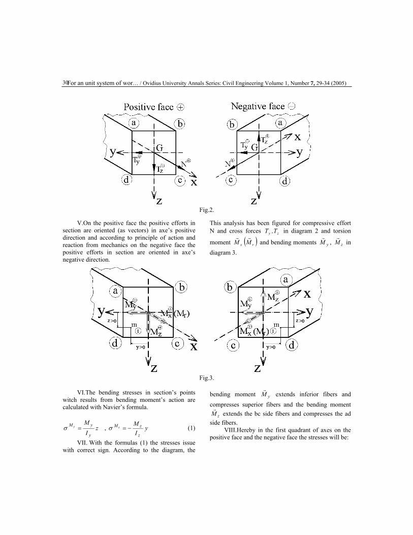
Fig.2.
V.On the positive face the positive efforts in
section are oriented (as vectors) in axe’s positive direction and according to principle of action and reaction from mechanics on the negative face the positive efforts in section are oriented in axe’s negative direction.
This analysis has been figured for compressive effort N and cross forces zy T,T in diagram 2 and torsion
moment ( )rx MMrr
and bending moments yMr
, zMr
in diagram 3.
Fig.3.
VI.The bending stresses in section’s points
witch results from bending moment’s action are calculated with Navier’s formula.
zI
M
y
yM y =σ , yI
M
z
zM z −=σ (1)
VII. With the formulas (1) the stresses issue with correct sign. According to the diagram, the
bending moment yMr
extends inferior fibers and compresses superior fibers and the bending moment
zMr
extends the bc side fibers and compresses the ad side fibers.
VIII.Hereby in the first quadrant of axes on the positive face and the negative face the stresses will be:

G. Kümbetlian and S. Gelmambet / Ovidius University Annals Series: Civil Engineering 7, 29-34 (2005) 31
0>= ⊕⊕
zI
M
y
yM yσ , 0<−= ⊕⊕
yI
M
z
zM zσ (2)
IX. As a result of double bending, in any
section’s point no matter what face you are working on, the stresses will be calculated with formula:
yI
MzI
M
z
z
y
yM y −=σ (3)
X. The zero axes from section will cross the
same axe’s quadrants no matter what face are you working on. Hereby if mn (zn ,yn) is a point which belonging to the zero axe, it equation will be:
0=− nz
zn
y
y yI
MzI
M (4)
and it angle of fall in proportion to y axes from section will be:
y
z
z
y
n
n
MM
II
yztg ==θ (5)
If zMr
and yMr
have the same sign, then 0>n
n
yz
and
zero axes crosses the first and third quadrants (diagram 4).
Fig.4.
If zMr
and yMr
have opposite signs, then 0<n
n
yz
and zero axes crosses the second and fourth quadrant (diagram 5).
Fig.5.
For an unit system of wor… / Ovidius University Annals Series: Civil Engineering Volume 1, Number 7, 29-34 (2005)
32
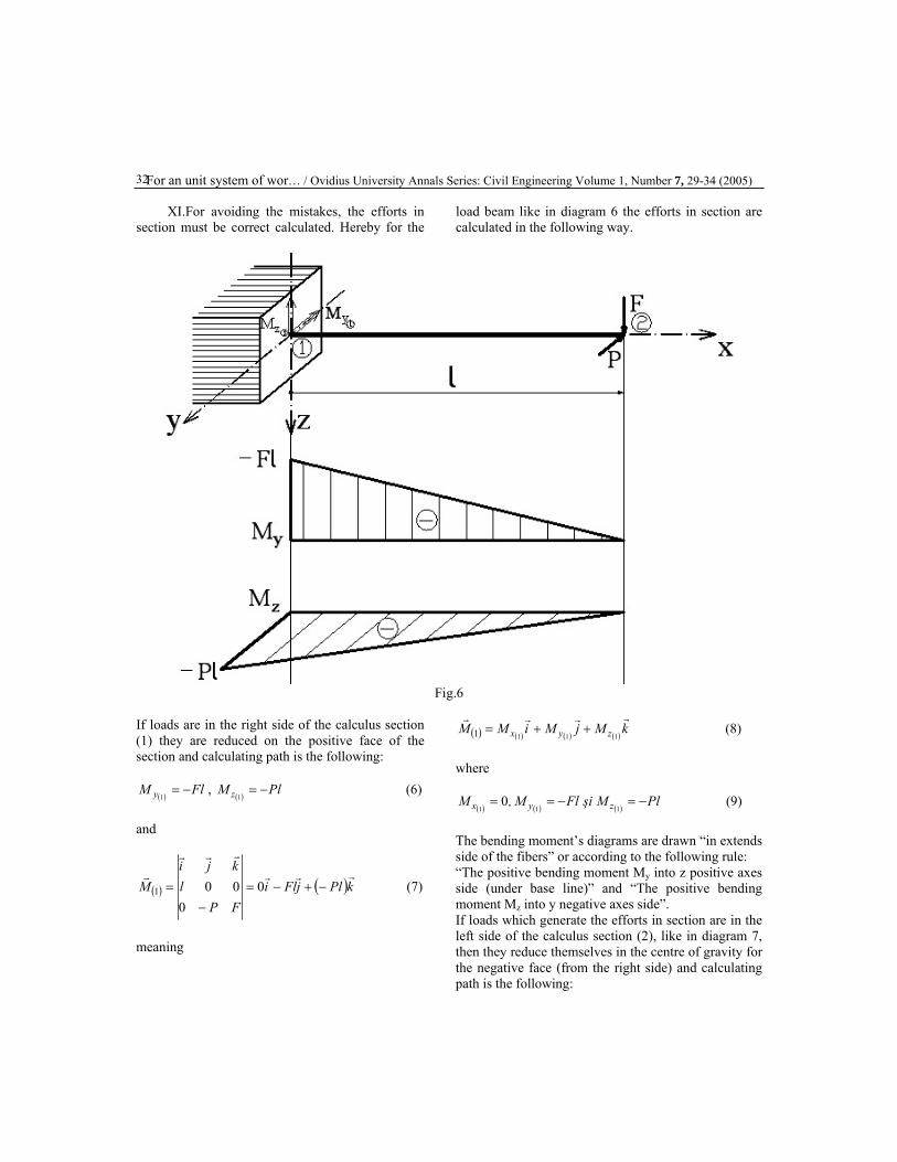
XI.For avoiding the mistakes, the efforts in section must be correct calculated. Hereby for the
load beam like in diagram 6 the efforts in section are calculated in the following way.
Fig.6
If loads are in the right side of the calculus section (1) they are reduced on the positive face of the section and calculating path is the following:
( )FlM y −=
1,
( )PlM z −=
1 (6)
and
( ) ( )kPljFliFP
lkji
Mrrr
rrr
r−+−=
−= 0
0001 (7)
meaning
( ) ( ) ( ) ( )kMjMiMM zyx
rrrr
1111 ++= (8)
where
( ) ( ) ( )PlMşiFlM,M zyx −=−==
1110 (9)
The bending moment’s diagrams are drawn “in extends side of the fibers” or according to the following rule: “The positive bending moment My into z positive axes side (under base line)” and “The positive bending moment Mz into y negative axes side”. If loads which generate the efforts in section are in the left side of the calculus section (2), like in diagram 7, then they reduce themselves in the centre of gravity for the negative face (from the right side) and calculating path is the following:

G. Kümbetlian and S. Gelmambet / Ovidius University Annals Series: Civil Engineering 7, 29-34 (2005) 33
Fig.7.
( )FlM y −=
2,
( )PlM z −=
2 (10)
or
( ) ( )kPljFliFP
lkji
Mrrr
rrr
r++−=
−−−= 00
002 (11)
meaning
( ) ( ) ( ) ( )kMjMiMM zyx
rrrr
2222 ++= (12)
where
( ) ( ) ( )PlMşiFlM,M zyx −=−==
2220 (13)
3. Conclusions a) The axes system and sign conventions for the efforts (on both faces of the same section) are coherent and consistency. b) In the vertical plain (xz) the conventions are in conformity with rules unanimous approved now. c) In the horizontal plain (xy) they issue in a logical path. d) The propounded way of work is according to theoretical mechanics basic rules. e) The axes system, sign conventions and rules issued from all this, for the efforts in section calculus on one or the other face of the same section, form a logical concept, scientific correctly and consistency in proportion to base science’s rules (mathematics, theoretical mechanics) and applicative sciences (strength materials, structural statics, etc).

For an unit system of wor… / Ovidius University Annals Series: Civil Engineering Volume 1, Number 7, 29-34 (2005)
34
4. References [1] Mazilu P., Posea N., Iordăchescu E., Strength materials problems, 1975, Ed. Tehnică Bucureşti. [2] Diaconu M., Strength materials problems, 1979, Institutul Politehnic Iaşi, vol. I. [3] Bia C., Ille V., Soare M.V., Strength materials and elasticity theory, 1983, E.D.P. Bucureşti. [4] Corâci V., Strength materials – Propounded problems for „Traian Lalescu”, competition 1987, Institutul de Construcţii Bucureşti.
[5] Soare M.V., Ille V., Bia C., ş.a., Strength materials in applications, 1996, Ed. Tehnică Bucureşti. [6] Kümbetlian G., Mândrescu G., Strength materials - Fundaments, 1998, Ed. Andrei Şaguna Constanţa. [7] Precupanu V., Fundaments of strength materials, 2000, Ed. Corpon Iaşi.

Ovidius University Annals Series: Civil Engineering Volume 1, Number 7, Nov. 2005
ISSN-12223-7221 © 2000 Ovidius University Press
Considerations Regarding Residual Mechanical Characteristics
Petru MIHAI a Nicolae FLOREA a Marinela BĂRBUŢĂ a
a “Gh. Asachi” Technical University Iassy, Iassy, 700050, Romania
__________________________________________________________________________________________ Rezumat:Lucrarea propune un procedeu de estimare a caracteristicilor mecanice reziduale ale elementelor din beton armat. Aplicarea calculului probabilistic în scopul ridicării gradului de reprezentativitate a informaţiilor, devine cu atât mai necesară, cu cât însăşi metodologia de efectuare a încercărilor introduce erori importante care afectează credibilitatea rezultatelor. Abstract: The paper presents a procedure to estimate the residual mechanical characteristics for reinforced concrete elements. The probabilistic calculus application in order to increase the information representativity becomes as necessary as the test realization methodology itself introduces important errors witch affect the results credibility. Keywords: residual, mechanical characteristics, concrete __________________________________________________________________________________________ 1. General Considerations
The impressive volume of units built in the last decades risk serious problems to the actual generation of specialists. However from the actual technical exigencies point of view, there has been made inadequate constructions due to the accelerate pace of finalizing some investments, to the adoption of technologies, materials and constructive systems not always according to the destination and real strain conditions, to the intervention, sometimes lacking of professionalism, of the decision factors the documentation authorizing process by the modifications imposed, to the incertitude regarding the nature and the intensity of the seismic movements in a certain geographical area, etc.
This situation generates serious questions and numerous concerns regarding the actually accepted safety level, especially in the case of the buildings witch suffered degradation or structural system damages in time.
An important ratio of the total units realized in Romania, before the appearance of the compulsory earthquake projecting norms (1963), as well as the constructions subsequently made in the so considered, till the 1977 earthquake, safe seismic zone implies a high proportion responsible action, to
evaluate the strength reserves of the units suspected to be unreliable.
During the undergoing verifications, there must be taken into account the fact that the concrete internal structure, the way of realizing its cooperation with the reinforcement as well as the stress existing in the two materials, suffer continuous quality and quantity changes, under the effect of both the exterior strains and the reologic phenomena which characterize the behavior in time of the concrete.
The above mentioned situation, which is not yet quantified in formulas or rigorous numerical calculations, being only partial emphasized by some projecting norms, requires to specify the concrete and reinforcement strengths and deformations effective values, know as residual mechanical characteristics.
To solve such an important problem, implies numerous difficulties, especially when significant degradation occurred during functioning. The practical possibility to take into account the concrete and reinforcement mechanical characteristics modifications under various actions is based upon the utilization of destructive/nondestructive tests as well as by using mathematics processing specific procedures of the data resulting from measurement. Currently there are preferred to be used the nondestructive methods of testing (superficial hardness method, ultrasonic method, combined method), being much simple and economic

Considerations regarding… / Ovidius University Annals Series: Civil Engineering Volume 1, Number 7, 35-38 05) (20
36
than the procedure based on carrots extraction followed by their behavior analysis in laboratory.
The concrete residual strengths evaluation using nondestructive tests methods presents a certain degree of imprecision due to the insufficient knowledge of the initial data referring to the compound composition (concrete type and dosage, the nature of the compound, the maximum granules dimension, fine ratio, etc.) elements that can not be easily specified after a number of years from the construction execution.
The value registered, using laboratory endowment, being usually affected by errors, must be cautiously treated, without exaggerating their importance, especially when they serve to the safety evaluation of a structure on the whole.
Apart from the used procedure, the low precision impressed by the indirect evaluation character of the mechanical characteristics, by the intermediary of another physical quantity (superficial hardness, ultrasound impulses propagation speed), determines the character strictly informative of the results regarding the quality of the material utilized.
In those conditions, the concrete non-destructive test methods usually serves to locate the objectives needing, with priority, intervention measures for increasing the strength capacity, in the prospect of a great intensity earthquake occurring in the near future.
The percentage of the concrete strength evaluation in earthquake damages structure by the combined method is ±(15...20) %. This one presents a higher trials precision, because it couples together primary elements of the two mentioned procedures, when there aren't carats for testing, but there is a great number of information regarding the composition of the concrete cost in the work.
If those primary elements are missing, the errors introduced increase considerably, the measurement precision being conditioned by the experience and the ability of the test leader. This one, in the considerations mode, will have to consider the quality of the materials used in similar works during the unit execution and, especially, by the usual recipes of obtaining the project prescribed concrete mark.
For increasing the veracity degree of the information obtained by nondestructive tests, it is
undirected that these ones are processed and interpreted according to the statistical mathematics methods. The probabilistic calculus application in order to increase the measurements representative level becomes as necessary as the test realization methodology causes the introduction of rough errors. Therefore it is recommended that the investigated zones to contain a dense, compact concrete, without fissures, segregation or other visible or presumed flaws existing under the superficial layer. Thus, there are avoided from the analysis, which should be as general and objective as possible, exactly those parts which influences, in a negative way, the strength and the stability of the elements and of the whole structure. 2. The Concrete Quality
The exemplification of the concrete quality and residual characteristics evaluation has been made utilizing the ultrasonic impulse method as well as the combine nondestructive method. It is necessary endowment for measuring both the superficial hardness using the rebound index and the ultrasonic impulse propagation speed.
On the element submitted to the test there are chosen at least 3 different sections in order to execute the measurements. In every examined section there must exist at least pairs of test points with ultrasonic waves and an area of 20x20 cm2 with at least 6 points for measuring the rebound index using a sclerometer. The test points and zones establishing, as well as the concrete surface processing, in order to obtain conclusive information, is done according to the specific norms stipulations.
The element submitted to the test is the average strength on a pillar cross section, the mean strength of the section considered in a pillar, of a group of pillars from a floor, as well as the one of all the analyzed pillars in the structure.
On the basis of the booth the rebound index and the ultrasonic waves propagation speed there as been calculated the measured quantities average values on each of the 3 considered sections in the investigated pillar.
After their transformation in compression strength, it is determined the average and minimum strength ( R ), respectively (Rmin) on the element, considering all tested sections.

37P.Mihai, N. Florea and M. Bărbuţă / Ovidius University Annals Series: Civil Engineering 6, 7-14 2004) (
The concrete quality and mechanical characteristics analysis methodology has been applied to studying the component material of a storied structure made in monolithically reinforced concrete.
Though at none of the studies pillars the concrete wasn't found inadequate, the qualificatives established according to the conditions imposed by the norms are not conclude for all the element parts and, so much the less for the whole structure, because the measurements has been done on the no-called "healthy concrete".
Being intentionally avoided the parts where the material presents structural degradation, there is obviously obtained more favorable quality evaluation than the real one. By the nondestructive test execution methodology itself it is impressed to the procedures a limited and un-representative character, because these are capable to furnish information regarding the homogeneity of the cast concrete only for the area situated exactly nearby the measurement points.
In the case of the structures which suffered important degradation manifested by the inner structure continuity destruction under the shape of fissures and cracks, the evaluation of the material quality on the basis of arbitrary relations between the average/minimum values of the compression strength resulted after testing the "healthy" concrete and the project prescribed class, is unconcludent, lacking, in fact, practical utility.
The actual norms do not include prescriptions by which to be quantitative evaluate the influence exerted by the concrete inner structure degradation on the deformation and efforts state.
A very important objective is to solve the problem of quantifying the effect exerted by the fissure state, especially of the one different from a structure element to another, on both its bearing capacity and its general stiffness. Actually, the mentioned aspects are empirically approached and solved, according to the works coordinator experience and intuition. The information provided by the technical literature is insufficient and incomplete, requiring the initiation and the execution of a vast and well argumented fundamental and technical scientific research program.
3. The Residual Characteristics Evaluation
In order to determine the concrete residual mechanical characteristics there has been used the ultrasonic impulse method, for which a statistical method of information processing can be applied. The object of statistical processing is the individual result of the ultrasound propagation speed measurement. For a correct estimation of the complete structure elastic deformation and strength reserves it is recommended to be done a probabilistic interpretation of the data, first separately on construction elements and afterwards, the results must be processed on each level and then on the whole structure.
The test results statistical processing, assuming gaussian distribution curves, includes the following operations: - the propagation speed calculus V on the element
∑=
=n
i
i
nVV
1 (1)
where Vi is the propagation speed measured in a point "i" [m/s] and n is the number of points in which there has been executed measurements - the absolute deviation calculus of each speed
VVii −=ε (2) -the root mean square deviation calculus of Sv speeds
1)(
−−
= ∑n
VVS
iv (3)
-the speeds variation coefficient calculus
%100% ⋅=VSC v
v (4)
this coefficient representing the final statistical quantity of the direct measurements processing -the concrete strength variation coefficient calculus CR%=αvCv (5) where (αv) is an experimental deduced coefficient whose values vary between 3.2 and 4.8, according to the concrete inhomogeneity; when this characteristics

Considerations regarding… / Ovidius University Annals Series: Civil Engineering Volume 1, Number 7, 35-38 05) (20
38
is not know before hand, it is recommended to be used αv=4.0
-the stretch strength for calculus
The coefficient CR% permits the appreciation, upon statistical basis, of the concrete homogeneity in the work from the ultrasonic measurements point of view.
bt
tkbtt
RmRγ
= (10)
where: For the case when CR %< 12% it is admitted
that the concrete homogeneity is very good, when 12%*CR %< 20%, from the homogeneity is satisfactory, whereas when CR %> 20%, the concrete homogeneity is weak.
- mbt, mbc are the coefficients of the concrete working conditions at stretching and compression; - γbt=1.50, γbc=1.35 are the concrete safety coefficients at stretching, respectively at compression.
The quantities determined using the relations (9) and (10), as well as the elasticity module corresponding to the characteristic strength, having a high degree of representative due to the fact that they are the outcome of rigorous mathematical processing, can be assimilated with the residual values which permit the determination of the existing unit bearing capacity. The results of the statistical analysis executed separately for every column do not present practical utility , because the supplied elements Rt, Rc, Eb can not be introduced as initial data in the statistical calculus programs.
Knowing the concrete strength variation coefficient (CR %), there can be determined the calculus compression and stretching strength as well as the elasticity module. These ones represent minimum values, accepted with a given probability in order to never be surpassed in the disadvantageous way, their calculus implying the following steps: - the characteristic strength (Rbk) determining
bbk RCtR R)1( ⋅−= (6) Comparing the measured data it is noticed that
the statistical processing executed separately for each pillar led to smaller values of the coefficient CR than in the case then there has been considered a level on the whole. These results are natural, because the dispersion degree increases together with the number of investigated elements whereas the homogeneity decreases when it is passed from one element to all the elements on the considered level.
where Rb is the concrete average strength for the examined points and t is a coefficient which depends on the asked trust level and on the member of points examined.
If it is granted to the concrete average strength on the element ( bR ) the significance of cubic strength, it is necessary to transform the characteristics strength in a quantity that has the meaning of cylindrical strength (Rck), using the relation:
If the medium values obtained for every level are considered to be primary elements of a statistical processing on the whole structure, there can be obtained concluded values of the residual mechanical characteristics. These ones becomes really representative after executing the statistical and dimensioning calculus.
bkbkck RRR )02.087.0( −= (7)
In that follows, where can be calculated:
- the stretch characteristic strength 4. References 3 2)(22.0 cktk RR ⋅= (8)
[1] Oneţ T. Caracteristici reziduale ale structurilor din beton armat. Bul. AICPS, 2-3, 15-21, 1993.
-the compression strength for calculus
[2] Bob C. Verificarea calităţii, siguranţei şi durabilităţii construcţiilor. Ed. Facla, Timişoara, 1989
bc
ckbcc
RmRγ
= (9)

Ovidius University Annals Series: Civil Engineering Volume 1, Number 7, Nov. 2005
ISSN-12223-7221 © 2000 Ovidius University Press
Evaluation of the Safety Degree for Two Old Masonry Churches
Petru MIHAI a Nicolae FLOREAa
a “Gh. Asachi” Technical University Iassy, Iassy, 700050, Romania
__________________________________________________________________________________________ Rezumat: Utilizând un program de calcul propriu, este analizată influenţa exercitată de coeficientul "ψ" asupra gradului de asigurare la acţiuni seismice pentru două biserici vechi alcătuite din pereţi structurali din zidărie de cărămidă. Se constată că, după cele două direcţii principale de calcul, gradul de asigurare R prezintă o lege de variaţie apropiată de cea antilogaritmică, în funcţie de "ψ". Începând de la o anumită valoare a acestuia, ce depinde de caracteristicile structurale ale clădirii, se manifestă tendinţa de variaţie asimptotică. Abstract: Using a personal computing software, it is analyzed the influence exerted by the “ψ” coefficient on the assurance degree to seismic actions (ADSA) for two churches made in brick structural walls. There is noticed that, considering the two main calculus directions, the ADSA, function of "ψ", presents a variation law close to the antilogarithmic one. Beginning from a certain value of the building structural characteristics, it become obvious an asymptotic variation trend. Keywords: masonry, safety, earthquake, church __________________________________________________________________________________________ 1. The Existing Constructions Safety
The important volume of civilian, industrial and public buildings realized in Romania before the appearance of the compulsory earthquake projecting norms (1963), as well as the constructions subsequently made in the so considered, till the 1977 earthquake, safe seismic zones, implies a consistent reevaluation action of the strength reserves presented by those buildings strength structure.
In discovering of the most urgent situations which must be analyzed, a remarkable role belongs to the laboratories, which, by destructive and non-destructive tests permit the promptly identification of the objectives who needing, by all means, interventions.
A much more difficult problem than to projecting new directives is to evaluate the safety level of the existing constructions, conceived by using absolute (from both technical and scope of the considered problems) design prescriptions, because these regulations didn't include the obligativity of observing rigorous strength and stability conditions under the actions of horizontal loadings.
Unlike new constructions, where earthquake
protection goal is to correctly dimensioning and assembling them to resist to a certain intensity seismic problem, in the old building case, where the shape and the structure dimensions as well as the materials quality should be known, the safety level evaluation means to determine the maximum strain intensity which can be undertaken.
In this late case, appear difficulties in determining of the real protection level, because the structure bearing are dependent on its geometry, on its material quality and, mostly, on its reinforcement quantity and distribution mode, elements that can not be acquaintance neither in the relative new constructions case, where a certain technical documentation exist. The difficulties increase because of the incertitude insert by the nature and the intensity of the future seismic movements, due to the fact that the seismic risk of some geographic zones is often bigger than the one predicted before.
The complexity of the approach results also from the fact that, according to the present design conceptions, the seismic resistance condition is much more extended than the classical acception of the

Evaluation of the … / Ovidius University Annals Series: Civil Engineering Volume 1, Number 7, 39-46 (2005)
40
earthquake notion which consists in comparing the bearing capacity with certain imposed exterior strain values. In the case of the earthquake resistant units, it is necessary considered that the strength structure has a sufficient deformation capacity in order to undertake the seismic strains, that is to store and to dissipate by elasto-plastic deformations the earthquake induced energy.
In conclusion, it can be ascertain that the problem of establishing the safety level for old constructions presents a remarkable complexity, caused mainly by the diversity and by the high number of parameters and aspects to be considered. This situation partly justifies the absence of a rigorous calculus method, in Romania and abroad. 2. The Protection Level Evaluation According to Present Standards
The seismic standard introduces, as element of absolute novelty in technical field regulations, the necessity of establishing the protection level for the existing constructions. In this respect, it is recommended to use a simplified calculus method which is based on the ADSA (R) determining, where (R) has the shape:
nec
cap
SSR = (1)
Received, at the beginning, with
circumspection by some specialists and even criticized by others, the proposed method of the seismic protection level evaluation is, however, a practical instrument to act with, mostly in the case of the objectives needing urgent intervention selection. Additionally, the method precision level can be noticeable improved if there is wisely acted on the terms defining the (R) factor.
For determining the strain Scap of the existing units, it is extremely important to precisely know the effective mechanical characteristics of the construction materials. These characteristics continuously diminish in time due to the phenomena of static and dynamic fatigue as well as because of the internal structure continuity deterioration under utilization strains. The evaluation of the residual strengths is made in
present by non-destructive tests which, unfortunately, present a high imprecision degree, determined mainly by the insufficient knowledge of the used materials preparation, treatment and utilization.
The results can be corrected in a certain proportion by statistical computing the measured data, but the probabilistic interpretation need a great volume of information which is obtained by great material and human efforts.
For eliminating the above mentioned deficiencies it is necessary to be changed the present optic regarding the materials mechanical residual characteristics evaluation. Appears to be indicated to act in order to elaborate and implement new techniques and procedures which are known or applied in Romania. In this case it is useful to be initiated a rigorous scientific research program which, starting with a theoretical approach, would have as purpose to physical modeling the studied material deteriorated inner structure. In the case of the reinforced concrete, there must be also taken into consideration the aspects resulting from the concrete-reinforcement cooperation damaging.
After systematizing the real phenomena included in the physical model, it will be possible to elaborate the mathematic model, which will permit to determine analytical the residual mechanical characteristics with a high level of precision.
Another direction to follow for improving the protection level determination method, recommended by the seismic standard, is the term Snec. In the relation (1), Snec represents the conventional seismic loading (fundamental seismic sharing force) when considering the existing construction as a new one.
For the self vibrating mode "r", in the case of the self oscillations produced in a plane, the horizontal seismic loadings resultant is determined with the relation:
rrsrnec kS εβα ⋅Ψ⋅⋅⋅=, (2) where the significance as well as the values of the coefficients are the ones given in Chapter 5.3 of the Standard P 100-92. Because the ADSA "R" expressed under the shape of a global indicator depends on a great number of parameters (general design conception, general and detailed structure, materials and execution quality, position conditions, etc.)

P. Mihai and N. Florea / Ovidius University Annals Series: Civil Engineering 7, 39-46 (2005) 41 difficult to be controlled, it is recommended that this quantity is used for constructions preliminary trial from the safety seismic action point of view. Subsequently, by analyzing attentively and competently all aspects regarding the construction behavior in time under loadings, using specialty computing methods and other specific techniques (in situ laboratory trials, comparations with other similar constructions, etc), it will be made the decision of acting or not and in what extent. 3. The ψ Factor Effect Analysis
In the relation (2), by the coefficient ψ of seismic action effects diminishing it are taken into consideration the strength structure seismic energy dissipation capacity. Thus, there are taken into account many difficult to be evaluated behavior factors, as: the construction ductility, the efforts re-distribution capacity, the extent with which the neglected strength reserves intervene in the calculus following an advantageous general behavior, as well as the vibrations damping effects others than the ones associated with the strength structure.
Therefore, it results that the differentiation of Snec values able to reflect with precision the structure real behavior, is quantified in the Romanian computing prescriptions using the ψ coefficient. The Standard P 100-92 indicates the following values for the ψ coefficient in the case of bearing masonry buildings: -structures with structural walls made in simple masonry .......................................... 0.30 -structures with structural walls made in masonry with girdles and little pillars.............0.25
The recommended reduction factor ψ is justified only in the case of new constructions which simultaneously fulfill both the ductility and strength conditions.
The conventional seismic loadings for calculus, on the basis on which the safety of existing constructions is appreciated, must be different from the situation of a new construction designing, because the buildings made many years ago lack, in a greater extent, the plastic deformation capacity. If, unrealistic, the Snec effort value would be calculated considering the value of ψ factor indicated in the P 100-92 Standard, the (R) ratio would result too big, situation which would confuse
the simplified evaluation method users, tempted, thus, to over-estimate the strength reserves.
Consequently, for the constructions which do not correspond to the requirements of configuration and ductility indicated by the present standards, the seismic loadings for calculus Snec will have to be determined using ψ coefficients of increased values compared to the ones mentioned above.
The design prescriptions from other countries have similar conditions that are either to reduce the strength for calculus of the materials or to increase the seismic strain.
The present Romanian standards do not reflect the influence exerted by the ψ factor on the value of the existing constructions safety degree. There is no explicit reference regarding the way of establishing its values as a function of the main parameters defining the construction in the present (age, materials technical state, nature and deterioration extent). There are noticed the activities existing at INCERC (National Institute for Research in Constructions) of elaborating a theoretic approach for determining the seismic effects reduction modified coefficient ψ1 which reflects the above mentioned aspects./2/
According to them, for buildings with the structure made in masonry diaphragms there are proposed for ψ1 the values of 0.5...0.75 for un-consolidated masonry and of 0.3...0.5 for consolidated masonry. Starting from these recommendations, using personal computing software, it has been undertaken a numerical study regarding the influence exerted by possible values of the ψ term on the size of the ADSA, taken into account two old churches.
In the case of the “St. Nicolae” Church from Botosani (fig.1) there has been determined the ADSA following the two principal directions for the actual situation (fig.2) and for proposed solution for rehabilitation (fig. 3).
For the "St. Gheorghe" Church from Botosani (fig.4) it has been established the way of (R) factor variation function of ψ, considering the construction before (fig.5) and after (fig.6) consolidation. The situation exposed in the last two graphics is presented in Table 1. Concerning the variation law R=f(ψ) empirical established, it can be notified that this one can be approximated with an antilogarithmic curve, which presents an asymptotic variation trend beginning from ψ=0.7..... 0.8 depending on the plane conformation of the structure, but no depending on the direction of calculus.

Evaluation of the … / Ovidius University Annals Series: Civil Engineering Volume 1, Number 7, 39-46 (2005)
42
51018042010012530016011520095 125
2330
105
670
380
1155
570 300 125 100 550 290 395
115
629
683
4514
0
143 210 217 185 145 150 430 115 70 95 465
10 10125145
R235
R235
R301
154 122 154 115 70 95150185
460
670
950
105
105
105
105
37,5 400 37,5
37,5 143 37,5 435 37,5440
342
Fig. 1 “St. Nicolae” Church Botosani - diaphragms positioning
Actual situation
0.00
0.05
0.10
0.15
0.20
0.25
0.30
0.30 0.40 0.50 0.60 0.70 0.80 0.90Ψ
R Longitudinal
Transversal
Fig. 2 “St. Nicolae” Church Botosani - ADSA variation for actual situation

P. Mihai and N. Florea / Ovidius University Annals Series: Civil Engineering 7, 39-46 (2005) 43
Proposed solution
0.00
0.10
0.20
0.30
0.40
0.50
0.60
0.70
0.80
0.90
1.00
0.25 0.35 0.45 0.55 0.65 0.75 0.85Ψ
R Longitudinal
Transversal
Fig. 3 “St. Nicolae” Church Botosani - ADSA variation for proposed solution
The variability character does not depend on
the number and the dimension of the existing
hollows in the walls, these ones resting the same in the case of both filled base cross section and weak one.
120188137418175420 188 120 100 145 310
2320
360
210
360
929
141
239
105
100
239
105
100
1029
120188137418175420 188 120 100 145 310
2320
Fig. 4 “St. Gheorghe” Church Botosani - diaphragms positioning

Evaluation of the … / Ovidius University Annals Series: Civil Engineering Volume 1, Number 7, 39-46 (2005)
44
Actual situation
0.00
0.05
0.10
0.15
0.20
0.25
0.30
0.35
0.40
0.45
0.50
0.30 0.40 0.50 0.60 0.70 0.80 0.90Ψ
R Longitudinal
Transversal
Fig. 5 “St. Gheorghe” Church Botosani - ADSA variation for actual situation
Proposed solution
0.00
0.20
0.40
0.60
0.80
1.00
1.20
0.25 0.35 0.45 0.55 0.65 0.75 0.85Ψ
R Longitudinal
Transversal
Fig. 6 “St. Gheorghe” Church Botosani - ADSA variation for proposed solution
The variation curves drawn for the two main directions (Rt - transversal and Rl - longitudinal) results more or less far one from another, function of the hollows proportion made in the walls.
The R=f(ψ) variation law character is not modified by taking masonry consolidation measures using little reinforced concrete pillars situated on both sides of the bricks or by using reinforced mortar jackets on one or on both sides of the walls.

P. Mihai and N. Florea / Ovidius University Annals Series: Civil Engineering 7, 39-46 (2005) 45
Table 1 Simple masonry Consolidated masonry Ψ RLX RLY RLX RLy
0.25 - - 1.04 0.75 0.30 0.46 0.25 0.87 0.62 0.35 0.40 0.21 0.74 0.54 0.40 0.35 0.19 0.65 0.47 0.45 0.31 0.17 0.58 0.42 0.50 0.28 0.15 0.52 0.37 0.55 0.25 0.14 0.47 0.34 0.60 0.23 0.13 0.43 0.31 0.65 0.21 0.12 0.40 0.29 0.70 0.20 0.11 0.37 0.27 0.75 0.18 0.10 0.35 0.25 0.80 0.17 0.09 0.32 0.23
The amendments proposed to the official
methodology of earthquake protection level determining have, mainly, the goal to rise the precision of the accomplished calculus. Meantime, it can be obtained an increasement of the designing process economic efficiency for the consolidation works.
Thus, after establishing the ψ factor value, from which its influence on the effort's Snec size become insignificant, there can be specified, by successive trials, increasing the cross sections of consolidation elements concrete and reinforcement, the material quantities which minimize the difference between the effective values and the recommended ones for the ADSA (R). 4. Conclusion and Research Capitalisation Propositions
A construction general safety level is influenced by the strength structure particularities, by the consequences emerging from certain calculus method utilization, as well as by the execution (materials, technologies) and exploitations conditions (the loadings type and their way of application, climatic aggression and conditions).
The factors which determine a structure insecurity are more numerous and act with an increased intensity in the case of a construction of 50...100 years age, because the unit is built with materials of mechanical characteristics inferior to the ones of the materials used in present;
furthermore, in those times there weren't concerns for ensuring the construction's durability and, in addition, there weren't taken into account protection measures regarding earthquake generated strains.
The safety level problem's remarkable complexity for existing constructions, caused by the depending parameters diversity and multitude, justifies the lack of a rigorous method for evaluating the earthquake protection level of such units.
The undertaken researches focused on eliminating the existing inconveniences by elaborating a simple and effective calculus procedure, which obey, meantime, the present technical regulations.
The investigation method used in determining the protection level is based upon the prescriptions in Chapter 11, Standard P 100, which implies the ADSA calculus (relation (1)).
The accomplished studies especially focused on increasing the precision level with which there are frequently established the quantities Scap and Snec.
Due to the fact that the construction materials characteristics are submitted to deterioration in time as a result of degradation endured by the internal structure under the exterior actions effect, it is considered to be absolutely necessary that by laboratory activities (destructive/non-destructive trials, statistical calculus, etc) to be evaluated, as exact as possible, the strengths and elasticity modulus effective values, situation that influences favorably the Scap quantity precision of estimation. In many cases, for computing, there are adopted for these quantities the design prescribed values or, when technical documentation is not available, they are estimated related to the period of time when the unit has been built.
For the existing buildings, which do not comply to the resistance and ductility exigencies of the actual standards, for increasing the precision level of the computing seismic loadings (Snec), implies to calibrate the ψ factor according to the field situation.
To clarify this aspect it has been defined, in an empirical way, the ADSA R variation law, function of ψ factor.
Using a self-made calculus program, there has been analyzed the influence exerted by the factor (ψ) on the ADSA (R), for two units of remarkable dimensions, importance and age (over 100 years old), characterized by an advanced degradation state.
It has been noticed that, following the two main directions of calculus, ADSA (R) presents an

Evaluation of the … / Ovidius University Annals Series: Civil Engineering Volume 1, Number 7, 39-46 (2005)
46
antilogarithmic variation law, for both the construction present situation and after its consolidation, by using vertical bearing elements of reinforced concrete (fig.2, 3, 5, 6).
Beginning from a certain ψ value, which depends, mainly, on the structure geometrical and stiffness characteristics, it is obvious an asymptotic variation trend of ADSA (R) function of (ψ).
It results that, for every existing building, it can be specified, by numerical calculus, the (ψ) factor value which do not exert noticeable influence on the ADSA (R). In this way, ADSA (R) can be determined with a much increased precision compared to the frequently used procedure in the buildings current evaluation activity, in which there are adopted arbitrary values for (ψ), without a scientific background. 5.References [1] Sandi H., Georgescu S., Preocupări INCERC pentru elaborarea unor instrucţiuni tehnice privind
evaluarea rezistenţei antiseismice a construcţiilor existente si formularea soluţiei de decizie de intervenţie pentru punerea în siguranţa a clădirilor presentînd un risc ridicat, Rev. Construcţii 5/1987. [2] Mironescu M., Metodologie de evaluare a nivelului de protecţie antisiesmica a construcţiilor existente, Rev. Construcţii 11/1997. [3] Căpătana D., Titaru E., Unele aprecieri privind determinarea forţelor seismice de cod, Rev. Construcţii 4-5/1987. [4] Normativ pentru proiectarea antiseismica a construcţiilor de locuinţe, social-culturale, agrozootehnice si industriale P 100-92. [5] Normativ privind alcătuirea, calculul si executarea structurilor de zidărie, Indicativ P 2-85. [6] Florea N., Donose I., Metodologie de determinare a caracteristicilor mecanice reziduale pentru structurile solicitate seismic, S.E.L.C. IX, Craiova, 4-6 octombrie 1996, p.84-92
Ovidius University Annals Series: Civil Engineering Volume 1, Number 7, Nov. 2005
ISSN-12223-7221 © 2000 Ovidius University Press
Problems and Benefits of Designing for a Composite Structures used in Construction
Alexandra NIŢǍ Maritime University, 104, Mircea cel Batrân, Constanţa,900592, România
__________________________________________________________________________________________ Rezumat: Lucrarea de faţǎ prezintǎ probleme ale procesului de proiectare cu materialele compozite şi deosebitele beneficii în cazul unei aplicaţii utilizând materialele compozite ranforsate cu fibre în construcţia şi reparaţia podurilor. În toatǎ lumea, structurile consolidate cu oţel au început sǎ fie depǎşite şi limitate din cauza coroziunii. În schimb, a apǎrut un nou tip de material compozit, plastic ranforsat cu fibre, acesta fiind o soluţie posibilǎ pentru reparaţia, consolidarea sau chiar înlocuirea unui numǎr mai mare de poduri. Calitǎţile acestor materiale de-a fi uşoare şi cu rezistenţǎ mare, incluzând şi rezistenţa la coroziune, instalarea cu uşurinţǎ permit consolidarea podurilor clasice. Abstract: This work presents the problems of the design process with composite materials and the profound benefits to an application of fiber reinforced polymer (FRP) for bridge repair and replacement. Throughout the world, concrete infrastructure reinforced with steel is waging a losing battle against corrosion. Plastic reinforced with fibers, a type of composite material, is seen as a possible solution for repair, strengthening, or replacement of an increasing number of substandard bridges. FRPs benefits of light weight and high strength, include its corrosion resistance and easily installation also make it attractive for strengthening existing concrete bridge structures. Keywords: composite materials, plastic reinforced with fibers, FRP for bridge. ________________________________________________________________________________________ 1. Introduction
Composites differ from common engineering
materials in many ways but perhaps the most important are that they are not isotropic, they lack yield, they have low shear modulus, they have infinite variety and possibly the most profound difference is that the material doesn’t exist until the component itself is made.
Composites have a higher stiffness and strength by weight than most other materials, including metals such as steel and aluminium. These differences present challenges to the engineer, but the appropriate use of composite materials can bring profound benefits to an application.
That it is important to study the design process with composite materials and to understand their behaviour becouse they are being used more extensively in the construction of different structures than ever before.
2. The design process
The design process with composite materials has the advantage that there are a large number of options available to the designer. The reinforcement type and its form produce an infinite variety. Thus stiffness and strength properties can be selected from a range that is comparable with thermoplastic materials to those, which are greater than high performance steel.
Although in principle the design process remains the same, in practice different activities dominate depending whether the design process is primarily „selective” or whether the intention is to produce an optimum such that the lowest possible cost or weight has been achieved. There are techniques available which allow this to be carried out efficiently.
In the case of optimum design of composites not only is the geometry (shape) designed but also the material itself. Material design and geometry cannot be solved in isolation. Candidate solutions are analysed and compared. The process is iterated until the optimum solution is found.

Problems and benefits … / Ovidius University Annals Series: Civil Engineering Volume 1, Number 7, 47-50 (2005)
48
Classical Analysis using isotropic equations can be used under appropriate circumstances but for complex constructions using multi-layers of differing materials laminate analysis is likely to be required.
The design process consists of several iterative stages, which result, hopefully, in the designer reaching a satisfactory solution to his problem and the designer must to take care of certain problems of the composite materials, which will be explain thereunder:
2.1. Anisotropic nature
It is relatively straightforward to design with materials that are isotropic such as steel and aluminium. However complications arise when the material to be designed is anisotropic such as a fibre composite.
For example a composite may consist of unidirectional fibres but with the fibre pointing off axis. If a tensile load is applied to the strip it will stretch as would be expected but it will also deform in shear.
Similarly in the case of a laminate strip reinforced with two layers of unidirectional fibre each offset from the axis by small but opposite angles. When a tensile load is applied to the axis the strip extends but will also twist. The resulting stresses and strains must be determined and this requires the use of laminate analysis methods.
These problems are significantly simplified if the laminate is balanced both in plane and about the neutral axis. Bi-directional reinforcements such as woven fabric can fall into this classification and are defined as orthotropic.
2.2. Material Choice
The designer of composite systems has available an extraordinary degree of variety in choice of fibre, fibre geometry, matrix and amount of fibre present. This results in an enormous range of potential properties, which allows optimised, very efficient designs to be created. But that is an expensive operation that would not be cost effective in many mundane applications.
In order to achieve the most effective design the designer has the option to optimise not only the construction but also the shape of the component by, for instance, putting the fibres in the direction of the principal stresses. Thus every design can
have a different construction depending on the stresses being applied. For those applications that are mundane the amount of work required would be prohibitive. Choosing between the two design approaches that are available alleviates this problem. It can be a selective process by the use of prescriptive design codes or it can be an analytical process and thus allow an optimum solution to be determined.
2.3. Methods of Modelling and Analysis
Composite components and structures may be analysed using standard methods of structural analysis but these need to be extended to take into account material anisotropy and through thickness lamination. The following points should be noted:
1. Laminates should be modelled as anisotropic or layered plates;
2. Linear elastic material behaviour should generally be assumed;
3. Shear deformations should be taken into account, particularly in the case of sandwich structures;
4. Large deflection analysis may be necessary depending on the slenderness of the structure;
5. Stress concentrations should be taken into account;
6. Time-dependent creep effects should be taken into account;
7. Hygrothermal effects should be taken into account.
Statically determinate structures may be analysed by the usual methods of structural analysis. Statically indeterminate structures should be analysed by finite element analysis. Some finite element packages support modelling composites as layered shells in which the stacking sequence is specified as a section property. In most practical applications it is however sufficient to precalculate laminate properties by laminate analysis and assign the resulting rigidity matrix to the shell or plate elements.
2.4. Design Guidelines
When checking laminates for strength, the multi-axial stress state should be taken into account, using a multiaxial failure criterion such as the Tsai-Hill criterion or the tensor polynomial criterion. It should be noted that the strength of composites varies according to direction and whether the stress is tensile or compressive. The Tsai-Hill criterion for a group of laminates of same type is:

A. Niţă / Ovidius University Annals Series: Civil Engineering 7, 47-50 (2005) 49
12
2
22
2
2
2
≤+−+ltr
lt
lr
tl
tr
t
lr
l
ττ
σσσ
σσ
σσ
(1)
where lrσ , trσ , ltrτ represents tensile stress of rupture of one laminate on direction l of the fiber and on direction t normal to the fiber, respectively shear stress of rupture to traction of a laminate.
The ratios of shear strength and compressive strength to principal tensile strength are considerably less for most orthotropic composite laminates than for steel or aluminium plate. The interlaminar shear strength of composites is likewise considerably less in relation to principal tensile strength.
The buckling strength of laminates can be low and should be checked early in the design process. The buckling strength of an orthotropic laminate is a function of all the moduli.
When checking the strength of structural details where stress concentrations are present, such as pinned connections, bonded connections, sections at ply drop-off, etc., material strength properties specific to the geometry of the detail may be necessary.
3. Application. Composite gives new life to bridge
All bridges are designed to allow loads to
cross obstacles. These obstacles may be rivers, valleys or lakes. Generally the loads will either be vehicular traffic, pedestrians or animals.
There are four basic types of bridges. These are Beam bridges, Arch bridges, Cantilever bridges and Suspension bridges. Bridges can twist or bend under severe weather conditions which can have disastrous consequences. In order to prevent this from happening bridges must be stiff enough to resist this movement and each member from which the bridge is made must be strong enough to withstand the load which is placed upon it.
Many existing concrete bridges, constructed with prestressed box-beams superstructures, are suspected of being unable to carry current legal loads due to loss of prestressing strands as a result of corrosion. An alternative to posting for lower loads or replacement is to improve load-carrying capacity of these bridges by strengthening
suspected deficient members using bonded fiber reinforced polymer (FRP) laminates. Although this technique has been effective in increasing strength of reinforced and unreinforced concrete members, it has not been widely used in strengthening deficient prestressed- concrete beams in bridges. This may be attributed to the lack of generally accepted methods for design of the strengthening system and lack of understanding its effect on beam behavior, and also due to limited knowledge of actual performance characteristics of the material.
In fig.1 is presented an innovative „plastic bridge”, offering a lightweight structure fabricated adjacent to the carriageway and lifted into position with the minimum disruption to the network.
Fig.1. Plastic bridge with fibre-reinforced polymers
This bridge will be half the weight of the old
bridge but twice as strong and far more durable. FRP for bridge offers the advantage of being
lighter than traditional forms of construction, making it easier and more economic to build. It also has the advantage of reducing future maintenance.
Throughout the world, concrete infrastructure reinforced with steel is waging a losing battle against corrosion. Concrete is crumbling, leaving reinforcing steel exposed and subject to rusting. Steel-reinforced concrete bridges are deteriorating from the corrosive effects of de-icing, marine salts, and environmental pollutants. Other factors contributing to the problem are aging, increasing daily traffic, increasing truck weights, more frequent vehicle overloads, and insufficient maintenance and repairs. Plastic reinforced with fibers, a type of composite material, is seen as a possible solution for repair, strengthening, or replacement of an increasing number of substandard bridges. In the broadest sense, composite materials are combinations of materials that have their own

Problems and benefits … / Ovidius University Annals Series: Civil Engineering Volume 1, Number 7, 47-50 (2005)
50
distinctive properties. Fiber reinforced plastics (FRP) are composite materials that consist of high strength fibers immersed in a structural matrix such as epoxy or other durable resin. The most common fibers used are glass, carbon, and aramid (trade name Kevlar). Brittle materials such as glass and carbon can acquire enormous strength and stiffness when produced in the form of a fiber. The addition of these fibers to a weak, compliant matrix results in a material that demonstrates a dramatic improvement in performance, producing a material with much greater mechanical properties than its constituents.
Interest in FRP as a solution to the problem of upgrading and replacing these deteriorating bridges is increasing. Various research projects are underway and a number of companies are designing, manufacturing, and installing composite material components for bridges. The applications of FRP for bridge repair and replacement include new bridge decks, strengthening of concrete structures, and internal reinforcement of concrete.
The advantages of employing FRP in new bridge decks include its corrosion resistance, high strength-to-weight ratio, and ease of installation. The composite material can be customized to dimensions of traditional decks and allows the economic reuse of existing support structures.
FRPs benefits of light weight and high strength also make it attractive for strengthening existing concrete bridge structures. FRP can be wrapped like wallpaper around bridge columns and beams to provide additional reinforcement to increase earthquake resistance, durability, and corrosion resistance. The wet lay-up procedure is one technique. High strength fibers are matted or woven into a fabric and then immersed in an epoxy matrix, followed by adhesive bonding of the material to the column.
In another application of FRP, reinforcing bar (rebar) fabricated from either glass-fiber or carbon-fiber reinforced plastic composites is being used to replace steel as an interior structural reinforcement element in concrete. FRP can be used in new structures for reinforcing both cast-in-place and precast concrete. Besides rebar, it can take the
shape of stirrups, grating, pavement joint dowels, tendons, and anchors.
As an increasing number of bridges require rehabilitation, strengthening, or replacement, interest has grown in fiber-reinforced plastic composites as a solution to the problem of an aging infrastructure. The range of composite materials manufactured for bridge construction and repair is expanding as more installations are undertaken. Soon, a bridge made of plastic may be coming to a highway near you!
4. Conclusion
Thus a set of rules has been developed over the years to allow the designer to produce appropriate designs, which will be cost effective and appropriate to the circumstances. The design process is not simple nor is it too expensive. Therefore design evaluations can be made that consider the use of composites as competitive materials against the common engineering materials.
Fiber Reinforced Polymer (FRP) composites are a natural for building bridges. They offer advantages such as: 1. Reduced weight - the reduced dead weight of the deck allows the bridge to carry an increased traffic load; 2. Decreased Effects from Environment - FRPs don't rust and aren't affected by salts and other contaminants. They can be affected by ultraviolet radiation (UV) but that is easily resolved by adding pigments to the polymer when it is constructed. This reduces their maintenance costs and promises a longer lifespan; 3. Speed in Installation - Since FRP bridges can be built in a factory, they can trucked to a site and installed in considerably less time than it would take to built a bridge on site. A bridge can be installed in hours or days instead of weeks or months.
5. References E-mail: [email protected]; URL: http://www.imc.ro [1] Opran C., Dumitraş Prelucrarea materialelor compozite, ceramice şi minerale, Ed. Tehnică Bucureşti, Romania, 1994 [2] Griffits J. R. , Plastic Highway bridges 2002 [3] Hadǎr A., Structuri din compozite stratificate, 2002, Ed.Academiei Române, Ed. Agir, Bucureşti [4] ***http://www.design-technology.org/.

Ovidius University Annals Series: Civil Engineering Volume 1, Number 7, Nov. 2005
ISSN-12223-7221 © 2000 Ovidius University Press
The Architectural Diversity Management in the Academic Environment
Emil Barbu POPESCU a Mircea Sergiu MOLDOVAN b
a Universitatea de Arhitecturã şi Urbanism „Ion Mincu” Bucureşti, Bucureşti, România b Universitatea Tehnicã Cluj Napoca, Cluj Napoca, România
__________________________________________________________________________________________ Rezumat: In toamna anului 2005 Bucurestiul a gazduit reuniunea ASOCIATIEI EUROPENE A SCOLILOR DE ARHITECTURA AEEA/EAAE cu tema “diversitatea arhitecturala”. Dincolo de definirea acesteia, care se deschide intr-un evantai larg, a parut interesanta abordarea managementului diversitatii in cadrul managementului universitar si a universitatii antreprenoriale, in mod traditional arhitectii apartinand unei profesii de vocatie si cu o mare apetenta mai ales pentru formalizarea configuratiilor create. Abstract: In the fall of 2005 Bucharest has hosted the reunion of THE EUROPEAN ASSOCIATION OF ARCHITECTURE SCHOOLS AEEA/EAAE on the subject “diversity in architecture”. Beyond defining this term, which opens a bigger perspective, the approach of diversity management within university management and entrepreneurial university became interesting, architects, traditionally belonging to a more satisfactory calling in their profession. Keywords: __________________________________________________________________________________________ 1. Arguments for the architectural diversity management
Architecture Universities are rare in the contemporary world and at this moment and this object (with a very intricate structure and curriculum) has to adapt from the old vocational and artistic or technical determinist dominant to scientific, academic and contractual.
It is not at all an easy process, the process of obiectivization particular to the science being difficult to accomplish in our profession by the conversion of the qualitative problems into quantitative problems, because we know that the science of the past century could have been classified as “soft” and “tough”, also the arts and the architecture from the second half of the 20th century willing to assume the post-modern shaping from the history (that had the comparatist and arts’ methodological heritage which became even lucrative) and structuralism and semiotics from the linguistic.
The process of obiectivization, particular to science, is therefore difficult to accomplish in our profession, classic aesthetics existing in two
different forms of knowledge: the scientific one and the artistic one.
Working with qualitative problems, is not easy to convert them into quantitative problems and we remember how in the former pluri-disciplinary design teams the executives were being frequently seduced by the crane logic, by the route lengths logic, by tones and cubic metres of material rather then our architectural or urbanistic arguments.
The fact that the expectations from the analogical computers were not full filed in our field and that they are dominated by the numerical ones makes that the studies of creativity and specific CAD applications, that wish to transform the blak box of creativity into a crystal one, that would be tributary to the creation algorithm and some have reasons to say that when this algorithm become of public use, usually this ineffable bird of the artistic creation flies away to other areas.
Another problem for us comes from that that comparative with the medieval tradition university,

The Architectural … / Ovidius University Annals Series: Civil Engineering Volume 1, Number 7, 51-60 (2005)
52
the contemporary one wants to depersonalize the relationships and to commute the empathy by the quantification which would generate in our field something that wakes up the rebellion in our colleagues: “the architecture and urbanism step by step”.
On the other hand, university of architecture cannot afford to lose its statute in the international academic community and to be the point of a outclass such as the ones that classify the universities in “with ivy, of brick and recent ones” and it is obvious that it should be integrated in a place as better as possible in this concerto, because, although AEEA/EAAE always proclaims the choice for variety, it is obvious that some schools are better placed than the others from the point of view EU rules. It is obvious that the university of architecture and urbanism “has to play” by the rules of academic and contemporary management and to become compatible with the accepted academic system. The architects had made a big mistake in the past, noticed in the F. L. Wright’s option for architecture after he read the chapter “This one will kill that one” from Victor Hugo’s novel, “Notre Dame de Paris”. In a comparison with the majority of interpreters that refer mainly to the pattern, we think that there is a specific book, Vitruviu, whose rediscovery at Monte Cassino and printing would have “broken” the medieval organic architecture that existed till that moment in shape, function, construction, after this vivisection the architects have successive discarded the construction and shape, and the result was the professional slough from the 19th century with all that architecture without an architect (meaning that there was only engineers’ and contractors’ architecture) and the latter seduction of the reparatory and re-integrator modernism and also of the arts.
On the other hand, the consecrated technical universities themselves comply with some contemporary pressures which come from the post-industrial economic mechanisms, the concept of managerial/contractant university that shows the necessity of the application of the managerial elements in their fields.
The ones above form a pleading for giving a minimal consideration for the concrete and arid parts and for the majority of the architects that
belong to the management, because too often from the idealism of the ones who have a vocation for their profession, we left aside the materialistic aspects for the others, forgetting that the person that is administrating the founds ends up thinking that those founds are his own. The best placed architects in some periods of time were considered like that due to some “secrets” and not due to some attempts of lobby of laws and, further more, the saying: “knowledge means power” should be working in universities. Some of us have to dedicate themselves to the accommodation of the element of academic and strategic management because there exists already a consistent documentation.
From the present sketch, presented to you, also results that we all apply the intuitive academic management, but even the main points that we should not intercede for adaptation, further, to the architecture’s and urbanism’s character. We should not hide the importance of this point of view in today’s world, which we are heading to, also it’s becoming an important mean of communication – where is more and more important to handle the slang appropriate to this field.
When we speak about diversity we speak (mainly in the anglo-saxon fields) as we speak about a true fact or a fatality and about education as a way of diversity restriction (so we don’t forget about the relation “shaping-deformation”).
Forasmuch the colleges and universities would play a large variety of roles, they would be solicited from many directions and would represent competitor interests and, as a result, the expectation that the teaching process should offer abilities with an immediate practical use.
This does not comply with another recent reality from Romania: that that the graduation of the university is not enough for the architect to be able work in the field. This also involves a complete training and a certificate given by the Order of the Architects.
On the other hand, we cannot deny a reality that becomes more and more obvious in the modern times (noticeable in the modern “star-system’s” great architects’ biographies, they changed the manners during an eight decades life) that that the biological and professional life of an architect is overlapping many other lives of architectural currents/orientations.

E. D. Popescu and M. S. Moldovan / Ovidius University Annals Series: Civil Engineering 7, 51-60 (2005) 53Because of this the curricula should present
to the student’s discernment a material that, developed
in projects, seminars and applications, should feed and sustain the own systems of values and that, during their professional life, should permit the regeneration solicited by the actual acceleration in the architectural currents changing, and they should become more like a “tool box” that would allow changes architectural and conceptual ensembles, adaptations etc. (the metaphor may be continued by the up-grades with masters and doctorates and other post-university courses, that oblige the architect to come, more or less periodically, in the university.
The opposite direction would be that of re-establishing educational standards that would integrate the academic or vocational objectives, confronted with the defenders of the idea that the academic curricula should be separated from the vocational one.
In Romania, The Government Decision No. 567/2005 and SECRETARY OF EDUCATION DECREE No. 4491 from the 6th of July 2005 stipulates, for example, the structuralization of the doctorate program into two –professional and scientific- and into two successive stages: the advanced academic training programme and the scientific research programme.
In the architecture field, a new academic management could ensure the connection to those diversity expectations.
The change from a standardized architectural shape (in an accord whit the modern architecture shape from the international style) to the post-modern one, where the diversity should become a resource for a good architectural education, implies some now orientations appropriate to the academic management. 2. The problem of the admittance in the architectural education system
The admittance into a vocational form of education is somehow a very important fact and it cannot be forgotten without the concordant repercussions.
The arguments for an admittance exam should be the following: the states and their
universities that have no resources could not make a selection during the years of study and they could not assume a great de-multiplication index
till the graduation (it would be something similar to the complete family from the past – versus the increase in the number of the mono-parental families from the today’s post-modern society. The efficacy of academic training itself would be increased if the costs of the basic training course would be “exported” in an account for admittance training (the history of architecture has shown that this is somehow “an old man’s job”, the training of an architect necessitating many years, just like an elephant baby).
For the actual moral level from the transition areas, where the fear for the totalitarianism was not yet replaced by the abstention made from ethnic dignity, an admittance exam (strict and that undergoes to the laws) seems better (at least for another period) than selection made during the years of study (we also know the repeated attempts made by the ones that “train” for the admittance exam to use the relations made at that moment, to subordinate the academic life).
The fact that in The University of Architecture an Urbanism “Ion Mincu” from Bucharest, were functioning during the academic year 2004-2005, more faculties, departments, schools and colleges made the themes for the admittance exam to be divers, to ensure a good steerage of the students and a matching between their aptitudes and the expectations of their future profession.
1 – The Faculty of Architecture – course 6 years;
2 – The Faculty of Interior Architecture – Interior Design Department + Design Department – course 5 years;
3 – Faculty de Urbanism – Urbanism Department + Landscape Arkitecture Department – course 6 years;
4 – Academic College of Architecture and Urbanism – course 3 years;
5 – The School for Advanced Studies (thoroughgoing studies, master, academic post-university studies and doctorate), made that even the themes of the admittance exam to be very diversified, to ensure a good supervision of the students, with a concordance between their aptitudes and the expectations of their future profession.

The Architectural … / Ovidius University Annals Series: Civil Engineering Volume 1, Number 7, 51-60 (2005)
54
On the other hand, they had in their mind when they chose the themes, also, a complementarity and they wished to leave the gates opened for a further diversification of professional choices for the students.
The arguments in favour of the free admittance in the architecture education system are also judicious: the training for the admittance exam can be sometimes the equivalent of a deformation more or less plastic and that, sometimes, is difficult to be corrected, if not even impossible, during the years of sturdy, and is brakeing even the implementation of an architectural diversity (the law of the minimal effort, which is so visible in the nature is not itself the source of reprehensible effects but it is obvious that a student that obtains satisfactory results, would not be tempted to experiment something new, or to change his way of presentation and to search exactly the architecture diversity).
The dissociation of qualification in the architect diploma and the free practice certificate in the Order of the Architects is befriending the extending of the architecture academic sharpening to the social, administrative and cultural fields, not considered by the architects in the societies where their number used to be low, because of the settlements regarding the number of places in the speciality education system.
3. The Management of the Ethnic Diversity
It was said about our world that it seems to become smaller and smaller and that the whole communication and information system leads to syncretism and to a form of “cultural cannibalism” in which after we consume our origins, we expand more and more the others’ universes.
We still remember the aesthetic shock that the Europeans had suffered in the age of the great geographical discoveries when they meet other aesthetic criteria in the new worlds and the way they have made infusions with architectural elements.
It is obvious that the architectural diversity is feeding from the ethno-cultural diversity and this is why we have appreciated many times that the new century that we have entered, seems to be
the one of cultural and architectural anthropology. For us it seems extremely important that, unlike the past “imperialisms” and “wars of culture”, the actual interface would be “soft” and using the seduction, the violence that comes mainly from the weaker, but institutionalized (and tempted to react trough different means of protection against the free circulation of configurations) cultures area.
Still from the Middle Ages, a ruler said that the ethnic diversity and of course cultural, of a kingdom would be a great treasure for that kingdom even though only a few were having a state policy.
A reality that we should confess is that of association between the national status and the national market and accepting this is much easier to accept that an international market would generate multicultural environment. On the other hand, after 11th and 7th of September it takes shape in the world an important anti-current.
At this moment, Romania is not a country used as a destination but more for transit, for the great contemporary migrations, but the phenomena may die in the groups of foreign entrepreneurs or foreign refugees established here and that come here with a specific cultural plus and, in time, with their own architecture.
A professional academic training, including notions of cultural anthropology, may offer many chances on the international architecture market and there are architecture schools in the world that include, exactly in this finality, stages and design homework in far away geographical areas.
To offer places for the foreign students, in all the stages of the architecture educational process, would be another source of consultation, beneficent because this diversification.
On the other hand, some demographic studies also show processes that take place now in the national territory, among which the traditional one, like the one connected to the gipsy population.
Beside the picturesque of the gipsy palaces after the year 1990 (and that more and more authors end up placing them in the new enriched people’s architecture in Romania and not in their real ethnologic character), the reality of the social construction still remains for this segment of population.
The advantage of the university comes form a so called liberty of sensitivity manifestation for the

E. D. Popescu and M. S. Moldovan / Ovidius University Annals Series: Civil Engineering 7, 51-60 (2005) 55social field that surrounds us. Because of those facts in the last years were offered, for example, places without an admittance exam in the construction,
architecture and urbanism education system, for the ones coming from the gipsy segment of population (probably this is one of the first manifestations of political fairness and positive discrimination that we can see here). 4. The Management of Curricular Diversity
According to the first chapter: PREAMBLE from the INFORMATIVE GUIDE 2004-2005, THE UNYVERSITY OF ARCHITECTURE AND
URBANISM “ION MINCU”, the advantages given by the diversification that exist in a university from this field, rather than in the architecture schools that function in the technical or visual arts universities.
So, based on the Education Law and on the Academic Charta in the University of Architecture and Urbanism during the academic year 2004-2005 there were: 1 – The Architecture Faculty –6 years course; 2 – Interior Architecture Faculty –Interior Design Department + Design Department – 5 years course; 3 – Urbanism Faculty – Urbanism Department + Landscape Architecture Department – 6 years course; 4 – The Academic College of Architecture and Urbanism – 3 years course; 5 – The School for Advanced Studies: thoroughgoing studies, master, academic post-university studies and doctorate.
We think that the implementation of the Bologna processes would not affect this curricular diversity, but it would adapt it to the new context.
As a chance for diversity we can see the regulations from the Chapter 7.8. The Second Specialization, according to which: The students and the graduates from UAUIM that wish to apply for a second specialization, without an admittance exam, within the same level of education, may do this in some conditions by the recognition (with the approval of the Rector) of the common credits.
The care for curricular diversity also appears in the EDUCATION PLAN (8.1.) which expresses the open character of the architecture education from UAUIM, because within the base training the students may chose different didactic ways
focused on particular aspects of the architect profession: architectural technology, interior architecture de interior, restoration and urbanism.
Within the general architecture the theory and professional practice appear.
This study orientation based on choices is accomplished through the facultative objects proposed by the curricula.
Another lever would be the Evaluation and Transferable Credits (ECTS) System and also the facultative component of the educational route (aprox. 18% from the total of study hours) that would impose that the student should be an active factor within this process. It is recommended to each student to choose A MULTI-YEAR STUDY PLAN, in concordance with the objectives, propensities and personal choices, that would guarantee him a correct and way to use the time dedicated to the academic studies. This is the way the stipulations of the 9th chapter: OPTIONAL OBJECTS.
9.1.3. Optional Objects (courses and projects) are provided by the teaching process starting with the third year of study, being grouped into 5 domains (disciplinary fields): urbanism, architecture technology, interior architecture and design, restoration, general architecture (theory and professional practice).
9.1.4. When they prepare the diploma project, the students, may chose to study more in one of this fields: restoration, urbanism, architectural technology, interior architecture and design.
9.1.5. The students may chose to obtain a graduation certificate of the optional specialized orientation module into one of the fields mentioned above, this being a professional recommendation.
9.2.1. The students are obliged, during their studies, to choose 11 courses (2 credits each) + 1 project (11 + 1 credits) from one of the 5 fields mentioned above. It is recommended that the 11 courses should cover all the 5 disciplinary fields.
9.2.7. The students that choose to prepare their project from the 10th semester in another field than general architecture may present their diploma project in general architecture.

The Architectural … / Ovidius University Annals Series: Civil Engineering Volume 1, Number 7, 51-60 (2005)
56
The diversification is pursued also through the regulations from the 10th chapter: THE PROFESSIONAL PRACTICE, according to which the practice is done like this: The First Year – documentation practice – 2 weeks - dep. B.P. I., with the theme “Bucharest – urban shape – architectural shape”; The Second Year – documentation practice – 2 weeks - dep. B.P. II, with the theme “The Architecture of the 20th century”; The Third Year – site practice – 2 weeks - dep. S.T., with the pin pointing of the process of materialization of the architectural ideas; The Fourth Year – documentation practice – 2 weeks - dep. I.T., the direct visual knowledge of the most important architectural achievements from Romania, historical or contemporary; The Fifth Year – historical monuments plans – 2 weeks - dep. I.T., to fundament the knowledge from the architecture history field and from the restoration of the architectural heritage, through direct research and plan; The sixth year – production practice – 12 weeks – office practice, to understand the legal, procedural, economic and contractual problems; to deepen the practical aspects of the profession; to understand the requirements of the profession; to know the relations between client and architect and between employer and employee; to form responsible professional options.
5. Diversity Exploring Using CAD
As I have already said, the fact that the hopes connected to the analogical computers did not fulfilled and that the numerical ones are dominating makes the study of creativity and the specific CAD applications, that wish to transform the black box of creativity into a crystal box to be tributary to the algorithm of creation and some of us have reasons to sustain that in the moment when those algorithms become of public use, usually this ineffable bird of the artistic creation takes its fly to other areas.
In the actual context, the architectural diversity from the school may be stimulated in a managerial manner by the regulations from the Informatics Laboratory’s Functioning Regulation, from the Library’s Functioning Regulation, by the Archive’s Functioning Regulations.
A very important backing, came from the EAAE/AEEA volume, Ethics in Architecture, Architectural Education in the Epoch of Virtuality/ L’Ethique en architecture, L’enseignement de l’architecture a l’ere virtuelle (Les Cahiers de l’enseignement de l’architecture, Transactions on architectural education No 08, Veterkopi, Arhus, Denmark, 1999), which makes the professional ethic more technique, without any moralizing ambitions or crisis of prestige so frequent in our field, that designate some directions.
The Organizational Committee of the workshop has structured the discussions, from that time into the following titles: Challenges coming from the rise of the complexity of the data of some artificial ecologies; Challenges coming from the possible implications of speed, movement, and network; Challenges coming from toe possible implications of the discussion over the essence of the requirements of a house; Challenges coming from the possible implications of the ecology and durable development requirements; Challenges coming from the architecture designed as an instrument of investigation, experiment and invention; Challenges regarding the professional ethics correlated with the market’s logics.
The computer covers many other directions. It has made a revolution in the historical methodology and in the architecture theory, exactly because of the huge number of possibilities offered to the comparatist methods and to data processing; all of those could be sources of diversity.
Trying to make the things clear, our colleagues used to start from postulates as the one that it would be an evidence that during the 20th century, the development in science would have lead to major changes in every fields, being quoted in this purpose the theory of relativity and the quantic mechanics as the catalyst for the change that came in the way the physicians perceive the world (this bringing a change in the way we think), then though notions of DNA structure and genetic code. So the great discoveries would have been though ones that changed the today’s society and the way we understand the science.
On the other hand, Christian Norberg-Schulz, quoted by our fellows said that the architectural shapes would not be neither “einesteinian”, but they would mean room, route and domain – in a word the

E. D. Popescu and M. S. Moldovan / Ovidius University Annals Series: Civil Engineering 7, 51-60 (2005) 57concrete structure of the human habitat, and the architecture could not be described in a satisfactory manner using geometrical or semiological concepts but in terms of significant shapes (symbolises), taking part in the history of the existential purport.
It seems to us that the problem in our times
would be exactly the fact that the knowledge frontiers are so far away that for the philosophers, that should interpose the export of such knowledge in other fields of the society, including the ones of artistic and architectural creation, that now it is more and more difficult to reach them. In this purpose the stylistic theory is a good example for the way the philosophical theory that is dominating an era is formalized, inclusive architectural, the problems of our days also coming from the multicultural impact.
Conceptual, the numeric computer puts problems of tuning with the artistic creativity and exactly a suitable management of the CAD department from the architectural education system should cure some of the limitations of the system and to promote the architectural diversity (not only by enlarging the number of softwares but also using element from the design regulation).
6. The Diversity Management and Different Academic Regulations
As it appears in the strategic plan and in the
operative one of UAUIM Bucharest, the documentary system management, the recognition of the studies, the conscription of the staff, the system of international relations, the design organization during the years before the diploma would suit the case study.
According to the INFORMATIVE GUIDE 2004-2005, THE UNIVERSITY OF ARCHITECTURE AND URBANISM“ION MINCU”, 7.6. STUDY RECOGNITION, in the credit system and because of the Regulation for the study equation it is possible the equation of the studies in some conditions: transfers between similar faculties and in case of obtaining scholarships in foreign countries.
a. Trough the Socrates programme – SOCRATES committee would specify the disciplines, the notes and the recognized credits and also the annual/half-yearly average;
b. On their own – Rector’s decision based on the
proposal of the committee with the mentions: disciplines, marks and recognized credits, the calculation method for the half-yearly/annual average.
The scholarship regulation and the one that refers to the selection of the students and teachers for abroad training stages – that results form conventions signed in the name of U.A.U.I.M., creates the premises for a diversification during the years and noticeable at every annual evaluation.
The preparation of designing activities stimulates the architectural diversity, multiplying the project made by each student with the different ones made in the own workshop and in the parallel workshops from the same year of study.
The orientation of the analytical programs and of the design themes contents is working exactly for this purpose, as we can see from the Design and Design Synthesis Chairs’ Archives of UAUIM Bucharest. The projects with a common theme are mixed with projects that have a workshop theme.
The creativity encouragement and the reward for the diversity of projects and solutions should be kept in mind when prepare regulations regarding the evaluation of the projects and works. The obligation that there should be a specific number of proofreads is working as a competition in which we see the diversity of projects and solutions. The evaluation of the project in the workshop and the display of the projects ensuring the anonymity are considered.
The diversity can be assimilated through the stipulations from the 11th Chapter: THE DIPLOMA EXAM: with two kind of different tests: - Test I: the evaluations of the fundamental and
speciality knowledge:: 1. the presentations of a theoretical work (the
dissertation ) – theoretical work of analysis and critics in the fields: architecture, constructions, structures, the theory of the city and urban practice, restoration, interior architecture and design.

The Architectural … / Ovidius University Annals Series: Civil Engineering Volume 1, Number 7, 51-60 (2005)
58
2. the presentation of the substantiation study (pre-diploma) realized by the candidate for the elaboration of the diploma project.
- Test II: the evaluation of the diploma project in a public presentation 11.2. THE CONTENTS OF THE DIPLOMA EXAM, with: 11.2.1. THE CONTENTS OF THE THEORETICAL WORK (THE DISERTATION), Being provided the fact that: - The subject may be chosen from any
theoretical field that belongs to the architecture, urbanism, restoration and protection of the monuments, constructions / structures / special technology, design etc.
- The choice should be done in such a manner that the study of that object would come to help the theoretical substantiation and the diploma project’s development. The onset of the subject is regarding:
- The development of the subject has to be coherent, argumentated, documentated and convincing.
- From the development of the subject it has to come out clearly the logical way that the subject is integrating into the diploma project’s study or the way that the study of the project integrates itself to a larger technical preoccupation that represents the subject of the theoretical work (the disquisition).
11.2.2. THE EVALUATION OF THE THEORETICAL WORK (THE DISQUISITION) would follow: The quality of the demarche; The quality of the plan of ideas; The quality of the bibliography; the development of the ideas in the work; Decency of expression; T The quality of the oral presentation; The motivation of the work though the point of view of the diploma subject. The way the originality is appreciated, the committees can stimulate the diversity. 7. Conclusions
We started our reunion from premises according to which in the contemporary globalization context, the diversification would be an essential quality but also its “absolute liberty” should be defined by existing contexts. In front of the traditional determinisms today we would ad
others coming from multiple contexts (including the real and/or virtual one) and mainly from multi-culturalism.
Because of these facts (the space we have here is not enough to repeat the argumentation) we have presented our sensation that, under multiple aspects, we are still facing a new Early European Middle Age.
But the diversity should be administrated. Many examples are showing that the artistic and architectural achievements made till this moment in this field would have came from the judicious usage of the conditions and resources that existed at a specific time.
The academic education system, including the architecture one, implies a certain degree of liberty unlike the other professional activities and the prospective dimension should be developed. AEEA/EAAE proves “sensitivity” (in the anglo-saxon meaning of the word) in the onset of the subject, and starting from its establishment, it is sustaining all the time the right for difference and distinct personality of its members. It managed to produce coagulation and to establish a direction in the environment build by the members. The theme we have here is other evidence.
Our contribution, based mainly on the intimate compared knowledge of two case studies allows us to present some considerations:
It is obvious that the resources for the diversification of an Architecture University (even though those are so rare in this world) are virtual, the managerial component being very important to potentate them.
Even though the idealism shown by the architect, as practitioners of a vocational art, is not predisposing them to some arid aspects and without plastic means of expression, the international context and the evolutions that take place nowadays impose attention on those managerial aspects from a contractual university.
The first step is the stocktaking of the diversity resources and the management of the appropriate directions. 8. References: [1].POPESCU, Emil Barbu şi SCAFA-UDRIŞTE, Ştefan, GHIDUL INFORMATIV 2004-2005, UNIVERSITATEA DE ARHITECTURĂ ŞI

E. D. Popescu and M. S. Moldovan / Ovidius University Annals Series: Civil Engineering 7, 51-60 (2005) 59URBANISM “ION MINCU”, FACULTATEA DE ARHITECTURĂ, Editura Universitară “Ion Mincu”, Bucureşti, 2004 [2].xxx, PLANURI STRATEGICE şi PLANURI OPERATIVE, UNIVERSITATEA DE ARHITECTURĂ ŞI URBANISM “ION MINCU” [3].xxx, Finanţarea Învăţământului Superior, Multiprint, Iaşi, 1998 [4].xxx, Învăţământul superior într-o societate a învăţării, Phare, Bucureşti, 1998 [5].xxx, IAU, Higher education research, IAU Press, Pergamon, 2002 [6].Achimaş Cadariu, A., Bojiţă, A., Managementul academic, Editura Accent, Cluj-Napoca, 2003 [7].Andreica, A., Todoran, H., Societatea informaţională şi evoluţia informaticii. Prelucrări birotice, Editura Fundaţiei pentru Studii Europene, Cluj-Napoca, 2001 [8].Agenţia Naţională Socrates, European Programmes in Romanian Education, Editura Alternative, Bucureşti, 1997 [9].Brătianu, C., Ciucă, I., Planul strategic instituţional (în colaborare cu Agenţia Socrates), Editura Alternative, Bucureşti, 1999 [10].Burcă, C., Bojiţă, A., Planificarea şi realizarea investiţiilor în conformitate cu legislaţia în vigoare, Editura Accent, Cluj-Napoca, 2003 [11].Burcă, C., Bidian, D., Bojiţă, A., Sistemul de achiziţii publice, Editura Accent, Cluj-Napoca, 2003 Cole, A.G., Organisational Behaviour. Theory and Practice, DP Publication Ltd, Aldine Place, London, 1995 [12].Deaconu, A. (coord.), Comportamentul organizaţional şi gestiunea resurselor umane, Editura ASE, Bucureşti, 2002 [13].Griffin, W.R., Fundamentals of Management, Core Concepts and Applications, Houghton Mifflin Company, 1997 [14].Hoza, G., Întreprinderea secolului XXI: întreprinderea inteligentă, Editura Economică Bucureşti, 2001 [15].Hriniuc, R., Bojiţă, A., Pleş, V., Comunicare şi redactare în instituţiile publice şi private, Editura Accent, Cluj-Napoca, 2003
[16].Korka, M., Reforma învăţământului de la opţiuni strategice la acţiune, Punct, Bucureşti, 2000 [17].Luthans, F., Organizational Behaviour, McGraw-Hill International Editions, 1992 [18].Mihăilescu, I., Academic assessement of higher Education, Editura Alternative, Bucureşti, 1997 [19].Mihuţ, I. (coord.), Management genera, Editura Carpatica, Cluj-Napoca, 2003 [20].Ministerul Educaţiei Naţionale, Ghid al Managementului Universitar, Editura Alternative, Bucureşti, 1998 [21].Moldovan, M., The Effective of Romanian Architectural Education in the Field of Urban Planning, Bulletin of People-Environment Studies 20/2001-2002, pag. 13 [22].Moldovan, M., Act urban, năruire, vocaţie şi jertfă- arhitectura şi urbanismul ca tradiţie în mod de existenţă / Urban Act, Crumbling, Calling and Sacrifice, în volum Act urban / Urban Act, U. T. Pres, Cluj-Napoca, 2003, pag. 120-125 [23].Moldovan, M.S., Scientific research and architectural research, Constructions 2000, Technical University of Cluj-Napoca, 1993, volume 3, pag.883-889 [24].Nica, P., Implicaţii manageriale ale trecerii la finanţarea globală a universităţilor, Multiprint, Iaşi, 1998 [25].Paina, N.D., Managementul calităţii, Editura Accent, Cluj-Napoca, 2003 [26].Paina, N.D., Managementul resurselor umane, Editura Accent, Cluj-Napoca, 2003 [27].Paina, N.D., Management strategic şi general, Editura Accent, Cluj-Napoca, 2003 Rohner, K., Ciber-Marketing, Editura All Education, Bucureşti, 1999 [28].Stăncioiu, I., Militaru, G, Management. Elemente fundamentale, Editura Teora, Bucureşti, 1998 [29].Stephen, R.C., Eficienţa în şapte trepte sau un abecedar al înţelepciunii, Editura All, Bucureşti, 1996 [30].Zamfir, C., National University Research Council, Editura Alternative, Bucureşti, 1998
The second Section of the Conference should focus on the ways diversity is to be considered, possibly in a largely agreed manner, in the architectural education process.

The Architectural … / Ovidius University Annals Series: Civil Engineering Volume 1, Number 7, 51-60 (2005)
60
- should we begin by considering a general strategy regarding the variety of aspects implied by the architectural education, recognising diversity as a one of its focal, structuring concepts ? and just after that should we, in a come and go process, reflect on the most appropriate ways to consider different ways to approach diversity, specific for different university departments
- is the study of the history of the city and the territory, of gardens and lanscapes, of materials and techniques, of the architectural theory – especially those of the modern period – is it to play a major role ?
what would be the best way to determine a method of orientation of a specific critical evaluation for the project options wheil accepting diversity.

Ovidius University Annals Series: Civil Engineering Volume 1, Number 7, Nov. 2005
ISSN-12223-7221 © 2000 Ovidius University Press
Seismic Stability of Reinforced Slopes Based on the Assessment of Permanent Displacement
Michael SAKELLARIOUa
a Associate Professor, National Technical University of Athens, Greece
__________________________________________________________________________________________ Rezumat: În această lucrare este prezentată o metodologie compiuterizată privind analiza seismică a taluzurilor consolidate. Metoda se bazează pe o cercetare pseudo-statică prin aplicarea expresiilor analitice derivate din teorema cinematică a stărilor limită. Câteva exemple sunt prezentate pentru a lămuri aplicarea metodei la probleme reale. Abstract: In this paper a computational methodology for the seismic analysis of reinforced slopes is presented. The method is based on the pseudo-static approach by applying published analytical expressions derived from the kinematical theorem of limit analysis. Some examples are presented to enhance the application of the method to real problems. Keywords: Reinforced earth, slope stability, critical acceleration, seismic-induced displacement. __________________________________________________________________________________________ 1. Introduction
In the manual “Mechanically Stabilized Earth Walls and Reinforced Slopes Design and Construction Guidelines” of FHWA [4], it is mentioned among others as advandage of MSE walls the fact that their height can exceed 25m and that they have the ability to deform instead of collapsing. In addition to that, these structures have financial and ecological benefits. According to international bibliography, reinforced structures have performed well during earthquakes showing little signs of distress compared to unreinforced ones [7]. The good performance of reinforced soil structures during the seismic events of Northridge and Kobe has lead to a renewed interest in analysis of earth structures subjected to seismic loads. It is interesing that in many of these cases there was no design against earthquake.
In the present paper, the seismic stability of reinforced slopes is analyzed within the framework of the design procedure presented by Ausilio et al [2]. This design procedure is based on the pseudo-static approach where the earthquake is considered as static force acting in the horizontal direction. In order to form the parametrical expression for the yield acceleration factor ky. This factor is defined as the horizontal factor of ground acceleration in the downhill direction required to bring the slope, with
respect to a potential failure surface, in a state of limit equilibrioum.
The next step is to find the critical (minimum) value kc for ky and the critical failure surface. This is achieved by minimizing the equations of ky with respect to the variables. The variables are the angles, which define the potential failure surface or surfaces.
The final criterion of this design procedure is the estimation of the horizontal component of the seismically induced permanent displacement based on the procedure presented by Ambraseys and Menu [1]. Michalowski and You [12], mention that a maximum horizontal displacement at the toe with a value u<0,005H can still lead to a safe design reducing significantly at the same time the reinforcement length.
In the present paper, the design procedure based on the assessment of permanent displacement is applied, by using Newton-Raphson method [7] in the Excel [9] environment, with the following objectives:
•To obtain quick results for the critical acceleration factor ky and the permanent horizontal displacement u, without solving and deriving each time the equations.
• To compare alternative solutions by changing the parameters.
• To analyze the stability for different failure mechanisms.

Seismic stability … / Ovidius University Annals Series: Civil Engineering Volume 1, Number 7, 61-68 (2005)
62
• To estimate the permanent horizontal displacement in the case of a seismic event, greater than the one that was first considered. 2. Method of Analysis
In order to analyze the stability of reinforced slopes under seismic loads, the limit analysis method and the kinematic theorem are applied under the pseudo-static approach [3, 10, 11].
In order to obtain an upper-bound solution we assume a kinematically admissible velocity field, in the context of obeying the so-called flow rule. The upper-bound theorem states that if a kinematically admissible velocity field can be found, uncontained plastic flow must impend or have taken place previously [3]. According to this theorem the solution determined by equating the external rate of work to the internal rate of dissipation in an assumed deformation mode, which is kinematically admissible, provides a solution not less than the actual one. The rate of external work is due to the rate of work done by the soil weight and seismic force. The rate of work due to internal forces is equal to the energy dissipation rate by the reinforcement.
Assumptions -Pore pressure and change of soil strength due
to earthquake are ignored. -The soil is considered to be homogeneous
and cohesionless. -The reinforcement layers are finite in number
and have the same length. The estimation of the horizontal permanent
displacement is based on the equation presented by Ambraseys and Menu [1]:
( )13.0
1log9.0log09.153.2
t
kk
kk
uh
c
h
c +⎥⎥⎦
⎤
⎢⎢⎣
⎡⎟⎟⎠
⎞⎜⎜⎝
⎛⋅⎟⎟
⎠
⎞⎜⎜⎝
⎛−+=
−
where:
u: permanent horizontal displacement in cm. kc: critical acceleration factor. kh: seismic coefficient.
t: coefficient dependent on the confidence level selected, which can be obtained from a normal distribution table.
Ausilio et al [2] proposed a design procedure
based only on the direct sliding mechanism because of the following reasons:
• The expression, which is used for the estimation of the permanent horizontal displacement u, refers to the horizontal component of the displacement.
• The equations are simpler. • The results differ only a few percent from those
calculated assuming a rotational mechanism. In this paper, three failure mechanisms are
analyzed in order to form the parametrical expression for the yield acceleration factor ky and the critical acceleration factor kc when possible.
Each failure mechanism is examined in a separate work sheet and values for kc are estimated. Although the direct sliding mechanism is taken into consideration for the estimation of the permanent horizontal displacement, the other failure mechanisms are used for the purpose of comparison.
• The critical acceleration factor kc which leads to the estimation of the permanent horizontal displacement u, is calculated with the help of Excel, either analytically or through the Newton-Raphson method. This method belongs to the category of the iteration methods of solution of equations. In using these methods we start from an initial guess and compute step-by-step better (in general) approximations of the unknown solutions. In general these methods are easy to program and if they converge, they are numerically stable [7]. 3. Direct Sliding Mechanism
In direct sliding mechanism there are two wedges (A and B) and two failure surfaces, which are defined by two angles (α and β’) that these planar surfaces make with the horizontal (Fig. 1).
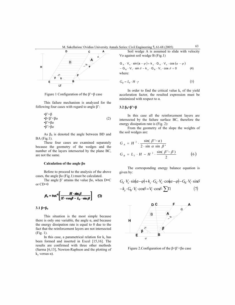
M. Sakellariou/ Ovidius University Annals Series: Civil Engineering 7, 61-68 (2005) 63
BH
←β
ELT
V1
D
α
←
B
β'
AVo
C A
δ
φ
Figure 1 Configuration of the β’=β case This failure mechanism is analyzed for the
following four cases with regard to angle β’: • β’=β • β<β’<βο (2) • β’=βο • β’>βο As β0 is denoted the angle between BD and
BA (Fig.1). These four cases are examined separately
because the geometry of the wedges and the number of the layers intersected by the plane BC, are not the same.
Calculation of the angle βο Before to proceed to the analysis of the above
cases, the angle βο (Fig.1) must be calculated. The angle β’ attains the value βο, when D≡C
or CD=0
3.1 β=β0
This situation is the most simple because there is only one variable, the angle α, and because the energy dissipation rate is equal to 0 due to the fact that the reinforcement layers are not intersected (Fig. 1).
In this case, a parametrical relation for kc has been formed and inserted in Excel [15,16]. The results are confirmed with three other methods (Sarma [6,13], Newton-Raphson and the plotting of ky versus α).
Soil wedge A is assumed to slide with velocity Vo against soil wedge B (Fig.1)
( ) ( )(4)0cosVGksinVG
cosVGkasinVG
1By1B
oAyoA
=⋅⋅⋅−⋅⋅−
−⋅⋅⋅+−⋅⋅
δδ
ϕαϕ
where:
( )5γ⋅⋅= HLG TB
In order to find the critical value kc of the yield acceleration factor, the resulted expression must be minimized with respect to α. 3.2 β0>β’>β
In this case all the reinforcement layers are intersected by the failure surface BC, therefore the energy dissipation rate is (Fig. 2):
From the geometry of the slope the weights of the soil wedges are:
( )62
)'sin('sinsin2
)'sin(
2
2
βββα
β
−⋅−⋅=
⋅−
⋅=
HHLG
aHG
TB
A
The corresponding energy balance equation is given by:
( ) ( )( )7coscos
sincossin
11
1
∑⋅⋅=⋅⋅⋅−
⋅⋅−−⋅⋅⋅+−⋅⋅
TiVVGk
VGVGkaVG
By
BoAyoA
δδ
δϕαϕ
B
LT
←V1
AVo
←
D C F Aα
ββ'
BE
H
Figure 2.Configuration of the β<β’<βο case

Seismic stability … / Ovidius University Annals Series: Civil Engineering Volume 1, Number 7, 61-68 (2005)
64
From equation (7) an expression of ky is obtained, which can be minimized by using Newton-Raphson method in Excel environment. 3.3 β΄=β0
Following the same procedure, the energy
balance equation for this case is:
( ) ( )( )80cos
sincossin
1
1
=⋅⋅⋅−
⋅⋅−−⋅⋅⋅+−⋅⋅
δ
δϕαϕ
VGk
VGVGkaVG
By
BoAyoA
H
ELT
←
B
D
B
F
←
A
A
βV1 β'
Vo
α
Figure 3.Configuration of the β’=β0 case
As in the previous case, we can use Newton-Raphson method to obtain the first derivative of the ky expression as follows from the above equation. 3.4 β’>β0
Here, the number of reinforcement layers, p, intersected by the plane BC can be expressed as function of the angle β’.
The energy balance equation is given by
( ) ( )
( )9coscos
sincossin
111
1
∑=
⋅⋅=⋅⋅⋅−
⋅⋅−−⋅⋅⋅+−⋅⋅p
iBy
BoAyoA
TiVVGk
VGVGkaVG
δδ
δϕαϕ
We estimate kc from all the cases of direct
sliding mechanisms and choose as kc the minimum. In the cases β<β’<βο, β’=βο, β’>βο we use Newton-Raphson method for the estimation of kc with constrains, among others, the equation to zero of the first derivatives of the relations for ky.
B
Eβ
LT
V1←
H
C
B
β'
Vo←
Aα
D F A
Figure 4.Configuration of the β’>βο case
It is likely that in many situations a minimum value of ky cannot be estimated because the function may not have a minimum within the constrains. 4. Plane Failure Mechanism
H
Eβ
LTB
←
DL
F C
ΩφV
Figure 5.Configuration of the plane failure mechanism Energy balance equation.
( )10)cos(
)cos()sin(
1∑=
⋅−Ω⋅=
=−Ω⋅⋅⋅+−Ω⋅⋅n
i
h
TiV
VGkVG
ϕ
ϕϕ
Using the relation for K, as suggested by Ling et al [8]
( )11)2/1( 2
1
H
TiK
n
i
⋅⋅=
∑=
γ
and from the energy balance equation can be obtained:
( )[ ] )12(tansinsin
)sin(hkK +−Ω⋅
Ω⋅Ω−
= ϕββ

M. Sakellariou/ Ovidius University Annals Series: Civil Engineering 7, 61-68 (2005) 65The procedure to obtain a critical value, kc,
for the acceleration is programmed in the Excel application developed specifically and presented at the end of the present paper. 5. Log-Spiral Failure Mechanism
This failure mechanism is described by the equation:
)13(tan0
0 ϕϑϑ ⋅−⋅= )(err
With the use of the limit equilibrium method and the kinematical theorem, Ausilio provides the following expressions for uniformly spaced layers [2]:
[ ])14(
)(
)())/((sin)/(
654
31
21022
fff
fffniinKk
n
iy −−
−−−+=
∑=
αθα
Where the f coefficients are functions of the
geometry of the slope [2].
F
H
r
β
LT
Α LB
ϑh
Oϑo
ro
Zi
C
↓d i
Figure 6.Configuration of the Log-Spiral case
In the results of Ausilio analysis it is mentioned that the planar failure mechanism leads to values of K that are fairly close to those obtained when the log-spiral failure mechanism is considered [2]. Because of this fact and for simplicity we use (Eq. 12) for the estimation of K.
Log-Spiral failure surface can extend beyond the reinforced zone (Fig. 7). In this case some of the top reinforcement layers could be pulled out
and it should be assumed that only the bottom layers contribute to global stability of the slope.
The maximum value m of the reinforcement layers, located at the bottom, that are necessary to ensure slope stability, can be estimated by the relation:
u
n
iiu
THKm
TTm
21
)2/1( ⋅⋅⋅=
⇒=⋅ ∑=
γ(15)
Therefore, the expression for ky is:
( )[ ] ( )
( ))16(
/sin
6542
2
13212
2
0
fffH
fffHHzT
k
m
ii
u
y
−−⋅⎟⎟⎠
⎞⎜⎜⎝
⎛
−−⋅⎟⎟⎠
⎞⎜⎜⎝
⎛−+⋅⎟⎟
⎠
⎞⎜⎜⎝
⎛
=∑=
α
ααθ
γ
Figure 7.Configuration of the extended Log-Spiral case
6. Application of the methodology in Excel
The procedure described above is introduced in the Excel enriched with attenuation formulas to estimate the local seismic acceleration kh.
The application makes use of the Solver of the Excel to calculate the minimum values of the acceleration caefficients for the four geometries of failure surface described in above. In case where the required reinforcement length exceeds a prescribed

Seismic stability … / Ovidius University Annals Series: Civil Engineering Volume 1, Number 7, 61-68 (2005)
66
limit, the slope height e.g., or the required strength Tu of the reinforcement is out of the available limits, a reduced k is used the “kh’”.
In estimating the permanent seismic-induced displacement, two cases are considered, namely, the symmetrical and unsymmetrical geometries of embankments or slopes. In case of sloping ground, the unsymmetrical configuration is more appropriate to be used. Moreover, the degree of confidence can be prescribed.
6.1 Examples
In the following examples we examine several cases of slopes for different heights and spacing of reinforcements.
The slope angle is equal to 650 and the friction angle is equal to 350.
The local seismic acceleration takes the values of 0.36 and 0.16, which represent a realistic upper bound and lower bound value respectively, whereas the as value of the confidence level the 50% and 90% has been selected. Probability of exceedance 50% 0.36g cases
kh 0.36 γ(kN/m3) 18 μ 0.8 C 0.8
β(degrees) 55 φ degrees) 30
UNSYMMETRICAL CASE
Η (m)
Tu (kΝ/m)
di (m) kc
U (cm)
10 20 0.25 0.16 4.3 20 20 0.25 0.16 4.3 30 20 0.25 0.06 35.3 40 20 0.25 -0.04 -
SYMMETRICAL CASE
Η (m)
Tu (kΝ/m)
di (m) kc
U (cm)
10 20 0.25 0.16 3.6 20 20 0.25 0.16 3.6 30 20 0.25 0.06 11.9 40 20 0.25 -0.04 -
β(degrees) 65 φ degrees) 35
UNSYMMETRICAL CASE
Η (m)
Tu (kΝ/m)
di (m) kc
U (cm)
10 20 0.25 0.26 0.5 20 30 0.25 0.26 0.5 30 40 0.25 0.26 0.5 40 50 0.25 0.26 0.5
SYMMETRICAL CASE
Η (m)
Tu (kΝ/m)
di (m) kc
U (cm)
10 20 0.25 0.26 0.4 20 30 0.25 0.26 0.4 30 40 0.25 0.26 0.4 40 50 0.25 0.26 0.4
Probability of exceedance 10%
kh 0.36 γ(kN/m3) 18 μ 0.8 C 0.8
UNSYMMETRICAL CASE
Η (m)
Tu (kΝ/m)
di (m) kc
U (cm)
10 40 0.25 0.26 1.1 20 40 0.25 0.26 1.1 30 40 0.25 0.26 1.1 40 40 0.25 0.16 10.7

M. Sakellariou/ Ovidius University Annals Series: Civil Engineering 7, 61-68 (2005) 67SYMMETRICAL CASE
Η (m)
Tu (kΝ/m)
di (m) kc
U (cm)
10 40 0.25 0.26 1.3 20 40 0.25 0.26 1.3 30 40 0.25 0.26 1.3 40 40 0.25 0.16 10.5
0.16g cases
kh 0.16 γ(kN/m3) 18
m 0.8 c 0.8
UNSYMMETRICAL CASE
Η (m)
Tu (kΝ/m)
di (m) kc
U (cm)
10 40 0.5 0.16 - 20 40 0.5 0.16 - 30 40 0.5 0.06 17.3 40 40 0.5 -0.04 -
SYMMETRICAL CASE
Η (m)
Tu (kΝ/m)
di (m) kc
U (cm)
10 40 0.5 0.16 - 20 40 0.5 0.16 - 30 40 0.5 0.06 15.0 40 40 0.5 -0.04 -
7. Conclusions
In this paper a methodology has been developed to calculate the critical acceleration for reinforced slopes to design embankments, based on an acceptable permanent seismic-induced displacement.
The analysis is based on the energy balance for three types of failure surface and minimization of the respective expressions of the acceleration coefficients ky to obtain the critical value kc for each case.
The whole procedure has been programmed in the Excel environment (Fig. 8). In addition to that,
an estimation of the local maximum accelerations can be done, according to different attenuation rules, as a function of the distance from tectonic faults and the earthquake magnitude.
In the included examples, different cases of reinforced slopes have been examined with symmetrical and unsymmetrical conditions. 8. Acknowledgments
The programming of the methodology has been executed as part of the Diploma Theses of Miss Helen Glarou and Mr Demetrios Karavassilis at the Laboratory of Structural Mechanics and Engineering Structures of the School of Rural and Surveying Engineers of Natioal Technical University of Athens. 9. References [1]Ambraseys, N.N., Menu, J.M., Earthquake-induced ground displacements. Earthquake Engineering and Structural Dynamics 1988; 16:985-1006. [2]Ausilio, E., Conte, E., Dente, G., Seismic stability analysis of reinforced slopes. Soil Dynamics and Earthquake Engineering 2000; 19:159-172. [3]Chen, W.F., Limit analysis and soil plasticity. Amsterdam: Elsevier, 1975. [4]Drucker, D.C and Prager, W., Soil mechanics and plastic analysis or limit design. Quarterly J. of Applied Mathematics 1958; 10: 157-165. [5]FWHA, Mechanically stabilized earth walls and reinforced soil slopes. Design and construction guidelines. FHWA-SA-96-071, U.S. Department of Transportation, 1999. [6]Hoek, E., General two-dimensional slope stability analysis In: Analytical and computational methods in engineering rock mechanics, Brown ET editor, London: Allen & Unwin, 1986. [7]Kreyszig, E., Advanced Engineering Mathematics. New York: John Wiley & Sons, 8th edition, 1999. [8]Ling, H.I., Leshchinsky, D., Chou NNS. Post-earthquake investigation on several geosynthetic-reinforced soil retaining walls and slopes during the Ji-Ji earthquake of Taiwan. Soil Dynamics and Earthquake Engineering 2001; 21:297-313. [9]Mastering Excel for Windows 95. Sybex Inc. 1995. [10]Michalowski, R.L., Soil reinforcement for seismic design of geotechnical structures. Computers and Geotechnics 1998; 23:1-17.

Seismic stability … / Ovidius University Annals Series: Civil Engineering Volume 1, Number 7, 61-68 (2005)
68
[11]Michalowski, R.L., Limit analysis in stability calculations of reinforced soil structures. Geotextiles and Geomembranes 1998; 16:311-331. [12]Michalowski, R.L., You, L., Displacements of reinforced slopes subjected to seismic loads. Journal of Geotechnical and Geoenvironmental Engineering 2000; 126(8): 685-694.
[13]Nova-Roessing, L., Sitar, N., Centrifuge studies of the seismic response of reinforced soil slopes. In: Proceedings of the Third Geotechnical Engineering and Soil Dynamics Conference, Geotechnical Special Publication No. 75, ASCE 1998; pp 458-468. [14]Sarma, S.K., Stability analysis of embankments and slopes. Geotechnique 1973; 23(3): 423-433.
Figure 8. An example of the program developed in Excel

Ovidius University Annals Series: Civil Engineering Volume 1, Number 7, Nov. 2005
ISSN-12223-7221 © 2000 Ovidius University Press
Determination of the Constant C for the Gerstner’s Traveller Wave Potential
Mircea Dimitrie CAZACU a Dan Aurel MĂCHIŢĂ b a Politehnica University Bucharest, Bucharest, 060042, Romania
b Ministry of Transport, Buildings and Tourism, Bucharest, 010873 , Romania
__________________________________________________________________________________________ Rezumat: Considerând expresia potenţialului vitezelor, corespunzător mişcării valului călător al lui Gerstner, se obţine relaţia ce dă valoarea constantei C, determinată în funcţie de înălţimea valului prin aplicarea relaţiei lui Daniel Bernoulli pe suprafaţa liberă a valului pentru un acelaşi moment de timp. Se determină în acest fel legătura dintre parametrii cinematici ai valului şi adâncimea medie a apei din canal, pentru a se obţine valori reale ale acestei constante. Abstract: Considering the velocity potential expression, corresponding to the Gerstner’s traveller wave motion, one obtains the relation that give the value of the constant C as function of the wave height, determined by applying of Daniel Bernoulli’s relation on the wave free surface for a same time moment. One determines in this kind the link between the wave kinetic parameters and water mean depth in the channel, to obtain the real values of this constant. Keywords: traveller wave, wave potential, Gerstner’s potential __________________________________________________________________________________________ 1. Introduction
We due to F.von Gerstner the renowned
potential of traveller wave in the year 1802 [1]
( ) ( ) ( ), , sinX Y t F Y kX tΦ = ⋅ −ω , (1)
from which derive the velocities of the unsteady, two-dimensional and irrotational motion of a heavy and in viscid liquid, representing the propagation of an infinite succession of waves in a channel of finite depth H. The potential was built on the basis of D.Bernoulli’s variable separation method and for the determination of F (Y) function, that mark the vertical amplitude of wave particle trajectory at different depth Y, and he used the liquid mass conservation equation, which introduce the harmonic condition for the velocity potential.
2 2X Y X Y X,Y0U V′ ′ ′′ ′′+ = Φ +Φ = Δ Φ = . (2)
By determination of the expression of wave height function, by solving of the ordinary differential equation with constant coefficients of Euler’s type and of his characteristic equation:
( ) ( )22
Y0F Y k F Y′′ − = , 2 2 0r k r k− = → = ± , (3)
he obtained the general solution of the form
( ) kY -kYF Y Ae Be= + with kH2CAe
= and -kH2CBe
= ,(4)
in which the condition of motion limitation on the channel bottom
( ) ( )( ) ( )
kH -kHYY=H Y=H
sin
sh sin 0, (5)
V k Ae Be kX t
k C k H Y kX t
′= Φ = − −ω =
= − − −ω =
permitted him to obtain the velocity potential dependent of a single integration constant C
( ) ( ) ( ), , ch sinX Y t C k H Y kX tΦ = − −ω . (6) 2. Bernoulli’s relation for the unsteady motion
From the two unsteady and irrotational motion equations of an ideal and heavy liquid [2]
t X Y X X10 U UU VU P VV′ ′ ′ ′ ′= + + + ±ρ
, (7)

Determination of … / Ovidius University Annals Series: Civil Engineering Volume 1, Number 7, 71-74 (2005)
72
t X Y Y Y1g V UV VV P UU′ ′ ′ ′ ′= + + + ±ρ
, (8)
one obtains, by their addition, multiplied with dx and dy respectively, as an exact total differential equal with zero and by their integration
( )2 2
t1 c t
2U V P
g g+′Φ + + + η =
γ, (9)
in which, corresponding to fig.1, we considered for the wave free surface Y = -η.
Fig. 1 The axis and wave kinetic parameters 3. The determination of the C constant
In this purpose we shall use the Bernoulli’s relation (9), in which to profit by the same constant value c (t) in the whole domain, occupied by the ideal fluid, we shall use it in the same moment of time, for example, initial time t = 0. Also, we shall consider the constant pressure P0 on the wave free surface and how η = -Y, the wave height will have consequently the expression
( ) ( )
2 2
t t
0,0 ,0 0,0 ,02 2
, ,0 0, ,02 2 2
2
1 , ,0 0, ,0 ,2 2 2
h Y Y
h hU U
g
h hg
λ λ⎛ ⎞ ⎛ ⎞= η −η = − + =⎜ ⎟ ⎜ ⎟⎝ ⎠ ⎝ ⎠
λ −⎛ ⎞ ⎛ ⎞−⎜ ⎟ ⎜ ⎟⎝ ⎠ ⎝ ⎠= +
⎡ λ − ⎤⎛ ⎞ ⎛ ⎞′ ′+ Φ −Φ⎜ ⎟ ⎜ ⎟⎢ ⎥⎝ ⎠ ⎝ ⎠⎣ ⎦
(10)
in which we also have took into consideration the relation V (0, -h/2, 0) = V (λ/2, h/2, 0) = 0 for the vertical velocity deduced from (5), and where by calculation of the maximum and minimum values of the horizontal velocity at the wave free surface
0, ,0 ch2 2h hU kC k H−⎛ ⎞ ⎛ ⎞+⎜ ⎟ ⎜ ⎟
⎝ ⎠ ⎝ ⎠ (11)
, ,0 ch2 2 2
h hU kC k Hλ⎛ ⎞ ⎛ ⎞− −⎜ ⎟ ⎜ ⎟⎝ ⎠ ⎝ ⎠
(12)
and by introduction also of the velocity potential derivatives with respect to the time
t 0, ,0 ch2 2h hC k H−⎛ ⎞ ⎛ ⎞′Φ −ω +⎜ ⎟ ⎜ ⎟
⎝ ⎠ ⎝ ⎠, (13)
t , , 0 ch2 2 2
h hC k Hλ⎛ ⎞ ⎛ ⎞′Φ ω −⎜ ⎟ ⎜ ⎟⎝ ⎠ ⎝ ⎠
(14)
the relation (10) will lead as to an equation of 2nd degree, from that we can determinate the expression of the constant C:
( ) ( ) ( ) ( )2 2 2 2ch ch 2 ch ch 2 0,2 2 2 2h h h hk k H k H C k H k H C gh⎡ ⎤ ⎡ ⎤+ − − − ω + + − + =⎣ ⎦ ⎣ ⎦ (15)
its solution being in the general case
( )
( )( )
( ) ( )( ) ( )
( ) ( )
22
2 2 2
2 2 2
ch ch ch2 2 2
ch 2 ch ch2 2 2, ,ch ch2 2
h h hk H k H k H
h h hk H ghk k H k HC H h
h hk k H k H
⎡ ⎤ ⎡ ⎤+ + ω + + − −⎣ ⎦⎢ ⎥ω ±⎢ ⎥ ⎡ ⎤+ − − + − −⎢ ⎥⎣ ⎦ ⎣ ⎦λ =⎡ ⎤+ − −⎣ ⎦
(16)
and consequently, the motion potential (6) will have the implicit expression

M. D. Cazacu and D. A. Măchiţă / Ovidius University Annals Series: Civil Engineering 7, 71-74 (2005) 73
( ) ( ) ( ) ( ), , , , , , , ch sinX Y t H h C H h k H Y kX tΦ λ = λ − −ω (6’) 4. The condition to obtain the real solutions for the constant C
With a view to obtain non-imaginary solutions for the constant C, it will must that in the
relation (16) the expression value under the root must be positive. In this case, denoting by Hℵ= λ and χ = h/λ the relative heights of the wave and of the static water level in the channel, after a simple calculus we obtain the condition
2
2ch2 ch2 ch2 ch22 2 2 2
ghc
χ χ ⎡ χ χ ⎤⎛ ⎞ ⎛ ⎞ ⎛ ⎞ ⎛ ⎞π ℵ+ + π ℵ− ≥ π ℵ+ − π ℵ−⎜ ⎟ ⎜ ⎟ ⎜ ⎟ ⎜ ⎟⎢ ⎥⎝ ⎠ ⎝ ⎠ ⎝ ⎠ ⎝ ⎠⎣ ⎦, (17)
or taking into account of the over-unitary value of the ratio calculated from (17) and of its expression
in infinite series by performing the division, we obtained the evaluation
( )( )
2
2 3 4
2
2 1ch2 + 2 1 1 1 1 11 1 2 12 1ch2 - 12
ghxc
gh x x x x xc
χ +π ℵ + ⎛ ⎞≤ = + + + +⎜ ⎟χ − ⎝ ⎠π ℵ −p L f , (18)
in which we denoted in the second ratio, over-unitary in practice, by 22 1x gh c= f , where by introducing of the propagation velocity expression of the traveller wave, obtained from the Gerstner’s
theory, 2 th 22gc λ
= πℵπ
, results the necessary
condition to fulfil between the relative values,
reported to the wave length, of the wave height and the water depth in the channel (fig.2), relation that stipulate the obtaining of the real values for the constant C
max10.08 th 2
4χ = ≥ χ πℵ
πf (19)
Fig. 2 The dependence of the relative wave height by the water relative depth in the cannel 5. Conclusions
The above obtained results permitted us to calculate the motion trajectories of different sand
particles, having divers sizes and positions in the water depth, under the action of traveller waves [3], by combined consideration of the weight, Archimedean static lift and hydrodynamic drag forces, exerted on the

Determination of … / Ovidius University Annals Series: Civil Engineering Volume 1, Number 7, 71-74 (2005)
74
solid particles in their relative motion, which has been presented in an other former paper [4].
These research present a special importance in the problem of the alluvial deposit motion in vue to stop the alarming erosion of Romanian coast and beaches in the last years [5], as a consequence of the hydroelectric power plants with dams built on the Danube, Dniester and Bug rivers of the North of Black Sea and of the usual works of land protection against the meteorological factors erosions.
In the last three decades many Romanian researchers have developed an intense activity to study the theoretical and experimental aspects of the installations able to put an end to the coastal erosion and to promote the technical devices, able to protect our coast and beaches [6] ÷ [13], applying the idea of complex uses, also the wind energy, of our former professor Dorin Pavel, Romanian famous hydro-energetician [14][15].
6. Contents
The authors express their gratitude to PhD. Eng. Petru Dan Lazar, Director of Romanian Senate, for his pains in the purpose to promote the renewable energies in general and to protect the Romanian coasts and beaches especially. 7. References [1]Mateescu C. Hidraulica. Editura Didactică şi Pedagogică, Bucureşti, 1968. [2]Oroveanu T. Mecanica fluidelor vâscoase. Ed.Acad.R.S.R., Bucureşti, 1967. [3]Cazacu M.D., Măchiţă D.A.. Theoretical and experimental modelling of the wave erosion action and an advantageous possibility of shore protection. International Symposium Coastal Erosion: Problems and Solutions, 26–28 June 2003, Mangalia – Romania, Ed. S.C. AQUA-PROIECT S.A., Bucureşti, 171 – 180. [4]Cazacu M.D., Măchiţă D.A.. Wave erosion action and the possibilities to protect the shore, using their energy. International Conference on Energy and Environment, 23-25 Oct.2003, Univ. Politehnica, Bucharest [5]Iulian C. Centrul internaţional pentru monitorizarea şi combaterea eroziunii marine. Rev.
Mediul înconjurător, nr.3, 2003, 8–19 şi Comunicare la International Symposium Coastal Erosion: Problems and Solutions, 26–28 June 2003, Mangalia – Romania, Ed. S.C. AQUA-PROIECT S.A., Bucureşti [6]Iulian C. Utilizarea energiei valurilor. Ed.Tehnică, Bucureşti, 1990. [7]M.D.Cazacu. Autostrada marină, caz interesant de folosinţe complexe. A 2-a Conf.Tehnico-Ştiinţifică “Profesorul Dorin Pavel – fondatorul hidroenergeticii româneşti”, 31 mai – 2 iunie 2002, Sebeş, Vol.I – Ştiinţă şi Inginerie, Ed. AGIR, 27 – 34. [8]M.Cazacu. Sea highway with multiples utilities. Simpoz.Ştiinţ. 25 ani de Învăţ.Superior. 18-20 aprilie 2002, Ovidius University Annals, Constanţa, Vol.1, 367-370. [9]M.D.Cazacu, S.C.Stăvărache. Energy catchement experimental study of traveling waves by inclined plane device. A III-a Conf.Dorin Pavel a Hidroenergeticienilor din România, 28-29 mai 2004, Univ. Politehnica, Bucureşti, Vol. I, 53-56. [10]M.D.Cazacu, S.C.Stăvărache. Wave generation by oscillating flape valve. A 2- Conferinţă a Hidroenergeticienilor din România, 24 – 25 mai 2002, Univ. Politehnica, Bucureşti, Vol.I, 31 – 36. [11]M. D. Cazacu - Valurile marine, importantã sursã de energie - Caiete de studii şi dezbateri, Acad. R.S.R., oct. 1974, 56 - 62. [12]M.D.Cazacu - Energia eolianã, veche şi mereu nouã sursã de energie. Caiete de studii şi dezbateri, Acad. R.S.R., oct. 1974, 86 - 87. [13]P. Terzi, M.D.Cazacu, I.Rusu, P.D.Pleşca, A.Ciocânea, D.Zahariea, O.Bizim, G.O.Pena. New types of wind turbines to extend the Dorin Pavel’ s variant of energy storage. Conferinţa Hidro-energeticenilor din România, 26 – 27 mai 2000, Univ. POLITEHNICA din Bucureşti, 485 – 492. [14]M.D.Cazacu. Dorin Pavel – the Founder of Romanian Hydroenergetics. Conferinţa Hidro-energeticenilor din România, 26 – 27 mai 2000, Univ. POLITEHNICA din Bucureşti, 21 – 32. [15]M.D.Cazacu. Dorin Pavel - Părintele hidroenergeticii româneşti. A 2-a Conf.Tehnico-Ştiinţifică “Profesorul Dorin Pavel – fondatorul hidroenergeticii româneşti”,31 mai – 2 iunie 2002, Sebeş, Vol.I – Ştiinţă şi Inginerie, Ed. AGIR, 11 – 20.

Ovidius University Annals Series: Civil Engineering Volume 1, Number 7, Nov. 2005
ISSN-12223-7221 © 2000 Ovidius University Press
Flow Compensation Reservoir at Hydro Power Plants with Lengthy Pressure Pipe
Claudiu Stefan NITESCU a a “Ovidius” University Constantza, Constantza, 900527, Romania
__________________________________________________________________________________________ Rezumat: In comunicare este analizată utilizarea unui rezervor de compensare amplasat pe aducţiunea de lungime mare a unei uzine hidroelectrice. Rezervorul de compensare este amplasat amonte de mijlocul de protecţie la şoc hidraulic (castel de echilibru). Debitul turbinat va fi compus din debitul rezervorului de compensare şi din lacul de acumulare. Astfel reducem pierderile de sarcina de pe conducta de aducţiune şi obţinem aceeasi putere instalată dar la un debit turbinat mai mic. Abstract: The paper describes the role of a compensation reservoir located on the length of the income flow of a hydropower plant. The compensation reservoir is situated upstream from the protection device in case of hydraulic shock ( the surge tank). The turbine flow will then consist of the compensation reservoir flow and the artificial lake flow. The load losses on the inflow pipe are hence reduced and we obtain the same the same electrical power at a smaller turbine flow. Keywords: Hydropower plant, surge tank, compensation reservoir. __________________________________________________________________________________________ 1. Introducere
We consider the design of the hydropower plant: lake (reservoir), pressure pipe, surge tank, pressure tunnel, turbines and evacuation channel. (fig 1).
As a result of the valve operations at the turbines (debit variations), the water hammer occurs only in the pressure tunnel, in the pressure pipe and in the surge tank; the water flow is slow variable.
In order to obtain the differential ecuation for the pressure pipe - surge tank system water level fluctuations we start with the following ecuation system – simplified [1], and also using the law of flows from a constant power of the powerplant.
By eliminating Q and QT variables in both ecuations [1] we obtain:
( )⎜⎝⎛ +
+++
dtdZ
ZHF
NdtdZ
gk
dt
ZdgfLF
ηγ22
2 (1)
( ) ( )0
2=+
+−⎟
⎟
⎠
⎞
++ Z
dtdZ
ZHgf
NL
ZHF
N
ηγηγ
This is a second degree non-linear differential ecuation, in which:
2
2
f
FdLk ⎟
⎠⎞
⎜⎝⎛ += ∑ξλ (2)
A unique solution with the initial conditions:
00 ZZt =→=
)0(0
0 ZHF
NWFf
dtdz
+−=ηγ
(3)
At the complete shutdown of the plant, the
ecuation for the oscilations becomes very simplified and is as follows:
022
2=++ Z
dtdZ
dtdZ
gk
dt
ZdgfLF (4)
with the initial restrictions: 00 ZZt =→=
FQ
dtdZ 0= .

Flow compensation reserv/ Ovidius University Annals Series: Civil Engineering Volume 1, Number 7, 75-78 (2005) 76
When we start the powerplant (with suddnely open valve) the ecuation for the scilations is the same but with new initial restrictions:
00 =→= Zt F
QdtdZ 0−= .
2. Compensation reservoir
A reservoir with large diameter and low
hight (compared to its diameter) situated on the income pressure pipe before the surge tank, is considered .
The role of this reservoir is to bring an additional flow to the pressure tunnel, reducing this way the loss of load on the lengthy pressure pipe. Practically, this reservoir is formed by blocking a wave or a depression in the surge tank zone.
For practical reasons (energy efficiency), it was considered that the hydropower plant would have a cyclical functioning schedule, with periods when the inflow comes from both the lake and the compensation reservoir, and periods when it is not functioning.
This way, the level H ( stady state head ) that appears in the powerplant power ecuation will be higher than in the situation where there is no compensation reservoir.
In this situation, the level will vary from Hmax to Hmin, comparatively with the situation in which there is no compensation reservoir and hence we’ll always have Hmin.
The result will be an average level Hmed>Hmin that will lead to a more efficient use of the water volume in the lake due to the fact that the energy will be produced with a smaller water volume.
.constRQLQTQ =+= (5)
We write the differential ecuation of the oscillations for the compensation reservoir, ecuation derived from the differential ecuation of oscillations for the surge tank, where:
0→dtdZ
and (6)
02
→⎟⎟
⎠
⎞
⎜⎜
⎝
⎛
FH
N
FH
Ng
k
ηγηγ
We obtain:
022
2=+− Z
dtdZ
fHg
NL
dt
ZdgfLF
γη (7)
that represents a second degree differential
ecuation with homogeneous and constant coefficients.
Fig.1.The schematic design of a hydropowerplant with compensation reservoir
L=15000 m
Compensation reservoir Y
H0
T LT,fT
Q
0,00
D=5 m QT=70mc/s
H=600m
F
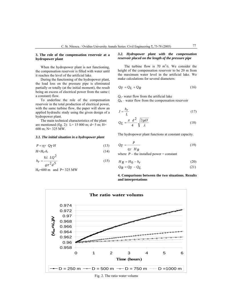
C. St. Nitescu. / Ovidius University Annals Series: Civil Engineering 7, 75-78 (2005) 77 3. The role of the compensation reservoir at a hydropower plant
When the hydropower plant is not functioning, the compensation reservoir is filled with water until it reaches the level of the artificial lake.
During the functioning of the hydropower plant, the load loss on the pressure pipe is eliminated partially or totally (at the initial moment), the result being an excess of electrical power from the same ( a constant) flow.
To underline the role of the compensation reservoir in the total production of electrical power, with the same turbine flow, the paper will show an applied hydraulic study using the given design of a hydropower plant.
The main technical characteristics of the plant are mentioned (fig. 2): L= 15 000 m; d= 5 m; H= 600 m; N= 325 MW. 3.1. The initial situation in a hydropower plant
HTQP ηγ= (13) H=H0-hr (14)
52
28
dg
LQrh
π
λ= (15)
H0=600 m and P= 325 MW
3.2. Hydropower plant with the compensation reservoir placed on the length of the pressure pipe
The turbine flow is 70 m3/s. We consider the height of the compensation reservoir to be 20 m from the maximum water level in the artificial lake. We make calculations for several diameters:
RQLQTQ += (16) QL- water flow from the artificial lake QR – water flow from the compensation reservoir
Lrh
J = (17)
λπ gdJd
LQ2
4
2= (18)
The hydropower plant functions at constant capacity.
RH
PTQ
ηγ= (19)
where P – the installed power = constant
rhHRH −= 0 (20)
LQTQRQ −= (21) 4. Comparisons between the two situations. Rezults and interpretations
The ratio water volums
0.9580.96
0.9620.9640.9660.968
0.970.9720.974
0 1 2 3 4 5 6Time (hours)
(Vla
c+V r
c)/V
D = 250 m D = 500 m D = 750 m D =1000 m
Fig. 2. The ratio water volums

Flow compensation reserv/ Ovidius University Annals Series: Civil Engineering Volume 1, Number 7, 75-78 (2005) 78
The ratio turbine flows
0.955
0.96
0.965
0.97
0.975
0.98
0.985
0 1 2 3 4 5 6
Time (hours)
(Qrc+Q
lac)/Q
D = 250 m D = 500 m D = 750 m D =1000 m
Fig. 3. The ratio turbine flows
Water volum saved by using the compensation reservoir
0100002000030000400005000060000
0 1 2 3 4 5 6
Time (hours)
Volu
m (m
3 )
D = 250 m D = 500 m D = 750 m D =1000 m
Fig. 4 . Water volume saved by using the compensation reservoir
V. FINAL CONSIDERATIONS
The calculations have been made for a 6 hour period of running of the hydropower plant and they took into consideration the impact of the diameter of the compensation reservoir. The efficiency of the reservoir depends on this diameters. The additional production of electrical power is calculated using the water volume not used from the artificial lake in
the presence of the compensation reservoir at the constant running of the plant.
VI. REFERENCES [1] Popescu M., Arsenie D.I., Metode de calcul hidraulic pentru uzine hidroelectrice si statii de pompare, Ed. Tehnica Bucuresti, 1987 [2] Mateescu C., Hidraulica , 1968,Ed.Did. şi Ped., Bucureşti

Ovidius University Annals Series: Civil Engineering Volume 1, Number 7, Nov. 2005
ISSN-12223-7221 © 2000 Ovidius University Press
A Kinematic Condition Concerning the Viscous Substratum (Laminar Limited Substratum) in the Pressure Pipes and some Consequences
for the Turbulent Regime Phases
Ichinur OMERa Dumitru Ion ARSENIE a a Ovidius University Constantza, Civil Engineering Faculty, Constantza, Romania
__________________________________________________________________________________________ Rezumat: Considerând condiţia cinematică referitoare la viteza unghiulară de rotaţie a particulei, în această lucrare se prezintă criteriile care definesc diferitele faze ale regimului turbulent (neted, semirugos şi rugos). Abstract: Considering the kinematic condition with reference to the rotation angular velocity of particle, in this paper we present the criteria which define the different turbulent regime’s phases (smooth, semi-rough and rough). Keywords: viscous substratum, turbulent regime, pressure pipes. ________________________________________________________________________________________ 1. Introduction It is known that in the transversal section of a circular pressure pipe where a liquid in the stationary regime (permanent regime) flows, we can distingue four zones, which are beginning from the pipeline’s wall [1], [2]:
I.Viscous substratum (laminar limited substratum) where the velocity’s variation (determined by the molecular viscosity) is approximately linear. The thickness of this zone is noted by δl.
II.Transition zone, a blotting stratum or intermediary, where the friction tensions, (due to the molecular viscosity) and the apparent tensions (due to the velocity’s fluctuations produced by the turbulent diffusion) have comparable values. The thickness of this zone is noted by δt.
III. Logarithmical zone or stratum completely turbulent, where the wall influence is still being felt, but where the turbulent diffusion is not enough developed (for the turbulent tensions preponderant by comparing to those laminar, which can be neglected). Into this stratum the temporal medium velocity varies under a logarithmical law.
IV.Turbulent nucleus or the turbulent heart of the flow, where the turbulence is also completive developed, but different from the previous stratum.
It is influenced by the whole outline of the pipeline section.
The first three zones extend across the section under an annular shape, having together the thickness of about 15% from the pipeline’s radius. The turbulent nucleus occupies the central zone having a circular form with the radius of about 85% from the pipeline’s radius.
The first two zones occupy only a little part from the pipeline’s radius. So, we appreciate the Reynolds number Red = 105. The external annular substratum thickness (representing the viscous substratum) is equal to the thousandth part of the pipeline’s radius. The transition zone thickness is equal to the hundredth part of the pipeline’s radius.
From another point of view, beginning with the Nikuradze’s experiences period, in the engineering calculus, it is considered [2], [3], [4] to exist the following kinds of flow regime: smooth turbulent regime, semi-rough (transitory) and rough (quadric).
In this classification intervenes the roughness parameter k, which expresses the hydraulic aspect of the asperities of the pipeline wall surface. This parameter is a quantity with length dimension and represents a global characterization, from hydraulic point of view of the above mentioned irregularities, which have different heights, forms and repartitions on the pipeline surface.

A kinematic condition… / Ovidius University Annals Series: Civil Engineering Volume 1, Number 7, 79-82 (2005)
80
It’s normal to try to make a connection between the hydraulic roughness parameter, the previous mentioned zones, distinguished in the transversal section of the current and the classification of the turbulent regime (smooth, semi-rough and rough).
Thus, if the asperities are totally integrated in the viscous substratum, where the flow velocity is very small, they don’t produce supplementary energy loss, comparative to a smooth ideal surface, proven at that time by Reynolds’s experiments.
Subsequently we will consider the case of the smooth hydraulic pipeline, the smooth turbulent regime (δl ≥ k), respectively.
If the roughness is important and the asperities exceed the I and II strata, entering the logarithmical stratum (III), then the energy loss due by the molecular viscosity may be neglected relative to the energy loss due to the turbulent diffusion, This is the case of the rough pipeline (quadric turbulent regime).
In the intermediary situation, where the irregularities don’t outsize the buffer stratum (II), the energy losses due to the molecular viscosity are comparable to those due to the turbulence (δl<k≤δt). This is the case of the semi-rough hydraulic pipeline or the transitory turbulent regime. Nowadays there are used different indirect criterions to determine where a certain movement belongs to: - limit stratum Reynolds number criterion or the
equivalent form given by Moody; - limit Reynolds number criterion.
Corresponding to the first criterion, used in the international and national technical literature, we have:
- smooth hydraulic pipeline when 5* ≤νδ lu
14Re ≤↔ λdk
- semi-rough hydraulic pipeline when
705 * ≤<νδ lu
↔ 200Re14 ≤< λdk
- rough hydraulic pipeline when 70* >νδ lu
↔ 200Re >λdk
The criterion equivalence results immediately if
we consider the relation2
*8 ⎟⎠
⎞⎜⎝
⎛=vu
λ , which leads to
the relation λν d
kkuRe
221* = .
In these relations u* - the friction stress velocity,
υ – the liquid kinematic viscosity, νvd
=Re Reynolds
number, λ – hydraulic resistance coefficient Darcy – Weisbach, v – average velocity on section, d – pipeline’s diameter.
According to the last criterion, used in Russia, the regime fields are:
- smooth hydraulic pipeline kd15Re' ≈
- semi-rough hydraulic pipeline
kd
kd 560Re15 <<
- rough hydraulic pipeline kd560Re" ≈
If we analyze the both criteria, we find that they differ overmuch because the equality
087,015141415
2
≅⎟⎠⎞
⎜⎝⎛=⇒= λλ leads to unreasonable
large λ value for the smooth hydraulic pipeline. This means that limit Reynolds number criterion is more restrictive. Therefore the same pipeline may be considered both semi-rough according to this criterion and smooth hydraulic according to Moody criterion.
Concerning other criteria which mark off the semi-rough hydraulic pipeline from the rough hydraulic pipeline there is also a difference which makes the previous conclusion to rest valuable, because the two criteria’s equality is results in an unreasonable large value of the hydraulic strength coefficient (λ):
128,0560200200560
2
≅⎟⎠⎞
⎜⎝⎛=⇒= λλ

I. Omer and D.I. Arsenie / Ovidius University Annals Series: Civil Engineering 7, 79-82 (2005) 81
2. Estimations (quantitative) concerning the limit viscous substratum (laminar limit substratum I) in the case of the smooth hydraulic, semi-rough and rough pipelines We take over some known theoretical and experimental results to determine a formula (semi-empirical) to calculate the limit laminar stratum thickness. The formula is wanted to be used as a right pipeline classification criterion. In the laminar substratum, named sometimes laminar film [4], due to the extremely small thickness, the velocity is very well approached by a linear function (the stratum is named sometimes laminar substratum too) which must satisfy the adherence condition, respectively the velocity cancellation at the pipeline wall (r=r0, r0 – the pipeline’s radius 0=→ u ):
l
rruu
δδ
−= 0 (1)
δu - the flow velocity at the interior boundary of the limit laminar stratum. In the buffer stratum we adopt Karman model [1] which considers the following modified logarithmical law:
( )05,3ln5 *0
*
−−
=ν
urruu
(2)
*u - the friction stress velocity, ν - kinematic viscosity. Considering that the velocity repartition must be expressed by a continue function, results that, at the separation boundary of the two strata, exists the relation:
**
* 05,3ln5 uu
uu l −=νδ
δ (3) Subsequently we’ll consider, in addition to the known models, a kinematic condition referring to the liquid particle movement, not only the same translation velocity but also the same angular rotation velocity (ω):
( )
( )*0
0
*
0 5
25
2uurr
rru
rru
l
II
I
=⇒=−⇒
⎪⎪⎭
⎪⎪⎬
⎫
−=
−=
δ
δ
δω
ω (4)
This relation permits to eliminate the velocity from boundary in the relation (3) which can have the following form:
**
64,1
Re5
uvd
uel ≅=
νδ (5)
On the other hand the relation exists [5], [6]:
λ22
*
=uv
(6)
which leads to the next formula for the thickness of the laminar limit stratum:
λδ
Red
l ≈ (7)
Corresponding to Moody criteria, based on the experimental results relative to pipelines with natural roughness (technical and homogeneous), the pipeline is considered smooth hydraulic if:
14Re ≤λdk
(8) We observe that the relation (7) leads to the remarkable conclusion, in this limit case, that the thickness of the limit laminar stratum is equal with the pipeline roughness:
k
dkk l
l =⇒== δλ
δ1
Re
14 (9)
consonant with the physical phenomenon and the experimental results. It differs slightly from the formula presented in some books, based on some results of Nikuradze concerning the measurements referring to the velocity ( δu ) from the limit laminar stratum (at the δ distance from the pipeline’s wall):
λδ
Re30d
= (10)
3. Estimates (quantitative) concerning the intermediary stratum (stratum II, buffer or transition) Concerning the separation boundary between the intermediary stratum (II) and the logarithmical stratum (III) we can’t analogously proceed because the Karman model previous used, which express the velocity’s distribution into the stratum with intense fluctuations of the velocity (II) is correct only until ( )
30*0 <−ν
urr . The experimental data indicate for the limit which separates the semi-rough hydraulic pipeline from the

A kinematic condition… / Ovidius University Annals Series: Civil Engineering Volume 1, Number 7, 79-82 (2005)
82
rough hydraulic pipeline 70* >ν
ku. For this reason,
we considered that in the zone 7030 * <<ν
kuis
also valuable the logarithmical relation, but with other constant values:
( )B
urrA
uu
+−
=ν
*0
*
ln (11)
To determinate the constants A and B we can utilize two conditions, representing the equality at the boundary of the translation and rotation velocities, at the boundary between stratums II and III:
- to the translation velocity
0*
max*
*
ln1lnru
uB
uA
uu TT δ
χνδ
+=+= (12)
- to the rotation velocity
5,21
21
2
*
*
≅=⇒
⎪⎪⎭
⎪⎪⎬
⎫
=
=
χδχ
ω
δω
Au
uA
tIII
tII
(13)
We take into consideration also the relation which results from the Prandtl’s logarithmical law of the velocity deficit. It results:
1,4;75,3 *max ≅+= nuvu (14) In the end results the value of the constant B:
λλ
Reln5,2228 −+≅B (15)
From the two conditions doesn’t result one formula for tδ so we’ll consider, like in the previous case, at the limit kt =δ and thus we obtain the formula:
λδ
Re200
Re70
*
duvd
t ≅= (16)
and at the separation limit kt =δ . 4. Conclusions In this paper we consider the kinematic condition with reference to the rotation angular
velocity of particle and we present the criteria which define the different turbulent regime phases (smooth, semi-rough and rough). Thus for the smooth turbulent regime the Moody criteria 14Re ≤λ
dk becomes equivalent with
kdIl <==
λδδ
Re14 . For the semi-rough turbulence
200Re14 ≤< λdk is equivalent with the criteria
λδδ
Re200 dk tl =<< and for the rough
turbulence 200Re >λdk is equivalent with the
criteria kt <δ . By this, the separation of turbulent regime phases acquire a direct physical interpretation: the smooth phase corresponds to the case in which the surface has the asperities integrated in the limit laminar stratum, the semi-rough phase to the case in which the surface has the asperities integrated in the intermediary stratum (buffer or of intense pulsations) and the rough phase to the case in which the asperities pervade into the turbulent nucleus. References [1] Reynolds A. J., Curgeri turbulente în tehnică (traducere din limba engleză), 1982, Ed. Tehnică, Bucureşti. [2] Isbăşoiu E. G. G., Georgescu S. C., Hidraulica , 1963, Ed. Did. şi Ped., Bucureşti. [3] Mateescu C., Hidraulica , 1968, Ed.Did. şi Ped., Bucureşti. [4] Cioc D., Hidraulica, 1975, Ed.Did. şi Ped., Bucureşti. [5] Idelcik I. E., Îndreptar pentru calcule hidraulice (traducere din limba rusă), 1984, Ed. Tehnică, Bucureşti. [6] Ionescu D. G., Matei P., Ancuşa V., Todicescu A., Buculei M., Mecanica fluidelor şi maşini hidraulice, 1983, Ed. Did. şi Ped., Bucureşti. [7] Schlichting H., Teoria pogranicinogo sloia, 1974, Ed. Nauka, Moscova. [8] Seteanu I., Rădulescu V., Vasiliu N., Vasiliu D., Mecanica fluidelor şi sisteme hidraulice, 1998, Ed. Tehnică, Bucureşti [9] David I., Hidraulică (pentru uzul studenţilor), vol. II, 1984, Litografia Institutului Politehnic “Traian Vuia”, Timişoara

Ovidius University Annals Series: Civil Engineering Volume 1, Number 7, Nov. 2005
ISSN-12223-7221 © 2000 Ovidius University Press
Installation with Hydraulic Channel for Hydro-elasticity Tests - Velocities Distribution
Ilie I. RUSU a Iosif BARTHAa Bogdan CIOBANUa
a“Gh. Asachi” Technical University Iassy, Iassy, 700050, Romania
__________________________________________________________________________________________ Rezumat: Lucrarea prezintă o serie de rezultate obţinute de autori în ceea ce priveşte distribuţia de viteze într-un canal hidraulic dreptunghiular cu înclinare zero, în care mişcarea apei are loc datorită „consumului” din energia specifică potenţială (adâncime) sau cinetică. S-a urmărit stabilirea posibilităţii de a utiliza un astfel de canal pentru efectuarea unor încercări de hidroelasticitate privind determinarea masei adiţionale şi a rezistenţei la înaintare pentru corpuri având diverse forme. Abstract: This work presents some results obtained by the authors regarding the velocities distribution in a rectangular hydraulic channel with zero geometric slopes in order to establish if this kind of channel’s shape is appropriate to made hydro-elasticity tests concerning the determination of additional mass and drug forces for bodies having different shapes. Keywords: Hydraulic channel, velocities distribution, hydro-elasticity, additional mass __________________________________________________________________________________________ 1. Introduction
Hydro-elasticity theory or, generally speaking, fluid-elasticity or structural vibrations induced by the current theories, consider that elastic deformations of the structure can modify the hydro-dynamic forces. These domains enfold many problems such as: body vibrations in liquids, close-range interactions between sea waves and different bodies, hydraulic structure vibrations, head resistance diminishing in case of vibratory walls, energy extraction from streams with induced vibrations devices. The interdependence between dynamic loads of a liquid and structure deformation need an experimental approach because of the complexity of these phenomenons.
For the determinations of the vibration inherit frequency for a structure placed in a liquid, a complex hydro-elasticity problem must be solved. This problem consists in the settlement of liquid additional mass for different bodies. The experimental approach takes into account the cinematic equivalence between the movement of a body in a static fluid and the movement of a fluid around a static body. From here emerge the necessity to know the velocities from the working section of the hydraulic channel used for hydro-elasticity researches.
2. Theoretical background
In the case of free surfaces turbulent uniform flows, the punctual velocities have a logarithmical distribution in each section with perpendicular orientation related to solid boundary. The velocity gradient is greater near boundary, with some exceptions on the edges area. The value of velocity from the bottom of the channel can be obtained by extrapolating the velocities profile from the lowers measurement point (Fig. 1)
Fig. 1. Velocity distribution in hydraulic channels

Installation with hydraulic … / Ovidius University Annals Series: Civil Engineering Volume 1, Number 7, 83-86 (2005)
84
Theoretically, the relations between average velocity vmed, surface velocity us, maximal velocity umax and bottom velocity uf are as follows [1]:
medf vu ⋅≈ 6.0
smed uv ⋅≈ 85.0 (1)
meds vuu ⋅≈⋅≈ 52.129.1max
The logarithmic velocity distribution law for rectangular channels with zero geometric slopes is given by the relation (2):
p
p
f
f
p
p
f
f
yz
kkb
kkh
kkyb
kkz
uu++
+−+
= 5.0lnln
5.0lnln
0 (2)
where: uyz is the velocity from the point with coordinates (y, z), u0 is the maximal velocity, z is the height and y is the ordinate of the point where we determine the velocity, kf is the absolute roughness of the bottom of the channel, kp is the absolute roughness of the walls, h is the deep of the water form the channel and b is the width of the channel bottom [2].
Fig. 2 Hydraulic channel diagram 3. Experimental installation
In order to establish the distribution of velocities for a channel with zero geometric slopes, we used a hydraulic channel having a rectangular cross section with 430 mm height and 760 mm width. The hydraulic channel was perfectly horizontal and has a total length of 12 m [3].
The bottom and the walls of the hydraulic channel are from glass with 10 mm thickness.
The experimental installation (Fig. 2) is feed by a centrifugal pump 2 that provides a flow rate of 240 m3/h at a pressure of 3.2 bars.
The pump is drive by an electromotor 3 having a power of 45 kW at a rotation speed of 1470 rot/min. The flow adjustment was made with the vane 5.
The input tank (Fig. 3) is made from glass and assures optimal conditions for the hydraulic channel water inlet by using following devices: • The diffusion network 4, placed at the end of the
pipe 6.00; • The water energy dissipation box 2; • The appease networks 6 and 7 and the hydraulic
current uniformity network 8; • The hydraulic current regulator device 10, that
direct the current in parallel planes;

I.Rusu et al./ Ovidius University Annals Series: Civil Engineering 7, 83-86 (2005) 85 • The turbulence free network 11, that diminish
the turbulences and velocities non-uniformities;
• The collector 12, that realize the controlled connection between the input tank and the hydraulic channel 8.00 The water level measurement device 9.00
(Fig. 2) consist in a carriage that have a mobile (on vertical direction) graduated rod with a peak used
to establish the water free surface position. The water depth used for experimental determinations of velocity was about 360 mm.
The device 17.00 used for maintain the water depth at a constant value is placed at the end of hydraulic channel.
The closing plate 18 is made from Plexiglas in a metallic frame and it was used for controlling channel discharge.
Fig. 3. Input tank construction Velocities measurement on hydraulic channel
The experimental determinations were made in the following conditions: • Maintaining of a constant water depth at a
specific flow rate; • Measurements were made at a distance of
minimum 20 hydraulic radius from upstream flow improvement devices and downstream adjustment devices.
For the measurement of water velocity in different points we used the method of velocity field scanning with a Pitot-Prandtl device having a diameter of 12 mm at the antenna. The Pitot-Prandtl device can be moved on two perpendicular directions (horizontally and vertically).
The measurement methodology follows the indications from STAS 6563-83.
36 measurement points, placed according figure 4, was chosen. The dynamic pressure given by the Pitot-Prandtl device was measured with an inversed “U” manometer with inclined tubes.

Installation with hydraulic … / Ovidius University Annals Series: Civil Engineering Volume 1, Number 7, 83-86 (2005)
86
Fig. 4 Velocity measurement points
The average velocities, corresponding to lines I, II, III, IV, V and VI, are given by relations (3):
122332 111111 VIVIVIIIIII
mIvvvvvvv +++++
= (3)
The total average velocity, corresponding to
the entire hydraulic channel cross section, was calculated with relations (4):
122332 mVImVmIVmIIImIImI
mvvvvvvv +++++
= (4)
Fig. 5 Velocity distribution in rectangular hydraulic
channels with zero geometric slopes
The velocity control using surface floats and average velocity control using composite float was made for each series of determinations.
Figure 5 show the velocity field obtained for a water depth of 360 mm in the hydraulic channel. 4. Conclusions
There is a very good correspondence between experimental data and theoretic relations regarding the average velocity of stream. Comparing theoretic average velocity vm-theor = 0.547 m/s (calculated considering that the absolute roughness of hydraulic channel bottom and walls was of 0.0015 mm and the maximal velocity was u0 = 0.636 m/s) and the experimental average velocity obtained in hydraulic channel vm-exp = 0.563 m/s, we obtain a difference under 3%.
The experimental data confirm the chosen hydraulic channel shape (rectangular with zero geometric slopes). In the central area of the channel, the velocities have approximately same values. In this specific area, test with forced vibrated bodies having amplitude of 10 to 62.5 mm, were made. These determinations allow comparative data for different bodies 5. References [1] Bartha I., Javgureanu V., Macarie N., Hidraulică vol. II, 2004, Ed. Performantica, Iaşi. [2] Popescu Şt., Alexandrescu O., Leu D., Popa A., Une loi de distribution des vitesses dans les canaux trapezoparaboliques. Applications, 1988, Bul. I.P.Iaşi, tom XXXIV (XXXVIII). [3] Rusu I.I., Contribuţii la studiul influenţei graniţelor asupra mişcărilor plane ale fluidelor incompresibile, Teză de doctorat, Universitatea Tehnică „Gh. Asachi” Iaşi, 1988.

Ovidius University Annals Series: Civil Engineering Volume 1, Number 7, Nov. 2005
ISSN-12223-7221 © 2000 Ovidius University Press
Aspects Regarding the Modelling of Environmental Impact upon the Complex Storage Lakes
Roxana BOLBAa Ioan CRĂCIUN a
a “Gh. Asachi” Technical University Iassy, Iassy, 700050, Romania __________________________________________________________________________________________ Rezumat:Lucrarea abordează problematica modelării matematice în domeniul impactului acumulărilor complexe asupra mediului. Este prezentat un modelul AquaDyn 3.01.031 care a fost utilizat la elaborarea unui studiu de caz privind impactul asupra mediului a acumulării complexe Gilău din judeţul Cluj. Abstract: This work presents the mathematical modelling aspects regarding the impact above the complex storage lakes. As a study case for the complex storage Gilău, Cluj county the AquaDyn 3.01 mathematical model.is being used. Keywords:complex storage lake, environmental impact, mathematical modeling. __________________________________________________________________________________________ 1.Introduction
The complex storage lakes are hydro technical structures used for managing the water resources. At the same time this lakes change the environment regarding the geographical, ecological and socially aspects. The evaluation of environmental impact elements represent solutions for minimizing the negative effects and for finding future solutions in the context of durable development. 2. Description of the Model
In this study it is used the software AquaDyn 3.01.031 (HydroSoft Energie Canada). The purpose of AquaDyn is to simulate the hydrodynamics of an open channel under unsteady as well as steady, supercritical as well as sub critical, flow conditions. This model provides solutions to a large range of problems affecting surface water flow and can be used to analyze both the existing situation and the impact of a change in the environment on its hydrodynamic conditions.
AquaDyn is based on the St. Venant equations, which are solved using the finite-element method [1]. 2.1. The hydrodynamic model
The governing equations for hydrodynamic flow are St. Venant equations which can be written
xtt FyU
yxU
x
hC
VUgU
xH
gfUyUV
xUU
tU
=⎟⎟⎠
⎞⎜⎜⎝
⎛∂∂
∂∂
−−⎟⎠
⎞⎜⎝
⎛∂∂
∂∂
−
−+
+∂∂
+−∂∂
+∂∂
+∂∂
νν
222
(1)
ytt FyV
yxV
x
hC
VUgV
yH
gfUyVV
xVU
tV
=⎟⎟⎠
⎞⎜⎜⎝
⎛∂∂
∂∂
−−⎟⎠
⎞⎜⎝
⎛∂∂
∂∂
−
−+
+∂∂
++∂∂
+∂∂
+∂∂
νν
222
(2)
0=∂∂
+∂∂
+∂∂
yhV
xhU
th (3)
where the variables are defined as follow: H, water level; h, water depth (h=H-z); Z, bed elevation; U, V two horizontal components of the depth-averaged velocity; f, the Coriolis coefficient;t, time; C, Chézy coefficient; νt, total cinematic viscosity; Fx, Fy external forces of wind imposed surface stress.
Chéezy coefficient is described by Manning
equation C=n1 h1/6 where n is the Manning coefficient
(m-1/3.s) and depends of the surface characteristics of the water bed.

Aspects regarding… / Ovidius University Annals Series: Civil Engineering Volume 1, Number 7, 89-92 (2005)
90
The total cinematic viscosity νt is the sum of the fluid viscosity and turbulent viscosity: 2.2. Water quality model
The governing equations for the dispersal of pollutant is:
csy
x
QQyC
Dy
xC
Dxy
CV
xC
UtC
+=⎟⎟⎠
⎞⎜⎜⎝
⎛∂∂
∂∂
−
−⎟⎠
⎞⎜⎝
⎛∂∂
∂∂
−∂∂
+∂∂
+∂∂
(4)
where C, is the concentration of the pollutant; U, V two horizontal components of the depth-averaged velocity; Dx, Dy total dispersive of the pollutant; Qs, source (sink) of incoming or outgoing pollutant mass; Qc, evaporation of pollutant mass into the ambient medium [1]. 2.3. Boundary conditions
AquaDyn allows the user to impose three different types of conditions at the boundaries of the domain under study. For each boundary node or segment, the user can impose: - closed boundaries, no slip conditions: U=V= 0; - closed boundaries with free slip conditions: Un=0; - discharge rate, water level or normal velocity of any constant or variable value at nodes or along cross-sections; - concentrated discharge (m3/s); - concentration source (km/m3); - pollutant source as total mass (kg/s or J/K s).
Un is the normal component of water velocity. By default, the finite-element method forces the derivative normal to the boundary of the velocities to be zero, unless a wall boundary, normal velocity or tangential velocity is imposed. 2.4. Initial conditions and numerical integration method
To start the analysis we must specify the initial velocity values and water level for all nodes. In the case of steady flow, the initial state is used as the first approximate solution of the iterative solver.
In the case of unsteady flow, the simulation will begin using the imposed initial state and the calculation will evolve as a function of time.
Galerkin’s method is used to numerically solve the hydrodynamic (St.Venant) equations. The domain to be simulated is decomposed into triangular elements. Each triangle contains 15 degrees of freedom. The interpolating functions are the standard Lagrangian interpolating functions.
Finally it is obtained a complete set of discredited equations, the finite-element method [1]. 3.Case study. Complex Storage Lake Gilău
The analysis of the impact purpose the comparison between the previous situation and the actual situation.
The complex storage lake Gilău is built 2.0 km down stream of the confluence between the Someşul Mic river and Someşul Rece river (Fig. 1) [2]. 3.1. The analysis of the previous situation
The Someşul Mic river and Someşul Rece river in the area of storage lake Gilău are the mountain hydraulic and hydrologic regime.
Fig.1 The previous situation plan
The comparison between the previous and present hydraulic regime is made for averaged monthly minimal yearly discharge with 95% probability:Someşul Mic 0.86 m3/s, Someşul Rece 0.50 m3/s and down-stream from the confluence in the dam cross-section 1.37 m3/s [3]. In the Fig.2 it is presented the study domain discredited in three-cornered elements.

R. Bolba and I. Crăciun / Ovidius University Annals Series: Civil Engineering 7, 89-92 (2005) 91
Fig. 2 The Discredited domain in three-cornered
finite elements in previous situation
The model is used to simulate the flow regime as monthly minimal yearly discharge averaged (Fig. 3).
Fig. 3 The velocity distribution in previous situation
The velocity distribution is in conformity with
the mountain area without local conditions for alluvium or suspended material storage 3.2. Actual situation of the Gilău storage lake area
From the hydrotechnical point of view the
Gilău storage lake is placed downstream of the hydro energetically storage lakes from Someşul Cald river (Fântânele, Tarniţa and Someş Cald) and from secondary intake Iara - Someşul Rece I - Rătăcău- Fântânele and Someş Rece II - Tarniţa.
The present situation is presented in the Fig. 4.
Fig. 4 The Gilău storage lake plan
The storage lake was discredited in three-
cornered finite elements for the surface corresponding with the normal retention level (Fig. 5).
Fig. 5 The discredited of storage lake limit Gilău
The modelling hypothesis was represented by the
assurance of the averaged monthly minimal yearly discharge with 95% probability for incoming in the lake from Someşul Mic river and Someşul Rece river respectively outgoing of the lake (by dewatering conduit). We obtain for this hypothesis a velocity distribution like the Fig. 6.
Fig. 6 Velocity distribution in the storage lake
The biggest velocity is at the incoming lake (0.90
m/s at Someşul Rece respectively 1.33 m/s at Someşul Mic) and outgoing lake at dewatering conduit (2.5 m/s). In the lake the water velocity is 0.05 m/s. The velocity distribution in the lake is very important for sediment and pollutant transport.
Regarding the changing of the pollutant substance regime the impact analysis show that in a situation of pollution with organically substances with BOD5 of 150 mg/l and discharge of 0.01 l/s from the right bank of lake and a diffusive organically source from the left bank from 78.3 meters length and 50 mg/l/m concentration.
According to National Agency Romanian Waters, Cluj Branch the BOD5 in 2002 concerning the back limit of surface water was between 1.11 mg/l and 2.67 mg/l and the thalweg level between 1.41 mg/l and 2.83 mg/l.

Aspects regarding… / Ovidius University Annals Series: Civil Engineering Volume 1, Number 7, 89-92 (2005)
92
In the middle of lake at surface the BOD5 was between 1.21 mg/l and 20.95 mg/l.
In the area of the intake water the BOD5 was between 1.16 mg/l and 2.26 mg/l [4].
In the simulation the most unfavorable values corresponding with the biggest concentration of BOD5 were considerated (Fig.7).
Fig.7 The distribution of the DOB5 concentration in the storage lake Gilău
In this situation the quality of water is
affected in the zone of discharge of pollutant and it is affecting the ecosystem from the back limit of lake.
4.Conclusions
The lower velocity favoured the deposition of little suspended substance. The changing of the hydraulic regime of the Someşul Mic river and Someşul Rece river favoured the settling of the lake, especially in the back limit of the lake and the concentration of the nutrients (nitrates, phosphorus, organically material) and toxic substance (pesticide from agriculture, industrial pollutant etc.). 5. Bibliography [1] HydroSoft Energie, User Manual of AquaDyn 3.01.031 soft ware, Ottawa, Canada, 1999. [2] Bolba R., Aspects regarding the water quality of the Gilău complex storage (county of Cluj), Bulletin of Tehnical University Gh.Asachi of Iasi, 1-4, Hidrotechnics, 2004. [3] Giurma I., Water Management Systems, (in romanian) ,Ed. CERMI, Iasi, 2000. [4] N.A.R.W., Cluj branch, Yearly Synthese regarding the Water Quality of Someş-Tisa Basin River, (in romanian), 2002.
Ovidius University Annals Series: Civil Engineering Volume 1, Number 7, Nov. 2005
ISSN-12223-7221 © 2000 Ovidius University Press
The Study of Potential Soil Erosivity in Area Bozovici-Reşiţa-Ezeriş
L. CONSTANTINESCUa N.NEMEŞa I. NEMEŞa A. GROZAVa a Faculty of Hydrotechnical Engineering of Timişoara, Timişoara, 300022, Romania
__________________________________________________________________________________________ Rezumat: Lucrarea prezintă cauzele producerii alunecărilor de teren şi a eroziunii solului, cercetări efectuate în zonele Bozovici, Reşiţa şi Ezeriş, situate în judeţul Caraş-Severin, precum şi implicaţiile şi efectele acestora asupra drumurilor, construcţiilor şi a localităţilor. Compoziţia mineralogică a argilei, analizele fizice şi chimice care s-au determinat în aceste zone stabilesc măsurile pentru combaterea eroziunii solului. Abstract: The paper deals with the causes that produced the landslides in the Bozovici, Reşiţa and Ezeriş areas, situated in Caraş-Severin county, as well as with their implications and effects on roads, constructions, and localities. The clay mineralogical composition as well as the physical and chemical analyses carried out in these areas establish the landslides prevention and control measures in the researched areas. Keywords: landslides, surface water, infiltration water, prevention and control measures. __________________________________________________________________________________________ I. INTRODUCTION
The land sliding phenomenon implies the materials movement on the slopes, influenced by gravitation and caused or not by surface waters, ice, and wind. The main factor determining the movement on the slopes is the infiltration water. (Munteanu et al., 1991).
In Romania, landslides affect 700,00 ha, of which 25,00 ha only in Caraş-Severin county (fig.1).
Fig. 1. Map of the Degradation – Affected Areas by Erosion, Landslides, and Humidity Exces
Landslides occur when instability between the
land mass forces and rocks appears.
When the ratio between the resistance and motion forces is sub unitary, the land masses dislocation and movement occurs. (C. Traci, 1995).
The factors contributing to the landslides production are: -Causal factor such as gravitation, water action, tectonic and seismic movement, man’s uncontrolled action. -Conditional factors such as rough ground, large slopes, alternation of pervious and impervious sloping, the ground nature, overloading and cracks in the sliding lands. Complex sliding forms result from the combination of ground movements on the sloping plan and after a curved surface. II. MATERIALS AND METHODS
This paper studies the landslides occurring in the Bozovici area, Ezeriş area and in the western part of the town of Reşiţa, on the Reşiţa –Oraviţa county road (fig.2).
The fact that in the Bozovici area, the soil is made up of a clayey material and that the layers are parallel to the slope makes the landslide comprise a 3 meter- thick land mass.
In the Reşiţa area, sandstones and black clays can be found at the base, alternating with coals over which multiple textured materials favourising the sliding were deposited. (D. Covaci, 2002).

The study of … / Ovidius University Annals Series: Civil Engineering Volume 1, Number 7, 93-96 (2005)
94
In Ezeriş area, landslides occur in some parts of the eroded slopes (area Soceni-Ezeriş-Fârliug)
The clay mineralogical composition was determined by the x – rays, infrared, and thermal differentiated analysis, by recalculating in percentages the smectite, illite, caolinite, and vermiculinite content.
The methods used to determine the soil losses in situ were:
the reconstructed profiles method; the reference points method; the remodeling method.
III. RESULTS AND DISCUSSIONS
The analyses done on the soil samples collected from the landslides present the soil chemical and physical characteristics as well as the clay mineralogical composition. (see Table1).
The analyses carried out at Reşiţa (table 1) come from the landslides that took place in the Reşiţa area, on the western slopes between Câlnic and the road to Lupac – Grădinari.
The analysis of the soil samples taken from the drilling situated in Ezeriş area shows that at the surface, the erosion removed the soil profiles almost completely so that the percentage of the residual clay decreased (4,9%-19,3%) and became acid (pH5,69-5,73).
The granulometrical differences between the samples analyzed on the Ezeriş site are not the same with the mineralogical differences at the colloidal level.
Fig. 2.Map of the Area BOZOVICI–REŞIŢA-EZERIŞ
Table 1. Physical, Chemical and Mineralogical Analyses
Test check Bozovici Reşiţa Ezeriş Depth cm 150 40-55 10-30 20-40 90-100 50-60 10-30 400 40-50 10-30 Coarse sand % 0,1 0,4 2,0 4,3 40,0 38,1 27,6 76,4 31,0 38,1 Fine sand % 10,7 14,0 31,4 26,0 36,9 33,3 37,5 18,1 39,7 35,2 Silt % 32,0 35,1 18,9 15,0 10,3 12,2 18,9 2,0 10,0 11,8 Clay <0.002 % 57,2 49,6 47,7 54,7 12,8 16,4 16,0 3,5 19,3 14,9 Clay <0.01 % 81 77.1 58.3 54.9 17.3 22.8 26 4,0 25,3 22,2 pH 7,92 8,22 7,07 7,77 5,68 5,07 5,31 6,77 5,73 5,69 Humus % 2,76 1,71 1,60 1,16 0,68 0,76 0,64 0,24- 0,32- 2,28- CaCO3 % 5,38 6,46 1,08 8,94 - - - - - - Smectite % 75,0 64,0 85,0 85,0 - - - 61 63 - Illite % 16,0 20,0 10,0 11,0 57,0 58,0 54,0 30 23 45 Caolinite % 9,0 16,0 5,0 4,0 23,0 22,0 28,0 9 14 32 Vermiculinite% - - - - 20,0 20,0 18,0 - - 23
The first 2 samples have a predominant
montmorilonitical composition white the last sample has a predominant illitical composition. In this sample, we also observed the vermicilinite as an expanded material.
The analytical results obtained at Bozovici

L. Constantinescu et al. / Ovidius University Annals Series: Civil Engineering 7, 93-96 (2005) 95
show that the slid land has a clayey texture, the clay varying from 47.7% to 57.2%. The pH is low alkaline (7.07-8.22) while the carbonates content is high, meaning that the clay is saturated in basic ions of calcium, magnesium, and sodium.
The analyses carried out on the colloidal clay presented large quantities of smectite and smaller quantities of illite and caolinite which reached their maximum at 40 - 55 cm deep.
Due to the watery solutions that circulate inside the slopes, a lot of changes in the colloidal system occur, leading to a change in the rocks structure and texture, modifying thus the physical and mechanical parameters.
Thus, under humidity, the clayey deposit doubles its size and the smectite imprints the tyxotropy phenomenon to the land.
This means that the clayey particles modify their orientation to any type of land deformations.
The geotechnical indexes such as the liquid limit and the plastic limits showed that under the action of some mechanical forces, the trepidations produced by heavy vehicles or the increase of loading, the smectite ground massif liquefies, increasing its resistance.
In order to consolidate these lands, substances injection is required.
The analyses carried out on the samples collected at Resita show low clay content (under 20%) and an acidpH.
From a mineralogical point of view, the predominant substances are: the illite, the caolinite and the vermiculite. The last one is found in small quantities, but represents a risk factor as the reactivation of the sliding processes is concerned, the sliding being in this case semis table.
The analyses carried out on the samples taken from the landslides on the downstream and upstream slopes of the Reşiţa – Oraviţa county road, situated at the exit limits of the town of Reşiţa, are presented in Table 2.
The granulometric analyses showed that down to 150 cm the clay content was low ( less than 25%) while the soil was rich in basic ions and salts.
On the road upstream slope, the pH is acid (5.51-5.59) and there is a large quantity of aluminum ions (1.01 me). In the area under the road, the pH is neuter- low alkaline (7.15-7.95).
The landslides causes in this area are multiple.
Precipitations represent an important factor in
landslides production and evolution. It was another cause of landslides production is the intensive heavy traffic. Due to vibrations, rocks modify their structure. Furthermore, on the slope, in the vicinity of the road, a petrol station was built. This will definitely increase the traffic in the area.
The earthworks led to the elimination of vegetation and to the closure of some springs, which means that the slope’s base oversets and the loss of the slope stability may occur.
Stabilizing the landslides is a complex interdisciplinary problem. In order to study the area, one must know the massif geological structure, the stratification, the slope, the tectonics of the area, the hydrological conditions, the ground waters chemical properties and the rocks physical and mechanical properties.
Finding the sliding surface depth, identifying the water resources, the ground water supply conditions and the drained layers is of utmost importance.
There are three classes of landslides prevention and reclamation according to their gravity:
A complex schema contains intensive works and afforesting, and radical solutions of landslides stabilization. The schema contains catching streams, evacuation channels of the humidity excess, drainage, massive modeling, afforesting and enclosures.
A schema containing works of medium complexity and afforesting. It also contains works for stabilizing the active and semis table slides, made up of catching streams, intercepting drains, outlet observed that the ditch that was supposed to collect the surface waters of the upstream slope of the county road is small and clogged. Therefore, it does not fulfill its collecting role, the water crossing the road downstream and powerfully wetting the bank slope.
A schema containing small complexity works and grass covering. It also comprises outlet channel waste ways, small land-shaping, fertilizations, grass-coverings and enclosures.
As a result, road settling and deformation occur, appearing cracks in the asphalt through which the surface water infiltrates, affecting the road infrastructure.
The sliding area reclamation project must comprise: - Surface and ground waters drainage works. - Reinforcement works as well as catching the
existent streams and afforesting. - Stabilizing the landslides by vegetation.

The study of … / Ovidius University Annals Series: Civil Engineering Volume 1, Number 7, 93-96 (2005)
96
Table 2. Analyses for the Reşiţa – Oraviţa county road area
Sample R1 R2 R3 R4 R5 R6 R7 R8 Depth (cm) 50-70 80-100 120-140 20-40 80-100 120-150 80-90 140-160 Coarse sand % 5.1 5.0 5.4 10.0 8.5 11.4 17.5 14.6 Fine sand % 32.9 34.4 33.3 39.1 46.8 50.2 41.3 41.5 Silt % 39.3 37.8 37.0 30.0 25.9 24.5 23.4 23.8 Clay % 22.7 22.8 24.3 20.9 18.8 13.9 17.8 20.1 pH 5.60 5.51 5.59 7.95 7.81 8.15 5.84 6.35 Humus % 1.18 0.97 0.59 3.29 1.01 0.76 1.18 0.59 CaCO3 % - - - 1.18 0.92 0.10 - - P mobile ppm 7.0 5.0 5.0 3.6 3.0 4.1 17.0 9.8 K mobile ppm 54 48 60 96 90 100 60 66 SH me 4.46 5.01 4.09 - - - 3.92 2.94 T me 12.86 13.19 14.45 - - - 14.50 15.92 V % 65.32 62.02 71.70 - - - 72.97 81.53 Al. mobile me/100g 0.92 1.01 0.64 - - - 0.60 0.09 Salts soluble % 10.97 12.35 6.17 - - - 5.67 0.69 R1 - at 150 m away from the road in the upstream slope, 50-70 cm deep R2 - at 150 m away from the road in the upstream slope, 80-120 cm deep R3 - at 150 m away from the road in the upstream slope, 20-40 cm deep R4 - 20 m downstream of the road, 20-40 cm deep R5 - 20 m downstream of the road, 80-100 cm deep R6 - 20 m downstream of the road, 120-150 cm deep R7 - 20 m downstream of the road, 80-90 cm deep R8 - 20 m downstream of the road, 140-160 cm deep.
IV. CONCLUSIONS
1.The opening of the first site in d. Caraş – Severin County, at Ezeriş, to study the erosion by using site- used methods was necessary because the Ezeriş area has the highest erosive potential in the county.
2.By using the reconstructed profiles method it was determined that the reconstructed eroded profile lost 6,8 cm soil and 12,73 Kg.P/ha and 19,71 t humus/ha respectively, on the used hay-field, while on the used agricultural land (maize) the reconstructed eroded profile lost 21,43 cm soil and 40,1 Kg.P/ha and 62,12 t humus/ha respectively.
3.By using the reference points method, the soil movements were measured by geometrical leveling.
4.The soil losses determined in the Ezeriş area conditions are gravimetrically closet o other areas situated in Romania or in other parts of the world and having approximately similar conditions.
5.On the Ezeriş site, the influence of the soil erosion by the former ruse and the evolution of the soil losses in the maize different growing phases (taking into account the covering degree of the land) were determined by the remodeling method.
6.Due to the terrible consequences for people, landslides must be identified, characterized and studied in all their complexity.
7.When dealing with stable and semis table landslides, it is recommended to set up some points of observation. The process of stabilization requires interdisciplinary studies in order to elaborate an engineering project.
8.The process of stabilization requires interdisciplinary studies in order to elaborate an engineering project.
V. REFERENCES
[1] Munteanu, A., Traci, C., Clinciu, L., Lazar, N., Untaru, D., Improving the Torrential Hydrographic Basins by Forrest and Hydrotechnical Works, Ed. Academiei Române, Bucureşti, 1991 [2]Traci C., Degraded Lands Afforestation, Ed. Ceres, Bucureşti, 1995 [3] Covaci, D., Research on Improving the Eroded Soils in Caraş-Severin County (PhD thesis), 2002. [4] Băloi, V., Ionescu V., Land Protection Against Erosion, Slides and Floods, Ed. Ceres, Bucureşti,1986

Ovidius University Annals Series: Civil Engineering Volume 1, Number 7, Nov. 2005
ISSN-12223-7221 © 2000 Ovidius University Press
Phosphorus Removal by Biological Processes
Valentin CREŢU a Viorel TOBOLCEAa a “Gh.Asachi” University Iassy, Iassy,700050, Romania
__________________________________________________________________________________________ Rezumat: Îndepărtarea fosforului pe cale biologică din apele uzate se poate realiza prin una din următoarele variante: procedeul Phostrip; procedeul Bardenpho modificat; procedeul A/O; procedeul UCT; procedeul SBR; procedeul cu nămol activat modificat. Alegerea uneia din metodele prezentate mai sus trebuie să ia în considerare toate aspectele referitoare la procesul de îndepărtare a fosforului din apele uzate incluzând impactul asupra eficienţei staţiei de epurare. Astfel există o serie de factori principali care conduc la realizarea acestui proces şi anume :a) gradul de îndepărtare a fosforului cerut; b) mărimea staţiei de epurare; c) costul total; d) impactul asupra tratării nămolului; e) impactul asupra operaţiilor tehnologice şi întreţinerii (exploatării). Abstract: Biological phosphorus removal is a developed technique of designing suspended growth activated sludge systems to remove soluble phosphorus from wastewater. There are six variations on this phenomenon. These alternatives are: Phostrip process; Modified Bardenpho process; A/O process; UCT (University of Capetown) process; Sequencing Batch Reactor (SBR) process; operationally modified activated sludge. The selection procedure must consider all aspects of the phosphorus removal process including its impact on plant performance, operations and maintenance.Important factors are: a) degree of phosphorus removal required; b) size of plant; c) impact on sludge handling; d) permanent or temporary nature of phosphorus removal requirement; e) total cost and f) impact on operation and maintenance. Keywords: Biological processes, modified Bardenpho process, denitrification and nitrification processes, biological oxygen demand, solids retention time __________________________________________________________________________________________ I. Introduction
Conventional secondary biological treatment systems accomplish phosphorus removal by using phosphorus for biomass synthesis during BOD removal.
Phosphorus is an important element in microorganisms for energy transfer and for such cell components as phospholipids, nucleotides, and nucleic acids.
A typical phosphorus content of microbial solids is 1,5-2 percent based on dry weight. Wasting of excess biological solids with this phosphorus content may result in a total phosphorus removal of 10-30 percent, depending on the BOD- to-phosphorus ratio, the system sludge age, sludge handling technique, and side stream return flows.
II.Biological phosphorus removal mechanism
The generally accepted theory for biological phosphorus removal is that anaerobic-aerobic contacting results in a competitive substrat utilization and selection of phosphorus-storing microoeganisms.
An understanding of the step involved in the biological phosphorus removal mechanism provides a useful insight into the factors that can affect the performance of biological phosphorus removal systems. [1], [2].
The organism associated with phosphorus removal belonged to the Acinetobacter genus. These bacteria are short, plump, gram-negative rods with a size of 1-1,5 μm. The anaerobic phase in excess phosphorus removal systems was important for production of simple carbohydrates such as ethanol, acetate, and succinate, which serve as carbon sources for Acinetobacter. A significant phosphorus release rate could be promoted by the addition of carbon
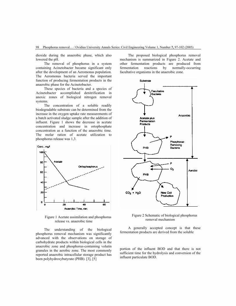
Phosphorus removal… / Ovidius University Annals Series: Civil Engineering Volume 1, Number 7, 97-102 (2005)
98
dioxide during the anaerobic phase, which also lowered the pH.
The removal of phosphorus in a system containing Acinetobacter became significant only after the development of an Aeromonas population. The Aeromonas bacteria served the important function of producing fermentation products in the anaerobic phase for the Acinetobacter.
These species of bacteria and a species of Acinetobacter accomplished denitrification in anoxic zones of biological nitrogen removal systems.
The concentration of a soluble readily biodegradable substrate can be determined from the increase in the oxygen uptake rate measurements of a batch activated sludge sample after the addition of influent. Figure 1 shows the decrease in acetate concentration and increase in ortophosphate concentration as a function of the anaerobic time. The molar ration of acetate utilization to phosphorus release was 1,3.
Figure 1 Acetate assimilation and phosphorus
release vs. anaerobic time The understanding of the biological
phosphorus removal mechanism was significantly advanced with the observations on storage of carbohydrate products within biological cells in the anaerobic zone and phosphorus-containing volutin granules in the aerobic zone. The most commonly reported anaerobic intracellular storage product has been polyhydroxybutyrate (PHB). [3], [5]
The proposed biological phosphorus removal mechanism is summarized in Figure 2. Acetate and other fermentation products are produced from fermentation reactions by normally-occurring facultative organisms in the anaerobic zone.
Figure 2 Schematic of biological phosphorus removal mechanism
A generally accepted concept is that these
fermentation products are derived from the soluble
portion of the influent BOD and that there is not sufficient time for the hydrolysis and conversion of the influent particulate BOD.

V. Creţu and V.Tobolcea / Ovidius University Annals Series: Civil Engineering 7, 97-102 (2005) 99
Table1-Typical Operating Conditions for Biological Phosphorus Removal Processes [6]
Phostrip Modified Bardenpho
Parameter Value Parameter Value AS System
F/M, kg TBOD/ kg MLVSS/d
1 F/M, kg TBOD/ kg MLVSS/d
01-0.2
SRT, days2 -1 SRT, days2 10-30 MLSS, mg/l 600-5,000 MLSS, mg/l 2,000-4,000
HRT, hr3 1-10 HRT, hr3 Anaerobic 1-2 Anoxic 1 2-4 Nitrification 4-12 (Aerobic 1) Anoxic 2 2-4 Aerobic 2 0.5-1.0
A/O A/O plus Nitrification Parameter Value Parameter Value
AS System F/M, kg TBOD/
kg MLVSS/d 02-07 F/M, kg TBOD/
kg MLVSS/d 015-0.25
SRT, days2 2-6 SRT, days2 4-8 MLSS, mg/l 2,000-4,000 MLSS, mg/l 3,000-5,000
HRT, hr3 HRT. hr3 Anaerobic 0.5-1.5 Anaerobic 0.5-1.5 Aerobic 1-3 Anoxic 0.5-1.0
Nitrification 3.5-6.0 Phostrip Stripper Feed, % of inf.
flow 20-30 Return Sludge, %
of inf. flow 100
SDT, hr 5-20 Int. Recycle, % of inf. flow
400
Sidewater Depth, m
6.1
Elutriation Flow, % of stripper feed
flow
50-100
Underflow, % of inf. flow
10-20
P Release, g P/g VSS
0.005-0.02
Reactor-Clanfier Overflow Rate,
m3/m2/d 48
pH 9-95 Lime Dosage,
mg/l 100-300
Phostrip Stripper Return Sludge, %
of inf. flow 25-40 Return Sludge, %
of inf. flow 20-50
Int. Recycle, % of inf. flow
100-300
The fermentation products are preferred and
readily assimilated and stored by the microorganisms capable of excess biological
phosphorus removal. This assimilation and storage is aided by the energy made available from the hydrolysis of the stored polyphosphates during the anaerobic period. The stored polyphosphate provides energy for active transport of substrate and for formation of acetoacetate, which is converted to PHB.
The fact that phosphorus-removing micro-organisms can assimilate the fermentation products in the anaerobic phase means that they have a competitive advantage compared to other normally-occurring microorganisms in activated sludge systems. [4].
There are three commercial biological phosphorus removal processes: the Phostrip process, the modified Bardenpho process and the A/O process. But, other options used are the UCT process, sequencing batch reactors (SBRs), and operationally modified activated sludge systems.
III.Design methodology 3.1. Phostrip process
The major design considerations for the Phostrip process are the size of the stripper and solids contact tanks and the lime feed rate.
The size of the solids contact tank will be a function of the stripper tank supernatant overflow rate.
This will be determinated by the return sludge feed rate to the stripper, the degree of solids thickening achieved, and the elutriation rate if the elutriate is composed of an outside flow instead of recycled stripper sludge. Typical values for stripper and reactor-clarifier design are given in table 1.
The stripper design procedure involves the following steps:
-determine or select the amount of return sludge that will pass through the stripper;
-select the stripper underflow sludge concentration;
-select the stripper SDT; -calculate the volume of sludge necessary in the
stripper; - using a solids flux analysis or appropiate solids
loadings, calculate the stripper area requirements; - determine the sludge depth in the stripper; - provide a selected supernatant water depth to
obtain the total stripper side water depth. The phosphorus removal efficiency was
correlated with three main operating parameters: the

Phosphorus removal… / Ovidius University Annals Series: Civil Engineering Volume 1, Number 7, 97-102 (2005)
100
amount of return sludge passing through the stripper relative to the plant flow, the stripper SDT, and the stripper supernatant flow. The correlation developed can be expressed as follows:
1,85-[log(100-E)]/2,11 = (SL-D)1/2 (SU) (1)
where: E – percent phosphorus removal; SL – return sludge passing through stripper
tank (100 lb dry solids/mil. gal of system influent flow);
D – SDT, h; SU – stripper supernatant flow as ratio of
influent flow.
3.2. Nitrate nitrogen removal design
Figure 3 illustrates the two modes of denitrification operation used in biological phosphorus removal systems. Nitrified mixed liquor is recycled to a pre-denitrification zone in the Modified Bardenpho process and also in the A/O process when nitrification occurs. In this zone, the incoming substrate drives the denitrification reaction as the facultative organisms use nitrate – released oxygen as the electron acceptor in lieu of DO.
The Modified Bardenpho process has a second anoxic tank, or post-denitrification zone. In the second anoxic zone, the denitrification rate is driven by the endogenous respiration oxygen demand as the mixed liquor since the influent substrate is depleted after the nitrification step.
The design objectives for biological phosphorus removal systems incorporating denitrification are to first determine the amount of nitrate nitrogen entering the pre-denitrification and post-denitrification zones and then to determine the volume of the anoxic zones. [7]
The first step in the design is the preparation of a mass balance to determine the amount of influent nitrogen that will be oxidized to nitrate nitrogen.
NO = No – NHe – Nsyn(2) where:
NO – amount of influent nitrogen converted to
oxidized nitrogen, mg/l; No – influent total nitrogen, mg/l; NHe – effluent ammonium nitrogen, mg/l; Nsyn - amount of influent nitrogen used in solids
synthesis, mg/l The amount of nitrogen used in syntesis can be
estimated from the amount of BOD removed, the net solids yield as a function of SRT, and the nitrogen content of the mixed liquor.
Nsyn = Yn(DBOD)Fn(3) where: Fn – fraction of nitrogen in mixed liquor solids,
g/g Once NO is determined, the next step is to
perform a mass balance describing the distribution of the nitrate produced in the nitrification zone, which results in the following:
N = NO/(R + r + 1)(4) where: N – nitrate nitrogen concentration in the
nitrification zone, mg/l; R – ratio of internal recycle flow (to the pre-
denitrification zone) to influent flow; R – ratio of return sludge flow to influent flow Equation (4) is applicable to both A/O and
Modified Bardenpho system designs. The rate of nitrate nitrogen addition to either denitrification zone can be calculated once the value of N is determined.
Anoxic 1 – Volume (applies to both A/O and Modified Bardenpho)
V1 = RQN/[(X)(SDNR1)](5) Anoxic 2 – Volume (Modified Bardenpho)
V2 = [(1 + r)NQ]/[(X)(SDNR2)] (6)
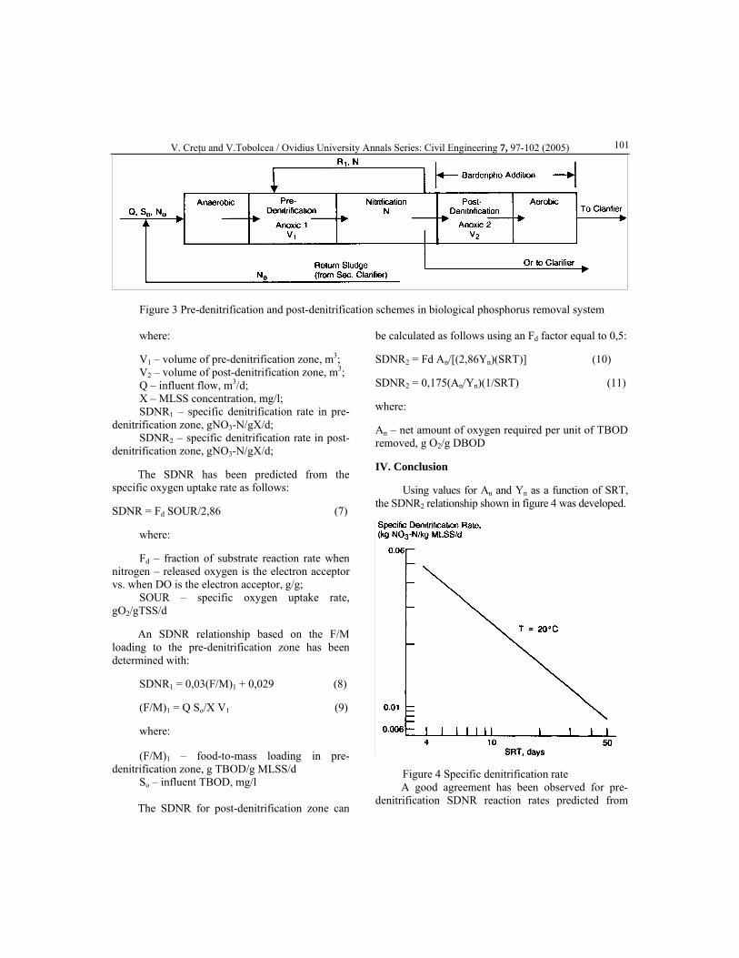
V. Creţu and V.Tobolcea / Ovidius University Annals Series: Civil Engineering 7, 97-102 (2005) 101
Figure 3 Pre-denitrification and post-denitrification schemes in biological phosphorus removal system
where: V1 – volume of pre-denitrification zone, m3; V2 – volume of post-denitrification zone, m3; Q – influent flow, m3/d; X – MLSS concentration, mg/l; SDNR1 – specific denitrification rate in pre-
denitrification zone, gNO3-N/gX/d; SDNR2 – specific denitrification rate in post-
denitrification zone, gNO3-N/gX/d; The SDNR has been predicted from the
specific oxygen uptake rate as follows:
SDNR = Fd SOUR/2,86 (7)
where: Fd – fraction of substrate reaction rate when
nitrogen – released oxygen is the electron acceptor vs. when DO is the electron acceptor, g/g;
SOUR – specific oxygen uptake rate, gO2/gTSS/d
An SDNR relationship based on the F/M
loading to the pre-denitrification zone has been determined with:
SDNR1 = 0,03(F/M)1 + 0,029 (8) (F/M)1 = Q So/X V1 (9) where: (F/M)1 – food-to-mass loading in pre-
denitrification zone, g TBOD/g MLSS/d So – influent TBOD, mg/l The SDNR for post-denitrification zone can
be calculated as follows using an Fd factor equal to 0,5: SDNR2 = Fd An/[(2,86Yn)(SRT)] (10) SDNR2 = 0,175(An/Yn)(1/SRT) (11) where: An – net amount of oxygen required per unit of TBOD removed, g O2/g DBOD IV. Conclusion
Using values for An and Yn as a function of SRT, the SDNR2 relationship shown in figure 4 was developed.
Figure 4 Specific denitrification rate A good agreement has been observed for pre-
denitrification SDNR reaction rates predicted from

Phosphorus removal… / Ovidius University Annals Series: Civil Engineering Volume 1, Number 7, 97-102 (2005)
102
treatment of a tannery wastewater in the presence of plentiful substrate and post-denitrification SDNR reaction rates predicted from endogenous respiration for domestic wastewater with limited available substrate.
The design procedure should check the TBOD:NO ratio to determine that there is sufficient TBOD available for amount of nitrate nitrogen to be reduced. A ratio of least 4:1 is recommended. In this case, there is sufficient TBOD available for denitrification. V. References [1]. Bosset, E. –“Eliminarea materiilor eutrofizante – a treia treapta de epurare a a pelor uzate”. In “La tehnique de l’eau”, 1970;
[2]. Beccari, M., Ramadari, R. -„Rimozione di azoto e fosforo dai liquani”, 1993,Editare Ulrico Hoepli, Milano,; [3]. Dima, M. - „Bazele epurării biologice a apelor uzate”, 2002, Ed. Tehnopress, Iaşi; [4].Lue –Hing ,C .–”Sludge Disposal and Management Alternatives”,1992, Lancaster, Pennsylvania : Technomic Publishing Company, Inc.; [5].Negulescu, M. - „Epurare apelor uzate orăşeneşti”, 1978, Ed. Tehnică, Bucureşti; [6]. Peschen, N. - „Phosphate Precipitation asign Line Honing regard to Nitrification and Denitrification”, 1989, Abwassertechnik, 4.0, nr. 1; [7]. Parker, H. W. – “Wastewater System Engineering”, New Jersey Edit P.E., 1975
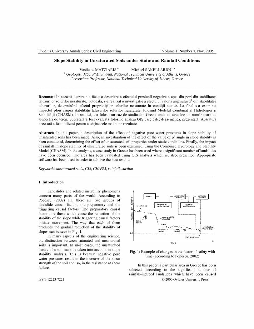
Ovidius University Annals Series: Civil Engineering Volume 1, Number 7, Nov. 2005
ISSN-12223-7221 © 2000 Ovidius University Press
Slope Stability in Unsaturated Soils under Static and Rainfall Conditions
Vasileios MATZIARIS a Michael SAKELLARIOU b a Geologist, MSc, PhD Student, National Technical University of Athens, Greece
b Associate Professor, National Technical University of Athens, Greece
__________________________________________________________________________________________ Rezumat: În această lucrare s-a făcut o descriere a efectului presiunii negative a apei din pori din stabilitatea taluzurilor solurilor nesaturate. Totodată, s-a realizat o investigaţie a efectului valorii unghiului φb din stabilitatea taluzurilor, determinând efectul proprietăţilor solurilor nesaturate în condiţii statice. La final s-a examinat impactul ploii asupra stabilităţii taluzurilor solurilor nesaturate, folosind Modelul Combinat al Hidrologiei şi Stabilităţii (CHASM). În analiză, s-a folosit un caz de studiu din Grecia unde au avut loc un număr mare de alunecări de teren. Suprafaţa a fost evaluată folosind analiza GIS care este, deasemenea, prezentată. Aparatura necesară a fost utilizată pentru a obţine cele mai bune rezultate. Abstract: In this paper, a description of the effect of negative pore water pressures in slope stability of unsaturated soils has been made. Also, an investigation of the effect of the value of φb angle in slope stability is been conducted, determining the effect of unsaturated soil properties under static conditions. Finally, the impact of rainfall in slope stability of unsaturated soils is been examined, using the Combined Hydrology and Stability Model (CHASM). In the analysis, a case study in Greece has been used where a significant number of landslides have been occurred. The area has been evaluated using GIS analysis which is, also, presented. Appropriate software has been used in order to achieve the best results. Keywords: unsaturated soils, GIS, CHASM, rainfall, suction __________________________________________________________________________________________ 1. Introduction
Landslides and related instability phenomena concern many parts of the world. According to Popescu (2002) [1], there are two groups of landslide causal factors, the preparatory and the triggering causal factors. The preparatory causal factors are those which cause the reduction of the stability of the slope while triggering causal factors initiate movement. The way that each of them produces the gradual reduction of the stability of slopes can be seen in Fig. 1.
In many aspects of the engineering science, the distinction between saturated and unsaturated soils is important. In most cases, the unsaturated nature of a soil must be taken into account in slope stability analysis. This is because negative pore water pressures result in the increase of the shear strength of the soil and, so, in the resistance at shear failure.
Fig. 1: Example of changes in the factor of safety with
time (according to Popescu, 2002)
In this paper, a particular area in Greece has been selected, according to the significant number of rainfall-induced landslides which have been caused

Slope stability in … / Ovidius University Annals Series: Civil Engineering Volume 1, Number 7, 103-110 (2005)
104
there. This area has been evaluated using a GIS tool (Landslide Hazard Analysis – LHA) according to the landslide hazard. From this area, a specific slope selected so as to perform a more accurate analysis.
At first, the analysis includes the investigation of the effect of an unsaturated property, φb angle, in slope stability. In this way, the significance of the unsaturated nature of a soil in slope stability analysis will be determined. For this reason, Slope/W software provided by GeoSlope Ltd. will be used. Then, the effect of rainfall in slope stability of unsaturated soils will be investigated. The Combined Hydrology and Stability Model (CHASM) will be used for the analysis as it has the advantage of generating pore water pressures in slope stability analysis. 2.1 Partially saturated soils
The main difference between saturated and unsaturated soils is on the pore water pressures. In saturated soils pore water pressures are positive which is unfavorable for the shear strength of the soil. According to Terzaghi (1936), the shear strength of the saturated soils can be described by Eq.(1):
'tan)(' φστ fwfff uc −+= (1)
where τff the shear stress on the failure plane at failure, c’ and φ’ the effective shear strength parameters and (σf – uw)f the effective normal stress on the failure plane at failure
Fredlund (1978) introduced the fundamental equation for the shear strength of unsaturated soils (Eq.(2)):
b
fwafafff uuuc ϕϕστ tan)('tan)(' −+−+= (2)
where (σf-uα)f is the net normal stress state on the failure plane at failure and φb an angle which indicates the rate of the increase of the shear strength of the soil due to matric suction. This angle can take values between zero and φ’. When φb is zero, suction does not have any effect on the shear strength, while for a value equal to φ’
suction causes the major increment on the shear strength.
We call suction the difference between the pore air pressure and the pore water pressure (ua-uw). At shallow depths, suction is equal to the negative pore water pressure of the soil; as the pore air pressure can be consider negligible [2]. Suction has two components, the matric and the osmotic suction. Total suction is equal to the sum of the two components. However, in most cases total suction is equal to the matric suction, as the osmotic component is negligible. The negative values of the water pressure are located in a zone above the water table, which is called capillary or unsaturated zone. Unsaturated soils occur either as a natural material in dry environments, or as an artificial material by remolding and compacting a mixture of dry soil and water. Natural unsaturated soils are occurring over large areas of the earth while compacted unsaturated soils are commonly used as a construction material [3].
Eq.(2) is the extension to the unsaturated domain of the saturated equation of shear strength and it is referred to as the “extended Mohr-Coulomb failure envelope”. The extended Mohr-Coulomb failure envelope for unsaturated soils can be seen in Fig. 2.
Fig. 2: Extended Mohr-Coulomb failure envelope for
unsaturated soils
Comparison of Eq.(1) and Eq.(2) show that in unsaturated soils there is an apparent component of the shear strength equal to “(ua-uw)·tanφb”. This component appears due to suction and becomes equal to zero when the soil re-saturates.
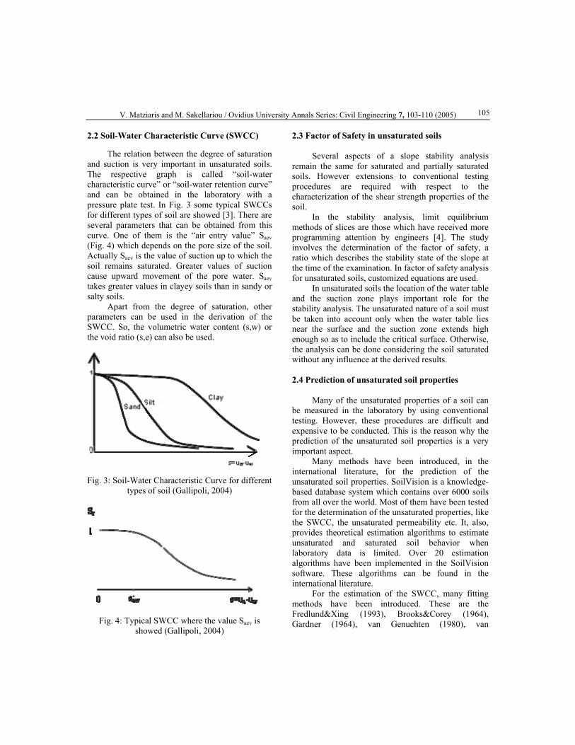
V. Matziaris and M. Sakellariou / Ovidius University Annals Series: Civil Engineering 7, 103-110 (2005) 105 2.2 Soil-Water Characteristic Curve (SWCC)
The relation between the degree of saturation and suction is very important in unsaturated soils. The respective graph is called “soil-water characteristic curve” or “soil-water retention curve” and can be obtained in the laboratory with a pressure plate test. In Fig. 3 some typical SWCCs for different types of soil are showed [3]. There are several parameters that can be obtained from this curve. One of them is the “air entry value” Saev (Fig. 4) which depends on the pore size of the soil. Actually Saev is the value of suction up to which the soil remains saturated. Greater values of suction cause upward movement of the pore water. Saev takes greater values in clayey soils than in sandy or salty soils.
Apart from the degree of saturation, other parameters can be used in the derivation of the SWCC. So, the volumetric water content (s,w) or the void ratio (s,e) can also be used.
Fig. 3: Soil-Water Characteristic Curve for different
types of soil (Gallipoli, 2004)
Fig. 4: Typical SWCC where the value Saev is showed (Gallipoli, 2004)
2.3 Factor of Safety in unsaturated soils
Several aspects of a slope stability analysis remain the same for saturated and partially saturated soils. However extensions to conventional testing procedures are required with respect to the characterization of the shear strength properties of the soil.
In the stability analysis, limit equilibrium methods of slices are those which have received more programming attention by engineers [4]. The study involves the determination of the factor of safety, a ratio which describes the stability state of the slope at the time of the examination. In factor of safety analysis for unsaturated soils, customized equations are used.
In unsaturated soils the location of the water table and the suction zone plays important role for the stability analysis. The unsaturated nature of a soil must be taken into account only when the water table lies near the surface and the suction zone extends high enough so as to include the critical surface. Otherwise, the analysis can be done considering the soil saturated without any influence at the derived results. 2.4 Prediction of unsaturated soil properties
Many of the unsaturated properties of a soil can be measured in the laboratory by using conventional testing. However, these procedures are difficult and expensive to be conducted. This is the reason why the prediction of the unsaturated soil properties is a very important aspect.
Many methods have been introduced, in the international literature, for the prediction of the unsaturated soil properties. SoilVision is a knowledge-based database system which contains over 6000 soils from all over the world. Most of them have been tested for the determination of the unsaturated properties, like the SWCC, the unsaturated permeability etc. It, also, provides theoretical estimation algorithms to estimate unsaturated and saturated soil behavior when laboratory data is limited. Over 20 estimation algorithms have been implemented in the SoilVision software. These algorithms can be found in the international literature.
For the estimation of the SWCC, many fitting methods have been introduced. These are the Fredlund&Xing (1993), Brooks&Corey (1964), Gardner (1964), van Genuchten (1980), van

Slope stability in … / Ovidius University Annals Series: Civil Engineering Volume 1, Number 7, 103-110 (2005)
106
Genuchten&Mualem (1976) and van Genuchten& Burdine (1953). The first one is considered to be the most accurate and it is used more often than the others. The equation that is used is the following (Eq.3) [5]:
( )⎥⎥⎥⎥⎥⎥⎥
⎦
⎤
⎢⎢⎢⎢⎢⎢⎢
⎣
⎡
⎥⎥
⎦
⎤
⎢⎢
⎣
⎡
⎥⎥
⎦
⎤
⎢⎢
⎣
⎡
⎟⎟⎠
⎞⎜⎜⎝
⎛+⎥
⎥⎥⎥⎥
⎦
⎤
⎢⎢⎢⎢⎢
⎣
⎡
⎟⎟⎠
⎞⎜⎜⎝
⎛+
⎟⎟⎠
⎞⎜⎜⎝
⎛+
−=f
fmn
fr
rsw
h
hww
αψ
ψ
1expln
1101ln
1ln1
6
(3)
where: ww the gravimetric water content at any soil suction, ψ the soil suction, ws the saturated gravimetric water content, αf a soil parameter which is primarily a function of the air entry value of the soil in kPa, nf a soil parameter which is a function of the rate of water extraction from the soil once the air entry value has been exceeded, mf a soil parameter that depends on the residual water content and hr the value of suction at which residual water content occurs. The advantage of this equation is that it can be applied in all kinds of soils. The above estimation has been used in this paper. 2.5 Rainfall effect on slope stability of unsaturated soils
It is, generally, accepted that rainfall affects the stability of slopes and can cause landslides. The way that rainfall causes the reduction of the slope stability is by infiltration of the rainfall water through the porous media of the soil. It is important to know the kind of the water flow, i.e. if the flow is transient or steady-state, because these have different affect on the stability’s reduction. The reduction of the shear strength of the soil can occur either by the rise of the water table or by the flow itself. In these cases suction zone tends to disappear resulting on the loss of the apparent component of the shear strength. So, the shear resistance of the soil at the base of the critical slip failure decreases and the factor of safety takes smaller values.
The phenomenon is more intense in areas with tropical climate where the evaporation rate is very high. Long dry periods cause long periods of evaporation and so the water from the aquifer tends
to rise on the surface. The development of the suction zone in these cases extends up to the surface and causes significant changes in the shear strength. In Fig. 6, a normal distribution of the pore water pressure in respect to the depth is presented for three different cases: at a normal period of dryness, at an extended period of dryness and after a rainfall event, according to Toll (2004). In most cases, landslides in tropical and subtropical areas occur during heavy rainfall events, which come after long dry periods [6].
Fig. 4: Distribution of the pore water pressure with depth after: a normal period of dryness (1), an
extended period of dryness (2) and rainfall (3), according to Toll (2004).
2.6 Combined Hydrology and Stability Model
In order to perform a stability analysis involving hydrology conditions, the Combined Hydrology and Stability Model (CHASM) can be used [7]. This is a model for the simulation of the dynamic hydrological condition in an area. It has the advantage of coupling the generated pore pressures (either positive or negative) with slope stability analysis. The model simulates dynamic stability conditions, allowing identification of the minimum factor of safety, the characteristics of the failure and the time of occurrence for any particular initial slope condition and rainfall event. The main characteristics of the model are: 1. A dynamic two-dimensional hillslope hydrology model is coupled directly to a two-dimensional slope stability model. 2. Both, positive and negative pore pressures are been calculated at each iteration period, taking into

V. Matziaris and M. Sakellariou / Ovidius University Annals Series: Civil Engineering 7, 103-110 (2005) 107 consideration their change due to the rainfall events. Each hour of the simulation the current hydrological conditions of the soil are used in order for the factor of safety to be predicted. 3. The stability model accounts for the influence of both pore water pressures and suctions on the strength conditions using effective stress concept. 4. Both individual models are able to accommodate potential uncertainty in the input parameter values. The procedure adopted in the modeling of the slope hydrological system is a forward difference explicit, block-centered finite difference scheme [7]. The type of the analysis is two-dimensional. The stability model uses Bishop Method in order to predict each hour the factor of safety of the slope in respect to the hydrology conditions. The fact that negative pore pressures are been taken into account in the analysis give the ability for partially saturated soils to be studied. The parameters that have to be designated are: evaporation, rainfall parameters, initial surface soil water conditions, initial groundwater table, slope height, slope angle, permeability and the soil strength parameters (c’ and φ’). Finally, the unsaturated parameters of the soil (zone that suction extends, φb angle) can be, also, designated. 2.7 The area of concern – Analysis using GIS
The area of concern lies in the North Peloponnesus where a significant number of rainfall-induced landslides have been occurred [8]. The geological formations that can be found in the area are, mostly, conglomerates, sand, clay and sandstone. We only take into consideration slopes formed by soils and not by rock. The available geotechnical properties that will be used for the analysis can be seen in Table 1.
Table 1: Geotechnical properties of soils in the area
of concern
Qc-l Q.f,c-l Qc-cm Q.f,c-cm Plc Pl.f-c γ
(kN/m3) 21.5 19.35 22.8 20 25 14
c’ (kPa) 49.05 68.95 250 200 1250 10 φ’ (º) 37.5 25 45 36 49 20
Figures 5 and 6 shows the geological map of the
area and the derived map coming from the analysis with GIS, respectively.
Fig.5: Geological map of the area of concern For the GIS analysis, a dynamic tool has been
used, Landslide Hazard Analysis (LHA) [9]. The procedure followed for the analysis will not be mentioned further, however one can find more in the literature [10], [11].
Fig. 6: Thematic map of the area of concern, indicating
the distribution of the factor of safety
The thematic map in Fig.6 indicates the distribution of the FoS in the area of concern. In this way, we can have a first indication about the most dangerous slopes in the area, those in which the FoS is smaller than 1.5. In general, a slope with FoS greater than 1.5 is considered to be safe against failure.
In order to perform a more accurate analysis, we selected a slope (cross-section 1 in Fig.6) which seems to have a static FoS between 1 and 1.5. The geological formation which forms this slope is the Pl.f-c whose geotechnical properties are showed in Table 1. In Fig.

Slope stability in … / Ovidius University Annals Series: Civil Engineering Volume 1, Number 7, 103-110 (2005)
108
7 the geometry of the selected slope can be seen, as well as the critical slip surface for saturated conditions. The static factor of safety, using Bishop’s method of slices, has been determined to be 1.476, something which confirms the GIS analysis.
1.476
Distance-5 0 5 10 15 20 25 30 35 40 45
Alti
tude
-5
0
5
10
15
20
25
30
35
Fig. 7: Cross-section 1 and slope stability analysis
under satura-ted conditions 3. The impact of suction in static FoS
The determination of the impact of suction in
slope stability of unsaturated soils will be determined by using Slope/W software, provided by GeoSlope Ltd. This is the most appropriate software for this kind of analysis, as it enables for unsaturated soil properties to be taken into account. In this stage, we have used different values for φb angle for the soil formation Pl.f-c so as to determine how this angle affects the FoS. When the soil is considered saturated, φb angle is becoming zero. As mentioned before, the greatest value that φb angle can take is to be equal to φ’. In this case, the shear strength of the soil takes its greatest value due to suction. Slope stability is been affected respectively, as the resistance of the slope at failure depends mostly on the shear strength.
y = 0.3599x + 1.4773
FoS=0.3599tanφb+FoSsat
1.46
1.48
1.5
1.52
1.54
1.56
1.58
1.6
0 0.05 0.1 0.15 0.2 0.25 0.3 0.35
tanφb
FoS
Fig. 8: Variation between FoS and φb angle
The performed analysis confirms what mentioned above, i.e. increments of φb angle result in the increase of the FoS, as Fig. 8 shows. The fact that this relationship in linear is observable. The relationship is the following:
satb FoSFoS += φtan3599.0 (4)
where FoSsat is the FoS for saturated conditions (φb=0). Eq. 4 can not be used in general, because it depends on the relative position of the slip surface to the unsaturated zone and on the hydrological conditions of the slope. However, it indicates how FoS changes when the soil, which forms the slope, is considered to be unsaturated. 4. The impact of rainfall in slope stability of unsaturated soils
As mentioned before, the impact of rainfall in the stability of unsaturated soils can be studied by using CHASM. The choice of this software has been made due to its ability to couple the hydrological conditions into the stability analysis.
The slope showed in Fig. 7 will be examined for its stability during and after a rainfall event. Rainfall rate and duration are two parameters that must be inserted in CHASM. For this reason, a statistical method has been used in order to estimate the maximum rainfall rate in the particular area of Greece (North Peloponnesus) in respect to the rainfall duration and the restoration period [12]. According to this method, the maximum rainfall rate for duration of 24

V. Matziaris and M. Sakellariou / Ovidius University Annals Series: Civil Engineering 7, 103-110 (2005) 109
hours in the area is 8.25mm/hr. So, this is the rate that has been used in the analysis.
The simulation went on for 72 hours assuming that after the 24hours period there is no rainfall. This is done so as to notice the reaction of the slope the period exactly after the rainfall event.
In order to perform a more accurate analysis, the unsaturated properties of the soil formations have been calculated using SoilVision. All the available information, concerning the mass-volume properties of the soil, has been derived by Rozos (1998) [13].
Fig. 9: Predicted SWCC for soil Pl-f.c, according to
Fredlund and Xing method
Using the available information about the geological formation Pl.f-c, it became possible to estimate its SWCC. This can be seen in Fig. 9. The method used for the prediction is the Fredlund & Xing. Before that, the grain-size distribution had to be estimated taking into consideration the geological description of the soil. The predicted curve can be seen in Fig. 10.
Fig. 10: Estimation of the particle-size distribution
for Pl-f.c formation
The results from the analysis, using CHASM can
be seen in Fig.11.
0.8
0.9
1
1.1
1.2
1.3
1.4
1.5
1.6
1.7
0 10 20 30 40 50 60 70
Time (hours)
Fact
or o
f Saf
ety
Fig. 11: Variation of FoS with time, during and after the rainfall event
Figure 11 shows the value of the factor of safey
for each hour of the rainfall event. It is obvious that during rainfall, the stability of the slope reduces as the factor of safety becomes smaller. This reduction is gradual and there is not linear relatioship between factor of safety and time. At the start of the simulation, the factor of safety was equal to 1.6. After 24 hours of rainfall, factor of safety becomes equal to 1.2. Even if rainfall stops at that time, the reduction continues up to the 27th hour, because of the infiltration of the rainfall water through the soil pores. Due to the small value of the soil permeability, the infiltration of the water has a delay, resulting in the delayed reaction of the slope stability.
After the 28th hour, the factor of safety seems to be restored to its initial value. So, there is a gradual increment of FoS which continues for a long time period. Normally, after a long time period, the factor of safety will take values near the initial one. This fact shows that the decreament of the slope stability is an impermanent procedure which lasts only untill few hours after the rainfall event. So, rainfall-induced landslides can be caused only when the initial FoS is small enough. In these cases, a rainfall event can cause the instant reduction of the slope stability which can lead to a landslide.
The influence of permeability is also important. The permeability of the soil controls the amount of water which infiltrates through the voids. When the value of the coefficient k is small (smaller than 10-7 m/s) then the impact of rainfall in slope stability of
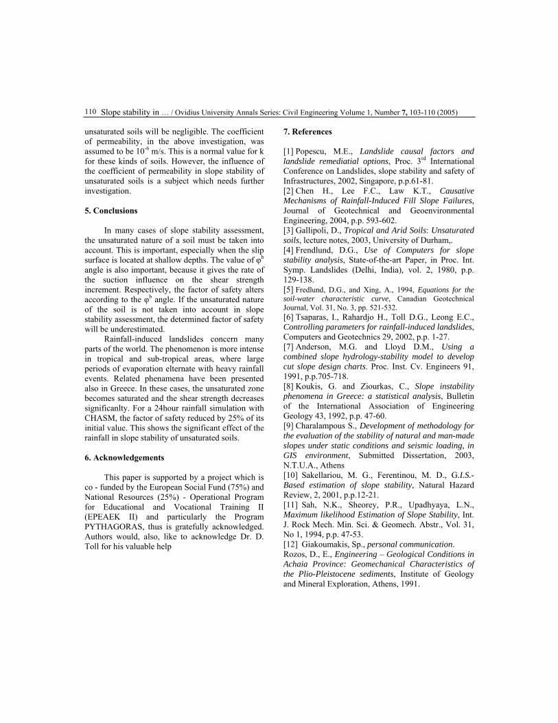
Slope stability in … / Ovidius University Annals Series: Civil Engineering Volume 1, Number 7, 103-110 (2005)
110
unsaturated soils will be negligible. The coefficient of permeability, in the above investigation, was assumed to be 10-6 m/s. This is a normal value for k for these kinds of soils. However, the influence of the coefficient of permeability in slope stability of unsaturated soils is a subject which needs further investigation.
5. Conclusions
In many cases of slope stability assessment, the unsaturated nature of a soil must be taken into account. This is important, especially when the slip surface is located at shallow depths. The value of φb angle is also important, because it gives the rate of the suction influence on the shear strength increment. Respectively, the factor of safety alters according to the φb angle. If the unsaturated nature of the soil is not taken into account in slope stability assessment, the determined factor of safety will be underestimated.
Rainfall-induced landslides concern many parts of the world. The phenomenon is more intense in tropical and sub-tropical areas, where large periods of evaporation elternate with heavy rainfall events. Related phenamena have been presented also in Greece. In these cases, the unsaturated zone becomes saturated and the shear strength decreases significanlty. For a 24hour rainfall simulation with CHASM, the factor of safety reduced by 25% of its initial value. This shows the significant effect of the rainfall in slope stability of unsaturated soils. 6. Acknowledgements
This paper is supported by a project which is co - funded by the European Social Fund (75%) and National Resources (25%) - Operational Program for Educational and Vocational Training II (EPEAEK II) and particularly the Program PYTHAGORAS, thus is gratefully acknowledged. Authors would, also, like to acknowledge Dr. D. Toll for his valuable help
7. References [1] Popescu, M.E., Landslide causal factors and landslide remediatial options, Proc. 3rd International Conference on Landslides, slope stability and safety of Infrastructures, 2002, Singapore, p.p.61-81. [2] Chen H., Lee F.C., Law K.T., Causative Mechanisms of Rainfall-Induced Fill Slope Failures, Journal of Geotechnical and Geoenvironmental Engineering, 2004, p.p. 593-602. [3] Gallipoli, D., Tropical and Arid Soils: Unsaturated soils, lecture notes, 2003, University of Durham,. [4] Frendlund, D.G., Use of Computers for slope stability analysis, State-of-the-art Paper, in Proc. Int. Symp. Landslides (Delhi, India), vol. 2, 1980, p.p. 129-138. [5] Fredlund, D.G., and Xing, A., 1994, Equations for the soil-water characteristic curve, Canadian Geotechnical Journal, Vol. 31, No. 3, pp. 521-532. [6] Tsaparas, I., Rahardjo H., Toll D.G., Leong E.C., Controlling parameters for rainfall-induced landslides, Computers and Geotechnics 29, 2002, p.p. 1-27. [7] Anderson, M.G. and Lloyd D.M., Using a combined slope hydrology-stability model to develop cut slope design charts. Proc. Inst. Cv. Engineers 91, 1991, p.p.705-718. [8] Koukis, G. and Ziourkas, C., Slope instability phenomena in Greece: a statistical analysis, Bulletin of the International Association of Engineering Geology 43, 1992, p.p. 47-60. [9] Charalampous S., Development of methodology for the evaluation of the stability of natural and man-made slopes under static conditions and seismic loading, in GIS environment, Submitted Dissertation, 2003, N.T.U.A., Athens [10] Sakellariou, M. G., Ferentinou, M. D., G.I.S.-Based estimation of slope stability, Natural Hazard Review, 2, 2001, p.p.12-21. [11] Sah, N.K., Sheorey, P.R., Upadhyaya, L.N., Maximum likelihood Estimation of Slope Stability, Int. J. Rock Mech. Min. Sci. & Geomech. Abstr., Vol. 31, No 1, 1994, p.p. 47-53. [12] Giakoumakis, Sp., personal communication. Rozos, D., E., Engineering – Geological Conditions in Achaia Province: Geomechanical Characteristics of the Plio-Pleistocene sediments, Institute of Geology and Mineral Exploration, Athens, 1991.