Sizing of Analog Cells by means of a Tabu Search

Approach

M.A. Aguirre, A.Torralba, J. Chavez, L. G. Franquelo

Dpto. de Ingenierıa Electronica

Escuela Superior de Ingenieros,

Avda. Reina Mercedes s/n, Sevilla–41012 (SPAIN)

e–mail: torralba@gtex02.us.es

Abstract

Although many design tools have been developed for digital design, analog design tools are only just being introduced.

This paper presents a new optimization method for automatically sizing the circuit topology of analog cells. This method

minimizes a cost function, which depends on a set of designer specifications. It employs the tabu search heuristic to avoid being

trapped in a local minimum of the cost function. Experimental results show that this method can get very close to the global

minimum of the cost function with a small number of iterations. Hence, an analog simulation program, such as SPICE, can be

used for the evaluation of the cost function at each iteration.

1

I. INTRODUCTION

There is an increasing trend towards the integration of analog blocks in ASIC circuits. Despite the great effort

that has been made in the development of CAD tools for analog and mixed circuits, the design of the analog

part of a chip continues to be a bottleneck [1]–[2].

Different optimization techniques have been used in the design of analog cells. An early review of these

techniques can be found in [3]. Other recentwork in this field can be found in [4]–[11]. Usually, the optimization

process is converted to a minimization problem by the formulation of a cost function. Different techniques

have been applied to minimize the cost function. Due to the complex dependencies that exist between design

parameters and circuit performances, these techniques can converge to a local minimum, whose performance is

significatively worse than the circuit’s best capabilities. In this sense, only statistical techniques, like Simulated

Annealing (SA) can assure optimal results at the expense of a high computational cost [12]–[14]: e.g., more than

100,000 simulations have been reported for the design of an op.amp., using an SA method.

To avoid using a complex circuit simulation program to evaluate the cost function at each iteration, simple

analytical models of the circuit have been used. These analytical models are created by good expert designers,

or automatically generated (up to some extent), by means of symbolic simulators [15].

However, as technology progresses, devices are scaled down, and simple analytical models become inaccurate.

In this case, an accurate estimation of the circuit performances requires the use of an analog simulation program

like SPICE to evaluate the cost function at each iteration, leading to excessively large computation times.

This paper presents a new optimization method for sizing the circuit topology of analog cells. This method is

based on a Tabu–Search (TS) heuristic [16]–[18]. The main characteristic of the TS heuristic is its ability to escape

from localminimabymaintaining a list of forbiddenmoves. This approach obtains excellent results with a small

number of iterations, allowing the use of an analog simulation program for the evaluation of the cost function.

As the proposed method uses SPICE to estimate circuit performances, there is no need to provide analytical

equations describing circuit behaviour.

This paper is organized as follows. Section II introduces the Tabu Search Heuristic. Section III presents the

Tabu Search algorithm proposed for the optimization process. Section IV describes the cost function for analog

cells optimization. Section V presents the results obtained with the proposed method and different topologies

of op.amps. Section VI addresses final conclusions.

2

II. THE TABU SEARCH HEURISTIC

Tabu–Search is a strategy to solve complex optimization problems. Due to F.Glover, TS has its origins in

combinatorial procedures applied to solve nonlinear problems in the late 1970’s, and it was subsequently

applied to a collection of different problems, such as general integer programming, task scheduling, graph

colouring, etc [16]–[18].

This section introduces Tabu Search concepts which are the origin of the method proposed in Section III.

Consider an optimization problem

Minimize c(x) : x 2 X in Rn (1)where the objective function c(x)may be linear or nonlinear, with or without constraints.A great number of solutions to this problem use a sequence of movements which lead from a trial solution to

another. We will define a move s to consist of a mapping defined on a subsetX(s) ofX .Associated with x 2 X is the set S(x) which consists of the moves s 2 S that can be applied to xS(x) = fs 2 S; x 2 X(s)g (2)S is considered to be a neighbourhood function.The class of hill climbing heuristics1 only accepts moves which lead to a decrease in the cost function. These

methods are able to find one minimum, although there is no any guarantee that it is the global minimum of

the cost function. Tabu search includes additional elements in the heuristic that guides the search to continue

exploration without becoming confused by an absence of improving moves, andwithout falling back into a local

minimum from which it previously emerged.

To this purpose, a subsetT ofS ismaintainedwhose elementsare called tabumoves. Theelements inT summarizethe history of the search process up to t iterations in the past. The objective of the tabu set is to mark searchregions which have already been visited. For an appropiately determined T and an evaluator function denotedOPTIMUM , subsequentlydefined in greater detail, the tabu search proceduremay be described as follows [16]Tabu Search Procedure

1the hill is inverted in a minimization problem

3

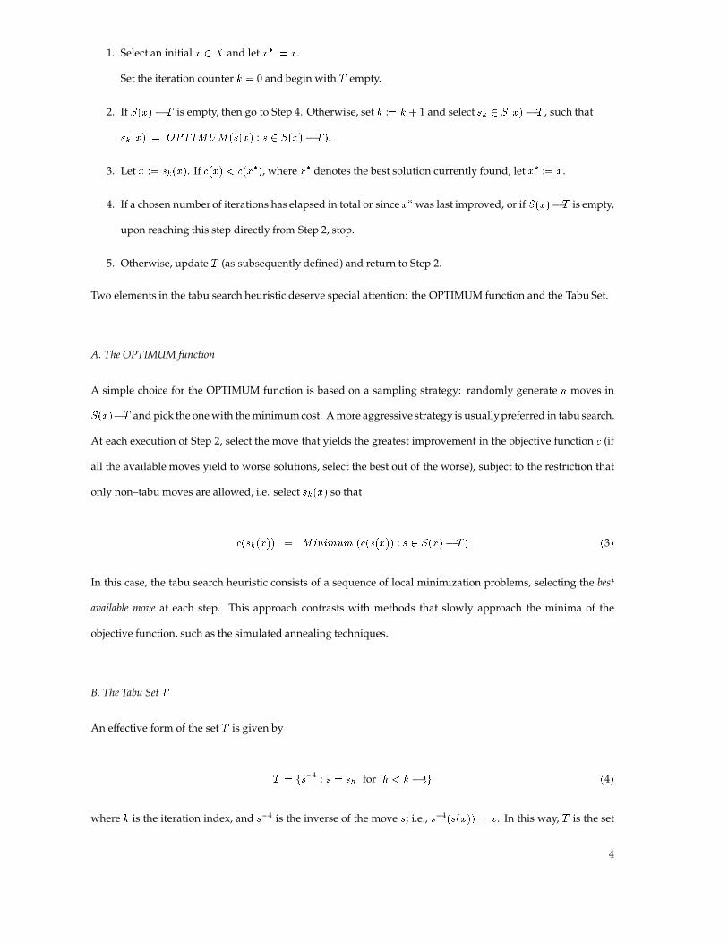
1. Select an initial x 2 X and let x� := x.Set the iteration counter k = 0 and begin with T empty.

2. If S(x)� T is empty, then go to Step 4. Otherwise, set k := k + 1 and select sk 2 S(x)� T , such thatsk(x) = OPTIMUM(s(x) : s 2 S(x)� T ).3. Let x := sk(x). If c(x) < c(x�), where x� denotes the best solution currently found, let x� := x.4. If a chosen number of iterations has elapsed in total or since x� was last improved, or if S(x)�T is empty,upon reaching this step directly from Step 2, stop.

5. Otherwise, update T (as subsequently defined) and return to Step 2.Two elements in the tabu search heuristic deserve special attention: the OPTIMUM function and the Tabu Set.

A. The OPTIMUM function

A simple choice for the OPTIMUM function is based on a sampling strategy: randomly generate n moves inS(x)�T and pick the onewith theminimumcost. Amore aggressive strategy is usuallypreferred in tabu search.At each execution of Step 2, select the move that yields the greatest improvement in the objective function c (ifall the available moves yield to worse solutions, select the best out of the worse), subject to the restriction that

only non–tabu moves are allowed, i.e. select sk(x) so thatc(sk(x)) = Minimum (c(s(x)) : s 2 S(x)� T ) (3)In this case, the tabu search heuristic consists of a sequence of local minimization problems, selecting the best

available move at each step. This approach contrasts with methods that slowly approach the minima of the

objective function, such as the simulated annealing techniques.

B. The Tabu Set TAn effective form of the set T is given byT = fs�1 : s = sh for h < k � tg (4)where k is the iteration index, and s�1 is the inverse of the move s; i.e., s�1(s(x)) = x. In this way, T is the set

4

of those moves that would reverse one of the moves made in the t most recent iterations of the search process.The operation of updating T at Step 3 of the tabu search procedure, consists of setting T := T � s�1k�t + s�1k .The main goal of T is to avoid returning to a previously visited solution. By preventing the selection of thosemoves that would reverse one of the moves in a sequence of t iterations, the procedure moves away from all thesolution states of the previous t iterations, and for t appropiately large, the likelihood of cycling vanishes.The Tabu Set concept, as defined in (4), is not easy to realize due to a number of reasons. Inmost of the problems

where Tabu Search finds an application, it is not possible to select, in an efficient way, the set of moves s whichlead to the same solution sh. In practice, the set T is implemented by means of a list of the last accepted moves(the tabu list) and a set of attributes associated to each one, which, approximately contain (4).

C. The Aspiration Level Concept

As elements other than s�1h are allowed to enter in T , the tabu statusmay also forbid moves leading to unvisitedsolutions, that may be attractive. Hence, a newmechanismhas to be devised to allow the acceptatance of a tabu

move, provided that this move gives a solution that has certain good attributes. This mechanism is called the

aspiration level. Different implementations of the aspiration level concept have been proposed, although most of

them are dependent on the problem.

The aspiration level in its simplest form has been considered in this paper: consider a tabu move s; if this moveyields to a solution which is better than the best solution currently found, then accept s in spite of its tabu status.

III. TABU SEARCH IN A CONTINUOUS SPACE

Existing applications of Tabu Search have been focused in combinatorial problems. In this paper, an extension

of the original TS heuristic to the case of a continous parameter space is proposed. The proposed algorithm

maintains the structure of the Tabu Search Procedure as defined in section II. The OPTIMUM function and

the structure of the Tabu Set, which have been selected for the continuous case, are described here.

A. The OPTIMUM function

As previouslymentioned, the OPTIMUMfunction could be implemented bymeans of random sampling around

the current solution. Amore efficient implementation of theOPTIMUMfunction tries to solve the localminimiza-

5

tion problem defined in (3), bymeans of a gradential technique: steppest descendent, Newton or quasi–Newton

methods or conjugate gradient [19].

To this purpose, the OPTIMUM function used in this paper employs a multistart gradential search strategy

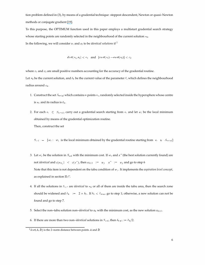
whose starting points are randomly selected in the neighbourhood of the current solution sk .In the following, we will consider s1 and s2 to be identical solutions if 2dist(s1; s2) < "1 and jcost(s1)� cost(s2)j < "2where "1 and "2 are small positive numbers accounting for the accuracy of the gradential routine.Let sk be the current solution, and �k be the current value of the parameter �, which defines the neighbourhoodradius around sk .1. Construct the setStrial which containsn points vi, randomly selected inside the hyperspherewhose centreis sk and its radius is �k .

2. For each vi 2 Strial , carry out a gradential search starting from vi and let wi be the local minimumobtained by means of the gradential optimization routine.

Then, construct the setSsol = fwi : wi is the local minimum obtained by the gradential routine starting from vi 2 Strialg3. Let wj be the solution in Ssol with the minimum cost. If wj and x� (the best solution currently found) arenot identical and c(swj ) < c(x�), then sk+1 := wj x� := wj and go to step 6Note that this item is not dependent on the tabu condition of wj . It implements the aspiration level concept,as explained in section II.C .

4. If all the solutions in Ssol are identical to sk or all of them are inside the tabu area, then the search zoneshould be widened and �k := 2 � �k . If �k < �max go to step 1; otherwise, a new solution can not befound and go to step 7.

5. Select the non–tabu solution non–identical to sk with the minimum cost, as the new solution sk+1.6. If there are more than two non–identical solutions in Ssol , then �k+1 := �k=2.2dist(A;B) is the 2–norm distance between points A and B

6

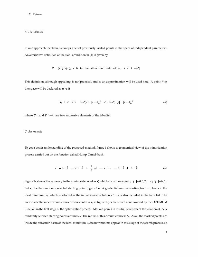
7. Return.

B. The Tabu Set

In our approach the Tabu list keeps a set of previously visited points in the space of independent parameters.

An alternative definition of the status condition in (4) is given byT = fs 2 S(x); s is in the attraction basin of sh; h < k � tgThis definition, although appealing, is not practical, and so an approximation will be used here. A point P inthe space will be declared as tabu if9i; 1 < i < t dist(P;T [i� 1])2 < dist(T [i]; T [i� 1])2 (5)where T [i] and T [i � 1] are two successive elements of the tabu list.C. An example

To get a better understanding of the proposed method, figure 1 shows a geometrical view of the minimization

process carried out on the function called Hump Camel–back.y = 4 x21 � 2:1 x41 + 1

3x61 � x1 x2 � 4 x22 + 4 x42 (6)

Figure 1a shows the value of y in theminima (denoted as �) which are in the rangex1 2 [�0:5;2] x2 2 [�1;1].Let sin be the randomly selected starting point (figure 1b). A gradential routine starting from sin leads to thelocal minimum s0, which is selected as the initial optimal solution x�. s0 is also included in the tabu list. Thearea inside the inner circumference whose centre is s0 in figure 1c, is the search zone covered by the OPTIMUMfunction in the first stage of the optimization process. Marked points in this figure represent the location of the nrandomly selected starting points around s0. The radius of this circumference is �0. As all the marked points areinside the attraction basin of the local minimum s0, no newminima appear in this stage of the search process, so

7

that �0 is doubled and n new random points are generated around s0. Now, the gradential routine starting fromv1 leads to a new minimum s1, which is accepted as the new current solution and included in the tabu list. Ascost(s1) < cost(x�), s1 is also considered to be the new optimal solution x�. Figure 1d shows the tabu area andthe search zone (the area inside the circumference whose centre is s1) in this stage of the optimization process.In the next iteration, the starting point v2 in figure 1d leads to a new local optimum s2, while v3 leads to s0 again.As s0 is inside the tabu area, s2 is selected as the new current solution. s2 is then included in the tabu list. Besides,s2 is a global minimum and x� is updated accordingly.The optimization process will still continue until niter iterations has elapsed without improving the optimalsolution x�, or until � � �max.D. Process Parameters

In short, the proposed method goes through a sequence of local minima of the objective function, performing a

multistart gradential search around each one.

A number of parameters have been introduced in the description of the proposed method. Their influence on

the final results is discussed here.� The number of searchs in each optimization stage n, affects the quality of the search around each localminimum. A large value of n guarantees an exhaustive search at the expense of a high computationalcost.� The radius of the local search � should be slightly larger than the radius of the attraction basin of the localminimumunder consideration. The proposed algorithm incorporates a simple, but efficient, technique for

updating �: � increases whenever no new minima appear during the search around the local minimum,and decreases if more than two new attraction basins are found.

If the value of � increases until covering the whole search space, (i.e., � > �max) the optimizationprocess stops.� The tabu list size t is a parameter which is characteristic of the tabu algorithms. A thorough discussionregarding the optimal value of t in a generic tabu algorithm can be found elsewhere [16]. As stated in [16],experimental results show that there is a wide, stable range of values of twhich provide excellent results.� Finally, niter (the number of iterations elapsed without improving the best solution), measures the persis-

8

tency of the global search.

There is also a choice to be made in the selection of the gradentialmethod to be used in the OPTIMUM function.

We propose a quasi–Newton gradential method whenever an explicit expression of the gradient of the function

is available. On the other hand, if only a black–box simulator is available for the evaluation of the cost function, a

gradient free method, such as the method of Rosenbrock or the conjugate directions method of Powell, should

be used.

E. Some improvements

Different modifications can be made to the basic proposed method in order to improve the quality of the results

and the convergence speed.

1. The number of gradential searchs around a local minimum n could be adaptively modified. For instance,it could be made dependent on the value of �. The greater the search zone, the larger the value of n.

2. The randomly generated startingpoints could be favourably biased towards the outer part of the non–tabu

area. In this way, chances of finding new minima would increase.

IV. THE COST FUNCTION FOR ANALOG CIRCUITS OPTIMIZATION

The optimization process in analog circuit design aims at minimizing a cost function which depends on a set

of performance specifications. A different set of specifications is defined for each type of circuit: op.amps.,

comparators, filters, etc.

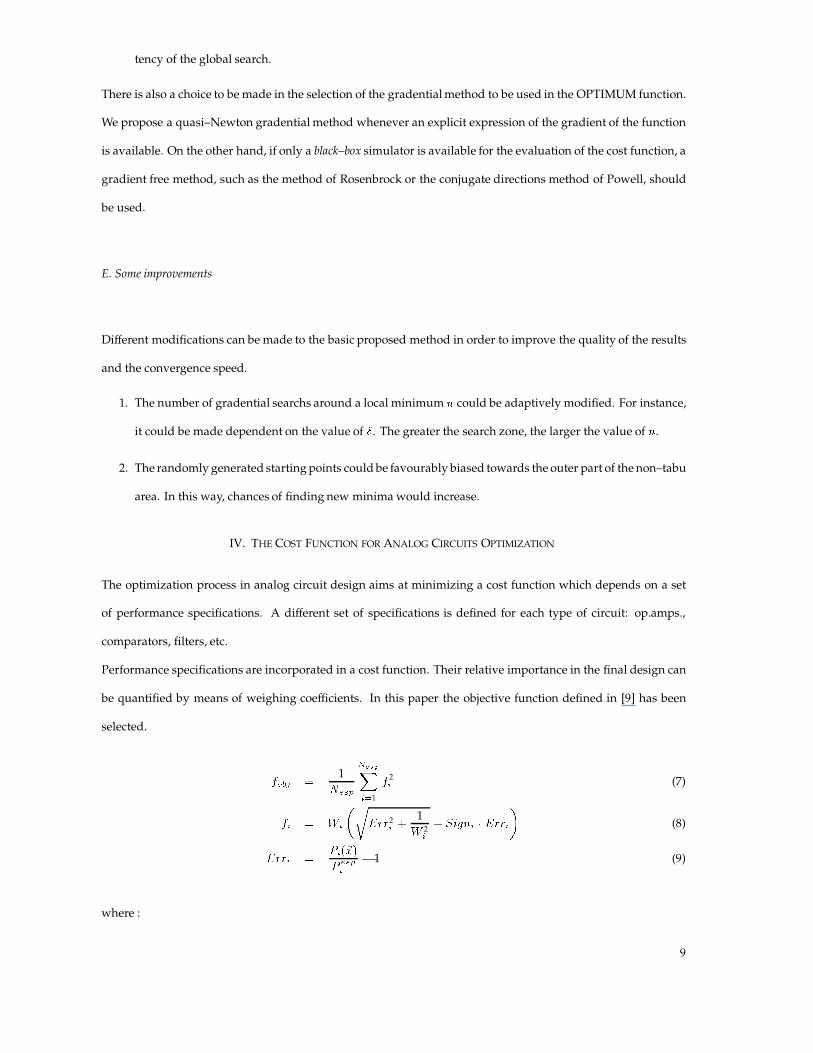
Performance specifications are incorporated in a cost function. Their relative importance in the final design can

be quantified by means of weighing coefficients. In this paper the objective function defined in [9] has been

selected. fobj = 1Nesp NespXi=1 f 2i (7)fi = Wi�rErr2i + 1W 2i + Signi � Erri� (8)Erri = Pi(~x)P espi � 1 (9)

where :

9

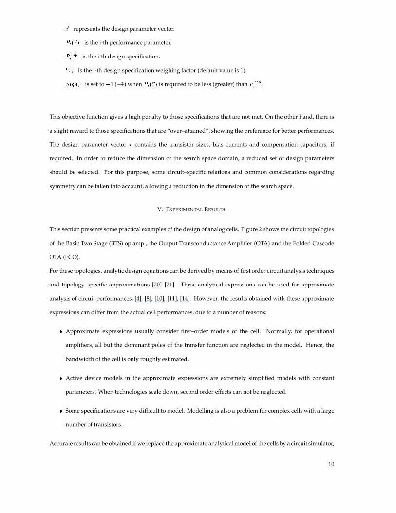
~x represents the design parameter vector.Pi(~x) is the i-th performance parameter.P espi is the i-th design specification.Wi is the i-th design specification weighing factor (default value is 1).Signi is set to+1 (�1) when Pi(~x) is required to be less (greater) than P espi .

This objective function gives a high penalty to those specifications that are not met. On the other hand, there is

a slight reward to those specifications that are “over–attained”, showing the preference for better performances.

The design parameter vector ~x contains the transistor sizes, bias currents and compensation capacitors, ifrequired. In order to reduce the dimension of the search space domain, a reduced set of design parameters

should be selected. For this purpose, some circuit–specific relations and common considerations regarding

symmetry can be taken into account, allowing a reduction in the dimension of the search space.

V. EXPERIMENTAL RESULTS

This section presents some practical examples of the design of analog cells. Figure 2 shows the circuit topologies

of the Basic Two Stage (BTS) op.amp., the Output TransconductanceAmplifier (OTA) and the Folded Cascode

OTA (FCO).

For these topologies, analytic design equations can be derived bymeans of first order circuit analysis techniques

and topology–specific approximations [20]–[21]. These analytical expressions can be used for approximate

analysis of circuit performances, [4], [8], [10], [11], [14]. However, the results obtained with these approximate

expressions can differ from the actual cell performances, due to a number of reasons:� Approximate expressions usually consider first–order models of the cell. Normally, for operationalamplifiers, all but the dominant poles of the transfer function are neglected in the model. Hence, the

bandwidth of the cell is only roughly estimated.� Active device models in the approximate expressions are extremely simplified models with constantparameters. When technologies scale down, second order effects can not be neglected.� Some specifications are very difficult to model. Modelling is also a problem for complex cells with a largenumber of transistors.

Accurate results can be obtained if we replace the approximate analyticalmodel of the cells by a circuit simulator,

10

such as SPICE. Unfortunately, experimental results show that the condition of the cost function gets worse when

a circuit simulator like SPICE is used to compute it. Hence, the probability of getting trapped at a localminimum

increases.

Next, experimental results obtained with the op.amps. in figure 2 are presented. HSPICE was used to evaluate

the cost function at each iteration, with the technology file of a commercial 1.5 �CMOS process. Optimizationparameters are presented in subsection A. Subsection B presents the experimental results obtained with theproposed method. They are compared to the results obtained using a randommultistart Powell method [19].

A. The parameters of the optimization process

Before starting the optimization process, the independent variables are normalized in the range [0..1].

1. n = 5

2. The tabu list size t = 7.3. Theprocess is stopped ifmore than 15 gradential searchshave elapsedwithout improving the best solutionx�.

B. Results

The Output Transconductance Amplifier (OTA)

The OTA schematic is depicted in (figure 2a). Table 1 contains a list of the independent variables and therelations between dependent and indenpendent variables. Two sets of specifications, which have been used for

optimization, are shown in table 3.

For testing purposes, only a reduced set of ac specifications is considered. The optimizer can also deal with any

requirements which can be obtained by means of a SPICE analysis, such as Slew Rate or 1=f noise.Table 2 shows the results obtainedwith the proposed method (TABU column). These results are compared with

the results obtained with a multistart Powell (MSP) algorithm which uses 10 random starting points. The final

value of the objective function has been used as a figure of merit. The number of calls to HSPICE is also recorded.

Table 3 shows the performances obtained after the optimization process. The standard deviation � of the MSPis also included in the table. Note that the large value of � indicates that the cost function is ill–conditioned, sothat a global optimizer is required to reach a good solution. The proposed method obtains a solution which is

11

better than the best minimum of the 10 Powell iterations.

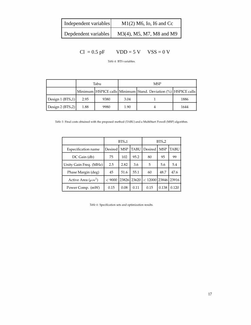
Basic Two Stage Opamp (BTS)

Table 4 contains a list of the variables of the Basic Two Stage Op.amp. (BTS) (figure 2b). Two requirement setsare presented in table 6. The final value of the cost function obtained after the optimization process using the

proposed method (TABU column) and a multistart Powell algorithm (MSP column) with 10 random starting

points, are shown in table 5. Table 6 shows the performances obtained after the optimization process with the

proposed method.

This case deserves special atention. The existence of five independent variables and the presence of a compen-

sating loop makes this design much more difficult to optimize. The main effect on the optimization process is

an increase in the number of HSPICE calls. But the minima obtained by the proposed method are better than

the minima obtained by the MSP method in all cases.

Folded Cascode OTA (FCO)

Variables and results for the Folded Cascode Ota (FCO) are shown in tables 7 and 8. Cell performances obtained

with the proposed method are displayed in table 9. The quick convergence of the optimization process in this

case is due to the existence of only three independent variables.

VI. CONCLUSIONS

This paper presents a new heuristic for the automatic sizing of analog cells. This heuristic is based on a Tabu

Search (TS) approach. The main characteristic of the TS approach is its ability to escape from local minima, by

maintaining a list of forbidden moves. This paper presents an extension of the TS heuristic to the continuous

space and its application to the sizing of analog cells. The results obtained show that the proposed heuristic is

able to provide good designs in only a few thousand iterations, allowing the use of an analog circuit simulator

such as SPICE to evaluate the circuit behaviour. The results also show that when SPICE is used to evaluate the

circuit performances, the cost function becomes ill–conditioned, so that naive approaches such as those based

on multistart gradential methods are not able to find good minima.

Acknowledgements

12

The authors would like to acknowledge Profs. J.Larraneta and F.Glover for providing guidance in Tabu Search

Techniques.

13

REFERENCES

[1] L.R.Carley and R.A.Rutenbar. “How to automate analog IC design”. IEEE Spectrum, pp.26–30, Aug. 1988.

[2] M.Ismail and J.Franca, Eds. “Introduction to analog VLSI design automation”. Kluwer Academic Publishers,

1990.

[3] R.K.Brayton, G.D.Hachtel and A.L.Sangiovanni–Vincentelli. “A survey of optimization techniques for in-

tegrated circuit design”. Proc. IEEE, vol. 69, pp. 1334–1362,Oct. 1981.

[4] M.G.R.Degrauwe, O.Nys, E.Dijkstra, J.Rijmenants, S.Bitz, B.L.A.G.Goffart, E.A.Vittoz, S.Cserveny,

C.Meixenberger, G.V.der Stappen and H.J.Oguey. “IDAC: an interactive design tool for analog CMOS

circuits”. IEEE J. Solid–State Circuits, vol. 22, no. 6, pp. 1106–1117, Dec. 1987.

[5] W.Nye, D.C.Riley, A.L.Sangiovanni–Vincentelli and A.L.Tits. “DELIGHT.SPICE: an optimization–based

system for the design of integrated circuits”. IEEE Trans. Computer–Aided Design, vol. 7, no. 4, pp. 501–519,

Apr. 1988.

[6] F.El–Turkey and E.E.Perry. “BLADES: an artificial intelligence approach to analog circuit design”. IEEE

Trans. Computer–Aided Design, vol. 8, no. 6, pp. 680– 692, June 1989.

[7] R.Harjani, R.A.Rutenbar and L.R.Carley. “OASYS: a framework for analog circuit synthesis”. IEEE Trans.

on Computer–Aided Design, vol. 8, no. 12, pp. 1247–1266, Dec. 1989.

[8] H.Y.Koh, C.H.Sequin and P.R.Gray. “OPASYN: a compiler for CMOS operational amplifiers”. IEEE Trans.

Computer–Aided Design, vol. 9, no. 2, pp. 113–125, Feb. 1990.

[9] H.Onodera, H.Kanbara and K.Tamaru. “Operational–amplifier compilation with performance optimiza-

tion”. IEEE J. Solid–State Circuits, vol. 25, no. 2, pp. 466–473, Apr. 1990.

[10] P.C.Maulik, L.R.Carley and D.J.Allstot. “Sizing of cell-level analog circuits using constrained optimization

techniques”. IEEE J. Solid–State Circuits, vol. 28, no. 3, pp. 233-241, March 1993.

[11] K.Swings and W.M.C. Sansen. “Ariadne: A constraint–based approach to computer–aided synthesis and

modelling of analog integrated circuits”. Analog Integrated Circuits and Signal Processing, vol. 3, no. 3, pp.

197–216, May 1993.

[12] G.G.E.Gielen,H.C.C.Walscharts andW.M.C.Sansen. “Analog circuitdesign optimization basedon symbolic

simulation and simulated annealing”. IEEE J. Solid–State Circuits, vol. 25, no. 3, pp. 707–713, June 1990.

[13] E.S.Ochotta, R.A.Rutenbar and L.R.Carley. “Equation–free synthesis of high–performance linear analog

circuits”. Proc. 1992 Brown/MIT Conf. Advanced Research in VLSI and Parallel Systems, Cambridge, MA:MIT

Press, pp. 129–143, 1992.

14

[14] J.Chavez, M.A.Aguirre and A.Torralba. “Analog design automation. A case study”. Proc. IEEE Int. Symp.

on CAS, pp. 2083–2085, 1993.

[15] G.E.Gielen and W.M.C.Sansen. Symbolic analysis for automated design of analog integrated circuits, Kluwer:

Boston, 1991.

[16] F. Glover. “Tabu search part I”.ORSA Journal on Computing, vol. 1, no. 3, pp. 190–206, 1989.

[17] F. Glover. “Tabu search part II”.ORSA Journal on Computing, vol. 2, no. 1, pp. 4–32, 1990.

[18] F.Glover, M.Laguna, E.Taillard andD.deWerra, eds. Tabu Search. Annals of Operations Research, vol. 41, 1993.

[19] MS.Bazaraa and C.M.Shetty. Nonlinear Programming. Theory and Algorithms. New York: John Wiley, 1979

[20] P.R.Gray and R.G.Meyer. Analysis and design of analog integrated circuits. New York: John Wiley, 1984.

[21] R.L.Geiger, P.E.Allen and N.R.Strader. VLSI design techniques for analog and digital circuits. McGraw–Hill,

1990.

15

WL3 = WL4 = 0.5 (Io/I6) WL6

WL5 = 2M5Kn (Vgs - Vt)

2 * Ibias

WL10 = WL5 (Ibias/Io)

WL7 = WL6 (Kp/Kn)

VSS = 0 VCl = 0.5 pF VDD = 5 V

Independent variables

Depdendent variables

M1(2), M6(8), Io and I6

M3(4), M5, M7(9) and M10

Table 1: OTA variables and dependencies.

Tabu MSP

Minimum HSPICE calls Minimum Stand. Deviation HSPICE calls

Design 1 (OTA 1) 1.71 4520 2.01 60 840

Design 2 (OTA 2) 0.48 4580 0.55 147 1140

Table 2: Final costs obtained with the proposed method (TABU) and a MultiStart Powell (MSP) algorithm.

OTA 1 OTA 2

Especification name Desired MSP TABU Desired MSP TABU

DC Gain (db) 70 40.9 41.8 50 48.8 55.4

Unity Gain Freq. (MHz) 2 12.3 9.3 2.5 5.6 6.1

Phase Margin (deg) 60 72.1 73.9 45 65 68

Active Area (�m2) < 100 212 196 < 500 340 292

Power Comp. (mW) 1 0.20 0.15 0.1 0.08 0.07

Table 3: Specification sets and optimization results.

16

VDD = 5 V VSS = 0 VCl = 0.5 pF

Independent variables

Depdendent variables

M1(2) M6, Io, I6 and Cc

M3(4), M5, M7, M8 and M9

Table 4: BTS variables.

Tabu MSP

Minimum HSPICE calls Minimum Stand. Deviation (%) HSPICE calls

Design 1 (BTS 1) 2.95 9380 3.04 1 1886

Design 2 (BTS 2) 1.88 9980 1.90 4 1644

Table 5: Final costs obtained with the proposed method (TABU) and a MultiStart Powell (MSP) algorithm.

BTS 1 BTS 2

Especification name Desired MSP TABU Desired MSP TABU

DC Gain (db) 75 102 95.2 80 95 99

Unity Gain Freq. (MHz) 2.5 2.82 3.6 5 5.6 5.4

Phase Margin (deg) 45 51.6 55.1 60 48.7 47.6

Active Area (�m2) < 9000 23826 23620 < 12000 23846 23916Power Comp. (mW) 0.15 0.08 0.11 0.15 0.138 0.120

Table 6: Specification sets and optimization results.

17

Independent variables

Depdendent variables M3(4), M5, M6(7), M8(9,10,11), M12, M13 and M14

M1(2), Io and I6

VSS = 0 VCl = 0.5 pF VDD = 5 V

Table 7: FCO variables.

Tabu MSP

Minimum HSPICE calls Minimum Stand. Deviation (%) HSPICE calls

Design 1 (FCO 1) 0.91 2228 0.96 2 742

Design 2 (FCO 2) 0.65 3216 0.67 3 664

Table 8: Final costs obtained with the proposed method (TABU) and a MultiStart Powell (MSP) algorithm.

FCO 1 FCO 2

Especification name Desired MSP TABU Desired MSP TABU

DC Gain (db) 80 78.7 79.8 90 81.67 83.24

Unity Gain Freq. (MHz) 1.5 6.4 5.1 3.5 8.62 8.20

Phase Margin (deg) 60 85 86 45 82.4 82.5

Active Area (�m2) < 300 384 388 < 500 412 428

Power Comp. (mW) 0.18 0.22 0.2 0.2 0.21 0.2

Table 9: Specification sets and optimization results.

18

Figure 1: Tabu search on a example. a) Local Maxima (�), Minima (�) and Saddle Points (�) of the cost function. The figure shows the value ofthe function in each minima. b), c) and d) show the evolution of the tabu search.

19

Io

Ibias

Io

Ibias

VDD VDD

VSS VSS

M3 M4 M6

M7M5

M1 M2

M8

M9

Cc Cl

I6

M7

M10 M5

M8 M3 M4

M1 M2

M6

M9

Cl

I6

a) Output Transconductance Amplifier (OTA) b) Basic Two Stage Operational Amplifier (BTS)

VDD

Cl

VSS

M5

M14

M13M3

M4

M1 M2

M10 M11

M9

Io

Ibias

Ibias

Ibias

M6M7 I6

M8

M12

c) Folded Cascode OTA (FCO)

Figure 2: Basic op.amp. topologies

20